Simulation of the flow of fresh cement suspensions by a Lagrangian finite element approach

This article appeared in a journal published by Elsevier. The attachedcopy is furnished to the author for internal non-commercial researchand education use, including for instruction at the authors institution

and sharing with colleagues.

Other uses, including reproduction and distribution, or selling orlicensing copies, or posting to personal, institutional or third party

websites are prohibited.

In most cases authors are permitted to post their version of thearticle (e.g. in Word or Tex form) to their personal website orinstitutional repository. Authors requiring further information

regarding Elsevier’s archiving and manuscript policies areencouraged to visit:

http://www.elsevier.com/copyright

http://www.elsevier.com/copyright

Author's personal copy

J. Non-Newtonian Fluid Mech. 165 (2010) 1555–1563

Contents lists available at ScienceDirect

Journal of Non-Newtonian Fluid Mechanics

journa l homepage: www.e lsev ier .com/ locate / jnnfm

Review

Simulation of the flow of fresh cement suspensions by a Lagrangian finiteelement approach

M. Cremonesi ∗, L. Ferrara, A. Frangi, U. PeregoDepartment of Structural Engineering, Politecnico di Milano, P.zza Leonardo da Vinci 32, 20133 Milan, Italy

a r t i c l e i n f o

Article history:Received 12 April 2010Received in revised form 27 July 2010Accepted 19 August 2010

Keywords:Fresh cement pasteMortarLagrangian approachNon-Newtonian fluidFree surface

a b s t r a c t

In this paper a Lagrangian formulation of the Navier–Stokes equations, based on a Particle Finite ElementApproach, is applied to the simulation of rheological tests for homogenized cement pastes and mortars,i.e. the L-box, slump and mini-slump and Marsh cone tests. Comparisons with both experiments andanalytical predictions are addressed by assuming a simple Bingham-like constitutive model. The analysesexplicitly and automatically account for the presence of evolving free surfaces thanks to a continuousre-triangulation of the domain. These feature and the excellent accuracy obtained in the benchmarksaddressed make the proposed approach an ideal tool for more advanced applications.

© 2010 Elsevier B.V. All rights reserved.

Contents

1. Introduction . . . . . . . . . . . . . . . . . . . . . . . . . . . . . . . . . . . . . . . . . . . . . . . . . . . . . . . . . . . . . . . . . . . . . . . . . . . . . . . . . . . . . . . . . . . . . . . . . . . . . . . . . . . . . . . . . . . . . . . . . . . . . . . . . . . . . . . . . . 15552. Governing equations . . . . . . . . . . . . . . . . . . . . . . . . . . . . . . . . . . . . . . . . . . . . . . . . . . . . . . . . . . . . . . . . . . . . . . . . . . . . . . . . . . . . . . . . . . . . . . . . . . . . . . . . . . . . . . . . . . . . . . . . . . . . . . . . . 15563. Numerical formulation. . . . . . . . . . . . . . . . . . . . . . . . . . . . . . . . . . . . . . . . . . . . . . . . . . . . . . . . . . . . . . . . . . . . . . . . . . . . . . . . . . . . . . . . . . . . . . . . . . . . . . . . . . . . . . . . . . . . . . . . . . . . . . . 1557

3.1. Space and time discretization . . . . . . . . . . . . . . . . . . . . . . . . . . . . . . . . . . . . . . . . . . . . . . . . . . . . . . . . . . . . . . . . . . . . . . . . . . . . . . . . . . . . . . . . . . . . . . . . . . . . . . . . . . . . . . . . 15573.2. Particle Finite Element Method . . . . . . . . . . . . . . . . . . . . . . . . . . . . . . . . . . . . . . . . . . . . . . . . . . . . . . . . . . . . . . . . . . . . . . . . . . . . . . . . . . . . . . . . . . . . . . . . . . . . . . . . . . . . . . 15573.3. Adding and removing particles. . . . . . . . . . . . . . . . . . . . . . . . . . . . . . . . . . . . . . . . . . . . . . . . . . . . . . . . . . . . . . . . . . . . . . . . . . . . . . . . . . . . . . . . . . . . . . . . . . . . . . . . . . . . . . . 1558

4. Application to the flow of concrete and cement pastes . . . . . . . . . . . . . . . . . . . . . . . . . . . . . . . . . . . . . . . . . . . . . . . . . . . . . . . . . . . . . . . . . . . . . . . . . . . . . . . . . . . . . . . . . . . . . 15584.1. L-box test . . . . . . . . . . . . . . . . . . . . . . . . . . . . . . . . . . . . . . . . . . . . . . . . . . . . . . . . . . . . . . . . . . . . . . . . . . . . . . . . . . . . . . . . . . . . . . . . . . . . . . . . . . . . . . . . . . . . . . . . . . . . . . . . . . . . . 15594.2. Slump-flow test . . . . . . . . . . . . . . . . . . . . . . . . . . . . . . . . . . . . . . . . . . . . . . . . . . . . . . . . . . . . . . . . . . . . . . . . . . . . . . . . . . . . . . . . . . . . . . . . . . . . . . . . . . . . . . . . . . . . . . . . . . . . . . 15594.3. Marsh cone test . . . . . . . . . . . . . . . . . . . . . . . . . . . . . . . . . . . . . . . . . . . . . . . . . . . . . . . . . . . . . . . . . . . . . . . . . . . . . . . . . . . . . . . . . . . . . . . . . . . . . . . . . . . . . . . . . . . . . . . . . . . . . . . 1562

5. Conclusions . . . . . . . . . . . . . . . . . . . . . . . . . . . . . . . . . . . . . . . . . . . . . . . . . . . . . . . . . . . . . . . . . . . . . . . . . . . . . . . . . . . . . . . . . . . . . . . . . . . . . . . . . . . . . . . . . . . . . . . . . . . . . . . . . . . . . . . . . . 1562Acknowledgments . . . . . . . . . . . . . . . . . . . . . . . . . . . . . . . . . . . . . . . . . . . . . . . . . . . . . . . . . . . . . . . . . . . . . . . . . . . . . . . . . . . . . . . . . . . . . . . . . . . . . . . . . . . . . . . . . . . . . . . . . . . . . . . . . . . 1563References . . . . . . . . . . . . . . . . . . . . . . . . . . . . . . . . . . . . . . . . . . . . . . . . . . . . . . . . . . . . . . . . . . . . . . . . . . . . . . . . . . . . . . . . . . . . . . . . . . . . . . . . . . . . . . . . . . . . . . . . . . . . . . . . . . . . . . . . . . . 1563

1. Introduction

The development of tools for the computational modeling offresh state behaviour of materials such as cement paste, mortar andconcrete is nowadays stimulating intensive research as testified,e.g. by the recent review paper [1]. Indeed, in civil engineering theadvent of advanced cement based materials has led to recognize theimportance of rheology as a tool to optimize the mix composition

∗ Corresponding author. Tel.: +39 0223994274.E-mail addresses: [email protected] (M. Cremonesi),

[email protected] (L. Ferrara), [email protected] (A. Frangi),[email protected] (U. Perego).

and the processing techniques to achieve the levels of engineer-ing properties required for the intended applications. Moreover,in order to exploit the potentials of concretes characterized by asuperior performance in the fresh state, such as Self-CompactingConcrete (SCC), procedures for predicting its flow behaviour areneeded in order to properly design casting procedures, such aspumping and grouting [2].

Fresh concrete and mortars are composite materials consistingof a suspension of solid particles in a fluid matrix [1]. Whether thesolid components should be considered as independent particlesor homogenized with the matrix strongly depends on the aims ofthe simulation and different solution strategies should be adoptedaccordingly. In this contribution we focus on situations where thescale of interest and the size of the aggregates is such that the fresh

0377-0257/$ – see front matter © 2010 Elsevier B.V. All rights reserved.doi:10.1016/j.jnnfm.2010.08.003


1556 M. Cremonesi et al. / J. Non-Newtonian Fluid Mech. 165 (2010) 1555–1563

composite can be described as a homogeneous non-Newtonianfluid obeying a non-linear constitutive law like the Bingham orHerschel–Bulkley viscous-plastic models, which are often regardedas an optimal compromise between complexity and realism.

Moreover, the essential feature of such analyses, i.e. the abilityto accurately simulate a fluid-like cementitious composite under-going large displacements with evolving free surfaces, goes wellbeyond this class of problems. Indeed, the flow of non-Newtonianfluids has been recently attracting considerable attention in thescientific community, both from an experimental and a numeri-cal stand point, for a wealth of different engineering applications.Thixotropic fluids [3,4] are widely used for drilling and are ofparamount importance in petroleum and tunnelling engineering[5]. Other applications include food industry, paints and tooth-pastes which present different types of thixotropic behaviour [6].Also the simulation of the moulding of polymers [7] leads to similarrequirements.

These applications call for further research aiming at the devel-opment of robust and general-purpose numerical tools. Indeed,analytical estimates can be applied only under certain circum-stances, like, e.g. in [3], where experiments on the dam break flowof thixotropic fluids are validated against theoretical results. But forthis and other simple situations, numerical simulations are almostalways mandatory in engineering applications. Moreover, even ifsome problems of flow cessation (see, e.g. [8]) can be solved as aone-dimensional Couette or Poiseuille flow of a Bingham fluid, ingeneral 2D or even 3D flow patterns have to be addressed, includingthe ability to track free surfaces undergoing large displacements.

The issue of simulating evolving free surfaces makes Eulerianapproaches, where material flows through a fixed mesh in space,not well suited for the problematic at hand. Indeed dedicated algo-rithms, like the Volume of Fluid [9] or the level set [10] methodsare required, but their application remains somewhat problematic.

Although several different alternative possibilities have beenproposed for the simulation of non-Newtonian fluid flow, likethe FEMLIP (finite element method with Lagrangian integrationpoints) [11] or the Lattice–Boltzmann method [12], available tech-niques can be regrouped in two major catergories: arbitraryLagrangian–Eulerian and fully Lagrangian approaches.

The Arbitrary Lagrangian–Eulerian (ALE) scheme is very effec-tive for addressing large deformation and large strain problems.The general concept of the ALE approach is that the motion of themesh is decoupled from that of the material domain in such a waythat it allows to smooth a distorted mesh without requiring a com-plete remeshing. The ALE method has become a standard numericalapproach for solving large strain deformation problems encoun-tered in material forming applications in some commercial codes.Applications have been recently presented for the analysis of freshSCC paste in [2], and for the modelling of thixotropic fluid mixingand Couette rheometry with either coaxial cylinders or vane-cupsetup in [6]. However, the main shortcoming of this technique isthat it is essentially limited to geometries where the material flowis relatively predictable and where the free surface movement israther limited.

In Lagrangian approaches, on the contrary, the motion of mate-rial particles is tracked, automatically capturing the free surfaceconfiguration and not limiting a priori in any way the movement ofthe analysed fluid. The associated mesh of a classical Finite ElementMethod (FEM) remains attached to material nodes and deformsalong with them. One major disadvantage is that the mesh maydistort severely and frequent time-consuming remeshing might benecessary, as discussed in the sequel of the paper.

Meshless Lagrangian approaches, like the Smoothed ParticleHydro-dynamics (SPH), avoid this issue by eliminating the need tomesh the domain. In [13] the SPH method has been applied to thesimulation of a Bingham-like fluid and has been validated against

some analytical benchmarks in the case of Poiseuille flow and tan-gential angular flow as well as against experiments conducted oncoaxial cylinders and vane rheometers. Similarly, in [7] the SPHhas been applied to the analysis of polymer molding with evolvingfree surfaces. However these approaches are generally based on thestrong form of equilibrium and conservation equations, which hassometimes attracted some criticism.

For this reason, following recent advances in the field ofLagrangian FEM and robust meshing algorithms, in this contribu-tion we investigate the applicability of a fully Lagrangian approachwith surface tracking capabilities to the analysis of incompressiblenon-Newtonian fluid flows based on a continuous re-triangulationof the domain, in the spirit of the so-called Particle Finite ElementMethod (PFEM) [14]. The PFEM is a method for the solution offluid dynamics problems including free-surface flows and breakingwaves [14], but also fluid–structure interactions [15] or fluid–objectinteractions [16]. This method has been applied to different engi-neering problems and has been also validated against experiments[17].

After recalling the basic governing equations in Section 2, webriefly review the concepts of the PFEM, with particular attentionfor the remeshing strategy adopted. We next present some appli-cations to the flow of concrete and cement pastes in Section 4 withspecific emphasis on the simulation of classical test procedures likethe L-box test, the slump and mini-slump-flow test, and Marsh conetest. In all these cases, numerical predictions are validated againsteither analytical estimates, whenever available, or experimentaldata, always displaying a highly encouraging predictive ability.

2. Governing equations

Let ˝0 represent the initial reference configuration of the fluidto analyse and ˝t denote its current configuration at time t ∈ [0, T].

If x0 is the position of a material particle at the initial time t = t0,its actual position will be denoted by x = �(x0, t), where � representsthe fluid transformation.

Introducing the velocity u = u(x, t) and the Cauchy stress tensor� = �(x,t), the motion of a homogeneous incompressible fluid fillingthe domain ˝t is governed by momentum and mass conservation:

�DuDt

= div � + �b in ˝t × (0, T) (1)

div u = 0 in ˝t × (0, T) (2)

where �(x) represents the fluid density, b(x,t) the external bodyforces, D/(Dt) denotes the material (i.e. total) time derivative anddiv is the divergence operator computed with respect to the currentconfiguration x.

Problem (1) and (2) has to be supplemented with appropriateinitial conditions:

u(x, t = 0) = u0 in ˝0 (3)

and suitable boundary conditions. The boundary � t = ∂ ˝t isassumed to be partitioned in two non-overlapping subsets � D

and � N, such that � D ∪ � N = � t and � D ∩ � N =∅. Dirichlet andNeumann boundary conditions are enforced on � D and � N, respec-tively:

u(x, t) = u(x, t) on �D × (0, T) (4)

�(x, t)n = h(x, t) on �N × (0, T) (5)

where u(x, t) and h(x, t) are given data and n denotes the unitoutward normal to the boundary � t.

The Cauchy stress tensor � can be decomposed, as usual, in itsisotropic and deviatoric parts:

� = −pI + � (6)


M. Cremonesi et al. / J. Non-Newtonian Fluid Mech. 165 (2010) 1555–1563 1557

The fluid is assumed to be isotropic, incompressible and to obeythe following Bingham-like constitutive law:

� = 2��(u) + �0�(u)

‖�(u)‖ if ‖�(u)‖ /= 0 (7)

‖�‖ ≤ �0 if ‖�(u)‖ = 0 (8)

which can also be expressed as:

�(u) =(

1 − �0

‖�‖)

�

2�if ‖�‖ > �0 (9)

�(u) = 0 otherwise (10)

where �(u) = (1/2)(grad u + grad uT) is the symmetric part of thevelocity gradient and ||·|| is the Euclidean norm:

‖�(u)‖ =√

12

� : � ‖�‖ =√

12

� : � (11)

It is worth stressing that the assumed form (7) of the constitutivelaw reduces to the well known 1D equation:

�xy = �∂ux

∂y+ �0 sign

(∂ux

∂y

)describing a flow along the x direction between two infinite platesseparated by a gap along the y axis.

Since the Bingham constitutive law displays a sort of “rigid-elastic” behaviour which can induce numerical difficulties, anapproximation based on a smoothing of Eqs. (7) and (8) is generallypreferred.

In the so-called biviscosity model [18,19] the “rigid” branchof the ideal behaviour is approximated with a very high, butbounded, viscosity. This bilinear approximation, however, can leadto inconsistent predictions. Hence, following Papanastasiou [20], alaw based on an exponential evolution of the viscosity is adoptedherein:

� = ��(u) =[

2� + �0

‖�‖ (1 − e−m‖�‖)]

�(u) ∀‖�‖ (12)

where the apparent viscosity � has been introduced. In the limitcase of m → ∞, the Bingham behaviour (8) is recovered and hencethe choice of the parameter m to be employed is actually a trade-off between numerical issues and accuracy of the mechanicalresponse. In all the examples presented in Section 4 a value ofm = 1000 s has been considered.

In the specific case of Bingham plastic flows through channels(see, e.g. [21]), in order to appreciate the importance of the yieldlimit it is customary to analyse the Bingham number Bn defined as:

Bn = �0D

�V

where D is typically the channel width and V is the average (ormaximum) velocity of the flow. Large values of Bn are gener-ally associated to extended unyielded regions. In Section 4 severalapplications to cement paste will be presented: in same cases thepaste initially flows through a channel only under the effexct of self-weight and finally spreads in a lower basin until arrest. Materialparameters and fluid velocity are such that the Bingham numberis always smaller than unity in the channel flow which essentiallyimplies the absence of unyielded regions; these, on the contrary,slowly develop in the basin before arrest.

It is worth stressing that, even if the Bingham model is the sim-plest law encompassing the concept of the yield limit, alternativechoices have been proposed, like the Herschel–Bulkley law [22]:

� =(

2�‖�(u)‖q−1 + �0

‖�(u)‖)

�(u) if ‖�‖ > �0 (13)

�(u) = 0 if ‖�‖ < �0 (14)

where q is a non-physical parameter. Since no major differenceexist between the numerical treatment of these models, in thepresent contribution we will focus on the smooth approximationof the Bingham law (12).

3. Numerical formulation

3.1. Space and time discretization

Following [23] the momentum and mass conservation Eqs. (1)and (2) can be written with respect to the fixed reference configu-ration as follows:

�0DuDt

= Div � + �0b in ˝0 × (0, T) (15)

Div(JF−1u) = 0 in ˝0 × (0, T) (16)

where u is the velocity of the material point which was in x0 at t = 0,�0 is the initial density, � = J�F−T is the first Piola–Kirchhoff stresstensor, F is the deformation gradient, J is the determinant of F andDiv represents the divergence operator computed with respect tothe initial coordinates x0.

Introducing a standard Galerkin isoparametric finite elementdiscretization, and assuming that the state of the system at t = tn isknown in terms of particle positions Xn = X(tn), velocities Un = U(tn)and pressures Pn, the state at time t = tn+1 is determined by enforc-ing (15) and (16) at t = tn+1 in the spirit of a backward Eulerintegration and hence the fully discretized problem writes:

MUn+1 − Un

t+ K(Xn+1)Un+1 + DT (Xn+1)Pn+1 = Bn+1 (17)

D(Xn+1)Un+1 = 0 (18)

where M is the mass matrix, K is the fluid stiffness matrix, D is thediscretization of the divergence operator, B is the vector of externalforces.

3.2. Particle Finite Element Method

Clearly (17) and (18) represent a system of equations whichdepend non-linearly on the main unknown vector Un+1. Its solu-tion can be performed with any method of choice like theNewton–Raphson approach or the Picard technique which is some-times preferred due to its greater simplicity and good convergencespeed (see [23]).

Mesh distortion is cured in the spirit of the Particle Method(PFEM) which has proven very efficient for the solution of fluiddynamics problems including free-surface flows (and breakingwaves) [14] which are key features for the simulations at hand.

Whenever the mesh quality is no longer satisfactory, accordingto some criteria associated to element distortion, the connectivityof existing nodes is recomputed using a Delaunay triangulation.This choice has some important implications.

First, nodes (which are also the vertices of the evolving triangu-lation) are the only topological entity which is preserved along thetime marching solution. Hence, to avoid interpolation of data fromthe old to the new mesh, linear shape functions are employed forboth velocity and pressure unknowns. However it is well knownthat this fully linear element does not satisfy the inf-sup condi-tion: oscillations in the pressure field may appear [24] so that astabilization method is required. In recent works [23] a pressure-stabilizing/Petrov-Galerkin (PSPG) stabilization technique [25–27]has proven very effective in the context of Lagrangian approachesand is also applied herein.



It is also worth stressing that external rigid boundaries areaccounted for, in this approach, by placing on them fictitious nodeswhich are not allowed to move.

Secondly, the Delaunay triangulation generates the convex fig-ure of minimum area which encloses all the points and which maybe not conformal with the external boundaries.

A possibility to overcome this problem is to couple the Delaunaytriangulation with the so-called �-shape method [28] as proposedin [14]. The key idea is to remove the unnecessary triangles fromthe mesh using a criterion based on the mesh distortion. For eachtriangle e of the mesh, the minimal distance he between two nodesin the element and the radius Re of the circumcircle of the elementare defined. If h is computed as the mean value of all the he, theshape factor:

˛e = Re

h≥ 1√

3, (19)

is an index of the element distortion. All the triangles that do notsatisfy the condition:

˛e ≤ ¯ (20)

are removed from the mesh, where ¯ ≥ 1 is assumed.To reduce computing effort, the mesh is regenerated only when

it is globally too distorted. Starting from the shape factor ˛e, definedin Eq. (19), a simple measure of mesh quality can be obtained defin-ing for each element a distortion factor ˇe:

ˇe =√

3˛e =√

3Re

he≥ 1 (21)

where the equilateral triangle (˛e = 1/√

3) has been considered asthe best possible element. The quality of the entire mesh is thenevaluated by an arithmetic mean:

ˇ = 1Nel

Nel∑e=1

ˇe (22)

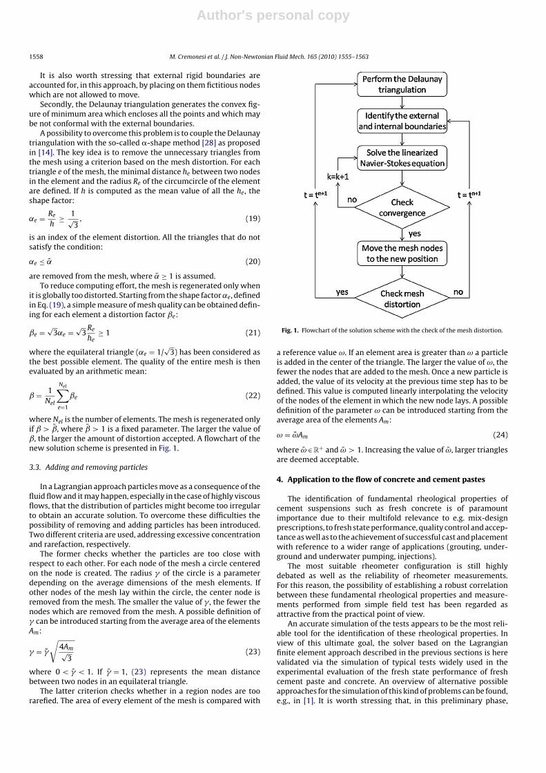
where Nel is the number of elements. The mesh is regenerated onlyif ˇ > ¯ , where ¯ > 1 is a fixed parameter. The larger the value ofˇ, the larger the amount of distortion accepted. A flowchart of thenew solution scheme is presented in Fig. 1.

3.3. Adding and removing particles

In a Lagrangian approach particles move as a consequence of thefluid flow and it may happen, especially in the case of highly viscousflows, that the distribution of particles might become too irregularto obtain an accurate solution. To overcome these difficulties thepossibility of removing and adding particles has been introduced.Two different criteria are used, addressing excessive concentrationand rarefaction, respectively.

The former checks whether the particles are too close withrespect to each other. For each node of the mesh a circle centeredon the node is created. The radius of the circle is a parameterdepending on the average dimensions of the mesh elements. Ifother nodes of the mesh lay within the circle, the center node isremoved from the mesh. The smaller the value of , the fewer thenodes which are removed from the mesh. A possible definition of can be introduced starting from the average area of the elementsAm:

=

√4Am√

3(23)

where 0 < < 1. If = 1, (23) represents the mean distancebetween two nodes in an equilateral triangle.

The latter criterion checks whether in a region nodes are toorarefied. The area of every element of the mesh is compared with

Fig. 1. Flowchart of the solution scheme with the check of the mesh distortion.

a reference value ω. If an element area is greater than ω a particleis added in the center of the triangle. The larger the value of ω, thefewer the nodes that are added to the mesh. Once a new particle isadded, the value of its velocity at the previous time step has to bedefined. This value is computed linearly interpolating the velocityof the nodes of the element in which the new node lays. A possibledefinition of the parameter ω can be introduced starting from theaverage area of the elements Am:

ω = ωAm (24)

where ω ∈R+ and ω > 1. Increasing the value of ω, larger trianglesare deemed acceptable.

4. Application to the flow of concrete and cement pastes

The identification of fundamental rheological properties ofcement suspensions such as fresh concrete is of paramountimportance due to their multifold relevance to e.g. mix-designprescriptions, to fresh state performance, quality control and accep-tance as well as to the achievement of successful cast and placementwith reference to a wider range of applications (grouting, under-ground and underwater pumping, injections).

The most suitable rheometer configuration is still highlydebated as well as the reliability of rheometer measurements.For this reason, the possibility of establishing a robust correlationbetween these fundamental rheological properties and measure-ments performed from simple field test has been regarded asattractive from the practical point of view.

An accurate simulation of the tests appears to be the most reli-able tool for the identification of these rheological properties. Inview of this ultimate goal, the solver based on the Lagrangianfinite element approach described in the previous sections is herevalidated via the simulation of typical tests widely used in theexperimental evaluation of the fresh state performance of freshcement paste and concrete. An overview of alternative possibleapproaches for the simulation of this kind of problems can be found,e.g., in [1]. It is worth stressing that, in this preliminary phase,



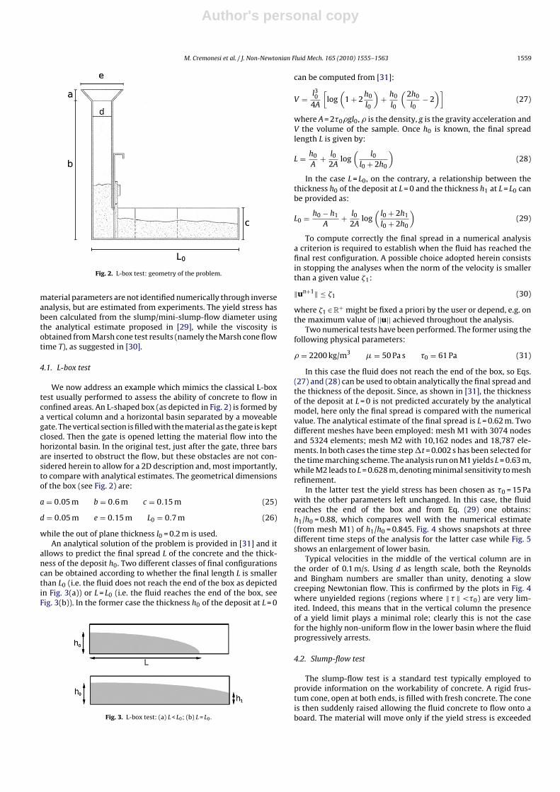
Fig. 2. L-box test: geometry of the problem.

material parameters are not identified numerically through inverseanalysis, but are estimated from experiments. The yield stress hasbeen calculated from the slump/mini-slump-flow diameter usingthe analytical estimate proposed in [29], while the viscosity isobtained from Marsh cone test results (namely the Marsh cone flowtime T), as suggested in [30].

4.1. L-box test

We now address an example which mimics the classical L-boxtest usually performed to assess the ability of concrete to flow inconfined areas. An L-shaped box (as depicted in Fig. 2) is formed bya vertical column and a horizontal basin separated by a moveablegate. The vertical section is filled with the material as the gate is keptclosed. Then the gate is opened letting the material flow into thehorizontal basin. In the original test, just after the gate, three barsare inserted to obstruct the flow, but these obstacles are not con-sidered herein to allow for a 2D description and, most importantly,to compare with analytical estimates. The geometrical dimensionsof the box (see Fig. 2) are:

a = 0.05 m b = 0.6 m c = 0.15 m (25)

d = 0.05 m e = 0.15 m L0 = 0.7 m (26)

while the out of plane thickness l0 = 0.2 m is used.An analytical solution of the problem is provided in [31] and it

allows to predict the final spread L of the concrete and the thick-ness of the deposit h0. Two different classes of final configurationscan be obtained according to whether the final length L is smallerthan L0 (i.e. the fluid does not reach the end of the box as depictedin Fig. 3(a)) or L = L0 (i.e. the fluid reaches the end of the box, seeFig. 3(b)). In the former case the thickness h0 of the deposit at L = 0

Fig. 3. L-box test: (a) L < L0; (b) L = L0.

can be computed from [31]:

V = l304A

[log

(1 + 2

h0

l0

)+ h0

l0

(2h0

l0− 2

)](27)

where A = 2�0�gl0, � is the density, g is the gravity acceleration andV the volume of the sample. Once h0 is known, the final spreadlength L is given by:

L = h0

A+ l0

2Alog

(l0

l0 + 2h0

)(28)

In the case L = L0, on the contrary, a relationship between thethickness h0 of the deposit at L = 0 and the thickness h1 at L = L0 canbe provided as:

L0 = h0 − h1

A+ l0

2Alog

(l0 + 2h1

l0 + 2h0

)(29)

To compute correctly the final spread in a numerical analysisa criterion is required to establish when the fluid has reached thefinal rest configuration. A possible choice adopted herein consistsin stopping the analyses when the norm of the velocity is smallerthan a given value �1:

‖un+1‖ ≤ �1 (30)

where �1 ∈R+ might be fixed a priori by the user or depend, e.g. onthe maximum value of ||u|| achieved throughout the analysis.

Two numerical tests have been performed. The former using thefollowing physical parameters:

� = 2200 kg/m3 � = 50 Pa s �0 = 61 Pa (31)

In this case the fluid does not reach the end of the box, so Eqs.(27) and (28) can be used to obtain analytically the final spread andthe thickness of the deposit. Since, as shown in [31], the thicknessof the deposit at L = 0 is not predicted accurately by the analyticalmodel, here only the final spread is compared with the numericalvalue. The analytical estimate of the final spread is L = 0.62 m. Twodifferent meshes have been employed: mesh M1 with 3074 nodesand 5324 elements; mesh M2 with 10,162 nodes and 18,787 ele-ments. In both cases the time step t = 0.002 s has been selected forthe time marching scheme. The analysis run on M1 yields L = 0.63 m,while M2 leads to L = 0.628 m, denoting minimal sensitivity to meshrefinement.

In the latter test the yield stress has been chosen as �0 = 15 Pawith the other parameters left unchanged. In this case, the fluidreaches the end of the box and from Eq. (29) one obtains:h1/h0 = 0.88, which compares well with the numerical estimate(from mesh M1) of h1/h0 = 0.845. Fig. 4 shows snapshots at threedifferent time steps of the analysis for the latter case while Fig. 5shows an enlargement of lower basin.

Typical velocities in the middle of the vertical column are inthe order of 0.1 m/s. Using d as length scale, both the Reynoldsand Bingham numbers are smaller than unity, denoting a slowcreeping Newtonian flow. This is confirmed by the plots in Fig. 4where unyielded regions (regions where ‖ � ‖ <�0) are very lim-ited. Indeed, this means that in the vertical column the presenceof a yield limit plays a minimal role; clearly this is not the casefor the highly non-uniform flow in the lower basin where the fluidprogressively arrests.

4.2. Slump-flow test

The slump-flow test is a standard test typically employed toprovide information on the workability of concrete. A rigid frus-tum cone, open at both ends, is filled with fresh concrete. The coneis then suddenly raised allowing the fluid concrete to flow onto aboard. The material will move only if the yield stress is exceeded



Fig. 4. L-box test. Snapshots at different time steps for �0 = 15 Pa using mesh M2.Yielded regions (‖ � ‖ >�0) are drawn in light grey while unyielded regions are indark grey.

Fig. 5. L-box test: zoom on a detail of the lower part of the box at t = 3.5 s.

Fig. 6. Slump-flow test: geometry of the problem.

and will otherwise stop flowing. The slump-flow parameter mea-sured from the test is the so-called slump-flow diameter which isthe diameter of the concrete “patty” resulting when concrete stopsflowing and determined as the average value of two measures alongtwo orthogonal diameters. The slump-flow diameter is correlatedto the yield stress of the fluid concrete, as it will be further dis-cussed below. The geometry of the problem is sketched in Fig. 6. Thefollowing geometrical parameters are used for the numerical sim-ulation which correspond to the worldwide employed geometry ofthe Abrams cone [32,33]:

h = 300 mm b1 = 100 mm b2 = 50 mm (32)

The initial configuration is axisymmetric and it is here assumedthat this feature is preserved during the flow, allowing to reducethe dimensionality of the analysis. The initial mesh of the generat-ing surface consists of 3075 nodes and 5324 elements. Fig. 7showssnapshots of the fluid domain at different time steps. In a first set ofanalyses the physical parameters have been chosen as follows: den-sity � = 2200 kg/m3, viscosity � = 50 Pa s and yield stress �0 = 50 Pawhich correspond to a self-consolidated concrete. For this examplea theoretical estimate of the final diameter is available, according to

Fig. 7. Slump-flow test: snapshots at different time steps. Yielded regions (‖ � ‖ >�0)are drawn in light grey while unyielded regions are in dark grey.



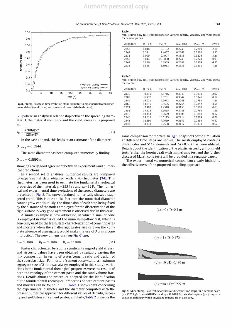
Fig. 8. Slump-flow test: time evolution of the diameter. Comparison between exper-imental data (solid curve) and numerical results (dashed curve).

[29] where an analytical relationship between the spreading diam-eter D, the material volume V and the yield stress �0 is proposedas:

�0 = 7200�gV2

128 2D5(33)

In the case at hand, this leads to an estimate of the diameter:

Dtheory = 0.5944 m

The same diameter has been computed numerically finding

Dnum = 0.5993 m

showing a very good agreement between experiments and numer-ical predictions.

In a second set of analyses, numerical results are comparedto experimental data obtained with a 4c-rheometer [34]. Thisrheometer has been used to estimate the fundametal rheologicalproperties of the material: � = 255 Pa s and �0 = 32 Pa. The numer-ical and experimental time evolutions of the spread diameters arepresented in Fig. 8. The curve obtained numerically shows a stag-gered trend. This is due to the fact that the numerical diametercannot grow continuously, the dimension of each step being fixedby the distance of the nodes employed for the discretization of therigid surface. A very good agreement is observed also in this case.

A similar example is now addressed, in which a smaller coneis employed in what is called the mini-slump-flow test, which isgenerally used for the fresh state characterization of cement pastesand mortars when the smaller aggregates size or even the com-plete absence of aggregates, would make the use of Abrams coneimpractical. The new dimensions (see Fig. 6) are:

h = 50 mm b1 = 50 mm b2 = 35 mm (34)

Pastes characterized by a quite significant range of yield stress �and viscosity values have been obtained by suitably varying themix composition in terms of water/cement ratio and design ofthe superplasticizer. For mortars (cement paste + sand; a maximumaggregate size of 2 mm was always employed in this study), varia-tions in the fundamental rheological properties were the results ofboth the rheology of the cement paste and the sand volume frac-tions. Details about the procedure adopted for the identificationof the foundamental rheological properties of both cement pastesand mortars can be found in [35]. Table 1 shows data concerningthe experimental diameter and the diameter computed with thepresent numerical approach for different values of density, viscos-ity and yield stress of cement pastes. Similarly, Table 2 presents the

Table 1Mini-slump-flow test: comparisons for varying density, viscosity and yield stressfor cement pastes.

� (kg/m3) � (Pa s) �0 (Pa) Dexp. (m) Dnum. (m) err (%)

2252 4.018 18.0182 0.2249 0.2200 2.182242 3.511 7.4457 0.2668 0.2520 5.552231 3.009 2.4997 0.3333 0.3226 3.212252 5.014 25.8860 0.2249 0.2228 0.932242 3.836 10.6969 0.2682 0.2804 4.552231 3.585 3.5913 0.3333 0.3291 1.26

Table 2Mini-slump-flow test: comparisons for varying density, viscosity and yield stressfor mortars.

� (kg/m3) � (Pa s) �0 (Pa) Dexp. (m) Dnum. (m) err (%)

2339 9.235 5.8716 0.3049 0.3138 2.922283 6.770 3.6231 0.3342 0.3346 0.122344 16.021 9.9053 0.2748 0.2788 1.462360 14.615 9.8525 0.2754 0.2852 3.562321 7.182 4.9518 0.3150 0.3170 0.632358 13.328 9.9635 0.2748 0.2788 1.462319 10.443 6.2629 0.3005 0.3010 0.172340 15.611 10.5113 0.2714 0.2708 0.222348 14.891 7.7619 0.2886 0.2898 0.422333 8.731 5.2508 0.3117 0.3138 0.67

same comparison for mortars. In Fig. 9 snapshots of the simulationat different time steps are shown. The mesh employed contains3038 nodes and 5117 elements and t = 0.002 has been utilized.Details about the identification of the plastic viscosity � from fieldtests (either the herein dealt with mini-slump test and the furtherdiscussed Marsh cone test) will be provided in a separate paper.

The experimental vs. numerical comparison clearly highlightsthe effectiveness of the proposed modeling approach.

Fig. 9. Mini-slump-flow test. Snapshots at different time steps for a cement paste(� = 2252 kg/m3, � = 4.018 Pa s and �0 = 18.0182 Pa). Yielded regions (‖ � ‖ >�0) aredrawn in light grey while unyielded regions are in dark grey.



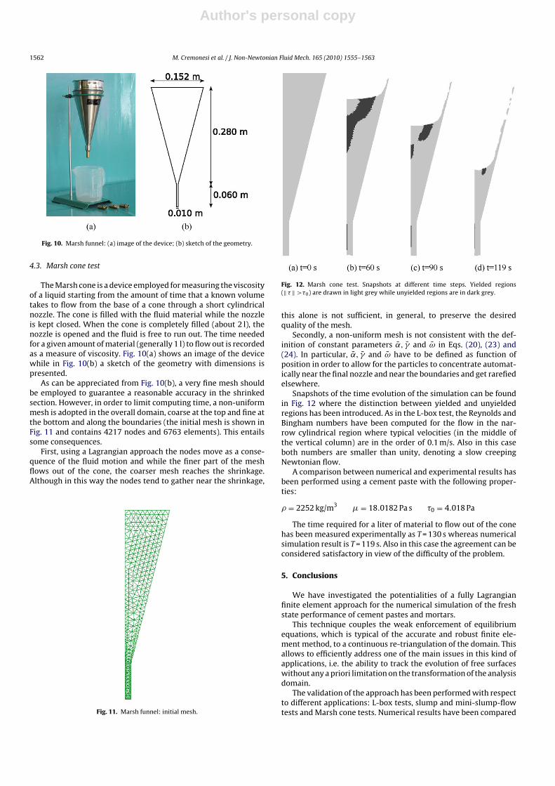
Fig. 10. Marsh funnel: (a) image of the device; (b) sketch of the geometry.

4.3. Marsh cone test

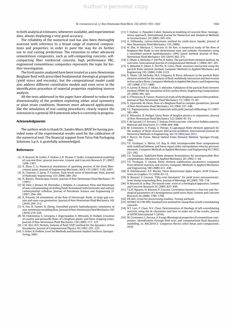
The Marsh cone is a device employed for measuring the viscosityof a liquid starting from the amount of time that a known volumetakes to flow from the base of a cone through a short cylindricalnozzle. The cone is filled with the fluid material while the nozzleis kept closed. When the cone is completely filled (about 2 l), thenozzle is opened and the fluid is free to run out. The time neededfor a given amount of material (generally 1 l) to flow out is recordedas a measure of viscosity. Fig. 10(a) shows an image of the devicewhile in Fig. 10(b) a sketch of the geometry with dimensions ispresented.

As can be appreciated from Fig. 10(b), a very fine mesh shouldbe employed to guarantee a reasonable accuracy in the shrinkedsection. However, in order to limit computing time, a non-uniformmesh is adopted in the overall domain, coarse at the top and fine atthe bottom and along the boundaries (the initial mesh is shown inFig. 11 and contains 4217 nodes and 6763 elements). This entailssome consequences.

First, using a Lagrangian approach the nodes move as a conse-quence of the fluid motion and while the finer part of the meshflows out of the cone, the coarser mesh reaches the shrinkage.Although in this way the nodes tend to gather near the shrinkage,

Fig. 11. Marsh funnel: initial mesh.

Fig. 12. Marsh cone test. Snapshots at different time steps. Yielded regions(‖ � ‖ >�0) are drawn in light grey while unyielded regions are in dark grey.

this alone is not sufficient, in general, to preserve the desiredquality of the mesh.

Secondly, a non-uniform mesh is not consistent with the def-inition of constant parameters ¯ , and ω in Eqs. (20), (23) and(24). In particular, ¯ , and ω have to be defined as function ofposition in order to allow for the particles to concentrate automat-ically near the final nozzle and near the boundaries and get rarefiedelsewhere.

Snapshots of the time evolution of the simulation can be foundin Fig. 12 where the distinction between yielded and unyieldedregions has been introduced. As in the L-box test, the Reynolds andBingham numbers have been computed for the flow in the nar-row cylindrical region where typical velocities (in the middle ofthe vertical column) are in the order of 0.1 m/s. Also in this caseboth numbers are smaller than unity, denoting a slow creepingNewtonian flow.

A comparison between numerical and experimental results hasbeen performed using a cement paste with the following proper-ties:

� = 2252 kg/m3 � = 18.0182 Pa s �0 = 4.018 Pa

The time required for a liter of material to flow out of the conehas been measured experimentally as T = 130 s whereas numericalsimulation result is T = 119 s. Also in this case the agreement can beconsidered satisfactory in view of the difficulty of the problem.

5. Conclusions

We have investigated the potentialities of a fully Lagrangianfinite element approach for the numerical simulation of the freshstate performance of cement pastes and mortars.

This technique couples the weak enforcement of equilibriumequations, which is typical of the accurate and robust finite ele-ment method, to a continuous re-triangulation of the domain. Thisallows to efficiently address one of the main issues in this kind ofapplications, i.e. the ability to track the evolution of free surfaceswithout any a priori limitation on the transformation of the analysisdomain.

The validation of the approach has been performed with respectto different applications: L-box tests, slump and mini-slump-flowtests and Marsh cone tests. Numerical results have been compared



to both analytical estimates, whenever available, and experimentaldata, always displaying a very good accuracy.

The reliability of the numerical tool has also been thoroughlyassessed with reference to a broad range of material composi-tions and properties, in order to pave the way for its furtheruse to real casting predictions. The extension to other advancedcementitious composites, such as self-compacting concrete, self-compacting fiber reinforced concrete, high performance FRC,engineered cementitious composites represents the topic for fur-ther investigation.

The fresh pastes analysed have been treated as a non-NewtonianBingham fluid with prescribed fundamental rheological properties(yield stress and viscosity), but the computational model couldalso address different constitutive models and even serve in theidentification procedure of material properties exploiting inverseanalysis.

All the tests addressed in this paper have allowed to reduce thedimensionality of the problem exploiting either axial symmetryor plain strain conditions. However more advanced applications,like the simulation of real casting procedures, clearly require theextension to a general 3D framework which is currently in progress.

Acknowledgments

The authors wish to thank Dr. Sandro Moro, BASF for having pro-vided some of the experimental results used for the calibration ofthe numerical tool. The financial support from Tetra Pak PackagingSolutions S.p.A. is gratefully acknowledged.

References

[1] N. Roussel, M. Geiker, F. Dufour, L.N. Thrane, P. Szabo, Computational modelingof concrete flow: general overview, Cement and Concrete Research 37 (2007)1298–1307.

[2] X. Zhou, Z. Li, Numerical simulations of upsetting process of the fresh fiber-cement paste, Journal of Engineering Mechanic, ASCE 133 (2007) 1192–2007.

[3] H. Chanson, S. Jarny, P. Coussot, Dam break wave of thixotropic fluid, Journalof Hydraulic Engineering 132 (2006) 280–293.

[4] H. Barnes, Thixotropya review, Journal of Non-Newtonian Fluid Mechanics 70(1997).

[5] M. Dolz, J. Jimnez, M. Hernndez, J. Delgido, A. Casanovas, Flow and thixotropyof non-contaminating oil drilling fluids formulated with bentonite and sodiumcarboxymethyl cellulose, Journal of Petroleum Science and Engineering 57(2007) 294–302.

[6] A. Potanin, 3d simulations of the flow of thixotropic fluids, in large-gap cou-ette and vane-cup geometries, Journal of Non-Newtonian Fluid Mechanics 165(2010) 299–312.

[7] X. Fan, R. Tanner, R. Zheng, Smoothed particle hydrodynamics simulation ofnon-newtonian moulding flow, Journal of Non-Newtonian Fluid Mechanics 165(2010) 219–226.

[8] M. Chatzimina, G. Georgiou, I. Argyropaidas, E. Mitsoulis, R. Huilgol, Cessationof couette and poiseuille flows of a bingham plastic and finite stopping times,Journal of Non-Newtonian Fluid Mechanics 129 (2005) 117–127.

[9] C.W. Hirt, B.D. Nichols, Volume of fluid (VOF) method for the dynamics of freeboundaries, Journal of Computational Physics 39 (1981) 201–225.

[10] S. Osher, R. Fedkiw, Level Set Methods and Dynamic Implicit Surfaces, Springer-Verlag, 2003.

[11] F. Dufour, G. Pijaudier-Cabot, Numerical modeling of concrete flow: homoge-neous approach, International Journal for Numerical and Analytical Methodsin Geomechanics 29 (2005) 395–416.

[12] A. Vikhansky, Lattice-boltzmann method for yield-stress liquids, Journal ofNon-Newtonian Fluid Mechanics 155 (2008).

[13] H. Zhu, N. Martysa, C. Ferraris, D. De Kee, A numerical study of the flow ofbingham-like fluids in two-dimensional vane and cylinder rheometers usinga smoothed particle hydrodynamics (SPH) based method, Journal of Non-Newtonian Fluid Mechanics 165 (2010) 362–375.

[14] E. Onate, S. Idelsohn, F. Del Pin, R. Aubry, The particle finite element method. Anoverview, International Journal of Computational Methods 1 (2004) 267–307.

[15] S. Idelsohn, E. Onate, F. Del Pin, N. Calvo, Fluid–structure interaction using theparticle finite element method, Computer Methods in Applied Mechanics andEngineering 195 (2006) 2100–2123.

[16] E. Onate, S.R. Idelsohn, M.A. Celigueta, R. Rossi, Advances in the particle finiteelement method for the analysis of fluid-multibody interaction and bed erosionin free surface flows, Computer Methods in Applied Mechanics and Engineering197 (2008) 1777–1800.

[17] A. Larese, R. Rossi, E. Onate, S. Idelsohn, Validation of the particle finite elementmethod (PFEM) for simulation of free surface flows, Engineering Computations25 (2008) 385–425.

[18] E. O’Donovan, R. Tanner, Numerical study of the Bingham squeeze film problem,Journal of Non-Newtonian Fluid Mechanics 15 (1984) 75–83.

[19] G. Lipscomb, M. Denn, Flow of a Bingham fluid in complex geometries, Journalof Non-Newtonian Fluid Mechanics 14 (1984) 337–346.

[20] T.C. Papanastasiou, Flows of materials with yield, Journal of Rheology 31 (1987)385–404.

[21] E. Mitsoulis, R. Huilgol, Entry flows of binghm plastics in expansions, Journalof Non-Newtonian Fluid Mechanics 122 (2004) 45–54.

[22] F. de Larrard, C.F. Ferraris, T. Sedran, Fresh concrete: a herschel-bulkley materia,Material and Structures 31 (1998) 494–498.

[23] M. Cremonesi, A. Frangi, U. Perego, A Lagrangian finite element approach forthe analysis of fluid–structure interaction problems, International Journal forNumerical Methods in Engineering, doi:10.1002/nme.2911.

[24] F. Brezzi, M. Fortin, Mixed Hybrid Finite Element Method, Springer-Veralg,1991.

[25] T.E. Tezduyar, S. Mittal, S.E. Ray, R. Shih, Incompressible flow computationswith stabilized bilinear and linear equal-order-interpolation velocity-pressureelements, Computer Methods in Applied Mechanics and Engineering 95 (1992)221–242.

[26] T.E. Tezduyar, Stabilized finite element formulations for incompressible flowcomputations, Advances in Applied Mechanics 28 (1992) 1–44.

[27] T.E. Tezduyar, Y. Osawa, Finite element stabilization parameters computedfrom element matrices and vectors, Computer Methods in Applied Mechanicsand Engineering 190 (2000) 411–430.

[28] H. Edelsbrunner, E.P. Mucke, Three dimensional alpha shapes, ACM Transac-tions on Graphics 13 (1994) 43–72.

[29] N. Roussel, P. Coussot, “Fifty-cent rheometer” for yield stress measurements:from slump tospreading flow, Journal of Rheology 49 (2005) 705–718.

[30] N. Roussel, R. Le Roy, The marsh cone: a test or a rheological apparatus, Cementand Concrete Research 35 (2005) 823–830.

[31] T.L.H. Nguyen, N. Roussel, P. Coussot, Correlation between L-box test and rhe-ological parameters of a homogeneous yield stress fluid, Cement and ConcreteResearch 36 (2006) 1789–1796.

[32] EN 445, Grout for prestressing tendons. Testing methods.[33] ASTM/C1611M-09b, Standard test method for slump flow of self-consolidating

concrete.[34] N.T. Lars, P. Claus, N.V. Claus, Determination of rheology of self-consolidating

concrete using the 4c-rheometer and how to make use of the results, Journalof ASTM International 7 (2010).

[35] M. Cremonesi, L. Ferrara, A. Frangi, Rheological properties of cementitious com-posites: identification through field tests and computational fluid dynamicsmodelling, in: BAC2010-2◦ Congresso Iberico sobre betao auto-compactavel,2010.

Simulation of the flow of fresh cement suspensions by a Lagrangian finite element approach

Documents

Transcript of Simulation of the flow of fresh cement suspensions by a Lagrangian finite element approach