Adaptive local dissimilarity measures for discriminative dimension reduction of labeled data

ARTICLE IN PRESS

Neurocomputing 73 (2010) 1074–1092

Contents lists available at ScienceDirect

Neurocomputing

0925-23

doi:10.1

� Corr

E-m

journal homepage: www.elsevier.com/locate/neucom

Adaptive local dissimilarity measures for discriminative dimensionreduction of labeled data

Kerstin Bunte a,�, Barbara Hammer d, Axel Wismuller b,c, Michael Biehl a

a University of Groningen, Johann Bernoulli Institute for Mathematics and Computer Science, P.O. Box 407, 9700 AK Groningen, The Netherlandsb Department of Radiology, University of Rochester, 601 Elmwood Avenue, Rochester, NY 14642-648, USAc Department of Biomedical Engineering, University of Rochester, 601 Elmwood Avenue, Rochester, NY 14642-648, USAd Bielefeld University, CITEC, Universitatsstraße 23, 33615 Bielefeld, Germany

a r t i c l e i n f o

Available online 18 January 2010

Keywords:

Dimension reduction

Learning vector quantization

Visualization

12/$ - see front matter & 2010 Elsevier B.V. A

016/j.neucom.2009.11.017

esponding author. Tel.: +31 (0)50 363 7049.

ail address: [email protected] (K. Bunte).

a b s t r a c t

Due to the tremendous increase of electronic information with respect to the size of data sets as well as

their dimension, dimension reduction and visualization of high-dimensional data has become one of the

key problems of data mining. Since embedding in lower dimensions necessarily includes a loss of

information, methods to explicitly control the information kept by a specific dimension reduction

technique are highly desirable. The incorporation of supervised class information constitutes an

important specific case. The aim is to preserve and potentially enhance the discrimination of classes in

lower dimensions. In this contribution we use an extension of prototype-based local distance learning,

which results in a nonlinear discriminative dissimilarity measure for a given labeled data manifold. The

learned local distance measure can be used as basis for other unsupervised dimension reduction

techniques, which take into account neighborhood information. We show the combination of different

dimension reduction techniques with a discriminative similarity measure learned by an extension of

learning vector quantization (LVQ) and their behavior with different parameter settings. The methods

are introduced and discussed in terms of artificial and real world data sets.

& 2010 Elsevier B.V. All rights reserved.

1. Introduction

The amount of electronic data doubles roughly every 20months [1], and its sheer size makes it impossible for humans tomanually scan through the available information. At the sametime, rapid technological developments cause an increase of datadimension, e.g. due to the increased sensitivity of sensortechnology (such as mass spectrometry) or the improved resolu-tion of imaging techniques. This causes the need for reliabledimension reduction and data visualization techniques to allowhumans to rapidly inspect large portions of data using theirimpressive and highly sensitive visual perception capabilities.

Dimension reduction and visualization constitutes an activefield of research, see, e.g. [2–4] for recent overviews. Theembedding of high-dimensional data into lower dimension isnecessarily linked to loss of information. In the last decades anenormous number of unsupervised dimension reduction methodshas been proposed. In general, unsupervised dimension reductionis an ill-posed problem since a clear specification which proper-ties of the data should be preserved, is missing. Standard criteria,

ll rights reserved.

for instance the distance measure employed for neighborhoodassignment, may turn out unsuitable for a given data set, andrelevant information often depends on the situation at hand.

If data labeling is available, the aim of dimension reduction canbe defined clearly: the preservation of the classification accuracyin a reduced feature space. Supervised linear dimension reducersare for example the generalized matrix learning vector quantiza-tion (GMLVQ) [5], linear discriminant analysis (LDA) [6], targetedprojection pursuit [7], and discriminative component analysis [8].Often, however, the classes cannot be separated by a linearclassifier while a nonlinear data projection better preserves therelevant information. Examples for nonlinear discriminativevisualization techniques include, extensions of the self-organizingmap (SOM) incorporating class labels [9] or more generalauxiliary information [10]. In both cases, the metric of SOM isadjusted such that it emphasizes the given auxiliary informationand, consequently, SOM displays the aspects relevant forthe given labeling. Further supervised dimension reductiontechniques are model-based visualization [11] and parametricembedding [12]. In addition, linear schemes such as LDA can bekernelized yielding a nonlinear supervised dimension reductionscheme [13]. These models have the drawback that they are oftenvery costly (squared or cubic with respect to the number ofdata points). Recent approaches provide scalable alternatives,

www.elsevier.com/locate/neucom

dx.doi.org/10.1016/j.neucom.2009.11.017

mailto:[email protected]

ARTICLE IN PRESS

K. Bunte et al. / Neurocomputing 73 (2010) 1074–1092 1075

sometimes at the cost of non-convexity of the problem [14–16].However, in most methods, the kernel has to be chosen prior totraining and no metric adaptation according to the given labelinformation takes place.

The aim of this paper is to identify and investigate principledpossibilities to combine an adaptive metric and recent visualiza-tion techniques towards a discriminative approach. We willexploit the discriminative scheme exemplary for different typesof visualization, necessarily restricting the number of possiblecombinations to exemplary cases. A number of alternativecombinations of metric learning and data visualization as wellas principled alternatives to arrive at discriminative visualizationtechniques (such as, e.g. colored maximum variance unfolding[17]) will not be tackled in this paper.

In this contribution we combine prototype-based matrixlearning schemes, which result in local discriminative dissim-ilarity measures and local linear projections of the data, withdifferent neighborhood based nonlinear dimension reductiontechniques and a charting technique. The complexity of thematrix learning technique is only linear in the number of points S,their dimension N and can be controlled by the number of theprototypes m and sweep through the training set t, leading to anoverall algorithm complexity of only OðS � N �m � tÞ. In the secondstep unsupervised techniques like manifold charting [18], Isomap[19], locally linear embedding (LLE) [20], the explorationobservation machine (XOM) [21] and stochastic neighbor embed-ding (SNE) [22] are performed incorporating the supervisedinformation from the LVQ approach. This leads to supervisednonlinear dimension reduction and visualization techniques.Note, for one presented training sample, the matrix learningscheme only needs to compute the distances to all prototypes.And the number of prototypes is usually much smaller than thenumber of data points. However, the combination with anotherdimension reduction technique may make the computation of thedistances of all data points necessary, e.g. with Isomap or SNE.This is at least a quadratic problem but can be moderated byapproximations [23–25].

The following section gives a short overview over thetechniques. We focus on the question in how far local lineardiscriminative data transformations as provided by GMLVQ offerprincipled possibilities to extend standard unsupervised visuali-zation tools to discriminative visualization. Section 3 discussesthe different approaches for one artificial and three real worlddata sets and compares the results to popular supervised as wellas unsupervised dimension reduction techniques. Finally weconclude in Section 4.

2. Supervised nonlinear dimension reduction

For general data sets a global linear reduction to lowerdimensions may not be sufficient to preserve the informationrelevant for classification. In [3] it is argued that the combinationof several local linear projections to a nonlinear mapping canyield promising results. We use this concept and learn discrimi-native local linear low-dimensional projections from labeled datausing an efficient prototype based learning scheme, generalizedmatrix learning vector quantization (GMLVQ). Locally linearprojections which result from this first step provide, on the onehand, local transformations of the data points which preservethe information relevant for the classification as much as possible.Instead of the local coordinates, local distances induced bythese local representation of data can be considered. As a conse-quence, visualization techniques which rely on local coordinatesystems or local distances, respectively, can be combined withthis first step to arrive at a discriminative global nonlinear

projection method. This way, an incorporation into techniquessuch as manifold charting [18], Isomap [19], locally linear embed-ding (LLE) [20], stochastic neighbor embedding (SNE) [22],maximum variance unfolding (MVU) [26] and the explorationobservation machine (XOM) [21] becomes possible.

The following subsections give a short overview over the initialprototype based matrix learning scheme and the differentvisualization algorithms.

2.1. Localized LiRaM LVQ

Learning vector quantization (LVQ) [27] constitutes a particu-larly intuitive classification algorithm which represents data bymeans of prototypes. LVQ itself constitutes a heuristic algorithm,hence extensions have been proposed for which convergence andlearnability can be guaranteed [28,29]. One particularly crucialaspect of LVQ schemes is the dependency on the underlyingmetric, usually the Euclidean metric, which may not suit theunderlying data structure. Therefore, general metric adaptationhas been introduced into LVQ schemes [29,30]. Recent extensionsparameterize the distance measure in terms of a relevance matrix,the rank of which may be controlled explicitly. The algorithmsuggested in [5] can be employed for linear dimension reductionand visualization of labeled data. The local linear versionpresented here provides the ability to learn local low-dimensionalprojections and combine them into a nonlinear global embeddingusing charting techniques or projection methods based on localdata topologies or local distances. Several schemes for adaptivedistance learning exist, for example large margin nearest neighbor(LMNN) [31] to name just one. We compared the LMNN techniquewith the LVQ based approach on the basis of a content basedimage retrieval application in an earlier publication (see [32]).Furthermore it should be mentioned that LMNN learns a globaldistance measure. More powerful, local distance learning wouldpresumably involve higher computational complexity and shouldbe feasible for small dimensionality N only.

We consider training data xiARN , i¼ 1 . . . S with labels yi

corresponding to one of C classes, respectively. The aim of LVQ is tofind m prototypes wjARN with class labels cðwjÞAf1; . . . ;Cg suchthat they represent the classification as accurately as possible.A data point xi is assigned to the class of its closest prototype wj

where dðxi;wjÞrdðxi;wlÞ for all ja l. d usually denotes the squaredEuclidean distance dðxi;wjÞ ¼ ðxi�wjÞ

>ðxi�wjÞ. Generalized LVQ

(GLVQ) [33] adapts prototype locations by minimizing the costfunction

EGLVQ ¼XS

i ¼ 1

FdðwJ ; xiÞ�dðwK ; xiÞ

dðwJ ; xiÞþdðwK ; xiÞ

� �; ð1Þ

where wJ denotes the closest prototype with the same class labelas xi, and wK is the closest prototype with a different class label. Fis a monotonic function, e.g. the logistic function or the identity. Inthis work we use the identity. This cost function aims at anadaptation of the prototypes such that a large hypothesis margin isobtained, this way achieving correct classification and, at the sametime, robustness of the classification, see [34]. A learning algorithmcan be derived from the cost function EGLVQ by means of astochastic gradient descent as shown in [29,28].

Matrix learning in GLVQ (GMLVQ) [30,34] substitutes the usualsquared Euclidean distance d by a more advanced dissimilaritymeasure which contains adaptive parameters, thus resulting in amore complex and better adaptable classifier. In [5], it wasproposed to choose the dissimilarity as

dLj ðwj; xiÞ ¼ ðxi�wjÞ>Ljðxi�wjÞ; ð2Þ

ARTICLE IN PRESS

K. Bunte et al. / Neurocomputing 73 (2010) 1074–10921076

with an adaptive, symmetric and positive semi-definite matrixLjARN�N locally attached to each prototype wj. The dissimilaritymeasure Eq. (2) possesses the shape of a Mahalanobis distance.Note, however, that the precise matrix is determined in adiscriminative way according to the given labeling, such thatsevere differences from the standard Mahalanobis distance basedon correlations can be observed. By setting Lj ¼O>j Oj semi-definiteness and symmetry is guaranteed. Optimization takesplace by a stochastic gradient descent of the cost function EGLVQ inEq. (1), with the distance measure d substituted by dLj (seeEq. (2)). After each training epoch (sweep through the trainingset) the matrices are normalized to

Pi½Lj�ii ¼ 1 in order to prevent

degeneration to 0. An additional regularization term in the costfunction proportional to �lnðdetðOjO

>

j ÞÞ can be used to enforcefull rank M of the relevance matrices and prevent over-simplification effects, see [35].

The cost function of GMLVQ is non-convex and, in conse-quence, different local optima can occur which lead to differentsubsequent data visualizations. The non-convexity of the costfunction is mainly due to the discrete data assignments toprototypes which is not unique in particular for realistic datasets with overlapping classes. In the experiments, differentassignments and, in consequence, different visualizations couldbe observed, where these visualizations focus on differentrelevant facets of the given data sets.

The choice OjARM�N with MrN transforms the data locally toan M-dimensional feature space. It can be shown that theadaptive distance dLj ðwj; xiÞ in Eq. (2) equals the squaredEuclidean distance in the transformed space under the transfor-mation x/Ojx, because dLj ðwj; xiÞ ¼ ½Ojxi�Ojwj�

2. The targetdimension M must be chosen in advance by intrinsic dimensionestimation or according to available prior knowledge. Forvisualization purposes, usually a value of two or three isappropriate. At the end of the learning process the algorithmprovides a set of prototypes wj, their labels cðwjÞ, and correspond-ing projections Oj and distances dLj . For every prototype, a lowdimensional embedding ni of each data point xi is then given by

PjðxiÞ ¼Ojxi ¼ ni: ð3Þ

This projection is a meaningful discriminative projection in theneighborhood of a prototype for a data point xi, usually theprojection Oj of its closest prototype wj is considered. This way, aglobal mapping is given as

xi/PjðxiÞ ¼Ojxi with dLj ðwj; xiÞ ¼mink

dLk ðwk; xiÞ: ð4Þ

We will refer to this prototype and matrix learning algorithm aslimited rank matrix LVQ (LiRaM LVQ), and we will address thelocal linear mappings induced by LiRaM LVQ as LiRaM LVQmappings. Note that the effort to obtain these projectionsdepends linearly on the number of data, the number ofprototypes, the number of training epochs, and the dimensional-ities N and M of the matrices.

Note that Oj is not uniquely given by the cost function Eq. (1)and it varies for different initializations, because the dissimilarityis invariant under operations such as rotation of the matrices. If aunique representation Oj of Oj is needed for comparison, theunique square root of Lj is chosen [36].

LiRaM LVQ directly provides a global linear discriminativeembedding of data if only one global adaptive matrix O¼Oj isused, as demonstrated in [5]. Alternatively, one can consider thelocal data projections provided by the LiRaM LVQ mappings onthe receptive fields of the prototypes as defined in Eq. (4).However, the cost function together with the distance definitiondoes not ensure that these local projections align correctly andthat they do not overlap when shown in one coordinate system.

Rather, the projections provide widely unconnected mappings tolow dimensions which offer only a locally valid visualization.Nevertheless the mapping defined by Eq. (4) can give a firstintuition about the problematic samples and distinguish ‘‘easy’’classes from more difficult ones. Therefore, we will use thisprojection as a comparison in the experiments.

In order to achieve interpretable global nonlinear mappings ofthe data points we have to align the local information provided bythe local projections. This can be done in different ways, using anexplicit charting technique of the maps or using visualizationtechniques based on the local distances provided by this method.In the following, we introduce a few principled possibilities tocombine the information of LiRaM LVQ and unsupervisedvisualization techniques to achieve a global nonlinear discrimi-native visualization.

2.2. Information provided by LiRaM LVQ for discriminative

visualization

LiRaM LVQ determines prototypes and matrices based on adiscriminative classification task. These parameters induce im-portant discriminative information which can be plugged intodifferent visualization schemes.

2.2.1. Local coordinates

As already stated, LiRaM LVQ gives rise to local linearprojection maps Pj as defined in Eq. (3) which assign localprojection coordinates to every data point xi. These projectionscan be accompanied by values which indicate the responsibility rji

of mapping j for data point i. Crisp responsibilities are obtained bymeans of the receptive fields, setting rji to 1 iff wj is the winner forxi. Alternatively, soft assignments can be obtained by centeringGaussian curves of appropriate bandwidth at the prototypes.

These two ingredients constitute a sufficient input for datavisualization methods which rely on local linear projections of thedata only, such as manifold charting, locally linear coordination(LLC) [3] and local tangent space alignment (LTSA) [37]. Basically,those methods arrive at a global embedding of data based on localcoordinates by gluing the points together such that the overallmapping is consistent with the original data points as much aspossible. The methods differ in the precise cost function which isoptimized: Manifold charting relying on the sum squared error ofpoints at overlapping pieces of the local charts, while LLC focuseson the local topology and tries to minimize the reconstructionerror of points from their neighborhood. Both approaches provideexplicit maps of the data manifold to low dimensions, such thatout-of-sample extensions are immediate. As an example for thisprinciple, we will investigate the combination of local linear mapsand manifold charting.

2.2.2. Global distances

The LiRaM LVQ learning procedure provides discriminativelocal distances induced by the matrices Lj in the receptive field ofprototype wj. We use this observation to define a discriminativedissimilarity measure for the given data points. We define thedissimilarity of a point xi to a point x:

dðxi; xÞ ¼ ðxi�xÞ>Ljðxi�xÞ where dLj ðxi;wjÞ ¼min dLk ðxi;wkÞ ð5Þ

using the distance measure Lj induced by the closest prototypewj of xi. Note that this definition leads to asymmetric dissim-ilarities, where dðxi; xjÞadðxj; xiÞ can hold. It is block wisesymmetric for data samples with the same winner prototype inthe classification task. Further, due to the nature of the LiRaM LVQcost function, the dissimilarity measure constitutes a valid choiceonly within or near receptive fields. The dissimilarity of far away

ARTICLE IN PRESS


points which are not located in the same or proximous receptivefields can be seen only as a rough estimation of a validdissimilarity.

The global dissimilarities defined by Eq. (5) can be useddirectly within visualization schemes which are based on distancepreservation. If necessary, the dissimilarity matrix can besymmetrized prior to the mapping. Distance based visualizationmethods include classical multidimensional scaling (MDS),Sammon’s map, stochastic neighbor embedding (SNE), t-distributedSNE (t-SNE), and the exploration observation machine (XOM), toname just a few [3,22,38,21]. It can be expected that thecombination of the global discriminative dissimilarities as givenby Eq. (5) yields to an appropriate visualization of the data only ifthe visualization method mainly focuses on the close points, sincethe dissimilarity of far away points can only be seen as a guess inthis case. Thus, classical MDS is likely to fail, while SNE or XOMseem more promising due to their focus on local distances.Further, these methods usually provide an embedding of thepoints only without giving an explicit map, such thatout-of-sample extensions are not immediate. As an example, wewill investigate the combination of the global dissimilarity matrixwith SNE and XOM, respectively, in the following.

In contrast to the charting approach, the ranks M of thedistance matrices Lj can be chosen larger than the embeddingdimension in these cases, using, e.g. full ranks or the intrinsicdimension of the data manifold.

2.2.3. Local distances or neighborhood

The problem that the dissimilarity measure as defined inEq. (5) should preferably only be used to compare data within areceptive field or in neighbored receptive fields is avoided byvisualization techniques which explicitly rely on local distancesonly. Instances of such visualization techniques are given byIsomap, Laplacian eigenmaps, locally linear embedding (LLE) [3]and maximum variance unfolding (MVU) [26]. These methodsuse the local neighborhood of a data point, i.e. its k nearestneighbors (k-NN neighborhood) or the points in an e�ball(e�neighborhood), and try to preserve properties of theseneighborhoods. Obviously, local neighborhoods can readily becomputed based on the dissimilarities given by Eq. (5), thus adiscriminative extensions of these methods is offered this way.

Isomap extends local distances within the local neighborhoodsto a global measure by means of the graph distance, using simpleMDS after this step. Laplacian eigenmaps use the neighborhoodgraph and try to map data points such that close points remainclose in the projection. LLE also relies on the local neighborhood,but it tries to preserve the local angles of points rather than thedistances. Obviously, these methods can be transferred todiscriminative visualization techniques by using the local neigh-borhood as given be the local discriminative distances and, ifrequired, the local discriminative distances themselves. As anexample, we will investigate the combination of Isomap and LLEwith this discriminative technique. Again, these techniquesprovide a map of the given data points only, rather than anexplicit embedding function.

Now we introduce four exemplary discriminative projectionmethods, covering the different possibilities to combine theinformation given by LiRaM LVQ and visualization techniques.We will compare these methods to a naive embedding directlygiven by the local linear maps as a baseline, linear discriminantanalysis (LDA) [6] (if applicable) as a classical linear discrimina-tive visualization tool, and t-SNE as one of the currently mostpowerful unsupervised visualization techniques. Further, we willemphasize the effect of discriminative information by presentingthe result of the corresponding unsupervised projection method.

2.3. Combination of local linear patches by charting

The charting technique introduced in [18] provides a frame forunsupervised dimension reduction by decomposing the sampledata into locally linear patches and combining them into a singlelow-dimensional coordinate system. This procedure can be turnedinto a discriminative visualization scheme by using the M low-dimensional local linear projections PjðxiÞARM for every datapoint xi and every local projection Oj provided by localized LiRaMLVQ in the first step. The second step of the charting method canthen directly be used to combine these maps. In charting, the localprojections PjðxiÞ are weighted by their responsibilities rji whichquantify the overlap of neighbored charts. Here we chooseresponsibilities induced by Gaussians centered at the prototypes,since a certain degree of overlap is needed for a meaningfulcharting step:

rjipexpð�ðxi�wjÞ>Ljðxi�wjÞ=sjÞ; ð6Þ

where sj40 constitutes an appropriate bandwidth. Further, wehave to normalize these responsibilities

Pjrji ¼ 1 in order to apply

charting. Since the combination step needs a reasonable overlapof neighbored patches, the bandwidth sj must be chosen toensure this property. We set sj to a fraction a (0oao1) of themean distance to the k nearest prototypes in the original featurespace

sj ¼ a �1

k

ffiffiffiffiffiffiffiffiffiffiffiffiffiffiffiffiffiffiffiffiffiffiffiffiffiffiffiffiffiffiffiffiffiffiffiffiffiffiffiffiffiffiXwl AN kðwjÞ

dLj ðwj;wlÞ

s; ð7Þ

where N kðwjÞ denotes the k closest prototypes to wj.Manifold charting minimizes a convex cost function that

measures the amount of disagreement between the linear modelson the global coordinates of the data points. The chartingtechnique finds affine mappings Aj from the data representationsPjðxiÞ to the global coordinates that minimize the cost function

Echarting ¼XS

i ¼ 1

Xm

j ¼ 1

Xm

k ¼ 1

rjirkiJAjðPjðxiÞÞ�AjðPkðxiÞÞJ2: ð8Þ

This function is based on the idea that whenever two linearmodels possess a high responsibility for a data point, the modelsshould agree on the final coordinates of that point. The costfunction can be rewritten as a generalized eigenvalue problemand an analytical solution can be found in closed form. Theprojection is given by the mapping xi/ni ¼

PjrjiAjðPjðxiÞÞ. We

refer to [18] for further details. Interestingly, an explicit map ofthe data manifold to low dimensions is obtained this way. Further,the charting step is linear in the number of data points S. we referto the extension of charting by local discriminative projections aschartingþ in the following.

2.4. Discriminative locally linear embedding

Locally linear embedding (LLE) [20] uses the criterion oftopology preservation for dimension reduction. The idea is toreconstruct each point xi by a linear combination of its nearestneighbors with coefficients Wi and to project data points suchthat this local representation of the data is preserved as much aspossible.

The first step of the LLE algorithm is the determination ofneighbors N i for each data point xi. Typical choices are either thek closest points or all points lying inside an e�ball with center xi.Following the ideas of supervised LLE [39] and probability-basedLLE [40] we take the label information into account by usingthe distance measure defined in Eq. (5) to determine the k

nearest neighbors of each point. The neighborhood of xi is referredto as N i.

ARTICLE IN PRESS

1

2

3

4

5

6

2 dimensions of the original data

Fig. 1. The two informational dimensions of the original Three Tip Star data set.


The second and third step of the LLE approach remainunchanged. In step two the reconstruction weights W for everydata point are computed by minimizing the squared reconstruc-tion error

ELLEðWÞ ¼XS

i ¼ 1

xi�X

jAN i

wijxj

��

2

; ð9Þ

by constrained linear fits such thatP

jwij ¼ 1. The entries wij ofthe matrix W weight the neighbors for the reconstruction of xi.Due to the constraints, this scheme is invariant to rotations,rescalings and translations of the data points. The third step of LLEbases on the idea, that these geometric properties should alsobe valid for a low-dimensional representation of the data. Thus,the low-dimensional representations n are found by minimizingthe cost function

CostLLEðnÞ ¼X

i

ni�X

jAN i

wijnj

0@

1A2

¼ trðn>ðI�WÞ>ðI�WÞnÞ; ð10Þ

with I being the identity matrix. The smallest D non-zeroeigenvalues of ðI�WÞ>ðI�WÞ yield the final embedding n. Furtherdetails can be found in [20]. Advantages of this method arethe elegant theoretical foundation which allows an analyticalsolution. LLE requires the solution of an S-by-S eigenproblem withS being the number of data points, i.e. the effort is squared in S. Asreported in [41], the parameters must be tuned carefully. Themethod provides a mapping of the given points only rather thanan explicit embedding function. We refer to this discriminativeextension of LLE by LLEþ in the following.

2.5. Discriminative Isomap

Isomap [19] is an extension of metric Multi-DimensionalScaling (MDS) which uses distance preservation as criterion forthe dimension reduction. It performs a low dimensional embed-ding based on the pairwise distance between data points.Whereas metric MDS is based on the Euclidean metric for allpairwise distances, Isomap incorporates the so called graphdistances as an approximation of the geodesic distances. For thispurpose, a weighted neighborhood graph is constructed byconnecting points i and j if their distance is smaller than e(e�Isomap), or if j is one of the k nearest neighbors of i (k-Isomap).Global distances between points are computed using shortestpaths in this neighborhood graph. The local neighborhood graphcan serve as an interface to incorporate discriminative informa-tion provided by LiRaM LVQ. We use the distances defined by Eq.(5) to determine the k nearest neighbors and to weight the edgesin the neighborhood graph. Afterwards, we simply apply the sameprojection technique as original Isomap.

The Isomap algorithm shares the same model type andoptimization procedure as principal component analysis (PCA)and metric MDS, thus a global optimum can be determinedanalytically. While PCA and MDS are designed for linearsubmanifolds, Isomap can handle developable manifolds due toits use of geodesic distances. However, it may yield disappointingresults if applied to not developable manifolds. Furthermore, thequality of the approximation of the geodesic distances by thegraph distances may be sensitive to the choice of the parameters.A similar problem exists for virtually all local manifold estimationtechniques which rely on critical parameters to define the localneighborhood such as the number of neighbors or the neighbor-hood size. For details we refer to [19]. Note that this method is ofcubic complexity with respect to the number of data because ofthe necessity to compute all shortest paths within the neighbor-hood graph with S vertices. As before, no explicit map is obtained

for the embedding when using Isomap. We refer to thisdiscriminative extension of Isomap as Isomapþ in the following.

2.5.1. Discriminative stochastic neighbor embedding

Stochastic neighbor embedding (SNE) constitutes an unsuper-vised projection which follows a probability based approach. AGaussian function is centered at every data point xi which inducesa conditional probability of a point xj given xi

pjji ¼expð�dðxi; xjÞ=2s2

i ÞPka iexpð�dðxi; xkÞ=2s2

i Þ; ð11Þ

where si is the variance and d denotes the dissimilarity measure,which is chosen as squared Euclidean distance in the originalapproach. Projection takes place in such a way that theseconditional probabilities are preserved as much as possible forthe projected points in the low-dimensional space. Moreprecisely, for counterparts ni and nj of the data points xi and xj

the conditional probability is defined similar to Eq. (11)

qjji ¼expð�Jni; njJ

2ÞP

ka iexpð�Jni;nkJ2Þ; ð12Þ

with fixed bandwidth 1=ffiffiffi2p

. The goal of SNE is to find a low-dimensional data representation that minimizes the mismatchbetween pjji and qjji. This is done by the minimization of the sumof the Kullback–Leibler divergences

ESNE ¼X

i

Xj

pjji logpj;i

qjji: ð13Þ

The minimization of this objective function is difficult and maystuck in local minima. Details can be found in [22].

An important parameter of SNE is the so-called perplexitywhich is used to determine the bandwidths of the Gaussians inthe data space based on the effective number of local neighbors.The performance of SNE is fairly robust to changes in theperplexity and typical values are between 5 for small data setsand 50 for large datasets with more than 10 000 instances.

It is easily possible to incorporate discriminative informationinto SNE by choosing the distances dðxi; xjÞ in Eq. (11) asdiscriminative distances as provided by Eq. (5). Then, thesubsequent steps can be done in the same way as in standardSNE. This way, a discriminative embedding of data which displaysquadratic effort in S can be obtained.

2.6. Discriminative exploration observation machine (XOM)

The exploratory observation machine (XOM) has recently beenintroduced as a novel computational framework for structure-preserving dimension reduction [42,43]. It has been shown thatXOM can simultaneously contribute to several different domains

ARTICLE IN PRESS

PCA t−SNE (Perplexity 35)

Fig. 2. Example embeddings of the Three Tip Star data set for PCA and tSNE.


of advanced machine learning, scientific data analysis, andvisualization, such as nonlinear dimension reduction, dataclustering, pattern matching, constrained incremental learning,and the analysis of non-metric dissimilarity data [44,45].

The XOM algorithm can be resolved into three simple,geometrically intuitive steps.

Step 1:
Define the topology of the input data in the high-dimensional data space by computing distances dðxi; xjÞ
between the data vectors xi; iAf1; . . . ; Sg.
Step 2: Define a ‘‘hypothesis’’ on the structure of the data in the
embedding space w, represented by ‘‘sampling’’ vectorswkAw; kAf1; . . . ;mg;mAN, and randomly initialize an‘‘image’’ vector niAw; iAf1; . . . ; Sg for each input vector xi.There is no principal limitation whatsoever of how such asampling distribution could be chosen. Typical choicesare a uniform distribution (e.g. in a 2D square) forstructure-preserving visualization and the choice w¼R2.

Step 3:
Reconstruct the topology induced by the input data bymoving the image vectors in the embedding space w usingthe computational scheme of a topology-preservingmapping. The final positions of the image vectors ni
represent the output of the algorithm.

1 http://infohost.nmt.edu/�borchers/csdp.html2 http://www.weinbergerweb.net/Downloads/MVU.html

The image vectors ni are incrementally updated by a sequentiallearning procedure. For this purpose, the neighborhood couplingsbetween the input data items are represented by a so-calledcooperativity (or neighborhood) function, which is typical chosenas a Gaussian.

The overall complexity of the algorithm is quadratic in thenumber of data points. We refer to [44] for further details.Obviously, discriminative information can be included into XOMby substituting the distances computed in Step 1 by thediscriminative distances as provided by LiRaM LVQ in Eq. (5).

2.7. Discriminative maximum variance unfolding (MVU)

Maximum variance unfolding (MVU) [26,46] is a dimensionreduction technique which aims at preservation if local distances.So distances between nearby high dimensional inputs fxig

Si ¼ 1

should match the distances between nearby low-dimensionaloutputs fnig

Si ¼ 1. Assume the inputs xi are connected to their k

nearest neighbors by rigid rods. The algorithm attempts to pullthe inputs apart, maximizing the sum of their pairwise distanceswithout breaking (or stretching) the rigid rods that connect thenearest neighbors. For the mathematical formulation let ZijAf0;1g

denote whether inputs xi and xj are k-nearest neighbors and solvethe following optimization:

MaximizeX

ij

Jni�njJ2subject to

ð1Þ ni�njJ2¼ Jxi�xjJ

2 for all ði; jÞ with Zij ¼ 1;

ð2ÞX

i

ni ¼ 0:

This optimization is not convex, so the optimization is reformu-lated as a semi-definite program (SDP) by defining the innerproduct matrix Kij ¼ ni � nj. The SDP over K can be written as

Maximize trace ðKÞ subject to

ð1Þ Kii�2KijþKjj ¼ Jxi�xjJ2 for all ði; jÞ;

ð2ÞX

ij

Kij ¼ 0;

ð3Þ Kk0 ðpositive semi� definitenessÞ:

This SDP is convex and can be solved with polynomial-timeguarantees. To include supervision in this dimension reductiontechnique the distance defined by Eq. (5) can be used todetermine the k nearest neighbors. Afterwards we simply applythe same optimization as original MVU. For our experiments weused the library for semi-definite programming called CSDP1 andthe MVU implementation provided by Kilian Q. Weinberger.2

2.8. Further embedding techniques

We will compare the results obtained within this discrimina-tive framework to a few standard embedding techniques. Moreprecisely, we will display the results of linear discriminantanalysis (LDA) [6] as a classical linear discriminative projectiontechnology, t-distributed SNE (t-SNE) as an extension of SNEwhich constitutes one of the most promising unsupervisedprojection techniques available today.

LDA constitutes a supervised projection and classificationtechnique. Given data points and corresponding labeling, itdetermines a global linear map such that the distances withinclasses of projected points are minimized whereas the distancesbetween classes of projected points are maximized. This objectivecan be formalized in such a way that an explicit analyticalsolution is obtained by means of eigenvalue techniques. It can beshown that the maximum dimension of the projection has to belimited to C�1, C being the number of classes, to give meaningful

http://infohost.nmt.edu/&sim;borchers/csdp.html

http://infohost.nmt.edu/&sim;borchers/csdp.html

http://www.weinbergerweb.net/Downloads/MVU.html

ARTICLE IN PRESS

1 2 3 4 5 6 7 8 9 100

0.2

0.4

0.6

Run

NN

Err

or

NN Errors on LiRaM LVQ projections

0.1 0.2 0.3 0.4 0.5 0.6 0.7 0.80

0.2

0.4

0.6

fraction α to nearest prototype

NN Errors on LiRaM LVQ+charting projections

k=1k=2k=3k=4k=5

10 20 30 40 50 60 70 80 90 1000

0.2

0.4

0.6

σ2

NN Errors on XOM projections

XOMXOM+ (M=2)

35 36 37 38 39 40 41 42 43 44 45 46 47 48 49 50 51 52 53 54 55 56 57 58 59 600

0.2

0.4

0.6

K

NN Errors on Isomap projections

IsomapIsomap+ (M=2)

5 6 7 8 9 10 11 12 13 14 15 16 17 18 19 20 21 22 23 24 25 26 27 28 29 300

0.2

0.4

0.6

K

NN Errors on LLE projections

LLELLE+ (M=2)

30 35 40 45 50 55 600

0.2

0.4

0.6

perplexity

NN Errors on SNE and tSNE projections

SNESNE+ (M=2)tSNE

2 3 4 50

0.2

0.4

0.6

K

NN Errors on MVU projections

MVUMVU+ (M=2)

Fig. 3. NN Errors in the three tip star data set for different methods and parameters. A ‘‘ þ ’’ appended to the name of the method indicates incorporation of local LiRaM

LVQ distances with rank M matrices.

3 John A. Lee, private communication, 2009.


results. Hence, this method can only be applied for data sets withthree or more classes. Further, the method is restricted to linearmaps and it relies on the assumption that classes can berepresented by unimodal clusters, which can lead to severelimitations in practical applications.

t-SNE constitutes an extension of SNE which achieved verypromising visualization for a couple of benchmarks [38]. UnlikeSNE, it uses a Student-t distribution in the projection space suchthat less emphasis is put on distant points. Further, it optimizesa slightly different cost criterion which leads to better resultsand an improved numerical robustness of the algorithm. Thebasic mapping principle of SNE and t-SNE, however, remainsthe same.

3. Experiments

3.1. Three tip star

This artificial dataset consists of 3000 samples in R10 with twooverlapping classes (C1 and C2), each forming three clusters asdisplayed in Fig. 1. The first two dimensions contain theinformation whereas the remaining eight dimensions contributehigh variance noise. Following the advise ‘‘always try principalcomponent analysis (PCA) first’’3 we achieve a leave-one-out

ARTICLE IN PRESS


nearest neighbor (NN) error of 29% in the data set mapped to twodimensions (the result is shown in Fig. 2 left panel).

The NN error on the two-dimensional projections of allmethods with either Euclidean or supervised adapted distanceare shown in Fig. 3. In the figure, a ‘‘ þ ’’ appended to the name ofa method indicates the use of the learned distance, in addition thereduced target dimension in matrix learning M is given. LocalizedLiRaM LVQ was trained for t¼ 500 epochs, with three prototypesper class and local matrices of target dimension M¼ 2. Each of theprototypes was initialized close to one of the cluster centers.Initial elements of Oj were generated randomly according to auniform distribution in ½�1;1� with subsequent normalization ofthe matrix. The learning rate for prototype vectors follows theschedule a1ðtÞ ¼ 0:01=ð1þðt�1Þ0:001Þ. Metric learning starts atepoch t¼ 50 with learning rate a2ðtÞ ¼ 0:001=ð1þðt�50Þ0:0001Þ.

1

2

34

5

6

LiRaM LVQ (Run 8)

prototypes

XOM (Sigma2=80, Init. 4)

C1C2

Isomap (K=47)

LLE (K=12)

SNE (Perplexity 60)

MVU (k=2)

Fig. 4. Example embeddings of the three tip star data set for different methods. A ‘‘ þ ’

distances with rank M matrices.

XOM was trained for tmax ¼ 50 000 iterations with a learningrate schedule eðtÞ ¼ e1ð�expðlogðe1=e2Þ=tmaxÞ � tÞ for the imagevectors n with e1 ¼ 0:9 and e2 ¼ 0:05. The cooperativity functionis chosen as Gaussian and like the learning rate eðtÞ thevariance s is changed by an appropriate annealing schemesðtÞ ¼ s1ð�expðlogðs1=s2Þ=tmaxÞt. The parameter s1 is set to roundthe maximum distance in the data space: 1500 and s2 is chosen asvalues between the interval ½10;100�. The sampling vectors areinitialized randomly in five independent runs.

We repeat localized LiRaM LVQ with 10 independent randominitializations. The resulting mean classification error in the threetip star data set is 9.7%. An example projection of the dataaccording to Eq. (4) is displayed in Fig. 4 in the upper left panel.Note that the aim of the LiRaM LVQ algorithm is not to preservetopology or distances, but to find projections which separate the

1 23

4

5

6

charting (Run 8, α=0.1)

XOM+ (σ2=10, Run 4, Init. 8)

Local Isomap+ (Run 7, K=35)

LLE+ (Run 8, K=5)

SNE+ (Perplexity 55, Run 8)

Local MVU+ (k=5, Run 8)

’ appended to the name of the method indicates incorporation of local LiRaM LVQ

ARTICLE IN PRESS


classes efficiently. Consequently, clusters four and six, forinstance, may be merged in the projection, as they carry thesame class label. Nevertheless, the relative orientation of all sixclusters persists in the low-dimensional representation. Thevisualization shown in Fig. 4 (top right panel) displays thecombination of the LiRaM LVQ projections with a charting step.Here, the parameter a for sj in Eq. (7) is set to 0.1. This value wasfound to give the best performance in a cross validation schemefor k¼ 3 nearest prototypes. Note that the quality of theprojection is not affected by rotations or reflections,consequently the actual positions and orientations of clusterscan vary.

Fig. 3 displays the NN errors and standard deviations of localLiRaM LVQ as observed over 10 random initializations. From topto bottom the following methods are compared:

1.
The NN errors in LiRaM LVQ projections based on Eq. (4). Inparticular, run 2 and 6 illustrate the problem that regions
100 400 700 1000 1300 160

10

20

30

40

50

60

70

80

90

Number of da

Tim

e in

sec

onds

Running time for different

LiRChXOLLEIsoSNMV

Fig. 5. The running time of different dimension reduction metho

PCA

C1C2C3

Fig. 6. Example embeddings of the Win

which are well separated in the original space can be projectedonto overlapping areas in low dimension when local projectionmatrices Oj are employed naively. Frequently, however, adiscriminative visualization is found, as an example theoutcome of run 8 is shown in Fig. 4 (upper left panel).

2.
The NN errors of the LiRaM LVQ projections followed bycharting with different choices of the responsibilities, cf. sj
Eq. (7). The x-axis corresponds to the factor a whichdetermines sj from the mean distance of the k nearestprototypes. Graphs are shown for several values of k, and barsmark the standard deviations observed over the 10 runs. Forlarge a and k the overlap of the local charts increases, yieldinglarger NN error in the final embedding. Small values of a; k leadto better projection results, an example is shown in Fig. 4(upper right panel).

3.
The NN errors of the XOM projections with different values ofthe parameter s2. The parameter s1 ¼ 1500 is fixed to a valueclose to the maximum Euclidean distance observed on the
00 1900 2200 2500 2800ta samples

number of data points

aM LVQartingM

mapEU

ds depending on the number of samples to embed.

LDA

e data set for PCA and LDA.

ARTICLE IN PRESS

Figdist


data. The actual value of s2 appears to influence the result onlymildly. The incorporation of the trained local distancesimproves the performance significantly. Example projectionsare shown in Fig. 4 (second row) using Euclidean distances(left panel) and for adaptive distance measure (right panel).The former, unsupervised version cannot handle this difficultdata set satisfactorily, while supervised adaptation of themetric preserves the basic structure of the cluster data set.

4.
The NN error of the Isomap projection with different numbersk of nearest neighbors taken into account. Also here theincorporation of the learned local distance reduces the NNerror on the two-dimensional embedding significantly. Theparameter k has to be large enough to ensure that a sufficientnumber of points is connected in the neighborhood graph.Otherwise several subgraphs emerge which are not connectedand lead to many missing points in the final embedding.Appropriate example embeddings are shown in Fig. 4 in thethird row, corresponding to Euclidean distance in the left paneland adaptive metrics in the right panel. In the former, purelyunsupervised case, the three main clusters are reproduced, but
1 2 3 4 50

0.1

0.2

Run

NN

Err

or

NN Errors on LiRaM L

0.1 0.2 0.3 0.40

0.1

0.2

fraction α to neare

NN Errors on LiRaM LVQ+

1 2 3 4 5 60

0.1

0.2

Initializati

NN Errors on XOM

12 13 14 15 16 17 18 19 20 21 22 23 240

0.2

0.4

k

NN Errors on Isoma

5 6 7 8 9 10 11 12 13 14 15 16 17 18 10

0.20.40.6

k

NN Errors on LLE

2 4 6 8 10 12 140

0.1

0.2

perplexi

NN Errors on Local S

3 4 5 6 7 8 9 10 10

0.1

0.2

k

NN Errors on MVU

. 7. NN Errors in the Wine data set for different methods and parameters. A ‘‘ þ ’’ app

ances with rank M matrices.

the classes are mixed. When the adaptive distance measure isused, the cluster structure is essentially lost, but the twoclasses remain separated.

5.
The NN errors of the LLE embedding for various numbers k ofnearest neighbors considered. LLE displays very limitedperformance in this data set, hardly any structure is preserved.Even the incorporation of the learned distance measure doesnot lead to significant improvement, in general. Only for verysmall values of k the NN error decreases in comparison withthe usage of the Euclidean distance. LLE tends to collapse largeportions of data onto a single point when the target dimensionis too low. Hence, even a small NN error may not indicate agood and interpretable visualization. The best embeddings areshown in Fig. 4 in the forth row.
6.
The NN errors of SNE and t-SNE are slightly better than theother unsupervised methods. Both methods preserve the maincluster structure, but not the class memberships.Like already observed with Isomapþ also with the supervisedversion SNE (SNEþ ) the cluster structure is essentially lost, butthe two classes are separated as much as possible and a
6 7 8 9 10

VQ projections

0.5 0.6 0.7 0.8st prototype

charting projections

7 8 9 10on

projections

XOMXOM+ (M=2)

25 26 27 28 29 30

p projections

IsomapIsomap+ (M=2)

9 20 21 22 23 24 25 26 27 28 29 30

projections

LLELLE+ (M=2)LLE+ (M=4)

16 18 20ty

NE projections

SNESNE+ (M=2)t−SNE

1 12 13 14 15

projections

MVUMVU+ (M=2)

ended to the name of the method indicates incorporation of local LiRaM LVQ

ARTICLE IN PRESS

LiRaM LVQ (Run 1)

C1C2C3

charting+ (Run 7, α=0.5)

XOM (Run 8) XOM+ (Run 5, Initialization 1)

Isomap (k=26) Isomap+ (Run 1, k=16)

LLE (k=6) LLE+ (Run 1, k=6)

SNE (Perplexity 4) SNE+ (M=2, Perplexity 20, Run 4)

MVU (k=9) MVU+ (M=2, k=15, Run 8)

Fig. 8. Example embeddings of the Wine data set for different methods. A ‘‘ þ ’’ � sign appended to the name of the method indicates incorporation of local LiRaM LVQ



remarkable increase in the NN error of the embedded data isobserved. Example embeddings are shown in Fig. 4 (fifth row)and for t-SNE in Fig. 2 right panel.

7.
The NN errors of MVU are comparable to the SNE and t-SNEresults. Like them the main cluster structure is visible, but notthe class memberships. In the supervised variant MVUþ thecluster structure is essentially lost as observed with Isomapþ
and SNEþ too, but the two classes are separated relativelywell. This leads to a remarkable decrease in the NN error of theembedded data points. The best embeddings are shown inFig. 4 at the bottom row.

4 Intel(R) Core(TM)2 Quad CPU Q6600 @2.40 GHz, 2.98 GB of RAM.

Note that, due to the presence of only two classes, standardlinear discriminance analysis (LDA) would yield a projection toone dimension only. We have also applied kernel PCA withGaussian kernel and different values of s. We have obtained onlypoor NN errors on the embedded data with a best value ofabout 41%.

As expected, purely unsupervised methods preserve hardlyany class structure in the obtained projections. For severalmethods, however, the performance with respect to discrimina-tive low-dimensional representation can be improved dramati-cally by taking into account label information in the local distancemeasures.

Fig. 5 shows the computation times vs. the number of points tobe embedded of different dimension reduction techniques on thethree tip star data set. We only measure the time necessary toembed the data after learning the local metrics with LiRaM LVQ.The algorithms were performed on the same Windows XP 32 bitversion machine4 using Matlab R2008b. The LiRaM LVQ algorithmwas applied using six prototypes and 100 epochs. The otherparameters were chosen as mentioned above. The chartingtechnique uses the six local linear projections provided by theLVQ approach with responsibilities computed by Eq. (6). XOM is

ARTICLE IN PRESS


trained for 1500 steps and above mentioned parameters, LLE usesk¼ 35, Isomap k¼ 35 and MVU k¼ 3 nearest neighbors. SNE wasperformed with a perplexity of 30. The LVQ based approach,charting and XOM show a linear relationship between the numberof points and the necessary computation time, whereas the othermethods show quadratic or even worse complexity.

3.2. Wine data set

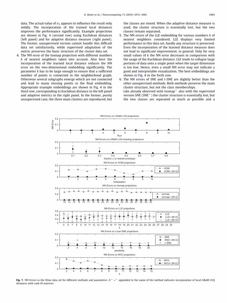
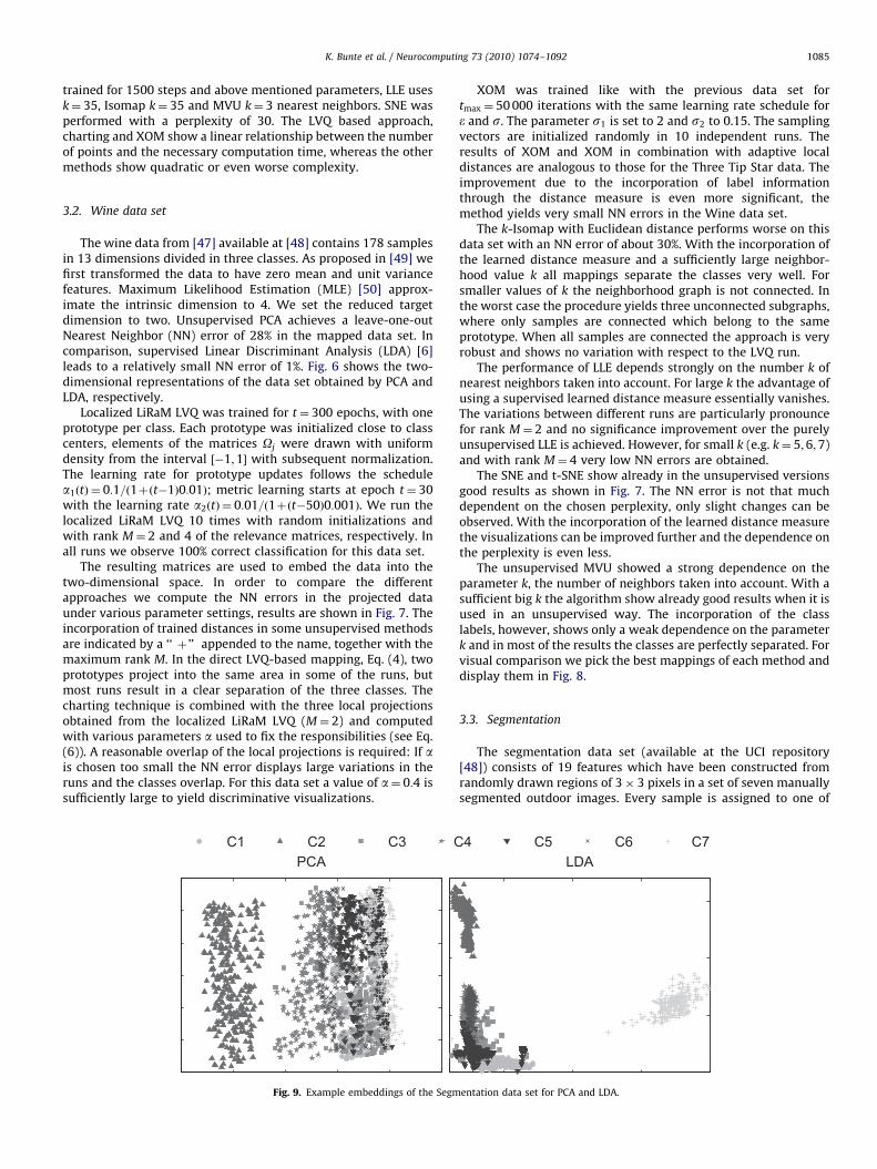
The wine data from [47] available at [48] contains 178 samplesin 13 dimensions divided in three classes. As proposed in [49] wefirst transformed the data to have zero mean and unit variancefeatures. Maximum Likelihood Estimation (MLE) [50] approx-imate the intrinsic dimension to 4. We set the reduced targetdimension to two. Unsupervised PCA achieves a leave-one-outNearest Neighbor (NN) error of 28% in the mapped data set. Incomparison, supervised Linear Discriminant Analysis (LDA) [6]leads to a relatively small NN error of 1%. Fig. 6 shows the two-dimensional representations of the data set obtained by PCA andLDA, respectively.

Localized LiRaM LVQ was trained for t¼ 300 epochs, with oneprototype per class. Each prototype was initialized close to classcenters, elements of the matrices Oj were drawn with uniformdensity from the interval ½�1;1� with subsequent normalization.The learning rate for prototype updates follows the schedulea1ðtÞ ¼ 0:1=ð1þðt�1Þ0:01Þ; metric learning starts at epoch t¼ 30with the learning rate a2ðtÞ ¼ 0:01=ð1þðt�50Þ0:001Þ. We run thelocalized LiRaM LVQ 10 times with random initializations andwith rank M¼ 2 and 4 of the relevance matrices, respectively. Inall runs we observe 100% correct classification for this data set.

The resulting matrices are used to embed the data into thetwo-dimensional space. In order to compare the differentapproaches we compute the NN errors in the projected dataunder various parameter settings, results are shown in Fig. 7. Theincorporation of trained distances in some unsupervised methodsare indicated by a ‘‘ þ ’’ appended to the name, together with themaximum rank M. In the direct LVQ-based mapping, Eq. (4), twoprototypes project into the same area in some of the runs, butmost runs result in a clear separation of the three classes. Thecharting technique is combined with the three local projectionsobtained from the localized LiRaM LVQ (M¼ 2) and computedwith various parameters a used to fix the responsibilities (see Eq.(6)). A reasonable overlap of the local projections is required: If ais chosen too small the NN error displays large variations in theruns and the classes overlap. For this data set a value of a¼ 0:4 issufficiently large to yield discriminative visualizations.

PCAC1 C2 C3 C

Fig. 9. Example embeddings of the Segm

XOM was trained like with the previous data set fortmax ¼ 50 000 iterations with the same learning rate schedule fore and s. The parameter s1 is set to 2 and s2 to 0.15. The samplingvectors are initialized randomly in 10 independent runs. Theresults of XOM and XOM in combination with adaptive localdistances are analogous to those for the Three Tip Star data. Theimprovement due to the incorporation of label informationthrough the distance measure is even more significant, themethod yields very small NN errors in the Wine data set.

The k-Isomap with Euclidean distance performs worse on thisdata set with an NN error of about 30%. With the incorporation ofthe learned distance measure and a sufficiently large neighbor-hood value k all mappings separate the classes very well. Forsmaller values of k the neighborhood graph is not connected. Inthe worst case the procedure yields three unconnected subgraphs,where only samples are connected which belong to the sameprototype. When all samples are connected the approach is veryrobust and shows no variation with respect to the LVQ run.

The performance of LLE depends strongly on the number k ofnearest neighbors taken into account. For large k the advantage ofusing a supervised learned distance measure essentially vanishes.The variations between different runs are particularly pronouncefor rank M¼ 2 and no significance improvement over the purelyunsupervised LLE is achieved. However, for small k (e.g. k¼ 5;6;7)and with rank M¼ 4 very low NN errors are obtained.

The SNE and t-SNE show already in the unsupervised versionsgood results as shown in Fig. 7. The NN error is not that muchdependent on the chosen perplexity, only slight changes can beobserved. With the incorporation of the learned distance measurethe visualizations can be improved further and the dependence onthe perplexity is even less.

The unsupervised MVU showed a strong dependence on theparameter k, the number of neighbors taken into account. With asufficient big k the algorithm show already good results when it isused in an unsupervised way. The incorporation of the classlabels, however, shows only a weak dependence on the parameterk and in most of the results the classes are perfectly separated. Forvisual comparison we pick the best mappings of each method anddisplay them in Fig. 8.

3.3. Segmentation

The segmentation data set (available at the UCI repository[48]) consists of 19 features which have been constructed fromrandomly drawn regions of 3� 3 pixels in a set of seven manuallysegmented outdoor images. Every sample is assigned to one of

LDA4 C5 C6 C7

entation data set for PCA and LDA.

ARTICLE IN PRESS


seven classes: brickface, sky, foliage, cement, window, path andgrass (referred to as C1; . . . ;C7). The set consists of 210 trainingpoints with 30 instances per class and the test set comprises 300instances per class, resulting in 2310 samples in total. We did notuse the features (3,4,5) as they display zero variance over the dataset. We do not preprocess or normalize the data because Isomap,LLE, and SNE displayed better performance on original data. Fort-SNE different magnitudes of features may constitute a problem,which we observed by a very high NN error in comparison withthe other methods, and we would expect it to perform better on,e.g. z-transformed data. An ML estimation yields an intrinsicdimension of about 3, so we use rank limits of MAf2;3g for thecomputation of the local distances in this data set.

1 2 3 4 50

0.1

0.2

R

NN

Err

or

NN Errors on LiR

0.1 0.2 0.3 0.40

0.1

0.2

fraction α to ne


5 10 15 20 25 30 35 40 450

0.2

0.4NN Errors on

48 49 50 51 52 53 54 55 56 57 58 59 60 60

0.2

0.4NN Errors on I

20 21 22 23 24 25 26 27 28 29 30 31 32 33 340

0.2

0.4

0.6NN Errors on

30 35 40 450

0.1

0.2

per

NN Errors on SNE

Fig. 10. NN errors on the segmentation data set for different methods and parameters. A

LVQ distances with rank M matrices.

Localized LiRaM LVQ was trained for t¼ 500 epochs, with oneprototype per class. Each prototype was initialized close to classcenter, and elements of the matrices Oj are drawn randomly from½�1;1� according to a uniform density with subsequent normal-ization of the matrices. The learning rate for prototypes follows theschedule a1ðtÞ ¼ 0:01=ð1þðt�1Þ0:001Þ. Metric adaptation starts atepoch t¼ 50 with learning rates a2ðtÞ ¼ 0:001= ð1þðt�50Þ0:0001Þ.We run localized LiRaM LVQ 10 times with random initialization andwith a rank limit of M¼ 2 and 3, respectively. For M¼ 2 we achievea mean classification error of about 8% in all runs and with M¼ 3 themean classification error is 7%.

LDA yields a classification error of approx. 20% for a projectioninto two dimensions while unsupervised PCA displays a NN error

6 7 8 9 10un

aM LVQ projections

0.5 0.6 0.7 0.8arest prototype k

VQ+charting projections

k=2k=3k=4k=5k=6

50 55 60 65 70σ2

XOM projections

XOMXOM+ (M=2)XOM+ (M=3)

1 62 63 64 65 66 67 68 69 70k

somap projections

IsomapIsomap+ (M=2)Isomap+ (M=3)

35 36 37 38 39 40 41 42 43 44 45 46 47 48 49 50k

LLE projections

LLELLE+ (M=2)LLE+ (M=3)

50 55 60plexity

and tSNE projections

SNE

SNE+ (M=2)

SNE+ (M=3)

‘‘ þ ’’ appended to the name of the method indicates incorporation of local LiRaM

ARTICLE IN PRESS


of 31% (Fig. 9). The obtained NN errors are shown in Fig. 10 andsome example visualizations are given in Fig. 11.

The quality of direct LiRaM LVQ projections vary from run to run.One favorable projection is shown in Fig. 11 in the first row on theleft side. The classes C2 and C6 are well separated with largedistances from the other classes. Also, most samples of C4 and C1 areclustered properly, while class C3 is spread and overlaps with classC7. This outcome is not too surprising, since C3 and C7 correspond tofoliage and grass, respectively, two classes that may be expected tohave similar characteristics in feature space.

1

2

34 5

6

7

LiRaM LVQ (Run 9)

prototypes

XOM (σ2=35, Init. 1)

Isomap (k=68)

LLE (k=50)

SNE (Perplexity 35)

C1 C2 C3

Fig. 11. Example embeddings of the segmentation data set for different methods. A ‘‘ þ

distances with rank M matrices. The inset in the upper right panel magnifies the regio

In the combination with a charting step results are ratherrobust with respect to the parameter settings (a; k). Here, the bestresult is achieved with a¼ 0:1 and k¼ 1 (Fig. 11, top right panel).Again, three classes are well separated from the others. Theremaining four classes are projected into a relatively small area.As can be seen in the inset, three of these classes are very close:window, brickface, and cement. Again, similar properties infeature space can be expected for these classes.

XOM was trained for tmax ¼ 50 000 iterations with the samelearning rate schedule for e and s like for the other data sets. We

charting+ (k=1, α=0.1, Run 9)

XOM+ (M=2, σ2= 5, Run 5, Init. 1)

Isomap+ (M=3, Run 8, k=63)

LLE+ (M=2, Run 9, k=27)

SNE+ (M=3, Perplexity 35, Run 6)

C4 C5 C6 C7

’’ appended to the name of the method indicates incorporation of local LiRaM LVQ

n to which four of the classes are mapped.

ARTICLE IN PRESS


set the parameters to e1 ¼ 0:9, e2 ¼ 0:05 and s1 to nearly themaximum distance in the data space: 1500 and s2 is chosen asvalues between the interval ½5;70�. The sampling vectors areinitialized randomly in five independent runs. In the applicationof XOM we observe once more a clear improvement whenincorporating the adaptive local metrics obtained in LiRaM LVQ.Example projections are shown in Fig. 11 (second row).

For Isomap a minimum value of kZ48 is necessary to obtainfully connected neighborhood graphs and, hence, embed allpoints. The incorporation of adaptive local distances leads to aclear improvement of the NN error in the mapping.

As expected, a low rank M of the local matrices results ininferior NN errors if M is smaller than the intrinsic dimension ofthe data. When incorporating adaptive distances with very large

1 2 3 4 50

0.20.40.60.8

1

R

NN

Err

or

NN Errors on LiR

0.1 0.2 0.3 0.40

0.20.40.60.8

1

fraction α to n


0.01 0.09 0.17 0.25 0.33 0.41 0.49 0.57 0.65 0.73 0.81 0.89 00

0.20.40.60.8

1NN Errors on

20 21 22 23 24 25 26 27 28 29 30 31 32 33 340

0.20.40.60.8

1NN Errors on Is

5 6 7 8 9 10 11 12 13 14 15 16 17 18 190

0.20.40.60.8

1NN Errors on

30 35 40 450

0.20.40.60.8

1

per

NN Errors on SNE

30

0.20.40.60.8

1

Fig. 12. NN errors on the USPS data set for different methods and parameters. A ‘‘ þ ’’


k, a fully connected graph can be obtained and all data aremapped. However, then, closer classes would highly overlap inthe projections and the visualization would not be discriminative.If, on the other hand, a smaller k is chosen, some of the classes areabsent in the graph and, consequently, in the visualization. As aconsequence of this effect, in Fig. 11 (third row, right panel) classC2 subgraph is absent.

Like in the previous examples, LLE performs relatively poor. TheNN error can be decreased by using adaptive distances but pointstend to be collapsed in the projection due to the discriminativenature of the distance measure. Most visualizations with relativelylow NN errors display an almost linear arrangement of all classes, cf.Fig. 11 (fourth row, left panel). An example visualization afterincorporation of adaptive metrics is shown in the right panel.

6 7 8 9 10un

aM LVQ projections

0.5 0.6 0.7 0.8earest prototype

VQ+charting projections

k=2k=3k=4k=5k=6k=7

.97 1.05 1.13 1.21 1.29 1.37 1.45 1.53 1.61 1.69 1.77 1.85 1.93σ2

XOM projections

XOMXOM+ (M=2)

35 36 37 38 39 40 41 42 43 44 45 46 47 48 49 50K

omap projections

IsomapIsomap+ (M=2)

20 21 22 23 24 25 26 27 28 29 30 31 32 33 34 35K

LLE projections

LLELLE+ (M=2)

50 55 60plexity

and tSNE projections

tSNESNESNE+ (M=2)

4K

MVU

appended to the name of the method indicates incorporation of local LiRaM LVQ

ARTICLE IN PRESS

1

23

4567 8

9 0

LiRaM LVQ (Run 3)

prototypes

charting (Run 6, α=0.1)

XOM (Sigma2=12, Init. 6) XOM+ (σ2=5, Run 6, Init. 4)

Isomap (K=22) Isomap+ (Run 1, K=10)

LLE (K=6) LLE+ (Run 7, K=6)

tSNE (Perplexity 40)

12

3

4

5

67

89

0

SNE+ (Perplexity 5, Run 8)

MVU (k=3) LDA

Fig. 13. Example embeddings of the USPS data set for different methods. A ‘‘ þ ’’ appended to the name of the method indicates incorporation of local LiRaM LVQ distances

with rank M matrices.

5 United States Postal Service (US Postal Service).


While the visualization appears to be better, qualitatively, the abovementioned basic problem of LLE persists.

The last row of Fig. 11 displays the two-dimensional represen-tations provided by SNE and SNEþ for perplexities in the interval[30 60]. The unsupervised variant performs already quite well, butthe incorporation of the learned local distances improves it evenfurther especially for higher perplexities and bigger values for thelimited rank M of the LiRaM LVQ algorithm (see Fig. 10).

Classes C2 (sky) and C7 (grass) are obviously separable by allapplied methods, both unsupervised and supervised. On the otherhand, the discrimination of classes C4 (foliage) and C5 (window)appears to be difficult, in particular in unsupervised dimensionreduction.

We could not evaluate MVU on this data set, because thiswould require the costly incorporation of in minimum k¼ 46neighbors. It appears, that a part of the data is already wellseparated, so that the neighborhood graph is not connected withsmaller values of k. The provided code demands a fully connectedgraph, so the number of constraints of the SDP becomes too large

to be solved in reasonable time and needs more memory thanwe have.

3.4. USPS digits

The USPS5 dataset consists of images of hand written digits of aresolution of 16� 16 pixel. We normalized the data to have zeromean and unit variance features and used a test set containing200 observations per class. Since it is a digit recognition task, wehave the classes A ½0; . . . ;9� resulting in 2000 samples for theembedding. The NN errors of all compared methods are shown inFig. 12.

Localized LiRaM LVQ was trained for t¼ 500 epochs, withone prototype per class and the same initialization scheme forthe prototypes and matrices, learning rates and learningschedules like explained in Section 3.3. The direct LiRaM LVQ

ARTICLE IN PRESS

Table 1NN errors (and standard deviation) on the different data sets.

Method Three tip star Wine Segmentation USPS

LiRaM LVQ 0.06 (0.0) 0.00 (0.0) 0.07 (0.0) 0.01 (0.0)

charting 0.14 (0.1) 0.01 (0.0) 0.13 (0.0) 0.06 (0.0)

XOM 0.49 (0.0) 0.04 (0.0) 0.25 (0.0) 0.64 (0.0)

XOMþðM¼ 2Þ 0.25 (0.0) 0.00 (0.0) 0.11 (0.0) 0.02 (0.0)

XOMþðM¼ 3Þ – – 0.11 (0.0) –

Isomap 0.36 (0.0) 0.25 (0.0) 0.23 (0.0) 0.53 (0.0)

IsomapþðM¼ 2Þ 0.20 (0.1) 0.00 (0.0) 0.18 (0.1) 0.01 (0.0)

IsomapþðM¼ 3Þ – – 0.13 (0.1) –

LLE 0.47 (0.0) 0.28 (0.0) 0.36 (0.0) 0.57 (0.0)

LLEþðM¼ 2Þ 0.34 (0.1) 0.18 (0.2) 0.25 (0.1) 0.11 (0.1)

LLEþðM¼ 3Þ – 0.03 (0.0) 0.19 (0.0) –

SNE 0.45 (0.0) 0.03 (0.0) 0.11 (0.0) 0.34 (0.0)

SNEþðM¼ 2Þ 0.14 (0.1) 0.00 (0.0) 0.10 (0.0) 0.01 (0.0)

SNEþðM¼ 3Þ – – 0.09 (0.0) –

t-SNE 0.41 (0.0) 0.04 (0.0) 0.85 (0.0) 0.08 (0.0)

MVU 0.40 (0.0) 0.04 (0.0) – 0.56 (0.0)

MVUþðM¼ 2Þ 0.16 (0.1) 0.00 (0.0) – –

LDA – 0.01 (0.0) 0.20 (0.0) 0.35 (0.0)


projections separate the classes nearly perfectly and onefavorable projection is shown in Fig. 13 in the first row on theleft side. In the combination with a charting step the best resultis achieved with a¼ 0:1 and k¼ 2 (Fig. 13, top right panel). Fourclasses appear to be squeezed together, but the overlap is stillsmall if zoomed.

XOM was trained in the same way like mentioned in Section3.3 with s2 chosen as values between the interval [0.01,2]. Theincorporation of the adaptive local metrics obtained in LiRaM LVQonce more improve the results of the XOM dramatically. Exampleprojections are shown in Fig. 13 (second row).

For Isomap the incorporation of adaptive local distances improvesthe NN error in the mapping. Like mentioned with the other data setssome data points appear to be too separated from the others if thelocal distances are used, so the mapping may miss them with a smallneighborhood parameter k. Like in the previous examples, LLEperforms relatively poor, but can be enhanced by using the localdissimilarities given by LiRaM LVQ (Fig. 13, fourth row).

SNE performs relatively well, but t-SNE showed a remarkablebetter NN error on this data set. Still the class structure is hardlyrecognizable on the unsupervised mapping, while it becomes clear ifthe local distances are incorporated (Fig. 13, fifth row, right panel).The supervised SNEþ results in 10 nicely recognizable clusters.

The last row of Fig. 13 displays the two-dimensionalrepresentations provided by MVU and LDA. MVU does notperform very well on this data set and LDA yields a classificationerror of 35% for a projection into two dimensions. We could notapply MVU with incorporation of the local distances provided byLiRaM LVQ, because the classes are separated so well in this casethat a huge value of nearest Neighbors k would be necessary toget a connected graph.

4. Conclusions

We have introduced the concept of discriminative non-linear data visualization based on local matrix learning.

Unlike unsupervised visualization schemes, the resulting techni-ques focus on the directions which are locally of particularrelevance for an underlying classification task such that theinformation which is important for this additional label informa-tion is preserved by the visualization as much as possible. Inter-estingly, local matrix learning gives rise to auxiliary informationwhich can be integrated into visualization techniques in differentform: as local discriminative coordinates of the data points forcharting techniques and similar methods, as global metric infor-mation for XOM, SNE, MDS, and the like, or as local neighbor-hood information for LLE, Isomap, MVU and similar schemes.We have introduced these different paradigms and we exemplarypresented the behavior of these schemes for six concrete visual-ization techniques, namely charting, LLE, Isomap, XOM, SNE andMVU. An extension to further methods such as t-SNE, diffusionmaps, etc. could be done along the same lines.

Interestingly, the resulting methods have quite different com-plexity: while charting uses the fact that information is compressedin the prototypes resulting in an only linear scheme depending onthe number of data, LLE, SNE, and Isomap end up with quadratic oreven cubic complexity. Further, charting techniques and similarprovide the only methods in this collection which yield an explicitembedding map rather than an embedding of the given points only.The behavior of the resulting discriminative visualization techniqueshas been investigated in one artificial and three real life data sets.The best results for all methods and data sets are summarized inTable 1. According to the different objectives optimized by thevisualization techniques, the results are quite diverse and no singlemethod which is optimum for every case can be identified. Ingeneral, discriminative visualization as introduced in this paperimproves all the corresponding unsupervised methods and alsoalternative state-of-the-art schemes such as t-SNE. Further, thetechniques presented in this paper are superior to discriminativeLDA which is restricted to linear embedding. It seems that chartingoffers a good choice in many cases, in particular since it is a methodwith only linear effort which provides an explicit embedding map.

Interestingly, a direct projection of the data by means of thelocal linear maps of LiRaM LVQ displays good results in manycases, although an appropriate coordination of these maps cannotbe guaranteed in this technique. It seems promising to investigatethe possibility to introduce the objective of valid coordination ofthe local projections directly into the LiRaM LVQ learning scheme.This issue as well an exhaustive comparison of more extensions ofunsupervised methods (such as t-SNE) to incorporate discrimi-native information are the subject of ongoing work.

Acknowledgment

This work was supported by the ‘‘Nederlandse organisatievoor Wetenschappelijk Onderzoek (NWO)’’ under project code612.066.620.

References

[1] W.J. Frawley, G. Piatetsky-Shapiro, C.J. Matheus, Knowledge discovery indatabases: an overview, in: G. Piatetsky-Shapiro, W. Frawley (Eds.), AAAI/MITPress, Cambridge, 1991, pp. 1–27.

[2] J. Lee, M. Verleysen, Nonlinear Dimensionality Reduction, third ed., Springer,Berlin, 2007.

[3] L.J.P. van der Maaten, E.O. Postma, H.J. van den Herik, Dimensionalityreduction: a comparative review, URL: /http://ticc.uvt.nl/� lvdrmaaten/Laurens_van_der_Maaten/Matlab_Toolbox_for_Dimensionality_Reduction_files/Paper.pdfS, Published online, 2007.

[4] D.A. Keim, Information visualization and visual data mining, IEEE Transac-tions on Visualization and Computer Graphics 8 (1) (2002) 1–8 ISSN 1077-2626 /http://doi.ieeecomputersociety.org/10.1109/2945.981847S.

[5] K. Bunte, P. Schneider, B. Hammer, F.-M. Schleif, T. Villmann, M. Biehl,Discriminative visualization by limited rank matrix learning, Technical

http://ticc.uvt.nl/&sim;lvdrmaaten/Laurens_van_der_Maaten/Matlab_Toolbox_for_Dimensionality_Reduction_files/Paper.pdf




http://doi.ieeecomputersociety.org/10.1109/2945.981847

ARTICLE IN PRESS


Report MLR-03-2008, Leipzig University, URL: /http://www.uni-leipzig.de/�compint/mlr/mlr_03_2008.pdfS, 2008.

[6] K. Fukunaga, Introduction to Statistical Pattern Recognition, second ed.,Computer Science and Scientific Computing Series, Academic Press, NewYork, 1990, ISBN 0122698517.

[7] J. Faith, R. Mintram, M. Angelova, Targeted projection pursuit for visuali-sing gene expression data classifications, Bioinformatics 22 (2006)2667–2673.

[8] J. Peltonen, J. Goldberger, S. Kaski, Fast discriminative component analysis forcomparing examples, NIPS.

[9] T. Villmann, B. Hammer, F.-M. Schleif, T. Geweniger, W. Hermann, Fuzzyclassification by fuzzy labeled neural gas, Neural Networks 19 (6–7) (2006)772–779.

[10] J. Peltonen, A. Klami, S. Kaski, Improved learning of Riemannian metrics forexploratory analysis, Neural Networks 17 (2004) 1087–1100.

[11] P. Kontkanen, J. Lahtinen, P. Myllymaki, T. Silander, H. Tirri, Supervisedmodel-based visualization of high-dimensional data, Intelligent DataAnalysis 4 (3, 4) (2000) 213–227 ISSN 1088-467X.

[12] T. Iwata, K. Saito, N. Ueda, S. Stromsten, T.L. Griffiths, J.B. Tenenbaum,Parametric embedding for class visualization, Neural Computation 19 (9)(2007) 2536–2556 URL: /http://dblp.uni-trier.de/db/journals/neco/neco19.html#IwataSUSGT07S.

[13] G. Baudat, F. Anouar, Generalized discriminant analysis using a kernelapproach, Neural Computation 12 (10) (2000) 2385–2404.

[14] B. Kulis, A. Surendran, J. Platt, Fast low-rank semidefinite programming forembedding and clustering, in: Eleventh International Conference on ArtificialIntelligence and Statistics, AISTATS 2007, 2007.

[15] N. Vasiloglou, A. Gray, D. Anderson, Scalable semidefinite manifold learning,in: IEEE Workshop on Machine Learning for Signal Processing, MLSP 2008,2008, pp. 368–373.

[16] R. Collobert, F. Sinz, J. Weston, L. Bottou, Trading convexity for scalability, in:Proceedings of the 23rd International Conference on Machine Learning, ACMNew York, NY, USA, 2006, pp. 201–208.

[17] L. Song, A.J. Smola, K. Borgwardt, A. Gretton, Colored maximum varianceunfolding, in: J.C. Platt, D. Koller, Y. Singer, S. Roweis (Eds.), 21th NeuralInformation Processing Systems Conference, MIT Press, Cambridge, MA,USA, 2008, pp. 1385–1392 URL: /http://books.nips.cc/papers/files/nips20/NIPS2007_0492.pdfS.

[18] M. Brand, Charting a manifold, Technical Report 15, Mitsubishi ElectricResearch Laboratories (MERL), URL: /http://www.merl.com/publications/TR2003-013/S, 2003.

[19] J.B. Tenenbaum, V.d. Silva, J.C. Langford, A global geometric framework fornonlinear dimensionality reduction, Science 290 (5500) (2000) 2319–2323, doi: ,doi:10.1126/science.290.5500.2319 URL: /http://www.sciencemag.org/cgi/content/abstract/290/5500/2319S.

[20] S.T. Roweis, L.K. Saul, Nonlinear dimensionality reduction by locally linearembedding, Science 290 (5500) (2000) 2323–2326, doi: , doi:10.1126/science.290.5500.2323 URL: /http://www.sciencemag.org/cgi/content/abstract/290/5500/2323S.

[21] A. Wismuller, The exploration machine: a novel method for analyzing high-dimensional data in computer-aided diagnosis, in: Society of Photo-OpticalInstrumentation Engineers (SPIE) Conference Series, Presented at the Societyof Photo-Optical Instrumentation Engineers (SPIE) Conference, vol. 7260,2009, 72600G-7, doi: 10.1117/12.813892.

[22] G. Hinton, S. Roweis, Stochastic neighbor embedding, in: Advances in NeuralInformation Processing Systems, vol. 15, MIT Press, Cambridge, MA, USA,2003, pp. 833–840.

[23] T. Liu, A.W. Moore, A. Gray, Ke Yang, An Investigation of PracticalApproximate Nearest Neighbor Algorithms, in: Proceedings of NeuralInformation Processing Systems (NIPS 2004), Vancouver, BC, Canada, 2004.

[24] A. Moore, An introductory tutorial on kd-trees, Ph.D. Thesis, University ofCambridge, Technical Report no. 209, 1990.

[25] A. Gray, A. Moore, N-Body’ problems in statistical learning, in: Advances inNeural Information Processing Systems, 2001, pp. 521–527.

[26] K. Weinberger, L. Saul, An introduction to nonlinear dimensionality reductionby maximum variance unfolding, in: Proceedings of the National Conferenceon Artificial Intelligence, vol. 21, AAAI Press, MIT Press, Menlo Park, CA,Cambridge, MA, London, 1999, 1683, 2006.

[27] T. Kohonen, Self-Organizing Maps, third ed., Springer, Berlin, Heidelberg,New York, 2001.

[28] B. Hammer, M. Strickert, T. Villmann, On the generalization ability of GRLVQnetworks, Neural Processing Letters 21 (2) (2005) 109–120.

[29] B. Hammer, T. Villmann, Generalized relevance learning vector quantization,Neural Networks 15 (8–9) (2002) 1059–1068.

[30] P. Schneider, M. Biehl, B. Hamer, Relevance matrices in LVQ, in: M. Verleysen(Ed.), Proceedings of European Symposium on Artificial Neural Networks(ESANN), Bruges, Belgium, 2007, pp. 37–42.

[31] K.Q. Weinberger, J. Blitzer, L.K. Saul, Distance metric learning for large marginnearest neighbor classification, Advances in Neural Information ProcessingSystems 18 (2006) 1473–1480.

[32] K. Bunte, M. Biehl, N. Petkov, M.F. Jonkman, Adaptive metrics for contentbased image retrieval in dermatology, in: M. Verleysen (Ed.), Proceedings ofEuropean Symposium on Artificial Neural Networks (ESANN), Bruges,Belgium, 2009, pp. 129–134.

[33] A.S. Sato, K. Yamada, Generalized learning vector quantization, in: Advancesin Neural Information Processing Systems, vol. 8, 1996, pp. 423–429.

[34] P. Schneider, M. Biehl, B. Hammer, Adaptive relevance matrices in learningvector quantization, Neural Computation, 21 (12) (2009) 3532–3561.

[35] P. Schneider, K. Bunte, B. Hammer, T. Villmann, M. Biehl, Regularization in matrixrelevance learning, Technical Report MLR-02-2008, Leipzig University, ISSN:1865-3960 /http://www.uni-leipzig.de/�compint/mlr/mlr_02_2008.pdfS, 2008.

[36] M. Koeber, U. Schafer, The unique square root of a positive semidefinitematrix, International Journal of Mathematical Education in Science andTechnology 37 (8) (2006) 990–992 URL: /http://www.informaworld.com/10.1080/00207390500285867S.

[37] Z. Zhang, H. Zha, Principal manifolds and nonlinear dimension reduction vialocal tangent space alignment, SIAM Journal of Scientific Computing 26(2002) 313–338.

[38] L. van der Maaten, G. Hinton, Visualizing data using t-SNE, Journal of MachineLearning Research 9 (2008) 2579–2605 URL: /http://www.jmlr.org/papers/volume9/vandermaaten08a/vandermaaten08a.pdfS.

[39] H. Wang, J. Zheng, Z. Yao, L. Li, Improved locally linear embedding throughnew distance computing, in: J. Wang, Z. Yi, J.M. Zurada, B.-L. Lu, H. Yin (Eds.),ISNN (1) of Lecture Notes in Computer Science, vol. 3971, Springer, Berlin,2006, pp. 1326–1333 ISBN 3-540-34439-X.

[40] L. Zhao, Z. Zhang, Supervised locally linear embedding with probability-baseddistance for classification, Computers & Mathematics with Applications 57(6) (2009) 919–926 ISSN 0898-1221 /http://dx.doi.org/10.1016/j.camwa.2008.10.055S.

[41] L.K. Saul, S.T. Roweis, Think globally, fit locally: unsupervised learning ofnonlinear manifolds, Journal of Machine Learning Research 4 (2003)119–155.

[42] A. Wismuller, The exploration machine—a novel method for structure-preserving dimensionality reduction, in: M. Verleysen (Ed.), EuropeanSymposium on Artificial Neural Networks (ESANN), Bruges, Belgium, 2009,pp. 59–64.

[43] A. Wismuller, A computational framework for exploratory data analysis, in:M. Verleysen (Ed.), European Symposium on Artificial Neural Networks(ESANN), Bruges, Belgium, 2009, pp. 547–552.

[44] A. Wismuller, Exploratory morphogenesis (XOM): a novel computationalframework for self-organization, Ph.D. Thesis, Technical University ofMunich, Department of Electrical and Computer Engineering, 2006.

[45] A. Wismuller, A computational framework for exploratory data analysis inbiomedical imaging, in: Proceedings of SPIE, vol. 7260, 2009, doi:10.1117/12.813892.

[46] N. Vasiloglou, A. Gray, D. Anderson, Learning isometric separation maps,Arxiv preprint arXiv:0810.4611.

[47] S. Aeberhard, D. Coomans, O. de Vel, Comparison of classifiers in highdimensional settings, Technical Report 02, James Cook University, 1992.

[48] A. Asuncion, D.J. Newman, S. Hettich, C.L. Blake, C.J. Merz, UCI Repository ofmachine learning databases /http://archive.ics.uci.edu/ml/S, last visit19.06.2009, 1998.

[49] S. Rogers, M. Girolami, Multi-class semisupervised learning with thee-truncated multinomial probit Gaussian process, Journal of MachineLearning Research: Gaussian Processes in Practice 1 (2007) 17–32.

[50] E. Levina, P.J. Bickel, Maximum likelihood estimation of intrinsic dimension,in: Advances in NIPS, MIT Press, Cambridge, USA, 2005, pp. 777–784.

Kerstin Bunte graduated at the Faculty of Technologyat the University of Bielefeld, Germany, and joined the‘Johann Bernoulli Institute for Mathematics and Com-puter Science’ of the University of Groningen, TheNetherlands, in September 2007. Her recent work hasfocused on machine learning techniques, especiallylearning vector quantization and their usability in thefield of image processing, dimension reduction andvisualization. Further information can be obtainedfrom http://www.cs.rug.nl/�kbunte/

Barbara Hammer received her Ph.D. in ComputerScience in 1995 and her venia legendi in ComputerScience in 2003, both from the University of Osnab-rueck, Germany. From 2000 to 2004, she was leader ofthe junior research group ‘‘Learning with NeuralMethods on Structured Data’’ at University of Osnab-rueck before accepting an offer as professor forTheoretical Computer Science at Clausthal Universityof Technology, Germany, in 2004. Several researchstays have taken her to Italy, UK, India, France, and theUSA. Her areas of expertise include various techniquessuch as hybrid systems, self-organizing maps, cluster-
ing, and recurrent networks as well as applications in
bioinformatics, industrial process monitoring, or cognitive science. Most of herpublications can be retrieved from http://www.in.tu-clausthal.de/�hammer.

http://www.uni-leipzig.de/~compint/mlr/mlr_03_2008.pdf

http://www.uni-leipzig.de/~compint/mlr/mlr_03_2008.pdf

http://dblp.uni-trier.de/db/journals/neco/neco19.html#IwataSUSGT07

http://dblp.uni-trier.de/db/journals/neco/neco19.html#IwataSUSGT07

http://books.nips.cc/papers/files/nips20/NIPS2007_0492.pdf

http://books.nips.cc/papers/files/nips20/NIPS2007_0492.pdf

http://www.merl.com/publications/TR2003-013/

http://www.merl.com/publications/TR2003-013/

dx.doi.org/10.1126/science.290.5500.2319

http://www.sciencemag.org/cgi/content/abstract/290/5500/2319






10.1117/12.813892

http://www.uni-leipzig.de/&sim;compint/mlr/mlr_02_2008.pdf

http://www.uni-leipzig.de/&sim;compint/mlr/mlr_02_2008.pdf

http://www.informaworld.com/10.1080/00207390500285867

http://www.informaworld.com/10.1080/00207390500285867

http://www.jmlr.org/papers/volume9/vandermaaten08a/vandermaaten08a.pdf

http://www.jmlr.org/papers/volume9/vandermaaten08a/vandermaaten08a.pdf

http://dx.doi.org/10.1016/j.camwa.2008.10.055

http://dx.doi.org/10.1016/j.camwa.2008.10.055

10.1117/12.813892

10.1117/12.813892

http://archive.ics.uci.edu/ml/

http://www.cs.rug.nl/&sim;kbunte/

http://www.cs.rug.nl/&sim;kbunte/

http://www.in.tu-clausthal.de/&sim;hammer

http://www.in.tu-clausthal.de/&sim;hammer

ARTICLE IN PRESS


Axel Wismuller, M.D. Ph.D., studied Medicine at the
Technical University of Munich and the University of from the University of Giessen, Germany, in 1992 and Regensburg, Germany, with study exchange programsin Switzerland and the USA (Yale University). Hereceived his M.D. degree from the Technical Universityof Munich for a scientific thesis in neurology in 1992.He successfully passed the U.S. medical examinationsECFMG and FLEX. In parallel to his clinical work ininternal medicine, he studied physics at the Universityof Munich where he received a German master’sdegree in Theoretical Physics from the University ofMunich in 1996 for a scientific thesis on patternrecognition. Since 1997, he has been working as a
fellow of radiology at the Department of Clinical Radiology, University of Munich,where he founded the Digital Image Processing Group. In 2006, he received a Ph.D.degree from the Department of Electrical and Computer Engineering at the
Technical University of Munich for a thesis on a novel pattern recognitionalgorithm invented by him. His main research interest is focussed on innovativestrategies for pattern recognition and computational intelligence, with a specificemphasis on computer-aided diagnosis in biomedical imaging, such as functionalMRI for human brain mapping or the diagnosis of breast cancer in MRImammography. Dr. Wismueller is author of more than 100 scientific journal andconference publications related to pattern recognition in biomedicine and holdstwo patents. Since August 2007, he is with the University of Rochester, New York,USA, as Associate Professor for both Radiology and Biomedical Engineering.
Michael Biehl received a Ph.D. in Theoretical Physics

the venia legendi in Theoretical Physics from theUniversity of Wurzburg, Germany, in 1996. He iscurrently Associate Professor with Tenure in ComputingScience at the University of Groningen, The Netherlands.His main research interest is in the theory, modeling andapplication of Machine Learning techniques. He isfurthermore active in the modeling and simulation ofcomplex physical systems. He has co-authored morethan 100 publications in international journals andconferences; preprint versions and further informationcan be obtained from http://www.cs.rug.nl/�biehl/

http://www.cs.rug.nl/&sim;biehl/

http://www.cs.rug.nl/&sim;biehl/

Adaptive local dissimilarity measures for discriminative dimension reduction of labeled data

Documents

Transcript of Adaptive local dissimilarity measures for discriminative dimension reduction of labeled data