A measure of group dissimilarity for psychological attributes

Una medida de la disimilitud en grupos para atributos psicológicos

Antonio Solanas1 2, Rumen Manolov1 2, David Leiva1 2, and Amara Andrés1

1 Department of Behavioral Sciences Methods, Faculty of Psychology, University of Barcelona

2 Institute for Research in Brain, Cognition, and Behavior (IR3C), University of Barcelona

MAILING ADDRESS

Correspondence concerning this article should be addressed to Antonio Solanas,

Departament de Metodologia de les Ciències del Comportament, Facultat de Psicologia,

Universitat de Barcelona, Passeig de la Vall d’Hebron, 171, 08035-Barcelona, Spain.

Phone number: +34933125076. Electronic mail may be sent to Antonio Solanas at

antonio.solanas@ub.edu.

AUTHORS’ NOTE

This research was partially supported by the Ministerio de Ciencia e Innovación grant

PSI2009-0706(PSIC) and the Generalitat de Catalunya grant 2009 SGR 1492.

RUNNING HEAD

Group dissimilarity

1

Resumen

El funcionamiento y el rendimiento de los grupos en contextos diferentes están

relacionados con el grado en que las características de los miembros son

complementarias o suplementarias. El presente artículo describe un procedimiento para

cuantificar el grado de disimilitud a nivel de grupo. A diferencia de la mayoría de

técnicas existentes, el procedimiento que aquí se describe está normalizado y es

invariante a los cambios de localización y escala. Por lo tanto, es posible comparar la

disimilitud en escalas con diferente métrica y en grupos de distinto tamaño. La

disimilitud está medida en términos relativos, independientemente de la posición que

ocupan los individuos en la dimensión que mide la escala. Cuando no existe una

justificación teórica para combinar las diversas propiedades medidas, se puede

cuantificar la disimilitud para cada escala por separado. También es posible obtener las

contribuciones diádicas e individuales respecto a la diversidad global y la asignada a

cada escala. Las medidas descriptivas pueden ser complementadas con la significación

estadística para, así, comparar los resultados obtenidos con distribuciones discretas de

referencia, ya sean simétricas o asimétricas. Se ha elaborado un paquete en R que

permite obtener los índices descriptivos y los valores p, además de contener las

expresiones desarrolladas para simular una amplia variedad de distribuciones discretas

de probabilidad.

2

Abstract

Group functioning and performance in different contexts is related to the extent to

which group members are complementary or supplementary in terms of psychological

attributes. This paper describes a procedure for quantifying the degree of dissimilarity at

group level. Unlike most existing techniques the one described here is normalized and is

both location and scale invariant, thereby making it suitable for comparing dissimilarity

on interval and ratio scales with different ranges and in groups of different sizes.

Dissimilarity is measured in relative terms regardless of the exact place on the scale at

which individuals are located. When a combination of several scales is not theoretically

justified, the dissimilarity for each scale can be quantified. Additionally, dyadic and

individual contributions to either the global or scale index can be obtained. The

descriptive measures are complemented by statistical significance values in order to

compare the results obtained with several discrete distributions of reference, both

symmetrical and skewed, which can be specified using the expressions developed. The

information that can be provided by the indices and the p values – both obtainable

through an R package – is illustrated using data from an empirical study.

3

In the current study a measure of dissimilarity in psychological attributes among group1

members is presented. Measuring the compatibility in terms of personality, social

interaction, task demands, and interpersonal perception is relevant for understanding

and improving team effectiveness. For instance, the attraction-selection-attrition

framework (Halfhill, Nielsen, & Sundstrom, 2008) states that individuals in the same

organization are expected to be similar to one another. Moreover, it has been shown that

compatibility in profiles is related to group cohesion and group satisfaction. These

group features can increase both when there is similarity in personality attributes

(Morse & Caldwell, 1979) and in the case of dissimilarity (Dryer & Horowitz, 1997),

corresponding, respectively, to the supplementary and complementary fit (Muchinsky &

Monahan, 1987). According to circumplex models (Plutchik & Conte, 1997), the former

type of fit is expected when people seek companionship (i.e., to get along), whereas the

latter is more probable in interactions related to power (i.e., to get ahead).

Regarding the measurement of attributes at the group level, it is important to note

that composites of individual measures have commonly been used (Humphreys,

Morgeson, & Mannor, 2009). One of the alternatives is to study whether the individual

measures are homogeneous and, thus, whether it is justified to aggregate them to obtain

a quantification at the group level (e.g., Sánchez & Amo, 2004). Homogeneity is also

important in order to know whether the mean of individual measures can be used to

represent the group (Cohen, Doveh, & Eick, 2001). For measuring dissimilarity,

standard deviation (SD) or variance can be used, two indices included in Chan’s (1998)

dispersion models and in Harrison and Klein’s (2007) conceptualization of diversity as

1 Groups can be conceptualized in different terms according to their origin, aim, etc. (Sundstrom, McIntyre, Halfhill, & Richards, 2000). However given that the current study is focused on measuring it is not necessary to distinguish between different types of groups. We will use the term “teams” in case the applications of the dissimilarity measures are more closely related to organizations.

4

separation (i.e., dissimilarity2 in quantitative scales measuring attitudes, opinions, and

attributes). For these measures there is evidence that different patterns may lead to the

same value, i.e., no distinction is made between minority belief, bimodal, and

fragmented patterns (DeRue, Hollenbeck, Ilgen, & Feltz, 2010). Another measure of

separation based on comparing discrepancies among all group members is the mean

Euclidean distance (MED).

The need for the index presented in the current article as an alternative for SD and

MED, arises from the fact that it is both location and scale invariant and thus it is

applicable to variables measured in either interval or ratio scale. Another differential

aspect in comparison to SD and MED is that in the index presented here absolute

instead of squared differences between pairs of scores are computed. Whereas squaring

gives greater weight to larger differences, despite the square root operation (Roberson,

Sturman, & Simons, 2007), using absolute differences implies a linear increase in

dissimilarity. We consider that applied researchers should have both kinds of models

available so that they can choose the one appropriate for their field and specific aim,

given that it is not a priori clear which of them is the optimal model when studying, for

instance, the functional relationship between dissimilarity and team performance.

Regarding the dissimilarity measure presented here, it will be shown that it is

possible to obtain a quantification for each attribute separately and also a global

measure of dissimilarity for several attributes, provided that adding up all scales into a

general composite has psychological meaning. Moreover, individual and dyadic

contributions to global or scale-specific dissimilarity become useful in order to identify

those group members or pairs of members mainly responsible for heterogeneity. All

2 Throughout the article we use indistinctly the terms “dissimilarity” and “diversity”, with the former term arising from Statistics, given the way the indices presented here are computed, whereas the latter term is based on conceptualizations such as the one made by Harrison and Klein (2007).

5

these quantifications are potentially relevant for understanding group processes and may

help to improve group output predictions (Andrés, Salafranca, & Solanas, 2011).

Moreover, we will illustrate how a correlational analysis can be carried out between

dyadic and individual contributions to diversity and dyadic and individual measures

referring to reciprocity (Kenny, Kashy, & Cook, 2006) and concordance in interpersonal

perceptions (Solanas, Leiva, & Manolov, 2010). Answering questions such as “Are

those dyads or individuals that contribute more to dissimilarity in psychological

attributes also responsible for the main discordance in interpersonal perceptions?” may

lead to a better understanding of group processes.

Finally, and in order to enhance the applicability of the procedure, R functions were

developed for both descriptive and inferential purposes. Inference is possible in

comparison with discrete distributions of different shapes via mathematical expressions

developed for specifying the mass probability function.

Analysis at the global level

The first aim of the present study consists in proposing an index for measuring the

dissimilarity among group members’ attributes when n individuals have been measured

on p psychological attributes. According to Harrison and Sin (2006) such a composite

of individual measures would be reasonable in the case of reflective indicators, that is,

operationalizations correlated with each other, which are assumed to be part of the same

underlying construct that is assumed to have a theoretical justification. By contrast,

formative indicators imply that a composite measure would be a simple sum of

uncorrelated scales and, therefore, their combination is not meaningful (Harrison &

Klein, 2007). For the latter type of indicators, the scale index presented later can be

applied to each scale separately.

6

7

Suppose a matrix X in which the n rows and p columns correspond respectively to

group members and psychological attributes (e.g., several intelligence characteristics):

11 12 1

21 22 2

1 2

.

p

p

n n np

x x x

x x x

x x x

X

Now, consider the first column vector of the matrix X, that is, (xR11R, xR21R,…, xRn1R)′, which

includes the scores of all individuals for the psychological attribute k = 1 (e.g., verbal

reasoning). An index for quantifying the degree of dissimilarity among group members’

scores on a single attribute may be founded on absolute differences and, just like

association coefficients, it is not sensitive to changes in location and scale parameters

(i.e., for changes in mean and variance values). A similar quantification has been

described in Stuart and Ord (1994) as the coefficient of mean difference, attributed to

Friedrich Helmert, and it has been applied to demographic variables. Suppose that the

following index is computed for the scale k:

1 1 1 1

2 0.n n n n

ik jk ik jki j i j i

x x x x

Its minimum value obviously equals zero, that is, all individuals score the same value. It

should be noted that the minimum value will be obtained irrespectively of where the

individuals are located along the psychological dimension. As regards the maximum

value, this occurs when team members are divided into two balanced sets at the

extremes of the psychological dimension. The maximum value for the previously

presented index is δ(xRmax(k)R−xRmin(k)R), where δ equals nP

2P/2 if n is even and (n P

2P − 1)/2 if n is

8

odd, and where xRmin(k)R and xRmax(k)R denote, respectively, the minimum and maximum

values for the scale k. The maximum value corresponds to the empirical mass of

probability for which half the individuals score xRmin(k)R and the other half xRmax(k)R if n is

even, this being consistent with the definition of a separation measure. Only a minor

change is required to obtain the maximum value if n is odd, that is, (n − 1)/2 individuals

score, for example, the minimum value of the scale while the remaining (n + 1)/2

individuals take values equal to the scale’s maximum. Therefore, the following index is

bounded as shown:

1 1

0 1,n n

ik jk

i j k

x x

r

where rRkR = xRmax(k)R − xRmin(k)R, that is, the difference between the maximum and minimum

values for the scale k, which is a novelty with respect to the coefficient of mean

difference. Note that in order to normalize the index it is necessary to know the bounds

of the measurement scale, as is usually the case for instruments measuring

psychological attributes. To obtain a global index for p psychological scales, the

following expression can be used:

1 1

1 1 1 1 1 1

2 , 0 1.p pn n n n

ik jk

k ik jkk i j k i j ik

x xp r x x

p r

The index λ is equal to 1 if the sum of the absolute differences reaches its maximum

value, given the range of the p scales. If the index equals zero, this means that all

individuals have scored the same value for each of the psychological scales, although

this value can be different for each scale as long as the individuals coincide.

9

Index strengths and limitations

These abovementioned bounds show that the global index is normalized and allows

comparisons across scales with different metrics, unlike SD and MED (Harrison &

Klein, 2007). The λ index satisfies location invariance, such that dissimilarity values

remain unchanged if a positive constant is added to everyone’s score. The index is

therefore applicable to interval scale variables. Moreover, it is applicable to ratio scale

variables as it also has the property of scale invariance, as is shown in the following

equality:

1 1 1 1

1 1 1 1 1 1

2 2 ,p pn n n n

k k k ik k jk k ik jkk i j i k i j i

p m r m x m x p r x x

where mRkR denotes a nonnegative scale factor for scale k. As λ remains unchanged if a

change of units is introduced, the relative contributions to dissimilarity do not depend

on the minimum and maximum values of psychological scales. Another strength of the

index is the possibility to obtain dyadic and individual contributions. Only for MED

have there been developments for computing an individual’s similarity to the remaining

group members (O’Reilly, Caldwell, & Barnett, 1989).

Among the limitations of the global index it should be reiterated that it is only

applicable in the case of reflective indicators. In that sense, as the global index can be

expressed as the average of the scale indices it would not be useful when there are

dissimilarities for some but not all of the scales, as this mean value would misrepresent

all of them. Related to this limitation, it has to be mentioned that both the global index

and the scale index presented below are quantifications for the whole group. However,

10

it would be more informative for applied researchers if they used the measurements

developed in the faultlines framework (Shaw, 2004; Trezzini, 2008) to detect possible

subgroups on the basis of categorical data and, afterwards, quantify dissimilarity in

quantitative attributes with the indices presented here. Otherwise, a group dissimilarity

quantification may be a misrepresentation of these subgroups. Finally, the fact that the

index is normalized entails a limitation (i.e., it does not show at which point of the scale

similarity takes place when present) and a requirement (i.e., the bounds of the scale

ought to be known).

Scale analysis

When the global index has no psychological meaning (i.e., for formative indicators),

researchers ought to quantify dissimilarity for each scale of interest. Thus, the index λ

should be decomposed into specific scale heterogeneities, denoted by λRkR, as follows:

11 1

1 1 1 1

2 , 0 1.p pn n

k ik jk k kk i j i k

p r x x p

If researchers are interested in obtaining a normalized measurement (i.e., ranging from 0

to 1) of the contribution of each scale to the global dissimilarity values, this can be

obtained by ξRkR = λRkR/λp for λ ≠ 0. For instance, suppose that two scales reach an identical

and maximal dissimilarity, and that the other scales show complete similarity, λRkR = 0.

Therefore, the λRkR values of the former two scales will be equal to 1, and thus ξRkR = .5.

Dyadic level of analysis

11

The dyadic level of analysis is required to detect the most significant pairs of

individuals responsible for the dissimilarity. The global dyadic contribution can be

obtained as follows:

1 1 1

1 1 1 1 1 1 1 1

2 , .p pn n n n n n

ik jk

k ik jk ij ij jii j k i j i k i j ik

x xp p r x x

r

Global dyad contributions can range between 0 and 2/δ. Note that the maximum value

for dyadic contributions only depends on group size. Taking into account the maximum

value, the index can be normalized by ωRijR = δβRijR / 2. If the dyadic contributions are to be

obtained with regard to each scale, it is only necessary to set p equal to 1 in the

expression presented above and carry out a separate analysis for the scale k of interest.

Individual level of analysis

The main aim of the individual level of analysis consists in identifying those individuals

who contribute more to the global dissimilarity measurement. The index can be

expressed in such a way that individuals’ contributions can be obtained as follows:

1 1

1 1 1 1

.pn n n

k ik jk ii k j i

p r x x

Individuals’ contributions can range between 0 and (n − 1)/δ. Note that this only

depends on the number of individuals, and is independent of the range of the scales. The

upper bound quickly approaches zero as the number of individuals tends to infinity. The

index can be normalized by τRiR = δαRi R/(n − 1) for n ≥ 2. In order to obtain the individual

12

contributions to dissimilarity for each scale, it is only necessary to set p equal to 1 in the

expression presented above and compute the specific λRkR for the scale k.

Statistical testing

Assessing statistical significance requires specifying a meaningful null distribution

against which to contrast the data at hand. This appropriate null distribution will depend

on the research aim, he type of instrument used, and the attributes of the participants.

For instance, a uniform distribution can be used, implying that each score between the

minimum and maximum of the scale is equally probable, as a way of representing

randomness. In that case two directional null hypotheses can be tested. Regarding the

lower tail of the sampling distribution of λ or λRkR, if the obtained value is, for example,

one of the lower 5% values, then there is evidence that the group is more similar than

expected by chance. Similar evidence regarding the upper tail is suggestive of group

dissimilarity beyond random fluctuation. The dyadic and individual contributions to

dissimilarity can also be compared to random contributions, and their statistical

significance can be estimated as the proportion of pseudostatistic values that are as large

as or larger than (or as small as or smaller than) the value computed for the actual data.

Apart from using the uniform distribution, the researcher can specify the mass

probability function on the basis of previous studies in the field of interest. For example,

there is some evidence that personality traits like neuroticism and extraversion can be

normally distributed (Norris, Larsen, & Cacioppo, 2007). In contrast, when applying an

instrument like the Beck Depression Inventory (Beck, Steer, & Brown, 1996) the

distribution in nonclinical samples has been found to be positively skewed (Long,

2005). Complementarily, it can logically be expected that for the clinical population

more individuals would score with higher values. Finally, asymmetric distributions have

13

been found (Micceri, 1989) to be common for scores on psychological attributes such as

anxiety, sociability, and locus of control, as well as clinical certain scales.

Several expressions have been derived in order to obtain mass probability

distributions for discrete skewed and symmetric distributions (see Appendix for the

mathematical details and Figure 1 for an example). The potential usefulness of skewed

distributions was commented above, whereas a symmetric discrete triangular or

inverted-U-shaped model may be useful for modeling approximately normal

distributions when the variables of interest are not continuous. The U-shaped

distribution may not have direct applicability to psychological attributes, but as shown

in the Appendix it is easily obtained from the inverted-U distribution. The expressions

were developed in order to avoid the need both to transform continuous distributions

into discrete ones (e.g., Timmerman, & Lorenzo-Seva, 2011) and to specify the mass

probabilities individually (e.g., LeBreton & Senter, 2008), which becomes time

consuming for psychological scales with many possible values.

INSERT FIGURE 1 ABOUT HERE

Monte Carlo sampling can be used to estimate the moments of the null distribution

and the probability that the scores in the group belong to the population described by the

null model. Monte Carlo sampling entails drawing random samples (i.e., matrices with

the same dimension as the original one) from the null distribution chosen, and it has

already been used in previous research (Cohen et al., 2001) for approximating statistical

significance. The indices presented in this paper (namely, λ, λRkR, ξRkR, βRijR, ωRijR, αRiR, and τRiR)

have been incorporated into an R package called dissimilarity (available from the

authors upon request), which is intended to enhance the application of the procedure.

14

This package also enables statistical decisions regarding dissimilarity to be made on the

basis of the reference distributions modeled by the expression in the Appendix.

Furthermore, given that the expressions do not cover all possible distributional shapes,

researchers may, via the dissimilarity package, define any mass probability they desire.

An illustration with social psychology data

The use of the indices presented here is illustrated with data from a study involving 16

four-member groups which had to solve a set of social dilemmas, with the number of

agreements reached being used as an indicator of group performance (for more details,

see Andrés et al., 2011). The NEO-FFI (Costa & McRae, 2002) was administered to

collect personality data. These data were used to calculate the composites using the

mean, SD, and MED, as well as λRkR, in order to describe group dissimilarity in each of

the traits separately, given that each scale can be conceptualized as a formative indicator

of an independent latent variable. Table 1 shows the personality scores for one of the

groups and the descriptive results for mean, SD, and MED.

INSERT TABLE 1 ABOUT HERE

For this group, statistical significance was estimated by means of a Monte Carlo

sampling procedure included in the dissimilarity.test function of the dissimilarity R

package. For illustrative purposes a uniform null distribution was assumed, drawing

99,999 random samples from it in order to estimate the sampling distributions of

dissimilarity indices. Results for λRkR measures (Table 2) show that Extraversion is the

only personality trait for which the similarity is greater than expected by chance (λRER =

.172 with a lower tail p = .031).

15

INSERT TABLE 2 ABOUT HERE

As regards dyadic contributions to dissimilarity on the Extraversion scale (chosen

here due to the fact that statistically significant similarities were obtained for it), ωRijR

values do not reveal any dyad whose contribution to dissimilarity is greater than

expected by chance, whereas the dyad 1-2 is significantly similar at the .10 level (see

Table 3). Finally, none of the individual contributions to dissimilarity were found to be

significant; in fact, and as shown in Table 4, their contribution values are significantly

lower than would be expected by chance, except for individual 4.

INSERT TABLES 3 AND 4 ABOUT HERE

In order to study the relationship between group-level measures of dissimilarity and

team performance separate regression analyses were then conducted with the standard

deviation in Neuroticism accounting for 26.9% of the outcome variability among the

sixteen groups and the dissimilarity measure λRkR for the same trait accounting for 33.9%.

In substantive terms, greater diversity in Neuroticism was associated with fewer

agreements are reached in the groups.

The following example serves to illustrate how the study group processes can

benefit from the joint analysis of psychological attributes and interpersonal perceptions

at different levels (i.e., dyadic and individual). For the same group shown in Table 1,

interpersonal perception scores were obtained for the item “Her/his dialogue was useful

for solving the task” (Table 5). Using these data, dyadic and individual contributions to

reciprocity in interpersonal perception were computed (Table 6) by a recently proposed

16

procedure (Solanas et al., 2010). The correlation between measures at the same level is

explored to determine whether differences in traits and discrepancies in interpersonal

perceptions are associated. For the data presented in Tables 3 and 6, dyadic

contributions show a correlation value equal to −.041, indicating lack of relationship

between the dyadic contributions to dissimilarity in Extraversion and those to

disagreement in interpersonal perception regarding the usefulness of a given

individual’s participation in solving the task. A similar analysis at the individual level

led to obtaining a correlation value of −.919 indicating that the individuals most

dissimilar in Extraversion are those who agree more in their interpersonal perceptions

regarding the question about solving the task.

INSERT TABLES 5 AND 6 ABOUT HERE

Discussion

In the present study an index for measuring group dissimilarity as separation (following

Harrison and Klein’s [2007] typology) has been proposed as a normalized version (i.e.,

ranging between 0 and 1) of the coefficient of mean difference, a normalization which is

possible when the bounds of the scales are known. Apart from quantifying dissimilarity

in psychological attributes the index may also measure lack of consensus, for instance,

when group members are rating a group outcome such as team efficacy (Bayazit &

Mannix, 2003).

The fact that the index is normalized enhances both interpretation (the values

obtained can be compared to the known bounds of the index) and comparisons between

different scales and different-sized groups. It should be noted that the normalized

indices can yield the maximum value for both even and odd groups. However, in the

17

case of the latter it is not possible to have a bipolar distribution at both extremes of the

scale. Thus, in conceptual terms what is achieved is not the maximum separation but

rather the maximum possible separation given the group size.

The λ index is only applicable to attributes for which reflective indicators can be

used (e.g., intelligence), whereas the λRkR (expressed at the same level as SD and MED) is

useful for formative indicators such as scales measuring specific orthogonal personality

traits. Further quantifications were provided in terms of the contribution of each dyad

and each individual to λ or λRkR. Therefore, researchers can use these quantifications to

obtain additional information to that provided by extant indices. Note that dyadic and

individual indices do not quantify diversity as separation, but only the contributions of

dyads and participants to global or scale diversity.

Both the global and the scale indices are based on computing discrepancies between

individual discrete measurements, regardless of the number of items that are included in

the scale. In other words, the items can be measured on a Likert (i.e., ordinal) scale, but

what is used for λ and λRkR are the sums of the items, which is considered in most research

as an interval scale although this kind of scales approximate only roughly an interval

scale as conceptualized in fundamental measurement theory (Townsend & Ashby,

1984). In such cases, λ and λRkR would be applicable, as they are invariant to changes in

location. Moreover, they can be used for ratio scale variables, as λ and λRkR are also scale

invariant. In general, separation indices are location invariant (Harrison & Klein, 2007),

which makes them appropriate only for interval scales.

As an additional contribution, mention should be made of the expressions developed

for simulating several discrete distributions, given that they allow statistical testing with

several reference distributions, beyond uniform or normal distributions, which are not

always appropriate (Bliese, Chan, & Ployhart, 2007) when making statistical decisions

18

or when studying the statistical properties of different indices via simulation. These

expressions also avoid the need to specify a set of arbitrary probability values according

to the number of possible values in the scale. Finally, an R package for making the

necessary computations was developed and is available from the authors upon request.

There is empirical evidence suggesting that dissimilarity in personality can be useful

for predicting team output. For instance, dissimilarity in neuroticism among group

members was found to be related to the number of agreements in a dilemmas task in an

artificial setting (Andrés et al., 2011), and it has also been shown that indices based on

dyads improve predictions of group performance in a natural educational context

(Sierra, Andrés, Solanas, & Leiva, 2010). These results suggest that indices founded on

dyadic discrepancies and dyadic relationships may be useful for obtaining composites at

the group level. However, further field tests are needed to gather evidence on the utility

of these indices for predicting group performance in, for instance, organizational and

educational settings. Specifically, it would be necessary to explore in more detail the

association between dissimilarity in psychological attributes and interpersonal

perception at different levels. In this regard, it should be noted that the present study

only included an illustration of the possible correlation between dissimilarity and

interpersonal perception measures for dyadic and individual levels. More research

should therefore be carried out to test the usefulness of this analytical alternative.

19

References

Andrés, A., Salafranca, Ll., & Solanas, A. (2011). Predicting team output using indices

at group level. The Spanish Journal of Psychology, 14(2), 773−788.

doi:10.5209/rev_SJOP.2011.v14.n2.25

Barrick, M. R., Stewart, G. L., Neubert, M. J., & Mount, M. D. (1998). Relating

member ability and personality to work-team processes and team effectiveness.

Journal of Applied Psychology, 83(3), 377−391. doi:10.1037/0021-9010.83.3.377

Bayazit, M., & Mannix, E. A. (2003). Should I stay or should I go?: Predicting team

members’ intent to remain in the team. Small Group Research, 34(3), 290−321.

doi:10.1177/1046496403034003002

Beck, A. T., Steer, R. A., & Brown, G. K. (1996). Manual for the Beck Depression

Inventory-II. San Antonio, TX: Psychological Corporation.

Bell, S. T. (2007). Deep-level composition variables as predictors of team performance:

A meta-analysis. Journal of Applied Psychology, 92(3), 595−615. doi:10.1037/0021-

9010.92.3.595

Bliese, P. D., Chan, D., & Ployhart, R. E. (2007). Multilevel methods: Future directions

in measurement, longitudinal analyses, and nonnormal outcomes. Organizational

Research Methods, 10(4), 551−563. doi:10.1177/1094428107301102

Chan, D. (1998). Functional relations among constructs in the same content domain at

different levels of analysis: A typology of composition models. Journal of Applied

Psychology, 83(2), 234−246. doi:10.1037/0021-9010.83.2.234

Cohen, A., Doveh, E., & Eick, U. (2001). Statistical properties of the rRWG(J)R index of

agreement. Psychological Methods, 6(3), 297−310. doi:10.1037/1082-989X.6.3.297

Costa, P. T., Jr., & McRae, R. R. (2002). Manual NEO PI-R. Madrid: TEA Ediciones.

20

DeRue, D. S., Hollenbeck, J., Ilgen, D., & Feltz, D. (2010). Efficacy dispersion in

teams: Moving beyond agreement and aggregation. Personnel Psychology, 63(1),

1−40. doi:10.1111/j.1744-6570.2009.01161.x

Dryer, D. C., & Horowitz, L. M. (1997). When do opposites attract? Interpersonal

complementarity versus similarity. Journal of Personality and Social

Psychology,72(3), 592−603. doi:10.1037/0022-3514.72.3.592

Halfhill, T. R., Nielsen, T. M., & Sundstrom, E. (2008). The ASA framework: A field

study of group personality composition and group performance in military action

teams. Small Group Research, 39(5), 616−635. doi:10.1177/1046496408320418

Harrison, D. A., & Klein, K. (2007). What’s the difference? Diversity, constructs as

separation, variety, or disparity in organizations. Academy of Management Review,

32(4), 1199−1228. doi:10.5465/AMR.2007.26586096

Harrison, D. A., & Sin, H.-S. (2006). What is diversity and how should it be measured?

In A. M. Konrad, P. Prasad, & J. K. Pringle (Eds.), Handbook of workplace diversity

(pp. 191−216). Newbury Park, CA: Sage.

Horwitz, S. K., & Horwitz, I. B. (2007). The effects of team diversity on team

outcomes: A meta-analytic review of team demography. Journal of Management,

33(6), 987–1015. doi:10.1177/0149206307308587

Humphreys, S. E., Morgeson, F. P., & Mannor, M. J. (2009). Developing a theory of the

strategic core of teams: A role composition model of team performance. Journal of

Applied Psychology, 94(1), 48−61. doi:10.1037/a0012997

Kenny, D. A., Kashy, D. A., & Cook, W. L. (2006). Dyadic data analysis. New York:

Guilford Press.

21

LeBreton, J. M., & Senter, J. L. (2008). Answers to 20 questions about interrater

reliability and interrater agreement. Organizational Research Methods, 11(4),

815−852. doi:10.1177/1094428106296642

Long, J. D. (2005). HOmnibus hypothesis testing in dominance-based ordinal multiple

regression.H Psychological Methods, 10(3), 329−351. doi:10.1037/1082-989X.10.3.329

Micceri, T. (1989). The unicorn, the normal curve, and other improbable creatures.

Psychological Bulletin, 105(1), 156−166. doi:10.1037/0033-2909.105.1.156

Morse, J. J., & Caldwell, D. F. (1979). Effects of personality and perception of the

environment on satisfaction with task group. The Journal of Psychology, 103(3),

183−192.

Muchinsky, P. M., & Monahan, C. J. (1987). What is person-environment congruence?

Supplementary versus complementary models of fit. Journal of Vocational Behavior,

31(3), 268−277. doi:10.1016/0001-8791(87)90043-1

Norris, C. J., Larsen, J. T., & Cacioppo, J. T. (2007). Neuroticism is associated with

larger and more prolonged electrodermal responses to emotionally evocative pictures.

Psychophysiology, 44(5), 823−827. doi:10.1111/j.1469-8986.2007.00551.x

O’Reilly, C. A., Caldwell, D. F., & Barnett, W. P. (1989). Work group demography,

social integration, and turnover. Administrative Science Quarterly, 34(1), 21−37.

Plutchik, R., & Conte, H. R. (1997). Circumplex models of personality and emotions.

Washington, DC: American Psychological Association.

Roberson, Q. M., Sturman, M. C., & Simons, T. L. (2007). Does the measure of

dispersion matter in multilevel research? A comparison of the relative performance of

dispersion indices. Organizational Research Methods, 10(4), 564−588.

doi:10.1177/1094428106294746

Sánchez, J. & Amo, E. A. (2004). Acuerdo intragrupal: una aplicación a la evaluación

22

de la cultura de los equipos de trabajo. Psicothema, 16(1), 88-93.

Shaw, J. B. (2004). The development and analysis of a measure of group faultlines.

Organizational Research Methods, 7(1), 66-100. HTdoi:10.1177/1094428TH103259562

Sierra, V., Andrés, A., Solanas, A., & Leiva, D. (2010). Agreement in interpersonal

perception as a predictor of group performance. Psicothema, 22(4), 848–857.

Solanas, A., Leiva, D., & Manolov, R. (2010, August). A dyadic approach for

measuring and testing agreement in interpersonal perception. Paper presented at the

Measuring Behavior 2010, Eindhoven, The Netherlands. Retrieved March 16P

thP 2012

from Uhttp://measuringbehavior.org/files/ProceedingsPDF%28website%29/Solanas_

FullPaper4.1.pdfU.

Stuart, A., & Ord, J. K. (1994). Kendall’s advanced theory of statistics. Volume 1.

Distribution theory (6P

thPPP Ed.). London: Edward Arnold.

Sundstrom, E., McIntyre, M., Halfhill, T., & Richards, H. (2000). Work groups: From

the Hawthorne studies to work teams of the 1990s and beyond. Group Dynamics:

Theory, Research, and Practice, 4(1), 44−67. HTdoi:10.1037/1089-2699.4.1.44T

Timmerman, M. E., & Lorenzo-Seva, U. (2011). Dimensionality assessment of ordered

polytomous items with Parallel analysis. Psychological Methods, 16(2), 209−220.

doi:10.1037/a0023353

Townsend, J. T., & Ashby, E G. (1984). Measurement scales and statistics: The

misconception misconceived. Psychological Bulletin, 96(2), 394-401.

doi:10.1037//0033-2909.96.2.394

Trezzini, B. (2008). Probing the group faultline concept: An evaluation of measures of

patterned multi-dimensional group diversity. Quality & Quantity, 42(3), 339 –368.

doi:10.1007/s11135-006-9049-z

23

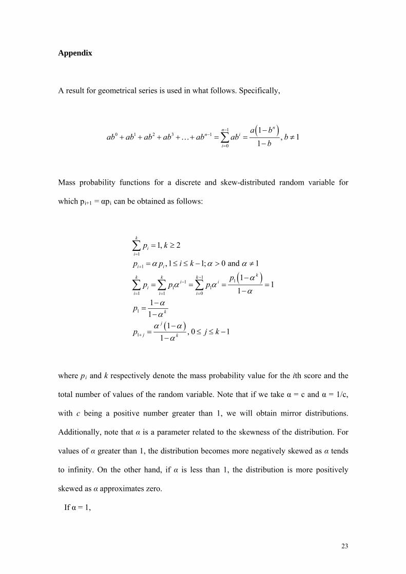
Appendix

A result for geometrical series is used in what follows. Specifically,

10 1 2 3 1

0

1, 1

1

nnn i

i

a bab ab ab ab ab ab b

b

Mass probability functions for a discrete and skew-distributed random variable for

which pRi+1R = αpRiR can be obtained as follows:

1

1

111

1 11 1 0

1

1

1, 2

,1 1; 0 and 1

11

1

1

1

1, 0 1

1

k

ii

i i

kk k ki i

ii i i

k

j

j k

p k

p p i k

pp p p

p

p j k

where pRiR and k respectively denote the mass probability value for the ith score and the

total number of values of the random variable. Note that if we take α = c and α = 1/c,

with c being a positive number greater than 1, we will obtain mirror distributions.

Additionally, note that α is a parameter related to the skewness of the distribution. For

values of α greater than 1, the distribution becomes more negatively skewed as α tends

to infinity. On the other hand, if α is less than 1, the distribution is more positively

skewed as α approximates zero.

If α = 1,

24

1

1

11 1 1

1 1 1

1

1

1, 2

,1 1

1 1 1

1

1, 0 1

k

ii

i i

k k ki

ii i i

j

p k

p p i k

p p p kp

pk

p j kk

we obtain the uniform discrete distribution.

In the case of symmetric patterns for k even,

1

1

1

/ 2

1

/ 2/ 2 / 2 111

1 11 0

1 / 2

1 / 2

1, 2 and int / 2 / 2

,1 / 2 1; 0 and 1

,1 / 2

2 1

2 12 2 1

1

1

2 1

1, 0 / 2 1

2 1

k

ii

i i

k i i

k

ii

kk ki i

i i

k

j

j k

p k k k

p p i k

p p i k

p

pp p

p

p j k

If α < 1, the mass probability function is U-shaped. On the other hand, it follows a

triangular distribution if α > 1. Note that if we take α = c and α = 1/c, with c being a

positive number greater than 1, we will obtain inverse distributions. It is also possible to

obtain the uniform discrete distribution for α = 1,

25

/ 2 / 21

1 1 1 11 0

1

2 1 2 1 2 12

1

k ki

i i

kp p p p k

pk

In the case of symmetric distributions for k odd,

1

1

1

1 / 2

1 / 21

1 / 21 / 2 1 / 2 111 / 2 1 / 2 1 / 21

1 1 1 1 11 0

1 / 2

1

1

1, 2 and int / 2 1 / 2

,1 1 / 2; 0 and 1

,1 1 / 2

2 1

2 12 2

1

2 11

11

k

ii

i i

k i i

k

i ki

kk kk k ki i

i i

k

p k k k

p p i k

p p i k

p p

pp p p p p

p

p

1 / 2

1 1 / 2

2 1

1, 0 1 / 2

2 1

k

j

j kp j k

If α < 1, the mass probability function resembles an inversion of the triangular. On the

other hand, it follows a triangular distribution if α > 1. Note that if we take α = c and α =

1/c, with c being a positive number greater than 1, we will obtain inverse distributions.

It is also possible to obtain the uniform discrete distribution for α = 1,

1 / 21 / 21

1 1 1 11

1

2 1 1 1 1

1

kki

i

p p p k p

pk

26

Tables

Table 1. Personality trait scores for each of the four participants (P1 to P4) and indices

values for the five personality traits.

N E O A C

P1 15 24 33 41 40

P2 3 22 25 41 31

P3 12 27 22 37 35

P4 32 32 32 22 28

Mean 15.50 26.25 28 35.25 33.50

SD 10.5 3.77 4.64 7.82 4.50

MED 14.37 5.20 6.51 10.70 6.23

SD – standard deviation; MED – Mean Euclidean distance. N – Neuroticism; E – Extraversion; O – Openness to experience; A – Agreeableness; C – Conscientiousness.

27

Table 2. Dissimilarity for each scale (λRkR). A Monte Carlo sampling with 99,999 samples

was carried out in order to estimate the sampling distributions of the index values and

their statistical significance under a uniform null distribution.

λRN λRE λRO λRA λRC

Index value .469 .172 .208 .318 .208

Upper tail p value .606 .973 .954 .851 .954

Lower tail p value .402 .031 .051 .158 .051

Mean .511 .511 .511 .511 .511

Variance .031 .031 .031 .031 .031

Minimum .016 .016 .016 .016 .016

25% percentile .385 .385 .385 .385 .385

50% percentile .521 .521 .521 .521 .521

75% percentile .641 .641 .641 .641 .641

Maximum .990 .990 .990 .990 .990

28

Table 3. Results for normalized dyadic contributions to dissimilarity (ωRijR) on the

Extraversion scale. Index values are shown above the main diagonal of the table, while

values below the diagonal represent lower tail p values, given that the upper tail p

values were greater than .05.

P1 P2 P3 P4

P1 - .042 .062 .167

P2 .098 - .104 .208

P3 .139 .213 - .104

P4 .320 .384 .213 -

29

Table 4. Normalized individual contributions (τRiR) to dissimilarity on the Extraversion

scale. Statistical significance was estimated by means of a Monte Carlo sampling under

the uniform null distribution.

τRiR statistic value Upper tail p

value

Lower tail p

value

P1 .090 .980 .024

P2 .118 .958 .049

P3 .090 980 .024

P4 .160 .904 .108

30

Table 5. Interpersonal perception matrix for the example about the item “Her/his

dialogue was useful for solving the task”, for the same group whose personality

dissimilarity measures are presented in Table 1.

P1 P2 P3 P4

P1 - 4 2 2

P2 2 - 2 2

P3 6 6 - 5

P4 6 4 4 -

31

Table 6. Dyadic (upper-triangular matrix) and individual contributions (rightmost

column) to the lack of reciprocity in interpersonal perception for the item “Her/his

dialogue was useful for solving the task”.

P1 P2 P3 P4 Individual

contribution

P1 - .027 .107 .107 .120

P2 - .107 .027 .080

P3 - .007 .110

P4 - .007

32

Figures

Figure 1. Four different mass probability distributions for a five-point rating scale

according to different combinations of α and symmetry values: a) U-shaped distribution

(α = .9091 and symmetric), b) triangular distribution (α = 1.1 and symmetric), c)

positively skewed distribution (α = .9091 and asymmetric), and d) negatively skewed

distribution (α = 1.1 and asymmetric).