Learning Pairwise Dissimilarity Profiles for Appearance Recognition in Visual Surveillance

Learning Pairwise Dissimilarity Profiles forAppearance Recognition in Visual Surveillance

Zhe Lin and Larry S. Davis

Institute of Advanced Computer StudiesUniversity of Maryland, College Park, MD 20742

{zhelin,lsd}@umiacs.umd.edu

Abstract. Training discriminative classifiers for a large number of classesis a challenging problem due to increased ambiguities between classes. Inorder to better handle the ambiguities and to improve the scalability ofclassifiers to larger number of categories, we learn pairwise dissimilarityprofiles (functions of spatial location) between categories and adapt theminto nearest neighbor classification. We introduce a dissimilarity distancemeasure and linearly or nonlinearly combine it with direct distances.We illustrate and demonstrate the approach mainly in the context ofappearance-based person recognition.

1 Introduction

Appearance-based person recognition is an important but still challenging prob-lem in vision. In visual surveillance, appearance information is crucial not only intracking, but also for identifying persons across space, time, and cameras. Posearticulation, viewpoint variation, and illumination change are common factorswhich affect the performance of recognition systems. More importantly, whenthe number of persons increases in the database, appearance ambiguities be-tween them become significant, and consequently, more and more discriminativefeature selection and classification approaches are needed.1 We aim to explorepairwise class relations in more details and incorporate them into traditionalnearest neighbor classification. Our approach is mainly motivated by the follow-ing observations: (1) A small region (or a feature) can be crucial in recognitionbecause it might be the only distinguishing element to discriminate two other-wise very similar appearances, (2) Discriminative features are much easier totrain in a pairwise scheme than in a one-against-all scheme, (3) Discriminativefeatures are characteristic for a certain pair of classes and generally different fordifferent pairs of classes.

There are numerous approaches to multiclass learning and recognition. Ininstance-based learning, nearest neighbor (NN) and k-NN are the most commonlyused nonparametric classifiers. In discriminative learning, linear discriminant1 In this paper, we formulate appearance-based person recognition as a multiclass

classification problem where each person is considered to be a class and his/herappearances are considered to be class samples.

G. Bebis et al. (Eds.): ISVC 2008, Part I, LNCS 5358, pp. 23–34, 2008.c© Springer-Verlag Berlin Heidelberg 2008

24 Z. Lin and L.S. Davis

analysis (LDA) and support vector machine (SVM) are well known classifica-tion methods successfully applied to many practical problems. There are severalschemes to decompose a multiclass classification problem into a set of binary clas-sification problems. For example, one-against-all [1], pairwise coupling [2, 3, 4],error correcting output codes [5], decision trees [6], etc. In [7], a multiclass classi-fication problem was transformed into a binary classification problem by model-ing intra- and extra-class distributions. Recently, multiclass learning approacheshave been successfully applied to object category recognition. k-NN and SVMare combined in [8] by performing a multiclass SVM only for a set of neigh-bors and query. Random forests and ferns classifier in [9] uses a one-against-all multiclass-SVM. Also, a number of approaches have been proposed in themachine learning community for learning locally or globally adaptive distancemetrics [10, 11, 12, 13, 14] by weighting features based on labeled training data.To simplify the one-against-all discrimination task for a huge number of cate-gories, a triplet-based distance metric learning framework was proposed in [15],and later was extended by learning weights for every prototype in [16] for imageretrieval. However, fixed weighting for each prototype can be inefficient for avery large number of classes, especially when ambiguities between classes aresignificant.

Most previous approaches to multiclass classification have focused on design-ing good classifiers with better separation margins and good generalization prop-erties, or on learning discriminative distance metrics. Our work is similar to thoseof learning discriminative distance metrics [13, 14, 16], but different in that, in-stead of learning weights for different features, we explore pairwise dissimilar-ities and adapt them into classification by calculating distances of a query toprototypes using both intra-class and inter-class invariant information. For ex-ample, in the context of person recognition, the intra-class invariance is basedon common appearance information in each class, i.e. appearance informationthat does not change dramatically for each individual as pose, viewpoint andillumination change. The inter-class invariance is based on the observation thatany pair of examplars EA and EB from two different classes A and B sharecertain common discriminative properties. For example, in the context of personappearance recognition, if person 1 and person 2 have different jacket colors, thenany variants of person 1 and person 2 will probably also have different jacketcolors.

2 Appearance Representation and Matching

2.1 Appearance Model

Color and texture are the primary cues for appearance-based object recognition.For human appearances, the most common model is the color histogram [17].Spatial information can be added by representing appearances in joint color-spatial spaces [18]. Other representations include spatial-temporal appear-ance modeling [19], spatial and appearance context modeling [20], part-based

Learning Pairwise Dissimilarity Profiles 25

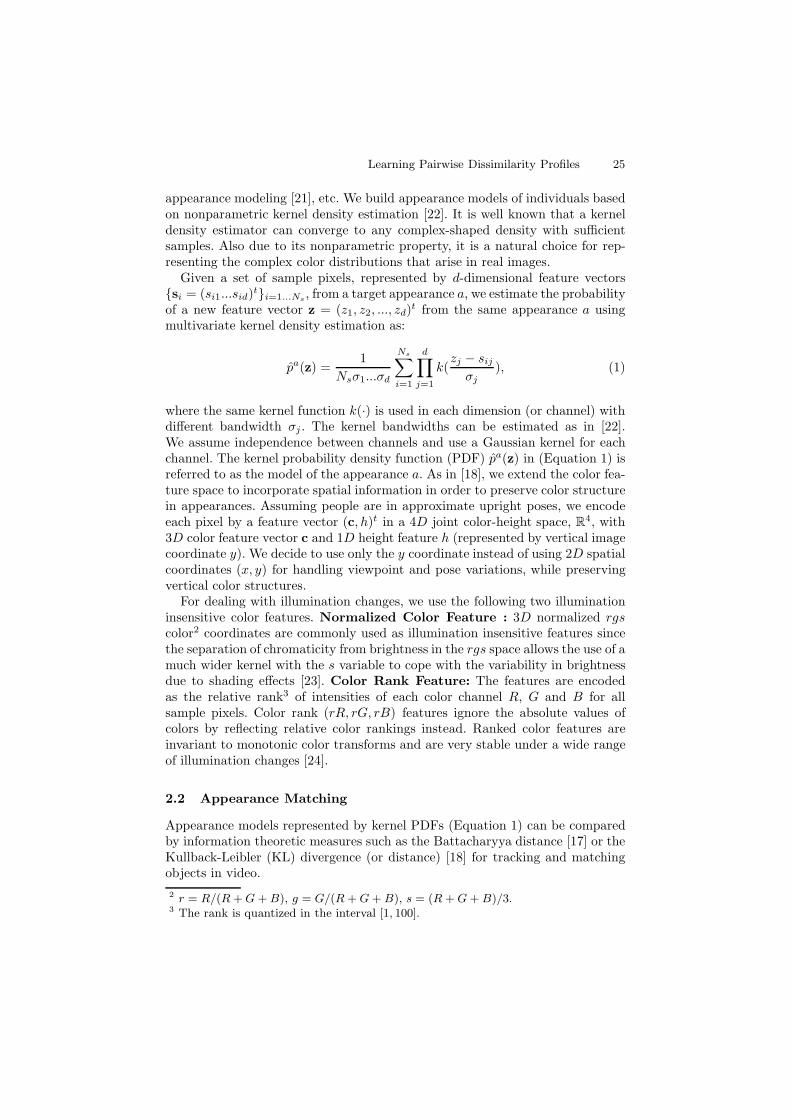
appearance modeling [21], etc. We build appearance models of individuals basedon nonparametric kernel density estimation [22]. It is well known that a kerneldensity estimator can converge to any complex-shaped density with sufficientsamples. Also due to its nonparametric property, it is a natural choice for rep-resenting the complex color distributions that arise in real images.

Given a set of sample pixels, represented by d-dimensional feature vectors{si = (si1...sid)t}i=1...Ns , from a target appearance a, we estimate the probabilityof a new feature vector z = (z1, z2, ..., zd)t from the same appearance a usingmultivariate kernel density estimation as:

p̂a(z) =1

Nsσ1...σd

Ns∑

i=1

d∏

j=1

k(zj − sij

σj), (1)

where the same kernel function k(·) is used in each dimension (or channel) withdifferent bandwidth σj . The kernel bandwidths can be estimated as in [22].We assume independence between channels and use a Gaussian kernel for eachchannel. The kernel probability density function (PDF) p̂a(z) in (Equation 1) isreferred to as the model of the appearance a. As in [18], we extend the color fea-ture space to incorporate spatial information in order to preserve color structurein appearances. Assuming people are in approximate upright poses, we encodeeach pixel by a feature vector (c, h)t in a 4D joint color-height space, R

4, with3D color feature vector c and 1D height feature h (represented by vertical imagecoordinate y). We decide to use only the y coordinate instead of using 2D spatialcoordinates (x, y) for handling viewpoint and pose variations, while preservingvertical color structures.

For dealing with illumination changes, we use the following two illuminationinsensitive color features. Normalized Color Feature : 3D normalized rgscolor2 coordinates are commonly used as illumination insensitive features sincethe separation of chromaticity from brightness in the rgs space allows the use of amuch wider kernel with the s variable to cope with the variability in brightnessdue to shading effects [23]. Color Rank Feature: The features are encodedas the relative rank3 of intensities of each color channel R, G and B for allsample pixels. Color rank (rR, rG, rB) features ignore the absolute values ofcolors by reflecting relative color rankings instead. Ranked color features areinvariant to monotonic color transforms and are very stable under a wide rangeof illumination changes [24].

2.2 Appearance Matching

Appearance models represented by kernel PDFs (Equation 1) can be comparedby information theoretic measures such as the Battacharyya distance [17] or theKullback-Leibler (KL) divergence (or distance) [18] for tracking and matchingobjects in video.2 r = R/(R + G + B), g = G/(R + G + B), s = (R + G + B)/3.3 The rank is quantized in the interval [1, 100].


Suppose two appearances a and b are modeled as kernel PDFs p̂a and p̂b inthe joint color-height space. Assuming p̂a as the reference model and p̂b as thetest model, the similarity of the two appearances can be measured by the KLdistance as follows:

DKL(p̂b||p̂a) =∫

p̂b(z)logp̂b(z)p̂a(z)

dz. (2)

Note that the KL distance is a nonsymmetric measure in that DKL(p̂b||p̂a) �=DKL(p̂a||p̂b). For efficiency, the distance is calculated using only samples insteadof the whole feature set. Given Na samples {si}i=1...Na from appearance a andNb samples {tk}k=1...Nb

from appearance b, Equation 2 can be approximated bythe following form given sufficient samples from the two appearances:

DKL(p̂b||p̂a) =1

Nb

Nb∑

k=1

logp̂b(tk)p̂a(tk)

, (3)

where p̂a(tk)= 1Na

∑Na

i=1∏d

j=1 k( tkj−sij

σj), and p̂b(tk) = 1

Nb

∑Nb

i=1∏d

j=1 k( tkj−tij

σj).

Let Φab denote the log-likelihood ratio function, i.e. Φab(u) = log p̂b(u)p̂a(u) , where

u is a d-dimensional feature vector in the color-height space. Since we sam-ple test pixels only from appearance b, p̂b is evaluated by its own samples, sop̂b is generally equal to or larger than p̂a for all test samples tk. Note that afew noisy (ambiguous) samples tk from appearance b can be better matchedby the reference model PDF p̂a than the test model pdf p̂b so that p̂b(tk) <p̂a(tk), and, consequently, the log-likelihood ratio Φab(tk) can be slightly lessthan zero. For minus log-likelihoods generated from those noisy samples, weforce them to zeros (positive correction). Then, Equation 3 can be written as:D+

KL = 1Nb

∑Nb

k=1 [Φab(tk)]+, where [Φab(tk)]+ = max(Φab(tk), 0

). The posi-

tively corrected KL distance D+KL is guaranteed to be nonnegative for all sam-

ples: D+KL(p̂b||p̂a) ≥ 0 , where equality holds if and only if two density models

are identical for all test samples. The direct appearance-based distance Da(q, pj)from a query q to a prototype pj is computed as: Da(q, pj) = D+

KL(p̂q||p̂j). In con-ventional NN classification, Da(q, pj) is evaluated for all prototypes {pj}j=1...N

and the minimum is chosen for classification.

3 Learning Pairwise Invariant Properties

For classifying large number of classes, it has been noted previously in [2,3] thata one-against-all scheme has difficulty separating one class from all of the othersand often very complex classification models (probably leading to overfitting) areused for that purpose. In contrast, pairwise coupling is much easier to train sinceit only needs to separate one class from an other. For handling the scalabilityproblem, we perform more detailed analysis of discriminative features betweenclasses by estimating invariant information from pairwise comparisons.


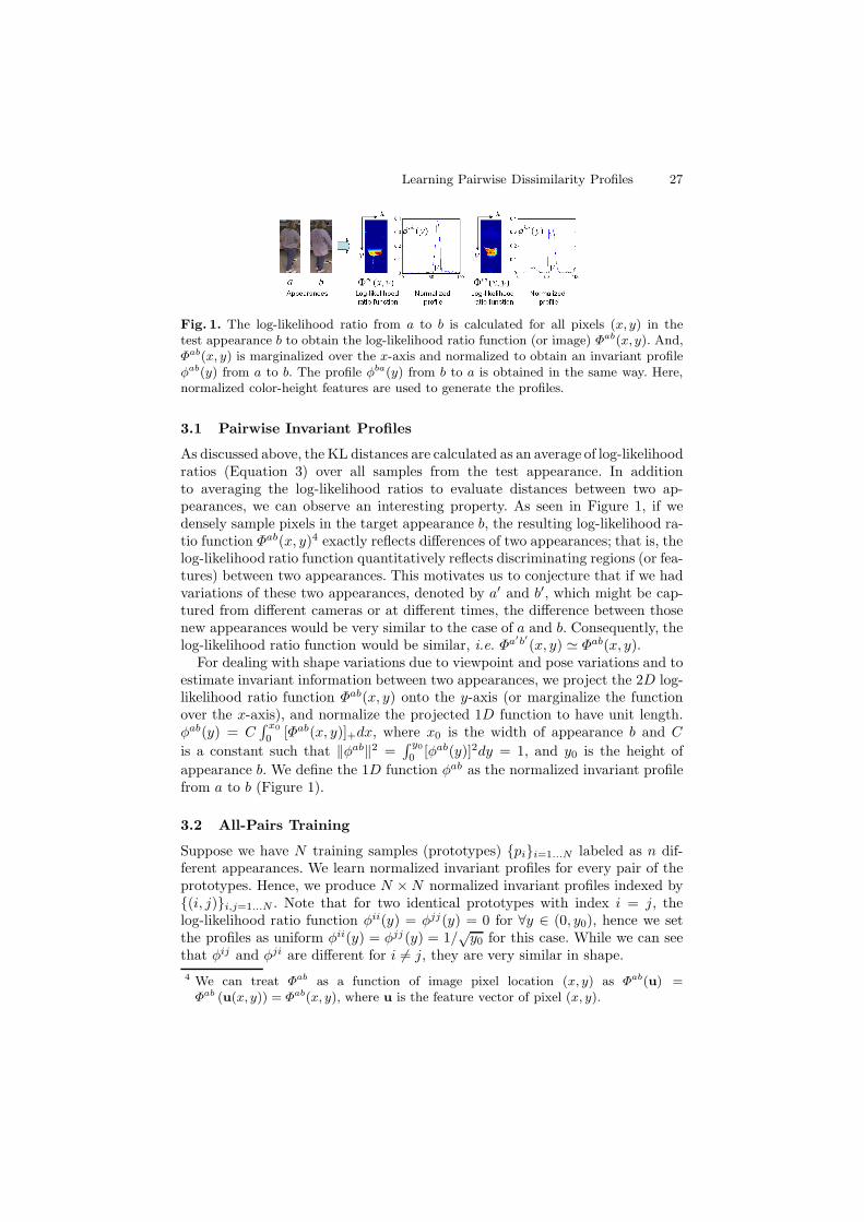
Fig. 1. The log-likelihood ratio from a to b is calculated for all pixels (x, y) in thetest appearance b to obtain the log-likelihood ratio function (or image) Φab(x, y). And,Φab(x, y) is marginalized over the x-axis and normalized to obtain an invariant profileφab(y) from a to b. The profile φba(y) from b to a is obtained in the same way. Here,normalized color-height features are used to generate the profiles.

3.1 Pairwise Invariant Profiles

As discussed above, the KL distances are calculated as an average of log-likelihoodratios (Equation 3) over all samples from the test appearance. In additionto averaging the log-likelihood ratios to evaluate distances between two ap-pearances, we can observe an interesting property. As seen in Figure 1, if wedensely sample pixels in the target appearance b, the resulting log-likelihood ra-tio function Φab(x, y)4 exactly reflects differences of two appearances; that is, thelog-likelihood ratio function quantitatively reflects discriminating regions (or fea-tures) between two appearances. This motivates us to conjecture that if we hadvariations of these two appearances, denoted by a′ and b′, which might be cap-tured from different cameras or at different times, the difference between thosenew appearances would be very similar to the case of a and b. Consequently, thelog-likelihood ratio function would be similar, i.e. Φa′b′

(x, y) � Φab(x, y).For dealing with shape variations due to viewpoint and pose variations and to

estimate invariant information between two appearances, we project the 2D log-likelihood ratio function Φab(x, y) onto the y-axis (or marginalize the functionover the x-axis), and normalize the projected 1D function to have unit length.φab(y) = C

∫ x0

0 [Φab(x, y)]+dx, where x0 is the width of appearance b and C

is a constant such that ‖φab‖2 =∫ y0

0 [φab(y)]2dy = 1, and y0 is the height ofappearance b. We define the 1D function φab as the normalized invariant profilefrom a to b (Figure 1).

3.2 All-Pairs Training

Suppose we have N training samples (prototypes) {pi}i=1...N labeled as n dif-ferent appearances. We learn normalized invariant profiles for every pair of theprototypes. Hence, we produce N × N normalized invariant profiles indexed by{(i, j)}i,j=1...N . Note that for two identical prototypes with index i = j, thelog-likelihood ratio function φii(y) = φjj(y) = 0 for ∀y ∈ (0, y0), hence we setthe profiles as uniform φii(y) = φjj(y) = 1/

√y0 for this case. While we can see

that φij and φji are different for i �= j, they are very similar in shape.4 We can treat Φab as a function of image pixel location (x, y) as Φab(u) =

Φab (u(x, y)) = Φab(x, y), where u is the feature vector of pixel (x, y).


4 Discriminative Information-Based Distances

Given a query q, we want to match it to prototypes {pi}i=1...N using the learnedset of profiles {φij}i,j=1...N . We first calculate a likelihood ratio function Φiq fromevery prototype pi to query q, and perform normalization (as in the learning step)to obtain a set of query profiles {φiq}i=1...N . The idea is to vote for the ID of q(which is unknown) by matching a query profile φiq to a learned profile φij forwhich the corresponding ID j is known. The distance D(j, q|i) between the queryprofile φiq and the learned profile φij is defined as follows: D(j, q|i) =

∫ y0

0 [φiq(y)−φij(y)]2dy. The intuition here is that the smaller the distance D(j, q|i), the moresimilar the two profiles are, consequently, the more confident to vote for j as theID of q. For each i, we calculate D(j, q|i) for all j = 1...N and then vote for theID of q. We perform such a voting procedure for all training samples {pi}i=1...N .

We can vote for the ID of q based only on the best matching profile φij∗for

each prototype pi, i.e. the one for which j∗i = argminj D(j, q|i), then assign onevote for j∗i : V (j∗i ) + 1 −→ V (j∗i ). This is referred to as hard voting. The votingcan be performed either in a soft manner, i.e. we vote for the ID of q based onthe evidence from all profiles {φij}i,j=1...N , instead of only choosing the bestmatching ID j∗ (corresponding to the lowest profile distance) for each i. Thesoft voting-based distance Dsv(q, pj) from query q to prototype pj is defined as:Dsv(q, pj) = 1

N

∑Ni=1 D(j, q|i).

Compared to hard voting, soft voting is less sensitive to ambiguities andnoise effects since it collects all possible evidence for calculating final voting-based distances instead of choosing the top one match as in hard voting. Fromexperiments, we verify that soft voting gives better performance in recogni-tion rate. Based on the above reasoning, we compute the (indirect) discrim-inative information-based distance from the a query q to a prototype pj as:Dd(q, pj) = Dsv(q, pj).

5 Classification and Recognition

As discussed previously, traditional nearest neighbor or k-NN methods directlyuse Da as the distance from a query to a prototype, and the classification isperformed by finding the minimum distance or by majority voting for k near-est neighbors. Da only considers information between a query and a proto-type, while Dd only considers inter-relations between different training samples;that is, the two distances are based on independent information. This leadsto the idea that combining the two would boost recognition performance. Wetested two parameterized distance measures D1 and D2 involving linear andnonlinear combinations: D1(q, pj) = (1 − α)Da(q, pj) + αDd(q, pj), D2(q, pj) =D1−β

a (q, pj)Dβd (q, pj). We learn the parameters α and β by evaluating the over-

all recognition rates using a large number of labeled testing samples. Experi-ments shows that the optimal parameter estimates are as listed in Table 1. Theparameters can be selected flexibly around the optimal values (±0.1) withoutperformance degradation. Given a query q, we want to estimate its unknown


a b c d e f g h i j0

5

10

15

Prototype ID

Da

Direct Appearance−based

direct


0.5

1

1.5

Prototype ID

Dsv

Discriminative Information−based

soft voting


5

10

Prototype ID

D1

Combine

combine1


5

10

Prototype ID

D2

Combine

combine2

1

1.5

2

Distances

Rel

ativ

e M

argi

ns

Comparison

directsoft votingcombine1combine2

Fig. 2. An illustration of the invariance of pairwise normalized profiles, and a compar-ison of direct, indirect, and combined distances for an example of 10 prototypes (withdifferent labels) and one query. Top: it can be observed that the current test profilesof appearance q are very similar to the learned profiles of appearance c (which is thetrue classification of q) while largely different for the case of other appearances suchas a and b. Bottom: distances Da, Dsv, D1, D2 from q to all prototypes are evaluatedand the relative margins are compared. We can see that all distance measures result incorrect top one recognition, while the combined distance measures D1 and D2 resultin larger relative margins than Da and Dsv.

Table 1. Learned optimal parameter values for combined distance measures D1 andD2. Total of 180 labeled test samples are used against 180 training samples of differentappearances for learning the parameters α and β.

Normalized Color + Height feature α = 0.24, β = 0.20Color Rank + Height feature α = 0.75, β = 0.30

class label (person ID) by calculating the distances between the query and alllabeled prototypes. Classification is done by the nearest neighbor rule using oneof the combined distance measures D1 and D2 as: j∗ = arg minj Dcombine(q, pj).Figure 2 shows an illustration of the invariance of pairwise dissimilarity profilesand an example of recognition using different distance measures.

6 Implementation Details

The bandwidths for each dimension of the 4D feature spaces are listed in Table 2.The bandwidths are generally estimated as 2% of the ranges of the correspond-ing channel and adjusted slightly by repeated trial-and-error procedures. Weresize image patches of a person to have fixed height of 50 pixels y0 = 50. Notethat all the parameters including bandwidths for different feature spaces, height


Table 2. Bandwidths estimated and used for our experiments

Feature Space Channel BandwidthNormalized Color + Height σr = σg = 0.02, σs = 20, σh = 1Color Rank + Height σrR = σrG = σrB = 4, σh = 1

sampling rate, distance model parameters α and β are fixed to the listed valuesthroughout the experimental evaluation.

For efficiently matching people in video, we select key frames (appearances) asprototypes of training and testing sequences and recognize appearances basedon the prototypes. The process is as follows. The first frame (t = 0) is au-tomatically selected as the first key frame K1. Then, we calculate the sym-metric KL distances of the subsequent frames (t = 1, 2...) to all current keyframes {Kj}j=1...i. The symmetric KL distance is defined as: DsKL(p̂b, p̂a) =min(D+

KL(p̂b||p̂a), D+KL(p̂a||p̂b)). For the current frame t ≥ 1, if all symmet-

ric KL distances {DsKL(p̂t, p̂Kj ), j = 1...i} are greater than a fixed threshold5

τ = 1.5, frame t becomes the next key frame Ki+1, and is added to the setof current key frames. In this way, those frames with large information gain orhaving new information are selected, and those not selected can be explainedby the key frames with a bounded deviation from one of the key frames inthe symmetric KL distance. We preprocess the videos by codebook-based back-ground subtraction [25] and neighborhood-based noise removal to obtain singleconnected component for each frame. Person sub-images (rectangular patches)are extracted from bounding box of foreground regions.

7 Experimental Results

We use Honeywell Appearance Datasets for experimental evaluation. The clas-sification and recognition performance is quantitatively analyzed in terms ofCumulative Match Curve (CMC) and Expected Relative Margin. The expectedrelative margin δ is defined as a geometric mean of relative margins for all testsamples: δ = (

∏NT

i=1di2

di1)1/NT , where NT denotes the number of test samples, di

1

denotes the distance of query qi to the correct (same class) prototype, and di2 de-

notes the distance of query qi to the closest incorrect (different class) prototype.Our test data include videos of 61 individuals taken by two overlapping cameraswidely separated in space. Figure 3 shows samples from all 61 appearances.Wecan observe that the dataset has many appearance ambiguities because a limitednumber of people were used to create a large number of ‘appearance’ classes by apartial change of clothing for each person. Also there are significant illumination,viewpoint and pose changes across the two cameras. Note that in all the followingexperiments, we listed comparisons of our approach with the baseline technique

5 The threshold is estimated such that on average, three key frames are selected foreach track of about 30 frames.


(a) appearances from cam1 (b) appearances from cam2

Fig. 3. List of sample appearances taken under two overlapping and widely separatedcameras

0 1 2 3 4 5 60

0.2

0.4

0.6

0.8

1CMCs − 30 persons − train(cam1) & test(cam2)

k

Rec

ogni

tion

rate

norm−directnorm−soft votingnorm−combine1norm−combine2rank−directrank−soft votingrank−combine1rank−combine2

0 1 2 3 4 5 60

0.2

0.4

0.6

0.8


k

Rec

ogni

tion

rate


cam1−>cam2 cam2−>cam10.8

0.9

1

1.1

1.2

1.3

Relative margins − 30 persons

Ave

rage

rel

ativ

e m

argi

n


0 1 2 3 4 5 60

0.2

0.4

0.6

0.8


k

Rec

ogni

tion

rate


0 1 2 3 4 5 60

0.2

0.4

0.6

0.8


k

Rec

ogni

tion

rate


cam1−>cam2 cam2−>cam10.8

0.9

1

1.1

1.2

1.3

Relative margins − 61 persons

Ave

rage

rel

ativ

e m

argi

n


Fig. 4. Recognition performance with respect to the increasing number of persons in-volved in training and testing. Note that, due to space limitation, only plots for casesN = 30, 61 are shown. (‘norm’: normalized color feature, ‘rank’: color rank feature, ‘di-rect’: appearance-based distance Da, ‘soft voting’: discriminative information-based dis-tance Dd = Dsv , ‘combine1’ and ‘combine2’: combined distances D1, D2.)

(i.e. nearest neighbor classifier) using the same type features. Our approach is la-beled as ‘combine’ and the baseline technique is labeled as ’direct’.

Scalability: To show the scalability of our voting-based and combined ap-proaches, we evaluated cumulative recognition rates and expected relative mar-gins for increasing number (N = 10, 20, 30, 40, 50, 60, 61) of individuals involvedin training and testing (Figure 4). For each of the 61 individuals, we select onekey frame from a camera for training and one key frame from another camerafor testing, and evaluated the performance using different features and differenttraining-testing data (cam1 to cam2, cam2 to cam1). The results show that ourcombined approaches consistently perform better than the direct appearance-based method. More importantly, we note that our voting-based approach and


0 1 2 3 4 5 60.5

0.6

0.7

0.8

0.9

1CMCs − comparison w.r.t. # of prototypes

k

Rec

ogni

tion

rate

1 prototype−direct1 prototype−soft voting1 prototype−combine11 prototype−combine23 prototypes−direct3 prototypes−soft voting3 prototypes−combine13 prototypes−combine2

1 prototype 3 prototypes1

1.1

1.2

1.3Relative margins − # of prototypes

Ave

rage

rel

ativ

e m

argi

n directsoft votingcombine1combine2

Fig. 5. Recognition performance with respect to the changing number of training sam-ples (prototypes) per class

Table 3. Comparisons of top one recognition rates to state of the art work. Ourcombined approaches with (color rank + height) features are marked as ‘bold’.

Approaches Avg. Recog. Ratenorm-direct-appearance 61 persons 0.56norm-soft voting 61 persons 0.35norm-combine1 61 persons 0.59norm-combine2 61 persons 0.61rank-soft voting 61 persons 0.71rank-direct-appearance 61 persons 0.84rank-combine1 61 persons 0.88rank-combine2 61 persons 0.89[24] rank-path length 61 persons 0.85[19] model fitting 44 persons 0.59[20] shape & appear. c. 99 persons 0.82

combined approaches only have very small degradations with increasing numbersof people, while direct methods resulted in large degradation in recognition per-formance. This is more obviously seen for the case of color rank features.We cansee that our discriminative information-based combined distances are more usefulin recognizing large number of classes than the direct appearance-based distances.

Effects of Number of Training Samples: We compared recognition perfor-mance over the number of training samples per class (Figure 5). We select threekey frames for each of 30 individuals from camera 2 as training samples andthree key frames for each of 30 individuals from camera 1 as test samples. Thefigure shows that increasing the number of training samples per class improvescumulative recognition rates and relative margins significantly.

Comparison with Previous Approaches: We also compared the perfor-mance of our voting-based and combined approaches to the direct appearance-based approach in terms of average top one recognition rates on 61 individuals.Both cases of (Normalized Color + Height) and (Color Rank + Height) featurespaces show that our combined approaches improve top one recognition ratesof direct appearance-based method by 5-6% (equivalently, the error rate is re-duced by 31%) (Table 3). Results on the same dataset with a same number


of individuals are compared to Yu et al. [24]6. Using similar number of pixels(500 samples) per appearance, our combined approach obtained 4% better topone recognition rate (equivalently, the error rate is reduced by 27%) and is 5-10times faster than [24]. This is because computing path-length features for allsamples significantly slows down the process. We used the much simpler normal-ized height feature to achieve better performance. Indirect comparisons (Table 3)to Gheissari et al. [19] and Wang et al. [20]7 on datasets with similar number ofpeople show that our approach is comparable to state of the art work on personrecognition. The computational complexity8 of our learning algorithm is O(N2),while the complexity of our testing algorithm for a single query image is onlyO(N), which is the same as the traditional nearest neighbor method.

8 Conclusion

We proposed a pairwise comparison-based learning and classification approachfor appearance-based person recognition. We used a learned set of pairwise in-variant profiles to adaptively calculate distances from a query to prototypesso that the expected relative margins can be improved. The combined distancesfrom appearance and discriminative information lead to significant improvementsover pure appearance-based nearest neighbor classification. We also experimen-tally validated the scalability of our approach to larger number of categories.

Acknowledgement

This research was funded in part by the U.S. Government VACE program. Theauthors would like to thank Yang Yu for discussion and help on this work.

References

1. Nakajima, C., Pontil, M., Heisele, B., Poggio, T.: Full-body person recognitionsystem. Pattern Recognition 36, 1997–2006 (2003)

2. Hastie, T., Tibshirani, R.: Classification by pairwise coupling. In: NIPS (1997)3. Roth, V., Tsuda, K.: Pairwise coupling for machine recognition of handprinted

japanese characters. In: CVPR (2001)4. Wu, T., Lin, C., Weng, R.C.: Probability estimates for multi-class classification by

pairwise coupling. Journal of Machine Learning Research 5, 975–1005 (2004)5. Dietterich, T., Bakiri, G.: Solving multiclass learning problems via error-correcting

output codes. Journal of Artificial Intelligence Research, 263–286 (1995)6. Amit, Y., Geman, D., Wilder, K.: Joint induction of shape features and tree clas-

sifiers. IEEE Trans. PAMI 19, 1300–1305 (1997)

6 The result of [24] is obtained from their most recent experiments.7 In [19,20], Datasets (publicly unavailable) of 44 and 99 individuals are used.8 Using about 500 samples per appearance, the learning time for 61 appearances is

about 2 minutes, and the time for matching a single query image to 61 prototypesis less than 2 seconds in C++ on a Intel Xeon CPU 2.40GHz machine.


7. Moghadam, B., Jebara, T., Pentland, A.: Bayesian face recognition, MERL Tech-nical Report, TR-2000-42 (2002)

8. Zhang, H., Berg, A., Maire, M., Malik, J.: SVM-KNN: Discriminative nearest neigh-bor classification for visual category recognition. In: CVPR (2006)

9. Bosch, A., Zisserman, A., Munoz, X.: Image classification using random forests andferns. In: ICCV (2007)

10. Hastie, T., Tibshirani, R.: Discriminant adaptive nearest neighbor classification.IEEE Trans. PAMI 18, 607–616 (1996)

11. Domeniconi, C., Gunopulos, D.: Adaptive nearest neighbor classification using sup-port vector machines. In: NIPS (2001)

12. Xing, E., Ng, A., Jordan, M., Russell, S.: Distance metric learning, with applicationto clustering with side information. In: NIPS (2002)

13. Shalev-Shwartz, S., Singer, Y., Ng, A.: Online and batch learning of pseudo metrics.In: ICML (2004)

14. Weinberger, K.Q., Blitzer, J., Saul, L.K.: Distance metric learning for large marginnearest neighbor classification. In: NIPS (2005)

15. Schultz, M., Joachims, T.: Learning a distance metric from relative comparisons.In: NIPS (2003)

16. Frome, A., Singer, Y., Sha, F., Malik, J.: Learning globally-consistent local distancefunctions for shape-based image retreval and classification. In: ICCV (2007)

17. Comaniciu, D., Ramesh, V., Meer, P.: Kernel-based object tracking. IJCV 25, 64–577 (2003)

18. Elgammal, A., Davis, L.S.: Probabilistic tracking in joint feature-spatial spaces.In: ICCV (2003)

19. Gheissari, N., Sebastian, T., Tu, P., Rittscher, J., Hartley, R.: Person reidentifica-tion using spatiotemporal appearance. In: CVPR (2006)

20. Wang, X., Doretto, G., Sebastian, T., Rittscher, J., Tu, P.: Shape and appearancecontext modeling. In: ICCV (2007)

21. Li, J., Zhou, S.K., Chellappa, R.: Appearance context modeling under geometriccontext. In: ICCV (2005)

22. Scott, D.: Multivariate density estimation. Wiley Interscience, Hoboken (1992)23. Zhao, L., Davis, L.S.: Iterative figure-ground discrimination. In: ICPR (2004)24. Yu, Y., Harwood, D., Yoon, K., Davis, L.S.: Human appearance modeling for

matching across video sequences. Mach. Vis. Appl. 18, 139–149 (2007)25. Kim, K., Chalidabhongse, T.H., Harwood, D., Davis, L.S.: Real-time foreground-

background segmentation using codebook model. Real-Time Imaging 11, 172–185(2005)

Learning Pairwise Dissimilarity Profiles for Appearance Recognition in Visual Surveillance

Documents

Transcript of Learning Pairwise Dissimilarity Profiles for Appearance Recognition in Visual Surveillance