Non-Inferiority Testing with a Variable Margin*

Zhiwei Zhang**

Division of Biostatistics, OSB, CDRH, FDA, HFZ-550, 1350 Piccard Drive, Rockville, MD 20850,USA

Received 26 January 2006, revised 16 May 2006, accepted 31 May 2006

Summary

There has been growing interest, when comparing an experimental treatment with an active controlwith respect to a binary outcome, in allowing the non-inferiority margin to depend on the unknownsuccess rate in the control group. It does not seem universally recognized, however, that the statisticaltest should appropriately adjust for the uncertainty surrounding the non-inferiority margin. In this paper,we inspect a naive procedure that treats an “observed margin” as if it were fixed a priori, and explainwhy it might not be valid. We then derive a class of tests based on the delta method, including theWald test and the score test, for a smooth margin. An alternative derivation is given for the asymptoticdistribution of the likelihood ratio statistic, again for a smooth margin. We discuss the asymptoticbehavior of these tests when applied to a piecewise smooth margin. A simple condition on the marginfunction is given which allows the likelihood ratio test to carry over to a piecewise smooth marginusing the same critical value as for a smooth margin. Simulation experiments are conducted, under asmooth margin and a piecewise linear margin, to evaluate the finite-sample performance of the asymp-totic tests studied.

Key words: Delta method; Likelihood ratio test; Non-inferiority; Power; Sample size; Scoretest; Wald test.

1 Introduction

Non-inferiority trials are becoming increasing popular, especially in areas of medicine where effectivetreatments are known to exist and use of placebo controls is considered unethical. The main objectiveof a non-inferiority trial is to demonstrate that the experimental treatment is not much inferior to anactive control. Here the meaning of “much” is made precise by a non-inferiority margin d > 0, whichrepresents the smallest clinically meaningful difference between the two treatment groups. Suppose,for example, that two proportions pj, j ¼ 1; 2, are to be compared, where p1 denotes a success rateassociated with the control and p2 the same rate for the experimental treatment. (By symmetry, thisdiscussion can be easily adapted to tests concerning rates of unfavorable events such as adverse clin-ical events.) In a non-inferiority test, the null hypothesis states that the experimental treatment isinferior to the control by at least d, while the alternative hypothesis states the opposite. Formally, wehave

H0* : p2 � p1 � d; H1* : p2 > p1 � d : ð1Þ

It is often convenient to identify the parameter space for ðp1; p2Þ with the unit square and the nullhypothesis with a subset of the unit square determined by d.

* The views expressed in this article do not necessarily represent those of the U.S. Food and Drug Administration.** e-mail: zhiwei.zhang@fda.hhs.gov, Phone: +1 240 276 3139, Fax: +1 240 276 3131

948 Biometrical Journal 48 (2006) 6, 948–965 DOI: 10.1002/bimj.200610271

# 2006 WILEY-VCH Verlag GmbH & Co. KGaA, Weinheim

The choice of d can be subtle and sometimes involves the success rate p1 in the control group.(Equivalently, this dependence can be, and often is, formulated in terms of the higher success rate inthe two treatment groups.) In anti-infective trials, for instance, a treatment difference of 15% in re-sponse rate is often perceived as tolerable for a control rate of 75%, but may be considered unaccep-tably large if the control rate increases to 95%. A fixed d is appropriate if p1 is essentially known orif this one d is reasonable for all plausible values of p1. In general, however, the uncertainty surround-ing p1 and hence d should be dealt with explicitly and rigorously. It is assumed here that a clearchoice of d exists for each possible value of p1; this variable non-inferiority margin will be written asdðp1Þ, where d denotes the margin function. The statistical hypotheses to be tested are then

H0: p2 � p1 � dðp1Þ; H1: p2 > p1 � dðp1Þ : ð2ÞGraphically, the null hypothesis H0 corresponds to the subgraph in the unit square of a curve runningbelow the main diagonal. The curve, given by p2 ¼ p1 � dðp1Þ, 0 < p1 < 1, will be referred to as theboundary (curve) of H0, ignoring other, statistically trivial boundary points of H0. A series of exam-ples are presented below to illustrate the relevance and generality of the variable margin framework.

Example (Fixed Margin). Just as a constant can be regarded as a (constant) function, a fixed non-inferiority margin can be treated as a constant margin function: dðp1Þ � d.

Example (Step Function). A well known step function used to define a non-inferiority margin canbe found in the 1992 FDA Points-to-Consider for anti-infective trials. In such trials, the effectivenessof a test drug relative to an active control is often evaluated in terms of the microbiologic eradicationrate. Actually, the Points-to-Consider only describes a test procedure without formulating the statisti-cal hypotheses of interest. It seems clear, however, that non-inferiority hypotheses are being testedwith margin function

dðp1Þ ¼0:2; p1 < 0:8;0:15; 0:8 � p1 < 0:9;0:1; p1 � 0:9:

8<:

The discontinuities of d at 0.8 and 0.9 have been found to cause “erratic behavior” of the powerfunction, which can create problems with sample size calculations (Weng and Liu, 1994; R�hmel,1998, 2001). In fact, the FDA no longer recommends this procedure, and a smooth margin function isnow widely preferred (R�hmel, 1998, 2001; Phillips, 2003; Kim and Xue, 2004).

Example (Linear Margin). In an effort to improve upon the Points-to-Consider procedure, Phillips(2003) considered a linear margin function:

dðp1Þ ¼ aþ bp1 ;

where a and b are constants chosen a priori to approximate the clinical judgement. This formulationincludes as special cases a fixed margin (b ¼ 0) and hypotheses concerning relative risks. Suppose, forexample, that one wishes to show that p2=p1 > c for some c < 1. This hypothesis can be written asp2 > p1 � dðp1Þ, where dðp1Þ ¼ ð1� cÞ p1 is a linear function. While a linear d is convenient to workwith and often represents a close approximation to clinical thinking over a small neighborhood ofsome target value of p1, it may not look as reasonable for other possible values of p1. The problem isthat the linearity requirement may be too stringent: the whole straight line (d) is determined as soonas we specify dðp1Þ for two different values of p1 and even these two points have to satisfy certainconstraints so as to keep the line in range (0 < dðp1Þ < p1 for all p1).

Example (Piecewise Linear Margin). A piecewise linear margin would offer more flexibility thandoes a linear margin. Kim and Xue (2004) described a real example of this, which will be sketched asfollows. The Safety of Estrogens in Systemic Lupus Erythematosus National Assessment (SELENA)study was conducted to determine whether exogenous estrogens in hormone replacement therapy(HRT) increase disease activity in postmenopausal women with systematic lupus erythematosus. Spe-

Biometrical Journal 48 (2006) 6 949

# 2006 WILEY-VCH Verlag GmbH & Co. KGaA, Weinheim www.biometrical-journal.com

cifically, the objective was to demonstrate that the severe flare rate at 12 months was not much higherin the HRT group than in the placebo group. It was clear that the non-inferiority margin shoulddepend on the flare rate in the placebo group, which was largely unknown. In order to define themargin function, eight investigators were independently asked to set the non-inferiority margin atseveral values of p1, say t0 � 0 < t1 < . . . < tm�1 < 1 � tm. The opinions of these investigators werethen averaged at each tj, j ¼ 1; . . . ;m� 1. After consensus was reached following extensive discus-sion, the final margin function was defined by linear interpolation. Algebraically, it takes the form

dðp1Þ ¼ aj þ bjp1; tj�1 � p1 < tj; j ¼ 1; . . . ;m :

Under this approach, we can pre-specify dðp1Þ at an arbitrary number of different values of p1, andthere are no mathematical constraints on their relationship provided each specified value is legitimate(i.e., 0 < dðtjÞ < tj, j ¼ 1; . . . ;m� 1). This extra flexibility (relative to a linear margin) comes at thecost of smoothness, as d may not be differentiable at the tj. The consequences of non-differentiabilitywill be examined in Section 5.

Example (R�hmel’s First Proposal). R�hmel (1998) proposed two types of smooth margin func-tions. His first proposal, originally due to John Lewis, was driven by the desire for a constant powerfunction over a range of plausible parameter values. R�hmel presented a numerical example derivedfrom a particular specification of statistical parameters. Although R�hmel did not elaborate on thecalculation, his reference to Farrington and Manning (1990) suggests that an asymptotic test for a fixeddelta was adopted. In a subsequent discussion on the same subject, R�hmel (2001) gave two formulas:

dðpÞ ¼ 0:333ffiffiffiffiffiffiffiffiffiffiffiffiffiffiffiffiffipð1� pÞ

p;

dðpÞ ¼ 0:223ffiffiffiffiffiffiffiffiffiffiffiffiffiffiffiffiffipð1� pÞ3

p; ð3Þ

and remarked that the second formula would perform better. However, a proof has not been presentedthat either formula satisfies the stated criterion. Margin functions that do satisfy the criterion will becharacterized in Section 3 based on tests designed for the variable margin situation.

Example (R�hmel’s Second Proposal). The second proposal of R�hmel (1998) is more theoreticallyoriented. It requires that the p1 and p1 � dðp1Þ quantiles of the standard normal distribution be sepa-rated by a constant distance d, i.e.,

F�1ðp1Þ �F�1ðp1 � dðp1ÞÞ ¼ d;

where F is the standard normal distribution function. It follows that

dðp1Þ ¼ p1 �FðF�1ðp1Þ � dÞ: ð4Þ

As R�hmel pointed out, this margin function is independent of the specification (n, a, b) of a trial andrelates naturally to non-inferiority margins for continuous variables. R�hmel remarked that “It re-mains, however, to find efficient tests for this situation”. Attempts will be made in Sections 3 and 4 tofill in the blank. Obviously, Eq. (4) can be modified to define a margin function using an arbitraryprobability distribution on the real line, that is,

dðp1Þ ¼ p1 � FðF�1ðp1Þ � dÞ; ð5Þ

where F is a distribution function and F�1 a pseudo-inverse of F if the true inverse does not exist.The margin function given by (5) will be called a generalized version of R�hmel’s second proposal.

Example (Odds Ratio). Garrett (2003) and Wellek (2003) proposed to use a fixed margin for theodds ratio in non-inferiority testing. Following their proposal, non-inferiority would be formulated as

p2=ð1� p2Þp1=ð1� p1Þ

> c ð6Þ

950 Z. Zhang: Non-Inferiority Testing with a Variable Margin

# 2006 WILEY-VCH Verlag GmbH & Co. KGaA, Weinheim www.biometrical-journal.com

for a fixed c < 1. Interestingly, this formulation can be cast in the variable margin framework of thepresent paper, that is, expression (6) can be rewritten as p2 > p1 � dðp1Þ with

dðp1Þ ¼ð1� cÞ p1ð1� p1Þ

1� ð1� cÞ p1:

This was also noted by R�hmel and Mansmann (1999). Perhaps more interesting is the observationthat (6) corresponds to a generalized version of R�hmel’s second proposal, with FðxÞ ¼ ð1þ e�xÞ�1,the standard logistic distribution function. This is so because F�1ðpÞ ¼ log fp=ð1� pÞg, so that (6) isequivalent to

F�1ðp2Þ � F�1ðp1Þ > log c:

Garrett (2003) and Wellek (2005) presented philosophical and practical considerations in favor oftreatment comparisons based on the odds ratio. Garrett also seemed concerned that “many researchersare more comfortable working with proportions and have less of an intuitive feel for parameters orsummaries expressed in terms of odds ratios”. For these researchers, the connections noted abovemight help link odds ratios to the more familiar proportions.

Clearly, the concept of variable d in non-inferiority testing is gaining popularity and the class ofpotential margin functions is growing. Much of the methodological research in this area has focusedon exact tests for small to moderate samples; see, for example, Barnard (1945, 1947), Dunnett andGent (1977), Chan (1998), R�hmel and Mansmann (1999), R�hmel (2001), Kim and Xue (2004),Skipka, Munk and Freitag (2004), and Wellek (2005). Skipka et al. (2001) and Munk, Skipka andStratmann (2005) reviewed these methods and compared them in extensive simulation experiments.For large samples, Phillips (2003) proposed a Wald test specifically for a linear margin and Munket al. (2005) derived the asymptotic distribution of the likelihood ratio statistic for a smooth margin.Kim and Xue (2004) and Wellek (2005) discussed Bayesian inference. Despite these methodologicaldevelopments, it remains common practice to determine the non-inferiority margin post hoc based onthe observed success rate in the control group, and treat the “observed margin” as fixed a priori inhypothesis testing. This practice was called the observed event rate approach by Kim and Xue (2004)and will be referred to as the naive approach in this paper. The naive approach has been found tohave an inflated type I error rate in some situations (R�hmel, 2001; Phillips, 2003; Kim and Xue,2004). One possible explanation for the common use of the naive approach might be the availabilityof simple methods for a fixed margin and the lack of such methods for a general variable margin.The present investigation aims to develop simple asymptotic methods, parallel to those routinely usedfor a fixed margin (e.g., Farrington and Manning, 1900), for a general (piecewise) smooth marginfunction.

The rest of the paper is organized as follows. In Section 2, we inspect a naive procedure that simplyapplies the usual tests for a fixed margin in a non-inferiority analysis with a variable margin. Thefindings there will help construct asymptotically valid tests for a smooth margin in Section 3. In Sec-tion 4, we revisit the likelihood ratio test with an alternative derivation for the asymptotic distributionof the likelihood ratio statistic, again for a smooth margin. We then extend the discussion to a piece-wise smooth margin in Section 5. Simulation experiments are conducted to evaluate the finite-sampleperformance of these tests and the results are reported in Section 6. The paper concludes with a dis-cussion in Section 7.

2 The Naive Approach

Let X1 (resp. X2) denote the number of successes in a random sample of size n1 (resp. n2) under thecontrol (resp. experimental) treatment. Thus Xj is a binomial variable with parameters ðnj; pjÞ, j ¼ 1; 2,and the two variables are assumed independent. Then natural estimates of p1 and p2 are given by thesample proportions p̂p1 ¼ X1=n1 and p̂p2 ¼ X2=n2, respectively.

Biometrical Journal 48 (2006) 6 951

# 2006 WILEY-VCH Verlag GmbH & Co. KGaA, Weinheim www.biometrical-journal.com

To begin, let us review the problem of testing non-inferiority hypotheses with a fixed margin, for-mulated as (1) in Section 1. There are a variety of approaches to this testing problem, but in thissection we will focus on tests based on an asymptotic normal approximation, which extend easily tothe variable margin situation. All of these tests begin with an empirical estimate p̂p2� p̂p1þd of the keyquantity p2 � p1 þ d, which is non-positive under H�0. This is an unbiased estimate, and its samplingvariance is well known to be

p1ð1� p1Þn1

þ p2ð1� p2Þn2

: ð7Þ

Usually the variance is estimated by substituting in (7) an estimate ð~pp1; ~pp2Þ of ðp1; p2Þ. For the result-ing test to have the right size, ð~pp1; ~pp2Þ need only be consistent for ðp1; p2Þ on the boundary of H0*, i.e.,when p2 ¼ p1 � d. There are several candidates for ð~pp1; ~pp2Þ. One may simply plug in the sampleproportions (~ppj ¼ p̂pj, j ¼ 1; 2), or use the restricted maximum likelihood estimate (MLE), which max-imizes the likelihood over the boundary of H0* (Miettinen and Nurminen, 1985). Alternatively, ð~pp1; ~pp2Þmay be obtained from the fixed marginal totals (n1~pp1 þ n2~pp2 ¼ X1 þ X2) together with the hypothe-sized constraint (~pp2 ¼ ~pp1�d) (Dunnett and Gent, 1977). Note that the last approach could result inestimates out of the unit interval. The choice of ð~pp1; ~pp2Þ is not the focus of this paper, and we shallleave it unspecified where appropriate. A test statistic for H0* versus H1* is given by

ZF ¼p̂p2� p̂p1þdffiffiffiffiffiffiffiffiffiffiffiffiffiffiffiffiffiffiffiffiffiffiffiffiffiffiffiffiffiffiffiffiffiffiffiffiffiffiffiffiffiffiffiffiffiffiffiffiffiffiffiffiffiffiffiffiffiffiffiffiffiffiffi

n�11 ~pp1ð1� ~pp1Þ þ n�1

2 ~pp2ð1� ~pp2Þp ;

where the subscript F denotes fixed d. By the central limit theorem and Slutsky’s theorem, ZF isasymptotically standard normal if ðp1; p2Þ is on the boundary of H0* (i.e., p2 ¼ p1 � d). If ðp1; p2Þ isinterior to H0*, then ZF diverges to �1. Under H1*, ZF diverges to 1. Hence an approximate level-atest rejects H0* when ZF > za, where za is the upper a quantile of the standard normal distribution. Asnoted by a referee, substituting sample proportions for ð~pp1; ~pp2Þ in the above yields the Wald test, whileusing the restricted MLE leads to the score test. The latter test has been found to keep the nominallevel more closely in finite samples (Farrington and Manning, 1990).

From now on, suppose a variable margin is in place, so non-inferiority hypotheses are formulated as(2) in Section 1. It might be tempting to carry over the above procedure with the fixed margin re-placed by an “observed margin”, that is, the margin function evaluated at the observed success rate inthe control group. This would result in a naive test based on the statistic

ZN ¼p̂p2 � p̂p1 þ dðp̂p1Þffiffiffiffiffiffiffiffiffiffiffiffiffiffiffiffiffiffiffiffiffiffiffiffiffiffiffiffiffiffiffiffiffiffiffiffiffiffiffiffiffiffiffiffiffiffiffiffiffiffiffiffiffiffiffiffiffiffiffiffiffi

n�11 ~pp1ð1� ~pp1Þ þ n�1

2 ~pp2ð1� ~pp2Þp ð8Þ

with reference to the standard normal distribution. For this test to have (approximately) correct size,ZN should (approximately) follow the standard normal distribution when p2 ¼ p1 � dðp1Þ. Under stan-dard theory, this essentially requires that the numerator in ZN estimates p2 � p1 þ dðp1Þ well and thatthe denominator estimates the standard deviation of the numerator well. Neither requirement shouldbe taken for granted. The first requirement is closely related to the smoothness of d. If d is discontin-uous, as in the FDA Points-to-Consider, dðp̂p1Þ may be inconsistent for dðp1Þ at a discontinuity pointp1 of d. On the other hand, if d is continuous, then dðp̂p1Þ will be consistent for dðp1Þ by the contin-uous mapping theorem. Further, if d is differentiable, then dðp̂p1Þ will be asymptotically normal by thedelta method. In regard to the second requirement, recall that the denominator in ZN was designed toestimate the square root of

var ðp̂p2 � p̂p1Þ ¼ var ðp̂p1Þ þ var ðp̂p2Þ:

The relevant standard deviation to estimate is the square root of

var ðp̂p2 � p̂p1 þ dðp̂p1ÞÞ ¼ var ðp̂p1 � dðp̂p1ÞÞ þ var ðp̂p2Þ:

952 Z. Zhang: Non-Inferiority Testing with a Variable Margin

# 2006 WILEY-VCH Verlag GmbH & Co. KGaA, Weinheim www.biometrical-journal.com

If d is constant (i.e., fixed margin), then var ðp̂p1Þ ¼ var ðp̂p1 � dðp̂p1ÞÞ and the denominator in ZN is avalid standard error. In general, however, the two variances are unequal and the naive test is notvalidated.

3 Tests Based on the Delta Method

The foregoing discussion suggests that a normal approximation would carry through if d is sufficientlysmooth and a valid standard error can be found. In what follows, d is assumed continuously differenti-able and a consistent variance estimate will be constructed.

Let d0 denote the derivative of d. An application of the delta method then yields thatffiffiffiffiffin1p ðdðp̂p1Þ � dðp1ÞÞ ¼ d0ðp1Þ

ffiffiffiffiffin1p ðp̂p1�p1Þ þ op1 ð1Þ

as n1 !1. It is assumed throughout that the two samples grow proportionally as the total samplesize n ¼ n1 þ n2 increases, i.e., lim

n!1n1=n ¼ l 2 ð0; 1Þ. Then the central limit theorem says thatffiffiffi

npfp̂p2� p̂p1þdðp̂p1Þ � ðp2 � p1 þ dðp1ÞÞg

¼ l�1=2ðd0ðp1Þ � 1Þ ffiffiffiffiffin1p ðp̂p1�p1Þ þ ð1� lÞ�1=2 ffiffiffiffiffi

n2p ðp̂p2�p2Þ þ opð1Þ

!d Nð0; l�1ðd0ðp1Þ � 1Þ2 p1ð1� p1Þ þ ð1� lÞ�1 p2ð1� p2ÞÞ : ð9ÞTo estimate the asymptotic variance, l in the above display will be replaced by n1=n, and ðp1; p2Þ byestimates ð~pp1; ~pp2Þ. Here again, ð~pp1; ~pp2Þ need only be consistent for ðp1; p2Þ on the boundary of H0. TheWald test is obtained by taking ~ppj ¼ p̂pj, j ¼ 1; 2, while the score test results when using the restrictedMLE in variance estimation. (Computation of the restricted MLE will be discussed in the next sec-tion.) Provided ð~pp1; ~pp2Þ is consistent for ðp1; p2Þ on the boundary of H0, the corresponding standarderror will be consistent because d0 is assumed continuous. (Thus the smoothness of d plays a role invariance estimation as well as point estimation.)

Now a large-sample test can be based on the statistic

ZS ¼p̂p2� p̂p1þdðp̂p1Þffiffiffiffiffiffiffiffiffiffiffiffiffiffiffiffiffiffiffiffiffiffiffiffiffiffiffiffiffiffiffiffiffiffiffiffiffiffiffiffiffiffiffiffiffiffiffiffiffiffiffiffiffiffiffiffiffiffiffiffiffiffiffiffiffiffiffiffiffiffiffiffiffiffiffiffiffiffiffiffiffiffiffiffiffiffiffiffiffiffi

n�11 ~pp1ð1� ~pp1Þ ðd0ð~pp1Þ � 1Þ2 þ n�1

2 ~pp2ð1� ~pp2Þq ; ð10Þ

where the subscript S denotes a smooth margin. The test statistic ZS converges to standard normal ifp2 ¼ p1 � dðp1Þ, diverges to �1 if p2 < p1 � dðp1Þ, and diverges to 1 under the alternative hypoth-esis H1. At significance level a, the null hypothesis H0 will be rejected if ZS > za. The only differ-ence between ZS and the naive test statistic ZN is the presence (absence) of the term ðd0ð~pp1Þ � 1Þ2 inthe denominator, which can be seen as a multiplicative correcting factor for the variability of dðp̂p1Þ.Greater variability of d near p1 would tend to produce a larger absolute value of d0ð~pp1Þ, which in turnwould result in a more significant correction.

Example (Fixed Margin, Continued). With a fixed margin (i.e., constant d), d0ðp1Þ � 0 and ZS

reduces to the usual test statistic ZF .

Example (Linear Margin, Continued). With a linear margin dðp1Þ ¼ aþ bp1, the test statistic de-rived above becomes

ZS ¼p̂p2�ð1� bÞ p̂p1þaffiffiffiffiffiffiffiffiffiffiffiffiffiffiffiffiffiffiffiffiffiffiffiffiffiffiffiffiffiffiffiffiffiffiffiffiffiffiffiffiffiffiffiffiffiffiffiffiffiffiffiffiffiffiffiffiffiffiffiffiffiffiffiffiffiffiffiffiffiffiffiffiffiffiffiffiffiffiffiffi

n�11 ~pp1ð1� ~pp1Þ ð1� bÞ2 þ n�1

2 ~pp2ð1� ~pp2Þq :

This coincides with the test statistic given by Phillips (2003) if sample proportions ðp̂p1; p̂p2Þ are substi-tuted for ð~pp1; ~pp2Þ in the above display. Thus the tests proposed here can be regarded as generalizationsof Phillips (2003).

Biometrical Journal 48 (2006) 6 953

# 2006 WILEY-VCH Verlag GmbH & Co. KGaA, Weinheim www.biometrical-journal.com

Example (R�hmel’s Second Proposal, Continued). The second proposal of R�hmel (1998), given by(4), is certainly continuously differentiable. More generally, a generalized version (5) of R�hmel’ssecond proposal will be continuously differentiable, with derivative

d0ðp1Þ ¼ 1� f ðF�1ðp1Þ � dÞf ðF�1ðp1ÞÞ

;

if F possesses a continuous, strictly positive density f . Following the general formula (10), an asymp-totic test can then be based on

ZS ¼p̂p2�FðF�1ðp̂p1Þ � dÞffiffiffiffiffiffiffiffiffiffiffiffiffiffiffiffiffiffiffiffiffiffiffiffiffiffiffiffiffiffiffiffiffiffiffiffiffiffiffiffiffiffiffiffiffiffiffiffiffiffiffiffiffiffi

~pp1ð1�~pp1Þ f ðF�1ð~pp1Þ�dÞ2

n1f ðF�1ð~pp1ÞÞ2þ ~pp2ð1�~pp2Þ

n2

r :

Interestingly, the special structure of this problem makes available a somewhat simpler solution that ismore symmetric with respect to the two arms. Under R�hmel’s second proposal, the testing problemcan be seen as a comparison of F�1ðp2Þ � F�1ðp1Þ with �d. This observation draws attention to theempirical difference F�1ðp̂p2Þ � F�1ðp̂p1Þ. Again by the delta method, it can be shown thatffiffiffi

npfF�1ðp̂p2Þ � F�1ðp̂p1Þ � ðF�1ðp2Þ � F�1ðp1ÞÞg is asymptotically normally distributed with mean 0

and variance

p1ð1� p1Þl f ðF�1ðp1ÞÞ2

þ p2ð1� p2Þð1� lÞ f ðF�1ðp2ÞÞ2

:

This suggests another test for R�hmel’s second proposal based on the statistic

F�1ðp̂p2Þ � F�1ðp̂p1Þ þ dffiffiffiffiffiffiffiffiffiffiffiffiffiffiffiffiffiffiffiffiffiffiffiffiffiffiffiffiffiffiffiffiffiffiffiffiffiffiffiffiffiffiffiffiffiffiffi~pp1ð1�~pp1Þ

n1 f ðF�1ð~pp1ÞÞ2þ ~pp2ð1�~pp2Þ

n2 f ðF�1ð~pp2ÞÞ2q ð11Þ

with reference to the standard normal distribution. These formulas apply to R�hmel’s original proposal(4) upon replacing F and f by F and f ¼ F0, respectively.

Example (Odds Ratio, Continued). As noted earlier, the formulation (6) of non-inferiority in termsof the odds ratio can be cast in the present framework with a margin function that happens to becontinuously differentiable. Therefore a statistic in the form of (10) could be used for this test. It wasalso noted that this testing problem is equivalent to a generalized version of R�hmel’s second propo-sal. As such it is amenable to another test statistic given by (11) with F being the standard logisticdistribution function and f the corresponding density. In a small simulation study (results not shown),these tests appear to behave similarly to the standard large-sample procedure (e.g., Agresti, 1990,Section 3.4).

In non-inferiority testing, it is customary to calculate the power of the test at equivalence (p1 ¼ p2)and determine the sample size accordingly. Under p1 ¼ p2 ¼ p, the estimates ð~pp1; ~pp2Þ used in thestandard error (denominator of ZS) will typically converge in probability, say to ð�pp1; �pp2Þ, which may ormay not equal p depending on the construction of ð~pp1; ~pp2Þ. Then the test statistic ZS will be asymptoti-cally equivalent to

p̂p2� p̂p1þdðp̂p1Þffiffiffiffiffiffiffiffiffiffiffiffiffiffiffiffiffiffiffiffiffiffiffiffiffiffiffiffiffiffiffiffiffiffiffiffiffiffiffiffiffiffiffiffiffiffiffiffiffiffiffiffiffiffiffiffiffiffiffiffiffiffiffiffiffiffiffiffiffiffiffiffiffiffiffiffiffiffiffiffiffiffiffiffiffiffiffiffiffiffin�1

1 �pp1ð1� �pp1Þ ðd0ð�pp1Þ � 1Þ2 þ n�12 �pp2ð1� �pp2Þ

q :

From the discussion leading to ZS, it follows that under p1 ¼ p2 ¼ p, the random variable

p̂p2� p̂p1þdðp̂p1Þ � dðpÞffiffiffiffiffiffiffiffiffiffiffiffiffiffiffiffiffiffiffiffiffiffiffiffiffiffiffiffiffiffiffiffiffiffiffiffiffiffiffiffiffiffiffiffiffiffiffiffiffiffiffiffiffiffiffiffiffiffiffiffiffiffiffiffiffiffipð1� pÞ fn�1

1 ðd0ðpÞ � 1Þ2 þ n�1

2 gq

954 Z. Zhang: Non-Inferiority Testing with a Variable Margin

# 2006 WILEY-VCH Verlag GmbH & Co. KGaA, Weinheim www.biometrical-journal.com

will be approximately standard normal in large samples. Thus the power of the test at p1 ¼ p2 ¼ p isapproximated by

FdðpÞ � za

ffiffiffiffiffiffiffiffiffiffiffiffiffiffiffiffiffiffiffiffiffiffiffiffiffiffiffiffiffiffiffiffiffiffiffiffiffiffiffiffiffiffiffiffiffiffiffiffiffiffiffiffiffiffiffiffiffiffiffiffiffiffiffiffiffiffiffiffiffiffiffiffiffiffiffiffiffiffiffiffiffiffiffiffiffiffiffiffiffiffin�1

1 �pp1ð1� �pp1Þ ðd0ð�pp1Þ � 1Þ2 þ n�12 �pp2ð1� �pp2Þ

qffiffiffiffiffiffiffiffiffiffiffiffiffiffiffiffiffiffiffiffiffiffiffiffiffiffiffiffiffiffiffiffiffiffiffiffiffiffiffiffiffiffiffiffiffiffiffiffiffiffiffiffiffiffiffiffiffiffiffiffiffiffiffiffiffiffipð1� pÞ fn�1

1 ðd0ðpÞ � 1Þ2 þ n�1

2 gq

0B@

1CA ð12Þ

in large samples. Consider now the problem of determining the minimal sample size required to detectequivalence at a plausible value p with a desired power of 1� b. Suppose that treatments are to be allo-cated according to a pre-specified ratio l ¼ n1=n ¼ n1=ðn1 þ n2Þ, as is often the case. Replacing ðn1; n2Þin (12) by ðln; ð1� lÞ nÞ and setting the power �1� b, the desired sample size is found to be

n � dðpÞ�2

� za

ffiffiffiffiffiffiffiffiffiffiffiffiffiffiffiffiffiffiffiffiffiffiffiffiffiffiffiffiffiffiffiffiffiffiffiffiffiffiffiffiffiffiffiffiffiffiffiffiffiffiffiffiffiffiffiffiffiffiffiffiffiffiffiffiffiffiffiffiffiffiffiffiffiffiffi�pp1ð1� �pp1Þ ðd0ð�pp1Þ � 1Þ2

lþ �pp2ð1� �pp2Þ

1� l

sþ zb

ffiffiffiffiffiffiffiffiffiffiffiffiffiffiffiffiffiffiffiffiffiffiffiffiffiffiffiffiffiffiffiffiffiffiffiffiffiffiffiffiffiffiffiffiffiffiffiffiffiffiffiffiffiffiffiffiffiffiffiffiffiffiffiffiffipð1� pÞ ðd0ðpÞ � 1Þ2

lþ pð1� pÞ

1� l

s0@

1A

2

:

Example (Fixed Margin, Continued). For a fixed margin, this reduces to the usual sample size formula(e.g., Farrington and Manning, 1990).

Example (R�hmel’s First Proposal, Continued). Since the power function (12) involves the limitð�pp1; �pp2Þ of ð~pp1; ~pp2Þ, solutions to R�hmel’s first proposal seeking a constant power function along themain diagonal (p1 ¼ p2 ¼ p) will necessarily depend on the choice for ð~pp1; ~pp2Þ in variance estimation.For simplicity, we shall take ~ppj ¼ p̂pj, j ¼ 1; 2, in the following derivation. Then �pp1 ¼ �pp2 ¼ p and thepower function (12) simplifies into

FdðpÞ � za

ffiffiffiffiffiffiffiffiffiffiffiffiffiffiffiffiffiffiffiffiffiffiffiffiffiffiffiffiffiffiffiffiffiffiffiffiffiffiffiffiffiffiffiffiffiffiffiffiffiffiffiffiffiffiffiffiffiffiffiffiffiffiffiffiffiffipð1� pÞ fn�1

1 ðd0ðpÞ � 1Þ2 þ n�1

2 gq

ffiffiffiffiffiffiffiffiffiffiffiffiffiffiffiffiffiffiffiffiffiffiffiffiffiffiffiffiffiffiffiffiffiffiffiffiffiffiffiffiffiffiffiffiffiffiffiffiffiffiffiffiffiffiffiffiffiffiffiffiffiffiffiffiffiffipð1� pÞ fn�1

1 ðd0ðpÞ � 1Þ2 þ n�1

2 gq

0B@

1CA:

Setting this equal to 1� b leads to

dðpÞ ¼ ðza þ zbÞffiffiffiffiffiffiffiffiffiffiffiffiffiffiffiffiffiffiffiffiffiffiffiffiffiffiffiffiffiffiffiffiffiffiffiffiffiffiffiffiffiffiffiffiffiffiffiffiffiffiffiffiffiffiffiffiffiffiffiffiffiffiffiffiffiffipð1� pÞ fn�1

1 ðd0ðpÞ � 1Þ2 þ n�1

2 gq

;

or equivalently,

d0ðpÞ ¼ 1�ffiffiffiffiffiffiffiffiffiffiffiffiffiffiffiffiffiffiffiffiffiffiffiffiffiffiffiffiffiffiffiffiffiffiffiffiffiffiffiffiffiffiffiffiffiffiffiffiffi

n1dðpÞ2

ðza þ zbÞ2 pð1� pÞ� n1

n2

s: ð13Þ

This is a non-linear, first-order, ordinary differential equation. Given initial values 0 < dðp0Þ < p0 < 1,solutions for d exist in a neighborhood of p0 (e.g., Boyce and DiPrima, 1986, Theorem 2.2). It ap-pears difficult, however, to obtain analytical expressions for the solutions.

4 The Likelihood Ratio Test Revisited

Since X1 and X2 are independent binomial variables, a likelihood for ðp1; p2Þ is readily available as

Lðp1; p2Þ ¼ pX11 ð1� p1Þn1�X1 pX2

2 ð1� p2Þn2�X2 ;

and it is natural to test H0 versus H1 using the likelihood ratio statistic

R ¼ 2ðlog Lðp̂p1; p̂p2Þ � log maxp2�p1�dðp1Þ

Lðp1; p2ÞÞ:

The likelihood ratio test has been studied by Kim and Xue (2004), Skipka et al. (2004) and Munket al. (2005). Kim and Xue (2004) proposed an exact test where the sample points are ordered accord-

Biometrical Journal 48 (2006) 6 955

# 2006 WILEY-VCH Verlag GmbH & Co. KGaA, Weinheim www.biometrical-journal.com

ing to the value of R and the rejection region is determined numerically. Skipka et al. (2004) foundthis test to be rather conservative and suggested ordering the sample points by an “estimated p-value”which is calculated under the restricted MLE of ðp1; p2Þ. For large samples, Munk et al. (2005) de-rived the asymptotic distribution of R, assuming that d is continuously differentiable. Given below isan alternative derivation under the same assumption, which extends easily to less smooth margin func-tions (to be discussed later).

We shall appeal to a general result for likelihood ratio tests based on local asymptotic normality(van der Vaart, 1998, Theorem 16.7). This approach requires that the data be representable as a ran-dom sample from a regular parametric model. To this end, let T denote the actual treatment receivedby a study participant (1 for control; 2 for experimental treatment), and let Y be the Bernoulli indica-tor of clinical success. The combined sample, comprising control and treated patients, will be concep-tualized as independent copies of ðT; YÞ under the joint distribution

PðT ¼ t; Y ¼ yÞ ¼ flpy1ð1� p1Þ1�ygIðt¼1Þ fð1� lÞ py

2ð1� p2Þ1�ygIðt¼2Þ; t ¼ 1; 2; y ¼ 0; 1;

where Ið�Þ is the indicator function. This is a regular parametric model, and the Fisher information forp ¼ ðp1; p2Þ is readily obtained as

Ip ¼ diagl

p1ð1� p1Þ;

1� l

p2ð1� p2Þ

� �:

Then Theorem 16.7 of van der Vaart (1998) says that in general, the likelihood ratio statistic R con-verges in distribution to

jjz� SI1=2p jj

2; ð14Þ

the squared distance of z, a bivariate standard normal vector, to the set SI1=2p , where S is the limit of

local null spaces (van der Vaart, 1998, Section 16.3). (With few matrix operations occurring, all vec-tors in this paper are written as row vectors for notational simplicity.) A precise definition of S isgiven in the Appendix. If the true parameter value p lies in the interior of H0 (i.e., p2 < p1 � dðp1Þ),then S is all of R

2 and (14) is the zero constant. So consider a boundary point p of H0, for whichp2 ¼ p1 � dðp1Þ. By invoking the continuous differentiability of d, Lemma 1 in the Appendix charac-terizes S as the half space under the straight line passing through the origin with slope 1� d0ðp1Þ, soSI1=2

p is a half space, too. Because the bivariate standard normal distribution is rotationally symmetric,we may take SI1=2

p to be the half space under the horizontal axis. It is now clear that (14) is distribu-ted as ðZ _ 0Þ2, where Z is a standard normal variable and _ denotes maximum. This distribution iscommon in likelihood ratio tests of one-sided hypotheses. The upper a quantile of the limiting distri-bution is easily seen to be c2

1;2a, the upper 2a quantile of the c21 distribution. This value is independent

of the particular value of p on the boundary of H0, and therefore is the critical value of the likelihoodratio test at level a.

The test statistic R may be computed as follows. If the MLE ðp̂p1; p̂p2Þ falls in the null hypothesis,then R is clearly 0. So suppose ðp̂p1; p̂p2Þ is outside of the null hypothesis. Then the restricted MLEunder H0 will lie on the boundary of H0, and the problem becomes maximizing

lðp1Þ ¼ log Lðp1; p1 � dðp1ÞÞ¼ X1 log p1 þ ðn1 � X1Þ log ð1� p1Þ þ X2 log ðp1 � dðp1ÞÞþ ðn2 � X2Þ log ð1� p1 þ dðp1ÞÞ

over p1. In many instances, this can be done by solving the equation

0 ¼ l0ðp1Þ ¼X1

p1� n1 � X1

1� p1þ X2ð1� d0ðp1ÞÞ

p1 � dðp1Þ� ðn2 � X2Þð1� d0ðp1ÞÞ

1� p1 þ dðp1Þð15Þ

for p1. A Newton-type algorithm may be used to find the restricted MLE.

956 Z. Zhang: Non-Inferiority Testing with a Variable Margin

# 2006 WILEY-VCH Verlag GmbH & Co. KGaA, Weinheim www.biometrical-journal.com

Example (Linear Margin, Continued). In the case of a linear margin dðp1Þ ¼ aþ bp1, Eq. (15) be-comes

X1

p1� n1 � X1

1� p1þ ð1� bÞX2

ð1� bÞ p1 � a� ð1� bÞðn2 � X2Þ

1þ a� ð1� bÞ p1¼ 0 : ð16Þ

This is a cubic equation in p1 which can be solved explicitly as in Miettinen and Nurminen (1985)and Farrington and Manning (1990). Note that in this example l is twice differentiable with secondderivative

l00ðp1Þ ¼ �X1

p21

� n1 � X1

ð1� p1Þ2� ð1� bÞ2X2

fð1� bÞ p1 � ag2 �ð1� bÞ2 ðn2 � X2Þf1þ a� ð1� bÞ p1g2 ;

which is negative. Therefore, if a solution to (16) exists, it is unique and may be found by a bisectionmethod. This is at least algebraically simpler than solving (16) directly as a cubic equation.

5 Piecewise Smooth Margins

It has been assumed so far that d is continuously differentiable. Although this condition holds in manyexamples, it unfortunately excludes some practically important margin functions like the piecewiselinear margin in the SELENA study. In this section, we discuss some implications of non-differentia-bility pertaining to the asymptotic tests studied earlier. We shall consider a piecewise smooth d thatbarely fails to be differentiable everywhere. Specifically, let t0 � 0 < t1 < . . . < tm�1 < 1 � tm be apartition of the unit interval. Assume that d is continuously differentiable on ½tj�1; tj, j ¼ 1; . . . ;m.Technically, this means that d is continuously differentiable in the usual sense on the open intervalðtj�1; tjÞ with derivative d0, differentiable from the right at tj�1 with derivative d0þðtj�1Þ¼ lim

h!0þðdðtj�1 þ hÞ � dðtj�1ÞÞ=h and differentiable from the left at tj with d0�ðtjÞ defined analogously,

satisfying d0þðtj�1Þ ¼ d0ðtj�1þÞ ¼ limh!0þ

d0ðtj�1 þ hÞ and d0�ðtjÞ ¼ d0ðtj�Þ. At each tj, d is necessarily

continuous but not differentiable, i.e., d0þðtjÞ 6¼ d0�ðtjÞ, which disqualifies d as a smooth margin con-sidered previously. This scenario includes the piecewise linear margin as a special case.

To see why such a d needs to be treated separately, consider again the empirical counterpartp̂p2� p̂p1þdðp̂p1Þ of the key quantity p2 � p1 þ dðp1Þ. If the true value p1 lies in some ðtj�1; tjÞ, thenexpression (9) continues to hold because d is differentiable at p1. The situation is slightly more com-plicated if p1 ¼ tj for some j ¼ 1; . . . ;m� 1. In the latter case, the standard delta method does notapply directly, but a “one-sided” delta method can be applied to each side of p1. Formally,ffiffiffiffiffi

n1p ðdðp̂p1Þ � dðp1ÞÞ ¼ Iðp̂p1 < p1Þ

ffiffiffiffiffin1p ðdðp̂p1Þ � dðp1ÞÞ þ Iðp̂p1 > p1Þ

ffiffiffiffiffin1p ðdðp̂p1Þ � dðp1ÞÞ

¼ fIðp̂p1 < p1Þ d0ðp1�Þ þ Iðp̂p1 > p1Þ d0ðp1þÞgffiffiffiffiffin1p ðp̂p1�p1Þ þ op1ð1Þ:

It follows thatffiffiffinpfp̂p2� p̂p1þdðp̂p1Þ � ðp2 � p1 þ dðp1ÞÞg

¼ l�1=2fIð ffiffiffiffiffin1p ðp̂p1�p1Þ < 0Þðd0ðp1�Þ � 1Þ þ Ið ffiffiffiffiffin1

p ðp̂p1�p1Þ > 0Þðd0ðp1þÞ � 1Þg� ffiffiffiffiffi

n1p ðp̂p1�p1Þ þ ð1� lÞ�1=2 ffiffiffiffiffi

n2p ðp̂p2�p2Þ þ opð1Þ

!d l�1=2ffiffiffiffiffiffiffiffiffiffiffiffiffiffiffiffiffiffiffiffiffip1ð1� p1Þ

pfIðZ1 < 0Þðd0ðp1�Þ � 1Þ þ IðZ1 > 0Þ ðd0ðp1þÞ � 1Þg Z1

þ ð1� lÞ�1=2ffiffiffiffiffiffiffiffiffiffiffiffiffiffiffiffiffiffiffiffiffip2ð1� p2Þ

pZ2

for independent standard normal variables Z1 and Z2, by the central limit theorem and the continuousmapping theorem. The limiting distribution is not even a normal distribution.

Biometrical Journal 48 (2006) 6 957

# 2006 WILEY-VCH Verlag GmbH & Co. KGaA, Weinheim www.biometrical-journal.com

Consider now the Wald test statistic given by (10) with ~ppj ¼ p̂pj, j ¼ 1; 2. This is a valid definitiononly if p̂p1 lies in some ðtj�1; tjÞ, because otherwise d0ðp̂p1Þ in the denominator is undefined. Theprecise definition of ZS for p̂p1 ¼ tj has no effect on its asymptotic properties and is left arbitrary inthis discussion. Obviously, ZS converges to the standard normal distribution if the true value p1

belongs to some ðtj�1; tjÞ and p2 ¼ p1 � dðp1Þ. So suppose p1 ¼ tj for some j ¼ 1; . . . ;m� 1 andp2 ¼ p1 � dðp1Þ. Then d0ðp̂p1Þ ¼ Iðp̂p1 < p1Þ d0ðp1�Þ þ Iðp̂p1 > p1Þ d0ðp1þÞ þ opð1Þ, and by a continuousmapping argument,

ZS!d

IðZ1 < 0Þ Z3 þ IðZ1 > 0ÞZ4;

where

Z3 ¼l�1=2

ffiffiffiffiffiffiffiffiffiffiffiffiffiffiffiffiffiffiffiffiffip1ð1� p1Þ

pðd0ðp1�Þ � 1ÞZ1 þ ð1� lÞ�1=2 ffiffiffiffiffiffiffiffiffiffiffiffiffiffiffiffiffiffiffiffiffi

p2ð1� p2Þp

Z2ffiffiffiffiffiffiffiffiffiffiffiffiffiffiffiffiffiffiffiffiffiffiffiffiffiffiffiffiffiffiffiffiffiffiffiffiffiffiffiffiffiffiffiffiffiffiffiffiffiffiffiffiffiffiffiffiffiffiffiffiffiffiffiffiffiffiffiffiffiffiffiffiffiffiffiffiffiffiffiffiffiffiffiffiffiffiffiffiffiffiffiffiffiffiffiffiffiffiffiffiffiffiffiffiffil�1p1ð1� p1Þ ðd0ðp1�Þ � 1Þ2 þ ð1� lÞ�1 p2ð1� p2Þ

q ;

Z4 ¼l�1=2

ffiffiffiffiffiffiffiffiffiffiffiffiffiffiffiffiffiffiffiffiffip1ð1� p1Þ

pðd0ðp1þÞ � 1Þ Z1 þ ð1� lÞ�1=2 ffiffiffiffiffiffiffiffiffiffiffiffiffiffiffiffiffiffiffiffiffi

p2ð1� p2Þp

Z2ffiffiffiffiffiffiffiffiffiffiffiffiffiffiffiffiffiffiffiffiffiffiffiffiffiffiffiffiffiffiffiffiffiffiffiffiffiffiffiffiffiffiffiffiffiffiffiffiffiffiffiffiffiffiffiffiffiffiffiffiffiffiffiffiffiffiffiffiffiffiffiffiffiffiffiffiffiffiffiffiffiffiffiffiffiffiffiffiffiffiffiffiffiffiffiffiffiffiffiffiffiffiffiffiffil�1p1ð1� p1Þ ðd0ðp1þÞ � 1Þ2 þ ð1� lÞ�1 p2ð1� p2Þ

q :

Although Z3 and Z4 are both standard normal variables, the limit of ZS is not in general standardnormal. It remains an open question whether a reasonable test statistic can be constructed that asymp-totically follows a standard normal distribution throughout the boundary curve of H0. Suppose thecritical value of the test stays at za; then the Wald test will have asymptotically correct type I errorrate on each differentiable piece of the boundary curve, and may have incorrect, possibly inflated typeI error rate at a junction point. One might argue that failures at finitely many points do not matter,particularly from a Bayesian perspective with a continuous prior distribution for p1. However, anasymptotic failure at p1 ¼ tj suggests poor finite-sample performance for p1 in a neighborhood of tj,as will be shown in a simulation study. Setting the critical value at the largest a quantile of ZS alongthe boundary of H0 would ensure that the test has correct size, at least asymptotically. However, if thecritical value is driven by just one or a few junction points, then the type I error rate can be substan-tially sub-nominal on the differentiable pieces (the bulk of the boundary curve), and the test maybecome unduly conservative.

For a piecewise smooth d, the asymptotic distribution of the likelihood ratio statistic R underp2 ¼ p1 � dðp1Þ again follows from (14). At a differentiable point, the limit S of local null spaces isagain a half space and the same asymptotic distribution holds as for a smooth margin. So assumep1 ¼ tj, j ¼ 1; . . . ;m� 1, and p2 ¼ p1 � dðp1Þ. It can be argued as in Lemma 1 that

S ¼ fðs1; s2Þ : s2 � Iðs1 < 0Þ ð1� d0�ðp1ÞÞ s1 þ Iðs1 > 0Þ ð1� d0þðp1ÞÞs1g :It follows that

SI1=2p ¼ fðz1; z2Þ : z2 � Iðz1 < 0Þ qð1� d0�ðp1ÞÞ z1 þ Iðz1 > 0Þ qð1� d0þðp1ÞÞ z1g ;

where

q ¼

ffiffiffiffiffiffiffiffiffiffiffiffiffiffiffiffiffiffiffiffiffiffiffiffiffiffiffiffiffiffiffiffiffiffiffiffið1� lÞ p1ð1� p1Þ

lp2ð1� p2Þ

s:

In other words, SI1=2p is a sector of the plane with angle

q ¼ pþ arc tan fqð1� d0þðp1ÞÞg � arc tan fqð1� d0�ðp1ÞÞg:The asymptotic distribution of R may be expressed using the polar representation of the bivariatestandard normal distribution. Note that the asymptotic distribution of R decreases stochastically as qincreases, because the distance of a point to a set decreases as the set grows. For q > p, the sector

958 Z. Zhang: Non-Inferiority Testing with a Variable Margin

# 2006 WILEY-VCH Verlag GmbH & Co. KGaA, Weinheim www.biometrical-journal.com

displayed above is strictly larger than a half space and the asymptotic distribution of R is stochasti-cally smaller than the limit derived in Section 4, and vice versa. Note further that q > p if and only ifd0þðtjÞ < d0�ðtjÞ. Thus if

d0þðtjÞ < d0�ðtjÞ; j ¼ 1; . . . ;m� 1; ð17Þ

then the maximal asymptotic distribution of R along the boundary of H0 is just the limit given inSection 4. In this case, the likelihood ratio test remains valid using the same critical value found inSection 4, although the asymptotic type I error rate is sub-nominal at the junction points. If the abovecondition does not hold, then the test will either have inflated type I error rate at some junctionpoint(s) or become overly conservative on the differentiable pieces, as argued earlier for the Wald test.

Example (Piecewise Linear Margin, Continued). For a piecewise linear margin, condition (17) sim-plifies into

bjþ1 < bj; j ¼ 1; . . . ;m� 1;

which means exactly that d is concave. This may be a natural condition if an umbrella-shaped marginfunction is deemed appropriate for clinical reasons. For a general piecewise smooth margin, condition(17) may be interpreted, roughly, as a local concavity condition.

6 Simulation Results

Simulation experiments are conducted to evaluate the finite-sample performance of the asymptotictests studied in this paper, in a similar setting to that considered by R�hmel (2001). R�hmel’s simula-tion study was designed with anti-infective trials in mind and included three margin functions: theFDA Points-to-Consider margin, a different margin based on a recommendation by the EuropeanCommittee for Proprietary Medicinal Products, and a smooth margin given by (3). The last marginfunction is adopted in the present study because the proposed tests are designed for a smooth margin.To assess the finite-sample performance of the proposed tests for a piecewise linear margin, we alsoconsider a piecewise linear approximation to the Points-to-consider margin. This is specified implicitlythrough a piecewise linear boundary curve of H0. Recall that the boundary curve corresponding to thePoints-to-consider margin passes through ð0:4; 0:2Þ, ð0:8; 0:6Þ and ð1; 0:9Þ. Our boundary curve is set topass through all three points together with ð0; 0Þ, and is completed by linear interpolation. No attempthas been made to optimize the approximation among infinitely many candidates, and the particularmargin function defined implicitly above is used merely as an illustrative example. As in R�hmel(2001), we shall confine p1 to the clinically plausible range between 0.5 and 1 with an increment of0.01, and for a given p1, set p2 ¼ p1 � dðp1Þ for computing the type I error rate and p2 ¼ p1 forpower calculation. Both balanced (n1 ¼ n2 ¼ 50; 100ð99Þ; 200) and unbalanced (n1 ¼ 50; 100; n2 ¼ 200)samples will be studied. A common sample size of 99 instead of 100 is adopted for the smoothmargin to allow a direct comparison with the results of R�hmel (2001). 100 000 replicates are gener-ated in each scenario.

We compare a simple naive test (NV) given by (8) with ~ppj ¼ p̂pj, j ¼ 1; 2, the Wald test (WD) andthe score test (SC) developed in Section 3, and the likelihood ratio test (LR) described in Section 4.Although exact tests are not included in this study, a comparison with Barnard’s test for a smoothmargin is made possible by the simulation effort of R�hmel (2001) in the same setting with n1 ¼n2 ¼ 99. Both NV and WD are straightforward to implement, while SC and LR require some compu-tational effort in finding the restricted MLE of ðp1; p2Þ along the boundary curve of H0. For thesmooth margin given by (3), the restricted MLE is found by using a Newton-Raphson algorithm. Forthe piecewise linear margin, the log-likelihood can be maximized separately over each linear piece ofthe boundary curve. As explained in Section 4, the maximizer of the log-likelihood over a line seg-ment is either one of the endpoints or computable with a bisection method. A significance level ofa ¼ 0:025 is used throughout.

Biometrical Journal 48 (2006) 6 959

# 2006 WILEY-VCH Verlag GmbH & Co. KGaA, Weinheim www.biometrical-journal.com

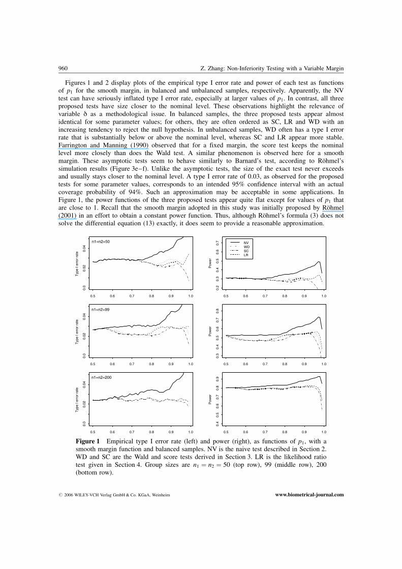
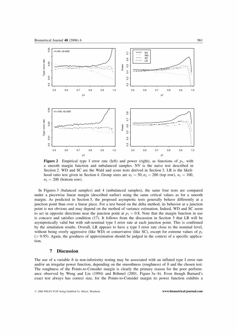
Figures 1 and 2 display plots of the empirical type I error rate and power of each test as functionsof p1 for the smooth margin, in balanced and unbalanced samples, respectively. Apparently, the NVtest can have seriously inflated type I error rate, especially at larger values of p1. In contrast, all threeproposed tests have size closer to the nominal level. These observations highlight the relevance ofvariable d as a methodological issue. In balanced samples, the three proposed tests appear almostidentical for some parameter values; for others, they are often ordered as SC, LR and WD with anincreasing tendency to reject the null hypothesis. In unbalanced samples, WD often has a type I errorrate that is substantially below or above the nominal level, whereas SC and LR appear more stable.Farrington and Manning (1990) observed that for a fixed margin, the score test keeps the nominallevel more closely than does the Wald test. A similar phenomenon is observed here for a smoothmargin. These asymptotic tests seem to behave similarly to Barnard’s test, according to R�hmel’ssimulation results (Figure 3e–f). Unlike the asymptotic tests, the size of the exact test never exceedsand usually stays closer to the nominal level. A type I error rate of 0.03, as observed for the proposedtests for some parameter values, corresponds to an intended 95% confidence interval with an actualcoverage probability of 94%. Such an approximation may be acceptable in some applications. InFigure 1, the power functions of the three proposed tests appear quite flat except for values of p1 thatare close to 1. Recall that the smooth margin adopted in this study was initially proposed by R�hmel(2001) in an effort to obtain a constant power function. Thus, although R�hmel’s formula (3) does notsolve the differential equation (13) exactly, it does seem to provide a reasonable approximation.

960 Z. Zhang: Non-Inferiority Testing with a Variable MarginT

ype

I err

or r

ate

0.5 0.6 0.7 0.8 0.9 1.0

0.0

0.02

0.04

Pow

er

0.5 0.6 0.7 0.8 0.9 1.0

0.2

0.3

0.4

0.5

0.6

0.7 NV

WDSCLR

Typ

e I e

rror

rat

e

0.5 0.6 0.7 0.8 0.9 1.0

0.0

0.02

0.04

Pow

er

0.5 0.6 0.7 0.8 0.9 1.0

0.3

0.4

0.5

0.6

0.7

0.8

Typ

e I e

rror

rat

e

0.5 0.6 0.7 0.8 0.9 1.0

0.0

0.02

0.04

Pow

er

0.5 0.6 0.7 0.8 0.9 1.0

0.4

0.5

0.6

0.7

0.8

0.9

n1=n2=50

n1=n2=99

n1=n2=200

Figure 1 Empirical type I error rate (left) and power (right), as functions of p1, with asmooth margin function and balanced samples. NV is the naive test described in Section 2.WD and SC are the Wald and score tests derived in Section 3. LR is the likelihood ratiotest given in Section 4. Group sizes are n1 ¼ n2 ¼ 50 (top row), 99 (middle row), 200(bottom row).

# 2006 WILEY-VCH Verlag GmbH & Co. KGaA, Weinheim www.biometrical-journal.com

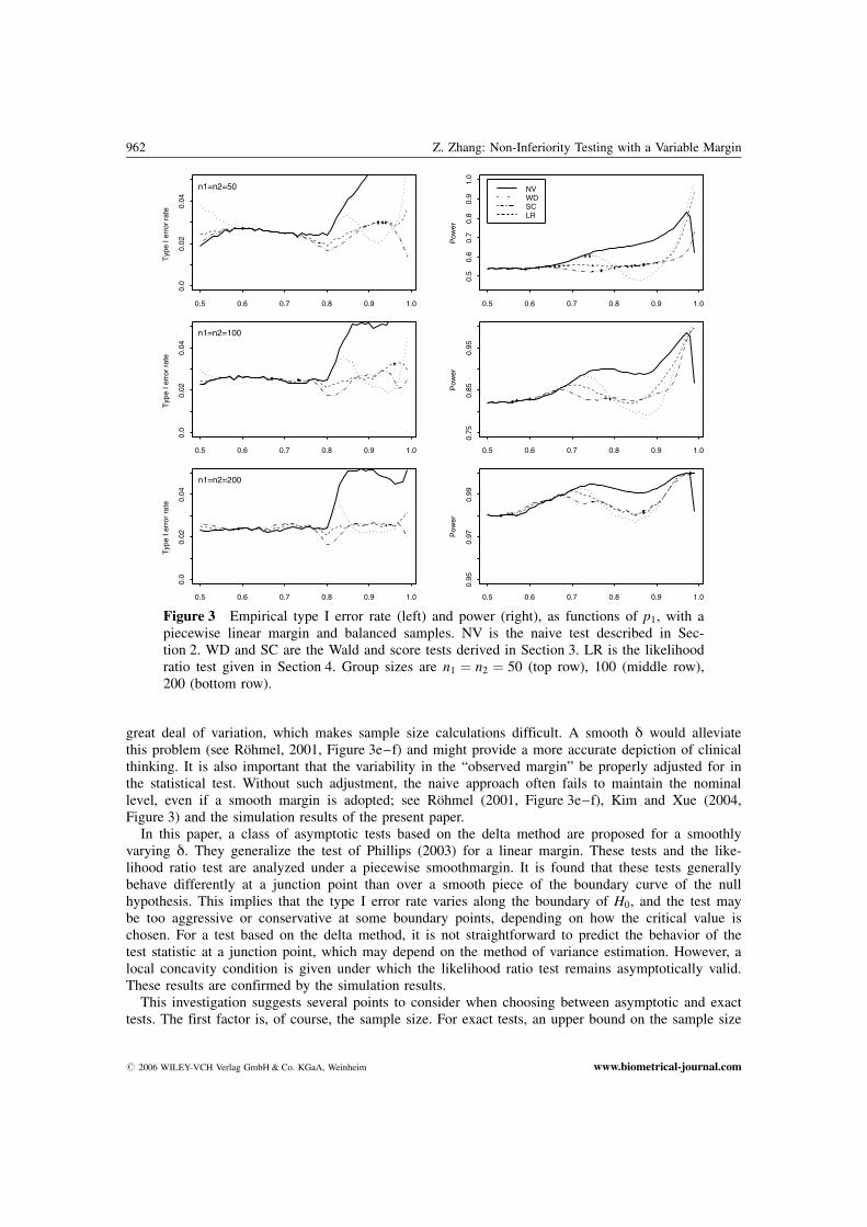
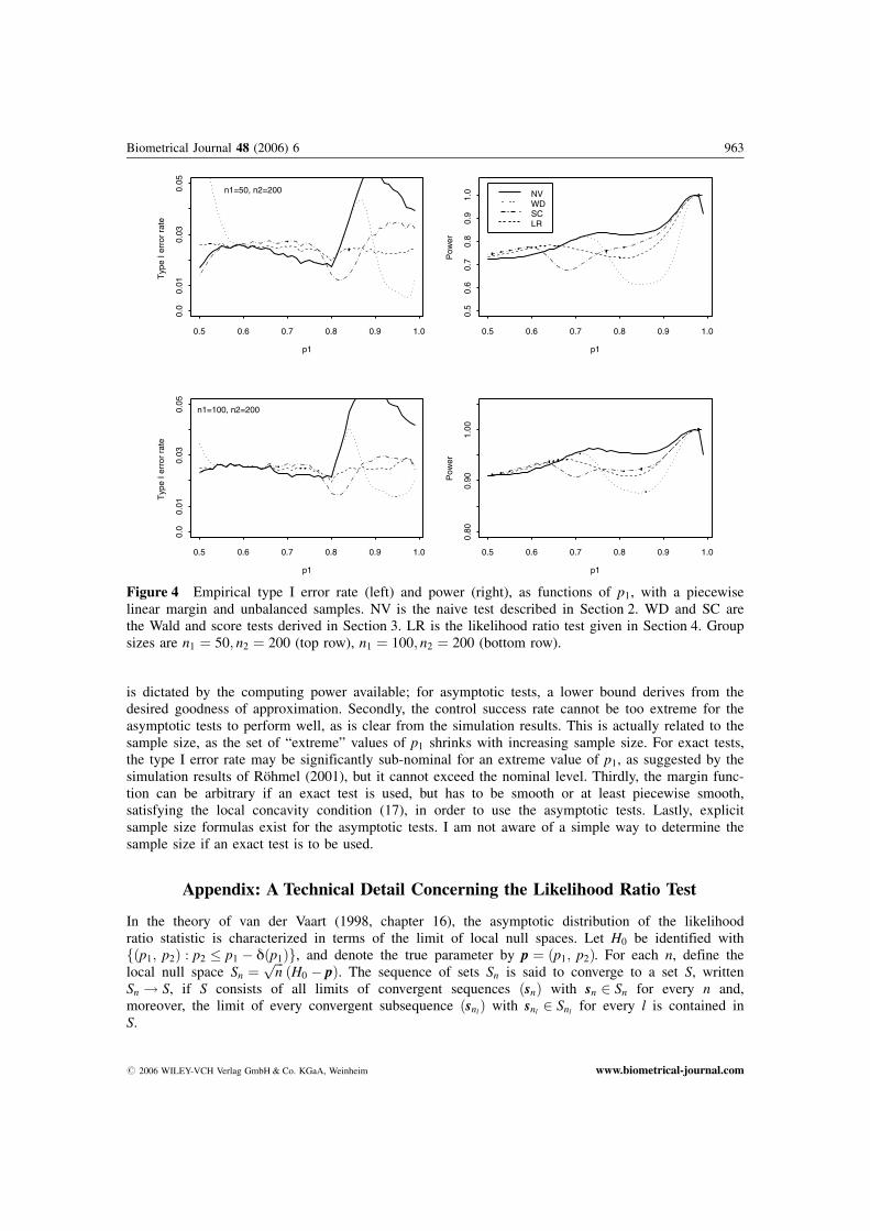
In Figures 3 (balanced samples) and 4 (unbalanced samples), the same four tests are comparedunder a piecewise linear margin (described earlier) using the same critical values as for a smoothmargin. As predicted in Section 5, the proposed asymptotic tests generally behave differently at ajunction point than over a linear piece. For a test based on the delta method, its behavior at a junctionpoint is not obvious and may depend on the method of variance estimation. Indeed, WD and SC seemto act in opposite directions near the junction point at p1 ¼ 0:8. Note that the margin function in useis concave and satisfies condition (17). It follows from the discussion in Section 5 that LR will beasymptotically valid but with sub-nominal type I error rate at each junction point. This is confirmedby the simulation results. Overall, LR appears to have a type I error rate close to the nominal level,without being overly aggressive (like WD) or conservative (like SC), except for extreme values of p1

(> 0:95). Again, the goodness of approximation should be judged in the context of a specific applica-tion.

7 Discussion

The use of a variable d in non-inferiority testing may be associated with an inflated type I error rateand/or an irregular power function, depending on the smoothness (roughness) of d and the chosen test.The roughness of the Points-to-Consider margin is clearly the primary reason for the poor perform-ance observed by Weng and Liu (1994) and R�hmel (2001, Figure 3a–b). Even though Barnard’sexact test always has correct size, for the Points-to-Consider margin its power function exhibits a

Biometrical Journal 48 (2006) 6 961

p1

Typ

e I e

rror

rat

e

0.5 0.6 0.7 0.8 0.9 1.0

0.0

0.01

0.03

0.05

p1

Pow

er

0.5 0.6 0.7 0.8 0.9 1.0

0.2

0.3

0.4

0.5

0.6

0.7 NV

WDSCLR

p1

Typ

e I e

rror

rat

e

0.5 0.6 0.7 0.8 0.9 1.0

0.0

0.01

0.03

0.05

p1

Pow

er

0.5 0.6 0.7 0.8 0.9 1.0

0.3

0.4

0.5

0.6

0.7

0.8

n1=50, n2=200

n1=100, n2=200

Figure 2 Empirical type I error rate (left) and power (right), as functions of p1, witha smooth margin function and unbalanced samples. NV is the naive test described inSection 2. WD and SC are the Wald and score tests derived in Section 3. LR is the likeli-hood ratio test given in Section 4. Group sizes are n1 ¼ 50; n2 ¼ 200 (top row), n1 ¼ 100;n2 ¼ 200 (bottom row).

# 2006 WILEY-VCH Verlag GmbH & Co. KGaA, Weinheim www.biometrical-journal.com

great deal of variation, which makes sample size calculations difficult. A smooth d would alleviatethis problem (see R�hmel, 2001, Figure 3e–f) and might provide a more accurate depiction of clinicalthinking. It is also important that the variability in the “observed margin” be properly adjusted for inthe statistical test. Without such adjustment, the naive approach often fails to maintain the nominallevel, even if a smooth margin is adopted; see R�hmel (2001, Figure 3e–f), Kim and Xue (2004,Figure 3) and the simulation results of the present paper.

In this paper, a class of asymptotic tests based on the delta method are proposed for a smoothlyvarying d. They generalize the test of Phillips (2003) for a linear margin. These tests and the like-lihood ratio test are analyzed under a piecewise smoothmargin. It is found that these tests generallybehave differently at a junction point than over a smooth piece of the boundary curve of the nullhypothesis. This implies that the type I error rate varies along the boundary of H0, and the test maybe too aggressive or conservative at some boundary points, depending on how the critical value ischosen. For a test based on the delta method, it is not straightforward to predict the behavior of thetest statistic at a junction point, which may depend on the method of variance estimation. However, alocal concavity condition is given under which the likelihood ratio test remains asymptotically valid.These results are confirmed by the simulation results.

This investigation suggests several points to consider when choosing between asymptotic and exacttests. The first factor is, of course, the sample size. For exact tests, an upper bound on the sample size

962 Z. Zhang: Non-Inferiority Testing with a Variable MarginT

ype

I err

or r

ate

0.5 0.6 0.7 0.8 0.9 1.0

0.0

0.02

0.04

Pow

er

0.5 0.6 0.7 0.8 0.9 1.0

0.5

0.6

0.7

0.8

0.9

1.0

NVWDSCLR

Typ

e I e

rror

rat

e

0.5 0.6 0.7 0.8 0.9 1.0

0.0

0.02

0.04

Pow

er0.5 0.6 0.7 0.8 0.9 1.0

0.75

0.85

0.95

Typ

e I e

rror

rat

e

0.5 0.6 0.7 0.8 0.9 1.0

0.0

0.02

0.04

Pow

er

0.5 0.6 0.7 0.8 0.9 1.0

0.95

0.97

0.99

n1=n2=50

n1=n2=100

n1=n2=200

Figure 3 Empirical type I error rate (left) and power (right), as functions of p1, with apiecewise linear margin and balanced samples. NV is the naive test described in Sec-tion 2. WD and SC are the Wald and score tests derived in Section 3. LR is the likelihoodratio test given in Section 4. Group sizes are n1 ¼ n2 ¼ 50 (top row), 100 (middle row),200 (bottom row).

# 2006 WILEY-VCH Verlag GmbH & Co. KGaA, Weinheim www.biometrical-journal.com

is dictated by the computing power available; for asymptotic tests, a lower bound derives from thedesired goodness of approximation. Secondly, the control success rate cannot be too extreme for theasymptotic tests to perform well, as is clear from the simulation results. This is actually related to thesample size, as the set of “extreme” values of p1 shrinks with increasing sample size. For exact tests,the type I error rate may be significantly sub-nominal for an extreme value of p1, as suggested by thesimulation results of R�hmel (2001), but it cannot exceed the nominal level. Thirdly, the margin func-tion can be arbitrary if an exact test is used, but has to be smooth or at least piecewise smooth,satisfying the local concavity condition (17), in order to use the asymptotic tests. Lastly, explicitsample size formulas exist for the asymptotic tests. I am not aware of a simple way to determine thesample size if an exact test is to be used.

Appendix: A Technical Detail Concerning the Likelihood Ratio Test

In the theory of van der Vaart (1998, chapter 16), the asymptotic distribution of the likelihoodratio statistic is characterized in terms of the limit of local null spaces. Let H0 be identified withfðp1; p2Þ : p2 � p1 � dðp1Þg, and denote the true parameter by p ¼ ðp1; p2Þ. For each n, define thelocal null space Sn ¼

ffiffiffinpðH0 � pÞ. The sequence of sets Sn is said to converge to a set S, written

Sn ! S, if S consists of all limits of convergent sequences ðsnÞ with sn 2 Sn for every n and,moreover, the limit of every convergent subsequence ðsnlÞ with snl 2 Snl for every l is contained inS.

Biometrical Journal 48 (2006) 6 963

p1

Typ

e I e

rror

rat

e

0.5 0.6 0.7 0.8 0.9 1.0

0.0

0.01

0.03

0.05

p1

Pow

er

0.5 0.6 0.7 0.8 0.9 1.0

0.5

0.6

0.7

0.8

0.9

1.0 NV

WDSCLR

p1

Typ

e I e

rror

rat

e

0.5 0.6 0.7 0.8 0.9 1.0

0.0

0.01

0.03

0.05

p1

Pow

er

0.5 0.6 0.7 0.8 0.9 1.0

0.80

0.90

1.00

n1=50, n2=200

n1=100, n2=200

Figure 4 Empirical type I error rate (left) and power (right), as functions of p1, with a piecewiselinear margin and unbalanced samples. NV is the naive test described in Section 2. WD and SC arethe Wald and score tests derived in Section 3. LR is the likelihood ratio test given in Section 4. Groupsizes are n1 ¼ 50; n2 ¼ 200 (top row), n1 ¼ 100; n2 ¼ 200 (bottom row).

# 2006 WILEY-VCH Verlag GmbH & Co. KGaA, Weinheim www.biometrical-journal.com

Lemma 1 Let p ¼ ðp1; p2Þ with 0 < dðp1Þ < p1 < 1 and p2 ¼ p1 � dðp1Þ. Assume that d is continu-ously differentiable in a neighborhood of p1 with derivative d0. Then

Sn ! fðs1; s2Þ : s2 � ð1� d0ðp1ÞÞ s1g ¼: S:

Proof. Suppose that sn ! s with sn 2 Sn for every n. It will be shown that s 2 S. Write s ¼ ðs1; s2Þand sn ¼

ffiffiffinpðpn � pÞ with pn ¼ ðpn1; pn2Þ 2 H0. Then s1 ¼ lim

ffiffiffinpðpn1 � p1Þ and

s2 ¼ limffiffiffinpðpn2 � p2Þ � lim

ffiffiffinpðpn1 � dðpn1Þ � p1 þ dðp1ÞÞ

¼ limffiffiffinpðpn1 � p1Þ � lim

ffiffiffinpðdðpn1Þ � dðp1ÞÞ ¼ s1 � d0ðp1Þ s1 ;

so that s 2 S. The inequality in the above display follows from the definition of H0 and the last stepfrom the differentiability of d. Clearly, the same argument applies to convergent subsequences.

Now let s ¼ ðs1; s2Þ 2 S be given. The proof will be complete if we can find a sequence ðpnÞ H0

such that sn :¼ffiffiffinpðpn � pÞ ! s. First consider the case that s2 < ð1� d0ðp1ÞÞ s1; so e :¼

ð1� d0ðp1ÞÞ s1 � s2 > 0. Set pn ¼ ðpn1; pn2Þ ¼ pþ n�1=2 s. Then it suffices to show that pn 2 H0, i.e.,pn2 � pn1 � dðpn1Þ, for large n. To this end, we write

pn2 � pn1 þ dðpn1Þ ¼ p2 þ n�1=2s2 � p1 � n�1=2s1 þ dðp1 þ n�1=2s1Þ¼ dðp1 þ n�1=2s1Þ � dðp1Þ þ n�1=2ðs2 � s1Þ¼ d0ðp1Þn�1=2s1 þ oðn�1=2Þ � n�1=2ðd0ðp1Þ s1 þ eÞ¼ �n�1=2eþ oðn�1=2Þ :

Because e > 0, the first term dominates and the above display is negative for large n. Next, considerthe case that s2 ¼ ð1� d0ðp1ÞÞ s1. Let en ¼ sup fjd0ðp1 þ hÞ � d0ðp1Þj : jhj � n�1=2js1jg. Then en is welldefined for large n and en ! 0 by the assumed continuity of d0. Let sn ¼ ðsn1; sn2Þ ¼ ðs1; s2 �

ffiffiffiffiffienpÞ;

then sn ! s. To see that pn :¼ pþ n�1=2sn eventually stays in H0, write

pn2 � pn1 þ dðpn1Þ ¼ p2 þ n�1=2sn2 � p1 � n�1=2sn1 þ dðp1 þ n�1=2sn1Þ¼ p2 þ n�1=2ðs2 �

ffiffiffiffiffienp Þ � p1 � n�1=2s1 þ dðp1 þ n�1=2s1Þ

¼ dðp1 þ n�1=2s1Þ � dðp1Þ þ n�1=2ðs2 � s1 �ffiffiffiffiffienp Þ

¼ d0ðp1*Þ n�1=2s1 � n�1=2ðd0ðp1Þ s1 þffiffiffiffiffienp Þ

for some p1* between p1 and p1 þ n�1=2s1, by the mean value theorem. It follows from the definitionof en that

pn2 � pn1 þ dðpn1Þ ¼ n�1=2s1ðd0ðp1*Þ � d0ðp1ÞÞ � n�1=2 ffiffiffiffiffienp � n�1=2s1en � n�1=2 ffiffiffiffiffi

enp

;

which is negative for large n because the second term eventually dominates. This completes the proof. &

Acknowledgements I would like to thank Dr. Edgar Brunner and two anonymous referees for constructive com-ments, and Dr. Yun-Ling Xu for generous help with the graphical presentation.

References

Agresti, A. (1990). Categorical Data Analysis. Wiley, New York.Barnard, G. A. (1945). A new test for 2� 2 tables. Nature 156, 177.Barnard, G. A. (1947). Significance tests for 2� 2 tables. Biometrika 34, 123–138.Boyce, W. E. and DiPrima, R. C. (1986). Elementary Differential Equations and Boundary Value Problems. Wiley,

New York.Chan, I. S. F. (1998). Exact tests of equivalence and efficacy with a non-zero lower bound for comparative

studies. Statistics in Medicine 17, 1403–1413.

964 Z. Zhang: Non-Inferiority Testing with a Variable Margin

# 2006 WILEY-VCH Verlag GmbH & Co. KGaA, Weinheim www.biometrical-journal.com

Dunnett, C. W. and Gent, M. (1977). Significance testing to establish equivalence between treatments with specialreference to data in the form of 2� 2 tables. Biometrics 33, 593–602.

Farrington, C. P. and Manning, G. (1990). Test statistics and sample size formulae for comparative binomial trialswith null hypothesis of non-zero risk difference or non-unity relative risk. Statistics in Medicine 9, 1447–1454.

Food and Drug Administration (1992). Points to Consider. Clinical development and labeling of anti-infectivedrug products. U.S. Dep. of Health and Human Services. FDA, CDER.

Garrett, A. D. (2003). Therapeutic equivalence: fallacies and falsification. Statistics in Medicine 22, 741–762.Kim, M. Y. and Xue, X. (2004). Likelihood ratio and a Bayesian approach were superior to standard noninferiority

analysis when the noninferiority margin varied with the control event rate. Journal of Clinical Epidemiology57, 1253–1261.

Miettinen, O. and Nurminen, M. (1985). Comparative analysis of two rates. Statistics in Medicine 4, 213–226.Munk, A., Skipka, G., and Stratmann, B. (2005). Testing general hypotheses under binomial sampling: The two

sample case –– asymptotic theory and exact procedures. Computational Statistics and Data Analysis 49, 723–739.

Phillips, K. F. (2003). A new test of non-inferiority for anti-infective trials. Statistics in Medicine 22, 201–212.R�hmel, J. (1998). Therapeutic equivalence investigations: statistical considerations. Statistics in Medicine 17,

1703–1714.R�hmel, J. (2001). Statistical considerations of FDA and CPMP rules for the investigation of new anti-bacterial

products. Statistics in Medicine 20, 2561–2571.R�hmel, J. and Mansmann, U. (1999). Unconditional non-asymptotic one-sided tests for independent binomial

proportions when the interest lies in showing non-inferiority and/or superiority. Biometrical Journal 41, 149–170.

Skipka, G., Munk, A., and Freitag, G. (2004). Unconditional exact tests for the difference of binomial probabil-ities: contrasted and compared. Computational Statistics and Data Analysis 47, 757–773.

van der Vaart, A. W. (1998). Asymptotic Statistics. Cambridge University Press, Cambridge.Wellek, S. (2005). Statistical methods for the analysis of two-arm non-inferiority trials with binary outcomes.

Biometrical Journal 47, 48–61.Weng, C. S. W. and Liu, J. P. (1994). Some pitfalls in sample size estimation for an anti-infective study. Proceed-

ings of the Pharmaceutical Section. American Statistical Association, 56–60.

Biometrical Journal 48 (2006) 6 965

# 2006 WILEY-VCH Verlag GmbH & Co. KGaA, Weinheim www.biometrical-journal.com