Variable Neighborhood Search - dei.unipd.it

Chapter 3Variable Neighborhood Search

Pierre Hansen, Nenad Mladenovic, Jack Brimberg and Jose A. Moreno Perez

Abstract Variable neighborhood search (VNS) is a metaheuristic for solvingcombinatorial and global optimization problems whose basic idea is a systematicchange of neighborhood both within a descent phase to find a local optimum andin a perturbation phase to get out of the corresponding valley. In this chapter wepresent the basic schemes of VNS and some of its extensions. We then describe arecent development, i.e., formulation space search. We then present five families ofapplications in which VNS has proven to be very successful: (i) exact solution oflarge-scale location problems by primal–dual VNS; (ii) generation of feasible so-lutions to large mixed integer linear programs by hybridization of VNS and localbranching; (iii) generation of good feasible solutions to continuous nonlinear pro-grams; (iv) generation of feasible solutions and/or improved local optima for mixedinteger nonlinear programs by hybridization of sequential quadratic programmingand branch and bound within a VNS framework, and (v) exploration of graph theoryto find conjectures, refutations, and proofs or ideas of proofs.

Pierre HansenGERAD and Ecole des Hautes Etudes Commerciales, 3000 ch. de la Cote-Sainte-Catherine,Montreal H3T 2A7, QC, Canadae-mail: [email protected]

Nenad MladenovicSchool of Mathematics, Brunel University-West London, Uxbridge, UB8 3PH, UKe-mail: [email protected]

Jack BrimbergDepartment of Mathematics and Computer Science, Royal Military College of Canada, KingstonON, Canada, K7K 7B4e-mail: [email protected]

Jose A. Moreno PerezIUDR and DEIOC, Universidad de La Laguna, 38271 La Laguna, Santa Cruz de Tenerife, Spaine-mail: [email protected]

M. Gendreau, J.-Y. Potvin (eds.), Handbook of Metaheuristics, 61International Series in Operations Research & Management Science 146,DOI 10.1007/978-1-4419-1665-5 3, c© Springer Science+Business Media, LLC 2010

62 Pierre Hansen, Nenad Mladenovic, Jack Brimberg and Jose A. Moreno Perez

3.1 Introduction

Optimization tools have greatly improved during the last two decades. This is dueto several factors: (i) progress in mathematical programming theory and algorithmicdesign; (ii) rapid improvement in computer performances; (iii) better communica-tion of new ideas and integration in widely used complex softwares. Consequently,many problems long viewed as out of reach are currently solved, sometimes in verymoderate computing times. This success, however, has led researchers and prac-titioners to address much larger instances and more difficult classes of problems.Many of these may again only be solved heuristically. Therefore thousands of papersdescribing, evaluating, and comparing new heuristics appear each year. Keepingabreast of such a large literature is a challenge. Metaheuristics, or general frame-works for building heuristics, are therefore needed in order to organize the study ofheuristics. As evidenced by this handbook, there are many of them. Some desirableproperties of metaheuristics [64, 67, 68] are listed in the concluding section of thischapter.

Variable neighborhood search (VNS) is a metaheuristic proposed by some of thepresent authors a dozen years ago [85]. Earlier work that motivated this approachcan be found in [28, 41, 44, 82]. It is based on the idea of a systematic change ofneighborhood both in a descent phase to find a local optimum and in a perturbationphase to get out of the corresponding valley. Originally designed for approximatesolution of combinatorial optimization problems, it was extended to address mixedinteger programs, nonlinear programs, and recently mixed integer nonlinear pro-grams. In addition VNS has been used as a tool for automated or computer-assistedgraph theory. This led to the discovery of over 1500 conjectures in that field, theautomated proof of more than half of them as well as the unassisted proof of about400 of them by many mathematicians.

Applications are rapidly increasing in number and pertain to many fields: loca-tion theory, cluster analysis, scheduling, vehicle routing, network design, lot-sizing,artificial intelligence, engineering, pooling problems, biology, phylogeny, reliabil-ity, geometry, telecommunication design, etc. (see, e.g., [20, 21, 31, 38, 39, 66,77, 99]). References are too numerous to be all listed here, but many others can befound in [69] and special issues of IMA Journal of Management Mathematics [81],European Journal of Operational Research [68], and Journal of Heuristics [89] aredevoted to VNS.

This chapter is organized as follows. In the next section we present the basicschemes of VNS, i.e., variable neighborhood descent (VND), reduced VNS (RVNS),basic VNS (BVNS), and general VNS (GVNS). Two important extensions arepresented in Section 3.3: skewed VNS and variable neighborhood decompositionsearch (VNDS). A further recent development called formulation space search(FSS) is discussed in Section 3.4. The remainder of this chapter describes appli-cations of VNS to several classes of large scale and complex optimization prob-lems for which it has proven to be particularly successful. Section 3.5 is devotedto primal–dual VNS (PD-VNS) and its application to location and clustering prob-lems. Finding feasible solutions to large mixed integer linear programs with VNS

3 Variable Neighborhood Search 63

is discussed in Section 3.6. Section 3.7 addresses ways to apply VNS in continuousglobal optimization. The more difficult case of solving mixed integer nonlinearprogramming by VNS is considered in Section 3.8. Applying VNS to graph the-ory per se (and not just to particular optimization problems defined on graphs) isdiscussed in Section 3.9. Brief conclusions are drawn in Section 3.10.

3.2 Basic Schemes

A deterministic optimization problem may be formulated as

min{ f (x)|x ∈ X ,X ⊆S }, (3.1)

where S , X , x, and f denote the solution space, the feasible set, a feasible solution,and a real-valued objective function, respectively. If S is a finite but large set, acombinatorial optimization problem is defined. If S = R

n, we refer to continuousoptimization. A solution x∗ ∈ X is optimal if

f (x∗)≤ f (x), ∀x ∈ X .

An exact algorithm for problem (3.1), if one exists, finds an optimal solution x∗,together with the proof of its optimality, or shows that there is no feasible solution,i.e., X = /0, or the solution is unbounded. Moreover, in practice, the time needed to doso should be finite (and not too long). For continuous optimization, it is reasonableto allow for some degree of tolerance, i.e., to stop when sufficient convergence isdetected.

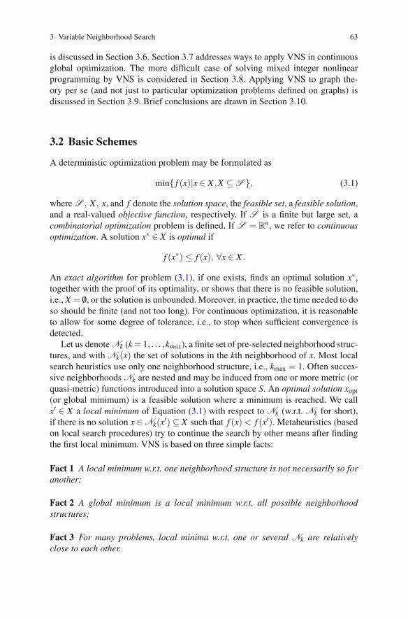
Let us denote Nk (k = 1, . . . ,kmax), a finite set of pre-selected neighborhood struc-tures, and with Nk(x) the set of solutions in the kth neighborhood of x. Most localsearch heuristics use only one neighborhood structure, i.e., kmax = 1. Often succes-sive neighborhoods Nk are nested and may be induced from one or more metric (orquasi-metric) functions introduced into a solution space S. An optimal solution xopt

(or global minimum) is a feasible solution where a minimum is reached. We callx′ ∈ X a local minimum of Equation (3.1) with respect to Nk (w.r.t. Nk for short),if there is no solution x ∈Nk(x′)⊆ X such that f (x) < f (x′). Metaheuristics (basedon local search procedures) try to continue the search by other means after findingthe first local minimum. VNS is based on three simple facts:

Fact 1 A local minimum w.r.t. one neighborhood structure is not necessarily so foranother;

Fact 2 A global minimum is a local minimum w.r.t. all possible neighborhoodstructures;

Fact 3 For many problems, local minima w.r.t. one or several Nk are relativelyclose to each other.


This last observation, which is empirical, implies that a local optimum often pro-vides some information about the global one. For instance, it might be several vari-ables with the same value in both solutions. However, it is usually not known whichvariables are such. Since these variables usually cannot be identified in advance, oneshould conduct an organized study of the neighborhoods of the local optimum untila better solution is found.

In order to solve Equation (3.1) by using several neighborhoods, facts 1 to 3 canbe used in three different ways: (i) deterministic, (ii) stochastic, (iii) both determin-istic and stochastic.

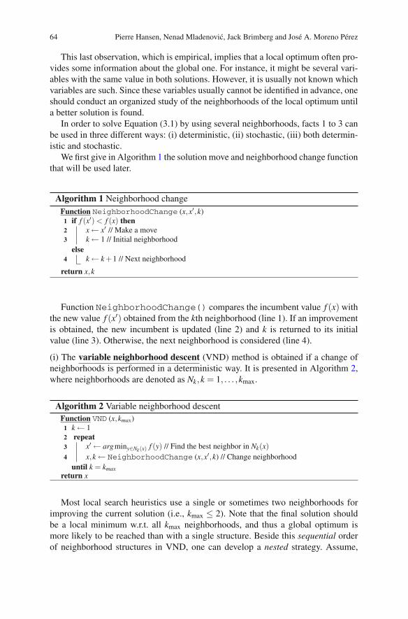
We first give in Algorithm 1 the solution move and neighborhood change functionthat will be used later.

Algorithm 1 Neighborhood changeFunction NeighborhoodChange (x,x′,k)

if f (x′) < f (x) then1x ← x′ // Make a move2k ← 1 // Initial neighborhood3

elsek ← k +1 // Next neighborhood4

return x,k

Function NeighborhoodChange() compares the incumbent value f (x) withthe new value f (x′) obtained from the kth neighborhood (line 1). If an improvementis obtained, the new incumbent is updated (line 2) and k is returned to its initialvalue (line 3). Otherwise, the next neighborhood is considered (line 4).

(i) The variable neighborhood descent (VND) method is obtained if a change ofneighborhoods is performed in a deterministic way. It is presented in Algorithm 2,where neighborhoods are denoted as Nk,k = 1, . . . ,kmax.

Algorithm 2 Variable neighborhood descentFunction VND (x,kmax)

k ← 11repeat2

x′ ← argminy∈Nk(x) f (y) // Find the best neighbor in Nk(x)3

x,k ← NeighborhoodChange (x,x′,k) // Change neighborhood4

until k = kmaxreturn x

Most local search heuristics use a single or sometimes two neighborhoods forimproving the current solution (i.e., kmax ≤ 2). Note that the final solution shouldbe a local minimum w.r.t. all kmax neighborhoods, and thus a global optimum ismore likely to be reached than with a single structure. Beside this sequential orderof neighborhood structures in VND, one can develop a nested strategy. Assume,


for example, that kmax = 3; then a possible nested strategy is to perform VND withAlgorithm 2 for the first two neighborhoods from each point x′ that belongs to thethird one (x′ ∈ N3(x)). Such an approach is successfully applied in [22, 27, 65].

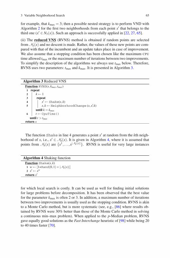
(ii) The reduced VNS (RVNS) method is obtained if random points are selectedfrom Nk(x) and no descent is made. Rather, the values of these new points are com-pared with that of the incumbent and an update takes place in case of improvement.We also assume that a stopping condition has been chosen like the maximum CPU

time allowed tmax or the maximum number of iterations between two improvements.To simplify the description of the algorithms we always use tmax below. Therefore,RVNS uses two parameters: tmax and kmax. It is presented in Algorithm 3.

Algorithm 3 Reduced VNSFunction RVNS(x,kmax, tmax)

repeat1k ← 12repeat3

x′ ← Shake(x,k)4x,k ← NeighborhoodChange (x,x′,k)5

until k = kmax

t ← CpuTime()6

until t > tmaxreturn x

The function Shake in line 4 generates a point x′ at random from the kth neigh-borhood of x, i.e., x′ ∈ Nk(x). It is given in Algorithm 4, where it is assumed thatpoints from Nk(x) are {x1, . . . ,x|Nk(x)|}. RVNS is useful for very large instances

Algorithm 4 Shaking functionFunction Shake(x,k)

w ← [1+Rand(0,1)×|Nk(x)|]1x′ ← xw2

return x′

for which local search is costly. It can be used as well for finding initial solutionsfor large problems before decomposition. It has been observed that the best valuefor the parameter kmax is often 2 or 3. In addition, a maximum number of iterationsbetween two improvements is usually used as the stopping condition. RVNS is akinto a Monte Carlo method, but is more systematic (see, e.g., [86] where results ob-tained by RVNS were 30% better than those of the Monte Carlo method in solvinga continuous min–max problem). When applied to the p-Median problem, RVNSgave equally good solutions as the Fast Interchange heuristic of [98] while being 20to 40 times faster [70].


(iii) The basic VNS (BVNS) method [85] combines deterministic and stochasticchanges of neighborhood. The deterministic part is represented by a local searchheuristic. It consists in (i) choosing an initial solution x, (ii) finding a direction ofdescent from x (within a neighborhood N(x)), and (iii) moving to the minimumof f (x) within N(x) along that direction. If there is no direction of descent, theheuristic stops, otherwise it is iterated. Usually the steepest descent direction, alsoreferred to as best improvement, is used. This is summarized in Algorithm 5, wherewe assume that an initial solution x is given. The output consists of a local minimum,also denoted by x, and its value. As the Steepest descent heuristic may be time-

Algorithm 5 Best improvement (steepest descent) heuristicFunction BestImprovement(x)

repeat1x′ ← x2x ← argminy∈N(x) f (y)3

until ( f (x)≥ f (x′))return x

consuming, an alternative is to use the first descent heuristic. Vectors xi ∈ N(x) arethen enumerated systematically and a move is made as soon as a direction for thedescent is found. This is summarized in Algorithm 6.

Algorithm 6 First improvement (first descent) heuristicFunction FirstImprovement(x)

repeat1x′ ← x; i ← 02

repeat3i ← i+14

x ← argmin{ f (x), f (xi)}, xi ∈ N(x)5

until ( f (x) < f (x′) or i = |N(x)|)until ( f (x)≥ f (x′))

return x

The stochastic phase is represented by the random selection of one point fromthe kth neighborhood. The BVNS is given in Algorithm 7.

Note that point x′ is generated at random in step 5 in order to avoid cycling, whichmight occur with a deterministic rule.

Example. We illustrate the basic steps on a minimum k-cardinality tree instancetaken from [76], see Figure 3.1. The minimum k-cardinality tree problem on graphG (k-card for short) consists in finding a subtree of G with exactly k edges whosesum of weights is minimum.

The steps of BVNS for solving the 4-card problem are illustrated in Figure 3.2.In step 0 the objective function value, i.e., the sum of edge weights, is equal to 40;


Algorithm 7 Basic VNSFunction BVNS(x,kmax, tmax)

t ← 01while t < tmax do2

k ← 13repeat4

x′ ← Shake(x,k) // Shaking5x′′ ← BestImprovement(x′) // Local search6x,k ← NeighborhoodChange(x,x′′,k) // Change neighborhood7

until k = kmax

t ← CpuTime()8

return x

2

1

3

4

5

6

7

9

8

11

10

12

1

26 6 23

25 15 16 24

17 2018 16

916

8 6 16 9 9

17 9

Fig. 3.1 4-cardinality tree problem.

40

47 39

39 43 39

49

4060

1 11

25 25258

88

8

886

6 6

6

6

6

26

17

16 16

16 16

169

9 9 9

9 9

9

18

9 9

9

LS

Shake-2 Shake-1LS

LS Shake-2 LS

LSShake-1

36

0

3 4 5

6 7 8

1 2

Fig. 3.2 Steps of the basic VNS for solving 4-card tree problem.


it is indicated in the right bottom corner of the figure. That first solution is a localminimum with respect to the edge-exchange neighborhood structure (one edge in,one out). After shaking, the objective function is 60, and after another local search,we are back to the same solution. Then, in step 3, we take out 2 edges and addanother 2 at random, and after a local search, an improved solution is obtained witha value of 39. Continuing in that way, the optimal solution with an objective functionvalue equal to 36 is obtained in step 8.

(iv) General VNS. Note that the local search step (line 6 in BVNS, Algorithm 7)may also be replaced by VND (Algorithm 2). This general VNS (VNS/VND) ap-proach has led to some of the most successful applications reported in the literature(see, e.g., [2, 27, 30, 32, 34, 36, 37, 65, 71, 92, 93]). The general VNS (GVNS) isgiven in Algorithm 8 below.

Algorithm 8 General VNSFunction GVNS (x, �max,kmax, tmax)


x′ ← Shake(x,k)4x′′ ← VND(x′, �max)5x,k ← NeighborhoodChange(x,x′′,k)6

until k = kmax

t ← CpuTime()7


3.3 Some Extensions

(i) The skewed VNS (SVNS) method [59] addresses the problem of exploring val-leys far from the incumbent solution. Indeed, once the best solution in a large regionhas been found, it is necessary to go quite far to obtain an improved one. Solutionsdrawn at random in far-away neighborhoods may differ substantially from the in-cumbent, and VNS may then degenerate, to some extent, into the multistart heuristic(in which descents are made iteratively from solutions generated at random, whichis known not to be very efficient). So some compensation for distance from theincumbent must be made and a scheme called skewed VNS is proposed for thatpurpose. Its steps are presented in Algorithms 9, 10, and 11. The KeepBest(x,x′)function (Algorithm 9) in SVNS simply keeps the best of solutions x and x′. TheNeighborhoodChangeS function (Algorithm 10) performs the move and neigh-borhood change for the SVNS.

SVNS makes use of a function ρ(x,x′′) to measure the distance between theincumbent solution x and the local optimum x′′. The distance function used to defineNk, as in the above examples, could be used also for this purpose. The parameter


Algorithm 9 Keep best solutionFunction KeepBest(x,x′)

if f (x′) < f (x) then1x ← x′2

return x

Algorithm 10 Neighborhood change for the skewed VNSFunction NeighborhoodChangeS(x,x′,k,α)

if f (x′)−αρ(x,x′) < f (x) then1x ← x′2k ← 13

elsek ← k +14

return x,k

Algorithm 11 Skewed VNSFunction SVNS (x,kmax, tmax,α)

xbest ← x1repeat2

k ← 13repeat4

x′ ← Shake(x,k)5x′′ ← FirstImprovement(x′)6x,k ← NeighborhoodChangeS(x,x′′,k,α)7

until k = kmax

xbest ← KeepBest (xbest ,x)8x ← xbest9t ← CpuTime()10


α must be chosen to allow movement to valleys far away from x when f (x′′) islarger than f (x) but not too much larger (otherwise one will always leave x). A goodvalue for α is to be found experimentally in each case. Moreover, in order to avoidfrequent moves from x to a close solution one may take a smaller value for α whenρ(x,x′′) is small. More sophisticated choices of a function of αρ(x,x′′) could bemade through some learning process.

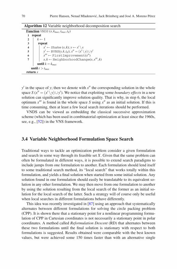
(ii) The variable neighborhood decomposition search (VNDS) method [70] ex-tends the basic VNS into a two-level VNS scheme based on decomposition of theproblem. It is presented in Algorithm 12, where td is an additional parameter thatrepresents the running time allowed for solving decomposed (smaller sized) prob-lems by basic VNS (line 5).

For ease of presentation, but without loss of generality, we assume that the solu-tion x represents a set of some attributes. In step 4 we denote by y a set of k solutionattributes present in x′ but not in x (y = x′ \ x). In step 5 we find the local optimum


Algorithm 12 Variable neighborhood decomposition searchFunction VNDS (x,kmax, tmax, td)


x′ ← Shake (x,k); y ← x′ \ x4y′ ← BVNS(y,k, td); x′′ = (x′ \ y)∪ y′5x′′′ ← FirstImprovement(x′′)6x,k ← NeighborhoodChange(x,x′′′,k)7

until k = kmax


y′ in the space of y; then we denote with x′′ the corresponding solution in the wholespace S (x′′ = (x′ \y)∪y′). We notice that exploiting some boundary effects in a newsolution can significantly improve solution quality. That is why, in step 6, the localoptimum x′′′ is found in the whole space S using x′′ as an initial solution. If this istime consuming, then at least a few local search iterations should be performed.

VNDS can be viewed as embedding the classical successive approximationscheme (which has been used in combinatorial optimization at least since the 1960s,see, e.g., [52]) in the VNS framework.

3.4 Variable Neighborhood Formulation Space Search

Traditional ways to tackle an optimization problem consider a given formulationand search in some way through its feasible set X . Given that the same problem canoften be formulated in different ways, it is possible to extend search paradigms toinclude jumps from one formulation to another. Each formulation should lend itselfto some traditional search method, its “local search” that works totally within thisformulation, and yields a final solution when started from some initial solution. Anysolution found in one formulation should easily be translatable to its equivalent so-lution in any other formulation. We may then move from one formulation to anotherby using the solution resulting from the local search of the former as an initial so-lution for the local search of the latter. Such a strategy will of course only be usefulwhen local searches in different formulations behave differently.

This idea was recently investigated in [87] using an approach that systematicallyalternates between different formulations for solving the circle packing problem(CPP). It is shown there that a stationary point for a nonlinear programming formu-lation of CPP in Cartesian coordinates is not necessarily a stationary point in polarcoordinates. A method called Reformulation Descent (RD) that alternates betweenthese two formulations until the final solution is stationary with respect to bothformulations is suggested. Results obtained were comparable with the best knownvalues, but were achieved some 150 times faster than with an alternative single


formulation approach. In the same paper the idea suggested above of FormulationSpace Search (FSS) is also introduced, using more than two formulations. Someresearch in that direction has also been reported in [74, 83, 88, 90]. One method-ology that uses the variable neighborhood idea when searching through the formu-lation space is given in Algorithms 13 and 14. Here φ (φ ′) denotes a formulationfrom a given space F , x (x′) denotes a solution in the feasible set defined with thatformulation, and � ≤ �max is the formulation neighborhood index. Note that Algo-rithm 14 uses a reduced VNS strategy in the formulation space F . Note also thatthe ShakeFormulation() function must provide a search through the solutionspace S ′ in order to get a new solution x′. Any appropriate method can be used forthis purpose.

Algorithm 13 Formulation changeFunction FormulationChange(x,x′,φ ,φ ′, �)

Set �min and �step1if f (φ ′,x′) < f (φ ,x) then2

φ ← φ ′3x ← x′4�← �min5

else�← �+ �step6

return x,φ , �7

Algorithm 14 Reduced variable neighborhood FSSFunction VNFSS(x,φ , �max)

repeat1�← 1 // Initialize formulation in F2while �≤ �max do3

x′,φ ′, �← ShakeFormulation(x,x′,φ ,φ ′,�) // (φ ′,x′)∈(N�(φ),N (x)) at random4x,φ , �← FormulationChange(x,x′,φ ,φ ′,�) // Change formulation5

until some stopping condition is metreturn x6

3.5 Primal–Dual VNS

For most modern heuristics the difference in value between the optimal solution andthe one obtained is completely unknown. Guaranteed performance of the primalheuristic may be determined if a lower bound on the objective function value isknown. To this end, the standard approach is to relax the integrality condition on theprimal variables, based on a mathematical programming formulation of the problem.However, when the dimension of the problem is large, even the relaxed problem maybe impossible to solve exactly by standard commercial solvers. Therefore, it seems


to be a good idea to solve dual relaxed problems heuristically as well. In this waywe get guaranteed bounds on the primal heuristic’s performance. The next problemarises if we want to get an exact solution within a branch and bound frameworksince having the approximate value of the relaxed dual does not allow us to branchin an easy way, for example, by exploiting complementary slackness conditions.Thus, the exact value of the dual is necessary.

In primal–dual VNS (PD-VNS) [58] one possible general way to get both theguaranteed bounds and the exact solution is proposed. It is given in Algorithm 15.

Algorithm 15 Basic PD-VNSFunction PD-VNS (x,kmax, tmax)

BVNS (x,kmax, tmax) // Solve primal by VNS1DualFeasible(x,y) // Find (infeasible) dual such that fP = fD2DualVNS(y) // Use VNS do decrease infeasibility3DualExact(y) // Find exact (relaxed) dual4BandB(x,y) // Apply branch-and-bound method5

In the first stage a heuristic procedure based on VNS is used to obtain a near-optimal solution. In [58] it is shown that VNS with decomposition is a very powerfultechnique for large-scale simple plant location problems (SPLP) with up to 15,000facilities and 15,000 users. In the second phase the objective is to find an exact solu-tion of the relaxed dual problem. Solving the relaxed dual is accomplished in threestages: (i) find an initial dual solution (generally infeasible) using the primal heuris-tic solution and complementary slackness conditions; (ii) find a feasible solutionby applying VNS to the unconstrained nonlinear form of the dual; and (iii) solvethe dual exactly starting with the found initial feasible solution using a customized“sliding simplex” algorithm that applies “windows” on the dual variables, thus sub-stantially reducing the problem size. On all problems tested, including instancesmuch larger than those previously reported in the literature, the procedure was ableto find the exact dual solution in reasonable computing time. In the third and finalphase, armed with tight upper and lower bounds obtained from the heuristic primalsolution in phase 1 and the exact dual solution in phase 2, respectively, a standardbranch-and-bound algorithm is applied to find an optimal solution of the originalproblem. The lower bounds are updated with the dual sliding simplex method andthe upper bounds whenever new integer solutions are obtained at the nodes of thebranching tree. In this way it was possible to solve exactly problem instances ofsizes up to 7000×7000 for uniform fixed costs and 15,000 × 15,000 otherwise.

3.6 Variable Neighborhood Branching—VNS for Mixed IntegerLinear Programming

The mixed integer linear programming (MILP) problem consists of maximizingor minimizing a linear function, subject to equality or inequality constraints, and


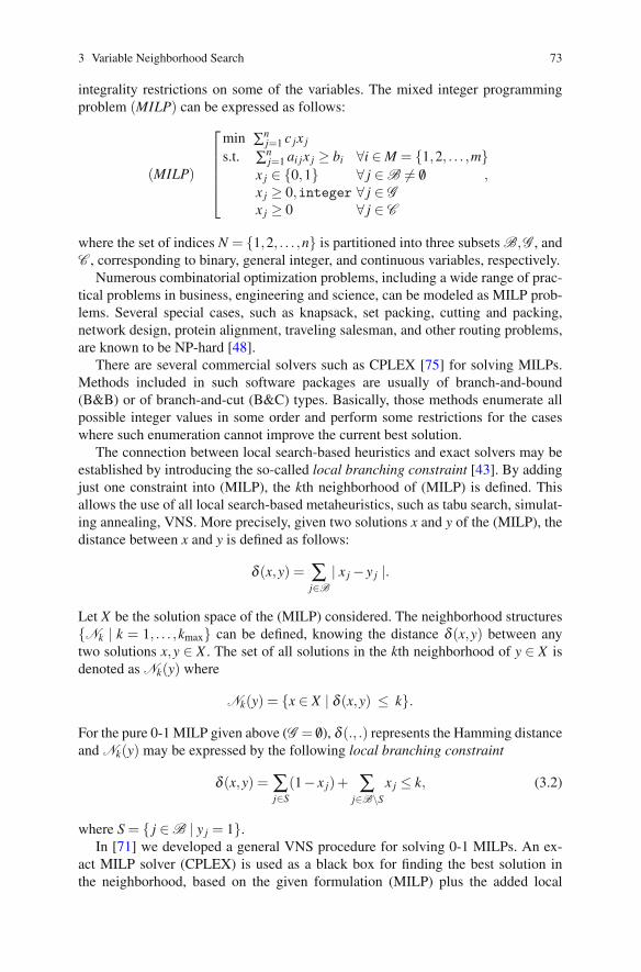
integrality restrictions on some of the variables. The mixed integer programmingproblem (MILP) can be expressed as follows:

(MILP)

⎡⎢⎢⎢⎢⎣

min ∑nj=1 c jx j

s.t. ∑nj=1 ai jx j ≥ bi ∀i ∈ M = {1,2, . . . ,m}

x j ∈ {0,1} ∀ j ∈B �= /0 ,x j ≥ 0,integer ∀ j ∈ Gx j ≥ 0 ∀ j ∈ C

where the set of indices N = {1,2, . . . ,n} is partitioned into three subsets B,G , andC , corresponding to binary, general integer, and continuous variables, respectively.

Numerous combinatorial optimization problems, including a wide range of prac-tical problems in business, engineering and science, can be modeled as MILP prob-lems. Several special cases, such as knapsack, set packing, cutting and packing,network design, protein alignment, traveling salesman, and other routing problems,are known to be NP-hard [48].

There are several commercial solvers such as CPLEX [75] for solving MILPs.Methods included in such software packages are usually of branch-and-bound(B&B) or of branch-and-cut (B&C) types. Basically, those methods enumerate allpossible integer values in some order and perform some restrictions for the caseswhere such enumeration cannot improve the current best solution.

The connection between local search-based heuristics and exact solvers may beestablished by introducing the so-called local branching constraint [43]. By addingjust one constraint into (MILP), the kth neighborhood of (MILP) is defined. Thisallows the use of all local search-based metaheuristics, such as tabu search, simulat-ing annealing, VNS. More precisely, given two solutions x and y of the (MILP), thedistance between x and y is defined as follows:

δ (x,y) = ∑j∈B

| x j − y j |.

Let X be the solution space of the (MILP) considered. The neighborhood structures{Nk | k = 1, . . . ,kmax} can be defined, knowing the distance δ (x,y) between anytwo solutions x,y ∈ X . The set of all solutions in the kth neighborhood of y ∈ X isdenoted as Nk(y) where

Nk(y) = {x ∈ X | δ (x,y) ≤ k}.

For the pure 0-1 MILP given above (G = /0), δ (., .) represents the Hamming distanceand Nk(y) may be expressed by the following local branching constraint

δ (x,y) = ∑j∈S

(1− x j)+ ∑j∈B\S

x j ≤ k, (3.2)

where S = { j ∈B | y j = 1}.In [71] we developed a general VNS procedure for solving 0-1 MILPs. An ex-

act MILP solver (CPLEX) is used as a black box for finding the best solution inthe neighborhood, based on the given formulation (MILP) plus the added local


Algorithm 16 VNS branchingFunction VnsBra(total time limit, node time limit, k step, x opt)

TL := total time limit; UB := ∞; first := true1stat := MIPSOLVE(TL, UB, first, x opt, f opt)2x cur:=x opt; f cur:=f opt3while (elapsedtime < total time limit) do4

cont := true; rhs := 1; first := false5while (cont or elapsedtime < total time limit) do6

TL = min(node time limit, total time limit-elapsedtime)7add local br. constr. δ (x,x cur)≤ rhs; UB := f cur8stat := MIPSOLVE(TL, UB, first, x next, f next)9switch stat do10

case ”opt sol found”:11reverse last local br. const. into δ (x,x cur)≥ rhs+112x cur := x next; f cur := f next; rhs := 1;13

case ”feasible sol found”:14reverse last local br. constr. into δ (x,x cur)≥ 115x cur := x next; f cur := f next; rhs := 1;16

case ”proven infeasible”:17remove last local br. constr.; rhs := rhs+1;18

case ”no feasible sol found”:19cont := false20

if f cur < f opt then21x opt := x cur; f opt := f cur; k cur := k step;22

elsek cur := k cur+k step;23

remove all added constraints; cont := true24while cont and (elapsedtime < total time limit) do25

add constraints k cur ≤ δ (x,x opt) < k cur +k step26TL := total time limit-elapsedtime; UB := ∞; first := true27stat := MIPSOLVE(TL, UB, first, x cur, f cur)28remove last two added constraints; cont =false29if stat = ”proven infeasible” or ”no feasible” then30

cont :=true; k cur := k cur+k step31

branching constraints. Shaking is performed using the Hamming distance definedabove. A detailed description of this VNS branching method is provided in Algo-rithm 16. The variables and constants used in the algorithm are defined as follows[71]:

. UB—input variable for CPLEX solver which represents the current upper bound.

. f irst—logical input variable for CPLEX solver which is true if the first solutionlower than UB is asked for in the output; if f irst = false, CPLEX returns the bestsolution found so far.. TL—maximum time allowed for running CPLEX.. rhs—right-hand side of the local branching constraint; it defines the size of theneighborhood within the inner or VND loop.


. cont—logical variable which indicates if the inner loop continues (true) or not(false).. x opt and f opt—incumbent solution and corresponding objective function value.x cur, f cur, k cur—current solution, objective function value and neighborhoodfrom where VND local search starts.. x next and f next—solution and corresponding objective function value obtainedby CPLEX in inner loop.

3.7 Variable Neighborhood Search for Continuous GlobalOptimization

The general form of the continuous constrained nonlinear global optimization prob-lem (GOP) is given as follows:

(GOP)

⎡⎢⎢⎣

min f (x)s.t. gi(x)≤ 0 ∀i ∈ {1,2, . . . ,m}

hi(x) = 0 ∀i ∈ {1,2, . . . ,r}a j ≤ x j ≤ b j ∀ j ∈ {1,2, . . . ,n}

,

where x∈ Rn, f : Rn → R, gi : Rn → R, i = 1,2, . . . ,m, and hi : Rn → R, i = 1,2, . . . ,r,are possibly nonlinear continuous functions, and a,b ∈ Rn are the variable bounds.A box constraint GOP is defined when only the variable bound constraints arepresent in the model.

The GOP naturally arises in many applications, e.g., in advanced engineering de-sign, data analysis, financial planning, risk management, scientific modeling. Mostcases of practical interest are characterized by multiple local optima and, therefore,a search effort of global scope is needed to find the globally optimal solution.

If the feasible set X is convex and objective function f is convex, then (GOP)is relatively easy to solve, i.e., the Karush–Kuhn–Tucker conditions can be applied.However, if X is not a convex set or f is not a convex function, we can have manylocal optima and the problem may not be solved with classical techniques.

For solving (GOP), VNS has been used in two different ways: (i) with neighbor-hoods induced by using an �p norm and (ii) without using an �p norm.

(i) VNS with �p norm neighborhoods [42, 79, 84, 86]. A natural approach in ap-plying VNS for solving GOPs is to induce neighborhood structures Nk(x) from an�p metric such as

ρ(x,y) =

(n

∑i=1

|xi − yi|p)1/p

(1 ≤ p < ∞) (3.3)

orρ(x,y) = max

1≤i≤n|xi − yi| (p → ∞). (3.4)


The neighborhood Nk(x) denotes the set of solutions in the kth neighborhood of x,and using the metric ρ , it is defined as

Nk(x) = {y ∈ X | ρ(x,y)≤ ρk} (3.5)

orNk(x) = {y ∈ X | ρk−1 < ρ(x,y)≤ ρk}, (3.6)

where ρk, known as the radius of Nk(x), is monotonically increasing with k.For solving box constraint GOPs, both [42] and [79] use neighborhoods as

defined in Equation (3.6). The basic differences between the two are as follows:(1) in the procedure suggested in [79] the �∞ norm is used, while in [42] the choiceof metric is either left to the analyst or changed automatically in some predefinedorder; (2) the commercial solver SNOPT [49] is used as a local search procedurewithin VNS in [79], while in [42], the analyst may choose one out of six differentconvex minimizers. A VNS-based heuristic for solving the generally constrainedGOP is suggested in [84]. There, the problem is first transformed into a sequence ofbox constrained problems within the well-known exterior point method:

mina≤x≤b

Fμ,q(x) = f (x)+1μ

m

∑i=1

(max{0,gi(x)})q +r

∑i=1

|hi(x)|q, (3.7)

where μ and q ≥ 1 are a positive penalty parameter and penalty exponent, respec-tively. Algorithm 17 outlines the steps for solving the box constraint subproblem asproposed in [84]:

Algorithm 17 VNS using a �p normFunction Glob-VNS (x∗,kmax, tmax)

Select the set of neighborhood structures Nk, k = 1, . . . ,kmax1Select the array of random distributions types and an initial point x∗ ∈ X2x ← x∗, f ∗ ← f (x), t ← 03while t < tmax do4

k ← 15repeat6

for all distribution types do7y ← Shake(x∗,k) // Get y ∈Nk(x∗) at random8y′ ← BestImprovment(y) // Apply LS to obtain a local minimum y′9if f (y′) < f ∗ then10

x∗ ← y′, f ∗ ← f (y′), go to line 511

k ← k +112

until k = kmaxt ← CpuTime()13

The Glob-VNS procedure from Algorithm 17 contains the following param-eters in addition to kmax and tmax: (1) Values of radii ρk, k = 1, . . . ,kmax. Those


values may be defined by the user or calculated automatically in the minimizingprocess; (2) Geometry of neighborhood structures Nk, defined by the choice of met-ric. Usual choices are the �1, �2, and �∞ norms; (3) Distribution used for obtainingthe random point y from Nk in the Shaking step. Uniform distribution in Nk isthe obvious choice, but other distributions may lead to much better performance onsome problems. Different choices of geometric neighborhood shapes and randompoint distributions lead to different VNS-based heuristics.

(ii) VNS without using �p norm. Two different neighborhoods, N1(x) and N2(x),are used in the VNS-based heuristic suggested in [97]. In N1(x), r (a parameter)random directions from the current point x are generated and a one-dimensionalsearch along each direction is performed. The best point (out of r) is selected asa new starting solution for the next iteration, if it is better than the current one.If not, as in VND, the search is continued within the next neighborhood N2(x).The new point in N2(x) is obtained as follows. The current solution is moved foreach x j ( j = 1, . . . ,n) by a value Δ j, taken at random from interval (−α,α), i.e.,

x(new)j = x j + Δ j or x(new)

j = x j −Δ j. Points obtained by the plus or minus sign foreach variable define the neighborhood N2(x). If a relative increase of 1% in the value

of x(new)j produces a better solution than x(new), the + sign is chosen; otherwise the −

sign is chosen.Neighborhoods N1 and N2 are used for designing two algorithms. The first, called

VND, iterates over these neighborhoods until there is no improvement in the solu-tion value. In the second variant, a local search is performed with N2 and kmax isset to 2 for the shaking step. In other words, a point from the neighborhood N2 isobtained by generating a random direction followed by a line search along it (asprescribed for N1) and then by changing each of the variables (as prescribed for N2).

It is interesting to note that computational results reported by all VNS-basedheuristics were very promising. They usually outperformed other recent approachesfrom the literature.

3.8 Mixed Integer Nonlinear Programming (MINLP) Problem

The problems we address here are cast in the following general form:

(MINLP)

⎡⎢⎢⎢⎢⎢⎢⎣

min f (x)s.t. �i ≤ gi(x)≤ ui ∀i ∈ {1, . . . ,m}

a j ≤ x j ≤ b j ∀ j ∈ Nx j ∈ {0,1} ∀ j ∈B �= /0 ,x j ≥ 0,integer ∀ j ∈ Gx j ≥ 0 ∀ j ∈ C

where the set of indices N = {1,2, . . . ,n}, as in the formulation of MILP, is parti-tioned into three subsets B,G and C , corresponding to binary, general integer and


continuous variables, respectively. Therefore, in the above formulation, the x j arethe decision variables, f : Rn → R is a possibly nonlinear function, g : Rn → Rm isa vector of m possibly nonlinear functions (assumed to be differentiable), �,u ∈ Rm

are the constraint bounds (which may be set to ±∞), and a,b ∈ Rn are the variablebounds.

In order to apply VNS for solving (MINLP), one needs to answer three questions:(i) how to define the set of neighborhoods around any solution x; (ii) how to perform(local) search starting from any point and finishing with a feasible solution; (iii) howto get a feasible solution starting from an infeasible point.

(i) Neighborhoods. Naturally, for the set of binary variables x j, j∈B, the Hammingdistance, expressed by local branching constraints (3.2), can be used. For the set ofcontinuous variables x j, j ∈ G one can use the �p norm (3.3) or (3.4); for the set ofinteger variables, either an extension of formula (3.2) given in [43] or (3.6) can beused. The point x′ ∈Nk(x) denotes a kth neighborhood solution of combined binary,continuous, and integer parts.

(ii) Local search. The local search phase mainly depends on available software.The simplest way is just to use an existing commercial solver for MINLP by addingconstraints that define neighborhood Nk. Such an approach for solving (MILP) is ap-plied in the local branching [43] and VNS branching [71] methods explained earlier.Since such a solver for MINLP does not exist on the market, it becomes necessaryto split the problem at any branching node into easier subproblems and alternatelysolve these subproblems until an improved feasible solution is hopefully found. Forexample, integrality conditions may be relaxed in one subproblem, and continu-ous variables fixed in the next. The partition into subproblems depends mostly onexisting solvers and their qualities. By relaxing all binary and integer variables, aNLP problem is obtained, whose complexity depends on the properties of f (x) andgi(x), i ∈ {1, . . . ,m}. If all functions are convex, the problem may be much easier tosolve. The relaxed solution is then used to get a lower bound within a branch andbound (BB) enumerative procedure. Thus, the quality of the solution obtained inthis local search phase mostly depends on the way different solvers are combinedand on the quality of such solvers.

(iii) Feasible solution. Realistically sized MINLPs can often have thousands (ortens of thousands) of variables (continuous and integer) and nonconvex constraints.With such sizes, it becomes a difficult challenge to even find a feasible solution,and BB algorithms become almost useless. Some good solvers targeting convexMINLPs exist in the literature [1, 24, 26, 45, 46, 78]; and although they can all beused on nonconvex MINLPs as well (forsaking the optimality guarantee), their qual-ity varies wildly in practice with the instance of the problem being solved, resultingin a high fraction of “false negatives” (i.e., feasible problems for which no feasiblesolution was found). The feasibility pump (FP) idea was recently extended to con-vex MINLPs [25], but again this does not work so well when applied to unmodifiednonconvex MINLPs.

In a recent paper [80] an effective and reliable MINLP heuristic based onVNS is suggested, called Relaxed-Exact Continuous-Integer Problem Exploration


(RECIPE for short). RECIPE puts together a global search phase based on VNSand a local search phase based on a BB-type heuristic. The VNS global phase relieson neighborhoods defined as hyperrectangles for the continuous and general inte-ger variables and by local branching constraints for the binary variables. The localphase employs a BB solver for convex MINLPs [46], which is applied to non-convex MINLPs heuristically. A local NLP solution using a sequential quadraticprogramming (SQP) algorithm [49] supplies an initial constraint-feasible solutionto be employed by the BB as initial upper bound. RECIPE (see Algorithm 18) isan efficient, effective, and reliable general-purpose algorithm for solving complexMINLPs of small and medium scale. The original contribution of RECIPE is theparticular combination of some well-known and well-tested tools to produce a verypowerful global optimization method. It turns out that RECIPE, acting on the wholeMINLPLib library [29], is able to find optima equal to or better than those reportedin the literature for 55% of the instances. The closest competitor is SBB+CONOPTwith 37%. The known optima are improved in 7% of the cases.

Algorithm 18 The RECIPE heuristic for solving MINLPFunction RECIPE (a,b,kmax, tmax,x∗)

x∗ = (a+b)/2; t ← 01while t < tmax do2

k ← 13while k ≤ kmax do4

i ← 15while i ≤ b do6

Sample x ∈Nk(x∗) at random7x ← SQP(x)8if x not feasible then9

x ← x10

x′ ← BB (x,k,kmax)11if x′ is better than x∗ then12

x∗ ← x′; k ← 0; Exit loop i13

i ← i+114

k ← k +115

t ← CpuTime()16

3.9 Discovery Science

In all the above applications, VNS is used as an optimization tool. It can also leadto results in “discovery science,” i.e., help in the development of theories. This hasbeen done for graph theory in a long series of papers with the common title “Vari-able neighborhood search for extremal graphs” that report on the development andapplications of the AutoGraphiX (AGX) system [4, 36, 37]. This system addressesthe following problems:


• Find a graph satisfying given constraints.• Find optimal or near optimal graphs for an invariant subject to constraints.• Refute a conjecture.• Suggest a conjecture (or repair or sharpen one).• Provide a proof (in simple cases) or suggest an idea of proof.

A basic idea is then to address all of these problems as parametric combina-torial optimization problems on the infinite set of all graphs (or in practice somesmaller subset) using a generic heuristic to explore the solution space. This is doneby applying VNS to find extremal graphs with a given number n of vertices (andpossibly also a given number of edges). Extremal graphs may be viewed as a familyof graphs that maximize some invariant such as the independence number or chro-matic number, possibly subject to constraints. We may also be interested in findinglower and upper bounds on some invariant for a given graph G. Once an extremalgraph is obtained, VND with many neighborhoods may be used to build other suchgraphs. Those neighborhoods are defined by modifications of the graphs such as theremoval or addition of an edge, rotation of an edge. Once a set of extremal graphs,parameterized by their order, is found, their properties are explored with variousdata mining techniques, leading to conjectures, refutations, and simple proofs orideas of proof.

The current list of references in the series “VNS for extremal graphs” is given by[3–8, 10–12, 17–19, 23, 32, 34, 36, 37, 40, 47, 53, 61–63, 72, 73, 94, 95]. Anotherlist of papers, not included in this series is given in [9, 13–16, 33, 35, 54–57, 60, 96].Papers in these two lists cover a variety of topics:

(i) Principles of the approach [36, 37] and its implementation [4];(ii) Applications to spectral graph theory, e.g., bounds on the index for various

families of graphs, graphs maximizing the index subject to some conditions[3, 17, 23, 40, 57];

(iii) Studies of classical graph parameters, e.g., independence, chromatic num-ber, clique number, average distance [5, 9–12, 94, 95];

(iv) Studies of little known or new parameters of graphs, e.g., irregularity, prox-imity, and remoteness [13, 62];

(v) New families of graphs discovered by AGX, e.g., bags, which are obtainedfrom complete graphs by replacing an edge by a path, and bugs, which areobtained by cutting the paths of a bag [8, 72];

(vi) Applications to mathematical chemistry, e.g., study of chemical graphenergy, and of the Randic index [18, 19, 34, 47, 53–56, 61];

(vii) Results of a systematic study of 20 graph invariants, which led to almost1500 new conjectures, more than half of which were proved by AGX and over300 by various mathematicians [7];

(viii) Refutation or strengthening of conjectures from the literature [6, 33, 56];(ix) Surveys and discussions about various discovery systems in graph theory,

assessment of the state of the art and the forms of interesting conjectures to-gether with proposals for the design of more powerful systems [35, 60].


3.10 Conclusions

The general schemes of variable neighborhood search have been presented and dis-cussed. In order to evaluate research development related to VNS, one needs a listof the desirable properties of metaheuristics. Eight of these are presented in Hansenand Mladenovic (2003):

(i) Simplicity: the metaheuristic should be based on a simple and clear principle,which should be widely applicable;

(ii) Precision: the steps of the metaheuristic should be formulated in precise math-ematical terms, independent of possible physical or biological analogies whichmay have been the initial source of inspiration;

(iii) Coherence: all steps of the heuristics for solving a particular problem shouldfollow naturally from the metaheuristic principles;

(iv) Effectiveness: heuristics for particular problems should provide optimal ornear-optimal solutions for all or at least most realistic instances. Preferably,they should find optimal solutions for most benchmark problems for whichsuch solutions are known;

(v) Efficiency: heuristics for particular problems should take a moderate comput-ing time to provide optimal or near-optimal solutions, or comparable or bettersolutions than the state of the art;

(vi) Robustness: the performance of the metaheuristics should be consistent over avariety of instances, i.e., not merely fine tuned to some training set and not sogood elsewhere;

(vii) User friendliness: the metaheuristics should be clearly expressed, easy tounderstand and, most importantly, easy to use. This implies they should haveas few parameters as possible, ideally none;

(viii) Innovation: the principle of the metaheuristic and/or the efficiency andeffectiveness of the heuristics derived from it should lead to new types ofapplication.

This list has been completed with three more items added by one member of thepresent team and his collaborators:

(ix) Generality: the metaheuristic should lead to good results for a wide variety ofproblems;

(x) Interactivity: the metaheuristic should allow the user to incorporate his knowl-edge to improve the resolution process;

(xi) Multiplicity: the metaheuristic should be able to produce several near-optimalsolutions from which the user can choose.

As shown above, VNS possesses, to a great extent, all of the above properties.This has led to heuristics which are among the very best ones for many problems.Interest in VNS is growing quickly. This is evidenced by the increasing number ofpapers published each year on this topic (10 years ago, only a few; 5 years ago,about a dozen; and about 50 in 2007). Moreover, the 18th EURO mini-conferenceheld in Tenerife in November 2005 was entirely devoted to VNS. It led to special


issues of IMA Journal of Management Mathematics in 2007 [81], European Journalof Operational Research [68], and Journal of Heuristics [89] in 2008. In retrospect,it appears that the good shape of VNS research is due to the following perspec-tives, strongly influenced by Karl Popper’s philosophy of science [91]: (i) in devis-ing heuristics favor insight over efficiency (which comes later) and (ii) learn fromheuristic failures.

References

1. Abhishek, K., Leyffer, S., Linderoth, J.: FilMINT: An outer-approximation based solverfor nonlinear mixed-integer programs. Technical Report ANL/MCSP1374- 0906, ArgonneNational Laboratory, 2007

2. Aloise, D.J., Aloise, D., Rocha, C.T.M., Ribeiro, C.C., Ribeiro, J.C., Moura, L.S.S.: Schedul-ing workover rigs for onshore oil production. Discrete Appl. Math. 154, 695–702 (2006)

3. Aouchiche, M., Bell, F.K., Cvetkovic, D., Hansen, P., Rowlinson, P., Simic, S.K.,Stevanovic, D.: Variable neighborhood search for extremal graphs 16. Some conjectures re-lated to the largest eigenvalue of a graph. Eur. J. Oper. Res. 191, 661–676 (2008)

4. Aouchiche, M., Bonnefoy, J.M., Fidahoussen, A., Caporossi, G., Hansen, P., Hiesse, L.,Lachere, J., Monhait, A.: Variable neighborhood search for extremal graphs 14. The Auto-GraphiX 2 system. In: Liberti, L., Maculan, N. (eds.) Global Optimization: From Theory toImplementation, pp. 281–309. Springer, Berlin (2006)

5. Aouchiche, M., Brinkmann, G., Hansen, P.: Variable neighborhood search for extremal graphs21. Conjectures and results about the independence number. Discrete Appl. Math. 156,2530–2542 (2009)

6. Aouchiche, M., Caporossi, G., Cvetkovic, D.: Variable neighborhood search for extremalgraphs 8. Variations on Graffiti 105. Congressus Numerantium 148, 129–144 (2001)

7. Aouchiche, M., Caporossi, G., Hansen, P.: Variable Neighborhood search for extremal graphs20. Automated comparison of graph invariants. MATCH. Commun. Math. Comput. Chem.58, 365–384 (2007)

8. Aouchiche, M., Caporossi, G., Hansen, P.: Variable neighborhood search for extremalgraphs 27. Families of extremal graphs. Les Cahiers du GERAD G-2007-87 (2007)

9. Aouchiche, M., Caporossi, G., Hansen, P., Laffay, M.: AutoGraphiX: a survey. Electron.Notes Discrete Math. 22, 515–520 (2005)

10. Aouchiche, M., Favaron, O., Hansen, P.: Variable neighborhood search for extremalgraphs 22. Extending bounds for independence to upper irredundance. Discrete Appl. Math.157, 3497–3510 (2009)

11. Aouchiche, M., Favaron, O., Hansen, P.: Recherche a voisinage variable de graphes extremes26. Nouveaux resultats sur la maille (French). Les Cahiers du GERAD G-2007-55 (2007)

12. Aouchiche, M., Hansen, P.: Recherche a voisinage variable de graphes extremes 13. A proposde la maille (French). RAIRO Oper. Res. 39, 275–293 (2005)

13. Aouchiche, M., Hansen, P.: Automated results and conjectures on average distance in graphs.Graph Theory in Paris, Trends Math. 6, 21–36 (2007)

14. Aouchiche, M., Hansen, P.: On a conjecture about the Randic index. Discrete Math. 307,262–265 (2007)

15. Aouchiche, M., Hansen, P.: Bounding average distance using minimum degree. Graph TheoryNotes of New York (to appear) (2009)

16. Aouchiche, M., Hansen, P.: Nordhaus-Gaddum relations for proximity and remoteness ingraphs. Les Cahiers du GERAD G-2008-36 (2008)

17. Aouchiche, M., Hansen, P., Stevanovic, D.: Variable neighborhood search for extremalgraphs 17. Further conjectures and results about the index. Discusiones Mathematicae: GraphTheory (to appear) (2009)


18. Aouchiche, M., Hansen, P., Zheng, M.: Variable neighborhood search for extremal graphs 18.Conjectures and results about the Randic index. MATCH. Commun. Math. Comput. Chem.56, 541–550 (2006)

19. Aouchiche, M., Hansen, P., Zheng, M.: Variable Neighborhood Search for Extremal Graphs19. Further Conjectures and Results about the Randic Index. MATCH. Commun. Math. Com-put. Chem. 58, 83–102 (2007)

20. Audet, C., Bachard, V., Le, Digabel, S.: Nonsmooth optimization through mesh adaptive di-rect search and variable neighborhood search. J. Global Optim. 41, 299–318 (2008)

21. Audet, C., Brimberg, J., Hansen, P., Mladenovic, N.: Pooling problem: alternate formulationand solution methods. Manage. Sci. 50, 761–776 (2004)

22. Belacel, N., Hansen, P., Mladenovic, N.: Fuzzy J-means: a new heuristic for fuzzy clustering.Pattern Recognit. 35, 2193–2200 (2002)

23. Belhaiza, S., de, Abreu, N., Hansen, P., Oliveira, C.: Variable neighborhood search for ex-tremal graphs 11. Bounds on algebraic connectivity. In: Avis, D., Hertz, A., Marcotte, O.(eds.) Graph Theory and Combinatorial Optimization, pp. 1–16. (2007)

24. Bonami, P., Biegler, L.T., Conn, A.R., Cornuejols, G., Grossmann, I.E., Laird, C.D., Lee, J.,Lodi, A., Margot, F., Sawaya, N., Wachter, A.: An algorithmic framework for convex mixedinteger nonlinear programs. Technical Report RC23771, IBM Corporation (2005)

25. Bonami, P., Cornuejols, G., Lodi, A., Margot, F.A.: Feasibility pump for mixed integer non-linear programs. Technical Report RC23862 (W0602-029), IBM Corporation (2006)

26. Bonami, P., Lee, J.: BONMIN User’s manual. Technical Report, IBM Corporation (2007)27. Brimberg, J., Hansen, P., Mladenovic, N., Taillard, E.: Improvements and comparison of

heuristics for solving the multisource Weber problem. Oper. Res. 48, 444–460 (2000)28. Brimberg, J., Mladenovic, N.: A. variable neighborhood algorithm for solving the continuous

location-allocation problem. Stud. Locat. Anal. 10, 1–12 (1996)29. Bussieck, M.R., Drud, A.S., Meeraus, A.: MINLPLib - A collection of test models for mixed-

integer nonlinear programming. INFORMS J. Comput. 15, 114–119 (2003)30. Canuto, S., Resende, M., Ribeiro, C.: Local search with perturbations for the prize-collecting

Steiner tree problem in graphs. Networks 31, 201–206 (2001)31. Caporossi, G., Alamargot, D., Chesnet, D.: Using the computer to study the dynamics of the

handwriting processes. Lect. Notes Comput. Sci. 3245, 242–254 (2004)32. Caporossi, G., Cvetkovic, D., Gutman, I., Hansen, P.: Variable neighborhood search for ex-

tremal graphs 2. Finding graphs with extremal energy. J. Chem. Inf. Comput. Sci. 39, 984–996(1999)

33. Caporossi, G., , Dobrynin, A.A., Gutman, I., Hansen, P.: Trees with palindromic Hosoyapolynomials. Graph Theory Notes New York 37, 10–16 (1999)

34. Caporossi, G., Gutman, I., Hansen, P.: Variable neighborhood search for extremalgraphs 4. Chemical trees with extremal connectivity index. Comput. Chem. 23, 469–477(1999)

35. Caporossi, G., Gutman, I., Hansen, P., Pavlovic, L., Graphs with maximum connectivity in-dex. Comput. Biol. Chem. 27, 85–90 (2003)

36. Caporossi, G., Hansen, P.: Variable neighborhood search for extremal graphs 1. The Auto-GraphiX system. Discrete Math. 212, 29–44 (2000)

37. Caporossi, G., Hansen, P.: Variable neighborhood search for extremal graphs 5. Three waysto automate finding conjectures. Discrete Math. 276, 81–94 (2004)

38. Carrabs, F., Cordeau, J.-F., Laporte, G.: Variable neighbourhood search for the pickup anddelivery traveling salesman problem with LIFO loading. INFORMS J. Comput. 19, 618–632(2007)

39. Carrizosa, E., Martın-Barragan, B., Plastria, F., Romero, Morales, D.: On the selection of theglobally optimal prototype subset for nearest-neighbor classification. INFORMS J. Comput.19, 470–479 (2007)

40. Cvetkovic, D., Simic, S., Caporossi, G., Hansen, P.: Variable neighborhood search for ex-tremal graphs 3. On the largest eigenvalue of color-constrained trees. Linear MultilinearAlgebra 49, 143–160 (2001)


41. Davidon, W.C.: Variable metric algorithm for minimization. Argonne National LaboratoryReport ANL-5990 (1959)

42. Drazic, M., Kovacevic-Vujcic, V., Cangalovic, M., Mladenovic, N.: GLOB - A. new VNS-based software for global optimization In: Liberti L., Maculan N. (eds.) Global Optimization:From Theory to Implementation, pp. 135–144, Springer, Berlin (2006)

43. Fischetti, M., Lodi, A.: Local branching. Math. Programming 98, 23–47 (2003)44. Fletcher, R., Powell, M.J.D.: Rapidly convergent descent method for minimization. Comput.

J. 6, 163–168 (1963)45. Fletcher, R., Leyffer, S.: Solving mixed integer nonlinear programs by outer approximation.

Math. Program. 66, 327–349 (1994)46. Fletcher, R, Leyffer, S.: Numerical experience with lower bounds for MIQP branch-and-

bound. SIAM J. Optim. 8, 604–616 (1998)47. Fowler, P.W., Hansen, P., Caporossi, G., Soncini, A.: Variable neighborhood search for

extremal graphs 7. Polyenes with maximum HOMO-LUMO gap. Chem. Phys. Lett. 49,143–146 (2001)

48. Garey, M.R., Johnson, D.S.: Computers and Intractability: A Guide to the Theory of NP-Completeness. Freeman, New York (1978)

49. Gill, P., Murray, W., Saunders, M.A.: SNOPT:An SQP algorithms for largescale constrainedoptimization. SIAM J. Optim. 12, 979–1006 (2002)

50. Gill, P., Murray, W., Wright, M.: Practical Optimization. Academic Press, London (1981)51. Glover, F., Kochenberger, G., (eds.) Handbook of Metaheuristics. Kluwer, Dorchester,

London, New York (2003)52. Griffith, R.E., Stewart, R.A.: A nonlinear programming technique for the optimization of

continuous processing systems. Manage. Sci. 7, 379–392 (1961)53. Gutman, I., Hansen, P., Melot, H., Variable neighborhood search for extremal graphs 10.

Comparison of irregularity indices for chemical trees. J. Chem. Inf. Model. 45, 222–230(2005)

54. Gutman, I., Miljkovic, O., Caporossi, G., Hansen, P.: Alkanes with small and large Randicconnectivity indices. Chem. Phys. Lett. 306, 366–372 (1999)

55. Hansen, P.: Computers in Graph Theory. Graph Theory Notes New York 43, 20–39 (2002)56. Hansen, P.: How far is, should and could be conjecture-making in graph theory an automated

process? Graph Discov., Dimacs Series Discrete Math. Theor. Comput. Sci. 69, 189–229(2005)

57. Hansen, P., Aouchiche, M., Caporossi, G., Melot, H, Stevanovic, D.: What forms do inter-esting conjectures have in graph theory? Graph Discov., Dimacs Ser. Discrete Math. Theor.Comput. Sci. 69, 231–251 (2005)

58. Hansen, P., Brimberg, J., Uro, sevic, D., Mladenovic, N.: Primal-dual variable neighborhoodsearch for the simple plant location problem. INFORMS J. Comput. 19, 552–564 (2007)

59. Hansen, P., Jaumard, B., Mladenovic, N., Parreira, A.: Variable neighborhood search forweighted maximum satisfiability problem. Les Cahiers du GERAD G-2000-62 (2000)

60. Hansen, P., Melot, H.: Computers and discovery in algebraic graph theory. Linear AlgebraAppl. 356, 211–230 (2002)

61. Hansen, P., Melot, H.: Variable neighborhood search for extremal graphs 6. Analysing boundsfor the connectivity index. J. Chem. Inf. Comput. Sci. 43, 1–14 (2003)

62. Hansen, P., Melot, H.: Variable neighborhood search for extremal graphs 9. Bounding theirregularity of a graph. Graph Discov., Dimacs Series Discrete Math. Theor. Comput. Sci. 69,253–264 (2005)

63. Hansen, P., Melot, H., Gutman, I.: Variable neighborhood search for extremal graphs 12.A note on the variance of bounded degrees in graphs. MATCH Commun. Math. Comput.Chem. 54, 221–232 (2005)

64. Hansen, P., Mladenovic, N.: Variable neighborhood search: Principles and applications. Eur.J. Oper. Research 130, 449–467 (2001)

65. Hansen, P., Mladenovic, N.: J-Means: A. new local search heuristic for minimum sum-of-squares clustering. Pattern Recognit. 34, 405–413 (2001)


66. Hansen, P., Mladenovic, N.: Developments of variable neighborhood search. In: Ribeiro, C.,Hansen, P. (eds.) Essays and Surveys in Metaheuristics, pp. 415–440, Kluwer, Dorchester,London, New York (2001)

67. Hansen, P., Mladenovic, N.: Variable neighborhood search. In: Glover F., Kochenberger G.(eds.) Handbook of Metaheuristics, pp. 145–184, Kluwer, Dorchester, London, New York(2003)

68. Hansen, P., Mladenovic, N., Moreno Perez, J.A.: Variable neighborhood search. Eur. J. Oper.Res. 191, 593–595 (2008)

69. Hansen, P., Mladenovic, N., Moreno Perez, J.A.: Variable neighborhood search: methods andapplications. 4OR. Q. J. Oper. Res. 6, 319–360 (2008)

70. Hansen, P., Mladenovic, N., Perez-Brito, D.: Variable neighborhood decomposition search. J.Heuristics 7, 335–350 (2001)

71. Hansen, P., Mladenovic, N., Urosevic, D.: Variable neighborhood search and local branching.Comput. Oper. Res. 33, 3034–3045 (2006)

72. Hansen, P., Stevanovic, D.: Variable neighborhood search for extremal graphs 15. On bagsand bugs, Discrete Appl. Math. 156, 986–997 (2005)

73. Hansen, P., Vukicevic, D.: Variable neighborhood search for extremal graphs 23. On theRandic index and the chromatic number. Discrete Math. 309, 4228–4234 (2009)

74. Hertz, A., Plumettaz, M., Zufferey, N.: Variable space search for graph coloring. DiscreteAppl. Math. 156, 2551–2560 (2008)

75. ILOG CPLEX 10.1. User’s Manual (2006)76. Jornsten, K., Lokketangen, A.: Tabu search for weighted k-cardinality trees. Asia-Pacific J.

Oper. Res. 14, 9–26 (1997)77. Lejeune, M.A.: A. variable neighborhood decomposition search method for supply chain

management planning problems. Eur. J. Oper. Res. 175, 959–976 (2006)78. Leyffer, S., User, manual, for, , minlp bb Technical Report, University of Dundee, UK

(1999)79. Liberti, L., Drazic, M.: Variable neighbourhood search for the global optimization of con-

strained NLPs. In: Proceedings of GO Workshop, Almeria, Spain (2005)80. Liberti, L., Nannicini, G., Mladenovic, N.: A good recipe for solving MINLPs.

In: Maniezzo, V., Stuetze, T., Voss, S. (eds.) MATHEURISTICS: Hybridizing metaheuristicsand mathematical programming, Operations Research/Computer Science Interface Series.Springer, Berlin (2008)

81. Melian, B., Mladenovic, N.: (eds.) IMA J. Manage. Math. 18, 99–100 (2007)82. Mladenovic, N.: A variable neighborhood algorithm—a new metaheuristic for combinatorial

optimization. Abstracts of papers presented at Optimization Days, Montreal, p. 112 (1995)83. Mladenovic, N.: Formulation space search—a new approach to optimization (plenary talk).

In: Vuleta, J. (ed.) Proceedings of XXXII SYMOPIS’05, pp. 3–5 Vrnjacka Banja, Serbia(2005)

84. Mladenovic, N., Drazic, M., Kovacevic-Vujcic, V., Cangalovic, M.: General variable neigh-borhood search for the continuous optimization. Eur. J. Oper. Res. 191, 753–770 (2008)

85. Mladenovic, N., Hansen, P.: Variable neighborhood search. Comput. Oper. Res. 24,1097–1100 (1997)

86. Mladenovic, N., Petrovic, J., Kovacevic-Vujcic, V., Cangalovic, M.: Solving spread spectrumradar polyphase code design problem by tabu search and variable neighborhood search. Eur.J. Oper. Res. 151, 389–399 (2003)

87. Mladenovic, N., Plastria, F., Urosevic, D.: Reformulation descent applied to circle packingproblems. Comput. Oper. Res. 32, 2419–2434 (2005)

88. Mladenovic, N., Plastria, F., Urosevic, D.: Formulation space search for circle packing prob-lems. Lect. Notes Comput. Sci. 4638, 212–216 (2007)

89. Moreno-Vega, J.M., Melian, B.: Introduction to the special issue on variable neighborhoodsearch. J. Heuristics 14, 403–404 (2008)

90. Plastria, F., Mladenovic, N., Urosevic, D.: Variable neighborhood formulation space searchfor circle packing. 18th Mini Euro Conference VNS., Tenerife, Spain (2005)


91. Popper K.: The Logic of Scientific Discovery. London, Hutchinson (1959)92. Ribeiro, C.C., de, Souza, M.C.: Variable neighborhood search for the degree-constrained min-

imum spanning tree problem. Discrete Appl. Math. 118, 43–54 (2002)93. Ribeiro, C.C., Uchoa, E., Werneck, R.: A hybrid GRASP with perturbations for the Steiner

problem in graphs. INFORMS J. Comput. 14, 228–246 (2002)94. Sedlar, J., Vukicevic, D., Aouchiche, M., Hansen, P.: Variable neighborhood search for

extremal graphs 24. Conjectures and results about the clique number. Les Cahiers du GERADG-2007-33 (2007)

95. Sedlar, J., Vukicevic, D., Aouchiche, M., Hansen, P.: Variable neighborhood search forextremal graphs 25. Products of connectivity and distance measures. Les Cahiers du GERADG-2007-47 (2007)

96. Stevanovic, D., Aouchiche, M., Hansen, P.: On the spectral radius of graphs with a givendomination number. Linear Algebra Appl. 428, 1854–1864 (2008)

97. Toksari, A.D., Guner, E.: Solving the unconstrained optimization problem by a variable neigh-borhood search. J. Math. Anal. Appli. 328, 1178–1187 (2007)

98. Whitaker, R.: A fast algorithm for the greedy interchange of large-scale clustering and medianlocation problems. INFOR 21, 95–108 (1983)

99. Zhang, C., Lin, Z., Lin, Z.: Variable neighborhood search with permutation distance for QAP.Lect. Notes Comput. Sci. 3684, 81–88 (2005)

Variable Neighborhood Search - dei.unipd.it

Documents

Transcript of Variable Neighborhood Search - dei.unipd.it