Transportation Research Part B 67 (2014) 344–356

Contents lists available at ScienceDirect

Transportation Research Part B

journal homepage: www.elsevier .com/ locate / t rb

A Granular Variable Tabu Neighborhood Searchfor the capacitated location-routing problem

http://dx.doi.org/10.1016/j.trb.2014.05.0140191-2615/� 2014 Elsevier Ltd. All rights reserved.

⇑ Corresponding author. Tel.: +39 051 2093028; fax: +39 051 2093973.E-mail addresses: johnwillmer.escobar2@unibo.it (J.W. Escobar), rlinfati@ubiobio.cl (R. Linfati), mgulnara@javerianacali.edu.co (M.G. Baldoquin

toth@unibo.it (P. Toth).

John Willmer Escobar a,c, Rodrigo Linfati b, Maria G. Baldoquin a, Paolo Toth c,⇑a Departamento de Ingeniería Civil e Industrial, Pontificia Universidad Javeriana, Cali, Colombiab Departamento de Ingeniería Industrial, Universidad del Bío-Bío, Concepción, Chilec DEI Dipartimento di Ingegneria dell’Energia Elettrica e dell’Informazione ‘‘Guglielmo Marconi’’, University of Bologna, Bologna, Italy

a r t i c l e i n f o

Article history:Received 5 June 2013Received in revised form 27 May 2014Accepted 27 May 2014

Keywords:Capacitated Location Routing ProblemGranular Tabu SearchVariable Neighborhood Search

a b s t r a c t

This paper proposes a new heuristic algorithm for the Capacitated Location-Routing Problem(CLRP), called Granular Variable Tabu Neighborhood Search (GVTNS). This heuristic includesa Granular Tabu Search within a Variable Neighborhood Search algorithm. The proposedalgorithm is experimentally compared on the benchmark instances from the literature withseveral of the most effective heuristics proposed for the solution of the CLRP, by taking intoaccount the CPU time and the quality of the solutions obtained. The computational resultsshow that GVTNS is able to obtain good average solutions in short CPU times, and to improvefive best known solutions from the literature. The main contribution of this paper is to showa successful new heuristic for the CLRP, combining two known heuristic approaches toimprove the global performance of the proposed algorithm for what concerns both the qual-ity of the solutions and the computing times required to find them.

� 2014 Elsevier Ltd. All rights reserved.

1. Introduction

The Capacitated Location-Routing Problem (CLRP) is a strategic problem of the supply chain management. The basic hier-archical structure of the CLRP is a supply chain involving two echelons: depots and customers. The CLRP is an NP-hard prob-lem, since it is a generalization of the two well known NP-hard problems: the Capacitated Facility Location Problem (CFLP) andthe Multi Depot Vehicle Routing Problem (MDVRP). Mathematical formulations for the location-routing problems have beenproposed by Perl and Daskin (1985), Laporte et al. (1986), Hansen et al. (1994), Prins et al. (2007). The most effective exactapproaches for the CLRP (see e.g. Baldacci et al. (2011), Belenguer et al. (2011), and Contardo et al. (2014a)) are able to solveto proven optimality only small-medium size instances. Several heuristic algorithms have been proposed to solve largerinstances of the problem. The most effective ones are shortly mentioned in the following.

A two-phase metaheuristic approach, which iterates between the location and the routing phases has been proposed byTuzun and Burke (1999). A greedy randomized adaptive search procedure (GRASP) with a path relinking methodology hasbeen proposed by Prins et al. (2006b). The same authors (see Prins et al. (2006a)) developed a memetic algorithm with pop-ulation management (MAjPM).

Prins et al. (2007) proposed a new iterative two phase method. In the location phase, a Lagrangian relaxation method isused to solve the CFLP by grouping the customers into clusters called ‘‘super customers’’. In the routing phase, a Granular

), paolo.

J.W. Escobar et al. / Transportation Research Part B 67 (2014) 344–356 345

Tabu Search (GTS) algorithm with one neighborhood has been used to solve the corresponding MDVRP. For more details onthe GTS approach see Toth and Vigo (2003) and, for a successful application of the GTS framework for the solution of difficultrouting problems, see, e.g., Kirchler and Wolfler Calvo (2013). Cluster based methods for the CLRP were proposed by Barretoet al. (2007).

More recently, Duhamel et al. (2010) developed a hybridized GRASP with an evolutionary local search (ELS) procedure. Yuet al. (2010) proposed a Simulated Annealing (SA) heuristic based on three random neighborhoods. Pirkwieser and Raidl(2010) proposed a Variable Neighborhood Search (VNS) (for further details see Mladenovic and Hansen (1997)) coupled withILP-based very large neighborhood searches to solve the (periodic) location-routing problem. An adaptive largeneighborhood algorithm for the Two-Echelon Vehicle Routing Problem (2E-VRP), which is also able to solve the CLRP, hasbeen introduced by Hemmelmayr et al. (2012). A GRASP with an ILP-based metaheuristic and a multiple ant colony optimi-zation method have been proposed by Contardo et al. (2014b), and by Ting and Chen (2013), respectively. Finally, a Two-Phase Hybrid heuristic (2-Phase HGTS) has been presented by Escobar et al. (2013). In this hybrid heuristic algorithm, aftera Construction phase (first phase), a modified Granular Tabu Search (GTS) approach, with different diversification strategies,is applied during the Improvement phase (second phase). In addition, a random perturbation procedure is considered to pre-vent the algorithm from remaining in a local optimum for a given number of iterations.

In this work, we propose a new heuristic algorithm, and computationally compare it with the most effective heuristicsproposed for the CLRP. The new algorithm, called Granular Variable Tabu Neighborhood Search (GVTNS), uses a hybrid initial-ization procedure and the most successful neighborhood structures proposed in the literature for the CLRP. GVTNS exploitsthe systematic changes of neighborhood structures known for the CLRP and the neighborhood topologies considered in theVariable Neighborhood Search (VNS) scheme to guide a trajectory local search procedure according to the GTS approach. Theproposed algorithm is a novel metaheuristic approach which combines VNS with GTS techniques for getting good resultswithin short computing times. While a combination between VNS and Tabu Search (TS) has been proposed in the literature(see e.g. Moreno Pérez et al. (2003) and Repoussis et al. (2006)), no attempt has been proposed for combining a GTS tech-nique within a VNS scheme. The basic VNS scheme sometimes meets difficulties to escape from local optima. A possibleway to overcome this drawback is to combine the VNS scheme with the GTS approach which has no such difficulties, sinceinfeasible solutions are allowed, and the memory technique prevents cycling, allowing the algorithm to escape from localoptima.

The paper is organized as follows. The Capacitated Location Routing Problem (CLRP) is described in Section 2. Section 3presents the general framework used by the proposed algorithm GVTNS, whose description is given in Section 4. A compu-tational comparative study on benchmark instances from the literature is provided in Section 5. Finally, Section 6 containsconcluding remarks.

2. Problem description

The Capacitated Location-Routing Problem (CLRP) can be defined as follows: let G ¼ ðV ; EÞ be an undirected graph, where Vis a set of nodes which is partitioned into a subset I ¼ f1; . . . ;mg of potential depots and a subset J ¼ f1; . . . ;ng of customers.Each potential depot i 2 I has a capacity wi and an opening cost oi. Each customer j 2 J has a nonnegative demand dj whichmust be fulfilled by a depot. An unlimited set of identical vehicles, each with capacity q and fixed cost f, is available at eachdepot i 2 I. Each edge ði; jÞ 2 E has an associated traveling cost cij. The goal of the CLRP is to determine the depots to beopened and the routes to be performed to fulfill the demand of the customers. Each route must start and finish at the samedepot, the global demand of each route must not exceed the vehicle capacity q, and the global demand of the routes assignedto a depot i must not exceed its capacity wi. The objective function of the CLRP is given by the sum of the costs of the opendepots, of the costs of the traveled edges, and of the fixed costs associated with the used vehicles. A multi-objective versionof the problem is considered in Perugia et al. (2011).

3. General framework

3.1. Granular search space

The granular search approach, proposed in Toth and Vigo (2003), is based on the utilization of a sparse graph containingthe edges incident to the depots, the edges belonging to the best solutions found so far, and the edges whose cost is smallerthan a granularity threshold # ¼ b�z, where �z is the average cost of the edges in the best solution found so far, and b is a spar-sification factor which is dynamically updated during the search. In particular, the search starts by initializing b to a smallvalue b0. After Ns � n iterations the value of b is increased to the value bn, and Nr � n additional iterations are performedby considering as current solution the best feasible solution found so far. Finally, the sparsification factor b is reset to its ori-ginal value b0 and the search continues. b0 , bn;Ns , and Nr are given parameters.

The main idea of the granularity approach is to obtain high quality solutions within short computing times. To evaluatethis significant effect, in Section 5 a computational study of algorithm GVTNS is performed, by executing it with and withoutthe granular search approach.

346 J.W. Escobar et al. / Transportation Research Part B 67 (2014) 344–356

3.2. Neighborhood structures

Algorithm GVTNS allows the solutions to be infeasible with respect to the depot and the vehicle capacities. Given a solu-tion S (feasible or infeasible), we assign to f ðSÞ a value equal to the sum of the setup costs of the open depots, of the travelingcosts of the edges belonging to the routes traversed by S, and of the fixed costs of the vehicles used in S. In addition, pdðSÞ is apenalty term obtained by multiplying the global over depot capacity of the solution S times a dynamically updated penaltyfactor ad, and prðSÞ is a penalty term obtained by multiplying the global over vehicle capacity of the solution S times adynamically updated penalty factor ar . In particular, ad ¼ cd � f ðS0Þ and ar ¼ cr � f ðS0Þ, where S0 is the initial feasible solu-tion, and the initial values of cd and cr are given parameters. Let us introduce FðSÞ ¼ f ðSÞ þ pdðSÞ þ prðSÞ as the objective func-tion for any solution S. Note that for each feasible solution S, we have FðSÞ ¼ f ðSÞ. It is useful to relate the penalty factors tothe value of f ðS0Þ because the order of magnitude of this value substantially changes by considering different instances.

In particular, if no infeasible solutions with respect to the depot capacity have been found over Nfact iterations, then thevalue of cd is set to maxfcmin; cd � dredg, where dred < 1. On the other hand, if no feasible solutions with respect to the depotcapacity have been found during Nfact iterations, then the value of cd is set to minfcmax; cd � dincg, where dinc > 1. A similarprocedure is applied to update the value of cr . Note that the values of cd and cr are set within the range cmincmax½ �.Nfact; dred; dinc; cmin and cmax are given parameters.

A similar approach was proposed by Gendreau et al. (1994) for the classical Capacitated Vehicle Routing Problem (CVRP). Inthe algorithm proposed in that paper, if the last Nfact solutions were all feasible (respectively, infeasible) with respect to thevehicle capacity, then the value of the penalty factor ar (initially equal to 1) is set to 0.5 ar (respectively, to 2ar). The maindifference of our approach with respect to that proposed in Gendreau et al. (1994), is that we use dynamically updated pen-alty factors related with the objective function value of the initial solution, instead of using penalty factors defined within afixed interval. We have experimentally seen that the utilization of this dynamic updating procedure within the proposedalgorithm generally produces good feasible solutions within short computing times.

Algorithm GVTNS uses intra-route moves (performed in the same route) and inter-route moves (performed between tworoutes assigned to the same depot or to different depots) corresponding to the well known neighborhood structures Nk

(k ¼ 1; . . . ;5) utilized in Escobar et al. (2013) and described in the following:

� Insertion. A customer is removed from its current position and inserted either in a different position of the same route orin a different route (belonging to the same depot or to a different depot).� Swap. Two customers (in the same route or in different routes, belonging to the same depot or to different depots)

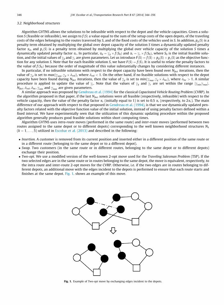
exchange their position.� Two-opt. We use a modified version of the well-known 2-opt move used for the Traveling Salesman Problem (TSP). If the

two selected edges are in the same route or in routes belonging to the same depot, the move is equivalent, respectively, tothe intra route and inter-route 2-opt moves for the CVRP. Otherwise, i.e. if the two edges are in routes belonging to dif-ferent depots, an additional move with the edges incident to the depots is performed to ensure that each route starts andfinishes at the same depot. Fig. 1. shows an example of this move.

Fig. 1. Example of Two-opt move by exchanging edges incident to the depots.

J.W. Escobar et al. / Transportation Research Part B 67 (2014) 344–356 347

� Double-insertion. Two consecutive customers are removed from their current position and inserted in the same route or ina different route (belonging to the same depot or to a different depot) by keeping the edge connecting them.� Double-swap. This move is an extension of the Swap move obtained by considering two pairs of consecutive customers.

The edge connecting each pair of customers is kept. The move is performed between pairs of customers in two differentroutes (belonging to the same depot or to different depots).

A move is performed only if all the new edges inserted in the solution are in the ‘‘granular’’ search space.

3.3. Initial solution procedure

The initial solution S0 is constructed by using a hybrid heuristic, proposed in Escobar et al. (2013) and based on a clusterapproach, which is able to find good initial feasible solutions within short computing times. The following steps areexecuted:

� Step 1. Construct a giant TSP tour containing all the customers, by using the well known Lin–Kernighan heuristic (LKH)(for further details see Lin and Kernighan (1973) and Helsgaun (2000)).� Step 2. Starting from an initial customer j�, split the giant TSP tour into several clusters composed of consecutive custom-

ers so that, for each cluster, the vehicle capacity constraint is satisfied.� Step 3. For each depot i and each cluster g, a TSP tour is obtained by using procedure LKH to evaluate the traveling cost for

visiting i and the customers belonging to g.� Step 4. Assign the depots to the clusters by solving an ILP model for the Single Source Capacitated Facility Location problem

(for further details see Barcelo and Casanovas (1984) and Klincewicz and Luss (1986)).� Step 5. Apply a Splitting Procedure to reduce the traveling cost by adding new routes, and by assigning them to different

depots. For each depot, the current solution is improved by the VRPH procedure for the CVRP proposed in Groer et al.(2010) and modified by Escobar et al. (2013). Each iteration of the splitting procedure considers a different route havingthe largest cost edges. This route is split into two subsets of customers by removing the two largest cost edges. The firstsubset of customers, which is still connected to the depot, replaces the original route. While the second subset of custom-ers, which has been disconnected from the depot, is assigned to a new depot generating a new route. For the new route aTSP tour is obtained by using procedure LKH.

The initial procedure is repeated n times, by considering each customer as initial customer to split the giant tour by fol-lowing its trajectory, and filling as much as possible all the vehicles. The first initialization procedure based on the construc-tion of a giant tour (route first - cluster second approach) was proposed by Beasley (1983) for the solution of the capacitatedVRP. The giant tour is then split into routes by solving a shortest path problem on an appropriate acyclic auxiliary directedgraph. Several generalizations of this approach have been proposed in the literature (see, e.g., Vidal et al. (2014) for an effec-tive initialization procedure for the solution of the Multi-Depot Vehicle Fleet Mix Problem). None of these initialization pro-cedures chooses simultaneously the depots to be opened and the subsets of customers to be assigned to each open depot bysolving to optimality a small-size ILP model.

4. Description of the Granular Variable Tabu Neighborhood Search heuristic algorithm (GVTNS)

Algorithm GVTNS combines the potentiality of the systematic changes of the neighborhood structures of the VariableNeighborhood Search (VNS) approach, proposed in Mladenovic and Hansen (1997) and Hansen and Mladenovic (2003),and the efficient Granular Tabu Search (GTS) approach, introduced in Toth and Vigo (2003). In the proposed algorithm,the VNS technique controls the neighborhood changes, while the GTS technique guides the search process by using theneighborhood structures described in Section 3.2, and the efficient search space detailed in Section 3.1.

After constructing the initial solution S0, the VNS procedure iterates through different neighborhood structures toimprove the best feasible solution (S�) found so far. The algorithm starts by setting S� ¼ S ¼ bS ¼ S0, where S is the current(feasible or infeasible) solution, and bS is the current feasible solution. The following steps are then repeated until a stoppingcriterion (number of iterations or computing time) is reached:

1. Select a neighborhood from the neighborhoods structures Nk(k ¼ 1; . . . ;5) described in Section 3.2. The neighborhoodstructures are explored in a cyclic sequential order (Sequential VNS) by beginning with the neighborhoodN1 ¼ Insertion. This procedure is proposed in Mladenovic and Hansen (1997);

2. Local search: apply a Granular Tabu Search (GTS) procedure in the selected neighborhood Nk S� �

until a local minimum S0

is found;3. If F S0

� �6 F S

� �, set S:¼ S0;

4. If S0 is feasible and F S0� �6 F bS� �

, set bS :¼ S0;

348 J.W. Escobar et al. / Transportation Research Part B 67 (2014) 344–356

5. Every Ng � n iterations apply the third diversification strategy used by Algorithm 2-Phase HGTS proposed by Escobar et al.(2013), where Ng is a given parameter which controls the number of iterations. This diversification strategy selects thebest feasible solution with respect to the depot capacity. Then, for each depot, the customers assigned to the depot areconsidered, and an initial feasible solution for the corresponding CVRP is built by using the savings procedure proposedin Groer et al. (2010). Then this solution is improved by using the CVRP procedures vrp_sa, vrp_rtr proposed in Groer et al.(2010). Note that these procedures are able to obtain, for the considered depot, feasible solutions with respect to the vehi-cle capacity constraint.

Finally, the best feasible solution found so far S� is kept. The GTS procedure explores the solution space by moving, at eachiteration, from a solution S to the best solution S in the neighborhood N S

� �. The best possible move is selected by considering

the move in N S� �

producing the smallest value of the objective function F Sð Þ, and by applying the following tabu aspirationcriterion: if the value of the objective function F Sð Þ of the new solution S is not greater than the cost of the best solutionfound so far, the move producing S is performed even if it corresponds to a tabu move. As usual, a move is considered tabuif it tries to reinsert an edge removed in one of the previous moves. The tabu tenure t for each move performed is an integerrandom value uniformly distributed in the interval [tmin,tmax], where tmin and tmax are given parameters.

5. Computational experiments

Algorithm GVTNS is a deterministic algorithm, and, for each instance, a single run, performing 7n iterations, has been exe-cuted. The implementation details and the results are discussed in the following subsections.

5.1. Implementation details

Algorithm GVTNS has been implemented in C++, and the computational experiments have been performed on an IntelCore 2 Duo (only one core is used) CPU (2.00 GHz) under Linux Ubuntu 11.04 with 2 GB of memory. The algorithm has beenevaluated by considering 79 benchmark instances from the literature. The complete set of instances considers three datasubsets proposed by Tuzun and Burke (1999), Prins et al. (2004) (called ‘‘Prodhon Instances’’ in the following), andBarreto (2004). In all the subsets, the customers and the depots are represented by points in the plane. Consequently, thetraveling cost of an edge is the Euclidean distance, multiplied by 100 and rounded up to the next integer (Prins et al.,2004), or calculated as a double-precision real number (Tuzun and Burke (1999) and Barreto (2004)).

The first data subset was proposed by Tuzun and Burke (1999), and contains 36 instances with uncapacitated depots. Thenumber of customers is n ¼ 100;150 and 200. The number of potential depots is either 10 or 20. The vehicle capacity is setto 150. The second data subset (containing the Prodhon instances) was introduced by Prins et al. (2004), and considers 30instances with capacity constraints on routes and depots. The number of customers is n ¼ 20;50;100 and 200. The numberof potential depots is either 5 or 10. The vehicle capacity is either 70 or 150. Finally, the third data subset is proposed byBarreto (2004), and considers 13 instances obtained by modifying some classical CVRP instances by adding new depots withcapacities and fixed costs. The number of customers ranges from 21 to 150, and the number of potential depots from 5 to 10.

5.2. Comparison of algorithms

We compare the performance of algorithm GVTNS, described in Section 4, with some of the most effective heuristic algo-rithms proposed in the literature for the solution of the CLRP: GRASP + ELS of Duhamel et al. (2010), SALRP of Yu et al. (2010),VNS + ILP of Pirkwieser and Raidl (2010), ALNS of Hemmelmayr et al. (2012), GRASP + ILP of Contardo et al. (2014b), 2-PhaseHGTS of Escobar et al. (2013), and MACO of Ting and Chen (2013).

In Tables 1–5, the following notation is used:

Table 1Summarized results of Gap PBKS, NBKS and NIBS for algorithm GVTNS with and without the ’’granular’’ search approach.

Set Size Initial solution GVTNS with the granular approach GVTNS without the granular approach Average CPU TimeAverage Gap PBKS Average Gap PBKS Average Gap PBKS

Tuzun-Burke 36 1.88 0.69 1.01 592Prodhon 30 1.46 0.32 0.76 265Barreto 13 2.04 0.66 1.11 160Total 79

Global Avg. 1.75 0.55 0.93 397NBKS 0 28 15NIBS 0 5 1

Table 2Summarized best results for all the algorithms on the complete data set.

Set Size GRASP + ELS SALRP VNS + ILP ALNS - 500 K ALNS - 5000 K GRASP + ILP 2-Phase HGTS MACO GVTNS

Gap BestPBKS

CPUtime

GapPBKS

CPUtime

Gap BestPBKS

Gap Avg.PBKS

CPUtime⁄

Gap BestPBKS

Gap Avg.PBKS

CPUtime

Gap BestPBKS

CPUtime

Gap BestPBKS

Gap Avg.PBKS

CPUtime⁄⁄

GapPBKS

CPUtime

Gap BestPBKS

CPUtime⁄⁄

GapPBKS

CPUtime

Tuzun–Burke 36 1.23 607 1.42 826 - - - 0.37 0.83 830 0.11 8103 0.11 0.49 2590 1.08 392 1.17 202 0.69 201Prodhon 30 1.06 258 0.41 422 0.08 0.90 7 0.39 0.67 451 0.21 4221 0.07 0.27 1163 0.52 176 0.35 191 0.32 91Barreto 13 0.07 188 0.29 161 - - - 0.15 0.24 177 0.05 1772 0.13 0.62 264 0.78 105 0.06 49 0.66 53Total 79halflineGlobal Avg. 0.97 405 0.85 564 - - - 0.34 0.67 579 0.14 5587 0.10 0.43 1665 0.81 263 0.67 173 0.55 135Total NBKS 28 24 16 2 29 17 53 39 15 22 26 28Total NIBS 0 0 2 0 4 0 16 16 0 1 0 5CPU Core 2 Quad

(2.83 Ghz)Core 2 Quad(2.66 Ghz)

Core2 Quad Q9550 (2.83Ghz)

AMD Opteron 275 (2.20Ghz)

AMD Opteron275 (2.20 Ghz)

Intel Xeon E5462 (3.00 Ghz) Core 2 Duo(2.00 Ghz)

Athlon XP 2500+(1.83 Ghz)

Core 2 Duo(2.00 Ghz)

CPU index 4373 4046 4049 1234 1234 9586 1398 374 1398

⁄ For each instance: average CPU time over 30 runs.⁄⁄ For each instance: average CPU time over 10 runs.

J.W.Escobar

etal./Transportation

Research

PartB

67(2014)

344–356

349

Table 3Best results for all algorithms on Tuzun-Burke Instances.

Instance PBKS GRASP+ELS SALRP ALNS - 500K ALNS - 5000K GRASP+ILP 2-Phase HGTS MACO GVTNS

BestCost

GapBestPBKS

CPUtime

Cost GapPBKS

CPUtime

BestCost

GapBestPBKS

Avg.Cost

GapAvg.PBKS

CPU time BestCost

GapBestPBKS

CPUtime

BestCost

GapBestPBKS

Avg.Cost

GapAvg.PBKS

CPUtime⁄

Cost GapPBKS

CPUtime

BestCost

GapBestPBKS

CPUtime⁄

Cost GapPBKS

CPUtime

111112 1467.68 1473.36 0.39 233 1477.24 0.65 369 1467.68 0.00 1475.67 0.54 275 1467.68 0.00 - 1469.40 0.12 1475.50 0.53 198 1479.21 0.79 152 1489.68 1.50 71 1479.21 0.79 84111122 1449.20 1449.20 0.00 9 1470.96 1.50 274 1452.14 0.20 1464.72 1.07 321 1449.20 0.00 - 1449.20 0.00 1452.00 0.19 580 1486.27 2.56 239 1453.89 0.32 46 1485.28 2.49 126111212 1394.80 1396.59 0.13 112 1408.65 0.99 231 1394.93 0.01 1400.49 0.41 244 1394.80 0.00 - 1394.90 0.01 1405.80 0.79 220 1407.26 0.89 120 1407.78 0.93 61 1402.59 0.56 74111222 1432.29 1432.29 0.00 114 1432.29 0.00 420 1433.42 0.08 1441.21 0.62 376 1432.29 0.00 - 1432.30 0.00 1440.60 0.58 755 1474.01 2.91 146 1433.42 0.08 54 1463.23 2.16 99112112 1167.16 1167.16 0.00 27 1177.14 0.86 348 1167.53 0.03 1173.04 0.50 489 1167.16 0.00 - 1169.10 0.17 1176.20 0.77 278 1167.16 0.00 232 1208.04 3.50 80 1167.16 0.00 83112122 1102.24 1102.24 0.00 259 1110.36 0.74 342 1102.24 0.00 1102.34 0.01 373 1102.24 0.00 - 1102.40 0.01 1103.60 0.12 634 1102.24 0.00 224 1102.24 0.00 65 1102.24 0.00 105112212 791.66 792.03 0.05 5 791.66 0.00 360 791.66 0.00 791.83 0.02 739 791.66 0.00 - 791.70 0.01 795.80 0.52 227 791.66 0.00 201 792.90 0.16 95 791.66 0.00 96112222 728.30 728.30 0.00 48 731.95 0.50 418 728.30 0.00 728.32 0.00 384 728.30 0.00 - 728.30 0.00 728.50 0.03 550 728.30 0.00 254 728.30 0.00 65 728.30 0.00 126113112 1238.49 1240.39 0.15 55 1238.49 0.00 300 1238.70 0.02 1240.31 0.15 357 1238.49 0.00 - 1238.49 0.00 1239.60 0.09 286 1238.49 0.00 160 1265.27 2.16 77 1238.49 0.00 82113122 1245.30 1246.00 0.06 233 1247.28 0.16 428 1246.52 0.10 1248.17 0.23 445 1245.31 0.00 - 1245.30 0.00 1246.30 0.08 646 1251.22 0.48 237 1256.95 0.94 50 1247.27 0.16 127113212 902.26 902.30 0.00 249 902.26 0.00 291 902.26 0.00 902.26 0.00 321 902.26 0.00 - 902.30 0.00 902.80 0.06 231 902.26 0.00 135 902.26 0.00 61 902.26 0.00 71113222 1018.29 1018.29 0.00 196 1024.02 0.56 316 1018.29 0.00 1018.56 0.03 386 1018.29 0.00 - 1018.29 0.00 1018.29 0.00 749 1018.29 0.00 157 1018.29 0.00 69 1018.29 0.00 85131112 1899.90 1944.57 2.35 518 1953.85 2.84 743 1922.70 1.20 1939.52 2.09 504 1914.41 0.76 - 1899.90 0.00 1924.10 1.27 1640 1961.75 3.26 485 1945.43 2.40 227 1933.67 1.78 179131122 1823.53 1864.24 2.23 705 1899.05 4.14 835 1847.93 1.34 1857.29 1.85 635 1823.53 0.00 - 1825.30 0.10 1831.00 0.41 3612 1856.51 1.81 298 1853.22 1.63 101 1852.14 1.57 173131212 1964.30 1992.41 1.43 727 2057.53 4.75 456 1975.83 0.59 2009.44 2.30 664 1975.83 0.59 - 1964.30 0.00 1969.30 0.25 1275 2012.69 2.46 406 1991.44 1.38 201 1983.09 0.96 184131222 1792.80 1835.25 2.37 415 1801.39 0.48 833 1806.31 0.75 1838.51 2.55 485 1796.45 0.20 - 1792.80 0.00 1800.30 0.42 3099 1803.01 0.57 302 1812.34 1.09 141 1803.01 0.57 175132112 1444.73 1453.78 0.63 103 1453.30 0.59 750 1447.43 0.19 1449.15 0.31 1049 1444.73 0.00 - 1446.80 0.14 1450.40 0.39 871 1445.25 0.04 449 1499.05 3.76 206 1443.32 �0.10 186132122 1434.63 1444.17 0.66 662 1455.50 1.45 828 1445.32 0.75 1446.91 0.86 805 1434.63 0.00 - 1443.90 0.65 1447.20 0.88 2738 1452.07 1.22 493 1446.63 0.84 163 1441.43 0.47 210132212 1204.42 1219.86 1.28 459 1206.24 0.15 752 1204.98 0.05 1205.83 0.12 2197 1204.42 0.00 - 1204.80 0.03 1205.90 0.12 2082 1204.42 0.00 270 1204.76 0.03 218 1204.42 0.00 128132222 931.28 945.81 1.56 224 934.62 0.36 842 931.49 0.02 933.14 0.20 982 931.28 0.00 - 931.30 0.00 931.90 0.07 3734 931.49 0.02 335 931.73 0.05 150 931.28 0.00 177133112 1694.18 1712.11 1.06 271 1720.81 1.57 742 1694.64 0.03 1700.39 0.37 1046 1694.18 0.00 - 1695.90 0.10 1703.80 0.57 938 1705.36 0.66 444 1724.02 1.76 226 1701.34 0.42 182133122 1392.01 1402.94 0.79 524 1415.85 1.71 833 1400.50 0.61 1403.50 0.83 925 1392.01 0.00 - 1398.00 0.43 1401.50 0.68 2751 1416.74 1.78 342 1401.05 0.65 123 1416.74 1.78 175133212 1198.28 1214.82 1.38 251 1216.84 1.55 756 1198.67 0.03 1199.27 0.08 1375 1198.28 0.00 - 1198.60 0.03 1199.60 0.11 1010 1234.83 3.05 526 1217.29 1.59 241 1213.87 1.30 207133222 1151.80 1155.96 0.36 375 1159.12 0.64 837 1152.01 0.02 1154.36 0.22 911 1151.80 0.00 - 1157.30 0.48 1158.70 0.60 3560 1156.05 0.37 380 1158.03 0.54 130 1151.80 0.00 208121112 2243.40 2295.90 2.34 655 2324.10 3.60 1328 2265.15 0.97 2278.27 1.55 944 2251.93 0.38 - 2243.40 0.00 2251.30 0.35 2805 2265.59 0.99 522 2304.67 2.73 461 2258.02 0.65 315121122 2138.40 2203.57 3.05 432 2258.16 5.60 1455 2183.05 2.09 2192.61 2.54 847 2159.93 1.01 - 2138.40 0.00 2154.90 0.77 5680 2166.43 1.31 603 2187.65 2.30 231 2166.20 1.30 300121212 2209.30 2246.39 1.68 1566 2260.30 2.31 1319 2233.55 1.10 2247.75 1.74 907 2220.01 0.48 - 2209.30 0.00 2226.10 0.76 3004 2249.40 1.82 527 2231.46 1.00 428 2239.65 1.37 287121222 2225.10 2265.53 1.82 2192 2326.53 4.56 1428 2230.94 0.26 2263.20 1.71 860 2230.94 0.26 - 2225.10 0.00 2241.70 0.75 6143 2237.81 0.57 558 2275.70 2.27 234 2236.73 0.52 351122112 2073.73 2106.47 1.58 1521 2112.65 1.88 1320 2082.60 0.43 2093.78 0.97 1606 2073.73 0.00 - 2077.80 0.20 2093.80 0.97 3462 2121.93 2.32 522 2098.56 1.20 570 2103.82 1.45 278122122 1692.17 1779.05 5.13 618 1722.99 1.82 1400 1710.67 1.09 1732.00 2.35 941 1692.17 0.00 - 1694.80 0.16 1704.40 0.72 8547 1749.10 3.36 691 1711.25 1.13 277 1717.92 1.52 433122212 1453.18 1474.25 1.45 514 1469.10 1.10 1299 1458.55 0.37 1462.15 0.62 1861 1453.18 0.00 - 1465.40 0.84 1467.80 1.01 3471 1473.27 1.38 724 1472.93 1.36 544 1469.45 1.12 318122222 1082.59 1085.69 0.29 1243 1088.64 0.56 1429 1085.29 0.25 1086.08 0.32 812 1082.74 0.01 - 1082.90 0.03 1086.00 0.31 5292 1082.59 0.00 616 1087.57 0.46 317 1082.46 �0.01 349123112 1954.70 2004.33 2.54 1451 1994.16 2.02 1318 1964.75 0.51 1971.01 0.83 968 1960.30 0.29 - 1954.70 0.00 1986.70 1.64 3865 1984.77 1.54 542 1978.74 1.23 387 1969.38 0.75 261123122 1926.64 1964.40 1.96 1273 1932.05 0.28 1412 1926.64 0.00 1952.31 1.33 740 1926.64 0.00 - 1931.10 0.23 1936.20 0.50 9367 1958.98 1.68 617 1959.71 1.72 230 1935.74 0.47 344123212 1762.03 1778.80 0.95 1398 1779.10 0.97 1314 1762.09 0.00 1764.16 0.12 2055 1762.03 0.00 - 1763.10 0.06 1766.20 0.24 3766 1778.41 0.93 697 1782.94 1.19 406 1776.90 0.84 349123222 1390.87 1453.82 4.53 2202 1396.42 0.40 1427 1393.06 0.16 1395.38 0.32 1038 1391.68 0.06 - 1392.00 0.08 1392.70 0.13 5157 1390.87 0.00 518 1392.70 0.13 269 1391.50 0.05 317Average 1522.01 1.23 607 1526.41 1.42 826 1507.44 0.37 1515.64 0.83 830 1502.90 0.11 8103 1502.18 0.11 1508.79 0.49 2590 1519.05 1.08 392 1520.22 1.17 202 1512.50 0.69 201NBKS 6 4 7 1 24 13 1 9 4 12NIBS 0 0 2 0 12 9 0 1 0 2

⁄ For each instance: average CPU time over 10 runs.

350J.W

.Escobaret

al./TransportationR

esearchPart

B67

(2014)344–

356

Table 4Best results for all algorithms on Prodhon Instances.

Instance PBKS GRASP + ELS SALRP VNS + ILP ALNS - 500 K ALNS - 5000 K GRASP + ILP 2-Phase HGTS MACO GVTNS

Best

Cost

Gap

Best

PBKS

CPU

time

Cost Gap

PBKS

CPU

time

Best

Cost

Gap

Best

PBKS

CPU

time

Avg.

Cost

Gap

Avg.

PBKS

CPU

time⁄Best

Cost

Gap

Best

PBKS

Avg.

Cost

Gap

Avg.

PBKS

CPU

time

Best

Cost

Gap

Best

PBKS

CPU

time

Best

Cost

Gap

Best

PBKS

Avg.

Cost

Gap

Avg.

PBKS

CPU

time⁄⁄Cost Gap

PBKS

CPU

time

Best

Cost

Gap

Best

PBKS

CPU

time⁄⁄Cost Gap

PBKS

CPU

time

20–5-1a 54793 54793 0.00 0 54793 0.00 20 54793 0.00 - 54890 0.18 1 54793 0.00 54793 0.00 39 54793 0.00 - 54793 0.00 54793 0.00 2 54793 0.00 3 54793 0.00 4 54793 0.00 2

20–5-1b 39104 39104 0.00 0 39104 0.00 15 39104 0.00 - 39104 0.00 1 39104 0.00 39104 0.00 54 39104 0.00 - 39104 0.00 39104 0.00 3 39104 0.00 4 39104 0.00 5 39104 0.00 3

20–5-2a 48908 48908 0.00 0 48908 0.00 19 48908 0.00 - 48934 0.05 1 48908 0.00 48908 0.00 38 48908 0.00 - 48908 0.00 48908 0.00 1 48945 0.08 3 48908 0.00 4 48945 0.08 2

20–5-2b 37542 37542 0.00 0 37542 0.00 15 37542 0.00 - 37542 0.00 1 37542 0.00 37542 0.00 67 37542 0.00 - 37542 0.00 37542 0.00 3 37542 0.00 4 37542 0.00 5 37542 0.00 3

50–5-1a 90111 90111 0.00 3 90111 0.00 75 90111 0.00 - 90389 0.31 2 90111 0.00 90111 0.00 101 90111 0.00 - 90111 0.00 90111 0.00 15 90402 0.32 27 90111 0.00 25 90111 0.00 13

50–5-1b 63242 63242 0.00 0 63242 0.00 58 63242 0.00 - 63472 0.36 3 63242 0.00 63242 0.00 65 63242 0.00 - 63242 0.00 63281 0.06 18 64073 1.31 27 63242 0.00 21 63242 0.00 9

50–5-2a 88298 88643 0.39 11 88298 0.00 95 88298 0.00 - 89859 1.77 2 88443 0.16 88576 0.31 99 88298 0.00 - 88298 0.00 88333 0.04 18 89342 1.18 23 88298 0.00 24 89342 1.18 12

50–5-2b 67308 67308 0.00 16 67340 0.05 59 67308 0.00 - 68013 1.05 4 67340 0.05 67448 0.21 200 67308 0.00 - 67373 0.10 67436 0.19 22 68479 1.74 21 67308 0.00 20 67951 0.96 10

50–5-2bis 84055 84055 0.00 0 84055 0.00 75 84055 0.00 - 84208 0.18 3 84055 0.00 84119 0.08 107 84055 0.00 - 84055 0.00 84055 0.00 21 84055 0.00 23 84055 0.00 25 84126 0.08 8

50–5-2bbis 51822 51822 0.00 11 51822 0.00 66 51822 0.00 - 52131 0.60 5 51822 0.00 51840 0.03 98 51822 0.00 - 51883 0.12 51898 0.15 27 52087 0.51 29 51822 0.00 17 52213 0.75 9

50–5-3a 86203 86203 0.00 0 86456 0.29 74 86203 0.00 - 86728 0.61 2 86203 0.00 86262 0.07 101 86203 0.00 - 86203 0.00 86203 0.00 17 86203 0.00 66 86203 0.00 33 86203 0.00 18

50–5-3b 61830 61830 0.00 0 62700 1.41 58 61830 0.00 - 62905 1.74 3 61830 0.00 61830 0.00 137 61830 0.00 - 61830 0.00 61853 0.04 23 61830 0.00 38 61830 0.00 26 61885 0.09 20

100–5-1a 275457 276960 0.55 148 277035 0.57 349 275813 0.13 - 278292 1.03 5 275636 0.06 276364 0.33 520 275524 0.02 - 275457 0.00 275628 0.06 220 276186 0.26 157 276220 0.28 117 276137 0.25 75

100–5-1b 213704 215854 1.01 68 216002 1.08 269 213973 0.13 - 216286 1.21 8 214735 0.48 215059 0.63 1190 213704 0.00 - 214056 0.16 214785 0.51 230 214892 0.56 136 214323 0.29 135 216154 1.15 59

100–5-2a 193671 194267 0.31 212 194124 0.23 349 193671 0.00 - 195022 0.70 4 193752 0.04 193903 0.12 463 193671 0.00 - 193708 0.02 194054 0.20 122 194625 0.49 145 194441 0.40 238 193896 0.12 76

100–5-2b 157095 157375 0.18 125 157150 0.04 212 157157 0.04 - 158217 0.71 5 157095 0.00 157157 0.04 859 157095 0.00 - 157178 0.05 157311 0.14 100 157319 0.14 193 157222 0.08 144 157180 0.05 82

100–5-3a 200160 200345 0.09 141 200242 0.04 250 200160 0.00 - 201748 0.79 4 200305 0.07 200496 0.17 454 200246 0.04 - 200339 0.09 200394 0.12 97 201086 0.46 163 201038 0.44 179 200777 0.31 69

100–5-3b 152441 152528 0.06 221 152467 0.02 197 152466 0.02 - 154917 1.62 4 152441 0.00 152900 0.30 684 152441 0.00 - 152466 0.02 152814 0.24 100 153663 0.80 168 152722 0.18 152 153435 0.65 68

100–10-1a 287892 301418 4.70 48 291043 1.09 270 288540 0.23 - 291775 1.35 9 296877 3.12 299982 4.20 210 292868 1.73 - 287892 0.00 292657 1.66 2622 289755 0.65 277 291134 1.13 105 287864 �0.01 203

100–10-1b 232230 269594 16.09 186 234210 0.85 203 232230 0.00 - 238059 2.51 10 235849 1.56 240829 3.70 188 233146 0.39 - 234080 0.80 236026 1.63 1067 238002 2.49 152 235348 1.34 82 232599 0.16 117

100–10-2a 243677 243778 0.04 260 245813 0.88 261 243677 0.00 - 245614 0.79 6 244740 0.44 245548 0.77 136 243829 0.06 - 243695 0.01 243851 0.07 236 245768 0.86 92 245263 0.65 123 245484 0.74 52

100–10-2b 203988 203988 0.00 139 205312 0.65 199 203988 0.00 - 205719 0.85 7 204016 0.01 204494 0.25 261 203988 0.00 - 203988 0.00 204253 0.13 259 204252 0.13 99 205524 0.75 85 204252 0.13 42

100–10-3a 250882 253511 1.05 164 250882 0.00 338 251128 0.10 - 255140 1.70 7 253801 1.16 254882 1.59 202 253722 1.13 - 252927 0.82 253610 1.09 723 254716 1.53 125 254302 1.36 113 254558 1.47 82

100–10-3b 204601 205087 0.24 203 205009 0.20 240 204706 0.05 - 207410 1.37 7 205609 0.49 206175 0.77 224 204601 0.00 - 204664 0.03 205110 0.25 584 205837 0.60 144 204786 0.09 79 205824 0.60 78

200–10-1a 475327 486467 2.34 1521 481002 1.19 1428 478349 0.64 - 481142 1.22 18 480883 1.17 483205 1.66 752 478951 0.76 - 475327 0.00 477656 0.49 3960 476778 0.31 671 478843 0.74 942 477009 0.35 320

200–10-1b 377327 382329 1.33 359 383586 1.66 1336 378631 0.35 - 381516 1.11 16 378961 0.43 380538 0.85 1346 378065 0.20 - 377327 0.00 378656 0.35 4006 378289 0.25 476 378351 0.27 562 377716 0.10 239

200–10-2a 449291 452276 0.66 112 450848 0.35 1796 449571 0.06 - 452374 0.69 17 450451 0.26 451750 0.55 1201 450377 0.24 - 449291 0.00 449797 0.11 4943 449951 0.15 483 451457 0.48 704 449006 �0.06 231

200–10-2b 374575 376027 0.39 1610 376674 0.56 1245 375129 0.15 - 376836 0.60 16 374751 0.05 376112 0.41 1349 374751 0.05 - 374575 0.00 374996 0.11 3486 374961 0.10 530 374972 0.11 404 374717 0.04 290

200–10-3a 469870 478380 1.81 1596 473875 0.85 1776 471024 0.25 - 475345 1.17 18 475373 1.17 479366 2.02 1251 474087 0.90 - 469870 0.00 471272 0.30 4075 472321 0.52 624 475155 1.12 879 471978 0.45 330

200–10-3b 363103 365166 0.57 591 363701 0.16 1326 363907 0.22 - 365705 0.72 15 366902 1.05 366902 1.05 1137 366416 0.91 - 363103 0.00 363581 0.13 7888 363252 0.04 389 365401 0.63 491 362827 �0.08 214

Average 199630 1.06 258 197778 0.41 422 196911 0.08 - 198643 0.90 7 197852 0.39 198648 0.67 451 197357 0.21 4221 196776 0.07 197332 0.27 1163 197617 0.52 176 197657 0.35 191 197229 0.32 91

NBKS 12 10 16 2 12 7 18 16 7 6 12 9

NIBS 0 0 2 0 2 0 4 5 0 0 0 3

⁄ For each instance: average CPU time over 30 runs.⁄⁄ For each instance: average CPU time over 10 runs.

J.W.Escobar

etal./Transportation

Research

PartB

67(2014)

344–356

351

Table 5Best results for all algorithms on Barreto Instances.

Instance PBKS GRASP + ELS SALRP ALNS - 500 K ALNS - 5000 K GRASP + ILP 2-Phase HGTS MACO GVTNS

Best Cost Gap

Best

PBKS

CPU

time

Cost Gap

PBKS

CPU

time

Best Cost Gap

Best

PBKS

Avg. Cost Gap

Avg.

PBKS

CPU

time

Best Cost Gap

Best

PBKS

CPU

time

Best Cost Gap

Best

PBKS

Avg. Cost Gap

Avg.

PBKS

CPU

time⁄Cost Gap

PBKS

CPU

time

Best Cost Gap

Best

PBKS

CPU

time⁄Cost Gap

PBKS

CPU

time

Christofides69-

50x5

565.6 565.6 0.00 8 565.6 0.00 53 565.6 0.00 565.6 0.00 73 565.6 0.00 - 569.5 0.69 584.9 3.41 18 580.4 2.62 45 565.6 0.00 29 580.4 2.62 22

Christofides69-

75x10

844.6 850.8 0.73 86 848.9 0.51 127 853.5 1.05 854.9 1.22 207 848.9 0.51 - 844.6 0.00 847.1 0.30 88 848.9 0.51 94 844.9 0.03 59 853.8 1.09 45

Christofides69-

100x10

833.4 833.4 0.00 127 838.3 0.59 331 833.4 0.00 835.4 0.24 403 833.4 0.00 - 840.7 0.88 850.0 1.99 492 838.6 0.62 234 836.8 0.40 84 837.1 0.44 111

Daskin95-88x8 355.8 355.8 0.00 130 355.8 0.00 577 355.8 0.00 355.8 0.00 250 355.8 0.00 - 355.8 0.00 356.1 0.08 210 362.0 1.74 148 355.8 0.00 100 361.6 1.63 97

Daskin95-150x10 43952.3 43963.6 0.03 1697 45109.4 2.63 323 44309.0 0.81 44497.2 1.24 613 44004.9 0.12 - 43952.3 0.00 44263.5 0.71 1842 44578.9 1.43 456 44131.0 0.41 167 44578.9 1.43 199

Gaskell67-21x5 424.9 424.9 0.00 0 424.9 0.00 18 424.9 0.00 424.9 0.00 25 424.9 0.00 - 424.9 0.00 424.9 0.00 2 424.9 0.00 6 424.9 0.00 6 424.9 0.00 4

Gaskell67-22x5 585.1 585.1 0.00 15 585.1 0.00 17 585.1 0.00 585.1 0.00 21 585.1 0.00 - 585.1 0.00 585.1 0.00 3 585.1 0.00 9 585.1 0.00 5 585.1 0.00 6

Gaskell67-29x5 512.1 512.1 0.00 9 512.1 0.00 24 512.1 0.00 512.1 0.00 40 512.1 0.00 - 512.1 0.00 512.1 0.00 5 512.1 0.00 11 512.1 0.00 9 512.1 0.00 7

Gaskell67-32x5 562.2 562.2 0.00 18 562.2 0.00 27 562.2 0.00 562.2 0.00 58 562.2 0.00 - 562.2 0.00 562.2 0.00 6 562.2 0.00 40 562.2 0.00 13 562.2 0.00 20

Gaskell67-32x5 504.3 504.3 0.00 34 504.3 0.00 25 504.3 0.00 504.3 0.00 55 504.3 0.00 - 504.3 0.00 504.3 0.00 8 504.3 0.00 22 504.3 0.00 10 504.3 0.00 15

Gaskell67-36x5 460.4 460.4 0.00 0 460.4 0.00 32 460.4 0.00 460.4 0.00 61 460.4 0.00 - 460.4 0.00 460.4 0.00 9 460.4 0.00 39 460.4 0.00 13 460.4 0.00 22

Min92-27x5 3062.0 3062.0 0.00 35 3062.0 0.00 23 3062.0 0.00 3062.0 0.00 38 3062.0 0.00 - 3062.0 0.00 3062.0 0.00 4 3062.0 0.00 11 3062.0 0.00 9 3062.0 0.00 7

Min92-134x8 5709.0 5719.3 0.18 280 5709.0 0.00 522 5713.0 0.07 5732.6 0.41 460 5709.0 0.00 - 5719.3 0.18 5801.9 1.63 750 5890.6 3.18 252 5709.0 0.00 137 5789.0 1.40 134

Average 4492.27 0.07 188 4579.85 0.29 161 4518.56 0.15 4534.81 0.24 177 4494.51 0.05 1772 4491.78 0.13 4524.19 0.62 264 4554.65 0.78 105 4504.16 0.06 49 4547.06 0.66 53

NBKS 10 10 10 9 11 10 7 7 10 7

NIBS 0 0 0 0 0 2 0 0 0 0

⁄ For each instance: average CPU time over 10 runs.

352J.W

.Escobaret

al./TransportationR

esearchPart

B67

(2014)344–

356

J.W. Escobar et al. / Transportation Research Part B 67 (2014) 344–356 353

Instance

instance name Cost solution cost obtained by the corresponding algorithm in one single run Best Cost best solution cost found by the corresponding algorithm over the executed runs Avg. Cost average solution cost found by the corresponding algorithm over the executed runs PBKS cost of the previous best-known solution given by the minimum cost among those found by

algorithms GRASP + ELS, SALRP, VNS + ILP, ALNS-500 K, ALNS-5000 K, GRASP + ILP, 2-Phase HGTS,and MACO

BKS

cost of the best known solution = min {PBKS, solution cost found by GVTNS} NBKS number of best results (BKS) obtained by the corresponding algorithm NIBS number of instances for which the corresponding algorithm is the only one which found BKS CPU CPU used by the corresponding algorithm CPU index Passmark performance test for the corresponding CPU CPU time running time in seconds on the CPU used by the corresponding algorithm; Gap PBKS percentage gap of the solution cost found by the corresponding algorithm in one single run with

respect to PBKS;

Gap Best PBKS percentage gap of the best solution cost found by the corresponding algorithm over the executed

runs with respect to PBKS;

Gap Avg. PBKS percentage gap of the average solution cost found by the corresponding algorithm over the

executed runs with respect to PBKS

In addition, for each instance, the solution costs which are equal to the corresponding BKS are reported in bold. Wheneverthe considered algorithm is the only one which found the corresponding BKS value, the reported cost is underlined. Finally,the CPU index of a CPU is given by the Passmark performance test (for further details see (PassMark, 2012)). This is a wellknown benchmark test focused on CPU and memory performance. A higher value of the CPU index indicates that the corre-sponding CPU is faster.

5.3. Parameter settings

A suitable set of parameters and stop conditions, whose values are based on extensive computational tests on the bench-mark instances, was selected for algorithm GVTNS. Initially, the values of all the parameters were set equal to the corre-sponding values used in Algorithm 2-Phase HGTS (see Escobar et al. (2013)), which generally obtained, for this latteralgorithm, good results. Then, for each parameter in turn (with the other parameters fixed to the corresponding current val-ues), two parameter values, different from the current one C have been considered: one value S, smaller than C withS ¼ C � r, and the other one L, larger than C with L ¼ C þ r, where r ¼ 0:1 (initial value of C). For each of these two param-eter values, algorithm GVTNS was executed on all the 79 benchmark instances, the value of the associated performanceindex Gap PBKS (see Section 5.2) was evaluated, and the parameter value (S;C or L) corresponding to the minimum perfor-mance index value was selected as the current parameter value. In case the parameter value was changed with respect to itscurrent value, the above step was repeated until no change occurred. We observed that the most critical parameters are bo,bn, cd, cr: Parameters bo and bn control the value of b, i.e. the graph sparsification, and hence the number of moves to be per-formed and the associated computing time. Larger values of b allow the algorithm to perform several moves before to obtaina local optimum, while smaller values lead to shorter computing times. Parameters cd and cr are related to the penalizationscheme used to deal with infeasible solutions. In general, smaller values of these parameters allow the algorithm to considermore moves (although many of them can lead to infeasible solutions), while larger values produce a more conservativebehavior of the algorithm, allowing it to obtain quickly feasible solutions. As a consequence, to obtain a good performanceof algorithm GVTNS, for what concerns both the quality of the solution found and the computing time, it is critical to defineappropriate values for all the previously mentioned parameters.

The values of the selected parameters are reported in the following:

Parameter

Selected value

bo

1.80 bn 2.40 Ns 2.00 Nr 1.00 Nfact 10 cd 0.0075 cr 0.0050

(continued on next page)

354 J.W. Escobar et al. / Transportation Research Part B 67 (2014) 344–356

cmin

1=FðS0Þ cmax 0.0400 dred 0.30 dinc 2.00 Ng 1.50 tmin 3 tmax 10

These values have been utilized for the execution of all the considered instances. In addition, the Splitting Procedure (seeStep 5 of the initialization procedure described in Section 3.3) is executed for 3 iterations.

5.4. Evaluation of the effect of the granularity

We evaluate the impact of the granularity approach on the performance of algorithm GVTNS by executing it with andwithout the granularity approach, and by fixing, for each instance, the same maximum CPU time as stopping criterion. Inparticular, the CPU time for each instance has been defined as the CPU time spent by algorithm GVTNS, using the granularityapproach and the parameter values detailed in Sub Section 5.3, to solve the given instance.

The results corresponding to the execution of the algorithm with and without the granular search approach are summa-rized in Table 1. The results show that the granular search approach significantly improves the performance of algorithmGVTNS.

5.5. Comparison of the most effective algorithms

In Tables 2–5, we compare algorithm GVTNS with the most effective heuristics proposed for the solution of the CLRP, i.e.,as previously mentioned, algorithms GRASP + ELS of Duhamel et al. (2010), SALRP of Yu et al. (2010), VNS + ILP of Pirkwieserand Raidl (2010), ALNS of Hemmelmayr et al. (2012), GRASP + ILP of Contardo et al. (2014b), 2-Phase HGTS of Escobar et al.(2013) and MACO of Ting and Chen (2013). In the tables, we report the results as presented in the corresponding papers.

The recent algorithms GRASP + PR of Prins et al. (2007), MAjPM of Prins et al. (2006b) and LRGTS of Prins et al. (2006a) aredominated by algorithm GRASP + ELS, proposed by Duhamel et al. (2010), and the corresponding results are not reported inTables 2–5.

For each instance, algorithm GRASP + ELS has been executed five times and only the best solution found over the five runsis reported. In addition, it is to note that the CPU time reported for each instance represents the time required to find the bestsolution within the corresponding run. The results reported for algorithm SALRP correspond to a single run of the algorithm.Algorithm VNS + ILP has been computationally evaluated only on the second data subset (Prodhon instances). The resultsreported for algorithm VNS + ILP correspond, for each instance, to the average cost found and to the average CPU time overthirty runs, and to the best cost found by considering several versions of the algorithm with thirty runs for each version (thecorresponding CPU time has not been reported). For algorithm ALNS, for each instance, the best and the average costs overfive runs for 500 K iterations (ALNS – 500 K), as well as the best costs over five runs for 5000 K iterations (ALNS – 5000 K), arereported. The CPU time reported for each instance corresponds to the total running time of the corresponding algorithm(only the global average CPU time for each data subset has been reported for ALNS – 5000 K). Algorithms GRASP + ILPand MACO have been executed for ten runs. The results reported for algorithm GRASP + ILP correspond, for each instance,to the best and to the average costs found, and to the average CPU time over the ten runs. The results reported for algorithmMACO correspond, for each instance, to the best cost found and to the average CPU time over the ten runs. Finally, the resultsreported for Algorithms 2-Phase HGTS and GVTNS correspond to a single run of the algorithm.

Table 2 shows a summary of the results found by the algorithms on the complete data set, while Tables 3–5 show thedetailed results for the three considered data sets. For what concerns a comparison among the reported CPU times, it is nec-essary to take into account the different speeds of the CPUs used in the computational experiments. In addition, for the algo-rithms reporting average values of the CPU times, i.e. algorithms GRASP + ILP and MACO which execute ten runs for eachinstance, the CPU times corresponding to the best found costs should be multiplied times the number of executed runs.As previously mentioned, the CPU times corresponding to the best costs found by algorithm VNS + ILP are not reported inPirkwieser and Raidl (2010), but they seem to be large.

As shown in Table 2, for what concerns the global average value of Gap PBKS, algorithm GVTNS obtains better results thanthose obtained by algorithms GRASP + ELS, SALRP, 2-Phase HGTS and MACO. Note that the average and best results on thecomplete data set are not available for algorithm VNS + ILP, therefore a global comparison with this algorithm cannot be per-formed. In addition, by considering the global average value of the gaps corresponding to the average costs computed overseveral runs (Gap Avg. PBKS), Table 2 shows that algorithm GVTNS obtains results better than those obtained (in comparableCPU times) by algorithm ALNS – 500 K, and slightly worse than those obtained (in much larger CPU times) by algorithmGRASP + ILP. The best results on the global average value of Gap Best PBKS are obtained, with very large CPU times, by algo-

J.W. Escobar et al. / Transportation Research Part B 67 (2014) 344–356 355

rithms GRASP + ILP and ALNS-5000 K. By taking into account the big difference of the corresponding CPU times, it is difficultto make a direct comparison of the quality of the solutions found by algorithm GVTNS with respect to the best resultsreported for algorithms GRASP + ILP and ALNS-5000 K.

For what concerns the number NBKS of the best known solutions found and the number NIBS of instances for which thecorresponding algorithm is the only one which finds the best known solution, algorithms ALNS-5000 K and GRASP + ILP areagain the best ones, while algorithms ALNS-500 K (Best solution) and GVTNS have comparable behaviors (although the for-mer algorithm has larger CPU times). Finally, it is to note that algorithm GVTNS is able to find, within short CPU times, 28best known solutions and to improve the previous best known solution for 5 instances.

As for the global CPU time, algorithm GVTNS is faster than the previous published algorithms which are able to find thebest results in terms of average gaps and number of best known solutions. Algorithm VNS + ILP takes smaller average CPUtimes, but the corresponding average solution quality is clearly worse than that of the proposed method. Algorithm MACOseems to require smaller CPU times than algorithm GVTNS, but since only the average computing times over ten runs arereported for the former algorithm, instead of the complete running times for executing the ten runs, a comparison betweenthe two algorithms may be biased.

6. Concluding remarks

We have proposed a new metaheuristic algorithm, called GVTNS and based on the Granular Tabu Search and the VariableNeighborhood Search approaches, for the solution of the CLRP. The computational experiments emphasize the importance ofthe granular search approach, by showing that it significantly improves the performance of algorithms GVTNS. We have alsocompared the performance of algorithm GVTNS with that of the most recent effective published heuristics for the CLRP on aset of benchmarking instances from the literature. The results show the effectiveness of algorithm GVTNS, which is able toimprove some best known results within short computing times.

Acknowledgments

This work has been partially supported by MIUR (Ministero Istruzione, Università e Ricerca), Italy, by Pontificia Univers-idad Javeriana, Cali, Colombia and by Universidad del Bío-Bío, Concepción, Chile. This support is gratefully acknowledged.We also wish to thank three anonymous reviewers for their helpful suggestions.

References

Baldacci, R., Mingozzi, A., Calvo, R., 2011. An exact method for the capacitated location-routing problem. Operations Research 59 (5), 1284–1296.Barcelo, J., Casanovas, J., 1984. A heuristic lagrangean algorithm for the capacitated plant location problem. European Journal of Operational Research 15 (2),

212–226.Barreto, S., 2004. Análise e modelização de problemas de localização-distribuição (analysis and modelling of location-routing problems) (Ph.D. thesis),

University of Aveiro, pp. 3810–4193.Barreto, S., Ferreira, C., Paixao, J., Santos, B., 2007. Using clustering analysis in a capacitated location-routing problem. European Journal of Operational

Research 179 (3), 968–977.Beasley, J.E., 1983. Route firstcluster second methods for vehicle routing. Omega 11 (4), 403–408.Belenguer, J., Benavent, E., Prins, C., Prodhon, C., Wolfler-Calvo, R., 2011. A branch-and-cut method for the capacitated location-routing problem. Computers

& Operations Research 38 (6), 931–941.Contardo, C., Cordeau, J., Gendron, B., 2014a. An exact algorithm based on cut-and-column generation for the capacitated location-routing problem.

INFORMS Journal on Computing 26 (1), 88–102.Contardo, C., Cordeau, J., Gendron, B., 2014b. A GRASP + ILP-based metaheuristic for the capacitated location-routing problem. Journal of Heuristics 20 (1),

1–38.Duhamel, C., Lacomme, P., Prins, C., Prodhon, C., 2010. A GRASP � ELS approach for the capacitated location-routing problem. Computers & Operations

Research 37 (11), 1912–1923.Escobar, J., Linfati, R., Toth, P., 2013. A two-phase hybrid heuristic algorithm for the capacitated location-routing problem. Computers & Operations Research

40 (1), 70–79.Gendreau, M., Hertz, A., Laporte, G., 1994. A tabu search heuristic for the vehicle routing problem. Management Science 40 (10), 1276–1290.Groer, C., Golden, B., Wasil, E., 2010. A library of local search heuristics for the vehicle routing problem. Mathematical Programming Computation 2 (2), 79–

101.Hansen, P., Hegedahl, B., Hjortkjaer, S., Obel, B., 1994. A heuristic solution to the warehouse location-routing problem. European Journal of Operational

Research 76 (1), 111–127.Hansen, P., Mladenovic, N., 2003. Variable neighborhood search. In: Handbook of Metaheuristics. Springer, pp. 145–184.Helsgaun, K., 2000. An effective implementation of the Lin–Kernighan traveling salesman heuristic. European Journal of Operational Research 126 (1), 106–

130.Hemmelmayr, V., Cordeau, J., Crainic, T., 2012. An adaptive large neighborhood search heuristic for two-echelon vehicle routing problems arising in city

logistics. Computers & Operations Research 39 (12), 3215–3228.Kirchler, D., Wolfler Calvo, R., 2013. A granular tabu search algorithm for the dial-a-ride problem. Transportation Research Part B: Methodological 56, 120–

135.Klincewicz, J., Luss, H., 1986. A lagrangian relaxation heuristic for capacitated facility location with single-source constraints. Journal of the Operational

Research Society 37 (5), 495–500.Laporte, G., Nobert, Y., Arpin, D., 1986. An exact algorithm for solving a capacitated location-routing problem. Annals of Operations Research 6 (9), 291–310.Lin, S., Kernighan, B., 1973. An effective heuristic algorithm for the traveling-salesman problem. Operations Research 21 (2), 498–516.Mladenovic, N., Hansen, P., 1997. Variable neighborhood search. Computers & Operations Research 24 (11), 1097–1100.Moreno Pérez, J., Marcos Moreno-Vega, J., Rodríguez Martín, I., 2003. Variable neighborhood tabu search and its application to the median cycle problem.

European Journal of Operational Research 151 (2), 365–378.

356 J.W. Escobar et al. / Transportation Research Part B 67 (2014) 344–356

PassMark, 2012. PassMark Performance Test. <http://www.passmark.com> (Online; accessed 28-Jun-2012).Perl, J., Daskin, M., 1985. A warehouse location-routing problem. Transportation Research Part B: Methodological 19 (5), 381–396.Perugia, A., Moccia, L., Cordeau, J.-F., Laporte, G., 2011. Designing a home-to-work bus service in a metropolitan area. Transportation Research Part B:

Methodological 45 (10), 1710–1726.Pirkwieser, S., Raidl, G., 2010. Variable neighborhood search coupled with ilp-based very large neighborhood searches for the (periodic) location-routing

problem. In: Proceedings of the International Conference on Hybrid Metaheuristics, pp. 174–189.Prins, C., Prodhon, C., Ruiz, A., Soriano, P., Wolfler-Calvo, R., 2007. Solving the capacitated location-routing problem by a cooperative lagrangean relaxation-

granular tabu search heuristic. Transportation Science 41 (4), 470–483.Prins, C., Prodhon, C., Wolfler-Calvo, R., 2004. Nouveaux algorithmes pour le problème de localisation et routage sous contraintes de capacité. In: MOSIM

(4éme Conférence Francophone de Modélisation et Simluation, Nantes, France, vol. 4. pp. 1115–1122.Prins, C., Prodhon, C., Wolfler-Calvo, R., 2006a. A memetic algorithm with population management (MAjPM) for the capacitated location-routing problem.

Lecture Notes in Computer Science 3906, 183–194.Prins, C., Prodhon, C., Wolfler-Calvo, R., 2006b. Solving the capacitated location-routing problem by a GRASP complemented by a learning process and a path

relinking. 4OR: A Quarterly Journal of Operations Research 4 (3), 221–238.Repoussis, P., Paraskevopoulos, D., Tarantilis, C., Ioannou, G., 2006. A reactive greedy randomized variable neighborhood tabu search for the vehicle routing

problem with time windows. In: Proceedings of the International Conference on Hybrid Metaheuristics, vol. 4030, pp. 124–138.Ting, C., Chen, C., 2013. A multiple ant colony optimization algorithm for the capacitated location routing problem. International Journal of Production

Economics 141 (1), 34–44.Toth, P., Vigo, D., 2003. The granular tabu search and its application to the vehicle-routing problem. INFORMS Journal on Computing 15 (4), 333–346.Tuzun, D., Burke, L., 1999. A two-phase tabu search approach to the location routing problem. European Journal of Operational Research 116 (1), 87–99.Vidal, T., Crainic, T.G., Gendreau, M., Prins, C., 2014. Implicit depot assignments and rotations in vehicle routing heuristics. European Journal of Operational

Research, http://dx.doi.org/10.1016/j.ejor.2013.12.044..Yu, V., Lin, S., Lee, W., Ting, C., 2010. A simulated annealing heuristic for the capacitated location routing problem. Computers & Industrial Engineering 58

(2), 288–299.