INSTITUTO DE INVESTIGAÇÃO E FORMAÇÃO

AVANÇADA

Supervisors-

Doctor Mouhaydine Tlemçani

Doctor Mário Rui Melício da Conceição

Doctor Teresa Cristina de Freitas Goncalves

Thesis presented to the University of Évora for obtaining the

Doctor's degree in Earth and Space Sciences

Specialty: (Atmospheric and Climate Physics)

Évora, July 2018

MODELING PHOTOVOLTAIC PANELS

UNDER VARIABLE INTERNAL AND

ENVIRONMENTAL CONDITIONS WITH

NON-CONSTANT LOAD

Masud Rana Rashel

INSTITUTO DE INVESTIGAÇÃO E FORMAÇÃO

AVANÇADA

MODELING PHOTOVOLTAIC PANELS UNDER VARIABLE INTERNAL AND

ENVIRONMENTAL CONDITIONS WITH NON-CONSTANT LOAD

Masud Rana Rashel

Supervisors-

Doctor Mouhaydine Tlemçani

Doctor Mário Rui Melício da Conceição

Doctor Teresa Cristina de Freitas Gonçalves

Respectfully, Assistant professor

Department of Physics, School of Science and Technology

UNIVERSIDADE DE ÉVORA

Assistant Professor with Habilitation

Department of Physics, School of Science and Technology

UNIVERSIDADE DE ÉVORA

Assistant professor

Department of Informatics, School of Science and Technology

UNIVERSIDADE DE ÉVORA

Thesis presented to the University of Évora for obtaining the Doctor's degree

in Earth and Space Sciences

Specialty: (Atmospheric and Climate Physics)

Évora, July 2018

i

ii

Abstract

This thesis focuses on the modeling and simulation of photovoltaic electric energy

conversion systems, that considering different internal and environmental parameters,

important for the forecast of the electric energy production. For the cell or panel

modeling, the single diode five-parameter model is used. The internal parameters

considered are the photocurrent, the cell temperature, the ideality factor, the series

resistance, the shunt resistance and the saturation current; and on the other hand the

external parameters considered are solar irradiance, ambient temperature and wind

speed. New contributions are presented in the context of the modeling and simulation of

the error function that identifies the more and less sensitive internal parameters of the

cell model and the sensitivity of the external parameters. In the context of obtaining the

experimental results, a monocrystalline silicon photovoltaic panel is used. And a signal

generator, data acquisition device, an anemometer, a pyranometer and a sensor for

measuring the ambient temperature are used. In the context of internal relation between

external parameters, correlation studies are performed in order to show the relationships

between them; and the obstacle concept is presented as a generalization of shadow types,

namely dust and elements that reduce solar irradiance on the surface of the cell or panel.

iii

Keywords

Photovoltaic Panel

Internal Parameters

Environmental Parameters

Error Function

Correlation

Modeling and Simulation

Shadow of Obstacles

iv

Modelação de painéis fotovoltaicos sob condições

internas e ambientais variáveis com carga não

constante

Resumo

Esta tese incide sobre o tema da modelação e simulação de sistemas de conversão de

energia elétrica fotovoltaica considerando diferentes parâmetros internos e ambientais,

importantes para a previsão da produção de energia elétrica. Para a modelação da

célula ou do painel é utilizado o modelo de cinco parâmetros de um díodo. Os parâmetros

internos considerados são a corrente que atravessa o díodo, a temperatura interna da

célula, o fator de idealidade, a resistência série da célula, a resistência paralela da célula

e a corrente de saturação; os parâmetros externos considerados são a irradiância solar,

a temperatura ambiente e a velocidade do vento. São apresentadas novas contribuições

no contexto da modelação e simulação da função de erro que identifica os parâmetros

internos mais e menos sensíveis do modelo da célula e a sensibilidade dos parâmetros

externos. No contexto para a obtenção dos resultados experimentais foram utilizadas

células e um painel fotovoltaico de silício monocristalino respetivamente, um gerador de

sinais, dispositivos aquisição de dados, um anemómetro, um piranómetro e um sensor

para medir a temperatura ambiente. Em ambos contextos, são realizados estudos de

correlação entre os parâmetros externos no sentido de mostrar as relações entre eles; e

é apresentado o conceito de obstáculo como uma generalização dos tipos de sombras,

nomeadamente a poeira e elementos que reduzem a irradiância solar na superfície da

célula ou do painel.

v

Palavras-chave

Painel Fotovoltaico

Parâmetros Internos

Parâmetros Ambientais

Função de Erro

Correlação

Modelação e Simulação

Sombra do Obstáculo

vi

I like to dedicate this work

to

my Father (1947 -2010)

vii

Acknowledgement

I like to give thanks to Professor Mouhaydine Tlemcani, Assistant Professor of Department of

Physics, School of Sciences and Technology, University of Évora, who is primarily responsible

for scientific guidance and as supervisor. I like to express my deepest thanks for his guides and

ideas that he has given me and helps me to generate new research articles during the journey of

my doctoral work. Also like to thanks him for availability and the good advices and also for giving

me rigor imposed of transmit important knowledge and for understanding the difficulties that

emerged during the doctoral work.

I like to give thanks to Professor Mário Rui Melício da Conceição, Assistant Professor with

Habilitation of Department of Physics, School of Sciences and Technology, University of Évora,

who is responsible as co-supervisor and like to express my deep appreciation, for the good advices,

the guidelines, and for transmitting knowledge in consistency imposed during doctoral studies.

I like to give thanks to Professor Teresa Cristina de Freitas Gonçalves, Assistant Professor of

Department of Informatics, School of Sciences and Technology, University of Évora, who is

responsible as co-supervisor and like to expressed a deep gratitude for the assistance that has given

during the doctoral work and specially for the guideline during writing period.

I like to thank the FUSION (Featured eUrope and South asIamObility Network) Erasmus Mundus

project for funding the scholarship and to ICT of University of Évora for enabling this work. The

work is also co-funded by the European Union through the European Regional Development Fund,

included in the COMPETE 2020 (Operational Program Competitiveness and Internationalization)

through the ICT project (UID /GEO/04683/2013) with the reference POCI-01-0145-FEDER-

007690.

To the professors and colleagues, specially to Professor António Heitor Reis and Professor Maria

João Costa of Department of Physics, University of Évora, I like to express my deep thankfulness

for the vigorous conditions that has given and for the encouragement, that has given during the

academic part of my 3rd cycle of studies in Higher Education, and in subsequent doctoral studies.

Also like to give thanks to Professor Hasan Sawar and Professor Chowdhury Mofizur Rahman.

viii

Special thanks to my supervisor’s laboratory people, specially Andre Albino for helping me to

start my research work smoothly and enlighten discussion about different problems and their

possible solutions, and also like to thanks Md. Tofael Ahmed and Ana Catarina Foles for their

fellowship and support.

Special thanks to my friends Md. Sajib Ahmed and his wife Sharmin Sultana Prite for their

assistance during the journey of the thesis writing. They helped me to forget about cooking by

providing various delicious food during this crucial time. Also my special thanks to Md. Mujahidul

Islam, Sakin Sarwar and Sk Md Obaidullah for their assistance during writing. I also like to thanks

my childhood friends Moni, Zamil, Sumon, Sabber, Rashel, Kamrul and Sabuj for continue giving

the encouragement and appreciation. I also like to thanks my fellow friends Moinul Islam Robin,

Prakash, Miguel, Ricardo, Fahad, Vanda and Sara.

To my father, Md. Abdur Rahim, who spent his life to help to build my dreams and who always

had given courage during his life. I like to express my deep appreciation to my mother, Monwara

Begum for her support and the strength that help me to continue my work. And I wish to express

my gratitude to my sisters, Sultana Akter, Mukta Begum, Hasna Hena Hawya, Nargis Surayia

Khushi, Nadia Parven and Nusrat Shahara Bithi.

To my wife Ishrat Jahan Reme and my son Ahmed Abdullah Ibn Masud whom I deprived of many

hours of deserved attention, I express deep appreciation for the support and the strength they have

given me.

To others that I did not mention for reasons of space, since there are many who contributed directly

or indirectly to the elaboration of this doctoral work, I wish to express my gratitude.

And above all thanks to almighty to give me strength and help me to finish this journey.

ix

Table of Contents

INTRODUCTION ................................................................................................................. 1

1.1 PRELUDE ........................................................................................................................... 2

History of solar energy.............................................................................................. 6

The sun ...................................................................................................................... 8

1.2 MOTIVATION ................................................................................................................... 11

1.3 OBJECTIVES ..................................................................................................................... 13

1.4 STATE OF THE ART .......................................................................................................... 15

1.5 ORGANIZATION OF THE DISSERTATION ........................................................................... 26

1.6 NOTATIONS ..................................................................................................................... 27

FUNDAMENTAL THEORY ............................................................................................. 28

2.1 INTRODUCTION ................................................................................................................ 29

2.2 SOLAR RADIATION SPECTRUM ........................................................................................ 30

2.3 SEMICONDUCTOR ............................................................................................................ 32

Intrinsic semiconductor ........................................................................................... 34

Extrinsic semiconductor.......................................................................................... 35

2.4 SEMICONDUCTOR DIODE ................................................................................................. 35

Real and ideal diode ................................................................................................ 36

Current-voltage characteristics of diode ................................................................. 37

2.5 PHOTOVOLTAICS ............................................................................................................. 38

Working principle ................................................................................................... 39

Modeling of PV cell ................................................................................................ 41

Analytical approach of five parameter PV cell model ............................................ 44

x

Datasheet values for a PV cell ................................................................................ 45

2.6 SENSITIVITY ANALYSIS AND ERROR FUNCTION .............................................................. 48

2.7 INTERNAL PARAMETERS.................................................................................................. 51

Photocurrent ............................................................................................................ 52

Internal cell temperature ......................................................................................... 53

Ideality factor .......................................................................................................... 53

Saturation current .................................................................................................... 53

Series resistance ...................................................................................................... 54

Shunt resistance ...................................................................................................... 54

2.8 ENVIRONMENTAL PARAMETERS ...................................................................................... 54

Irradiance ................................................................................................................ 54

Ambient temperature and effects on cell temperature ............................................ 56

Wind speed.............................................................................................................. 58

2.9 NON-CONSTANT LOAD .................................................................................................... 59

2.10 SHADOW OF OBSTACLE ON PV PANEL ............................................................................ 60

Time-dependent obstacles ....................................................................................... 60

Time-independent obstacles.................................................................................... 61

Evaluation of obstacles ........................................................................................... 62

2.11 EXPERIMENT AND SIMULATION ....................................................................................... 63

Instrumentation and measurement .......................................................................... 63

MATLAB and Simulink modeling ......................................................................... 70

2.12 SUMMARY ....................................................................................................................... 71

RESULTS AND DISCUSSION .......................................................................................... 72

3.1 INTRODUCTION ................................................................................................................ 73

xi

3.2 CASE STUDY 1: SENSITIVITY ANALYSIS FOR INTERNAL PARAMETERS ............................ 75

Photocurrent ............................................................................................................ 76

Internal cell temperature ......................................................................................... 77

Diode ideality factor ............................................................................................... 78

Series resistance ...................................................................................................... 79

Shunt resistance ...................................................................................................... 80

Saturation current .................................................................................................... 81

Simplified PV model............................................................................................... 82

3.3 CASE STUDY 2: SENSITIVITY ANALYSIS FOR ENVIRONMENTAL PARAMETERS ................ 84

Irradiance ................................................................................................................ 84

Ambient temperature .............................................................................................. 88

Wind speed.............................................................................................................. 91

Changing irradiance and ambient temperature ....................................................... 94

Changing ambient temperature and wind speed ..................................................... 95

Changing irradiance and wind speed ...................................................................... 97

Correlation between environmental parameters ..................................................... 98

3.4 CASE STUDY 3: NON-CONSTANT LOAD ......................................................................... 101

Different resistances as non-constant load ............................................................ 101

3.5 CASE STUDY 4: SHADOW OF OBSTACLE ON PV PANEL ................................................. 107

PV cells under obstacle ......................................................................................... 107

3.5.1.1 Cells in series connection .............................................................................. 107

3.5.1.2 Cells with parallel connection ....................................................................... 108

PV panel under obstacle........................................................................................ 109

3.5.2.1 Time-dependent obstacle ............................................................................... 111

xii

3.5.2.2 Time-independent obstacle ............................................................................ 122

Different type obstacles on a PV panel ................................................................. 128

3.6 SUMMARY ..................................................................................................................... 130

CONCLUSION .................................................................................................................. 131

4.1 CONTRIBUTIONS ............................................................................................................ 132

4.2 PUBLICATIONS............................................................................................................... 134

4.3 FUTURE RESEARCH DIRECTION ..................................................................................... 136

REFERENCES .......................................................................................................................... 137

APPENDIX......................................................................................................................... 153

APPENDIX – I ............................................................................................................................ 153

APPENDIX – II .......................................................................................................................... 155

xiii

List of Figures

Figure 1.1 Future state of the world CO2 emission. ........................................................................ 2

Figure 1.2 Decreasing price of PV module cost. ............................................................................ 4

Figure 1.3 PV in remote area for improving life standard. ............................................................. 5

Figure 1.4 Increasing efficiency of different PV technologies in different time period. ................ 6

Figure 1.5 PV installation growth around the world....................................................................... 8

Figure 1.6 The burning Sun. ........................................................................................................... 9

Figure 1.7 World map of insolation. ............................................................................................. 10

Figure 1.8 World energy consumption. ........................................................................................ 11

Figure 1.9 World energy consumption by energy source prediction till 2040. ............................ 12

Figure 2.1 Spectral irradiance of the solar radiation with different wavelengths. ........................ 31

Figure 2.2 Standard spectral irradiance with wavelengths. .......................................................... 32

Figure 2.3 Diagrams of different energy bands for conventional materials. (a)Insulator

(b)conductor (c)semiconductor. .................................................................................................... 33

Figure 2.4 Different types of Silicon. ........................................................................................... 34

Figure 2.5 p-n junction diode. ....................................................................................................... 36

Figure 2.6 Symbol for diode. ........................................................................................................ 36

Figure 2.7 Voltage-current curve of real diode. ............................................................................ 36

Figure 2.8 Voltage-current curve of ideal diode. .......................................................................... 37

Figure 2.9 Different regions of a diode. ........................................................................................ 37

Figure 2.10 Different types of PV technologies. .......................................................................... 39

Figure 2.11 Photovoltaic device working process. ....................................................................... 40

Figure 2.12 Simple single diode PV model. ................................................................................. 41

xiv

Figure 2.13 Four-parameter of PV cell model. ............................................................................. 42

Figure 2.14 Single diode five parameters PV cell model. ............................................................ 43

Figure 2.15 Typical structure of a c-Si PV cell. ........................................................................... 46

Figure 2.16 Voltage-current curve for single diode five parameters PV cell model. ................... 46

Figure 2.17 Voltage-current curve for single diode five parameters PV cell model. ................... 47

Figure 2.18 Flow chart of sensitivity analysis. ............................................................................. 48

Figure 2.19 Parameter with error function for identify sensitiveness. .......................................... 49

Figure 2.20 Flowchart describing the model to get sensitive parameters for internal model. ...... 52

Figure 2.21 Sequential daily average irradiance of year 2017. ..................................................... 55

Figure 2.22 Pyranometer. .............................................................................................................. 56

Figure 2.23 Sequential daily average temperature of year 2017. ................................................. 57

Figure 2.24 Vaisala weather station with temperature sensor. ..................................................... 57

Figure 2.25 Sequential daily average wind speed of year 2017. .................................................. 58

Figure 2.26 Anemometer. ............................................................................................................. 59

Figure 2.27 Cloud shadow on PV panels as time-dependent obstacle. ........................................ 61

Figure 2.28 Shadow of birds as time-dependent obstacle............................................................. 61

Figure 2.29 Dust on PV as time-independent obstacles. .............................................................. 62

Figure 2.30 Physical damage as time-independent obstacles. ...................................................... 62

Figure 2.31 Instrumentation interface with computer for controlling. ......................................... 64

Figure 2.32 Data Acquisition interface with computer. ................................................................ 64

Figure 2.33 NI USB-6009 DAQ. .................................................................................................. 65

Figure 2.34 Signal description for NI USB-6009. ........................................................................ 66

Figure 2.35 AFG 320 function generator. ..................................................................................... 66

Figure 2.36 GPIB-USB-HS interface. .......................................................................................... 67

xv

Figure 2.37 Monocrystalline silicon PV panel. ............................................................................ 67

Figure 2.38 DAQ and signal generator connect to computer. ...................................................... 68

Figure 2.39 Circuit diagram for PV for measurement. ................................................................. 69

Figure 3.1 Smart Grid System. ..................................................................................................... 74

Figure 3.2 Predict PV output to integrate with SG system. .......................................................... 75

Figure 3.3 Change of error function with different photocurrent. ................................................ 76

Figure 3.4 Change of error function with different cell temperature. ........................................... 78

Figure 3.5 Change of error function with different diode ideality factor. .................................... 79

Figure 3.6 Change of error function with different series resistance. ........................................... 80

Figure 3.7 Change of error function with different shunt resistance. ........................................... 81

Figure 3.8 Change of error function with different saturation current. ........................................ 82

Figure 3.9 I-V curve for simple and single diode five parameters PV cell model. ...................... 83

Figure 3.10 P-V curve for simple and single diode five parameter PV cell model. ..................... 83

Figure 3.11 Irradiance with error function. ................................................................................... 85

Figure 3.12 I-V curve under different irradiance. ......................................................................... 86

Figure 3.13 P-V curve under different irradiance. ........................................................................ 87

Figure 3.14 Maximum power points with increasing irradiance. ................................................. 87

Figure 3.15 Ambient temperature with Error function to identify sensitivity. ............................. 88

Figure 3.16 Voltage-current curve under different ambient temperature. .................................... 89

Figure 3.17 Voltage-power curve under different ambient temperature. ..................................... 90

Figure 3.18 Maximum power points with increasing ambient temperature. ................................ 91

Figure 3.19 Wind speed with error function. ................................................................................ 92

Figure 3.20 Voltage-current curve under different wind speed. ................................................... 92

Figure 3.21 Power-voltage curve under different wind speed. ..................................................... 93

xvi

Figure 3.22 Maximum power point with increasing wind speed.................................................. 94

Figure 3.23 Power with changing irradiance and ambient temperature. ...................................... 95

Figure 3.24 Power with changing ambient temperature and wind speed. .................................... 96

Figure 3.25 Power with changing wind speed and irradiance. ..................................................... 97

Figure 3.26 Correlation matrix of irradiance and temperature. .................................................... 98

Figure 3.27 Correlation matrix between irradiance and wind speed. ........................................... 99

Figure 3.28 Correlation matrix between wind speed and temperature. ...................................... 100

Figure 3.29 I-V curve with resistance load value of 100 Ω. ....................................................... 101

Figure 3.30 P-V curve with resistance load value of 100 Ω. ...................................................... 102

Figure 3.31 I-V curve with resistance as load value of 220 Ω. ................................................... 102

Figure 3.32 P-V curve with resistance load value of 220 Ω. ...................................................... 103

Figure 3.33 I-V curve with resistance as the load value of 560 Ω. ............................................. 103

Figure 3.34 P-V curve with resistance as the load value of 560 Ω. ............................................ 104

Figure 3.35 I-V curve with resistance as load value of 1500 Ω. ................................................. 104

Figure 3.36 P-V curve with resistance as load value of 1500 Ω. ................................................ 105

Figure 3.37 I-V curve with resistance as load value of 4.7 kΩ. .................................................. 105

Figure 3.38 P-V curve with resistance as load value of 4.7 kΩ. ................................................. 106

Figure 3.39 P-V curves of two cells in series connection and one of them is under different level

of obstacle. .................................................................................................................................. 108

Figure 3.40 P-V curves of two cells in parallel connection and one cell is under different level of

obstacle. ...................................................................................................................................... 109

Figure 3.41 I-V curve without obstacle and constant irradiance source. .................................... 110

Figure 3.42 P-V curve without obstacle and constant irradiance source. ................................... 110

Figure 3.43 I-V curve with time under dynamic obstacle. ......................................................... 112

Figure 3.44 P-V curve with time under time-dependent obstacle. ............................................. 112

xvii

Figure 3.45 I-V curve with time under rapid changing obstacles. .............................................. 113

Figure 3.46 P-V curve with time under rapid changing obstacles. ............................................. 113

Figure 3.47 I-V curve with time, 48 cells get constant irradiance, and 24 cells are under obstacles

and without diode between cells. ................................................................................................ 114

Figure 3.48 I-V curve with time, 48 cells get constant irradiance, and 24 cells are under obstacles

and diode between the cells. ....................................................................................................... 115

Figure 3.49 P-V curve with time and without diode between cell, 48 cells having constant

irradiance, and 24 cells get varying irradiance. .......................................................................... 115

Figure 3.50 P-V curve with time, cells are connected with diode, and 48 cells get constant

irradiance, and 24 cells get varying irradiance. .......................................................................... 116

Figure 3.51 I-V curve with time, 36 cells having constant irradiance, and 36 cells get varying

irradiance and no diode between cells. ....................................................................................... 117

Figure 3.52 I-V curve with time with connected diode cells, 36 cells having constant irradiance

and 36 cells get varying irradiance. ............................................................................................ 117

Figure 3.53 P-V curve with time and cells are connected in series without diode, 36 cells get

constant radiance, and 36 cells get varying irradiance. .............................................................. 118

Figure 3.54 P-V curve with time, 36 cells get irradiance, and 36 cells get varying irradiance with

diode connection. ........................................................................................................................ 118

Figure 3.55 I-V curve with time without diode, 24 cells get irradiance, and 48 cells get various

irradiance..................................................................................................................................... 119

Figure 3.56 I-V curve with time, 24 cells having irradiance, and 48 cells get varying irradiance

with diode connection. ................................................................................................................ 120

Figure 3.57 P-V curve with time, 24 cells get irradiance, and 48 cells get varying irradiance and

without diode between cells. ....................................................................................................... 120

Figure 3.58 P-V curve with time, connected with diode, 24 cells having irradiance, and 48 cells

having varying irradiance. .......................................................................................................... 121

Figure 3.59 I-V curve under thin layer with uniform thickness dust on the surface of a PV panel.

..................................................................................................................................................... 122

Figure 3.60 P-V curve under thin layer with uniform thickness dust on the surface of a PV panel.

..................................................................................................................................................... 123

xviii

Figure 3.61 I-V curve for 54 cells of a 72 cells’ panel is under time-independent obstacle. ..... 124

Figure 3.62 P-V curve for 54 cells of a 72 cells’ panel is under time-independent obstacle. .... 124

Figure 3.63 I-V curve when 4 cells is fully damaged of a PV panel. ......................................... 125

Figure 3.64 P-V curve when 4 cells is fully damaged of a PV panel. ........................................ 125

Figure 3.65 I-V curve having 54 cells under time-independent obstacle. .................................. 126

Figure 3.66 P-V curve with 54 cells under time-independent obstacle condition. ..................... 127

Figure 3.67 I-V curve with 18 cells under static obstacle condition and rest in healthy condition.

..................................................................................................................................................... 127

Figure 3.68 P-V curve with 18 cells under time-independent obstacle. ..................................... 128

Figure 3.69 I-V curve with constant irradiance, time-independent obstacle, and time-dependent

obstacle. ...................................................................................................................................... 129

Figure 3.70 P-V curve with constant standard irradiance, time-independent obstacle, and time-

dependent obstacle. ..................................................................................................................... 129

xix

List of Tables

Table 1.1 Power generation from different renewable sources ...................................................... 4

Table 1.2 Population without electricity and with electrification rate ............................................ 5

Table 2.1 Data for the c-Si PV cell at STC. .................................................................................. 45

Table 2.2 Physical properties of a c-Si PV Cell ............................................................................ 45

Table 3.1 Changing irradiance and ambient temperature with their maximum power point ....... 95

Table 3.2 Changing wind speed and ambient temperature with their maximum power .............. 96

Table 3.3 Changing wind speed and irradiance with their maximum power ............................... 97

Table 3.4 Different additive load resistance with respective maximum power .......................... 106

xx

List of Acronyms

AC Alternating Current

AFG Arbitrary Function Generator

AM Air Mass

c-Si Crystalline Silicon

DHI Direct Horizontal Irradiance

DNI Direct Normal Irradiance

DC Direct Current

DAQ Data Acquisition

ECMWF European Centre for Medium-Range Weather Forecasts

FF Fill Factor

GaAs Gallium arsenide

GHI Global Horizontal Irradiance

GPIB General Purpose Interface Bus

GW Giga Watt

HS High Speed

MPPT Maximum Power Point Tracking

MPP Maximum Power Point

NREL National Renewable Energy Laboratory

xxi

NI National Instruments

OECD Organization for Economic Co-operation and Development

PV Photovoltaic

STC Standard Test Condition

SG Smart Grid

USB Universal Serial Bus

xxii

List of Nomenclatures

CO2 Carbon dioxide

C Speed of light

Ev Valence band

Ec Conduction band

Eg Energy band gap

Ep Photon energy

e Euler’s constant

eV Electron Volt

G Irradiance

Gn Irradiance at standard condition

h Planck´s constant

I Current

I0 Saturation current

Ion Internal diode current

IL Photocurrent

Isc Short circuit current

Imp Current at maximum point

Ip Intensity of light

xxiii

ID Current at diode

NA Acceptor atoms

ND Donor atoms

ni Intrinsic semiconductor

np Number of photon

k Boltzmann constant

Kl Temperature coefficient

L Length

Lo Zenith path span at sea level

mh Effective mass of a hole

me Effective mass of an electron

Nc Effective density at conduction band

Nv Effective density at valance band

n Diode ideality factor

pi Hole density

q Electron charge

Rs Series Resistance

Rsh Shunt Resistance

T Internal cell temperature

xxiv

Tcell Cell temperature with ambient condition

Tair Ambient temperature

V Voltage

Voc Open circuit voltage

Vmp Voltage at maximum point

VT Thermal voltage

VD Voltage at diode

v Frequency

Z Zenith angle

𝜆 Wavelength

CHAPTER

1

Introduction

In this chapter, the discussion is about the work’s fundamental aspects. It starts with an

introduction about the chapter and describes the motivations of the proposed work. After that, the

dissertation’s objectives and motivations are discussed to give an idea about the ground of the

work. State of the art is included with all the related literature research done. Then, the proposed

approach is briefly described and the main idea of this work is discussed in short to provide an

idea about the findings. At the end of this chapter, the organization of the dissertation is given.

Introduction

2

1.1 Prelude

The use of electricity is increasing all over the world with the increase of electronic equipment.

All electronic devices run on this electrical energy. People use such devices in their daily life. To

fulfil the power requirement from the consumers, enough sources of power are needed. Existing

power plants cannot give enough electricity power, and the most part of the sources of energy is

fossil fuel. Fossil fuel power plant generates massive amount of CO2 and lots of other gases which

are not suitable for the environment [COP2115]. This a major reason for global warming. It causes

an increase in the temperature of the environment [IEA13, UNFCC15, UN16].

Figure 1.1 shows the future of the world for different scenarios where CO2 increases in different

ways [IEA15]. If the emission of CO2 and other harmful gases are controlled, then it will be

possible to reduce the temperature of the world. Observing the surrounding environment, it is

possible to observe the effect of global warming. The icebergs are melting and causing an increase

in the water level [IEA11, IEA14a, IEA14b]. This is an alarming situation for several countries

those have the low height relative to sea level.

Figure 1.1 Future state of the world CO2 emission.

Introduction

3

Figure 1.1 shows three predicted scenarios using different strategy of energy sources and their

power conversion system. The first one, 6oC scenario, is the process what is going on now if there

is no control over the situation of carbon emission. This will cause huge damage of atmosphere

and increase the global temperature, thus melting the ice of the poles and increasing the water

level. Many land will go under the water. The temperature of the earth will increase on average by

5.5oC in long period of time. The second scenario (4oC) is the process, which will happen if

emission is controlled and efficiency of energy system is improved; it will cause an increase in

temperature of 4oC temperature in the long term. In the third scenario (2oC) reports an ambitious

strategy that needs huge effort to control the emission; this strategy will keep the atmospheric

temperature within increase of 2oC. This should be aspiration for all the world policies [IEA15].

Renewable energy has a big role to play in the control CO2 emission. It is the energy source that

already got attention from scientists, businessmen and policymakers. This is a sustainable solution

to protect the atmosphere by reducing the greenhouse effect and control the rising temperature.

There are different kinds of renewable energy sources. They are wind, solar, hydro, biomass etc.

Among these, solar is the most significant.

There are two types of system in solar energy: solar thermal and photovoltaic. Solar thermal had

more economical efficiency than PV system, but for the last few years, the cost of PV panel has

been kept to the minimum and on the other hand, the performance is increasing. Among these two

types of technology, Photovoltaic is growing faster due to easy establishment. It is portable and

very flexible to use. For the last few decades the cost of PV reduced dramatically. This cost

reduction [Solarcellcentral11, Weforum15] is shown in Figure 1.2.

Introduction

4

Figure 1.2 Decreasing price of PV module cost.

From Figure 1.2 it can be seen that the cost of PV module is decreasing in high rate in last few

years (2010-2015), making it affordable to general people. During the year 2007 and 2008, due to

shortage of polysilicon, PV module price was increased. Later on the price of the PV was decreased

again and the trained is still remaining same. To establish a large power plant using PV module

has now become cost effective than before [Graichen15, GTM17]. Moreover, maintenance cost is

low for a PV plants. In the case of solar thermal, it is very expensive and lot of financial resources

are needed to maintenance the plant.

The increasing usability and power generation from Photovoltaics and other renewable energy

sources are shown in the Table 1.1 [REN16].

Table 1.1 Power generation from different renewable sources

Different Technology 2014 2015

Photovoltaics 177 GW 227 GW

Concentrating Solar Power 4.3 GW 4.8 GW

Wind Power 370 GW 433 GW

Bio Power 101 GW 106 GW

Geothermal power 12.9 GW 13.2 GW

Hydro Power 1036 GW 1064 GW

Introduction

5

Table 1.2 presents different regions population all over the world without electricity and the

electrification rate [IEA15].

Table 1.2 Population without electricity and with electrification rate

Region Population without

Electricity(Millions)

Rate of

Electrification

Rate of Urban

Electrification

Rate of Rural

Electrification

Developing Asia 526 86% 96% 78%

Sub-Sahara Africa 634 32% 59% 17%

Latin America 22 95% 98% 84%

Middle East 17 92% 98% 78%

World 1201 83% 95% 70%

PV panel now reaches rural and remote areas to make life over there more comfortable. The

education system also gets pace due to portable PV systems; in villages, schools and houses are

using them to get electricity. Electricity helps those people to improve their life quality. Figure 1.3

shows a PV in a remote area for improving life standard [Solar98].

Figure 1.3 PV in remote area for improving life standard.

PV is a kind of energy conversion system that uses solar power to produce electrical directly. The

working principle is very simple and this process of energy conversion does not produce any

harmful gases. This makes it suitable to play a vital role to develop the sustainable future. Scientists

all over the world are trying to increase the efficiency by using different types of materials with

different kind of technologies. Figure 1.4 represents the present state of the research on

Introduction

6

Photovoltaics and how much efficiency different technologies have achieved in different time

period [NREL15].

Figure 1.4 Increasing efficiency of different PV technologies in different time period.

Mainly five different technologies are shown; among them, multi-junction cells are in the leading

position for the efficiency and has reached 44.4% efficiency in laboratory environment. After them

the single-junction cells are in second position and reports 29.1% efficiency; then crystalline

silicon technology has achieved 27.6% efficiency, thin-film technology comes at fourth position

with 23.3% efficiency (cost is lower than other efficient technologies). At the bottom line the

emerging PV technologies have less efficiency; among them Perovskite cell has 16.2% efficiency

and are progressing very fast and promising.

History of solar energy

People from the early ages have been utilizing solar energy; from the beginning of mankind

history, human and the sun have had a good relation. The sun is always the symbol of hope, after

the darkness of night, the sun comes out as a symbol of hope. The sunlight is abundantly distributed

all over the world. Depending on the geographical location the solar resource percentage varies.

Introduction

7

Solar radiation itself is a primary resource for Photovoltaics system; it converts solar radiation into

electricity following the law of photoelectric effect.

The History of using the solar energy is as old as the history of mankind. Human started to use the

solar energy in different ways. In the early time, around 7th-century B.C. people have used

magnifying glasses to concentrate the sun rays to make fire; in the 3rd century that Romans and

Greeks used mirrors to light the torches. After that, Archimedes used reflection properties of light

to fire wooden ships of the Roman Empire. At 20 A.D. Chinese people also used mirror to light

up the torches. From the 1st to 4th century A.D., the Romans had south-facing windows to warm

the bathhouses and in the 6th century A.D. Justinian people used sunrooms on houses. In 1767 the

Solar collector was created by the Swiss scientist Horace de Saussure and in 1839 the French

scientist Edmond Becquerel first saw the photovoltaic effect when he was doing experiments with

two metal electrodes in a solution. In 1860 the French mathematician first come up with an idea

to build a solar-powered steam engine. Willoughby Smith discovered the Selenium as

photoconductivity in 1873 [Eere17].

In 1905 Albert Einstein described the photovoltaic effect in his paper [Einstein1905]. In 1916

Robert Millikan proved the photovoltaic effect and in the year of 1918 the Polish scientist Jan

Czochralski built a way to grow single-crystal silicon. In 1932 Audobert and Stora identified the

photovoltaic effect in Cadmium sulfide and in 1954 Daryl Chapin, Calvin Fuller and Gerald

Pearson developed the first silicon photovoltaic cell at Bell labs which could convert sunlight to

electricity; at first its efficiency was 4% which raised to 11% later on. After that, Western

Electronic started to sell commercial licenses for silicon photovoltaic technologies in 1955. In

1959, PV was first used in satellite and in 1963, the Japanese built a lighthouse with array of

photovoltaic which generated power value equivalent to 242 W. In 1970s Dr. Elliot Berman

successfully designed a low cost solar cell and in 1976 David Carlon and Christopher Wronski

prepared the first amorphous silicon PV cell. The first thin film solar cell was built at the University

of Delaware in 1980 [ Eere17].

Later on, the PV technologies spread worldwide and it has come from industry level to household

standalone systems. Different companies all around the world are producing PV panels; different

Introduction

8

countries come forward to investigate more about these technologies, implemented them and

connected them to a central grid. From 2001 to 2017 the investment on PV systems has grown

very rapidly. This rapid growth of PV is shown in Figure 1.5 [Greentechmedia16].

Figure 1.5 PV installation growth around the world.

There has been an enormous amount of PV installations done in the last 10 years. Their energy

production was linked with central electrical grid and distributed. This energy source is clean and

sustainable.

The sun

Our solar system is built up with only with one star named Sun, the ultimate energy source. This

source of energy is the main reason for life on this planet Earth. It is important to know about the

sun and its internal energy to comprehend the precise knowledge of solar energy.

The mass of the Sun is 1.99 × 1030 kg, and its radius is 6.96 × 108 m. Until now, it is not possible

to access its internal information directly. Based on the theoretical information and analysis of the

solar surface it is assumed that the interior temperature is about 15 million kelvins. Every moment

it is producing energy by burning different elements it contains. It consists of hydrogen (~73%),

helium (~25%) and rest of the part is oxygen, carbon, neon, and iron. The birth of the Sun is

thought to be about 4.5 billion years ago, and it has a vast amount of fuel which can be used for

Introduction

9

another 5 billion years. The source of its fuel is hydrogen and helium gases [Chen11]. In the core,

two isotopes, named Tritium and Deuterium, collide with each other under a massive amount of

heat. In this process, a new molecule is formed, named Helium, and an enormous amount of energy

is released in the form of heat and light. It travels from the core to the sun surface which is called

photosphere. After the photosphere, there exists the Sun’s atmosphere, called chromosphere. This

layer absorbs a few colors of the radiation emitted from the photosphere [Wieder92, Chen11].

The energy is produced and release every single moment. Because of relatively transparent nature

of chromosphere, its effect is being ignored to calculate solar radiation. The spectrum of solar

radiation is counting by the thermal and optical properties of the solar surface. Typically, it is

considered that the Sun behaves like a black body whose temperature is consistent at around

6000 K [Wieder92, Chen11].

Solar energy comes to the Earth being the primary source of life of all living elements. Thermal

energy keeps the planet warm and helps the plants to do photosynthesis. There is lots of fossil fuel

because of the photosynthesis, where plants convert the solar energy to chemical energy. The flow

of wind and water depends on the thermal energy of it. In the ecosystem, solar radiation is an

essential part to continue the process. The burning Sun is shown in the Figure 1.6

[Sunnymorgan16, ESA17].

Figure 1.6 The burning Sun.

Introduction

10

The radiation from the Sun travels to the Earth as electromagnetic waves without any medium.

The power density of average solar radiation outside the atmosphere is 1366W/m2. The annual

solar energy the Earth gets is around 5.46 × 1024J [Chen11].

Among the total solar radiation which comes to the Earth, 30% is reflected and back to space, 20%

is absorbed by the clouds and air molecules and rest reaches the Earth’s surface. However, a

majority part of the Earth consists of water, where only 10% radiation is utilizable. Even though

only 0.1% percent of it is enough to supply the energy to entire world [Chen11], so a huge amount

of solar resource is available all over the world.

On the Earth’s land, the solar radiation is not equally distributed. Someplace have a vast amount

of solar power, and others have very less. Figure 1.7 presents the average distribution insolation

of solar radiation through the Earth [Altestore17].

Figure 1.7 World map of insolation.

It is observed that Earth has been divided into six zones depending on the average amount of solar

radiation over a year on a surface of 1 m2 (in kilojoules) [Chen11]. From the world map, there are

some places which can generate a tremendous amount of energy from solar irradiation; in Europe,

Portugal is one of the places which gets more solar irradiance. The condition in Portugal is perfect

Introduction

11

for producing an enormous amount of energy from irradiation for its geographical position; it does

not have very high temperatures but has sufficient amount of sun light. This situation makes

Portugal a splendid place for utilizing solar energy.

1.2 Motivation

Imagining our life without energy is becoming quite impossible due to the reliance on

technologies. Future development of technology and civilization is depending on the development

of energy. This civilization is based on electrical and electronics equipment and without energy

these components are useless. World energy consumption is shown in the Figure 1.8 [EIA17] It

depicts the present state and future prediction till 2040 of energy. The red part represents the non-

OECD (non-Organization for Economic Co-operation and Development) member countries and

grey part represents OECD (Organization for Economic Co-operation and Development) member

countries.

Figure 1.8 World energy consumption.

From the Figure 1.8, it is viewed that the non-OECD countries need more energy than OECD

countries. Non-OECD countries include China and India; these two countries are using massive

amounts of energy to grow their industries and its productions. All over the world the energy

Introduction

12

demand is growing and, on the other side, people are trying to decrease the use of fossil fuel. Fossil

fuel in power conversion systems is identified as a threat to the world atmosphere [EIA17, UN16].

Figure 1.9 presents the consumption prediction increase until 2040 for different energy sources.

Energy sources like gas, oil, coal etc. will finish due to their limited quantity. On the other hand,

renewable energy sources like wind, solar and hydro energy are abundant [EIA14a, EIA14b,

EIA17].

Figure 1.9 World energy consumption by energy source prediction till 2040.

Fossil fuels have more consumption than any other sources. But it has critical impacts on

atmosphere and generates CO2 and other harmful components. These gases have negative impact

and cause global warming. People are willing to leave the sources of energy that have negative

impacts. All are trying to develop sustainable energy.

Renewable sources are sustainable and helpful for developing sustainable system. According to

working principle, PV is one of the technologies that utilize the solar energy and have not

generated any damaging elements during lifetime working period. It is now cheap in production

and maintaining cost is low.

For increasing energy conversion efficiency, the key areas are:

Introduction

13

1. Explore materials for improving of PV cell efficiency (Different kind of

semiconductors and other materials);

2. Power conditioner technologies (DC/AC and DC/DC converters, MPPT Devices);

3. Healthy surrounding conditions for the system (Dust, human-created shadow).

Focusing on the increasing efficiency, researchers all over the world are working on these three

vital areas. All kinds of photovoltaics technologies are operating with solar energy and have the

same working principle. Due to lack of system knowledge, poor maintenance and environmental

effect, the performance of a PV panel decreases a lot. If the system is not maintained properly,

then the output quality will decline gradually.

Analysis through the present PV power conversion system, it is identified that due to lack of

maintenance its performance declines [Rashel18b]. Also surrounding parameters have a

noteworthy effect on it. Maintaining surrounding conditions improves the performance

[Rashel18a]. Shadow of obstacles on PV surface like dust and shadow are two significant

detrimental elements that decrease its efficiency. Classification and identification of the obstacles

type and magnitude is important to identify the problem that occurs to PV panel and also acquire

information about the fault in real-time.

Prediction of photovoltaics power conversion system’s output has full dependency on

environmental parameters. Identification of the behavior under different environmental conditions

assist to predict future production and that’s helpful to enrich knowledge of smart grid (SG)

system.

These are the motivation for the dissertation, to get appropriately the maximum output from the

PV system, predict system’s output in advance and also to identify the fault. This identified

knowledge will enrich the SG to design a load balancing system that would more efficient than

existing system.

1.3 Objectives

Important tasks of this work is to understand the single diode five parameters PV cell model,

namely their sensitivity of internal and environmental parameters. Also environmental effects on

Introduction

14

the PV power conversion rate. Another objective is to classify the obstacles of PV panel in real-

time aiming to identify different types of fault. Precise modeling of the PV conversion system

could give rise to prediction model with more accurate results. PV is nonlinear in nature with

dependency on environmental parameters which shows complex behavior. These effects are

observed and identified by computational simulation and experimental work. Also work has done

to get results for non-constant load effect on it. Objectives of this work is given below:

The work’s first objective is to create an error function that analyses the sensitivity of different

internal parameters. By constructing the error function, a computational model is created for

understanding different internal parameters and simulated their behaviors. This model is observed

under varying parameter values that simulate different conditions of the model. This is done to

understand internal parameters’ sensitivity.

Secondly, the error function is used to identify the sensitivity of environmental parameters and a

model can be built for the same PV model under different environmental conditions. Correlation

between environmental parameters must also be analyzed to understand the affiliation between

them.

Thirdly, to understand the non-constant load effect on PV power conversion, PV panels are put

under different load experimentally. A signal generator is used to generate the desire signal

(RAMP signal) and the Matlab environment is used to collect the data from the real-time system.

This data is used to analyze voltage and current behavior that is acquire from the PV panel with

other instrumentations (DAQ and GPIB).

At the end, the obstacles are classified and its influence on PV panels is analyzed. Obstacles are

something that interrupt the sunlight to reach its surface; a simulation model is used to categorize

and recognize different types of shadow of obstacles. This simulation gives valuable information

about faults on the surface that reduce the panels’ performance. Identifying the problem enriches

and helps to solve fault of the system and improve the productivity.

All these computational simulation and physical models are created to analyze PV under different

conditions and its power conversion efficiency under different situations. This bottom-up approach

Introduction

15

will give hints to create better PV models under distinctive situations that integrate with smart grid

(SG).

1.4 State of the Art

Energy, renewable energy and climate

In December 2015, 195 countries gathered together in the Paris climate conference [COP2115]

agreed to set a goal to limit the global warming below 20C. Almost all governments from all over

the world were united in the decision to keep the temperature level low, reduce the emissions of

harmful gases and help each other to reach the common goals using the available science and

technology. Developing countries will get continuous support from the EU and other developed

countries for tackling the climate change effects. It was a historical agreement for the world to

save the environment and develop a sustainable climate. Renewable energy sources have a huge

role to reach this goal [UN16].

Bozkurt et al. [Bozkurt10] states that there is no energy resource that is risk free. For choosing a

source of energy, it is important to keep in mind environmental effects and cost issues. Renewable

energies are the solution and can help reverse the global warming.

In [Omer11, Mitoula11] discuss renewable energy and sustainable development environmental

issues from the perspectives of past, present and future. Different renewable energies like solar,

biomass, wind, geothermal etc. are discussed from the economic and environmental point of view.

At the end of this work concern is shown about temperature rising caused by different greenhouse

gases.

The works of [Dresner08, Dincer12, Heshmati15] introduce the concept of sustainable

engineering, a new type of engineering branch that designs, develops and encourages sustainable

energy production systems. They discuss about different sources of energy like solar energy,

geothermal energy, biomass, natural gases, petroleum, coal, nuclear energy etc. and briefly discuss

the effect of energy efficiency.

Introduction

16

Demirel et al. [Demirel16] divided the sources of energy between primary and secondary energy

sources. Primary sources are available in environment and are fulfilled from the nature; secondary

sources are derived from primary sources. This deriving processes generate harmful components,

or the process itself could be harmful. It also briefly gives evidence of various implication of the

energy effects on the environment.

In [Kverndokk94, Nada14, BP17], the details of the energy consumption are shown with latest

status about oil, natural gas, coal, nuclear energy, hydroelectricity, renewable energy, electricity,

carbon dioxide. The report shows world’s and regions carbon emission rate.

In [Shell97, Zeman14] the scenario for diversification of energy source is given for the 21st century

and gives brief status of the electricity generation and consumption at different levels.

[IEA14a, IEA14b] report a brief overview of the present state of the energy and the total production

from different sources of energy and the consumption; graphical and numerical data are availed

on the reports.

[WEC16] reports details about technologies, economics and markets, socio-economics and

environmental impacts about energy sources (coal, oil, natural gas, uranium and nuclear,

hydropower, bioengineering, waste to energy, solar, geothermal, wind and marine). It also

discusses carbon capture and storage, e-storage giving detailed status about different countries and

their production related to different energy sources. The report shows the importance of solar

energy: its growth, the cost-benefit analysis and the impact over the environment.

The future of renewable energy and their statistical analysis is given in [REN16] and the

production of CO2 from fossil fuel and the importance of renewable energy to make sustainable

world is also discussed in [Isoaho16].

Smart grid and PV system

In [Phuangpornpitaka13] a description of how renewable energy could connect with smart grid

and an indication about the work that should have been done to make a stable smart grid connecting

with renewable energy is presented. PV power conversion is nonlinear and to connect with SG an

Introduction

17

improvement of computational tools and other hardware component like huge power storage is

needed.

[Gomes16] describes how wind and PV system can integrate with central grid system. showing

the reduction of risk factor when the two systems work together to supply electricity to SG. It also

discusses about electricity marketplace.

Viegas et al. [Viegas15] tries to predict the electricity load profile mainly for residential areas. The

outcome from this work helps market policy makers to get estimation about the total load of the

consumers assisting to design load balance model integration of renewable energy power with

central grid.

[Netl10, Gharavi11] describe how the society and world can benefit from the smart grid. This is

important to make a balance between demand and supply; it also helps to reduce the price of the

electricity and is one of the solutions to integrate all sources of electricity and make a good plan

for an efficient supply and distribution process.

[Kaur15, Benabdallah17] give details about the challenges to integrate PV systems with SG. One

important part is to make the prediction of PV power generation more precise; though lots of work

is going on related to this, more work needs to be done to predict the PV power generation. They

also suggest to improve and establish integrated energy storage system to efficient connection

between PV plants and SG.

[Mekkaoui17, Shafiullah13] describe the model and simulation for integrating smart grid with

solar plant and wind farm. The model is built with Simulink. Gives idea about smart house system.

It shows the PV modeling and importance of a good modeling to predict the PV power for future.

Prakesh et al. [Prakesh17] describe different methods for forecasting PV power in the ground for

grid system. It gives details about why prediction of PV is needed for the SG for optimize the load

and balancing system. Introduce prediction algorithm like; artificial neural network, hybrid

models.

Saleem et al. [Saleem17] in one of the recent work, describes the SG integrate with internet of

things (IoT) to make communication with energy sources and with energy consumer for efficient

Introduction

18

energy distribution. IoT is combination of sensors that collect information from different end and

then central SG system analyses the total scenario based on the information it gives.

Rauf et al. [Rauf17] gives detail method about PV generation integrates with SG introducing the

DC-AC hybrid grid system and also describe battery storage system.

In [Meena14, Wan15] show the integrated system between the rooftop PV and SG. This system

generates electricity in efficient way and it possible to financially benefited as a house owner. They

also developed a forecasting system that predict solar power generation.

In [Kempener13, Elzinga15] is described the SG as solution for the future electric system. When

renewable sources and distribute electricity is connected with central system and can efficiently

do the load balancing. Forecasting is important for this system. In [IEA11] report describes the

details about the deployment and structure of SG with renewable energies.

In [Fialho14a, Fialho14e, Fialho15a, Fialho15b, Fialho15c, Fialho15d] describe different methods

for connecting PV with smart grid system and also about control method. These works describe

method to integrate SG with PV plat through DC-DC boost converter and two-level converter.

Also describe three level inverter. Fialho et al. [Fialho15c] shows the way to connect the Poly-Si

PV system with the central grid. It introduces the fuzzy controller to control the converter and

connected with SG in efficient way.

Batista et al. [Batista14] describe an architecture in secure and reliable method to connect with

smart grid. It also introduces ZigBee technology for communication between renewable generation

with SG in secure way.

Different technologies of PV

Gangopadhyay et al. [Gangopadhyay13] give the detail description about different existing

technologies of PV materials. It shows that the price decreased very rapidly because of finding

usability of using different cheap materials.

Introduction

19

Zeman et al. [Zeman10] describe the thin film technology based on silicon materials. It includes

description about the structure and characteristics of amorphous and crystalline silicon thin film

and also the photon management inside cell to increase the performance.

Tamirat et al. [Tamirat17] describe the nanotechnology with semiconductor solar cells. The

existing technology with nanotechnology, together they are improving the performance by using

more solar radiation.

Parida et al. [Parida11] describe different PV technologies, named amorphous silicon, crystalline

silicon, cadmium telluride, organic cell, polymer cell, hybrid cell, thin film PV cells.

Kalkman et al. [Kalkman18] state three promising technologies of PV named perovskite, quantum-

dots and concentrated photovoltaics. It mentions that crystalline silicon PV is the dominant

technology in the market, and it has high efficiency than maximum available technologies.

In [Hudedmani17, Sharma15] describe different type of materials that are using to do research to

find future materials for manufacturing efficient PV with low cost.

Rwenyagila et al. [Rwenyagila17] discuss about organics PV cell, their structure and working

process. In [Chu11, Smets16] describe review for different type of solar energy technologies and

their cons and pros.

Candelise et al. [Candelise11] describes the new type of PV technologies like; Cadmium Telluride,

Copper Indium Gallium Selenide TF technologies. Mainly these materials are exploring because

of low cost and availability.

Modeling of PV cell

Kalogirou et al. [Kalogirou09] discuss about the importance of solar energy at the introduction

chapter. The book has total overview about the solar energy and its different technologies. It

describes detail modeling and characteristics of PV cell and panel.

In [Vergura16] states a way to model a PV cell that only depend on manufacturer datasheet values.

It describes two PV models; one is with five parameters in a standard one and another one is a

simplified model that has not include the shunt resistance. Ahmed et al. [Ahmed16] describe

Introduction

20

different parameters and their variation effect on PV model, that is important to get vital

information about the parameters sensitivity.

Tayyan [Tayyan11, Tayyan13] describes to get I-V and P-V characteristics from five parameters

single diode PV model based on the datasheet values. This work gets five parameters value after

solving five equations and using datasheet. Different test condition is described under changing

irradiation and temperature.

Aoun et al. [Aoun14] show a model using five parameters named; photocurrent, dark saturation

current, series resistance, shunt resistance and diode ideality factor. This model also created based

on datasheet parameters like [Tayyan13]. This model is tested under real environmental conditions

and under simulation. Simulation value has very good accuracy with real scenarios.

Lineykin et al. [Lineykin12] describe a PV cell model building from single diode with seven

parameters values, named; the photocurrent, the reverse bias saturation current, the ideality factor,

the series resistance, the shunt resistance, the bandgap energy, and the temperature coefficient of

the photo-generating current.

Chatterjee et al. [Chatterjee11] describe the PV model for a cell, string model, array model using

the datasheet values provided by manufacturer. Matlab is used for simulation of different scenarios

model.

Fialho et al. [Fialho14d, Fialho15d, Fialho15e] describes method of the five parameters of PV cell

model. In [Fialho15d] describes the parameters extraction procedure using a heuristic method. It

gives detail method that connects PV system with grid system. Its included the partial shading

condition in the simulation model. In [Fialho15e] describes model that is built on the basis of

monocrystalline PV cell’s characteristics.

Bikaneria et al. [Bikaneria13] describe one-diode model and simulate that using different values

of different parameters of the model. Saraiva et al. [Saraiva12] describes monocrystalline PV cell

model for equivalent circuit model. It introduces iteration process to find values of series

resistance, shunt resistance and diode ideality factor.

Introduction

21

Bonkoungou et al. [Bonkoungou13] find parameters value of a single diode five parameter model

using Newton Raphson’s method. The values that they get from the iterative method is validated

by the values provided from manufacturer datasheet.

Cubas et al. [Cubas13] describe an analytical method to get parameters’ value of five parameters

circuit model. Pereira et al. [Pereira14] focus on five parameters PV model, consisting on a current

controlled generator. They derive details PV Simulink model that is approximate model for the

real seniors one.

Sera et al. [Sera07] describes a model, it is constructed from the given manufacturer datasheet

values. This model includes the series and shunt resistance in the cell model. It is tested under

different irradiance and temperature conditions.

Rodrigues et al. [Rodrigues11] derive the single diode PV cell model and has done simulation with

temperature, solar irradiance, series resistance and ideality factor. It compares ideal diode model

with their constructed model.

Masmoudi et al. [Masmoudi16] describe single diode and double diode models for mono-

crystalline PV cell. Proposed model’s derived values are compared with datasheet values of the

real PV cell. The simulation is created using Matlab environment. Ghani et al. [Ghani14] give a

numerical process for calculating the values for single diode PV cell model.

Chenni et al. [Chenni07] describe details method for PV cell modeling and include irradiance,

series resistance and temperature variation to see their effect on the model. Datasheet values are

used to evaluated the model under changing irradiance and temperature. Also shows effect of

parallel and series connections of cells.

Environmental effects on PV power conversion

In [Wieder92, Zeman10, Kalogirou09] give clear idea about the sun and its behavior with changing

the Sun’s position and time. Position of the Sun is always changed with the seasons around the

year. The irradiation varies region to region based on their geographical. In their text, they describe

annual motion of the earth around the Sun.

Introduction

22

Gokmen et al. [Gokmen16] show the wind speed effect on PV panels. It examines the relationship

between wind speed and tilt angles to get maximum output. Wind speed cool the PV modules and

increase the performance. The tilt angle is not similar during the whole year; it changes time to

time to get better performance.

Dubey et al. [Dubey13] show that operating temperature is a key parameter of PV that is important

to get maximum from the PV power conversion. They find temperature has linear relation with

PV power conversion rate.

Arjyadhara et al. [Arjyadhara13] state a detail analysis about the PV cell performance under

changing irradiance and temperature. They conclude that with increasing temperature the photon

generation rate increases and reverse saturation current also increases fast that reduce the band

gap. Katz et al. [Katz01] describe temperature and irradiance effect on polymer solar cell. They

state temperature as a negative factor for the PV performance.

Salim et al. [Salim13] shows a practical simulation for irradiance effect to the PV performance. In

their work, they test performance of Solara-130 PV module with different irradiance using solar

model tester.

Bhattacharya et al. [Bhattacharya14] describe the effects of wind speed and ambient temperature

on the performance of monocrystalline PV. They collect information from real environment and

analysis them to get the effects from those factors.

Islam et al. [Islam14] show that different internal parameters of PV changes with changing value

of irradiance. They show how series and shunt resistance change with changing irradiation.

Singla et al. [Singla16] state that PV performance is not only dependent on the internal parameter

of PV, it is also strongly connected with environmental variables. Shadow have great impact on

PV and it decrease the performance of PV power generation.

Darwish et al. [Darwish13] describes about different environmental parameters named; humidity,

irradiation, air population with dust in the ground of PV panel performance. The paper gives clear

evidence that dust have significant effect on PV power conversion and decreases its performance.

Introduction

23

In [Homadi16] show that the elevation has effect on PV performance with other environmental

parameters named; irradiance and temperature. Huld et al. [Huld15] describe PV module

performance under changing irradiance, air temperature and wind speed. This paper gives clear

idea that PV power conversion dependent on these environmental factors.

Schwingshackla et al. [Schwingshackla13] show how wind effect the PV module’s cell

temperature. It states different techniques to estimate the PV performance based on wind speed

prediction. They use ECMWF for weather parameters prediction and get better performance in

prediction than standard approach.

Nordmann et al. [Nordmann03] give data analysis for different PV plants and shows temperature

is a significant factor for PV module performance. To make airflow through modules that decrease

temperature of it and increase the performance.

Fesharak et al. [Fesharaki11] state temperature effects on the PV efficiency and it shows that the

PV power generation efficiency and temperature has linear relationship. Lay-Ekuakille et al. [Lay-

Ekuakille13] describe CdTe and CIS PV modules performance with different environmental

parameters. It states the performance curve with temperature, ambient temperature, humidity and

irradiance.

Load analysis with PV

Kuai et al. [Kuai05] state the load analysis for PV. Describes a method to quick scanning the load

of a PV in field condition to get maximum power. It describes PV output as nonlinear nature and

is needed for PV to scan the load fast to maximize the power conversion.

In [Hategekimana17] describes the load as an important factor for PV power management. In

standalone system, during less load condition and high production of PV, has power loss. On the

other hand, in the reverse situation the system needs power but PV has less generation. PV

connected with grid is a balance system that is the way to reduce the power loss and also connected

with battery storage could reduce the loss of the system.

Introduction

24

Bataineh et al. [Bataineh12] describe a stand-alone PV system with converter and battery for a

remote area in Jordan. It states that load analysis is important to design the PV system with

controller and battery.

Zerhouni et al. [Zerhouni10] describe the optimized system for PV at processing state under

changing weather situation. In changing weather condition load is changing depending on the

environmental condition. In hot or cold weather people use air conditioner to control the air

temperature and it increase the load. They state load as an important factor that needed to make an

optimized system.

Shadow of obstacle effect on PV power conversion

In this work, different types of shadow effects, dust effect is given a generalized name obstacle. In

this section, different obstacles reviews are given.

Mohamed et al. [Mohamed12] state PV performance under different types of dust in Libya. It gives

details performance overview of PV under clean and dust environment. The dust on PV surface

decreases performance a lot. Piazza et al. [Piazza10] design a simulator under partial and dynamic

shadow condition, that simulates the shading effect of PV.

In [Saluos15] describe different types of shadow in form of dust. There are different types of dust

in the environment and those are not clearly identified. Dust reduces the PV performance in

rustically.

Wang et al. [Wang12] give details about shadow and partial shadowing condition and proposed an

architecture for get better efficiency under these conditions. Develop a hybrid method to get better

performance in such condition.

Wang et al. [Wang17] describe dust effect on PV modules. They got a relation between dust

deposition on PV and the sunlight transmit in that condition. They also include the incident

radiation with tilt angle.

Nguyen et al. [Nguyen08] propose an architecture for adaptive reconfiguration scheme in the

ground of reducing shadow effect on the PV. The new architecture is a switching technique due to

shadow to improve performance.

Introduction

25

Zaihidee et al. [Zaihidee16] show the deposition density of dust is related with PV power

conversion rate. Low dense dust has low effect and high dense dust have high effect on the PV

performance, it reduces more solar radiation to reach to the surface. For dust the PV module gets

more temperature.

Haoyuan et al. [Haoyuan15] state the dynamic shadow simulation in Matlab environment. In lab

it performs experiment for validate the model.

Casanova et al. [Casanova11] give details about the dust that became an obstacle on the PV surface

that reduce the radiation and change the incident angle of the Sun ray. It shows due to dust on the

module it loss 4.4% of energy in daily basis.

Fialho et al. [Fialho14b, Fialho14c] state the shadow effect on a series solar modules of

monocrystalline silicon PV modules. In simulation it shows that this effect makes the performance

low and gives several peaks in the voltage-power curves and in this way misguide the maximum

power point tracking (MPPT) system to get the global maxima. Fialho et al. [Fialho14d] simulate

partial shading with five parameters single diode PV model. They validate the simulation result

with real-time data.

Anjos et al. [Anjos17] simulate the hot-spot using crystalline silicon PV module and it is under

shadow on the module. It describes the conditions under fully shaded or some cells under shaded

condition. They simulate hot-spot condition when the cells are without bypass diode. Ibrahim et

al. [Ibrahim11] describe indoor measurement system for making experiment to understand the dust

effect. They use silicon solar cells for the experiment.

In [Francisco15] state the solar PV cell’s performance under shadow effect. It describes that PV

power conversion is strongly related with weather and ambient parameters and has strong relation

with seasonal environment. Also states that shadow makes the PV output more uncertain to predict

the power conversion rate.

Mani et al. [Mani10] describe the review about the dust impact on PV system. Regular cleaning

of the PV is a way to improve the performance and it is the way to keep the efficiency high.

Introduction

26

Alam et al. [Alam12] analyze the dynamic shadow effect for both diffuse and direct radiation.

They observe the shadow from the aspect of city area and analyzes different kind of shadow on

PV. 3D city model is used to analyze different type of properties that causes the shadow. Romano

et al. [Romano13] discuss about shadow effect and introduced a switching matrix technique to

make the system more efficient under shadowing condition.

Gao et al. [Gao09] discuss about portable PV power system and include the rapid change

environmental condition, that includes the shadow condition also. Parallel connection of cells give

better performance in rapidly changing condition for PV power conversion.

Nguyen et al. [Nguyen12] discuss potential of Photovoltaics in urban area and states the losses due

to shading effect. They used GRASS and Scilab software for modeling the scenarios.

Menoufi [Menoufi17] give details about the dust accumulation on the surface of the PV and

introduce photovoltaic soiling index, that states the health condition of PV under different type of

situation. Storey et al. [Storey13] show the relation between number of cell of PV under shadow

effect. They used Matlab for making simulation of the behavior.

1.5 Organization of the Dissertation

This dissertation is completed with four chapters, including this one. This section gives the

organization of each chapter.

Chapter 1 describes the introductory literature with other important point ideas to make the

dissertation. It contains motivations, objectives, state of the art and at the end, this section that

gives the organization of the dissertation.

Chapter 2 introduces the fundamental theory and the mathematical formulation of PV model. It

starts by describing the solar radiation spectrum that is the primary source of PV energy. Next, the

photovoltaics (PV) working mechanism is introduced. It gives brief details about semiconductor

and diode, then it describes the working principle of PV and the characterization of the PV using

the single diode five parameters PV cell model and also its mathematical formulation is given. The

error function is introduced with a mathematical formulation that identifies the sensitivity of

Introduction

27

different internal and environmental parameters; the basic of the non-constant load are described.

Measurement and instrumentation system is introduced. Finally, obstacles theory is introduced to

understand different types of shadow or dust on PV and methods and simulation techniques are

described at the end part of the chapter.

Chapter 3 presents the results of this work and includes different case studies. Each case study has

a particular identification on behalf of PV modeling. These results are significant for increasing

the efficiency of the PV conversion system; this is also important for smart grid systems. The first

case study is about internal parameters behavior and sensitivity; the second case study is about

environmental parameters sensitivity; then environmental effects to PV output are also analyzed

and correlation between environmental parameters also included. The third case study is about

non-constant load where significant behavior of the non-constant load is analyzed using laboratory

experiments. The last case study is about the shadow of obstacles on PV; in this part different

simulation model are constructed to identify the behavior.

Chapter 4 depicts the conclusions of this work. It describes the contributions and includes the list

of the publication related to this dissertation. At the end, it gives the guideline principle for the

future work.

1.6 Notations

Every chapter of this thesis uses the most common notation. Mathematical expressions, tables and

figures are given with their right reference. They are presented and numbered sequentially with

respected chapter. Numbering is restarted for each new chapter. Mathematical expressions are

identified using curved parentheses, (). The identification of references are done using brackets,

[].

CHAPTER

2

Fundamental Theory

In this chapter, it presents the theoretical foundations followed by the modeling of the photovoltaic

panel with other required theories to understand the work. It describes the theoretical concepts

that are used in this work. Starting from the knowledge about solar radiation which is the

fundamental element and source to generate electric energy from PV and heat from concentrated

solar system, the theory of ideal diode and its characteristics are briefly described. The single

diode five parameter PV cell model is introduced and its analytical solution is derived. The error

function is fully described in next section to understand the internal parameters of PV model.

Environmental parameters are discussed and different sensors used to collect these parameters

are introduced. Concepts for load and non-constant load are given to understand their effect on

PV. Then, the obstacle theory on behalf of PV is discussed it is developed to understand different

types of fault in PV panel in real-time. Methods for this work are described in detail for Matlab

and Simulink. Details of different measurements and instrumentation systems are recited.

Fundamental Theory

29

2.1 Introduction

The rapid advancement in technologies creates vast demands for energy. There is a significant

relation between energy consumption and economic growth. Energy creates the opportunities to

produce different kinds of new businesses; that keeps further growth of the economy. In the year

1973, the growing energy crisis made people think about new kinds of energy sources. This is vital

to ensure securing power supply and an obligation to protect the environment in the process of

energy production.

Last one hundred years, because of consuming huge energy considered necessary for advancement

in technology, creates momentous amount of damage of climate. To mitigate the effect of climate

change, it is essential to produce clean and green energy. There are harmful gases that are generated

at the time of producing power. Earlier; the main sources of energy were from fossil fuel. It

becomes very urgent to reduce the consumption of fossil fuel, this emerge search for new sources

that is available and clean. The resurgence of renewable energies has motivated many countries to

research and development in this sustainable future.

Solar energy is a source of renewable energy that is available all over the world. In advanced

research of solar energy, there are two types of technologies, named solar thermal and solar

electricity. Solar thermal energy is the system for generating thermal energy for industry and

household works. Solar electricity production has two sections, named concentrated solar power

(CSP) and Photovoltaics (PV). CSP uses the sunlight to generate high temperature and, from that

it generates electricity and heat. Photovoltaics is a simple device based on the photo effect

[Einstein1905], it directly generates electricity from sunlight. Last few years, due to large amount

of research work, PV becomes one of the cheap renewable sources. Its efficiency also has

improved a lot. For standalone system, this is an ideal source of energy due to portability.

At present, PV power conversion system has improved a lot. Its price also becomes less that is

affordable by masses. It has changed quality of rural people’s life. PV is eradicating poverty

through supplying electricity. Among all other renewable sources of energy, because of portability

Fundamental Theory

30

it gets more attention in remote areas. It is easy to establish a standalone system for a house or a

school. There are rural and remote areas without electricity, they need it to grow their economy.

PV panel shows increasing high efficiency at laboratory standard test conditions. In real-time

environmental condition, power conversion rate is decreased a lot and not stable. It varies with

environmental parameters variation. PV plants are connected with central grid. The grid system

becomes smart grid with different kind of intelligent programs and smart sensors. This smart grid

handles the load balancing in efficient way, that helps to build sustainable energy production

system.

It is needed to understand PV power conversion system profoundly to predict future power

production. It is also needed to understand model of PV internal configuration. It is necessary to

get internal acquaintance about relation between environment and PV. Nonlinear behavior of

environmental factors makes it nonlinear and it becomes default to predict the future power

generation from it. Forecasting environmental parameters early helps to predict the PV output.

Modeling of PV panel is a continuing research process to make an improved indulgent to get

enhanced approximate of it power generation. It becomes imperative to predict PV output with

better model.

2.2 Solar Radiation Spectrum

The sun is the source of primary energy for the planet earth. This energy comes in the form of

electromagnetic waves of a broad spectrum. In the spectrum, shorter wavelength has more energy

than longer wavelength once. The sunlight passes through the atmosphere and interacts with

different elements of the atmosphere, some part of them are absorbed, and some are scattered. The

higher the thickness of the atmosphere, the more is the attenuation of the light. In the solar energy

and PV field, the air mass expresses as AM. The air mass is the path distance for the light from the

solar ray source to pass through the atmosphere. Outside of the atmosphere where the free space

exists is named an air mass zero (AM0). Air mass coefficient is calculated as [Würfel05].

Fundamental Theory

31

𝐴𝑀 =𝐿

𝐿0=

1

𝑐𝑜𝑠𝑧 (2.1)

where L is the total path span through the atmosphere, Lo is the zenith path span at the sea level,

and z is the zenith angle (measured at degree) [Würfel05].

Spectral irradiance of the solar radiation with different wavelengths is shown in Figure 2.1

[Pvlighthouse17].

Figure 2.1 Spectral irradiance of the solar radiation with different wavelengths.

In Figure 2.1 spectral irradiance is given with different wavelength to view their spectral analysis.

The drawn figure is getting from the data under different air mass at standard value ASTM G173-

03 Reference Spectra Derived from SMARTS v. 2.9.2. AM0 is on the outer surface of the

atmosphere where there are no elements to collision with, and the spectrum irradiance has the

highest level of radiation in every wavelength. AM1.5 global tilted spectral irradiance, and AM1.5

direct is direct normal irradiance. Standard spectral irradiance with wavelengths is shown in

Figure 2.2 [Pvlighthouse17].

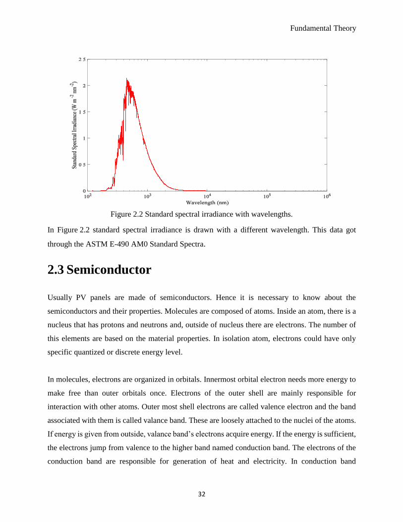
Fundamental Theory

32

Figure 2.2 Standard spectral irradiance with wavelengths.

In Figure 2.2 standard spectral irradiance is drawn with a different wavelength. This data got

through the ASTM E-490 AM0 Standard Spectra.

2.3 Semiconductor

Usually PV panels are made of semiconductors. Hence it is necessary to know about the

semiconductors and their properties. Molecules are composed of atoms. Inside an atom, there is a

nucleus that has protons and neutrons and, outside of nucleus there are electrons. The number of

this elements are based on the material properties. In isolation atom, electrons could have only

specific quantized or discrete energy level.

In molecules, electrons are organized in orbitals. Innermost orbital electron needs more energy to

make free than outer orbitals once. Electrons of the outer shell are mainly responsible for

interaction with other atoms. Outer most shell electrons are called valence electron and the band

associated with them is called valance band. These are loosely attached to the nuclei of the atoms.

If energy is given from outside, valance band’s electrons acquire energy. If the energy is sufficient,

the electrons jump from valence to the higher band named conduction band. The electrons of the

conduction band are responsible for generation of heat and electricity. In conduction band

Fundamental Theory

33

electrons are free to move. The energy difference of an electron at valence band and at the

conduction band’s innermost shell is called band gap.

There are three types of materials named insulator, conductor, and semiconductor. Insulator has

wider band gap than any other type of materials. The band gap in materials is more than 3eV. In

conductor materials, there is no band gap, valence and conduction band overlap with each other.

Diagrams of different energy bands for conventional materials [Kalogirou09, Zeman10, Zeman14,

Hu09] is shown in Figure 2.3.

Empty conduction band

Full valance band

Maximum part of conduction

band is empty

Maximum part of valence

band is full

Conduction band is almost full

Valance band

Insulator Semiconductor Conductor

Energy gap

> 9eV Energy gap~ 1eV

Figure 2.3 Diagrams of different energy bands for conventional materials. (a)Insulator

(b)conductor (c)semiconductor.

Semiconductors have less band gap than 3eV. Semiconductor associations have few properties

like metals and few characteristics from insulators. This recombination of different essential

properties from metal and insulator, makes the semiconductor a particular kind of material.

There are two types of semiconductors; named as:

a. Intrinsic semiconductor.

b. Extrinsic semiconductor.

Fundamental Theory

34

Intrinsic semiconductor

Intrinsic semiconductors have no impurity. This is a pure form of semiconductors, and they are

chemically pure and undoped. The number of excited electrons is equal with the number of holes

in it. Pure silicon and germanium are an example of an intrinsic semiconductor. These types of

materials’ band gap are minimal, and electrons can gain sufficient energy and jump from valence

band to conduction band in the room temperature condition. The known symbol for intrinsic

semiconductor is ni; it refers as the intrinsic carrier density. Different types of Silicon [Warwick10,

Answers10, Hu09] is shown in Figure 2.4.

Figure 2.4 Different types of Silicon.

In Figure 2.4, it shows the pure silicon that is included in intrinsic semiconductor and the n-type

and p-type silicon that counts in the extrinsic semiconductor.

Temperature has an influence on intrinsic carrier density. The density of charge carrier in intrinsic

semiconductor [Kalogirou09] is given by:

𝑛𝑖 = 𝑁𝑐 [exp (𝐸𝑓−𝐸𝑐

𝑘𝑇)] (2.2)

where, 𝑁𝑐 = 2(2𝜋𝑚𝑒𝑘𝑇

ℎ2 )

3

2

𝑝𝑖 = 𝑁𝑣 [exp (𝐸𝑣−𝐸𝑓

𝑘𝑇)] (2.3)

where, 𝑁𝑣 = 2 (2𝜋𝑚ℎ𝑘𝑇

ℎ2 )

3

2

where, ni is the carrier density, pi is hole density, 𝑁𝑐 is the effective density when states is the

conduction band, 𝑁𝑣 is the effective density when states in the valance band, value of k is

Fundamental Theory

35

1.38 × 10−23J𝐾−1 is the Boltzmann constant, Ef is Fermi energy, Ev is energy level of valence

band, Ec is energy level of conduction band, T is temperature, h is Plank constant and its value is

6.624 × 10−34 Js, me is effective mass of the electron and mh is effective mass of the hole.

Extrinsic semiconductor

An extrinsic semiconductor is an impure one that is created by doping. It has excess electrons or

holes. Electricity conductivity is high for this type of materials. Depending on the doping process,

there are two types of extrinsic semiconductors. They are an n-type and p-type.

If the semiconductor is doped by materials which have more electrons in the valence band, it is

called n-type. In n-type, there are more electrons. And if it is doped by the materials which have

fewer electrons in the valance band are called p-type that has positive particles named holes. In p-

type, there are more holes.

In both of the types electrons and holes could move freely. These both types together make the p-

n junction. In the junction, from n-type electrons try to go to p-type to fill the holes and the holes

from p-type spread to the n-type side. After occurring this, the negative charge of the p side restricts

the movement of extra electrons from n side. There are positive charges at the junction of n side

that ease the movement of negative charges from p side. In this way this p-n junction works as a

diode. The n-type semiconductor is known as a donor because it gives extra electrons in work to

fill the hole and p-type semiconductor is known as an acceptor because it gets electrons to fill its

holes [Kalogirou09, Hu09].

2.4 Semiconductor Diode

Diodes are consisting of p-type and n-type semiconductors. When a semiconductor is made of n

materials region and a p material region. This n-p together make a p-n junction, in the n region

there are many electrons, and the p region has many holes. In the combination of p-n, there is a

significant number of positive and negative ions created near the p-n junction and created the

depletion region. p-n junction diode is shown in Figure 2.5 [Kalogirou09, Eon12].

Fundamental Theory

36

Figure 2.5 p-n junction diode.

Real and ideal diode

Real diode and ideal diode both have two terminals named anode and cathode. Anode is the

positive and cathode is the negative terminal as shown in Figure 2.6 [Kalogirou09, Eon12].

ID

+ VD -

Anode Cathode

Figure 2.6 Symbol for diode.

where VD is voltage over the diode and ID is the current flows from anode to cathode. It is in

forward biased when the positive polarity is applied at the anode, and negative is at the cathode.

In this time, it is in conducting process. In the other direction when the positive polarity applied at

the cathode and negative polarity applied at anode then the diode is at reverse bias. In this time, it

is not conducting process.

A diode works like a switch, in the time of forward biasing it acts like a switch is on and when the

reversed bias is given, then it acts like an open switch. For understanding the diode, it is vital to

know the current-voltage behaviors of it. Real voltage and current is shown in Figure 2.7

[Electronicsdesignhq18].

Figure 2.7 Voltage-current curve of real diode.

Voltage and current curve for ideal diode is shown in Figure 2.8 [Electronicsdesignhq18].

Fundamental Theory

37

Figure 2.8 Voltage-current curve of ideal diode.

Current-voltage characteristics of diode

It is considered that diode is a device that has a little resistance in one direction called forward bias

and very high resistance in other called reverse bias. The diode law named as Shockley diode is

given by:

𝐼 = 𝐼𝑜 (𝑒𝑉𝐷𝑛𝑉𝑇 − 1) (2.4)

where, I is the diode current, I0 is the reverse bias saturation current, VD is the voltage across the

diode, VT is the thermal voltage, n is the diode ideality factor.

In the ideal diode case, the value for the n is 1. The thermal voltage is given by:

𝑉𝑇 =𝑘𝑇

𝑞 (2.5)

where, k is the Boltzmann constant, T is the absolute internal temperature of the p-n junction, q is

the electron charge. Different regions of a diode are shown in Figure 2.9 [Lu17,

ElectronicsTutorials17].

Figure 2.9 Different regions of a diode.

Fundamental Theory

38

Figure 2.9 shows different regions of a diode, right part of the graph gives the forward region, and

cut-in voltage value is 0.5 V. The diode is fully conduction at voltage value 0.7 V. Diode has

dependency on the temperature. For a given current, voltage decreases in increasing temperature.

For a given voltage, current increases when the temperature increases.

In the situation, when the voltage is greater than zero (V > 0) then it is in forwarding bias region.

The resistance that linked with the diode is near to zero. In the ideal diode curve, the slope of

forwarding bias is infinite.

In the condition when a voltage is less than zero (V < 0) the diode works in the reverse bias region

and the resistance linked with the diode is an infinite state. The reverse biased slope is zero for

ideal diode curve.

In reverse biased condition there is a voltage point where the diode performs appreciably in

reverse. This voltage point is called Zener voltage.

2.5 Photovoltaics

Photovoltaic (PV) is known as the source of renewable energy that converts solar energy to

electrical energy. Usually it is a semiconductor device, and simple in its working principle.

Utilizing the photovoltaic effect, it converts sunlight to electricity. The source of the power for it

is free and abundant. For sustainable development it has got importance. There are different types

of PV cells exist, and new types of research are improving the performance by converting most of

the solar radiation to power. Different types of PV technologies are shown in Figure 2.10

[Ahmed17, Foles17].

Fundamental Theory

39

PV Cell Technologies

Crystalline silicon Thin film Compound Structure

Compound semiconductor

GaAs-basedMono-crystalline

Multi-crystalline

Amorphous-Si

Copper Indium Gallium

diSelenide

Cadmium Telluride

Titanium dioxide

Figure 2.10 Different types of PV technologies.

Most of the PV cells are from different semiconductors and combination of them. Most of them

are different kinds of composition of silicon components. Thin film is a kind of technology that

decreases the size and also makes the panel cheap. This technology has used Amorphous Silicon,

Cadmium Telluride, Titanium Dioxide etc. There is also compound structure, that have more than

two junctions and they show good performance. There is organic solar cell technology, that makes

it very cheap and flexible. But in the performance, it hasn’t shown good efficiency.

Working principle

The sunlight come to the earth as electromagnetic wave and hit on the PV panel surface. The light

reaches the PV materials; it consists of packets of energy named as photons. After light hit on the

PV surface different events are happened; a. It can reflect, b. It can absorb and c. It can transmit.

If the photon is absorbed by the valence electrons of the atoms of PV materials, i,e. when the

photon energy is sufficient enough then it help the electron to jumps from the conduction band and

travelled freely. In semiconductor with p-n junction when there is electric field is applied across

the front and back of the materials and external load is connected, then electron flows throw the

load to complete the circuit. If the photon has less energy that needs to generate to flow electron,

then this photon energy is absorbed by electron. It increases kinetic energy that causes increase of

heat in the device.

Fundamental Theory

40

Photovoltaic device working process is shown in Figure 2.11 [Kalogirou09].

p-type n-type

Electron flow

directionI

External Load

V Figure 2.11 Photovoltaic device working process.

Figure 2.11 shows a photovoltaics cell arrangement having p-n junction, I shows current flow, V

shows voltage across the load. When photon having more energy than band gap hit on the surface

of a PV cell, it frees electrons with sufficient energy. Electron and hole pairs are created and when

they are enough near to p-n junction then the electric field make them split. Hole goes to p-type

side and electron goes to n-type side. In this condition when system is connected by wire with an

external load the current start to flow through the wire. As long the sunlight is there the current

continues to flow.

It is possible to calculate the number of photons from the intensity of light. The light is the

electromagnetic radiation, and it maintains the law of energy. The photon energy is given by:

𝐸𝑝 = ℎ𝑣 (2.6)

where, h is the Planks constant is 6.625 × 10−34Js, 𝑣 is frequency (s-1) and is expressed as 𝑣 =𝑐

𝜆

Then it becomes,

𝐸𝑃 =ℎ𝐶

𝜆 (2.7)

where, C is the speed of light, 𝜆 is wavelength. The number of photons (np) could calculate the

intensity of light and the wavelength given by:

𝑛𝑝 =𝐼𝑝

𝐸𝑝 (2.8)

where, Ip is the intensity of light.

Fundamental Theory

41

Modeling of PV cell

Single PV cell is a small building block that made up the big PV power conversion system for

generating power. When the negative and positive lead is connected to a load, makes an electrical

circuit, there electrons flow completing the circuit.

The generated current in PV is named photocurrent (IL). In a simple single diode model of PV is

constructed with photocurrent source that is connected with a diode in parallel. The electrical

behavior of this part works like a p-n junction. The current generated from irradiance (G) is

proportional to the solar radiation that direct fall on the surface. Simple PV model has not counted

the series and shunt resistance. This simple model is possible to describe with Shockley diode

theory. PV is not a constant source of current. Simple single diode PV model [Sera07, Rashel17a]

is shown in Figure 2.12.

ID

IL I

D

G

V

+

-

T

Figure 2.12 Simple single diode PV model.

Figure 2.12 shows simple single diode PV model that has no series and shunt resistance. This

model is represented based on Shockley diode equation [Shockley61]. In Figure 2.12 G is the

irradiance. The diode current is given by:

𝐼𝐷 = 𝐼0[exp (𝑞𝑉

𝑛𝑘𝑇) − 1] (2.9)

According to the Kirchhoff’s current law, total incoming current and the outgoing current

summation are always zero. From Kirchhoff’s current law, the current generated from PV is given

by:

𝐼 = 𝐼𝐿 − 𝐼𝐷 (2.10)

Fundamental Theory

42

The total current is the photocurrent minus the diode current is given by:

𝐼 = 𝐼𝐿 − 𝐼𝐷 = 𝐼𝐿 − 𝐼0[exp (𝑞𝑉

𝑛𝑘𝑇) − 1] (2.11)

In (2.10), IL is photocurrent, ID is diode current, and I0 is dark saturation current, n is diode ideality

factor, q is electron charge, k is Boltzmann's constant, T is the cell temperature of the junction.

For characterization of PV cell, short-circuit (Isc) current and open-circuit (Voc) voltage have

considerable influence. When a voltage is zero then, Isc is equal to photocurrent (IL).

Therefore, 𝐼𝑠𝑐 = 𝐼 = 𝐼𝐿.

The simple model gives the value for PV output. A series resistance is added with simple PV

model. Four-parameter model of PV cell is shown in Figure 2.13 [Ahmed17].

ID

RsIL I

D

G

V

+

-

T

Figure 2.13 Four-parameter of PV cell model.

The four-parameter mathematical model gives the current-voltage characteristics of PV cell. The

total current is given by:

𝐼 = 𝐼𝐿 − 𝐼𝐷 = 𝐼𝐿 − 𝐼0[exp (𝑞𝑉+𝑞𝑅𝑠𝐼

𝑛𝑘𝑇) − 1] (2.12)

In (2.11), Rs is the internal series resistance in the PV equivalent circuit. For making more

approximate to get the output from it, needs a more sophisticated model that includes series and

shunt resistance. Five parameters single diode PV model is well known and most used to simulate

the PV cell. This model is the electrical equivalent of PV cell. It shows approximate behavior like

solar cells in a PV panel. Series resistance and shunt resistance is included in the parallel in the PV

Fundamental Theory

43

equivalent circuit and it becomes five parameters model of the PV cell. Five parameters model of

PV cell is shown in Figure 2.14 [Rashel17a].

RsIL

Rsh

Ish

I

G

V

+

-

ID

T

D

Figure 2.14 Single diode five parameters PV cell model.

In Figure 2.14, IL Photocurrent which is the current source for the circuit, single diode D which

have ID current across it, a series resistance Rs which represents the resistance in the cell, shunt

resistance Rsh is in parallel.

The current across the shunt resistance (Ish) is given by:

𝐼𝑠ℎ =𝑉+𝐼𝑅𝑠

𝑅𝑠ℎ (2.13)

For Figure 2.15, applying the Kirchhoff’s current law, the total incoming current and the outgoing

current summation are always zero. From Kirchhoff’s current law, the current generated from PV

is given by:

𝐼 = 𝐼𝐿 − 𝐼𝐷 − 𝐼𝑠ℎ (2.14)

After putting all the values, the total current is given by:

𝐼 = 𝐼𝐿 − 𝐼𝐷 − 𝐼𝑠ℎ = 𝐼𝐿 − 𝐼0 {exp [(𝑞(𝑉+𝐼𝑅𝑆)

𝑛𝑘𝑇)] − 1} − (

𝑉+𝐼𝑅𝑠

𝑅𝑠ℎ) (2.15)

In (2.15), the series resistance and shunt resistance is included. It is used for the different

simulations.

If the shunt resistance is much more significant than the load resistance, and series resistance is

much smaller than the load resistance, then it is possible to ignore their loss in the cell. When the

loss is ignored, then the series resistance and shunt resistance also could be ignored from the model.

Fundamental Theory

44

Then the total current is the difference between photocurrent and diode current and the equation

becomes like as same as (2.11). It is the ideal PV model without series and shunt resistance.

The current and voltage has different significant characteristics for PV model. The open circuit

voltage (Voc) is the voltage when the current is zero. The power output is also zero. The short-

circuit current (Isc) is the condition when the voltage is zero and power production is zero. Current

at maximum power (Imp) is the current when the PV gives the maximum power output, depending

on internal and environmental conditions. The voltage at maximum power (Vmp) is the voltage

when the PV gives the maximum power. Maximum power point (MPP) is important when the PV

gives the best output. This point depends on the different value that is related to internal and

environmental parameters.

Analytical approach of five parameter PV cell model

An analytical approach is carried on to solve the (2.15) to get the parameters values.

The (2.15) is re-writes as [Ahmed17]:

𝐼 = 𝐼𝐿 − 𝐼0 [exp (𝑞𝑉+𝑞𝐼𝑅𝑠

𝑛𝑘𝑇) − 1] −

𝑉

𝑅𝑠ℎ−

𝐼𝑅𝑠

𝑅𝑠ℎ (2.16)

From (2.16), it is possible to write as below:

𝐼 +𝐼𝑅𝑠

𝑅𝑠ℎ+ 𝐼0 [exp (

𝑞𝑉+𝑞𝐼𝑅𝑠

𝑛𝑘𝑇)] = 𝐼0 −

𝑉

𝑅𝑠ℎ+ 𝐼𝐿 (2.17)

After going through different calculation and divided both sides of (2.17) with I0 is written as:

(𝑅𝑠+𝑅𝑠ℎ

𝐼𝑅𝑠ℎ) 𝐼 + (exp (

𝑞𝑉+𝑞𝐼𝑅𝑠

𝑛𝑘𝑇)) = 1 −

𝑉

𝑅𝑠𝐼𝑠+

𝐼𝐿

𝐼0 (2.18)

From (2.18), left side part have I the current, that makes the equation impossible to solve

analytically. It is possible to solve the equation in another way by making the series resistance Rs

to zero makes the term zero that has contained the Rs. The (2.18) then becomes as:

𝐼 =1−

𝑉

𝐼0𝑅𝑠ℎ−(exp(

𝑞𝑉

𝑛𝑘𝑇))+

𝐼𝐿𝐼0

(𝑅𝑠ℎ𝐼𝑅𝑠ℎ

) (2.19)

This is the analytical solution for the output current from five parameters PV cell model. It is

difficult to find an analytical solution for PV model[Ahmed17].

Fundamental Theory

45

Datasheet values for a PV cell

In this work, the datasheet values are used to build a computational model to characterize the PV

cell behavior. This characterization is done under standard condition. Then it included variable

internal parameters value and environmental parameters value.

The five parameters single diode cell model is used for getting simulation result, and it gives an

excellent result that is close to the real scenario under standard condition. This model is used for

sensitivity analysis of internal and environmental parameters. In this work, crystalline silicon solar

cell is used, the values of different parameters are obtained from the datasheet. The values for a c-

Si cell under STC condition is given in Table 2.1.

Table 2.1 Data for the c-Si PV cell at STC.

Technology Vm Im Voc Isc ∞sc

c-Si 0.55 V 1.98 A 0.64 V 2.1 A 1.7 mA/ºC

Table 2.1 values used for doing the simulation under different internal and environmental

conditions. Isc is the value for short circuit current, Voc is the open circuit voltage, and Vmp is

maximum voltage, Imp is the current when there is maximum power output from the PV cell.

Below Table 2.2 gives the typical physical properties of a c-Si PV cell. The specific area is given

in millimeter unit. Thickness is in micrometer unit. Different layers doping type are also specified.

Physical properties of a c-Si PV Cell is given in Table 2.2 [Ahmed17].

Table 2.2 Physical properties of a c-Si PV Cell

Name Description Unit

Doping Type p-type N/A

Thickness 300 [μm]

Area 100 × 100 or 120.5 ×120.5 [mm2]

Top side doping n+ type N/A

Backside doping p+ type N/A

Reduced thickness 250 [μm]

Reduced Area 200 × 200 [mm2]

Fundamental Theory

46

After manufacturing the PV device, industry tests different values for the PV and it releases the

datasheet. These values from datasheet are useful to understand the behaviors of PV cell under

different condition and choose the perfect condition to get maximum power. Typical structure of

a c-Si solar cell is shown in Figure 2.15 [Zeman14].

Figure 2.15 Typical structure of a c-Si PV cell.

Using (2.15) and the values from Table.2.1, making simulation under STC condition and get the

Figure 2.16 of voltage-current, and get the Figure 2.17 of voltage-power. Voltage and current

curve for single diode five parameters PV cell is shown in Figure 2.16 [Rashel17a, Rashel16b].

Figure 2.16 Voltage-current curve for single diode five parameters PV cell model.

Fundamental Theory

47

Figure 2.16 shows the ideal behavior of PV cell, the short circuit current (Isc) value is 2.1 A, there

the voltage is zero. The open circuit voltage (Voc) value is 0.64 V, there the current is zero. Voltage

and power curve for single diode five parameters PV cell voltage-power behavior is shown in

Figure 2.17 [Rashel17c].

Figure 2.17 Voltage-current curve for single diode five parameters PV cell model.

Figure 2.17 has the total power graph including the maximum power point where the PV reaches

the peak point of the power. The maximum power (Pmax) value is 1.1 W and the voltage at

maximum power (Vmp) value is 0.56 V.

The Pmax is the point where the load resistance is at the most favorable point. At Pmax the power

output through the PV to the resistive load is maximum and is given by:

𝑃𝑚𝑎𝑥 = 𝐼𝑚𝑝 × 𝑉𝑚𝑝 (2.20)

where, 𝐼𝑚𝑝 is the current at 𝑃𝑚𝑎𝑥 and 𝑉𝑚𝑝 is the voltage at 𝑃𝑚𝑎𝑥.

This maximum point also given by:

𝑃𝑚𝑎𝑥 = 𝐼𝑠𝑐 𝑉𝑜𝑐 𝐹𝐹 (2.21)

where, FF is the fill factor:

𝐹𝐹 =𝑃𝑚𝑎𝑥

𝐼𝑠𝑐 𝑉𝑜𝑐=

𝐼𝑚𝑝 𝑉𝑚𝑝

𝐼𝑠𝑐 𝑉𝑜𝑐 (2.22)

Fundamental Theory

48

The fill factor gives the real measurement of voltage and current characteristics. If the quality of

the PV is fair enough, then it should be greater than value 0.7 V [Kalogirou09]. Depending on the

environmental condition its values decrease.

2.6 Sensitivity Analysis and Error Function

In all measurement systems, there is always the presence of uncertainties. All of them, sensitivity

analysis is the study to identify the uncertainty of inputs for a particular model’s (mathematical

model and computational model) output value. It determines the impact of different values of an

independent parameter to a dependent variable under specific circumstances. Sensitivity analysis

gives critical information about independent parameters. The boundary values for an independent

parameter takes from the real-time scenario or a valid source for the particular system. Inside a

system when one parameter is varying to implement different circumstance, effects imposed on

the output. In the real-time system, between entire workflow there are many events occurred. The

changes that take place because of changing the values of the parameters values. Flow chart for

Sensitivity Analysis is shown in Figure.2.18.

Simulation model

Different

parameters

Is model uncertainty

and sensitive cross

threshold level

Start

Sensitivity analysis

End

Yes

No

Give feedback and update

model

Figure 2.18 Flow chart of sensitivity analysis.

Fundamental Theory

49

This flow chart shows the sensitivity analysis of different parameters that are includes in the model.

There are valid purpose and importance to go through sensitivity analysis that recalculated the

outcomes with alternative assumptions determining the impact of a parameter. Sensitivity analysis

helps to improve a model that includes:

a. Increase the understanding between input and output parameters of a model;

b. Reduce the complexity of a model by identifying the critical parameters;

c. Identify the error in the model through observing the unexpected relations between input

and output parameters;

d. Reduction of the uncertainty of the model, giving more attention on the parameters that

make a significant change to output;

e. In a high dimension of inputs space, identify an area that optimized the model to give the

best output for a model;

f. Analyze the strength of the results of a model under uncertainty;

g. Identify valuable parameters in a model.

In this work, to understanding parameter effects to the system is identified using the sensitivity

test, through error function. Error function of a parameter gives the precise value how an output

value is sensitive to that parameter. The figure describes a sample graph of a single parameter with

an error function, gives the idea about the certainty of output in that value position. Parameter with

sensitivity function is shown in Figure 2.19 [Rashel17a, Rashel17c].

Figure 2.19 Parameter with error function for identify sensitiveness.

Fundamental Theory

50

The main idea is to identify the effect of the parameters for the PV system through the sensitivity

identification. The sensitivity is tested through the error function 𝐸(𝐼), it is a function of output of

PV, that gives the difference of output from standard condition to the different variable conditions

where the parameters values are changed. Below the equation is described for error function. This

helps to identify sensitivity for a particular parameter of a model given by:

𝑃 = 𝑉𝑒𝑐𝑡𝑜𝑟 𝑜𝑓 𝑝𝑎𝑟𝑎𝑚𝑡𝑒𝑟𝑠.

𝐼𝑖𝑃 =The model estimated current with optimal values.

𝐼𝑖𝑀 = 𝑀𝑒𝑎𝑠𝑢𝑟𝑒 𝑣𝑎𝑙𝑢𝑒 (𝑣𝑎𝑟𝑦𝑖𝑛𝑔 𝑡ℎ𝑒 𝑣𝑎𝑙𝑢𝑒 𝑜𝑓 𝑎 𝑝𝑎𝑟𝑡𝑖𝑐𝑢𝑙𝑒𝑟 𝑝𝑎𝑟𝑎𝑚𝑒𝑡𝑒𝑟 𝑖𝑛 𝑠𝑖𝑚𝑢𝑙𝑎𝑡𝑖𝑜𝑛).

For a specific parameter the error function is calculated as below:

𝐸(𝑃)1 = (1

𝑛√∑ (𝐼𝑖𝑃 − 𝐼𝑖𝑀)2𝑛

𝑖=1 )

𝐸(𝑃)2 = (1

𝑛√∑ (𝐼𝑖𝑃 − 𝐼𝑖𝑀)2𝑛

𝑖=1 )

For nth parameter, it is express as:

𝐸(𝑃)𝑛 = (1

𝑛√∑ (𝐼𝑖𝑃 − 𝐼𝑖𝑀)2𝑛

𝑖=1 )

In general, it is expressed as:

𝐸(𝑃)1…..n =1

𝑛√∑ (𝐼𝑖𝑃 − 𝐼𝑖𝑀)2𝑛

𝑖=1 (2.23)

where Istd is the output under standard condition.

Calculation of the sensitivity of different parameters through error function is given by:

Step 1: Input, P1 = Analyzed Parameter

Step 2: Input, O1.....On = Other Parameters

Step 3: Calculating, IiP = output value calculation from standard value of parameter

Step 4: for i = 1 to n

IiM, 1...n= output value calculation from variable P1,1...n

end

𝑃 =

[

𝐼𝐿𝑅𝑠

𝑅𝑠h

𝑇𝑐𝑒𝑙𝑙𝑎

𝐼𝑠 ]

Fundamental Theory

51

Step 5: Output, 𝐸(𝑃)1…..n =1

𝑛√∑ (𝐼𝑖𝑃 − 𝐼𝑖𝑀)2𝑛

𝑖=1

Sensitivity analysis is done for internal parameters and environmental parameters, those are related

with the model of PV cell and effect its performance. This is used to identify the valuable, sensitive

variable in the system. After identifying the valuable parameters, it is possible to give more

concern to improve the quality of model and invent system to improve the situation for getting

more power from the PV system.

2.7 Internal Parameters

Five parameters PV cell model is represented by (2.15) that is equivalent representation of

Figure 2.14 that is consists of different parameters. Photocurrent (𝐼𝐿), internal cell temperature (𝑇),

diode idelaity factor (𝑛), Series resistance (𝑅𝑆), shunt resistance (𝑅𝑠ℎ) and saturation current (𝐼0)

are internal parameters. Variation of these parameters have impact on PV system performace.

Using sensitivity analysis, these parameters sensitivity to the system is identified. For identifying

less sensitive parameters in work, all the parameters IL, T, n, Rs, Rsh and I0 are tested through the

𝐸(𝐼). It gives clear idea about the sensitiveness of parameters of PV model. Flowchart gives clear

picture to get sensitive internal parameters is shown in Figure 2.20 [Rashel17a].

Figure 2.20 shows flow chart to identify sensitive parameters from five parameters PV model and

get a simplified model of PV. This is simulated in Matlab. All the internal parameters are going

through the error function to see their sensitivity. After analyzing the sensitivity of each parameter,

creates a new simplified model.

Fundamental Theory

52

Figure 2.20 Flowchart describing the model to get sensitive parameters for internal model.

Photocurrent

The photocurrent is produced in PV device from the sunlight when the light strikes on the PV

surface with enough quantity of energy. This current is get from the negative terminal of the PV

cell. But according to the circuit model, there is also diode current and current across the shunt

resistance, those are minus from the photocurrent (𝐼𝐿), that gives the final current output from a

PV. Photocurrent mainly depends on irradiance (G) and temperature and it is given by:

𝐼𝐿 = (𝐺

𝐺𝑛)[𝐼𝑠𝑐 + 𝐾𝑙(𝑇 − 𝑇𝑛)] (2.24)

where, G is irradiance, Gn is irradiance at standard test condition (STC), Kl is temperature current

coefficient, T is working internal temperature of cell and Tn is internal cell temperature at STC and

Isc is short circuit current. The photocurrent is the primary current that produces from the PV cell

and keeps the wheel moving for the system.

Start

Internal Parameters Array

For i=1,i<=6,i++

End of the for Loop

Single Diode Model without

less Sensitive Parameters

Store

Sensitive

Parameters

Stop

Continue TrueIs the Parameter Sensitive?

(Using Error Function)

Sensitivity Analysis

False

Fundamental Theory

53

Internal cell temperature

A typical PV panel efficiency is 15%. Rest of the irradiance convert to heat. This heat has a reverse

effect on the performance of PV. Cell temperature is a critical part; its fluctuation shaves a

significant impact on PV output. In (2.9) and (2.15) both model have this parameter and it has

significant importance on the performance of PV cell. This is also analyzed through the error

function to understand the sensitivity with the model.

Ideality factor

Diode ideality factor (𝑛) is used in (2.14) and change of this value makes change in the value of

diode current (ID). It is the measurement of a diode how it is close to ideal diode. There are many

moving carriers over the p-n junction of PV. The value of this parameter varies in accordance with

its diode behavior. PV model does not follow the ideal diode behavior so ideality factor is

introduced to describe its deviation from the ideal characteristics. Usually the value of diode

ideality factor varies in the range between 1 to 2. It is important because changing of the value of

the parameter, changes the value of PV output.

Saturation current

Following (2.15), Saturation current (𝐼0) has a high impact on the PV power conversion. 𝐼0

variation effects the output of PV. The value of 𝐼0 is given by:

𝐼0 = 𝐼0𝑛 (𝑇

𝑇𝑛)3

exp [𝑒×𝐸𝑔

𝑛×𝑘(

1

𝑇𝑛−

1

𝑇)] (2.25)

where, T is working internal temperature of cell, Tn is internal cell temperature at STC, Eg is band

gap, n is diode ideality factor, k is Boltzmann constant, e is the value of electron charge and Ion is

internal diode current is calculated using (2.28). Ion is express as:

𝐼𝑜𝑛 =𝐼𝑠𝑐

exp(𝑉𝑜𝑐

𝑛×𝑉𝑇) (2.26)

where, Isc short circuit current, Voc is open circuit voltage and VT is thermal voltage that calculated

using (2.5).

Fundamental Theory

54

Series resistance

Series resistance (𝑅𝑠) is a part of the single diode five parameters PV cell model. Changing of the

value makes changes in the value of the output but it is not significant amount. The series resistance

has less dependency on irradiance and temperature [Soto06]. When the load resistance is bigger

enough then the effect of series resistance is not significant at all [Kalogirou09].

Shunt resistance

Shunt resistance (𝑅𝑠ℎ) is situated at the parallel to the diode and it is included in the single diode

five parameters PV cell model. It is enormous in quantity, then the load resistance. The effect to

the total output also becomes less significant. This parameter’s sensitivity test is done through

error function.

2.8 Environmental Parameters

Irradiance, ambient temperature, wind speed, cloud, humidity, and perspiration are different

environmental parameters that have an impact on PV power conversion. In this work, irradiance,

ambient temperature, and wind speed are analyzed through error function to identify their

sensitivity to PV power conversion. Other parameters of the environment were not analyzed. Work

with other parameters is an ongoing process of the work but were not included in the thesis. For

real-time data, the weather station at University of Évora’s data has been used.

Irradiance

Irradiance is the power per unit received by a solar power conversion system. This power is

received in the form of electromagnetic radiation. It is measured on the Earth surface and, is the

environmental factor that is the primary energy for producing electricity. With sufficient power

solar rays strike on the PV surface and generate electricity. In (2.24), photocurrent is depending

on the irradiance. More the sunlight more the electricity will be produced. Name of measurement

instrument of irradiation is by radiometry device. On average a PV cell can convert 15% of

irradiance to be utilized. The generated heat in the PV cell becomes the obstacle for the

performance of the system. It is vital to understand the irradiance with other environmental

parameters. Total irradiance is the measurement of all wavelengths per area that fall on the upper

Fundamental Theory

55

atmosphere of Earth. This gives the total solar power. But for the PV system, global horizon

irradiance is counted. It is the total irradiance that comes from the sun on a horizontal surface on

Earth. It is given by:

𝐺𝐻𝐼 = 𝐷𝐻𝐼 + 𝐷𝑁𝐼 × cos (𝑧) (2.27)

where, GHI is global horizontal irradiance, DHI is diffuse horizontal irradiance and DNI is direct

normal irradiance.

The SI unit for irradiance is watt per square meter, and it is expressed as W/m2. Yearly (31st

December 2016 to 30th December 2017) irradiance data from University of Évora Weather station

is shown in Figure 2.21 [Clima18].

Figure 2.21 Sequential daily average irradiance of year 2017.

Figure 2.21 shows the total irradiance all over the year for a specific area. Middle of the year the

irradiance is more than any other time of the year, but in the same time, the temperature also gets

very high. Pyranometer is shown in Figure 2.22 [Clima18].

Fundamental Theory

56

Figure 2.22 Pyranometer.

Ambient temperature and effects on cell temperature

Ambient temperature is a significant factor for PV performance. This parameter is easily measured

by a thermometer. In the equation, it is possible to calculate the value of cell temperature knowing

the ambient temperature. The increase of ambient temperature increases the cell temperature.

There is a propositional relationship between ambient temperature with cell temperature is given

by [Rashel18b].

𝑇𝑐𝑒𝑙𝑙 ∝𝑇𝑎𝑖𝑟

𝑣𝑤𝑖𝑛𝑑 (2.28)

where Tcell is cell temperature with ambient condition, Tair is air temperature of surrounding and

𝑣𝑤𝑖𝑛𝑑 is wind speed. The (2.28) shows that cell temperature with ambient temperature is

propositional to ambient temperature and inverse proportional to wind speed. It is one of the

important parts of PV conversion system. Tcell value depends on irradiance, ambient temperature,

and wind speed. Other environmental factors is not take in account for this model and simulation.

Using these parameter values the cell temperature with ambient condition value is calculated and

given by:

𝑇𝑐𝑒𝑙𝑙 = 𝑇𝑎𝑖𝑟 + 0.035 × 𝐺 (2.29)

Where, Tcell is cell temperature with ambient condition, Tair is ambient temperature and G is the

irradiance.

Tcell is calculated with wind speed is given by:

𝑇𝑐𝑒𝑙𝑙 = 𝑇𝑎𝑖𝑟 + (0.32

8.91+(2 × 𝑣𝑤𝑖𝑛𝑑)) × 𝐺 (2.30)

Where G is the irradiance and 𝑣𝑤𝑖𝑛𝑑 is wind speed. It is observed that cell temperature rises with

irradiance and ambient temperature. [Migan13]. In (2.30), it is clear that Tcell is directly related to

𝑣𝑤𝑖𝑛𝑑. Tcell has directly relation with the PV power conversion system.

Fundamental Theory

57

Getting knowledge about ambient temperature is essential to create an improvement in the model

of PV and is vital to predicting the PV power conversion more precisely. Yearly (From 31st

December 2016 to 30th December 2017) temperature data from University of Évora Weather

station is shown in Figure 2.23 [Clima18].

Figure 2.23 Sequential daily average temperature of year 2017.

Figure 2.23 shows one-year temperature of a specific area, and it has very close behavior like

irradiance. There is a different unit that uses as SI unit for temperature, from the most used is

Celsius (C) and Kelvin (K). 0-degree Celsius is equal to 273.15 Kelvin. Vaisala weather station

with temperature sensor is shown in Figure.2.24 [Clima18].

Figure 2.24 Vaisala weather station with temperature sensor.

Fundamental Theory

58

Figure 2.24 is a portable weather station that is light and flexible and also has a USB port to connect

with computer. Its software directly gives the values of different environmental parameters with

temperature value.

Wind speed

Wind speed is the flow velocity of the wind. It is one of the fundamental quantity of atmosphere.

The behavior of air is its flows from high pressure to low pressure, and it caused wind speed. Wind

speed is measured by an anemometer. It is already identified that Wind speed has effect on the PV

and in (2.30) wind speed is needed to calculate the cell temperature with ambient condition. Tcell

is directly related to wind temperature, and it is inverse proportional to wind speed. For improving

the performance of PV, this parameter plays a vital role. Wind speed is a natural process, it is

possible to predict the wind speed and that helps to predict the PV power conversion more

accurately. Yearly (From 31st, 2016 to 30th Dec 2017) wind speed data from University of Évora

Weather station is shown in Figure 2.25 [Clima18].

Figure 2.25 Sequential daily average wind speed of year 2017.

Figure 2.25 shows the yearly wind speed. It does not follow any defined pattern, and it is very

random. Wind speed is measured in meter per second (m/s). Anemometer is shown in Figure 2.26

[Clima18].

Fundamental Theory

59

Figure 2.26 Anemometer.

Figure 2.26 shows Anemometer, it is the device that measures the wind speed. This device is

connected to central system to collect data in real-time.

2.9 Non-constant Load

An electrical load is the part of an electrical circuit which consumes the electric power of the

electric system. If PV is not connected to the battery and direct connection is to the load. In this

time if the load is varied with the use of power then it becomes a variable load for PV system and

become the non-constant load. The non-constant load has an effect on the maximum power point

of the PV Panel. Generally, with a controller, this non-constant load’s effect is minimized to get

MPP. But in the stand-alone system, if PV has a direct connect with the load then the MPP varies

with the load behavior. It is important to understand the relationship between maximum power

point and non-constant load.

This work is done using a PV panel in the laboratory. The PV panel is connected with different

resistances having different values. It connects with a breadboard that connects with DAQ. The

DAQ measures the open-circuit voltage. Based on the open-circuit voltage Matlab sends request

to signal generator for generating signal to measure the voltage-current under specific load over

different point. This same work is continuing with different resistances and store the data for

analysis.

Fundamental Theory

60

2.10 Shadow of Obstacle on PV Panel

Shadow of obstacle on the PV surface makes the performance of the PV cell deficient, and in some

time it becomes zero. There could be different types of obstacles around the PV; these obstacles

could be shadows or dust or physical damage of cells. All of these factors decrease efficiency and

performance of PV dramatically. In this work all the things those create barrier to reach the

irradiance to PV conducting surface are named as obstacles. Identification of different types of

obstacles is critical for remotely control a big PV plant. This helps to identify the fault in PV

panels.

Few obstacles are temporary, and few of them are permanent. Temporary obstacles are

environmental obstacles, like clouds, flying birds, etc. There are permanent obstacles also exist,

those are not removable without human interaction, like dust, damage of cells.

Obstacles are divided with dependency of time variable,

a. Time-dependent obstacles;

b. Time-independent obstacles.

Time-dependent obstacles

Time-dependent obstacles are depending on the time change the obstacles behavior. With time this

type of obstacles moves away or stay, like a cloud, flying object shadow, etc. These type of

obstacles are expressed with the variation of time given by:

𝑃𝑉𝑜 𝛼 𝑂𝑏𝑠 (𝑡) (2.31)

In (2.31), in the situation of time-dependent obstacles the power generation from a PV panel is

proportional to the shadow of obstacles with time function. Shadow on PV panels as time-

dependent obstacle is shown in Figure 2.27 [Pixabay17].

Fundamental Theory

61

Figure 2.27 Cloud shadow on PV panels as time-dependent obstacle.

Shadow of bird as time-dependent obstacle is shown in Figure 2.28 [Blog17].

Figure 2.28 Shadow of birds as time-dependent obstacle.

Time-independent obstacles

This type of obstacles is not change their characteristics with the time. This type of fault of PV

panel should solve manually. Example of this type of faults is: thick layer of dust, physical damage

of a cell in a panel. Dust on PV as time-independent obstacles is shown in Figure 2.29

[Solarglassshield17].

Fundamental Theory

62

Figure 2.29 Dust on PV as time-independent obstacles.

Physical damage as time-independent obstacles is shown in Figure 2.30 [Homepower11].

Figure 2.30 Physical damage as time-independent obstacles.

Evaluation of obstacles

These two types of obstacles are classified and identified in this work with simulation. This work

is important to detect fault of a PV panel. In result part the details identification of obstacles is

given. The obstacles effect that create shadow on PV is simulated from two cells to a PV panel.

PV cells are analyzed through two cells connected in series and parallel condition. This model is

built under SIMULINK model. A PV panel consist of 72 cells is constructed to get significant

behavior using SIMULINK model.

Fundamental Theory

63

2.11 Experiment and Simulation

In this section, a detailed method is described for this work. Matlab, Simulink, measurement and

instrumentation system are used for the whole work. MATLAB code is generated for

computational modeling of PV cell. In Matlab error function modeling is created and the both

models are used to identify the sensitiveness of internal parameters. This PV model with

environmental parameters through error function the sensitiveness is analyzed. Correlation

between different parameters of the environment is demonstrated in Matlab. Also, the correlation

coefficient is calculated using person correlation function of this software.

For non-constant load analysis, the instrumentation and measurement system is used to get the

real-time data from PV panel. In this process different resistances are used to simulate non-constant

load. These data are analyzed in Matlab software to identify their significant.

Smart grid (SG) system needs information from different parts of PV plants that makes it more

efficient. More knowledge about the system helps to build efficient central system of SG.

Modeling of the system is vital to enrich the knowledge of SG that help to create intelligent

workable system.

Instrumentation and measurement

This part explains about the measurement and instrumentation process from the aspect of PV

measurement. Doing experiment with PV panel in a real environment and get the information with

more accuracy is important to identify the underlying behavior of the panel. There are many

different processes to do the work. Data acquisition (DAQ) and single generator are using in this

work to get the valid information from the real-time system. This information later on used for

identifying different characteristics.

In an instrumentation control system which included instrumentation, hardware for a connection

established between computer program and instrument, a computer that has the programmable

software. Mainly instrumentation control is a system to connect instruments with programmable

software using different hardware that makes connectivity and measures automatically from a

Fundamental Theory

64

third-party device. Instrumentation is essential in the field of automatic control and analyses

sensors and devices. Recent colossal development of instrumentation helps to understand different

system easily. It also helps to observe the devices remotely, and all the information that is occurring

in a system is automatically logged in a workstation. Later this information is used to understand

the behavior of environment both the internal and external of the system. Instrumentation interface

with computer for controlling is shown in Figure 2.31 [Autosofttech18].

Figure 2.31 Instrumentation interface with computer for controlling.

In this diagram, it shows that instruments connect with computer with different types of ports.

These ports could be easily readable by a computer that has drivers and application software to

read the data. Universal serial bus (USB) is a standard interface for enabling the communication

between instruments and the controller such as computer [Techopedia18]. It replaces a wide range

of interfaces in communication with the control system. Hot swapping makes USB more usable

that helps to control device continuing the work without a system reboot. Another important thing

about USB is it uses direct current (DC). In the experiments, the devices use USB port for

connecting with the computer. Data Acquisition interface with computer is shown in Figure 2.32

[Autosofttech18].

Figure 2.32 Data Acquisition interface with computer.

Fundamental Theory

65

This is a diagram for a pathway from sensor or device that needs to measure is connected with

DAQ that is connected with the workstation. It is smart enough to convert the Analog signal to

digital signal. Then the digital signal is recognized by computer using driver and application

software.

In this part of the work, MATLAB 2017a is used as programmable software that establishes a

connection with instrumentation. PC could be connected with USB, Ethernet, GPIB, serial ports.

GPIB port to USB is used for connection of this work. Drivers for different hardware had been

installed in the computer. Windows 7 environment is used for the work.

Data acquisition (DAQ) device plays an important role as a middleware that connects with sensors

and on the other hand connects with a computer which has its driver. The computer can understand

the signal from DAQ because it has the driver and the application software. Using application

software, the computer can decode the signal from DAQ and also sends the signal to

instrumentation part. NI USB-6009 DAQ is shown in Figure 2.33 [NI16].

Figure 2.33 NI USB-6009 DAQ.

Figure.2.33 is the NI USB-6009 data acquisition; it is very efficient and low-cost device with

multifunction that communicates with the computer. It connects with a computer with USB. Signal

description for NI USB-6009 is shown in Figure 2.34 [NI16].

Fundamental Theory

66

Figure 2.34 Signal description for NI USB-6009.

Figure 2.34 shows the signal description of the NI-6009 that is used for the work. It has 8 Analog

inputs at 12 or 14 bit and up to 48 KS/s and 2 Analog output at 12 bits. It has one 32 bit, 5 MHz

counter. Digital input-output lines 12 bit and 32-bit counter. The triggering technique is digital. It

is normally used for environmental data logging in a faster way. For lab experiment, it is an ideal

device.

AFG 320 is an arbitrary function generator. It has two independent channels. It loads waveforms

from Oscilloscopes using GPIB interface. From computer software interface using GPIB, different

waveforms are possible to generate as per requirement. AFG 320 function generator is shown in

Figure.2.35 [Tektronix16].

Figure 2.35 AFG 320 function generator.

Fundamental Theory

67

Figure 2.35 shows the AFG 320 function generator in operating mode and is connected with a

computer to generate required waveform. Matlab code is used to give command to the signal

generator for expected signal type, frequency and amplitude.

GPIB-USB-HS is an IEEE 488 controller device which is namely an instrument control device

that is possible to connect with computer with USB. In this work, this one is used to control

function generator instrument to generate a different kind of wave functions to measure different

point of PV panel. GPIB-USB-HS interface is shown in Figure 2.36 [NI16].

Figure 2.36 GPIB-USB-HS interface.

A low power PV panel is used for the experiment, and it is a monocrystalline silicon PV panel.

This output is suitable for the DAQ, if it is more power conversion one then the DAQ, that is used

would not work because it works in low voltage and low current situation. Monocrystalline silicon

PV panel is shown in Figure 2.37 [Rashel16a].

Figure 2.37 Monocrystalline silicon PV panel.

Fundamental Theory

68

Figure 2.37 shows a PV panel that is used for the experiment. It is used for different design scenario

of non-constant load. The PV is connected in a breadboard, and through the breadboard, it connects

with DAQ and function generator.

The computer had the driver software installed and the application software. The interface of

Matlab helps to do the work in a simple way. Matlab code is powerful enough to communicate

with both DAQ and GPIB. DAQ and signal generator connect to computer is shown in Figure 2.38

[Autosofttech18].

Figure 2.38 DAQ and signal generator connect to computer.

Figure 2.38 shows the working setup for the experiment’s different phenomenon. The computer

has drivers for all devices of National Instrumentation. Matlab is installed in the computer to do

the total work and gives the command to the function generator. DAQ is connected with the

computer and gives the information of the PV output to the computer, and it is translated through

Matlab. The resistance that is used for the experiments is inputted through the Matlab code.

The PV panel is connected with a breadboard. PV panel’s voltage measure to get the open circuit

voltage point and then it connects with a series resistance that works as a load resistance and the

voltage is measured for the load resistance. The function generator is connected with PV panel in

parallel and connected with resistance, and it generates a function to get the different point of the

I-V and P-V curve. This curve is for a specific scenario that is created in a lab to identify the

Fundamental Theory

69

importance of the situation. This setup is used for non-constant load and also for the obstacle

observe section.

The equivalent circuit diagram is drawn for the work. In the circuit diagram, the set up for the PV

panel is given. Circuit diagram for PV for measurement is shown in Figure 2.39 [Ahmed17].

Figure 2.39 Circuit diagram for PV for measurement.

Figure 2.39 shows the circuit diagram of the PV panel with instruments to measure the current and

voltage with non-constant load.

Both channel 1 (Ch1) and channel 2 (Ch2) of DAQ is connected with measurement system and also

with workstation by USB cable. Signal generator is connected with workstation with GPIB cable.

For measurement process, at first the signal generator is disabled from the system to measure the

open circuit voltage using, Ch1 (Channel 1). Then the value passes to the workstation. Using the

value computer calculate the amplitude and offset for the RAMP signal. Then workstation send

the value to the signal generator to start the measurement process. Signal generator generates

RAMP signal with specific value that comes from workstation. Then Ch2 (Channel 2) measures

the voltage. Using the value of additive resistance (R) and the value of voltage, workstation

calculate the current. In this process the frequency of the signal is 10 Hz. All the values are stored

in the workstation. These values are used to analyze and generated the I-V and P-V curves.

Measurement gives numerical value or point of an object or an event [Pedhazur91, VIM08]. This

numerical value must follow a standard unit system and in this way compare with any other same

type of event that happened in the world. In every field of research, engineering and daily day life

measurement is an essential part. Measurement has an international system of units. All over the

Fundamental Theory

70

world people try to maintain a standard way to make the numerical value in a specific way that is

recognizable by all.

In the experiment, measurement is done for all the instrument and devices that are related to the

experimental work. The instruments are connected with a computer with USB device and the

driver software are installed in the user computer and Matlab software is used as application

software. All data is collected through the Matlab interface. The values for measurement is given

to the Matlab output space. The data are collected and used for different analysis. These data are

used for making a different graph.

MATLAB and Simulink modeling

This work is done under windows 7 of the 64-bit version. For simulation of this thesis, Matlab and

Simulink are used. Matlab is one of the pioneer software for solving the mathematical equation

and for solving model in mathematical approach. It is a good software and support the massive

amount of facility to solve the diversified problem in the real-time system.

Simulink is block based simulation software that was developed by MathWorks. It is a block

diagram based modeling environment that simulates and analyses multi domain dynamic and

model-based system. [Mathworks15]. It has an enormous standard library that has built in a model

of different of real-time components. These small pieces of the model are used to create a big

system that is used to simulate real scenarios. The information of the Simulink system is transferred

to Matlab and analysis with different functions.

Fundamental Theory

71

2.12 Summary

This chapter describes essential theories in brief to make the work understandable to all. It also

narrates important formulation that is needed. Instrumentation and measurement systems are

described related to the experiment of the work. Detail simulation and modeling techniques are

described. Experimental setup and the theory includes in this chapter. Good and approximate

simulation and modeling of a system helps to get valuable information and gives estimated result

that is close to real-time value. Next chapter gives detail results and discussion of the work and

that is the continuation of the theory work.

CHAPTER

3

Results and Discussion

This chapter describes the outcomes of the work. In this journey, several results have been found.

These results are important to enrich knowledge about the PV power conversion system aiming to

improve the modeling and predicting power generation. The information about power generation

capacity of energy resources connected with Smart Grid is important. Among them, PV is

significant because of its nonlinear behavior; different types of internal and external behaviors

are simulated and experimented to better model a PV system. At the beginning of this chapter, the

work to identify the sensitive parameters of PV five parameters single diode model is introduced;

using the understand ability of sensitiveness, the simplified model is created and compared with

the standard one; later, three environmental parameters are analyzed to understand their effect

on the system and correlation between them is analyzed. Non-constant load is analyzed for

different circumstances using variable resistances. Finally, different types of obstacles are

classified and the behaviors are identified using Simulink models.

Results and Discussion

73

3.1 Introduction

Improvement of the PV power conversion system’s performance and efficiency has vital part that

is modeling of the PV system under different internal and environmental conditions. Presently, in

the operation phase, the efficiency of the system is not up to the mark, but a huge amount of plants

has established already generated and contributed with a significant amount of electricity. This

contribution to the energy sector enables a sustainable development grow. Green energy and

sustainable development is the ultimate solution to reach the Paris agreement goal [COP2115].

After a colossal research work, the efficiency of PV has reached 46% in the laboratory (NREL)

[NREL15]; in commercial places the efficiency reaches 22.5% under standard testing condition

(STC). The efficiency variation depends on technologies and surrounding environmental factor.

The power generation from the PV is entirely dependent on the environmental and ambient

conditions. There are different kinds of studies going on to improve the performance: a group of

researchers is working on new types of materials able to use the sunlight more efficiently

increasing the efficiency of PV cells and a group of people is trying to enhance conditions to

generate more power; due to the environmental deprived behaviors and poor performance of

electrical equipment under rapid changing condition, the power conversion rate decreased

significantly; sometimes become less than 5%, but this research aims to get optimized

environmental conditions and surroundings able to generate a maximum power equal to standard

conditions.

This work aims to identify the system’s internal strength, making the way to increase the

performance of PV, protect it from the external noise that decreases the performance dramatically.

Here, noise are those components that decrease the performance of the system; they can be internal

or external. There are internal parameters and environmental parameters directly related to the

power conversion. Among all these parameters, some of them have a positive effect, and others

have an adverse effect. There are different crucial issues where the system needs more focus to

improve the performance.

Results and Discussion

74

For establishing a PV plant that integrates with smart grid, it is essential to take care of all the

factors that have even a little influence on PV power generation. Smart grid system overview is

shown in Figure 3.1[Tranverter18, Rashel17a].

Figure 3.1 Smart Grid System.

SG is a control center that is connected with PV and also with other renewable energy sources in

bidirectional way utilizing all the possible procedure to improve the performance. Renewable

energy and SG is the right combination for a sustainable energy in the future. This work contributes

to understanding the PV and its surrounding environment, to identify the sensitive features and

faults.

Smart Grid system integrates with future predictable PV power conversion system is shown in

Figure 3.2 [Rashel16b, Rashel17a]. In the flow chart the process is as, first it collects the forecasted

data from the meteorological station on that day. This values are used with the single diode five

parameter model to estimate the PV power generation from the system. Get the value of PV power

generation from historical data. Analysis both data and find their absolute difference with each

other. If absolute value of the difference is less than five percent, then go to the next step otherwise

run the first simulation with present meteorological data and also analyze the historical data with

present meteorological data to check their variation. After getting difference less than five percent,

calculate the mean value from both predicted and historical data. Give this value to smart grid to

calculate the rest of the power needed from the other kind of power generation. This system helps

Smart Grid

Control centre

Results and Discussion

75

to reduce the fossil fuel power generation using renewable energy and among them PV plays an

important role.

Start

Forecast Environmental

Parameters

Run Simulation

Get Simulated Value

Mean Value(Simulation

Data, Historical Data)

Estimated Power = Total

Power Needed – Mean

Value

Historical Data (Values

under STD

Environmental Condition)

If

(Abs(Simulation Data – Historical Data) >

5%))

Generate Estimated

Power

Stop

True

False

Figure 3.2 Predict PV output to integrate with SG system.

3.2 Case Study 1: Sensitivity Analysis for Internal

Parameters

This section describes the result and discusses the details of the outcome from the simulation to

identify the sensitiveness of the internal parameters of the five parameters single diode model.

Semiconductor photovoltaic cells that is simple in the mechanism that use irradiance to generate

power. According to Figure 2.14 the five internal parameters are: photocurrent, cell temperature,

diode ideality factor, series resistance, shunt resistance and diode saturation current. In this work,

Results and Discussion

76

cell temperature also includes to see the sensitivity. All these parameters are observed through the

sensitivity test using error function. The error function introduces the optimal value for each

parameter by minimizing the error.

Photocurrent

In the electrical equivalent circuit (Figure 2.14) of PV modelled in Section 2.5.2, the photocurrent

is the source of electricity. Depending on irradiation, its conversion rate varies: less irradiation

generates less output and high irradiation generates much electricity. The irradiance with enough

power gives strength to electrons to jump out and help to travel on the surface of the

semiconductor, thus generating electricity.

The simulation assists checking the behavior of power generation with changing values of

photocurrent. In this simulation, the current value varies from 0 A to 4.2577 A and this is done

changing the irradiation value in (2.24) and get the value of photocurrent (IL). The current (I) output

is generated using (2.15). After doing several calculations by using (2.23), the error function is

calculated. These values are used to generate the graph that shows the sensitivity of the parameter.

Changes of the error function with different photocurrent values is shown in Figure 3.3

[Rashel17a, Rashel17c, Rashel16b].

Figure 3.3 Change of error function with different photocurrent.

Results and Discussion

77

The curve behavior is significant enough to understand the sensitivity. The curve is drawn in

logarithmic scale to view the full region of both x and y axis. The IL values are changing and,

at the same time, the curve behavior is changing. The curve has two part, one left before the

optimal value and another one is the right side in that. The right side of the curve is more

convergence to the optimal value. So, to get optimal value for this parameter, it is important

to overestimate the value to get the optimal value quickly. The value of the parameter is

changing in a small range, and the effect is significant for PV power generation, the

photocurrent is one of the most critical parts and plays a vital role. Concluding, the error

function analysis identified the sensitiveness of this parameter and its behavior is one of the

most significant among all other internal parameters (as it will be seen in the following sub-

sections).

Internal cell temperature

Internal cell temperature (T) has direct impact on (2.15), and it has a significant impact on the

performance of PV power conversion. Changing the value of this factor, changes the power

conversion rate. This parameter has shown significant influence on the productivity

[Rashel17a].

The error function is used to get the information about the sensitivity of cell temperature. It is

calculated through (2.23). In the sensitivity analysis, the value of T is start from 273K and is

gradually increases till 353K. It is done to identify the sensitivity of this parameter. Calculated

values are used to create the graph presented on Figure 3.4 and it can be seen that the parameter

presents a vital behavior [Rashel17a, Rashel17c, Rashel16b].

The shape of the curve demonstrates a considerable change in the error function when changing

the value of T. The line is sensing the small change, and it is counted as sensitiveness of the

parameter. For y-axis, the logarithmic scale is used to observe the total behavior of the curve

in a frame. The result is significant to identify it as a sensitive parameter. Due to its variation

the output of the PV changes in a significant range.

Results and Discussion

78

Figure 3.4 Change of error function with different cell temperature.

In the Figure 3.4, the curve has two part, one left before the optimal value and another one is

the right side of it. The left side of the curve is more convergence to the optimal value. So, to

get optimal value for this parameter, it is important to underestimate the value to get it quickly.

Diode ideality factor

Diode ideality factor changes the PV power conversion rate. During operation, changing

parameter’s values produces a change in the output value.

For understanding diode ideality factor’s (n) sensitiveness, the error function is calculated

using (2.23) changing the value of n and the output is obtained using (2.15). In the simulation,

the value of the parameter is kept in the range between zero to two. One is the ideal diode

ideality factor. The results of this simulation are presented in Figure 3.5 (y-axis uses a

logarithmic scale to get the full picture in the box of the graph) [Rashel17a, Rashel17c,

Rashel16b].

Results and Discussion

79

Figure 3.5 Change of error function with different diode ideality factor.

From the curve variation, a definite idea about the behavior of n with error function is observed.

It shows sensitiveness and has a significant behavior. The curve has two part, one left before

the optimal value and another one is the right side of it. The left side of the curve is more

quickly convergence to the optimal value. So, to get optimal value for this parameter, it is

important to underestimate the value to get the it quickly.

Series resistance

Series resistance(Rs) is included in (2.15) and changes in this parameter are used to calculate the

error function. Range of series resistance is from 0 Ω to 0.02 Ω. Changes along the error function

are significant and the simulation gives Figure 3.6, giving the idea that it has sensitivity (y-axis is

taken in logarithmic scale for keeping them in a single frame).

In Figure 3.6, the graph shows sensitiveness through changing error function. It also shows

identical behavior. In the simple ideal diode model of PV (Figure 2.12), the series resistance is not

included; When Series resistance’s value is 0 Ω then it supports the simple diode model of PV.

Concluding, when Rs value is 0 then it gives the maximum output and behave like ideal cell model.

Results and Discussion

80

Figure 3.6 Change of error function with different series resistance.

The curve has only one part, zero is the optimal value for this parameter. After going right

from the optimal value, the right side is showing convergence toward optimal value. It is better

to overestimate this parameter.

Shunt resistance

Shunt resistance (Rsh) is included in (2.15) it is also considered in the simulation model to

verify its sensitivity. (2.23) is used to calculate the error function with changing values from

50 Ω to 2.5 kΩ.

Figure 3.7 shows the simulation results (both axis of the curve is drawn under logarithmic

scale) and it can be concluded that, in this range, the error function is sensitive to changes on

the shunt resistance [Rashel17a, Rashel17c, Rashel16b]. The curve has two part, one left before

the optimal value and another one is the right side of it. The left side of the curve is more

quickly convergence to the optimal value. So, to get optimal value for this parameter, it is

important to underestimate the staring value of this parameter to get optimal value quickly. To

get the total picture in a single window, the x-axis and y-axis are converted to logarithmic

scale.

Results and Discussion

81

Figure 3.7 Change of error function with different shunt resistance.

In the Figure 3.7, the curve has the fluctuation that is evidently observed. A significant change

in the value of the parameter gives a small change in the curve of the graph, giving the idea

that it is not as significant as the other parameters and that it could be excludes from the single

diode five parameters PV model that shows in Figure 2.12.

Saturation current

The single diode five parameters model contains another essential parameter called diode

saturation current (I0) and it includes in (2.15).

The error function is calculated from (2.23) and changes of error function with different diode

saturation current is shown in Figure 3.8 (both axes are taken in logarithmic scale for keeping

them in a single frame) [Rashel17a, Rashel17c, Rashel16b].

This graph gives a clear idea of the behavior of the parameter; when a small changes happens

a noticeable variation in the error function is shown. This concludes that it is a sensitive

parameter.

Results and Discussion

82

Figure 3.8 Change of error function with different saturation current.

In Figure 3.8, the curve has two part, one left before the optimal value and another one is the

right side of it. The right side of the curve is more quickly convergence to the optimal value.

So, to get optimal value for this parameter, it is important to overestimate the value to get the

it quickly.

All of these curve shows minimum point, where the optimal values are occurred by minimizing

the error between optimal and measure values (here measured values are getting through

simulating a specific parameter’s variation at a time).

Simplified PV model

The sensitivity analysis made shows different significant indications for different internal

parameters. The simplified model, presented in (2.11), is an ideal single diode PV equation

and takes these results into account as it does not include series and shunt resistance.

It is identified that the majority of the internal parameters have a vital importance to create

simplified model, namely the photocurrent, internal cell temperature, saturation current and

diode ideality factor and series resistance. They show significant sensitiveness when compared

Results and Discussion

83

to shunt resistance. When series resistance become zero and shunt resistance value is larger

than load resistance then as ideal case (2.15) become (2.11)

Figure 3.9 shows voltage vs. current curve for the simplified and the five parameter model,

using (2.11) and (2.15). It is clearly observed that the difference is not noticeable [Rashel17a,

Rashel16d].

Figure 3.9 I-V curve for simple and single diode five parameters PV cell model.

Figure 3.10 P-V curve for simple and single diode five parameter PV cell model.

Results and Discussion

84

Figure 3.10 presents the voltage vs. power curve for the simple and the five parameter model

using both (2.11) and (2.15). Like the voltage-current curve differences are not noticeable in

this figure also [Rashel17a, Rashel16d].

In conclusion, the sensitivity tests done and the simple model and five parameter model is

compare in Figure 3.9 and Figure 3.10. The five parameters single diode model and the simple

model for PV has close result.

3.3 Case Study 2: Sensitivity Analysis for

Environmental Parameters

PV has direct relation with environmental parameters. This work shows that it has dependency

on irradiation, ambient temperature, and wind speed [Rashel16c, Rashel17b, Rashel18a].

Sensitivity analysis is done to understand the sensitiveness of environmental parameters. Using

(2.15) and (2.23) is used in Matlab to create the simulation model for error function.

Sensitiveness is identified using sensitivity analysis through error function.

In the first three sub-section, error function is build and identify the sensitiveness of each

environmental parameters. Voltage-current and voltage-power curves for changing value of

these parameters is observed.

After that in next few sub-sections, two parameters values have changed in the same time to

get output behavior of PV in that scenarios. These simulations give the information to

understand the PV power conversion under rapidly changing environmental conditions. Later

on other sub-sections, correlation test on environmental parameters to get the internal

relationship of them. It is known that atmosphere itself is very sophisticated in nature, and

many more variables are related to each other.

Irradiance

Irradiance is one of the essential environmental parameter that is the primary energy to

generate electricity from PV. Irradiance sensitivity is analysis through error function. The

simulation is build using Matlab to visualize the sensitiveness. The irradiance value varies

Results and Discussion

85

from 0 W/m2 to 2000 W/m2. 1000 W/m2 is count as STC condition for PV power conversion.

Using (2.15), with changing irradiance value to get output. Using (2.23) the error function is

calculated. Using these values, the graph is constructed. Irradiance with error function is shown

in Figure 3.11 [Rashel18, Rashel17b, Rashel16c].

Figure 3.11 Irradiance with error function.

This graph shows the clear picture for irradiance sensitiveness with PV output. Y-axis is kept

in logarithmic scale to see the total view in a window. With the change of values, the error

function slope is changing. A small change of the value gives a significant response to the

error function and it defines as a sensitive one to PV.

The output of (2.15) is observed with different irradiance value. It shows that with varying

irradiance, voltage, current and power are also changing. This fluctuating makes change on

maximum power. Increasing of irradiance also quick increases Isc and increase Voc. Voltage

and current curve under different irradiance is shown in Figure 3.12 [Rashel18a, Rashel17b,

Rashel16c].

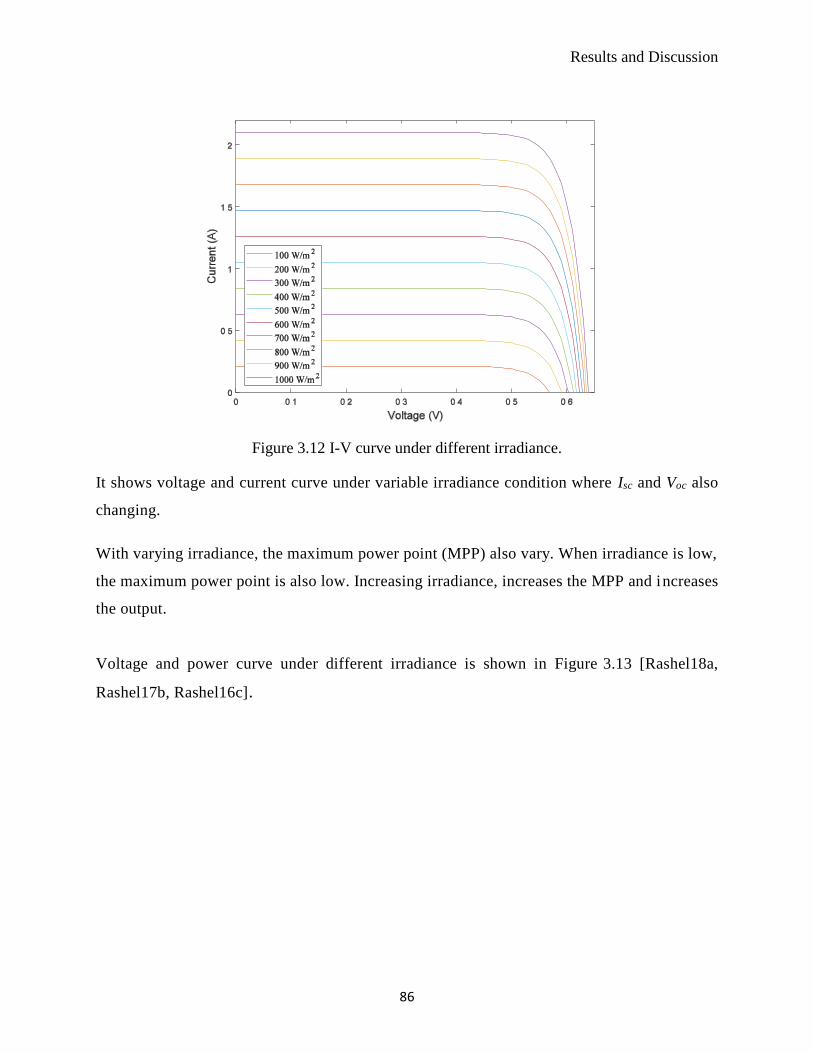
Results and Discussion

86

Figure 3.12 I-V curve under different irradiance.

It shows voltage and current curve under variable irradiance condition where Isc and Voc also

changing.

With varying irradiance, the maximum power point (MPP) also vary. When irradiance is low,

the maximum power point is also low. Increasing irradiance, increases the MPP and increases

the output.

Voltage and power curve under different irradiance is shown in Figure 3.13 [Rashel18a,

Rashel17b, Rashel16c].

Results and Discussion

87

Figure 3.13 P-V curve under different irradiance.

This graph shows the voltage power curve under variable irradiance condition with varying

MPP. The power is increasing with increasing irradiance. MPP is with changing irradiance is

shown below Figure 3.14.

Figure 3.14 Maximum power points with increasing irradiance.

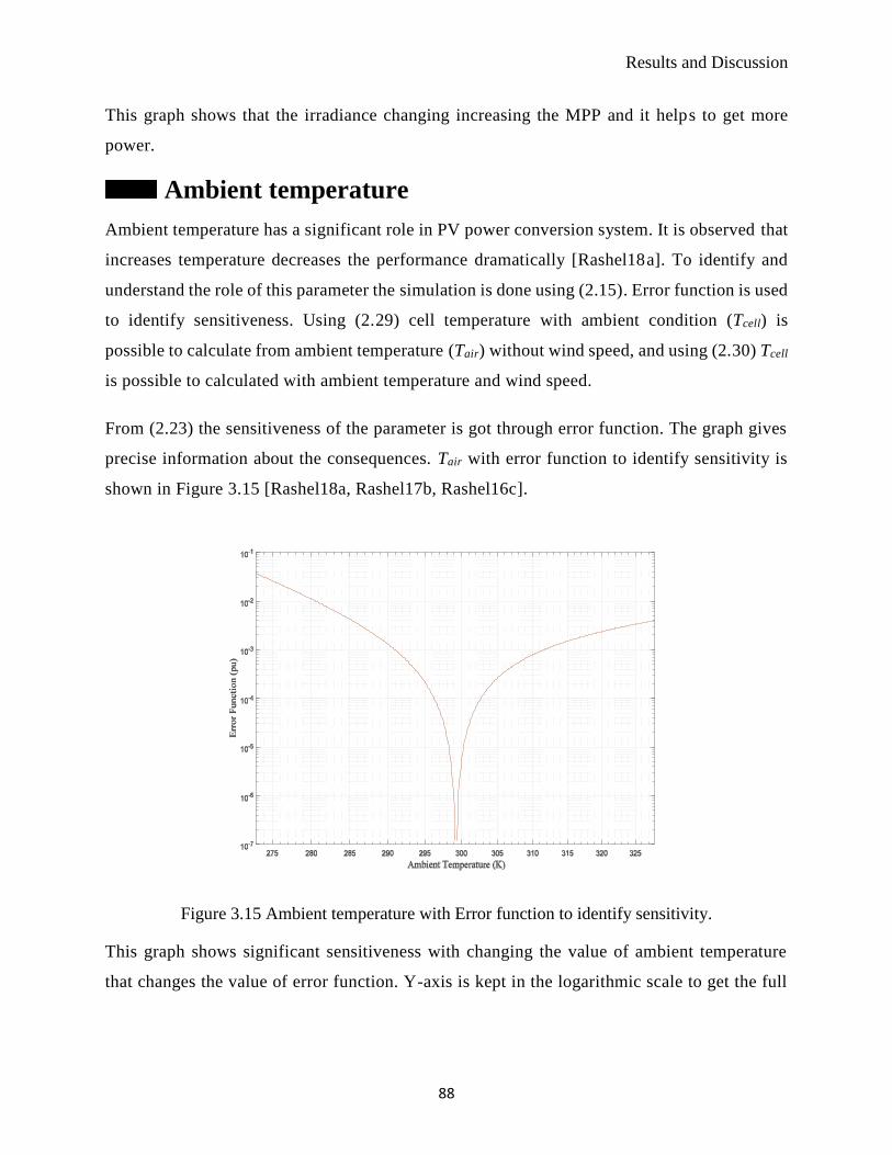
Results and Discussion

88

This graph shows that the irradiance changing increasing the MPP and it helps to get more

power.

Ambient temperature

Ambient temperature has a significant role in PV power conversion system. It is observed that

increases temperature decreases the performance dramatically [Rashel18a]. To identify and

understand the role of this parameter the simulation is done using (2.15). Error function is used

to identify sensitiveness. Using (2.29) cell temperature with ambient condition (Tcell) is

possible to calculate from ambient temperature (Tair) without wind speed, and using (2.30) Tcell

is possible to calculated with ambient temperature and wind speed.

From (2.23) the sensitiveness of the parameter is got through error function. The graph gives

precise information about the consequences. Tair with error function to identify sensitivity is

shown in Figure 3.15 [Rashel18a, Rashel17b, Rashel16c].

Figure 3.15 Ambient temperature with Error function to identify sensitivity.

This graph shows significant sensitiveness with changing the value of ambient temperature

that changes the value of error function. Y-axis is kept in the logarithmic scale to get the full

Results and Discussion

89

picture in a single window. Small change of ambient temperature makes a momentous

conversion in error function.

Using different ambient temperature, the voltage and current curve is drawn. Increasing

ambient temperature decrease the open circuit voltage (Voc) and increase short-circuit current

(Isc). Voltage and current curve under different ambient temperature is shown in Figure 3.16

[Rashel18a, Rashel17b, Rashel16c].

Figure 3.16 Voltage-current curve under different ambient temperature.

It shows the specific behavior of PV current and voltage under different ambient temperature.

Ambient temperature has a direct relation with cell temperature; this relation is got through (2.29)

and (2.30). When ambient temperature increases, it assists to increase the cell temperature also.

Because of increasing ambient temperature cell could not reduce its temperature by convection or

radiation with its surrounding area. On the other hand, reduces ambient temperature assists to

decrease cell temperature.

Voltage and power curve is important for understanding the maximum power and ambient

temperature relation. Voltage and power curve under different ambient temperature is shown in

Figure 3.17 [Rashel18a, Rashel17b, Rashel16c].

Results and Discussion

90

Figure 3.17 Voltage-power curve under different ambient temperature.

This graph shows clear view of the maximum power point (MPP) properties. It is decreasing with

changing ambient temperature. The power generation is decreased when the ambient temperature

is increased.

Both I-V and P-V curves is include the ambient temperature effect and due to the 𝑇𝑎𝑖𝑟 effect the

𝑉𝑚𝑎𝑥 decrease to 0.6V. To see MPP behavior with the different ambient temperature a graph is

created. MPP with increasing ambient temperature is shown in Figure 3.18 [Rashel18a,

Rashel17b, Rashel16c].

This graph gives the clear visualization of ambient temperature and MPP that states that during

low ambient temperature is a helpful condition for PV. During operation time, PV starts to generate

power and the same time it produces heat. In maximum PV technologies, on average 15% of

irradiance converted to electricity and rest of them converted to heat. This generated heat, increases

PV cell temperature and also by the process of radiation it goes to surrounding areas and assists to

rise ambient temperature. And due to hot ambient temperature, the PV cells could not release heat

to surrounding environment. In this way, it makes adverse effect on PV performance. This result

is supported by [Katz01, Dubey13].

Results and Discussion

91

Figure 3.18 Maximum power points with increasing ambient temperature.

Wind speed

This is another environmental parameter that has a decent role on the performance of PV system.

This parameter is helped to reduce the ambient temperature of the PV cell. Ambient temperature

and PV have a negative correlation with each other. Increasing ambient temperature always

decreases the performance of PV. Wind speed (𝑣𝑤𝑖𝑛𝑑) aids to take out ambient heated air, that

helps to reduce cell temperature by forced convection and radiation process.

The sensitivity of 𝑣𝑤𝑖𝑛𝑑 to the PV model is understood through error function. It has a direct

relation to ambient temperature, and (2.30) calculates cell temperature with wind speed. Using

(2.23) is used to get the error function. 𝑣𝑤𝑖𝑛𝑑 with error function is shown in Figure 3.19

[Rashel18a, Rashel17b, Rashel16c].

This graph shows changes in wind speed assist to change in error function. A small change of

𝑣𝑤𝑖𝑛𝑑 changes error function and show sensitiveness.

Results and Discussion

92

Figure 3.19 Wind speed with error function.

Voltage and current is an informative curve that gives knowledge about the output of PV on the

basis of changing 𝑣𝑤𝑖𝑛𝑑. 𝑣𝑤𝑖𝑛𝑑 is linked to cell temperature. Voltage and current curve under

different wind speed is shown in Figure 3.20 [Rashel18a, Rashel17b, Rashel16c].

Figure 3.20 Voltage-current curve under different wind speed.

Results and Discussion

93

This graph shows that variation of 𝑣𝑤𝑖𝑛𝑑 changes the voltage and current value. The increasing

speed of the wind makes a positive impact on the PV output. Mainly the wind flew away from the

heated ambient air that surrounding around PV panel. It makes force conversion; when heated air

goes away, it carries the heat from PV. It helps PV to radiate the temperature from panel to

surrounding area. PV releases temperature to surrounding area by using heat transfer process:

conversion and radiation. Wind flow helps to continue heat transfer process. Voltage and power

curve under different 𝑣𝑤𝑖𝑛𝑑 is shown in Figure 3.21 [Rashel17b].

Figure 3.21 Power-voltage curve under different wind speed.

This graph shows the voltage and power curve for changing 𝑣𝑤𝑖𝑛𝑑. Increasing 𝑣𝑤𝑖𝑛𝑑, increasing

the maximum power point and it is because of reducing the cell temperature. Maximum power

point with increasing 𝑣𝑤𝑖𝑛𝑑 is shown in Figure 3.22 [Rashel17b].

Both I-V and P-V curves is include the ambient temperature effect and due to the 𝑇𝑎𝑖𝑟 with 𝑣𝑤𝑖𝑛𝑑

the 𝑉𝑚𝑎𝑥 decrease to 0.6V. This graph gives the graph of 𝑣𝑤𝑖𝑛𝑑 with maximum power point. It

shows that the increasing speed of wind makes increasing the maximum power point. The increase

rate of maximum power point is not linear with 𝑣𝑤𝑖𝑛𝑑. The increment of maximum power point

with increasing 𝑣𝑤𝑖𝑛𝑑 follows the logarithmic function, as Pmax = In x.

Results and Discussion

94

Figure 3.22 Maximum power point with increasing wind speed.

Changing irradiance and ambient temperature

In this sub-section, two parameters’ values have changed at the same time; irradiance and ambient

temperature values. This work is done to simulate the dynamic behavior of the atmosphere. In real

time environmental parameters are always changing and the change randomly. Simulation of the

environment is complicated enough. PV power with changing irradiance and ambient temperature

is shown in Figure 3.23 [Rashel18a, Rashel17b, Rashel16c].

This graph shows that in the condition of increasing irradiance and low ambient temperature give

the maximum power. And decreasing of irradiance with increased ambient temperature give the

minimum power output.

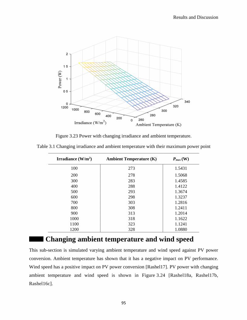
Results and Discussion

95

Figure 3.23 Power with changing irradiance and ambient temperature.

Table 3.1 Changing irradiance and ambient temperature with their maximum power point

Irradiance (W/m2) Ambient Temperature (K) Pmax (W)

100 273 1.5431

200 278 1.5068

300 283 1.4585

400 288 1.4122

500 293 1.3674

600 298 1.3237

700 303 1.2816

800 308 1.2411

900 313 1.2014

1000 318 1.1622

1100 323 1.1241

1200 328 1.0880

Changing ambient temperature and wind speed

This sub-section is simulated varying ambient temperature and wind speed against PV power

conversion. Ambient temperature has shown that it has a negative impact on PV performance.

Wind speed has a positive impact on PV power conversion [Rashel17]. PV power with changing

ambient temperature and wind speed is shown in Figure 3.24 [Rashel18a, Rashel17b,

Rashel16c].

Results and Discussion

96

Figure 3.24 Power with changing ambient temperature and wind speed.

This graph states that changing ambient temperature and changing wind speed made change in PV

power output. At the point where wind speed is zero, and the ambient temperature is high, there

occurred lowest power. At the point where the power rises to the highest point, there wind speed

is at the highest point, and ambient temperature is at the lowest point. In low ambient temperature,

the cell temperature is increasing because PV cell itself generate heat in the working process.

Table 3.2 Changing wind speed and ambient temperature with their maximum power

Wind Speed (m/s) Ambient Temperature (K) Pmax (W)

0 273 1.0170

1 278 1.0618

2 283 1.0942

3 288 1.1179

4 293 1.1366

5 298 1.1519

6 303 1.1640

7 308 1.1739

8 313 1.1828

9 318 1.1901

10 323 1.1960

11 328 1.2022

Results and Discussion

97

Changing irradiance and wind speed

In this sub-section, changing irradiance and changing wind speed is observed at same time. PV

power with changing wind speed and irradiance is shown in Figure 3.25 [Rashel18a, Rashel17b,

Rashel16c].

Figure 3.25 Power with changing wind speed and irradiance.

This graph shows the highest power output is occurred where irradiance is high and the wind speed

also high, and lowest power point is consisting of low irradiance and low wind speed.

Table 3.3 Changing wind speed and irradiance with their maximum power

Wind Speed (m/s) Irradiance (W/m2) Pmax (W)

0 100 0.9961

1 200 1.0500

2 300 1.0898

3 400 1.1185

4 500 1.1413

5 600 1.1600

6 700 1.1750

7 800 1.1869

8 900 1.1980

9 1000 1.2068

10 1100 1.2142

11 1200 1.2218

From this sub-section, it is clear that both of the irradiance and wind speed have positive effect on

PV power conversion and ambient temperature has a negative impact on it.

Results and Discussion

98

Correlation between environmental parameters

Irradiance, ambient temperature and wind speed data are logged in the weather station of the

University of Évora. This weather station has many other environmental data, and it is collecting

data in real time and log them in the database. These stored data are used for correlation analysis.

The correlation between irradiance, ambient temperature, and wind speed is analysis using person

correlation test. This test helps to visualize the parameters’ correlation between each other. These

correlation coefficient plots are created with last four years’ data of Évora, weather station. Only

linear correlation is analyzed using this data [Clima18].

Correlation relation between irradiance and temperature is shown in Figure 3.26.

Figure 3.26 Correlation matrix of irradiance and temperature.

First correlation test is done between irradiance and temperature. The correlation coefficient value

is equal to 0.59, and it is positive. It describes that they have a positive relationship between them.

It tells that one variable increases and the other also increases. This fact makes the complicated

situation for PV power conversion. Irradiance has a positive effect to PV, and on the other hand,

ambient temperature has an adverse effect. Due to irradiance the ambient temperature also

Results and Discussion

99

increases in the environment. The positive value of correlation means when the irradiance increase

then temperature also increases and with decreasing irradiance, temperature also decreases.

Another person correlation test is done with irradiance and wind speed, and they have a very low

linear correlation, the value is equal to positive 0.10. Correlation relation matrix between

irradiance and wind speed is shown in Figure 3.27.

Figure 3.27 Correlation matrix between irradiance and wind speed.

This graph gives the correlation relation between irradiance and wind speed that has a positive

correlation and is not significant enough. Irradiance and wind speed are linearly correlated with

each other, but their relationship is shallow in a linear manner.

Correlation relation matrix between wind speed and temperature is shown in Figure 3.28.

Results and Discussion

100

Figure 3.28 Correlation matrix between wind speed and temperature.

This graph shows correlation matrix between wind speed and temperature. The test correlation

coefficient value is negative, and it value is equal to 0.05. Changing of wind speed has small

negative effect on temperature. It is like, when wind speed increase then temperature decrease.

This is important observation that due to wind blowing the ambient temperature is decreasing that

is important for PV power generation

These correlation tests are done to see the internal correlation behavior of three imperative

environmental parameters and their effect to each other. Irradiance, temperature and wind speed

have direct impact on PV performance. From this correlation, it is identified that irradiance has

positive correlation with temperature, where irradiance has positive effect on PV, and on the other

hand, temperature has negative effect on PV and wind speed has positive impact on PV output

performance by decreasing the temperature. That makes complex scenario for the improvement of

PV performance.

Results and Discussion

101

3.4 Case study 3: Non-constant Load

The load is a significant part of any kind of electrical source component. PV is a semiconductor

component that generates electricity using solar energy. Changing of load make a significant

impact on maximum power point of PV. Maximum PV system has batteries to store electrical

energy. Some PV system has a direct connection to the grid system. The PV system that direct

connection with a load needs a better understanding of load effect. In this section, with different

resistances as a load is observed in real-time lab experiment. This work helps to identify behavior

of PV with the non-constant load.

Different resistances as non-constant load

Different resistances are used for understanding the variable loads against PV. Using GPIB and

DAQ the computer gets the value from the real-time system. It gives different voltage and current

values that keep in the computer system to calculate the power for different resistances. The curves

are fitted by fifth degree polynomial function.

Start with the resistance of 100 Ω as an additive load with the PV panel. Here the open circuit

voltage (Voc) is 5.0909 V, and short circuit (Isc) current is 0.0055 A. Voltage and current with

resistance load value of 100 Ω is shown in Figure 3.29.

Figure 3.29 I-V curve with resistance load value of 100 Ω.

Results and Discussion

102

For the given resistance the maximum power is 0.0281 W. For given load resistance value 100 Ω,

the voltage and power is shown in Figure 3.30.

Figure 3.30 P-V curve with resistance load value of 100 Ω.

For the resistance 220 Ω, the Voc value is 5.0959 V, and Isc value is .0057 A. Voltage and current

with resistance load value of 220 Ω is shown in Figure 3.31.

Figure 3.31 I-V curve with resistance as load value of 220 Ω.

Results and Discussion

103

For the given resistance the maximum power value is 0.0275 W. Voltage and power with

resistance load value of 220 Ω is shown in Figure 3.32.

Figure 3.32 P-V curve with resistance load value of 220 Ω.

For the resistance 560 Ω, the Voc value is 5.1214 V, and Isc value is .0046 A. Voltage and current

with resistance load value of 560 Ω is shown in Figure 3.33.

Figure 3.33 I-V curve with resistance as the load value of 560 Ω.

Results and Discussion

104

For given resistance the maximum power value is 0.0204 W. Voltage and power with resistance

load value of 560 Ω is shown in Figure 3.34.

Figure 3.34 P-V curve with resistance as the load value of 560 Ω.

For the resistance 1500 Ω, the Voc value is 5.1048 V, and Isc value is 0.0029A. Voltage and current

with resistance load value of 1500 Ω is shown in Figure 3.35.

Figure 3.35 I-V curve with resistance as load value of 1500 Ω.

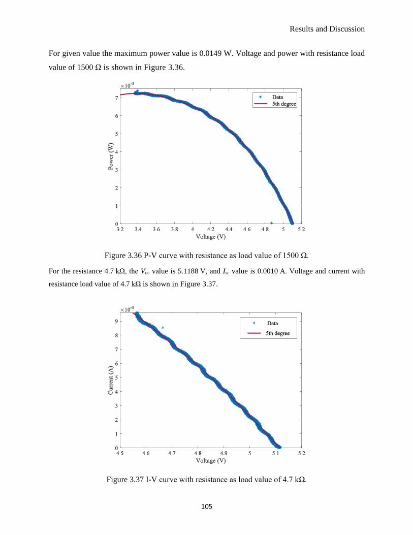
Results and Discussion

105

For given value the maximum power value is 0.0149 W. Voltage and power with resistance load

value of 1500 Ω is shown in Figure 3.36.

Figure 3.36 P-V curve with resistance as load value of 1500 Ω.

For the resistance 4.7 kΩ, the Voc value is 5.1188 V, and Isc value is 0.0010 A. Voltage and current with

resistance load value of 4.7 kΩ is shown in Figure 3.37.

Figure 3.37 I-V curve with resistance as load value of 4.7 kΩ.

Results and Discussion

106

For given resistance the maximum power value is 0.0053 W. Voltage and power with resistance

load value of 4.7 kΩ is shown in Figure 3.38.

Figure 3.38 P-V curve with resistance as load value of 4.7 kΩ.

The different additive load resistance with respective maximum power is shown in Table 3.4.

Table 3.4 Different additive load resistance with respective maximum power

Resistance Voc Isc Pmax

100 Ω 5.0909 V 0.0055 A 0.0281 W

220 Ω 5.0959 V 0.0057 A 0.0275 W

560 Ω 5.1214 V 0.0046 A 0.0204 W

1.5 kΩ 5.1048 V 0.0029 A 0.0149 W

4.7 kΩ 5.1188 V 0.0010 A 0.0053 W

Table 3.4 shows increasing load values decrease the maximum power point of particular PV panel.

Identify an optimal load for a PV panel is important. It is identified that the current at maximum

power (Imp) and voltage at maximum power (Vmp) is changing and change the MPP with the value

of the load. Using five different resistances, get a different result with same PV panel under real

environmental condition. Variation of load makes PV power and behavior unpredictable.

Results and Discussion

107

3.5 Case Study 4: Shadow of Obstacle on PV Panel

There are different kind of things that become obstacles for irradiance to reach PV panel working

surface. Because of obstacles; like shadow, dust etc. maximum power point (MPP) get multiple

picks meaning multiple local maxima in power curve. In this condition, it becomes difficult to get

the global maxima.

In the section, the obstacles are divided into two categories, time-dependent obstacles, and time-

independent obstacles. Like cloud in the sky is time-dependent obstacle; it is not a permanent one.

Physical damage of cells is count as time-independent obstacles because of not changing with time.

These two types of obstacles are analyzed in this section.

At the beginning the analysis is done for PV cells; for series and parallel connected two cells and

they are investigated under different irradiance level. After that, a PV panel with 72 cells is used

to do simulation for time-dependent obstacles, and time-independent obstacles. Simulations are

done in Simulink. Results are discussed in details for different types of scenarios.

PV cells under obstacle

Two PV cells connected with series and parallel is observed under different irradiance level. It

gives the vital identification about the obstacles behavior when they are connected in different way

[Rashel16a, Rashel18b].

3.5.1.1 Cells in series connection

Here, two PV cells are connected in series for making a simulation with Simulink. One of them is

under a different level of irradiance. Different level of irradiance simulates the obstacles on a cell.

Voltage and power curves with two cells in series connection is shown in Figure 3.39

[Rashel16a].

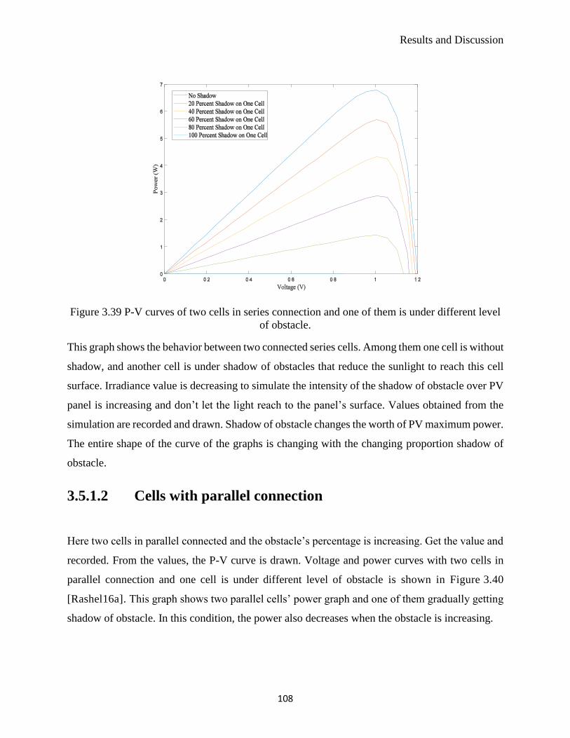
Results and Discussion

108

Figure 3.39 P-V curves of two cells in series connection and one of them is under different level

of obstacle.

This graph shows the behavior between two connected series cells. Among them one cell is without

shadow, and another cell is under shadow of obstacles that reduce the sunlight to reach this cell

surface. Irradiance value is decreasing to simulate the intensity of the shadow of obstacle over PV

panel is increasing and don’t let the light reach to the panel’s surface. Values obtained from the

simulation are recorded and drawn. Shadow of obstacle changes the worth of PV maximum power.

The entire shape of the curve of the graphs is changing with the changing proportion shadow of

obstacle.

3.5.1.2 Cells with parallel connection

Here two cells in parallel connected and the obstacle’s percentage is increasing. Get the value and

recorded. From the values, the P-V curve is drawn. Voltage and power curves with two cells in

parallel connection and one cell is under different level of obstacle is shown in Figure 3.40

[Rashel16a]. This graph shows two parallel cells’ power graph and one of them gradually getting

shadow of obstacle. In this condition, the power also decreases when the obstacle is increasing.

Results and Discussion

109

Figure 3.40 P-V curves of two cells in parallel connection and one cell is under different level of

obstacle.

In case of changing the intensity of the shadow of obstacle over a single PV cell, series connected

cells’ power decreases more than the parallel connection one and on the other hand, in parallel

connected cells’, the power decreases less than the series connected cells.

PV panel under obstacle

A PV panel with 72 cells is used to simulate different types of obstacles. A full part of the PV is

operating in a healthy condition without obstacles. Irradiance is used in this part is 1000 W/m2 as

STC condition. Voltage and current curve without obstacle and constant irradiance source is shown

in Figure 3.41. This graph shows voltage and current curve follows the ideal behavior without

obstacle condition, and the irradiance is used as a constant source.

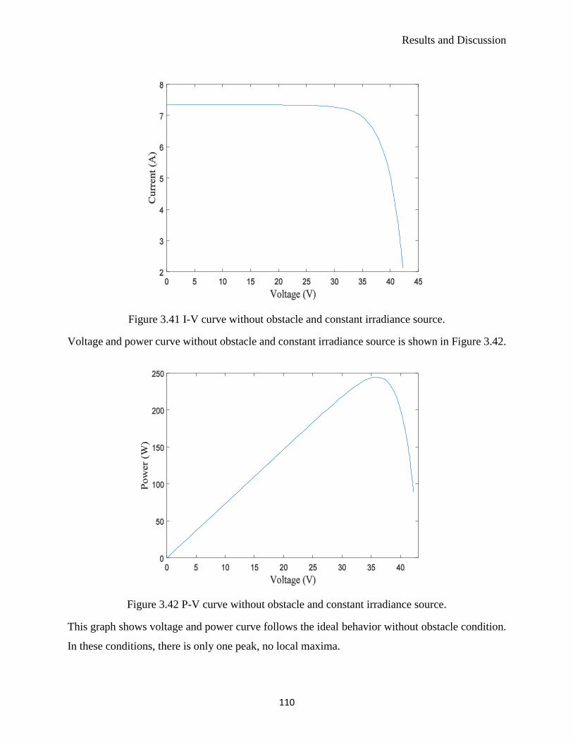
Results and Discussion

110

Figure 3.41 I-V curve without obstacle and constant irradiance source.

Voltage and power curve without obstacle and constant irradiance source is shown in Figure 3.42.

Figure 3.42 P-V curve without obstacle and constant irradiance source.

This graph shows voltage and power curve follows the ideal behavior without obstacle condition.

In these conditions, there is only one peak, no local maxima.

Results and Discussion

111

3.5.2.1 Time-dependent obstacle

This type of obstacle’s shape is changing with time. The effect of the obstacles is not permanent

on PV. The obstacle makes change to the value of irradiance and variation of irradiance value

varies the output of a PV panel. Obstacles like a sudden cloud, a flying bird over the PV, etc. that

causes an interrupt of irradiance to reach the PV surface, and the count as time-dependent obstacle.

These time-dependent obstacle comes over the panel and go away from the site of PV panel with

time [Rashel18b].

This section is going to describe the different condition of a PV panel under various of shape and

different magnitude of obstacle. Various shape means; like small cloud or big cloud the panel

whole at a time or small part of it. The different magnitude of obstacle means; some can have

shaded like dark cloud or some can have shaded like clear sky with white cloud. In this section,

simulate both the scenarios on a PV panel and analysis the result with voltage-current curve and

voltage –power curve. The shape of the curve is important to identify their behavior.

In this simulation, without bypass diode and with bypass diode both scenarios are observed. In PV

panel normally bypass diodes are used to get away from the hotspot condition. If bypass diode is

not used in the real time PV panel, then the total panel could be damage due to heat increase in the

panel. The work, analyze to see the output behavior in both conditions.

Scenario 1:

First scenario is, a big cloud goes through over a PV panel. Voltage and current with time under

dynamic obstacle on a PV panel is shown in Figure 3.43 [Rashel18b]. This graph shows the voltage

and current graph with different time period of time-dependent obstacle, where the obstacle

decrease irradiance over the full panel and its vary. Simulation is done duration of 10 second (s).

Results and Discussion

112

Figure 3.43 I-V curve with time under dynamic obstacle.

Voltage and power performance with time under time-dependent obstacles on a PV panel is shown

in Figure 3.44. This graph shows the voltage and power with variable time when obstacle is

moving over the PV panel, irradiance value is changing rapidly.

Figure 3.44 P-V curve with time under time-dependent obstacle.

Results and Discussion

113

In this scenario; small cloud come then go away and then another cloud come that make another

obstacle over the PV panel. For this simulation, voltage and current behavior with time under

changing of time-dependent obstacles is shown in Figure 3.45.

Figure 3.45 I-V curve with time under rapid changing obstacles.

This graph shows the voltage and current with varying time with a rapid environmental condition

that already explained. The variation of the irradiance is very high with time.

Figure 3.46 P-V curve with time under rapid changing obstacles.

Results and Discussion

114

For the same scenario, voltage and power with time under rapid changing obstacles is shown in

Figure 3.46. This graph shows the voltage and power with time when the pattern of the obstacles

is very random that described. This curve shows several peaks in very short time. The pattern of

curve is changing with the pattern of obstacles.

Scenario 2:

In this scenario, 48 cells out of 72 cells of a panel have constant irradiation because of no obstacle

on them. On the other hand, 24 cells are under obstacles. Two type of arrangement take in account;

cells are connected with and without diode. For this conditions, voltage-current and voltage-power

curve with time is simulation result is given below. Simulation is done duration of 20 second (s).

Figure 3.47 I-V curve with time, 48 cells get constant irradiance, and 24 cells are under obstacles

and without diode between cells.

This graph shows voltage and current curve with time where curve pattern is changing with the

pattern of obstacle over time.

Results and Discussion

115

Figure 3.48 I-V curve with time, 48 cells get constant irradiance, and 24 cells are under obstacles

and diode between the cells.

This graph shows a phenomenon, same like the before voltage and current curve but in this time,

cells are connected with diodes the different irradiance means having a dynamic obstacle and have

diode between cells.

Figure 3.49 P-V curve with time and without diode between cell, 48 cells having constant

irradiance, and 24 cells get varying irradiance.

Results and Discussion

116

This graph shows voltage and power curve with time and under the same scenario that describe

above. The panel’s cells are not connected with diode and all of them are in series connected.

There is no additional peak in the power curve, no local maxima are showed.

Figure 3.50 P-V curve with time, cells are connected with diode, and 48 cells get constant

irradiance, and 24 cells get varying irradiance.

This graph shows the voltage and power curve with time, in the same scenario like above. The

cells are connected with diode. In the curve there are several peaks. The peaks introduce local

maxima and misguide maximum power point tracker.

Scenario 3:

This is another scenario, where 36 cells get constant irradiance, and 36 cells get varying irradiance

due to time-dependent obstacle. In PV panel, one scenario there is no diode and another has diode

connection between cells. Simulation is done duration of 20 second (s).

This graph shows the voltage and current curve with time for the condition when the half part is

under time-dependent obstacle and half part is under constant irradiance. Between the cells there

is no diode.

Results and Discussion

117

Figure 3.51 I-V curve with time, 36 cells having constant irradiance, and 36 cells get varying

irradiance and no diode between cells.

Figure 3.52 I-V curve with time with connected diode cells, 36 cells having constant irradiance

and 36 cells get varying irradiance.

In Figure 3.52, under the same scenario, voltage and current curve with time when there is diode

between cells is shown. This graph shows the curve when there is diode connection between cells.

The curve has peaks in single fraction of time.

Results and Discussion

118

Voltage and power curve with time for the same scenario without diode is shown in Figure 3.53.

Figure 3.53 P-V curve with time and cells are connected in series without diode, 36 cells get

constant radiance, and 36 cells get varying irradiance.

This graph shows voltage and power curve with time where the cells are connected without diode

and all are in series connection. The curve has no extra peak and no local maxima.

Figure 3.54 P-V curve with time, 36 cells get irradiance, and 36 cells get varying irradiance with

diode connection.

Results and Discussion

119

In the same scenario, voltage and power curve with time, having diode between them is shown in

Figure 3.54. This graph shows voltage and power curve with time for the scenario that cells are

connected by diodes. The curve is having extra peaks. Half of the cells are under constant

irradiance and half of them is having variable irradiance due to time-dependent obstacle.

Scenario 4:

In this scenario, in a PV panel among 72 cells, 24 cells having constant irradiance, and 48 cells

having various irradiance due to time-dependent obstacles. One part of the simulation is done with

diode connected cells and another part is done under without diode. Simulation is done duration

of 20 second (s).

Under the scenario, voltage and current curve with time, without diode between them is shown in

Figure 3.55. This graph shows the curve with time for the present scenario and cells are connected

without the diode. When the time-dependent obstacle is moving away the shape of the curve is

also changing.

Figure 3.55 I-V curve with time without diode, 24 cells get irradiance, and 48 cells get various

irradiance.

In the same situation when cells are connected with diode is shown in Figure 3.56.

Results and Discussion

120

Figure 3.56 I-V curve with time, 24 cells having irradiance, and 48 cells get varying irradiance

with diode connection.

When t = 0, one part of the panel has full STD irradiance and other part have zero irradiance; graph

shows I-V curve having peaks due this scenario and also for the connection of cells by bypass

diode. When time-dependent obstacle is moving over the panel, shape of the curve is changing.

Figure 3.57 P-V curve with time, 24 cells get irradiance, and 48 cells get varying irradiance and

without diode between cells.

Results and Discussion

121

This graph shows P-V curve with time for the same scenario and having no extra peak due to

absent of bypass diode between cells. At the starting when maximum part of the panel is under

obstacle the output is very low. With the time when the obstacle is movie away, the power is also

start to increase.

With diode connection in the same scenario, voltage and power curve is shown in Figure 3.58.

Figure 3.58 P-V curve with time, connected with diode, 24 cells having irradiance, and 48 cells

having varying irradiance.

This graph shows peaks in the curve because of the time-dependent obstacle. The behavior of

obstacle is identified using curve structure.

After seeing all these results from the simulations, it is identified that due to diode there is the extra

peaks are generated and in the other hand when there is no diode in PV panel cell could damage

and had hotspot. For safety the bypass diode is needed. Using diode also increase the performance

of the panel. Understanding curve structure, it is possible to identify the obstacle characteristics

and the percentage of effected area. For identifying exact problem this need future process of the

signal that getting from the panels. This is one of our future work to continue.

Results and Discussion

122

3.5.2.2 Time-independent obstacle

This type of obstacle is permanent damage to PV panel or have to fix manually. These obstacles

are like few cells of PV panel may damage, or something fall on the panel like layer of dust, bird

droppings etc. that should be clean manually.

For different time independent situation, Simulink simulation is designed and get the I-V and P-V

curves. This section is to see the structure of the curve with changing patterns of obstacle on

changing number of cell. Time-independent obstacles have not change with time and the pattern

are fixed, so time has not taken in account to see the curves pattern.

Scenario 1:

In this scenario, PV panel has uniform thin layer of dust on the surface. This type of scenario is

occurred in desert due to the sand and also city area for air pollution. Dust reduce the percentage

of irradiance to reach the PV operating part that convert light to electricity. Simulation gives the

underlying characteristics.

For this scenario, in Figure 3.59 voltage and current curve is shown.

Figure 3.59 I-V curve under thin layer with uniform thickness dust on the surface of a PV panel.

Results and Discussion

123

For the same scenario, in Figure 3.60 voltage and power curve is shown.

Figure 3.60 P-V curve under thin layer with uniform thickness dust on the surface of a PV panel.

Due to thin uniform layer of dust accumulated over the surface, the power is reduced than the

normal standard condition. There is no peak is shown in the curve. In state of the art, it is observed

that due to the dust the power is reduced.

Scenario 2:

In this scenario, 54 cells among 72 cells of a PV panel is under time-independent shadow of

obstacles. Usually the pattern of the shadow of obstacle is not changing with time. And it is

considered that the cells are not connected with bypass diode. Normally in real scenario in panel,

PV cells are connected with diode to reduce the thermal effect. The simulation is observed in

describe condition and identify and recode PV panel’s behavior under this conditions.

With this condition, in Figure 3.61 voltage and current curve is shown using collected data from

the simulation.

Results and Discussion

124

Figure 3.61 I-V curve for 54 cells of a 72 cells’ panel is under time-independent obstacle.

Figure 3.62 P-V curve for 54 cells of a 72 cells’ panel is under time-independent obstacle.

This graph shows voltage and power curve that having less power than a standard PV panel output.

Due to time-independent obstacle the performance of PV panel has decreased.

Results and Discussion

125

Scenario 3:

This scenario, among 72 cells of a PV panel 4 cells are totally damaged and they don’t have diode

to connect them. In this condition, in Figure 3.63 voltage and current curve is shown.

Figure 3.63 I-V curve when 4 cells is fully damaged of a PV panel.

Figure 3.64 P-V curve when 4 cells is fully damaged of a PV panel.

Results and Discussion

126

In same condition, in Figure 3.64 voltage and power curve is shown. This graph shows voltage

and power curves that power has reduced than a standard healthy PV panel. There is no other peak

in the curve. Small damage of a PV reduces the power that reduces the performance of PV.

Scenario 4:

In this scenario, among 72 cells, 54 cells are under time-independent obstacle condition and other

part is having standard irradiance. The cells are connected with bypass diode. For this condition,

in Figure 3.65 voltage and current curve is shown.

Figure 3.65 I-V curve having 54 cells under time-independent obstacle.

This I-V curve is different from the condition where the bypass diode is not used. Due to bypass

diode the extra peaks is observed.

Under the same condition, Figure 3.66 is drawn with collected data from the simulation. Due to

the bypass diode, the curve has extra peak. It introduces the local maxima that could misguide

MPP tracker to get maximum power. Below the Figure 3.66 shows voltage and power curve with

bypass diode with extra peak.

Results and Discussion

127

Figure 3.66 P-V curve with 54 cells under time-independent obstacle condition.

Scenario 5:

In this scenario, among 72 cells of a PV panel, 18 cells are under time-independent obstacle

condition and rest of them is under standard irradiance. The cells of the panel are connected with

diode. In this condition, in Figure 3.67 voltage and current curve is shown.

Figure 3.67 I-V curve with 18 cells under static obstacle condition and rest in healthy condition.

Results and Discussion

128

In Figure 3.68 voltage and power curve is shown.

Figure 3.68 P-V curve with 18 cells under time-independent obstacle.

In Figure 3.67 shows voltage and current curve and Figure.3.68 shows voltage and power curve

both of them have extra peak. In curves, this extra peaks introduces local maxima.

All these scenarios have different pattern and they show different characteristic. Due to bypass

diode in the curve, it introduces extra peaks. All of them are separable from each other. Base on

the characteristics of curves, it is the fact that will help to identify and classify the shadow of

obstacles effect on PV panel. This could guide the remote PV system checking to identify the

fault’s rate and type.

Different type obstacles on a PV panel

In this scenario, three different types of condition are applied on a PV panel that consist of 72 cells.

On the PV surface, it is simulated that it has constant irradiance, statistical obstacle, and dynamic

obstacle. Cells are connected with diode and time is considered due to time-dependent obstacle.

In this scenario, in Figure 3.69 voltage and current curve is shown. This graph shows voltage and

current curve is under three different condition. The pattern of the curve is different than before

observed curves. Simulation is done duration of 20 second (s).

Results and Discussion

129

Figure 3.69 I-V curve with constant irradiance, time-independent obstacle, and time-dependent

obstacle.

In the same scenario, in Figure 3.70 voltage and power is shown.

Figure 3.70 P-V curve with constant standard irradiance, time-independent obstacle, and time-

dependent obstacle.

Results and Discussion

130

This graph shows voltage and power curve under three different condition. The curves have several

peaks. It introduces local maxima and it is become difficult to get the maximum power point using

MPP tracker.

All these Figures are important to analysis the fault characteristics of a PV panel in the working

ground. These figures’ shapes are unusual than a standard one. The results are vital to keep track

of the faulty/damage PV and to identify the type of fault.

3.6 Summary

PV is fast growing renewable resource. Plant and small PV system are connected with smart grid.

Deep understanding about PV’s nonlinear behavior is important. Due to directly relation with

environment factors and changing characteristics with environment make it more complex system.

Better modeling of PV system under diverse condition is essential to get maximum from it.

Sensitiveness of internal parameters of five parameters PV model is made using error function.

Series resistance is identified as a less sensitive parameter. Shunt resistance shows less sensitivity

after series resistance. Rest of the internal parameters show significant behavior.

Three environmental parameters, named irradiance, ambient temperature and wind speed show

significant sensitivity to PV power conversion efficiency. Ambient temperature has negative effect

with PV output and Wind speed has positive effect.

Non-constant loads show momentous behavior with PV power conversion system. Changing the

load effects the power conversion rate.

Obstacle on a PV panel have shown significant behavior. Different types of arrangement on a PV

panel surface are modelled in the Simulink to observe their behaviors. These models are key to

identify the fault on a PV in real-time. When cells are connected with diode then it shows extra

peak due to obstacles and introduce local maxima that misguide to get maximum power point.

Next chapter gives the conclusion of the work with main contributions, publications and the future

direction this research work.

CHAPTER

4

Conclusion

In this chapter, we present the original contributions of this thesis on the subject of PV

modeling under variable internal and environmental conditions with the non-constant

load. It further discusses the contribution of different types of obstacles on PV surface that

decrease performance. Next, the scientific publications that were carried out during the

work done for this thesis aiming its dissemination to the scientific community are

enumerated. Finally, guidelines are given for future research work.

Conclusion

132

4.1 Contributions

For sustainable development, it is needed to concern about the environment safety that headed to

the Paris Agreement and the decision is made to limit the emission of greenhouse gases (GHG).

To cooperate with this decision, it is important to develop energy sources that are clean in nature.

Figure 1.1 shows three different scenarios of world’s temperature prediction following different

way of energy production. Renewable energy is an area identified as an important factor to reduce

greenhouse gases and help control the temperature [IEA15].

The integration of renewable energy sources assists to decrease the usage of fossil power plants in

the energy generating sector. This combination is important to pursuit the objective of limiting

GHG emissions to the atmosphere, aiming to comply with the Paris Agreement and subsequent

decisions.

PV gets attention from scientists, businessman and policy makers due to its increasing performance

with decreasing price and clean energy generation in production life. It is abundant all over the

world. Ongoing research on PV system has global importance for the suitability and quality of the

forthcoming society.

This research work was carried out on modeling of Photovoltaics under different environmental

conditions. This thesis leading to the explanation of the work that is structured as:

T1 The simulation is done using the error function to identify sensitiveness effects of

internal and environmental parameters;

T2 The effect of different environmental parameters on PV power conversion is

simulated to get their impact on PV’s performance;

T3 Experimental work is done with different resistances with a fixed PV panel to

identify the effect of non-constant load;

T4 Simulink model is created to implement the different kind of obstacles effect on PV

power conversion and classify obstacles.

Conclusion

134

4.2 Publications

The topic of this thesis was chosen to do research in the area of sustainable energy development

and, at the same time, get work for pursuing the academic degree. To compete the task, different

computational simulations with laboratory experiments were done. Important results have come

out and the work was published periodically helping to enrich the dissertation with comments from

scientific committee.

For contributing in the branch of energy, especially in photovoltaics power conversion system, the

thesis contributions were prepared and submitted to scientific community. The list of published

works is presented next.

Scientific publications in journals

1 Rashel, M.R., Rifath, J., Gonçalves, T., Tlemçani, M., Melicio, R., “Sensitivity analysis

through error function of Crystalline-Si photovoltaic cell model integrated in a smart grid”,

International Journal of Renewable Energy Research. Vol. 7(4), December 2017.

2 Rashel, M.R., Ahmed, T., Goncalves, T., Tlemcani, M., Melicio, R., “Analysis of

Environmental Parameters Sensitivity to Improve Modeling of a c-Si Panel” Sensor

Letters, Vol.16, pp. 1-6, March 2018.

Scientific publications in conferences and workshops

1 Rashel, M.R., Ahmed, T., Goncalves, T., Tlemcani, M., Melicio, R., “Analysis of different

types of obstacles for PV panel”, Poster paper in Eradication Poverty through Energy

Innovation Workshop, Arizona State University, United State of America, 2018.

2 Rashel, M. R., Gonçalves, T., Tlemçani, M., Melicio, R., “Photovoltaic cell performance

analysis under different ambient temperature and wind speed for sustainable energy”, proc.

Of Workshop on Sustainability and Green Technology, 2017.

3 Rashel, M. R., Albino, A., Gonçalves, T., Tlemçani, M., “Sensitivity Analysis of

Environmental and Internal Parameters of a Photovoltaic cell”, 3rd Energy for

Conclusion

135

Sustainability International Conference, Designing Cities & Communities for the Future,

Portugal, 2017.

4 Rashel, M. R., Albino, A., Gonçalves, T., Tlemçani, M., “Error Function Analysis of Five-

Parameter Model of Photovoltaic Cell”, 5th Anniversary of ANSOLE, International

Conference on Renewable Energy, Egypt, 2016.

5 Rashel, M.R., Albino, A., Gonçalves, T., Veiga, A., Ahmed, T., Tlemçani, M.,

“Comparison of Photovoltaic panel’s standard and simplified models”, The International

Conference for Students on Applied Engineering, Newcastle, United Kingdom, 2016

(IEEE xplorer, Scopus)

6 Rashel, M.R., Albino, A., Gonçalves, T., Tlemçani, M., “MATLAB Simulink modeling of

Photovoltaic Cells for understanding shadow effect”, International Conference on

Renewable Energy Research and Applications, Birmingham, United Kingdom, 2016

(IEEE xplorer, Scopus)

7 Rashel, M.R., Albino, A., Gonçalves, T., Tlemçani, M., “Sensitivity analysis of parameters

of a photovoltaic cell under different condition”, 10th International Conference on

Software, Knowledge, Information Management & Applications, China, 2016 (IEEE

xplorer, Scopus)

8 Rashel, M.R., Albino, A., Gonçalves, T., Tlemçani, M., “Analyzing Ambient Temperature

and Wind Speed Effect on the Photovoltaic Cell”, Workshop on Earth Sciences, Portugal,

2016.

9 Ahmed, T., Gonçalves, T., Albino, A., Rashel, M.R., Veiga, A., Tlemçani, M., “Different

parameters variation analysis of a PV cell”, The International Conference for Students on

Applied Engineering, Newcastle, United Kingdom, 2016 (IEEE xplorer, Scopus)

Conclusion

136

4.3 Future Research Direction

This section, gives the future direction of the research. They are not the objectives of this thesis

but deserve consideration for the continuation of the studies of the application of precise modeling

of PV power conversion to build efficient PV plants and to integrate with the smart grid system.

Thus, the research direction for future development are enunciated as:

D1 Experimental workout in laboratory with PV panel under real environmental

conditions for getting valuable information aiming at modeling more accurate PV

system enabling the integration with SG.

D2 Database development on the base of different types of obstacles on PV aiming to

identify faults and improve the system’s performance.

D3 Faster maximum power point tracker development for rapid changing dynamic

time-dependent, and also for time-independent obstacles conditions.

References

[Autosofttech18] URL: http://www.autosofttech.net/resources/(Accessed:12.09.2017)

[Anjos17] Anjos, R.S., Melício, R., Mendes, V.M.F., Pousinho, H.M.I., “Crystalline

silicon PV module under effect of shading simulation of the hot-spot

condition”, in Technological Innovation for Smart Systems, SPRINGER,

pp. 479-487, May 2017.

[Ahmed17] Ahmed, M,T, “Modelization and Characterization of Photovoltaic-

Panels”, Master’s Thesis, University of Évora, January 2017.

[Altestore17] URL: https://www.altestore.com/howto/solar-insolation-map-world-a43/

(Accessed:07.09.2017)

[Ahmed16] Ahmed, T., Gonçalves, T., Albino, A., Rashel, M.R., Veiga, A., Tlemçani,

M., “Different parameters variation analysis of a PV cell”, in Proc. Of

International Conference for Students on Applied Engineering, Newcastle,

United Kingdom, October 2016.

[Aoun14] Aoun, N., Chenni, R., Nahman, B., Bouchouicha, K., “Evaluation and

validation of equivalent five-Parameter model performance for

photovoltaic panels using only reference data”, Energy and Power

Engineering, Vol. 06, No. 9, pp. 235-245, September 2014.

[Arjyadhara13] Arjyadhara1, P., Ali S.M., Chitralekha, J., “Analysis of solar PV cell

performance with changing irradiance and temperature”, International

Journal of Engineering and Computer Science, Vol. 2, No. 1, pp. 214-220,

January 2013.

[Alam12] Alam, N., Coors, V., Zlatanova, S., Oosterom, P.J.M., “Shadow effect on

photovoltaic potentiality analysis using 3d city models”, International

Archives of the Photogrammetry, Remote Sensing and Spatial Information

Sciences, Volume XXXIX-B8, Melbourne, Australia, September 2012.

[Answers10] URL: http://www.answers.com/topic/n-type-silicon-technology

(Accessed:07.01.2018)

References

138

[Benabdallah17] Benabdallah, I., Oun, A., Cherif, A., “Grid Connected PV plant based on

smart grid control and monitoring”, International Journal of Advanced

Computer Science and Applications, Vol. 8, No. 6, 2017.

[Blog17] URL:https://blogs.thomsonreuters.com/answerson/christiana-figueres-

addressing-climate-change-is-our-task/ (Accessed:03.01.2018)

[BP17] BP Statistical Review of World Energy, 2017.

[Batista14] Batista, N.C., Melício, R., Mendes, V.M.F., “Layered smart grid

architecture approach and field tests by ZigBee technology”, Energy

Conversion and Management, Vol. 88, pp. 49-59, December 2014.

[Bonkoungou13] Bonkoungou, D., Koalaga, Z., Njomo, D., “Modelling and simulation of

photovoltaic module considering single diode equivalent circuit model in

MATLAB”, International Journal of Emerging Technology and Advanced

Engineering, Vol. 3, pp. 593–502, March 2013.

[Bikaneria13] Bikaneria, J., Joshi, S. P., Joshi, A. R., “Modeling and simulation of PV

cell using one-diode model”, International Journal of Scientific and

Research Publications, Vol. 3, No. 10, October 2013.

[Bozkurt10] Bozkurt, I., “Energy resources and their effects on environment”, WSEAS

Transactions on Environment and Development, Vol. 6, No. 5, May 2010.

[Bhattacharya14] Bhattacharya, T., Chakraborty, A.K., Pal, K., “Effects of ambient

temperature and wind speed on performance of monocrystalline solar

photovoltaic module in Tripura, India”, Hindawi Publishing Corporation

Journal of Solar Energy, Vol. 2014, September 2014.

[Bataineh12] Bataineh, K., Dalalah, D., “Optimal configuration for design of stand-alone

pv system”, Smart Grid and Renewable Energy, Vol. 3, pp. 139-147, May

2012.

[Clima18] URL: http://www.clima.ict.uevora.pt/ (Accessed:01.02.2018)

[COP2115] Paris Climate Change Conference, (FCCC/CP/2015/L.9/Rev.1), The

global standard of globalization is not limited to the limitations of the

system,XXI 2ºC, 2015.

[Cubas13] Cubas, J., Pindado, S., Farrahi, A., “New method for analytical

photovoltaic parameter extraction”, in Proc. Of International Conference

References

139

on Renewable Energy Research and Applications, pp. 873–877, Madrid,

Spain, October 2013.

[Chatterjee11] Chatterjee, A., Keyhani, A., Kapoor, D., “Identification of Photovoltaic

source models”, IEEE Transactions on Energy Conversion, Vol. 26,

pp. 883–889, September 2011.

[Candelise11] Candelise, C., Spiers, J., Gross, R., “Materials availability for thin film (TF)

PV technologies development: a real concern?”, Renewable and

Sustainable Energy Reviews, Vol. 15, No. 9, December 2011.

[Chu11] Chu, Y., Meisen, P., “Review and comparison of different solar energy

technologies”, Global Energy Network Institute, August 2011.

[Casanova11] Casanova, J.Z., Piliougine, M., Carretero, J., Bernaola, P., Carpena, P.,

Lopez, L.M., Cardona, M.S., “Analysis of dust losses in photovoltaic

modules”, In Proc. Of World Renewable Energy Congress, Linkoping,

Sweden, May 2011.

[Chen11] Chen, C.J., Physics of Solar Energy, John Wiley & Sons, Inc, August 2011.

[Chenni07] Chenni, R., Makhlouf, M., Kerbache, T., Bouzid, A., “A detailed modeling

method for photovoltaic cells”, Energy, Vol. 32, No. 9, pp. 724–730,

September 2007.

[Demirel16] Demirel., Y., Energy: production, conversion, storage, conservation and

coupling, Springer, Springer International Publisher, 2016.

[Dubey13] Dubey, S., Sarvaiya, J.N., Seshadri, B., “Temperature dependent

photovoltaic (PV) efficiency and its effect on PV production in the world

A Review”, Energy Procedia, Vol. 33, pp. 311 – 321, June 2013.

[Darwish13] Darwish, Z.A., Kazem, H.A, Sopian, K., Alghoul, M.A., Chaichan, M.T.,

“Impact of some environmental variables with dust on solar photovoltaic

(PV) performance: review and research status”, International Journal of

Energy and Environment, Vol. 7, No. 4, 2013.

[Dincer12] Dincer, I., Zamfirescu, C., Sustainable energy systems and application,

Springer, Springer US, 2012.

[Dresner08] Dresner, S., The Principles of sustainability, 2nd Edition, Earthscan, UK

and USA, 2008.

References

140

[Electronicsdesignhq18] URL: https://www.electronicsdesignhq.com/diodes/ (Accessed:

06.04.2018)

[EIA17] International Energy Outlook, 2017.

[ESA17] NASA & European Space Agency (ESA)

[ElectronicsTutorials17] URL: https://www.electronics-tutorials.ws. (Accessed:07.10.2017).

[Eere17] URL: https://www1.eere.energy.gov/solar/pdfs/solar_timeline.pdf

(Accessed:01.11.2017)

[Elzinga15] Elzinga, D., “Electricity system development: a focus on - Smart Grids

Overview of activities and players in Smart Grids”, United Nations

Economic Commission for Europe, 2015.

[EIA14a] U.S. Energy Information Administration, "International Energy Statistics",

URL:http://www.eia.gov/cfapps/ipdbproject/iedindex3.cfm?tid=2&pid=2

&aid=2&cid=regions&syid=1982&eyid=2012&unit=BKWH,

(Accessed:07.10.2016).

[EIA14b] U.S. Energy Information Administration, International Energy Outlook

2014.

[Eon12] URL: http://eon.sdsu.edu/~johnston/ME204/Lecture_Notes/

(Accessed:07.02.2016).

[Einstein1905] Einstein, A., “On a heuristic point of view concerning the Production and

Transformation of Light,” Annalen der Physik, Vol. 17, pp. 132-148, Bern,

March 1905.

[Fialho14a] Fialho, L., Melício, R., Mendes, V.M.F, Viana, S, Rodrigues, C.,

Estanqueiro, A., "A simulation of integrated photovoltaic conversion into

electric grid", Solar Energy, Vol. 110, pp. 578–594, December 2014.

[Fialho14b] Fialho, L., Melício, R., Mendes, V.M.F., Figueiredo, J., Collares-Pereira,

M., “Amorphous solar modules simulation and experimental results: effect

of shading”, in: Technological Innovation for Collective Awareness

Systems, Springer, pp. 315–323, April 2014.

[Foles17] Foles, A.C.N., “MPPT study from a solar photovoltaic panel-

according to perturbations induced by shadows”, Masters’s Thesis,

University of Évora, 2017.

References

141

[Francisco15] Francisco, C.S.J., “Shadowing effect on the performance in solar PV cells”,

Master´s Thesis, University of Gavle, June 2015.

[Fialho15a] Fialho, L., Melício, R., Mendes, V.M.F., Pereira, M. C., “Simulation of a-

Si PV system linked to the grid by DC boost and three-level inverter under

cloud scope”, Technological Innovation for Cloud-Based Engineering

Systems, Springer, pp. 423-430, April 2015.

[Fialho15b] Fialho, L., Melício, R., Mendes, V.M.F., Estanqueiro, A., “Simulation of

a-Si PV system grid connected by boost and inverter”, International

Journal of Renewable Energy Research, Vol. 5, No. 2, pp. 443-451, 2015.

[Fialho15c] Fialho, L., Melicio, R., Mendes, V.M.F., “Poly-Si PV system grid

connected and fuzzy controlled”, Proceedings of the 16th IEEE

International Conference on Computer as a Tool, pp. 1–6, Salamanca,

Spain, 08–11 September 2015.

[Fialho15d] Fialho, L., Melicio, R., Mendes, V.M.F., Estanqueiro, A., Collares-Pereira,

M., “PV systems linked to the grid: parameter identification with a heuristic

procedure”, Sustainable Energy Technologies and Assessments, Vol. 10,

pp. 29-39, June 2015.

[Fialho15e] Fialho, L., Melicio, R., Mendes, V.M.F., “Simulation and experimental

results for a m-Si PV by five parameters”, Atas das 5as Jornadas de

Informática da Universidade de Évora-JIUE 2015, pp. 1–7, Évora,

Portugal, 26–27 fevereiro 2015.

[Fialho14c] Fialho, L., Melicio, R., Mendes, V.M.F., Figueiredo, J., Collares-Pereira,

M., “Effect of shading on series solar modules: simulation and

experimental results”, Procedia Technology, Vol. 17, pp. 295-302,

December 2014.

[Fialho14d] Fialho, L., Melicio, R., Mendes, V.M.F., “PV system modeling by five

parameters and in situ test”, Proceedings of the International Symposium

on Power Electronics, Electrical Drives and Motion, pp. 573–578, Ischia,

Italy, June 2014.

[Fialho14e] Fialho, L., Melicio, R., Mendes, V.M.F., Rodrigues, L, Viana, S.,

Estanqueiro, A., “Simulation of a-Si PV system linked to the grid by DC-

References

142

DC boost and two-level converter”, Proceedings of the 16th International

Power Electronics and Motion Control Conference and Exposition pp.

934–938, Antalya, Turkey, September 2014.

[Fesharaki11] Fesharaki, V.J., Dehghani, M., Fesharaki, J.J., “The effect of -temperature

on photovoltaic cell efficiency”, in Proc of the 1st International Conference

on Emerging Trends in Energy Conservation, Iran, November 2011.

[GTM17] IEA: Global Installed PV Capacity Leaps to 303 Gigawatts, 2017.

[Greentechmedia16] URL:https://www.greentechmedia.com/articles/read/iea-global-installed-

pv-capacity-leaps-to-303-gw#gs.v6tqMGI (Accessed:01.09.2016).

[Gomes16] Gomes, I.L.R., Pousinho, H.M.I., Melício, R., Mendes, V.M.F.-, “-Bidding

and optimization strategies for Wind-PV systems in electricity markets

assisted by CPS”, Energy Procedia, Vol. 106, pp. 111–121, December

2016.

[Gokmen16] Gokmen, N., Hu, W., Hou, P., Chen, Z., Sera, D., Spataru, S.,

“Investigation of wind speed cooling effect on PV panels in windy

locations” Renewable Energy, Vol. 90, pp. 283-290, May 2016.

[Graichen15] Graichen, P., “Current and future cost of photovoltaics”, Fraunhofer-

institute for solar energy systems, February 2015.

[Ghani14] Ghani, F., Rosengarten, G., Duke, M., Carson, J. K., “The numerical

calculation of single-diode solar-cell modelling parameters”, Renewable

Energy, Vol. 72, pp. 105–112, December 2014.

[Gharavi11] Gharavi, H., Ghafurian, R., “Smart grid: the electric energy system of the

future” in Proc of the IEEE, Vol. 99, No. 6, May 2011.

[Gao09] Gao, L., Dougal, R.A., Liu, S., Iotova, A.P., “Parallel-connected solar PV

system to address partial and rapidly fluctuating shadow conditions”, IEEE

Transactions on Industrial Electronics, Vol. 56, No. 5, pp. 1548-1556,

May 2009.

[Hudedmani17] Hudedmani, M.G., Soppimath, V., Jambotkar, C., “A study of materials for

solar pv technology and challenges”, Scholars Research Library European

Journal of Applied Engineering and Scientific Research, Vol. 5, No. 1,

pp. 1-13, 2017.

References

143

[Hategekimana17] Hategekimana, P., “Analysis of electrical loads and strategies for

increasing self-consumption with BIPV Case study Skarpnes zero energy

House”, Master’s Thesis, University of Agder, Grimstad, Norway, 2017.

[Homadi16] Homadi, A.M., “Effect of elevation and wind direction on silicon solar

panel efficiency”, World Academy of Science, Engineering and Technology

International Journal of Energy and Power Engineering, Vol. 10, No. 9,

2016.

[Huld15] Huld, T., Amillo, A.M.G., “Estimating PV module performance over large

geographical regions: the role of irradiance, air temperature, wind speed

and solar spectrum”, Energies, Vol. 8, pp. 5159-5181, June 2015.

[Haoyuan15] Haoyuan, Y., Shuo, Y., Tan, S.C., Hui, S.Y.R., “Dynamic modeling of

partial shading on photovoltaic arrays”, IEEE Energy Conversion Congress

and Exposition, September 2015.

[Heshmati15] Heshmati, A., Abolhosseini, S., altmann, J., “The Energy and environment

relationship”, The development of renewable energy sources and its

significance for the environment, Springer, 2015.

[Gangopadhyay13] Gangopadhyay, U., Jana, S., Das, S., “State of art of solar photovoltaic

technology”, Hindawi Publishing Corporation Conference Papers in

Energy, Vol. 2013, April 2013.

[Homepower11] URL: https://www.homepower.com/articles/solar-electricity/design-

installation/potential-pv-problems (Accessed:05.10.2016).

[Hu09] Hu, C., “Electrons and holes in semiconductors”,

URL:https://people.eecs.berkeley.edu/~hu/Chenming-Hu_ch1.pdf,

(Accessed:06.01.2016).

[IEA15] International Energy Agency, Energy and Climate Change, 2015.

[IEA14a] International Energy Agency, Key World Energy Statistics Report, 2014.

[IEA14b] International Energy Agency, Energy, climate change and environment

Executive summary, 2014.

[IEA13] International Energy Agency, World Energy Outlook, 2013.

[IEA11] Technology Roadmap Smart Grids, 2011.

References

144

[Isoaho16] Isoaho, K., Goritz, A., Schulz, N., “Governing clean energy transitions in

China and India”, The Political Economy of Clean Energy Transitions,

Oxford Scholarship, May 2017.

[Smets16] Smets, A., Jäger, K.,. Isabella, O., Swaaij, V.R., Zeman, M., “Solar Energy,

The physics and engineering of photovoltaic conversion, technologies and

systems”, UIT Cambridge Ltd, England, 2016.

[Islam14] Islam, M.N., Rahman, M.Z., Mominuzzaman, S.M., “The effect of

irradiation on different parameters of monocrystalline photovoltaic solar

cell”, in Proc of 3rd International Conference on the Developments in

Renewable Energy Technology, Dhaka, Bangladesh, May 2014.

[Kalkman18] Kalkman, J., Merhaba, A., Bose, S., Bradely, H., “Emerging technologies

in Solar PV: identifying and cultivating potential winners, Traversing the

PV lab-to-fab valleys of death”, 2015. URL:

http://www.adlittle.com/sites/default/files/viewpoints/ADL-Renewable-

Energy-Emerging-PV-Technology.pdf, (Accessed:05.02.2018).

[Kaur15] Kaur, T., “Solar PV Integration in smart grid issues and challenges”,

International Journal of Advanced Research in Electrical, Electronics and

Instrumentation Engineering, Vol. 4, No. 7, July 2015.

[Kempener13] Ruud Kempener, R., Komor, P., Hoke, A., “Smart grids and renewables: a

guide for effective deployment”, International Renewable Energy Agency,

November 2013.

[Kalogirou09] Kalogirou, S., “Solar energy engineering: processes and systems”, 2nd

Edition, Elsevier, Burlington, USA, 2009.

[Kuai05] Kuai, Y., Yuvarajan, S., “An electronic load for testing photovoltaic

panels”, Journal of Power Sources, Vol. 54, No. 1, pp. 308–313, March

2006.

[Katz01] Katz. E.A., Faimana, D., Cohena, Y., Padingerc, F., Brabecc, C.,

Sariciftci.N.S., “Temperature and irradiance effect on the photovoltaic

parameters of a fullerene/conjugated-polymer solar cell” in Proc of the

SPIE--The International Society for Optical Engineering, Vol. 4108, pp.

117-124, February 2001.

References

145

[Kverndokk94] Kverndokk, S., “Depletion of fossil fuels and the impacts of global

warming”, Resource and Energy Economics, Vol. 18, No. 2, pp. 115-136,

June 1994.

[Lu17] Lu, L., “Diodes in NTUEE Electronics”, URL: http://resources.-

stkfupm.com/download/dXBsb2Fkcy9FRS9FRTIwMy9Ob3RlcyUyMCU

yNiUyMFNsaWRlcy9FRTIwM19fTm90ZXMtU2xpZGVzX19MaWFuZ

y1IdW5nLUx1X19DaDMucGRm/h/86ad311876f99dfb0edbabc5241a0af

6 (Accessed:06.05.2017).

[Lay-Ekuakille13] Lay-Ekuakille, A., Vergallo, P., Arnesano, A., Morello, R., Capua. C.,

“Effects of environmental conditions on photovoltaic module

measurements”, in Proc of Seventh International Conference on Sensing

Technology, Wellington, New Zealand, December 2013.

[Lineykin12] Lineykin, S., Averbukh, M., Kuperman, A., “Five-parameter model of

photovoltaic cell based on STC data and dimensionless”, in Proc. Of

Electrical & Electronics Engineers in Israel, pp. 1–5, November 2012.

[Mekkaoui17] Mekkaoui, A., Laouer, M., Mimoun, Y., “Modeling and simulation for

smart grid integration of solar/wind energy”, Leonardo Journal of

Sciences, Vol. 30, pp. 31-46, June 2017.

[Menoufi17] Menoufi, K., “Dust accumulation on the surface of photovoltaic panels:

introducing the photovoltaic soiling index (PVSI)”, Sustainability-Open

Access Journal, MDPI, June 2017.

[Masmoudi16] Masmoudi, F., Salem, F.B., Derbel, N., “Single and double diode models

for conventional mono-crystalline solar cell with extraction of internal

parameters”, in Proc of International Multi-Conference on Systems,

Signals and Devices, Leipzig, Germany, March 2016.

[Mathworks15] URL: https://www.mathworks.com/ (Accessed: 05.03.2015)

[Meena14] Meena, M.R.S., Rathore, J.S., Johri. S., “Grid connected roof top solar

power generation: A Review”, International Journal of Engineering

Development and Research, Vol. 3, No.1, 2014.

[Migan13] Migan, G.A., “Study of the operating temperature of a PV module”,

References

146

Project Report 2013 MVK160 Heat and Mass Transfer, Lund, Sweden,

May 2013.

[Mohamed12] Mohamed, A.O., Hasan, A., “Effect of dust accumulation on performance

of photovoltaic solar modules in Sahara environment” Journal of Basic and

Applied Scientific Research, Vol. 2, No. 11, pp. 11030-11036, 2012.

[Mitoula11] Mitoula, R., Abeliotis, K., Vamvakari, M., Gratsani, A., “Sustainable

regional development through the use of photovoltaic (PV) systems. The

case of the Thessaly region”, in Proc. of World renewable energy congress,

Linkoping, Sweden, May 2011.

[Mani10] Mani, M., Pillai, R., “Impact of dust on solar photovoltaic (PV)

performance: Research status, challenges and recommendations”,

Renewable and Sustainable Energy Reviews, Vol. 14, pp. 3124–3131,

December 2010.

[NI16] URL: http://www.ni.com/en-gb.html(Accessed:03.10.2016).

[NREL15] Photovoltaic Research, NREL, 2015.

[Nada14] Nada, Kh, Alrikabi, M.A., “Renewable Energy Types”, Journal of Clean

Energy Technologies, Vol.2, No. 1, pp. 61-64, January 2014.

[Nguyen12] Nguyen, H., Pearce, J., “Incorporating shading losses in solar photovoltaic

potential assessment at the municipal scale.” Solar Energy, Vol. 86, No. 5,

pp. 1245-1260, April 2012.

[Netl10] National Energy Technology Laboratory, U.S. Department of Energy,

Understanding the Benefits of the Smart Grid, June 2010.

[Nguyen08] Nguyen, D., Lehman, B., “a reconfigurable solar photovoltaic array

under shadow conditions”, Twenty-Third Annual IEEE Applied Power

Electronics Conference and Exposition, Austin, USA, May 2008.

[Nordmann03] Nordmann, T., Clavadestscher, L., “Understanding temperature effects on

PV system performance”, In Proc of 3rd World Conference on

Photovoltaic Energy Conversion, Osaka, Japan, May 2003.

[Omer11] Omer, A.M., “Energy and environment: applications and sustainable

development”, British Journal of Environment & Climate Change, Vol. 1,

No. 4, pp. 118-158, October-December 2011.

References

147

[Pixabay17] URL: https://pixabay.com/en/photovoltaic-system-solar-

2742308/(Accessed:01.01.18).

[Pedhazur91] Pedhazur, Elazar J.; Schmelkin, Liora Pedhazur, “Measurement, design,

and analysis: an integrated approach”, NJ: Lawrence Erlbaum Associates,

pp. 15–29,Taylor & Francis, New York, USA, 1991.

[VIM08] International Vocabulary of Metrology – Basic and General Concepts

and Associated Terms (VIM) (3rd ed.). International Bureau of Weights

and Measures. 2008.

[Prakesh17] Prakesh, S., Sherine, S.,“Forecasting Methodologies Of Solar Resource

And PV Power For Smart Grid Energy Management”, International

Journal of Pure and Applied Mathematics, Vol. 116, No. 18, pp. 313-318,

2017.

[Pvlighthouse17] PV Lighthouse is a website of online resources for photovoltaic (PV)

engineers and scientists,

URL:http://pvlighthouse.com.au(Accessed:07.10.2017).

[Pereira14] Pereira, R.J., Melicio, R., Mendes, V.M.F., Joyce, A., “PV System with

maximum power point tracking: modeling, simulation and experimental

results”, Procedia Technology, Vol. 17, pp. 495 – 501, 2014.

[Phuangpornpitaka13] Phuangpornpitaka, N., Tia, S., “Opportunities and challenges of integrating

renewable energy in smart grid system”, 10th Eco-Energy and Materials

Science and Engineering Symposium, Energy Procedia, Vol. 34, pp. 282-

290, 2013.

[Parida11] Parida, B., Iniyan, S., Goic, R., “A review of solar photovoltaic

technologies”, Renewable and Sustainable Energy Reviews, Vol. 15,

pp. 1625-1636, 2011.

[Piazza10] Piazza, M.C.D., Vitale, G., “Photovoltaic field emulation including

dynamic and partial shadow conditions”, Applied Energy, Vol. 87,

pp. 814–823, March 2010.

[Rashel18a] Rashel, M.R., Ahmed, T., Goncalves, T., Tlemcani, M., Melicio, R.,

“Analysis of environmental parameters sensitivity to improve modeling of

a c-Si panel”, Sensor Letters, Vol.16, Nº 3, pp. 176-181, March 2018.

References

148

[Rashel18b] Rashel, M.R., Ahmed, T., Goncalves, T., Tlemcani, M., Melicio, R., “Analysis

of different types of obstacles for PV panel”, Poster paper in Eradication

Poverty through Energy Innovation Workshop, Arizona State University,

poster, Tempe, Arizona, USA, 12–14 February 2018.

[Rashel17a] Rashel, M.R., Rifath, J., Gonçalves, T., Tlemçani, M., Melício, R.,

“Sensitivity analysis through error function of crystalline-Si photovoltaic

cell model integrated in a smart grid”, International Journal of Renewable

Energy Research, Vol. 7, No.º 4, pp. 1926–1933, December 2017.

[Rashel17b] Rashel, M. R., Gonçalves, T., Tlemçani, M., Melicio, R., “Photovoltaic cell

performance analysis under different ambient temperature and wind speed

for sustainable energy”, Vietnam Journal of Science, Vol. 3, No.º 1, pp. 1–

16, 22 August 2017.

[Rashel17c] Rashel, M.R., Albino, A., Gonçalves, T., Tlemçani, M. “Sensitivity

analysis of environmental and internal parameters of a photovoltaic cell”,

in Proc. of Energy for Sustainability International Conference - Designing

Cities & Communities for the Future, Madeira, Portugal, February 2017.

[Rauf17] Rauf, S., Khan, N., “Application of DC-AC hybrid grid and solar

photovoltaic generation with battery storage using smart grid”, Hindawi

International Journal of Photoenergy, Vol. 2017, 2017.

[Rwenyagila17] Rwenyagila, E.R., “A review of organic photovoltaic energy source and its

technological designs”, Hindawi International Journal of Photoenergy,

Vol. 2017, 2017.

[Rashel16a] Rashel, M.R., Albino, A., Gonçalves, T., Tlemçani, M., “MATLAB

Simulink modeling of photovoltaic cells for understanding shadow effect”,

in Proc. Of International Conference on Renewable Energy Research and

Applications, Birmingham, UK, November 2016.

[Rashel16b] Rashel, M.R., A. Albino, Gonçalves, T., Tlemçani, M., “Sensitivity

analysis of parameters of a photovoltaic cell under different condition”, in

Proc. of International Conference on Software, Knowledge, Information

Management & Applications, Chengdu, China, December 2016.

References

149

[Rashel16c] Rashel, M.R., Albino, A., Gonçalves, T., Tlemçani, M., “Analyzing

ambient temperature and wind speed effect on the photovoltaic cell”,

Workshop on Earth Sciences, University of Évora, Portugal, December

2016.

[Rashel16d] Rashel, M.R., Albino, A., Gonçalves, T., Veiga, A., Ahmed, T., Tlemçani,

M., “Comparison of Photovoltaic panel’s standard and simplified models”,

in Proc. of International Conference for Students on Applied Engineering,

UK, October 2016.

[REN16] REN21, Renewables 2016, Global Status report, 2016

[Romano13] Romano, P., Candela, R., Cardinale, M., Vigni, V.L., Musso, D.,

Sanseverino, R., “Optimization of photovoltaic energy production through

an efficient switching matrix”, Journal of Sustainable Development of

Energy, Water and Environment Systems, Vol. 1, No. 3, pp. 227-236, 2013.

[Rodrigues11] Rodrigues, E.M.G., Melício, R., Mendes, V.M.F., Catalão, J.P.S.,

“Simulation of a solar cell considering single-diode equivalent circuit

model”, in Proc. of International Conference on Renewable Energies and

Power Quality, pp. 1–5, Las Palmas de Gran Canaria, Spain, 13–15 April

2011.

[Saleem17] Saleem, Y., Rehmani, M.H., “Internet of things-aided smart grid:

technologies, Architectures, Applications, Prototypes, and Future Research

Directions”, ArXiv, April 2017.

[Solarglassshield17] URL:https://www.solarglassshield.com/construction-mining-dust

(Accessed:10.11.2017).

[Singla16] Singla, A., Singh, K., Yadav, V.K., “Environmental effects on performance

of solar photovoltaic module”, Biennial International Conference on

Power and Energy Systems: Towards Sustainable Energy, Bangalore,

India, January 2016.

[Sunnymorgan16] URL: http://sunnymorgan.co.za/(Accessed:10.11.2017)

[Sharma15] Sarma, S., Jain, K.K., Sharma, A., “Solar cells: in research and

applications—A Review”, Scientific Research Publishing, Materials

Sciences and Applications, Vol. 6, pp. 1145-1155, December 2015.

References

150

[Saluos15] Saluos, W.A., “Dust effect on photovoltaic electric systems”, International

Journal of Emerging Engineering Research and Technology, Vol. 3,

No. 10, pp. 4-9, October 2015.

[Shafiullah13] Shafiullah, G.M., Amanullah, M. T.O., Ali, A.B.M.S., Wolfs, P., “Smart

Grid for a Sustainable Future”, Scientific Research open access, February

2013.

[Salim13] Salim, M.S., Najim. J.M., Salih, S.M., “Practical evaluation of solar

irradiance effect on PV performance”, CSCanada Energy Science and

Technology, Vol. 6, No. 2, pp. 36-40, November 2013.

[Schwingshackla13] C. Schwingshackla, C., Petittaa, M., Wagnera, J.E., G. Belluardoc, G.,

Moserc, D., Castellia, M., Zebischa, M., Tetzlaff, A., “Wind effect on PV

module temperature: analysis of different techniques for an accurate

estimation”, European Geosciences Union General Assembly, Energy

Procedia, Vol. 40, pp. 77-86, 2013.

[Storey13] Storey, J.P., Wilson, P.R., “Improved optimization strategy for irradiance

equalization in dynamic photovoltaic arrays”, IEEE Transactions On

Power Electronics, Vol. 28, No. 6, June 2013.

[Saraiva12] Saraiva, S., Melicio, R., Matias, J.C.O., Cabrita, C.M.P., Catalao, J.P.S.,

“Simulation and experimental results for a photovoltaic system formed by

monocrystalline solar modules”, Technological Innovation for Value

Creation, Springer, pp. 329–336, February 2012.

[Solarcellcentral11] URL:http://solarcellcentral.com/markets_page.html

(Accessed:10.11.2016).

[Sera07] Sera, D., Teodorescu, R., Rodriguez, P., “PV panel model based on

datasheet values”, in Proc. of IEEE International Symposium on Industrial

Electronics, pp. 2392-2396, Vigo, Spain, June 2007.

[Soto06] Soto, W. D., Klein, S. A., Beckman, W. A., “Improvement and validation

of a model for photovoltaic array performance”, Solar Energy, Vol. 80,

pp. 78-88, January 2006.

[Solar98] URL: http://www.solar.coppe.ufrj.br/pr03.html (Accessed:10.01.2016).

References

151

[Shell97] Veer, J.V., Dawson, J., Shell International Renewables. Web page:

http:/www.shell.com, 1997, Transcript of a Press conference in

London,1997, (Accessed:10.11.2016).

[Shockley61] Shockley, W., Queisser. H., "Detailed balance limit of efficiency of p-n

junction solar cells", Journal of Applied Physics, Vol. 32, No. 3, March

1961.

[Tranverter18] URL: http://www.transverter.com/smart.html (Accessed: 13.03.2017).

[Techopedia18] URL:https://www.techopedia.com/definition/2320/universal-serial-bus-

usb (Accessed:10.12.2018).

[Tamirat17] Tamirat, Y., “The Role of nanotechnology in semiconductor industry:

Review Article”, Journal of Materials Science & Nanotechnology, Vol. 5,

No. 2, September 2017.

[Tektronix16] URL:https://www.tek.com/datasheet/afg310-afg320

(Accessed:10.01.2017).

[Tayyan13] Tayyan, A. A. E., “A simple method to extract the parameters of the single-

diode model of a PV system”, Turkish Journal of Physics, Vol. 37,

pp. 121–131, March 2013.

[Tayyan11] Tayyan, A. A. E., “PV system behavior based on datasheet”, Journal of

Electron Devices, Vol. 9, pp. 335–341, 2011.

[UN16] Paris Agreement. Paris: United Nations, pp.1-27, 2016.

[UNFCC15] United Nations Framework Convention on Climate Change, 2015.

[Vergura16] Vergura, S., “A Complete and simplified datasheet-based model of PV

cells in variable environmental conditions for circuit simulation” energies,

April 2016.

[Viegas15] Viegas, J.L., Susana, M., Melicio, R., Mendes, V.M.F., “Electricity

demand profile prediction based on household characteristics”, in Proc of

12th International Conference on the European Energy Market, Lisbon,

Portugal, May 2015.

[Wang17] Wang, J., Gong, H., Zou, Z., “Modeling of dust deposition affecting

transmittance of PV modules” Journal of Clean Energy Technologies,

Vol. 5, No. 3, May 2017.

References

152

[WEC16] World Energy Council, World Energy Resources 2016.

[Weforum15] URL: https://www.weforum.org/ (Accessed:17.05.2016)

[Wan15] Wan, C., Zhao, J., Song, Y., Xu, Z., Lin, J., Hu, Z., “Photovoltaic and solar

power forecasting for smart grid energy management” CSEE Journal of

Power and Energy Systems, Vol. 1, No. 4, December 2015.

[Wang12] Wang, Y., Lin, X., Kim, Y., Chang, N., Pedram, M., “Enhancing efficiency

and robustness of a photovoltaic power system under partial shading”, in

Proc of 13th International Symposium on Quality Electronic Design, Santa

Clara, USA, March 2012.

[Warwick10] URL:https://warwick.ac.uk/fac/sci/physics/current/postgraduate/-

regs/mpagswarwick/ex5/bandstructure/ (Accessed:12.01.2018).

[Würfel05] Würfel, P., The physics of solar cells: from principles to new concepts, 1st

Edition, Wiley-VCH, Germany, 2005.

[Wieder92] Wider, S., An introduction to solar energy for scientist and engineers, 1st

Edition, John Wiley & Sons, Inc. Florida, USA, 1992.

[Zaihidee16] Zaihidee, F.M., Mekhilef, S., Seyedmahmoudian, M., Horan. B., “Dust as

an unalterable deteriorative factor affecting PV panel's efficiency: Why and

how”, Renewable and Sustainable Energy Reviews, Vol. 65, pp. 1267-

1278, November 2016.

[Zeman14] Zeman, M., Solar cells, Open Education Consortium, Delft University of

Technology, Netherland, 2014.

[Zeman10] Zeman, M., “Thin–Film Silicon PV technology”, Journal of Electrical

Engineering, Vol. 61, No. 5, pp.271–276, 2010.

[Zerhouni10] Zerhouni, Z.F., Zerhouni, M.H., Zegrar, M., Benmessaoud, M.T.,

Stambouli, A.B., Midoun, A., “Proposed methods to increase the output

efficiency of a photovoltaic (PV) system”, Acta Polytechnica Hungarica,

Vol. 7, No. 2, July 2010.

Appendix

154

value2 = (V+(I_STD(i,r)*Rs))/Rsh;

I_temp = (Io*(exp(value1)))-(value2);

I_STD(i,r) = Iph - I_temp;

%V1(i,1) = V; %Voltage value store in a 2D array

P_STD(i,r) = V * I_STD (i,r);

i = i + 1;

end

end

Appendix

156

Simulink model for identify the shadow of obstacles on PV panel.

Contactos:

Universidade de Évora

Instituto de Investigação e Formação Avançada - IIFA

Palácio do Vimioso | Largo Marquês de Marialva, Apart. 94

7002-554 Évora | Portugal

Tel: (+351) 266 706 581

Fax: (+351) 266 744 677