Battery powered energizer installation instructions - Gallagher ...
Upload
khangminh22Category
view
0download
0
A Modular Design Architecture for Application to Community-Scale Photovoltaic-Powered Reverse Osmosis Systems
by
Amy M. Bilton
Bachelor of Applied Science, Engineering Science, University of Toronto, 2004
Master of Science, Aeronautics and Astronautics, Massachusetts Institute of Technology, 2006
Submitted to the Department of Aeronautics and Astronautics in Partial Fulfillment of the Requirements for the Degree of
Doctor of Philosophy in Aeronautics and Astronautics
at the
MASSACHUSETTS INSTITUTE OF TECHNOLOGY
February 2013
© 2013 Massachusetts Institute of Technology, All rights reserved
Signature of Author: .......................................................................................................................... Department of Aeronautics and Astronautics
October 16, 2012 Certified by: .......................................................................................................................................
Steven Dubowsky Professor of Aeronautics and Astronautics & Mechanical Engineering
Thesis Supervisor
Certified by: ....................................................................................................................................... John H. Lienhard V
Samuel C. Collins Professor of Mechanical Engineering
Certified by: ....................................................................................................................................... Karen Willcox
Professor of Aeronautics and Astronautics
Accepted by: ...................................................................................................................................... Eytan Modiano
Professor of Aeronautics and Astronautics Chairman, Graduate Program Committee

2

3
A Modular Design Architecture for Application to Community-Scale Photovoltaic Reverse Osmosis Systems
by
Amy M. Bilton
Submitted to the Department of Aeronautics and Astronautics
on October 16, 2012 in Partial Fulfillment of the Requirements for the Degree of Doctor of Philosophy in
Aeronautics and Astronautics
ABSTRACT
Access to safe, clean drinking water is a major challenge for many communities. These communities are often near seawater and/or brackish groundwater sources, making desalination a possible solution. Unfortunately, desalination is energy intensive and a reliable, inexpensive power supply is also challenging for remote locations. Photovoltaic reverse osmosis systems (PVRO) can be used to provide water for underserved communities. A feasibility study which demonstrates the economic viability of such systems is discussed here.
PVRO systems are assembled from mass-produced modular components. This approach reduces manufacturing costs. However, designing a system optimized for a specific location is difficult. For even a small inventory of components, the number of design choices is enormous. A designer with significant expertise is required to tailor a PVRO system for a given location, putting this technology out of reach of many communities.
This thesis develops a modular design architecture which can be implemented in a computer program to enable non-experts to configure systems from inventories of modular components. This architecture is not limited to PVRO systems, but can also be used to design other systems composed of modular components such as cars, electronics, and computers. The method uses a hierarchy of filters to limit the design space based on design principles and calculations. The system is then configured from the reduced design space using optimization methods and detailed system models.
In this thesis, the modular design architecture is implemented for PVRO systems. A set of detailed physics-based system models are developed to enable this process. A novel method of representing a PVRO system using a graph is developed to enable rapid evaluation of different system configurations. This modeling technique is validated using the MIT Experimental PVRO system constructed as part of this research.
A series of case studies are conducted to validate the modular design approach for PVRO systems. The first set of case studies considers a deterministic solar input and water demand. The design goal is to determine the lowest cost system that meets the water demand requirements. It is shown that the method is able to tailor systems for a wide range of locations and water demands from a large system inventory. The validity of these solutions is demonstrated by simulating a custom designed system in the wrong location. Another case study shows that the approach can be used to determine market potential of new components.

4
The second set of case studies considers variations in the solar radiation and water demand. The design goal is to determine the lowest cost PVRO system that meets the water demand profile with a specified probability. Two methods that use historical solar insolation and water demand to account for variations are presented. The first method characterizes the historical data and develops models to synthetically generate solar insolation and water demand profiles, and then simulates the system performance over 100 years to calculate the loss-of-water probability. In the second method, distributions of solar radiation and water demand are calculated from historical data and used to directly calculate the probability of running out of water in the worst month of the year. Both methods are implemented and shown to produce feasible system configurations. The direct calculation method is shown to reduce the required computation time and is suitable for different systems with variable inputs.
Thesis Supervisor: Steven Dubowsky
Title: Professor of Aeronautics and Astronautics & Mechanical Engineering

5
ACKNOWLEDGEMENTS
Writing a Ph.D. dissertation is a long process that many graduate students dread, myself
included. Over the course of the past couple of months while preparing this thesis, I’ve had a
chance to reflect on my past four years at MIT and the people who’ve helped me out along the
way. As I slogged through those chapters, I’ve looked forward to writing this tribute to all these
sources of support.
I’d like to thank the sponsors of this research. Thanks to the Cyprus Institute for the
fellowship which supported the first 3 years of this research. The feedback received during our
meetings aided in the development of this work. Thanks also to the MIT-KFUPM Center for
Clean Energy and Water for the financial support of the experimental equipment and the
financial support of this research.
I’d like to thank the members of my Ph.D. committee. Professor Dubowsky, thank you
for giving me the fantastic opportunity of working in the FSRL. I’ve learned about both life and
research from you during the course of my M.S. and Ph.D. You’ve been a great research advisor,
mentor and friend. I’d also like to thank my committee members Professor Willcox and
Professor Lienhard for their helpful discussions and critiques of my work over the past few
years.
Research is something that you can’t do on your own and there is no way I would have
been able to complete this work without the assistance of my fellow lab members. Thanks to
Roman Geykhman and Davide Del Pozzo for their assistance with the construction of the
experimental system. I also want to thank Francesco Mazzini and Elizabeth Reed for their useful
feedback on my work and keeping the lab spirits high. I especially thank Leah Kelley for
providing feedback on my ideas, helping with experiments, reading this thesis, supporting me
during tough times and just being a great friend.
I’d also like to thank my support outside the lab. These past four years, I’ve been so
fortunate to become part of an enormous family at Sidney-Pacific. Thanks so much to Professor
Roger Mark and Dottie Mark for inviting me into their home so many times and making sure that
I’m always well fed. I’ve learned so much from both of you. I’ve made so many great friends at
SP (way more than I can list here) and it’s been fantastic to live with all of you these past few
years. SP has taught me to always think big and that anything is possible as long as you have a
great team.
I also want to thank my friends and family. Been Kim, thanks for being a great source of
support throughout my degree. I know my qualifying exam experience would have been much
different without you (the study sessions would not have been nearly as fun). Mom and Dad,
thanks for always believing in me and supporting my endeavors no matter how crazy they may
seem.
Last, I want to thank my biggest source of support. Andreas, thanks for always being
there, even though you are on the other side of the globe. Thanks for being a sounding board for

6
my ideas, lifting my spirits, and for encouraging me when things seem out of reach. You’ve
always been my biggest fan and there’s no way this thesis would have been completed without
your love and support.

7
CONTENTS
ABSTRACT ................................................................................................................................... 3
ACKNOWLEDGEMENTS ......................................................................................................... 5
CONTENTS................................................................................................................................... 7
FIGURES ..................................................................................................................................... 11
TABLES ....................................................................................................................................... 15
CHAPTER 1. INTRODUCTION .............................................................................................. 17
1.1 MOTIVATION ................................................................................................................. 17
1.2 MODULAR DESIGN ......................................................................................................... 19
1.3 PROBLEM STATEMENT ................................................................................................... 19
1.4 THESIS CONTRIBUTIONS ................................................................................................ 21
1.5 THESIS ORGANIZATION .................................................................................................. 22
CHAPTER 2. BACKGROUND AND LITERATURE REVIEW .......................................... 23
2.1 PHOTOVOLTAIC REVERSE OSMOSIS SYSTEMS ............................................................... 23
2.1.1 PVRO Overview ........................................................................................................ 23
2.1.2 PVRO System Design and Control ........................................................................... 24
2.1.3 RO System Design and Control ................................................................................ 25
2.2 MODULAR DESIGN ......................................................................................................... 27
2.2.1 Modular Design of Robotic Systems ......................................................................... 27
2.2.2 Modular Design of Electronic Circuits..................................................................... 27
2.2.3 Modular Design of Computer Programs .................................................................. 28
2.2.4 Synthesis of Chemical Networks ............................................................................... 28
2.3 DESIGN WITH UNCERTAIN INPUTS ................................................................................. 29
2.3.1 General Design Rules ............................................................................................... 29
2.3.2 Robust Design Methods ............................................................................................ 29
2.4 SUMMARY ...................................................................................................................... 31
CHAPTER 3. PVRO SYSTEM FEASIBILITY ...................................................................... 32
3.1 INTRODUCTION .............................................................................................................. 32
3.2 APPROACH ..................................................................................................................... 32
3.3 ANALYSIS ...................................................................................................................... 34
3.3.1 Assumptions .............................................................................................................. 34
3.3.2 Energy Requirements ................................................................................................ 34
3.3.2.1 Photovoltaic Reverse Osmosis System Sizing .................................................. 34
3.3.2.2 Diesel Reverse Osmosis System Sizing ............................................................ 35
3.3.2.3 Reverse Osmosis Power Requirements ............................................................ 35

8
3.3.2.4 Water Transportation Energy Requirements .................................................... 37
3.3.3 Energy Source ........................................................................................................... 38
3.3.3.1 Solar Array Requirements................................................................................. 38
3.3.3.2 Diesel Generator Requirements ........................................................................ 38
3.3.4 System Cost ............................................................................................................... 39
3.3.4.1 Assumptions ...................................................................................................... 39
3.3.4.2 Overall Cost of Desalinated Water ................................................................... 39
3.3.4.3 Capital Costs ..................................................................................................... 39
3.3.4.4 Reverse Osmosis System .................................................................................. 40
3.3.4.5 Photovoltaic Power System .............................................................................. 40
3.3.4.6 Diesel Generator System................................................................................... 40
3.4 OPERATING COSTS ......................................................................................................... 41
3.4.1 Reverse Osmosis ....................................................................................................... 41
3.4.2 Photovoltaic Power System....................................................................................... 42
3.4.3 Diesel Generator System........................................................................................... 42
3.5 CASE STUDIES................................................................................................................ 44
3.5.1 Seawater Systems ...................................................................................................... 44
3.5.1.1 Analysis for Any Location ................................................................................ 44
3.5.1.2 Site Analysis ..................................................................................................... 47
3.5.2 Brackish Water Systems ............................................................................................ 48
3.5.3 Comparison with Other PVRO Studies ..................................................................... 49
3.6 CONCLUSIONS ................................................................................................................ 49
CHAPTER 4. MODULAR DESIGN APPROACH ................................................................. 51
4.1 MODULAR DESIGN ......................................................................................................... 51
4.2 DESIGN APPROACH ........................................................................................................ 52
4.3 PVRO SYSTEM DESIGN SPACE STUDY .......................................................................... 53
4.3.1 Overview ................................................................................................................... 53
4.3.2 Enumerating Full Design Space ............................................................................... 54
4.3.3 Module Level Filters ................................................................................................. 56
4.3.3.1 Motor/Pump Filters ........................................................................................... 56
4.3.3.2 Reverse Osmosis Membrane Filters ................................................................. 57
4.3.3.3 Energy Recovery Device and Pressure Control Valve Filters .......................... 58
4.3.3.4 PV Panel Filters ................................................................................................ 58
4.3.4 Subassembly Filters .................................................................................................. 59
4.3.5 Topology Filters ........................................................................................................ 60
4.4 PARALLEL EXAMPLE – HYBRID CAR POWERTRAIN ....................................................... 63
4.5 SUMMARY ...................................................................................................................... 67
CHAPTER 5. PVRO SYSTEM MODEL ................................................................................. 68
5.1 ENVIRONMENT MODELS ................................................................................................ 68
5.1.1 Solar Energy Model .................................................................................................. 68

9
5.1.2 Water Salinity Model ................................................................................................ 71
5.1.3 System Demand ......................................................................................................... 71
5.2 COMPONENT MODELS .................................................................................................... 71
5.2.1 PV System.................................................................................................................. 71
5.2.2 PV Tracking/Mounting.............................................................................................. 74
5.2.3 Motors ....................................................................................................................... 76
5.2.4 Pumps ........................................................................................................................ 78
5.2.5 Reverse Osmosis Membranes ................................................................................... 78
5.2.6 Energy Recovery Devices ......................................................................................... 81
5.2.7 Control Electronics ................................................................................................... 84
5.3 GRAPH REPRESENTATION .............................................................................................. 84
5.3.1 Surrogate Model ....................................................................................................... 87
5.4 EXPERIMENTAL MODEL VERIFICATION ......................................................................... 89
5.4.1 Experimental System Description ............................................................................. 89
5.4.2 Model Representation ............................................................................................... 93
5.4.3 Model Validation ...................................................................................................... 94
5.5 ECONOMIC MODELS ...................................................................................................... 96
5.5.1 Total Costs ................................................................................................................ 96
5.5.2 Capital Costs ............................................................................................................. 97
5.5.3 Operating and Maintenance Costs ........................................................................... 99
5.6 SUMMARY .................................................................................................................... 100
CHAPTER 6. DETERMINISTIC CASE STUDIES ............................................................. 101
6.1 PROBLEM DESCRIPTION ............................................................................................... 101
6.1.1 System Inventory ..................................................................................................... 102
6.1.2 Power Source .......................................................................................................... 104
6.1.3 System Demand ....................................................................................................... 105
6.2 OPTIMIZATION SETUP .................................................................................................. 105
6.3 OPTIMIZATION RESULTS .............................................................................................. 111
6.3.1 Varied Location ...................................................................................................... 111
6.3.2 Varied System Size .................................................................................................. 114
6.3.3 Cost Sensitivity ........................................................................................................ 115
6.3.4 Varied Inventory ..................................................................................................... 116
6.3.5 Convergence Properties.......................................................................................... 117
6.4 SUMMARY .................................................................................................................... 118
CHAPTER 7. ACCOMMODATING VARIATIONS ........................................................... 119
7.1 PROBLEM DESCRIPTION ............................................................................................... 119
7.2 STOCHASTIC MODELING APPROACH ............................................................................ 120
7.2.1 Simulation Model .................................................................................................... 120

10
7.2.2 Solar Radiation Model ............................................................................................ 122
7.2.3 System Demand Model ............................................................................................ 127
7.3 STOCHASTIC MODELING CASE STUDIES ...................................................................... 134
7.3.1 Full Year Simulations ............................................................................................. 134
7.3.2 Critical Month Simulations ..................................................................................... 136
7.4 CALCULATION OF LOSS-OF-WATER PROBABILITY USING HISTORICAL DATA ............. 138
7.5 DIRECT CALCULATION CASE STUDIES ......................................................................... 144
CHAPTER 8. SUMMARY AND CONCLUSIONS ............................................................... 147
8.1 SUMMARY .................................................................................................................... 147
8.2 SUGGESTIONS FOR FUTURE WORK ............................................................................... 149
REFERENCES .......................................................................................................................... 151
APPENDIX A. ENUMERATION OF PVRO DESIGN SPACE .......................................... 159
A.1 RULES OF COMBINATORICS ......................................................................................... 159
A.2 NUMBER OF POSSIBLE REVERSE OSMOSIS SYSTEMS.................................................... 161
A.2.1 Distinct Reverse Osmosis Components ............................................................... 161
A.2.2 Identical Reverse Osmosis Components ............................................................. 164
A.2.3 Full Reverse Osmosis Component Inventory ...................................................... 165
A.3 NUMBER OF POSSIBLE PHOTOVOLTAIC POWER SYSTEMS ............................................ 166

11
FIGURES
Figure 1.1: Water scarcity [7] (left) and average solar insolation, data from [8]. ........................ 18
Figure 1.2: PVRO modular design problem. ................................................................................ 20
Figure 2.1: Simple PVRO system. ................................................................................................ 23
Figure 3.1: Array area required for 10m3 system. ........................................................................ 45
Figure 3.2: Water cost for 10m3 system........................................................................................ 45
Figure 3.3: Water cost for a 10m3 system in the Middle East. ..................................................... 46
Figure 3.4: Areas where PVRO systems are feasible. .................................................................. 47
Figure 3.5: Areas in Middle East where PVRO systems are feasible. .......................................... 47
Figure 4.1: Modular design approach. .......................................................................................... 53
Figure 4.2: Inventory used in design space study. ........................................................................ 53
Figure 4.3: Examples of RO system configurations eliminated by the topology filter. ............... 62
Figure 4.4: Parallel hybrid car (left) and series hybrid car (right) configurations. ....................... 64
Figure 5.1: Solar cell operation. .................................................................................................... 72
Figure 5.2. Electrical circuit representation of the one diode solar module model. ..................... 73
Figure 5.3. Photovoltaic panel operating curves. .......................................................................... 73
Figure 5.4. Radiation incident of PV panels with different tracking mechanisms on clear May day in Boston. ................................................................................................................... 76
Figure 5.5. Reverse osmosis membrane configuration. ................................................................ 79
Figure 5.6. Pressure intensifier mechanics (left) and typical system configuration (right). ......... 83
Figure 5.7. Isobaric pressure exchanger mechanics (left) and typical system configuration (right)............................................................................................................................................ 83
Figure 5.8: Sample reverse osmosis system and its graph representation. ................................... 85
Figure 5.9: Connection matrix for sample reverse osmosis system.............................................. 86
Figure 5.10: Solution method for reverse osmosis system equations. .......................................... 87
Figure 5.11: Water production and water concentration vs. power input for sample PVRO system. .............................................................................................................................. 88
Figure 5.12: Error in water production based on number of evaluations. .................................... 89
Figure 5.13: Experimental PVRO system. .................................................................................... 90
Figure 5.14: Experimental PVRO system layout. ......................................................................... 90
Figure 5.15: MIT experimental PVRO system electronics. .......................................................... 91
Figure 5.16: Power produced by PV panels.................................................................................. 92

12
Figure 5.17: Specific power consumption of experimental PVRO system. ................................. 93
Figure 5.18: Graph representation of MIT experimental PVRO system. ..................................... 94
Figure 5.19: Solar radiation input for model validation. .............................................................. 95
Figure 5.20: Experimental validation of modeling approach. ...................................................... 95
Figure 5.21: Model specific energy consumption. ........................................................................ 96
Figure 6.1: Inventory used for case studies. ............................................................................... 102
Figure 6.2: Typical solar profile used for case studies. .............................................................. 104
Figure 6.3: Optimization and model setup for PVRO design problem. ..................................... 106
Figure 6.4: Optimization performance for different population sizes. ....................................... 108
Figure 6.5: Optimization performance for different elite count. ................................................ 109
Figure 6.6: Optimization performance for different crossover fraction. .................................... 110
Figure 6.7: Optimization performance for different mutation percentage. ................................. 110
Figure 6.8: Optimization performance for different termination criteria. .................................. 111
Figure 6.9: Comparison of two systems simulated in Boston. ................................................... 114
Figure 6.10: System designed in Cyprus using original inventory (left) and expanded inventory (right). ............................................................................................................................. 116
Figure 6.11: Convergence of PVRO design for 1 m3 system in Boston. .................................... 117
Figure 7.1: Stochastic modeling approach. ................................................................................. 121
Figure 7.2: Markov model of solar radiation. ............................................................................. 123
Figure 7.3: Solar insolation profile for Boston, MA. .................................................................. 123
Figure 7.4: Transition probabilities for Boston, MA. ................................................................. 124
Figure 7.5: Solar insolation residual for Boston, MA. ................................................................ 125
Figure 7.6: Solar insolation residual autocorrelation for Boston, MA. ...................................... 126
Figure 7.7: Generated solar insolation sequence for Boston, MA. ............................................. 127
Figure 7.8: Water use and yearly average in Boston, MA. ......................................................... 128
Figure 7.9: Normalized water demand and solar insolation residuals. ....................................... 129
Figure 7.10: Water demand residual autocorrelation. ................................................................. 130
Figure 7.11: Cross-correlation between solar insolation and water demand residuals. .............. 130
Figure 7.12: Autocorrelation of whitened daily solar insolation sequence. ............................... 131
Figure 7.13: Whitened cross-correlation between solar radiation and water use. ...................... 132
Figure 7.14: Water use and the model fit. ................................................................................... 133
Figure 7.15: Assumed hourly water demand profile. ................................................................. 134
Figure 7.16: Pareto plot of lifetime system cost versus loss-of-water probability. .................... 135

13
Figure 7.17: Demand solar insolation ratio for sample year and 100-year average. .................. 137
Figure 7.18: Pareto plot of lifetime system cost versus loss-of-water probability. .................... 138
Figure 7.19: Normalized histogram of Boston daily solar insolation in December. .................. 139
Figure 7.20: Daily water production for a small PVRO system in Boston and the normalized histogram of daily water production in December. ........................................................ 140
Figure 7.21: Normalized histograms of daily water demand in December for different ranges of solar insolation. ............................................................................................................... 141
Figure 7.22: Normalized histogram of daily tank volume change for a 1 m3 PVRO system in Boston during the month of December. .......................................................................... 142
Figure 7.23: Evolution of water tank storage distribution in December..................................... 144
Figure 7.24: Pareto plot of lifetime system cost versus loss-of-water probability for direct LOWP calculation approach. ...................................................................................................... 145
Figure 7.25: Systems designed for LOWP = 0.05% using full-year simulations (left) and direct calculation of LOWP in the critical month (right). ......................................................... 146
Figure A.1: Pareto plot of lifetime system cost versus loss-of-water probability for direct LOWP calculation approach. ...................................................................................................... 162

14

15
TABLES
Table 1.1: Energy consumption of common desalination processes [6]. ..................................... 18
Table 3.1: Reverse osmosis components cost breakdown [102]. ................................................. 40
Table 3.2: Replacement rates for reverse osmosis components [93]. ........................................... 42
Table 3.3: Input parameters for seawater reverse osmosis analysis. ............................................ 44
Table 3.4: Site-specific analysis results – seawater without incentives and carbon tax. .............. 48
Table 3.5: Input parameters for brackish water reverse osmosis analysis. ................................... 48
Table 3.6: Site-specific analysis results – brackish water without incentives and carbon tax...... 49
Table 3.7: Summary of estimated water costs for PVRO systems. .............................................. 49
Table 4.1: Sample inventory used for design space study. ........................................................... 54
Table 4.2: Summary of PVRO modular design study. ................................................................. 62
Table 4.3: Modules considered in hybrid car design study. ......................................................... 63
Table 4.4: Modules considered in hybrid car design study. ......................................................... 66
Table 5.1: Model parameters of MIT Experimental PVRO system. ............................................ 94
Table 5.2: Assumed replacement rate of PVRO system components. ......................................... 99
Table 6.1: Locations used for deterministic modular design case studies. ................................. 101
Table 6.2: PV panel inventory used for case studies [131]......................................................... 102
Table 6.3: PV panel mounting inventory used for case studies [132]. ....................................... 103
Table 6.4: RO membrane inventory used for case studies [133]. ............................................... 103
Table 6.5: Motor inventory used for case studies [134]. ............................................................ 103
Table 6.6: Pump inventory used for case studies [135]. ............................................................. 103
Table 6.7: Pressure exchange energy recovery inventory used for case studies. ....................... 103
Table 6.8: Costs of membrane pressure vessels used in case studies [136]. .............................. 104
Table 6.9: Starting point for genetic algorithm parameters. ....................................................... 108
Table 6.10: Parameters used for genetic algorithm in modular design studies. ......................... 111
Table 6.11: Results of modular design approach for 1 m3 systems in various locations. ........... 113
Table 6.12: Results of modular design approach for various size systems in Boston, MA........ 115
Table 6.13: Sensitivity of water cost for various interest rates and system lifetimes for 1m3 Boston, MA system. ........................................................................................................ 116
Table 7.1: Water tank details. ..................................................................................................... 120
Table 7.2: Water demand models tested. .................................................................................... 132

16
Table 7.3: Demand model coefficients. ...................................................................................... 132
Table 7.4: Results of modular design approach for 1 m3 systems with various LOWP. ............ 136
Table 7.5: Results of modular design approach for 1 m3 systems when using the direct LOWP calculation. ...................................................................................................................... 145

Chapter 1. Introduction 17
CHAPTER
1 INTRODUCTION
1.1 Motivation
Access to safe, clean drinking water is a major concern for many communities. Currently,
over 880 million people don’t have access to an adequate fresh water source [1]. Many of these
people live in coastal areas with an abundance of seawater. Additionally, many inland areas have
access to brackish groundwater. Desalination is a natural solution for these locations.
For densely populated areas, large-scale desalination plants are practical. Desalination
requires tremendous amounts of energy, and system efficiency is a driving factor that determines
the operating costs and practicality of these systems. Large-scale plants are advantageous
because they have lower capital costs due to economies of scale and tend to be more energy
efficient than small-scale systems. The economics of these large systems justify one-of-a-kind
optimized designs.
As shown in Table 1.1, there are a broad range of potential desalination solutions for these
large communities [2-6]. These processes can be divided into two groups: thermal processes and
membrane processes. Membrane processes include reverse osmosis, where water is forced
through a membrane using a pressure higher than the osmotic pressure, leaving behind
concentrated brine. In thermal processes, a phase change is used to make fresh water. Table 1.1
shows the energy requirements for the different processes which are separated into thermal
energy used to heat the seawater and electrical energy used to drive pumps, compressors and
auxiliary equipment. For seawater desalination, reverse osmosis requires the least amount of
overall energy. However, if thermal energy is inexpensive, a thermal desalination process like
multi-effect distillation can be practical.

Chapter 1. Introduction 18
Table 1.1: Energy consumption of common desalination processes [6].
Desalination Process Thermal Energy
(kJ/kg) Electrical Energy
(kWh/m3)
Seawater Multi-Stage Flash (MSF) Multi-Effect Distillation (MED) Vapor Compression (VC) Reverse Osmosis (RO) without Energy Recovery Reverse Osmosis (RO) with Energy Recovery Brackish Water Reverse Osmosis (RO) with Energy Recovery Reverse Osmosis (RO) without Energy Recovery Electrodialysis
190-290 150-290
- - - - - -
4-6
2.5-3 8-12 7-10 3-5
1-3
1.5-4 1.5-4
For small, remote communities, custom designs are not a viable solution. These areas are
often off major electrical grids and rely on transported water or small-scale desalination plants.
Diesel generators are commonly used to meet desalination energy requirements. However, diesel
generators pollute the environment and their fuel cost makes them expensive to operate.
Fortunately, these arid areas also typically have an abundance of sunshine. This is shown in
Figure 1.1. Areas which are shown on the left as water scarce coincide with areas which have
high solar insolation on the right. This shows that using clean, renewable solar energy to produce
clean water would be ideal for these communities.
Figure 1.1: Water scarcity [7] (left) and average solar insolation, data from [8].
For large communities, with tens of thousands of people, solar thermal desalination
systems can be economical [4, 9]. However, this technology is not easily scaled for small
communities with lower water demands. For smaller communities, photovoltaic reverse osmosis
(PVRO) systems assembled from mass-produced, modular components are a potential solution.
PVRO has minimal environmental impact, and can be configured for different demand profiles
using modular components. PVRO systems can also be easily maintained and repaired by non-
Average Daily Solar Insolation (kWh/m2/day)
0 1 2 3 4 5 6 7
Legend
Physical Water Scarcity
Approaching Physical WaterScarcity
Economic Water Scarcity
Little or No Water Scarcity
Not Estimated

Chapter 1. Introduction 19
expert technicians. However, to be most efficient, such systems should be custom configured for
the water demand, solar insolation and water characteristics of a specific location. Making these
systems accessible to small communities is the motivation of the modular design algorithms
developed in this research.
1.2 Modular Design
System manufacturing costs are often a dominant factor that determines the success of a
product. A common method to reduce manufacturing costs in many applications, such as
automobiles, electronics, and robotics, is to develop products composed of mass-produced
modular components. The advantages include ease of construction, repair and recycling of
system components.
Systems composed of modular components still require a custom design for a particular
application. Designing a custom system configured from an inventory of potential modular
components is not a simple task. For a given modular inventory, a large number of possible
system configurations exist. A designer with significant expertise is required to select the correct
components and configuration. This process is expensive and time consuming. For individuals
without these skills, selecting the best components and system architecture is nearly impossible.
This thesis presents design methods to configure custom systems from inventories of
modular components. These methods apply simple engineering principles to first reduce the size
of the design space. Optimization methods are then be employed to determine the modular
system configuration. The methods are formulated to be robust to uncertainties in system
requirements and operating conditions. The modular design methods developed in this research
enable non-experts to configure tailored systems for their particular application, opening
technologies to previously unreachable areas.
1.3 Problem Statement
This thesis considers the problem of designing complex systems assembled from
inventories of available modular components. It is assumed that there is an inventory of well-
characterized components that can be included in the system. It is also assumed that the behavior
of the assembled system is a complex function of the components. In these problems, the

Chapter 1. Introduction 20
performance of a system is highly coupled to the design choices, unlike the effect paint color
choice has on car performance. In addition, the operating environment of the system is variable
and has a direct impact on the system performance. This research develops design algorithms to
enable custom design of modular systems given these assumptions.
The design of a PVRO desalination system for a remote community is the motivating
problem of this research. The basic structure of this problem is shown in Figure 1.2. Here, it is
assumed that the designer has access to an inventory consisting of different photovoltaic (PV)
panels, pumps, reverse osmosis (RO) membranes, pressure vessels, energy recovery devices and
control electronics. Also, it is assumed that the designer has access to the system specifications
which define the location and water demand for the community. Using this information, the
algorithms developed in this research can be used to configure a custom system for the
community.
Figure 1.2: PVRO modular design problem.
One challenge of designing a system composed of modular components is, for a given
inventory, a very large number of possible system configurations exist. Any algorithms that are
developed must be able to efficiently deal with this large design space to find the best
configuration. Another challenge is that there is often uncertainty in many parameters that
determine the system performance. For example, in the PVRO system, the amount of input solar
energy and water demand is variable. The final challenge is that component age and degradation
will affect system performance. These factors need to be considered in an effective modular
design algorithm.
Reverse
Osmosis
Membranes
ControlElectronics
Pumps
Energy
Recovery
Devices
PV
Panels
SystemSpecifications
- System Location
- System Demand
PVRO ModularDesign
Algorithms
Component Inventory
Fresh
Water
Brine
ReverseOsmosis
MembranesSalt
Water
Intake
Energy
Recovery
Device
FeedWater
Pump
HighPressure
Pump
Tracking
System Custom System
Control
Electronics

Chapter 1. Introduction 21
1.4 Thesis Contributions
This research develops a new design approach to tailor a modular system from an
inventory of potential components. The application of interest considered here is the design of a
PVRO system. The contributions of this thesis can be separated into three main parts: a method
to study the feasibility of photovoltaic reverse osmosis systems, the development of a general
modular design approach, and the application of the design approach to photovoltaic reverse
osmosis systems while considering the stochastic nature of the environment.
The primary contribution of this work is the development of a new design method to tailor
systems composed of modular components for individual applications. The challenge is that even
with a small modular inventory, there are a very large number of possible system configurations.
This method employs engineering principles to first limit the size of the design space and make
the design problem tractable. Optimization methods are then used over the reduced design space
to determine a customized system for an individual application. This method has many different
potential uses. The obvious use is to easily determine a tailored system configuration for an
individual application. Another use of this approach is to determine if new components would
make an impact on the market. Both of these uses are demonstrated for the application of
interest, the design of PVRO systems.
This thesis also presents a new method to analyze the feasibility of PVRO systems as water
supplies for remote communities. This method determines the lifetime water cost based on local
solar insolation and water salinity data. This cost is compared with the lifetime costs of other
water sources such as diesel-powered desalination systems. The analysis shows that there are a
wide range of locations where PVRO systems are economically feasible.
The application of the modular design approach to PVRO systems results in new system
analysis techniques. First, to implement the approach, a new graph-based model representation is
developed to facilitate the analysis of any potential PVRO system configuration. In this
formulation, a PVRO system can be simply represented by a series of integer and binary
variables. Secondly, since the analysis of the system performance is complex due to the
variations in the power source and demand, this thesis presents two methods to incorporate these
temporal variations into the design of the system to ensure it is able to meet the requirements
with a specified probability. The first new method analyzes the historical solar data and
simulates the system performance over a long time horizon. The second new method uses a

Chapter 1. Introduction 22
statistical approach to analyze the PVRO system performance during the critical period of the
year. These two methods are compared to deterministic design cases and are shown to develop
robust system topologies.
1.5 Thesis Organization
This thesis has eight chapters. This chapter presents motivation and the problem being
addressed in this thesis. Chapter 2 provides a detailed technical discussion of the system of
interest, photovoltaic reverse osmosis systems and a review of the background literature. Chapter
3 presents a method to evaluate the feasibility of using PVRO systems to provide water for small
communities. Chapter 4 presents the modular design approach developed in this thesis and
design space studies used to demonstrate the power of the approach. Chapter 5 presents system
models which were developed for the application of interest, PVRO systems, and the
experimental validation of those models. Chapters 6 and 7 present the application of the modular
design approach to PVRO systems for deterministic and uncertain environmental conditions.
Chapter 8 summarizes the thesis and suggests avenues for future research.

Chapter 2. Background and Literature Review 23
CHAPTER
2 BACKGROUND AND LITERATURE REVIEW
2.1 Photovoltaic Reverse Osmosis Systems
2.1.1 PVRO Overview
There are many ways to configure a PVRO system. One simple configuration is shown in Figure
2.1. As shown, the photovoltaic panels power a feed pump and a high-pressure pump to pressurize the
source water. The water is then driven through the reverse osmosis membrane array by the high pressure,
producing clean, drinkable water. Due to energy considerations, the membranes are configured as
crossflow separators and only a portion of the water is desalinated, leaving high salt concentration brine.
The high-pressure brine passes through an energy recovery device, such as a pressure exchanger or
turbine, to recover the useful energy in the brine before it exits the system.
Figure 2.1: Simple PVRO system.
PVRO systems have been a topic of much research. Accurately modeling the reverse
osmosis system has been a topic of interest [10-17]. One focus of these models has been to
evaluate system suitability for individual locations such as Jordan [10, 11], Greece [12, 13], or
Eritrea [14, 15]. Studies between different system components, such as energy recovery devices
[16], and different system configurations have been performed [14, 15]. Finally, system models
FreshWater
Brine
ReverseOsmosis
Membranes
ControlElectronics
PV Array
SaltWaterIntake
EnergyRecovery
Device
Feed
WaterPump
High
PressurePump

Chapter 2. Background and Literature Review 24
are used in control development for particular systems [14, 15, 17]. These models are fixed for a
specific system configuration and are not suitable for implementation in a modular design
approach, where multiple configurations must be considered.
Many PVRO systems have been built and field tested [11, 14, 15, 18-30]. All of these
systems are community scale, producing between 100 L and 10 m3 of water per day. These
systems can be divided into two main categories: brackish water systems and seawater systems.
Brackish water PVRO systems have been designed and tested in a wide range of locations
[18-21, 29, 30]. Many of these systems are simple and do not incorporate an energy recovery
device due to the small scale and reduced pressure requirements. Examples include small
systems designed and tested in Brazil [20], the Southwestern United States [19], Jordan [29], and
Portugal [21]. There are also small brackish water PVRO systems that incorporate energy
recovery devices. The most notable of these systems is SolarFlow, which has been tested in the
Australian Outback [18].
Seawater PVRO systems have also been developed [13-15, 22-28, 31]. Many of the early
systems were simply a photovoltaic array and battery bank used to power an existing reverse
osmosis system. Such systems were found to be inefficient, so recent research has focused on
increasing system efficiency, with some success. The Canary Islands Technological Institute has
developed a small battery-based system [22, 23]. Battery-based systems have also been
commercialized by Spectra Watermakers [28]. Hybrid solar/wind reverse osmosis systems have
been developed [25-27]. Research has also led to the development of more cost-effective
seawater PVRO systems without batteries [13-15, 31].
2.1.2 PVRO System Design and Control
Despite the large body of work in designing and field testing PVRO systems, very little
research has been done to determine the most effective way to operate such systems. Control
techniques in systems containing batteries focus on maximizing the power transferred to the
batteries and then running the system at a fixed operating point. Some simple batteryless systems
operate using only one pump and maximize the power transfer. For example, Carvalho optimizes
system performance by controlling the operating point of the reverse osmosis pump to maximize
the PV panel power output [32]. More complex systems have multiple pumps and other actuators
to control the system operation. For these cases, researchers have treated system operation as a

Chapter 2. Background and Literature Review 25
power management problem and distribute the power to maximize the overall water produced
[14, 15, 17, 31, 33].
Although these strategies have been shown to maximize water production for a given
system in the short-term, none of these strategies consider the degradation effects of different
components. A common concern with variable operation of PVRO systems is the fouling of the
reverse osmosis membranes [5, 14, 15, 25]. Studies have shown that this is not a major concern
over the course of days [33], but no studies have yet quantified the long term effects. Long term
degradation effects need to be quantified for an effective system design.
Methods for designing PVRO systems have also been developed. Mohamed presents a
method to design a hybrid PV and wind powered RO system using a spreadsheet model and
average solar and wind data to size the individual system components [13]. Voivontas describes
a design program to aid in the design of a renewable energy powered desalination system [34].
The software tool uses the user inputs to size the energy system and perform a financial analysis,
and allows users to analyze different options. Bourouni, et al., developed a method to optimize a
renewable energy powered RO system that considers photovoltaics and wind energy as possible
power sources [35]. Their software sizes the components and simulates the system operations
over a typical year to determine if the configurations are feasible. Though similar to the modular
design problem proposed, none of these approaches include different types of components,
system topology optimization, uncertainty in power available, variations in system demand and
the effects of component degradation.
2.1.3 RO System Design and Control
Researchers have developed different system operation and cost models to guide the design
of reverse osmosis systems. Aspects of these models can be used to develop modular design
algorithms for PVRO systems. The models range from cost models based on empirical
relationships to technical models based on first principles. Wilf develops basic models that can
be used for evaluating the cost of RO systems, and how these costs vary by water type [36, 37].
Malek determined empirical cost relationships for components in a reverse osmosis system [38].
Gambier developed a model of the reverse osmosis system based on first principles for use in
control system design [39].

Chapter 2. Background and Literature Review 26
Design methods for reverse osmosis desalination systems have been developed. El-
Halwagi was the first to formulate the optimization of reverse osmosis networks as a mixed
integer non-linear programming (MINLP) problem [40]. El-Halwagi used a general
superstructure to represent any two-stage reverse osmosis network and used a resolution method
to minimize the system capital cost. Voros simplified El-Halwagi’s approach and formulated the
problem as a non-linear program (NLP) [41]. Marcovecchio used an iterative solution method to
solve the same problem [42]. Saif used the same general superstructure and solved the problem
using a branch and bound approach [43]. Recently, Lu used the general superstructure to
optimize reverse osmosis systems with different membrane types and also considered membrane
degradation [44, 45]. Vince extended the problem using the set structure to a multi-objective
optimization to determine a system that minimizes the cost and environmental impact [46].
Although these methods are useful, their ability to determine the most effective reverse osmosis
system configuration is limited, as they were restricted to two stage problems. In addition, they
are not appropriate for a modular design approach considered in this research, since only a few
types of membranes are considered and no inventory is considered for other system components.
Another representation of reverse osmosis systems for design optimization has been
developed by Maskan that uses an alternate representation of the reverse osmosis system based
on graph theory [47]. Despite having a framework to evaluate many different configurations,
Maskan only considered eight standard system configurations in design. Additionally, only one
type of each component is considered.
The operation of reverse osmosis systems has also been topic of some research. Typically,
the operating point of a reverse osmosis system is determined during the design stage and the
control problem becomes a regulator problem. Approaches considered include model predictive
control [48, 49], fault tolerant control [50] and optimal control methods [51]. The setpoint
optimization for a given reverse osmosis system has been considered. Bartman developed a
method to minimize the specific energy consumption for a system without energy recovery [52].
Poullikkas developed a method to evaluate the economics of different operational schemes for
reverse osmosis desalination systems [53]. Guria used genetic algorithms to determine optimum
pressure setpoints for reverse osmosis systems [54]. These methods, while useful for reverse
osmosis systems without power limitations, are not directly applicable to PVRO systems. A

Chapter 2. Background and Literature Review 27
PVRO system must be able to accommodate power fluctuations to maximize system production
while considering system component degradation.
2.2 Modular Design
There are many different systems composed of modular components. Automatic modular
design methods have been developed for applications such as robotic systems, electronics, and
chemical processing plants. These developments are briefly reviewed in this section.
2.2.1 Modular Design of Robotic Systems
The robotics community has looked to modular systems to reduce system cost and
fabrication times [55-60]. As a result, modular design methods have been developed for robotic
systems. Rutman developed a method to configure a field robot from an inventory of modular
components using a series of design filters to reduce the number of possible configurations and
then searched the design space for the best option [58]. Farritor further refined this design
approach and used a genetic algorithm to determine the best robot configurations [57]. Hornby
developed another method to configure modular robots, in which the robots are defined as a
serial chain and evolutionary algorithms are used to design both the robots and the control
commands to accomplish a given task [59]. Another notable work in the area of modular robotics
was Leger’s software package Darwin2K, which synthesizes robotic designs from modular
components [60]. Leger developed a graph approach to represent the robot structure and coupled
this to a set of evolutionary algorithms to determine the best modular robot design.
2.2.2 Modular Design of Electronic Circuits
Modular design has been widely used in the field of electronics, especially in the areas of
automated analog and digital circuit design. The vast majority of work in analog circuit design
uses evolutionary algorithms to optimize a circuit [61-64]. Koza developed a method to design
filters using genetic programming [61, 62]. Similarly, Lohn developed a method using genetic
algorithms to automatically design filters and transistor based amplifier circuits [63]. They
configured the optimization algorithm to operate in parallel and used the circuit simulation tool
SPICE to evaluate different configurations. Other optimization algorithms such as simulated
Chapter 2. Background and Literature Review 28
annealing [64] have also been used in automated analog circuit design problems with somewhat
limited success.
The majority of the methods used for automated digital circuit design also employ genetic
algorithms to configure the circuits. One example is Miller, who used genetic algorithms to
configure circuits to perform arithmetic operations [65]. Miller’s method was somewhat limited
as it requires the total number of components to be input as a parameter. Another example of
digital circuit design is Sentovich, who focused on synthesizing VLSI circuits using evolutionary
algorithms [66].
2.2.3 Modular Design of Computer Programs
Another area where modular design optimization algorithms have been employed is the
automated generation of computer programs. This field, called Genetic Programming, was
pioneered by Koza [67, 68]. In this application, a desired program output is specified and the
evolutionary algorithm generates program trees that are optimized using the algorithm to have
the specified behavior. Genetic programming uses a population of potential designs like genetic
algorithms, but uses special operators to perform the mating and mutation tasks.
2.2.4 Synthesis of Chemical Networks
Design algorithms have been employed for heat exchangers, mass exchangers and
chemical processing networks. These problems are commonly solved using genetic algorithms
[69-71]. An example of the mass exchange problem that can be used with a genetic algorithm
was formulated by Garrard [69], but requires the user to specify the overall system size. Lewin
formulated a heat exchanger network problem as a mixed integer linear program which was
solved in two parts [70]. First, a genetic algorithm was used to determine the heat exchanger
network configuration. Second, a linear program was used to solve for the system parameters. In
this approach, the overall system size was also a user input parameter. These methods provide
insight for the modular design problem, but are not directly applicable. Another approach,
considered by Cantoni, used genetic algorithms to optimize a plant configuration while
considering downtime of components for maintenance [72]. This approach only considered
simple processes such as transporting and crushing materials. All of these approaches have

Chapter 2. Background and Literature Review 29
limited system topology optimization, and do not incorporate variations in available power or
variations in system demand.
2.3 Design with Uncertain Inputs
PVRO desalination system design should incorporate knowledge about the statistical
nature of the environment. This topic has not been directly addressed in literature, but the design
of similar systems, such as PV power systems and renewable energy systems have been
discussed. An overview of methods developed to accommodate this uncertainty using design
rules, simulation, and statistical design methods is presented in this section.
2.3.1 General Design Rules
Uncertainty is commonly accommodated by applying general design rules, such as
historical averaging and safety factors. For example, PV-battery systems are often sized using
historical average values to determine the required array size and the number of consecutive
cloudy days to determine the sizing of the components. Safety factors are incorporated to ensure
that the system load is met with a defined level of confidence. Mack developed a method to size
stand-alone PV-battery systems for remote telecommunication systems [73]. This method used
general rules of thumb to size the individual components. Mack’s method was simplified by
Chapman, who used average data from the worst month to determine the PV array and battery
capacities that would provide a power supply with a desired reliability [74]. Another method,
developed by Sidrach-de-Cardona, uses relationships derived from detailed numerical studies of
individual locations to determine system configurations using data found in any solar radiation
atlas [75]. Although these methods provide useful guidelines, they are unable to guarantee a
system reliability level and often result in oversized or undersized PV-battery systems. In
addition, they do not consider variations in system load, which are critical for the design of
PVRO systems.
2.3.2 Robust Design Methods
Robust optimization has been studied extensively in many fields including operations
research. The robust optimization methods outlined in literature can be differentiated into two

Chapter 2. Background and Literature Review 30
main classes [76]. In the first class, the robustness metrics can be directly calculated using
numerical techniques and the resulting optimization problem can be solved deterministically. In
the second class, the uncertainties are treated directly by optimizing noisy functions and
constraints through Monte Carlo techniques. Both classes of methods have been employed in the
design of PV systems.
Methods of the first class make simplifications to the statistical properties of the solar
radiation to achieve a closed form expression for the probability of meeting a given power
demand. Researchers developed methods to determine the loss of load probability for different
system configurations. Bucciarelli developed a random walk method to determine probability
that a PV system with storage is able to meet demand [77]. This method used two states –
increasing or decreasing capacity – to determine if a system would meet demand and resulted in
a closed-form solution to the loss of power probability. Bucciarelli then expanded this approach
to consider correlations between consecutive days to improve the overall accuracy [78]. Bagul
expanded the method to include three states when analyzing the reliability of a PV-battery
system [79]. Gordon also used a random-walk method to determine the loss-of-load probability
[80]. McComber assumed daily insolation is an uncorrelated normal random variable with
known mean and variance to estimate the loss of load probability for different PV-battery
systems[81]. These methods have not been implemented in an optimization framework to
determine the system configuration, but the analytical insight they provide is directly
transferrable to the PVRO design problem.
Other approaches for designing renewable energy systems have used time-series data to
determine which systems are able to meet demand. In an approach developed by Koutroulis, a
measured solar radiation profile and wind profile is used over a 20-year time period to determine
which PV-Wind-battery systems are able to meet demand [82]. Different combinations of
components are selected and then sized using a genetic algorithm to determine the best system
configuration. Other researchers have also used recorded data to simulate the performance of
renewable energy systems and determine the lowest cost option to satisfy a given demand [83-
85]. Since time-series analysis requires significant computation time, other researchers have
limited the time-series analysis to reduce it. Markvart extracted critical times from the year to
determine the sizing curve for a PV-battery system with a given reliability [86]. The use of time-
series data is convenient, but due to the limited number of years of data available (~20 years),

Chapter 2. Background and Literature Review 31
it’s impossible to guarantee a loss of load probability less than 1% [87]. In addition, time-series
data is not available for all locations, making its use for design limited. Some researchers have
developed methods which use simulated time-series data that matches the statistical parameters
of the locations to circumvent these issues [88].
Sampling methods have also been used to accommodate the variations in solar radiation in
the design of renewable energy systems. Gainnakoudis developed a method to optimize the
design of a renewable energy system using Monte Carlo sampling [89]. In the optimization, the
renewable energy system was evaluated for an average year where the random input was a
percentage deviation from the normal year. Arun used a similar method to consider variations on
the solar radiation [90]. Dominguez-Munoz developed a method to analyze the reliability of a
solar thermal system using Monte Carlo methods [91]. Roy used a similar technique to analyze
the reliability of stand-alone wind-battery energy systems [92]. While the work done in
designing stand-alone renewable energy systems provides insight, there are additional factors
that should be considered when designing PVRO systems. None of these methods incorporate
variation in the load into the design, something that is critical for PVRO systems.
2.4 Summary
This section provided an overview of related work to the modular design problem applied
to the photovoltaic reverse osmosis systems. Modular design approaches for different
applications such as robotics, circuit design, and computer programs were overviewed. Methods
for designing PV and RO systems were also reviewed. The methods developed provide insight
into the problem, but none are directly applicable to the PVRO modular design problem. The
challenges of dealing with a large inventory, complex system physics, and variations in the
system environment make this problem challenging and unique.

Chapter 3. PVRO System Feasibility 32
CHAPTER
3 PVRO SYSTEM FEASIBILITY
3.1 Introduction
In this section, a method for determining the engineering feasibility of community-scale
PVRO systems is developed. A PVRO system is engineering feasible if it is both technically and
economically feasible. Technical feasibility of community-scale PVRO systems has been
established [11, 14, 15, 18-30]. Economic feasibility for the PVRO system is established based
on a cost comparison with equivalent water supply methods for remote locations. Several
examples illustrating application to both remote and populated areas are presented.
Studies have been conducted to evaluate the economic feasibility of community-scale
photovoltaic reverse osmosis systems for remote locations. A cost analysis was performed for a
photovoltaic reverse osmosis system in Oman [24]. The economic feasibility of a reverse
osmosis system powered by wind turbines and photovoltaics in Greece has also been analyzed
[12]. Photovoltaic and diesel powered reverse osmosis systems in the United Arab Emirates have
been compared [93]. These studies have shown that engineering feasibility of these systems is
critically dependent on location. Typically, the focus is on the cost of the photovoltaic panels and
reverse osmosis membranes, which are generally very expensive. To date, no generalized
methods to evaluate the feasibility of these systems including the effects of location have been
developed.
3.2 Approach
In this section, a generalized method to determine the engineering feasibility of
community-scale, photovoltaic-powered seawater and brackish water reverse osmosis systems is
presented. As discussed above, PVRO has been shown to be technically feasible. However, to be
practical for implementation, PVRO systems must also be economically feasible. Economic

Chapter 3. PVRO System Feasibility 33
feasibility is heavily dependent on local political and social considerations [94, 95]. Here,
economic feasibility is determined by comparing the PVRO water cost with water provided by
conventional methods. The main means to provide fresh water to remote, water scarce regions is
by transporting water or by using diesel powered water desalination. Here, the feasible regions
are considered to be water scarce areas that satisfy the following two criteria. First, the cost of
water produced by the photovoltaic reverse osmosis system is less than the cost of transported
water. The second criterion is that the photovoltaic reverse osmosis system must be less
expensive than an equivalent diesel-powered reverse osmosis system. Grid-based systems are not
evaluated.
In this approach, the lifecycle costs (capital, operation, and maintenance costs) of
photovoltaic-powered and diesel-powered reverse osmosis systems are analyzed. The lifecycle
cost for both systems is broken into two main components, the system capital costs and the
operating costs. These costs are based on the water demands, local solar energy resource, and
water characteristics. Due to the energy intensive nature of reverse osmosis, a detailed energy
analysis is used to determine the solar array size, diesel generator size and the diesel fuel
consumption. Then, local political factors such as carbon taxes and renewable energy incentives
are added. The resulting water cost for the PVRO system is compared with the cost of water
produced by a diesel generator system and transported water to determine the most cost effective
option.
To demonstrate the method, seawater reverse osmosis case studies were completed for
representative locations. Clearly, solar energy and water type vary by location. To account for
these variations, global Geographic Information Systems (GIS) data was obtained for solar
energy and water characteristics [8, 96]. The lifecycles for diesel and photovoltaic-powered 10
m3 water per day reverse osmosis systems were analyzed to determine the overall water cost. A
10 m3 system provides 100 people with 100 liters of water per day, more than enough to meet
basic household needs [97]. These two costs were then compared to determine where the
photovoltaic-powered systems are less expensive. Areas which have lower costs for the
photovoltaic-powered system and an overall water cost less than $10.00 per m3 (approximate
cost of water transportation in the Greek Islands [98]) are considered feasible. Individual sites
were then chosen for a detailed cost breakdown.

Chapter 3. PVRO System Feasibility 34
Brackish water reverse osmosis case studies are also presented. The feasibility of
photovoltaic-powered brackish water reverse osmosis is also location dependent. Unfortunately,
global GIS data for groundwater conditions is not available, so only a site-specific analysis could
be conducted. For these sites, the analysis was conducted in the same manner as the seawater
systems. The energy requirements for each site were determined based on water salinity and
water depth. The required solar energy and diesel power systems were configured. A full life
cycle cost analysis was performed for both systems to determine where photovoltaic-powered
reverse osmosis systems would be economically feasible.
3.3 Analysis
3.3.1 Assumptions
For this analysis, it is assumed that the solar-powered reverse osmosis systems do not
incorporate any energy storage and will only operate when the solar power is available. In
addition, average yearly values for solar insolation, water salinity, and water temperature are
used. Also, this analysis considers only the energy required to perform the reverse osmosis. It
does not include the energy requirements for pretreatment, post-treatment, water transportation
and brine disposal. The energy required for these tasks is relatively small compared to the energy
for the reverse osmosis process. Finally, it is assumed that water is incompressible and is taken
from the nearest possible seawater or brackish water source.
3.3.2 Energy Requirements
3.3.2.1 Photovoltaic Reverse Osmosis System Sizing
For the photovoltaic-powered system, it is assumed that the reverse osmosis system will
operate intermittently when solar power is available, eliminating the cost and complications of
batteries. As a result, the plant capacity as well as feed and product flows need to be scaled
according to the number of hours that the system operates. For the photovoltaic-powered system,
the average product flow in m3/hour during daylight operation, Qp,s, is given by:
cap
p ,s
sun
VQ
t=
(3.1)

Chapter 3. PVRO System Feasibility 35
where Vcap is the daily system production capacity in m3/day and tsun is the number of daylight
hours at the location. The size of the reverse osmosis system is scaled to produce the required
amount of water in the daylight hours and this value varies by location due to the variation in
daily sunshine hours. In the analysis presented below, an availability factor is used to account for
daylight hours when the photovoltaic reverse osmosis plant is not operational due to limited
sunlight or maintenance.
3.3.2.2 Diesel Reverse Osmosis System Sizing
The diesel-powered system is assumed to operate 24 hours a day and the corresponding
flow of desalinated water for the diesel system in m3/hour is computed as:
,24
cap
p d
VQ = (3.2)
In this analysis, the capacity of the system and the diesel system product flow rate are the same
for all locations. The product flow rate for the solar-powered system will be greater than that of
the diesel-powered system.
3.3.2.3 Reverse Osmosis Power Requirements
A simple schematic of the photovoltaic reverse osmosis system considered is shown in
Figure 2.1. The diesel generator system differs only in the power source, otherwise the schematic
is identical. In this system, the energy source powers a feed pump and a high-pressure pump to
pressurize the incoming water. The water is then driven through the reverse osmosis membrane
array by the high pressure produced by the pumps, leaving high salt concentration brine on one
side and low salt concentration water on the other side. The high-pressure brine stream passes
through a turbine to recover its energy before exiting the system.
The power required by the reverse osmosis system can be expressed as:
RO HP ERP P P= −
(3.3)
where PHP is the power required by all pumps and PER is the power recovered from the exiting
bring by the energy recovery device. All power units are in kW.
The power required to pressurize the high pressure stream is determined by:

Chapter 3. PVRO System Feasibility 36
27 78f f
HP
HP
p QP .
η=
(3.4)
where pf is the reverse osmosis membrane feed pressure in bar, Qf is the reverse osmosis unit
feed flow rate in m3/hour, the constant is the unit conversion factor, and ηHP is the efficiency of
the motor and pump.
The brine exits the reverse osmosis unit at a high pressure. It is important to recapture this
energy to reduce the power consumption of the reverse osmosis process and hence the cost. The
power recovered by an energy recovery device is given by:
27 78
ER b b ERP . p Qη= (3.5)
where pb is the reverse osmosis membrane brine exit pressure in bar, Qb is the reverse osmosis
membrane brine flow rate in m3/hour, the constant is a unit conversion factor, and ηER is the
efficiency of the energy recovery system.
The pressures and flow rates for the reverse osmosis system are found using equations
(3.6)-(3.10) given below. Water is nearly incompressible under pressures considered here.
Hence, the volume of the water is conserved and the system flow rates are related by:
f b pQ Q Q= + (3.6)
where Qf is the feed flow rate, Qb is the brine flow rate and Qp is the product flow rate in
m3/hour. The flow of the product water through the reverse osmosis membrane is related to the
feed pressure by [99]:
p p TCF mem ndQ K K A p= (3.7)
where Kp is the permeability of the membrane to water in m/bar-hour, KTCF is the membrane
permeability temperature correction factor, Amem is the membrane area in m2, and pnd is the net
driving pressure in bar as given by:
ndp p π= ∆ − ∆ (3.8)
where p∆ is the average differential pressure across the membrane in bar, and π∆ is the average
difference in osmotic pressure across the membrane in bar. The osmotic pressure differential can
be determined using the method outlined in [99]. The pressure of the brine is determined using
the following empirical relation [99]:

Chapter 3. PVRO System Feasibility 37
2
0 0542
f b
b f
Q Qp p .
+ = −
(3.9)
As the feed water temperature increases, the membrane permeability also increases. This is
incorporated into the reverse osmosis model through the membrane permeability temperature
correction factor, empirically found to be [99]:
1 12640 25
298 273
1 13020 25
298 273
TCF
exp TT
C
exp TT
− ≥
+ =
− < +
(3.10)
where T is the feed water temperature in oC.
The system recovery ratio is an important design variable of a reverse osmosis system,
which is given by:
p
f
QR
Q= (3.11)
3.3.2.4 Water Transportation Energy Requirements
It is assumed that the reverse osmosis unit is located close to the sea or a brackish well and
that transporting the water over long distances is not necessary. However, the reverse osmosis
unit will be located some distance above the water line. The power required to raise the water in
kW is given by:
63 6 10
f
FP
FP
Q ghP
.
ρ
η=
× (3.12)
where ρ is the water density in kg/m3, g is the acceleration due to gravity in m/s2, h is the change
in the water height in m, and ηFP is the feed pump efficiency. For the seawater analysis, h is
given by the site elevation above sea level. For the brackish water analysis, h is the depth of the
water source.

Chapter 3. PVRO System Feasibility 38
3.3.3 Energy Source
3.3.3.1 Solar Array Requirements
For the photovoltaic powered reverse osmosis system, the total energy required in kWh is
given by:
PV FP RO sunE ( P P )t= + (3.13)
Assuming that the desired water production is averaged over many years, the solar array
area necessary to provide this power can be written as:
PVPV
PV
EA
Hη= (3.14)
where H is the solar insolation at the location in kWh/m2-day and ηPV is the efficiency of the
array.
The photovoltaic array power rating in kW can then be found from the array area using:
p PV PV r
W A Gη= (3.15)
where Gr is the radiation that is used for the solar array peak power rating in kW/m2. The
standard value used by most solar panel manufacturers is 1 kW/m2.
3.3.3.2 Diesel Generator Requirements
If a diesel generator is providing the energy required for the reverse osmosis system, it can
run continuously. The power rating of the generator required, in kW, can be written as:
FP ROGEN
P PP
LF
+= (3.16)
where LF is the generator load factor. For this rate of power generation, the rate of diesel fuel
used in kg/s is given by:
0
FP ROfuel
GEN comb
P Pm
Hη
+=
∆ (3.17)
where ηGEN is the diesel-powered generator overall efficiency, and 0
combH∆ is the net calorific
value of diesel fuel, which equals 42.8 MJ/kg at 25oC [100].

Chapter 3. PVRO System Feasibility 39
3.3.4 System Cost
This section outlines the financial analysis of reverse osmosis systems. The method utilized
was the annualized life cycle cost method outlined by Ettouney [94]. The costs are separated into
capital system costs and operating costs. The cost elements are presented in this section.
3.3.4.1 Assumptions
It is assumed that system costs, including capital costs and costs of consumables such as
diesel, are a function of location. Accounting for these local political and social considerations
on a global scale is beyond the scope of this analysis. Here, average values for system capital
costs and consumable costs are used as an example. These values can be modified for a
particular location and demand.
3.3.4.2 Overall Cost of Desalinated Water
The total equivalent annual cost for the solar-powered and the diesel-powered reverse
osmosis systems can be expressed as:
Total ,PV CC ,PV Op,RO Op,PVA A A A= + + (3.18)
Total ,GEN CC ,GEN Op,RO Op,GENA A A A= + + (3.19)
where ACC,PV is the annual capital cost of the photovoltaic reverse osmosis system in USD,
ACC,GEN is the annual capital cost of the diesel reverse osmosis system in USD, and AOp,RO
represents the annual subsystem operating costs.
From the total equivalent annual cost for both systems, the cost per m3 of water can be
found using:
365
Totalw
cap
AC
nfV= (3.20)
where n is the system lifetime in years, f is the reverse osmosis plant availability, and Vcap is the
system water production capability in m3/day.
3.3.4.3 Capital Costs
Capital costs consist of the cost of the reverse osmosis system and the cost of the energy
production system. The capital costs are converted into equivalent annual costs using [94]:
Chapter 3. PVRO System Feasibility 40
( )
( )
1
1 1
n
cc n
i iA DC
i
+=
+ − (3.21)
where i is the interest rate, and DC is the full system direct capital cost of the photovoltaic or
diesel reverse osmosis system.
3.3.4.4 Reverse Osmosis System
The costs for a reverse osmosis system vary with system size. The total cost of the reverse
osmosis system including water intake, pretreatment, post-treatment and installation is given by:
24RO p RO
C Q U= (3.22)
where URO is the specific cost of the reverse osmosis system in $/m3/day. For the community-
scale seawater systems considered here, the total capital costs of $2400 and $1200 per m3 of
daily capacity are assumed for seawater and brackish water systems respectively [94, 101]. The
breakdown of the reverse osmosis system components is shown in Table 3.1.
Table 3.1: Reverse osmosis components cost breakdown [102]. System Component Contribution to Capital Costs
Intake Cost 25% of System Capital Costs Pretreatment System 10% of System Capital Costs Reverse Osmosis Components 25% of System Capital Costs Post-Treatment & Brine Disposal 5% of System Capital Costs Installation & Infrastructure 30% of System Capital Costs Professional Costs 5% of System Capital Costs
3.3.4.5 Photovoltaic Power System
The capital cost of the entire photovoltaic power system, including the costs of the control
electronics, wiring, supporting structures and installation can determined using:
PV p PV
C W U= (3.23)
where Wp is the peak power rating of the array in Watts and UPV is the unit cost in $/Watt.
Government incentives can substantially change these costs. For this analysis, a historical price
$9.00 per watt peak was chosen for the installed cost of the solar energy systems [103].
3.3.4.6 Diesel Generator System
For comparison with the solar energy system, the capital cost of the diesel generator
system should be included. Here, the cost of the diesel generator system is estimated from
manufacturer cost data [104]. An installation cost of 10% is assumed in addition to the generator
price, so the total cost of the diesel generator system is given by:
Chapter 3. PVRO System Feasibility 41
1 1GEN GEN
C . U= (3.24)
where UGEN is the cost of the generator set in $.
3.4 Operating Costs
3.4.1 Reverse Osmosis
The total annual operational cost for the reverse osmosis system is given by:
Op,RO l chem r ,RO
A A A A= + + (3.25)
where Al is the annual labor cost, Achem is the annual chemical cost, and Ar,RO is the annual cost of
component replacement in $.
The annual cost of the labor is expressed as:
365l cap
A fVγ= (3.26)
where γ is the specific operating labor cost in $/m3-day, f is the fraction of time the reverse
osmosis system is operating (the plant availability factor), and Vcap is the plant capacity in
m3/day. In this analysis, the nominal labor cost was chosen as $3.00/m3-day [93].
The chemical costs are also location specific as the pre-treatment chemicals are dependent
on local water conditions. The total annual cost of treatment chemicals is given by:
365chem cap
A kfV= (3.27)
where k is the average cost of chemicals $/m3. In this analysis, the treatment chemical cost per
m3 is assumed to be $0.033 [94].
Throughout its lifetime, certain components of the reverse osmosis system will require
replacement. The major components that will require regular replacement are the reverse
osmosis membranes. Although it’s never been shown, researchers have speculated that
membrane life in PVRO systems would be reduced due to the cycles associated with system
operation. To address this issue, it is assumed that the membranes in the PVRO system will be
replaced twice as often. Less frequently, the motors and pumps may also require replacement.
The components and their replacement rates for a typical system are given in Table 3.2.

Chapter 3. PVRO System Feasibility 42
Table 3.2: Replacement rates for reverse osmosis components [93].
Component Cost Annual Replacement Rate –
Diesel-RO System Annual Replacement Rate –
PVRO System
Membranes 40% of RO Components 20% 40% Pumps 15% of RO Components 10% 10% Motors 15% of RO Components 10% 10% Energy Recovery Devices 15% of RO Components 10% 10%
Using the data in Table 3.2 and the component costs found in Table 3.1, the annual cost for
component replacement can written as:
r ,RO mem mem p p motor motor er er
A C RR C RR C RR C RR= + + + (3.28)
where C represents the component costs and RR is the component replacement rate.
3.4.2 Photovoltaic Power System
The annual costs for the photovoltaic-power system are low since the energy for this
system comes directly from the sun. The photovoltaic panels will not require replacement during
the system lifetime since their expected life is 25 years. Other portions of the photovoltaic-power
system will require maintenance and replacement over the system operational life. The system
electronics are the major component that will require replacement; the replacement rate for the
electronics is taken to be 10% annually and the cost is given by:
0 72PV ,E p
C . W= (3.29)
where Wp is the peak power rating of the photovoltaic array in W, and the average cost of
electronics is $0.72/W [105]. The equivalent annual operating cost for the photovoltaic power
system is given by:
r ,PV PV ,E PV ,EA C RR= (3.30)
where RRPV,E is the replacement rate for the photovoltaic system components.
3.4.3 Diesel Generator System
The total annual cost for the generator is given by:
Op,GEN f ,GEN O&M ,GEN r ,GEN Ctax,GEN
A A A A A= + + + (3.31)
where Af,GEN is the annual fuel cost, AO&M,GEN is the annual operation and maintenance cost,
Ar,GEN is the annual replacement cost for the generator system, and ACtax,GEN is the annual carbon
tax on the generator emissions.
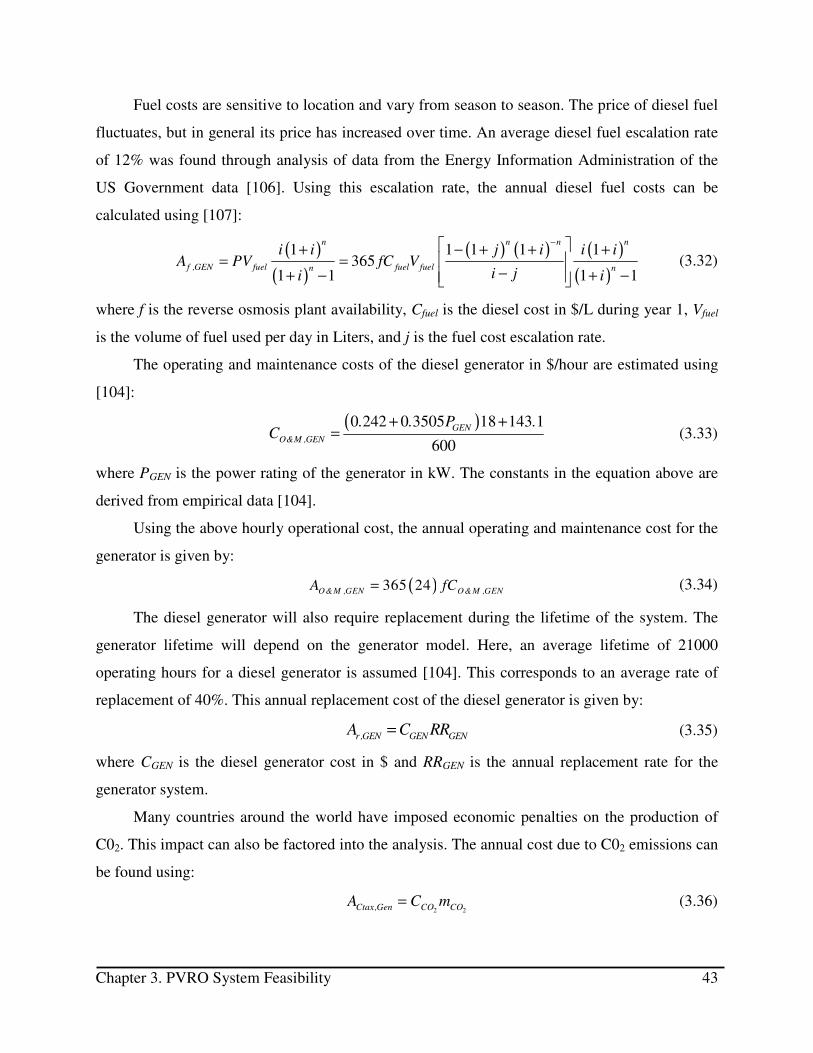
Chapter 3. PVRO System Feasibility 43
Fuel costs are sensitive to location and vary from season to season. The price of diesel fuel
fluctuates, but in general its price has increased over time. An average diesel fuel escalation rate
of 12% was found through analysis of data from the Energy Information Administration of the
US Government data [106]. Using this escalation rate, the annual diesel fuel costs can be
calculated using [107]:
( )
( )
( ) ( ) ( )
( )
1 1 1 1 1365
1 1 1 1
n n n n
f ,GEN fuel fuel fueln n
i i j i i iA PV fC V
i ji i
− + − + + += =
−+ − + −
(3.32)
where f is the reverse osmosis plant availability, Cfuel is the diesel cost in $/L during year 1, Vfuel
is the volume of fuel used per day in Liters, and j is the fuel cost escalation rate.
The operating and maintenance costs of the diesel generator in $/hour are estimated using
[104]:
( )0 242 0 3505 18 143 1
600
GEN
O&M ,GEN
. . P .C
+ += (3.33)
where PGEN is the power rating of the generator in kW. The constants in the equation above are
derived from empirical data [104].
Using the above hourly operational cost, the annual operating and maintenance cost for the
generator is given by:
( )365 24O&M ,GEN O&M ,GENA fC= (3.34)
The diesel generator will also require replacement during the lifetime of the system. The
generator lifetime will depend on the generator model. Here, an average lifetime of 21000
operating hours for a diesel generator is assumed [104]. This corresponds to an average rate of
replacement of 40%. This annual replacement cost of the diesel generator is given by:
r ,GEN GEN GENA C RR= (3.35)
where CGEN is the diesel generator cost in $ and RRGEN is the annual replacement rate for the
generator system.
Many countries around the world have imposed economic penalties on the production of
C02. This impact can also be factored into the analysis. The annual cost due to C02 emissions can
be found using:
2 2Ctax,Gen CO COA C m= (3.36)

Chapter 3. PVRO System Feasibility 44
where CCO2 is the carbon tax in $/kg, and mCO2
is the mass of CO2 produced per year in kg which
can be found using equation (3.37). Carbon taxes are due to the local political conditions: for
example, in France, the current carbon tax is $0.25/kg [108].
The rate of carbon dioxide production by the generator can be calculated using the
relationship [93]:
2 2
2
CO CO
CO C fuel C
C C
M Mm m m w
M M= = (3.37)
where MCO2is the molar mass of carbon dioxide, MC is the molar mass of carbon, and wc is the
mass fraction of carbon in the diesel fuel.
3.5 Case Studies
3.5.1 Seawater Systems
3.5.1.1 Analysis for Any Location
The feasibility of community-scale seawater reverse osmosis systems is analyzed for all
locations using Geographic Information Systems (GIS) data. GIS data on a 1° by 1° grid was
collected for annual average solar insolation for latitude tilt [8], water salinity and water
temperature [96]. This data was then analyzed using the method outlined in equations (3.1)-
(3.37). The constants used in the analysis are given in Table 3.3.
Table 3.3: Input parameters for seawater reverse osmosis analysis. Parameter Value
Plant Capacity, Vcap Plant Lifetime, n Interest Rate, i Plant Availability Factor, f Recovery Ratio, R Reverse Osmosis Membrane Permeability, Kp [99] Reverse Osmosis Motor & Pump Efficiency, ηHP & ηFP [93] Energy Recovery System Efficiency, ηER [93] Array System Efficiency, ηPV Generator Efficiency, ηGEN [104] Generator Load Factor, LF [104] Reverse Osmosis System Cost, URO [94] Installed Array System Cost, UPV [103] Initial Diesel Fuel Cost, Cfuel [106] Diesel Fuel Annual Inflation Rate, j [106]
10 m3 25 years 5% 90% 40% 3.5 x 10⁻¹⁰ m/bar-s 70% 80% 15% 30% 80% $2400 / m3 $9.00 / Wp $0.66 / L ($2.50 / Gallon) 12%
The Middle East is a large market for desalination since the majority of the region does not
have access to an adequate freshwater resource. Hence, a more detailed analysis was carried out

Chapter 3. PVRO System Feasibility 45
for this region. GIS data was obtained for a denser grid of 0.25° by 0.25° to provide a more
detailed picture of this region.
The solar array area required for the 10 m3 per day reverse osmosis system discussed above
is shown in Figure 3.1. It is evident from this figure that array area requirements are lower for
equatorial regions that have high solar insolation. Also, the majority of areas in the Middle East
require less than 40 m2 of solar array area to power a small reverse osmosis system. The area
requirements for systems in equatorial regions are reasonable.
Figure 3.1: Array area required for 10m3 system.
The cost of water produced by the photovoltaic powered reverse osmosis system is
presented in Figure 3.2 and Figure 3.3. Figure 3.2 shows that the majority of equatorial regions
are able to produce fresh water for less than $6.00 per m3. Based on published water
transportation cost data of $10.00 per m3 [109], PVRO is a feasible alternative to transported
water supplies.
Figure 3.2: Water cost for 10m3 system.
Chapter 3. PVRO System Feasibility 46
Figure 3.3 shows water prices for the photovoltaic reverse osmosis system in the Middle
East. Many coastal areas in this region are able to produce clean water using photovoltaics for
less than $5.00 per m3. As expected, water prices increase for Northern areas that receive less
sunshine. Water prices also increase in areas that have higher salinity feed water, such as the
Persian Gulf and the Mediterranean Sea.
Figure 3.3: Water cost for a 10m3 system in the Middle East.
In order for the photovoltaic-powered reverse osmosis system to be cost competitive, the
cost of the water produced should be less than the cost of water produced by an equivalent
diesel-powered system. Figure 3.4 and Figure 3.5 show regions where a solar-powered reverse
osmosis system would be more cost effective than using diesel-powered reverse osmosis.
Photovoltaic-powered reverse osmosis systems are economically feasible throughout large areas
of water scarce regions. The coastal regions of Northern Africa, the Middle East, South Africa,
Mexico and the Caribbean are all examples of water stressed areas where a solar-powered
seawater reverse osmosis system could feasibly deliver clean water to small communities at a
lower cost than a diesel powered reverse osmosis system.

Chapter 3. PVRO System Feasibility 47
Figure 3.4: Areas where PVRO systems are feasible.
Figure 3.5: Areas in Middle East where PVRO systems are feasible.
3.5.1.2 Site Analysis
Table 3.4 gives detailed results for six sites. As expected, the areas with higher water
salinity require more energy to perform reverse osmosis. Also, as expected, the areas listed with
low solar insolation are not favorable for the solar powered systems. For the price assumptions
made, the photovoltaic-powered systems are less expensive for sites in Cyprus, Haiti and Saudi
Arabia. PVRO is feasible in areas with a good solar resource.

Chapter 3. PVRO System Feasibility 48
Table 3.4: Site-specific analysis results – seawater without incentives and carbon tax.
Location Boston, USA
Los Angeles, USA
Limassol, Cyprus
Aqaba, Jordan
Cap-Haïtien, Haiti
Jeddah, Saudi Arabia
Latitude Longitude Average Latitude Tilt Solar Insolation (kWh/m2-day) Daylight Hours (hours) Water Salinity (ppm) Energy Required per day (kWh) Solar Array Area (m2) Total Solar RO System Capital Cost ($) Solar RO System Equivalent Annual Cost ($) Total Diesel System Capital Cost ($) Diesel System Equivalent Annual Cost ($) Cost of Water Solar ($/m3) Cost of Water Diesel ($/m3)
42.35 N 71.06 W 4.4 9.08 32664 29.2 44.2 149,830 23,042 46,718 17,147 7.01 5.21
34.05 N 118.24 W 5.6 9.88 33505 30.1 35.8 123,349 18,553 46,644 17,295 5.64 5.25
34.67 N 33.03 E 6.1 9.87 39182 34.1 37.3 120049 17,494 46,362 17,983 5.32 5.47
29.52 N 35.07 E 5.9 10.25 41160 35.7 40.3 125,696 18,225 46,279 18,231 5.55 5.54
19.76 N 72.2 W 6.0 10.93 36275 31.9 34.8 118,296 17,457 46,497 17,626 5.31 5.36
16.89 N 42.55 E 6.6 11.13 38340 33.4 33.7 111,748 16,311 46,445 17,758 4.96 5.41
3.5.2 Brackish Water Systems
Brackish groundwater is present in many water stressed locations. For these areas, brackish
water RO desalination could be a major potential solution to fresh water shortage. These areas
also typically have an abundance of sunshine, so photovoltaics can be coupled with RO systems
to provide the required energy. Due to a lack of global data sets for groundwater salinity and
depth, only a site specific analysis was performed to demonstrate the methodology for brackish
water desalination. The input parameters for this analysis are given in Table 3.5.
Table 3.5: Input parameters for brackish water reverse osmosis analysis. Parameter Value
Plant Capacity, Vcap Plant Lifetime, n Interest Rate, i Plant Capacity Factor, f Recovery Ratio, R Reverse Osmosis Membrane Permeability, Kp [99] Reverse Osmosis Motor & Pump Efficiency, ηHP & ηFP [93] Energy Recovery System Efficiency, ηER [93] Array System Efficiency, ηPV Generator Efficiency, ηGEN [104] Generator Load Factor, LF [104] Reverse Osmosis System Cost, URO [94] Installed Array System Cost, UPV [103] Initial Diesel Fuel Cost, Cfuel [106] Diesel Fuel Annual Inflation Rate, j [106]
10 m3 25 years 5% 90% 40% 7.5 x 10⁻¹⁰ m/bar-s 70% 80% 15% 30% 80% $1200 / m3 $9.00 / Wp $0.66 / L ($2.50 / Gallon) 12%
Table 3.6 gives the details for all four sites analyzed. As expected, the energy requirements
are higher for the areas with higher salinity water. Also, there is an energy penalty associated
with raising the water from the source. Additionally, the high cost of diesel fuel results in a lower
unit price for the solar powered reverse osmosis systems in all four cases. Photovoltaic reverse
osmosis systems are economically feasible for brackish water desalination.

Chapter 3. PVRO System Feasibility 49
Table 3.6: Site-specific analysis results – brackish water without incentives and carbon tax.
Location Alamogordo, NM, USA [110]
Jurf El-Darwish, Jordan [111]
Broken Hill Australia [112]
Djebeniana, Tunisia [113]
Latitude Longitude Average Solar Insolation (kWh/m2-day) Daylight Hours (hours) Water Salinity (ppm) Water Depth (m) Energy Required (kWh) Solar Array Area (m2) Total Solar RO System Capital Cost ($) Solar RO System Equivalent Annual Cost ($) Total Diesel System Capital Cost ($) Diesel System Equivalent Annual Cost ($) Cost of Water Solar ($/m3) Cost of Diesel Water($/m3)
32.88 N 105.95 W 5.8 9.98 3000 120 20.8 23.9 71,189 7,944 32,154 12,652 2.41 3.85
30.700 N 35.867 E 5.7 10.15 2421 100 19.9 23.3 68,263 7,775 30,274 12,306 2.36 3.75
31.95 S 141.43 E 5.7 10.07 6000 15 18.4 21.5 58,227 7,148 21,977 11,438 2.17 3.48
35.05 N 10.9 E 5.2 9.80 3500 20 16.0 20.5 59,509 7,512 22,882 10,987 2.28 3.34
3.5.3 Comparison with Other PVRO Studies
Other researchers have also investigated PVRO systems and estimated the overall cost of
water produced. A summary of these systems are listed in Table 3.7. The estimated water costs
vary greatly due to variable system efficiency and assumptions that are made during the cost
analysis. It should be noted that the calculated costs of between $4.96/m3 and $7.00/m3 for
seawater photovoltaic reverse osmosis systems and between $3.34/m3 and $3.85/m3 for brackish
water systems lie within the established range.
Table 3.7: Summary of estimated water costs for PVRO systems.
Location Water
Salinity (mg/L)
Water Production
(m3/day)
PV Power Rating (kWp)
Batteries (kWh)
Energy Recovery
Water Cost
($US/m3) Year
Cituis, Indonesia[114] Coité–Pedreiras, Brazil [115] Hammam Lif, Tunisia [116] Heelat Ar Rakah, Oman [24, 117] Mesquite, Nevada [19] Athens, Greece[13] Canary Islands, Spain [22, 23] Massawa, Eritia[14, 15]
3500* 1200* 2800* 1010* 3910* 40000 35500 32800
12.0 0.55 0.05 5.0 1.5
0.35 3.0 3.0
25.7 1.1
0.59 3.4
0.54 0.85 4.8 2.4
132 9.6 No 9.6 No No 60 No
No No No No No Yes Yes Yes
$3.68 $12.76 $8.00 $6.52 $3.46
$11.45 $9.60 $3.00
1983 2004 2005 1998 2003 2008 1998 2001
*brackish water
3.6 Conclusions
This chapter presented a method for determining the engineering feasibility of community-
scale photovoltaic reverse osmosis systems as a function of location and water demand. This
method compares the cost of water produced using photovoltaic reverse osmosis to water
produced using diesel-powered reverse osmosis. This method uses physics-based models to size
the system and determine the system energy requirements. The energy requirements are then

Chapter 3. PVRO System Feasibility 50
used to determine the water cost for each system. A PVRO system is considered feasible if it is
more cost effective than an equivalent diesel-based system or transported water.
Case studies presented in this chapter clearly show the location dependence of the
feasibility of photovoltaic-powered reverse osmosis. This dependency is due to the differences in
terrain characteristics, the solar resources and water characteristics. For the conditions analyzed,
the photovoltaic reverse osmosis is feasible for many water stressed regions. The high fuel costs
for the diesel-powered systems results in higher water costs for most locations. When the system
is configured for a region without a good solar resource, the high capital costs for community-
scale seawater photovoltaic reverse osmosis systems are not recovered during the system
lifetime. With modular design methodologies and intelligent system control of the photovoltaic-
powered reverse osmosis systems, it is possible that the system costs could be further reduced,
and the PVRO systems could become affordable for larger geographic regions.

Chapter 4. Modular Design Approach 51
CHAPTER
4 MODULAR DESIGN APPROACH
This section provides an overview of the modular design approach developed in this thesis.
This approach can be used to custom tailor modular systems from inventories of potential
components. This section also demonstrates the power of the developed approach for the
application of interest, the design of PVRO systems, as well as the design of a hybrid
automobile.
4.1 Modular Design
A common method to reduce manufacturing costs in many applications, such as
automobiles, electronics, and robotics, is to develop products composed of mass-produced
modular components. As stated in Chapter 1, this approach has many advantages, but designing
a custom system configured from an inventory of potential modular components is not a simple
task. For a given modular inventory, a large number of possible system configurations exist. A
designer with significant expertise is required to select the correct components and configuration.
The problem considered in this thesis is the design of a system from an inventory of mass-
produced, modular components. Here, it is assumed that the design algorithms have access to an
inventory of potential components with known characteristics and a design objective. It is also
assumed that the performance of a system is highly coupled to the design choices.
For the PVRO problem, this inventory consists of different PV panels, motors, pumps,
reverse osmosis membranes, pressure vessels, energy recovery devices and control electronics.
For the cases considered, the systems are designed to operate variably to eliminate the need for
energy storage in the form of batteries, instead storing the energy in the form of clean water and
reducing overall system cost. Also, the design algorithms have access to the system
specifications which define the location and water demand of the community. The algorithm
developed should enable a non-expert to configure a custom system for the community from

Chapter 4. Modular Design Approach 52
modular components. The design goal of the modular design of the PVRO system is to determine
the most cost-effective option in terms of lowest lifetime cost that meets the water production
and quality requirements.
4.2 Design Approach
The design framework developed to configure a custom system from a library of potential
modular components can be seen in Figure 4.1. In this framework, a series of different filters are
used to systematically reduce the size of the design space. The preliminary filters are based on
computationally efficient, simple tests to eliminate inappropriate modules and subassemblies
quickly. The smaller design space is further refined by a topology filter using simple, low-
fidelity models and tests. Finally, a high-fidelity model is used on the fully reduced design space
to optimize the system and determine the final system configuration. This approach greatly
reduces the size of the design space and dramatically speeds the optimization, as is shown in
examples in sections 4.3 and 4.4.
Different optimization techniques can be used on the reduced design space to determine a
final system configuration. For the design of a PVRO system, a genetic algorithm is used to
optimize the final system configuration [118]. This method is used because the PVRO system
configuration is represented by a series of binary, integer and continuous design variables. In
addition, the equations which describe the system performance are non-linear. Genetic
algorithms can easily encode discrete variables and can handle non-linear equations by
evaluating a large population of potential configurations. Genetic algorithms are often the
preferred choice for topology optimization problems and are well-matched for the design of
other modular systems [47, 57, 59, 60, 63, 69, 71].

Chapter 4. Modular Design Approach 53
Figure 4.1: Modular design approach.
4.3 PVRO System Design Space Study
4.3.1 Overview
To show the effectiveness of this approach for a PVRO system, a design space study for a
modular inventory was performed. In this study, the total number of system combinations is
enumerated through each of the steps outlined in the modular design approach. The inventory
considered in the design space study is shown in Figure 4.2 and the component details are given
in Table 4.1. In this example, this simple inventory will be used to design a small, 1 m3/day
water production, brackish water system for Haiti.
Figure 4.2: Inventory used in design space study.
EnvironmentCharacteristic
Database
System Simulation
& Optimization
Location
Subassembly
Level Filter
Water ReqsModule Level Filter
Module
Database
Solar
Insolation,Water
Characteristics,Temperature
Topology Filter
Task
Description
Optimal
Design
Reduced Design
Space
Simple Tests
Detailed Simulations
ReverseOsmosis
Membranes
Control
Electronics
Pumps Energy Recovery
& Pressure
Control DevicesPV Panels

Chapter 4. Modular Design Approach 54
Table 4.1: Sample inventory used for design space study. Component Details
PV Panels Quantity Power Rating Efficiency Cost
PV Model 1 6 250 W 15% $500 PV Model 2 6 200 W 13% $300 PV Model 3 6 300 W 18% $450
RO Membranes Quantity Water Type Area Rated Water Production
Cost
RO Membrane Model 1 3 Brackish Water 2.8 m2 3.2 m3/day $120 RO Membrane Model 2 3 Brackish Water 7.5 m2 9.1 m3/day $220 RO Membrane Model 3 3 Seawater 2.8 m2 2.6 m3/day $150
Motor + Pump Units Quantity Maximum Pressure
Maximum Power
Efficiency Cost
Pump Model 1 3 25 bar 200 W 65% $300 Pump Model 2 3 80 bar 400 W 82% $800 Pump Model 3 3 80 bar 800 W 80% $1500
Energy Recovery + Pressure Control Valves
Quantity Maximum Pressure
Maximum Flow Rate
Efficiency Cost
Energy Recovery Model 1 1 80 bar 0.5 L/s 85% $3500 Energy Recovery Model 2 1 80 bar 0.3 L/s 90% $3000 Pressure Control Valve 1 1 80 bar 1 L/s 0% $200
4.3.2 Enumerating Full Design Space
To determine the initial design space, it is assumed that each system must contain at least
one PV panel, one pump and motor, one RO membrane, and one energy recovery device or
pressure control valve. It is also assumed that the required pressure vessels, connecting
components and power control electronics are readily available. The system is being configured
for a location with one water intake, one brine disposal, and one potable water storage facility in
place. It is also assumed that not all the components need to be used.
The PVRO system has two main subsystems, the reverse osmosis system and the
photovoltaic power system which are coupled via the control electronics. The total number of
system configurations is given by
PVRO RO PVN N N= × (4.1)
where NRO is the number of different RO system configurations and NPV is the number of PV
system configurations.
Each reverse osmosis system is formed by selecting and connecting components from the
modular inventory. This results in a large number of possibilities for a given inventory, which
can be expressed as:

Chapter 4. Modular Design Approach 55
( )( )
, , ,,1 ,1 ,1
,1 , ,1 , , ,1 ,, ,0 0 0
1 1
, , ,
1 1 1
! ! !
2
1p N ro N er Np p ro erro er
p p N ro ro N ro base er er N er basep ro er
outputs in
p ro er
p b
put
outputs inputs
ase
N N
N N NN
p i ro i e
NN N N
RO
n n n n N n n N
n nn
r i
i i i
n
l m
n n n
N= = = = = =
=
=
= =
=
×
=
+
∑ ∑ ∑ ∑ ∑ ∑∏ ∏ ∏
∑
( )( ) ( )( )
( )( ) ( ) ( )( ) ( )
2 1
2 1 2 1
s
outputs inputs
outputs inputs outputs inputs
n l n m l moutputs inputs
n l n m l n l n m moutputs inputs
n n
l m
n n
l m
− − +
− − − −
−
+ − + −
∑
(4.2)
where Np,i is the number pumps of type i in the inventory, Nro,i is the number of reverse osmosis
membranes of type i in the inventory, Ner,i is the number of energy recovery devices and pressure
control valves of type i in the inventory, ninputs is the number of component inputs for a
configuration as given by:
, , ,
1 1 1
2 1p ro er
N N N
outputs p i ro i er i
i i i
n n n n= = =
= + + +∑ ∑ ∑ (4.3)
and noutputs is the number of components outputs for the configuration as given by:
, , ,
1 1 1
2p ro er
N N N
inputs p i ro i er i
i i i
n n n n= = =
= + + +∑ ∑ ∑ (4.4)
Np,base, Nro,base, and Ner,base are indices that ensure each configuration has at least one pump, one
reverse osmosis membrane, and one energy recovery or pressure control valve and are expressed
as:
1
, ,1
max(1 , 0)
N p
p base p ii
N n
−
=
= − ∑ (4.5)
1
, ,1
max(1 , 0)
Nro
ro base ro ii
N n
−
=
= − ∑ (4.6)
1
, ,1
max(1 , 0)
Ner
er base er ii
N n
−
=
= − ∑ (4.7)
The derivation of equations (4.2) - (4.7) are presented in Appendix A.
There are many ways to configure a PV system from an inventory of PV panels. Provided
the PV array voltage and current output is compatible with the control electronics, the
configuration of the PV array does not greatly impact the overall power production. Therefore,

Chapter 4. Modular Design Approach 56
the number of distinct configurations can be determined by the number of ways to select groups
of PV panels from the inventory as given by:
( ),
,
1
1 1pv typeN
PV pv i
i
N n=
= + −∏ (4.8)
where Npv,type is the number of different types of PV panels in the inventory, npv,i is the number of
PV panels of type i in the inventory. The derivation of equation (4.8) is presented in Appendix A.
Using equations (4.1)-(4.8), the total number of configurations for the inventory presented
in Figure 4.2 can be computed. The resulting number of system configurations is 1.9 x 10173.
This number far exceeds the approximate number of atoms in the observable universe, which is
estimated to be 9.4 x 1079 [119]. Optimizing a system with a design space this large is infeasible.
4.3.3 Module Level Filters
Using the modular design approach outlined in Figure 4.1, the size of the design space is
reduced. In the initial step, module level filters are applied to the motor/pump units, reverse
osmosis membranes, energy recovery devices and PV panels to remove inappropriate elements
from the inventory. The filters applied for PVRO systems are detailed here.
For the PVRO system, the design goal is to minimize the lifetime system cost. The filters
presented here assume that the expected life of all components of the same type is identical. As a
result, the applied value metrics only consider capital costs. If lifetimes of components are
different and known, the value metrics should be adjusted to account for such differences.
4.3.3.1 Motor/Pump Filters
For the motors and pumps, the following filters are applied to reduce the size of the design
space:
1. Motor/pump combinations that are designed for pressures that are inappropriate for the
given system are eliminated from the inventory. Since the salt concentration varies for
different source waters, the typical operating pressures also vary. For brackish
desalination, the typical operating pressure is 30 bar, while for seawater desalination,
the operating pressures go up to 80 bar.

Chapter 4. Modular Design Approach 57
2. Motors and pumps with inappropriate power ratings are eliminated from the inventory.
Based on the energy requirements, shown in Table 1.1, the average power requirement
of the system can be calculated as follows:
Average Energy Requirements Average Energy Requirements
Number of Operating Hours Number of Peak Sun HoursP = = (4.9)
Using the solar data at the site, the power requirement can be estimated. Pumps that
are rated for more than two times the average power requirement are oversized and are
removed from the inventory.
3. Value metrics are applied to pumps/motor units. The cost per percent efficiency is
used to compare possibilities. Since different system scales require different types of
pumps, these metrics are evaluated by power rating. Pump/motor units that do not rank
in the top 50% for one of these metrics are removed from the design problem.
When applied in the context of designing a brackish water PVRO system capable of producing 1
m3 of clean water per day in Haiti, these filters remove Pump/Motor 3 from the inventory since it
is oversized for the system energy requirements.
4.3.3.2 Reverse Osmosis Membrane Filters
For the reverse osmosis membranes, the following filters are applied to reduce the size of
the design space:
1. Membranes are removed that are for the incorrect water type. For example, when
designing a system for brackish water desalination, the seawater filters are removed
from the design space.
2. Value metrics are applied to membranes. The cost per water permeability and cost per
salt permeability are calculated for each type of component. Since different system
scales require different membrane areas, these metrics are compared by membrane
size. Membranes that do not rank in the top 50% of their category for one of these
metrics are removed from the design problem.
For the sample Haiti PVRO system design problem, the filters remove Reverse Osmosis
Membrane 3 from the inventory.

Chapter 4. Modular Design Approach 58
4.3.3.3 Energy Recovery Device and Pressure Control Valve Filters
The following filters are applied to the energy recovery/pressure control devices to reduce
the size of the design space:
1. Components that have inappropriate pressure and flow ratings for the application are
eliminated from the design space. Expected operating pressures for the brackish water
systems are 30 bar and for seawater systems the expected operating pressure is
between 60-80 bar. Devices that have pressure ratings too low are removed from the
inventory.
The expected flowrate through the energy recovery system is calculated as follows:
Sys
ERD
R= (4.10)
where Qsys is the rated system flowrate and R is the expected recovery ratio. For the
small systems considered here, the recovery ratio will range between 10% and 30%.
Using these numbers, the range of required flowrates is calculated. Energy recovery
devices with maximum flowrates below the expected range will be eliminated from
the inventory.
2. Value metrics are applied to energy recovery devices. The cost per percentage
efficiency is calculated for each ERD. ERDs that do not rank in the top 50% for one of
these metrics are removed from the inventory.
When applied to the brackish water system design problem for Haiti, these filters remove Energy
Recovery Model 1 from the inventory based on the component value metric.
4.3.3.4 PV Panel Filters
For the PV panels, the following filters are applied to reduce the size of the design space:
1. Value metrics are applied to the PV panels. The cost per percentage efficiency and
cost per power rating is calculated for each PV panel. Since the possible power ratings
of the PV array are discrete, the inventory should contain PV panels with lower power
ratings to ensure that PV array is not oversized. As a result, value metrics are
compared for PV panels with power ratings less than or equal to 200 Watts or greater
than 200 W. Panels that do not rank in the top 50% in their category for one of these
metrics are removed from the inventory.
Chapter 4. Modular Design Approach 59
The filters remove PV Model 2 from the inventory based on the value metric when applied to the
Haiti brackish system design problem.
After eliminating these components from the inventory, the total number of possible
system configurations has decreased to 7.5 x 1088. The design space at this stage is still much too
large to configure a system design using optimization methods. Further design space reduction is
required to make the problem tractable.
4.3.4 Subassembly Filters
In the next algorithm step, subassembly level filters are applied to limit the design space.
This step configures subassemblies that can be used in the full system. For the small-scale PVRO
system design problem, subassemblies such as the PV array and reverse osmosis membrane array
are sized. In addition, the total numbers of pumps and energy recovery devices to be considered
during the design are determined.
The PV array is sized based on simple energy calculations. For the brackish water case, the
range of energy consumption is assumed to range from 1 kWh/m3 to 5 kWh/m3. These numbers
can be used with the solar insolation at the site to set the limits on the PV array power ratings as
follows:
max/min
max/min
cap rateE V G
PH
= (4.11)
where Pmax/min is the maximum or minimum array rating required in kW, Emax/min is the maximum
or minimum specific energy requirement for the water desalination in kWh/m3 as given in Table
1.1, Vcap is the desired system capacity, Grate is the solar radiation that the panels are tested at
(typically 1 kW/m2) and H is the average annual solar insolation in kWh/m2 at the site. For the
Haiti system with an average insolation of 6.05 kWh/m2 [8], the maximum array power rating is
661 W and the minimum requirements are 165 W. Using these max and minimum values, limits
are placed on the number of panels required. Panels in a PVRO system configuration are limited
to a single model unless the calculated limits exceed what is available for a single model in the
inventory.
Similarly, the maximum and minimum size for the reverse osmosis array can be
determined. For given water production, the average clean water flow rate can be determined by:

Chapter 4. Modular Design Approach 60
,
p
p ave
sun
VQ
n= (4.12)
where nsun is the number of hours of peak sunshine. For the 1 m3/day Haiti system being
considered, the average flowrate would be 165 L/hour. Using this flowrate, the number of each
membrane type required can be determined. A 50% safety factor is incorporated to ensure that
resulting subsystems result in feasible system designs.
For the system pumps and energy recovery devices, rules of thumb are used to limit the
total number of pumps that can be included. For the community-scale systems considered here,
conventional systems are used as a guide. For small systems with a daily capacity less than 2m3,
typical systems contain two pumps or fewer. To allow for innovative designs, an upper bound on
the number of pumps in the system is placed at 3. For larger systems with daily production
capacities above 2m3, the number of pumps allowed in the system is placed at 5 to allow for
innovative configurations.
For small-scale PVRO systems, energy recovery devices are typically expensive and
dominate the system cost. As the devices are scaled up for larger flowrates, they tend to be more
cost effective. As a result, the total number of energy recovery devices that can be placed in the
system is limited to one. In addition, one pressure control valve will be allowed in the final RO
system.
After these subassembly level filters are applied, the size of the design space for the Haiti
system design problem is reduced to 9.8 x 1049. This design space is still very large for direct
application of an optimization algorithm.
4.3.5 Topology Filters
The next step in the modular design algorithm is the topology filter. This limits the number
of configurations which can be assembled from the subsystems by applying simple calculations
and design rules. For the PVRO system design problem, unreasonable system topologies are
eliminated. The filters applied here can be broken into two categories: RO system topology
filters and PVRO system filters.
The topology filters for the RO system eliminate the following cases:
1. Configurations with permeate stream and brine stream mixing which negates the
purpose of the reverse osmosis process. Mixing of the permeate stream and the feed is
Chapter 4. Modular Design Approach 61
allowed for brackish water systems. Given the low water salinity and the discrete
nature of the system configurations, diluting desalinated water with feed water may be
the most cost effective option and is used in practice [120].
2. Configurations where not all components are connected or a path does not exist from
the reverse osmosis water input and the brine and permeate outputs.
3. Configurations where input water is not pressurized before entering the reverse
osmosis membranes. In these cases, there would not be the driving force necessary for
desalination.
4. Configurations containing loops without pumps or energy recovery devices in the
reverse osmosis setup. These cases are infeasible.
5. Configurations where pumps are directly connected to energy recovery exhaust
streams. In these cases, energy is being put into the water by the pumps and then being
removed by the energy recovery unit without any product water being produced. Since
these processes are not 100% efficient, this results in wasted energy.
6. Configurations where high pressure pumps are directly connected to permeate or brine
outputs. Any pump connected to these outlets would waste energy. In addition any
configuration where the exiting brine stream doesn’t pass through a pressure control
valve or energy recovery device is eliminated. These components are required to
produce the pressure for reverse osmosis.
Examples of these cases are depicted in Figure 4.3 below.

Chapter 4. Modular Design Approach 62
Figure 4.3: Examples of RO system configurations eliminated by the topology filter.
The remaining assembly filters match the size of the PV array with the RO system designs.
The amount of energy required for the desalination will vary greatly depending on the use of
energy recovery devices, as shown in Table 1.1. The allowable power ratings for each PV array
for systems with/without energy recovery devices are determined using the expected energy
requirements and equation (4.11).
After applying assembly level filters, the design space is greatly reduced to 3.4 x 10⁷
different configurations. This size of design space is a much more reasonable size for
optimization. The modular design algorithm has made this problem more tractable. A summary
of the results of the design space study are shown in Table 4.2.
Table 4.2: Summary of PVRO modular design study. Filter Level Design Space Size
Component Library 1.9 x 10173 Module Filter 7.5 x 1088 Subassembly Filter 9.8 x 1049 Topology Filter 3.4 x 10⁷
Fresh
Water
Brine
Reverse
Osmosis
Membranes
Control
Electronics
Salt
Water
Intake
Feed
Water
Pump
High
Pressure
Pump
Tracking System
Fresh
Water
Brine
Reverse
Osmosis
Membranes
Control
Electronics
PV Array
SaltWater
Intake
Energy
Recovery
Device
Feed
Water
Pump
High
Pressure
Pump
Tracking System
Fresh
Water
Brine
ReverseOsmosis
Membranes
Control
Electronics
SaltWater
Intake
EnergyRecovery
Device
Feed
Water
Pump
High
Pressure
Pump
Tracking System
FreshWater
Brine
ReverseOsmosis
Membranes
Control
Electronics
PV Array
Salt
Water
Intake
EnergyRecovery
Device
High
Pressure
Pump
Tracking System
Brine
Fresh
Water
Brine
Reverse
OsmosisMembranes
ControlElectronics
Salt
WaterIntake
Energy
RecoveryDevice
Feed
Water
Pump
High
Pressure
Pump
Tracking System
FreshWater
Brine
Reverse
OsmosisMembranes
ControlElectronics
PV Array
Salt
WaterIntake
Energy
RecoveryDevice
Feed
Water
Pump
High
Pressure
Pump
Tracking System
Case 1: Permeate and Brine Blending Case 2: Disconnected Components
Case 3: Unpressurized Feed Case 4: Feedback Loops
Case 5: Pump – ERD Direct Connection Case 6: Pressurized Stream Exiting System
Missing
Connection

Chapter 4. Modular Design Approach 63
4.4 Parallel Example – Hybrid Car Powertrain
There are many different modular systems that can be configured using the approach
developed in this thesis. This section details a simplified design example for a hybrid electric car.
Here, the design problem is to determine the vehicle configuration with the minimum fuel
consumption while maintaining the following objectives:
1. 0-100 kph time less than 12 seconds
2. Minimum all electric range of 25 km.
3. Range of 600 km.
For this design space study, the module inventory detailed in Table 4.3 is used. This
inventory has a selection of vehicle platforms, combustion engines, electric motors, generators,
batteries, and gas tank sizes.
Table 4.3: Modules considered in hybrid car design study.
Batteries Chemistry Number of Cells
in Inventory Cell
Voltage Cell Capacity Cell Weight
Charge/Discharge Efficiency
Battery 1 Li-ion 150 3.3 V 4.2 Ah 205g 97% Battery 2 Li-ion 150 3.7 V 21 Ah 313g 95% Battery 3 Li-ion 150 3.6 V 52 Ah 1000g 97% Battery 4 NiMH 150 1.2V 6.5 Ah 170g 70% Battery 5 NiMH 150 1.2V 30 Ah 760g 67%
Motors Type Maximum Power
Output Max Torque
Output Weight Max Efficiency
Motor 1 AC 91.0 kW 166.8 Nm 162 kg 89.2% Motor 2 AC 50.0 kW 151.8 Nm 115 kg 89.3% Motor 3 DC 21.5 kW 94.9 Nm 70.8 kg 89.1% Motor 4 DC 27.7 kW 183.0 Nm 104 kg 91.4% Motor 5 DC 22.1 kW 162.7 Nm 167 kg 86.4%
Engines Engine Size Max Power Output Max Torque
Output Weight Max Efficiency
Engine 1 1 L 48.5 kW 118.0 Nm 97.5 kg 32% Engine 2 1.4 L 62.7 kW 131.5 Nm 99.8 kg 29% Engine 3 1.6L 110.4 kW 229.1 Nm 101.6 kg 30% Engine 4 2.0L 149.2 kW 299.6 Nm 133.8 kg 33% Engine 5 2.4L 167.9 kW 348.5 Nm 164.7 kg 29%
Generators Max Power
Output Weight Efficiency
Generator 1 54 kW 74 kg 92% Generator 2 44 kW 82 kg 90% Generator 3 34 kW 35 kg 85% Generator 4 22 kW 55 kg 89% Generator 5 8 kW 10 kg 80%
Platforms Type Average Drag Area
(CdA) Average Weight
Platform 1 Subcompact 0.7 m2 2000 lbs Platform 2 Compact 0.65 m2 2500 lbs Platform 3 Midsize 0.58 m2 3000 lbs Platform 4 SUV 1.08 m2 3500 lbs
Tank Volume
Tank 1 37.8 L Tank 2 45.4 L Tank 3 56.8 L
Tank 4 68.1 L

Chapter 4. Modular Design Approach 64
For hybrid cars, there are two main system configurations. In one configuration, the
electric motor and fuel powered engine are in parallel, in the other the motor and engine are
connected in series. These two configurations can be seen in Figure 4.4. It is assumed for this
study that the transmission and electronics are readily available and selected independent of the
other components.
Figure 4.4: Parallel hybrid car (left) and series hybrid car (right) configurations.
The total number of system configurations can be determined as follows:
hybrid para series
N N N= + (4.13)
where Npara is the number of parallel configurations and Nseries is the number of series system
configurations. The number of parallel system configurations is determined by the product rule:
para Plat Bat Eng Motor Gas
N N N N N N= (4.14)
where NPlat is the number of vehicle platforms, NBat is the number of different battery system
configurations, NEng is the number of engines in the inventory, Nmotor is the number of motors in
the inventory, and NGas is the number of gas tanks in the inventory. The number of series system
configurations is determined by the product rule:
series Plat Bat Eng Gen Motor Gas
N N N N N N N= (4.15)
where NGen is the number of generators in the inventory.
Assuming that all batteries in the vehicle pack are the same and the arrangement of
batteries in series and parallel can be accommodated by the electronics, the number of battery
configurations is given by:
( ),
,
1
1 1Bat typeN
Bat Bat i
i
N n=
= + −∏ (4.16)
where nBat,i is the number of batteries of type i in the inventory, and NBat,type is the total number of
battery types.
Transmission
Battery ConverterElectricMotor
EngineGas Tank
Transmission
Battery
ConverterElectricMotor
Gas TankGenerator Engine
BatteryCharger

Chapter 4. Modular Design Approach 65
Using equations (4.13) to (4.16), the full design space can be enumerated. For the
inventory specified, the total number of system configurations is 2.4 x 10¹⁴. This number of
configurations here is much smaller than the PVRO system since there are a limited number of
system topologies.
The design space is reduced by applying the module level filters. Since the design goal
here is to maximize the fuel economy while maintaining performance, efficiency and power
metrics are applied. For the platform, the different configurations are ranked based on weight and
drag. The platforms that didn’t rank in the top 50% in either category were eliminated. For the
example, the SUV design is eliminated due to high mass and drag characteristics.
The engine configurations are filtered based on weight, power, and efficiency. Engines are
ranked according to maximum power output per unit weight and efficiency. Engines that don’t
rank in the top 50% are eliminated. Engine 5 is eliminated due to low efficiency and power
output.
The generators are used to convert mechanical energy from the gasoline engine into
electrical energy to store in the batteries and must be sized appropriately. For the inventory
selected, the minimum power input to the generator would be 48 kW. Generators with maximum
power ratings below this value are undersized for the application. As a result, Generator 4 and 5
are eliminated from the inventory.
The batteries are filtered based on energy density, power density and charge/discharge
efficiency. Again, batteries are ranked for each of the above categories and the components that
do not rank in the top 50% for any of the criteria are eliminated. For the batteries, the NiMH
configurations are eliminated due to their high weight and low efficiency.
The filtering of the electric motors is broken into two categories. If the vehicle has the
series configuration, the motor must provide all the power to the wheels. In the parallel
configuration, the electric motor assists the gasoline engine. Motors which are able to provide
high power (above 100 kWh) are evaluated separately from the smaller motors. The motors are
ranked in terms of overall efficiency and maximum power output per unit weight. The motors
that do not rank in the top 50% are eliminated. As a result, Motor 5 is eliminated from the
inventory.
The number of tanks in the inventory is limited using simple mileage calculations. A
reasonable hybrid car achieves at least 12.75 km/L in the city. Therefore to guarantee a 600 km

Chapter 4. Modular Design Approach 66
range, a tank volume of 47 L is required. As a result, the 68.1 L tank is removed from the
inventory.
Based on the filters specified above, the total number of system configurations drops to 9.9
x 108. This is a large reduction from the initial design space size, but with additional filters, this
number can further decreased.
In the next step of the modular design approach, subassembly level filters are applied to
reduce the size of the design space. In this step, engines and generators are matched based on
torque and speed characteristics. In addition, battery packs are configured from battery modules.
Maximum and minimum numbers of batteries are determined based on energy calculations. The
average power usage of current hybrid vehicles is 22 kWh per 100 km [121]. The minimum
capacity on each battery pack is set at 4 kWh, which provides enough energy to drive the
minimum range considering a 25% increase in system efficiency. Using these filters, the size of
the design space is reduced to 2.8 x 10⁶.
In the final step, full system assemblies are considered. Since there is limited topology
optimization for the hybrid car case, only a few filters are applied. In the series configuration, all
the power is applied to the wheels using the electric motor, and only the higher power
configurations (Motor 1 and Motor 2) are considered. For the parallel configuration, the electric
motors share the power with the gasoline engine and the smaller motors (Motor 3 and Motor 4)
are considered. The total number of system configurations is 1.4 x 10⁶. Detailed analysis can
then be used on these configurations to determine the system configuration using optimization
methods.
The reduction of the design space size of the hybrid car problem using the modular design
approach is detailed in Table 4.4. This section provides an example of how this approach can be
used for other modular design problems. It does not provide an exhaustive list of potential filters
for the design of a hybrid car drivetrain. This example only considers the fuel economy
objective, but other objectives involving cost can also be incorporated into the design approach.
Table 4.4: Modules considered in hybrid car design study. Filter Level Design Space
Size
Component Library 2.4 x 10¹⁴ Module Filter 9.9 x 10⁸ Subassembly Filter 2.8 x 10⁶ Topology Filter 1.4 x 10⁶

Chapter 4. Modular Design Approach 67
4.5 Summary
This section presented the modular design approach. The approach uses a series of tests
based on engineering principles to reduce the size of the discrete design space and make the
problem tractable for optimization algorithms. The power of the approach is demonstrated
through two sample design space studies, the design of a photovoltaic reverse osmosis system
and the design of a hybrid car. In both cases, the approach is shown to greatly reduce the size of
the design space.
The final step in the modular design algorithm is to optimize the system over the reduced
design space using a detailed system model. The optimization problem is challenging as the cost
function and constraints are non-linear, resulting in a mixed integer nonlinear program (MINLP).
The detailed system model is described in Chapter 5 and the optimization setup is described in
Chapter 6.

Chapter 5. PVRO System Model 68
CHAPTER
5 PVRO SYSTEM MODEL
This section describes the models used for the modular design of PVRO systems. The
components overviewed below are: the environment, PV system, control electronics, motors,
pumps, reverse osmosis membranes, and energy recovery devices. These models account for all
the main physical characteristics and losses. However, these models neglect the fast system
dynamics and assume the system can quickly adapt to changing levels of solar insolation.
5.1 Environment Models
5.1.1 Solar Energy Model
Solar radiation varies greatly from location to location. For any given location, the
radiation varies greatly over the course of the day and year. The solar energy model used for the
design of modular PVRO systems accounts for these variations by using site specific solar
radiation data provided by the NASA Solar Radiation Database [8]. This database provides daily
solar insolation values for any location derived from satellite imagery.
This solar radiation data is used differently for each of the case studies presented in
chapters 6 and 7. In all of the cases presented, the daily solar insolation is used to generate daily
radiation profiles to analyze the system performance. The hourly data is generated from the daily
insolation as follows. First, the sun position for each hour is calculated using:
cos sin sin cos cos cos sinzs s
θ δ φ δ φ ω γ= + = (5.1)
( )
( )sin sin sin
coscos cos
s
s
s
signγ φ δ
ψ φγ φ
−= (5.2)
where θzs is the solar zenith angle (angle between vertical and the sunlight direction), ψs is the
solar azimuth (angle between the meridian and the sun), γs is the solar elevation (angle between

Chapter 5. PVRO System Model 69
the sun and the horizon), ω is the true solar time, φ is the latitude of the location, δ is the solar
declination as given by:
( )360 284
23.45 sin365
nod
δ+
=
(5.3)
where dn is the day number. All angles are expressed in degrees.
The true solar time is the angular difference between solar noon and current time as given
by:
( )4 9.87sin 2 7.53cos 1.5sin
15 1260
o
GMTTς δ δ δ
ω+ − −
= − ∆ + −
(5.4)
where T is the local time in hours, ∆GMT the time difference between Greenwich Mean Time in
hours, and ς the longitude of the site.
Using equation (5.1), the sunrise angle, ωs can be found. At sunrise, the solar elevation (γs)
is 0, and therefore:
( )arccos tan tansω δ φ= − − (5.5)
Outside the earth’s atmosphere, the radiation from the sun can be easily determined. The
radiation on a flat surface outside the atmosphere, in W/m2, is given by:
( )0 0 0 cos ZSB T B ε θ= (5.6)
where B0 is the solar constant outside the earth’s atmosphere which equals 1367 W/m2 and ε0 is
eccentricity of the earth’s orbit which is given by:
0
3601 0.033cos
365n
dε
= +
(5.7)
The extraterrestrial radiation integrated over the course of the day gives:
0 0 0
24sin sin cos cos sin
180d s sB B
πε ω δ φ δ φ ω
π
= − −
(5.8)
The ratio between the extraterrestrial radiation at a given instant and the daily irradiation can be
used to determine the radiation at the earth’s surface as follows [122]:
( )0
0
( )( ) cosd
d
B t GG t a b
Bω= + (5.9)
where Gd is the measured or generated daily solar insolation at the earth’s surface in Wh/m2 and
a and b are empirically derived as follows:

Chapter 5. PVRO System Model 70
( )0.409 0.5016 sin 60sa ω= − + (5.10)
( )0.6609 0.4767 sin 60sb ω= + + (5.11)
Equation (5.9) approximates the radiation on a flat plate at any instant in time given the
daily solar insolation. This radiation has two components: beam radiation which comes from the
direction of the sun, and diffuse radiation which is scattered by the atmosphere and comes from
all directions. The breakdown of the radiation components can be found as follows.
Due to the atmosphere, only a fraction of the radiation reaches the earth’s surface. This is
referred to as the clearness index and for a day’s time period it is given by:
0
dTd
d
GK
B= (5.12)
The clearness index has been used to empirically determine the amount of diffuse radiation.
Based on data from the European weather station network, the diffuse fraction of radiation was
derived as:
2 3
0.952 for 0.13
0.868 1.335 5.782 +3.721 for 0.13 0.8
0.141 for 0.13
Td
Dd Td Td Td Td
Td
K
F K K K K
K
≤
= + − < ≤ >
(5.13)
Using this fraction, the daily diffuse insolation is given by:
d Dd dD F G= (5.14)
Given the daily diffuse insolation, the diffuse insolation at any period of time is determined
using the following empirical relationship:
0
0
( )( ) d
d
B tD t D
B= (5.15)
and the beam radiation at the earth’s surface is given by:
( ) ( ) ( )B t G t D t= − (5.16)
The diffuse radiation and beam radiation falling on the earth’s surface along with the sun
position as outlined in equations (5.1) and (5.2) can be used in the solar panel model for a given
panel orientation as outlined in section 5.2.2.

Chapter 5. PVRO System Model 71
5.1.2 Water Salinity Model
Water salinity varies greatly by location. For the purpose of the modular design approach,
water salinity numbers are taken for each case study location from the World Ocean Atlas [96].
The water salinity will change over the course of the year due to the natural water cycle. These
variations are typically less than 10%. To simplify the analysis here, average yearly values of
water salinity and temperature values from a depth of 10 m are used. For system design for a
specific location, measurements of the local water salinity should be taken to provide an accurate
performance estimates.
5.1.3 System Demand
The water demand varies for each case and greatly affects the system design. In the case
studies detailed in Chapter 6 and Chapter 7, the demand is treated differently. In the case studies
in Chapter 6, the demand is assumed to be constant and known and the PVRO system is designed
to meet these needs. In the case studies presented in Chapter 7, the water demand is assumed to
vary according to historical water demand statistics. These statistics and predicted demand trends
are detailed in Chapter 7.
5.2 Component Models
5.2.1 PV System
Photovoltaics convert light energy directly to electrical energy. A PV cell is composed of
two or more layers of doped semiconducting materials as shown in Figure 5.1. When exposed to
sunlight, electrons are excited from the valence band to the conduction band in the
semiconducting material. The electrons then move via diffusion to the PN junction where they
are separated from their corresponding holes. The electrons are then conducted by electrical
contacts to an external circuit. A typical PV cell produces only a few watts of power. Cells are
typically strung together in series and are encapsulated in a PV module to provide adequate
voltage. These modules are then strung together in array to provide enough power for a given
application.

Chapter 5. PVRO System Model 72
Figure 5.1: Solar cell operation.
Due to the bandgap of the semiconductor and the cell structure, photovoltaics can only
convert a portion of the solar spectrum into electrical energy. The remainder of the solar energy
is lost to heat. Conversion efficiencies of photovoltaic cells vary depending the material and
process used to produce the cells. Many different types of semiconducting materials are used in
PV cells. The majority of commercial PV modules on the market today are made of silicon (Si)
which can be divided into three main categories: monocrystalline silicon, which has the highest
efficiency and cost, polycrystalline silicon, which has a less ordered crystal structure and lower
efficiency, and amorphous silicon, which is a thin film technology with relatively low efficiency.
Other compounds that are commonly used in solar cells include cadmium telluride (CdTe),
gallium arsenide (GaAs), and copper indium gallium selenide (CIGS). Common efficiencies for
commercial monocrystalline silicon modules are 15-18% [123].
The basic operation of a solar cell can be represented using the classic one diode model. In
this model, depicted in Figure 5.2, the current produced by a solar module is given by [124]:
0 exp 1( 273.15) /
s sph
cell sh
V IR V IRI I I
nk T q R
+ += − − −
+ (5.17)
where Iph is the light generated current, I0 is the reverse saturation current which is affected by
temperature, V is the panel operating voltage, I is the operating current, Rs is the panel series
resistance, Rsh is the panel shunt resistance, n is the diode ideality factor, k is the Boltzmann
constant, Tcell is the cell temperature in oC, and q is the charge of the electron. Note that I0, Rs, Rsh
and n are all panel specific parameters. All currents are in A, voltages are in V, and resistances
are in Ohms. The light generated current can be represented by:
( )0 1ph panel cell PVI A C C T G= + (5.18)
where Apanel is the area of the solar panel in m2, GPV is the incoming solar radiation normal to the
cell, and C0 and C1 are panel specific constants.
P-type
N-type
Rear Contact
+e-
Sunlight
-
+
e-
FrontContact
ExternalLoad

Chapter 5. PVRO System Model 73
Figure 5.2. Electrical circuit representation of the one diode solar module model.
From the above equations, it is evident that the output current of the photovoltaic module is
dependent on many factors including the operating voltage, the solar radiation, and the solar cell
temperature. Output current and power produced by a typical solar panel for a given amount of
solar radiation and different cell temperatures are shown in Figure 5.3. At each temperature or
radiation level, there exists an operating voltage at which the solar panel produces its maximum
amount of power. In general, connecting a load directly to a solar panel will not result in the
voltage that gives maximum power output. Typically, a power converter with a maximum power
point tracking algorithm is required to optimize the power output.
Figure 5.3. Photovoltaic panel operating curves.
The PV model which is used in the modular design approach assumes that the electronics
are able to track the maximum power output for the given solar radiation. Using this assumption,
the PV system model determines the power output for a given solar profile, panel type, and
number of panels. For each PV module in the inventory, dimensions, efficiency, and thermal
properties are extracted from the manufacturer’s data sheet. Using these properties, the power
produced by the PV system can be determined using:
Rs
Rsh
ID1
Iph
I
V

Chapter 5. PVRO System Model 74
[ ](1 ( 298))Solar panel PV PV PV cellP n G A Tη α= + − (5.19)
where Psolar is the power produced by the PV system, npanel is the number of PV panels, ηPV panel
efficiency of the PV panel considered, GPV is the solar radiation incident on the PV panel, APV is
the PV panel area, α is the temperature coefficient of the panel and Tcell is the cell temperature.
The cell temperature can be estimated using the following relationship:
( )20
800
PV
cell amb
G NOCTT T
−= + (5.20)
where Tamb is the ambient temperature in oC and NOCT is the normal operating cell temperature
of the model being considered in oC.
5.2.2 PV Tracking/Mounting
The amount of solar radiation being received by the solar panel depends on time of day,
weather conditions, and the panel orientation. This section outlines the calculation of the panel
radiation, GPV, for an input solar radiation (which factors weather conditions and time of day)
and panel position. One and two-axis PV tracking systems and fixed mounting configurations
were also considered. Tracking systems add expense to the PV system, but can be cost effective
when used in locations with clear skies.
The solar radiation calculated using the method outlined in section 5.1.1 determines the
solar radiation falling on a horizontal panel over the course of the day from the daily solar
insolation value. To determine the radiation falling on the PV panel, this must be translated to the
panel orientation. For a given sun position, the angle between the incident solar rays and the
panel position, θs, is given by:
[ ]
[ ]
cos sin sin cos ( ) sin cos sin cos cos cos cos cos
( ) cos sin sin cos cos cos sin sin sin
ssign
sign
θ δ φ β φ δ φ β α δ φ β ω
φ δ φ β α ω δ α ω β
= − +
+ + (5.21)
where β is the panel slope, and α is the panel azimuth. All angles are expressed in degrees.
The simplest mounting case considers fixed PV panels with the azimuth facing the equator.
For this case, equation (5.21) simplifies to:
( ) ( )( ) ( )( )cos sin sin cos cos coss sign abs absθ φ δ φ β δ φ β ω= − + − (5.22)

Chapter 5. PVRO System Model 75
The one-axis tracking systems considered in these studies are all polar mount systems. In
these mechanisms, the axis of rotation is aligned north-south and tilted relative to the ground by
an angle, βPV. To maximize the power output, the panel will rotate about the polar axis by:
sin cosarctan , 0
cos cos sin sin cos
0, 0
s ss
PV s s PV s PV
s
cψ γ
γθ ψ γ β γ β
γ
+ >
= +
≤
(5.23)
where c is a constant associated to the quadrant of θPV as follows:
180 for cos cos sin sin cos 0 & 90
180 for cos cos sin sin cos 0 & 90
0 otherwise
s s PV s PV s
s s PV s PV sc
ψ γ β γ β ψ
ψ γ β γ β ψ
− + < < −
= + < >
(5.24)
Note that θPV is limited between +/- 90o due to the mechanism design. From this relationship, the
panel slope and azimuth are calculated as follows:
( )arccos cos * cosPV PVβ θ β= (5.25)
It is assumed that two-axis tracking systems are able to follow the sun exactly. For these
mechanisms, the azimuth and slope of the PV panel are given by:
90
s
s
α ψ
β γ
=
= − (5.26)
With the slope of the PV panel defined for all possible mounting mechanisms, the solar
radiation incident on the panel surface can be calculated as follows. The radiation incident on the
sloped PV panel has 3 components: beam radiation, diffuse radiation, and reflected radiation.
The beam radiation incident on the panel, in W/m2, is calculated using:
( )( )max 0,cos
( )cos
s
PV
zs
B tB t
θ
θ= (5.27)
Assuming that diffuse radiation comes equally for all directions, the amount of diffuse radiation
falling on the PV panel, in W/m2, is proportional to the panel’s view factor of the sky as given
by:
( ) ( )1 cos
2PVD t D t
β+= (5.28)
Finally, the reflected radiation component, in W/m2, is given by the panel’s view factor of the
ground as given by:

Chapter 5. PVRO System Model 76
1 cos
( ) ( )2
PVR t G tβ
ρ−
= (5.29)
where ρ represents the reflectivity of the ground. For the studies conducted here, a general
number of 0.2 was assumed.
By adding together the different radiation components, the total radiation incident on the
PV panels, in W/m2, can be found.
( ) ( ) ( ) ( )PV PV PV PV
G t B t D t R t= + + (5.30)
The total solar radiation incident on the PV panel for the three different panel tracking
configurations is shown in Figure 5.4. These cases are considered for a day in mid-May in
Boston with the fixed panels and 1-axis tracking systems oriented at latitude tilt. It is evident that
there is substantial gain from the 1-axis tracking mechanism, but only a small additional
improvement is seen for the 2-axis tracking mechanism. With latitude tilt for the polar 1-axis
tracking system, the largest gains are seen during the summer and winter solstice. This
cost/performance tradeoff will be analyzed in the modular design approach.
Figure 5.4. Radiation incident of PV panels with different tracking mechanisms on clear May
day in Boston.
5.2.3 Motors
Two different types of motors are considered in the modular design approach, DC motors
and AC motors. For low-power applications, DC motors tend to be cost effective and efficient.

Chapter 5. PVRO System Model 77
As the power requirements increase, AC motors become more cost effective. The models used to
describe the different types of motors used are detailed in this section.
A simple, non-dynamic, DC motor model was used. In this model, the motor torque output,
τm, is directly proportional to the motor current as given by:
( )0, ,/m m m T mI I Kτ = − (5.31)
where Im is the motor current in A, I0,m is the friction related current in A, and KT,m is the torque
constant in Nm/A.
The internal motor back-EMF, Vm, is related to the motor speed, Ωm as shown:
,Ω /m m V m
V K= (5.32)
where KV,m is the motor speed constant.
The motor terminal voltage, Vmotor, can be found by adding the resistive voltage drop to the
back-EMF, Vm, as shown:
,
Ω m
motor m motor m motor m
V m
V V I R I RK
= + = + (5.33)
where Rm is the resistance of the motor in Ohms.
Similar equations can be derived for AC motors. The sync speed of the AC motor, Ωsync, in
revolutions per second, is dependent on the frequency set by the drive as given by:
2
msync
poles
f
nΩ = (5.34)
where fm is the motor frequency in Hz, and npoles is the number of AC motor poles. Taking the
motor slip into account, the speed of the AC motor can be written as:
, ,
2m
m sync s m m s m m
poles
fK K
nτ τΩ = Ω − = − (5.35)
where Ks,m is the motor slip constant.
The motor current for the AC motor is related to the torque output as follows:
( ) ( )2 22 2
motor a r a m a r m rI I I m b m bτ τ= + = + + + (5.36)
where Ia is the active current and Ir is the reactive current. The active and reactive currents are
approximated by linear functions of the motor torque where ma and mr are the slopes and ba and
br are the intercepts of the relationship. Using the active current, the power required to drive the
AC motor can be calculated using:

Chapter 5. PVRO System Model 78
, ,3m AC m AC aP V I= (5.37)
5.2.4 Pumps
Due to the pressures and flow rates involved in the reverse osmosis system, positive
displacement pumps are commonly used. Positive displacement pumps used in reverse osmosis
systems take on many different forms, such as vane pumps, progressive cavity pumps,
diaphragm pumps and piston pumps. Fortunately, these pumps all have similar operating
characteristics. The flow rate produced by a positive displacement pump, in L/s, is found using:
, ,
2
p p
pump p p s p R p
D pQ D n c Q
π µ
∆= − − (5.38)
where np is the pump speed in revolutions per second, Dp is the pump volumetric displacement in
L per revolution, cs,p is the pump slip coefficient, µ is the dynamic viscosity of the water, ∆pp is
the pressure difference across the pump in bar, and QR,p is the flow loss due to inlet flow
restriction in L/s.
The torque required by a positive displacement pump, in Nm, is given by:
, , ,1002 2
p p p
p d p p p f p p c p
p D Dc D n c p Tτ µ
π π
∆= + + ∆ + (5.39)
where cd,p is the coefficient of viscous drag for the pump, cf,p is the coefficient of friction for the
pump geometry, and Tc,p is the pump torque constant in Nm. Since the motor and pump share the
same shaft, the speed and torque of the motor and pump are identical.
5.2.5 Reverse Osmosis Membranes
The reverse osmosis membranes are the essential components affecting separation. The
prevalent construction used in PVRO systems are composite, spiral-wound membranes, as
shown in Figure 5.5. In this configuration, permeate is driven through the membrane by the high
pressure into the permeate carrier, and then spirals in to the permeate tube. The membrane itself
is composed of a thin, nonporous polyamide active layer supported by a thicker, porous
polysulfone backing. The membrane is configured as a cross-flow separator wherein a portion of
the water is recovered. The rest leaves the membrane module as high concentrate brine.

Chapter 5. PVRO System Model 79
Figure 5.5. Reverse osmosis membrane configuration.
The membranes are modeled as a cross-flow separator with the permeate water well mixed.
The flow rate of clean water across the membrane is proportional to pressure difference minus
the osmotic pressure difference, given by
( ) ( )p A TCFmemQ KK pA FF π= ∆ − ∆ (5.40)
where Amem is the membrane surface area in m2, KA is the membrane permeability for water, KTCF
is the water permeability temperature correction factor, FF is the membrane fouling factor, p∆
is the average pressure applied across the membrane in bar, and π∆ is the average osmotic
pressure applied across the membrane in bar. This equation shows that increasing the membrane
area, permeability and driving pressure result in increased water production.
The osmotic pressure must be overcome to produce fresh water by reverse osmosis. The
osmotic pressure varies depending on the amount of salt dissolved in the water and the
composition of the salt. For the majority of seawater sources, the composition of dissolved
minerals scales proportionally with overall salinity. For these cases, the following relationship is
used to estimate the osmotic pressure of the water in bar [125]:
( )32.654 10 273.15
10001000
w w
w
w
C T
Cπ
−× +=
− (5.41)
where Cw is the water concentration in mg/L and Tw is the water temperature in °C. Using this
relationship, the average osmotic pressure across the membrane can be determined using:
( )2
f b
ppfπ π
π π+
∆ = − (5.42)
where πf is the osmotic pressure of the feed water, πb is the osmotic pressure in the brine, πp is
the osmotic pressure in the permeate, and pf is the membrane polarization factor.
Water Flow
Feedwater
Permeate
Brine
Membrane Layers
Feed Channel Spacer
Permeate Carrier

Chapter 5. PVRO System Model 80
The membrane polarization factor accounts for the boundary layer effect next to the
membrane. In this region, the salt concentration is higher and increases the osmotic pressure. For
the model used in the modular design approach, the polarization factor is given by the following
empirical relationship [99]:
exp(0.7 ) exp 0.7p
f
Qpf R
Q
= =
(5.43)
where R is the membrane recovery ratio, and Qf is the feed water flow rate.
The membrane permeability increases with rising water temperature. This can greatly
affect performance and has been exploited in the design of PVRO systems [126]. The
temperature effect is accounted for in the model using the empirical temperature correction
factor relationship given by [99]:
0
0
1 1exp 2640 ; 25 C
298 273
1 1exp 3020 ; 25 C
298 273
w
f
w
f
TT
TCF
TT
− ≥ +
=
− < +
(5.44)
where Tw is the temperature of the feed water in °C.
The pressure applied along the length of the membrane is not constant due to the pressure
drop associated with water flowing through a constrained space. The average pressure applied
across the membrane is found using:
2
fc
H p
pp p p
∆∆ = − − (5.45)
where pp is the pressure of the fresh water exiting the membrane in bar and ∆pfc is the pressure
drop over the membrane module in bar, estimated empirically using [99]:
1.7( )
0.7562
C Ffc
Q Qp
+ ∆ =
(5.46)
where Qb and Qf are the brine and feed flow rates in L/s, respectively. The pressure drop over the
membrane can also be used to calculate the pressure in the brine using:
fC F c
P P P= − ∆ (5.47)
Since separation across an RO membrane is not perfect, some salt is also transmitted. The
concentration of salt in the fresh water is given by [99]:

Chapter 5. PVRO System Model 81
( )B E TCF fc
p
p
K S pf K CC
Q= (5.48)
where KB is the membrane permeability to salt and Cfc is the average concentration of the water
on the concentrate side of the membrane, given by:
2
f b
fc
C CC
+= (5.49)
where Cf is the salt concentration in the feed water and Cb is the salt concentration in the exiting
brine.
In order to solve for the pressures, flowrates and concentrations of the feed, brine, and
permeate streams, two more physical relationships are required. First, the volume of water
flowing through the membrane must be conserved as shown by:
f b p
Q Q Q= + (5.50)
In addition, the salt must also be conserved, as given by:
f f b b p p
Q C Q C Q C= + (5.51)
5.2.6 Energy Recovery Devices
Different types of energy recovery devices and pressure control options were considered in
the modular design approach. These devices consist of hydraulic motors coupled to electric
generators, pressure exchangers, and pressure control valves. The physical models used for these
systems are described in this section.
The first type of energy recovery devices considered enable direct control of the system
operating pressure and water recovery ratio. These devices consist of a turbine or hydraulic
motor connected to an electric generator. The equations that describe a hydraulic motor are
similar to those of a positive displacement pump. The speed of the hydraulic motor in rev/s, nhm,
can be calculated using:
,
,2
hm R hm hmhm s hm
hm
Q Q pn c
D πµ
− ∆= − (5.52)
where Qhm is the flow through the hydraulic motor in L/s, QR,hm is the flow restriction in L/s, Dhm
is the displacement per revolution of the hydraulic motor in L/rev, cs,hm is the motor slip
coefficient and ∆phm is the pressure difference across the motor in bar.
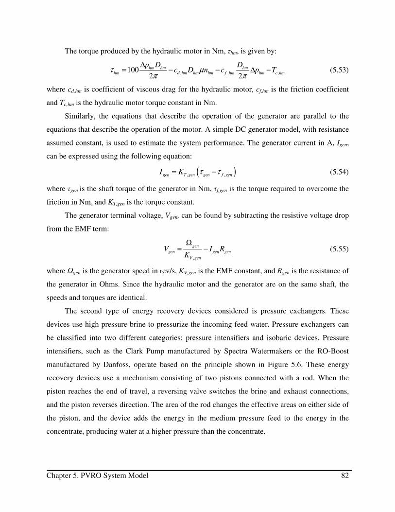
Chapter 5. PVRO System Model 82
The torque produced by the hydraulic motor in Nm, τhm, is given by:
,, ,1002 2hm hm hm
hm d hm hm hm f hm hm c hm
p D Dc D n c p Tτ µ
π π
∆= − − ∆ − (5.53)
where cd,hm is coefficient of viscous drag for the hydraulic motor, cf,hm is the friction coefficient
and Tc,hm is the hydraulic motor torque constant in Nm.
Similarly, the equations that describe the operation of the generator are parallel to the
equations that describe the operation of the motor. A simple DC generator model, with resistance
assumed constant, is used to estimate the system performance. The generator current in A, Igen,
can be expressed using the following equation:
( ), ,gen T gen gen f genI K τ τ= − (5.54)
where τgen is the shaft torque of the generator in Nm, τf,gen is the torque required to overcome the
friction in Nm, and KT,gen is the torque constant.
The generator terminal voltage, Vgen, can be found by subtracting the resistive voltage drop
from the EMF term:
,
Ωgen
gen gen gen
V gen
V I RK
= − (5.55)
where Ωgen is the generator speed in rev/s, KV,gen is the EMF constant, and Rgen is the resistance of
the generator in Ohms. Since the hydraulic motor and the generator are on the same shaft, the
speeds and torques are identical.
The second type of energy recovery devices considered is pressure exchangers. These
devices use high pressure brine to pressurize the incoming feed water. Pressure exchangers can
be classified into two different categories: pressure intensifiers and isobaric devices. Pressure
intensifiers, such as the Clark Pump manufactured by Spectra Watermakers or the RO-Boost
manufactured by Danfoss, operate based on the principle shown in Figure 5.6. These energy
recovery devices use a mechanism consisting of two pistons connected with a rod. When the
piston reaches the end of travel, a reversing valve switches the brine and exhaust connections,
and the piston reverses direction. The area of the rod changes the effective areas on either side of
the piston, and the device adds the energy in the medium pressure feed to the energy in the
concentrate, producing water at a higher pressure than the concentrate.

Chapter 5. PVRO System Model 83
Figure 5.6. Pressure intensifier mechanics (left) and typical system configuration (right).
Isobaric devices pressurize the incoming seawater directly. These devices have different
configurations. All the different pressure exchanger configurations have a constant area between
brine and feedwater which results in both having the same pressure. A schematic of one of the
device configurations, the Dual Work Energy Exchanger (DWEER) manufactured by Flowserve,
can be seen in Figure 5.7. Since the high pressure feedwater exits the device at the same pressure
as the brine, an additional pump is required to boost the pressure, as shown in Figure 5.7.
Figure 5.7. Isobaric pressure exchanger mechanics (left) and typical system configuration
(right).
Fortunately, these two types of pressure exchangers can be described by the same set of
equations. These are fixed displacement devices and the flow rate of the brine is related to the
flow rate of the feed water by:
, ,f ER b ERQ Qϕ= (5.56)
where Qf,ER is the flow of the feed through the energy recovery device in L/s, Qb,ER is the flow of
the brine through the energy recovery device in L/s, φ is the ratio between the feed flow and the
brine flow defined by the energy recovery device geometry. For pressure intensifiers, this
number is greater than 1. For isobaric pressure exchangers, this number equals 1.
The pressure relationship for these devices varies with system flow rate. To simply the
analysis, the pressure relationship is taken to be constant and is given by:
Pressure
Intensifier
Low Pressure
Pump
Reverse Osmosis
Membrane
Brine
FeedPermeate
Medium
PressureFeed – Qf, Pf
High PressureOutput – Qh, Ph
HighPressure
Concentrate–
Qc, Pc
Low PressureConcentrate–
Qe, Pe
Isobaric
PressureExchanger
High PressurePump
Reverse OsmosisMembrane
Brine
FeedPermeate
BoostPump
High PressureFeedwater
Low PressureFeedwater
Low PressureBrine
High PressureBrine
High PressureBrine
Low PressureFeedwater
Low PressureBrine
High PressureFeedwater
ReversingValves

Chapter 5. PVRO System Model 84
, , , ,f ER f ER ER b ER b ERp Q p Qη∆ = ∆ (5.57)
where ∆pf,ER is the change in feed stream pressure, ∆pb,ER is the change in pressure in the brine
stream, and ηER is the efficiency of the energy recovery device.
5.2.7 Control Electronics
The control electronics condition power from the PV panels and other power sources such
as the generator in the energy recovery system for use by the system pumps. The overall power
in the system must be conserved, as shown by:
Power In Power Out=∑ ∑
, , , ,
1 1
Pumps DC Pumps ACn n
m DC i m AC i
i i
mppt solar gen
DCDC inv
P P
P Pηη η
− −
= =+ = +∑ ∑
(5.58)
where ηmppt is the efficiency of the maximum power point tracking algorithm used for the PV
system, ηDCDC is the efficiency of the DC to DC conversion, ηinv is the efficiency of the inverter
used for any AC motors.
The control electronics will dictate the distribution of power amongst the different system
motors. In order to accommodate this, additional design variables, θi, are added to the
optimization problem. The number of design variables added are equal to the number of pumps
in the system and determine the output power as follows:
( ), ,
1
pumps
im DC i DCDC mppt solar genn
i
i
P P Pθ
η η
θ=
= +
∑ (5.59)
( ), ,
1
pumps
im AC i inv mppt solar genn
i
i
P P Pθ
η η
θ=
= +
∑ (5.60)
5.3 Graph Representation
Section 5.1 above describes individual component models. This section describes a new
structure which was developed to link the component models together to represent any PVRO
system configuration and estimate the overall system performance. As stated above, the models

Chapter 5. PVRO System Model 85
are segmented into two parts, the PV system and the RO system, whose performance is coupled
via the electrical power transmitted through the control electronics.
The RO system model must determine the water output flow rate and water quality for a
given component selection, system topology, pressure operating point, power input, and input
water salinity. To represent and analyze the reverse osmosis system, a graph-based model was
developed. In this model, the RO system components and connecting pipes are represented using
edges and the nodes are the points of connection. Each edge has an assigned type based on the
component it represents and associated equations, presented in section 5.1 above, which govern
the pressure, flow and water concentrations. These edge types include: pumps, reverse osmosis
membranes, energy recovery devices, and pipes which serve to connect all components. An
example system and its graph representation can be seen in Figure 5.8.
Figure 5.8: Sample reverse osmosis system and its graph representation.
This representation has advantages. First, it can easily capture any reverse osmosis system
configuration using a node adjacency matrix of zeros and ones, as shown in Figure 5.9, and a
vector representing the system components, which is can be implemented in a genetic algorithm
optimization. Second, it allows the system equations to be uncoupled and allows for an iterative
solution approach, detailed below.
FreshWater
Brine
ReverseOsmosis
Membranes
ControlElectronics
SaltWaterIntake
EnergyRecovery
Device
FeedWaterPump
HighPressure
Pump
Intake
Brine
Energy
Recovery
Device
ReverseOsmosis
Membranes
Pumps
Permeate
Reverse Osmosis System Schematic Graph Representation

Chapter 5. PVRO System Model 86
Figure 5.9: Connection matrix for sample reverse osmosis system.
For the given system connection matrix, component types, pressure operating point, and
power input, the method outlined in Figure 5.10 is used to calculate the output water flowrate
and concentration. This method was programmed using Matlab and starts by ordering the system
nodes and generating a node-arc incidence matrix for the system graph. The incidence matrix is a
l × m matrix, where l is the number of nodes and m is the number of edges. The matrix, B, is
defined as:
1 if edge enters node
1 if edge leaves node ij
j ib
i j
=
− (5.61)
This matrix defines conservation of water and salt over the network as follows:
in out= −Bq q q (5.62)
where q is the vector of flows through each edge, qin is the vector of flows entering the system at
each of the node and qout is the flow exiting the system at each node.
The node-arc incidence matrix also defines the concentration of salt over the network as
follows:
( )
in in out out= −B q c q c q c (5.63)
where denotes component-wise multiplication of vectors, c is the vector of water
concentrations along each edge, cin is the vector of water concentrations entering the system at
each of the node and cout is the vector of water concentrations exiting the system at each node.
1 0 0 0 0 0 0
0 1 0 0 0 0 0
0 0 1 0 0 0 0
0 0 0 0 0 1 0
0 0 0 1 0 0 0
0 0 0 0 0 1 0
0 0 0 0 1 0 0
0 0 0 0 0 0 1
Reverse Osmosis 1 Brine
Reverse Osmosis 1 Permeate
En
erg
yR
ecove
ryF
ee
d
System Feed
Pump 1 Outlet
Pu
mp
1In
let
Pu
mp
2In
let
Pump 2 Outlet
Reverse Osmosis 2 Brine
Reverse Osmosis 2 Permeate
Energy Recovery Outlet
Reve
rse
Osm
osis
1In
let
Reve
rse
Osm
osis
2In
let
Drin
kin
gW
ate
rT
ank
Brin
eD
ispo
sal
Co
mp
on
en
tO
utlets
Component Inlets

Chapter 5. PVRO System Model 87
Once this graph structure is generated, an initial guess of the overall water production is
made based on the power input using equation (4.11). An average system recovery rate (10% for
systems which produce less than 5 m3 per day, and 30% for all other systems) is assumed to fully
define qin and qout for the system. Using these system flowrate guesses, a feasible system
flowrate vector is determined using equation (5.62). The pressures at each of the system nodes
and the concentration of water at each edge are determined using the system equations in section
5.1 and the initial flowrate guesses. This calculation neglects the membrane pressure flow
calculation defined in equation (5.40) as it is used to correct the flowrates in the next step. The
calculated pressures are then used to determine the flow across the membrane and the system
flows are recalculated using equation (5.62). The calculated flow rate is averaged with the
previous guess and the process is repeated until the change in the flow rate is less than the
specified tolerance. This solution method is very robust and the process typically converges in
less than 1 second.
Figure 5.10: Solution method for reverse osmosis system equations.
5.3.1 Surrogate Model
The model discussed above requires several seconds to compute the water output for a
single power setting. Hence, this model cannot be used directly for optimization since the
Guess fresh water flowratebased on power input
Solve for pump operating pressuresand pressure drops for input power
and water flow rate.
Calculate water
concentrations for given waterflowrates
Find feasible system flowrates (Qsys,1)
Solve for product flow rateand system flow rates based
on pressures (Qsys,2)
Is Qsys,1-Qsys,2<Tol
Qsys,1=(Qsys,1+Qsys,2)/2
No
SolutionReached
Yes

Chapter 5. PVRO System Model 88
computation of the water output using a varying power input for an average year would take
many minutes. Fortunately, the resulting system of equations, while non-linear, can be accurately
approximated by interpolating between evaluated function points. The resulting water production
for the sample PVRO system depicted in Figure 5.8 is shown in Figure 5.11.
Figure 5.11: Water production and water concentration vs. power input for sample PVRO
system.
To determine the number of interpolation points required, a study evaluating the error
versus the number of points was performed for an array of 10 different RO system
configurations. In this study, the each system was simulated for an average spring day in Boston
using the full model. Then water production and output water salinity were evaluated using a
different surrogate model where the system output is determined by interpolating between
evaluation points of the original model output. The sample points of the original model are
evenly distributed between zero system power and the maximum system power. The number of
times the original model is sampled is varied to determine the number of samples required to
meet a desired accuracy. Here, the criteria was set that the surrogate model have a less than 1%
error.
The average percentage error in the water production and the water salinity for the
surrogate model versus the number of function evaluations is shown in Figure 5.12. As expected,
as the number of evaluations increases, the error goes to zero. In order to achieve <1% error, a
total of 8 evaluations of the full system model at varying power levels are required. For each

Chapter 5. PVRO System Model 89
PVRO system evaluated in the final stage of the modular design approach, this surrogate model,
formed by 8 evaluations of the full system model, will be used to determine the system output
over varying solar profiles.
Figure 5.12: Error in water production based on number of evaluations.
The interpolation approach saves substantial computation time. The time saved varies
depending on the PVRO system being evaluated and the length of the simulation. An average
value of 10.2 seconds is saved for a day-long simulation of a PVRO system with an hourly time
step. When simulated over the course of a year, an average time of 2.9 hours is saved. The
surrogate model enables the implementation of the modular design approach.
5.4 Experimental Model Verification
5.4.1 Experimental System Description
The PVRO system modeling approach outlined above was verified using data from the
MIT Experimental PVRO System. The system is modular and has been constructed on a campus
rooftop (see Figure 5.13). The system schematic and model representation can be seen in Figure
5.14. It is composed of a tracking PV panel, custom control electronics, parallel DC pumps, a
Clark pump energy recovery system, a reverse osmosis membrane within a pressure vessel, and
plastic water tanks. The system is equipped with custom control electronics and designed to
operate variably to eliminate the need for batteries. The system is fully instrumented and

Chapter 5. PVRO System Model 90
computer controlled to optimize the system water output, and is designed to produce
approximately 350 L of fresh water per day in Boston on a sunny summer day.
Figure 5.13: Experimental PVRO system.
The system instrumentation consists of 18 different sensors that provide sufficient
information for model validation and control feedback (see Figure 5.14). Sensors include
thermistors for measuring solar panel, feed water, and ambient air temperature, flow sensors,
salinity sensors, pressure transducers, and sensors for measuring solar panel orientation. The
sensors are connected via custom electronics to the data acquisition and control computer, shown
in Figure 5.15.
Figure 5.14: Experimental PVRO system layout.
TrackingSystem
Main Sensor
ConditioningBoard
Reverse Osmosis
Modules
Low Pressure
Concentrate
Sea Water
Intake
Water Tank
High Pressure
Concentrate
1213
ConcentrationFlow
Flow
8
Pressure
9
PressureTemp
essure
10
Concentration11
PowerElectronics Current
Voltage
6
Flow
5
1 2Current
Voltage
Orientation15
Temp
EnvironmentSensors
Solar Radiation
Ambient Temperature
Optimal PowerManagement
MasterPIC24 MCU
16
Permeate
14
Flow
7
3 4
17
18
Pressure
Exchanger
Accumulator
Pr

Chapter 5. PVRO System Model 91
Figure 5.15: MIT experimental PVRO system electronics.
Two PIC24 microcontrollers in a Master/Slave configuration are used to acquire sensor
data through a sensor conditioning board, and to perform computation and control tasks. The
Master PIC24 is used to control a DC/DC step down converter that receives power from the solar
panels and converts it to the voltage desired by the two DC boost pumps. This electrical system
configuration was designed with student Roman Geykman [127]. Custom control software was
developed to track the maximum power point of the solar panel throughout variable solar
radiation and temperature conditions and maximize the system water production. The Slave
PIC24 is used to drive the solar panel tracker motors. The Master PIC24 also communicates with
a base station PC running Linux over a wireless modem. The base station is used to record the
acquired data and to display it in real time.
The water type used for the experimental system greatly affects the system performance.
The seawater salinity varies from location to location, but the reference value commonly used is
35.164 g of salts per kg of seawater [128]. The majority of seawater in the world has water
salinities close to this value, although there are areas in the Arabian Gulf and Red Sea where
salinities can exceed 45 g/kg [2]. Since the MIT experimental system is located far from any
natural salt water source, surrogate seawater was used to test the performance of the
Optimal Power
Management
Master PIC24
MCU
SlavePIC24
MCU
PV Panel
Tracker Moter
SensorConditioning
Board
Analog
Sensors
Flow Sensors
RO Pumps
PVRO Control/Monitor
Software
Experimental SystemBase Station
(Linux PC)RS-232 – 900 Mhz RF
Electronics
Power
Legend
Electrical Power
Signals
PV Panel
DC/DC
Converter
Tracker/
Charger IOBoard
24 Volt
GelBattery
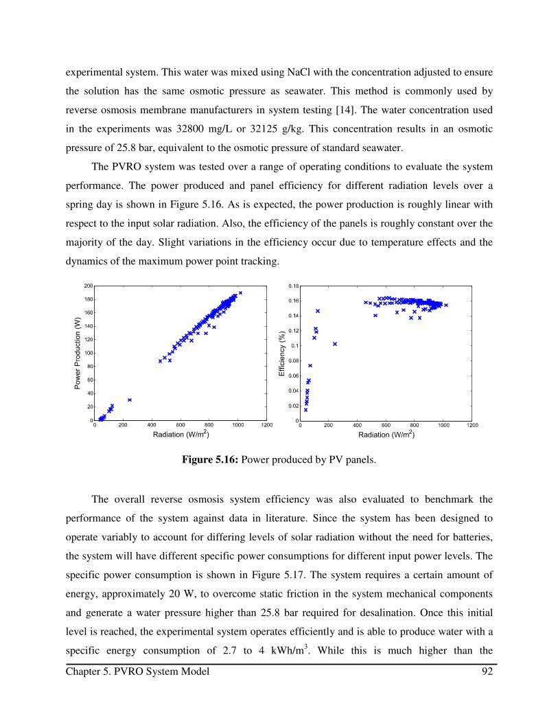
Chapter 5. PVRO System Model 92
experimental system. This water was mixed using NaCl with the concentration adjusted to ensure
the solution has the same osmotic pressure as seawater. This method is commonly used by
reverse osmosis membrane manufacturers in system testing [14]. The water concentration used
in the experiments was 32800 mg/L or 32125 g/kg. This concentration results in an osmotic
pressure of 25.8 bar, equivalent to the osmotic pressure of standard seawater.
The PVRO system was tested over a range of operating conditions to evaluate the system
performance. The power produced and panel efficiency for different radiation levels over a
spring day is shown in Figure 5.16. As is expected, the power production is roughly linear with
respect to the input solar radiation. Also, the efficiency of the panels is roughly constant over the
majority of the day. Slight variations in the efficiency occur due to temperature effects and the
dynamics of the maximum power point tracking.
Figure 5.16: Power produced by PV panels.
The overall reverse osmosis system efficiency was also evaluated to benchmark the
performance of the system against data in literature. Since the system has been designed to
operate variably to account for differing levels of solar radiation without the need for batteries,
the system will have different specific power consumptions for different input power levels. The
specific power consumption is shown in Figure 5.17. The system requires a certain amount of
energy, approximately 20 W, to overcome static friction in the system mechanical components
and generate a water pressure higher than 25.8 bar required for desalination. Once this initial
level is reached, the experimental system operates efficiently and is able to produce water with a
specific energy consumption of 2.7 to 4 kWh/m3. While this is much higher than the

Chapter 5. PVRO System Model 93
thermodynamic limit of 0.8 kWh/m3 for the 9% water recovery ratio (this number is 0.7 kWh/m3
as the recovery ratio goes to 0), this is very efficient for such a small scale system. Typical
specific energy consumption of large scale reverse osmosis plants is between 3 to 5 kWh/m3 [6].
It should be noted that energy numbers for large plants include plant overhead, pretreatment, and
brine disposal that are not accounted for here. When only considering desalination, power
consumptions of new, highly-efficient plants have been shown to reach values of 2.5 kWh/m3
[129].
Figure 5.17: Specific power consumption of experimental PVRO system.
5.4.2 Model Representation
A graph-based model was generated for the MIT Experimental PVRO system using the
approach detailed in section 5.3. This graph is shown in Figure 5.18. The system consists one
tracking Sunpower 230W solar panel, two Shurflo 8050-243-169 pumps and DC motors, one
DOW Filmtec SW30-2540 reverse osmosis membrane, and a Clark Pump energy recovery
device manufactured by Spectra Watermakers. Parameters of the system components are
outlined in Table 5.1.

Chapter 5. PVRO System Model 94
Figure 5.18: Graph representation of MIT experimental PVRO system.
Table 5.1: Model parameters of MIT Experimental PVRO system. Component Parameter Value
Sunpower 230W Solar Panel [23]
Solar panel efficiency, ηPV 18.5 %
Solar panel area, APV 1.23 m2
Solar panel temperature coefficient, α 0.38 %/K
Normal operating cell temperature, NOCT 45 °C
Shurflo 8050-243-169 Pump & DC Motor
Pump coefficient of viscous drag cd 3.803 x10⁻⁴ N-m/bar-L Pump friction coefficient, cf 4.033 N-m/bar-L Pump slip coefficient, cs 3.361 x10⁻¹⁰ Pump volumetric displacement per revolution, D 2.60 x10⁻³ L/rev Motor friction related current,I0 0.65 A Motor torque constant, KT 2.252 A/N-m Motor speed constant, KV 1.824 rev/V-s Motor resistance, Rm 0.1546 Ω Pump torque constant, Tc 0.05 Nm
DOW Filmtec SW30-2540 Reverse Osmosis Membrane [24]
Membrane water permeability, KA 3.714x10⁻⁴ L/m2-bar-s Membrane salt permeability, B
5.842x10⁻⁵ L/m2-s
Membrane area, SE 2.6 m2
Other System Parameters Feed water salt concentration, Cf 32800 mg/L Clark pump recovery ratio, Rt 0.090
5.4.3 Model Validation
Data from a partly cloudy summer day was used to validate the modeling approach. The
solar profile used as an input to the model is shown in Figure 5.19. The resulting water
production for the experimental system and the model prediction is shown in Figure 5.20. There
is a very good agreement between the data and model values, with an error of less than 8%. This
shows that the graph modeling approach and the simplified analysis method accurately predict
system water production.
Intake Fresh
Water
Brine
Pressure Exchanger
Energy Recovery
Reverse Osmosis
Membrane
Pumps
RO SystemElectricalPower In
Electrical
Power In
PV System
Control
ElectronicsElectrical
Power Out

Chapter 5. PVRO System Model 95
Figure 5.19: Solar radiation input for model validation.
Figure 5.20: Experimental validation of modeling approach.
The specific energy consumption of the experimental system was compared to the values
determined in the model. For a wide operating range, the model accurately predicts the overall
system performance. This shows that the physical models detailed in section 5.2 capture the
important system characteristics and are appropriate for use with the modular design approach.

Chapter 5. PVRO System Model 96
Figure 5.21: Model specific energy consumption.
5.5 Economic Models
As stated in section 4.1, the goal of the modular design approach as applied to PVRO
systems is to configure the lowest lifetime cost system that is able to meet the fresh water
demands of a particular location. Therefore, a set of economic models are required to estimate
the overall system cost. These models are described here.
5.5.1 Total Costs
The equivalent annualized cost method used in Chapter 3 is applied here to compare the
economics of different PVRO systems. The costs are separated into capital system costs and
operating costs. The total annualized costs are given by:
PVRO CC Op
A A A= + (5.64)
Using the total annual cost, the total water cost can be estimated using the following:
PVROw
w
AC
V= (5.65)
where Vw is the amount of water produced by the system during an average year.
0 20 40 60 80 100 120 140 160 1800
2
4
6
8
10
12
Input Power (W)
Spe
cific
Ene
rgy C
onsum
ption
(kW
h/m
3)
Model
Experimental Data

Chapter 5. PVRO System Model 97
5.5.2 Capital Costs
The capital costs of a PVRO desalination system are given by:
PVRO Infra PV RO
C C C C= + + (5.66)
where CInfra is the capital cost of the system infrastructure, CPV is the capital cost of the PV
system and CRO is the capital cost of the RO system.
The infrastructure capital costs encompass a wide array of items such as system
installation, site preparation, brine disposal system, water intake, and water distribution system.
These costs will vary greatly from location to location. For the purpose of the case studies done
in this thesis, these costs are accounted for by scaling the costs of RO plant as follows:
infra infra ROC Cϕ= (5.67)
where φinfra is the cost of the infrastructure relative to the reverse osmosis components. Based on
literature surveying installed reverse osmosis systems, this value is taken to be 1.71 [102].
The photovoltaic system costs include the cost associated with the PV panels, the mounting
system and the control electronics. They are calculated using:
,
, ,1
PV typeN
PV PV i PV i mount elec
i
C n C C C=
= + +∑ (5.68)
where nPV,i is the number of panels of type i which are included in the system configuration, CPV,i
is the cost of panel I, Cmount is the cost of the mounting system, and Celec to the cost of the
electrical components. The mounting cost is directly calculated based on the mounting
component type and the number of panels. Different types of electronics modules are not
considered in this thesis. Equation 3.29 is used to calculate the cost associated with the
electronics, repeated here [105]:
0.72elec p
C W= (5.69)
where Wp is the power rating of the PV array in Watts.
The reverse osmosis system capital costs are given by:
Pre _RO RO comp PostC C C C= + + (5.70)
where CPre is the pre-treatment system cost, CRO_comp is the cost of the reverse osmosis
components, and Cpost is the cost is cost of the post-treatment system and water storage.
Pre-treatment systems are often required for reverse osmosis systems to ensure that system
components, such as the membranes, do not degrade prematurely. While completely

Chapter 5. PVRO System Model 98
characterizing reverse osmosis pretreatment options is beyond the scope of this thesis, including
these components in the overall cost analysis is required for accuracy. For this work, it is
assumed that the capital cost of the pre-treatment components is proportional to the overall
reverse osmosis system cost as follows:
Pre Pre _RO compC Cϕ= (5.71)
where φPre is the cost of the pretreatment relative to the reverse osmosis components. Based on
literature surveying installed reverse osmosis systems, this value is taken to be 0.35 [102].
The costs associated with the reverse osmosis components are directly taken from the
components selected during the modular design approach. The total component cost is calculated
using:
_RO comp mem press p motor er connectC C C C C C C= + + + + + (5.72)
where Cmem is the total cost of membranes selected for the system, Cpress is the total cost of
pressure vessels required to hold those membranes, Cp is the total cost of the system pumps,
Cmotor is the total cost of the system motors, Cer is the total cost of the system energy recovery
devices, and Cconnect is the total cost of the component piping and other connections.
The costs associated with post-treatment systems are typically low when compared with
with other system costs. The chemical post-treatment system cost is estimated based on literature
values. In addition to chemical post-treatment, investment is also required for water storage to
supply water when the system is not operating due to cloudy weather. The overall post-treatment
cost is given by:
_post post RO comp storageC C Cϕ= + (5.73)
where φpost is the cost of the post-treatment chemical system relative to the reverse osmosis
components and Cstorage is the cost of the water storage component selected by the modular
design approach. Based on literature surveying installed reverse osmosis systems, φpost is taken to
be 0.03 [102].
The capital costs are converted into annualized costs using Equation 3.21, presented again
here:
(1 )
(1 ) 1
n
cc PVROn
i iA C
i
+=
+ − (5.74)
where i is the interest rate, and CPVRO is the total PVRO system capital cost.

Chapter 5. PVRO System Model 99
5.5.3 Operating and Maintenance Costs
The total annual operational cost for the photovoltaic reverse osmosis system is given by:
Op l chem r ,RO
A A A A= + + (5.75)
where Al is the annual labor cost, Achem is the annual chemical cost, and Ar is the annual cost of
component replacement in $.
The annual cost of the labor will be highly dependent on the system location. Here, it is
assumed the labor cost can be expressed as:
365l cap
A Vγ= (5.76)
where γ is the specific operating labor cost in $/m3-day, and Vcap is average system production in
m3/day. In this analysis, the specific operating labor cost was $3.00/m3-day [93].
The chemical costs are also location specific as the pre-treatment chemicals are dependent
on local water conditions. The total annual cost of treatment chemicals is given by:
365chem cap
A kV= (5.77)
where k is the average cost of chemicals $/m3. In this analysis, the treatment chemical cost per
m3 was $0.033 [94].
From time-to-time, system components will require replacement. The major components
that will require regular replacement are the reverse osmosis membranes. Less frequently,
pumps, motors, energy recovery units, pre- and post-treatment systems and control electronics
will require replacement. The replacement rates assumed are specified in Table 5.2. Using the
replacement rates, the annual replacement cost is given by:
e er PV PV elec lec mem mem p p motor motor er r pre pre post postA C RR C RR C RR C RR C RR C RR C RR C RR= + + + + + + + (5.78)
where RR represents the replacement rate of each component.
Table 5.2: Assumed replacement rate of PVRO system components. Component Annual Replacement
Rate
PV Components 4% Control Electronics 10% Membranes 20% Pumps 10% Motors 10% Energy Recovery Units 10% Pre-treatment 10% Post-treatment 10%

Chapter 5. PVRO System Model 100
5.6 Summary
This section developed the physical system and economic models used for the modular
design of PVRO systems. Physics-based models are developed for individual system
components. The component models are implemented in a graph-based system model to
represent any PVRO system configuration. A surrogate model of the solar radiation to water
production relationship is developed to increase calculation speed for different solar profiles.
This model is validated using an experimental PVRO system that was constructed as a part of
this research. The model use is demonstrated in the case studies in Chapters 6 and 7.

Chapter 6. Deterministic Case Studies 101
CHAPTER
6 DETERMINISTIC CASE STUDIES
A series of case studies were performed to study the performance of the modular design
approach applied to PVRO systems. To simplify the analysis, initial case studies were performed
with deterministic solar radiation inputs and system demands. These case studies are detailed in
this chapter.
6.1 Problem Description
Several representative case studies were conducted to demonstrate the modular design
approach. Systems were designed for four different locations with a seawater source and for one
location with a brackish water source. The location details are shown in Table 6.1. These
locations provide a range of different water salinities and solar insolation values. The objective
of this design process is to minimize the net present cost of the PVRO system assuming a system
life of 25 years and a 4% interest rate. Both system capital costs and maintenance costs are
included as described in section 5.5. The system must meet the specified water demand and
produce water which is below the drinkable salinity level of 500 ppm as outlined by the World
Health Organization [130].
Table 6.1: Locations used for deterministic modular design case studies.
Location Water Salinity
(ppm) Average Yearly Solar Insolation
(kWh/m2/day)
Albuquerque, NM 3000* 5.79 Boston, MA 32664 4.21 Brisbane, Australia 35438 5.31 Cape Haiten, Haiti 36275 6.05 Limassol, Cyprus 39182 6.25
*Brackish Groundwater

Chapter 6. Deterministic Case Studies 102
6.1.1 System Inventory
Systems are designed for different average water demands, ranging between 1 m3/day and
20 m3/day. To accommodate the wide range of system requirements, a large component
inventory was constructed. Figure 6.1 shows this inventory. It consists of 6 different types of
motors, 8 different types of pumps, 8 different reverse osmosis membranes, 8 different types of
PV panels, 3 different PV panel mounting/tracking configurations, 2 different hydraulic motors,
2 different generators, 5 pressure exchange energy recovery devices, and one pressure control
valve.
Figure 6.1: Inventory used for case studies.
The inventory details are presented in Table 6.2 through Table 6.7. Individual component
specifications are derived from manufacturers’ datasheets and costs are given by local
component distributers.
Table 6.2: PV panel inventory used for case studies [131].
PV Panels Quantity Power
Rating (W) Efficiency Temperature Factor (%/K)
NOCT (oC) Cost
Model 1 – First Solar – FS-385 40 85 11.8% 0.25 45 $399 Model 2 – First Solar – FS-280 40 80 11.8% 0.25 45 $299 Model 3 – Sunpower – 315W 40 315 19.3% 0.38 45 $999 Model 4 – Trina Solar – TSM-230PA05 40 230 14.1% 0.45 46 $529 Model 5 – Trina Solar – TSM-225PA05 40 225 14.1% 0.45 46 $399 Model 6 – Sanyo – HIT-N220A01 40 220 17.4% 0.336 44 $619 Model 7– Suntech – STP205-24UD 40 205 13.9% 0.47 45 $408 Model 8 – Suntech – STP295-24VDC 40 295 15.2% 0.4 45 $587
Reverse Osmosis Membranes
ControlElectronics
Pumps
Energy Recovery Devices
PV Panels
Motors
M M M
M M M
M M M
M M M
M M
PX PX PX
M
G
X 40 X 40
X 40 X 40
X 40
X 40
X 40 X 40
PX PX
PV Mount
Fixed
Panels
2-AxisTrack
1-Axis
Track
2-AxisTrack
2-Axis
Track
2-Axis
Track

Chapter 6. Deterministic Case Studies 103
Table 6.3: PV panel mounting inventory used for case studies [132]. PV Panels Tracking Type Average Power Use (W) Max Array Area Per Mount (m2) Cost
Model 1 – No Tracking None 0 11.6 $500 Model 2 – Wattsun-AZ-125 1 – Axis 1.5 11.6 $3985 Model 3 – Wattsun-AZ-125 2 – Axis 1.5 11.6 $4710 Model 4 – Wattsun-AZ-225 2 - Axis 1.5 15.7 $7250 Model 5 – Wattsun-AZ-225 2 - Axis 1.5 17.6 $7645 Model 5 – Wattsun-AZ-225 2 - Axis 1.5 20.9 $8175
Table 6.4: RO membrane inventory used for case studies [133].
RO Membranes Quantity Water Type Water
Permeability (L/m2-bar-s)
Salt Permeability
(L/m2 -s)
Area (m2)
Max Pressure
(bar) Cost
Model 1 – Dow SW30XLE-400i 3 Seawater 4.25 x 10⁻⁴ 1.93 x 10⁻⁵ 37 83 $990 Model 2 – Dow SW30HRLE-400i 3 Seawater 3.48 x 10⁻⁴ 1.59 x 10⁻⁵ 37 83 $982 Model 3 – Dow SW30-2540 3 Seawater 4.22 x 10⁻⁴ 5.84 x 10⁻⁵ 2.8 69 $188 Model 4 – Dow SWHRLE-4040 3 Seawater 3.50 x 10⁻⁴ 2.02 x 10⁻⁵ 7.9 83 $435 Model 5 – AM M-B2540A 3 Brackish Water 9.95 x 10⁻⁴ 1.09 x 10⁻⁴ 2.8 41 $163 Model 6 – AM M-B4040AHF 3 Brackish Water 1.31 x 10⁻³ 1.44 x 10⁻⁴ 7.5 41 $303 Model 7– Koch 4820HR 3 Brackish Water 5.94 x 10⁻⁴ 2.51 x 10⁻⁵ 7.5 41 $343 Model 8 – Koch 8822HR-400 3 Brackish Water 6.09 x 10⁻⁴ 2.55x10⁻⁵ 7.5 41 $844
Table 6.5: Motor inventory used for case studies [134]. Motor Quantity Motor Type Max Power (HP) Rated RPM Max Efficiency Cost
Leeson 116698.00 3 AC Motor 5 3600 93.6 % $845 Leeson G141121.00 3 AC Motor 10 3600 89.3 % $1319 Leeson 170615.60 3 AC Motor 15 3600 92.4% $2141 Shurflo 8050-243-169 3 DC Motor 1/6 3600 80.2% $150 Leeson 108014.00 3 DC Motor 0.5 1750 81.7 % $754 Leeson 108022.00 3 DC Motor 1 1750 83.7 % $968
Table 6.6: Pump inventory used for case studies [135].
Pumps Quantity Volumetric
Displacement (mL/rev) Max Rated RPM
Max Pressure (bar)
Cost
Danfoss APP 0.8 3 5.1 3450 80 $700 Danfoss APP 1.8 3 10.0 3450 80 $4239 Danfoss APP 2.5 3 15.3 3450 80 $4782 Danfoss APP 3.5 3 20.5 3450 80 $7452 Shurflo 8050-243-169 3 2.6 3450 10 $150 Procon 140 GPH 3 5.3 1725 17.3 $152 NRD PRG 10 3 13.1 1725 18 $190
Table 6.7: Pressure exchange energy recovery inventory used for case studies.
Energy Recovery Unit Quantity Max Brine Flow
(L/h) Feed to Brine Flow
Ratio Average Efficiency Cost
ERI PX-30S 1 6800 1 90% $6000 Spectra Clark Pump 1 760 1.08 95% $3500 Spectra Clark Pump 1 1160 1.18 95% $4500 Flowserve DWEER 1 12000 1 95% $8000 Pressure Control Valve 1 1000 N/A N/A $45 Pressure Control Valve 1 10000 N/A N/A $171
In addition to the component costs outlined above, there are costs associated with the
pressure vessels required to hold the individual reverse osmosis membranes. In the

Chapter 6. Deterministic Case Studies 104
representation chosen, the pressure vessel itself is not one of the design choices, but is contingent
on the selection of the reverse osmosis membrane configuration. The pressure vessel costs are
outlined in Table 6.8.
Table 6.8: Costs of membrane pressure vessels used in case studies [136]. Number of 40” Long Membranes
Water Type Membrane Diameter 1 2 3
Brackish Water 2.5” $144 N/A N/A 4” $294 $356 $418
Seawater 2.5” $244 N/A N/A 4” $539 $611 $685 8” $1190 $1338 $1453
6.1.2 Power Source
Solar radiation varies greatly over the course of the year due to changing seasons and local
weather. To account for these variations, an average sunny day and an average cloudy day are
simulated for each of the four seasons. The average values of solar insolation for cloudy and
sunny days are determined from historical solar radiation data [8]. Using the method outlined in
section 5.1.1, the solar profile is determined for a typical sunny and cloudy day for each season.
Example solar radiation profiles for a sloped photovoltaic panel in Boston, MA are shown in
Figure 6.2.
Figure 6.2: Typical solar profile used for case studies.
Winter Spring
Summer Fall
Cloud Sun Cloud Sun
Cloud Sun Cloud Sun
0 6 12 18 240
200
400
600
800
1000
Time (hours)
So
lar
Ra
dia
tio
n (
W/m
2)
0 6 12 18 240
200
400
600
800
1000
Time (hours)
So
lar
Ra
dia
tio
n (
W/m
2)
0 6 12 18 240
200
400
600
800
1000
Time (hours)
So
lar
Ra
dia
tio
n (
W/m
2)
0 6 12 18 240
200
400
600
800
1000
Time (hours)
So
lar
Ra
dia
tio
n (
W/m
2)
0 6 12 18 240
200
400
600
800
1000
Time (hours)
So
lar
Ra
dia
tio
n (
W/m
2)
0 6 12 18 240
200
400
600
800
1000
Time (hours)
So
lar
Ra
dia
tio
n (
W/m
2)
0 6 12 18 240
200
400
600
800
1000
Time (hours)
So
lar
Ra
dia
tio
n (
W/m
2)
0 6 12 18 240
200
400
600
800
1000
Time (hours)
So
lar
Ra
dia
tio
n (
W/m
2)
Chapter 6. Deterministic Case Studies 105
The PVRO system is simulated over these eight average days. The number of typical days
in each season is determined from the average seasonal solar insolation using the following
relationship:
, ,
, ,
, ,
1sun i sun i
i sun i cloud i
total i total i
n nH H H
n n
= + −
(6.1)
where Hi is the average solar insolation in season i, Hsun,i is the solar insolation on a sunny day
during season i, Hcloud,i is the solar insolation on a cloudy day during season i, nsun,i is the number
of sunny days in season i, and ntotal,i is the total number of days in season i.
6.1.3 System Demand
The system demand is simplified for the deterministic case studies. Here, the system must
meet the demand measured as an average daily water production. Average system demands
between 1 m3 per day and 20 m3 per day are examined. Although using an average system
demand simplifies the analysis, in reality, the system demand and water production will vary on
a daily basis. Any system design must be able to accommodate these variations. This effect is
accounted for in the case studies presented in Chapter 7.
Using the water produced on each of the typical days, the average daily water production is
determined from the number of sunny and cloudy days in each season using:
4
, , , ,
1
1
365ave sun i sun i cloud i cloud i
i
V n V n V=
= + ∑ (6.2)
where Vsun, is the water production on a sunny day in season i, and Vcloud,i is the water production
on a cloudy day in season i.
6.2 Optimization Setup
The modular design algorithm was implemented using Matlab. Starting with the inventory
specified in section 6.1.1, the number of possible system configurations is decreased by applying
the module, subassembly, and topology filters using the approach detailed in chapter 4. The final
step in the modular design algorithm is to optimize the system over the reduced design space.
Modular systems are composed of discrete components, making the optimization problem
difficult. To add to the complexity, the cost function and constraints are non-linear, resulting in a

Chapter 6. Deterministic Case Studies 106
mixed integer nonlinear program (MINLP). Different optimization routines have been developed
that can accommodate MINLPs such as Branch and Bound, genetic algorithms and simulated
annealing. Any optimization algorithm can be used with the modular design approach. For the
PVRO system, the topology must also be optimized, adding to the number of discrete variables
and the complexity. This large number of discrete variables can easily be incorporated into a
genetic algorithm, which is used here.
The genetic algorithm optimization routine is coupled to a detailed system model as shown
in Figure 6.3. For the PVRO system design, the number of design variables depends on the
individual location and requirements. For the cases studied, this ranges between 20 and 50 design
variables. These variables represent the number of different components (integer design
variables), the type of each component (integer design variables), the reverse osmosis system
connections (binary design variables), reverse osmosis system operating pressure (discrete
variable), and pump power division (discrete variable).
Figure 6.3: Optimization and model setup for PVRO design problem.
The design goal is to minimize the lifecycle cost of the PVRO system while meeting the
water volume requirements, water quality requirements, and system pressure and flowrate
limitations. The problem statement is written as follows:
PV SystemModel
Cost Model
PV Panel Type and Quantity
Flow and Concentration Constraints
System Cost
Solar Radiation
Optimizer
RO SystemModel
PV Power
EnvironmentModel
Water CharacteristicsLocation
Parameters
RO Component Types, Component Connections, and Operating Characteristics
Component Types and Quantities
System Model

Chapter 6. Deterministic Case Studies 107
min
max
max
min max
minimize ( , )
subject to ( , ) 0
500ppm
0,1
ave
ave
f
V V
C
I
=
>
<
<
<
≤ ≤
∈
∈
x y
g x y
p p
q q
y y y
x
y
(6.3)
where f(x,y) represents the system cost as outlined in section 5.5.1, g(x,y) represents the system
equations outlined in section 5.3, x represents the reverse osmosis system connections, and y
represents the remainder of the design variables.
For genetic algorithms, constraints are incorporated using penalty functions. The overall
fitness function for the PVRO design problem becomes:
max max
min
( 5)( max(0, ) max(0, )
max(0, ) max(0, 500))
PVRO all p q
V ave
fitness A j
V V Cp
κ κ κ
κ
= + + − + −
+ − + −
p p q q (6.4)
where κall represents the scaling factor on the constraint violation, κp is the scaling factor of the
pressure violations, κq is the scaling factor on flowrate violations, κV is the scaling factor on
water production violations, and j is the number of generations. The scaling factors are used to
scale the violations to the same order of magnitude.
As stated above, the genetic algorithm was chosen because it can accommodate the
discrete design variables and the non-linear system equations. A genetic algorithm is a heuristic
optimization method that mimics the behavior of natural selection. It uses a population of
individuals which represent different system configurations. The population is evaluated at each
iteration to determine their fitness. The fittest individuals are then selected to produce the next
generation of individuals. The next generation is produced by mating selected individuals. The
process continues until the termination criteria are met. This termination criterion is typically
specified in terms of the number of generations since the latest cost improvement. More details
on genetic algorithms are available in [118].
The main downside of genetic algorithms is that their execution takes considerable
amounts of computation since the cost function must be evaluated for every individual in each
generation. Even with the simplifications made, the computation time for one system power level

Chapter 6. Deterministic Case Studies 108
of the PVRO system model is on the order of seconds, and the time required to compute the
average water production in on the order of minutes. The genetic algorithm parameters must be
carefully selected to ensure that the computation time is reasonable.
A set of design studies were conducted to select the parameters of the genetic algorithm
optimization. In these design studies, the parameters of the genetic algorithm were varied for the
example case of designing a 1 m3 system in Boston, MA. Different sampling methods can be
used to study these effects, such as Latin Hypercubes and one-factor-at-a-time. For these cases,
the one-factor-at-a-time approach was used to gain intuition.
Table 6.9 shows the starting point for the one-factor-at-a-time sampling. Each case was run
three times to ensure that the random nature of the genetic algorithm optimization isn’t
dominating the results. The difference in genetic algorithm performance for different population
sizes is shown in Figure 6.4. As the population size increases, the overall system cost decreases
but the computation requirements increase. To balance this, a population size of 60 individuals
was used in the case studies and the remainder of the genetic algorithm parameter study.
Table 6.9: Starting point for genetic algorithm parameters. Parameter Value
Population Size 80 Elite Count 10% of Population Size Crossover Fraction 50% Maximum Number of Generations 100 Mutation Probability 1%
Figure 6.4: Optimization performance for different population sizes.
Similar studies were conducted for the elite count, the number of individuals that are
directly transferred the next generation. The elite individuals are those that have the best fitness.

Chapter 6. Deterministic Case Studies 109
The variation in the overall cost and computation time required when the elite count is varied is
shown in Figure 6.5. Based on the simulation results, an elite count of 6, or 10% of the
population was chosen for the case studies and the remainder of the genetic algorithm parameter
study.
Figure 6.5: Optimization performance for different elite count.
The effect of the variation of crossover probability was also studied. The crossover
probability determines the likelihood that children are produced through mating of two pairs of
the previous generation. If no children are produced, the parents are directly carried into the next
generation. The variation in overall system cost and computation time required when the
crossover probability is varied is shown in Figure 6.7. Based on the results, a value of 0.7 was
used for the modular design case studies and the remainder of the genetic algorithm parameter
study.

Chapter 6. Deterministic Case Studies 110
Figure 6.6: Optimization performance for different crossover fraction.
Once the children are generated, the genetic algorithm performs a mutation operation. In
this operation, bits in the system representation are randomly flipped. The probability of these
bits being flipped was varied to study the effect. The variation in system cost and convergence
time for different probability of mutation is shown in Figure 6.7. Based on these results, a value
of 2% was selected for the modular design case studies and the remainder of the genetic
algorithm parameter study.
Figure 6.7: Optimization performance for different mutation percentage.

Chapter 6. Deterministic Case Studies 111
Genetic algorithms have no clear stopping point, so criteria such as the maximum number
of generations and the number of generations since the last fitness function improvement are
commonly used to terminate the algorithm. Here, the effect of varying the termination criteria of
the number of stalled generations is studied. The results are shown in Figure 6.8. Based on these
results, a value of 30 generations was selected for the modular design case studies. The final
parameters selected for the modular design case studies are shown in Table 6.10.
Figure 6.8: Optimization performance for different termination criteria.
Table 6.10: Parameters used for genetic algorithm in modular design studies. Parameter Value
Population Size 60 Elite Count 10% of Population Size Crossover Fraction 70% Number of Generations for Convergence 30 Maximum Number of Generations 100 Mutation Probability 2%
6.3 Optimization Results
6.3.1 Varied Location
Table 6.11 shows the results for a 1 m3 system designed for the following locations:
Albuquerque, NM, Boston, MA, Brisbane, Australia, Cape Haïtien, Haiti and Limassol, Cyprus.
The configurations are similar for most locations except for Limassol, Cyprus, where an energy
recovery device was excluded from the design. Energy recovery devices, especially for small-
scale applications, are expensive. Cyprus has an abundant solar resource, so the power produced
Chapter 6. Deterministic Case Studies 112
by the PV panels is less expensive. As a result, the most cost-effective design is a less efficient
system with more PV panels. This is not an obvious tradeoff and it would be difficult for a non-
expert to capture this subtlety.
Water costs for systems designed using the modular design approach are in the range
reported by other researchers developing photovoltaic reverse osmosis systems, shown in Table
3.7. The calculated water costs for the systems designed using the modular design approach are
at lower end of the reported range, as expected since the system is optimized for system cost.
Another factor which contributes to low water costs when compared to previously reported
numbers is the dramatic reduction in the cost of installed small-scale photovoltaic systems (≤5
kWp), which dropped by $3.40/Wp or 30% between 2000-2010 [137].

Chapter 6. Deterministic Case Studies 113
Table 6.11: Results of modular design approach for 1 m3 systems in various locations.
System Location
System Stats System Configuration Component Details
Albuquerque (Brackish Water)
Lifetime Cost: $36668 Capital Cost: $12834 Water Cost: $3.78/m3
Panel Trina Solar 225 W Panels
Panel Mounting
Fixed Panels
Motor Leeson 0.5 HP Motor
Pump Procon 140 GPH Pump
Energy Recovery
18% Spectra Clark Pump
Membrane
2.5” Diameter, 40” long, Applied Membranes M-B2540AHF
Boston Lifetime Cost: $43874 Capital Cost: $17104 Water Cost: $4.71/m3
Panel Trina Solar 225 W Panels
Panel Mounting
Fixed Panels
Motor Leeson 1 HP Motor
Pump NRD PRG 10 Vane Pump
Energy Recovery
18% Spectra Clark Pump
Membrane 4” Diameter, 40” long, Dow SWHRLE
Brisbane Lifetime Cost: $40663 Capital Cost: $15088 Water Cost: $4.41 /m3
Panel Suntech 295 W Panels Panel Mounting
Fixed Panels
Motor Leeson 1 HP Motor
Pump NRD PRG 10 Vane Pump
Energy Recovery
8% Spectra Clark Pump
Membrane 4” Diameter, 40” long, Dow SWHRLE
Limassol, Cyprus
Lifetime Cost: $39943 Capital Cost: $18324 Water Cost: $3.93/m3
Panel Trina Solar 225 W Panels
Panel Mounting
Fixed Panels
Motor Leeson 5 HP Motor
Pump Danfoss APP 0.8 Energy Recovery
None
Membrane 4” Diameter, 40” long, Dow SWHRLE
Haiti Lifetime Cost: $40663 Capital Cost: $15088 Water Cost: $4.03/m3
Panel Suntech 295 W Panels
Panel Mounting
Fixed Panels
Motor Leeson 1 HP Motor
Pump NRD PRG 10 Vane Pump
Energy Recovery
8% Spectra Clark Pump
Membrane 4” Diameter, 40” long, Dow SWHRLE
18% PX
Control
ElectronicsM
18% PX
Control
ElectronicsM
8% PX
Control
ElectronicsM
M
ControlElectronics
8% PX
Control
ElectronicsM

Chapter 6. Deterministic Case Studies 114
To demonstrate both the effectiveness of the modular design approach and the location
dependency, the performance of the system designed to produce an average of 1 m3 average in
Haiti was simulated in Boston. The results for this system were compared to those of the system
designed for Boston. The system simulation for an average spring day is shown in Figure 6.9.
The system tailored for Boston produces 1.09 m3 of water on the spring day, while the system
tailored for Haiti is only produces 0.69 m3 of water.
Figure 6.9: Comparison of two systems simulated in Boston.
Over the course of the year, the system optimized for Boston is able to produce 1.03 m3 of
water per day on average at a cost of $4.71/m3. The system optimized for Haiti produces 0.65 m3
of water per day on average at a cost of $6.85/m3. The algorithm effectively designs a system for
a location and demand.
6.3.2 Varied System Size
Different scale systems were designed for Boston, MA. The results for systems which
produce 1 m3, 5 m3 and 20 m3 of water per day are shown in Table 6.12. The system
configuration becomes more complex as the water demand increases. The effect of economies of
scale can be seen. For the 1m3 system, the water cost is $4.71/m3. For the 20 m3 system, the
water cost decreases to $3.01/m3. This demonstrates the modular design algorithm is effective at
designing systems of different sizes.

Chapter 6. Deterministic Case Studies 115
Table 6.12: Results of modular design approach for various size systems in Boston, MA.
6.3.3 Cost Sensitivity
The cases conducted above assume a discount rate of 4% and a system life of 25 years.
These factors can vary depending on the economic climate and the maintenance abilities of the
communities in which the systems are implemented. To show the trends in water cost due to
these factors, a sensitivity study was conducted. The results for this study are shown in Table
6.13. For the baseline case of 4% interest and a 25 year system life, the overall cost of water
produced by the system is $4.71/m3. At the other end of the spectrum, a system that has an 8%
interest rate and lasts 10 years produces water at a cost of $7.23/m3, a cost increase of over 50%.
This shows that the choosing the correct values is critical for accurate cost modeling. Future
System Location
System Stats System Configuration Component Details
1 m3 Lifetime Cost: $43874 Capital Cost: $17104 Water Cost: $4.71/m3
Panel Trina Solar 225 W Panels
Panel Mounting
Fixed Panels
Motor Leeson 1 HP Motor
Pump NRD PRG 10 Vane Pump
Energy Recovery
18% Spectra Clark Pump
Membrane 4” Diameter, 40” long, Dow SWHRLE
5 m3 Lifetime Cost: $160672 Capital Cost: $49562 Water Cost: $3.45 /m3
Panel Trina Solar 225 W Panels
Panel Mounting
Fixed Panels
Motor 2 x Leeson 5 HP Motor
Pump 2 x Danfoss APP 2.5 Energy Recovery
ERI PX-30S
Membrane 8” Diameter, 40” long, Dow SWHRLE
20 m3 Lifetime Cost: $547279 Capital Cost: $120761 Water Cost: $3.01/m3
Panel
39 x Suntech 295 W Panels 40 x Trina Solar 225 W Panels
Panel Mounting
Fixed Panels
Motors Leeson 15 HP Motor, Leeson 10 HP Motor
Pumps Danfoss APP 3.5 Danfoss APP 2.5
Energy Recovery
Flowserve DWEER
Membrane 2 x 8” Diameter, 40” long, Dow SW30XLE-400i
18% PX
Control
ElectronicsM
M
PX
M
Control
Electronics
M
PX
M
Control
Electronics
X 39
X 40

Chapter 6. Deterministic Case Studies 116
work could implement the modular design approach with uncertainty in these two cost
parameters.
Table 6.13: Sensitivity of water cost for various interest rates and system lifetimes for 1m3
Boston, MA system. Interest Rate
4% 6% 8%
System Life
25 Years $4.71/m3 $5.13/m3 $5.59/m3 20 Years $4.99/m3 $5.40/m3 $5.84/m3 15 Years $5.48/m3 $5.87/m3 $6.28/m3 10 Years $6.47/m3 $6.84/m3 $7.23/m3
6.3.4 Varied Inventory
The modular design approach can also be used by companies to determine if new
components will make an impact on the overall market. In order to validate that claim, a case
study was conducted with a new component added to the inventory. The new component is a
pressure exchange device, the RO-Boost, manufactured by Danfoss. It operates on the same
principles as the Clark Pump manufactured by Spectra Watermakers, and has a 13% recovery
ratio. Based on personal communication, this device would likely be priced at $2499 per unit.
This expanded inventory was used to design a system a new 1 m3 PVRO system for
Cyprus. With the original inventory, the most cost effective system design did not include an
energy recovery device, see Table 6.11. The total lifetime cost of the system using the original
inventory is $39943 and the water cost is $3.92/m3. When the expanded inventory is used, the
new design includes the Danfoss energy recovery device. The total lifetime cost of the new
configuration is $38,139 and the total water cost is $3.87/m3. The configurations are shown in
Figure 6.10.
Figure 6.10: System designed in Cyprus using original inventory (left) and expanded inventory
(right).
M
Control
Electronics
13% PX
Control
ElectronicsM

Chapter 6. Deterministic Case Studies 117
6.3.5 Convergence Properties
The case study results show that the modular design approach is effective when used to
configure systems for different locations and different water demand requirements. The
computation time and convergence properties of process must also be considered. Since the
proposed solution is meant for design of PVRO systems by non-experts, all cases were
conducted on a regular desktop computer containing an Intel 2.8 GHz Dual Core processor and 4
GB of RAM. The total CPU time required for an individual case ranged from 5.2 hours to 32.7
hours, with an average time of 16.1 hours. The designs are not generated instantaneously, but
total computation time is not unreasonable.
The convergence properties of the genetic algorithm optimization were also studied. The
genetic algorithm optimization process is heuristic, so there is no guarantee that the optimizer
will converge to a minimum. Convergence was studied by repeating the 1 m3 system
optimization for Boston 10 times. A sample convergence pattern for one of these cases can be
seen in Figure 6.11. In this case, the final system configuration is reached by a path which
includes infeasible system configurations that don’t meet the water production requirements. In
the end, the optimizer determines a low-cost feasible solution.
In the 10 cases conducted, the optimization converges to the same, lowest-cost
configuration 7 times. This lowest cost solution has an equivalent annual cost of $2,809 or a net
present cost of $43,874. The cases that didn’t converge to this configuration also had low overall
costs, with the maximum case having an equivalent annual cost of $2,876 and a net present cost
of $44,923.
Figure 6.11: Convergence of PVRO design for 1 m3 system in Boston.

Chapter 6. Deterministic Case Studies 118
6.4 Summary
This section presented case studies for the design of PVRO systems using the modular
design approach. The approach uses filters to limit the size of the design space and then uses a
genetic algorithm to optimize the system design. The parameters of the genetic algorithm are
selected based on a study presented in this section. It is shown that the approach is able to tailor
systems for a wide range of locations and water demands from a large system inventory. In
addition, it is shown that the approach is able to repeatedly generate low-cost configurations for a
given application.

Chapter 7. Accommodating Variations 119
CHAPTER
7 ACCOMMODATING VARIATIONS
The previous chapter demonstrated that the modular design approach can be used to
configure PVRO systems under deterministic environmental conditions. However, the solar
radiation and water demand vary considerably from year-to-year and a PVRO design must meet
the water demand in spite of such uncertainty. This chapter presents two approaches to
accommodate these variations during the design phase, and case studies to evaluate their
performance.
7.1 Problem Description
In this chapter, the variations in the water demand and solar insolation are incorporated
into the design. The overall design goal remains the same: determine the PVRO system with the
lowest lifetime cost that meets the water demand of an individual location. When considering
these variations, the sequence of events and the water storage becomes important. The design
requirements are slightly different for the problems in this chapter. Instead of meeting an average
daily water production requirement, the water demand must be met with a specified probability.
The problem statement for this case becomes:
max
tank
max
max
min max
minimize ( , )
subject to ( , ) 0
500ppm
0,1
f
LOWP LOWP
C
I
=
<
<
<
<
≤ ≤
∈
∈
x y
g x y
p p
q q
y y y
x
y
(7.1)

Chapter 7. Accommodating Variations 120
where Ctank represents the concentration of the desalinated water in the storage tank, and LOWP
represents the loss-of-water probability as given by:
# , water not supplied
#
hoursLOWP
total hours= (7.2)
Details of the LOWP calculation for the different design methods are presented in the following
section.
The PVRO component inventory used for these design problems is identical to the
inventory specified in section 6.3.3. However, since the sequence in which the events occur is
important, the size of water storage plays a large role, so this cost is considered separately. The
overall cost of water storage varies greatly since these units are usually constructed locally for
each system. The assumed costs used in these studies are from approximated tank costs for
developing world applications and are listed in Table 7.1 [138].
Table 7.1: Water tank details. Tank Volume Cost
1 m3 $200 2 m3 $300 5 m3 $600
10 m3 $1000 20 m3 $1600 40 m3 $3000 60 m3 $5000
Bacterial contamination and algal growth of stored water is a common concern. To
alleviate these effects; water storage will be limited to 10 times the average daily water
consumption. In addition, it is assumed that the water is chlorinated to maintain drinkability. The
cost of the post-treatment chlorination system is factored into the infrastructure costs described
in section 5.5.2.
7.2 Stochastic Modeling Approach
The first method evaluates the PVRO systems using a time-series simulation. This section
describes these simulation models.
7.2.1 Simulation Model
The time-series model used to evaluate the loss-of-water probability for a given PVRO
system is shown in Figure 7.1. In this model, the graph method described in section 5.3 is used to

Chapter 7. Accommodating Variations 121
develop a simple relationship for the system production as a function of input power. This
relationship is used to determine the loss-of-water probability for a given water demand and solar
input profile.
Figure 7.1: Stochastic modeling approach.
The flowrate and concentration of the water being produced by the PVRO system are
determined at each time step. These values are used to update the volume of stored water as
follows:
( ) ( )1 1
12
t t t t
t t
Q Q D DV V t
− −
−
+ − += + ∆ (7.3)
where Qt is the water being produced by the PVRO system at time t, and Dt is the water demand
at time t and ∆t is the time step length. A one hour time-step is used for all simulations. The
volume in the tank is limited by the tank capacity, Vtank as follows:
tank0t
V V≤ ≤ (7.4)
If the tank is empty, the water demand is not met during the time-period.
Since the salt concentration of the produced by the system varies with the power input, the
salt concentration in the water tank must also be updated at each step as follows:
Generate RO system
graph
Use RO graph model to
determine Power vs.
Flow/ConcentrationRelationships
Analyze historical
solar data and
generate 100 years ofsolar data
Generate water
demand profile
Time-Series
Simulation
Design Variables
x, y
Loss-of-Water ProbabilityLOWP
Location
Average WaterRequirements

Chapter 7. Accommodating Variations 122
( ) ( )( )
( )1 tank , 1 1 , , 1 11
1tank,t
1
/ 4, 0
2
2
0, otherwise
t t t t prod t prod t t tt
t tt
V C Q Q C C t Q QV
Q QC V
− − − − −−
−−
+ + + ∆ + + > += +
(7.5)
This expression assumes that all the water is withdrawn from the tank at the end of the time
period. If the concentration in the tank exceeds the maximum allowable value of 500 ppm, the
water quality limit set by the World Health Organization [130], the water demand is not met.
The system is simulated over a 100-year time period. This length of simulation was chosen
because it has been shown that long-term simulations are required to provide reliable loss-of-
load probabilities for photovoltaic systems [139]. The models used to generate the solar data and
water demand data for the 100-year time period are described below. To initialize the simulation,
the water tank is assumed to be half-full and the water concentration is assumed to be 250 ppm.
Since simulations are run for long time periods, the initial state of the water in the tank has little
effect.
Due to the seasonal water demand and solar energy cycles, the PVRO system is only
seriously stressed during one period of the year. Therefore, the analysis can be simplified by only
considering this time period. A series of case studies are conducted only considering the most
critical month and are compared to the results using the full-year analysis.
7.2.2 Solar Radiation Model
Solar data is available for any location over a 21-year time horizon from the NASA
Surface Meteorology and Solar Energy Database [8]. Unfortunately, data from this time period is
not sufficient to ensure a loss-of-water probability lower than 0.01. In order to simulate the
system performance over a longer time period, representative solar data is generated. A first-
order Markov chain model is used to generate the solar data is based on a method outlined by
Richardson [140]. As shown in Figure 7.2, the model has two states: mostly sunny or mostly
cloudy days. The characteristics of this model can be extracted from solar insolation data.

Chapter 7. Accommodating Variations 123
Figure 7.2: Markov model of solar radiation.
The sunny and cloudy days have distinctly different levels of solar insolation. The mean
insolation values for sunny and cloudy days over a 21-year time horizon in Boston, MA are
shown in Figure 7.3. A first-order Fourier series is used to smooth the seasonal solar insolation
for the sunny and cloudy days as follows:
0,
1, 1,
2 2( ) cos sin
2 365 365
sun
sun sun sun
a d dH d a b
π π= + + (7.6)
0,
1, 1,
2 2( ) cos sin
2 365 365
cloud
cloud cloud cloud
a d dH d a b
π π= + + (7.7)
Figure 7.3: Solar insolation profile for Boston, MA.
One of the characteristics that define the Markov chain model is the state transition
probabilities. The probabilities are determined by counting the number of transitions over the 21-
Cloud
Sun
P(Cloud/Sun)P(Sun/Cloud)
P(Sun/Sun)
P(Cloud/Cloud)

Chapter 7. Accommodating Variations 124
year history for the site. These transition probabilities vary over the course of the year and were
fit using a first-order Fourier series:
0,
1, 1,
2 2( ) cos sin
2 365 365
P
P P
a d dP d a b
π π= + + (7.8)
The probability of transitioning from a sunny day to a sunny day and a cloudy day to a cloudy
day for Boston, MA is shown in Figure 7.4. The other transition probabilities are determined as
follows:
( / ) 1 ( / )
( / ) 1 ( / )
P sun cloud P cloud cloud
P cloud sun P sun sun
= −
= − (7.9)
where P(cloud/cloud) is the probability of having a cloudy day after a cloudy day, P(sun/cloud)
is the probability of having a sunny day after a cloudy day, P(sun/sun) is the probability of
having a sunny day following a sunny day, and P(cloud/sun) is the probability of having a
cloudy day after a sunny day.
Figure 7.4: Transition probabilities for Boston, MA.
The characteristics of the solar insolation time series are determined from the Markov
chain characteristics. The first step reduces the measured solar insolation sequence to residual
elements. The residual is calculated as follows:

Chapter 7. Accommodating Variations 125
( ) ( ), ( )
( )( )
( ) ( ), ( )
( )
sun
sun
cloud
cloud
H d H dX d sun
dd
H d H dX d cloud
d
σχ
σ
−=
=
− =
(7.10)
where H(d) is the measured solar insolation on day d, ( )sun
H d is the mean solar insolation on day
d when the day is sunny, σsun(d) is the standard deviation of the solar insolation on day d when
the day is sunny, ( )cloud
H d is the solar insolation on day d when the day is cloudy, σcloud(d) is the
standard deviation of the solar insolation on day d when the day is cloudy, and X(d) is the state of
day d. This translation results in a stationary, zero-mean, unit variance sequence. An example
residual sequence for Boston, MA is shown in Figure 7.5.
Figure 7.5: Solar insolation residual for Boston, MA.
A general model is developed from the properties of the solar insolation residuals. Figure
7.6 shows the autocorrelation of the solar insolation residuals for Boston, MA. From the figure, it
is evident that there is statistically significant correlation between the value of the residual from
one day to the next. As such, a first-order autoregressive model is used to represent the residuals:
( 1) ( ) ( )i a i b iχ χ ε+ = + (7.11)
where a is given by the value of the first-order lag in the autocovariance function, b is given by:
21b a= − (7.12)

Chapter 7. Accommodating Variations 126
and ε(i) is unit variance, white noise. For Boston, MA, a takes on a value of 0.19 and b takes on
a value of 0.96. These values can be calculated for any location by analyzing the solar insolation
sequence.
Figure 7.6: Solar insolation residual autocorrelation for Boston, MA.
Using the characterization of the solar insolation above, the simulated solar insolation
sequence for the PVRO system is generated using the following process:
1. The initial state (sunny or cloudy) is generated based on the overall day state
probability on January 1.
2. The sequence of day states is generated using the Markov chain model and transition
probabilities.
3. The sequence of residuals is generated using the first-order autoregressive model in
equation (7.11).
4. The residuals are translated back to daily solar insolation values depending on the state
of the day, as given by:
( ) ( ), ( )
( )( ) ( ), ( )
s s
c c
i H i X i sH i
i H i X i c
σ χ
σ χ
+ ==
+ = (7.13)
5. The hourly insolation sequences are then generated from the daily solar insolation
using the method specified in 5.1.1.
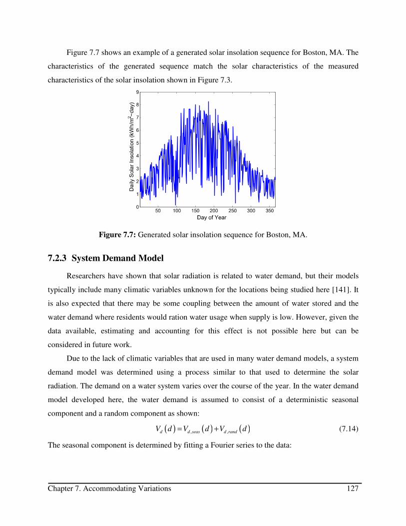
Chapter 7. Accommodating Variations 127
Figure 7.7 shows an example of a generated solar insolation sequence for Boston, MA. The
characteristics of the generated sequence match the solar characteristics of the measured
characteristics of the solar insolation shown in Figure 7.3.
Figure 7.7: Generated solar insolation sequence for Boston, MA.
7.2.3 System Demand Model
Researchers have shown that solar radiation is related to water demand, but their models
typically include many climatic variables unknown for the locations being studied here [141]. It
is also expected that there may be some coupling between the amount of water stored and the
water demand where residents would ration water usage when supply is low. However, given the
data available, estimating and accounting for this effect is not possible here but can be
considered in future work.
Due to the lack of climatic variables that are used in many water demand models, a system
demand model was determined using a process similar to that used to determine the solar
radiation. The demand on a water system varies over the course of the year. In the water demand
model developed here, the water demand is assumed to consist of a deterministic seasonal
component and a random component as shown:
( ) ( ) ( ), ,d d seas d randV d V d V d= + (7.14)
The seasonal component is determined by fitting a Fourier series to the data:

Chapter 7. Accommodating Variations 128
( ) 0,
, , ,
1
2 2cos sin
2 365 365d
d d
kV
d seas i V i V
i
a id idV d a b
π π
=
= + +
∑ (7.15)
To analyze the variations in water demand, data was solicited from the Massachusetts
Water Resources Authority. Data was obtained for 2005-2010 and the average value was fit with
a Fourier series to determine the seasonal component. Since only the first harmonic had a
significant contribution, higher order terms were ignored. The 2005 water demand and the
calculated seasonal component are shown in Figure 7.8.
Figure 7.8: Water use and yearly average in Boston, MA.
The residuals of the water use data were calculated using the following relationship:
( )( ) ( )
( )demand
D
D d D dd
dχ
σ
−= (7.16)
where D(d) is the measured water demand on day d, ( )D d is the mean demand on day d, σD(d)
is the standard deviation of the demand on day d. Since the water demand is taken relative to the
yearly average, regardless of the state of the day, the solar radiation residual is calculated without
regard of the day state as follows:
( ) ( )
( )solar
H
H d H d
dχ
σ
−= (7.17)

Chapter 7. Accommodating Variations 129
where ( )H d is mean solar radiation on day d, and σH(d) is the standard deviation of the solar
radiation on day d.
The residuals of the water demand and solar insolation for 2005 are shown in Figure 7.9.
Periods of high solar insolation often coincide with periods of high water use. This suggests that
the water demand model should depend on the level of solar insolation. Therefore, both the water
residual autocorrelation and cross-correlation between the water demand and solar insolation are
examined.
Figure 7.9: Normalized water demand and solar insolation residuals.
The autocorrelation of the water demand residuals can be seen in Figure 7.10. Statistically
significant correlation between the values of the residuals from one day to the next is evident.
This indicates that an autoregressive term should be included in the water demand model.

Chapter 7. Accommodating Variations 130
Figure 7.10: Water demand residual autocorrelation.
The cross-correlation function between the solar insolation and the water demand is shown
in Figure 7.11. This indicates evidence of a lagged relationship between the solar insolation and
the water demand. However, since each of the sequences is autocorrelated, this cross-correlation
may be misleading. To determine if the signals are correlated, each signal is pre-whitened [142].
Figure 7.11: Cross-correlation between solar insolation and water demand residuals.

Chapter 7. Accommodating Variations 131
The water demand and solar insolation sequences are pre-whitened using the simple first-
order filter:
( ) ( ) ( )' 1Y d Y d Y dα= − − (7.18)
where α is the first order lag of the solar insolation autocorrelation function. The autocorrelation
of the whitened solar insolation function is shown in Figure 7.12. The only statistically
significant occurs at a lag of 0, indicating that the resulting signal is nearly white.
Figure 7.12: Autocorrelation of whitened daily solar insolation sequence.
The cross-correlation of the two whitened signals, see Figure 7.13, shows that a correlation
exists between the solar insolation and the water demand. Significant correlations exist at lags of
0 and 1. Based on these results, different models are fit to the water demand data.

Chapter 7. Accommodating Variations 132
Figure 7.13: Whitened cross-correlation between solar radiation and water use.
The variable component of demand is modeled using an autoregressive distributed lag
system that depends on current and previous values of the solar insolation residuals as well as the
previous values water use:
( ) ( ) ( ) ( ) ( ), , 0
1 0
m n
d rand i d rand i
i i
V d V d i H d i H d i u dα β α= =
= − + − − − + + ∑ ∑ (7.19)
where u(d) is a noise input. The coefficients α and β are determined by fitting the data. Table 7.2
shows testing results of three different model configurations. The tests show that there is only a
small amount of accuracy gained by including a lag input for the solar insolation. As a result, the
final model used is given by:
( ) ( ) ( ) ( ) ( ), 1 , 0 01d rand d rand
V d V d H d H d u dα β α = − + − + + (7.20)
The coefficients are selected for each season and the values used in simulation are shown in
Table 7.3. The agreement between the model and the measured data is shown in Figure 7.14.
Table 7.2: Water demand models tested. Case Conditions MSE R2 Chi-Squared Value
1 m=0, n=0 199.6 0.840 0.369 2 m=1, n=0 121.6 0.901 0.251 3 m=1, n=1 121.1 0.903 0.248
Table 7.3: Demand model coefficients. Coefficient Jan 1 – April 30 May 1 – Aug 31 Sept 1 – Dec 31
α0 -0.169 -1.184 -0.198 α1 0.982 0.828 0.859 Β0 2.41 x 10⁻⁴ 3.46 x 10⁻³ 1.63 x 10⁻³

Chapter 7. Accommodating Variations 133
Figure 7.14: Water use and the model fit.
The model developed above is tailored for Boston, but the general model representation
can be used to develop models for other locations. Ideally, demand data is available for analysis
at every location to allow for estimation of the model coefficients. Unfortunately, this is not
always the case. By making the assumption that the relationship between water demand and solar
insolation is the same in other locations, the demand model can be scaled to determine the water
demand for other locations and system sizes. The demand scaling factor is given by:
0,
,2dV
d ave
a
Vφ = (7.21)
where a0,Vd is the Fourier coefficient for the analyzed water data, and Vd,ave is the average water
demand for the case of interest. With the scaling factor, the demand for the individual application
is given by:
( ) ( ) ( ) ( ), , ,d app d d seas d randV d V d V d V dφ φ φ= = + (7.22)
The above analysis provides the amount of water used over the course of a day. However,
a shorter time step is needed to determine if the PVRO system is able to instantaneously meet the
water demand. All cases considered here use an hourly time-step to determine system
performance. An average daily water use profile was developed based on [141]. The average
profile for a small family, shown in Figure 7.15, has usage peaks in the morning and evening.
For simulation, this hourly profile is scaled based on the daily water demand as follows:

Chapter 7. Accommodating Variations 134
( ) ( )( )
( )
,
, , 24
,
0
, d base
d hour d app
d base
V hV d h V d
V h dh
=
∫ (7.23)
where Vd,base(h) is the baseline hourly water demand specified in Figure 7.15.
Figure 7.15: Assumed hourly water demand profile.
7.3 Stochastic Modeling Case Studies
A series of case studies were conducted to test the stochastic modeling approach and to
demonstrate the effect of various loss of water probabilities. In these case studies, a PVRO
system capable of providing an average water production of 1 m3 in Boston, MA, was designed.
Two sets of studies are conducted: one that considers the entire year and one that only considers
the month during which the system is most stressed.
7.3.1 Full Year Simulations
In the full-year simulations, the stochastic solar radiation model and water demand model
described above are used to generate typical profiles for 100 years. The method described in
section 7.2.1 is used to analyze the system loss-of-water probability. The inventory specified in
section 6.3.3 is used to configure the lowest lifecycle cost system. As in the deterministic case
studies, a system lifetime of 25-years and an interest rate of 4% are assumed.
Cases are run for varying loss-of-water probabilities to illustrate the economic impact of
more reliable PVRO systems. Designs are generated for loss-of-water probabilities ranging from

Chapter 7. Accommodating Variations 135
0.01% to 10%. A Pareto plot of the loss-of-water probability versus the resulting lifetime PVRO
system costs is shown in Figure 7.16. Different methods can be used in multi-objective
optimization to generate Pareto plots. Here, the plot is generated by specifying the required loss
of water probability and optimizing a system to meet the requirement. It is evident as probability
of meeting demand increases, so does system cost. Here, the overall expense increases by almost
30%. The additional expense for higher reliability may not be justified in some locations if there
are other backup water options available, so the appropriate level of reliability is also location
dependent. As the higher loss of water probabilities are reached, the Pareto plot levels off. This
occurs due to constraints of the discrete inventory. As the loss-of-water probability increases, the
systems become smaller and there are fewer components and subsystems which can be decreased
or eliminated while meeting the system requirements.
Figure 7.16: Pareto plot of lifetime system cost versus loss-of-water probability.
Table 7.4 details system configurations resulting from different loss-of-water probability
constraints. As the loss of water probability increases, the overall system cost and complexity
decrease. For the low probability levels, the system configurations are different. The inventory
has a limited number of small-scale energy recovery devices. The small-scale energy recovery
devices in the inventory are unable to provide the required flowrates to meet the demands due to
the component operational limits and are not included in the final system configuration as a
result. For the remaining configurations, the number of membranes and PV panels decrease as
the probability increases, resulting in lower system costs.

Chapter 7. Accommodating Variations 136
Table 7.4: Results of modular design approach for 1 m3 systems with various LOWP.
7.3.2 Critical Month Simulations
In the critical month of case studies, the stochastic solar radiation model and water demand
model described above are used to generate typical profiles for 100 years, which are used to
determine the months of highest water stress. Since the amount of water produced is proportional
to the solar insolation is the month in which the system is most stressed. The water demand/solar
Loss of Water Probability
System Stats System Configuration Component Details
0.01% Lifetime Cost: $47788 Capital Cost: $23563 Average Cost of Water: $5.24/m3
Panel Trina Solar 225 W Panels
Panel Mounting
Fixed Panels
Motor Leeson 5 HP Motor Pump Danfoss APP 1.8 Energy Recovery
None
Membrane 4” Diameter, 40” long, Dow SWHRLE
Water Tank Size
10m3
0.1% Lifetime Cost: $41344 Capital Cost: $17247 Average Cost of Water: $4.53/m3
Panel Trina Solar 225 W Panels
Panel Mounting
Fixed Panels
Motor Leeson 1 HP Motor
Pump NRD PRG 10 Vane Pump
Energy Recovery
13% Danfoss RO Boost
Membrane 4” Diameter, 40” long, Dow SWHRLE
Water Tank Size
10m3
1% Lifetime Cost: $38262 Capital Cost: $12687 Average Cost of Water: $4.19/m3
Panel Suntech 295 W Panels Panel Mounting
Fixed Panels
Motor Leeson 1 HP Motor
Pump NRD PRG 10 Vane Pump
Energy Recovery
8% Spectra Clark Pump
Membrane 4” Diameter, 40” long, Dow SWHRLE
Water Tank Size
5m3
10% Lifetime Cost: $37344 Capital Cost: $11769 Average Cost of Water: $4.09/m3
Panel Trina Solar 225 W Panels
Panel Mounting
Fixed Panels
Motor 1 HP Leeson Motor
Pump NRD PRG 10 Vane Pump
Energy Recovery
8% Spectra Clark Pump
Membrane 4” Diameter, 40” long, Dow SWHRLE
Water Tank Size
5m3
M
ControlElectronics
13% PX
Control
ElectronicsM
8% PX
Control
ElectronicsM
8% PX
Control
ElectronicsM

Chapter 7. Accommodating Variations 137
insolation ratio is determined for every month over the 100-year period, and the month with the
highest ratio is selected for each year. This ratio varies by location. Figure 7.17 shows the
system demand ratio over one year for the 1 m3 Boston system, as well as the long-term average.
The average over the 100-year time window indicates that December is the critical period and is
used in the simulations.
Figure 7.17: Demand solar insolation ratio for sample year and 100-year average.
The method described in section 7.2.1 is used to analyze the system loss-of-water
probability. The loss-of-water probability for the entire year is estimated using two methods to
provide an upper and lower bound. Since simulation data is only provided for the critical month,
the lower bound on the year-long loss-of-water probability is determined by assuming all other
time periods are able to satisfy demand. The upper bound on the year-long loss-of-water
probability is determined by assuming all other months during the year provide the same level of
performance. The inventory specified in section 6.3.3 is again used to configure the lowest
lifecycle cost system and a system lifetime of 25-years and an interest rate of 4% are again
assumed.
Designs are generated for loss-of-water probabilities ranging from 0.1% to 10%. A Pareto
plot showing the how the total lifetime cost varies with loss of water probability is shown in
Figure 7.18. Both methods for estimating the year-long loss-of-water probability are shown. The
results show that the assumption that the rest of the year the system is able to provide water fails
as these cases consistently result in lower-cost configurations than the full-year simulations. This

Chapter 7. Accommodating Variations 138
indicates the system is stressed at other points of the year. The failure in assuming the non-
simulated months are able to meet demand is especially evident at high loss of water
probabilities. For this case, at a probability of 10%, the system does not need to provide any
water during the critical month to meet the design requirements. As a result, the system is
configured to meet the minimum requirements of a valid system.
The cases where the loss-of-water probability for the unsimulated portion of the year is
assumed to be the same as the critical month result in solutions that are more expensive than the
full-year cases. This is expected as the system is sized to the worst month. As the loss-of-water
probability increases, the distance between the upper bound and the full-year simulation cases
narrows. This occurs since the systems get smaller as the probability increases and accordingly,
there are fewer system design choices.
Figure 7.18: Pareto plot of lifetime system cost versus loss-of-water probability.
The overall computation time for the month long cases is greatly reduced. The
computation time required on a normal desktop computer ranged from 22.3 to 43.1 hours with an
average value of 28.5 hours. However, greater reduction in computation time is still desired.
7.4 Calculation of Loss-of-Water Probability Using Historical Data
Section 7.3 presented a simulation-based approach to estimate the loss-of-water probability
for a given system design. While this approach was shown to be effective, the computation time

Chapter 7. Accommodating Variations 139
required for a single optimization ranges between 3-5 days on a standard desktop computer. A
faster method is needed.
To decrease the computation time required, an analytic method for computing the LOWP is
developed by using the knowledge of the solar insolation and water demand distributions to
determine the distribution of the net change in stored water. The amount of water in storage is
represented by a number of discrete states. The probability of transitioning between these states
during a day is determined using the tank volume change distribution. Using this representation,
the loss of water probability can be determined analytically.
Several simplifying assumptions are applied in order to estimate the LOWP using the data
from the month with the highest solar demand. First, it is assumed that the solar radiation and
water demand on a given day are independent of the values on previous days. It is also assumed
that the critical water storage level is reached at the end of the day.
The solar insolation during the critical month is analyzed first. The daily data from a 21-
year time period is obtained for any location using the NASA Surface Meteorology Database [8].
This data can be analyzed to determine a solar insolation histogram. An example for the month
of December in Boston, MA can be seen in Figure 7.19.
Figure 7.19: Normalized histogram of Boston daily solar insolation in December.
Next, the probability distribution is generated from the solar insolation distribution for a
given PVRO system. Hourly solar radiation profiles are generated using the standard outlined in
section 5.1.1 and the relationship between solar insolation and water production is calculated

Chapter 7. Accommodating Variations 140
[122]. The daily water production distribution is directly calculated from the daily solar
insolation distribution using this relationship. Figure 7.20 shows the relation between solar
insolation and water production for a small PVRO system in Boston, as well as the resulting
water production distribution for the critical month of December.
Figure 7.20: Daily water production for a small PVRO system in Boston and the normalized
histogram of daily water production in December.
Variation in the water demand is then considered. A histogram of the water demand over
the month of December is generated from the collected data from the Massachusetts Water
Resources Authority. Individual histograms are generated for different levels of solar radiation to
account for correlation between the two random variables. The water demand histograms for a 1
m3 system located in Boston during the month of December are shown in Figure 7.21. The
correlation between water demand and solar insolation is low during the month of December, but
is included here to illustrate the general method. Other locations may have higher correlation. As
mentioned above, there may be other effects which are not accounted for here due to lack of
information, such as coupling between water tank level and system demand.

Chapter 7. Accommodating Variations 141
Figure 7.21: Normalized histograms of daily water demand in December for different ranges of
solar insolation.
Once distributions for the solar insolation and water demand are generated, the distribution
of the change in water tank level is calculated. The water production is calculated for each level

Chapter 7. Accommodating Variations 142
of solar insolation. The distribution in the water tank level is calculated by comparing water
production and water use for that insolation level. The probability of a given change in water
tank level is calculated by summing over all insolation levels as follows:
1
1 tank 2 ,1 ,2 ,1 ,2
,1 ,2 1 ,2 ,1 2
( ) ( | ) ( | )
s.t. - & -
NHH
prod prod prod use use use
H H
prod use prod use
P V V V P V V V H P V V V H
V V V V V V
=
≤ ∆ < = ≤ < ≤ <
> <
∑ (7.24)
where ∆Vtank is the change in tank water level, Vprod is the volume of water produced and Vuse is
the volume of water used. The resulting distribution for the example case of a 1 m3 system in
Boston is shown in Figure 7.22.
Figure 7.22: Normalized histogram of daily tank volume change for a 1 m3 PVRO system in
Boston during the month of December.
The tank is discretized into N levels, with level 1 being an empty tank and level N being a
full tank. Given the probability distribution of water in the tank on day i, the distribution on day
i+1 can be determined using the following:
1i i+ =π Aπ (7.25)
where A is the transition probability matrix and π is and N x 1 vector representing the probability
water volume in the being at a given level. The entries of A are given by the tank volume
change probability as follows:

Chapter 7. Accommodating Variations 143
min
min
max
max
0
1,1
1,2
2,1
2,2
2,3
, 1
,
0
( )
( )
( )
( 0)
( )
( )
( )
t
t
i V
V
i V
t
t
V
N N
i V
V
N N
i
A P V i
A P V i
A P V V
A P V
A P V V
A P V i
A P V i
=∆
−
=∆
∆
−=
∆
=
= ∆ =
= ∆ =
= ∆ =
= ∆ =
= ∆ = −
= ∆ =
= ∆ =
∑
∑
∑
∑
u(7.26)
where Vt is the size of the discretization of the tank volume.
Given a known initial volume of a half-full tank, the probability distribution of the tank
storage level can be determined throughout the course of the month. This is done for the example
of 1 m3 system in Boston starting with a half-full 5 m3 tank, and the resulting tank volume
distributions are shown in Figure 7.23. Due to the limits of the tank size, spikes occur in the
probability distribution when the tank is empty (0 m3) and when the tank is at full capacity (5
m3). Since the initial volume is unknown, the steady state value is utilized to determine the
system loss-of-water probability. The steady state distribution can be determined using:
( ) 0ss− =I A π (7.27)
The system loss of water probability is given by the probability that the system is in the lowest
state in the steady state condition. For the example case, the loss-of-water probability is 0.81%.

Chapter 7. Accommodating Variations 144
Figure 7.23: Evolution of water tank storage distribution in December.
This method can be used to calculate the loss-of-water probability in the final optimization
stage of the modular design approach for PVRO systems. This approach substitutes for the time-
series simulations. Case studies for this approach are presented below.
7.5 Direct Calculation Case Studies
Case studies were conducted using the direct calculation of the loss-of water probability.
The problem statement remains the same as the cases presented in section 7.3. The inventory
specified in section 6.3.3 is again used to configure the lowest lifecycle cost system, and a
system lifetime of 25-years and an interest rate of 4% are assumed. Cases are run for varying
loss-of-water probabilities to see the tradeoff between cost and reliability. Designs are generated
for loss-of-water probabilities between 0.01% and 10%. A Pareto plot of the loss-of-water
probability versus the resulting lifetime PVRO system costs can be seen in Figure 7.24 and
resulting system configurations can be seen in Table 7.5. It can be seen that the results are very
similar to the full-year simulation case studies. The resulting systems are typically larger since
they are sized according to the worst period of the year.
0
0.01
0.02
0.03
0.04
0.05
0.06
0.07
0 1 2 3 4 5
No
rma
lize
d D
istr
ibu
tio
n
Tank Volume (m3)
0
0.005
0.01
0.015
0.02
0.025
0.03
0 1 2 3 4 5
No
rma
lize
d D
istr
ibu
tio
n
Tank Volume (m3)
0 1 2 3 4 50
0.02
0.04
0.06
0.08
0.1
0.12
Tank Volume (m3)
No
rma
lize
d D
istr
ibu
tio
n
0
0.02
0.04
0.06
0.08
0.1
0.12
0.14
0.16
0.18
0 1 2 3 4 5
No
rma
lize
d D
istr
ibu
tio
n
Tank Volume (m3)
0
0.02
0.04
0.06
0.08
0.1
0.12
0.14
0.16
0.18
0.2
0 1 2 3 4 5
No
rma
lize
d D
istr
ibu
tio
n
Tank Volume (m3)
0
0.05
0.1
0.15
0.2
0.25
0 1 2 3 4 5
No
rma
lize
d D
istr
ibu
tio
n
Tank Volume (m3)
Day 1 Day 5 Day 10
Day 30Day 20 Steady State

Chapter 7. Accommodating Variations 145
Figure 7.24: Pareto plot of lifetime system cost versus loss-of-water probability for direct
LOWP calculation approach.
Table 7.5: Results of modular design approach for 1 m3 systems when using the direct LOWP
calculation.
For the cases considered, the direct calculation method typically results in a higher cost
system cost than the full-year simulation. This matches intuition as the system components are
Loss of Water Probability
System Stats System Configuration Component Details
0.01% Lifetime Cost: $48586 Capital Cost: $24092 Average Cost of Water: $5.32/m3
Panel Trina Solar 225 W Panels
Panel Mounting
Fixed Panels
Motor Leeson 5 HP Motor Pump Danfoss APP 1.8 Energy Recovery
None
Membrane 4” Diameter, 40” long, Dow SWHRLE
Water Tank Size
10m3
10% Lifetime Cost: $37344 Capital Cost: $11769 Average Cost of Water: $4.09/m3
Panel Trina Solar 225 W Panels
Panel Mounting
Fixed Panels
Motor 1 HP Leeson Motor
Pump NRD PRG 10 Vane Pump
Energy Recovery
8% Spectra Clark Pump
Membrane 4” Diameter, 40” long, Dow SWHRLE
Water Tank Size
5m3
M
Control
Electronics
8% PX
Control
ElectronicsM

Chapter 7. Accommodating Variations 146
sized to meet demand in the worst month. An exception occurs at a loss-of-water probability of
0.05%. The resulting system configurations for this case can be seen in Figure 7.25. It is seen
that the resulting system topologies are different. This occurs due to the limited one month time-
window which is considered during the direct calculation approach. During this worst month,
which is the winter for the case studied, the system demand and water production flowrates are
lower. As a result, the system components which can meet demand during this month may reach
their operational limits when system flowrates are required to be higher during the summer
months. This is the case with the energy recovery device and a different configuration is required
when the full year is considered.
Figure 7.25: Systems designed for LOWP = 0.05% using full-year simulations (left) and direct
calculation of LOWP in the critical month (right).
The computation time for this method is also greatly reduced from the full-year simulation
method. In the cases studied, the total computation time on a computer with an Intel 2.8 GHz
Dual Core processor and 4 GB of RAM ranged between 18.3 and 31.7 hours with an average of
22.5 hours. This method decreases the computation time required, and can be used to design
systems with the required loss-of-water probability. For the majority of cases studies, the direct
LOWP calculation method provides similar results to the full-year simulations. Due to
simplifications made, checks should be implemented to ensure the resulting system can meet the
required LOWP during the remaining portion of the year. \ \
M
Control
Electronics
13% PX
Control
ElectronicsM

Chapter 8. Summary and Conclusions 147
CHAPTER
8 SUMMARY AND CONCLUSIONS
8.1 Summary
This thesis describes an approach for automatically designing systems composed of
modular components. Engineering principles are used to limit the scope of the design problem.
Optimization methods are then used to determine the modular system configuration. The
application considered in detail here is the design of PVRO systems for small communities. The
methods are formulated to be robust to uncertainties in system requirements. Software tools can
be created from the modular design methods developed in this research to enable modular system
design by non-experts.
Chapter 1 presents the motivation for this research. Clean drinking water is a major issue
for many locations and PVRO systems can provide a possible solution. PVRO systems are
composed of modular components, so designing a system for an individual location is beyond
the expertise available in many parts of the world. For a given modular inventory, a large number
of possible system configurations exist. Methods which enable non-experts to custom configure
PVRO systems for individual locations can make this technology accessible to many parts of the
world.
Chapter 2 presents relevant literature on the topics of PVRO systems and modular design
methods. PVRO systems have been designed and deployed in many regions. These systems are
custom designed for individual locations and water demands. No general design methods have
been developed for PVRO, although they exist for other applications including robotics,
electronic circuits, and computer programs. These methods are application specific and do not
consider many aspects important for PVRO system design, such as accommodating a large
component inventory, complex system physics, and variations in the system environment.
Chapter 8. Summary and Conclusions 148
Chapter 3 presents a PVRO feasibility study that was conducted to determine the potential
impact of this research. The feasibility study compares the economics of PVRO systems to those
of diesel reverse osmosis systems and transported water for a wide range of locations. It shows
that PVRO systems are economically viable for many small communities located in equatorial
regions. It also shows the area where PVRO is economically viable will increase as the system
costs decrease. Decreasing the system costs can be accomplished using by using modular design
methods.
Chapter 4 presents the details of the modular design approach. Engineering principles are
used to reduce the system design space, and optimization methods are then used to configure a
modular system for an individual application. The method is applied in a design space study for a
PVRO system, where it greatly reduces the size of the design space. A parallel example is
presented for the design of a hybrid car. The design studies show that this method has great
potential and can be applied to many modular systems.
Chapter 5 presents the PVRO system models used in the modular design approach.
Physics-based models are developed for individual system components. A new method of
representing different reverse osmosis system configurations is developed which uses a graph to
indicate the component connections. This graph representation is implemented in Matlab to
calculate the PVRO system production for given solar input. A surrogate model of the solar
radiation to water production relationship is developed to increase calculation speed for different
solar profiles. This model is validated using an experimental PVRO system that was constructed
as a part of this research.
Chapter 6 presents the implementation of the modular design approach for PVRO system
design using deterministic solar radiation inputs and demands. The approach is able to tailor
systems for a wide range of locations and water demands from a large system inventory. The
validity of these solutions is demonstrated by simulating a custom designed system in the wrong
location. A final case study demonstrates that the method can be used to determine if new
components are capable of impacting the market.
Chapter 7 presents the implementation of the modular design approach for PVRO systems
using variable solar insolation and water demand. Two methods that use historical solar
insolation and water demand to account for variations are presented. The first method
characterizes the historical data and develops models to synthetically generate data, then

Chapter 8. Summary and Conclusions 149
simulates the system over a period of 100 years to determine the loss-of-water probability. In the
second method, distributions of solar radiation and water demand are calculated from historical
data and used to directly calculate the probability of running out of water in the worst month of
the year. Modular design cases were conducted for both methods. The full-year simulation
method is able to design systems for varying loss-of-water probabilities, but the computation
time required is over 3 days for every case considered. The direct calculation method is shown to
yield similar results to the full-year simulation method, and the computation time is greatly
reduced to less than 1 day in many instances. The direct calculation method can be used to
quickly estimate the failure probability of many systems with variable inputs.
8.2 Suggestions for Future Work
This thesis presents a general design approach for modular systems and studies its
application to the design of PVRO systems in detail. There are many interesting opportunities for
future research on both the design approach and the application of PVRO systems.
A major challenge with reverse osmosis desalination is proper pre-treatment of the
incoming feedwater. In certain locations, the feedwater may contain bacteria or salts that are near
their saturation limits. This is of particular concern when designing brackish water systems. This
research did not consider the effects and costs associated with different pre-treatment systems.
Modeling these aspects and adding them to the modular design approach will greatly aid system
designers.
As PVRO systems age, the performance of individual components will degrade. These
effects may result in much lower PVRO system production as the components reach the end of
their lives. The effects of degradation can be incorporated into the system models for to ensure
that the designed system is able to meet the demands over the entire system life.
Another design issue that may be incorporated into a modular design approach is
accommodating component failure. Many of the system configurations produced by the modular
design implementation will fail if one key component fails. Failure of the system may have
terrible consequences. Developing a method to analyze the effects of component failure and
address them during the design can be an interesting extension of this work.
In some locations where PVRO systems are economically viable, the system would not be
required to provide all the water for community. For example, locations in the developing world
Chapter 8. Summary and Conclusions 150
may already have rainwater catchments in place. Rainwater systems complement PVRO systems
since they provide water during inclement weather. Designing these complementary systems
provides a different set of challenges and would be an interesting avenue for future research.
This thesis developed a method to directly calculate the probability of failing to provide
adequate water from statistical solar radiation and water use data. The method made simplifying
assumptions to allow for the calculation. The main simplifications are that the system is only
stressed during one-month of the year and that the solar radiation and water use are independent
of previous values. As a result, this method provides an estimate of the loss-of-water probability.
The method should be expanded to ensure conditions outside the critical month are considered.
In addition, development of an expanded approach that considers day-to-day persistence of solar
radiation and demand will improve the accuracy of loss-of-water probability calculation and
make it useful for future design applications.
Another promising avenue of research is the implementation of the PVRO technology from
this research in the developing world. For a PVRO system to have a long-term impact on a
community in the developing world, it must be properly operated and maintained. Developing a
control system with a robust user interface that identifies potential system issues will be essential
to the successful implementation of these systems. In addition, effective training programs and
maintenance programs will be required. The technical and social aspects of deploying such
systems provide interesting avenues for future research.

References 151
REFERENCES
[1] World Health Organization and Unicef, "Progress on Sanitation and Drinking Water:
2010 Update," World Health Organization and Unicef, Geneva, Switzerland, 2010. [2] H. T. El-Dessouky and H. M. Ettouney, Fundamentals of salt water desalination.
Amsterdam; New York: Elsevier, 2002. [3] F. Trieb and H. Müller-Steinhagen, "Concentrating solar power for seawater desalination
in the Middle East and North Africa," Desalination, vol. 220, pp. 165-183, 2008. [4] F. Trieb, et al., "Concentrating Solar Power for Seawater Desalination," German
Aerospace Center (DLR), Stuttgart, 2007. [5] S. A. Kalogirou, "Seawater desalination using renewable energy sources," Progress in
Energy and Combustion Science, vol. 31, pp. 242-281, 2005. [6] E. Tzen and R. Morris, "Renewable energy sources for desalination," Solar Energy, vol.
75, pp. 375-379, 2003. [7] United Nations, "World Water Day 2007 Brochure - Coping With Water Scarcity," 2007. [8] National Aeronautics and Space Administration. Surface Meteorology and Solar Energy:
A renewable energy resource web site (release 6.0) [Online]. Available: http://eosweb.larc.nasa.gov/sse/
[9] Center for Renewable Energy Systems (CRES), "Desalination guide using renewable energies. THERMIE – DG XVII," European Commission Report, Greece, 1998.
[10] M. S. Mohsen and J. O. Jaber, "A photovoltaic-powered system for water desalination," Desalination, vol. 138, pp. 129-136, 2001.
[11] E. S. Hrayshat, "Brackish water desalination by a stand alone reverse osmosis desalination unit powered by photovoltaic solar energy," Renewable Energy, vol. 33, pp. 1784-1790, 2008.
[12] E. S. Mohamed and G. Papadakis, "Design, simulation and economic analysis of a stand-alone reverse osmosis desalination unit powered by wind turbines and photovoltaics," Desalination, vol. 164, pp. 87-97, 2004.
[13] E. S. Mohamed, et al., "A direct coupled photovoltaic seawater reverse osmosis desalination system toward battery based systems — a technical and economical experimental comparative study," Desalination, vol. 221, pp. 17-22, 2008.
[14] A. M. Thomson, "Reverse-Osmosis Desalination of Seawater Powered by Photovoltaics Without Batteries," Ph.D., Loughborough University, Loughborough, U.K., 2003.
[15] M. Thomson and D. Infield, "A photovoltaic-powered seawater reverse-osmosis system without batteries," Desalination, vol. 153, pp. 1-8, 2003.
[16] J. Went, et al., "The energy demand for desalination with solar powered reverse osmosis units," Desalination and Water Treatment, vol. 21, pp. 138-147, 2010.
[17] A. Schies, et al., "Operating control strategies and dimensioning of photovoltaic-powered reverse osmosis desalination plants without batteries," Desalination and Water
Treatment, vol. 21, pp. 131-137, 2010. [18] S. Dallas, et al., "Efficiency analysis of the Solarflow – An innovative solar-powered
desalination unit for treating brackish water," Renewable Energy, vol. 34, pp. 397-400, 2009.

References 152
[19] S. F. Cheah, "Photovoltaic Reverse Osmosis Desalination System," ITN Energy Systems, Inc., Littleton, CO2004.
[20] D. B. Riffel and P. C. M. Carvalho, "Small-scale photovoltaic-powered reverse osmosis plant without batteries: Design and simulation," Desalination, vol. 247, pp. 378-389, 2009.
[21] A. Joyce, et al., "Small reverse osmosis units using PV systems for water purification in rural places," Desalination, vol. 137, pp. 39-44, 2001.
[22] D. Herold, et al., "Small scale photovoltaic desalination for rural water supply - demonstration plant in Gran Canaria," Renewable Energy, vol. 14, pp. 293-298, 1998.
[23] D. Herold and A. Neskakis, "A small PV-driven reverse osmosis desalination plant on the island of Gran Canaria," Desalination, vol. 137, pp. 285-292, 2001.
[24] Z. Al Suleimani and V. R. Nair, "Desalination by solar-powered reverse osmosis in a remote area of the Sultanate of Oman," Applied Energy, vol. 65, pp. 367-380, 2000.
[25] E. Tzen, et al., "Autonomous reverse osmosis units driven by RE sources experiences and lessons learned," Desalination, vol. 221, pp. 29-36, 2008.
[26] E. Tzen, et al., "Design of a stand alone PV - desalination system for rural areas," Desalination, vol. 119, pp. 327-333, 1998.
[27] E. Tzen, et al., "Design and development of a hybrid autonomous system for seawater desalination," Desalination, vol. 166, pp. 267-274, 2004.
[28] Spectra Watermakers, "SSW 3500 Datasheet," 2009. [29] S. Abdallah, et al., "Performance of a photovoltaic powered reverse osmosis system
under local climatic conditions," Desalination, vol. 183, pp. 95-104, 2005. [30] B. S. Richards and A. I. Schäfer, "Photovoltaic-powered desalination system for remote
Australian communities," Renewable Energy, vol. 28, pp. 2013-2022, 2003. [31] M. Thomson and D. Infield, "Laboratory demonstration of a photovoltaic-powered
seawater reverse-osmosis system without batteries," Desalination, vol. 183, pp. 105-111, 2005.
[32] P. C. M. de Carvalho, et al., "Control method of a photovoltaic powered reverse osmosis plant without batteries based on maximum power point tracking," in Transmission and
Distribution Conference and Exposition: Latin America, 2004 IEEE/PES, 2004, pp. 137-142.
[33] I. de la Nuez Pestana, et al., "Optimization of RO desalination systems powered by renewable energies. Part I: Wind energy," Desalination, vol. 160, pp. 293-299, 2004.
[34] D. Voivontas, et al., "A tool for the design of desalination plants powered by renewable energies," Desalination, vol. 133, pp. 175-198, 2001.
[35] K. Bourouni, et al., "Design and optimization of desalination reverse osmosis plants driven by renewable energies using genetic algorithms," Renewable Energy, vol. 36, pp. 936-950, 2011.
[36] M. Wilf and C. Bartels, "Optimization of seawater RO systems design," Desalination,
vol. 173, pp. 1-12, 2005. [37] M. Wilf and K. Klinko, "Optimization of seawater RO systems design," Desalination,
vol. 138, pp. 299-306, 2001. [38] A. Malek, et al., "Design and economics of RO seawater desalination," Desalination, vol.
105, pp. 245-261, 1996.
References 153
[39] A. Gambier, et al., "Dynamic Modeling of a Simple Reverse Osmosis Desalination Plant for Advanced Control Purposes," in American Control Conference, 2007. ACC '07, 2007, pp. 4854-4859.
[40] M. M. El-Halwagi, "Synthesis of reverse-osmosis networks for waste reduction," AIChE
Journal, vol. 38, pp. 1185-1198, 1992. [41] N. Voros, et al., "Optimization of reverse osmosis networks for seawater desalination,"
Computers & Chemical Engineering, vol. 20, Supplement 1, pp. S345-S350, 1996. [42] M. G. Marcovecchio, et al., "Global optimal design of reverse osmosis networks for
seawater desalination: modeling and algorithm," Desalination, vol. 184, pp. 259-271, 2005.
[43] Y. Saif, et al., "Global Optimization of Reverse Osmosis Network for Wastewater Treatment and Minimization," Industrial & Engineering Chemistry Research, vol. 47, pp. 3060-3070, 2008/05/01 2008.
[44] Y.-Y. Lu, et al., "Optimum design of reverse osmosis system under different feed concentration and product specification," Journal of Membrane Science, vol. 287, pp. 219-229, 2007.
[45] Y.-y. Lu, et al., "Optimum design of reverse osmosis seawater desalination system considering membrane cleaning and replacing," Journal of Membrane Science, vol. 282, pp. 7-13, 2006.
[46] F. Vince, et al., "Multi-objective optimization of RO desalination plants," Desalination,
vol. 222, pp. 96-118, 2008. [47] F. Maskan, et al., "Optimal design of reverse osmosis module networks," AIChE Journal,
vol. 46, pp. 946-954, 2000. [48] A. Abbas, "Model predictive control of a reverse osmosis desalination unit,"
Desalination, vol. 194, pp. 268-280, 2006. [49] A. R. Bartman, et al., "Nonlinear Model-Based Control of an Experimental Reverse-
Osmosis Water Desalination System," Industrial & Engineering Chemistry Research,
vol. 48, pp. 6126-6136, 2009/07/01 2009. [50] A. Gambier, et al., "Fault-tolerant control of a small reverse osmosis desalination plant
with feed water bypass," in American Control Conference (ACC), 2010, 2010, pp. 3611-3616.
[51] A. Gambier, et al., "Optimal control of a reverse osmosis desalination plant using multi-objective optimization," in Computer Aided Control System Design, 2006 IEEE
International Conference on Control Applications, 2006 IEEE International Symposium
on Intelligent Control, 2006 IEEE, 2006, pp. 1368-1373. [52] A. R. Bartman, et al., "Minimizing energy consumption in reverse osmosis membrane
desalination using optimization-based control," Journal of Process Control, vol. 20, pp. 1261-1269, 2010.
[53] A. Poullikkas, "Optimization algorithm for reverse osmosis desalination economics," Desalination, vol. 133, pp. 75-81, 2001.
[54] C. Guria, et al., "Multi-objective optimization of reverse osmosis desalination units using different adaptations of the non-dominated sorting genetic algorithm (NSGA)," Computers & Chemical Engineering, vol. 29, pp. 1977-1995, 2005.
[55] D. Rus and M. Vona, "Crystalline Robots: Self-Reconfiguration with Compressible Unit Modules," Auton. Robots, vol. 10, pp. 107-124, 2001.

References 154
[56] M. Yim, et al., "PolyBot: a modular reconfigurable robot," in Robotics and Automation,
2000. Proceedings. ICRA '00. IEEE International Conference on, 2000, pp. 514-520 vol.1.
[57] S. Farritor, et al., "A systems-level modular design approach to field robotics," in Robotics and Automation, 1996. Proceedings., 1996 IEEE International Conference on, 1996, pp. 2890-2895 vol.4.
[58] N. Rutman, "Automated design of modular field robots," M.S., Mechanical Engineering, Masssachusetts Institute of Technology, Cambridge, MA, 1995.
[59] G. S. Hornby, et al., "Generative representations for the automated design of modular physical robots," Robotics and Automation, IEEE Transactions on, vol. 19, pp. 703-719, 2003.
[60] C. Leger, "Automated Synthesis and Optimization of Robot Configurations: An Evolutionary Approach," The Robotics Institute, Carnegie Mellon University, Pittsburgh, PA, 1999.
[61] J. R. Koza, et al., "Automated synthesis of analog electrical circuits by means of genetic programming," Evolutionary Computation, IEEE Transactions on, vol. 1, pp. 109-128, 1997.
[62] J. R. Koza, et al., "Automated WYWIWYG design of both the topology and component values of electrical circuits using genetic programming," presented at the Proceedings of the First Annual Conference on Genetic Programming, Stanford, California, 1996.
[63] J. D. Lohn and S. P. Colombano, "A circuit representation technique for automated circuit design," Evolutionary Computation, IEEE Transactions on, vol. 3, pp. 205-219, 1999.
[64] E. S. Ochotta, et al., "Synthesis of high-performance analog circuits in ASTRX/OBLX," Computer-Aided Design of Integrated Circuits and Systems, IEEE Transactions on, vol. 15, pp. 273-294, 1996.
[65] J. F. Miller, et al., "Principles in the Evolutionary Design of Digital Circuits—Part I," Genetic Programming and Evolvable Machines, vol. 1, pp. 7-35, 2000.
[66] E. M. Sentovich, et al., "Sequential circuit design using synthesis and optimization," in Computer Design: VLSI in Computers and Processors, 1992. ICCD '92. Proceedings.,
IEEE 1992 International Conference on, 1992, pp. 328-333. [67] J. R. Koza, Genetic programming: on the programming of computers by means of natural
selection: MIT Press, 1992. [68] J. R. Koza, Genetic Programming II: Automatic Discovery of Reusable Programs: MIT
Press, 1994. [69] A. Garrard and E. S. Fraga, "Mass exchange network synthesis using genetic algorithms,"
Computers & Chemical Engineering, vol. 22, pp. 1837-1850, 1998. [70] D. R. Lewin, et al., "A generalized method for HEN synthesis using stochastic
optimization – I. General framework and MER optimal synthesis," Computers &
Chemical Engineering, vol. 22, pp. 1503-1513, 1998. [71] B. Gross and P. Roosen, "Total process optimization in chemical engineering with
evolutionary algorithms," Computers & Chemical Engineering, vol. 22, Supplement 1, pp. S229-S236, 1998.
[72] M. Cantoni, et al., "Genetic algorithms and Monte Carlo simulation for optimal plant design," Reliability Engineering & System Safety, vol. 68, pp. 29-38, 2000.

References 155
[73] M. Mack, "Solar power for telecommunications," The Telecommunication Journal of
Australia, vol. 29, pp. 20-44, 1979. [74] R. N. Chapman, "A simplified technique for designing least cost stand-alone PV/storage
systems," in 19th IEEE Photovoltaic Specialists Conference, New Orleans, LA, 1987. [75] M. Sidrach-de-Cardona and L. Mora López, "A simple model for sizing stand alone
photovoltaic systems," Solar Energy Materials and Solar Cells, vol. 55, pp. 199-214, 1998.
[76] H.-G. Beyer and B. Sendhoff, "Robust optimization – A comprehensive survey," Computer Methods in Applied Mechanics and Engineering, vol. 196, pp. 3190-3218, 2007.
[77] L. L. Bucciarelli Jr, "Estimating loss-of-power probabilities of stand-alone photovoltaic solar energy systems," Solar Energy, vol. 32, pp. 205-209, 1984.
[78] L. L. Bucciarelli Jr, "The effect of day-to-day correlation in solar radiation on the probability of loss-of-power in a stand-alone photovoltaic energy system," Solar Energy,
vol. 36, pp. 11-14, 1986. [79] A. D. Bagul, et al., "Sizing of a stand-alone hybrid wind-photovoltaic system using a
three-event probability density approximation," Solar Energy, vol. 56, pp. 323-335, 1996. [80] J. M. Gordon, "Optimal sizing of stand-alone photovoltaic solar power systems," Solar
Cells, vol. 20, pp. 295-313, 1987. [81] H. L. Macomber, et al., "Photovoltaic stand-alone systems: preliminary engineering-
design handbook," DOE/NASA/0195-1; NASA-CR-165352; Other: ON: DE82000678 United StatesOther: ON: DE82000678Thu Feb 07 15:45:28 EST 2008NTIS, PC A11/MF A01.ERA-07-014040; EDB-82-028230English, 1981.
[82] E. Koutroulis, et al., "Methodology for optimal sizing of stand-alone photovoltaic/wind-generator systems using genetic algorithms," Solar Energy, vol. 80, pp. 1072-1088, 2006.
[83] S. Diaf, et al., "A methodology for optimal sizing of autonomous hybrid PV/wind system," Energy Policy, vol. 35, pp. 5708-5718, 2007.
[84] A. Bilton, et al., "Design Optimization of Sustainable Off-Grid Power Systems for the Developing World," ASME Conference Proceedings, vol. 2011, pp. 1531-1540, 2011.
[85] A. Fragaki and T. Markvart, "Stand-alone PV system design: Results using a new sizing approach," Renewable Energy, vol. 33, pp. 162-167, 2008.
[86] T. Markvart, et al., "PV system sizing using observed time series of solar radiation," Solar Energy, vol. 80, pp. 46-50, 2006.
[87] M. Egido and E. Lorenzo, "The sizing of stand alone PV-system: A review and a proposed new method," Solar Energy Materials and Solar Cells, vol. 26, pp. 51-69, 1992.
[88] A. Balouktsis, et al., "Sizing stand-alone photovoltaic systems," International Journal of
Photoenergy, vol. 2006, 2006. [89] G. Giannakoudis, et al., "Optimum design and operation under uncertainty of power
systems using renewable energy sources and hydrogen storage," International Journal of
Hydrogen Energy, vol. 35, pp. 872-891, 2010. [90] P. Arun, et al., "Optimum sizing of photovoltaic battery systems incorporating
uncertainty through design space approach," Solar Energy, vol. 83, pp. 1013-1025, 2009. [91] F. Domínguez-Muñoz, et al., "Design of solar thermal systems under uncertainty,"
Energy and Buildings, vol. 47, pp. 474-484, 2012.

References 156
[92] A. Roy, et al., "Physical design space for isolated wind-battery system incorporating resource uncertainty," Proceedings of the Institution of Mechanical Engineers, Part A:
Journal of Power and Energy, vol. 225, pp. 421-442, June 1, 2011 2011. [93] A. M. Helal, et al., "Economic feasibility of alternative designs of a PV-RO desalination
unit for remote areas in the United Arab Emirates," Desalination, vol. 221, pp. 1-16, 2008.
[94] H. M. Ettouney, et al., "Evaluating the economics of desalination," Chemical
Engineering Progress, vol. 12, pp. 32-38, 2002. [95] T. Jackson and M. Oliver, "The viability of solar photovoltaics," Energy Policy, vol. 28,
pp. 983-988, 2000. [96] National Oceanographic Data Center (U.S.). World Ocean Atlas 2005 [Online].
Available: http://www.nodc.noaa.gov/OC5/WOA05/pr_woa05.html [97] United Nations World Water Assessment Programme, "The 2nd United Nations World
Water Development Report - Water: A Shared Responsibility," UNESCO, Paris, France, 2006.
[98] I. C. Karagiannis and P. G. Soldatos, "Current status of water desalination in the Aegean Islands," Desalination, vol. 203, pp. 56-61, 2007.
[99] Dow Filmtec Membrane Systems. Filmtec Membranes – System design: System performance projection [Online]. Available: http://www.dow.com/PublishedLiterature/dh_0036/0901b803800362e9.pdf
[100] M. Q. Wang, "GREET 1.5 - transportation fuel-cycle model - Vol. 1 : methodology, development, use, and results," AH200130, 1999.
[101] O. Barron, "Desalination options and their possible implementation in Western Australia: Potential role for CSIRO Land and Water," CSIRO: Water for a Healthy Country National Research Flagship, Canberra, Australia, 2006.
[102] A. Hafez and S. El-Manharawy, "Economics of seawater RO desalination in the Red Sea region, Egypt. Part 1. A case study," Desalination, vol. 153, pp. 335-347, 2003.
[103] R. Wiser, et al., "Letting the sun shine on solar costs: An empirical investigation of photovoltaic cost trends in California," Berkeley, California, LBNL-59282, 2006.
[104] M. Muselli, et al., "Design of Hybrid-Photovoltaic Power Generator with Optimization of Energy Management," Solar Energy, vol. 65, pp. 143-157, 1999.
[105] Solarbuzz. (2012, July 19, 2012). Inverter Prices. Available: http://www.solarbuzz.com/facts-and-figures/retail-price-environment/inverter-prices
[106] United States Energy Information Administration. (2009). Annual U.S. No. 2 diesel retail
sales by all sellers, Dec. 1, 2009. Available: http://tonto.eia.doe.gov/dnav/pet/hist/d220600002m.htm
[107] T. G. Eschenbach, "Engineering Economy - Applying Theory to Practice (2nd Edition)," Oxford University Press, 2003.
[108] Reuters, "France sets carbon tax at 17 Euros a ton," in The New York Times. New York City, NY, 2009.
[109] J. K. Kaldellis, et al., "Renewable energy desalination plants for the Greek islands—technical and economic considerations," Desalination, vol. 170, pp. 187-203, 2004.
[110] C. Burroughs. (2009, April 3, 2009). Desalination of saline and brackish water becoming
more affordable. Available: https://share.sandia.gov/news/resources/news_releases/desalination-of-saline-and-brackish-water/

References 157
[111] S. M. Habali and I. A. Saleh, "Design of stand-alone brackish water desalination wind energy system for Jordan," Solar Energy, vol. 52, pp. 525-532, 1994.
[112] S. J. Lewis, et al., "Assessment of groundwater resources in the Broken Hill region," Geoscience Australia Professional Opinion, 2008.
[113] R. Trabelsi, et al., "Groundwater salinization of the Sfax superficial aquifer, Tunisia," Hydrogeology Journal, vol. 15, pp. 1341-1355, 2007.
[114] Y. Effendi, "Three years experiences for PVRO-desalination," in Photovoltaic Specialists
Conference, 1988., Conference Record of the Twentieth IEEE, 1988, pp. 1194-1199 vol.2.
[115] P. C. M. de Carvalho, et al., "The Brazilian experience with a photovoltaic powered reverse osmosis plant," Progress in Photovoltaics: Research and Applications, vol. 12, pp. 373-385, 2004.
[116] S. Bouguecha, et al., "Small scale desalination pilots powered by renewable energy sources: case studies," Desalination, vol. 183, pp. 151-165, 2005.
[117] A. Al Malki, et al., "Experimental study of using renewable energy in the rural areas of Oman," Renewable Energy, vol. 14, pp. 319-324, 1998.
[118] J. H. Holland, Adaptation in Natural and Artificial Systems: The University of Michigan Press, Ann Arbor, 1975.
[119] NASA/WMAP Science Team. (2011, July 12, 2012). WMAP: What is the Universe Made
of? Available: http://map.gsfc.nasa.gov/universe/uni_matter.html [120] L. F. Greenlee, et al., "Reverse osmosis desalination: Water sources, technology, and
today's challenges," Water Research, vol. 43, pp. 2317-2348, 2009. [121] United States Department of Energy. (2012). New Plug-in Hybrids. Available:
http://www.fueleconomy.gov/feg/phevsbs.shtml [122] E. Lorenzo, "Energy Collected and Delivered by PV Modules," in Handbook of
Photovoltaic Science and Engineering, A. Luque and S. Hegedus, Eds., ed: John Wiley & Sons, Ltd, 2005, pp. 905-970.
[123] L. L. Kazmerski, "Photovoltaics: A review of cell and module technologies," Renewable
and Sustainable Energy Reviews, vol. 1, pp. 71-170, 1997. [124] S.R. Wenham, et al., Applied Photovoltaics. London, U.K.: Earthscan, 2007. [125] ASTM, "D4516-00 Standard Practice for Standardizing Reverse Osmosis Performance
Data," ASTM Interational, 2010. [126] L. Kelley, "The design and control of a thermal management system for a photovoltaic
reverse osmosis system," M.S., Mechanical Engineering, Massachusetts Insistute of Technology, Cambridge, MA, 2011.
[127] A. M. Bilton, et al., "MIT Lavare PVRO Experimental System," Field and Space Robotics Laboratory, 2010.
[128] F. J. Millero, et al., "The composition of Standard Seawater and the definition of the Reference-Composition Salinity Scale," Deep Sea Research Part I: Oceanographic
Research Papers, vol. 55, pp. 50-72, 2008. [129] Miguel Angel Sanz and R. L. Stover, "Low Energy Consumption in the Perth Seawater
Desalination Plant," presented at the IDA World Congress, Gran Canaria, Spain, 2007. [130] World Health Organization, Guidelines for Drinking-water Quality - Fourth Edition:
World Health Organization, 2011. [131] SolarPanelsOnlne.org. (2011, Nov. 17, 2011). Solar Panel Center. Available:
http://solarpanelsonline.org

References 158
[132] Array Technologies. (2010, November 17, 2011). Wattsun Solar Tracker Retail Price
Sheet. Available: http://www.wattsun.com/prices/Wattsun_Tracker_Prices.pdf [133] Wateranywhere.com. (2011). Reverse Osmosis Membranes. Available:
http://www.wateranywhere.com/Water_Filtration_Products/index.php?cPath=22 [134] Leeson Motors. (2011, July 17, 2011). Leeson Electric Motors, Gearmotors and Drives.
Available: http://www.leeson.com/ [135] BigBrandWater.com. (2011, November 17, 2011). Water Pumps, Well Pumps, Industrial
Pumps, Delivery Pumps. Available: http://www.bigbrandwater.com/waterpumps.html [136] Atlantic RO. (2012). Atlantic RO Price List. Available:
http://www.atlanticro.com/Code.pdf [137] G. Barbose, "Tracking the Sun III; The Installed Cost of Photovoltaics in the United
States from 1998-2009," 2011. [138] J. Worm and T. van Hattum, Rainwater harvesting for domestic use. Wageningen, The
Netherlands: Agromisa Foundation and CTA, 2006. [139] S. A. Klein and W. A. Beckman, "Loss-of-load probabilities for stand-alone photovoltaic
systems," Solar Energy, vol. 39, pp. 499-512, 1987. [140] C. W. Richardson, "Stochastic simulation of daily precipitation, temperature, and solar
radiation," Water Resour. Res., vol. 17, pp. 182-190, 1981. [141] S. L. Zhou, et al., "Forecasting operational demand for an urban water supply zone,"
Journal of Hydrology, vol. 259, pp. 189-202, 2002. [142] G. M. Jenkins and D. G. Watts, Spectral analysis and its applications: Holden-Day,
1969. [143] P. A. MacMahon, Collected Papers - Volume 1: Combinatorics,. Boston, MA: MIT
Press, 1978.

Appendix A. Enumeration of PVRO Design Space 159
APPENDIX
A ENUMERATION OF PVRO DESIGN SPACE
A.1 Rules of Combinatorics
The enumeration of the total number of system configurations for a given inventory of PV
and RO components rely on basic rules of combinatorics, which are outlined here.
Product Rule
If event A can occur in α ways and event B can occur in β ways and the events are
independent, then the total number of ways that A and B can simultaneously occur is αβ ways.
Sum Rule
If event A can occur in α ways and event B can occur in β ways and the two events
cannot occur at that same time, then the total number of ways that A and B can occur is α + β
ways.
Permutations
A permutation is an ordered arrangement of the elements of a set. The number of
permutations with r elements that can be formed from a set with n distinct elements is given by:
!
( , ) ( 1)( 2) ( 1)!
nP n r n n n n r
n r= − − − + =
− (A.1)
Combinations
A combination is an unordered arrangement of the elements of a set. The number of
combinations with r elements that can be formed from a set with n distinct elements is given by:
!( , )
( )! !
n nC n r
r n r r
= =
− (A.2)

Appendix A. Enumeration of PVRO Design Space 160
Combinations and Permutations of Multi-Sets
A multi-set is a set which contains multiple elements that are not unique. An example of a
multi-set with 8 elements and 3 objects is S=a,a,b,b,c,c,c,c.
Infinite repetition number
If there is an infinite number of each type of object in the set, the objects are said to have
an infinite repetition number. In this special case the number of r-permutations of the set is:
( , ) rP n r k= (A.3)
where n is the total number of objects and k is the number of distinct objects. When there are
finite numbers of objects, this expression is also true if nk≤r for all k, where nk is the number of
object k available in the inventory.
For cases with infinite repetition number, the number of r-combinations of the multi-set is:
1 1
( , )1
n n r n rC n r
r r n
+ − + − = = =
− (A.4)
Again, this expression is also valid for finite repetition number sets where nk<r for all k.
Finite Repetition Number
If there are finite numbers of each type of object in the set, the objects are said to have a
finite repetition number. In this case the number of permutations of the set is:
1 2
!( )
! ! !k
nP n
n n n=
(A.5)
where ni is the total number of type i objects.
The number of r-combinations of a multi-set is as follows [143]:
1 2
11 2
0 1
1( ; , , , ) ( 1)
1
j
p
p
kip
jk
p i i i k
k r n pC r n n n
k
=
= ≤ ≤ ≤ ≤ ≤
+ − − −
= − −
∑∑ ∑
… (A.6)
where the sum is taken for all terms where 1
1j
p
i
j
k r n p=
+ − − −∑ >0.
For example, for simple set, S=a,a,b,b,b, the 3-combinations are a,a,b,a,b,b and b,b,b,
and the total number can be calculated as:

Appendix A. Enumeration of PVRO Design Space 161
1
2
11 2
0 1 2
4 4 4 2 1 4 3 1(3; , ) ( 1) 3
1 1 11
j
p
p
ipj
p i i
n pC n n =
= ≤ ≤ ≤
− − − − − −
= − = − + =
∑∑ ∑ (A.7)
A.2 Number of Possible Reverse Osmosis Systems
In this section, the number of possible reverse osmosis systems is determined for different
inventories. A simple case with all distinct pumps, membranes, and energy recovery devices is
considered first. This is followed by a case with all identical components. Finally, a realistic
inventory with mixed component types is considered.
A.2.1 Distinct Reverse Osmosis Components
To determine the total number of configurations, the component connection matrix
representation is used. A simple connection matrix for a RO system with two pumps, two reverse
osmosis membranes and one energy recovery device is shown in Figure A.1. In this connection
matrix, the columns represent individual component inputs and the rows represent the individual
component outputs. An entry of 1 within the matrix indicates that the components are connected.
Using this representation, it can be seen that the total number of system configurations for a
selection of distinct components can be written as:
2 inputs outputsn n
confign = (A.8)
where ninputs are the total number of component inputs and noutputs are the total number of
component outputs for a given subset of components.
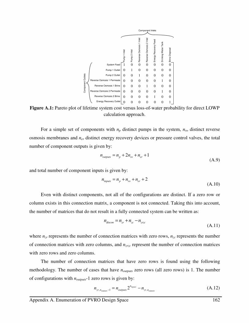
Appendix A. Enumeration of PVRO Design Space 162
Figure A.1: Pareto plot of lifetime system cost versus loss-of-water probability for direct LOWP
calculation approach.
For a simple set of components with np distinct pumps in the system, nro distinct reverse
osmosis membranes and ner distinct energy recovery devices or pressure control valves, the total
number of component outputs is given by:
2 1
outputs p ro ern n n n= + + +
(A.9)
and total number of component inputs is given by:
2
inputs p erron n n n= + + +
(A.10)
Even with distinct components, not all of the configurations are distinct. If a zero row or
column exists in this connection matrix, a component is not connected. Taking this into account,
the number of matrices that do not result in a fully connected system can be written as:
discon zr zc zrzc
n n n n= + − (A.11)
where nzr represents the number of connection matrices with zero rows, nzc represents the number
of connection matrices with zero columns, and nzrzc represent the number of connection matrices
with zero rows and zero columns.
The number of connection matrices that have zero rows is found using the following
methodology. The number of cases that have noutputs zero rows (all zero rows) is 1. The number
of configurations with noutputs-1 zero rows is given by:
, 1 ,2 inputs
outputs outputs
n
zr n outputs zr nn n n− −= (A.12)
1 0 0 0 0 0 0
0 1 0 0 0 0 0
0 0 1 0 0 0 0
0 0 0 0 0 1 0
0 0 0 1 0 0 0
0 0 0 0 0 1 0
0 0 0 0 1 0 0
0 0 0 0 0 0 1
Reverse Osmosis 1 Brine
Reverse Osmosis 1 Permeate
En
erg
yR
ecove
ryF
ee
d
System Feed
Pump 1 Outlet
Pu
mp
1In
let
Pu
mp
2In
let
Pump 2 Outlet
Reverse Osmosis 2 Brine
Reverse Osmosis 2 Permeate
Energy Recovery Outlet
Reve
rse
Osm
osis
1In
let
Reve
rse
Osm
osis
2In
let
Drin
kin
gW
ate
rT
ank
Brin
eD
ispo
sal
Co
mp
on
en
tO
utlets
Component Inlets

Appendix A. Enumeration of PVRO Design Space 163
Next, considering the number of configurations with noutputs-2 zero rows,
( )2
, 2 , 122 outputs inputs
outputs outputs
n noutputs
zr n zr n
outputs
nn n
n
−
− −
−
−= (A.13)
This trend continues and total number of connection matrices with zero rows is given by:
( ) ( )
1
1
2 1outputs
outputs inputs
nn i n ioutputs
zr
i
nn
i
− +
=
= −
∑ (A.14)
Similarly, the number of connection matrices that have zero columns is given by:
( ) ( )
1
1
2 1inputs
inputs outputs
nn i n iinputs
zc
i
nn
i
− +
=
= −
∑ (A.15)
The same methodology can be followed to determine the number of cases that contain a zero row
and zero column:
( )( ) ( )( )
1 1
2 1outputs inputs
outputs inputs
n nn i n j i joutputs inputs
zrzc
i j
n nn
i j
− − +
= =
= −
∑ ∑ (A.16)
Using equations (A.8)-(A.11) and equations (A.14)-(A.16), the total number of configurations
for a given selection of components when all components in the inventory are distinct can be
written as:
( )( ) ( )( )
( ) ( )
,
1 1
2 2
1
2 1
outputs inputs
outputs inputsinputs outputs
outputs inputs
config exact conmatrix discon
n nn i n j i jn n outputs inputs
i j
n i n ioutputs
n n n
n n
i j
n
i
− − +
= =
−
= −
= + −
+ − +
∑ ∑
( ) ( )2 1inputs outputsn j n jinputsn
j
− −
(A.17)
Taking into account the number of different ways to select the components, the total
number of configurations when all components are distinct is given by

Appendix A. Enumeration of PVRO Design Space 164
[
( ) ( )( )
( , , ) ( , , )
( ,
,
1 1
, ) ( , , )( , , ) ( , , )
1
1 1
2
(
2 1
, , ) ( , , )
p
out in
out in
ou
ro er
t in
N N Np ro er
config tota
n i j k n i j k
n i j k n i j kn i j k n i j k
l
i j k
lo mm
l
n
m
ut i
N N N
n i j k n i j k
ni j k
l m
= = =
+−
= =
=
+ −
∑∑∑
∑ ∑
( ) ( ) ( )( ) ( )( , , ) ( , , ) ( , , ) ( , , )( , , 2
) ( , )1 2 1
,out in in outn i j k n i j k n i j k n i j kout i mnll m l
l
n i j k n i j
m
k− − −
+ − + −
(A.18)
where Np is the total number of pumps in the inventory, Nro is the total number of reverse
osmosis membranes in the inventory, and Ner is the total number of energy recovery units or
pressure control valves in the inventory. The number of component outputs for configuration
(i,j,k) is given by:
( , , ) 2 1out
n i j k i j k= + + + (A.19)
and the number of component inputs for configuration (i,j,k) is given by:
( , , ) 2in
n i j k i j k= + + + (A.20)
A.2.2 Identical Reverse Osmosis Components
Determining the number of different configurations that can result from an inventory in
which all the pumps, reverse osmosis membranes, and energy recovery devices are the same
follows a similar methodology. The main difference here is that the order of the rows and
columns in the connection matrix associated with individual components does not matter, and
different connection matrices result in the same system configuration. As a result, the number of
configurations for a given selection of components becomes:
[ ( )( ) ( )( )
( ) ( )
,
1 1
1
2 2 1! ! !
2 1 2
outputs inputs
inputs outputs outputs inputs
outputs inputs inputs
n nn n n i n j i joutputs inputs
config exact
i j
n i n i noutputs inputs
p ro ern
n nn
i jn
n n
i j
n
− − +
= =
−
+ −
+ − +
=
∑ ∑
( ) ( )1outputsj n j−−
(A.21)
Using the sum rule, the total number of configurations that result when accounting for the
number of different ways to select components is:

Appendix A. Enumeration of PVRO Design Space 165
( )( ) ( )( )
( , , ) ( , , )
( , , ) ( , , )
,
( , , )
1 1 1
( , , )
1 1
12
! ! !
2 1
( , , )
( , ,
)
( , ,
p pv er
out in
out in
out in
n i j k n i j k
n i j k n i j kn i j k n i
N N N
config tot
j kout in
ou
al
i j k
l ml m
l m
t
n i j k n i j
ni j
k
k
l m
n i j
= = =
+− −
= =
=
+ −
+
∑∑∑
∑ ∑
( ) ( ) ( )( ) ( )( , , ) ( , , ) ( , , ) ( , , )2 1 2
) ( , ,1
)out in in outn i j k n i j k n i j k n i j kinl ml m lk n i j k
l m
− − − − + −
(A.22)
A.2.3 Full Reverse Osmosis Component Inventory
A realistic inventory for an RO system consists of different types of pumps, membranes
and energy recovery devices. The inventory will likely consist of more than one of each type of
component. This example is a combination of the cases presented above. For this case, the
number of system configurations for a given selection of components is given by:
( )( )
( )( ) ( )( )
,
, , ,1 1 1
1 1
2( !) ( !) ( !)
2 1
1 outputs inputs
p PV ER
outputs inputs
outputs inputs
n n
config exact N N N
p i ro i er ii i i
n nn l n m l moutputs inputs
l m
outputs
nn n n
n n
l m
n
l
= = =
− − +
= =
=
×
+ −
+
∏ ∏ ∏
∑ ∑
( )( ) ( ) ( )( ) ( )2 1 2 1outputs inputs outputs inputsn l n m l n l n m minputsn
m
− − − − − + −
(A.23)
where np,i is the number of pumps of type i, nro,i is the number of RO membranes of type i in the
configuration, ner,i is the number of energy recovery devices or pressure control valves of type i
in the configuration, Np is the total number of different types of pumps, Nro is the number of
different types of reverse osmosis membranes, and Ner is the number of different types of energy
recovery devices. The number of component outputs will be given by:
, , ,
1 1 1
2 1p ro er
N N N
outputs p i ro i er i
i i i
n n n n= = =
= + + +∑ ∑ ∑ (A.24)
and the total number of component inputs is given by:
, , ,
1 1 1
2p ro er
N N N
inputs p i ro i er i
i i i
n n n n= = =
= + + +∑ ∑ ∑ (A.25)

Appendix A. Enumeration of PVRO Design Space 166
Using the sum rule, the total number of system configurations for the mixed reverse osmosis
system component inventory is:
, ,,1 ,1 ,1
1 1 1,1 ,1 ,1
, , , ,, ,1 11
,
0 0 0, , ,1 1 1max(1 ,0) max(1 ,0)max(1
( !) ( !)
1
( !)
ro N er Np ro erro er
p PV ERN N Np ro er
p ro er
ro N ro i er N er ip N p i ro erpi ii
N NN N N
config total N N Nn n n
p i ro i er ii i in n n nn n
nn n n− − −
= ==
= = == = == − = −= − ∑
=
∑∑
∑ ∑∏
∑∏
∑ ∑∏
( )( ) ( )( ) ( )( )
( )( ) ( )
,
,0)
1 1
2 2 1
2 1 2
p N p
outputs inputs
outputs inputs outputs inputs
outputs inputs output
N
n nn n n l n m l moutputs inputs
l m
n l n m l noutputs inputs
n n
l m
n n
l m
− − +
= =
− −
× + −
+ − +
∑ ∑
∑
( )( ) ( )1s inputsl n m m− −
−
(A.26)
where Np,i is the total number of pumps of type i in the inventory, Nro,i is the total number of RO
membranes in the inventory of type i and Ner,i is the total number of energy recovery devices of
type i in the inventory. Using this relationship, the total number of distinct configurations can be
derived for any reverse osmosis component inventory.
A.3 Number of Possible Photovoltaic Power Systems
This section determines the number of possible configurations for a PV system. A PV
array consists of multiple PV panels in combinations of series and parallel connections. The
layout of the array will affect the voltage and current output. The overall power will not be
impacted as long as the modules connected in an individual sub array are matched in
power/current output and configured in a way that is compatible with the control electronics.
Since the configuration of panels does not impact the performance, the design choice for
the PV subsystem is the number of panels to include in the system. For an inventory containing
multiple types of PV panels, the number of configurations can be determined using the following
methodology. For a given number of panels, the number of distinct configurations is given
directly from the rules for combinations of multi-sets given in equation (A.6) as follows:
,
,
1 2 ,
, ,
1, ,1 ,2 ,
0 1
,
1( ; , , , ) ( 1)
1
pv type
j
pv type
p pv type
p
Npv type pv ip
jpv exact pv pv pv N
p i i i N
pv type
N r n pn C r n n n
N
=
= ≤ ≤ ≤ ≤ ≤
+ − − −
= = − −
∑∑ ∑
… (A.27)
where npv,j is the number of PV panels of type j in the inventory, Npv,type is the number of different
types of PV panels, and r is the number of PV panels selected for the configuration.
Fortunately, when considering the total number of panels in the inventory, the calculation
becomes much simpler. Since there are (npv,i + 1) ways to choose the number of PV panel type i

Appendix A. Enumeration of PVRO Design Space 167
to include in the system, the number of different PV system configurations can be written using
the product rule:
( ),
,
1
1 1pv typeN
PV pv i
i
N n=
= + −∏ (A.28)
Copyright © 2022 FDOKUMEN