VARIABLE ORDER NESTED HYBRID MULTISTEP ...
17
Available online at http://scik.org J. Math. Comput. Sci. 10 (2020), No. 1, 78-94 https://doi.org/10.28919/jmcs/4147 ISSN: 1927-5307 VARIABLE ORDER NESTED HYBRID MULTISTEP METHODS FOR STIFF ODES P. O. OLATUNJI 1,* , M. N. O. IKHILE 2 1 Department of Mathematical Sciences, Adekunle Ajasin University, Akungba Akoko, Ondo State, Nigeria 2 Advanced Research Laboratory, University of Benin, Benin City, Nigeria Copyright c 2020 the author(s). This is an open access article distributed under the Creative Commons Attribution License, which permits unrestricted use, distribution, and reproduction in any medium, provided the original work is properly cited. Abstract. A family of variable order nested hybrid multistep method for the numerical integration of stiff initial value problems of an ordinary differential equation is presented in this paper. These methods possess high order with A-stability properties making it suitable for solving stiff problems. The method has been implemented on some non-linear problems. Keywords: multistep method; nested hybrid; stiff problem; order; error; stability; variable step size. 2010 AMS Subject Classification: 65L05, 65L06. 1. I NTRODUCTION Multistep methods with off-step points, variously known as hybrid methods for the system of initial value problems (IVPs) for stiff ordinary differential equations (ODEs) of the form (1) y 0 (x)= f (x, y), x ∈ [x 0 , X ] y(x 0 )= y 0 * Corresponding author E-mail address: [email protected] Received May 30, 2019 78
-
Upload
khangminh22 -
Category
Documents
-
view
8 -
download
0
Transcript of VARIABLE ORDER NESTED HYBRID MULTISTEP ...
Available online at http://scik.org
J. Math. Comput. Sci. 10 (2020), No. 1, 78-94
https://doi.org/10.28919/jmcs/4147
ISSN: 1927-5307
VARIABLE ORDER NESTED HYBRID MULTISTEP METHODS FOR STIFF ODES
P. O. OLATUNJI1,∗, M. N. O. IKHILE2
1Department of Mathematical Sciences, Adekunle Ajasin University, Akungba Akoko, Ondo State, Nigeria
2Advanced Research Laboratory, University of Benin, Benin City, Nigeria
Copyright c© 2020 the author(s). This is an open access article distributed under the Creative Commons Attribution License, which permits
unrestricted use, distribution, and reproduction in any medium, provided the original work is properly cited.
Abstract. A family of variable order nested hybrid multistep method for the numerical integration of stiff initial
value problems of an ordinary differential equation is presented in this paper. These methods possess high order
with A-stability properties making it suitable for solving stiff problems. The method has been implemented on
some non-linear problems.
Keywords: multistep method; nested hybrid; stiff problem; order; error; stability; variable step size.
2010 AMS Subject Classification: 65L05, 65L06.
1. INTRODUCTION
Multistep methods with off-step points, variously known as hybrid methods for the system of
initial value problems (IVPs) for stiff ordinary differential equations (ODEs) of the form
(1)
y′(x) = f (x,y), x ∈ [x0,X ]
y(x0) = y0
∗Corresponding author
E-mail address: [email protected]
Received May 30, 201978
VONHMM FOR STIFF ODES 79
where f : Rn→Rn, were introduced by independent authors, some of which are [1, 2, 3]. These
hybrid methods were proposed in a bid to search for good numerical schemes for the numerical
solution of initial value problems (IVPs) in ODEs. Most ODEs arising from scientific modelling
exhibit a characteristics of high stability, which when solved by standard numerical methods,
instability sets in [4]. This kind of ODEs are called stiff ODEs. In solving stiff systems of
ODEs, the numerical method must have good accuracy and some reasonable wide region of
absolute stability [5], in which A-stable methods are very good choice. Hence, the need to de-
velop numerical methods with a wide region of absolute stability. However, this requirement of
A-stability puts a severe limitation on the choice of suitable multistep methods, which is fondly
known as the Dahlquist order barrier [6]. Hybrid methods are modified from the linear multi-
step methods by incorporating off-step points, this is done in an attempt to bypass the Dahlquist
order barrier that exist in the linear multistep methods.
In the quest of solving stiff ODEs, several authors have developed numerical methods that
circumvent the so called Dahlquist order barrier, som of which includes; the second derivative
multistep methods of [7], hybrid linear multistep method of [8, 9], high order numerical method
of [10], extended backward differentiation formulas of [11].
The paper presented is organized thus; in section 2 we discuss the derivation of the proposed
method, as well as give some examples of the method, section 3 considers the local truncation
error and order of the method proposed, we analyze the A-stability property of the proposed
method in section 4, in section 5, we implemented the schemes on some test problems and
compare with existing methods. The paper is concluded in section 6 with giving a brief sum-
mary.
Kulikov and Shindin [12, 13] considered nested implicit Runge-kutta formulas based on Gauss
quadrature formula. Here, we consider nested hybrid multistep methods.
80 P. O. OLATUNJI AND M. N. O. IKHILE
2. DERIVATION OF THE METHODS
The variable order nested hybrid multistep method (VONHM) considered in this paper for
the numerical integration of (1) is the second derivative hybrid multistep method defined as
(2) yn+k =k−1
∑j=0
α(m)j yn+ j +h
(γ(m)k fn+k +β
(m)vm fn+vm
)+h2
Ω(m)k f ′n+k
where xn+ j = xn + jh (h being the step size), k the step number (k ∈ Z+), m = k− 1 and the
hybrid value vm is chosen as
vm = k− 12
In addition to (2), the hybrid point yn+vm is computed from the nested hybrid
yn+vl+1 = yn+k +h
(k
∑j=0
β(l)j fn+ j +β
(l)vl fn+vl
)l = 0(1)m−1(3)
The hybrid method (3) is nested in that we have k number of hybrid point, that is, from (3) we
have the set of hybrid points
yn+vl+1,yn+vl ,yn+vl−1,yn+vl−2, · · · ,yn+v2,yn+v1,yn+v0
where yn+v0 is the nested hybrid predictor. The hybrid value vl; l = 0(1)m− 1 is computed
using
(4) vl =vl+1 + k
2, l = 0(1)m−1
Two cases of hybrid predictors are considered, given as
(5) yn+v0 =
yn+k +h∑
kj=0 β
(−1)j fn+ j V1
yn+k +h∑kj=0 β
(−1)j fn+ j +h2λ
−1k f ′n+k V2
yn+k in (2) is the numerical approximation (output solution) to the exact solution y(xn+k). Two
cases of VONHM are considered above in which the first being the combination of (2), (3) and
V1, while the second is the combination of (2), (3) and V2. The implicitness of the VONHM is
on the output method (2)
VONHMM FOR STIFF ODES 81
We derive the schemes based on the assumption of the polynomial interpolant
(6) y(x) =N
∑j=0
a jx j
where
a jN
j=0 are real parameter constants to be determined, differentiating (6), we have
(7) f (x,y) = y′(x) =N
∑j=0
ja jx j−1 and f ′(x,y) = y′′(x) =N
∑j=0
j( j−1)a jx j−2
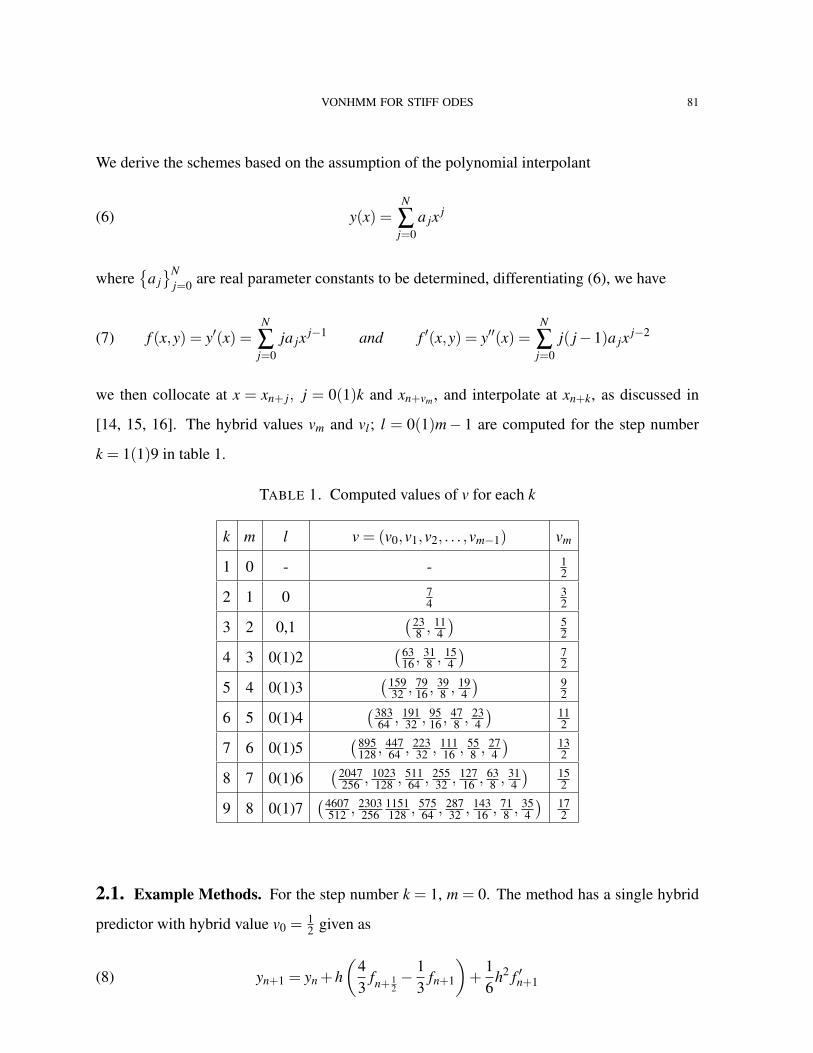
we then collocate at x = xn+ j, j = 0(1)k and xn+vm , and interpolate at xn+k, as discussed in
[14, 15, 16]. The hybrid values vm and vl; l = 0(1)m− 1 are computed for the step number
k = 1(1)9 in table 1.
TABLE 1. Computed values of v for each k
k m l v = (v0,v1,v2, . . . ,vm−1) vm
1 0 - - 12
2 1 0 74
32
3 2 0,1(23
8 ,114
) 52
4 3 0(1)2(63
16 ,318 ,
154
) 72
5 4 0(1)3(159
32 ,7916 ,
398 ,
194
) 92
6 5 0(1)4(383
64 ,19132 ,
9516 ,
478 ,
234
) 112
7 6 0(1)5(895
128 ,44764 ,
22332 ,
11116 ,
558 ,
274
) 132
8 7 0(1)6(2047
256 ,1023128 ,
51164 ,
25532 ,
12716 ,
638 ,
314
) 152
9 8 0(1)7(4607
512 ,2303256
1151128 ,
57564 ,
28732 ,
14316 ,
718 ,
354
) 172
2.1. Example Methods. For the step number k = 1, m = 0. The method has a single hybrid
predictor with hybrid value v0 =12 given as
(8) yn+1 = yn +h(
43
fn+ 12− 1
3fn+1
)+
16
h2 f ′n+1
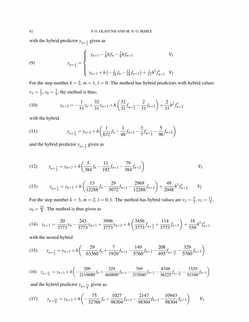
82 P. O. OLATUNJI AND M. N. O. IKHILE
with the hybrid predictor yn+ 12
given as
(9) yn+ 12=
yn+1− 1
8h fn− 38h fn+1 V1
yn+1 +h(− 1
24 fn− 1124 fn+1
)+ 1
12h2 f ′n+1 V2
For the step number k = 2, m = 1, l = 0. The method has hybrid predictors with hybrid values
v1 =32 , v0 =
74 , the method is thus;
(10) yn+2 =−1
31yn +
3231
yn+1 +h(
3231
fn+ 32− 2
31fn+2
)+
231
h2 f ′n+2
with the hybrid
(11) yn+ 32= yn+2 +h
(1
672fn−
148
fn+1−37
fn+ 74− 5
96fn+2
)and the hybrid predictor yn+ 7
4given as
(12) yn+ 74= yn+2 +h
(5
384fn−
11192
fn+1−79
384fn+2
)V1
(13) yn+ 74= yn+2 +h
(13
12288fn−
293072
fn+1−296912288
fn+2
)+
492048
h2 f ′n+2 V2
For the step number k = 3, m = 2, l = 0,1. The method has hybrid values are v2 =52 , v1 =
114 ,
v0 =238 . The method is thus given as
(14) yn+3 =20
3773yn−
2433773
yn+1 +39963773
yn+2 + h(
34563773
fn+ 52+
1143773
fn+3
)+
18539
h2 f ′n+3
with the nested hybrid
(15) yn+ 52= yn+3 +h
(− 29
63360fn +
71920
fn+1−1495760
fn+2−208495
fn+ 114− 329
5760fn+3
)
(16) yn+ 114= yn+3 + h
(− 209
2119680fn +
329460800
fn+1 −769
215040fn+2 −
834836225
fn+ 238− 1529
92160fn+3
)and the hybrid predictor yn+ 23
8given as
(17) yn+ 238= yn+3 +h
(− 75
32768fn +
102798304
fn+1−2147
98304fn+2−
1094398304
fn+3
)V1
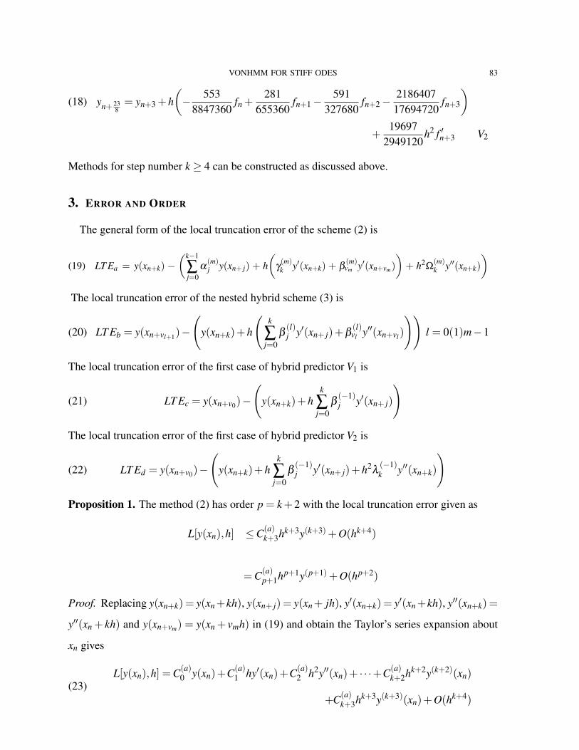
VONHMM FOR STIFF ODES 83
(18) yn+ 238= yn+3 +h
(− 553
8847360fn +
281655360
fn+1−591
327680fn+2−
218640717694720
fn+3
)+
196972949120
h2 f ′n+3 V2
Methods for step number k ≥ 4 can be constructed as discussed above.
3. ERROR AND ORDER
The general form of the local truncation error of the scheme (2) is
(19) LT Ea = y(xn+k) −(k−1
∑j=0
α(m)j y(xn+ j) + h
(γ(m)k y′(xn+k) + β
(m)vm y′(xn+vm)
)+ h2
Ω(m)k y′′(xn+k)
)The local truncation error of the nested hybrid scheme (3) is
(20) LT Eb = y(xn+vl+1)−
(y(xn+k)+h
(k
∑j=0
β(l)j y′(xn+ j)+β
(l)vl y′′(xn+vl)
))l = 0(1)m−1
The local truncation error of the first case of hybrid predictor V1 is
(21) LT Ec = y(xn+v0)−
(y(xn+k)+h
k
∑j=0
β(−1)j y′(xn+ j)
)
The local truncation error of the first case of hybrid predictor V2 is
(22) LT Ed = y(xn+v0)−
(y(xn+k)+h
k
∑j=0
β(−1)j y′(xn+ j)+h2
λ(−1)k y′′(xn+k)
)
Proposition 1. The method (2) has order p = k+2 with the local truncation error given as
L[y(xn),h] ≤C(a)k+3hk+3y(k+3)+O(hk+4)
=C(a)p+1hp+1y(p+1)+O(hp+2)
Proof. Replacing y(xn+k) = y(xn+kh), y(xn+ j) = y(xn+ jh), y′(xn+k) = y′(xn+kh), y′′(xn+k) =
y′′(xn + kh) and y(xn+vm) = y(xn + vmh) in (19) and obtain the Taylor’s series expansion about
xn gives
L[y(xn),h] =C(a)0 y(xn)+C(a)
1 hy′(xn)+C(a)2 h2y′′(xn)+ · · ·+C(a)
k+2hk+2y(k+2)(xn)
+C(a)k+3hk+3y(k+3)(xn)+O(hk+4)
(23)
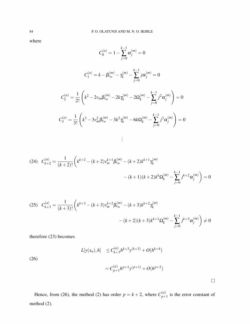
84 P. O. OLATUNJI AND M. N. O. IKHILE
where
C(a)0 = 1−
k−1
∑j=0
α(m)j = 0
C(a)1 = k−β
(m)vm − γ
(m)k −
k−1
∑j=0
jα(m)j = 0
C(a)2 =
12!
(k2−2vmβ
(m)vm −2kγ
(m)k −2Ω
(m)k −
k−1
∑j=0
j2α(m)j
)= 0
C(a)3 =
13!
(k3−3v2
mβ(m)vm −3k2
γ(m)k −6kΩ
(m)k −
k−1
∑j=0
j3α(m)j
)= 0
...
(24) C(a)k+2 =
1(k+2)!
(kk+2− (k+2)vk+1
m β(m)vm − (k+2)kk+1
γ(m)k
− (k+1)(k+2)kkΩ
(m)k −
k−1
∑j=0
jk+2α(m)j
)= 0
(25) C(a)k+3 =
1(k+3)!
(kk+3− (k+3)vk+2
m β(m)vm − (k+3)kk+2
γ(m)k
− (k+2)(k+3)kk+1Ω
(m)k −
k−1
∑j=0
jk+3α(m)j
)6= 0
therefore (23) becomes
(26)
L[y(xn),h] ≤C(a)k+3hk+3y(k+3)+O(hk+4)
=C(a)p+1hp+1y(p+1)+O(hp+2)
Hence, from (26), the method (2) has order p = k+ 2, where C(a)p+1 is the error constant of
method (2).
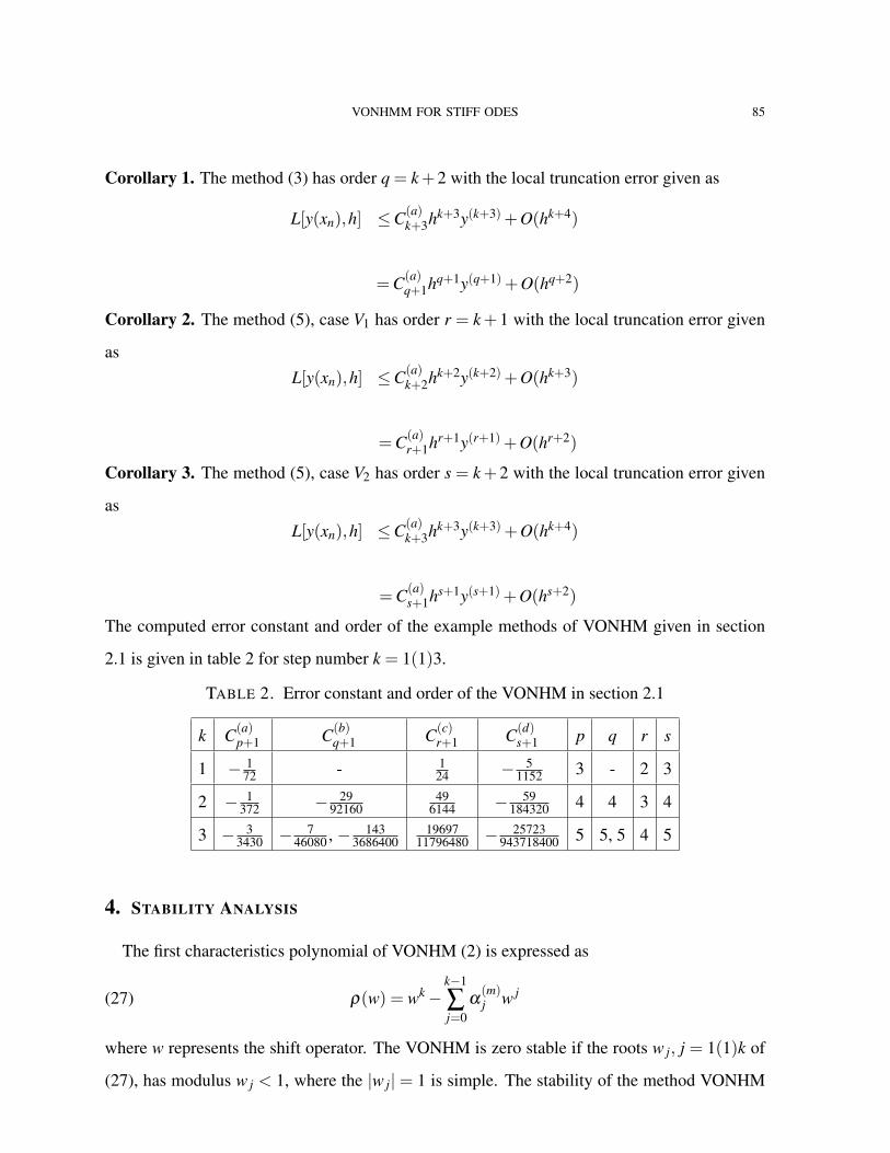
VONHMM FOR STIFF ODES 85
Corollary 1. The method (3) has order q = k+2 with the local truncation error given as
L[y(xn),h] ≤C(a)k+3hk+3y(k+3)+O(hk+4)
=C(a)q+1hq+1y(q+1)+O(hq+2)
Corollary 2. The method (5), case V1 has order r = k+1 with the local truncation error given
asL[y(xn),h] ≤C(a)
k+2hk+2y(k+2)+O(hk+3)
=C(a)r+1hr+1y(r+1)+O(hr+2)
Corollary 3. The method (5), case V2 has order s = k+2 with the local truncation error given
asL[y(xn),h] ≤C(a)
k+3hk+3y(k+3)+O(hk+4)
=C(a)s+1hs+1y(s+1)+O(hs+2)
The computed error constant and order of the example methods of VONHM given in section
2.1 is given in table 2 for step number k = 1(1)3.
TABLE 2. Error constant and order of the VONHM in section 2.1
k C(a)p+1 C(b)
q+1 C(c)r+1 C(d)
s+1 p q r s
1 − 172 - 1
24 − 51152 3 - 2 3
2 − 1372 − 29
9216049
6144 − 59184320 4 4 3 4
3 − 33430 − 7
46080 , − 1433686400
1969711796480 − 25723
943718400 5 5, 5 4 5
4. STABILITY ANALYSIS
The first characteristics polynomial of VONHM (2) is expressed as
(27) ρ(w) = wk−k−1
∑j=0
α(m)j w j
where w represents the shift operator. The VONHM is zero stable if the roots w j, j = 1(1)k of
(27), has modulus w j < 1, where the |w j| = 1 is simple. The stability of the method VONHM
86 P. O. OLATUNJI AND M. N. O. IKHILE
for the cases V1 and V2 is investigated through the application to the scalar test problem defined
as
(28) y′(x) = λy(x) x≥ 0, Re(λ )< 0
which yields
(29) π(w,z)iyn = 0, i = 1,2
Theorem 1. The resultant stability polynomial of the VONHM for the case V1 is
(30) π(w,z)1 = wk−k−1
∑j=0
α(m)j w j− z
[γ(m)k wk +β
(m)vm (R(w,z)1)
]− z2
Ω(m)k wk
where
(31) R(w,z)1 = wk+zk
∑j=0
β(m−1)j w j+β
(m−1)vm−1
(· · ·(
wk+z( k
∑j=0
β(1)j +β
(0)v0
(wk+z
k
∑j=0
β(−1)j w j
))))
Proof. Taking the right hand side (R.H.S) of (2) to the left hand side (L.H.S) and equating to
zero yields
(32) yn+k−k−1
∑j=0
α(m)j yn+ j−h
(γ(m)k fn+k +β
(m)vm fn+vm
)−h2
Ω(m)k f ′n+k = 0
applying the scalar test problem (28) on (32) and taking z = λh, yields
(33) wk−k−1
∑j=0
α(m)j w j− z
(γ(m)k wk +β
(m)vm yn+vm
)− z2
Ω(m)k wk = 0
where w is used as the shift operator, the stability polynomial is given as defined in (30). How-
ever, we need to prove that yn+vm = R(w,z)1 as given in (31), this is obtained by applying the
scalar test problem on (3) and (5). The scheme (3) is expanded as follows;
when l = 0
(34) yn+v1 = yn+k +h
(k
∑j=0
β(0)j fn+ j +β
(0)v0 fn+v0
)when l = 1
(35) yn+v2 = yn+k +h
(k
∑j=0
β(1)j fn+ j +β
(1)v1 fn+v1
)
VONHMM FOR STIFF ODES 87
the process continues till l = m−1
(36) yn+vm = yn+k +h
(k
∑j=0
β(m−1)j fn+ j +β
(m−1)vm−1 fn+vm−1
)Recall from (5) case V1 that
(37) yn+v0 = yn+k +hk
∑j=0
β(−1)j fn+ j
applying the scalar test problem (28) on the R.H.S of (34) to (37), using the shift operator and
taking z = λh, we have
(38) yn+v1 = wkyn + z
(k
∑j=0
β(0)j w jyn +β
(0)v0 yn+v0
)when l = 1
(39) yn+v2 = wkyn + z
(k
∑j=0
β(1)j w jyn +β
(1)v1 yn+v1
)this process continues till
(40) yn+vm = wkyn + z
(k
∑j=0
β(m−1)j w jyn +β
(m−1)vm−1 yn+vm−1
)and
(41) yn+v0 = wkyn + zk
∑j=0
β(−1)j w jyn
from above, the R.H.S of (41) is replaced with yn+v0 in (38) and the result of this R.H.S of (38)
is replaced with yn+v1 in (39), this process continues recursively. Hence, we obtain
(42)
yn+vm =R(w,z)1 =wk+zk
∑j=0
β(m−1)j w j+β
(m−1)vm−1
(· · ·(
wk+z( k
∑j=0
β(1)j +β
(0)v0
(wk+z
k
∑j=0
β(−1)j w j
))))the · · · denotes some recursive terms obtained between 2 ≤ l ≤ m− 2 after the application of
the scalar test problem. Hence, the result of the stability polynomial given in (30) and (31).
Theorem 2. The resultant stability polynomial of the case V2 is
(43) π(w,z)2 = wk−k−1
∑j=0
α(m)j w j− z
[γ(m)k wk +β
(m)vm (R(w,z)2)
]− z2
Ω(m)k wk
88 P. O. OLATUNJI AND M. N. O. IKHILE
where
(44) R(w,z)2 = wk + zk
∑j=0
β(m−1)j w j +β
(m−1)vm−1
(· · ·(
wk + z( k
∑j=0
β(1)j w j
+β(0)v0
(wk + z
k
∑j=0
β(−1)j w j + z2
λ(−1)k wk
))))Definition 1. The region of absolute stability of the VONHM is the set
Ψ =
z ∈C : |w j| ≤ 1, j = 1(1)k
i.e. if the root of w j, j = 0(1)k of (30) and (43) are less or equal to one in absolute value, such
that those of magnitude one are not repeated.
Definition 2. The VONHM is Astable if the region of absolute stability lies in the entire left
half of the zplane (i.e.z ∈C−).
Definition 3. The VONHM is A(α)-stable for some α ∈[0, π
2
)if the wedge
Sα = z : |Arg(−z)|< α,z 6= 0
is contained in its region of absolute stability.
The VONHM is Astable for the step number k = 1(1)5 and k = 2(1)5 for the cases V1 and
V2 respectively. However as at the time this research was carried out, the point at which insta-
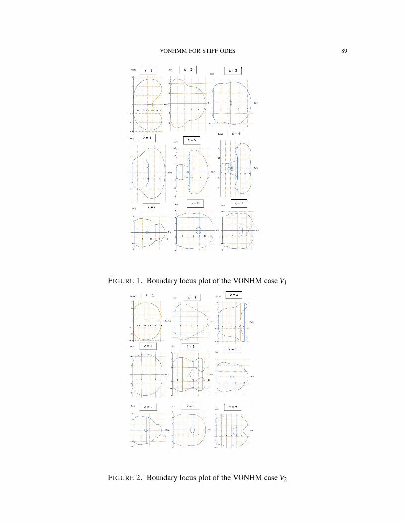
bility sets in, was not investigated. The boundary locus plot of the VONHM, cases V1 and V2
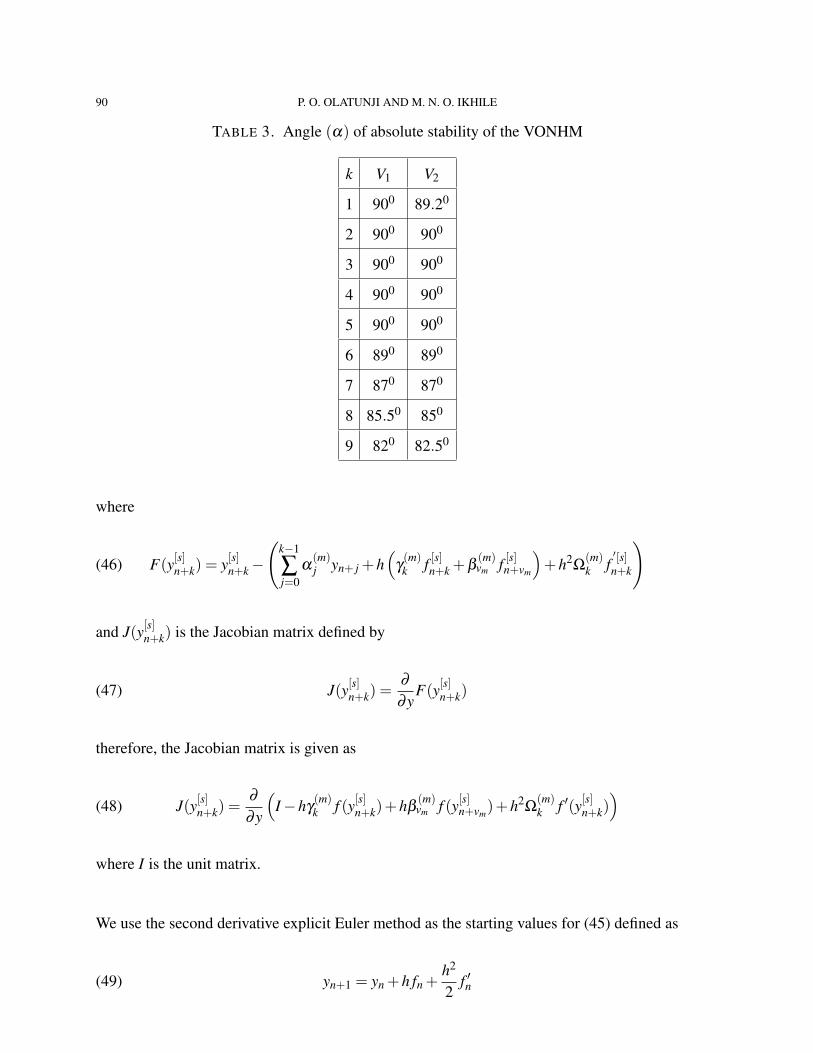
for the step number k = 1(1)9 are shown figures 1 ans 2. Table 3 shows the angle of absolute
stability of the VONHM, where those of 900 indicate A stable methods.
5. NUMERICAL EXPERIMENTS
We implement the third order VONHM (2) on some non-linear stiff problems using fixed step
size and variable step size. Implementing the method leads to solving a system of non-linear
equations in yn+k. Hence, the need to resolve its implicitness by the Newton-Raphson scheme
(45) y[s+1]n+k = y[s]n+k− J(y[s]n+k)
−1F(y[s]n+k)
VONHMM FOR STIFF ODES 89
FIGURE 1. Boundary locus plot of the VONHM case V1
FIGURE 2. Boundary locus plot of the VONHM case V2
90 P. O. OLATUNJI AND M. N. O. IKHILE
TABLE 3. Angle (α) of absolute stability of the VONHM
k V1 V2
1 900 89.20
2 900 900
3 900 900
4 900 900
5 900 900
6 890 890
7 870 870
8 85.50 850
9 820 82.50
where
(46) F(y[s]n+k) = y[s]n+k−
(k−1
∑j=0
α(m)j yn+ j +h
(γ(m)k f [s]n+k +β
(m)vm f [s]n+vm
)+h2
Ω(m)k f
′[s]n+k
)
and J(y[s]n+k) is the Jacobian matrix defined by
(47) J(y[s]n+k) =∂
∂yF(y[s]n+k)
therefore, the Jacobian matrix is given as
(48) J(y[s]n+k) =∂
∂y
(I−hγ
(m)k f (y[s]n+k)+hβ
(m)vm f (y[s]n+vm
)+h2Ω
(m)k f ′(y[s]n+k)
)
where I is the unit matrix.
We use the second derivative explicit Euler method as the starting values for (45) defined as
(49) yn+1 = yn +h fn +h2
2f ′n
VONHMM FOR STIFF ODES 91
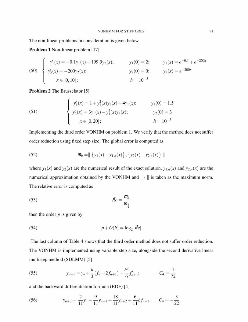
The non-linear problems in consideration is given below.
Problem 1 Non-linear problem [17].
(50)
y′1(x) =−0.1y1(x)−199.9y2(x); y1(0) = 2; y1(x) = e−0.1 + e−200x
y′2(x) =−200y2(x); y2(0) = 0; y2(x) = e−200x
x ∈ [0,10] ; h = 10−3
Problem 2 The Brusselator [5].
(51)
y′1(x) = 1+ y2
1(x)y2(x)−4y1(x); y1(0) = 1.5
y′2(x) = 3y1(x)− y21(x)y2(x); y2(0) = 3
x ∈ [0,20] ; h = 10−3
Implementing the third order VONHM on problem 1. We verify that the method does not suffer
order reduction using fixed step size. The global error is computed as
(52) ϖh =‖
y1(x)− y1,n(x),
y2(x)− y2,n(x)‖
where y1(x) and y2(x) are the numerical result of the exact solution, y1,n(x) and y2,n(x) are the
numerical approximation obtained by the VONHM and ‖ · ‖ is taken as the maximum norm.
The relative error is computed as
(53) Re =ϖh
ϖ h2
then the order p is given by
(54) p+O(h) = log2 |Re|
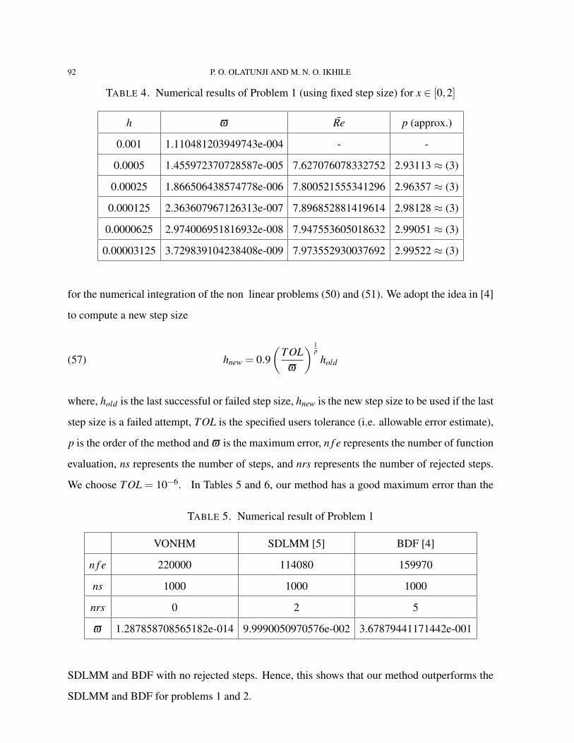
The last column of Table 4 shows that the third order method does not suffer order reduction.
The VONHM is implemented using variable step size, alongside the second derivative linear
multistep method (SDLMM) [5]
(55) yn+1 = yn +h3( fn +2 fn+1)−
h2
6f ′n+1; C4 =
172
and the backward differentiation formula (BDF) [4]
(56) yn+3 =2
11yn−
911
yn+1 +1811
yn+2 +6
11h fn+3 C4 =−
322
92 P. O. OLATUNJI AND M. N. O. IKHILE
TABLE 4. Numerical results of Problem 1 (using fixed step size) for x ∈ [0,2]
h ϖ Re p (approx.)
0.001 1.110481203949743e-004 - -
0.0005 1.455972370728587e-005 7.627076078332752 2.93113 ≈ (3)
0.00025 1.866506438574778e-006 7.800521555341296 2.96357 ≈ (3)
0.000125 2.363607967126313e-007 7.896852881419614 2.98128 ≈ (3)
0.0000625 2.974006951816932e-008 7.947553605018632 2.99051 ≈ (3)
0.00003125 3.729839104238408e-009 7.973552930037692 2.99522 ≈ (3)
for the numerical integration of the non linear problems (50) and (51). We adopt the idea in [4]
to compute a new step size
(57) hnew = 0.9(
TOLϖ
) 1p
hold
where, hold is the last successful or failed step size, hnew is the new step size to be used if the last
step size is a failed attempt, TOL is the specified users tolerance (i.e. allowable error estimate),
p is the order of the method and ϖ is the maximum error, n f e represents the number of function
evaluation, ns represents the number of steps, and nrs represents the number of rejected steps.
We choose TOL = 10−6. In Tables 5 and 6, our method has a good maximum error than the
TABLE 5. Numerical result of Problem 1
VONHM SDLMM [5] BDF [4]
n f e 220000 114080 159970
ns 1000 1000 1000
nrs 0 2 5
ϖ 1.287858708565182e-014 9.9990050970576e-002 3.67879441171442e-001
SDLMM and BDF with no rejected steps. Hence, this shows that our method outperforms the
SDLMM and BDF for problems 1 and 2.

VONHMM FOR STIFF ODES 93
TABLE 6. Numerical result of Problem 2
VONHM SDLMM [5] BDF [4]
n f e 440000 239978 288320
ns 20000 20000 2000
nrs 0 11 198
ϖ 3.159554022663061e-010 1.005387230111084e-006 8.20707935075017e-001
6. CONCLUSION
Second derivative variable order nested hybrid multistep method for the numerical integra-
tion of stiff initial value problems of ordinary differential equation is presented. The method
presented possess high order with A-stability properties for the step number k = 1(1)5. The
method is also implemented using fixed and variable step size. The fixed step size implemen-
tation on the non-linear problem 1 suggest that the method did not suffer from order reduction,
while the variable step size implementation of our method shows that the scheme presented
outperforms the SDLMM and BDF.
CONFLICT OF INTERESTS
The author(s) declare that there is no conflict of interests.
REFERENCES
[1] W. B. Gragg and H.J. Stetter, Generalized multistep predictor-corrector methods, J. Assoc. Comput. Mach.
11 (2) (1964), 188-209.
[2] C. W. Gear, Hybrid methods for initial value problems in ordinary differential equations, SIAM. J. Numer.
Anal. 2 (1965), 69-86.
[3] J. C. Butcher and A. E. OSullivan, Nordsieck methods with an off-step point, Numer. Algorithms, 31 (2002),
87 - 101.
[4] J.C. Butcher, Numerical methods for ordinary differential equivalent, John Willey & Sons, Ltd Chichester,
2016.
[5] W. H. Enright, Second derivative multistep method for stiff ordinary differential equations, SIAM J. Numer.
Anal. 11 (2) (1974), 321-331.
94 P. O. OLATUNJI AND M. N. O. IKHILE
[6] G. Dahlquist, A special stability problem for Linear Multistep Methods, Academic Press, New York, 1963.
[7] E. Hairer, and G. Wanner, Solving ordinary differential equations II. Stiff and Differential - Algebraic prob-
lems Vol. II, Springer-Verlag, 2010.
[8] R. I. Okuonghae and M. N. O. Ikhile, On the construction of high order A(α)-stable hybrid linear multistep
methods for stiff IVPs and ODEs, J. Numer. Anal. Appl. 15(3) (2012), 231-241.
[9] R. I. Okuonghae and M. N. O. Ikhile, A class of hybrid linear multistep methods with A(α)-stability proper-
ties for stiff IVPs in ODEs, J. Numer. Math. 21 (2) (2013), 157-172.
[10] J. C. Butcher, High order A-stable numerical methods for stiff problems, J. Sci. Comput. 25 (2005), 51-66.
[11] J.R. Cash, Second derivative extended backward differential formulas for the numerical integration of stiff
systems, SIAM J. Numer. Anal. 18 (1981), 21-36.
[12] G. Yu Kulikov and S. K. Shindin, Numerical Tests with Gauss-Type Nested Implicit Runge-Kutta Formulas,
International Conference on Computational Science. Springer, Berlin, Heidelberg, 2007, 136-143.
[13] G. Yu Kulikov and S. K. Shindin, Adaptive nested IRK formulas of Gauss Type, J. Appl. Numer. Math. 59
(2009), 707-722.
[14] P. O. Olatunji, Second Derivative Multistep methods with Nested Hybrid Evaluation, M.Sc. Thesis, 2017.
[15] P. O. Olatunji, and M. N. O. Ikhile, Modified Backward Differentiation Formulas with Recursively Nested
Hybrid Evaluation; J. Nigerian Assoc. Math. Phys. 40 (2017), 83-90.
[16] P. O. Olatunji, and M. N. O. Ikhile, Second Derivative Multistep Method with Nested Hybrid Evaluation;
Asian Res. J. Math. 11 (4) (2018), 1-11.
[17] S. O. Fatunla, Numerical Methods for Initial Value Problems in Ordinary Differential equations; Academic
Press Inc. New York, 1988.