Rocking and rolling down an incline: the dynamicsof nested cylinders on a ramp

by

David Paul Vener

B.S. Applied Mathematics, Georgia Institute of Technology, 2001B.S. Physics, Georgia Institute of Technology, 2001

Submitted to the Department of Mathematicsin partial fulfillment of the requirements for the degree of

DOCTOR OF PHILOSOPHY

at the

MASSACHUSETTS INSTITUTE OF TECHNOLOGY

June 2006

®David Paul Vener, 2006. All Rights Reserved.

The author hereby grants to MIT permission to reproduce anddistribute publicly paper and electronic copies of this thesis document

in whole or in part.

Author.r o z A u th or .................................. ................

Department of MathematicsMav 12. 2006

Certified by........................

Accepted by.......................

..- - . . . . . . I h/3zJu W. M. Bush/,.-~ Associate P fessor-5 upervisor

-V .U.................Rodolfo Ruben Rosales

Chairman, Applied Mathematics Committee/

Accepted by.................................) Pavel I. E 4nof

Chairman, Department Committee on Graduate Students

ARCHIVES

MASSACHUSETTS INSUREOF TECHNOLOGY

JUN 0 5 2006

L ,,i .9 ES

Rocking and rolling down an incline: the dynamics of nested

cylinders on a ramp

by

David Paul Vener

Submitted to the Department of Mathematicson May 12, 2006, in partial fulfillment of the

requirements for the degree ofDOCTOR OF PHILOSOPHY

AbstractIn this thesis, I report the results of a combined experimental and theoretical investi-gation of a journal bearing, specifically, a cylinder suspended in a viscous fluid housedwithin a cylindrical shell, rolling down an incline under the influence of gravity. Par-ticular attention is given to rationalizing the distinct modes of motion observed. Weperformed a series of experiments in which the inner cylinder density and the fluidviscosity were varied. Three distinct types of behavior were observed. First, in whatwe shall call the "rocking" mode, after an initial settling period, the shell rocks backand forth without moving down the ramp. Second, we observed "slow, quasi-steadyrolling"; this mode is characterized by the system proceeding down the hill at essen-tially a constant velocity. Finally, the cylinders roll down the incline with constantacceleration; we shall call this mode "unbounded acceleration." An accompanyingtheoretical model is developed and enables us to rationalize the rocking and acceler-ating modes. In the rocking solutions, potential and kinetic energy are dissipated inthe fluid as the inner cylinder approaches the bottom of the outer cylinder. In theaccelerating solutions, the whole system moves as a solid body so that no dissipationoccurs and potential energy is continually converted into kinetic energy. In order tounderstand the quasi-steady motion, we analyze the motion of a similar system: ametal cylinder is placed inside a larger plastic cylinder filled with fluid and attachedto a motor which fixes the larger cylinder's rotation rate. Our observations of thissystem, specifically, the differences betweeen experiments and theory lead us to con-sider the effect of internal friction due to surface roughness. The resulting model'spredictions are well supported by our observations. Finally, to rationalize the slow,quasi-steady rolling motion of the system, we incorporate surface roughness and cav-itation into the theoretical model. These effects provide a restoring force on the innercylinder; however, we find that surface roughness is the dominant effect.

Thesis Supervisor: John W. M. BushTitle: Associate Professor

3

4

Acknowledgments

I'd like to take this opportunity to thank some of the many people whose academic

and personal efforts have made writing this thesis possible.

On the academic side, I'd first like to thank Neil Balmforth whose ideas were my

main guide through the problem. Bill Young was invaluable in getting past several

mathematical hurdles that appeared along the way. My advisor, John Bush, first

conceived of the problem, and his guidance made this thesis both more readable and

more understandable. Finally, the other members of my thesis committee, Ruben

Rosales, Peko Hosoi, and Darren Crowdy, also provided great suggestions which I

have done my best to incorporate into this final version.

Since a doctoral thesis is such a large project, one's personal life invariably becomes

involved in its completion. Without Ellen Weinstein's support I could not have gotten

through the last year of this process. Nicole Simi also provided a great deal of

valuable guidance over the past three years. I'd also like to mention Bobak Ferdowsi,

Kim Clarke, Heidi Davidz, and Christine Taylor who made Cambridge a fun place for

several years. Finally, I'd like to thank Wes Gifford, Jaehyuk Choi, Eugene Weinstein,

and Parag Vaidya for making my living space livable.

5

6

Contents

1 Introduction

2 Initial observations

2.1 The snail cylinder ...............

2.1.1 Laboratory set-up ..........

2.1.2 Observations ............

2.2 Experiments with the fixed outer cylinder .

2.2.1 Laboratory set-up ..........

2.2.2 Observations .............

2.3 Bubbles ....................

3 Formulation of the rolling problem

3.1 Geometry ..................

3.2 Dynamical equations for the cylinder centers

3.2.1 Motion of the inner center relative to

equation ...............3.2.2 Rotational equations of motion . . .

3.3 Hydrodynamic forces and torques ......

3.3.1 Lubrication analysis ........

3.3.2 The rotational flow, uR(z, 0) .....

3.3.3 The squeeze flow, uS(z,) ......

3.3.4 Calculating forces and torques ....

3.4 Closing the equations of motion .......

23

........ .. 23

........ .. 23. . . . . . . . 25

........ .. 26

........ .. 26

........ .. 27

. . . . . . . . 29

31

31

33t o c t.. . . . . . . . .. h

the outer center: the e

. . . ... . . 35

. . . ... . . 36

. . . ... . . 36

. . . . . . 37

. . . ... . . 38

. . . ... . . 39

. . . ... . . 39

. . . ... . . 41

7

19

3.5

3.6

3.7

3.4.1 Understanding (3.44) in terms of tota

A steady solution ...............

A quasi-steady solution ............

Energetics ..................

4 A reduced lubrication model

4.1 Reduction of the dynamics .........

4.2 An useful recasting of the reduced system

4.3 The sedimenting solution with s = 0 . . .

4.4 Solutions with s 0 ............

4.4.1 The Sommerfeld equilibrium ....

4.4.2 Other solutions ..........

4.4.3 Numerical solutions ........

4.5 Shortcomings of the model .........

1 angular momentum . . 41

. . . . . . . . . . . . . . 43

. . . . . . . . . . . . . . 44

. . . . . . . . . . . . . . 45

49

. . . . . . . . . . . . . . 49

. ... . ... .. . .. . . ....51

. . . . . . . . . . . . . . 51

. . . . . . . . . . . . . . 52

. . . . . . . . . . . . . . 52

. . . . . . . . . . . . . . 53

. . . . . . . . . . . . . . 54

. . . . . . . . . . . . . . 56

5 Theoretical formulation of the stationary mixer problem

5.1 Geometry ................................

5.2 Dynamic equations for the inner cylinder center ............

6 Dimensionless formulation of the fixed outer cylinder system

6.1 Determining the dimensionless system .................

6.2 The journal bearing ............................

6.3 The fixed outer cylinder .........................

6.3.1 Adding a sliding contact .....................

6.4 Summary .................................

7 Experiments

7.1 Comparison of simulation and experiment with the fixed outer cylinder

7.2 Additional experiments with the snail cylinders ............

8 Rough contact and cavitation in the rolling system

8.1 Cavitation ................................

8

59

59

61

65

65

67

69

73

76

77

77

82

87

87

8.2 Rough contact . . . . . . . . . . . . . . . . . . . . . . . . . . . . . . . 91

9 Conclusions 97

A Dimensionless groups and physical quantities 101

B The Calculations of Finn and Cox[8] 103

B.1 Rotlets and Stokeslets .......................... 103

B.2 Forces and torques from the stream function ............. . 106

9

10

List of Figures

2-1 Photographs showing various views of the snail cylinder. In order of ap-

pearance, the views are (a) angled from the front, (b) angled from behind,

(c) face on from the front, and (d) edge on. Note that several small bubbles

are trapped inside and have risen to the top of the fluid, and that the inner

cylinder lies along the base of the outer cylinder ................... . 24

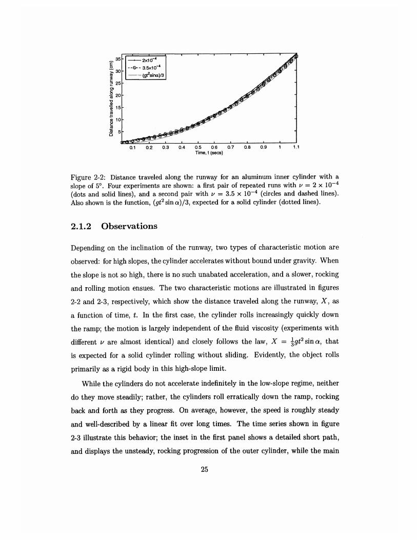
2-2 Distance traveled along the runway for an aluminum inner cylinder with a

slope of 5° . Four experiments are shown: a first pair of repeated runs with

v = 2 x 10- 4 (dots and solid lines), and a second pair with v = 3.5 x 10

- 4

(circles and dashed lines). Also shown is the function, (gt2 sin a)/3, expected

for a solid cylinder (dotted lines) ............................... . 25

2-3 Distance traveled along the runway for a steel inner cylinder with various

slopes. Panel (a) shows a long run at 2.4°; the inset shows a magnification

of the path. Panel (b) shows four different slopes, as marked. The dotted

lines show the best-fit linear fits calculated for all the experiments .... . 26

2-4 The experimental apparatus ....................... ........... . 27

2-5 The various observed modes. Rotation speed increases from left to right. 28

3-1 The geometry. The point B is the center of the outer, hollow cylinder

(radius b) and A is the center of the inner solid cylinder (radius a). The

displacement vector from A to B is E(t). The 'line of centers' is BAO. The

origin of the gap coordinate system, (z, 0) = (0, 0) is the point 0. If the

center of mass of the apparatus lies on vertical line CD then the torque on

the right hand side of (3.44) vanishes .................... 32

11

3-2 The instantaneous speeds associated with points on the surface of the two

cylinders . ................................. 37

4-1 Sample rocking solution with T = 1, mb= 0 (Al = ma) and s = 1/4.

The panels show (a) the locus of the center of the inner cylinder on the

polar (, 3) plane (with 3 = 0 pointing vertically downwards), (b) (t), (c)

3(t) and Xb(t) (blue and red, respectively), and (d) Qa(t) and Qb(t) (blue

and red, respectively). The initial position of the inner cylinder is shown,

and Qa(0) = Qb(O) = 0. The star in the polar plot marks the limiting

sedimentation solution . . . . . . . . . . . . . . . . . . . . . . . . . . . 55

4-2 Sample rocking solution with T = 1, mb= 0 ( = ma) and s = .9. The

layout of the figure is largely as in figure 4-1. The cylinders are initially at

rest ..................................... 55

4-3 Instability of the Sommerfeld solution for T = 1, mb= 0 and s = 1/4. The

layout of the figure is largely as in figure 4-1. Initial conditions are chosen

very close to the Sommerfeld fixed point (indicated by the circle) .... . 56

5-1 The geometry. The point B is the center of the outer, hollow cylinder (radius

b) and A is the center of the inner solid cylinder (radius a). The 'line of

centers' is BAO ............................................ 60

6-1 The relation between Qb, Qa* and , for several values of 6 = (b - a)/a (as

labeled) ................................................. 70

6-2 Stability boundaries of the equilibrium point on the (, ,c, )-plane for several

values of ,y (as indicated). Note that 7y is defined in (6.5), , is defined by

(6.27), and = (b- a)/a .......................... 70

12

6-3 Phase portraits and time series for = 0.5, K. = 0.5 and y = 0.1. The

phase portrait shows the locus of the center of the inner cylinder on the

(Xi,Zi)-plane. The outer circle shows the limiting curve on which the

inner cylinder touches the outer one, and the star shows the equilibrium

point, (Sr,,0). The time series of (t) also shows K., and the horizontal

lines in the plot of Qa(t) show Qb and a* ................. 71

6-4 Phase portraits and time series for = 0.3, , = 0.4 and o_ = 0.01. The

phase portrait shows the locus of the center of the inner cylinder on the

(Xi, Zi)-plane. The outer circle shows the limiting curve on which the inner

cylinder touches the outer one, and the star shows the equilibrium point,

(,., 0). Two solutions are shown; one converges to the stable equilibrium,

the other diverges towards the outer cylinder. The time series of (t) also

shows ,, and the horizontal lines in the plot of fa(t) show Qb and a*. . 72

6-5 Phase portraits and time series for = 0.176, , = 0.93 and y = 0.02.

The phase portrait shows the locus of the center of the inner cylinder on

the (Xi, Zi)-plane. The outer circle shows the limiting curve on which the

inner cylinder touches the outer one, and the star shows the equilibrium

point, (SK*, 0). Two solutions are shown, each converging to a stable limit

cycle. The time series of K(t) also shows en, and the horizontal lines in the

plot of Qa(t) show Qb and a* ...................... .......... . 73

6-6 Sliding inner cylinder: Phase portraits of the locus of the center of the inner

for = 2, oy = 0.1 and several values of , (top row: 0.999, 0.996, 0.993,

0.99, middle row: 0.984, 0.983, 0.982, 0.981, bottom row: 0.98 and 0.978),

which correspond to a sequence of increasing rotation rates of the outer

cylinder ................................................ 75

7-1 Experimental observations collected with decreasing Re. Re bb2 / is

plotted against Fr = Q2 b/g', with g' = g(Pa - Pf)/Pf. Modes corespond to

those defined in figure 2-5 . .................................. . 79

13

7-2 Experimental observations collected with increasing Re. Re- Qbb 2 / is

plotted against Fr = Q2b/g', with g' =- g(Pa - pf)/Pf . .......... 80

7-3 Numerically simulated results with hm= .98 are plotted with the observed

behavior from figure 7-1. Re Qbb2 /v is plotted against Fr = Q2b/g', with

g = (Pa - pf)/pf. The numerical points are the plus signs ....... . 81

7-4 The average speeds fitted to the experiments. Panel (a) shows the raw data,

plotted against slope, with the different symbols corresponding to different

viscosities (as labeled in centipoise) and inner cylinders. In panel (b) we

scale the speeds by the factor, V, in (7.7), and add rough estimates of the

error bars. The two lines show theoretical predictions assuming -=0.1

and 0.2 in (8.30). The data shown by green circles indicate measurements

taken for 500 centiStoke oil in which a large number of small bubbles are

entrained in the fluid and migrate into the narrowest part of the gap between

the cylinders to form a line of cavitation .................. 83

7-5 The average speeds of the two cylinders, (Va = a(Qa) (stars) and (Vb) =

b(Qb) (dots), against slope for the steel inner cylinder and (a) 500 centiStoke

and (b) 60 centiStoke oil .......................... 84

7-6 Panel (a) shows the average speeds of the outer cylinder scaled by V, plotted

against slope for the steel inner cylinder and 500 centiStoke silicone oil. The

stars indicate the speeds with the usual, smooth cylinder. The circles show

the speeds when the inner cylinder is covered by rough sandpaper with

varying scales of roughness, as indicated. In panel (b), a further scaling

of is used to collapse the data. The values used are calculated using the

roughness scales listed in table 7.1 .............................. . 85

8-1 In panel (a), normalized pressure, p(0), is plotted for am= 0.9 with (6a2pv/ 2 ) (Qa + b - )-

1. In panel (b), r (defined in (8.13)) is plotted versus rm, the minimum gap

size ..................................... 88

14

8-2 Sample rocking solution for T = 1, mb = 0 ( = ma) and s = 1/4, with

n limited to the range (0, /m = 0.98), and 7p = 0.05. The layout of panels

(a)-(d) is as for figure 4-1, except that the unlimited sedimenting solution

is also shown by the dotted lines ............................... . 94

8-3 Sample solution for T = 1, mb = 0 ( = ma) and s = 1/4, with Km = 0.98

and four values of / (0.5, 0.05, 0.1 and 0; the curves are offset of clarity).

The vertical dashed line shows the moment of contact .............. . 94

8-4 Scaled, steady rotation rates, a/(3(m) and Qb/(3 (,m), for X = 0.15. . . . 95

15

16

List of Tables

2.1 Physical data. The viscosity of the oil (Dow Corning 200 fluid) was

approximately 5 x 10- 5, 2 x 10 - 4 and 3.5 x 10 - 4 m 2/sec. The per-

spex outer cylinder was 1.5mm thick. The runway was inclined by the

angles: 1.4 ° , 2.4 ° , 3.3° , 4.2 ° , 5 and 5.6°................. 24

2.2 Physical parameters for the model. The fluid is assumed to largely fill

the gap between the two cylinders and have negligible mass at the ends

(we estimate there to be about 4 g of the total 24 g actually at the ends). 24

7.1 Roughness scales for the various grades of sandpaper (as given by the

"grit" value listed). The "measured" value indicates the number used

to collapse the data in figure 7-6; the "expected" value is the number

quoted by the American CAMI standard and refers to average particle

size .............................................. 85

A.1 Various dimensionless groups used in the thesis ........... . 102

A.2 Various physical quantities and their meanings ............ ..... . 102

17

18

Chapter 1

Introduction

We consider two problems related to the dynamics of a hollow cylindrical shell filled

with fluid and another rigid cylinder and placed on an incline. This work is also

being reported in two papers in preparation[4, 3]. This study was inspired by the

commercially available "snail ball," 1 a smooth gold ball that feels solid to the touch

and when shaken, but rolls very slowly down an incline. The slow movement is a

consequence of the ball containing a heavy weight and a viscous fluid. The associated

internal dissipation greatly impedes the ball's progress.

First, an experimental and theoretical investigation of an analogous cylindrical

system where a heavy cylinder is placed inside a fluid filled outer cylinder is consid-

ered. This "snail cylinder" exhibits several different behaviors when placed on an

incline: rocking back and forth, slow quasi-steady rolling, and unbounded accelera-

tion. In the rocking modes, the outer cylinder is observed to oscillate with decreasing

amplitude around a pivot point; the system makes no net progress down the incline.

When the system makes slow progress down the incline at low speed, we call this

quasi-steady rolling. In this mode, we observe some jerking, but the average velocity

may be taken as constant. Finally, we observed a mode characterized by almost con-

stant acceleration as the system rolls down the incline; we call this mode unbounded

acceleration. In order to rationalize our observations, we develop a theoretical model

valid in the limit that the gap space between the cylinders is very small.

'The snail ball can be purchased at http://www.grand-illusions.com/toyshop/snail-ball

19

In order to test the range of validity of our model, we then consider a similar

system, in which the space between the cylinders may be arbitrary in size, but the

outer cylinder is held at a constant angular velocity. A series of experiments were

performed. We then develop a hierarchy of reduced theoretical models of increasing

complexity in order to examine the dynamics in several limits. We briefly look at the

classical journal bearing limit to verify that the model agrees with previous results.

Next we allow the inner cylinder to move and rotate freely and investigate the resulting

dynamics. In order to account for a marked discrepancy between experiments and

theory, we then add surface roughness effects to the model and compare its predictions

to our laboratory observations. We conclude this thesis by considering the influence of

surface roughness and cavitation on the motion of the original snail cylinder system.

These effects ultimately allow us to explain the snail cylinder's curious quasi-steady

slow rolling motion.

Reynolds appears to be the first to look at the dynamics of nested cylinders; he

considered the special case where the radii of the cylinders only differs by a small

amount so that the gap between them is small everywhere [16]. This corresponds

to the lubrication approximation for the journal bearing, a problem that has subse-

quently been well studied, owing to its many direct applications to large industrial

machinery, such as steam turbines and large motors. In these applications, the bearing

(i.e. the outer cylinder) serves as a rotor support, providing a low-friction environ-

ment to protect and guide a rotating shaft. Due in part to its usefulness, the journal

bearing has been treated exhaustively in the engineering literature. When design-

ing large, expensive equipment, an engineer wants to understand the flow within the

bearing to prevent instabilities that could lead to chaotic motion, unpredictable re-

sults, and, possibly, damage to the equipment. Pinkus and Sternlicht discuss various

aspects of the problem in their textbook on hydrodynamic lubrication. These include

dynamically loaded bearings and hydrodynamic instabilities within the bearing. They

also discuss fluid inertia and turbulence effects on the the fluid flow [13]. More recent

research has concentrated on the nonlinear interactions between the fluid and the

rotor. In particular, Brindley, Savage and Taylor perform a numerical study of an

20

incomplete bearing, in which the gap is not entirely filled with lubricating fluid [6].

The journal bearing is just one example of a larger class of fluid dynamics problems

called lubrication theory. One may easily notice that two solids slide over each other

much more easily when they are separated by a thin layer of fluid. Because the fluid

layer is so small, a large pressure may develop holding the surfaces apart which reduces

friction between them [5]. Mathematically, the lubrication approximation implies that

the nonlinear inertial forces within the fluid are dominated by the linear pressure

and viscous forces. General lubrication is also very prominent in the engineering

literature. For example, Pinkus and Sternlicht apply the approximation to thrust

bearings, squeeze films, and dynamically loaded bearing. In addition, they consider

modifications to the theory to account for several types of fluid instability, the use of

non-Newtonian fluids, and several other applications [13].

Zhukowski, Jeffrey, Dufing, Reissner, and others have all calculated the load nec-

essary to hold the location of both cylinders fixed while maintaining their rotational

speeds for any sized gap between the cylinders [22, 10, 7, 15]. Then Ballal and Rivlin

make the same calculation, adding inertial effects [2]. Each of these authors does

this calculation for arbitrary differences in the radii by using a specific curvilinear

coordinate reference frame to solve the biharmonic equation for the stream function

in the case that both cylinders are held stationary. Wannier, however, discovered a

more general complex variable technique to solve nested cylinder problems [20]. The

complex methods of Wannier have since been extended to describe the case where the

center of mass of the inner cylinder is also allowed to move. Finn and Cox adapted

these methods and the work of Stevenson to determine the forces on the inner and

outer cylinders in terms of the geometric parameters of the system by using an ap-

plication of the images of point rotlets and stokeslets in the outer cylinder [8, 19].

These forces will be adapted in our study of the nested cylinders holding the outer

cylinder's rotation rate constant in section 5.2. Recently, Yue also studied this sys-

tem, concentrating on boundary integral techniques to compute trajectories of the

inner cylinder [21].

Much work also has been done on problems related to objects moving near a

21

solid wall in a Stokes flow. Goldman, Cox, and Brenner [9] discuss the motion of a

sphere moving vertically next to a plane wall in a viscous fluid by solving the Stokes

equations exactly in this geometry. Close to the wall, surface effects such as roughness

or cavitation can affect the motion of the moving object. Cavitation occurs when the

pressure in the fluid gap falls below the vapor pressure in the fluid, at which small

bubbles precipitate out of solution. Goldman, et al., consider that cavitation could

account for the failure of their theory to match the observed motion of a neutrally

buoyant sphere in Stokes flow adjacent to a vertical wall [9]. Several other authors

have done experimental studies of the cavitation of slowly moving spheres [12, 14].

Smart, Beimfohr, and Leighton discuss the effect of surface roughness on the motion of

the sphere rolling down a flat incline [18]. Tom Mullin and his group have performed

experiments with both spheres and cylinders moving near the wall of a rotating outer

cylinder [11]. They also observe cavitation bubbles in their experiments and consider

the effect it has on the inner body. Seddon and Mullin perform experiments using

cylinders and propose that cavitation may reverse the direction that the inner cylinder

rotates [17]. Ashmore, del Pino, and Mullin develop an analytical theory of cavitation

to describe their observations of spheres near the wall of a rotating cylinder [1]. Their

work was adapted in our cavitation analysis in section 8.1.

We first report the results of several initial experiments performed with the snail

cylinders and the simpler system in which the outer cylinder is rotated at a prescribed

constant rate. We proceed in chapters 3 and 4 by modeling the snail cylinders numer-

ically but find that the model as formulated does not fully match our observations.

Chapters 5 and 6 detail our model of the simpler system. We find that to rationalize

the observations in chapter 2, we must incorporate surface roughness effects into our

model. In chapter 7 we perform additional experiments with the fixed outer cylinder

and compare the results with the theory from chapter 6. We then report the results

of a more detailed set of experiments with several different roughness scales using

the snail cylinders. Finally, in chapter 8, we add surface roughness to the snail ball

theory constructed in chapter 4 and find that this effect dominates that of cavitation.

22

Chapter 2

Initial observations

In this section we present our initial observations of the snail cylinders using two

different weights and several fluids of differing viscosities. Special attention is paid

to the low-slope regime where a quasi-steady rolling mode appears that does not ac-

celerate indefinitely. To better understand this mode, we also performed experiments

on a simplified system in which the outer cylinder's rotation rate is prescribed by a

motor.

2.1 The snail cylinder

2.1.1 Laboratory set-up

A photograph of the apparatus used in our experiment is shown in figure 2-1. A

perspex tube filled with silicone oil and containing a steel or aluminum inner cylinder

rolls without sliding down an inclined runway. The ends of the tube are stoppered by

black rubber corks. Metal nails are inserted through the middle of each cork so that

a sharp point intrudes slightly into the fluid and prevents the inner cylinder from

impinging on the corks. Physical data for the apparatus is given in table 2.1; the

corresponding physical parameters are listed in table 2.2.

23

Figure 2-1: Photographs showing various views of the snail cylinder. In order of appear-ance, the views are (a) angled from the front, (b) angled from behind, (c) face on from thefront, and (d) edge on. Note that several small bubbles are trapped inside and have risento the top of the fluid, and that the inner cylinder lies along the base of the outer cylinder.

Density Radius Mass LengthSteel inner cylinder 7.85 g/cm3 0.8 cm 155 g 10.35 cmAluminum inner cylinder 2.7 g/cm3 0.8 cm 54 g 10.35 cmOuter cylinder 1.125 cm 46 g . 13.7 cmSilicone oil 1 g/cm3 24 g

Table 2.1: Physical data. The viscosity of the oil (Dow Corning 200 fluid) wasapproximately 5 x 10-5, 2 X 10-4 and 3.5 x 10-4 m2/sec. The perspex outer cylinderwas 1.5mm thick. The runway was inclined by the angles: 1.4°, 2.4°, 3.3°, 4.2°, 5°and 5.6°.

a 8 L mb0.8 cm 0.325 cm 10.35 cm 46 g

M ma m' mila a

Steel 225 g 155 g 131 g 65 gAluminum 124 g 54g 30 g 65 g

Table 2.2: Physical parameters for the model. The fluid is assumed to largely fillthe gap between the two cylinders and have negligible mass at the ends (we estimatethere to be about 4 g of the total 24 g actually at the ends).

24

35

Ki30~~ 25Cl

~ 2010"0Ql

~ 15

~~ 1010

~ 5

--2><10-4

--€;-- 3.5x10-4

............ (gt2sinaY3

0.1 0.2 0.3 0.4 0.5 0.6 0.7 0.8 0.9 1.1Time, t (secs)

Figure 2-2: Distance traveled along the runway for an aluminum inner cylinder with aslope of 5°. Four experiments are shown: a first pair of repeated runs with lJ = 2 x 10-4

(dots and solid lines), and a second pair with lJ = 3.5 X 10-4 (circles and dashed lines).Also shown is the function, (gt2 sin a) /3, expected for a solid cylinder (dotted lines).

2.1.2 Observations

Depending on the inclination of the runway, two types of characteristic motion are

observed: for high slopes, the cylinder accelerates without bound under gravity. When

the slope is not so high, there is no such unabated acceleration, and a slower, rocking

and rolling motion ensues. The two characteristic motions are illustrated in figures

2-2 and 2-3, respectively, which show the distance traveled along the runway, X, as

a function of time, t. In the first case, the cylinder rolls increasingly quickly down

the ramp; the motion is largely independent of the fluid viscosity (experiments with

different v are almost identical) and closely follows the law, X = ~gt2 sin a, that

is expected for a solid cylinder rolling without sliding. Evidently, the object rolls

primarily as a rigid body in this high-slope limit.

While the cylinders do not accelerate indefinitely in the low-slope regime, neither

do they move steadily; rather, the cylinders roll erratically down the ramp, rocking

back and forth as they progress. On average, however, the speed is roughly steady

and well-described by a linear fit over long times. The time series shown in figure

2-3 illustrate this behavior; the inset in the first panel shows a detailed short path,

and displays the unsteady, rocking progression of the outer cylinder, while the main

25

90 4

80 3

70 2

30

20

20 40 eo 80 100 120Time. t

40

35

30

20

15

10

5 10

(b) '1=2><10-4

15

Figure 2-3: Distance traveled along the runway for a steel inner cylinder with variousslopes. Panel (a) shows a long run at 2.4°; the inset shows a magnificationof the path.Panel (b) shows four different slopes, as marked. The dotted lines showthe best-fit linearfits calculated for all the experiments.

picture shows the long-time linear fit.

Observations further show that the rocking corresponds to differential motion

between the two cylinders. In particular, throughout the evolution the inner cylinder

lies close to its lowest possible point; however, it is dragged up the rear side of the

outer cylinder somewhat by the fluid (see figure 2-1); the rocking coincides with

irregular sliding of the inner cylinder over the lower surface of the outer one.

2.2 Experiments with the fixed outer cylinder

We next observed a simplified experiment where the rotation rate of the outer cylinder

was held constant by a motor to better understand the observed quasi-steady slow

rolling motion of the snail cylinders.

2.2.1 Laboratory set-up

An aluminum rod, of length 33.4cm, diameter 2.5cm, and mass 470.2g was placed

inside a larger hollow plastic cylinder of length 38.9cm and diameter 10.4cm. (This

corresponds to a density of 2.87gcm-a.) The plastic cylinder was then filled with a

26

.................................:.:.:.:.::.:.~ :.:.:.:.:-:-:.>:.:.:-'.'.' ; : . :.:.:.:.t::::::}::::::::::::::;:}::::::::.:.;:: .. :.}:.................................................... ... .......................................... ........................... ........ . ... .. . . ...

Figure 2-4: The experimental apparatus

viscous fluid and closed. The system was allowed to sit in order to drain off as many of

the air bubbles that were trapped in the system as possible. The cylinder was mounted

horizontally and attached to a motor, which drove the system by rotating the cylinder

along its major axis. Immediately after observing the motion of the inner cylinder,

the fluid was collected to record its viscosity and density. The collection was done

after the experiment so that we could be reasonably sure of obtaining a homogeneous

sample without reintroducing excess air into the container. This process was repeated

several times with fluids of different viscosities and densities. The initial experiments

were performed with pure Glycerol with viscosity 1186cS and density 1.26gcm-3•

Higher viscosities were achieved with silicon oils by blending 10000cS Dow Corning

200 Fluid with Dow Corning 200 Fluids with viscosities 350cS, 200cS, and 10cS.

The observed viscosities ranged between 886cS and 8353cS while the corresponding

densities were between 0.953gcm-3 and 0.969gcm-3•

2.2.2 Observations

The observed behavior of the inner rod can be divided into five main types as sum-

marized in figure 2-5. These were steady modes, bobbing modes, oscillating modes

with changing amplitude, steady oscillating modes, and sticking modes. Generally,

these modes occurred in turn as the angular speed increased progressively; however,

27

I/ ?( P?))1 ( "

Ineresn,t{nathona!so si tal if

Speed f OufeCyfinder (S

Figure 2-5: The various observed modes. Rotation speed increases from left to right.

all modes were not observed with all fluids. Most notably, for the most viscous fluids,

the motor could not be used to generate slow enough speeds to observe more than

just the sticking mode; this is most likely due to internal friction within the system.

The steady mode is characterized by the rod remaining stationary at a fixed

angular position with respect to the horizontal. The theory of chapter 6 predicts that

the center of the rod should lie so that the the line segment between the centers of the

cylinders is perpendicular to gravity; however, the rod is observed to lie between 15

and 55 degrees below the horizontal line. The inner rod is not observed to rotate along

its own axis of symmetry. When the angular speed of the outer cylinder is increased,

the inner cylinder begins to bob. The rod moves principally in the vertical direction,

hitting the wall at its highest and lowest points, and also a few mm in the horizontal.

The range of angles observed at maximum amplitude was 25-45 degrees above the

horizontal and 15-40 degrees below. Once again, the rod was not observed to rotate

around its axis of symmetry. As the angular speed increases further, the amplitude

of the horizontal motion increases; moreover, the motion becomes irregular. This is

referred to as the oscillating, changing mode. The rod tends to stick to the outer

cylinder, moving with it until it reaches a critical angle above the horizontal. In this

mode the critical angle changes between approximately 70 and 110 degrees. Upon

reaching its critical angle, the rod's trajectory takes a sharp turn as it falls vertically

28

t3wady Bob I. 1-, ing, 0 36112tting (Clanvng) 0 501 r4ng (Stan,,, e�- Stxk�ng

(

towards the bottom of the inner cylinder. When it reaches the bottom this process is

repeated. Further increasing the angular speed results in the stable oscillating mode.

This mode is similar to the oscillating, changing mode; however, the critical angle

above the horizontal, at which the rod falls, remains steady at 110 degrees. In certain

experiments, the rod changed directly from the oscillating mode to the sticking mode

without an observed stable oscillating mode. Finally, when the angular speed of the

outer cylinder exceeds a critical speed, the rod sticks to the wall of the outer cylinder

and rotates with it, having been flung out by centripetal forces. We note that in

certain experiments, the rod changed directly from the unstable oscillating, changing

mode to the sticking mode without an observed stable oscillating mode. Finally, we

noticed hysteresis within the system; the transitions between the modes occurred

at different spots depending on whether the outer rotation rate was increasing or

decreasing.

2.3 Bubbles

It is worth noting that it was very difficult to avoid entraining small air bubbles

into the silicon oil when filling both apparati. We tried to remove as many of these

bubbles as possible; however, it was impossible to remove them all because some

bubbles remained trapped well away from container openings. In the lower viscosity

fluids, the bubbles appeared to collect and merge into one or two bigger bubbles that

rose to the top of the fluid and remained there while the cylinders rolled down the

runway (as is visible in figure 2-1. In these cases, we did not observe any smaller

bubbles collecting in the low pressure regions that occur near the point where the

cylinders become closest. However, with the higher viscosity (500 centiStoke) oil,

the action of filling and even rapid rolling appeared to create many small bubbles

that took several hours to collect together. When the cylinders were rolled down

the runway with such "bubbly" oil, we noted a systematic increase of speed of up to

20 percent, especially for higher slopes (see figure 7-4). This is presumably due to

reduced dissipation. In these cases, the small bubbles were clearly collecting and in

29

the narrowest part of the fluid-filled gap, creating a line of cavitation in our system.

The total volume of air in the system appears to increase during while the system is

in motion. Thus cavitation is clearly dynamically important (though, perhaps, not a

dominant effect), as it is in the journal bearing.

30

Chapter 3

Formulation of the rolling problem

In this chapter, we construct a theoretical model for the snail cylinder's motion. We

begin by writing Newton's equations for the force balance on the cylinders. We next

change co-ordinates, so that we may simplify the boundary conditions of the fluid

dynamics problem that determines the hydrodynamic forces exerted on the cylinders.

The lubrication limit is applied to the resulting Navier-Stokes equations allowing us

to more readily calculate the viscous force on the cylinders. To close the equations

in the model, we consider the total angular momentum in the system. Finally, in

section 3.7 we interpret the results of the model in terms of its energetics.

3.1 Geometry

Figure 3-1 illustrates the geometry of interest. A hollow cylinder with center B and

radius b contains a smaller solid cylinder with center A and radius a. We use the

notation b = a + 5 and assume that << b. The angular speeds of the inner and outer

cylinders are denoted by Qa(t) and Qb(t), respectively. In the narrow gap between the

two cylinders there is a viscous fluid with density p and kinematic viscosity, v. The

inner and outer cylinders have masses, ma and mb, respectively, whereas the fluid has

mass rnf = 7r(b2- a2)Lp, with L denoting the axial length of the arrangement. In

31

Figure 3-1: The geometry. The point B is the center of the outer, hollow cylinder (radiusb) and A is the center of the inner solid cylinder (radius a). The displacement vector fromA to B is e(t). The 'line of centers' is BAO. The origin of the gap coordinate system,(z, 0) = (0, 0) is the point 0. If the center of mass of the apparatus lies on vertical line CDthen the torque on the right hand side of (3.44) vanishes.

total, the apparatus has mass

M ma +mb + mf. (3.1)

The reduced mass of the inner cylinder is m' a ma - ma, where ma' 7ra2Lp is the

mass of fluid it displaces.

We use a Cartesian coordinate system attached to a plane inclined at an angle

o to the horizontal; the unit vector points up the slope and the unit normal is

perpendicular to the plane. The position vector is X = XS+Zh and the gravitational

acceleration is -g, where

g = g (sina + cos aft) . (3.2)

In this (X, Z)-coordinate system, the two cylinders have centers at the positions

Xa = XaA + Zah and Xb = XbA + ZbfL, respectively. The requirement that the outer

32

cylinder rolls without slipping down the plane dictates that

-'Xb =- -bQb, Zb = b.

Geometry implies that the center of the inner cylinder is given by

Xa = Xb + , E _ e (sin -cos 3 )

Thus the distance between the centers A and B is denoted by (t), and 3(t) is the

angle between the line of centers and the perpendicular connecting B to the inclined

plane.

Further geometric considerations show that the center of mass of the fluid is at

mfXf = mfXb - ma.~ _ _ _ /T/~a£. (3.5)

Using the relations above, one finds that the center of mass of the whole apparatus,

AIX c =- aXa + mbXb + mfXf, is at

MX = MXb + m'aE (3.6)

The relations above express Xa, Xf and Xc in terms of our main independent vari-

ables Xb and e.

3.2 Dynamical equations for the cylinder centers

Considering the motion of the two cylinders we obtain further dynamical relations.

In our inertial, (X, Z)-frame, these are

maXa = Fa - mag, (3.7)

and

mbXb Fb - rmbg + E

33

(3.3)

(3.4)

(3.8)

Fa and Fb denote the forces that the fluid exerts on the two cylinders. E is the

external force exerted on cylinder B at the point of contact with the plane; this

consists of the friction force fF, acting along the plane, that prevents the outer cylinder

from freely sliding downhill, and the normal reaction, fR, required to hold the cylinder

on the plane: E = -fFS + fRfi.

The fluid has velocity U(X, Z, t) and pressure P(X, Z, t), and the Navier-Stokes

equation is

p(Ut + U.VU) = -VP + pvV2U - pg, (3.9)

with V (x, Oz). Integration of (3.9) over the gap occupied by the fluid provides a

third differential equation for the fluid center of mass, Xf:

mfXf = -Fa - Fb - mfg.- (3.10)

Summing (3.7), (3.8) and (3.10) we obtain the total momentum equation of the

apparatus

MXc = E-Mg. (3.11)

The left hand side is the acceleration of the center of mass. The forces on the right

of (3.11) include gravity, g, and the external contact force, E, introduced above in

(3.8).

We now apply the lubrication approximation for the fluid so as to calculate the

fluid forces and torques. This approximation is valid provided the gap is thin, and the

characteristic Reynolds number (Re = b2Qb/v) is sufficiently small. Low Reynolds

number allows us to neglect fluid accelerations; however, given that the whole appa-

ratus can be in a state of acceleration down the inclined plane, care must be taken in

choosing the frame of reference in which to apply the lubrication approximation. The

most logical choice is the frame in which the center-of-mass of the fluid remains at

rest: in this frame, the average acceleration within the fluid must be zero, so we may

expect the local accelerations to be small compared with the pressure and viscous

forces per gram throughout the fluid.

34

Thus we now move to the fluid frame by introducing the transformation

X = X - Xf(t), u(X, t) = U(X, t) - Xf(t), p= P+p(g+Xf) .x.- (3.12)

We recast (3.9) into the form,

p(ut + U VU) = -Vp + pVV2 , (3.13)

where now V- (, az). We may now solve the lubrication problem in the gap, as

described in section 3.3, and so obtain the fluid force on the cylinders stemming from

the viscous flow within the gap. Denoting these viscous forces by fa and fb, we have

fa = -fb, and the total hydrodynamic forces are

Fa = fa + ma'(g + Xf) and Fb =-f -(mf + ma)(g + Xf). -

The terms proportional to g + Xf in (3.14) follow from integrating P in (3.12) over

the surface of each cylinder. Expressions for the components of fa are derived below

and presented in (3.38) and (3.39).

3.2.1 Motion of the inner center relative to the outer center:

the equation

Using (3.14) to replace Fa in (3.7), and (3.4) to eliminate Xa, gives

me = fa-mag + m'abMbA, (3.15)

where the effective inertial mass me of the inner cylinder is

m/ 2

me -ma + amf

(3.16)

As made more apparent below in section 3.3, in the lubrication problem, the fluid

flow in the gap is determined purely by the instantaneous speeds of the cylinders.

35

(3.14)

Because the natural coordinates that describe the relative motion of the centers of

the cylinder are e and , it is then convenient to represent the hydrodynamic force as

fa = fee + f 3 . (3.17)

fe and f denote the components of the hydrodynamic force on the inner cylinder.

The unit vector e = E/IeI is directed from B to A (increasing e); /3 is perpendicular

to E and oriented in the direction of increasing /3. Now we resolve the equation of

motion of the inner cylinder (3.15) in terms of these polar variables centered on B:

me(e/ + 2e/) = f- m'g sin(a + ) + m'b'b cos /3, (3.18)

and

me(E- _ e/2) = fe + mag cos(a + /3) + m'bQb sin . (3.19)

3.2.2 Rotational equations of motion

The rotations of the two cylinders satisfy the angular equations of motion,

1 2']maa 2 a = Ta, (3.20)

and

mbb Qb = Tb - bfF. (3.21)

Here Ta and Tb denote the fluid torques on the two cylinders. Above we have assumed

that the inner cylinder is a uniform solid so that the moment of inertia is maa2/2,

and that B is a cylindrical shell with moment of inertia mbb2.

3.3 Hydrodynamic forces and torques

For low Reynolds number flow, the hydrodynamic force in (3.17) may be constructed

analytically by solving the bi-harmonic equation in the domain between the two solid

36

dE/d

bQ t

a+z

Figure 3-2: The instantaneous speeds associated with points on the surface of the twocylinders.

cylinders[8]. We follow a different route here, however, and make use of the lubrication

approximation (that is 6 = (b - a) << a) to derive a simpler set of relations for the

fluid torques and forces.

3.3.1 Lubrication analysis

For lubrication theory, it is convenient to move into a coordinate system in which the

centers of the cylinders are not moving and to position a polar coordinate system,

(r, 9), at the inner cylinder (i.e., on point A in figure 3-2). The angle 0 is measured

positive in the counterclockwise direction with the ray 09 = 0 running along the line

of centers, BAO, and passing through the narrowest point of the gap. Then the gap

width h(9) is approximately

h(O) = - ecos9, (3.22)

where 6 b- a < a. We then use a 'gap coordinate', 0 z < h(9), defined by

r -a + z so that (z, ) = (0, 0) is the point O in Figure 3-1.

To leading order in d/a, the lubrication equations take the form

1pvuz = a-po, pz = 0, -u + w = 0. (3.23)a

37

These must be solved subject to the velocity boundary conditions on the cylinders.

In our new frame of reference, the fluid flow is dictated by the motions of the two

cylinders. As shown in figure 3-1, these motions can be divided into the rotations,

a - and Qb = Qb- , and a "squeeze flow" in which the outer cylinder

moves left with a speed and compresses the fluid within the narrowest part of the

gap. To ease the construction of the fluid forces and torques, we split the lubrication

problem into these two parts and construct the full solution via linear superposition.

The form of the rotational and squeeze film flows are deduced in sections 3.3.2 and

3.3.3, respectively.

3.3.2 The rotational flow, uR(z, 0)

To leading order, the boundary conditions are

uR(O, 0) = aa, wR(o, 0) = 0, (3.24)

and

uR(h, 0) = ab, WR(h, ) = 0. (3.25)

The solution is then,

UR(z,) = + - z(h-z) (3.26)

An integral of the continuity equation in z then provides the additional condition,

h

uR(z, 0) dz = q, (3.27)

where q is only a function of time. Introducing uR(z, 0) in (3.26) into (3.27) leads to

ah - h3pR

l~apv (3.28)

38

Moreover, since f poR dO = 0,

q = a(Qb + Qa) 2 + 2'

with ; -= e/5. The result (3.29) is obtained using the integrals:

dOs1 - coso

27r

1- 2 'dO 2r

(1- ~COS0)2 (1- 2)3/2

dO = r(2 + 2)(1- r, cos 0) 3 (1- K2)5/2 -

(3.31)

Returning to (3.28), and eliminating q with (3.29), we obtain a convenient ex-

pression for the dynamic pressure gradient associated with differential rotation in the

gap:12a2pv

PR (0) h ((a + Q) -( 6>

3.3.3 The squeeze flow, uS(z, 0)

The boundary conditions are

US(o, 0) = wS(O, ) = , and uS(h,) = e sin0, w s (h, 0) =-e cos 0,

(3.33)

from which it follows that

zSz,) hsiS-Poz~-zuS (z, h) = zsin0 - z(h- )2apv

(3.34)

and eventually S () 6a2pvePS (0)- =h 2 (3.35)

3.3.4 Calculating forces and torques

The viscous force on the inner cylinder is composed of dynamic pressure forces due to

the two characteristic fluid motions. In view of our solution obtained in the geometry

39

(3.29)

and

(3.30)

(3.32)

of figure 3-1, the dynamic pressure forces are most easily resolved into components

acting along and transverse to the line of centers. Recall denotes the unit vector

pointing from B to A, and /3 denotes the perpendicular unit vector lying in the

direction of increasing 3. Then,

fa =-aL p(O) (e cos +/3 sin ) dO -fe + f 3 . (3.36)

Because of the specific symmetries of the induced pressures, we observe that

f = -aLf pS(O) cos dO f3 = -aL pR(0) sin 0 dO,

which can be evaluated to yield

12vam"e ~ 5~2~a62

k(1 - r2)3/2'

and12vamP' K(Qfa + fib - 23)

f,3 -- 2 2 +2) /--- 2 '

where we have defined the non-dimensional distance between the centers by

-.,_ (t)

Symmetry also demands that the torque on the inner cylinder (about its center)

is provided solely by the rotational fluid motion. In particular,

Ta a2 pLv uR (0, 0) dO.

This implies

(3.42)6

In the absence of fluid inertia, the forces on the two cylinders must necessarily

40

(3.41)

(3.37)

(3.38)

(3.39)

(3.40)

12vam" (I - r, 2 )(Qb - ) - 1 2 K2) (Q. - )a + r2) V��3(2 I - K2

balance. Hence, the hydrodynamic force on the outer cylinder is fb fa. Likewise,

about any specific fulcrum, the torque on the outer cylinder must be equal and op-

posite to that on the inner cylinder. Hence, the torque exerted by fluid on the outer

cylinder about its center (point B) is

Tb = -Ta -f. (3.43)

(The torque about point B is equivalent to the torque about point A plus the moment

of the force about B acting at A.)

3.4 Closing the equations of motion

To obtain a final equation relating the independent variables [/3, c, a, Qb] we eliminate

the friction force fF between along-plane component of the center of mass momentum

equation (3.11) and (3.21). Using (3.6), (3.11),(3.18), (3.20) and (3.43) one can

proceed to eliminate all hydrodynamic forces and torques, and so finally obtain an

angular momentum equation in terms of [3, E, Qa, Qb]:

dt [maa2Qa + (M + mb)b2 Qb + me 23 _ m'b d(esin) - m bQbcos3

= Mgbsina- mgcsin(a + 3). (3.44)

3.4.1 Understanding (3.44) in terms of total angular mo-

mentum

The total angular momentum balance about the origin of the (X, Z)-coordinate

system boils down to equating the rate of change of total angular momentum to the

applied torque. The torque consists of three parts: the moment of the normal reaction

at the point of contact, the gravitational torque on the mass Al - m' centered at B,

and the gravitational torque on the mass ma' centered at A.

41

At the point of contact between the incline and the outer cylinder, we have

XbfR Xb(Mgcos + MZc). (3.45)

Making use of the Z-component of (3.6), i.e.

MZc - Mb - m' cosa3, (3.46)

we have the angular momentum due to the normal reaction:

XbfR = Xb Mg cos a - m )-(ecos f) . (3.47)

The gravitational torque on the mass M- ma' centered at B and on mass ma centered

at A are

Zb(M - m;)gsina - Xb(M - m'a)g cos a, (3.48)

(b -e cos /3)mag sin . - Xam'ag cosa, (3.49)

respectively. Setting Zb = b and Za = b - cos , these torques sum to

Mgbsina - emg sin(a + i) -Xbma d- ( cos /3) (3.50)

(taking the anti-clockwise sense as positive).

Similarly, we may account for the angular momentum in the system. It consists

of the spin of the two cylinders (maa2Qa/2 + mbb 2 Qb/2), the angular momentum of

the shell around B (mbb2Qb), the angular momentum of the inner cylinder around A

(ma[ZaXa - XaZa]), and the angular momentum of the fluid around Xf (mf[fXf -

XfZf ) -

Totaling up the contributions of the angular moment gives

lmaa2Qa + (M + mb)b2Qb + (ma ± m a I2 ) E2/+ a)2mf

42

and

-m [b ( sin 3) + Xb (e cos/ 3) + bQbe cos3 (3.51)

We may now equate the time derivative of (3.51) with (3.50) to arrive at (3.44).

If the apparatus is in a state of uniform rotation then all of the angular acceler-

ations on the left hand side of (3.44) vanish. The remaining terms in (3.44), namely

Mlb sin o = m'ae sin(a + 3), imply that the center of mass Xc lies on the vertical line

CD in Figure 3-1: (Xc - XbA) x g = 0. Thus, consistent with the assumed uniform

rotation, the gravitational torque about the point of contact C vanishes. This shows

that (3.44) is best interpreted as the angular momentum equation with reference to

the contact point C in figure 3-1 as its center of rotation.

To summarize, the motion of the snail cylinder is described by four main indepen-

dent variables: two angular speeds Qa(t) and Qb(t), and the relative coordinates 3(t)

and (t). Lubrication theory in the gap provides expressions for the forces f, and f3

in (3.38) and (3.39); the viscous torque on the inner cylinder is Ta in (3.42). Then,

(3.18), (3.19), (3.20) and (3.44) is a closed sixth-order system for [3, e, Qa, Qb].

3.5 A steady solution

In chapter 2 we observed that the snail cylinder could hold steady without rolling for

inclines of sufficiently low slope. Setting Qa = b = 0 and taking all time derivatives

to be zero, (3.18),(3.19), and (3.44) become

f - mtg sin(a + 3) = 0, (3.52)

f + m'ag cos(a + 3) = 0, (3.53)

Mgb sin ao - mge sin(ao + 3) = 0. (3.54)

Since we have taken k = 0, (3.53) and (3.38) imply that = so that we may solve

for a + ,3 in (3.54) to get

c+/3=sin-l (bsinlA) (3.55)! l

43

We may interpret this steady configuration in terms of a static force balance by

observing that f and f, act as static friction forces, opposing motion in the 3 and e

directions, respectively. This interpretation makes sense since

&fl/9/3, &f,,/&k < O. (3.56)

Furthermore, since both f and fe are proportional to v, the fluid viscosity is analo-

gous to a coefficient of static friction. Therefore, we expect that the snail cylinder can

hold still at steeper inclines when higher viscosity fluids are used in its construction.

The maximum value of a for which the steady configuration can be found at any

finite viscosity is determined by (3.55) and is

a < sin-1 , M b) (3.57)

3.6 A quasi-steady solution

In an "equilibrium solution," the cylindrical apparatus rolls down the inclined plane

at constant speed. That is, all angular accelerations vanish (Qa = b = = Ta = 0).

The two cylinders maintain constant separation so that k = /3 = 0. With k = 0 it

follows from (3.38) that there is no radial hydrodynamic force: fe = 0. Then since

= 0 it follows from (3.19), a + = 7r/2. In other words, the line of centers is

necessarily horizontal. This condition simplifies (3.18) to

f3 = m g, (3.58)

and then (3.44) implies that

Mbsina = ma'e = m'd/. (3.59)

An alternative interpretation of this relation is that the total moment must vanish of

all forces acting about a fulcrum at the point of contact between the outer cylinder

44

and inclined plane.

The vanishing of the fluid torque Ta in (3.42) and (3.20) signifies that

Qb 1 2 Qa. (3.60)

The expression for f, together with (3.58), now implies the rolling speed,

m g62' (1 + 22) (3.61)127rpvLa 3

which is a monotonically decreasing function of n over the relevant physical range

(0 < K < 1).

The resulting equilibrium, with its curious horizontal line of centers, is equiv-

alent to the classical Sommerfeld solution in the lubrication theory of the journal

bearing[13]. A further important feature of this equilibrium is that, according to

(3.59), as the slope decreases, so must the separation of the cylinder centers, e = r.

Consequently, the rotation rate, Qb, increases as we reduce the slope. Both of these

deductions (horizontal line of centers and increasing rotation with reducing slope)

sound unrealistic and are, in fact, at odds with the observations reported in chap-

ter 2. As we indicate later, for physically relevant parameter values, the Sommerfeld

equilibrium is not realizable since it is unstable, and different kinds of solutions are

observed instead.

3.7 Energetics

An energy equation can be derived from (3.18), (3.19), (3.20) and (3.44):

Ij {ma(K '+ Z2a) + IaQ2 + [(l - ma)b2 + Ib]Q22 + (ma + mf) [(Xa - Xb) + 2Za ]}

d a= d [mage cos(ar + d3) - gXb sinao] - p5- pDR (3.62)

The left-hand side of this relation corresponds to the change in total kinetic energy

(with the moments of inertia, Ia and Ib, explicitly written in). The first gravitational

45

term on the right corresponds to the increase in potential energy as the inner cylinder

adjusts its position inside the outer one, whereas the second represents the loss as the

whole apparatus moves down the inclined plane. The final combination,

Ds + R E(Qb - )f3 + Ta(Qb - Qa)- (3.63)

is the energy dissipation rate in the fluid.

We may check (3.63) by returning to the lubrication theory in section 3.3. The

mechanical energy dissipation in the gap between the cylinders is given by

D = pvLa f UR(Z0)2 dz. (3.64)

Due to the angular symmetry we can decompose the dissipation into its rotational

and squeeze flow components, D = DR + Ds. Taking the rotational part, we find

h~~~~~~~ a p dO 3.5Pv j UR(z, 0)2 dzdO = pva 2 (Qb - Qa) 2 + (f-b + a) hpR d. (3.65)

z +

Evaluating the integrals, one has

R 27rpvLaa [2 + n2)(Ob - 'a)2 + 3n2(fb + 'a)2]= 5366[(2 + (2 + 2)v/- J (3.66)

A similar calculation gives

s 12w'pvLa3D = 121[P~tA A 7 (3.67)

6 (1 - ,n2)3/2'

for the squeeze flow contribution. Noting (3.38)-(3.42), adding these contributions

together verifies (3.63).

We have modeled the snail cylinder with a sixth-order system of differential equa-

tions for the free physical variables in the system. This model was then interpreted in

terms of its energetics which will be useful in understanding the consequences of the

model. In the next chapter, we will non-dimensionalize this system in order to create

46

a computational model whose predictions can be compared with our observations

from chapter 2.

47

48

Chapter 4

A reduced lubrication model

In this chapter, we determine non-dimensional quantities that will allow us to model

the snail cylinder computationally and describe its dynamics in terms of three non-

dimensional quantities. The Sommerfeld equilibrium is discussed and discarded as an

explanation for the quasi-steady mode observed in chapter 2. We are able to produce

numerical solutions that predict the rocking and the unbounded accelerating modes;

however, we find that we must expand the model to encapsulate the quasi-steady

rolling.

4.1 Reduction of the dynamics

The equations of motion in (3.18), (3.19), (3.20) and (3.44), and the hydrodynamic

quantities defined in (3.38) through (3.42), comprise a sixth-order dynamical system.

However, we have already chosen the lubrication limit in which 6/a 0. Moreover,

unless the slope is small, the cylinder accelerates downhill without bound. Hence we

focus on the distinguished limit in which also sin a 6/a. In this limit, the sixth-

order dynamics is systematically simplified by first non-dimensionalizing using the

time scale,Mliva

r = 12 Ma (4.1)a~ 2 ·

49

The definition of Ts is motivated by taking the case a = 0 and allowing the inner

cylinder to settle along the vertical diameter of the outer cylinder; Ts in (4.1) then

corresponds to the settling time.

Using T, we introduce dimensionless variables

(Qa, Qb) T (Qa, Q b), (4.2)

and a dimensionless time t- t/T,. It is also convenient to introduce

;O = a +/3. (4.3)

Then, suppressing the hats, the dimensionless version of (3.20) is

(1 -K2)(Qb -)- (1 + 2K2 )(Qa -( )-1 TQ" = - ~~~~~~~~~~~~(4.4)3(2 + K2)

To leading-order in 6/a, (3.18), (3.19) and (3.44) yield, respectively,

=cos ~v, (4.5)(1 - 2)3/2

(Q + Qb - 2) so,(2 + K2)(1 - 2)1/2 i, (4.6)

and

ATb + 1TQ = st- sin Q. (4.7)

In (4.4), (4.5),(4.6) and (4.7) terms of order 6/a have been neglected, but the dimen-

sionless combinations:

M q-mb g6 3 mm' asina Mma m X = 144v 2

mn2

= ', (4.8)a a

are taken to be of 0(1). Rough estimates of the size of these combinations based

on numbers suitable for the snail ball and cylinders indicates that this choice is

reasonable: according to the values listed in Tables 2.1 and 2.2, T roughly lies in the

range 10- 2 to 5, whereas s ranges from 0.1 to 1.

50

4.2 An useful recasting of the reduced system

Here we rewrite the reduced equations in a form that will more easily allow us to look

at the linear stability of any of the system's fixed "equilibria." Let us define

01Q = 2 (Qa ± Qb). (4.9)

2

Some algebraic manipulation allows us to rewrite (4.4) - (4.7) in the following

form:

k = (1-r2) 3/2cosp (4.10)

1(2 + K2 ) 1 2

= Q+ 2 sin (4.11)2 K

s 1 + 2 Q_ 1 -2p- st (l ~ >L.+ r sin p (4.12)

2pT 6pT (1 - 2) 1/ 2 4pTs - 2 - 1 - 2 _ 1 + 2

~~~~.+ _ - si --. (4.13)21iT 6pT (1 - K2) 1/ 2 4pT (4.13)

In the following discussion, we will find this restatement of the dynamical equations

useful when analyzing the system near some special solutions.

4.3 The sedimenting solution with s = 0

The reduction in (4.4)-(4.7) was motivated by the "sedimenting solution" that arrises

when s = 0; i.e., the snail ball is on a horizontal plane. If the initial condition is

Qa(0) = Qb(O) = o(0) = 0 but (0) = no then the reduced model has an analytic

solution Qa(t) = Qb(t) = W(t) 0 for all t, and r(t) is obtained from the differential

equation

( 1- K2)3 = 1, (4.14)(1 - 2)3/2

with solution,t + /1-c( 4.15)n +=1iO/ (4.15)

A/l+(t+o/)51

In other words, the inner cylinder falls vertically through the center of the outer cylin-

der and ultimately settles onto the bottom surface. It takes infinite time, however, for

contact to occur. This result is equivalent to some well-known lubrication solutions

for sedimentation [13].

4.4 Solutions with s 0

We proceed by examining the stability of an equilibrium solution that arises on a

finite slope, i.e. s ~ 0.

4.4.1 The Sommerfeld equilibrium

The Sommerfeld equilibrium in the reduced model takes the simple form,

7 1 - s2='is, 2 -- 1 +2s 2 b Q b = s- 1/ - s2(1 + 2S2). (4.16)

Note that = r/2 indicates that the center axes of symmetry of the inner and outer

cylinders lie in the same horizontal plane. In terms of our symmetric angular velocity

variables in (4.10) - (4.13), we have

3Qf_= 35x/1S2,2

(1+282) 1s22s

(4.17)

To study the behavior near the Sommerfeld equilibrium we define

i7 3 sVT -s 2 (2+s5) 1S2q _ SaK-, ( 90-2 W_ -= -_ + -_ Q+ 21' 2 2

(4.18)

so that when we linearize (4.10)-(4.11)

0

284 -- 2+2= 2s2V2

1 -2/+4/us2

W J 4pT(ls2)

/W T1+2p-8s2--4/T(l-s2)

- (1 - S2)3/2

0

0

0

52

0

0

- 1+2/u6 1 iTv'T-s

1-2p6/pT vl/--s 2

0

1

0

0

7+

(4.19)

Therefore, we have reduced the question of the stability of the system around the

Sommerfeld equilibrium to calculating the eigenvalues of a 4 by 4 matrix. That is,

we must ask whether or not the matrix in (4.19) has an eigenvalue which has a

positive real part. Recall that the eigenvalues of a matrix A satisfy the equation

det (A - AI) = 0, so that we must determine the roots of the following:

4_ 1+2L A32 3s +3s4-2sA 2 ((1- s 2)2 + , (2 4s 2+ 8s4)) 1 - 2

6pTV - s2 2s2 6pJTs2 3 T2(4.20)

We can easily verify that, for all 0 < s < 1,

1+2/ 2-3s2+3s4-2s6 V1 2((1-s 2)2 + (2 4 2 +8s4 )) 1s 2

7 - ~~ > 0.6pYTV ' 2s2 ' 6pTs2 ' 3/iT2 -(4.21)

Therefore, by Descarte's Rule of Signs, (4.20) must have exactly one positive real

root, and the equilibrium is unstable.

4.4.2 Other solutions

There is another special solution of (4.4)-(4.7), namely the "pushed pendulum mo-

tion", which is characterized by

= 1, Qa = b =- (4.22)

V(t) is then obtained from

T(,u + 1) + s + sin, = 0. (4.23)

This system is conservative because the gap is closed when nc = 1, and the fluid and

cylinders behave like a solid body. That is, there is no relative motion between the

fluid and the cylinders and the apparatus is effectively an eccentrically weighted solid

cylinder on an inclined plane. Thus, there is either acceleration down (if s > 1), or if

s is small the apparatus can sit stably at the bottom of a stable energy well.

The stability of the solid-body solutions can be determined as follows: First we

53

set = -2 <K 1. Then, it follows from model equations that

= _(2 cos + 0((3) (4.24)

and

T(M + ); + s + sinp = 3T2(/z2 + )(d3 + 0((2). (4.25)

These equations can be solved by the method of multiple scales. Of special interest

is the fixed point, sin = -s and Q = Qb = 0, whose stability can be determined

by linearization in (4.24) and (4.25):

i 2 d3~¢ (2V S2, T( + )-i + V - 3+ (4.26)

2dt2

4 (426

where = - sin-1 s. The multiple-scale solution is

~(0)I t(()V' _ 2 q it

1 ± t(O) 1s2' = [1 + t((O)-] -q eit + c.c., (4.27)

with2 _ 1 - 2 3(1 + 4 2 )

T(/ + ) = 2(1 + 2/) 2 '

indicating that this special point is always stable. However, being stationary, this

special solution cannot explain a slow migration down the plane with constant speed.

4.4.3 Numerical solutions

To progress further, we solve the reduced model numerically by integrating the equa-

tions with a varying time-step Runga-Kutta method. Two characteristic types of so-

lutions are obtained: First, when s is not too large, solutions settle vertically through

the fluid, rocking back and forth, and rolling somewhat downhill; see figure 4-1. Ul-

timately the inner cylinder sediments onto the outer one, with a limiting solution,

K --+ 1, (a, Qb) --+ 0 and sin - s.

Second, when s is too large (exceeding a value just below unity, and depending on

the initial condition), the solution locks into a runaway rolling solution as illustrated

54

....... / ....,I K(t) P) "' "b") -oatL u - b m. 1

K '1 0.8

0.6

·. \ .... 0.4

0.2n1

6

0. 0.-2 \ -4 -.. [_________

0 10 20 0 10 20 0 10 20ime, t Time, t Time, t

Figure 4-1: Sample rocking solution with T = 1, mb = 0 (M = ma) and s = 1/4. Thepanels show (a) the locus of the center of the inner cylinder on the polar (,,/3) plane(with = 0 pointing vertically downwards), (b) (t), (c) ,6(t) and Xb(t) (blue and red,respectively), and (d) 0a(t) and Qb(t) (blue and red, respectively). The initial position ofthe inner cylinder is shown, and Qa(0) = Qb() = 0. The star in the polar plot marks thelimiting sedimentation solution.

K(t) J(t) and Xb(t) Qa(t) and Qb(t)1. 4UUU! 1 2000

0.5 _

2000I% l' t n

bU

40

20

0

,Oh

0 50 100 0 50 100 0 50 100Time, t Time, t Time, t

Figure 4-2: Sample rocking solution with T = 1, mb = 0 (M = ma) and s = .9. The layoutof the figure is largely as in figure 4-1. The cylinders are initially at rest.

in figure 4-2. The runaway solution has the limiting form, Qa b ( t and c

approaches a constant determined by the initial conditions; aside from some rapidly

oscillating factors,2mast

M + mb + 2ma (4.28)

Over a range of s, both rocking and rolling solutions are possible; which one

emerges is selected by the initial condition. The sedimenting, rocking solution dis-

appears for s > 1 (since then sin < s), and only runaway solutions are possible

beyond that critical slope. The unbounded acellerating solution, on the other hand,

appears to persist at relatively small values of s, although the initial conditions that

generate the runaway solution become rather extreme.

55

R1. , Vno 1 E.t, n Ate ante - 1n

P(t) and Xb(t)

. .. . . ... ..... K(t) 1.5

' 1K0.5

v0 50 100

-100 I N

-200 N\-0 50 1 00o 0 50 loC

Time, t - Time, t0 50 100

Time, t

Figure 4-3: Instability of the Sommerfeld solution for T = 1, mb = 0 and s = 1/4. Thelayout of the figure is largely as in figure 4-1. Initial conditions are chosen very close to theSommerfeld fixed point (indicated by the circle).

Finally, we expose the fate of a solution starting near the Sommerfeld solution.

Figure 4-3 shows an initial-value problem in which the solution is kicked off near the

fixed point. Although the system remains near the fixed point for several full rota-

tions of the outer cylinder, ultimately it diverges from that equilibrium, revealing it

to be an unstable solution; hence, it cannot provide a means by which to rationalize

the observed quasi-steady mode. Since the Sommerfeld solution is not stable, it is

not physically realizable despite its apparent similarity with our observations. How-

ever, the Sommerfeld equilibrium predicts steady acceleration and an exact balance

between the reduced gravity and viscous forces yielding o = r/2; neither of these are

characteristic of the quasi-steady rolling.

4.5 Shortcomings of the model

The rocking and runaway rolling solutions we have generated with the model explain

only some of the snail cylinder's observed behavior. Furthermore, since the Sommer-

feld solution is unstable, we cannot use it to rationalize the quasi-static slow rolling

which accounted for our initial interest in the problem. Nevertheless, these issues

reveal a significant flaw in the theory: in the rocking solutions, the inner cylinder

continually sediments and the rocking slows down as the gap between the cylinders

thins. In contrast, the observed quasi-steady rolling motion becomes roughly steady.

56

... "' ~~~.. 1

/' '', 0.8

! ,'i o 0.6

0.2

", ....... ...... , '"

V

.. ......... go1. --- -n #-'A

i -- -. ---.-... I .. aty

Hence there must be additional physical effects that halt sedimentation and allow

roughly steady rolling.

In chapters 5 and 6, we consider a similar physical system with one less degree

of freedom; namely, we force Qb to be a constant. This will lead us to consider

two possible explanations for the quasi-steady rolling in chapter 8: a rough contact

between the surface that limits the thinness of the gap, and cavitation near the point

of contact.

57

58

Chapter 5

Theoretical formulation of the

stationary mixer problem

In this chapter, we develop a theoretical model for the simplified experiments dis-

cussed in chapter 2, in which the outer cylinder's rotation rate was held constant.

We develop a fifth-order system of differential equations to describe the motion of

the inner cylinder in this system. We apply the results of Finn and Cox [8] in order

to avoid relying on the lubrication limit assumed for the snail cylinders in chapters 3

and 4.

5.1 Geometry

We now consider a fixed hollow cylinder, with center B and radius b, containing a

smaller solid cylinder with center A, radius a, and mass ma, as shown in figure 5-1.

This system is analogous to the geometry of figure 3-1 with a = 0 and mb= 0. Unless

noted otherwise, all variables in this chapter are defined in chapter 3. In particular,

AI ma + mf = m' + m" + mf = m' + 7rbaLp (5.1)

where mra 7ra2Lp is the mass of fluid displaced by the inner cylinder and m'

ma - m"' is its reduced mass.

59

Figure 5-1: The geometry. The point B is the center of the outer, hollow cylinder (radiusb) and A is the center of the inner solid cylinder (radius a). The 'line of centers' is BAO.

We use a stationary Cartesian coordinate system centered at B, the center of the

outer cylinder. n and 8 are now unit vectors in the vertical and horizontal directions,

respectively. In this frame, the position vector is X = X8 +Zn and the gravitational

acceleration is, purely in the vertical direction.

In this (X, Z)-coordinate system, the center of the inner cylinder at time t is taken

to be Xa (t) = Xa8 + Zaii. We define f and {3 as the distance the center of the inner

cylinder is from the center of outer cylinder and the angle that line between those

centers makes with -ii, respectively. That is f:?1 I

(5.2)

. -J

As previously, we also define unit normal'vectors E ~ Xa/f and ~ so that E points in

the direction from B to A, and ~ is perpEmdicular'to E'and points in the direction of

increasing {3. Finally, we remark that the geometry determines the fluid's center of

mass,milXf = __ a Xa,

mf

since B denotes the center of the fluid filled cylinder.

60

(5.3)

5.2 Dynamic equations for the inner cylinder cen-

ter

In the inertial, (X, Z), frame the force balance on the center of the inner cylinder is

given by

maXa Fa - magfi, (5.4)

where Fa denotes the force exerted on the inner cylinder by the fluid. In this iner-

tial frame we can apply the Navier-Stokes momentum equation to the fluid velocity

U (X, Z, t) and its pressure P (X, Z, t). That is,

P (Ut + U.VU) = -VP + pVV2U - pgii, (5.5)

where V - O&x + Ozit

Now we intend to calculate the hydrodynamic forces within the system by solving

the Stokes flow equations within the fluid. For this approximation of the full Navier-

Stokes equations to be valid, the flow must be characterized by low Reynolds number.

Therefore, we reformulate the Navier-Stokes equations in the non-inertial reference

frame centered at the fluid's center of mass, as we did in chapter 3. In this frame all

fluid accelerations must sum to zero.

Thus we transform coordinates so that

X = X-Xf(t), u(x,t)= U(X,t)-Xf(t), p = P + p(gt + Xf) .X. (5.6)

In this reference frame (5.5) is simplified into

P(ut + u. Vu) =-Vp + pVV2u, (5.7)

where now V = x + Oft. We may now use the solution[8] of this system to

determine the viscous pressure forces, due to dynamic p, on the inner cylinder. Let

us denote this force by f the components of which are given below in (5.11). By

61

integrating the total pressure, P, in (5.6) around the surface of the inner cylinder we

may summarize our calculation of Fa as

Fa = a + m'(gf + JXf). (5.8)

Plugging (5.8) and (5.3) into (5.4), we now find

(ma +- (59a = a - mag. (59)Mf a

In light of (5.9), we may define me = ma + m'/mf to be the effective mass of the

inner cylinder taking into account the added mass of fluid which must be displaced

by its motion.

To calculate f a, we exploit the summary provided by Finn and Cox [8]. (See

Appendix B for a brief synopsis of their methods.) We first define = 6/; in terms

of our variables, they find

fa= fe= + f3 (5.10)

8maly { (a + b -e 2)k _ [a2 (Qa -/3) + b2(Qb -)]} (5.11)a

2 2A/[1 + (b2 + a2 - E2 ),] 2A/[1 + (b2 + a2 )] J

where

A2 = (b + a +e)(b + a-e)(b-a + e)(b-a- e) (5.12)

and

LJ=~2A log (b2 _ a 2 _ e2 + A)( b 2 _ a 2 + e2 _ ) (5.13)

The fluid also exerts a torque on the inner cylinder, due to rotational fluid motion,

about its center (point A):

(3) b2 1 + (b2 + a2 )J](Qa - b)Ta =8ma' VH 2A[1 + (b2 +a 2)] (5.14)

We are now in a position to write a closed system of equations for the motion

of the inner cylinder in terms of , /3, and Qa. Writing (5.9) in terms of its and 3

62

components, we have

me (E/+26/)

me (-( d )

8m'v -[a2(-3 + b 2(b -/3)]] --mgsin3 (5.15)a2 2A[1 + (b2+ a 2 )J]

8m"v6 f (a2 1b2 - 2)k 1a2 a2A[l (b2+aS - ), ] +mgcos;3. (5.16)

To close the system we write the torque balance on the inner cylinder using (5.14).

That is

2 ,, 6~e2(a _ ) -b 2[1 + (b2 + a 2 _ E2)J](a -fQb)!maa = 8m+ (b2 + a2)

2 a ~~~~~2All + (b2 + a)j](5.17)

In the following chapter, we non-dimensionalize our model and computationally

predict solutions. Comparison with observations reported in chapter 2 will lead us to

consider the effects of surface roughness which will be the key to understanding the

snail cylinder.

63

64

Chapter 6

Dimensionless formulation of the

fixed outer cylinder system

Here we shall find the dimensionless parameters that allow us to model our system

numerically. We find that the motion can be characterized by only two numerical

parameters. The resulting model is then compared with the snail cylinder model

of chapter 3. We then proceed by analyzing the consequences of our model for the

classical journal bearing problem, in which both Qa and Qb are held constant. After

verifying the predicted results, we produce time series to examine the case where we

allow the inner cylinder to rotate freely. Since these predictions do not encapsulate

the most interesting aspect of the experiment, namely the fact that the inner cylinder

fall onto the outer cylinder wall, we add a sliding contact term that enables the model

to better rationalize the observations.

6.1 Determining the dimensionless system

We define a sedimentation time, Tm, which corresponds to the amount of time needed

for the inner cylinder to fall a distance 65,

8m"t,5Tr -- a (6.1)mtga2 '

65

and introduce the dimensionless variables, Qa = QaT, Qb = QbT, t = t, = /a,

r, = e/5,f = A/a2 and J = /a2 . Then, keeping the hat notation (to reduce

confusion when comparing the numerical results to the experiments in chapter 7)

while defining X = dX/dt, (5.15)-(5.17) become, respectively

K/3 + 2 = -73Kjfl[Qa - + (1 + S)2(Qb -- )] - Ysin3,

k - 02 = YJ2(2 + 25 + 82 _- 82 2)k + y cos ,

(6.2)

(6.3)

y = 64 V26=Me64 amemI ga4

1

Me (1 + )2jT1

ma 2- (Qa - Qb),Ma 2 J2

8m"VT m'a 2

ea 2_ e 'mea2 -me

6

q. /f _ 1

2/A(,) (1 + (2 + 25 + 2) (n)) - 2A(K) (1 + (2 + 2 + ±2 - (52I2)J())

(6.6)

In chapter 3,

journal bearing,

we derived the following equations describing the motion of a rolling

described in figure 3-1.

me(e0 + 2e) = f3- mg sin(a + 7) + mabQb cos (6.7)a~~~~~ a

mre(- e2) f + m'ag cos(ao + 3) + mabQb sin 3. (6.8)

1 2'maa 2Qa = Ta. (6.9)

d [1 29,+2 +M, d]dt [maa2Qa + (M + mb)b2Qb + mee2 - m'ab (esin/3) - mbQbecos3

= Mgbsina - m'gesin(a + 7). (6.10)

In these equations, a is the angle of inclination and mb is the mass of the outer

cylinder. The hydrodynamic forces and torques, f, fe, and Ta were then calculated

in the small gap limit.

66

and

where

d0 = tMe 2tC2,,l(0-i d(3a 3`rne2J2i(a 7)2 adt ma

(6.4)

(6.5)

We may also derive (5.15)-(5.17) from (3.18)-(3.44), by taking dQb/dt = 0, mb = 0,

and a = 0. The additional external force and torque which must be applied to the

outer cylinder in order to keep its rotational speed constant makes (6.10) superfluous.

The remaining equations, (6.7)-(6.9), correspond to (5.15)-(5.17). Furthermore, by

considering the limit - 0, in (5.11) and (5.14), we find

1A -2a6v1-2, J-2 - 2-, (6.11)

-1 a3nvL~~ / f ,' a -- + Qb - 23f3- 2-pvL (1 - 2 )3/2' f --+ 1 2rpvL6T (2 + 2)v/-- (6.12)

and

Ti 4rpvLa3(Qb /)(1 - 2) -(1 + 2K 2 )(Qa 6 3)T~~-4irpv~~a 6(2+K2)VfT~~~~ , (6.13)5(2 + 2)V/- n

which are in agreement with the lubrication forces calculated to derive (6.7)-(6.10).

6.2 The journal bearing

For this problem, one prescribes the (steady) rotation of the two cylinders, and ex-

plores the motion of the inner cylinder under an applied load. With Qa and Qb

prescribed, the equations of motion (6.2)-(6.4) reduce to

/3 + 2K/ = - YJil[Qa - ± + (1 +6)2(b -/)] - sin/3 (6.14)

and

K- / 2 = y,2( 2 + 26 + 2 _ &2n2 )/ + ycos/3, (6.15)

since (6.4) is now superfluous. The only fixed point is that with 3 = 7r/2 and K =

such that

K.*J1 (.) [Qa + (1 + 6)2 Qb] =-1. (6.16)

To check the validity of our model, we shall verify that this fixed point is unstable

for any choice of Qa, Qb and 6.

67

We may linearize (6.14) and (6.15) in , 3, k, and near this equilibrium to find

[ J;(1 +) 1I2 ( 2- V*) + a2 + 2!+ 2 1()d (6.17)

and

s +(2)+ (2+ <+ i_ ii2)X( ) 2 (6.18)

In matrix form, these correspond to

(/3 /~ (0 0 r/2d I4 110 1d so O O O 1 -/* (6.19)

dt 3 0 7c32 (*) -?C33 (/*) 0

--? o0 0 -7C44 (*) K

whereJ(K 1C32(*) - ) + (6.20)C33 (K*) -(2 + 20 + 62) 1 ("*) (6.21)

and

C44 (,*) =-(2 + 2 + 2 _ 2 K2) 2 (*) . (6.22)C44Q'Z*) -~~~~~~~~~~ (6.22)The fixed point is stable if and only if none of the eigenvalues of the matrix in (6.19)

has positive real part. However, one may easily verify that C3 2 , C33 , c44 > 0 for all *

and . Furthermore, if A is an eigenvalue of the linear system, then lambda satisfies

the characteristic equation,

A4+ 7 (C33 + C4 4 ) A3 + 72C3 3 C4 4 A2 + 2C3 2 = 0. (6.23)

By Decarte's Law of Signs, (6.23) has no positive real roots and either zero or two

negative real roots. Let Al, A2, A3, A4 be the roots of (6.23). Without loss of generality,

we may write Al = + i7 and A2 = ( - i for real (, r and r7 - 0, since at least two

68

of the roots are not real. From (6.23),

= A1A2 (A3 +- A4) + (Al + A2) A3A4 (6.24)

= ((2 + t/2) Re (A3 + A4 ) + 2(A3A4. (6.25)

Hence, if A3 and 4 are both real and negative, > 0, and ReA1 > 0. Otherwise, A3

and A4 must be complex conjugates, so that ( and ReA3 = ReA4 have opposite signs.

Therefore, in either case, at least one of the eigenvalues has positive real part which

implies that the fixed point of the journal bearing is unstable.

6.3 The fixed outer cylinder

We now allow the inner cylinder to rotate and translate freely; recall that the inner

cylinder's motion is determined by (6.2)-(6.4).

This system has the fixed point, (, 3, Q) = (,,/2, Qa*), where

( )2

(a* 2 (6.26)(1 + ) 2 _ 2 2A2(n,)

and2 A

(I + - 2625i ,A2(K*,)Ob ~~~~~~~~~~~~~~~~~6.27)

i+) ( 1 ()I + ) 1()[1 + )(1 2 -26202,2J2(. )] .)In an experiment, we would control the rotation of the outer cylinder and therefore

!b. However, to locate the fixed point it is more expedient to fix K* and compute the

corresponding ]b. The relation between K* and 2b is illustrated in figure 6-1. Linear

stability analysis reveals that the fixed point is stable over a parameter regime like that

illustrated in figure 6-2. Direct numerical computations of solutions to the dynamical

system confirm the predictions of this figure (see figures 6-3-6-5). The first of these

figures displays an example in which the equilibrium point is unstable. The system

spirals away from the fixed point, and ultimately latches onto a solution that diverges

69

0.9

..........

0.8

.........................................".

0.7

................

0.80.5lC

................ ~~~~~.:~~::::.:.~ .........................

0.4

......................................................................................... "

0.3

.............. - .

...............................................

02O.t10'"o

1r1

10°

r:!'i.'0-2

C-

5-0.1

10""

Figure 6-1: The relation between nb, no. and K. for several values of 8 = (b - a)/a (aslabeled).

0.40.35

UNSTABLE

0.30.15 02 Q.25a (dlmen.lon .... )

0.1

0.7

0.8

o.s STABLE

0.1

0.3

02

0.4 y.O.OOt •

11

Figure 6-2: Stability h9undaries of the equilibrium point on the (8, K.)-plane for severalvalues of'Y (as indicated). Note that 'Yis defined in (6.5), K. is defined by (6.27), and8 = (b - a)/a ..

70

0.8

0.6l'

0.4

0.2

00 2000 4000 6000 8000 1000c

0.14

0.12

0.1C-

0.08

o. :.0.06 --_ ,1iIQIV!A'....~ " " ..

0.040 2000 4000 6000 8000 1000c

Figure 6-3: Phase portraits and time seriesfor 8= 0.5, "'.= 0.5 and "y = 0.1. The phaseportrait shows the locus of the center of the inner cylinder on the (Xi)Zi)-plane. The outercircleshows the limiting curve on which the inner cylinder touches the outer one, and thestar shows the equilibrium point, (8",.,0). The time series of ",(t) also shows "'.)and thehorizontal linesin the plot of Oa(t) show Ob and OM.

to K, = 1, whereupon the inner cylinder touches the outer. The orbital motion of theinner cylinder then becomes locked to the outer cylinder and the rotation rate of theinner cylinder approaches nb. Over much of the parameter space, it appears thatthe solution invariably finds such a singular solution, and so the fate of the systemis for the two cylinders to come into contact. The second figure shows an examplein which the equilibrium point is stable, and solutions are able to spiral into thatfixed point. However, the diverging solution stillexists, and the fate of the systemdepends on the initialconditions. The phase portrait on figure 6-4 suggests that thebasins of attraction of the two solutions are bordered by an unstable limit cycle andits stable manifolds. The unstable periodic orbit can be traced back to the onsetof instability of the equilibrium point on the lower branch of the stability boundaryin figure 6-2, which. further indicates that this transition to instability occurs via a"sub-critical (Hopf) bifurcation. Figure 6-5 shows a third example which liesnear theupper branch of the stability boundary. In this instance, trajectories of the solution

71

00 0.5 1.5 2 2.5

0.045

0.04 :.

0.035

ClO.03

0.025

0 0.5 1.5 2 2.5

x 104

Figure 6-4: Phase portraits and time series for J = 0.3, "'* = 0.4 and / = 0.01. The phaseportrait shows the locus of the center of the inner cylinder on the (Xi, Zi)-plane. The outercircle shows the limiting curve on which the inner cylinder touches the outer one, and thestar shows the equilibrium point, (J",*, 0). Two solutions are shown; one converges to thestable equilibrium, the other diverges towards the outer cylinder. The time series of ",(t)also shows "'*, and the horizontal lines in the plot of na (t) show nb and na*.

72

-2'----.&..----'----'-------'----1o 2 4 6 8 10

X 104

Figure 6-5: Phase portraits and time series for 8 = 0.176, K. = 0.93 and'Y = 0.02. Thephase portrait shows the locus of the center of the inner cylinder on the (Xi, Zi) -plane. Theouter circle shows the limiting curve on which the inner cylinder touches the outer one, andthe star shows the equilibrium point, (8K.,0). Two solutions are shown, each converging toa stable limit cycle. The time series of K(t) also shows K., and the horizontal lines in theplot of na(t) show nb and na•.

approach a stable limit. That periodic orbit can also be traced back to the onset

of instability along the upper branch of the stability boundary, showing that the

bifurcation is supercritical along the upper branch.

6.3.1 Adding a sliding contact

Given that the inner cylinder often looks to fall onto the outer one, we are left

needing to revise the theory to take into account a contact between the two cylinders.

Following Smart, et al. [18], we assume that the surfaces are rough, and that when

contact occurs, it does so at a small number of distinct points. The cylinders surfaces

mostly remain a certain distance apart, and the lubrication gap is prescribed by this

distance. i.e. we take", to be given by a maximum value, "'m == 1 - d8/d, where d8

is the rough separation at contact, Le. the average minimum gap size possible due

to surface irregularities. Now, in addition to the hydrodYnamic forces and gravity,

a normal reaction and a sliding friction force act on the inner cylinder. Provided

73

that the cylinders remain in contact, the rotational and angular equations of motion

become

1<2 = fmeS2<~Jim(< )-m-*( + (2 m(a - Qb) - af (6.28)ma 2/Am2m

and

Km = --YimJlm[a- +-(1 + (1 + 6)2(b - -i)] - sin/ - f, (6.29)

where f represents the effect of sliding friction at the rough contact, and the subscript

m refers to the quantity evaluated for = m. The equation of motion for is

discarded, given that we are assuming that the normal reaction perfectly balances

all other radially directed forces. If we assume further that f 0, then we can

simply avoid reformulating the equations and instead simply set = Km should the

integration predict values of n beyond this limit. In this way, we may integrate the

system up to rough contact, and then continue to follow the inner cylinder as it slides

along the outer one. However, rough contact can also be broken if the radial motion of

the inner cylinder becomes reversed and this object begins to fall away from the outer

cylinder. This may arise if the inner cylinder slides all the way up to the underside

of the top section of the outer cylinder. To account for this situation, we must track

the radial acceleration, and restart the integration of the full system of equations

should become negative. The algorithm is conveniently expressed by introducing

a variable, V(t), analogous to radial speed, and then writing the radial equation of

motion in the form,

0 if K > sm and V >0, 2 (2 62 2)k~ ~ = - =/ n/~2 +572(2 + 2 - (2 - (22)V +y COS/~.

V otherwise,

(6.30)

The modified system predicts the dynamics illustrated in figure 6-6. For higher values

of K. (lower rotation rates of the outer cylinder), the inner cylinder falls onto the lower

surface of the outer cylinder, then slides partly around that surface and comes to rest

74

.... ~ . L)l) i). !j) 0: .. .. . .: '.: : :..... . . .. . . ..........0.....

W.. .. .. .. .. .. .. .. .. .. .. .. .. .. . . .. . : .: ..... .

' .... ...... : :..

..~.

Figure 6-6: Sliding inner cylinder: Phase portraits of the locus of the center of the innerfor 8 = 2, "( = 0.1 and several values of K. (top row: 0.999, 0.996, 0.993, 0.99, middle row:0.984, 0.983, 0.982, 0.981, bottom row: 0.98 and 0.978), which correspond to a sequence ofincreasing rotation rates of the outer cylinder.

at an equilibrium position (top row of the figure). The equilibrium state is given by

(6.31)

and

(6.32)

Since 1 - "'m ~ 0, we see that

(3 • -1 ["'m-+ sm 283(1. + 8)5 A ] = . -1 [ nb ]1 2 ub -sm A- "'m nbm

(6.33)

and

(6.34)

As we lower "'. (r~ nb), the equilibrium position of the inner cylinder lies higher

and higher. Eventually, that equilibrium is lost when (3 exceeds 1r/2 and the rough

contact becomes broken because. the inner cylinder falls away from the outer one.

75

From (6.33), we see that this occurs for r = m (the minimum separation equals

the equilibrium separation without contact). Oscillations in the position of the inner

cylinder then begin, first close by 3 = 7r/2, but of increasing amplitude as , is raised

still further (see the remaining rows of figure 6-6). For much lower n (higher rotation

rates), the inner cylinder orbits close to the outer cylinder, and near the minimum

separation.

6.4 Summary

We have adapted the model of chapter 5 to incorporate the effects of surface roughness

yielding a series of numerical experiments in figure 6-6 that appear to model the steady

and oscillating modes observed in the experiments to be detailed in the next chapter.

Furthermore, we will find that the model may be calibrated by choosing 'm so that

the model and experiment yield very similar results.

76

Chapter 7

Experiments

In this chapter, we compare our numerical simulations of chapter 6 with additional

experiments performed with the stationary apparatus (figure 2-4). Then we performed

additional experiments with the snail cylinders (figure 2-1) in order to interpret the

quasi-steady rolling modes in terms of surface roughness in chapter 8.

7.1 Comparison of simulation and experiment with

the fixed outer cylinder

In order to rationalize the experiment, we must interpret the physical variables in

terms of the parameters used in the model. Since the experiments were performed

using the same inner cylinder, we consider the dimensionless (b - a)/a = 3.2 to be

fixed in the model. Furthermore, since the total variation of the fluid density was less

than 2 percent throughout the silicon oil experiments, we take the fluid density as fixed

at p = .96gcm- 3. This leaves only ?y and n. as independent, dimensionless parameters

in the numerical model and v and Qb as independent, dimensional parameters in the

lab. From (6.1), (6.5) and (6.27), we may write

v = (7.53cm2s-1) 1/2, (7.1)1.16K* 2(K") 1/2~(7.1

Qb =- (.68s-') ( 1- 162AJ2( * ) (7.2),j(,)[ - I177 ()]

77

Furthermore, we may use these expressions to express standard laboratory dimension-

less quantities, Reynolds and Froude numbers, in terms of the numerical parameters.

We have

2 2~~-'1nA2(r*Re _Qbb _ _ 2.5 1-1.6* 7R V e /*, 1(*)[1- 1.1 0OK2AJ2(,3)]

Fr Qbb pf - 1.29 x 0 - 10- 3 .16K* 2 (*) 2 (7.4)

9 Pa -Pf 1y r),n ( T( M )g~~~~~ Pa1 ,)[ - 1.10I,2AJ 2(F~)]

With these calculations in hand, we may consider where in the physical parameter

space we may look for stable fixed points; that is, we may choose n* and 7y and test

the numerical convergence of the corresponding fixed point if it exists. However, we

find that there are no stable fixed points in the numerical space with = 3.2. In fact,

we have found no stable points with > .5 and expect that one can find an upper

bound on for which stable fixed points exist.

Therefore, in order to compare our model with our data shown in figures (7-1)

and (7-2) we must turn to the sliding contact theory presented in chapter 6. To

facilitate comparison, let us rewrite the non-dimensional parameters, ?y and Qb, used

in (6.28)-(6.30) in terms of the Reynolds and Froude numbers. We may write

= (4.84 x 103) Fr2 (7.5)Re 2

b (1.07 x 102) Fr (7.6)Re

To make an appropriate choice for m, note that (6.33) implies that we expect the

transition between steady and oscillating modes to occur when Qb is such that n =

im. Therefore, we choose im so that b and , in (7.2) and (7.1), respectively,

correspond to -y and Qb in (7.5) and (7.6) using the Froude and Reynolds numbers

for the steady point with smallest value of Re/Fr. We find Km = .98.

We then chose several values of the Froude and Reynolds numbers and integrated

(6.28)-(6.30). In figure 7-3, the observed behaviors are superimposed onto the exper-

imental results from figure 7-1. For the data points based on numerical simulations,

we only observed the steady, oscillating and sticking modes. We believe that the

78

Q)a:

12

10

o 0.5

f

Fr1.5 2

I

2.5X 10-5

o Steady

;.:: Bobbing

.. Oscillating

.6. Sticking

Figure 7-1: Experimental observations collected with decreasing Re. Re == nbb2/v isplotted against Pr = n~b/ g', with 9' = g(Pa - PI)/ PI. Modes corespond to those defined infigure 2-5.

79

Q)

a:

X 10-3

1.8

1.6

1.4

1.2

0.5 1.5Fr

I

2

I

2.5

o Steady

x Bobbing

*' Oscillating

l:i. Sticking

Figure 7-2: Experimental observations collected with increasing Re. Re == nbb2 Iv is plottedagainst Fr = n~blg', with g' = g(Pa - pJ}lpJo

80

X 10-4

16() Steady

14 I) :<: Bobbing

I .. Oscillating

12 I) A Sticking

* Numerical Steady~t 1) Numerical Oscillating

<> Numerical Sticking10 ~II)

\1 11)Q)

*\f~f f ~a: 8

6

1< ; ~~! IJ <>

4 T t f f~*+ ~~ 1e\)I ~

<>••<> <>

00 0.5 1.5 2 2.5

Fr x 10-5

Figure 7-3: Numerically simulated results with "'m = .98 are plotted with the observedbehavior from figure 7-1. Re == nbb2/ 11 is plotted against Pr = n~b/ g', with g' = g(Pa -PI)/ PI. The numerical points are the plus signs.

bobbing mode and the two oscillating modes that were observed are due to weakthree-dimensional effects not captured by the model such as yawing and boundaryeffects.The numerical model predicts that transitions between modes occur at criti-cal values of nb (represented by lines through the origin in Proude- Reynolds numberspace), which we recall isa ratio between the period of rotation and the settling timeof the inner weight. The discrepancy between the numerics and the experiments nearthe sticking-oscillatingtransition may be due to the difficultyinherent in differenti-ating between the two modes visually and/or the weak three-dimensional effects.

81

7.2 Additional experiments with the snail cylin-

ders

On the lowest slopes, the cylinders seem able to stop abruptly and remain completely

stationary on the runway for as long as one observes them. Sometimes this resulted

from the lateral drift of the inner cylinder onto one of the guiding nails piercing the

bounding corks, whereupon imperfections on the edges appeared to catch the cylinder.

On other occasions, the inner cylinder lay well away from the nails. Notably, when

the surface of the runway was significantly smoothed (by sand-papering the surface)

this residual sticking behavior was significantly reduced. Thus we concluded that the

sticking was largely due to additional, uneven frictional contact between the cylinders,

nail and runway, and neglected any data containing such features.

Average speeds of the outer cylinder for the various experiments are shown in

figure 7-4. These averages are obtained either by linear fits to the recorded position

or by taking the mean of the time required to roll 25cm during several different

experiments. As illustrated in the second panel of the figure, a scaling of the speeds

by the factor,bM~g

V.= 4ma"' (7.7)

looks to collapse them all down onto a single curve, where a and b denote the inner

and outer cylinder radii, M is the total mass, v is fluid viscosity, and ma" is the mass

of fluid displaced by the inner cylinder. This scaling is predicted by theory presented

below in which a rough, frictional contact is allowed between the cylinders.

Although the position of the outer cylinder on the runway was the main source of

data, in one set of experiments we also measured the rotation of the inner cylinder

by tracking surface markers. Figure 7-5 shows the results, plotting the dependence

of average speeds, (Vb) = b(Qb) and (Va) = a(fa), on the runway slope, where 2a

and 9b are the respective rotation rates and the angular brackets signify averages

over time. For low slopes, the cylinder speeds match one another, indicating that the

two cylinders roll over one another like the cogs of a gear. As the slope and speeds

82

• Standard steel.. Aluminium" Bubbly steelx

+x

+x

x

3 4Slope (degrees)

2

x

1 -

x * + ~t:.L:J.+ &.&'~* i'Pt:. • Steel, 50

+ J:t->B- 0 Alum SO

1::. ~ ';j ~ Steel, 60V~ L:J. )( Steel, 200

" * Alum 2001::.10-3 ".';/ Steel, 350

o Alum 350L:J. Steel, 500

v Alum SOO

Figure 7-4: The average speeds fitted to the experiments. Panel (a) shows the raw data,plotted against slope, with the different symbols corresponding to different viscosities (aslabeled in centipoise) and inner cylinders. In panel (b) we scale the speeds by the factor,V*, in (7.7), and add rough estimates of the error bars. The two lines show theoreticalpredictions assuming c = 0.1 and 0.2 in (8.30). The data shown by green circles indicatemeasurements taken for 500 centiStoke oil in which a large number of small bubbles areentrained in the fluid and migrate into the narrowest part of the gap between the cylindersto form a line of cavitation.

83

x 10

0 1 2 3 4 5Slope (degrees) Slope (degrees)

Figure 7-5: The average speeds of the two cylinders, (Va) = a(Qa) (stars) and (Vb) = b(ib)

(dots), against slope for the steel inner cylinder and (a) 500 centiStoke and (b) 60 centiStokeoil.

increase, a sliding or reduced effective contact arises, and the inner cylinder rotates

less quickly.

Theory also predicts that the speed should depend on the scale of roughness of

the surfaces of the cylinders. To explore whether such a dependence is indeed present

in the real cylinders, we ran experiments in which the steel cylinder was first covered

with differing grades of sandpaper. The sandpapers used had scales of roughness

ranging from 0.07mm to about 0.4mm (more specifically, we used 50, 80 120, 150

and 220 "grit", American standard). The roughened cylinder speeds are compared

to those of the original, smooth cylinder in figure 7-6, and are faster by an amount

depending on the grade of sandpaper, confirming the dependence on roughness. In

fact, the data all collapse again when we scale by a further "roughness" factor,

c= 1 (1b-a ' (7.8)

where a is the actual roughness scale. The measurements suggest the roughness

scales listed in table 7.1, which compare favorably with the mean particle size of the

sandpapers as given by the American CAMI standard (also listed). The speed data

for the smooth cylinder also collapse onto that of the roughened cylinders if it has

a roughness scale of about 15 microns, which was consistent with images taken by a

microscope.

84

0.07(b) Cylinder speeds, 60 cs oil

0.06

0.05

0.0 bQband Vb--* * *0.04b b. *0.03 *

0.02 . * * * .0.01

o . ..

0.08

0.07

0.06

0.05

0.04

0.03

0.02

0.01

u0 1 2 3Slope (degrees)

4 5 0 1 2

Figure 7-6: Panel (a) shows the average speeds of the outer cylinder scaled by V, plottedagainst slope for the steel inner cylinder and 500 centiStoke silicone oil. The stars indicatethe speeds with the usual, smooth cylinder. The circles show the speeds when the innercylinder is covered by rough sandpaper with varying scales of roughness, as indicated. Inpanel (b), a further scaling of c is used to collapse the data. The values used are calculatedusing the roughness scales listed in table 7.1.

a (mm) 220 150 120 80 50 SmoothMeasured 0.077 0.105 0.12 0.24 0.4 0.015Expected 0.07 0.09 0.12 0.2 0.36

Table 7.1: Roughness scales for the various grades of sandpaper (as given by the"grit" value listed). The "measured" value indicates the number used to collapse thedata in figure 7-6; the "expected" value is the number quoted by the American CAMIstandard and refers to average particle size.

85

0 50 grit 0O9 80 grit (a) Scaled speed, Vb / V120 grit180 grit

, Smooth 0 0

0 5

V~~~ 4C'O '/ 4 '' : ,;. o+.~ ~ v7 ': 'SA

0.16

0.14

0.12

0.1

0.08

0.06

0.04

0.02

v(b) Vb / E V. ,'

O* .,

. - . . . . .

n

Note that the data for the rough cylinders begin at larger and larger inclination

angles as the roughness increases because we found that the object could come to a

halt on the runway if the slope was too small. This is consistent with the notion that

when contact occurs between the cylinders, any roughness in the surfaces can allow

inclined points of equilibrium.

We are now in the position to add the effects of surface roughness to the numerical

model from chapter 4. In the next chapter, we do just that, finally reaching an

understanding of the snail cylinder's quasi-steady rolling motion.

86

Chapter 8

Rough contact and cavitation in

the rolling system

We return now to the rolling journal bearing with the insight we have gained by

examining the simplified system in chapters 5 and 6. We first try to rationalize the

quasi-steady rolling modes as a consequence of the cavitation bubbles observed in

chapter 2. However, we find that cavitation does not generate enough force to hold

the cylinders apart. Instead, we find that by adding the effect of surface roughness,

we may understand the mechanism that allows the snail cylinder to roll quasi-steadily

at low slopes.

8.1 Cavitation

In our experiments we observe a line of bubbles beneath the inner cylinder. If these

bubbles are created by cavitation, then the air has replaced a region of very low

pressure fluid. Therefore, the force on the inner cylinder will increase in the direction

away from the wall so that the minimum gap thickness occurs where this increase

balances the reduced weight of the inner cylinder. Upon reaching this minimum

separation, we can again suppose that the system dynamics are described by the

modified model (8.15)-(8.18) and use several of the conclusions reached in the previous

section assuming no friction.

87

-3 -2 -1 0 1 2 3 0 0.2 0.4 0.6 0.8 1e (radians) Km

Figure 8-1: In panel (a), normalized pressure, p(0), is plotted for cm -= 0.9 with

(6a2pL'O/62) (Qa + fQ b- ) 1. In panel (b), r (defined in (8.13)) is plotted versus m,

the minimum gap size.

In section 3.3 we calculate the lubrication pressure inside the fluid gap. We quote

the result from (3.32) and (3.35) for k = 0 (i.e. = /C):

po () = p () + p ()

= 12ap (a + Qb(6 - COS )3

-2/3) [6 - cos 0 (1 -2 m .2+~

Integrating (8.2) gives us an expression for the pressure as a function of . We have

p (0) = (6a 2pv/5) (Qa + Qb* )) K", -2 + m cos o sin s )

)22 + M ( -'rNmCOS ) 2 ,which is plotted in figure 8-1(a).

We note that p (0) has a local minimum with Oo > 0. This minimum occurs at

2cos + 2 (8.4)

where we expect the bubble to form. Note that as Kim - 1, the center of the bubble

approaches the minimum separation point at 0 = 0. More formally, defining =

88

CD-6a

(8.1)

(8.2)

(8.3)

1 - n2 as before, we have

S ( -1)- ±0 + ( o 5/2) (8.5)

Near this minimum we have (recalling that b = 3s, Qa = 0, and sin = s)2V0el/ _ [(1 (3 + £)1/ 2 (3 )3/2 ( -)-/2 (+ )12 0 ) 2]() [2 8(3-s) -32 (

(8.6)

WVe see that as £ 0, p (0o) - -oc and that if we assume that a bubble exists for

01 = 0o -- E < 0 < 02 = o + O, we approximate the effective increase in normal force

by3saa Lu E/2 +E1/2

FN - 462T [(1-)1/2 (3 - )1/2 (3 - )2 6-3/2] (8.7)

If we assume that the bubble extends to the minimum separation point, then E - 7

and FN is an O (1) term which should be included in the force balance and could, in

principle, make a significant contribution to the effect holding the inner cylinder off

the outer cylinder's wall.

To compare the effect with the experimental data, we can attempt to find an ap-

propriate cut-off pressure in order to achieve - 0.14 as implied by the experimental

data. To that end, we note that p (0) has a closed-form anti-derivative given by

p (0) ad0 = 18sapv log (1 -rm os 0)] (8.8)(2 + ,) I1-- mCos0

which simplifies calculating the restorative force given the vapor pressure where the

pressure is cut-off by the bubble. If the bubble satisfies 01 0 < 02 where the

pressure is cut-off at p (0 1) = (02), we can calculate the net normal force on the

inner cylinder. That is

r02FN [= [p(01)-p (0)] aLdO (8.9)

18sa 3LpV/6 2 T (-2 + cos 01) sin 01_ 18sa~L [irm M (02 - 01)

/m (1 - m COS 01)

89

+ Knm (COS 01- cos 02 ) + 1 imCOS 0 ] (810)(1 - COS 01) (1 - m COS 02) -/~m COS 02 '

(1KCO~i)(KmCO52 ) g(1- m COSO1)J] (8.10)At a stable configuration, this normal force must cancel the effective gravitational

force pushing the inner cylinder towards the wall when cos V = s and Qb = 3se/t.

That is FN = mags. Therefore, we wish to solve the following system of equations

for the cut-off pressure, Pc. Furthermore, we seek a solution for a Km 0.14.

2aLir 2 s+ 2 - 2 + mcos 1 -2 Km cos 02P=c- nPc o s1 2 sin0

1 CO 2 sin 2 2, (8.11)3sgmn Km (1-KmCosi) (10-1Kmcos2)

27 _ 1-K [ 1 1-mcos 022+=,m L~Mc-012 - 4- 1 - ;mCOS +log 1- KmCO-- iI

3 2 2m COS01 1 COS (8.12)

Since the bubbles are relatively small, we may maximize the right hand side of

(8.12) over all choices of pc for any given Km by choosing Pc = 0. This implies 01 = 0

and 02 = T. Let us now define a function r(Km) by

1_K 2 + KM 2 Kmr (Km) = 2 log + 2± v (8.13)

which is the right hand side of 8.12 with these choices for p~, 01 and 2. In figure

8-1(b), we plot r(rm) as a function of Km and immediately see that r < 2/3. This

implies that the magnitude of the cavitation-driven restoring force, at any Km, will

be less than that of the reduced gravity. Therefore, the effect of cavitation can, at

most, be responsible for delaying the approach of the inner cylinder onto the outer

cylinder. It cannot, however, account for the observed quasi-steady modes.

Ashmore, et al. [1] derive a similar set of nonlinear algebraic equations to de-

termine the size of a bubble created by cavitation by a sphere moving next to a

rotating cylinder. However, their system of equation has a solution which indicates

that cavitation sets the gap size between the two bodies.

90

8.2 Rough contact

The theoretical solutions in chapter 4 suggest that the inner cylinder inexorably falls

down onto the lower surface of the outer cylinder in the quasi-steady modes. In this

circumstance, the continual thinning of the fluid gap generates a steadily increasing

amount of viscous dissipation, with the result that the cylinders brake to a halt.

By contrast, the cylinders in the experiment continue to roll, suggesting that the

gap never really closes. One possible explanation is offered by the roughness of the

cylinder surfaces: asperities on the surfaces could, in principle, prevent full contact of

the cylinders and maintain a minimum gap through which fluid continues to flow. The

cylinders then become free to roll steadily, but at a rate determined by the roughness

of the surfaces. This is indeed what is observed experimentally. A similar argument

was put forward by Smart, Beimfohr, and Leighton [18] for the motion of a sphere

down an inclined plane.

Frictional contact between the two cylinders demands the inclusion of two contact

forces in the equations of motion: C acting on cylinder A, and -C on cylinder B.

Thus, the equations of motion become

maXa Fa -mag + C,

mbXb = Fb-mbg+E-C,

½maa2 Oa = Ta-aC0,

mbb2Qb = Tb + bEx + bCo, (8.14)

where C = C9 + Coj3, with C, as the frictional component and C as the normal

reaction. The main idea is that, when the contact is rough, C prevents the cylinders

from moving closer than a certain maximum distance (i.e. e or ), allowing fluid

flow through the gap to generate finite viscous forces and torques. Thus, we set

K < Km < 1, where Km parameterizes the roughness scale.

Depending on the normal reaction, C, the cylinder surfaces may become either

locked together by the force of friction, C~, or slide over one another when that force

is less than the imposed traction. Let X denote the effective angle of friction that

91

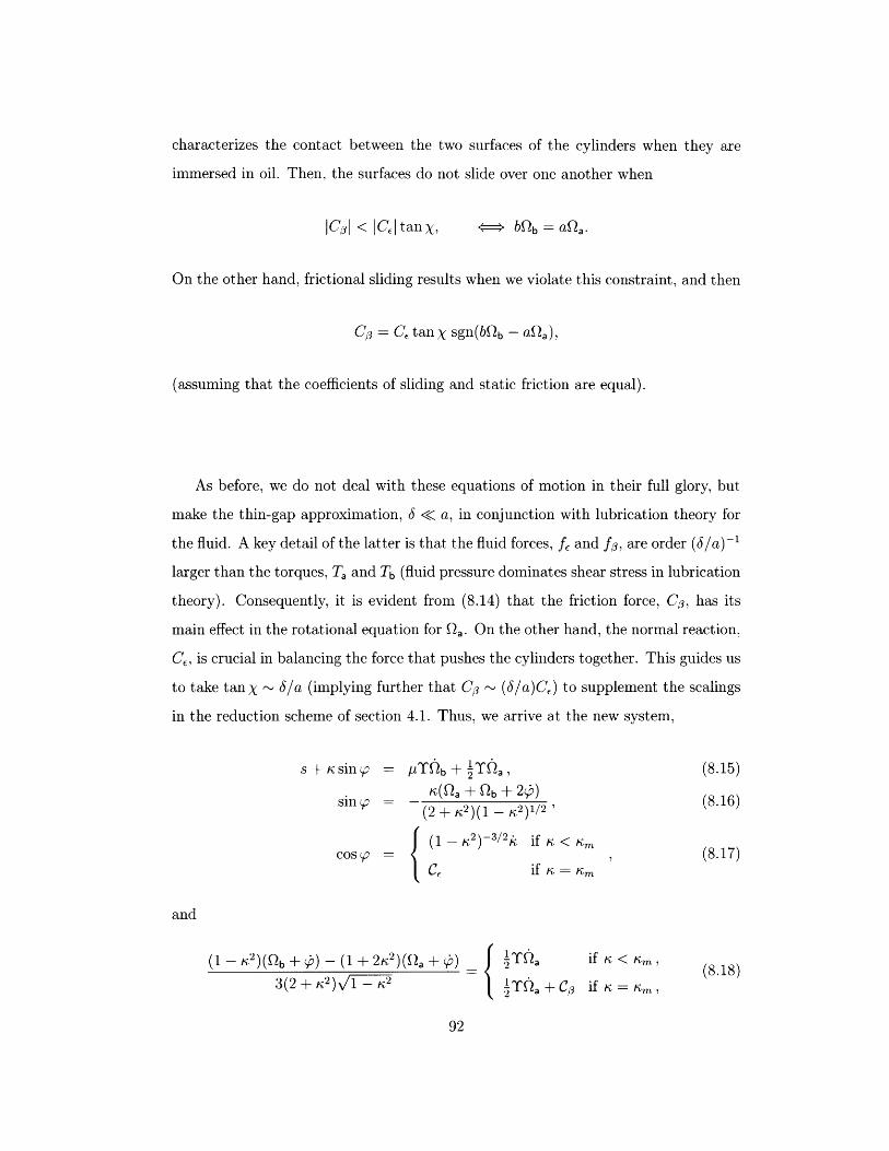
characterizes the contact between the two surfaces of the cylinders when they are

immersed in oil. Then, the surfaces do not slide over one another when

IC0 < IC]tanX, # bfb = a,.

On the other hand, frictional sliding results when we violate this constraint, and then

C = C tanX sgn(bQb - aQa),

(assuming that the coefficients of sliding and static friction are equal).

As before, we do not deal with these equations of motion in their full glory, but

make the thin-gap approximation, 6 << a, in conjunction with lubrication theory for

the fluid. A key detail of the latter is that the fluid forces, f and fo, are order (6/a) -

larger than the torques, Ta and Tb (fluid pressure dominates shear stress in lubrication

theory). Consequently, it is evident from (8.14) that the friction force, CO, has its

main effect in the rotational equation for Qa. On the other hand, the normal reaction,

C~, is crucial in balancing the force that pushes the cylinders together. This guides us

to take tan X - 6/a (implying further that C - (/a)CE) to supplement the scalings

in the reduction scheme of section 4.1. Thus, we arrive at the new system,

s +sinh : PTQb + T!Qa , (8.15)sin = I(Qa+Qb + 2) (816)

(2 + /42)(1 - 2)1/2 ' (8.6)

(1 - /42 )- 3/2k if < r4mCos =' (8.17)

CE if = m

and

r2) To" ~~~~~~~~~if/4 <4m,,(1 - 4 2 )(fb + 95) - (1 + 2/42 )(Qa + 95) = f TQa if ic < sum (8.18)3(2 + 2) ( 2TQa + C if (8.18)3(2 +/42)v/'-1-T),+¢ i4=4,

92

whereC- =-a--, C = C. (8.19)

am'g' mlg

The condition that the cylinders become locked together now becomes

JCOT < CJ tan 0, (8.20)

where tan q = (a/6) tan X. But given that fa = b when this occurs, we find from

(8.16) and (8.18) thatC =2s + (1- 2)jKmsin p (8.21)

2(1+2) ,(8.

and so locking results when

2(1- 2 )si 2s + (1 - 21L),sin V < I cosopl tan+. (8.22)2(1 + 2/4)

We illustrate the behavior of the model including rough contact in figure 8-2.

This picture displays a solution computed from an initial condition with K(0) <Km.

The integration continues up to a "collision time", tin, at which point, K(tm) = Km.

Beyond that instant, we switch to C, = cos p and continue the solution, monitoring

whether or not the traction between the cylinders is sufficient to overcome friction

and force the surfaces to slide over one another. In the example shown, the ultimate

fate of the system is a steadily rolling solution in which the cylinders are in sliding

contact. A case in which the final rolling solution has the cylinders locked together

by friction is shown in figure 8-3.

Note that the computation switches abruptly between the different versions of the

equations of the model. In particular, when the cylinders first come into contact, if

friction is sufficient to lock the cylinders together, then fa must jump discontinu-

ously at the moment of contact. This can be rationalized physically in terms of an

instantaneous impulse that affects the inner cylinder. In principle, at collision, there

should also be an equal and opposite impulse acting on the outer cylinder. However,

that cylinder is also resting on its contact point with the inclined plane, and the

model effectively assumes that any impulse from the collision of the two cylinders is

93

4020Time, t

(d) O.(t) and~(t)

4020Time, t

(c) .(t) and ,\(t)

0.8

/.. ....._..•.• 0.64 /.r.:....- .•••~..•.•• 0.4

('-" 0.22 I 0

0.2

o

8

6

20 0

(b) K(t)

10Time, t

__ ,,--0.98

............,,--10.4

o

; 0.8

l 0.6.'....

Figure 8-2: Sample rocking solution for T = 1, mb = 0 (M = ma) and s = 1/4, with K,

limited to the range (0, Km = 0.98), and 1/J = 0.05. The layout of panels (a)-( d) is as forfigure 4-1, except that the unlimited sedimenting solution is also shown by the dotted lines.

............... - - --- --- -..-..

3

2.5

o 5

I,I

: +- cont81:t

10 15TIme, t

20 25

r===o:l~

11'=0 (ahIfted by 2)

y=O.05 (shifted by 1)

1V=O.530 35

Figure 8-3: Sample solution for T = 1, fflb = 0 (M = mal and s = 1/4, with Km = 0.98and four values of 1/J (0.5, 0.05, 0.1 and 0; the curves are offset of clarity). The verticaldashed line shows the moment of contact.

cushioned by the other contact point.

As apparent from figure 8-3, the system has a fixed point. The limiting solution

is given by

-8 = K.,nsincp, (8.23)

sincp = K.,n(fla +flb) (8.24)(2 + ~~)(1 - ~~)1/~ '

coscp - Ce, , (8.25)

and(1 -' X;~)flb - (1 + 2,,~)fla _ C (8.26)

3(2 +x;~)v'l -,,~ - p.

94

0.35 DbI(3t.

0.3V0.25§

0.2 .

0.15

0.1 a~ I(3~)

0.05 , O~ _*7~~ Locking ' Sliding --

0 0.1 0.2 0.3 0.4 0.5S

Figure 8-4: Scaled, steady rotation rates, 0,a/(3(m) and Qb/( 3 (m), for 4 = 0.15.

The condition (8.22) for locking now reduces to s < 2 /1- s 2/2 m tan q, which, if

true, implies that

Ra = b = 22 s(2 + (8.27)

Otherwise,

s( - m)3/2 s(2 + .2) V1_ m Qa.~la 3V/1 - cosoptan + s(1, 2,

(8.28)

When the minimum gap is relatively narrow, and (m -/1 -T ~ < 1, we may write

both solutions in the compact form,

Sa = 3S Min ( 1'-s2 tan ), b = 3(s Max ( 1 - S tan ).S 2 8

(8.29)

The steady rolling speeds predicted by these formulae are illustrated in figure 8-4.

In dimensional terms, the equilibrium cylinder speed is expected to be

V = EbM sin aMax (, 1 tan (8.30)

The functional dependence on parameters contained in the prefactor is used to scale

the experimental observations in figure 7-4. The comparison suggests that E 0.1. In

turn, this implies a roughness scale of around 15 microns, which seems reasonable in

view of images taken of the surface of the cylinders with a microscope. Applying the

95

same approach to the rough cylinders coated with sandpaper also gives fair agreement

with the expected roughness scale (based on the American CAMI standard).

The expected rotation rates (figure 8-4) also share some common points with the

experimental observations (figure 7-5). For smaller slope angles, the rotation rates are

closely matched, and they diverge from one another once a critical slope is exceeded.

Given that the roughness of the surfaces keeps the cylinders apart and the effective

minimum gap is not expected to be the same all the way around the cylinder surfaces,

it is unlikely that the cylinders could ever become perfectly locked. According to the

theory, the critical slope measures the friction angle for sliding; we estimate X 3°

given the data in figure 7-5. One notable point of disagreement is the rotation rate

of the inner cylinder once sliding begins: in the theory, Q2 a decreases once sliding sets

in. The observations, on the other hand, show no tendency for Qa to decrease.

If one were to add slight stochastic variations in rtm, to simulate a rough angular

dependence of the minimum gap size, one might imagine that the system would be

randomly kicked off the equilibrium and rock slowly back to it, again similar to the

observations.

In this chapter, we have completed the two-dimensional model of the snail cylinder

by incorporating the dominating effect of surface roughness between the two cylinders

and neglecting cavitation forces when the cylinders are very close to each other. This

effect accounts for the slow quasi-steady motion which originally piqued our interest

in the problem.

96

Chapter 9

Conclusions

We have succeeded in elucidating the subtle dynamics of the snail cylinder. To sim-

plify the analysis, we have considered systems in which the distance between the

cylinders is always small. This allows us to take advantage of the vast engineering

literature on lubrication theory in general and the journal bearing in particular.

Several snail cylinders were constructed, using different inner weights and fluid

viscosities, and were placed on ramps. Three distinct modes of motion were observed

and recorded in chapter 2: a rocking motion, a slow, quasi-steady rolling motion, and

an unbounded accelerating mode. At low inclines (i.e. less than 5 degrees), one is able

to find the rocking mode, unless the cylinders are initially pushed too hard. For slopes

between 1 and 5 degrees, the quasi-steady, slow rolling motion also appeared; in this

case, the cylinders' velocity depends on the inner cylinder weight, fluid viscosity, and

surface roughness. At higher slopes, only the unbounded, accelerating mode could

be seen; in this mode, the motion appears independent of the fluid viscosity. Finally,

we noted small bubbles in the system that could not be completely removed and

appeared to congregate along the line of minimum separation during the slow rolling

motion.

The general features of the snail cylinder dynamics can be understood by con-

sidering our theoretical model in chapters 3 and 4; these include both the observed

accelerating and rocking motions. Qualitatively, we expect the system to accelerate

in either of two cases: first, when its initial period of rotation is much shorter than

97

the settling time, i.e. /Qb << Ts; or second, when the gravitational component

that acts on the center-of-mass of the whole system, accelerating it down the incline,

dominates the effective gravitational force acting on the inner cylinder, leading it to

sediment onto the outer cylinder. We note that the parameter s in the theoretical

model can be rewritten asMg sin a9

s = a (9.1)a ag

Therefore, our observation in chapter 4 that s I allows only accelerating modes,

implies that if Mgsin a/m'g >> d/a, only unbounded accelerating modes are pos-

sible. Conversely, we may expect to find rocking motion if both << 1/Qb and

Mgsina/m'g << 5/a.

We may also distinguish between the accelerating and rocking modes by consider-

ing energy conversion within the system. The frictional force between the outer shell

and the incline does no work because the contact point moves with no instantaneous

velocity; therefore, any energy loss occurs within the system. In the accelerating sys-

tem, the gravitational potential of the whole system is converted into kinetic energy

with a minimal amount of energy dissipated into heat. Since the dissipation in the

fluid is negligible, one expects and finds that the bearing's acceleration is indepen-

dent of the fluid viscosity. However, in the rocking system, all potential energy is

ultimately dissipated into heat by the fluid viscosity. Therefore, for the snail cylin-

der to roll slowly down the incline, potential energy must be dissipated in the fluid

without a significant change in kinetic energy.

To understand the energetics of the snail cylinder, we studied a modified nested

cylinder system in chapters 5 and 6. A cylinder was placed inside a larger fluid-

filled cylinder whose angular velocity was prescribed by a motor. The discrepancy

between the inner cylinder's observed motion and our predictions suggested that we

include a frictional interaction between the two cylinders. By adjusting the model to

account for surface roughness, we found reasonable agreement between a new series

of experiments and our modified model in chapter 7.

In light of this study, we proposed that some combination of surface roughness

98

and cavitation holds the inner cylinder off the outer wall by supporting its weight

to rationalize the quasi-steady mode. We performed more experiments in section 7.2

to test the effect of cavitation bubbles and different roughness scales on the snail

cylinder's motion. Either surface roughness or cavitation could have the effect of

keeping the fluid gap thickness constant at a physically determined minimum distance.

In turn, a constant gap thickness would imply a constant rate of energy dissipation

which is a necessary condition for slow rolling.

Following recent work by Ashmore, et al. [1], we examined the effect of cativation

bubbles underneath the inner cylinder in section 8.1. When we examine the mag-

nitude of the resulting forces due to the bubbles, we find that cavitation is not a

viable mechanism to account for the anomalous observations. That is, we find that

the cavitation bubbles cannot generate enough force to hold the inner cylinder away

from the outer wall. Ashmore, et al., draw a different conclusion in their work on a

sphere next to the rotating cylinder wall. They predict that the minimum gap size is

determined by cavitation. We reconcile these differing conclusions by noting that in

the spherical problem, the pressures created in the gap are proportional to gap size

to the -3/2; in the cylindrical problem, the the pressures are only proportional to gap

size to the -1/2, so one may expect cavitation to play a bigger roll for the sphere.

Furthermore, Seddon and Mullin's observations suggest that cavitation affects the

rotation of the inner cylinder; this may still be the case despite surface roughness

determining the dimensions of the region where cavitation takes place.

Since cavitation cannot be the dominant effect, we build on our hierarchy of

theoretical models, in section 8.2, by considering only the effect of surface roughness

on the rolling speed of the quasi-steady mode, neglecting cavitation. We calculated

an expected gap size that produces predicted velocities that are comparable to those

seen in experiment. Furthermore, this gap size is comparable to roughness scales for

the materials used to build the snail cylinders.

Summarizing, we have rationalized the curiously slow, quasi-steady rolling of the

snail cylinder system. We have rephrased the problem in terms of the journal bearing

so that we could take advantage of the wealth of research that has been done on that

99

problem. However, the standard lubrication theory explanation of the fluid dynamics

within the system did not account for the particular motion that we observed. There-

fore, we built upon work by Smart, et al., and Ashmore, et al., on the interaction

of a sphere in Stokes flow near a moving boundary to consider the effects of surface

roughness and cavitation in the cylindrical geometry. We have built these effects into

the lubrication theory and have learned that dissipation in the region between the

cylinders, held at a constant size by surface roughness, is the mechanism by which

the cylinder's acceleration is impeded in the quasi-steady mode.

100

Appendix A

Dimensionless groups and physical

quantities

101

Definition Section Introduced Range of Values/ aV+mb 4.1 (1, 10)ma

r 3mam 4.1 (10-2,5)144v2m,,"

S a sinax, 4.1 (0, 1)

64m,'2mg 6.1 (102, 105)mem'ga4

6 6 6.1 (0,5)a

b Qbmga2 6.1 (0, 10)~,' (6.27) 6.3 (0, 1)

Re Qbb2 7.1 (0,2 x 10- 3 )

Fr 7.1 (0,3 x 10- 5 )

9/

Table A. 1: Various dimensionless groups used in the thesis

Meaninginner cylinder radiusinner cylinder mass

system lengthouter cylinder radiusouter cylinder mass

angular velocity of outer cyl.fluid density

fluid kinematic viscosityfluid mass

total system massdisplaced fluid mass

ma reduced by buoyancyrolling time scale

fixed outer cylinder time scale

NotesE (0, 5cm)

E (.5cm, 2cm)E (5cm, 50cm)

E (0, 20cm)

46gE (0, 2sec - 1

E (.85g cm - 3 , 1.5g cm - 3 )E (lcm2 sec -1 , 12000cm 2 sec- 1)

7rpL(b2 - a 2 )

ma + mb + mf7rpa2L

ma - m a12 m;'va1m62

8 m, Aotn

Table A.2: Various physical quantities and their meanings

102

amaLb

mb

Qb

pP

mfM

TmI7 a

ma

Tm

Appendix B

The Calculations of Finn and

Cox[8]

B.1 Rotlets and Stokeslets

Recall that the equations of motion for Stokes flow are

-VI + vV2 = 0 (

V-. = 0. (

Since the flow is two dimenional, the second equation implies that we can write

u = V A [ (x, y, t) (= ax-y. (Taking the curl of the momentum equation gives

(B.5)

103

B.1)

B.2)

B.3)

B.4)

V [,j� (t . (�Vi) _ V2 ,

so that the fact that I is independent of z yields

V4T = 0. (B.6)

Introducing the complex notation, w = x+iy and T = x-iy, the biharmonic equation

is equivalent to the complex equation

04

w2D= 2 0 (B.7)

which is easily seen to have the (purely real) solution

I (w, T) = of (w) + wf () + g (w) + (), (B.8)

for arbitrary choices of the complex functions f and g. In their paper, Finn and

Cox make an important realization. Supposing that I takes the form of the general

solution above with no singularities on the circle IwI = a, they constructed another

stream function

4 (w, w) = wf (w) + wf () + g (w) + g (T)-zf (a2/w)- f (a2 /)- (a2/w)-g (a2/W)

+ (a2 _ Iw2) {7' (a2/w) + f' (a2/T) + w-'' (a2/Z) + T-lg (a2/T) } (B.9)

Any singularity of I at w0 with IwoI < a will also be a sigularity of A. has additional

singularites at the image points of the singularities of and perhaps at w = 0.

Futhermore, b is also a solution of the biharmonic equation which generates zero

velocity and has = 0 on Iwl = a. They then remove any nonphysical singularities

at w = 0 of 4 by a method of successive reflections. For example, consider the stream

function corresponding to a rotlet at w = s

1 = C [log (w -s) +log (W -s)], (B.10)2

104

where C and s are real numbers. The coresponding O for the image system is

T = wF (w) + wF () + G (w) + G (w), (B.11)

where

Fw 2 W G(w) = log ( - a+logw}, (B.12)

where or = a2 /s is the image of s in IwI = a. We see from this expression that O has

a new singularity asymptotic to log w at the origin. To remove this singularity, we

consider a , = P log w + P log w and find that the image of this stream function is

T~ = : wF (w) + wF (w) + G (w) + G (), (B.13)

where

F1 =-Pwa 2 , G = P(1-loga 2)+ (P + P)logw. (B.14)

Therefore, if we set P = -C/4 and add this stream function to the image of the orig-

inal rotlet stream function, we find the final stream function for the rotlet contained

in a cylinder of radius a. That is

=C log '7 f -s +i Owl 2-a ) (Iw W f 12 _ (B212 ~ slw-u + a2lw-(B.15)2~ losw_ ey12 a 2 Jw - _ ey12'

A similar calculation is done for the stokeslet contained in a cylinder of radius a.

After removing all non-physical singularities within the cylinder with image stokeslets,

Finn and Cox calculate its stream function as

1 = [A (w + ) - iB (w - )] log 12

A (]w12 - a 2) [W+S w+s] iB (w - ) ( -s) (Iw] - a 2)(B 16

4s w- 4s 1w - or[2

105

B.2 Forces and torques from the stream function

Now let us suppose that the stream function inside a circle of radius a contains a

Stokes flow with stream function

(B.17)

Then since

O 0 0 0 .(OOx Ow o' Oy =

(B.18)

and VII = vV2u, we have

8 4i 2 = 4ivF" (w),,5~ awOu aw

n = iv YT - - awa OE = 4ivF" (w)

This implies that

H = 4iv [F' (w) - F ()] + io.

We next calculate the deviatoric stress tensor. We have

:( 0=

OW2J

auyOy

Ouy

Ox

= i 02V)aW 2

Ox

X 2- -i 92 10

aoW2

= (W + 2 r a+

= - 920 + 2 920 +ajw2 awaw-

Oux

aya

ow(O2o

= _ _w2

Ow Ow)

O2 +-2 +OwSw

106

(B.19)

(B.20)

(B.21)

(B.22)

(B.23)

(B.24)

0 = TF (w) + wY (T) + G (w) + ?7 (T).

t- 9�b

,'r-ow

19

19W

Therfore, i( .) -( ± ) (

T = 2pv t v ) - m+) )(B.25)

Since both II and T are real, we can use complex notation to calculate the force on

the outer cylinder due to the fluid. That is we can write = w/a, so that

F = I (pn -T-)dlI=a

= 4pvi [wF' (w) - wF () + 2 ] dO

= 4pvi [wF' (w) - wF (w) + a2F" (w) + wG (w)] dO

= 4pv =a dF (w)dw-4pv Jia [ ( G'(] C

= -4pv {-F (w) + wF () + G' () I}c ' (B.26)

where {H}c is the change in the value of H when we go around the C one time in

the counter-clockwise direction. We can also calculate the moment generated by the

fluid motion on the outer cylinder using complex methods. We have

To = FA (pl-T .h) dl (B.27)I=a

2,,

= -Im 4pvi wT WF (w) - w (T) + w-] dO} (B.28)

= Im {-4pv [a2T" (w) + G" (w)] iwdO} (B.29)

= 4 pvIm {1 2 [a2r () + TwG () G ()] d} (B.30)

= 4pvIm {a2F' (W) + (W) - G (U)}c (B.31)

From these simplified expressions, Finn and Cox calculate the instantaneous forces

and torques by choosing appropriately placed rotlets and stokeslets to satisfy the

velocity boundary conditions at the boundaries of both cylinders and plugging this

stream function into (B.26) and (B.31). The results are quoted above in chapter 5.

107

108

Bibliography

[1] J. Ashmore, C. del Pino, and T. Mullin. Cavitation in a lubrication flow between

a moving sphere and a boundary. Phys. Rev. Lett., 94:124501, 2005.

[2] B. Y. Ballal and R. S. Rivlin. Flow of a newtonian fluid between eccentric

rotating cylinders: Inertial effects. Arch. Rat. Mech. Anal., 62(3):237-294, 1976.

[3] N. J. Balmforth, D. P. Vener, J. W. M. Bush, and W. R. Young. A numeri-

cal and experimental investigation of the cylindrical mixer. J. Fluid Mech. (in

preparation), 2006.

[4] N. J. Balmforth, D. P. Vener, J. W. M. Bush, and W. R. Young. Rocking and

rolling down an incline. J. Fluid Mech. (in preparation), 2006.

[5] G. K. Batchelor. An Introduction to Fluid Dynamics. Cambridge University

Press, second edition, 1967.

[6] J. Brindley, M. D. Savage, and C. M. Taylor. The non linear dynamics of journal

bearings. Phil. Trans. R. Soc. Lond. A, 332:107-119, 1990.

[7] Duffing. Z. angew. Math. Mech. (ZAMM), 4:279-314, 1924.

[8] M. D. Finn and S. M. Cox. Stokes flow in a mixer with changing geometry. J.

Eng. Math., 41:75-99, 2001.

[9] A. Goldman, R. Cox, and H. Brenner. Slow viscous motion of a sphere parallel

to a plane wall-i: Couette flow. Chem. Eng. Sci., 22:637-651, 1967.

109

[10] G. B. Jeffrey. The rotation of two circular cylinders in a viscous fluid. Phil.

Trans. R. Soc. Lond. A, 101:169-174, 1922.

[11] T. Mullin, Y. Li, C. del Pino, and J. Ashmore. An experimental study of fixed

points and chaos in the motion of spheres in a stokes flow. IMA Journal of

Applied Mathematics, 70:666-676, 2005.

[12] I. A. Nyrkova, A. N. Semenov, A. R. Khokhlov, K. Linliu, and B. Chu. Motion

of a probe ball in the fluid under centrifugal acceleration. J. Phys. II France,

7:1709-1728, 1997.

[13] O. Pinkus and B. Sternlicht. Theory of Hydrodynamic Lubrication. McGraw-Hill,

first edition, 1961.

[14] A. Prokunin. On a paradox in the motion of a rigid particle along a wall in a

fluid. Fluid Dyn., 38:443-457, 2003.

[15] H. Reisner. Z. angew. Math. Mech. (ZAMM), 15:81-87, 1935.

[16] O. Reynolds. On the theory of lubrication. Phil. Trans. R. Soc. Lond.,

177(I):157-234, 1886.

[17] J. R. T. Seddon and T. Mullin. Reverse rotation of a cylinder in a stokes flow.

Phys. Rev Lett. (submitted), 2006.

[18] J. R. Smart, S. Beimfohr, and D. T. Leighton Jr. Measurement of the transla-

tional and rotational velocities of a noncolloidal sphere rolling down a smooth

inclined plane at low reynolds number. Phys. Fluids A, 5:13-24, 1993.

[19] A. C. Stevenson. Plane stress and plane strain in bipolar coordinates. Phil. R.

Soc. Lond., A184:129-179, 1945.

[20] G. H. Wannier. A contribution to the hydrodynamics of lubrication. Quart.

Appl. Math., 8:1-32, 1950.

[21] Q. Yue. The motion of a rod in a rotating Stokes flow. PhD thesis, Pennsylvannia

State University, 1995.

110

[22] N. E. Zhukowski. Comm. Math. Soc. Kharkov, 17:31-46, 1887.

111