NOTICE:

This research was funded by the Wisconsin Council on Research of the Wisconsin Department of Transportation and the Federal Highway Administration under Project #SPR-0092-45-17. The contents of this report reflect the views of the authors who are responsible for the facts and the accuracy of the data presented herein. The contents do not necessarily reflect the official views of the Wisconsin Department of Transportation or the Federal Highway Administration at the time of publication.

This document is disseminated under the sponsorship of the Department of Transportation in the interest of information exchange. The United States Government assumes no liability for its contents or use thereof. This report does not constitute a standard, specification or regulation.

The United States Government does not endorse products or manufacturers. Trade and manufacturers’ names appear in this report only because they are considered essential to the object of the document.

Technical Report Documentation Page

1. Report No.

0092-45-17

2. Government Accession No 3. Recipient’s Catalog No

4. Title and Subtitle

Evaluation of Ramp Meter Effectiveness for Wisconsin Freeways, A Milwaukee

Case Study: Part 1, Diversion and Simulation

5. Report Date

October 2004

6. Performing Organization Code

7. Authors

Alan Horowitz, Jingcheng Wu, Juan P. Duarte

8. Performing Organization Report No.

0092-45-17

9. Performing Organization Name and Address

University of Wisconsin, Milwaukee

P.O. Box 784

Milwaukee, WI 53201

10. Work Unit No. (TRAIS)

11. Contract or Grant No.

0092-45-17

12. Sponsoring Agency Name and Address

Wisconsin Department of Transportation, Council on Research

4802 Sheboygan Ave., Room 451

P.O. Box 7965

Madison, WI 53707-7965

13. Type of Report and Period Covered

Final Report

14. Sponsoring Agency Code

15. Supplementary Notes

16. Abstract

The purpose of the research is to determine the benefits of ramp meters in the Milwaukee area freeway system, to determine

underlying relationships that permit evaluation of new ramp meters or ramp meter systems elsewhere, and to develop a

coherent framework for performing evaluation of ramp meter effectiveness on a whole system. Part 1 concentrates on

diversion and traffic simulation. In order to assure that the conclusions are relevant to Wisconsin drivers and conditions on

Wisconsin freeways, the research focused on data collected from the US 45 corridor, mostly in Milwaukee County, from

before and after the deployment of seven new ramp meters in the southbound direction in early March 2000. This corridor

spanned about 15 miles and included the freeway itself and two parallel arterials. Statistically significant diversions away

from US 45 occurred at times and places where traffic volumes were heaviest and ramp queues were longest. The data also

revealed that there was diversion between on-ramps along US 45 in response to queuing at ramps. The data did not reveal

any temporal diversions due to the meters. This study investigated three types of simulation software packages:

microscopic (Paramics), mesoscopic (Dynasmart-P) and macroscopic (QRS II). US 45 was simulated with two packages

(Paramics and QRS II) within which a reasonable representation of a meter could be achieved. The most convincing

simulations of US 45 (without parallel arterials) was created with Paramics. There were two simulations, one for the

“before” period and one for the “after” period, both of which matched mainline speeds closely and behaved realistically at

the meters.

17. Key Words

Ramp meter, freeway, diversion, traffic simulation, OD

table estimation.

18. Distribution Statement

No restriction. This document is available to the public

through the National Technical Information Service

5285 Port Royal Road

Springfield VA 22161

18. Security Classif.(of this report)

Unclassified

19. Security Classif. (of this page)

Unclassified

20. No. of Pages 21. Price

Form DOT F 1700.7 (8-72) Reproduction of completed page authorized

Technical Report Documentation Page

1. Report No.

0092-45-17

2. Government Accession No 3. Recipient’s Catalog No

4. Title and Subtitle

Evaluation of Ramp Meter Effectiveness for Wisconsin Freeways, A Milwaukee

Case Study: Part 2, Ramp Metering Effect on Traffic Operations and Crashes

5. Report Date

October 2004

6. Performing Organization Code

7. Authors

Alex Drakopoulos, Mery Patrabansh and Georgia Vergou

8. Performing Organization Report No.

0092-45-17

9. Performing Organization Name and Address

Marquette University

Department of Civil and Environmental Engineering

P.O. Box 1881, Milwaukee, WI 53201-1881

10. Work Unit No. (TRAIS)

11. Contract or Grant No.

0092-45-17

12. Sponsoring Agency Name and Address

Wisconsin Department of Transportation, Council on Research

4802 Sheboygan Ave., Room 451

P.O. Box 7965

Madison, WI 53707-7965

13. Type of Report and Period Covered

Final Report

14. Sponsoring Agency Code

15. Supplementary Notes

16. Abstract

The purpose of the research is to determine the benefits of ramp meters in the Milwaukee area freeway system, to determine

underlying relationships that permit evaluation of new ramp meters or ramp meter systems elsewhere, and to develop a

coherent framework for performing evaluation of ramp meter effectiveness on a whole system. Part 2 concentrates on the

traffic operations affect six new ramp meters had on the 14-mile long corridor where six ramp meters were already

operational. A crash rate comparison was performed between the periods the corridor operated without and with the six new

ramp meters. Metered on-ramp queue length and delay information is presented in Appendix A; details of the operation of a

metered on-ramp as well as mainline speed occupancy and volume information in the vicinity of the ramp are presented in

Appendix B.

Average corridor speeds improved when the new ramp meters were operational. Vehicle-hours of travel were lower during

the more congested afternoon peak period. It is suggested that fine-tuning of ramp metering parameters is very likely to

result in additional benefits for the corridor.

Crash rates during ramp metering hours were lower by 13% with the new ramp meters operational.

17. Key Words

Ramp meter, freeway, measures of effectiveness, speed,

vehicle hours of travel, vehicle miles of travel, average

corridor speed, crash rates, ramp delay, mainline delay,

ramp queue length.

18. Distribution Statement

No restriction. This document is available to the public

through the National Technical Information Service

5285 Port Royal Road

Springfield VA 22161

18. Security Classif.(of this report)

Unclassified

19. Security Classif. (of this page)

Unclassified

20. No. of Pages 21. Price

Form DOT F 1700.7 (8-72) Reproduction of completed page authorized

Table of Contents

Combined Executive Summary for Parts 1 and 2

Overview....................................................................................................................................... i

Case Study: US 45 in Milwaukee ................................................................................................. i

Findings........................................................................................................................................ ii

Conclusions................................................................................................................................. iv

Recommendations.........................................................................................................................v

Part 1: Diversion and Simulation

Chapter 1 Ramp Metering and Diversion: A Review of Literature..............................................1

Chapter 2 Diversion of Traffic from Ramp Meters on US 45 ....................................................22

Chapter 3 Ramp Meters Relation to Freeway Segment Trip Length..........................................64Chapter 4 Methods for Evaluating Ramp Meters in Milwaukee: Case Studies of Microscopic

and Macroscopic Models ............................................................................................................69

Part 2: Ramp Metering Effect on Traffic Operations and Crashes

Chapter 5 Ramp Metering Effect on Traffic Operations and Crashes..........................................1

Appendix A Inventory of Ramp Delay and Queue Length Information ................................. A-0

Appendix B Wisconsin Avenue Ramp Meter Operation, Afternoon Peak Period (4:00 pm to

5:30 pm) Wednesday, February 9, 2000...................................................................................B-1

Transit Benefits Resulting From Access to Education ...............................................................14

i

Evaluation of Ramp Meter Effectiveness for

Wisconsin Freeways, A Milwaukee Case Study:

Part 1, Diversion and Simulation

Combined Executive Summary for Part 1 and Part 2

Overview

This report is one of two companion reports that identify methods for evaluating the

effectiveness of ramp meters on Wisconsin freeways. The other report, “Evaluation of Ramp

Meter Effectiveness for Wisconsin Freeways, A Milwaukee Case Study: Part 2, Travel Times,

Speeds and Collisions” has been prepared by Marquette University. This Executive Summary is

a description of the procedures, conclusions and recommendations from both reports.

The purpose of the research is to determine the benefits of ramp meters in the Milwaukee

area freeway system, to determine underlying relationships that permit evaluation of new ramp

meters or ramp meter systems elsewhere, and to develop a coherent framework for performing

evaluation of ramp meter effectiveness on a whole system.

A better understanding of ramp meter operation can lead to more optimal placement of

new ramp meters and optimal design of each new ramp meter (including its geometry, HOV

lane, storage capacity, upstream signalization strategies, timing plan, and ITS strategies), and

optimized coordination between ramp meters. Toward this end, the project also identified and

tested simulation software packages for modeling ramp meter operations at a system level.

The project focused on the three most critical areas of ramp meter system effectiveness:

collision reduction, congestion reduction, and traffic diversion behavior and related effects. A

systems viewpoint is critical. The presence of the meter at a freeway on-ramp has implications

for this particular ramp, any upstream traffic controls, the downstream freeway mainline and the

parallel arterials. The geometry and operational characteristics of the meter influence delay (as

one measure of congestion), collisions, and other measures of effectiveness (MOEs) for the

system as a whole. This project also recognizes that a single ramp meter influences and is

influenced by traffic conditions considerably upstream and downstream of its own location and

that coordination of the meter with other meters needs to be investigated. Traffic diversion can

only be analyzed in the context of a system, as this behavior depends upon the operation of the

meter and the freeway, the conditions on parallel arterials, driver experience, and information

provided to the driver just ahead of the diversion decision.

Case Study: US 45 in Milwaukee

In order to assure that the conclusions are relevant to Wisconsin drivers and conditions on

Wisconsin freeways, the research focused on data collected from the US 45 corridor, mostly in

Milwaukee County, from before and after the deployment of seven new ramp meters in the

southbound direction in early March 2000. This corridor spanned about 15 miles and included

ii

the freeway itself and two parallel arterials, Highway 100 and 124th

Street. There were 14 on-

ramps to US 45 (southbound) within the corridor, of which 13 were eventually metered.

A comprehensive data collection, coordinating the efforts of Marquette University, the

University of Wisconsin – Milwaukee and the Wisconsin Department of Transportation, resulted

in precise snap-shots of the traffic conditions before and after deployment. Data related to traffic

flow were collected on six weekdays (Tuesdays, Wednesdays and Thursdays) before deployment

and six weekdays after deployment for 1 ½ hours in each of the morning and evening peaks.

Data covered these items.

�� Travel Times. Floating car runs were made continuously during the 1 ½ hour peak

periods on southbound US 45, Highway 100 and 124th

Street. Travel times were

recorded for segments along US 45 of about 1 mile in length every 15 minutes. Segment

lengths on Highway 100 and 124th

Street average a little more than ½ mile, also at 15

minute intervals.

�� Detector and Tube Counts. Count data from all loop detectors on US 45 were assembled.

These loop detectors included mainline detectors for each metered ramp and other

mainline detectors between ramps. In addition, counts were obtained from detectors

located on the ramp (both at the top of the ramp, the “queue” detector, and at the stopline,

the “passage” detector). Road tubes were deployed at all locations that could not be

adequately counted by loop detectors: the southbound lanes of Highway 100 and 124th

Street; all off-ramps; and all on-ramps without meters in the southbound direction of US

45.

�� Origin-Destination Tables. Two tables giving the split of vehicle to each off-ramp from

each on-ramp were obtained by video logging of license plates. The data for these tables

were collected in 1999 and 2001, well before and well after the ramp meter deployment.

�� Detector Speeds. Mainline detectors were arrayed in pairs so that speeds could be

obtained continuously at many points along US 45. Because of the possibility of detector

error, these speeds were verified against the floating car runs.

�� Queue Length Counts. Queue lengths were hand counted at all metered on-ramps in the

southbound direction of US 45.

�� Collision History. Collision records for US 45 were obtained from the Milwaukee

County Sheriff’s office for 3 years before and 2 years after the ramp meter deployment.

In addition, a survey of Wisconsin drivers administered by the University of Wisconsin—

Madison provided insights into drivers’ route choices in reaction to ramp meter deployment.

Findings

Diversion

The consensus of the literature is that the ability to divert selected traffic from the

freeway mainline is essential in achieving positive benefits of ramp meters. Thus, it is important

to understand the diversion propensity of Wisconsin drivers when faced with the need to wait for

vehicles ahead of them at a ramp meter. There are three common forms of diversion: spatial,

temporal or modal. Modal diversion (such as shifts to carpools or transit) was not analyzed and

iii

there was no evidence in the collected data that temporal diversion (sometimes referred to as

“peak spreading”) occurred in the study corridor. Spatial diversion was ascertained by three

different methods from the before and after data.

�� Origin Destination Tables. The average trip length from the origin-destination tables

increased from the before to the after periods. There was a 7% increase in the morning

and a 4% increase in the afternoon. A contributing factor to this increase was a reduction

in very short trips.

�� Traffic Counts. Mainline and arterial traffic counts were compiled for each 15 minutes

along eight east-west cutlines across US 45, Highway 100 and 124th

Street. Traffic counts

indicated that diversion occurred between the freeway and parallel arterials, although not

all times and not all cutlines were impacted the same. Statistically significant diversions

away from US 45 occurred at times and places where traffic volumes were heaviest and

ramp queues were longest. The data also revealed that there was diversion between on-

ramps along US 45 in response to queuing at ramps.

�� Questionnaire. From the questionnaire responses from those Wisconsin drivers who said

that they regularly encountered ramp meters, it was found that 72% of drivers are aware of

alternate routes and 65% have a good idea of the travel time the alternate route would

take. Only 24% of drivers said they would divert if the ramp was half full, but 62% said

they would divert if the ramp was nearly full and 82% said they would divert if the ramp

was overflowing.

Speeds and Travel Times

During the period with new ramp meters in operation the most congested south part of the

analysis corridor experienced an improvement in traffic operations measures of effectiveness,

during the most critical (most congested) afternoon peak period.

During the afternoon peak period, a substantial reduction in vehicle-hours of travel due to

increases in travel speeds, under minimal volume changes (a zero to two percent increase) was

documented between Capitol Drive and Greenfield Avenue. Speeds increased by 13% in the

segment between Capitol Drive and Burleigh Street, by 10% between North Avenue and

Wisconsin Avenue, and by 6% between Bluemound Road and Greenfield Avenue.

Corridor average speed increased by only four percent during the afternoon peak, because no

speed changes were effected on the north part of the corridor where near-free-flow speeds

existed at all times. Although mainline vehicle hours of travel decreased by five percent, when

ramp delay was also taken into account, total vehicle hours of travel decreased by two percent.

There was an overall increase of two percent in corridor vehicle miles of travel.

Crashes

The crash rate was 298 crashes per 100 MVM of travel “Without,” and 260 crashes per 100

MVM of travel “With” the new ramp meters. Operation of the new ramp meters in conjunction

with improved ramp merging geometrics and mainline pavement resurfacing resulted in an

overall 13% crash rate reduction (16% reduction in the number of crashes) during ramp

metering hours.

iv

Simulation

The traffic impact of ramp meters can be simulated using a variety of methods; the choice

of method would depend upon needs of the analysis. This study investigated three types of

simulation software packages: microscopic (Paramics), mesoscopic (Dynasmart-P) and

macroscopic (QRS II). US 45 was simulated with two packages (Paramics and QRS II) within

which a reasonable representation of a meter could be achieved. A simulation has the advantage

of isolating only those effects that need to be analyzed. Thus, the impact of a new ramp meter

could be investigated without worrying about weather, incidents, fluctuations in traffic volumes

or any other confounding influences.

The most convincing simulations of US 45 (without parallel arterials) was created with

Paramics. There were two simulations, one for the “before” period and one for the “after”

period, both of which matched mainline speeds closely and behaved realistically at the meters.

These models were given a minimum of calibration to obtain a relatively “hands-free” evaluation

of the performance of the software. Model parameters were adopted verbatim from a study of I-

5 in Irvine, California. The largest impediments to implementing Paramics on US 45 were the

complexity of the software, the inadequate documentation and the need to adapt standard

features of the software to match the peculiarities of US 45. For example, the project team

encountered problems getting Paramics to represent alternative release of vehicles from two-lane

approaches to meters and to represent the split of traffic to HOV lanes.

A comparison of the two simulations for US 45 indicated that traffic flowed better after

the new meters were added. Both delays at meters and along the mainline were considered in

this assessment. However, these simulations did not contain creation of platoons at upstream

signalized intersections, so the benefits associated with platoon dispersion by meters could not be

assessed. The traffic impacts on adjacent arterials were not considered.

Conclusions

The analysis and simulation of US 45 lead to the following major conclusions.

�� Drivers react to recurrent delays at ramp meters and along freeway mainlines when

choosing between alternate routes. When faced with a long queue at an on-ramp, some

drivers divert to another on-ramp while some others avoid the freeway entirely. The US

45 experience suggests that average trip length on the freeway increases when meters are

deployed, thereby resulting in less entering or exiting for a given level of traffic on the

mainline.

�� During the period with new ramp meters in operation the most congested south part of

the analysis corridor experienced an improvement in traffic operations measures of

effectiveness, during the most critical (most congested) afternoon peak period: a

substantial reduction in vehicle-hours of travel and increases in travel speeds, under

minimal volume changes (a zero to two percent increase) was documented between

Capitol Drive and Greenfield Avenue. Speeds increased by 13% in the segment between

Capitol Drive and Burleigh Street, by 10% between North Avenue and Wisconsin

Avenue, and by 6% between Bluemound Road and Greenfield Avenue. Corridor average

speed increased by four percent during the afternoon peak.

v

�� New ramp meter operation, in conjunction with geometric improvements in ramp

merging areas and mainline resurfacing resulted in a 21% crash rate reduction for the

analyzed corridor during ramp metering hours.

�� It is possible to develop high quality mathematical models for assessing of the impact of

ramp meters with a suitable microscopic traffic simulation software package. The

software package currently used by WisDOT to simulate the Milwaukee freeway system,

Paramics, is a good choice.

�� The simulations of before and after conditions on US 45 indicated that traffic on the

freeway flowed better after the meters were deployed.

Recommendations

Because an unwarranted ramp meter can cause delay on the ramp without achieving

sufficient offsetting travel time savings on the mainline, the deployment of ramp meters should

proceed cautiously. The deployment decision should be based on a careful engineering study

that includes collection and analysis of speed and volume data and an assessment of impact on

mainline speeds, arterial speeds, entrance and exit volumes and ramp queuing. A simulation

model, such as the ones developed in this study with Paramics, should be used to assist this

evaluation.

Ramp meters can have significant effects on traffic flow within a freeway mainline. Any

simulation model of a freeway in Wisconsin should include ramp meters, if present. Any future

forecasts of traffic volumes on freeways should consider the possible diversion effects of ramp

meters.

The current ramp meter timing algorithm used in Milwaukee has not had a thorough

review. WisDOT should undertake such a review to determine whether it still fully satisfies the

objectives of freeway operation. Other algorithms should be considered that have the potential

to more effectively optimize traffic flow downstream from the meter. The current algorithm

deals with each ramp meter in isolation from other ramp meters. WisDOT should consider

means by which several adjacent ramp meters could be jointly timed to provide better traffic

flow. It is important that any software for ramp meter evaluation be capable of correctly

representing the timing algorithm.

The Paramics models for US 45, both before and after ramp metering, that were

developed for this study should be used to investigate the effects of freeway operational policies

that are not location specific. The models should be upgraded to increase the realism of the

simulations. These Paramics models did not invoke Paramics’ ability to divert traffic to alternate

routes; such capability should be added. In addition, the Paramics models did not contain traffic

signals upstream from the ramps that would create platoons of vehicles, which would have a

serious impact on mainline traffic flow, if not metered.

Fine-tuning of ramp metering parameters during the morning peak period in order to

reduce ramp delays is very likely to produce a reduction in total freeway veh-hr of travel.

Further reductions in total freeway veh-hr of travel during the afternoon peak may also be

possible by reducing ramp delay on the existing Good Hope Road loop ramp where the mainline

is not very congested; the current high level of ramp delay on the new Burleigh Street ramp

could probably also be reduced. County Line Road and Pilgrim Road ramp metering probably

vi

contributes rather small mainline benefits at the present time, given the lower traffic volumes and

substantial distance from the currently congested part of the corridor. Minimizing delays on

these ramps would, in all likelihood decrease corridor delays.

Any changes in ramp metering parameters aiming to reduce ramp delays, should be

carefully balanced against possible increases in mainline travel times.

Evaluation of Ramp Meter Effectiveness for Wisconsin Freeways, A Milwaukee Case Study: Part 1, Diversion and

Simulation

Project identification number 0092-45-17

Final Report

Alan J. Horowitz Jingcheng Wu Juan P. Duarte University of Wisconsin, Milwaukee

Submitted to the Wisconsin Department of Transportation October 2004

Table of Contents

Chapter 1 Ramp Metering and Diversion: A Review of Literature .........................................1

Introduction ..................................................................................................................................1

Ramp Metering Diversion Effects ................................................................................................1Field Study in Twin Cities, Minnesota...............................................................................................................1

Route Diversion.................................................................................................................................................3

Time-of-Day Diversion .....................................................................................................................................3

Ramp Diversion.................................................................................................................................................3

Route Diversion.................................................................................................................................................3

Time-of-Day Diversion .....................................................................................................................................3

Field Study in Paris .............................................................................................................................................3

Field Study in Chicago ........................................................................................................................................4

Simulation Studies ...............................................................................................................................................5

A Methodology Study ..........................................................................................................................................6

Reluctance and Equity of Diversion...................................................................................................................8

Simulation Models for Determining Ramp Meter Benefits .........................................................8 Limitations and Strengths of Simulation Modeling..........................................................................................9

Selection of Simulation Models.........................................................................................................................10

Evaluation of Simulation Models .....................................................................................................................11

ITS Features Modeled......................................................................................................................................12

Traffic Assignment and Prediction of Diversions ......................................................................14 Minimum Path (all-of-nothing) Traffic Assignment.......................................................................................14

Equilibrium Traffic Assignment ......................................................................................................................14

Stochastic Traffic Assignment ..........................................................................................................................15

Dynamic Traffic Assignment ............................................................................................................................15

Application to Freeway Corridors and Prediction of Diversions ..................................................................16

Conclusions ................................................................................................................................18

References ..................................................................................................................................19

Chapter 2 Diversion of Traffic from Ramp Meters on US 45 .................................................22

Evaluation Framework ...............................................................................................................22Evaluation Background.....................................................................................................................................22

Site Description ..................................................................................................................................................23

Field Data Collection .........................................................................................................................................26

Evaluation Results ......................................................................................................................32 Diversion from Freeway to Arterial Streets ....................................................................................................32

Cut Lines..........................................................................................................................................................32

Diverted Traffic from Freeway to Arterial Streets.........................................................................................35

Statistical Significance Tests ...........................................................................................................................40

Diversion between Entrance Ramps ................................................................................................................41

Entering Traffic Distribution Pattern between On-Ramps...............................................................................41

Statistical Significance Tests ...........................................................................................................................47

Temporal Diversion ...........................................................................................................................................48

Statistical Significance Tests ...........................................................................................................................48

Temporal Diversion, Whole Cutline................................................................................................................50

Combination of Temporal and Spatial Diversion ...........................................................................................52

Conclusion ..................................................................................................................................54Summary ............................................................................................................................................................54Findings ..............................................................................................................................................................55

Appendix 2-1: Temporal Distribution of Traffic at Cutlines 2 to 7 ..........................................56Appendix 2-2: Volume Changes on US 45 and Parallel Arterials ............................................60Appendix 2-3: Volume Changes on Selected US 45 Ramps.....................................................62

Table of Contents (continued)

Chapter 3 Ramp Meters Relation to Freeway Segment Trip Length.....................................64Diversion Propensity of Wisconsin Drivers ...............................................................................64Trip Lengths from Origin-Destination Observations .................................................................66

Chapter 4 Methods for Evaluating Ramp Meters in Milwaukee: Case Studies of

Microscopic and Macroscopic Models .......................................................................................69Introduction ................................................................................................................................69

Problem Summary.............................................................................................................................................69Types of Ramp Metering Systems....................................................................................................................69Scope of Report..................................................................................................................................................70

Microscopic, Mesoscopic and Macroscopic Models for Freeway Ramp Meter Operation .......71Paramics: Microsimulation Software ..............................................................................................................71Travel Forecasting with Integrated Macroscopic Traffic Simulation: QRS II ...........................................73Mesoscopic Traffic Simulator with Dynamic Traffic Assignment: Dynasmart-P ......................................76OD Matrix Estimation.......................................................................................................................................78

Model Framework ......................................................................................................................78Evaluation Background.....................................................................................................................................78Data Preparation and Calibration ...................................................................................................................79General Issues in Modeling the Network.........................................................................................................84Paramics Simulation..........................................................................................................................................84QRS II Simulation .............................................................................................................................................95

Evaluation and Analysis of the Simulation Results.................................................................. 98Ground Data .................................................................................................................................................... 98Analysis of Paramics Results ..........................................................................................................................102Analysis of QRS II Results..............................................................................................................................106Comparing Speeds between Paramics, QRS II and Ground Data ..............................................................111Overall Validation Quality..............................................................................................................................118Criteria for Models Evaluation ......................................................................................................................119

Conclusions and Recommendations.........................................................................................121Conclusions ......................................................................................................................................................121Recommendations............................................................................................................................................122

References ................................................................................................................................124

1

Chapter 1

Ramp Metering and Diversion:

A Review of Literature

Introduction

Ramp metering is the most widely used method of freeway traffic control. Ramp meters

are traffic signals on freeway entrance ramps that limit the rate at which vehicles can enter the

freeway so that demand does not exceed capacity.

There are three types of application of ramp metering: freeway entrance ramp metering,

freeway-to-freeway connector metering, and freeway mainline metering. The simplest form of

control is a fixed-time operation. The next level of control is a traffic responsive operation,

which establishes metering rates based on actual freeway conditions. The third level is system-

wide control, which is also a form of traffic responsive control but operates on the basis of

conditions on the whole freeway system.

Piotrowicz and Robinson (1995) provide a general update on the status of ramp metering

in the US. Ramp metering has been applied since the 1960’s in the Chicago, Detroit, and Los

Angeles areas. The success of these early applications contributed to the expansion of ramp

metering systems to 22 additional metropolitan areas in the US by the early 1990’s.

However, inappropriate use of ramp meters can produce negative benefits. A major issue

that is raised in connection with ramp metering is the potential diversion of freeway trips to

adjacent surface streets to avoid queues at the meters. Studies of the impact of ramp metering on

parallel arterials have been conducted in Los Angeles, Denver, Seattle, Detroit and other cities.

No significant diversion from the freeway to parallel arterials occurred in any of these locations

(Piotrowicz and Robinson, 1995).

Ramp Metering Diversion Effects

Significant diversion from metered ramps is required in order to improve the overall

network performance by ramp metering. Diversion is essential to achieve positive benefits.

While diversion is an important metering concern, empirical results suggest no more than 5-10%

of vehicles will be diverted when ramp meters are turned on (Kang and Gillen, 1999).

Field Study in Twin Cities, Minnesota

The Minnesota Department of Transportation (MN/DOT, 2001) conducted a study of the

effectiveness of ramp meters in selected corridor segments in the fall of 2000 by turning off all

ramp meters in the Twin Cities metropolitan area. It was found that with the meters off, the peak

period traffic volume was reduced by about nine percent for all study corridors, or approximately

1,200 vehicles per corridor. An average decrease of 56 vehicles per studied parallel arterial was

observed with the meters off. In the absence of metering, there was an increase of freeway

point-to-point travel time of 22 percent during the peak period on the tested corridor segments,

which averaged about nine miles in length and about 12 minutes of travel time.

2

The study concluded that there was some diversion to other time periods (Figure 1-1) or

different ramp entrances, and no significant diversion to different routes or other transportation

modes. However, Figure 1-1 appears inconclusive as to whether there was peak spreading or

simply a suppression of the peak between 3 PM and 6 PM

Figure 1-1. I-94 EB Afternoon Volume Spread (MN/DOT, 2001)

Through random and corridor surveys when the meters were on, it was found that about 70

percent of travelers would use alternate routes to avoid waiting at ramp meters, more than 75

percent of travelers would leave at a different time of day to avoid congestion, and over 75

percent travelers would use a different ramp entrance to avoid back-ups (Table 1-1 and Table 1-

2). These percentages suggest that diversion should have been a very significant effect of

turning off the meters. However, significant diversion cannot be concluded from the traffic data

available within this study. MN/DOT did not monitor all possible diversion routes and therefore

could have missed a large amount of diverted traffic.

3

Table 1-1. Diversion Patterns in the “With Ramp Meters” Surveys (MN/DOT, 2001)

Random

Sample

I-494

Corridor

I-35E

Corridor

I-35W

Corridor

I-94

Corridor

Route Diversion

Sometimes use alternate

routes to avoid waiting at

ramp meters

68.8% 71.4% 72.0% 72.0% 71.0%

No 31.2% 28.6% 28.0% 28.0% 29.0%

Time-of-Day Diversion

Sometimes leave earlier or

later to avoid traffic

congestion

78.7% 75.4% 78.4% 85.6% 74.8%

No 21.3% 24.6% 21.6% 14.4% 25.2%

Ramp Diversion

Sometimes avoid a ramp that

is backed up with traffic and

use a different ramp to enter a

freeway

75.1% 77.0% 76.0% 80.0% 79.4%

No 24.9% 23.0% 24.0% 20.0% 20.6%

Table 1-2. Diversion by Frequent Freeway Users in the “Without Ramp Meters” Surveys

(MN/DOT, 2001)

Random

Sample

I-494

Corridor

I-35E

Corridor

I-35W

Corridor

I-94

Corridor

Route Diversion

Tried other routes since the

ramp meter shutdown

23.3% 45.3% 36.0% 35.7% 41.9%

Always used the same route

since the ramp meter

shutdown

76.7% 54.7% 64.0% 64.3% 58.1%

Time-of-Day Diversion

Sometimes leave earlier or

later to avoid traffic

congestion

25.6% 40.2% 33.9% 41.7% 33.1%

Did not leave earlier or later

to avoid congestion

74.4% 59.8% 66.1% 58.3% 66.9%

Field Study in Paris

Haj-Salem and Papageorgiou (1995) conducted a field study of the corridor traffic pattern

and the impact of ramp metering in the southern part of the Corridor Périphérique in Paris. The

Corridor Périphérique consisted of two parallel rings around the city of Paris. The two rings

were connected by a number of radial roads with corresponding on-ramps and off-ramps. The

4

impacts of application of ramp metering were the ameliorations by 8.1 percent and 6.9 percent in

total travel time for the two parallel rings including the ramps. There was an increase by 20

percent in total travel time for the radial roads, which addressed only 5 percent of the overall

system travel demand. Overall system travel time was reduced by 6.1 percent. The benefits of

ramp metering were even higher under nonrecurrent congestion. The total travel times were

reduced by 10.8 percent, 11.6 percent, and 10 percent for the system and the two parallel rings,

respectively. This study is the most comprehensive analysis of the timesaving effects of ramp

metering in an actual system. The travel time reductions are likely the most accurate values

available.

The ramp metering strategy applied for the field test is ALINEA (Papageorgiou et al.,

1991). ALINEA is a local ramp control algorithm that is based on a feedback principle. The

basic idea is to maintain an optimal occupancy on the mainline that will maximize the

throughput. The control law of ALINEA can be stated as:

)OO(Krr kkk 1

where kr and 1kr are on-ramp volumes at discrete time periods k and 1k , respectively, kO is

the measured downstream occupancy at discrete time k , O is a pre-set desired occupancy value

(typically O is set equal to the critical occupancy) and K is a regulation parameter. If the

measured occupancy kO at cycle k is found to be lower than the desired occupancy O , the

second term of the right hand side of the equation becomes positive and the ordered on-ramp

volume kr is increased as compared to its last value 1kr .

ALINEA may be considered a highly efficient local ramp metering strategy according to

the reported field results (Papageorgiou et al., 1998). The main distinguishing features of

ALINEA are the following:

Simplicity. ALINEA consists of a single equation without any switching, threshold

values, and so forth.

Transferability.

Low implementation cost. ALINEA requires only one mainstream measurement,

downstream of the ramp.

Efficiency. ALINEA was found not to be inferior to coordinated ramp metering

(METALINE) in the absence of incidents.

Flexibility.

Field Study in Chicago

The Chicago Area Expressway Surveillance Project (Fonda, 1976) undertook a ramp

metering study on the northbound Dan Ryan Expressway. It was found that the severity of

congestion was reduced such that individual motorists saved up to five minutes in traversing the

3.6-mile study section. A daily average of 627 vehicle hours of expressway travel time was

saved during control, while the peak-period vehicle-miles of expressway travel increased by 5

percent. Ramp metering at just four ramps did not produce enough diversion to downstream

ramps and/or surface street routes to completely prevent expressway overloading from occurring

in the study section, but shifted the point of initial overloading upstream. It is unclear from the

report whether parallel arterials were affected.

5

Simulation Studies

Based on their simulation of a freeway section including two ramp junctions and a

parallel arterial, Hellinga and Aerde (1995) concluded that a reduction of 12.17 percent in system

travel time could be obtained under a user-optimal diversion condition and a reduction of 14.21

percent reduction under a system-optimal diversion condition. However, in the absence of the

diversion of vehicles, ramp metering was shown to be an inefficient means of reducing total

travel time, which was only a 0.39 percent reduction in system travel time. In their analysis, a

fixed-rate time-of-day metering control was assumed. The INTEGRATION simulation model

was used. In their study, a number of factors were examined to show their impacts on the

benefits of ramp metering. These factors included diversion strategies, O-D demands, metering

rates, initiation time of metering, and capacity drop.

It should be noted that a user-optimal traffic assignment (including diversion effects) is

considered the most reasonable representation of actual traffic patterns in a congested traffic

system. The results of this simulation study are consistent with the results from Haj-Salem and

Papageorgiou (1995) described earlier, indicating that simulation can be a valid approach to

measuring benefits of ramp metering.

Using the INTRAS simulation model, Nsour et al. (1992) evaluated the effects of ramp

metering and traffic diversion on a system’s performance for a seven-mile long corridor

comprising a freeway, two parallel arterials and seven connecting arterials. It was concluded that

significant diversions from metered ramps were required in order to improve the overall network

performance by ramp metering. There was a 10.5 percent reduction in system delay and a 4.1

percent increase in average speed under ideal metering and diversion conditions. While a more

restrictive ramp metering strategy significantly improved freeway flow, it adversely affected the

overall system performance because overflowing queues behind meters blocked street traffic,

creating a severe disturbance on feeder streets. A less restrictive ramp metering strategy was

reported to be insufficient to bring the congested freeway to its normal condition during the

simulated time period.

Three levels of ramp metering were designed for simulation (Nsour et al., 1992):

Meter Level I: restrictive metering: The restrictive ramp metering plan was designed to

reduce the demand at the incident site to the observed capacity at the incident site.

Meter Level II: more restrictive metering: The total hourly demand on the incident link would be further reduced by 400 vehicles compared with the demand in the Level I

restrictive metering. It is the best strategy for alleviating the effects of the incident.

Meter Level III: less restrictive metering: This strategy was based on metering rates that did not result in any overflow queues from the ramp meters. It is the best strategy

considering metering only without diversion. It is the least effective for alleviating

congestion on the freeway.

The findings of this study are highly consistent with the previously mentioned study

(Hellinga and Aide, 1995), in spite of the differences in simulation methodology. Both studies

cap the travel times saving at about 10 percent when diversion is allowed and the metering is

optimized for the traffic situation.

A series of simulations, using KRONOS and INTEGRATION, and a two-week

experiment of ramp closure experiment were conducted for Honolulu’s H-1 freeway, which was

6

one of the busiest and most congested 6-lane freeways in the nation (Prevedouros, 1998).

KRONOS was used for freeway simulation and INTEGRATION was applied for detailed

network assessment. Simulations showed that diversions eliminated some merging activity and

was very beneficial to the city streets that fed the Lunalilo on-ramp. The arterial streets were

wide and offered reentry onto the freeway. In the actual ramp closure experiment, it was found

that travel times on routes feeding the Lunalilo on-ramp decreased by about 2 minutes. Travel

times for paths requiring reentry to the freeway increased by 2 to 4 minutes, depending on the

specific destination and the reentry ramp chosen.

Another simulation study (Hasan, 1999) evaluated two ramp control algorithms: a local

control algorithm (ALINEA, described earlier) and a coordinated algorithm (FLOW) using the

MITSIM microscopic traffic simulator on a network including a part of the Central

Artery/Tunnel (CA/T) Project in Boston. It should be noted that ALINEA was the method of

control in the Paris study (Haj-Salem and Papageorgiou, 1995). The system travel time was

significantly increased by ramp metering for a large number of scenarios, especially at low

demand levels. The performance of ALINEA was satisfactory when there was not a bottleneck

downstream of the metered ramps. FLOW outperformed ALINEA under a downstream

bottleneck scenario. The improvements of total travel time in FLOW were higher than those in

ALINEA when demand was high (110% and 120% of the base demand). The study concluded

that for ramp queues occupying 75% of the physical length of the on-ramp, both algorithms’

performance was better than that for ramp queues occupying the entire length of the on-ramp.

This study indicated the superiority of system-wide optimization of ramp meter control.

It also illustrated the possibility of negative benefits of ramp metering if not applied

appropriately.

A Methodology Study

Stephanedes et al. (1989) proposed a utility-based approach for the dynamic diversion

problem, which, when combined with an appropriate filter, will more realistically model the

commuter diversion process for simulation, control, and guidance-navigation in congested

freeway corridors. It was assumed for this particular study that diversion occurs at two points:

the trip origin and the entrance to the freeway ramp.

From a survey of approximately 1,100 commuters in the south I-35W corridor of the

Twin Cities metropolitan area, two logit specifications of the diversion choice were estimated.

The data indicated that diversion at the origin is a function of trip time, route length, and the

number of intersections along the trip. However, trip time is the dominant determining factor

and can be employed to estimate the decision in the absence of additional information.

Diversion at freeway entrance ramps depends on the perceived trip time on the freeway and

arterial and the perceived waiting time at the ramp queue. Further, the data confirmed that

socioeconomic indicators do not play a role in the diversion decision. It was also determined

that for commuter trips shorter than one hour, freeway drivers consider only one diversion

alternative, a preferred arterial, and do not divert to downstream ramps.

According to Stephanedes and Kwon (1993), drivers approaching the freeway have two

major opportunities for diversion before entering the freeway through the ramp. The first

diversion opportunity occurs at the intersection directly upstream from the ramp. The second

diversion opportunity occurs at a frontage road, which might be used by drivers when the

7

entrance-ramp traffic conditions deteriorate. Diversion is primarily influenced by the perceived

traffic condition of the ramp, which includes two major factors: the size of the queue on the

ramp and the speed of queue reduction.

This study developed behavioral demand-diversion models and an extended Kalman filter

to predict (over a very short-term) the ramp approaching flow at the intersection upstream from

the ramp, and the ramp entering proportions in the flow approaching the ramp from the

intersection. The proposed method was tested and validated in the I-35W freeway corridor in

Minneapolis, Minnesota.

Results from three typical ramp areas along the I-35W corridor indicated mean absolute

error (MAE) of the freeway- and ramp-approaching proportions between 3% and 7%. This

research is not useful in predicting behavior if real-time data are unavailable, and therefore not

useful for benefits analysis.

Zhang and Recker (1998) analyzed the state and control relationships to arrive at general

analytical results regarding optimal metering policies. Their traffic dynamics of a simple

corridor consisted of three parts — freeway traffic dynamics, freeway alternative traffic

dynamics, and queue dynamics on the ramp.

Driver’s diversion behavior and queuing are two major factors influencing ramp traffic

dynamics. The authors assumed that without real-time traffic information, a driver’s propensity

to divert from a metered ramp was a function of the driver’s estimate of the waiting time due to

queuing on the ramp and an expectation of the travel time on the alternate route. It was also

assumed that there would be no diversion in the absence of any queue on the ramp and any

traffic would always divert if the queue on the ramp reached its maximum storage capacity.

There are variations of diversion between these two extremes.

Zhang and Recker concluded that the optimal control strategy for metering depended on

whether or not travel time saved on the freeway could offset travel time delayed at controlled

ramps. Optimal ramp control policies depended not only on traffic diversion but also on

differentials between freeway and parallel arterial traffic conditions. Unless drivers had at least

some propensity to divert from entering the freeway based on the queue at the entry ramp, it

would never be beneficial to the total system performance to meter the entry ramps. Even in the

limiting case in which drivers were extremely sensitive to the presence of ramp queues, metering

a congested freeway might not be beneficial to overall system performance.

Chen, Hotz and Ben-Akiva (1997) developed a dynamic ramp metering control system

for real-time freeway operations. They proposed a hierarchical control system that manages

traffic at both local and area-wide levels. It included the following four modules: state

estimation, OD prediction, local control, and area-wide control. The dynamic area-wide

metering control model captures the mainline traffic and the ramp queuing dynamics by

modeling the traffic flows according to their origin-destination pairs. The model uses a generic

nonlinear speed-density function that is valid under most traffic conditions.

The proposed dynamic traffic control system and the algorithms were tested in the

MITSIM microscopic traffic simulator. The selected network consisted of a 2.7-mile freeway

with four to five lanes, six on-ramps and five off-ramps. All of the MOEs in this simulation

study demonstrated that the local linear-quadratic (LQ) feedback control algorithm and the area

dynamic optimal control algorithm show very close results. However, the bilevel algorithm that

8

combines the local and the area algorithms in a hierarchical structure shows a substantial

improvement over any of the other strategies.

In another methodological study, Lovell and Daganzo (1999) explored control strategies

for metered networks with unique O-D paths, with particular emphasis on those situations where

some time-dependent O-D information was known in advance. The application in mind was a

small freeway network with signalized meters, such as circumferential ring freeways or

congested weaving sections where upstream access could be controlled.

For networks with a single origin or a single bottleneck a myopic strategy, which

required the solution of a sequence of simple linear programs, was optimal. For networks with a

single destination, the nonlinearities disappeared and the problem became a large-scale linear

program. This was also true for general networks if the fractional distribution of flow across

destinations for every origin is independent of time.

Reluctance and Equity of Diversion

Ullman, Dudek and Balke (1994) conducted two short telephone surveys of a group of 44

subjects known to travel to and from work on the North Central Expressway in Dallas, Texas.

Subjects were read a series of eight traffic messages in random order and were asked to envision

themselves receiving these messages over the radio as a traffic advisory broadcast. The subjects

were asked how much time they would need to save to cause them to consider diverting. The

resulting average time saved thresholds ranged from a low of 10.2 min to a high of 17.6 min.

The 50th

percentile subject in this study required a nearly 15-minute timesavings before he or she

would consider diverting. This study illustrates the reluctance to divert for preplanned individual

trips, but does not give an indication of behavior over larger time frames.

Because ramp metering favors through traffic, metering benefits longer trips at the

expense of "local" motorists. Trips may be diverted to local surface streets, and residents close

to the CBD may be deprived of access given to suburban dwellers. In Milwaukee, for example,

where equity proved to be a delicate subject, metering rates were adjusted so that delay to the

average motorist was the same on close-in ramps and on outlying ramps (Kang and Gillen,

1999).

Simulation Models for Determining Ramp Meter Benefits

Traffic simulation models are becoming an increasingly important tool for traffic control.

Simulations are needed, not only to assess the benefits of ITS in a planning mode, but also to

generate scenarios, optimize control, and predict network behavior at the operational level.

Traffic simulation models can be classified as either microscopic, mesoscopic, or

macroscopic (Boxill and Yu, 2000). Microscopic models continuously or discretely predict the

state of individual vehicles. Microscopic models measure individual vehicle speeds and

locations. Macroscopic models aggregate the description of traffic flow. Macroscopic measures

of effectiveness are speed, flow, and density. Mesoscopic models are models that have aspects

of both macro and microscopic models. In addition, simulation models can be classified by

functionality, i.e. signal, freeway, or integrated.

9

Limitations and Strengths of Simulation Modeling

May (1990) points out that it is important to keep simulation modeling in its context and

view simulation modeling as one of several analytical techniques available to the traffic and

transportation analyst. May emphasizes these potential pitfalls to simulation modeling.

1. There may be easier ways to solve the problem.

2. Simulation can be time-consuming.

3. Simulation models require considerable input characteristics and data, which may be

difficult or impossible to obtain.

4. Simulation models require verification, calibration and validation that if overlooked

renders the model useless.

5. A simulation model may be difficult for persons other than the developer to use because

of lack of documentation.

6. Simulation is not possible unless the modeler fully understands the system.

7. Some users may treat simulation models as black boxes, while not understanding what

they represent.

8. Some users may not know or appreciate model limitations and assumptions.

May also points out the following strengths of simulation modeling.

1. Other analytical approaches may not be appropriate.

2. Models allow for experiments off-line without using an on-line trial and error approach.

3. Models allow for experiments with new situations that do not exist today.

4. Models can yield insights into which variables are important and how they interrelate.

5. Models give time and space sequence information in addition to mean and variances.

6. Systems can be studied in real time, compressed time, or expanded time.

7. Potentially unsafe experiments can be conducted without risk to system users.

8. Models can replicate base conditions for equitable comparison of improvement

alternatives.

9. An individual can study the effects of changes on the operation of a system: “What

if…happens?”

10. Models can handle interacting queuing processes.

11. Models can transfer unserved queue traffic from one time period to the next.

12. Demand can be varied over time and space.

13. Unusual arrival and service patterns, which do not follow more traditional mathematical

distributions, can be modeled.

With regard to traffic simulation within an ITS framework, some limitations have also been

identified by Smartest (1997) as follows.

Modeling congestion. Most simulation models use simple car following and lane

changing algorithms to determine vehicle movements. During congested conditions these do not

realistically reflect driver behavior. The way congestion is modeled is often critical to the results

obtained.

Environmental modeling. Considerable effort is being directed at producing emission

models for incorporation into simulation models. For some emissions this is straightforward but

10

for others complex chemical reactions are taking place within car exhausts making predictions

difficult. It is also proving difficult to get reliable emission data for a reasonable mix of traffic.

Integrated environments and common data. Simulation models are often used with other

models such as assignment models. There are common inputs required by all these models, such

as origin-destination data, network topology, and bus route definitions. However, each model

often requires the data in a different format so effort is wasted in re-entering data or writing

conversion programs.

Safety evaluation. Safety is a very complex issue. Most safety prediction models are

very crude, being based on vehicle flows on given roadways or on lane changes in mean vehicle

speeds. Simulation models completely ignore vulnerable road users such as cyclists or

pedestrians.

Standard procedures and indicators for evaluation. The traffic simulation must produce

outputs, which will rank the alternatives realistically. Alternative rankings are a function of the

chosen performance indicators and the weights used. Standard sets of performance indicators

and procedures need to be produced.

Selection of Simulation Models

Elefteriadou et al. (1999) presented a framework for selecting simulation models that are

applicable to the problem at hand, including ramp metering. The authors presented a series of

steps to follow when selecting and applying a simulation model.

1. Project Scoping: The first step is to identify the problem and the purpose of the study.

2. HCM Assessment: The next step is to consider the available Highway Capacity Manual

procedures, and determine if any of them can be applied to the issues identified in project

scoping. Limitations of the HCM procedures, with respect to the problem statement and

issues from step 1 should be identified. If the limitations cannot be overcome with HCM

procedures, simulation may be a viable alternative. The HCM does not have delay

relations for ramp meters.

3. As the authors note, every simulation model has its strengths and weaknesses. It is

important for the analyst to understand model limitations and deficiencies, relate the

limitations to the needs of the project, and select the model that best satisfies the specified

needs. Model capabilities, data requirements and availability, ease of use, staff expertise,

technical support, and past model application and experience should all be taken into

consideration.

4. Data Assembly: The analyst should identify the existing data and develop a

comprehensive plan for collecting those data that are missing.

5. Data Input: This step creates the input files according to the input format required by the

selected model.

6. Model Calibration and Validation: This step refers to the process by which the analyst

confirms that the model provides a reasonable approximation of reality.

7. Output Analysis: The analyst can conduct a statistical analysis of the simulation results

for the baseline case with calibrated parameters.

8. Alternatives Analysis: The last step is to prepare data sets for alternative cases by

varying geometry, controls, traffic demand, or all of these parameters.

11

Evaluation of Simulation Models

Boxill and Yu (2000) conducted a two-step evaluation study of simulation models: initial

screening and in-depth evaluation. Criteria for initial screening were developed in order to

eliminate models with no potential for use with ITS applications. In-depth evaluation attempts to

identify more specific features and limitations of models selected from the initial screening

process.

It is found that CORSIM appears to be the leading model for testing most of the scenarios

involving alternative geometric configurations (weaving, merging, diverging), incident and work

zone impacts, and various ramp metering options. It also appears to be the leading model for

testing scenarios involving intersection design, signal coordination options, and transit modeling

for exclusive lanes or mixed traffic. CORSIM can assess advanced traffic control scenarios in

which the route is fixed (such as adaptive traffic signal control on arterials and traffic responsive

ramp metering without diversion).

INTEGRATION appears to be the leading model for evaluating ITS scenarios along

corridors that involve effects of real time route guidance systems, or changes in traffic patterns as

a result of freeway ramp metering options.

Table 1-3 summarizes the in-depth evaluation. In the table the rows most pertinent to the

evaluation of benefits of ramp meters have been shaded.

12

Table 1-3. Summary of Models Based of In-Depth Criteria (Boxill and Yu, 2000)

ITS Features Modeled AIM

SU

N 2

CO

NT

RA

M

CO

RF

LO

CO

RS

IM

FL

EX

YT

II

HU

TS

IM

INT

EG

RA

TIO

N

PA

RA

MIC

S

VIS

SIM

Traffic devices X X X

Traffic device functions X X X

Traffic calming X X X X X

Driver behavior X X X X X

Vehicle interaction X X X X X

Congestion pricing X X

Incidents X X X X X X X X

Queue spillback X X X X X X X

Ramp metering X X X X X X X

Coordinated traffic signals X X X X X X X X

Adaptive traffic signals X X X X X X X X

Interface w/other ITS algorithms X

Network conditions X X X

Network flow pattern predictions X X X X X

Route guidance

Integrated simulation X X X X X X X

Other properties

Runs on a PC X X X X X X X X

Graphical network builder X X X X X

Graphical presentation of results X X X X X X X X

Well documented X X X X X X X X X

Table 1-4 is the summary of application areas of selected models.

13

Table 1-4. Summary of Application Areas of Selected Models (Boxill and Yu, 2000)

AIMSUN 2 Traffic control systems

Route guidance, VMS

Evaluation of roadway design alternatives

CONTRAM Time varying traffic demands

Prediction of variation of traffic through time of the resulting

routes, queues, and delays

Design of urban traffic management options

CORSIM Assessment of advanced traffic control scenarios

Adaptive traffic signal control on arterials

Traffic responsive ramp metering without diversion

FLEXYTT II Effects of control strategies of comparison of different strategies

of control

HUTSIM Evaluation and testing of signal control strategies and different

traffic arrangements

Development of new control systems

Evaluation of ITS applications

INTEGRATION Corridor improvement strategies (HOV)

Assessment of real time route guidance and information benefits

PARAMICS Simulation of

Impact of traffic signals

Ramp meters

Loop detectors linked to variable speed signs

VMS and CMS signing strategies

In-vehicle network state display devices

In-vehicle route guidance

VISSIM Transit signal priority studies

Intersection/interchange design and operations

Two well-known models are the INTEGRATION and the CORSIM microscopic traffic

simulation models. CORSIM consists of two sub-models: NETSIM and FRESIM. NETSIM is

used to simulate urban surface street conditions while FRESIM is used to simulate freeway

conditions. INTEGRATION can be used for network-wide ramp metering impacts, particularly

for traffic diversions. CORISM can be used in the assessment of traffic control strategies in

which route selection is fixed.

According to Crowther (2001), when various models were applied to an urban arterial,

they were consistent in estimates of delay time and travel time, and inconsistent in estimates of

vehicle stops, stopped delay, fuel consumption, and emissions. Specifically, it was observed that

NETSIM underestimates the number of vehicle stops in comparison with INTEGRATION. It

was also observed that NETSIM’s vehicle speed and acceleration profiles can be characterized

by more abrupt accelerations than observed in INTEGRATION. It was observed that the abrupt

accelerations and decelerations of the FRESIM vehicles significantly impacted estimates of

14

stopped delay and vehicle emissions. The differences in emissions estimates were also attributed

to differences in the embedded fuel consumption and emissions rate tables of each model.

When the models were applied to a freeway environment with under-saturated

conditions, INTEGRATION returned higher values of travel time and delay time, and lower

values of average speed than FRESIM. For saturated conditions, FRESIM vehicles were

observed to undergo substantial decelerations upon entering the reduced-capacity link. These

decelerations, along with the resultant queues and lower average speeds, resulted in longer travel

times and delay estimates with FRESIM than with INTEGRATION.

In over-saturated conditions, both models showed consistency in the estimates of travel

time, delay time and average speed. However, longer queue lengths were observed in FRESIM

than in INTEGRATION, resulting in slightly higher travel and delay estimates in the FRESIM

model. For random arrivals at volume-to-capacity ratios ranging from 0.5 to 1.5,

INTEGRATION consistently estimated higher travel times than FRESIM.

Traffic Assignment and Prediction of Diversions

The success of ramp meter deployment depends on the availability of advanced traffic

analysis tools to predict network conditions and to analyze network performance in the planning

and operational stages. Ramp meter operation is heavily dependent on the availability of timely

and accurate wide-area estimates of prevailing and emerging traffic conditions. FHWA is

sponsoring the development of a Traffic Estimation and Prediction System (TrEPS) to meet

these information requirements and to aid in the evaluation of traffic management and

information strategies. Traffic assignment is one of the most important parts of TrEPS. Traffic

assignment techniques include minimum path (all-or-nothing) assignment, equilibrium

assignment, stochastic assignment, and dynamic assignment.

Minimum Path (All-or-Nothing) Traffic Assignment

The all-or-nothing technique simply assumes that all of the traffic between a particular

origin and destination (O-D) will take the shortest path with respect to time. A given route

between a given O-D pair receives either all of the traffic or none of the traffic.

Advantages of this approach are that it is simple and inexpensive to use; it depicts the

routes most travelers would be expected to use in the absence of capacity and/or congestion

effects; and the results are easy to understand and interpret. The major disadvantage of the

approach is that it clearly generates unrealistic flow patterns in situations where capacity

constraints and congestion effects exist (Meyer and Miller, 2001).

Equilibrium Traffic Assignment

Equilibrium assignment techniques consider the existence of capacity constraints and

congestion. The more congested a highway link is, the more cost will be associated with travel

along it. The fundamental paradigm of congested network equilibrium is the user-optimal

principle, attributed originally to Wardrop (1952). He mentions that under network equilibrium

conditions each individual chooses the route perceived as being the best. Each individual

15

minimizes or optimizes travel time or cost. No driver can achieve a lower travel time or cost by

switching to another route.

In contrast, the system-optimal principle requires that the total cost of travel (e.g. total

travel time) in the network be minimized. That means the system average cost of travel is

minimum. All unused routes, therefore, must have travel cost greater than that of the used

routes. The user-optimal principle will not always yield the lowest possible average system cost.

The user-optimal principle is more approximate to the real situation and involves less

complicated techniques for solution than system-optimal principle.

Stochastic Traffic Assignment

Equilibrium assignment methods assume that all users in the system have perfect

information about the travel times on alternative paths within the network and that they can make

perfectly correct route choice decisions base on this information. However, in practice, users

generally do not have perfect information about the travel times. Thus, various stochastic traffic

assignment approaches have been proposed and sometimes used. These procedures recognize

that several routes between an origin and a destination might be perceived to have equal travel

times or otherwise be equally attractive to a traveler. As a result, these routes would be equally

likely to be used by that traveler. These procedures treat link costs as random variables that can

vary among individuals given their individual preferences, experiences, and perceptions (Meyer

and Miller, 2001). However, stochastic assignment approaches have seen more limited

applications than equilibrium approaches, due both to a relative lack of commercially available

software and to their considerably greater theoretical and computational complexity.

Dynamic Traffic Assignment

Both equilibrium approaches and stochastic approaches generally are developed in a

static way. That is, these procedures assume that each vehicle is simultaneously located on

every link on its chosen path and therefore cannot capture detailed temporal and spatial

dynamics. However, these dynamics are important for capturing congestion patterns within

small intervals of time.

A dynamic representation of route choice behavior and resulting network performance is

required in which the movements of vehicles along their chosen paths is explicitly simulated

through time. At each point in simulated time t , a given vehicle i will have a computed location

itx , a speed itv , etc. Dynamic assignment models may be either probabilistic in terms of the

simulation of users’ route choices and/or determination of vehicles’ travel time along given links,

or they can be deterministic. They may solve for an equilibrium traffic pattern or simply

generate a “single outcome” from a distribution of possible flow patterns, and they can be

developed at various levels of spatial and temporal aggregation (Meyer and Miller, 2001).

Several approaches to the dynamic network flow problem have emerged, including:

Simulation-based approaches;

Optimal control theory;

Variational inequality;

Dynamic systems approaches;

Mathematical optimization.

16

Simulation-based dynamic network flow modeling uses numerical methods to predict

dynamic flow and network performance, often within a traditional iterative flow assignment

procedure such as incremental assignment. The objective of conventional optimal control theory

is to determine control strategies that cause a process to satisfy the physical constraints while at

the same time minimize or maximize performance criterion. An alternative but related approach

is to describe the behavior of a traffic network as a variational inequality problem with exact

flow propagation constraints. The dynamic system approach generally takes the form of a

system of differential equations that describe a trajectory of disequilibrium states tending

towards equilibrium. In a mathematical optimization approach, time-dependent network flows

are defined by a set of link performance functions and an equilibrium condition that extends the

Wardrop’s user-optimal principle (Wu et al., 2001)

Application to Freeway Corridors and Prediction of Diversions

Romph et al. (1994) conducted a study using the dynamic assignment model 3DAS as a

planning tool. The 3DAS model is based on the work carried out by Hamerslag and Opstal

(1987) and Hamerslag (1989). The model determines the flow distribution in the network with

an iterative process. In each iteration the shortest paths in the network are calculated for all O-D

pairs and for every departure period. The link parameters are defined separately for each period.

The properties of the network and travel demand are presumed to be given. The model was

applied to the eastern part (Virginia part) of the Capital Beltway around Washington, D.C. The

major Interstates were I-95, I-66, and I-495; a larger part of the arterial network was also

included. Three different scenarios were calculated: a morning peak hour scenario, a scenario

with several ramp metering installations, and a scenario with an incident.

The results show that more detailed information about the occurrences of traffic jams,

and the location or cause of congestion can be identified more precisely than using static

assignment approaches. Dynamic assignment has the advantage that all kinds of temporary

disturbances, such as accidents or roadwork, can be simulated and the duration of delays can be

derived. However, data requirements are much more stringent, and the calculation time required

is longer than that required for static assignment approaches. To alleviate congestion ramp

metering can be simulated, and all kinds of evaluations are possible, such as the influence on

travel time and jam length and the effects of ramp metering and rerouting.

Robles and Janson (1995) applied a dynamic traffic assignment model (DYMOD) to

predict time-varying traffic conditions on a moderate-sized urban network in the southeastearn

Denver metropolitan area during incidents and congested periods. With speed-volume functions

to predict travel times and a set of zone-to-zone trip tables containing the number of vehicle trips

departing from each zone and headed towards each zone in successive time intervals, DYMOD

finds the volume of vehicles on each link within a network in each time interval that satisfies

dynamic user-optimal equilibrium conditions.

Peak-hour counts for about 20 percent of the network links were used to estimate a

morning peak-period trip matrix between 110 zones covering this area. Volume counts of 5

minutes collected from loop detectors at the on-ramps to I-25 and I-225 were used to estimate the

departure times of these trips from each zone.

17

The results indicate that DYMOD can be used off-line to develop proactive response

plans for accidents at critical network locations, work-zone traffic control and detour routing

plans, or traffic impact predictions for a major spectator event or storms. Dynamic traffic

modeling yields much closer estimates of traffic conditions than conventional transportation

planning models when applied to urban area networks during congested periods. The key to

successful dynamic traffic modeling is the care with which the supply and demand databases are

developed. Much more detail is needed than for a typical static model. Wider regional coverage

of traffic detection must be a priority to support the successful development and operation of

dynamic traffic modeling and route guidance from a traffic management center. O-D and

departure time estimation is operationally the weakest link in dynamic travel modeling because

of such limited count coverage in most urban areas.

Eventually, dynamic traffic models will be integrated with traffic control centers that

respond directly to real-time conditions through adjustments of arterial signals, ramp meters, and

variable message signs (VMS).

An integrated system-optimum control model for commuting traffic corridors is

described by Chang, Ho and Wei (1993). The proposed model has five principal components:

1. Dynamic Traffic Forecasting Module (DTFM): With this module, one can predict the

time-dependent arriving flows to each ramp and surface street segment based on both

historical data and on-line traffic information. It also yields a time-dependent, O-D

matrix to indicate the fraction of traffic from a given ramp to various destinations.

2. Dynamic Ramp Assignment Model (DRAM)

3. Diversion Flow Prediction Model (DFPM): DFPM is used to estimate ramp flow

diversion since commuters may choose to use different ramps after perceiving

unexpected queues. The underlying assumption is that a commuter’s choice between the

freeway and the surface street is based mainly on the difference in the expected travel

time. Such a pretrip decision may be revised if unexpected long ramp queues have been

observed. The diversion traffic is a function of the ramp metering rate and queue length,

which along with the original surface street and off-ramp flows constitute the principal

elements for estimating both the surface street and intersection delays. The resulting

delay in the surface street sections, and the waiting time at ramps as well as intersections,

are then used to determine the optimal metering rates for all ramps during the subsequent

interval.

4. System–Optimum Control Model (SOCM): SOCM is employed to determine the optimal

ramp metering rates and intersection signal settings.

5. System Monitoring and Feedback Component (SMFC): This component serves to

monitor the performance of ATMS based on the predicted demands and actual flows

detected by the traffic surveillance system.

An integrated model and a heuristic algorithm for optimal diversion control in

commuting corridors are presented by Wu and Chang (1999). The proposed optimal control

integrates ramp metering, intersection signal timing, and off-ramp diversion in a real-time

environment that can minimize the total travel time of time-varying demand in nonrecurrent

congestion. In order to reliably capture the flow interactions during freeway incidents, the

proposed control model embodies the following three unique features:

18

Modeling traffic state evolution on surface streets with flow conservation within sections,

flow transition between sections, and flow discharge at downstream intersections;

Estimating time-dependent model parameters adaptively with real-time traffic

measurements; and

Having an efficient solution algorithm.

FHWA’s Traffic Estimation and Prediction System (TrEPS) includes dynamic traffic

assignment as one means of ascertaining traffic demands. TrEPS in intended for:

Estimating and predicting (short-term) traffic OD demand for traffic control and management

Estimating and predicting traffic network conditions

Providing travel mode, departure time, route, and other traffic information and advisory to travelers through ATIS for meeting various traffic management and control objectives

Interacting with other ITS sub-systems or, in the interim, interfacing with other ATMS support systems within the TMCs and with ATIS (FHWA, 20001)

Two different simulation models are being evaluated for inclusion in TrEPS: DynaMIT and

DYNASMART-X. Both packages use real-time as well as historical data in their forecasts.

DYNASMART-X, in particular, has a dynamic traffic assignment module.

Conclusions

Simulation studies and field measurement place the VHT reductions owing to ramp

metering at about 10%, at most. Inappropriate use of ramp meters can produce negative benefits.

Diversion is essential to achieve positive benefits.

Drivers are reluctant to divert from preplanned routes in reaction to traffic congestion.

Long-term route selection is based primarily on travel time. Equilibrium concepts are

valid for determining long-term effects of ramp meters.

Both microscopic and macroscopic simulation models have been effective at modeling

ramp meters in freeway corridors. Selection of the appropriate model depends on several criteria

and no single model stands out as best.

The Minnesota study provided contradictory results. Diversions that would have been

predicted from a stated choice survey were not measured in field data. The study saw a

reduction in freeway volumes when meters were turned off, but the reasons for the reduction are

unknown.

System-wide optimization schemes using real-time data appear to perform better than

localized methods of ramp meter control.

Fairness is a criterion when establishing ramp metering, but strict rules of fairness may

undermine time-savings benefits.

19

References

Boxill, S. A. and L. Yu, “An Evaluation of Traffic Simulation Models for Supporting ITS

Development”, Center for Transportation Training and Research, Texas Southern University,

October 2000.

Chang, G., P. Ho, and C. Wei, “A Dynamic System-Optimum Control Model for Commuting

Traffic Corridors”, Transportation Research, C Vol. 1C, No. 1, pp. 3-22, 1993.

Chen, O. J., F. H. Anthony, and M. E. Ben-Akiva, “Development and Evaluation of a Dynamic

Ramp Metering Model”, Proceedings of the 8th International Federation of Automatic Control

(IFAC) Symposium on Transportation System. Chania, Greece, June 16-18, 1997, pp. 1162-1168.

Crowther, B. C., “A Comparison of Corsim and Integration for The Modeling Of Stationary

Bottlenecks”, Virginia Polytechnic Institute and State University, May 9, 2001.

Elefteriadou, L., J. D. Leonard II, G. List, H. Lieu, M. Thomas, R. Giguere, G. Johnson, and R.

Brewish, “Beyond the Highway Capacity Manual. Framework for Selecting Simulation Models

in Traffic Operational Analyses”, Transportation Research Record #1678, 1999, pp. 96-106.

Federal Highway Administration, TrEPS Web Site, http://www.dynamictrafficassignment.org,

2001.

Fonda, R. D., “An Analysis of Short-Term Implementation of Ramp Control on the Dan Ryan

Expressway”, Transportation Research Record #1603, 1976, pp. 8-9.

Haj-Salem, H., and M. Papageorgiou, ”Ramp Metering Impact On Urban Corridor Traffic: Field

Results”, Transportation Research A, Vol. 29A, No. 4, 1995, pp. 303-319.

Hamerslag, R., and P. C. H. Opstal”, “A Three-Dimensional Assignment Method in Timespace”,

Report 87-94, Faculty of Mathematics and Informatics, Delft University of Technology, Delft,

The Netherlands, 1987.

Hamerslag, R., “Dynamic Assignment in the Three Dimensional Timespace”, Transportation

Research Record #1220, 1989, pp. 28-32.

Hasan, M., “Evaluation of Ramp Control Algorithms Using A Microscopic Traffic Simulation

Laboratory, MITSIM”, Massachusetts Institute Of Technology, February 1999.

Hellinga, B., and M. V. Aerde, “Examining The Potential of Using Ramp Metering as a

Component of an ATMS”, Transportation Research Record #1494, 1995, pp. 75-83.

Kang, S., and D. Gillen, “Assessing the Benefits and Costs of Intelligent Transportation Systems:

Ramp Meters”, California Partners for Advanced Transit and Highways Research Report, UCB-

ITS-PRR-99-19, July 1999.

20

Lovell, D. J., and C. F. Daganzo, “Access Control on Networks with Unique Origin-Destination

Paths”, California Partners For Advanced Transit and Highways, April 19, 1999.

May, A.D., Traffic Flow Fundamentals, Prentice Hall, Englewood Cliffs, New Jersey, 1990.

Meyer, M. D., and E. J. Miller, Urban Transportation Planning (2nd

Edition), McGraw Hill,

New York, 2001.

The Minnesota Department of Transportation, “Twin Cities Ramp Meter Evaluation Final

Report”, Prepared by Cambridge Systematics, Inc. with SRF Consulting Group, Inc. N.K.

Friedrichs Consulting, Inc, February 1, 2001.

Nsour, S. A., S. L. Cohen, J. E. Clark, and A. J. Santiago, “Investigation of the Impacts of Ramp

Metering on Traffic Flow with and without Diversion”, Transportation Research Record #1365,

1992, pp. 116-124.

Papageorgiou, M., H. Hadj Salem, and J. M. Blosseville, “ALINEA: A Local Feedback Control

Law for On-Ramp Metering”, Transportation Research Record #1320, 1991, pp. 58-64.

Papageorgiou, M., H. Haj-Salem, and F. Middelham, “ALINEA Local Ramp Metering:

Summary of Field Results”, Transportation Research Record #1603, 1998, pp. 90-98.

Piotrowicz, G., and J. Robinson, “Ramp Metering Status in North America — 1995 Update”,

Report No. DOT-T-95-17, Federal Highway Administration, U.S. Department of Transportation,

Washington, D.C., June 1995.

Prevedouros, P. D. “H-1 Freeway Ramp Closure: Simulation and Real-World Experiment”,

Transportation Research Board, 78th Annual Meeting, January 10-15, 1999, Washington, D.C.

Robles, J., and B. N. Janson, “Dynamic Traffic Modeling of the I-25/HOV Corridor Southeast of

Denver”, Transportation Research Record #1516, 1995, pp. 48-60.

Romph, E, H. J. M. Van Grol, and R. Hamerslag, “Application of Dynamic Assignment in

Washington, D.C., Metropolitan Area”, Transportation Research Record #1443, 1994, pp. 100-

109.

The Smartest Project, “Review of Micro-Simulation Models Appendix D: Analysis of Tools”,

Leeds University, 1997.

Stephanedes, Y. J., E. Kwon, and P. G. Michalopoulos, “Demand Diversion for Vehicle

Guidance, Simulation, and Control in Freeway Corridors”, Transportation Research Record

#1220, 1989, pp. 12-20.

Stephanedes, Y. J., and E. Kwon, “Adaptive Demand-Diversion Prediction for Integrated

Control of Freeway Corridors”, Transportation Research C, Vol 1C, No. 1, pp. 23-42, 1993.

21

Ullman, G. L., C. L. Dudek, and K. N. Balke, “Effect of Freeway Corridor Attributes on

Motorist Diversion Responses to Travel Time Information”, Transportation Research Record

#1464, 1994, pp. 19-27.

Wardrop, J. G., “Some Theoretical Aspects of Road Traffic Research, Proceedings of the

Institution of Civil Engineers, Part II, 1, pp.325-378, 1952.

Wu, J., and G. Chang, “Heuristic Method for Optimal Diversion Control in Freeway Corridors”,

Transportation Research Record #1667, 1999, pp. 8-15.

Wu, Y, H. J. Miller, and M Hung, “A GIS-Based Decision Support System for Analysis of Route

Choice in Congested Urban Road Networks”, Journal of Geographical Systems, Vol. 3, Issue 1,

2001, pp. 3-24.

Zhang, H. M., and W. W. Recker, “On Optimal Freeway Ramp Control Policies for Congested

Traffic Corridors”, Transportation Research B, Vol. 33B, 1999, pp. 417-436.

Chapter 2

Diversion of Traffic from Ramp Meters on US 45

Evaluation Framework

Diverting traffic from the freeway to alternate surface routes and from high volume,

substandard, or other problem ramps to more desirable entrance ramps would be one of the

positive benefits of ramp metering. Such an operation policy would require a thorough

evaluation of the alternate routes, the entrance ramps, and the impacts of diversion on those

routes and ramps. This evaluation study consists of three stages:

Field data collection;

Data preparation and calibration; and

Analysis and evaluation.

Evaluation Background

The first metered ramp in the United States was installed in Chicago on the Eisenhower

Expressway in 1963. In the Milwaukee metropolitan area, the first ramp meters began to operate

in 1969. There were three ramp meters installed along I-94 westbound at 17th Street, 28th Street

and Hawley Road. Since 1969, more ramp meters, VMS and CCTV cameras have been

installed, which have become today’s MONITOR. MONITOR is the Milwaukee metropolitan

area computerized freeway management system consisting of electronic detectors, ramp meters,

VMS, and CCTV. There are 3000 detectors along the system with 117 ramp meters, 51 of which

offer HOV lanes. The Wisconsin Department of Transportation (WisDOT) uses ramp meters to

manage freeway access on approximately 110 miles of freeways in the Milwaukee metropolitan

area.

WisDOT began operation of seven new ramp meters on USH 45 southbound from the

week of February 21, 2000, which are intended to improve traffic flow during weekday

congestion and other incident related activities. One such incident would be the USH 45

southbound resurfacing project starting in late March 2000. Fifteen miles of southbound USH

45 from County Q (Washington/Waukesha County Line) to Lincoln Avenue in West Allis were

resurfaced from March through September in 2000.

After the new ramp meters began operation, travelers would make corresponding

adjustments to choose the route perceived as being the best. The probable new traffic patterns,

including diversion, can then either be accommodated in the design and operation of the system,

or become part of a decision that metering is not feasible. The objective of this study is to

evaluate the impacts of traffic diversion resulting from ramp metering. Thus, improvements

could be made to utilize the network capacity more efficiently.

The studied roadway network is a USH 45 section located in Milwaukee metropolitan

area and two parallel arterial streets, STH 100 and 124th Street. The study was conducted in

February 2000 as a “without ramp metering” period and in March 2000 as a “with ramp

metering” period.

23

Site Description

The USH 45 corridor is located in the western part of the Milwaukee metropolitan area

(Figure 2-1). The studied southbound USH 45 section is from County Q (Washington/Waukesha

County Line) to Lincoln Avenue, which is about fifteen miles long and has three lanes

throughout. There are 34 ramps in the studied section (Table 2-1). Among them, six ramps are

freeway-to-freeway connectors, which are not metered. Fourteen ramps are exit ramps, which

also do not have ramp meters. The remaining fourteen ramps are entrance ramps, thirteen of

which are being metered. The only entrance ramp without a ramp meter is the on-ramp from

Silver Spring Drive

There are two surface arterial streets, STH 100 and 124th Street, paralleling to USH 45.

The studied section of STH 100 is from Silver Spring Drive to Lincoln Avenue, which is about 8

miles long and mostly has three lanes in both directions. The studied segment of 124th Street is

from Silver Spring Drive to a location 0.5 mile south to North Avenue, which is about 5 miles

long and mostly has two lanes in both directions. There are 13 major signalized intersections

within the studied area.

The USH 45 corridor is one of the Milwaukee metropolitan area’s busiest north-south

freeway corridors. The studied corridor carries various types of traffic, including traffic from

outside the Milwaukee metropolitan area and commuter traffic between the residential area north

of the corridor and employment destinations to the south. It also serves the traffic induced by

baseball games and holidays. Recurrent traffic congestion occurs regularly both in the AM peak

period and in the PM peak period. When it is a holiday or a baseball game is held at Miller Park,

traffic congestions can extend for several hours and for several miles.

There are two alternate routes for this corridor, STH 100 and 124th street. Drivers

traveling southbound within the network may choose USH 45 or a parallel alternate route. When

traffic congestion begins on USH 45, the two parallel arterial streets are operating under light

traffic conditions. When ramp meters are operating in the peak period, traffic may be diverted

from the congested freeway to the more attractive and possibly more efficient alternate routes.

24

Figure 2-1. USH 45 Corridor

124th

Street

STH 100

USH 45

USH 45

25

Table 2-1. List of Ramps in Studied Corridor

Ramp Location Ramp Type Metering Controller ID

1 Off to County Q Exit No N/A

2 On from County Q Entrance Yes RM 91

3 Off to Pilgrim Road Exit No N/A

4 On from Pilgrim Road Entrance Yes RM 92

5 Off to Main Street Exit No N/A

6 On from Main Street Entrance Yes RM 93

7 Off to Fond du Lac Freeway Freeway Connector No N/A

8 On from Fond du Lac Freeway Freeway Connector No N/A

9 Off to Good Hope Road Exit No N/A

10 On from Good Hope Road WB Entrance (Loop) Yes RM 89

11 On from Good Hope Road EB Entrance (Slip) Yes RM 90

12 Off to Appleton Avenue Exit No N/A

13 On from Appleton Avenue Entrance Yes RM 96

14 Off to Silver Spring Drive Exit No N/A

15 On from Silver Spring Drive Entrance No N/A

16 Off to Hampton Avenue Exit No N/A

17 On from Hampton Avenue Entrance Yes RM 100

18 Off to Capitol Drive Exit No N/A

19 On from Capitol Drive Entrance Yes RM 102

20 Off to Burleigh Street Exit No N/A

21 On from Burleigh Street Entrance Yes RM 103

22 Off to North Avenue Exit (WB) No N/A

23 Off to North Avenue Exit (EB) No N/A

24 On from North Avenue Entrance Yes RM 26

25 Off to Watertown Plank Road Exit No N/A

26 On from Watertown Plank Road Entrance Yes RM 25

27 Off to Wisconsin Avenue Exit No N/A

28 On from Wisconsin Avenue Entrance Yes RM 24

29 Off to I-94 WB Freeway Connector No N/A

30 Off to I-94 EB Freeway Connector No N/A

31 On from I-94 EB Freeway Connector No N/A

32 On from I-94 WB Freeway Connector No N/A

33 Off to Greenfield Avenue Exit No N/A

34 On from Greenfield Avenue Entrance Yes RM 41

26

Field Data Collection

Data related to the measures of effectiveness (MOE) were collected in February 2000 as a

“without ramp metering” period and March 2000 as a “with ramp metering” period.

Data collected during the first period were used to assess the baseline or “without ramp

metering” scenario for the purpose of identifying the traffic diversion occurring in the “with

ramp metering” scenario. In this scenario, the ramp meters were operating only at six entrance

ramps (Table 2-2).

Table 2-2. Ramp Meters Operating in the “Without Ramp Metering” Period

Ramp Location Ramp Type Metered Controller ID

1 On from Good Hope Road WB Entrance (Loop) Yes RM 89

2 On from Good Hope Road EB Entrance (Slip) Yes RM 90

3 On from North Avenue Entrance Yes RM 26

4 On from Watertown Plank Road Entrance Yes RM 25

5 On from Wisconsin Avenue Entrance Yes RM 24

6 On from Greenfield Avenue Entrance Yes RM 41

Table 2-3. Ramp Meters Operating in the “With Ramp Metering” Period

Ramp Location Ramp Type Metered Controller ID

1 On from County Q Entrance Yes RM 91

2 On from Pilgrim Road Entrance Yes RM 92

3 On from Main Street Entrance Yes RM 93

4 On from Good Hope Road WB Entrance (Loop) Yes RM 89

5 On from Good Hope Road EB Entrance (Slip) Yes RM 90

6 On from Appleton Avenue Entrance Yes RM 96

7 On from Silver Spring Drive Entrance No N/A

8 On from Hampton Avenue Entrance Yes RM 100

9 On from Capitol Drive Entrance Yes RM 102

10 On from Burleigh Street Entrance Yes RM 103

11 On from North Avenue Entrance Yes RM 26

12 On from Watertown Plank Road Entrance Yes RM 25

13 On from Wisconsin Avenue Entrance Yes RM 24

14 On from Greenfield Avenue Entrance Yes RM 41

27

Data collected during the second period were used to evaluate the “with ramp metering”

scenario. In this scenario, thirteen ramp meters were operating (Table 2-3), including the seven

new ramp meters beginning operation in the week of February 21, 2000.

Data collection occurred over a two-week period during both the “without ramp

metering” and “with ramp metering” scenarios. “Without ramp metering” data collection

occurred between February 1 and February 3, 2000, and between February 8 and February 10,

2000. “With ramp metering” data collection occurred between March 14 and March 16, 2000,

and between March 21 and March 23, 2000. Message display signs were placed at each ramp a

week before the seven new ramp meters began operation to advise motorists.

The premise of the field data collection was to measure the traffic diversion impacts of

the ramp metering system in the USH 45 corridor. This task involved an extensive “without

ramp metering” and “with ramp metering” traffic data collection program to address the impacts

on traffic diversion. Traffic data were collected at specific ramps, along USH 45 mainline and

along the two arterial streets (Figure 2-1) over two weeks for both the “without” and “with” ramp

metering evaluation scenario. Data collection occurred during the morning and afternoon peak

periods for approximately 1.5 hours per peak period each day within the evaluation timeframe.

Traffic volume data were collected to examine the traffic diversion impacts of the ramp

metering system. These data include traffic volume data from freeway mainline, freeway ramps

and the two alternate routes. Two different data collection methods were used including existing

freeway loop detectors and portable counting devices (road tubes).

Freeway mainline and entrance ramp traffic volume data were obtained from loop

detectors (Figure 2-2). There are three main types of vehicle detectors used in modern traffic

control systems: inductive loop detectors, magnetic detectors, and magnetometers. By far, the

inductive loop detector system is the most widely used method of vehicle detection. As shown

in Figure 2-3, the system consists of three parts: a detector oscillator, a lead-in cable, and a loop

embedded in the pavement consisting of one or more turns of wire. The oscillator serves as

source of energy for the loop. When a vehicle passes over the loop or is stopped within the loop

area, it reduces the loop inductance, causing an increase in the oscillator frequency. The change

in inductance or frequency activates a relay or circuit which sends an electrical output to the

controller signifying that it has detected the presence of a vehicle (ITE, 1990).

As many as three important types of traffic data are collected by the loop detector system

every twenty seconds. They are volume, occupancy and speed. Volume is the flow rate of

traffic derived from the number of vehicles that pass over a loop detector in a twenty second

period. Occupancy is the percentage of time that a loop detector is occupied by a vehicle during

the surveillance period. Speed can only be obtained directly when there is a pair of loop

detectors in a lane or through a calibrated empirical formula.

In this study, traffic volume data are twenty seconds per lane, 24 hours per day. Freeway

mainline traffic volume data were obtained by retrieving data from the primary mainline loop

detectors of System Detector Stations (SDS) and ramp meters. Entrance ramp traffic volume

data were obtained by retrieving data from the passage loop detectors of ramp meters.

Road tubes were used to collect traffic volume data along the two arterial streets and the

freeway exit ramps under evaluation. In this case, traffic volume data are fifteen minutes for all

lanes during the AM and PM peak periods.

28

Ramp queue length data at the metered entrance ramps were also collected. One observer

was positioned at each metered entrance ramp. Throughout the AM and PM peak periods,

observations of the number of the vehicles in the on-ramp queue were made approximately every

twenty seconds.

Figure 2-3. Loop Detector System

29

Figure 2-2. Freeway Mainline and Entrance Ramp Data Collection Location

30

Data Preparation and Calibration

Spreadsheets and databases are used to process the data. After all of the data are input

into the spreadsheets and databases, the first and the most important step is the screening process

of the collected data. First, the data of all of the time periods that included major detector and

road tube failures are discarded. Second, data from all time periods with atypical traffic patterns

are discarded. Finally, data from all time periods that included significant crashes or other

incidents are discarded. This screening process eventually delivered three PM peak periods in

the “without ramp metering” period and three PM peak periods in the “with ramp metering”

period.

The results reported are, in fact, based on this final set of data. Although the total number

of days available for the evaluation is not very high, traffic conditions appearing in the

corresponding data are judged to be quite representative.

After the screening process, both traffic volume data and ramp queue length data are

aggregated to 15 -minute intervals during the PM peak periods. Data are also aggregated to

hourly totals to allow analysis of traffic diversion. Average on-ramp delay and queue length are

calculated for the same purpose.

It is necessary to mention that in order to collect the data, two different data collection

methods were used, including existing freeway loop detectors and portable counting devices

(road tubes). These two methods may cause inconsistent traffic counts.

The tubes count number of axles instead of the number of vehicles. If a large number of

commercial vehicles and trucks pass by, road tubes can cause overcounting. The loop detector

will give only a single output for most vehicles, regardless of the number of axles. However, the

loop detector tends to miscount vehicles. If a second vehicle moves over part of a loop before

the first vehicle has left its part of the loop, only one continuous output will be registered. When

counts are made in multiple lanes and vehicles change lanes without a good lane discipline,

vehicles can pass between loops and can also straddle two loops. As the tubes are laid over the

roadway, they are especially vulnerable to the wear and tear of passing traffic. The tube tends to

distort counts prior to failure. However, if the buried loops experience a failure, all counting will

stop.

Since the objective of this study is to evaluate the impacts of traffic diversion resulting

from ramp metering, only the data relevant to conduct the evaluation were collected. Because

the freeway mainline and most of the entrance ramps have loop detectors, most of the road tubes

were placed on the exit ramps and the two arterial streets. As a result, was not possible for this

study to calibrate the traffic volume data between loop detectors data and road tubes data.

However, the special character of this study is that it compares the traffic volume counts at the

same location between the “without ramp metering” period and the “with ramp metering” period.

The same location uses the same method to collect data. Therefore, the difference caused by

different data collection methods should be negligible.

It is also necessary to note that because of the failure of freeway loop detectors and road

tubes, traffic volume data at some locations were not collected successfully. In order to conduct

the evaluation, it is necessary to have these locations filled with approximate traffic volume data.

The theory used in this process is that the downstream freeway mainline volume is equal to the

upstream freeway mainline volume plus the on-ramp volume or the upstream freeway mainline

31

volume less any off-ramp volume. As a result of calculation, each location with traffic volume

data missing can have two traffic volume count numbers, calculated from upstream and

downstream, respectively. The final data used in the evaluation is an average of these two

numbers. This process may introduce a data inconsistency caused by mixing loop detectors data

and road tubes data. However, because of the reasons mentioned above, it is not possible for this

study to calibrate the traffic volume data between loop detectors data and road tubes data. It is

assumed that this data inconsistency would not affect the results of the evaluation. The analysis

is based mainly on the locations where the data were collected successfully.

Table 2-4 shows an example of the traffic volume counts in the second 15 minute period,

which are averages of three PM peak periods in both the “without” and the “with” periods and

are in vehicles per 15 minutes for all of the lanes.

Table 2-4. Average Traffic Volume Counts

Second 15 Minutes

Location February March

124th Street Between Hampton & Capitol 128 106

124th Street Between Burleigh & North 202 229

124th Street South to North Avenue 140 149

USH45 SB Between Hampton & Capitol 1275 1296

USH45 SB Between Burleigh & North 1413 1321

USH45 SB South to North Avenue 1422 1457

USH45 SB North to Watertown Plank Road 1391 1485

USH45 SB Between Watertown & Wisconsin 1602 1577

USH45 SB Between Blue Mound & I-94 1645 1614

USH45 SB Between I-94 & Greenfield 1840 1832

USH45 SB Between Greenfield & Lincoln 1764 1748

STH 100 Between Hampton & Capitol 156 173

STH 100 Between Burleigh & North 381 407

STH 100 South to North Avenue 367 406

STH 100 North to Watertown Plank Road 370 405

STH 100 Between Watertown & Wisconsin 372 404

STH 100 Between Blue Mound & I-94 429 453

STH 100 Between I-94 & Greenfield 365 441

STH 100 Between Greenfield & Lincoln 379 494

32

Evaluation Results

The first section analyzes the traffic diversion from USH 45 to the alternate arterial

streets. Then the traffic diversion between different entrance ramps is evaluated. The last

section provides the analysis of temporal diversion.

Diversion from Freeway to Arterial Streets

Traffic volume counts were collected along USH 45 mainline and the two arterial streets

during the morning and afternoon peak periods for approximately 1.5 hours per peak period each

day within the evaluation timeframe. After the screening process, three PM peak periods in both

the “without” and the “with” periods were remained.

Cut Lines

Depending on the data availability and the potential traffic diversion pattern, eight cut

lines are defined within the study corridor (Figure 2-4 and Table 2-5). The cut lines are

numbered 1 through 8 from the north to the south. The analysis of the traffic diversion from

USH 45 to the alternate arterial streets is then based on these eight cut lines. Table 2-6

summarizes the traffic volume counts passing these cut lines, which are averages of three PM

peak periods in both the “without” and the “with” periods and are in vehicles per 15 minutes for

all of the lanes.

Table 2-5. Cut Line Distribution

Cut

Line

No. 124th

Street SB USH 45 SB STH 100 SB

1 Between Hampton & Capitol Between Hampton & Capitol Between Hampton & Capitol

2 Between Burleigh & North Between Burleigh & North Between Burleigh & North

3 South to North Avenue South to North Avenue South to North Avenue

4 — North to Watertown Plank Road North to Watertown Plank Road

5 — Between Watertown &

Wisconsin

Between Watertown &

Wisconsin

6 — Between Blue Mound & I-94 Between Blue Mound & I-94

7 — Between I-94 & Greenfield Between I-94 & Greenfield

8 — Between Greenfield & Lincoln Between Greenfield & Lincoln

33

Figure 2-4. Cut Line Distribution

1

2

3

4

5

6

7

8

34

Tab

le 2

-6.

Av

erag

e T

raff

ic V

olu

me

Co

un

ts —

Veh

icle

s P

er 1

5 M

inu

tes

For

All

Lan

es

1st 1

5 m

in.

2n

d 1

5 m

in.

3rd

15

min

. 4

th 1

5 m

in.

5th

15

min

. 6

th 1

5 m

in.

Cu

t

Lin

eL

oca

tio

nF

eb.

Ma

r.F

eb.

Ma

r.F

eb.

Ma

r.F

eb.

Ma

r.F

eb.

Ma

r.F

eb.

Ma

r.

11

24

th S

tree

t S

B B

etw

een

Ham

pto

n &

Cap

ito

l 1

35

12

61

28

10

61

55

1

51

13

01

20

15

91

51

11

61

23

21

24

th S

tree

t S

B B

etw

een

Bu

rlei

gh

& N

ort

h

23

22

30

20

22

29

25

0

28

72

23

26

12

83

29

22

50

24

9

31

24

th S

tree

t S

B S

ou

th t

o N

ort

h A

ven

ue

15

11

55

14

01

49

18

8

18

51

54

17

01

75

17

91

80

17

1

1U

SH

45

SB

Bet

wee

n H

amp

ton

& C

apit

ol

12

71

12

79

12

75

12

96

14

07

1

43

51

36

01

34

21

35

51

33

61

14

31

06

3

2U

SH

45

SB

Bet

wee

n B

url

eig

h &

No

rth

1

39

41

34

61

41

31

32

11

41

7

14

14

14

23

14

00

13

52

13

50

11

92

10

27

3U

SH

45

SB

So

uth

to

No

rth

Av

enu

e 1

47

71

46

51

42

21

45

71

51

2

14

53

14

85

15

17

14

08

14

61

13

63

13

43

4U

SH

45

SB

No

rth

to

Wat

erto

wn

Pla

nk

Ro

ad

14

69

15

15

13

91

14

85

14

95

1

46

21

41

31

48

41

38

11

46

01

15

31

30

0

5U

SH

45

SB

Bet

wee

n W

ater

tow

n &

Wis

con

sin

1

68

01

65

71

60

21

57

71

62

8

15

45

16

00

16

20

15

83

15

99

15

00

14

89

6U

SH

45

SB

Bet

wee

n B

lue

Mo

un

d &

I-9

4

17

74

17

10

16

45

16

14

17

21

1

64

51

67

71

67

61

66

21

67

91

53

01

51

0

7U

SH

45

SB

Bet

wee

n I

-94

& G

reen

fiel

d

18

05

17

85

18

40

18

32

17

61

1

76

11

79

61

79

01

75

81

75

51

54

31

70

2

8U

SH

45

SB

Bet

wee

n G

reen

fiel

d &

Lin

coln

1

77

31

75

21

76

41

74

81

71

7

17

34

17

72

17

37

17

46

17

77

13

44

13

85

1S

TH

10

0 S

B B

etw

een

Ham

pto

n &

Cap

ito

l 1

53

16

81

56

17

31

87

2

15

20

82

07

20

62

25

20

92

05

2S

TH

10

0 S

B B

etw

een

Bu

rlei

gh

& N

ort

h

36

94

07

38

14

07

41

2

42

44

04

41

24

54

51

93

91

40

9

3S

TH

10

0 S

B S

ou

th t

o N

ort

h A

ven

ue

38

74

02

36

74

06

43

3

44

14

12

43

14

44

50

04

08

43

6

4S

TH

10

0 S

B N

ort

h t

o W

ater

tow

n P

lan

k R

oad

4

06

39

83

70

40

54

50

4

58

42

44

50

45

74

81

43

84

63

5S

TH

10

0 S

B B

etw

een

Wat

erto

wn

& W

isco

nsi

n4

25

39

33

72

40

44

65

4

74

43

54

69

46

94

63

46

84

90

6S

TH

10

0 S

B B

etw

een

Blu

e M

ou

nd

& I

-94

4

76

44

94

29

45

35

07

5

42

47

45

18

57

35

66

53

05

33

7S

TH

10

0 S

B B

etw

een

I-9

4 &

Gre

enfi

eld

3

98

40

43

65

44

14

07

4

59

40

54

68

45

24

78

45

65

06

8S

TH

10

0 S

B B

etw

een

Gre

enfi

eld

& L

inco

ln

38

94

43

37

94

94

41

6

49

74

08

54

24

33

52

74

47

55

7

35

Diverted Traffic from Freeway to Arterial Streets

Drivers traveling southbound within the study corridor may choose USH 45 or a parallel

alternate route. When traffic congestion starts on USH 45, the two parallel arterial streets are

operating under nearly free flow conditions. When ramp meters are operating in the peak period,

traffic may be diverted from the congested freeway to the attractive alternate routes. The traffic

volume counts of three PM peak periods in both the “without” and the “with” periods are

aggregated into six 15 minute periods, which are from 4 PM to 5:30 PM

Traffic diversion impacts can be obtained by comparing the traffic volume counts on the

freeway and the arterial streets between the “without” and the “with” periods. In this case, the

“without ramp metering” period is February 2000 and the “with ramp metering” period is March

2000. Table 2-7 through Table 2-12 illustrate the diverted traffic from USH 45 to the arterial

streets on each cut line for each 15 minute period.

Table 2-13 presents the total traffic counts in the 1.5 peak hour periods. Based on the

“without ramp metering” period, a positive diverted volume shows an increase of traffic in the

“with ramp metering” period, and a negative number shows a decrease. The percentage of

diverted volume is also calculated based on the “without” period.

Table 2-7. Diversion from USH 45 to Arterial Streets in First Fifteen Minutes

124th

Street USH 45 STH 100 Cut

Line Feb. Mar. Diversion % Feb. Mar. Diversion % Feb. Mar. Diversion %

1 135 126 -9 -6.67% 1271 1279 8 0.63% 153 168 15 9.80%

2 232 230 -2 -0.86% 1394 1346 -48 -3.44% 369 407 38 10.30%

3 151 155 4 2.65% 1477 1465 -12 -0.81% 387 402 15 3.88%

4 1469 1515 46 3.13% 406 398 -8 -1.97%

5 1680 1657 -23 -1.37% 425 393 -32 -7.53%

6 1774 1710 -64 -3.61% 476 449 -27 -5.67%

7 1805 1785 -20 -1.11% 398 404 6 1.51%

8 1773 1752 -21 -1.18% 389 443 54 13.88%

Table 2-8. Diversion from USH 45 to Arterial Streets in Second Fifteen Minutes

124th

Street USH 45 STH 100 Cut

Line Feb. Mar. Diversion % Feb. Mar. Diversion % Feb. Mar. Diversion %

1 128 106 -22 -17.19% 1275 1296 21 1.65% 156 173 17 10.90%

2 202 229 27 13.37% 1413 1321 -92 -6.51% 381 407 26 6.82%

3 140 149 9 6.43% 1422 1457 35 2.46% 367 406 39 10.63%

4 1391 1485 94 6.76% 370 405 35 9.46%

5 1602 1577 -25 -1.56% 372 404 32 8.60%

6 1645 1614 -31 -1.88% 429 453 24 5.59%

7 1840 1832 -8 -0.43% 365 441 76 20.82%

8 1764 1748 -16 -0.91% 379 494 115 30.34%

36

Table 2-9. Diversion from USH 45 to Arterial Streets in Third Fifteen Minutes

124th

Street USH 45 STH 100 Cut

Line Feb. Mar. Diversion % Feb. Mar. Diversion. % Feb. Mar. Diversion %

1 155 151 -4 -2.58% 1407 1435 28 1.99% 187 215 28 14.97%

2 250 287 37 14.80% 1417 1414 -3 -0.21% 412 424 12 2.91%

3 188 185 -3 -1.60% 1512 1453 -59 -3.90% 433 441 8 1.85%

4 1495 1462 -33 -2.21% 450 458 8 1.78%

5 1628 1545 -83 -5.10% 465 474 9 1.94%

6 1721 1645 -76 -4.42% 507 542 35 6.90%

7 1761 1761 0 0.00% 407 459 52 12.78%

8 1717 1734 17 0.99% 416 497 81 19.47%

Table 2-10. Diversion from USH 45 to Arterial Streets in Fourth Fifteen Minutes

124th

Street USH 45 STH 100 Cut

Line Feb. Mar. Diversion % Feb. Mar. Diversion % Feb. Mar. Diversion %

1 130 120 -10 -7.69% 1360 1342 -18 -1.32% 208 207 -1 -0.48%

2 223 261 38 17.04% 1423 1400 -23 -1.62% 404 412 8 1.98%

3 154 170 16 10.39% 1485 1517 32 2.15% 412 431 19 4.61%

4 1413 1484 71 5.02% 424 450 26 6.13%

5 1600 1620 20 1.25% 435 469 34 7.82%

6 1677 1676 -1 -0.06% 474 518 44 9.28%

7 1796 1790 -6 -0.33% 405 468 63 15.56%

8 1772 1737 -35 -1.98% 408 542 134 32.84%

Table 2-11. Diversion from USH 45 to Arterial Streets in Fifth Fifteen Minutes

124th

Street USH 45 STH 100 Cut

Line Feb. Mar. Diversion % Feb. Mar. Diversion % Feb. Mar. Diversion %

1 159 151 -8 -5.03% 1355 1336 -19 -1.40% 206 225 19 9.22%

2 283 292 9 3.18% 1352 1350 -2 -0.15% 454 519 65 14.32%

3 175 179 4 2.29% 1408 1461 53 3.76% 444 500 56 12.61%

4 1381 1460 79 5.72% 457 481 24 5.25%

5 1583 1599 16 1.01% 469 463 -6 -1.28%

6 1662 1679 17 1.02% 573 566 -7 -1.22%

7 1758 1755 -3 -0.17% 452 478 26 5.75%

8 1746 1777 31 1.78% 433 527 94 21.71%

37

Table 2-12. Diversion from USH 45 to Arterial Streets in Sixth Fifteen Minutes

124th

Street USH 45 STH 100 Cut

Line Feb. Mar. Diversion % Feb. Mar. Diversion % Feb. Mar. Diversion %

1 116 123 7 6.03% 1143 1063 -80 -7.00% 209 205 -4 -1.91%

2 250 249 -1 -0.40% 1192 1027 -165 -13.84% 391 409 18 4.60%

3 180 171 -9 -5.00% 1363 1343 -20 -1.47% 408 436 28 6.86%

4 1153 1300 147 12.75% 438 463 25 5.71%

5 1500 1489 -11 -0.73% 468 490 22 4.70%

6 1530 1510 -20 -1.31% 530 533 3 0.57%

7 1543 1702 159 10.30% 456 506 50 10.96%

8 1344 1385 41 3.05% 447 557 110 24.61%

Table 2-13. Diversion from USH 45 to Arterial Streets in 1.5 Hours

124th Street USH 45 STH 100 Cut

Line Feb. Mar. Diversion % Feb. Mar. Diversion % Feb. Mar. Diversion %

1 823 777 -46 -5.59% 7811 7751 -60 -0.77% 1119 1193 74 6.61%

2 1440 1548 108 7.50% 8191 7858 -333 -4.07% 2411 2578 167 6.93%

3 988 1009 21 2.13% 8667 8696 29 0.33% 2451 2616 165 6.73%

4 8302 8706 404 4.87% 2545 2655 110 4.32%

5 9593 9487 -106 -1.10% 2634 2693 59 2.24%

6 10009 9834 -175 -1.75% 2989 3061 72 2.41%

7 10503 10625 122 1.16% 2483 2756 273 10.99%

8 10116 10133 17 0.17% 2472 3060 588 23.79%

By checking the traffic volumes in Tables 2-7 through 2-13, it can be concluded that

traffic diversion does take place between 124th street, USH 45 and STH 100 when the seven new

ramp meters are operating, although the diversion is not large. The largest amount of diverted

traffic from USH 45 in a 15 minute period is 165 vehicles. The largest total traffic diverted in

the 1.5 peak hours is 333 vehicles. For STH 100, the largest volume increase in a fifteen-minute

period is 134 vehicles, and the largest total increase in 1.5 hours is 588 vehicles. The result of

Mn/DOT’s study (Mn/DOT, 2001) shows an average decrease of 56 vehicles per studied parallel

arterial with the meters off.

Not only can traffic be diverted from the freeway, traffic can also be attracted onto USH

45. In the “with ramp metering” period, the largest increase of volume in 1.5 hours is 404

vehicles. These results can be seen graphically in Appendix II.

Tables 2-7 through 2-13 show that traffic diverted from USH 45 is almost always less

than 10%. The results from Kang and Gillen’s study (1999) are that no more than 5-10% of

vehicles will be diverted when ramp meters are turned on. It can also be found that with the

same amount change of traffic volume, the percentage of change on the freeway is much lower

than that on the arterial street, which is reasonable because the freeway has a much higher base

volume.

38

Traffic diversion resulting from ramp metering is very uncertain and not consistent

between cut lines. Even for one cut line, traffic diversion is not always consistent between time

periods. A good example is Cut Line 8, which is located between Greenfield Avenue and

Lincoln Avenue Traffic on STH 100 passing this cut line consistently increases more than 10%

with meters on for all six fifteen-minute periods. However, traffic on USH 45 passing this cut

line only diverts in three fifteen-minute periods and in the remaining three fifteen-minute periods

traffic is attracted to the freeway.

Traffic diversion resulting from ramp metering is reasonably consistent with the theory

underlying dynamic traffic assignment models, which can capture detailed spatial and temporal

dynamics as reviewed in literature review. It should be noticed that fifteen minutes is an

appropriate time period for the study of traffic diversion resulting from ramp metering, although

shorter time periods could not be investigated. A period longer than fifteen minutes may tend to

reduce the apparent impacts of traffic diversion.

Generally, the amount of traffic diverted from USH 45 is not equal to the total traffic

increase on 124th street and STH 100. Moreover, the traffic volume increase on USH45 is not

always equal to the total traffic decrease on 124th street and STH 100. It suggests that the

alternate routes of the freeway are not always parallel to and close to the freeway. The alternate

arterial streets can be far away from the freeway. Thus, a thorough study of the diversion

impacts of ramp metering should be based on the whole roadway network system.

Considering that the actual traffic volume change in the network during the “without”

and “with” periods may affect the results of the analysis, a percentage distribution of volume

between 124th street, USH 45 and STH 100 on each cut line is calculated (Table 2-14). Table 2-

14 shows a more consistent pattern of traffic diversion between 124th street, USH 45 and STH

100.

Table 2-14a. Percentage Distribution of Volume on Each Cut Line

First 15 Minutes

Cut Line 124th

Street USH 45 STH 100 Total

Feb. Mar. Feb. Mar. Feb. Mar. Feb. Mar.

1 8.66% 8.01% 81.53% 81.31% 9.81% 10.68% 100.00% 100.00%

2 11.63% 11.60% 69.87% 67.88% 18.50% 20.52% 100.00% 100.00%

3 7.49% 7.67% 73.30% 72.45% 19.21% 19.88% 100.00% 100.00%

4 78.35% 79.19% 21.65% 20.81% 100.00% 100.00%

5 79.81% 80.83% 20.19% 19.17% 100.00% 100.00%

6 78.84% 79.20% 21.16% 20.80% 100.00% 100.00%

7 81.93% 81.54% 18.07% 18.46% 100.00% 100.00%

8 82.01% 79.82% 17.99% 20.18% 100.00% 100.00%

39

Table 2-14b. Percentage Distribution of Volume on Each Cut Line

Second 15 Minutes

Cut Line 124th

Street USH 45 STH 100 Total

Feb. Mar. Feb. Mar. Feb. Mar. Feb. Mar.

1 8.21% 6.73% 81.78% 82.29% 10.01% 10.98% 100.00% 100.00%

2 10.12% 11.70% 70.79% 67.50% 19.09% 20.80% 100.00% 100.00%

3 7.26% 7.41% 73.72% 72.42% 19.03% 20.18% 100.00% 100.00%

4 78.99% 78.57% 21.01% 21.43% 100.00% 100.00%

5 81.16% 79.61% 18.84% 20.39% 100.00% 100.00%

6 79.32% 78.08% 20.68% 21.92% 100.00% 100.00%

7 83.45% 80.60% 16.55% 19.40% 100.00% 100.00%

8 82.31% 77.97% 17.69% 22.03% 100.00% 100.00%

Third 15 Minutes

Cut Line 124th

Street USH 45 STH 100 Total

Feb. Mar. Feb. Mar. Feb. Mar. Feb. Mar.

1 8.86% 8.38% 80.45% 79.68% 10.69% 11.94% 100.00% 100.00%

2 12.03% 13.51% 68.16% 66.54% 19.82% 19.95% 100.00% 100.00%

3 8.81% 8.90% 70.89% 69.89% 20.30% 21.21% 100.00% 100.00%

4 76.86% 76.15% 23.14% 23.85% 100.00% 100.00%

5 77.78% 76.52% 22.22% 23.48% 100.00% 100.00%

6 77.24% 75.22% 22.76% 24.78% 100.00% 100.00%

7 81.23% 79.32% 18.77% 20.68% 100.00% 100.00%

8 80.50% 77.72% 19.50% 22.28% 100.00% 100.00%

Fourth 15 Minutes

Cut Line 124th

Street USH 45 STH 100 Total

Feb. Mar. Feb. Mar. Feb. Mar. Feb. Mar.

1 7.66% 7.19% 80.09% 80.41% 12.25% 12.40% 100.00% 100.00%

2 10.88% 12.59% 69.41% 67.53% 19.71% 19.87% 100.00% 100.00%

3 7.51% 8.03% 72.40% 71.62% 20.09% 20.35% 100.00% 100.00%

4 76.92% 76.73% 23.08% 23.27% 100.00% 100.00%

5 78.62% 77.55% 21.38% 22.45% 100.00% 100.00%

6 77.96% 76.39% 22.04% 23.61% 100.00% 100.00%

7 81.60% 79.27% 18.40% 20.73% 100.00% 100.00%

8 81.28% 76.22% 18.72% 23.78% 100.00% 100.00%

40

Table 2-14c. Percentage Distribution of Volume on Each Cut Line

Fifth 15 Minutes

Cut Line 124th

Street USH 45 STH 100 Total

Feb. Mar. Feb. Mar. Feb. Mar. Feb. Mar.

1 9.24% 8.82% 78.78% 78.04% 11.98% 13.14% 100.00% 100.00%

2 13.55% 13.51% 64.72% 62.47% 21.73% 24.02% 100.00% 100.00%

3 8.63% 8.36% 69.46% 68.27% 21.90% 23.36% 100.00% 100.00%

4 75.14% 75.22% 24.86% 24.78% 100.00% 100.00%

5 77.14% 77.55% 22.86% 22.45% 100.00% 100.00%

6 74.36% 74.79% 25.64% 25.21% 100.00% 100.00%

7 79.55% 78.59% 20.45% 21.41% 100.00% 100.00%

8 80.13% 77.13% 19.87% 22.87% 100.00% 100.00%

Sixth 15 Minutes

Cut Line 124th

Street USH 45 STH 100 Total

Feb. Mar. Feb. Mar. Feb. Mar. Feb. Mar.

1 7.90% 8.84% 77.86% 76.42% 14.24% 14.74% 100.00% 100.00%

2 13.64% 14.78% 65.03% 60.95% 21.33% 24.27% 100.00% 100.00%

3 9.23% 8.77% 69.86% 68.87% 20.91% 22.36% 100.00% 100.00%

4 72.47% 73.74% 27.53% 26.26% 100.00% 100.00%

5 76.22% 75.24% 23.78% 24.76% 100.00% 100.00%

6 74.27% 73.91% 25.73% 26.09% 100.00% 100.00%

7 77.19% 77.08% 22.81% 22.92% 100.00% 100.00%

8 75.04% 71.32% 24.96% 28.68% 100.00% 100.00%

Statistical Significance Tests

In order to identify the statistical significance level of traffic volume differences observed

on USH 45 and the arterial streets in the “without” and “with” study periods, chi-square tests are

conducted. Table 2-15 shows the results. Forty-eight chi-square tests are conducted based on

the total traffic volume counts of three PM peak periods on each of the eight cut lines in each of

the six 15 minute periods. For nineteen of them, traffic diversion resulting from ramp metering

is statistically significant with a 95% confidence interval.

41

Table 2-15. Results of Chi-Square Tests

First 15

Minutes

Second 15

Minutes

Third 15

Minutes

Fourth 15

Minutes

Fifth 15

Minutes

Sixth 15

MinutesCut

Line2

df2

df2

df2

df2

df2

df

1 2.92 2 9.11 2 4.55 2 0.82 2 3.48 2 3.22 2

2 8.02 2 15.78 2 6.67 2 9.36 2 9.80 2 19.38 2

3 1.12 2 2.78 2 1.74 2 1.45 2 3.85 2 3.92 2

4 1.22 1 0.29 1 0.83 1 0.06 1 0.01 1 2.05 1

5 2.05 1 4.51 1 2.78 1 2.09 1 0.28 1 1.55 1

6 0.26 1 2.81 1 7.51 1 4.58 1 0.32 1 0.21 1

7 0.34 1 18.46 1 7.52 1 11.49 1 1.83 1 0.02 1

8 10.14 1 38.98 1 15.22 1 51.18 1 17.99 1 19.71 1

Shaded areas are statistically significant with a 95% confidence interval. 2 — Chi-Square; df — Degree of Freedom

It can be concluded that traffic diversion does take place between 124th Street, USH 45

and STH 100 when the seven new ramp meters are operating, although the diversion is not large.

Traffic diverted from the freeway is almost always less than 10%.

Diversion between Entrance Ramps

The spatial traffic diversion of ramp metering involves the diversion of trips from the

freeway to alternate surface network routes. Traffic diverted from one specific ramp may come

back by entering the freeway through different downstream ramps or keep staying on the arterial

streets never coming back to the freeway. This section analyzes the distribution of the traffic

entering USH 45 between different entrance ramps in both the “without” and “with” period.

Entering Traffic Distribution Pattern between On-Ramps

Depending on the data availability and the potential traffic distribution pattern between

on-ramps, eight entrance ramps are identified within the study corridor. Table 2-16 illustrates

the average traffic diverted on these entrance ramps in each 15 minute period for both the

“without” and the “with” peak periods. Based on the “without ramp metering” period, a positive

diverted volume shows an increase of entering traffic in the “with ramp metering” period, and a

negative number shows a decrease. The percentage of diverted volume is also calculated based

on the “without” period. Considering that the actual traffic volume change in the network during

the “without” and “with” periods may affect the results of the analysis, a percentage distribution

of volume between these entrance ramps is calculated (Table 2-17).

42

Table 2-16. Average On-Ramp Volume — Vehicles Per 15 Minutes For All Lanes

First 15 Minutes Second 15 Minutes

Ramp Location Feb. Mar. Diversion % Feb. Mar. Diversion %

On from County Q 116 109 -7 -6.03% 95 95 0 0.00%

On from Pilgrim Road 108 111 3 2.78% 93 92 -1 -1.08%

On from Main Street 145 150 5 3.45% 127 137 10 7.87%

On from Silver Spring Drive 281 294 13 4.63% 247 289 42 17.00%

On from North Avenue 164 160 -4 -2.44% 153 148 -5 -3.27%

On from Watertown Plank Road 154 167 13 8.44% 142 149 7 4.93%

On from Wisconsin Avenue 148 146 -2 -1.35% 112 105 -7 -6.25%

On from Greenfield Avenue 135 139 4 2.96% 113 132 19 16.81%

Third 15 Minutes Fourth 15 Minutes

Ramp Location Feb. Mar. Diversion % Feb. Mar. Diversion %

On from County Q 107 105 -2 -1.87% 106 107 1 0.94%

On from Pilgrim Road 120 108 -12 -10.00% 83 83 0 0.00%

On from Main Street 212 201 -11 -5.19% 128 140 12 9.38%

On from Silver Spring Drive 324 349 25 7.72% 241 280 39 16.18%

On from North Avenue 188 163 -25 -13.30% 138 136 -2 -1.45%

On from Watertown Plank Road 146 150 4 2.74% 138 148 10 7.25%

On from Wisconsin Avenue 163 162 -1 -0.61% 152 153 1 0.66%

On from Greenfield Avenue 154 157 3 1.95% 143 150 7 4.90%

Fifth 15 Minutes Sixth 15 Minutes

Ramp Location Feb. Mar. Diversion % Feb. Mar. Diversion %

On from County Q 122 132 10 8.20% 109 114 5 4.59%

On from Pilgrim Road 95 110 15 15.79% 71 80 9 12.68%

On from Main Street 132 152 20 15.15% 109 119 10 9.17%

On from Silver Spring Drive 274 317 43 15.69% 230 275 45 19.57%

On from North Avenue 165 159 -6 -3.64% 167 109 -58 -34.73%

On from Watertown Plank Road 153 122 -31 -20.26% 120 113 -7 -5.83%

On from Wisconsin Avenue 147 159 12 8.16% 113 91 -22 -19.47%

On from Greenfield Avenue 157 157 0 0.00% 132 131 -1 -0.76%

Shaded areas are entrance ramps without a meters

43

Table 2-17. Percentage Distribution of Volume on Each Entrance Ramp

First 15 Minutes Second 15 Minutes Third 15 Minutes

Ramp Location Feb. Mar. Feb. Mar. Feb. Mar.

On from County Q 9.26% 8.52% 8.78% 8.31% 7.55% 7.55%

On from Pilgrim Road 8.65% 8.67% 8.57% 8.02% 8.49% 7.74%

On from Main Street 11.61% 11.78% 11.77% 11.91% 15.02% 14.43%

On from Silver Spring Drive 22.47% 23.01% 22.81% 25.19% 22.90% 25.01%

On from North Avenue 13.10% 12.54% 14.10% 12.93% 13.28% 11.66%

On from Watertown Plank Road 12.30% 13.11% 13.13% 12.99% 10.33% 10.75%

On from Wisconsin Avenue 11.82% 11.47% 10.36% 9.12% 11.53% 11.59%

On from Greenfield Avenue 10.78% 10.89% 10.48% 11.53% 10.90% 11.28%

Total 100.00% 100.00% 100.00% 100.00% 100.00% 100.00%

Fourth 15 Minutes Fifth 15 Minutes Sixth 15 Minutes

Ramp Location Feb. Mar. Feb. Mar. Feb. Mar.

On from County Q 9.36% 8.92% 9.82% 10.07% 10.33% 11.02%

On from Pilgrim Road 7.38% 6.94% 7.65% 8.41% 6.78% 7.75%

On from Main Street 11.37% 11.73% 10.57% 11.62% 10.33% 11.53%

On from Silver Spring Drive 21.32% 23.40% 22.02% 24.26% 21.89% 26.66%

On from North Avenue 12.25% 11.37% 13.27% 12.13% 15.91% 10.57%

On from Watertown Plank Road 12.19% 12.34% 12.28% 9.33% 11.41% 10.95%

On from Wisconsin Avenue 13.43% 12.79% 11.80% 12.16% 10.77% 8.82%

On from Greenfield Avenue 12.70% 12.51% 12.60% 12.03% 12.58% 12.70%

Total 100.00% 100.00% 100.00% 100.00% 100.00% 100.00%

Shaded areas are entrance ramps without a meters

By checking the traffic volumes in Table 2-16 and the percentages in Table 2-17, it can

be concluded that traffic diversion does take place between different entrance ramps when the

seven new ramp meters are operating, and the diversion is not small. It is important to observe

that the only consistent increase of entering traffic in the “with ramp metering” periods is at the

on-ramp from Silver Spring Drive, which is the only entrance ramp without a ramp meter among

the fourteen on-ramps in the studied southbound USH 45 section. Furthermore, the entering

traffic at the on-ramp from North Avenue, which is an on-ramp south of the on-ramp from Silver

Spring Drive, decreases consistently. These results can be seen graphically in Appendix III.

These results suggest that traffic entering the freeway could be diverted from high

volume, substandard, or other problem ramps to a more desirable entrance. More than 10% of

vehicles can be diverted between different entrance ramps. Figures 2-5 through 2-10 present the

average percentage distribution of on-ramp volume in each of the six 15 minute periods for both

the “without” and the “with” peak periods. Obviously, a consistent traffic diversion pattern is

presented.

44

0.00%

5.00%

10.00%

15.00%

20.00%

25.00%

County Q Pilgrim Rd. Main St. Silver

Spring

North Ave. Watertown Wisconsin Greenfield

Ramp Location

Feb

Mar

Figure 2-5. Percentage Distribution of On-Ramp Volume in First 15 Minutes

0.00%

5.00%

10.00%

15.00%

20.00%

25.00%

30.00%

County Q Pilgrim Rd. Main St. Silver

Spring

North Ave. Watertown Wisconsin Greenfield

Ramp Location

Feb

Mar

Figure 2-6. Percentage Distribution of On-Ramp Volume in Second 15 Minutes

45

0.00%

5.00%

10.00%

15.00%

20.00%

25.00%

30.00%

County Q Pilgrim Rd. Main St. Silver

Spring

North Ave. Watertown Wisconsin Greenfield

Ramp Location

Feb

Mar

Figure 2-7. Percentage Distribution of On-Ramp Volume in Third 15 Minutes

0.00%

5.00%

10.00%

15.00%

20.00%

25.00%

County Q Pilgrim Rd. Main St. Silver

Spring

North Ave. Watertown Wisconsin Greenfield

Ramp Location

Feb

Mar

Figure 2-8. Percentage Distribution of On-Ramp Volume in Fourth 15 Minutes

46

0.00%

5.00%

10.00%

15.00%

20.00%

25.00%

30.00%

County Q Pilgrim Rd. Main St. Silver

Spring

North Ave. Watertown Wisconsin Greenfield

Ramp Location

Feb

Mar

Figure 2-9. Percentage Distribution of On-Ramp Volume in Fifth 15 Minutes

0.00%

5.00%

10.00%

15.00%

20.00%

25.00%

30.00%

County Q Pilgrim Rd. Main St. Silver

Spring

North Ave. Watertown Wisconsin Greenfield

Ramp Location

Feb

Mar

Figure 2-10. Percentage Distribution of On-Ramp Volume in Sixth 15 Minutes

47

Statistical Significance Tests

In order to identify the statistical significance level of traffic diversion observed at

entrance ramps in the studied southbound USH 45 section in the “without” and “with” study

periods, chi-square tests were conducted. Table 2-18 shows the calculation results. Six chi-

square tests were based on the total traffic volume counts of three PM peak periods on each of

the eight entrance ramps in each of the six 15 minute periods. For two (or one third) of them,

traffic diversion between different entrance ramps was statistically significant with a 95%

confidence interval.

Table 2-18. Results of Chi-Square Tests, Diversion between Entrance Ramps

15 Minute Periods2

df

1 3.11 7

2 11.20 7

3 10.83 7

4 6.03 7

5 25.67 7

6 59.10 7

Shaded areas are statistically significant with a 95% confidence interval. 2 — Chi-Square; df — Degree of Freedom

In order to identify the statistical significance level of the relationship between on-ramps

at Silver Spring Drive and North Avenue, six more chi-square tests are conducted. In fact, there

are three entrance ramps between on-ramps at Silver Spring Drive and North Avenue. They are

on-ramps at Hampton Avenue, Capitol Drive, and Burleigh Street. Because of the reasons

mentioned above, the data obtained at these locations are not appropriate to be used to conduct

the analysis. Therefore, these locations are excluded from the evaluation. However, the results

of the evaluation should be the same and the traffic diversion pattern may only be a little slighter,

because the on-ramp at North Avenue is farther from the on-ramp at Silver Spring Drive than

those three on-ramps. As a result, the on-ramp at Silver Spring Drive should have less effect on

the on-ramp at North Avenue.

Table 2-19 shows the results of calculation. For four of six 15 minute periods, traffic

diversion from the North Avenue on-ramp to the Silver Spring Drive on-ramp is statistically

significant with a 95% confidence interval. It indicates that traffic traveling to the south on the

arterial streets will tend to enter the freeway earlier in order to avoid the on-ramp delay at the

entrance ramps in the south side.

48

Table 2-19. Results of Chi-Square Tests, North Avenue to Silver Spring Drive

15 Minute Periods2

df

1 0.76 1

2 5.23 1

3 8.13 1

4 3.64 1

5 5.24 1

6 47.96 1

Shaded areas are statistically significant with a 95% confidence interval. 2 — Chi-Square; df — Degree of Freedom

Temporal Diversion

Ramp metering can also result in temporal diversion, where drivers shift ramp arrival

time, earlier or later. Thus, flow peaks can be spread out over a longer period resulting in better

freeway capacity utilization.

Because on-ramp traffic volume data were only collected during the peak periods, USH

45 mainline traffic volume data are used to conduct the temporal diversion analysis. Two cut

lines were placed according to the data availability. One cut line was located between Hampton

Avenue and Capitol Drive, and the other one was located on Watertown Plank Road Table 2-20

summarizes the traffic volume counts passing the two cut lines.

Figure 2-11 and Figure 2-12 present the temporal traffic diversion at each of the two

locations. The traffic volume are averages of three PM periods in both the “without” and the

“with” periods and are in vehicles per hour per lane. Slightly significant temporal variation is

indicated, but the results were difficult to interpret as temporal diversion.

Statistical Significance Tests

In order to identify the statistical significance level of temporal variation observed in the

studied southbound USH 45 section in the “without” and “with” study periods, chi-square tests

were conducted with SPSS (Table 2-21). Two chi-square tests were conducted based on the total

traffic volume counts of three PM periods in both the “without” and the “with” periods. For both

of them, temporal variation was statistically significant with a 95% confidence interval.

49

Table 2-20. Average Traffic Volume Counts —Vehicles Per Hour Per Lane

Hampton & Capitol Watertown Plank Time Feb. PM Mar. PM Feb. PM Mar. PM

14:00 1332 1357 1703 1647

14:15 1396 1338 1687 1753

14:30 1646 1615 1838 1962

14:45 1561 1510 1958 2018

15:00 1700 1661 2004 1922

15:15 1741 1716 2093 2142

15:30 1913 1819 2027 1975

15:45 1852 1851 2084 2070

16:00 1649 1664 1945 1951

16:15 1754 1762 1941 1974

16:30 1855 1880 1946 1872

16:45 1849 1822 1971 1977

17:00 1774 1749 1845 1895

17:15 1785 1860 1805 1835

17:30 1623 1664 1589 1838

17:45 1515 1513 1582 1710

18:00 1385 1447 1601 1637

18:15 1305 1391 1583 1609

18:30 1142 1181 1392 1508

18:45 1015 1061 1304 1353

19:00 855 925 1188 1186

19:15 784 845 1144 1157

19:30 670 707 927 986

19:45 590 632 855 901

Table 2-21. Results of Chi-Square Tests

Cut Lines 2

df

Between Hampton Ave. and Capitol Dr. 60.98 23

At Watertown Plank Road 107.43 23

Shaded areas are statistically significant with a 95% confidence interval. 2 — Chi-Square; df — Degree of Freedom

50

0

500

1000

1500

2000

2500

14:00 14:30 15:00 15:30 16:00 16:30 17:00 17:30 18:00 18:30 19:00 19:30 20:00

Time

Ve

hic

les

pe

r H

ou

r p

er

La

ne

Feb PM

Mar PM

Figure 2-11. Temporal Diversion on USH 45 at Watertown Plank Road

0

500

1000

1500

2000

2500

14:00 14:30 15:00 15:30 16:00 16:30 17:00 17:30 18:00 18:30 19:00 19:30 20:00

Time

Ve

hic

les

pe

r H

ou

r p

er

La

ne

Feb PM

Mar PM

Figure 2-12. Temporal Diversion on USH 45 between Hampton Avenue and Capitol Drive

Temporal Diversion, Whole Cutline

Figures 2-13 and 2-14 show the sum of all 15-minute counts for streets at the first and

eighth cut lines. The other cut lines are displayed in the appendix. These graphs do not extend

51

outside the peak, so it is more difficult to use them to confirm peak spreading than Figures 2-10

and 2-11. In Figure 2-13, the before and after volumes are nearly identical, suggesting that no

peak spreading is occurring. In Figure 2-14, the before and after curves are almost parallel,

again suggesting that peak spreading is absent. The other cutlines (see appendix) show a greater

random variation, but the conclusion about peak spreading is the same.

1800

2000

2200

2400

2600

2800

3000

3200

16:00 16:15 16:30 16:45 17:00 17:15 17:30 17:45

Time

Veh

icle

s p

er

Ho

ur

per

Lan

e

Feb PM

Mar PM

Figure 2-13. Temporal Distribution of Counts at Cutline 1

1800

2000

2200

2400

2600

2800

3000

3200

16:00 16:15 16:30 16:45 17:00 17:15 17:30 17:45

Time

Veh

icle

s p

er

Ho

ur

per

Lan

e

Feb PM

Mar PM

Figure 2-14. Temporal Distribution of Counts at Cutline 8

52

Combination of Temporal and Spatial Diversion

Two analyses of variance (ANOVA) were performed on the traffic volumes to determine

whether the interpretations from the chi square tests remained valid when combinations of

factors are considered together. The first analysis of variance deals with volumes at all cutlines

during the 6 15 minute intervals. These four factors were defined:

Metered: before period; after period (2 levels)

Cutline: #1, #2, #3, #4, #5, #6, #7, #8 (8 levels)

Time: 1st 15 minute, 2

nd 15 minute, 3

rd 15 minute, 4

th 15 minute, 5

th 15 minute, 6

th 15 minute (6

levels)

Street: US 45, STH 100, 124th

St (3 levels)

Generally, there were three replications per cell; however, cells for 124th

street at cutlines

4-8 were empty for all periods and intervals. Table 2-22 summarizes the results for first order

effects and second order interactions. Of greatest interest to this study are the effects and

interactions that involve the “metered” factor. “Metered” is significant by itself and with

“cutline” and “street”. It is not significant with “time”. Third and fourth order interactions were

not interesting and have been omitted from this report. This table is further evidence that spatial

and temporal diversions are occurring because of ramp meters and is entirely consistent with the

chi square tests.

53

Table 2-22. Analysis of Variance of Cutlines

Tests of Between-Subjects Effects

Dependent Variable: VOLUME

246017206a 83 2964062.719 962.351 .000

312883609 1 312883608.8 101584.8 .000

209684346 2 104842172.9 34039.407 .000

7397175.528 7 1056739.361 343.095 .000

296992.095 5 59398.419 19.285 .000

29373.936 1 29373.936 9.537 .002

2532796.779 9 281421.864 91.370 .000

1350198.158 10 135019.816 43.837 .000

40510.207 2 20255.103 6.576 .001

251899.682 35 7197.134 2.337 .000

73128.537 7 10446.934 3.392 .001

17804.766 5 3560.953 1.156 .330

1848014.073 600 3080.023

735893348 684

247865220 683

Source

Corrected Model

Intercept

STREET

CUTLINE

TIME

METERED

STREET * CUTLINE

STREET * TIME

STREET * METERED

CUTLINE * TIME

CUTLINE * METERED

TIME * METERED

Error

Total

Corrected Total

Type III Sum

of Squares df Mean Square F Sig.

R Squared = .993 (Adjusted R Squared = .992)a.

The second analysis of variance concerns the data used to draw Figures 5 and 10 and

involves three factors. “Metered” and “time” are the same as before. The third factor, “location”

refers to on-ramps and is defined as follows:

Location: County Q, Pilgrim, Main, Silver Spring, North, Watertown, Wisconsin, Greenfield (8

levels)

The analysis of variance statistics, Table 2-22, show that “metered” was barely

significant, but the interaction between “metered” and “location” is much stronger. Again, this

result is consistent with the chi-square tests.

54

Table 2-22. Analysis of Variance of On-Ramps

Tests of Between-Subjects Effects

Dependent Variable: VOLUME

940137.667a 60 15668.961 36.048 .000

6549485.281 1 6549485.281 15067.724 .000

814048.302 7 116292.615 267.542 .000

67360.615 5 13472.123 30.994 .000

1686.837 1 1686.837 3.881 .050

43728.635 35 1249.390 2.874 .000

10703.302 7 1529.043 3.518 .001

2609.976 5 521.995 1.201 .310

98670.052 227 434.670

7588293.000 288

1038807.719 287

Source

Corrected Model

Intercept

LOCATION

TIME

METERED

LOCATION * TIME

LOCATION * METERED

TIME * METERED

Error

Total

Corrected Total

Type III Sum

of Squares df Mean Square F Sig.

R Squared = .905 (Adjusted R Squared = .880)a.

Conclusion

Summary

Ramp meters are traffic signals on freeway entrance ramps used to control the rate of

vehicles entering the freeway so that demand stays below capacity. Implementation of ramp

metering to control freeway traffic can bring both positive and negative impacts. A major and

controversial issue that is raised in connection with ramp metering is the potential diversion of

freeway trips to adjacent arterial streets. Depending on traffic conditions on arterial streets, the

diversion can be a positive benefit or be a negative impact.

Ramp metering can be operated under a diversionary strategy or a nondiversionary

strategy. The objective of metering with a diversionary strategy is to cause freeway traffic to

divert. The traffic diversion resulting from ramp metering can be divided into three types: spatial

diversion, temporal diversion, and modal diversion. Spatial diversion involves the diversion of

trips from the freeway to alternate surface network routes and from high volume, substandard, or

other problem ramps to a more desirable entrance.

A review of literature in Chapter 1 shows that simulation studies and field measurements

place the vehicle hours of travel reductions owing to ramp metering at about 10%, at most.

Diversion is essential to achieve positive benefits. Drivers are reluctant to divert from

preplanned routes, in reaction to traffic congestion. Long-term route selection is based primarily

on travel time. Fairness is a criterion when establishing ramp metering, which may undermine

time-savings benefits.

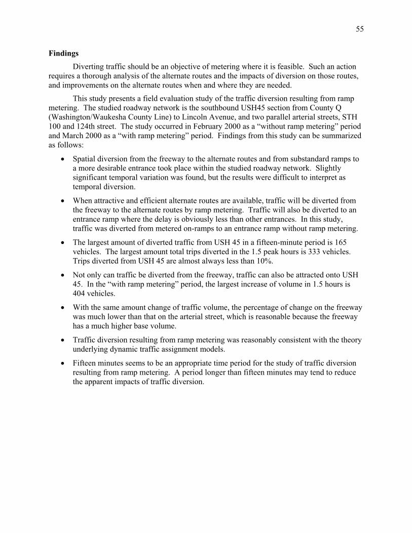
55

Findings

Diverting traffic should be an objective of metering where it is feasible. Such an action

requires a thorough analysis of the alternate routes and the impacts of diversion on those routes,

and improvements on the alternate routes when and where they are needed.

This study presents a field evaluation study of the traffic diversion resulting from ramp

metering. The studied roadway network is the southbound USH45 section from County Q

(Washington/Waukesha County Line) to Lincoln Avenue, and two parallel arterial streets, STH

100 and 124th street. The study occurred in February 2000 as a “without ramp metering” period

and March 2000 as a “with ramp metering” period. Findings from this study can be summarized

as follows:

Spatial diversion from the freeway to the alternate routes and from substandard ramps to

a more desirable entrance took place within the studied roadway network. Slightly

significant temporal variation was found, but the results were difficult to interpret as

temporal diversion.

When attractive and efficient alternate routes are available, traffic will be diverted from

the freeway to the alternate routes by ramp metering. Traffic will also be diverted to an

entrance ramp where the delay is obviously less than other entrances. In this study,

traffic was diverted from metered on-ramps to an entrance ramp without ramp metering.

The largest amount of diverted traffic from USH 45 in a fifteen-minute period is 165

vehicles. The largest amount total trips diverted in the 1.5 peak hours is 333 vehicles.

Trips diverted from USH 45 are almost always less than 10%.

Not only can traffic be diverted from the freeway, traffic can also be attracted onto USH

45. In the “with ramp metering” period, the largest increase of volume in 1.5 hours is

404 vehicles.

With the same amount change of traffic volume, the percentage of change on the freeway

was much lower than that on the arterial street, which is reasonable because the freeway

has a much higher base volume.

Traffic diversion resulting from ramp metering was reasonably consistent with the theory

underlying dynamic traffic assignment models.

Fifteen minutes seems to be an appropriate time period for the study of traffic diversion

resulting from ramp metering. A period longer than fifteen minutes may tend to reduce

the apparent impacts of traffic diversion.

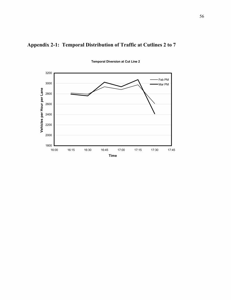
56

Appendix 2-1: Temporal Distribution of Traffic at Cutlines 2 to 7

Temporal Diversion at Cut Line 2

1800

2000

2200

2400

2600

2800

3000

3200

16:00 16:15 16:30 16:45 17:00 17:15 17:30 17:45

Time

Ve

hic

les

pe

r H

ou

r p

er

La

ne

Feb PM

Mar PM

57

Temporal Diversion at Cut Line 3

1800

2000

2200

2400

2600

2800

3000

3200

16:00 16:15 16:30 16:45 17:00 17:15 17:30 17:45

Time

Ve

hic

les

pe

r H

ou

r p

er

La

ne

Feb PM

Mar PM

Temporal Diversion at Cut Line 4

1800

2000

2200

2400

2600

2800

3000

3200

16:00 16:15 16:30 16:45 17:00 17:15 17:30 17:45

Time

Ve

hic

les

pe

r H

ou

r p

er

La

ne

Feb PM

Mar PM

58

Temporal Diversion at Cut Line 5

1800

2000

2200

2400

2600

2800

3000

3200

16:00 16:15 16:30 16:45 17:00 17:15 17:30 17:45

Time

Ve

hic

les

pe

r H

ou

r p

er

La

ne

Feb PM

Mar PM

Temporal Diversion at Cut Line 6

1800

2000

2200

2400

2600

2800

3000

3200

16:00 16:15 16:30 16:45 17:00 17:15 17:30 17:45

Time

Ve

hic

les

pe

r H

ou

r p

er

La

ne

Feb PM

Mar PM

59

Temporal Diversion at Cut Line 7

1800

2000

2200

2400

2600

2800

3000

3200

16:00 16:15 16:30 16:45 17:00 17:15 17:30 17:45

Time

Ve

hic

les

pe

r H

ou

r p

er

La

ne

Feb PM

Mar PM

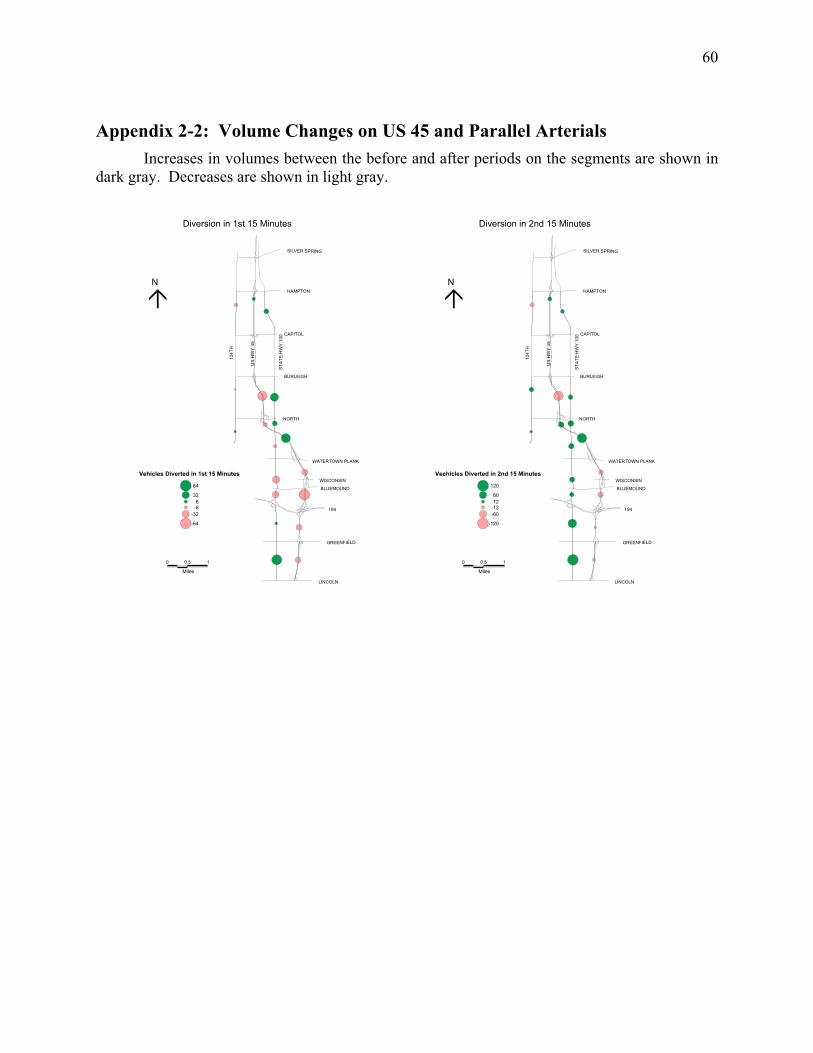
60

Appendix 2-2: Volume Changes on US 45 and Parallel Arterials

Increases in volumes between the before and after periods on the segments are shown in

dark gray. Decreases are shown in light gray.

0 0.5

Miles

1

WATERTOWN PLANK

BLUEMOUND

WISCONSIN

BURLEIGH

NORTH

ST

AT

E H

WY

10

0

US

HW

Y 4

5

12

4T

H

CAPITOL

I 94

GREENFIELD

LINCOLN

HAMPTON

SILVER SPRING

Diversion in 1st 15 Minutes

Vehicles Diverted in 1st 15 Minutes

64

32

6-6

-32

-64

N

0 0.5

Miles

1

WATERTOWN PLANK

BLUEMOUND

WISCONSIN

BURLEIGH

NORTH

ST

AT

E H

WY

10

0

US

HW

Y 4

5

12

4T

H

CAPITOL

I 94

GREENFIELD

LINCOLN

HAMPTON

SILVER SPRING

Diversion in 2nd 15 Minutes

Vechicles Diverted in 2nd 15 Minutes

120

60

12-12

-60

-120

N

61

0 0.5

Miles

1

WATERTOWN PLANK

BLUEMOUND

WISCONSIN

BURLEIGH

NORTH

ST

AT

E H

WY

10

0

US

HW

Y 4

5

12

4T

H

CAPITOL

I 94

GREENFIELD

LINCOLN

HAMPTON

SILVER SPRING

Diversion in 3rd 15 Minutes

Vechicles Diverted in 3rd 15 Minutes

83

42

8-8

-42

-83

N

0 0.5

Miles

1

WATERTOWN PLANK

BLUEMOUND

WISCONSIN

BURLEIGH

NORTH

ST

AT

E H

WY

10

0

US

HW

Y 4

5

12

4T

H

CAPITOL

I 94

GREENFIELD

LINCOLN

HAMPTON

SILVER SPRING

Diversion in 4th 15 Minutes

Vechicles Diverted in 4th 15 Minutes

140

70

14-14

-70

-140

N

0 0.5

Miles

1

WATERTOWN PLANK

BLUEMOUND

WISCONSIN

BURLEIGH

NORTH

ST

AT

E H

WY

10

0

US

HW

Y 4

5

12

4T

H

CAPITOL

I 94

GREENFIELD

LINCOLN

HAMPTON

SILVER SPRING

Diversion in 5th 15 Minutes

Vechicles Diverted in 5th 15 Minutes

94

47

9-9

-47

-94

N

0 0.5

Miles

1

WATERTOWN PLANK

BLUEMOUND

WISCONSIN

BURLEIGH

NORTH

ST

AT

E H

WY

10

0

US

HW

Y 4

5

12

4T

H

CAPITOL

I 94

GREENFIELD

LINCOLN

HAMPTON

SILVER SPRING

Diversion in 6th 15 Minutes

Vechicles Diverted in 6th 15 Minutes

170

85

17-17

-85

-170

N

62

Appendix 2-3: Volume Changes on Selected US 45 Ramps

Increases in volumes between the before and after periods on the ramps are shown in

dark gray. Decreases are shown in light gray.

0 1

Miles

2

NORTH

BURLEIGH

US

HW

Y 4

5

ST

AT

E H

WY

10

0

12

4T

H CAPITOL

HAMPTON

SILVER SPRING

GOOD HOPE

WATERTOWN PLANK

WISCONSINBLUEMOUND

GREENFIELD

LINCOLN

I 94

PIL

GR

IM

COUNTY LINE

MAIN

Vehicles Diverted in 1st 15 Minutes

13

7

1-1

-7

-13

Diversion in 1st 15 Minutes on Entrance Ramps

N

0 1

Miles

2

NORTH

BURLEIGH

US

HW

Y4

5

ST

AT

EH

WY

10

0

12

4T

H CAPITOL

HAMPTON

SILVER SPRING

GOOD HOPE

WATERTOWN PLANK

WISCONSINBLUEMOUND

GREENFIELD

LINCOLN

I 94

PIL

GR

IM

COUNTY LINE

MAIN

Vehicles Diverted in 2nd 15 Minutes

42

21

4-4

-21

-42

Diversion in 2nd 15 Minutes on Entrance Ramps

N

63

0 1

Miles

2

NORTH

BURLEIGH

US

HW

Y4

5

ST

AT

EH

WY

10

0

12

4T

H CAPITOL

HAMPTON

SILVER SPRING

GOOD HOPE

WATERTOWN PLANK

WISCONSINBLUEMOUND

GREENFIELD

LINCOLN

I 94

PIL

GR

IM

COUNTY LINE

MAIN

Vehicles Diverted in 3rd 15 Minutes

25

12

2-2

-12

-25

Diversion in 3rd 15 Minutes on Entrance Ramps

N

0 1

Miles

2

NORTH

BURLEIGH

US

HW

Y4

5

ST

AT

EH

WY

10

0

12

4T

H CAPITOL

HAMPTON

SILVER SPRING

GOOD HOPE

WATERTOWN PLANK

WISCONSINBLUEMOUND

GREENFIELD

LINCOLN

I 94

PIL

GR

IM

COUNTY LINE

MAIN

Vehicles Diverted in 4th 15 Minutes

39

20

4-4

-20

-39

Diversion in 4th 15 Minutes on Entrance Ramps

N

0 1

Miles

2

NORTH

BURLEIGH

US

HW

Y4

5

ST

AT

EH

WY

10

0

12

4T

H CAPITOL

HAMPTON

SILVER SPRING

GOOD HOPE

WATERTOWN PLANK

WISCONSINBLUEMOUND

GREENFIELD

LINCOLN

I 94

PIL

GR

IM

COUNTY LINE

MAIN

Vehicles Diverted in 5th 15 Minutes

43

22

4-4

-22

-43

Diversion in 5th 15 Minutes on Entrance Ramps

N

0 1

Miles

2

NORTH

BURLEIGH

US

HW

Y4

5

ST

AT

EH

WY

10

0

12

4T

H CAPITOL

HAMPTON

SILVER SPRING

GOOD HOPE

WATERTOWN PLANK

WISCONSINBLUEMOUND

GREENFIELD

LINCOLN

I 94

PIL

GR

IM

COUNTY LINE

MAIN

Vehicles Diverted in 6th 15 Minutes

58

29

6-6

-29

-58

Diversion in 6th 15 Minutes on Entrance Ramps

N

64

Chapter 3

Ramp Meters Relation to Freeway Segment Trip Length

Diversion Propensity of Wisconsin Drivers

A series of questions related to diversion from ramp meters was administered to a random

sample of Wisconsin drivers as part of a larger study of variable message signs. A total of 221

valid questionnaires were returned. The portion of the questionnaire that contains the diversion

questions is shown in Figure 3-1.

Figure 3-1. Questions Related to Ramp Meters from Questionnaire Administered to Wisconsin

Drivers

65

The analysis of diversion required that Question 18 (“Are there ramp meters on any of

the routes you travel most frequently?”) be answered yes. After selecting those respondents and

eliminating any respondents who failed to answer any part of question 22 (Would you take one

of these alternative routes?), there were 91 remaining questionnaires.

Table 3-1 contains collective responses to each of the questions yes/no questions, except

question 18.

Table 3-1. Summary of Responses from Yes/No Questions

Question (Shortened) Percent indicating “Yes”

20. Aware of alternate routes 72%

21. Idea of how long the trip 65%

22a. Divert if ramp empty 15%

22b. Divert if ramp half full 24%

22c. Divert if ramp nearly full 62%

22d. Divert if ramp overflowing 82%

The average trip length (Question 19) across all valid respondents is 25.5 minutes. It is

interesting that most drivers who encounter a ramp meter on a frequent trip are aware of an

alternative route and have a good idea of how long that alternative route will take.

Of greatest interest are the responses to question 22, as this question establishes a

relationship between a driver’s propensity to divert and the length of queue at a ramp meter.

Question 22 asks drivers for their stated preference and does not necessarily predict actual

behavior. Table 3-1 suggests that drivers are quite sensitive to the length of the queue at the

ramp meter, with only a few drivers stating they would divert even if there is no queue. Many of

these drivers are probably already taking the alternative route.

Table 3-2 compares average trip length between drivers who divert and drivers who do

not divert for each of the four queue lengths of Question 22.

Table 3-2. Average Trip Lengths for Diverted and Not Diverted Trips from All Respondents

Queue Length Question

(Shortened)

Average Trip Length

for Drivers Who Divert

(Minutes)

Average Trip Length

for Drivers Who Do Not

Divert (Minutes)

22a. Divert if ramp empty 16.5 27.1

22b. Divert if ramp half full 21.5 26.7

22c. Divert if ramp nearly full 26.9 23.2

22d. Divert if ramp overflowing 25.9 23.8

For each part of question 22, the two means are not significantly different within a 95%

confidence using the t-test. Nonetheless, there is a pattern in the data that suggests that drivers

are more likely to divert when their trips are short. A larger sample size would be needed to

validate this hypothesis.

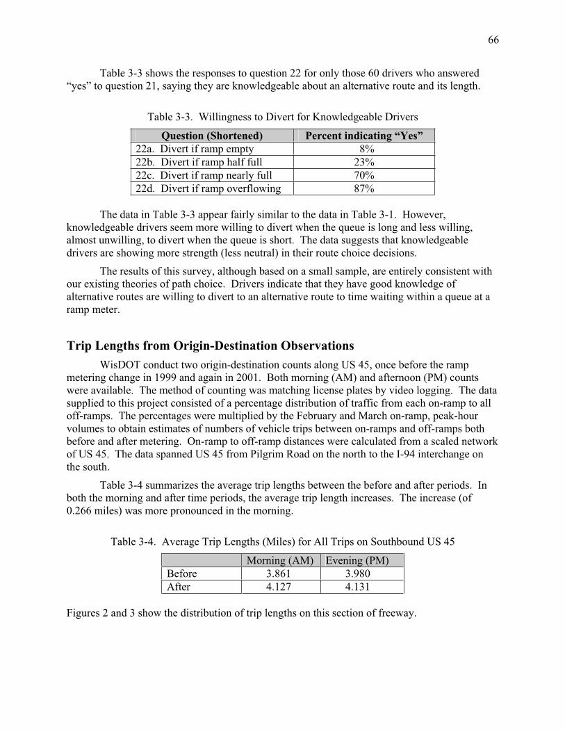
66

Table 3-3 shows the responses to question 22 for only those 60 drivers who answered

“yes” to question 21, saying they are knowledgeable about an alternative route and its length.

Table 3-3. Willingness to Divert for Knowledgeable Drivers

Question (Shortened) Percent indicating “Yes”

22a. Divert if ramp empty 8%

22b. Divert if ramp half full 23%

22c. Divert if ramp nearly full 70%

22d. Divert if ramp overflowing 87%

The data in Table 3-3 appear fairly similar to the data in Table 3-1. However,

knowledgeable drivers seem more willing to divert when the queue is long and less willing,

almost unwilling, to divert when the queue is short. The data suggests that knowledgeable

drivers are showing more strength (less neutral) in their route choice decisions.

The results of this survey, although based on a small sample, are entirely consistent with

our existing theories of path choice. Drivers indicate that they have good knowledge of

alternative routes are willing to divert to an alternative route to time waiting within a queue at a

ramp meter.

Trip Lengths from Origin-Destination Observations

WisDOT conduct two origin-destination counts along US 45, once before the ramp

metering change in 1999 and again in 2001. Both morning (AM) and afternoon (PM) counts

were available. The method of counting was matching license plates by video logging. The data

supplied to this project consisted of a percentage distribution of traffic from each on-ramp to all

off-ramps. The percentages were multiplied by the February and March on-ramp, peak-hour

volumes to obtain estimates of numbers of vehicle trips between on-ramps and off-ramps both

before and after metering. On-ramp to off-ramp distances were calculated from a scaled network

of US 45. The data spanned US 45 from Pilgrim Road on the north to the I-94 interchange on

the south.

Table 3-4 summarizes the average trip lengths between the before and after periods. In

both the morning and after time periods, the average trip length increases. The increase (of

0.266 miles) was more pronounced in the morning.

Table 3-4. Average Trip Lengths (Miles) for All Trips on Southbound US 45

Morning (AM) Evening (PM)

Before 3.861 3.980

After 4.127 4.131

Figures 2 and 3 show the distribution of trip lengths on this section of freeway.

67

0.0%

2.0%

4.0%

6.0%

8.0%

10.0%

12.0%

14.0%

16.0%

18.0%

20.0%

1 2 3 4 5 6 7 8 9 10 11

Distance (miles)

Tri

ps

% 1999 AM

2001 AM

Figure 3-2. Trip Length Distribution on US 45, both Before and After Ramp Metering, Morning

0.0%

2.0%

4.0%

6.0%

8.0%

10.0%

12.0%

14.0%

16.0%

18.0%

20.0%

1 2 3 4 5 6 7 8 9 10 11

Distance (miles)

Tri

ps

% 1999 PM

2001 PM

Figure 3-3. Trip Length Distribution on US 45, both Before and After Ramp Metering,

Afternoon

68

These figures indicate that there is a reduced number of very short trips, both during the

morning and afternoon periods. Otherwise, there are no obvious patterns in the data.

69

Chapter 4

Methods for Evaluating Ramp Meters in Milwaukee: Case

Studies of Microscopic and Macroscopic Models

Introduction

A simulation model allows traffic engineers to create and evaluate scenarios and

alternatives during the planning phase of a traffic system modification in order to optimize traffic

controls. This study presents an assessment of two existing traffic simulation software packages,

in order to identify which class of model can potentially be most useful in ramp metering

simulation analysis.

Problem Summary

During the past three decades the Milwaukee area freeway system has been enhanced

with the deployment of ramp meters on most on-ramps. The deployment of more meters along

US Highway 45 in March of 2000 provided an opportunity to study the impacts before and after

the implementation. There were only five meters working along US 45 in February of 2000 in

the following on-ramps: Good Hope loop; Good Hope slip; North Avenue; Watertown Road;

Wisconsin Avenue; and Greenfield Avenue. In March of the same year, WisDOT deployed

seven new meters along all but one of the remaining on-ramps of this freeway: County Q;

Pilgrim Road; Main Street; Appleton Avenue; Hampton Avenue; Capitol Drive; and Burleigh

Street. As expected, there were some flow rate variations on the freeway and on the arterials

next to it. An earlier study recorded traffic counts of the whole corridor from the before

(February 2000) and after (March 2000) periods. Detector speeds and floating car speeds were

also obtained. Queue lengths were recorded at all of the ramp meters. Additionally, there were

two origin-destination tables obtained by video logging for periods about one year before and

one year after the deployment.

The data obtained makes it possible to evaluate ramp meter’s benefits directly or by using

simulation models. Currently, WisDOT is in the early stages of developing a model of the whole

Milwaukee area freeway system with a microscopic simulation program called Paramics. This

model, at present, does not contain any ramp meters. Paramics could be used for ramp metering

evaluation, but it first needs validation for this application. A comparison of a model’s

calculations with data other than those used in estimating the model is required in order to

reliably use this simulation model to forecast future traffic behavior.

Types of Ramp Metering Systems

There are three major types of ramp meters.

Fixed time operation that has the basic function to break down platoons and smooth out

fluctuations in entering traffic volumes.

Traffic responsive control where timing is based on the actual freeway conditions in the

vicinity of the ramp, with the idea of storing vehicles on the ramp to provide more

efficient downstream traffic flow.

70

System-wide control where timing is traffic responsive to total freeway conditions and

optimizes traffic flow across the whole system.

Milwaukee implements the second type of ramp meter control. The Milwaukee ramp

meter algorithm will be fully explained later.

Under all three forms of ramp meter control maximum discharge rate of a single metered

lane is about 900 vehicles per hour (vph). This capacity is based on a minimum reasonable cycle

length of 4 seconds: 2.5 seconds of red and 1.5 seconds of green. By increasing the cycle to 6

seconds or 6.5 seconds two vehicles can be served from adjacent lanes, thereby increasing the

discharge rate to 1100 or 1200 vph. A maximum discharge per lane of 1800 vph can be

produced when the meter permits one or two vehicles per green and the ramp has two or more

lanes at the meter. Drivers will not wait more than 15 seconds, so the most restrictive rate is

about 240 vph (Piotrowicz and Robinson, 1995).

Scope of Chapter

This chapter reviews three major software products for simulating freeway systems with

ramp meters: Paramics, QRS II and Dynasmart-P. Two of these products (Paramics and QRS

II) are used to build models of US 45, both before and after the deployment of ramp meters.

These models are tested against ground data with a minimum of calibration to similar data in

order to obtain a relatively hands-free validation. Once built, the models can show the travel

time savings benefits of ramp meter deployment and provide other measures of effectiveness.

71

Microscopic, Mesoscopic and Macroscopic Models for Freeway Ramp Meter

Operation

This section describes the three models considered for evaluating the benefits of ramp

meters. In addition, a short review of origin destination trip (OD) matrix estimation is provided,

because of the need to develop a good time-dependent OD table for each of the three models.

Traffic simulation models can be classified as either microscopic, macroscopic or

mesoscopic (Boxill and Yu, 2000). Microscopic models predict and analyze the path of

individual vehicles throughout the system; their results are based on the average of all vehicles

modeled. These models require an extreme amount of input data, consequently these models are

most often used in small areas. Macroscopic models forecast traffic flows; they concentrate on

groups of vehicles that are more general and whose results are group-wide or area-wide.

Macroscopic models are mostly used in large area networks. Mesoscopic models have aspects of

both microscopic and macroscopic models.

In this study three different software packages are reviewed. Paramics (microscopic),

Dyanasmart-P (mesoscopic) and Quick Response System II, QRS II (macroscopic). These

models are each respected representatives of their class.

Paramics: Microsimulation Software

Paramics is an example of a traffic microsimulation software package, of which there are

many available. This software package was selected for this study because WisDOT has adopted

it for its current evaluation of the Milwaukee area freeway system.

Traffic demands are given to Paramics in the form of a zone-to-zone OD (origin-

destination) trip matrix. The software simulates the movements and behavior of individual

vehicles on a given traffic network. Paramics consists of three parts: a Modeller, a Processor

and an Analyzer. The Modeller uses a GUI (graphical user interface) to visualize the simulation

of the traffic flow on the network. The Processor simulates the traffic situation without the GUI,

thereby increasing simulation speed when numerous tests are required. The Analyzer reads and

analyzes the simulation outputs, providing graphics to compare the results.

To perform the traffic simulation, Paramics requires a time-dependent OD trip matrix.

The trips are represented from zone to zone and are separated into vehicle types and into time

slices as small as 5 minutes. Vehicle trips are not loaded at centroids but directly to links. The

number of trips between any origin and any destination is used to create a probability that a trip

is made during a time slice, so that vehicle trips can be randomly created. Parking lots can be

used as origin or destination points.

A traffic assignment is applied to all vehicles except fixed route vehicles, such as buses.

Route choice in Paramics depends upon network coding, link cost factors, sign posted routes,

lane and turn restrictions, model parameters, generalized cost coefficients, percent of familiar

drivers and default parking origin/destination assumptions.

A major feature of Paramics is its application programmer’s interface (API) that allows

customization of the simulation to local traffic controls, conditions and future ITS options.

72

Paramics uses one of three assignment methods: stochastic, dynamic feedback or all-or-

nothing.

All-or-nothing assignment: This assignment method assumes that drivers traveling from

zone A to zone B choose the same shortest path using a cost function based on free flow

speed, distance and tolls. Path choice is also influenced by assumptions about driver

familiarity with the route.

Stochastic: This assignment method chooses paths randomly for each vehicle based on

assumptions about driver’s perceptions of the shortest path and variability in travel costs.

Path choice is re-evaluated at every node encountered along the trip.

Dynamic Feedback: At each time slice the amount of congestion is estimated. The

algorithm re-routes the remaining parts of a trip for a familiar driver, given assumptions

about the driver’s perceptions of the new traffic situation.

Driver Behavior: Paramics documentation states, “The movement of individual vehicles

is governed by three interacting models representing vehicle following, gap acceptance and lane

changing. Vehicle dynamics are relatively simple, combining a mixture of driver behavior and

some limitations based on vehicles' physical type and kinematics (e.g., size,

acceleration/deceleration). These models are applied simultaneously at the level of individual

vehicles.” Consequently, each simulation is unique; i.e., the same inputs can have different

results.

Geometry and Controls: Paramics allows a wide variety of road geometries, vehicle

restrictions and intersection controls to be placed on the network, including detector locations.

Paramics does not provide for a large array of ITS elements. However, Paramics can create

random incidents and evaluate the performance of the traffic systems with such incidents.

Paramics also has the capacity to simulate the effects of variable message signs, provided that the

user specifies a set of compliance rules. Unlike some other microsimulation packages, Paramics

can handle very large arterial networks.

Paramics sets the timing for actuated traffic signals by programming language code,

written by the user, that controls temporary and permanent changes to timings. For each

particular signal, the user must design a “plan”. The plan includes a set of loop detectors and an

optional set of parameters. Each plan is given the phases that would be controlled by that plan.

The programming language is C-like. The “if-then-else” statements are used in this language.

The following program is an example of fixed-time ramp metering taken from the

Paramics Modeller user guide.

73

This plan assumes a two-phase signal, with one phase all green (red time is zero) and the

other phase all red (green time is zero). This plan is applied to the all red phase. A fixed-time

ramp metering policy is implemented if a vehicle is detected on a loop. If no vehicle is present

the signal is on green permanently, which is equivalent to “meter-off” conditions.

Link speed is calculated according to mean speed. It represents the average speed of all

vehicles traversing the link in the current time step. Particularly, the speed calculation is as

follows.

link speed = link length / actual time

Link delay is calculated according to absolute delay. The units for delay are seconds, and

delay is calculated as the actual time taken by vehicles to traverse the link minus their free flow

time. Specifically:

min speed= the smaller of link and vehicles maximum speed

free flow time = link length / min speed

link delay = actual time – free flow time

Travel Forecasting with Integrated Macroscopic Traffic Simulation: QRS II

The Quick Response System II (QRS II) is a travel forecasting software package, which

performs macroscopic traffic simulation and uses the four-step travel demand process (trip

generation, trip distribution, mode split and traffic assignment). Several minor steps are included

in the model such as activity allocation, auto occupancy and time of day simulation. QRS II uses

the traffic analysis procedures from the Highway Capacity Software (HCS) and other sources.

Plan count 1

Plan 1 definition

Loops 1

Parameters 1

If (init) { variable;

}

If (occupied[1])

{

red3 =

parameter[1];

}

else

{

74

Refer to Figure 4-1 for a flow diagram of conventional travel forecasting models, including QRS

II.

Trip Generation

Trip Distripution

Mode Split

All-or-Nothing

Traffic

Assignment

Activity

Allocation

Measures of

Effectiveness

Volume

Averaging and

Delay

Calculations

Transit

Assignment

Figure 4-1. Flow Diagram of a Typical Travel Forecasting Model

QRS II has the ability to work with any trip generation model because it is possible for

the user to supply the mathematical expressions for it. Also QRS II has default the trip

generation rates and procedures from the National Cooperative Highway Research Program

(NCHRP) Reports #187 and #365.

Trip distribution primarily works with the gravity model, which is a method analogous to

Newton’s law of gravity. The gravity model is used to allocate trips between a pair of zones

depending on the proximity between them and the overall levels of trip making activity in each

zone.

75

The multinomial logit model is used in the mode split step. Based on trip utility, the

proportion of trips choosing a particular mode is assigned to that mode. The modes can be

automobile, generalized transit and a user-defined third mode.

Automobile occupancy is a minor step done by QRS II in which factors are applied to

person trips that can change by time of day. Also, a long range forecast simulation could be

performed by QRS II by using the optional land-use forecasting module.

The traffic assignment step uses a static user-optimal equilibrium traffic assignment. The

specific algorithm recommend for the software is the method of successive averages MSA. In

this study, an experimental version of QRS II is used. This version performs dynamic traffic

assignment. The software is able to assign traffic in time slices depending on the demand

percentage applied for each time slice.

QRS II uses the Bureau of Public Roads (BPR) curve to obtain travel times on

uninterrupted facilities, such as freeways and uncontrolled long portions of the arterial streets.

QRS II comes with its own network editor. The General Network Editor (GNE) is used

in order to represent the network characteristics.

Ramp meters are represented in QRS II as one-way streets. The lane geometry and sign

code must be set to “M” for a two-lane on-ramp, and an “m” for a one lane on-ramp.

In 1994, John A. Biebetitz developed a macroscopic ramp metering delay and queuing

model in a master’s thesis called “Area wide Impacts of Ramp Metering”. This study

determined the area wide impacts of different ramp metering plans. A new delay model was

developed at the same time because of the lack of a macroscopic ramp metering delay/queuing

model. The ramp metering delay/queuing model was included in QRS II giving satisfactory

results after testing different ramp meters schemes with it.

In QRS II, delay calculations are made depending upon volume/capacity (V/C) ratio. For

high V/C (>>1) storage will occur over an extended period of time, up to one full hour. For low

V/C (<<1) queues occasionally form due to the randomness of vehicles arrivals. And for a V/C

near 1, QRS II interpolates between both of the above.

The storage delay model in QRS II is based on a cumulative flow diagram to handle

stored vehicles. The delay on the ramp due to queuing during saturated conditions corresponds

to the shaded area in Figure 4-2. To calculate delay it is required that the arrival and departure

lines meet at the end of the period of analysis (T). The arrival line represents the demand and the

departure line represents the metering rate. This type of delay occurs only when the

volume/capacity ratio is greater than 1.0 (Bieberitz, 1994). For delay when the volume to

capacity ratio is less than 1, QRS II uses an M/G/1 queuing model with constant service times.

76

Figure 4-2. Graphical Representation of On-Ramp Queuing and Delay Used by QRS II

These delays are included in the link travel times in addition to the acceleration delay,

red-time delay, and travel time on the link where the ramp meter is placed.

QRS II requires the user to set two important parameters for the ramp meter

representation, the metered period fraction and the meter volume fraction. The metered period

fraction is an approximation of peaking characteristics. It is the fraction of the time period,

typically 1 hour, that is metered at the rate given in the capacity attribute. A higher meter rate is

used to discharge a queue. The meter volume fraction is the fraction of the time period’s volume

that occurs during the metered period. The critical attribute of each ramp meter is the meter rate.

QRS II does not represent a traffic responsive ramp meter. It is necessary to manually set the

meter rate, which is the same as the capacity of the ramp meter.

QRS II generates a file where the measures of effectiveness (MOEs) are shown. This file

provides the general results of speeds, vehicle-hours-traveled, vehicle-miles-traveled and vehicle

emissions for the whole system.

It is possible for QRS II to be run as a subroutine of another computer program, such as

one that is intended to optimize traffic control strategies.

Mesoscopic Traffic Simulator with Dynamic Traffic Assignment: Dynasmart-P

Dynasmart-P is an example of a mesoscopic traffic simulation with dynamic traffic

assignment. Dynasmart-P is one of two, essentially duplicative, software products being

developed by the TrEPS (Traffic Estimation and Prediction System) project sponsored by the

Federal Highway Administration. Its forerunner, Dynasmart, has been used for many years at

the University of Texas at Austin and elsewhere for research purposes.

Dynasmart-P is a software package that allows users to simulate and evaluate the design

and planning of traffic in intelligent transportation networks. The software is able to simulate

Time

D

Cumulative Vehicles

E

C

B

A

TaTTo

Cumulative Arrivals

Cumulative Departures

F

Slope = Demand=Volume

Slope=Capacity=Meter Rate

77

most driver behavior within a network, such as variations of traffic flow patterns over time and

drivers’ routing decisions. Dynasmart-P allows calculating for each of many short time slices

the speeds, densities, queues, vehicles trajectories and different characteristics of every link in

the network. The software has capabilities to evaluate an array of operational strategies,

including ATMS (Advanced Transportation Management System) strategies, HOV facilities,

ramp meters and special use lanes. Dynasmart was developed for short-term forecasting of

traffic in real-time; Dynasmart-P is a version of Dynasmart for the purposes of traffic planning.

Dynasmart-P simulates intelligent transportation networks using two different methods of

vehicle generation. The first method requires the user to specify origin and destination trip

matrices, aggregated to zones, for different demand time slices. The second requires the user to

specify the characteristics of vehicles, their stops and their corresponding travel times.

The vehicles generated can be assigned in two different ways. The first way is “one step

simulation assignment”, in which all vehicles are individually assigned to its currently best path,

a random path among a limited set of shortest paths or any predetermined path. The second way

is “iterative simulation assignment” in which Dynasmart-P applies dynamic user-optimal

equilibrium assignment using MSA. MSA is applied to time slices as short as 1 minute, with

different demands and different network characteristics applicable to each slice.

Dynasmart-P is able to evaluate traffic management strategies such as ramp metering,

variable message signs (VMS) and path and corridor coordination. Dynasmart-P can also

calculate congestion pricing for regular links, HOV links and HOT (high occupancy toll) links.

It can simulate incidents, including their starting time, ending time, location and severity.

Dynasmart-P also has the ability to find system optimal traffic assignments, which can

serve as upper bounds on the benefits that might be achieved by rerouting traffic to avoid

incidents or other random traffic events.

Dynasmart-P assumes that ramp metering follows the ALINEA procedure (Papageorgiou,

Hadj-Salem and Middelham, 1997). ALINEA is a traffic responsive feedback process where the

metering rate is set according to the occupancy at a point downstream on the mainline. To

evaluate ramp metering in a network it is necessary to create a text file in which the following

data items must be included: the number of ramps, the frequency in which the ramp metering is

checked by the simulator, and the location of two detectors downstream from the meter.

Dynasmart-P also asks for two constants required by ALINEA for each ramp that are used to

determine the ramp’s meter rate. The first constant is the target occupancy (defaulted to 0.2);

ALINEA will adjust the metering rate in an attempt to achieve this occupancy value. The second

constant relates to how much the metering rate changes for a given difference between the actual

occupancy and the target (defaulted to 0.32 vehicles per minute per lane per difference in

occupancy from target). Also required are the time slices in which the ramp metering is effective

and the ramp saturation flow rate. The ALINEA procedure calculates, at each period T=1,2,3…,

the rate as follows:

]2[1)()1( OccConsConsTRateTRate

Where Cons1= 0.32 or as externally specified, Cons2=0.2 or externally specified, Occ is the

upstream occupancy, and Rate is the measurable on ramp traffic volume (5 veh/min-lane < Rate

(t) < 25-35 veh/min-lane).

78

Dynasmart-P is not being used in this study because of the following reasons.

Dynasmart-P uses a traffic responsive algorithm called ALINEA to determine ramp

meter rates. This software cannot replicate the WisDOT meter rates because its

algorithm uses different thresholds and different loop detector locations for the meter rate

calculation.

Dynasmart-P uses the same dynamic traffic assignment procedure found in QRS II.

Thus, having more knowledge about the use of QRS II, the results obtained would be

more reliable.

The Dynasmart-P software requires text files for all its data inputs. Convenient network

or data editors are not available at this time, although it is possible to edit many text files

within Dynasmart-P’s graphical user interface. The time and resources necessary to code

a network from scratch and provide all the necessary input data are substantial. Network

data can be converted from other sources, such as a GISs (geographic information

systems), CORSIM (a microscopic simulation model) and several planning models.

To effectively use the dynamic aspects of the software, it is necessary to supply complete

OD trip tables for very small time slices. Dynasmart-P eases this data requirement

somewhat by allowing the user to factor a static OD trip table into time slices, but it does

not contain algorithms for creating a static OD trip table from planning data.

OD Matrix Estimation

All three models must be provided with a trip table in order to represent trips between

zones during the simulation. When the only reliable data available is traffic counts, it is possible

to obtain an OD trip matrix using the generalized least squares (GLS) technique. In summary,

the GLS technique finds a final OD trip matrix obtained from a target OD trip matrix that is

assumed to contain probabilistic error. The objective is to obtain the OD trip matrix most

matching the link counts and closest to the target OD trip matrix.

It is possible that the obtained OD trip matrix does not precisely reproduce all traffic

counts. This is caused by irregularities in traffic counts caused during the traffic flow data

collection at different times or from an aggregated transportation network representation

(Abrahamsson, 1998).

Model Framework

Evaluation Background

Ground data for this study was collected for two different time periods. Data from

February of 2000 are the “before” period which represents “without ramp metering”, and data

from March of 2000 represent the “after” period or “with ramp metering”.

The corridor of study is US Highway 45. This urban freeway is located at the west side

of the Milwaukee metropolitan area. The study section is the southbound lanes of US Highway

45 from Good Hope Road to a point just past Wisconsin Avenue. The section of freeway north

79

of Good Hope was removed from the study because ground data revealed little congestion and

this section had been omitted from WisDOT’s Paramics model.

The ramp meters working in the before period (February) were located at the following

on-ramps:

Good Hope Road (loop);

Good Hope Road (slip);

North Avenue;

Watertown Road; and

Wisconsin Avenue.

In March, more meters were added at the following on-ramps:

Appleton Avenue;

Hampton Avenue;

Capitol Drive; and

Burleigh Street.

Silver Spring Drive was the only on-ramp that did not have a meter in either the before or after

period.

Data Preparation and Calibration

It is necessary to build an OD (origin-destination) trip matrix that replicates the traffic

counts recorded by WisDOT. There are two trip matrices, one for the before period (February

2000), and the other for the after period (March 2000). The generalized least squares (GLS)

technique is used for this estimation.

The data sample of OD trips that was obtained from the video logging gave a distribution

percentage table that did not match well with the traffic counts for the PM peak hour. Video

logging misses a large percentage of vehicles, either entering or leaving the freeway. In addition,

the detectors and road tubes used to get traffic counts have their own errors.

Given that these tables are the only distribution of vehicles to off-ramps available, it was

necessary to adjust them using the GLS technique to better match ground data. Each crossing

street that has access to US Highway 45 is assumed to be a zone. The on-ramp volumes are the

number of trips, whose origin is the corresponding zone and the off-ramp volumes are the

number of trips, whose destination is to that zone.

The following problems were found at the beginning of this process.

Some data was missing, such as entering volumes and mainline volumes.

The mainline volumes did not agree with the entering and exiting volumes.

Table 4-1 shows this percentage distribution table for the before period. Table 4-2 shows the

new distribution percentages matrix where the last three columns are aggregated to just one

downstream zone. An OD trip table is obtained by multiplying those percentages by the

upstream zone volumes and by the on-ramps volumes.

80

Tab

le 4

-1. D

istr

ibuti

on P

erce

nta

ges

fro

m Z

one

to Z

one

(Raw

)

Upstream

Zone

Good Hope

Road

Appleton

Avenue

Silver Spring

Drive

Hampton

Avenue

Capitol Drive

Burleigh

Street

North Avenue

Watertown

Plank Rd

Wisconsin

Avenue

I94 West

I94 East

Greenfield

Downstream

Zone

Up

stre

am

Zo

ne

04

.49

1.8

63

.36

5.5

91

2.6

81

1.9

35

.92

5.9

75

.59

13

.79

22

.75

5.9

74

2.5

1

Go

od

Ho

pe R

oad

0

1.9

53

.52

5.8

61

3.2

81

2.5

6.2

6.2

55

.86

14

.45

23

.83

6.2

54

4.5

3

Ap

ple

ton

Av

en

ue

08

.16

01

5.3

11

0.2

11

.24

.08

3.0

61

2.2

42

9.5

96

.12

47

.95

Sil

ver

Sp

rin

g D

r.

00

.67

8.3

6.9

55

.62

.91

1.7

91

9.0

64

9.7

84

.93

73

.77

Ham

pto

n A

ven

ue

05

.68

4.5

3.7

31

.87

25

.33

45

.87

5.0

77

6.2

7

Cap

ito

l D

riv

e

04

.69

3.5

2.6

51

.84

26

.53

57

.35

3.4

78

7.3

5

Bu

rlei

gh

Str

eet

03

.72

.63

0.7

92

9.2

15

7.1

16

.58

92

.90

No

rth

Av

enu

e 0

0.2

71

.37

34

.34

54

.67

9.3

49

8.3

5

Wate

rto

wn

Pla

nk

Rd

0

1.4

92

8.3

35

9.4

10

.78

98

.51

Wis

con

sin

04

.36

9.3

42

6.3

71

00

.01

I94

wes

t 0

I94

Eas

t0

Gre

enfi

eld

0

Do

wn

stre

am

Zo

ne

0

Tab

le 4

-2. D

istr

ibuti

on P

erce

nta

ges

fro

m Z

one

to Z

one

(Aggre

gat

ed)

Upstream

Zone

Good Hope

Road

Appleton

Avenue

Silver Spring

Drive

Hampton

Avenue

Capitol Drive

Burleigh

Street

North Avenue

Watertown

Plank Rd

Wisconsin

Avenue

Downstream

Zone

Up

stre

am

Zo

ne

04

.49

1.8

63

.36

5.5

91

2.6

81

1.9

35

.92

5.9

75

.59

42

.51

Go

od

Ho

pe

Ro

ad

0

1.9

53

.52

5.8

61

3.2

81

2.5

6.2

6.2

55

.86

44

.53

Ap

ple

ton

Av

enu

e

08

.16

01

5.3

11

0.2

11

.24

.08

3.0

64

7.9

5

Sil

ver

Sp

rin

g D

r.

00

.67

8.3

6.9

55

.62

.91

1.7

97

3.7

7

Ham

pto

n A

ven

ue

05

.68

4.5

3.7

31

.87

76

.27

Cap

ito

l D

riv

e

04

.69

3.5

2.6

51

.84

87

.35

Bu

rleig

h S

treet

03

.72

.63

0.7

99

2.9

0

No

rth

Av

enu

e

00

.27

1.3

79

8.3

5

Wate

rto

wn

Pla

nk

Rd

0

1.4

99

8.5

1

Wis

co

nsi

n0

10

0.0

1

Do

wn

stre

am Z

on

e0

81

The OD table estimation process minimizes this function.

LinksVolj i

jijij

i j

iijij

i j

ijij VactVestDTXYOTXYXYTz2

22

22)()()1(min

where,

z is a weight factor (=1 in this case)

Tij is the original trip table,

Yj is the adjustment factor applied to destinations,

Xi is the adjustment factor applied to origins,

Oi are the origins,

Dj are the destinations,

Vest is the estimated volume on the mainline,

Vact is the actual or real volume on the mainline.

Good Hope Road has two on-ramps, a loop ramp for traffic coming from the east, and a

slip ramp for traffic coming from the west. Most of the trips coming from Good Hope use the

loop ramp; thus, one more zone was added to the system on the east side of US 45. Figure 4-3

illustrates all the zones assumed for this study.

82

Figure 4-3. Study Location and Zone System

The trips exiting Good Hope Road are assigned to the Good Hope Road slip zone. The

final OD trip matrices for the February and March periods are shown in Tables 4-3 and 4-4,

respectively.

83

Tab

le 4

-3. F

ebru

ary O

D M

atri

x

Up

str

ea

m Z

on

e0

18

93

01

41

63

39

49

42

61

21

61

28

14

31

68

1

Go

od

Ho

pe

Ro

ad

(S

lip

) 0

01

72

42

02

91

51

37

89

7

Go

od

Ho

pe

Ro

ad

(lo

op

)0

09

81

35

11

01

60

85

70

41

46

54

5

Ap

ple

ton

Av

en

ue

0

00

49

02

91

12

04

49

3

Sil

ve

r S

pr

ing

Dr

. 0

00

09

73

34

46

14

10

65

9

Ha

mp

ton

Av

en

ue

0

00

00

13

11

10

53

18

4

Ca

pit

ol

Dr

ive

0

00

00

01

41

88

74

88

Bu

rle

igh

Str

ee

t 0

00

00

00

27

11

47

39

No

rth

Av

en

ue

0

00

00

00

01

77

94

Wa

ter

tow

n P

lan

k R

d

00

00

00

00

05

52

6

Wis

co

nsin

Av

00

00

00

00

00

57

8

Do

wn

str

ea

m Z

on

e0

Tab

le 4

-4. M

arch

OD

Mat

rix

Up

str

ea

m Z

on

e0

29

42

01

27

52

64

50

02

57

19

91

43

22

31

35

2

Go

od

Ho

pe

Ro

ad

(sli

p)

00

10

14

14

26

13

10

71

27

1

Go

od

Ho

pe

Ro

ad

(L

oo

p)

00

59

80

77

14

67

55

84

26

53

95

Ap

ple

ton

Av

en

ue

0

00

52

04

71

73

08

10

12

0

Sil

ve

r S

pr

ing

Dr

. 0

00

01

01

08

49

62

23

24

77

4

Ha

mp

ton

Av

en

ue

0

00

00

24

18

16

98

25

8

Ca

pit

ol

Dr

ive

0

00

00

02

22

61

41

66

19

Bu

rle

igh

Str

ee

t 0

00

00

00

28

14

76

66

No

rth

Av

en

ue

0

00

00

00

01

11

61

6

Wa

ter

tow

n P

lan

k R

d

00

00

00

00

01

05

48

Wis

co

nsin

Av

00

00

00

00

00

48

9

Do

wn

str

ea

m Z

on

e0

84

General Issues in Modeling the Network

The simulations have two principal outputs: speeds and OD travel times. These two

measures of effectiveness (MOEs) are compared between both periods in order to determine the

effect caused by the meters. For validation purposes, it is necessary to compare the speeds given

by the models with ground data.

Both models require the percentage of vehicles released during each 15-minute period.

From the traffic counts, the percentages during the peak hour were set as follows: 25%, 26%,

25%, and 24%.

Paramics Simulation

WisDOT sketched the US 45 corridor in Paramics. They coded the mainline of the

freeway and the crossing arterials, including the off and on-ramps to the freeway. The

northbound and southbound lanes of the freeway are coded, but only the southbound lanes are

analyzed. This original network had to be changed substantially in order to represent the ramp

meters.

The following data files in Paramics must to be added for ramp meters.

Plans File: In order to set the timing for actuated signals, the user must define a “plan”

for each signal by using a programming language. The plan includes a set of loop

detectors and parameters. Each plan is given the phases that would be controlled by that

plan. Different plans can be contained in this file. An example is shown later.

Phases File: This file is used for actuated signals. It contains the node number where the

signal is located, the plan number to be applied at this node, the name of each loop used

by the plan and the value of each parameter.

Profile File: .This file defines the percentages of demand applied in each time slice

during a period of time.

Ramp meters in Paramics are represented by using a “plan file” defined by the user for a

standard traffic signal. This plan depends on the geometric characteristics of the ramp, such as

the number of lanes in the mainline before the merging area and the number of lanes before the

meter. It is possible to have different plans for different geometries. A plan is applied at the

node where the meter is located; therefore, a node needed to be added to each on-ramp.

Additionally, WisDOT sets different thresholds for the PM and AM peak hours so that meters

will be responsive to the actual traffic conditions and modify red and green times accordingly.

Four different flow characteristics have these thresholds, which are the following:

Volume in the mainline;

Occupancy in the mainline;

Vehicle speed in the mainline; and

Occupancy in the queue at a point on the ramp farthest upstream from the meter.

Different thresholds were set for each on-ramp in the freeway. Refer to Table 4-5 for the values.

85

Table 4-5. Timing Strategies for US Highway 45 Southbound

Good Hope Loop

PM Interval Timing

1 2 3 4 5 6

Green 2 2 2 2 2 2

Yellow 0 0 0 0 0 0

Red 2 2 3 4 5 6

Red Extension 0 0 0 0 0 0

PM Thresholds

1 2 3 4 5 6

Volume 1600 1650 1725 1800 2050 2300

Occupancy 23 25 27 30 33 36

Vehicle Speed 55 50 45 40 33 25

Queue Occupancy 40 35 33 30 25 20

GoodHope Slip

PM Interval Timing

1 2 3 4 5 6

Green 2 2 2 2 2 2

Yellow 0 0 0 0 0 0

Red 3 4 6 8 9 10

Red Extension 0 0 0 0 0 0

PM Thresholds

1 2 3 4 5 6

Volume 592 646 1034 1149 1264 1418

Occupancy 5 6 9 10 11 36

Vehicle Speed 60 59 58 57 56 55

Queue Occupancy 60 55 50 40 30 20

Appleton Ave

PM Interval Timing

1 2 3 4 5 6

Green 2 2 2 2 2 2

Yellow 0 0 0 0 0 0

Red 2 3 4 5 7 8

Red Extension 0 0 0 0 0 0

86

PM Thresholds

1 2 3 4 5 6

Volume 730 930 1191 1249 1507 1710

Occupancy 5 6 7 9 11 13

Vehicle Speed 60 59 58 57 56 55

Queue Occupancy 40 35 33 30 25 20

Silver Spring Drive

PM Interval Timing

1 2 3 4 5 6

Green 2 2 2 2 2 2

Yellow 0 0 0 0 0 0

Red 2 3 5 7 9 10

Red Extension 0 0 0 0 0 0

PM Thresholds

1 2 3 4 5 6

Volume 714 900 1183 1254 1325 1478

Occupancy 5 7 8 9 10 11

Vehicle Speed 60 59 58 57 56 55

Queue Occupancy 50 45 40 35 30 20

Hampton Avenue

PM Interval Timing

1 2 3 4 5 6

Green 2 2 2 2 2 2

Yellow 0 0 0 0 0 0

Red 2 3 5 7 8 10

Red Extension 0 0 0 0 0 0

PM Thresholds

1 2 3 4 5 6

Volume 818 822 1419 1521 1622 1761

Occupancy 6 8 10 11 12 13

Vehicle Speed 60 59 58 57 56 55

Queue Occupancy 40 35 30 25 20 15

87

Capitol Drive

PM Interval Timing

1 2 3 4 5 6

Green 2 2 2 2 2 2

Yellow 0 0 0 0 0 0

Red 2 3 4 6 8 10

Red Extension 0 0 0 0 0 0

PM Thresholds

1 2 3 4 5 6

Volume 966 1064 1161 1356 1735 1789

Occupancy 6 7 11 14 28 40

Vehicle Speed 58 50 42 34 26 17

Queue Occupancy 40 35 30 25 20 10

Burleigh Street

PM Interval Timing

1 2 3 4 5 6

Green 2 2 2 2 2 2

Yellow 0 0 0 0 0 0

Red 2 3 4 6 8 10

Red Extension 0 0 0 0 0 0

PM Thresholds

1 2 3 4 5 6

Volume 900 1100 1300 1500 1700 1850

Occupancy 6 13 20 27 34 41

Vehicle Speed 60 50 40 30 20 10

Queue Occupancy 35 30 25 20 15 10

North Avenue

PM Interval Timing

1 2 3 4 5 6

Green 2 2 2 2 2 2

Yellow 0 0 0 0 0 0

Red 2 3 5 7 9 10

Red Extension 0 0 0 0 0 0

88

PM Thresholds

1 2 3 4 5 6

Volume 1050 1250 1450 1650 1850 2050

Occupancy 6 13 21 28 35 41

Vehicle Speed 60 50 40 30 20 15

Queue Occupancy 40 35 30 25 22 20

Watertown Plank Road

PM Interval Timing

1 2 3 4 5 6

Green 2 2 2 2 2 2

Yellow 0 0 0 0 0 0

Red 2 2 3 3 4 6

Red Extension 0 0 0 0 0 0

PM Thresholds

1 2 3 4 5 6

Volume 1150 1390 1550 1750 1950 2150

Occupancy 7 11 15 19 24 29

Vehicle Speed 60 55 50 40 30 25

Queue Occupancy 34 30 26 22 18 14

Wisconsin Avenue

PM Interval Timing

1 2 3 4 5 6

Green 2 2 2 2 2 2

Yellow 0 0 0 0 0 0

Red 2 3 5 7 9 10

Red Extension 0 0 0 0 0 0

PM Thresholds

1 2 3 4 5 6

Volume 976 1031 1451 1556 1662 1780

Occupancy 7 10 13 15 17 22

Vehicle Speed 60 57 55 48 43 30

Queue Occupancy 50 40 35 30 25 20

89

The following is an example of how to use the thresholds for the ramp meters and at the

same time to see how the “plan file” and “phases file” work together.

Assume the following flow characteristics for the vicinity of the Good Hope loop ramp

meter: Mainline volume = 2000 vph, mainline speed = 47 mph, mainline occupancy = 18%, and

on-ramp occupancy = 10 %. Each of these values is compared with the corresponding threshold

in the table for this on-ramp (the plan file makes the comparison and it makes reference to the

parameters contained in the phases file).

As is shown in the corresponding table for the Good Hope loop, the volume corresponds

to column 4 in the table because 2000 vph is greater than 1800 vph (column 4) and is lower than

2050 vph (column 5). The speed of 47 mph is between 50 mph (column 2) and 45 mph (column

3), corresponding to column 2. With 18% of occupancy in the mainline, the corresponding

column would be number 1 because it is less than 23%. As is shown, the most critical value is

the volume because it needs a lower meter rate. But, the corresponding timing for that column is

set only to the extent that the queue occupancy allows it. Queue occupancy must be less than the

threshold for it in column 4. In this case 10% is less than 33%. Therefore, the red time is equal

to 4 seconds and the green time is equal to 2 seconds (corresponding to timings for column 4).

Here is one more example for the same ramp:

Volume = 1750 vph, corresponding column 3;

Occupancy = 35%, corresponding column 5;

Speed = 43 mph, corresponding column 3; and

Queue occupancy = 41%, corresponding column 1.

As is shown, the most critical characteristic is the mainline occupancy that corresponds to

column 5. However, the queue occupancy is very high; so it needs a higher meter rate than

column 1 (Red 2 seconds, green 2 seconds).

In addition to the plan file, a “phases file” is required to create a place where all these

thresholds can be referenced. The following is an example of the plan and phases files for the

Good Hope loop ramp. This on-ramp is a two-lane ramp; the mainline before the merging area

consists of two lanes. Depending on the occupancy, speed and volume of the mainline, and the

occupancy of the queue, the cycle length is set. The phases file for the Good Hope loop is shown

in Figure 4-4.

90

Figure 4-4. Example of Phases File used by Paramics

use plan 4

on node 3264 phase 2

with loops

D5GH lane 1

D5GH lane 2

D4GH lane 1

D4GH lane 2

with parameters

2300

36

25

20

2050

33

33

25

1800

30

40

30

1725

27

45

33

1650

25

50

35

1600

23

55

40

6

5

4

3

2

2

2

91

Plan 4 applies to this meter, and it is shown below. Node 3264 is the location of the

meter, and loops D4GH and D5GH are detectors located on the mainline before the merging

area. Figure 4-5 is an illustration of the vicinity of the on-ramp at Good Hope Road.

L1

L2

L1 L2

Detectors

Figure 4-5. Illustration of On-ramp

92

Figure 4-5 shows the required locations of the detectors. Data from them is collected lane by

lane. It is necessary to make reference in the plan file to each of the thresholds per lane, and then

add them together and divide them by the number of lanes. The following is the plan used for

the Good Hope on-ramp loop.

plan 4 definition

loops 4

parameters 31

If (init) { variable; }

If ((((flow [1] + flow [2]) / 2) > Parameter[1]) || (((((occupancy [1] / (gap [1] + occupancy [1]

)) + (occupancy [2] /(gap [2] + occupancy [2] ))) / 2)*100) > Parameter[2]) || (((speed [1] +

speed [2]) / 2) < Parameter[3]))

{

If ((((((occupancy [3] /(gap [3] + occupancy [3] )) + (occupancy [4] / (gap [4] +

occupancy [4] ))) / 2)*100) < parameter[4]))

{

green2 [2] = Parameter [31];

green2 [1] = Parameter [25];

}

else

If ((((flow [1] + flow [2]) / 2) > Parameter[5]) || (((((occupancy [1] / (gap [1] +

occupancy [1] )) + (occupancy [2] /(gap [2] + occupancy [2] ))) / 2)*100) > Parameter[6]) ||

(((speed [1] + speed [2]) / 2) < Parameter[7]))

{

If ((((((occupancy [3] /(gap [3] + occupancy [3] )) + (occupancy [4] / (gap [4]

+ occupancy [4] ))) / 2)*100) < parameter[8]))

{

green2 [2] = Parameter [31];

green2 [1] = Parameter [26];

}

else

If ((((flow [1] + flow [2]) / 2) > Parameter[9]) || (((((occupancy [1] / (gap [1] +

occupancy [1] )) + (occupancy [2] /(gap [2] + occupancy [2] ))) / 2)*100) > Parameter[10]) ||

(((speed [1] + speed [2]) / 2) < Parameter[11]))

{

If ((((((occupancy [3] /(gap [3] + occupancy [3] )) + (occupancy [4] /

(gap [4] + occupancy [4] ))) / 2)*100) < parameter[12]))

{

green2 [2] = Parameter [31];

green2 [1] = Parameter [27];

}

else

93

If ((((flow [1] + flow [2]) / 2) > Parameter[13]) || (((((occupancy [1] / (gap

[1] + occupancy [1] )) + (occupancy [2] /(gap [2] + occupancy [2] ))) / 2)*100) >

Parameter[14]) || (((speed [1] + speed [2]) / 2) < Parameter[15]))

{

If ((((((occupancy [3] /(gap [3] + occupancy [3] )) + (occupancy

[4] / (gap [4] + occupancy [4] ))) / 2)*100) < parameter[16]))

{

green2 [2] = Parameter [31];

green2 [1] = Parameter [28];

}

else

If ((((flow [1] + flow [2]) / 2) > Parameter[17]) || (((((occupancy

[1] / (gap [1] + occupancy [1] )) + (occupancy [2] /(gap [2] + occupancy [2] ))) / 2)*100) >

Parameter[18]) || (((speed [1] + speed [2]) / 2) < Parameter[19]))

{

If ((((((occupancy [3] /(gap [3] + occupancy [3] )) +

(occupancy [4] / (gap [4] + occupancy [4] ))) / 2)*100) < parameter[20]))

{

green2 [2] = Parameter [31];

green2 [1] = Parameter [29];

}

else

If ((((flow [1] + flow [2]) / 2) > Parameter[21]) ||

(((((occupancy [1] / (gap [1] + occupancy [1] )) + (occupancy [2] /(gap [2] + occupancy [2]

))) / 2)*100) > Parameter[22]) || (((speed [1] + speed [2]) / 2) < Parameter[23]))

{

If ((((((occupancy [3] /(gap [3] + occupancy [3] ))

+ (occupancy [4] / (gap [4] + occupancy [4] ))) / 2)*100) < parameter[24]))

{

green2 [2] = Parameter [31];

green2 [1] = Parameter [30];

}

else

{

green2 [2] = parameter [31];

green2 [1] = parameter [30];

}

}

}

}

}

94

}

}

This plan consists of four different comparisons, one for each threshold. There are 4

loops, one for each lane and there are 31 parameters, one for each condition or threshold and one

for each red and green time. As mentioned before, green times for all phases were set to 2

seconds because it is not possible in Paramics to use fractions of seconds. It is also important to

know that the “occupancy” in Paramics is the actual time that the loop is occupied and not the

percentage of time in which the loop has been occupied by a vehicle. For that reason, the

occupancy in Paramics is divided by the sum of the gap plus the occupancy for the current time

slice, and then multiplied by 100.

The simulation is started 30 minutes early in order to have a stable flow of vehicles on

the network before the peak hour demand. Paramics requires a “profile file” in order to

distribute the demand in the time slices. Figure 4-6 shows the “profile file” used for the

Paramics runs.

demand profile

period count 1

divisor 1

interval 5

period 1 start 16:30:00

5 5 5 5 6 6 5 6 6 6 6 6 6 6 6 5 5 5

Figure 4-6. Profile file Used in Paramics

The demand was distributed for one hour and 30 minutes, where the last hour represents

the peak hour of the freeway. Each number corresponds to the percentage of total demand

released during a time slice of 5 minutes.

During trial simulations it was observed that the Paramics network required many fixes.

On-ramp links were replaced with simple links because of they malfunctioned in the merging

areas. Other problems and details were fixed in order to better accommodate congestion caused

along the mainline.

For the best hands-free calibration it is important to use past efforts elsewhere at

calibrating a Paramics model. In a previous study done by the University of California at

Berkley it was found that increasing or decreasing the mean target headway and the mean

reaction time could change the overall behavior of the Paramics model. The default values for

these parameters are both one, which represent United Kingdom (UK) traffic conditions. A

value of 0.615 seconds for mean target headway and 0.415 seconds for the mean reaction time

are recommended in the Berkeley study for US applications. Other factors were also calibrated,

such as the curve speed factor from 1 to 5, the time step detail from 2 to 5 and the speed memory

from 3 to 8 (Gardes, May, Dahlgren and Skabardonis, 2001).

95

The default truck percentage in Paramics is very high (12%). From the Quick Response

Freight Manual (1996) new truck percentages were estimated for the area in study. It is

important to recognize that those truck percentages are applied by Paramics uniformly to the

entire network. The “signposting” default values were also changed in order to give all vehicles

simulated a larger section of decision space before any particular hazard.

Figure 4-7 shows Paramics during a simulation.

Figure 4-7. Screen Image of a Paramics Simulation

QRS II Simulation

In order to develop a macroscopic representation of the network in study, the General

Network Editor (GNE) was used to code a network, and QRS II was used to analyze it. An

experimental version of QRS II was used in this study because it is able to perform dynamic

traffic assignment (DTA).

The network was coded using the QRSDetailed.dta application schema in GNE to obtain

a better representation of reality. A correctly-scaled map of the western part of the Milwaukee

metropolitan area was used as a background graphic to code the network.

96

The freeway section is the southbound lanes of US 45, including the principal arterials

with access to the freeway. Also, 124th

Street and Highway 100 are in the network but those

roads are not used in this study.

There are 12 zones representing centroids along the freeway: a centroid for each on-ramp,

the upstream zone and the downstream zone. There are no intersections with delay in the section

in use. The meters are represented as intersections without delay, and the software represents

them by using approach codes: “m” for a ramp with a meter of one lane and “M” for a ramp with

a meter of two lanes.

Two-way links are used for the arterials, and one-way links are used for the freeway

mainlines. The default value of speed in QRS II is for a level of service (LOS) C. The speed in

the mainline is set to 55 mph. Depending on the number of lanes, the capacity attribute is set as

follows:

1 lane at 1800 vph;

2 lanes at 3600 vph;

3 lanes at 5400 vph; and

4 lanes at 7200 vph.

The capacities were not calibrated to existing traffic counts, as is traditionally done in

travel forecasting models.

The speed for links upstream of the meter was 25 mph. The capacity corresponds to the

meter’s rate, which was initially set to 600 vph for one lane links, and 900 vph for two-lane links

(these values were later adjusted in order to replicate real meter rates and delays). The speed for

on-ramps downstream from meters was 55 mph. The speed for on-ramps without meters was set

to 45 mph.

Each period, February and March, required a separate network. The differences between

them were the new meters implemented in March.

The delay caused by the meters was calculated using the same network as a reference but

without the meters. Thus, the difference between the travel time on the link with a meter and the

travel time on the link without the meter would be the delay caused by the meter implementation.

Figure 4-8 shows the network coded for this simulation.

97

55

55

55

45

55

30

55

40

55

25

25

55

55

55

55

40

40

30 45

30

55

45

55

45

45

30

45

55

55

55

55

30

30

55

45

55

30

55

3 0 3 0454

5

30

45

30

55

55

55

55

55

45

55

30

30

55

30

45

3 0 30

55

55

55

55

30

55

45

55

30

30

30

30

30

55

3045

3 0

55

55

55

55

30

30

30 55

45

55

55

45

30

55

30

30

30

55

55

55

30

30

55

45

55

55

5530

30 30

25

55

30

55

55

30

30

30

55

45

55

3 0

30

30

3 0

25

30

55

55

55

55

55

55

45

55

55

25 30

55

55

55

55

30

55

Upst ream

G oodHope

G oodHope2

A ppleton

S ilve r S pring

Ham pto n

Capitol

B u rle igh

Nor th A v e

W ater town

W isc onsin A v e

Do wnst rea m

Figure 4-8. QRS II Network of US 45

98

Evaluation and Analysis of the Simulation Results

Ground Data

Traffic counts, speeds, and ramp queue length caused by ramp meters had been collected

along US Highway 45 mainline and the on-ramps during the before and after periods. The data

was collected for one and a half hours during the PM peak. The speeds and travel times are used

for comparison purposes only.

Queue length information had been gathered by personnel in the field during an earlier

WisDOT project. This data consists of the queue length of the on-ramps throughout the PM

peak period. The queue length was reported every 20 seconds during that period. Tables 6 and 7

show the total delay and average delay caused by the ramp meters in each period:

Table 4-6. February Ground On-Ramp Delays

On Ramp Sec Sec

GoodHope Loop 70460 54.6202

GoodHope Slip 1320 5.7391

North Ave 67760 84.3836

Watertown 90980 171.3371

Wisconsin 20880 36.1246

Total Delay Delay/Vehicle

Table 4-7. March Ground On-Ramp Delays

On Ramp Sec Sec

GoodHope Loop 53160 53.2665

GoodHope Slip 1140 6.4045

Appleton 4960 17.5265

Silver Spring 0 0

Hampton 21120 57.7049

Capitol 15360 22.0057

Burleigh 77940 109.0070

North Ave 51480 81.9745

Watertown 93840 168.1720

Wisconsin 22260 45.5215

Total Delay Delay/Vehicle

Figure 4-9 compares the delay caused by the meters in February and March. Notice that

the delay is very similar for the ramps with meters in both periods.

99

0

20

40

60

80

100

120

140

160

180

Dela

y (

sec)

GoodH

ope

Loop

GoodH

ope

Slip

Apple

ton

Silv

erS

pring

Ham

pto

n

Capito

l

Burleig

h

North

Ave

Wate

rtow

n

Wis

consi

n

On Ram p

Ground Delay Com parison

February

March

Figure 4-9. Ground Delay Comparison

Speeds were reported by detectors every 20 seconds and these speeds were validated

against floating car runs. Tables 8 and 9 summarize the average speeds for each 15 minutes at

several points along the freeway.

100

Table 4-8. February Ground Speeds (Speed Summary and Speed Profile for USH 45 Feb. 1

to Feb. 10, 2000 - Southbound PM Period (4:00 to 5:30) Source: Marquette University,

Ramp meter project)

Ped. (OH)

67.36 66.51 64.68 65.09 68.08 67.07 66.46

Pilgrim Road

68.69 70.34 68.32 67.92 68.50 67.04 68.47

Main Street

67.46 67.22 67.89 68.53 66.45 69.40 67.82

N. 124th Street

61.86 62.94 58.09 62.96 61.18 59.94 61.16

Good Hope

58.76 60.69 61.78 61.81 60.01 60.62 60.61

Silver Spring

62.39 63.66 64.61 61.17 62.52 65.27 63.27

Hampton

64.27 66.74 63.28 60.32 66.44 65.33 64.40

STH 190

57.05 61.71 60.34 49.21 58.12 54.44 56.81

Burleigh

57.75 58.53 52.11 46.31 39.51 52.02 51.04

North

45.38 57.88 53.88 32.09 28.66 45.02 43.82

STH 100

56.46 54.67 52.03 35.37 43.25 47.16 48.16

Watertown Plank

48.36 50.33 49.69 32.68 36.94 47.30 44.22

Bluemound

42.74 55.66 37.56 32.81 35.59 34.90 39.88

Schlinger

51.36 52.27 50.74 39.93 33.61 51.10 46.50

Belton (RR)

Total 57.73 57.87 55.55 48.35 48.92 55.44 53.97

5:15 to

5:30

4:15 to

4:30

4:30 to

4:45

4:45 to

5:00

5:00 to

5:15

Average

SpeedCheckpoint

4:00 to

4:15

101

Table 4-9. March Ground Speeds (Speed Summary and Speed Profile for USH 45, Mar. 14 to

Mar. 23, 2000 - Southbound PM Period (4:00 to 5:30) Source: Marquette University, Ramp

meter project)

Unlike ramp meter delay, speeds vary from February to March. Figure 4-10 compares

February and March average speeds along southbound US 45 in order to see the impact of the

ramp metering.

Ped. (OH)

68.74 57.49 65.25 65.64 67.70 60.47 64.21

Pilgrim Road

69.74 79.08 66.89 61.93 69.72 57.81 67.53

Main Street

63.79 61.51 68.50 66.42 66.37 65.20 65.30

N. 124th Street

59.77 74.93 65.58 59.45 60.89 47.00 61.27

Good Hope

64.39 55.14 61.36 57.38 58.72 48.76 57.63

Silver Spring

61.55 62.67 63.00 58.87 56.73 59.64 60.41

Hampton

66.98 58.73 64.18 62.32 64.98 57.66 62.48

STH 190

62.18 61.91 56.91 46.16 57.66 69.10 58.99

Burleigh

59.15 49.72 49.19 43.58 61.01 67.42 55.01

North

55.35 45.00 25.34 44.39 50.34 23.42 40.64

STH 100

57.29 54.42 51.33 42.53 40.37 52.07 49.67

Watertown Plank

53.50 48.15 65.11 34.13 27.16 36.72 44.13

Bluemound

52.77 42.81 48.40 42.61 25.25 25.83 39.61

Schlinger

56.82 64.20 51.06 41.39 38.69 33.66 47.64

Belton (RR)

Total 60.82 55.71 53.40 49.54 49.56 48.07 52.85

5:15 to

5:30

4:15 to

4:30

4:30 to

4:45

4:45 to

5:00

5:00 to

5:15

Average

SpeedCheckpoint

4:00 to

4:15

102

Ground Speeds Comparison (February Vs March)

0.00

10.00

20.00

30.00

40.00

50.00

60.00

70.00

Goo

d Hop

e

Silv

er S

pring

Ham

pton

STH

190

Bur

leigh

Nor

th

STH

100

Wat

erto

wn

Plank

Bluem

ound

Check Point

Sp

ee

d (

mp

h)

February Speeds

March Speeds

Figure 4-10. Total Average Ground Speeds Comparison

The speeds and delays showed in Figure 4-10 are compared below with the results

obtained by modeling the network with both Paramics and QRS II.

Analysis of Paramics Results

The simulation covered a period of 1 hour and 30 minutes in order to generate a spin-up

of vehicles into the network. Speed comparisons are for the last hour of the simulation, only.

Tables 10 and 11 show the speeds obtained at specific Paramics detector locations.

103

Table 4-10. February Paramics Speeds

4:30 to

4:45

4:45 to

5:00

5:00 to

5:15

5:15 to

6:00

Good Hope Loop 58.8 61.1 55.1 53.35

Good Hope Slip 65.5 57.6 62.6 36.8

Appleton 63.2 55.1 59.7 65.6

Silver Spring 63.3 63.1 57.2 59.2

Hampton 66.3 63.3 66.0 58.2

Capitol 66.0 63.8 64.0 54.5

Burleigh 53.9 61.7 19.1 37.5

North 41.3 26.3 28.6 41.8

Water Town 50.5 19.9 5.3 55.8

Wisconsin 49.1 23.9 25.8 14.8

Table 4-11 March Paramics Speeds

4:30 to

4:45

4:45 to

5:00

5:00 to

5:15

5:15 to

6:00

Good Hope Loop 62.9 67.5 59.2 63.3

Good Hope Slip 61.8 56.7 60.7 59.9

Appleton 63.0 57.9 62.9 58.9

Silver Spring 62.2 58.7 66.2 61.9

Hampton 51.6 54.5 63.6 51.1

Capitol 39.9 63.8 64.4 0.0

Burleigh 57.2 57.8 51.5 64.0

North 50.2 48.0 38.6 48.6

Water Town 60.8 38.2 60.4 62.2

Wisconsin 56.9 36.6 29.7 12.9

The variations of the speeds for each 15-minute interval depend on the percentage of

demand assigned to that time slice. It is important to note that Paramics did not record the

speeds obtained for some 15-minute slices at some lanes. The value of the speed equal to zero at

Capitol Drive is an example of a non-recorded value in any of the lanes. February and March

speeds are compared in Figure 4-11. Total average speeds simulated by Paramics increased by

about 10% from February to March.

104

0

10

20

30

40

50

60

70

Sp

ee

d (

mp

h)

Good

Hope

Loop

Good

Hope

Slip

Apple

ton

Silv

erS

pring

Ham

pto

n

Capito

l

Burleig

hN

orth

Ave

Wate

rTow

nW

isco

nsi

n

Check Point

Paramics Speed Comparison

February

March

Figure 4-11. Paramics Speed Comparison

In addition to speeds, travel times from zone to zone were extracted from Paramics.

Tables 12 and 13 present travel times found by Paramics from zone to zone.

Table 4-12. February Zone to Zone Travel Times

February Travel Times 1 2 12 3 4 5 6 7 8 9 10 11

1 Upstream Zone 0.0 1.4 0.0 2.8 3.3 4.0 4.7 6.4 8.0 8.9 10.3 9.7

2 Good Hope Road (Slip) 0.0 0.0 0.0 1.8 2.6 3.6 4.0 5.2 6.7 9.8 10.4 10.4

12 Good Hope Road (loop) 0.0 0.0 0.0 3.3 4.3 4.9 5.1 7.3 8.5 10.3 10.3 11.5

3 Appleton Avenue 0.0 0.0 0.0 0.0 1.7 0.0 3.7 4.8 6.3 3.6 9.7 8.9

4 Silver Spring Drive 0.0 0.0 0.0 0.0 0.0 0.6 2.4 3.5 4.5 7.4 9.1 8.7

5 Hampton Avenue 0.0 0.0 0.0 0.0 0.0 0.0 1.2 2.9 6.3 4.8 0.0 7.9

6 Capitol Drive 0.0 0.0 0.0 0.0 0.0 0.0 0.0 4.1 4.3 7.0 7.3 8.7

7 Burleigh Street 0.0 0.0 0.0 0.0 0.0 0.0 0.0 0.0 3.2 4.3 2.2 6.8

8 North Avenue 0.0 0.0 0.0 0.0 0.0 0.0 0.0 0.0 0.0 0.0 5.3 7.2

9 Watertown Plank Road 0.0 0.0 0.0 0.0 0.0 0.0 0.0 0.0 0.0 0.0 1.5 3.3

10 Wisconsin Avenue 0.0 0.0 0.0 0.0 0.0 0.0 0.0 0.0 0.0 0.0 0.0 3.1

11 Downstream 0.0 0.0 0.0 0.0 0.0 0.0 0.0 0.0 0.0 0.0 0.0 0.0

105

Table 4-13. March Zone to Zone Travel Times

March Travel Times 1 2 12 3 4 5 6 7 8 9 10 11

1 Upstream Zone 0.0 1.4 0.0 2.8 3.5 4.1 4.6 6.9 8.1 7.6 8.7 8.9

2 Good Hope Road (Slip) 0.0 0.0 0.0 1.9 3.0 3.9 4.4 5.8 6.4 5.7 8.0 10.7

12 Good Hope Road (loop) 0.0 0.0 0.0 3.7 4.2 5.2 5.9 7.7 7.0 9.8 9.0 10.9

3 Appleton Avenue 0.0 0.0 0.0 0.0 2.3 0.0 4.2 6.2 6.3 7.6 8.2 8.9

4 Silver Spring Drive 0.0 0.0 0.0 0.0 0.0 1.4 2.2 4.2 5.1 6.3 6.2 7.9

5 Hampton Avenue 0.0 0.0 0.0 0.0 0.0 0.0 2.0 3.1 4.6 5.9 4.1 7.3

6 Capitol Drive 0.0 0.0 0.0 0.0 0.0 0.0 0.0 3.3 3.4 4.6 5.2 6.7

7 Burleigh Street 0.0 0.0 0.0 0.0 0.0 0.0 0.0 0.0 3.8 5.4 6.7 6.4

8 North Avenue 0.0 0.0 0.0 0.0 0.0 0.0 0.0 0.0 0.0 0.0 4.9 6.7

9 Watertown Plank Road 0.0 0.0 0.0 0.0 0.0 0.0 0.0 0.0 0.0 0.0 1.5 2.9

10 Wisconsin Avenue 0.0 0.0 0.0 0.0 0.0 0.0 0.0 0.0 0.0 0.0 0.0 2.6

11 Downstream 0.0 0.0 0.0 0.0 0.0 0.0 0.0 0.0 0.0 0.0 0.0 0.0

Note that in Tables 12 and 13 there are travel times equal to 0. Paramics did not calculate

those values because there were no trips between those two zones.

There are also longer travel times for closer zones (for example, notice that sometimes it

is faster to travel from zone 1 to zone 9 than to travel from zone 1 to zone 8). This could be

happening because the types of vehicles traveling between two zones are different for each pair;

the vehicles traveling longer distances use the left most lanes, which usually allows greater

speeds; or there is stochastic variation in the model. For trips between a different pair of zones

these travel times include the delay caused by the ramp meter at the on-ramp of the origin zone.

After simulating US 45 with Paramics the following observations and comments about its

limitations are noted.

Paramics is sensitive to the percentage of trucks, but the vehicle mix is constant for the

network; it cannot be varied zone to zone.

Driver behavior cannot be varied from zone to zone.

Paramics has traffic signals, but it does not have true ramp meters. The following ramp

meter characteristics cannot be represented:

o Alternate release of vehicles for on-ramps of more than one lane;

o Provision of HOV lanes at meters;

o Identification of HOV’s at any location; and

o Fractional seconds of cycle lengths and green times.

It is not easy to compare Paramics queue lengths at meters with field data because:

o Paramics reported queue length at the start of each green phase, which occurs at

variable times depending on the traffic flow characteristics;

o Queues of zero length were not reported;

o Paramics default definition of a queue was a group of vehicles moving at less than

4.5 mph, which is too low for the definition of “queue” at some on-ramps.

The way that Paramics splits trips to all links in a zone is not behaviorally plausible.

106

Some peculiarities of geometry cannot be accommodated except speed, width, type and

curve speed reduction,

The default parameters are erroneous. Parameter adjustment is required for US

applications.

Consequently, these issues limit how well a simulation can approximate reality.

Analysis of QRS II Results

As mentioned previously, an experimental version of QRS II was used for this analysis.

This version performs dynamic traffic assignment (DTA) using time slices that were set at 15

minutes for the study. A percentage of demand is assigned to each time slice in order to simulate

real traffic conditions.

QRS II provides a summary report where all the network characteristics are presented.

The measures of effectiveness (MOE’s) given by QRS II show that vehicle distance traveled

(VDT) decreased from 50,713 miles in February to 47,473 miles in March, or 6% less. This

occurred because the March flow rates are less than the February flow rates. The vehicles hours

traveled (VHT) also decreases from 1,717 in February to 1,380 in March, or 20% less.

The average speed increased from February to March. In QRS II uninterrupted speeds

are calculated using the BPR (Bureau of Public Roads) curve, which depends on the

volume/capacity (V/C) ratio. Thus, having lower flow rates causes the speed to increase. Tables

4.10 and 4.11 present the speeds obtained by QRS II for each period.

Table 4-14. February QRS II Speeds (mph)

4:30 to

4:45

4:45 to

5:00

5:00 to

5:15

5:15 to

6:00

Good Hope Loop 25.93 22.7 25.93 29.42

Good Hope Slip 36.66 33.29 36.66 40.05

Appleton 39.62 36.35 39.62 42.84

Silver Spring 46.04 43.21 46.04 48.7

Hampton 40.37 37.14 40.37 43.54

Capitol 48.95 46.42 48.95 51.28

Burleigh 47.5 44.82 47.5 50.01

North Ave 42.07 38.93 42.07 45.1

Water Town 32.77 29.86 32.77 36.28

Wisconsin 28.28 24.96 28.28 31.81

107

Table 4-15. March QRS II Speeds (mph)

4:30 to

4:45

4:45 to

5:00

5:00 to

5:15

5:15 to

6:00

Good Hope Loop 39.04 35.75 39.04 42.3

Good Hope Slip 49.69 47.25 49.69 51.93

Appleton 50.87 48.59 50.87 52.96

Silver Spring 52.56 50.5 52.56 54.41

Hampton 43.07 39.99 43.07 46.02

Capitol 50.5 48.17 50.5 52.63

Burleigh 47.15 44.42 47.15 49.69

North Avenue 42.86 39.78 42.86 45.84

Water Town 37.02 33.66 37.02 40.38

Wisconsin 34.26 30.86 34.26 37.73

The speeds for each 15-minute interval depend on the percentage of demand assigned to

that time slice. Notice that the speeds obtained for the first and third 15-minute slices are the

same. This occurs because QRS II calculates the travel times depending on V/C ratios; the

volumes assigned for these two time slices (15 and 45 minutes) are equal and vehicles in these

time slices are able to finish their trip within the 15-minute length of the time slice.

0

10

20

30

40

50

60

Sp

eed

(m

ph

)G

ood

Hope

Loop

Good

Hope

Slip

Apple

ton

Silv

erS

pring

Ham

pto

n

Capito

l

Burleig

h

North

Ave

Wate

rTow

n

Wis

consi

n

Check Point

QRS II Speed Comparison

February

March

Figure 4-12. QRS II Speeds Comparison

108

Using QRS II total average speeds increased in by 15.1% between February and March.

Figure 4-12 compares the February and March average speeds along US Highway 45 obtained

by QRS II.

Ramp meter rates in QRS II are represented as single “capacity” of the ramp. As a

starting point meter rates of 900 vph and 600 vph were assigned to two-lane and one-lane on-

ramps, respectively. Meter rates needed to be adjusted to obtain a better approximation of the

model to rates actually experienced. Tables 16 and 17 show the adjusted meter rates and the new

delays obtained by running QRS II for each period:

Table 4-16. February Meter Rates and Delay Adjustment

Meter

Rate

Travel

Time

Travel

Time No

Meter

Delay

(Seconds)

GH Loop 1200 4.741 0.246 269.706

GH Slip 850 0.497 0.202 17.718

North 1000 1.577 0.154 85.410

Watertown 600 3.142 0.121 181.266

Wisconsin 800 0.752 0.063 41.358

Table 4-17. March Meter Rates and Delay Adjustment

Meter

Rate

Travel

Time

Travel

Time No

Meter

Delay

(Seconds)

GH Loop 1200 1.938 0.237 102.048

GH Slip 850 0.491 0.201 17.400

Appleton 650 0.431 0.140 17.472

Silver Spring - 0.077 0.077 0.000

Hampton 470 0.984 0.126 51.486

Capitol 1000 0.520 0.043 28.674

Burleigh 840 2.106 0.167 116.370

North 790 1.587 0.152 86.124

Watertown 620 2.896 0.121 166.500

Wisconsin 660 0.954 0.061 53.538

Figures 13 and 14 show the comparison between QRS II delays and ground delays for the

on-ramps for each period.

109

Figure 4-13. February Ramp Delay Comparison

Figure 4-14. March Ramp Delay Comparison

110

On most ramp meters, QRS II delays are very similar to ground delays. The Good Hope

ramp presents the only large difference between ground and QRS II delays. The meter rate used

for both periods is 1200 vehicles per hour (vph), which corresponds to the minimum reasonable

cycle length of 4 seconds (2.5 seconds of red and 1.5 of green). Higher values of meter rates

would be similar to the no-meter condition.

Tables 18 and 19 present the travel times obtained by QRS II from zone to zone.

Table 4-18 February QRS II Travel Times

QRS Travel Times 1 2 12 3 4 5 6 7 8 9 10 11

1 Upstream 0.0 2.3 0.0 3.6 4.6 5.4 6.6 7.6 8.9 10.5 11.0 11.1

2 GoodHope Slip 0.0 0.0 0.0 2.8 3.8 4.7 5.8 6.8 8.1 9.7 10.3 10.3

12 GoodHope Loop 0.0 0.0 0.0 3.5 4.5 5.4 6.5 7.5 8.8 10.4 10.9 11.0

3 Appleton 0.0 0.0 0.0 0.0 2.9 3.8 4.9 5.9 7.2 8.8 9.3 9.4

4 Silver Spring 0.0 0.0 0.0 0.0 0.0 2.3 3.4 4.5 5.7 7.3 7.9 7.9

5 Hampton 0.0 0.0 0.0 0.0 0.0 0.0 2.6 3.6 4.9 6.5 7.0 7.1

6 Capitol 0.0 0.0 0.0 0.0 0.0 0.0 0.0 2.6 3.9 5.5 6.0 6.1

7 Burleigh 0.0 0.0 0.0 0.0 0.0 0.0 0.0 0.0 2.9 4.5 5.1 5.1

8 North Ave 0.0 0.0 0.0 0.0 0.0 0.0 0.0 0.0 0.0 3.7 4.3 4.3

9 Watertown 0.0 0.0 0.0 0.0 0.0 0.0 0.0 0.0 0.0 0.0 3.1 3.1

10 Wisconsin Ave 0.0 0.0 0.0 0.0 0.0 0.0 0.0 0.0 0.0 0.0 0.0 2.4

11 Downstream 0.0 0.0 0.0 0.0 0.0 0.0 0.0 0.0 0.0 0.0 0.0 0.0

Table 4-19 March QRS II Travel Times

QRS Travel Times 1 2 12 3 4 5 6 7 8 9 10 11

1 Upstream 0.0 2.3 0.0 3.6 4.6 5.4 6.6 7.6 8.9 10.5 11.0 11.1

2 GoodHope Slip 0.0 0.0 0.0 2.8 3.8 4.7 5.8 6.8 8.1 9.7 10.3 10.3

12 GoodHope Loop 0.0 0.0 0.0 3.5 4.5 5.4 6.5 7.5 8.8 10.4 10.9 11.0

3 Appleton 0.0 0.0 0.0 0.0 3.0 3.9 5.0 6.0 7.3 8.9 9.5 9.5

4 Silver Spring 0.0 0.0 0.0 0.0 0.0 2.3 3.4 4.5 5.7 7.3 7.9 7.9

5 Hampton 0.0 0.0 0.0 0.0 0.0 0.0 2.7 3.7 5.0 6.6 7.2 7.2

6 Capitol 0.0 0.0 0.0 0.0 0.0 0.0 0.0 2.7 3.9 5.5 6.1 6.1

7 Burleigh 0.0 0.0 0.0 0.0 0.0 0.0 0.0 0.0 3.1 4.7 5.2 5.3

8 North Ave 0.0 0.0 0.0 0.0 0.0 0.0 0.0 0.0 0.0 3.7 4.3 4.3

9 Watertown 0.0 0.0 0.0 0.0 0.0 0.0 0.0 0.0 0.0 0.0 3.1 3.1

10 Wisconsin Ave 0.0 0.0 0.0 0.0 0.0 0.0 0.0 0.0 0.0 0.0 0.0 2.4

11 Downstream 0.0 0.0 0.0 0.0 0.0 0.0 0.0 0.0 0.0 0.0 0.0 0.0

It is important to note that Paramics travel distances are somewhat longer than those

obtained by QRS II. The vehicles travel until a link end in Paramics, which is farther away than

the trip-ending centroid in QRS II.

111

Comparing Speeds between Paramics, QRS II and Ground Data

The following several figures (15 to 28) show the speed comparison between ground,

Paramics and QRS II for each segment. Those speeds were measured or obtained at the mainline

link before each on-ramp (at the detectors’ location).

Good Hope Speeds

0

10

20

30

40

50

60

70

16:30:00 16:45:00 17:00:00 17:15:00 17:30:00 17:45:00

Time

Sp

eed

(m

ph

)

Ground

QRS

Paramics

Figure 4-15. February Good Hope Speed Comparison

112

Silver Spring Speeds

0

10

20

30

40

50

60

70

16:30:00 16:45:00 17:00:00 17:15:00 17:30:00 17:45:00

Time

Sp

eed

(m

ph

)

Ground

Paramics

QRS

Figure 4-16. February Silver Spring Drive Speed Comparison

Hampton Speeds

0

10

20

30

40

50

60

70

16:30:00 16:45:00 17:00:00 17:15:00 17:30:00 17:45:00

Time

Sp

eed

(m

ph

)

Ground

Paramics

QRS

Figure 4-17. February Hampton Avenue Speed Comparison

113

Burleigh Speeds

0

10

20

30

40

50

60

70

16:30:00 16:45:00 17:00:00 17:15:00 17:30:00 17:45:00

Time

Sp

eed

s (

mp

h)

Ground

Paramics

QRS

Figure 4-18. February Burleigh Street Speed Comparison

North Ave Speeds

0

10

20

30

40

50

60

16:30:00 16:45:00 17:00:00 17:15:00 17:30:00 17:45:00

Time

Sp

eed

(m

ph

)

Ground

Paramics

QRS

Figure 4-19. February North Avenue Speed Comparison

114

Water Town Speeds

0

10

20

30

40

50

60

16:30:00 16:45:00 17:00:00 17:15:00 17:30:00 17:45:00

Time

Sp

eed

(m

ph

)

Ground

QRS

Paramics

Figure 4-20. February Watertown Speed Comparison

Wisconsin Ave Speeds

0

10

20

30

40

50

60

16:30:00 16:45:00 17:00:00 17:15:00 17:30:00 17:45:00

Time

Sp

eed

(m

ph

)

Ground

Paramics

QRS

Figure 4-21. February Wisconsin Avenue Speed Comparison

115

Good Hope Speeds

0

10

20

30

40

50

60

70

80

16:30:00 16:45:00 17:00:00 17:15:00 17:30:00 17:45:00

Time

Sp

eed

(m

ph

)

Ground

Paramics

QRS

Figure 4-22. March Good Hope Speed Comparison

Silver Spring Speeds

0

10

20

30

40

50

60

70

16:30:00 16:45:00 17:00:00 17:15:00 17:30:00 17:45:00

Time

Sp

eed

(m

ph

)

Ground

Paramics

QRS

Figure 4-23. March Silver Spring Drive Speed Comparison

116

Hampton Speeds

0

10

20

30

40

50

60

70

16:30:00 16:45:00 17:00:00 17:15:00 17:30:00 17:45:00

Time

Sp

eed

(m

ph

)

Ground

Paramics

QRS

Figure 4-24. March Hampton Avenue Speed Comparison

Burleigh Speeds

0

10

20

30

40

50

60

70

80

16:30:00 16:45:00 17:00:00 17:15:00 17:30:00 17:45:00

Time

Sp

eed

s (

mp

h)

Ground

Paramics

QRS

Figure 4-25. March Burleigh Street Speed Comparison

117

North Ave Speeds

0

10

20

30

40

50

60

16:30:00 16:45:00 17:00:00 17:15:00 17:30:00 17:45:00

Time

Sp

eed

(m

ph

)

Ground

Paramics

QRS

Figure 4-26. March North Avenue Speed Comparison

Watertown Speeds

0

10

20

30

40

50

60

70

16:30:00 16:45:00 17:00:00 17:15:00 17:30:00 17:45:00

Time

Sp

eed

(m

ph

)

Paramics

QRS

Ground

Figure 4-27. March Watertown Speed Comparison

118

Wisconsin Ave Speeds

0

10

20

30

40

50

60

16:30:00 16:45:00 17:00:00 17:15:00 17:30:00 17:45:00

Time

Sp

eed

(m

ph

)

Ground

Paramics

QRS

Figure 4-28. March Wisconsin Avenue Speed Comparison

Paramics gives speeds estimates that are similar to actual speeds. On the other hand, the

QRS II speeds are generally lower than Paramics speeds. Ground data shows that speeds are not

increasing as was expected to occur after the ramp meter implementation (March period).

Speeds resulting from the simulation of both models increased.

Overall Validation Quality

A root mean square (RMS) deviation analysis is conducted in order to establish the

quality of results obtained after simulating using both models. The speeds from each model are

compared in order to identify which model provides the more accurate results. The following is

the formula used in this analysis:

2)(1

XXN

RMS

where X is the average mean speed taken from the traffic counts for each of N points along the

freeway, and X is the average mean speed obtained by the model at the same point. Table 4-20

shows the RMS errors.

119

Table 4-20. Root Mean Square Deviation from Ground Speeds

Root Mean

Square

QRS II Paramics

February 17.8 5.3

March 11.1 7.9

The RMS deviations show that Paramics gives a more accurate speed results than QRS II,

given the relatively hands-free calibrations of the models. QRS II’s consistent underestimation

could be improved by changing the lane capacity assumption.

Criteria for Models Evaluation

In order to identify different capabilities and limitations of the models in this evaluation,

it was helpful to establish the following list of criteria in which they are compared.

General: A general comparison was made in order to compare the models’ capabilities

such as:

o How much data does the model require?

o Does it have a network editor?

o What is its complexity?

o What is its learning time (comparing the models to each other)?

o What is its ease of use?

o What units can be used (SI and British)?

o What is the computation time (minutes)?

o Is it well documented?

Ramp Metering: This criterion compares how well the model represents ramp meters. The

most important point is if the model is capable of replicating WisDOT meters rates.

o Strategies: fixed time, local traffic responsive, system wide traffic responsive.

o Devices: Meters and detectors

o Capability of replicating WisDOT ramp meter rates

Simulation outputs: It is necessary that the outputs of the model are useful, readable and

reported at the required period of time.

Summarized: Is there a general report of the measures of effectiveness?

o Is it exportable to other formats?

o Usefulness

o Does it have speeds?

o Does it have queue length?

o Does it have travel times?

o Are results reported at the required time slice?

Accuracy: The most comparable output with ground data is the speed; its accuracy needs

to be calculated.

o February speeds: % of the ground speed

o March speeds: % of the ground speed

o Root mean square error

The Table 4-21 shows the comparison between Paramics and QRS II using these criteria.

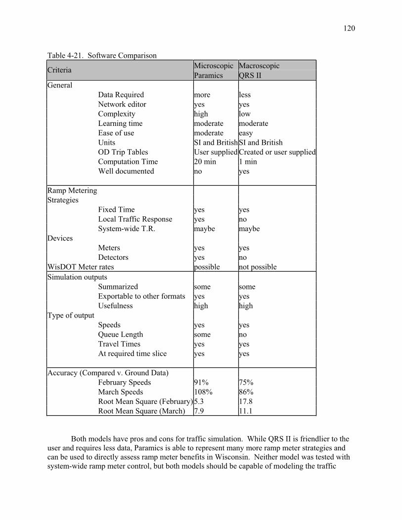
120

Table 4-21. Software Comparison

Microscopic Macroscopic Criteria

Paramics QRS II

General

Data Required more less

Network editor yes yes

Complexity high low

Learning time moderate moderate

Ease of use moderate easy

Units SI and BritishSI and British

OD Trip Tables User supplied Created or user supplied

Computation Time 20 min 1 min

Well documented no yes

Ramp Metering

Strategies

Fixed Time yes yes

Local Traffic Response yes no

System-wide T.R. maybe maybe

Devices

Meters yes yes

Detectors yes no

WisDOT Meter rates possible not possible

Simulation outputs

Summarized some some

Exportable to other formats yes yes

Usefulness high high

Type of output

Speeds yes yes

Queue Length some no

Travel Times yes yes

At required time slice yes yes

Accuracy (Compared v. Ground Data)

February Speeds 91% 75%

March Speeds 108% 86%

Root Mean Square (February)5.3 17.8

Root Mean Square (March) 7.9 11.1

Both models have pros and cons for traffic simulation. While QRS II is friendlier to the

user and requires less data, Paramics is able to represent many more ramp meter strategies and

can be used to directly assess ramp meter benefits in Wisconsin. Neither model was tested with

system-wide ramp meter control, but both models should be capable of modeling the traffic

121

impacts of such control given a considerable amount of additional computer programming.

Because of QRS II’s speed advantage, it would be better for finding optimal control strategies.

A critical MOE is the average trip duration of all trips made from every zone. Before

(without meters) and after (with meters) periods are compared by using Paramics results, in order

to see whether ramp meters are improving traffic conditions.

In order to get the total travel time of all vehicles from one zone to other, the number of

trips between an OD pair is multiplied by the average travel time for that trip during the peak

hour. Then, the average trip duration is obtained by dividing the sum of all average travel times

by the total number of trips in each period (before and after). The results of this comparison is

shown on Table 4-22.

Table 4-22. Ramp Meter’s Average Trip Duration Improvement

Average Trip

Duration (min) Improvement

February 6.76

March 6.24 7.6%

The results obtained show a reduction in average trip duration from February to March by

7.6%, though the fraction of very short trips is smaller in March than in February.

Conclusions and Recommendations

Conclusions

The use of a simulation model enables planners and engineers to model actual traffic

situations and estimate impacts caused by any improvement to a traffic network. A simulation

model also allows engineers to create and evaluate scenarios and alternatives during the planning

phase to obtain better results in optimizing traffic control.

This study evaluates two different software packages for simulating the traffic conditions

of US Highway 45 before and after new ramp meters are deployed. The study section includes

the southbound lanes from upstream at Good Hope Road to downstream at Wisconsin Avenue.

Ground data was collected in February 2000 as a “without ramp metering” period and March

2000 as a “with ramp metering” period by UWM, Marquette University and WisDOT.

Prior to both simulations, it was necessary to estimate the OD trip table. The generalized

least squares (GLS) technique worked well.

Testing Paramics and QRS II gives an idea of how different types of traffic simulation

models (microscopic and macroscopic, respectively) represent actual conditions. Both models

were tested with a minimumal amount of calibration to ground data, so that the validation would

not be compromised.

122

During Paramics network augmentation, it was found that this model is able to simulate

more realistic traffic situations such as driver behavior, different vehicle types, and advanced

signal control. The large amount of data needed by Paramics and the time required to code the

network could be detrimental. Also, programming is required in order to represent an actuated

traffic signal, making it even more time-consuming. QRS II uses less data for the same

representation and requires far less time for coding and computation.

By using traffic signals Paramics represents ramp meters closely to how they are operated

in the field. Each meter rate is responsive to the actual traffic conditions in the vicinity of the

respective on-ramp. Ramp metering can be simulated for a diversity of plans. Each ramp meter

has its own plan to be implemented, depending on the network characteristics.

However, traffic responsive meters cannot be represented by QRS II. Thus, QRS II

requires adjusting the meter rates (“capacity” attribute) in order to approximate the meter rate

during a peak period. QRS II’s results, such as speeds, are somewhat lower than ground speeds.

The simulation presented by Paramics was closer to actual traffic conditions. Paramics is

a very useful traffic simulation tool that can be adapted for ramp meter representation. However,

some ramp meter’s characteristics such as HOV lanes, alternate release and fractional timings

cannot be represented by this software package.

After executing both simulation models, it was found that in order to obtain the most

accurate results, the modeler must be completely familiar with the network system being

simulated. It is often necessary to know what the software can do and what assumptions should

be made in order to avoid possible problems. This is particularly true using Paramics, where

many of its limitations were unknown before its initial execution. It is likely that even better

results are obtainable with a more intensive calibration than the “hands-free” calibration used in

this study.

Neither model was tested with algorithms to optimize ramp meters system-wide, so their

capabilities for this purpose remain unclear.

Recommendations

More experimentation with Paramics is needed because it seems to be a very powerful

software package that has potential in any application when its limitations are known and where

its calibration is complete before being implemented. The US Highway 45 model should be used

in order to improve actual traffic conditions by simulating new and different strategies. In

addition, the model should be used for testing diversion, recognizing that it would need a much

larger network with many more zones.

A complete evaluation of benefits requires simulations of every time period in which the

meters are in operation, not just the PM peak hour as performed in this study.

A software package selected for ramp meter simulation should be able to represent every

type of strategy (fixed time operation, local traffic responsive, system-wide traffic responsive).

Ramp meter representation made by QRS II is limited, out-of-the-box, to a fixed time operation

strategy. A traffic responsive strategy in ramp meter representation should be included in this

software to increase its ability to model different strategies.

123

Both packages should be tested for their abilities to optimize ramp meters system-wide.

Because QRS II can be embedded within another computer program as a subroutine and because

of its superior computation speed, it should be able to be used to optimize the operation of a

variety of traffic controls. Paramics may be able to simulate an already optimized ramp meter

control strategy, but this simulation would require features of Paramics’s API (application

programmers interface) that go well beyond the actuated signals “plan” that was used for the US

45 tests.

124

References

T. Abrahamsson, “Estimation of Origin-Destination Matrices Using Traffic Counts -- A

Literature Survey”, International Institute for Applied Systems Analysis, 1998.

J. A. Bieberitz, “Area Wide Impacts of Ramp Metering”, MS Thesis, University of Wisconsin

Milwaukee, December 1994.

S. A. Boxill, and L. Yu, “An Evaluation of Traffic Simulation Models for Supporting ITS

Development”, Center for Transportation Training and Research, Texas Southern University,

October 2000.

Center for Transportation Research, “Dynasmart-P Intelligent Transportation Network Planning

Tool, Version 0.926, User’s Guide”, University of Texas at Austin, 2001.

Y. Gardes, A.D. May, J. Dahlgren, A. Skabardonis, “Freeway Calibration and Application of the

Paramics Model”, Transportation Research Board 81st Annual Meeting CD ROM, 2001.

A. J. Horowitz, “Reference Manual Quick Response System II”, Version 6, Center for Urban

Transportation Studies, University of Wisconsin – Milwaukee, 2001.

A. J. Horowitz, “Reference Manual Advanced General Network Editor for Windows” Version 7,

Center for Urban Transportation Studies, University of Wisconsin – Milwaukee, 2002.

Papageorgiou M., H. Hadj-Salem, and F. Middelham, “ALINEA Local Ramp Metering,

Summary of Field Results”, Transportation Research Record #1603, pp. 90-98, 1997.

G. Piotrowicz and J. Robinson, “Ramp Metering Status in North America. 1995 Update”,

Federal Highway Administration, DOT-T-95-17, June 1995

Quadstone, Paramics-Online Modeller V3.0, User Guide

Quadstone, Paramics-Online Modeller V3.0, Reference Manual

Quadstone, Paramics-Online Processor V3.0, Reference Manual

Quadstone, Paramics-Online Analyser V3.0, Reference Manual

“Quick Response Freight Manual” Final Report. Prepared by Cambridge Systematics, Inc.,

COMSIS Corporation and University of Wisconsin-Milwaukee, DOT-T-97-10, September 1996.

Evaluation of Ramp Meter Effectiveness for Wisconsin Freeways, A Milwaukee Case Study:

Part 2, Ramp Metering Effect on Traffic Operations and Crashes

Project identification number 0092-45-17

Final Report

Alex Drakopoulos Mery Patrabansh Georgia Vergou Marquette University, Milwaukee

Submitted to the Wisconsin Department of Transportation October 2004

Table of Contents

Chapter 5 Ramp Metering Effect on Traffic Operations and Crashes ....................................1

Introduction ..................................................................................................................................1 Analysis Corridor ................................................................................................................................................1

Analysis Methodology .........................................................................................................................................1

Database........................................................................................................................................3Travel Time Runs ................................................................................................................................................3

Volume and Speed Data from Pavement-Embedded Detectors ......................................................................4

On-Ramp Queue Length.....................................................................................................................................4

Freeway Operations Measures of Effectiveness...........................................................................5

Traffic Flow Characteristics-Discussion ....................................................................................10

Crashes........................................................................................................................................12

Conclusions ................................................................................................................................12

Recommendations ......................................................................................................................13

Appendix A Inventory of Ramp Delay and Queue Length Information............................. A-0

Introduction .............................................................................................................................. A-i

Ramp Index for Week 1 (February 1-3, 2000) ........................................................................ A-ii

Ramp Index for Week 1 (February 8-10, 2000) .....................................................................A-iii

Ramp Index for Week 1 (March 14-16, 2000) ....................................................................... A-iv

Ramp Index for Week 1 (March 21-23, 2000) ........................................................................ A-v

County Line Road.................................................................................................................... A-1

Pilgrim Road............................................................................................................................ A-6

Good Hope Road Loop Ramp ................................................................................................. A-8

Good Hope Road Slip Ramp ................................................................................................. A-16

Appleton Avenue................................................................................................................... A-35

Hampton Avenue................................................................................................................... A-40

Capitol Drive ......................................................................................................................... A-49

Burleigh Street ....................................................................................................................... A-60

North Avenue ........................................................................................................................ A-72

Watertown Plank Road.......................................................................................................... A-83

Wisconsin Avenue............................................................................................................... A-100

Greenfield Avenue............................................................................................................... A-110

Appendix B Wisconsin Avenue Ramp Meter Operation, Afternoon Peak Period (4:00 pm

to 5:30 pm) Wednesday, February 9, 2000. ..........................................................................B-1

Introduction ..............................................................................................................................B-2

Table B-1. PM Peak Period Ramp Metering Settings-Wisconsin Avenue Ramp...................B-2

Table B-2. Ramp Metering Plan Selection Information..........................................................B-4

Table B-3. Reason for Metering Rate Selection and Metering Rate Duration (minutes). ......B-7

Figure B-1. Ramp Delay & Queue Length Wisconsin Ave. 2/9/2000...................................B-10

Figure B-2. Reason for Setting Metering Rate .......................................................................B-11

Figure B-3. Mainline Speed....................................................................................................B-12

Figure B-4. Mainline Lane Volume .......................................................................................B-13

Figure B-5. Mainline Lane Occupancy ..................................................................................B-14

Figure B-6. Ramp Occupancy. ...............................................................................................B-15

Figure B-7. Chosen Metering Rate.........................................................................................B-16

Figure B-8. Metering Rates Based on Ramp Occupancy.......................................................B-17

Table of Contents (continued)

Appendix B Wisconsin Avenue Ramp Meter Operation, Afternoon Peak Period (4:00 pm

to 5:30 pm) Wednesday, February 9, 2000.

Figure-B-9. Mainline Speed-Volume Feb 9,2000. ...............................................................B-18

Figure B-10. Mainline Speed-Occupancy Feb 9, 2000.. ........................................................B-19

Figure B-11. Mainline Speed-Volume All Days. ...................................................................B-20

Figure B-12. Mainline Speed-Occupancy All Days. ..............................................................B-21

Figure B-13. Mainline Occupancy, Speed and Volume.........................................................B-22

Figure B-14. Mainline Speed and Volume.............................................................................B-23

Figure B-15. Mainline Occupancy and Speed........................................................................B-24

Figure B-16. Mainline Occupancy and Volume.....................................................................B-25

1

Chapter 5

Ramp Metering Effect on

Traffic Operations and Crashes

Introduction

The objective of the present chapter is to evaluate the incremental traffic operations

impact of newly introduced ramp metering on six ramps in the southbound direction of

USH 45. The evaluated corridor extended from the Waukesha – Washington County

line on the North to just South of the Greenfield Avenue (a length of 14 miles). Ramp

metering was already present on six ramps; four of these ramps were located at the south

end of the corridor, which carried the heaviest traffic volumes.

The chapter addresses ramp and mainline freeway traffic operations Measures of

Effectiveness (MOE) separately; overall MOE are also provided.

Analysis Corridor

The analysis corridor consisted of the southbound U.S. 45 direction, starting at the

Washington/Waukesha County line on the North, crossing into Milwaukee County and

extending through the interchange with I-94 (Zoo interchange) and continuing on to I-894

(the extension of U.S. 45) to a point just South of the Greenfield Avenue on-ramp

(Figure 5-1).

Ramp metering was operational on six on-ramps along the analysis corridor when the

study was initiated. Six additional on-ramps began to be metered as part of the WisDOT

ramp metering program (see Figure 5-1). It was desired to evaluate the impact that these

additional ramp meters would have on traffic operations in the analysis corridor.

Analysis Methodology

A “Without” and “With” new ramp meters comparison evaluation was chosen as an

appropriate way to measure the impact of the newly installed ramp meters on freeway

operations. The “Without” period represented freeway conditions when only the six

existing ramp meters were operational. The “With” period represented freeway

conditions when the additional six ramp meters were also operational.1

Detailed information on ramp delay and queue length patterns during the evaluation

period is provided in Appendix A. Ramp metering settings and details of the ramp meter

operation during the afternoon peak period of February 9 of 2000 are presented in

Appendix B for Wisconsin Avenue, one of the most congested parts of the analyzed

corridor. This information allows a detailed insight into metered ramp queue patterns and

the effect of the chosen ramp metering

1 The Main Street ramp meter was installed but not turned on during the evaluation period, thus only six

new ramp meters were operating during the “With” period.

Cutline #0

Cutline #1

Cutline #2

Cutline #8

Figure 5-1. Cutlines Used for Traffic Operations MOE Evaluation

& Ramp Meter Locations

Cutline #6

Existing RM New RM RM not operating

3

parameters on metered ramp operation. Information on mainline traffic operations

parameters at the same location is also presented in detail.

Database

Traffic data was gathered on Tuesdays, Wednesdays and Thursdays during consecutive

weeks, in order to capture travel patterns that were most representative of weekday

commuter traffic. “Without” period data were gathered on February 1, 2, and 3 (week 1),

February 8, 9, and 10 (week 2) of 2000. “With” period data were gathered on March 14,

15, and 16 (week 3), March 21, 22, and 23 (week 4), starting on the 33rd

day after the

end of the “Without” period. The time period separating the Without and With periods

was intended to allow drivers to become accustomed to the presence of the new ramp

meters. Data was collected during the morning and the afternoon peak periods (7:00 am

to 8:30 am and 4:00 pm to 5:30 pm, respectively).

Gathered data consisted of:

1. Travel time runs performed every 15 minutes during the peak periods.

2. Traffic volume and speed, collected through mainline and ramp pavement-

embedded detectors, every 20 seconds.

3. Fifteen-minute traffic volume counts were collected through specially-installed

on-ramp counters (on-ramps not equipped with pavement-embedded detectors).

4. On-ramp queue lengths recorded every 20 seconds (videotaped or observer-

recorded in the field).

Travel Time Runs

Vehicles were dispatched every fifteen minutes during the analyzed peak periods and a

crew recorded travel times between fixed landmarks along the analysis corridor. Thus,

no more than six travel time runs were performed during any given one and one-half

hour peak period. Travel time data were scheduled to be collected on the dates indicated

above. However, no data were collected during certain dates as shown in Table 5-1

below, due to certain circumstances (e.g., predicted adverse weather, traffic incidents,

etc.)

Table 5-1. Number of Travel Time Runs Performed on US 45.

Without With

Day/Date AM Peak

Period

PM Peak

Period

Day/Date AM Peak

Period

PM Peak

Period

Tue 2/1/00 0 6 Tue 3/14/00 0 0

Wed 2/2/00 6 0 Wed 3/15/00 6 0

Thu 2/3/00 0 0 Thu 3/16/00 6 0

Tue 2/8/00 6 6 Tue 3/21/00 4 4

Wed 2/9/00 4 6 Wed 3/22/00 4 6

Thu 2/10/00 4 0 Thu 3/23/00 6 4

Total 20 18 26 14

4

Volume and speed data from pavement-embedded detectors.

Volume and speed data were collected through 13 controllers (see “RM” listings in

column “Controller ID,” Table 2-1). However, due to various equipment problems,

uninterrupted information for the Without and the With periods was available only for the

five controllers that collected information corresponding to cutlines#1 (Congress Str.), #2

(Center Str.), #6 (S. of Wisconsin Ave.) and #8 (Lapham Str.) 2 An additional cutline

(cutline #0) was established for Part 2 of the report at the Waukesha/Milwaukee County

line (Figure 5-1). Each controller provided 20-second summary information for an on-

ramp and each of the three mainline lanes.

On-Ramp Queue Length

Table 5-2 summarizes available on-ramp data availability for each peak period (morning

and afternoon) and each analysis period (Without and With ramp metering). A detailed

inventory of ramp queue length and delay information is presented in Appendix A.

Table 5-2. Ramp Delay-Available Data.

On-Ramp Delay Data Inventory

Location Ramp meter

AM Peak

Without

AM Peak

With

PM Peak

Without

PM Peak

With

County Line Rd.¹ New

Pilgrim Rd.¹ New

Main Str.² New

Good Hope Rd. Loop Ramp Existing

Good Hope Rd. Slip Ramp Existing

Appleton Ave. New

Hampton Ave. New

Capitol Dr. New

Burleigh St. New

North Ave. Existing

Watertown Plank Rd. Existing

Wisconsin Ave. Existing

Greenfield Ave. Existing

Check marks indicate that data was available.

¹ The County Line Rd. and Pilgrim Rd. ramp meters did not operate during the PM peak in the With period.

²The Main Str. Ramp meter was installed but did not operate during the evaluation period.

2 These cutline numbers are shown in Figure 5-1, and Table 2-5 page 32 and Figure 2-4 page 33 in Part 1

of the present report.

5

Freeway Operation Measures of Effectiveness

Loop detector data, collected in 20-second intervals were converted to equivalent hourly

volumes and cumulative statistics were compiled for the morning and afternoon one and

one-half hour peak periods. Thus, 270 values were used as inputs for volumes and an

identical number for speeds for each lane at each cut line during each analyzed peak

period of any given day.

Travel times compiled based on travel time runs were compared to travel times based on

loop detector data in order to verify the validity of loop detector information. The two

data sources were found to be in close agreement. It was decided to use loop detector

data in lieu of travel time run data, because they provided travel time information

compiled every 20 seconds (270 values per peak period) compared to six travel time

runs—at most—during any given peak period (see Table 5-1 for available number of

travel time runs).

Data collected at the cut lines were aggregated into one and one-half hour average values

for each peak period and each analysis day. The tables presented below show overall

averages for all “Without” days and all “With” days at each cut line. The freeway

lengths on which cut line statistics are applied is provided in Table 5-3. Cumulative

statistics for the entire analyzed corridor are provided in each table.

Mainline Traffic Volumes: Table 5-3 indicates small traffic volume increases along the

corridor. A two-to-three percent increase was experienced at the south, most congested,

end of the analyzed corridor during the morning peak; the same area experienced a zero-

to-two percent increase during the afternoon peak, when the largest increase, percentage-

wise (4%) was evidenced at the north end of the corridor, which had lighter traffic

volumes.

Freeway Vehicle-Miles of Travel: Table 5-3 presents the changes in Vehicle-Miles of

Travel (VMT) that occurred between the Without and With periods for each of the daily

peak traffic periods. There was an overall VMT increase of one percent during the

morning peak; the increase was two percent for the afternoon peak.

Freeway-Vehicle Hours of Travel: Mainline freeway hours of travel decreased by 2%

during the morning peak and by 5% during the afternoon peak period (see Table 5-4).

However, total freeway vehicle hours increased by 4% (69.32 veh-hr) during the morning

peak and decreased by 2% (36.32 veh-hr) during the afternoon peak.

Ramp Delay: This discrepancy between mainline and total vehicle hours of travel is

explained by ramp delay statistics (see Table 5-5): ramp delay increased 64% (106.17

veh-hr) during the morning peak and 34% (54.14 veh-hr) during the afternoon peak.

Minor overall delay increases were evident on existing ramps (15.14 veh-hr during the

am peak, 6.24 veh-hr during the pm peak). The operation of new ramp meters introduced

91.03 veh-hr of delay during the morning peak and 47.91 veh-hr of delay during the

6

afternoon peak. Thus the new ramp meters played a pivotal role in overall veh-hr

statistics.

Ramp delay was 3.2% of total freeway veh-hr without the new ramp meters and 8.6%

with the new ramp meters during the morning peak period. For the afternoon peak

period, the corresponding percentages were 4.9% without and 7.6% with the new ramp

meters in operation.

Freeway Speeds: Corridor speeds increased during both peaks when the new ramp

meters were operational (Table 5-6). The increase was 1.83 mph (3%) during the

morning peak, and 2.35 mph (4%) during the afternoon peak.

On-Ramp Queue Lengths: Appendix A presents all collected queue length and delay

information. The longest queues occurred on the existing Good Hope loop ramp where

maximum queue lengths averaged 60 vehicles during the morning and 50 vehicles during

the afternoon peak period (pp. 8-15, Appendix A). Although queue lengths did not

change substantially when the new ramp meters were operational, ramp delays increased.

Table 5-3. Freeway Vehicle-Miles of Travel: Without-and-With New Ramp

Meters.

AM peak period (7:00 am to 8:30 am) PM peak period (4:00 pm to 5:30 pm)

Mainline Volume Per Peak Period (vehicles)

Cut Line Miles

AM Peak

Without

AM Peak

With % Change

PM Peak

Without

PM Peak

With % Change

3.2

#0 Waukesha Co. Line 6476 6491 0 4044 4209 4

4.5

#1 Congress Str.8485 8411 -1 7881 8009 2

2.0

#2 Center Str.8418 8677 3 8006 8112 1

2.4

#6 Wisconsin Ave. 8380 8550 2 9829 9827 0

1.9

#8 Belton RR 7027 7243 3 10174 10434 2

Total Freeway VMT 109208 110254 1 107338 109144 2

7

Table 5-4. Freeway Vehicle-Hours of Travel: Without-and-With New Ramp Meters.

AM peak period (7:00 am to 8:30 am) PM peak period (4:00 pm to 5:30 pm)

Mainline Vehicle-Hours of Travel Per Peak Period

Cut Line AM Peak

Without

AM Peak

With % Change

PM Peak

Without

PM Peak

With % Change

#0 Waukesha Co. Line 297.64 300.96 1 188.11 196.49 4

#1 Congress Str. 618.42 570.11 -8 524.29 532.87 2

#2 Center Str. 294.96 294.64 0 331.92 298.24 -11

#6 Wisconsin Ave. 353.43 357.68 1 547.23 489.94 -12

#8 Belton RR 223.69 227.92 2 416.95 400.51 -4

Freeway VHT 1788.15 1751.30 -2 2008.51 1918.05 -5

Ramp VH Delay 58.88 165.05 64 103.63 157.77 34

Total Freeway VH 1847.03 1916.35 4 2112.14 2075.82 -2

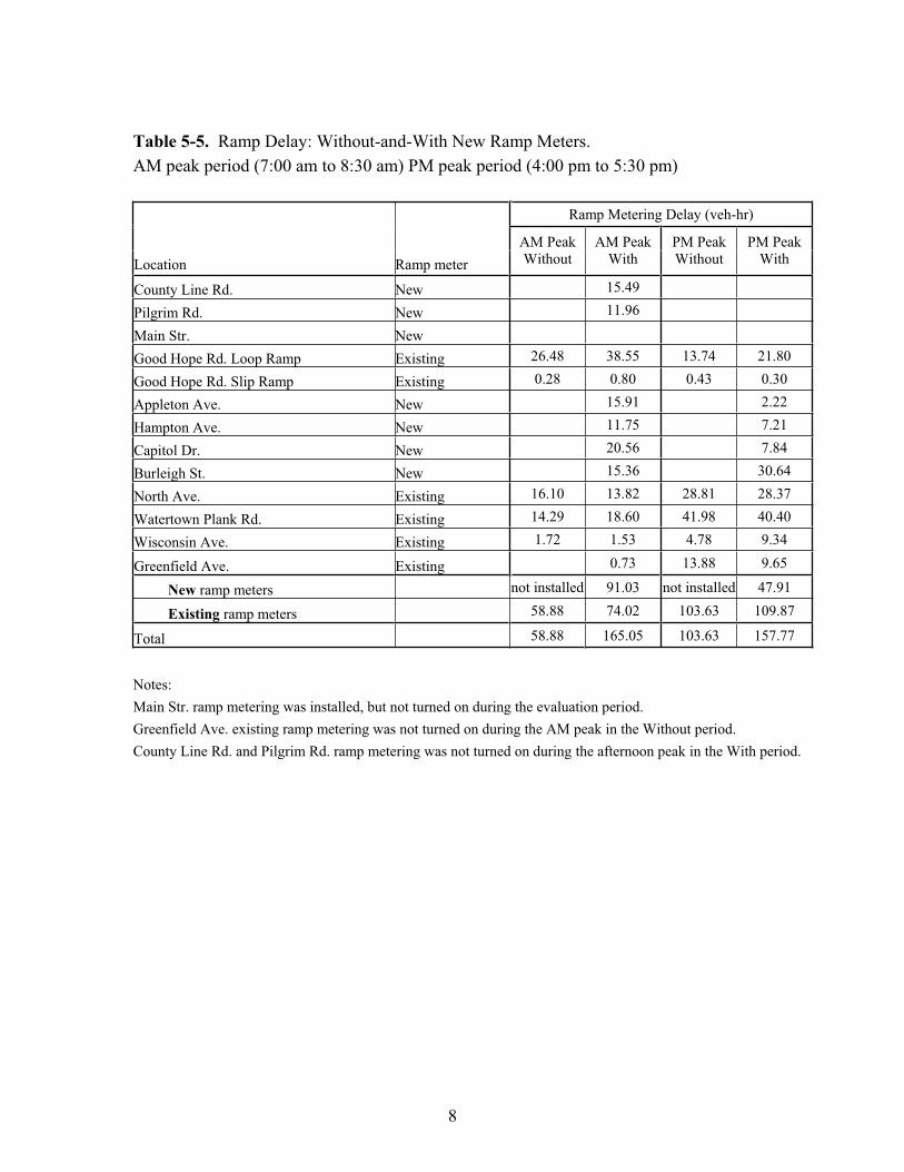
8

Table 5-5. Ramp Delay: Without-and-With New Ramp Meters.

AM peak period (7:00 am to 8:30 am) PM peak period (4:00 pm to 5:30 pm)

Ramp Metering Delay (veh-hr)

Location Ramp meter

AM Peak

Without

AM Peak

With

PM Peak

Without

PM Peak

With

County Line Rd. New 15.49

Pilgrim Rd. New 11.96

Main Str. New

Good Hope Rd. Loop Ramp Existing 26.48 38.55 13.74 21.80

Good Hope Rd. Slip Ramp Existing 0.28 0.80 0.43 0.30

Appleton Ave. New 15.91 2.22

Hampton Ave. New 11.75 7.21

Capitol Dr. New 20.56 7.84

Burleigh St. New 15.36 30.64

North Ave. Existing 16.10 13.82 28.81 28.37

Watertown Plank Rd. Existing 14.29 18.60 41.98 40.40

Wisconsin Ave. Existing 1.72 1.53 4.78 9.34

Greenfield Ave. Existing 0.73 13.88 9.65

New ramp meters not installed 91.03 not installed 47.91

Existing ramp meters 58.88 74.02 103.63 109.87

Total 58.88 165.05 103.63 157.77

Notes:

Main Str. ramp metering was installed, but not turned on during the evaluation period.

Greenfield Ave. existing ramp metering was not turned on during the AM peak in the Without period.

County Line Rd. and Pilgrim Rd. ramp metering was not turned on during the afternoon peak in the With period.

9

Table 5-6. Freeway Speeds: Without-and-With New Ramp Meters.

AM peak period (7:00 am to 8:30 am) PM peak period (4:00 pm to 5:30 pm)

Freeway Speeds (MPH)

Cut Line

AM Peak

Without

AM Peak

With

%

Change

PM Peak

Without

PM Peak

With

%

Change

#0 Waukesha Co. Line 69.62 69.01 -1 68.81 68.55 0

#1 Congress Str. 61.94 66.39 7 67.64 67.63 0

#2 Center Str. 57.09 58.90 3 48.29 54.42 13

#6 Wisconsin Ave. 56.91 57.39 1 44.09 48.28 10

#8 Belton RR 59.69 60.38 1 46.78 49.53 6

Corridor Average Speed 61.45 63.28 3 55.96 58.31 4

Table 5-5 indicates that the highest ramp delays (42 and 40 veh-hr during the afternoon

per peak period without and with the new meters, respectively) occurred on the existing

Watertown Plank Road on-ramp. These delays corresponded to queues with average

maximum lengths of 47 and 40 vehicles Without and With the new ramp meters

operational, respectively (pp. 83-100, Appendix A). Maximum queue length for the

HOV lane was one vehicle.

Maximum queue length on the new Burleigh Street ramp meter was about 30 vehicles

during the morning peak and 45 vehicles during the afternoon peak, when ramp delay

averaged 30.6 veh-hr. The High Occupancy Vehicle ramp was seldom utilized; queue

length did not exceed 2-3 vehicles.

Maximum queue lengths on the existing North Avenue ramp meter averaged 32 vehicles

during the afternoon peak, with ramp delays of approximately 28 veh-hr throughout the

evaluation period.

High Occupancy Vehicle ramps were seldom utilized; queue lengths rarely exceeded one

or two vehicles at a time.

10

Traffic Flow Characteristics-Discussion

Ramp meters were already installed in the southern, most congested part of the analyzed

corridor, where ramp metering would be anticipated to have the greatest impact in terms

of facilitating merging into the mainline and potentially diverting traffic to alternate

routes during peak periods. Smoother merging into the mainline was expected to lead to

increased capacity and decreased mainline travel times by minimizing the potential of

shock wave formation at merge areas. The six new ramp meters were installed north of

the most congested part of the corridor, thus they were expected to smooth traffic feeding

into this most congested part of the corridor. The strongest smoothing effects were

expected to be from the new ramp meters installed immediately upstream of the existing

ramp metering installations, at Burleigh Street, Capitol Drive, and Hampton Avenue.

Because two of the remaining three new ramp meters were installed in the northern-most,

less traveled part of the corridor (County Line Road and Pilgrim Road), their incremental

impact on freeway operations MOE would not be expected to result in a net benefit for

the north end of the corridor in terms of speeds and travel times:

Speeds at cutline #0 were at- or near-free-flow levels before the new meters

became operational and could not be expected to increase significantly. (Speeds

were somewhat lower at cutline #1, allowing some room for a moderate speed

increase.)

Ramp delays (not present in this part of the corridor before the new ramp meters

were operational) would thus mainly increase travel times, because drivers would

not be able to make up for ramp delay by traveling much faster on the mainline.

Given the traffic flow conditions at the north end of the analysis corridor before the new

ramp meters became operational, it is mainly traffic volumes that could experience an

increase among the reported MOE: the highest per lane volume was 1,885 vehicles per

hour (at cutline #1), allowing room for a substantial increase. These two ramps were

more than four miles away from cutline #2 where the first significant speed reductions

were present, thus their impact on mainline operations south of cutline #2 would be

minimal.

Moderate congestion existed between cutlines #1 and #2, where the new Capitol Drive

and Burleigh Street ramp meters were installed, with maximum per lane volumes of

1,870 vehicles per hour at cutline #2.

On-ramps at the south end of the corridor, represented by statistics at cutlines #6 and #8,

were metered during both analysis periods (Without and With the new ramp meters).

This was the most congested part of the corridor (with maximum per lane volumes of

2,260 vehicles during the afternoon peak period) operating at speeds significantly lower

than the north end of the corridor. Thus there was substantially more room for speed

improvement in this part of the corridor than at the north end, where speeds were near

free-flow levels.

Speed increases were evident for the corridor (Table 5-6) with the most encouraging

findings being speed increases observed at the south end of the corridor at cutlines #2, #6

and #8, during the most heavily-traveled afternoon peak period. Speeds increased by

11

13%, 10% and 6% at these cutlines, respectively, resulting in an overall corridor five

percent reduction in mainline vehicle-hours of travel. Vehicle-hours of travel were two

percent lower during the morning peak period.

An added benefit was that the above-mentioned speed increases occurred in the presence

of small mainline traffic volume increases (0 - 2% during the afternoon peak and 2 - 3%

during the morning peak) at the south end of the corridor. Corridor vehicle-miles of travel

increased by two percent during the afternoon peak and by one percent during the

morning peak.

The following discussion is based on information presented in Table 5-7, which is

compiled from Tables 5-4 and 5-5.

Table 5-7. Corridor Vehicle-Hours of Travel.

Vehicle-Hours of Travel (veh-hr)

AM Peak

Without

AM Peak

With

Change

(veh-hr)

PM Peak

Without

PM Peak

With

Change

(veh-hr)

Freeway VHT 1788.15 1751.30 -36.85 2008.51 1918.05 -90.46

New ramp meters

not

installed 91.03 91.03

not

installed 47.91 47.91

Existing ramp meters 58.88 74.02 15.14 103.63 109.87 6.24

Total Ramp VH Delay 58.88 165.05 106.17 103.63 157.77 54.14

Total Freeway VH 1847.03 1916.35 69.32 2112.14 2075.82 -36.32

Ramp delay was a higher percentage of total freeway vehicle hours of travel when the

new meters were operational. Ramp delay at 3.2% of total freeway vehicle hours of

travel in the morning peak, increased to 8.6%; for the afternoon peak the increase was

from 4.9% to 7.6%.

Ramp delay increases were mostly due to the new ramp meters. New ramp meters added

91.03 vehicle-hours of delay to the morning peak (the total increase was 106.17 veh-hr of

delay) and 47.91 veh-hr of delay to the afternoon peak (total increase was 54.14 veh-hr of

delay).

Ramp delays were a small percentage of total veh-hr of travel, however, increases in

ramp delays when the new ramp meters were operational, had a drastic impact on overall

vehicle-hours of travel. Despite a decrease of 36.85 veh-hr of travel on the mainline

during the morning peak, an increase of 106.17 veh-hr of ramp delay resulted in an

overall increase of 69.32 corridor veh-hr of travel (a 4% increase).

The impact of increased ramp meter delays was of a smaller magnitude during the

afternoon peak. Due to the smaller magnitude of the ramp delay, and the larger

magnitude of the mainline veh-hr of travel during this peak, ramp delay had a much

smaller impact on overall freeway veh-hr of travel. Despite the increased ramp delay,

12

overall veh-hr of travel decreased by two percent when the new ramp meters were

operational.

Crashes

New ramp metering equipment was installed in 1999 and was activated on February 15,

2000. Crash statistics presented herein are based on a six-month period that the corridor

operated without the new ramp meters (from August 10, 1999 to February 10, 2000) and

a six-month period that the corridor operated with the new ramp meters (from August 10,

2000, to February 10, 2001). The analysis included all I-94 Southbound crashes between

the Waukesha County/Washington County line, and the Zoo interchange, as well as all I-

894 southbound crashes between the Zoo interchange and Lincoln Avenue.

Crash statistics changes along the corridor were due to the ramp meters installed in

addition to those already in operation at Good Hope Rd., North Ave., Watertown Plank

Rd., Wisconsin Ave. and Greenfield Ave., as well as geometric improvements to ramps

and pavement resurfacing that took place during the new ramp meter installation project.

During ramp metering hours of operation3 a total of 152 crashes occurred along the

analysis corridor in the period when the freeway operated without the new ramp meters,

and 128 crashes occurred in the period that the freeway operated with the new ramp

meters in place. The crash rate was 298 crashes per 100 MVM of travel “Without,” and

260 crashes per 100 MVM of travel “With” the new ramp meters.

Operation of the new ramp meters in conjunction with improved ramp merging

geometrics and mainline pavement resurfacing resulted in an overall 16% reduction in the

number of crashes (a 13% crash rate reduction) during ramp metering hours.

Conclusions

During the period with new ramp meters in operation the most congested south part of

the analysis corridor experienced an improvement in traffic operations measures of

effectiveness, during the most critical (most congested) afternoon peak period.

During the afternoon peak period, a substantial reduction in vehicle-hours of travel due to

increases in travel speeds, under minimal volume changes (a zero to two percent

increase) was documented between Capitol Drive and Greenfield Avenue. Speeds

increased by 13% in the segment between Capitol Drive and Burleigh Street, by 10%

between North Avenue and Wisconsin Avenue, and by 6% between Bluemound Road

and Greenfield Avenue.

However, corridor average speed increased by only four percent during the afternoon

peak, because no speed changes were effected on the north part of the corridor where

near-free-flow speeds existed at all times. Although mainline vehicle hours of travel

3 Assumed to be 6:00 am to 9:00 am (morning peak period) and 2:00 pm to 7:00 pm (afternoon peak

period), Monday through Friday for the crash analysis.

13

decreased by five percent, when ramp delay was also taken into account, total vehicle

hours of travel decreased by two percent. There was an overall increase of two percent in

corridor vehicle miles of travel.

It is interesting to note that morning peak period ramp delays without the new ramp

meters were approximately half the ramp delays of the afternoon peak period ramp

delays. Ramp delays with the new ramp meters were approximately equal during both

peak periods. Given that traffic volumes were lighter during the morning peak period, it

is quite likely that ramp metering rates were more restrictive than their optimal values

during this period.

The operation of new ramp meters, in conjunction with geometric improvements in ramp

merging areas and mainline resurfacing resulted in a 13% crash rate reduction for the

analyzed corridor during ramp metering hours.

Appendix B information indicates that ramp metering rate override due to high ramp

occupancy occurs rather frequently and over a large portion of peak periods. When

queue override occurs, ramp queues are very likely to be discharged at the highest

metering rate when heavier mainline volumes demand more restrictive metering rates.

This situation moderates potential ramp metering benefits.

Recommendations

Ramp delay played a critical role in the balance of overall corridor veh-hr of delay:

although mainline veh-hr of travel decreased when the new ramp meters were

operational, overall veh-hr of travel increased during the morning peak due to ramp

delays. Travel time reduction benefits in the most congested part of the corridor during

the afternoon peak were tempered due to additional ramp delays. Fine-tuning of ramp

metering parameters during the morning peak period in order to reduce ramp delays is

very likely to produce a reduction in total freeway veh-hr of travel.

Further reductions in total freeway veh-hr of travel during the afternoon peak may also be

possible by reducing ramp delay on the existing Good Hope Road loop ramp where the

mainline is not very congested; the current high level of ramp delay on the new Burleigh

Street ramp could probably also be reduced. County Line Road and Pilgrim Road ramp

metering probably contributes rather small mainline benefits at the present time, given

the lower traffic volumes and substantial distance from the currently congested part of the

corridor. Minimizing delays on these ramps would, in all likelihood decrease corridor

delays.

Any changes in ramp metering parameters aiming to reduce ramp delays, should be

carefully balanced against possible increases in mainline travel times.

Appendices A and B provide detailed information that can serve as the decision-making

foundation for desired ramp metering parameter changes.

Appendix A

Inventory of

Ramp Delay and Queue Length Information

A - i

Introduction

The present appendix contains all collected ramp delay and queue length information.

Information is presented in spatial order, from the North to the South end of the analyzed

corridor. Data for each ramp are presented in a temporal sequence; High-Occupancy-

Vehicle (HOV) ramp data are presented, wherever available, following Single-

Occupancy-Vehicle (SOV) ramp data. Where no HOV ramp was present, the term SOV

was used, although high-occupancy vehicles would also use the same ramp.

The index in pages A - ii through A - v provides Appendix page numbers where

information about a specific location can be found for a specific peak period and a

specific ramp. Shaded cells indicate that ramp metering was not operational during this

time. Blank cells indicate that, although the ramp was operational, information for a

specific period was not available. HOV cells left blank for all four weeks indicate

locations that did not have an HOV ramp.

Weeks 1 and 2 (February 1-3 and 8-10) correspond to freeway operation without the new

ramp meters; weeks 3 and 4 (March 14-16 and 21-23) correspond to freeway operation

with the new ramp meters on-line.

Graphs contained in this Appendix provide a visual representation of queue length (used

as the y-axis) and delay (the shaded area in each graph) during any instant (the x-axis

represents time) of a reported peak period. Heavily shaded graphs represent peak periods

with more significant ramp delay.

Certain ramps present an appearance of frequent narrow “spikes,” indicating an increased

arrival rate (the left side of the spike, leading to the peak), followed by vehicles being

released from the stop line, leading to shorter queues or completely dissipated queues (the

right side of the spike). When ramp occupancies reached a predetermined level, “queue

override” took over and set the fastest ramp metering rate, until ramp occupancy was at a

predetermined low level. Such occurrences would be indicated by a faster queue length

dissipation.

The operation of the Wisconsin Avenue ramp meter during the afternoon peak period of

February 9, 2000, is examined in Appendix B, where the factors determining ramp

metering rates are analyzed in detail.

RA

MP

DE

LA

Y D

AT

A A

VA

ILA

BIL

ITY

Feb

ruar

y-M

arch

2000

Tab

le e

ntr

ies

indic

ate

appen

dix

pag

e num

ber

2/1

2/2

2/3

AM

PM

AM

PM

AM

PM

SO

VH

OV

SO

VH

OV

SO

VH

OV

SO

VH

OV

SO

VH

OV

SO

VH

OV

County

Lin

e R

d. (N

ort

h e

nd)

Pil

gri

m R

d.

Go

od H

ope

Rd. L

oop

Ram

p8

9

Go

od H

ope

Rd. S

lip R

amp

16

16

17

17

18

18

19

19

20

20

21

21

Ap

ple

ton A

ve.

Ham

pto

n A

ve.

Cap

itol

Dr.

Burl

eigh S

t.

No

rth A

ve.

72

73

73

74

74

75

Wat

erto

wn P

lank R

d.

83

83

84

84

85

85

86

86

87

87

Wis

consi

n A

ve.

10

01

01

10

1

Gre

enfi

eld A

ve.

(S

ou

th e

nd)

11

01

11

NO

TE

S:

SO

V =

Sin

gle

-Occ

up

ancy

-Veh

icle

lan

e

HO

V =

Hig

h-O

ccupan

cy-V

ehic

le l

ane

Sh

aded

are

as:

ram

p m

eter

s oper

atio

nal

only

duri

ng t

he

afte

r p

erio

d

Wee

k 1

A -

ii

RA

MP

DE

LA

Y D

AT

A A

VA

ILA

BIL

ITY

Feb

ruar

y-M

arch

2000

Tab

le e

ntr

ies

indic

ate

appen

dix

pag

e num

ber

Co

unty

Lin

e R

d. (N

ort

h e

nd)

Pil

gri

m R

d.

Good H

ope

Rd. L

oop

Ram

p

Good H

ope

Rd. S

lip R

amp

Apple

ton A

ve.

Ham

pto

n A

ve.

Cap

itol

Dr.

Bu

rlei

gh S

t.

Nort

h A

ve.

Wat

erto

wn P

lank R

d.

Wis

consi

n A

ve.

Gre

enfi

eld A

ve.

(S

outh

end)

NO

TE

S:

SO

V =

Sin

gle

-Occ

up

ancy

-Veh

icle

lan

e

HO

V =

Hig

h-O

ccupan

cy-V

ehic

le l

ane

Shad

ed a

reas

: ra

mp m

eter

s oper

atio

nal

only

du2

/82

/92

/10

AM

PM

AM

PM

AM

PM

SO

VH

OV

SO

VH

OV

SO

VH

OV

SO

VH

OV

SO

VH

OV

SO

VH

OV

910

10

11

11

22

22

23

23

24

24

25

25

26

26

27

27

75

76

76

77

77

78

88

88

89

8

99

09

09

19

19

29

2

102

10

21

03

10

31

04

11

11

12

11

2

Wee

k 2

A -

iii

RA

MP

DE

LA

Y D

AT

A A

VA

ILA

BIL

ITY

Feb

ruar

y-M

arch

2000

Tab

le e

ntr

ies

indic

ate

appen

dix

pag

e num

ber

Co

unty

Lin

e R

d. (N

ort

h e

nd)

Pil

gri

m R

d.

Good H

ope

Rd. L

oop

Ram

p

Good H

ope

Rd. S

lip R

amp

Apple

ton A

ve.

Ham

pto

n A

ve.

Cap

itol

Dr.

Bu

rlei

gh S

t.

Nort

h A

ve.

Wat

erto

wn P

lank R

d.

Wis

consi

n A

ve.

Gre

enfi

eld A

ve.

(S

outh

end)

NO

TE

S:

SO

V =

Sin

gle

-Occ

up

ancy

-Veh

icle

lan

e

HO

V =

Hig

h-O

ccupan

cy-V

ehic

le l

ane

Shad

ed a

reas

: ra

mp m

eter

s oper

atio

nal

only

du3

/14

3/1

53

/16

AM

PM

AM

PM

AM

PM

SO

VH

OV

SO

VH

OV

SO

VH

OV

SO

VH

OV

SO

VH

OV

SO

VH

OV

11

22

33

66

12

12

13

13

14

28

28

29

29

30

30

31

31

3

2

35

36

36

37

37

38

40

41

41

42

42

43

43

44

49

50

50

51

51

52

52

53

53

54

60

61

61

62

62

63

63

64

64

65

65

66

78

79

79

80

80

93

93

94

94

95

95

96

96

97

97

104

10

51

05

10

61

06

10

7

11

31

13

11

41

14

Wee

k 3

A -

iv

RA

MP

DE

LA

Y D

AT

A A

VA

ILA

BIL

ITY

Feb

ruar

y-M

arch

2000

Tab

le e

ntr

ies

indic

ate

appen

dix

pag

e num

ber

Co

unty

Lin

e R

d. (N

ort

h e

nd)

Pil

gri

m R

d.

Good H

ope

Rd. L

oop

Ram

p

Good H

ope

Rd. S

lip R

amp

Apple

ton A

ve.

Ham

pto

n A

ve.

Cap

itol

Dr.

Bu

rlei

gh S

t.

Nort

h A

ve.

Wat

erto

wn P

lank R

d.

Wis

consi

n A

ve.

Gre

enfi

eld A

ve.

(S

outh

end)

NO

TE

S:

SO

V =

Sin

gle

-Occ

up

ancy

-Veh

icle

lan

e

HO

V =

Hig

h-O

ccupan

cy-V

ehic

le l

ane

Shad

ed a

reas

: ra

mp m

eter

s oper

atio

nal

only

du3

/21

3/2

23

/23

AM

PM

AM

PM

AM

PM

SO

VH

OV

SO

VH

OV

SO

VH

OV

SO

VH

OV

SO

VH

OV

SO

VH

OV

44

55

77

8

14

15

15

32

33

33

34

34

35

38

39

39

40

44

45

45

46

46

47

47

48

48

49

54

55

55

56

56

57

57

58

58

59

59

60

66

67

67

68

68

69

69

70

70

71

71

72

81

81

82

82

98

98

99

99

10

0

107

10

81

08

10

91

09

11

0

11

5

Wee

k 4

A -

v

A - 1

County Line Road 3/14/2000 AM peak

Data Collection Time

8:29

8:24

8:19

8:15

8:10

8:05

8:01

7:56

7:51

7:47

7:42

7:37

7:33

7:28

7:23

7:19

7:14

7:09

7:05

7:00

SO

V q

ueue length

20

10

0

County Line Road 3/14/2000 AM peak

Data Collection Time

8:29

8:24

8:19

8:15

8:10

8:05

8:01

7:56

7:51

7:47

7:42

7:37

7:33

7:28

7:23

7:19

7:14

7:09

7:05

7:00

HO

V q

ueue length

1.2

1.0

.8

.6

.4

.2

0.0

A - 2

County Line Road 3/15/2000 AM peak

Data Collection Time

8:29

8:24

8:19

8:15

8:10

8:05

8:01

7:56

7:51

7:47

7:42

7:37

7:33

7:28

7:23

7:19

7:14

7:09

7:05

7:00

SO

V q

ueue length

50

40

30

20

10

0

County Line Road 3/15/2000 AM peak

Data Collection Time

8:29

8:24

8:19

8:15

8:10

8:05

8:01

7:56

7:51

7:47

7:42

7:37

7:33

7:28

7:23

7:19

7:14

7:09

7:05

7:00

HO

V q

ueue length

2.5

2.0

1.5

1.0

.5

0.0

A - 3

County Line Road 3/16/2000 AM peak

Data Collection Time

8:28

8:24

8:19

8:14

8:10

8:05

8:00

7:56

7:51

7:46

7:42

7:37

7:32

7:28

7:23

7:18

7:14

7:09

7:04

.

SO

V q

ueue length

50

40

30

20

10

0

County Line Road 3/16/2000 AM peak

Data Collection Time

8:28

8:24

8:19

8:14

8:10

8:05

8:00

7:56

7:51

7:46

7:42

7:37

7:32

7:28

7:23

7:18

7:14

7:09

7:04

.

HO

V q

ueue length

2.5

2.0

1.5

1.0

.5

0.0

A - 4

County Line Road 3/21/2000 AM peak

Data Collection Time

8:28

8:24

8:19

8:14

8:10

8:05

8:00

7:56

7:51

7:46

7:42

7:37

7:32

7:28

7:23

7:18

7:14

7:09

7:04

.

SO

V q

ueue length

20

10

0

County Line Road 3/21/2000 AM peak

Data Collection Time

8:28

8:24

8:19

8:14

8:10

8:05

8:00

7:56

7:51

7:46

7:42

7:37

7:32

7:28

7:23

7:18

7:14

7:09

7:04

.

HO

V q

ueue length

1.2

1.0

.8

.6

.4

.2

0.0

A - 5

County Line Road 3/23/2000 AM peak

Data Collection Time

8:28

8:24

8:19

8:14

8:10

8:05

8:00

7:56

7:51

7:46

7:42

7:37

7:32

7:28

7:23

7:18

7:14

7:09

7:04

.

SO

V q

ueue length

30

20

10

0

County Line Road 3/23/2000 AM peak

Data Collection Time

8:28

8:24

8:19

8:14

8:10

8:05

8:00

7:56

7:51

7:46

7:42

7:37

7:32

7:28

7:23

7:18

7:14

7:09

7:04

.

HO

V q

ueue length

1.2

1.0

.8

.6

.4

.2

0.0

A - 6

Pilgrim Road 3/14/2000 AM peak

Data Collection Time

8:29

8:24

8:19

8:15

8:10

8:05

8:01

7:56

7:51

7:47

7:42

7:37

7:33

7:28

7:23

7:19

7:14

7:09

7:05

7:00

SO

V q

ueue length

30

20

10

0

Pilgrim Road 3/16/2000 AM peak

Data Collection Time

8:29

8:24

8:19

8:15

8:10

8:05

8:01

7:56

7:51

7:47

7:42

7:37

7:33

7:28

7:23

7:19

7:14

7:09

7:05

7:00

SO

V q

ueue length

30

20

10

0

A - 7

Pilgrim Road 3/21/2000 AM peak

DATA_COL

8:29

8:24

8:19

8:15

8:10

8:05

8:01

7:56

7:51

7:47

7:42

7:37

7:33

7:28

7:23

7:19

7:14

7:09

7:05

7:00

SO

V q

ueue length

30

20

10

0

Pilgrim Road 3/22/2000 AM peak

DATA_COL

8:29

8:24

8:19

8:15

8:10

8:05

8:01

7:56

7:51

7:47

7:42

7:37

7:33

7:28

7:23

7:19

7:14

7:09

7:05

7:00

SO

V q

ueue length

40

30

20

10

0

A - 8

Pilgrim Road 3/23/2000 AM peak

DATA_COL

8:29

8:24

8:19

8:15

8:10

8:05

8:01

7:56

7:51

7:47

7:42

7:37

7:33

7:28

7:23

7:19

7:14

7:09

7:05

7:00

SO

V q

ueue length

40

30

20

10

0

Good Hope Road Loop Ramp 2/1/2000 AM peak

DATA_COL

8:29

8:24

8:19

8:15

8:10

8:05

8:01

7:56

7:51

7:47

7:42

7:37

7:33

7:28

7:23

7:19

7:14

7:09

7:05

7:00

SO

V q

ueue length

100

80

60

40

20

0

A - 9

Good Hope Loop Ramp 2/3/2000 PM peak

TIME

17:27

17:23

17:18

17:13

17:09

17:04

17:00

16:55

16:50

16:46

16:41

16:37

16:32

16:27

16:23

16:18

16:14

16:09

16:04

16:00

SO

V q

ueue length

50

40

30

20

10

0

Good Hope Loop Ramp 2/8/2000 PM peak

TIME

17:27

17:23

17:18

17:14

17:09

17:04

17:00

16:55

16:51

16:46

16:41

16:37

16:32

16:27

16:23

16:18

16:14

16:09

16:04

16:00

SO

V q

ue

ue

le

ng

th

50

40

30

20

10

0

A - 10

Good Hope Loop Ramp 2/9/2000 AM peak

TIME

8:27

8:23

8:18

8:13

8:09

8:04

8:00

7:55

7:50

7:46

7:41

7:37

7:32

7:27

7:23

7:18

7:13

7:09

7:04

7:00

SO

V q

ueue length

80

60

40

20

0

Good Hope Loop Ramp 2/9/2000 PM peak

TIME

17:27

17:23

17:18

17:14

17:09

17:04

17:00

16:55

16:51

16:46

16:41

16:37

16:32

16:27

16:23

16:18

16:14

16:09

16:04

16:00

SO

V q

ueue length

60

50

40

30

20

10

0

A - 11

Good Hope Loop Ramp 2/10/2000 AM peak

TIME

8:27

8:23

8:18

8:13

8:09

8:04

8:00

7:55

7:50

7:46

7:41

7:37

7:32

7:27

7:23

7:18

7:13

7:09

7:04

7:00

SO

V q

ueue length

60

50

40

30

20

10

0

Good Hope Loop Ramp 2/10/2000 PM peak

TIME

17:27

17:23

17:18

17:14

17:09

17:04

17:00

16:55

16:50

16:46

16:41

16:37

16:32

16:27

16:23

16:18

16:14

16:09

16:04

16:00

SO

V q

ueue length

60

50

40

30

20

10

0

A - 12

Good Hope Loop Ramp 3/14/2000 AM peak

TIME

8:27

8:23

8:18

8:14

8:09

8:04

8:00

7:55

7:51

7:46

7:41

7:37

7:32

7:27

7:23

7:18

7:14

7:09

7:04

7:00

SO

V q

ueue length

70

60

50

40

30

20

10

0

Good Hope Loop Ramp 3/15/2000 AM peak

TIME

8:27

8:23

8:18

8:14

8:09

8:04

8:00

7:55

7:51

7:46

7:41

7:37

7:32

7:27

7:23

7:18

7:14

7:09

7:04

7:00

SO

V q

ueue length

70

60

50

40

30

20

10

0

A - 13

Good Hope Loop Ramp 3/15/2000 PM peak

TIME

17:27

17:23

17:18

17:13

17:09

17:04

17:00

16:55

16:50

16:46

16:41

16:37

16:32

16:27

16:23

16:18

16:13

16:09

16:04

16:00

SO

V q

ueue length

50

40

30

20

10

0

Good Hope Loop Ramp 3/16/2000 AM peak

TIME

8:27

8:23

8:18

8:14

8:09

8:04

8:00

7:55

7:51

7:46

7:41

7:37

7:32

7:27

7:23

7:18

7:14

7:09

7:04

7:00

SO

V q

ueue length

70

60

50

40

30

20

10

0

A - 14

Good Hope Loop Ramp 3/16/2000 PM peak

TIME

17:27

17:23

17:18

17:13

17:09

17:04

17:00

16:55

16:50

16:46

16:41

16:36

16:32

16:27

16:23

16:18

16:13

16:09

16:04

16:00

SO

V q

ueue length

60

50

40

30

20

10

0

Good Hope Road Loop Ramp 3/21/2000 PM peak

DATA_COL

17:28

17:24

17:19

17:14

17:10

17:05

17:00

16:56

16:51

16:46

16:42

16:37

16:32

16:28

16:23

16:18

16:14

16:09

16:04

16:00

SO

V q

ueue length

60

50

40

30

20

10

0

A - 15

Good Hope Road Loop Ramp 3/22/2000 AM peak

DATA_COL

8:29

8:24

8:19

8:15

8:10

8:05

8:01

7:56

7:51

7:47

7:42

7:37

7:33

7:28

7:23

7:19

7:14

7:09

7:05

7:00

SO

V q

ueue length

70

60

50

40

30

20

10

0

Good Hope Road Loop Ramp 3/23/2000 PM peak

DATA_COL

17:28

17:24

17:19

17:14

17:10

17:05

17:00

16:56

16:51

16:46

16:42

16:37

16:32

16:28

16:23

16:18

16:14

16:09

16:04

16:00

SO

V q

ueue length

40

30

20

10

0

A - 16

Good Hope Road Slip Ramp 2/1/2000 AM peak

TIME

8:27

8:21

8:15

8:09

8:02

7:56

7:50

7:44

7:37

7:31

7:25

7:18

7:12

7:06

7:00

SO

V q

ueue length

6

5

4

3

2

1

0

Good Hope Road Slip Ramp 2/1/2000 AM peak

TIME

8:27

8:21

8:15

8:09

8:02

7:56

7:50

7:44

7:37

7:31

7:25

7:18

7:12

7:06

7:00

HO

V q

ueue length

5

4

3

2

1

0

A - 17

Good Hope Road Slip Ramp 2/1/2000 PM peak

TIME

17:27

17:21

17:15

17:08

17:02

16:56

16:50

16:43

16:37

16:31

16:25

16:18

16:12

16:06

15:59

SO

V q

ueue length

5

4

3

2

1

0

Good Hope Road Slip Ramp 2/1/2000 PM peak

TIME

17:27

17:21

17:15

17:08

17:02

16:56

16:50

16:43

16:37

16:31

16:25

16:18

16:12

16:06

15:59

HO

V q

ueue length

5

4

3

2

1

0

A - 18

Good Hope Road Slip Ramp 2/2/2000 AM peak

TIME

8:27

8:21

8:15

8:08

8:02

7:56

7:50

7:43

7:37

7:31

7:25

7:18

7:12

7:06

7:00

SO

V q

ueue length

5

4

3

2

1

0

Good Hope Road Slip Ramp 2/2/2000 AM peak

TIME

8:27

8:21

8:15

8:08

8:02

7:56

7:50

7:43

7:37

7:31

7:25

7:18

7:12

7:06

7:00

HO

V q

ueue length

4

3

3

2

2

1

1

0

A - 19

Good Hope Road Slip Ramp 2/2/2000 PM peak

TIME

17:27

17:21

17:14

17:08

17:02

16:56

16:49

16:43

16:37

16:31

16:24

16:18

16:12

16:06

15:59

SO

V q

ueue length

3

2

2

1

1

0

Good Hope Road Slip Ramp 2/2/2000 PM peak

TIME

17:27

17:21

17:14

17:08

17:02

16:56

16:49

16:43

16:37

16:31

16:24

16:18

16:12

16:06

15:59

HO

V q

ueue length

3

2

2

1

1

0

A - 20

Good Hope Road Slip Ramp 2/3/2000 AM peak

TIME

8:27

8:21

8:15

8:09

8:02

7:56

7:50

7:43

7:37

7:31

7:25

7:18

7:12

7:06

7:00

SO

V q

ueue length

4

3

3

2

2

1

1

0

Good Hope Road Slip Ramp 2/3/2000 AM peak

TIME

8:27

8:21

8:15

8:09

8:02

7:56

7:50

7:43

7:37

7:31

7:25

7:18

7:12

7:06

7:00

HO

V q

ueue length

4

3

3

2

2

1

1

0

A - 21

Good Hope Road Slip Ramp 2/3/2000 PM peak

TIME

17:28

17:22

17:16

17:09

17:03

16:57

16:50

16:44

16:38

16:31

16:25

16:19

16:12

16:06

16:00

SO

V q

ueue length

4

3

3

2

2

1

1

0

Good Hope Road Slip Ramp 2/3/2000 PM peak

TIME

17:28

17:22

17:16

17:09

17:03

16:57

16:50

16:44

16:38

16:31

16:25

16:19

16:12

16:06

16:00

HO

V q

ueue length

5

4

3

2

1

0

A - 22

Good Hope Road Slip Ramp 2/8/2000 AM peak

TIME

8:27

8:21

8:15

8:08

8:02

7:56

7:50

7:43

7:37

7:31

7:25

7:18

7:12

7:06

7:00

SO

V q

ueue length

4

3

3

2

2

1

1

0

Good Hope Road Slip Ramp 2/8/2000 AM peak

TIME

8:27

8:21

8:15

8:08

8:02

7:56

7:50

7:43

7:37

7:31

7:25

7:18

7:12

7:06

7:00

HO

V q

ueue length

4

3

3

2

2

1

1

0

A - 23

Good Hope Road Slip Ramp 2/8/2000 PM peak

TIME

17:27

17:21

17:15

17:09

17:02

16:56

16:50

16:44

16:37

16:31

16:25

16:19

16:12

16:06

16:00

SO

V q

ueue length

3

2

2

1

1

0

Good Hope Road Slip Ramp 2/8/2000 PM peak

TIME

17:27

17:21

17:15

17:09

17:02

16:56

16:50

16:44

16:37

16:31

16:25

16:19

16:12

16:06

16:00

HO

V q

ueue length

3

2

2

1

1

0

A - 24

Good Hope Slip Ramp 2/9/2000 AM peak

TIME

8:27

8:23

8:18

8:14

8:09

8:04

8:00

7:55

7:51

7:46

7:41

7:37

7:32

7:27

7:23

7:18

7:14

7:09

7:04

7:00

SO

V q

ueue length

3.5

3.0

2.5

2.0

1.5

1.0

.5

0.0

Good Hope Slip Ramp 2/9/2000 AM peak

TIME

8:27

8:23

8:18

8:14

8:09

8:04

8:00

7:55

7:51

7:46

7:41

7:37

7:32

7:27

7:23

7:18

7:14

7:09

7:04

7:00

HO

V q

ueue length

3.5

3.0

2.5

2.0

1.5

1.0

.5

0.0

A - 25

Good Hope Slip Ramp 2/9/2000 PM peak

TIME

17:27

17:23

17:18

17:13

17:09

17:04

17:00

16:55

16:50

16:46

16:41

16:36

16:32

16:27

16:23

16:18

16:13

16:09

16:04

16:00

SO

V q

ueue length

6

5

4

3

2

1

0

Good Hope Slip Ramp 2/9/2000 PM peak

TIME

17:27

17:23

17:18

17:13

17:09

17:04

17:00

16:55

16:50

16:46

16:41

16:36

16:32

16:27

16:23

16:18

16:13

16:09

16:04

16:00

HO

V q

ueue length

3.5

3.0

2.5

2.0

1.5

1.0

.5

0.0

A - 26

Good Hope Slip Ramp 2/10/2000 AM peak

TIME

8:27

8:23

8:18

8:13

8:09

8:04

8:00

7:55

7:50

7:46

7:41

7:36

7:32

7:27

7:23

7:18

7:13

7:09

7:04

7:00

SO

V q

ueue length

2.5

2.0

1.5

1.0

.5

0.0

Good Hope Slip Ramp 2/10/2000 AM peak

TIME

8:27

8:23

8:18

8:13

8:09

8:04

8:00

7:55

7:50

7:46

7:41

7:36

7:32

7:27

7:23

7:18

7:13

7:09

7:04

7:00

HO

V q

ueue length

3.5

3.0

2.5

2.0

1.5

1.0

.5

0.0

A - 27

Good Hope Slip Ramp 2/10/2000 PM peak

TIME

17:27

17:23

17:18

17:14

17:09

17:04

17:00

16:55

16:50

16:46

16:41

16:37

16:32

16:27

16:23

16:18

16:14

16:09

16:04

16:00

SO

V q

ueue length

2.5

2.0

1.5

1.0

.5

0.0

Good Hope Slip Ramp 2/10/2000 PM peak

TIME

17:27

17:23

17:18

17:14

17:09

17:04

17:00

16:55

16:50

16:46

16:41

16:37

16:32

16:27

16:23

16:18

16:14

16:09

16:04

16:00

HO

V q

ueue length

3.5

3.0

2.5

2.0

1.5

1.0

.5

0.0

A - 28

Good Hope Slip Ramp 3/14/2000 AM peak

TIME

8:27

8:23

8:18

8:14

8:09

8:04

8:00

7:55

7:51

7:46

7:41

7:37

7:32

7:27

7:23

7:18

7:14

7:09

7:04

7:00

SO

V q

ueue length

5

4

3

2

1

0

Good Hope Slip Ramp 3/14/2000 AM peak

TIME

8:27

8:23

8:18

8:14

8:09

8:04

8:00

7:55

7:51

7:46

7:41

7:37

7:32

7:27

7:23

7:18

7:14

7:09

7:04

7:00

HO

V q

ueue length

6

5

4

3

2

1

0

A - 29

Good Hope Slip Ramp 3/14/2000 PM peak

TIME

17:27

17:23

17:18

17:13

17:09

17:04

17:00

16:55

16:50

16:46

16:41

16:37

16:32

16:27

16:23

16:18

16:13

16:09

16:04

16:00

SO

V q

ueue length

3.5

3.0

2.5

2.0

1.5

1.0

.5

0.0

Good Hope Slip Ramp 3/14/2000 PM peak

TIME

17:27

17:23

17:18

17:13

17:09

17:04

17:00

16:55

16:50

16:46

16:41

16:37

16:32

16:27

16:23

16:18

16:13

16:09

16:04

16:00

HO

V q

ueue length

3.5

3.0

2.5

2.0

1.5

1.0

.5

0.0

A - 30

Good Hope Slip Ramp 3/15/2000 PM peak

TIME

17:27

17:23

17:18

17:14

17:09

17:04

17:00

16:55

16:51

16:46

16:41

16:37

16:32

16:27

16:23

16:18

16:14

16:09

16:04

16:00

SO

V q

ueue length

2.5

2.0

1.5

1.0

.5

0.0

Good Hope Slip Ramp 3/15/2000 PM peak

TIME

17:27

17:23

17:18

17:14

17:09

17:04

17:00

16:55

16:51

16:46

16:41

16:37

16:32

16:27

16:23

16:18

16:14

16:09

16:04

16:00

HO

V q

ueue length

3.5

3.0

2.5

2.0

1.5

1.0

.5

0.0

A - 31

Good Hope Slip Ramp 3/16/2000 AM peak

TIME

8:27

8:23

8:18

8:14

8:09

8:04

8:00

7:55

7:51

7:46

7:41

7:37

7:32

7:27

7:23

7:18

7:14

7:09

7:04

7:00

SO

V q

ueue length

3.5

3.0

2.5

2.0

1.5

1.0

.5

0.0

Good Hope Slip Ramp 3/16/2000 AM peak

TIME

8:27

8:23

8:18

8:14

8:09

8:04

8:00

7:55

7:51

7:46

7:41

7:37

7:32

7:27

7:23

7:18

7:14

7:09

7:04

7:00

HO

V q

ueue length

5

4

3

2

1

0

A - 32

Good Hope Slip Ramp 3/16/2000 PM peak

TIME

17:27

17:23

17:18

17:13

17:09

17:04

17:00

16:55

16:50

16:46

16:41

16:36

16:32

16:27

16:23

16:18

16:13

16:09

16:04

16:00

HO

V q

ueue length

6

5

4

3

2

1

0

Good Hope Road Slip Ramp 3/21/2000 PM peak

DATA_COL

17:28

17:24

17:19

17:14

17:10

17:05

17:00

16:56

16:51

16:46

16:42

16:37

16:32

16:28

16:23

16:18

16:14

16:09

16:04

16:00

SO

V q

ueue length

3.5

3.0

2.5

2.0

1.5

1.0

.5

0.0

A - 33

Good Hope Road Slip Ramp 3/21/2000 PM peak

DATA_COL

17:28

17:24

17:19

17:14

17:10

17:05

17:00

16:56

16:51

16:46

16:42

16:37

16:32

16:28

16:23

16:18

16:14

16:09

16:04

16:00

HO

V q

ueue length

3.5

3.0

2.5

2.0

1.5

1.0

.5

0.0

Good Hope Road Slip Ramp 3/22/2000 AM peak

DATA_COL

8:29

8:24

8:19

8:15

8:10

8:05

8:01

7:56

7:51

7:47

7:42

7:37

7:33

7:28

7:23

7:19

7:14

7:09

7:05

7:00

SO

V q

ueue length

8

6

4

2

0

A - 34

Good Hope Road Slip Ramp 3/22/2000 AM peak

DATA_COL

8:29

8:24

8:19

8:15

8:10

8:05

8:01

7:56

7:51

7:47

7:42

7:37

7:33

7:28

7:23

7:19

7:14

7:09

7:05

7:00

HO

V q

ueue length

1.2

1.0

.8

.6

.4

.2

0.0

Good Hope Road Slip Ramp 3/23/2000 PM peak

DATA_COL

17:28

17:24

17:19

17:14

17:10

17:05

17:00

16:56

16:51

16:46

16:42

16:37

16:32

16:28

16:23

16:18

16:14

16:09

16:04

16:00

SO

V q

ueue length

2.5

2.0

1.5

1.0

.5

0.0

A - 35

Good Hope Road Slip Ramp 3/23/2000 PM peak

DATA_COL

17:28

17:24

17:19

17:14

17:10

17:05

17:00

16:56

16:51

16:46

16:42

16:37

16:32

16:28

16:23

16:18

16:14

16:09

16:04

16:00

HO

V q

ueue length

2.5

2.0

1.5

1.0

.5

0.0

Appleton Avenue Street 3/14/2000 AM peak

Data Collection Time

8:29

8:24

8:19

8:15

8:10

8:05

8:01

7:56

7:51

7:47

7:42

7:37

7:33

7:28

7:23

7:19

7:14

7:09

7:05

7:00

SO

V q

ueue length

40

30

20

10

0

A - 36

Appleton Avenue 3/14/2000 PM peak

Data Collection Time

17:28

17:24

17:19

17:14

17:10

17:05

17:00

16:56

16:51

16:46

16:42

16:37

16:32

16:28

16:23

16:18

16:14

16:09

16:04

16:00

SO

V q

ueue length

8

6

4

2

0

Appleton Avenue 3/15/2000 AM peak

Data Collection Time

8:29

8:24

8:19

8:15

8:10

8:05

8:01

7:56

7:51

7:47

7:42

7:37

7:33

7:28

7:23

7:19

7:14

7:09

7:05

7:00

SO

V q

ueue length

50

40

30

20

10

0

A - 37

Appleton Avenue 3/15/2000 PM peak

Data Collection Time

17:28

17:24

17:19

17:14

17:10

17:05

17:00

16:56

16:51

16:46

16:42

16:37

16:32

16:28

16:23

16:18

16:14

16:09

16:04

16:00

SO

V q

ueue length

6

5

4

3

2

1

0

Appleton Avenue 3/16/2000 AM peak

Data Collection Time

8:29

8:24

8:19

8:15

8:10

8:05

8:01

7:56

7:51

7:47

7:42

7:37

7:33

7:28

7:23

7:19

7:14

7:09

7:05

7:00

SO

V q

ueue length

30

20

10

0

A - 38

Appleton Avenue 3/16/2000 PM peak

Data Collection Time

17:28

17:23

17:19

17:14

17:09

17:05

17:00

16:55

16:51

16:46

16:41

16:37

16:32

16:27

16:23

16:18

16:13

16:09

16:04

.

SO

V q

ueue length

10

8

6

4

2

0

Appleton Avenue 3/21/2000 AM peak

Data Collection Time

8:29

8:24

8:19

8:15

8:10

8:05

8:01

7:56

7:51

7:47

7:42

7:37

7:33

7:28

7:23

7:19

7:14

7:09

7:05

7:00

SO

V q

ueue length

30

20

10

0

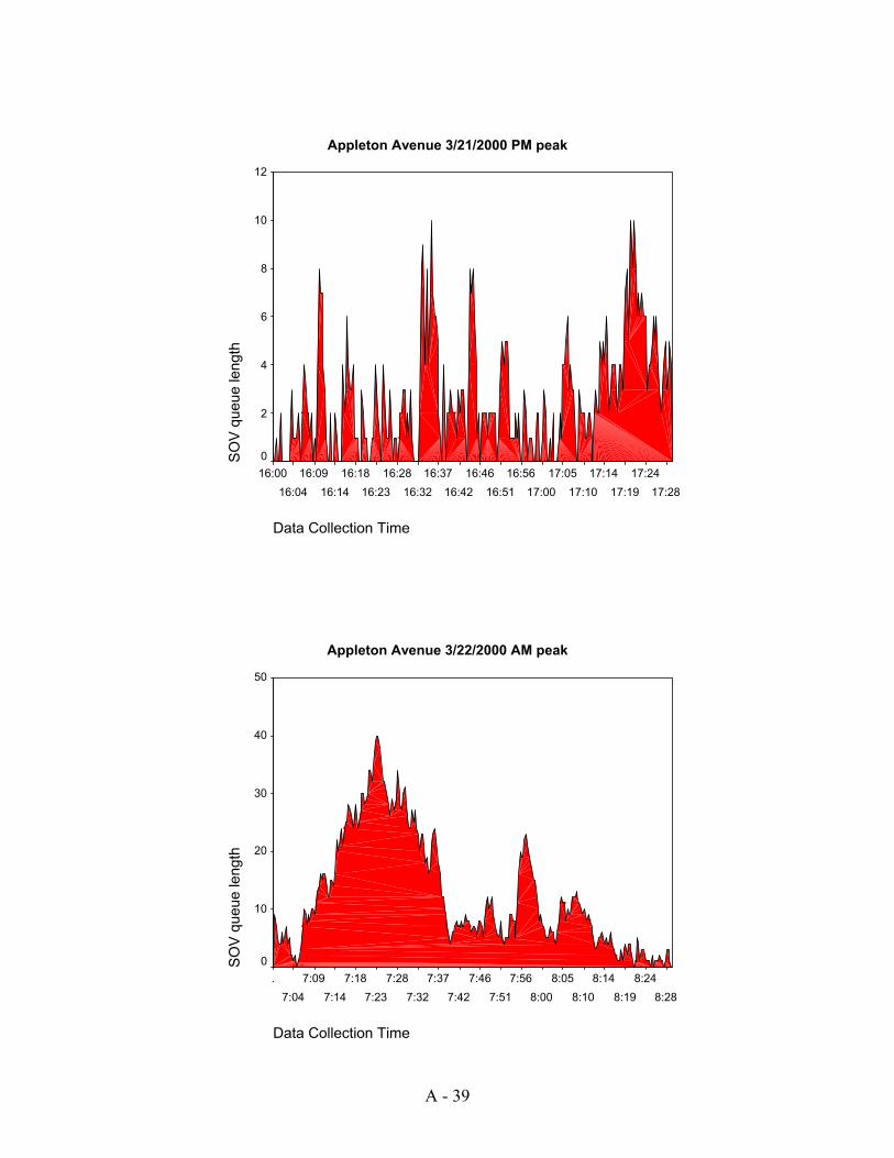
A - 39

Appleton Avenue 3/21/2000 PM peak

Data Collection Time

17:28

17:24

17:19

17:14

17:10

17:05

17:00

16:56

16:51

16:46

16:42

16:37

16:32

16:28

16:23

16:18

16:14

16:09

16:04

16:00

SO

V q

ueue length

12

10

8

6

4

2

0

Appleton Avenue 3/22/2000 AM peak

Data Collection Time

8:28

8:24

8:19

8:14

8:10

8:05

8:00

7:56

7:51

7:46

7:42

7:37

7:32

7:28

7:23

7:18

7:14

7:09

7:04

.

SO

V q

ueue length

50

40

30

20

10

0

A - 40

Appleton Avenue 3/23/2000 AM peak

Data Collection Time

8:29

8:24

8:19

8:15

8:10

8:05

8:01

7:56

7:51

7:47

7:42

7:37

7:33

7:28

7:23

7:19

7:14

7:09

7:05

7:00

SO

V q

ueue length

30

20

10

0

Hampton Avenue 3/14/2000 AM peak

Data Collection Time

8:29

8:24

8:19

8:15

8:10

8:05

8:01

7:56

7:51

7:47

7:42

7:37

7:33

7:28

7:23

7:19

7:14

7:09

7:05

7:00

SO

V q

ueue length

20

10

0

A - 41

Hampton Avenue 3/14/2000 AM peak

Data Collection Time

8:29

8:24

8:19

8:15

8:10

8:05

8:01

7:56

7:51

7:47

7:42

7:37

7:33

7:28

7:23

7:19

7:14

7:09

7:05

7:00

HO

V q

ueue length

1.2

1.0

.8

.6

.4

.2

0.0

Hampton Avenue 3/15/2000 AM peak

Data Collection Time

8:28

8:24

8:19

8:14

8:10

8:05

8:00

7:56

7:51

7:46

7:42

7:37

7:32

7:28

7:23

7:18

7:14

7:09

7:04

.

SO

V q

ueue length

30

20

10

0

A - 42

Hampton Avenue 3/15/2000 AM peak

Data Collection Time

8:28

8:24

8:19

8:14

8:10

8:05

8:00

7:56

7:51

7:46

7:42

7:37

7:32

7:28

7:23

7:18

7:14

7:09

7:04

.

HO

V q

ueue length

1.2

1.0

.8

.6

.4

.2

0.0

Hampton Avenue 3/16/2000 AM peak

Data Collection Time

8:29

8:24

8:19

8:15

8:10

8:05

8:01

7:56

7:51

7:47

7:42

7:37

7:33

7:28

7:23

7:19

7:14

7:09

7:05

7:00

SO

V q

ueue length

30

20

10

0

A - 43

Hampton Avenue 3/16/2000 AM peak

Data Collection Time

8:29

8:24

8:19

8:15

8:10

8:05

8:01

7:56

7:51

7:47

7:42

7:37

7:33

7:28

7:23

7:19

7:14

7:09

7:05

7:00

HO

V q

ueue length

2.5

2.0

1.5

1.0

.5

0.0

Hampton Avenue 3/16/2000 PM peak

Data Collection Time

17:28

17:23

17:19

17:14

17:09

17:05

17:00

16:55

16:51

16:46

16:41

16:37

16:32

16:27

16:23

16:18

16:13

16:09

16:04

.

SO

V q

ueue length

14

12

10

8

6

4

2

0

A - 44

Hampton Avenue 3/16/2000 PM peak

Data Collection Time

17:28

17:23

17:19

17:14

17:09

17:05

17:00

16:55

16:51

16:46

16:41

16:37

16:32

16:27

16:23

16:18

16:13

16:09

16:04

.

HO

V q

ueue length

1.2

1.0

.8

.6

.4

.2

0.0

Hampton Avenue 3/21/2000 AM peak

DATA_COL

8:29

8:24

8:19

8:15

8:10

8:05

8:01

7:56

7:51

7:47

7:42

7:37

7:33

7:28

7:23

7:19

7:14

7:09

7:05

7:00

SO

V q

ueue length

20

10

0

A - 45

Hampton Avenue 3/21/2000 AM peak

DATA_COL

8:29

8:24

8:19

8:15

8:10

8:05

8:01

7:56

7:51

7:47

7:42

7:37

7:33

7:28

7:23

7:19

7:14

7:09

7:05

7:00

HO

V q

ueue length

1.2

1.0

.8

.6

.4

.2

0.0

Hampton Avenue 3/21/2000 PM peak

DATA_COL

17:28

17:24

17:19

17:14

17:10

17:05

17:00

16:56

16:51

16:46

16:42

16:37

16:32

16:28

16:23

16:18

16:14

16:09

16:04

16:00

SO

V q

ueue length

30

20

10

0

A - 46

Hampton Avenue 3/21/2000 PM peak

DATA_COL

17:28

17:24

17:19

17:14

17:10

17:05

17:00

16:56

16:51

16:46

16:42

16:37

16:32

16:28

16:23

16:18

16:14

16:09

16:04

16:00

HO

V q

ueue length

1.2

1.0

.8

.6

.4

.2

0.0

Hampton Avenue 3/22/2000 PM peak

DATA_COL

17:28

17:24

17:19

17:14

17:10

17:05

17:00

16:56

16:51

16:46

16:42

16:37

16:32

16:28

16:23

16:18

16:14

16:09

16:04

16:00

SO

V q

ueue length

30

20

10

0

A - 47

Hampton Avenue 3/22/2000 PM peak

DATA_COL

17:28

17:24

17:19

17:14

17:10

17:05

17:00

16:56

16:51

16:46

16:42

16:37

16:32

16:28

16:23

16:18

16:14

16:09

16:04

16:00

HO

V q

ueue length

1.2

1.0

.8

.6

.4

.2

0.0

Hampton Avenue 3/23/2000 AM peak

DATA_COL

8:29

8:24

8:19

8:15

8:10

8:05

8:01

7:56

7:51

7:47

7:42

7:37

7:33

7:28

7:23

7:19

7:14

7:09

7:05

7:00

SO

V q

ueue length

30

20

10

0

A - 48

Hampton Avenue 3/23/2000 AM peak

DATA_COL

8:29

8:24

8:19

8:15

8:10

8:05

8:01

7:56

7:51

7:47

7:42

7:37

7:33

7:28

7:23

7:19

7:14

7:09

7:05

7:00

HO

V q

ueue length

1.2

1.0

.8

.6

.4

.2

0.0

Hampton Avenue 3/23/2000 PM peak

DATA_COL

17:28

17:24

17:19

17:14

17:10

17:05

17:00

16:56

16:51

16:46

16:42

16:37

16:32

16:28

16:23

16:18

16:14

16:09

16:04

16:00

SO

V q

ueue length

16

14

12

10

8

6

4

2

0

A - 49

Hampton Avenue 3/23/2000 PM peak

DATA_COL

17:28

17:24

17:19

17:14

17:10

17:05

17:00

16:56

16:51

16:46

16:42

16:37

16:32

16:28

16:23

16:18

16:14

16:09

16:04

16:00

HO

V q

ueue length

1.2

1.0

.8

.6

.4

.2

0.0

Capitol Drive 3/14/2000 AM peak

Data Collection Time

8:29

8:24

8:19

8:15

8:10

8:05

8:01

7:56

7:51

7:47

7:42

7:37

7:33

7:28

7:23

7:19

7:14

7:09

7:05

7:00

SO

V q

ueue length

30

20

10

0

A - 50

Capitol Drive 3/14/2000 AM peak

Data Collection Time

8:29

8:24

8:19

8:15

8:10

8:05

8:01

7:56

7:51

7:47

7:42

7:37

7:33

7:28

7:23

7:19

7:14

7:09

7:05

7:00

HO

V q

ueue length

3.5

3.0

2.5

2.0

1.5

1.0

.5

0.0

Capitol Drive 3/14/2000 PM peak

Data Collection Time

17:28

17:24

17:19

17:14

17:10

17:05

17:00

16:56

16:51

16:46

16:42

16:37

16:32

16:28

16:23

16:18

16:14

16:09

16:04

16:00

SO

V q

ueue length

16

14

12

10

8

6

4

2

0

A - 51

Capitol Drive 3/14/2000 PM peak

Data Collection Time

17:28

17:24

17:19

17:14

17:10

17:05

17:00

16:56

16:51

16:46

16:42

16:37

16:32

16:28

16:23

16:18

16:14

16:09

16:04

16:00

HO

V q

ueue length

2.5

2.0

1.5

1.0

.5

0.0

Capitol Drive 3/15/2000 AM peak

Data Collection Time

8:28

8:24

8:19

8:14

8:10

8:05

8:00

7:56

7:51

7:46

7:42

7:37

7:32

7:28

7:23

7:18

7:14

7:09

7:04

.

SO

V q

ueue length

30

20

10

0

A - 52

Capitol Drive 3/15/2000 AM peak

Data Collection Time

8:28

8:24

8:19

8:14

8:10

8:05

8:00

7:56

7:51

7:46

7:42

7:37

7:32

7:28

7:23

7:18

7:14

7:09

7:04

.

HO

V q

ueue length

2.5

2.0

1.5

1.0

.5

0.0

Capitol Drive 3/15/2000 PM peak

Data Collection Time

17:28

17:23

17:19

17:14

17:09

17:05

17:00

16:55

16:51

16:46

16:41

16:37

16:32

16:27

16:23

16:18

16:13

16:09

16:04

.

SO

V q

ueue length

30

20

10

0

A - 53

Capitol Drive 3/15/2000 PM peak

Data Collection Time

17:28

17:23

17:19

17:14

17:09

17:05

17:00

16:55

16:51

16:46

16:41

16:37

16:32

16:27

16:23

16:18

16:13

16:09

16:04

.

HO

V q

ueue length

2.5

2.0

1.5

1.0

.5

0.0

Capitol Drive 3/16/2000 PM peak

Data Collection Time

17:28

17:24

17:19

17:14

17:10

17:05

17:00

16:56

16:51

16:46

16:42

16:37

16:32

16:28

16:23

16:18

16:14

16:09

16:04

16:00

SO

V q

ueue length

50

40

30

20

10

0

A - 54

Capitol Drive 3/16/2000 PM peak

Data Collection Time

17:28

17:24

17:19

17:14

17:10

17:05

17:00

16:56

16:51

16:46

16:42

16:37

16:32

16:28

16:23

16:18

16:14

16:09

16:04

16:00

HO

V q

ueue length

2.5

2.0

1.5

1.0

.5

0.0

Capitol Drive 3/21/2000 AM peak

Data Collection Time

8:28

8:24

8:19

8:14

8:10

8:05

8:00

7:56

7:51

7:46

7:42

7:37

7:32

7:28

7:23

7:18

7:14

7:09

7:04

.

SO

V q

ueue length

40

30

20

10

0

A - 55

Capitol Drive 3/21/2000 AM peak

Data Collection Time

8:28

8:24

8:19

8:14

8:10

8:05

8:00

7:56

7:51

7:46

7:42

7:37

7:32

7:28

7:23

7:18

7:14

7:09

7:04

.

HO

V q

ueue length

2.5

2.0

1.5

1.0

.5

0.0

Capitol Drive 3/21/2000 PM peak

Data Collection Time

17:28

17:24

17:19

17:14

17:10

17:05

17:00

16:56

16:51

16:46

16:42

16:37

16:32

16:28

16:23

16:18

16:14

16:09

16:04

16:00

SO

V q

ueue length

16

14

12

10

8

6

4

2

0

A - 56

Capitol Drive 3/21/2000 PM peak

Data Collection Time

17:28

17:24

17:19

17:14

17:10

17:05

17:00

16:56

16:51

16:46

16:42

16:37

16:32

16:28

16:23

16:18

16:14

16:09

16:04

16:00

HO

V q

ueue length

2.5

2.0

1.5

1.0

.5

0.0

Capitol Drive 3/22/2000 AM peak

Data Collection Time

8:29

8:24

8:19

8:15

8:10

8:05

8:01

7:56

7:51

7:47

7:42

7:37

7:33

7:28

7:23

7:19

7:14

7:09

7:05

7:00

SO

V q

ueue length

40

30

20

10

0

A - 57

Capitol Drive 3/22/2000 AM peak

Data Collection Time

8:29

8:24

8:19

8:15

8:10

8:05

8:01

7:56

7:51

7:47

7:42

7:37

7:33

7:28

7:23

7:19

7:14

7:09

7:05

7:00

HO

V q

ueue length

2.5

2.0

1.5

1.0

.5

0.0

Capitol Drive 3/22/2000 PM peak

Data Collection Time

17:28

17:23

17:19

17:14

17:09

17:05

17:00

16:55

16:51

16:46

16:41

16:37

16:32

16:27

16:23

16:18

16:13

16:09

16:04

.

SO

V q

ueue length

20

10

0

A - 58

Capitol Drive 3/22/2000 PM peak

Data Collection Time

17:28

17:23

17:19

17:14

17:09

17:05

17:00

16:55

16:51

16:46

16:41

16:37

16:32

16:27

16:23

16:18

16:13

16:09

16:04

.

HO

V q

ueue length

5

4

3

2

1

0

Capitol Drive 3/23/2000 AM peak

Data Collection Time

8:28

8:24

8:19

8:14

8:10

8:05

8:00

7:56

7:51

7:46

7:42

7:37

7:32

7:28

7:23

7:18

7:14

7:09

7:04

.

SO

V q

ueue length

40

30

20

10

0

A - 59

Capitol Drive 3/23/2000 AM peak

Data Collection Time

8:28

8:24

8:19

8:14

8:10

8:05

8:00

7:56

7:51

7:46

7:42

7:37

7:32

7:28

7:23

7:18

7:14

7:09

7:04

.

HO

V q

ueue length

3.5

3.0

2.5

2.0

1.5

1.0

.5

0.0

Capitol Drive 3/23/2000 PM peak

Data Collection Time

17:28

17:24

17:19

17:14

17:10

17:05

17:00

16:56

16:51

16:46

16:42

16:37

16:32

16:28

16:23

16:18

16:14

16:09

16:04

16:00

SO

V q

ueue length

20

10

0

A - 60

Capitol Drive 3/23/2000 PM peak

Data Collection Time

17:28

17:24

17:19

17:14

17:10

17:05

17:00

16:56

16:51

16:46

16:42

16:37

16:32

16:28

16:23

16:18

16:14

16:09

16:04

16:00

HO

V q

ueue length

2.5

2.0

1.5

1.0

.5

0.0

Burleigh Street 3/14/2000 AM peak

Data Collection Time

8:28

8:24

8:19

8:14

8:10

8:05

8:00

7:56

7:51

7:46

7:42

7:37

7:32

7:28

7:23

7:18

7:14

7:09

7:04

.

SO

V q

ueue length

30

20

10

0

A - 61

Burleigh Street 3/14/2000 AM peak

Data Collection Time

8:28

8:24

8:19

8:14

8:10

8:05

8:00

7:56

7:51

7:46

7:42

7:37

7:32

7:28

7:23

7:18

7:14

7:09

7:04

.

HO

V q

ueue length

2.5

2.0

1.5

1.0

.5

0.0

Burleigh Street 3/14/2000 PM peak

Data Collection Time

17:28

17:23

17:19

17:14

17:09

17:05

17:00

16:55

16:51

16:46

16:41

16:37

16:32

16:27

16:23

16:18

16:13

16:09

16:04

.

SO

V q

ueue length

50

40

30

20

10

0

A - 62

Burleigh Street 3/14/2000 PM peak

Data Collection Time

17:28

17:23

17:19

17:14

17:09

17:05

17:00

16:55

16:51

16:46

16:41

16:37

16:32

16:27

16:23

16:18

16:13

16:09

16:04

.

HO

V q

ueue length

3.5

3.0

2.5

2.0

1.5

1.0

.5

0.0

Burleigh Street 3/15/2000 AM peak

Data Collection Time

8:28

8:22

8:16

8:09

8:03

7:57

7:50

7:44

7:38

7:31

7:25

7:19

7:12

7:06

.

SO

V q

ueue length

40

30

20

10

0

A - 63

Burleigh Street 3/15/2000 AM peak

Data Collection Time

8:28

8:24

8:19

8:14

8:10

8:05

8:00

7:56

7:51

7:46

7:42

7:37

7:32

7:28

7:23

7:18

7:14

7:09

7:04

.

HO

V q

ueue length

2.5

2.0

1.5

1.0

.5

0.0

Burleigh Street 3/15/2000 PM peak

Data Collection Time

17:28

17:24

17:19

17:14

17:10

17:05

17:00

16:56

16:51

16:46

16:42

16:37

16:32

16:28

16:23

16:18

16:14

16:09

16:04

16:00

SO

V q

ueue length

50

40

30

20

10

A - 64

Burleigh Street 3/15/2000 PM peak

Data Collection Time

17:28

17:24

17:19

17:14

17:10

17:05

17:00

16:56

16:51

16:46

16:42

16:37

16:32

16:28

16:23

16:18

16:14

16:09

16:04

16:00

HO

V q

ueue length

1.2

1.0

.8

.6

.4

.2

0.0

Burleigh Street 3/16/2000 AM peak

Data Collection Time

8:29

8:24

8:19

8:15

8:10

8:05

8:01

7:56

7:51

7:47

7:42

7:37

7:33

7:28

7:23

7:19

7:14

7:09

7:05

7:00

SO

V q

ueue length

50

40

30

20

10

0

A - 65

Burleigh Street 3/16/2000 AM peak

Data Collection Time

8:29

8:24

8:19

8:15

8:10

8:05

8:01

7:56

7:51

7:47

7:42

7:37

7:33

7:28

7:23

7:19

7:14

7:09

7:05

7:00

HO

V q

ueue length

2.5

2.0

1.5

1.0

.5

0.0

Burleigh Street 3/16/2000 PM peak

Data Collection Time

17:28

17:23

17:19

17:14

17:09

17:05

17:00

16:55

16:51

16:46

16:41

16:37

16:32

16:27

16:23

16:18

16:13

16:09

16:04

.

SO

V q

ueue length

50

40

30

20

10

A - 66

Burleigh Street 3/16/2000 PM peak

Data Collection Time

17:28

17:23

17:19

17:14

17:09

17:05

17:00

16:55

16:51

16:46

16:41

16:37

16:32

16:27

16:23

16:18

16:13

16:09

16:04

.

HO

V q

ueue length

2.5

2.0

1.5

1.0

.5

0.0

Burleigh Street 3/21/2000 AM peak

Data Collection Time

8:29

8:24

8:19

8:15

8:10

8:05

8:01

7:56

7:51

7:47

7:42

7:37

7:33

7:28

7:23

7:19

7:14

7:09

7:05

7:00

SO

V q

ueue length

30

20

10

0

A - 67

Burleigh Street 3/21/2000 AM peak

Data Collection Time

8:29

8:24

8:19

8:15

8:10

8:05

8:01

7:56

7:51

7:47

7:42

7:37

7:33

7:28

7:23

7:19

7:14

7:09

7:05

7:00

HO

V q

ueue length

1.2

1.0

.8

.6

.4

.2

0.0

Burleigh Street 3/21/2000 PM peak

DATA_COL

17:28

17:24

17:19

17:14

17:10

17:05

17:00

16:56

16:51

16:46

16:42

16:37

16:32

16:28

16:23

16:18

16:14

16:09

16:04

16:00

SO

V q

ueue length

40

30

20

10

0

A - 68

Burleigh Street 3/21/2000 PM peak

DATA_COL

17:28

17:24

17:19

17:14

17:10

17:05

17:00

16:56

16:51

16:46

16:42

16:37

16:32

16:28

16:23

16:18

16:14

16:09

16:04

16:00

HO

V q

ueue length

1.2

1.0

.8

.6

.4

.2

0.0

Burleigh Street 3/22/2000 AM peak

DATA_COL

8:29

8:24

8:19

8:15

8:10

8:05

8:01

7:56

7:51

7:47

7:42

7:37

7:33

7:28

7:23

7:19

7:14

7:09

7:05

7:00

SO

V q

ueue length

30

20

10

0

A - 69

Burleigh Street 3/22/2000 AM peak

DATA_COL

8:29

8:24

8:19

8:15

8:10

8:05

8:01

7:56

7:51

7:47

7:42

7:37

7:33

7:28

7:23

7:19

7:14

7:09

7:05

7:00

HO

V q

ueue length

1.2

1.0

.8

.6

.4

.2

0.0

Burleigh Street 3/22/2000 PM peak

DATA_COL

17:28

17:24

17:19

17:14

17:10

17:05

17:00

16:56

16:51

16:46

16:42

16:37

16:32

16:28

16:23

16:18

16:14

16:09

16:04

16:00

SO

V q

ueue length

60

50

40

30

20

10

0

A - 70

Burleigh Street 3/22/2000 PM peak

DATA_COL

17:28

17:24

17:19

17:14

17:10

17:05

17:00

16:56

16:51

16:46

16:42

16:37

16:32

16:28

16:23

16:18

16:14

16:09

16:04

16:00

HO

V q

ueue length

2.5

2.0

1.5

1.0

.5

0.0

Burleigh Street 3/23/2000 AM peak

DATA_COL

8:29

8:24

8:19

8:15

8:10

8:05

8:01

7:56

7:51

7:47

7:42

7:37

7:33

7:28

7:23

7:19

7:14

7:09

7:05

7:00

SO

V q

ueue length

30

20

10

0

A - 71

Burleigh Street 3/23/2000 AM peak

DATA_COL

8:29

8:24

8:19

8:15

8:10

8:05

8:01

7:56

7:51

7:47

7:42

7:37

7:33

7:28

7:23

7:19

7:14

7:09

7:05

7:00

HO

V q

ueue length

2.5

2.0

1.5

1.0

.5

0.0

Burleigh Street 3/23/2000 PM peak

DATA_COL

17:28

17:24

17:19

17:14

17:10

17:05

17:00

16:56

16:51

16:46

16:42

16:37

16:32

16:28

16:23

16:18

16:14

16:09

16:04

16:00

SO

V q

ueue length

60

50

40

30

20

10

0

A - 72

Burleigh Street 3/23/2000 PM peak

DATA_COL

17:28

17:24

17:19

17:14

17:10

17:05

17:00

16:56

16:51

16:46

16:42

16:37

16:32

16:28

16:23

16:18

16:14

16:09

16:04

16:00

HO

V q

ueue length

2.5

2.0

1.5

1.0

.5

0.0

North Avenue 2/1/2000 AM peak

Data Collection Time

8:28

8:24

8:19

8:14

8:10

8:05

8:00

7:56

7:51

7:46

7:42

7:37

7:32

7:28

7:23

7:18

7:14

7:09

7:04

7:00

SO

V q

ueue length

30

20

10

0

A - 73

North Avenue 2/1/2000 PM peak

DATA_COL

17:28

17:24

17:19

17:14

17:10

17:05

17:00

16:56

16:51

16:46

16:42

16:37

16:32

16:28

16:23

16:18

16:14

16:09

16:04

16:00

SO

V q

ueue length

40

30

20

10

0

North Avenue 2/2/2000 AM peak

DATA_COL

8:29

8:24

8:19

8:15

8:10

8:05

8:01

7:56

7:51

7:47

7:42

7:37

7:33

7:28

7:23

7:19

7:14

7:09

7:05

7:00

SO

V q

ueue length

30

20

10

0

A - 74

North Avenue 2/2/2000 PM peak

DATA_COL

17:28

17:24

17:19

17:14

17:10

17:05

17:00

16:56

16:51

16:46

16:42

16:37

16:32

16:28

16:23

16:18

16:14

16:09

16:04

16:00

SO

V q

ueue length

40

30

20

10

0

North Avenue 2/3/2000 AM peak

DATA_COL

8:29

8:24

8:19

8:15

8:10

8:05

8:01

7:56

7:51

7:47

7:42

7:37

7:33

7:28

7:23

7:19

7:14

7:09

7:05

7:00

SO

V q

ueue length

30

20

10

0

A - 75

North Avenue 2/3/2000 PM peak

DATA_COL

17:28

17:24

17:19

17:14

17:10

17:05

17:00

16:56

16:51

16:46

16:42

16:37

16:32

16:28

16:23

16:18

16:14

16:09

16:04

16:00

SO

V q

ueue length

40

30

20

10

0

North Avenue 2/8/2000 AM peak

Data Collection Time

8:29

8:24

8:19

8:15

8:10

8:05

8:01

7:56

7:51

7:47

7:42

7:37

7:33

7:28

7:23

7:19

7:14

7:09

7:05

7:00

SO

V q

ueue length

40

30

20

10

0

A - 76

North Avenue 2/8/2000 PM peak

Data Collection Time

17:28

17:23

17:19

17:14

17:09

17:05

17:00

16:55

16:51

16:46

16:41

16:37

16:32

16:27

16:23

16:18

16:13

16:09

16:04

16:00

SO

V q

ueue length

50

40

30

20

10

0

North Avenue 2/9/2000 AM peak

DATA_COL

8:29

8:24

8:19

8:15

8:10

8:05

8:01

7:56

7:51

7:47

7:42

7:37

7:33

7:28

7:23

7:19

7:14

7:09

7:05

7:00

SO

V q

ueue length

30

20

10

0

A - 77

North Avenue 2/9/2000 PM peak

Data Collection Time

17:28

17:23

17:19

17:14

17:09

17:05

17:00

16:55

16:51

16:46

16:41

16:37

16:32

16:27

16:23

16:18

16:13

16:09

16:04

16:00

SO

V q

ueue length

40

30

20

10

0

North Avenue 2/10/2000 AM peak

DATA_COL

8:29

8:24

8:19

8:15

8:10

8:05

8:01

7:56

7:51

7:47

7:42

7:37

7:33

7:28

7:23

7:19

7:14

7:09

7:05

7:00

SO

V q

ueue length

30

20

10

0

A - 78

North Avenue 2/10/2000 PM peak

Data Collection Time

17:28

17:24

17:19

17:14

17:10

17:05

17:00

16:56

16:51

16:46

16:42

16:37

16:32

16:28

16:23

16:18

16:14

16:09

16:04

16:00

SO

V q

ueue length

40

30

20

10

0

North Avenue 3/14/2000 AM peak

Data Collection Time

8:28

8:24

8:19

8:14

8:10

8:05

8:00

7:56

7:51

7:46

7:42

7:37

7:32

7:28

7:23

7:18

7:14

7:09

7:04

.

SO

V q

ueue length

30

20

10

0

A - 79

North Avenue 3/14/2000 PM peak

Data Collection Time

17:28

17:23

17:19

17:14

17:09

17:05

17:00

16:55

16:51

16:46

16:41

16:37

16:32

16:27

16:23

16:18

16:13

16:09

16:04

.

SO

V q

ueue length

30

20

10

0

North Avenue 3/15/2000 PM peak

Data Collection Time

17:28

17:24

17:19

17:14

17:10

17:05

17:00

16:56

16:51

16:46

16:42

16:37

16:32

16:28

16:23

16:18

16:14

16:09

16:04

16:00

SO

V q

ueue length

30

20

10

0

A - 80

North Avenue 3/16/2000 AM peak

Data Collection Time

8:29

8:24

8:19

8:15

8:10

8:05

8:01

7:56

7:51

7:47

7:42

7:37

7:33

7:28

7:23

7:19

7:14

7:09

7:05

7:00

SO

V q

ueue length

30

20

10

0

North Avenue 3/16/2000 PM peak

Data Collection Time

17:28

17:23

17:19

17:14

17:09

17:05

17:00

16:55

16:51

16:46

16:41

16:37

16:32

16:27

16:23

16:18

16:13

16:09

16:04

.

SO

V q

ueue length

30

20

10

0

A - 81

North Avenue 3/21/2000 PM peak

Data Collection Time

17:28

17:24

17:19

17:14

17:10

17:05

17:00

16:56

16:51

16:46

16:42

16:37

16:32

16:28

16:23

16:18

16:14

16:09

16:04

16:00

SO

V q

ueue length

50

40

30

20

10

0

North Avenue 3/22/2000 AM peak

Data Collection Time

8:29

8:24

8:19

8:15

8:10

8:05

8:01

7:56

7:51

7:47

7:42

7:37

7:33

7:28

7:23

7:19

7:14

7:09

7:05

7:00

SO

V q

ueue length

30

20

10

0

A - 82

North Avenue 3/22/2000 PM peak

Data Collection Time

17:28

17:23

17:19

17:14

17:09

17:05

17:00

16:55

16:51

16:46

16:41

16:37

16:32

16:27

16:23

16:18

16:13

16:09

16:04

.

SO

V q

ueue length

40

30

20

10

0

North Avenue 3/23/2000 PM peak

Data Collection Time

17:28

17:24

17:19

17:14

17:10

17:05

17:00

16:56

16:51

16:46

16:42

16:37

16:32

16:28

16:23

16:18

16:14

16:09

16:04

16:00

SO

V q

ueue length

40

30

20

10

0

A - 83

Watertown Plank Road 2/1/2000 AM peak

DATA_COL

8:29

8:24

8:19

8:15

8:10

8:05

8:01

7:56

7:51

7:47

7:42

7:37

7:33

7:28

7:23

7:19

7:14

7:09

7:05

7:00

SO

V q

ueue length

16

14

12

10

8

6

4

2

0

Watertown Plank Road 2/1/2000 AM peak

DATA_COL

8:29

8:24

8:19

8:15

8:10

8:05

8:01

7:56

7:51

7:47

7:42

7:37

7:33

7:28

7:23

7:19

7:14

7:09

7:05

7:00

HO

V q

ueue length

1.2

1.0

.8

.6

.4

.2

0.0

A - 84

Watertown Plank Road 2/1/2000 PM peak

TIME

17:27

17:23

17:18

17:14

17:09

17:04

17:00

16:55

16:51

16:46

16:41

16:37

16:32

16:27

16:23

16:18

16:14

16:09

16:04

16:00

SO

V q

ueue length

50

40

30

20

10

Watertown Plank Road 2/2/2000 AM peak

TIME

8:27

8:23

8:18

8:14

8:09

8:04

8:00

7:55

7:51

7:46

7:41

7:37

7:32

7:27

7:23

7:18

7:14

7:09

7:04

7:00

SO

V q

ueue length

60

50

40

30

20

10

0

A - 85

Watertown Plank Road 2/2/2000 AM peak

TIME

8:27

8:23

8:18

8:14

8:09

8:04

8:00

7:55

7:51

7:46

7:41

7:37

7:32

7:27

7:23

7:18

7:14

7:09

7:04

7:00

HO

V q

ueue length

1.2

1.0

.8

.6

.4

.2

0.0

Watertown Plank Road 2/2/2000 PM peak

TIME

17:27

17:23

17:18

17:13

17:09

17:04

17:00

16:55

16:50

16:46

16:41

16:37

16:32

16:27

16:23

16:18

16:13

16:09

16:04

16:00

SO

V q

ueue length

60

50

40

30

20

10

0

A - 86

Watertown Plank Road 2/2/2000 PM peak

TIME

17:27

17:23

17:18

17:13

17:09

17:04

17:00

16:55

16:50

16:46

16:41

16:37

16:32

16:27

16:23

16:18

16:13

16:09

16:04

16:00

HO

V q

ueue length

1.2

1.0

.8

.6

.4

.2

0.0

Watertown Plank Road 2/3/2000 AM peak

TIME

8:27

8:23

8:18

8:13

8:09

8:04

8:00

7:55

7:50

7:46

7:41

7:37

7:32

7:27

7:23

7:18

7:13

7:09

7:04

7:00

SO

V q

ueue length

40

30

20

10

0

A - 87

Watertown Plank Road 2/3/2000 AM peak

TIME

8:27

8:23

8:18

8:13

8:09

8:04

8:00

7:55

7:50

7:46

7:41

7:37

7:32

7:27

7:23

7:18

7:13

7:09

7:04

7:00

HO

V q

ueue length

1.2

1.0

.8

.6

.4

.2

0.0

Watertown Plank Road 2/3/2000 PM peak

TIME

17:27

17:23

17:18

17:14

17:09

17:04

17:00

16:55

16:51

16:46

16:41

16:37

16:32

16:27

16:23

16:18

16:14

16:09

16:04

16:00

SO

V q

ueue length

50

40

30

20

10

A - 88

Watertown Plank Road 2/8/2000 AM peak

TIME

8:27

8:23

8:18

8:13

8:09

8:04

8:00

7:55

7:50

7:46

7:41

7:37

7:32

7:27

7:23

7:18

7:14

7:09

7:04

7:00

SO

V q

ueue length

40

30

20

10

0

Watertown Plank Road 2/8/2000 AM peak

TIME

8:27

8:23

8:18

8:13

8:09

8:04

8:00

7:55

7:50

7:46

7:41

7:37

7:32

7:27

7:23

7:18

7:14

7:09

7:04

7:00

HO

V q

ueue length

1.2

1.0

.8

.6

.4

.2

0.0

A - 89

Watertown Plank Road 2/8/2000 PM peak

TIME

17:27

17:23

17:18

17:14

17:09

17:04

17:00

16:55

16:51

16:46

16:41

16:37

16:32

16:27

16:23

16:18

16:14

16:09

16:04

16:00

SO

V q

ueue length

50

40

30

20

10

0

Watertown Plank Road 2/9/2000 AM peak

TIME

8:27

8:23

8:18

8:14

8:09

8:04

8:00

7:55

7:51

7:46

7:41

7:37

7:32

7:27

7:23

7:18

7:14

7:09

7:04

7:00

SO

V q

ueue length

40

30

20

10

0

A - 90

Watertown Plank Road 2/9/2000 AM peak

TIME

8:27

8:23

8:18

8:14

8:09

8:04

8:00

7:55

7:51

7:46

7:41

7:37

7:32

7:27

7:23

7:18

7:14

7:09

7:04

7:00

HO

V q

ueue length

1.2

1.0

.8

.6

.4

.2

0.0

Watertown Plank Road 2/9/2000 PM peak

TIME

17:27

17:23

17:18

17:13

17:09

17:04

17:00

16:55

16:50

16:46

16:41

16:37

16:32

16:27

16:23

16:18

16:13

16:09

16:04

16:00

SO

V q

ueue length

60

50

40

30

20

10

A - 91

Watertown Plank Road 2/9/2000 PM peak

TIME

17:27

17:23

17:18

17:13

17:09

17:04

17:00

16:55

16:50

16:46

16:41

16:37

16:32

16:27

16:23

16:18

16:13

16:09

16:04

16:00

HO

V q

ueue length

1.2

1.0

.8

.6

.4

.2

0.0

Watertown Plank Road 2/10/2000 AM peak

TIME

8:27

8:23

8:18

8:13

8:09

8:04

8:00

7:55

7:50

7:46

7:41

7:37

7:32

7:27

7:23

7:18

7:13

7:09

7:04

7:00

SO

V q

ueue length

40

30

20

10

0

A - 92

Watertown Plank Road 2/10/2000 AM peak

TIME

8:27

8:23

8:18

8:13

8:09

8:04

8:00

7:55

7:50

7:46

7:41

7:37

7:32

7:27

7:23

7:18

7:13

7:09

7:04

7:00

HO

V q

ueue length

1.2

1.0

.8

.6

.4

.2

0.0

Watertown Plank Road 2/10/2000 PM peak

TIME

17:27

17:23

17:18

17:14

17:09

17:04

17:00

16:55

16:51

16:46

16:41

16:37

16:32

16:27

16:23

16:18

16:14

16:09

16:04

16:00

SO

V q

ueue length

60

50

40

30

20

10

0

A - 93

Watertown Plank Road 3/14/2000 AM peak

DATA_COL

8:29

8:24

8:19

8:15

8:10

8:05

8:01

7:56

7:51

7:47

7:42

7:37

7:33

7:28

7:23

7:19

7:14

7:09

7:05

7:00

SO

V q

ueue length

40

30

20

10

0

Watertown Plank Road 3/14/2000 AM peak

DATA_COL

8:29

8:24

8:19

8:15

8:10

8:05

8:01

7:56

7:51

7:47

7:42

7:37

7:33

7:28

7:23

7:19

7:14

7:09

7:05

7:00

HO

V q

ueue length

1.2

1.0

.8

.6

.4

.2

0.0

A - 94

Watertown Plank Road 3/14/2000 PM peak

DATA_COL

17:28

17:24

17:19

17:14

17:10

17:05

17:00

16:56

16:51

16:46

16:42

16:37

16:32

16:28

16:23

16:18

16:14

16:09

16:04

16:00

SO

V q

ueue length

50

40

30

20

10

0

Watertown Plank Road 3/15/2000 AM peak

DATA_COL

8:29

8:22

8:16

8:10

8:03

7:57

7:51

7:44

7:38

7:32

7:25

7:19

7:13

7:06

7:00

SO

V q

ueue length

40

30

20

10

0

A - 95

Watertown Plank Road 3/15/2000 AM peak

DATA_COL

8:29

8:24

8:19

8:15

8:10

8:05

8:01

7:56

7:51

7:47

7:42

7:37

7:33

7:28

7:23

7:19

7:14

7:09

7:05

7:00

HO

V q

ueue length

1.2

1.0

.8

.6

.4

.2

0.0

Watertown Plank Road 3/15/2000 PM peak

DATA_COL

17:28

17:24

17:19

17:14

17:10

17:05

17:00

16:56

16:51

16:46

16:42

16:37

16:32

16:28

16:23

16:18

16:14

16:09

16:04

16:00

SO

V q

ueue length

60

50

40

30

20

10

A - 96

Watertown Plank Road 3/15/2000 PM peak

DATA_COL

17:28

17:24

17:19

17:14

17:10

17:05

17:00

16:56

16:51

16:46

16:42

16:37

16:32

16:28

16:23

16:18

16:14

16:09

16:04

16:00

HO

V q

ueue length

1.2

1.0

.8

.6

.4

.2

0.0

Watertown Plank Road 3/16/2000 AM peak

DATA_COL

8:29

8:24

8:19

8:15

8:10

8:05

8:01

7:56

7:51

7:47

7:42

7:37

7:33

7:28

7:23

7:19

7:14

7:09

7:05

7:00

SO

V q

ueue length

40

30

20

10

0

A - 97

Watertown Plank Road 3/16/2000 AM peak

DATA_COL

8:29

8:24

8:19

8:15

8:10

8:05

8:01

7:56

7:51

7:47

7:42

7:37

7:33

7:28

7:23

7:19

7:14

7:09

7:05

7:00

HO

V q

ueue length

1.2

1.0

.8

.6

.4

.2

0.0

Watertown Plank Road 3/16/2000 PM peak

DATA_COL

17:28

17:24

17:19

17:14

17:10

17:05

17:00

16:56

16:51

16:46

16:42

16:37

16:32

16:28

16:23

16:18

16:14

16:09

16:04

16:00

SO

V q

ueue length

50

40

30

20

10

A - 98

Watertown Plank Road 3/21/2000 AM peak

TIME

8:27

8:23

8:18

8:14

8:09

8:04

8:00

7:55

7:51

7:46

7:41

7:37

7:32

7:27

7:23

7:18

7:14

7:09

7:04

7:00

SO

V q

ueue length

40

30

20

10

0

Watertown Plank Road 3/21/2000 PM peak

TIME

17:27

17:23

17:18

17:13

17:09

17:04

17:00

16:55

16:50

16:46

16:41

16:37

16:32

16:27

16:23

16:18

16:13

16:09

16:04

16:00

SO

V q

ueue length

50

40

30

20

10

0

A - 99

Watertown Plank Road 3/22/2000 AM peak

TIME

8:27

8:23

8:18

8:13

8:09

8:04

8:00

7:55

7:50

7:46

7:41

7:37

7:32

7:27

7:23

7:18

7:13

7:09

7:04

7:00

SO

V q

ueue length

40

30

20

10

0

Watertown Plank Road 3/22/2000 PM peak

TIME

17:27

17:23

17:18

17:14

17:09

17:04

17:00

16:55

16:51

16:46

16:41

16:37

16:32

16:27

16:23

16:18

16:14

16:09

16:04

16:00

SO

V q

ueue length

50

40

30

20

10

A - 100

Watertown Plank Road 3/23/2000 PM peak

TIME

17:27

17:23

17:18

17:13

17:09

17:04

17:00

16:55

16:50

16:46

16:41

16:36

16:32

16:27

16:23

16:18

16:13

16:09

16:04

16:00

SO

V q

ueue length

40

30

20

10

Wisconsin Avenue 2/1/2000 PM peak

Data Collection Time

17:28

17:23

17:18

17:14

17:09

17:04

17:00

16:55

16:50

16:46

16:41

16:36

16:32

16:27

16:22

16:18

16:13

16:08

16:04

.

SO

V q

ueue length

20

10

0

A - 101

Wisconsin Avenue 2/2/2000 AM peak

Data Collection Time

8:28

8:24

8:19

8:14

8:10

8:05

8:00

7:56

7:51

7:46

7:42

7:37

7:32

7:28

7:23

7:18

7:14

7:09

7:04

.

SO

V q

ueue length

14

12

10

8

6

4

2

0

Wisconsin Avenue 2/3/2000 AM peak

Data Collection Time

8:29

8:24

8:19

8:15

8:10

8:05

8:01

7:56

7:51

7:47

7:42

7:37

7:33

7:28

7:23

7:19

7:14

7:09

7:05

7:00

SO

V q

ueue length

20

10

0

A - 102

Wisconsin Avenue 2/8/2000 AM peak

DATA_COL

8:29

8:24

8:19

8:15

8:10

8:05

8:01

7:56

7:51

7:47

7:42

7:37

7:33

7:28

7:23

7:19

7:14

7:09

7:05

7:00

SO

V q

ueue length

10

8

6

4

2

0

Wisconsin Avenue 2/9/2000 AM peak

Data Collection Time

8:28

8:24

8:19

8:14

8:10

8:05

8:00

7:56

7:51

7:46

7:42

7:37

7:32

7:28

7:23

7:18

7:14

7:09

7:04

.

SO

V q

ueue length

8

6

4

2

0

A - 103

Wisconsin Avenue 2/9/2000 PM peak

Data Collection Time

17:28

17:24

17:19

17:14

17:10

17:05

17:00

16:56

16:51

16:46

16:42

16:37

16:32

16:28

16:23

16:18

16:14

16:09

16:04

16:00

SO

V q

ueue length

16

14

12

10

8

6

4

2

0

Wisconsin Avenue 2/10/2000 AM peak

Data Collection Time

8:28

8:24

8:19

8:14

8:10

8:05

8:00

7:56

7:51

7:46

7:42

7:37

7:32

7:28

7:23

7:18

7:14

7:09

7:04

.

SO

V q

ueue length

6

5

4

3

2

1

0

A - 104

Wisconsin Avenue 2/10/2000 PM peak

Data Collection Time

17:28

17:24

17:19

17:14

17:10

17:05

17:00

16:56

16:51

16:46

16:42

16:37

16:32

16:28

16:23

16:18

16:14

16:09

16:04

16:00

SO

V q

ueue length

16

14

12

10

8

6

4

2

0

Wisconsin Avenue 3/14/2000 AM peak

Data Collection Time

8:28

8:24

8:19

8:14

8:10

8:05

8:00

7:56

7:51

7:46

7:42

7:37

7:32

7:28

7:23

7:18

7:14

7:09

7:04

.

SO

V q

ueue length

14

12

10

8

6

4

2

0

A - 105

Wisconsin Avenue 3/14/2000 PM peak

Data Collection Time

17:28

17:24

17:19

17:14

17:10

17:05

17:00

16:56

16:51

16:46

16:42

16:37

16:32

16:28

16:23

16:18

16:14

16:09

16:04

16:00

SO

V q

ueue length

20

10

0

Wisconsin Avenue 3/15/2000 AM peak

Data Collection Time

8:29

8:24

8:19

8:15

8:10

8:05

8:01

7:56

7:51

7:47

7:42

7:37

7:33

7:28

7:23

7:19

7:14

7:09

7:05

7:00

SO

V q

ueue length

14

12

10

8

6

4

2

0

A - 106

Wisconsin Avenue 3/15/2000 PM peak

Data Collection Time

17:28

17:24

17:19

17:14

17:10

17:05

17:00

16:56

16:51

16:46

16:42

16:37

16:32

16:28

16:23

16:18

16:14

16:09

16:04

16:00

SO

V q

ueue length

20

10

0

Wisconsin Avenue 3/16/2000 AM peak

Data Collection Time

8:29

8:24

8:19

8:15

8:10

8:05

8:01

7:56

7:51

7:47

7:42

7:37

7:33

7:28

7:23

7:19

7:14

7:09

7:05

7:00

SO

V q

ueue length

7

6

5

4

3

2

1

0

A - 107

Wisconsin Avenue 3/16/2000 PM peak

Time (On Site)

17:28

17:22

17:16

17:09

17:03

16:57

16:50

16:44

16:38

16:31

16:25

16:19

16:12

16:06

16:00

SO

V q

ueue length

20

10

0

Wisconsin Avenue 3/21/2000 AM peak

Data Collection Time

8:28

8:24

8:19

8:14

8:10

8:05

8:00

7:56

7:51

7:46

7:42

7:37

7:32

7:28

7:23

7:18

7:14

7:09

7:04

.

SO

V q

ueue length

10

8

6

4

2

0

A - 108

Wisconsin Avenue 3/21/2000 PM peak

Data Collection Time

17:28

17:24

17:19

17:14

17:10

17:05

17:00

16:56

16:51

16:46

16:42

16:37

16:32

16:28

16:23

16:18

16:14

16:09

16:04

16:00

SO

V q

ueue length

16

14

12

10

8

6

4

2

0

Wisconsin Avenue 3/22/2000 AM peak

Data Collection Time

8:28

8:24

8:19

8:14

8:10

8:05

8:00

7:56

7:51

7:46

7:42

7:37

7:32

7:28

7:23

7:18

7:14

7:09

7:04

.

SO

V q

ueue length

5

4

3

2

1

0

A - 109

Wisconsin Avenue 3/22/2000 PM peak

Time (On Site)

17:28

17:22

17:16

17:09

17:03

16:57

16:50

16:44

16:38

16:31

16:25

16:19

16:12

16:06

16:00

SO

V q

ueue length

20

10

0

Wisconsin Avenue 3/23/2000 AM peak

Data Collection Time

8:29

8:24

8:19

8:15

8:10

8:05

8:01

7:56

7:51

7:47

7:42

7:37

7:33

7:28

7:23

7:19

7:14

7:09

7:05

7:00

SO

V q

ueue length

5

4

3

2

1

0

A - 110

Wisconsin Avenue 3/23/2000 PM peak

Time (On Site)

17:28

17:22

17:16

17:09

17:03

16:57

16:50

16:44

16:38

16:31

16:25

16:19

16:12

16:06

16:00

SO

V q

ueue length

20

10

0

Greenfield Avenue 2/1/2000 PM peak

Data Collection Time

17:28

17:22

17:15

17:09

17:03

16:56

16:50

16:44

16:37

16:31

16:25

16:18

16:12

16:06

.

SO

V q

ueue length

40

30

20

10

0

A - 111

Greenfield Avenue 2/2/2000 PM peak

Data Collection Time

17:28

17:22

17:15

17:09

17:03

16:56

16:50

16:44

16:37

16:31

16:25

16:18

16:12

16:06

.

SO

V q

ueue length

30

20

10

0

Greenfield Avenue 2/8/2000 PM peak

Data Collection Time

17:28

17:22

17:16

17:09

17:03

16:57

16:50

16:44

16:38

16:31

16:25

16:19

16:12

16:06

16:00

SO

V q

ueue length

30

20

10

0

A - 112

Greenfield Avenue 2/9/2000 PM peak

Data Collection Time

17:28

17:22

17:16

17:09

17:03

16:57

16:50

16:44

16:38

16:31

16:25

16:19

16:12

16:06

16:00

SO

V q

ueue length

30

20

10

0

Greenfield Avenue 2/10/2000 PM peak

Data Collection Time

17:28

17:22

17:15

17:09

17:03

16:56

16:50

16:44

16:37

16:31

16:25

16:18

16:12

16:06

.

SO

V q

ueue length

30

20

10

0

A - 113

Greenfield Avenue 2/14/2000 PM peak

Data Collection Time

17:28

17:22

17:16

17:09

17:03

16:57

16:50

16:44

16:38

16:31

16:25

16:19

16:12

16:06

16:00

SO

V q

ueue length

30

20

10

0

Greenfield Avenue 2/15/2000 AM peak

Data Collection Time

8:29

8:22

8:16

8:10

8:03

7:57

7:51

7:44

7:38

7:32

7:25

7:19

7:13

7:06

7:00

SO

V q

ueue length

4

3

3

2

2

1

1

0

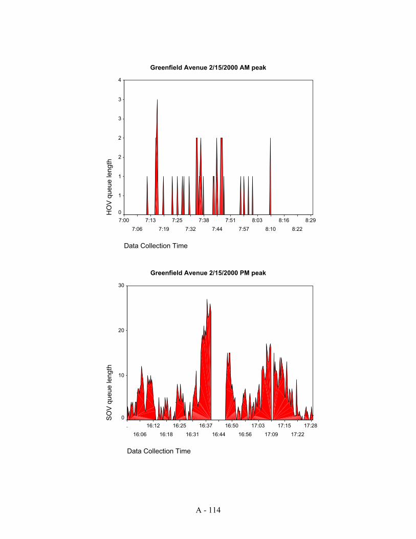
A - 114

Greenfield Avenue 2/15/2000 AM peak

Data Collection Time

8:29

8:22

8:16

8:10

8:03

7:57

7:51

7:44

7:38

7:32

7:25

7:19

7:13

7:06

7:00

HO

V q

ueue length

4

3

3

2

2

1

1

0

Greenfield Avenue 2/15/2000 PM peak

Data Collection Time

17:28

17:22

17:15

17:09

17:03

16:56

16:50

16:44

16:37

16:31

16:25

16:18

16:12

16:06

.

SO

V q

ueue length

30

20

10

0

A - 115

Greenfield Avenue 2/23/2000 PM peak

Data Collection Time

17:28

17:22

17:16

17:09

17:03

16:57

16:50

16:44

16:38

16:31

16:25

16:19

16:12

16:06

16:00

SO

V q

ueue length

16

14

12

10

8

6

4

2

0

Appendix B

Wisconsin Avenue Ramp Meter Operation, Afternoon Peak Period (4:00 pm to 5:30 pm)

Wednesday, February 9, 2000.

B-2

Introduction

The present Appendix provides detailed information on the operation of the Wisconsin

Avenue ramp meter during the afternoon peak period (4:00 pm to 5:30 pm) on

Wednesday, February 9, 2000. Information presented herein was compiled from data

collected through pavement-embedded loop detectors on the ramp and the adjacent

mainline lanes.

The Wisconsin Avenue ramp was chosen for this detailed presentation, because a

complete set of traffic data was available at this location during the study period; the

location coincides with cutline #6 for which additional information is presented

elsewhere in the report.

Ramp metering settings for the presented period are shown in Table B-1 below.

Table B-1. PM Peak Period Ramp Metering Settings-Wisconsin Avenue Ramp

Interval Times

Rate 1 2 3 4 5 6

Green 2.5 2.5 2.5 2.5 2.5 2.5

Yellow 0.0 0.0 0.0 0.0 0.0 0.0

Red 2.5 3.0 3.4 3.8 4.5 6.0

Thresholds

Rate 1 2 3 4 5 6

Volume 1700 1800 1900 2050 2150 2250

Occupancy 19 21 24 27 30 33

Speed 55 50 45 40 35 30

Ramp Occupancy 50 40 35 30 25 20

Time Of Day(TOD)

Time

15:00 Must/May

15:15 Traffic Responsive Min Plan 1

15:15 Most Restrictive

18:00 Must/May

18:15 Non-Metering

B-3

According to information presented in Table B-1, under the “Interval Times” section of

the table, six metering Rates (Rates 1-6) were pre-programmed for the Wisconsin Avenue

ramp. All six metering rates allowed for 2.5 seconds of Green; no Yellow indication was

present; rates differed in Red interval durations. Rate 1 was the least restrictive, with 2.5

seconds of Red; rate 6 was the most restrictive with 6.0 seconds of Red.

Table B-2 presents ramp metering plan selection information, extracted from the

Milwaukee FTMS MONITOR program “Field Equipment Software Reference Manual,”

prepared by JHK & Associates in 1994. The “TOD1” Plan Selection was in effect during

the analyzed period (“Plan Selection” choice #3).

Under this Table B-2 choice, afternoon peak ramp metering operation was operational

during the hours indicated in the “Time Of Day (TOD)” part of Table B-1. Explanations

of terms are provided below.

15:00 Must/May Explanation: No ramp metering was in effect before 3:00 pm. Ramp

metering started at 3:00 pm, if traffic conditions met any of the preset ramp metering

controller thresholds (see explanations below) in Table B-1.

15:15 Responsive Min Plan 1 Explanation: Metering rate 1 (the least restrictive rate,

with a Red duration of 2.5 seconds) would be in effect at this time if traffic did not meet

any of the thresholds for a more restrictive metering rate (even if metering rate 1

thresholds were not met).

15:15 Most Restrictive Explanation: Metering rate selection was based on the Volume,

Occupancy, or Speed threshold that required the most restrictive rate (longer red interval

duration). However, all of these thresholds would be overridden, if queue occupancy

values were high enough to dictate a less restrictive metering rate, so the ramp queue

could be dissipated before it spilled into an adjacent arterial.

18:00 Must/May Explanation: If traffic conditions met any of the thresholds at 6:00 pm,

ramp metering would have continued, otherwise it would have terminated at this time.

18:15 Non-Metering Explanation: Ramp metering would have been turned off at 6:15

pm, regardless of traffic conditions.

Metering rate choice depended on four ramp metering inputs: mainline volume,

occupancy and speed, and ramp queue occupancy values indicated under the

“Thresholds” part of Table B-1. Volume, occupancy and speed summary information

was received from mainline pavement-embedded detectors; ramp queue occupancy

information was received from detectors embedded on the ramp.

1 TOD: Time of Day

Table B-2. Ramp Metering Plan Selection Information.

B-5

Metering rate choice example

For example, if detected traffic conditions were between the values shown for Rates 2

and 3, say, volume 1850 vph, occupancy 22%, speed 49 mph, ramp queue override 37%,

then ramp metering rate 2 would have been chosen (Green 2.5 sec., Red 3.0 sec.) If all

other values remained the same, but speed was 42 mph, which was between the

thresholds for rates 3 and 4, rate 3 would have been chosen, the most restrictive rate that

the specific traffic conditions warranted. If all other values in the original example

remained the same, but the ramp queue occupancy value was 43%, ramp metering rate 1

would have been chosen; ramp occupancy was programmed to override mainline input

demands for more restrictive metering rates.

Description of Appendix figures

Figures B-1 through B-8 in this Appendix are intended to provide a detailed view into

the operation of the Wisconsin Avenue ramp on Wednesday, February 9, 2000, between

4:00 pm and 5:30 pm. These figures use the same time axis; they can be superimposed

on one-another in order to provide insights into which thresholds were met at specific

times, why a certain metering rate was chosen, and how metering rates affected ramp

queue length.

Figures B-3 through B-6 are based on 20-second mainline speed, volume and occupancy

data that were averaged using a moving average of six observations (two minutes);

Figure B-6 represents 20-second ramp occupancy observations. Thresholds for each

metering rate are marked on each of these graphs for easy reference.

Speed-volume and speed-occupancy graphs (Figures B-9 and B-10) are provided for

each quarter hour during this peak period. Similar graphs (Figures B-11 and B-12) are

provided for prevailing weekday afternoon peak conditions at this location based on

information collected at the same location during all data collection days: February 1, 2,

and 3 (week 1), February 8, 9, and 10 (week 2) March 14, 15, and 16 (week 3), and

March 21, 22, and 23 (week 4).

A matrix graph (Figure B-13) relating volume, speed and occupancy at this location is

provided to establish the relationship between all three traffic parameters. Each of the

three distinct graphs on the matrix is presented separately on a larger scale for easier

reference (Figures B-14 through B-16).

Except for graphs indicating that they are based on two-minute average data, all other

information is based on data collected every 20-seconds.

Description of ramp operation

The Wisconsin Avenue ramp queue length is shown in Figure B-1 (the shaded area

represents veh-min of delay). Maximum recorded queue length was 15 vehicles; there

were many instances during the peak period that queue lengths were 12 or more vehicles.

A characteristic see-saw pattern emerged throughout the peak period, when periods of

longer queues were followed by periods of much shorter queues (1 or 2 vehicles-long).

B-6

The most persistent presence of long queues was observed approximately between 16:35

and 16:45.

The reason for choosing a certain ramp metering rate during a specific time can be seen

in Figure B-2. For example, between 16:00 and 16:05, when the “most restrictive” plan

was in effect (see Table B-1), plan reason #7 (see y-axis) controlled the metering rate.

Plan reason #7 corresponds to the entry “Traffic Responsive, Most Restrictive, Volume”

in Table B-2, indicating that mainline traffic volume was the first ramp metering input

that crossed the threshold corresponding to the most restrictive metering rate.

Speeds during this period were 48-50 mph (Figure B-3) corresponding to ramp metering

rate 2, volumes crossed into metering rates 3 and 4 (Figure B-4), mainline occupancies

were well below 19% (Figure B-5) required for rate 1, and ramp occupancy did not

exceed 25% (Figure B-6), thus queue override was not called for. The most restrictive

metering rate was therefore dictated by mainline traffic volumes. The metering rate in

effect at any time is shown in Figure B-7—rates 3 and 4 were in effect during these five

minutes.

At approximately 16:05, ramp queue length increased to 12 vehicles (Figure B-1) within

a short period of time, thus ramp occupancy increased as well. Figure B-2 indicates that

between 16:05 and 16:08, plan reason #16 controlled the metering rate (“Traffic

Responsive, Queue Override” in Table B-2). Indeed, ramp occupancy exceeded 70%

(Figure B-6), overriding all other inputs, and setting the least restrictive metering rate 1

(see Figure B-7) in order to dissipate the ramp queue.

Figure B-8 provides a detailed presentation of metering rates based solely on ramp

occupancy. These rates governed only during the time periods that they were less

restrictive than the rates demanded by mainline metering inputs.

Although mainline speed and occupancy did not change much during these three minutes,

mainline volumes would have demanded rate 5 during this interval, had it not been for

ramp queue occupancies overriding this demand and setting rate 1 instead. Thus, more

vehicles were released onto the freeway (due to the queue override) at a time when the

freeway could handle fewer vehicles because a heavy traffic volume was present.

Ramp operation summary

The most frequent reason for metering rate selection was mainline traffic volume (reason

#7 Table B-2), which occurred 16 times, for a total of 45 minutes (see Figure B-2).

Ramp queue override (reason # 16) occurred 14 times during the peak period, for a total

36 minutes. Mainline speed (reason #9) decided metering rate on four occasions for a

total of 5 minutes, minimum plan values (reason #8) occurred five times for a total of 2

minutes; and mainline occupancy (reason #11) on one occasion for a total of 2 min.

Table B-3 summarizes how long each metering rate remained in effect when any of the

most commonly used plan reasons (mainline volume, ramp queue override and mainline

speed) was present. For example, when queue override was the plan reason, metering

B-7

rate 1 was in effect for a total of 27.7 minutes, metering rate was in effect for 4.3 min.,

etc.

Table B-3. Reason for Metering Rate Selection and Metering Rate Duration (minutes)

Current Plan Plan Reason

1 2 3 4 5 6 Total

Mainline Volume 0.0 6.0 21.3 14.7 3.3 0.0 45.3

Queue Override 27.7 4.3 2.3 1.3 0.3 0.0 36.0

Mainline Speed 0.0 0.0 0.0 2.7 1.7 0.7 5.0

Traffic characteristics in the vicinity of the ramp

Figures B-9 and B-10 present mainline speed-volume and speed-occupancy relationships

during the analyzed afternoon peak period. Forty-five observations, representing a 20-

second interval each are plotted in each 15-minute chart.2 The Figures indicate that

speeds remained above 50 mph, and occupancies did not exceed 22% between 16:00 and

17:00; congestion was present for much of the last 30 minutes.

Figures B-11 through B-16 present similar information at the same location, based on the

12 afternoon peak periods of the study data collection days. This information is intended

to provide a background of traffic conditions at the analyzed location, for comparisons

with the afternoon peak period of February 9, 2000, and fine-tuning ramp metering

parameters.

Figures B-11 and B-12 indicate that it was not uncommon for the mainline to be

congested during any given quarter of an hour of the afternoon peak period. Congestion

often was even more pronounced than during the February 9 afternoon peak, with lower

speeds and higher occupancies.

Figure B-13 presents all two-way relationships between mainline volume, speed and

occupancy. The peak period volume-speed relation is presented in Figure B-14,

occupancy-speed in Figure B-15 and occupancy-volume in Figure B-16.

Observations about the February 9, 2000 pm peak period

Overall, much wider ranges of mainline volume, speed and occupancy occurred near the

Wisconsin Avenue ramp during the twelve field data collection dates, than the

corresponding ranges measured during the February 9 afternoon peak (Figures B-11 and

B-12). Congestion was present quite frequently, throughout the afternoon peak period.3

The most congested part of the afternoon peak was between 16:45 and 17:30.

When mainline volume controlled metering rate, metering rates 3-5 were implemented

early-on, rates 2-3 between 16:18 and 16:37, and rates 3-5 later during the peak period.

2 As expected, a wider variability is present among 20-sec observations than among 2-min averaged

observations in Figures B-3 through B-6. For example occupancy values exceeding 40% are present-

averaged values do not exceed 24%. 3 These graphs are based on 20-second data, thus each 15-minute graph is based on 540 observations.

Darker parts of the graphs indicate the most frequently occurring values.

B-8

Ramp queues built very fast and ramp occupancy values rose sharply very often. These

ramp occupancy values exceeded 40%, thus the fastest metering rate 1 was set (green 2.5

sec, red 2.5 sec) during 75% of the duration of ramp metering under queue override

control. Under this metering rate, queues dissipated quickly and ramp metering control

returned to the volume, speed or occupancy thresholds.

All abrupt changes (changes that skip two or more metering rates) to metering rate 1

during the peak period were the result of queue override taking effect (Figure B-7).

Unfortunately, queue override most often occurred during periods that mainline volume,

occupancy or speed thresholds would have demanded more restrictive metering rates.

For example, between 16:37 and 16:47, when a queue override was in effect, mainline

volumes would have set a metering rate 4 or 5 (Figure B-4).

Ramp queues could build up very fast. In one instance, a 14-vehicle queue built up at

16:13:20, within 20 seconds. This corresponded to an arrival rate of one vehicle every

1.4 seconds (this arrival rate is too fast to be realistic—some rounding error is involved

due to sampling at discrete time intervals). The arrival rate of one vehicle every 2

seconds that occurred at 16:17:20, when a queue of 10 vehicles occurred within the next

20 seconds is within reason.

The fastest queue dissipation rate was one vehicle every five seconds (metering rate 1)

and the slowest one vehicle every 8.5 sec (metering rate 6). Thus, if a sustained arrival

rate of one vehicle every two seconds occurred at any time during the metered period,

ramp queue spillover could not have been avoided.

If no ramp queue spillover into adjacent surface streets is to be allowed, queue override

must remain in effect, allowing a less restrictive metering rate when the ramp is about to

overflow. If, during the same time period, mainline congestion warrants more restrictive

metering rates, a compromise must be found between these competing ramp metering

goals. A reasonable compromise would be to attempt to precisely manage ramp queue

length, avoiding ramp spillover, but also avoiding complete ramp queue dissipation. If

this compromise is successfully met, the “valleys” of Figure B-1 will not reach queue

lengths of zero vehicles when mainline volumes require more restrictive metering rates,

but will remain at values of, for example 5 or 6 vehicles (thus the shaded part of Figure

B-1 will cover a larger portion of the Figure). This task is quite challenging and perhaps

not worth pursuing for the following reasons:

1. Overall, ramp queue delay during the afternoon peak was 4.9% of all freeway

delay during the before period, and 7.6% during the after period. The proposed

change in ramp metering strategy is likely to affect a very small percentage of

ramp delay, representing a negligible percentage of total delay. Labor (and

perhaps additional hardware) costs to achieve the proposed strategy may not be

justified.

2. The arrival rates of one vehicle every 1.4-2.0 seconds, observed on a couple of

occasions following periods when no vehicles were present on the ramp were

much higher than the fastest ramp metering rate of one vehicle every 5 seconds.

B-9

Thus, the possibility of ramp overflow would increase if ramp queues were

intentionally not allowed to completely dissipate and such an arrival rate were to

materialize.

The benefit of spacing out on-ramp vehicle platoons is reaped regardless of how often

metering rate 1 is used. However, if mainline congestion is very high when the least

restrictive metering rate is set, a number of vehicles released from the stop line would be

clustered at the merge area.

Fig

ure

B-1

. R

amp

Del

ay &

Queu

e L

ength

Wis

consi

n A

ve.

2/9

/2000

Dat

a C

oll

ecti

on T

ime

.

17:2

7

17:2

4

17:2

1

17:1

8

17:1

5

17:1

2

17:0

9

17:0

6

17:0

3

17:0

0

16:5

7

16:5

4

16:5

1

16:4

8

16:4

5

16:4

2

16:3

9

16:3

6

16:3

3

16:3

0

16:2

7

16:2

4

16:2

1

16:1

8

16:1

5

16:1

2

16:0

9

16:0

6

16:0

3

16:0

0

Queue length (vehicles)16

14

12

10 8 6 4 2 0

B-1

0

Fig

ure

B-2

. R

easo

n f

or

Set

ting M

eter

ing R

ate

Dat

a C

oll

ecti

on T

ime

.

17

:26

17

:23

17

:20

17

:16

17

:13

17

:10

17:0

6

17:0

3

17:0

0

16:5

6

16:5

3

16:5

0

16:4

6

16:4

3

16:4

0

16:3

6

16:3

3

16:3

0

16:2

6

16:2

3

16:2

0

16:1

6

16:1

3

16:1

0

16:0

6

16:0

3

16:0

0

Plan Reason1

8

17

16

15

14

13

12

11

10 9 8 7 6 5 4

B-1

1

Fig

ure

B-3

. M

ain

line S

peed.

Data

Colle

ction T

ime

.

17

:26

17

:23

17

:20

17

:16

17

:13

17

:10

17

:06

17

:03

17

:00

16

:56

16

:53

16

:50

16

:46

16

:43

16

:40

16

:36

16

:33

16

:30

16

:26

16

:23

16

:20

16

:16

16

:13

16

:10

16

:06

16

:03

16

:00

2-Min Average Speed (MPH)6

0

55

50

45

40

35

30

25

20

15

10 5 0

Ra

te 1

Ra

te 2

Ra

te 3

Ra

te 4

Ra

te 5

Ra

te 6

B-1

2

Fig

ure

B-4

. M

ain

line L

ane V

olu

me.

Data

Colle

ction T

ime

.

17

:26

17

:23

17

:20

17

:16

17

:13

17

:10

17

:06

17

:03

17

:00

16

:56

16

:53

16

:50

16

:46

16

:43

16

:40

16

:36

16

:33

16

:30

16

:26

16

:23

16

:20

16

:16

16

:13

16

:10

16

:06

16

:03

16

:00

2-Min Average Volume (VPH)2

60

0

25

00

24

00

23

00

22

00

21

00

20

00

19

00

18

00

17

00

16

00

Ra

te 4

Ra

te 2

Ra

te 3

Ra

te 1

Ra

te 5

Ra

te 6

B-1

3

Fig

ure

B-5

. M

ain

line L

ane O

ccupancy.

Data

Colle

ction T

ime

.

17

:26

17

:23

17

:20

17

:16

17

:13

17

:10

17

:06

17

:03

17

:00

16

:56

16

:53

16

:50

16

:46

16

:43

16

:40

16

:36

16

:33

16

:30

16

:26

16

:23

16

:20

16

:16

16

:13

16

:10

16

:06

16

:03

16

:00

2-Min Average Occupancy (% time)3

0

27

24

21

18

15

12 9 6 3 0

Ra

te 1

Ra

te 2

Ra

te 3

Ra

te 4

B-1

4

Fig

ure

B-6

. R

am

p O

ccupancy.

Data

Colle

ction T

ime

.

17

:26

17

:23

17

:20

17

:16

17

:13

17

:10

17

:06

17

:03

17

:00

16

:56

16

:53

16

:50

16

:46

16

:43

16

:40

16

:36

16

:33

16

:30

16

:26

16

:23

16

:20

16

:16

16

:13

16

:10

16

:06

16

:03

16

:00

Ramp Occupancy (% time)1

00

90

80

70

60

50

40

30

20

10 0

Ra

te 1

Ra

te 2

Ra

te 3

Ra

te 4

Ra

te 5

Ra

te 6

B-1

5

Fig

ure

B-7

. C

hosen M

ete

ring R

ate

.

Data

Colle

ction T

ime

.

17

:26

17

:23

17

:20

17

:16

17

:13

17

:10

17

:06

17

:03

17

:00

16

:56

16

:53

16

:50

16

:46

16

:43

16

:40

16

:36

16

:33

16

:30

16

:26

16

:23

16

:20

16

:16

16

:13

16

:10

16

:06

16

:03

16

:00

Ramp Metering Rate7 6 5 4 3 2 1 0

B-1

6

Fig

ure

B-8

. M

ete

ring R

ate

s B

ased o

n R

am

p O

ccupancy.

Data

Colle

ction T

ime

.

17

:26

17

:23

17

:20

17

:16

17

:13

17

:10

17

:06

17

:03

17

:00

16

:56

16

:53

16

:50

16

:46

16

:43

16

:40

16

:36

16

:33

16

:30

16

:26

16

:23

16

:20

16

:16

16

:13

16

:10

16

:06

16

:03

16

:00

Metering Rate7 6 5 4 3 2 1 0

B-1

7

B-1

8

B-1

9

B-2

0

B-2

1

40

00

30

00

20

00

10

00

06

0

50

40

30

20

10

0

30

00

20

00

10

00 0

50

40

30

20

10

0

60

50

40

30

20

10 0

60

50

40

30

20

10 0

Occu

p (

%)

Occup (%) Speed (MPH)

Sp

ee

d (

MP

H)

Occu

p (

%)

Vol (VPH)

Sp

ee

d (

MP

H)

Vo

l (V

PH

)

Vo

l (V

PH

)

Fig

ure

B-1

3. M

ain

line O

ccupancy, S

peed a

nd V

olu

me

B-2

2

Fig

ure

B-1

4. M

ain

line S

peed a

nd V

olu

me.

Vol (V

PH

)

40

00

30

00

20

00

10

00

0

Speed (MPH)7

0

60

50

40

30

20

10 0

B-2

3

Fig

ure

B-1

5. M

ain

line O

ccupancy a

nd S

peed.

Speed (

MP

H)

70

60

50

40

30

20

10

0

Occup (%)6

0

50

40

30

20

10 0

B-2

4

Fig

ure

B-1

6. M

ain

line O

ccupancy a

nd V

olu

me.

Vol (V

PH

)

40

00

30

00

20

00

10

00

0

Occup (%)6

0

50

40

30

20

10 0

B-2

5