Projection and nested force-gradient methods for quantum ...
104
Projection and nested force-gradient methods for quantum field theories Dissertation zur Erlangung des akademischen Grades eines Doktors der Naturwissenschaften (Dr. rer. nat.) der Fakultät 4 – Mathematik und Naturwissenschaften der Bergischen Universität Wuppertal (BUW) vorgelegt von Dmitry Shcherbakov betreut von: Prof. Dr. Michael Günther (BUW) Prof. Dr. Matthias Ehrhardt (BUW) Wuppertal, 26. Juli 2017
-
Upload
khangminh22 -
Category
Documents
-
view
0 -
download
0
Transcript of Projection and nested force-gradient methods for quantum ...
Projection and nested force-gradientmethods for quantum field theories
Dissertation
zur Erlangungdes akademischen Grades
einesDoktors der Naturwissenschaften (Dr. rer. nat.)
derFakultät 4 – Mathematik und Naturwissenschaften
derBergischen Universität Wuppertal (BUW)
vorgelegt von
Dmitry Shcherbakov
betreut von: Prof. Dr. Michael Günther (BUW)Prof. Dr. Matthias Ehrhardt (BUW)
Wuppertal, 26. Juli 2017

Die Dissertation kann wie folgt zitiert werden:
urn:nbn:de:hbz:468-20170802-120731-0[http://nbn-resolving.de/urn/resolver.pl?urn=urn%3Anbn%3Ade%3Ahbz%3A468-20170802-120731-0]

Acknowledgments
First and foremost I would like to express my deepest gratitude to Prof. Michael Güntherand Prof. Matthias Ehrhardt for the continuous support of my doctoral study and relatedresearch, for their patience, motivation, and immense knowledge. Their guidance helpedme through all the time of my research and writing this thesis. I would like to thankmy colleagues from the physics department Prof. Dr. Francesco Knechtli and Dr. JacobFinkenrath for the fruitful discussions and useful meetings. They have played a veryimportant role in my research and without their help it would be almost impossible tocomplete this thesis. I would like to thank Prof. Dr. Mike Peardon from Trinity CollegeDublin for his inspiring ideas and helpful supervision during my secondment in Ireland.
I also would like to thank all my colleagues from the chair of Applied Mathematics andNumerical Analysis for providing a great working atmosphere. I have learned a lot fromthem and the experience we shared together through all these years has truly made me abetter person.
I would like to thank my friend Alexey Gutermann and his wonderful parents, who havebeen kind to me and have supported me from my first day in Germany. I owe a greatdebt to my friend Nemanja Bozovic and his lovely wife Milana for making my life brighterduring my staying in this rainy city of Wuppertal. I also would like to thank all my friendsfrom Russia and all over the world for always been their for me no matter how far distanceswere between us.
And last but not least I would like to thank my family. I could not have achieved anythingin my life without their endless support, love and understanding.
I


Contents
ACKNOWLEDGMENTS I
CONTENTS I
LIST OF FIGURES V
1 MOTIVATION AND OVERVIEW 1
2 GEOMETRIC NUMERICAL INTEGRATORS 32.1 Geometric time integration of ODEs . . . . . . . . . . . . . . . . . . . . . 32.2 Hamiltonian mechanics . . . . . . . . . . . . . . . . . . . . . . . . . . . . . 52.3 Conservation of physical properties . . . . . . . . . . . . . . . . . . . . . . 7
2.3.1 Symmetry, time-reversibility . . . . . . . . . . . . . . . . . . . . . . 82.3.2 Volume-preservation, symplecticity . . . . . . . . . . . . . . . . . . 82.3.3 Energy conservation, convergence order . . . . . . . . . . . . . . . 9
2.4 Backward error analysis . . . . . . . . . . . . . . . . . . . . . . . . . . . . 102.5 Numerical time integrators for ODEs . . . . . . . . . . . . . . . . . . . . . 13
2.5.1 Splitting and composition methods . . . . . . . . . . . . . . . . . . 132.5.2 Runge-Kutta methods . . . . . . . . . . . . . . . . . . . . . . . . . 142.5.3 Projection methods . . . . . . . . . . . . . . . . . . . . . . . . . . . 152.5.4 Variational methods . . . . . . . . . . . . . . . . . . . . . . . . . . 152.5.5 Linear multistep methods . . . . . . . . . . . . . . . . . . . . . . . 15
2.6 Numerical integration on Lie groups . . . . . . . . . . . . . . . . . . . . . 162.6.1 Methods based on Magnus expansion . . . . . . . . . . . . . . . . . 172.6.2 Crouch-Grossman methods . . . . . . . . . . . . . . . . . . . . . . 182.6.3 Munthe-Kaas methods . . . . . . . . . . . . . . . . . . . . . . . . . 19
3 QUANTUM FIELD THEORIES ON THE LATTICE 213.1 Basic concepts of quantum field theories . . . . . . . . . . . . . . . . . . . 213.2 Regularization on the lattice . . . . . . . . . . . . . . . . . . . . . . . . . . 24
3.2.1 Gauge fields . . . . . . . . . . . . . . . . . . . . . . . . . . . . . . . 253.2.2 Fermion fields . . . . . . . . . . . . . . . . . . . . . . . . . . . . . . 26
3.3 Hybrid Monte Carlo algorithm . . . . . . . . . . . . . . . . . . . . . . . . 30
4 PROJECTION METHODS 334.1 Introduction in the projection methods . . . . . . . . . . . . . . . . . . . . 334.2 Another view on symmetric projection schemes . . . . . . . . . . . . . . . 354.3 The Structure-preserving approach . . . . . . . . . . . . . . . . . . . . . . 374.4 Structure-preserving approach (µ = µ(h)) . . . . . . . . . . . . . . . . . . 404.5 Linear projection methods . . . . . . . . . . . . . . . . . . . . . . . . . . . 414.6 Conclusion . . . . . . . . . . . . . . . . . . . . . . . . . . . . . . . . . . . . 43
III

IV Contents
5 NESTED FORCE-GRADIENT METHODS 455.1 Splitting decomposition schemes . . . . . . . . . . . . . . . . . . . . . . . 455.2 Force-gradient decomposition method . . . . . . . . . . . . . . . . . . . . . 485.3 Multirate approach . . . . . . . . . . . . . . . . . . . . . . . . . . . . . . . 535.4 Nested force-gradient schemes . . . . . . . . . . . . . . . . . . . . . . . . . 555.5 Adapted nested force-gradient schemes . . . . . . . . . . . . . . . . . . . . 57
6 NUMERICAL RESULTS 676.1 N-body problem . . . . . . . . . . . . . . . . . . . . . . . . . . . . . . . . 676.2 Schwinger model . . . . . . . . . . . . . . . . . . . . . . . . . . . . . . . . 72
7 SUMMARY AND OUTLOOK 81
A Shadow Hamiltonian for the projection methods with µ = µ(h) 85
B Shadow Hamiltonian for the projection methods with µ1 = µ1(h) and µ2 = µ2(h) 87
C Shadow Hamiltonian for linear projection methods with µ = µ(h) 91

List of Figures
2.1 Time-reversibility. . . . . . . . . . . . . . . . . . . . . . . . . . . . . . . . 62.2 Symplecticity(volume preservation). . . . . . . . . . . . . . . . . . . . . . 7
3.1 Plaquette. . . . . . . . . . . . . . . . . . . . . . . . . . . . . . . . . . . . . 26
4.1 Standard Projection Method (left); Symmetric Projection Method (right) 344.2 Symmetry(time-reversibility) (left); Symplecticity (right). . . . . . . . . . 394.3 Energy drift. . . . . . . . . . . . . . . . . . . . . . . . . . . . . . . . . . . 394.4 Symmetry(time-reversibility) (left); Symplecticity (right). . . . . . . . . . 434.5 Energy drift. . . . . . . . . . . . . . . . . . . . . . . . . . . . . . . . . . . 43
5.1 Splitting of a vector field. . . . . . . . . . . . . . . . . . . . . . . . . . . . 465.2 Multirate time stepping structure. . . . . . . . . . . . . . . . . . . . . . . 54
6.1 Computational costs for different numerical methods(Sun-Moon-Earth prob-lem). . . . . . . . . . . . . . . . . . . . . . . . . . . . . . . . . . . . . . . . 71
6.2 Absolute error for different numerical integrators (Sun-Moon-Earth problem). 726.3 Absolute error for different numerical integrators (Schwinger model). . . . 776.4 Computational costs for different numerical methods (Schwinger model). . 78
V


1 Chapter 1
MOTIVATION AND OVERVIEW
The need of developing structure-preserving algorithms for special classes of problemsarose independently from very different areas of research as mechanics, astronomy, molec-ular dynamics, theoretical physics as well as from other areas of both applied and puremathematics. Numerical methods that preserve geometric properties of the flow of a differ-ential equation: symplectic integrators for Hamiltonian systems, symmetric integrators forreversible systems, methods preserving first integrals and numerical methods on manifoldsetc. show that the conservation of geometric properties of the flow not only produces animproved qualitative behavior, but also allows for a more accurate long-time integrationthan with general-purpose methods [28].
For the Hybrid Monte Carlo algorithm (HMC) [16], often used to study the fundamentalquantum field theory of quarks and gluons, quantum chromodynamics (QCD), on thelattice, one is interested in efficient numerical time integration schemes which preservegeometric properties of the flow and are optimal in terms of computational costs pertrajectory for a given acceptance rate. High order numerical methods allow the use oflarger step sizes, but demand a larger computational effort per step; low order schemes donot require such large computational costs per step, but need more steps per trajectory.So there is a need to balance these opposing effects.
Omelyan integration schemes [42] of a force-gradient type have proved to be an efficientchoice, since it is easy to obtain higher order schemes that demand a small additionalcomputational effort. These schemes use higher-order information from force-gradientterms to both increase the convergence of the method and decrease the size of the leadingerror coefficient. Other ideas to achieve better efficiency for numerical time integratorsare given by multirate or nested approaches. These schemes do not increase the orderbut reduce the computational costs per path by recognizing the different dynamical time-scales generated by different parts of the action. Slow forces, which are usually expensiveto evaluate, need only to be sampled at low frequency while fast forces which are usuallycheap to evaluate need to be sampled at a high frequency. The important feature of boththese class of numerical methods is that their construction guarantees the preservation ofsome geometrical properties of the flow. A natural way to inherit the advantages fromboth force-gradient type schemes and multirate approaches is to combine these two ideas.
A different approach to improve the efficiency of the HMC can be a possibility of ne-glecting the accept/reject step of the algorithm by using the idea of symmetric projectionmethods [25]. This class of numerical methods conserves the energy of a system exactly,which leads to a hundred percent acceptance rate of the HMC and hence there is no needfor the accept/reject step in HMC. Due to the requirements for the numerical integratorin HMC to preserve a certain geometric properties the idea of projection methods has tobe modified and analyzed accordingly.
This thesis is organized in the following way. First we introduce the basis concepts of
1

2 1 MOTIVATION AND OVERVIEW
geometric numerical time integrators for ordinary differential equations in Chapter 2. Wepresent some geometric properties in the context of Hamiltonian mechanics and thentransfer these concepts to a structure-preserving approach for numerical methods togetherwith an idea how to estimate a qualitative behavior of the numerical schemes. Examplesof different geometric integrators, most commonly used in the integration on manifolds forboth Abelian and non-Abelian cases, are presented.
Chapter 3 introduces the main application for the methods developed in this thesis. Wepresent the main ideas how to treat quantum field theories on the lattice. We introducebasic concepts for the path integral formulation of quantum field theories together withclassical examples of such theories. The HMC algorithm is shown as the main way to treatproblems given in the path integral formulation. The role of structure-preserving numericalmethods and the need to conserve geometric properties of the considered physical systemis also explained.
The idea of the structure-preserving projection methods is presented in Chapter 4. Weanalyze the possibility to construct a projection method which would satisfy all the require-ments needed for HMC simulations. We present another view on symmetric projectionmethod and show our attempts to develop symplectic projection schemes. At the end theconclusion about structure-preserving projection methods is given based on both analyticaland numerical results.
In Chapter 5 we give a short introduction to the two well-known ideas based on operatorsplitting, namely decomposition splitting and multirate splitting. The force-gradient ex-tension of the decomposition approach is introduced. We analyze the structure-preservingproperties of these numerical schemes as well as order conditions. Then we introduce andstudy a novel class of numerical integrators, the adapted nested force-gradient schemes,obtained via combination of both the force-gradient and the nested algorithm approachesin order to obtain more efficient numerical integrators.
In the end, we study the behavior of the adapted nested force-gradient schemes for anexample of the n-body problem in order to learn more about their usefulness for latticefield theory calculations and confirm our analytical findings. We also show the derivationof a force-gradient term. Then we test these methods for the Schwinger model on thelattice, a well known benchmark problem to cope with the problems given by the non-Abelian setting in the HMC for lattice QCD. We derive the analytical basis of nestedforce-gradient type methods and demonstrate the advantage of the proposed approach,namely reduced computational costs compared with other numerical integration schemesin HMC.
Our main goal is to develop novel geometric numerical time integrators in order to improvethe efficiency of the HMC algorithm in application to the problems of quantum fieldtheories. This thesis is based on author’s publications [51, 52].
2 Chapter 2
GEOMETRIC NUMERICALINTEGRATORS
The motion of various objects, whether we are talking about particles or planets, is de-scribed by differential equations, which are derived from the laws of physics. These equa-tions define the current state of the system including all the physical laws relevant tothe particular situation. Due to the usual complexity of the underlying physical prob-lem, in order to obtain necessary information about the considered system one has to usenumerical methods to find the solution of the differential equations, describing the givenproblem [24].
Standard numerical integration methods for simulating motion take an initial conditionand move the objects in the direction specified by the differential equations. Unfortunatelythey completely ignore some of the hidden physical laws contained within the equations.Geometric integrators on the other hand obey these extra laws. Naturally, those physicallaws have to be known if the integrator is going to obey it. The advantages of this structure-preserving approach may yield faster, simpler, more stable and/or more accurate methodsas well as more robust schemes with quantitatively better results than standard methods.Also it must be mentioned that the requirement of structure preservation necessity restrictsthe choice of the method and may increase the cost. Therefore in each case the benefitsand costs must be balanced [38].
In this chapter we briefly introduce the basic concept of geometric numerical time integra-tors for ordinary differential equations (ODEs), where we mainly focus on the Hamiltonianequations. We also recall some definitions of geometric properties of physical systems,which can be conserved by structure-preserving numerical methods. We show how toestimate the qualitative behavior of such integrators. Examples of the most commonlyused geometric integrators are presented as well. Finally we give a short insight in thenumerical treatment of differential equations on manifolds, more precisely Lie groups.
2.1 Geometric time integration of ODEs
Let us first introduce the standard formulation of numerical time integration of an initialvalue problem (IVP) for a system of ODEs to be solved. It is usually written in thefollowing form
dydt
= y = f(t, y), 0 ≤ t ≤ T, y(0) = y0 ∈ Rd, (2.1)
which can describe a couple of real life physical problems.
It can easily happen that the solution y(t) of the system (2.1) might be deduced from thegiven problem. Our main focus is related to its conservation laws, i.e. if y(t) is a solution
3

4 2 GEOMETRIC NUMERICAL INTEGRATORS
of the IVP (2.1) which satisfiesg(t, y(t)) = 0 (2.2)
for some t, then it satisfies the equation (2.2) for all t of interest. There are some otherhidden apriori information, which can be unfortunately lost by the numerical solutionobtained via numerical integration. Here we must emphasize that the solution y(t) is de-termined completely by the IVP (2.1). Laws, such as equation (2.2), represent conclusionsdrawn about y(t) but not conditions imposed on it [10].
For example, linear conservation laws arise, if for the right side f of the ODE (2.1) thereexist a column vector x such that
x>f(t, y(t)) ≡ 0
identically in t and y(t). This immediately implies from (2.1)
x>y = x>f(t, y(t)) = 0
and thus it can be further represented by integration as
g(t, y(t)) = x>y(t)− x>y(0) = 0.
Such laws are associated with terms like charge balance or conservation of mass.
Nonlinear conservation laws can arise, for example, if there is a function F (t, y) such as
∂F
∂t(t, y(t)) +
∂F
∂y(t, y(t))f(t, y(t)) = 0
identically, then for the total derivative we have
ddtF (t, y(t)) = 0
for any solution y(t) of the system (2.1). This yields by integration to the followingcondition
g(t, y(t)) = F (t, y(t))− F (0, y(0)) = 0.
These type of laws are associated with the conservation of energy or the conservation ofangular momentum.
Generally numerical time integrators do not preserve geometric properties of the underly-ing physical problem, even so, in principle, most numerical methods satisfy linear conserva-tion laws [9]. But since it is very important to obtain a numerical solution, which possessesmeaningful physical properties and exhibits a correct qualitative behavior, obviously thereis a need in developing efficient structure-preserving numerical algorithms.
The research in geometric integration focuses on three main areas [4]:
1. development of new types of integrators, and integrators preserving new structures;
2. improvement of the efficiency of the integrators, by constructing methods tuned forspecial cases of systems;
3. and study of the behavior of the integrators, especially their long-time dynamics;
2.2 Hamiltonian mechanics 5
and the extent to which the phase portrait of the system is preserved.
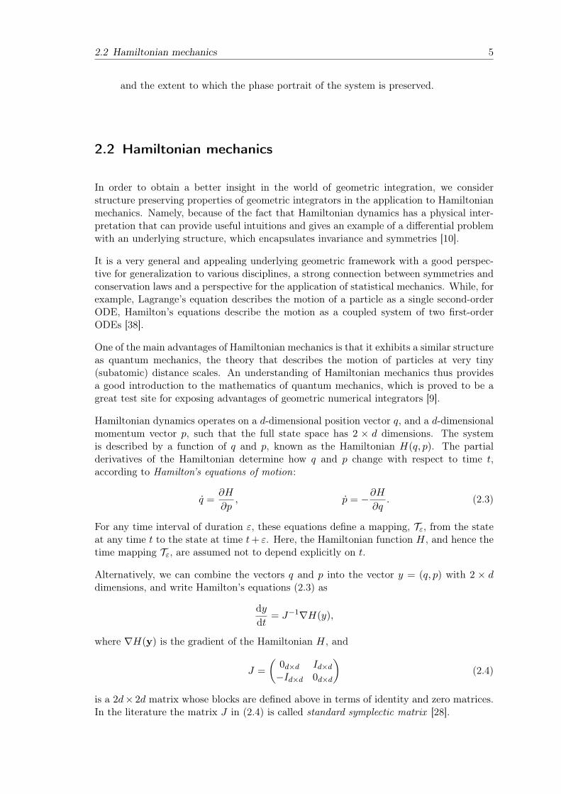
2.2 Hamiltonian mechanics
In order to obtain a better insight in the world of geometric integration, we considerstructure preserving properties of geometric integrators in the application to Hamiltonianmechanics. Namely, because of the fact that Hamiltonian dynamics has a physical inter-pretation that can provide useful intuitions and gives an example of a differential problemwith an underlying structure, which encapsulates invariance and symmetries [10].
It is a very general and appealing underlying geometric framework with a good perspec-tive for generalization to various disciplines, a strong connection between symmetries andconservation laws and a perspective for the application of statistical mechanics. While, forexample, Lagrange’s equation describes the motion of a particle as a single second-orderODE, Hamilton’s equations describe the motion as a coupled system of two first-orderODEs [38].
One of the main advantages of Hamiltonian mechanics is that it exhibits a similar structureas quantum mechanics, the theory that describes the motion of particles at very tiny(subatomic) distance scales. An understanding of Hamiltonian mechanics thus providesa good introduction to the mathematics of quantum mechanics, which is proved to be agreat test site for exposing advantages of geometric numerical integrators [9].
Hamiltonian dynamics operates on a d-dimensional position vector q, and a d-dimensionalmomentum vector p, such that the full state space has 2 × d dimensions. The systemis described by a function of q and p, known as the Hamiltonian H(q, p). The partialderivatives of the Hamiltonian determine how q and p change with respect to time t,according to Hamilton’s equations of motion:
q =∂H
∂p, p = −∂H
∂q. (2.3)
For any time interval of duration ε, these equations define a mapping, Tε, from the stateat any time t to the state at time t+ ε. Here, the Hamiltonian function H, and hence thetime mapping Tε, are assumed not to depend explicitly on t.
Alternatively, we can combine the vectors q and p into the vector y = (q, p) with 2 × ddimensions, and write Hamilton’s equations (2.3) as
dydt
= J−1∇H(y),
where ∇H(y) is the gradient of the Hamiltonian H, and
J =
(0d×d Id×d−Id×d 0d×d
)(2.4)
is a 2d× 2d matrix whose blocks are defined above in terms of identity and zero matrices.In the literature the matrix J in (2.4) is called standard symplectic matrix [28].

6 2 GEOMETRIC NUMERICAL INTEGRATORS
We usually use separated Hamiltonian functions that can be written as
H(q, p) = T (p) + V (q), (2.5)
where V (q) represents the potential energy of the system and T (p) its kinetic energy oftendefined as
T (p) =p>M−1p
2. (2.6)
Here, M ∈ Rd×d denotes a symmetric, positive-definite mass matrix, which is typicallydiagonal, and is often a scalar multiple of the identity matrix. With these forms fordecoupled H and T , Hamilton’s equations of motion (2.3) can be written
dqjdt
=[M−1p
]j,
dpjdt
= −∂V∂qj
, j = 1, . . . , d. (2.7)
Let us now take a look at some geometric properties of the solution to the given system(2.7).
Time-reversibility. First, Hamiltonian dynamics is reversible. The mapping Tε fromthe state (q(t), p(t)) at time t to the state (q(t+ ε), p(t+ ε)) at time t+ ε, is one-to-one,and hence has an inverse, T−ε. This inverse mapping is obtained by simply negating thetime derivatives in equations (2.7). If the Hamiltonian has the form (2.5)
H(q, p) = T (p) + V (q),
and T (p) = T (−p), assign the quadratic form for the kinetic energy (2.6), the inversemapping can also be obtained by negating p, applying Tε, and then negating p again, likeit is shown in Figure 2.1.
b b
bb
Tε
Tε
(q(t), p(t))
(q(t),−p(t)) (q(t+ ε),−p(t+ ε))
(q(t+ ε), p(t+ ε))
−p(t)p(t)−p(t) p(t)
Figure 2.1: Time-reversibility.
Conservation of the Hamiltonian. A second property of the dynamics is that it keepsthe Hamiltonian invariant (i.e. conserved). This is easily seen from equations (2.7) asfollows:
dHdt
=d∑j=1
[dqjdt
∂H
∂qj+
dpjdt
∂H
∂pj
]=
d∑j=1
[∂H
∂pj
∂H
∂qj− ∂H
∂qj
∂H
∂pj
]= 0.
We will see later, however, that a numerical time integration can only make H approxi-mately invariant, and hence we will not be able to achieve this conservation exactly. But
2.3 Conservation of physical properties 7
using numerical time integrators of higher order we can obtain a better conservation ofthe Hamiltonian H (2.5).
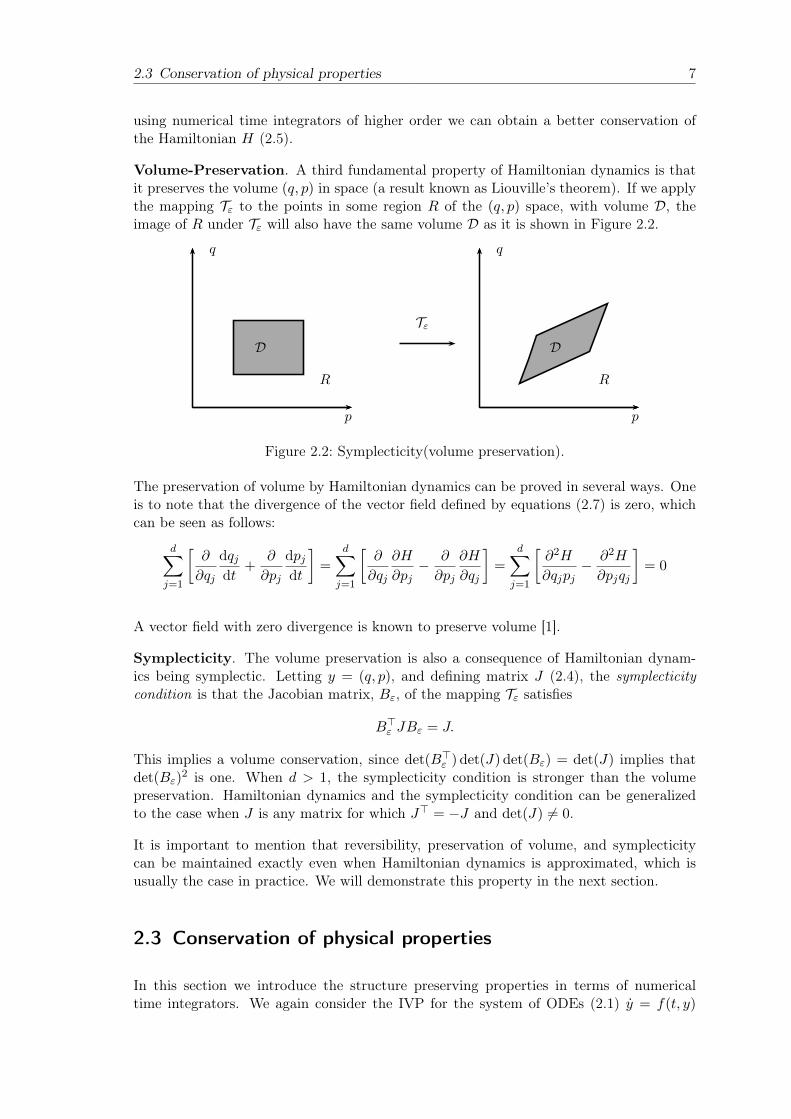
Volume-Preservation. A third fundamental property of Hamiltonian dynamics is thatit preserves the volume (q, p) in space (a result known as Liouville’s theorem). If we applythe mapping Tε to the points in some region R of the (q, p) space, with volume D, theimage of R under Tε will also have the same volume D as it is shown in Figure 2.2.
Tε
q q
pp
D D
R R
Figure 2.2: Symplecticity(volume preservation).
The preservation of volume by Hamiltonian dynamics can be proved in several ways. Oneis to note that the divergence of the vector field defined by equations (2.7) is zero, whichcan be seen as follows:
d∑j=1
[∂
∂qj
dqjdt
+∂
∂pj
dpjdt
]=
d∑j=1
[∂
∂qj
∂H
∂pj− ∂
∂pj
∂H
∂qj
]=
d∑j=1
[∂2H
∂qjpj− ∂2H
∂pjqj
]= 0
A vector field with zero divergence is known to preserve volume [1].
Symplecticity. The volume preservation is also a consequence of Hamiltonian dynam-ics being symplectic. Letting y = (q, p), and defining matrix J (2.4), the symplecticitycondition is that the Jacobian matrix, Bε, of the mapping Tε satisfies
B>ε JBε = J.
This implies a volume conservation, since det(B>ε ) det(J) det(Bε) = det(J) implies thatdet(Bε)
2 is one. When d > 1, the symplecticity condition is stronger than the volumepreservation. Hamiltonian dynamics and the symplecticity condition can be generalizedto the case when J is any matrix for which J> = −J and det(J) 6= 0.
It is important to mention that reversibility, preservation of volume, and symplecticitycan be maintained exactly even when Hamiltonian dynamics is approximated, which isusually the case in practice. We will demonstrate this property in the next section.
2.3 Conservation of physical properties
In this section we introduce the structure preserving properties in terms of numericaltime integrators. We again consider the IVP for the system of ODEs (2.1) y = f(t, y)
8 2 GEOMETRIC NUMERICAL INTEGRATORS
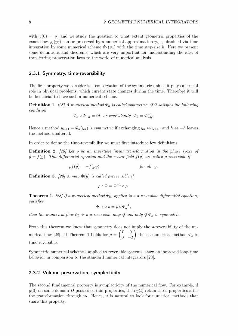
with y(0) = y0 and we study the question to what extent geometric properties of theexact flow ϕt(y0) can be preserved by a numerical approximation yn+1 obtained via timeintegration by some numerical scheme Φh(yn) with the time step-size h. Here we presentsome definitions and theorems, which are very important for understanding the idea oftransferring preservation laws to the world of numerical analysis.
2.3.1 Symmetry, time-reversibility
The first property we consider is a conservation of the symmetries, since it plays a crucialrole in physical problems, which current state changes during the time. Therefore it willbe beneficial to have such a numerical scheme.
Definition 1. [28] A numerical method Φh is called symmetric, if it satisfies the followingcondition
Φh Φ−h = id or equivalently Φh = Φ−1−h.
Hence a method yn+1 = Φh(yn) is symmetric if exchanging yn ↔ yn+1 and h↔ −h leavesthe method unaltered.
In order to define the time-reversibility we must first introduce few definitions.
Definition 2. [28] Let ρ be an invertible linear transformation in the phase space ofy = f(y). This differential equation and the vector field f(y) are called ρ-reversible if
ρf(y) = −f(ρy) for all y.
Definition 3. [28] A map Φ(y) is called ρ-reversible if
ρ Φ = Φ−1 ρ.
Theorem 1. [28] If a numerical method Φh, applied to a ρ-reversible differential equation,satisfies
Φ−h ρ = ρ Φ−1h ,
then the numerical flow φh is a ρ-reversible map if and only if Φh is symmetric.
From this theorem we know that symmetry does not imply the ρ-reversibility of the nu-
merical flow [28]. If Theorem 1 holds for ρ =
(I 00 −I
)then a numerical method Φh is
time reversible.
Symmetric numerical schemes, applied to reversible systems, show an improved long-timebehavior in comparison to the standard numerical integrators [28].
2.3.2 Volume-preservation, symplecticity
The second fundamental property is symplecticity of the numerical flow. For example, ify(0) on some domain D possess certain properties, then y(t) retain those properties afterthe transformation through ϕt. Hence, it is natural to look for numerical methods thatshare this property.
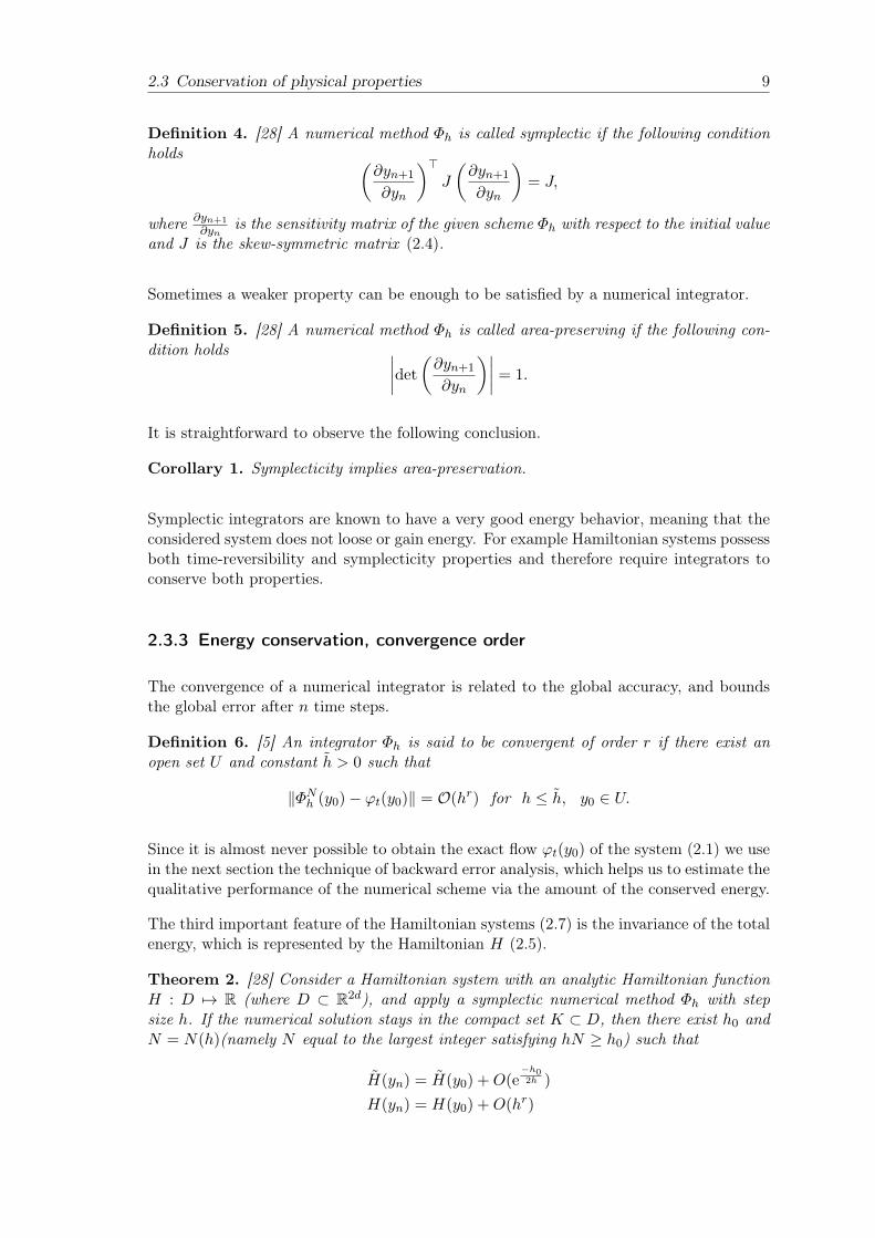
2.3 Conservation of physical properties 9
Definition 4. [28] A numerical method Φh is called symplectic if the following conditionholds (
∂yn+1
∂yn
)>J
(∂yn+1
∂yn
)= J,
where ∂yn+1
∂ynis the sensitivity matrix of the given scheme Φh with respect to the initial value
and J is the skew-symmetric matrix (2.4).
Sometimes a weaker property can be enough to be satisfied by a numerical integrator.
Definition 5. [28] A numerical method Φh is called area-preserving if the following con-dition holds ∣∣∣∣det
(∂yn+1
∂yn
)∣∣∣∣ = 1.
It is straightforward to observe the following conclusion.
Corollary 1. Symplecticity implies area-preservation.
Symplectic integrators are known to have a very good energy behavior, meaning that theconsidered system does not loose or gain energy. For example Hamiltonian systems possessboth time-reversibility and symplecticity properties and therefore require integrators toconserve both properties.
2.3.3 Energy conservation, convergence order
The convergence of a numerical integrator is related to the global accuracy, and boundsthe global error after n time steps.
Definition 6. [5] An integrator Φh is said to be convergent of order r if there exist anopen set U and constant h > 0 such that
‖ΦNh (y0)− ϕt(y0)‖ = O(hr) for h ≤ h, y0 ∈ U.
Since it is almost never possible to obtain the exact flow ϕt(y0) of the system (2.1) we usein the next section the technique of backward error analysis, which helps us to estimate thequalitative performance of the numerical scheme via the amount of the conserved energy.
The third important feature of the Hamiltonian systems (2.7) is the invariance of the totalenergy, which is represented by the Hamiltonian H (2.5).
Theorem 2. [28] Consider a Hamiltonian system with an analytic Hamiltonian functionH : D 7→ R (where D ⊂ R2d), and apply a symplectic numerical method Φh with stepsize h. If the numerical solution stays in the compact set K ⊂ D, then there exist h0 andN = N(h)(namely N equal to the largest integer satisfying hN ≥ h0) such that
H(yn) = H(y0) +O(e−h02h )
H(yn) = H(y0) +O(hr)

10 2 GEOMETRIC NUMERICAL INTEGRATORS
over exponentially long time intervals nh ≤ eh02h . The modified analytic Hamiltonian H is
exactly preserved by the numerical scheme Φh
H(q, p) = H(q, p) + hH2(q, p) + h2H3(q, p) + . . . , (2.8)
where the smooth functions Hj : R2d 7→ R for j = 2, 3, . . . , such that fj(y) = J−1∇Hj(y),where defined by (2.9).
For non-symplectic methods we can obtain an estimate of the energy preservation by acomputation similar to that of the proof of Theorem 2 which is given in [24]. And froma Lipschitz condition of the Hamiltonian H and from the standard local error estimate,we obtain H(yn+1) −H(ϕh(yn)) = O(hr+1). Since H(ϕh(yn)) = H(yn), a summation ofthese terms leads to H(yn) − H(y0) = O(thr) for t = nh. This means that the energydoes not stay invariant for non-symplectic methods.
From Theorem 2 we can conclude that numerical methods cannot be symplectic andconserve the total energy exactly. They can preserve the Hamiltonian H up to somedegree r, which depends of the convergence order of the numerical scheme. Meaning, thehigher the convergence order of the integrator the better it conserves the total energy.
2.4 Backward error analysis
The idea of backward error analysis is the following: for a given numerical integrator searchfor a modified differential equations, such that the exact solution of this modified equationapproximates very well the numerical solution. An analysis of the modified differentialequation then gives much insight into the numerical flow [27].
Unlike, a forward error analysis, which consists of the study of the errors y1−ϕh(y0) (localerror) and en = yn − ϕnh(y0) (global error) in the solution space, the idea of backwarderror analysis is to search for a modified differential equation ˙y = fh(y) of the form
˙y = f(y) + hf2(y) + h2f3(y) + . . . , (2.9)
such that yn = y(nh), and in studying the difference of the vector fields f(y) and fh(y).This approach then gives much insight into the qualitative behavior of the numericalsolution and into the global error yn − y(nh) = y(nh)− y(nh). We remark that the series(2.9) usually diverges and that one has to truncate it suitably. For the moment we contentourselves with a formal analysis without taking care of convergence issues. The idea ofinterpreting the numerical solution as the exact solution of a modified equation is commonto many numerical analysts [28].
Theorem 3. [28] Suppose that the method yn+1 = Φh(yn) is of order r, i.e.,
Φh(y) = ϕh(y) + hr+1δr+1(y) +O(hr+2),
where ϕt(y) denotes the exact flow of y = f(y), and hr+1δr+1(y) the leading term of thelocal truncation error. The modified equation then satisfies
˙y = f(y) + hrfr+1(y) + hr+1fr+2(y) + · · · , y(0) = y0

2.4 Backward error analysis 11
with fr+1(y) = δr+1(y).
A first application of the modified equation is the existence of an asymptotic expansionof the global error. Indeed, by the nonlinear variation of constants formula, the differencebetween its solution y(t) and the solution y(t) of ˙y = fh(y) satisfies
y(t)− y(t) = hrer(t) + hr+1er+1(t) + . . . ,
where ei(t) are terms of the global truncation error. Since yn = y(nh) + O(hn) for thesolution of a truncated modified equation, this proves the existence of an asymptoticexpansion in powers of h for the global error yn − y(nh).
Theorem 4. [28](Modified Hamiltonians) If a symplectic method Φh is applied to a Hamil-tonian system with a smooth Hamiltonian H : R2d 7→ R, then the modified equation (2.9)is also Hamiltonian. More precisely, there exist smooth functions Hj : R2d 7→ R forj = 2, 3, . . . such that fj(y) = J−1∇Hj(y).
The result of the above theorem allows us to estimate the energy conservation of the sym-plectic numerical schemes via the difference between the Hamiltonian of the system andthe Hamiltonian preserved by numerical method as we show in the next section.
Modified Hamiltonian functions.The motivation for studying numerically the conservation properties of these modifiedHamiltonians are multifaceted [54], e.g. numerical evidence for the existence of a Hamilto-nian for a particular calculation, exposure of energy drifts caused by numerical instability,etc.. Skeel and Hardy [54] proposed a simple strategy for deriving highly accurate esti-mates for modified Hamiltonians. Since these modified Hamiltonians approximate wellthe true Hamiltonian, they are referred as "shadow" Hamiltonians H (2.8), cf. [18]. Theexistence of these shadow Hamiltonians guarantees the boundedness of the error in thesymplectic map, in fact we have H(q, p, h)→ H(q, p) for h→ 0.
Conversely, if one starts from a given numerical solver then it is well known that anysymplectic integrator different from the Hamiltonian flow itself does not preserve theHamiltonian however a nearby system, the so-called shadow Hamiltonian H is conserved.The energy computed from the shadow Hamiltonian of a symplectic integrators differs byH(q, p)− H(q, p, h) = O(hr) from the true Hamiltonian [30], with r being the order of theintegration scheme. Hence, computing the shadow Hamiltonian of a symplectic integratoris equivalent to determining the order of the integrator.
To compute a shadow Hamiltonian it is necessary to expand an exponential map to aHausdorff series. Let T and V be a random (usually non-commuting) operators then theBaker-Campbell-Hausdorff (BCH) formula [32] reads
ln(eT eV ) =
∞∑n=1
cn(T, V ), (2.10)
where the coefficients cn are recursively determined from the relations c1 = T + V and
(n+ 1)cn+1 =
bn/2c∑m=1
B2m
(2m)!
∑k1,...,k2m≥1
adck1 . . . adck2m(T + V )− 1
2(adcn)(T − V ),

12 2 GEOMETRIC NUMERICAL INTEGRATORS
for n ≥ 0, where ada : b 7→ [a, b] and Bn denote the Bernoulli numbers.
For a differential equationy = f [1](y) + f [2](y),
it is convenient to study the composition of the flows ϕ[1]t and ϕ[2]
t of the systems
y = f [1](y) y = f [2](y), (2.11)
respectively.
Let us introduce a Lie derivative, the differential operators of the following form
Di =∑j
f[i]j (y)
∂
∂yj,
which means that for some differentiable functions F : Rn 7→ Rm we have
DiF (y) = F ′(y)f [i](y).
It follows from the chain rule that, for the solutions ϕ[i]t (y0) of the system (2.11),
ddtF(ϕ
[i]t (y0)
)= (DiF )
(ϕ
[i]t (y0)
)(2.12)
and iteratively applying this operator we obtain
dk
dtkF(ϕ
[i]t (y0)
)= (Dk
i F )(ϕ
[i]t (y0)
),
and Taylor series of F(ϕ
[i]t (y0)
)at t = 0 yield
F(ϕ
[i]t (y0)
)=∑k≥0
tk
k!(Dk
i F )(y0) = exp(tDi)F (y0).
Setting F (y) = Id(y) = y to be the identity map, we can see that this is the Taylor seriesof the solution itself
ϕ[i]t (y0) =
∑k≥0
tk
k!(Dk
i Id)(y0) = exp(tDi) Id(y0).
Lemma 1. [22] Let ϕ[2]s and ϕ[1]
t be the flows of the differential equations y = f [1](y) andy = f [2](y), respectively. For their composition we then have(
ϕ[2]s ϕ
[1]t
)(y0) = esD1 etD2 Id(y0).
For example, in case of the Hamiltonian function (2.5) for the system (2.3) the standard
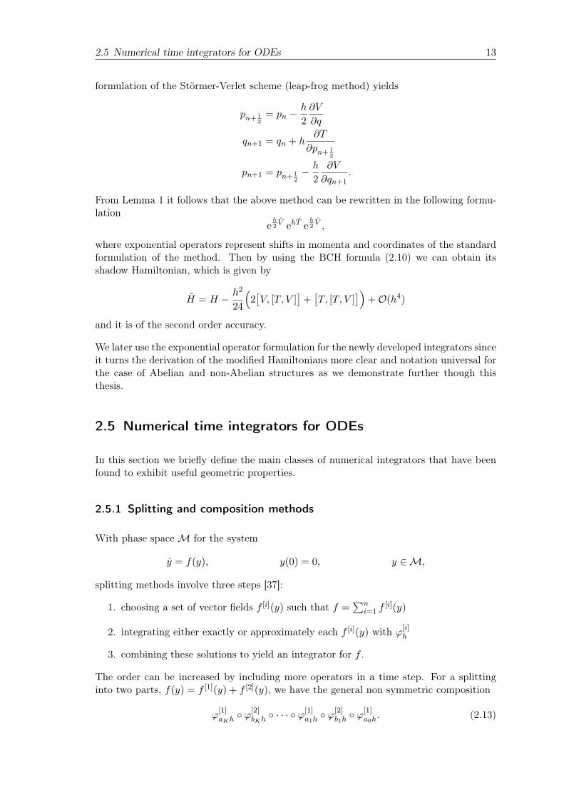
2.5 Numerical time integrators for ODEs 13
formulation of the Störmer-Verlet scheme (leap-frog method) yields
pn+ 12
= pn −h
2
∂V
∂q
qn+1 = qn + h∂T
∂pn+ 12
pn+1 = pn+ 12− h
2
∂V
∂qn+1.
From Lemma 1 it follows that the above method can be rewritten in the following formu-lation
eh2V ehT e
h2V ,
where exponential operators represent shifts in momenta and coordinates of the standardformulation of the method. Then by using the BCH formula (2.10) we can obtain itsshadow Hamiltonian, which is given by
H = H − h2
24
(2[V, [T, V ]
]+[T, [T, V ]
])+O(h4)
and it is of the second order accuracy.
We later use the exponential operator formulation for the newly developed integrators sinceit turns the derivation of the modified Hamiltonians more clear and notation universal forthe case of Abelian and non-Abelian structures as we demonstrate further though thisthesis.
2.5 Numerical time integrators for ODEs
In this section we briefly define the main classes of numerical integrators that have beenfound to exhibit useful geometric properties.
2.5.1 Splitting and composition methods
With phase spaceM for the system
y = f(y), y(0) = 0, y ∈M,
splitting methods involve three steps [37]:
1. choosing a set of vector fields f [i](y) such that f =∑n
i=1 f[i](y)
2. integrating either exactly or approximately each f [i](y) with ϕ[i]h
3. combining these solutions to yield an integrator for f .
The order can be increased by including more operators in a time step. For a splittinginto two parts, f(y) = f [1](y) + f [2](y), we have the general non symmetric composition
ϕ[1]aKh ϕ[2]
bKh · · · ϕ[1]
a1h ϕ[2]
b1h ϕ[1]
a0h. (2.13)
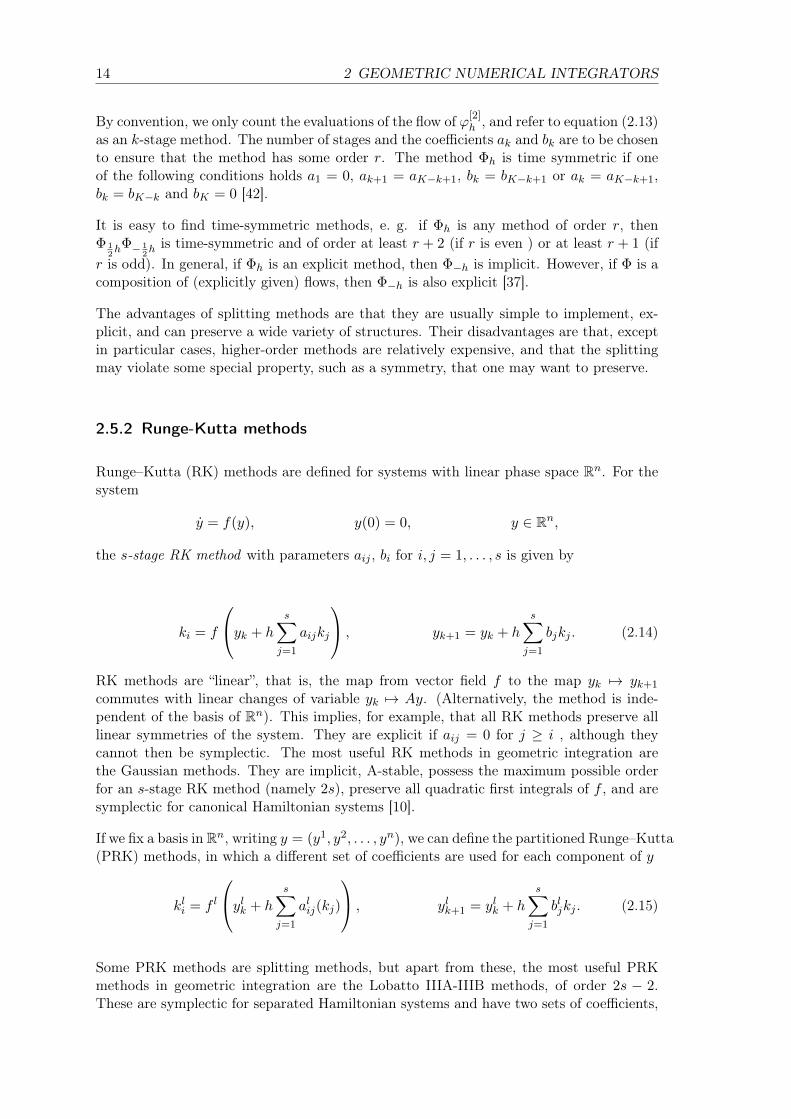
14 2 GEOMETRIC NUMERICAL INTEGRATORS
By convention, we only count the evaluations of the flow of ϕ[2]h , and refer to equation (2.13)
as an k-stage method. The number of stages and the coefficients ak and bk are to be chosento ensure that the method has some order r. The method Φh is time symmetric if oneof the following conditions holds a1 = 0, ak+1 = aK−k+1, bk = bK−k+1 or ak = aK−k+1,bk = bK−k and bK = 0 [42].
It is easy to find time-symmetric methods, e. g. if Φh is any method of order r, thenΦ 1
2hΦ− 1
2h is time-symmetric and of order at least r + 2 (if r is even ) or at least r + 1 (if
r is odd). In general, if Φh is an explicit method, then Φ−h is implicit. However, if Φ is acomposition of (explicitly given) flows, then Φ−h is also explicit [37].
The advantages of splitting methods are that they are usually simple to implement, ex-plicit, and can preserve a wide variety of structures. Their disadvantages are that, exceptin particular cases, higher-order methods are relatively expensive, and that the splittingmay violate some special property, such as a symmetry, that one may want to preserve.
2.5.2 Runge-Kutta methods
Runge–Kutta (RK) methods are defined for systems with linear phase space Rn. For thesystem
y = f(y), y(0) = 0, y ∈ Rn,
the s-stage RK method with parameters aij , bi for i, j = 1, . . . , s is given by
ki = f
yk + hs∑j=1
aijkj
, yk+1 = yk + hs∑j=1
bjkj . (2.14)
RK methods are “linear”, that is, the map from vector field f to the map yk 7→ yk+1
commutes with linear changes of variable yk 7→ Ay. (Alternatively, the method is inde-pendent of the basis of Rn). This implies, for example, that all RK methods preserve alllinear symmetries of the system. They are explicit if aij = 0 for j ≥ i , although theycannot then be symplectic. The most useful RK methods in geometric integration arethe Gaussian methods. They are implicit, A-stable, possess the maximum possible orderfor an s-stage RK method (namely 2s), preserve all quadratic first integrals of f , and aresymplectic for canonical Hamiltonian systems [10].
If we fix a basis in Rn, writing y = (y1, y2, . . . , yn), we can define the partitioned Runge–Kutta(PRK) methods, in which a different set of coefficients are used for each component of y
kli = f l
ylk + h
s∑j=1
alij(kj)
, ylk+1 = ylk + hs∑j=1
bljkj . (2.15)
Some PRK methods are splitting methods, but apart from these, the most useful PRKmethods in geometric integration are the Lobatto IIIA-IIIB methods, of order 2s − 2.These are symplectic for separated Hamiltonian systems and have two sets of coefficients,
2.5 Numerical time integrators for ODEs 15
one for the q and one for the p variables.
2.5.3 Projection methods
Some properties can be preserved by simply taking a step of an arbitrary method and thenenforcing the property. Integrals and weak integrals (invariant manifolds) can be preservedby projecting onto the desired manifold at the end of a step or steps, typically using or-thogonal projection with respect to a suitable metric. For example, energy-preserving in-tegrators have been constructed using discrete gradient methods, a form of projection [25].Although it is still used, projection is something of a last resort, as it typically destroysother properties of the method (such as symplecticity) and may not yield good long-timebehavior. Reversibility is an exception, for R-reversibility can be imposed on the map Φ byusing ΦRΦ−1R−1, where R : M → M is an arbitrary diffeomorphism of the phase space.Since this is a composition, it can preserve the group properties of Φ such as symplecticity.Symmetries are a partial exception; the composition ΦSΦS is not S-equivalent, but it iscloser to S-equivalent than Φ is, when S2 = 1.
2.5.4 Variational methods
Many ODEs and PDEs of mathematical physics are derived from variational principleswith natural discrete analogs. For an ODE with Lagrangian L(q, q) one can construct anapproximate discrete Lagrangian Ld(q0, q1) such as Ld(q0, q1) = Ld(q0, (q1 − q0)/τ) from
an integrator by requiring that the discrete actionN∑i=0
Ld(qi, qi+1) be stationary with re-
spect to all variations of the qi, for i = 1, . . . , N − 1, with fixed end-points q0 and qN .For regular Lagrangian, the integrator can be seen to be symplectic in a very naturalway, and in fact the standard symplectic integrators such as leapfrog and the symplecticRunge–Kutta methods can be derived in this way [38]. The advantage of the discrete La-grangian approach is that it acts as a guide in new situations. The Newmark method, wellknown in computational engineering, is variational, a fact that allowed the determinationof the (nonstandard) symplectic form it preserves; singular Lagrangian can be treated;it suggests a natural treatment of holonomic (position) and nonholonomic (velocity) con-straints and of non smooth problems involving collisions; and powerful “asynchronous”variational integrators can be constructed, which use different, even incommensurate timesteps on different parts of the system. In these situations variational integrators appearto be natural, and to work extremely well in practice, even if the reason for their goodperformance (e.g., by preserving some geometric feature) is not yet fully understood [35].
2.5.5 Linear multistep methods
Defined on a linear space M ∈ Rn s-step method is
s∑j=0
αjyk+j = τs∑j=0
βjf(yk+j). (2.16)
16 2 GEOMETRIC NUMERICAL INTEGRATORS
Such methods define a map on the product space M s, and can sometimes preserve astructure (e.g. a symplectic form) in this space. However, this will not usually give goodlong-time behavior of the sequence of points yk ∈M . Instead, one considers the so-calledunderlying one-step method Φh : M → M , which is defined such that the sequence ofpoints yk := Φh(y0) satisfies the multistep formula. (It always exists, at least as a formalpower series in τ). Often the dynamics of Φ dominates the long-term behavior of themultistep method. Recently it has been proved that the underlying one-step methodsfor a class of time-symmetric multistep methods for second-order problems y = f(y) areconjugate to symplectic, which explains their near-conservation of energy over long timesand their practical application in solar system dynamics [11].
2.6 Numerical integration on Lie groups
For certain applications numerical time integration of ODEs on manifold is required. Thereare a number of techniques to preserve geometric properties of the numerical flow andnumerical integrators on Lie groups play a very important role. In this section we give ashort insight for numerical treatment of ODEs defined on Lie groups.
First letM∈ Rd be a given manifold then the system of ODEs (2.1)
y = f(y), y(0) = 0, y ∈ Rn,
is a differential equation on the manifoldM, if y0 ∈ M implies y(t) ∈ M for all t. Thisis equivalent to the requirement on the vector field that f(y) ∈ TyM for y ∈ M, whereTyM is the tangent space ofM at the point y ∈M and for a manifold given by [26]
M = y ∈ Rd|g(y) = 0,
the tangent space takes the form
TyM = v ∈ Rd|g′(y)v = 0.
Then a Lie group is a differentiable manifold G, for which the product is a differentiablemapping G×G→ G. The tangent space g = TIG at the identity I of a matrix Lie groupG is closed under commutators of its elements. This makes g an algebra, the Lie algebraof the Lie group G [28]. As an example of a Lie group, which can be widely used inquantum field theory, is the special unitary group SU(n) of n× n unitary matrices with adeterminant equals to 1.
Next two lemmas introduce some important properties of Lie groups.
Lemma 2. Let G be a matrix Lie group and let g = TIG be the tangent space at theidentity. The Lie bracket (or commutator)
[A,B] = AB −BA (2.17)
defines an operation g× g→ g which is bilinear, skew-symmetric and satisfies the Jacobiidentity
[A, [B,C]] + [C, [A,B]] + [B, [C,A]] = 0 (2.18)

2.6 Numerical integration on Lie groups 17
Lemma 3. Consider a matrix Lie group G and its Lie algebra g. The matrix exponentialis a map
exp : g→ G, (2.19)
i. e., for A ∈ g we have exp(A) ∈ G.
Further in this section we present some general ideas for numerical treatment of the prob-lems defined on the Lie groups.
2.6.1 Methods based on Magnus expansion
Let us consider the linear matrix differential equations
Y = A(t)Y, (2.20)
where the matrix A depends constantly on t. For the scalar case the solution of (2.20)with Y (0) = Y0 is given by
Y (t) = exp
t∫0
A(τ)dτ
Y0. (2.21)
Defining the inverse of the derivative of the matrix exponential by
d exp−1Ω (Λ) =
∑k≥0
Bkk
adkΩ(Λ), (2.22)
where Bk are the Bernoulli numbers, and adΩ(A) is the adjoint operator, we can formulateTheorem 5
Theorem 5. The solution of the differential equation (2.20) can be written as Y (t) =exp(Ω(t))Y0 with Ω(t) defined by
Ω = d exp−1Ω (A(t)) , Ω(0) = 0 (2.23)
As long as ‖Ω(t)‖ < π, the convergence of the d exp−1Ω expansion (2.22) is assured.
The so-called Magnus expansion is obtained via integrating (2.23) and yields
Ω(t) =
t∫0
A(τ)dτ − 1
2
t∫0
τ∫0
A(σ)dσ,A(τ)
dτ
+1
4
t∫0
τ∫0
σ∫0
A(µ)dµ,A(σ)
dσ,A(τ)
dτ
+1
2
t∫0
τ∫0
A(σ)dσ,
τ∫0
A(µ)dµ,A(τ)
dτ + . . . .
(2.24)
The truncated series (2.24) give an excellent approximation to the solution of (2.20),

18 2 GEOMETRIC NUMERICAL INTEGRATORS
cf. [28].
In order to approximate (2.20) it is proposed in [29] to use Yn+1 = exp(hΩn)Yn, whereΩn is an approximation of Ω(h) given by (2.24) with A(tn + τ) instead of A(τ) and thecollocation approach yields to replace A(t) with
A(t) =
s∑i=1
li(t)A(tn + cih)
and to solve Y = A(t)Y on [tn, tn + h] by use of (2.24).
It is possible to construct methods of arbitrary high order with reduced number of com-mutators [26].
2.6.2 Crouch-Grossman methods
The idea of RK methods (2.14) applied to differential equations (2.20) on Lie groups hasthe disadvantage since for any Y ∈ G and Z ∈ G the update of the form Y + haA(Z)Zis not general in the Lie group G. The replacement of the above update operation withexp (haA(Z))Y was proposed to resolve this disadvantage in [15].
Definition 7. Let bi, aij (i, j = 1, . . . , s) be real numbers. An explicit s-stage Crouch-Grossman method is given by
Y (i) = exp(hai,i−1Ki−1) . . . exp(hai1K1)Yn, Ki = A(Y i),
Yn+1 = exp(hbsKs) . . . exp(hb1K1)Yn.
The Crouch-Grossman methods yield the approximation Yn which lie exactly on the man-ifold defined by a Lie group and the accuracy order is defined in Theorem 6
Theorem 6. [29] Let ci =∑
j aij. A Crouch-Grossman method has order p (p ≤ 3) if thefollowing order conditions are satisfied:
order 1 :∑i
bi = 1
order 2 :∑i
b1ci =1
2
order 3 :∑i
bic2i =
1
3∑ij
biaijcj =1
6∑i
b2i ci + 2∑i<j
bicibj =1
3.
We note that the construction of the high order Crouch-Grossman methods is very com-plicated [28].
2.6 Numerical integration on Lie groups 19
2.6.3 Munthe-Kaas methods
The main purpose to develop this class of numerical methods was to develop a theory ofRK methods in a coordinate free framework [28].
Let us consider the problem (2.20) with A(Y ) ∈ g for Y ∈ G. From Theorem 5 we knowthat the solution of (2.20) can be written as Y (t) = exp(Ω(t))Y0, where Ω(t) is the solutionof Ω = d exp−1
Ω (A(Y (t))), Ω(0) = 0.
Suitably truncating the series (2.24) and considering the differential equation
Ω = A (exp(Ω)Y0) +
q∑k≥0
Bkk
adkΩ (A (exp(Ω)Y0)) , Ω(0) = 0. (2.25)
yields the following algorithm.
Assume that Yn lies in the Lie group G, then, the step Yn 7→ Yn+1 can be defined as follows
• consider the differential equation (2.25) with Yn instead of Y0 and apply a RK method(2.14) to get an approximation Ω1 ≈ Ω(h)
• define the numerical solution by Yn+1 = exp(Ω1)Yn.
Important properties of the Munthe-Kass methods are given in the two following theorems.
Theorem 7. [29] Let G be a matrix Lie group and g its Lie algebra. If A(Y ) ∈ g forY ∈ G and if Y0 ∈ G, then the numerical solution of the Lie group Munthe-Kass methodlies in G, i. e., Yn ∈ G for all n = 0, 1, 2, . . . .
Theorem 8. [29] If the RK method is of (classical) order p and if the truncation indexin (2.25) satisfies q ≥ r − 2, then the method of this type is of the order r.
Every classical RK method defines a Munthe-Kaas method of the same order, unlikeCrouch-Grossman methods, which need more stages for the same order [28].
Munthe-Kaas methods are in general not symmetric, even if the underlying Runge–Kuttamethod is symmetric [28], but symmetric versions of these methods have been devel-oped [62]. As well as the symplectic versions based on the variational principles wererecently presented in [7]. But so far there is no time-reversible and symplectic Lie groupmethod.
It is important to mention that the projection methods are suited for the numerical treat-ment of equation of the type (2.20) since it is a special case of differential equation on themanifolds. As well as the splitting methods with a small modification (we introduce later)are capable to take care of problems on the Lie groups. In this thesis we use these twoideas as a benchmark of our research and to study our main application, which we presentin the next chapter.

3 Chapter 3
QUANTUM FIELD THEORIES ONTHE LATTICE
Quantum field theory is a set of ideas and tools that combines three of the major themes ofmodern physics: the quantum theory, the field concept and the principle of relativity. Thetheory underlies modern elementary particle physics and supplies essential tools to nuclearphysics, atomic physics, condensed matter physics and astrophysics [45]. It summarizesthe knowledge about the fundamental forces of electromagnetism, as well as the weakand strong interactions and it has been tested over an extremely wide range of lengthor energy scales. Quantum field theory includes a vast number of physical theories, suchas quantum electrodynamics, which describes all phenomena of both electromagnetic andweak interactions, and quantum chromodynamics, which focus on the strong interactionsbetween quarks and gluons [23].
Due to the author’s involvement in the Marie Curie Initial Training Network STRONGneton Strong Interaction Supercomputing Training Network and later in the project B5 withinthe SFB/Transregio 55 Hadronenphysik mit Gitter-QCD, the main goal of this thesis lieswithin the application to the theory of lattice quantum chromodynamics.
In this chapter we briefly introduce basic concepts of quantum field theory, show thequantization approach from classical field theory up to quantum fields. Also very shortlythe idea of regularization path integral formulation of quantum field theory on the latticeis presented as well as couple examples of quantum field theories. Later we show one ofthe way to solve a path integral on the lattice, namely the hybrid Monte Carlo algorithm.Finally, we discuss the challenges for numerical integration and the reasons for studyingstructure preserving geometric numerical time integrators.
3.1 Basic concepts of quantum field theories
Quantum field theory in its function integral formulation follows from two classical con-cepts of physics: classical field theory and quantum mechanics. We do not consider herethe complete path from point mechanics to quantum field theory, but rather just shortlyintroduce the basic ideas of the underlying theories for better understanding of the quan-tum field theory itself.
Classical field theory represent the generalization of point mechanics to n degrees of free-dom in each space-time point x = (t,x) and a system with infinite number of degreesof freedom is described by a field φ(x). The examples of fields are Abelian gauge fieldsAµ ∈ R, describing the electromagnetic potential, where µ = 0, . . . , 3 and has n = 4 de-grees of freedom with two of them corresponding to U(1) gauge group; and non-Abeliangauge fields Aaµ, where µ = 0, . . . , 3, a = 1, . . . , 8 and n = 16, represents a gluon field and
21

22 3 QUANTUM FIELD THEORIES ON THE LATTICE
corresponds to gauge group SU(3).
Adding formalism of quantum mechanics we obtain the representation of probability am-plitude for a particle to move from point x to point x′ within the time interval T and~ = 1
〈x′| e−iHT |x〉, (3.1)
where a state |x〉 of the position operator is a vector in Hilbert space and H representsthe Hamilton operator. Here standard bra-ket notation 〈|〉 defines the scalar product.
The propagator given in (3.1) can be approximated as following Feynman path integral [39]
〈x′| e−iHT |x〉 =
∫Dx eiS[x] . (3.2)
Here the functional measure Dx represents
Dx = limN→∞
( m
2πiε
)N/2dx1 · · · dxN−1 (3.3)
and represents the integration over all possible paths from (t, x) to (t′, x′). The functionalformalism has been proved to be very useful in field theory since many results can be de-rived in a compact and easy way through formal manipulations of functional integrals [39].
Introducing the concept of Euclidean time T → −iτ gives us a different representation forthe path integral (3.2)
〈x′| e−Hτ |x〉 =
∫Dx e−SE [x], (3.4)
where the functional measure Dx differs from one in (3.3) and given by
Dx = limN→∞
( m
2πε
)N/2dx1 · · · dxN (3.5)
and the Euclidean action SE is related to the action S through
S = iSE .
The path integral (3.4) is real now and has an integrand, which is damped for widelyoscillating paths with a large Euclidean action SE [39].
It is possible, according to quantum statistical mechanics, to extract thermal expectationvalues for some chosen operator O using the path integral formulation (3.4) in the followingway
〈O〉 =1
Z
∫DxO(x) e−SE [x] . (3.6)
Here Z defines a partition function known from statistical mechanics
Z = Tr e−βH =
∫Dx e−SE , (3.7)
where β = T and the integral measure Dx is given by (3.5). Particularly it is interesting
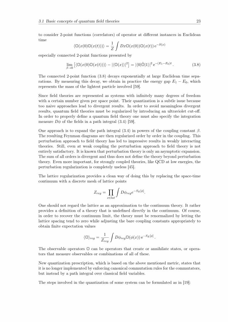
3.1 Basic concepts of quantum field theories 23
to consider 2-point functions (correlators) of operator at different instances in Euclideantime
〈O(x(0)O(x(t)))〉 =1
Z
∫DxO(x(0))O(x(t)) e−S(x)
especially connected 2-point functions presented by
limβ→0
[〈O(x(0)O(x(t)))〉 − |〈O(x)〉|2
]= |〈0|O|1〉|2 e−(E1−E0)t . (3.8)
The connected 2-point function (3.8) decays exponentially at large Euclidean time sepa-rations. By measuring this decay, we obtain in practice the energy gap E1 − E0, whichrepresents the mass of the lightest particle involved [59].
Since field theories are represented as systems with infinitely many degrees of freedomwith a certain number given per space point. Their quantization is a subtle issue becausetoo naive approaches lead to divergent results. In order to avoid meaningless divergentresults, quantum field theories must be regularized by introducing an ultraviolet cut-off.In order to properly define a quantum field theory one must also specify the integrationmeasure Dφ of the fields in a path integral (3.4) [59].
One approach is to expand the path integral (3.4) in powers of the coupling constant β.The resulting Feynman diagrams are then regularized order by order in the coupling. Thisperturbation approach to field theory has led to impressive results in weakly interactingtheories. Still, even at weak coupling the perturbation approach to field theory is notentirely satisfactory. It is known that perturbation theory is only an asymptotic expansion.The sum of all orders is divergent and thus does not define the theory beyond perturbationtheory. Even more important, for strongly coupled theories, like QCD at low energies, theperturbation regularization is completely useless [45].
The lattice regularization provides a clean way of doing this by replacing the space-timecontinuum with a discrete mesh of lattice points
Zreg =∏x∈lat
∫Dφrege
−SE [φ].
One should not regard the lattice as an approximation to the continuum theory. It ratherprovides a definition of a theory that is undefined directly in the continuum. Of course,in order to recover the continuum limit, the theory must be renormalized by letting thelattice spacing tend to zero while adjusting the bare coupling constants appropriately toobtain finite expectation values
〈O〉reg =1
Zreg
∫DφregO(φ(x)) e−SE [φ] .
The observable operators O can be operators that create or annihilate states, or opera-tors that measure observables or combinations of all of these.
New quantization prescription, which is based on the above mentioned metric, states thatit is no longer implemented by enforcing canonical commutation rules for the commutators,but instead by a path integral over classical field variables.
The steps involved in the quantization of some system can be formulated as in [19]:

24 3 QUANTUM FIELD THEORIES ON THE LATTICE
1: Replace the continuum space time by an Euclidean lattice with a lattice constant a.The degrees of freedom are the classical field variables φ living on the lattice.
2: Discretize the Euclidean action SE [φ] on the lattice such that in the limit a→ 0 theEuclidean continuum action is obtained.
3: The operators that appear in the Euclidean correlator to be studied are translated tofunctionals by replacing the field operators with the classical lattice field variables.
4: Compute the Euclidean correlation functions (3.8) by evaluating these functionalson some lattice field configuration, weighting them with the Boltzmann factor andintegrating over all possible field configurations.
Once physical observables are calculated on the lattice one is interested in their values inthe limit a → 0, the so-called continuum limit. We will discuss this topic since it not apart of our research.
In the next section we consider the lattice regularization for different kinds of field variablesand introduce examples of the quantum field theory as the main application of this work.
3.2 Regularization on the lattice
Lattice field theory is the only regularization scheme, which captures finite couplings forfield interaction on a non-perturbative level. By the analogy with quantum mechanicalpath integral (3.2), defined as a limit of a finite-dimensional integral, which resulted from adiscretization in time, the same procedure is applied to quantum field theory by consideringthe integral (3.4) as a limit of well defined integral over discretized Euclidean space-time [39].
Here we consider a hypercubic lattice Λ with a lattice spacing constant a given by
Λ = aZ4 =x|xµa∈ Z
. (3.9)
One can consider φ4 theory, which is one of the simplest field theories with interactionterms, which in certain cases does not actually requires regularization in order to showthe most important features and techniques of lattice field theory.
For example, for the scalar fields φ(x), defined on the points x ∈ Λ with the action S[φ(x)]the partition function Z is given by
ZΛ =
∫ ∏x∈Λ
Dφ(x)e−SE [φ(x)]
and observables 〈O〉Λ can be evaluated numerically by means of Monte Carlo simulations.
We will discuss the Monte Carlo algorithm at the end of this chapter in more details butfirst we briefly introduce a regularization procedure from the continuum to the lattice fordifferent field variables, which are necessary to introduce our main application.
3.2 Regularization on the lattice 25
3.2.1 Gauge fields
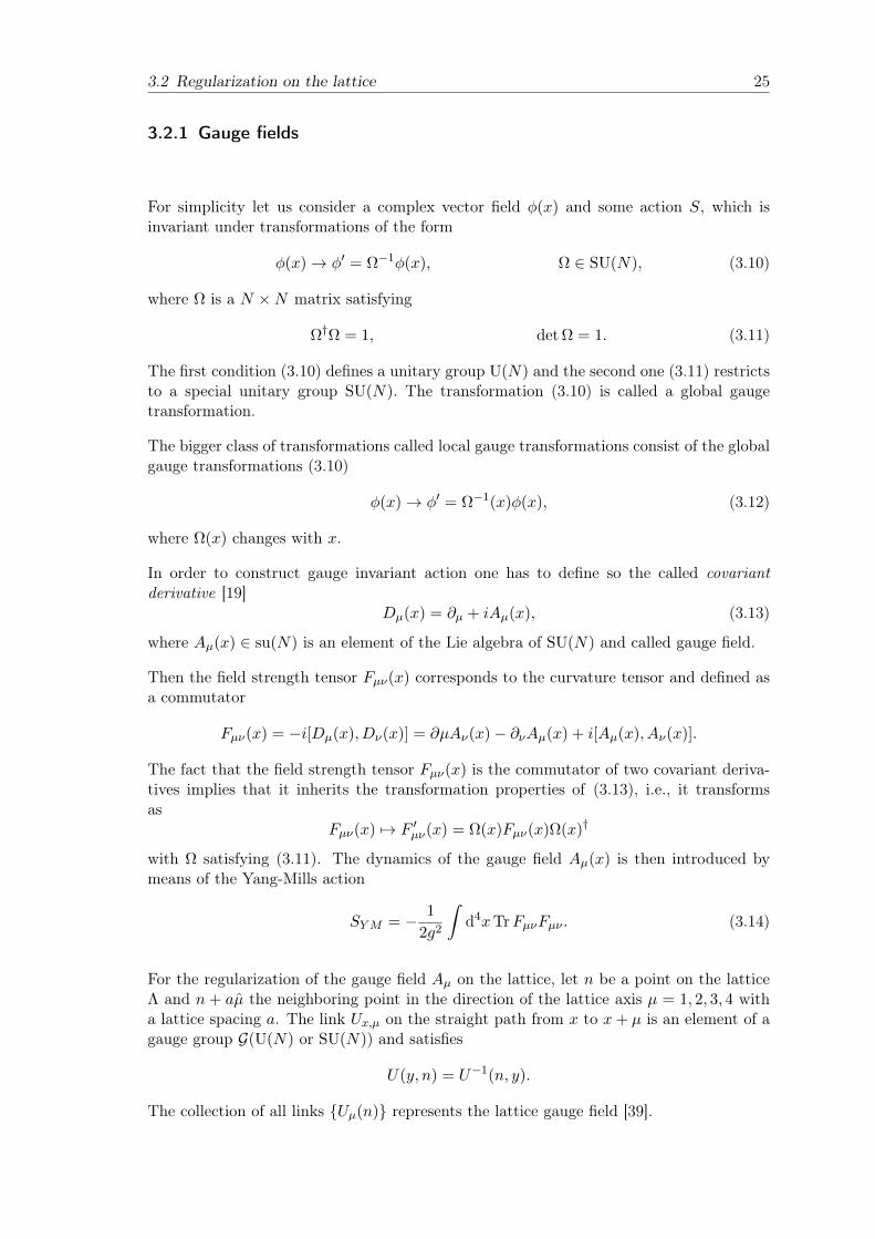
For simplicity let us consider a complex vector field φ(x) and some action S, which isinvariant under transformations of the form
φ(x)→ φ′ = Ω−1φ(x), Ω ∈ SU(N), (3.10)
where Ω is a N ×N matrix satisfying
Ω†Ω = 1, det Ω = 1. (3.11)
The first condition (3.10) defines a unitary group U(N) and the second one (3.11) restrictsto a special unitary group SU(N). The transformation (3.10) is called a global gaugetransformation.
The bigger class of transformations called local gauge transformations consist of the globalgauge transformations (3.10)
φ(x)→ φ′ = Ω−1(x)φ(x), (3.12)
where Ω(x) changes with x.
In order to construct gauge invariant action one has to define so the called covariantderivative [19]
Dµ(x) = ∂µ + iAµ(x), (3.13)
where Aµ(x) ∈ su(N) is an element of the Lie algebra of SU(N) and called gauge field.
Then the field strength tensor Fµν(x) corresponds to the curvature tensor and defined asa commutator
Fµν(x) = −i[Dµ(x), Dν(x)] = ∂µAν(x)− ∂νAµ(x) + i[Aµ(x), Aν(x)].
The fact that the field strength tensor Fµν(x) is the commutator of two covariant deriva-tives implies that it inherits the transformation properties of (3.13), i.e., it transformsas
Fµν(x) 7→ F ′µν(x) = Ω(x)Fµν(x)Ω(x)†
with Ω satisfying (3.11). The dynamics of the gauge field Aµ(x) is then introduced bymeans of the Yang-Mills action
SYM = − 1
2g2
∫d4xTrFµνFµν . (3.14)
For the regularization of the gauge field Aµ on the lattice, let n be a point on the latticeΛ and n + aµ the neighboring point in the direction of the lattice axis µ = 1, 2, 3, 4 witha lattice spacing a. The link Ux,µ on the straight path from x to x+ µ is an element of agauge group G(U(N) or SU(N)) and satisfies
U(y, n) = U−1(n, y).
The collection of all links Uµ(n) represents the lattice gauge field [39].

26 3 QUANTUM FIELD THEORIES ON THE LATTICE
In order to construct a gauge invariant action for the lattice gauge field the smallest closedloops on the lattice called plaquettes are used.
A plaquette Pµ(n) consisting of four links and containing points
n, n+ aµ, n+ aµ+ aν, n+ aν
presented as a product of links in the following form
Pµ(n) = Uµ(n)Uν(n+ µ)U †µ(n+ ν)U †ν (n), (3.15)
where the link on opposite direction is defined by
U−µ(n) = U †µ(n− µ)
and can be visualized as it is shown on Figure 3.1.
n+ ν n+ ν + µ
n+ µn
U †µ(n+ ν)
U †ν (n) Uν(n+ µ)
Uµ(n)
n+ ν n+ ν + µ
n+ µn
Uµ(n+ ν)
Uν(n) U †ν (n+ µ)
U †µ(n)
Figure 3.1: Plaquette.
The action proposed for the pure gauge theory is called Wilson action and defined in termsof the plaquettes (3.15)
S[U ] =∑n;µ,ν
Sn;µ,ν(Pµ,ν(n)),
with the plaquette term
Sn;µ,ν = β
1− 1
NRe TrUµ,ν(n)
for SU(N).
There are other possibilities for defining gauge invariant actions, but the choice of Wilsonaction appears to be the simplest one [39].
3.2.2 Fermion fields
Theories with fermions have no immediate classical limit, and the definition of the pathintegral needs special care [59].
It requires an introduction of the anti-commutating variables ηi with i ∈ 1, 2, . . . ,N definedon a so-called Grassmann algebra, which is characterized by the following relations
ηi, ηj = ηiηj + ηjηi = 0,

3.2 Regularization on the lattice 27
such that any function f(η) has a representation in terms of finite degree polynomials ofthe form
f(η) = f +∑i
fiηi +∑ij
fijηiηj +∑ijk
fijkηiηjηk + · · · ,
where the numbers fij···l are complex or real numbers and antisymmetric in i, j, · · · , l.Then formal differentiation and integration procedures are also defined correspondinglyfor differentiation
∂
∂ηiηi = 1,
∂
∂ηiηiηj = ηj ,
∂
∂ηjηi = −ηj ,
and for integration ∫dηi = 0,
∫dηiηi = 1,
∫dηidηiηiηj = −1.
The fermion action SF is presented by
SF [φφ] =
∫ddxφ(γµ∂µ +m)φ, (3.16)
with γµ are Euclidean Dirac matrices.
The Grassmann algebra is used to define fermion fields generated by independent Grass-mann numbers φn and φn. The index n varies over all space-time points as well as overall spin, flavor and color indices. On the lattice the continuum field φ, φ is replaced byGrassmann variables φn, φn.
There are different ways to discretize the fermion action (3.16). First we introduce thenaive discretization of the fermion action (3.16).
Naive lattice fermions. The idea is to discretize the continuum derivative in (3.16) bya finite difference, such that
SN [φ, φ] = ad∑n,µ
1
2a
(φnγµφn+µ − φn+µγµφn
)+ ad
∑n
mφnφn. (3.17)
Unfortunately this approach does not lead to the correct continuum theory, due to thefermion doubling effect, which pose a severe problem in lattice field theory.
There are two basic types of lattice formulation, applied in most cases are the Wilsonformulation and the Kogut Susskind staggered formulation [39]. In this thesis we stick tothe Wilson fermion formulation as it is sufficient for achieving the main goal of our work.
Wilson fermions. This discretization is based on the naive idea with an introduction ofan additional term the so called Wilson term, which gives the fermion doublers a mass ofthe order of the cut off while the physical fermion remain massless. The discretized actionthen looks like
SW [φ, φ] = SN [φ, φ] + ad∑n,µ
1
2a
(2φnφn − φnγµφn+µ − φn+µγµφn
),
where SN is a naive discretization given by (3.17).
28 3 QUANTUM FIELD THEORIES ON THE LATTICE
Here we introduce two important examples of quantum field theories, namely quantumelectrodynamics and quantum chromodynamics.
Quantum electrodynamics
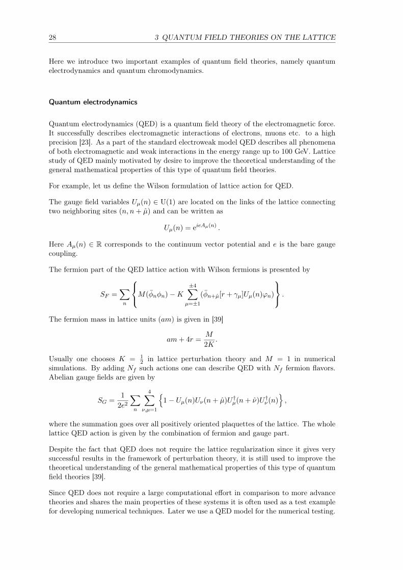
Quantum electrodynamics (QED) is a quantum field theory of the electromagnetic force.It successfully describes electromagnetic interactions of electrons, muons etc. to a highprecision [23]. As a part of the standard electroweak model QED describes all phenomenaof both electromagnetic and weak interactions in the energy range up to 100 GeV. Latticestudy of QED mainly motivated by desire to improve the theoretical understanding of thegeneral mathematical properties of this type of quantum field theories.
For example, let us define the Wilson formulation of lattice action for QED.
The gauge field variables Uµ(n) ∈ U(1) are located on the links of the lattice connectingtwo neighboring sites (n, n+ µ) and can be written as
Uµ(n) = eieAµ(n) .
Here Aµ(n) ∈ R corresponds to the continuum vector potential and e is the bare gaugecoupling.
The fermion part of the QED lattice action with Wilson fermions is presented by
SF =∑n
M(φnφn)−K±4∑
µ=±1
(φn+µ[r + γµ]Uµ(n)ϕn)
.
The fermion mass in lattice units (am) is given in [39]
am+ 4r =M
2K.
Usually one chooses K = 12 in lattice perturbation theory and M = 1 in numerical
simulations. By adding Nf such actions one can describe QED with Nf fermion flavors.Abelian gauge fields are given by
SG =1
2e2
∑n
4∑ν,µ=1
1− Uµ(n)Uν(n+ µ)U †µ(n+ ν)U †ν (n)
,
where the summation goes over all positively oriented plaquettes of the lattice. The wholelattice QED action is given by the combination of fermion and gauge part.
Despite the fact that QED does not require the lattice regularization since it gives verysuccessful results in the framework of perturbation theory, it is still used to improve thetheoretical understanding of the general mathematical properties of this type of quantumfield theories [39].
Since QED does not require a large computational effort in comparison to more advancetheories and shares the main properties of these systems it is often used as a test examplefor developing numerical techniques. Later we use a QED model for the numerical testing.

3.2 Regularization on the lattice 29
Quantum chromodynamics
Quantum chromodynamics (QCD) is the fundamental quantum field theory of quarks andgluons. QCD is believed by most physicists to be the correct theory of strong nuclearforce [39]. Lattice QCD has become a standard tool in elementary particle physics [19].
QCD is a type of quantum field theory, a non-Abelian gauge theory with symmetry groupSU(3). The QCD analogue of electric charge is a property called color. Gluons are theforce carrier of the theory, like photons are for the electromagnetic force in quantumelectrodynamics. The theory is an important part of the Standard Model of particlephysics. A large body of experimental evidence for QCD has been gathered over theyears [55].
The lattice action of QCD depends on the gauge group field Uµ(n) ∈ SU(3) on latticelinks and Grassmann fields ϕqn, ϕqn on lattice sites. Here n represents a lattice pointand µ = ±1, ±2, ±3, ±4 are the directions of neighboring points n + µ on the four-dimensional hypercubic lattice.
For example, let us define the Wilson formulation of lattice action for QCD.
The pure gauge lattice action is an sum over all plaquettes
Sg[U ] = β∑n,µ
(1− 1
3Re TrPµ(n)
),
where β = 6g−2 is the coupling term and the plaquette is given by
Pµ(n) = Uµ(n)Uν(n+ µ)U †µ(n+ ν)U †ν (n).
The quark fields φqn = φqnαc and φqn = φqnαc have flavor index q = u, d, c, s, t, b, Diracspinor index α = 1, 2, 3, 4 and SU(3) color index c = 1, 2, 3.
The Wilson action for QCD is
S[U, φ, φ] = Sg[U ] + Sq[U, φ, φ],
where the quark field action is
Sq[U, φ, φ] =∑n,µ
(φqnφqn)−Kq
±4∑µ=±1
(φqn+µ[rq + γµ]Uµ(n)φqn)
.
Here the hopping parameter Kq and Wilson parameter rq can depend on the flavor indexq. In most cases the Wilson parameter is chosen to be rq = 1. There are another repre-sentations of quark action for QCD such as an idea of staggered fermions [19], which wedo not consider here.
The lattice QCD is a very perspective quantum field theory with a lot of room for im-provement. Therefore we consider it as the main application of this thesis. In the nextsection we introduce algorithm to treat the path integral formulation of the quantum fieldtheories regularized on the lattice.

30 3 QUANTUM FIELD THEORIES ON THE LATTICE
3.3 Hybrid Monte Carlo algorithm
The main purpose of numerical simulations in lattice quantum field theory is to find anestimation of some observable O[φ] of the field variables φ which is given by the pathintegral as
〈O〉 =1
Z
∫[dφ] e−S[φ] O[φ], Z =
∫[dφ] e−S[φ], (3.18)
which leads to systems with a high number of integration variables (around 104) [40].
So the only possibility would be to use Monte Carlo integration. It would mean to ran-domly generate field configurations φ in the space of field variables, but since the numberof lattice point is very large only a small amount of the free energy density will contributein the path integral.
Hence the importance sampling is required in the Monte Carlo integration in such waythat the distribution of configurations follows the Boltzmann factor exp(−S[φ]) [16].
The task in numerical simulations is to generate samples consisting of large number Nof configurations [φn], n = 1, 2, · · · , N, in such a way that the distribution within asample approximates the desired distribution is the canonical ensemble[16].
The sequence of field configuration [φn], n = 1, 2, · · · , N is obtained by repeatedlyapplying an algorithm, which updates a configuration [φn] to the next state [φn+1] with agiven transition probability P ([φ′] ← [φ]), which refers to a large number of independentupdating.
The most useful technique for generating a sequence of configurations with the desiredprobability is to construct a Markov process. A Markov process is a stochastic proce-dure which generates a new configuration [φ′] from its predecessor [φ] with probabilityPM ([φ′] ← [φ]). Any Markov process converges to a unique fixed point distribution PSprovided that it is ergodic and that it satisfies the detailed balance
PS(φ)PM ([φ′]← [φ]) = PS(φ′)PM ([φ]← [φ′]). (3.19)
The convenient way to construct a Markov process is to choose a new configuration φ′ withprobability PC([φ′] ← [φ]) and then to either accept φ′ with the probability PA([φ′]← [φ])or to reject it and keep the old configuration φ.
The Metropolis algorithm [21] provides one choice of PA to reach a detailed balance (3.19)for any probability PC in the following generalized procedure
PA([φ′]← [φ]) = min
(1,PS(φ′)PC([φ]← [φ′])
PS(φ)PC([φ′]← [φ])
).
This approach is not very efficient because in most cases the new value of the action willbe larger than the previous one and hence the proposed change would be not accepted [39].However, if the updating process is defined by a Hamiltonian, then the classical dynamicsequations will give new configurations with different field variables, but the value of aHamiltonian is close to the original one [16].

3.3 Hybrid Monte Carlo algorithm 31
The HMC algorithm can be briefly summarized in three steps [34]:
• The construction of samples, pairs of links U ∈ Ω = SU(N) and momenta P ∈ Ω =su(N) according to the probability distribution FV with probability density V(U,P )given by
V(U,P ) =(2π)N/2
ZHexp(−S[U ])
1
(2π)N/2exp(−〈P, P 〉/2) =
1
ZHexp(−H(U,P )),
with ZH =∫
Ω×Ω V(U,P )d(U,P ) and H(U,P ) = 〈P, P 〉/2 + S[U ], where〈P, P 〉 =
∑x,µ〈Px,µ, Px,µ〉 is a natural scalar product.
• The transition from one configuration (U0, P0) to the next consists of a proposal step
(U0, P0)→ g(U0, P0) (3.20)
with mapping g : Ω× Ω→ Ω× Ω.
• The acceptance step, where the new configuration g(U0, P0) is accepted with prob-ability
PA((U0, P0), g(U0, P0)) = min
(1,V(g(U0, P0))
V(U0, P0)
)= min
(1, e−(H(g(U0,P0))−H(U0,P0))
),
(3.21)
otherwise the old configuration (U0, P0) is kept as the next entry in the chain.
In order for process (3.21) to satisfy the detailed balance condition (3.19) exactly thedynamics (3.20) must be time-reversible and generate an area-preserving map on the phasespace for any value of ∆t as it is shown in details in [39]. It can be achieved by defining gto be the Hamiltonian flow and therefore Hamilton’s equation of motion has to be solved.In practice equations of motion are integrated by numerical schemes approximately.
Due to the fact that the detailed balance condition (3.19) must be satisfied, it is requiredfrom numerical time integrators to preserve some geometric properties of the numericalflow such as time-reversibility and area-preservation.
Also since the acceptance rate of the Hybrid Monte Carlo (HMC) algorithm dependson ∆H = H(g(U0, P0)) − H(U0, P0) the higher convergence order of a numerical timeintegrator or the full conservation of energy ∆H = 0 will be an advantage because in thefirst case we obtain higher acceptance for the new configurations and in the second casethe acceptance rate is a hundred percent (PA = 1).
In the next two chapters we propose newly developed numerical time integrators, whichwould satisfy all the requirements to be suitable for the molecular dynamics step of theHMC. In the sequel we will show a detailed analysis.


4 Chapter 4
PROJECTION METHODS
As we emphasized in the previous chapter, we are highly interested in the energy conser-vation property of the numerical time integrators, since it yields hundred percent accep-tance rate in the accept/reject step of the HMC algorithm. There is a class of numericalmethods we must pay attention to, so-called projection methods. The main advantageof this kind of integrators is to preserve the energy of the system completely. Unfortu-nately, as it was mentioned before, the numerical scheme for the molecular dynamics stepof HMC algorithm has to be also time-reversible and symplectic. And while symmetric(time-reversible) projection methods have been presented in [25], projection integratorspreserving both time-reversibility and symplecticity are unknown. In spite of the abovementioned properties symmetric projection methods seem to be a suitable candidate foran improvement of the HMC algorithm, namely to neglect the accept/reject step.
In this chapter, first we introduce the standard approach of projection methods. Then weinvestigate projection schemes, which allow to interpret both the perturbation and pro-jection step as a one-step scheme with step size µ, applied to the underlying HamiltonianH(y). We introduce our attempts to construct a new class of projection schemes, whichpreserve the Hamiltonian and at the same time preserve the physical properties of time-reversibility and symplecticity of the Hamiltonian flow (4.3) via choosing the symmetric,time-reversible and symplectic one-step method Φh for the intermediate step of the classicprojection algorithm (4.2), preserve these properties and obey the energy conservationproperties by choosing suitable perturbation and projection steps of the method (4.2).After that we show our attempts to obtain high-order integrators via investigating mod-ified Hamiltonians of the numerical integrators presented in previous sections, where wetry to increase the order of conserved energy by eliminating the low order error terms ofits shadow Hamiltonians. At last we show our last try to construct a structure-preservingmodification of the classical projection approach and give a short conclusion, based ontheoretical and numerical results.
4.1 Introduction in the projection methods
For t ∈ [0, T ], we consider the solution y(t; y0) of an initial value problem of ODEs in Rddefined by
y = f(t, y), y(0) = y0, (4.1)
lying on a (d−m) submanifoldM = y : g(t, y) = 0 defined by a function g : Rd → Rm.Geometric numerical integration aims at determining a numerical approximate to thesolution y(t; y0) fulfilling the constraint defined byM at the same time. One such approachis given by the projection methods [24], where one step reads as follows:
• compute yn+1 = Φh(yn) , where Φh is an arbitrary one-step method,
33
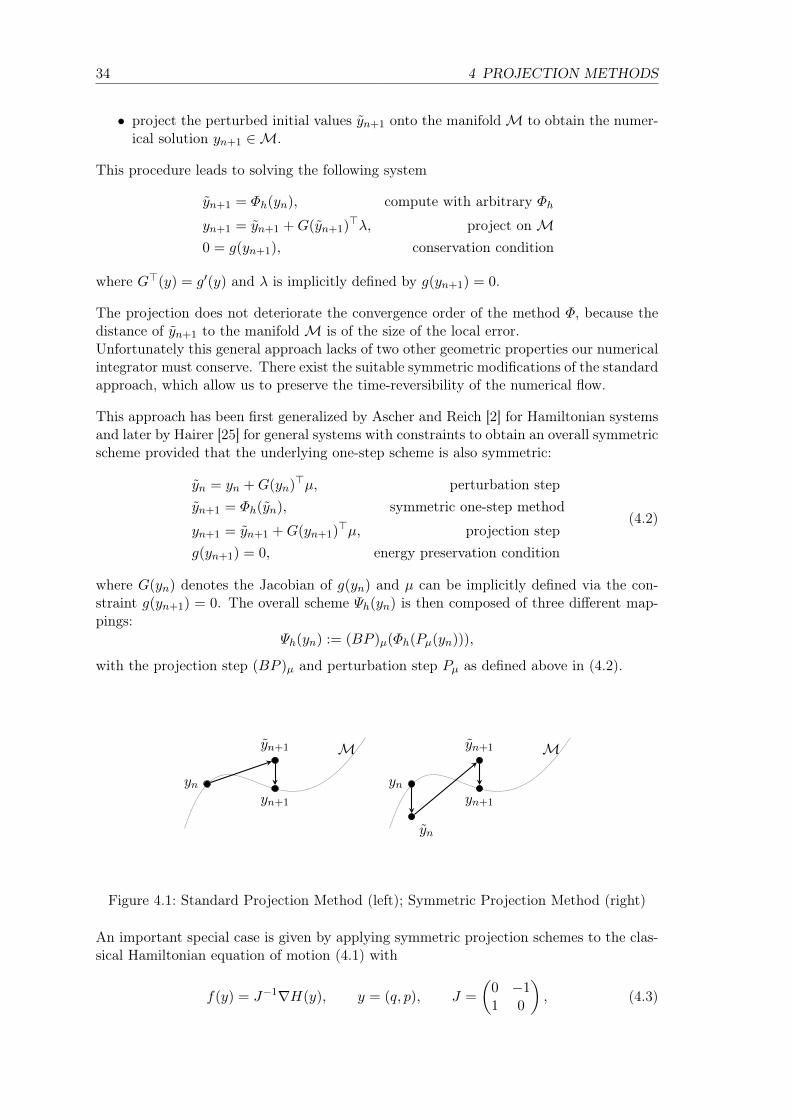
34 4 PROJECTION METHODS
• project the perturbed initial values yn+1 onto the manifoldM to obtain the numer-ical solution yn+1 ∈M.
This procedure leads to solving the following system
yn+1 = Φh(yn), compute with arbitrary Φhyn+1 = yn+1 +G(yn+1)>λ, project onM0 = g(yn+1), conservation condition
where G>(y) = g′(y) and λ is implicitly defined by g(yn+1) = 0.
The projection does not deteriorate the convergence order of the method Φ, because thedistance of yn+1 to the manifoldM is of the size of the local error.Unfortunately this general approach lacks of two other geometric properties our numericalintegrator must conserve. There exist the suitable symmetric modifications of the standardapproach, which allow us to preserve the time-reversibility of the numerical flow.
This approach has been first generalized by Ascher and Reich [2] for Hamiltonian systemsand later by Hairer [25] for general systems with constraints to obtain an overall symmetricscheme provided that the underlying one-step scheme is also symmetric:
yn = yn +G(yn)>µ, perturbation stepyn+1 = Φh(yn), symmetric one-step method
yn+1 = yn+1 +G(yn+1)>µ, projection stepg(yn+1) = 0, energy preservation condition
(4.2)
where G(yn) denotes the Jacobian of g(yn) and µ can be implicitly defined via the con-straint g(yn+1) = 0. The overall scheme Ψh(yn) is then composed of three different map-pings:
Ψh(yn) := (BP )µ(Φh(Pµ(yn))),
with the projection step (BP )µ and perturbation step Pµ as defined above in (4.2).
yn
yn+1
yn+1
M
yn
yn
yn+1
yn+1
M
Figure 4.1: Standard Projection Method (left); Symmetric Projection Method (right)
An important special case is given by applying symmetric projection schemes to the clas-sical Hamiltonian equation of motion (4.1) with
f(y) = J−1∇H(y), y = (q, p), J =
(0 −11 0
), (4.3)

4.2 Another view on symmetric projection schemes 35
where ∇H(y) = H ′(y)>, H(y) is a Hamiltonian function, q and p are the generalizedcoordinates and impulses of the system, and the matrix J denotes the standard symplecticmatrix. In this case, the constraint to be preserved is the Hamiltonian itself: g(y) :=H(y(T ))−H(yn).
So far, projection schemes are regarded as one-step schemes Ψh, starting from an initialvalue yn, and computing a new approximation yn+1 with step size h. The parameter µ isonly an internal variable fixed by the demand of fulfilling the constraint. Thus the solutionΨh depends on the initial value yn only, with µ implicitly defined by yn. If one wants togeneralize such projection schemes to symplectic or volume-preserving schemes, one hasto carefully check the sensitivity of Ψh with respect to yn, and the dependence of µ on ynhas to be included. For such schemes, if existing, also the perturbed solutions satisfy theconstraints.
However, when generalizing projection schemes to symplectic and/or volume-preservingschemes, the µ-dependence on yn is not easy to handle. Taking another point of view,one can get rid of this problem: we regard projection schemes as a class of schemes Ψµhwith step size h, parametrized by µ. Hereby, the optimal parameter µ0 is defined byH(y) = const. . For one step under consideration, this µ = µ0 is then constant, andwe use the scheme Ψµ0h . To check for symplecticity or volume preservation, we have toinvestigate the sensitivity of Ψµ0 with respect to the initial value with a fixed and constantµ0. Obviously, the perturbed solutions will not fulfill the energy constraint, but we do nothave to care about it.
Taking this point of view, we can easily generalize the symmetric projection scheme (4.2)to time-reversible and volume-preserving schemes: the perturbation and projection step in(4.2), if G evaluated at J−1yn and J−1yn+1 instead of yn and yn+1, represent an explicitand implicit Euler step with step size µ, resp., applied to a Hamiltonian equation ofmotion (4.3) with Hamiltonian H(y) := H(J−1y) instead of H(y). If we replace thesesteps by time-reversible and symplectic one-step schemes such as implicit midpoint ruleor leap-frog, the overall scheme Ψµh , consisting of three one-step schemes with step sizesµ, h and µ applied to the Hamiltonians H, H and H, resp., inherits these properties forall feasible parameters µ, if the intermediate scheme Φh is symmetric, time-reversible andsymplectic, too.
4.2 Another view on symmetric projection schemes
In our first approach, we replace the perturbation and projection step in the symmetricprojection scheme (4.2) by a symmetric, time-reversible and symplectic one-step methodΦµ of order q, which performs one step of step size µ applied to the Hamiltonian equationof motion (4.3) with the Hamiltonian H(y) := H(J−1y) instead of H(y).
The overall scheme Ψµh (yn) is then composed of three different mappings:
Ψµh (yn) := Φµ(Φh(Φµ(yn))). (4.4)
Ψµh is a composition of three symmetric, symplectic and time-reversible schemes with stepsizes µ, h and µ, resp. In composition methods, one step size is the multiple of the others,and these properties are preserved. Though this is not the case for Ψµh , it inherits these

36 4 PROJECTION METHODS
properties:
• Symmetry: Ψµh Ψ−µ−h = id.
We have
Ψµh Ψ−µ−h = (Φµ Φh Φµ) (Φ−µ Φ−h Φ−µ)
= (Φµ Φh Φµ) ((Φµ)−1 (Φh)−1 (Φµ)−1)
= id
due to the symmetry of the underlying methods.
• Time reversibility: Ψµh ρ Ψµh ρ = id with ρ =
(I 00 −I
).
This condition is equivalent to
Ψµh ρ Ψµh ρ = Φµ Φh Φµ ρ Φµ Φh Φµ ρ
= Φµ Φh Φµ ρ Φµ ρ︸ ︷︷ ︸=id
ρ Φh Φµ ρ
= Φµ Φh ρ Φh ρ︸ ︷︷ ︸=id
ρ Φµ ρ
= id
due to the time-reversibility of the underlying methods.
• Symplecticity:(∂Ψµh (yn)
∂yn
)>J(∂Ψµh (yn)
∂yn
)= J .
The symplecticity of Ψµh is a direct consequence of the symplecticity of the underlyingmethods:(
∂Ψµh∂yn
)>J
(∂Ψµh∂yn
)=
(∂Φµ∂yn
∂Φh∂yn
∂Φµ∂yn
)>J
(∂Φµ∂yn
∂Φh∂yn
∂Φµ∂yn
)
=
(∂Φµ∂yn
)>(∂Φh∂yn
)>(∂Φµ∂yn
)>J∂Φµ∂yn︸ ︷︷ ︸
=J
∂Φh∂yn
∂Φµ∂yn
=
(∂Φµ∂yn
)>(∂Φh∂yn
)>J∂Φh∂yn︸ ︷︷ ︸
=J
∂Φµ∂yn
=
(∂Φµ∂yn
)>J∂Φµ∂yn
= J.
For a given fixed step size h, the optimal µ opt to preserve the Hamiltonian is then fixedby the non-linear system
F (h, yn+1, µ) =
(yn+1 − Ψµh (yn)
H(yn+1)−H(yn)
), (4.5)

4.3 The Structure-preserving approach 37
which can be rewritten as scalar equation
gh(µ) := g(Ψµh (yn)) = H(Ψµh (yn))−H(yn) = 0, (4.6)
if Ψµh is explicit.
With F (0, yn, 0) = 0 and
∂F
(yn+1, µ)(0, yn, 0) =
(I −2∇H(yn)
∇H(yn)> 0
)regular ⇔ ∇H(yn) 6= 0,
the argument in [28] regarding the existence of the numerical solution also applies toour case: for sufficiently small step size h, the existence of the numerical approximationΨµopth (yn) with local order O(hr+1) is guaranteed, and µ = O(hr+1), independent of the
order k of Ψµ.
For non-separable Hamiltonians, all symplectic schemes with order larger than one are im-plicit, and one has to solve the nonlinear system (4.5) to obtain the approximate Ψµopt
h (yn).However, for separable Hamiltonians, the leap-frog scheme is explicit, and one has to solvethe scalar equation (4.6) only. The solvability of this scalar equations directly follows fromthe argument above, or directly via
g′h(µ) = ∇H((Ψµh (yn))> ·∂Ψµh (yn)
∂µ
= ∇H((Ψµh (yn))>(∂Φh(Φµ(yn)))
∂Φµ(yn)∇H(yn) +∇H(Φh(Φµ(yn)))
)+
+O(h) +O(µ)
= 2||∇H(yn)||22 +O(h) +O(µ).
4.3 The Structure-preserving approach
In our second approach, we replace the perturbation and projection step in the symmetricprojection scheme (4.2) by a symmetric, time-reversible and symplectic one-step methodΦµ of order k, which performs one step of step size µ applied to the original Hamilto-nian equation of motion (4.3) with Hamiltonian H(y). In contrast to the first approach,the right-hand sides of the perturbation and projection step contain linearly transformedJacobian of the constraint, and not the Jacobian itself.
The overall scheme, depending on the parameter µ is then defined by the composition ofthree numerical integration schemes
yn+1 = Ψµh (yn) := Φµ(Φh(Φµ(yn))), (4.7)
with step size µ, h and µ, resp. Similar to the first approach, the overall numerical schemeΨµ(yn) inherits the properties of symmetry, time-reversibility and symplecticity from thethree basis schemes.
To obtain preservation of the Hamiltonian in addition, µ is fixed by the constraint
0 = g(yn+1) := H(yn+1)−H(yn). (4.8)

38 4 PROJECTION METHODS
For a given fixed step size h, the optimal µ opt to preserve the Hamiltonian is then fixedby the nonlinear system
0 = F (h, yn+1, µ) :=
(yn+1 − Ψµh (yn)
H(yn+1)−H(yn)
). (4.9)
Since F (0, yn, 0) = 0, existence of the numerical approximation is given for sufficientlysmall step sizes h by the implicit function theorem, if the Jacobian
∂F
∂(yn+1, µ)
∣∣∣(h,yn,0)
=
(I −∂Φh(yn)
∂ynJ−1∇H(yn) + J−1∇H(yn+1)
∇H(yn+1)> 0
)
is regular for h→ 0, which is equivalent to a non-vanishing Schur complement
g′h(0) =∂H(Φh(yn))
∂ynJ−1∇H(yn) (4.10)
with gh(µ) := g(Ψµh (yn)). The Schur complement depends only on the intermediate schemeΦh. For a scheme of order 2, the numerical approximate Φh(yn) can be written by Taylorseries expansion as
Φh(yn) = yn + hJ−1∇H(yn) +1
2h2J−1∇2H(yn)J−1∇H(yn) + h3δ(yn) +O(h4).
Inserting this expansion into (4.10), and expanding H around yn, one gets
g′h(0) = h3∂S(yn)
∂ynJ−1∇H(yn) +O(h4)
withS(yn) := ∇H>(yn)δ(yn) +
1
6∇3H(yn)(J−1∇H,J−1∇H,J−1∇H).
If we now replace the constraint g(y) = H(y)−H(yn) by
g(y) =H(y)−H(yn)
h3, (4.11)
the corresponding Schur complement reads
g′0(0) =∂S(yn)
∂ynJ−1∇H(yn).
If this Schur complement is not zero, we can repeat the argument of the first approach:for sufficiently small step size h, the existence of the numerical approximation Ψµ opt
h (yn)with local order O(hr+1) is guaranteed, and µ = O(hr+1), independent of the order k ofΨµ.
For the leap-frog (Störmer-Verlet) method, for example, one gets for a separable Hamil-tonian
δ(yn) =
(18Hppp(yn)(Hq(yn), Hq(yn))
−14(Hqqq(yn)(Hp(yn), Hp(yn))−Hqq(yn)Hpp(yn)Hq(yn))
),

4.3 The Structure-preserving approach 39
resulting in the Schur complement
S(yn) =7
24Hppp(Hq(yn), Hq(yn), Hq(yn))− 1
12Hqqq(Hp(yn), Hp(yn), Hp(yn))
+1
4Hqq(yn)Hpp(yn)(Hq(yn), Hp(yn)).
Unfortunately despite all positive results, obtained, it is clear that the parameter µ dependson not only step-size h, but also on the initial values y0, thus we cannot rely on the resultsobtained in previous sections, since we cannot guarantee conservation of the geometricproperties in general with µ(h).
h, step-size10 -2 10 -1
|pn-p
n+1
|+|q
n-q
n+1
|
10 -18
10 -17
10 -16
10 -15
10 -14
time-reversibilitysymmetry
h, step-size10 -3 10 -2 10 -1
1-|d
et|
10 -16
10 -15
10 -14
Numerical Jacobian
Figure 4.2: Symmetry(time-reversibility) (left); Symplecticity (right).
h, step-size10 -3 10 -2 10 -1
|"H
|
10 -16
10 -14
10 -12
10 -10
10 -8Energy preservation
Figure 4.3: Energy drift.
Figures 4.2–4.3 show numerically the conservation of geometrical properties by the method(4.7) with µ = µ(y0, h) applied to the simple Harmonic oscillator (SHO) given by theHamiltonian function H = 1
2p2 + 1
2q2. We can clearly observe very promising results.
Unfortunately we must realize that it would require a computation of µ(yn, h) satisfying(4.8) on every time-step of the algorithm (4.7) and even in the case of SHO it results inextensive computational time.
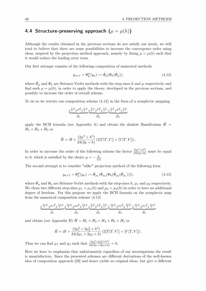
40 4 PROJECTION METHODS
4.4 Structure-preserving approach (µ = µ(h))
Although the results obtained in the previous sections do not satisfy our needs, we stilltend to believe that there are some possibilities to increase the convergence order usingideas, inspired by the projection method approach, namely by fixing µ = µ(h) such thatit would reduce the leading error term.
Our first attempt consists of the following composition of numerical methods
yn+1 = Ψµh (yn) := Φµ(Φh(Φµ)), (4.12)
where Φµ and Φh are Störmer-Verlet methods with the step-sizes h and µ respectively andfind such µ = µ(h), in order to apply the theory, developed in the previous sections, andpossibly to increase the order of overall scheme.
To do so we rewrite our composition scheme (4.12) in the form of a symplectic mapping
eµ2V eµT e
µ2V︸ ︷︷ ︸
H1
eh2V ehT e
h2V︸ ︷︷ ︸
H2
eµ2V eµT e
µ2V︸ ︷︷ ︸
H3
apply the BCH formula (see Appendix A) and obtain the shadow Hamiltonian H =H1 +H2 +H3 or
H = H +(2µ3 + h3)
24(2µ+ h)(2[T [T, V ]] + [V [T, V ]]) .
In order to increase the order of the following scheme the factor (2µ3+h3)24(2µ+h) must be equal
to 0, which is satisfied by the choice µ = − h3√2
The second attempt is to consider "alike" projection method of the following form
yn+1 = Ψµh (yn) := Φµ1(Φµ2(Φh(Φµ2(Φµ1)))), (4.13)
where Φµ and Φh are Störmer-Verlet methods with the step-sizes h, µ1 and µ2 respectively.We chose two different step-sizes µ1 = µ1(h) and µ2 = µ2(h) in order to have an additionaldegree of freedom. For this purpose we apply the BCH formula on the symplectic mapfrom the numerical composition scheme (4.13)
eµ12V eµ1T e
µ12V︸ ︷︷ ︸
H1
eµ22V eµ2T e
µ22V︸ ︷︷ ︸
H2
eh2V ehT e
h2V︸ ︷︷ ︸
H3
eµ22V eµ2T e
µ22V︸ ︷︷ ︸
H4
eµ12V eµ1T e
µ12V︸ ︷︷ ︸
H5
and obtain (see Appendix B) H = H1 +H2 +H3 +H4 +H5 or
H = H +(2µ3
1 + 2µ32 + h3)
24(2µ1 + 2µ2 + h)(2[T [T, V ]] + [V [T, V ]]) .
Thus we can find µ1 and µ2 such that (2µ31+2µ32+h3)24(2µ1+2µ2+h) = 0.
Here we have to emphasize that unfortunately regardless of our investigations the resultis unsatisfactory. Since the presented schemes are different derivations of the well-knownidea of composition approach [28] and hence yields no original ideas, but give a different

4.5 Linear projection methods 41
representation of already existing numerical time integration schemes.
4.5 Linear projection methods
After obtaining rather disappointing results we have decided to reconsider our understand-ing of the idea of symmetric projection methods. Also taking into account that using thecomposition approach can dramatically increase the computation time, thus making theeffort of getting the higher convergence order virtually worthless. We have come up withthe idea of substituting the perturbation and the projection steps of the scheme (4.2) bysome linear transformation.
It leads us to consider the following scheme
yn+1 = L−1ΦhL(yn), (4.14)
where L is a linear operator.
As we can see the symmetry of the method is satisfied by the construction of the method.The time-reversibility can be shown by using the definition of time-reversibility
ρ · L−1 · Φh · L · ρ · L−1 · Φh · L!
= id .
Using the time-reversibility of the underlying method Φh and the fact that ρ is idempotent,we can replace Φh with ρ · Φ−1
−h · ρ and get
id!
= ρ · L−1 · Φh · (L · ρ · L−1ρ) · Φ−1−h · ρ · L.
If we assume L · ρ · L−1ρ = id the time-reversibility condition is satisfied, it holds onlywhen L has a block-diagonal structure.
The volume-preservation is satisfied; it can be proved simply by applying the definition ofthe volume-preservation
1 = det
(∂L−1ΦhL(y0)
∂y0
)= |L−1| Φ′h︸︷︷︸
=1
|L| = 1.
The open question is whether it possible to achieve the higher order of convergence for themethod (4.14). To check it we write down the scheme (4.14) in the form of a symplecticmapping
eL−1 h
2V ehT e
h2V L
and by applying the BCH formula (see Appendix C) we obtain
H = H + L−1h
2V + hT +
h
2V L− h2
4[T, L−1V ] +
h2
4[T, V L]
− h3
48[L−1V, [T, L−1V ]] +
h3
24[T, [T, L−1V ]] +
h3
16[V L, [T, L−1V ]]
+h3
48[L−1V, [T, V L]]− h3
48[V L, [T, V L]] +
h3
24[T, [T, V L]].

42 4 PROJECTION METHODS
It is easy to see that L has to be equal to L−1 to sustain the second order of the underlyingmethod, but that would mean, together with above conditions, L is the identity matrix.This indicates, our scheme (4.14) will not yield any advantages, in the case of µ = µ(h).Only if we consider µ = µ(y0, h) for the numerical method (4.14) and L = (I+Aµ), whereA is block diagonal matrix, we can obtain rather interesting results. We illustrate theadvantages of this approach using an example.
Let us consider a simple harmonic oscillator (SHO) given by
H =p2
2+q2
2
with the equation of motions
p = −∂H∂q
= −q, q =∂H
∂p= p. (4.15)
The full scheme will look like
pn = (1 + µ)pn
qn = qn
pn+ 12
= pn −h
2qn
qn+1 = qn + hpn+ 12
pn+1 = pn+ 12− h
2qn+1
pn+1 =pn+1
1 + µ=
(1 + µ)pn − hqn2 −
12h(qn + h
((1 + µ)pn − hqn
2
))1 + µ
qn+1 = qn+1 = qn + h
((1 + µ)pn −
hqn2
).
The energy conservation condition reads
p2n+1
2+q2n+1
2− p2
n
2− q2
n
2= 0
and solving this equation with respect to µ we obtain
µ1 =−2pn + hqn
2pnµ2 =
−2hpn − 4qn + h2qn2hpn
µ3 =1
2
(−2−
√4− h2
), µ4 =
1
2
(−2 +
√4− h2
).
Since the time-reversibility and the symmetry of (4.14) are satisfied by the construction ofthe method and the symplecticity can be checked simply by computing the determinantof the Jacobian of the scheme (4.14)
det
(∂pnpn+1 ∂qnpn+1
∂pnqn+1 ∂qnqn+1
)= −1,

4.6 Conclusion 43
where the result is obtained by using the symbolic computation of Mathematica, and itsatisfies the area-preservation condition.
h, step-size10 -3 10 -2 10 -1
|pn-p
n+1
|+|q
n-q
n+1
|
10 -16
10 -15
10 -14
time-reversibilitysymmetry
h, step-size10 -3 10 -2 10 -1
|1-d
et|
10 -17
10 -16
10 -15
10 -14
Numerical Jacobian
Figure 4.4: Symmetry(time-reversibility) (left); Symplecticity (right).
h, step-size10 -3 10 -2 10 -1
|"H
|
10 -17
10 -16
10 -15
10 -14
Energy preservation
Figure 4.5: Energy drift.
Figures 4.4–4.5 show conservation of the geometric structure numerically. As we canobserve all desired properties are preserved exactly (up to machine precision).
4.6 Conclusion
Despite very promising results of the previous section regarding the linear projection (4.14)we must admit that the outcome of this whole chapter is only semi-positive. The presentedideas work only for rather simple problems, where with an increase of degrees of freedomand use of more general (non-linear, non-separable) Hamiltonian function, the calculationof µ(y0, h) on each time step of the algorithm would result in very high computationalcosts, minimizing the practicability of this schemes. For our main application, presentedin Chapter 3, it plays a crucial role, since the constrains (4.8) are extremely complicatedsystems and they would require additional numerical treatment and hence lead to vastcomputational costs, which are not affordable. Summarizing everything written above weconclude that we have to choose the other direction of our research, namely developinghigher order geometric numerical integrator and at the same time reducing the computa-tional effort. In the next chapter we present our research in this direction.


5 Chapter 5
NESTED FORCE-GRADIENTMETHODS
Previously we mentioned in Chapter 3 that for the HMC algorithm, used in QCD, one isinterested in efficient numerical time integration schemes, which are optimal in terms ofcomputational costs per trajectory for a given acceptance rate level. High order numericalmethods allow the usage of larger step sizes, but ask for larger computational effort perstep; low order schemes do not require vast computational costs per step, but need moresteps per trajectory. So there is a need to balance these opposing effects.
Omelyan’s numerical time integration schemes [42] of a force-gradient type have beenshown to be an efficient choice, since it is easy to obtain a higher order for a scheme andit demands just a small additional computational effort. These methods use high orderinformation of the force-gradient terms in order to increase the convergence order of thegiven numerical scheme and/or decrease the size of the leading error coefficient. Anotheridea to achieve the better efficiency of numerical time integrators is given by the multirateor nested approach. These schemes do not increase the order of the scheme, but reducethe computational costs per path by exploiting the multirate behavior given the differentparts of the right-hand side: slow forces, which are usually expensive to evaluate, but needonly to be sampled at low frequency; and fast forces, which are usually cheap to evaluate,but need to be sampled at a high frequency. The natural way to inherit the advantagesfrom force-gradient type schemes and multirate approach would be to combine these twoideas [52].
In this chapter we first briefly present the idea of splitting decomposition schemes, whichare actually a basis to both of the above mentioned approaches. Then we use this classof methods to introduce the force-gradient decomposition integrators and consider theirstructure preserving properties as well as order conditions for this type of numerical timeintegrators. We continue by presenting the idea of multirate time integration and use theadvantages of these two classes of methods to combine both approaches in order to obtaina more efficient numerical scheme.
5.1 Splitting decomposition schemes
The main idea of this type of numerical time integrators is to decompose the vector fieldinto integrable pieces and treat them separately [28]. Here we consider an arbitrary systemy = f(t, y) ∈ Rn, and suppose that the vector field is split as
y = f [1](t, y) + f [2](t, y),
and it can be visualized as in Figure 5.1.
45
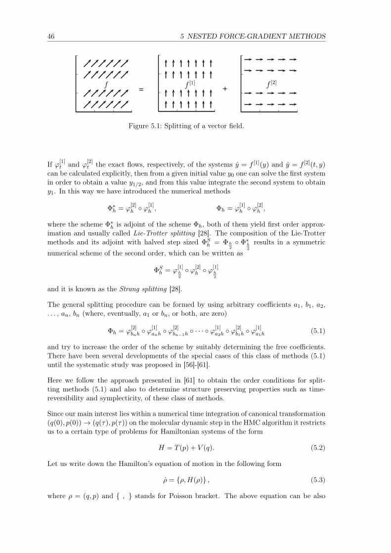
46 5 NESTED FORCE-GRADIENT METHODS
= +f [2]f [1]f
Figure 5.1: Splitting of a vector field.
If ϕ[1]t and ϕ[2]
t the exact flows, respectively, of the systems y = f [1](y) and y = f [2](t, y)can be calculated explicitly, then from a given initial value y0 one can solve the first systemin order to obtain a value y1/2, and from this value integrate the second system to obtainy1. In this way we have introduced the numerical methods
Φ∗h = ϕ[2]h ϕ
[1]h , Φh = ϕ
[1]h ϕ
[2]h ,
where the scheme Φ∗h is adjoint of the scheme Φh, both of them yield first order approx-imation and usually called Lie-Trotter splitting [28]. The composition of the Lie-Trottermethods and its adjoint with halved step sized ΦS
h = Φh2 Φ∗h
2
results in a symmetricnumerical scheme of the second order, which can be written as
ΦSh = ϕ
[1]h2
ϕ[2]h ϕ
[1]h2
and it is known as the Strang splitting [28].
The general splitting procedure can be formed by using arbitrary coefficients a1, b1, a2,. . . , an, bn (where, eventually, a1 or bn, or both, are zero)
Φh = ϕ[2]bnh ϕ[1]
anh ϕ[2]
bn−1h · · · ϕ[1]
a2h ϕ[2]
b1h ϕ[1]
a1h(5.1)
and try to increase the order of the scheme by suitably determining the free coefficients.There have been several developments of the special cases of this class of methods (5.1)until the systematic study was proposed in [56]-[61].
Here we follow the approach presented in [61] to obtain the order conditions for split-ting methods (5.1) and also to determine structure preserving properties such as time-reversibility and symplecticity, of these class of methods.
Since our main interest lies within a numerical time integration of canonical transformation(q(0), p(0))→ (q(τ), p(τ)) on the molecular dynamic step in the HMC algorithm it restrictsus to a certain type of problems for Hamiltonian systems of the form
H = T (p) + V (q). (5.2)
Let us write down the Hamilton’s equation of motion in the following form
ρ = ρ,H(ρ) , (5.3)
where ρ = (q, p) and , stands for Poisson bracket. The above equation can be also

5.1 Splitting decomposition schemes 47
written asρ = Hρ, (5.4)
where H is a differential operator Hρ := ρ,H(ρ) and , represents
f, g =∂f
∂p
∂g
∂q− ∂f
∂q
∂g
∂p.
Then the formal solution, or exact time evolution ρ(t) from t = 0 to t = τ is given by
ρ(T ) = eτH ρ(0). (5.5)
For the Hamiltonian of the form (5.2), the differential operator H = T + V , the solution(5.5) becomes
ρ(T ) = eτ(T+V ) ρ(0). (5.6)
Here we use Lemma 1 to write the method (5.1) as a product of exponentials and for-mally apply the Baker-Campbell-Hausdorff (BCH) formula (2.10) in order to obtain oneexponential of a series in powers of step-size h. Finally, we compare this series with (5.6),which corresponds to the exact solution, which results, cf. [28]
e(T+V )h+O(hr+1) =K∏k=1
eT akh eV bkh, (5.7)
where the evolution operators eT akh and eV bkh displace q and p forward in time with
q → q + akhTρ and p→ p+ bkhV ρ. (5.8)
The coefficients ak and bk in evolution operators (5.7) have to be chosen in such way toobtain the highest possible order r ≥ 1 for a given integer K ≥ 1.
Before we comment on the choice of coefficients for the order conditions for our splittingmethods (5.7) let us first have a look at the structure-preserving properties of this par-ticular class of numerical schemes. Since it results a simplification, better understandingand an improvement of the original decomposition scheme (5.7).
The most important feature of this decomposition approach (5.7) is its exact conservationof the symplectic map of the numerical flow, because the separate shifts (5.15) of coordinatevariables q and momenta variables p do not change the phase volume and decomposition(5.7) is just a product of the symplectic mappings [61].
Time-reversibility can be ensured by imposing two conditions, namely a1 = 0, ak+1 =aK−k+1 and bk = bK−k+1 as well as ak = aK−k+1 and bk = bK−k with bK = 0. Then thesingle-exponential propagator enters into the decomposition (5.7), providing automaticallythe required reversibility [43]. This symmetry also leads to elimination of all the even-order terms in the error function of the splitting integrators (5.7) setting r = 2, 4, 6, 8, . . . ,i.e.
O(hr+1
)= O1h+O3h
3 +O5h5 + · · ·+Or+1h
r+1 + . . . . (5.9)
For example we can represent the famous the Störmer-Verlet scheme (leap-frog method)
48 5 NESTED FORCE-GRADIENT METHODS
by the decomposition (5.7) by putting K = 2 with a1 = 0, b1 = b2 = 1/2, and a2 = 1
ehV2 ehT eh
V2 . (5.10)
The fourth-order (r = 4) numerical scheme from [17] is obtained via setting K = 4 witha1 = 0, a2 = a4 = θ, a3 = (1 − 2θ), b1 = b4 = θ/2, and b = 2 = b3 = (1 − θ)/2, whereθ = 1/(2− 3
√2) and given by
eθ2hV eθhT e
1−θ2hV e(1−2θ)hT e
1−θ2hV eθhT e
θ2hV . (5.11)
Schemes of the sixth order (r = 6) are derivable starting from K = 8 with numericalrepresentation of time coefficients [42].
In Chapter 2 we introduced the concept of the modified Hamiltonian for symplectic inte-grators as the way to determine the convergence order of numerical schemes. Here we canapply BCH formula (2.10) the same way as in (5.9) and show that for the method (5.11)the shadow Hamiltonian has the following form
HFR = H+
((32− 20
3√
4)
[V,[V,[V, [V, T ]
]]]+ . . .
+(8 + 203√
4)
[T,[T,[T, [V, T ]
]]]) h4
34560+O(h6).
The decomposition (5.7) has certain disadvantages. First and foremost with an increasingorder of the integration from 6 to 8 and higher, the number 2K of unknowns ak and bkincreases too fast. This makes it impossible to explicitly represent algorithms (5.7) for thecase r > 6, since one cannot solve the same number of the resulting nonlinear equationswith respect to ap and bp even using the capabilities of modern supercomputers [43]. Alsoit is impossible to derive a decomposition scheme (5.7) for r > 2 at any K with onlypositive time coefficients [56]. For example, the numerical scheme (5.11) has negativecoefficients, namely, a3, b2 and b3, and since schemes with negative time coefficients havea restricted region of application and are not acceptable for simulating non-equilibriumstatistical mechanics, quantum statistics, stochastic dynamics, and other important pro-cesses. Moreover, for schemes expressed in terms of force evaluation only, the main termO(hr+1) of truncation uncertainties appears to be, as a rule, too big, resulting in a decreasein the efficiency of the computations [42].
5.2 Force-gradient decomposition method
The drawbacks, mentioned above, make it quite desirable to introduce a more generalapproach that is free of all disadvantages. At the same time, the proposed approach mustbe explicit, in order to lead to analytical propagations. And, in addition, the alreadyknown decomposition algorithms should be able to be derived from it as particular cases.
A so called force-gradient decomposition approach [42] follows from the standard decom-

5.2 Force-gradient decomposition method 49
position (5.7) via adding the force-gradient term C , which results to the splitting
e(T+V )h+O(hr+1) =K∏k=1
eT akh eV bkh+Cckh3 , (5.12)
where C = [V, [T, V ]] and [ , ] denotes the commutator of two operators. Here the force-gradient term C arises from the third order leading error term O(h3) from (5.9), whichcan be obtained via Taylor expansion and yields
O(h3) =
(1
12[T, [T, V ]] +
1
24[V, [T, V ]]
)h3 +O(h5). (5.13)
Taking into account the explicit expressions for operators T and V it can be shown that oneof the two third-order operators in (5.13), namely [V, [T, V ]], is relatively simple and, moreimportantly, it allows to be handled explicitly, contrary to the operator [T, [T, V ]] [43].Therefore by choosing in the certain ck one can reduce the leading error term.
For example, the force-gradient version of the leap-frog method (5.10)
eh2V−h
3
48C ehT eh
V2
+h3
48C , (5.14)
has the shadow Hamiltonian
HLPfg = H − h2
12
[T, [T, V ]
]+O(h4),
which is smaller and therefore better preserves energy for the system in the comparisonto the standard leap frog formulation, which shadow Hamiltonian yields
HLP = H − h2
24
(2[V, [T, V ]
]+[T, [T, V ]
])+O(h4).
Since the force-gradient term C not only affects the third order leading error term O(h3)but also higher order error terms it is possible to obtain an improvement for higher ordernumerical schemes.
Let us first mention the conservation properties of the force-gradient approach (5.12). Inthe similar way as for methods presented in (5.7) the coefficients ak, bk and ck in (5.12)have to be chosen in such way to obtain the highest possible order r ≥ 1 for a given integerK ≥ 1. The expression (5.12) represents the general form of the decomposition, while forck ≡ 0 the decomposition reduces to the standard non-gradient factorization (5.7).
The evolution operators eT akh and eV bkh+Cckh3 in (5.12) displace p and q forward in timewith
p→ p+ bkhV (ρ) + ckCh3 and q → q + akhT (ρ). (5.15)
Symplecticity of the decomposition integration (5.12) is conserved (similar to the decom-position (5.7)), since the separate shifts (5.15) of positions and velocities do not changethe phase volume. Here, it is important to mention that in the non-Abelian case, when,for example, the gauge fields U are elements of some Lie group, and the momenta P ,elements of the corresponding Lie algebra, substituting the separable shifts (5.15) with

50 5 NESTED FORCE-GRADIENT METHODS
the following
eT h : U → U ′ = exp(iPh)U
eV h : P → P ′ = P − ihFV (U),
results the symplectic mapping and therefore the conservation of the phase volume. Itmakes the formulation (5.12) universal for the Abelian case as well as for the case of theintegration on the manifolds.
Time-reversibility with the addition of the coefficient ck can be ensured by imposing twoconditions, namely a1 = 0, ak+1 = aK−k+1, bk = bK−k+1, ck = cK−k+1, as well asak = aK−k+1, bk = bK−k, ck = cK−k with bK = 0 and cK = 0 [42].
As well as for the standard decomposition (5.7) the above symmetry will result to anautomatic disappearing of all even-order terms in the error function (5.9) for the force-gradient version (5.12). The cancellation of the remaining error terms in (5.9) is providedby fulfilling a set of basic conditions for ak, bk, and ck.
For example the assumptionK∑k=1
ak =K∑k=1
bk = 1
results in the elimination of the first order leading error term O1(h) in (5.9) and the errorfunction (5.9) can be then rewritten
O(hr+1
)= O3h
3 +O5h5 + · · ·+Or+1h
r+1 + . . . . (5.16)
In order to annihilate high order error terms in (5.16) first we need to explicitly derivethese terms by expanding both sides of the decomposition (5.12) in Taylor series, whichyields
O1 = (ν − 1)T + (σ − 1)V, O3 = α[T, [T, V ]] + β[V, [T, V ]]
O5 = γ1 [T, [T, [T, [T, V ]]]] + γ2 [T, [T, [V, [T, V ]]]] + γ3 [V, [T, [T, [T, V ]]]]
+ γ4 [V, [B, [T, [T, V ]]]] ,
(5.17)
where coefficients ν, σ, α, β and γ1−4 are chosen in such a way to eliminate error terms(5.17) further we show the optimal algorithm proposed by Omelyan et al. [42] to definethese coefficients. Here we also keep the error term O1 in mind for the generalization ofthe order conditions.
Omelyan et al. [42] proposed the following algorithm to derive the multipliers ν, σ, α,β and γ1−4, arising in (5.17), which depend on the coefficients ak, bk, and ck, wherek = 1, 2, . . . ,K . Since we are dealing with self-adjoint schemes here, the total number ofsingle-exponential operators (stages) in (5.12) actually equals to S = 2K − 1, and takinginto account the time-reversibility condition a1 = 0 or bK = cK = 0, it only accepts oddvalues. Then the simplest way to obtain explicit expressions according to [43] consistsof repeatedly choosing a central single-exponential operator and apply K − 1 times thefollowing two types of symmetric transformations
5.2 Force-gradient decomposition method 51
eW(n+1)
= eTa(n)h eW
(n)eTa
(n)h
eW(n+1)
= eV b(n)h+Cc(n)h3 eW
(n)eV b
(n)h+Cc(n)h3 ,(5.18)
whereW = (νT + σV )h+O3h
3 +O5h5 + · · ·+ . . . . (5.19)
The result leads us to the factorization (5.12), where the time coefficients ak, bk, and ckwill be related to the quantities a(n), b(n), and c(n), respectively.
For the first kind of self-adjoint constraints (when a1 = 0) with even P or the second one(when bP = cP = 0) with odd K , the central operator of the symmetric decompositionswill be correspondingly eT a(K−2)/2+1h or eT a(K−1)/2+1h. So that here we must put σ(0) = 0,α(0) = β(0) = γ0
1−4 = 0 as well as either ν(0) = a(K−2)/2+1 or ν(0) = a(K−1)/2+1 on thevery beginning (n = 0) of the recursive procedure (5.18). Moreover, we should start fromthe second line of (5.18) at b(0) = b(K−2)/2 and c(0) = c(K−2)/2 or b(0) = b(K−1)/2 andc(0) = c(K−1)/2 with further consecutive decreasing the index k by unity with increasingthe number n = 1, 2, . . . ,K − 1 at a(n) ≡ ak, b(n) ≡ bk, and c(n) ≡ ck on both lines oftransformation (5.18) [42].
For the first kind of constraints with odd K or the second kind with even K, the centraloperator is eV b(K−1)/2+1h+Cc(K−1)/2+1h
3or eV b(K−2)/2+1h+Cc(K−2)/2+1h
3that corresponds to
σ(0) = b(K−1)/2+1 and β(0) = c(K−1)/2+1 or σ(0) = b(K−2)/2+1 and β(0) = c(K−2)/2+1,respectively, with ν(0) = 0 and α(0) = γ
(0)1−4 = 0. In this case, the procedure should
be started from the first line of (5.18) at a(0) = a(K−1)/2+1 or a(0) = a(K−2)/2+1 withdecreasing k at increasing n for b(n) ≡ bk, c(n) ≡ ck, and a(n) ≡ ak [42].
The recursive relations between the multipliers ν, σ, α, β, and γ1−4 corresponding to thefirst line of (5.18) are:
ν(n+1) = ν(n) + 2a(n), σ(n+1) = σ(n),
α(n+1) = α(n) −a(n)σ(n)
(a(n) + ν(n)
)6
,
β(n+1) = β(n) − a(n)σ(n)2
6,
γ(n+1)1 = γ
(n)1 +
a(n)(a(n) + ν(n)
) ((7a(n)2 + 7a(n)ν(n) + ν(n)2
)σ(n) − 60α(n)
)360
,
γ(n+1)2 = γ
(n)2 +
a(n)(30α(n)σ(n) − 30a(n)β(n) − 30β(n)ν(n)
)180
,
+a(n)
(3a(n)2σ(n)2 + 2a(n)ν(n)σ(n)2 + ν(n)2σ(n)2
)180
,
γ(n+1)3 = γ
(n)3 +
a(n)σ(n)((
8a(n)2 + 12a(n)ν(n) + ν(n)2)σ(n) − 120α(n)
)360
,
γ(n+1)4 = γ
(n)4 +
a(n)σ(n)((
6a(n) + ν(n))σ(n)2 − 60β(n)
)180
.
(5.20)

52 5 NESTED FORCE-GRADIENT METHODS
The relations between the multipliers ν, σ, α, β, and γ1−4 corresponding to the secondline of (5.18) are:
ν(n+1) = ν(n), σ(n+1) = σ(n) + 2b(n),
α(n+1) = α(n) +b(n)ν(n)2
6,
β(n+1) = β(n) −12c(n) + b(n)ν(n)
(b(n) + σ(n)
)6
,
γ(n+1)1 = γ
(n)1 − b(n)ν(n)4
360,
γ(n+1)2 = γ
(n)2 −
ν(n)(60α(n)b(n) − ν(n)
(30c(n) − b(n)ν(n)
(6b(n) + σ(n)
)))180
,
γ(n+1)3 = γ
(n)3 +
b(n)ν(n)(
60α(n) + ν(n)2(4b(n) − σ(n)
))360
,
γ(n+1)4 = γ
(n)4 −
30α(n)b(n)(b(n) + σ(n)
)− ν(n)
(30β(n)b(n) + 60b(n)c(n)
)180
−ν(n)
(3b(n)3ν(n) + 30c(n)σ(n) − 2b(n)2ν(n)σ(n) − b(n)ν(n)σ(n)2
)180
.
(5.21)
Thus, the multipliers can readily be obtained at the end (i.e. after K − 1 steps) of therecursive process [42].
As we mentioned above the first two multipliers are particularly simple and look as ν =∑Kk=1 ak and σ =
∑Kk=1 bk then setting ν = 1 and σ = 1 cancels the first-order error
leading term O1 = 0. The next multipliers α, β, γ1−4 in order to eliminate higher-ordererror terms, namely, O3 and O5 (5.16) have to be set to zero.
The required order conditions form a system of non-linear equations, which must be solvedwith respect to unknown time coefficients ak, bk, and ck. The number m of the conditionsas well as the minimal numbers S(f)
min = 2m − 1 and S(g)min of stages, which are necessary
to obtain at least the same number m of unknowns within non-gradient (f) and gradient(g) self-adjoint decomposition schemes [42].
According to the idea proposed in [42] the minimal number of stages corresponding to agradient scheme of an order r can be considerably smaller (especially for high r) than thatof a non-gradient (ck ≡ 0) integrator of the same order, which plays the crucial role forthe main application of this work, since we would like to find an efficient algorithm thisproperty of the force-gradient decomposition methods is essential.
Here we consider the most efficient versions of the force-gradient approach (5.12) due toOmelyan [42] and present the most commonly used numerical time integrations schemesin molecular dynamics and particularly in molecular dynamics step of the HMC algorithmfor QCD.
The second order numerical time integrators include the leap-frog method, a 3-stage com-position scheme
∆(h) = ehV2 ehT eh
V2 , (5.22)

5.3 Multirate approach 53
with the shadow Hamiltonian
HLF = H − h2
24
(2[V, [T, V ]
]+[T, [T, V ]
])+O(h4)
and a 5-stage extension widely used in QCD computations:
∆(h)5 = e16hV e
12hT e
23hV e
12hT e
16hV , (5.23)
which conserves the shadow Hamiltonian [14]
H5S = H−[V, [T, V ]
]h2
72+O(h4).
The forth order numerical integrators are presented by a basic scheme is given by the5-stage force-gradient scheme proposed by Omelyan et al [42]
∆(h)5C = e16hV e
12hT e
23hV+ 1
72h3C e
12hT e
16hV . (5.24)
This scheme conserves the shadow Hamiltonian [31]
H5C = H+
(41
[V,[V,[V, [V, T ]
]]]+ . . .
+54
[T,[T,[T, [V, T ]
]]]) h4
155520+O(h6),
which gains two orders of accuracy in the comparison to its non-gradient (5.23) case, andan extension is given by the 11-stage decomposition approach [42], recently mentioned asthe integrator in the open source code openQCD as one of the standard options [36]
∆(h)11 = eσhV eηhT eλhV eθhT e(1−(λ+σ))hV e(1−(θ+η))hT e(1−(λ+σ))hV eθhT eλhV eηhT eσhV , (5.25)
where σ, θ, λ, γ1 . . . γ4 and η are parameters from [42, eqn.(71)] with a shadow Hamiltonianof the following form
H11 = H+
(γ1
[V,[V,[V, [V, T ]
]]]+ . . .
+γ4
[T,[T,[T, [V, T ]
]]]) h4
32440+O(h6).
We use above mentioned methods as a benchmark for the comparison of the numericalresults and introduce nested versions of these numerical schemes in the next section.
5.3 Multirate approach
In this section we consider the case, that many solution components of an ordinary differ-ential equation vary slowly and only a few components exhibit fast dynamics. Here it istempting to use large step sizes for the slow components and small step sizes for the fastones. Such integrators, called multirate methods (commonly termed nested schemes in thephysics community), were first formulated by Rice (1960) and Gear and Wells [20]. These

54 5 NESTED FORCE-GRADIENT METHODS
schemes do not increase the order of the scheme, but reduce the computational costs perpath by exploiting the multirate behavior given in the different parts of the right-handside: slow forces, which are usually expensive to evaluate, but need only to be sampledat a low frequency; and fast forces, which are usually cheap to evaluate, but need to besampled at a high frequency. In the case of our primal application to the quantum fieldtheories we have a chance to exploit this property to our advantage, since the generalproblem of quantum field theory has a slow and costly fermion part and fast and cheapgauge part as we showed in Chapter 3.
First we consider a system of ODEs and suppose that the vector field f is split intosummands contributing to slow and fast dynamics as following
y = f(t, y), y = f [slow](t, y) + f [fast](t, y), y ∈ Rn, (5.26)
where f [ slow](t, y) is more expensive to evaluate than f [ fast](t, y). Multirate methods canoften be cast into this framework by collecting in f [slow](t, y) those components of f(t, y)which produce slow dynamics and in f [fast](t, y) the remaining components [20].
For a given N ≥ 1 and for the ODE (5.26) a multiple time stepping method is obtainedfrom
Φ[slow]h2
(
Φ[fast]hM
)M Φ
[slow]h2
(5.27)
where Φ[slow]h and Φ
[fast]h are numerical integrators consistent with y = f [ slow](t, y), respec-
tively and y = f [fast](t, y). The method (5.27) is already stated in symmetric form . Itis often called the impulse method, because the slow part f [ slow](t, y) of the vector fieldis used - impulse-like - only at the beginning and at the end of the step, whereas themany small sub-steps in between are concerned solely through integrating the fast systemy = f [fast](t, y) [47]. Multirate time stepping approach can be visualized as it is shown onFigure 5.2.
t0 t0 + h
h
h
M
. . .
f [slow]
f [fast]
Figure 5.2: Multirate time stepping structure.
Structure preserving properties of fast-slow splitting multirate algorithms (5.26) can beeasily checked via using the representation of the multirate numerical schemes by thecomposition approach, which results the following Lemma 4
Lemma 4. Let Φ[slow]h be an arbitrary method of order 1, and Φ
[fast]h a symmetric method

5.4 Nested force-gradient schemes 55
of order 2. Then, the multiple time stepping algorithm (5.27) is symmetric and of order2.
If f [slow](t, y) and f [fast](t, y) are Hamiltonian and if Φ[slow]h and Φ
[fast]h are both symplectic,
then the multiple time stepping method is also symplectic.
The most important application of multiple time stepping is in Hamiltonian systems witha separable Hamiltonian
H(p, q) = T (p) + V (q), V (q) = V1(q) + V2(q), (5.28)
where T represents the kinetic part, V1 is the potential energy of the small (fast) scale partof the system and V2 corresponds to the potential energy of the large (slow) scale part.
For example, using the notation of the standard decomposition approach (5.7) we choosethe following integrator to compute the inner part H = T + V1
∆(h)M =[eh
2MV1 e
hMT e
h2M
V1]M
,
and therefore define ∆ (h) a nested integrator to solve the split problem (5.28), it yields
∆(h) = eh2V2 ∆ (h)M e
h2V2 . (5.29)
The obtained method, called nested leap-frog, conserves the shadow Hamiltonian [53]
HM = H +
(− 1
24
[V2, [V2, T ]
]+
1
12
[V1, [V2, T ]
]+
1
12
[T, [V2, T ]
]+
1
M2
(− 1
24
[V1, [V1, T ]
]+
1
12
[T, [V1, T ]
]))h2 +O(h4).
Notice that for M = 1 the method (5.29) reduces to the Störmer-Verlet scheme applied tothe Hamiltonian system withH(q, p). This is a consequence of the fact that ϕ[fast]
t ϕ[slow]t =
ϕVt is the exact flow of the Hamiltonian system corresponding to V (q) of (5.28) [6].
5.4 Nested force-gradient schemes
Our main idea in this thesis is to combine the idea of force-gradient decomposition methods(5.12) to improve the energy preservation of symplectic schemes applied to Hamiltoniansystems with multiple time splitting techniques for multi-time scales problems, using thefact that the potential of the general quantum field problems has different parts withstrongly varying dynamics, thereby reducing the computational costs.
In order to get a better insight into the multi-rate formulation of the force-gradient ap-proach, we start this section with a short introduction into the nested integration ideaproposed by Sexton and Weingarten [49].
The basis for multirate schemes is to split the action into different parts according to the
56 5 NESTED FORCE-GRADIENT METHODS
activity level:
H(U,P ) =〈P, P 〉
2+
M∑m=0
Sk[U, φ] (5.30)
If the actions of the Hamiltonian (5.30) are ordered such that computational costs areincreasing, while at the same time the strength of the forces is decreasing, a multi-rateintegration based on the leap-frog scheme with macro step size h0 and micro step sizeh1 := h0/m1 due to Sexton and Weingarten [49] proceeds as follows:
VH(h0) = VH2(h0
2) (VH1(h1))m1 VH2(
h0
2)
with H1(U,P ) := 〈P, P 〉/2 +∑M−1
m=0 Sk[U, φ] and H2(U,P ) = SM [U, φ]. This scheme canbe nested, by introducing a next finer step size h2 := h1/m2 and further splitting H1 into
H1(U,P ) = H11(U,P ) +H12(U,P )
H11(U,P ) := 〈P, P 〉/2 +∑M−2
m=0 Sk[U, φ] and H12(U,P ) = SM−1[U, φ] in order to replaceVH1(h1) above by
VH1(h1) = VH12(h1
2) (VH11(h2))m2 VH12(
h1
2)
This procedure can be applied recursively [58] to obtain M different step size ratios at theend, corresponding to the activity levels of the M actions Sk[U, φ].
This approach can be easily generalized to base schemes of higher order such as force-gradient schemes. It can be easily shown that by construction the overall multirate schemeinherits the properties of the underlying base scheme: symmetry, time-reversibility, volumepreservation and order (according to the slowest time step h). Nested force-gradientschemes in QCD have been tested by [14]; applications to Domain Wall fermions arediscussed in [3].
A nested version of a standard force-gradient integrator (5.24), which probably has beenused in [3] reads
∆5C(h) = e16hV2 ∆2
(h
2
)M
e23hV2+ 1
72h3Cf ∆2
(h
2
)M
e16hV2 , (5.31)
where∆2(h)M =
(e
16M
hV1 e1
2MhT e
23M
hV1+ 172( h
M )3Cg e
12M
hT e1
6MhV1)M
,
with Cg = [V1, [T, V1]] and Cf = [V2, [T, V2]]. It is important to notice that, apart of imple-mentation of the integrator (5.31), there was no detailed analysis made for the integratorproperties.
Despite the fact that the idea of nested force-gradient methods is of a great interest, ingeneral it remained relatively unknown and there is not that many research been publishedon this matter.
One serious drawback of this approach is that the same base scheme is used at all levels,i.e., high computational costs of high order schemes appear at all levels. In order toovercome this limitation it is natural to suggest using different schemes of different orderat the different levels without loosing the effective high order of the overall multirate
5.5 Adapted nested force-gradient schemes 57
scheme. For the latter, we could make use of the idea of including appropriate force-gradient information. For this, we restrict the system (5.30) to two time levels, as theultimate goal will be to develop nested force-gradient schemes for lattice QCD, where thegauge field plays the role of the fast action and cheap part, and the fermion field plays therole of the slow action and expensive part, i.e., only two time scales are involved.
If one uses a second-order scheme for the fast action with time step h/M and a fourth-order scheme for the slow action with time step h, the error of the overall multirate schemewill be of order O(h2) +O
((hM
)2)+O(h4) the use of force-gradient information only at
the slowest level it is possible to cancel the leading error term of order O(h2). As M ≥ 1h
usually holds in the multirate setting, the overall order is then given by the leading errorterm of order O(h4), i.e., the scheme has an effective order of four. In the next section weperform the proof of this statement.
5.5 Adapted nested force-gradient schemes
In order to overcome the previously mentioned drawbacks of a standard nested force-gradient integrator (5.31) we propose the following scheme introduced in [51]
∆5C(h) = e16hV2 ∆1
(h
2
)M
e23hV2+ 1
72h3Cf ∆1
(h
2
)M
e16hV2 . (5.32)
To summarize, the adapted scheme (5.32) differs from the original one (5.31) in twoperspectives:
• The force gradient scheme for the fast action is replaced by a leap-frog scheme.
• Only the part [V2, [T, V2]] of the full force gradient [V1 + V2, [T, V1 + V2]] is neededto gain the effective order of four.
Geometric properties of the numerical flow such as time-reversibility and symplecticitypreserved by the construction, since the scheme (5.32) can be presented as the compositionof the time-reversible and symplectic integrators and hence also possesses these properties.
Now it is crucial to show that the proposed integrator has the effective order of four. Letus start by introducing following alike 5-stage nested integrator
∆(h) = eλhV2 ∆
(h
2
)M
e(1−2λ)hV2 ∆
(h
2
)M
eλhV2 , (5.33)
where∆
(h
2
)M
=[eh
4MV1 e
h2M
T eh
4MV1]M
and analyzing the energy conservation of this scheme. The method (5.33) was chosen tobe a base of our proposed integrator (5.32), because it has an optimal number of stages,necessary for increasing its order.
We have to find the shadow Hamiltonian for the integrator (5.33). In order to do so, weuse the BCH formula (2.10). To simplify this task we consider the limit of the integratorgiven in (5.33), as M tends to infinity.

58 5 NESTED FORCE-GRADIENT METHODS
We obtain the following representation of (5.33)
∆(h) = eλhV2 eh2
(V1+T ) e(1−2λ)hV2 eh2
(V1+T ) eλhV2 . (5.34)
Theorem 9 (Shadow Hamiltonian of (5.34)). The shadow Hamiltonian of the nestedmultirate integrator (5.34) is given by
H = H +(−1 + 6λ− 6λ2
12
[V2, [T, V2]
]+−1 + 6λ
24
[V1, [T, V2]
]+−1 + 6λ
24
[T, [T, V2]
])h2 +O(h4). (5.35)
Proof: We apply the BCH formula to the first two evolution operators
X = ln
(eλhV2 eh
V1+T2
)= c1h+ c2h
2 + c3h3 +O(h5),
where
c1 = λV2 +V1 + T
2,
2c2 =B2
2!adc1
(λV2 +
V1 + T
2
)− 1
2adc1
(λV2 −
V1 + T
2
),
c2 = −1
4
[λV2 +
V1 + T
2, λV2 −
V1 + T
2
]= −λ
4[V1, V2]− λ
4[T, V2],
3c3 =B3
3!adc1adc1
(λV2 +
V1 + T
2
)− 1
2adc2
(λV2 −
V1 + T
2
),
c3 = −1
6
[−λ
4[V1, V2]− λ
4[T, V2], λV2 −
V1 + T
2
]= −λ
2
24
[V2, [V1, V2]
]− λ2
24
[V2, [T, V2]
]+
λ
48
[V1, [V1, V2]
]+
λ
48
[V1, [T, V2]
]+
λ
48
[T, [V1, V2]
]+
λ
48
[T, [T, V2]
].
Then we have the result for our first two operators
X =
(λV2 +
V1 + T
2
)h+
(−λ
4[V1, V2]− λ
4[T, V2]
)h2
+
(−λ
2
24
[V2, [V1, V2]
]− λ2
24
[T, [T, V2]
]+
λ
48
[V1, [V1, V2]
]+λ
48
[V1, [T, V2]
]+
λ
48
[T, [V1, V2]
]+
λ
48
[T, [T, V2]
])h3 +O(h5).
The next step is to apply the BCH formula on the following operators
Y = ln(
eX e(1−2λ)hV2)
= c1 + c2 + c3 +O(h5)

5.5 Adapted nested force-gradient schemes 59
and coefficients
c1 = X + (1− 2λ)hV2 =
((1− λ)V2 +
V1 + T
2
)h+ (. . .)h2 + (. . .)h3,
2c2 =B2
2!adc1
(X + (1− 2λ)hV2
)− 1
2adc1
(X − (1− 2λ)hV2
),
c2 = −1
4
[X + (1− 2λ)hV2, X − (1− 2λ)hV2
]=
(1− 2λ
4[V1, V2] +
1− 2λ
4[T, V2]
)h2
+
(λ− 2λ2
8
[V2, [V1, V2]
]+λ− 2λ2
8
[V2, [T, V2]
])h3
3c3 =B3
3!adc1adc1
(X + (1− 2λ)hV2
)− 1
2adc2
(X − (1− 2λ)hV2
),
c3 = −1
6
[c2, X − (1− 2λ)hV2
]=
(−(1− 2λ)(1− 3λ)
24
[V2, [V1, V2]
]− (1− 2λ)(1− 3λ)
24
[V2, [T, V2]
]+
(1− 2λ)
48
[V1, [V1, V2]
]+
(1− 2λ)
48
[V1, [T, V2]
]+
(1− 2λ)
48
[T, [V1, V2]
]+
(1− 2λ)
48
[T, [T, V2]
])h3,
and we obtain the following expansion
Y =
((1− λ)V2 +
V1 + T
2
)h+
(1− 3λ
4[V1, V2] +
1− 3λ
4[T, V2]
)h2
+
(−1 + 8λ− 13λ2
24
[V2, [V1, V2]
]+−1 + 8λ− 13λ2
24
[T, [T, V2]
]+
1− λ48
[V1, [V1, V2]
]+
1− λ48
[V1, [T, V2]
]+
1− λ48
[T, [V1, V2]
]+
1− λ48
[T, [T, V2]
])h3 +O(h5),
The next step would be to repeat the previous procedures to find
Z = ln
(eY eh
V1+T2
)= c1 + c2 + c3 +O(h5).
60 5 NESTED FORCE-GRADIENT METHODS
Using the BCH formula we obtain
c1 = Y + hV1 + T
2= ((1− λ)V2 + V1 + T )h+ (. . .)h2 + (. . .)h3,
2c2 =B2
2!adc1
(Y + h
V1 + T
2
)− 1
2adc1
(Y − hV1 + T
2
),
c2 = −1
4
[Y + h
V1 + T
2, Y − hV1 + T
2
]=
(−1− λ
4[V1, V2]− 1− λ
4[T, V2]
)h2
+
(−1− 3λ
16
[V1, [V1, V2]
]− 1− 3λ
16
[V1, [T, V2]
]−1− 3λ
16
[T, [V1, V2]
]− 1− 3λ
16
[T, [T, V2]
])h3,
3c3 =B3
3!adc1adc1
(Y + h
V1 + T
2
)− 1
2adc2
(Y − hV1 + T
2
)c3 = −1
6
[c2, Y − h
V1 + T
2
],
=
(−(1− λ)2
24
[V2, [V1, V2]
]− (1− λ)2
24
[V2, [T, V2]
])h3.
Therefore we obtain
Z =((1− λ)V2 + V1 + T
)h+
(−λ2
[V1, V2] +−2λ
2[T, V2]
)h2
+
(−1 + 5λ− 7λ2
12
[V2, [V1, V2]
]+−1 + 5λ− 7λ2
12
[T, [T, V2]
]+−1 + 4λ
48
[V1, [V1, V2]
]+−1 + 4λ
48
[V1, [T, V2]
]+−1 + 4λ
48
[T, [V1, V2]
]+−1 + 4λ
48
[T, [T, V2]
])h3 +O(h4).
Applying the BCH formula for a last time we obtain the shadow Hamiltonian
H = ln(
eZ eλV2h)
= c1 + c2 + c3 +O(h5),

5.5 Adapted nested force-gradient schemes 61
with the coefficients
c1 = Z + λV2h = (V2 + V1 + T )h+ (. . .)h2 + (. . .)h3,
2c2 =B2
2!adc1 (Z + λV2h)− 1
2adc1 (Z − λV2h) ,
c2 = −1
4[Z + λV2h, Z − λV2h]
=
(λ
2[V1, V2] +
λ
2[T, V2]
)h2 +
(λ2
4
[V2, [V1, V2]
]+λ2
4
[V2, [T, V2]
])h3,
3c3 =B3
3!adc1adc1 (Z + λV2h)− 1
2adc2 (Z − λV2h) ,
c3 = −1
6[c2, Z − λV2h]
=
(λ(1− 2λ)2
12
[V2, [V1, V2]
]+λ(1− 2λ)2
12
[V2, [T, V2]
]+
λ
12
[V1, [V1, V2]
]+λ
12
[V1, [T, V2]
]+
λ
12
[T, [V1, V2]
]+
λ
12
[T, [T, V2]
])h3,
and finally
H = H +
(−1 + 6λ− 6λ2
12
[V2, [V1, V2]
]+−1 + 6λ
24
[V1, [T, V2]
]+−1 + 6λ− 6λ2
12
[V2, [T, V2]
]+−1 + 6λ
24
[V1, [V1, V2]
]+−1 + 6λ
24
[T, [V1, V2]
]+−1 + 6λ
24
[T, [T, V2]
])h2 +O(h4).
Finally, taking into account that [V1, V2] = 0, hence[V2, [V1, V2]
],[V1, [V1, V2]
]and[
T, [V1, V2]]are equal to zero, we obtain (5.35).
We can eliminate a couple of terms by choosing λ = 1/6, thus
H = H − 1
72
[V2, [T, V2]
]h2 +O(h4).
We would like to increase the order of the method (5.33) by adding the force-gradientterm, but first we consider the force-gradient itself. Due to the splitting (5.28) it can berepresented as
C =[V, [T, V ]
]=[V2 + V1, [T, V2 + V1]
]=[V2, [T, V2]
]+[V1, [T, V1]
]+[V1, [T, V2]
]+[V2, [T, V1]
].
Then we can tune the original algorithm (5.33) by adding the first term of the forcegradient
[V2, [T, V2]
]and neglect the last three terms:
∆(h) = e16hV2 ∆
(h
2
)M
e23hV2+ 1
72h3[V2,[T,V2]
]∆
(h
2
)M
e16hV2 , (5.36)
which preserves the fourth-order accurate shadow Hamiltonian
H = H +O(h4).

62 5 NESTED FORCE-GRADIENT METHODS
So now we can analyze the shadow Hamiltonian for the nested method (5.33) for thegeneral case when the parameter M does not tend to infinity.
First, let us show that the evolution operator ∆(h)M can also be presented as
∆
(h
2
)M
= eh2
(V1+T )+ h3
M2 ( 1192
[V1, [T, V1]]+ 196
[T, [T, V1]])+O(h5) .
It is derived by applying the BCH formula on the original propagator ∆(h)M . Thereforethe proposed scheme (5.33) can be rewritten as
∆(h) = eλhV2 eh2
(V1+T )+ h3
M2 ...O(h5) e(1−2λ)hV2 eh2
(V1+T )+ h3
M2 ...+O(h5) eλhV2 .
To find the shadow Hamiltonian we apply the BCH formula to the first two evolutionoperators
X = ln
(eλhV2 eh
V1+T2
+ h3
M2 (...)
)= c1h+ c2h
2 + c3h3 +O(h5),
where
c1 = λV2 +V1 + T
2+
h3
M2(. . .) +O(h5)
2c2 =B2
2!adc1
(λV2 +
V1 + T
2
)− 1
2adc1
(λV2 −
V1 + T
2
)c2 = −1
4
[λV2 +
V1 + T
2, λV2 −
V1 + T
2
]= −λ
4[T, V2],
3c3 =B3
3!adc1adc1
(λV2 +
V1 + T
2
)− 1
2adc2
(λV2 −
V1 + T
2
)c3 = −1
6
[−λ
4[T, V2], λV2 −
V1 + T
2
]= −λ
2
24[V2, [T, V2]] +
λ
48[V1, [T, V2]] +
λ
48[T, [T, V2]] .
Then for the first two operators we have
X = h
(λV2 +
V1 + T
2
)− λh2
4[T, V2]− λ2h3
24[V2, [T, V2]]
+λh3
48[V1, [T, V2]] +
λh3
48[T, [T, V2]] +
h3
M2(. . .) +O(h5).
Next we apply the BHC formula to
Y = ln(
eX e(1−2λ)hV2)
= c1h+ c2h2 + c3h
3 +O(h5)
with coefficients

5.5 Adapted nested force-gradient schemes 63
c1 = X + (1− 2λ)V2 = (1− λ)V2 +V1 + T
2+ . . .+O(h5)
2c2 =B2
2!adc1 (X + (1− 2λ)V2)− 1
2adc1 (X − (1− 2λ)V2)
c2 = −1
4[X + (1− 2λ)V2, X − (1− 2λ)V2] =
1− 2λ
4[T, V2] +
λ− 2λ2
8[V2, [T, V2]]
3c3 =B3
3!adc1adc1 (X + (1− 2λ)V2)− 1
2adc2 (X − (1− 2λ)V2)
c3 = −1
6[c2, X − (1− 2λ)V2] =
(1− 2λ)(−1 + 3λ)
24[V2, [T, V2]]
+(1− 2λ)
48[V1, [T, V2]] +
(1− 2λ)
48[T, [T, V2]]
and we obtain the following expansion
Y =
((1− λ)V2 +
V1 + T
2
)h+
(1− 3λ)h2
4[T, V2] +
(−1 + 8λ− 13λ2)h3
24[V2, [T, V2]]
+(1− λ)h3
48[V1, [T, V2]] +
(1− λ)h3
48[T, [T, V2]] +
h3
M2(. . .) +O(h5).
Then by repeating the previous procedures we obtain
Z = ln
(eY e+ h3
M2 ...+O(h5)
)= c1h+ c2h
2 + c3h3 +O(h5).
Using the BCH formula yields
c1 = Y +V1 + T
2= (1− λ)V2 + V1 + T + . . .+O(h5)
2c2 =B2
2!adc1
(Y +
V1 + T
2
)− 1
2adc1
(Y − V1 + T
2
)c2 = −1
4
[Y +
V1 + T
2, Y − V1 + T
2
]= −1− λ
4[T, V2]
− 1− 3λ
16[V1, [T, V2]]− 1− 3λ
16[T, [T, V2]]
3c3 =B3
3!adc1adc1
(Y +
V1 + T
2
)− 1
2adc2
(Y − V1 + T
2
)c3 = −1
6
[c2, Y −
V1 + T
2
]= −(1− λ)2
24[V2, [T, V2]]
and hence we obtain
64 5 NESTED FORCE-GRADIENT METHODS
Z = ((1− λ)V2 + V1 + T )h+−λh2
2[T, V2] +
(−1 + 5λ− 7λ2)h3
12[V2, [T, V2]]
+(−1 + 4λ)h3
48[V1, [T, V2]] +
(−1 + 4λ)h3
48[T, [T, V2]] +
2h3
M2(. . .) +O(h5).
Then using the BCH formula for the last time we obtain the shadow Hamiltonian
H = ln(
eZ eλV2)
= c1h+ c2h2 + c3h
3 +O(h5)
with coefficients
c1 = Z + λV2 = (V2 + V1 + T )h+ . . .+O(h5)
2c2 =B2
2!adc1(Z + λV2)− 1
2adc1(Z − λV2)
c2 = −1
4[Z + λV2, Z − λV2] =
λ
2[T, V2] +
λ2
4[V2, [T, V2]]
3c3 =B3
3!adc1adc1(Z + λV2)− 1
2adc2(Z − λV2)
c3 = −1
6[c2, Z − λV2]
=λ(1− 2λ)
12[V2, [T, V2]] +
λ
12[V1, [T, V2]] +
λ
12[T, [T, V2]],
which finally yields
H = V2 + V1 + T +(−1 + 6λ− 6λ2)h2
12[V2, [T, V2]] +
(−1 + 6λ)h2
24[V1, [T, V2]]
+(−1 + 6λ)h2
24[T, [T, V2]] +
h2
M2
(1
96[V1, [T, V1]] +
1
48[T, [T, V1]]
)+O(h4).
Similar to the case when M →∞ a choice λ = 1/6 eliminates the error terms [V1, [T, V2]]and [T, [T, V2]]; by adding the force-gradient term as for the numerical scheme (5.36) weobtain
H = H +h2
M2
(1
96[V1, [T, V1]] +
1
48[T, [T, V1]]
)+O(h4),
which results to an order of the method (5.32) to be O((
hM
)2)+O(h4) but since in the
multirate setting the parameter M usually satisfies the relation M ≥ 1h , the overall order
is then given by the leading error term of order O(h4), i.e., the numerical scheme (5.32)has an effective order of four. We show the numerical proof in the next chapter.

5.5 Adapted nested force-gradient schemes 65
In this chapter we have introduced a new decomposition scheme for Hamiltonian systems,which combines the idea of the force-gradient time-reversible and symplectic integratorsand the splitting approach of nested algorithms. The new method (5.32) is fourth-orderaccurate. We also introduced some of the most commonly used numerical time integratorsfor the molecular dynamics such as for example leap-frog (5.22), its nested version (5.29),standard 5 stage decomposition integrator (5.23) and its nested version (5.33), which aresecond order; (5.24) and (5.25), which have the fourth order of convergence. Hence theseare competitors to the proposed method (5.32).
We do not consider integrators of the order higher than 4, since the computational costsare too high. The schemes of the same convergence order differ from each other by thenumber of stages (updates of momenta and links per time step). Usually methods withmore stages have smaller leading error coefficients and therefore have better accuracy, buthigher computational costs. We would like to determine which integrator would representthe best compromise between high accuracy and computational efficiency.
In the next chapter we test our proposed numerical integrator in the comparison to theabove mentioned standard numerical methods for the molecular dynamics step of theHMC algorithm. In order to analyze the behavior of the integrators we apply them to twodifferent test problems, which are introduced next.


6 Chapter 6
NUMERICAL RESULTS
We compare the behavior of numerical time integration schemes currently used for HMC[42] with the nested force-gradient integrator [14] and the adapted version introduced in[51]. We investigate the computational costs needed to perform numerical calculations,as well as the effort required to achieve a satisfactory acceptance rate during the HMCevolution. Our goal is to find a numerical scheme for the HMC algorithm which wouldprovide a sufficiently high acceptance rate while not drastically increasing the simulationtime.
In this chapter we present results of numerical experiments, which were designed to test thenew idea of the adapted nested force-gradient method. Since it was previously mentionedthat all the considered numerical schemes preserve geometric properties of the numericalflow of the system of ODEs here we concentrate on the convergence order of the integratorsand their computational efficiency.
First we test most commonly used geometric integrators on the classical n-body problem,then we apply these integrators to QED’s two-dimensional Schwinger model and discussour obtained results.
6.1 N-body problem
In order to obtain a better insight in dealing with the force-gradient (5.12) and multirate(5.27) numerical integration schemes we first apply certain numerical methods for solvingthe well known problem n-body problem of astrophysics.
This problem has been chosen because it can model the multirate time scaling for themultirate methods to be used. Also the case of the n-body problem we chose to consideris fairly simple (3-body problem) and may not yield significant advantages for the nestedtype integrators (the difference between fast and slow part of the action is too small), butit can still demonstrate important features of the proposed nested force-gradient schemes.
We recall that for classical mechanical systems, the equation of motion can be written as
dρdt
= ρ,H ≡ L(t)ρ(t), (6.1)
where ρ is the set of phase variables, , denotes the Poisson bracket, H represents theHamiltonian function, and L denotes the Liouville operator.
For the case of N particles, located in a spatially inhomogeneous time-dependent externalfield u(qi, t) and interacting through the pair-wise potential ϕ(qij) ≡ ϕ(|qi − qj |), the
67

68 6 NUMERICAL RESULTS
Hamiltonian reads
H =
N∑i=1
miv2i
2+
1
2
N∑i 6=j
ϕ(qij) +
N∑i=1
u(qi, t) ≡ T (v) + V (q, t). (6.2)
Here qi represents the position of particle i (i = 1, 2, . . . , N) moving with velocity vi =dqi/dt and carrying the mass mi, so that T and V are the total kinetic and potentialenergies, respectively. Then ρ = qi, vi ≡ q, v, and the Liouville operator of thesystem takes the form
L(t) =N∑i=1
(vi ·
∂
∂qi+fi(t)
mi· ∂∂vi
), (6.3)
where
fi(t) = −N∑
j(j 6=i)
ϕ′(qij)(qi − qj)qij
− ∂u(qi, t)
∂qi
are forces acting on the particles due to their interactions.
If the initial configuration ρ(0) is specified, the unique solution to the problem of equa-tion (6.1) can be presented by the time propagator operator as
ρ(t) =[e(D+L)h
]lρ(0), (6.4)
where h is a temporal step size and l = t/h the total number of steps. D =←−∂ /∂t denotes
the time derivative operator acting on the left of time-dependent functions. We considerin our paper L, which does not depend explicitly on time, thus we set D = 0.
In case of many-particle systems (N > 2) the time propagator cannot be computed ex-actly even in the absence of time dependent potentials. Hence one has to apply numericalintegration methods such as decomposition schemes, which both preserve the physicalproperties of the Hamiltonian system (6.4) (symplecticity, time reversibility) and are com-putationally efficient [42].
As we presented in the previous chapter the force-gradient schemes are based on the factthat the total propagator in (6.4) can be split in the following way:
e(T+V )h+O(hK+1) =P∏p=1
eT aph eV bph+Ccph3 ,
where C = [V, [T, V ]] and [ , ] denotes the commutator of two operators and for the caseof the Hamiltonian function (6.2) it yields
C ≡[V, [T, V ]
]=
N∑i=1
gimi· ∂∂v,
wheregiα = 2
∑jβ
fjβmj
∂fiα∂qjβ
,
α and β denote the Cartesian components of the vectors. The force-gradient evaluations

6.1 N-body problem 69
∂fiα/∂qjβ can be explicitly represented taking into account that
fiα = miwiα −∂u(qi, t)
∂qiα,
wherewiα = − 1
mi
∑j(j 6=i)
ϕ′(qij)(qiα − qjα)
qij
is the inter-particle part of the acceleration. The result is
gi = −2N∑
j(j 6=i)
[(wi − wj)
ϕ′ijqij
+(qi − qj)q3ij
(qijϕ
′′ij − ϕ′ij
) (qi · (wi − wj)
)]+ hi, (6.5)
where
hiα =2
mi
∑β
∂u
∂qiβ
∂2u
∂qiα∂qiβ.
For this type of problem (6.1) we test well-known, commonly used second order integrationschemes in molecular dynamics such as
• the leap-frog method, a 3-stage composition scheme:
∆(h) = ehV2 ehT eh
V2 , (6.6)
• and a 5-stage extension widely used in QCD computations:
∆5(h) = e16hV e
12hT e
23hV e
12hT e
16hV . (6.7)
We also consider the nested versions of the leap-frog method (6.6)
∆(h) = eh2V2 ∆1 (h)M e
h2V2 , (6.8)
where the inner cheaper system H = T [P ] + V1[U ] is solved by
∆1(h)M =(
eh
2MV1 e
hMT e
h2M
V1)M
,
with M being a number of iterations for the fast part of the action; and similar 5-stagedecomposition scheme (6.7), nested version of which has been recently introduced:
∆5(h) = e16hV2 ∆1
(h
2
)M
e23hV2 ∆1
(h
2
)M
e16hV2 . (6.9)
We test force gradient schemes (5.12) such as 5-stage force-gradient scheme proposed byOmelyan et al [42]
∆5C(h) = e16hV e
12hT e
23hV− 1
72h3C e
12hT e
16hV (6.10)
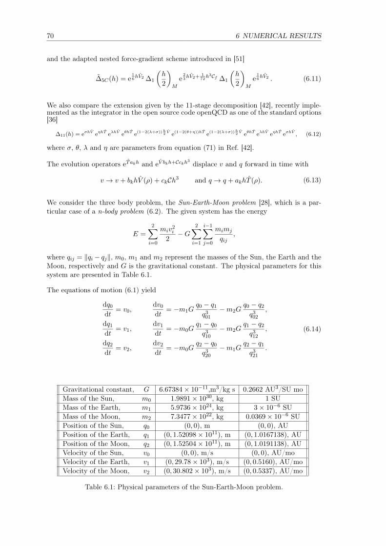
70 6 NUMERICAL RESULTS
and the adapted nested force-gradient scheme introduced in [51]
∆5C(h) = e16hV2 ∆1
(h
2
)M
e23hV2+ 1
72h3Cf ∆1
(h
2
)M
e16hV2 . (6.11)
We also compare the extension given by the 11-stage decomposition [42], recently imple-mented as the integrator in the open source code openQCD as one of the standard options[36]
∆11(h) = eσhV eηhT eλhV eθhT e(1−2(λ+σ))h2V e(1−2(θ+η))hT e(1−2(λ+σ))h
2V eθhT eλhV eηhT eσhV , (6.12)
where σ, θ, λ and η are parameters from equation (71) in Ref. [42].
The evolution operators eT akh and eV bkh+Cckh3 displace v and q forward in time with
v → v + bkhV (ρ) + ckCh3 and q → q + akhT (ρ). (6.13)
We consider the three body problem, the Sun-Earth-Moon problem [28], which is a par-ticular case of a n-body problem (6.2). The given system has the energy
E =2∑i=0
miv2i
2−G
2∑i=1
i−1∑j=0
mimj
qij,
where qij = ‖qi− qj‖, m0, m1 and m2 represent the masses of the Sun, the Earth and theMoon, respectively and G is the gravitational constant. The physical parameters for thissystem are presented in Table 6.1.
The equations of motion (6.1) yield
dq0
dt= v0,
dv0
dt= −m1G
q0 − q1
q301
−m2Gq0 − q2
q302
,
dq1
dt= v1,
dv1
dt= −m0G
q1 − q0
q310
−m2Gq1 − q2
q312
,
dq2
dt= v2,
dv2
dt= −m0G
q2 − q0
q320
−m1Gq2 − q1
q321
.
(6.14)
Gravitational constant, G 6.67384× 10⁻¹¹,m3/kg s 0.2662 AU3/SU moMass of the Sun, m0 1.9891× 1030, kg 1 SUMass of the Earth, m1 5.9736× 1024, kg 3× 10⁻⁶ SUMass of the Moon, m2 7.3477× 10²², kg 0.0369× 10⁻⁶ SUPosition of the Sun, q0 (0, 0), m (0, 0), AUPosition of the Earth, q1 (0, 1.52098× 10¹¹), m (0, 1.0167138), AUPosition of the Moon, q2 (0, 1.52504× 10¹¹), m (0, 1.0191138), AUVelocity of the Sun, v0 (0, 0), m/s (0, 0), AU/moVelocity of the Earth, v1 (0, 29.78× 10³), m/s (0, 0.5160), AU/moVelocity of the Moon, v2 (0, 30.802× 10³), m/s (0, 0.5337), AU/mo
Table 6.1: Physical parameters of the Sun-Earth-Moon problem.
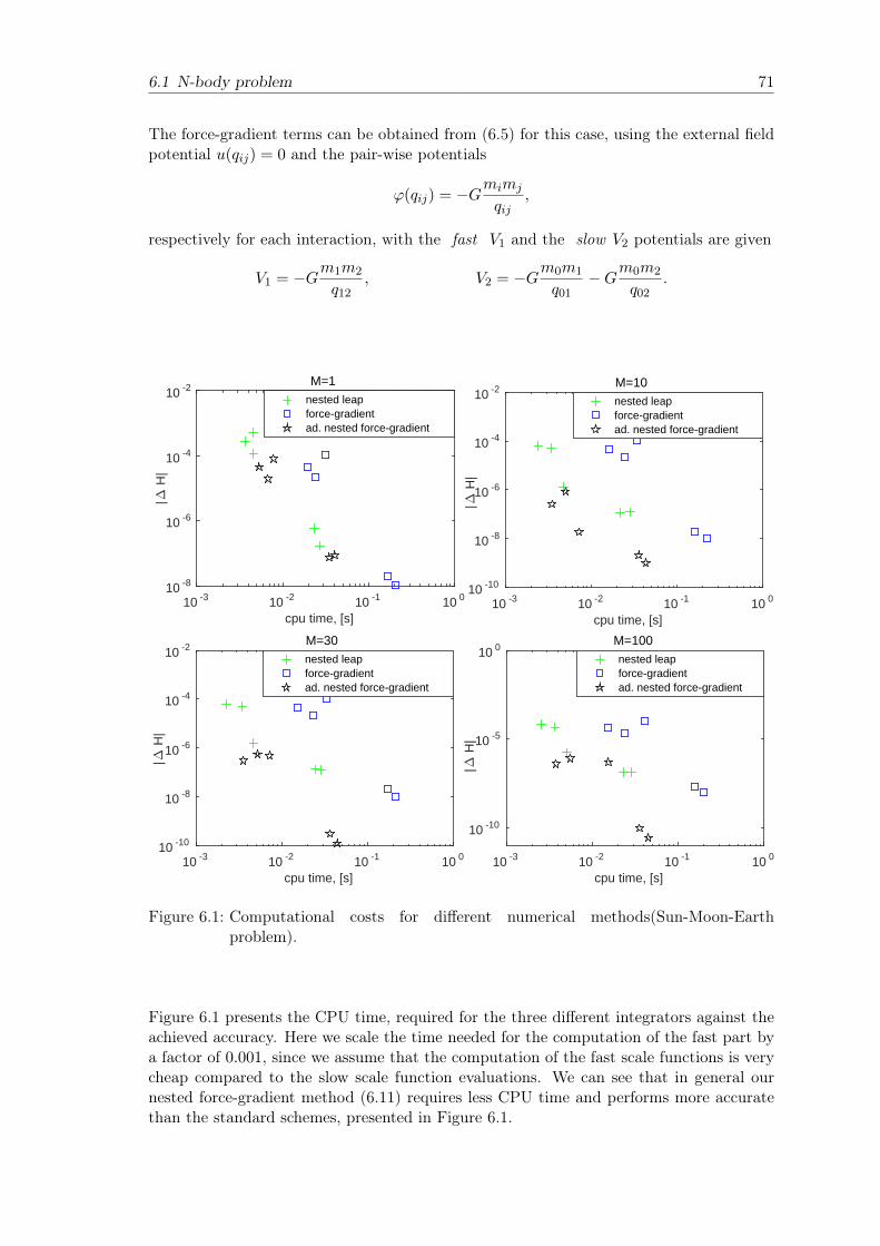
6.1 N-body problem 71
The force-gradient terms can be obtained from (6.5) for this case, using the external fieldpotential u(qij) = 0 and the pair-wise potentials
ϕ(qij) = −Gmimj
qij,
respectively for each interaction, with the fast V1 and the slow V2 potentials are given
V1 = −Gm1m2
q12, V2 = −Gm0m1
q01−Gm0m2
q02.
cpu time, [s]10 -3 10 -2 10 -1 10 0
|" H
|
10 -8
10 -6
10 -4
10 -2M=1
nested leapforce-gradient ad. nested force-gradient
cpu time, [s]10 -3 10 -2 10 -1 10 0
|" H
|
10 -10
10 -8
10 -6
10 -4
10 -2M=10nested leapforce-gradient ad. nested force-gradient
cpu time, [s]10 -3 10 -2 10 -1 10 0
|" H
|
10 -10
10 -8
10 -6
10 -4
10 -2M=30nested leapforce-gradient ad. nested force-gradient
cpu time, [s]10 -3 10 -2 10 -1 10 0
|" H
|
10 -10
10 -5
10 0 M=100
nested leapforce-gradientad. nested force-gradient
Figure 6.1: Computational costs for different numerical methods(Sun-Moon-Earthproblem).
Figure 6.1 presents the CPU time, required for the three different integrators against theachieved accuracy. Here we scale the time needed for the computation of the fast part bya factor of 0.001, since we assume that the computation of the fast scale functions is verycheap compared to the slow scale function evaluations. We can see that in general ournested force-gradient method (6.11) requires less CPU time and performs more accuratethan the standard schemes, presented in Figure 6.1.

72 6 NUMERICAL RESULTS
step-size, h0.01 0.02 0.05 0.1
|" H
|
10 -20
10 -18
10 -16
10 -14
10 -12
h 2
h 4
leap5-stagenested leapnested 5-stageforce-gradientad. nested force-gradient11-stage
Figure 6.2: Absolute error for different numerical integrators (Sun-Moon-Earth problem).
Figure 6.2 presents a comparison between the standard numerical algorithms (6.6)-(6.7),nested approaches (6.8)–(6.9), the force-gradient (6.10) and our combined method (6.11), itshows the absolute error versus the step-size. The proposed integrator (6.11) withM = 30,which combines nested and force-gradient ideas, yields a better energy conservation evencompared to 11-stage numerical scheme (6.12). These numerical results correspond to ouranalytical observations.
Thus we can argue that, if the evaluation of the fast function is significantly cheaperthan the slow function, computational costs decrease. This is exactly the case found inour long-term goal applications in lattice quantum chromodynamics (LQCD), where theaction can be split into two parts: the gauge action (whose force evaluations are cheap)and the fermion action (expensive). We have introduced a new decomposition scheme forHamiltonian systems, which combines the idea of the force-gradient time-reversible andsymplectic integrators and the splitting approach of nested algorithms. The new methodof (5.36) is fourth-order accurate. Compared to other fourth-order schemes, the leadingerror coefficient is smaller and computational costs are lower.
6.2 Schwinger model
Previously, we studied the behavior of the adapted nested force-gradient scheme in theAbelian case on the example of the n-body problem [51]. Numerical tests have verified thepotential of these schemes with increasing multirate potential, nested versions of force-gradient schemes outperform the unnested versions. This promising result suggested toperform the step from the Abelian to the non-Abelian setting of lattice QCD.
Due to the complexity of the lattice QCD problem requiring the huge computational effort
6.2 Schwinger model 73
it was natural to concentrate on the intermediate step from Abelian to the non-Abeliancase. We chose a well known problem of quantum electrodynamics (QED), the two-dimensional Schwinger model, since it suits the best as a test case for new concepts andideas for more computational demanding problems [13]. As a lattice quantum field theory,it has many of the properties of more sophisticated models such as QCD, for example thenumerical cost is still dominated by the fermion part of the action. The fact that thismodel, with far fewer degrees of freedom, does not require such large computational effortmakes it the perfect choice for our testing purposes.
We apply the numerical integration schemes (6.6)–(6.11) to the two-dimensional Schwingermodel, where the discrete updates (6.13) are given in the following form
eT h : U → U ′ = exp(iPh)U
eV h : P → P ′ = P − ihFV (U),
where the gauge fields U are elements of some Lie group, and the momenta P , elementsof the corresponding Lie algebra.
As well as the modification of the force-gradient method (6.10) proposed in [60], wherethe force-gradient term C is approximated via a Taylor expansion and a nested version of(6.10), which has been used in [3], which reads
∆5C(h) = e16hV2 ∆2
(h
2
)M
e23hV2+ 1
72h3Cf ∆2
(h
2
)M
e16hV2 , (6.15)
where∆2(h)M =
(e
16M
hV1 e1
2MhT e
23M
hV1+ 172( h
M )3Cg e
12M
hT e1
6MhV1)M
,
with Cg = V1, T, V1 and Cf = V2, T, V2.
The most challenging task from the theoretical point of view is to derive the force-gradientterm C. First we introduce the Schwinger model and explain how to obtain the force-gradient term. The two-dimensional Schwinger model is defined by the following Hamil-tonian function
H =1
2
V,2∑n=1,µ=1
p2n,µ + Sfull[U ] =
1
2
V,2∑n=1,µ=1
p2n,µ + SG[U ] + SF [U ]. (6.16)
with V = L×T the volume of the lattice. Unlike QCD, where U ∈ SU(3) and pn,µ ∈ su(3),for this QED problem (6.16), the links U are the elements of the Lie group U(1) and themomenta pn,µ belong to R, which represents the Lie algebra of the group U(1). This makesthis test example (6.16) very cheap in terms of the computational time. This together withthe fact that the Schwinger model also shares many of the features of QCD simulations,makes the Schwinger model an excellent test example when considering numerical integra-tors: a fast dynamics given by the computationally cheap gauge part SG[U ] of the actiondemanding small step sizes, and a slow dynamics given by the computationally expensivefermion part SF [U ] allowing large step sizes.
The pure gauge part of the action SG sums up over all plaquettes P(n) in the two-

74 6 NUMERICAL RESULTS
dimensional lattice with
P(n) = U1(n)U2(n+ 1)U †1(n+ 2)U †2(n),
and is given by
SG = β
V∑n=1
(1− ReP(n)) . (6.17)
The links U can be written in the form Uµ(n) = eiqµ(n) ∈ U(1) and connect the sites nand n + µ on the lattice; qµ(n) ∈ [−π, π], µ, ν ∈ x, t are respectively space and timedirections and β is a coupling constant. Note that from now on we will set the latticespacing a = 1.
The fermion part of the action SF is given by
SF = η†(D†D
)−1η, (6.18)
where η is a complex pseudofermion field. Here, D denotes the Wilson–Dirac operatorgiven by
Dn,m = (2 +m0)δn,m −1
2
2∑µ=1
((1− σµ)Uµ(n)δn,m−µ + (1 + σµ)U †µ(n− µ)δn,m+µ
),
where σµ are the Pauli matrices
σ1 =
(0 11 0
)and σ2 =
(0 −ii 0
).
m0 is the mass parameter and the Kronecker delta δn,m acts on the pseudofermion fieldby
V∑m=1
δn,mη(m) = η(n)
with η(n) the pseudofermion field, a vector in the two-dimensional spinor space takingvalues at each lattice point n.
In order to proceed with the numerical integration we need to obtain the force F and theforce gradient term C. The force term F (n, µ) with respect to the link Uµ(n) is given bythe first derivative of the action Sfull and can be written as
F (n, µ) = FSG(n, µ) + FSF (n, µ) =∂SG∂qµ(n)
+∂SF∂qµ(n)
. (6.19)
Since the numerical schemes (6.9)–(6.11) use the multi-rate approach, the shifts in themomenta updates are split on FSG and FSF and we can consider them separately. Theforce terms FSG and FSF are obtained by differentiation over U(1) group elements, whichfor the Schwinger model is the standard differentiation.
The force associated with link Uµ(n) from the gauge action is given by
βg(n, µ) := FSG(n, µ) = β Im (P(n)− P(n− ν))|µ 6=ν . (6.20)
6.2 Schwinger model 75
The force term of the fermion part is given by
f(n, µ) := FSF= − Im
[χ†(n)(1− σµ)Uµ(n)ξ(n+ µ)− χ†(n+ µ)(1 + σµ)U†µ(n)ξ(n)
](6.21)
where vectors χ and ξ are given
χ = D†−1η, ξ = D−1D†
−1η. (6.22)
For the numerical methods (6.10) and (6.15) we need to find the force gradient term C(n, µ)with respect to the link Uµ(n). In case of the Schwinger model (6.16) this term reads
C(n, µ) = 2
V,2∑m=1,ν=1
∂Sfull∂qν(m)
∂2Sfull∂qν(m)∂qµ(n)
. (6.23)
For simplicity we decompose the force gradient term (6.23) in four parts
CGG = 2
V,2∑m=1,ν=1
∂SG∂qν(m)
∂2SG∂qν(m)∂qµ(n)
, CFG = 2
V,2∑m=1,ν=1
∂SF∂qν(m)
∂2SG∂qν(m)∂qµ(n)
,
CGF = 2
V,2∑m=1,ν=1
∂SG∂qν(m)
∂2SF∂qν(m)∂qµ(n)
, CFF = 2
V,2∑m=1,ν=1
∂SF∂qν(m)
∂2SF∂qν(m)∂qµ(n)
.
(6.24)
This decomposition is also useful since the numerical integrator (6.15) only uses the termCFF by construction. As shown in [51], to obtain the fourth order convergent scheme(6.15) from the second order convergent method (6.9) we must eliminate the leading errorterm, which is exactly represented by CFF . For completeness we discuss all 4 parts below.
The CGG part of the force-gradient term is
CGG = 2β2 [Im(4P1(n, µ)− P2(n, µ)− P3(n, µ)− P4(n, µ)− P5(n, µ)) Re(P1(n, µ))
− Im(4P2(n, µ)− P1(n, µ)− P6(n, µ)− P7(n, µ)− P8(n, µ)) Re(P2(n, µ))]
with the set of plaquettes
P1(n, µ) = Uµ(n)Uν(n+ µ)U †µ(n+ ν)U †ν (n),
P2(n, µ) = Uµ(n− ν)Uν(n− ν + µ)U †µ(n)U †ν (n− ν),
P3(n, µ) = Uµ(n+ µ)Uν(n+ 2µ)U †µ(n+ ν + µ)U †ν (n+ µ),
P4(n, µ) = Uµ(n+ ν)Uν(n+ µ+ ν)U †µ(n+ 2ν)U †ν (n+ ν),
P5(n, µ) = Uµ(n− µ)Uν(n)U †µ(n+ ν − µ)U †ν (n− µ),
P6(n, µ) = Uµ(n− µ− ν)Uν(n− ν)U †µ(n− µ)U †ν (n− µ− ν),
P7(n, µ) = Uµ(n− 2ν)Uν(n− 2ν + µ)U †µ(n− ν)U †ν (n− 2ν),
P8(n, µ) = Uµ(n− ν + µ)Uν(n− ν + 2µ)U †µ(n+ µ)U †ν (n− ν + µ).
Then by using the vectors f(n, µ) defined in (6.21) we obtain the CFG piece of the force-gradient term given by
CFG(n, µ)= 2β [(f(n, µ) + f(n+ µ, ν)− f(n+ ν, µ)− f(n, ν)) Re(P1)
+ (f(n, µ)− f(n+ µ− ν, ν)− f(n− ν, µ) + f(n− ν, ν)) Re(P2)] .

76 6 NUMERICAL RESULTS
The second derivative of the fermion action is
∂2SF∂qν(m)∂qµ(n)
=
2 Reχ†[
∂D
∂qν(m)D−1
∂D
∂qµ(n)+
∂D
∂qµ(n)D−1
∂D
∂qν(m)− ∂2D
∂qν(m)∂qµ(n)
]ξ+
2 Reχ†∂D
∂qµ(n)(D†D)−1
∂D†
∂qν(m)χ ,
= 2 Re
[z†1,m,ν
∂D
∂qµ(n)ξ + χ†
∂D
∂qµ(n)D−1w2,m,ν − χ†
∂2D
∂qν(m)∂qµ(n)ξ + χ†
∂D
∂qµ(n)D−1z1,m,ν
]= 2Re
[z†1,m,νw2,n,µ + w†1,n,µz2,m,ν − χ†
∂2D
∂qν(m)∂qµ(n)ξ
]in terms of the vectors χ and ξ defined in (6.22). Now the fields z1,m,ν and z2,m,ν are givenby
z1,m,ν := D†−1 ∂D†
∂qν(m)χ = D†
−1w1,m,ν
z2,m,ν := D−1(∂D
∂qν(m)ξ + z1,m,ν) = D−1(w2,m,ν + z1,m,ν)
with
w1,m,ν(n) :=∑n′
∂D†n,n′
∂qν(m)χ(n′) = δn,m+ν
i
2(1− σν)U†ν (m)χ(m)− δn,m
i
2(1 + σν)Uν(m)χ(m+ ν) ,
w2,m,ν(n) :=∑n′
∂Dn,n′
∂qν(m)ξ(n′) = −δn,m
i
2(1− σν)Uν(m)ξ(m+ ν) + δn,m+ν
i
2(1 + σν)U†ν (m)ξ(m) .
In order to calculate CGF and CFF it is possible to perform the summation of∑
m,ν beforethe inversions of D and D† to get z1 and z2 which save O(V ) additional inversions for theforce gradient terms. It follows for the force gradient term CFF
CFF (n, µ) = 4Re[Z†1w2,n,µ + w†1,n,µZ2 − χ†
∂2D
∂qµ(n)∂qµ(n)ξ · f(n, µ)
](6.25)
with
Z1 := D†−1
V,2∑m=1,ν=1
(w1,m,ν · f(m, ν)) ,
Z2 := D−1
V,2∑m=1,ν=1
[w2,m,ν · f(m, ν)] + Z1
.
(6.26)
The expression for CGF can be obtained from the one for CFF by replacing in (6.25) and(6.26) the vector f with βg defined in (6.20).
It is important to mention that the computationally most demanding part of the numericalintegration of the Schwinger model and quantum field theory in general is the inverse of theDirac operatorD−1. Every momenta update, which includes fermion action (6.21) requires2 inversions of the Dirac operator, the addition of the force-gradient term C requires 4 moreinversions. Therefore leap-frog based methods (6.6) and (6.8) need 4 computations of D−1
per time step; schemes (6.7) and (6.9) 6 times; force-gradient based methods 8 for (6.15)and (6.11), 10 for (6.10) and the 11 stage method (6.12) has 12 inversions of the Dirac

6.2 Schwinger model 77
operator. Since we use the multi-rate approach for schemes (6.9), (6.15) and (6.11), whichleads generally to fewer macro time steps needed than for the standard schemes, we expectthe integrator (6.11) will be the most efficient choice among the methods considered. Inthe next section we present numerical tests of this prediction.
We consider a 32 by 32 lattice with a coupling constant β = 1.0, scaling variable z = 0.2and mass m0 = −0.231367, simulate it on the trajectory τ = 2.0 with 200 configurations.The parameters were taken from [13] for the better physical representation and also inorder to increase the impact of the fermion part of the action.
step-size, h0.01 0.02 0.0325 0.05 0.1
|"H
|
10 -4
10 -3
10 -2
10 -1
h 2
h 4
leapnested leap5-stagenested 5-stageforce-gradientapprox. force-gradientad. nested force-gradientnested force-gradient11-stage
Figure 6.3: Absolute error for different numerical integrators (Schwinger model).
Figure 6.3 presents the comparison between the numerical integrators (6.6) – (6.15). Itshows the absolute error versus the step-size. Here the multi-rate schemes (6.8), (6.9) and(6.15) are using four times smaller step-size for the gauge action (6.17). The numericaltests correspond to our analytical observations with the nested integrators perform betterthan their standard versions.
Figure 6.4 presents the CPU time, required for the proposed integrators (6.7)-(6.11), versusthe achieved accuracy. We can observe that the nested force-gradient method (6.15)and adapted nested force-gradient method (6.11) show much better results in terms of acomputational efficiency than the integrators (6.9) and (6.10); and even compared to the11 stage scheme (6.12). Here we can see that the modification of (6.10) proposed in [60]also performs better than its original version. It shows almost similar computational costsas nested versions of the force-gradient approach (6.15)-(6.11).

78 6 NUMERICAL RESULTS
cpu time, [s]1500 3500 5500 7500
|" H
|
10 -3
10 -2
10 -1
leapnested leap5-stagenested 5-stageforce-gradientapprox. force-gradientad. nested force-gradientnested force-gradient11-stage
Figure 6.4: Computational costs for different numerical methods (Schwinger model).
Table 6.2 shows the number of inversions of the Dirac operator D, which is needed to reach90% acceptance rate of the HMC. Since D−1 is the most computationally demanding partit is important to see how many of these inversions are required per each trajectory. FromTable 6.2 it easy to see that the adapted nested force-gradient method (6.11) and nestedforce-gradient method (6.15) need the least number of D−1 evaluations per trajectory toreach the chosen acceptance rate ≈ 90%.
Integrator: step size h M D−1 per step D−1 per trajectory5 stage method 0.0294 - 6 420
nested 5 stage method 0.0286 700 6 4085 stage force-gradient 0.0550 - 10 370
approx.force-gradient [60] 0.0540 - 8 290nested force-gradient 0.0560 450 8 285
adapted nested force-gradient 0.0560 450 8 28511 stage method 0.0625 - 12 384
Table 6.2: Step-sizes and number of inversions of D per step and per trajectory for accep-tance rate of 90%.
6.2 Schwinger model 79
In this chapter we have presented the nested force-gradient approach (6.15) and its adaptedversion (6.11) applied to a model problem in quantum field theory, the two-dimensionalSchwinger model. The derivation of the force-gradient terms was given and the Schwingermodel was introduced. Nested force-gradient schemes seem to be an optimal choice withrelatively high convergence order and low computational effort.
It also would be possible to improve the algorithm (6.11) by measuring the Poisson bracketsof the shadow Hamiltonian of the proposed integrator and then tuning the set of optimalparameters, e. g. micro and macro step sizes.
We can also claim that methods (6.15) and (6.11) have a potential to perform even betterwith respect to the computational effort in the case of lattice QCD problems, since theimpact of the fermion action (6.18) and the computational time to obtain the inversion ofthe Dirac operator D is much more significant.
In the last part of this thesis we summarize the numerical results obtained in this Chapter,draw the conclusion based on these results and give a short outlook on future researchdirections.


7 Chapter 7
SUMMARY AND OUTLOOK
In this thesis the general idea of geometric numerical time integration for ordinary dif-ferential equations was introduced. We presented this idea for the case of Hamiltonianmechanics as a basis of our main area of application for this work. We showed in detailthe preservation of physical properties of a system such as time-reversibility, symplecticityand energy conservation for the numerical methods. We provided a brief introduction tothe backward error analysis, which included the concept of shadow Hamiltonians. Themain classes of geometric numerical time integrators were given as examples to treat thenumerical problems on Abelian and non-Abelian manifolds.
Next we presented the main application of thesis quantum field theories where we gavea short summary of a quantization process. The basic concepts of the path integralformulation for quantum field theories were introduced as well as its regularization onthe lattice. Two different kinds of field variables were presented in order to show a fewimportant examples of quantum field theories such as QED and QCD. The role of geometricnumerical time integrators were explained as the main way to treat the physical problemsin path integral formulation is the HMC algorithms and numerical methods to be used inthe molecular dynamics step of HMC have to conserve certain properties of quantum fieldtheories.
The first attempt to improve the efficiency of HMC simulations were made by proposingthe idea to use projection methods in order to eliminate the accept/reject step of the HMCalgorithm, since this class of numerical methods conserves energy of a physical system ex-actly. We introduced both standard and symmetric variants of projection methods andpresented an alternative view on symmetric projection schemes as well as a structure pre-serving approach for projection methods. We analyzed both analytically and numericallythe conservation of geometric properties of the flow. Unfortunately we had to concludethat even so we were able to reach certain success in developing symplectic projectionschemes for our main application it would require a huge computational effort and henceto use proposed methods is not advantageous.
We introduced another option to increase the efficiency of numerical time integratorsfor the HMC algorithm. We combined two operator splitting approaches, namely, force-gradient decomposition methods and multirate stepping strategy in order to gain a higherorder of accuracy by adding the force-gradient term and reduce the computational cost bytreating the slow and the fast part of the action of a system with not only different step size(smaller for the fast part and bigger for the slow one) but also applying different numer-ical schemes to each of these parts accordingly. The introduction into the force-gradientdecomposition approach and the multirate time stepping methods was presented togetherwith the analysis for the structure-preserving properties of these numerical scheme. Theresulting adapted nested force-gradient approach satisfies the main goal of this thesis. Wetested these methods first analytically to show that they satisfy the necessary structure-preserving properties necessary to be used in the HMC simulations and then numerically
81
82 7 SUMMARY AND OUTLOOK
to prove that they are more efficient than the other numerical integrators which are usedfor solving path integrals of quantum field theories.
The numerical tests were designed, first, to investigate the convergence order of the pro-posed adapted nested force-gradient decomposition schemes; then to derive the force-gradient term by applying them to the rather simple case of the n-body problem (Sun-Moon-Earth problem); and at last to estimate the efficiency of the proposed scheme viascaling the computational costs for the fast part of the action by small factor. The pos-itive outcome of the first numerical test allowed us to carry on and we considered the2-dimensional Schwinger model of quantum electrodynamics to showcase the advantagesof the new integrator. The derivation of the force-gradient term was presented since it isthe most challenging part of the implementation process and also to show the differencewith the standard force-gradient and nested force-gradient schemes. Numerical resultsshows that we can claim that the proposed adapted nested force-gradient methods seemto be an optimal choice with relatively high convergence order and low computationaleffort.
The numerical results obtained by testing adapted force-gradient numerical integratorson the Schwinger model were very promising and showed that the adapted force-gradientintegrators have a large potential for the ultimate goal of Lattice QCD applications, wheretwo efficiency factors will act in favor of nested schemes: the multirate factor of latticeQCD is much higher than in the Schwinger model case; the number of inversions of theDirac-Wilson operator is much lower for five stage than for eleven stage schemes.
The future work can be summarized as following
• Apply the adapted nested force-gradient schemes to the Lattice QCD applicationsand generalize this approach to more than two multirate time levels recursively,allowing to exploit additional sources of multirate potential. Since for the adaptednested force-gradient scheme we use cheaper integrators for the fast part of the actioncomparing to the standard nested force-gradient approach.
• Based on a first test implementation of the adapted nested force gradient integrators,the range of feasibility of this new scheme has to be tested against a series of com-petitors for a range of possible applications. For lattice QCD, the choice of the bestintegrator should be based on a cost metric introduced by Clark et al. [14], whichscales the CPU time needed for a trajectory with the acceptance rate. If the timeintegration error (measured as the deviation from the Hamiltonian) is log-normaldistributed, the latter will be given by the complementary error function, evaluatedat one eighth of the variance σ2 of the time integration error [33]. The variance willdepend not only on the step size h, but also on the volume V , the mass m and thegauge coupling β, expecting a dependence of the type
σ2(h, V,m, β) = A(β)V bhc
(m−mcrit)α,
where the unknown parameters can be detected by numerical experiments. For everysetting, an optimal step size can be derived according to the cost metric above.
• To make the best use of the adapted nested force gradient integrators in LatticeQCD, one must implement the scheme, together with a proposal for an optimalchoice of the step size according to the cost metric above, in the openQCD package
83
(see http://luscher.web.cern.ch/luscher/openQCD/) of Martin Lüscher and StefanSchaefer. This choice is based on our previous experience in adding a softwarepackage for mass reweighing to the openQCD package.
We must also mention that there are possibilities to improve the proposed methods, bymeasuring the Poisson brackets of the shadow Hamiltonian of the adapted nested force-gradient scheme and then tuning the set of optimal parameters, e.g. micro and macro stepsizes or/and to approximate the force-gradient term as it is proposed in [60].
Therefore we conclude that nested force-gradient methods have a huge potential to beused in Lattice QCD application, although it requires some additional work. Neverthelesswe reached our main goal to develop a new geometric numerical time integrator for themolecular dynamics step of the HMC algorithm, which performs better with respect toaccuracy and computational effort than most of numerical schemes generally used and stilloffers some space for improvements.

A Appendix A
Shadow Hamiltonian for theprojection methods with µ = µ(h)
Let us consider the following scheme
eµ2V eµT e
µ2V︸ ︷︷ ︸
H1
eh2V ehT e
h2V︸ ︷︷ ︸
H2
eµ2V eµT e
µ2V︸ ︷︷ ︸
H3
.
We know that it is the composition of three methods each of them preserves the corre-sponding shadow Hamiltonians
H1,3 = (T + V )µ+µ3
24(2[T [T, V ]] + [V [T, V ]])
H2 = (T + V )h+h3
24(2[T [T, V ]] + [V [T, V ]]) .
Therefore, in order to find the shadow Hamiltonian for our method, we need to apply theBCH formula on
eH1eH2eH3
First we consider the first parteH1eH2
which yields
c1 = H1 +H2,
c2 = −1
4[H1 +H2, H1 −H2] = −1
4[(T + V )h+ (T + V )µ, (T + V )h− (T + V )µ]
= −1
4
((T + V )(T + V )µh+ (T + V )(T + V )µ2 − (T + V )(T + V )h2 − (T + V )(T + V )µh
−(T + V )(T + V )µh− (T + V )(T + V )µ2 + (T + V )(T + V )µh+ (T + V )(T + V )h2)
c3 = −1
6[0, H1 −H2] = 0.
Here we skip the interaction of h3 terms since we do not consider the error terms higherthan h3 and obtain
eH1eH2 = eH1+H2 .
Then apply it for the second parteH1+H2eH3 ,
85

86 A Shadow Hamiltonian for the projection methods with µ = µ(h)
c1 = H1 +H2 +H3,
c2 = −1
4[H1 +H2 +H3, H1 +H2 −H3] = −1
4[(T + V )2µ+ (T + V )h, (T + V )h]
= −1
4
((T + V )(T + V )2µh+ (T + V )(T + V )h2 − (T + V )(T + V )2µh− (T + V )(T + V )h2
)= 0
c3 = −1
6[0, H1 +H2 −H3] = 0.
and obtainH = H1 +H2 +H3
or
H = (2µ+ h)(T + V ) +(2µ3 + h3)
24(2[T [T, V ]] + [V [T, V ]]) .
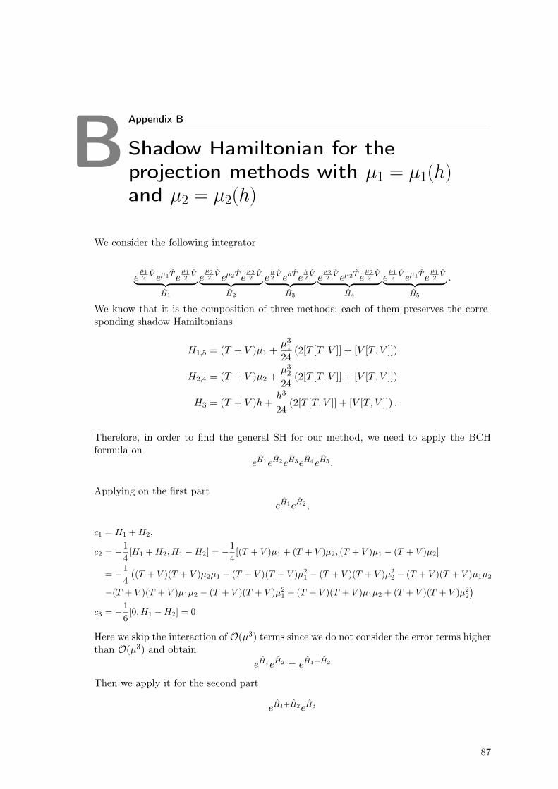
B Appendix B
Shadow Hamiltonian for theprojection methods with µ1 = µ1(h)and µ2 = µ2(h)
We consider the following integrator
eµ12V eµ1T e
µ12V︸ ︷︷ ︸
H1
eµ22V eµ2T e
µ22V︸ ︷︷ ︸
H2
eh2V ehT e
h2V︸ ︷︷ ︸
H3
eµ22V eµ2T e
µ22V︸ ︷︷ ︸
H4
eµ12V eµ1T e
µ12V︸ ︷︷ ︸
H5
.
We know that it is the composition of three methods; each of them preserves the corre-sponding shadow Hamiltonians
H1,5 = (T + V )µ1 +µ3
1
24(2[T [T, V ]] + [V [T, V ]])
H2,4 = (T + V )µ2 +µ3
2
24(2[T [T, V ]] + [V [T, V ]])
H3 = (T + V )h+h3
24(2[T [T, V ]] + [V [T, V ]]) .
Therefore, in order to find the general SH for our method, we need to apply the BCHformula on
eH1eH2eH3eH4eH5 .
Applying on the first parteH1eH2 ,
c1 = H1 +H2,
c2 = −1
4[H1 +H2, H1 −H2] = −1
4[(T + V )µ1 + (T + V )µ2, (T + V )µ1 − (T + V )µ2]
= −1
4
((T + V )(T + V )µ2µ1 + (T + V )(T + V )µ2
1 − (T + V )(T + V )µ22 − (T + V )(T + V )µ1µ2
−(T + V )(T + V )µ1µ2 − (T + V )(T + V )µ21 + (T + V )(T + V )µ1µ2 + (T + V )(T + V )µ2
2
)c3 = −1
6[0, H1 −H2] = 0
Here we skip the interaction of O(µ3) terms since we do not consider the error terms higherthan O(µ3) and obtain
eH1eH2 = eH1+H2
Then we apply it for the second part
eH1+H2eH3
87

88 B Shadow Hamiltonian for the projection methods with µ1 = µ1(h) and µ2 = µ2(h)
c1 = H1 +H2 +H3,
c2 = −1
4[H1 +H2 +H3, H1 +H2 −H3]
= −1
4[(T + V )µ1 + (T + V )µ2 + (T + V )h, (T + V )µ1 + (T + V )µ2 − (T + V )h]
= −1
4
((T + V )(T + V )µ2
1 + (T + V )(T + V )µ1µ2 + (T + V )(T + V )µ1h
+(T + V )(T + V )µ1µ2 + (T + V )(T + V )µ22 + (T + V )(T + V )µ2h
−(T + V )(T + V )µ1h− (T + V )(T + V )µ2h− (T + V )(T + V )h2
−(T + V )(T + V )µ21 − (T + V )(T + V )µ1µ2 + (T + V )(T + V )µ1h
−(T + V )(T + V )µ1µ2 − (T + V )(T + V )µ22 + (T + V )(T + V )µ2h
(T + V )(T + V )µ1h+ (T + V )(T + V )µ2h+ (T + V )(T + V )h2)
= 0
c3 = −1
6[0, H1 +H2 −H3] = 0
and obtaineH1eH2eH3 = eH1+H2+H3
and then we apply BCH toeH1+H2+H3eH4
which yields
c1 = H1 +H2 +H3 +H4,
c2 = −1
4[H1 +H2 +H3 +H4, H1 +H3]
= −1
4[(T + V )µ1 + 2(T + V )µ2 + (T + V )h, (T + V )µ1 + (T + V )h]
= −1
4
((T + V )(T + V )µ2
1 + 2(T + V )(T + V )µ1µ2 + (T + V )(T + V )µ1h
+(T + V )(T + V )µ1h+ 2(T + V )(T + V )µ2h+ (T + V )(T + V )h2
−(T + V )(T + V )µ21 − 2(T + V )(T + V )µ1µ2 − (T + V )(T + V )µ1h
−(T + V )(T + V )µ1h− 2(T + V )(T + V )µ2h− (T + V )(T + V )h2)
= 0
c3 = −1
6[0, H1 +H3] = 0
and thereforeeH1eH2eH3eH4 = eH1+H2+H3+H4 .
At the end applying BCH formula on
eH1+H2+H3+H4eH5

89
c1 = H1 +H2 +H3 +H4 +H5,
c2 = −1
4[H1 +H2 +H3 +H4 +H5, H2 +H3 +H4]
= −1
4[2(T + V )µ1 + 2(T + V )µ2 + (T + V )h, 2(T + V )µ2 + (T + V )h]
= −1
4
(4(T + V )(T + V )µ2
2 + 4(T + V )(T + V )µ1µ2 + 2(T + V )(T + V )µ2h
+2(T + V )(T + V )µ1h+ 2(T + V )(T + V )µ2h+ (T + V )(T + V )h2
−4(T + V )(T + V )µ22 − 4(T + V )(T + V )µ1µ2 − 2(T + V )(T + V )µ2h
−2(T + V )(T + V )µ1h− 2(T + V )(T + V )µ2h− (T + V )(T + V )h2)
= 0
c3 = −1
6[0, H2 +H3 +H4] = 0
and obtainH = H1 +H2 +H3 +H4 +H5
or
H = (2µ1 + 2µ2 + h)(T + V ) +(2µ3
2 + 2µ32 + h3)
24(2[T [T, V ]] + [V [T, V ]]) .

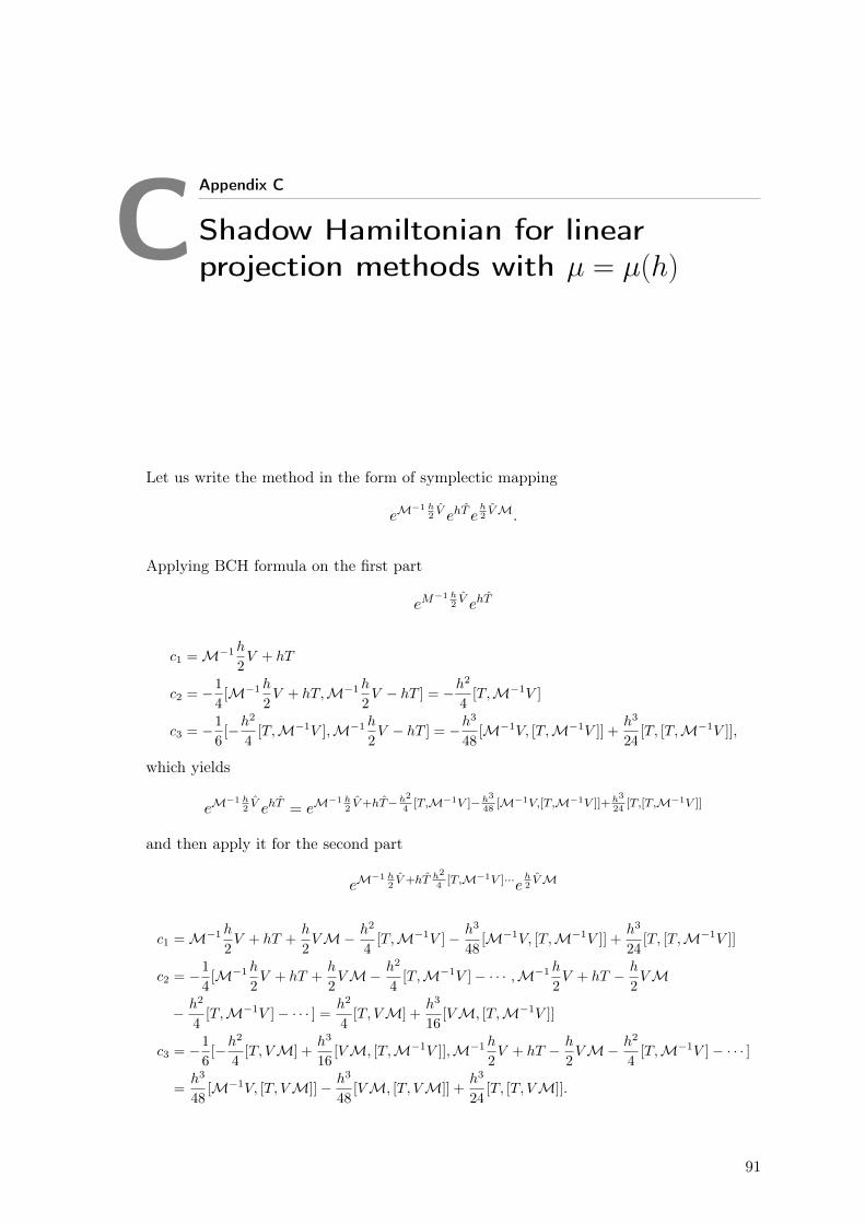
C Appendix C
Shadow Hamiltonian for linearprojection methods with µ = µ(h)
Let us write the method in the form of symplectic mapping
eM−1 h
2V ehT e
h2VM.
Applying BCH formula on the first part
eM−1 h
2V ehT
c1 =M−1h2V + hT
c2 = −1
4[M−1h
2V + hT,M−1h
2V − hT ] = −h
2
4[T,M−1V ]
c3 = −1
6[−h
2
4[T,M−1V ],M−1h
2V − hT ] = −h
3
48[M−1V, [T,M−1V ]] +
h3
24[T, [T,M−1V ]],
which yields
eM−1 h
2V ehT = eM
−1 h2V+hT−h
2
4[T,M−1V ]−h
3
48[M−1V,[T,M−1V ]]+h3
24[T,[T,M−1V ]]
and then apply it for the second part
eM−1 h
2V+hT h
2
4[T,M−1V ]···e
h2VM
c1 =M−1h2V + hT +
h
2VM− h2
4[T,M−1V ]− h3
48[M−1V, [T,M−1V ]] +
h3
24[T, [T,M−1V ]]
c2 = −1
4[M−1h
2V + hT +
h
2VM− h2
4[T,M−1V ]− · · · ,M−1h
2V + hT − h
2VM
− h2
4[T,M−1V ]− · · · ] =
h2
4[T, VM] +
h3
16[VM, [T,M−1V ]]
c3 = −1
6[−h
2
4[T, VM] +
h3
16[VM, [T,M−1V ]],M−1h
2V + hT − h
2VM− h2
4[T,M−1V ]− · · · ]
=h3
48[M−1V, [T, VM]]− h3
48[VM, [T, VM]] +
h3
24[T, [T, VM]].
91

92 C Shadow Hamiltonian for linear projection methods with µ = µ(h)
The result is following
H =M−1h
2V + hT +
h
2VM− h2
4[T,M−1V ] +
h2
4[T, VM]
− h3
48[M−1V, [T,M−1V ]] +
h3
24[T, [T,M−1V ]] +
h3
16[VM, [T,M−1V ]]
+h3
48[M−1V, [T, VM]]− h3
48[VM, [T, VM]] +
h3
24[T, [T, VM]].

Bibliography
[1] V. I. Arnold, Mathematical Methods of Classical Mechanics, Springer-Verlag NewYork 1989.
[2] U. Ascher, S. Reich, On some difficulties in integrating highly oscillatory Hamiltoniansystems, in: Proceedings of Computational Molecular Dynamics, Springer LectureNotes in Computational Science and Engineering, Vol. 4, 1998, pp. 281–296.
[3] A. Bazavov et al., Chiral transition and U(1)A symmetry restoration from latticeQCD using domain wall fermions, Phys. Rev. D 86 (201), 094503.
[4] S. Blanes, C. J. Budd, Adaptive Geometric Integrators for Hamiltonian Problemswith Approximate Scale Invariance, J. Sci. Comput., Vol. 26, (2005), pp. 1089–1113.
[5] S. Blanes, F. Casas, Raising the order of geometric numerical integrators by compo-sition and extrapolation, Numerical Algorithms, Springer, (2005) 38 pp 305–326.
[6] S. Blanes, F. Calas, A. Murua, Splitting and composition methods in the numericalintegration of differential equations, Bol. Soc. Esp. Mat. Apl. 45(2008) pp. 89–145.
[7] G. Bogfjellmo, H. Marthinsen, High-Order Symplectic Partitioned Lie Group Meth-ods, Foundations of Computational Mathematics 16.2 (2016) pp. 493–530.
[8] E. Borici, C. Joó, A. Frommer, Numerical methods in QCD, Springer, Berlin, 2002.
[9] C. J. Budd, A. Iserles, Geometric Integration: Numerical Solution of DifferentialEquations on Manifolds, Phil. Trans. R. Soc. Lond., Volume 357, 1999.
[10] C. J. Budd, M. D. Piggott, Geometric Integration and its Applications, Handbook ofNumerical Analysis, vol. XI, Elsevier Science, 2003.
[11] J. C. Butcher, Numerical Methods for Ordinary Differential Equations, Wiley, 2003.
[12] E. Celledoni, H. Marthinsen, B. Owren, An introduction to Lie group integrators-basics, new developments and application, J. Comput. Phys., (2012).
[13] N. Christian, K. Jansen, K. Nagai, B. Pollakowski, Scaling test of fermion actions inthe Schwinger model, Nuclear Physics B 739 (2006), pp. 60–84.
[14] M.A. Clark, B. Joó, A.D. Kennedy, P.J. Silva, Better HMC integrators for dynamicalsimulations, PoS 323(2010).
[15] P. E. Crouch, R. Grossman, Numerical integration of ordinary differential equationson manifolds, J. Nonlinear Sci., 3 (1993), pp. 1–33.
[16] S. Duane, A.D. Kennedy, B.J. Pendleton, D. Roweth, Hybrid Monte Carlo, Phys.
93

94 Bibliography
Lett. B195 (1987), pp. 216–222.
[17] E. Forest, R. D. Ruth, Fourth-order symplectic integration, Physica D 43 105 (1990).
[18] J. Gans, D. Shalloway, Shadow mass and the relationship between velocity and mo-mentum in symplectic numerical integration, Phys. Rev. E (3), 61 (2000), pp. 4587–4592.
[19] C. Gattringer, C. B. Lang, Quantum Chromodynamics on the Lattice: An Intro-ductory Presentation, Lect. Notes Phys. 788, Springer, Berlin Heidelberg, 2010, DOI10.1007/978-3-642-01850-3.
[20] C. W. Gear, D. R. Wells, Multirate linear multistep methods, BIT 24(1984) pp 484–502.
[21] W. R. Gilks, S. Richardson, D. J. Spiegelhalter, Markov Chain Monte Carlo in Prac-tice, Chapman & Hall (1995), pp. 1-19.
[22] W. Gröbner, Die Liereihen und ihre Anwendungen, VEB Deutscher Verlag der Wis-senschaften, Berlin 1960.
[23] R. Gupta, Introduction to Lattice QCD, arXiv:hep-lat/9807028(1998).
[24] E. Hairer, G. Wanner, Solving Ordinary Differential Equations II. Stiff andDifferential-Algebraic Problems, 2nd ed., Springer Series in Comput. Math., Vol. 14,Springer-Verlag, Berlin, 1996.
[25] E. Hairer, Symmetric Projection Methods for Differential Equations on Manifolds,BIT Numerical Mathematics Vol. 40 (2000), pp. 726–734.
[26] E. Hairer, Geometric Integration of Ordinary Differential Equations on Manifolds,BIT (2001), Vol. 41, No. 5, pp. 996–1007.
[27] E. Hairer, Global modified Hamiltonian for constrained symplectic integrators, Nu-merical Mathematics Vol. 95 (2002), pp. 325–336.
[28] E. Hairer, C. Lubich, G. Wanner, Geometric Numerical Integration: Structure-Preserving Algorithms for Ordinary Differential Equations, Springer, Berlin, 2006.
[29] A. Iserles, H. Z. Munthe-Kass, S. P. Norsett, A. Zanna, Lie-group methods, ActaNumerica, (2004) pp.1–148.
[30] A.D. Kennedy, M.A. Clark, Speeding up HMC with better integrators, PoS 038(2007).
[31] A. D. Kennedy, M. A. Clark, P. J. Silva, Force Gradient Integrators, PoS 021(2009).
[32] A.D. Kennedy, P.J. Silva, M.A. Clark, Shadow Hamiltonians, Poisson Brackets andGauge Theories, Phys. Rev. D 87 (2013), 034511.
[33] F. Knechtli, U. Wolf, Dynamical fermions as a global correction, Nucl. Phys. B663(2003) pp. 3–32.
[34] F. Knechtli, M. Günther, M. Peardon, Lattice Quantum Chromodynamics: PracticalEssentials Springer (2016).
Bibliography 95
[35] A. Lew, J. E. Marsden, M. West, M. Ortiz, Variational time integrators, Int. J.Numer. Methods Eng., 60 (2004) pp.153–212.
[36] M. Lüscher, S. Schäfer, Lattice QCD with open boundary conditions and twisted-massreweighting, Comput. Phys. Commun. 184(2013), pp 519–528.
[37] R. I. McLachlan, G. R. W. Quispel, Splitting methods, Acta Numerica (2002), pp.341–434.
[38] R. I. McLachlan, G. R. W. Quispel, Geometric Integrators for ODEs, J. Phys. A39(19) (2006), pp. 5251-5286.
[39] I. Montvay, G. Münster, Quantum Fields on a Lattice, Cambridge University Press:Cambridge, 1994.
[40] C. Morningstar, The Monte Carlo method in Quantum Field Theory, arXiv:hep-lat/0702020(2007).
[41] H. Munthe-Kaas, Runge-Kutta methods on Lie groups, BIT, 38 (1995), pp. 92–111.
[42] I.P. Omelyan, I.M. Mryglod, R. Folk, Symplectic analytically integrable decompo-sition algorithms: classification, derivation, and application to molecular dynamics,quantum and celestial mechanics, Comput. Phys. Commun. 151 (2003), pp. 272–314.
[43] I.P. Omelyan, I.M. Mryglod, R. Folk, Algorithm for Molecular Dynamics Simulationsof Spin Liquids, Phys. Rev. Lett. 86 (2001) 898.
[44] I.P. Omelyan, Advanced gradient like methods for rigid-body molecular dynamics, J.Chem. Phys. 127(2003), 044102.
[45] M. E. Peskin, D. V. Schroeder, An Introduction to Quantum Field Theory, WestviewPress, 1995 ISBN: 9780201503975, 0201503972.
[46] J. M. Sanz-Serna, Symplectic Methods, Encyclopedia of Applied and ComputationalMathematics, Springer (2013).
[47] V. Savcenco, W. Hundsdorfer, G. J. Verwer, A multirate time stepping strategy forstiff ordinary differential equations, BIT Numerical Mathematics 47(2007) pp. 137–155.
[48] J.S. Schwinger, Gauge Invariance and Mass. 2, Phys. Rev. 128 (1962), pp. 2425–2429.
[49] J.C. Sexton, D.H. Weingarten, Hamiltonian evolution for the hybrid Monte Carloalgorithm, Nucl. Phys. B380 (1992), pp. 665–678.
[50] D. Shcherbakov, M. Ehrhardt, Multistep Methods for Lattice QCD Simulations, PoS(Lattice 2011), pp. 327–333.
[51] D. Shcherbakov, M. Ehrhardt, M. Günther, M. Peardon, Force-gradient nested mul-tirate methods for Hamiltonian systems, Comput. Phys. Commun. 187(2015), pp91–97.
[52] D. Shcherbakov, M. Ehrhardt, J. Finkenrath, M. Günther, F. Knechtli M. Peardon,Adapted nested force-gradient integrators: the Schwinger model case, Commun. in
96 Bibliography
Comput. Phy. 21(4) (2017), pp 1141–1153.
[53] P.J. Silva, A.D. Kennedy, M.A. Clark, Tuning HMC using Poisson brackets, PoS041(2008).
[54] R.D. Skeel, D.J. Hardy, Practical Construction of Modified Hamiltonians, SIAM J.Sci. Comput., 23 (2001), pp. 1172–1188.
[55] J. Smit, Introduction to quantum fields on a lattice: a robust mate, CambridgeLecture Notes in Physics, 2002, ISBN 0521890519.
[56] M. Suzuki, General theory of higher-order decomposition of exponential operatorsand symplectic integrators, Phys. Lett. A 165 (1992) 387.
[57] C.R. Sweet, S.S. Hampton, R.D. Skeel, J.A. Izaguirre, A separable shadow Hamilto-nian hybrid Monte Carlo method, J. Chem. Phys. 131, 174106 (2009) (7 pages)
[58] C. Urbach, K. Jansen, A. Shindler, U. Wenger, HMC algorithm with multiple timescale integration and mass preconditioning, Comput. Phys. Commun. 174 (2006), pp.87–98.
[59] U.J. Wiese, An Introduction to Lattice Field Theory, Lecture Material (2009).
[60] H. Yin, R. D. Mawhinney, Improving DWF Simulations: the Force Gradient Integra-tor and the Möbius Accelerated DWF Solver, PoS (Lattice 2011) 051.
[61] H. Yoshida, Construction of higher order symplectic integrators, Phys. Lett. A 150(1990) 262.
[62] A. Zanna, K. Engø, H. Z. Munthe-Kaas, Adjoint and selfadjoint Lie group methods,BIT 2001 Vol. 41 No. 2 pp. 395–421.