arX

iv:c

ond-

mat

/000

4196

v1 [

cond

-mat

.sta

t-m

ech]

12

Apr

200

0

Relevance of memory in Minority Games

Damien Challet(1) and Matteo Marsili(2)(1) Institut de Physique Theorique, Universite de Fribourg, CH-1700

(2) Istituto Nazionale per la Fisica della Materia (INFM), Trieste-SISSA Unit, V. Beirut 2-4, Trieste I-34014,(February 1, 2008)

By considering diffusion on De Bruijn graphs, we study in details the dynamics of the histories inthe Minority Game, a model of competition between adaptative agents. Such graphs describe thestructure of temporal evolution of M bits strings, each node standing for a given string, i.e. a historyin the Minority Game. We show that the frequency of visit of each history is not given by 1/2M

in the limit of large M when the transition probabilities are biased. Consequently all quantitiesof the model do significantly depend on whether the histories are real, or uniformly and randomlysampled. We expose a self-consistent theory of the case of real histories, which turns out to be invery good agreement with numerical simulations.

I. INTRODUCTION

The Minority Game [1,2] has been designed as the most drastic possible simplification of Arthur’s El Farol’s barproblem [3]. It is believed to capture some essential and general features of competition between adaptative agents,which is found for instance in financial markets. In this model, agents have to take each time step one of two decisions;they share a common piece of information µ ∈ {0, · · · , P − 1} that encodes the state of the world, use it to make theirchoice, and those who happen to be in minority are rewarded. In its original formulation, the piece of informationis the binary encoding of the M last winning choices, hence P = 2M . Hence, the dynamics of µ is coupled to thedynamics of agents.

Cavagna [4] claimed that all quantities of the system “are completely independent from the memory of the agents”.This means that replacing the dynamics of µ induced by agents by a random history µ drawn at random at each timestep, one finds the same results. While this statement has turned out to be wrong for many extensions of the MG [5–8],it has been helpful as a first approximation for the analytical understanding of the standard MG: an exact solutionfor random histories has been found in the “thermodynamic” limit [7,8]. Interestingly, this solution shows that allquantities depend on the frequencies {ρµ} of visit of histories. The random history case is recovered if ρµ = 1/P , butin the real dynamics of the MG the distribution ρµ is determined by the behavior of agents (indeed modifying thebehavior of agents may have strong effects on ρµ as shown in ref. [7,8]). It turns out, that the frequencies ρµ are notuniform for all parameters of the MG.

In this paper we study quantitatively this problem. The first step is to characterize the properties of the dynamics ofreal histories, which amounts to study randomly biased diffusion on De Bruijn graphs. Depending on the asymmetryof the bias, we quantify the deviation δρµ = ρµ − 1/P from the uniform distribution. Then we move to the MG andquantify the bias which agents induce on the dynamics of µ in the asymmetric phase. Using a simple parameterizationof ρµ which is inferred from numerical data, we generalize the calculations of refs. [7,8]. This leads to a self-consistentequation between the asymmetry of the game and the diffusion bias, which we can solve. The results are in excellentagreement with numerical simulations and show a systematic deviation from the random history MG. Hence, ourconclusion is that, even though the random history MG is qualitatively similar to the original MG, memory isactually not irrelevant, and one can quantify the difference between the two cases.

II. DE BRUIJN GRAPHS

Let us begin with the definition of some elementary concepts. A binary sequence µ(t) of length m consists of mordered elements {b(t− m), · · · , b(t− 1)} where b is a letter belonging to the alphabet {0, 1}. µ(t + 1) is obtained byadding b(t) to the right of µ(t) and erasing b(t−m). Thus, for a given µ(t), there are two possible µ(t + 1), which wecall “next neighbours”. This updating rule defines the De Bruijn graph [9] of order m (see Fig. 1 for an example).

1

000 111

011

110

101010

001

100

FIG. 1. De Bruijn graph of order 3

Let G be the P × P adjacency matrix of the De Bruijn graph of order m. if we adopt the convention that itselements are indiced by the decimal value of the binary strings, that is, µ = 0, · · · , P − 1,

Gµ,ν = δ[2µ%P ],ν + δ[2µ%P ]+1,ν (1)

where A%B stands for the remainder of the division of B by A and δi,j is the Kronecker symbol. The adjacencymatrix for m = 3 is:

G =

1 1 0 0 0 0 0 00 0 1 1 0 0 0 00 0 0 0 1 1 0 00 0 0 0 0 0 1 11 1 0 0 0 0 0 00 0 1 1 0 0 0 00 0 0 0 1 1 0 00 0 0 0 0 0 1 1

(2)

III. UNBIASED DIFFUSION

The unbiased diffusion is defined as follows : a particle moves on the directed De Bruijn graph G and at each timestep t, it jumps with equal probability to one of the next neighbours of the vertex it stands on at this time. Thusthe transition probabilities matrix is W0 = G/2. In the long run, the fraction of time spent on vertex ν is given by[(W0)

∞]0,ν . It can be seen (see appendix) that

[(W0)k]µ,ν =

1

2k

2k−1∑

n=0

δ[2kµ%P ]+n,ν . (3)

In particular, (WM+k0 )µ,ν = 1

P for all k ≥ 0, that is, all strings µ are visited with the same frequency ρµ = 1/P .In order to have a intuitive feeling of those graphs, we write them for M = 3 :

W 20 =

1

4

1 1 1 1 0 0 0 00 0 0 0 1 1 1 11 1 1 1 0 0 0 00 0 0 0 1 1 1 11 1 1 1 0 0 0 00 0 0 0 1 1 1 11 1 1 1 0 0 0 00 0 0 0 1 1 1 1

W 30 = W 4

0 = W 50 = . . . =

1

8

1 1 1 1 1 1 11 1 1 1 1 1 11 1 1 1 1 1 11 1 1 1 1 1 11 1 1 1 1 1 11 1 1 1 1 1 11 1 1 1 1 1 11 1 1 1 1 1 1

(4)

IV. RANDOMLY BIASED DIFFUSION

The perturbations are introduced by adding a term to the transition probabilities matrix Wǫ = W0 + ǫW1 where ǫquantifies the asymmetry and W1 contains the disorder ξ

(W1)µ,ν = (−1)νξµ(W0)µ,ν (5)

2

where the ξ are iid from the pdf P (ξ) = 1/2 δ(ξ − 1) + 1/2 δ(ξ + 1) and the (−1)ν comes from the normalizationof the perturbed probabilities. We are looking for the stationary transition probabilities, i.e., W∞

ǫ such that W∞ǫ =

limk→∞ (Wǫ)k. It exists since Wǫ is a bounded operator. Its formal series expansion in ǫ is noted by W∞

ǫ =∑

k≥0 ǫkW∞k where W∞

0 is a matrix whose all coefficients are equal to 1/P (see above). The relationship W∞ǫ =

W∞ǫ Wǫ provides the recurrence

W∞k = W∞

k W0 + W∞k−1W1 (6)

Since WMk W∞

0 = 0, we iterate m − 1 times this equation by replacing W∞k with W∞

k W0 + W∞k−1W1 in the r.h.s.,

yielding to

W∞k = W∞

k−1W1V = W∞0 [W1V ]k , (7)

where V =∑M−1

c=0 (W0)c. At this point, it is useful to remark that multiplying a matrix on the left by W∞

0 isequivalent to averaging its columns :

(W∞0 A)µ,ν =

P−1∑

a=0

(W∞0 )µ,aAa,ν =

1

P

P−1∑

a=0

Aa,ν = average of the ν-th column of A (8)

thus the matrices W∞k consist of averages of columns of (W1V )k. Therefore, (W∞

k )µ,ν is the k-th order correction tothe frequency of vertex ν, that will be called ρν

(k) in the following. Note that 〈ρν(k)〉ξ = 0 for all k ≥ 1. The square root

of the second moment of ρν(k) averaged over the disorder gives an indication of the typical value of ρν

(k). In appendixB we obtain the approximation

〈||ρ(k)||2〉ξ ∼ (1 − 1/P )k

P. (9)

which is exact for the first order perturbation. Therefore ρν(k) is of the same order as the unperturbed ρν

(0), thus it

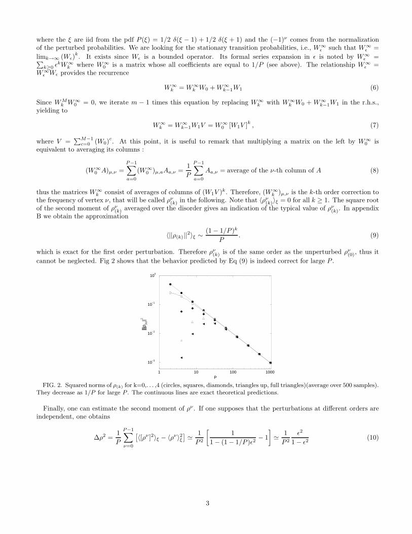
cannot be neglected. Fig 2 shows that the behavior predicted by Eq (9) is indeed correct for large P .

1 10 100 1000P

10−3

10−2

10−1

100

||ρ(k

)||2

FIG. 2. Squared norms of ρ(k) for k=0,. . . ,4 (circles, squares, diamonds, triangles up, full triangles)(average over 500 samples).They decrease as 1/P for large P . The continuous lines are exact theoretical predictions.

Finally, one can estimate the second moment of ρν . If one supposes that the perturbations at different orders areindependent, one obtains

∆ρ2 =1

P

P−1∑

ν=0

[

〈[ρν ]2〉ξ − 〈ρν〉2ξ]

≃ 1

P 2

[

1

1 − (1 − 1/P )ǫ2− 1

]

≃ 1

P 2

ǫ2

1 − ǫ2(10)

3

V. APPLICATION TO MG

Let us first define the game1: MG consists of N agents trying to be at each time step in minority. Each agent hasS strategies, or lookup tables ai,s, s = 1, · · · , S , and dynamically assigns a score to each of them . At each time stept, the system’s history µ(t) is made available to all agents; the latter use their best strategy2 si(t) take the decision

aµi,si(t)

(t) = +1 or −1 and a market maker sums up all decisions into the aggregate quantity A(t) =∑N

i=1 aµi,si(t)

(t) .

Macroscopic quantities of interest include the temporal averages of A(t) conditional to µ(t) = µ, for all µ, noted by〈Aµ〉. The MG undergoes a second order phase transition with symmetry breaking as the control parameter α = P/Nis varied [10,11]: the system is in the symmetric phase (〈Aµ〉 = 0 for all µ) if α < αc and it is in the asymmetricphase for α > αc. One convenient order parameter is3 H = 〈A〉2: it is equal to zero in the symmetric phase, andgrows monotonically with α in the asymmetric phase [11] (see Fig. 4). One other relevant macroscopic quantity isthe fluctuations σ2 = 〈A2〉 which quantifies the performance of the agents [10,11,8,12].

Before doing any analytic calculations, it is worth looking at Figures 3 and 4 which clearly show that Cavagna’sassertion is right as long as the system is in the symmetric phase. Indeed, if 〈Aµ〉 = 0, the transition probabilitiesfrom µ to its next neighbours are unbiased, that is ǫµ = 0; therefore in the symmetric phase, where 〈Aµ〉 = 0 for all µ,the frequencies of visit are uniform ρµ = 1/P . Accordingly, numerical simulations show that these quantities collapseon the same curve.

0.1 1 10α

0

0.5

1

σ2 /N

FIG. 3. Comparison between the fluctuations of MG with uniformly sampled (squares) and real histories (full circles). Inthe symmetric phase, there are equal whereas they differ significantly in the asymmetric phase. Dashed and continuous linesare corresponding theoretical predictions; they overlap in the symmetric phase (M = 8, S = 2, 300P iterations, average over200 samples)

1See refs [11,7,8,12] for more details2the one with the highest score3R =

∑

µρµRµ is the notation for the weighted average over the histories.

4

0.1 1 10α

0

0.1

0.2

0.3

0.4

0.5

H/N

FIG. 4. Comparison between the available information of MG with uniformly sampled (squares) and real histories (circles).Dashed and continuous lines are corresponding theoretical predictions (M = 8, S = 2, 300P iterations, average over 200samples)

As α increases, the critical point is crossed, and 〈Aµ〉 6= 0 for some µ. The dynamics of the history is biased onall such histories and consequently all macroscopic quantities are significantly different: both σ2/N and H/N arelower for real histories than for uniformly sampled histories. This can be understood by the facts that σ2/N and Hare increasing functions of α and that the biases on the De Bruijn graph of histories reduce the effective number of

histories, that can be defined as 2−log2 ρ: in other words, effective α of MG with real histories is smaller than that ofMG with uniform histories. This explanation is indeed confirmed by Fig 5; this shows the fraction of frozen agents4

φ which is a decreasing function of α in the asymmetric phase. As expected from the above argument, φ of MG withreal histories is larger than that of MG with uniformly sampled histories.

0.1 1 10α

0

0.2

0.4

0.6

φ

FIG. 5. Comparison between the fraction of frozen agents in MG with uniformly sampled (squares) and real histories(circles). In the symmetric phase, there are equal whereas they differ significantly in the asymmetric phase (M = 8, S = 2,300P iterations, average over 200 samples)

The bias ǫµ on a particular history can be estimated for large N : in this limit Aµ is a Gaussian variable withaverage 〈Aµ〉 and variance 〈(Aµ)2〉 − 〈Aµ〉2, leading to

ǫµ = 〈sgn(Aµ)〉 ≃ ǫµth = erf

(√

〈Aµ〉22[〈(Aµ)2〉 − 〈Aµ〉2]

)

. (11)

4See [11]: they are agents that stop to be adaptative.

5

0 0.2 0.4 0.6 0.8 1εµ

0

0.2

0.4

0.6

0.8

1

ε th

µ

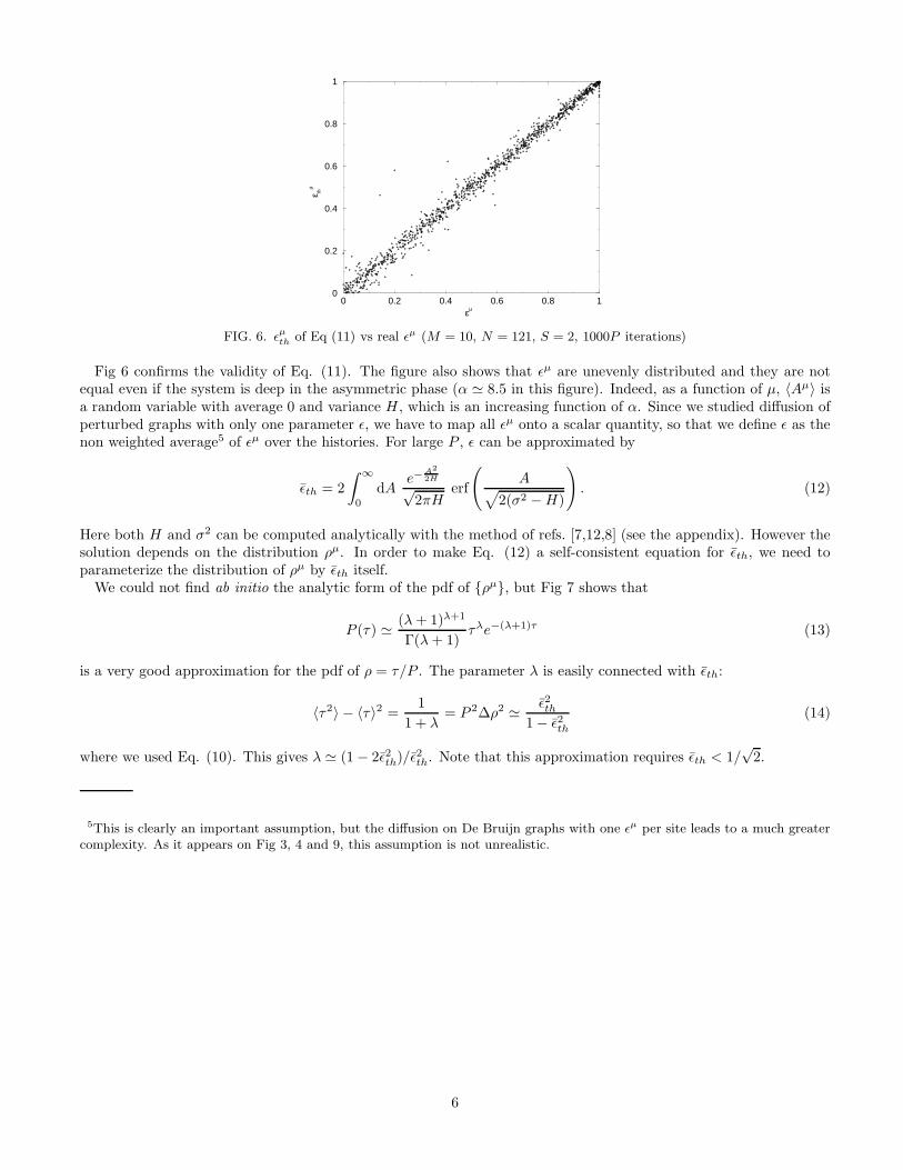
FIG. 6. ǫµ

th of Eq (11) vs real ǫµ (M = 10, N = 121, S = 2, 1000P iterations)

Fig 6 confirms the validity of Eq. (11). The figure also shows that ǫµ are unevenly distributed and they are notequal even if the system is deep in the asymmetric phase (α ≃ 8.5 in this figure). Indeed, as a function of µ, 〈Aµ〉 isa random variable with average 0 and variance H , which is an increasing function of α. Since we studied diffusion ofperturbed graphs with only one parameter ǫ, we have to map all ǫµ onto a scalar quantity, so that we define ǫ as thenon weighted average5 of ǫµ over the histories. For large P , ǫ can be approximated by

ǫth = 2

∫ ∞

0

dAe−

A2

2H

√2πH

erf

(

A√

2(σ2 − H)

)

. (12)

Here both H and σ2 can be computed analytically with the method of refs. [7,12,8] (see the appendix). However thesolution depends on the distribution ρµ. In order to make Eq. (12) a self-consistent equation for ǫth, we need toparameterize the distribution of ρµ by ǫth itself.

We could not find ab initio the analytic form of the pdf of {ρµ}, but Fig 7 shows that

P (τ) ≃ (λ + 1)λ+1

Γ(λ + 1)τλe−(λ+1)τ (13)

is a very good approximation for the pdf of ρ = τ/P . The parameter λ is easily connected with ǫth:

〈τ2〉 − 〈τ〉2 =1

1 + λ= P 2∆ρ2 ≃ ǫ2th

1 − ǫ2th(14)

where we used Eq. (10). This gives λ ≃ (1 − 2ǫ2th)/ǫ2th. Note that this approximation requires ǫth < 1/√

2.

5This is clearly an important assumption, but the diffusion on De Bruijn graphs with one ǫµ per site leads to a much greatercomplexity. As it appears on Fig 3, 4 and 9, this assumption is not unrealistic.

6

0 2 4 6 8τ=ρP

0

0.2

0.4

0.6

0.8

P(τ

)

FIG. 7. Distribution of the frequency of visit of the histories in the minority game. The continuous line is the best fit for apdf given by Eq (13) (M = 13, N = 801, S = 2, 400P iterations)

This turns Eq. (12) into an equation for ǫth, and the theory is self consistent. Figure 8 reports measured ǫ and itsapproximation ǫth. What clearly appears from this figure is that ǫ is far from being negligible, and that ǫth is a quitegood approximation to ǫ.

0.1 1 10α

0

0.2

0.4

0.6

0.8

ε th

M=7M=9self−consistent

FIG. 8. ǫ versus α = P/N (M = 8, S = 2, 300P iterations, average over 200 samples). The straight line is ǫth, the theoreticalprediction of the self consistent theory.

We can also check the validity of Eq. (10) against the self-consistent theory. Fig 9 shows that Eq. (10) is in goodagreement with numerical simulations as long as all histories are visited. Moreover the approximation ǫth for ǫ leadsto qualitatively similar results, but underestimates ∆ρ2 because ǫth < ǫ (see figure 8).

0 1 10α

0.00

10−5.00

10−4.70

10−4.52

10−4.40

∆ρ2

0.1 1 10α

253

254

255

256

Pef

f

7

FIG. 9. Inhomogeneity of the frequency of histories ∆ρ2 versus α = P/N from: numerical simulations (full circles), Eq(10) with ǫ from numerical simulations (void squares) and Eq (10) with ǫth (continuous line); inset: average number of visitedhistories versus α; (M = 8, S = 2, 300P iterations, average over 200 samples).

The self-consistent replica calculation for the Minority Game of refs. [7,12,8] with the ansatz ρ = τ/P and τ givenby the pdf (13) is discussed in the appendix. Fig 3 and 4 indicate that analytic predictions are well supported bynumerical simulations.

In the asymmetric phase, which is arguably the most relevant and interesting in the MG [8], all quantities of MGchange significantly if one replaces real histories with random uniform histories. A dependence on the frequenciesρµ does not necessarily imply the relevance of the detailed dynamics of the histories. If the histories µ where drawnrandomly from the “correct” distribution ρµ, the results would be the same (actually it suffices to know the pdf of ρµ).The problem is that the distribution ρµ depends on the asymmetry 〈Aµ〉, which in turn depend on the microscopicconstitution of all agents [11]. In other words, ρµ is a self-consistently determined quantity and hence it is only knowna posteriori.

VI. CONCLUSION

We have shown that the dynamics of histories cannot be considered as irrelevant. Indeed, even for the canonical MG,it is relevant and cannot be replaced by randomly drawn histories. In addition, for many extensions and variations ofthe MG, the dynamics of histories is not only relevant, but crucial.

We acknowledge fruitful discussions with Philippe Flajolet and Paolo De Los Rios. This work has been partiallysupported by the Swiss National Science Foundation under Grant Nr 20-46918.98.

APPENDIX A:

Let us prove by induction that

(W k0 )µ,ν =

1

2k

2k−1∑

n=0

δ[2kµ%P ]+n,ν (A1)

It is sufficient to calculate explicitly (W k0 )µ,ν from (W k−1

0 )µ,ν

(W k0 )µ,ν =

P−1∑

τ=0

(W0)µ,τ (W k−10 )τ,ν

=

2k−1−1∑

n=0

{

δ[2k−1([2µ%P ])%P ]+n,ν + δ[2k−1([2µ%P ]+1)%P ]+n,ν

}

=1

2k

2k−1∑

n=0

δ[2kµ%P ]+n,ν (A2)

since A(B%P )%P = AB%P and (2kµ + 2k−1)%P = [2kµ%P ] + 2k−1 if P = 2M and k ≤ m − 1.

APPENDIX B:

In order to simplify the notations, we define

(Xc)µ,ν =

2c−1∑

n=0

δ[2c+1µ%P ]+n,ν − δ[2c+1µ%P ]+n+2c,ν (B1)

This matrix is such that

8

(Xc)µ,ν =

1 if 2c+1µ%P ≤ ν < [2c+1µ%P ] + 2c}−1 if [2c+1µ%P ] + 2c ≤ ν < 2c+1(µ + 1)%P

0 else(B2)

With this formalism, one can write W1V as

(W1V )µ,ν =ξµ

2

M−1∑

c=0

1

2c(Xc)µ,ν (B3)

Let us calculate the perturbation at order 1: one has to compute ||ρ(1)||2 in order to have an estimation of the

typical value of a generic ρν(1): since the ξ are uncorrelated and

∑P−1ν=0 (Xc)µ,ν(Xd)µ,ν = 2c+1δc,d ,

〈||ρ(1)||2〉ξ =1

4P 2

P−1∑

µ,ν=0

M−1∑

c=0

[(Xc)µ,ν ]2

22c=

(1 − 1/P )

P(B4)

The next orders of perturbation are much harder to handle. However, for large P , one can approximate them bysupposing that

〈||ρ(k)||2〉ξ ∼ (1 − 1/P )〈||ρ(k−1)||2〉ξ =(1 − 1/P )k

P. (B5)

Consequently, ρν(k) ∼ (1 − 1/P )k/2 1

P ≃ 1P at leading order

APPENDIX C:

Since agents actually minimize H/N , one can consider this quantity as a Hamiltonian and find its ground state.This is possible by methods of statistical physics such as replica trick [14,15]. The generalization of the calculus ofrefs [7,12,8] to ρµ = τµ/P drawn from the pdf given by Eq (13) and (12) is straightforward; the free energy reads inthe thermodynamic limit

F (β, Q, q, R, r) =⟨ α

2βlog[1 + χτ ]

⟩

τ+

1 + q

2

⟨ 11τ + χ

⟩

τ

+αβ

2(RQ − rq) − 1

β〈log

∫ 1

−1

dse−β(ζs2−√

αr z s)〉z (C1)

where χ = β(Q − q)/α and ζ = −√

α/r β(R − r). Next, the β → ∞ limit is taken while keeping finite χ and ζ. Oneobtains

H =1 + Q

2

[

⟨ 11τ + χ

⟩

τ− χ

⟨ 1

[ 1τ + χ]2

⟩

τ

]

(C2)

and

σ2 = H +1 − Q

2(C3)

where Q and χ take their saddle point values, given by the solution of

Q(ζ) = 1 −√

2

π

e−ζ2/2

ζ−(

1 − 1

ζ2

)

erf

(

ζ√2

)

(C4)

Q(ζ) =1

α

[

erf(ζ/√

2)

χζ

]21

〈 1[1/τ+χ]2 〉τ

− 1 (C5)

χ⟨ 1

1τ + χ

⟩

τ=

erf(ζ/√

2)

α(C6)

Eqs (C5) and (C6), together with Eq (12), form a closed set of equations that has to be solved numerically. Note thatas in the random histories case, χ becomes infinite at the critical point, where αc = erf(ζ/

√2).

9

[1] Challet D. and Zhang Y.-C., Physica A 246, 407 (1997) (adap-org/9708006).[2] See the Minority Game’s web page on http://www.unifr.ch/econophysics/minority[3] Arthur W. B., Am. Econ. Assoc. Papers and Proc 84, 406, 1994. (http://www.santafe.edu/arthur/Papers/El Farol.html)[4] A. Cavagna, Phys. Rev. E 59 R3783 (1999) preprint cond-mat/9812215[5] N. F. Johnson, P. M. Hui, D. Zheng, M. Hart, preprint cond-mat/9903164[6] N. F. Johnson, M. Hart, P. M. Hui, D. Zheng, preprint cond-mat/9910072[7] D. Challet, M. Marsili and R. Zecchina, Phys. Rev. Lett 84, 1824 (2000), preprint cond-mat/9904392[8] M. Marsili, D. Challet and R. Zecchina, to appear in Physica A (2000), preprint cond-mat/9908480[9] See the web page http://www.scs.carleton.ca/∼quesnel/papers/debruijn/paper.html for a nice introduction to De Bruijn

graphs.[10] Savit R., Manuca R., and Riolo R., PRL, 82(10), 2203 (1999), (adap-org/9712006).[11] Challet D. and M. Marsili, Phys. Rev. E 60, 6271 (1999), preprint cond-mat/9904071[12] Challet D., M. Marsili and Y.-C. Zhang, Physica A 276, 284 (2000) preprint cond-mat/9909265[13] Challet D. and Zhang Y.-C., Physica A 256, 514 (1998) (cond-mat/9805084);[14] M. Mezard, G. Parisi, M. A. Virasoro, Spin glass theory and beyond (World Scientific, 1987).[15] V. Dotsenko, An introduction to the theory of spin glasses and neural networks; World Scientific Publishing (1995).

10