Shaping Ethnic Inequalities - CADMUS, EUI Research ...

Shaping Ethnic Inequalities

The production and reproduction of social and

spatial inequalities among ethnic minorities in

England and Wales

Carolina Viviana Zuccotti

Thesis submitted for assessment with a view to

obtaining the degree of Doctor of Political and Social Sciences

of the European University Institute

Florence, 22 September 2015 (defence)

European University Institute

Department of Political and Social Sciences

Shaping Ethnic Inequalities

The production and reproduction of social and spatial inequalities

among ethnic minorities in England and Wales

Carolina Viviana Zuccotti

Thesis submitted for assessment with a view to

obtaining the degree of Doctor of Political and Social Sciences

of the European University Institute

Examining Board

Prof. Fabrizio Bernardi, European University Institute (supervisor)

Prof. Alessandra Venturini, European University Institute

Prof. Anthony Heath, University of Oxford

Prof. Héctor Cebolla-Boado, UNED

© Carolina V. Zuccotti, 2015

No part of this thesis may be copied, reproduced or transmitted without prior

permission of the author

Para mis viejos

Para Mati

Para Sigi y Moni

Para mis ancestros

i

Abstract

This thesis is about the production and reproduction of social and spatial inequalities among ethnic minorities

in England and Wales. More specifically, I study how the interaction of different forms of

inequality shapes the opportunities of individuals in a series of outcomes. The main source of

inequality explored here is that which derives from ethnicity and migration status. Alongside this,

two dimensions of inequality are also explored: social origins and the characteristics of the

neighbourhood of residence.

The analysis, carried out for second generation ethnic minorities (Indian, Pakistani, Bangladeshi,

Chinese, Caribbean and African) and the white British, is based on rich individual, household and

neighbourhood-level data: the ONS Longitudinal Study, a dataset that links census information

for a 1% sample of the population of England and Wales and to which it is possible to attach

household and neighbourhood information, and aggregated census data (1971-2011).

I show that ‘ethnic penalties’ in the labour market are, partly or totally, penalties related to the

socio-economic origins of ethnic minorities, usually less advantaged as compared to that of the

white British. This suggests that scholars in migration might overestimate the ‘ethnic gap’ if social

origins are not considered. A second crucial finding is that the geographical space is a source of

production and reproduction of ethnic inequalities. Three outcomes support this. First, I found

evidence of ethnic enclave and place stratification spatial models: most ethnic minorities, but

particularly individuals with lower educational and occupational attainments and Pakistani and

Bangladeshi populations, are less likely than the white British to improve the neighbourhood in

which they were raised, both in terms of deprivation levels and in terms of the share of non-

whites. Second, I found evidence of neighbourhood effects: having been raised in areas with a

high share of co-ethnics has a negative effect on the labour market outcomes of some groups,

mainly Pakistani and Bangladeshi. Third, I found evidence of increasing spatial segregation:

between 2001 and 2011, non-whites, and in particular Pakistani populations, increased their

spatial clustering and their likelihood of sharing the space with other co-ethnics.

iii

Acknowledgments

I have reached the end of the thesis, finally! I am sitting in what looks like one of the nicest cafés

in the main street of Brighton, my new home since mid-January. It’s Sunday, and a mix of

feelings invades me: happy feelings, sad feelings, nostalgic feelings, existential feelings. “How did

I get here?” I have asked myself more than once. Although I never found the correct answer,

trying to think of one now is, I believe, a good way to start writing these acknowledgments; in

particular, because it makes me think of all the people that have accompanied me, to a greater or

lesser extent, in this journey.

I don’t remember exactly when I decided I wanted to do a Ph.D. However, I do know that the

idea of becoming a Doctor emerged while doing my early research experience, at the Instituto de

Investigaciones Gino Germani, based at the Faculty of Social Sciences of the University of

Buenos Aires. Back in 2002, around halfway my studies in Sociology, I found myself knocking at

Professor’s Raúl Jorrat door, my first academic mentor and the person who introduced me to

sociological research. I told him that, parallel to my studies, I wanted to do some ‘practical

experience’: the next day I became a member of the CEDOP, the Centro de Estudios de

Opinión Pública, where not only I learnt the ‘day to day’ of survey research, but also I was able to

develop small research projects thanks to UBACyT and CONICET research grants, who Prof.

Jorrat supervised. Thank you so much Raúl for having received me in your office, for your initial

input, for encouraging me to continuing developing my career, and for all the crucial

recommendation letters you wrote for me. In the CEDOP I also had the opportunity to meet

other very valuable people. Professor Darío Canton gave me the first opportunity to publish a

small research work in one of the books he co-authored with Prof. Jorrat: “Elecciones en la

Ciudad (1864-2005)”; and he also showed me that scientists can be a bit artists as well. Thank

you, Darío, for that and for all the nice chats in La Opera. A very special thank you goes also to

my dearest friend and colleague Teresa, who I met while working at the CEDOP. Thank you also

to Manuel, my friend and colleague of pizzas and projects, Majo, Natalia, Eli and Daniela, my

official partner of breakfasts in Marcelo T.

Another important influence and motivation to start the Ph.D. came from Professor Ruth Sautu,

the chair of the course Methods in the Social Sciences, in which I participated in the last years of

my undergrad studies. Thank you Ruth for allowing me to have my first teaching experience and

iv

for showing me that teaching is the best way to learn. Thanks also to all the members of the team

I met while teaching, in particular, Alejandra, my dear friend and colleague, with whom I share

not only academic discussions but also, and most importantly, life experiences and love stories.

Many thanks also to Mercedes Di Virgilio, for sharing your interest in urban sociology with me;

and thanks to Pablo, Carolina N, Santiago, Cecilia, Gaby, Paula, Carolina P, Diego and Maria Pia,

for the nice afternoons of sociological mates in Olleros.

In 2006 I had my first academic experience in Europe. You see, for Argentineans, and probably

for South Americans in general, Europe is one big place with many tiny countries in it. So we

tend to say Europe, rather than a single country, once we have crossed the ocean. However, I

have to say that my experience has actually been very European, if you think that in nine years-

time I lived in four different countries, both from the North and South of Europe; and if you

consider that I only met Argentineans before 2006, and now I know people from at least 20

different nationalities. I have to admit it: I have become a bit European myself… and I have

loads of people to be thankful for around Europe.

Thank you Professor Yuri Kazepov (Universita’ degli Studi di Urbino) for taking me in the E-

Urbs Master and allowing me to have the first in-depth contact with urban studies; thanks

Professor Marisol Garcia (Universidad de Barcelona) for guiding my first master thesis on spatial

segregation; thanks Professor Clara Mulder (Universiteit van Amsterdam) for supervising my

research done for the master on Human Geography, Planning and Development Studies; thank

you Professor Chris Kesteloot (KU Leuven) for believing in me and in my work.

A special thank you goes to Professor Harry Ganzeboom (VU Amsterdam) with whom I

collaborated for two years as a researcher and with whom I am finishing a co-authored paper,

together with Prof. Ayse Guveli. Your guidance and support have been fundamental for

developing the topic and methods of my thesis: I have learnt so much while being at VU. Thank

you for having me as part of your research team and for showing me that you really need to make

your tables at least 20 times before you get the final ones: I have corroborated it in many

occasions already! Thanks also to Heike, my roommate in VU, colleague and friend, for making

my stay in the Netherlands so much nicer, and to Tamira and the rest of the members of the

(now) Department of Sociology at VU.

v

This thesis would not have been possible without the help of my supervisor, Professor Fabrizio

Bernardi. Thank you so much Fabrizio: not only you have provided me with advice and guidance

on how to develop my research but, at the same time, you have given me freedom to develop my

own interests. This has been extremely valuable for me. Thanks also for the understanding in the

moments of stress, for reading so fast, for the informal chats and for showing me the

Argentinean song for the Brazilian World Cup. These small things have added a lot to the more

formal student-supervisor relationship! I have enjoyed working with you, and I hope there will be

opportunities to collaborate in the future. Grazie ancora Fabrizio! Thanks also to Monika, my

main administrative supporter at the EUI, for making the bureaucratic side of writing and

finishing the thesis much easier!

A very big thank you also goes to Professor Lucinda Platt with whom I worked during most of

2013 and part of 2014 at the Institute of Education and the London School of Economics, in

London. First of all, thanks for making me part of the LS Beta Test Project, which gave me

access to the ONS-LS data and, with it, the opportunity to add a strong spatial dimension to the

thesis. Thanks also for the daily work, for reading the tables with me, for helping with the

development of the chapters and for your advice on theory and methods. Thanks also for always

being so positive and encouraging, for the informal chats and your moral support, and for being

my companion during long days in VML.

Special thanks go also to Wei, our project supporter in VML, the section of the Office of

National Statistics (ONS) where I accessed most of the data used in this thesis. Thanks for being

always fast and efficient in solving my data-related problems, and also always funny and smiling.

You are a very valuable person in VML. Thanks also to Rachel and Chris, who as Wei, where

always there when I needed them, and always fast and happy to respond to all my questions and

my long-distance syntaxes! A special thank you goes also to the “Data Without Boundaries”

project, a grant program through which I received financial support during my year in London

that helped me cover the expenses of my daily work at VML. Thanks also to the ONS team that

cleared the results of my thesis and all the people involved in the data management.

So many other friends have accompanied me in the process of finding and doing this Ph.D.

Matilde, my favorite tango player who visited me many times in Europe; Flavia, Betta, Cheng, Fer

and Ceylan, with whom I shared many beers in Amsterdam; Eli and Monica, my flatmates while

doing my first master thesis in Barcelona; and the so many international friends – some of them

vi

‘my family’ – while being in Florence. Special thanks go to Ines and Bene, my two dearest and

favourite European friends, for sharing the years of Ph.D.-making with me (and hopefully more

post Ph.D. to come); thank you Jorge, Antoine, Stefano, Paula, Elisa, Stefi, Emanuelle, Nina,

Mara, Fulvia, Sanni, Alan and Kaarlo. Thanks also to Juana, Pedro and German for making me a

fan of the Drink Team; thank you Sofi, for sharing your feelings and thoughts about life abroad;

thanks to the Inequality Working Group ‘gang’, Marit, Chiara, Anne Cristine, Michael, Alexi and

Jenny, for making me feel I was not the only crazy person obsessed with numbers; thanks to

Robi and my belly-dancing team, for opening my life in Florence and giving me so much joy. A

big thank you to the lovely friends I made in London: Mia, Georgia and Georgina, dearest

housemates, thanks for making me feel a bit more at home; Stella, thanks for the gossip and for

filling my statistical days with funny stories; thanks Oriana for the long and lively Spanish-

speaking chats; thanks Roxanne, Simon and Carla. Thanks Sheila for your patience while

finishing the last bits in Brighton!

While doing my research in London I met Alessandro, my partner and friend. Caro Ale, magari

avresti dovuto pensare due volte prima di metterti insieme con una studentessa nel ultimo anno

di dottorato (scherzo!). Grazie dalla tua pazienza infinita, per ascoltarmi, per aiutarmi, per darmi il

tuo amore e la tua positivita, per mettere la vita in perspetiva, per insegnarmi che le persone

possono prendere vie diverse, tutte di uguale valore. Grazie per starmi accanto ogni giorno, e per

essere tu, Ale.

But perhaps those to whom I owe the most are my loving family and closest friends. Gracias

Claudia, por estar siempre que te necesito y por decirme que estoy bárbara! Gracias Noe, por

compartir tantos lindos momentos en familia. Gracias tía Silvia por recordarme lo importante que

es ser Argentina, por darme siempre buenas energías en mis viajes, por quererme tanto y, sobre

todo, por ser mi tía del corazón. Te fuiste muy pronto, tía. Cómo me hubiese gustado tenerte en

mi ceremonia de graduación; cómo te extraño. Gracias Gaby y Gusti, por hacerme siempre reír

(¡creo que nunca río tanto como lo hago con ustedes!). Gracias Sigi y Moni, porque sin los

maullidos y el ronrroneo, nunca habría conocido el valor de los animales en la vida de las

personas. Cuán difícil fue continuar la tesis luego de perderte, mi Moni. Gracias Mati, por ser

como sos, por nuestras charlas en Skype, por estar siempre ahí, y por ser el mejor hermano que

podría tener. Gracias ma y pa, por quererme y cuidarme, por escucharme siempre, por la

paciencia. Si llegue acá es por ustedes. Y espero que algún día ayudarlos como ustedes me

ayudaron a mí.

vii

Fueron años de alegrías y desafíos, de nuevas experiencias y amistades que quedarán para

siempre; pero también de noticias tristes, que ponen la vida (y el doctorado) en perspectiva. Una

perspectiva más real, más verdadera, más simple, que espero llevar conmigo en esta nueva etapa

que comienza.

Gracias nuevamente,

Carolina

ix

Table of Contents

Abstract ………………………………………………………………………..……… i

Acknowledgements .....…………………………………………………..….……… iii

Table of Contents …………………………………………………………………… ix

List of Tables …...…………………………………………………………………. xiii

List of Figures ...……………………………………………………………..…….. xix

List of Maps ..……………………………………………………………..……...... xxi

1 CHAPTER 1: INTRODUCTION ..................................................................... 1

1.1 Motivation: an interesting topic in an interesting context .................................................... 1

1.1.1 An interesting topic .............................................................................................................................. 1

1.1.2 An interesting context ......................................................................................................................... 2

1.2 Three sources of inequality: a guiding theoretical framework for this thesis .................... 3

1.3 Ethnic minorities in the UK ..................................................................................................... 7

1.3.1 Arrival and population growth ........................................................................................................... 7

1.3.2 The geography of ethnic minorities.................................................................................................16

1.3.3 Economic activity and social class: an overview for 2011 ...........................................................21

1.4 Migration and integration policies and the public debate on ethnic minorities in the UK

27

1.4.1 Migration policy: a bit of history ......................................................................................................28

1.4.2 Integration policies and the ‘multiculturalism debate’ ..................................................................30

1.5 Wrapping up and moving forward… .................................................................................... 35

2 CHAPTER 2: THE ONS LONGITUDINAL STUDY: DATA STRUCTURE

AND VARIABLES ................................................................................................... 37

2.1 Part 1: Data structure ............................................................................................................... 37

2.1.1 Introduction ........................................................................................................................................37

2.1.2 What is the ONS Longitudinal Study? ............................................................................................37

2.1.3 Defining origin and destination: the structure and sources of data ................................................39

2.1.3.1 Age structure .............................................................................................................................................. 39

2.1.3.2 Data sources: individual, household and neighbourhood data ......................................................... 40

2.1.4 Unit of analysis and samples .............................................................................................................41

x

2.1.5 A brief comment on attrition and sampling ...................................................................................46

2.2 Part 2: Variables ........................................................................................................................ 49

2.2.1 List of variables ...................................................................................................................................49

2.2.2 Individual-level variables ...................................................................................................................50

2.2.2.1 Ethnic group and second generation .................................................................................................... 50

2.2.2.2 Education ................................................................................................................................................... 54

2.2.2.3 Employment .............................................................................................................................................. 55

2.2.2.4 Social class .................................................................................................................................................. 56

2.2.2.5 Other individual-level variables .............................................................................................................. 58

2.2.3 Household-level variables .................................................................................................................58

2.2.3.1 Parental social class ................................................................................................................................... 58

2.2.3.2 Other household-level variables in origin ............................................................................................. 60

2.2.3.3 Partner’s ethnicity ..................................................................................................................................... 60

2.2.4 Neighbourhood-level variables ........................................................................................................61

2.2.4.1 What are Wards? Main characteristics and population ...................................................................... 61

2.2.4.2 Non-white and (co-)ethnic concentration quintiles ............................................................................ 64

2.2.4.3 Deprivation quintiles ................................................................................................................................ 68

2.2.5 Other variables ....................................................................................................................................70

3 CHAPTER 3: ‘ETHNIC PENALTY’ OR ‘SOCIAL ORIGINS PENALTY’? 71

3.1 Introduction .............................................................................................................................. 71

3.2 Previous studies in the UK ..................................................................................................... 74

3.3 Theoretical background and hypotheses .............................................................................. 77

3.4 Data and variables .................................................................................................................... 84

3.5 Descriptive statistics ................................................................................................................ 85

3.6 Access to employment ............................................................................................................ 92

3.7 Social class and social mobility ............................................................................................. 100

3.8 Discussion ............................................................................................................................... 113

4 CHAPTER 4: IS SPATIAL SEGREGATION OF ETHNIC MINORITIES

REALLY DECREASING? ..................................................................................... 119

4.1 Introduction ............................................................................................................................ 119

4.2 Spatial segregation in the UK ............................................................................................... 121

4.3 Measuring spatial segregation ............................................................................................... 125

4.3.1 Some issues in the selection of areas ............................................................................................ 125

4.3.2 The areas selected in this study ..................................................................................................... 128

4.3.2.1 Lower Layer Super Output Areas ........................................................................................................ 129

xi

4.3.2.2 Housing Market Areas ........................................................................................................................... 130

4.3.3 Segregation indices .......................................................................................................................... 134

4.4 What is high and what is low in terms of spatial segregation? ........................................ 143

4.5 Distribution of groups in HMAs and metropolitan areas ................................................ 148

4.6 Analysis of spatial segregation (2001-2011)........................................................................ 155

4.6.1 Results for White British and (pooled) non-white ethnic minorities ...................................... 155

4.6.2 Results for ethnic minority groups ............................................................................................... 159

4.7 Summary and discussion ....................................................................................................... 166

5 CHAPTER 5: NEIGHBOURHOOD EFFECTS? EXPLORING THE ROLE

OF EARLY EXPOSURE TO CO-ETHNICS ...................................................... 179

5.1 Introduction ............................................................................................................................ 179

5.2 Mechanisms underlying neighbourhood effects ................................................................ 180

5.3 Neighbourhood effects and the migration literature ........................................................ 182

5.4 The problem of selectivity and endogeneity: a proposal for a model of analysis ......... 185

5.4.1 What are selectivity and endogeneity? .......................................................................................... 185

5.4.2 Addressing selectivity and endogeneity ....................................................................................... 187

5.4.3 Model of analysis ............................................................................................................................. 189

5.5 Descriptive statistics .............................................................................................................. 191

5.6 Isolating the effect of co-ethnics ......................................................................................... 196

5.7 Discussion ............................................................................................................................... 208

6 CHAPTER 6: RESIDENTIAL CHANGE AND EQUALITY OF

OPPORTUNITIES: A TEST OF THE SPATIAL ASSIMILATION THEORY 213

6.1 Introduction ............................................................................................................................ 213

6.2 Assimilation, spatial assimilation and other models of spatial integration .................... 214

6.3 The locational attainment model ......................................................................................... 218

6.4 Model of analysis: adapting the ‘locational attainment model’ ........................................ 220

6.5 Hypotheses .............................................................................................................................. 224

6.6 Data and variables .................................................................................................................. 229

6.7 The problem of reverse causality ......................................................................................... 233

6.8 Descriptive statistics .............................................................................................................. 235

6.9 Testing the spatial assimilation, place stratification and ethnic enclave models ........... 240

6.10 Discussion ............................................................................................................................... 255

7 CHAPTER 7: CONCLUDING REMARKS .................................................. 259

xii

7.1 Introduction ............................................................................................................................ 259

7.2 A summary .............................................................................................................................. 259

7.3 Discussion ............................................................................................................................... 262

7.3.1 Crucial findings in perspective ...................................................................................................... 262

7.3.2 Assimilation, multiculturalism and interculturalism: (limiting) constraints, (allowing)

preferences and (promoting) social cohesion ............................................................................................ 265

7.3.3 Some limitations (and potential for future research) ................................................................. 269

8 ANNEX A: CHAPTERS’ ANNEXES ........................................................... 271

8.1 Annex to Chapter 3 ............................................................................................................... 271

8.2 Annex to Chapter 4 ............................................................................................................... 300

8.3 Annex to Chapter 5 ............................................................................................................... 304

8.4 Annex (I) to Chapter 6 .......................................................................................................... 337

8.5 Annex (II) to Chapter 6 ........................................................................................................ 350

9 ANNEX B: A COMPARISON OF ‘POOLED’ AND ‘UNIQUE’ DATA .... 375

10 ANNEX C: ORIGIN AND DESTINATION EFFECTS ............................. 379

11 BIBLIOGRAPHY ........................................................................................... 395

xiii

List of Tables

Table 1.1: Economic activity in 2011 (extended) .................................................................................. 23

Table 2.1: Sources and types of data ....................................................................................................... 40

Table 2.2: The unit of analysis: example ................................................................................................. 42

Table 2.3: Initial and final samples: pooled and unique cases ............................................................. 43

Table 2.4: Age distributions by origin and destination years; initial sample ...................................... 44

Table 2.5: Ethnic groups by origin and destination years; initial sample ........................................... 45

Table 2.6: Ethnic groups by number of census points in which the individual has participated;

initial sample ................................................................................................................................................ 45

Table 2.7: Individuals with Level 4+ education and service class by ethnic group and destination

year; sample with one measurement per individual (%) ....................................................................... 47

Table 2.8: Variables .................................................................................................................................... 49

Table 2.9: Individuals in various origin households by ethnic group; initial sample (column %) .. 51

Table 2.10: Parental social class and access to the service class for mixed/non-mixed parents;

initial sample (column %) .......................................................................................................................... 52

Table 2.11: Individuals born in the UK, by ethnic group and origin year (%).................................. 53

Table 2.12: Economic activity by ethnic group; initial sample ............................................................ 56

Table 2.13: The NS-SEC and applications to Chapters 3, 5 and 6 ..................................................... 57

Table 2.14: Parental social class ................................................................................................................ 59

Table 2.15: Characteristics of Census Wards ......................................................................................... 63

Table 2.16: Non-white and (co-)ethnic concentration: variables and categories used in each

census point ................................................................................................................................................. 65

Table 2.17: Average share of ethnic minorities (non-white and individuals groups) in non-white

and ethnic quintiles respectively, by census points................................................................................ 67

Table 2.18: Average Carstairs scores and average percentages of each variable in quintiles, by

census points ............................................................................................................................................... 69

Table 3.1: Research questions, hypotheses and possible explanations ............................................... 80

Table 3.2: Employment and access to the service class by ethnic group, gender and year (%) ..... 86

Table 3.3: Descriptive statistics for men; 2001 and 2011 pooled (% and mean) .............................. 88

Table 3.4: Descriptive statistics for women; 2001 and 2011 pooled (% and mean) ........................ 90

Table 3.5: Access to employment. Men. ................................................................................................. 93

Table 3.6: Access to employment. Women. ........................................................................................... 97

xiv

Table 3.7: Access to the service class. Men. ......................................................................................... 101

Table 3.8: Access to the service class. Women. ................................................................................... 102

Table 3.9: Access to the service class; models of social mobility. Men. ........................................... 104

Table 3.10: Access to the service class; models of social mobility. Women. ................................... 109

Table 4.1: Segregation indices of previous findings in England and Wales .................................... 122

Table 4.2: Spatial segregation outcomes for different geographical scales ...................................... 127

Table 4.3: Most commonly used geographical units in England ....................................................... 129

Table 4.4: Descriptive statistics for housing market areas: population and land area (2011) ....... 134

Table 4.5: Dimensions and segregation indices ................................................................................... 135

Table 4.6: Dissimilarity Index* ............................................................................................................... 136

Table 4.7: Interaction and Isolation Indices ......................................................................................... 137

Table 4.8: Relative Concentration Index .............................................................................................. 140

Table 4.9: Absolute Clustering and Spatial Proximity Indices ........................................................... 142

Table 4.10: Correlation between segregation indices (2011) .............................................................. 143

Table 4.11: Segregation indices for immigrants and ethnic minorities in metropolitan areas in the

US (2000), France (1999) and the United Kingdom (2001) ............................................................... 145

Table 4.12: Segregation indices for individuals with high professional/managerial and routine

occupational status (NS-SEC) in each HMA (2011) ........................................................................... 147

Table 4.13: Distribution of white British and ethnic minorities in England (row %) and across

housing market areas (column %); 2001 and 2011 .............................................................................. 149

Table 4.14: Percentage of white British and ethnic minorities in metropolitan areas (in England

and within HMAs, except for London); percentage of white British and ethnic minorities in

inner, outer and extended London (column %); 2001 and 2011 ...................................................... 151

Table 4.15: Distribution of white British and ethnic minorities within HMAs (row %); 2001 and

2011 ............................................................................................................................................................ 154

Table 4.16: Segregation indices for non-white ethnic minorities and white British in 2011, and

difference with respect to 2001; HMAs ................................................................................................ 157

Table 4.17: Segregation indices for ethnic minority groups in 2011, and difference with respect to

2001; HMAs .............................................................................................................................................. 160

Table 4.18: Number of LSOAs by percentage of non-white ethnic minorities (2001 and 2011) 168

Table 5.1: Access to employment and the service class (in %) by quintile of co-ethnic

concentration (Q1=lowest concentration; Q5: highest concentration) ........................................... 192

xv

Table 5.2: Individual, household and neighbourhood characteristics by quintile of co-ethnic

concentration (Q1=lowest concentration; Q5: highest concentration). Pooled ethnic minorities.

..................................................................................................................................................................... 195

Table 5.3: Access to employment. Pooled ethnic minorities. ............................................................ 198

Table 5.4: Access to employment by ethnic group and gender; predicted values (standard errors)

..................................................................................................................................................................... 200

Table 5.5: Access to the service class. Pooled ethnic minorities. ...................................................... 201

Table 5.6: Access to the service class by ethnic group and gender; predicted values (standard

errors) ......................................................................................................................................................... 203

Table 5.7: Avoidance of semi-routine and routine occupations. Pooled ethnic minorities. ......... 205

Table 5.8: Avoidance of semi-routine and routine occupations by ethnic group and gender;

predicted values (standard errors) .......................................................................................................... 207

Table 6.1: Equations used in the analysis.............................................................................................. 224

Table 6.2: Hypotheses and mechanisms, and their link to research questions and equations ...... 228

Table 6.3: Total number of Wards and average percentage of groups in Wards, by non-white

quintile in 2011 ......................................................................................................................................... 229

Table 6.4: Deprivation quintiles by non-white quintiles, 2011 (row %)........................................... 230

Table 6.5: Non-white quintiles by ethnic quintiles (column %) ........................................................ 231

Table 6.6: Probability of being in a neighbourhood with low share of non-whites (quintiles 1+2)

in 2001 and in 2011, by cohort and non-white quintile in origin (%) ............................................. 235

Table 6.7: Probability of being in a neighbourhood with a low share of non-white (Quintiles 1+2)

by origin neighbourhood (%) ................................................................................................................. 236

Table 6.8: Probability of being in a neighbourhood with a low share of non-white (quintiles 1+2)

in 2011 by origin neighbourhood and education (%) .......................................................................... 237

Table 6.9: Probability of being in a neighbourhood with a low share of non-whites (Quintiles 1-2)

in 2011 by origin neighborhood1 and partner’s ethnicity (%) ............................................................ 238

Table 6.10: Probability of being in a neighbourhood with a low share of non-white (quintiles 1-2)

in 2011 by origin neighbourhood and social class (%) ........................................................................ 239

Table 6.11: Probability of being in a neighbourhood with a low share of non-white (quintiles 1-2)

in 2011. Linear regression with robust SE; ethnic minorities only. .................................................. 241

Table 6.12: Probability of being in a neighbourhood with a low share of non-whites (quintiles 1-

2). Linear regression with robust SE; ethnic minorities and white British men.............................. 243


2). Linear regression with robust SE; ethnic minorities and white British women. ....................... 247

xvi

Table 6.14: Probability of being in a neighbourhood with low share of non-whites (quintiles 1-2).

Predicted values for selected cases. ........................................................................................................ 254

Table 8.1: Distribution of groups in number of census points, origin years and destination years.

Men and women. ...................................................................................................................................... 271

Table 8.2: Access to employment. Full model. Men. .......................................................................... 272

Table 8.3: Access to employment. Full model. Women. .................................................................... 277

Table 8.4: Access to the service class. Full model. Men. .................................................................... 282

Table 8.5: Access to the service class. Full model. Women. .............................................................. 286

Table 8.6: Access to the service class. Full models of social mobility. Men and women. ............. 290

Table 8.7: Access to employment and to the service class. Replication of Model 5 from Tables

3.5-3.8 using logistic regression with average marginal effects; in the table: average marginal

effects, robust (clustered) standard errors and p-value ....................................................................... 297

Table 8.8: Local Authorities within housing market areas ................................................................. 300

Table 8.9: Number of LSOAs by percentage of ethnic minorities (2001 and 2011)...................... 302

Table 8.10: Access to employment: full model. Pooled ethnic minorities; men. ............................ 304

Table 8.11: Access to employment: full model. Pooled ethnic minorities; women. ....................... 309

Table 8.12: Access to the service class: full model. Pooled ethnic minorities; men. ...................... 314

Table 8.13: Access to the service class: full model. Pooled ethnic minorities; women. ................. 319

Table 8.14: Avoidance of semi-routine and routine occupations: full model. Pooled ethnic

minorities; men. ........................................................................................................................................ 324

Table 8.15: Avoidance of semi-routine and routine occupations: full model. Pooled ethnic

minorities; women. ................................................................................................................................... 329

Table 8.16: Access to employment, to the service class and avoidance of semi-routine and routine

occupations. Model 4 in Tables 5.3, 5.5 and 5.7 using logistic regression with average marginal

effects; in the table: average marginal effects, robust (clustered) standard errors and p-value. .... 334

Table 8.17: Probability of being in a neighbourhood with low deprivation (quintiles 1-3) in 2011

by origin neighbourhood (%) ................................................................................................................. 337

Table 8.18: Probability of being in a neighbourhood with low deprivation (Q1-3) in 2011 by

origin neighbourhood and education in 2011....................................................................................... 338


origin neighbourhood and partnership .................................................................................................. 339


origin neighborhood1 and social class .................................................................................................... 339

xvii

Table 8.21: Probability of being in a neighbourhood with low deprivation (Quintiles 1-3). Linear

regression with robust SE; ethnic minorities and white British men. .............................................. 341

Table 8.22: Probability of being in a neighbourhood with low deprivation (Quintiles 1-3). Linear

regression with robust SE; ethnic minorities and white British women. ......................................... 345

Table 8.23: Probability of being in a neighbourhood with low deprivation (Quintiles 1-3).

Predicted values for selected cases. ........................................................................................................ 349

Table 8.24: Probability of being in a neighbourhood with a low share of non-white (Quintiles 1-2)

in 2011. Linear regression with robust SE; ethnic minorities only. Full model. ............................. 350

Table 8.25: Probability of being in a neighbourhood with a low share of non-whites (Quintiles 1-

2). Linear regression with robust SE; ethnic minorities and white British men. Full model ........ 356


2). Linear regression with robust SE; ethnic minorities and white British women. Full model. .. 364


2) and low deprivation (quintiles 1-3). Replication of Equation a) from Tables 6.12 and 6.13 and

from Tables 8.23 and 8.24, using logistic regression with average marginal effects; in the table:

average marginal effects, robust (clustered) standard errors and p-value ........................................ 372

Table 9.1: Pooled and unique cases by ethnic group; initial sample ................................................. 376

Table 9.2: Parental social class by ethnic group; initial sample, pooled and unique cases ............. 377

Table 9.3: Education by ethnic group; initial sample, pooled and unique cases ............................. 378

Table 9.4: Access to the service class by ethnic group; initial sample, pooled and unique cases . 378

Table 10.1: Distribution of key variables by group and origin/destination years; final samples .. 380

Table 10.2: Access to employment for individuals raised in different origin years (1971-1991) and

individuals measured in different destination years (2001-2011). Test for Chapter 3. ................... 383

Table 10.3: Access to the service class for individuals raised in different origin years (1971-1991)

and individuals measured in different destination years (2001-2011). Test for Chapter 3. ........... 384

Table 10.4: Access to the service class (models of social mobility) for individuals raised in

different origin years (1971-1991) and individuals measured in different destination years (2001-

2011). Test for Chapter 3. ....................................................................................................................... 385

Table 10.5: Access to employment for individuals raised in different origin years (1971-1991) and

individuals measured in different destination years (2001-2011). Test for Chapter 5. ................... 388

Table 10.6: Avoidance of routine and semi-routine occupations for individuals raised in different

origin years (1971-1991) and individuals measured in different destination years (2001-2011). Test

for Chapter 5. ............................................................................................................................................ 390

xviii


2) for individuals raised in different origin years (1971-1991) and individuals measured in

different destination years (2001-2011). Test for Chapter 6 (men and women pooled). .............. 392

xix

List of Figures

Figure ‎1.1: White British and non-white in England and Wales* (1971-2011); % of total ............... 8

Figure ‎1.2: Ethnic minorities in England and Wales* (1971-2011); % of total population ............ 12

Figure ‎1.3: Ethnic minorities in England and Wales* (1971-2011); % of non-white population .. 13

Figure ‎1.4: Components of relative growth; ethnic minorities and white British in England and

Wales (2001-2011) ...................................................................................................................................... 15

Figure ‎1.5: UK-born and elsewhere-born individuals by (grouped) ethnic group (2011); England

and Wales ..................................................................................................................................................... 16

Figure ‎1.6: Average Carstairs deprivation score for areas with different shares of non-white ethnic

minorities (England; 2011) ........................................................................................................................ 18

Figure ‎1.7: Average Carstairs deprivation score for areas with different shares of co-ethnics

(England; 2011)........................................................................................................................................... 19

Figure ‎1.8: Percentage of ethnic minorities that live in the 10% most-deprived areas (IMD) ....... 21

Figure ‎1.9: Economic activity: main categories ...................................................................................... 24

Figure ‎1.10: Employed (as a share of the total active population) ...................................................... 25

Figure ‎1.11: Social class (grouped categories from NS-SEC) .............................................................. 26

Figure ‎2.1: The ONS Longitudinal Study ............................................................................................... 38

Figure ‎2.2: Origin and destination; age structure of the data ............................................................... 39

Figure ‎2.3: Employment and access to the service class by ethnic group: census data and ONS-LS

compared (%) (2011). ................................................................................................................................ 48

Figure ‎3.1: Status attainment and ethnic penalties: three models ........................................................ 78

Figure ‎3.2: Probability of being in employment in 2001 and 2011 (for all and separated by

education); predicted values from the regression (confidence intervals 90%). Men. ....................... 95

Figure ‎3.3: Probability of being employed in 2001 and 2011 (for all and separated by education);

predicted values from the regression (confidence intervals 90%). Women. ..................................... 98

Figure ‎3.4: Probability of being in the service class by parental social class; predicted values from

the regression (confidence intervals 90%). ........................................................................................... 107

Figure ‎3.5: Probability of being in the service class by parental social class and education;

predicted values from the regression (confidence intervals 90%). Men. ......................................... 108

Figure ‎3.6: Probability of being in the service class by parental social class; predicted values from

regression (confidence intervals 90%). .................................................................................................. 112

Figure ‎4.1: A hypothetical metropolitan area with three different population distributions ........ 126

xx

Figure ‎4.2: Dimensions of segregation .................................................................................................. 138

Figure ‎5.1: The problems of selectivity and endogeneity ................................................................... 186

Figure ‎5.2: Model of analysis: main variables and their measurement year ..................................... 189

Figure ‎6.1: Residential gains as a function of socio-economic gains: examples .............................. 219

Figure ‎6.2: Variables and their relationships; reference to research questions ................................ 233

Figure ‎6.3: The problem of reverse causality ....................................................................................... 234

xxi

List of Maps

Map 1.1: Non-white ethnic minorities in England (2011).................................................................... 17

Map 4.1: Identification of HMAs; geographical units are Local Authorities (a) and Local

Authorities + LSOAs (b) ........................................................................................................................ 133

Map 4.2: Indians in Leicester .................................................................................................................. 172

Map 4.3: Pakistani in Bradford ............................................................................................................... 173

Map 4.4: Bangladeshi in London ........................................................................................................... 174

Map 4.5: Chinese in Manchester ............................................................................................................ 175

Map 4.6: Caribbeans in London ............................................................................................................. 176

Map 4.7: African in London ................................................................................................................... 177

1

1 CHAPTER 1: Introduction

1.1 Motivation: an interesting topic in an interesting context

1.1.1 An interesting topic

This thesis is about the production and reproduction of social and spatial inequalities among ethnic minorities

in England and Wales. More specifically, it studies how the interaction of different forms of

inequality shapes the opportunities of individuals in a series of outcomes.

My interest in ethnic minorities or immigrants is of relatively long duration, and the same can be

said about the appeal for me of urban sociology and the relationship between social and spatial

processes. Even longer is my commitment to the study of social inequalities. But if I had to

identify the single most fascinating aspect of the discipline of sociology, it would be the idea that

there are patterns of behaviour in society, ways of doing and thinking that, when identified, can

allow us to predict what could happen to individuals in certain contexts and under certain

circumstances. These patterns of behaviour are connected to what Emile Durkheim has called

social facts. In simple terms, a social fact can be understood as a social force that, while being the

product of individualities, has a separate and independent effect on individuals. Think for

example of ethnicity: we know that being black is not the same as being white in terms of finding a

job or buying a house. Ethnicity, therefore, is a social force that ‘makes a difference’ that affects

individualities and that has a social nature: the fact that ethnicity plays a role in our societies today

is the product of years of slavery, discrimination and mutual adaptation, that is, of social history

and interactions between individuals. The same can be thought of social origins or the social class

of the family of origin, a concept that refers to the distribution of socio-economic resources in a

society, which are the product of work relations. Social origins, as ethnicity, also ‘make a

difference’ and have an effect on individualities: individuals who grew up in higher-class families

or families with higher socio-economic resources have better chances of succeeding in life, for

example in terms of education and work, than individuals raised in families with fewer resources.

Similarly, the social and ethnic composition of the neighbourhood can also be understood as a force that,

while being the consequence of individuals’ choices (and constraints) to access a residence, can

have an effect on individuals’ lives. There is evidence, for example, that living in neighbourhoods

2

with high deprivation, poor amenities, degraded public spaces and limited access can have

consequences on various outcomes, such as wellbeing and health.

The objective of this thesis is to explore how these three social forces affect individuals on a

variety of outcomes and, most importantly, how and to what degree they are interrelated. In

particular, I pay special attention to the role of ethnicity, and how this interacts with the other two

elements. In so doing, this thesis takes an innovative approach to the understanding of social

inequalities. In fact, not only ethnicity, social origins and neighbourhood composition are crucial pillars of

the social structure of a society, but also they are sources of inequality in society and, most

importantly, they have the potential to reproduce social inequalities over time. By studying

them together this thesis adds a fresh and more complex view to the debate on equality of

opportunities, especially those that concern ethnic minority groups.

1.1.2 An interesting context

The result of long-term research interests, this thesis is also the product of having found an

excellent setting in which to develop the interests. The UK offers a very favourable environment

for studying ethnicity, the main source of inequality explored in this thesis. Three primary reasons

drive this statement. First, the UK has a strong mix of non-white ethnic groups that come from a

variety of countries and bring diverse cultures: Caribbean, Asian and African minorities are the

biggest groups – constituting nowadays around 12% of the population – and are also the ones

studied in this thesis. The advantage of studying varied groups in one destination is that it allows

one to explore different patterns of integration at the same time (although this does not

necessarily imply that the receiving context is the same for all groups) and also to examine

differences connected with the groups themselves. Furthermore, ethnic minorities have a

relatively long presence in the country, which permits me to identify second generations, that is,

those who were born and/or raised in the UK. Following assimilation theories, it has been widely

argued that in order to see how immigrants are doing in a certain destination country, the study

of the second generation is of vital importance. The reason is that these individuals have been

exposed, practically from the beginning of their lives, to the majoritarian population, to the local

culture and, most importantly, to mainstream institutions such as the educational system. This

should situate them more or less as the majoritarian population is situated, or at least, should put

them in a more favourably position as compared to their own parents. This implies that finding

3

disadvantages among second generation minorities is probably a relatively good indicator of poor

integration (as compared to finding disadvantages among the first generation).

Second, in the UK, the ‘ethnic minority’ or ‘migrant’ issue has long been at the heart of political

and public discourse. Gripping debates have been generated by various disturbances such as

those that occurred in 2001 in northern England, and in 2005 around the bombing of the

London underground. These led to statements like ethnic minorities live ‘parallel lives,’ or that

multiculturalism policies lead to extremism and encourage, therefore, terrorism. The need to

control immigration and, at the same time, to promote integration have characterized UK

policies practically from the beginning of the mass arrivals, and are still part of the daily public

discourse, which renders migration research even more compelling and current.

Last but not least, studying the UK case I was able to make a good match between specific

research questions and data to answer them. As described in Chapter 2, I use very unusual and

rich data that not only encompasses a large number of ethnic minorities, but also allows me to

explore changes over time and combine individual data with geographical information.

In the remaining part of this introduction, I discuss in more detail the three forms or dimensions

of inequality studied in this thesis and their theoretical foundations, and briefly introduce the

main analytical chapters (Section 1.2); then I provide a brief overview of ethnic minorities in

UK, with particular attention paid to their geographical patterns in the country and to their socio-

economic position (Section 1.3); finally, I review the main migration and integration policies

developed in the UK in the past 50 years (Sections 1.4) and wrap up the chapter (Section 1.5).

1.2 Three sources of inequality: a guiding theoretical framework for this

thesis

This study combines approaches from different literatures: migration, social stratification and

inequality and urban studies. Its driving assumption is that inequality has different sources. The

main source of inequality explored here is that which derives from ethnicity and migration status.

Alongside this, two other bases of inequality are also explored: family background or social

origins and the characteristics of the neighbourhood in which individuals live. These three

dimensions are, to a greater or lesser extent, present in all chapters.

4

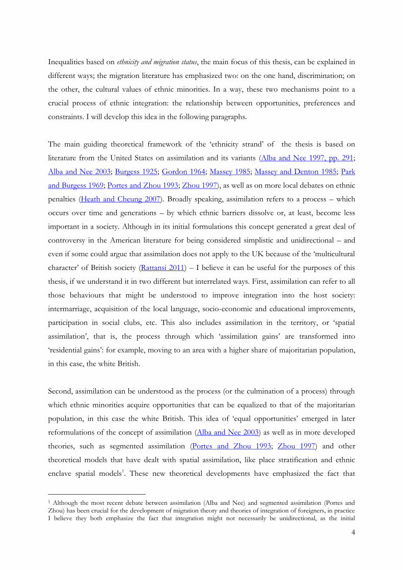
Inequalities based on ethnicity and migration status, the main focus of this thesis, can be explained in

different ways; the migration literature has emphasized two: on the one hand, discrimination; on

the other, the cultural values of ethnic minorities. In a way, these two mechanisms point to a

crucial process of ethnic integration: the relationship between opportunities, preferences and

constraints. I will develop this idea in the following paragraphs.

The main guiding theoretical framework of the ‘ethnicity strand’ of the thesis is based on

literature from the United States on assimilation and its variants (Alba and Nee 1997, pp. 291;

Alba and Nee 2003; Burgess 1925; Gordon 1964; Massey 1985; Massey and Denton 1985; Park

and Burgess 1969; Portes and Zhou 1993; Zhou 1997), as well as on more local debates on ethnic

penalties (Heath and Cheung 2007). Broadly speaking, assimilation refers to a process – which

occurs over time and generations – by which ethnic barriers dissolve or, at least, become less

important in a society. Although in its initial formulations this concept generated a great deal of

controversy in the American literature for being considered simplistic and unidirectional – and

even if some could argue that assimilation does not apply to the UK because of the ‘multicultural

character’ of British society (Rattansi 2011) – I believe it can be useful for the purposes of this

thesis, if we understand it in two different but interrelated ways. First, assimilation can refer to all

those behaviours that might be understood to improve integration into the host society:

intermarriage, acquisition of the local language, socio-economic and educational improvements,

participation in social clubs, etc. This also includes assimilation in the territory, or ‘spatial

assimilation’, that is, the process through which ‘assimilation gains’ are transformed into

‘residential gains’: for example, moving to an area with a higher share of majoritarian population,

in this case, the white British.

Second, assimilation can be understood as the process (or the culmination of a process) through

which ethnic minorities acquire opportunities that can be equalized to that of the majoritarian

population, in this case the white British. This idea of ‘equal opportunities’ emerged in later

reformulations of the concept of assimilation (Alba and Nee 2003) as well as in more developed

theories, such as segmented assimilation (Portes and Zhou 1993; Zhou 1997) and other

theoretical models that have dealt with spatial assimilation, like place stratification and ethnic

enclave spatial models1. These new theoretical developments have emphasized the fact that

1 Although the most recent debate between assimilation (Alba and Nee) and segmented assimilation (Portes and Zhou) has been crucial for the development of migration theory and theories of integration of foreigners, in practice I believe they both emphasize the fact that integration might not necessarily be unidirectional, as the initial

5

integration of ethnic minorities is not necessarily unidirectional, and that either due to preferences

(for example, cultural values, community factors, motivation, etc.) or constraints (for example

discrimination in the labour or housing markets), the classical model of integration might be

interrupted or might follow different directions.

This conceptualization of assimilation is very much linked to what Heath and Cheung (2007)

have termed ‘ethnic penalties’. This concept, discussed in more detail in Chapter 3, refers to any

remaining difference between ethnic minorities and majoritarian populations after crucial

individual and background factors have been taken into account. An ethnic penalty thus

connotes that there is something intrinsic to being an ethnic minority that explains why they

differ with respect to the majoritarian population, in this case the white British. In this context,

preferences and constraints might explain the notion of ‘ethnic penalties’ and, therefore, why some

groups might be doing better in the labour market, or why some are more spatially segregated, or

why some are penalized if have been raised in neighbourhoods with many co-ethnics: why, in

short, ethnic inequalities persist over time. Conversely, the disappearance of ‘ethnic penalties’

points to the idea that ‘equal opportunity’ has been achieved, which also implies that factors

other than ethnicity are at play. This leads me to two other sources of social inequality: social

origins and neighbourhood.

Inequality based on social origins, considered in most of chapters, stems from the fact that

individuals are raised in families with different resources and that the mechanisms that allocate

individuals in certain parts of the social structure vary across social classes (Blau and Duncan

1967; Boudon 1973; Goldthorpe 2000). Overall, being raised in a household with more economic

resources usually exerts a positive effect on individuals, independent of their ethnic background.

For example, individuals with high-status parents are usually more likely to go to better schools,

to achieve higher educational levels, to access better social networks and to have financial

support at their disposal. Although this type of inequality has in fact been acknowledged as part

of the reformulation of assimilation theories (Alba and Nee 2003), given the volume of literature

on social mobility and social stratification, it would be unfair to subsume the role of social origins

to migration theory. Rather, this thesis emphasises that social origins – studied in practice

through the parental social class and household resources in origin – have a determining role in

formulations of assimilation (i.e. Gordon) have argued. In particular, Alba and Nee (2003) allude very explicitly to this idea of divergent trends of integration that is at the core of the segmented assimilation theory. I therefore do not take a position in this debate, but just use the ‘bits’ that these (apparently contradictory) theories have in common.

6

shaping opportunities and should therefore be considered independently from ethnic factors,

even if they are highly related. In this sense, if one wants to better isolate the specificity

associated to belonging to a particular ethnic minority group, the variation in terms of social

origins that exist across these groups needs to be considered.

The final type of inequality this thesis deals with is inequality based on the characteristics of the

neighbourhood in which individuals live and on the geographical distribution of groups. On the one

hand, neighbourhoods are important because they plausibly have an impact on individuals living

in them. A voluminous literature treats not only the role that living in certain neighbourhoods has

on various outcomes (see for example: Galster et al. 2007a; Galster 2010; Musterd and

Andersson 2006; Musterd, Ostendorf and De Vos 2003), but also the impact of living in areas

with a high concentration of ethnic minorities or co-ethnics (see for example: Clark and

Drinkwater 2002; Urban 2009; Van Kempen and Şule Özüekren 1998). On the other hand,

spatial segregation – the spatial concentration of individuals that share certain socio-economic or

ethnic characteristics – has also been a matter of concern for researchers, as it prevents

individuals from interacting with others that are different, with possible negative consequences

for trust and social cohesion (Uslaner 2012).

These three bases of inequality are found, with more or less salience, in all the analytical chapters

(Chapters 3-6). In particular, the role of social origins in shaping ethnic inequalities is developed

in Chapter 3. This chapter seeks to disentangle to what extent the so-called ‘ethnic penalties’,

that is, disadvantages associated with the fact of belonging to a certain ethnic minority group, are

actually ‘social origins penalties’ related to the fact that second generation ethnic minorities are

typically raised in households and neighbourhoods with fewer resources relative to the

majoritarian population. In so doing, this chapter adds a fresh view on already-existing

discussions on the social mobility of ethnic minorities in the UK. The three remaining analytical

chapters are more centred on the link between ethnic and spatial inequalities.

Chapter 4, based on aggregated census data only, explores recent trends on spatial segregation of

ethnic minorities in England (2001-2011). Using as a starting point the quite-polarized

discussions around whether ethnic minorities are more or less segregated now than before – and

by means of studying various dimensions of segregation in an innovative way – this chapter

adduces evidence for both tendencies and, most importantly, reveals important differences based

on ethnicity.

7

Chapter 5 examines neighbourhood effects. Specifically, it asks to what extent having been

raised in a neighbourhood with a high share of co-ethnics has an impact on labour market

outcomes in later life among second generation ethnic minorities.

Chapter 6, finally, tests contrasting theories that seek to explain the link between assimilation

gains and residential gains: spatial assimilation, place stratification and ethnic enclave. In other

words, it analyses to what extent an improvement in socio-economic and cultural terms translates

into an improvement in terms of the characteristics of the neighbourhoods in which individuals

live. In so doing, this chapter also tests whether all ethnic groups, including the white British,

have the same residential opportunities given equality of conditions.

1.3 Ethnic minorities in the UK

As noted above, I have chosen the UK to carry out this thesis thanks to the large number of

ethnic minorities, the co-existence of many diverse groups and the possibility of studying second

generation immigrants. This section gives an overview of these figures and presents as well

information on population growth, a bit of history of arrivals and some relevant contextual

information: the location of ethnic minorities and the situation of first and second generations in

the labour market.

1.3.1 Arrival and population growth

Immigration to the UK – at least on a large scale – started after the Second World War. As

happened in many other Western European countries (i.e. Germany, France, Austria, The

Netherlands and Belgium) the initial settlements were a consequence of the high demand for

labour force, which could not be satisfied by the local population, and which was needed in order

to reconstruct the economy of the country and incentivize growth. Most of these countries first

recruited immigrants from other European countries: in the case of the UK, the Irish and Poles

came in the greatest numbers. But in the face of the persistence of the labour shortage, other

sources of manpower from outside Europe started to appear. The arrival of non-white ethnic

minorities – mainly with black and Asian origins – started in the late 1940s and continued in the

following decades. As shown in Figure 1.1, between 1971 and 2011 the population of non-white

ethnic minorities in England and Wales, which from 1991 onwards includes also those born in

8

the UK, went from being 2.3% of the population to almost 12%, with the highest increase

occurring in the last decade. As can be seen from the graph, this process was accompanied by a

parallel decrease of the white British population.

Figure ‎1.1: White British and non-white in England and Wales* (1971-2011); % of total

* For Chinese in 1971 and 1981 data refers to the UK. Source: Author’s own calculations based on aggregated census data (obtained from: casweb.mimas.ac.uk and www.neighbourhood.statistics.gov.uk).

The initial pull of immigration to the UK, at least the one that involves the groups studied here,

was thus mainly (although not solely) economic, rooted in the need for foreign labour in a

context of economic recovery (Panayi 2010). These post-war labour shortages, which motivated

the arrival of thousands of foreigners especially before the installation of controls in 1962, tended

to take two distinct forms (Robinson and Valeny 2005). First of all, local shortages were created

because of rapid economic growth in certain local labour markets. This growth had two effects:

on the one hand, some industries simply could not find enough local offers to meet their

demand, and therefore were forced to rely on immigrant workers to fill their vacancies. This was

the case, for example, for the car industry in Essex, West Midlands and Oxford. On the other

hand, new growth industries offering attractive jobs were filling their vacancies with local people

at the expense of leaving other industries offering less attractive jobs with empty vacancies. These

empty vacancies were occupied, later on, by immigrants, keen to maximize their income

regardless of work conditions. Foundry work in West Midlands as well as low-level occupations

in hospitals and transport services in London, are examples of these vacancies.

1971 1981 1991 2001 2011

White British 93,78 93,37 94,08 87,49 80,49

Non-white 2,29 3,04 5,92 7,42 11,84

0,0

10,0

20,0

30,0

40,0

50,0

60,0

70,0

80,0

90,0

100,0

White British

Non-white

http://casweb.mimas.ac.uk/

http://www.neighbourhood.statistics.gov.uk/

9

The second form of local shortages originated as a consequence of the transformation of the

economy, where the reduction of labour costs, translated into the proliferation of poor working

conditions, was used as a means to increase productivity. This facilitated the incorporation of

immigrants who not only were willing to accept jobs that the local population rejected, but who

were trying to find ways to escape racial discrimination, which limited the opportunities in the

labour market (Rattansi 2011; Robinson and Valeny 2005). Examples of this are the textile

industry of Lancashire and the woollen textile industry of Yorkshire.

Immigrants, then, either came to fill empty spaces by constituting ‘replacement populations’

(Peach 2005; Phillips 1998), or to create new opportunities, by filling positions that could not be

fully covered by the local population: they spearheaded a process that Robinson and Valeny

(2005) have described as ‘ethnic succession’.

The main sources of manpower in these post-war waves came from the black and Asian New

Commonwealth. Immigrants from the West Indies were in fact among the first to immigrate, and

their arrival was the consequence of an active recruitment organized through missions sent to the

Caribbean, and in some cases also facilitated by the governments of origin (Robinson and Valeny

2005). Most Caribbean immigrants came from Jamaica, although there were large numbers from

all Caribbean islands. The natural peak of post-war West Indian was between 1955 and 1957, and

a sharp rise occurred right before the introduction of the immigration controls in 1962. In fact,

before 1962 immigrants from the Commonwealth were granted citizenship rights upon arrival,

which gave them freedom to enter at will, and also voting rights (Heath et al. 2013; Sunak and

Rajeswaran 2014).

Contrary to other migrants in Europe who were part of similar programs of active recruitment of

workers – the so-called ‘guest worker programs’ (which, for example, brought Turks to various

northern European countries, including Germany, France and Belgium) – the Caribbean was a

skilled population and that had been exposed to British institutions and values, including the

English language and participation in the armed forces. However, with the exception of nurses

recruited under the newly created National Health Service, most of the jobs that Caribbean

persons performed were blue-collar and manual-labor, many of these located in the public sector,

such as London Transport (Cheung and Heath 2007b; Peach 2005).

10

The next major groups to arrive were South Asians, Indians and Pakistanis in particular. This

immigration was more voluntary, and far less of it came from direct recruitment (Robinson and

Valeny 2005), although it was also a response to the changing economy. In the case of many

South Asians, economic motivations were also combined with processes of dislocation and

displacement. On the one hand, the partition of India in 1947 attracted displaced Indian Sikhs

and Muslim Punjabis; on the other, East African countries, where many Indians (and to a lesser

extent Muslim Pakistani) were already working under the British government, gained

independence in the 1960s and expelled Indians and Pakistani from their territories (Heath et al.

2013). This was, for example, the case of Kenya and Uganda, where South Asians, in particular

Indians, were in qualified occupations, including white-collar jobs in the government, but also in

entrepreneurship and business activities. The Indian community was, in fact, among the most

skilled, and they managed to use those skills in the UK: their role as doctors is well known,

although they also occupied positions in car and engineering industries and transport and

communication (Robinson and Valeny 2005). The first Indians and Pakistanis to arrive were male

(this differentiates them from the Caribbean group, which had a large proportion of women

migrating as nurses), and much recent migration of these groups had taken the form of family

reunion. Pakistanis also participated in the transport sector, like British Rail, and were particularly

present in textile and woollen industries located in the centre and north of England. However,

Pakistanis as well as Caribbean people were in general less skilled than Indians, and performed in

less-qualified occupations, a difference that is still present nowadays.

Bangladeshi, African and Chinese’s waves, smaller in number, followed these initial waves of

immigration. Bangladeshi immigration, which occurred after the mass arrival of Indians and

Pakistanis, had its peak in the 1970s, when men arrived to the UK attracted by low-wage

occupations (mainly in London, where most of them are located nowadays). Women and

dependents followed this arrival, expanding the population during the 1980s. As with the other

South Asian groups, the migration of Bangladeshis was also in part a response to displacement

processes, in particular the one generated by the war of independence against Pakistan in 1971,

and earlier the partition of India. Moreover, this group also established connections with the UK,

in particular through their work in the British merchant navy (Heath et al. 2013).

Black Africans have a long history of small-scale settlement in the UK, which started in the late

1940s. However, the higher peak occurred, as for Bangladeshis, in the 1970s, following the

political instability and waves of independence across the African continent, mostly Sub-Saharan

11

Africa. This is a quite-diversified group in terms of culture and background, and they also come

from different countries: most of them have their origins in Nigeria, but sizeable proportions are

from Ghana, Tanzania, Zambia and Zimbabwe. Africans are also diverse in terms of their

motivations to migrate. Although, as with the other groups, economic improvement was an

important reason for migration, many Africans also migrated to the UK to study. This makes

them one of the most qualified ethnic minorities, together with Indians (Cheung and Heath

2007b; Dobbs, Green and Zealey 2006; Peach 2005).

Chinese, finally, came predominantly from UK’s former dependency, Hong Kong, and to a lesser

extent from Singapore, Malaysia and South Africa. As with Indians, some of them were also

former members of the (in this case Chinese) diaspora to countries of the British Empire. The

first Chinese arrived to the UK as seafarers sojourning at the major seaports of the UK; later on,

the collapse of the rural rice economy in Hong Kong and the influx of refugees of Communist

China, together with the British need for economic recovery after the Second World War,

generated an immigration of Chinese who started specializing in the catering industry. These

migrants, who together with Caribbean and South Asian populations have been considered as

replacement populations, were also subject to the same immigration laws, like the 1962

Commonwealth Immigrants Act that imposed restriction on entry of immigrants (Luk 2009).

Chinese however, continued to arrive through family reunion and a peak occurred in the mid-

1980s, when negotiations with China over the return of Hong Kong began. These migrants, who

came not only from Hong Kong but also from other South-East Asian countries, tended to be

much more skilled and educated than their predecessors (Cheung and Heath 2007b), a fact that

facilitated their entrance. Another feature of Chinese immigration is that contrary to the other

groups, they have tended to be quite dispersed in the space, something that emerges in Chapter 4.

In order to have an idea of the numbers and weight of the various ethnic minority groups in the

UK, Figure ‎1.2 and Figure ‎1.3 show the percentage of ethnic minorities as a share of the total

and non-white population respectively for the period 1971-2011. Numbers are based on country

of birth for 1971-1981 and on ethnic self-identification for 1991-2011, and are calculated for

England and Wales. An exception is the Chinese, for whom data based on country of birth also

applies to 1991, and for whom data for 1971-1981 refers to the entire UK (and not only to

England and Wales). Note also that Bangladeshis in 1971 are measured together with the

12

Pakistanis, since Bangladesh did not exist before 19712; and consider as well that the

measurement of ethnicity based on the country of birth might lead to an underestimation of

ethnic minorities, especially in 1981, when the number of second generation ethnic minorities

(the children of immigrants) probably started to be more relevant in size.

Figure ‎1.2: Ethnic minorities in England and Wales* (1971-2011); % of total population

* For Chinese in 1971 and 1981 data refers to the UK. Source: Author’s own calculations based on aggregated census data (obtained from: casweb.mimas.ac.uk and www.neighbourhood.statistics.gov.uk).

2 Refer to the section “Non-white and (co-)ethnic concentration quintiles” under “Neighbourhood variables” in Chapter 2 for more details on how ethnic categories were created.

1971 1981 1991 2001 2011

Indian 0,64 0,79 1,66 1,99 2,52

Pakistani 0,28 0,37 0,91 1,37 2,01

Bangladeshi 0,10 0,32 0,54 0,80

Chinese 0,03 0,04 0,04 0,44 0,70

Caribbean 0,62 0,61 1,00 1,08 1,06

African 0,32 0,58 0,42 0,92 1,76

0,00

0,50

1,00

1,50

2,00

2,50

3,00

Indian

Pakistani

Bangladeshi

Chinese

Caribbean

African



13

Figure ‎1.3: Ethnic minorities in England and Wales* (1971-2011); % of non-white

population

* For Chinese in 1971 and 1981 data refers to the UK. Source: Author’s own calculations based on aggregated Census data (obtained from: casweb.mimas.ac.uk and www.neighbourhood.statistics.gov.uk).

Caribbeans and Indians are the most numerous groups in 1971 and 1981, constituting

respectively around 0.6% of the total population (circa 300000 members) in 1971, and a bit more

for Indians in 1981. These groups represent also the highest proportion with respect to the total

non-white population: together, they comprise around 60% of non-white ethnic minorities. Over

time, however, Caribbean and Indian populations have followed different patterns of growth.

While the Indian population has continued to grow steadily, constituting the most numerous

ethnic minority group in all subsequent years (reaching almost 1.5 million in 2011), the Caribbean

population became quite stable after 1991, maintaining their proportion with respect to the total

population in around 1% and systematically decreased their relative share in the non-white

population. This, however, might be related to the fact that there are now more individuals who

identify themselves as of mixed origin, in particular ‘white Caribbean’, who are not considered in

this figure. As a matter of fact, in the UK, intermarriage between blacks and whites is more

common than intermarriage between Asians and whites, and this has probably led to the rise in

individuals who consider themselves as having a mixed origin (and a decrease of individuals who

identify themselves as solely Caribbean or African). Note however, that for the purposes of this

1971 1981 1991 2001 2011

Indian 28,08 25,97 28,12 26,86 21,27

Pakistani 12,28 12,33 15,43 18,52 16,93

Bangladeshi 3,25 5,48 7,28 6,73

Chinese 1,24 1,19 0,75 5,88 5,92

Caribbean 27,15 19,93 16,91 14,61 8,96

African 13,84 19,16 7,10 12,43 14,90

0,0

5,0

10,0

15,0

20,0

25,0

30,0

Indian

Pakistani

Bangladeshi

Chinese

Caribbean

African



14

thesis individuals who identify themselves as ‘half white’ are excluded from the analysis (see

Chapter 2 for more details).

Pakistani and Bangladeshi populations, on the other hand, are lower in number (in particular

Bangladeshi), but, like Indians, they have also grown steadily since 1981; and the same is true

with regard to their relative share within the non-white population (which has grown from 3% to

7% for Bangladeshi and from 12% to 17% for Pakistanis). In particular, the Pakistani is the

second most numerous ethnic minority group in the most recent decades: there are more than

one million Pakistanis living in England and Wales in 2011. African and Chinese groups, finally,

start growing rapidly in 1991; in 2011 Africans constituted the third most important ethnic

minority group3.

An important aspect to consider regarding the growth of non-white ethnic minority groups is the

components of this growth. In fact, while at the beginning of the period most of this

population’s growth was associated with new arrivals (including those for whom family reunion

was relevant), in more recent years new births have started play a greater role: these are the so-

called second generations, that is, individuals who identify themselves as belonging to a certain

ethnic minority, but who were born in the UK. Figure ‎1.4 shows the components of population

growth for different groups between 2001 and 2011.

3 The peak observed for Africans in 1981 is puzzling, since I would have expected the value to be inflated in 1971, where the measure for identifying Africans is less precise (see Chapter 2 for details on this).

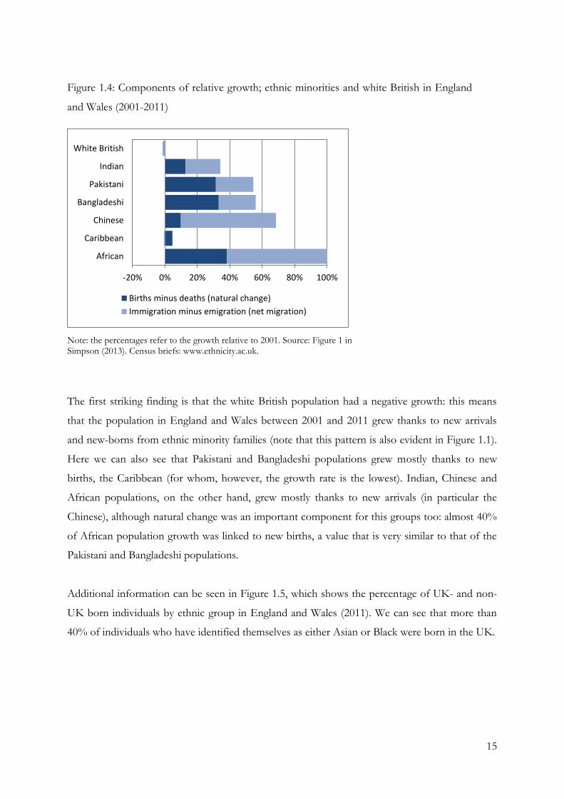
15

Figure ‎1.4: Components of relative growth; ethnic minorities and white British in England

and Wales (2001-2011)

Note: the percentages refer to the growth relative to 2001. Source: Figure 1 in Simpson (2013). Census briefs: www.ethnicity.ac.uk.

The first striking finding is that the white British population had a negative growth: this means

that the population in England and Wales between 2001 and 2011 grew thanks to new arrivals

and new-borns from ethnic minority families (note that this pattern is also evident in Figure 1.1).

Here we can also see that Pakistani and Bangladeshi populations grew mostly thanks to new

births, the Caribbean (for whom, however, the growth rate is the lowest). Indian, Chinese and

African populations, on the other hand, grew mostly thanks to new arrivals (in particular the

Chinese), although natural change was an important component for this groups too: almost 40%

of African population growth was linked to new births, a value that is very similar to that of the

Pakistani and Bangladeshi populations.

Additional information can be seen in Figure 1.5, which shows the percentage of UK- and non-

UK born individuals by ethnic group in England and Wales (2011). We can see that more than

40% of individuals who have identified themselves as either Asian or Black were born in the UK.

-20% 0% 20% 40% 60% 80% 100%

White British

Indian

Pakistani

Bangladeshi

Chinese

Caribbean

African

Births minus deaths (natural change)

Immigration minus emigration (net migration)

16

Figure ‎1.5: UK-born and elsewhere-born individuals by (grouped) ethnic group (2011); England

and Wales

Source: Author’s own calculations based on aggregated census data (obtained from: www.neighbourhood.statistics.gov.uk).

1.3.2 The geography of ethnic minorities

The geography of ethnic minorities in the UK, a crucial component of this thesis, has been very

much determined by the location of jobs. Upon arrival, most ethnic minorities established

themselves in the north and central areas of the UK, and mainly in metropolitan areas (Simpson

and Finney 2009): London, in particular, was the main point of attraction, but also urban areas in

the East and West Midlands (Birmingham and Leicester), North West (Great Manchester) and

Yorkshire and the Humber (Bradford and Leeds). As can be seen in Map 1.1, this is still the main

location of non-white ethnic minorities nowadays: in fact, migration chains and

institutionalization, expressed, for example, in the emergence of supermarkets with typical

products or in the creation of churches, has led to the persistence of these patterns of settlement,

and hence, to the spatial segregation of ethnic minorities (Massey 1985). Currently 80% of non-

white ethnic minorities live in metropolitan areas and 50% in London only. Black and

Bangladeshi populations are the groups who are most likely to be found in this city, while Indian

and Pakistani and Chinese populations are most dispersed. Furthermore, of all the groups, the

Chinese most predominantly live in non-metropolitan areas.

0,0 20,0 40,0 60,0 80,0 100,0

White British

Asian

Black

WhiteBritish

Asian Black

UK-born 97,9 42,0 46,8

Elsewhere 2,1 58,0 53,2

UK-born

Elsewhere


17

Map ‎1.1: Non-white ethnic minorities in England (2011)

Source: Author’s own calculations based on aggregated census data (obtained from: www.neighbourhood.statistics.gov.uk; UK geographies available at: geoportal.statistics.gov.uk).

In addition to the spatial concentration (whose characteristics are further studied in Chapter 4),

an important aspect of these settlements, which has been constant over the decades and applies

(to a greater or lesser extent) to all ethnic minority groups, is that areas with a high concentration

of ethnic minorities have usually been areas with high levels of deprivation.

The initial settlement of most non-white migrants in metropolitan areas was marked by poverty

and hostility (Phillips 1998; Rattansi 2011). Immigrants were located either in poor private

accommodations or in the worst of owner-occupied houses; and the same apply to public

housing, to which they gained access in the mid-1960s. Spatial segregation based on ethnicity

started therefore to emerge as a problem, and this was reinforced by white suburbanization.

Moreover, the link between race and deprivation became evident, not only in terms of public

perception, but also as a factor that would generate a legacy of disadvantage in the years to come.


http://www.geoportal.statistics.gov.uk/

18

Many minorities were found to be trapped in marginal areas in regions of industrial decline,

which would later on affect their opportunities in terms of employment and housing (Phillips

1998).

Figures 1.6-1.8 show different aspects of the relationship between segregation of ethnic

minorities and deprivation. Figure 1.6, based on my own calculations for 2011, shows the average

Carstairs deprivation score4 (Norman, Boyle and Rees 2005) for areas with different shares of

non-white ethnic minorities5. The values observed in Figures 1.7 and 1.8 show results separated

by ethnic group.

Figure ‎1.6: Average Carstairs deprivation score for areas with different shares of non-white

ethnic minorities (England; 2011)

Descriptive characteristics for Carstairs:

Mean: 0.03 Percentile 25: -1.52

Minimum: -4.71 Percentile 50: -0.48

Maximum: 11.37 Percentile 75: 1.12

Percentile 95: 4.28

Source: Author’s own calculations based on aggregated census data (obtained from: www.neighbourhood.statistics.gov.uk and from Prof. Paul Norman).

4 The Carstairs deprivation score is a summarizing measure based on four variables: proportion of male

unemployment, proportion of overcrowded households, proportion of households with no car/van and proportion of individuals with low social class. The more positive the values, the higher the deprivation. Refer to Chapter 2 for details on how the Carstairs deprivation index is constructed. 5 For all figures, areas for which ethnic and deprivation data is obtained are Lower Layer Super Output Areas, which have an average of 1500 individuals.

More than75%

Over 50%and up to

75%

Over 25%and up to

50%

Over 10%and up to

25%

Over 5% andup to 10%

Up to 5%

Carstairs 0,98 0,76 0,17 -0,18 -0,22 0,03

-0,40

-0,20

0,00

0,20

0,40

0,60

0,80

1,00

1,20


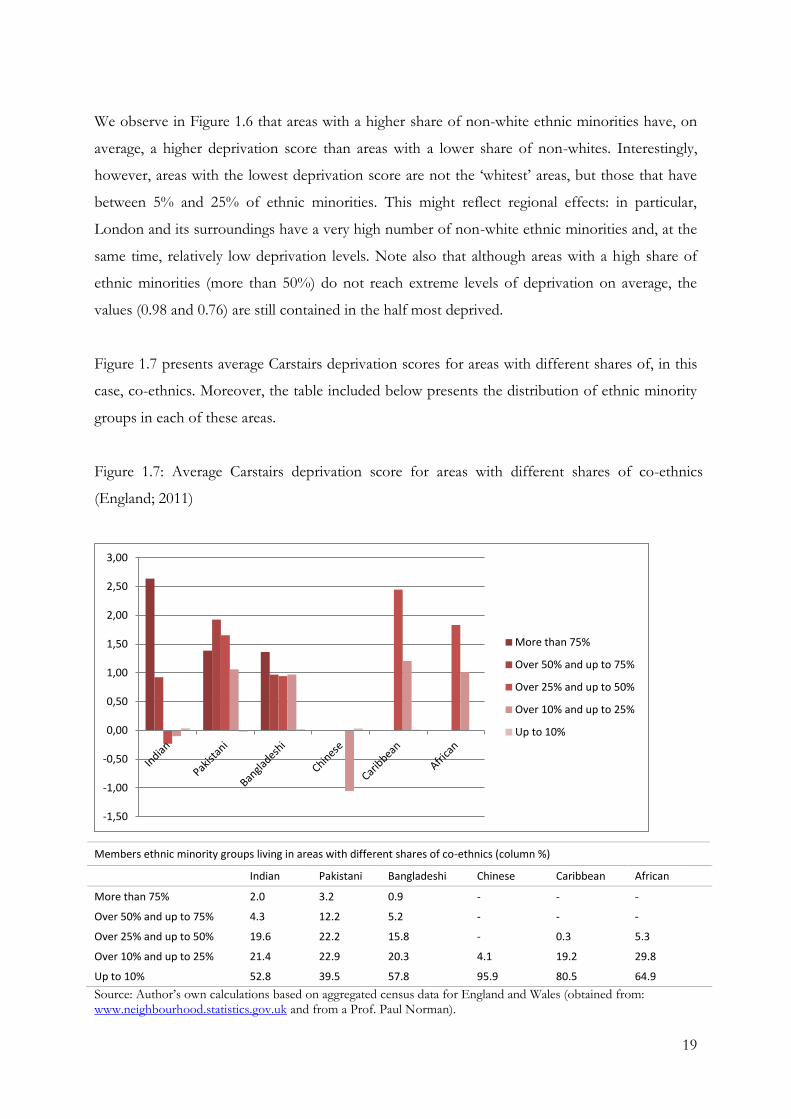
19

We observe in Figure 1.6 that areas with a higher share of non-white ethnic minorities have, on

average, a higher deprivation score than areas with a lower share of non-whites. Interestingly,

however, areas with the lowest deprivation score are not the ‘whitest’ areas, but those that have

between 5% and 25% of ethnic minorities. This might reflect regional effects: in particular,

London and its surroundings have a very high number of non-white ethnic minorities and, at the

same time, relatively low deprivation levels. Note also that although areas with a high share of

ethnic minorities (more than 50%) do not reach extreme levels of deprivation on average, the

values (0.98 and 0.76) are still contained in the half most deprived.

Figure 1.7 presents average Carstairs deprivation scores for areas with different shares of, in this

case, co-ethnics. Moreover, the table included below presents the distribution of ethnic minority

groups in each of these areas.

Figure ‎1.7: Average Carstairs deprivation score for areas with different shares of co-ethnics

(England; 2011)

Members ethnic minority groups living in areas with different shares of co-ethnics (column %)

Indian Pakistani Bangladeshi Chinese Caribbean African

More than 75% 2.0 3.2 0.9 - - -

Over 50% and up to 75% 4.3 12.2 5.2 - - -

Over 25% and up to 50% 19.6 22.2 15.8 - 0.3 5.3

Over 10% and up to 25% 21.4 22.9 20.3 4.1 19.2 29.8

Up to 10% 52.8 39.5 57.8 95.9 80.5 64.9

Source: Author’s own calculations based on aggregated census data for England and Wales (obtained from: www.neighbourhood.statistics.gov.uk and from a Prof. Paul Norman).

-1,50

-1,00

-0,50

0,00

0,50

1,00

1,50

2,00

2,50

3,00

More than 75%

Over 50% and up to 75%



Up to 10%


20

The first clear outcome of Figure 1.7 is that the Chinese are in a much better relative position as

compared to the other groups: most of them are located in areas which have average levels of

deprivation (values close to zero): these are areas where the number of co-ethnics is 10% or less.

Moreover a small number of Chinese who live in areas with a relatively higher share of co-ethnics

seem to be particularly advantaged in terms of deprivation. Next to Chinese, Indians also enjoy a

favourable situation, overall: more than 90% live in areas where deprivation levels are below the

mean. In some cases these are also areas where the concentration of Indians is relatively high: for

example, areas where there are 25%-50% of Indians (and where almost 20% of Indians live) have

on average a deprivation score of -0.23. This is a pattern that only applies to this group, as can be

seen from the figure. However, Indians who live in areas with a very high share of co-ethnics are

in a much worse position: these areas have much higher deprivation levels, in particular those

areas that are more than 75% Indian in make-up (almost all of them located in Leicester).

Caribbean and African groups, which, like the Chinese, are in general more spread out in the

space, present more intermediate patterns. Those living in areas with 25%-50% of co-ethnics

have one of the worst deprivation conditions, although there are very few members living in

these areas (0.3% of Caribbean and 5% of African). However, around 20% of the Caribbean and

30% of the African population that lives in areas where there are 10%-25% of co-ethnics, are in

the half- (or even quarter-) most-deprived areas. Note, however, that most Caribbeans and

Africans (although to a lesser extent) live in areas of 10% of co-ethnics or less, and these also

tend to be less deprived.

The Pakistani and Bangladeshi finally, are the two worst positioned groups. Except for those

living in areas where the share of co-ethnics is 10% or less (around 40% of Pakistani and 60% of

Bangladeshi), the rest lives in areas that are above the mean deprivation level, and also in the

worst half. But there are also clear differences between both. Pakistanis are in fact more

disadvantaged than Bangladeshis, overall, and this is not only because areas with high

concentrations of Pakistanis tend to be more deprived than areas with a high concentration of

Bangladeshis, but also because Pakistanis are more likely to live in such areas than Bangladeshis.

For example, around 12% of Pakistanis live in areas with 50%-75% of co-ethnics, and these areas

have an average Carstairs score of 1.93; for equivalent ‘Bangladeshi areas’ – where only 5% of

Bangladeshis live – the average deprivation score is of 0.97.

21

Figure ‎1.8: Percentage of ethnic minorities that live in the 10% most-deprived areas (IMD)

Source: Figure 1 (adapted) in Jivraj and Khan (2013). Census briefs: www.ethnicity.ac.uk.

Figure 1.8 offers additional evidence on the relationship between ethnicity and area deprivation.

Adapted from Jivraj and Khan (2013), it shows the percentage of white British and each ethnic

minority group living in the 10% most-deprived areas, for 2001 and 2011, measured in this case

with the Index of Multiple Deprivation. Here we can see that the ordering of groups is similar,

with Indian and Chinese (resembling the white British) as the more advantageous groups, and

Pakistani and Bangladeshi as the most disadvantageous ones. Moreover, this figure also shows

that all groups are less likely to be in deprived areas in 2011, as compared to 2001. In particular,

the decrease has been the greatest for the Pakistani and Bangladeshi populations.

1.3.3 Economic activity and social class: an overview for 2011

This section gives an overview of the economic activity and social class of white British and UK

and non-UK born ethnic minorities. The tables presented here show information for the entire

population of England and Wales, constituting therefore the best available figures of labour market

outcomes of first- and second generation ethnic minorities (defined here as non-UK and UK

born).

0,0

5,0

10,0

15,0

20,0

25,0

30,0

35,0

40,0

45,0

2001

2011

http://www.ethnicity.ac.uk/

22

Table 1.1 and Figures 1.9 and 1.10 show the economic activity of ethnic minorities in England

and Wales (ages 16-74) in two versions: an extended version (Table 1.1), where a distinction is

made between all possible situations of economic activity; and a reduced version (Figures 1.9 and

1.10) where I have identified the most relevant outcomes for the purposes of this thesis. Note

that in all figures and tables present in this section, ethnic minorities are divided between non-

UK and UK born, while for the white British no distinction is made. The definition of ethnicity

is based on a self-reported question, as explained in Chapter 2.

A first outcome from Table 1.1 is that levels of activity vary across ethnic groups and generation:

among the white British, around 70% are active, while Pakistani and Bangladeshi populations

tend to have the lowest levels of activity in both generations. In the first generation, this is likely

to be driven by women: we can see that these groups have the highest shares of individuals

looking after the home or a family (see Chapter 3 for gender-based tables); in the second

generation, students play the most important role, although these groups still continue to have

the highest shares in the category of individuals looking after the home or a family. Also, first-

generation Chinese have particularly low activity levels; in their case however, this is mainly

driven by students. Note also that among the second generations most ethnic groups have very

high shares in the student categories. Another outcome of interest is that, with the exception of

the African population, all ethnic minority groups increase their levels of activity between the

first and second generations, reaching levels that resemble more those of the white British, and

even surpassing them (as it is the case of Indian and Caribbean populations).

In order to have more meaningful outcomes and comparisons, Figure 1.9 shows the share of the

following categories for each (non-UK and UK born) ethnic minority group and the white

British: employed; short-term unemployed (unemployed for 1 year or less); long-term

unemployed (unemployed for more than one year); and some inactive groups (looking after

home or family, long-term sick or disabled and other). As will be explained in Chapter 2, in this

thesis employment is calculated as a share of the total active population plus the three above-

mentioned inactive groups. This wider definition of employment, in which some non-employed

(inactive) groups are included in the reference category, is meant to capture variation observed in

the categories of inactivity that might be speaking of ‘discouraged workers’ or other sources of

inequality that prevent individuals from going to work (in particular women doing housework).

23

Table ‎1.1: Economic activity in 2011 (extended)

White British


Non-UK born

Economically active

Employee: pt 14.2 12.5 11.6 18.8 9.1 12.8 12.6

Employee: ft 39.0 39.1 18.2 14.4 26.7 33.5 32.9

Self-employed 9.7 10.5 13.7 8.6 9.9 6.5 6.2

Unemployed 4.0 3.9 5.3 6.8 3.0 7.3 9.6

Ft student 3.0 4.3 3.9 6.3 4.2 2.6 9.7

Economically inactive

Retired 15.7 11.1 7.4 5.9 6.4 21.6 2.7

Student 4.6 4.9 6.2 5.3 31.2 3.7 12.4

Looking after home or family

3.8 6.8 19.6 20.3 5.3 3.1 5.6

Long-term sick or disabled

4.4 3.5 6.0 5.5 0.9 4.7 2.6

Other 1.7 3.5 8.1 8.1 3.3 4.1 5.6

Total active 69.8 70.2 52.8 54.9 52.9 62.8 71.0

Total inactive 30.2 29.8 47.2 45.1 47.1 37.2 29.0

Total activity 33157467 719208 441844 199307 281423 193407 581079

UK born

Economically active

Employee: pt 14.2 11.7 13.3 13.9 9.7 13.8 9.0

Employee: ft 39.0 44.0 24.5 23.1 42.5 42.1 31.8

Self-employed 9.7 8.3 8.0 3.5 7.3 6.5 6.4

Unemployed 4.0 5.4 8.5 9.1 4.1 10.5 7.7

Ft student 3.0 7.1 7.8 12.3 7.7 6.3 12.2

Economically inactive

Retired 15.7 0.3 0.2 0.2 0.9 0.7 0.4

Student 4.6 16.2 20.1 25.5 22.4 8.6 25.3

Looking after home or family

3.8 3.1 9.4 6.5 2.3 3.1 1.8

Long-term sick or disabled

4.4 2.0 3.2 2.1 1.1 4.9 2.3

Other 1.7 2.0 4.9 3.7 2.0 3.5 3.1

Total active 69.8 76.4 62.1 61.9 71.3 79.3 67.1

Total inactive 30.2 23.6 37.9 38.1 28.7 20.7 32.9

Total activity 33157467 377859 292935 86661 53449 259943 103557

Note: The figure for white British refers to both UK and non-UK born. Source: Author’s own calculations based on data from the Office for National Statistics © Crown Copyright 2014 Population: 16-74 years old

24

Figure 1.9: Economic activity: main categories

Source: Author’s own calculations based on data from the Office for National Statistics © Crown Copyright 2014 Population: 16-74 years old (but most of them are 18-64 since students and retired are excluded)

Figure 1.9 shows that the level of employment of ethnic minorities is in general lower, compared

to that of the white British. An exception, however, are second generation Indians and Chinese,

who not only are advantaged with respect to the white British in the second generation, but their

employment levels among the first generation, although lower, are still very similar to those of

the white British. On the contrary, groups that consistently have the lowest employment levels

are Pakistani and Bangladeshi, in particular those in the first generation, who have around 30%

points difference with respect to the white British. For these two groups we can see that the

weight of the “some inactive” category (which refers mainly to women doing housework) is very

strong. Among the second generation, who have still a considerable gap of around 20% with

respect to the white British, the category referring to inactive people continues to be relevant;

however, we can see that short- and long-term unemployed gain considerable weight as well.

Caribbean and African populations, finally, are in an intermediate position, with a disadvantage

that varies between 6 and 13%. This gap, however, is mainly connected to their higher

unemployment levels, which are actually the highest among those in the first generation.

0%

10%

20%

30%

40%

50%

60%

70%

80%

90%

100%

non-UK born UK born

Some inactive

Long-term unemployed

Short-term unemployed

Employed

25

I have also explored how the groups distribute when using the classical definition of

employment, that is, the one calculated as a share of the total active population. This can be seen

in Figure 1.10. The patterns are very similar to those observed in Figure 1.9: Indian and Chinese

have the most similar employment levels to the white British; while the other groups present

more disadvantages. However, while Pakistanis and Bangladeshis are the most disadvantaged in

the second generation, as in the previous figure, Africans and Bangladeshis take the lead among

those in the first generation. Note also that measured in this way, employment levels of most

second generation groups (in particular Indian, Pakistani, Bangladeshi and Caribbean) are higher

compared to those of the first generation. This is related to the fact that in the second generation

the level of unemployment is higher for most groups, but their level of inactivity lower.

Figure 1.10: Employed (as a share of the total active population)


Moving to the study of occupation or social class of individuals, Figure 1.11 shows the

distribution of these by ethnic minority group and generation, using the National Statistics Socio-

economic Classification (NS-SEC), the classification used in the analytical chapters of this thesis.

This measure is available for all individuals who have or had a job in the past; however, it is not

available for full-time students who might be working or have worked in the past, or for the

0%

10%

20%

30%

40%

50%

60%

70%

80%

90%

100%

Employed

26

long-term unemployed. Figure 1.11 shows (grouped) NSSEC categories6: service class (categories

1 and 2); intermediate (category 3); petit bourgeoisie (category 4); and manual (categories 5, 6 and

7). This shorter version is also the one used in Chapter 6.

Figure 1.11: Social class (grouped categories from NS-SEC)


Figure 1.11 shows that the share of ethnic minorities in the highest-status positions – the service

class – increased from one generation to the next. In fact, among those born in the UK, groups

have a similar (Pakistani, Bangladeshi and Caribbean) or a much higher participation in the

service class (Indian, Chinese and African), as compared to the white British. Specifically, while

around 36% of the white British have a service class position, the percentage varies between 35%

and 39% for the Pakistanis, Bangladeshis and Caribbeans and is of around 52% for Indians,

Chinese and Africans. Note also that the advantage for these three groups, although smaller, is

also observed in the first generation: they might be representing more recent migrants entering

the country through the points-based system, in which high qualifications are particularly 6 NSSEC categories are: 1) Higher managerial, administrative and professional occupations, including large

employers; 2) Lower managerial, administrative and professional occupations; 3) Intermediate occupations; 4) Small employers (<25 employees) and own account workers; 5) Lower supervisory and technical occupations; 6) Semi-routine occupations; 7) Routine occupations

0%

10%

20%

30%

40%

50%

60%

70%

80%

90%

100%

non-UK born UK born

Manual

Petit bourgeoisie

Intermediate

Service class

27

appreciated (also recall from Figure 1.4 that these three groups are the ones that grew the most

thanks to new arrivals).

The UK-born minorities also increased their share in intermediate positions and decreased their

share in manual ones. Furthermore, an interesting pattern emerged in that they are less frequently

self-employed than those who arrive, as can be seen from the high percentage of self-

employment among Pakistanis, Bangladeshis and Chinese, in particular. This might be an

indication that ethnic entrepreneurship – which can very often been seen by the naked eye as one

transits neighbourhoods with a high share of minorities – is not so much the choice of those who

are born and possibly attend school in the UK, but rather a most feasible option for those who

arrive.

1.4 Migration and integration policies and the public debate on ethnic

minorities in the UK

This thesis deals with theoretically relevant but also very delicate and socially sensitive topics. In

fact, immigration and the integration of ethnic minorities in the UK has been a matter of concern

not only for academics, but also for politicians and policy-makers.

In the UK, efforts to secure fair treatment for minorities has gone hand-in-hand with the aim of

restricting immigration (Cheung and Heath 2007b; Heath and Yu 2005): these two contradictory

elements have characterized government policies practically since the first arrivals of immigrants.

Most recently, the tension between ‘fair treatment’ and ‘restriction’ has been further exacerbated

by concerns about ‘radicalization’ of British Muslims and the ‘fail of multiculturalism’, which has

made the British context particularly interesting for research. Are immigrants self-segregating?

Does this lead to radicalization and extremists attitudes? Should immigration be reduced? How

should be integration improved? These and other questions are among the ‘hot’ topics in the

British public debate, and I hope this research will provide some empirical evidence with which

to respond to some of them.

28

1.4.1 Migration policy: a bit of history

The initial migration legislation was developed in the UK during the post-war period, and it had a

marked liberal quality. Members of the colonies were free to enter the UK thanks to the

possibility of becoming British citizens through the 1948 British Nationality Act. But as

immigration increased, so did concerns regarding the massive flow of non-white populations.

Discrimination became a key issue: black populations, in particular, found difficulties both in the

labour and housing markets. Along with this, widespread public support for restrictions on

immigration also became evident, as well as crude racial stereotyping, which could be observed

for example in a report commissioned by ministers, which referred to black populations as

irresponsible and mentally slow (Cheung and Heath 2007b; Panayi 2010; Wray 2011). This

generated increasing concern in the government, and the reaction of the main political parties, in

spite of their different approaches, was in the same direction. In fact, although Conservatives

were relatively hostile to newcomers and the Labour party more liberal and multicultural in their

rhetoric, in general both agreed on the need to limit immigration (Cheung and Heath 2007b).

The first important example of immigration restriction was the 1962 Commonwealth

Immigration Act, which emerged as a result of indecision rather than of acceptance of ethnic

minorities, in a context of increasing concern. The 1962 Act, opposed by the Labour Party,

prevented entrance to those who had passports issued from colonial countries, which was an

implicit racial bias, and established a voucher system for intending migrants (Wray 2011). In fact,

we saw before that in anticipation of this Act, immigration of Caribbean and some Asian groups

peaked right before 1962. However, the implementation of this Act, presented as an emergency

measure, did not have the expected effects, since immigrants continued to arrive through the –

improperly controlled – voucher system and through family reunion. Later on, new legislation in

1965 restricted the vouchers to 8500 per year; however, immigrants were still allowed to bring

their family with them, for which new migrants continued to arrive. In 1968, a new Act limited

for the first time the entrance to the UK of British passport holders’ that did not have a direct

relationship to the UK. This was directed mainly towards Asians located in East Africa, who had

started to arrive following their expulsion from countries that had recently become independent,

like Kenya. These were Indians, and to a lesser extent Pakistani, many of whom were working

for the British government in Africa. Eventually, however, this restriction also became flexible,

since the UK let many to enter (Heath et al. 2013).

29

The 1971 Immigration Act followed this up and introduced the concept of ‘patriality’, which

granted free entrance to the country only to individuals who had at least one parent or

grandparent born in the UK. This was replaced 10 years later, by the 1981 British Nationality

Act, which created the concept of British citizenship (replacing therefore the 1948 citizenship of

the United Kingdom and Colonies, prevalent up until then) and gave citizenship to all those who

had previously held a right to enter the country through partiality. The Act also created the

concepts of British Dependent Territories Citizenship and British Overseas citizenship, although

none of these granted the right to enter the UK. The 1981 Act ‘brought the citizenship legislation

into line with immigration legislation’ (Cheung and Heath 2007b: pp. 513) and was considered

racially discriminatory as it directly curtailed immigration form the New Commonwealth (van

Oers 2014).

The year 1997 witnessed a shift in policy approach towards immigration, with the establishment

of the ‘New Labour’. These changes were expressed in new approaches towards the desirability

of immigration and how it should be controlled, and were part of a wider international context of

European enlargement and increasing movements of individuals across borders, as well as of an

ageing population and labour shortages (Kicinger 2013; Wray 2011). In striking contrast to the

preceding policy, the Labour government was open to contemplate the benefits of immigration:

‘restriction’ was therefore replaced by ‘regulation’. In this context, skilled migrants and

international students were particularly welcome: in 2000 and 2001 two schemes where created to

attract qualified individuals, even if they did not have a work offer; and overseas students were

also given the possibility of working in the UK after finishing their graduate studies. However,

with a few exceptions for mainly fixed-terms jobs, unskilled workers were less welcome in the

UK, which made the liberal approach to immigration more restricted: it was actually a

programme of managed migration, rather than a program of free migration (Wray 2011: pp. 141).

In fact, this regulation was necessary for the stability of the government, given the historical

resentment of at least part of British society towards immigration (Robinson and Valeny 2005).

Along the same lines, the struggle against illegal migration as well as the increased regulation of

asylum seekers, also part of the new governmental strategies, were also measures intended to win

support for the liberalization of migration (Kicinger 2013).

Following these measures, in 2007 a non-statutory and advisory non-departmental public body

was created with the objective of advising the Government on where migration can fill skills gaps

within the United Kingdom economy: the Migration Advisory Committee. Composed mainly of

30

economists, this body would help to ‘attract the people with the right skills to the United

Kingdom’7 by means of detailing shortage occupation lists every year. One year later, and still in

line with a policy that predominantly privileges the entry of skilled workers, a Point-Based System

was created which, as in other countries such as Australia, Canada or the US, gives points

according to the qualification of individuals: higher points mean more chances of entering the

country. Most recently, the 2014 Immigration Act has added additional restrictions in particular

towards illegal immigrants. In the words of the Immigration Minister Mark Harper, the Act ‘will

stop migrants abusing public services to which they are not entitled, reduce the pull factors which

draw illegal immigrants to the UK and make it easier to remove people who should not be here’

(UK Home Office 2013).

1.4.2 Integration policies and the ‘multiculturalism debate’

But as immigration restrictions have increased over time, the integration of those who are already

settled has improved since the arrival of immigrants after World War II. More recently, however,

increasing concerns about the mechanisms of integration, or the ‘success’ of the multiculturalist

model in the UK, have emerged, following the 2001 and 2005 .

The first important legislation regarding equality of treatment of ethnic minorities was the 1965

Race Relations Act, which made discrimination in public spaces (such as pubs, restaurants and

cinemas) unlawful (Cheung and Heath 2007b). Following this, the 1968 Race Reactions Act

prohibited discrimination in labour markets, in particular, those pertaining to access to and

maintenance of employment, and also in housing, including discrimination pertaining to housing

access (whether rental or purchase) and in the tenant-landlord relationship. These first two acts

were replaced by the 1976 Act, which extended the definition of discrimination to include

indirect discrimination (Cheung and Heath 2007b; Rattansi 2011). ‘Indirect discrimination can be

thought of as any case where, even in the absence of a deliberate intention to discriminate,

practices and procedures applying to everyone have the effect of putting people of a particular

racial group at a disadvantage’ (Cheung and Heath 2007b: pp. 514). This Act also established a

new monitoring authority, the Commission for Racial Equality, created with the objectives of

promoting equality of opportunity, working towards the elimination of discrimination, enhancing

7 For further information refer to: http://webarchive.nationalarchives.gov.uk/20100411133104/http:/www.ukba.homeoffice.gov.uk/aboutus/workingwithus/indbodies/mac/mac-milestones/howthemacwasestablished/

http://webarchive.nationalarchives.gov.uk/20100411133104/http:/www.ukba.homeoffice.gov.uk/aboutus/workingwithus/indbodies/mac/mac-milestones/howthemacwasestablished/

http://webarchive.nationalarchives.gov.uk/20100411133104/http:/www.ukba.homeoffice.gov.uk/aboutus/workingwithus/indbodies/mac/mac-milestones/howthemacwasestablished/

31

interaction between different racial groups and keeping under review the functioning of the Act.

The implementation of the 1976 Act ‘served to curve to curb the worst excess of racial exclusion

and improved minority group rights as citizens in gaining access to resources such as jobs,

housing, health, education and social services’ (Phillips 1998: pp. 1684).

Some years later, the Race Relations (Amendment) Act 2000 extended further the 1976 Act by

prohibiting discrimination in public authorities, in particular the police; it also placed as a duty of

specific public authorities working towards the elimination of discrimination (Cheung and Heath

2007b; Meer and Modood 2013). In 2006, a new Equality Act extended the prohibition to cover

discrimination based on religion; moreover, it created the Equality and Human Rights

Commission, still active nowadays, which replaced the Commission for Racial Equality. Like its

predecessor, this Commission was established with the objective of promoting equality of

opportunity, although its duties are aimed at tackling discrimination on all grounds: age, race and

ethnicity, gender, disability, sexuality and religion and belief (Meer and Modood 2013). More

recently, finally, the Equality Act 2010, which replaced the 2001 Act, included the illegalization of

discrimination based on racial grounds by public authorities including the Home Office,

immigration authorities and the entrance clearing service. Moreover, it also placed a duty on

public bodies carrying out immigration functions to promote the elimination of unfair treatment

and promote good relations between individuals of different racial groups.

These developments in terms of increasing the rights of ethnic minorities have occurred under

the umbrella of what has been defined as a ‘multicultural’ approach to ethnic minority

integration. In the words of Rattansi (2011), multiculturalism ‘usually refers to policies by central

states and local authorities that have been put in place to manage and govern the new

multiethnicity created by non-white immigrant populations, after the Second World War’ (pp.

12). In fact, on top of creating measures to tackle discrimination, the British government has also

developed policies and funding programmes (predominant from the 1980s to the 1990s) aiming

at incorporating ethnic minorities while respecting their cultural differences. The setting up of

community associations of ethnic minorities, often fully or partially funded by the minorities

themselves, and many with provision of buildings by local authorities (Finney and Simpson

2009b; Rattansi 2011), is an example of this approach. Also, school dietary and dress guidelines

were extended to allow for some non-standard British rules, such as provisions of halal meat for

Muslims or wearing the turban for Sikhs (Finney and Simpson 2009b; Heath and Demireva

2013). In the educational sphere, the Swann Report (1985) was also an important improvement in

32

terms of multiculturalism. This report emerged as the result of a 6-year inquiry carried out as a

response to observed underachievement in school among ethnic minorities. Considered the most

influential text on policymakers and the policy process nationwide in terms of education, its

creation, and its subsequent acceptance by all major political parties, conferred official legitimacy

on multicultural education (Hessari and Hill 1990).

However, as multicultural policies emerged, concerns around them did as well. According to

Rattansi (2011) the, symbolically, most powerful move against multicultural and anti-racist

initiatives was the Thatcher government’s abolition in 1986 of the Left-leaning Greater London

Council, committed at promoting equality, especially in education. This was combined with

media attacks on Labour-controlled local authorities with a strong public commitment to

multiculturalism, especially in London; and also with misleading explanations regarding the 1981

riots of black youth in Brixton and other parts of England, which put the blame on the spatial

concentration of economic disadvantages rather on discrimination from public institutions.

These concerns became even stronger after the 2001 riots in Brixton and other cities in the north

of England, this time involving the Muslim population, as well as right-wing white population

and the police. Right after these events, the government initiated an investigation to determine

the cause of the riots. Although several causes were identified – including economic deprivation,

housing discrimination and increasing separation and antagonism between ethnic minorities and

whites – the emphasis in some of the reports was put on the fractured nature of communities

and social isolation, with the result that Asians and whites were leading ‘parallel lives’ and self-

segregating, processes that were closely linked to their spatial concentration (Rattansi 2011;

Uslaner 2012). This emphasis immediately directed attention to the role of multicultural policies:

‘parallel lives’ meant indeed that multiculturalism was leading to social divisions rather than to

‘integration in the diversity’, and was therefore failing.

This discourse became even stronger after the 2005 London underground bombings and,

especially, after it became known that (except for one) the perpetrators were educated Muslims

born in the UK (Wray 2011). Above all, it was a speech in 2005 by the chairman of the

Commission for Racial Equality, Trevor Phillips, that established the basis for a huge debate. In

this speech, Phillips argued that British society was ‘sleepwalking’ its way towards segregation,

and that it was becoming more divided by race and religion; moreover, he said that some districts

were on their way to becoming ‘fully fledged ghettos – black holes in into which no-one goes

without fear and trepidation’ (Rattansi 2011: pp.75). But in particular, he also emphasised that

33

multiculturalism had to accept a large share of the blame, since too much focus had been put on

the ‘multi’ and not enough on the common culture. He said: ‘We have allowed tolerance of

diversity to harden into effective isolation of communities, in which some people think special

separate values ought to apply’ (ibid. pp. 76). Multiculturalism, segregation, violence and

terrorism were therefore linked in the public imagination, helped by the right-wing media, as well

as by influential politicians, both from Labour and Conservative parties.

Following these events, concrete measures such as the above-mentioned additional restrictions

on new arrivals and the increasing limitations for acquiring British citizenship via naturalization

(van Oers 2014; Wray 2011) were implemented. Moreover, increasing measures were established

to combat terrorism. These were expressed in various Terrorism Acts and in the so-called

CONTEST program, the official counter-terrorism strategy initiated in 2006, which according to

Pantazis and Pemberton (2009) have helped to undermine the relations between the Muslim

community and the wider society.

At the same time, however, a general concern about ‘integration’ and ‘social cohesion’ of

communities also started to emerge in the public debate, which was further developed with the

concept of ‘interculturalism’, as opposed to multiculturalism (although some authors have argued

that 'community cohesion', interculturalism' and multiculturalism' follow similar principles and -

hence - are not really contrasting policies; see for example: Bagguley 2014; Modood and Meer

2012). In this emergent discourse, which was later on materialized in concrete measures8 and

formalized institutions, such as the Community Cohesion Unit (2002) and the Commission for

Integration and Cohesion (2006), a stronger emphasis was given to the need for dialogue between

the different cultures; a dialogue that should especially be promoted at the local level (Cantle

2012). In other words, “instead of a mere celebration of diversity and different cultures as in

versions of classic multiculturalism, what is involved here is the positive encouragement of

encounters between different ethnic and faith groups and the setting up of dialogues and joint

activities” (Rattansi 2011: pp.152). In this context, equality of life opportunities, mutual trust,

sense of belonging and knowledge of rights and responsibilities, among others, became

constitutive elements of what an ‘integrated and cohesive community’ should be. According to

Cantle (2012), “cohesion programmes represented the first real attempt in the UK to promote

8 For example, the introduction of the duty to promote community cohesion in schools, which in practise meant that all children educated in state-funded schools would be introduced to ‘others’, virtually or actually, and would be provided with positive experiences of difference.

34

meaningful interaction between communities from different backgrounds and to promote trust

and understanding and to break down myths and stereotypes” (pp. 102). However, these policies

have also encountered problems, and have been criticized for being too local and not achieving

long-term outcomes (Bagguley 2014).

Parallel to these developments at the policy level, researchers have also made important efforts to

investigate if, and to what extent, ethnic minorities are actually moving in the direction of

‘radicalization’ or ‘self-segregation’. Findings are not conclusive in this respect. On the one hand,

some authors have argued that there are no ghettos in the UK and that both natural growth and

discrimination partly explain ethnic minority concentration (Finney and Simpson 2009a; Finney

and Simpson 2009b; Phillips 2006). In fact, if the presence of discrimination is a plausible

explanation for the lack of integration, this contradicts the idea that multiculturalism – by

exacerbating cultural differences – is leading to self-segregation (Heath and Demireva 2013). In

this respect, increasing residential segregation and self-segregation of ethnic minorities, especially

of Asian populations, has even been labelled as a ‘myth’ (Finney and Simpson 2009b). Moreover,

the idea that ethnic minorities prefer to have friends of their own ethnic group has also been

challenged (Finney and Simpson 2009b); and evidence of the positive orientation of ethnic

minorities towards integration, together with high levels of British identification and low levels of

hostility towards white people has been shown as well (Heath and Demireva 2013; Uslaner 2012).

On the other hand, these same studies, and some others, concur on the existence of strong

bonding ties, especially among the Asian population. This has been observed, for example, in

high rates of intra-group marriage and friendships (Heath and Demireva 2013); qualitative studies

have also provided evidence that some ethnic minorities are motivated to live alongside other co-

ethnics. While fear of discrimination is certainly part of the picture, cultural preferences and the

possibility of enjoying ethnic local amenities such as supermarkets and restaurants with certain

kinds of food, churches, social centres, etc. ( see also Carling 2008 for more examples; Phillips

2006) have emerged as important factors. Carling (2008), clearly countering the work of Simpson

and colleagues, has even stated that ethnic minorities in Bradford are self-segregating and spatial

segregation is increasing; and he goes as far as to warn that this might lead to social polarization if

counter-policies are not implemented.

35

1.5 Wrapping up and moving forward…

The ethnic and social diversity in the UK is high: not only there are individuals with different

ethnic backgrounds and migration histories, but also ethnic minorities differ in terms of their

location and socio-economic background. Although the multiculturalist approach to ethnic

minorities is based on the idea that ethnic minorities should have a ‘space’ for maintaining their

own culture, following a more assimilationist approach, receiving countries should also aim at

promoting a more equal society where immigrants and their descendants have the same

opportunities of educational and occupational achievement as the majoritarian population. This

tension between ‘letting them live their lives’ and ‘incorporating them’ has permeated the public

discourse practically since the arrival of immigrants, and has also influenced research in the past

years. Whether ethnic minorities are doing well or poorly is something that should be tested

empirically; whether their situation in the destination country is improving or not is something

that demands structured research, both quantitative and qualitative.

By exploring different sources of inequality, this thesis not only offers a fresh view and updated

data on well-discussed topics such as the labour market integration of ethnic minorities or their

levels of spatial segregation, but also responds to questions that are still unanswered for these

groups in the UK: these are the role of co-ethnics in the neighbourhood and the link between

social and spatial integration. The contrasting evidence shows that there is no single response the

question of how second- generation ethnic minorities are doing in the UK. Variation based on

the outcomes under study, as well as on the ethnic groups, is too great to give a straightforward

response: in particular, differences between ethnic minority groups are as important as

differences found between some of these groups and the white British, which points to how

varied the patterns of integration are. However, common findings for specific ethnic minority

groups found across all chapters call attention to processes that might require extra attention

from the government in the coming years. The desire to keep the culture of origin and, at the

same time, to integrate and relate to mainstream institutions – which is the individual’s

perspective of the tension between ‘multiculturalism’ and ‘assimilation’ – is and will be, I believe,

a crucial element in these debates.

37

2 CHAPTER 2: The ONS Longitudinal Study: Data

Structure and Variables

2.1 Part 1: Data structure

2.1.1 Introduction

This chapter presents the data used for Chapters 3, 5 and 6: in these three chapters, individual-

level data from the ONS Longitudinal Study is used in combination with aggregated census data,

for the years 1971, 1981, 1991, 2001 and 2011. Moreover, it gives a detailed description of the

variables used and provides a comparative overview of the designs, which are similar in many but

not all ways, as well as insight into the main advantages and limitations of the data.

2.1.2 What is the ONS Longitudinal Study?

The ONS Longitudinal Study (ONS-LS) is a unique dataset that links census information for a

1% sample of the population of England and Wales. In other words, the dataset consists of a set

of census records for individuals linked between successive censuses (1971, 1981, 1991, 2001 and

2011). The original sample was selected from the 1971 Census, and incorporated data on

individuals born on one of four selected dates. The sample was updated at each successive census

by taking individuals with the same four dates of birth in each year and linking them to existing

data (Hattersley and Creeser 1995).

Life event information has been added to the ONS-LS since the 1971 Census. New members

enter the study through birth and immigration and existing members leave through death and

emigration. Furthermore, some individuals might exit the study (e.g. someone who went to live

abroad for a period) and then re-enter at a later census point. In this regard, it is important to

recall that individuals are never ‘removed’ from the dataset, nor do they actively ‘leave’ from it.

A bit more than 500,000 individuals can be found in each census point; however, information for

people who participated in more than one census point is more limited. For example, there are

38

about 400,000 people who have information in two census points, on average; while people who

have information in all five census points total around 200,000. In total, around 1,000,000

records are available nowadays (see Figure 2.1).

Figure ‎2.1: The ONS Longitudinal Study

Source: ONS

Entrants between 1971 and 2011 Births: 294,000 Immigration: 193,000 Exits between 1971 and 2011 Deaths: 262,000 Embarks: 43,000

A fascinating feature of this data – in addition to its large sample – is that both household and

aggregated census data can be attached to each individual and for each census point. On the one

hand, the ONS-LS has, on top of the ‘members file’ (which is the main file), a ‘non-members file’

that contains information on members of a household in which the individual lives at the point

that he/she is ‘interviewed’9 (in 2011 there were approximately 1.2 million ONS-LS non-

members linked to ONS-LS members). On the other, it is also possible to attach aggregated

census information measured at the Ward level, a geographical unit that has an average of 4000

individuals. This provides a reasonable idea of the ‘neighbourhoods’ in which individuals live at

different moments of their lives. In this regard, an important feature of this data is that rather

9 Remember that the ONS Longitudinal Study is an ad-hoc dataset based on census records. Hence, individuals are not interviewed for the ONS-LS, but as part of the census occurring every ten years (in other words: selected census records based on census interviews are matched to create the ONS-LS).

39

than collecting information through retrospective questions (as cross-sectional studies do), the

particular structure of the ONS-LS – which resembles that of a panel – allows for collecting both

individual and contextual information at the point that individuals are actually selected or

‘interviewed’. The analysis present in Chapters 3, 5 and 6 exploits such a structure, and creates

different household and neighbourhood environments for individuals at different time-points.

2.1.3 Defining origin and destination: the structure and sources of data

2.1.3.1 Age structure

In order to select individuals studied in Chapters 3, 5 and 6, I follow a design used previously by

Platt (2005a; 2005b; 2007), which uses both individual and household-level information at each

census point. Specifically, the cases studied here are individuals who were between 0 and 15 years

old in 1971, 1981 and 1991 and lived with at least one parent (mother and/or father) at that time-

point. These individuals are then followed up in 2001 and 2011 – the two years in which I study

outcomes – when they are aged 20-55. The main rationale behind this selection is that it allows for

separating between the initial socio-economic and neighbourhood conditions in which

individuals are presumably raised – origin characteristics – and their outcomes in later life, that is,

their socio-economic and neighbourhood conditions when they are adults – destination

characteristics. All three chapters follow this rationale.

Figure 2.2: Origin and destination; age structure of the data

Figure 2.2 shows the age structure that I have used to select the cases. As can be seen in the

figure, individuals that are between 0 and 15 years old in 1971 are followed in destination when

they are between 30 and 55; individuals that are between 0 and 15 years old in 1981 are followed

in destination when they are between 20 and 45; finally, individuals that are between 0 and 15 years

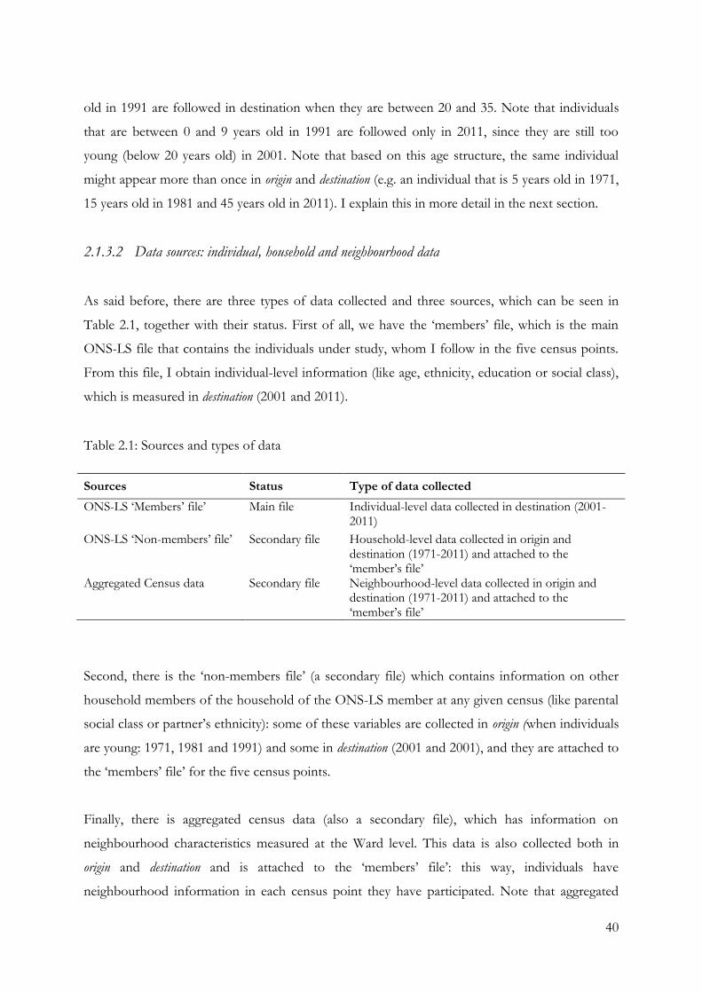
40

old in 1991 are followed in destination when they are between 20 and 35. Note that individuals

that are between 0 and 9 years old in 1991 are followed only in 2011, since they are still too

young (below 20 years old) in 2001. Note that based on this age structure, the same individual

might appear more than once in origin and destination (e.g. an individual that is 5 years old in 1971,

15 years old in 1981 and 45 years old in 2011). I explain this in more detail in the next section.

2.1.3.2 Data sources: individual, household and neighbourhood data

As said before, there are three types of data collected and three sources, which can be seen in

Table 2.1, together with their status. First of all, we have the ‘members’ file, which is the main

ONS-LS file that contains the individuals under study, whom I follow in the five census points.

From this file, I obtain individual-level information (like age, ethnicity, education or social class),

which is measured in destination (2001 and 2011).

Table ‎2.1: Sources and types of data

Sources Status Type of data collected

ONS-LS ‘Members’ file’ Main file Individual-level data collected in destination (2001-2011)

ONS-LS ‘Non-members’ file’ Secondary file Household-level data collected in origin and destination (1971-2011) and attached to the ‘member’s file’

Aggregated Census data Secondary file Neighbourhood-level data collected in origin and destination (1971-2011) and attached to the ‘member’s file’

Second, there is the ‘non-members file’ (a secondary file) which contains information on other

household members of the household of the ONS-LS member at any given census (like parental

social class or partner’s ethnicity): some of these variables are collected in origin (when individuals

are young: 1971, 1981 and 1991) and some in destination (2001 and 2001), and they are attached to

the ‘members’ file’ for the five census points.

Finally, there is aggregated census data (also a secondary file), which has information on

neighbourhood characteristics measured at the Ward level. This data is also collected both in

origin and destination and is attached to the ‘members’ file’: this way, individuals have

neighbourhood information in each census point they have participated. Note that aggregated

41

census data is not ONS-LS data, but external data collected by myself and other researchers10 and

then attached to the ONS-LS by the ONS team11.

2.1.4 Unit of analysis and samples

In all three chapters (Chapters 3, 5 and 6), the unit of analysis is not the individual but the pair of

origin-destination variables. This implies that, potentially, each individual could have up to 6

measurements; 1971-2001; 1971-2011; 1981-2001; 1981-2011; 1991-2001; 1991-2011. The total

number of cases allowing for up to 6 measurements per individual (which also means that

individuals have at least one measurement in origin and one measurement in destination) is

1,966,881. Of these, 472,925 (24%) are unique individuals.

But given the age restrictions observed in Figure 2.2, the maximum number of observations per

individuals is lower; in fact, individuals can be between 0 and 15 years of age in one or two

census-census points, but not in three. This reduces the possible number of measurements to up

to four, and applies to Chapter 3 and 5. In Chapter 6 an extra requirement is that individuals are

both present in 2001 and 2011, for which the maximum number of measurements is two. This is

better understood with an example.

Consider an individual who has participated in 4 census points and has complete information in

all of them. The information we study from this individual is as the one shown in Table 2.2.

Given that the individual is younger than 16 in two census points, we measure the origin

variables twice: in 1981 and in 1991. Furthermore, as this individual has also participated in 2001

and 2011, we measure outcomes in these both years. In Chapters 3 & 5 individuals need to have

at least one measure in origin and one measure in destination, for which this individual will appear

four times in the dataset. In Chapter 6, individuals need to have at least one measure in origin, but

two measures in destination, for which this individual will appear only twice in the data.

10Sources: Ethnic composition in the neighbourhood was obtained from http://casweb.mimas.ac.uk/ and https://neighbourhood.statistics.gov.uk/dissemination/. Carstairs deprivation data was obtained from Prof. Paul Norman, also a user of the ONS-LS data. 11 For a detail on the variables collected in origin and destination, as well as their status as dependent or independent variables, refer to Table 2.8.


https://neighbourhood.statistics.gov.uk/dissemination/

42

Table ‎2.2: The unit of analysis: example

Unit of analysis Origin Destination

1981 1991 2001 2011

age=3 age=13 age=23 age=33

Chapters 3 & 5

Unit 1 X X

Unit 2 X X

Unit 3 X X

Unit 4 X X

Chapter 6

Unit 1 X X X Unit 2 X X X

Given the age and destination-year restrictions, the so-called initial samples are the following: for

Chapters 3 & 5 the total sample is 432,756, of which around 40% are ‘unique’ individuals. For

Chapter 6 the total sample is 195,328, of which around 70% are unique individuals. Note that the

sample for Chapter 6 reduces to around half: part of this reduction is because some individuals

have only one value in destination, for which I drop them from Chapter 612; but most of this

difference in the number of cases occurs because individuals that are measured twice in

destination in Chapters 3 & 5 are measured only once in Chapter 6. This is also the reason why in

Chapter 6 much more cases are ‘unique’.

In the chapters themselves, the initial samples reduce to cover: 1) the ethnic groups under study,

that is, second generation ethnic minorities and the white British; 2) individuals who comply with

certain parental characteristics: in the case of the white British, individuals both of whose parents

were born in the UK (or one, for single-parent households) and in the case of ethnic minorities,

individuals both of whose parents were born abroad (or one, for single-parent households);

excluding therefore individuals who have “mixed parents” (i.e. one parent born abroad and one

born in the UK) as well as white British with foreign-born parents (or one, for single-parent

households) and ethnic minorities with UK-born parents (or one, for single-parent households)13;

3) individuals with valid information on all variables present in the analytical models (see Table

2.8 below for details on this). These are the so-called final samples. Both types of samples, as well

12 Note also that all individuals that have a value in origin also have a value in destination. 13 Refer to Tables 2.9 and 2.10 for a distribution of these categories and a comparison between individuals with mixed and non-mixed parents.

43

as the number of unique individuals in each of them are shown in Table 2.3, separated by

chapter.

Note that there are variations in the chapters in terms of the groups covered and the age

structure of the population. As regards groups covered, Chapters 3 and 6 include both ethnic

minorities (EM) and white British (WB) in the analysis, while Chapter 5 studies only ethnic

minorities. Note also some variations in terms of the ethnic groups: while in Chapter 3 the six

most numerous non-white ethnic minority groups are covered (Indian, Pakistani, Bangladeshi,

Chinese, Caribbean and African); in Chapters 5 and 6 Chinese are left outside. The reason for

this is that in Chapter 5 I use a measure of co-ethnics living in the origin neighbourhood that is

not available for Chinese; following this, and for comparative purposes, Chapter 6 only includes

groups that were studied in Chapter 5, since the topics of both chapters are very much related.

Table ‎2.3: Initial and final samples: pooled and unique cases

Chapter Sample Groups Parenthood Variables

All pop. WB 6 EM 5 EM All

types Not

mixed All

Valid values

Chapter 3

Initial Pooled 432756

X X

X

Unique 169923

Final Pooled 369477

X X

X

X Unique 143661

Chapter 5


X X

X

Unique 169923

Final Pooled 14287

X

X

X Unique 6300

Chapter 6


X X

X

Unique 139338

Final Pooled 161168

X X

X

X Unique 115951

Source: Author’s own calculations based on ONS-LS

Regarding the age structure, Chapters 3 & 5 include the population between 20 and 45 years old.

This is because I study outcomes in both 2001 and 2011, and I wanted to make the populations

more equal (recall from Figure 2.2 that people between 46 and 55 years old are only present in

2011). Chapter 6 studies outcomes only in 2011, for which I use the total number of cases

available. Table 2.4 contains the age distributions for each chapter.

44

Table ‎2.4: Age distributions by origin and destination years; initial sample

Age

Chapters 3 & 5 Chapter 6

2001 2011 2001

1971 1981 1991 1971 1981 1991 1971 1981 1991

20 5037 5338 6253 4263 4510

21 5722 5940 6036 4857 5043

22 5147 5259 5484 4447 4532

23 4400 4536 5272 3804 3910

24 4216 4277 5127 3653 3726

25 4502 4559 5783 3929 3963

26 5180 5645 4510

27 5530 5007 4846

28 5695 4837 5033

29 5771 5021 5086

30 5812 5968 4855 5138 5149 5278

31 6056 6136 5552 5776 5370 5439

32 6525 6642 5122 5229 5781 5877

33 6404 6521 4486 4610 5696 5809

34 6493 6539 4253 4346 5757 5811

35 6693 6777 4645 4658 5976 6049

36 6665 5282 5997

37 6852 5641 6195

38 6984 5827 6294

39 6638 5809 6022

40 6330 5911 6065 5756

41 5989 6073 6157 5463

42 6273 6477 6607 5714

43 6038 6370 6518 5493

44 5898 6422 6485 5336

45 5484 6520 6631 4954

Total 101134 89783 29909 37773 89935 84222 90953 78691 25684


As additional information, Tables 2.5 and 2.6 show the distributions of ethnic minorities and

white British in origin and destination years and in terms of the number of census-points in

which they have participated, respectively. These are shown for initial samples of Chapters 3 & 5

and Chapter 6.

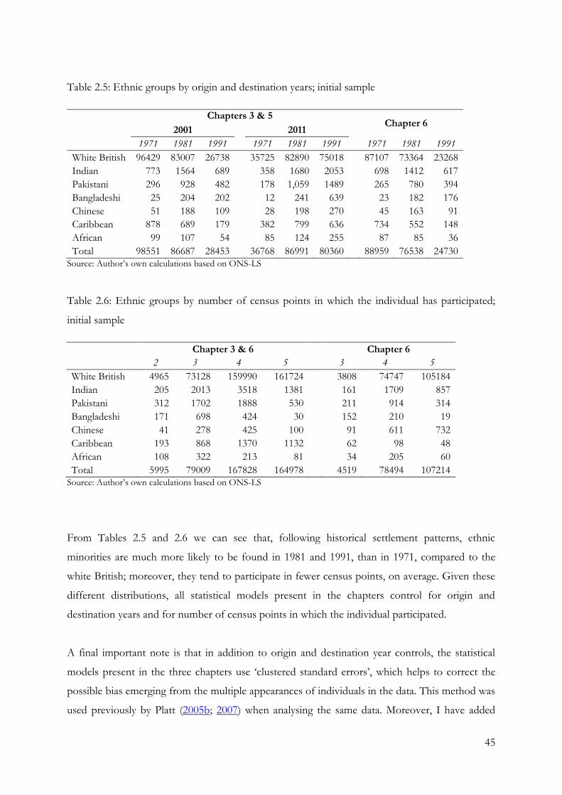
45

Table ‎2.5: Ethnic groups by origin and destination years; initial sample


2001 2011

1971 1981 1991 1971 1981 1991 1971 1981 1991

White British 96429 83007 26738 35725 82890 75018 87107 73364 23268

Indian 773 1564 689 358 1680 2053 698 1412 617

Pakistani 296 928 482 178 1,059 1489 265 780 394

Bangladeshi 25 204 202 12 241 639 23 182 176

Chinese 51 188 109 28 198 270 45 163 91

Caribbean 878 689 179 382 799 636 734 552 148

African 99 107 54 85 124 255 87 85 36

Total 98551 86687 28453 36768 86991 80360 88959 76538 24730


Table ‎2.6: Ethnic groups by number of census points in which the individual has participated;

initial sample

Chapter 3 & 6 Chapter 6

2 3 4 5 3 4 5

White British 4965 73128 159990 161724 3808 74747 105184

Indian 205 2013 3518 1381 161 1709 857

Pakistani 312 1702 1888 530 211 914 314

Bangladeshi 171 698 424 30 152 210 19

Chinese 41 278 425 100 91 611 732

Caribbean 193 868 1370 1132 62 98 48

African 108 322 213 81 34 205 60

Total 5995 79009 167828 164978 4519 78494 107214


From Tables 2.5 and 2.6 we can see that, following historical settlement patterns, ethnic

minorities are much more likely to be found in 1981 and 1991, than in 1971, compared to the

white British; moreover, they tend to participate in fewer census points, on average. Given these

different distributions, all statistical models present in the chapters control for origin and

destination years and for number of census points in which the individual participated.

A final important note is that in addition to origin and destination year controls, the statistical

models present in the three chapters use ‘clustered standard errors’, which helps to correct the

possible bias emerging from the multiple appearances of individuals in the data. This method was

used previously by Platt (2005b; 2007) when analysing the same data. Moreover, I have added

46

two Annexes at the end of the thesis with the following information. Annex B shows some

descriptive statistics of a random sample of ‘unique’ individuals chosen from the initial samples

used in Chapters 3 & 5 and Chapter 6, and compares it with the same statistics obtained from the

pooled data. Annex C explores more in detail variations based on origin and destination years by

means of replicating key analytical models in the chapters for the various origin/destination

years. Note that although some of these models still use clustered standard errors (those that

replicate models in Chapters 3 & 5), the number of multiple observations decreases to a

maximum of two, because I select either one origin year or one destination year (in the case of

replications made for Chapter 6 there are no multiple observations per individual when running

the models for different origin years, given that I only have one destination year).

2.1.5 A brief comment on attrition and sampling

As regards the issue of attrition, present in all data that have a panel-like structure, the following

problems can be posed. On the one hand, we could ask: are individuals who have information

both in origin and destination different from those who have information in origin only? If the

reasons why individuals that are present in both in origin and destination are related to any of the

outcomes under study, and if we do not measure these reasons, it could be argued that the results

are biased, because they are based on a self-selected sample. As a response to this question,

although not all individuals are present in all census points, all individuals that have information

in origin (be it 1971, 1981 or 1991) have also information in destination (be it 2001 or 2011),

which means no attrition in this respect.

On the other hand, and only for Chapter 6, we could also ask: are individuals who have

information in origin, 2001 and 2011 different from those who have information in origin and

2001 only; or in origin and 2011 only? Here the data shows that not all of individuals who have

information in 2001(2011) have also information in 2011(2001). I have therefore calculated some

descriptive statistics to see how different these groups are. Table 2.7 shows the distribution of

people with a Level 4+ of education and in the service class for various groups and years: those

who have information in 2001 only, those who have information for 2011 only; and those who

have information for both years (here I show the distribution for 2001 and 2011: the first to

compare with 2001 only; the second to compare with 2011 only). The table is calculated with the

age restrictions used in Chapter 6 (i.e. individuals between 0 and 15 in each origin year, and with

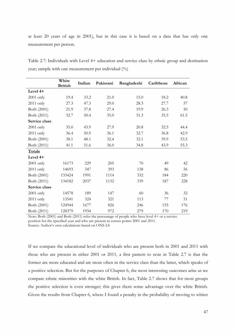
47

at least 20 years of age in 2001), but in this case it is based on a data that has only one

measurement per person.

Table ‎2.7: Individuals with Level 4+ education and service class by ethnic group and destination

year; sample with one measurement per individual (%)

White British

Indian Pakistani Bangladeshi Caribbean African

Level 4+

2001 only 19.4 33.2 21.0 15.0 18.2 40.8

2011 only 27.3 47.3 29.0 28.3 27.7 57

Both (2001) 21.9 37.8 27.4 19.9 26.3 50

Both (2011) 32.7 50.4 35.0 31.3 35.5 61.5

Service class

2001 only 35.0 43.9 27.9 20.8 32.5 44.4

2011 only 36.4 50.9 36.1 32.7 36.8 42.9

Both (2001) 38.1 48.1 32.4 32.1 39.9 53.5

Both (2011) 41.1 51.6 36.0 34.8 43.9 55.3

Totals

Level 4+

2001 only 16173 229 205 70 49 42

2011 only 14693 347 393 138 86 56

Both (2001) 133424 1991 1114 332 184 220

Both (2011) 134182 2037 1132 339 187 228

Service class

2001 only 14578 189 147 60 36 32

2011 only 13541 324 321 113 77 51

Both (2001) 124944 1677 826 246 155 176

Both (2011) 128379 1934 972 279 170 219

Note: Both (2001) and Both (2011) refer the percentage of people who have level 4+ or a service position for the specified year and who are present in census points 2001 and 2011. Source: Author’s own calculations based on ONS-LS

If we compare the educational level of individuals who are present both in 2001 and 2011 with

those who are present in either 2001 or 2011, a first pattern to note in Table 2.7 is that the

former are more educated and are more often in the service class than the latter, which speaks of

a positive selection. But for the purposes of Chapter 6, the most interesting outcomes arise as we

compare ethnic minorities with the white British. In fact, Table 2.7 shows that for most groups

the positive selection is even stronger; this gives them some advantage over the white British.

Given the results from Chapter 6, where I found a penalty in the probability of moving to whiter

48

areas for ethnic minorities, the values from Table 2.7 suggest that this penalty might actually be

higher, given that I am leaving outside the less-educated/lower-status minorities.

Finally, as additional information connected to sampling, is interesting to see to what extent the

distributions of cases in ONS-LS follows the distribution of the ‘real population’. Figure 2.3

compares the levels of employment (vs. unemployed and some inactive groups) and of service

class positions (vs. other occupations, present or past) for each ethnic minority group in 2011

using two sources of information: the ONS-LS and the census table obtained from the Office for

National Statistics, which refers to the entire population of England and Wales. In practice, I am

comparing the outcomes observed in Table 3.4 from Chapter 3 (but pooling genders) with the

outcomes for UK born individuals observed in Figures 1.10 and 1.11 from Chapter 1. Note that

the main difference between the two populations is that in the case of the census data I am not

considering foreign-born individuals who arrived at a young age in the UK (i.e. the so-called

generation 1.5). Figure 2.3 shows that the distribution of employment and service positions for

the various groups in the ONS-LS tends to follow the distribution observed in the census;

however, in most of cases, there seems to be a positive selection of individuals in the ONS-LS.

Figure ‎2.3: Employment and access to the service class by ethnic group: census data and ONS-LS

compared (%) (2011).

Source: Author’s own calculations based on ONS-LS and aggregated census data

84 86

67 66

86 81 82

40

56

38 35

54

43 47

82 84

64 65

86

74 76

36

52

35 35

53

39

51

00

10

20

30

40

50

60

70

80

90

100% Employed % Service class

ONS-LS

CENSUS

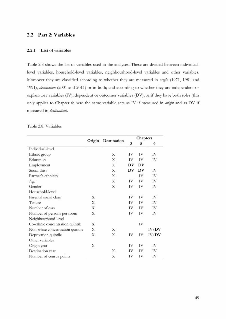
49

2.2 Part 2: Variables

2.2.1 List of variables

Table 2.8 shows the list of variables used in the analyses. These are divided between individual-

level variables, household-level variables, neighbourhood-level variables and other variables.

Moreover they are classified according to whether they are measured in origin (1971, 1981 and

1991), destination (2001 and 2011) or in both; and according to whether they are independent or

explanatory variables (IV), dependent or outcomes variables (DV), or if they have both roles (this

only applies to Chapter 6: here the same variable acts as IV if measured in origin and as DV if

measured in destination).

Table ‎2.8: Variables

Origin Destination

Chapters

3 5 6

Individual-level

Ethnic group X IV IV IV

Education X IV IV IV

Employment X DV DV

Social class X DV DV IV

Partner’s ethnicity X IV IV

Age X IV IV IV

Gender X IV IV IV

Household-level

Parental social class X IV IV IV

Tenure X IV IV IV

Number of cars X IV IV IV

Number of persons per room X IV IV IV

Neighbourhood-level

Co-ethnic concentration quintile X IV

Non-white concentration quintile X X IV/DV

Deprivation quintile X X IV IV IV/DV

Other variables

Origin year X IV IV IV

Destination year X IV IV IV

Number of census points X IV IV IV

50

2.2.2 Individual-level variables

2.2.2.1 Ethnic group and second generation

The analyses contained in Chapters 3, 5 and 6 are made for six ethnic minorities: Indian,

Pakistani, Bangladeshi, Caribbean, African and Chinese (the latter group only for Chapter

3); moreover, Chapters 3 and 6 also include the white British. The construction of the groups is

based on two variables: ethnic self-identification and country of birth of the parent(s).

Ethnic self-identification is measured in 2011 and, when missing, self-identification in 2001 is

used. In 2011 the question is formulated as follows: “What is your ethnic group?” The options

are: White (English/Welsh/Scottish/Northern Irish/British; Irish; Gypsy or Irish traveller; other

White); Mixed/multiple ethnic groups (White and Black Caribbean; White and Black African;

White and Asian; any other Mixed/multiple ethnic background, open question); Asian/Asian

British (Indian, Pakistani, Bangladeshi, Chinese; any other Asian background, open question);

Black/African/Caribbean/Black British (African; Caribbean; any other Black/African/Caribbean

background, open question); Other ethnic group (Arab; any other ethnic group). Note that the

‘Gypsy or Irish traveller’ and ‘Arab’ categories were not separately specified in the 2001 Census

form. The parental country of birth is measured in origin, that is, when individuals are between 0

and 15 years old. I differentiate between individuals with both parents born in the UK (one

parent, in the case of single-parent households) and those with both parents born abroad (one

parent, in the case of single-parent households).

In this study, white British are those who identify themselves as white

British/English/Scottish/North Irish and have both parents (or one parent, in case of

individuals raised in single-parent origin households) born in the UK. Ethnic minorities, on the

other hand, are those who identify themselves as belonging to each of the main ethnic groups

and have one (in case of single-parent origin households) or two parents born abroad. Individuals

in mixed households, that is, individuals in households where one parent is born abroad and the

other in the UK are therefore excluded from the analysis. White British with foreign-born

parents (or a foreign-born parent in case of single-parent households) and ethnic minorities with

UK-born parents (or a foreign-born parent in case of single-parent households) are also

excluded. Finally, note as well that individuals who consider themselves as ‘half white’ in terms of

ethnic identity are not part of this study either. These decisions aim at having a ‘cleaner’ version

51

of ‘white British’ and ‘second generation migrants’. In particular, my sample of ethnic minorities

includes individuals who define themselves as belonging solely to a single ethnic group and who

have parents who immigrated to the UK (note that among single-parent households we cannot

know this for sure, since the country of birth of the missing parent is not available14). Table 2.9

shows the distribution of ethnic groups in origin households with different characteristics.

Table ‎2.9: Individuals in various origin households by ethnic group; initial sample (column %)

White British Indian Pakistani Bangladeshi Caribbean African Chinese

Both UK-born 81.3 1.3 2.4 1.6 2.1 1.4 1.3

Both foreign 1.1 89.8 86.4 87.0 59.3 62.6 88.8

Both mixed 5.2 3.6 3.1 1.5 2.5 3.7 4.2

Single UK-born 11.8 0.4 0.6 0.8 11.8 5.0 0.0

Single foreign 0.5 4.9 7.4 9.1 24.3 27.4 5.7

Total 511563 8843 5555 1718 4576 956 1043


Table 2.9, based on the initial sample of Chapters 3 & 5, shows that most individuals were raised in

households where both parents are present: in the case of the white British, these are two UK-

born parents; in the case of ethnic minorities, these are two foreign-born parents. These

proportions, however, are much smaller for black populations: in fact, more than 30% of black

Caribbean and Africans were raised in single-parent households (mostly foreign). As a robustness

check, I have explored for each chapter whether including a dummy for single-parent households

changed the results of the main analytical models: it did not. Moreover, and under the

assumption that having been raised in a single-parent household might affect ethnic minorities

and white British differently, I have also estimated interaction effects between ethnicity and

single-parent households in the study of employment (tables available upon request). Again, I did

not find substantive differences between groups. This topic is not further explored in the thesis;

although I am aware that it would certainly deserve more attention in future research.

Only for those who had information on both parents, I have also explored some basic socio-

economic characteristics of those who belong to mixed and non-mixed households, in order to

determine if those raised in non-mixed households are different from those raised in mixed ones.

In particular, it could be argued that ethnic minorities with non-mixed parents are negatively

14 Notice, however, that most individuals that declare themselves as ‘half white’ have at least one UK-born parent.

52

selected (because the parents have decided to marry or cohabit with another foreigner, usually a

co-ethnic), while white British with non-mixed parents are positively selected (because the

parents have decided to marry or cohabit with another UK-born). Table 2.10 shows the

percentage of individuals who have low class parents (Manual + No earners/no code) and

individuals who have reached the service class according to whether they have mixed parents or

not.

Table ‎2.10: Parental social class and access to the service class for mixed/non-mixed parents;

initial sample (column %)

White British Indian

Pakistani & Bangladeshi

Caribbean & African

Chinese

Low parental class

Non-mixed 42.6 56.1 76.7 59.7 34.7

Mixed 36.4 42.4 55.8 32.4 22.7

Service class

Non-mixed 37.8 51.2 34.7 41.4 51.8

Mixed 45.0 42.2 23.6 38.5 43.5

Totals

Low parental class

Non-mixed 476499 8374 6862 4686 982

Mixed 26765 321 199 148 44

Service class

Non-mixed 400521 6190 4432 3833 677

Mixed 22649 154 55 78 23

Note: The non-mixed category here includes all categories that are not mixed, but excludes (as it is excluded in the thesis) white British with foreign-born parents (or one, in case of single-parent households) and ethnic minorities with both (single) UK born parents (perhaps it would have been useful to include Caribbean and African in ‘Single UK’ households in the ‘Mixed’ category, but it is not possible at this point). Source: Author’s own calculations based on ONS-LS

The results show that having mixed parents benefits ethnic minorities in terms of the parental

social class, which is higher on average; interestingly, the white British also benefit from this.

However, as we look at the results on the social class of individuals, we observe that while the

white British with mixed parents are doing better that those with non-mixed parents, among

ethnic minorities the opposite occurs: they are in the service class in a higher proportion if they

have non-mixed parents. If we compare ethnic minorities with the white British, we can see that

although having non-mixed parents puts them in a worst relative position in terms of parental

social class, they are in a much better position with regard to the acquired social class. This

53

evidence suggests that the negative selection of ethnic minorities only occurs at the parental level,

but not at the individual level (note however that the number of cases is very small for individuals

with mixed parenthood).

Following the same arguments, leaving outside individuals who consider themselves as ‘half

white’ might also imply that I am leaving outside a positively selected sample of individuals who

either consider themselves as ‘half white or half British’ or who have a white (British) parent,

with the benefits this might incur (this is the case mostly of ‘white Caribbean’). All these

differences based on the ethnicity of the individuals, the parental country of birth and whether

only one or both parents are present in the origin household, are issues that have not been delved

into in this thesis, but which for sure would deserve more detailed analyses. I shall just say that

the results presented in the coming chapters represent how the majority of individuals and groups

is doing.

Finally, another important clarification needs to be made. We saw in the previous section that

this study covers individuals that were between 0 and 15 years old in any of the three origin years,

and that lived with at least one parent at the time of measurement. This means that we could

have two types of individuals: those who were born in the UK, and those who arrived at age 15

or earlier. While, in the case of ethnic minorities, the former can be strictly called second

generation, the second has been referred to as generation 1.5. Note that in the chapters, I refer to

both of them as “second generation.” Table 2.11 shows the distribution of the groups depending

on whether they were born in the UK or abroad, by origin year.

Table ‎2.11: Individuals born in the UK, by ethnic group and origin year (%)

White British Indian Pakistani Bangladeshi Caribbean African Chinese

1971 98.8 61.1 64.1 54.1 89 91.8 74.7

1981 98.7 81.6 72.3 42.2 97.6 84.7 77.6

1991 98.8 95.2 83.8 51.9 97.4 64.2 79.9

Totals

1971 132123 1130 474 37 1260 184 79

1981 165321 3205 1976 443 1484 229 379

1991 100622 2665 1946 836 805 299 369


54

Table 2.11 shows that most of individuals in the sample are born in the UK; however, important

differences remain, based on the origin year and on the ethnic group. In particular, Bangladeshis,

who are among the most recent immigrants in the UK, have high proportions of individuals born

abroad (around half of them). Moreover, Asian groups measured in 1971 are less likely to be

born in the UK.

Although the models control for origin year, they do not control for whether individuals were

born abroad or not. Why might this be relevant? Thinking of ethnic minorities, a main difference

between those born in the UK and those born abroad is that the former entered the educational

system from the beginning, while the latter may have, but did not necessarily do so: therefore,

not only is it possible that their school socializations varied (those who arrived at later ages might

not even have a schooling experience in the UK at all), but this might make a difference for

employers, who might be unable to recognize a foreign title (even if this is a primary/lower

secondary school title). Given the figures in Table 2.11, we might think that Bangladeshis are the

most affected by this. In order to explore this issue, I have tested in the main analytical models

whether including a dummy for individuals born in the UK made a difference in the results: it did

not. Moreover, I have also estimated key models for UK born individuals only: although I found

differences in the models with respect to those present in the thesis, the main results do not

change substantively (tables available upon request). This does not necessarily mean that those

born in the UK are doing exactly the same as those born abroad: from a theoretical point of

view, we could expect that the former are doing better. However, differences might not be as big;

or perhaps we would need more cases in order to make a proper test (which might be particularly

relevant for Pakistani and Bangladeshi populations). This remains to be explored in the future.

2.2.2.2 Education

The level of education of individuals is measured with the following scale:

No academic or professional qualifications

Other qualifications/level unknown (other qualifications – e.g. City and Guilds etc.; other professional qualifications

Level 1: CSEs (grades 2-5), GCSEs (grades D-G), 1-4 CSEs (grade 1), 1-4 GCSEs (grades A-C), 1-4 O levels, NVQ level 1, Foundation GNVQ

Level 2: 5+O levels, 5+CSEs (grade1), 5+GCSEs (grades A-C) etc, 1 A level, 1-3 AS levels, NVQ level 2, Intermediate GNVQ

55

Level 3: 2+ A levels, 4+ AS levels, Higher School Certificate, NVQ level 3, Advanced GNVQ

Level 4+: First degree, Higher degree, NVQ levels 4-5, HNC, HND. Qualified Teacher status, Qualified Medical Doctor, Qualified Dentist, Qualified Nurse, Midwife, Health Visitor

In this classification, Level 1 refers to individuals that have reached primary education or lower

levels of secondary education; levels 2-3 represent intermediate levels of secondary education;

and level 4+ represents higher education. In all chapters, individuals with “no” and “other”

classifications are pooled together; moreover, in Chapters 3 and 4, which have less number of

cases, I pool together these two with those who have Level 1 education, and also merge Levels 2

and 3.

2.2.2.3 Employment

Employment is measured as the percentage of people who are currently employed with respect to

unemployed and (some) inactive groups: individuals doing housework, long term disabled and

other inactive. The reason for including inactive groups in the comparison category is that they

might be speaking of additional disadvantages, like being discouraged in the search of

employment or being constrained in the possibilities of working.

Table 2.12 shows the distribution of various active/inactive positions by ethnic group. In

particular, it shows that Pakistani and Bangladeshi men are more likely than the white British to

be in other inactive groups, and Pakistani and Bangladeshi women are much more likely to be

doing housework or being permanently sick. Note also that ethnic minorities are generally more

likely to be students as compared to the white British, which is a product of the younger age

composition of these groups. However, students are excluded from the analyses present in

Chapters 3, 5 and 6 (by default, they are part of Chapter 4, based on aggregated census data).

56

Table ‎2.12: Economic activity by ethnic group; initial sample

White British


Men

Employed 84.8 78.5 67.9 69.4 79.2 72.8 65.7

Unemployed 5.1 6.1 10.1 10.8 4.2 11.0 9.1

Retired 0.1 0.0 0.0 0.0 0.0 0.0 0.0

Student 3.7 10.5 11.2 12.4 16.6 6.2 18.8

Housework 0.9 0.5 2.0 1.6 0.0 1.6 0.0

Perm. sick 3.5 1.9 3.1 2.1 0.0 3.3 3.2

Other 1.9 2.6 5.7 3.7 0.0 5.1 3.2

Total 193516 3539 2110 621 380 1578 309

Women

Employed 73.6 71.3 45.7 43.8 73.1 71.0 68.3

Unemployed 3.4 4.2 6.2 9.0 2.8 7.3 8.2

Retired 0.1 0.0 0.0 0.0 0.0 0.0 0.0

Student 4.6 11.1 10.5 8.4 12.5 7.4 12.4

Housework 12.8 8.9 25.8 27.1 7.0 8.2 4.2

Perm. sick 3.3 2.1 4.5 3.5 2.3 2.8 2.5

Other 2.3 2.5 7.2 8.2 2.3 3.4 4.5

Total 204116 3444 2268 691 431 1962 404


2.2.2.4 Social class

The social class of individuals is measured with the National Statistics Socio-Economic

Classification (NS-SEC). This classification is based on the Erikson and Goldthorpe class schema

(Erikson and Goldthorpe 1992) and was constructed to measure the employment relations and

conditions of occupations. Although occupationally based, the NS-SEC seeks to identify typical

‘employment relations’. Among employees, there are quite diverse employment relations: they

differ in terms of income, economic security and prospects of economic advancement (labour

market situation), and also in terms of location in systems of authority and control at work (work

situation).

Within the NS-SEC, there are three main forms of employment relations. In the service

relationship, “the employee renders service to the employer in return for compensation, which

can be both immediate rewards (for example, salary) and long-term or prospective benefits (for

57

example, assurances of security and career opportunities). The service relationship typifies Class 1

and is present in a weaker form in Class 2”(Office for National Statistics 2010: pp. 3). In the

labour contract, “the employee gives discrete amounts of labour in return for a wage calculated

on the amount of work done or time worked. The labour contract is typical in Class 7 and, in

weaker forms, in Classes 5 and 6” (ibid). Finally, the intermediate form “combines aspects from

both the service relationship and labour contract, and are typical in Class 3” (ibid).

Table ‎2.13: The NS-SEC and applications to Chapters 3, 5 and 6

NSSEC Chapters 3 & 5

Chapter 5 Chapter 6

1 Higher managerial, administrative and professional occupations, including large employers Service class

Avoidance of lowest occupations

Service class

2 Lower managerial, administrative and professional occupations

3 Intermediate occupations

(Comparison category)

Intermediate

4 Small employers (<25 employees) and own account workers

Petit bourgeoisie

5 Lower supervisory and technical occupations

Manual 6 Semi-routine occupations (Comparison category) 7 Routine occupations

8 Never worked and long-term unemployed

(Excluded) (Excluded) (Excluded)

- Full-time students (active or inactive) (Excluded) (Excluded) (Excluded)

Table 2.13 shows the NS-SEC categories and how I have collapsed them. In Chapters 3 and 5,

the NS-SEC is one of the dependent variables studied, while in Chapter 6 it is a mediating or

independent variable. As a dependent variable, the categories are collapsed to study the “access

to the Service class”, which has been used in many studies on ethnic penalties and social mobility

in the UK (Cheung and Heath 2007b; Heath and Li 2010; Platt 2007). The reference categories

are all individuals with a valid NSSEC outside categories 1 and 2. These are: intermediate

occupations, the petit bourgeoisie and the so-called manual occupations (which however may

involve supervisory tasks). Moreover, Chapter 5 also studies ‘avoidance of lowest occupations’:

given the strong link between the presence of ethnic minorities in a neighbourhood and the low

social class of individuals, I also test to what extent living in areas with more co-ethnics prevents

(or not) individuals from having in semi-routine and routine class outcomes (the lowest

occupations in the social class scale), even after controlling for other background characteristics.

58

In Chapter 6, finally, all categories of NS-SEC are explored, but emphasis is put on the difference

that makes having a Service class vs. a Manual class.

The NS-SEC is available for those who are currently employed or had a job in the past (and are

currently inactive or short-term unemployed): I have considered both measurements as a way to

determine the social status of a person, even if he/she is not working at the time. Note that in

this classification, long-term unemployed individuals, that is, unemployed who had their last job

more than one year ago are a separate category and, therefore, are not assigned an occupation

within the NS-SEC: I have excluded them from the analysis of social class. Although this might

bring some bias, since ethnic minorities are more likely to be found in this category, I have done

robustness checks by assigning long-term unemployed a crude occupation – based on the

classification of occupations SOC 2000 and 201015 – and the results did not change substantially.

I reached similar results by doing the same checks for full-time students who had done a job in

the past or declared to work while studying (analyses available upon request).

2.2.2.5 Other individual-level variables

Other individual-level variables are gender (male/female) and age. Note that given the presence

of age mismatches, priority was given to the age declared in 2011 and then to the one declared in

2001. I have used this age to create all above-mentioned age filters.

2.2.3 Household-level variables

2.2.3.1 Parental social class

The parental social class is available through a 7-category class schema whose members broadly

share similar market and work situations, and which is based upon the 36 categories of the Hope-

Goldthorpe scale (Goldthorpe and Hope 1974)16. The class schema was devised for men, but is

widely used for both men and women. The categories are shown in Table 2.14; here it is also

possible to see how the reduced version (used in all Chapters) is created.

15 Refer to: http://www.ons.gov.uk/ons/guide-method/classifications/archived-standard-classifications/standard-occupational-classification-2000/about-soc-2000/index.html and http://www.ons.gov.uk/ons/guide-method/classifications/current-standard-classifications/soc2010/index.html. 16 This is the only social class measure available and harmonized for the three origin years (1971, 1981 and 1991).

http://www.ons.gov.uk/ons/guide-method/classifications/archived-standard-classifications/standard-occupational-classification-2000/about-soc-2000/index.html

http://www.ons.gov.uk/ons/guide-method/classifications/archived-standard-classifications/standard-occupational-classification-2000/about-soc-2000/index.html

http://www.ons.gov.uk/ons/guide-method/classifications/current-standard-classifications/soc2010/index.html

http://www.ons.gov.uk/ons/guide-method/classifications/current-standard-classifications/soc2010/index.html

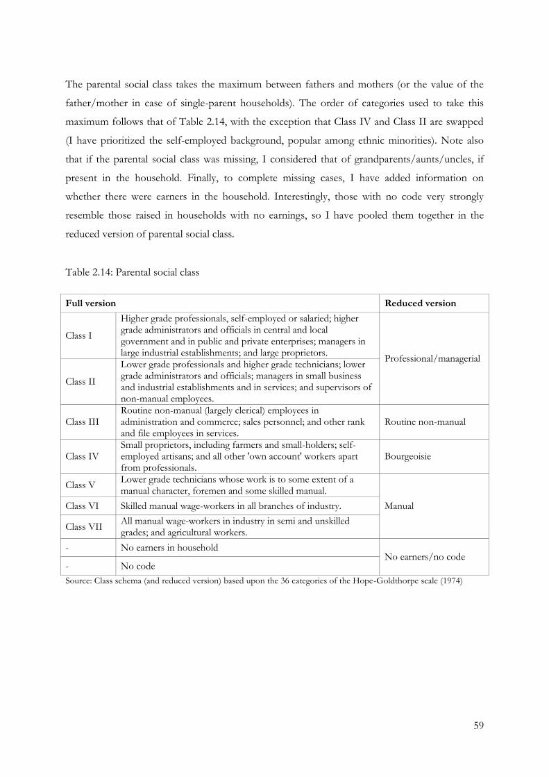
59

The parental social class takes the maximum between fathers and mothers (or the value of the

father/mother in case of single-parent households). The order of categories used to take this

maximum follows that of Table 2.14, with the exception that Class IV and Class II are swapped

(I have prioritized the self-employed background, popular among ethnic minorities). Note also

that if the parental social class was missing, I considered that of grandparents/aunts/uncles, if

present in the household. Finally, to complete missing cases, I have added information on

whether there were earners in the household. Interestingly, those with no code very strongly

resemble those raised in households with no earnings, so I have pooled them together in the

reduced version of parental social class.

Table ‎2.14: Parental social class

Full version Reduced version

Class I

Higher grade professionals, self-employed or salaried; higher grade administrators and officials in central and local government and in public and private enterprises; managers in large industrial establishments; and large proprietors.

Professional/managerial

Class II

Lower grade professionals and higher grade technicians; lower grade administrators and officials; managers in small business and industrial establishments and in services; and supervisors of non-manual employees.

Class III Routine non-manual (largely clerical) employees in administration and commerce; sales personnel; and other rank and file employees in services.

Routine non-manual

Class IV Small proprietors, including farmers and small-holders; self-employed artisans; and all other 'own account' workers apart from professionals.

Bourgeoisie

Class V Lower grade technicians whose work is to some extent of a manual character, foremen and some skilled manual.

Manual Class VI Skilled manual wage-workers in all branches of industry.

Class VII All manual wage-workers in industry in semi and unskilled grades; and agricultural workers.

- No earners in household No earners/no code

- No code

Source: Class schema (and reduced version) based upon the 36 categories of the Hope-Goldthorpe scale (1974)

60

2.2.3.2 Other household-level variables in origin

Other household variables measured in origin are tenure, number of cars and number of persons

per room, which have the following categories:

Tenure: owner, social rent and private rent

Number of cars: 0, 1 and 2+

Number of persons per room (ppp): over 1.5 ppp; 1.5 ppp; over 1 but less than 1.5 ppp;

over 0.75 but less than 1 ppp; 0.75 ppp; over 0.5 but less than 0.75 ppp; and 0.5 ppp

These variables are introduced with the aim of having a better picture of the socio-economic

conditions of origin. Note that in the case of the number of cars, I have transformed the

continuous variable into a categorical variable with three categories; moreover, I have used a

reduced version of the number of persons per room for Chapters 5 and 6, given the low number

of cases for some categories (refer to the chapters for a detail on this).

2.2.3.3 Partner’s ethnicity

Chapters 5 and 6 include the partner’s ethnicity in the analysis. This information is obtained in

destination, by attaching household information to the individual (note that this is also a self-

defined ethnicity, but here I do not replace the ethnicity of 2001 with that of 2011).

Two types of measures are used. In Chapter 5 the analysis is only done for ethnic minorities and

I have used a measure that differentiates between having (or not) a co-ethnic partner. A co-ethnic

partner is a partner that has exactly the same ethnicity as the respondent: i.e. Indian, Pakistani,

Bangladeshi, Caribbean or African. In Chapter 6 I was more interested in estimating the effect of

having a white British partner. Therefore, I have differentiated between having a white British

partner, a non-white partner or other. A ‘non-white partner’ is a partner that has declared to be

Asian/Asian British, Black/African/Caribbean/Black British or other non-white (including Arab

in 2011). The category ‘other’ includes those who self-declare to be white (but not British) and

those who have mixed/multiple ethnicity. The two variables with their categories are therefore

the following. For Chapter 5: no partner, co-ethnic and other (includes white and non-white); for

Chapter 6: no partner, white British, non-white and other (includes other white and

mixed/multiple ethnicity)

61

2.2.4 Neighbourhood-level variables

Neighbourhood-level variables classify neighbourhoods for each individual in each census point

in terms of deprivation and number of ethnic minorities. The variables were constructed by

means of linking aggregated census data obtained at the Ward level to individuals in the ONS

Longitudinal Study in each of the census-census points. Specifically:

i. Using aggregated census data, census Wards were first classified according to: their level

of deprivation; the number of non-white ethnic minorities; and the number of each

ethnic minority group in them (only for five minority groups: Indian, Pakistani,

Bangladeshi, Caribbean and African). This led to 7 aggregated census variables (note that

due to a limitation imposed by the Office for National Statistics, only quintiles were

created).

ii. In the second place, this information was attached to individuals (job carried out by the

Office for National Statistics). This means that each unit of analysis in the ONS-LS has

been allocated in each census point: a (population weighted) deprivation quintile, a

(population weighted) non-white concentration quintile and a (population weighted (co-)

ethnic concentration quintile.

In what follows, I describe how neighbourhood data on ethnicity and deprivation was created,

before its linkage to ONS-LS data: the focus is then on point i), although we will see that for the

co-ethnic concentration variable, both information on aggregated census data and ONS-LS data

was needed.

2.2.4.1 What are Wards? Main characteristics and population

The Ward is the key building block of UK administrative geography, being the geographical unit

used to elect local government councillors in metropolitan and non-metropolitan districts, unitary

authorities and the London boroughs in England and unitary authorities in Wales. Wards can be

very varied in terms of the population they contain and their size. In general, the smallest and

most populous ones are in metropolitan areas, where the majority of ethnic minorities are found;

while in the countryside, where people are more disperse, Wards tend to be bigger and less

populated. Wards are also subject to change over time. In fact, the fundamental principle of

ward/division organization is electoral equality, meaning that within a higher administrative area,

62

each elector's vote bears a similar weight. As population sizes in Wards should be approximately

equal within a certain higher administrative area, and because people are constantly moving, so

the boundaries need frequent review and alteration. In some years several hundred electoral

wards or divisions are affected, and in the extreme case of 2002 no fewer than 1,549 got changed

(Office for National Statistics; from http://www.ons.gov.uk/ons/guide-

method/geography/beginner-s-guide/administrative/our-changing-geography/boundary-

changes/index.html).

Table 2.15 shows, for each census point and for all and non-white (NW) population respectively,

three sets of information: the total population and the total number of Wards in which they are

found (set 1), the characteristics of Wards in terms of the size of their populations (set 2) and the

distribution of populations across Wards (set 3). In set 2 we see the average population in Wards,

the minimum and maximum population in Wards and percentiles 50, 75 and 90, which should be

read as follows: “up to 50/75/90% of Wards have a population of X individuals or less”. The

third set of descriptives (set 3) shows three percentiles that should be read as follows: up to

50/75/90% of Wards contain X% of the population; moreover, the number of individuals living

in the most populated Wards (these are those above percentile 90: for example, in 1991, Wards

that have a population of 10789 or more) are shown.

There are various elements worth noting in Table 2.15. First of all, the number of Wards has

changed dramatically between 1971 and the rest of the census-census points: from 1981 onwards

Wards have reduced to almost half, moving from 16063 in 1971 to around 8570 in 2011. With

the reduction of Wards, the average population in each of them has, as expected, increased.

However, the maximum number of total individuals in each Ward has not: on the contrary, even

though Wards are very unequal in terms of the population they contain, they have tended to

become slightly more equal after 1971. Moreover, note that the maximum number of non-white

population per Ward has increased over time, approaching the maximum number observed for

the total population. This is a first indication of the weight of non-white population in England

and Wales. Other important information contained in Table 2.15 is that non-whites are

concentrated in a smaller number of Wards as compared to the entire population (mainly in

metropolitan areas, as shown in Chapter 2). Moreover, they are also more likely to be found in

the most populated Wards.

63

Tab

le ‎2

.15: C

har

acte

rist

ics

of

Cen

sus

War

ds

1971

19

81

1

991

2001

2

011

A

ll

NW

A

ll

NW

A

ll

NW

A

ll

NW

A

ll

NW

Set

1

Po

pula

tio

n

47496022

1086366

48521382

1473659

49890476

2952022

52041636

3859855

56075912

6642117

# W

ards

16063

11914

9300

9222

9509

9340

8850

8610

8570

8563

Set

2:

po

pu

lati

on

in

Ward

s

Aver

age

2957

68

5217

158

5247

310

5880

436

6543

775

Min

. 1

0

1

0

77

0

106

0

136

0

Max

. 40719

10238

41875

8683

31617

18856

35102

25398

36412

27950

Per

cen

tile

50

876

4

4108

32

4247

37

4821

48

5251

104

Per

cen

tile

75

4216

24

6796

94

6955

144

7688

194

8726

443

Per

cen

tile

90

8796

107

11032

327

10789

721

11890

1026

13196

2085

Set

3:

dis

trib

uti

on

of

po

pu

lati

on

P

erce

nti

le 5

0 5.1

%

3.5

%

21.2

%

6.8

%

22.5

%

2.9

%

24.5

%

2.6

%

24.8

%

3.1

%

Per

cen

tile

75

23.8

%

12.7

%

46.9

%

16.2

%

48.8

%

9.3

%

50.1

%

8.7

%

50.1

%

10.7

%

Per

cen

tile

90

55.3

%

25.0

%

71.9

%

31.3

%

73.4

%

25.2

%

75.0

%

24.1

%

75.1

%

30.7

%

Po

p. in

mo

st

po

pula

ted

War

ds

21254850

(45%

) 737704

(68%

) 13660399

(28%

) 594185

(40%

) 13258812

(27%

) 1278567

(43%

) 13025249

(25%

) 1917118

(50%

) 13981709

(25%

) 3628410

(55%

)

So

urc

e: A

uth

or’

s o

wn

cal

cula

tio

ns

bas

ed o

n a

ggre

gate

d C

ensu

s d

ata

for

En

glan

d a

nd

Wal

es (

fro

m h

ttp

://

casw

eb.m

imas

.ac.

uk a

nd

ww

w.n

eigh

bo

urh

oo

d.s

tati

stic

s.go

v.u

k).



64

An important note is that no lookups are available to make the translation from the ‘Ward

geography’ of a certain year to the ‘Ward geography’ of another year. This means that the

neighbourhood information attached to individuals at each census point is based on different

census geographies. As a consequence, if an individual belongs to a neighbourhood with the

worst deprivation level (Quintile 5) in 1991 and then moves to a Quintile 3 in 2001, we cannot

really disentangle if this change is the product of: a residential movement, an improvement of the

Ward itself, or a change in the limits of the Ward. This is a limitation of the data, which however

has only a small impact in terms of my research questions.

2.2.4.2 Non-white and (co-)ethnic concentration quintiles

In order to create the non-white and ethnic concentration quintiles I used the best available

measure of ethnicity for each census point: in 1971 and 1981 this is the country of birth; from

1991 onwards, this is the ethnic self-identification. Unfortunately, the question on ethnic identity

is not present in the first two census-census points, although it is likely that an important part of

ethnic minorities in these years are born abroad (therefore being either first or 1.5 generations,

that is, young children that emigrated with their parents). The information used to create these

quintiles was obtained at: http://casweb.mimas.ac.uk/ (for 1971, 1981 and 1991) and

http://www.neighbourhood.statistics.gov.uk/ (for 2001 and 2011).

Table 2.16 shows the variables I used to create the non-white and ethnic concentration quintiles

in each census point. Note that for the creation of “co-ethnic concentration quintiles” I have

attached the neighbourhood variable to the (self-declared) ethnicity of individuals in the ONS LS:

Indian, Pakistani, Bangladeshi, Caribbean and African (it was not possible to have a co-ethnic

concentration measure for Chinese). Two comments on this: first of all, in 1971 it is not possible

to exclude East Africa, from where many Indians come from. This means, on the one hand, that

in 1971 I only capture neighbourhoods where Indians live with others that come from India, but

not from East Africa; and, on the other, that African neighbourhoods (attached to self-identified

African) might have some Indians as well. Secondly, in 1971 Bangladesh was still not an

independent state, but was part of Pakistan. Therefore, Bangladeshi neighbourhoods in 1971 are

neighbourhoods where people come from Pakistan (which are then attached to self-identified

Bangladeshi). Note, in any case, that Bangladeshis in 1971 are very few.



65

Tab

le ‎2

.16: N

on

-wh

ite

and (

co-)

eth

nic

co

nce

ntr

atio

n: var

iab

les

and c

ateg

ori

es u

sed in

eac

h c

ensu

s p

oin

t

Neig

hb

ou

rho

od

C

ou

ntr

y o

f b

irth

E

thn

ic s

elf

-id

en

tifi

cati

on

*

1971

1981

1991

2001

2011

No

n-w

hit

e A

ll co

un

trie

s in

N

ew

Co

mm

on

wea

lth

All

coun

trie

s in

N

ew

Co

mm

on

wea

lth

+

Pak

ista

n

India

n +

Pak

ista

ni +

B

angl

ades

hi +

Car

ibb

ean

+

Afr

ican

+ C

hin

ese

+ A

sian

o

ther

+ B

lack

oth

er +

Oth

er

eth

nic

gro

up

India

n +

Pak

ista

ni +

B

angl

ades

hi +

Car

ibb

ean

+

Afr

ican

+ C

hin

ese

+ A

sian

o

ther

+ B

lack

oth

er +

Oth

er

eth

nic

gro

up

Ind

ian

+ P

akis

tan

i +

B

angl

ades

hi +

Car

ibb

ean

+

Afr

ican

+ C

hin

ese

+ A

rab

+

Asi

an o

ther

+ B

lack

oth

er +

O

ther

eth

nic

gro

up

India

n

Ind

ia

Ind

ia

India

n

India

n

Ind

ian

Pak

ista

ni

Pak

ista

n

Pak

ista

n

Pak

ista

ni

Pak

ista

ni

Pak

ista

ni

Ban

glad

esh

i P

akis

tan

Ban

glad

esh

B

angl

ades

hi

Ban

glad

esh

i B

angl

ades

hi

Car

ibb

ean

A

mer

ica

Car

ibb

ean

C

arib

bea

n

Car

ibb

ean

C

arib

bea

n

Afr

ican

A

fric

a A

fric

a o

ther

A

fric

an

Afr

ican

A

fric

an

No

tes:

N

ew C

om

mo

nw

ealt

h (

1971):

In

dia

, P

akis

tan

, C

eylo

n, A

fric

a (G

han

a, K

enya

, M

alaw

i, N

iger

ia, R

ho

des

ia, Sie

rra

Leo

ne,

Tan

zan

ia, U

gan

da,

Zam

bia

an

d o

ther

Afr

ican

C

om

mo

nw

ealt

h, in

clud

ing

Asc

ensi

on

Isl

and

, B

ots

wan

a, B

riti

sh I

nd

ian

Oce

an T

erri

tori

es, G

amb

ia, L

eso

tho

, M

auri

tius,

Sey

chel

les,

St

Hel

ena,

Sw

azila

nd

an

d T

rist

an d

a C

un

ha)

, A

mer

ica

(Bar

bad

os,

Guya

na,

Jam

aica

, T

rin

idad

an

d T

ob

ago

an

d o

ther

an

d u

nsp

ecif

ied

co

un

trie

s in

Am

eric

a, in

clud

ing

Bah

amas

Isl

and

s, B

arb

ud

a, B

erm

ud

a, B

riti

sh H

on

dura

s,

Cay

man

Isl

and

s, F

alkla

nd

Isl

and

s, L

eew

ard

Isl

and

s, R

edo

nd

a, T

urk

s an

d C

aico

s Is

lan

ds,

Win

dw

ard

Isl

and

s an

d W

est

Ind

ies)

, F

ar E

ast

(Ho

ng

Ko

ng,

Mal

aysi

a, S

inga

po

re a

nd

o

ther

co

un

trie

s in

Asi

a an

d O

cean

ia)

and

oth

er (

Cyp

rus,

Gib

ralt

ar, M

alta

an

d G

ozo

an

d o

ther

).

New

Co

mm

on

wea

lth

(1981):

In

dia

, B

angl

ades

h, A

fric

a E

ast

(Ken

ya, M

alaw

i, T

anza

nia

, U

gan

da

and

Zam

bia

), A

fric

a re

st (

Bo

tsw

ana,

Les

oth

o a

nd

Sw

azila

nd

, Z

imb

abw

e,

Gam

bia

, G

han

a, N

iger

ia a

nd

Sie

rra

Leo

ne)

, C

arib

bea

n (

Bar

bad

os,

Jam

aica

, T

rin

idad

an

d T

ob

ago

, W

est

Ind

ies

Ass

oci

ated

Sta

tes,

Wes

t In

die

s (s

o s

tate

d))

, F

ar E

ast

(Ho

ng

Ko

ng,

Mal

aysi

a, S

inga

po

re),

Med

iter

ran

ean

(C

ypru

s, G

ibra

ltar

an

d M

alta

an

d G

ozo

) an

d o

ther

(Sri

Lan

ka,

Mau

riti

us,

Sey

chel

les

and

oth

er).

*

Th

e d

efin

itio

n o

f et

hn

icit

y is

th

e sa

me

as t

he

on

e use

d f

or

ind

ivid

ual

s in

th

e m

ain

file

of

the

ON

S L

S. F

or

a d

etai

l o

n h

ow

th

is q

ues

tio

n is

form

ula

ted

ref

er t

o t

he

sect

ion

ab

ove:

“E

thn

ic g

rou

p a

nd

sec

on

d g

ener

atio

n”.

66

Both non-white and ethnic concentration quintiles are population-weighted. In simple terms, this

means that for each census point, each ethnic group – defined either in terms of country of birth

or ethnic self-identification – is divided into five equal parts in terms of their population: Quintile

1 refers then to areas where the 20% less concentrated live, while Quintile 5 refers to the 20% of

the members of the same group that live in areas with the highest concentration of that group.

Note that although the quintile is quite an imprecise measure, which does not allow exploring,

for example, threshold effects, it has the advantage of being a relative measure, particularly useful

if one is pooling years and if Wards limits change over time.

The steps to create the quintiles are the same for all census-census points and are the following:

a) For each group, I calculate their percentage in each Ward (as a percentage of the total

population in each Ward) and then sort these percentages from low to high. Example:

for 1981 I calculate the percentage of individuals born in India in each Ward and then I

sort these percentages from low to high.

b) For each group, I calculate the proportion in each Ward as a proportion of the entire

population of that group in England and Wales. Example: for 1981 I divide the number

of Indian in a certain Ward by the total number of Indian in England and Wales, and I

do this for all Wards.

c) Finally, I divide the distribution in b), which is sorted according to a), into 5 equal parts:

the first 20% (Quintile 1) comprise areas with lowest concentration of the group; the last

20% compose the areas with the highest concentration. Following the example, Quintile

5 for Indian contains the 20% of Indian that live in the most concentrated Indian

neighbourhoods in 1981.

In order to have an idea of how quintiles look like, Table 2.17 shows the average share of ethnic

minorities in each quintile for each census point. Note that the year 1971, for which not only

Wards are much more but also some variables are less precise, looks quite in line with the rest of

the census-census points. Notice also that, as would be expected from the increase in population,

Quintile 5 means different things in different census-census points. But most importantly, it also

means different things for different groups. Specifically, the average share of ethnic minorities in

Wards in Quintile 5 is much higher for Asian than for the Black population (we will see in

Chapter 4 that this is connected with higher segregation). This implies that when studying

neighbourhood effects, the probability of contact among co-ethnics in Quintile 5 is more likely to

67

happen for Indian, Pakistani and Bangladeshi than for Caribbean and African (although I will go

back to this issue in Chapter 5, I shall recall here that this might explain, at least in part, why no

effect is found for the black population; unfortunately, I was not able to attach more detailed

neighbourhood characteristics to the ONS-LS).

Table ‎2.17: Average share of ethnic minorities (non-white and individuals groups) in non-white

and ethnic quintiles respectively, by census points

Non-white Indian Pakistani Bangladeshi Caribbean African

1971

Quintile 1 0.46 0.10 0.03

0.06 0.04

Quintile 2 2.73 0.76 0.83

1.82 0.45

Quintile 3 7.26 1.89 2.28

3.98 1.05

Quintile 4 12.94 4.55 5.07

6.56 2.05

Quintile 5 23.46 13.07 14.14

11.99 4.24

1981

Quintile 1 0.81 0.20 0.06 0.01 0.10 0.15

Quintile 2 3.37 0.90 1.22 0.32 1.54 0.70

Quintile 3 9.38 2.62 3.50 0.93 3.62 1.93

Quintile 4 16.34 6.37 7.31 2.71 6.28 3.86

Quintile 5 28.21 15.73 14.09 14.54 10.71 8.60

1991

Quintile 1 1.15 0.28 0.12 0.05 0.15 0.07

Quintile 2 10.25 3.31 3.79 1.16 2.85 1.51

Quintile 3 22.00 9.00 9.42 3.60 6.12 3.41

Quintile 4 35.14 19.49 17.68 10.87 10.24 5.49

Quintile 5 55.04 40.54 34.67 34.02 16.83 9.23

2001

Quintile 1 1.46 0.36 0.20 0.08 0.17 0.15

Quintile 2 13.23 3.36 4.30 1.58 2.73 3.02

Quintile 3 26.87 8.73 11.53 5.09 5.87 6.44

Quintile 4 41.81 19.35 21.85 15.32 10.08 10.67

Quintile 5 63.75 39.57 42.90 42.04 15.76 18.29

2011

Quintile 1 2.59 0.52 0.30 0.14 0.19 0.33

Quintile 2 18.15 3.51 5.49 1.69 2.17 3.26

Quintile 3 33.02 8.04 13.27 5.56 4.44 6.24

Quintile 4 49.39 17.84 24.79 12.91 7.60 10.61

Quintile 5 71.45 38.83 49.30 34.01 12.46 18.45

Source: Author’s own calculations based on aggregated Census data for England and Wales (from http://casweb.mimas.ac.uk and www.neighbourhood.statistics.gov.uk).



68

2.2.4.3 Deprivation quintiles

Neighbourhood deprivation is measured with the Carstairs scale. Initially developed by Carstairs

and Morris (1991) for the 1981 Census in Scotland, “the scores are described as a measure which

reflects those material resources which provide access to ‘those goods and services, resources and

amenities and of a physical environment which are customary in society’” (McLoone 2004, pp.1).

The Carstairs index was calculated later on for England and Wales, and also has been used widely

in previous studies, including some based the ONS Longitudinal Study. The Carstairs scores (and

their transformation into quintiles) used in this thesis have been created and made available by

Prof. Paul Norman (Boyle, Norman and Rees 2004; Norman 2010; Norman and Boyle 2014;

Norman, Boyle and Rees 2005; Norman and Riva 2012).

The Carstairs score is a summarizing measure based on four variables: proportion of male

unemployment, proportion of overcrowded households, proportion of households with no

car/van and proportion of individuals with low social class, which are constructed in the

following way:

Proportion of male unemployment: Unemployed male 16-74 / Active males 16-74

Proportion of overcrowded households: (Households Over 1 and up to 1.5 persons per

room + Households over 1.5 persons per room) / All households

Proportion of no car/van ownership: No car or vans in household / All households

Proportion of low social class: (Lower technical + Semi-routine + Routine occupations) /

All persons

As with measures of non-white and (co-)ethnic concentration, Carstairs quintiles are also

population-weighted: the total population is divided in five equal parts: Quintile 1 covers the least

deprived areas where 20% of the total population resides; Quintile 5 contains the most deprived

areas where one fifth of the population lives.

It is important to recall that deprivation could have different meanings in different years: for

example, while having no car in 1971 was probably not such a strong indicator of deprivation, it

is probably more so in 2011, when cars are considered much more available. However, the main

aim of this variable is to classify individuals in a relative way within each year. Even if deprivation

scores vary across years, the measure is still valid for acknowledging the relative position of

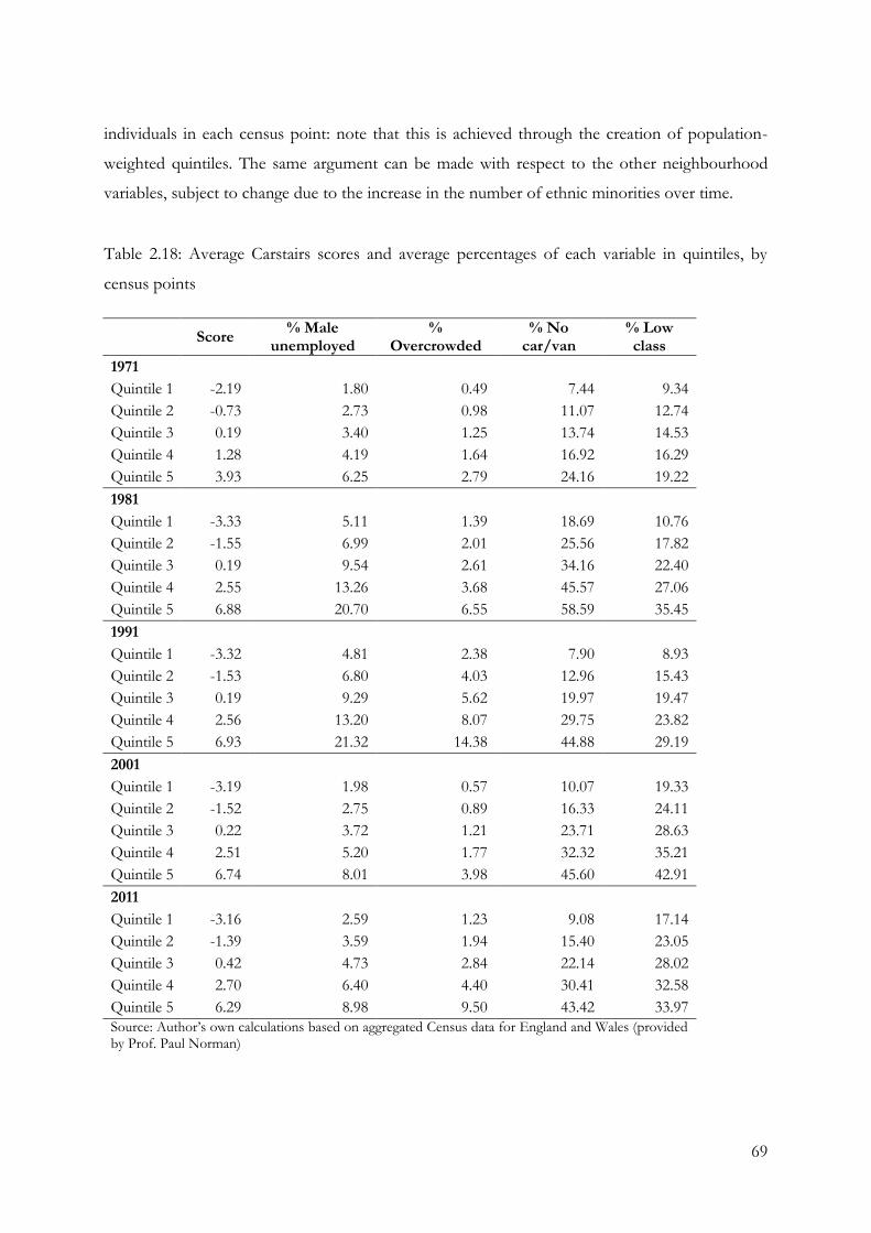
69

individuals in each census point: note that this is achieved through the creation of population-

weighted quintiles. The same argument can be made with respect to the other neighbourhood

variables, subject to change due to the increase in the number of ethnic minorities over time.

Table ‎2.18: Average Carstairs scores and average percentages of each variable in quintiles, by

census points

Score

% Male unemployed

% Overcrowded

% No car/van

% Low class

1971

Quintile 1 -2.19 1.80 0.49 7.44 9.34

Quintile 2 -0.73 2.73 0.98 11.07 12.74

Quintile 3 0.19 3.40 1.25 13.74 14.53

Quintile 4 1.28 4.19 1.64 16.92 16.29

Quintile 5 3.93 6.25 2.79 24.16 19.22

1981

Quintile 1 -3.33 5.11 1.39 18.69 10.76

Quintile 2 -1.55 6.99 2.01 25.56 17.82

Quintile 3 0.19 9.54 2.61 34.16 22.40

Quintile 4 2.55 13.26 3.68 45.57 27.06

Quintile 5 6.88 20.70 6.55 58.59 35.45

1991

Quintile 1 -3.32 4.81 2.38 7.90 8.93

Quintile 2 -1.53 6.80 4.03 12.96 15.43

Quintile 3 0.19 9.29 5.62 19.97 19.47

Quintile 4 2.56 13.20 8.07 29.75 23.82

Quintile 5 6.93 21.32 14.38 44.88 29.19

2001

Quintile 1 -3.19 1.98 0.57 10.07 19.33

Quintile 2 -1.52 2.75 0.89 16.33 24.11

Quintile 3 0.22 3.72 1.21 23.71 28.63

Quintile 4 2.51 5.20 1.77 32.32 35.21

Quintile 5 6.74 8.01 3.98 45.60 42.91

2011

Quintile 1 -3.16 2.59 1.23 9.08 17.14

Quintile 2 -1.39 3.59 1.94 15.40 23.05

Quintile 3 0.42 4.73 2.84 22.14 28.02

Quintile 4 2.70 6.40 4.40 30.41 32.58

Quintile 5 6.29 8.98 9.50 43.42 33.97

Source: Author’s own calculations based on aggregated Census data for England and Wales (provided by Prof. Paul Norman)

70

Table 2.18 shows the average Carstairs scores and the average percentages of each constituting

variable for each quintile and census point. We can see that except for 1971, average Carstairs

scores for each quintile tend to be quite stable across census-census points (in 1971 scores are

smaller). However, the composition of quintiles based on the average percentage of these

variables in Wards is quite varied, and there seem to be no very clear-cut patterns. For example,

while in 1981 and 1991 areas in Quintile 5 had an average of 20% male unemployed, in 2001 and

2011 this drops to around 8%. Similar description can be made on the other variables; however,

no clear patterns emerge.

2.2.5 Other variables

Finally, all models control for ‘other’ variables, which are: origin and destination years and

number of census points in which the individual participated. A description of these was shown

earlier in this chapter.

Important notes:

Some cell counts, percentages and totals shown in the tables created with ONS-LS data

have been modified in order to comply with publication rules established by the Office

for National Statistics. These modifications, however, do not affect the main findings

derived from the regression models.

The permission of the Office for National Statistics to use the Longitudinal Study is

gratefully acknowledged, as is the help provided by staff of the Centre for Longitudinal

Study Information & User Support (CeLSIUS). CeLSIUS is supported by the ESRC

Census of Population Programme (Award Ref: ES/K000365/1). The authors alone are

responsible for the interpretation of the data.

This work contains statistical data from ONS, which is Crown Copyright. The use of the

ONS statistical data in this work does not imply the endorsement of the ONS in relation

to the interpretation or analysis of the statistical data. This work uses research datasets,

which may not exactly reproduce National Statistics aggregates.

71

3 CHAPTER 3: ‘Ethnic Penalty’ or ‘Social Origins

Penalty’?

3.1 Introduction

It is well-known that social origins influence the educational and labour market outcomes of

individuals. This is reflected in the fact that individuals with higher social origins typically have

higher educational and occupational attainments than individuals with lower social origins. This

concern, central in the literature on social stratification, has been less highlighted in the migration

literature. In fact, while the origin of individuals in terms of parental education and occupation

has increasingly been incorporated in studies of ethnic inequalities in education (see also

Brinbaum and Cebolla-Boado 2007; Dustmann 2008; Dustmann, Frattini and Lanzara 2012;

Heath, Rothon and Kilpi 2008; Kalter, Granato and Kristen 2007; Kristen and Granato 2007;

Silberman, Alba and Fournier 2007; Van De Werfhorst and Van Tubergen 2007; Wood et al.

2009) its treatment has been much more limited in the study of labour market outcomes.

Moreover, little has been said about the role of other social origin variables – at the household

and neighbourhood levels17 – that might impact on labour market outcomes.

The migration literature has defined ‘ethnic penalties’ in labour market outcomes as any

remaining difference between ethnic minorities and the majoritarian population after education

(and in some cases, other background characteristics such as marital status and length of stay in

the country) have been taken into account (Heath and Cheung 2007). Ethnic penalties can mean

different things, for example, that ethnic minorities do not have enough information on jobs, or

that they lack the necessary networks to best-match their qualifications to occupations, or that

there is discrimination in the labour market. But more strictly speaking, the term ‘ethnic penalty’

implies that there is something about being an ethnic minority that explains differences with

respect to the majoritarian population. This chapter argues that before defining a difference as an

17 Note that in the introduction (Chapter 1) I did not include the neighbourhood variables in the ‘social origins’ definition. The reason why I do it here is twofold. First, because the focus of this chapter is not on the origin neighbourhood but on family social background, and that is what the title points at; second, because the neighbourhood variable used here (neighbourhood deprivation) might still be seen as a ‘social origins’ variable. In the other analytical chapters, the characteristics of the neighbourhood in which individuals live are the main factors of interest, and this is emphasised accordingly.

72

ethnic penalty, we have to consider as well other background characteristics – especially social

origin factors – that may influence the observed labour market outcomes.

Most studies on ethnic penalties in the labour market have used education as the crucial

explanatory variable (i.e. Algan et al. 2010; Cheung and Heath 2007b; Crul and Vermeulen 2003;

Heath and Li 2010). In fact, one could argue that education is the main predictor of labour

market outcomes, and that most parental (and other social origins) effects on these occur

through the positioning of individuals in the educational system (i.e. in an indirect way). However,

it is also well-known that parents exert a direct effect on their children’s outcomes, in particular on

occupation, for example by helping them to search for employment or providing them with

contacts (Blau and Duncan 1967; Breen 2004; Breen and Jonsson 2005; Bukodi and Goldthorpe

2011; Goldthorpe 2000; Kuha and Goldthorpe 2010). And the same argument can be made of

other variables like neighbourhood deprivation or household socio-economic level, as having an

influence on labour market outcomes.

This remaining effect has been assumed to work equally for the majoritarian population and

ethnic minorities in most studies on labour market outcomes of second generations in Europe.

In other words, studies on ethnic penalties implicitly make two assumptions: first, that social

origins are equal for ethnic minorities and the majoritarian population; and second, that its effect

is equal for both groups. However, these assumptions are not realistic. Ethnic minorities differ

from the majoritarian population in terms of their parental backgrounds – usually, these are of a

lower status – and also in terms of the contexts in which they are raised – usually, more deprived.

That is to say, in the presence of very different first generation social starting points in a country

that is highly stratified (as is the UK), we would not necessarily expect all groups to end up in the

same place, even after controlling for education (Platt 2007). As well, the migration literature has

provided evidence of patterns of behaviour among ethnic minorities that make the classical

mechanisms of social reproduction (see Boudon 1973; Goldthorpe 2000) less applicable to them,

suggesting therefore the presence of ethnically-specific social reproduction mechanisms.

Thinking in terms of the classical status attainment model (Blau and Duncan 1967: see Figure 3.1

below), these ethnically-specific mechanisms might lead ethnic minorities to get different returns

to education and to experience differently the effect of the parental social background (and/or

other social origins), as compared the majoritarian population.

73

Previous studies on ethnic penalties in the UK (Cheung and Heath 2007b; Heath and Li 2010)

have shown that the fortunes of second generation ethnic minorities in the labour market are

very much varied, and are dependent as well on the outcomes we consider. While results are

generally quite pessimistic with respect to the chances of being employed, they are more diverse

when the quality of the occupation is considered. In particular, emphasis has been put on

Pakistani and Bangladeshi populations, as those who experience the highest penalties in the

labour market. Alongside this literature, a smaller body of research (Heath and McMahon 2005;

Heath and Ridge 1983; Platt 2005a; Platt 2005b; Platt 2007; Zuccotti 2014) has attempted to

amplify the understanding of some of the second generation’s outcomes in the labour market, by

evaluating the contribution of parental background. These studies found that some ethnic

minority groups tend to be more socially mobile than the white British, with their achievements

depending more on education and less on social origins. However, in the context of a non-

meritocratic society such as the UK, social mobility and less dependence on social origins can be

detrimental for ethnic minority groups given that they might not be able to gain from higher-

status parental backgrounds, thus generating an ethnic penalty (this is the case, for example, for

Caribbean and Pakistani men).

Building upon this literature, this chapter analyses the role that education and social origins play

in the study of penalties (or gains) that ethnic minorities experience in the labour market of

England and Wales. Specific research questions are:

1. Do social origins help explain ethnic penalties in labour market outcomes?

2. Do social reproduction patterns vary by ethnic group?

o Do ethnic minorities get different returns to education?

o Does the direct effect of the parental social class on labour market outcomes vary by

ethnic group?

o And hence: do ethnic penalties depend on the level of education and parental social

class?

There are several ways in which this chapter advances our previous knowledge. First, it adds a

fresh view on the relationship between ethnic penalties and social reproduction processes by

combining approaches from the social stratification and migration literatures. In so doing, it

challenges the traditional measurement of ethnic penalties in labour market outcomes. Second, it

updates and discusses previous findings on ethnic inequalities with more recent and rich data:

general trends are delineated for 2001 and 2011 thanks to the recent availability of the ONS

74

Longitudinal Study. Third, this study sheds light on groups of which less is known, like Pakistani,

Bangladeshi (many times studied together), African and Chinese. The ONS Longitudinal Study –

by constituting 1% sample of the the population of England and Wales – is, to my knowledge,

among the best datasets in the UK to study social mobility of ethnic minorities, and has been

used before for the same purposes. Fourth, this chapter explores access to employment and

access to a certain social class separately, diverging then from previous studies on social mobility

of ethnic minorities that studied both outcomes together. Finally, the study shows results

separately for men and women, revealing gender differences worth considering.

3.2 Previous studies in the UK

In the UK, the children of immigrants – considered here as second generation ethnic minorities18

– have followed different patterns with respect to their incorporation into the labour market. A

main finding is that, like their parents, they are less likely to be employed when compared to the

white British. This result has been found for groups with relatively higher resources such as

Indians and Caribbeans, and groups with lower ones, such as Pakistanis and Bangladeshis

(Cheung and Heath 2007b).

The study of occupational attainment (which, for the purposes of this chapter, I will use

interchangeably with social class) shows that the two most advantaged groups are the Indian and

African, which have higher chances of accessing service class positions; that is, managerial and

professional occupations (Cheung and Heath 2007b; Heath and Li 2010). All other characteristics

being equal, Indian men are more likely to be in service class positions as compared to the white

British, and women have improved their chances of this over time, performing on the level of the

white British. This group is quite unique in showing this pattern, and some explanations have

pointed to the positive effect of ‘ethnic capital’ at the group and also at the individual level,

promoted by selected residential proximity (Platt 2007). Africans (both men and women) also

tend to have higher probabilities of accessing service class occupations than the white British.

Regarding equality of characteristics; however, it has also been found that among the most

educated (which covers a high percentage of Africans) this has not been the case, due to lower

returns to education (although an improvement over time is observed).

18 Note that this study also includes the so-called generation 1.5, that is, those who were born abroad but arrived at a young age

75

The other groups presented more gender differences in the same studies (Cheung and Heath

2007b; Heath and Li 2010), with men being typically disadvantaged. Among the Caribbean

population, and on equality of characteristics, women usually have a better chance of being in the

service class than the white British, which might point to self-selectivity into the labour market;

men, on the other hand, have usually been disadvantaged, although with improvements over

time. Pakistani and Bangladeshi persons, finally, usually studied together, are among the most

disadvantaged groups next to Caribbean men; women in these studies, however, present an

advantage with respect to the white British, but in a context of a very low employment rate, and

probably a high selectivity into the labour market. Some studies that have looked at these groups

separately (although not by gender), have found them equally disadvantaged in their probabilities

of accessing service class occupations (Platt 2005b; Platt 2007), accompanied by a high degree of

clustering in low qualified occupations (Platt, Longhi and Nicoletti 2012).

These findings, however, are quite limited in the analysis of ‘unequal chances’ in the labour

market, given that the parental social class has hardly been a part of the story. As argued before,

the inclusion of parental background in the analysis and, in particular, assuming that social

reproduction processes might vary between ethnic groups, might not only help explain

differences between minorities and the majoritarian population, but also might lead to fining

divergent ethnic penalties – or gains – depending on the parental social class of individuals.

In the UK, various authors have considered the perspective of social mobility (Heath and

McMahon 2005; Heath and Ridge 1983; Platt 2005a; Platt 2005b; Platt 2007; Zuccotti 2014).

Among the most relevant ones we find those of Platt, who used the same data as the one used in

this chapter, the ONS Longitudinal Study, which has the highest number of cases to study this

topic. The author shows that given similar social backgrounds, Indian, Caribbean, Black African

and Chinese persons are more likely to be found in the service class (i.e. more likely to be in

professional and managerial occupations than in other occupations or unemployment), as

compared to the white British. This advantage, however, disappears once education is

considered, which reveals that the gains in education mediate the parental effect on occupation

for these groups. In other words, ethnic minorities are more mobile compared to the white

British, who depend more on their parental backgrounds for achieving higher educational levels.

Another finding that emerged from these studies is that while Indians are also able to capitalize

on higher parental social class, for Caribbeans a higher origin does not bring any advantage (Platt

calls this a “within-group meritocracy” in the non-meritocratic British context), creating a penalty

76

among those with higher social backgrounds. Pakistanis and Bangladeshis, on the other hand, not

only are less upwardly mobile than would be expected from their high concentration in lower-

origin backgrounds, but also once education is controlled for, being born in a family of

intermediate- or working-class origins confers less advantage, as compared to white British.

Furthermore, this penalization is also higher at lower educational levels.

Platt’s findings, however, were based on an outcome variable that merged access to the labour

market and the attainment of certain occupational levels, which might be misleading since

penalties tend to be concentrated in access to employment, rather than in access to occupations

(Cheung and Heath 2007b). Moreover these findings are based on households, for which there is

no differentiation made between genders. My own previous research on the topic, based on the

United Kingdom Household Longitudinal Study (UKHLS: 2009-2010), has advanced on some of

these issues. Although the UKHLS has fewer cases, I found (in line with Platt) that the lower

social reproduction of Pakistanis, Caribbeans and Africans (based on a linear measure of

occupation, the International of Socio-Economic Index, ISEI) has particularly negative

consequences for higher educated minorities, who do not gain – as the white British do – from

more advantageous origins. These mechanisms, however, apply only to men, but not to women;

and are actually not found for Bangladeshi populations (only Bangladeshi women show a

disadvantage when the access to the service class is studied, but not when studying the ISEI).

The fortunes of ethnic minorities are very varied, and are dependent as well on the outcomes we

consider. While results are generally quite pessimistic with respect to access to jobs – since most

ethnic minorities are less likely to be employed as compared to white British – they are more

diverse when access to occupations is considered. On one side, we find Indians with quite a good

performance and ability to transfer advantaged backgrounds; on the other, we find Pakistani and

Caribbean (in particular men), who are particularly disadvantage among those with relatively

higher-level backgrounds.

Based on the ONS Longitudinal Study, the analysis below studies both access to the labour

market and access to occupations (or social class). Keeping these two outcomes separate is

important since gaining employment and getting a particular type of occupation might not be

necessarily regulated by the same processes. In particular, parental background probably exerts a

stronger effect on the second process. Moreover, I study men and women separately. The gender

division is also relevant since the labour market integration of men and women is different across

77

groups: for example, Pakistani and Bangladeshi women are much more likely to be outside the

labour market, and this is a gender-group specificity that should be considered. In a way, this

study builds on my previous research and arguments, but with richer data and with partly

different outcomes.

3.3 Theoretical background and hypotheses

Figure 3.1 shows three models of analysis. The starting point of this theoretical discussion is

Figure 3.1a. This reflects the classical model of analysis of ethnic penalties in the labour market

(Cheung and Heath 2007a), where education (E) is used as a main control variable in the

estimation of occupations or other labour market outcomes – denoted here as destination (D) –

among different ethnic minority groups (G). In this model, ethnic penalties are the (average)

difference between ethnic minorities and white British after education has been taken into

account. The content of this ethnic remaining effect can be very varied. Often, it has been

attributed to discrimination in the labour market (Heath and Cheung 2006; Wrench and Modood

2000); however, ethnic penalties can also mean that minorities do not have enough information

on jobs, or that they lack the right networks, or that they have different values regarding the role

of work that makes them relate differently to the labour market. Within the model of ethnic

penalties, different returns to education have also been acknowledged (reflected in the blue

arrow). That is, studies have also considered the fact that the ED effect might vary by ethnic

group and that ethnic penalties might therefore vary according to the level of education of

individuals.

78

Figure ‎3.1: Status attainment and ethnic penalties: three models

In what follows, I argue that the model in Figure 3.1a is incomplete, the reason being that a

crucial factor is missing: social origins. Look at Figure 3.1b. This shows a reduced version of the

classical Blau and Duncan model (1967) – and includes as well some extra controls used in this

study. Blau and Duncan showed that the attainment of occupations – or intergenerational

reproduction – occurs along two causal pathways: direct and indirect (see Figure 3.1b). An indirect

effect occurs because higher-class families (O) more successfully position their children in higher

education (E) than lower-class families, and education determines the occupational outcomes

(D). A direct effect covers all intergenerational reproduction outside education. The contents of

this effect may include both genetic and social aspects: for example, parents can influence their

children by giving them job advice, helping them to look for a job or providing them with

material economic resources; they can also transfer them ability and cognitive skills (not entirely

captured by education), offer them social and relational aptitudes and supply them with a wide

range of networks and connections. The amount and characteristics of this content vary between

Education (E) Class of origin (O)

+ Other origins (O*)

Destination (D)

Ethnic group (G) Ethnic penalties

Education (E)

Destination (D)

Ethnic group (G)

Education (E)

Destination (D)

Class of origin (O)

+ Other origins (O*)

Ethnic penalties

a

b

c

79

social classes. For example, even if two individuals have achieved the same education, if one of

them has parents that belong to the service class and – possibly – has higher economic resources,

he/she might be able to attend particularly good universities with good employment connections;

or might wait longer to find a more suitable job for his/her capacities; or he/she might be able to

use his/her parents connections for better matching jobs, or jobs with a higher remuneration (see

also Bernardi 2012). In addition, there is also a range of origin factors (O*) that might have a

separate impact on individual outcomes as well. I refer here to household and area characteristics

– like the number of cars or deprivation of the neighbourhood – which provide evidence of the

socioeconomic resources available to the individual. The measurement of these factors is rare in

the literature on social mobility, with some important exceptions (Platt 2005b; Platt 2007).

Look now at Figure 3.1c. This combines Figures 3.1a and 3.1b, and therefore includes the

parental social class (and other origin resources) in the analysis of ethnic penalties (see Kalter,

Granato and Kristen 2007 for a similar discussion). The consideration of social origins (in

particular the parental social class, typically measured in terms of parental occupation) in the

study of differences between second generation ethnic minorities and white British is important

for two reasons. On the one hand, because most ethnic minorities and white British have, on

average, different social origins: this compositional effect (expressed in the OG/O*G arrow),

might affect the average ethnic penalty (when encountered). On the other, because the

mechanisms of intergenerational social reproduction (for simplicity – and to follow the classical

social mobility models – I refer only to the OED model, leaving aside the O* factors) might vary

between groups.

There are three ways in which the total relationship between parents and children can vary. First,

this could be through a variation in the OE relationship, which refer to the social reproduction of

education, and is of no concern in this study. Second, as stated before, this could be through a

variation in the ED relationship, that is, through the existence of different returns to education.

Finally, and this is the key aspect of this research, this could also be related to a variation in the

OD relationship, that is, in the social reproduction that happens outside education. Differences

both in the ED and OD relationships (expressed in the blue arrows) implicitly presuppose that

ethnic penalties can vary according to the education and parental social class of individuals, or

that opportunities are dependent both on their own education and on social origins. The

following paragraphs analyse these statements more in detail. Moreover, four guiding hypotheses

80

are presented. A summary of these, as well of the mechanisms behind them and the link to the

research questions stated in the introduction of this chapter can be seen in Table 3.1.

Table ‎3.1: Research questions, hypotheses and possible explanations

Research question

Hypotheses Possible explanations

1 Hypothesis 1: Compositional effect

Ethnic minorities are more likely to have parents with low-status jobs and to be raised in more deprived contexts (both at the household and neighbourhood levels)

2

Hypothesis 2: Social reproduction outside education:

a: Lower dependence on the parental social class among ethnic minorities;

b: Higher dependence on the parental social class among ethnic minorities

Hypothesis 3: Lower returns to education

Higher motivation among the lower classes and/or lack of “extra” parental resources among the higher classes (2a); cultural and community factors, external constraints (2b); discrimination at higher occupational levels (3)

The first hypothesis refers to the compositional effect. We observed in Figure 3.1b that social

origins (expressed as the parental social class and other household and area factors) affect

occupational outcomes on top of education. If ethnic minorities and white British have different

compositions in terms of these variables, the amount of ethnic penalties found by previous

research might be biased. Driving this argument is that second generation ethnic minorities tend

to have parents – who also immigrated to the country – with lower social backgrounds. It is well-

known that upon arrival, first-generation ethnic minorities do worse in the labour market than

the majoritarian population (Algan et al. 2010; Kogan 2006; Van Tubergen, Maas and Flap 2004).

In addition to possible underlying discrimination processes (Allasino et al. 2004; Wood et al.

2009), this is mostly related to the incapacity of immigrants to transfer their own cultural capital –

in particular education and language – to the destination society: in many cases, they end up

doing jobs that do not correspond to their capacities. The fact that the parents of ethnic

minorities are hence often overrepresented in poor quality jobs might have a direct impact on

their children’s occupational outcomes and, therefore, might help to explain the disadvantages

observed for some groups, like Pakistani, Bangladeshi or Caribbean (see also Kalter, Granato and

Kristen 2007). Moreover, ethnic minorities also tend to live in poorer conditions in terms of

housing, and in areas in which the deprivation levels are higher. This fact – related to processes

of initial settlement of immigrants in areas where housing prices are lower – might affect their

81

possibilities of attaining better labour market outcomes as compared to the majoritarian

population, helping therefore to complete this compositional effect. Summarizing, I expect that

including the parental occupation and other social origins as control variables should help to

reduce the ethnic penalties observed for some groups in previous studies (Cheung and Heath

2007b; Heath and Li 2010) (Hypothesis 1).

The next three hypotheses refer to differences in terms of social reproduction, that is, to

differences in how the OED model works for the various groups. Specifically, I expect that (at

least part of) the mechanisms of social reproduction that apply to the general (white British)

population do not apply to some groups, or work for them in different ways. The main concern

of this study refers to refer to social reproduction outside education, that is, to the direct effect of

the parental social class on labour maker outcomes. However, I also explore returns to education,

for a more complete analysis.

With regard to social reproduction outside education, two contrasting hypotheses are tested. One

states that (after controlling for education) ethnic minorities are less dependent on their parental

social backgrounds as compared to the majoritarian population, i.e. the white British (Hypothesis

2a); the other states the opposite (Hypothesis 2b). Why could we expect a lower dependence of

ethnic minorities on their parental social class? According to Goldthorpe (2000), one of the main

driving forces behind the stability of the class structure – and the reason why, on average, the

children of higher-class parents do better than the children of lower-class parents – is that the

individuals’ priority is to achieve the class of the parents or, more specifically, to avoid downward

mobility (see also Boudon 1973). In this context, achieving upward social mobility is of secondary

concern. However, this reasoning might not apply strictly to some ethnic minorities. It has been

argued that immigrants who arrive to a country and decide to stay and – eventually – build a

family there, will want to see their children rise in the new society, and will therefore invest in

them (Dustmann 2008). Motivation and high aspirations of parents have been found to be a

powerful source when explaining educational mobility among ethnic minorities (Heath, Rothon

and Kilpi 2008). This might well be complemented with a direct motivation to find a good job

and to progress in a career. In the case of minorities with lower-class backgrounds (which actually

covers the majority), higher motivation might then mean lower dependence on parental

backgrounds and possibly overperformance by the children of immigrants. Note that this process

might be in part linked to the recovery of family occupational status in the origin country.

82

Among the higher classes, a lower dependence on the parental background might also occur,

although is likely to be promoted by other types of mechanisms (and have, perhaps, negative

consequences for ethnic minorities). Going back to Goldthorpe’s (2000) suggestion that

individuals seek to avoid downward mobility, among the higher classes this is achieved primarily

through education. For example, a university degree is necessary if the aim is to continue with a

certain family professional tradition. However, higher classes have also a repertoire of strategies

on top of education that might influence the labour market outcomes of their children. Parents,

for example, might pay for the best universities or have key connections in certain work

industries; they might also transfer certain lifestyles and manners, and particular social skills that

have a ‘signalling’ effect in the labour market. These factors – more relevant among those

aspiring to jobs with higher qualifications – might play a crucial role when comparing the

majoritarian population and ethnic minorities. Even if the parents of ethnic minorities have good

jobs, they might lack all or some of these ‘extra’ properties that individuals from the majoritarian

population have presumably gained by having been raised in the local culture (and knowing the

social rules better). This, in turn, would presumably make these children more dependent on

education, and less dependent on parental backgrounds, with possible negative consequences in

terms of ethnic penalties among those with higher social backgrounds. In the words of Platt

(2005a), finding a lower dependence on parental background might play against better-positioned

minorities in a context in which the occupational status of the majoritarian population, i.e. the

white British, depends strongly on that of the parents. Basically, it could mean that these

minorities are unable to use class resources for achieving better positions.

Nonetheless, the migration literature has revealed other ethnic-specific mechanisms (especially

for those with lower/middle parental backgrounds) that might push the relationship between

parents and children in the opposite direction. Goldthorpe (2000) has argued that one reason that

the lower social classes tend to reproduce their own social class is that this is considered less

“risky” as compared to aiming at a university degree, which would possibly lead to a higher status

occupation or social class. But in contexts of discrimination or where the labour market is more

selective (or even in contexts of crisis, like the one studied here), ethnic minorities might be

pushed to do jobs that are closer to their family tradition or more familiar to them, rather than

seeking to rise through their careers. In other words, this rationale of following the parental social

background due to its associated lower risk could become stronger among ethnic minorities in an

unfavourable context (note that this argument stands in opposition to the ‘motivational

argument’).

83

Other factors might also contribute to a stronger relationship between parents and children, like

cultural factors and the community environment. In fact, even if minorities adapt to the cultural

premises of the receiving society, this does not mean that their own cultural backgrounds – and

those of their co-ethnics – have lost their effects (Vermeulen and Perlmann 2000). For example,

south Asian communities tend to follow a ‘patriarchal model’ (Peach 2005) in which concepts

such as control, family honour and status are crucial, and in which men are meant to be the main

‘providers’ of the family. Women, then, might be more disadvantaged with regard to access to

jobs or more limited in the types of jobs that they can access (Brah 1993; Dale et al. 2002),

making them possibly more dependent on a certain family tradition. Strong relationships with co-

ethnics might also lead ethnic minorities to relate more closely to jobs that are typically attached

to their family or community. A similar argument can be made among those born in

communities with a tradition of ethnic entrepreneurship or in which ethnic niches – that is

specialization in certain occupations by a certain ethnic group – are the most common sources of

jobs (Portes 1998). For example, a recent study has shown that Pakistani and Bangladeshi

minorities had a higher self-employment rate increase between 1991 and 2001 (Clark and

Drinkwater 2010) than the one that would have been expected given the changes in their

demographic characteristics (mainly gains in education). This should probably be reflected in a

stronger intergenerational transmission of resources for these groups than the one found in the

majoritarian population (although we cannot really know if this is due to discrimination in the

mainstream economy or to an election of these minorities). All these mechanisms will be

reflected in a stronger intergenerational social reproduction among ethnic minorities, or a

stronger OD effect (after controlling for education). This, in turn, will have an impact on the

level of ethnic penalties, which will be higher or lower depending on whether or not the

suggested higher dependence on the parental social background actually implies a “constraint”

for ethnic minorities.

With regard to the value of education in the labour market, previous research has shown that

being of Indian, Pakistani/Bangladeshi, Caribbean (for men) or Chinese (for women) ethnic

minority status presupposes lower returns to education (Heath and Li 2010). Although it is not

clear from this research how first- and second generation status contributes to this outcome, it

can be argued that this is likely to be driven by the first generation, who in many cases cannot

convert their foreign educational credentials into matching occupations. In this sense, this

problem should not be an issue for the second generations, most of whom have obtained their

education in the destination country. However, in the presence of a more discriminatory labour

84

market at higher occupational levels, this could be a plausible outcome for second generations as

well. For the purposes of this study, I will hypothesize that some second generation groups might

experience lower returns to education as compared to white British (Hypothesis 3), and that this

could mean higher ethnic penalties among the more highly educated. In particular, I will explore

the value of a degree level for ethnic minorities and white British.

3.4 Data and variables

The analysis is based on the ONS Longitudinal Study, which follows individuals in five time-

points (1971-2011), and is done for second generation ethnic minorities (Indian, Pakistani,

Bangladeshi, Chinese, Caribbean and African) and white British. Second generations are defined

as those who lived with at least one parent between 0 and 15 years of age in any of the three so-

called ‘origin’ years: 1971, 1981 or 1991; the definition of second generation includes, therefore,

both individuals born in Britain and individuals born abroad, who arrived before age 16. These

individuals are then followed in 2001 and 2011, where two outcomes are studied: employment

(vs. unemployment and some inactive groups) and access to the service class, which comprises

professional and managerial occupations (vs. other social classes/occupations). Note that the

social class of individuals can be current or past.

The main independent variables – in addition to the ethnic group – can be divided between

individual-level variables and household- and neighbourhood-level variables. Individual-level

variables are measured in ‘destination’ (2001 and 2011) and are: age, gender and education.

Household- and neighbourhood-level variables are measured in ‘origin’ (1971, 1981 and 1991),

that is, when the individual is between 0 and 15 years of age in any of the three time points. They

are: parental social class, tenure, number of cars, number of persons per room and

neighbourhood deprivation. Other control variables are: origin year, destination year and number

of census points in which the individual has participated.

The pooled sample includes individuals between 20 and 45 years old, and I only work with cases

that have valid values in all variables, so as to have a common N. More details on the sample,

variables and measurements can be found in Chapter 2.

85

3.5 Descriptive statistics

Table 3.2 shows descriptive statistics of the dependent variables – access to employment and

access to the service class – separated by group, gender and also year, to give a general view of

the trends in the decade.

Starting with second generation men, Table 3.2 shows that in 2001 Pakistani, Bangladeshi,

Caribbean and, to a lesser extent, African men have lower employment levels as compared to

white British men, while the other groups have rates more similar to that of the white British. In

2011 we observe an improvement for all groups, which leads to a considerable closing of the gap

for Pakistani and Bangladeshi men, in particular. With regard to access to the service class, we

observe a similar pattern as with employment for Pakistani, Bangladeshi and Caribbean persons,

that is, an initial gap and subsequent improvement. Indian, Chinese and African, persons on the

other hand, have higher shares in the service class than white British, a difference that intensified

in 2011 only for the former two, while the opposite is observed for Africans.

Among women the story is quite different. First, only Pakistani and Bangladeshi women are very

much disadvantaged with respect to access to employment (many of them are inactive), a result

that has been maintained over time. In the decade, however, these two groups make important

improvements in terms of accessing the labour market, which leads to a reduction in the gap;

other groups, however, have seen their participation drop (Chinese and African). With regard to

access to the service class, we observe that the Pakistani and the Bangladeshi are the only

disadvantaged groups (the others have actually higher shares in the service class as compared to

the British) and, again, both improve their situation in 2011.

86

Table ‎3.2: Employment and access to the service class by ethnic group, gender and year (%)

White British Indian Pakistani Bangladeshi Chinese Caribbean African

Men

Employment

2001 88.6 85.8 71.3 73.0 91.2 76.0 80.0

2011 87.7 89.1 79.8 82.3 92.6 83.6 87.5

Service class

2001 39.0 51.6 34.6 36.4 52.7 32.8 52.1

2011 40.9 56.9 37.8 37.0 58.5 40.7 45.1

Women

Employment

2001 74.8 77.9 45.1 40.2 90.4 74.9 80.6

2011 79.6 81.9 54.4 52.3 80.9 79.4 77.8

Service class

2001 34.6 44.3 30.4 28.5 46.6 42.4 52.4

2011 39.3 54.3 37.3 32.4 48.8 44.0 48.9

Totals employment

Men 2001 88621 1202 655 159 111 674 75

Men 2011 84748 1831 1132 367 202 611 152

Women 2001 92366 1216 716 184 135 846 134

Women 2011 88763 1737 1235 432 220 759 194

Totals service class

Men 2001 86331 1169 596 151 110 637 73

Men 2011 81017 1757 1018 332 200 577 142

Women 2001 88984 1158 572 137 131 794 126

Women 2011 84582 1645 1023 352 211 713 180 Population: Individuals between 20 and 45 years old Source: Author’s own calculations based on ONS-LS

Ethnic penalties in the labour market, however, are not concerned with average levels, but with

differences between ethnic minorities and white British that remain after controlling for key

variables that predict labour market outcomes. In fact, the idea behind ethnic penalties is that

there is something ‘ethnically specific’ that produces the gap. As argued before, education has

been used as the main control variable, given that it is the most important predictor of labour

market outcomes. This research, however, argues that other factors – the social origin of

individuals, for instance – might also be at play. The distribution of groups across these social

background characteristics is shown in Tables 3.3 (men) and 3.4 (women).

87

Tables 3.3 and 3.4 show that Asian ethnic minorities are on average younger than the white

British, while the black population resembles them more. Ethnic minorities also tend to be more

educated. In particular, this is observed among Indians, Chinese and African, who have very high

shares in higher education (Level 4+). Looking at their origin characteristics, however, we

observe that the proportion of ethnic minorities with parents in Professional/Managerial

positions – which could be thought of as a good predictor of higher education – is usually lower.

This suggests that ethnic minorities are educationally mobile with respect to parental

backgrounds; that is, they are getting more education compared to what would have been

expected given their relatively lower parental backgrounds. However, their gains in terms of

occupation do not seem to correlate with these educational gains. Different explanations might

apply. Discrimination in the labour market is the most straightforward one. However, this

chapter argues that the parental social class – and other social origin variables – might have an

impact as well. Note, for example, that ethnic minorities are overrepresented in the most

deprived areas and, in general, tend to be disadvantaged in other household measures, like the

number of cars and number of persons per room (with respect to tenure, only black populations

and Bangladeshis are more likely to be in social rental housing, which probably indicates a

“London” factor, given that these populations have the highest shares in this city)19.

19 One could ask: if these disadvantages at origin affect labour market outcomes, why they do not seem to be affecting education? One response is that discrimination mechanisms in schools might be less strong, for example because many schools have followed a ‘multicultural approach’ to teaching. The other is that the labour market is less meritocratic as compared to the educational system. Notice as well that the parental education – not measured here – is probably higher relative to the parental occupation and ethnic minorities are perhaps less educationally mobile with respect to education. Unfortunately, there is no good measure of parental education in this data.

88

Tab

le ‎3

.3: D

escr

ipti

ve

stat

isti

cs f

or

men

; 2001 a

nd 2

011 p

oo

led (

% a

nd m

ean

)

Bri

tish

In

dia

n

Pak

ista

ni

Ban

gla

desh

i C

hin

ese

C

ari

bb

ean

A

fric

an

Ag

e

Mea

n a

ge

33.5

32.3

31.7

30.0

31.7

35.6

32.1

Ed

ucati

on

No

ne

& o

ther

18.3

9.3

18.0

16.2

7.3

17.1

8.8

Lev

el 1

22.2

14.4

21.3

22.6

8.0

26.5

13.2

Lev

el 2

21.0

13.5

17.2

16.5

13.1

22.1

23.3

Lev

el 3

12.5

10.3

8.5

9.9

8.3

7.7

11.5

Lev

el 4

+

26.0

52.5

35.0

34.8

63.3

26.5

43.2

Pare

nta

l so

cial

cla

ss

N

o e

arn

ers/

No

cod

e 5.3

7.1

18.0

24.3

10.2

10.7

12.8

Man

ual

(V

+V

I+V

II)

38.6

52.1

60.1

50.8

23.3

52.7

35.7

Ro

uti

ne

no

n-m

anual

(II

I)

15.8

10.0

4.0

4.6

6.4

20.9

24.2

Pet

it B

ourg

eois

ie (

IV)

11.3

13.4

10.9

13.1

42.5

2.2

0.0

Pro

fess

ion

al/

Man

ager

ial (I

+II

) 29.0

17.4

7.1

7.2

17.6

13.5

27.3

Cars

No

car

s 24.7

32.8

44.8

64.3

30.7

58.9

55.1

1 c

ar

54.3

52.3

47.3

31.4

53.0

35.6

38.3

2 c

ars

21.0

15.0

7.9

4.4

16.3

5.5

6.6

Ten

ure

Ow

ner

62.6

85.5

85.5

41.4

62.3

49.4

28.6

So

cial

ren

t 28.2

7.1

7.9

42.8

22.7

40.2

48.9

Pri

vat

e re

nt

9.3

7.5

6.7

15.8

15.0

10.4

22.5

Pers

on

s p

er

roo

m

>

1.5

per

son

s 1.9

14.8

24.1

35.2

23.0

14.0

18.9

1.5

per

son

s 1.0

4.9

6.4

8.2

5.8

5.9

6.6

>1 &

<1.5

per

son

s 9.3

22.6

29.7

29.7

18.2

26.2

26.4

89

Bri

tish

In

dia

n

Pak

ista

ni

Ban

gla

desh

i C

hin

ese

C

ari

bb

ean

A

fric

an

1 p

erso

n

18.9

21.2

18.9

12.7

18.8

23.0

18.5

>=

0.7

5 &

<1 p

erso

n

29.7

19.6

12.8

8.7

15.3

17.0

17.6

<0.7

5 p

erso

n

39.3

16.9

8.1

5.5

18.8

13.9

11.9

Cars

tair

s q

uin

tile

s

Q1 (

less

dep

rivat

ion

) 21.0

4.7

1.8

1.9

13.4

3.1

4.4

Q2

21.4

6.3

3.9

3.6

17.6

6.7

5.7

Q3

20.7

11.4

5.5

6.3

13.1

12.7

15.4

Q4

20.0

20.1

17.0

12.5

22.7

20.9

22.9

Q5 (

mo

re d

epri

vat

ion

) 16.9

57.5

71.9

75.7

33.2

56.6

51.5

N

173369

3033

1787

526

313

1285

227

Po

pula

tio

n: In

div

idual

s b

etw

een

20 a

nd

45 y

ears

old

So

urc

e: A

uth

or’

s o

wn

cal

cula

tio

ns

bas

ed o

n O

NS

-LS

90

Tab

le ‎3

.4: D

escr

ipti

ve

stat

isti

cs f

or

wo

men

; 2001 a

nd 2

011 p

oo

led (

% a

nd m

ean

)

B

riti

sh

Ind

ian

P

ak

ista

ni

Ban

gla

desh

i C

hin

ese

C

ari

bb

ean

A

fric

an

Ag

e

Mea

n a

ge

33.5

5

32.3

3

30.8

3

29.2

0

31.2

1

35.6

7

33.7

7

Ed

ucati

on

No

ne

& o

ther

13.4

7.7

18.8

17.0

5.6

7.0

6.1

Lev

el 1

21.9

14.2

18.6

21.6

9.6

23.0

8.2

Lev

el 2

24.0

16.7

18.7

21.4

11.3

21.6

11.3

Lev

el 3

13.2

11.7

12.9

12.0

9.3

12.0

4.6

Lev

el 4

+

27.6

49.8

31.1

27.9

64.2

36.4

69.8

Pare

nta

l so

cial

cla

ss

No

ear

ner

s/N

o c

od

e 5.9

5.8

15.0

31.8

11.5

12.8

18.0

Man

ual

(V

+V

I+V

II)

39.2

56.0

63.4

53.1

25.9

50.0

26.2

Ro

uti

ne

no

n-m

anual

(II

I)

15.7

10.1

2.9

1.6

5.1

21.0

28.4

Pet

it B

ourg

eois

ie (

IV)

11.0

12.9

12.2

9.7

43.7

2.1

3.0

Pro

fess

ion

al/

Man

ager

ial (I

+II

) 28.1

15.2

6.5

3.7

13.8

14.1

24.4

Cars

No

car

s 26.1

34.1

44.7

73.2

32.1

57.9

59.5

1 c

ar

53.6

50.9

47.5

24.0

53.0

36.4

37.5

2 c

ars

20.3

15.0

7.8

2.8

14.9

5.7

3.0

Ten

ure

Ow

ner

60.8

84.9

85.4

40.4

58.9

50.0

35.7

So

cial

ren

t 29.7

8.5

7.5

43.3

28.7

38.3

38.4

Pri

vat

e re

nt

9.5

6.5

7.0

16.2

12.4

11.7

25.9

Pers

on

s p

er

roo

m

> 1

.5 p

erso

ns

2.0

16.6

24.8

38.1

20.6

15.5

20.4

1.5

per

son

s 1.1

6.1

8.0

8.6

7.6

6.9

7.6

>1 &

<1.5

per

son

s 9.8

24.1

32.3

25.3

19.2

25.3

22.6

91

B

riti

sh

Ind

ian

P

ak

ista

ni

Ban

gla

desh

i C

hin

ese

C

ari

bb

ean

A

fric

an

1 p

erso

n

19.1

21.4

18.0

14.9

18.6

21.1

26.5

>=

0.7

5 &

<1 p

erso

n

29.5

18.0

10.3

9.1

24.2

16.5

12.8

<0.7

5 p

erso

n

38.6

13.9

6.6

3.9

9.9

14.7

10.1

Cars

tair

s q

uin

tile

s

Q

1 (

less

dep

rivat

ion

) 20.7

5.6

1.6

1.6

11.8

3.1

3.7

Q2

21.0

7.1

3.4

2.6

14.1

6.7

8.2

Q3

20.5

9.8

5.8

6.5

17.2

12.8

20.7

Q4

20.1

17.5

18.0

10.2

21.4

24.0

25.6

Q5 (

mo

re d

epri

vat

ion

) 17.7

60.1

71.1

79.1

35.5

53.4

41.8

N

181129

2953

1951

616

355

1605

328

Po

pula

tio

n: In

div

idual

s b

etw

een

20 a

nd

45 y

ears

old

So

urc

e: A

uth

or’

s o

wn

cal

cula

tio

ns

bas

ed o

n O

NS

-LS

92

In what follows, I study access to employment and the attainment of a service class through

more sophisticated models, in which the roles of education and social origins are tested together.

More specifically, I first study the extent of ethnic penalties in employment and occupation

before and after accounting for education and social origins: this addresses Research question 1.

Second, I study social reproduction processes with respect to occupation and explore whether

the effect20 of the parental occupation and education on the access to the service class varies

across groups. This is achieved by adding interaction effects between parental social class and

ethnic group and between education and ethnic group, and addresses Research question 2 (note

that I also test for returns to education with respect to employment, but have preferred to leave it

outside the arguments on social mobility, which are more strictly related to the attainment of

occupations). Finally, the analysis also tests for year effects, to explore the extent to which

changes have occurred between 2001 and 2011.

3.6 Access to employment

Tables 3.5 and 3.6 show the probability of being employed for men and women respectively and

for the different ethnic groups. The coefficients are based on linear regressions with robust

(clustered) standard errors and – when multiplied by 100 – refer to the difference in percentage

points with respect to white British. All models control for: age, origin year, destination year and

number of census points in which the individual participated. The distribution of individuals in

the latter three variables can be found in the Table 8.1 in Annex A. Moreover, the full models,

where the effect of all control variables is shown, can be found in Tables 8.2 (men) and 8.3

(women). Finally, as a robustness check given that I am working with dichotomous dependent

variables, Table 8.7 shows the key models on employment presented here (Model 5 from Tables

3.5-3.6), but estimated with logistic regression with average marginal effects.

20 Please note that the present study is of a largely descriptive nature and does not offer any counter-factual estimates on the causal effects of ethnic background or other key independent variables. The use of “causal” terminology in this thesis (“effect,” “consequences,” etc.) is purely for stylistic purposes, and connected to the aim of acknowledging theory. For example, every time I say that “there is effect of A on B” I will be referring to an association between A and B that is based on a theory that says that A has an impact on B (although, in technical terms, I will not be measuring this in terms of a causal mechanism).

93

Table ‎3.5: Access to employment. Men.

M1 M2 M3 M4 M5 M63 M73

Ethnic group (ref. white British)

Indian 0.006 -0.023*** 0.022*** -0.013* 0.008 + ns

(0.0077) (0.0074) (0.0077) (0.0075) (0.0077)

Pakistani -0.089*** -0.090*** -0.047*** -0.067*** -0.042*** + +

(0.0127) (0.0122) (0.0126) (0.0122) (0.0124)

Bangladeshi -0.045** -0.047** 0.002 -0.020 0.028 + ns

(0.0205) (0.0194) (0.0205) (0.0195) (0.0195)

Chinese 0.063*** 0.023 0.066*** 0.026 0.053*** ns –

(0.0175) (0.0182) (0.0177) (0.0181) (0.0181)

Caribbean -0.070*** -0.077*** -0.048*** -0.065*** -0.035** + ns

(0.0142) (0.0136) (0.0142) (0.0136) (0.0137)

African 0.014 -0.029 0.023 -0.018 0.022 + +

(0.0268) (0.0254) (0.0267) (0.0254) (0.0257)

Adjusted R2 0.013 0.089 0.035 0.095 0.102 0.103 0.072

N 180540 180540 180540 180540 180540 180540 180540

Base model1 X X X X X X X

Education X X X X X

Parental social class X X X X X

Other origins2 X X X

Year*Ethnic group X X

Education*Ethnic group

X

1 Controls for: age, origin year, destination year and number of census points. 2 Includes tenure, number of persons per room, number of cars and deprivation quintile at the ward level 3 + means a positive interaction; - means a negative interaction; and ns means a non-significant interaction (p-value>=.10). The effects refer to the year 2011 vs. 2001 (M6); and to educational Level 4+ vs. Level 1 or less (M7). * p-value<.10 ** p-value<.05 *** p-value<.01. Robust (clustered) standard errors in parentheses Population: Individuals between 20 and 45 years old Source: Author’s own calculations based on ONS-LS

Model 1 or the ‘base model’ in Table 3.5, which only controls for the variables common to all

models (age, origin and destination years and number of census points), shows that Pakistani,

Bangladeshi and Caribbean men are less likely to be employed as compared to white British, the

former being those with the highest disadvantage. Chinese, on the other hand, have an advantage

as compared to the British, while Indians and Africans show no statistically significant

differences. When education is included in the analysis (Model 2) – taking us to the classical

models of ethnic penalties – we observe that Indians now experience a penalty and, for the

Chinese, the initial advantage disappears. Model 3 removes education, and adds the parental

94

social class instead: given that most ethnic minorities have low social origins, the positive gaps

(Indians and Chinese) or absence of penalties (Bangladeshis) is actually of no surprise. Models 4

and 5, finally, include education, parental social class and other social origins in the analysis. Here

we observe that the penalty observed for Indians and Bangladeshis in Model 2 disappears, and

the Chinese gain again an advantage over the white British in the probability of employment of

around 5% points. The existence of a penalty for Pakistanis and Caribbeans, however, does not

seem to be affected by the introduction of these variables. Nonetheless, it diminishes

considerably for both groups (from 9% points difference to 4% for Pakistanis; and from 7%

points difference to 3.5% for Caribbeans).

Next, I calculated the interaction effects between ethnic group and the year in which employment

was measured (Model 6) and between ethnic group and education (Model 7). The sign of these

effects for each ethnic minority (with respect to white British) can be seen in Table 3.5, but a

more simple way to look at interactions is to plot them in graphs. Figure 3.2 shows the average

changes in the penalties between 2001 and 2011 for all respondents (a) and for those with high

(Level 4+) and low (Level 1 or less) levels of education (b). Note that in Figure 3.2b only groups

that showed statistically significant interactions are plotted.

The results for all men or average results (Figure 3.2a) show that there was an improvement over

the decade. Groups either gained an advantage over white British (Indian, Bangladeshi and

African populations) or reduced their penalties to non-existent (Pakistani and Caribbean

populations21). However, these results change for some groups once we add interaction effects

with education. Figure 3.2b shows that although both less-educated and highly educated

Pakistanis and Africans improved their situation in 2011, penalties for the least educated are

much larger (approximately: between 10% and 20% points difference with respect to white

British for Pakistanis; and between 15% and 30% points difference for Africans, although there

are very few less-educated Africans). Actually, among those in higher education there is no

penalty at all, and a positive gap appears in 2011. This figure also shows that less-educated

Chinese mainly drive the advantage in employment observed in Model 5 of Table 3.5 (but note

that there are very few less-educated Chinese).

21 Recall from Figure 2.3 in Chapter 2 that there might be an effect of positive selection for Caribbean persons: note that the gap between ONS-LS and census data is bigger for this group compared to the white British.

95

Figure 3.2: Probability of being in employment in 2001 and 2011 (for all and separated by

education); predicted values from the regression (confidence intervals 90%). Men.

a. All

b. By education

Note: Figures are based on Models 6 (a) and 7 (b) from Table 3.5. Figure 2b plots only statistically significant interaction effects (p-value<.10). Note that in Graph b the lines for African and Pakistani overlap among those with Level 1 or less education. Population: Individuals between 20 and 45 years old Source: Author’s own calculations based on ONS-LS

.8.9

1

Pro

b. e

mp

loym

en

t

2001 2011Destination year

British Indian

Pakistani Bangladeshi

Caribbean African

Chinese

.5.6

.7.8

.91

1.1

2001 20112001 2011

Level 1 or less Level 4

British Pakistani

AfricanChinese

Pro

b. e

mp

loym

en

t

Destination year

96

Table 3.6 shows the results in the access to employment for women. Model 1, or ‘base model’,

shows that Pakistani and Bangladeshi women are less likely to be employed as compared to the

white British. Note that these values are quite high, of around 25% points less probability, and

are mainly driven by the high levels of inactivity of this group. Indian and Chinese persons, on

the other hand, have an advantage as compared to the white British, and black groups show

neither substantive nor statistically significant differences. After adding education into the

analysis (Model 2) we observe that, except for Indians and Chinese, all groups now experience a

penalty. As for men, Model 3 includes only the parental social class, and Models 4 and 5 add both

education and social origin variables. We can see that the penalty observed for Caribbean and

African persons in Model 2 disappears in Model 4, which includes the parental background. Note

as well that in Model 5, the penalty diminishes for Pakistanis and in particular Bangladeshis: for

the latter this goes from 25% (Model 2) to around 18% (Model 5) points difference.

As for men, I also calculated interaction effects with the year in which employment was

measured (Model 6) and with education (Model 7), which can be observed in Figure 3.3. The

average results for women (Figure 3.3a) show that there was an improvement for Pakistanis and

Bangladeshis, while the probability of employment for the Chinese diminished (approaching the

British mean). Figure 3.3b, which shows results separated by education (which are statistically

significant), shows more interesting results. Penalties for less-educated Pakistani and Bangladeshi

women are much bigger (around 25-30% points difference with respect to white British)

compared to penalties for the highly educated (around 5-10% points difference). Actually, among

Bangladeshi women this penalty practically disappears in 2011. The opposite occurs for

Caribbean women, who seem to be advantaged at lower educational levels.

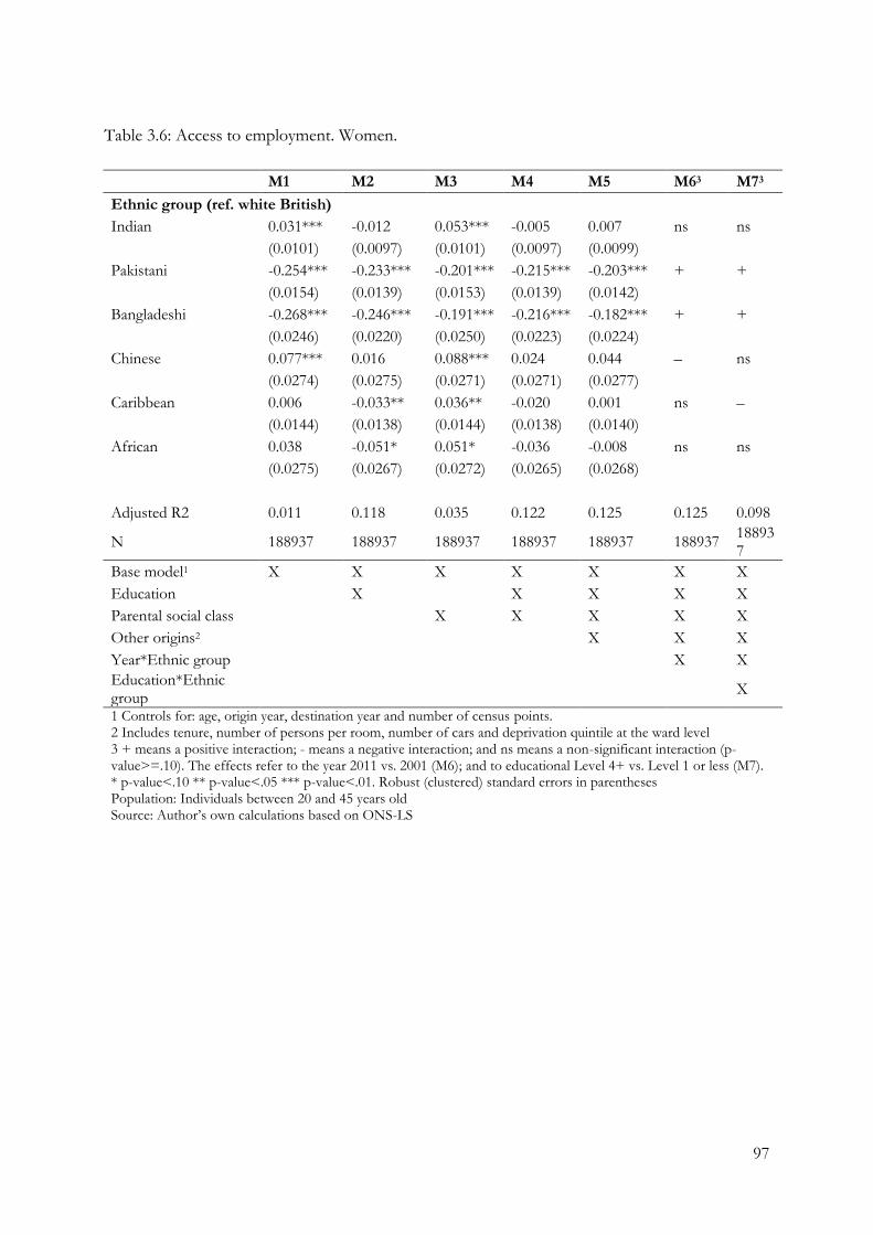
97

Table ‎3.6: Access to employment. Women.

M1 M2 M3 M4 M5 M63 M73


Indian 0.031*** -0.012 0.053*** -0.005 0.007 ns ns

(0.0101) (0.0097) (0.0101) (0.0097) (0.0099)

Pakistani -0.254*** -0.233*** -0.201*** -0.215*** -0.203*** + +

(0.0154) (0.0139) (0.0153) (0.0139) (0.0142)

Bangladeshi -0.268*** -0.246*** -0.191*** -0.216*** -0.182*** + +

(0.0246) (0.0220) (0.0250) (0.0223) (0.0224)

Chinese 0.077*** 0.016 0.088*** 0.024 0.044 – ns

(0.0274) (0.0275) (0.0271) (0.0271) (0.0277)

Caribbean 0.006 -0.033** 0.036** -0.020 0.001 ns –

(0.0144) (0.0138) (0.0144) (0.0138) (0.0140)

African 0.038 -0.051* 0.051* -0.036 -0.008 ns ns

(0.0275) (0.0267) (0.0272) (0.0265) (0.0268)

Adjusted R2 0.011 0.118 0.035 0.122 0.125 0.125 0.098

N 188937 188937 188937 188937 188937 188937 188937

Base model1 X X X X X X X

Education X X X X X

Parental social class X X X X X

Other origins2 X X X

Year*Ethnic group X X

Education*Ethnic group

X

1 Controls for: age, origin year, destination year and number of census points. 2 Includes tenure, number of persons per room, number of cars and deprivation quintile at the ward level 3 + means a positive interaction; - means a negative interaction; and ns means a non-significant interaction (p-value>=.10). The effects refer to the year 2011 vs. 2001 (M6); and to educational Level 4+ vs. Level 1 or less (M7). * p-value<.10 ** p-value<.05 *** p-value<.01. Robust (clustered) standard errors in parentheses Population: Individuals between 20 and 45 years old Source: Author’s own calculations based on ONS-LS

98

Figure ‎3.3: Probability of being employed in 2001 and 2011 (for all and separated by education);

predicted values from the regression (confidence intervals 90%). Women.

a. All

b. By education

Note: Figures are based on Models 6 (a) and 7 (b) from Table 3.6. Figure 3b plots only statistically significant interaction effects (p-value<.10). Population: Individuals between 20 and 45 years old Source: Author’s own calculations based on ONS-LS

.5.6

.7.8

.9

Pro

b. e

mp

loym

en

t

2001 2011Destination year

British Indian

Pakistani Bangladeshi

Caribbean African

Chinese

99

Various conclusions can be derived from the analysis of employment. First of all, in response to

Research question 1, and confirming Hypothesis 1, social origins matter. That is, considering

additional social background characteristics has explained completely the ethnic penalty of Indian

(men and women), Bangladeshi men, Chinese women (who actually gain an advantage, as men

do) and Caribbean women; and partly, the ethnic penalty of Pakistani (men and women),

Bangladeshi women and Caribbean men. In other words, this means that the so-called ‘ethnic

penalty’ (when only education is considered) is actually a ‘social origins penalty’, that is, a penalty

related to the fact that ethnic minorities and white British differ, on average, in their social

origins. Second, the period 2001-2011 has been positive in terms of ethnic inequalities as far as

employment is concerned, as most of the ethnic penalties in this domain diminished for second-

generation ethnic minorities. Third, education is an important moderator of ethnic penalties in

employment. Pakistani and African men, and Pakistani and Bangladeshi women have been

revealed to be particularly disadvantaged among the lower educated; but at the same time, having

acquired higher education seems to be a good barrier against unemployment for them. For these

groups a higher education (Level 4+) is more valuable than for the white British.

Having said this, an important note needs to be made. I have replicated the models in Tables 3.5

and 3.6 but for a different dependent variable: the probability of being employed vs. unemployed,

hence excluding the inactive population (tables available upon request). Here I find that the

penalty does not disappear for Caribbean and African women. These groups have high levels of

activity (even higher than those of the white British); however, their levels of unemployment are

higher – on equality of characteristics – than those of white British women. The inclusion of

social origin variables (slightly) reduces the penalty for Caribbean women, but not for African

women.

This difference in terms of measurement of employment probably points to different

mechanisms that would deserve further exploration. While among Pakistani and Bangladeshi

women, family and cultural pressures probably play a great role in making them not only more

likely to be unemployed but also more likely to be inactive than white British women, among

black women findings might be pointing to discrimination. In fact, although on equality of

characteristics Caribbean and African women are more likely to be active than their counterparts

white British, they are less likely to be employed than them (tables that explore activity/inactivity

are also available upon request).

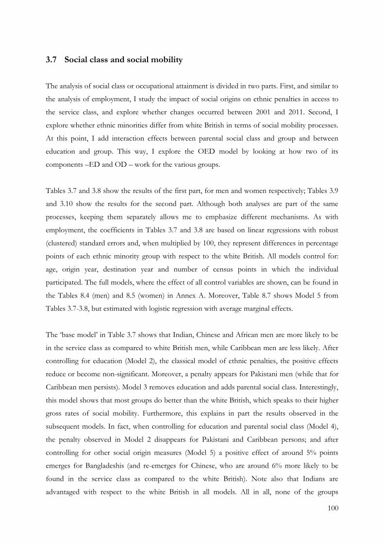
100

3.7 Social class and social mobility

The analysis of social class or occupational attainment is divided in two parts. First, and similar to

the analysis of employment, I study the impact of social origins on ethnic penalties in access to

the service class, and explore whether changes occurred between 2001 and 2011. Second, I

explore whether ethnic minorities differ from white British in terms of social mobility processes.

At this point, I add interaction effects between parental social class and group and between

education and group. This way, I explore the OED model by looking at how two of its

components –ED and OD – work for the various groups.

Tables 3.7 and 3.8 show the results of the first part, for men and women respectively; Tables 3.9

and 3.10 show the results for the second part. Although both analyses are part of the same

processes, keeping them separately allows me to emphasize different mechanisms. As with

employment, the coefficients in Tables 3.7 and 3.8 are based on linear regressions with robust

(clustered) standard errors and, when multiplied by 100, they represent differences in percentage

points of each ethnic minority group with respect to the white British. All models control for:

age, origin year, destination year and number of census points in which the individual

participated. The full models, where the effect of all control variables are shown, can be found in

the Tables 8.4 (men) and 8.5 (women) in Annex A. Moreover, Table 8.7 shows Model 5 from

Tables 3.7-3.8, but estimated with logistic regression with average marginal effects.

The ‘base model’ in Table 3.7 shows that Indian, Chinese and African men are more likely to be

in the service class as compared to white British men, while Caribbean men are less likely. After

controlling for education (Model 2), the classical model of ethnic penalties, the positive effects

reduce or become non-significant. Moreover, a penalty appears for Pakistani men (while that for

Caribbean men persists). Model 3 removes education and adds parental social class. Interestingly,

this model shows that most groups do better than the white British, which speaks to their higher

gross rates of social mobility. Furthermore, this explains in part the results observed in the

subsequent models. In fact, when controlling for education and parental social class (Model 4),

the penalty observed in Model 2 disappears for Pakistani and Caribbean persons; and after

controlling for other social origin measures (Model 5) a positive effect of around 5% points

emerges for Bangladeshis (and re-emerges for Chinese, who are around 6% more likely to be

found in the service class as compared to the white British). Note also that Indians are

advantaged with respect to the white British in all models. All in all, none of the groups

101

experience ethnic penalties in the access to the service class, and Indian, Bangladeshi and Chinese

persons even experience an advantage over white British. These outcomes are connected with the

general lower dependence of ethnic minorities on their parental social class. The last model,

finally, adds interactions with year (Model 6). Here we only observe an effect for Africans, which

basically reveals that an initial advantage they have in 2001 disappears in 2011 (see Table 8.4 in

Annex A).

Table ‎3.7: Access to the service class. Men.

M1 M2 M3 M4 M5 M63


Indian 0.155*** 0.027*** 0.206*** 0.060*** 0.078*** ns

(0.0129) (0.0102) (0.0126) (0.0102) (0.0104)

Pakistani -0.012 -0.055*** 0.084*** -0.011 0.010 ns

(0.0161) (0.0125) (0.0154) (0.0125) (0.0128)

Bangladeshi 0.009 -0.030 0.107*** 0.013 0.056** ns

(0.0278) (0.0228) (0.0279) (0.0231) (0.0233)

Chinese 0.179*** 0.003 0.211*** 0.033 0.063* ns

(0.0395) (0.0331) (0.0372) (0.0324) (0.0324)

Caribbean -0.035* -0.044*** 0.016 -0.023 0.002 ns

(0.0188) (0.0163) (0.0189) (0.0165) (0.0165)

African 0.110** -0.014 0.114*** -0.005 0.036 –

(0.0448) (0.0409) (0.0424) (0.0401) (0.0399)

Adjusted R2 0.012 0.238 0.079 0.249 0.253 0.253

N 174110 174110 174110 174110 174110 174110

Base model1 X X X X X X

Education X X X X

Parental social class X X X X

Other origins2 X X

Year*Ethnic group X

1 Controls for: age, origin year, destination year and number of census points. 2 Includes tenure, number of persons per room, number of cars and deprivation quintile at the ward level 3 + means a positive interaction; - means a negative interaction; and ns means a non-significant interaction (p-value>=.10). The effects refer to the year 2011 vs. 2001. * p-value<.10 ** p-value<.05 *** p-value<.01. Robust (clustered) standard errors in parentheses Population: Individuals between 20 and 45 years old Source: Own calculations based on ONS-LS

102

Table ‎3.8: Access to the service class. Women.

M1 M2 M3 M4 M5 M63


Indian 0.128*** 0.021** 0.174*** 0.044*** 0.054*** ns

(0.0129) (0.0108) (0.0126) (0.0108) (0.0110)

Pakistani -0.021 -0.038*** 0.064*** -0.007 0.004 ns

(0.0164) (0.0136) (0.0162) (0.0137) (0.0139)

Bangladeshi -0.044* -0.041** 0.063** -0.004 0.027 ns

(0.0264) (0.0207) (0.0258) (0.0206) (0.0209)

Chinese 0.108*** -0.057* 0.137*** -0.039 -0.015 ns

(0.0369) (0.0295) (0.0367) (0.0296) (0.0297)

Caribbean 0.059*** -0.000 0.106*** 0.019 0.039** ns

(0.0178) (0.0152) (0.0176) (0.0151) (0.0152)

African 0.135*** -0.086** 0.138*** -0.074** -0.041 ns

(0.0374) (0.0364) (0.0382) (0.0365) (0.0364)

Adjusted R2 0.007 0.242 0.060 0.248 0.251 0.251

N 180608 180608 180608 180608 180608 180608

Base model1 X X X X X X

Education X X X X

Parental social class X X X X

Other origins2 X X

Group*Year X

1 Controls for: age, origin year, destination year and number of census points. 2 Includes tenure, number of persons per room, number of cars and deprivation quintile at the ward level 3 + means a positive interaction; - means a negative interaction; and ns means a non-significant interaction (p-value>=.10). The effects refer to the year 2011 vs. 2001. * p-value<.10 ** p-value<.05 *** p-value<.01. Robust (clustered) standard errors in parentheses Population: Individuals between 20 and 45 years old Source: Own calculations based on ONS-LS

Moving to women, Model 1 in Table 3.8 shows that Indian, Chinese, Caribbean and African

persons are more likely to be in the service class as compared to white British, while Bangladeshis

are less likely. After controlling for education (Model 2), the positive effects turn into negative for

Chinese and African persons and disappear for Caribbean individuals. On the other hand, the

negative effect for Bangladeshis persists and also a negative effect appears for Pakistani women.

When controlling for the parental social class only (Model 3), we observe that similar to men,

there is an advantage for all ethnic groups, which denotes the overrepresentation of low class

origins among the ethnic minorities as well as their higher gross social mobility rates. Model 4,

which includes both education and parental social class, reveals that the penalty observed in

Model 2 (the classical ethnic penalty model) disappears for Pakistani, Bangladeshi and Chinese

103

women. Model 5, finally, which controls for other social origins, removes the penalty for African

and gives an advantage to Caribbean women. In fact, Caribbean and also Indian persons have

around 4-5% points greater likelihood of being in the service class than the white British (as for

men, Indian women are advantaged in all models). Finally, no statistically significant interactions

are found when adding interactions with year (Model 6).

The first part of the analysis of occupation has revealed that social origins matter, confirming

Hypothesis 1. In fact, they matter even more than when estimating the access to employment.

After controlling for background characteristics, none of the groups suffer penalties in the access

to the service class: specifically, the disadvantage observed for some groups when controlling

only for education disappears once we control for social origins (this is the case for Pakistani and

Caribbean men and for Pakistani, Bangladeshi, Chinese and African women). Moreover, an

advantage is observed for some groups: in some cases the parental social class reinforces an

advantage already present in the classical ethnic penalties model (Indian men and women); in

other cases, it makes it happen (Bangladeshi and Chinese men and Caribbean women).

Part two of this analysis deals with processes of social mobility. This is presented in Table 3.9. As

with the previous tables, the coefficients are based on linear regressions with robust (clustered)

standard errors. Given that I am studying processes of intergenerational reproduction, I include

the main effects for ethnic minorities together with the effect of parental social class (as

interaction). Here the interaction effects represent the difference in the effect of the parental

social class between a certain ethnic group and the white British. Specifically, I study the effect of

having routine non-manual (III), petit bourgeoisie (IV) and professional/managerial (I+II)

parents with respect to having lower technical, skilled manual and semi- and unskilled manual

parents (V+VI+VII). For example, a positive interaction effect for professional/managerial

parental origins among a certain minority means that the effect of having

professional/managerial parents (as compared to having manual parents) is higher for that ethnic

minority than it is for the white British. Finally, in addition to age, origin and destination years

and number of census points controls, all models control for the other origin effects (the base

model includes therefore all these variables). In this way, I isolate the effect of the social class of

parents. The full models, where the effect of all control variables can be observed, can be found

in Table 8.6 in Annex A.

104

Table ‎3.9: Access to the service class; models of social mobility. Men.

M1 M2 M32


Indian 0.218*** 0.068*** +

(0.0174) (0.0138)

Pakistani 0.099*** 0.000 +

(0.0199) (0.0161)

Bangladeshi 0.236*** 0.096*** Ns

(0.0378) (0.0296)

Chinese 0.231*** 0.033 Ns

(0.0797) (0.0695)

Caribbean 0.079*** 0.018 Ns

(0.0247) (0.0214)

African 0.174*** -0.005 Ns

(0.0673) (0.0598)

Parental social class - reduced (ref. V+VI+VII)

No earners / No code 0.024*** 0.025***

(0.0061) (0.0054)

III (Routine non-manual) 0.077*** 0.045***

(0.0042) (0.0037)

IV (Pet B) -0.010** -0.008*

(0.0051) (0.0045)

I + II (Professional/Managerial) 0.197*** 0.093***

(0.0042) (0.0038)

Interactions with parental social class

Indian* No earners / No code -0.047 -0.016

(0.0437) (0.0369)

Indian*III 0.025 0.010

(0.0358) (0.0310)

Indian*IV 0.083** 0.059**

(0.0341) (0.0281)

Indian*I+II 0.009 0.001

(0.0288) (0.0246)

Pakistani* No earners / No code -0.067** -0.041

(0.0331) (0.0266)

Pakistani*III 0.152** 0.087

(0.0664) (0.0595)

Pakistani*IV 0.074* 0.043

(0.0443) (0.0372)

Pakistani*I+II 0.139*** 0.075*

(0.0489) (0.0422)

Bangladeshi* No earners / No code -0.071 -0.072

(0.0604) (0.0446)

Bangladeshi*III -0.151 -0.173

(0.1552) (0.1501)

Bangladeshi*IV -0.042 -0.038

(0.0768) (0.0717)

105

M1 M2 M32

Bangladeshi*I+II -0.150 -0.147*

(0.1010) (0.0815)

Chinese* No earners / No code 0.183 0.126

(0.1311) (0.1093)

Chinese*III -0.022 0.001

(0.1285) (0.1100)

Chinese*IV 0.006 -0.012

(0.0953) (0.0826)

Chinese*I+II 0.112 0.127

(0.0915) (0.0782)

Caribbean* No earners / No code 0.077 0.032

(0.0566) (0.0497)

Caribbean*III -0.035 -0.040

(0.0410) (0.0358)

Caribbean*IV -0.030 -0.025

(0.1124) (0.1063)

Caribbean*I+II -0.106** -0.095**

(0.0482) (0.0467)

African* No earners / No code 0.060 0.055

(0.1316) (0.1249)

African*III 0.004 -0.013

(0.0969) (0.0832)

African*IV 0.554*** 0.768***

(0.0678) (0.0596)

African*I+II 0.057 0.113

(0.0915) (0.0885)

Adjusted R2 0.098 0.253 0.253

N 174,110 174,110 174110

Base model1 X X X

Education X X

Group*Education X

1 Controls for: age, other origin variables, origin year, destination year and number of census points. 2 + means a positive interaction; - means a negative interaction; and ns means a non-significant interaction (p-value>=.10). Effects refer to educational level 4+ vs. Level 1 or less. * p-value<.10 ** p-value<.05 *** p-value<.01. Robust (clustered) standard errors in parentheses Population: Individuals between 20 and 45 years old Source: Author’s own calculations based on ONS-LS

The first outcome to note in Model 1 from Table 3.9 is that the main terms for ethnic minority

groups, which refer to individuals with low class parents (V+VI+VII), are positive for all groups.

This is additional evidence that ethnic minorities tend to be quite mobile, on average. The

interactions, on the other hand, reveal that having parents in class IV (the petit bourgeoisie) vs.

having low class parents brings a higher advantage to Indian and Pakistani men than to white

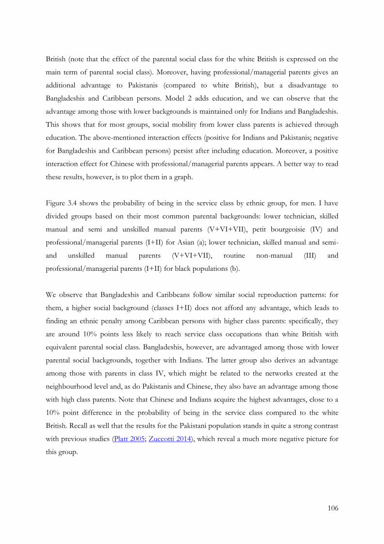
106

British (note that the effect of the parental social class for the white British is expressed on the

main term of parental social class). Moreover, having professional/managerial parents gives an

additional advantage to Pakistanis (compared to white British), but a disadvantage to

Bangladeshis and Caribbean persons. Model 2 adds education, and we can observe that the

advantage among those with lower backgrounds is maintained only for Indians and Bangladeshis.

This shows that for most groups, social mobility from lower class parents is achieved through

education. The above-mentioned interaction effects (positive for Indians and Pakistanis; negative

for Bangladeshis and Caribbean persons) persist after including education. Moreover, a positive

interaction effect for Chinese with professional/managerial parents appears. A better way to read

these results, however, is to plot them in a graph.

Figure 3.4 shows the probability of being in the service class by ethnic group, for men. I have

divided groups based on their most common parental backgrounds: lower technician, skilled

manual and semi and unskilled manual parents (V+VI+VII), petit bourgeoisie (IV) and

professional/managerial parents (I+II) for Asian (a); lower technician, skilled manual and semi-

and unskilled manual parents (V+VI+VII), routine non-manual (III) and

professional/managerial parents (I+II) for black populations (b).

We observe that Bangladeshis and Caribbeans follow similar social reproduction patterns: for

them, a higher social background (classes I+II) does not afford any advantage, which leads to

finding an ethnic penalty among Caribbean persons with higher class parents: specifically, they

are around 10% points less likely to reach service class occupations than white British with

equivalent parental social class. Bangladeshis, however, are advantaged among those with lower

parental social backgrounds, together with Indians. The latter group also derives an advantage

among those with parents in class IV, which might be related to the networks created at the

neighbourhood level and, as do Pakistanis and Chinese, they also have an advantage among those

with high class parents. Note that Chinese and Indians acquire the highest advantages, close to a

10% point difference in the probability of being in the service class compared to the white

British. Recall as well that the results for the Pakistani population stands in quite a strong contrast

with previous studies (Platt 2005; Zuccotti 2014), which reveal a much more negative picture for

this group.

107

Fig

ure

3.4

: P

rob

abili

ty o

f b

ein

g in

th

e se

rvic

e cl

ass

by

par

enta

l so

cial

cla

ss; p

redic

ted v

alues

fro

m t

he

regr

essi

on

(co

nfi

den

ce in

terv

als

90%

).

a.

Asi

an m

en

b

. B

lack

men

No

te: F

igure

s ar

e b

ased

on

Mo

del

2 f

rom

Tab

le 3

.9.

Po

pula

tio

n: In

div

idual

s b

etw

een

20 a

nd

45 y

ears

old

So

urc

e: A

uth

or’

s o

wn

cal

cula

tio

ns

bas

ed o

n O

NS

-LS

.3.4.5.6.7

Prob. service class

Ma

nu

al

Ro

utin

e n

on-m

anu

al

Pro

f/M

ana

gP

are

nta

l so

cia

l cla

ss

Bri

tish

Ca

rib

be

an

Afr

ica

n

108

I have also tested for interaction effects with education (Model 3). I found that having Level 4+

(vs. a Level 1 or less) gives a greater advantage to Indians and Pakistanis. Note that by

introducing the interaction, the positive effect of having professional/managerial parents

diminishes (and becomes statistically non-significant at p-value <.10) for Pakistanis (see Table 8.6

in Annex A). I have plotted these results in a graph (see Figure 3.5). Here we can see that, among

those who have parents in the petit bourgeoisie, the advantage for Indians is higher among those

who reach higher educational levels (level 4+). Among Pakistanis, it seems that the positive effect

of higher parental background observed in Figure 3.4 is channelled canalized by the education

they acquire.

Figure 3.5: Probability of being in the service class by parental social class and education;

predicted values from the regression (confidence intervals 90%). Men.

Note: Figure is based on Model 3 from Table 3.9. Population: Individuals between 20 and 45 years old Source: Author’s own calculations based on ONS-LS

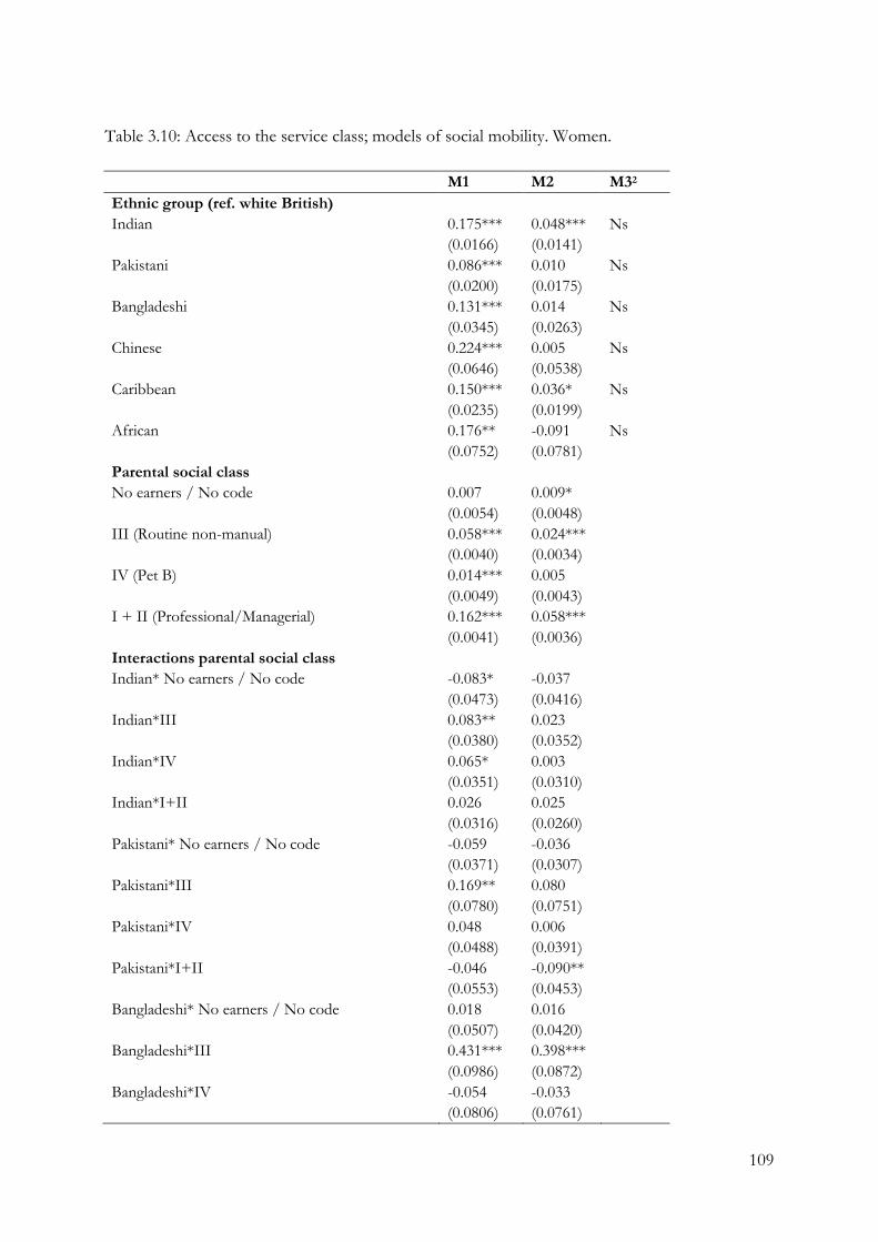
109

Table ‎3.10: Access to the service class; models of social mobility. Women.

M1 M2 M32


Indian 0.175*** 0.048*** Ns

(0.0166) (0.0141)

Pakistani 0.086*** 0.010 Ns

(0.0200) (0.0175)

Bangladeshi 0.131*** 0.014 Ns

(0.0345) (0.0263)

Chinese 0.224*** 0.005 Ns

(0.0646) (0.0538)

Caribbean 0.150*** 0.036* Ns

(0.0235) (0.0199)

African 0.176** -0.091 Ns

(0.0752) (0.0781)

Parental social class

No earners / No code 0.007 0.009*

(0.0054) (0.0048)

III (Routine non-manual) 0.058*** 0.024***

(0.0040) (0.0034)

IV (Pet B) 0.014*** 0.005

(0.0049) (0.0043)

I + II (Professional/Managerial) 0.162*** 0.058***

(0.0041) (0.0036)

Interactions parental social class

Indian* No earners / No code -0.083* -0.037

(0.0473) (0.0416)

Indian*III 0.083** 0.023

(0.0380) (0.0352)

Indian*IV 0.065* 0.003

(0.0351) (0.0310)

Indian*I+II 0.026 0.025

(0.0316) (0.0260)

Pakistani* No earners / No code -0.059 -0.036

(0.0371) (0.0307)

Pakistani*III 0.169** 0.080

(0.0780) (0.0751)

Pakistani*IV 0.048 0.006

(0.0488) (0.0391)

Pakistani*I+II -0.046 -0.090**

(0.0553) (0.0453)

Bangladeshi* No earners / No code 0.018 0.016

(0.0507) (0.0420)

Bangladeshi*III 0.431*** 0.398***

(0.0986) (0.0872)

Bangladeshi*IV -0.054 -0.033

(0.0806) (0.0761)

110

M1 M2 M32

Bangladeshi*I+II 0.035 0.059

(0.1554) (0.1310)

Chinese* No earners / No code -0.151 -0.072

(0.1115) (0.0772)

Chinese*III -0.042 0.121

(0.1512) (0.1224)

Chinese*IV 0.005 -0.032

(0.0755) (0.0640)

Chinese*I+II -0.086 -0.023

(0.1130) (0.0884)

Caribbean* No earners / No code 0.067 0.047

(0.0455) (0.0417)

Caribbean*III 0.012 0.003

(0.0398) (0.0329)

Caribbean*IV -0.094 -0.086

(0.0922) (0.0640)

Caribbean*I+II -0.073 -0.019

(0.0448) (0.0388)

African* No earners / No code 0.112 0.065

(0.1035) (0.1026)

African*III 0.163* 0.169*

(0.0910) (0.0945)

African*IV 0.171 0.174

(0.2236) (0.1568)

African*I+II -0.124 -0.056

(0.0944) (0.0936)

Adjusted R2 0.081 0.251 0.251

N 180608 180608 180608

Base model1 X X X

Education X X

Group*Education X

1 Controls for: age, other origin variables, origin year, destination year and number of census points. 2 + means a positive interaction; - means a negative interaction; and ns means a non-significant interaction (p-value>=.10). Effects refer to educational level 4+ vs. level 1; in parentheses are the (statistically significant) effects when comparing level 4+ vs. all the others. * p-value<.10 ** p-value<.05 *** p-value<.01. Robust (clustered) standard errors in parentheses Population: Individuals between 20 and 45 years old Source: Author’s own calculations based on ONS-LS

Table 3.10 shows the results on social mobility for women. As for men, the first thing to note in

Model 1 is the positive effect that having parents in the lower social classes has for all groups

(observed in the main terms for ethnic group): ethnic minority women also tend to be quite

mobile, on average. The interactions, on the other hand, reveal that having parents in class IV

111

(vs. classes V+VI+VII) brings a higher advantage to Indians than to white British persons.

Furthermore, having professional/managerial parents gives a disadvantage Caribbean persons,

equally to what was found for men. An advantage is also observed among African women with

routine non-manual parents. When adding education (Model 2), we observe that the advantage

among those with lower backgrounds is maintained only for Indian and Caribbean populations,

while for the rest of the groups it becomes statistically non-significant. Education, therefore, is an

important mediator of the effect of parental social background, as would be expected. With

regard to the interactions, they disappear for Indian (with parents in class IV) and Caribbean

(with parents in class I+II) and become negative for Pakistani women with

professional/managerial backgrounds. Figure 3.6 shows these results in a graph, separately for

Asian (a) and black (b) women.

Figure 3.6 shows that Pakistani women, the only ones who present a statistically significant

interaction effect, gain less from advantageous origins (vs. manual origins) as compared to the

white British. This creates a gap among those who have advantageous social origins: specifically,

they are around 8% less likely to be in the service class compared to the white British. Note how

different this result is with respect to Pakistani men, who actually presented a positive interaction

effect, gaining more than the white British from higher parental backgrounds. A similar effect is

observed for African women with advantageous origins, although the interaction is statistically

non-significant in Table 3.10. Finally, I tested for interaction effects with education (Model 3),

and I did not find statistically significant negative effects of Level 4+ when compared to Level 1

or less, although there are some indications that the negative effect for Africans might be related

to penalties among the higher educated.

112

Fig

ure

3.6

: P

rob

abili

ty o

f b

ein

g in

th

e se

rvic

e cl

ass

by

par

enta

l so

cial

cla

ss; p

redic

ted v

alues

fro

m r

egre

ssio

n (

con

fiden

ce in

terv

als

90%

).

a. A

sian

wo

men

b

. B

lack

wo

men

Fig

ure

is

bas

ed o

n M

od

el 2

fro

m T

able

3.1

0.

Po

pula

tio

n: In

div

idual

s b

etw

een

20 a

nd

45 y

ears

old

So

urc

e: A

uth

or’

s o

wn

cal

cula

tio

ns

bas

ed o

n O

NS

-LS

.1.2.3.4.5

Prob. service classM

anual

Routine n

on-m

anual

Pro

f/M

anag

Pare

nta

l socia

l cla

ss

Bri

tish

Caribb

ean

Afr

ican

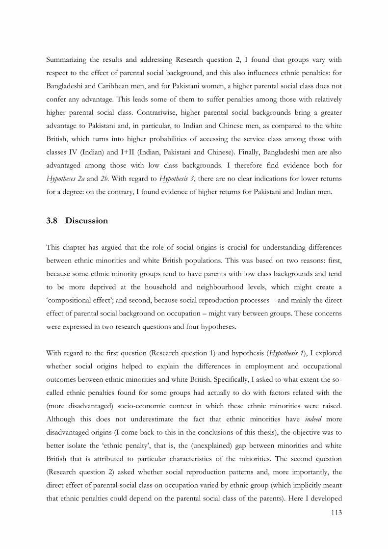
113

Summarizing the results and addressing Research question 2, I found that groups vary with

respect to the effect of parental social background, and this also influences ethnic penalties: for

Bangladeshi and Caribbean men, and for Pakistani women, a higher parental social class does not

confer any advantage. This leads some of them to suffer penalties among those with relatively

higher parental social class. Contrariwise, higher parental social backgrounds bring a greater

advantage to Pakistani and, in particular, to Indian and Chinese men, as compared to the white

British, which turns into higher probabilities of accessing the service class among those with

classes IV (Indian) and I+II (Indian, Pakistani and Chinese). Finally, Bangladeshi men are also

advantaged among those with low class backgrounds. I therefore find evidence both for

Hypotheses 2a and 2b. With regard to Hypothesis 3, there are no clear indications for lower returns

for a degree: on the contrary, I found evidence of higher returns for Pakistani and Indian men.

3.8 Discussion

This chapter has argued that the role of social origins is crucial for understanding differences

between ethnic minorities and white British populations. This was based on two reasons: first,

because some ethnic minority groups tend to have parents with low class backgrounds and tend

to be more deprived at the household and neighbourhood levels, which might create a

‘compositional effect’; and second, because social reproduction processes – and mainly the direct

effect of parental social background on occupation – might vary between groups. These concerns

were expressed in two research questions and four hypotheses.

With regard to the first question (Research question 1) and hypothesis (Hypothesis 1), I explored

whether social origins helped to explain the differences in employment and occupational

outcomes between ethnic minorities and white British. Specifically, I asked to what extent the so-

called ethnic penalties found for some groups had actually to do with factors related with the

(more disadvantaged) socio-economic context in which these ethnic minorities were raised.

Although this does not underestimate the fact that ethnic minorities have indeed more

disadvantaged origins (I come back to this in the conclusions of this thesis), the objective was to

better isolate the ‘ethnic penalty’, that is, the (unexplained) gap between minorities and white

British that is attributed to particular characteristics of the minorities. The second question

(Research question 2) asked whether social reproduction patterns and, more importantly, the

direct effect of parental social class on occupation varied by ethnic group (which implicitly meant

that ethnic penalties could depend on the parental social class of the parents). Here I developed

114

three hypotheses: the two most relevant for this study referred to the direct role of the parental

background on occupation, and were built in opposition: one expected a lower dependence on

parental social background among ethnic minorities (Hypothesis 2a); the other expected a higher

dependence (Hypothesis 2b). The last hypothesis referred to the role of education, and expected

lower returns to education for ethnic minorities (Hypothesis 3).

Regarding the first question, we saw that most ethnic minorities (African were an exception) have

lower parental social classes as compared to white British; we also saw that most of them tended

to be in deprived areas and in a worse position in terms of household resources. What is the

impact of considering this ‘compositional effect’? The results have shown that social origins

matter: in fact, not only they have helped to explain (partly or completely) ethnic penalties in

employment and occupation (mainly for Pakistani, Bangladeshi and Caribbean populations), but

in some cases it has also widened a positive gap (among Indian and Chinese populations). As

regards the first process, that is, the reduction of the (expected) ethnic penalties for some groups,

the outcome goes in line with Hypothesis 1. The second process – the appearance/widening of a

positive gap for other groups – reveals that coming from relatively low social backgrounds has a

certain advantage if one belongs to an ethnic minority. This is an interesting finding and possibly

points to motivational factors, typical of ethnic minorities who have seen their occupation

degraded in the origin country and want to see their children improve in destination and ‘recover’

the initial status. The fact that this applies particularly to Indian and Chinese populations is no

surprise, given the good performance that these populations have not only in the UK, but also in

other countries such as the US (Farley and Alba 2002; Kim and Kulkarni 2009).

The role of parental background was, later on, further explored with the analysis of social

reproduction patterns. A main argument in this study was that the postulates that Goldthorpe

(2000) uses to explain the stability and reproduction of the social structure for the general

population might not always apply to ethnic minorities.

If we look back at Figures 4.4 and 4.6 and assume that parental social class categories have a

certain order – from low to high – we could think of social reproduction patterns in terms of

how flat these lines are. Steeper lines mean that individuals depend more on the parental social

background, while flatter lines mean that the parental social class matters less. In a pure

meritocratic world, we would see flat lines: that is, no matter where you come from, you can

always have the same probabilities of accessing the service class. This world does not exist, and

115

we know that parents influence the occupations that their children choose. In this sense, very

steep lines mean that those who have parents in with professional/managerial occupations are

much more likely to acquire service class occupations, compared to those whose parents are in

the lower classes. In the extreme case, we would find all individuals with professional/managerial

origins in service class positions, and all low-class-origin individuals in low-class positions. This

world, as we know, does not exist either. In reality, our world has a mix of these lines, which

depend – for example – on the country we consider (for example, the UK line has been found to

be steeper than Scandinavian lines: Hout and DiPrete 2006) or the gender of the individuals (this

study shows, for example, that male lines tend to be steeper than female lines). But this chapter

has also argued that lines might depend on the ethnicity of individuals. Specifically, I argued that

differences in terms of motivation and aspirations, manners and ways of behaving, constraints

related to the economic context and family, community and cultural factors might contribute to

the development of divergent social reproduction processes and, therefore, to the development

of ethnic-specific lines. A direct consequence of this is, as we saw, that ethnic penalties might

depend on the parental social class. For example, if one group with low parental social

background has the same probability of being in the service class as the white British with the

same social background, but they get lower returns to their social origins (i.e. a less steep line), we

will find that a gap is generated among those who have higher social origins.

The analysis has shown that most male minority groups and Pakistani women have different

social mobility patterns than the white British. Bangladeshi and Caribbean men and Pakistani

women typically have flat lines, depending therefore less on their social origins (in line with

Hypothesis 2a). However, there is a difference between the groups in terms of ethnic penalties:

while for Bangladeshi men, a lower effect of having professional/managerial parents is

complemented with a positive gap among those with low backgrounds; for Caribbean men and

Pakistani women, it actually means a penalty among those with professional/managerial origins.

Indian, Chinese and Pakistani men, on the other hand, have steeper lines and, therefore, seem to

be more dependent on parental background (in line with Hypothesis 2b). However, rather than

being a constraint – as it was mostly argued in the theoretical section – this has given them an

advantage over the white British: Indian men have an advantage in particular among those with

petit bourgeoisie origins, while Pakistani and Chinese are particularly advantaged among those

with professional/managerial origins.

116

I argued before that ethnic minorities may outperform individuals from the majoritarian

population, i.e. the white British, in response to the high aspirations that ethnic minority parents

may have of their children (i.e. Dale et al. 2002). This, I claimed, might explain the success of

Indian and Chinese populations and could account as well for the overperformance of

Bangladeshi men of lower social origins, and perhaps also that of Pakistani men with higher

social origins. Not finding the same results for Pakistani and Bangladeshi women, on the other

hand, might speak of gender constraints that these groups experience (in particular the former),

especially if we also consider their disadvantage in terms of employment. Finally, with regard to

the disadvantages found among some (better positioned) black populations (Caribbean men and

to some extent African women) a possible explanation might be the lack of ‘signalling’ resources

among ethnic minorities – which the British higher classes would have – but also the existence of

selective processes of discrimination connected with skin colour, or with certain occupational

niches or sectors of the economy. Note also that for African women this might be linked to

lower educational returns (Hypothesis 3), although the results are not robust. More research is

needed in order to elucidate why some groups gain and others lose from particular social

backgrounds.

This chapter has shown that the study of ethnic inequalities in the labour market is more

complex than what the literature, at least on the European level, has disclosed. The role of social

origins has been revealed to be an important element in understanding how second generation

ethnic minorities are faring in England and Wales. Specifically, not considering them in the

analysis might lead to an overestimation of ethnic penalties: for example, in the case of

employment of Pakistani and Caribbean men, the unadjusted penalty is almost double the penalty

adjusted for social origins. Moreover, I have also shown that the average effects with regard to

the relative performance of ethnic minorities in the labour market depends both on their levels of

education – especially in access to employment – and on their parental social backgrounds.

Finally, I would like to highlight as well a few outcomes connected to this study, which are not

directly linked to the research questions. These outcomes will help to put inti perspective the

results delineated in the coming chapters. First, ethnic penalties in employment diminished for

most groups between 2001 and 2011; however, low educated Pakistani men continued to be

disadvantaged with respect to the white British in 2011, and Pakistani and Bangladeshi women

(especially the low educated) continued to have very low employment levels. Second, in general,

employment seems to be a more serious problem for ethnic minorities, compared to the type of

117

occupation they acquire, in line with previous findings (Cheung and Heath 2007b). Third, Indians

and Chinese are doing very well, both in terms of employment and in terms of access to the

highest occupations, sometimes even better than the white British. The same is true for

Bangladeshi men and Caribbean women in terms of their social class. Finally, the Bangladeshi

population seems to be doing slightly better than the Pakistani population, which serves as an

argument to treat them separately.

119

4 CHAPTER 4: Is Spatial Segregation of Ethnic

Minorities Really Decreasing?

4.1 Introduction

The study of the spatial segregation of individuals in terms of their characteristics has received a

great deal of attention in the human geography and migration literature. Spatial segregation

alludes to the idea that the distribution of a population over space is unequal: in simple terms, it

means that inequalities (based, for example, on ethnicity or socio-economic resources) have a

spatial ‘translation’ or, more specifically, are produced and reproduced in space. In this regard,

one of the reasons why spatial segregation has been a matter of extensive research – and why I

believe it is a relevant topic – is because it might contribute to undermining the social cohesion

of a society as a whole, by preventing individuals from having contact with others who are

different from themselves (see for example Cantle 2012; Uslaner 2012).

Within the literature on spatial segregation, the spatial location of immigrants and/or ethnic

minorities has been of particular interest: in fact, countless studies have shown that ethnic

minorities tend to live close to one another (i.e. Johnston, Forrest and Poulsen 2002a; Johnston,

Poulsen and Forrest 2007; Logan and Stults 2011; Logan, Stults and Farley 2004; Musterd 2005;

Van Kempen and Şule Özüekren 1998). This pattern is usually attributed to the potential of the

neighbourhood to offer all kinds of ‘ethnic’ resources, ranging from the exchange of information,

to the development of ethnic entrepreneurship or the possibility of maintaining one’s own

culture and speaking one’s own language. According to spatial assimilation theory (Massey 1985),

it is expected that as ethnic minorities spend more time in the destination country, they also start

to disperse in its space. This dispersion is typically coupled with an improvement in socio-

economic status. In fact, areas with a high concentration of ethnic minorities are also usually

areas with high levels of deprivation, and studies conducted in the US have demonstrated that an

improvement in socio-economic status implies, in many cases, an improvement in terms of the

neighbourhood, which leads to a movement out of the ethnic neighbourhood (Massey 1985;

Massey and Denton 1985). However, other studies (i.e. Bolt and Van Kempen 2010; Lersch

2013) have shown that this might not be the case, and that either due to preference or constraint,

120

the classical model of spatial assimilation might not necessarily apply here; ethnic minorities

might remain segregated over time (more details on this discussion are to be found in Chapter 6).

Using aggregated census data for England (2001 & 2011) at a very detailed geographical level, the

objective of this chapter is to give a general overview of the changes in spatial segregation of

ethnic minorities within eight defined ‘housing market areas’ (HMAs) of England between 2001

and 2011. The analysis is done for white British, pooled non-white ethnic minorities and six

chosen ethnic minority groups: Indian, Pakistani, Bangladeshi, Chinese, Caribbean and African. It

answers the following questions, the second one being the most relevant:

1. What was the spatial distribution of ethnic minorities in England in 2011? Which groups

were more segregated and in which HMAs?

2. Did the spatial segregation of ethnic minorities decrease in the period 2001-2011? If so,

for which groups and HMAs?

The analysis in this chapter is doubly novel: the first innovative aspect pertains to my choice of

housing market areas as the major geographical units to study spatial segregation. HMAs can be

defined as relatively self-contained areas that express people’s choice of location of a new

residence. This means that, when studying changes in spatial segregation in these areas, I am able

to control, to some extent, for the fact that individuals are ‘constrained’ to a geographical space.

This allows me to assume that changes are likely to be related (at least in part, since changes also

occur due to immigration from abroad) with relocations of individuals within a certain HMA.

The second novel aspect of this chapter is that I look at more than one dimension of segregation.

The bulk of the research in this area has relied on the Dissimilarity Index, which is the most

common – and easy to use – measure of spatial segregation. This Index, however, measures only

one dimension of segregation, the uneven distribution of individuals in a given space. In this

chapter, I include three other dimensions: interaction, which refers to the probability of contact

between members of a group within a neighbourhood; concentration, that is, the extent to which

ethnic minorities occupy a small share of the space; and finally, clustering, that is, the extent to

which ethnic minorities live in neighbourhoods that adjoin each other. In order to explore these

different dimensions, I use geo-referenced information on the characteristics, location and size of

the areas, by means of specialized geographical software.

121

4.2 Spatial segregation in the UK

Previous studies on spatial segregation in the UK can be divided into two categories. On the one

hand, one finds studies that explore spatial segregation through different segregation indices,

mainly the Dissimilarity Index, which assesses the evenness of the distribution of a group in

space (1955; Duncan and Duncan 1955a), and to a lesser extent the Isolation Index, which is a

measure of potential contact between members of a group in a certain geographical area (for

more specific definitions, please refer to the sections below). On the other hand, we find studies

that treat spatial segregation by means of creating different ‘ideal types’ of areas, with varied

relative shares of ethnic minorities.

In the first group, we find studies that cover three decades of changes: from 1981 to 2011.

Starting with the first two decades, 1981-2001, the most systematic study of spatial segregation

was done by Rees and Butt (Rees and Butt 2004), who compared Dissimilarity indices for three

time points, based on 20 metropolitan/non-metropolitan regions (for a discussion on

geographical units used to calculate segregation indices, please refer to the next section). They

showed that in 1981, the most unevenly distributed groups – that is, groups with the highest

Dissimilarity Index – are Caribbean and African, followed by Bangladeshi, Pakistani, Indian and

Chinese (see Table 4.1). These authors also noted that between 1981 and 1991, spatial

segregation measured in this way increased for all groups; while for the period 1991-2001 it

increased only for Pakistani and Bangladeshi, and decreased for the remaining groups (although

the relative ordering of groups remained the same, with black populations as the most segregated,

in particular African). However, in a departure from common practise in studies on ethnic

minorities, this study merged within the main groups those who identify themselves as white and

African, white and Caribbean or white and Asian22.

A more recent study, based on definitions of ethnicity that do not include ‘half-white’

populations showed a slightly different picture (Simpson 2012). The Dissimilarity Indices, based

in this case on 348 Local Authorities, showed that although black populations in 1991/2001 also

had higher segregation levels than Asians, the difference is smaller as compared to the previous

study. As regards changes between 1991 and 2001, Indian, Pakistani and Chinese decreased their

uneven distribution, while black populations and Bangladeshi increased it. When using an even

22 In this and the other chapters, individuals who consider themselves as ‘half-white’ have been excluded from the analysis.

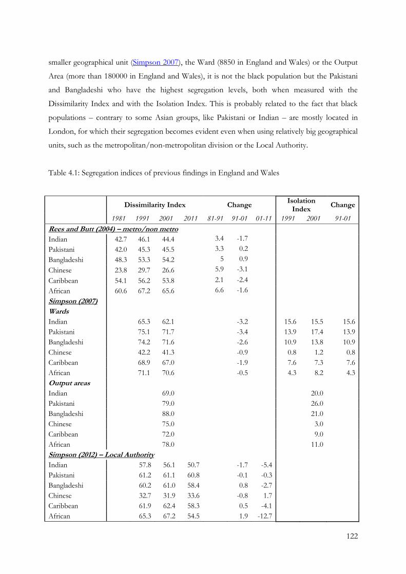
122

smaller geographical unit (Simpson 2007), the Ward (8850 in England and Wales) or the Output

Area (more than 180000 in England and Wales), it is not the black population but the Pakistani

and Bangladeshi who have the highest segregation levels, both when measured with the

Dissimilarity Index and with the Isolation Index. This is probably related to the fact that black

populations – contrary to some Asian groups, like Pakistani or Indian – are mostly located in

London, for which their segregation becomes evident even when using relatively big geographical

units, such as the metropolitan/non-metropolitan division or the Local Authority.

Table ‎4.1: Segregation indices of previous findings in England and Wales

Dissimilarity Index Change

Isolation Index

Change

1981 1991 2001 2011 81-91 91-01 01-11 1991 2001 91-01

Rees and Butt (2004) – metro/non metro

Indian 42.7 46.1 44.4

3.4 -1.7

Pakistani 42.0 45.3 45.5

3.3 0.2

Bangladeshi 48.3 53.3 54.2

5 0.9

Chinese 23.8 29.7 26.6

5.9 -3.1

Caribbean 54.1 56.2 53.8

2.1 -2.4

African 60.6 67.2 65.6

6.6 -1.6

Simpson (2007)

Wards

Indian

65.3 62.1

-3.2 15.6 15.5 15.6

Pakistani

75.1 71.7

-3.4 13.9 17.4 13.9

Bangladeshi

74.2 71.6

-2.6 10.9 13.8 10.9

Chinese

42.2 41.3

-0.9 0.8 1.2 0.8

Caribbean

68.9 67.0

-1.9 7.6 7.3 7.6

African

71.1 70.6

-0.5 4.3 8.2 4.3

Output areas

Indian

69.0

20.0

Pakistani

79.0

26.0

Bangladeshi

88.0

21.0

Chinese

75.0

3.0

Caribbean

72.0

9.0

African

78.0

11.0

Simpson (2012) – Local Authority

Indian 57.8 56.1 50.7 -1.7 -5.4

Pakistani 61.2 61.1 60.8 -0.1 -0.3

Bangladeshi 60.2 61.0 58.4 0.8 -2.7

Chinese 32.7 31.9 33.6 -0.8 1.7

Caribbean 61.9 62.4 58.3 0.5 -4.1

African 65.3 67.2 54.5 1.9 -12.7

123

Regarding findings available for the period under study in this chapter, 2001-2011, Simpson

(2012), who calculated the Dissimilarity Index using Local Authorities as geographical units,

showed that in 2011 the most segregated groups are Pakistanis, followed closely by Bangladeshi

and Caribbean (see again Table 4.1). Moreover, the tendencies are of a decrease of spatial

segregation for most groups, especially African, who reduced their D by almost 13 points, and

Indian; only Chinese increased their segregation. A similar study, which like Simpson’s work was

also part of the “Dynamics of Diversity series” of the 2011 Census (see research outputs in:

www.ethnicity.ac.uk), takes a more micro view of segregation, using as well the Dissimilarity

Index (Catney 2013). In this case, the Index is based on the Output Area level as a geographical

unit (areas of around 300 people) and is calculated for each Local Authority separately. The

results of this analysis show that segregation decreased for all ethnic minority groups in most

Local Authorities, including those in the largest metropolitan areas. In particular, Bangladeshi and

Chinese in Outer London experienced the highest decreases in segregation, followed by the other

ethnic minority groups; these outcomes, it is argued, can be linked to processes of

suburbanization. Only segregation for Caribbean and African in Inner London went in the

opposite direction, although with very small increases.

Other researchers, arguing that the Dissimilarity Index is overly simplistic, have investigated the

spatial segregation of ethnic minorities using different methods. I refer to the various works by

Johnston, Poulsen and Forrest (Johnston, Forrest and Poulsen 2002a; Johnston, Forrest and

Poulsen 2002b; Johnston, Poulsen and Forrest 2007), who created different typologies of areas –

in this case Wards – based on the relative share of ethnic minorities and white populations in

each of them. Specifically, they created a 6-category classification, wherein category I are areas

where 80% or more of the population is white and category VI are areas where the non-white

population is around 70-80% of the total and one ethnic minority group is: a) more than twice as

large as any other, and b) constitutes more than 30% of the population of that group (also

defined as a ‘ghetto’) (Johnston, Poulsen and Forrest 2007). Among other findings, these studies

show that black populations are much more likely than Asian populations to live in areas with

white members. Among the latter, Indians and to a lesser extent Pakistanis, are more likely to be

found in areas with higher share of whites; furthermore, Bangladeshis are also more likely to be

‘encapsulated’, that is, to share areas only with other co-ethnics, than the rest of the groups.

However, there are no category VI areas in London (i.e. ghettos). On the contrary, analyses done

for other metropolitan areas actually show that Indian in Leicester and Pakistanis in Bradford are

the basis for the creation of two ghetto-types in these cities. The analyses also show that around

http://www.ethnicity.ac.uk/research/outputs/briefings/dynamics-of-diversity

124

43% of Indian and 36% of Pakistani living in Leicester live in these ghetto-type areas; similarly,

27% of Pakistanis in Bradford live in the Pakistani ghetto.

These authors also offer a different perspective regarding changes between decades. For example,

they argue that while between 1991 and 2001 many areas became more mixed, revealing

processes that might speak of decreasing spatial segregation, there are also clear tendencies in the

opposite direction. For example, in a paper that studies changes between 1991 and 2001, they

showed that in London the extreme types are disappearing (types I and V&VI), and both ethnic

minorities and white British were more likely to live in ethnically mixed areas in 2001 than in

1991. Similarly, Pakistanis in Bradford were also more likely to live in relatively mixed, white-

dominated areas. However, they also presented evidence pointing to an increase of spatial

segregation: for example, they showed that between 1991 and 2011, Pakistani in Bradford also

increased their probability of being in the Pakistani-dominated type-V area (Poulsen and

Johnston 2006).

Summarizing, both approaches show evidence that Asians are more segregated than black

populations (at the micro-level). Moreover, they both present evidence of decreasing spatial

segregation for ethnic minority groups as well as of a tendency towards greater dispersion – in

particular out of metropolitan areas – and mixing between whites and non-whites. However, a

key difference between them is that the second approach is more cautious in their claims and

presents some counter-tendencies as well. In this regard, I find the discussion in Carling (2008)

very illustrative of these debates. Using the same findings that Simpson and collaborators

presented to argue that spatial segregation of ethnic minorities is decreasing, he made a ‘novel

interpretation’ and emphasized – as Poulsen and Johnston did with other type of data – that both

tendencies of decrease and increase in spatial segregation are present: more importantly, he stated

that the latter might even be related to processes of self-segregation of groups, a notion rejected

by Simpson and collaborators (these debates arose as a consequence of disturbances occurred in

Brighton 2001; see Finney and Simpson 2009b; Rattansi 2011; and the discussion in Chapter 1).

The present study is based on the first approach, that is, I explore segregation indices for various

groups. However, rather than focusing on one or two indices – as has been done to date – my

analysis is based on more complex and diverse measures, which in the end lead me to

conclusions that are more in line with the second approach, and with the work of Carling (2008).

125

4.3 Measuring spatial segregation

4.3.1 Some issues in the selection of areas

Spatial segregation can be defined as the concentration of people having certain characteristics in

common. It alludes to the idea that the distribution of the population in space is unequal:

individuals tend to locate close to others who are similar to them, mainly in terms of socio-

economic status and ethnicity. While this phenomenon is quite easy to apprehend on an intuitive

basis – it is observable to the naked eye – it is very complex to measure. A number of decisions

need to be made toward this goal.

The usual way to study spatial segregation is to measure the distribution of individuals across

geographical units within a larger area. This means, on the one hand, that we need to choose the

area in which segregation will be measured, for example, countries, regions or metropolitan areas;

and on the other, that we must define the geographical units in which individuals live. The

selection of one or another area level or geographical unit will impact on the conclusions we

reach. These issues have been grouped under the Modifiable Area Unit Problem (Openshaw

1984). For the purposes of this chapter, I discuss the effect of the geographical scale (both of the

larger area and smaller geographical unit) and the effect of the size of the geographical unit,

which is linked to the density of population (see also Simpson 2007 for a discussion on these

topics).

The problem of geographical scale is illustrated in Figure 4.1 (adapted from Rodríguez Vignoli

2001). The three main squares represent a hypothetical metropolitan area with three possible

distributions of its two main populations (represented in white and grey colours) in: districts

(North and South), neighbourhoods and blocks. In Figure 4.1a, the white population lives in the

North, while the grey population lives in the South. In Figure 4.1b white and grey populations are

mixed within districts, but not within neighbourhoods. In Figure 4.1c, finally, white and grey

populations are mixed within districts and neighbourhoods, but not within blocks.

126

Figure 4.1: A hypothetical metropolitan area with three different population distributions

Imagine first that we are interested in studying the wider metropolitan area, and that the smaller

geographical unit used for studying segregation is the district (North-South). Here we would find

that while Figure 4.1a has very high segregation (there is only one group in each district); Figures

5.1b and 5.1c have very low segregation, since there is equal number of groups in the North and

South districts. Consider now that the unit used for measuring segregation is the neighbourhood.

Here we would find that both Figures 5.1a and 5.1b have high segregation, since there is no

mixing of groups within neighbourhoods, while Figure 4.1c would be a case of low segregation.

Finally, consider the block as a geographical unit for studying spatial segregation: here we would

find high segregation in all figures, since there is no mixing of groups within blocks.

Imagine now that instead of studying the wider metropolitan area, we choose to study the

districts separately, perhaps because we think that they are more relevant as a geographical entity

(for example, because they respond to different local governments or housing markets). Both if

the geographical unit chosen were the neighbourhood or the block, we would find that Figure

4.1a presents a case of low segregation: each neighbourhood has the same proportion of grey (or

white) population, in this case 100%. The segregation results for the other figures would be the

same as when considering the larger metropolitan area. Table 4.2 summarizes all these

possibilities.

Neighbourhood

North

district

South

district

Block

a. b. c.

Metropolitan area

127

Table ‎4.2: Spatial segregation outcomes for different geographical scales

Larger area Figure Geographical unit

District Neighbourhood Block

Metropolitan area

Figure 1a High High High

Figure 1b Low High High

Figure 1c Low Low High

District

Figure 1a

Low High

Figure 1b

High High

Figure 1c

Low High

This brief exercise shows that the areas we select to measure segregation can have an impact on

the results we get. In an attempt to test some of this issues, Simpson (2007) showed that the

measurement of segregation (with two different indices) with smaller geographical units usually

leads to an inflation of segregation, which is what we also observe in the example above (and can

also be observed in Table 4.1). Moreover, the relative position of groups also varies (at least when

comparing relatively big geographical units with relative small ones): for example, when

calculating segregation with Local Authorities, Caribbean and African tend to be the most

segregated groups; while when using the Ward or the Output Area, it is the Pakistani and

Bangladeshi who have the highest segregation levels.

Let’s imagine now that we have selected the geographical units and wider area we want to use.

We are confronted with the problem of the size of the geographical unit. The main idea behind the

selection of geographical units is that they can be considered as spaces of interaction between

individuals, and therefore, potential ‘neighbourhoods’. This is an assumption that researchers

make, and by no means constitutes an absolute truth.

In most geographies available to researchers, we encounter the problem that some geographical

units are bigger than others and, therefore, that the density of population varies. There are areas

that are very small, with a high population density, and there are areas that are very large, with a

low population density. This means that for any geography we use there are very different

definitions of what a ‘neighbourhood’ is, and this could have an impact on segregation. For

example, Simpson (2007) showed that excluding areas of low density reduces the Dissimilarity

Indices based on Output Areas for all main ethnic minority groups. Further, while we could

assume that in denser areas people are more exposed to each other, it might also be the case that

128

inhabitants of certain cities of a few thousand individuals know each other more or have more

interactions than those in a small neighbourhood in London. However, this is very difficult to

control.

Some good news regarding the problem of area selection is that there is evidence that the relative

position of groups in terms of their segregation levels usually remains the same when using

geographical units that, although different, are relatively small (see for example the values for

Wards and Output Areas in Table 4.1; and my own calculations made for London in Table 4.5).

Therefore, it could be argued that if the objective is to study, for example, which groups are more

segregated than others in a certain metropolitan area, the impact of the scale and size of areas

should be lower. However, these relative positions are of course not fixed, and there could also

be misinterpretations if we are studying changes over time.

Another (more relevant) concern that arises is connected to the comparison of segregation levels

of groups in different cities or metropolitan areas, as I plan to do in this chapter. If these cities

have different geographies, that is, if, for example, the geographical units in them have different

densities of population or different sizes, or if we cannot use the same geographical units in all of

them, can we say that segregation of a certain group is higher in one city than in another? Can we

say that segregation has increased to a greater extent in one city than in another?

I believe there are two ways of, at least partly, tackling these issues (although they will hardly ever

be resolved). The first is to have some theoretical and/or empirical justification that validates the

selection of areas, which also implies working with only one type of geographical unit and having

a common definition for identifying the wider areas. The second is to measure segregation in

more than one way, which in practical terms means capturing different dimensions of segregation

and, therefore, using more than one segregation index: in particular those that consider the size

and location of geographical units. I discuss both in the next two sections.

4.3.2 The areas selected in this study

In this chapter I use the Lower Layer Super Output Areas (LSOAs) as the lower-level

geographical unit; and the ‘housing market area’ (HMA) as the larger area for which spatial

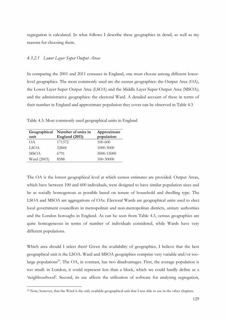
129

segregation is calculated. In what follows I describe these geographies in detail, as well as my

reasons for choosing them.

4.3.2.1 Lower Layer Super Output Areas

In comparing the 2001 and 2011 censuses in England, one must choose among different lower-

level geographies. The most commonly used are the census geographies: the Output Area (OA),

the Lower Layer Super Output Area (LSOA) and the Middle Layer Super Output Area (MSOA);

and the administrative geographies: the electoral Ward. A detailed account of these in terms of

their number in England and approximate population they cover can be observed in Table 4.3

Table ‎4.3: Most commonly used geographical units in England

Geographical unit

Number of units in England (2011)

Approximate population

OA 171372 100-600

LSOA 32844 1000-3000

MSOA 6791 5000-15000

Ward (2003) 8588 100-30000

The OA is the lowest geographical level at which census estimates are provided. Output Areas,

which have between 100 and 600 individuals, were designed to have similar population sizes and

be as socially homogenous as possible based on tenure of household and dwelling type. The

LSOA and MSOA are aggregations of OAs. Electoral Wards are geographical units used to elect

local government councillors in metropolitan and non-metropolitan districts, unitary authorities

and the London boroughs in England. As can be seen from Table 4.3, census geographies are

quite homogeneous in terms of number of individuals considered, while Wards have very

different populations.

Which area should I select then? Given the availability of geographies, I believe that the best

geographical unit is the LSOA. Ward and MSOA geographies comprise very variable and/or too-

large populations23. The OA, in contrast, has two disadvantages. First, the average population is

too small: in London, it could represent less than a block, which we could hardly define as a

‘neighbourhood’. Second, its use affects the utilization of software for analysing segregation,

23 Note, however, that the Ward is the only available geographical unit that I was able to use in the other chapters.

130

given that they are too many and they need large amounts of memory to be processed. So there

are both theoretical and practical justifications for selecting the LSOA as a geographical unit, and

also for choosing it as the best proxy of ‘neighbourhood’.

The LSOA has an average of 1500 individuals: 32,482 in 2001 and 32,844 in 2011. In their

majority (97.5% with respect to the 2001 figure), LSOAs are exactly the same for both years;

among the rest, around 2% have been merged or split, and the last 0.5% cannot be comparable

across censuses. For comparative purposes, I have only worked with the areas that have not

undergone transformations between 2001 and 2011: they are 31,672 for England (note that this

did not affect housing market areas, which have complete LSOAs in all cases). Census data on

ethnic groups is thus obtained at the LSOA level24. Specifically, for each LSOA I have collected

information on the number of individuals from each ethnic group, using the question on self-

identification25.

4.3.2.2 Housing Market Areas

With regard to the larger areas for which segregation indices are calculated, metropolitan areas

are the most commonly used, both in Europe (i.e. Musterd and Van Kempen 2009; Safi 2009)

and in the US (i.e. Logan and Stults 2011; Logan, Stults and Farley 2004; Massey and Denton

1989). The reason behind this selection is that metropolitan areas are ‘reasonable approximations

of housing markets’ (Iceland, Weinberg and Steinmetz 2002). Why is this important? Spatial

segregation occurs because people move in geographical space. These movements are determined

both by preferences and constraints, which are themselves linked to contextual factors, such as

housing prices, amenities of an area or public subsidies; and individual factors, such as socio-

24 The data to calculate segregation indices was obtained from: http://www.neighbourhood.statistics.gov.uk/. 25 In 2011 the question was formulated as follows: “What is your ethnic group?” The options were: White (English/Welsh/Scottish/Northern Irish/British; Irish; Gypsy or Irish traveller; other White); Mixed/multiple ethnic groups (White and Black Caribbean; White and Black African; White and Asian; any other Mixed/multiple ethnic background, open question); Asian/Asian British (Indian, Pakistani, Bangladeshi, Chinese; any other Asian background, open question); Black/African/Caribbean/Black British (African; Caribbean; any other Black/African/Caribbean background, open question); Other ethnic group (Arab; any other ethnic group). Note that the ‘Gypsy or Irish traveller’ and ‘Arab’ categories were missing in 2001. This chapter studies eight groups: white British, pooled non-whites (main non-white groups + other), Indian, Pakistani, Bangladeshi, Chinese, Caribbean and African. Note however that, contrary to the other chapters, based on the ONS Longitudinal Study, I was not able to differentiate between first and 1.5/second generations. The analysis presented here includes, therefore, individuals born in the UK (2nd generation), individuals born abroad and arrived at a young age (generation 1.5) and individuals born abroad and arrived at a later age or as adults (1st generation).

http://www.neighbourhood.statistics.gov.uk/dissemination/

131

economic level, ethnicity, life stage or location of relatives, friends or a new job26. Residential

mobility and spatial segregation are therefore two sides of the same coin. However, relocation

decisions typically do not take into account an entire country, rather, individuals mostly remain

constrained to certain areas, the so-called ‘housing market areas’. Housing market areas are

therefore relatively self-contained areas that express people’s choice of relocation. This means

that when studying changes in spatial segregation within housing markets, we somehow control

for the fact that individuals are ‘constrained’ in their choices to a certain geographical space, or

that they tend to ‘prefer’ that geographical space vs. others. This is important because it allows us

to assume that if they need to relocate, they are likely to do so within that geographical area:

segregation therefore acquires a more substantive meaning. In other words, if individuals are

constrained to an area and segregation increases, we can be more confident in saying that ethnic

groups are moving away from each other, or that when houses become available, they still prefer

those where other co-ethnics are found. This, of course, is an assumption, and by no means

applies to all individuals. Nonetheless, the idea of individuals being ‘spatially constrained’ has

been used in previous studies, although with other purposes (refer to the literature on

neighbourhood effects: Cutler, Glaeser and Vigdor 2008; Evans, Oates and Schwab 1992; Galster

2003; Galster et al. 2007b)27.

In the UK, rather than using metropolitan areas as approximations of housing markets, more

detailed information is available. A recent study carried out at Newcastle University and funded

by the National Housing and Planning Advisory Unit (Jones, Coombes and Wong 2010) created

a map of England that explicitly divides the country into housing market areas. These areas were

created by means of analysing three types of information: commuting, migration and housing

prices. Unfortunately, no information on ethnicity was used to construct the HMAs, for which I

need to assume that ethnic minorities and white British share the same HMA – which might not

be the case, since they might have, for example, different commuting and migration patterns.

Housing market areas are, therefore, based on data studied for the entire population and

represent an average of these (potentially diverse) ethnic patterns.

26 Note that segregation can also occur because individuals remain in an area and others move, as is the case in ‘white flight’, a process that explains the movement of whites out of ethnic areas. 27 Segregation is also related to new arrivals, which occurs outside the logic of the HMA (based on movements that occur within England). However, if new arrivals occur, and if there is a process of ‘white flight’, it is still expected that residential moves of the white British (if they do happen) occur within the HMA.

132

There are two classifications for HMAs: one is more local, while the other is based on larger

areas. I use the second one, also called an ‘upper tier’ framework. This is the wider classification

that sets the limits of the more local classification. The ‘upper tier’ framework – which divides

the country into 75 HMAs – is considered to be the ‘most effective in providing a longer term

overview of projected household changes, transport connectivity, housing land availability,

housing market change and urban capacity’ (Jones, Coombes and Wong 2010).

This framework requires that a link be made between HMAs and the smaller geographical units

or ‘neighbourhoods’ (LSOAs); that is, we need to be able to classify each LSOA according to the

housing market area they belong to. In the study by Jones, Coombes and Wong, there are two

versions that link HMAs with commonly used geographical units: the ‘gold standard’ version

best-fits each HMA with Wards (2003), which are a geographical unit that contains an average of

4000 individuals; the ‘silver standard’ version, best-fits the Ward-based ‘gold standard’ to Local

Authorities (LAs), which are the smallest administrative unit in England (there are 376 LA in

total). For this chapter I was not able to use the more precise ‘gold standard version’, since there

is no lookup that relates the smaller geographical unit used in this study (LSOA) to the Ward

(and hence to the HMAs). I have used instead the ‘silver standard’ version and, therefore, have

linked each LSOA to a Local Authority and hence to a specific HMA. This implied, perforce, a

loss of information, as Local Authorities do not exactly fit the HMAs, as Wards more accurately

do.

After linking each LSOA or ‘neighbourhoods’ with their respective HMA, I selected the housing

market areas that I considered most relevant for studying spatial segregation: out of the 75

HMAs, I study the eight with the highest number of non-white ethnic minorities (comprising, in

total, 80% of non-white ethnic minorities). As could be expected, these also follow the main

metropolitan areas. The housing market area with the highest number of non-white ethnic

minorities is the London HMA, followed by the Manchester HMA. Other areas are: the Luton &

Milton Keynes HMA and the Reading HMA (next to the London HMA); the Birmingham HMA and

the Leicester HMA in the region of West Midlands; and the Bradford HMA and the Leeds HMA in

the region of West Yorkshire. Map 4.1 shows the location of the selected HMAs in England. In

the first case, Local Authorities are used as geographical units (a); in the second, Local

Authorities and LSOAs (within HMAs) are used (b). From Map 1b we can see that the smallest

LSOAs also match the location of metropolis in England (Table 8.8 in Annex A shows the

distribution of Local Authorities within the selected housing market areas).

133

Map

4.1

: Id

enti

fica

tio

n o

f H

MA

s; g

eogr

aph

ical

un

its

are

Lo

cal A

uth

ori

ties

(a)

an

d L

oca

l A

uth

ori

ties

+ L

SO

As

(b)

a)

b

)

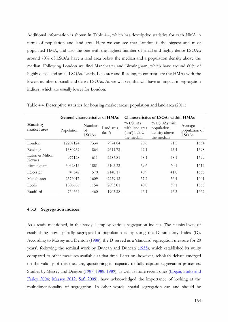
134

Additional information is shown in Table 4.4, which has descriptive statistics for each HMA in

terms of population and land area. Here we can see that London is the biggest and most

populated HMA, and also the one with the highest number of small and highly dense LSOAs:

around 70% of LSOAs have a land area below the median and a population density above the

median. Following London we find Manchester and Birmingham, which have around 60% of

highly dense and small LSOAs. Leeds, Leicester and Reading, in contrast, are the HMAs with the

lowest number of small and dense LSOAs. As we will see, this will have an impact in segregation

indices, which are usually lower for London.

Table ‎4.4: Descriptive statistics for housing market areas: population and land area (2011)

Housing market area

General characteristics of HMAs Characteristics of LSOAs within HMAs

Population Number of LSOAs

Land area (km2)

% LSOAs with land area (km2) below the median

% LSOAs with population density above the median

Average population of LSOAs

London 12207124 7334 7974.84 70.6 71.5 1664

Reading 1380252 864 2611.72 42.1 43.4 1598

Luton & Milton Keynes

977128 611 2285.81 48.1 48.1 1599

Birmingham 3032813 1881 3102.32 59.6 60.1 1612

Leicester 949342 570 2140.17 40.9 41.8 1666

Manchester 2576017 1609 2259.12 57.2 56.4 1601

Leeds 1806686 1154 2893.01 40.8 39.1 1566

Bradford 764664 460 1903.28 46.1 46.3 1662

4.3.3 Segregation indices

As already mentioned, in this study I employ various segregation indices. The classical way of

establishing how spatially segregated a population is by using the Dissimilarity Index (D).

According to Massey and Denton (1988), the D served as a ‘standard segregation measure for 20

years’, following the seminal work by Duncan and Duncan (1955), which established its utility

compared to other measures available at that time. Later on, however, scholarly debate emerged

on the validity of this measure, questioning its capacity to fully capture segregation processes.

Studies by Massey and Denton (1987; 1988; 1989), as well as more recent ones (Logan, Stults and

Farley 2004; Massey 2012; Safi 2009), have acknowledged the importance of looking at the

multidimensionality of segregation. In other words, spatial segregation can and should be

135

explored through different angles or dimensions. In this chapter, I consider four dimensions of

segregation: evenness, exposure, concentration and clustering (Massey and Denton 1988).

The various dimensions of segregation are measured with indices that can be classified in two

ways: absolute or relative, and aspatial or spatial. Absolute indices refer to one group, while relative

indices measure the relative level of segregation of one group with respect to another (usually the

majority population). The difference between aspatial and spatial measures is that the latter require

information on size and location of the areas (LSOA) to be computed, while the former does

not. Based on Massey and Denton (1988), who studied the performance of a wide range of

indices, and following as well more recent studies (Iceland, Weinberg and Steinmetz 2002), this

study makes use of six indices: Dissimilarity (D) to measure evenness; Isolation (xPx) and

Interaction (xPy) to measure exposure; Relative Concentration (RCO) to measure concentration;

and Absolute Clustering (ACL) and Spatial Proximity (SP) to measure clustering. Table 4.5 shows

the four dimensions, along with the indices and their situation with respect to the above-

mentioned classifications.

Table ‎4.5: Dimensions and segregation indices

Dimension Index Type

Absolute Relative Aspatial Spatial

Evenness Dissimilarity (D) X X

Exposure Isolation (xPx) X X

Interaction (xPy) X X

Concentration Relative Concentration (RCO) X X

Clustering Absolute Clustering (ACL) X X

Spatial Proximity (SP) X X

The Dissimilarity Index, used to determine evenness, measures the distribution of minority

population across all units (LSOAs) within a larger area (HMA). Specifically, it can be interpreted

as the proportion of a certain (minority) population that would need to change their

neighbourhood or LSOA in order to achieve an equal distribution in the HMA; it can also be

understood as the proportion of individuals of a certain group that would need to move for each

neighbourhood to have the same percentage of that group as the housing market area overall.

The formula of this index is shown in Table 4.16, where pi is the proportion of unit’s i

136

population that is minority, P is the proportion of minority members in the HMA, and T and ti

are the total populations in the wider area (HMA) and geographical unit (LSOA), respectively.

Table ‎4.6: Dissimilarity Index*

What this index measures can be better understood in Figure 4.2 (adapted from Iceland,

Weinberg and Steinmetz 2002), which illustrates how indices capture different dimensions of

segregation, and also how high and low segregation look for each index. The eight bigger squares

in Figure 4.2 represent housing market areas, while the nine smaller squares within them

represent LSOAs; each circle represents an individual, which can be either from the majority

population (blue) or from the minority population (red). Figure 4.2a, which illustrates the

evenness dimension, shows that a situation of high segregation would be one in which each

neighbourhood or LSOA is inhabited by only one group, no matter where these neighbourhoods

are located within the larger area; conversely, a situation of low segregation would be one in

which each area contains more or less equal quantities of each group. The Dissimilarity Index

varies between 0 (even distribution; no segregation) and 1 (completely uneven distribution; high

segregation).

The dimension of exposure refers to the degree of potential contact between individuals in the

same LSOA. The basic assumption is that by virtue of living in the same neighbourhood or

residential area, individuals are physically exposed to one another. Thus, exposure indices

measure the extent to which individuals have the opportunity to confront each other in a given

space and, following Massey and Denton (1988), they can also be interpreted in terms of

Index Formula

Dissimilarity D =

T = Total population in the HMA.

ti = Total population in geographical unit i.

P = The ratio of X (total population of group X in the HMA) to T

pi = The ratio of xi (total population of group X in geographical unit i) to ti

n = Number of spatial units in the HMA.

* All formulas are taken from (Iceland, Weinberg and Steinmetz 2002).

137

“experienced segregation”. There are two main indices within this dimension: the Isolation Index

(xPx) and the Interaction Index (xPy). The first is used to measure the exposure between

individuals of the same group; while the second measures exposure between minority and

majority/other groups. The formulas of these indices can be observed in Table 4.15, where xi, yi

and ti are the numbers of X members (e.g. Pakistani), Y members (e.g. white British) and the total

population of unit i, respectively, and X represents the number of X individuals in the wider area

(e.g. total number of Pakistanis in the HMA). These indices are interrelated: in the hypothetical

situation in which there are only two groups in the HMA, the sum of xPx and xPy will equal 1; if

there are more than two groups, then the sum of all intergroup probabilities plus the isolation

index will equal 1.

Table ‎4.7: Interaction and Isolation Indices

A specific feature of these indices is that they are sensitive to the relative sizes of the groups. If

the group being compared is relatively large within a certain HMA, then the likelihood that their

members will meet someone of the same group is greater (and the likelihood that they will meet

someone from another group is smaller). Conversely, if the group is small, their members have a

greater likelihood of meeting people from the majority/comparison group. In this regard, a group

might be unevenly distributed, but at the same time, be very likely to meet people from the

majoritarian or other groups if its number of members is small. This can be better observed in

Figure 4.2b.

Index Formula

Isolation xPx =

Interaction xPy =



X = Total population of group X in the HMA.

xi = Total population of group X in geographical unit i.

yi = Total population of group Y in geographical unit i.


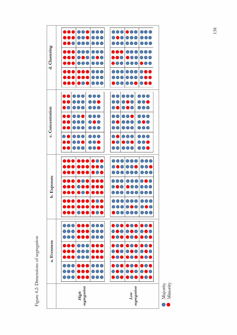
138

Fig

ure

4.2

: D

imen

sio

ns

of

segr

egat

ion

a.

Eve

nn

ess

b

. E

xp

osu

re

c.

Co

ncen

trati

on

d

. C

lust

eri

ng

Hig

h

seg

reg

atio

n

Lo

w

seg

reg

atio

n

139

The upper part of Figure 4.2b presents an area in which the number of minority members is

quite large: here we would find high segregation, since they have a greater likelihood of meeting

someone from their own group (measured with xPx), and a smaller likelihood of meeting

someone from the majority group (measured with xPy). Conversely, the lower part of the figure

shows a situation of low segregation, that is, a situation in which there is a great deal of contact

between minority and majority members, due to the fact that the former constitute a small share

of the total population living in the larger area or HMA. Note finally that this dependence on the

sizes of the groups has two other implications. On the one hand, it implies that the Interaction

Index is not symmetrical: that is, xPy is different than yPx, unless the two groups cover the entire

population. On the other hand, and in terms of comparison over time, it also implies that

Isolation and Interaction Indices are affected by population growth: an increase of members of a

minority group is likely to lead to an increase in xPx for that group, and a decrease in xPy with

respect to the white British. Both the Isolation and Interaction Indices vary between 0 and 1 and

can be interpreted as the likelihood of sharing the same area with an individual of the same or

different group. For the purposes of this chapter, I use two versions of xPy: one compares each

ethnic minority to the white British (xPy_wb); the other compares each ethnic minority and the

white British to all non-white ethnic minorities (xPy_nw).

The dimension of concentration expresses the degree to which minority members occupy a small

share of a wider geographical area. In practise, this means that ethnic minorities are mainly

located in the smaller neighbourhoods (in our case, LSOAs). I measure concentration with a

relative index, the Relative Concentration Index (RCO), which measures the concentration of a

group relative to a second group, in this case the white British. The Index varies between -1 and

1, where a score of 1 means that the concentration of the minority group exceeds the one of the

white British to the maximum extent possible; -1 means the converse; and 0 means that both

groups are equally concentrated in the urban space. This index is ‘spatial’ in that it takes into

consideration the shape and size of LSOAs (although not their relative position in the wider

area). The formula for this index can be seen in Table 4.13, where the geographical units are

ordered by geographic size from smallest to largest; ai is the land area of unit i, and the two

numbers nl and n2 refer to different points in the rank ordering of geographical units from

smallest to largest: nl is rank of the LSOA where the cumulative total population of

geographical units equals the total minority population of the HMA, summing from the

smallest unit up; and n2 is the rank of the LSOA where the cumulative total population of

140

units equals the minority population totalling from the largest unit down. Tl equals the total

population of units from 1 to nl, and T2 equals the total population of units from n2 to n. As

before, X and Y is the number of group X and group Y members in the HMA. “This index

takes the ratio of X members' to Y members' concentration and compares it with the

maximum possible ratio that would be obtained if X were maximally concentrated and Y

minimally concentrated, standardizing the quotient so that the index varies between -1 and 1

(...) The relative concentration index measures the share of urban space occupied by group X

compared to group Y” (Massey and Denton 1988, pp. 291). Figure 4.2c again shows examples

of housing market areas with high and low segregation: in the upper part of the figure, we can see

that most minority members are located in the smaller neighbourhoods, while the lower part

shows a more equal distribution.

Table ‎4.8: Relative Concentration Index

Index Formula

Relative Concentration

RCO =

T1 = Sum of all ti in geographical unit 1 to geographical unit n1.

T2 = Sum of all ti in geographical unit n2 to geographical unit n.



xi = Total population of group X in geographical unit i.

Y = Total population of group Y in the HMA.

ai = Land area of geographical unit i.


n1 = Rank 1.

n2 = Rank 2.

Spatial units are sorted by land area in

ascending order

141

The last dimension studied is clustering. This dimension refers to the degree to which area units

inhabited by certain social groups adjoin one another, or cluster, in the space. The more clustered

the areas are, the higher the segregation will be. For example, if we compare with the previous

measure, it might be the case that minorities occupy the smallest areas in two given cities; but if

in one of the cities these areas are also close to one another, segregation in such city will be

higher. Figure 4.2d shows very clearly what clustering means: in the upper part of the figure,

neighbourhoods where ethnic minorities are located are also next to each other; while the lower

part shows that these neighbourhoods are more spread out.

Within the dimension of clustering, Massey and Denton (1988) suggest that Spatial Proximity

(SP) in the first place, and then Absolute Clustering (ACL) indices are the best measures28. The

ACL, which varies between 0 and (a number close to) 1 and can be interpreted as the average

number of members of a certain group in nearby tracts, as a proportion of the total population in

nearby tracts. Table 4.14 shows the formula for this index, in which the most important element

is cij, which indicates to what extent areas are close to one another. This element represents the

negative exponential of the distances between units i and j, and approximates contiguity by

recognizing that the influence of surrounding areas drops off rapidly with distance from the

target unit (Massey and Denton 1988).

The SP refers to the average of intra-group proximities weighted by the proportion of each group

in the population. It equals 1 if there is no differential clustering between both groups; and is

greater than one when member of both groups live nearer one another than each other. I have

subtracted 1 from the index, so that it varies between 0 and 1. These are also ‘spatial’ indices, but

rather than considering the size of areas (as the RCO), they take into consideration the relative

location of the LSOAs in the space: specifically, they measure the extent to which LSOAs where

a certain ethnic minority group lives are contiguous. The formula for this index, which can also

be seen in Table 4.14, shows that SP is the average of intra-group proximities (Pxx/Ptt and

Pyy/Ptt) weighted by the fraction of each group in the population.

28 Note that although ACL is not very commonly used, I use it as complementary measure since I was not able to calculate SP at the national level and for London. The SP measures distance between geographical units, and this requires a large amount of disk space to make the calculations, which is not possible to make in areas where the number of LSOAs is very high.

142

Table ‎4.9: Absolute Clustering and Spatial Proximity Indices

Additional information about the relationship between various indices can be found in Table

4.15, which shows the correlation between indices used in this chapter. The correlation

coefficients were created by analysing a dataset containing the segregation indices observed in

Tables 4.16 and 4.17, that is, those for each ethnic minority group and the white British in each

HMA (indices for non-whites were excluded). A first finding from this table is that all indices are

related to each other; moreover, there are some particularly high correlations: for example, the

evenness measure (D) is very much (positively) correlated with the interaction measures, meaning

that groups (within HMAs) that have a high D also usually have a high interaction with non-

whites (and a low interaction with white British); the isolation index (xPx) has a high correlation

with clustering measures, meaning that groups that are more exposed to each other are also more

likely to be clustered in the space. We also observe that the highest the relative concentration

Index Formula

Absolute Clustering

ACL =

Spatial Proximity

SP =

P = Proportion of group in the HMA, X/T.


ti = Total population in spatial unit i.


xi = Total population of group X in spatial unit i.

xj = Total population of group X in spatial unit j.

Y = Total population of group Y in the HMA.

yj = Total population of group Y in spatial unit i.

yj = Total population of group Y in spatial unit j

cij = cij the exponential transform of dij [= exp(-dij)] (dij = distance between the centroids of spatial units i and j.)


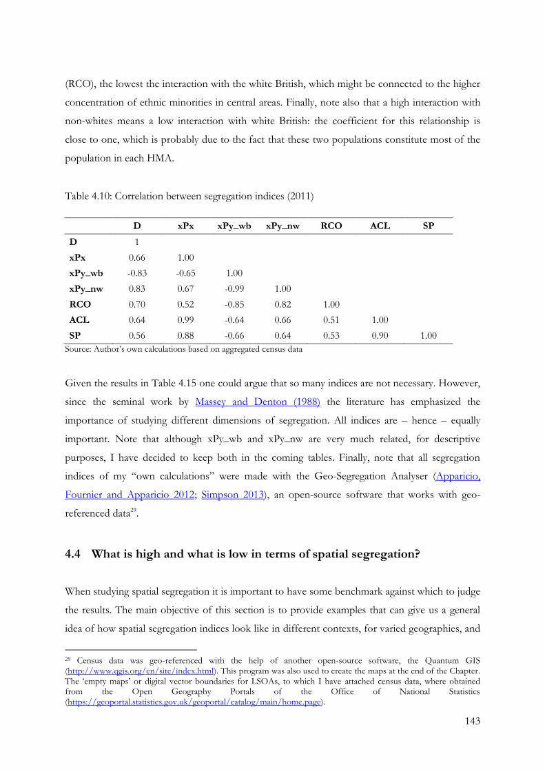
143

(RCO), the lowest the interaction with the white British, which might be connected to the higher

concentration of ethnic minorities in central areas. Finally, note also that a high interaction with

non-whites means a low interaction with white British: the coefficient for this relationship is

close to one, which is probably due to the fact that these two populations constitute most of the

population in each HMA.

Table ‎4.10: Correlation between segregation indices (2011)

D xPx xPy_wb xPy_nw RCO ACL SP

D 1

xPx 0.66 1.00

xPy_wb -0.83 -0.65 1.00

xPy_nw 0.83 0.67 -0.99 1.00

RCO 0.70 0.52 -0.85 0.82 1.00

ACL 0.64 0.99 -0.64 0.66 0.51 1.00

SP 0.56 0.88 -0.66 0.64 0.53 0.90 1.00

Source: Author’s own calculations based on aggregated census data

Given the results in Table 4.15 one could argue that so many indices are not necessary. However,

since the seminal work by Massey and Denton (1988) the literature has emphasized the

importance of studying different dimensions of segregation. All indices are – hence – equally

important. Note that although xPy_wb and xPy_nw are very much related, for descriptive

purposes, I have decided to keep both in the coming tables. Finally, note that all segregation

indices of my “own calculations” were made with the Geo-Segregation Analyser (Apparicio,

Fournier and Apparicio 2012; Simpson 2013), an open-source software that works with geo-

referenced data29.

4.4 What is high and what is low in terms of spatial segregation?

When studying spatial segregation it is important to have some benchmark against which to judge

the results. The main objective of this section is to provide examples that can give us a general

idea of how spatial segregation indices look like in different contexts, for varied geographies, and

29 Census data was geo-referenced with the help of another open-source software, the Quantum GIS (http://www.qgis.org/en/site/index.html). This program was also used to create the maps at the end of the Chapter. The ‘empty maps’ or digital vector boundaries for LSOAs, to which I have attached census data, where obtained from the Open Geography Portals of the Office of National Statistics (https://geoportal.statistics.gov.uk/geoportal/catalog/main/home.page).

http://www.qgis.org/en/site/index.html

https://geoportal.statistics.gov.uk/geoportal/catalog/main/home.page

144

for different groups. Table 4.11 shows segregation indices for the most numerous non-white

immigrants and ethnic minorities in the US (Iceland, Weinberg and Steinmetz 2002), France (Safi

2009) and England (own calculations). The indices were calculated for selected metropolitan

areas in each country (the most populous ones), and in the US a summary of these30 is also

provided. The table also includes what Massey and Denton (1989) have declared, in the US case,

as the thresholds that should be met in various segregation indices to refer to a group as ‘highly

segregated’.

Looking at the three measures available for the three countries (D, xPx and SP), we observe that

in London, and particularly in Paris, the levels of segregation of the most numerous non-white

groups tend to be lower than in the selected US metropolitan areas. The Dissimilarity Index

varies roughly between 25 and 80. African populations in Paris and Chinese in London are the

least segregated groups, while blacks in New York and Chicago are the most segregated ones. For

example, between 60% and 80% of the African population in the selected US cities would need

to change their residence (i.e. census tract) in order to make their distribution even in the larger

metropolitan area; this drops to around half (or even less) in Paris and London. The Isolation

Index varies between 2% and 83%, with the highest values found in the US, where the

probabilities that ethnic minorities ‘interact’ with a co-ethnic in the same geographical unit are

between 55% and 83%. Paris, on the other hand, presents particularly low levels of segregation

measured in this way, with values that vary between 3% and 4%. For London the values have an

intermediate position, but are still farther away from the 70% threshold when compared to US

cities. A similar pattern is observed for the Spatial Proximity Index, which varies between 0.25

and 0.73 in the US, but drops to less than 0.29 in Europe. In the selected US metropolitan areas,

minority groups tend to be closer to each other than to the white majoritarian population, when

compared to those in Paris or London. Another piece of information emerging from Table 4.11

is that differences in terms of segregation levels are higher when we compare indices for different

metropolitan areas than when we compare indices calculated with different geographical units (in

the case of segregation in London, measured by Wards and LSOAs).

30 Metropolitan Areas included here are those that in 1980 have at least 10 tracts and 3% (or a minimum of 20000) of the group for which the index is calculated.

145

Tab

le ‎4

.11:

Seg

rega

tio

n i

ndic

es f

or

imm

igra

nts

an

d e

thn

ic m

ino

riti

es i

n m

etro

po

litan

are

as i

n t

he

US (

2000),

Fra

nce

(1999)

and t

he

Un

ited

Kin

gdo

m

(2001)

Geo

gra

ph

ical

un

its

Are

a

Gro

up

E

ven

ness

E

xp

osu

re

Co

ncen

trati

on

C

lust

eri

ng

D

xP

x

xP

y R

CO

A

CL

S

P

US

Cen

sus

trac

ts

2500-8

000 ind

ivid

uals

“Hig

h se

greg

atio

n”

>60

>70

>

0.7

>0.6

All

met

rop

olit

an a

reas

(av

erag

e)

Afr

ican

64.5

60.1

0.3

8

His

pan

ic

51.7

58.5

0.2

5

New

Yo

rk

Afr

ican

81.2

82.7

0.4

7

His

pan

ic

66.7

70.8

0.3

5

Ch

icag

o

Afr

ican

79.9

77.6

0.7

3

His

pan

ic

61.1

55.0

0.4

2

Lo

s A

nge

les

Afr

ican

66.4

65.2

0.5

6

H

isp

anic

63.1

79.1

0.3

5

Fra

nce

Par

is (

Ille

-de-

Fra

nce

)

Alg

eria

n

34.0

4.0

76.0

3.0

0.0

1

M

oro

ccan

35.0

4.0

76.0

2.3

0.0

1

Co

mm

un

es d

e re

sid

ence

500-1

0000 ind

ivid

uals

Sub

-Sah

aran

Afr

ica

33.0

4.0

76.0

3.0

0.0

1

Turk

49.0

3.0

74.0

1.0

0.0

1

Par

is (

pet

ite

couro

nn

e)

Alg

eria

n

28.0

4.0

75.0

1.6

0.0

1

Mo

rocc

an

27.0

4.0

75.0

1.2

0.0

0

Sub

-Sah

aran

Afr

ica

26.0

4.0

75.0

2.0

0.0

1

Turk

43.0

4.0

72.0

0.0

0.0

0

UK

War

ds

100-3

0000 ind

ivid

uals

L

on

do

n (

inn

er+

oute

r)

India

n

47.2

17.8

45.7

0.1

9

11.0

0.1

3

Pak

ista

ni

47.2

6.4

44.3

0.3

3

3.9

0.0

7

Ban

glad

esh

i 62.2

19.6

42.6

0.5

9

14.5

0.2

9

146

Geo

gra

ph

ical

un

its

Are

a

Gro

up

E

ven

ness

E

xp

osu

re

Co

ncen

trati

on

C

lust

eri

ng

D

xP

x

xP

y R

CO

A

CL

S

P

Ch

ines

e 25.1

1.7

55.7

0.2

4

0.6

0.0

1

Car

ibb

ean

40.5

9.3

48.7

0.4

2

5.1

0.0

7

Afr

ican

37.1

10.0

49.2

0.4

1

5.1

0.0

8

LSO

As

1500-3

000 ind

ivid

uals

L

on

do

n (

inn

er+

oute

r)

India

n

49.2

19.4

44.2

0.2

0

13.8

0.1

5

Pak

ista

ni

50.2

7.3

42.6

0.3

2

5.0

0.0

8

Ban

glad

esh

i 64.9

22.5

39.7

0.5

4

17.8

0.2

8

Ch

ines

e 32.1

2.1

55.0

0.2

2

0.7

0.0

1

Car

ibb

ean

42.8

9.9

47.7

0.4

4

5.4

0.0

8

Afr

ican

41.3

11.3

47.3

0.4

5

5.4

0.0

8

Min

imu

m a

nd

maxim

um

Min

imum

25.1

1.7

39.7

0.1

9

0

0

Max

imum

81.2

82.7

76

0.5

9

17.8

0.7

3

No

te: xP

y (a

nd

D f

or

the

Fre

nch

cas

e o

nly

) is

cal

cula

ted

wit

h r

esp

ect

to w

hit

es (

US; U

K)

and

in

div

idual

s b

orn

in

th

e co

un

try

(Fra

nce

). S

P is

SP

-1. T

he

un

its

of

anal

ysis

are

ce

nsu

s tr

acts

in

th

e U

S (

aver

age

4000 p

eop

le);

co

mm

un

es in

Fra

nce

(le

ss t

han

500 in

th

eir

maj

ori

ty, to

10000);

an

d L

SO

As

in E

ngl

and

(av

erag

e 1500 p

eop

le).

So

urc

es: U

S I

cela

nd

, W

ein

ber

g an

d S

tein

met

z (2

002);

Fra

nce

Saf

i (2

009);

En

glan

d: th

e au

tho

r’s

ow

n c

alcu

lati

on

s b

ased

on

agg

rega

ted

cen

sus

dat

a (o

bta

ined

fro

m:

ww

w.n

eigh

bo

urh

oo

d.s

tati

stic

s.go

v.u

k).


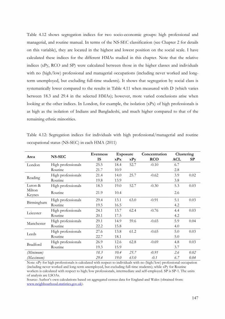
147

Table 4.12 shows segregation indices for two socio-economic groups: high professional and

managerial, and routine manual. In terms of the NS-SEC classification (see Chapter 2 for details

on this variable), they are located in the highest and lowest position on the social scale. I have

calculated these indices for the different HMAs studied in this chapter. Note that the relative

indices (xPy, RCO and SP) were calculated between those in the higher classes and individuals

with no (high/low) professional and managerial occupations (including never worked and long-

term unemployed, but excluding full-time students). It shows that segregation by social class is

systematically lower compared to the results in Table 4.11 when measured with D (which varies

between 18.3 and 29.4 in the selected HMAs); however, more varied conclusions arise when

looking at the other indices. In London, for example, the isolation (xPx) of high professionals is

as high as the isolation of Indians and Bangladeshi, and much higher compared to that of the

remaining ethnic minorities.

Table ‎4.12: Segregation indices for individuals with high professional/managerial and routine

occupational status (NS-SEC) in each HMA (2011)

Area NS-SEC Evenness Exposure Concentration Clustering

IS xPx xPy RCO ACL SP

London

High professionals 25.5 18.4 52.7 -0.10 6.7

Routine 21.7 10.9 2.8

Reading High professionals 21.4 14.0 25.7 -0.62 3.9 0.02

Routine 19.8 13.9 3.8

Luton & Milton Keynes

High professionals 18.3 19.0 52.7 -0.30 5.3 0.03

Routine 21.9 10.4 2.6

Birmingham High professionals 29.4 13.1 63.0 -0.91 5.1 0.03

Routine 19.5 16.5 4.2

Leicester High professionals 24.1 13.7 62.4 -0.76 4.4 0.03

Routine 20.1 17.5 4.2

Manchester High professionals 29.1 14.9 59.6 -0.65 5.9 0.04

Routine 22.2 15.8 4.0

Leeds High professionals 27.6 13.8 61.2 -0.65 5.0 0.03

Routine 22.7 18.1 5.0

Bradford High professionals 26.9 12.6 62.8 -0.69 4.8 0.03

Routine 19.3 15.9 3.7

(Minimum) 18.3 10.4 25.7 -0.91 2.6 0.02

(Maximum) 29.4 19.0 63.0 -0.1 6.7 0.04 Note: xPy for high professionals is calculated with respect to individuals with no (high/low) professional occupation (including never worked and long-term unemployed, but excluding full-time students); while xPy for Routine workers is calculated with respect to high/low professionals, intermediate and self-employed. SP is SP-1. The units of analysis are LSOAs. Source: Author’s own calculations based on aggregated census data for England and Wales (obtained from: www.neighbourhood.statistics.gov.uk).


148

This section has provided a baseline for discussing the various indices shown below; but before

moving to the segregation analysis, I offer a general overview of how white British and ethnic

minorities distribute across housing market areas, and also across metropolitan areas, in 2001 and

2011.

4.5 Distribution of groups in HMAs and metropolitan areas

Table 4.13 shows the distribution of white British and ethnic minorities in England as well across

housing market areas in 2001 and 2011. Between 2001 and 2011, non-white ethnic minorities in

England increased in their proportion, while white British decreased. The highest relative increase

was in the African population, followed by Pakistani, Bangladeshi and Chinese populations; the

group with the most stable population was Caribbean, which is also the ethnic minority with the

longest stay in the country.

Regarding their location in HMAs, looking at the 2001 data, most Africans lived in London;

Caribbean and Bangladeshi populations also held their majority in this HMA, with sizeable

proportions in Birmingham. Bangladeshis are also found in Manchester and a HMA next to

London: Luton & Keynes. Pakistanis are more dispersed in England: the biggest proportions are

in London, Birmingham, Manchester and Bradford. Smaller groups are in the HMAs around

London (Reading and Luton & Milton Keynes) and Leeds. Indian and Chinese populations,

finally, have a bit less than half of their number in London; sizeable groups of Indians are also

located in Birmingham and Leicester, while Chinese are more spread out. In fact, they are the

group with the highest proportion in the category ‘Rest of England’, which are the HMAs with

relatively lower proportions of non-whites. This structure was more or less maintained for most

groups in 2011. An exception, however, is the Caribbean population, which decreased its

proportion in London by around 17% points (and its proportion in the ‘Rest of England’

doubled). Note also that all groups decreased their proportion in London, but to a much lesser

extent (the maximum is a 5%- point decrease for Bangladeshi persons).

149

Tab

le 4

.13: D

istr

ibuti

on

of

wh

ite

Bri

tish

an

d e

thn

ic m

ino

riti

es in

En

glan

d (

row

%)

and a

cro

ss h

ousi

ng

mar

ket

are

as (

colu

mn

%);

2001 a

nd 2

011

W

hit

e B

riti

sh

All

no

n-w

hit

e In

dia

n

Pak

ista

ni

Ban

gla

desh

i C

hin

ese

C

ari

bb

ean

A

fric

an

2001

En

glan

d

87.1

7

7.6

3

2.0

9

1.4

0

0.5

4

0.4

4

1.1

2

0.9

4

L

on

do

n

18.9

52.9

47.8

23.6

59.8

45.2

64.3

82.8

Rea

din

g 2.7

2.8

3.2

4.8

0.6

2.5

2.3

1.5

Luto

n &

Milt

on

Key

nes

1.8

2.4

2.0

3.7

4.2

2.1

2.6

1.6

Bir

min

gham

5.6

10.5

12.9

17.3

9.0

4.0

12.8

1.7

Lei

cest

er

1.7

3.3

8.8

0.7

1.3

1.7

1.0

0.8

Man

ches

ter

5.1

5.0

3.5

10.8

7.5

5.2

2.9

2.1

Lee

ds

3.8

2.8

2.9

6.5

1.1

2.1

2.0

0.6

Bra

dfo

rd

1.4

2.8

1.3

11.2

1.7

0.6

0.6

0.2

Res

t o

f E

ngl

and

59.0

17.5

17.5

21.4

14.9

36.5

11.5

8.6

To

tal

41739029

3655288

999218

671320

259479

210002

538470

451819

2011

E

ngl

and

80.0

9

12.0

8

2.6

0

2.0

8

0.8

1

0.6

6

1.1

0

1.7

9

L

on

do

n

17.7

50.0

45.6

23.4

54.8

41.7

62.5

66.1

Rea

din

g 2.6

3.1

3.9

5.0

0.9

2.5

2.2

2.3

Luto

n &

Milt

on

Key

nes

1.8

2.7

2.2

3.9

4.6

1.9

2.7

2.8

Bir

min

gham

5.5

9.8

11.5

16.5

9.9

4.5

13.0

4.3

Lei

cest

er

1.7

3.1

8.8

0.9

1.4

2.0

1.0

1.5

Man

ches

ter

5.0

5.7

3.9

11.9

8.2

6.4

3.0

4.3

Lee

ds

3.8

2.9

2.8

6.3

1.3

2.3

2.0

2.0

Bra

dfo

rd

1.4

2.7

1.1

11.0

2.2

0.7

0.7

0.6

Res

t o

f E

ngl

and

60.6

19.9

20.3

20.9

16.7

37.9

12.8

16.1

To

tal

40925897

6172142

1327640

1063792

412420

338522

564593

914097

So

urc

e: A

uth

or’

s o

wn

cal

cula

tio

ns

bas

ed o

n a

ggre

gate

d c

ensu

s d

ata

150

Table 4.14 shows the proportion of ethnic minorities in metropolitan areas in England and

within each HMA, both for 2001 and 2011. Note that within the London HMA, only 1% is non-

metropolitan. For this reason, I delineated Inner London, Outer London and an extended area

(all metropolitan), which comprise 99% of the London HMA. The definition of metropolitan

and non-metropolitan, as well as of inner, outer and extended London, are based on Rees and

Butt (2004)31.

Following an historical pattern of settlement – related to sources of jobs – ethnic minorities tend

to reside in metropolitan areas: around 85% of non-white ethnic minorities live in urban areas,

while only a bit less than 50% of white British do. Between 2001 and 2011, the share of ethnic

minorities living in metropolitan areas decreased for all groups, except the Pakistani. This might

suggest suburbanization processes, in line with previous findings based on migration data for

1991-2001 (Rees and Butt 2004; Simpson and Finney 2009). The groups with the highest relative

decrease in metropolitan areas are African and Indian: interestingly, are also the most educated

groups, which might speak of processes of spatial assimilation that are a consequence of socio-

economic improvement.

Moving to more detailed information on HMAs, we observe that in general ethnic minorities

have higher shares in metropolitan areas than white British. Leaving aside London, we observe

that housing market areas where this contrast is more dramatic are Birmingham, Leicester and

Luton & Milton Keynes. In London, where the majority of ethnic minorities are located, Table

4.14 shows that ethnic minorities are usually more likely to be in inner and outer London, while

the white British are more overrepresented in the extended area. Moreover, contrary to the earlier

decade, for which the analysis by Rees and Butt did not show much consistency in the patterns of

change between 1991 and 2001, the data for 2001-2011 shows a pattern that might suggest a

process of suburbanization to the outskirts of the city, if we assume that HMAs work as such,

that is, as areas within which individuals more often search for a new residence. Except for

Chinese, all groups decreased their proportion in Inner London, and increased their proportion

in the extended area (many groups also increased their proportion in Outer London).

31 The authors include Luton and Reading in the extended area around London, while here I have privileged their situation as separate HMAs.

151

Tab

le ‎4

.14: P

erce

nta

ge o

f w

hit

e B

riti

sh a

nd e

thn

ic m

ino

riti

es i

n m

etro

po

litan

are

as (

in E

ngl

and a

nd w

ith

in H

MA

s, e

xce

pt

for

Lo

ndo

n);

perc

enta

ge o

f

wh

ite

Bri

tish

an

d e

thn

ic m

ino

riti

es in

in

ner

, o

ute

r an

d e

xte

nded

Lo

ndo

n (

colu

mn

%);

2001 a

nd 2

011

W

hit

e B

riti

sh

All

no

n-w

hit

e

Ind

ian

P

ak

ista

ni

Ban

gla

desh

i C

hin

ese

C

ari

bb

ean

A

fric

an

En

gla

nd

2001

47.2

4

86.5

9

85.2

0

86.6

1

87.5

1

70.2

8

91.7

6

93.5

8

2011

45.4

0

84.8

7

81.9

2

86.7

5

86.3

1

70.1

0

90.5

5

89.0

8

Lo

nd

on

2001

Inne

r 17.1

41.8

17.4

26.9

78.5

38.8

52.9

58.1

Out

er

36.0

50.5

72.2

61.3

16.1

42.4

43.2

38.5

Exte

nded

45.5

7.7

10.3

11.7

5.3

18.5

3.8

3.4

2011

Inne

r 16.3

36.4

17.0

23.3

68.2

42.0

47.3

43.4

Out

er

32.9

53.0

69.6

64.2

25.0

39.5

46.9

46.8

Exte

nded

49.1

10.5

13.3

12.5

6.7

18.4

5.7

9.6

Read

ing

2001

75.9

94.4

94.8

98.9

78.2

82.4

92.5

94.0

2011

74.5

93.7

93.7

98.6

86.2

83.9

92.8

92.2

Lu

ton

& M

ilto

n K

eyn

es

2001

29.2

55.2

42.0

69.1

70.6

31.4

57.7

48.6

2011

26.8

54.1

41.2

71.2

72.1

32.8

58.3

40.9

Bir

min

gh

am

2001

71.5

97.4

97.5

98.4

98.5

87.7

97.4

96.3

2011

69.6

97.1

96.4

98.1

98.9

88.7

97.2

97.9

Leic

est

er

2001

22.7

77.7

79.9

83.7

58.3

37.7

81.5

82.9

2011

19.8

75.9

76.5

79.4

61.2

48.9

77.4

85.6

152

W

hit

e B

riti

sh

All

no

n-w

hit

e

Ind

ian

P

ak

ista

ni

Ban

gla

desh

i C

hin

ese

C

ari

bb

ean

A

fric

an

Man

ch

est

er

2001

86.4

97.5

97.9

98.5

96.2

94.1

98.5

98.3

2011

85.8

97.5

96.5

98.7

95.4

95.3

97.9

98.9

Leed

s

2001

90.9

98.7

99.3

99.9

99.0

90.7

99.3

95.4

2011

90.6

97.7

98.4

99.8

98.7

89.0

98.7

96.7

Bra

dfo

rd

2001

91.0

99.4

99.7

99.6

99.7

90.7

99.4

98.3

2011

90.5

99.4

98.9

99.6

99.6

95.3

99.8

99.1

Rest

of

the c

ou

ntr

y

2001

21.2

37.4

35.9

45.9

32.3

29.9

44.8

39.2

2011

20.6

37.8

31.7

45.8

33.1

31.3

42.2

46.8

So

urc

e: A

uth

or’

s o

wn

cal

cula

tio

ns

bas

ed o

n a

ggre

gate

d c

ensu

s d

ata

153

Finally, another piece of information refers to the change in the ethnic composition in each of

the HMAs. Rather than looking at the distribution of ethnic minorities across HMAs (shown in

Table 4.13), Table 4.15 focuses on each HMA separately, so that we get a picture of how they

changed in terms of their ethnic composition between 2001 and 2011. This information is

valuable for the assessment of exposure indices, which, as we saw, depend on the relative share

of groups.

Table 4.15 shows that the ethnic composition of HMAs is very varied, with London and

Bradford having the highest (absolute and relative to the white British) share of non-white ethnic

minorities: in 2011 London had 25% of ethnic minorities and Bradford 22%; these are followed

by Birmingham (20%) and Leicester (20%). Manchester and Leeds, by comparison, have the

lowest (relative to white British) share of ethnic minorities. In London, Indian and African form

around 40% of all non-white ethnic minorities and 10% of the total population, and in Bradford

15% of the population is Pakistani. In Birmingham, Indian and Pakistani persons make up 10%

of the population; while in Leicester Indian persons only comprise 12% of the total population.

With regard to changes made in the decade, there was a higher increase of ethnic minorities than

of white British in all HMAs, which led to a change in the relative proportions of the groups. As

we will see, this had a direct impact on the probabilities of interaction between the groups and

therefore, in exposure indices: in particular, the results show that exposure to white British

persons decreased for all groups, while exposure to non-whites increased for all groups (and for

both ethnic minorities and white British).

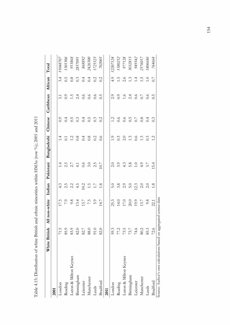
154

Tab

le ‎4

.15: D

istr

ibuti

on

of

wh

ite

Bri

tish

an

d e

thn

ic m

ino

riti

es w

ith

in H

MA

s (r

ow

%);

2001 a

nd

2011

W

hit

e B

riti

sh

All

no

n-w

hit

e In

dia

n

Pak

ista

ni

Ban

gla

desh

i C

hin

ese

C

ari

bb

ean

A

fric

an

T

ota

l

2001

L

on

do

n

71.5

17.5

4.3

1.4

1.4

0.9

3.1

3.4

11048707

Rea

din

g 85.9

7.9

2.5

2.5

0.1

0.4

0.9

0.5

1301306

Luto

n &

Milt

on

Key

nes

83.9

9.8

2.2

2.7

1.2

0.5

1.5

0.8

913868

Bir

min

gham

82.0

13.4

4.5

4.1

0.8

0.3

2.4

0.3

2857091

Lei

cest

er

82.7

13.7

10.2

0.6

0.4

0.4

0.6

0.4

868892

Man

ches

ter

88.0

7.5

1.5

3.0

0.8

0.5

0.6

0.4

2426500

Lee

ds

91.0

5.9

1.7

2.5

0.2

0.3

0.6

0.2

1725523

Bra

dfo

rd

82.0

14.7

1.8

10.7

0.6

0.2

0.5

0.2

702005

2011

Lo

ndo

n

59.3

25.3

5.0

2.0

1.9

1.2

2.9

4.9

12207124

Rea

din

g 77.2

14.0

3.8

3.9

0.3

0.6

0.9

1.5

1380252

Luto

n &

Milt

on

Key

nes

73.5

17.0

2.9

4.3

2.0

0.6

1.6

2.6

977128

Bir

min

gham

73.7

20.0

5.0

5.8

1.3

0.5

2.4

1.3

3032813

Lei

cest

er

74.6

19.9

12.3

1.0

0.6

0.7

0.6

1.4

949342

Man

ches

ter

80.2

13.7

2.0

4.9

1.3

0.8

0.7

1.5

2576017

Lee

ds

85.3

9.8

2.0

3.7

0.3

0.4

0.6

1.0

1806686

Bra

dfo

rd

72.6

22.1

1.8

15.4

1.2

0.3

0.5

0.7

764664

So

urc

e: A

uth

or’

s o

wn

cal

cula

tio

ns

bas

ed o

n a

ggre

gate

d c

ensu

s d

ata

155

4.6 Analysis of spatial segregation (2001-2011)

This section presents the results on spatial segregation. As we have seen, the previous findings

based on segregation indices pointed to a decrease in segregation. However, I will show that this

is not the case for all dimensions of segregation. Moreover, group differences remain, as well as

differences based on the HMA under investigation.

4.6.1 Results for White British and (pooled) non-white ethnic minorities

Table 4.16 shows segregation indices for the white British and (pooled) non-white ethnic

minorities for 2011, as well as the absolute difference with respect to the equivalents in 2001.

Although the focus of the analysis is the spatial segregation of ethnic minorities, having a general

idea of spatial segregation of the majoritarian population affords a better comparative

perspective. The results show that for most housing market areas in 2011, non-white ethnic

minorities were more unevenly distributed (have a higher D) than the white British; still, as can

be seen from the table, the values of the Dissimilarity Index for the white British are

considerable, if we compare them with some values obtained for France and the US (see Table

4.16). Furthermore, the white British were more exposed to one another than ethnic minorities

(which is linked to the relative weight of each group), and generally more clustered in the space,

although they were less concentrated (which is due to the highest share of ethnic minorities

residing in inner metropolitan areas).

More interesting results arise from comparing the HMAs. In particular, two extremes can be

identified: on the one hand we have Bradford (and to a lesser extent, Leicester and Leeds) as an

example of an area with higher segregation, both of ethnic minorities and of white British. On

the other hand, we have London (and, to a lesser extent, Luton & Milton Keynes and Reading),

which has the lowest segregation levels, also for both groups. Bradford is the area where ethnic

minorities (and also the white British) have the highest Dissimilarity Index: around 71% of non-

white ethnic minorities and 65% of white British would need to change their place of residence

to make their distribution even across LSOAs in Bradford. In London, these values drop to 34%

156

and 48% respectively, also positioning ethnic minorities in a better position as compared to the

majoritarian population (which is actually a minority in London in 2011)32.

Differences between Bradford and London arise as well in other dimensions of segregation. In

Bradford, exposure of non-whites to each other within the neighbourhood (or LSOA) is very

high: non-whites have around 61% probability of being in an area with other non-whites,

compared to a 2% probability London (a very low value). The same is observed for the white

British, who in Bradford have around 85% probability of sharing the neighbourhood with other

co-ethnics, while this value drops to 71% in London. Also in Bradford, ethnic minorities occupy

the smallest share of the space compared to the white British (have the highest RCO) and were

both absolute (ACL) and relative (SP) measures of clustering are the highest. This means, on the

one hand, that the location of white British and ethnic minorities is, to a greater extent,

determined by neighbourhoods of similar ethnic characteristics that adjoin one another in the

space; and, on the other, that members of each group live closer to one another than to each

other. Note also that London is the only HMA in which ethnic minorities are both more evenly

distributed and less clustered than the white British.

This better picture for London is good news in terms of segregation, since, as we saw, many non-

white ethnic minorities are located here. Although segregation based on ethnicity is still higher

compared to segregation based on social class (see Table 4.12), it is lower compared to the

segregation levels of some ethnic minorities in the US (see Table 4.11). This, however, is not the

case of Bradford and Leicester. Here, the Dissimilarity Index for non-whites is quite similar to

the average Dissimilarity Index of blacks in metropolitan areas in the US (although the US figure

would probably be higher if measured for smaller geographical areas). Furthermore, given the

values of D (between 64 and 71), xPx (between 56 and 61), RCO (around 0.9) and SP (between

0.5 and 0.8), these two areas approach what Massey and Denton (1988) have defined as “highly

segregated” groups. Note finally that these patterns are very similar to those observed for 2001,

which reveals that the relative position of HMAs in terms of their levels of segregation did not

change much in the decade. However, there are some tendencies toward change worth noting,

which I detail below.

32 Note that although London has a very high population density, which might be a reason why segregation levels are relatively lower, the areas next to it (Luton & Milton Keynes and Reading) do not (see Table 4.4).

157

Tab

le ‎4

.16: Seg

rega

tio

n indic

es f

or

no

n-w

hit

e et

hn

ic m

ino

riti

es a

nd w

hit

e B

riti

sh in

2011, an

d d

iffe

ren

ce w

ith

res

pec

t to

2001; H

MA

s

Are

a

Gro

up

E

ven

nes

s E

xp

osu

re

Co

nce

ntr

atio

n

Clu

ster

ing

D

Dif

. xP

x

Dif

. xP

y_w

b

Dif

. xP

y_n

w

Dif

. R

CO

D

if.

AC

L

Dif

. S

P

Dif

.

Lo

ndo

n

Wh

ite

Bri

tish

47.9

9

0.3

5

70.9

6

-7.5

4

16.3

8

4.3

0

38.1

9

-6.3

4

All

no

n-w

hit

e 46.7

2

-3.8

5

43.2

0

6.6

7

38.3

7

-10.9

5

0.8

1

-0.0

1

27.6

3

4.0

6

Luto

n &

M

ilto

n K

eyn

es

Wh

ite

Bri

tish

44.4

3

3.9

4

80.2

1

-6.5

9

11.4

3

4.1

5

44.5

8

-8.6

7

All

no

n-w

hit

e 49.1

6

-0.6

7

37.7

7

8.5

9

49.5

5

-12.9

1

0.8

3

-0.0

1

29.2

8

7.3

7

0.4

6

0.1

4

Rea

din

g W

hit

e B

riti

sh

40.9

2

4.3

0

82.0

9

-5.8

9

9.9

3

3.8

3

46.5

9

-8.6

1

All

no

n-w

hit

e 49.2

5

-2.0

0

33.3

5

6.7

3

54.8

1

-11.2

5

0.7

3

0.0

1

23.4

3

5.3

5

0.3

5

0.0

9

Bir

min

gham

W

hit

e B

riti

sh

52.5

7

1.0

9

82.7

3

-4.9

1

11.7

1

3.4

8

51.3

9

-7.2

5

All

no

n-w

hit

e 56.9

4

-2.4

7

48.3

0

4.8

5

43.1

5

-7.0

7

0.8

3

-0.0

1

35.6

7

3.5

4

0.4

1

0.0

4

Lei

cest

er

Wh

ite

Bri

tish

58.7

8

0.5

6

85.0

6

-4.0

1

10.0

1

2.4

7

55.4

5

-6.0

4

All

no

n-w

hit

e 64.2

2

-1.9

9

55.7

0

5.8

5

37.5

6

-8.0

6

0.8

8

-0.0

1

44.2

2

5.2

7

0.7

9

0.1

1

Man

ches

ter

Wh

ite

Bri

tish

47.9

8

1.4

2

85.5

2

-5.0

7

8.9

7

3.7

7

50.1

3

-11.2

6

All

no

n-w

hit

e 55.3

9

-3.8

5

39.0

6

6.8

1

52.6

0

-8.3

3

0.7

8

0.0

2

27.9

5

7.5

2

0.2

5

0.0

8

Lee

ds

Wh

ite

Bri

tish

51.9

0

0.3

6

89.2

4

-3.7

9

6.3

3

2.2

3

58.4

8

-8.6

5

All

no

n-w

hit

e 61.0

6

-2.7

2

37.0

4

4.9

2

55.0

7

-7.9

2

0.7

7

-0.0

1

26.9

7

4.9

6

0.3

2

0.0

9

Bra

dfo

rd

Wh

ite

Bri

tish

65.3

1

1.5

0

85.8

1

-3.6

5

9.6

6

2.3

3

57.3

1

-3.6

5

All

no

n-w

hit

e 70.8

4

-2.1

6

61.0

6

6.1

2

31.6

7

-9.3

1

0.9

4

0.0

0

48.9

9

5.9

3

0.5

4

0.1

0

So

urc

e: A

uth

or’

s o

wn

cal

cula

tio

ns

bas

ed o

n a

ggre

gate

d c

ensu

s d

ata

158

First of all, ethnic minorities were more evenly distributed in 2011 than in 2001: they decreased

their D at the national level and also in each HMA, London and Manchester being the areas with

the highest decreases (around 4 points). Interestingly, the white British have, in most cases,

followed the opposite pattern: in particular, their Dissimilarity Index mostly increased in the two

areas situated next to London: Luton & Milton Keynes and Reading (also an increase of around 4

points). Another finding is that, due to the change in the composition of the HMAs observed in

Table 4.15, in 2011 both white British and non-white ethnic minorities were more likely to meet

other non-white ethnic minorities and less likely to meet other white British in the

neighbourhood, which is observed in the increases of xPx and xPy indices. However, these

patterns are stronger for ethnic minorities (i.e. the increases are higher), which might encourage

higher spatial segregation of minorities in the long term. Going to the other measures, the RCO

reveals that the concentration of ethnic minorities with respect to the white British was generally

maintained (the variations are very small); while the measures of clustering show that, for all

areas, ethnic minority groups are more clustered in 2011 than in 2001, while the white British

experienced the opposite pattern. This is expressed in the increases in ACL and SP for all HMAs:

in 2011, ethnic minorities are more likely to live in neighbourhoods that adjoin one another, and

also to live closer to one another than to the white British, compared to one decade earlier.

All in all, these results show that although non-white ethnic minorities have become more evenly

distributed across units in the space, the other dimensions point to a higher segregation: first of

all, their exposure to white British (and to other non-white) decreased (increased) more,

compared to that experienced by white British; second, their levels of clustering increased (both

ACL and SP), for which they are more likely to be in areas that adjoin one another, and also

more likely to meet someone from the own group (vs. a white British). Third, considering again

the two extreme cases, London and Bradford, and looking at the tendencies between 2001 and

2011, it comes out that the gap between the two in terms of segregation levels increased. In other

words, although the patterns of increase/decrease in segregation are the same direction for both

areas, the improvement that Bradford made in terms of spatial segregation is not as good as that

that London made (or the worsening not as bad). For example, while the white British increased

their D by 0.35 points in London, they did so by 1.5 points in Bradford; similarly, ethnic

minorities decreased their Dissimilarity by almost 4 points in London, while this decrease was

only half in Bradford. Measures of clustering also show this pattern very well: while in London

the decrease in ACL is of around 6 points for the white British, meaning that in 2011 they lived

in areas that had on average 6% points fewer white British, in Bradford the reduction is less than

159

4%. For ethnic minorities, on the other hand, the increase in clustering is higher in Bradford,

where they are now around 6% points more likely to live in neighbourhoods with other non-

whites, on average (while this drops to 4% in London). Finally, recall that the greatest

improvements in terms of segregation seem to be the case of Birmingham and, to a lesser extent,

Leeds; while the worst situation seems to be that of Luton and Milton Keynes.

4.6.2 Results for ethnic minority groups

Table 4.17 shows the results divided by ethnic minority group. The values express the same as

Table 4.16, that is, segregation indices for 2011 and the difference with respect to 2001, which are

shown for England and for each HMA. Moreover, I added as well a ranking of groups/HMAs in

terms of their average segregation levels for 2001 and 2011, and a ranking in terms of the average

change in the decade33. A higher rank means that segregation levels are higher for a certain group

in a certain HMA, or that the group/HMA is worse-positioned in terms of change in the levels of

segregation (either because its segregation levels tended to increase, or because it experienced a

less-pronounced decrease compared to the other groups/HMAs).

33 For calculating the ranking of groups/HMAs I followed the following steps. First I selected one segregation measure for each dimension, so as to give equal weight to each dimension: D, xPy_wb, RCO and ACL. D, RCO were unique measures of evenness and concentration, respectively, while ACL was preferred to SP since SP could not be calculated for London. Among the measures of interaction, I excluded xPx, due to its high correlation with RCO and ACL (see Table 4.10); correlations between xPy measures with the other indices where very similar, and I preferred xPy_wb because I found the interaction with the white British more relevant as a measure, in line with the assimilation perspective (as a robustness check, I also produced rankings with all indices, and the order of groups/HMAs is practically the same: available upon request). After selecting the four indices, I assigned a rank to each group/HMA based on their value of each segregation index in 2001 and 2011, and also on their change between 2001 and 2001: this led to 12 ranks (4 indices x 3). Then, for each year and for the change 2001-2011, I summarized these ranks (calculated the average); and finally, I ranked these averages, which led to having one ranking of groups/HMAs for 2001, one for 2011 and one for the change 2001-2011. The ranking of groups/HMAs varies between 1 and 43 for 2001, between 1 and 44 for 2011 and between 1 and 39 for the difference (this variation is due to some repetition in the averages, which led some groups/HMAs to have the same rank).

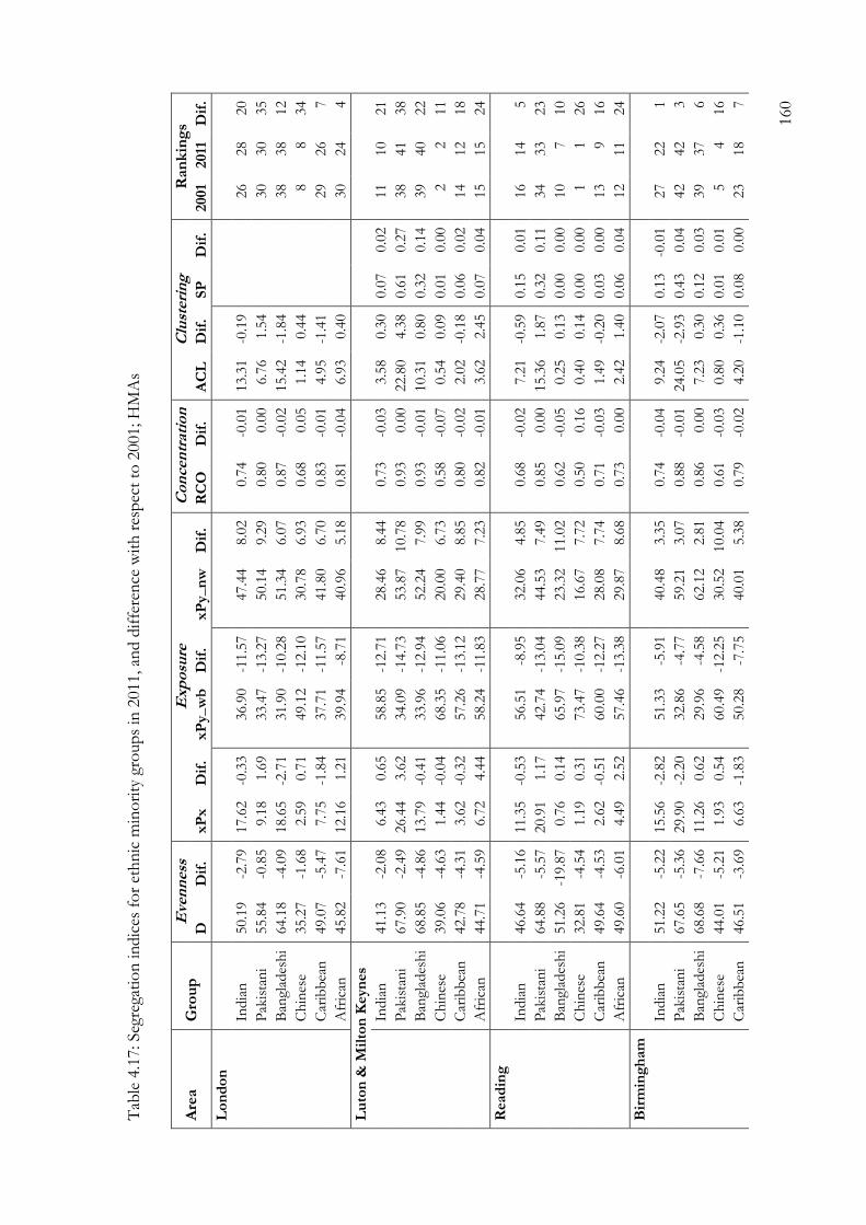
160

Tab

le 4

.17: Seg

rega

tio

n indic

es f

or

eth

nic

min

ori

ty g

roup

s in

2011, an

d d

iffe

ren

ce w

ith

res

pec

t to

2001; H

MA

s

Are

a

Gro

up

E

ven

nes

s E

xp

osu

re

Co

nce

ntr

atio

n

Clu

ster

ing

R

an

kin

gs

D

Dif

. xP

x

Dif

. xP

y_w

b

Dif

. xP

y_n

w

Dif

. R

CO

D

if.

AC

L

Dif

. S

P

Dif

. 2001

2011

D

if.

Lo

nd

on

India

n

50.1

9

-2.7

9

17.6

2

-0.3

3

36.9

0

-11.5

7

47.4

4

8.0

2

0.7

4

-0.0

1

13.3

1

-0.1

9

26

28

20

Pak

ista

ni

55.8

4

-0.8

5

9.1

8

1.6

9

33.4

7

-13.2

7

50.1

4

9.2

9

0.8

0

0.0

0

6.7

6

1.5

4

30

30

35

Ban

glad

esh

i 64.1

8

-4.0

9

18.6

5

-2.7

1

31.9

0

-10.2

8

51.3

4

6.0

7

0.8

7

-0.0

2

15.4

2

-1.8

4

38

38

12

Ch

ines

e 35.2

7

-1.6

8

2.5

9

0.7

1

49.1

2

-12.1

0

30.7

8

6.9

3

0.6

8

0.0

5

1.1

4

0.4

4

8

8

34

Car

ibbea

n

49.0

7

-5.4

7

7.7

5

-1.8

4

37.7

1

-11.5

7

41.8

0

6.7

0

0.8

3

-0.0

1

4.9

5

-1.4

1

29

26

7

Afr

ican

45.8

2

-7.6

1

12.1

6

1.2

1

39.9

4

-8.7

1

40.9

6

5.1

8

0.8

1

-0.0

4

6.9

3

0.4

0

30

24

4

Lu

ton

& M

ilto

n K

eyn

es

In

dia

n

41.1

3

-2.0

8

6.4

3

0.6

5

58.8

5

-12.7

1

28.4

6

8.4

4

0.7

3

-0.0

3

3.5

8

0.3

0

0.0

7

0.0

2

11

10

21

P

akis

tan

i 67.9

0

-2.4

9

26.4

4

3.6

2

34.0

9

-14.7

3

53.8

7

10.7

8

0.9

3

0.0

0

22.8

0

4.3

8

0.6

1

0.2

7

38

41

38

B

angl

ades

hi

68.8

5

-4.8

6

13.7

9

-0.4

1

33.9

6

-12.9

4

52.2

4

7.9

9

0.9

3

-0.0

1

10.3

1

0.8

0

0.3

2

0.1

4

39

40

22

C

hin

ese

39.0

6

-4.6

3

1.4

4

-0.0

4

68.3

5

-11.0

6

20.0

0

6.7

3

0.5

8

-0.0

7

0.5

4

0.0

9

0.0

1

0.0

0

2

2

11

C

arib

bea

n

42.7

8

-4.3

1

3.6

2

-0.3

2

57.2

6

-13.1

2

29.4

0

8.8

5

0.8

0

-0.0

2

2.0

2

-0.1

8

0.0

6

0.0

2

14

12

18

A

fric

an

44.7

1

-4.5

9

6.7

2

4.4

4

58.2

4

-11.8

3

28.7

7

7.2

3

0.8

2

-0.0

1

3.6

2

2.4

5

0.0

7

0.0

4

15

15

24

Read

ing

In

dia

n

46.6

4

-5.1

6

11.3

5

-0.5

3

56.5

1

-8.9

5

32.0

6

4.8

5

0.6

8

-0.0

2

7.2

1

-0.5

9

0.1

5

0.0

1

16

14

5

P

akis

tan

i 64.8

8

-5.5

7

20.9

1

1.1

7

42.7

4

-13.0

4

44.5

3

7.4

9

0.8

5

0.0

0

15.3

6

1.8

7

0.3

2

0.1

1

34

33

23

B

angl

ades

hi

51.2

6

-19.8

7

0.7

6

0.1

4

65.9

7

-15.0

9

23.3

2

11.0

2

0.6

2

-0.0

5

0.2

5

0.1

3

0.0

0

0.0

0

10

7

10

C

hin

ese

32.8

1

-4.5

4

1.1

9

0.3

1

73.4

7

-10.3

8

16.6

7

7.7

2

0.5

0

0.1

6

0.4

0

0.1

4

0.0

0

0.0

0

1

1

26

C

arib

bea

n

49.6

4

-4.5

3

2.6

2

-0.5

1

60.0

0

-12.2

7

28.0

8

7.7

4

0.7

1

-0.0

3

1.4

9

-0.2

0

0.0

3

0.0

0

13

9

16

A

fric

an

49.6

0

-6.0

1

4.4

9

2.5

2

57.4

6

-13.3

8

29.8

7

8.6

8

0.7

3

0.0

0

2.4

2

1.4

0

0.0

6

0.0

4

12

11

24

Bir

min

gh

am

In

dia

n

51.2

2

-5.2

2

15.5

6

-2.8

2

51.3

3

-5.9

1

40.4

8

3.3

5

0.7

4

-0.0

4

9.2

4

-2.0

7

0.1

3

-0.0

1

27

22

1

P

akis

tan

i 67.6

5

-5.3

6

29.9

0

-2.2

0

32.8

6

-4.7

7

59.2

1

3.0

7

0.8

8

-0.0

1

24.0

5

-2.9

3

0.4

3

0.0

4

42

42

3

B

angl

ades

hi

68.6

8

-7.6

6

11.2

6

0.6

2

29.9

6

-4.5

8

62.1

2

2.8

1

0.8

6

0.0

0

7.2

3

0.3

0

0.1

2

0.0

3

39

37

6

C

hin

ese

44.0

1

-5.2

1

1.9

3

0.5

4

60.4

9

-12.2

5

30.5

2

10.0

4

0.6

1

-0.0

3

0.8

0

0.3

6

0.0

1

0.0

1

5

4

16

C

arib

bea

n

46.5

1

-3.6

9

6.6

3

-1.8

3

50.2

8

-7.7

5

40.0

1

5.3

8

0.7

9

-0.0

2

4.2

0

-1.1

0

0.0

8

0.0

0

23

18

7

161

Are

a

Gro

up

E

ven

nes

s E

xp

osu

re

Co

nce

ntr

atio

n

Clu

ster

ing

R

an

kin

gs

D

Dif

. xP

x

Dif

. xP

y_w

b

Dif

. xP

y_n

w

Dif

. R

CO

D

if.

AC

L

Dif

. S

P

Dif

. 2001

2011

D

if.

A

fric

an

52.7

4

-4.5

7

5.2

7

4.0

0

44.1

2

-13.2

0

45.9

4

11.2

0

0.7

9

0.0

6

3.2

2

2.6

2

0.0

6

0.0

5

17

22

36

Leic

est

er

In

dia

n

66.1

8

-1.6

0

44.2

9

0.1

5

32.9

6

-9.1

9

61.0

6

7.4

6

0.8

9

-0.0

3

33.9

6

-0.0

3

0.8

3

0.1

7

41

43

17

P

akis

tan

i 61.2

4

-5.1

9

4.4

0

0.7

6

33.9

7

-9.1

7

59.1

4

7.2

5

0.8

7

0.0

4

3.1

3

0.6

7

0.1

4

0.0

6

31

31

19

B

angl

ades

hi

72.3

3

-7.8

4

8.6

4

-0.7

7

37.5

0

-10.1

4

54.6

3

8.1

9

0.8

7

0.0

0

5.4

9

-0.2

6

0.1

1

0.0

4

36

36

9

C

hin

ese

54.1

9

4.2

4

4.3

6

2.8

9

63.5

3

-15.3

6

27.5

9

11.5

8

0.7

6

0.0

5

2.5

6

1.9

1

0.0

4

0.0

3

7

13

39

C

arib

bea

n

49.4

7

-5.4

1

1.8

2

-0.4

9

51.6

0

-9.8

4

40.0

8

7.3

1

0.8

2

-0.0

1

0.9

8

-0.2

8

0.0

4

0.0

0

21

16

8

A

fric

an

58.3

3

-3.9

4

6.6

1

2.9

3

48.8

9

-8.2

0

41.9

4

5.6

1

0.8

8

0.0

3

3.4

6

1.9

7

0.1

0

0.0

6

28

29

26

Man

ch

este

r

In

dia

n

53.9

1

-6.2

0

15.2

7

-1.3

4

57.6

1

-7.0

7

35.1

5

5.2

9

0.7

0

0.0

1

9.5

0

-0.6

6

0.1

1

0.0

2

22

19

6

P

akis

tan

i 65.1

3

-3.4

2

27.3

3

2.9

1

46.2

3

-10.0

5

46.0

0

8.8

0

0.8

0

0.0

1

19.2

5

3.6

2

0.1

8

0.0

6

32

32

32

B

angl

ades

hi

73.3

8

-5.4

1

26.4

4

-0.6

7

43.0

0

-5.3

4

51.6

4

4.6

1

0.7

8

-0.0

1

19.5

9

1.9

4

0.1

6

0.0

6

35

34

15

C

hin

ese

42.2

9

-4.5

5

3.8

1

1.6

4

66.6

4

-12.7

0

24.2

2

11.1

2

0.6

5

0.0

5

2.5

4

1.6

5

0.0

3

0.0

2

4

6

33

C

arib

bea

n

55.0

0

-3.2

6

4.2

1

-1.8

8

55.2

2

-9.4

7

33.8

5

8.4

2

0.7

2

-0.0

2

3.4

2

-1.0

4

0.0

5

0.0

0

20

17

13

A

fric

an

57.1

4

-3.2

0

7.4

1

3.2

3

58.2

3

-6.3

9

31.3

8

6.2

4

0.7

7

0.0

7

5.2

9

2.5

1

0.0

7

0.0

3

19

20

29

Leed

s

In

dia

n

60.2

9

-1.8

3

19.4

9

1.7

2

53.2

7

-8.7

2

41.0

8

6.9

7

0.7

4

0.0

1

14.0

8

1.9

2

0.1

7

0.0

5

25

27

28

P

akis

tan

i 72.0

9

-1.2

2

26.5

8

4.3

7

47.2

3

-11.5

9

45.0

9

8.4

6

0.8

5

0.0

1

18.2

5

4.2

9

0.2

3

0.0

9

33

35

37

B

angl

ades

hi

77.7

4

-8.7

8

11.8

3

-1.6

5

36.7

6

-8.2

8

52.9

9

3.9

7

0.8

8

-0.0

3

6.5

9

0.1

1

0.0

7

0.0

3

40

38

2

C

hin

ese

45.9

8

-8.4

4

1.5

5

0.5

3

75.7

2

-9.0

2

16.7

3

6.2

6

0.2

9

-0.2

8

0.5

8

0.2

4

0.0

1

0.0

0

3

3

2

C

arib

bea

n

63.6

1

-2.4

4

5.7

4

-1.3

6

57.7

1

-9.2

5

31.8

6

6.3

6

0.7

5

-0.0

2

4.4

4

-0.4

4

0.0

6

0.0

0

24

21

14

A

fric

an

57.5

2

-5.3

9

5.3

8

4.1

6

66.1

8

-10.4

2

24.1

7

6.9

0

0.7

4

0.1

1

3.3

8

2.8

4

0.0

6

0.0

5

9

14

30

Bra

dfo

rd

In

dia

n

50.8

3

-4.8

7

6.2

0

-1.7

2

45.8

7

-10.0

2

47.4

0

7.4

3

0.8

8

-0.0

1

3.0

2

-0.8

8

0.0

8

0.0

1

30

25

9

P

akis

tan

i 73.1

4

-4.1

2

51.7

7

2.4

3

26.6

1

-9.2

5

66.2

5

6.1

1

0.9

6

0.0

0

40.2

8

1.9

5

0.5

6

0.1

2

43

44

24

B

angl

ades

hi

69.1

5

-7.7

5

10.2

9

2.5

5

30.1

2

-7.7

1

63.0

9

4.9

3

0.9

5

-0.0

1

5.3

9

1.7

6

0.0

8

0.0

4

37

39

11

C

hin

ese

43.1

1

-13.0

0

2.2

0

0.9

6

57.9

7

-18.2

0

33.8

9

15.0

8

0.4

7

0.5

0

0.8

6

0.3

8

0.0

1

0.0

0

6

5

27

C

arib

bea

n

46.7

5

-0.8

4

1.3

9

-0.0

3

56.1

6

-11.9

7

36.2

0

8.8

9

0.8

7

0.0

3

0.7

1

0.0

0

0.0

2

0.0

1

14

15

31

A

fric

an

53.5

4

-7.7

6

2.9

8

2.1

7

46.1

1

-12.5

9

44.4

6

8.6

2

0.8

7

0.1

3

2.0

1

1.4

9

0.0

4

0.0

3

18

23

25

So

urc

e: A

uth

or’

s o

wn

cal

cula

tio

ns

bas

ed o

n a

ggre

gate

d c

ensu

s d

ata

162

A first and simple way to look at the results is to refer to the ranks. Table 4.17 shows that

Pakistani and Bangladeshi tend to have the highest ranks, and this is a pattern observed for most

HMAs, including London, where the majority of other ethnic minority groups are also located.

Luton & Milton Keynes, Birmingham and Bradford are HMAs where both groups tend to have

particularly high scores. Moreover, Bangladeshis also score high in London, and Leeds. Next to

Pakistani and Bangladeshi, we find that Indians in Leicester also have a high score in the ranking.

On the opposite side, Chinese have very low segregation levels in all HMAs: their scores in the

ranking are the lowest. Caribbean and African populations, finally, occupy intermediate positions;

and the majority that resides in London seems to have similar segregation levels as Pakistanis in

that HMA.

Moving to more detailed analyses of indices and groups, Dissimilarity indices are among the

highest for Pakistanis in most HMAs. In many cases, they also surpass by 10 points or more the

threshold (D=60) established for this index by Massey and Denton (1988) to identify “highly

segregated” groups (see Table 4.16). This group also reveals high levels of exposure to co-ethnics,

particularly in Bradford, where the probability of interaction with other members of the same

ethnic group in the neighbourhood is more than 50%, the closest value to the threshold

established by Massey and Denton for this index (xPx=70). Also in this HMA they present high

levels of clustering, living therefore in areas that adjoin one another, as well as one of the highest

probabilities of meeting a member of their own group rather than a white British, revealed by the

SP index, which almost reaches the 0.6 threshold for highly segregated areas. Note that if we

consider as well that Pakistanis in this area also surpass by far the threshold of 0.7 for

concentration (RCO), I believe there is evidence for defining this group as “highly segregated” in

Bradford. A similar, although more moderate, pattern of segregation is observed for this group in

two HMAs where it has a relatively high share of its population, Birmingham and Manchester,

and also in Luton & Milton Keynes and Leeds.

Among Bangladeshis, although on average they tend to be more unevenly distributed than

Pakistanis (scoring therefore higher in D), they have lower levels of segregation in other

dimensions. An important feature of the Bangladeshi population is that it is the most segregated

group in London, scoring the highest values in most of indices: it is the most unevenly

distributed group, when compared to the other groups, and also score the highest in xPx

(although very close to the Indian group) and have the highest levels of clustering (ACL).

Moreover, if we look at the other HMAs where they have a relatively high share of population,

163

we can see that they present the highest segregation levels in Manchester, resembling those of

Pakistanis.

Moving to the other groups, note the quite high segregation levels of Indians in Leicester, a

HMA in which Indians constitute around 12% of the population living in there. As with

Pakistanis in Bradford, we could identify this as a group that fulfils most of the conditions for

being termed “highly segregated”: not only does their dissimilarity index go beyond 60, but also

they have one of the highest values in exposure to other co-ethnics (44) and clustering (34), and

the highest value in the SP index (0.8), making them the case where members of a group have the

highest probability of contact with each other than with white British. Chinese, on the other

hand, have the lowest segregation levels in all HMAs. In London, where we find around half of

this population, they also score the lowest segregation levels in all dimensions. The remaining

groups, Caribbean and African, tend to present more intermediate segregation levels, if we

consider all groups in all HMAs. If we focus on London, where the majority of the black

population is located, we see that their ranks are very close to that of Indians and Pakistanis in

this HMA. In particular, their Dissimilarity indices are a few points less compared to that of

Indians, they have concentration and clustering levels that resemble those of Pakistanis, and

Africans have even higher interaction with co-ethnics in the neighbourhood than the Asian

group.

The analysis for individual groups has shown that as there are extreme cases in terms of HMAs

(London and Bradford); there are also extreme cases in terms of ethnic groups. On the one hand,

we have Pakistani and Bangladeshi populations (and Indian, but just in Leicester); on the other,

we have Chinese. At the same time, Pakistanis in Bradford and Indians in Leicester were found

to be the most segregated groups, considering all groups and HMAs, since they are the closest to

the definition of ‘highly segregated’ groups by Massey and Denton. Furthermore, together with

the Bangladeshi in Manchester, they, of all groups, most approach the patterns of segregation

found for some groups in the US. For example, the values for D, xPx and SP for the Hispanic

population in Chicago are 61, 55 and 0.42 respectively; and that for the African population in Los

Angeles are 66, 65 and 0.56 (see Table 4.11). The same values for Pakistanis in Bradford are 73,

52 and 0.56; for Indians in Leicester are 66, 44 and 0.83; and for Bangladeshis in Manchester are

73, 26 and 0.16. Although groups in England do not reach the levels of segregation found among

Africans in New York or Chicago, especially in regards to their uneven distribution and

interaction in the neighbourhood, these can be considerable in some cases. Note that in France,

164

the segregation levels are much lower in general. Finally, as we saw from the ranks, the above-

mentioned tendencies were generally maintained between both years, that is, groups with high

segregation in 2001 were still highly segregated in 2011; however, it is necessary to discuss in

more detail the main tendencies for the decade, already preliminarily delineated in Table 4.16.

Looking at the changes that occurred between 2001 and 2011, a first and clear outcome from

Table 4.17 is that segregation levels measured with the Dissimilarity Index decreased for all

groups and HMAs (an exception are the Chinese in Leicester). Note that similar results were

found for bigger geographical units: local authorities (see Table 4.11). Moreover, interaction with

white British persons decreased for all groups, while that with non-white ethnic minorities

increased, which is related to the highest relative increase of non-white ethnic minorities with

respect to the white British (see Table 4.15): if ethnic minorities increase their proportion with

respect to the white British, then the indices will inevitably follow this pattern. However, as we

saw in the comparison between non-white and white British, the extent of the

increases/decreases for these indices varies, as well as the changes observed for the other indices,

which do not necessarily point – as does, for example, D – to less segregation.

The last column of Table 4.17 shows the rank of group/HMAs in terms of the average changes

they experienced between 2001 and 2011. Groups/HMAs with a lower score are better off in

relative terms with regard to changes in segregation; while the opposite is true for areas with a

higher rank. A striking initial finding pertains to how different Pakistani and Bangladeshi – the

two populations with relatively higher segregation levels in various HMAs – are in terms of the

changes they experienced during the decade. Although, as we saw, in 2011 their positioning in

the ranking did not change much relative to the positioning of other ethnic minority groups, we

find that the tendencies for Pakistanis are relatively worse. This can be easily observed in the

higher ranks that this group has in most of HMAs. Take, as an example, the London HMA.

Although Bangladeshis are clearly more segregated than Pakistanis in all dimensions of

segregation, they also experienced higher reductions in most of them between 2001 and 2011.

For example, they reduced their Dissimilarity Index by 4 points, while the reduction was less than

one point for Pakistanis; also, the probability of interaction with co-ethnics in the neighbourhood

and level of clustering were reduced for Bangladeshis, while they increased for Pakistanis. Similar

patterns were observed by Luton & Milton Keynes and Manchester, where both groups have

considerable populations, but also in other areas where Bangladeshis are fewer, like Leeds and

Bradford. Note that this outcome appears to be particularly worrisome for the Pakistani

165

population, since some of these HMAs are also the ones in which this group is mostly segregated.

Pakistanis in Leeds and Bradford, for example, increased their probability of exposure to each

other in the neighbourhood (between 2% and 4% points more) and also their clustering (between

2 and 4 points increase in ACL and around 0.1 increase in SP).

Moving to other groups, Chinese in London and Manchester HMAs – where most of them are

found – increased their segregation in more than one dimension, following closely the Pakistanis

in these two areas. Indians have more intermediate positions, if we look at their rank based on

changes between 2001 and 2011. However, note that both in London and in Leicester – where

the majority of their population is located – their relative position in terms of segregation

(observed in the 2001 and 2011 ranks) moved up from 26 to 28 in London and from 41 to 43 in

Leicester. As we look more closely at the segregation indices, however, it is actually in Leicester

where we can see clear signs of increasing segregation: Indians in this HMA have one of the

highest increases in the SP index, and also increased their xPx, indicating that they were more

likely to meet a member of the own group rather than a white British person, and also more likely

to interact with co-ethnics in the neighbourhood. As with Pakistanis, this is bad news in terms of

segregation, as the Indian population in Leicester was already one of the most segregated groups

in England in 2001. Caribbean and African populations, finally, mostly located in London, also

experienced improvements in terms of segregation in this HMA. The Caribbean population, in

particular, reduced their exposure to other co-ethnics in the neighbourhood and their clustering,

while African became more evenly distributed and less concentrated during the decade (although

their clustering and interaction within the neighbourhood also increased).

Summarizing, we find on the one hand, Pakistanis, followed by Chinese (and to a lesser extent,

Indians), with increasing segregation levels. As we saw, this might be particularly problematic for

Pakistanis (and Indians in Leicester), since their levels of segregation were among the highest in

2001. On the other hand, we find Caribbean and Bangladeshi populations, the latter with

relatively high segregation levels in 2011, but with important improvements in the decade

(particularly relevant for the London HMA). Finally, note that Birmingham seems to be an area

particularly favourable for changes in spatial segregation, since four of the six groups under

analysis have very low ranks (1, 3 6 and 7). This outcome, already observed when studying pooled

non-white ethnic minorities, might speak to particular processes taking place in this HMA.

166

4.7 Summary and discussion

The aim of this chapter has been to assess the current situation of non-white ethnic minority

groups in England in terms of their levels of spatial segregation, as well as to reveal the main

tendencies of change in this respect for the period 2001-2011. A key question was: did spatial

segregation of ethnic minorities decrease? By means of exploring various dimensions of

segregation (evenness, exposure, concentration and clustering) for groups residing in areas that

are relatively self-contained in terms of their population (HMAs), the analysis has provided a

quite-detailed and complex picture of the patterns of spatial segregation of ethnic minorities.

The results of the analysis can be sub-divided. First, we have the results on spatial segregation for

different groups and HMAs in 2011; second, we have the results on the changes that took place

within the decade. With regard to the first issue, a first outcome is that segregation levels of non-

whites are considerably higher than that of white British. Moreover, we also saw that London and

the neighbouring areas (Luton & Milton Keynes and reading) seem to be particularly favourable

locations in terms of segregation, as both white British and non-white ethnic minorities have

lower segregation levels and a higher probability of interacting in the space; the opposite situation

was found in Bradford, where both groups seem to be more isolated.

A detailed analysis of groups showed, in accord with most recent findings, that the Chinese

population is the most integrated in the space, while the Pakistani and Bangladeshi have the

highest segregation levels in most HMAs. In particular, this is true for Pakistanis in Leeds and

Bradford and for Bangladeshis in Manchester; in addition, Bangladeshis are the most segregated

group in London. We also saw that Indians have very high segregation levels in Leicester, where

they constitute an important share of the population living in that HMA. In this regard, I also

argued that Pakistanis in Bradford and Indians in Leicester are the two cases that most approach

what Massey and Denton (1989), based on data from the US, termed “highly segregated” groups.

These results are also in line with the arguments presented by Johnston, Forrest and Poulsen

(2002a). Caribbean and African populations, finally, located mainly in London, present

segregation levels that resemble that of Indians and Pakistanis in that city; however, on average,

their segregation levels are lower.

In order to paint a better ‘picture’ of these patterns, Maps 4.2-4.8 (below) present the distribution

of ethnic minority groups in selected housing market areas (or more specifically, in selected areas

167

within these HMAs). They show that Indians, Pakistanis and Bangladeshis occupy in general a

much smaller and compact share of the space, as compared to the rest of the groups; on the

other hand, Chinese, and to a lesser extent the Caribbean population, tend to be more spread

out in the space.

With regard to the tendencies of change between 2001 and 2011, we saw that the relative

position of groups/HMAs did not vary much: highly segregated groups in 2001 were still highly

segregated groups in 2011, and the same can be said of low segregated groups. But alongside the

general persistence of the socio-spatial structure, changes still occurred.

In line with previous findings, we saw, firstly, that the share of ethnic minority populations in

metropolitan areas was reduced, pointing to processes of suburbanization. Moreover, following

the work of Simpson (2012), segregation measured with the most popular index, the Dissimilarity

Index, decreased for non-whites in all HMAs. This shows that in 2011 all groups were more

evenly distributed than in 2001. Moreover, there was also an increase in shared spaces, as

previous studies have already shown (Johnston, Poulsen and Forrest 2010; Poulsen and Johnston

2006). The generalized increase in exposure between non-whites and white British, points to the

creation of areas that are more mixed. As additional evidence, Table 4.18, which divides LSOAs

according to their percentage of non-white ethnic minorities in 2001 and 2011, shows that areas

that had between 5% and 25% non-white ethnic minorities grew from 5431 to 7731 (something

we would expect given that ethnic minorities lead the population growth).

However, the other dimensions revealed two processes that go in the opposite direction. On the

one hand, non-white ethnic minorities increased their probability of meeting a non-white to a

greater extent than did the white British (and decreased, to a lesser extent, their probability of

meeting a white British person). The increase in the number of areas with a high concentration of

non-white ethnic minorities (i.e. more than 75%) supports this statement (see Table 4.18). On the

other hand, non-whites also increased their levels of clustering, meaning that the percentage of

non-whites living in adjacent areas increased for this group, on average. Hence, I agree with

Johnston, Poulsen and Forrest (2010) that relying solely on the Dissimilarity Index might result in

a misleading interpretation of what is happening with the spatial segregation of ethnic minorities.

168

Table ‎4.18: Number of LSOAs by percentage of non-white ethnic minorities (2001 and 2011)

2001

2011 75% and

more 50.01% -

75% 25.01% -

50% 10.01% -

25% 5.01 % -

10% Up to 5% Total

75% + 274 295 36 1 606

50.01% - 75% 6 323 752 32 4

1117

25.01% - 50% 1 14 1175 1444 142 37 2813

10.01% - 25% 24 1350 1859 975 4208

5.01 % - 10%

21 533 2969 3523

Up to 5%

1 44 19360 19405

Total 281 632 1987 2849 2582 23341 31672

Descriptive statistics based on the Table

% with respect to total number of LSOAs

Diagonal 72.7

Below diagonal 0.4

Above diagonal 26.9

Number of areas 2001 2011

Very high concentrated areas (>75%) 281 606

High concentrated areas (>50%) 913 1723

Mixed areas (5%-25%) 5431 7731

Source: Source: Author’s own calculations based on aggregated census data; England

Looking at more specific results, differentiated by ethnic minority group, I found that the

generalized decrease in the Dissimilarity Index did not occur equally for all groups; moreover,

while some groups also presented clear signs of improvement in the other dimensions of

segregation, others followed the opposite pattern. Of particular importance is the difference

found between Pakistani and Bangladeshi, the two most spatially segregated groups: while the

former presented signs of increasing segregation in the decade (in particular as regards their

interaction and clustering), the latter, including those who reside in London, tended to improve

with respect to 2001. Additional information in Table ‎8.9 in Annex A shows that while the

number of neighbourhoods (LSOAs) with more than 50% of Pakistani increased from 96 to 137,

for Bangladeshi it decreased from 27 to 23. Note that a tendency similar to that of the Pakistani

population was observed for the Indian one in Leicester: neighbourhoods with 75% or more of

an Indian population (except for one, all located in Leicester) grew from 17 to 21.

These changes will become more evident when the reader looks at Maps 4.2, 4.3 and 4.4, which

present the distribution of Indian, Pakistani and Bangladeshi populations in (selected areas in)

169

Leicester, Bradford and London respectively, in 2001 and 2011. These maps clearly show that

while for Indians in Leicester and Pakistanis in Bradford the increase in the share of ethnic

minorities in neighbourhoods occurred (at least to a considerable extent) in areas that were

already very much populated with these groups, for Bangladeshi in London there is a clear

tendency of expansion and dispersion in the urban space.

The increase in segregation levels for Chinese is also a strong finding, especially in London,

where the majority of them are located; however, we also saw that Chinese still have very low

levels of spatial segregation as compared to other groups: note, for example, that none of the

LSOAs has more than 25% Chinese (see Table ‎8.9 in Annex A). This can be seen easily as well in

Map 4.5, which shows the distribution of Chinese in (selected areas of) Manchester. Even if they

are among the groups that experienced the highest increase in segregation, this is minimal as

compared to the segregation of the other Asian groups: only a few areas in the centre of

Manchester become darker on the map between 2001 and 2011.

Finally, Caribbean (and to a lesser extent African) populations show clear signs of improvement

in London, where the majority of them are located. Maps 4.6 and 4.7, which present the

distribution of Caribbean and African populations in (selected areas of) London, clearly show a

tendency of these groups to spread out in the space, as seen previously with Bangladeshi. For

Africans, however, the increase in clustering and interaction within the neighbourhood is also

evident.

What are the implications of these results? Is spatial segregation increasing or decreasing? Should it be a

matter of concern? Spatial segregation of non-white ethnic minorities is decreasing in some

aspects and increasing in others. It would be misleading, then, to claim that spatial segregation is

either decreasing or increasing in England. Based on these results, however, I can state with

confidence that while some groups are decreasing their levels of spatial segregation, in particular

Caribbean individuals and Bangladeshi in London, others, such as Pakistani in Bradford and

Leeds and Indians in Leicester, are following the opposite pattern. Of course, a key issue here is

why a decrease in spatial segregation is better than an increase. As argued above, I believe the

main advantage of a decrease in spatial segregation is that it offers an enhanced likelihood that

individuals will interact with others who are different from themselves, or conversely, that it

decreases the likelihood that they will meet others who are similar to themselves. While

segregation might result in both benefits and disadvantages, depending on what outcomes we are

170

interested in, the unequal distribution of individuals can be seen per se as an impediment to social

cohesion (Cantle 2012; Uslaner 2012).

A related issue pertaining to the implications of these results is the nature of the explanations of

the patterns we observed. The decrease in segregation observed for the Caribbean population in

London is something we would expect, following the spatial assimilation theory (Massey and

Denton 1985). Caribbean individuals were among the first to arrive to the country, and as shown

in Chapter 1, their growth rate is low. Based on new births only, one would expect this group to

slowly move out of areas with a high concentration of co-ethnics. Contrariwise, the fact that the

Chinese population growth is mainly due to new arrivals might preclude higher segregation in the

space, since upon arrival immigrants usually go to areas where other co-ethnics reside (which at

the same time might be pushing the white British in other directions). However, even if these

mechanisms hold, they are still far from being problematic, given the very low segregation levels

that Chinese have in any case.

One of the most interesting and puzzling findings of this study are the different patterns of

change experienced by the Pakistani and Bangladeshi populations, respectively. Given that both

groups have similar segregation levels on average, that their components of population growth

are also very similar (mainly based on new births) and that in cultural terms the literature has in

many cases addressed them together, I would have expected to find that they experienced similar

patterns of change. What is more, given that Bangladeshis are a younger population, I might have

expected an increase in segregation to occur among them. In fact, the spatial assimilation theory

predicts that the movement out of ethnic areas occurs as individuals improve in socio-economic

terms, which happens inevitably at a later age.

Thus, the findings lead me to think that other factors are affecting the segregation patterns of

Pakistanis and Bangladeshis. These might be related both to preferences and constraints. The

first element that comes to mind concerns London’s housing market, to which most of

Bangladeshis are exposed. We could hypothesize that this market is more open-minded as

compared to others, and therefore we see the positive patterns for the Bangladeshi and

Caribbean populations; however, the increase in various aspects of segregation for Pakistanis

occurs in most HMAs, including London. Another mechanism might be that the housing market

discriminates against Pakistanis to a greater extent than it does Bangladeshis. Although there is

no clear evidence for this, it is certainly a notion that deserves further analysis. Finally, the

171

observed differences may be based on cultural differences and, hence, on preferences of the

groups, including preferences of those who arrive to the country. This is another aspect that

warrants future research.

172

Map

‎4.2

: In

dia

ns

in L

eice

ster

2001

2011

1

So

urc

e: A

uth

or’

s o

wn

cre

atio

n b

ased

on

geo

-ref

eren

ced

agg

rega

ted

cen

sus

dat

a

173

Map

‎4.3

: P

akis

tan

i in

Bra

dfo

rd 2

001

2011

So

urc

e: A

uth

or’

s o

wn

cre

atio

n b

ased

on

geo

-ref

eren

ced

agg

rega

ted

cen

sus

dat

a

174

Map

‎4.4

: B

angl

ades

hi in

Lo

ndo

n

2001

2011

So

urc

e: A

uth

or’

s o

wn

cre

atio

n b

ased

on

geo

-ref

eren

ced

agg

rega

ted

cen

sus

dat

a

175

Map

‎4.5

: C

hin

ese

in M

anch

este

r 2001

2011

So

urc

e: A

uth

or’

s o

wn

cre

atio

n b

ased

on

geo

-ref

eren

ced

agg

rega

ted

cen

sus

dat

a

176

Map

‎4.6

: C

arib

bea

ns

in L

on

do

n 2001

2011

So

urc

e: A

uth

or’

s o

wn

cre

atio

n b

ased

on

geo

-ref

eren

ced

agg

rega

ted

cen

sus

dat

a

177

Map

‎4.7

: A

fric

an in

Lo

ndo

n

2001

2011

So

urc

e: A

uth

or’

s o

wn

cre

atio

n b

ased

on

geo

-ref

eren

ced

agg

rega

ted

cen

sus

dat

a

179

5 CHAPTER 5: Neighbourhood Effects? Exploring the

Role of Early Exposure to Co-Ethnics

5.1 Introduction

The spatial concentration of ethnic minorities is an indisputable fact, as Chapter 4 has clearly

shown, and the literature has pointed to both positive and negative outcomes from it. On the one

hand, living close to co-ethnics can be particularly advantageous for first-generation immigrants,

who leverage the resources of spatial proximity for integrating into the host society. Among other

things, these resources can contribute to the securing of a job and a place to live, as well as

managing practical issues upon arrival. In this sense, living close to other co-ethnics and building

social capital (Lin 2001) in these areas can have positive effects for individuals. This has been

shown as well from a longer-term perspective, with the formation of the so-called ‘ethnic

enclave’ (Portes and Zhou 1993) and the possibilities this offers for ethnic entrepreneurship and

the maintenance of one’s own culture. On the other hand, however, living close to co-ethnics

might also have negative consequences. I mentioned already that spatial segregation can be seen

as a negative phenomenon not only because it constitutes an impediment to daily interaction

between individuals who are different, but also because segregation of minorities is usually linked

with deprivation. There are other negative aspects that we could think of too: for example, due to

the limited channels in which information circulates, concentration might prevent individuals

from finding other (better) occupational opportunities, or could impede proper language

acquisition or the establishment of relationships with the majoritarian population (Van Kempen

and Şule Özüekren 1998); segregation might also reinforce particular cultural patterns that might

reduce more generalized contact with other groups.

Based on data from the ONS Longitudinal Study, this chapter studies to what extent the ethnic

composition of the neighbourhood in which ethnic minorities are ‘raised’ or ‘grow up’ (that is,

the neighbourhood in which individuals live at some point when they are between 0 and 15 years

old in any of the three ‘origin’ years: 1971, 1981 and 1991) has an impact on labour market

outcomes in later stages of life (2001-2011). In so doing, this chapter also disentangles

mechanisms that might explain (or not) these effects. In particular, deprivation at the

neighbourhood level – a variable very much linked with ethnic concentration, as shown at the

180

beginning of this thesis – and other household/individual characteristics are included in the

analysis. This chapter answers the following questions:

1. Does the ethnic concentration of the neighbourhood where ethnic minorities are raised

have an effect on their labour market outcomes in later life? If yes, then:

1.1. Can this effect be explained by other context variables, like deprivation?

1.2. Can this effect be explained by background-household level variables, mainly

socio-economic background?

1.3. Can this effect be explained by other variables that mediate the relationship

between context/household variables and labour market outcomes, like education

or co-ethnic partnership?

2. Are there group and gender differences with regard to the effect of the neighbourhood?

5.2 Mechanisms underlying neighbourhood effects

What is a neighbourhood effect? There is no straightforward answer to this question, as a

neighbourhood effect can be expressed in many ways. Generally, one can say that a

neighbourhood effect refers to the fact that there is something about the neighbourhood in

which individuals live that affects them in terms of various outcomes such as health, labour

market performance or happiness. The mechanisms, however, that explain why this effect

actually occurs can be many. In an exhaustive literature review, Galster (2010) identified different

possible causal linkages, which he divided into four main groups: social interaction mechanisms,

geographical mechanisms, institutional mechanisms and environmental mechanisms.

Social interaction mechanisms refer to social processes endogenous to neighbourhoods. In other

words, they emerge as a consequence of the social contact among individuals in the

neighbourhood. For example, individuals might be encouraged to conform to local social norms

or follow certain rules based on role models present in the neighbourhood (the so-called

‘collective socialization’ mechanism); as well, they might be influenced by interpersonal

communication of information and resources of various kinds, transmitted through neighbours:

the so-called strong and weak ties (‘social networks’ mechanism). Similarly, behaviours,

aspirations and attitudes, might also be changed by contact with peers who are neighbours

(‘social contagion’ mechanism).

181

Geographical mechanisms refer to aspects of spaces that might affect individuals and that, rather than

arising from endogenous processes (as are those related to social interactions), emerge from the

relative position of the neighbourhood in a wider area, both in terms of geography and in terms

of political and social forces. For example, certain neighbourhoods might have little accessibility,

in either spatial proximity or mediated by local transportation, to job opportunities (‘spatial

mismatch’ mechanism); or they might lack proper public resources such as hospitals, schools or

general community services, which might in turn affect outcomes such as education and health

(‘public services’ mechanism). In fact, there is evidence both from the US and Western Europe

(Galster et al. 2007a; Galster 2010 for a review; Galster and Hedman 2013; Galster et al. 2007b;

Musterd and Andersson 2006; Urban 2009) that areas with a concentration of poverty or

disadvantage have a negative effect on a variety of child and adult outcomes.

Institutional mechanisms involve those who do not typically reside in the neighbourhood but either

control important institutional resources located there or are points of interface between the

residents and vital markets. For example, neighbourhoods might be stigmatized on the basis of

public stereotypes held by powerful actors (regardless of its current population), which might

impact on the job opportunities or self-esteem of its residents (‘stigmatization’ mechanism). An

example of this is the well-known work by Wacquant (1993), which compares the experiences of

individuals living in the black American ghetto and in the Parisian “banlieu”. Among other

findings, this study shows that black populations residing in these areas tend to be discriminated

against by employers, based on their place of residence. Finally, environmental mechanisms refer to

natural and human-made attributes of the local space that might affect directly the mental and/or

physical health of residents.

Galster has noted as well that the above-mentioned mechanisms might be activated only under

certain circumstances. For example, mechanisms of ‘collective socialization’ might only apply

after a certain amount of the population that is thought to be generating this effect is actually

living in a neighbourhood. This “threshold effect” has been considered, for example, in studies

on ‘white flight’, in which the neighbourhood change in terms of its ethnic composition

influences the moving out of white or majoritarian populations (perhaps linked to process of

‘stigmatization’ generated by those outside it). These studies have shown that emigration occurs

only once a certain number of ethnic minorities living in the neighbourhood has been reached

(for some discussion on the topic see for example Goering 1978). Other circumstances are

related to the timing of the neighbourhood effect: for example, living in a neighbourhood with

182

poor health facilities might have effects that are not immediately visible, but that appear later in

the life-course. In addition, neighbourhood effects might not necessarily apply to all those living

in the neighbourhood, and some might be more affected than others. Although these more

detailed mechanisms will not be tested empirically – due mainly to the availability of data and the

relatively imprecise neighbourhood measures I am allowed to use – I will seek to incorporate

them within the explanations. The next section gives an overview of the link between

neighbourhood effects and the migration literature.

5.3 Neighbourhood effects and the migration literature

Within the literature of neighbourhood effects, a more specific body of research has been

dedicated to the effect of ethnic composition of neighbourhoods. In particular, attention has

been paid to the presence of co-ethnics and how these might affect all sorts of outcomes, mainly

those related to the labour market (Clark and Drinkwater 2002; Urban 2009), but also social

cohesion (Becares et al. 2011; Sturgis et al. 2013), trust (Sturgis et al. 2011) and life satisfaction

(Knies, Nandi and Platt 2013). There has been much discussion on whether living in areas with a

high concentration of ethnic minorities has positive or negative effects for the residents of the

neighbourhood. In point of fact, the best way to approach this issue is to accept that it may

actually have both types of effects.

The positive effects of ethnic concentration are mainly related to mechanisms that emerge from

the (spatially located) ethnic community itself, and can therefore be subsumed under Galster’s

(2010 social interaction mechanisms. First of all, spatial proximity with co-ethnics can facilitate the

exchange of information and can help make basic arrangements to those who have just arrived to

the country. In fact, neighbourhoods where other ethnic minorities or co-ethnics live are usually

the preferred places for newcomers: many times this is simply because they know someone from

their own country living there already. From a longer-term perspective, and thinking of the

second generations (the population of this study), social contacts can also lead to the

development of ethnic entrepreneurship, such as the case of Chinese neighbourhoods in the US

(Li 2004; Van Kempen and Şule Özüekren 1998). Furthermore, living close to co-ethnics might

also promote the preservation of the culture of origin by means of being able to access local

churches, shop in groceries with certain types of food, or participate in social centres. This is the

case, for example, of Pakistani and Bangladeshi populations who are among the most segregated

groups in the UK, and whose members, especially older populations and married women, often

183

manifest a preference for these neighbourhoods (Bowes, Dar and Sim 2002; Bowes, Dar and Sim

1997; Phillips 2006)34. This, in turn, might promote a sense of belonging to a certain community

and might impact positively the wellbeing of individuals, thanks to the creation of bonds with

similar others. For example, there is evidence in the UK that second generation minorities living

in areas with a higher share of co-ethnics score higher in measures of subjective well-being (Platt,

Knies and Nandi 2014).

Contrariwise, it has been argued that ethnic concentration might be negative for the residents of

such neighbourhoods. First of all, and in line again with social interaction mechanisms, although social

networks might be valuable for everyday life and the maintenance of culture, as well as for the

creation of small ethnic enterprises, too much contact with co-ethnics might prove detrimental.

For instance, such contact might prevent individuals from relating with the majoritarian group

and establishing what is called “bridging ties” (Lin 2001); that is, ties that are fairly loose, but

which can result in improved outcomes, in particular as regards the labour market. In relation to

this, speaking the language of origin – rather than the local language – might make accessing

information and establishing relationships with the majoritarian population and mainstream

institutions, including the educational system, more difficult (Urban 2009).

Focusing on the groups under study, concentration might be particularly detrimental for labour

market outcomes of Muslim women, embedded in social contexts in which values such as family

control, honour and status are of great value, and in which men are conceived of as the main

‘providers’ – what (Peach 2005) calls the ‘patriarchal model’. In fact, previous studies have

suggested that migrants coming from countries where there is less gender equality indeed show

less gender-egalitarian attitudes compared to other migrants or the local populations in Europe

(Röder and Mühlau 2014). Furthermore, it has also been shown that non-egalitarian attitudes

tend to remain particularly strong for Muslim populations, even across generations. This might

have a direct impact on women raised in contexts where more co-ethnics are present. For

instance, Andersson, Musterd et al. (2014) have argued that ethnic minority women living in high

concentration areas where patriarchal norms prevail, may not only achieve relatively success in

34 As we will see in Chapter 6, these mechanisms are also part of the explanatory premises behind so-called ‘ethnic enclave’ model, which assumes that – following these positive effects derived from the community life – ethnic minorities will actively decide to stay in areas with other co-ethnics.

184

the labour market, but also may be more limited in the type of jobs they can access (which might

depend more on localised social networks) 35.

Another negative aspect that might accrue from living in areas with a high share of ethnic

minorities is related to institutional mechanisms, particularly in regards to stigmatization. In the UK,

much recent discussion has centred on areas with high proportions of Muslim populations –

especially after the 2001 riots in the North of England. At this time, the idea that ethnic

minorities are self-segregating emerged, and linked to it was a whole range of discourses that

Britain is ‘sleepwalking to segregation’ and that ethnic minorities are living ‘parallel lives’ and do

not wish to integrate into the British society (Finney and Simpson 2009b; Phillips 2006; Rattansi

2011). This sort of public debate might well have an impact on the opportunities of ethnic

minorities living in areas with high ethnic concentration, in particular if these are predominantly

Muslim.

Finally, in addition to these purely ‘ethnic’ factors, linked to social interaction (i.e. cultural) and

institutional (i.e. stigmatization) mechanisms, the ‘socio-economic’ factor has also been relevant in

studies of neighbourhood effects among ethnic minorities: this is linked to the so-called

geographical mechanisms. Indeed, areas with a higher level of ethnic concentration also typically show

higher levels of deprivation. Upon arrival, ethnic minorities tend to gravitate towards areas in

which housing prices are low; these areas also afford less access to all kinds of resources in the

public space. Therefore, the negative impact of living in neighbourhoods with high concentration

of ethnic minorities might be connected to the fact that these neighbourhoods have poor socio-

economic resources.

Living in neighbourhoods of a high share of co-ethnics – or ethnic minorities in general – can

therefore have positive and negative effects on individuals. But most importantly for our

35 A clarification needs to be made. Peach (2005) has argued that living close to the majoritarian population does not necessarily mean that cultural constraints will be lower, or that ethnic minorities will have a higher interaction with them (which would allow for the formation, for example, of bridging ties). In his study of ethnic minorities in Britain, the author shows that even though the segregation levels of Indians, Pakistanis and Bangladeshis vary, by following the ‘patriarchal model’ their marriage patterns tend to be very similar. My data shows indeed that Caribbeans who, according to Peach, follow a more ‘individualistic’ model, are more likely to have white British partners than Asians. However, I believe that it is still reasonable to think that a community effect – if it exists – might be stronger in areas where ethnic concentration is also higher. As a matter of fact, this data reveals that there is a higher prevalence of co-ethnic partnership among people living in areas with high ethnic concentration (Table 6.2), and that this applies to all ethnic minority groups (not shown). Or think, for example, of the use of the burka and the consequences of not using it in neighbourhoods with different shares of co-ethnics. In my view, therefore, Peach’s cultural models do not necessary override the role of the neighbourhood.

185

purposes, having been raised in such neighbourhoods might exacerbate these impacts, be it that

they are positive or negative. In fact, if we think of the children of immigrants, like the ones

considered in this study, experiencing early socialization in an environment that allows for more

contact with others that are similar (and less contact with the majoritarian population) might have

stronger impacts in their social and cultural values, as well as in their educational and labour

market opportunities. Consider, for example, the ethnic composition of schools and the

development of friendships and networks in this context; or the impact of (local) role models at

an early age.

A final important note regarding the theoretical background and its link to the model to study

neighbourhood effects – detailed below – is that my aim in this chapter is to isolate the

neighbourhood effects connected ‘purely’ to ethnicity which, as we saw, are more strongly linked

to social interaction and institutional mechanisms. This means that I will seek to control for the

geographical mechanisms linked to the socio-economic characteristics of the neighbourhood (in

addition to other household and individual characteristics).

5.4 The problem of selectivity and endogeneity: a proposal for a model of

analysis

5.4.1 What are selectivity and endogeneity?

Within the literature on neighbourhood effects, two crucial issues have received a great deal of

attention (Bergström and van Ham 2012; Cutler, Glaeser and Vigdor 2008; Dietz 2002; Galster et

al. 2007a; Galster and Hedman 2013; Galster et al. 2007b): the problem of selectivity and the

problem of endogeneity.

The problem of selectivity in neighbourhood effects’ studies refers to the fact that individuals

choose where to live, and in consequence, individual characteristics might affect both this

residential decision and the outcome under study. Let’s imagine we want to study whether

individuals who live in more deprived areas are more likely to be unemployed than individuals

who live in less deprived areas (Figure 5.1a). We could conjecture that living in a deprived area

has an impact on the likelihood of finding a job, for example, because such an area is far from

sources of jobs, or because the quality of the schools is poor and this affects competition in the

186

labour market, or because the networks in the neighbourhood do not provide appropriate

channels of information.

However, we could also think that a discouraged or depressed person, for instance, is more likely

than a non-discouraged or depressed person to move to deprived neighbourhoods, because the

former ascribes less importance to housing and neighbourhood amenities. In such a case, what is

the line of causation? Is this person more likely to be unemployed because he/she lives in a

deprived area? Or is the circumstance of discouragement what pushes this person both to move

to an area with disadvantages and to be unemployed? In practise, we find a positive relationship

between neighbourhood deprivation and unemployment, but we do not know to the degree to

which the neighbourhood plays a role. This can also be understood as an omitted variable bias. If we

do not know that the person is discouraged or depressed before moving to the area, we might

then overestimate the neighbourhood effect. The underlying idea is that the individual situation

prior to relocation affects both the selection of the neighbourhood and the outcome under study

(that is, being currently unemployed).

Figure ‎5.1: The problems of selectivity and endogeneity

a. Selectivity

b. Endogeneity

The problem of endogeneity is related to the fact that the choice of neighbourhood is usually

associated with other choices – such as the type of tenure – and these other factors might in turn

Neighbourhood deprivation

Unemployment

Discouragement

Neighbourhood amenities

Life satisfaction

Homeownership

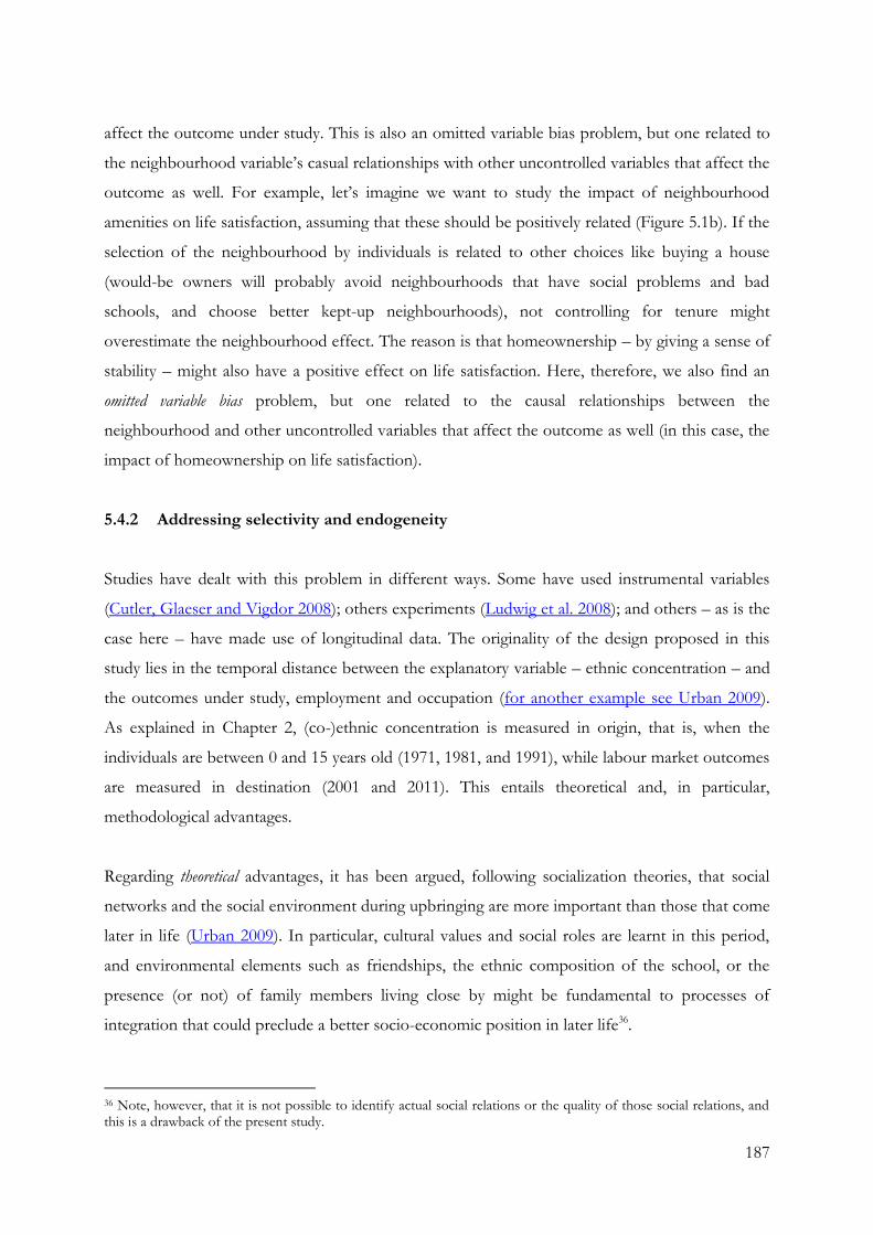
187

affect the outcome under study. This is also an omitted variable bias problem, but one related to

the neighbourhood variable’s casual relationships with other uncontrolled variables that affect the

outcome as well. For example, let’s imagine we want to study the impact of neighbourhood

amenities on life satisfaction, assuming that these should be positively related (Figure 5.1b). If the

selection of the neighbourhood by individuals is related to other choices like buying a house

(would-be owners will probably avoid neighbourhoods that have social problems and bad

schools, and choose better kept-up neighbourhoods), not controlling for tenure might

overestimate the neighbourhood effect. The reason is that homeownership – by giving a sense of

stability – might also have a positive effect on life satisfaction. Here, therefore, we also find an

omitted variable bias problem, but one related to the causal relationships between the

neighbourhood and other uncontrolled variables that affect the outcome as well (in this case, the

impact of homeownership on life satisfaction).

5.4.2 Addressing selectivity and endogeneity

Studies have dealt with this problem in different ways. Some have used instrumental variables

(Cutler, Glaeser and Vigdor 2008); others experiments (Ludwig et al. 2008); and others – as is the

case here – have made use of longitudinal data. The originality of the design proposed in this

study lies in the temporal distance between the explanatory variable – ethnic concentration – and

the outcomes under study, employment and occupation (for another example see Urban 2009).

As explained in Chapter 2, (co-)ethnic concentration is measured in origin, that is, when the

individuals are between 0 and 15 years old (1971, 1981, and 1991), while labour market outcomes

are measured in destination (2001 and 2011). This entails theoretical and, in particular,

methodological advantages.

Regarding theoretical advantages, it has been argued, following socialization theories, that social

networks and the social environment during upbringing are more important than those that come

later in life (Urban 2009). In particular, cultural values and social roles are learnt in this period,

and environmental elements such as friendships, the ethnic composition of the school, or the

presence (or not) of family members living close by might be fundamental to processes of

integration that could preclude a better socio-economic position in later life36.

36 Note, however, that it is not possible to identify actual social relations or the quality of those social relations, and this is a drawback of the present study.

188

As concerns methodological advantages, by using a design that separates in time the explanatory and

explained variables, I reduce the problems of individuals self-selecting into neighbourhoods, and

also that of endogeneity. First of all, given that I consider the neighbourhood of individuals at

some point between 0 and 15 years of age37, it was probably their parents (and not themselves)

who chose the neighbourhood. Of course, it could be argued that there are unmeasured

characteristics of parents that might influence the outcome variable, like ways of raising children

and expectations. Moreover parents may have chosen a neighbourhood with a higher share of co-

ethnics because they want their children to work in particular ethnic niches or enterprises, or

because they want their children to be in contact with other co-ethnics, thinking in terms of how

these contacts could affect their future. In these cases, the effect of the neighbourhood would

actually be capturing some unmeasured parental effect. Although I cannot control for all this, I

do consider other variables – such as parental social class and education – that probably capture

at least some of these unmeasured characteristics of parents.

Secondly, the temporal separation of dependent and independent variables, together with the

control of a series of mediating variables, also helps solve the problem of endogeneity. For

example, studies on educational outcomes (i.e. Galster et al. 2007a) have argued that

neighbourhoods effects could be overestimated if school characteristics in terms, for example, of

ethnicity, are not controlled for. In fact, if parents prefer to be in areas with more ethnic

minorities, schools in these areas will probably be more mixed, and this in turn might affect

educational outcomes. In this study, there is a temporal distance between the neighbourhood and

the outcome variable. Moreover, controlling not only for education and parental social class, but

also for other variables at the household level, will hopefully capture other factors that might be

related to the choice of the area and labour market outcomes; for example, tenure or level of

overcrowding in the household.

In short, I believe that the strongest aspect of this design is that while the parental choice of

neighbourhood might be very relevant for outcomes of the younger population (like education),

it is less likely that their impact is equally strong for labour market outcomes, which come later in

life and which are mediated by other variables that I do control for. Of course, other factors

might still point to selectivity. In particular, the argument related to the strength of ethnic ties

within the neighbourhood – and their potential for future jobs – needs to be taken into

37 I have done a robustness check for people between 4 and 15 (the school age, thinking in terms of contacts that are created in schools, friends, etc.) and the results are the same.

189

consideration when studying the results. Moreover, as suggested in Chapter 3, other elements

such as parental motivation might also figure in to the picture. Very motivated parents might be

those who actually leave to better neighbourhoods in order to provide a better future for their

children, while those who stay are negative-selected, and so are their children.

5.4.3 Model of analysis

Figure 5.2 shows the model of analysis. Following the arguments above, ethnic and socio-

economic characteristics are included in the model. On the left-hand side, we have origin

variables, which are measured in 1971, 1981 and 1991 when individuals are between 0 and 15

years old in any of these three years. Origin variables are co-ethnic concentration quintile – the

main independent or explanatory variable – and other control variables related to socio-economic

characteristics of the neighbourhood (deprivation) and the household of the individual (parental

social class, tenure, number of cars and number of persons per room). Co-ethnic concentration

quintile is the product of combining two variables: a measure of ethnic concentration in the

neighbourhood – expressed in population-weighted quintiles obtained from aggregated census

data at the Ward level38, that are attached later on attached to the ONS-LS – and the ethnicity of

the individual.

Figure ‎5.2: Model of analysis: main variables and their measurement year

38 Unfortunately, it is not possible to use the LSOA as a neighbourhood measure, as I do use in Chapter 5. This is due to data restrictions from the ONS.

Co-ethnic concentration quintile

Labour market outcomes

Ethnic group

Partner’s ethnicity?

Education

Origin (1971-1991) Destination (2001-2011)

Neighbourhood and household controls

A

B

190

On the right-hand side we have labour market outcomes – employment and social class, the

dependent variables – as well as ethnic group, education and partner’s ethnicity. These are

measured in 2001-2011 for individuals that are between 20 and 45 years old at the time of

measurement. The variable employment compares employed individuals with unemployed and

some inactive groups. The variables that measure social class are two: access to the service class

and avoidance of the lowest occupations (semi-routine and routine occupations)39; they include

all individuals that have or had an occupation in the past (with the exception of the long-term

unemployed, who are excluded). Full-time students are excluded from both employment and

social class.

The model in Figure 5.2 shows various things: first, labour market outcomes depend, on the one

hand, on education, ethnic group and origin variables; and, on the other – I expect – on the

concentration of co-ethnics in the neighbourhood, expressed in Figure 5.2 as the red line ‘A’.

Second, origin variables are all mutually dependent: the level of ethnic concentration is related to

the level of deprivation of the neighbourhood, and to other socio-economic household variables.

Third, education acts as a mediator between origin variables and labour market outcomes. This is

important, since the initial levels of education start in schools that are usually located in the

neighbourhood where individuals reside, and the quality of this education might affect the levels

of education as measured in destination. In this sense, I expect education to be an important

mediator of the impact of the neighbourhood on labour market outcomes.

Fourth, I expect partner ethnicity to be part of the mechanism of the neighbourhood effect, since

co-ethnic partnerships may be formed, among other reasons, thanks to interaction within the

neighbourhood (individuals that have a co-ethnic partner are also more likely to be raised in areas

with more co-ethnics: see Table 5.2). Fifth, in this chapter I also explore whether the effect of co-

ethnics in the neighbourhood might vary across ethnic groups: this is represented by the red line

‘B’. Recall that the analysis is done for second generation ethnic minorities (Indian, Pakistani,

Bangladeshi, Caribbean and African populations), who lived with at least one parent between 0

and 15 years of age in any of the three ‘origin’ years, and who might therefore be born in Britain

or abroad (note that I combine second generation with the 1.5 generation, although for practical

purposes I call them “second generation”). Finally, the analysis is done separately for men and

39 I do not mean to argue here that “avoiding semi-routine and routine occupations” is a social class per se; following the NSS-SEC classification, these are the two lowest positions in the social scale and the ones that more often are regulated by labour contracts. Refer to Chapter 2 for more details on this.

191

women and other controls (not stated in Figure 5.2) are also included in the models: age, origin

and destination years and number of census points in which the individual has participated. Refer

to Chapter 2 for more details on the sample, variables and measurement.


Table 5.1 shows the percentage of ethnic minorities employed, those who have (or had) a service

class and those who avoid(ed) the lowest occupations, for each level of co-ethnic concentration

in the neighbourhood where individuals lived at a young age. This has been calculated for each

group individually and for the five groups pooled together, and I have also differentiated between

men and women. Table 5.1 also shows the percentage difference between the first quintile –

where concentration of co-ethnics is the lowest – and the fifth quintile – where the concentration

of co-ethnics is the highest. A positive difference can be interpreted as a positive effect of living

in a neighbourhood that has a low concentration of ethnic minorities, while a negative states the

contrary; furthermore, the higher the difference, the higher the effect of being in quintile 1 (Q1)

vs. quintile 5 (Q5).

A first general outcome from Table 5.1 is that there is an association between ethnic

concentration or the share of co-ethnics in the neighbourhood and the outcomes under study for

most groups and genders, where a lower share of co-ethnics (Q1) leads to a better labour market

outcome. Looking at the results more in detail, we can see that the influence of ethnic

concentration understood as the difference between Q1 and Q5, seems to be stronger (reflected

in a greater difference) when estimating the access to different social classes (for men and

women) and when estimating employment for women. There are also both group and gender

effects: Pakistanis and Bangladeshis (in particular women) seem to be the most affected by the

level of concentration of their origin neighbourhood. For example, while for the five female

groups pooled together having been raised in Q5 (vs. Q1) reduces the probability of being

employed by 7% points and the probability of being in the service class by 13% points, for

Pakistani women these values grow to 19% and 24% respectively. Indians are the next group to

be most strongly affected by the concentration of the neighbourhood in their probabilities of

being in the service class. For Caribbeans, the impact of neighbourhood is the lowest, while for

African the results are not robust; note, however, that the number of cases is small for this group.

192

Tab

le ‎5.1

: A

cces

s to

em

plo

ymen

t an

d th

e se

rvic

e cl

ass

(in

%

) b

y quin

tile

o

f co

-eth

nic

co

nce

ntr

atio

n (Q

1=

low

est

con

cen

trat

ion

; Q

5:

hig

hes

t

con

cen

trat

ion

)

M

en

W

om

en

Q

1 Q

2

Q3

Q4

Q5

Q1-

Q5

Q1

Q2

Q3

Q4

Q5

Q1-

Q5

Em

plo

ymen

t

5

min

ori

ty g

rou

ps

83.3

84

.4

82.9

82

.3

80.9

2.

4 74

.1

69.5

69

.2

68.7

66

.9

7.2

India

n

89.0

88.3

87.8

87.8

86.9

2.0

81.1

79.1

80.7

79.6

80.8

0.3

Pak

ista

ni

75.9

80.8

76.9

75.9

73.8

2.2

63.9

55.5

47.6

48.7

44.9

19.0

Ban

glad

esh

i 81.2

86.7

81.3

78.0

73.7

7.5

57.5

54.0

50.7

47.9

38.6

19.0

Car

ibb

ean

82.9

81.0

79.6

78.5

76.0

6.9

80.1

74.5

77.4

78.1

76.2

3.8

Afr

ican

78.3

88.1

81.8

80.4

82.1

-7

.5

82.4

81.1

82.4

74.7

76.2

6.2

Serv

ice c

lass

5 m

ino

rity

gro

up

s 52

.2

48.2

45

.3

43.5

40

.9

11.3

52

.3

46.9

42

.6

41.4

39

.3

13.0

India

n

58.5

61.4

54.4

52.7

51.1

7.4

59.3

58.9

53.5

44.5

44.1

15.3

Pak

ista

ni

51.8

39.3

31.7

37.8

29.0

22.8

49.8

40.5

29.6

34.4

25.8

24.0

Ban

glad

esh

i 51.6

40.0

38.4

40.0

23.1

28.5

43.8

30.4

22.3

32.4

33.0

10.8

Car

ibb

ean

39.5

39.8

42.0

29.1

34.1

5.4

50.6

41.6

40.9

43.1

42.3

8.3

Afr

ican

81.0

38.5

47.2

44.4

46.3

34.7

38.2

49.0

47.9

50.7

58.7

-2

0.4

Avo

idan

ce o

f lo

west

occu

pati

on

s

5 m

ino

rity

gro

up

s 81

.2

81.2

77

.8

75.4

73

.7

7.4

83.6

80

.1

76.9

78

.5

73.8

9.

7

India

n

83.6

90.0

82.6

81.0

81.0

2.6

85.3

87.2

85.6

81.4

78.9

6.4

Pak

ista

ni

80.9

78.4

71.6

73.4

67.4

13.5

84.7

74.6

61.1

70.6

59.8

24.9

Ban

glad

esh

i 81.3

78.8

72.7

67.8

60.7

20.6

79.7

64.1

65.3

66.7

63.0

16.7

Car

ibb

ean

75.6

70.7

74.0

66.4

64.8

10.8

83.0

79.2

79.2

81.7

81.9

1.1

Afr

ican

100.0

74.4

81.1

77.8

77.8

22.2

70.6

87.8

80.8

91.3

80.0

-9

.4

193

M

en

W

om

en

Q

1 Q

2

Q3

Q4

Q5

Q1-

Q5

Q1

Q2

Q3

Q4

Q5

Q1-

Q5

To

tals

Em

plo

ymen

t

5 m

ino

rity

gro

up

s 868

1250

1493

1685

1554

965

1358

1607

1694

1813

In

dia

n

344

479

680

769

757

317

455

643

716

817

P

akis

tan

i 216

360

372

431

404

280

364

393

423

490

B

angl

ades

hi

69

90

107

127

133

73

113

148

142

140

C

arib

bea

n

216

279

279

307

204

261

373

349

334

282

A

fric

an

46

84

55

51

56

57

53

74

79

84

S

erv

ice c

lass

& A

void

an

ce

of

low

est

occu

pati

on

s

5 m

ino

rity

gro

up

s 824

1187

1404

1568

1432

900

1239

1436

1478

1600

In

dia

n

335

469

656

732

720

300

436

613

667

774

P

akis

tan

i 199

328

334

384

359

249

311

311

320

391

B

angl

ades

hi

64

85

99

115

117

64

92

121

111

100

C

arib

bea

n

205

266

262

292

182

253

351

318

311

260

A

fric

an

53

39

53

45

54

34

82

73

115

75

P

op

ula

tio

n: In

div

idual

s b

etw

een

20 a

nd

45 y

ears

old

So

urc

e: A

uth

or’

s o

wn

cal

cula

tio

ns

bas

ed o

n O

NS

-LS

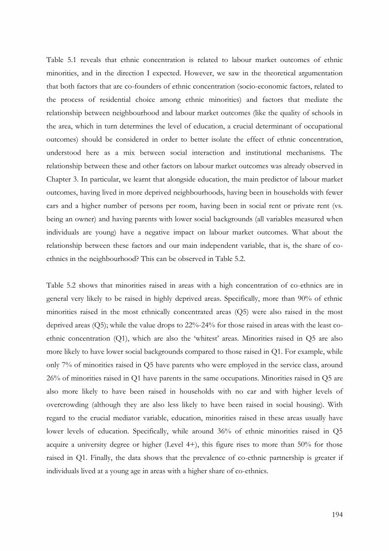
194

Table 5.1 reveals that ethnic concentration is related to labour market outcomes of ethnic

minorities, and in the direction I expected. However, we saw in the theoretical argumentation

that both factors that are co-founders of ethnic concentration (socio-economic factors, related to

the process of residential choice among ethnic minorities) and factors that mediate the

relationship between neighbourhood and labour market outcomes (like the quality of schools in

the area, which in turn determines the level of education, a crucial determinant of occupational

outcomes) should be considered in order to better isolate the effect of ethnic concentration,

understood here as a mix between social interaction and institutional mechanisms. The

relationship between these and other factors on labour market outcomes was already observed in

Chapter 3. In particular, we learnt that alongside education, the main predictor of labour market

outcomes, having lived in more deprived neighbourhoods, having been in households with fewer

cars and a higher number of persons per room, having been in social rent or private rent (vs.

being an owner) and having parents with lower social backgrounds (all variables measured when

individuals are young) have a negative impact on labour market outcomes. What about the

relationship between these factors and our main independent variable, that is, the share of co-

ethnics in the neighbourhood? This can be observed in Table 5.2.

Table 5.2 shows that minorities raised in areas with a high concentration of co-ethnics are in

general very likely to be raised in highly deprived areas. Specifically, more than 90% of ethnic

minorities raised in the most ethnically concentrated areas (Q5) were also raised in the most

deprived areas (Q5); while the value drops to 22%-24% for those raised in areas with the least co-

ethnic concentration (Q1), which are also the ‘whitest’ areas. Minorities raised in Q5 are also

more likely to have lower social backgrounds compared to those raised in Q1. For example, while

only 7% of minorities raised in Q5 have parents who were employed in the service class, around

26% of minorities raised in Q1 have parents in the same occupations. Minorities raised in Q5 are

also more likely to have been raised in households with no car and with higher levels of

overcrowding (although they are also less likely to have been raised in social housing). With

regard to the crucial mediator variable, education, minorities raised in these areas usually have

lower levels of education. Specifically, while around 36% of ethnic minorities raised in Q5

acquire a university degree or higher (Level 4+), this figure rises to more than 50% for those

raised in Q1. Finally, the data shows that the prevalence of co-ethnic partnership is greater if

individuals lived at a young age in areas with a higher share of co-ethnics.

195

Table ‎5.2: Individual, household and neighbourhood characteristics by quintile of co-ethnic

concentration (Q1=lowest concentration; Q5: highest concentration). Pooled ethnic minorities.

Men Women

Q1 Q2 Q3 Q4 Q5 Q1 Q2 Q3 Q4 Q5

Education

Level 1 or less 24.9 28.2 33.8 36.3 35.1 22.8 25.9 29.7 31.2 30.6

Level 2+3 24.5 27.0 24.4 24.6 29.2 24.4 30.4 31.1 30.0 32.8

Level 4+ 50.6 44.9 41.8 39.1 35.7 52.8 43.7 39.1 38.8 36.6

Partner’s ethnicity

No partner 54.4 48.4 49.0 45.3 46.4 53.0 50.5 50.7 48.7 44.7

Co-ethnic 26.3 35.8 35.8 43.0 45.1 32.7 36.2 39.6 42.3 46.6

Other 19.4 15.8 15.1 11.7 8.5 14.3 13.3 9.6 9.0 8.7

Class of origin

No earners/No code 8.8 11.8 11.9 12.8 13.6 10.3 11.6 13.5 12.8 12.7

Manual (V+VI+VII) 35.0 48.3 53.4 58.9 62.8 35.9 49.2 55.1 60.2 65.1

Routine non-manual (III) 9.7 12.6 11.9 10.5 8.2 12.5 11.3 10.9 10.2 9.4

Petit Bourgeoisie (IV) 20.7 10.2 9.2 7.8 8.0 15.6 12.6 10.1 7.6 6.0

Professional/Managerial (I+II) 25.8 17.2 13.6 10.0 7.3 25.7 15.3 10.4 9.2 6.8

Cars

No cars 27.3 40.5 44.0 50.0 49.7 30.6 41.2 47.1 49.4 55.3

1 car 53.5 47.4 46.8 42.2 42.9 50.1 47.3 43.2 43.2 39.9

2 cars 19.2 12.2 9.2 7.8 7.5 19.4 11.4 9.6 7.4 4.7

Tenure

Owner 66.9 69.4 73.5 78.2 75.2 67.3 67.3 70.6 76.4 74.1

Social rent 24.4 21.4 17.5 13.8 15.0 24.7 24.2 18.4 14.4 16.5

Private rent 8.6 9.2 9.0 8.0 9.8 8.1 8.5 11.0 9.2 9.4

Persons per room

> 1.5 persons 10.9 16.5 18.0 21.7 22.7 11.3 19.3 20.3 20.6 26.3

1.5 persons 5.2 4.8 4.2 7.2 7.0 5.3 5.1 6.7 8.1 8.8

>1 & <1.5 persons 21.5 25.3 25.1 27.1 27.8 22.7 25.3 28.8 26.4 27.7

1 person 20.2 19.4 22.3 19.2 19.8 22.9 19.2 19.5 22.6 17.8

>= 0.75 & <1 person 19.1 17.4 16.7 14.9 15.6 16.3 18.3 14.3 13.9 12.4

<0.75 person 23.0 16.7 13.7 10.0 7.0 21.6 12.8 10.4 8.4 7.0

Carstairs quintiles

Q1 (least deprived) 15.4 5.5 1.7 0.0 0.0 16.1 4.3 2.5 0.6 0.0

Q2 17.5 10.2 5.4 1.4 0.0 16.1 11.2 6.0 1.4 0.0

Q3 20.7 16.2 11.2 7.3 0.0 19.2 15.8 10.1 7.5 1.4

Q4 22.5 28.4 25.8 15.8 6.3 26.3 27.9 24.5 14.1 7.2

Q5 (most deprived) 23.8 39.6 55.9 75.4 93.7 22.4 40.7 56.9 76.3 91.4

N 868 1250 1493 1685 1554 965 1358 1607 1694 1813

Population: Individuals between 20 and 45 years old Source: Author’s own calculations based on ONS-LS

196

Given this evidence, we could argue that the link between ethnic concentration and labour

market outcomes observed in Table 5.1, that is, the poorer labour market outcomes observed for

those raised in Q5 (vs. those raised in Q1) might be actually related to the fact that ethnic

concentration is related to other measures that also predict labour market outcomes. In

particular, that being raised in Q5 also means being raised in areas of higher deprivation, having

lower social backgrounds and having less education, factors that in turn negatively affect labour

market outcomes. The analyses that follow, based on regression models, consider all these factors

together, and therefore, seek to isolate the effect of co-ethnics. Note that the partner’s ethnicity

will be introduced only if a neighbourhood effect is found, and with the aim to test whether

having a co-ethnic partner could be part of the mechanism.

5.6 Isolating the effect of co-ethnics

The analysis below explores the effect of having been raised in areas with a relatively high

proportion of co-ethnics (vs. having been raised in areas with lower proportions of ethnic

minorities) on the probabilities of employment, access to the service class and avoidance of

lowest occupations. I do this for the five groups pooled together, and then I also add interactions

between ethnic group and origin neighbourhood, to explore group differences in the effect of the

origin neighbourhood.

Tables 5.3-5.8 show the probability of employment, access to the service class and avoidance of

lowest occupations, by quintile of co-ethnic concentration and separately for men and women.

For each dependent variable, a pooled model is estimated first (Tables 5.3, 5.5 and 5.7), and then

predicted values are calculated for each group separately, based on the model with interactions

(Tables 5.4, 5.6 and 5.8). The coefficients of Tables 5.3, 5.5 and 5.7 are based on linear

regressions with robust (clustered) standard errors and – when multiplied by 100 – refer to the

difference in percentage points with respect to the reference category (in the case of the key

independent variable, co-ethnic concentration quintiles, the reference is individuals raised in

Quintile 1). In these tables, Model 1 includes only controls for origin and destination years,

number of census points and age; Model 2 adds neighbourhood deprivation measures; Model 3

adds household-level variables (class of origin, tenure, number of cars and number of persons per

room); Model 4 adds education of the respondent; and Model 5 adds interactions between ethnic

group and co-ethnic quintile (only Q5 is shown). The full models for the three outcome variables,

197

and for men and women, can be found in: Table ‎8.10, Table ‎8.11, Table ‎8.12, Table ‎8.13,

Table ‎8.14 and Table ‎8.15 in Annex A. Moreover, Table ‎8.16 shows selected models estimated

with logistic regression with average marginal effects: Model 4 in Tables 5.3, 5.5 and 5.7.

Model 1 of Table 5.3 shows – in accordance to the descriptive tables – that individuals raised in a

neighbourhood with a higher concentration of co-ethnics are relatively less likely to be employed.

This holds both for men and women, who are around 3% and 8% points less likely to be

employed if raised in quintile 5 instead of in quintile 1. This effect remains statistically significant

for men after controlling for neighbourhood deprivation (M2); and for women after controlling

for household socio-economic characteristics (M3), which would point to an absence of

neighbourhood effects, on average. However, Model 5 shows a quite different picture. This

model, which shows group differences by adding interaction effects between ethnic group and

co-ethnic concentration in origin, reveals that for Pakistani and Bangladeshi women there is quite

a substantive negative effect of being raised in Q5. These ethnic-specific results are better

observed in Table 5.4, which shows predicted values for the various ethnic groups, separated by

co-ethnic quintiles in origin (Q1 and Q5) and gender (the other variables are set to their mean).

The results from Table 5.4 show that, while among men, having been raised in Q5 does not exert

much influence on the probability of being employed, among women this seems to be

particularly relevant for Pakistanis and Bangladeshis. More precisely, while around 62% of

Pakistani women raised in Q1 are employed, this value drops to 51% among those raised in Q5.

A similar disadvantage is seen for Bangladeshi women, for whom having lived at a young age in

Q5 areas gives them almost 13% points less probability of being employed (note, however, that

the estimation is less precise for this group).

198

Tab

le ‎5

.3: A

cces

s to

em

plo

ymen

t. P

oo

led e

thn

ic m

ino

riti

es.

M

en

W

om

en

M

1 M

2

M3

M4

M5

M1

M2

M3

M4

M5

Co

-eth

nic

qu

inti

le (

ref.

Q1:

lo

west

co

ncen

trati

on

)

Q2

0.0

13

0.0

21

0.0

26

0.0

27

0.0

00

-0.0

46**

-0

.040*

-0.0

32

-0.0

31

-0.0

08

(0

.0188)

(0.0

188)

(0.0

188)

(0.0

179)

(0.0

239)

(0.0

213)

(0.0

217)

(0.0

214)

(0.0

205)

(0.0

337)

Q3

-0.0

10

0.0

05

0.0

10

0.0

19

0.0

11

-0.0

55**

-0

.042*

-0.0

29

-0.0

21

0.0

14

(0

.0185)

(0.0

190)

(0.0

193)

(0.0

183)

(0.0

237)

(0.0

212)

(0.0

225)

(0.0

224)

(0.0

212)

(0.0

313)

Q4

-0.0

17

0.0

04

0.0

08

0.0

18

0.0

23

-0.0

62**

* -0

.044*

-0.0

33

-0.0

27

0.0

19

(0

.0184)

(0.0

197)

(0.0

199)

(0.0

191)

(0.0

241)

(0.0

211)

(0.0

232)

(0.0

233)

(0.0

219)

(0.0

320)

Q5

-0.0

33*

-0.0

08

-0.0

02

0.0

08

0.0

18

-0.0

76**

* -0

.052**

-0

.035

-0.0

34

0.0

42

(0

.0188)

(0.0

210)

(0.0

211)

(0.0

201)

(0.0

254)

(0.0

214)

(0.0

244)

(0.0

245)

(0.0

228)

(0.0

333)

Eth

nic

gro

up

(re

f. I

nd

ian

)

Pak

ista

ni

-0.1

01**

* -0

.096**

* -0

.081**

* -0

.062**

* -0

.090**

-0

.295**

* -0

.290**

* -0

.267**

* -0

.227**

* -0

.137**

*

(0

.0149)

(0.0

151)

(0.0

153)

(0.0

147)

(0.0

388)

(0.0

185)

(0.0

188)

(0.0

192)

(0.0

185)

(0.0

409)

Ban

glad

esh

i -0

.057**

* -0

.051**

-0

.009

0.0

03

-0.0

25

-0.3

19**

* -0

.311**

* -0

.259**

* -0

.224**

* -0

.175**

*

(0

.0219)

(0.0

221)

(0.0

232)

(0.0

228)

(0.0

483)

(0.0

273)

(0.0

276)

(0.0

295)

(0.0

273)

(0.0

573)

Car

ibb

ean

-0

.088**

* -0

.086**

* -0

.065**

* -0

.032*

-0.0

06

-0.0

29

-0.0

28

-0.0

20

-0.0

07

0.0

23

(0

.0166)

(0.0

167)

(0.0

178)

(0.0

176)

(0.0

370)

(0.0

185)

(0.0

185)

(0.0

196)

(0.0

191)

(0.0

422)

Afr

ican

-0

.005

-0.0

06

0.0

20

0.0

18

-0.0

69

-0.0

06

-0.0

11

-0.0

05

-0.0

52*

0.0

03

(0

.0281)

(0.0

282)

(0.0

300)

(0.0

287)

(0.0

997)

(0.0

300)

(0.0

300)

(0.0

314)

(0.0

310)

(0.0

766)

Eth

nic

gro

up

* c

o-e

thn

ic

qu

inti

le

Pak

ista

ni *

Q5

0.0

16

-0.1

48**

*

(0

.0470)

(0.0

516)

Ban

glad

esh

i *

Q5

-0.0

11

-0.1

67**

(0

.0704)

(0.0

720)

199

M

en

W

om

en

M

1 M

2

M3

M4

M5

M1

M2

M3

M4

M5

Car

ibb

ean

* Q

5

-0.0

66

-0.0

59

(0

.0493)

(0.0

525)

Afr

ican

* Q

5

0.1

08

-0.1

07

(0

.1088)

(0.0

937)

Ad

just

ed

R-s

qu

are

d

0.0

36

0.0

37

0.0

43

0.0

79

0.0

78

0.0

95

0.0

95

0.1

02

0.1

66

0.1

67

N

6,8

50

6,8

50

6,8

50

6,8

50

6,8

50

7,4

37

7,4

37

7,4

37

7,4

37

7,4

37

Bas

e m

odel

1

X

X

X

X

X

X

X

X

X

X

Nei

ghb

ourh

oo

d2

X

X

X

X

X

X

X

X

Ho

use

ho

ld3

X

X

X

X

X

X

Educa

tio

n

X

X

X

X

Eth

nic

gro

up

* E

M q

uin

tile

X

X

1 C

on

tro

ls f

or:

age

, o

rigi

n y

ear,

des

tin

atio

n y

ear

and

num

ber

of

cen

sus

po

ints

. 2 A

dd

s: C

arst

airs

dep

rivat

ion

quin

tile

at

the

war

d lev

el.

3 A

dd

s: t

enure

, n

um

ber

of

per

son

s p

er r

oo

m, n

um

ber

of

cars

an

d c

lass

of

ori

gin

. *

p-v

alue<

.10 *

* p

-val

ue<

.05 *

** p

-val

ue<

.01; ro

bust

(cl

ust

ered

) (c

lust

ered

) st

and

ard

err

ors

in

par

enth

eses

P

op

ula

tio

n: In

div

idual

s b

etw

een

20 a

nd

45 y

ears

old

So

urc

e: A

uth

or’

s o

wn

cal

cula

tio

ns

bas

ed o

n O

NS

-LS

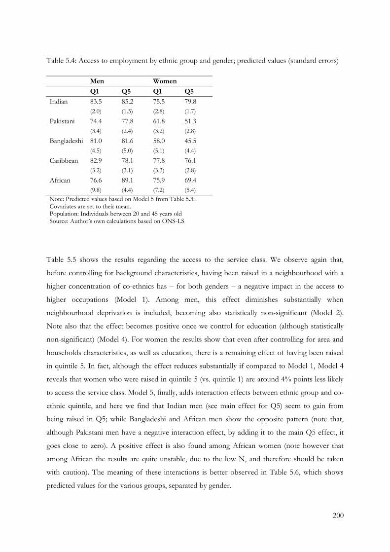
200

Table ‎5.4: Access to employment by ethnic group and gender; predicted values (standard errors)

Men Women

Q1 Q5 Q1 Q5

Indian 83.5 85.2 75.5 79.8

(2.0) (1.5) (2.8) (1.7)

Pakistani 74.4 77.8 61.8 51.3

(3.4) (2.4) (3.2) (2.8)

Bangladeshi 81.0 81.6 58.0 45.5

(4.5) (5.0) (5.1) (4.4)

Caribbean 82.9 78.1 77.8 76.1

(3.2) (3.1) (3.3) (2.8)

African 76.6 89.1 75.9 69.4

(9.8) (4.4) (7.2) (5.4)

Note: Predicted values based on Model 5 from Table 5.3. Covariates are set to their mean. Population: Individuals between 20 and 45 years old Source: Author’s own calculations based on ONS-LS

Table 5.5 shows the results regarding the access to the service class. We observe again that,

before controlling for background characteristics, having been raised in a neighbourhood with a

higher concentration of co-ethnics has – for both genders – a negative impact in the access to

higher occupations (Model 1). Among men, this effect diminishes substantially when

neighbourhood deprivation is included, becoming also statistically non-significant (Model 2).

Note also that the effect becomes positive once we control for education (although statistically

non-significant) (Model 4). For women the results show that even after controlling for area and

households characteristics, as well as education, there is a remaining effect of having been raised

in quintile 5. In fact, although the effect reduces substantially if compared to Model 1, Model 4

reveals that women who were raised in quintile 5 (vs. quintile 1) are around 4% points less likely

to access the service class. Model 5, finally, adds interaction effects between ethnic group and co-

ethnic quintile, and here we find that Indian men (see main effect for Q5) seem to gain from

being raised in Q5; while Bangladeshi and African men show the opposite pattern (note that,

although Pakistani men have a negative interaction effect, by adding it to the main Q5 effect, it

goes close to zero). A positive effect is also found among African women (note however that

among African the results are quite unstable, due to the low N, and therefore should be taken

with caution). The meaning of these interactions is better observed in Table 5.6, which shows

predicted values for the various groups, separated by gender.

201

Tab

le ‎5

.5: A

cces

s to

th

e se

rvic

e cl

ass.

Po

ole

d e

thn

ic m

ino

riti

es.

M

en

W

om

en

M

1 M

2

M3

M4

M5

M1

M2

M3

M4

M5

Co

-eth

nic

qu

inti

le (

ref.

Q1:

lo

west

co

ncen

trati

on

)

Q2

-0.0

40

-0.0

10

0.0

08

0.0

18

0.0

62*

-0.0

61**

-0

.038

-0.0

20

-0.0

13

0.0

33

(0

.0268)

(0.0

269)

(0.0

261)

(0.0

224)

(0.0

347)

(0.0

259)

(0.0

263)

(0.0

259)

(0.0

220)

(0.0

356)

Q3

-0.0

83**

* -0

.031

-0.0

08

0.0

22

0.0

36

-0.1

10**

* -0

.071**

* -0

.044*

-0.0

27

0.0

02

(0

.0269)

(0.0

279)

(0.0

273)

(0.0

232)

(0.0

345)

(0.0

250)

(0.0

266)

(0.0

264)

(0.0

225)

(0.0

347)

Q4

-0.1

00**

* -0

.028

0.0

02

0.0

35

0.0

79**

-0

.123**

* -0

.070**

-0

.043

-0.0

38

-0.0

62*

(0

.0267)

(0.0

286)

(0.0

283)

(0.0

239)

(0.0

351)

(0.0

254)

(0.0

279)

(0.0

280)

(0.0

244)

(0.0

359)

Q5

-0.1

34**

* -0

.047

-0.0

14

0.0

23

0.0

89**

-0

.148**

* -0

.081**

* -0

.044

-0.0

42*

-0.0

40

(0

.0274)

(0.0

305)

(0.0

302)

(0.0

255)

(0.0

363)

(0.0

255)

(0.0

293)

(0.0

293)

(0.0

248)

(0.0

359)

Eth

nic

gro

up

(re

f. I

nd

ian

)

Pak

ista

ni

-0.1

74**

* -0

.155**

* -0

.110**

* -0

.060**

* 0.0

11

-0.1

59**

* -0

.144**

* -0

.101**

* -0

.050**

* -0

.035

(0

.0206)

(0.0

208)

(0.0

209)

(0.0

172)

(0.0

424)

(0.0

207)

(0.0

210)

(0.0

213)

(0.0

185)

(0.0

428)

Ban

glad

esh

i -0

.153**

* -0

.131**

* -0

.057*

-0.0

22

0.0

53

-0.1

80**

* -0

.159**

* -0

.082**

-0

.036

0.0

02

(0

.0306)

(0.0

307)

(0.0

324)

(0.0

272)

(0.0

733)

(0.0

301)

(0.0

306)

(0.0

326)

(0.0

268)

(0.0

667)

Car

ibb

ean

-0

.193**

* -0

.184**

* -0

.173**

* -0

.060**

* -0

.045

-0.0

77**

* -0

.073**

* -0

.075**

* -0

.044**

-0

.019

(0

.0235)

(0.0

234)

(0.0

244)

(0.0

217)

(0.0

519)

(0.0

227)

(0.0

227)

(0.0

236)

(0.0

203)

(0.0

472)

Afr

ican

-0

.045

-0.0

46

-0.0

47

-0.0

32

0.2

71**

0.0

10

0.0

00

-0.0

19

-0.1

10**

* -0

.203**

*

(0

.0468)

(0.0

464)

(0.0

459)

(0.0

428)

(0.1

197)

(0.0

409)

(0.0

406)

(0.0

418)

(0.0

392)

(0.0

739)

Eth

nic

gro

up

* c

o-e

thn

ic

qu

inti

le

Pak

ista

ni *

Q5

-0.1

16**

-0

.023

(0

.0520)

(0.0

525)

Ban

glad

esh

i *

Q5

-0.1

94**

0.0

00

(0

.0857)

(0.0

819)

202

M

en

W

om

en

M

1 M

2

M3

M4

M5

M1

M2

M3

M4

M5

Car

ibb

ean

* Q

5

-0.0

54

-0.0

17

(0

.0655)

(0.0

607)

Afr

ican

* Q

5

-0.3

25**

0.1

77*

(0

.1387)

(0.0

983)

Ad

just

ed

R-s

qu

are

d

0.0

47

0.0

56

0.0

83

0.2

91

0.2

94

0.0

34

0.0

39

0.0

59

0.2

29

0.2

30

N

6,4

44

6,4

44

6,4

44

6,4

44

6,4

44

6,6

85

6,6

85

6,6

85

6,6

85

6,6

85

Bas

e m

odel

1

X

X

X

X

X

X

X

X

X

X

Nei

ghb

ourh

oo

d2

X

X

X

X

X

X

X

X

Ho

use

ho

ld3

X

X

X

X

X

X

Educa

tio

n

X

X

X

X

Eth

nic

gro

up

* E

M q

uin

tile

X

X

1 C

on

tro

ls f

or:

age

, o

rigi

n y

ear,

des

tin

atio

n y

ear

and

num

ber

of

cen

sus

po

ints

. 2 A

dd

s: C

arst

airs

dep

rivat

ion

quin

tile

at

the

war

d lev

el.

3 A

dd

s: t

enure

, n

um

ber

of

per

son

s p

er r

oo

m, n

um

ber

of

cars

an

d c

lass

of

ori

gin

. *

p-v

alue<

.10 *

* p

-val

ue<

.05 *

** p

-val

ue<

.01; ro

bust

(cl

ust

ered

) st

and

ard

err

ors

in

par

enth

eses

P

op

ula

tio

n: In

div

idual

s b

etw

een

20 a

nd

45 y

ears

old

So

urc

e: A

uth

or’

s o

wn

cal

cula

tio

ns

bas

ed o

n O

NS

-LS

203

Table ‎5.6: Access to the service class by ethnic group and gender; predicted values (standard

errors)

Men Women

Q1 Q5 Q1 Q5

Indian 42.2 51.0 48.3 44.3

(3.0) (1.9) (2.9) (1.9)

Pakistani 43.3 40.6 44.8 38.5

(3.2) (2.6) (3.3) (2.6)

Bangladeshi 47.5 37.0 48.5 44.5

(6.7) (4.4) (6.0) (4.6)

Caribbean 37.7 41.1 46.5 40.7

(4.2) (3.8) (3.8) (3.6)

African 69.2 45.6 28.0 41.7

(11.7) (6.9) (6.9) (6.5)

Note: Predicted values based on Model 5 from Table 5.5. Covariates are set to their mean. Population: Individuals between 20 and 45 years old Source: Own calculations based on ONS-LS

Table 5.6 shows that having been raised in areas with a high share of co-ethnics exerts a positive

effect (around 9% points more) on the probability of accessing the service class for Indian men;

on the other hand, there is also a considerable negative effect for Bangladeshi men (although less

precise, due to their high standard errors). Among women we see a negative effect for most

groups (African are an exception), which probably leads to the average result observed in Table

5.5.

Tables 5.7 and 5.8, finally, show the results for the analysis of the last variable studied in this

chapter: avoidance of the lowest occupations, that is, semi-routine and routine occupations. This

analysis shows very similar results to those found in the previous one. First of all, we find that

while among men, neighbourhood and household variables in origin (M2) take away practically

all the disadvantage experienced by those raised in Q5 (when compared to those raised in Q1);

for women, this disadvantage remains statistically significant even after controlling for education.

Specifically, if raised in Q5 – instead of in Q1 – women have on average 4% less probability of

avoiding the lowest occupations in the NS-SEC scale. The interaction terms are negative for all

male groups (when compared to Indian, the reference category), however, only Bangladeshi,

Caribbean and African men seem to suffer a penalty when raised in Q5 (for Pakistani men the

effect goes to close to zero when subtracted from the main Q5 effect). Among women, the

204

Pakistani and Bangladeshi are again those mostly disadvantaged. As with the other dependent

variables, I have estimated predicted probabilities to have a better picture of these interactions.

These are shown in Table 5.8

Table 5.8 shows that Pakistani and Bangladeshi women are 12%-13% points less likely to avoid

low occupations if raised in Q5, compared to those raised in Q1. The results are similar for

Bangladeshi and African men, for whom the gap is around 9%-10% points, and for Caribbean

men, for whom the gap is around 7% (note, however, that for most groups the results are

uncertain, given the relatively high standard errors) as when estimating the access to higher

occupations, Indian men present again an advantage when raised in Q5: specifically, they are

around 7% more likely to avoid semi-routine and routine occupations if they lived at a young age

in areas with a relatively higher share of co-ethnics (note that the same pattern is found for

African women, for whom, however, the low N leads to very high standard errors).

All in all, the analysis shows that that the effect of being raised in areas with a high share of co-

ethnics seems to be particularly detrimental for women, in particular Pakistani and Bangladeshi

women, who seem to be disadvantaged both in terms of access to employment and the types of

occupations they end up going into. Among men, Bangladeshis and Africans show a consistent

disadvantage when access to the two measures of occupation is estimated; while Caribbeans are

disadvantaged only when the avoidance of lower occupations is estimated. Indian men are the

only group that consistently presents an advantage with regards to access to occupations if raised

in Q540.

40 Note that I prefer not to comment again on the results for African, given their low number of cases and the high standard errors of the coefficients.

205

Tab

le ‎5

.7: A

vo

idan

ce o

f se

mi-

routi

ne

and r

outi

ne

occ

up

atio

ns.

Po

ole

d e

thn

ic m

ino

riti

es.

M

en

W

om

en

M

1 M

2

M3

M4

M5

M1

M2

M3

M4

M5

Co

-eth

nic

qu

inti

le (

ref.

Q1:

lo

west

co

ncen

trati

on

)

Q2

0.0

01

0.0

17

0.0

31

0.0

36*

0.0

83**

* -0

.040**

-0

.026

-0.0

12

-0.0

11

0.0

42

(0

.0205)

(0.0

207)

(0.0

204)

(0.0

188)

(0.0

260)

(0.0

195)

(0.0

201)

(0.0

198)

(0.0

183)

(0.0

271)

Q3

-0.0

45**

-0

.017

0.0

01

0.0

21

0.0

38

-0.0

76**

* -0

.054**

-0

.032

-0.0

23

0.0

39

(0

.0207)

(0.0

217)

(0.0

214)

(0.0

196)

(0.0

272)

(0.0

195)

(0.0

210)

(0.0

207)

(0.0

192)

(0.0

265)

Q4

-0.0

70**

* -0

.030

-0.0

07

0.0

15

0.0

57**

-0

.062**

* -0

.029

-0.0

08

-0.0

06

0.0

14

(0

.0208)

(0.0

225)

(0.0

225)

(0.0

206)

(0.0

276)

(0.0

195)

(0.0

217)

(0.0

218)

(0.0

202)

(0.0

282)

Q5

-0.0

92**

* -0

.043*

-0.0

19

0.0

04

0.0

70**

-0

.110**

* -0

.069**

* -0

.038

-0.0

39*

0.0

08

(0

.0218)

(0.0

248)

(0.0

245)

(0.0

225)

(0.0

296)

(0.0

204)

(0.0

238)

(0.0

239)

(0.0

219)

(0.0

299)

Eth

nic

gro

up

(re

f. I

nd

ian

)

Pak

ista

ni

-0.0

90**

* -0

.079**

* -0

.046**

* -0

.014

0.0

25

-0.1

36**

* -0

.127**

* -0

.093**

* -0

.061**

* 0.0

43

(0

.0169)

(0.0

172)

(0.0

174)

(0.0

158)

(0.0

380)

(0.0

183)

(0.0

187)

(0.0

188)

(0.0

174)

(0.0

313)

Ban

glad

esh

i -0

.105**

* -0

.094**

* -0

.040

-0.0

17

0.0

49

-0.1

42**

* -0

.129**

* -0

.059**

-0

.033

0.0

69

(0

.0257)

(0.0

257)

(0.0

271)

(0.0

253)

(0.0

547)

(0.0

274)

(0.0

276)

(0.0

294)

(0.0

278)

(0.0

592)

Car

ibb

ean

-0

.145**

* -0

.140**

* -0

.134**

* -0

.066**

* 0.0

01

-0.0

31*

-0.0

29

-0.0

27

-0.0

12

0.0

15

(0

.0199)

(0.0

199)

(0.0

205)

(0.0

191)

(0.0

396)

(0.0

178)

(0.0

178)

(0.0

186)

(0.0

175)

(0.0

373)

Afr

ican

-0

.009

-0.0

10

-0.0

08

-0.0

05

0.1

40**

* 0.0

08

0.0

01

-0.0

02

-0.0

56**

-0

.149*

(0

.0368)

(0.0

364)

(0.0

358)

(0.0

337)

(0.0

515)

(0.0

285)

(0.0

287)

(0.0

298)

(0.0

279)

(0.0

806)

Eth

nic

gro

up

* c

o-e

thn

ic

qu

inti

le

Pak

ista

ni *

Q5

-0.0

77

-0.1

43**

*

(0

.0485)

(0.0

465)

Ban

glad

esh

i *

Q5

-0.1

58**

-0

.124

(0

.0761)

(0.0

805)

206

M

en

W

om

en

M

1 M

2

M3

M4

M5

M1

M2

M3

M4

M5

Car

ibb

ean

* Q

5

-0.1

39**

-0

.003

(0

.0575)

(0.0

494)

Afr

ican

* Q

5

-0.1

67**

0.0

68

(0

.0829)

(0.0

927)

Ad

just

ed

R-s

qu

are

d

0.0

48

0.0

52

0.0

69

0.1

79

0.1

80

0.0

39

0.0

42

0.0

59

0.1

54

0.1

58

N

6,4

44

6,4

44

6,4

44

6,4

44

6,4

44

6,6

85

6,6

85

6,6

85

6,6

85

6,6

85

Bas

e m

odel

1

X

X

X

X

X

X

X

X

X

X

Nei

ghb

ourh

oo

d2

X

X

X

X

X

X

X

X

Ho

use

ho

ld3

X

X

X

X

X

X

Educa

tio

n

X

X

X

X

Eth

nic

gro

up

* E

M q

uin

tile

X

X

1 C

on

tro

ls f

or:

age

, o

rigi

n y

ear,

des

tin

atio

n y

ear

and

num

ber

of

cen

sus

po

ints

. 2 A

dd

s: C

arst

airs

dep

rivat

ion

quin

tile

at

the

war

d lev

el.

3 A

dd

s: t

enure

, n

um

ber

of

per

son

s p

er r

oo

m, n

um

ber

of

cars

an

d c

lass

of

ori

gin

. *

p-v

alue<

.10 *

* p

-val

ue<

.05 *

** p

-val

ue<

.01; ro

bust

(cl

ust

ered

) st

and

ard

err

ors

in

par

enth

eses

P

op

ula

tio

n: In

div

idual

s b

etw

een

20 a

nd

45 y

ears

old

So

urc

e: A

uth

or’

s o

wn

cal

cula

tio

ns

bas

ed o

n O

NS

-LS

207

Table ‎5.8: Avoidance of semi-routine and routine occupations by ethnic group and gender;

predicted values (standard errors)

Men Women

Q1 Q5 Q1 Q5

Indian 73.6 80.6 78.0 78.8

(2.4) (1.7) (2.4) (1.7)

Pakistani 76.1 75.4 82.3 68.8

(3.2) (2.7) (2.3) (3.1)

Bangladeshi 78.5 69.8 84.9 73.3

(5.0) (5.0) (5.5) (5.4)

Caribbean 73.7 66.9 79.5 80.0

(3.3) (3.9) (3.1) (3.0)

African 87.6 77.9 63.1 70.7

(4.7) (6.4) (7.8) (4.5)

Note: Predicted values based on Model 5 from Table 5.7. Covariates are set to their mean. Population: Individuals between 20 and 45 years old Source: Author’s own calculations based on ONS-LS

Finally, I have tested whether having a co-ethnic partner helped reduce, in particular for women,

the penalty found for those raised in Q5 (see Models f and g in Table ‎8.10, Table ‎8.11, Table ‎8.12,

Table ‎8.13, Table ‎8.14 and Table ‎8.15 in Annex A). The rationale for including this variable is that

women raised in Q5 are more likely to have a co-ethnic partner and – particularly for Pakistani

and Bangladeshi women – this might be detrimental to their labour market outcomes, in a

context where patriarchal rules prevail. Although I found this variable to have a negative effect

on the probability of employment and access to occupations of women (interestingly, this effect

is not consistent for men), the results regarding the effect of being raised in Q5 did not change.

This suggests that even if the prevalence of co-ethnic partnering is actually greater for individuals

raised in areas with more co-ethnics, it does not seem to be a strong mechanism through which

the neighbourhood exerts its effect.

208

5.7 Discussion

This chapter has sought to identify to what extent having lived at a young age in an area with a

high share of co-ethnics exerts an effect on labour market outcomes in later life among second

generation ethnic minorities. By using a design that partly reduced (although did not solve) the

problem of self-selection and endogeneity, principally because it was parents – and not

individuals themselves – who decided on the location into neighbourhoods, I tried to determine

whether there is evidence of neighbourhood effects in terms of ethnicity taking place in England

and Wales.

Following the questions posted at the beginning of the chapter, these are my conclusions.

Starting with Research question 1, the descriptive results showed first that there is indeed an

effect of share of co-ethnics in the neighbourhood where ethnic minorities are raised on their

labour market outcomes in later life: for both men and women, and for the three dependent

variables studied, this is effect is negative. However, we saw in the theoretical argumentation that

in order to better isolate the effect of ethnic concentration, understood here mainly in terms of in

terms of social interaction and institutional mechanisms of neighbourhood effects, socio-economic

factors that are both linked to labour market outcomes and to our explanatory variable – i.e. co-

ethnic concentration – should be considered (Research questions 1.1, 1.2 and 1.3).

The inclusion of neighbourhood deprivation – the main indicator of geographical mechanisms of

neighbourhood effects – led initially to a reduction and in some cases a disappearance of the

effect of co-ethnic concentration. This is because areas with a high share of ethnic minorities are

also usually areas with high deprivation: in other words, living in areas with a high share of co-

ethnics is to a large extent bad because these are also deprived areas. Household variables also

played a role in explaining the disadvantage associated to being raised in neighbourhoods with a

higher share of co-ethnics, and in most cases they also overrode the effect of neighbourhood

deprivation. As regards education, I argued that it could be partly an expression of the quality of

schools of the area and, hence, I expected it to have the same effect as the other co-varieties, that

is, to explain the neighbourhood disadvantage for those raised in Q5. However, this was generally

not the case, as its impact was usually irrelevant in terms diluting any neighbourhood-originated

disadvantage. In addition, when studying occupational outcomes of women, rather than reducing

the negative neighbourhood effect, it made it more relevant. This outcome points to the fact that

209

women in ethnically concentrated neighbourhoods are not necessarily less educated that women

in whiter ones; however, the former are less able to use their education in the labour market.

After adding neighbourhood-, household- and individual-level controls, and considering the five

ethnic minority groups pooled together, I found a negative neighbourhood effect for ethnic

minority women when estimating their occupation. However, most interesting findings arose as I

explored group and gender differences (Research question 2). In particular, Pakistani and

Bangladeshi women were particularly affected by being raised in Q5, both in terms of

employment and occupation. Among men, Bangladeshi and to a lesser extent the black

populations also presented a penalty in access to occupations if raised in Q5. The only group that

seemed to benefit from high concentration of co-ethnics were Indian men. This was observed in

access to occupations.

In searching for explanations to these results, I believe the main mechanism underlying the

findings of this chapter is the social interaction mechanism. In fact, it is no surprise that women, and

in particular Pakistani and Bangladeshi women, are among the most affected by having been

raised in areas with a high share of co-ethnics. I argued before that these groups belong to

particularly culturally closed communities, where patriarchal ways and non-egalitarian views on

gender prevail, and where men are supposed to be the main providers. For these women, having

been raised in areas with a higher concentration of co-ethnics means having been in greater

contact with these cultural constraints, which is then translated into poorer labour market

opportunities. But as suggested by Antje Röder (personal conversation, 2014), this negative effect

might also be linked to processes of parental self-selection. In other words, Muslims parents

interested in having ‘greater control’ over their daughters might choose to live in neighbourhoods

with a higher share of co-ethnics. The negative effect we observe could then be related to this

parental self-selectivity. As an additional test to explore mechanisms, I have estimated a series of

models that are equivalent to those observed in the chapter, but with the difference that

interactions between ethnic group and the share of co-ethnics in the origin neighbourhood is

included from the beginning (results available upon request). It is interesting to note that

although the penalty that Pakistani and Bangladeshi women suffer in a model without controls is

higher as compared to the result we obtain with all controls, the difference is actually quite small

(only around one fourth smaller): this speaks of a very strong neighbourhood effect at play for

these women.

210

Social interaction mechanisms might also be an explanation for Indian men, who, contrary to Indian

women, gain when raised in areas where other Indians live. We saw in Chapter 3 how well

Indians do in the labour market, both in terms of employment and in terms of accessing the

service class. Living close to other Indians might therefore be a good thing, and might explain the

positive effect found among those living in areas with a high share of co-ethnics. Supporting this

argument is the fact that this positive effect does not seem to hold in the region of East

Midlands, which includes the city of Leicester, an area where spatial segregation of Indians is very

high (see Chapter 4), but also where Indian neighbourhoods are very deprived and Indians

themselves have, in general, jobs with lower qualifications. However, there are probably some

other (unmeasured) factors, like motivation, which are be playing a role as well: the

overperformance of Indians with respect to the white British in terms of labour market outcomes

(see Chapter 3) speaks, I believe, to these unobserved factors as well.

As regards the negative effect found for Bangladeshi populations (which includes also men), we

could think – in line with social interaction mechanisms – that the worse-off Bangladeshis are located

in the most ethnically concentrated areas, and there is a negative group effect playing a role in

terms of early socialization. However, we might also think that there are institutional mechanisms

playing a role. Although it is hard to conceive, for example, that (in line with the stigmatization

hypothesis) employers will base their decisions on the neighbourhood in which individuals were

raised, it might be a plausible explanation for why both genders are negatively affected by having

been raised in such areas, if we consider that the current and origin neighbourhoods are usually

very much related in terms of their characteristics, and also that Bangladeshis are particularly

segregated populations. To explore this issue, I have included the current neighbourhood in the

analysis (results available upon request). The results show a negative effect of being in Q5 for all

groups and genders but, most importantly, it reveals that while for Bangladeshi men the initial

origin neighbourhood effect reduces to around half after including the current neighbourhood,

for women it remains practically the same (note that this also is observed for Pakistani women).

This might indicate that the origin neighbourhood – which can be linked more strictly to

interaction mechanisms connected with early socialization – has a stronger and also long-lasting

effect for women; while the current neighbourhood – which could be linked both to social

interaction and institutional mechanisms – might be more relevant to Bangladeshi men.

The results presented in this chapter suggest, therefore, the existence of neighbourhood effects

based on the share of co-ethnics in an area, for some groups and genders. Two final remarks:

211

first, I did not find negative effects for women raised in Q5 when I considered a measure of non-

whites in the origin neighbourhood instead of a measure of co-ethnics (results available upon

request). This reinforces the idea of social interaction mechanisms, which in the case of Pakistani and

Bangladeshi women, speaks of cultural constraints that are stronger in areas where a high

proportion of other co-ethnics live.

Second, I have explored whether the results obtained in this chapter hold in the southeast region,

where London and the majority of ethnic minorities are located (results available upon request).

In the case of women, the disadvantage experienced by Pakistanis – especially regarding access to

employment – seem to be taking place outside the South-East region, while that of Bangladeshis

inside it (these are probably related to the distribution of segregation of these groups within

England and Wales: we saw in Chapter 4 that segregation for Bangladeshis is very high in

London, while that for Pakistanis is very high in Bradford). In the case of men, the disadvantage

for Bangladeshis in terms of access to occupations surprisingly occurs mainly outside the South-

East region, while the advantage for Indians does hold in the South-East, but also in West

Midlands, where Birmingham is located (and not in East Midlands, as argued before). For the

black populations, the negative effect found in terms of occupations also hold principally in the

South-East, something I would have expected given that these groups are mainly located here.

However, further research needs to be done in order to elucidate why a negative neighbourhood

effect seems to be present for this population: as with Bangladeshis, a plausible explanation

might be that of stigmatization, as the current neighbourhood partly drives the effect. However,

this does not eliminate the effect of the origin neighbourhood. Finally, note that there are also

some indications of a negative neighbourhood effect on occupation for Pakistani men in the

South-East region, something that did not appear in the full sample.

Further analysis is needed in order to clarify regional differences; moreover, more in depth

research is needed in order to elucidate the mechanisms underlying the neighbourhood effects.

213

6 CHAPTER 6: Residential Change and Equality of

Opportunities: a Test of the Spatial Assimilation

Theory

6.1 Introduction

In the previous chapters, I argued that, upon arrival, ethnic minorities use the resources of spatial

proximity for integrating into the host society: living close to other ethnic minorities – especially

co-ethnics – can aid in the securing of a job and a place to live, as well as getting along with

practical issues upon arrival. It is expected, however, that ethnic minorities disperse over time

and, in particular, over generations. According to the spatial assimilation model, as minorities

integrate into the host society, adapting to the local culture (i.e. acculturating) and improving their

socio-economic condition, they also move out of areas with a high share ethnic minorities or co-

ethnics (Massey 1985; Massey and Denton 1985), which are usually also areas with high

deprivation. In other words, ethnic minorities will be willing to transform these cultural and

socio-economic gains into residential gains, just like the majoritarian population – in this case the

white British – does.

However, it has also been argued that this phenomenon, observed initially by the members of the

Chicago School in the US context, does not necessarily occur for all ethnic minorities. Against

spatial assimilation, the place stratification and ethnic enclave models state that either due to external

constraints (like discrimination) or because it is their preference, ethnic minorities might not

disperse in the space over time; that is, they might not necessarily move to areas where the white

British predominate, and presumably, deprivation tends to be lower.

This chapter studies whether second generation ethnic minorities and the white British are

equally likely to reside in ‘whiter’ neighbourhoods (which are also less deprived ones); in

particular, I explore the transitions to these neighbourhoods for individuals raised in more ‘non-

white’ ones (note that, as in Chapter 5, with ‘raised’ I mean ‘lived at some point between 0 and 15

years old’ in any of the three origin years: 1971-1991). The research questions are:

214

1. Are ethnic minorities with higher acculturation and socio-economic resources more likely to

be in ‘whiter’ areas, as the spatial assimilation model would preclude?

2. Is there evidence for place stratification and/or ethnic enclave models? Specifically:

2.1. Are ethnic minorities as likely as the white British to be in ‘whiter’ neighbourhoods, on

equality of characteristics?

2.2. Is the effect of acculturation and socio-economic resources on the probability of being

in ‘whiter’ neighbourhoods similar across different ethnic minority groups?

2.3. For those raised in ‘non-white’ neighbourhoods, are ethnic minorities as likely as the

white British to move to ‘whiter’ neighbourhoods, given equality of characteristics?

6.2 Assimilation, spatial assimilation and other models of spatial

integration

As already highlighted in the introduction of this thesis, the concept of assimilation refers to the

process through which ethnic minorities (or immigrants) integrate into the host society. Its

origins can be traced back to the discussions in the Chicago School in the early XX Century, for

whose members the transformation of cities in the context of increasing immigration became of

a great concern (see for example Burgess 1925). In particular, the mass arrivals of European

immigrants to the city of Chicago was the starting point of a broad inquiry that sought to

understand the characteristics of this population, where were they living, in which conditions,

and whether and how fast they were not only adapting to the local ways of behaving, but also

improving in terms of aspects such as language, class and geographical environment. Some

decades later, Gordon (1964) introduced a more systematic definition of the concept of

assimilation, which included various levels or dimensions. In his view, acculturation, that is, the

acquisition of the local culture and structural assimilation, that is, the integration into primary

groups, like social clubs and cliques, were the most important aspects of assimilation and also the

basis for the development of other forms of assimilation, including intermarriage, identification with

members of the host society and decrease in discrimination. Later on, following seminal works such as Blau

and Duncan’s “American occupational structure” (1967), researchers shifted their interest from

structural assimilation and acculturation to socio-economic assimilation (Alba and Nee 2003). This

shift reinforced the view – already highlighted in previous works – that assimilation and social

mobility and/or socio-economic improvements are inextricably linked.

215

Socio-economic improvement, as a crucial step toward assimilation, is fundamental to the study of

spatial integration, the main topic of this chapter. In point of fact, the idea of assimilation – as

already conceptualized by the scholars of the Chicago School – meant not only that immigrants

would slowly adapt to the host society and achieve similar opportunities as the majoritarian

population, but also would integrate in terms of their location thanks to processes of

occupational mobility. This idea emerged through ecological studies, centred on ‘mapping’ or

‘georeferencing’ census information on various racial, socio-economic and behavioural factors. In

particular, these initial observers saw that upon arrival immigrants were concentrated in the most

deprived areas of the city and that, over time, a process of incorporation into the host society

accompanied by spatial de-concentration started to occur (Park 1925). This process was later on

formalized by the so-called model of spatial assimilation (Massey 1985), which definitely established

the significance of residence for the assimilation paradigm (Alba and Nee 2003). Formally, this

model states that as immigrants acculturate and improve their socio-economic situation in

destination, they also tend to transform these ‘gains’ into residential gains, moving to areas where

the segregation of ethnic minorities is lower. In the US context, these are usually the suburbs,

where housing, school and environmental conditions are better.

Residential gains can be interpreted in two (interconnected) ways, according to the spatial

assimilation model: first, ‘gains’ arise because moving to areas with a higher share of majoritarian

population (in this case, the white British) creates the conditions for increased contact with

others who have a longer term presence in the country. In terms of social capital theory, this

means creating bridging ties that could lay the ground for ‘bigger steps’ in the process of

integration (Lin 2001). Second, ‘gains’ are also connected to the fact that moving to areas with

better socio-economic and living conditions can have a positive effect on the process of

integration, especially if we think of amenities such as good-quality schools. The spatial

assimilation process, then, would dictate that the spatial distribution of ethnic groups is a

reflection of their human capital and the state of their socio-economic assimilation and

acculturation41. Residential mobility is an intermediate step that comes on the heels of processes

of social mobility and cultural integration, and that precludes so-called structural assimilation

(Alba and Logan 1993) which, as noted earlier, is a key element in the entire process of

assimilation.

41 Recall from Chapter 1 that the definition of assimilation in this chapter is linked to the attainment of a certain position, while the concept of spatial assimilation is actually more linked to the idea of ‘equality of opportunities’ in terms of the neighbourhood of residence, as we will see later on.

216

After its initial theorization by Massey (1985), the spatial assimilation model started to be widely

used in studies of spatial integration of ethnic minorities. These studies have looked at the extent

to which measures such as language proficiency, length of residence in the country, generation

(proxies of cultural assimilation), education, class or income (proxies of socio-economic

assimilation) affect a residential movement (from more) to less deprived areas or (from more) to

less ethnically segregated areas (see for example Alba and Logan 1993; Alba et al. 1999; Bolt and

Van Kempen 2010; Lersch 2013; Schaake, Burgers and Mulder 2013). In general, a higher value

in these measures has a positive effect on the probability of moving to a better area; however,

this also varies depending on the ethnic group in question. In fact, it has been argued that the

spatial assimilation model might not be universally applicable, or at least not with the same

strength across groups. Other explanatory models therefore emerged, in particular, the place

stratification and ethnic enclave models (Bolt and Van Kempen 2010).

The place stratification model states that neighbourhoods, as social classes, can be hierarchized and

therefore associated with different levels of quality of life and life chances for the people living in

them (Alba and Logan 1993). Most importantly, the hierarchy of places is seen as a means by

which more affluent groups or groups with certain characteristics, such as a particular ethnicity,

separate themselves – and hold fast to this separation – from less-affluent ones or from

individuals from other ethnic groups. A way to keep this hierarchy functioning is, for example,

through discrimination in the housing market or harassment, something documented by many

studies, including some conducted in the UK (Bolt, Şule Özüekren and Phillips 2010; Bowes, Dar

and Sim 2002; Bowes, Dar and Sim 1997; Peach 1998; Phillips 1998; Phillips 2006). In the case of

the spatial integration of ethnic minorities, this model then presupposes that even given equality

of conditions, such as education or socio-economic resources, ethnic minorities will be less likely

to move to more-affluent neighbourhoods or to areas in which the local population

predominates. It assumes as well, that some particularly stigmatized groups might also get lower

returns to a socio-economic improvement; that is, they will not be able to convert their

socioeconomic gains into residential gains as do other groups. This is, for example, the case of

black populations in the US (Alba and Logan 1993). The place stratification model assumes then

that ethnic minorities would want to move out of certain areas, or move into some others, but

are held to their location by external factors like discrimination or harassment. This keeps

segregation – and the hierarchy of areas – functioning, and with it, the possible negative

consequences for the members living in those areas with the worst social and economic resources

or with higher levels of deprivation (Bolt and Van Kempen 2010).

217

The third model is associated with another major factor, common to all groups: cultural

background. In fact, the so-called ethnic enclave model (Bolt and Van Kempen 2010; Schaake,

Burgers and Mulder 2010) states that a person’s bonds with his/her own ethnic community will

not necessarily weaken in the course of time. This would mean that ethnic minorities are not

necessarily motivated to move to a ‘whiter’ area or simply prefer to stay in the ethnic

neighbourhood, where they might take advantage of the benefits it offers. In this model,

preferences – rather than constraints – play the major role in explaining why, for example, being

in a good socio-economic class or having a good income does not necessarily imply moving out

of an area with a high share of co-ethnics or an area with high levels of deprivation. Different

groups, and even different households, have divergent ideas of what constitutes a desirable

housing situation (Özüekren and van Kempen 2002; Schaake, Burgers and Mulder 2010). And

for ethnic minorities, in particular, living close to co-ethnics might bring a whole range of

benefits – i.e. groceries or restaurants with certain types of food, churches, social centres – that

they might not find in an area with a higher share of the majoritarian population. Further, living

among co-ethnics might bring a welcome sense of belonging to a certain community, as well as

generate an ethnic identity. Note that the definition of ethnic enclave here is more linked to

residential location than to work location, although these might be linked in practice (for a

discussion on this topic refer to Portes and Jensen 1989; Portes and Jensen 1992; Sanders and

Nee 1987; Sanders and Nee 1992).

In what follows, I delineate a model of analysis and hypotheses based on the three above-

mentioned theoretical models. Note that distinguishing between the ethnic enclave and place

stratification models is, in terms of measurement, a difficult task. As Peach (1998) argues, both

choice and constraint are always present when studying housing preferences, in particular that of

ethnic minorities; moreover, a constraint might also become a choice, if this constraint is

somehow ‘naturalized’ by the group members. However, and contrary to previous studies (i.e.

Schaake, Burgers and Mulder 2013), the analysis proposed in this chapter aims at empirically

differentiating between the two. Although I cannot tell if a constraint has been internalized as a

preference, I expect some indication of whether or not both are present.

218

6.3 The locational attainment model

In order to carry out the analysis, I follow (with some modifications) a model initially developed

by Alba and Logan (1993), called the ‘locational attainment model’. In this model, which they

estimate separately for each group or ethnic minority, the characteristics of the neighbourhood of

destination (Y) are set as a function of various cultural (X1) and socio-economic (X2) indicators of

assimilation:

Y = a + b1*X1+ b2*X2 + e (Equation 7.1)

Assuming that higher values of Y represent a ‘good neighbourhood’ (i.e. a neighbourhood with

more amenities or a higher share of the local or majoritarian population), the spatial assimilation

model predicts that b1 and b2 will have a positive effect on Y. For example, a higher level of

language proficiency or longer stay in the country (indicators of cultural assimilation), or a higher

socio-economic status or income (indicators of socio-economic assimilation), will lead to a higher

probability of being in a less deprived neighbourhood or a neighbourhood with more whites; in

other words, socio-economic and cultural gains will have been translated into residential gains.

The spatial assimilation model predicts as well that all groups will have the same expected

probability of residing in a good neighbourhood given equal socio-economic and cultural

characteristics, which also implies equal intercept (a) and b-coefficients (b1 and b2). But, as argued

before, in the presence of different preferences and/or constraints, this might not be the case.

The place stratification and ethnic enclave models call attention to variations in the intercept (a) and in

the values of the b-coefficients (b1 and b2). Alba and Logan give different examples of how these

could vary and what the implications could be. We could argue, for example, that regardless of

socio-economic status, some ethnic minority groups will always be more likely to be found in

deprived neighbourhoods compared to the local population (or to other ethnic minority groups),

due to discrimination mechanisms in the housing market. We could also argue that some groups

will consistently be less likely to be found in neighbourhoods with a predominantly local

population due to their relatively low level of acceptance by the locals, because they have been in

the country for a shorter period, because their cultural background is relatively unfamiliar to the

local population, or because they simply prefer areas where other co-ethnics live. This can be

observed in Figure 6.1a, where the y-axis refers to the level of amenities in a neighbourhood (or

the percentage of the local population living in it) and the x-axis is the socio-economic level of

219

individuals. Two lines are plotted: one refers to the local population (blue); the other refers to an

ethnic minority group (red). The parallel lines here mean that even if assimilation occurs for the

ethnic minority group, because an increase in their socio-economic status leads to an increase in

the quality of the neighbourhood, there is a constant gap (which equals the value of the intercept,

a) that, we assume, is related to the above-mentioned mechanisms of preference and/or

constraint.

Figure ‎6.1: Residential gains as a function of socio-economic gains: examples

In the second place, Alba and Logan also argue that for the most stigmatized ethnic minority

groups, acquiring a higher socio-economic status might give fewer or even no ‘returns’ in terms

of the neighbourhood; that is, that they might find it more difficult to transform socio-economic

gains into residential gains. This can be seen in Figure 6.1b, where not only there is a gap, but this

is even bigger among those with a higher socio-economic status. In this case, although the

positive slope still means that spatial assimilation continues to hold for the ethnic minority, it does

so at a slower pace compared to Figure 6.1a. An extreme case would be the one seen in Figure

6.1c, where there are no gains associated with a higher socio-economic status for the ethnic

minority.

Finally, the authors state that other situations might obtain. For example, we could find that the

intercept is lower for the less-integrated ethnic minority, but that the slope is higher, meaning

220

that they gain more from investments in their socio-economic status. A reason might be that they

are more motivated to live in better neighbourhoods, with a potentially larger share of local

population, and, once they acquire the means, actually do so (as Schaake, Burgers and Mulder

2013 find in their research). This can be observed in Figure 6.1d, where spatial assimilation occurs

at a faster pace for the ethnic minority group compared to the other figures, although there is

also evidence that supports the place stratification/ethnic enclave models.

Of course, we could think of other combinations. Yet, what is important to capture in these

examples is the extent to which spatial assimilation vs. place stratification and ethnic enclave models will

depend on two (interrelated) factors: first, on the extent to which belonging to a certain ethnic

minority group makes a difference when searching for a new neighbourhood, that is, whether

groups differ in terms of the types of neighbourhoods they want/can access; and second, on the

extent to which all groups have the same residential gains when they gain, in the example above,

socio-economic status. These mechanisms, as we saw, might be related both to external factors

or constraints – such as discrimination in the housing market – or to factors related to cultural

differences and group preferences.

6.4 Model of analysis: adapting the ‘locational attainment model’

This chapter considers the ‘locational attainment model’ as a starting point for a more complex

model that will allow a richer analysis. This model has specific characteristics that I detail below.

First, the model on which the current analysis is based benefits from the (“panel-like”) structure

of the data, which allows for differentiating neighbourhoods and cultural/socio-economic

statuses in different time-points and, therefore, permits us to control sequence. I use three time

points. In the first one, I measure the characteristics of the neighbourhood at ‘origin’ (1971, 1981

and 1991), that is, when individuals are between 0 and 15 years old. In the second time point

(2001) I measure three variables that act as proxies of assimilation: education and ethnicity of the

partner, as proxies of acculturation42, and social class, as a proxy of socio-economic assimilation.

42 Education has been more linked to socio-economic assimilation (Alba and Logan 19913; Alba and Nee 2003) than to acculturation, in as much as a person with more education can usually obtain more economic resources. However, I have two main reasons for assuming that it could be a good proxy of cultural assimilation. First, being more educated also means having spent more time in the educational system, which together with the family is one of the most important places for socialization. The level of education could then reflect the degree to which one is socialized in the culture and norms of the mainstream society. Alongside this, it has also been argued that education can have a separate impact on housing preferences and residential moves by providing, for example, a higher

221

Finally, in the third time point (2011) I measure the characteristics of the ‘destination’

neighbourhood: in this case, if it is a neighbourhood with a lower share of non-whites (or with a

lower level of deprivation).

Second, this model is built in a way that – following the arguments below – will permit me to

distinguish between mechanisms of place stratification and mechanisms of ethnic enclave. As

mentioned above, this will be relevant for the first analysis, centred on movements across areas

with different shares of non-white/co-ethnics. The possibility of differentiating between the two

models stems from the fact that the analysis of residential change or residential mobility43 can be

approached in two different ways. On the one hand, we can study the probability of improving

the neighbourhood in terms of certain characteristics, that is, of moving from less-white or more-

deprived areas to whiter or less-deprived ones. On the other hand, we can also study the

probability of being in a neighbourhood with certain ‘good’ characteristics in 2011 (i.e. more

white or less-deprived) regardless of the characteristics of the origin neighbourhood.

Why is the differentiation between an approach that studies the ‘improvement’ of the

neighbourhood and one that studies ‘being’ in a certain neighbourhood relevant for identifying

the model of ethnic enclave separately from that of place stratification? Think first of the place

stratification model. There is no reason to assume that constraints such as discrimination or

harassment will be applied unequally to those raised in more or less ethnically concentrated

knowledge of how the housing market functions (Özüekren and van Kempen 2002). In the case of ethnic minorities, this might be an extra ‘cultural asset’ in terms knowing better ways of managing the housing market. The second reason is that I will study the effect of education after controlling for both background socio-economic factors and class, which means that the role of education as a socio-economic asset will be, at least partly, removed. Partner’s ethnicity (or intermarriage), on the other hand, has also been identified by Gordon (1964) as a separate dimension of assimilation; however, I believe it can be treated as a measure of acculturation if we consider having a partner of the majoritarian population as an indicator of a willingness not only to approach the mainstream culture, but also to incorporate elements of it. 43 Residential mobility is an assumption in this chapter since I do not have information to measure it (actually, the information has been collected but I am not able to access it). This means that, for example, if an individual has improved the neighbourhood, I will assume that he/she has made a residential movement. Of course, it could also be argued that the improvement in the neighbourhood is the consequence of a change in the neighbourhood itself in which individual was raised, which would mean that the individual has actually not moved. However, this is less likely to happen. The neighbourhood measure used in this chapter is based on quintiles, where Q1 is the ‘whiter’ area. For each year, I classify neighbourhoods into five equal parts according to the level of non-whites in them: this is therefore a relative measure. Given that the location of ethnic minorities has not changed much since their arrival, and given that I only work with 5 categories of neighbourhoods, I believe that most of these neighbourhoods will have the same quintile-category over the years (given the different geographies for the various years, I cannot look at this in detail). Of course, changes in neighbourhoods still occur: however, while there is some probability that a Q1 neighbourhood in 1981 will become a Q5 in 2011, it is very unlikely that a Q5 neighbourhood in 1981 will become a Q1 in 2011, given how fast ethnic minority populations grow in the UK, and also given the results from Chapter 4 (which shows that neighbourhoods tend to gain rather than to loose ethnic minorities). Since the focus of this research is on the transition from non-white to white neighbourhoods, I believe that (at least most of) the improvements are a consequence of residential movements of individuals.

222

neighbourhoods. In other words, if discrimination, harassment or any other form of intolerance

of ethnic minorities – which are the main mechanisms behind the place stratification model – is

present, the place where ethnic minorities were raised should matter less, as compared to the fact

that they indeed belong to an ethnic minority group. However, while place stratification – if present

– should apply more or less equally to all ethnic minorities no matter where they lived at a young

age, I expect the ethnic enclave model to work differently. Specifically, I argue that cultural bonds

and the desire for an ‘ethnic community’ will probably be stronger among those raised in areas

with a higher share of minorities, given that they have been socialized in that environment. This

leads me to infer that if I find that those raised in areas with a higher ethnic concentration are

also the least likely to move to whiter areas, processes related to the ethnic enclave model might be

taking place. Of course, it is also fair to say that it would be wrong to argue that if we do not

observe a stronger penalty for those raised in areas with a high ethnic concentration there are no

processes of ethnic enclave taking place. Nonetheless, and as Phillips (1998) puts it, we cannot

disregard either the fact that choices might reflect both the perceived risk of racial harassment

outside the ethnic territory and the cultural forces associated with the maintenance of distinctive

ethnic identities and lifestyles (pp. 1694). Only qualitative work allows for this more subtle

differentiation.

The third peculiarity of the model presented here is that, due to the low number of cases, I do

not run a model separately for each ethnic group, as Alba and Logan (1993). However, I do test

for interactions between ethnic groups and the key indicators of cultural and socio-economic

assimilation (education, partner’s ethnicity and social class in 2001), to capture the ‘returns’ to

these indicators for the various groups.

Finally, for the purposes of this chapter, I distinguish between ‘full’ and ‘partial’ spatial

assimilation. ‘Full’ spatial assimilation means that a certain ethnic minority group has the same

patterns of residential mobility as the white British. In other words, regarding equality of

conditions they have the same probabilities of being in an area with certain characteristics; for

example, a low percentage of non-whites. ‘Partial’ spatial assimilation denotes that although a

certain ethnic minority group might experience residential gains thanks to socio-economic and

cultural gains, this is combined with some type of disadvantage, either as an average ethnic group

effect or as interaction effect; for example, when the gains they make from entering a high social

class are lower as compared to the white British.

223

The model of analysis is based on different equations. These are shown in Table 6.1, together

with a brief explanation of what they test in terms of theory. Equation i controls for: ethnic

group (Z), the three key mediating variables – education (X1), social class (X2) and partners’

ethnicity (X3) – the non-white quintile in origin (W) and social background characteristics and

other controls (V), including neighbourhood deprivation and household characteristics in origin.

The main rationale behind this equation is: when the effect of being part of an ethnic minority

(vs. being a white British person) is negative even after controlling for background characteristics

and mediating variables, it indicates the presence of either place stratification or ethnic enclave models.

Conversely, when the effect of Z is null, it means that residential opportunities of ethnic

minorities are equivalent to that of the white British, and therefore, we can say that they

experience ‘full’ spatial assimilation. In my analysis, I also apply this equation to ethnic minorities

only, to test for general tendencies of spatial assimilation (i.e. to obtain general trends of the

effect of X1, X2 and X3 for pooled ethnic minorities).

Equation ii refers to three interactions between ethnic group and education, social class and

partner’s ethnicity, which I test separately. When interactions are negative place stratification is

reinforced; conversely, when interactions are positive it speaks of a convergence towards ‘full’

spatial assimilation.

Equation iii, finally, serves to test the ethnic enclave model by adding an interaction between the

ethnic group (Z) and the non-white quintile in origin (W). When the gap between ethnic

minorities and white British is stronger among those raised in areas with higher share of non-

whites, it points to processes of ethnic enclave. Note also that this equation is tested before and

after including the partnership variable (X3), as a way to test for partnership as a mechanism of

ethnic enclave (under the assumption that having a non-white partner is more common among

those raised in areas with a high share of non-whites or co-ethnics and is has a negative effect on

the probability moving to a whiter area).

224

Table ‎6.1: Equations used in the analysis

Equations Explanation

Main effects

i Y(2011) = a + b1*Z + b2*X1(2001)+ b3*X2(2001)

+ b4*X3(2001) + b5*W + b6*V + e

Place stratification/ethnic enclave is true when Z is negative (hence, ‘full’ spatial assimilation occurs when the effect of Z is null).

Interactions with key mediating variables

ii Equation i + b7*Z*X1(2001) + e or b7*Z*X2(2001) + e or

b7*Z*X3(2001) + e

Place stratification is reinforced when interactions are negative; when interactions are positive it speaks of a convergence towards ‘full’ spatial assimilation1.

Interactions with origin neighbourhood

iii

Equation i + b6*Z*W + e

Ethnic enclave processes can be delineated when the interaction Z*W is negative

1 Note that even if interactions are negative, ‘partial’ spatial assimilation is still true if the effects of X1, X2 and X3 are positive for ethnic minorities. Notation: Y(2011)= non-white quintile in 2011; Z= ethnic group; X1(2001)= education in 2001; X2(2001)= social class in 2001; X3(2001)= ethnicity of the partner in 2001; W= non-white quintile in origin; V= social background variables measured in and other controls.

6.5 Hypotheses

This research is guided by the following hypotheses. A summary of these and their link to

research questions, equations and theoretical models are shown in Table 6.2.

Following the spatial assimilation model, a first general expectation is that for both ethnic

minorities and white British, more education, a white British partner and a higher social class in

2001 has a positive effect on the probability of being in an area with a lower share of non-white

population (Hypothesis 1). Irrespective of their ethnic background, having more cultural and

economic resources should push individuals to search for housing in neighbourhoods with more

locals, which as we saw, are also usually less-deprived ones (South and Crowder 1997). Although

a situation like the one observed in Figure 6.1c, where resources do not matter at all for ethnic

minorities, might also be possible, it is quite unlikely given that we are talking of an extreme case.

Furthermore, there was evidence among some groups (in this case Asian) that living in a mixed

neighbourhood was seen as a desirable outcome for ethnic minorities, especially when

considering their children and grandchildren. In the same study, some youngsters also expressed

225

this preference: for these, moving to a mixed neighbourhood represented a means towards more

freedom from community constraints, especially among women (Phillips 2006).

I have, however, some expectations that go hand-in-hand with the models of place stratification and

ethnic enclave (and that would therefore make spatial assimilation ‘partial’). Specifically, there are

mechanisms that might lead to the emergence of a ‘gap’, or to a difference in the ‘returns’ to

cultural or socio-economic factors, between the white British and ethnic minorities, and also

between different minority groups. In the case of the place stratification model, the literature has

shown that although there have been improvements in terms of discrimination in the housing

market, especially after the Race Relations Act was introduced in 1967 and the local authority

housing was opened to ethnic minorities in the late 1960s, ethnic minorities continue to

experience difficulties when choosing where to live. These are related not only to discrimination

by estate agents or housing corporations, but also to harassment that is known to occur in some

areas, and that makes these areas, therefore, undesirable to ethnic minorities (Bowes, Dar and

Sim 2002; Phillips 1998; Phillips 2006).

For example, a study among Caribbean persons living in council housing showed that their

relocation decision-making was strongly motivated by fear of harassment (Phillips 1998). This,

according to the author, has helped to maintain racial segregation in the public sector, with

minorities living in areas with the worst amenities, a pattern present from the initial settlement of

the Caribbean population in public housing. Similarly, in a study in the city of Bradford, Phillips

(2006) shows that although agents are aware of the law and unlikely to discriminate explicitly,

they did disclose stereotyped views about and mistrust of the Asian (Pakistani and Bangladeshi)

population. Moreover, some Asian residents manifested concerns about the social rented sector,

as a ‘perpetuator’ of spatial divisions; fear of rejection and victimisation was also a recurrent

theme. In relation to this, it is interesting to note that some authors agree on the fact that while

the ‘otherness’ in the UK was, some decades ago, focused on the black and South Asian

population in general, in more recent years this started to be linked to the Muslims, especially

after 9/11 and the 2001 disturbances in northern England (Alexander 2002; Bolt, Şule Özüekren

and Phillips 2010; Heath and Li 2010; Phillips 2006). This has rendered the Pakistani and

Bangladeshi populations particularly vulnerable.

In line with the ethnic enclave model, another mechanism that would explain why we might observe

a ‘gap’ between groups is that staying in an area with a high share of co-ethnics might bring

226

‘extra’ benefits. For example, Phillips (1998) showed that living close to family and community

was an important consideration for Caribbean persons applying for council housing. This

preference for living close to co-ethnics was also found among Pakistani and Bangladeshi

populations (Bowes, Dar and Sim 2002; Bowes, Dar and Sim 1997; Phillips 2006), although most

strongly among the older populations and married women, who are also likely to move to their

husband’s house after marriage (Finney 2011). In fact, these populations might gain more from

spatial concentration in terms their social life; moreover, among married women, living outside

the community might mean more dependence on men and fewer possibilities of developing a

personal network of acquaintances and friends. Supporting this idea, Peach (2005) has also

argued that Asian populations have a strong sense of community, and that concepts of control,

family honour and status dominate, for which the role of co-ethnics is likely to be stronger

compared to other groups. Moreover, there is evidence that Pakistani and Bangladeshi

populations are more likely to move shorter distances as compared to other groups (Finney and

Simpson 2008).

These combined mechanisms led me to the following hypotheses. First, and following the place

stratification and ethnic enclave models, I expect that even after controlling for background

characteristics and for cultural and socio-economic indicators in 2001, ethnic minorities – in

particular Pakistani and Bangladeshi populations – are less likely to be found in more white areas,

compared to the white British, and independent of their origin neighbourhood (Hypothesis 2).

Second, and in line with the place stratification model and the arguments of Alba and Logan (1993)

observed in Figures 6.1b and 6.1c, I expect that the role of education and class is less strong for

more stigmatized ethnic minorities, in particular Pakistanis and Bangladeshis, than it is for the

white British, when estimating changes in neighbourhoods in terms of their share of white

population (Hypothesis 3), again in line with the place stratification model.

Third, contrary to my expectations with respect to the effect of education and class, I expect that

having a white British partner has a more positive effect for ethnic minorities than for the white

British (Hypothesis 4) concerning the probability of being in a neighbourhood with a low share of

non-whites in 2011. This might be related, in part, to self-selection mechanisms; for example,

ethnic minorities looking for partners outside their own community might be predisposed to

move to more ‘white’ areas. A ‘local’ partner should therefore reduce the (expected) gap, as

shown in Figure 6.1d (which goes in the direction of ‘full’ spatial assimilation). In particular, and

227

given the higher segregation of Asian populations, I expect them to be especially positively self-

selected if partnered with a white British person.

Finally, I expect Asian persons raised in areas with a higher share of non-white or co-ethnics – in

particular Pakistanis and Bangladeshis – to have a lower probability of being in non-white areas

compared to those raised in more white areas (Hypothesis 5). This would support the argument of

the ethnic enclave, which seems to be particularly strong among Muslim populations. Moreover, I

expect the partner’s ethnicity to partly explain this effect. Although, as Peach (2005) argues,

endogamous marriage patterns among Asians are very common, and, therefore, less dependent

on spatial concentration, it can still be argued that a Pakistani person raised in a whiter area will

have a greater chance of having a white British partner compared to one raised in a non-

white/Pakistani area. This relationship between neighbourhood and partner’s ethnicity makes me

expect a reduction in the interaction effect.

Finally, the analysis will also look at differences between genders, although I have not developed

precise hypotheses on this. Following the results in Chapter 5, however, I would expect women,

and in particular Asian women, to find it more difficult to improve their neighbourhoods, as

compared to men.

228

Tab

le ‎6

.2: H

ypo

thes

es a

nd m

ech

anis

ms,

an

d t

hei

r lin

k t

o r

esea

rch

ques

tio

ns

and e

quat

ion

s

Rese

arc

h q

uest

ion

:

Wh

at

is i

t te

sted

? E

qu

ati

on

H

yp

oth

esi

s M

ech

an

ism

1

Eff

ect

of

educa

tio

n, w

hit

e B

riti

sh

par

tner

an

d s

oci

al c

lass

fo

r et

hn

ic

min

ori

ty g

roup

s i*

P

osi

tive

effe

ct o

n t

he

pro

bab

ility

of

mo

vin

g to

m

ore

‘w

hit

e’ n

eigh

bo

urh

oo

ds

(Hyp

othe

sis

1)

Gai

ns

in s

oci

o-e

con

om

ic a

nd

cult

ura

l as

sim

ilati

on

sho

uld

b

e ex

pre

ssed

in

res

iden

tial

gai

ns.

2.1

G

roup

dif

fere

nce

s

aver

age

i

Eth

nic

min

ori

ties

, es

pec

ially

Pak

ista

ni an

d

Ban

glad

esh

i, ar

e le

ss lik

ely

than

th

e w

hit

e B

riti

sh t

o m

ove

to n

eigh

bo

urh

oo

ds

wit

h m

ore

‘w

hit

e’ p

op

ula

tio

n (

Hyp

othe

sis

2).

Dis

crim

inat

ion

in t

he

housi

ng

mar

ket

; st

igm

atiz

atio

n;

fear

of

har

assm

ent

(pla

ce s

trat

ifica

tion

); c

om

mun

ity

con

stra

ints

; ben

efit

s o

f liv

ing

clo

se t

o c

o-e

thn

ics

(eth

nic

enclav

e).

2.2

G

roup

dif

fere

nce

s v

aria

tio

n in

th

e ef

fect

s, e

duca

tio

n, so

cial

cla

ss

and p

artn

er’s

eth

nic

ity

ii

Wea

ker

eff

ect

of

educa

tio

n a

nd s

oci

al c

lass

for

Pak

ista

ni an

d B

angl

ades

hi (H

ypot

hesi

s 3);

st

ron

ger

effe

ct o

f h

avin

g a

wh

ite

Bri

tish

p

artn

er f

or

eth

nic

min

ori

ties

(p

arti

cula

rly

Asi

an)

than

fo

r w

hit

e B

riti

sh (

Hyp

othe

sis

4).

Pak

ista

ni &

Ban

glad

esh

i ar

e p

arti

cula

rly

stig

mat

ized

gr

oup

s; A

sian

min

ori

ties

who

hav

e w

hit

e B

riti

sh p

artn

ers

are

po

siti

vel

y se

lf-s

elec

ted

in t

erm

s o

f m

oti

vat

ion

to

be

in m

ore

‘w

hit

e’ a

reas

.

2.3

G

roup

dif

fere

nce

s

var

iati

on

in

th

e ef

fect

of

‘ori

gin

’ n

eigh

bo

urh

oo

d

iii

Asi

an p

op

ula

tio

ns,

esp

ecia

lly P

akis

tan

i an

d

Ban

glad

esh

i, ar

e ev

en m

ore

un

likel

y to

mo

ve

to m

ore

‘w

hit

e’ a

reas

(H

ypot

hesi

s 5);

th

is is

par

tial

ly r

elat

ed t

o p

artn

ers’

eth

nic

ity.

Co

mm

un

ity

con

stra

ints

; ben

efit

s of

livin

g cl

ose

to

co

-et

hn

ics

(a t

est

for

iso

lati

ng

the

ethn

ic e

ncla

ve);

in

div

idual

s liv

ing

in a

reas

wit

h h

igh

sh

are

of

no

n-w

hit

e or

co-e

thn

ic

are

mo

re lik

ely

to m

arry

a c

o-e

thn

ic (

a te

st f

or

exp

lori

ng

the

mec

han

ism

s of

ethn

ic e

ncla

ve)

* E

xclu

din

g th

e w

hit

e B

riti

sh.

229

6.6 Data and variables

The analysis in based on the ONS Longitudinal Study, whose main characteristics were already

described in Chapter 2. The main dependent variable in this chapter is the probability of being in

non-white quintiles 1 and 2 in 2011, which identify areas with low share of non-whites44. I have

chosen these two quintiles for two main reasons. The first reason is that they are areas that, on

average, have a higher proportion of white British. Table 6.3 shows the number of

neighbourhoods (Wards) and the average share of groups in neighbourhoods for the five non-

white quintiles in 2011. Quintile 1 – which comprises most of Wards in England and Wales –

has on average 93% of white British in Wards and 2.6% of non-white, while quintile 2 is more

mixed, but still with a majority of white British, on average. Quintiles 3, 4 and 5, on the other

hand, much smaller in terms of the area they occupy (around 7% of Wards) are on average much

more mixed in terms of ethnicity, and white British start being more often a minority in Wards

too.

Table ‎6.3: Total number of Wards and average percentage of groups in Wards, by non-white

quintile in 2011

Wards British Non-white Indian Pakistani Bangladeshi Caribbean African

Q1 7258 93.1 2.6 0.6 0.2 0.1 0.2 0.3

Q2 700 68.7 18.2 4.2 2.8 0.9 1.4 2.6

Q3 304 48.9 33.0 5.9 5.3 1.8 3.5 5.9

Q4 189 32.6 49.4 8.9 8.4 3.8 5.7 9.2

Q5 119 17.3 71.4 21.9 18.7 7.6 3.9 5.5

Source: Author’s own calculations based on aggregated Census data for England and Wales (from

www.neighbourhood.statistics.gov.uk).

The second reason is that most of the areas in quintiles 1 and 2 are also relatively better in terms

of deprivation. Table 6.4 shows deprivation quintiles in 2011 by non-white quintiles in the same

year. Here we can see that more than 80% of Wards in quintiles 3, 4 and 5 have a deprivation

level of 4 or 5; this drops to 48% for quintile 2 and to 21 for quintile 1. Note that in order to test

whether the move to a whiter area is linked to a move to a less-deprived area, I replicated the

analysis in this chapter using neighbourhood deprivation as a dependent variable (i.e. probability

44 For details on how quintiles were constructed refer to Chapter 2.


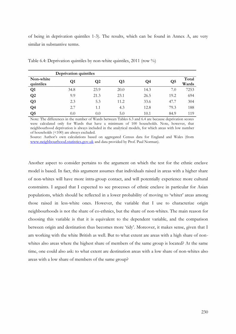
230

of being in deprivation quintiles 1-3). The results, which can be found in Annex A, are very

similar in substantive terms.

Table ‎6.4: Deprivation quintiles by non-white quintiles, 2011 (row %)

Deprivation quintiles

Non-white quintiles

Q1 Q2 Q3 Q4 Q5 Total

Wards

Q1 34.8 23.9 20.0 14.3 7.0 7253

Q2 9.9 21.3 23.1 26.5 19.2 694

Q3 2.3 5.3 11.2 33.6 47.7 304

Q4 2.7 1.1 4.3 12.8 79.3 188

Q5 0.0 0.0 5.0 10.1 84.9 119

Note: The differences in the number of Wards between Tables 6.3 and 6.4 are because deprivation scores were calculated only for Wards that have a minimum of 100 households. Note, however, that neighbourhood deprivation is always included in the analytical models, for which areas with low number of households (<100) are always excluded. Source: Author’s own calculations based on aggregated Census data for England and Wales (from

www.neighbourhood.statistics.gov.uk and data provided by Prof. Paul Norman).

Another aspect to consider pertains to the argument on which the test for the ethnic enclave

model is based. In fact, this argument assumes that individuals raised in areas with a higher share

of non-whites will have more intra-group contact, and will potentially experience more cultural

constraints. I argued that I expected to see processes of ethnic enclave in particular for Asian

populations, which should be reflected in a lower probability of moving to ‘whiter’ areas among

those raised in less-white ones. However, the variable that I use to characterize origin

neighbourhoods is not the share of co-ethnics, but the share of non-whites. The main reason for

choosing this variable is that it is equivalent to the dependent variable, and the comparison

between origin and destination thus becomes more ‘tidy’. Moreover, it makes sense, given that I

am working with the white British as well. But to what extent are areas with a high share of non-

whites also areas where the highest share of members of the same group is located? At the same

time, one could also ask: to what extent are destination areas with a low share of non-whites also

areas with a low share of members of the same group?


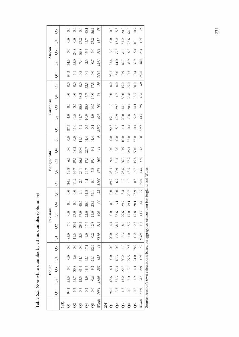
231

Tab

le ‎6

.5: N

on

-wh

ite

quin

tile

s b

y et

hn

ic q

uin

tile

s (c

olu

mn

%)

In

dia

n

Pak

ista

ni

Ban

gla

desh

i C

ari

bb

ean

A

fric

an

Q

1

Q2

Q3

Q4

Q5

Q1

Q2

Q3

Q4

Q5

Q1

Q2

Q3

Q4

Q5

Q1

Q2

Q3

Q4

Q5

Q1

Q2

Q3

Q4

Q5

1981

Q1

94.1

25.3

0.0

0.0

0.0

85.0

7.0

0.0

0.0

0.0

84.9

19.8

6.5

0.0

0.0

87.5

4.0

0.0

0.0

0.0

94.3

34.6

0.0

0.0

0.0

Q2

5.3

55.7

30.8

1.6

0.0

11.5

33.2

27.0

0.0

0.0

11.2

33.7

29.6

18.2

0.0

11.0

49.5

3.7

0.0

0.0

5.1

55.0

24.8

0.0

0.0

Q3

0.5

13.5

41.4

34.1

0.0

2.3

29.4

37.0

45.7

9.1

2.5

24.1

26.9

50.0

11.1

1.2

31.7

55.8

38.3

0.0

0.5

7.4

56.8

27.2

0.0

Q4

0.2

4.9

18.5

43.1

17.1

1.0

17.6

22.0

30.4

31.8

1.1

14.7

17.6

22.7

44.4

0.3

10.9

25.8

45.7

52.5

0.1

2.3

15.4

45.7

43.1

Q5

0.0

0.6

9.2

21.1

82.9

0.2

12.8

14.0

23.9

59.1

0.4

7.8

19.4

9.1

44.4

0.1

4.0

14.7

16.0

47.5

0.0

0.7

3.0

27.2

56.9

War

ds

7684

1160

292

123

41

8819

313

100

46

22

8765

374

108

44

9

8580

404

163

94

59

7519

1241

331

151

58

2011

Q1

94.6

42.6

6.1

0.0

0.0

90.0

14.4

0.0

0.0

0.0

89.9

23.3

9.6

0.0

0.0

92.3

19.1

1.0

0.0

0.0

93.5

23.4

3.0

0.0

0.0

Q2

3.3

35.3

53.4

16.3

0.0

6.5

38.7

35.6

3.1

0.0

6.7

30.9

21.1

13.0

0.0

5.8

42.9

29.8

4.7

0.0

5.0

44.0

33.8

13.2

5.3

Q3

1.3

13.2

22.8

30.2

1.8

2.3

18.6

29.6

29.7

3.4

1.9

25.6

26.3

10.9

10.0

1.1

20.0

34.6

50.0

15.0

0.9

16.7

31.6

51.2

20.0

Q4

0.6

7.0

13.6

29.5

19.3

1.0

15.9

17.0

39.1

20.7

1.0

13.5

27.2

26.1

35.0

0.4

8.8

20.4

36.8

65.0

0.3

8.9

16.2

25.6

64.0

Q5

0.2

1.9

4.1

24.0

78.9

0.2

12.3

17.8

28.1

75.9

0.5

6.7

15.8

50.0

55.0

0.4

9.2

14.1

8.5

20.0

0.4

6.9

15.4

10.1

10.7

War

ds

7303

787

294

129

57

8009

333

135

64

29

7944

446

114

46

20

7768

445

191

106

60

7628

504

234

129

75

So

urc

e: A

uth

or’

s o

wn

cal

cula

tio

ns

bas

ed o

n a

ggre

gate

d c

ensu

s d

ata

for

En

glan

d a

nd

Wal

es.

232

Table 6.5 shows, for 1981 and 2011, the relationship between non-whites and ethnic quintiles

(for 1971/1991 the distributions are almost equal). We can see that between 90 and 100% of

origin areas in ethnic quintile 5 – areas with the highest share of ethnic minorities of a certain

group and also those that exert a negative effect in labour market outcomes of women, as shown

in Chapter 5 – are contained in non-white quintiles 4 and 5. When testing for the ethnic enclave

hypothesis in the analytical models, I will therefore explore the effects of origin non-white

quintiles 4 and 5. Note also that none of the areas with the highest share of members of the same

group in 2011 are contained in non-white quintiles 1+2, which supports the selection of non-

white quintiles 1+2 as a dependent variable.

Moving to the other variables used in the analysis, the three main mediating variables, measured in

2001, are the following: education, measured with a 3-category variable (Level 1 or less, Levels

2+3 and Level 4+); social class, measured with a 4-category variable (Manual, Petit Bourgeoisie,

Intermediate and Service; and partner’s ethnicity: measured with a 4-category variable (no

partner, white British, non-white and other).

Finally, this study compares five main ethnic minority groups with the white British, for which

ethnic group is included as a crucial control variable. Recall that I only work with second

generation ethnic minorities (Indian, Pakistani, Bangladeshi, Chinese, Caribbean and African),

defined as those who lived with at least one parent between 0 and 15 years of age in any of the

three origin years: I include therefore individuals born in Britain and individuals born abroad who

arrived before age 16. Other controls – including background characteristics in origin (parental

social class, tenure, number of cars, overcrowding and neighbourhood deprivation), age, number

of census points and origin year – are also included in the analysis.

Figure 6.2 shows the main variables and their relationships; moreover, a reference to the research

questions is also shown. Research Question 1 is about the main effect of the mediating variables

on the probability of being in a non-white quintile 1+2; Research Question 2a is about the main

ethnic group effect; research questions 3 and 4, finally, are about interaction effects between

ethnic group and mediating variables, and between ethnic group and non-white concentration in

origin. For more details on data and variables refer to Chapter 2.

233

Figure 6.2: Variables and their relationships; reference to research questions

6.7 The problem of reverse causality

An issue that I would like to briefly comment on, before moving to the analysis, is the problem

of reverse causality, shown in Figure 6.3. So far, I have assumed that more education, higher social

class and a white British partner – proxies of socio-economic and cultural assimilation – are

‘gains’ that, later on, are transformed into residential gains. In other words, these factors act as

predictors of the characteristics of the neighbourhood in 2011. This influence might occur in two

different ways: directly and indirectly. The direct effect means that there is an effect of these

variables on top of the effect of the characteristics of the neighbourhood in 2001. The indirect

effect means that the effect of these variables occurs through the characteristics of the

neighbourhood in 2001, which also have an effect on the characteristics of the neighbourhood in

2011. This study does not distinguish between the two, since I consider that they are both part of

the same process, that is, that socio-economic and cultural assimilation promote spatial

assimilation.

However, the following problem arises: what if individuals moved to a certain neighbourhood in

2001 with the objective of achieving socio-economic and cultural assimilation? In this case, the

classical model of spatial assimilation would be reversed (this is expressed in the red arrow). In

other words, rather than means, more socio-economic and cultural assimilation would be a

consequence of being in a neighbourhood with a higher share of non-whites. This implies that if

I find a positive relationship between assimilation and being in a white neighbourhood in 2011, I

cannot know whether individuals improved their neighbourhood in 2011 because they improved

234

their socio-economic and cultural assimilation, or because they moved in 2001 to a white

neighbourhood with the objective of improving their assimilation, and assimilation and a white

neighbourhood in 2001 positively affect the probability of being in a white neighbourhood in

2011. The key issue is then: do socio-economic and cultural assimilation function as a means – as

the theory of spatial assimilation argues – or as a consequence?

Figure 6.3: The problem of reverse causality

Disentangling the two mechanisms is a difficult task that is not solved in this chapter: in fact, the

assumption that spatial assimilation occurs after socio-economic and cultural assimilation is based

solely on theory. However, as a way to show some very exploratory evidence that might support

the spatial assimilation model, we can have a look at a specific group: individuals raised in an area

with a high share of non-whites in 1991. These individuals are between 10 and 15 years old in

1991, between 20 and 25 years old in 2001 and between 30 and 35 in 2011, and are an interesting

group to consider, since we can observe them at a time of their life when they experience many

changes, such as acquiring an education, finding a job, getting married and also changing their

neighbourhood. Even if groups in Q5 are probably less likely to experience assimilation gains

and, hence, residential gains, as compared to individuals raised in neighbourhoods with more

whites, over time (i.e. as we move from 1991 to 2001 and 2011) we should see that they are more

likely to be in whiter areas. This, I believe, would support the idea of assimilation as a means. On

the contrary, if we see that the number of individuals in whiter areas in 2001 is the same as in

2011, and they are both higher than in 1991, the idea of assimilation as a means is less supported,

because it would suggest that they have already improved the neighbourhood at a stage of life

(20-25 years old) just before assimilation achievements (such as getting a highly qualified job)

really occur.

235

Table 6.6 shows the probability of being in non-white quintiles 1+2 in 2001 and 2011 by non-

white quintile and origin year. White British and the five-pooled ethnic minorities are shown. We

can see that younger cohorts raised in non-white areas (Q5) are actually more likely to improve

their neighbourhoods in 2011 than in 2001 (although some individuals do make the big

improvement in 2001). This supports the idea of assimilation as a means.

Table ‎6.6: Probability of being in a neighbourhood with low share of non-whites (quintiles 1+2)

in 2001 and in 2011, by cohort and non-white quintile in origin (%)

White British Ethnic minorities (pooled)

2001 2011 Total 2001 2011 Total

1971

Q1 96.8 96.7 61,203 75.2 74.3 101

Q2 91.8 91.1 10,455 63.8 58.3 271

Q3 82.4 82.0 2,931 42.8 45.6 397

Q4 79.1 81.1 1,330 40.6 39.1 384

Q5 79.0 79.7 610 39.7 41.4 466

1981

Q1 96.5 96.9 49,283 80.8 76.9 182

Q2 90.9 90.1 9,471 63.6 62.0 382

Q3 74.1 79.2 2,201 43.3 43.8 566

Q4 65.9 75.6 1,012 31.1 37.9 531

Q5 64.9 71.2 382 26.3 30.4 654

1991

Q1 97.0 96.3 15,332 87.8 77.6 98

Q2 87.7 84.9 1,568 83.4 61.6 151

Q3 49.1 69.3 407 22.3 30.9 139

Q4 35.0 58.7 206 13.3 24.7 166

Q5 39.4 60.6 94 10.8 17.9 195



Table 6.7 shows the probability of being in a neighbourhood with a low share of non-white

population (quintiles 1+2) by origin quintile. For illustrative purposes, I have divided between

people raised in quintiles 4+5 and people raised in quintiles 1-3.

236

A first outcome from Table 6.7 is that those raised in neighbourhoods with more white

population are also more likely to end up in neighbourhoods with more whites, and this applies

to all groups. Note, however, that important differences emerge between the white British and

ethnic minority groups. A clear indication of this is that even white British raised in areas with the

highest share of non-whites (Q4+5) are more likely to be found in white areas in 2011 compared

to ethnic minorities raised in areas with the lowest share of non-whites (Q1-3). Differences

between ethnic minority groups are also noticeable. For example, as we compare ethnic

minorities raised in Q4+5 – that is, groups raised in areas with the highest share of non-whites –

Pakistani and Bangladeshi populations have the lowest transition to a whiter neighbourhood in

2011; while Indians have the highest. For example, while only 22-25% of Pakistanis and 17-18%

of Bangladeshis raised in Q4+5 are found in Q1+2 in 2011, this value grows to 38-43% for

Indian.

Table ‎6.7: Probability of being in a neighbourhood with a low share of non-white (Quintiles 1+2)

by origin neighbourhood (%)

White British Indian Pakistani Bangladeshi Caribbean African

Non-white Q1-3

Men 95.1 63.9 49.3 42.9 54 48.0

Women 95.3 59.5 51.1 63.0 44.8 64.0

Non-white Q4+5

Men 76.0 38.4 24.8 16.9 38.7 29.4

Women 76.9 42.7 21.5 18.2 33.7 22.9

Totals: Q1-3

Men 73282 512 223 49 265 25

Women 79569 462 225 54 386 50

Totals: Q4+5

Men 1705 529 258 71 230 34

Women 1929 586 270 66 306 48


Up to this point, these results reveal that white British are more likely than ethnic minorities both

to stay in more-white areas and to move to them. This, however, is not surprising, given that

changes in socio-spatial structure typically take place at a very low pace. What is interesting to

know is to what extent these differences remain after we consider a whole range of individual and

household background characteristics that should predict neighbourhood choice, and, at the

237

same time, whether and to what extent these factors preclude an improvement of the

neighbourhood for the different groups.

Tables 6.8, 6.9 and 6.10 show the role of education, partner’s ethnicity and social class (measured

in 2001) in mediating the relationship between origin and destination neighbourhoods, for

pooled ethnic minorities and white British. A first outcome from Table 6.8 is that education

generally improves the probabilities of being in a white neighbourhood in 2011, in particular for

ethnic minorities. For example, among those raised in areas with high share of non-whites

(Q4+5), having a Level 4+ education gives ethnic minorities around 15% points more chances of

being in Q1+2 in 2011 compared to having Level 1 or less. However, this table also shows that

given equality of education and origin neighbourhood, white British are always advantaged with

respect to ethnic minorities. For example, while around 82% of white British raised in non-white

Q4+5 who got a Level 4+ in 2001 have improved their neighbourhood; only around 42% of

ethnic minorities with the same education have done so. Interestingly, note also that the best-

educated ethnic minorities raised in the whitest neighbourhoods do not reach the levels of the

least-educated white British raised in areas with the lowest share of whites. This does not occur

for the (parallel) analysis on deprivation that can be found in Annex A (see Table ‎8.18), which

might be an indicator of higher segregation based on ethnicity.

Table ‎6.8: Probability of being in a neighbourhood with a low share of non-white (quintiles 1+2)

in 2011 by origin neighbourhood and education (%)


Level 1 or less Levels 2+3 Level 4+ Level 1 or less Levels 2+3 Level 4+

Non-white Q1-3

Men 95.5 95.9 93.1 51.2 58.5 60.8

Women 95.2 96.3 93.9 50.9 49.5 58.5

Non-white Q4+5

Men 74 76.8 81.7 28.3 32.2 42.9

Women 74.1 79.8 82.3 27.6 32.9 41.6

Totals: Q1-3

Men 32355 24839 16088 365 287 439

Women 31598 30542 17429 350 412 422

Totals: Q4+5

Men 903 556 246 438 298 378

Women 985 654 282 413 441 428


238

Moving to the next indicator of cultural assimilation, partner’s ethnicity, Table 6.9 shows that

having a white British partner (vs. a non-white one) has a positive effect for ethnic minorities.

For example, ethnic minorities raised in areas with a high share of non-whites, have around 30%

points greater probability of being in whiter areas in 2011 if their partner is white British than if

he or she is non-white.

Table ‎6.9: Probability of being in a neighbourhood with a low share of non-whites (Quintiles 1-2)

in 2011 by origin neighbourhood1 and partner’s ethnicity (%)


No

Partner Other

Non- White

White British

No partner

Other Non-white

White British

Non-white Q1-3

Men 93.5 91.0 86.1 96.4 57.4 37.0 49.6 84.5

Women 93.2 90.7 82.8 96.7 46.3 0 54.5 86.3

Non-white Q4+5

Men 64.6 78.2 100.0 83.9 31.7 - 32.5 65.3

Women 66.6 66.7 63.0 85.2 27.1 - 35.8 72.0

Totals: Q1-3

Men 28506 1286 360 43122 561 27 381 116

Women 26958 1166 483 50956 629 0 453 95

Totals: Q4+5

Men 649 55 10 986 526 0 496 72

Women 764 33 27 1098 606 0 576 82


Table 6.10, which shows the mediating role of social class, reveals similar results to those

observed for education: both ethnic minorities and white British obtain residential gains from a

higher social class. For example, for ethnic minorities raised in areas with the highest share of

non-whites, having a service class position in 2001 gives around 15% points greater chance of

being in a whiter neighbourhood in 2011, compared to having a manual class. However,

inequalities based on ethnicity persist. For example, while around 82% of white British male

raised in areas with a high share of non-whites that got a service class position in 2001 have

improved their neighbourhood; only around 41% of ethnic minority males have done so. As with

education, here we also observe that even the white British raised in areas with the highest share

of non-whites in the lowest social class are still more likely to be in whiter areas in 2011, when

compared to ethnic minorities raised in the whitest neighbourhoods who achieved a service class

239

in 2001 (around 10-12 % points more) (again, this phenomenon is not observed for the results

on deprivation; see Table ‎8.20 in Annex A).

Table ‎6.10: Probability of being in a neighbourhood with a low share of non-white (quintiles 1-2)

in 2011 by origin neighbourhood and social class (%)


Manual

Petit Bourg.

Interm. Service Manual Petit

Bourg. Interm. Service

Non-white Q1-3

Men 95.5 95.9 94.3 94.6 52.6 64.7 50.4 60

Women 95.4 96.8 95.5 94.9 44.3 61.9 52.9 58

Non-white Q4+5

Men 70.7 81.3 71.8 82 26.5 37.8 35.5 40.5

Women 72.2 86.8 80.7 80.1 24.7 54.3 33.3 41

Totals: Q1-3

Men 30734 7559 5751 29238 384 102 117 492

Women 31420 3337 17173 27638 300 26 346 512

Totals: Q4+5

Men 767 192 131 615 437 98 107 472

Women 827 76 472 549 401 35 339 503


Note also that, both in Tables 6.8 and 6.10, education and social class seem to matter more for

those raised in Q4+5 than for those raised in Q1-3. Look for example at the role of education

for ethnic minority men. For those raised in areas with a low share of non-whites (Q1-3), the gain

of a Level 4+ education (vs. Level 1 or less) is of around 10% points; this grows to 15% for

those raised in areas with higher levels of non-white population. Note also that when looking at

the role of education and social class in the analysis of deprivation we observe that, although the

effect is stronger in terms of the size of the gains, these do not seem to vary much between

individuals raised in areas with different deprivation levels (see Table ‎8.18 and Table ‎8.20 in

Annex A).

These preliminary results show, as expected, that more education, a white British partner and a

higher social class lead to an increase in the probability of being in a whiter area for ethnic

minorities; most importantly, they result in a greater likelihood of moving out of non-white (and

deprived) areas. These outcomes point to processes of spatial assimilation, in the sense that having

240

a better education or social class or partnering with a white person favours an improvement of

the neighbourhood in which the individual lives. However, these descriptive statistics suggest as

well persistent inequalities between ethnic minorities and the white British in terms of the areas

they can access, and therefore point to processes connected to the place stratification/ethnic enclave

models. I explore this more in detail in the following section.

6.9 Testing the spatial assimilation, place stratification and ethnic enclave

models

Table 6.11 presents estimates of linear probability models for the probability of being in areas

with a low share of non-whites (Q1+2) for ethnic minorities only (note that this refers to Equation i,

but without the white British). The main aim of this initial analysis is to test to what extent an

increase in cultural and socio-economic assimilation leads to both being in a non-white area and

to improving the area, that is, by moving from areas with more to fewer non-whites. This is a test

for the classical model of spatial assimilation, concerned with whether immigrants transform their

assimilation gains into residential gains.

The full models can be found in Table ‎8.24 in Annex A and, as with the other chapters, this and

the coming models are based on linear regressions with robust (clustered) standard errors. Given

that most variables are categorical, the coefficients, when multiplied by 100, represent differences

in percentage points with respect to the reference category. For example, a coefficient of 0.05 for

educational level 4+ means that individuals with Level 4+ are 5% points more likely than

individuals with Level 1 or less (the reference category) to move to non-white quintiles 1+2.

My expectations are confirmed when looking at Table 6.11. Having a Level 4+ (vs. a Level 1 or

less), a Service class (vs. a Manual one) and a white British partner (vs. a non-white one) have a

positive effect in the probability of being in a neighbourhood with a low share of non-whites.

Note that for men only education matters, while for women it is their social class; and note also

that the partner’s ethnicity seems to have a particularly strong effect: having a white partner (vs. a

non-white one) increases 27-29% points the probabilities of being in a neighbourhood with more

whites.

241

Table ‎6.11: Probability of being in a neighbourhood with a low share of non-white (quintiles 1-2)

in 2011. Linear regression with robust SE; ethnic minorities only.

Men Women

NW quintile (ref. Q1: lowest share)

Q2 -0.105** -0.193***

(0.0451) (0.0439)

Q3 -0.295*** -0.337***

(0.0456) (0.0428)

Q4 -0.350*** -0.403***

(0.0466) (0.0443)

Q5 -0.393*** -0.437***

(0.0477) (0.0460)

Ethnic group (ref. Indian)

Pakistani -0.108*** -0.124***

(0.0314) (0.0315)

Bangladeshi -0.080 -0.027

(0.0500) (0.0570)

Caribbean -0.060* -0.094***

(0.0352) (0.0314)

African -0.053 -0.047

(0.0822) (0.0569)

Education (ref. Level 1 or less)

Level 2+3 0.032 0.001

(0.0313) (0.0289)

Level 4+ 0.081** 0.043

(0.0349) (0.0327)

Social class (ref. Manual)

Petit Bourgeoisie 0.107** 0.128*

(0.0433) (0.0754)

Intermediate 0.020 0.062**

(0.0450) (0.0307)

Service 0.033 0.079**

(0.0324) (0.0308)

Partner’s ethnicity (ref. non-white)

No partner 0.053* -0.083***

(0.0299) (0.0265)

Other 0.059 0.114

(0.0866) (0.1108)

White British 0.292*** 0.269***

(0.0436) (0.0428)

Adjusted R2 0.136 0.135

N 2209 2474 Note: Models control for age, gender, origin year, and number of census points, neighbourhood deprivation, tenure, number of persons per room, number of cars and parental social class. * p-value<.10 ** p-value<.05 *** p-value<.01; robust (clustered) standard errors in parentheses Population: Individuals between 20 and 55 years old Source: Author’s own calculations based on ONS-LS

242

I have also tested for interactions between origin neighbourhood and the three mediating

variables (see Table ‎8.24 in Annex A), to explore whether the positive effect of these variables

differs for individuals raised in areas with different shares of non-whites (I compare those raised

in non-white quintile 4+5 with those raised in non-white quintile 1+2). The results show no

difference for women, while for men the effect of education and a white partner is stronger in

origin quintiles 4+5. Finally, Table 6.11 suggests differences based on ethnicity: on equality of

characteristics, Indians (the reference group) seem to be doing better in terms of their area of

residence in 2011, and Pakistanis are doing the worst.

In what follows, I compare ethnic minorities with the white British, following Equations i, ii and

iii from Table 6.1. This can be observed in Tables 6.12 and 6.13, which present estimates of

linear probability models for the probability of being in areas with low share of non-whites

(quintiles 1 and 2) for men and women respectively. The full models can be found in Table ‎8.25

and Table ‎8.26 in Annex A; moreover, Table ‎8.27 in Annex A shows selected models estimated

with logistic regression with average marginal effects: Equation i from Tables 6.12 and 6.13 and

Equation i from Table ‎8.21 and Table ‎8.22 (these two refer to the deprivation analysis found in

Annex A).

243

Tab

le ‎6

.12: P

rob

abili

ty o

f b

ein

g in

a n

eigh

bo

urh

oo

d w

ith

a lo

w s

har

e o

f n

on

-wh

ites

(quin

tile

s 1-2

). L

inea

r re

gres

sio

n w

ith

ro

bust

SE

; et

hn

ic m

ino

riti

es

and w

hit

e B

riti

sh m

en.

B

ase

E

q.

i E

q.

ii

(*ed

ucati

on

)

Eq

. ii

(*

cla

ss)

Eq

. ii

(*

part

ner)

E

q.

iii

(wit

ho

ut

part

ner)

NW

qu

inti

le (

ref.

Q1:

lo

wes

t sh

are

)

Q2

-0.0

64**

* -0

.064**

* -0

.064**

* -0

.064**

* -0

.064**

*

(0

.0034)

(0.0

034)

(0.0

034)

(0.0

034)

(0.0

034)

Q

3

-0.1

76**

* -0

.174**

* -0

.175**

* -0

.174**

* -0

.174**

*

(0

.0086)

(0.0

085)

(0.0

085)

(0.0

085)

(0.0

085)

Q

4

-0.2

19**

* -0

.216**

* -0

.216**

* -0

.214**

* -0

.214**

*

(0

.0122)

(0.0

122)

(0.0

122)

(0.0

121)

(0.0

122)

Q

5

-0.2

70**

* -0

.267**

* -0

.264**

* -0

.264**

* -0

.263**

*

(0

.0163)

(0.0

162)

(0.0

161)

(0.0

161)

(0.0

161)

N

W q

uin

tile

(re

f. Q

1-2)

Q3

-0

.162**

*

(0.0

089)

Q4+

5

-0

.197**

*

(0.0

117)

Eth

nic

gro

up

(re

f. w

hit

e B

riti

sh)

In

dia

n

-0.2

74**

* -0

.224**

* -0

.266**

* -0

.267**

* -0

.229**

* -0

.189**

*

(0

.0196)

(0.0

210)

(0.0

352)

(0.0

345)

(0.0

356)

(0.0

300)

Pak

ista

ni

-0.4

11**

* -0

.355**

* -0

.413**

* -0

.464**

* -0

.319**

* -0

.328**

*

(0

.0265)

(0.0

282)

(0.0

390)

(0.0

389)

(0.0

408)

(0.0

535)

Ban

glad

esh

i -0

.448**

* -0

.406**

* -0

.386**

* -0

.485**

* -0

.360**

* -0

.326**

*

(0

.0441)

(0.0

448)

(0.0

681)

(0.0

576)

(0.0

726)

(0.0

957)

Car

ibb

ean

-0

.324**

* -0

.294**

* -0

.380**

* -0

.354**

* -0

.339**

* -0

.331**

*

(0

.0273)

(0.0

273)

(0.0

373)

(0.0

387)

(0.0

564)

(0.0

471)

244

B

ase

E

q.

i E

q.

ii

(*ed

ucati

on

)

Eq

. ii

(*

cla

ss)

Eq

. ii

(*

part

ner)

E

q.

iii

(wit

ho

ut

part

ner)

Afr

ican

-0

.342**

* -0

.315**

* -0

.386**

* -0

.136

-0.0

87

-0.4

77**

*

(0

.0773)

(0.0

782)

(0.1

226)

(0.1

563)

(0.1

905)

(0.1

521)

Ed

ucati

on

(re

f. L

eve

l 1

or

less

)

L

evel

2+

3

0.0

06**

* 0.0

05**

0.0

06**

* 0.0

06**

* 0.0

06**

*

(0.0

023)

(0.0

023)

(0.0

023)

(0.0

023)

(0.0

023)

Lev

el 4

+

-0

.018**

* -0

.023**

* -0

.019**

* -0

.019**

* -0

.019**

*

(0.0

033)

(0.0

032)

(0.0

033)

(0.0

033)

(0.0

033)

So

cia

l cla

ss (

ref.

Man

ual)

P

etit

Bo

urg

eois

ie

0.0

05

0.0

05

0.0

01

0.0

05

0.0

06*

(0.0

033)

(0.0

033)

(0.0

032)

(0.0

033)

(0.0

034)

Inte

rmed

iate

-0.0

04

-0.0

04

-0.0

05

-0.0

04

-0.0

07

(0.0

043)

(0.0

043)

(0.0

042)

(0.0

043)

(0.0

043)

Ser

vic

e

0.0

01

0.0

01

-0.0

01

0.0

02

0.0

02

(0.0

026)

(0.0

026)

(0.0

026)

(0.0

026)

(0.0

026)

Part

ner’

s eth

nic

ity (

ref.

no

n-

wh

ite)

No

par

tner

0.0

72**

* 0.0

66**

* 0.0

75**

* 0.0

79**

*

(0.0

173)

(0.0

173)

(0.0

172)

(0.0

220)

O

ther

0.0

58**

* 0.0

54**

* 0.0

61**

* 0.0

65**

*

(0.0

197)

(0.0

197)

(0.0

196)

(0.0

238)

W

hit

e B

riti

sh

0.1

06**

* 0.1

00**

* 0.1

10**

* 0.1

11**

*

(0.0

173)

(0.0

173)

(0.0

172)

(0.0

219)

In

tera

cti

on

s

In

dia

n*L

evel

4+

0.0

92**

(0

.0434)

P

akis

tan

i*L

evel

4+

0.1

47**

(0

.0574)

245

B

ase

E

q.

i E

q.

ii

(*ed

ucati

on

)

Eq

. ii

(*

cla

ss)

Eq

. ii

(*

part

ner)

E

q.

iii

(wit

ho

ut

part

ner)

Ban

glad

esh

i*L

evel

4+

-0

.014

(0

.1048)

C

arib

bea

n*L

evel

4+

0.1

89**

*

(0

.0661)

A

fric

an*L

evel

4+

0.1

89

(0

.1778)

In

dia

n*S

ervic

e

0.0

70*

(0.0

415)

Pak

ista

ni*

Ser

vic

e

0.1

83**

*

(0.0

574)

Ban

glad

esh

i*Ser

vic

e

0.1

23

(0.0

942)

Car

ibb

ean

*Ser

vic

e

0.1

52**

*

(0.0

587)

Afr

ican

*Ser

vic

e

-0.3

35*

(0.1

846)

India

n*w

hit

e B

riti

sh

0.2

34**

*

(0

.0670)

P

akis

tan

i*w

hit

e B

riti

sh

0.2

89**

*

(0

.1115)

B

angl

ades

hi*

wh

ite

Bri

tish

-0

.371**

*

(0

.0727)

C

arib

bea

n*w

hit

e B

riti

sh

0.2

29**

*

(0

.0780)

A

fric

an*w

hit

e B

riti

sh

-0.4

17*

(0

.2507)

In

dia

n*Q

4+

5

-0

.176**

*

246

B

ase

E

q.

i E

q.

ii

(*ed

ucati

on

)

Eq

. ii

(*

cla

ss)

Eq

. ii

(*

part

ner)

E

q.

iii

(wit

ho

ut

part

ner)

(0.0

398)

Pak

ista

ni*

Q4+

5

-0

.169**

*

(0.0

608)

Ban

glad

esh

i*Q

4+

5

-0

.188*

(0.1

061)

Car

ibb

ean

*Q4+

5

-0

.032

(0.0

592)

Afr

ican

*Q4+

5

0.1

65

(0.1

814)

A

dju

sted

R-s

quar

ed

0.1

52

0.1

59

0.1

60

0.1

62

0.1

61

0.1

47

N

77,1

96

77,1

96

77,1

96

77,1

96

77,1

96

77,1

96

No

te: M

od

els

con

tro

l fo

r ag

e, g

end

er, o

rigi

n y

ear,

an

d n

um

ber

of

cen

sus

po

ints

, n

eigh

bo

urh

oo

d d

epri

vat

ion

, te

nure

, n

um

ber

of

per

son

s p

er

roo

m, n

um

ber

of

cars

an

d p

aren

tal so

cial

cla

ss. *

p-v

alue<

.10 *

* p

-val

ue<

.05 *

** p

-val

ue<

.01; ro

bust

(cl

ust

ered

) st

and

ard

err

ors

in

par

enth

eses

P

op

ula

tio

n: In

div

idual

s b

etw

een

20 a

nd

55 y

ears

old

So

urc

e: A

uth

or’

s o

wn

cal

cula

tio

ns

bas

ed o

n O

NS

-LS

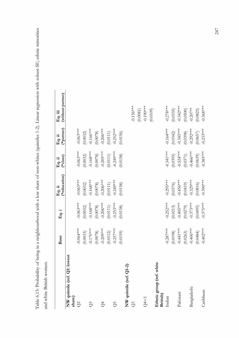
247

Tab

le ‎6

.13: P

rob

abili

ty o

f b

ein

g in

a n

eigh

bo

urh

oo

d w

ith

a lo

w s

har

e o

f n

on

-wh

ites

(quin

tile

s 1-2

). L

inea

r re

gres

sio

n w

ith

ro

bust

SE

; et

hn

ic m

ino

riti

es

and w

hit

e B

riti

sh w

om

en.

B

ase

E

q.

i E

q.

ii

(*ed

ucati

on

)

Eq

. ii

(*

cla

ss)

Eq

. ii

(*

part

ner)

E

q.

iii

(wit

ho

ut

part

ner)

NW

qu

inti

le (

ref.

Q1:

lo

wes

t sh

are

)

Q2

-0.0

64**

* -0

.063**

* -0

.063**

* -0

.063**

* -0

.063**

*

(0

.0033)

(0.0

032)

(0.0

032)

(0.0

032)

(0.0

032)

Q

3

-0.1

70**

* -0

.168**

* -0

.168**

* -0

.168**

* -0

.166**

*

(0

.0078)

(0.0

078)

(0.0

078)

(0.0

078)

(0.0

078)

Q

4

-0.2

09**

* -0

.206**

* -0

.206**

* -0

.205**

* -0

.206**

*

(0

.0112)

(0.0

111)

(0.0

111)

(0.0

111)

(0.0

111)

Q

5

-0.2

57**

* -0

.253**

* -0

.249**

* -0

.249**

* -0

.252**

*

(0

.0159)

(0.0

158)

(0.0

158)

(0.0

158)

(0.0

156)

N

W q

uin

tile

(re

f. Q

1-2)

Q3

-0

.156**

*

(0.0

081)

Q4+

5

-0

.190**

*

(0.0

109)

Eth

nic

gro

up

(re

f. w

hit

e

Bri

tish

)

India

n

-0.2

87**

* -0

.252**

* -0

.295**

* -0

.341**

* -0

.164**

* -0

.278**

*

(0

.0198)

(0.0

213)

(0.0

376)

(0.0

395)

(0.0

342)

(0.0

335)

Pak

ista

ni

-0.4

41**

* -0

.405**

* -0

.456**

* -0

.524**

* -0

.345**

* -0

.342**

*

(0

.0263)

(0.0

279)

(0.0

419)

(0.0

371)

(0.0

398)

(0.0

500)

Ban

glad

esh

i -0

.406**

* -0

.373**

* -0

.329**

* -0

.466**

* -0

.292**

* -0

.207**

(0

.0484)

(0.0

495)

(0.0

816)

(0.0

639)

(0.0

657)

(0.0

825)

Car

ibb

ean

-0

.402**

* -0

.375**

* -0

.390**

* -0

.383**

* -0

.233**

* -0

.368**

*

248

B

ase

E

q.

i E

q.

ii

(*ed

ucati

on

)

Eq

. ii

(*

cla

ss)

Eq

. ii

(*

part

ner)

E

q.

iii

(wit

ho

ut

part

ner)

(0

.0226)

(0.0

228)

(0.0

378)

(0.0

434)

(0.0

515)

(0.0

413)

Afr

ican

-0

.357**

* -0

.327**

* -0

.459**

* -0

.592**

* 0.0

03

-0.2

43**

(0

.0540)

(0.0

545)

(0.1

245)

(0.0

942)

(0.1

139)

(0.1

075)

Ed

ucati

on

(re

f. L

eve

l 1

or

less

)

L

evel

2+

3

0.0

09**

* 0.0

09**

* 0.0

09**

* 0.0

09**

* 0.0

10**

*

(0.0

022)

(0.0

021)

(0.0

022)

(0.0

022)

(0.0

022)

Lev

el 4

+

-0

.012**

* -0

.015**

* -0

.012**

* -0

.011**

* -0

.011**

*

(0.0

032)

(0.0

031)

(0.0

032)

(0.0

032)

(0.0

032)

So

cia

l cla

ss (

ref.

Man

ual)

P

etit

Bo

urg

eois

ie

0.0

11**

0.0

11**

0.0

07*

0.0

11**

0.0

12**

*

(0.0

042)

(0.0

042)

(0.0

040)

(0.0

042)

(0.0

043)

Inte

rmed

iate

0.0

02

0.0

02

0.0

01

0.0

02

0.0

02

(0.0

026)

(0.0

026)

(0.0

025)

(0.0

026)

(0.0

026)

Ser

vic

e

0.0

02

0.0

02

-0.0

02

0.0

02

0.0

01

(0.0

026)

(0.0

026)

(0.0

025)

(0.0

026)

(0.0

026)

Part

ner’

s eth

nic

ity (

ref.

no

n-

wh

ite)

No

par

tner

0.0

32*

0.0

24

0.0

27*

0.0

97**

*

(0.0

164)

(0.0

165)

(0.0

164)

(0.0

209)

O

ther

0.0

16

0.0

08

0.0

11

0.0

73**

*

(0.0

194)

(0.0

195)

(0.0

193)

(0.0

232)

W

hit

e B

riti

sh

0.0

71**

* 0.0

63**

* 0.0

66**

* 0.1

32**

*

(0.0

164)

(0.0

165)

(0.0

163)

(0.0

208)

In

tera

cti

on

s

In

dia

n*L

evel

4+

0.0

80*

(0

.0465)

P

akis

tan

i*L

evel

4+

0.1

76**

*

249

B

ase

E

q.

i E

q.

ii

(*ed

ucati

on

)

Eq

. ii

(*

cla

ss)

Eq

. ii

(*

part

ner)

E

q.

iii

(wit

ho

ut

part

ner)

(0

.0633)

B

angl

ades

hi*

Lev

el 4

+

-0.0

50

(0

.1357)

C

arib

bea

n*L

evel

4+

0.0

48

(0

.0538)

A

fric

an*L

evel

4+

0.2

12

(0

.1419)

In

dia

n*S

ervic

e

0.1

27**

*

(0.0

465)

Pak

ista

ni*

Ser

vic

e

0.2

17**

*

(0.0

590)

Ban

glad

esh

i*Ser

vic

e

0.1

74

(0.1

143)

Car

ibb

ean

*Ser

vic

e

0.0

40

(0.0

545)

Afr

ican

*Ser

vic

e

0.3

20**

*

(0.1

183)

India

n*w

hit

e B

riti

sh

0.1

97**

*

(0

.0590)

P

akis

tan

i*w

hit

e B

riti

sh

0.2

42**

(0

.1218)

B

angl

ades

hi*

wh

ite

Bri

tish

-0

.096

(0

.3312)

C

arib

bea

n*w

hit

e B

riti

sh

0.1

26

(0

.0822)

A

fric

an*w

hit

e B

riti

sh

-0.0

99

(0

.1936)

250

B

ase

E

q.

i E

q.

ii

(*ed

ucati

on

)

Eq

. ii

(*

cla

ss)

Eq

. ii

(*

part

ner)

E

q.

iii

(wit

ho

ut

part

ner)

India

n*Q

4+

5

-0

.057

(0.0

415)

Pak

ista

ni*

Q4+

5

-0

.200**

*

(0.0

585)

Ban

glad

esh

i*Q

4+

5

-0

.347**

*

(0.0

981)

Car

ibb

ean

*Q4+

5

-0

.055

(0.0

510)

Afr

ican

*Q4+

5

-0

.253*

(0.1

299)

A

dju

sted

R-s

qu

are

d

0.1

68

0.1

75

0.1

76

0.1

77

0.1

80

0.1

63

N

83,9

72

83,9

72

83,9

72

83,9

72

83,9

72

83,9

72

No

te: M

od

els

con

tro

l fo

r ag

e, g

end

er, o

rigi

n y

ear,

an

d n

um

ber

of

cen

sus

po

ints

, n

eigh

bo

urh

oo

d d

epri

vat

ion

, te

nure

, n

um

ber

of

per

son

s p

er r

oo

m, n

um

ber

of

cars

an

d p

aren

tal so

cial

cla

ss. *

p-v

alue<

.10 *

* p

-val

ue<

.05 *

** p

-val

ue<

.01; ro

bust

(cl

ust

ered

) st

and

ard

err

ors

in

p

aren

thes

es.

Po

pula

tio

n: In

div

idual

s b

etw

een

20 a

nd

55 y

ears

old

So

urc

e: A

uth

or’

s o

wn

cal

cula

tio

ns

bas

ed o

n O

NS

-LS

251

The base model45 shows that – given equality of neighbourhood characteristics in origin – all

ethnic minorities are less likely to be found in areas with a low share of non-whites as compared

to the white British; in particular Pakistani and Bangladeshi populations and Caribbean women

present the highest disadvantages (of around 40% points less probability); while Indians the least,

but still considerable (almost 30% points less). When adding the three key mediating variables

measured in 2001, that is, education, social class and partner’s ethnicity (Equation i) these

differences remain practically the same, which points to the presence of mechanisms of place

stratification/ethnic enclave. Note, however, the quite-surprising effect of having a degree (Level 4+),

which, contrary to what I expected, is negative. This effect is most likely driven by white British

moving from whiter to whiter areas (the majority), given that for ethnic minorities and for white

British moving from less- to more-white areas it is positive, as observed in Tables 6.8 and 6.11.

Since I am controlling for the social class of individuals, this negative effect might be connected

to the attraction of cities – where most ethnic minorities are located – as cultural places, but only

for those who were raised in whiter areas; it might also be connected to those better positioned

white British (hence raised in better – i.e. whiter – areas) who move to cities to complete their

graduate studies46.

The next three models represent the three variations of Equation ii. The first one, which adds

interactions between ethnic group and education, shows that, contrary to expectations, having a

higher educational level has a more positive effect for Indian and Pakistani populations, and also

for Caribbean men, than for the white British. In fact, for ethnic minorities, education – when

measured on top of social class – seems to have a different role than for the white British, giving

them a greater chance of being in a whiter area in 2011, on average. For example, while less-

educated Indian men are around 27% points less likely to be in a non-white area in 2011,

compared to an equivalent white British person, this gap reduces to around 17% for those who

45 In addition to the observed variables, this model controls for other basic individual, household and neighbourhood characteristics (see notes in Tables 6.12 and 6.13). 46 The positive effect of having been raised in a deprived area (see Table ‎8.26 in Annex A) on the probability of

being in a ‘whiter’ area (for women), also driven by the white British, is also puzzling. This might be related to the fact that non-white share and deprivation are very much related at the neighbourhood level: white British who were raised in very white and deprived areas are very few, as those who were raised in non-white and less deprived ones, so this positive effect probably refers to a very specific population. Note that Schaake, Burgers et al. (2013) found the same effect in their study in the Netherlands: while the share of Dutch in the ‘origin’ area has a positive effect in the share of Dutch in the destination area, a higher socio-economic level has the opposite effect, just as I find in the present study.

252

have at least one degree. Note, however, that this is an average effect that does not discriminate

depending on the areas where individuals where raised47.

In the next model, I test for interactions with social class. Here I observe a similar effect for most

ethnic minorities, and for the white British the effect is close to zero. Social class, like education,

reduces the gap between most ethnic minorities and the white British in terms of accessing

whiter areas. For example, among those who have manual jobs, Pakistani women are around

52% points less likely to be in non-white areas compared to the white British; however, this gap

reduces to almost half among those who have a service class position (note that African men are

the only group who followed my initial expectation: for them a service position brings a

disadvantage; however, given the positive result for women and the low N for this group, I have

some concerns regarding the precision of this outcome).

A similar outcome is observed when I add interactions with a white British partner: most ethnic

groups benefit from this48, thus reducing the gap. An interesting finding is that the effect of a

white British partner for men seems to be stronger than for women; I would have expected the

contrary, given that in some communities, such as the Asian one, women are more subject to

cultural constraints, and a white partner might be a way to ‘escape’ these. A lower effect for them

might be an indicator that gender constraints still obtain, even taking into account a mixed

partner’s ethnicity.

The last model (Equation iii) tests whether the negative effect for ethnic minorities is higher for

those raised in areas with a higher share of non-whites (quintiles 4+5) as compared to those

raised in areas with a lower share of non-whites (quintiles 1+2), before controlling for partner’s

ethnicity. I argued that, if a negative interaction effect was found, this might be indicative of

processes of ethnic enclave taking place. The results show this pattern for Pakistani and Bangladeshi

populations, and also for Indian men (there is also an effect for African women but the N is very

low for this group). In other words, if we compare white British and ethnic minorities raised in

areas with a high share of non-whites, compared to those raised in the whitest areas, the gap

47 I have also estimated a model for individuals raised in Q45 only and I found, in accordance with Table 7.8, that there is a positive effect of education, both for white British and ethnic minorities; in this model, with a few exceptions, the interactions between education and ethnic group are statistically non-significant for both genders. In any case, the expected negative interaction effect for ethnic minorities does not appear here either (analysis available upon request). 48 The negative exceptions in both education and partnership among African and Bangladeshi are likely to be outliers, since these groups have very few cases; moreover, most Bangladeshis are coupled with co-ethnics.

253

between the two is bigger. For example, for Indian men, having lived at a young age in Q4+5

gives them around 35% points less chance of living in whiter areas in 2011 compared to an

equivalent white British; this gap is lower for those raised in Q1+2 (around 18%). Similarly, for

Pakistanis and Bangladeshis raised in areas with the least whites, their probability of being in

whiter areas in 2011 is around 50-55% points less, as compared to the white British; this drops to

almost half when comparing individuals raised in whiter areas. Finally, I have also tested whether

this model changed once I included the partner’s ethnicity variable, under the assumption that

having a non-white partner (more likely to happen in non-white areas) might be a mechanism

that explains the bigger gap: this was refuted, as the model remains the same (see

Table ‎8.25Table ‎8.26in Annex A).

In order to gain a better understanding of differences and similarities between ethnic minority

groups and white British with various individual and origin neighbourhood characteristics, I have

calculated predictions for ‘extreme types’: individuals with the least education, lowest social class

and a non-white partner (type 1), on the one hand, and individuals with the most education,

highest social class and a white British partner (type 2), on the other. Moreover, I have also

differentiated between individuals raised in Q4+5 and individuals raised in Q1+2. To calculate

these margins all interactions are included in one equation. The results are shown in Table 6.14.

Before moving to the description of results, note the following. First of all, in Table 6.14 the

effect of the three key mediating variables (education, class and partner’s ethnicity) are not

allowed to vary by ‘origin’ neighbourhood; however, we saw in Tables 6.8-6.10 that these

variables have in general a stronger effect among those raised in quintiles with higher share of

non-whites, and even more so for ethnic minorities. Given this, the estimates calculated for the

‘best’ ideal type (level 4+, Service and white British partner) probably should have been higher

(and the gap with white British lower) for individuals raised in quintiles 4+5; while the estimates

for those raised in Q1+2 probably should have been lower: note that for some ethnic minorities

the estimation goes beyond 100%, which is an unreal probability. Second, given that the results

for Bangladeshis and Africans are based on low Ns, and given the counterintuitive results for

male regarding the effect of partnership, I have added extra predictions for type 2, but without

specifying the ethnicity of the partner, which yields results that are more in line with the other

groups, in particular for Bangladeshis (although with still high standard errors for the

coefficients).

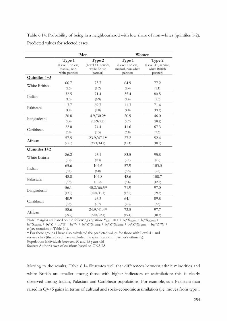
254

Table ‎6.14: Probability of being in a neighbourhood with low share of non-whites (quintiles 1-2).

Predicted values for selected cases.

Men Women

Type 1 Type 2 Type 1 Type 2

(Level 1 or less, manual, non-white partner)

(Level 4+, service, white British

partner)

(Level 1 or less, manual, non-white

partner)

(Level 4+, service, white British

partner)

Quintiles 4+5

White British 66.7 75.7 64.9 77.2

(2.5) (1.2) (2.4) (1.1)

Indian 32.5 71.4 35.4 80.5

(4.3) (6.9) (4.6) (5.5)

Pakistani 13.7 69.7 11.3 71.4

(4.8) (9.8) (4.0) (13.3)

Bangladeshi 20.8 4.9/30.2* 20.9 46.0

(9.4) (10.9/9.2) (9.7) (28.2)

Caribbean 22.0 74.4 41.6 67.3

(6.0) (7.5) (6.8) (7.6)

African 57.5 23.9/47.1* 27.2 52.4

(25.0) (23.3/14.7) (15.1) (18.5)

Quintiles 1+2

White British 86.2 95.1 83.5 95.8

(2.2) (0.3) (2.1) (0.2)

Indian 65.6 104.6 57.9 103.0

(5.1) (6.8) (5.5) (5.9)

Pakistani 48.8 104.8 48.6 108.7

(6.9) (10.2) (6.6) (12.5)

Bangladeshi 56.1 40.2/66.5* 71.9 97.0

(13.2) (14.0/11.4) (12.0) (29.5)

Caribbean 40.9 93.3 64.1 89.8

(6.9) (7.7) (7.3) (7.5)

African 58.6 24.9/41.4* 72.5 97.7

(29.7) (22.8/22.4) (19.1) (18.3)

Note: margins are based on the following equation: Y(2011) = a + b1*X1(2001)+ b2*X2(2001) + b3*X3(2001) + b4*Z + b5*W + b6*V + b7*Z*X1(2001) + b8*Z*X2(2001) + b9*Z*X3(2001) + b10*Z*W + e (see notation in Table 6.1). * For these groups I have also calculated the predicted values for those with Level 4+ and service class (therefore, I have excluded the specification of partner’s ethnicity). Population: Individuals between 20 and 55 years old Source: Author’s own calculations based on ONS-LS

Moving to the results, Table 6.14 illustrates well that differences between ethnic minorities and

white British are smaller among those with higher indicators of assimilation: this is clearly

observed among Indian, Pakistani and Caribbean populations. For example, as a Pakistani man

raised in Q4+5 gains in terms of cultural and socio-economic assimilation (i.e. moves from type 1

255

to type 2), the gap with respect to an equivalent white British in terms of the probability of being

in a neighbourhood with a low share of non-whites reduces from 53% points to 6% points. For

Bangladeshis and Africans, the results are very unstable, although they point in general to lower

effects of assimilation on residential mobility. The other clear outcome is that for Pakistani and

Bangladeshi populations and for Indian men the gaps are clearly bigger if individuals are raised in

Q4+5. For example, the difference in the probability of being in a Q1+2 neighbourhood in 2011

between a type 1 Pakistani woman and a type 1 white British woman is of around 35% points for

those raised in Q1+2; this grows to 54% points for those raised in Q4+5. Note finally, that

assimilation seems to have a stronger effect on the probability of moving to a less-deprived area,

as compared to the probability of moving to a ‘whiter’ area (see Table ‎8.23 in Annex A) , which

might speak to higher segregation based on ethnicity rather than on socio-economic conditions.

6.10 Discussion

We saw in the previous chapters that segregation levels vary between groups and also have varied

effects on ethnic minorities’ outcomes; we also saw that the segregation of minorities is linked to

deprivation. This chapter has added to this knowledge by examining to what extent higher levels

of socio-economic and cultural assimilation are connected with ‘residential gains’, understood

here as the possibility of being in ‘whiter’ and less-deprived areas. Moreover, it has explored to

what extent all groups have the same opportunities in terms of the characteristics of the

neighbourhoods they can access. In brief, this chapter has tested the model of spatial assimilation

vis-à-vis other models of spatial integration of ethnic minorities in the British context: place

stratification and ethnic enclave. First of its kind and, in a way, still quite exploratory, this chapter has

shown that ethnicity is an important factor when studying inequality of opportunities in the

housing market. The analysis was guided by different research questions and hypothesis, whose

answers I detail and discuss below.

First of all, I argued that – following the spatial assimilation model – an increase in education or

social class, or having a white British partner (measures of cultural and socio-economic

assimilation) should have a positive effect not only on the probability of being in a

neighbourhood with a higher share of white population (which are usually also less deprived) but

also on the probability of improving the neighbourhood with respect to where the individual

lived at a young age (between 0 and 15 years old). This hypothesis (Hypothesis 1), connected to

256

Research question 1, was confirmed by my results: assimilation gains are transformed, to a greater or

lesser extent, into residential gains for all ethnic minority groups.

However, this data has supported other models of spatial integration as well, i.e. place stratification

and ethnic enclave. First, I asked whether ethnic minorities were as likely as the white British to be

found in ‘whiter’ (Q1+2) areas in 2011 (Research question 2.1). I found that, on average, ethnic

minorities are less likely to be in whiter areas as compared to the white British, which confirmed

Hypothesis 2. Furthermore, Pakistani and Bangladeshi populations were also found to be

particularly disadvantaged, together with Caribbean women. Indians were in the opposite case,

having the lowest gaps with respect to the white British. Next, I asked whether the effect of

acculturation and socio-economic resources on the probability of being in ‘whiter’ areas were

similar across different ethnic minority groups (Research question 2.2). In this regard, I expected

that more stigmatized ethnic minorities, in particular Pakistanis and Bangladeshis, get lower

returns to education and social class – that is, gain less from and improvement in these two

indicators of assimilation – as compared to the white British (Hypothesis 3). On the other hand, I

also expected ethnic minorities to gain more from a white British partner as compared to the

white British (Hypothesis 4), under the assumption that these might be self-selected individuals

willing to be in a whiter environment. The results show that for most groups, all indicators of

assimilation have a more positive effect for ethnic minorities than for the white British. In other

words, this means that the gaps in terms of the probability of accessing whiter areas reduce for

individuals that are better educated, have higher social class or have a white partner. These

findings support Hypothesis 4, but refute Hypothesis 3. This finding might be linked to a greater

motivation to live in better neighbourhoods (in line with Schaake, Burgers and Mulder 2013) or

to the finding that more educated minorities are more likely to build relationships outside the

own neighbourhood (de Palo, Faini and Venturini 2006), adding hence an extra reason to move

out.

Finally, I asked whether for those raised ‘non-white’ areas, ethnic minorities were as likely as the

white British to move to more ‘white’ areas, on equality of characteristics (Research question 2.3).

The argument was that if the gap between ethnic minorities (especially Asian populations) and

white British was larger for those raised in areas with the highest share of non-whites, it would

speak to processes related to the ethnic enclave (Hypothesis 5). This was confirmed by the data:

Pakistani and Bangladeshi populations as well as Indian men, raised in areas with a higher share

of non-whites, were less likely to be found in ‘whiter’ areas in 2011, compared to those raised in

257

whiter areas. However, I did not find evidence for partnership with a co-ethnic as a mediator of

this effect.

All in all, the analysis shows that spatial assimilation is taking place. More importantly, we also saw

that socio-economic and cultural indicators of assimilation seem to more easily induce ethnic

minorities (as compared to the white British) to change to a better neighbourhood, or simply to

be in a better area. This, as we saw, reduces considerably the gap between the (more assimilated)

minorities and the white British. However, we also saw that, differences between ethnic

minorities and white British remain, in particular among those who were raised in areas with a

higher share of non-whites and those who are less assimilated in terms of the indicators I have

chosen, pointing to mechanisms of place stratification and ethnic enclave (especially for Asians).

These results show clearly that we are witnessing a process of reproduction of ethnic inequalities

in space. How do we read this outcome? One the one hand, we could argue that if ethnic

minorities prefer to live in areas with a higher share of non-white population, the mere existence

of the gap should not be, per se, a problem. I mentioned above the benefits this could bring in

terms of social life, and there is also evidence that second generation minorities living in areas

with a higher share of co-ethnics score higher in measures of subjective well-being (Platt, Knies

and Nandi 2014). Moreover, the finding that Indian men raised in areas with more co-ethnics are

relatively less inclined to move to ‘whiter’ areas compared to other groups (which suggested

mechanisms of ethnic enclave) might also be seen as a positive outcome, if we consider that spatial

concentration can be positive for their occupational gains (see Chapter 5).

However, other counter-arguments arise. First, as argued before, the maintenance of spatial

inequalities can affect negatively the social cohesion of a society, since it prevents individuals who

are different from interacting with each other (Cantle 2012). Second, the fact that the least-

assimilated ethnic minorities (especially those with the least education and lowest occupation) are

also the least likely to improve their neighbourhood in terms the share of non-whites can be

particularly problematic, since it points to an overlap between the reproduction of ethnic

inequalities and the reproduction of social inequalities (Cantle 2012). In addition, since poorer

people typically have fewer opportunities to learn about and actually meet ‘others’ (Cantle 2012;

de Palo, Faini and Venturini 2006), this might, in turn, lead to prejudice and negative attitudes

towards those who are unknown, and hence not only promote and reinforce a more conservative

residential movement – i.e. within co-ethnic areas – but also add additional negative

258

consequences for social cohesion (note that, as Cantle contends, this does not diminish the fact

that the patterns of residential movement among the white British might also help to reinforce

spatial inequalities).

Third, we saw that areas with more non-whites are usually more deprived, which means that

staying in or moving to less-white areas also means staying in or moving to more-deprived ones.

As additional evidence, I also showed, with a parallel analysis, that ethnic minorities are

disadvantaged when neighbourhood deprivation is studied as outcome variable (here, black

populations were mostly affected).

Finally, having found negative neighbourhood effects for some groups – especially Pakistani and

Bangladeshi women – might add further disadvantages (and perhaps even more so for Pakistanis,

given the increasing spatial segregation for this group, pointed out in Chapter 4). For these

groups, at play might be a vicious circle that prevents them both from improving in the labour

market and from moving out of ethnic concentration areas. As I put forth above, it is likely that

factors associated with cultural constraints play a role in this: note that Pakistani and Bangladeshi

women who actually manage to achieve assimilation gains are more likely to transform these into

residential gains (as compared to the white British).

The spatial location of ethnic minorities is the result of preferences and constraints. Thinking in

terms of policy, while changing preferences might be a difficult and delicate process, diminishing

constraints, that is, promoting the conditions for all groups to be equally free to choose where

they want to live, should definitely be part of the government agenda. This will be taken up in

more in detail in the conclusions of this thesis.

259

7 CHAPTER 7: Concluding Remarks

7.1 Introduction

As I reach the end of this research and look back, I discover that the steps that led to the final

outcome, this thesis, were not precisely those planned at the beginning. This is a peculiar aspect

of doing research: as we go deeper into a topic and learn more about it, we discover that some

questions should be posed in certain ways, that some aspects should be studied with certain

methods and that some information that we thought was non-existent, was actually available

under certain circumstances.

As mentioned in the introduction of this thesis, my interest in social inequality, migration studies and

urban sociology is of relatively long standing; however, it took me some years before I decided to

focus on the UK. It was actually the discovery of so much potential for research in this country –

even if studies on ethnic minorities were already well established – that impelled me to move my

work in this direction. In particular, I was able to combine in one piece of work the three main

research areas of interest, something that I had not planned from the beginning of my doctoral

studies. This was possible thanks to the availability of very rich data containing information not

only about individuals themselves, but also about their social backgrounds and geographical

locations: a rare combination.

In what follows I first give an overview of the findings contained in the main analytical chapters;

next, I discuss the implications of these findings, both in terms of the theoretical and policy

debates in the UK connected with the processes of integration of ethnic minorities; finally, I

highlight some limitations of this study and how it could be improved with further research.

7.2 A summary

The topic of this thesis is the production and reproduction of social and spatial inequalities among ethnic

minorities in England and Wales, and all chapters were guided by an important assumption: that

there are different sources of inequality and, especially, that their interaction shapes the

opportunities of individuals in a series of outcomes. The main source of inequality studied here

260

was that based on ethnicity; next to it, two other sources were crucial components as well:

inequality based on social origins and inequality based on the neighbourhood composition or the

characteristics of the area of residence.

In Chapter 3, I show that the so-called ‘ethnic penalties’, that is, the disadvantages associated

with the fact of belonging to a certain ethnic minority group, are often overestimated. More

specifically, I adduce evidence that part (and sometimes all) of the penalty is actually a ‘social

origins penalty’ connected to the fact that second generation ethnic minorities are usually raised

in households and neighbourhoods with fewer resources than are found in white British

households and neighbourhoods. In this chapter, I also present more updated evidence on the

social mobility of ethnic minorities in the UK. Following the previous findings, I show that,

overall, ethnic minorities tend to be quite mobile populations, with their social class depending

less on their social origins: to a great degree, this is mediated by their high educational mobility.

Furthermore, I offer evidence that the extent of ethnic penalties (but also gains) vary depending

on the social origin of individuals: this is because the intergenerational transmission that occurs

outside education (that is, the direct parental effect on social class) varies across ethnic groups.

In Chapter 4, I explore recent trends on spatial segregation of ethnic minorities in England

(2001-2011). I show that in 2011 Pakistani, Bangladeshi and (to a lesser extent) Indian

populations were more spatially segregated than black and Chinese populations, confirming a

pattern that has been maintained for at least three decades. Moreover, I show that Pakistanis in

Bradford and Indians in Leicester were the groups with the highest spatial segregation, and those

who approach the most what has been defined as ‘highly segregated groups’ in the US literature.

More interesting findings, however, are those that concern changes between 2001 and 2011. I

observe that – as a consequence of the higher relative increase of non-white minorities – the

number of neighbourhoods shared by white British and minorities increased in the decade: this

outcome is positive to the extent that opportunities for interaction augment. Moreover, some

groups present clear signs of decreasing spatial segregation: this is the case of black populations

and Bangladeshi in London. Parallel to this, however, I also find evidence of increasing spatial

segregation, especially for Pakistani – who increase their segregation in most of areas studied –,

Chinese and Indian (but only in Leicester). This pattern is particularly problematic for the

Pakistani, since they are one of the most spatially segregated groups in England.

261

In Chapter 5 I study neighbourhood effects in terms of the ethnic composition of the

neighbourhoods. I used a model in which I was able to control, to some extent, the self-selection

of individuals into neighbourhoods. In practise, instead of concentrating on the current

neighbourhood of individuals, I focused on the neighbourhood of origin: such where individuals

were presumably raised and which the parents have probably chosen. I find that having been

raised in an area with a higher share of co-ethnics has an effect on labour market outcomes for

some groups and genders. In particular, a negative effect is found for Pakistani and Bangladeshi

women mainly in the access to employment; moreover, I also find a negative effect for

Bangladeshi (and to a lesser extent black) men in terms of their social class, and a positive effect

for Indian men. In the case of Asian women, I argue that this effect is most likely explained by

‘interaction mechanisms’, such as strong community effects characterized by a patriarchal view

on gender roles. It is also particularly interesting to find that this negative effect remains quite

strong even after controlling for the current neighbourhood, which speaks of long-lasting effects

of the origin neighbourhood. The positive effect for Indians is also noteworthy and might speak

to ‘interaction mechanisms’ as well. The good labour market performance of this group and,

possibly, the existence of unmeasured factors like motivation, are likely to amplify their strength

in areas with a high concentration of co-ethnics (for example, through shared experiences) and

hence, to affect positively individuals who grew up in them.

In Chapter 6, finally, I test the model of spatial assimilation vs. other alternative explanations to

residential change: place stratification and ethnic enclave. Spatial assimilation suggests that as

ethnic minorities integrate in the society, and gain socio-economic and educational assets, they

will also move to whiter and presumably less-deprived areas, as the majoritarian populations do. I

find evidence for this pattern for all ethnic minorities. However, I also show that, even after

controlling for factors that predict neighbourhood allocation, ethnic minorities are always less

likely than the white British to be in whiter and less-deprived areas, and also to make

improvements in terms of the neighbourhood. This gives evidence for place stratification/ethnic

enclave processes, which point respectively to constraints and preferences of ethnic minorities as

the causes of the gap. As a way to disentangle these two possible explanatory mechanisms, I

explored whether this negative effect is stronger for individuals raised in areas with a high share

of non-whites, adducing that this might be an indicator of processes of ethnic enclave taking

place, understood here as community effects exerting a role on individuals and encouraging them

to stay in the neighbourhood. I find that this is particularly the case for Asian populations,

especially Pakistani and Bangladeshi.

262

7.3 Discussion

Sources of inequality are varied: some ethnic minority groups do better than others (ethnic-based

inequality), individuals with higher social origins do better than individuals with lower social

origins (social origins-based inequality) and neighbourhoods can have diverse effects on

individuals (neighbourhood-based inequality). But most importantly, these different sources of

inequality interact among each other in different ways: in particular, the key source of inequality

studied here – that based on ethnicity – interacts with the others sources, leading to different

outcomes for the different groups under study. The acknowledgement of this interaction is, I

believe, the main contribution of this thesis. In the following paragraphs I explore the

implications of my results in relation to both theoretical and public policy debates.

7.3.1 Crucial findings in perspective

A first important finding of this thesis, shown in Chapter 3, is that ‘ethnic penalties’ (Heath and

Cheung 2007) in the labour market are, partly or totally, penalties related to the socio-economic

origins of ethnic minorities, usually less advantaged as compared to that of the white British. This

finding suggests that scholars in migration studies who do not take into consideration this factor,

risk attributing the unexplained gap between ethnic minorities and white British to the wrong

mechanisms. In other words, if the ‘ethnic penalty’ is, at least in part, a ‘social origins penalty’, the

explanations behind the gap are not entirely connected with the fact of belonging to a certain

ethnic group, but with other factors: in this case, the socio-economic resources available to

individuals when they were growing up.

However, the following counter-argument can be posed: ethnic minorities are indeed more

disadvantaged in terms of their origins; and, most importantly, these disadvantages might actually

have an ‘ethnic’ origin. For example, the fact that most immigrant parents have low occupational

statuses is, to a large extent, connected to the fact that upon arrival, these first generations are not

able to properly use their qualifications in the labour market (for example, because employers are

unable to asses them or because of discrimination). Or the fact that ethnic minorities are more

likely to be raised in deprived areas or to live in poor housing conditions, might also speak of

discrimination in the housing market against first generation ethnic minorities. This penalty that

occurs in the family of origin – which might actually more strictly be called an ‘ethnic penalty’ –

263

becomes a ‘social origins penalty’ for their children. A key question is then: to what extent can we

conceive this reduction or disappearance of the ‘ethnic gap’ observed in Chapter 3 as a positive

outcome for the second-generation ethnic minorities studied here?

If labour market discrimination in the parental (first) generation is part of the explanation why

second-generation ethnic minorities are doing worse in the labour market than the white British,

then not finding large ‘ethnic penalties’ in the labour market for the second generation – with a

few exceptions – is a good outcome for the generations to come. Thinking in terms of equality of

opportunities and integration of ethnic minorities from an assimilationist point of view, this

outcome is positive to the extent that it indicates that differences based purely on ethnicity are

disappearing, or at least that they tend to disappear from one generation to the next. Of course,

this will also depend on whether ethnic minorities are able to transfer these advantages to the

next generation (the third generation), which is something that remains to be seen.

The results of the other chapters entail, however, more troublesome implications for the

integration of ethnic minorities. Indeed, I have found that second-generation ethnic minorities

continue to be disadvantaged in terms of the areas they reside. Not only do they live – as they do

from their arrival to the UK – in deprived areas and areas with a high concentration of ethnic

minorities, but, most importantly, they are also less likely to make residential improvements as

compared to the white British (Chapter 6), a strong evidence that supports the ethnic enclave and

place stratification models (Alba and Logan 1993; Bolt and Van Kempen 2010; Lersch 2013).

This is particularly true of individuals with relatively lower ‘assimilation gains’ (i.e. those with

lower educational and occupational attainments and those who are partnered with a non-white),

individuals raised in areas with a higher share of non-whites, and Pakistani and Bangladeshi

populations. Connected to this finding, Pakistanis – one of the most spatially segregated groups –

also present clear signs of increasing segregation when both first and second generations are

considered (Chapter 4). What can be the consequences of these spatial inequalities on the

possibilities of integration, in particular in what regards the labour market performance?

I believe a key issue here is that both neighbourhood deprivation and co-ethnic concentration

can have negative impacts on the labour market outcomes of individuals. In fact, I showed

evidence of neighbourhood deprivation in origin as having a negative effect on the labour market

outcomes of individuals in general, on top of individual and household characteristics (Chapter

3); and I have also presented evidence of remaining negative effects for ethnic minority men

264

when estimating access to the service class (Chapter 5). These findings are supported by previous

studies which show a negative effect of neighbourhood deprivation on employment outcomes of

ethnic minorities in England and Wales (Feng, Flowerdew and Feng 2013). Moreover,

neighbourhood deprivation has also been found to affect negatively other important outcomes

such as mortality and health (Boyle, Norman and Rees 2004). Finally, and most importantly, I

also provided evidence regarding the role of co-ethnics in the neighbourhood: for some groups –

in particular Pakistani and Bangladeshi women – having been raised in areas with a high share of

co-ethnics seems to have a long-term negative impact on their labour market outcomes (Chapter

5).

These combined negative effects – which not only affect labour market outcomes but also other

spheres of life – might have long-term impacts on ethnic minorities’ opportunities if they

continue to reside in these areas. In other words, the geographical space might be a source of

production and reproduction of ethnic inequalities. If, as I mentioned before, some groups are

less likely to either make an improvement or to reside in a better neighbourhood (Chapter 6); and

if living in areas with high deprivation or a high share of co-ethnics can indeed have a negative

effect on individuals’ outcomes (Chapter 5), then ethnic inequalities will continue to persist. This,

I believe, is mainly the story of Pakistani and Bangladeshi women, who are also the only groups

that have presented consistent drawbacks across all chapters.

Pakistani and Bangladeshi women experience disadvantages in more than one dimension. On the

one hand, their ethnicity ‘makes a difference’ when searching for a job or a house, meaning that

they are less likely to work or to be in ‘more desirable’ areas as compared to other groups. On the

other, their origin neighbourhood has a negative effect on their labour market outcomes when its

share of co-ethnics is high; plus, if they were raised in these areas they are more likely to have

difficulty moving out as well, especially if they have not achieved enough ‘assimilation gains’.

Following the conceptualization that DiPrete and Eirich (2006) make based on Blau and

Duncan’s work in the 1960s, we could say that Pakistani and Bangladeshi women have

‘cumulative disadvantages’, also defined as “a persisting direct and interaction effect of a status

variable, where the interaction effects imply group differences in the returns to socio-economic

resources” (pp. 273). In other words, not only they are penalized because they belong to a certain

ethnic minority group, but they are particularly penalized if they are raised in areas with a high

concentration of co-ethnics, which is precisely the interaction effect (in this case between

ethnicity and neighbourhood resources) to which the idea of ‘cumulative disadvantage’ alludes.

265

Note that here we could also add an extra factor of accumulation, which has not been

theoretically developed in this thesis, but that has acquired particular relevance as I discovered

the results: that is, the fact that they are women.

The evidence of the interaction between different sources of inequality – ethnicity, social origins

and the neighbourhood composition – is, in itself, a relevant result of this thesis, not only for

social scientists, but also for individuals engaged in policy-making. In fact, the acknowledgment

that we need to explore more than one source of inequality in order to understand how groups

and, in particular, how ethnic minorities are doing on various life dimensions is something that

this research has particularly brought to light. Although I am not aiming at discussing policy in

detail, I shall simply say that this finding is relevant in as much as it might place into question

policies that assume a single problem source.

In the next section, I discuss other equally important issues that emerged from this analysis,

which I believe should also be considered by policymakers before engaging in policies aiming at

social change.

7.3.2 Assimilation, multiculturalism and interculturalism: (limiting) constraints,

(allowing) preferences and (promoting) social cohesion

Knowing whether ethnic minorities are ‘doing well’ or ‘doing poorly’ is something that scientific

research should aim at; however, this is not always an easy task. The reason is that this ‘absolute’

perspective about the performance of ethnic minorities in destination societies has a relative

perspective too. This relativity is connected, on the one hand, to the outcomes we study; and on

the other, to how these minorities experience the process of incorporating into a new society,

and how the ‘local population’ (i.e. the white majority) adapts to it. In this section I refer to the

tension that exists between constraints and preferences, and also to the issue of what promotes social

cohesion in a society. These concepts are connected to the well-known debates around assimilation,

multiculturalism and, more recently, interculturalism as models of how societies should incorporate

minorities.

One of the definitions of assimilation – and the most interesting for the purposes of this

discussion – is that, given equality of conditions, ethnic minorities should have the same

opportunities as the majoritarian population, in this case the white British. Although it is a well-

266

known finding that first generations are usually exposed to difficulties in the labour and housing

markets (for reasons that are not always related to discrimination) it is expected that over time

and, especially, over generations, these tend to vanish. That is, ethnicity should be less and less

important in determining, for example, whether or not a person secures employment, or whether

or not he/she lives in an area with certain desirable characteristics.

My results have shown that equality of opportunities in terms of labour market outcomes (given

similar initial conditions) is something that many second generation groups seem to have

achieved. Specifically, this was expressed in the disappearance of ‘ethnic penalties’ and, in some

cases, the appearance of an advantage for ethnic minorities (mainly for Indian and Chinese).

However, we also saw persistent ‘gaps’ with respect to the white British: some of them were

reflected in the labour market; others, and for most of minorities, were reflected in the housing

market. In other words, we saw that ethnic minorities are less likely to reside in (or move to)

areas considered as ‘more desirable’, especially in terms of their deprivation levels, but also in

terms of the share of non-whites (which, as argued already, might be a source of long-term ethnic

inequalities, especially for Asian women).

In this section, I would like to discuss the following questions: to what extent are some of the so-

called ‘disadvantages’ actually disadvantages? What do they mean to individuals and what

can/should policy makers do about them? To what extent are they a matter of concern for

society as a whole? This leads me to a crucial question that should help in disentangling this,

which is: what are the mechanisms behind these so-called ‘disadvantages’?

I argued in Chapter 6 that discrimination in the housing market and harassment may explain the

observed difference between ethnic minorities and white British persons. Interviews with

members of minority groups, in particular Asian, revealed these concerns clearly: when house-

hunting, not only did they encounter distrust and stereotyping from real estate agents, but they

had concerns about the social rented sector and direct harassment occurring in certain areas.

These mechanisms are what I have defined as constraints, which in simple terms refers to the idea

that due to factors that are extrinsic to ethnic minority groups, these are not able to reside where

they would want to, or where they would be expected to, given their socio-economic situation.

However, it would be naïve to think that discrimination alone explains the persistent gap. In fact,

this thesis has garnered evidence that suggests that there are other factors at play, which I define

267

here as preferences or, more precisely, culturally-defined preferences (that for some could also be

conceived as ‘within-group constraints’). It is not surprising that groups that experience the most

inequalities – not only in terms of the neighbourhoods in which they reside but also in some

aspects of their labour market integration – are also those that have stronger community

networks and role models. I refer here to Pakistani and Bangladeshi groups, in particular women,

who are immersed in patriarchal cultural values that, as I suggested, possibly exert a stronger role

in areas where there is a higher concentration of these groups.

From this point of view, then, one could say that the persistence of ethnic inequalities is not

solely a matter of discrimination – which should be a key concern at the level of public policy –

but also a matter of cultural conviction. In fact, qualitative studies on neighbourhood preferences

(i.e. Bowes, Dar and Sim 2002; Bowes, Dar and Sim 1997; Phillips 2006) have also shown that

Asian groups sometimes prefer to live next to other co-ethnics and take advantage of the benefits

this may bring in terms of access to local groceries, restaurants, churches or simply the possibility

of developing social networks that provide a sense of community. At the same time, there is also

evidence that the life satisfaction of second generation ethnic minorities living in areas with a

high share of co-ethnics is higher than those living in ‘whiter’ areas (Platt, Knies and Nandi

2014), in particular for UK-born Indian and Pakistani populations. Can we then say that a

Pakistani woman is ‘disadvantaged’ if she lives in a Pakistani neighbourhood and is unemployed

but, at the same time, enjoys the benefits of a certain type of social life? Should policies aim at

bringing this woman back to work and reducing the possible ‘cultural constraints’ that she gets

from the community? To what extent should policies encourage these cultural particularities?

These kinds of questions have permeated the debates in the UK in the past years, as already

discussed in the introduction. In particular, and in light of the events that occurred in 2001 (riots)

and 2005 (London bombings), policy-makers, politicians and also scholars in the field have re-

opened the debate on multiculturalism and started discussing new ways for integrating minorities.

In this context, a view that emphasizes a dialogue between cultures, in particular at the local level,

started to emerge: I refer to interculturalism.

Given the results, I believe the emphasis that interculturalism puts in the need of dialogue is a good

way to move forward and to re-think processes of integration and mutual adaptation. By

promoting the knowledge of and exchange between different cultures, the intercultural dialogue

might, for example, help Pakistani women who would want to be employed but feel ‘constrained’

268

by the community cultural values, achieve their goal. Exposing groups to others that are different

can help relativizing the importance of the own culture and, at the same time, acknowledging the

advantages of others lifestyles. The increase of spatial segregation observed for some ethnic

minorities (in particular Pakistani in Bradford) requires, I believe, these kinds of ‘intercultural’

measures as well, in order to promote more social cohesion and trust at the societal level. In fact, if

spatial segregation prevents individuals from having more extended contacts with others that are

different, and if this has the potential to affect negatively the levels of social cohesion in the

society (Uslaner 2012), then developing policies that bring together – at the local level – groups

that come from different cultures, might help building a more cohesive society.

Having said this, I also believe these debates should pay more attention to the idea of assimilation

in its more simple definition, that is, the one that emphasizes equality of opportunities; moreover,

and as argued in the previous section, more attention should be paid to the multiple sources of

inequality and how these interact with ethnicity. The connection between ethnicity and

deprivation at the spatial level is something that demands immediate governmental attention. In

this regard, the finding that individuals with the most ‘assimilation gains’ are more likely to leave

areas with a high concentration of co-ethnics (which follows the spatial assimilation model)

involves the risk of leaving behind the most economically disadvantaged, with a possible increase

in the link between ethnic concentration and deprivation. On the other hand, the government

should also make real efforts to control discrimination and harassment – key external constraints

mentioned by ethnic minorities in previous studies – in order to allow for everyone to have the

same opportunities of changing residence, if they desire so.

The ethnic minority integration issue should, hence, be discussed alongside the social inequality

and neighbourhood issues. The intercultural dialogue should be promoted along with policies

that aim at reducing spatial inequalities and constraints experienced by ethnic minorities. In a

way, a ‘perfect’ policy in this context is, in my view, one that is able to minimize constraints while, at

the same time, allowing preferences: this is, I believe, the link that can be created between assimilation

and interculturalism, in a context where inequalities can have different sources and – therefore –

different solutions.

269

7.3.3 Some limitations (and potential for future research)

The exploration of the interaction between three forms of inequality has helped us to understand

the sources of ethnic disadvantages. This thesis, however, has some limitations that call for

further research.

First of all, this study does not consider ethnic minorities that have mixed parents (i.e. one UK-

born and one foreign parent), or ethnic minorities that consider themselves as “half white.”

Although this population is not the majority, it seems to be growing, especially among the

Caribbeans. Mixed parenthood and mixed identities can be considered as indicators of

assimilation: not only does it mean more intermarriage, but also it shows that an individual’s

identity has two sides, which are potentially equally important. In the future, these groups should

be included in the analyses for comparative purposes, especially since it seems that their size will

continue to grow (although intermarriages where one of the members is Asian are still the

fewest).

Second, I believe that better measures of neighbourhood are needed. Given that Asian and black

populations have different levels of segregation, quintiles reflect different things. Although black

populations are indeed relatively less segregated, perhaps a more specific neighbourhood measure

would have captured stronger effects for these groups.

Third, other forms of inequality have become evident in this thesis: in particular, inequalities

based on gender. I have not theorized much on this, and it is something that may deserve further

inquiry.

Finally, the analyses of neighbourhood effects and residential mobility would probably benefit

from more sophisticated modelling that takes into account the self-selection of individuals and

the problems of reverse causality. In connection to this, I believe a key issue that remains

unexplored is to what extent preferences are ‘internalized’ constraints, not only in terms of ethnic

minorities preferring certain areas because of discrimination, but also in terms of some

individuals preferring certain neighbourhoods because of cultural constraints coming from their

own community. I believe that both the migration literature and policy makers would gain much

from research that seeks to disentangle preferences and constraints. This would allow the

identification not only of vulnerable groups, but also of vulnerable individuals within groups.

271

8 ANNEX A: Chapters’ Annexes

8.1 Annex to Chapter 3

Table ‎8.1: Distribution of groups in number of census points, origin years and destination years.

Men and women.

British Indian Pakistani Bangladeshi Chinese Caribbean African

Men

Number of census points

2 2135 75 142 77 12 59 35

3 32340 784 673 250 99 299 100

4 69973 1526 723 187 176 504 72

5 68921 648 249 12 26 423 20

Origin year

1971 58302 553 242 18 32 519 55

1981 72977 1447 844 199 160 609 84

1991 42090 1033 701 309 121 157 88

Destination year

2001 88621 1202 655 159 111 674 75

2011 84748 1831 1132 367 202 611 152

Women

Number of census points

2 2015 80 122 73 17 41 29

3 28931 717 678 342 106 239 117

4 71058 1440 897 184 175 664 124

5 79125 716 254 17 57 661 58

Origin year

1971 61070 558 211 18 37 679 120

1981 76565 1432 940 196 172 707 121

1991 43494 963 800 402 146 219 87

Destination year

2001 92366 1216 716 135 184 846 134

2011 88763 1737 1235 220 432 759 194 Population: Individuals between 20 and 45 years old Source: Author’s own calculations based on ONS-LS

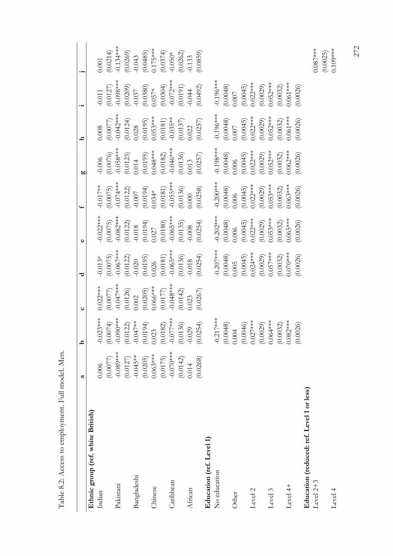
272

Tab

le ‎8

.2: A

cces

s to

em

plo

ymen

t. F

ull

mo

del

. M

en.

a

b

c

d

e

f g

h

i

j

Eth

nic

gro

up

(re

f. w

hit

e B

riti

sh)

In

dia

n

0.0

06

-0.0

23**

* 0.0

22**

* -0

.013*

-0.0

22**

* -0

.017**

-0

.006

0.0

08

-0.0

11

0.0

01

(0

.0077)

(0.0

074)

(0.0

077)

(0.0

075)

(0.0

075)

(0.0

075)

(0.0

076)

(0.0

077)

(0.0

127)

(0.0

214)

Pak

ista

ni

-0.0

89**

* -0

.090**

* -0

.047**

* -0

.067**

* -0

.082**

* -0

.074**

* -0

.058**

* -0

.042**

* -0

.098**

* -0

.134**

*

(0

.0127)

(0.0

122)

(0.0

126)

(0.0

122)

(0.0

122)

(0.0

122)

(0.0

123)

(0.0

124)

(0.0

209)

(0.0

269)

Ban

glad

esh

i -0

.045**

-0

.047**

0.0

02

-0.0

20

-0.0

18

-0.0

07

0.0

14

0.0

28

-0.0

37

-0.0

43

(0

.0205)

(0.0

194)

(0.0

205)

(0.0

195)

(0.0

194)

(0.0

194)

(0.0

195)

(0.0

195)

(0.0

380)

(0.0

485)

Ch

ines

e 0.0

63**

* 0.0

23

0.0

66**

* 0.0

26

0.0

27

0.0

34*

0.0

48**

* 0.0

53**

* 0.0

57*

0.1

75**

*

(0

.0175)

(0.0

182)

(0.0

177)

(0.0

181)

(0.0

180)

(0.0

181)

(0.0

182)

(0.0

181)

(0.0

304)

(0.0

374)

Car

ibb

ean

-0

.070**

* -0

.077**

* -0

.048**

* -0

.065**

* -0

.065**

* -0

.055**

* -0

.046**

* -0

.035**

-0

.072**

* -0

.050*

(0

.0142)

(0.0

136)

(0.0

142)

(0.0

136)

(0.0

135)

(0.0

136)

(0.0

136)

(0.0

137)

(0.0

191)

(0.0

262)

Afr

ican

0.0

14

-0.0

29

0.0

23

-0.0

18

-0.0

08

0.0

00

0.0

13

0.0

22

-0.0

44

-0.1

33

(0

.0268)

(0.0

254)

(0.0

267)

(0.0

254)

(0.0

254)

(0.0

258)

(0.0

257)

(0.0

257)

(0.0

492)

(0.0

859)

Ed

ucati

on

(re

f. L

eve

l 1)

N

o e

duca

tio

n

-0

.217**

*

-0.2

07**

* -0

.202**

* -0

.200**

* -0

.198**

* -0

.196**

* -0

.196**

*

(0.0

048)

(0

.0048)

(0.0

048)

(0.0

048)

(0.0

048)

(0.0

048)

(0.0

048)

O

ther

0.0

04

0.0

05

0.0

06

0.0

06

0.0

06

0.0

07

0.0

07

(0.0

046)

(0

.0045)

(0.0

045)

(0.0

045)

(0.0

045)

(0.0

045)

(0.0

045)

L

evel

2

0.0

27**

*

0.0

24**

* 0.0

22**

* 0.0

22**

* 0.0

22**

* 0.0

22**

* 0.0

22**

*

(0.0

029)

(0

.0029)

(0.0

029)

(0.0

029)

(0.0

029)

(0.0

029)

(0.0

029)

L

evel

3

0.0

64**

*

0.0

57**

* 0.0

53**

* 0.0

53**

* 0.0

52**

* 0.0

52**

* 0.0

52**

*

(0.0

032)

(0

.0032)

(0.0

032)

(0.0

032)

(0.0

032)

(0.0

032)

(0.0

032)

L

evel

4+

0.0

82**

*

0.0

70**

* 0.0

65**

* 0.0

63**

* 0.0

62**

* 0.0

61**

* 0.0

61**

*

(0.0

026)

(0

.0026)

(0.0

026)

(0.0

026)

(0.0

026)

(0.0

026)

(0.0

026)

E

du

cati

on

(re

du

ced

: re

f. L

eve

l 1

or

less

)

Lev

el 2

+3

0.0

87**

*

(0.0

025)

Lev

el 4

0.1

09**

*

273

a

b

c

d

e

f g

h

i

j

(0.0

025)

Pare

nta

l so

cial

cla

ss (

ref.

Sem

i an

d u

nsk

ille

d m

an

ual

- V

II)

Skill

ed m

anual

(V

I)

0.0

34**

* 0.0

17**

* 0.0

12**

* 0.0

10**

* 0.0

09**

* 0.0

08**

0.0

08**

0.0

13**

*

(0

.0035)

(0.0

033)

(0.0

033)

(0.0

033)

(0.0

033)

(0.0

033)

(0.0

033)

(0.0

034)

Lo

wer

tec

hn

icia

n (

V)

0.0

72**

* 0.0

42**

* 0.0

34**

* 0.0

27**

* 0.0

26**

* 0.0

24**

* 0.0

24**

* 0.0

31**

*

(0

.0043)

(0.0

041)

(0.0

040)

(0.0

040)

(0.0

040)

(0.0

040)

(0.0

040)

(0.0

041)

Pet

it B

ourg

eois

ie (

IV)

0.0

76**

* 0.0

48**

* 0.0

35**

* 0.0

22**

* 0.0

21**

* 0.0

18**

* 0.0

18**

* 0.0

22**

*

(0

.0036)

(0.0

035)

(0.0

035)

(0.0

035)

(0.0

035)

(0.0

035)

(0.0

035)

(0.0

036)

Ro

uti

ne

no

n-m

anual

(II

I)

0.0

71**

* 0.0

34**

* 0.0

24**

* 0.0

19**

* 0.0

17**

* 0.0

15**

* 0.0

15**

* 0.0

25**

*

(0

.0033)

(0.0

031)

(0.0

031)

(0.0

031)

(0.0

031)

(0.0

031)

(0.0

031)

(0.0

032)

Lo

wer

pro

fess

ion

al/

man

ager

ial (I

I)

0.1

01**

* 0.0

45**

* 0.0

29**

* 0.0

19**

* 0.0

16**

* 0.0

12**

* 0.0

12**

* 0.0

20**

*

(0

.0032)

(0.0

031)

(0.0

031)

(0.0

031)

(0.0

031)

(0.0

031)

(0.0

031)

(0.0

032)

Hig

her

pro

fess

ion

al/m

anag

eria

l (I

)

0.1

11**

* 0.0

43**

* 0.0

25**

* 0.0

13**

* 0.0

11**

* 0.0

06*

0.0

06

0.0

13**

*

(0

.0034)

(0.0

033)

(0.0

033)

(0.0

034)

(0.0

034)

(0.0

034)

(0.0

034)

(0.0

035)

Ear

ner

s b

ut

un

cod

ed

-0.0

52**

* -0

.045**

* -0

.043**

* -0

.041**

* -0

.039**

* -0

.040**

* -0

.040**

* -0

.044**

*

(0

.0086)

(0.0

081)

(0.0

080)

(0.0

080)

(0.0

080)

(0.0

080)

(0.0

080)

(0.0

083)

No

ear

ner

s in

hh

-0

.079**

* -0

.070**

* -0

.064**

* -0

.052**

* -0

.054**

* -0

.053**

* -0

.054**

* -0

.058**

*

(0

.0066)

(0.0

061)

(0.0

061)

(0.0

062)

(0.0

062)

(0.0

062)

(0.0

062)

(0.0

064)

Ten

ure

(re

f. o

wn

er)

So

cial

ren

t

-0

.043**

* -0

.033**

* -0

.030**

* -0

.030**

* -0

.030**

* -0

.041**

*

(0

.0025)

(0.0

026)

(0.0

026)

(0.0

026)

(0.0

026)

(0.0

027)

Pri

vat

e re

nt

-0.0

15**

* -0

.009**

* -0

.006**

-0

.006**

-0

.006**

-0

.010**

*

(0

.0031)

(0.0

031)

(0.0

031)

(0.0

031)

(0.0

031)

(0.0

032)

Nu

mb

er

of

cars

(re

f. n

on

e)

1 c

ar

0.0

39**

* 0.0

37**

* 0.0

32**

* 0.0

31**

* 0.0

37**

*

(0.0

026)

(0.0

026)

(0.0

026)

(0.0

026)

(0.0

027)

2+

car

s

0.0

47**

* 0.0

46**

* 0.0

37**

* 0.0

37**

* 0.0

43**

*

(0.0

031)

(0.0

031)

(0.0

031)

(0.0

031)

(0.0

032)

Pers

on

s p

er

roo

m (

ref.

1)

O

ver

1.5

pp

p

-0.0

42**

* -0

.041**

* -0

.040**

* -0

.060**

*

(0

.0072)

(0.0

072)

(0.0

072)

(0.0

074)

274

a

b

c

d

e

f g

h

i

j

1.5

pp

p

-0.0

17*

-0.0

15

-0.0

14

-0.0

23**

(0

.0091)

(0.0

091)

(0.0

090)

(0.0

093)

Over

1 b

ut

less

th

an 1

.5 p

pp

-0

.012**

* -0

.011**

* -0

.011**

* -0

.018**

*

(0

.0037)

(0.0

037)

(0.0

037)

(0.0

038)

Over

0.7

5 b

ut

less

th

an 1

pp

p

0.0

10**

* 0.0

09**

* 0.0

09**

* 0.0

11**

*

(0

.0025)

(0.0

025)

(0.0

025)

(0.0

026)

0.7

5 p

pp

-0

.002

-0.0

02

-0.0

02

0.0

01

(0

.0046)

(0.0

046)

(0.0

046)

(0.0

047)

Over

0.5

but

less

th

an 0

.75 p

pp

0.0

06**

0.0

04

0.0

04

0.0

07**

*

(0

.0026)

(0.0

026)

(0.0

026)

(0.0

026)

0.5

pp

p

0.0

08**

0.0

06

0.0

06

0.0

09**

(0

.0037)

(0.0

037)

(0.0

037)

(0.0

038)

Les

s th

an 0

.5 p

pp

0.0

02

-0.0

01

-0.0

01

0.0

01

(0

.0044)

(0.0

044)

(0.0

044)

(0.0

045)

Cars

tair

s q

uin

tile

s (r

ef.

Q1:

less

dep

riva

tio

n)

Car

stai

rs Q

2

-0

.001

-0.0

01

-0.0

01

(0.0

022)

(0.0

022)

(0.0

023)

Car

stai

rs Q

3

-0

.004

-0.0

04

-0.0

04*

(0.0

024)

(0.0

024)

(0.0

025)

Car

stai

rs Q

4

-0

.017**

* -0

.017**

* -0

.020**

*

(0.0

026)

(0.0

026)

(0.0

027)

Car

stai

rs Q

5

-0

.039**

* -0

.040**

* -0

.044**

*

(0.0

031)

(0.0

031)

(0.0

032)

Ag

e

Age

in

des

tin

atio

n

-0.0

01**

* 0.0

01**

* -0

.001**

* 0.0

01**

* 0.0

01**

* 0.0

01**

* 0.0

01**

* 0.0

01**

* 0.0

01**

* 0.0

00

(0

.0002)

(0.0

002)

(0.0

002)

(0.0

002)

(0.0

002)

(0.0

002)

(0.0

002)

(0.0

002)

(0.0

002)

(0.0

002)

Ori

gin

year

(ref.

1971)

1981

0.0

18**

* 0.0

12**

* 0.0

12**

* 0.0

11**

* 0.0

10**

* 0.0

04**

* 0.0

02

0.0

03**

0.0

03**

0.0

01

(0

.0015)

(0.0

014)

(0.0

015)

(0.0

014)

(0.0

014)

(0.0

015)

(0.0

015)

(0.0

015)

(0.0

015)

(0.0

015)

1991

0.0

26**

* 0.0

19**

* 0.0

06**

* 0.0

12**

* 0.0

09**

* 0.0

00

-0.0

02

-0.0

00

-0.0

00

-0.0

07**

*

(0

.0023)

(0.0

022)

(0.0

024)

(0.0

023)

(0.0

023)

(0.0

024)

(0.0

024)

(0.0

024)

(0.0

024)

(0.0

025)

275

a

b

c

d

e

f g

h

i

j

Dest

inati

on

year

(ref

. 2001)

2011

0.0

16**

* -0

.014**

* 0.0

17**

* -0

.011**

* -0

.012**

* -0

.011**

* -0

.011**

* -0

.011**

* -0

.013**

* -0

.004*

(0

.0023)

(0.0

023)

(0.0

023)

(0.0

023)

(0.0

023)

(0.0

023)

(0.0

023)

(0.0

023)

(0.0

024)

(0.0

024)

Nu

mb

er

of

cen

sus

po

ints

(re

f. 2

)

3 c

ensu

s p

oin

ts

0.0

85**

* 0.0

60**

* 0.0

71**

* 0.0

53**

* 0.0

51**

* 0.0

49**

* 0.0

49**

* 0.0

48**

* 0.0

50**

* 0.0

55**

*

(0

.0091)

(0.0

085)

(0.0

089)

(0.0

084)

(0.0

084)

(0.0

084)

(0.0

084)

(0.0

084)

(0.0

084)

(0.0

086)

4 c

ensu

s p

oin

ts

0.1

48**

* 0.1

02**

* 0.1

27**

* 0.0

93**

* 0.0

88**

* 0.0

86**

* 0.0

85**

* 0.0

83**

* 0.0

85**

* 0.0

94**

*

(0

.0091)

(0.0

086)

(0.0

089)

(0.0

085)

(0.0

085)

(0.0

085)

(0.0

085)

(0.0

085)

(0.0

085)

(0.0

087)

5 c

ensu

s p

oin

ts

0.1

96**

* 0.1

42**

* 0.1

72**

* 0.1

32**

* 0.1

26**

* 0.1

23**

* 0.1

21**

* 0.1

19**

* 0.1

21**

* 0.1

38**

*

(0

.0095)

(0.0

090)

(0.0

093)

(0.0

089)

(0.0

089)

(0.0

089)

(0.0

089)

(0.0

089)

(0.0

089)

(0.0

091)

Inte

racti

on

s w

ith

dest

inati

on

year

India

n*2

011

0.0

31**

0.0

30**

(0

.0146)

(0.0

148)

Pak

ista

ni*

2011

0.0

88**

* 0.0

86**

*

(0

.0235)

(0.0

235)

Ban

glad

esh

i*2011

0.0

94**

0.1

06**

*

(0

.0414)

(0.0

412)

Ch

ines

e*2011

-0.0

06

0.0

06

(0

.0381)

(0.0

377)

Car

ibb

ean

*2011

0.0

78**

* 0.0

74**

*

(0

.0255)

(0.0

263)

Afr

ican

*2011

0.0

99*

0.0

83

(0

.0545)

(0.0

545)

Inte

racti

on

s w

ith

ed

ucati

on

(re

du

ced

)

India

n*L

evel

2+

3

-0

.027

(0.0

258)

India

n*L

evel

4

0.0

12

(0.0

218)

Pak

ista

ni*

Lev

el 2

+3

0.0

18

(0.0

329)

Pak

ista

ni*

Lev

el 4

0.1

24**

*

276

a

b

c

d

e

f g

h

i

j

(0.0

257)

Ban

glad

esh

i*L

evel

2+

3

0.0

23

(0.0

535)

Ban

glad

esh

i*L

evel

4

0.0

31

(0.0

452)

Ch

ines

e*L

evel

2+

3

-0

.108*

(0.0

596)

Ch

ines

e*L

evel

4

-0

.142**

*

(0.0

472)

Car

ibb

ean

* L

evel

2+

3

-0

.033

(0.0

349)

Car

ibb

ean

* L

evel

4

0.0

23

(0.0

331)

Afr

ican

*Lev

el 2

+3

0.1

58*

(0.0

895)

Afr

ican

*Lev

el 4

0.1

56*

(0.0

846)

Co

nst

ant

0.7

06**

* 0.7

62**

* 0.6

77**

* 0.7

50**

* 0.7

80**

* 0.7

58**

* 0.7

59**

* 0.7

80**

* 0.7

79**

* 0.7

05**

*

(0

.0093)

(0.0

089)

(0.0

093)

(0.0

091)

(0.0

092)

(0.0

093)

(0.0

095)

(0.0

097)

(0.0

097)

(0.0

097)

Adju

sted

R-s

quar

ed

0.0

13

0.0

89

0.0

35

0.0

95

0.0

98

0.1

00

0.1

01

0.1

02

0.1

03

0.0

72

N

180,5

40

180,5

40

180,5

40

180,5

40

180,5

40

180,5

40

180,5

40

180,5

40

180,5

40

180,5

40

***

p<

0.0

1 *

* p

<0.0

5 *

p<

0.1

R

ob

ust

(cl

ust

ered

) st

and

ard

err

ors

in

par

enth

eses

P

op

ula

tio

n: In

div

idual

s b

etw

een

20 a

nd

45 y

ears

old

So

urc

e: A

uth

or’

s o

wn

cal

cula

tio

ns

bas

ed o

n O

NS

-LS

277

Tab

le ‎8

.3: A

cces

s to

em

plo

ymen

t. F

ull

mo

del

. W

om

en.

a

b

c

d

e

f g

h

i

j

Eth

nic

gro

up

(re

f. w

hit

e B

riti

sh)

In

dia

n

0.0

31**

* -0

.012

0.0

53**

* -0

.005

-0.0

15

-0.0

11

-0.0

00

0.0

07

0.0

16

0.0

65**

(0

.0101)

(0.0

097)

(0.0

101)

(0.0

097)

(0.0

097)

(0.0

097)

(0.0

099)

(0.0

099)

(0.0

148)

(0.0

264)

Pak

ista

ni

-0.2

54**

* -0

.233**

* -0

.201**

* -0

.215**

* -0

.231**

* -0

.226**

* -0

.210**

* -0

.203**

* -0

.230**

* -0

.289**

*

(0

.0154)

(0.0

139)

(0.0

153)

(0.0

139)

(0.0

140)

(0.0

140)

(0.0

141)

(0.0

142)

(0.0

213)

(0.0

258)

Ban

glad

esh

i -0

.268**

* -0

.246**

* -0

.191**

* -0

.216**

* -0

.216**

* -0

.207**

* -0

.190**

* -0

.182**

* -0

.231**

* -0

.296**

*

(0

.0246)

(0.0

220)

(0.0

250)

(0.0

223)

(0.0

222)

(0.0

223)

(0.0

224)

(0.0

224)

(0.0

377)

(0.0

415)

Ch

ines

e 0.0

77**

* 0.0

16

0.0

88**

* 0.0

24

0.0

27

0.0

31

0.0

42

0.0

44

0.1

12**

* 0.1

94**

*

(0

.0274)

(0.0

275)

(0.0

271)

(0.0

271)

(0.0

274)

(0.0

275)

(0.0

277)

(0.0

277)

(0.0

312)

(0.0

703)

Car

ibb

ean

0.0

06

-0.0

33**

0.0

36**

-0

.020

-0.0

20

-0.0

13

-0.0

04

0.0

01

-0.0

05

0.0

75**

(0

.0144)

(0.0

138)

(0.0

144)

(0.0

138)

(0.0

138)

(0.0

138)

(0.0

139)

(0.0

140)

(0.0

178)

(0.0

300)

Afr

ican

0.0

38

-0.0

51*

0.0

51*

-0.0

36

-0.0

30

-0.0

23

-0.0

11

-0.0

08

0.0

18

0.0

05

(0

.0275)

(0.0

267)

(0.0

272)

(0.0

265)

(0.0

267)

(0.0

269)

(0.0

269)

(0.0

268)

(0.0

372)

(0.0

960)

Ed

ucati

on

(re

f. L

eve

l 1)

N

o e

duca

tio

n

-0

.274**

*

-0.2

62**

* -0

.255**

* -0

.253**

* -0

.250**

* -0

.249**

* -0

.249**

*

(0.0

053)

(0

.0054)

(0.0

054)

(0.0

054)

(0.0

054)

(0.0

054)

(0.0

054)

O

ther

-0.0

00

0.0

02

0.0

04

0.0

05

0.0

05

0.0

06

0.0

06

(0.0

092)

(0

.0092)

(0.0

092)

(0.0

092)

(0.0

092)

(0.0

092)

(0.0

092)

L

evel

2

0.0

84**

*

0.0

81**

* 0.0

78**

* 0.0

78**

* 0.0

77**

* 0.0

77**

* 0.0

77**

*

(0.0

038)

(0

.0038)

(0.0

038)

(0.0

038)

(0.0

038)

(0.0

038)

(0.0

038)

L

evel

3

0.1

66**

*

0.1

59**

* 0.1

55**

* 0.1

54**

* 0.1

54**

* 0.1

53**

* 0.1

53**

*

(0.0

042)

(0

.0042)

(0.0

042)

(0.0

042)

(0.0

042)

(0.0

042)

(0.0

042)

L

evel

4+

0.1

94**

*

0.1

83**

* 0.1

76**

* 0.1

75**

* 0.1

74**

* 0.1

73**

* 0.1

73**

*

(0.0

036)

(0

.0036)

(0.0

036)

(0.0

036)

(0.0

037)

(0.0

037)

(0.0

037)

E

du

cati

on

(re

du

ced

: re

f. L

eve

l 1

or

less

)

Lev

el 2

+3

0.1

74**

*

(0.0

033)

Lev

el 4

0.2

34**

*

278

a

b

c

d

e

f g

h

i

j

(0.0

035)

Pare

nta

l so

cial

cla

ss (

ref.

Sem

i an

d u

nsk

ille

d m

an

ual

- V

II)

Skill

ed m

anual

(V

I)

0.0

45**

* 0.0

22**

* 0.0

16**

* 0.0

15**

* 0.0

14**

* 0.0

13**

* 0.0

13**

* 0.0

18**

*

(0

.0043)

(0.0

039)

(0.0

039)

(0.0

039)

(0.0

039)

(0.0

039)

(0.0

039)

(0.0

040)

Lo

wer

tec

hn

icia

n (

V)

0.0

80**

* 0.0

35**

* 0.0

25**

* 0.0

21**

* 0.0

19**

* 0.0

18**

* 0.0

18**

* 0.0

27**

*

(0

.0055)

(0.0

051)

(0.0

051)

(0.0

052)

(0.0

052)

(0.0

052)

(0.0

052)

(0.0

053)

Pet

it B

ourg

eois

ie (

IV)

0.0

88**

* 0.0

33**

* 0.0

19**

* 0.0

10**

0.0

09**

0.0

08*

0.0

08*

0.0

15**

*

(0

.0046)

(0.0

043)

(0.0

044)

(0.0

044)

(0.0

045)

(0.0

045)

(0.0

045)

(0.0

045)

Ro

uti

ne

no

n-m

anual

(II

I)

0.1

01**

* 0.0

40**

* 0.0

29**

* 0.0

26**

* 0.0

24**

* 0.0

23**

* 0.0

23**

* 0.0

33**

*

(0

.0040)

(0.0

037)

(0.0

038)

(0.0

038)

(0.0

038)

(0.0

038)

(0.0

038)

(0.0

039)

Lo

wer

pro

fess

ion

al/

man

ager

ial (I

I)

0.1

37**

* 0.0

39**

* 0.0

22**

* 0.0

15**

* 0.0

12**

* 0.0

11**

* 0.0

11**

* 0.0

20**

*

(0

.0040)

(0.0

038)

(0.0

039)

(0.0

039)

(0.0

039)

(0.0

040)

(0.0

040)

(0.0

040)

Hig

her

pro

fess

ion

al/m

anag

eria

l (I

)

0.1

53**

* 0.0

34**

* 0.0

15**

* 0.0

07

0.0

04

0.0

02

0.0

02

0.0

10**

(0

.0043)

(0.0

042)

(0.0

043)

(0.0

044)

(0.0

044)

(0.0

044)

(0.0

044)

(0.0

045)

Ear

ner

s b

ut

un

cod

ed

-0.0

57**

* -0

.035**

* -0

.033**

* -0

.032**

* -0

.030**

* -0

.029**

* -0

.030**

* -0

.041**

*

(0

.0093)

(0.0

085)

(0.0

085)

(0.0

085)

(0.0

085)

(0.0

085)

(0.0

085)

(0.0

088)

No

ear

ner

s in

hh

-0

.109**

* -0

.086**

* -0

.079**

* -0

.071**

* -0

.074**

* -0

.073**

* -0

.073**

* -0

.082**

*

(0

.0070)

(0.0

063)

(0.0

063)

(0.0

063)

(0.0

063)

(0.0

063)

(0.0

063)

(0.0

066)

Ten

ure

(re

f. o

wn

er)

So

cial

ren

t

-0

.046**

* -0

.039**

* -0

.035**

* -0

.035**

* -0

.035**

* -0

.050**

*

(0

.0031)

(0.0

031)

(0.0

032)

(0.0

032)

(0.0

032)

(0.0

033)

Pri

vat

e re

nt

-0.0

15**

* -0

.011**

* -0

.008**

-0

.008**

-0

.008**

-0

.013**

*

(0

.0040)

(0.0

040)

(0.0

040)

(0.0

040)

(0.0

040)

(0.0

041)

Num

ber

of

cars

(re

f. n

on

e)

1 c

ar

0.0

26**

* 0.0

24**

* 0.0

22**

* 0.0

22**

* 0.0

30**

*

(0.0

030)

(0.0

030)

(0.0

030)

(0.0

030)

(0.0

031)

2+

car

s

0.0

32**

* 0.0

31**

* 0.0

27**

* 0.0

27**

* 0.0

35**

*

(0.0

039)

(0.0

039)

(0.0

039)

(0.0

039)

(0.0

040)

Pers

on

s p

er

roo

m (

ref.

1)

O

ver

1.5

pp

p

-0.0

29**

* -0

.028**

* -0

.028**

* -0

.053**

*

(0

.0076)

(0.0

076)

(0.0

076)

(0.0

078)

279

a

b

c

d

e

f g

h

i

j

1.5

pp

p

-0.0

01

0.0

00

0.0

00

-0.0

18*

(0

.0102)

(0.0

102)

(0.0

102)

(0.0

105)

Over

1 b

ut

less

th

an 1

.5 p

pp

-0

.017**

* -0

.016**

* -0

.016**

* -0

.026**

*

(0

.0043)

(0.0

043)

(0.0

043)

(0.0

044)

Over

0.7

5 b

ut

less

th

an 1

pp

p

0.0

12**

* 0.0

11**

* 0.0

11**

* 0.0

16**

*

(0

.0032)

(0.0

032)

(0.0

032)

(0.0

032)

0.7

5 p

pp

0.0

07

0.0

07

0.0

07

0.0

11*

(0

.0057)

(0.0

057)

(0.0

057)

(0.0

058)

Over

0.5

but

less

th

an 0

.75 p

pp

0.0

12**

* 0.0

11**

* 0.0

11**

* 0.0

16**

*

(0

.0032)

(0.0

032)

(0.0

032)

(0.0

033)

0.5

pp

p

0.0

09*

0.0

08*

0.0

08*

0.0

13**

*

(0

.0047)

(0.0

047)

(0.0

047)

(0.0

048)

Les

s th

an 0

.5 p

pp

-0

.001

-0.0

03

-0.0

03

0.0

03

(0

.0057)

(0.0

057)

(0.0

057)

(0.0

058)

Cars

tair

s q

uin

tile

s (r

ef.

Q1:

less

dep

riva

tio

n)

Car

stai

rs Q

2

0.0

04

0.0

04

0.0

04

(0.0

031)

(0.0

031)

(0.0

031)

Car

stai

rs Q

3

0.0

01

0.0

01

0.0

00

(0.0

032)

(0.0

032)

(0.0

033)

Car

stai

rs Q

4

-0

.002

-0.0

02

-0.0

06*

(0.0

034)

(0.0

034)

(0.0

035)

Car

stai

rs Q

5

-0

.017**

* -0

.017**

* -0

.026**

*

(0.0

038)

(0.0

038)

(0.0

039)

Ag

e

Age

in

des

tin

atio

n

-0.0

01**

0.0

02**

* -0

.001**

* 0.0

02**

* 0.0

02**

* 0.0

02**

* 0.0

02**

* 0.0

02**

* 0.0

02**

* 0.0

01**

(0

.0003)

(0.0

003)

(0.0

003)

(0.0

003)

(0.0

003)

(0.0

003)

(0.0

003)

(0.0

003)

(0.0

003)

(0.0

003)

Ori

gin

year

(ref.

1971)

1981

0.0

02

-0.0

04**

-0

.006**

* -0

.004**

* -0

.005**

* -0

.009**

* -0

.011**

* -0

.010**

* -0

.010**

* -0

.013**

*

(0

.0017)

(0.0

016)

(0.0

018)

(0.0

017)

(0.0

017)

(0.0

018)

(0.0

018)

(0.0

018)

(0.0

018)

(0.0

018)

1991

0.0

26**

* 0.0

17**

* -0

.000

0.0

12**

* 0.0

08**

* 0.0

03

0.0

01

0.0

02

0.0

02

-0.0

09**

*

(0

.0028)

(0.0

026)

(0.0

029)

(0.0

027)

(0.0

028)

(0.0

029)

(0.0

030)

(0.0

030)

(0.0

030)

(0.0

030)

280

a

b

c

d

e

f g

h

i

j

Dest

inati

on

year

(ref

. 2001)

2011

0.0

60**

* 0.0

04

0.0

65**

* 0.0

08**

0.0

07**

0.0

08**

* 0.0

07**

0.0

07**

0.0

07**

0.0

24**

*

(0

.0030)

(0.0

029)

(0.0

030)

(0.0

030)

(0.0

030)

(0.0

030)

(0.0

030)

(0.0

030)

(0.0

030)

(0.0

030)

Nu

mb

er

of

cen

sus

po

ints

(re

f. 2

)

3 c

ensu

s p

oin

ts

0.1

33**

* 0.0

80**

* 0.1

07**

* 0.0

72**

* 0.0

69**

* 0.0

68**

* 0.0

68**

* 0.0

67**

* 0.0

68**

* 0.0

75**

*

(0

.0103)

(0.0

094)

(0.0

101)

(0.0

093)

(0.0

093)

(0.0

093)

(0.0

093)

(0.0

093)

(0.0

093)

(0.0

094)

4 c

ensu

s p

oin

ts

0.1

73**

* 0.0

95**

* 0.1

45**

* 0.0

86**

* 0.0

81**

* 0.0

81**

* 0.0

79**

* 0.0

78**

* 0.0

79**

* 0.0

91**

*

(0

.0105)

(0.0

096)

(0.0

103)

(0.0

096)

(0.0

096)

(0.0

095)

(0.0

095)

(0.0

095)

(0.0

095)

(0.0

097)

5 c

ensu

s p

oin

ts

0.1

93**

* 0.1

17**

* 0.1

62**

* 0.1

06**

* 0.1

00**

* 0.0

99**

* 0.0

97**

* 0.0

97**

* 0.0

97**

* 0.1

18**

*

(0

.0112)

(0.0

103)

(0.0

110)

(0.0

103)

(0.0

103)

(0.0

102)

(0.0

102)

(0.0

102)

(0.0

102)

(0.0

104)

Inte

racti

on

s w

ith

dest

inati

on

year

India

n*2

011

-0.0

16

-0.0

21

(0

.0166)

(0.0

169)

Pak

ista

ni*

2011

0.0

44*

0.0

30

(0

.0238)

(0.0

247)

Ban

glad

esh

i*2011

0.0

69*

0.0

44

(0

.0414)

(0.0

411)

Ch

ines

e*2011

-0.1

10**

* -0

.115**

*

(0

.0366)

(0.0

357)

Car

ibb

ean

*2011

0.0

13

0.0

12

(0

.0228)

(0.0

231)

Afr

ican

*2011

-0.0

43

-0.0

58

(0

.0434)

(0.0

432)

Inte

racti

on

s w

ith

ed

ucati

on

(re

du

ced

)

India

n*L

evel

2+

3

-0

.056*

(0.0

312)

India

n*L

evel

4

-0

.023

(0.0

279)

Pak

ista

ni*

Lev

el 2

+3

0.0

64*

(0.0

339)

Pak

ista

ni*

Lev

el 4

0.1

81**

*

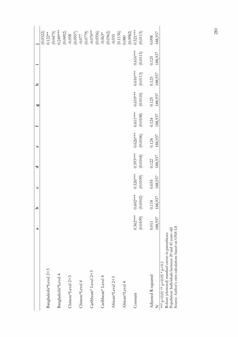
281

a

b

c

d

e

f g

h

i

j

(0.0

322)

Ban

glad

esh

i*L

evel

2+

3

0.1

22**

(0.0

475)

Ban

glad

esh

i*L

evel

4

0.2

49**

*

(0.0

492)

Ch

ines

e*L

evel

2+

3

-0

.058

(0.0

957)

Ch

ines

e*L

evel

4

-0

.077

(0.0

779)

Car

ibb

ean

* L

evel

2+

3

-0

.070**

(0.0

356)

Car

ibb

ean

* L

evel

4

-0

.063*

(0.0

362)

Afr

ican

*Lev

el 2

+3

-0

.035

(0.1

136)

Afr

ican

*Lev

el 4

0.0

80

(0.0

982)

Co

nst

ant

0.5

62**

* 0.6

02**

* 0.5

26**

* 0.5

93**

* 0.6

26**

* 0.6

11**

* 0.6

10**

* 0.6

16**

* 0.6

16**

* 0.5

21**

*

(0

.0109)

(0.0

102)

(0.0

109)

(0.0

104)

(0.0

106)

(0.0

108)

(0.0

110)

(0.0

113)

(0.0

113)

(0.0

113)

Adju

sted

R-s

quar

ed

0.0

11

0.1

18

0.0

35

0.1

22

0.1

24

0.1

24

0.1

25

0.1

25

0.1

25

0.0

98

N

188,9

37

188,9

37

188,9

37

188,9

37

188,9

37

188,9

37

188,9

37

188,9

37

188,9

37

188,9

37

***

p<

0.0

1 *

* p

<0.0

5 *

p<

0.1

R

ob

ust

(cl

ust

ered

) st

and

ard

err

ors

in

par

enth

eses

P

op

ula

tio

n: In

div

idual

s b

etw

een

20 a

nd

45 y

ears

old

So

urc

e: A

uth

or’

s o

wn

cal

cula

tio

ns

bas

ed o

n O

NS

-LS

282

Tab

le ‎8

.4: A

cces

s to

th

e se

rvic

e cl

ass.

Full

mo

del

. M

en.

a

b

c

d

e

f g

i

j

Eth

nic

gro

up

(re

f. w

hit

e B

riti

sh)

India

n

0.1

55**

* 0.0

27**

* 0.2

06**

* 0.0

60**

* 0.0

49**

* 0.0

53**

* 0.0

71**

* 0.0

78**

* 0.0

71**

*

(0

.0129)

(0.0

102)

(0.0

126)

(0.0

102)

(0.0

103)

(0.0

103)

(0.0

103)

(0.0

104)

(0.0

153)

Pak

ista

ni

-0.0

12

-0.0

55**

* 0.0

84**

* -0

.011

-0.0

27**

-0

.022*

0.0

02

0.0

10

-0.0

02

(0

.0161)

(0.0

125)

(0.0

154)

(0.0

125)

(0.0

126)

(0.0

126)

(0.0

127)

(0.0

128)

(0.0

185)

Ban

glad

esh

i 0.0

09

-0.0

30

0.1

07**

* 0.0

13

0.0

16

0.0

23

0.0

50**

0.0

56**

0.0

74*

(0

.0278)

(0.0

228)

(0.0

279)

(0.0

231)

(0.0

232)

(0.0

231)

(0.0

233)

(0.0

233)

(0.0

378)

Ch

ines

e 0.1

79**

* 0.0

03

0.2

11**

* 0.0

33

0.0

35

0.0

40

0.0

60*

0.0

63*

0.0

54

(0

.0395)

(0.0

331)

(0.0

372)

(0.0

324)

(0.0

325)

(0.0

325)

(0.0

325)

(0.0

324)

(0.0

465)

Car

ibb

ean

-0

.035*

-0.0

44**

* 0.0

16

-0.0

23

-0.0

23

-0.0

18

-0.0

04

0.0

02

-0.0

14

(0

.0188)

(0.0

163)

(0.0

189)

(0.0

165)

(0.0

164)

(0.0

164)

(0.0

165)

(0.0

165)

(0.0

210)

Afr

ican

0.1

10**

-0

.014

0.1

14**

* -0

.005

0.0

07

0.0

12

0.0

30

0.0

36

0.1

19*

(0

.0448)

(0.0

409)

(0.0

424)

(0.0

401)

(0.0

400)

(0.0

401)

(0.0

399)

(0.0

399)

(0.0

607)

Ed

ucati

on

(re

f. L

eve

l 1)

No

educa

tio

n

-0

.146**

*

-0.1

29**

* -0

.124**

* -0

.123**

* -0

.120**

* -0

.119**

* -0

.119**

*

(0.0

040)

(0

.0040)

(0.0

040)

(0.0

040)

(0.0

040)

(0.0

040)

(0.0

040)

Oth

er

-0

.076**

*

-0.0

72**

* -0

.071**

* -0

.071**

* -0

.071**

* -0

.071**

* -0

.071**

*

(0.0

054)

(0

.0053)

(0.0

053)

(0.0

053)

(0.0

053)

(0.0

053)

(0.0

053)

Lev

el 2

0.1

10**

*

0.1

01**

* 0.0

99**

* 0.0

99**

* 0.0

98**

* 0.0

98**

* 0.0

98**

*

(0.0

042)

(0

.0042)

(0.0

042)

(0.0

042)

(0.0

042)

(0.0

042)

(0.0

042)

Lev

el 3

0.1

94**

*

0.1

76**

* 0.1

72**

* 0.1

72**

* 0.1

70**

* 0.1

69**

* 0.1

69**

*

(0.0

052)

(0

.0052)

(0.0

052)

(0.0

052)

(0.0

052)

(0.0

052)

(0.0

052)

Lev

el 4

+

0.5

28**

*

0.4

87**

* 0.4

81**

* 0.4

80**

* 0.4

76**

* 0.4

75**

* 0.4

75**

*

(0.0

039)

(0

.0041)

(0.0

041)

(0.0

042)

(0.0

042)

(0.0

042)

(0.0

042)

Pare

nta

l so

cial

cla

ss (

ref.

Sem

i an

d u

nsk

ille

d m

an

ual

- V

II)

Skill

ed m

anual

(V

I)

0.0

47**

* 0.0

15**

* 0.0

09**

0.0

08**

0.0

07*

0.0

07*

0.0

07*

(0

.0046)

(0.0

040)

(0.0

040)

(0.0

040)

(0.0

040)

(0.0

040)

(0.0

040)

Lo

wer

tec

hn

icia

n (

V)

0.1

20**

* 0.0

54**

* 0.0

45**

* 0.0

42**

* 0.0

41**

* 0.0

39**

* 0.0

39**

*

283

a

b

c

d

e

f g

i

j

(0

.0066)

(0.0

057)

(0.0

057)

(0.0

058)

(0.0

058)

(0.0

058)

(0.0

058)

Pet

it B

ourg

eois

ie (

IV)

0.0

90**

* 0.0

32**

* 0.0

18**

* 0.0

08*

0.0

06

0.0

03

0.0

03

(0

.0053)

(0.0

047)

(0.0

047)

(0.0

048)

(0.0

048)

(0.0

048)

(0.0

048)

Ro

uti

ne

no

n-m

anual

(II

I)

0.1

54**

* 0.0

74**

* 0.0

63**

* 0.0

60**

* 0.0

56**

* 0.0

55**

* 0.0

55**

*

(0

.0046)

(0.0

041)

(0.0

042)

(0.0

042)

(0.0

042)

(0.0

042)

(0.0

042)

Lo

wer

pro

fess

ion

al/

man

ager

ial (I

I)

0.2

92**

* 0.1

28**

* 0.1

11**

* 0.1

03**

* 0.0

97**

* 0.0

93**

* 0.0

93**

*

(0

.0048)

(0.0

044)

(0.0

045)

(0.0

046)

(0.0

046)

(0.0

046)

(0.0

046)

Hig

her

pro

fess

ion

al/m

anag

eria

l (I

)

0.3

86**

* 0.1

62**

* 0.1

42**

* 0.1

33**

* 0.1

25**

* 0.1

19**

* 0.1

19**

*

(0

.0053)

(0.0

051)

(0.0

052)

(0.0

053)

(0.0

053)

(0.0

053)

(0.0

053)

Ear

ner

s b

ut

un

cod

ed

0.0

22**

0.0

20**

0.0

21**

0.0

21**

0.0

23**

* 0.0

22**

* 0.0

22**

*

(0

.0098)

(0.0

085)

(0.0

084)

(0.0

084)

(0.0

084)

(0.0

084)

(0.0

084)

No

ear

ner

s in

hh

0.0

35**

* 0.0

31**

* 0.0

38**

* 0.0

44**

* 0.0

35**

* 0.0

35**

* 0.0

35**

*

(0

.0074)

(0.0

064)

(0.0

064)

(0.0

064)

(0.0

064)

(0.0

065)

(0.0

065)

Ten

ure

(re

f. o

wn

er)

So

cial

ren

t

-0

.047**

* -0

.042**

* -0

.034**

* -0

.034**

* -0

.034**

*

(0

.0032)

(0.0

033)

(0.0

034)

(0.0

034)

(0.0

034)

Pri

vat

e re

nt

-0.0

23**

* -0

.020**

* -0

.016**

* -0

.017**

* -0

.017**

*

(0

.0044)

(0.0

044)

(0.0

045)

(0.0

045)

(0.0

045)

Nu

mb

er

of

cars

(re

f. n

on

e)

1 c

ar

0.0

15**

* 0.0

14**

* 0.0

10**

* 0.0

10**

*

(0.0

032)

(0.0

032)

(0.0

032)

(0.0

032)

2+

car

s

0.0

36**

* 0.0

33**

* 0.0

24**

* 0.0

24**

*

(0.0

043)

(0.0

043)

(0.0

044)

(0.0

044)

Pers

on

s p

er

roo

m (

ref.

1)

Over

1.5

pp

p

-0.0

40**

* -0

.040**

* -0

.040**

*

(0

.0071)

(0.0

071)

(0.0

071)

1.5

pp

p

-0.0

14

-0.0

13

-0.0

13

(0

.0104)

(0.0

104)

(0.0

104)

Over

1 b

ut

less

th

an 1

.5 p

pp

-0

.013**

* -0

.013**

* -0

.013**

*

(0

.0044)

(0.0

044)

(0.0

044)

Over

0.7

5 b

ut

less

th

an 1

pp

p

0.0

10**

* 0.0

09**

* 0.0

09**

*

284

a

b

c

d

e

f g

i

j

(0

.0035)

(0.0

035)

(0.0

035)

0.7

5 p

pp

0.0

13**

0.0

13**

0.0

13**

(0

.0063)

(0.0

063)

(0.0

063)

Over

0.5

but

less

th

an 0

.75 p

pp

0.0

28**

* 0.0

25**

* 0.0

25**

*

(0

.0036)

(0.0

037)

(0.0

037)

0.5

pp

p

0.0

33**

* 0.0

30**

* 0.0

30**

*

(0

.0055)

(0.0

055)

(0.0

055)

Les

s th

an 0

.5 p

pp

0.0

43**

* 0.0

40**

* 0.0

40**

*

(0

.0066)

(0.0

066)

(0.0

066)

Cars

tair

s q

uin

tile

s (r

ef.

Q1:

less

dep

riva

tio

n)

Car

stai

rs Q

2

-0

.020**

* -0

.020**

*

(0.0

037)

(0.0

037)

Car

stai

rs Q

3

-0

.026**

* -0

.026**

*

(0.0

039)

(0.0

039)

Car

stai

rs Q

4

-0

.037**

* -0

.037**

*

(0.0

040)

(0.0

040)

Car

stai

rs Q

5

-0

.036**

* -0

.036**

*

(0.0

042)

(0.0

042)

Ag

e

Age

in

des

tin

atio

n

0.0

04**

* 0.0

06**

* 0.0

03**

* 0.0

06**

* 0.0

06**

* 0.0

06**

* 0.0

06**

* 0.0

06**

* 0.0

06**

*

(0

.0003)

(0.0

003)

(0.0

003)

(0.0

003)

(0.0

003)

(0.0

003)

(0.0

003)

(0.0

003)

(0.0

003)

Ori

gin

year

(ref.

1971)

1981

0.0

26**

* 0.0

09**

* 0.0

03

0.0

00

-0.0

02

-0.0

06**

* -0

.010**

* -0

.009**

* -0

.009**

*

(0

.0021)

(0.0

018)

(0.0

022)

(0.0

018)

(0.0

019)

(0.0

019)

(0.0

020)

(0.0

020)

(0.0

020)

1991

0.0

20**

* -0

.003

-0.0

44**

* -0

.030**

* -0

.035**

* -0

.043**

* -0

.048**

* -0

.046**

* -0

.046**

*

(0

.0034)

(0.0

029)

(0.0

036)

(0.0

030)

(0.0

031)

(0.0

032)

(0.0

033)

(0.0

033)

(0.0

033)

Dest

inati

on

year

(ref

. 2001)

2011

0.0

18**

* -0

.064**

* 0.0

23**

* -0

.054**

* -0

.056**

* -0

.054**

* -0

.055**

* -0

.055**

* -0

.055**

*

(0

.0034)

(0.0

031)

(0.0

033)

(0.0

031)

(0.0

031)

(0.0

031)

(0.0

031)

(0.0

031)

(0.0

031)

Nu

mb

er

of

cen

sus

po

ints

(re

f. 2

)

3 c

ensu

s p

oin

ts

0.0

49**

* -0

.005

0.0

23**

-0

.011

-0.0

14

-0.0

15*

-0.0

16*

-0.0

17*

-0.0

17*

285

a

b

c

d

e

f g

i

j

(0

.0100)

(0.0

090)

(0.0

097)

(0.0

090)

(0.0

090)

(0.0

090)

(0.0

090)

(0.0

090)

(0.0

090)

4 c

ensu

s p

oin

ts

0.1

12**

* 0.0

09

0.0

75**

* 0.0

03

-0.0

03

-0.0

04

-0.0

06

-0.0

07

-0.0

08

(0

.0102)

(0.0

092)

(0.0

100)

(0.0

092)

(0.0

092)

(0.0

092)

(0.0

091)

(0.0

091)

(0.0

092)

5 c

ensu

s p

oin

ts

0.1

22**

* 0.0

21**

0.0

83**

* 0.0

15

0.0

08

0.0

06

0.0

03

0.0

02

0.0

02

(0

.0111)

(0.0

098)

(0.0

107)

(0.0

098)

(0.0

098)

(0.0

098)

(0.0

098)

(0.0

098)

(0.0

098)

Inte

racti

on

s w

ith

dest

inati

on

year

India

n*2

011

0.0

12

(0

.0186)

Pak

ista

ni*

2011

0.0

19

(0

.0225)

Ban

glad

esh

i*2011

-0.0

25

(0

.0423)

Ch

ines

e*2011

0.0

14

(0

.0525)

Car

ibb

ean

*2011

0.0

33

(0

.0296)

Afr

ican

*2011

-0.1

25**

(0

.0619)

Co

nst

ant

0.2

74**

* 0.2

50**

* 0.1

84**

* 0.2

11**

* 0.2

46**

* 0.2

37**

* 0.2

33**

* 0.2

63**

* 0.2

64**

*

(0

.0105)

(0.0

097)

(0.0

105)

(0.0

099)

(0.0

102)

(0.0

104)

(0.0

106)

(0.0

111)

(0.0

111)

N

0.0

12

0.2

38

0.0

79

0.2

49

0.2

51

0.2

51

0.2

52

0.2

53

0.2

53

Adju

sted

R-s

quar

ed

174,1

10

174,1

10

174,1

10

174,1

10

174,1

10

174,1

10

174,1

10

174,1

10

174,1

10

***

p<

0.0

1 *

* p

<0.0

5 *

p<

0.1

R

ob

ust

(cl

ust

ered

) st

and

ard

err

ors

in

par

enth

eses

P

op

ula

tio

n: In

div

idual

s b

etw

een

20 a

nd

45 y

ears

old

So

urc

e: A

uth

or’

s o

wn

cal

cula

tio

ns

bas

ed o

n O

NS

-LS

286

Tab

le ‎8

.5: A

cces

s to

th

e se

rvic

e cl

ass.

Full

mo

del

. W

om

en.

a

b

c

d

e

f g

i

j

Eth

nic

gro

up

(re

f. w

hit

e B

riti

sh)

India

n

0.1

28**

* 0.0

21**

0.1

74**

* 0.0

44**

* 0.0

33**

* 0.0

38**

* 0.0

49**

* 0.0

54**

* 0.0

41**

(0

.0129)

(0.0

108)

(0.0

126)

(0.0

108)

(0.0

108)

(0.0

108)

(0.0

109)

(0.0

110)

(0.0

164)

Pak

ista

ni

-0.0

21

-0.0

38**

* 0.0

64**

* -0

.007

-0.0

22

-0.0

16

-0.0

01

0.0

04

-0.0

14

(0

.0164)

(0.0

136)

(0.0

162)

(0.0

137)

(0.0

137)

(0.0

137)

(0.0

138)

(0.0

139)

(0.0

223)

Ban

glad

esh

i -0

.044*

-0.0

41**

0.0

63**

-0

.004

-0.0

03

0.0

08

0.0

23

0.0

27

0.0

28

(0

.0264)

(0.0

207)

(0.0

258)

(0.0

206)

(0.0

206)

(0.0

206)

(0.0

208)

(0.0

209)

(0.0

386)

Ch

ines

e 0.1

08**

* -0

.057*

0.1

37**

* -0

.039

-0.0

36

-0.0

29

-0.0

17

-0.0

15

-0.0

36

(0

.0369)

(0.0

295)

(0.0

367)

(0.0

296)

(0.0

297)

(0.0

297)

(0.0

298)

(0.0

297)

(0.0

494)

Car

ibb

ean

0.0

59**

* -0

.000

0.1

06**

* 0.0

19

0.0

20

0.0

27*

0.0

35**

0.0

39**

0.0

48**

(0

.0178)

(0.0

152)

(0.0

176)

(0.0

151)

(0.0

152)

(0.0

152)

(0.0

152)

(0.0

152)

(0.0

197)

Afr

ican

0.1

35**

* -0

.086**

0.1

38**

* -0

.074**

-0

.066*

-0.0

57

-0.0

44

-0.0

41

-0.0

04

(0

.0374)

(0.0

364)

(0.0

382)

(0.0

365)

(0.0

364)

(0.0

364)

(0.0

364)

(0.0

364)

(0.0

494)

Ed

ucati

on

(re

f. L

eve

l 1)

No

educa

tio

n

-0

.113**

*

-0.1

00**

* -0

.093**

* -0

.091**

* -0

.088**

* -0

.088**

* -0

.088**

*

(0.0

037)

(0

.0037)

(0.0

037)

(0.0

037)

(0.0

037)

(0.0

037)

(0.0

037)

Oth

er

-0

.035**

*

-0.0

31**

* -0

.029**

* -0

.028**

* -0

.028**

* -0

.028**

* -0

.028**

*

(0.0

074)

(0

.0074)

(0.0

074)

(0.0

074)

(0.0

074)

(0.0

074)

(0.0

074)

Lev

el 2

0.0

83**

*

0.0

76**

* 0.0

73**

* 0.0

73**

* 0.0

72**

* 0.0

72**

* 0.0

72**

*

(0.0

037)

(0

.0037)

(0.0

037)

(0.0

037)

(0.0

037)

(0.0

037)

(0.0

037)

Lev

el 3

0.1

80**

*

0.1

67**

* 0.1

63**

* 0.1

62**

* 0.1

61**

* 0.1

60**

* 0.1

61**

*

(0.0

048)

(0

.0048)

(0.0

048)

(0.0

048)

(0.0

048)

(0.0

048)

(0.0

048)

Lev

el 4

+

0.5

50**

*

0.5

22**

* 0.5

15**

* 0.5

13**

* 0.5

10**

* 0.5

10**

* 0.5

10**

*

(0.0

037)

(0

.0039)

(0.0

039)

(0.0

040)

(0.0

040)

(0.0

040)

(0.0

040)

Pare

nta

l so

cial

cla

ss (

ref.

Sem

i an

d u

nsk

ille

d m

an

ual

- V

II)

Skill

ed m

anual

(V

I)

0.0

44**

* 0.0

19**

* 0.0

13**

* 0.0

11**

* 0.0

11**

* 0.0

11**

* 0.0

11**

*

(0

.0043)

(0.0

037)

(0.0

037)

(0.0

038)

(0.0

038)

(0.0

038)

(0.0

038)

Lo

wer

tec

hn

icia

n (

V)

0.0

91**

* 0.0

38**

* 0.0

28**

* 0.0

25**

* 0.0

24**

* 0.0

24**

* 0.0

24**

*

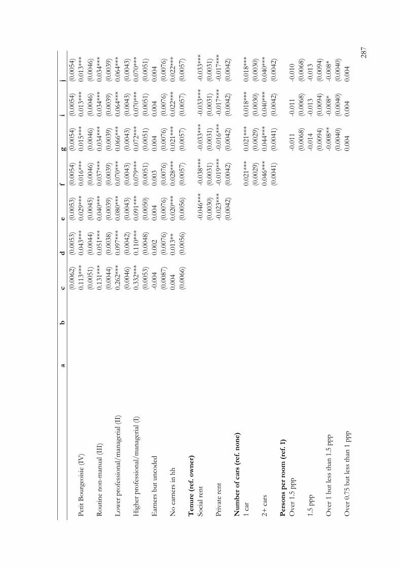
287

a

b

c

d

e

f g

i

j

(0

.0062)

(0.0

053)

(0.0

053)

(0.0

054)

(0.0

054)

(0.0

054)

(0.0

054)

Pet

it B

ourg

eois

ie (

IV)

0.1

13**

* 0.0

43**

* 0.0

29**

* 0.0

16**

* 0.0

15**

* 0.0

13**

* 0.0

13**

*

(0

.0051)

(0.0

044)

(0.0

045)

(0.0

046)

(0.0

046)

(0.0

046)

(0.0

046)

Ro

uti

ne

no

n-m

anual

(II

I)

0.1

31**

* 0.0

51**

* 0.0

40**

* 0.0

37**

* 0.0

34**

* 0.0

34**

* 0.0

34**

*

(0

.0044)

(0.0

038)

(0.0

039)

(0.0

039)

(0.0

039)

(0.0

039)

(0.0

039)

Lo

wer

pro

fess

ion

al/

man

ager

ial (I

I)

0.2

62**

* 0.0

97**

* 0.0

80**

* 0.0

70**

* 0.0

66**

* 0.0

64**

* 0.0

64**

*

(0

.0046)

(0.0

042)

(0.0

043)

(0.0

043)

(0.0

043)

(0.0

043)

(0.0

043)

Hig

her

pro

fess

ion

al/m

anag

eria

l (I

)

0.3

32**

* 0.1

10**

* 0.0

91**

* 0.0

79**

* 0.0

72**

* 0.0

70**

* 0.0

70**

*

(0

.0053)

(0.0

048)

(0.0

050)

(0.0

051)

(0.0

051)

(0.0

051)

(0.0

051)

Ear

ner

s b

ut

un

cod

ed

-0.0

04

0.0

02

0.0

04

0.0

03

0.0

04

0.0

04

0.0

04

(0

.0087)

(0.0

076)

(0.0

076)

(0.0

076)

(0.0

076)

(0.0

076)

(0.0

076)

No

ear

ner

s in

hh

0.0

04

0.0

13**

0.0

20**

* 0.0

28**

* 0.0

21**

* 0.0

22**

* 0.0

22**

*

(0

.0066)

(0.0

056)

(0.0

056)

(0.0

057)

(0.0

057)

(0.0

057)

(0.0

057)

Ten

ure

(re

f. o

wn

er)

So

cial

ren

t

-0

.046**

* -0

.038**

* -0

.033**

* -0

.033**

* -0

.033**

*

(0

.0030)

(0.0

031)

(0.0

031)

(0.0

031)

(0.0

031)

Pri

vat

e re

nt

-0.0

23**

* -0

.019**

* -0

.016**

* -0

.017**

* -0

.017**

*

(0

.0042)

(0.0

042)

(0.0

042)

(0.0

042)

(0.0

042)

Nu

mb

er

of

cars

(re

f. n

on

e)

1 c

ar

0.0

21**

* 0.0

21**

* 0.0

18**

* 0.0

18**

*

(0.0

029)

(0.0

029)

(0.0

030)

(0.0

030)

2+

car

s

0.0

46**

* 0.0

44**

* 0.0

40**

* 0.0

40**

*

(0.0

041)

(0.0

041)

(0.0

042)

(0.0

042)

Pers

on

s p

er

roo

m (

ref.

1)

Over

1.5

pp

p

-0.0

11

-0.0

11

-0.0

10

(0

.0068)

(0.0

068)

(0.0

068)

1.5

pp

p

-0.0

14

-0.0

13

-0.0

13

(0

.0094)

(0.0

094)

(0.0

094)

Over

1 b

ut

less

th

an 1

.5 p

pp

-0

.008**

-0

.008*

-0.0

08*

(0

.0040)

(0.0

040)

(0.0

040)

Over

0.7

5 b

ut

less

th

an 1

pp

p

0.0

04

0.0

04

0.0

04

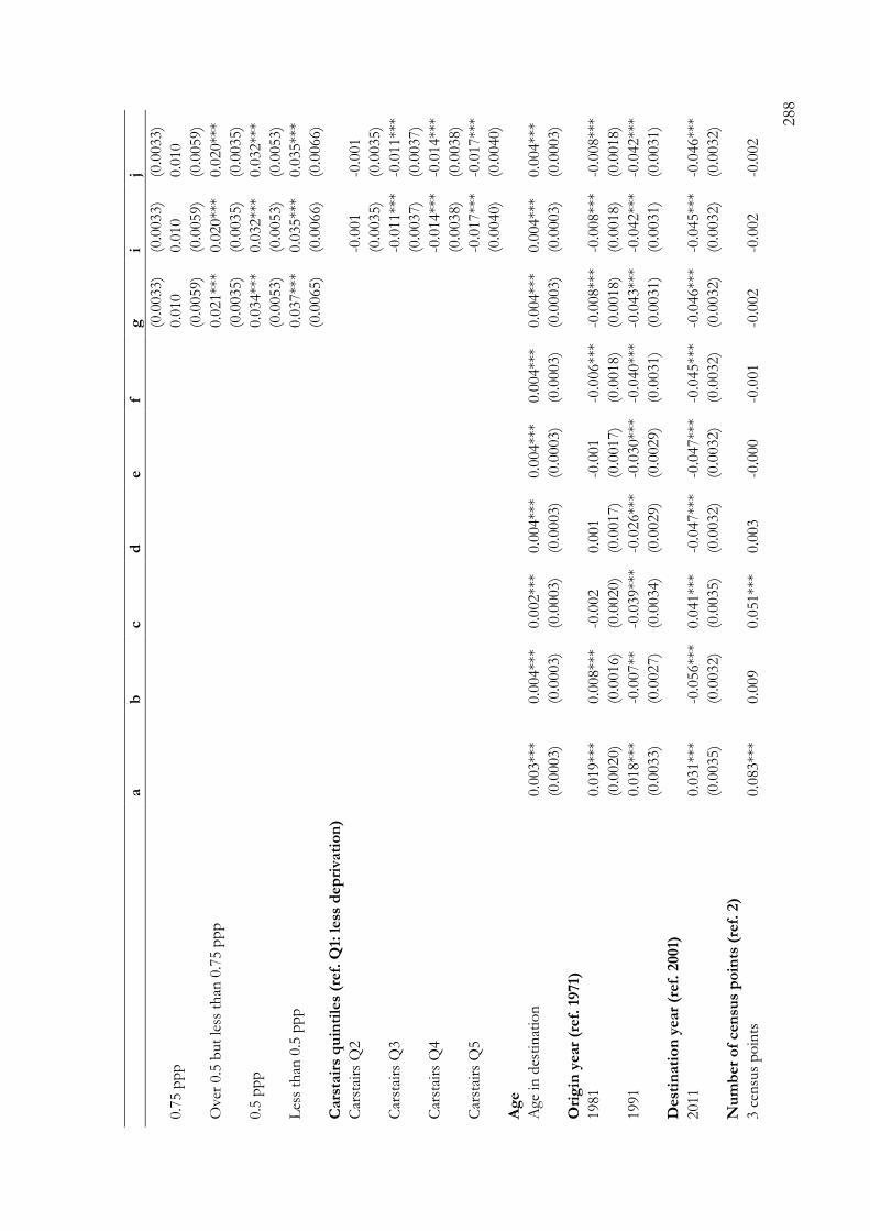
288

a

b

c

d

e

f g

i

j

(0

.0033)

(0.0

033)

(0.0

033)

0.7

5 p

pp

0.0

10

0.0

10

0.0

10

(0

.0059)

(0.0

059)

(0.0

059)

Over

0.5

but

less

th

an 0

.75 p

pp

0.0

21**

* 0.0

20**

* 0.0

20**

*

(0

.0035)

(0.0

035)

(0.0

035)

0.5

pp

p

0.0

34**

* 0.0

32**

* 0.0

32**

*

(0

.0053)

(0.0

053)

(0.0

053)

Les

s th

an 0

.5 p

pp

0.0

37**

* 0.0

35**

* 0.0

35**

*

(0

.0065)

(0.0

066)

(0.0

066)

Cars

tair

s q

uin

tile

s (r

ef.

Q1:

less

dep

riva

tio

n)

Car

stai

rs Q

2

-0

.001

-0.0

01

(0.0

035)

(0.0

035)

Car

stai

rs Q

3

-0

.011**

* -0

.011**

*

(0.0

037)

(0.0

037)

Car

stai

rs Q

4

-0

.014**

* -0

.014**

*

(0.0

038)

(0.0

038)

Car

stai

rs Q

5

-0

.017**

* -0

.017**

*

(0.0

040)

(0.0

040)

Ag

e

Age

in

des

tin

atio

n

0.0

03**

* 0.0

04**

* 0.0

02**

* 0.0

04**

* 0.0

04**

* 0.0

04**

* 0.0

04**

* 0.0

04**

* 0.0

04**

*

(0

.0003)

(0.0

003)

(0.0

003)

(0.0

003)

(0.0

003)

(0.0

003)

(0.0

003)

(0.0

003)

(0.0

003)

Ori

gin

year

(ref.

1971)

1981

0.0

19**

* 0.0

08**

* -0

.002

0.0

01

-0.0

01

-0.0

06**

* -0

.008**

* -0

.008**

* -0

.008**

*

(0

.0020)

(0.0

016)

(0.0

020)

(0.0

017)

(0.0

017)

(0.0

018)

(0.0

018)

(0.0

018)

(0.0

018)

1991

0.0

18**

* -0

.007**

-0

.039**

* -0

.026**

* -0

.030**

* -0

.040**

* -0

.043**

* -0

.042**

* -0

.042**

*

(0

.0033)

(0.0

027)

(0.0

034)

(0.0

029)

(0.0

029)

(0.0

031)

(0.0

031)

(0.0

031)

(0.0

031)

Dest

inati

on

year

(ref

. 2001)

2011

0.0

31**

* -0

.056**

* 0.0

41**

* -0

.047**

* -0

.047**

* -0

.045**

* -0

.046**

* -0

.045**

* -0

.046**

*

(0

.0035)

(0.0

032)

(0.0

035)

(0.0

032)

(0.0

032)

(0.0

032)

(0.0

032)

(0.0

032)

(0.0

032)

Nu

mb

er

of

cen

sus

po

ints

(re

f. 2

)

3 c

ensu

s p

oin

ts

0.0

83**

* 0.0

09

0.0

51**

* 0.0

03

-0.0

00

-0.0

01

-0.0

02

-0.0

02

-0.0

02

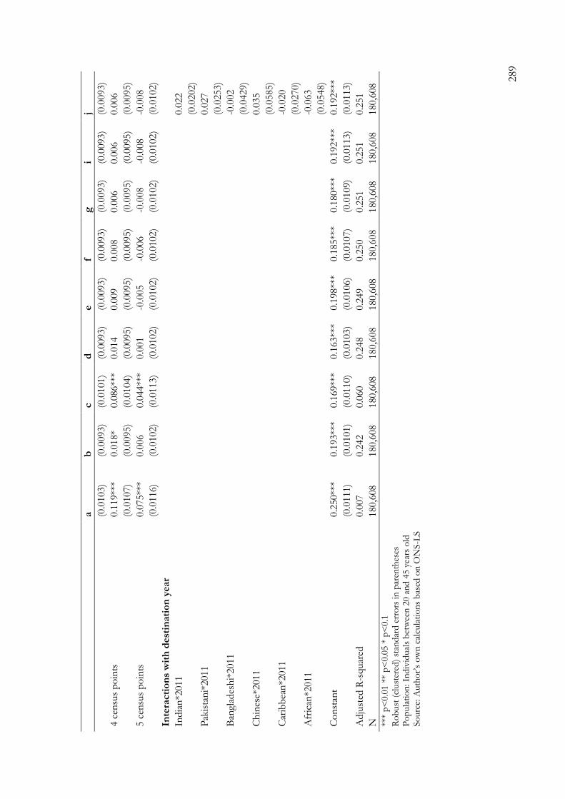
289

a

b

c

d

e

f g

i

j

(0

.0103)

(0.0

093)

(0.0

101)

(0.0

093)

(0.0

093)

(0.0

093)

(0.0

093)

(0.0

093)

(0.0

093)

4 c

ensu

s p

oin

ts

0.1

19**

* 0.0

18*

0.0

86**

* 0.0

14

0.0

09

0.0

08

0.0

06

0.0

06

0.0

06

(0

.0107)

(0.0

095)

(0.0

104)

(0.0

095)

(0.0

095)

(0.0

095)

(0.0

095)

(0.0

095)

(0.0

095)

5 c

ensu

s p

oin

ts

0.0

75**

* 0.0

06

0.0

44**

* 0.0

01

-0.0

05

-0.0

06

-0.0

08

-0.0

08

-0.0

08

(0

.0116)

(0.0

102)

(0.0

113)

(0.0

102)

(0.0

102)

(0.0

102)

(0.0

102)

(0.0

102)

(0.0

102)

Inte

racti

on

s w

ith

dest

inati

on

year

India

n*2

011

0.0

22

(0

.0202)

Pak

ista

ni*

2011

0.0

27

(0

.0253)

Ban

glad

esh

i*2011

-0.0

02

(0

.0429)

Ch

ines

e*2011

0.0

35

(0

.0585)

Car

ibb

ean

*2011

-0.0

20

(0

.0270)

Afr

ican

*2011

-0.0

63

(0

.0548)

Co

nst

ant

0.2

50**

* 0.1

93**

* 0.1

69**

* 0.1

63**

* 0.1

98**

* 0.1

85**

* 0.1

80**

* 0.1

92**

* 0.1

92**

*

(0

.0111)

(0.0

101)

(0.0

110)

(0.0

103)

(0.0

106)

(0.0

107)

(0.0

109)

(0.0

113)

(0.0

113)

Adju

sted

R-s

quar

ed

0.0

07

0.2

42

0.0

60

0.2

48

0.2

49

0.2

50

0.2

51

0.2

51

0.2

51

N

180,6

08

180,6

08

180,6

08

180,6

08

180,6

08

180,6

08

180,6

08

180,6

08

180,6

08

***

p<

0.0

1 *

* p

<0.0

5 *

p<

0.1

R

ob

ust

(cl

ust

ered

) st

and

ard

err

ors

in

par

enth

eses

P

op

ula

tio

n: In

div

idual

s b

etw

een

20 a

nd

45 y

ears

old

So

urc

e: A

uth

or’

s o

wn

cal

cula

tio

ns

bas

ed o

n O

NS

-LS

290

Tab

le ‎8

.6: A

cces

s to

th

e se

rvic

e cl

ass.

Full

mo

del

s o

f so

cial

mo

bili

ty. M

en a

nd w

om

en.

M

en

W

om

en

a

b

c

a

b

c

Eth

nic

gro

up

(re

f. w

hit

e B

riti

sh)

India

n

0.2

18**

* 0.0

68**

* 0.0

46**

0.1

75**

* 0.0

48**

* 0.0

40*

(0

.0174)

(0.0

138)

(0.0

203)

(0.0

166)

(0.0

141)

(0.0

220)

Pak

ista

ni

0.0

99**

* 0.0

00

-0.0

00

0.0

86**

* 0.0

10

0.0

33

(0

.0199)

(0.0

161)

(0.0

177)

(0.0

200)

(0.0

175)

(0.0

237)

Ban

glad

esh

i 0.2

36**

* 0.0

96**

* 0.1

18**

* 0.1

31**

* 0.0

14

0.0

20

(0

.0378)

(0.0

296)

(0.0

371)

(0.0

345)

(0.0

263)

(0.0

275)

Ch

ines

e 0.2

31**

* 0.0

33

-0.0

01

0.2

24**

* 0.0

05

-0.0

02

(0

.0797)

(0.0

695)

(0.0

787)

(0.0

646)

(0.0

538)

(0.0

543)

Car

ibb

ean

0.0

79**

* 0.0

18

0.0

33

0.1

50**

* 0.0

36*

0.0

61**

(0

.0247)

(0.0

214)

(0.0

247)

(0.0

235)

(0.0

199)

(0.0

274)

Afr

ican

0.1

74**

* -0

.005

-0.0

28

0.1

76**

-0

.091

-0.0

56

(0

.0673)

(0.0

598)

(0.0

766)

(0.0

752)

(0.0

781)

(0.0

761)

Pare

nta

l so

cial

cla

ss -

red

uced

(re

f. V

+V

I+V

II)

Ear

ner

s b

ut

un

cod

ed +

no

ear

ner

s in

hh

0.0

24**

* 0.0

25**

* 0.0

21**

* 0.0

07

0.0

09*

0.0

05

(0

.0061)

(0.0

054)

(0.0

055)

(0.0

054)

(0.0

048)

(0.0

048)

Ro

uti

ne

no

n-m

anual

(II

I)

0.0

77**

* 0.0

45**

* 0.0

50**

* 0.0

58**

* 0.0

24**

* 0.0

27**

*

(0

.0042)

(0.0

037)

(0.0

037)

(0.0

040)

(0.0

034)

(0.0

035)

Pet

it B

ourg

eois

ie (

IV)

-0.0

10**

-0

.008*

-0.0

08*

0.0

14**

* 0.0

05

0.0

07

(0

.0051)

(0.0

045)

(0.0

045)

(0.0

049)

(0.0

043)

(0.0

043)

Pro

fess

ion

al/

Man

ager

ial (I

+II

) 0.1

97**

* 0.0

93**

* 0.0

97**

* 0.1

62**

* 0.0

58**

* 0.0

61**

*

(0

.0042)

(0.0

038)

(0.0

038)

(0.0

041)

(0.0

036)

(0.0

036)

Inte

racti

on

s w

ith

Pare

nta

l so

cia

l cla

ss

India

n*E

arn

ers

un

cod

ed/

No

ear

ner

s -0

.047

-0.0

16

-0.0

03

-0.0

83*

-0.0

37

-0.0

34

(0

.0437)

(0.0

369)

(0.0

368)

(0.0

473)

(0.0

416)

(0.0

414)

291

M

en

W

om

en

a

b

c

a

b

c

India

n*I

II

0.0

25

0.0

10

-0.0

00

0.0

83**

0.0

23

0.0

20

(0

.0358)

(0.0

310)

(0.0

315)

(0.0

380)

(0.0

352)

(0.0

362)

India

n*I

V

0.0

83**

0.0

59**

0.0

55*

0.0

65*

0.0

03

0.0

02

(0

.0341)

(0.0

281)

(0.0

281)

(0.0

351)

(0.0

310)

(0.0

311)

India

n*I

+II

0.0

09

0.0

01

-0.0

27

0.0

26

0.0

25

0.0

21

(0

.0288)

(0.0

246)

(0.0

256)

(0.0

316)

(0.0

260)

(0.0

280)

Pak

ista

ni*

Ear

ner

s un

cod

ed/N

o e

arn

ers

-0.0

67**

-0

.041

-0.0

31

-0.0

59

-0.0

36

-0.0

36

(0

.0331)

(0.0

266)

(0.0

262)

(0.0

371)

(0.0

307)

(0.0

306)

Pak

ista

ni*

III

0.1

52**

0.0

87

0.0

70

0.1

69**

0.0

80

0.0

84

(0

.0664)

(0.0

595)

(0.0

600)

(0.0

780)

(0.0

751)

(0.0

765)

Pak

ista

ni*

IV

0.0

74*

0.0

43

0.0

39

0.0

48

0.0

06

0.0

01

(0

.0443)

(0.0

372)

(0.0

375)

(0.0

488)

(0.0

391)

(0.0

396)

Pak

ista

ni*

I+II

0.1

39**

* 0.0

75*

0.0

47

-0.0

46

-0.0

90**

-0

.095**

(0

.0489)

(0.0

422)

(0.0

452)

(0.0

553)

(0.0

453)

(0.0

462)

Ban

glad

esh

i*E

arn

ers

un

coded

/N

o e

arn

ers

-0.0

71

-0.0

72

-0.0

66

0.0

18

0.0

16

0.0

25

(0

.0604)

(0.0

446)

(0.0

446)

(0.0

507)

(0.0

420)

(0.0

425)

Ban

glad

esh

i*II

I -0

.151

-0.1

73

-0.1

60

0.4

31**

* 0.3

98**

* 0.3

96**

*

(0

.1552)

(0.1

501)

(0.1

539)

(0.0

986)

(0.0

872)

(0.1

046)

Ban

glad

esh

i*IV

-0

.042

-0.0

38

-0.0

31

-0.0

54

-0.0

33

-0.0

43

(0

.0768)

(0.0

717)

(0.0

722)

(0.0

806)

(0.0

761)

(0.0

776)

Ban

glad

esh

i*I+

II

-0.1

50

-0.1

47*

-0.1

59*

0.0

35

0.0

59

0.0

49

(0

.1010)

(0.0

815)

(0.0

823)

(0.1

554)

(0.1

310)

(0.1

379)

Ch

ines

e*E

arn

ers

un

cod

ed/N

o e

arn

ers

0.1

83

0.1

26

0.1

29

-0.1

51

-0.0

72

-0.0

74

(0

.1311)

(0.1

093)

(0.1

093)

(0.1

115)

(0.0

772)

(0.0

794)

Ch

ines

e*II

I -0

.022

0.0

01

-0.0

19

-0.0

42

0.1

21

0.1

17

(0

.1285)

(0.1

100)

(0.1

093)

(0.1

512)

(0.1

224)

(0.1

194)

Ch

ines

e*IV

0.0

06

-0.0

12

-0.0

18

0.0

05

-0.0

32

-0.0

40

292

M

en

W

om

en

a

b

c

a

b

c

(0

.0953)

(0.0

826)

(0.0

815)

(0.0

755)

(0.0

640)

(0.0

662)

Ch

ines

e*I+

II

0.1

12

0.1

27

0.1

09

-0.0

86

-0.0

23

-0.0

32

(0

.0915)

(0.0

782)

(0.0

848)

(0.1

130)

(0.0

884)

(0.0

891)

Car

ibb

ean

*Ear

ner

s un

cod

ed/

No

ear

ner

s 0.0

77

0.0

32

0.0

39

0.0

67

0.0

47

0.0

48

(0

.0566)

(0.0

497)

(0.0

502)

(0.0

455)

(0.0

417)

(0.0

418)

Car

ibb

ean

*III

-0

.035

-0.0

40

-0.0

42

0.0

12

0.0

03

0.0

02

(0

.0410)

(0.0

358)

(0.0

365)

(0.0

398)

(0.0

329)

(0.0

334)

Car

ibb

ean

*IV

-0

.030

-0.0

25

-0.0

25

-0.0

94

-0.0

86

-0.0

97

(0

.1124)

(0.1

063)

(0.1

040)

(0.0

922)

(0.0

640)

(0.0

670)

Car

ibb

ean

*I+

II

-0.1

06**

-0

.095**

-0

.091**

-0

.073

-0.0

19

-0.0

15

(0

.0482)

(0.0

467)

(0.0

460)

(0.0

448)

(0.0

388)

(0.0

393)

Afr

ican

*Ear

ner

s un

cod

ed/N

o e

arn

ers

0.0

60

0.0

55

0.0

49

0.1

12

0.0

65

0.0

79

(0

.1316)

(0.1

249)

(0.1

263)

(0.1

035)

(0.1

026)

(0.0

975)

Afr

ican

*III

0.0

04

-0.0

13

-0.0

12

0.1

63*

0.1

69*

0.1

82**

(0

.0969)

(0.0

832)

(0.0

839)

(0.0

910)

(0.0

945)

(0.0

868)

Afr

ican

*IV

0.5

54**

* 0.7

68**

* 0.7

25**

* 0.1

71

0.1

74

0.2

11

(0

.0678)

(0.0

596)

(0.0

843)

(0.2

236)

(0.1

568)

(0.1

584)

Afr

ican

*I+

II

0.0

57

0.1

13

0.1

09

-0.1

24

-0.0

56

-0.0

44

(0

.0915)

(0.0

885)

(0.0

892)

(0.0

944)

(0.0

936)

(0.0

899)

Ed

ucati

on

(re

f. L

eve

l 1)

N

o e

duca

tio

n

-0

.120**

*

-0

.088**

*

(0.0

040)

(0.0

037)

O

ther

-0.0

71**

*

-0

.028**

*

(0.0

053)

(0.0

074)

L

evel

2

0.0

98**

*

0.0

72**

*

(0.0

042)

(0.0

037)

L

evel

3

0.1

70**

*

0.1

61**

*

293

M

en

W

om

en

a

b

c

a

b

c

(0.0

052)

(0.0

048)

L

evel

4+

0.4

76**

*

0.5

10**

*

(0.0

042)

(0.0

040)

E

du

cati

on

(re

du

ced

: re

f. L

eve

l 1

or

less

)

Lev

el 2

+3

0.1

65**

*

0.1

25**

*

(0

.0034)

(0.0

031)

Lev

el 4

+

0.5

12**

*

0.5

30**

*

(0

.0038)

(0.0

038)

Inte

racti

on

s w

ith

ed

ucati

on

(re

du

ced

)

India

n*L

evel

2+

3

-0.0

06

0.0

44

(0

.0298)

(0.0

298)

India

n*L

evel

4

0.0

69**

*

0.0

04

(0

.0245)

(0.0

281)

Pak

ista

ni*

Lev

el 2

+3

-0.0

47

-0.0

32

(0

.0292)

(0.0

301)

Pak

ista

ni*

Lev

el 4

0.0

53*

-0.0

19

(0

.0308)

(0.0

332)

Ban

glad

esh

i*L

evel

2+

3

-0.0

62

-0.0

11

(0

.0557)

(0.0

408)

Ban

glad

esh

i*L

evel

4

0.0

13

0.0

19

(0

.0505)

(0.0

511)

Ch

ines

e*L

evel

2+

3

0.0

77

0.0

09

(0

.0893)

(0.0

816)

Ch

ines

e*L

evel

4

0.0

50

0.0

24

(0

.0754)

(0.0

602)

Car

ibb

ean

* L

evel

2+

3

0.0

20

0.0

13

(0

.0362)

(0.0

360)

294

M

en

W

om

en

a

b

c

a

b

c

Car

ibb

ean

* L

evel

4

-0.0

47

-0.0

49

(0

.0398)

(0.0

353)

Afr

ican

*Lev

el 2

+3

0.0

97

0.1

37

(0

.0861)

(0.1

123)

Afr

ican

*Lev

el 4

0.0

02

-0.0

83

(0

.0842)

(0.0

748)

Ten

ure

(re

f. o

wn

er)

So

cial

ren

t -0

.101**

* -0

.036**

* -0

.044**

* -0

.102**

* -0

.034**

* -0

.040**

*

(0

.0038)

(0.0

034)

(0.0

034)

(0.0

035)

(0.0

031)

(0.0

031)

Pri

vat

e re

nt

-0.0

54**

* -0

.019**

* -0

.021**

* -0

.057**

* -0

.017**

* -0

.020**

*

(0

.0051)

(0.0

045)

(0.0

045)

(0.0

048)

(0.0

042)

(0.0

042)

Nu

mb

er

of

cars

(re

f. n

on

e)

1 c

ar

0.0

32**

* 0.0

11**

* 0.0

15**

* 0.0

43**

* 0.0

19**

* 0.0

22**

*

(0

.0036)

(0.0

032)

(0.0

032)

(0.0

034)

(0.0

029)

(0.0

029)

2+

car

s 0.0

59**

* 0.0

27**

* 0.0

29**

* 0.0

77**

* 0.0

40**

* 0.0

43**

*

(0

.0049)

(0.0

044)

(0.0

044)

(0.0

048)

(0.0

042)

(0.0

042)

Pers

on

s p

er

roo

m (

ref.

1)

Over

1.5

pp

p

-0.0

80**

* -0

.041**

* -0

.051**

* -0

.042**

* -0

.012*

-0.0

20**

*

(0

.0081)

(0.0

071)

(0.0

071)

(0.0

077)

(0.0

068)

(0.0

068)

1.5

pp

p

-0.0

34**

* -0

.013

-0.0

17*

-0.0

34**

* -0

.014

-0.0

20**

(0

.0117)

(0.0

103)

(0.0

105)

(0.0

106)

(0.0

094)

(0.0

094)

Over

1 b

ut

less

th

an 1

.5 p

pp

-0

.027**

* -0

.013**

* -0

.017**

* -0

.025**

* -0

.008**

-0

.011**

*

(0

.0049)

(0.0

044)

(0.0

044)

(0.0

046)

(0.0

040)

(0.0

040)

Over

0.7

5 b

ut

less

th

an 1

pp

p

0.0

28**

* 0.0

10**

* 0.0

11**

* 0.0

19**

* 0.0

04

0.0

05

(0

.0040)

(0.0

035)

(0.0

035)

(0.0

038)

(0.0

033)

(0.0

033)

0.7

5 p

pp

0.0

39**

* 0.0

13**

0.0

16**

0.0

33**

* 0.0

10*

0.0

12**

(0

.0072)

(0.0

063)

(0.0

063)

(0.0

068)

(0.0

059)

(0.0

060)

295

M

en

W

om

en

a

b

c

a

b

c

Over

0.5

but

less

th

an 0

.75 p

pp

0.0

68**

* 0.0

26**

* 0.0

28**

* 0.0

60**

* 0.0

20**

* 0.0

22**

*

(0

.0041)

(0.0

036)

(0.0

037)

(0.0

040)

(0.0

035)

(0.0

035)

0.5

pp

p

0.0

89**

* 0.0

31**

* 0.0

34**

* 0.0

92**

* 0.0

33**

* 0.0

35**

*

(0

.0062)

(0.0

055)

(0.0

055)

(0.0

061)

(0.0

053)

(0.0

053)

Les

s th

an 0

.5 p

pp

0.1

12**

* 0.0

41**

* 0.0

43**

* 0.1

13**

* 0.0

35**

* 0.0

38**

*

(0

.0076)

(0.0

066)

(0.0

067)

(0.0

076)

(0.0

065)

(0.0

066)

Cars

tair

s q

uin

tile

s (r

ef.

Q1:

less

dep

riva

tio

n)

Car

stai

rs Q

2

-0.0

30**

* -0

.020**

* -0

.021**

* -0

.014**

* -0

.002

-0.0

01

(0

.0042)

(0.0

037)

(0.0

037)

(0.0

041)

(0.0

035)

(0.0

036)

Car

stai

rs Q

3

-0.0

44**

* -0

.027**

* -0

.028**

* -0

.029**

* -0

.011**

* -0

.011**

*

(0

.0044)

(0.0

039)

(0.0

039)

(0.0

042)

(0.0

037)

(0.0

037)

Car

stai

rs Q

4

-0.0

65**

* -0

.038**

* -0

.040**

* -0

.038**

* -0

.014**

* -0

.015**

*

(0

.0045)

(0.0

040)

(0.0

040)

(0.0

043)

(0.0

038)

(0.0

038)

Car

stai

rs Q

5

-0.0

67**

* -0

.037**

* -0

.040**

* -0

.052**

* -0

.017**

* -0

.020**

*

(0

.0048)

(0.0

042)

(0.0

042)

(0.0

046)

(0.0

040)

(0.0

040)

Ag

e

Age

in

des

tin

atio

n

0.0

04**

* 0.0

06**

* 0.0

05**

* 0.0

03**

* 0.0

04**

* 0.0

03**

*

(0

.0003)

(0.0

003)

(0.0

003)

(0.0

003)

(0.0

003)

(0.0

003)

Ori

gin

year

(ref.

1971)

1981

-0.0

21**

* -0

.010**

* -0

.011**

* -0

.025**

* -0

.008**

* -0

.009**

*

(0

.0023)

(0.0

020)

(0.0

020)

(0.0

021)

(0.0

018)

(0.0

018)

1991

-0.0

83**

* -0

.047**

* -0

.051**

* -0

.078**

* -0

.042**

* -0

.046**

*

(0

.0038)

(0.0

033)

(0.0

033)

(0.0

036)

(0.0

031)

(0.0

031)

Dest

inati

on

year

(ref

. 2001)

2011

0.0

13**

* -0

.055**

* -0

.047**

* 0.0

34**

* -0

.046**

* -0

.035**

*

(0

.0033)

(0.0

031)

(0.0

031)

(0.0

034)

(0.0

032)

(0.0

032)

Num

ber

of

cen

sus

po

ints

(re

f. 2

)

296

M

en

W

om

en

a

b

c

a

b

c

3 c

ensu

s p

oin

ts

0.0

06

-0.0

17*

-0.0

14

0.0

32**

* -0

.003

0.0

00

(0

.0097)

(0.0

090)

(0.0

090)

(0.0

100)

(0.0

093)

(0.0

093)

4 c

ensu

s p

oin

ts

0.0

43**

* -0

.008

-0.0

02

0.0

55**

* 0.0

05

0.0

10

(0

.0099)

(0.0

091)

(0.0

092)

(0.0

103)

(0.0

095)

(0.0

095)

5 c

ensu

s p

oin

ts

0.0

45**

* 0.0

01

0.0

11

0.0

11

-0.0

09

-0.0

02

(0

.0106)

(0.0

098)

(0.0

098)

(0.0

111)

(0.0

102)

(0.0

102)

Co

nst

ant

0.3

24**

* 0.2

74**

* 0.2

22**

* 0.2

83**

* 0.2

01**

* 0.1

67**

*

(0

.0116)

(0.0

109)

(0.0

107)

(0.0

119)

(0.0

111)

(0.0

110)

Adju

sted

R-s

quar

ed

0.0

98

0.2

53

0.2

47

0.0

81

0.2

51

0.2

46

N

174,1

10

174,1

10

174,1

10

180,6

08

180,6

08

180,6

08

***

p<

0.0

1 *

* p

<0.0

5 *

p<

0.1

R

ob

ust

(cl

ust

ered

) st

and

ard

err

ors

in

par

enth

eses

P

op

ula

tio

n: In

div

idual

s b

etw

een

20 a

nd

45 y

ears

old

So

urc

e: A

uth

or’

s o

wn

cal

cula

tio

ns

bas

ed o

n O

NS-L

S

297

Tab

le ‎8

.7:

Acc

ess

to e

mp

loym

ent

and t

o t

he

serv

ice

clas

s. R

eplic

atio

n o

f M

odel

5 f

rom

Tab

les

3.5

-3.8

usi

ng

logi

stic

reg

ress

ion

wit

h a

ver

age

mar

gin

al

effe

cts;

in

th

e ta

ble

: av

erag

e m

argi

nal

eff

ects

, ro

bust

(cl

ust

ered

) st

andar

d e

rro

rs a

nd p

-val

ue

E

mp

loym

ent

Serv

ice c

lass

M

en

W

om

en

M

en

W

om

en

d

y/

dx

SE

p

-valu

e d

y/

dx

SE

p

-valu

e d

y/

dx

SE

p

-valu

e d

y/

dx

SE

p

-valu

e

Eth

nic

gro

up

(re

f. w

hit

e B

riti

sh)

In

dia

n

-0.0

06

0.0

08

0.4

26

0.0

00

0.0

11

0.9

69

0.0

80

0.0

10

0.0

00

0.0

56

0.0

11

0.0

00

Pak

ista

ni

-0.0

36

0.0

09

0.0

00

-0.1

95

0.0

14

0.0

00

0.0

13

0.0

13

0.3

19

0.0

08

0.0

14

0.5

61

Ban

glad

esh

i 0.0

18

0.0

11

0.1

02

-0.1

62

0.0

21

0.0

00

0.0

62

0.0

25

0.0

12

0.0

32

0.0

23

0.1

56

Ch

ines

e 0.0

42

0.0

19

0.0

24

0.0

43

0.0

32

0.1

81

0.0

66

0.0

32

0.0

40

-0.0

08

0.0

26

0.7

49

Car

ibb

ean

-0

.033

0.0

11

0.0

02

-0.0

05

0.0

14

0.7

14

0.0

05

0.0

17

0.7

50

0.0

41

0.0

15

0.0

05

Afr

ican

0.0

05

0.0

20

0.8

00

-0.0

26

0.0

29

0.3

74

0.0

43

0.0

37

0.2

48

-0.0

27

0.0

30

0.3

58

Ed

ucati

on

(re

f. L

eve

l 1)

N

o e

duca

tio

n

-0.1

74

0.0

05

0.0

00

-0.2

39

0.0

06

0.0

00

-0.1

32

0.0

04

0.0

00

-0.1

01

0.0

04

0.0

00

Oth

er

0.0

06

0.0

04

0.1

46

0.0

07

0.0

09

0.4

13

-0.0

74

0.0

06

0.0

00

-0.0

31

0.0

08

0.0

00

Lev

el 2

0.0

22

0.0

03

0.0

00

0.0

77

0.0

04

0.0

00

0.0

99

0.0

04

0.0

00

0.0

73

0.0

04

0.0

00

Lev

el 3

0.0

51

0.0

03

0.0

00

0.1

53

0.0

04

0.0

00

0.1

75

0.0

05

0.0

00

0.1

64

0.0

05

0.0

00

Lev

el 4

+

0.0

67

0.0

03

0.0

00

0.1

78

0.0

04

0.0

00

0.4

75

0.0

04

0.0

00

0.5

09

0.0

04

0.0

00

Pare

nta

l so

cial

cla

ss (

ref.

Sem

i an

d

un

skil

led

man

ual

- V

II)

Skill

ed m

anual

(V

I)

0.0

05

0.0

03

0.0

96

0.0

11

0.0

03

0.0

02

0.0

10

0.0

04

0.0

23

0.0

14

0.0

04

0.0

01

Lo

wer

tec

hn

icia

n (

V)

0.0

22

0.0

04

0.0

00

0.0

17

0.0

05

0.0

01

0.0

41

0.0

06

0.0

00

0.0

26

0.0

06

0.0

00

Pet

it B

ourg

eois

ie (

IV)

0.0

16

0.0

03

0.0

00

0.0

06

0.0

04

0.1

42

0.0

06

0.0

05

0.2

26

0.0

16

0.0

05

0.0

01

Ro

uti

ne

no

n-m

anual

(II

I)

0.0

13

0.0

03

0.0

00

0.0

22

0.0

04

0.0

00

0.0

56

0.0

04

0.0

00

0.0

36

0.0

04

0.0

00

Lo

wer

pro

fess

ion

al/

man

ager

ial

(II)

0.0

15

0.0

03

0.0

00

0.0

12

0.0

04

0.0

03

0.0

90

0.0

05

0.0

00

0.0

62

0.0

04

0.0

00

Hig

her

pro

fess

ion

al/m

anag

eria

l (I

) 0.0

10

0.0

04

0.0

20

0.0

02

0.0

05

0.6

40

0.1

16

0.0

06

0.0

00

0.0

65

0.0

05

0.0

00

Ear

ner

s b

ut

un

cod

ed

-0.0

28

0.0

06

0.0

00

-0.0

24

0.0

07

0.0

01

0.0

25

0.0

09

0.0

07

0.0

04

0.0

09

0.6

95

No

ear

ner

s in

hh

-0

.028

0.0

04

0.0

00

-0.0

59

0.0

06

0.0

00

0.0

34

0.0

07

0.0

00

0.0

19

0.0

07

0.0

05

298

E

mp

loym

ent

Serv

ice c

lass

M

en

W

om

en

M

en

W

om

en

d

y/

dx

SE

p

-valu

e d

y/

dx

SE

p

-valu

e d

y/

dx

SE

p

-valu

e d

y/

dx

SE

p

-valu

e

Ten

ure

(re

f. o

wn

er)

So

cial

ren

t -0

.026

0.0

02

0.0

00

-0.0

33

0.0

03

0.0

00

-0.0

35

0.0

03

0.0

00

-0.0

34

0.0

03

0.0

00

Pri

vat

e re

nt

-0.0

09

0.0

03

0.0

03

-0.0

10

0.0

04

0.0

12

-0.0

16

0.0

04

0.0

00

-0.0

16

0.0

04

0.0

00

Nu

mb

er

of

cars

(re

f. n

on

e)

1 c

ar

0.0

26

0.0

02

0.0

00

0.0

19

0.0

03

0.0

00

0.0

10

0.0

03

0.0

02

0.0

20

0.0

03

0.0

00

2+

car

s 0.0

33

0.0

03

0.0

00

0.0

26

0.0

04

0.0

00

0.0

25

0.0

04

0.0

00

0.0

40

0.0

04

0.0

00

Pers

on

s p

er

roo

m (

ref.

1)

Over

1.5

pp

p

-0.0

27

0.0

05

0.0

00

-0.0

22

0.0

06

0.0

01

-0.0

44

0.0

08

0.0

00

-0.0

12

0.0

08

0.1

25

1.5

pp

p

-0.0

11

0.0

07

0.1

16

0.0

01

0.0

09

0.9

13

-0.0

13

0.0

11

0.2

32

-0.0

16

0.0

11

0.1

50

Over

1 b

ut

less

th

an 1

.5 p

pp

-0

.009

0.0

03

0.0

03

-0.0

14

0.0

04

0.0

00

-0.0

13

0.0

05

0.0

05

-0.0

09

0.0

04

0.0

42

Over

0.7

5 b

ut

less

th

an 1

pp

p

0.0

10

0.0

02

0.0

00

0.0

11

0.0

03

0.0

00

0.0

09

0.0

04

0.0

10

0.0

04

0.0

03

0.2

66

0.7

5 p

pp

-0

.002

0.0

04

0.6

17

0.0

07

0.0

05

0.2

08

0.0

13

0.0

06

0.0

37

0.0

10

0.0

06

0.1

06

Over

0.5

but

less

th

an 0

.75 p

pp

0.0

06

0.0

03

0.0

24

0.0

12

0.0

03

0.0

00

0.0

24

0.0

04

0.0

00

0.0

19

0.0

04

0.0

00

0.5

pp

p

0.0

07

0.0

04

0.0

71

0.0

08

0.0

05

0.0

88

0.0

29

0.0

05

0.0

00

0.0

30

0.0

05

0.0

00

Les

s th

an 0

.5 p

pp

-0

.001

0.0

05

0.7

75

-0.0

05

0.0

06

0.4

55

0.0

39

0.0

07

0.0

00

0.0

32

0.0

06

0.0

00

Cars

tair

s q

uin

tile

s (r

ef.

Q1:

less

d

ep

riva

tio

n)

Car

stai

rs Q

2

-0.0

03

0.0

03

0.2

44

0.0

03

0.0

03

0.3

04

-0.0

18

0.0

04

0.0

00

-0.0

01

0.0

03

0.8

54

Car

stai

rs Q

3

-0.0

06

0.0

03

0.0

20

0.0

01

0.0

03

0.7

94

-0.0

25

0.0

04

0.0

00

-0.0

10

0.0

04

0.0

07

Car

stai

rs Q

4

-0.0

19

0.0

03

0.0

00

-0.0

02

0.0

04

0.5

11

-0.0

36

0.0

04

0.0

00

-0.0

13

0.0

04

0.0

00

Car

stai

rs Q

5

-0.0

35

0.0

03

0.0

00

-0.0

16

0.0

04

0.0

00

-0.0

36

0.0

04

0.0

00

-0.0

17

0.0

04

0.0

00

Ag

e

Age

in

des

tin

atio

n

0.0

01

0.0

00

0.0

00

0.0

02

0.0

00

0.0

00

0.0

06

0.0

00

0.0

00

0.0

04

0.0

00

0.0

00

Ori

gin

year

(ref.

1971)

1981

0.0

06

0.0

02

0.0

00

-0.0

10

0.0

02

0.0

00

-0.0

09

0.0

02

0.0

00

-0.0

08

0.0

02

0.0

00

1991

-0.0

01

0.0

02

0.7

29

0.0

01

0.0

03

0.6

73

-0.0

44

0.0

03

0.0

00

-0.0

40

0.0

03

0.0

00

Dest

inati

on

year

(ref

. 2001)

2011

-0.0

11

0.0

02

0.0

00

0.0

08

0.0

03

0.0

04

-0.0

56

0.0

03

0.0

00

-0.0

47

0.0

03

0.0

00

299

E

mp

loym

ent

Serv

ice c

lass

M

en

W

om

en

M

en

W

om

en

d

y/

dx

SE

p

-valu

e d

y/

dx

SE

p

-valu

e d

y/

dx

SE

p

-valu

e d

y/

dx

SE

p

-valu

e

Nu

mb

er

of

cen

sus

po

ints

(re

f.

2)

3 c

ensu

s p

oin

ts

0.0

29

0.0

07

0.0

00

0.0

60

0.0

09

0.0

00

-0.0

12

0.0

10

0.2

49

0.0

05

0.0

11

0.6

61

4 c

ensu

s p

oin

ts

0.0

61

0.0

07

0.0

00

0.0

72

0.0

09

0.0

00

-0.0

01

0.0

10

0.8

92

0.0

12

0.0

11

0.2

64

5 c

ensu

s p

oin

ts

0.0

97

0.0

08

0.0

00

0.0

89

0.0

10

0.0

00

0.0

07

0.0

11

0.5

35

-0.0

02

0.0

11

0.8

45

Pse

udo

R-s

quar

ed

0.1

20

0.1

09

0.2

02

0.1

99

N

180540

188937

174110

180608

No

te: th

e co

effi

cien

ts a

re v

ery

sim

ilar

wit

h r

esp

ect

to t

ho

se o

bse

rved

in

th

e eq

uiv

alen

t m

od

els

pre

sen

ted

in

th

e ch

apte

r: t

he s

ub

stan

tive

resu

lts

rem

ain

th

eref

ore

th

e sa

me.

I

reac

h t

he

sam

e co

ncl

usi

on

fo

r th

e m

od

els

on

so

cial

mo

bili

ty (

mo

del

s av

aila

ble

up

on

req

ues

t).

Po

pula

tio

n: In

div

idual

s b

etw

een

20 a

nd

45 y

ears

old

So

urc

e: A

uth

or’

s o

wn

cal

cula

tio

ns

bas

ed o

n O

NS

-LS

300

8.2

A

nn

ex

to

Ch

ap

ter

4

Tab

le ‎8

.8: L

oca

l A

uth

ori

ties

wit

hin

ho

usi

ng

mar

ket

are

as

Lo

nd

on

R

ead

ing

L

uto

n &

Mil

ton

Keyn

es

Bir

min

gh

am

Bar

kin

g an

d D

agen

ham

H

aver

ing

Sutt

on

B

asin

gsto

ke

and D

ean

e A

yles

bury

Val

e B

irm

ingh

am

Bar

net

H

erts

mer

e Sw

ale

Bra

ckn

ell F

ore

st

Bed

ford

B

rom

sgro

ve

Bas

ildon

H

illin

gdo

n

Tan

dri

dge

H

art

Luto

n

Can

no

ck C

has

e

Bex

ley

Ho

un

slo

w

Th

ree

Riv

ers

Rea

din

g M

id B

edfo

rdsh

ire

Dud

ley

Bre

nt

Islin

gto

n

Th

urr

ock

Slo

ugh

M

ilto

n K

eyn

es

Lic

hfi

eld

Bre

ntw

oo

d

Ken

sin

gton

an

d C

hel

sea

To

nb

ridge

an

d M

allin

g So

uth

Buck

s So

uth

Bed

ford

shir

e N

ort

h W

arw

icksh

ire

Bro

mle

y K

ings

ton

up

on

Th

ames

T

ow

er H

amle

ts

Surr

ey H

eath

Red

dit

ch

Bro

xbo

urn

e L

amb

eth

T

un

bri

dge

Wel

ls

Wes

t B

erks

hir

e San

dw

ell

Cam

den

L

ewis

ham

W

alth

am F

ore

st

Win

dso

r an

d M

aiden

hea

d

So

lihull

Cas

tle

Po

int

Mai

dst

on

e W

andsw

ort

h

Wo

kin

gham

So

uth

Sta

fford

shir

e

Ch

ilter

n

Med

way

W

atfo

rd

Wyc

om

be

Str

atfo

rd-o

n-A

von

Cit

y o

f L

on

do

n

Mer

ton

W

aver

ley

Tam

wo

rth

Cro

ydo

n

Mo

le V

alle

y W

elw

yn H

atfi

eld

Wal

sall

Dac

oru

m

New

ham

W

estm

inst

er

Wo

lver

ham

pto

n

Dar

tfo

rd

No

rth

Her

tfo

rdsh

ire

Wo

kin

g

Eal

ing

Red

bri

dge

E

ast

Her

tfo

rdsh

ire

Rei

gate

an

d B

anst

ead

Elm

bri

dge

R

ich

mo

nd

up

on

Th

ames

En

fiel

d

Ro

chfo

rd

Ep

pin

g F

ore

st

Run

nym

ede

Ep

som

an

d E

wel

l R

ush

mo

or

Gra

ves

ham

Sev

eno

aks

Gre

enw

ich

So

uth

end-o

n-S

ea

Guild

ford

So

uth

war

k

Hac

kn

ey

Sp

elth

orn

e

Ham

mer

smit

h a

nd

Fulh

am

St

Alb

ans

Har

inge

y Ste

ven

age

301

Leic

est

er

Man

ch

est

er

L

eed

s B

rad

ford

B

lab

y B

olt

on

B

arnsl

ey

Bra

dfo

rd

Ch

arn

wo

od

Bury

H

arro

gate

C

alder

dal

e

H

arb

oro

ugh

H

igh

Pea

k K

irkle

es

Cra

ven

H

inck

ley

and

Bo

swo

rth

M

accl

esfi

eld

Lee

ds

L

eice

ster

M

anch

este

r W

akef

ield

Mel

ton

O

ldh

am

No

rth

Wes

t L

eice

ster

shir

e R

och

dal

e

O

adb

y an

d W

igst

on

R

oss

end

ale

Sal

ford

Sto

ckp

ort

Tam

esid

e

Tra

ffo

rd

302

Tab

le ‎8

.9: N

um

ber

of

LSO

As

by

per

cen

tage

of

ethn

ic m

ino

riti

es (

2001 a

nd 2

011)

2001

2011

75%

an

d m

ore

50.0

1% -

75%

25.0

1% -

50%

10

.01%

- 2

5%

5.0

1 %

- 1

0%

U

p t

o 5

%

To

tal

Ind

ian

75%

+

16

5

0

0

0

0

21

50.0

1%

- 7

5%

1

34

20

0

0

0

55

25.0

1%

- 5

0%

0

24

268

118

5

2

417

10.0

1%

- 2

5%

0

0

71

615

235

66

987

5.0

1 %

- 1

0%

0

0

0

124

544

694

1362

Up

to

5%

0

0

0

7

230

28593

28830

To

tal

17

63

359

864

1014

29355

31672

Pak

ista

ni

75%

+

9

12

0

0

0

0

21

50.0

1%

- 7

5%

2

62

49

3

0

0

116

25.0

1%

- 5

0%

0

11

193

140

12

8

364

10.0

1%

- 2

5%

0

0

7

380

290

160

837

5.0

1 %

- 1

0%

0

0

0

17

276

635

928

Up

to

5%

0

0

0

0

54

29352

29406

To

tal

11

85

249

540

632

30155

31672

Ban

gla

desh

i

75%

+

1

1

0

0

0

0

2

50.0

1%

- 7

5%

2

14

5

0

0

0

21

25.0

1%

- 5

0%

0

9

58

26

1

2

96

10.0

1%

- 2

5%

0

0

6

147

77

55

285

5.0

1 %

- 1

0%

0

0

1

14

122

231

368

Up

to

5%

0

0

0

0

39

30861

30900

To

tal

3

24

70

187

239

31149

31672

Ch

inese

10.0

1%

- 2

5%

3

15

24

42

303

2001

2011

75%

an

d m

ore

50.0

1% -

75%

25.0

1% -

50%

10

.01%

- 2

5%

5.0

1 %

- 1

0%

U

p t

o 5

%

To

tal

5.0

1 %

- 1

0%

1

17

115

133

Up

to

5%

1

28

31468

31497

To

tal

5

60

31607

31672

Cari

bb

ean

25.0

1%

- 5

0%

1

2

0

0

3

10.0

1%

- 2

5%

11

388

44

2

445

5.0

1 %

- 1

0%

0

299

529

141

969

Up

to

5%

0

9

431

29815

30255

To

tal

12

698

1004

29958

31672

Afr

ican

25.0

1%

- 5

0%

31

45

8

4

88

10.0

1%

- 2

5%

14

449

269

247

979

5.0

1 %

- 1

0%

0

61

388

899

1348

Up

to

5%

0

2

151

29104

29257

To

tal

45

557

816

30254

31672

So

urc

e: A

uth

or’

s o

wn

cal

cula

tio

ns

bas

ed o

n a

ggre

gate

d C

ensu

s dat

a.

304

8.3

A

nn

ex

to

Ch

ap

ter

5

Tab

le ‎8

.10: A

cces

s to

em

plo

ymen

t: f

ull

mo

del

. P

oo

led e

thn

ic m

ino

riti

es; m

en.

a

b

c

d

e

f g

EM

qu

inti

le (

ref.

Q1:

lo

wes

t co

ncen

trati

on

)

Q2

0.0

13

0.0

21

0.0

26

0.0

27

0.0

00

0.0

22

-0.0

00

(0

.0188)

(0.0

188)

(0.0

188)

(0.0

179)

(0.0

239)

(0.0

176)

(0.0

238)

Q3

-0.0

10

0.0

05

0.0

10

0.0

19

0.0

11

0.0

15

0.0

12

(0

.0185)

(0.0

190)

(0.0

193)

(0.0

183)

(0.0

237)

(0.0

180)

(0.0

236)

Q4

-0.0

17

0.0

04

0.0

08

0.0

18

0.0

23

0.0

11

0.0

17

(0

.0184)

(0.0

197)

(0.0

199)

(0.0

191)

(0.0

241)

(0.0

188)

(0.0

241)

Q5

-0.0

33*

-0.0

08

-0.0

02

0.0

08

0.0

18

0.0

03

0.0

11

(0

.0188)

(0.0

210)

(0.0

211)

(0.0

201)

(0.0

254)

(0.0

198)

(0.0

253)

Eth

nic

gro

up

(re

f. I

nd

ian

)

Pak

ista

ni

-0.1

01**

* -0

.096**

* -0

.081**

* -0

.062**

* -0

.090**

-0

.071**

* -0

.092**

(0

.0149)

(0.0

151)

(0.0

153)

(0.0

147)

(0.0

388)

(0.0

144)

(0.0

378)

Ban

glad

esh

i -0

.057**

* -0

.051**

-0

.009

0.0

03

-0.0

25

-0.0

01

-0.0

14

(0

.0219)

(0.0

221)

(0.0

232)

(0.0

228)

(0.0

483)

(0.0

225)

(0.0

485)

Car

ibb

ean

-0

.088**

* -0

.086**

* -0

.065**

* -0

.032*

-0.0

06

-0.0

05

0.0

19

(0

.0166)

(0.0

167)

(0.0

178)

(0.0

176)

(0.0

370)

(0.0

183)

(0.0

372)

Afr

ican

-0

.005

-0.0

06

0.0

20

0.0

18

-0.0

69

0.0

39

-0.0

67

(0

.0281)

(0.0

282)

(0.0

300)

(0.0

287)

(0.0

997)

(0.0

285)

(0.0

988)

Eth

nic

gro

up

* E

M q

uin

tile

Pak

ista

ni *

Q2

0.0

71

0.0

57

(0

.0463)

(0

.0453)

Pak

ista

ni *

Q3

0.0

42

0.0

28

(0

.0479)

(0

.0469)

Pak

ista

ni *

Q4

0.0

18

0.0

10

305

a

b

c

d

e

f g

(0

.0464)

(0

.0455)

Pak

ista

ni *

Q5

0.0

16

0.0

14

(0

.0470)

(0

.0459)

Ban

glad

esh

i *

Q2

0.1

00

0.0

85

(0

.0633)

(0

.0633)

Ban

glad

esh

i *

Q3

0.0

59

0.0

37

(0

.0621)

(0

.0631)

Ban

glad

esh

i *

Q4

0.0

04

-0

.015

(0

.0629)

(0

.0625)

Ban

glad

esh

i *

Q5

-0.0

11

-0

.026

(0

.0704)

(0

.0693)

Car

ibb

ean

* Q

2

-0

.007

-0

.008

(0

.0464)

(0

.0463)

Car

ibb

ean

* Q

3

-0.0

22

-0

.028

(0

.0463)

(0

.0462)

Car

ibb

ean

* Q

4

-0.0

33

-0

.030

(0

.0487)

(0

.0485)

Car

ibb

ean

* Q

5

-0.0

66

-0

.052

(0

.0493)

(0

.0492)

Afr

ican

* Q

2

0.1

33

0.1

34

(0

.1106)

(0

.1089)

Afr

ican

* Q

3

0.0

72

0.0

92

(0

.1116)

(0

.1107)

Afr

ican

* Q

4

0.0

75

0.1

11

(0

.1128)

(0

.1116)

Afr

ican

* Q

5

0.1

08

0.1

31

(0

.1088)

(0

.1081)

Cars

tair

s q

uin

tile

(re

f. Q

1: l

east

dep

rive

d)

Q2

-0

.022

-0.0

13

-0.0

11

-0.0

14

-0.0

04

-0.0

08

306

a

b

c

d

e

f g

(0.0

282)

(0.0

281)

(0.0

274)

(0.0

277)

(0.0

275)

(0.0

278)

Q3

-0

.027

-0.0

10

-0.0

09

-0.0

13

-0.0

04

-0.0

08

(0.0

254)

(0.0

253)

(0.0

248)

(0.0

248)

(0.0

247)

(0.0

246)

Q4

-0

.041

-0.0

25

-0.0

24

-0.0

29

-0.0

19

-0.0

25

(0.0

246)

(0.0

246)

(0.0

239)

(0.0

239)

(0.0

239)

(0.0

238)

Q5

-0

.059**

-0

.031

-0.0

26

-0.0

33

-0.0

23

-0.0

29

(0.0

246)

(0.0

249)

(0.0

242)

(0.0

242)

(0.0

242)

(0.0

241)

Ten

ure

(re

f. o

wn

er)

So

cial

ren

t

-0

.046**

* -0

.041**

-0

.036**

-0

.038**

-0

.034**

(0

.0167)

(0.0

162)

(0.0

164)

(0.0

159)

(0.0

161)

Pri

vat

e re

nt

0.0

06

0.0

09

0.0

13

0.0

11

0.0

15

(0

.0176)

(0.0

171)

(0.0

172)

(0.0

171)

(0.0

173)

Nu

mb

er

of

cars

(re

f. n

on

e)

1 c

ar

0.0

29**

0.0

21*

0.0

22*

0.0

20*

0.0

20*

(0

.0117)

(0.0

113)

(0.0

113)

(0.0

110)

(0.0

111)

2+

car

s

0.0

30*

0.0

28

0.0

29*

0.0

26

0.0

28

(0

.0179)

(0.0

175)

(0.0

176)

(0.0

173)

(0.0

174)

Pers

on

s p

er

roo

m (

ref.

1 p

pp

)

> 1

.5 p

erso

ns

-0.0

17

-0.0

04

-0.0

04

-0.0

13

-0.0

12

(0

.0165)

(0.0

161)

(0.0

162)

(0.0

159)

(0.0

160)

1.5

per

son

s

0.0

04

0.0

11

0.0

12

0.0

03

0.0

03

(0

.0224)

(0.0

216)

(0.0

216)

(0.0

215)

(0.0

214)

>1 &

<1.5

per

son

s

-0

.002

0.0

02

0.0

01

-0.0

01

-0.0

01

(0

.0147)

(0.0

142)

(0.0

143)

(0.0

141)

(0.0

141)

>=

0.7

5 &

<1 p

erso

n

0.0

12

0.0

08

0.0

09

0.0

07

0.0

07

(0

.0154)

(0.0

149)

(0.0

149)

(0.0

146)

(0.0

146)

<0.7

5 p

erso

n

0.0

33**

0.0

23

0.0

25

0.0

20

0.0

21

(0

.0164)

(0.0

159)

(0.0

160)

(0.0

157)

(0.0

158)

Pare

nta

l so

cial

cla

ss (

ref.

Man

ual (V

+V

I+V

II))

307

a

b

c

d

e

f g

No

ear

ner

s/N

o c

od

e

-0

.037**

-0

.031*

-0.0

32*

-0.0

33**

-0

.034**

(0

.0174)

(0.0

169)

(0.0

169)

(0.0

167)

(0.0

167)

Ro

uti

ne

no

n-m

anual

(II

I)

0.0

09

-0.0

07

-0.0

06

-0.0

01

0.0

00

(0

.0172)

(0.0

165)

(0.0

167)

(0.0

161)

(0.0

162)

Pet

it B

ourg

eois

ie (

IV)

0.0

08

0.0

01

0.0

01

0.0

03

0.0

03

(0

.0175)

(0.0

171)

(0.0

173)

(0.0

170)

(0.0

171)

Pro

fess

ion

al/

Man

ager

ial (I

+II

)

0.0

23

-0.0

15

-0.0

14

-0.0

05

-0.0

05

(0

.0150)

(0.0

147)

(0.0

147)

(0.0

145)

(0.0

145)

Ed

ucati

on

(re

f. L

eve

l 1

or

less

)

Lev

el 2

+3

0.1

02**

* 0.1

03**

* 0.1

01**

* 0.1

02**

*

(0.0

167)

(0.0

167)

(0.0

164)

(0.0

164)

Lev

el 4

0.1

81**

* 0.1

82**

* 0.1

79**

* 0.1

80**

*

(0.0

144)

(0.0

145)

(0.0

142)

(0.0

142)

Part

ners

’ et

hn

icit

y (

ref.

no

n c

o-e

thn

ic)

Sin

gle

-0

.094**

* -0

.094**

*

(0.0

168)

(0.0

167)

Co

-eth

nic

0.0

33**

0.0

33**

(0.0

160)

(0.0

160)

Ag

e

Age

in

des

tin

atio

n

0.0

04**

* 0.0

04**

* 0.0

04**

* 0.0

05**

* 0.0

06**

* 0.0

01

0.0

01

(0

.0012)

(0.0

012)

(0.0

011)

(0.0

011)

(0.0

011)

(0.0

012)

(0.0

012)

Ori

gin

year

(ref.

1971)

1981

0.0

31**

* 0.0

33**

* 0.0

23*

0.0

24**

0.0

25**

0.0

12

0.0

13

(0

.0112)

(0.0

112)

(0.0

125)

(0.0

121)

(0.0

122)

(0.0

118)

(0.0

118)

1991

0.0

39**

0.0

40**

0.0

18

0.0

29*

0.0

30*

0.0

17

0.0

18

(0

.0156)

(0.0

157)

(0.0

178)

(0.0

173)

(0.0

173)

(0.0

169)

(0.0

169)

Dest

inati

on

year

(ref

. 2001)

2011

0.0

53**

* 0.0

53**

* 0.0

51**

* 0.0

23

0.0

22

0.0

35**

0.0

34**

(0

.0139)

(0.0

139)

(0.0

139)

(0.0

140)

(0.0

140)

(0.0

138)

(0.0

139)

308

a

b

c

d

e

f g

Nu

mb

er

of

cen

sus

po

ints

(re

f. 2

)

3 c

ensu

s p

oin

ts

0.0

52**

0.0

51**

0.0

42*

0.0

30

0.0

29

0.0

34

0.0

33

(0

.0242)

(0.0

242)

(0.0

241)

(0.0

234)

(0.0

235)

(0.0

233)

(0.0

233)

4 c

ensu

s p

oin

ts

0.0

92**

* 0.0

91**

* 0.0

79**

* 0.0

56**

0.0

55**

0.0

57**

0.0

56**

(0

.0248)

(0.0

248)

(0.0

248)

(0.0

243)

(0.0

244)

(0.0

242)

(0.0

242)

5 c

ensu

s p

oin

ts

0.1

32**

* 0.1

33**

* 0.1

20**

* 0.0

93**

* 0.0

91**

* 0.0

89**

* 0.0

87**

*

(0

.0290)

(0.0

291)

(0.0

290)

(0.0

283)

(0.0

284)

(0.0

280)

(0.0

281)

Co

nst

an

t 0.7

50**

* 0.7

79**

* 0.7

53**

* 0.6

69**

* 0.6

76**

* 0.6

98**

* 0.7

03**

*

(0

.0320)

(0.0

371)

(0.0

405)

(0.0

402)

(0.0

402)

(0.0

415)

(0.0

414)

Ad

just

ed

R-s

qu

are

d

0.0

36

0.0

37

0.0

43

0.0

79

0.0

78

0.0

98

0.0

98

N

6,8

50

6,8

50

6,8

50

6,8

50

6,8

50

6,8

50

6,8

50

Ro

bust

(cl

ust

ered

) st

and

ard

err

ors

in

par

enth

eses

**

* p

<0.0

1 *

* p

<0.0

5 *

p<

0.1

P

op

ula

tio

n: In

div

idual

s b

etw

een

20 a

nd

45 y

ears

old

So

urc

e: A

uth

or’

s o

wn

cal

cula

tio

ns

bas

ed o

n O

NS

-LS

309

Tab

le ‎8

.11: A

cces

s to

em

plo

ymen

t: f

ull

mo

del

. P

oo

led e

thn

ic m

ino

riti

es; w

om

en.

a

b

c

d

e

f g

EM

qu

inti

le (

ref.

Q1:

lo

wes

t co

ncen

trati

on

)

Q2

-0.0

46**

-0

.040*

-0.0

32

-0.0

31

-0.0

08

-0.0

31

-0.0

08

(0

.0213)

(0.0

217)

(0.0

214)

(0.0

205)

(0.0

337)

(0.0

204)

(0.0

338)

Q3

-0.0

55**

-0

.042*

-0.0

29

-0.0

21

0.0

14

-0.0

20

0.0

15

(0

.0212)

(0.0

225)

(0.0

224)

(0.0

212)

(0.0

313)

(0.0

211)

(0.0

315)

Q4

-0.0

62**

* -0

.044*

-0.0

33

-0.0

27

0.0

19

-0.0

25

0.0

21

(0

.0211)

(0.0

232)

(0.0

233)

(0.0

219)

(0.0

320)

(0.0

218)

(0.0

322)

Q5

-0.0

76**

* -0

.052**

-0

.035

-0.0

34

0.0

42

-0.0

31

0.0

45

(0

.0214)

(0.0

244)

(0.0

245)

(0.0

228)

(0.0

333)

(0.0

228)

(0.0

335)

Eth

nic

gro

up

(re

f. I

nd

ian

)

Pak

ista

ni

-0.2

95**

* -0

.290**

* -0

.267**

* -0

.227**

* -0

.137**

* -0

.221**

* -0

.131**

*

(0

.0185)

(0.0

188)

(0.0

192)

(0.0

185)

(0.0

409)

(0.0

185)

(0.0

406)

Ban

glad

esh

i -0

.319**

* -0

.311**

* -0

.259**

* -0

.224**

* -0

.175**

* -0

.216**

* -0

.170**

*

(0

.0273)

(0.0

276)

(0.0

295)

(0.0

273)

(0.0

573)

(0.0

273)

(0.0

570)

Car

ibb

ean

-0

.029

-0.0

28

-0.0

20

-0.0

07

0.0

23

-0.0

23

0.0

10

(0

.0185)

(0.0

185)

(0.0

196)

(0.0

191)

(0.0

422)

(0.0

194)

(0.0

427)

Afr

ican

-0

.006

-0.0

11

-0.0

05

-0.0

52*

0.0

03

-0.0

61**

-0

.008

(0

.0300)

(0.0

300)

(0.0

314)

(0.0

310)

(0.0

766)

(0.0

308)

(0.0

760)

Eth

nic

gro

up

* E

M q

uin

tile

Pak

ista

ni *

Q2

-0.0

46

-0

.046

(0

.0524)

(0

.0521)

Pak

ista

ni *

Q3

-0.1

01*

-0

.102*

(0

.0527)

(0

.0524)

Pak

ista

ni *

Q4

-0.0

92*

-0

.094*

(0

.0507)

(0

.0504)

Pak

ista

ni *

Q5

-0.1

48**

*

-0.1

47**

*

(0

.0516)

(0

.0514)

310

a

b

c

d

e

f g

Ban

glad

esh

i *

Q2

0.0

23

0.0

25

(0

.0804)

(0

.0797)

Ban

glad

esh

i *

Q3

-0.0

06

-0

.004

(0

.0736)

(0

.0731)

Ban

glad

esh

i *

Q4

-0.0

56

-0

.057

(0

.0739)

(0

.0734)

Ban

glad

esh

i *

Q5

-0.1

67**

-0.1

63**

(0

.0720)

(0

.0718)

Car

ibb

ean

* Q

2

-0.0

29

-0

.031

(0

.0520)

(0

.0523)

Car

ibb

ean

* Q

3

-0.0

03

-0

.006

(0

.0523)

(0

.0526)

Car

ibb

ean

* Q

4

-0.0

24

-0

.027

(0

.0514)

(0

.0518)

Car

ibb

ean

* Q

5

-0.0

59

-0

.063

(0

.0525)

(0

.0527)

Afr

ican

* Q

2

-0.0

29

-0

.024

(0

.0900)

(0

.0893)

Afr

ican

* Q

3

-0.0

18

-0

.017

(0

.0885)

(0

.0879)

Afr

ican

* Q

4

-0.0

76

-0

.074

(0

.0980)

(0

.0970)

Afr

ican

* Q

5

-0.1

07

-0

.105

(0

.0937)

(0

.0930)

Cars

tair

s q

uin

tile

(re

f. Q

1: l

east

dep

rive

d)

Q2

0.0

17

0.0

30

0.0

38

0.0

30

0.0

41

0.0

33

(0.0

362)

(0.0

354)

(0.0

347)

(0.0

343)

(0.0

348)

(0.0

345)

Q3

0.0

13

0.0

27

0.0

37

0.0

27

0.0

39

0.0

28

(0.0

354)

(0.0

347)

(0.0

346)

(0.0

345)

(0.0

347)

(0.0

346)

311

a

b

c

d

e

f g

Q4

-0

.006

0.0

12

0.0

27

0.0

12

0.0

31

0.0

16

(0.0

338)

(0.0

331)

(0.0

329)

(0.0

328)

(0.0

330)

(0.0

329)

Q5

-0

.028

0.0

01

0.0

26

0.0

12

0.0

29

0.0

16

(0.0

340)

(0.0

334)

(0.0

331)

(0.0

330)

(0.0

332)

(0.0

331)

Ten

ure

(re

f. o

wn

er)

So

cial

ren

t

-0

.013

-0.0

09

-0.0

04

-0.0

10

-0.0

05

(0

.0179)

(0.0

171)

(0.0

173)

(0.0

172)

(0.0

173)

Pri

vat

e re

nt

0.0

16

0.0

11

0.0

15

0.0

11

0.0

15

(0

.0203)

(0.0

195)

(0.0

195)

(0.0

195)

(0.0

195)

Nu

mb

er

of

cars

(re

f. n

on

e)

1 c

ar

0.0

34**

0.0

14

0.0

13

0.0

13

0.0

12

(0

.0140)

(0.0

134)

(0.0

134)

(0.0

133)

(0.0

134)

2+

car

s

0.0

47**

0.0

28

0.0

31

0.0

27

0.0

31

(0

.0224)

(0.0

212)

(0.0

212)

(0.0

212)

(0.0

212)

Pers

on

s p

er

roo

m (

ref.

1 p

pp

)

> 1

.5 p

erso

ns

-0.0

56**

* -0

.030

-0.0

27

-0.0

28

-0.0

26

(0

.0193)

(0.0

182)

(0.0

182)

(0.0

181)

(0.0

182)

1.5

per

son

s

0.0

23

0.0

38

0.0

38

0.0

38

0.0

38

(0

.0254)

(0.0

244)

(0.0

244)

(0.0

243)

(0.0

243)

>1 &

<1.5

per

son

s

-0

.021

-0.0

04

-0.0

05

-0.0

04

-0.0

06

(0

.0172)

(0.0

161)

(0.0

161)

(0.0

161)

(0.0

160)

>=

0.7

5 &

<1 p

erso

n

0.0

32*

0.0

34*

0.0

34*

0.0

33*

0.0

33*

(0

.0183)

(0.0

175)

(0.0

175)

(0.0

174)

(0.0

174)

<0.7

5 p

erso

n

-0.0

07

-0.0

17

-0.0

16

-0.0

20

-0.0

18

(0

.0204)

(0.0

199)

(0.0

200)

(0.0

199)

(0.0

199)

Pare

nta

l so

cial

cla

ss (

ref.

Man

ual (V

+V

I+V

II))

No

ear

ner

s/N

o c

od

e

-0

.034*

-0.0

22

-0.0

22

-0.0

21

-0.0

21

(0

.0202)

(0.0

191)

(0.0

192)

(0.0

191)

(0.0

192)

Ro

uti

ne

no

n-m

anual

(II

I)

0.0

42**

0.0

15

0.0

16

0.0

13

0.0

14

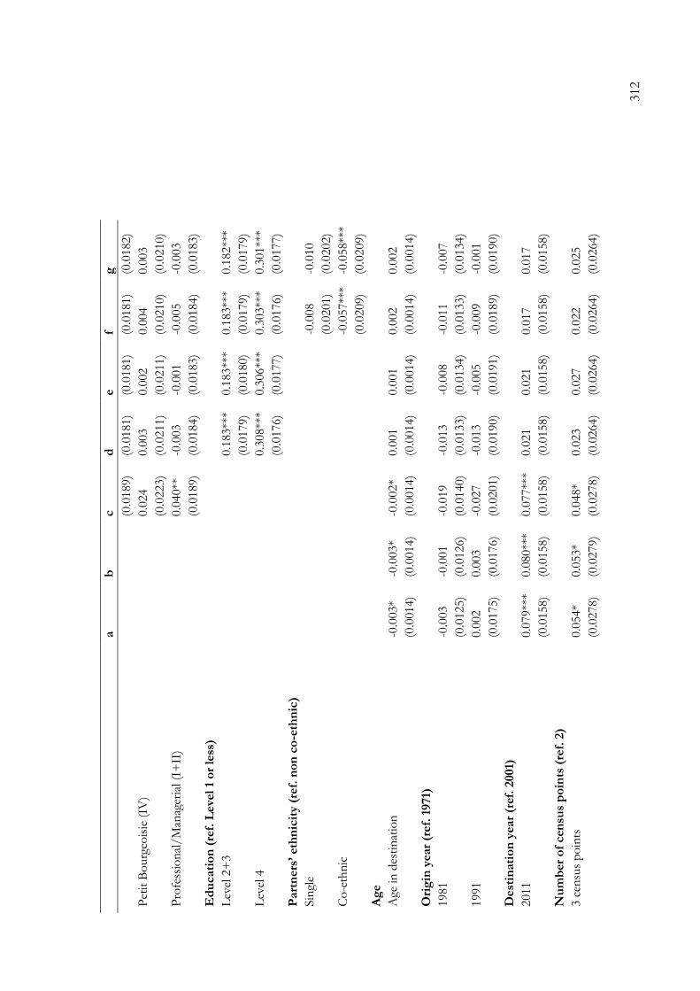
312

a

b

c

d

e

f g

(0

.0189)

(0.0

181)

(0.0

181)

(0.0

181)

(0.0

182)

Pet

it B

ourg

eois

ie (

IV)

0.0

24

0.0

03

0.0

02

0.0

04

0.0

03

(0

.0223)

(0.0

211)

(0.0

211)

(0.0

210)

(0.0

210)

Pro

fess

ion

al/

Man

ager

ial (I

+II

)

0.0

40**

-0

.003

-0.0

01

-0.0

05

-0.0

03

(0

.0189)

(0.0

184)

(0.0

183)

(0.0

184)

(0.0

183)

Ed

ucati

on

(re

f. L

eve

l 1

or

less

)

Lev

el 2

+3

0.1

83**

* 0.1

83**

* 0.1

83**

* 0.1

82**

*

(0.0

179)

(0.0

180)

(0.0

179)

(0.0

179)

Lev

el 4

0.3

08**

* 0.3

06**

* 0.3

03**

* 0.3

01**

*

(0.0

176)

(0.0

177)

(0.0

176)

(0.0

177)

Part

ners

’ et

hn

icit

y (

ref.

no

n c

o-e

thn

ic)

Sin

gle

-0

.008

-0.0

10

(0.0

201)

(0.0

202)

Co

-eth

nic

-0.0

57**

* -0

.058**

*

(0.0

209)

(0.0

209)

Ag

e

Age

in

des

tin

atio

n

-0.0

03*

-0.0

03*

-0.0

02*

0.0

01

0.0

01

0.0

02

0.0

02

(0

.0014)

(0.0

014)

(0.0

014)

(0.0

014)

(0.0

014)

(0.0

014)

(0.0

014)

Ori

gin

year

(ref.

1971)

1981

-0.0

03

-0.0

01

-0.0

19

-0.0

13

-0.0

08

-0.0

11

-0.0

07

(0

.0125)

(0.0

126)

(0.0

140)

(0.0

133)

(0.0

134)

(0.0

133)

(0.0

134)

1991

0.0

02

0.0

03

-0.0

27

-0.0

13

-0.0

05

-0.0

09

-0.0

01

(0

.0175)

(0.0

176)

(0.0

201)

(0.0

190)

(0.0

191)

(0.0

189)

(0.0

190)

Dest

inati

on

year

(ref

. 2001)

2011

0.0

79**

* 0.0

80**

* 0.0

77**

* 0.0

21

0.0

21

0.0

17

0.0

17

(0

.0158)

(0.0

158)

(0.0

158)

(0.0

158)

(0.0

158)

(0.0

158)

(0.0

158)

Nu

mb

er

of

cen

sus

po

ints

(re

f. 2

)

3 c

ensu

s p

oin

ts

0.0

54*

0.0

53*

0.0

48*

0.0

23

0.0

27

0.0

22

0.0

25

(0

.0278)

(0.0

279)

(0.0

278)

(0.0

264)

(0.0

264)

(0.0

264)

(0.0

264)

313

a

b

c

d

e

f g

4 c

ensu

s p

oin

ts

0.0

56*

0.0

56*

0.0

47

0.0

11

0.0

16

0.0

12

0.0

17

(0

.0300)

(0.0

301)

(0.0

299)

(0.0

285)

(0.0

284)

(0.0

285)

(0.0

284)

5 c

ensu

s p

oin

ts

0.1

09**

* 0.1

11**

* 0.1

03**

* 0.0

70**

0.0

74**

0.0

70**

0.0

74**

(0

.0356)

(0.0

357)

(0.0

355)

(0.0

341)

(0.0

340)

(0.0

341)

(0.0

340)

Co

nst

an

t 0.7

41**

* 0.7

39**

* 0.7

05**

* 0.5

56**

* 0.5

16**

* 0.5

84**

* 0.5

45**

*

(0

.0384)

(0.0

464)

(0.0

488)

(0.0

485)

(0.0

522)

(0.0

513)

(0.0

549)

Ad

just

ed

R-s

qu

are

d

0.0

95

0.0

95

0.1

02

0.1

66

0.1

67

0.1

68

0.1

70

N

7,4

37

7,4

37

7,4

37

7,4

37

7,4

37

7,4

37

7,4

37

Ro

bust

(cl

ust

ered

) st

and

ard

err

ors

in

par

enth

eses

**

* p

<0.0

1 *

* p

<0.0

5 *

p<

0.1

P

op

ula

tio

n: In

div

idual

s b

etw

een

20 a

nd

45 y

ears

old

So

urc

e: A

uth

or’

s o

wn

cal

cula

tio

ns

bas

ed o

n O

NS

-LS

314

Tab

le ‎8

.12: A

cces

s to

th

e se

rvic

e cl

ass:

full

mo

del

. P

oo

led e

thn

ic m

ino

riti

es; m

en.

a

b

c

d

e

f g

EM

qu

inti

le (

ref.

Q1:

lo

wes

t co

ncen

trati

on

)

Q2

-0.0

40

-0.0

10

0.0

08

0.0

18

0.0

62*

0.0

19

0.0

64*

(0

.0268)

(0.0

269)

(0.0

261)

(0.0

224)

(0.0

347)

(0.0

225)

(0.0

347)

Q3

-0.0

83**

* -0

.031

-0.0

08

0.0

22

0.0

36

0.0

23

0.0

38

(0

.0269)

(0.0

279)

(0.0

273)

(0.0

232)

(0.0

345)

(0.0

232)

(0.0

346)

Q4

-0.1

00**

* -0

.028

0.0

02

0.0

35

0.0

79**

0.0

37

0.0

82**

(0

.0267)

(0.0

286)

(0.0

283)

(0.0

239)

(0.0

351)

(0.0

240)

(0.0

351)

Q5

-0.1

34**

* -0

.047

-0.0

14

0.0

23

0.0

89**

0.0

26

0.0

94**

*

(0

.0274)

(0.0

305)

(0.0

302)

(0.0

255)

(0.0

363)

(0.0

254)

(0.0

363)

Eth

nic

gro

up

(re

f. I

nd

ian

)

Pak

ista

ni

-0.1

74**

* -0

.155**

* -0

.110**

* -0

.060**

* 0.0

11

-0.0

60**

* 0.0

15

(0

.0206)

(0.0

208)

(0.0

209)

(0.0

172)

(0.0

424)

(0.0

172)

(0.0

423)

Ban

glad

esh

i -0

.153**

* -0

.131**

* -0

.057*

-0.0

22

0.0

53

-0.0

23

0.0

57

(0

.0306)

(0.0

307)

(0.0

324)

(0.0

272)

(0.0

733)

(0.0

273)

(0.0

728)

Car

ibb

ean

-0

.193**

* -0

.184**

* -0

.173**

* -0

.060**

* -0

.045

-0.0

68**

* -0

.054

(0

.0235)

(0.0

234)

(0.0

244)

(0.0

217)

(0.0

519)

(0.0

224)

(0.0

523)

Afr

ican

-0

.045

-0.0

46

-0.0

47

-0.0

32

0.2

71**

-0

.037

0.2

64**

(0

.0468)

(0.0

464)

(0.0

459)

(0.0

428)

(0.1

197)

(0.0

432)

(0.1

209)

Eth

nic

gro

up

* E

M q

uin

tile

Pak

ista

ni *

Q2

-0.0

90*

-0

.096*

(0

.0538)

(0

.0538)

Pak

ista

ni *

Q3

-0.0

67

-0

.070

(0

.0519)

(0

.0520)

Pak

ista

ni *

Q4

-0.0

46

-0

.051

(0

.0513)

(0

.0513)

Pak

ista

ni *

Q5

-0.1

16**

-0.1

22**

(0

.0520)

(0

.0520)

315

a

b

c

d

e

f g

Ban

glad

esh

i *

Q2

-0.0

86

-0

.089

(0

.0864)

(0

.0860)

Ban

glad

esh

i *

Q3

0.0

06

-0

.000

(0

.0892)

(0

.0890)

Ban

glad

esh

i *

Q4

-0.0

66

-0

.071

(0

.0865)

(0

.0862)

Ban

glad

esh

i *

Q5

-0.1

94**

-0.2

03**

(0

.0857)

(0

.0853)

Car

ibb

ean

* Q

2

-0.0

10

-0

.007

(0

.0597)

(0

.0597)

Car

ibb

ean

* Q

3

0.0

68

0.0

66

(0

.0624)

(0

.0623)

Car

ibb

ean

* Q

4

-0.0

68

-0

.068

(0

.0605)

(0

.0605)

Car

ibb

ean

* Q

5

-0.0

54

-0

.055

(0

.0655)

(0

.0652)

Afr

ican

* Q

2

-0.3

75**

*

-0.3

82**

*

(0

.1386)

(0

.1393)

Afr

ican

* Q

3

-0.2

85**

-0.2

78*

(0

.1408)

(0

.1421)

Afr

ican

* Q

4

-0.3

97**

*

-0.3

94**

*

(0

.1441)

(0

.1458)

Afr

ican

* Q

5

-0.3

25**

-0.3

23**

(0

.1387)

(0

.1398)

Cars

tair

s q

uin

tile

(re

f. Q

1: l

east

dep

rive

d)

Q2

-0

.065

-0.0

36

-0.0

30

-0.0

33

-0.0

26

-0.0

29

(0.0

444)

(0.0

441)

(0.0

415)

(0.0

412)

(0.0

416)

(0.0

413)

Q3

-0

.152**

* -0

.100**

-0

.094**

-0

.096**

* -0

.093**

-0

.095**

*

(0.0

396)

(0.0

391)

(0.0

367)

(0.0

365)

(0.0

368)

(0.0

365)

316

a

b

c

d

e

f g

Q4

-0

.144**

* -0

.090**

-0

.080**

-0

.079**

-0

.077**

-0

.077**

(0.0

384)

(0.0

378)

(0.0

356)

(0.0

355)

(0.0

357)

(0.0

355)

Q5

-0

.220**

* -0

.133**

* -0

.115**

* -0

.119**

* -0

.112**

* -0

.116**

*

(0.0

379)

(0.0

382)

(0.0

364)

(0.0

363)

(0.0

365)

(0.0

363)

Ten

ure

(re

f. o

wn

er)

So

cial

ren

t

-0

.015

0.0

00

0.0

07

0.0

01

0.0

07

(0

.0215)

(0.0

182)

(0.0

182)

(0.0

182)

(0.0

182)

Pri

vat

e re

nt

0.0

20

0.0

26

0.0

33

0.0

26

0.0

33

(0

.0254)

(0.0

213)

(0.0

213)

(0.0

213)

(0.0

213)

Nu

mb

er

of

cars

(re

f. n

on

e)

1 c

ar

0.0

48**

* 0.0

30**

0.0

30**

0.0

29**

0.0

30**

(0

.0162)

(0.0

135)

(0.0

135)

(0.0

135)

(0.0

135)

2+

car

s

0.0

67**

0.0

60**

* 0.0

61**

* 0.0

60**

* 0.0

61**

*

(0

.0265)

(0.0

221)

(0.0

220)

(0.0

221)

(0.0

220)

Pers

on

s p

er

roo

m (

ref.

1 p

pp

)

> 1

.5 p

erso

ns

-0.0

73**

* -0

.033*

-0.0

33*

-0.0

33*

-0.0

33*

(0

.0225)

(0.0

190)

(0.0

190)

(0.0

190)

(0.0

190)

1.5

per

son

s

-0

.058*

-0.0

30

-0.0

24

-0.0

30

-0.0

25

(0

.0325)

(0.0

262)

(0.0

262)

(0.0

262)

(0.0

262)

>1 &

<1.5

per

son

s

-0

.039*

-0.0

26

-0.0

26

-0.0

26

-0.0

26

(0

.0202)

(0.0

170)

(0.0

170)

(0.0

170)

(0.0

170)

>=

0.7

5 &

<1 p

erso

n

0.0

23

0.0

16

0.0

15

0.0

16

0.0

14

(0

.0227)

(0.0

191)

(0.0

191)

(0.0

191)

(0.0

191)

<0.7

5 p

erso

n

0.0

48**

0.0

21

0.0

22

0.0

20

0.0

22

(0

.0241)

(0.0

206)

(0.0

205)

(0.0

205)

(0.0

205)

Pare

nta

l so

cial

cla

ss (

ref.

Man

ual (V

+V

I+V

II))

No

ear

ner

s/N

o c

od

e

-0

.019

-0.0

00

-0.0

02

-0.0

00

-0.0

02

(0

.0226)

(0.0

185)

(0.0

184)

(0.0

184)

(0.0

183)

Ro

uti

ne

no

n-m

anual

(II

I)

0.0

74**

* 0.0

25

0.0

29

0.0

24

0.0

28

317

a

b

c

d

e

f g

(0

.0242)

(0.0

214)

(0.0

214)

(0.0

214)

(0.0

214)

Pet

it B

ourg

eois

ie (

IV)

0.0

39

0.0

20

0.0

25

0.0

21

0.0

26

(0

.0257)

(0.0

218)

(0.0

218)

(0.0

218)

(0.0

218)

Pro

fess

ion

al/

Man

ager

ial (I

+II

)

0.1

82**

* 0.0

54**

* 0.0

60**

* 0.0

54**

* 0.0

59**

*

(0

.0229)

(0.0

205)

(0.0

204)

(0.0

205)

(0.0

204)

Ed

ucati

on

(re

f. L

eve

l 1

or

less

)

Lev

el 2

+3

0.1

51**

* 0.1

49**

* 0.1

50**

* 0.1

47**

*

(0.0

173)

(0.0

172)

(0.0

172)

(0.0

172)

Lev

el 4

0.5

50**

* 0.5

48**

* 0.5

47**

* 0.5

45**

*

(0.0

162)

(0.0

162)

(0.0

162)

(0.0

162)

Part

ners

’ et

hn

icit

y (

ref.

no

n c

o-e

thn

ic)

Sin

gle

-0

.060**

* -0

.061**

*

(0.0

230)

(0.0

230)

Co

-eth

nic

-0.0

50**

-0

.054**

(0.0

235)

(0.0

234)

Ag

e

Age

in

des

tin

atio

n

0.0

02

0.0

02

0.0

03*

0.0

06**

* 0.0

06**

* 0.0

05**

* 0.0

05**

*

(0

.0015)

(0.0

015)

(0.0

015)

(0.0

013)

(0.0

012)

(0.0

014)

(0.0

014)

Ori

gin

year

(ref.

1971)

1981

0.0

37**

0.0

42**

* 0.0

07

0.0

12

0.0

13

0.0

10

0.0

11

(0

.0152)

(0.0

153)

(0.0

169)

(0.0

142)

(0.0

142)

(0.0

141)

(0.0

141)

1991

0.0

23

0.0

22

-0.0

47**

-0

.012

-0.0

09

-0.0

14

-0.0

11

(0

.0203)

(0.0

204)

(0.0

231)

(0.0

191)

(0.0

192)

(0.0

190)

(0.0

191)

Dest

inati

on

year

(ref

. 2001)

2011

0.0

53**

* 0.0

52**

* 0.0

45**

* -0

.046**

* -0

.048**

* -0

.045**

* -0

.046**

*

(0

.0177)

(0.0

177)

(0.0

174)

(0.0

158)

(0.0

158)

(0.0

159)

(0.0

159)

Nu

mb

er

of

cen

sus

po

ints

(re

f. 2

)

3 c

ensu

s p

oin

ts

0.0

39

0.0

38

0.0

18

-0.0

06

-0.0

09

-0.0

07

-0.0

11

(0

.0285)

(0.0

285)

(0.0

280)

(0.0

253)

(0.0

255)

(0.0

253)

(0.0

255)

318

a

b

c

d

e

f g

4 c

ensu

s p

oin

ts

0.1

04**

* 0.0

99**

* 0.0

73**

0.0

14

0.0

11

0.0

12

0.0

08

(0

.0306)

(0.0

305)

(0.0

300)

(0.0

266)

(0.0

267)

(0.0

267)

(0.0

268)

5 c

ensu

s p

oin

ts

0.1

32**

* 0.1

32**

* 0.1

12**

* 0.0

37

0.0

29

0.0

32

0.0

24

(0

.0386)

(0.0

384)

(0.0

378)

(0.0

328)

(0.0

328)

(0.0

329)

(0.0

329)

Co

nst

an

t 0.4

86**

* 0.6

07**

* 0.5

13**

* 0.2

74**

* 0.2

41**

* 0.3

23**

* 0.2

92**

*

(0

.0419)

(0.0

510)

(0.0

544)

(0.0

504)

(0.0

544)

(0.0

545)

(0.0

584)

Ad

just

ed

R-s

qu

are

d

0.0

47

0.0

56

0.0

83

0.2

91

0.2

94

0.2

92

0.2

95

N

6,4

44

6,4

44

6,4

44

6,4

44

6,4

44

6,4

44

6,4

44

Ro

bust

(cl

ust

ered

) st

and

ard

err

ors

in

par

enth

eses

**

* p

<0.0

1 *

* p

<0.0

5 *

p<

0.1

P

op

ula

tio

n: In

div

idual

s b

etw

een

20 a

nd

45 y

ears

old

So

urc

e: A

uth

or’

s o

wn

cal

cula

tio

ns

bas

ed o

n O

NS-L

S

319

Tab

le ‎8

.13: A

cces

s to

th

e se

rvic

e cl

ass:

full

mo

del

. P

oo

led e

thn

ic m

ino

riti

es; w

om

en.

a

b

c

d

e

f g

EM

qu

inti

le (

ref.

Q1:

lo

wes

t co

ncen

trati

on

)

Q2

-0.0

61**

-0

.038

-0.0

20

-0.0

13

0.0

33

-0.0

13

0.0

32

(0

.0259)

(0.0

263)

(0.0

259)

(0.0

220)

(0.0

356)

(0.0

220)

(0.0

356)

Q3

-0.1

10**

* -0

.071**

* -0

.044*

-0.0

27

0.0

02

-0.0

25

0.0

04

(0

.0250)

(0.0

266)

(0.0

264)

(0.0

225)

(0.0

347)

(0.0

225)

(0.0

346)

Q4

-0.1

23**

* -0

.070**

-0

.043

-0.0

38

-0.0

62*

-0.0

36

-0.0

59

(0

.0254)

(0.0

279)

(0.0

280)

(0.0

244)

(0.0

359)

(0.0

245)

(0.0

360)

Q5

-0.1

48**

* -0

.081**

* -0

.044

-0.0

42*

-0.0

40

-0.0

40

-0.0

39

(0

.0255)

(0.0

293)

(0.0

293)

(0.0

248)

(0.0

359)

(0.0

249)

(0.0

359)

Eth

nic

gro

up

(re

f. I

nd

ian

)

Pak

ista

ni

-0.1

59**

* -0

.144**

* -0

.101**

* -0

.050**

* -0

.035

-0.0

46**

-0

.031

(0

.0207)

(0.0

210)

(0.0

213)

(0.0

185)

(0.0

428)

(0.0

186)

(0.0

426)

Ban

glad

esh

i -0

.180**

* -0

.159**

* -0

.082**

-0

.036

0.0

02

-0.0

33

0.0

04

(0

.0301)

(0.0

306)

(0.0

326)

(0.0

268)

(0.0

667)

(0.0

269)

(0.0

666)

Car

ibb

ean

-0

.077**

* -0

.073**

* -0

.075**

* -0

.044**

-0

.019

-0.0

48**

-0

.023

(0

.0227)

(0.0

227)

(0.0

236)

(0.0

203)

(0.0

472)

(0.0

207)

(0.0

473)

Afr

ican

0.0

10

0.0

00

-0.0

19

-0.1

10**

* -0

.203**

* -0

.113**

* -0

.206**

*

(0

.0409)

(0.0

406)

(0.0

418)

(0.0

392)

(0.0

739)

(0.0

396)

(0.0

738)

Eth

nic

gro

up

* E

M q

uin

tile

Pak

ista

ni *

Q2

-0.0

67

-0

.066

(0

.0546)

(0

.0544)

Pak

ista

ni *

Q3

-0.0

60

-0

.062

(0

.0520)

(0

.0517)

Pak

ista

ni *

Q4

0.0

64

0.0

60

(0

.0556)

(0

.0553)

Pak

ista

ni *

Q5

-0.0

23

-0

.023

(0

.0525)

(0

.0524)

320

a

b

c

d

e

f g

Ban

glad

esh

i *

Q2

-0.0

88

-0

.084

(0

.0818)

(0

.0818)

Ban

glad

esh

i *

Q3

-0.1

06

-0

.106

(0

.0795)

(0

.0794)

Ban

glad

esh

i *

Q4

0.0

14

0.0

12

(0

.0791)

(0

.0790)

Ban

glad

esh

i *

Q5

0.0

00

0.0

01

(0

.0819)

(0

.0817)

Car

ibb

ean

* Q

2

-0.0

83

-0

.082

(0

.0565)

(0

.0566)

Car

ibb

ean

* Q

3

-0.0

39

-0

.036

(0

.0576)

(0

.0576)

Car

ibb

ean

* Q

4

0.0

09

0.0

09

(0

.0583)

(0

.0583)

Car

ibb

ean

* Q

5

-0.0

17

-0

.015

(0

.0607)

(0

.0609)

Afr

ican

* Q

2

0.0

08

0.0

06

(0

.1137)

(0

.1158)

Afr

ican

* Q

3

0.0

51

0.0

45

(0

.0965)

(0

.0960)

Afr

ican

* Q

4

0.1

57

0.1

58

(0

.1000)

(0

.1000)

Afr

ican

* Q

5

0.1

77*

0.1

79*

(0

.0983)

(0

.0982)

Cars

tair

s q

uin

tile

(re

f. Q

1: l

east

dep

rive

d)

Q2

-0

.077*

-0.0

45

-0.0

33

-0.0

32

-0.0

30

-0.0

30

(0.0

439)

(0.0

434)

(0.0

390)

(0.0

386)

(0.0

389)

(0.0

385)

Q3

-0

.066

-0.0

28

-0.0

12

-0.0

08

-0.0

11

-0.0

07

(0.0

417)

(0.0

418)

(0.0

376)

(0.0

374)

(0.0

375)

(0.0

374)

321

a

b

c

d

e

f g

Q4

-0

.087**

-0

.039

-0.0

10

-0.0

05

-0.0

08

-0.0

03

(0.0

403)

(0.0

403)

(0.0

356)

(0.0

353)

(0.0

355)

(0.0

353)

Q5

-0

.152**

* -0

.083**

-0

.033

-0.0

28

-0.0

31

-0.0

26

(0.0

403)

(0.0

404)

(0.0

359)

(0.0

355)

(0.0

358)

(0.0

355)

Ten

ure

(re

f. o

wn

er)

So

cial

ren

t

0.0

07

0.0

14

0.0

09

0.0

14

0.0

09

(0

.0204)

(0.0

175)

(0.0

177)

(0.0

175)

(0.0

177)

Pri

vat

e re

nt

0.0

52**

0.0

34

0.0

29

0.0

36*

0.0

30

(0

.0242)

(0.0

211)

(0.0

211)

(0.0

211)

(0.0

211)

Nu

mb

er

of

cars

(re

f. n

on

e)

1 c

ar

0.0

52**

* 0.0

18

0.0

17

0.0

18

0.0

17

(0

.0158)

(0.0

137)

(0.0

137)

(0.0

137)

(0.0

137)

2+

car

s

0.0

93**

* 0.0

56**

0.0

53**

0.0

55**

0.0

52**

(0

.0273)

(0.0

240)

(0.0

239)

(0.0

239)

(0.0

238)

Pers

on

s p

er

roo

m (

ref.

1 p

pp

)

> 1

.5 p

erso

ns

-0.0

63**

* -0

.024

-0.0

25

-0.0

22

-0.0

23

(0

.0222)

(0.0

191)

(0.0

190)

(0.0

190)

(0.0

190)

1.5

per

son

s

-0

.065**

-0

.039

-0.0

40

-0.0

38

-0.0

39

(0

.0298)

(0.0

261)

(0.0

262)

(0.0

260)

(0.0

261)

>1 &

<1.5

per

son

s

-0

.053**

* -0

.023

-0.0

22

-0.0

22

-0.0

21

(0

.0194)

(0.0

167)

(0.0

166)

(0.0

167)

(0.0

166)

>=

0.7

5 &

<1 p

erso

n

0.0

08

0.0

15

0.0

14

0.0

15

0.0

14

(0

.0225)

(0.0

194)

(0.0

194)

(0.0

195)

(0.0

195)

<0.7

5 p

erso

n

0.0

16

0.0

03

0.0

04

0.0

02

0.0

03

(0

.0245)

(0.0

214)

(0.0

214)

(0.0

214)

(0.0

214)

Pare

nta

l so

cial

cla

ss (

ref.

Man

ual (V

+V

I+V

II))

No

ear

ner

s/N

o c

od

e

-0

.021

-0.0

01

-0.0

01

-0.0

01

-0.0

01

(0

.0221)

(0.0

193)

(0.0

195)

(0.0

193)

(0.0

194)

Ro

uti

ne

no

n-m

anual

(II

I)

0.1

19**

* 0.0

60**

* 0.0

57**

* 0.0

57**

0.0

54**

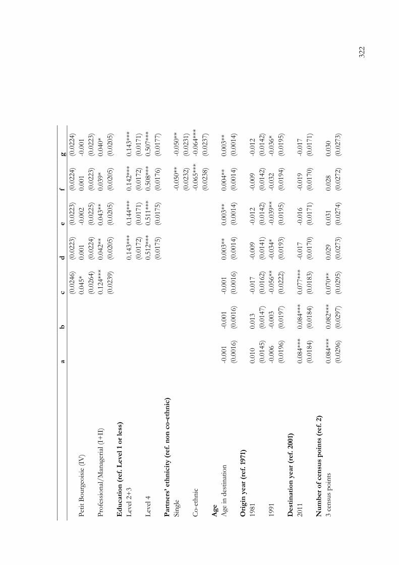
322

a

b

c

d

e

f g

(0

.0246)

(0.0

223)

(0.0

223)

(0.0

224)

(0.0

224)

Pet

it B

ourg

eois

ie (

IV)

0.0

45*

0.0

01

-0.0

02

0.0

01

-0.0

01

(0

.0264)

(0.0

224)

(0.0

225)

(0.0

223)

(0.0

223)

Pro

fess

ion

al/

Man

ager

ial (I

+II

)

0.1

24**

* 0.0

42**

0.0

43**

0.0

39*

0.0

40*

(0

.0239)

(0.0

205)

(0.0

205)

(0.0

205)

(0.0

205)

Ed

ucati

on

(re

f. L

eve

l 1

or

less

)

Lev

el 2

+3

0.1

43**

* 0.1

44**

* 0.1

42**

* 0.1

43**

*

(0.0

172)

(0.0

171)

(0.0

172)

(0.0

171)

Lev

el 4

0.5

12**

* 0.5

11**

* 0.5

08**

* 0.5

07**

*

(0.0

175)

(0.0

175)

(0.0

176)

(0.0

177)

Part

ners

’ et

hn

icit

y (

ref.

no

n c

o-e

thn

ic)

Sin

gle

-0

.050**

-0

.050**

(0.0

232)

(0.0

231)

Co

-eth

nic

-0.0

65**

* -0

.064**

*

(0.0

238)

(0.0

237)

Ag

e

Age

in

des

tin

atio

n

-0.0

01

-0.0

01

-0.0

01

0.0

03**

0.0

03**

0.0

04**

0.0

03**

(0

.0016)

(0.0

016)

(0.0

016)

(0.0

014)

(0.0

014)

(0.0

014)

(0.0

014)

Ori

gin

year

(ref.

1971)

1981

0.0

10

0.0

13

-0.0

17

-0.0

09

-0.0

12

-0.0

09

-0.0

12

(0

.0145)

(0.0

147)

(0.0

162)

(0.0

141)

(0.0

142)

(0.0

142)

(0.0

142)

1991

-0.0

06

-0.0

03

-0.0

56**

-0

.034*

-0.0

39**

-0

.032

-0.0

36*

(0

.0196)

(0.0

197)

(0.0

222)

(0.0

193)

(0.0

195)

(0.0

194)

(0.0

195)

Dest

inati

on

year

(ref

. 2001)

2011

0.0

84**

* 0.0

84**

* 0.0

77**

* -0

.017

-0.0

16

-0.0

19

-0.0

17

(0

.0184)

(0.0

184)

(0.0

183)

(0.0

170)

(0.0

171)

(0.0

170)

(0.0

171)

Nu

mb

er

of

cen

sus

po

ints

(re

f. 2

)

3 c

ensu

s p

oin

ts

0.0

84**

* 0.0

82**

* 0.0

70**

0.0

29

0.0

31

0.0

28

0.0

30

(0

.0296)

(0.0

297)

(0.0

295)

(0.0

273)

(0.0

274)

(0.0

272)

(0.0

273)

323

a

b

c

d

e

f g

4 c

ensu

s p

oin

ts

0.1

29**

* 0.1

28**

* 0.1

15**

* 0.0

61**

0.0

63**

0.0

61**

0.0

62**

(0

.0324)

(0.0

324)

(0.0

322)

(0.0

293)

(0.0

294)

(0.0

292)

(0.0

292)

5 c

ensu

s p

oin

ts

0.1

33**

* 0.1

36**

* 0.1

29**

* 0.0

87**

0.0

87**

0.0

84**

0.0

84**

(0

.0408)

(0.0

409)

(0.0

407)

(0.0

361)

(0.0

362)

(0.0

360)

(0.0

361)

Co

nst

an

t 0.4

36**

* 0.5

08**

* 0.4

16**

* 0.2

00**

* 0.1

90**

* 0.2

50**

* 0.2

40**

*

(0

.0435)

(0.0

536)

(0.0

572)

(0.0

523)

(0.0

568)

(0.0

553)

(0.0

596)

Ad

just

ed

R-s

qu

are

d

0.0

34

0.0

39

0.0

59

0.2

29

0.2

30

0.2

30

0.2

31

N

6,6

85

6,6

85

6,6

85

6,6

85

6,6

85

6,6

85

6,6

85

Ro

bust

(cl

ust

ered

) st

and

ard

err

ors

in

par

enth

eses

**

* p

<0.0

1 *

* p

<0.0

5 *

p<

0.1

P

op

ula

tio

n: In

div

idual

s b

etw

een

20 a

nd

45 y

ears

old

So

urc

e: A

uth

or’

s o

wn

cal

cula

tio

ns

bas

ed o

n O

NS

-LS

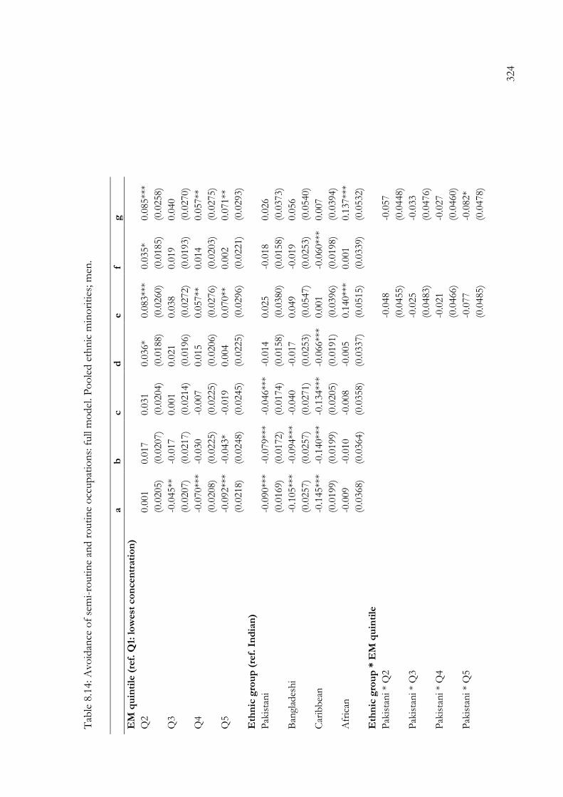
324

Tab

le ‎8

.14: A

vo

idan

ce o

f se

mi-

routi

ne

and r

outi

ne

occ

up

atio

ns:

full

mo

del

. P

oo

led e

thn

ic m

ino

riti

es; m

en.

a

b

c

d

e

f g

EM

qu

inti

le (

ref.

Q1:

lo

wes

t co

ncen

trati

on

)

Q2

0.0

01

0.0

17

0.0

31

0.0

36*

0.0

83**

* 0.0

35*

0.0

85**

*

(0

.0205)

(0.0

207)

(0.0

204)

(0.0

188)

(0.0

260)

(0.0

185)

(0.0

258)

Q3

-0.0

45**

-0

.017

0.0

01

0.0

21

0.0

38

0.0

19

0.0

40

(0

.0207)

(0.0

217)

(0.0

214)

(0.0

196)

(0.0

272)

(0.0

193)

(0.0

270)

Q4

-0.0

70**

* -0

.030

-0.0

07

0.0

15

0.0

57**

0.0

14

0.0

57**

(0

.0208)

(0.0

225)

(0.0

225)

(0.0

206)

(0.0

276)

(0.0

203)

(0.0

275)

Q5

-0.0

92**

* -0

.043*

-0.0

19

0.0

04

0.0

70**

0.0

02

0.0

71**

(0

.0218)

(0.0

248)

(0.0

245)

(0.0

225)

(0.0

296)

(0.0

221)

(0.0

293)

Eth

nic

gro

up

(re

f. I

nd

ian

)

Pak

ista

ni

-0.0

90**

* -0

.079**

* -0

.046**

* -0

.014

0.0

25

-0.0

18

0.0

26

(0

.0169)

(0.0

172)

(0.0

174)

(0.0

158)

(0.0

380)

(0.0

158)

(0.0

373)

Ban

glad

esh

i -0

.105**

* -0

.094**

* -0

.040

-0.0

17

0.0

49

-0.0

19

0.0

56

(0

.0257)

(0.0

257)

(0.0

271)

(0.0

253)

(0.0

547)

(0.0

253)

(0.0

540)

Car

ibb

ean

-0

.145**

* -0

.140**

* -0

.134**

* -0

.066**

* 0.0

01

-0.0

60**

* 0.0

07

(0

.0199)

(0.0

199)

(0.0

205)

(0.0

191)

(0.0

396)

(0.0

198)

(0.0

394)

Afr

ican

-0

.009

-0.0

10

-0.0

08

-0.0

05

0.1

40**

* 0.0

01

0.1

37**

*

(0

.0368)

(0.0

364)

(0.0

358)

(0.0

337)

(0.0

515)

(0.0

339)

(0.0

532)

Eth

nic

gro

up

* E

M q

uin

tile

Pak

ista

ni *

Q2

-0.0

48

-0

.057

(0

.0455)

(0

.0448)

Pak

ista

ni *

Q3

-0.0

25

-0

.033

(0

.0483)

(0

.0476)

Pak

ista

ni *

Q4

-0.0

21

-0

.027

(0

.0466)

(0

.0460)

Pak

ista

ni *

Q5

-0.0

77

-0

.082*

(0

.0485)

(0

.0478)

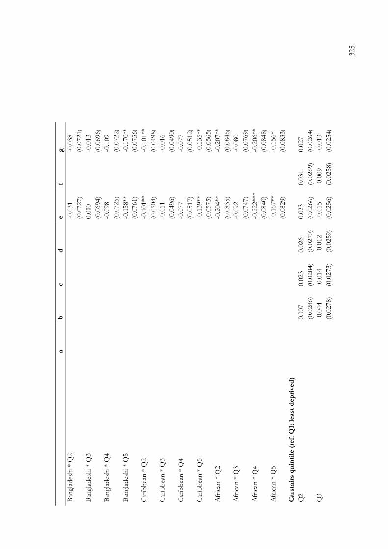
325

a

b

c

d

e

f g

Ban

glad

esh

i *

Q2

-0.0

31

-0

.038

(0

.0727)

(0

.0721)

Ban

glad

esh

i *

Q3

0.0

00

-0

.013

(0

.0694)

(0

.0696)

Ban

glad

esh

i *

Q4

-0.0

98

-0

.109

(0

.0725)

(0

.0722)

Ban

glad

esh

i *

Q5

-0.1

58**

-0.1

70**

(0

.0761)

(0

.0756)

Car

ibb

ean

* Q

2

-0.1

01**

-0.1

01**

(0

.0504)

(0

.0498)

Car

ibb

ean

* Q

3

-0.0

11

-0

.016

(0

.0496)

(0

.0490)

Car

ibb

ean

* Q

4

-0.0

77

-0

.077

(0

.0517)

(0

.0512)

Car

ibb

ean

* Q

5

-0.1

39**

-0.1

35**

(0

.0575)

(0

.0565)

Afr

ican

* Q

2

-0.2

04**

-0.2

07**

(0

.0835)

(0

.0846)

Afr

ican

* Q

3

-0.0

92

-0

.080

(0

.0747)

(0

.0769)

Afr

ican

* Q

4

-0.2

22**

*

-0.2

06**

(0

.0840)

(0

.0848)

Afr

ican

* Q

5

-0.1

67**

-0.1

56*

(0

.0829)

(0

.0833)

Cars

tair

s q

uin

tile

(re

f. Q

1: l

east

dep

rive

d)

Q2

0.0

07

0.0

23

0.0

26

0.0

23

0.0

31

0.0

27

(0.0

286)

(0.0

284)

(0.0

270)

(0.0

266)

(0.0

269)

(0.0

264)

Q3

-0

.044

-0.0

14

-0.0

12

-0.0

15

-0.0

09

-0.0

13

(0.0

278)

(0.0

273)

(0.0

259)

(0.0

256)

(0.0

258)

(0.0

254)

326

a

b

c

d

e

f g

Q4

-0

.061**

-0

.032

-0.0

28

-0.0

30

-0.0

25

-0.0

27

(0.0

268)

(0.0

264)

(0.0

251)

(0.0

250)

(0.0

249)

(0.0

248)

Q5

-0

.095**

* -0

.043

-0.0

35

-0.0

40

-0.0

32

-0.0

37

(0.0

266)

(0.0

264)

(0.0

250)

(0.0

247)

(0.0

248)

(0.0

245)

Ten

ure

(re

f. o

wn

er)

So

cial

ren

t

-0

.000

0.0

08

0.0

14

0.0

09

0.0

16

(0

.0185)

(0.0

171)

(0.0

175)

(0.0

170)

(0.0

174)

Pri

vat

e re

nt

-0.0

04

0.0

01

0.0

08

0.0

02

0.0

09

(0

.0210)

(0.0

191)

(0.0

192)

(0.0

190)

(0.0

192)

Nu

mb

er

of

cars

(re

f. n

on

e)

1 c

ar

0.0

44**

* 0.0

31**

0.0

32**

0.0

30**

0.0

31**

(0

.0138)

(0.0

126)

(0.0

126)

(0.0

125)

(0.0

126)

2+

car

s

0.0

39*

0.0

35*

0.0

37*

0.0

35*

0.0

37*

(0

.0210)

(0.0

192)

(0.0

193)

(0.0

192)

(0.0

193)

Pers

on

s p

er

roo

m (

ref.

1 p

pp

)

> 1

.5 p

erso

ns

-0.0

50**

* -0

.024

-0.0

25

-0.0

28

-0.0

28

(0

.0192)

(0.0

177)

(0.0

177)

(0.0

177)

(0.0

177)

1.5

per

son

s

-0

.052*

-0.0

35

-0.0

34

-0.0

38

-0.0

36

(0

.0274)

(0.0

246)

(0.0

246)

(0.0

245)

(0.0

245)

>1 &

<1.5

per

son

s

-0

.034**

-0

.025

-0.0

26*

-0.0

26*

-0.0

27*

(0

.0166)

(0.0

153)

(0.0

152)

(0.0

152)

(0.0

152)

>=

0.7

5 &

<1 p

erso

n

0.0

07

0.0

02

-0.0

00

0.0

01

-0.0

01

(0

.0178)

(0.0

163)

(0.0

162)

(0.0

162)

(0.0

162)

<0.7

5 p

erso

n

0.0

17

0.0

01

0.0

03

-0.0

00

0.0

01

(0

.0180)

(0.0

168)

(0.0

169)

(0.0

168)

(0.0

169)

Pare

nta

l so

cial

cla

ss (

ref.

Man

ual (V

+V

I+V

II))

No

ear

ner

s/N

o c

od

e

-0

.053**

-0

.044**

-0

.045**

-0

.044**

-0

.046**

(0

.0214)

(0.0

200)

(0.0

200)

(0.0

198)

(0.0

198)

Ro

uti

ne

no

n-m

anual

(II

I)

0.0

69**

* 0.0

37**

0.0

39**

0.0

39**

0.0

41**

327

a

b

c

d

e

f g

(0

.0189)

(0.0

174)

(0.0

175)

(0.0

175)

(0.0

175)

Pet

it B

ourg

eois

ie (

IV)

0.0

54**

* 0.0

41**

0.0

46**

0.0

43**

0.0

47**

*

(0

.0192)

(0.0

179)

(0.0

179)

(0.0

180)

(0.0

180)

Pro

fess

ion

al/

Man

ager

ial (I

+II

)

0.0

96**

* 0.0

19

0.0

24

0.0

23

0.0

27*

(0

.0164)

(0.0

153)

(0.0

153)

(0.0

153)

(0.0

153)

Ed

ucati

on

(re

f. L

eve

l 1

or

less

)

Lev

el 2

+3

0.1

65**

* 0.1

64**

* 0.1

64**

* 0.1

63**

*

(0.0

190)

(0.0

190)

(0.0

189)

(0.0

189)

Lev

el 4

0.3

52**

* 0.3

52**

* 0.3

50**

* 0.3

50**

*

(0.0

157)

(0.0

157)

(0.0

156)

(0.0

156)

Part

ners

’ et

hn

icit

y (

ref.

no

n c

o-e

thn

ic)

Sin

gle

-0

.071**

* -0

.072**

*

(0.0

183)

(0.0

184)

Co

-eth

nic

-0.0

15

-0.0

17

(0.0

181)

(0.0

182)

Ag

e

Age

in

des

tin

atio

n

0.0

07**

* 0.0

07**

* 0.0

07**

* 0.0

10**

* 0.0

10**

* 0.0

08**

* 0.0

08**

*

(0

.0014)

(0.0

014)

(0.0

013)

(0.0

013)

(0.0

013)

(0.0

013)

(0.0

013)

Ori

gin

year

(ref.

1971)

1981

0.0

31**

0.0

34**

* 0.0

09

0.0

13

0.0

14

0.0

07

0.0

08

(0

.0125)

(0.0

126)

(0.0

142)

(0.0

130)

(0.0

131)

(0.0

129)

(0.0

130)

1991

0.0

34**

0.0

35**

-0

.010

0.0

12

0.0

15

0.0

06

0.0

10

(0

.0170)

(0.0

171)

(0.0

198)

(0.0

183)

(0.0

186)

(0.0

182)

(0.0

185)

Dest

inati

on

year

(ref

. 2001)

2011

0.0

61**

* 0.0

61**

* 0.0

55**

* -0

.004

-0.0

06

0.0

01

-0.0

01

(0

.0157)

(0.0

157)

(0.0

157)

(0.0

152)

(0.0

153)

(0.0

152)

(0.0

153)

Nu

mb

er

of

cen

sus

po

ints

(re

f. 2

)

3 c

ensu

s p

oin

ts

0.0

49*

0.0

49*

0.0

33

0.0

17

0.0

14

0.0

17

0.0

14

(0

.0271)

(0.0

271)

(0.0

271)

(0.0

256)

(0.0

257)

(0.0

257)

(0.0

258)

328

a

b

c

d

e

f g

4 c

ensu

s p

oin

ts

0.0

92**

* 0.0

91**

* 0.0

70**

0.0

33

0.0

30

0.0

31

0.0

29

(0

.0280)

(0.0

278)

(0.0

279)

(0.0

262)

(0.0

263)

(0.0

263)

(0.0

264)

5 c

ensu

s p

oin

ts

0.0

91**

* 0.0

92**

* 0.0

74**

0.0

28

0.0

21

0.0

23

0.0

17

(0

.0332)

(0.0

331)

(0.0

330)

(0.0

308)

(0.0

309)

(0.0

308)

(0.0

309)

Co

nst

an

t 0.7

51**

* 0.7

89**

* 0.7

39**

* 0.5

73**

* 0.5

39**

* 0.6

12**

* 0.5

78**

*

(0

.0365)

(0.0

410)

(0.0

447)

(0.0

429)

(0.0

457)

(0.0

450)

(0.0

473)

Ad

just

ed

R-s

qu

are

d

0.0

48

0.0

52

0.0

69

0.1

79

0.1

80

0.1

83

0.1

84

N

6,4

44

6,4

44

6,4

44

6,4

44

6,4

44

6,4

44

6,4

44

Ro

bust

(cl

ust

ered

) st

and

ard

err

ors

in

par

enth

eses

**

* p

<0.0

1 *

* p

<0.0

5 *

p<

0.1

P

op

ula

tio

n: In

div

idual

s b

etw

een

20 a

nd

45 y

ears

old

So

urc

e: A

uth

or’

s o

wn

cal

cula

tio

ns

bas

ed o

n O

NS

-LS

329

Tab

le ‎8

.15: A

vo

idan

ce o

f se

mi-

routi

ne

and r

outi

ne

occ

up

atio

ns:

full

mo

del

. P

oo

led e

thn

ic m

ino

riti

es; w

om

en.

a

b

c

d

e

f g

EM

qu

inti

le (

ref.

Q1:

lo

wes

t co

ncen

trati

on

)

Q2

-0.0

40**

-0

.026

-0.0

12

-0.0

11

0.0

42

-0.0

11

0.0

41

(0

.0195)

(0.0

201)

(0.0

198)

(0.0

183)

(0.0

271)

(0.0

183)

(0.0

270)

Q3

-0.0

76**

* -0

.054**

-0

.032

-0.0

23

0.0

39

-0.0

22

0.0

40

(0

.0195)

(0.0

210)

(0.0

207)

(0.0

192)

(0.0

265)

(0.0

192)

(0.0

264)

Q4

-0.0

62**

* -0

.029

-0.0

08

-0.0

06

0.0

14

-0.0

04

0.0

16

(0

.0195)

(0.0

217)

(0.0

218)

(0.0

202)

(0.0

282)

(0.0

201)

(0.0

282)

Q5

-0.1

10**

* -0

.069**

* -0

.038

-0.0

39*

0.0

08

-0.0

38*

0.0

09

(0

.0204)

(0.0

238)

(0.0

239)

(0.0

219)

(0.0

299)

(0.0

218)

(0.0

297)

Eth

nic

gro

up

(re

f. I

nd

ian

)

Pak

ista

ni

-0.1

36**

* -0

.127**

* -0

.093**

* -0

.061**

* 0.0

43

-0.0

60**

* 0.0

44

(0

.0183)

(0.0

187)

(0.0

188)

(0.0

174)

(0.0

313)

(0.0

173)

(0.0

311)

Ban

glad

esh

i -0

.142**

* -0

.129**

* -0

.059**

-0

.033

0.0

69

-0.0

34

0.0

68

(0

.0274)

(0.0

276)

(0.0

294)

(0.0

278)

(0.0

592)

(0.0

277)

(0.0

587)

Car

ibb

ean

-0

.031*

-0.0

29

-0.0

27

-0.0

12

0.0

15

-0.0

08

0.0

16

(0

.0178)

(0.0

178)

(0.0

186)

(0.0

175)

(0.0

373)

(0.0

179)

(0.0

375)

Afr

ican

0.0

08

0.0

01

-0.0

02

-0.0

56**

-0

.149*

-0.0

55*

-0.1

45*

(0

.0285)

(0.0

287)

(0.0

298)

(0.0

279)

(0.0

806)

(0.0

280)

(0.0

809)

Eth

nic

gro

up

* E

M q

uin

tile

Pak

ista

ni *

Q2

-0.1

09**

-0.1

08**

(0

.0423)

(0

.0422)

Pak

ista

ni *

Q3

-0.1

84**

*

-0.1

86**

*

(0

.0446)

(0

.0446)

Pak

ista

ni *

Q4

-0.0

51

-0

.053

(0

.0435)

(0

.0435)

Pak

ista

ni *

Q5

-0.1

43**

*

-0.1

43**

*

(0

.0465)

(0

.0464)

330

a

b

c

d

e

f g

Ban

glad

esh

i *

Q2

-0.1

49*

-0

.145*

(0

.0833)

(0

.0831)

Ban

glad

esh

i *

Q3

-0.1

14

-0

.116

(0

.0749)

(0

.0745)

Ban

glad

esh

i *

Q4

-0.0

96

-0

.097

(0

.0764)

(0

.0760)

Ban

glad

esh

i *

Q5

-0.1

24

-0

.126

(0

.0805)

(0

.0801)

Car

ibb

ean

* Q

2

-0.0

57

-0

.054

(0

.0452)

(0

.0451)

Car

ibb

ean

* Q

3

-0.0

36

-0

.031

(0

.0464)

(0

.0464)

Car

ibb

ean

* Q

4

-0.0

15

-0

.013

(0

.0472)

(0

.0470)

Car

ibb

ean

* Q

5

-0.0

03

0.0

01

(0

.0494)

(0

.0494)

Afr

ican

* Q

2

0.1

25

0.1

20

(0

.0861)

(0

.0861)

Afr

ican

* Q

3

0.0

52

0.0

45

(0

.0961)

(0

.0962)

Afr

ican

* Q

4

0.1

97**

0.1

98**

(0

.0889)

(0

.0887)

Afr

ican

* Q

5

0.0

68

0.0

68

(0

.0927)

(0

.0928)

Cars

tair

s q

uin

tile

(re

f. Q

1: l

east

dep

rive

d)

Q2

-0

.037

-0.0

18

-0.0

10

-0.0

17

-0.0

10

-0.0

17

(0.0

295)

(0.0

285)

(0.0

272)

(0.0

273)

(0.0

272)

(0.0

273)

Q3

-0

.048*

-0.0

23

-0.0

15

-0.0

23

-0.0

15

-0.0

22

(0.0

281)

(0.0

273)

(0.0

261)

(0.0

262)

(0.0

261)

(0.0

262)

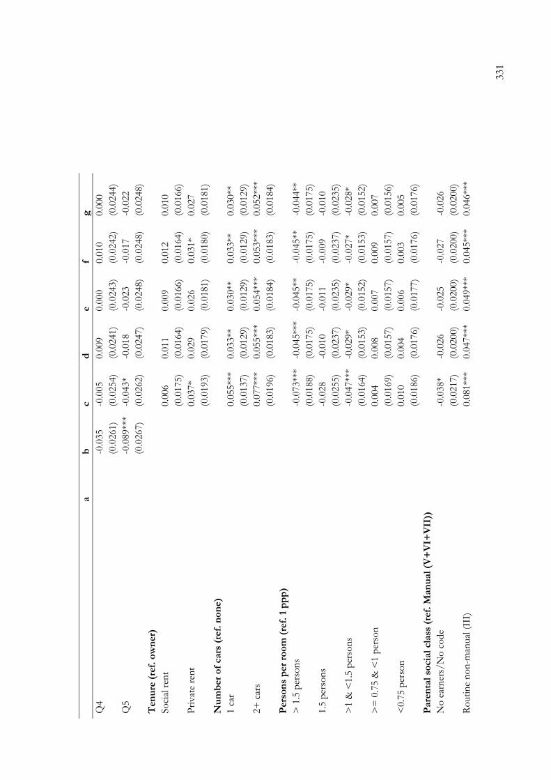
331

a

b

c

d

e

f g

Q4

-0

.035

-0.0

05

0.0

09

0.0

00

0.0

10

0.0

00

(0.0

261)

(0.0

254)

(0.0

241)

(0.0

243)

(0.0

242)

(0.0

244)

Q5

-0

.089**

* -0

.043*

-0.0

18

-0.0

23

-0.0

17

-0.0

22

(0.0

267)

(0.0

262)

(0.0

247)

(0.0

248)

(0.0

248)

(0.0

248)

Ten

ure

(re

f. o

wn

er)

So

cial

ren

t

0.0

06

0.0

11

0.0

09

0.0

12

0.0

10

(0

.0175)

(0.0

164)

(0.0

166)

(0.0

164)

(0.0

166)

Pri

vat

e re

nt

0.0

37*

0.0

29

0.0

26

0.0

31*

0.0

27

(0

.0193)

(0.0

179)

(0.0

181)

(0.0

180)

(0.0

181)

Nu

mb

er

of

cars

(re

f. n

on

e)

1 c

ar

0.0

55**

* 0.0

33**

0.0

30**

0.0

33**

0.0

30**

(0

.0137)

(0.0

129)

(0.0

129)

(0.0

129)

(0.0

129)

2+

car

s

0.0

77**

* 0.0

55**

* 0.0

54**

* 0.0

53**

* 0.0

52**

*

(0

.0196)

(0.0

183)

(0.0

184)

(0.0

183)

(0.0

184)

Pers

on

s p

er

roo

m (

ref.

1 p

pp

)

> 1

.5 p

erso

ns

-0.0

73**

* -0

.045**

* -0

.045**

-0

.045**

-0

.044**

(0

.0188)

(0.0

175)

(0.0

175)

(0.0

175)

(0.0

175)

1.5

per

son

s

-0

.028

-0.0

10

-0.0

11

-0.0

09

-0.0

10

(0

.0255)

(0.0

237)

(0.0

235)

(0.0

237)

(0.0

235)

>1 &

<1.5

per

son

s

-0

.047**

* -0

.029*

-0.0

29*

-0.0

27*

-0.0

28*

(0

.0164)

(0.0

153)

(0.0

152)

(0.0

153)

(0.0

152)

>=

0.7

5 &

<1 p

erso

n

0.0

04

0.0

08

0.0

07

0.0

09

0.0

07

(0

.0169)

(0.0

157)

(0.0

157)

(0.0

157)

(0.0

156)

<0.7

5 p

erso

n

0.0

10

0.0

04

0.0

06

0.0

03

0.0

05

(0

.0186)

(0.0

176)

(0.0

177)

(0.0

176)

(0.0

176)

Pare

nta

l so

cial

cla

ss (

ref.

Man

ual (V

+V

I+V

II))

No

ear

ner

s/N

o c

od

e

-0

.038*

-0.0

26

-0.0

25

-0.0

27

-0.0

26

(0

.0217)

(0.0

200)

(0.0

200)

(0.0

200)

(0.0

200)

Ro

uti

ne

no

n-m

anual

(II

I)

0.0

81**

* 0.0

47**

* 0.0

49**

* 0.0

45**

* 0.0

46**

*

332

a

b

c

d

e

f g

(0

.0166)

(0.0

161)

(0.0

161)

(0.0

161)

(0.0

161)

Pet

it B

ourg

eois

ie (

IV)

0.0

42**

0.0

17

0.0

13

0.0

17

0.0

13

(0

.0205)

(0.0

190)

(0.0

191)

(0.0

190)

(0.0

191)

Pro

fess

ion

al/

Man

ager

ial (I

+II

)

0.0

57**

* 0.0

10

0.0

11

0.0

08

0.0

09

(0

.0172)

(0.0

163)

(0.0

162)

(0.0

162)

(0.0

162)

Ed

ucati

on

(re

f. L

eve

l 1

or

less

)

Lev

el 2

+3

0.1

84**

* 0.1

84**

* 0.1

84**

* 0.1

84**

*

(0.0

192)

(0.0

192)

(0.0

192)

(0.0

191)

Lev

el 4

0.3

44**

* 0.3

40**

* 0.3

43**

* 0.3

39**

*

(0.0

176)

(0.0

176)

(0.0

176)

(0.0

176)

Part

ners

’ et

hn

icit

y (

ref.

no

n c

o-e

thn

ic)

Sin

gle

-0

.053**

* -0

.054**

*

(0.0

174)

(0.0

174)

Co

-eth

nic

-0.0

43**

-0

.043**

(0.0

178)

(0.0

178)

Ag

e

Age

in

des

tin

atio

n

0.0

01

0.0

01

0.0

01

0.0

04**

* 0.0

04**

* 0.0

04**

* 0.0

04**

*

(0

.0014)

(0.0

014)

(0.0

014)

(0.0

013)

(0.0

013)

(0.0

014)

(0.0

014)

Ori

gin

year

(ref.

1971)

1981

0.0

06

0.0

07

-0.0

22

-0.0

15

-0.0

14

-0.0

16

-0.0

15

(0

.0121)

(0.0

122)

(0.0

134)

(0.0

125)

(0.0

125)

(0.0

125)

(0.0

125)

1991

-0.0

12

-0.0

11

-0.0

57**

* -0

.040**

-0

.037**

-0

.039**

-0

.036**

(0

.0169)

(0.0

170)

(0.0

191)

(0.0

178)

(0.0

179)

(0.0

178)

(0.0

179)

Dest

inati

on

year

(ref

. 2001)

2011

0.0

70**

* 0.0

70**

* 0.0

65**

* 0.0

03

0.0

05

0.0

03

0.0

06

(0

.0156)

(0.0

156)

(0.0

155)

(0.0

151)

(0.0

151)

(0.0

151)

(0.0

151)

Nu

mb

er

of

cen

sus

po

ints

(re

f. 2

)

3 c

ensu

s p

oin

ts

0.0

67**

0.0

66**

0.0

56*

0.0

32

0.0

35

0.0

33

0.0

35

(0

.0296)

(0.0

295)

(0.0

294)

(0.0

276)

(0.0

276)

(0.0

276)

(0.0

276)

333

a

b

c

d

e

f g

4 c

ensu

s p

oin

ts

0.1

23**

* 0.1

23**

* 0.1

10**

* 0.0

75**

0.0

81**

* 0.0

74**

0.0

81**

*

(0

.0312)

(0.0

311)

(0.0

311)

(0.0

293)

(0.0

292)

(0.0

292)

(0.0

292)

5 c

ensu

s p

oin

ts

0.1

06**

* 0.1

08**

* 0.1

00**

* 0.0

73**

0.0

78**

0.0

70**

0.0

75**

(0

.0367)

(0.0

365)

(0.0

365)

(0.0

342)

(0.0

341)

(0.0

342)

(0.0

341)

Co

nst

an

t 0.7

57**

* 0.7

96**

* 0.7

42**

* 0.5

72**

* 0.5

34**

* 0.6

12**

* 0.5

75**

*

(0

.0379)

(0.0

411)

(0.0

445)

(0.0

436)

(0.0

465)

(0.0

464)

(0.0

488)

Ad

just

ed

R-s

qu

are

d

0.0

39

0.0

42

0.0

59

0.1

54

0.1

58

0.1

55

0.1

59

N

6,6

85

6,6

85

6,6

85

6,6

85

6,6

85

6,6

85

6,6

85

Ro

bust

(cl

ust

ered

) st

and

ard

err

ors

in

par

enth

eses

**

* p

<0.0

1 *

* p

<0.0

5 *

p<

0.1

P

op

ula

tio

n: In

div

idual

s b

etw

een

20 a

nd

45 y

ears

old

So

urc

e: A

uth

or’

s o

wn

cal

cula

tio

ns

bas

ed o

n O

NS

-LS

334

Tab

le ‎8

.16:

Acc

ess

to e

mp

loym

ent,

to

th

e se

rvic

e cl

ass

and a

vo

idan

ce o

f se

mi-

routi

ne

and r

outi

ne

occ

up

atio

ns.

Mo

del

4 i

n T

able

s 5.3

, 5.5

an

d 5

.7

usi

ng

logi

stic

reg

ress

ion

wit

h a

ver

age

mar

gin

al e

ffec

ts; in

th

e ta

ble

: av

erag

e m

argi

nal

eff

ects

, ro

bust

(cl

ust

ered

) st

andar

d e

rro

rs a

nd

p-v

alue.

E

mp

loym

en

t S

erv

ice c

lass

A

void

sem

i- a

nd

ro

uti

ne o

ccu

pati

on

s

M

en

W

om

en

M

en

W

om

en

M

en

W

om

en

d

y/d

x SE

p

-val

ue

dy/

dx

SE

p

-val

ue

dy/

dx

SE

p

-val

ue

dy/

dx

SE

p

-val

ue

dy/

dx

SE

p

-val

ue

dy/

dx

SE

p

-val

ue

EM

qu

inti

le (

ref.

Q

1: l

ow

est

co

ncen

trati

on

)

Q2

0.0

32

0.0

19

0.1

05

-0.0

28

0.0

21

0.1

71

0.0

19

0.0

22

0.3

89

-0.0

13

0.0

22

0.5

56

0.0

45

0.0

22

0.0

38

-0.0

1

0.0

2

0.6

36

Q3

0.0

23

0.0

2

0.2

39

-0.0

15

0.0

21

0.4

78

0.0

23

0.0

23

0.3

12

-0.0

29

0.0

22

0.2

03

0.0

27

0.0

22

0.2

19

-0.0

19

0.0

21

0.3

59

Q4

0.0

22

0.0

2

0.2

83

-0.0

21

0.0

22

0.3

44

0.0

36

0.0

23

0.1

29

-0.0

4

0.0

24

0.0

98

0.0

22

0.0

23

0.3

32

-0.0

02

0.0

21

0.9

31

Q5

0.0

12

0.0

21

0.5

69

-0.0

28

0.0

23

0.2

15

0.0

24

0.0

25

0.3

39

-0.0

43

0.0

25

0.0

81

0.0

11

0.0

24

0.6

5

-0.0

34

0.0

23

0.1

37

Eth

nic

gro

up

(re

f.

Ind

ian

)

Pak

ista

ni

-0.0

61

0.0

15

0

-0.2

2

0.0

19

0

-0.0

6

0.0

17

0

-0.0

52

0.0

19

0.0

06

-0.0

11

0.0

15

0.4

62

-0.0

5

0.0

16

0.0

02

Ban

glad

esh

i -0

.003

0.0

2

0.8

76

-0.2

13

0.0

28

0

-0.0

21

0.0

28

0.4

39

-0.0

37

0.0

28

0.1

82

-0.0

15

0.0

22

0.5

18

-0.0

2

0.0

23

0.3

87

Car

ibb

ean

-0

.033

0.0

18

0.0

57

-0.0

1

0.0

19

0.6

09

-0.0

59

0.0

21

0.0

06

-0.0

43

0.0

2

0.0

32

-0.0

69

0.0

19

0

-0.0

16

0.0

18

0.3

7

Afr

ican

0.0

09

0.0

28

0.7

51

-0.0

58

0.0

36

0.1

05

-0.0

31

0.0

4

0.4

3

-0.1

02

0.0

34

0.0

03

-0.0

16

0.0

36

0.6

48

-0.0

77

0.0

36

0.0

3

Cars

tair

s q

uin

tile

s (r

ef.

Q1:

less

d

ep

riva

tio

n)

Car

stai

rs Q

2

-0.0

11

0.0

33

0.7

39

0.0

41

0.0

42

0.3

2

-0.0

32

0.0

45

0.4

73

-0.0

31

0.0

39

0.4

19

0.0

27

0.0

36

0.4

53

-0.0

22

0.0

38

0.5

72

Car

stai

rs Q

3

-0.0

13

0.0

3

0.6

6

0.0

43

0.0

41

0.2

99

-0.0

98

0.0

39

0.0

13

-0.0

1

0.0

38

0.8

-0

.027

0.0

34

0.4

21

-0.0

28

0.0

36

0.4

37

Car

stai

rs Q

4

-0.0

32

0.0

29

0.2

65

0.0

27

0.0

39

0.4

87

-0.0

83

0.0

38

0.0

3

-0.0

07

0.0

36

0.8

34

-0.0

47

0.0

33

0.1

55

-0.0

09

0.0

34

0.8

Car

stai

rs Q

5

-0.0

32

0.0

29

0.2

58

0.0

26

0.0

39

0.5

08

-0.1

18

0.0

39

0.0

02

-0.0

3

0.0

36

0.4

02

-0.0

52

0.0

32

0.1

05

-0.0

35

0.0

34

0.3

01

Ten

ure

(re

f. o

wn

er)

So

cial

ren

t -0

.035

0.0

16

0.0

24

-0.0

12

0.0

17

0.4

84

0.0

01

0.0

18

0.9

6

0.0

14

0.0

17

0.4

32

0.0

1

0.0

15

0.5

29

0.0

1

0.0

16

0.5

13

Pri

vat

e re

nt

0.0

1

0.0

16

0.5

45

0.0

12

0.0

19

0.5

39

0.0

26

0.0

22

0.2

35

0.0

34

0.0

21

0.1

08

0.0

05

0.0

18

0.7

65

0.0

28

0.0

17

0.1

09

Nu

mb

er

of

cars

(re

f.

335

E

mp

loym

en

t S

erv

ice c

lass

A

void

sem

i- a

nd

ro

uti

ne o

ccu

pati

on

s

M

en

W

om

en

M

en

W

om

en

M

en

W

om

en

d

y/d

x SE

p

-val

ue

dy/

dx

SE

p

-val

ue

dy/

dx

SE

p

-val

ue

dy/

dx

SE

p

-val

ue

dy/

dx

SE

p

-val

ue

dy/

dx

SE

p

-val

ue

no

ne)

1 c

ar

0.0

2

0.0

11

0.0

65

0.0

11

0.0

13

0.3

97

0.0

29

0.0

14

0.0

32

0.0

18

0.0

14

0.1

91

0.0

29

0.0

12

0.0

17

0.0

3

0.0

12

0.0

14

2+

car

s 0.0

26

0.0

18

0.1

56

0.0

27

0.0

22

0.2

36

0.0

61

0.0

22

0.0

06

0.0

56

0.0

24

0.0

2

0.0

32

0.0

21

0.1

19

0.0

58

0.0

2

0.0

03

Pers

on

s p

er

roo

m

(ref.

1 p

pp

)

> 1

.5

per

son

s -0

.004

0.0

15

0.8

13

-0.0

27

0.0

18

0.1

28

-0.0

34

0.0

19

0.0

8

-0.0

24

0.0

19

0.2

06

-0.0

25

0.0

17

0.1

37

-0.0

43

0.0

17

0.0

11

1.5

per

son

s 0.0

1

0.0

2

0.6

11

0.0

34

0.0

23

0.1

4

-0.0

31

0.0

27

0.2

41

-0.0

38

0.0

26

0.1

47

-0.0

35

0.0

23

0.1

2

-0.0

14

0.0

22

0.5

29

>1 &

<1.5

p

erso

ns

0.0

01

0.0

14

0.9

5

-0.0

05

0.0

16

0.7

78

-0.0

27

0.0

17

0.1

13

-0.0

22

0.0

17

0.1

8

-0.0

28

0.0

15

0.0

57

-0.0

29

0.0

15

0.0

57

>=

0.7

5 &

<

1 p

erso

n

0.0

08

0.0

15

0.6

03

0.0

36

0.0

19

0.0

55

0.0

14

0.0

19

0.4

48

0.0

15

0.0

19

0.4

28

0.0

01

0.0

17

0.9

73

0.0

07

0.0

17

0.6

85

<0.7

5

per

son

0.0

27

0.0

17

0.1

09

-0.0

18

0.0

22

0.4

17

0.0

21

0.0

21

0.3

16

0.0

04

0.0

21

0.8

55

0.0

06

0.0

18

0.7

35

0.0

08

0.0

2

0.6

98

Pare

nta

l so

cial

cla

ss

(ref.

Man

ual

(V+

VI+

VII

))

No

ea

rner

s/N

o

code

-0.0

25

0.0

14

0.0

89

-0.0

19

0.0

17

0.2

72

-0.0

02

0.0

19

0.9

08

-0.0

02

0.0

2

0.9

18

-0.0

34

0.0

17

0.0

54

-0.0

17

0.0

17

0.3

32

Ro

uti

ne

no

n-

man

ual

(II

I)

-0.0

08

0.0

17

0.6

55

0.0

2

0.0

2

0.3

2

0.0

23

0.0

21

0.2

61

0.0

56

0.0

22

0.0

1

0.0

39

0.0

18

0.0

27

0.0

61

0.0

18

0.0

01

Pet

it

Bo

urg

eois

ie

(IV

)

0.0

01

0.0

18

0.9

7

0.0

02

0.0

21

0.9

25

0.0

19

0.0

21

0.3

67

0

0.0

22

0.9

88

0.0

43

0.0

19

0.0

23

0.0

16

0.0

21

0.4

52

Pro

fess

ion

al/M

anag

eria

l (I

+II

)

-0.0

12

0.0

18

0.5

1

0.0

01

0.0

21

0.9

76

0.0

53

0.0

21

0.0

11

0.0

4

0.0

2

0.0

46

0.0

34

0.0

2

0.0

85

0.0

18

0.0

2

0.3

75

Ed

ucati

on

(re

f.

Leve

l 1

or

less

)

336

E

mp

loym

en

t S

erv

ice c

lass

A

void

sem

i- a

nd

ro

uti

ne o

ccu

pati

on

s

M

en

W

om

en

M

en

W

om

en

M

en

W

om

en

d

y/d

x SE

p

-val

ue

dy/

dx

SE

p

-val

ue

dy/

dx

SE

p

-val

ue

dy/

dx

SE

p

-val

ue

dy/

dx

SE

p

-val

ue

dy/

dx

SE

p

-val

ue

Lev

el 2

+3

0.0

97

0.0

16

0

0.1

79

0.0

18

0

0.1

57

0.0

18

0

0.1

44

0.0

17

0

0.1

6

0.0

19

0

0.1

82

0.0

19

0

Lev

el 4

0.1

81

0.0

15

0

0.3

07

0.0

18

0

0.5

51

0.0

16

0

0.5

12

0.0

17

0

0.3

52

0.0

16

0

0.3

44

0.0

18

0

Ag

e

Age

in

des

tin

atio

n

0.0

05

0.0

01

0

0.0

01

0.0

01

0.6

21

0.0

06

0.0

01

0

0.0

03

0.0

01

0.0

15

0.0

09

0.0

01

0

0.0

04

0.0

01

0.0

01

Ori

gin

year

(ref.

19

71)

1981

0.0

32

0.0

14

0.0

22

-0.0

09

0.0

13

0.4

86

0.0

12

0.0

14

0.4

07

-0.0

09

0.0

14

0.5

19

0.0

19

0.0

13

0.1

53

-0.0

09

0.0

12

0.4

36

1991

0.0

35

0.0

18

0.0

55

-0.0

08

0.0

19

0.6

58

-0.0

12

0.0

19

0.5

3

-0.0

35

0.0

19

0.0

69

0.0

14

0.0

18

0.4

39

-0.0

37

0.0

17

0.0

37

Dest

inati

on

year

(ref.

2001)

2011

0.0

24

0.0

13

0.0

76

0.0

21

0.0

15

0.1

77

-0.0

46

0.0

16

0.0

04

-0.0

17

0.0

17

0.3

1

-0.0

02

0.0

14

0.8

97

0.0

04

0.0

15

0.8

08

Nu

mb

er

of

cen

sus

po

ints

(re

f. 2

)

3 c

ensu

s p

oin

ts

0.0

23

0.0

21

0.2

69

0.0

23

0.0

24

0.3

53

-0.0

03

0.0

27

0.9

01

0.0

31

0.0

29

0.2

8

0.0

11

0.0

22

0.6

28

0.0

23

0.0

25

0.3

54

4 c

ensu

s p

oin

ts

0.0

5

0.0

22

0.0

26

0.0

09

0.0

27

0.7

23

0.0

15

0.0

28

0.5

88

0.0

63

0.0

3

0.0

39

0.0

29

0.0

23

0.2

1

0.0

69

0.0

27

0.0

11

5 c

ensu

s p

oin

ts

0.0

89

0.0

26

0.0

01

0.0

66

0.0

32

0.0

39

0.0

38

0.0

34

0.2

59

0.0

9

0.0

37

0.0

15

0.0

27

0.0

28

0.3

46

0.0

66

0.0

33

0.0

42

Pse

udo

R-

squar

ed

0.0

93

0.1

42

0.2

32

0.1

82

0.1

88

8

0.1

58

N

6850

7437

6444

6685

6444

6685

No

te: th

e co

effi

cien

ts a

re v

ery

sim

ilar

wit

h r

esp

ect

to t

ho

se o

bse

rved

in

th

e eq

uiv

alen

t m

od

els

pre

sen

ted

in

th

e ch

apte

r: t

he

sub

stan

tive

resu

lts

rem

ain

th

eref

ore

th

e sa

me.

P

op

ula

tio

n: In

div

idual

s b

etw

een

20 a

nd

45 y

ears

old

So

urc

e: A

uth

or’

s o

wn

cal

cula

tio

ns

bas

ed o

n O

NS

-LS

337

8.4 Annex (I) to Chapter 6

In this Annex I replicate the analysis done in the main chapter, but with a different dependent

variable: the probability of being in areas with low deprivation, defined here as quintiles 1, 2 and

3. Moreover, I compare individuals in two different origin neighbourhoods: those with

deprivation quintiles 1-3 and those with deprivation quintiles 4+5. The analysis of deprivation

shows results that go in a similar direction as those observed for the share of non-whites.

Table ‎8.17: Probability of being in a neighbourhood with low deprivation (quintiles 1-3) in 2011

by origin neighbourhood (%)

White British Indian Pakistani Bangladeshi Caribbean African

Deprivation Q1-3

Men 76.4 68.9 43.1 100.0 36.3 0.0

Women 76.6 63.6 53.2 - 32.8 32.3

Deprivation Q4+5

Men 54.2 44.6 21.6 20.3 28.2 31.3

Women 53.3 42.0 22.5 20.2 22.9 22.0

Totals: Q1-3

Men 48173 193 51 10 113 10

Women 51345 214 47 0 177 31

Totals: Q4+5

Men 26814 848 421 118 379 32

Women 30153 835 448 114 512 59


Table 8.19 shows that individuals who lived in a less-deprived neighbourhood at a young age are

also more likely to end up in a low-deprivation neighbourhood in 2011 (note that some groups,

in particular Bangladeshis and Africans, have very few cases in origin areas Q1-3, which makes it

hard to discuss these results). However, we can see clear differences between the groups.

Focusing on those raised in areas with the highest deprivation levels (Q45), we observe that all

ethnic minority groups are less likely to be in Q1-3 compared to the white British. Specifically,

while around 53-54% of white British raised in Q45 are found in Q1-3 in 2011, the proportions

for ethnic minority groups vary between 20% and 45%. In particular, Pakistanis and Bangladeshis

are in the worst situation, while Indians are in the best situation.

338

Next, Tables 8.20-8.22 show the relationship between deprivation quintiles and the three key

mediating variables – education, social class and partner’s ethnicity. These are presented for white

British and for the five ethnic minority groups pooled together. These tables show that more

education, a higher social class and a white British partner are positively related with the

probability of improving the neighbourhood in terms of deprivation. For example, a Level 4+

gives ethnic minorities raised in the most-deprived areas while young (quintiles 4+5) around 22-

25% points more chances of improving the neighbourhood compared to those with the lowest

educational levels. Similarly, having a service class position or a white British partner in 2001

gives them around 25% points more chances of improving the neighbourhood. Note that I have

also tested this effect while controlling for other background characteristics in a regression model

(available upon request), which gives evidence for the spatial assimilation model.

However, differences between ethnic minorities and white British persons appear here as well.

For example, while around 70% of white British raised in deprivation Q4+5 who got a Level 4+

in 2001 have improved their neighbourhood; only around 45-49% of ethnic minorities with the

same education have done so. Similarly, while around 67% of white British males raised in areas

with high deprivation that got a Service class position in 2001 have improved their

neighbourhood; only around 47% of ethnic minority males with the same class have done so.

Table ‎8.18: Probability of being in a neighbourhood with low deprivation (Q1-3) in 2011 by

origin neighbourhood and education in 2011


Level 1 or

less Levels 2+3

Level 4+ Level 1 or

less Levels 2+3

Level 4+

Deprivation Q1-3

Men 71.6 77.6 82.5 39.0 53.3 64.0

Women 70.2 78.8 82.6 33.1 41.8 60.7

Deprivation Q4+5

Men 48.2 55.6 69.8 22.5 31.2 48.7

Women 44.8 56.5 69.9 23.1 25.5 45.1

Totals: Q1-3

Men 19714 16545 11914 118 107 175

Women 18608 19944 12793 130 134 229

Totals: Q4+5

Men 13544 8850 4420 689 478 641

Women 13975 11252 4926 627 719 628


339


origin neighbourhood and partnership


No

partner Other

Non- white

White British

No partner

Other Non- white

White British

Deprivation Q1-3

Men 73.4 77.4 75.8 78.4 55.0 0.0 48.0 80.0

Women 72.1 75.9 63.4 79.2 44.1 0.0 49.1 74.0

Deprivation Q4+5

Men 45.4 62.3 62.9 59.4 30.5 25.0 34.3 50.7

Women 43.6 57.7 50.0 58.6 24.2 - 33.0 64.6

Totals: Q1-3

Men 19095 953 265 27860 222 0 125 50

Women 17174 814 328 33029 279 0 163 50

Totals: Q4+5

Men 10060 390 116 16248 865 40 752 150

Women 10548 392 188 19025 956 0 866 127



origin neighbourhood1 and social class


Routine

Petit Bourg.

Interm. Service Routine Petit

Bourg. Interm. Service

Deprivation Q1-3

Men 69.0 80.3 75.0 82.1 38.7 60.0 69.6 60.4

Women 69.3 82.2 78.8 81.6 24.2 - 43.6 60.9

Deprivation Q4+5

Men 43.7 60.3 54.9 67.6 22.0 30.2 30.7 47.0

Women 41.9 68.4 58.6 65.9 16.8 30.9 30.3 41.7

Totals: Q1-3

Men 18340 5085 3930 20818 106 25 33 217

Women 18215 2376 11295 19459 95 0 140 248

Totals: Q4+5

Men 13161 2666 1952 9035 710 169 179 747

Women 14032 1043 6350 8728 596 55 545 769


340

Tables 8.23-8.24 are equivalent to the ones shown in the main chapter (Tables 6.12 and 6.13), in

terms of the equations they follow; but here, the dependent variable is the probability of being in

an area of low deprivation (Q1-3), and the focus is on individuals raised in neighbourhoods with

different levels of deprivation. The full models are available upon request.

The base models, which have basic controls common to all models (see notes in the tables), show

that ethnic minorities are less likely to be in less-deprived areas, given equality of neighbourhood

deprivation in origin. However, while for Indians this difference is of around 5%-8% points, for

the other groups it rises to more than 20% in most cases. After controlling for education, class

and partner’s ethnicity (Eq. i), these differences remain the same: again, none of these variables

helps to explain neighbourhood differences. I have also tested for interaction effects with

education, social class and partner’s ethnicity (Eq. ii). In the case of education and class, the

results run against my expectations: none of the interactions is negative; on the contrary, they are

positive for some groups (consistently for Indian men and women), denoting a reduction of gaps

in education and class increase, for example. Most importantly, among Indians these gaps fall to

zero among educationally and occupationally qualified populations. Having a white British

partner, on the other hand, helps particularly the Caribbean population, which also reduces the

gap to almost null. The final model (Eq. iii) adds an interaction between ethnic groups and

quintile 5 (note the reference is Q1-4 given that there are very few ethnic minorities raised in the

least deprived neighbourhoods). It shows that although the Caribbean population (and probably

the African as well) are still less likely than the white British to improve their area of residence –

i.e. moving from Q5 to Q1-3 – this gap is smaller when compared to individuals moving from

Q1-4 to Q1-3. However, many movements might be occurring here, and I have not developed a

hypothesis around this.

341

Tab

le ‎8

.21:

Pro

bab

ility

of

bei

ng

in a

nei

ghb

ourh

ood w

ith

lo

w d

epri

vat

ion

(Q

uin

tile

s 1-3

). L

inea

r re

gres

sio

n w

ith

ro

bust

SE

; et

hn

ic m

ino

riti

es a

nd

wh

ite

Bri

tish

men

.

B

ase

E

q.

i E

q.

ii

(*ed

uca

tio

n)

Eq

. ii

(*

clas

s)

Eq

. ii

(*

par

tner

) E

q.

iii

(wit

ho

ut

par

tner

)

Dep

riva

tio

n q

uin

tile

(re

f. Q

1: l

east

dep

rive

d)

Q2

-0.0

25**

* -0

.022**

* -0

.022**

* -0

.022**

* -0

.022**

*

(0

.0046)

(0.0

046)

(0.0

046)

(0.0

046)

(0.0

046)

Q3

-0.0

64**

* -0

.060**

* -0

.060**

* -0

.060**

* -0

.060**

*

(0

.0050)

(0.0

050)

(0.0

050)

(0.0

050)

(0.0

050)

Q4

-0.1

76**

* -0

.170**

* -0

.171**

* -0

.170**

* -0

.170**

*

(0

.0055)

(0.0

055)

(0.0

055)

(0.0

055)

(0.0

055)

Q5

-0.2

54**

* -0

.246**

* -0

.246**

* -0

.246**

* -0

.246**

*

(0

.0063)

(0.0

062)

(0.0

062)

(0.0

062)

(0.0

062)

Dep

riva

tio

n q

uin

tile

-red

uced

(re

f. Q

1-4:

less

dep

rive

d)

Q5

-0

.173**

*

(0.0

053)

Eth

nic

gro

up

(re

f. w

hit

e B

riti

sh)

India

n

-0.0

46**

-0

.053**

-0

.114**

* -0

.110**

* -0

.039

-0.1

01**

*

(0

.0201)

(0.0

214)

(0.0

351)

(0.0

341)

(0.0

385)

(0.0

284)

Pak

ista

ni

-0.2

46**

* -0

.246**

* -0

.268**

* -0

.265**

* -0

.285**

* -0

.250**

*

(0

.0248)

(0.0

266)

(0.0

347)

(0.0

332)

(0.0

397)

(0.0

451)

Ban

glad

esh

i -0

.175**

* -0

.184**

* -0

.214**

* -0

.233**

* -0

.156**

-0

.110

(0

.0406)

(0.0

399)

(0.0

544)

(0.0

480)

(0.0

680)

(0.0

827)

Car

ibb

ean

-0

.215**

* -0

.202**

* -0

.255**

* -0

.220**

* -0

.286**

* -0

.288**

*

(0

.0259)

(0.0

255)

(0.0

325)

(0.0

342)

(0.0

544)

(0.0

361)

Afr

ican

-0

.199**

* -0

.214**

* -0

.261**

* 0.1

36

-0.0

29

-0.4

09**

*

(0

.0746)

(0.0

764)

(0.0

966)

(0.1

355)

(0.1

812)

(0.0

867)

Ed

ucati

on

(re

f. L

eve

l 1

or

less

)

Lev

el 2

+3

0.0

29**

* 0.0

29**

* 0.0

29**

* 0.0

29**

* 0.0

29**

*

342

B

ase

E

q.

i E

q.

ii

(*ed

uca

tio

n)

Eq

. ii

(*

clas

s)

Eq

. ii

(*

par

tner

) E

q.

iii

(wit

ho

ut

par

tner

)

(0.0

049)

(0.0

049)

(0.0

049)

(0.0

049)

(0.0

049)

Lev

el 4

+

0.0

46**

* 0.0

42**

* 0.0

45**

* 0.0

46**

* 0.0

46**

*

(0.0

058)

(0.0

059)

(0.0

058)

(0.0

058)

(0.0

059)

Occu

pati

on

(re

f. R

ou

tin

e)

Pet

it B

ourg

eois

ie

0.0

88**

* 0.0

88**

* 0.0

88**

* 0.0

89**

* 0.0

96**

*

(0.0

068)

(0.0

068)

(0.0

068)

(0.0

068)

(0.0

068)

Inte

rmed

iate

0.0

46**

* 0.0

46**

* 0.0

46**

* 0.0

46**

* 0.0

48**

*

(0.0

081)

(0.0

081)

(0.0

083)

(0.0

081)

(0.0

083)

Ser

vic

e

0.1

01**

* 0.1

01**

* 0.1

00**

* 0.1

01**

* 0.1

12**

*

(0.0

051)

(0.0

051)

(0.0

052)

(0.0

051)

(0.0

052)

Part

ner’

s eth

nic

ity (

ref.

no

n-w

hit

e)

No

par

tner

-0.0

13

-0.0

20

-0.0

13

-0.0

21

(0.0

181)

(0.0

181)

(0.0

181)

(0.0

266)

Wh

ite

Bri

tish

0.0

58**

* 0.0

51**

* 0.0

58**

* 0.0

49*

(0.0

181)

(0.0

181)

(0.0

181)

(0.0

264)

Oth

er

0.0

21

0.0

14

0.0

21

0.0

11

(0.0

225)

(0.0

225)

(0.0

225)

(0.0

297)

Inte

racti

on

s

India

n*L

evel

4+

0.1

23**

*

(0

.0429)

Pak

ista

ni*

Lev

el 4

+

0.0

46

(0

.0522)

Ban

glad

esh

i*L

evel

4+

0.0

96

(0

.0965)

Car

ibb

ean

*Lev

el 4

+

0.1

41**

(0

.0626)

Afr

ican

*Lev

el 4

+

0.0

39

(0

.1592)

India

n*S

ervic

e

0.1

05**

*

343

B

ase

E

q.

i E

q.

ii

(*ed

uca

tio

n)

Eq

. ii

(*

clas

s)

Eq

. ii

(*

par

tner

) E

q.

iii

(wit

ho

ut

par

tner

)

(0.0

409)

Pak

ista

ni*

Ser

vic

e

0.0

40

(0.0

515)

Ban

glad

esh

i*Ser

vic

e

0.0

93

(0.0

818)

Car

ibb

ean

*Ser

vic

e

0.0

38

(0.0

557)

Afr

ican

*Ser

vic

e

-0.4

72**

*

(0.1

673)

India

n*W

hit

e B

riti

sh p

artn

er

0.0

68

(0

.0755)

Pak

ista

ni*

Wh

ite

Bri

tish

par

tner

0.1

14

(0

.1341)

Ban

glad

esh

i*W

hit

e B

riti

sh p

artn

er

-0.2

33**

*

(0

.0682)

Car

ibb

ean

*Wh

ite

Bri

tish

par

tner

0.2

70**

*

(0

.0784)

Afr

ican

*Wh

ite

Bri

tish

par

tner

-0

.243

(0

.2586)

India

n*Q

5

0.0

33

(0.0

347)

Pak

ista

ni*

Q5

-0

.025

(0.0

503)

Ban

glad

esh

i*Q

5

-0.1

16

(0.0

858)

Car

ibb

ean

*Q5

0.1

20**

*

(0.0

440)

Afr

ican

*Q5

0.3

54**

*

(0.1

195)

344

B

ase

E

q.

i E

q.

ii

(*ed

uca

tio

n)

Eq

. ii

(*

clas

s)

Eq

. ii

(*

par

tner

) E

q.

iii

(wit

ho

ut

par

tner

)

Ad

just

ed

R2

0.1

08

0.1

26

0.1

26

0.1

27

0.1

26

0.1

08

N

77,1

96

77,1

96

77,1

96

77,1

96

77,1

96

77,1

96

No

te: M

od

els

con

tro

l fo

r ag

e, g

end

er, o

rigi

n y

ear,

an

d n

um

ber

of

cen

sus

po

ints

, te

nure

, n

um

ber

of

per

son

s p

er r

oo

m, n

um

ber

of

cars

, cl

ass

of

ori

gin

an

d s

har

e o

f n

on

-wh

ite

in ‘o

rigi

n’ n

eigh

bo

urh

oo

d. *

p-v

alue<

.10 *

* p

-val

ue<

.05 *

** p

-val

ue<

.01; ro

bust

(cl

ust

ered

) st

and

ard

err

ors

in

par

enth

eses

P

op

ula

tio

n: In

div

idual

s b

etw

een

20 a

nd

55 y

ears

old

So

urc

e: A

uth

or’

s o

wn

cal

cula

tio

ns

bas

ed o

n O

NS-L

S

345

Tab

le ‎8

.22:

Pro

bab

ility

of

bei

ng

in a

nei

ghb

ourh

ood w

ith

lo

w d

epri

vat

ion

(Q

uin

tile

s 1-3

). L

inea

r re

gres

sio

n w

ith

ro

bust

SE

; et

hn

ic m

ino

riti

es a

nd

wh

ite

Bri

tish

wo

men

.

B

ase

E

q.

i E

q.

ii

(*ed

uca

tio

n)

Eq

. ii

(*

clas

s)

Eq

. ii

(*

par

tner

) E

q.

iii

(w

ith

out

par

tner

)

Dep

riva

tio

n q

uin

tile

(re

f. Q

1: l

east

dep

rive

d)

Q2

-0.0

27**

* -0

.024**

* -0

.024**

* -0

.024**

* -0

.024**

*

(0

.0044)

(0.0

044)

(0.0

044)

(0.0

044)

(0.0

044)

Q3

-0.0

77**

* -0

.073**

* -0

.073**

* -0

.073**

* -0

.073**

*

(0

.0048)

(0.0

048)

(0.0

048)

(0.0

048)

(0.0

048)

Q4

-0.1

83**

* -0

.177**

* -0

.177**

* -0

.177**

* -0

.177**

*

(0

.0052)

(0.0

052)

(0.0

052)

(0.0

052)

(0.0

052)

Q5

-0.2

66**

* -0

.255**

* -0

.255**

* -0

.255**

* -0

.255**

*

(0

.0059)

(0.0

058)

(0.0

058)

(0.0

058)

(0.0

058)

Dep

riva

tio

n q

uin

tile

-red

uced

(re

f. Q

1-4:

less

dep

rive

d)

Q5

-0

.176**

*

(0.0

050)

Eth

nic

gro

up

(re

f. w

hit

e B

riti

sh)

India

n

-0.0

78**

* -0

.067**

* -0

.130**

* -0

.131**

* 0.0

05

-0.1

09**

*

(0

.0198)

(0.0

211)

(0.0

351)

(0.0

369)

(0.0

369)

(0.0

287)

Pak

ista

ni

-0.2

29**

* -0

.205**

* -0

.186**

* -0

.241**

* -0

.166**

* -0

.228**

*

(0

.0253)

(0.0

266)

(0.0

392)

(0.0

332)

(0.0

407)

(0.0

480)

Ban

glad

esh

i -0

.124**

* -0

.120**

* -0

.068

-0.1

88**

* -0

.063

-0.0

11

(0

.0434)

(0.0

443)

(0.0

806)

(0.0

523)

(0.0

645)

(0.0

960)

Car

ibb

ean

-0

.275**

* -0

.261**

* -0

.238**

* -0

.305**

* -0

.208**

* -0

.357**

*

(0

.0208)

(0.0

208)

(0.0

346)

(0.0

298)

(0.0

515)

(0.0

288)

Afr

ican

-0

.295**

* -0

.304**

* -0

.308**

* -0

.424**

* -0

.332**

* -0

.391**

*

(0

.0518)

(0.0

502)

(0.1

039)

(0.0

694)

(0.0

930)

(0.0

614)

Ed

ucati

on

(re

f. L

eve

l 1

or

less

)

Lev

el 2

+3

0.0

51**

* 0.0

52**

* 0.0

51**

* 0.0

51**

* 0.0

52**

*

346

B

ase

E

q.

i E

q.

ii

(*ed

uca

tio

n)

Eq

. ii

(*

clas

s)

Eq

. ii

(*

par

tner

) E

q.

iii

(w

ith

out

par

tner

)

(0.0

046)

(0.0

047)

(0.0

046)

(0.0

046)

(0.0

047)

Lev

el 4

+

0.0

67**

* 0.0

64**

* 0.0

67**

* 0.0

68**

* 0.0

67**

*

(0.0

058)

(0.0

058)

(0.0

058)

(0.0

058)

(0.0

058)

Occu

pati

on

(re

f. R

ou

tin

e)

Pet

it B

ourg

eois

ie

0.1

06**

* 0.1

06**

* 0.1

05**

* 0.1

06**

* 0.1

18**

*

(0.0

090)

(0.0

089)

(0.0

090)

(0.0

089)

(0.0

091)

Inte

rmed

iate

0.0

76**

* 0.0

76**

* 0.0

76**

* 0.0

76**

* 0.0

81**

*

(0.0

053)

(0.0

053)

(0.0

054)

(0.0

053)

(0.0

053)

Ser

vic

e

0.0

85**

* 0.0

85**

* 0.0

82**

* 0.0

85**

* 0.0

91**

*

(0.0

051)

(0.0

051)

(0.0

052)

(0.0

051)

(0.0

052)

Part

ner’

s eth

nic

ity (

ref.

no

n-w

hit

e)

No

par

tner

0.0

08

-0.0

02

0.0

03

0.0

48*

(0.0

174)

(0.0

175)

(0.0

174)

(0.0

257)

Wh

ite

Bri

tish

0.0

98**

* 0.0

89**

* 0.0

93**

* 0.1

36**

*

(0.0

175)

(0.0

175)

(0.0

175)

(0.0

255)

Oth

er

0.0

44*

0.0

34

0.0

39*

0.0

80**

*

(0.0

230)

(0.0

230)

(0.0

230)

(0.0

297)

Inte

racti

on

s

India

n*L

evel

4+

0.1

44**

*

(0

.0435)

Pak

ista

ni*

Lev

el 4

+

0.0

60

(0

.0618)

Ban

glad

esh

i*L

evel

4+

-0

.036

(0

.1262)

Car

ibb

ean

*Lev

el 4

+

0.0

11

(0

.0501)

Afr

ican

*Lev

el 4

+

0.0

51

(0

.1227)

India

n*S

ervic

e

0.1

18**

*

347

B

ase

E

q.

i E

q.

ii

(*ed

uca

tio

n)

Eq

. ii

(*

clas

s)

Eq

. ii

(*

par

tner

) E

q.

iii

(w

ith

out

par

tner

)

(0.0

437)

Pak

ista

ni*

Ser

vic

e

0.0

72

(0.0

558)

Ban

glad

esh

i*Ser

vic

e

0.2

62**

*

(0.1

018)

Car

ibb

ean

*Ser

vic

e

0.0

84*

(0.0

435)

Afr

ican

*Ser

vic

e

0.1

42

(0.0

976)

India

n*W

hit

e B

riti

sh p

artn

er

0.0

86

(0

.0649)

Pak

ista

ni*

Wh

ite

Bri

tish

par

tner

0.1

32

(0

.1439)

Ban

glad

esh

i*W

hit

e B

riti

sh p

artn

er

-0.0

47

(0

.3156)

Car

ibb

ean

*Wh

ite

Bri

tish

par

tner

0.1

81**

(0

.0856)

Afr

ican

*Wh

ite

Bri

tish

par

tner

0.4

56**

(0

.2024)

India

n*Q

5

0.0

02

(0.0

349)

Pak

ista

ni*

Q5

-0

.028

(0.0

519)

Ban

glad

esh

i*Q

5

-0.1

62

(0.1

031)

Car

ibb

ean

*Q5

0.0

97**

*

(0.0

343)

Afr

ican

*Q5

0.1

20

(0.0

798)

348

B

ase

E

q.

i E

q.

ii

(*ed

uca

tio

n)

Eq

. ii

(*

clas

s)

Eq

. ii

(*

par

tner

) E

q.

iii

(w

ith

out

par

tner

)

Ad

just

ed

R2

0.1

23

0.1

44

0.1

45

0.1

44

0.1

45

0.1

21

N

83,9

72

83,9

72

83,9

72

83,9

72

83,9

72

83,9

72

No

te: M

od

els

con

tro

l fo

r ag

e, g

end

er, o

rigi

n y

ear,

an

d n

um

ber

of

cen

sus

po

ints

, te

nure

, n

um

ber

of

per

son

s p

er r

oo

m, n

um

ber

of

cars

, cl

ass

of

ori

gin

an

d s

har

e o

f n

on

-wh

ite

in ‘o

rigi

n’ n

eigh

bo

urh

oo

d. *

p-v

alue<

.10 *

* p

-val

ue<

.05 *

** p

-val

ue<

.01; ro

bust

(cl

ust

ered

) st

and

ard

err

ors

in

par

enth

eses

P

op

ula

tio

n: In

div

idual

s b

etw

een

20 a

nd

55 y

ears

old

So

urc

e: A

uth

or’

s o

wn

cal

cula

tio

ns

bas

ed o

n O

NS

-LS

349

In order to have a better understanding of differences and similarities between different ethnic

minority groups and white British with various individual and origin neighbourhood

characteristics, I have also calculated – as done in the main analysis – predicted probabilities for

‘extreme types’: individuals with the highest education and social class and a white British partner

(type 1), on the one hand, and individuals with the lowest education and social class and a non-

white partner (type 2). These predicted probabilities are based on a model that includes

interactions with the three mediating variables, and are shown in Table 8.25.

Table ‎8.23: Probability of being in a neighbourhood with low deprivation (Quintiles 1-3).

Predicted values for selected cases.

Men Women

Level 1 or less, routine, non-white

partner

Level 4+, Managerial/

Professional, white British partner

Level 1 or less, routine, non-white

partner

Level 4+, Managerial/

Professional, white British partner

White British 58.8 77.9 48.9 77.2 (2.7) (0.5) (2.6) (0.4)

Indian 48.6 88.5 42.8 94.9 (4.2) (6.8) (4.2) (5.6)

Pakistani 28.5 62.8 32.8 82.6 (4.0) (13.1) (4.0) (14.7)

Bangladeshi 36.6 52.0 46.5 88.9 (6.7) (9.4) (8.8) (21.8)

Caribbean 27.4 83.0 28.2 79.2 (5.3) (7.3) (5.7) (7.5)

African 60.7 43.4 14.3 97.2 (19.0) (19.9) (12.3) (17.8)

Note: margins are based on the following equation: Y(2011) = a + b1*X1(2001)+ b2*X2(2001) + b3*X3(2001) + b4*Z + b5*W + b6*V + b7*Z*X1(2001) + b8*Z*X2(2001) + b9*Z*X3(2001) + e (see notation in Table 6.1).


The results from Table 8.25 are similar to those observed in the main chapter. The gaps between

ethnic minorities and white British not only reduce as we move from type 1 to type 2 individuals,

but a positive distance also appears for most groups. Although these are extreme cases and

standard errors overlap in some cases, these positive gaps might suggest that the spatial structure

in terms of ethnicity is more rigid.

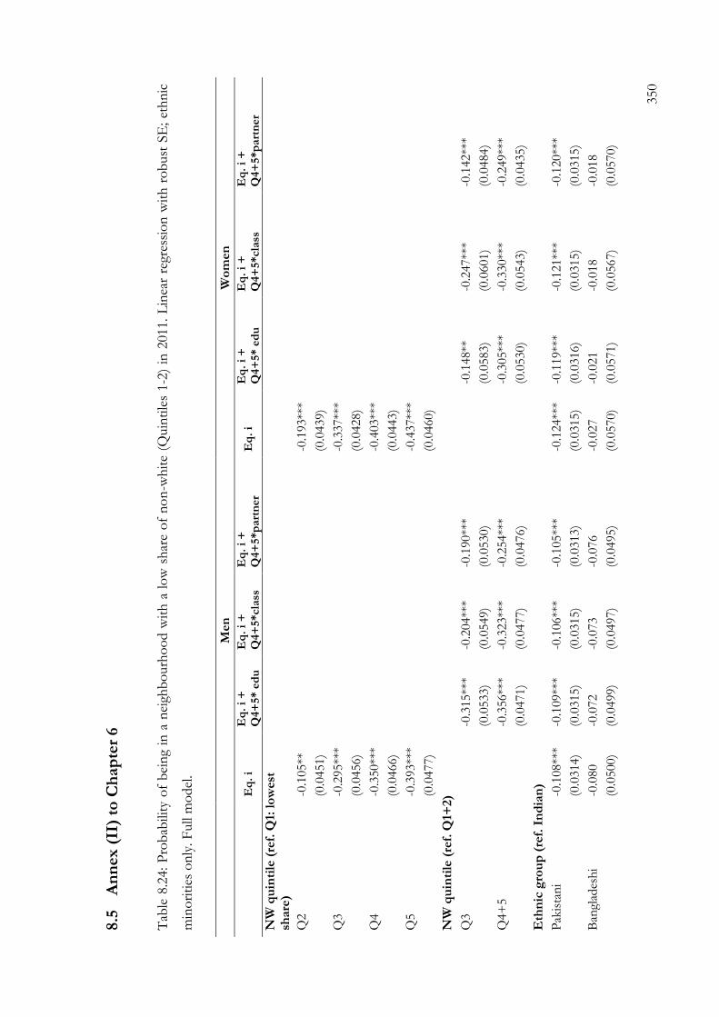
350

8.5

A

nn

ex

(II

) to

Ch

ap

ter

6

Tab

le ‎8

.24:

Pro

bab

ility

of

bei

ng

in a

nei

ghb

ourh

oo

d w

ith

a l

ow

sh

are

of

no

n-w

hit

e (Q

uin

tile

s 1-2

) in

2011.

Lin

ear

regr

essi

on

wit

h r

ob

ust

SE

; et

hn

ic

min

ori

ties

on

ly. F

ull

mo

del

.

M

en

W

om

en

E

q.

i E

q.

i +

Q

4+

5* e

du

E

q.

i +

Q

4+

5*cla

ss

Eq

. i

+

Q4+

5*p

art

ner

Eq

. i

Eq

. i

+

Q4+

5* e

du

E

q.

i +

Q

4+

5*cla

ss

Eq

. i

+

Q4+

5*p

art

ner

NW

qu

inti

le (

ref.

Q1:

lo

wes

t sh

are

)

Q2

-0.1

05**

-0.1

93**

*

(0

.0451)

(0

.0439)

Q

3

-0.2

95**

*

-0.3

37**

*

(0

.0456)

(0

.0428)

Q

4

-0.3

50**

*

-0.4

03**

*

(0

.0466)

(0

.0443)

Q

5

-0.3

93**

*

-0.4

37**

*

(0

.0477)

(0

.0460)

N

W q

uin

tile

(re

f. Q

1+2)

Q

3

-0

.315**

* -0

.204**

* -0

.190**

*

-0.1

48**

-0

.247**

* -0

.142**

*

(0.0

533)

(0.0

549)

(0.0

530)

(0

.0583)

(0.0

601)

(0.0

484)

Q4+

5

-0

.356**

* -0

.323**

* -0

.254**

*

-0.3

05**

* -0

.330**

* -0

.249**

*

(0.0

471)

(0.0

477)

(0.0

476)

(0

.0530)

(0.0

543)

(0.0

435)

Eth

nic

gro

up

(re

f. I

nd

ian

)

Pak

ista

ni

-0.1

08**

* -0

.109**

* -0

.106**

* -0

.105**

* -0

.124**

* -0

.119**

* -0

.121**

* -0

.120**

*

(0

.0314)

(0.0

315)

(0.0

315)

(0.0

313)

(0.0

315)

(0.0

316)

(0.0

315)

(0.0

315)

Ban

glad

esh

i -0

.080

-0.0

72

-0.0

73

-0.0

76

-0.0

27

-0.0

21

-0.0

18

-0.0

18

(0

.0500)

(0.0

499)

(0.0

497)

(0.0

495)

(0.0

570)

(0.0

571)

(0.0

567)

(0.0

570)

351

M

en

W

om

en

E

q.

i E

q.

i +

Q

4+

5* e

du

E

q.

i +

Q

4+

5*cla

ss

Eq

. i

+

Q4+

5*p

art

ner

Eq

. i

Eq

. i

+

Q4+

5* e

du

E

q.

i +

Q

4+

5*cla

ss

Eq

. i

+

Q4+

5*p

art

ner

Car

ibb

ean

-0

.060*

-0.0

55

-0.0

56

-0.0

62*

-0.0

94**

* -0

.095**

* -0

.092**

* -0

.088**

*

(0

.0352)

(0.0

351)

(0.0

352)

(0.0

351)

(0.0

314)

(0.0

314)

(0.0

315)

(0.0

315)

Afr

ican

-0

.053

-0.0

49

-0.0

54

-0.0

46

-0.0

47

-0.0

46

-0.0

47

-0.0

37

(0

.0822)

(0.0

828)

(0.0

822)

(0.0

825)

(0.0

569)

(0.0

569)

(0.0

574)

(0.0

564)

Ed

ucati

on

(re

f. L

eve

l 1

or

less

)

Lev

el 2

+3

0.0

32

-0.0

24

0.0

32

0.0

31

0.0

01

0.0

31

0.0

07

0.0

02

(0

.0313)

(0.0

595)

(0.0

313)

(0.0

311)

(0.0

289)

(0.0

583)

(0.0

292)

(0.0

290)

Lev

el 4

+

0.0

81**

-0

.021

0.0

84**

0.0

84**

0.0

43

0.0

19

0.0

47

0.0

42

(0

.0349)

(0.0

555)

(0.0

348)

(0.0

347)

(0.0

327)

(0.0

591)

(0.0

330)

(0.0

328)

So

cia

l cla

ss (

ref.

Man

ual)

Pet

it B

ourg

eois

ie

0.1

07**

0.1

07**

0.1

13

0.1

09**

0.1

28*

0.1

26*

-0.0

52

0.1

24

(0

.0433)

(0.0

436)

(0.0

802)

(0.0

437)

(0.0

754)

(0.0

759)

(0.1

616)

(0.0

756)

Inte

rmed

iate

0.0

20

0.0

18

0.0

16

0.0

23

0.0

62**

0.0

55*

0.0

19

0.0

57*

(0

.0450)

(0.0

450)

(0.0

796)

(0.0

452)

(0.0

307)

(0.0

310)

(0.0

637)

(0.0

310)

Ser

vic

e 0.0

33

0.0

29

-0.0

00

0.0

28

0.0

79**

0.0

70**

0.0

14

0.0

74**

(0

.0324)

(0.0

324)

(0.0

551)

(0.0

322)

(0.0

308)

(0.0

310)

(0.0

582)

(0.0

310)

Part

ner’

s eth

nic

ity (

ref.

no

n-

wh

ite)

No

par

tner

0.0

53*

0.0

51*

0.0

55*

0.1

28**

-0

.083**

* -0

.079**

* -0

.079**

* -0

.007

(0

.0299)

(0.0

300)

(0.0

300)

(0.0

526)

(0.0

265)

(0.0

264)

(0.0

265)

(0.0

485)

Oth

er

0.0

59

0.0

57

0.0

61

0.3

50**

0.1

14

0.0

97

0.0

95

0.0

74

(0

.0866)

(0.0

862)

(0.0

878)

(0.1

434)

(0.1

108)

(0.1

123)

(0.1

111)

(0.1

723)

Wh

ite

Bri

tish

0.2

92**

* 0.2

92**

* 0.2

99**

* 0.1

95**

* 0.2

69**

* 0.2

70**

* 0.2

71**

* 0.1

99**

*

(0

.0436)

(0.0

439)

(0.0

434)

(0.0

684)

(0.0

428)

(0.0

429)

(0.0

428)

(0.0

663)

Inte

racti

on

s

Q

3*L

evel

2+

3

0.1

31

-0

.119

(0.0

811)

(0

.0740)

352

M

en

W

om

en

E

q.

i E

q.

i +

Q

4+

5* e

du

E

q.

i +

Q

4+

5*cla

ss

Eq

. i

+

Q4+

5*p

art

ner

Eq

. i

Eq

. i

+

Q4+

5* e

du

E

q.

i +

Q

4+

5*cla

ss

Eq

. i

+

Q4+

5*p

art

ner

Q3*L

evel

4+

0.1

61**

-0.0

31

(0.0

713)

(0

.0757)

Q3*P

etit

Bo

urg

eois

ie

0.0

29

0.1

82

(0

.1115)

(0

.1957)

Q3*I

nte

rmed

iate

-0

.101

0.0

72

(0

.1086)

(0

.0818)

Q3*S

ervic

e

-0

.007

0.0

53

(0

.0706)

(0

.0732)

Q3*N

o p

artn

er

-0

.083

-0

.131**

(0.0

691)

(0

.0629)

Q3*W

hit

e B

riti

sh

0.1

81*

0.1

22

(0.0

964)

(0

.0930)

Q3*O

ther

-0.3

77*

0.2

06

(0.1

924)

(0

.2584)

Q4+

5*L

evel

2+

3

0.0

46

0.0

05

(0.0

681)

(0

.0664)

Q4+

5*L

evel

4+

0.1

28**

0.0

72

(0.0

627)

(0

.0662)

Q4+

5*P

etit

B

ourg

eois

ie

-0.0

25

0.2

36

(0

.0958)

(0

.1853)

Q4+

5*I

nte

rmed

iate

0.0

59

0.0

38

(0

.0963)

(0

.0720)

Q4+

5*S

ervic

e

0.0

63

0.0

89

(0

.0609)

(0

.0653)

Q4+

5*N

o p

artn

er

-0

.106*

-0

.075

(0.0

589)

(0

.0553)

353

M

en

W

om

en

E

q.

i E

q.

i +

Q

4+

5* e

du

E

q.

i +

Q

4+

5*cla

ss

Eq

. i

+

Q4+

5*p

art

ner

Eq

. i

Eq

. i

+

Q4+

5* e

du

E

q.

i +

Q

4+

5*cla

ss

Eq

. i

+

Q4+

5*p

art

ner

Q4+

5*O

ther

-0.2

93*

-0

.013

(0.1

729)

(0

.2152)

Q4+

5*W

hit

e B

riti

sh

0.1

65*

0.1

17

(0.0

913)

(0

.0889)

Cars

tair

s q

uin

tile

(re

f. Q

1: l

east

dep

rive

d)

Q2

-0.0

12

-0.0

26

-0.0

19

0.0

03

0.0

55

0.0

44

0.0

47

0.0

51

(0

.0716)

(0.0

706)

(0.0

725)

(0.0

722)

(0.0

649)

(0.0

660)

(0.0

659)

(0.0

645)

Q3

-0.0

31

-0.0

42

-0.0

40

-0.0

20

0.0

30

0.0

03

0.0

01

0.0

11

(0

.0664)

(0.0

655)

(0.0

673)

(0.0

661)

(0.0

616)

(0.0

617)

(0.0

620)

(0.0

610)

Q4

0.0

09

-0.0

10

-0.0

08

0.0

17

0.0

82

0.0

46

0.0

45

0.0

54

(0

.0651)

(0.0

641)

(0.0

656)

(0.0

648)

(0.0

600)

(0.0

606)

(0.0

606)

(0.0

598)

Q5

-0.0

21

-0.0

43

-0.0

43

-0.0

22

0.0

65

0.0

27

0.0

24

0.0

33

(0

.0660)

(0.0

648)

(0.0

664)

(0.0

655)

(0.0

599)

(0.0

601)

(0.0

602)

(0.0

595)

Ten

ure

(re

f. o

wn

er)

So

cial

ren

t -0

.103**

* -0

.103**

* -0

.098**

* -0

.094**

* -0

.027

-0.0

21

-0.0

23

-0.0

23

(0

.0333)

(0.0

332)

(0.0

331)

(0.0

329)

(0.0

289)

(0.0

288)

(0.0

290)

(0.0

290)

Pri

vat

e re

nt

-0.0

46

-0.0

48

-0.0

44

-0.0

44

0.0

23

0.0

21

0.0

19

0.0

20

(0

.0372)

(0.0

372)

(0.0

374)

(0.0

371)

(0.0

358)

(0.0

360)

(0.0

361)

(0.0

358)

Nu

mb

er

of

cars

(re

f. n

on

e)

1 c

ar

0.0

49**

0.0

52**

0.0

52**

0.0

55**

0.0

20

0.0

25

0.0

25

0.0

25

(0

.0242)

(0.0

241)

(0.0

242)

(0.0

241)

(0.0

222)

(0.0

222)

(0.0

222)

(0.0

222)

2+

car

s 0.0

40

0.0

44

0.0

42

0.0

45

0.0

89**

0.1

06**

* 0.1

04**

* 0.1

01**

(0

.0422)

(0.0

425)

(0.0

425)

(0.0

424)

(0.0

396)

(0.0

401)

(0.0

401)

(0.0

400)

Pers

on

s p

er

roo

m (

ref.

1 p

pp

)

> 1

.5 p

erso

ns

-0.0

56*

-0.0

57*

-0.0

60*

-0.0

58*

-0.0

17

-0.0

22

-0.0

21

-0.0

24

(0

.0331)

(0.0

332)

(0.0

333)

(0.0

331)

(0.0

298)

(0.0

300)

(0.0

299)

(0.0

300)

354

M

en

W

om

en

E

q.

i E

q.

i +

Q

4+

5* e

du

E

q.

i +

Q

4+

5*cla

ss

Eq

. i

+

Q4+

5*p

art

ner

Eq

. i

Eq

. i

+

Q4+

5* e

du

E

q.

i +

Q

4+

5*cla

ss

Eq

. i

+

Q4+

5*p

art

ner

1.5

per

son

s -0

.049

-0.0

44

-0.0

47

-0.0

50

0.0

04

0.0

05

0.0

08

0.0

05

(0

.0457)

(0.0

452)

(0.0

454)

(0.0

451)

(0.0

392)

(0.0

393)

(0.0

393)

(0.0

394)

>1 &

<1.5

per

son

s -0

.068**

-0

.068**

-0

.067**

-0

.070**

0.0

16

0.0

18

0.0

16

0.0

12

(0

.0308)

(0.0

310)

(0.0

309)

(0.0

309)

(0.0

282)

(0.0

283)

(0.0

283)

(0.0

283)

>=

0.7

5 &

<1 p

erso

n

-0.0

27

-0.0

26

-0.0

26

-0.0

25

0.0

33

0.0

35

0.0

34

0.0

30

(0

.0352)

(0.0

351)

(0.0

351)

(0.0

349)

(0.0

334)

(0.0

336)

(0.0

336)

(0.0

338)

<0.7

5 p

erso

n

-0.0

03

0.0

07

0.0

05

-0.0

02

-0.0

28

-0.0

17

-0.0

20

-0.0

26

(0

.0393)

(0.0

394)

(0.0

394)

(0.0

393)

(0.0

380)

(0.0

381)

(0.0

382)

(0.0

382)

Pare

nta

l so

cial

cla

ss (

ref.

Man

ual (V

+V

I+V

II))

N

o e

arn

ers/

No

cod

e 0.0

17

0.0

20

0.0

17

0.0

17

-0.0

15

-0.0

09

-0.0

08

-0.0

07

(0

.0343)

(0.0

342)

(0.0

345)

(0.0

346)

(0.0

318)

(0.0

322)

(0.0

327)

(0.0

322)

Ro

uti

ne

no

n-m

anual

(I

II)

0.0

26

0.0

28

0.0

26

0.0

24

0.0

06

0.0

11

0.0

10

0.0

09

(0

.0361)

(0.0

361)

(0.0

359)

(0.0

359)

(0.0

338)

(0.0

338)

(0.0

338)

(0.0

335)

Pet

it B

ourg

eois

ie (

IV)

0.0

30

0.0

43

0.0

45

0.0

36

0.0

71*

0.0

77*

0.0

81**

0.0

80**

(0

.0417)

(0.0

412)

(0.0

416)

(0.0

416)

(0.0

406)

(0.0

404)

(0.0

405)

(0.0

407)

Ser

vic

e (I

+II

) -0

.019

-0.0

11

-0.0

14

-0.0

17

0.0

17

0.0

28

0.0

30

0.0

24

(0

.0372)

(0.0

373)

(0.0

375)

(0.0

371)

(0.0

353)

(0.0

352)

(0.0

354)

(0.0

350)

Ag

e

Age

in

des

tin

atio

n

0.0

04

0.0

04

0.0

04

0.0

04

-0.0

03

-0.0

02

-0.0

02

-0.0

02

(0

.0029)

(0.0

028)

(0.0

028)

(0.0

028)

(0.0

026)

(0.0

026)

(0.0

026)

(0.0

026)

Ori

gin

year

(ref.

19

71)

1981

-0.0

33

-0.0

31

-0.0

34

-0.0

33

-0.0

36

-0.0

31

-0.0

33

-0.0

30

(0

.0239)

(0.0

242)

(0.0

240)

(0.0

241)

(0.0

223)

(0.0

223)

(0.0

224)

(0.0

223)

1991

-0.0

93**

* -0

.089**

* -0

.092**

* -0

.096**

* -0

.106**

* -0

.099**

* -0

.102**

* -0

.101**

*

(0

.0342)

(0.0

344)

(0.0

345)

(0.0

346)

(0.0

323)

(0.0

325)

(0.0

325)

(0.0

326)

355

M

en

W

om

en

E

q.

i E

q.

i +

Q

4+

5* e

du

E

q.

i +

Q

4+

5*cla

ss

Eq

. i

+

Q4+

5*p

art

ner

Eq

. i

Eq

. i

+

Q4+

5* e

du

E

q.

i +

Q

4+

5*cla

ss

Eq

. i

+

Q4+

5*p

art

ner

Nu

mb

er

of

cen

sus

po

ints

(re

f. 2

)

4 c

ensu

s p

oin

ts

-0.0

14

-0.0

07

-0.0

07

-0.0

11

0.0

45

0.0

47

0.0

45

0.0

47

(0

.0372)

(0.0

372)

(0.0

370)

(0.0

369)

(0.0

359)

(0.0

361)

(0.0

359)

(0.0

362)

5 c

ensu

s p

oin

ts

-0.0

38

-0.0

30

-0.0

35

-0.0

39

0.0

82*

0.0

81*

0.0

81*

0.0

82*

(0

.0451)

(0.0

451)

(0.0

449)

(0.0

449)

(0.0

448)

(0.0

450)

(0.0

449)

(0.0

450)

Co

nst

ant

0.6

30**

* 0.6

12**

* 0.5

63**

* 0.5

07**

* 0.7

50**

* 0.6

15**

* 0.6

58**

* 0.5

85**

*

(0

.1303)

(0.1

279)

(0.1

290)

(0.1

278)

(0.1

169)

(0.1

161)

(0.1

197)

(0.1

140)

Adju

sted

R2

0.1

36

0.1

35

0.1

33

0.1

38

0.1

35

0.1

29

0.1

27

0.1

30

N

2,2

09

2,2

09

2,2

09

2,2

09

2,4

74

2,4

74

2,4

74

2,4

74

* p

-val

ue<

.10 *

* p

-val

ue<

.05 *

** p

-val

ue<

.01; ro

bust

(cl

ust

ered

) st

and

ard

err

ors

in

par

enth

eses

P

op

ula

tio

n: In

div

idual

s b

etw

een

20 a

nd

55 y

ears

old

So

urc

e: A

uth

or’

s o

wn

cal

cula

tio

ns

bas

ed o

n O

NS

-LS

356

Tab

le ‎8

.25: P

rob

abili

ty o

f b

ein

g in

a n

eigh

bo

urh

oo

d w

ith

a lo

w s

har

e o

f n

on

-wh

ites

(Q

uin

tile

s 1-2

). L

inea

r re

gres

sio

n w

ith

ro

bust

SE

; et

hn

ic m

ino

riti

es

and w

hit

e B

riti

sh m

en. F

ull

mo

del

B

ase

E

q.

i E

q.

ii

(*ed

uca

tio

n)

Eq

. ii

(*

clas

s)

Eq

. ii

(*

par

tner

) E

q.

iii

(wit

ho

ut

par

tner

) E

q.

iii

(wit

h p

artn

er)

NW

qu

inti

le (

ref.

Q1:

lo

wes

t sh

are

)

Q2

-0.0

64**

* -0

.064**

* -0

.064**

* -0

.064**

* -0

.064**

*

(0

.0031)

(0.0

031)

(0.0

031)

(0.0

031)

(0.0

031)

Q3

-0.1

76**

* -0

.174**

* -0

.175**

* -0

.174**

* -0

.174**

*

(0

.0077)

(0.0

077)

(0.0

076)

(0.0

076)

(0.0

076)

Q4

-0.2

19**

* -0

.216**

* -0

.216**

* -0

.214**

* -0

.214**

*

(0

.0112)

(0.0

112)

(0.0

112)

(0.0

111)

(0.0

112)

Q5

-0.2

70**

* -0

.267**

* -0

.264**

* -0

.264**

* -0

.263**

*

(0

.0147)

(0.0

147)

(0.0

146)

(0.0

146)

(0.0

146)

NW

qu

inti

le (

ref.

Q1-

2)

Q

3

-0

.162**

* -0

.160**

*

(0.0

080)

(0.0

080)

Q4+

5

-0

.197**

* -0

.195**

*

(0.0

105)

(0.0

104)

Eth

nic

gro

up

(re

f. w

hit

e B

riti

sh)

In

dia

n

-0.2

74**

* -0

.224**

* -0

.266**

* -0

.267**

* -0

.229**

* -0

.189**

* -0

.155**

*

(0

.0159)

(0.0

168)

(0.0

289)

(0.0

275)

(0.0

303)

(0.0

256)

(0.0

259)

Pak

ista

ni

-0.4

11**

* -0

.355**

* -0

.413**

* -0

.464**

* -0

.319**

* -0

.328**

* -0

.270**

*

(0

.0220)

(0.0

232)

(0.0

330)

(0.0

318)

(0.0

349)

(0.0

465)

(0.0

467)

Ban

glad

esh

i -0

.448**

* -0

.406**

* -0

.386**

* -0

.485**

* -0

.360**

* -0

.326**

* -0

.293**

*

(0

.0387)

(0.0

390)

(0.0

616)

(0.0

516)

(0.0

684)

(0.0

879)

(0.0

859)

Car

ibb

ean

-0

.324**

* -0

.294**

* -0

.380**

* -0

.354**

* -0

.339**

* -0

.331**

* -0

.306**

*

(0

.0225)

(0.0

225)

(0.0

311)

(0.0

317)

(0.0

486)

(0.0

415)

(0.0

410)

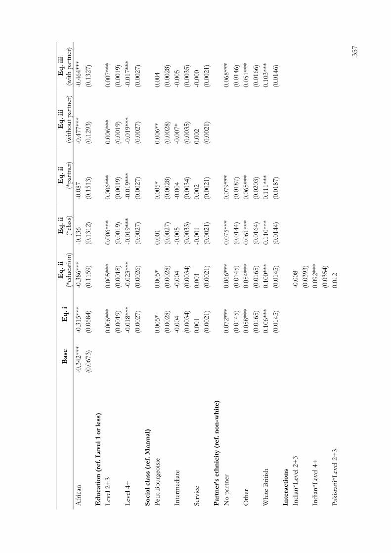
357

B

ase

E

q.

i E

q.

ii

(*ed

uca

tio

n)

Eq

. ii

(*

clas

s)

Eq

. ii

(*

par

tner

) E

q.

iii

(wit

ho

ut

par

tner

) E

q.

iii

(wit

h p

artn

er)

Afr

ican

-0

.342**

* -0

.315**

* -0

.386**

* -0

.136

-0.0

87

-0.4

77**

* -0

.464**

*

(0

.0673)

(0.0

684)

(0.1

159)

(0.1

312)

(0.1

513)

(0.1

293)

(0.1

327)

Ed

ucati

on

(re

f. L

eve

l 1

or

less

)

Lev

el 2

+3

0.0

06**

* 0.0

05**

* 0.0

06**

* 0.0

06**

* 0.0

06**

* 0.0

07**

*

(0.0

019)

(0.0

018)

(0.0

019)

(0.0

019)

(0.0

019)

(0.0

019)

Lev

el 4

+

-0

.018**

* -0

.023**

* -0

.019**

* -0

.019**

* -0

.019**

* -0

.017**

*

(0.0

027)

(0.0

026)

(0.0

027)

(0.0

027)

(0.0

027)

(0.0

027)

So

cia

l cla

ss (

ref.

Man

ual)

Pet

it B

ourg

eois

ie

0.0

05*

0.0

05*

0.0

01

0.0

05*

0.0

06**

0.0

04

(0.0

028)

(0.0

028)

(0.0

027)

(0.0

028)

(0.0

028)

(0.0

028)

Inte

rmed

iate

-0.0

04

-0.0

04

-0.0

05

-0.0

04

-0.0

07*

-0.0

05

(0.0

034)

(0.0

034)

(0.0

033)

(0.0

034)

(0.0

035)

(0.0

035)

Ser

vic

e

0.0

01

0.0

01

-0.0

01

0.0

02

0.0

02

-0.0

00

(0.0

021)

(0.0

021)

(0.0

021)

(0.0

021)

(0.0

021)

(0.0

021)

Part

ner’

s eth

nic

ity (

ref.

no

n-w

hit

e)

N

o p

artn

er

0.0

72**

* 0.0

66**

* 0.0

75**

* 0.0

79**

*

0.0

68**

*

(0.0

145)

(0.0

145)

(0.0

144)

(0.0

187)

(0

.0146)

Oth

er

0.0

58**

* 0.0

54**

* 0.0

61**

* 0.0

65**

*

0.0

51**

*

(0.0

165)

(0.0

165)

(0.0

164)

(0.0

203)

(0

.0166)

Wh

ite

Bri

tish

0.1

06**

* 0.1

00**

* 0.1

10**

* 0.1

11**

*

0.1

03**

*

(0.0

145)

(0.0

145)

(0.0

144)

(0.0

187)

(0

.0146)

Inte

racti

on

s

India

n*L

evel

2+

3

-0.0

08

(0

.0393)

India

n*L

evel

4+

0.0

92**

*

(0

.0354)

Pak

ista

ni*

Lev

el 2

+3

0.0

12

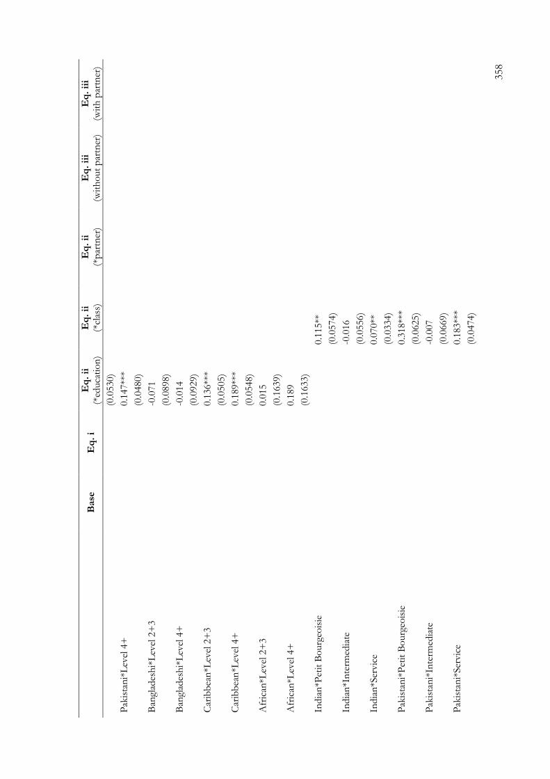
358

B

ase

E

q.

i E

q.

ii

(*ed

uca

tio

n)

Eq

. ii

(*

clas

s)

Eq

. ii

(*

par

tner

) E

q.

iii

(wit

ho

ut

par

tner

) E

q.

iii

(wit

h p

artn

er)

(0

.0530)

Pak

ista

ni*

Lev

el 4

+

0.1

47**

*

(0

.0480)

Ban

glad

esh

i*L

evel

2+

3

-0.0

71

(0

.0898)

Ban

glad

esh

i*L

evel

4+

-0

.014

(0

.0929)

Car

ibb

ean

*Lev

el 2

+3

0.1

36**

*

(0

.0505)

Car

ibb

ean

*Lev

el 4

+

0.1

89**

*

(0

.0548)

Afr

ican

*Lev

el 2

+3

0.0

15

(0

.1639)

Afr

ican

*Lev

el 4

+

0.1

89

(0

.1633)

India

n*P

etit

Bo

urg

eois

ie

0.1

15**

(0.0

574)

In

dia

n*I

nte

rmed

iate

-0.0

16

(0.0

556)

In

dia

n*S

ervic

e

0.0

70**

(0.0

334)

P

akis

tan

i*P

etit

Bo

urg

eois

ie

0.3

18**

*

(0.0

625)

P

akis

tan

i*In

term

edia

te

-0

.007

(0.0

669)

P

akis

tan

i*Ser

vic

e

0.1

83**

*

(0.0

474)

359

B

ase

E

q.

i E

q.

ii

(*ed

uca

tio

n)

Eq

. ii

(*

clas

s)

Eq

. ii

(*

par

tner

) E

q.

iii

(wit

ho

ut

par

tner

) E

q.

iii

(wit

h p

artn

er)

Ban

glad

esh

i*P

etit

Bo

urg

eois

ie

0.2

79*

(0.1

483)

B

angl

ades

hi*

Inte

rmed

iate

0.0

95

(0.1

637)

B

angl

ades

hi*

Ser

vic

e

0.1

23

(0.0

812)

C

arib

bea

n*P

etit

Bo

urg

eois

ie

-0

.179**

(0.0

766)

C

arib

bea

n*I

nte

rmed

iate

0.1

58**

(0.0

697)

C

arib

bea

n*S

ervic

e

0.1

52**

*

(0.0

484)

A

fric

an*P

etit

Bo

urg

eois

ie

0.2

98**

(0.1

418)

A

fric

an*I

nte

rmed

iate

-0.1

25

(0.2

069)

A

fric

an*S

ervic

e

-0.3

35**

(0.1

573)

In

dia

n*N

o p

artn

er

-0.0

15

(0

.0440)

India

n*O

ther

-0

.048

(0

.2132)

India

n*w

hit

e B

riti

sh

0.2

34**

*

(0

.0670)

Pak

ista

ni*

No

par

tner

-0

.120**

(0

.0561)

Pak

ista

ni*

Oth

er

0.1

12

360

B

ase

E

q.

i E

q.

ii

(*ed

uca

tio

n)

Eq

. ii

(*

clas

s)

Eq

. ii

(*

par

tner

) E

q.

iii

(wit

ho

ut

par

tner

) E

q.

iii

(wit

h p

artn

er)

(0

.2540)

Pak

ista

ni*

wh

ite

Bri

tish

0.2

89**

*

(0

.1115)

Ban

glad

esh

i*N

o p

artn

er

-0.0

60

(0

.0926)

Ban

glad

esh

i*O

ther

-0

.331**

*

(0

.0762)

Ban

glad

esh

i*w

hit

e B

riti

sh

-0.3

71**

*

(0

.0727)

Car

ibb

ean

*No

par

tner

-0

.010

(0

.0674)

Car

ibb

ean

*Oth

er

0.0

30

(0

.1216)

Car

ibb

ean

*wh

ite

Bri

tish

0.2

29**

*

(0

.0780)

Afr

ican

*No

par

tner

-0

.233

(0

.2147)

Afr

ican

*Oth

er

-0.6

77**

*

(0

.1909)

Afr

ican

*wh

ite

Bri

tish

-0

.417*

(0

.2507)

India

n*Q

3

-0.0

97**

-0

.092**

(0.0

463)

(0.0

459)

India

n*Q

4+

5

-0

.176**

* -0

.160**

*

(0.0

398)

(0.0

399)

Pak

ista

ni*

Q3

-0

.078

-0.0

92

(0.0

720)

(0.0

718)

361

B

ase

E

q.

i E

q.

ii

(*ed

uca

tio

n)

Eq

. ii

(*

clas

s)

Eq

. ii

(*

par

tner

) E

q.

iii

(wit

ho

ut

par

tner

) E

q.

iii

(wit

h p

artn

er)

Pak

ista

ni*

Q4+

5

-0

.169**

* -0

.177**

*

(0.0

608)

(0.0

604)

Ban

glad

esh

i*Q

3

-0.1

94

-0.1

85

(0.1

219)

(0.1

208)

Ban

glad

esh

i*Q

4+

5

-0

.188*

-0.1

85*

(0.1

061)

(0.1

050)

Car

ibb

ean

*Q3

0.0

04

0.0

05

(0.0

670)

(0.0

661)

Car

ibb

ean

*Q4+

5

-0

.032

-0.0

28

(0.0

592)

(0.0

585)

Afr

ican

*Q3

0.1

53

0.1

69

(0.1

919)

(0.1

935)

Afr

ican

*Q4+

5

0.1

65

0.1

73

(0.1

814)

(0.1

847)

Cars

tair

s q

uin

tile

(re

f. Q

1: l

east

dep

rive

d)

Q2

0.0

01

0.0

01

0.0

01

0.0

01

0.0

01

0.0

02

0.0

02

(0

.0025)

(0.0

025)

(0.0

025)

(0.0

025)

(0.0

025)

(0.0

025)

(0.0

025)

Q3

0.0

04

0.0

02

0.0

02

0.0

02

0.0

02

0.0

04*

0.0

03

(0

.0026)

(0.0

026)

(0.0

026)

(0.0

026)

(0.0

026)

(0.0

026)

(0.0

026)

Q4

0.0

09**

* 0.0

07**

0.0

07**

0.0

07**

0.0

07**

0.0

08**

* 0.0

07**

(0

.0027)

(0.0

027)

(0.0

027)

(0.0

027)

(0.0

027)

(0.0

027)

(0.0

027)

Q5

0.0

06*

0.0

04

0.0

04

0.0

04

0.0

04

0.0

02

0.0

01

(0

.0032)

(0.0

032)

(0.0

032)

(0.0

032)

(0.0

032)

(0.0

032)

(0.0

032)

Ten

ure

(re

f. o

wn

er)

So

cial

ren

t -0

.004*

-0.0

07**

* -0

.007**

* -0

.007**

* -0

.006**

* -0

.005**

-0

.006**

*

(0

.0024)

(0.0

024)

(0.0

024)

(0.0

024)

(0.0

024)

(0.0

024)

(0.0

024)

Pri

vat

e re

nt

0.0

08**

0.0

05

0.0

05

0.0

05

0.0

05

0.0

02

0.0

01

362

B

ase

E

q.

i E

q.

ii

(*ed

uca

tio

n)

Eq

. ii

(*

clas

s)

Eq

. ii

(*

par

tner

) E

q.

iii

(wit

ho

ut

par

tner

) E

q.

iii

(wit

h p

artn

er)

(0

.0033)

(0.0

033)

(0.0

033)

(0.0

033)

(0.0

033)

(0.0

033)

(0.0

033)

Nu

mb

er

of

care

s (r

ef.

no

ne)

1 c

ar

0.0

09**

* 0.0

08**

* 0.0

08**

* 0.0

08**

* 0.0

08**

* 0.0

10**

* 0.0

09**

*

(0

.0024)

(0.0

024)

(0.0

024)

(0.0

024)

(0.0

024)

(0.0

024)

(0.0

024)

2+

car

s 0.0

07**

0.0

07**

0.0

07**

0.0

07**

0.0

07**

0.0

08**

0.0

08**

(0

.0033)

(0.0

033)

(0.0

033)

(0.0

033)

(0.0

033)

(0.0

033)

(0.0

033)

Pers

on

s p

er

roo

m (

ref.

1 p

pp

)

> 1

.5 p

erso

ns

-0.0

14**

-0

.011

-0.0

09

-0.0

11

-0.0

12*

-0.0

11

-0.0

08

(0

.0069)

(0.0

069)

(0.0

068)

(0.0

068)

(0.0

068)

(0.0

069)

(0.0

069)

1.5

per

son

s -0

.023**

-0

.022**

-0

.022**

-0

.022**

-0

.024**

-0

.022**

-0

.022**

(0

.0099)

(0.0

099)

(0.0

098)

(0.0

098)

(0.0

098)

(0.0

100)

(0.0

099)

>1 &

<1.5

per

son

s -0

.014**

* -0

.013**

* -0

.013**

* -0

.013**

* -0

.013**

* -0

.013**

* -0

.013**

*

(0

.0035)

(0.0

035)

(0.0

035)

(0.0

034)

(0.0

034)

(0.0

035)

(0.0

035)

>=

0.7

5 &

<1 p

erso

n

0.0

01

0.0

02

0.0

02

0.0

02

0.0

02

0.0

01

0.0

02

(0

.0024)

(0.0

024)

(0.0

024)

(0.0

024)

(0.0

024)

(0.0

024)

(0.0

024)

<0.7

5 p

erso

n

0.0

00

0.0

03

0.0

03

0.0

03

0.0

02

0.0

02

0.0

03

(0

.0025)

(0.0

025)

(0.0

025)

(0.0

025)

(0.0

025)

(0.0

025)

(0.0

025)

Pare

nta

l so

cial

cla

ss (

ref.

Man

ual (V

+V

I+V

II))

N

o e

arn

ers/

No

cod

e -0

.008*

-0.0

08*

-0.0

08

-0.0

07

-0.0

07

-0.0

08*

-0.0

08*

(0

.0047)

(0.0

047)

(0.0

047)

(0.0

047)

(0.0

047)

(0.0

048)

(0.0

047)

Ro

uti

ne

no

n-m

anual

(II

I)

-0.0

05**

-0

.004*

-0.0

05*

-0.0

04

-0.0

04*

-0.0

06**

-0

.006**

(0

.0026)

(0.0

026)

(0.0

026)

(0.0

026)

(0.0

026)

(0.0

026)

(0.0

026)

Pet

it B

ourg

eois

ie (

IV)

0.0

03

0.0

03

0.0

02

0.0

03

0.0

03

0.0

02

0.0

02

(0

.0030)

(0.0

030)

(0.0

030)

(0.0

030)

(0.0

030)

(0.0

030)

(0.0

030)

Ser

vic

e (I

+II

) -0

.016**

* -0

.012**

* -0

.012**

* -0

.012**

* -0

.012**

* -0

.015**

* -0

.014**

*

(0

.0026)

(0.0

026)

(0.0

026)

(0.0

026)

(0.0

026)

(0.0

027)

(0.0

026)

Ag

e

363

B

ase

E

q.

i E

q.

ii

(*ed

uca

tio

n)

Eq

. ii

(*

clas

s)

Eq

. ii

(*

par

tner

) E

q.

iii

(wit

ho

ut

par

tner

) E

q.

iii

(wit

h p

artn

er)

Age

in

des

tin

atio

n

0.0

00

-0.0

00

-0.0

00

-0.0

00

-0.0

00

0.0

00

-0.0

00

(0

.0002)

(0.0

002)

(0.0

002)

(0.0

002)

(0.0

002)

(0.0

002)

(0.0

002)

Ori

gin

year

(ref.

1971)

1981

0.0

01

0.0

00

0.0

00

0.0

00

0.0

00

0.0

01

-0.0

00

(0

.0015)

(0.0

015)

(0.0

015)

(0.0

015)

(0.0

015)

(0.0

015)

(0.0

015)

1991

-0.0

11**

* -0

.010**

* -0

.010**

* -0

.010**

* -0

.010**

* -0

.008**

* -0

.006**

(0

.0027)

(0.0

027)

(0.0

027)

(0.0

027)

(0.0

027)

(0.0

027)

(0.0

027)

Nu

mb

er

of

cen

sus

po

ints

(re

f. 2

)

4 c

ensu

s p

oin

ts

0.0

07

0.0

09

0.0

07

0.0

08

0.0

08

0.0

08

0.0

09

(0

.0072)

(0.0

072)

(0.0

072)

(0.0

072)

(0.0

072)

(0.0

072)

(0.0

072)

5 c

ensu

s p

oin

ts

0.0

16**

0.0

14*

0.0

12*

0.0

14*

0.0

13*

0.0

18**

0.0

15**

(0

.0074)

(0.0

074)

(0.0

073)

(0.0

073)

(0.0

074)

(0.0

074)

(0.0

074)

Co

nst

an

t 0.9

45**

* 0.8

74**

* 0.8

83**

* 0.8

72**

* 0.8

70**

* 0.9

34**

* 0.8

67**

*

(0

.0099)

(0.0

202)

(0.0

202)

(0.0

201)

(0.0

242)

(0.0

101)

(0.0

203)

Ad

just

ed

R-s

qu

are

d

0.1

52

0.1

59

0.1

60

0.1

62

0.1

61

0.1

47

0.1

52

N

77,1

96

77,1

96

77,1

96

77,1

96

77,1

96

77,1

96

77,1

96

* p

-val

ue<

.10 *

* p

-val

ue<

.05 *

** p

-val

ue<

.01; ro

bust

(cl

ust

ered

) st

and

ard

err

ors

in

par

enth

eses

P

op

ula

tio

n: In

div

idual

s b

etw

een

20 a

nd

55 y

ears

old

So

urc

e: A

uth

or’

s o

wn

cal

cula

tio

ns

bas

ed o

n O

NS

-LS

364

Tab

le ‎8

.26: P

rob

abili

ty o

f b

ein

g in

a n

eigh

bo

urh

oo

d w

ith

a lo

w s

har

e o

f n

on

-wh

ites

(Q

uin

tile

s 1-2

). L

inea

r re

gres

sio

n w

ith

ro

bust

SE

; et

hn

ic m

ino

riti

es

and w

hit

e B

riti

sh w

om

en. F

ull

mo

del

.

B

ase

E

q.

i E

q.

ii

(*ed

uca

tio

n)

Eq

. ii

(*

clas

s)

Eq

. ii

(*

par

tner

) E

q.

iii

(wit

ho

ut

par

tner

) E

q.

iii

(wit

h p

artn

er)

NW

qu

inti

le (

ref.

Q1:

lo

wes

t sh

are

)

Q2

-0.0

64**

* -0

.063**

* -0

.063**

* -0

.063**

* -0

.063**

*

(0

.0033)

(0.0

032)

(0.0

032)

(0.0

032)

(0.0

032)

Q3

-0.1

70**

* -0

.168**

* -0

.168**

* -0

.168**

* -0

.166**

*

(0

.0078)

(0.0

078)

(0.0

078)

(0.0

078)

(0.0

078)

Q4

-0.2

09**

* -0

.206**

* -0

.206**

* -0

.205**

* -0

.206**

*

(0

.0112)

(0.0

111)

(0.0

111)

(0.0

111)

(0.0

111)

Q5

-0.2

57**

* -0

.253**

* -0

.249**

* -0

.249**

* -0

.252**

*

(0

.0159)

(0.0

158)

(0.0

158)

(0.0

158)

(0.0

156)

NW

qu

inti

le (

ref.

Q1-

2)

Q

3

-0

.156**

* -0

.154**

*

(0.0

081)

(0.0

080)

Q4+

5

-0

.190**

* -0

.187**

*

(0.0

109)

(0.0

109)

Eth

nic

gro

up

(re

f. w

hit

e B

riti

sh)

In

dia

n

-0.2

87**

* -0

.252**

* -0

.295**

* -0

.341**

* -0

.164**

* -0

.278**

* -0

.247**

*

(0

.0198)

(0.0

213)

(0.0

376)

(0.0

395)

(0.0

342)

(0.0

335)

(0.0

341)

Pak

ista

ni

-0.4

41**

* -0

.405**

* -0

.456**

* -0

.524**

* -0

.345**

* -0

.342**

* -0

.304**

*

(0

.0263)

(0.0

279)

(0.0

419)

(0.0

371)

(0.0

398)

(0.0

500)

(0.0

504)

Ban

glad

esh

i -0

.406**

* -0

.373**

* -0

.329**

* -0

.466**

* -0

.292**

* -0

.207**

-0

.171**

(0

.0484)

(0.0

495)

(0.0

816)

(0.0

639)

(0.0

657)

(0.0

825)

(0.0

829)

Car

ibb

ean

-0

.402**

* -0

.375**

* -0

.390**

* -0

.383**

* -0

.233**

* -0

.368**

* -0

.340**

*

(0

.0226)

(0.0

228)

(0.0

378)

(0.0

434)

(0.0

515)

(0.0

413)

(0.0

414)

365

B

ase

E

q.

i E

q.

ii

(*ed

uca

tio

n)

Eq

. ii

(*

clas

s)

Eq

. ii

(*

par

tner

) E

q.

iii

(wit

ho

ut

par

tner

) E

q.

iii

(wit

h p

artn

er)

Afr

ican

-0

.357**

* -0

.327**

* -0

.459**

* -0

.592**

* 0.0

03

-0.2

43**

-0

.222**

(0

.0540)

(0.0

545)

(0.1

245)

(0.0

942)

(0.1

139)

(0.1

075)

(0.1

075)

Ed

ucati

on

(re

f. L

eve

l 1

or

less

)

Lev

el 2

+3

0.0

09**

* 0.0

09**

* 0.0

09**

* 0.0

09**

* 0.0

10**

* 0.0

10**

*

(0.0

022)

(0.0

021)

(0.0

022)

(0.0

022)

(0.0

022)

(0.0

022)

Lev

el 4

+

-0

.012**

* -0

.015**

* -0

.012**

* -0

.011**

* -0

.011**

* -0

.010**

*

(0.0

032)

(0.0

031)

(0.0

032)

(0.0

032)

(0.0

032)

(0.0

032)

So

cia

l cla

ss (

ref.

Man

ual)

Pet

it B

ourg

eois

ie

0.0

11**

0.0

11**

0.0

07*

0.0

11**

0.0

12**

* 0.0

10**

(0.0

042)

(0.0

042)

(0.0

040)

(0.0

042)

(0.0

043)

(0.0

043)

Inte

rmed

iate

0.0

02

0.0

02

0.0

01

0.0

02

0.0

02

0.0

01

(0.0

026)

(0.0

026)

(0.0

025)

(0.0

026)

(0.0

026)

(0.0

026)

Ser

vic

e

0.0

02

0.0

02

-0.0

02

0.0

02

0.0

01

0.0

01

(0.0

026)

(0.0

026)

(0.0

025)

(0.0

026)

(0.0

026)

(0.0

026)

Part

ner’

s eth

nic

ity (

ref.

no

n-w

hit

e)

N

o p

artn

er

0.0

32*

0.0

24

0.0

27*

0.0

97**

*

0.0

34**

(0.0

164)

(0.0

165)

(0.0

164)

(0.0

209)

(0

.0164)

Oth

er

0.0

16

0.0

08

0.0

11

0.0

73**

*

0.0

16

(0.0

194)

(0.0

195)

(0.0

193)

(0.0

232)

(0

.0194)

Wh

ite

Bri

tish

0.0

71**

* 0.0

63**

* 0.0

66**

* 0.1

32**

*

0.0

74**

*

(0.0

164)

(0.0

165)

(0.0

163)

(0.0

208)

(0

.0164)

Inte

racti

on

s

India

n*L

evel

2+

3

0.0

23

(0

.0473)

India

n*L

evel

4+

0.0

80*

(0

.0465)

Pak

ista

ni*

Lev

el 2

+3

-0.0

14

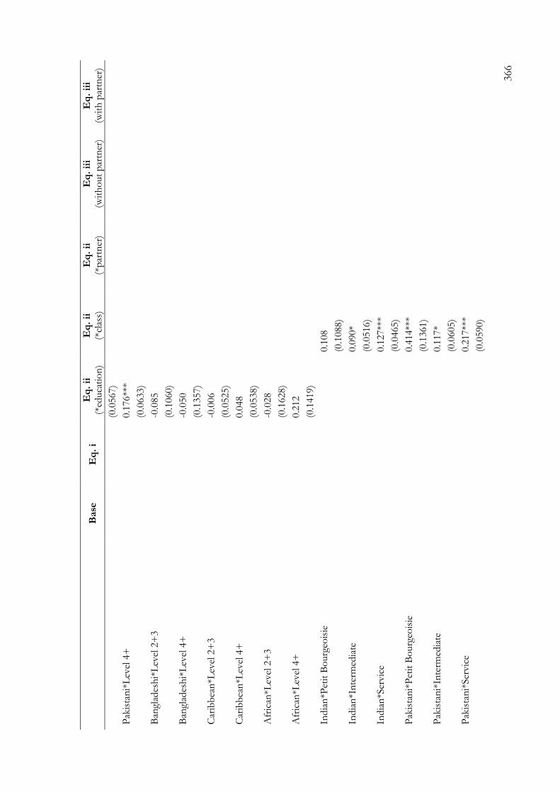
366

B

ase

E

q.

i E

q.

ii

(*ed

uca

tio

n)

Eq

. ii

(*

clas

s)

Eq

. ii

(*

par

tner

) E

q.

iii

(wit

ho

ut

par

tner

) E

q.

iii

(wit

h p

artn

er)

(0

.0567)

Pak

ista

ni*

Lev

el 4

+

0.1

76**

*

(0

.0633)

Ban

glad

esh

i*L

evel

2+

3

-0.0

85

(0

.1060)

Ban

glad

esh

i*L

evel

4+

-0

.050

(0

.1357)

Car

ibb

ean

*Lev

el 2

+3

-0.0

06

(0

.0525)

Car

ibb

ean

*Lev

el 4

+

0.0

48

(0

.0538)

Afr

ican

*Lev

el 2

+3

-0.0

28

(0

.1628)

Afr

ican

*Lev

el 4

+

0.2

12

(0

.1419)

India

n*P

etit

Bo

urg

eois

ie

0.1

08

(0.1

088)

In

dia

n*I

nte

rmed

iate

0.0

90*

(0.0

516)

In

dia

n*S

ervic

e

0.1

27**

*

(0.0

465)

P

akis

tan

i*P

etit

Bo

urg

eois

ie

0.4

14**

*

(0.1

361)

P

akis

tan

i*In

term

edia

te

0.1

17*

(0.0

605)

P

akis

tan

i*Ser

vic

e

0.2

17**

*

(0.0

590)

367

B

ase

E

q.

i E

q.

ii

(*ed

uca

tio

n)

Eq

. ii

(*

clas

s)

Eq

. ii

(*

par

tner

) E

q.

iii

(wit

ho

ut

par

tner

) E

q.

iii

(wit

h p

artn

er)

Ban

glad

esh

i*P

etit

Bo

urg

eois

ie

-0

.059

(0.1

627)

B

angl

ades

hi*

Inte

rmed

iate

0.1

98

(0.1

256)

B

angl

ades

hi*

Ser

vic

e

0.1

74

(0.1

143)

C

arib

bea

n*P

etit

Bo

urg

eois

ie

-0

.009

(0.1

858)

C

arib

bea

n*I

nte

rmed

iate

-0.0

35

(0.0

580)

C

arib

bea

n*S

ervic

e

0.0

40

(0.0

545)

A

fric

an*P

etit

Bo

urg

eois

ie

0.1

99

(0.2

936)

A

fric

an*I

nte

rmed

iate

0.3

07**

(0.1

435)

A

fric

an*S

ervic

e

0.3

20**

*

(0.1

183)

In

dia

n*N

o p

artn

er

-0.1

82**

*

(0

.0438)

India

n*O

ther

0.2

06

(0

.1808)

India

n*w

hit

e B

riti

sh

0.1

97**

*

(0

.0590)

Pak

ista

ni*

No

par

tner

-0

.090

(0

.0559)

Pak

ista

ni*

Oth

er

-0.0

93

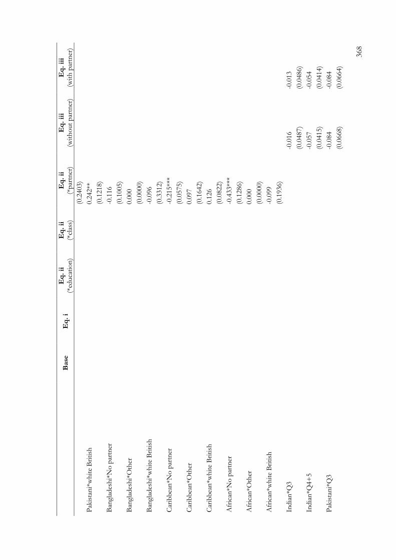
368

B

ase

E

q.

i E

q.

ii

(*ed

uca

tio

n)

Eq

. ii

(*

clas

s)

Eq

. ii

(*

par

tner

) E

q.

iii

(wit

ho

ut

par

tner

) E

q.

iii

(wit

h p

artn

er)

(0

.2403)

Pak

ista

ni*

wh

ite

Bri

tish

0.2

42**

(0

.1218)

Ban

glad

esh

i*N

o p

artn

er

-0.1

16

(0

.1005)

Ban

glad

esh

i*O

ther

0.0

00

(0

.0000)

Ban

glad

esh

i*w

hit

e B

riti

sh

-0.0

96

(0

.3312)

Car

ibb

ean

*No

par

tner

-0

.215**

*

(0

.0575)

Car

ibb

ean

*Oth

er

0.0

97

(0

.1642)

Car

ibb

ean

*wh

ite

Bri

tish

0.1

26

(0

.0822)

Afr

ican

*No

par

tner

-0

.433**

*

(0

.1286)

Afr

ican

*Oth

er

0.0

00

(0

.0000)

Afr

ican

*wh

ite

Bri

tish

-0

.099

(0

.1936)

India

n*Q

3

-0.0

16

-0.0

13

(0.0

487)

(0.0

486)

India

n*Q

4+

5

-0

.057

-0.0

54

(0.0

415)

(0.0

414)

Pak

ista

ni*

Q3

-0

.084

-0.0

84

(0.0

668)

(0.0

664)

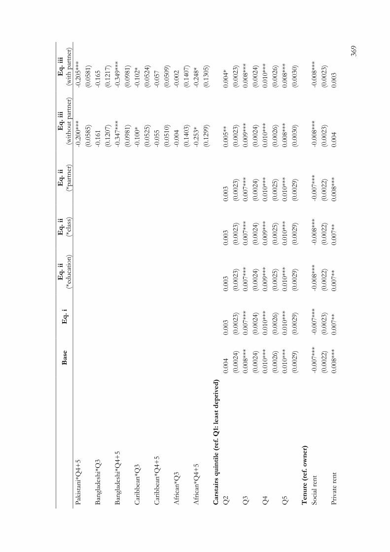
369

B

ase

E

q.

i E

q.

ii

(*ed

uca

tio

n)

Eq

. ii

(*

clas

s)

Eq

. ii

(*

par

tner

) E

q.

iii

(wit

ho

ut

par

tner

) E

q.

iii

(wit

h p

artn

er)

Pak

ista

ni*

Q4+

5

-0

.200**

* -0

.205**

*

(0.0

585)

(0.0

581)

Ban

glad

esh

i*Q

3

-0.1

61

-0.1

65

(0.1

207)

(0.1

217)

Ban

glad

esh

i*Q

4+

5

-0

.347**

* -0

.349**

*

(0.0

981)

(0.0

981)

Car

ibb

ean

*Q3

-0

.100*

-0.1

02*

(0.0

525)

(0.0

524)

Car

ibb

ean

*Q4+

5

-0

.055

-0.0

57

(0.0

510)

(0.0

509)

Afr

ican

*Q3

-0

.004

-0.0

02

(0.1

403)

(0.1

407)

Afr

ican

*Q4+

5

-0

.253*

-0.2

48*

(0.1

299)

(0.1

305)

Cars

tair

s q

uin

tile

(re

f. Q

1: l

east

dep

rive

d)

Q2

0.0

04

0.0

03

0.0

03

0.0

03

0.0

03

0.0

05**

0.0

04*

(0

.0024)

(0.0

023)

(0.0

023)

(0.0

023)

(0.0

023)

(0.0

023)

(0.0

023)

Q3

0.0

08**

* 0.0

07**

* 0.0

07**

* 0.0

07**

* 0.0

07**

* 0.0

09**

* 0.0

08**

*

(0

.0024)

(0.0

024)

(0.0

024)

(0.0

024)

(0.0

024)

(0.0

024)

(0.0

024)

Q4

0.0

10**

* 0.0

10**

* 0.0

09**

* 0.0

09**

* 0.0

10**

* 0.0

10**

* 0.0

10**

*

(0

.0026)

(0.0

026)

(0.0

025)

(0.0

025)

(0.0

025)

(0.0

026)

(0.0

026)

Q5

0.0

10**

* 0.0

10**

* 0.0

10**

* 0.0

10**

* 0.0

10**

* 0.0

08**

* 0.0

08**

*

(0

.0029)

(0.0

029)

(0.0

029)

(0.0

029)

(0.0

029)

(0.0

030)

(0.0

030)

Ten

ure

(re

f. o

wn

er)

So

cial

ren

t -0

.007**

* -0

.007**

* -0

.008**

* -0

.008**

* -0

.007**

* -0

.008**

* -0

.008**

*

(0

.0022)

(0.0

023)

(0.0

022)

(0.0

022)

(0.0

022)

(0.0

023)

(0.0

023)

Pri

vat

e re

nt

0.0

08**

* 0.0

07**

0.0

07**

0.0

07**

0.0

08**

* 0.0

04

0.0

03

370

B

ase

E

q.

i E

q.

ii

(*ed

uca

tio

n)

Eq

. ii

(*

clas

s)

Eq

. ii

(*

par

tner

) E

q.

iii

(wit

ho

ut

par

tner

) E

q.

iii

(wit

h p

artn

er)

(0

.0030)

(0.0

030)

(0.0

030)

(0.0

030)

(0.0

030)

(0.0

030)

(0.0

030)

Nu

mb

er

of

care

s (r

ef.

no

ne)

1 c

ar

0.0

13**

* 0.0

12**

* 0.0

12**

* 0.0

12**

* 0.0

12**

* 0.0

13**

* 0.0

12**

*

(0

.0023)

(0.0

023)

(0.0

023)

(0.0

023)

(0.0

023)

(0.0

023)

(0.0

023)

2+

car

s 0.0

16**

* 0.0

16**

* 0.0

15**

* 0.0

16**

* 0.0

15**

* 0.0

17**

* 0.0

16**

*

(0

.0031)

(0.0

031)

(0.0

031)

(0.0

031)

(0.0

031)

(0.0

031)

(0.0

031)

Pers

on

s p

er

roo

m (

ref.

1 p

pp

)

> 1

.5 p

erso

ns

-0.0

13**

-0

.010

-0.0

10

-0.0

09

-0.0

12*

-0.0

11*

-0.0

09

(0

.0066)

(0.0

066)

(0.0

065)

(0.0

065)

(0.0

064)

(0.0

066)

(0.0

065)

1.5

per

son

s -0

.019**

-0

.018**

-0

.018**

-0

.018**

-0

.016*

-0.0

17*

-0.0

16*

(0

.0093)

(0.0

092)

(0.0

092)

(0.0

092)

(0.0

092)

(0.0

093)

(0.0

092)

>1 &

<1.5

per

son

s -0

.009**

* -0

.008**

-0

.008**

-0

.007**

-0

.007**

-0

.008**

-0

.007**

(0

.0032)

(0.0

032)

(0.0

032)

(0.0

032)

(0.0

032)

(0.0

033)

(0.0

033)

>=

0.7

5 &

<1 p

erso

n

0.0

04*

0.0

04*

0.0

04*

0.0

04*

0.0

04*

0.0

05**

0.0

05**

(0

.0023)

(0.0

023)

(0.0

023)

(0.0

023)

(0.0

023)

(0.0

023)

(0.0

023)

<0.7

5 p

erso

n

-0.0

02

-0.0

01

-0.0

01

-0.0

01

-0.0

01

-0.0

01

-0.0

01

(0

.0024)

(0.0

024)

(0.0

024)

(0.0

024)

(0.0

024)

(0.0

024)

(0.0

024)

Pare

nta

l so

cial

cla

ss (

ref.

Man

ual (V

+V

I+V

II))

No

ear

ner

s/N

o c

od

e -0

.012**

* -0

.010**

-0

.010**

-0

.010**

-0

.010**

-0

.012**

* -0

.011**

(0

.0044)

(0.0

044)

(0.0

043)

(0.0

043)

(0.0

043)

(0.0

044)

(0.0

044)

Ro

uti

ne

no

n-m

anual

(II

I)

-0.0

03

-0.0

02

-0.0

03

-0.0

03

-0.0

03

-0.0

04

-0.0

04

(0

.0025)

(0.0

025)

(0.0

025)

(0.0

025)

(0.0

024)

(0.0

025)

(0.0

025)

Pet

it B

ourg

eois

ie (

IV)

0.0

03

0.0

03

0.0

03

0.0

03

0.0

03

0.0

03

0.0

03

(0

.0028)

(0.0

028)

(0.0

028)

(0.0

028)

(0.0

028)

(0.0

028)

(0.0

028)

Ser

vic

e (I

+II

) -0

.010**

* -0

.007**

* -0

.006**

* -0

.006**

* -0

.007**

* -0

.010**

* -0

.009**

*

(0

.0024)

(0.0

024)

(0.0

024)

(0.0

024)

(0.0

024)

(0.0

024)

(0.0

024)

Ag

e

371

B

ase

E

q.

i E

q.

ii

(*ed

uca

tio

n)

Eq

. ii

(*

clas

s)

Eq

. ii

(*

par

tner

) E

q.

iii

(wit

ho

ut

par

tner

) E

q.

iii

(wit

h p

artn

er)

Age

in

des

tin

atio

n

-0.0

00

-0.0

01**

* -0

.001**

* -0

.001**

* -0

.001**

* -0

.000

-0.0

01**

*

(0

.0002)

(0.0

002)

(0.0

002)

(0.0

002)

(0.0

002)

(0.0

002)

(0.0

002)

Ori

gin

year

(ref.

1971)

1981

-0.0

01

-0.0

02

-0.0

02

-0.0

02

-0.0

02

-0.0

01

-0.0

02

(0

.0014)

(0.0

014)

(0.0

014)

(0.0

014)

(0.0

014)

(0.0

014)

(0.0

014)

1991

-0.0

15**

* -0

.013**

* -0

.013**

* -0

.013**

* -0

.013**

* -0

.011**

* -0

.009**

*

(0

.0025)

(0.0

024)

(0.0

024)

(0.0

024)

(0.0

024)

(0.0

025)

(0.0

024)

Nu

mb

er

of

cen

sus

po

ints

(re

f. 2

)

4 c

ensu

s p

oin

ts

0.0

02

0.0

03

0.0

03

0.0

00

0.0

02

0.0

01

0.0

02

(0

.0065)

(0.0

065)

(0.0

065)

(0.0

065)

(0.0

065)

(0.0

065)

(0.0

065)

5 c

ensu

s p

oin

ts

0.0

13*

0.0

09

0.0

09

0.0

07

0.0

08

0.0

12*

0.0

09

(0

.0068)

(0.0

068)

(0.0

068)

(0.0

067)

(0.0

068)

(0.0

068)

(0.0

067)

Co

nst

ant

0.9

60**

* 0.9

16**

* 0.9

24**

* 0.9

25**

* 0.8

53**

* 0.9

42**

* 0.9

01**

*

(0

.0089)

(0.0

189)

(0.0

190)

(0.0

188)

(0.0

227)

(0.0

091)

(0.0

189)

Adju

sted

R-s

quar

ed

0.1

68

0.1

75

0.1

76

0.1

77

0.1

80

0.1

63

0.1

69

N

83,9

72

83,9

72

83,9

72

83,9

72

83,9

72

83,9

72

83,9

72

* p

-val

ue<

.10 *

* p

-val

ue<

.05 *

** p

-val

ue<

.01; ro

bust

(cl

ust

ered

) st

andar

d e

rro

rs in

par

enth

eses

P

op

ula

tio

n: In

div

idual

s b

etw

een

20 a

nd

55 y

ears

old

So

urc

e: A

uth

or’

s o

wn

cal

cula

tio

ns

bas

ed o

n O

NS

-LS

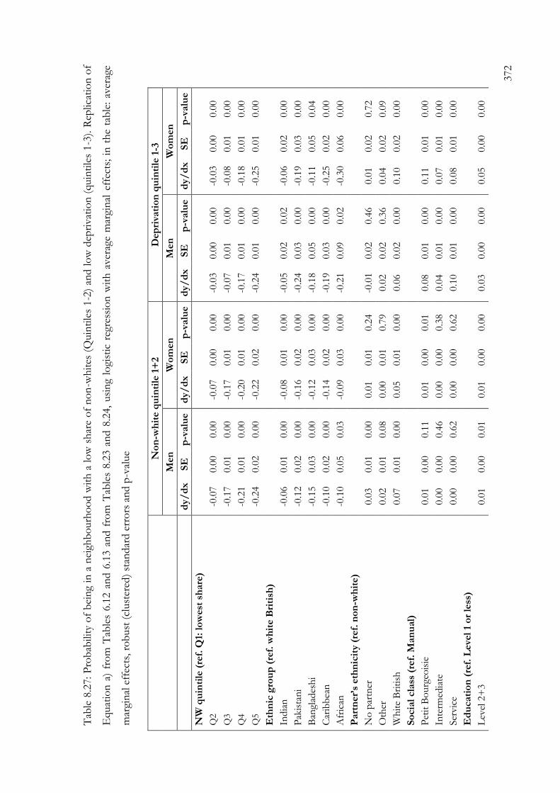
372

Tab

le ‎8

.27: P

rob

abili

ty o

f b

ein

g in

a n

eigh

bo

urh

oo

d w

ith

a l

ow

sh

are

of

no

n-w

hit

es (

Quin

tile

s 1-2

) an

d l

ow

dep

rivat

ion

(quin

tile

s 1-3

). R

eplica

tio

n o

f

Equat

ion

a)

fro

m T

able

s 6.1

2 a

nd 6

.13 a

nd f

rom

Tab

les

8.2

3 a

nd 8

.24,

usi

ng

logi

stic

reg

ress

ion

wit

h a

ver

age

mar

gin

al e

ffec

ts;

in t

he

tab

le:

aver

age

mar

gin

al e

ffec

ts, ro

bust

(cl

ust

ered

) st

andar

d e

rro

rs a

nd p

-val

ue

N

on

-wh

ite q

uin

tile

1+

2

Dep

riva

tio

n q

uin

tile

1-3

M

en

W

om

en

M

en

W

om

en

d

y/

dx

SE

p

-valu

e d

y/

dx

SE

p

-valu

e d

y/

dx

SE

p

-valu

e

dy/

dx

SE

p

-valu

e

NW

qu

inti

le (

ref.

Q1:

lo

wes

t sh

are

)

Q

2

-0.0

7

0.0

0

0.0

0

-0.0

7

0.0

0

0.0

0

-0.0

3

0.0

0

0.0

0

-0.0

3

0.0

0

0.0

0

Q3

-0.1

7

0.0

1

0.0

0

-0.1

7

0.0

1

0.0

0

-0.0

7

0.0

1

0.0

0

-0.0

8

0.0

1

0.0

0

Q4

-0.2

1

0.0

1

0.0

0

-0.2

0

0.0

1

0.0

0

-0.1

7

0.0

1

0.0

0

-0.1

8

0.0

1

0.0

0

Q5

-0.2

4

0.0

2

0.0

0

-0.2

2

0.0

2

0.0

0

-0.2

4

0.0

1

0.0

0

-0.2

5

0.0

1

0.0

0

Eth

nic

gro

up

(re

f. w

hit

e B

riti

sh)

India

n

-0.0

6

0.0

1

0.0

0

-0.0

8

0.0

1

0.0

0

-0.0

5

0.0

2

0.0

2

-0.0

6

0.0

2

0.0

0

Pak

ista

ni

-0.1

2

0.0

2

0.0

0

-0.1

6

0.0

2

0.0

0

-0.2

4

0.0

3

0.0

0

-0.1

9

0.0

3

0.0

0

Ban

glad

esh

i -0

.15

0.0

3

0.0

0

-0.1

2

0.0

3

0.0

0

-0.1

8

0.0

5

0.0

0

-0.1

1

0.0

5

0.0

4

Car

ibb

ean

-0

.10

0.0

2

0.0

0

-0.1

4

0.0

2

0.0

0

-0.1

9

0.0

3

0.0

0

-0.2

5

0.0

2

0.0

0

Afr

ican

-0

.10

0.0

5

0.0

3

-0.0

9

0.0

3

0.0

0

-0.2

1

0.0

9

0.0

2

-0.3

0

0.0

6

0.0

0

Part

ner’

s eth

nic

ity (

ref.

no

n-w

hit

e)

No

par

tner

0.0

3

0.0

1

0.0

0

0.0

1

0.0

1

0.2

4

-0.0

1

0.0

2

0.4

6

0.0

1

0.0

2

0.7

2

Oth

er

0.0

2

0.0

1

0.0

8

0.0

0

0.0

1

0.7

9

0.0

2

0.0

2

0.3

6

0.0

4

0.0

2

0.0

9

Wh

ite

Bri

tish

0.0

7

0.0

1

0.0

0

0.0

5

0.0

1

0.0

0

0.0

6

0.0

2

0.0

0

0.1

0

0.0

2

0.0

0

So

cia

l cla

ss (

ref.

Man

ual)

P

etit

Bo

urg

eois

ie

0.0

1

0.0

0

0.1

1

0.0

1

0.0

0

0.0

1

0.0

8

0.0

1

0.0

0

0.1

1

0.0

1

0.0

0

Inte

rmed

iate

0.0

0

0.0

0

0.4

6

0.0

0

0.0

0

0.3

8

0.0

4

0.0

1

0.0

0

0.0

7

0.0

1

0.0

0

Ser

vic

e 0.0

0

0.0

0

0.6

2

0.0

0

0.0

0

0.6

2

0.1

0

0.0

1

0.0

0

0.0

8

0.0

1

0.0

0

Ed

ucati

on

(re

f. L

eve

l 1

or

less

)

L

evel

2+

3

0.0

1

0.0

0

0.0

1

0.0

1

0.0

0

0.0

0

0.0

3

0.0

0

0.0

0

0.0

5

0.0

0

0.0

0

373

N

on

-wh

ite q

uin

tile

1+

2

Dep

riva

tio

n q

uin

tile

1-3

M

en

W

om

en

M

en

W

om

en

d

y/

dx

SE

p

-valu

e d

y/

dx

SE

p

-valu

e d

y/

dx

SE

p

-valu

e

dy/

dx

SE

p

-valu

e

Lev

el 4

+

-0.0

2

0.0

0

0.0

0

-0.0

1

0.0

0

0.0

0

0.0

5

0.0

1

0.0

0

0.0

7

0.0

1

0.0

0

Cars

tair

s q

uin

tile

s (r

ef.

Q1:

less

dep

riva

tio

n)

Car

stai

rs Q

2

0.0

0

0.0

0

0.7

8

0.0

0

0.0

0

0.1

3

0.0

0

0.0

1

0.6

9

0.0

0

0.0

0

0.4

3

Car

stai

rs Q

3

0.0

0

0.0

0

0.3

7

0.0

1

0.0

0

0.0

1

0.0

0

0.0

1

0.7

9

0.0

0

0.0

1

0.6

7

Car

stai

rs Q

4

0.0

1

0.0

0

0.0

2

0.0

1

0.0

0

0.0

0

0.0

1

0.0

1

0.6

2

0.0

3

0.0

1

0.0

0

Car

stai

rs Q

5

0.0

0

0.0

0

0.2

0

0.0

1

0.0

0

0.0

0

0.0

2

0.0

1

0.1

5

0.0

4

0.0

1

0.0

0

Ten

ure

(re

f. o

wn

er)

So

cial

ren

t -0

.01

0.0

0

0.0

0

-0.0

1

0.0

0

0.0

0

-0.0

7

0.0

0

0.0

0

-0.0

7

0.0

0

0.0

0

Pri

vat

e re

nt

0.0

0

0.0

0

0.3

1

0.0

1

0.0

0

0.0

4

-0.0

1

0.0

1

0.1

3

-0.0

1

0.0

1

0.0

2

Nu

mb

er

of

cars

(re

f. n

on

e)

1 c

ar

0.0

1

0.0

0

0.0

0

0.0

1

0.0

0

0.0

0

0.0

6

0.0

0

0.0

0

0.0

7

0.0

0

0.0

0

2+

car

s 0.0

1

0.0

0

0.0

6

0.0

1

0.0

0

0.0

0

0.0

9

0.0

1

0.0

0

0.1

0

0.0

1

0.0

0

Pers

on

s p

er

roo

m (

ref.

1 p

pp

)

>

1.5

per

son

s -0

.01

0.0

1

0.0

8

-0.0

1

0.0

0

0.1

1

-0.0

5

0.0

1

0.0

0

-0.0

6

0.0

1

0.0

0

1.5

per

son

s -0

.02

0.0

1

0.0

2

-0.0

1

0.0

1

0.1

2

-0.0

5

0.0

1

0.0

0

-0.0

7

0.0

1

0.0

0

>1 &

<1.5

per

son

s -0

.01

0.0

0

0.0

0

-0.0

1

0.0

0

0.0

2

-0.0

4

0.0

1

0.0

0

-0.0

2

0.0

1

0.0

0

>=

0.7

5 &

<1 p

erso

n

0.0

0

0.0

0

0.3

6

0.0

0

0.0

0

0.0

4

0.0

1

0.0

0

0.1

0

0.0

1

0.0

0

0.0

1

<0.7

5 p

erso

n

0.0

0

0.0

0

0.2

4

0.0

0

0.0

0

0.6

1

0.0

2

0.0

0

0.0

0

0.0

2

0.0

0

0.0

0

Pare

nta

l so

cial

cla

ss (

ref.

Man

ual (V

+V

I+V

II))

N

o e

arn

ers/

No

cod

e -0

.01

0.0

0

0.0

9

-0.0

1

0.0

0

0.0

6

0.0

1

0.0

1

0.4

1

0.0

2

0.0

1

0.0

1

Ro

uti

ne

no

n-m

anual

(II

I)

0.0

0

0.0

0

0.0

6

0.0

0

0.0

0

0.2

4

0.0

2

0.0

0

0.0

0

0.0

3

0.0

0

0.0

0

Pet

it B

ourg

eois

ie (

IV)

0.0

0

0.0

0

0.4

3

0.0

0

0.0

0

0.1

4

0.0

6

0.0

1

0.0

0

0.0

5

0.0

1

0.0

0

Pro

fess

ion

al/

Man

ager

ial (I

+II

) -0

.01

0.0

0

0.0

0

-0.0

1

0.0

0

0.0

0

0.0

3

0.0

1

0.0

0

0.0

4

0.0

0

0.0

0

Ag

e

Age

in

des

tin

atio

n

0.0

0

0.0

0

0.0

6

0.0

0

0.0

0

0.0

0

0.0

0

0.0

0

0.1

4

0.0

0

0.0

0

0.5

4

Ori

gin

year

(ref.

1971)

374

N

on

-wh

ite q

uin

tile

1+

2

Dep

riva

tio

n q

uin

tile

1-3

M

en

W

om

en

M

en

W

om

en

d

y/

dx

SE

p

-valu

e d

y/

dx

SE

p

-valu

e d

y/

dx

SE

p

-valu

e

dy/

dx

SE

p

-valu

e

1981

0.0

0

0.0

0

0.7

6

0.0

0

0.0

0

0.2

1

-0.0

2

0.0

0

0.0

0

-0.0

3

0.0

0

0.0

0

1991

-0.0

1

0.0

0

0.0

0

-0.0

1

0.0

0

0.0

0

-0.0

6

0.0

1

0.0

0

-0.0

7

0.0

0

0.0

0

Nu

mb

er

of

cen

sus

po

ints

(re

f. 3

)

4 c

ensu

s p

oin

ts

0.0

1

0.0

1

0.3

0

0.0

0

0.0

0

0.8

3

0.0

0

0.0

1

0.6

9

-0.0

1

0.0

1

0.5

5

5 c

ensu

s p

oin

ts

0.0

1

0.0

1

0.0

4

0.0

1

0.0

1

0.2

0

0.0

1

0.0

1

0.4

1

0.0

0

0.0

1

0.9

2

Pse

udo

R-s

quar

ed

0.1

858

0.2

047

0.1

033

0.1

179

N

77196

83972

77196

73972

No

te: th

e co

effi

cien

ts a

re v

ery

sim

ilar

wit

h r

espec

t to

th

ose

ob

serv

ed in

the

equiv

alen

t m

odel

s p

rese

nte

d in

th

e ch

apte

r: t

he s

ub

stan

tive

resu

lts

rem

ain

th

eref

ore

th

e sa

me.

P

op

ula

tio

n: In

div

idual

s b

etw

een

20 a

nd

55 y

ears

old

So

urc

e: A

uth

or’

s o

wn

cal

cula

tio

ns

bas

ed o

n O

NS-L

S

375

9 ANNEX B: A Comparison of ‘Pooled’ and ‘Unique’

data

The main aim of this Annex is to explore the extent to which the data that pools cases, that is,

which allows more than one measurement per individual, varies from data in which only one

origin/destination for each individual is randomly chosen.

The main rationale for pooling data is that it allows one to have more cases. Working with ethnic

minorities is always problematic in this regard, and by allowing multiple entrances per individual I

have achieved more stable models. Of course, there is the issue of to what extent pooling models

generates noise in the results. In this Annex, therefore, I offer some descriptive statistics of how

key variables behave for a version of the data in which only one individual is present. The more

similar the distribution of variables, the more we can say that the pooled version of the data is an

‘extended’ version of the individual version of the data, and also an expression a ‘life course

average’ of each individual. This exploration is complemented, in Annex C, with an analysis of

the effect of origin/destination years.

Table 9.1 shows the number of pooled and unique cases by group for the so-called initial sample

(see Chapter 2). We can see that there are variations between groups: in particular, Bangladeshis

and Africans, and those who have less-repeated measurements. This is related to the fact that

they are the populations with the least number of cases and, in the case of Bangladeshis, are also

younger, which means that they are less likely to be in earlier census points.

376

Table ‎9.1: Pooled and unique cases by ethnic group; initial sample


Pooled Unique % Unique Pooled Unique % Unique

British 399807 155089 38.8 183739 130907 71.2

Indian 7117 2940 41.3 2727 1883 69.1

Pakistani 4432 2038 46.0 1439 1022 71.0

Bangladeshi 1323 685 51.8 381 311 81.6

Chinese 844 350 41.5 299 211 70.6

Caribbean 3563 1584 44.5 1434 1064 74.2

African 724 386 53.3 208 174 83.7

Total 417810 163072 39.0 190227 135572 71.3


Tables 9.2-9.4 show the distribution of parental social class, education and the service class and

for the six ethnic minority groups and white British, using pooled and unique data (in both cases,

the so-called initial samples are used). In the first case, all possible values of these variables for

each individual are considered; in the second, each individual is randomly assigned one parental

social class, education and social class (note that in Chapter 6 only the parental social class varies;

education and occupation refer to 2001). I have selected these variables since they can be

considered as key indicators of average socio-economic conditions of groups in origin (parental

social class) and destination (education and social class).

These tables reveal that that for all groups, the distribution the key selected variables is very

similar in the pooled and unique datasets. In other words, the distribution of class of origin,

education and the service class for each group does not reveal important differences across

datasets. This suggests that, on average, the pooled and unique datasets are similar in terms of

their structure and the way the variables behave: pooling the cases has probably not harmed the

substantive findings (recall that I still make a correction for the standard errors). However, it

could also be argued that differences might exist for different origin/destination years: I explore

this further in Annex C.

377

Tab

le ‎9

.2: P

aren

tal so

cial

cla

ss b

y et

hn

ic g

roup

; in

itia

l sa

mp

le, p

oo

led a

nd u

niq

ue

case

s

P

oo

led

Un

iqu

e

N

E/

NC

V

+V

I +

VII

II

I IV

I+

II

Tot

al

N

E/

NC

V

+V

I +

VII

II

I IV

I+

II

Tot

al

Ch

ap

ters

3 &

5

Wh

ite

Bri

tish

5.5

38.0

15.5

11.1

29.9

399767

5.9

37.5

16

11.1

29.5

155075

India

n

6.1

50.9

10.5

14.2

18.2

7117

6.7

48.9

10.9

15.3

18.2

2940

Pak

ista

ni

16.1

60.0

4.0

12.3

7.7

4431

16.7

58.4

3.9

13.2

7.8

2037

Ban

glad

esh

i 27.8

52.3

3.1

11.3

5.5

1322

28.2

52.8

2.5

10.4

6.1

684

Ch

ines

e 11.0

24.1

5.5

40.9

18.6

844

10.9

23.7

6.6

42.9

16.0

350

Car

ibb

ean

14.0

47.1

22.1

2.3

14.5

3563

14.3

46.0

23.7

2.1

14.0

1584

Afr

ican

18.4

27.8

24.8

1.5

27.5

723

21.2

28.0

23.1

0.0

27.7

386

Ch

ap

ter

6

W

hit

e B

riti

sh

5.0

40.0

15.8

10.8

28.5

183726

5.0

40.1

16.4

10.7

27.9

130978

India

n

6.2

56.4

9.4

12.0

16.0

2727

6.8

57.6

9.4

11.3

14.9

1887

Pak

ista

ni

14.5

64.8

2.9

10.6

7.2

1439

13.7

65.3

2.9

10.6

7.5

1012

Ban

glad

esh

i 28.1

50.9

3.7

11.8

5.5

381

28.4

51.1

3.2

11.2

6.1

313

Ch

ines

e 10.1

25.0

7.4

42.2

17.2

296

9.4

25.9

9.0

41.5

14.2

212

Car

ibb

ean

11.7

52.9

19.4

1.9

14.2

1431

10.3

54.8

18.7

2.0

14.2

1060

Afr

ican

15.0

29.9

27.6

4.7

22.9

214

14.9

31.6

30.5

0.0

23.0

174

I+II

: P

rofe

ssio

nal

/m

anag

eria

l; II

I: R

outi

ne

no

n-m

anual

; IV

: B

ourg

eois

ie; V

+V

I+V

II: M

anual

; N

E/

NC

: N

o e

arn

ers/

no

co

de.

So

urc

e: A

uth

or’

s o

wn

cal

cula

tio

ns

bas

ed o

n O

NS

-LS

378

Table ‎9.3: Education by ethnic group; initial sample, pooled and unique cases

Pooled Unique

Level 1 or

less Level 2+3

Level 4+

Total Level 1 or

less Level 2+3

Level 4+ Total

Chapters 3 & 5

British 36.4 36.7 27.0 397662 37.6 36.0 26.4 154370

Indian 21.2 30.4 48.4 6991 21.1 31.0 47.9 2894

Pakistani 35.5 32.0 32.5 4391 36.5 31.9 31.7 2025

Bangladeshi 36.7 33.4 29.9 1311 37.9 32.5 29.7 681

Chinese 14.1 29.8 56.1 823 19.0 27.8 53.2 342

Caribbean 34.1 35.7 30.2 3544 34.4 36.9 28.7 1577

African 15.2 31.3 53.5 712 14.8 31.1 54.1 379

Chapter 6

British 41.4 37.0 21.6 182334 42.8 35.3 22.0 130192

Indian 26.0 35.3 38.6 2638 27.7 33.8 38.6 1839

Pakistani 38.8 32.6 28.7 1410 40.4 30.6 29.0 994

Bangladeshi 40.1 38.4 21.5 372 42.8 36.3 20.9 306

Chinese 13.7 37.0 49.3 284 16.3 34.0 49.8 203

Caribbean 38.4 35.5 26.1 1424 40.0 33.7 26.3 1055

African 21.0 30.7 48.3 205 21.6 29.8 48.5 171

Source: Own calculations based on ONS-LS

Table ‎9.4: Access to the service class by ethnic group; initial sample, pooled and unique cases

Pooled Unique

Service class Total Service class Total

Chapters 3 & 5

White British 38.8 381668 38.4 148003

Indian 52.2 6259 51.5 2600

Pakistani 35.5 3934 35.1 1812

Bangladeshi 34.1 1180 31.5 607

Chinese 51.4 706 51.2 297

Caribbean 39.5 3324 39.1 1464

African 49.3 605 51.0 310

Chapter 6

White British 37.6 174559 38.1 125770

Indian 48.2 2237 48.7 1605

Pakistani 33.2 1202 33.3 867

Bangladeshi 33.8 321 33.0 269

Chinese 48.4 227 47.9 170

Caribbean 39.5 1333 39.9 1001

African 53.4 189 54.5 153


379

10 ANNEX C: Origin and Destination Effects

Chapters 3, 5 and 6 are not mainly concerned with exploring changes over time; rather, I am

interested in average results. However, some differences between years do emerge, for example

in Chapter 3 when studying employment. This Annex provides, first of all, descriptive statistics

for selected (origin and destination) key variables from each chapter by origin and destination

year. It is not my aim here to discuss these findings in detail, but to reveal potential differences

for various origin/destination years. Secondly, I show the results of some key models for

different origin/destination years. Since these models control for all relevant variables, including

age, I expect to explore in a more direct way whether there are year effects worth considering.

Regarding origin variables, Table 10.1 shows that except for Bangladeshis, those raised in more

recent years (and most of those measured in 2001) are less likely to have lower-class parents. The

results on the distribution of groups in neighbourhoods show that for Indians the share of co-

ethnics in the neighbourhood is lower in more recent origin years. Similar results are observed for

white British and Indians when the share of non-whites is estimated. For the other groups, the

share of co-ethnics (and for most groups also the share of non-whites) is the highest in 1981 (and

also when measured in 2001). As regards key destination variables, individuals are in general

more likely to be employed and more likely to be in the service class in 2011 than in 2001.

Another outcome to note is that individuals raised in 1991 are less likely to be found in a non-

white neighbourhood: this might be related to an age effect, in the sense that those raised in 1991

are still too young to make a move to a more white area in 2011.

380

Table ‎10.1: Distribution of key variables by group and origin/destination years; final samples

1971 1981 1991 2001 2011

Variables measured in origin

% Low parental class (manual or less)

White British 50.9 46.6 32.1 46.4 42.7

Indian 76.3 65.8 44.0 67.8 55.5

Pakistani 86.8 79.9 73.7 82.1 76.0

Bangladeshi 61.1 78.0 82.7 81.6 79.8

Chinese - 39.5 38.2 34.1 36.5

Caribbean 71.5 61.6 41.2 65.2 60.7

African 45.7 48.3 43.4 44.5 46.8

% Q5 co-ethnic

Indian 35.0 27.2 20.2 28.1 25.1

Pakistani 19.9 25.7 23.1 25.8 22.9

Bangladeshi - 25.1 23.5 24.2 23.8

Caribbean 16.1 17.8 16.0 16.3 17.5

African 14.5 35.0 25.1 27.2 24.3

% Q45 non-white

White British 2.5 2.2 1.7

Indian 60.1 52.1 44.3

Pakistani 50.5 55.2 53.3

Bangladeshi - 50.4 61.1

Caribbean 46.2 44.9 37.7

African 47.9 47.1 -

Variables measured in destination

% Employed

White British 82.5 82.8 82.1 81.6 83.6

Indian 83.4 84.2 84.2 81.8 85.6

Pakistani 65.8 62.9 63.0 57.6 66.5

Bangladeshi 50.0 62.3 63.9 55.4 66.1

Chinese 87.0 89.5 87.3 91.5 86.5

Caribbean 79.0 78.3 75.5 75.4 81.3

African 78.3 86.3 78.9 80.4 82.1

% Service class

White British 38.6 39.8 35.5 36.8 40.1

Indian 46.0 53.7 54.6 48.0 55.7

Pakistani 44.4 37.7 31.1 32.7 37.7

Bangladeshi 39.3 37.6 31.9 32.6 34.7

Chinese 55.2 50.8 52.5 49.0 53.7

381

1971 1981 1991 2001 2011

Caribbean 40.6 40.3 40.5 38.4 42.7

African 51.9 54.5 41.3 53.3 47.4

% Q1+2 non-white

White British 95.0 94.7 94.0

Indian 50.9 51.4 46.4

Pakistani 44.0 33.4 31.4

Bangladeshi - 30.4 34.5

Caribbean 43.6 43.8 29.9

African 42.5 47.1 -

Note: Percentages are calculated using the final samples: for % Low parental class, % Q5 co-ethnic, % Employed and % Service class, the final samples for Chapters 3 and 5 are used; for % Q45 non-white and % Q1+2 non-white, the final sample for Chapter 5 is used. Some percentages are not shown due to the low number of cases. For the approximate totals by year and ethnicity refer to Table 2.5 in Chapter 2. Source: Author’s own calculations based on ONS-LS

Tables 10.2-10.4 replicate Model 5 from Tables 3.5-3.8 and Model 2 from Tables 3.9 and 3.10 in

Chapter 3, but dividing by origin and destination years. In other words, the models that test for

ethnic penalties in employment (Tables 3.5 and 3.6) and access to the service class (Tables 3.7

and 3.8) and the models that explore social mobility patterns, after controlling for education

(Tables 3.9-3.10) are estimated separately for people raised in 1971, 1981 and 1991 and for

people whose outcomes are measured in 2001 and 2011. Similarly, Tables 10.5 and 10.6 replicate

Model 5 from Tables 5.3 and 5.7 in Chapter 5: this model estimates the effect of the share of co-

ethnics in the origin neighbourhood in the access to employment and in the probability of

avoiding routine and semi-routine occupations, after controlling for background characteristics

and for each ethnic group. Finally, Table 10.7 replicates Eq. i from Tables 6.12 and 6.13 in

Chapter 6, which tests for the existence of ethnic enclave/place stratification models. The full

models are available upon request.

Starting with Chapter 3, as regards access to employment (Table 10.2), the results are very similar

to those observed in the chapter. Among men, the penalty for Pakistanis and Caribbeans and the

advantage of the Chinese is observed in most of estimations (note that in 2011 the penalty

disappears, as Chapter 3 also shows). Among women, the disadvantage of Pakistanis and

Bangladeshis is more than evident, and constant across all models, although for Bangladeshis the

situation seems to improve over time. As regards access to the service class (Table 10.3), the

advantage for Indians (both men and women) is clear in all models; moreover, the advantage for

382

Caribbean women also seems to be quite constant, while the advantage for Bangladeshi and

Chinese men less so (still, most of coefficients are positive). Regarding the estimations of social

mobility (Table 10.4), we see that the positive effect of parental social class IV for Indians occurs

mainly in the recent cohort/destination year; while for Pakistani men/women and Caribbean

men it is in the older cohorts/destination year where the positive/negative effects of parental

social class I+II is most prevalent.

Moving to Chapter 5, Tables 10.4 and 10.5 show that the negative neighbourhood effect found

for Pakistani and Bangladeshi women is, to a greater or lesser extent, negative in all

cohorts/destination years. The same can be said of the positive effect for Indian men in terms of

occupation, and the negative effect for Bangladeshi and black populations. Table 10.6, finally,

which refers to Chapter 6, shows results pooled for men and women, given that no strong gender

effects were observed in the chapter itself. We can see that the coefficients go in the same

direction as the ones observed in the main chapter.

383

Tab

le ‎1

0.2

: A

cces

s to

em

plo

ymen

t fo

r in

div

idual

s ra

ised

in

dif

fere

nt

ori

gin

yea

rs (

1971-1

991)

and i

ndiv

idual

s m

easu

red i

n d

iffe

ren

t des

tin

atio

n y

ears

(2001-2

011).

Tes

t fo

r C

hap

ter

3.

M

en

W

om

en

19

71

1981

1991

2001

2011

19

71

1981

1991

2001

2011

Eth

nic

gro

up

(re

f. w

hit

e B

riti

sh)

In

dia

n

0.0

27*

0.0

08

-0.0

10

0.0

00

0.0

08

0.0

33*

0.0

05

-0.0

15

0.0

22

-0.0

05

(0

.0146)

(0.0

093)

(0.0

110)

(0.0

127)

(0.0

089)

(0.0

189)

(0.0

120)

(0.0

133)

(0.0

150)

(0.0

115)

Pak

ista

ni

-0.0

24

-0.0

34**

-0

.049**

* -0

.087**

* -0

.018

-0.2

07**

* -0

.217**

* -0

.157**

* -0

.227**

* -0

.188**

*

(0

.0255)

(0.0

152)

(0.0

176)

(0.0

211)

(0.0

141)

(0.0

347)

(0.0

174)

(0.0

181)

(0.0

216)

(0.0

164)

Ban

glad

esh

i -0

.090

0.0

62**

0.0

24

-0.0

28

0.0

50**

-0

.433**

* -0

.244**

* -0

.084**

* -0

.225**

* -0

.162**

*

(0

.0891)

(0.0

269)

(0.0

247)

(0.0

383)

(0.0

211)

(0.1

161)

(0.0

363)

(0.0

245)

(0.0

381)

(0.0

250)

Ch

ines

e 0.1

40**

* 0.0

79**

* -0

.007

0.0

73**

0.0

39*

-0.0

40

0.0

69**

0.0

41

0.1

18**

* 0.0

01

(0

.0223)

(0.0

191)

(0.0

297)

(0.0

304)

(0.0

230)

(0.0

913)

(0.0

327)

(0.0

297)

(0.0

312)

(0.0

340)

Car

ibb

ean

-0

.027

-0.0

33**

-0

.053

-0.0

69**

* 0.0

02

0.0

17

0.0

02

-0.0

28

-0.0

01

0.0

05

(0

.0175)

(0.0

166)

(0.0

329)

(0.0

191)

(0.0

182)

(0.0

168)

(0.0

174)

(0.0

300)

(0.0

178)

(0.0

184)

Afr

ican

0.0

31

0.0

58*

-0.0

06

-0.0

27

0.0

44

-0.0

17

0.0

49

-0.0

09

0.0

27

-0.0

32

(0

.0511)

(0.0

349)

(0.0

392)

(0.0

497)

(0.0

277)

(0.0

426)

(0.0

356)

(0.0

442)

(0.0

372)

(0.0

322)

A

dju

sted

R2

0.0

88

0.1

04

0.1

26

0.0

88

0.1

24

0.0

81

0.1

36

0.2

06

0.1

06

0.1

46

N

59,7

21

76,3

20

44,4

99

91,4

97

89,0

43

62,6

93

80,1

33

46,1

11

95,5

97

93,3

40

All

mo

del

s co

ntr

ol fo

r: a

ge, n

um

ber

of

cen

sus

po

ints

, cl

ass

of

ori

gin

, te

nure

, n

um

ber

of

per

son

s p

er r

oo

m, n

um

ber

of

cars

an

d d

epri

vat

ion

quin

tile

at

the

war

d lev

el. M

ore

over

, m

od

els

for

1971-1

991 c

on

tro

l fo

r d

esti

nat

ion

yea

r, w

hile

mo

del

s fo

r 2001-2

011 c

on

tro

l fo

r o

rigi

n y

ear.

*

p-v

alue<

.10 *

* p

-val

ue<

.05 *

** p

-val

ue<

.01. R

ob

ust

(cl

ust

ered

) R

ob

ust

(cl

ust

ered

) st

and

ard

err

ors

in

par

enth

eses

. P

op

ula

tio

n: In

div

idual

s b

etw

een

20 a

nd

45 y

ears

old

So

urc

e: A

uth

or’

s o

wn

cal

cula

tio

ns

bas

ed o

n O

NS

-LS

384

Tab

le ‎1

0.3

: A

cces

s to

th

e se

rvic

e cl

ass

for

indiv

idual

s ra

ised

in

dif

fere

nt

ori

gin

yea

rs (

1971-1

991)

and i

ndiv

idual

s m

easu

red i

n d

iffe

ren

t des

tin

atio

n

year

s (2

001-2

011).

Tes

t fo

r C

hap

ter

3.

M

en

W

om

en

19

71

1981

1991

2001

2011

19

71

1981

1991

2001

2011

Eth

nic

gro

up

(re

f. w

hit

e B

riti

sh)

In

dia

n

0.0

56**

* 0.0

82**

* 0.0

82**

* 0.0

78**

* 0.0

74**

* 0.0

23

0.0

53**

* 0.0

77**

* 0.0

42**

0.0

60**

*

(0

.0196)

(0.0

123)

(0.0

146)

(0.0

154)

(0.0

129)

(0.0

203)

(0.0

131)

(0.0

154)

(0.0

165)

(0.0

138)

Pak

ista

ni

0.0

39

0.0

14

-0.0

23

0.0

11

0.0

08

0.0

59*

-0.0

08

-0.0

01

-0.0

08

0.0

09

(0

.0282)

(0.0

162)

(0.0

170)

(0.0

188)

(0.0

160)

(0.0

342)

(0.0

171)

(0.0

178)

(0.0

225)

(0.0

163)

Ban

glad

esh

i -0

.008

0.0

17

0.0

51*

0.0

95**

0.0

37

0.1

53

0.0

41

0.0

04

0.0

41

0.0

19

(0

.1156)

(0.0

329)

(0.0

281)

(0.0

381)

(0.0

266)

(0.1

142)

(0.0

357)

(0.0

229)

(0.0

391)

(0.0

236)

Ch

ines

e -0

.040

0.0

52

0.0

90**

0.0

64

0.0

59

0.1

37*

-0.0

15

-0.0

42

-0.0

32

-0.0

05

(0

.0764)

(0.0

384)

(0.0

432)

(0.0

470)

(0.0

375)

(0.0

757)

(0.0

347)

(0.0

380)

(0.0

493)

(0.0

353)

Car

ibb

ean

-0

.014

-0.0

01

0.0

64*

-0.0

11

0.0

20

0.0

50**

* 0.0

35*

-0.0

09

0.0

45**

0.0

30

(0

.0206)

(0.0

202)

(0.0

385)

(0.0

210)

(0.0

235)

(0.0

188)

(0.0

189)

(0.0

323)

(0.0

197)

(0.0

211)

Afr

ican

-0

.026

0.0

65

0.0

40

0.1

27**

-0

.007

-0.0

45

0.0

35

-0.1

64**

* -0

.001

-0.0

68

(0

.0823)

(0.0

534)

(0.0

548)

(0.0

597)

(0.0

422)

(0.0

517)

(0.0

494)

(0.0

541)

(0.0

490)

(0.0

424)

Adju

sted

R2

0.2

67

0.2

55

0.2

32

0.2

48

0.2

62

0.2

61

0.2

54

0.2

41

0.2

48

0.2

53

N

58,1

80

73,8

17

42,1

13

89,0

67

85,0

43

60,6

16

76,6

35

43,3

57

91,9

02

88,7

06

All

mo

del

s co

ntr

ol fo

r: a

ge, n

um

ber

of

cen

sus

po

ints

, cl

ass

of

ori

gin

, te

nure

, n

um

ber

of

per

son

s p

er r

oo

m, n

um

ber

of

cars

an

d d

epri

vat

ion

quin

tile

at

the

war

d lev

el. M

ore

over

, m

od

els

1971-1

991 c

on

tro

l fo

r d

esti

nat

ion

yea

r, w

hile

mo

del

s 2001-2

011 c

on

tro

l fo

r o

rigi

n y

ear.

*

p-v

alue<

.10 *

* p

-val

ue<

.05 *

** p

-val

ue<

.01. R

ob

ust

(cl

ust

ered

) st

and

ard

err

ors

in

par

enth

eses

. P

op

ula

tio

n: In

div

idual

s b

etw

een

20 a

nd

45 y

ears

old

So

urc

e: A

uth

or’

s o

wn

cal

cula

tio

ns

bas

ed o

n O

NS

-LS

385

Tab

le ‎1

0.4

: A

cces

s to

th

e se

rvic

e cl

ass

(mo

del

s o

f so

cial

mo

bili

ty)

for

indiv

idual

s ra

ised

in

dif

fere

nt

ori

gin

yea

rs (

1971-1

991)

and i

ndiv

idual

s m

easu

red

in d

iffe

ren

t d

esti

nat

ion

yea

rs (

2001-2

011).

Tes

t fo

r C

hap

ter

3.

M

en

W

om

en

19

71

1981

1991

2001

2011

19

71

1981

1991

2001

2011

Eth

nic

gro

up

(re

f. w

hit

e B

riti

sh)

India

n

0.0

39*

0.0

77**

* 0.0

71**

* 0.0

70**

* 0.0

64**

* 0.0

36

0.0

54**

* 0.0

53**

0.0

41**

0.0

49**

*

(0

.0231)

(0.0

162)

(0.0

248)

(0.0

189)

(0.0

181)

(0.0

233)

(0.0

167)

(0.0

244)

(0.0

202)

(0.0

188)

Pak

ista

ni

0.0

07

-0.0

09

-0.0

08

-0.0

06

0.0

03

0.0

43

0.0

09

-0.0

04

0.0

04

0.0

11

(0

.0322)

(0.0

197)

(0.0

247)

(0.0

223)

(0.0

203)

(0.0

381)

(0.0

206)

(0.0

251)

(0.0

267)

(0.0

211)

Ban

glad

esh

i 0.1

13

0.0

53

0.0

85**

0.1

51**

* 0.0

68*

0.0

55

-0.0

05

0.0

06

0.0

34

0.0

01

(0

.1546)

(0.0

410)

(0.0

411)

(0.0

447)

(0.0

355)

(0.1

471)

(0.0

435)

(0.0

303)

(0.0

500)

(0.0

289)

Ch

ines

e 0.3

12

0.0

48

-0.0

45

0.0

79

-0.0

07

0.3

09**

* 0.0

15

0.0

09

0.0

06

-0.0

02

(0

.3045)

(0.0

839)

(0.1

045)

(0.0

936)

(0.0

778)

(0.0

691)

(0.0

665)

(0.0

739)

(0.0

776)

(0.0

635)

Car

ibb

ean

0.0

06

0.0

21

0.0

93

0.0

28

0.0

08

0.0

42*

0.0

23

0.0

12

0.0

44*

0.0

23

(0

.0244)

(0.0

285)

(0.0

664)

(0.0

260)

(0.0

323)

(0.0

234)

(0.0

282)

(0.0

628)

(0.0

240)

(0.0

286)

Afr

ican

-0

.024

0.0

73

-0.1

34*

0.0

62

-0.0

39

-0.0

98

-0.0

42

-0.1

92*

-0.0

82

-0.0

97

(0

.1508)

(0.0

795)

(0.0

796)

(0.0

790)

(0.0

636)

(0.0

898)

(0.1

454)

(0.1

090)

(0.0

944)

(0.0

906)

Pare

nta

l so

cial

cla

ss -

red

uced

(re

f. V

+V

I+V

II)

No

ear

ner

s /

No

co

de

0.0

24**

* 0.0

19**

0.0

08

0.0

24**

* 0.0

24**

* -0

.001

0.0

18**

-0

.001

0.0

14**

0.0

03

(0

.0092)

(0.0

083)

(0.0

099)

(0.0

070)

(0.0

071)

(0.0

083)

(0.0

075)

(0.0

086)

(0.0

062)

(0.0

066)

III

(Ro

uti

ne

no

n-m

anual

) 0.0

54**

* 0.0

53**

* 0.0

29**

* 0.0

43**

* 0.0

45**

* 0.0

26**

* 0.0

28**

* 0.0

29**

* 0.0

27**

* 0.0

20**

*

(0

.0058)

(0.0

060)

(0.0

066)

(0.0

046)

(0.0

049)

(0.0

054)

(0.0

056)

(0.0

065)

(0.0

044)

(0.0

048)

IV (

Pet

B)

-0.0

21**

* -0

.006

0.0

01

-0.0

07

-0.0

08

0.0

03

0.0

06

0.0

12

0.0

09

0.0

01

(0

.0070)

(0.0

065)

(0.0

076)

(0.0

056)

(0.0

059)

(0.0

066)

(0.0

061)

(0.0

076)

(0.0

055)

(0.0

057)

I +

II

(Pro

fess

ion

al/

Man

ager

ial)

0.0

91**

* 0.1

02**

* 0.0

79**

* 0.0

86**

* 0.0

96**

* 0.0

54**

* 0.0

57**

* 0.0

69**

* 0.0

54**

* 0.0

59**

*

(0

.0058)

(0.0

053)

(0.0

067)

(0.0

048)

(0.0

049)

(0.0

055)

(0.0

050)

(0.0

066)

(0.0

046)

(0.0

048)

Inte

racti

on

s w

ith

pare

nta

l so

cia

l cla

ss

India

n*

No

ear

ner

s /

No

cod

e 0.0

77

-0.0

21

-0.0

45

0.0

31

-0.0

52

-0.1

17

0.0

11

-0.0

86

-0.0

28

-0.0

39

(0

.0924)

(0.0

507)

(0.0

628)

(0.0

526)

(0.0

433)

(0.0

942)

(0.0

640)

(0.0

556)

(0.0

546)

(0.0

549)

386

M

en

W

om

en

19

71

1981

1991

2001

2011

19

71

1981

1991

2001

2011

India

n*I

II

0.0

98

0.0

05

-0.0

13

0.0

27

0.0

00

0.0

54

0.0

15

0.0

20

0.0

31

0.0

20

(0

.0734)

(0.0

403)

(0.0

460)

(0.0

513)

(0.0

392)

(0.0

814)

(0.0

511)

(0.0

475)

(0.0

482)

(0.0

417)

India

n*I

V

-0.0

57

0.0

14

0.0

91**

0.0

28

0.0

70**

-0

.204**

* -0

.048

0.0

79*

-0.0

34

0.0

24

(0

.0904)

(0.0

421)

(0.0

379)

(0.0

443)

(0.0

326)

(0.0

750)

(0.0

425)

(0.0

429)

(0.0

516)

(0.0

352)

India

n*I

+II

0.0

44

0.0

14

-0.0

22

-0.0

18

0.0

09

-0.0

27

0.0

05

0.0

47

0.0

16

0.0

28

(0

.0509)

(0.0

297)

(0.0

377)

(0.0

389)

(0.0

298)

(0.0

670)

(0.0

326)

(0.0

388)

(0.0

436)

(0.0

328)

Pak

ista

ni*

No

ear

ner

s /

No

co

de

0.1

07

0.0

18

-0.0

89**

-0

.040

-0.0

40

-0.0

05

-0.0

81*

-0.0

14

-0.0

19

-0.0

43

(0

.1003)

(0.0

445)

(0.0

352)

(0.0

418)

(0.0

348)

(0.1

535)

(0.0

469)

(0.0

406)

(0.0

493)

(0.0

352)

Pak

ista

ni*

III

0.1

06

0.0

75

0.0

89

0.1

02

0.0

77

0.3

13**

0.1

36

0.0

33

0.1

40

0.0

65

(0

.1076)

(0.1

017)

(0.0

903)

(0.1

095)

(0.0

665)

(0.1

221)

(0.1

426)

(0.0

849)

(0.1

192)

(0.0

839)

Pak

ista

ni*

IV

0.2

30

0.0

65

-0.0

06

0.1

06*

0.0

14

0.1

21

-0.0

38

0.0

35

-0.0

34

0.0

25

(0

.1412)

(0.0

564)

(0.0

497)

(0.0

599)

(0.0

447)

(0.1

007)

(0.0

489)

(0.0

519)

(0.0

654)

(0.0

434)

Pak

ista

ni*

I+II

0.1

20**

0.1

05**

0.0

36

0.1

55**

0.0

38

-0.1

47

-0.1

31**

-0

.027

-0.1

57*

-0.0

62

(0

.0567)

(0.0

508)

(0.0

670)

(0.0

674)

(0.0

517)

(0.1

405)

(0.0

652)

(0.0

598)

(0.0

885)

(0.0

503)

Ban

glad

esh

i* N

o e

arn

ers

/ N

o c

od

e

-0.0

45

-0.0

92

-0.1

06

-0.0

54

0.0

78

0.0

02

0.0

12

0.0

23

(0.0

786)

(0.0

590)

(0.0

759)

(0.0

539)

(0

.0926)

(0.0

468)

(0.0

797)

(0.0

483)

Ban

glad

esh

i*II

I -0

.786**

* -0

.141

-0.1

28

-0.1

92

-0.1

55

0.2

14

0.2

77**

* 0.5

35**

* 0.0

79

0.5

65**

*

(0

.1550)

(0.2

439)

(0.1

498)

(0.1

874)

(0.1

574)

(0.1

477)

(0.0

442)

(0.1

127)

(0.1

863)

(0.1

243)

Ban

glad

esh

i*IV

-0

.169

-0.0

57

0.0

13

-0.1

26

0.0

02

0.1

04

-0.0

94

-0.0

88

-0.0

09

(0

.2265)

(0.0

972)

(0.0

954)

(0.1

054)

(0.0

789)

(0

.1158)

(0.0

784)

(0.1

389)

(0.0

915)

Ban

glad

esh

i*I+

II

-0

.205

-0.0

61

-0.1

09

-0.1

70*

0.3

59**

0.3

44**

* -0

.193

0.2

30

0.0

14

(0.1

319)

(0.0

987)

(0.1

256)

(0.0

884)

(0.1

474)

(0.1

301)

(0.1

337)

(0.1

672)

(0.1

503)

Ch

ines

e* N

o e

arn

ers

/ N

o c

od

e -0

.745**

0.0

93

0.2

20

0.1

27

0.1

44

-0.5

20**

* -0

.081

-0.0

45

-0.0

11

-0.0

96

(0

.3048)

(0.1

420)

(0.1

577)

(0.1

560)

(0.1

240)

(0.0

698)

(0.0

874)

(0.1

217)

(0.1

226)

(0.0

853)

Ch

ines

e*II

I -0

.556*

0.1

96**

0.2

78

-0.2

27*

0.2

99**

-0

.137

0.3

38**

* -0

.140

0.2

61

0.0

35

(0

.3223)

(0.0

853)

(0.2

282)

(0.1

351)

(0.1

503)

(0.1

709)

(0.0

680)

(0.1

912)

(0.1

675)

(0.1

271)

Ch

ines

e*IV

-0

.308

-0.0

61

0.1

04

-0.0

35

0.0

15

-0.1

92

-0.0

26

-0.0

85

-0.0

93

0.0

28

(0

.3260)

(0.1

029)

(0.1

250)

(0.1

123)

(0.0

950)

(0.1

198)

(0.0

856)

(0.0

948)

(0.0

921)

(0.0

838)

Ch

ines

e*I+

II

-0.1

51

0.0

99

0.2

21*

0.1

12

0.1

52*

-0

.094

-0.0

23

-0.0

38

-0.0

18

387

M

en

W

om

en

19

71

1981

1991

2001

2011

19

71

1981

1991

2001

2011

(0

.3070)

(0.0

937)

(0.1

238)

(0.1

012)

(0.0

900)

(0

.1088)

(0.1

186)

(0.1

530)

(0.1

019)

Car

ibb

ean

* N

o e

arn

ers

/ N

o c

od

e 0.0

28

0.0

36

-0.0

23

0.0

02

0.0

63

0.0

49

0.0

86

-0.0

28

0.0

72

0.0

31

(0

.0771)

(0.0

605)

(0.1

210)

(0.0

653)

(0.0

623)

(0.0

701)

(0.0

570)

(0.1

022)

(0.0

622)

(0.0

570)

Car

ibb

ean

*III

-0

.076

-0.0

59

-0.0

27

-0.0

96**

0.0

17

0.0

16

0.0

12

-0.0

15

-0.0

05

0.0

16

(0

.0705)

(0.0

452)

(0.1

034)

(0.0

474)

(0.0

493)

(0.0

631)

(0.0

440)

(0.0

903)

(0.0

441)

(0.0

426)

Car

ibb

ean

*IV

0.2

49

-0.0

33

-0.4

06**

* -0

.170

0.0

70

-0.1

89*

-0.0

24

-0.0

63

-0.0

75

-0.0

94

(0

.2820)

(0.1

161)

(0.1

507)

(0.1

147)

(0.1

395)

(0.0

994)

(0.0

916)

(0.1

527)

(0.1

132)

(0.0

791)

Car

ibb

ean

*I+

II

-0.1

20**

-0

.165*

-0.0

42

-0.1

54**

-0

.023

0.0

23

-0.0

49

-0.0

34

-0.0

33

0.0

03

(0

.0569)

(0.0

939)

(0.0

985)

(0.0

610)

(0.0

605)

(0.0

493)

(0.0

685)

(0.0

868)

(0.0

535)

(0.0

517)

Afr

ican

* N

o e

arn

ers

/ N

o c

od

e -0

.052

-0.1

83

0.3

80**

0.2

61

0.0

13

0.1

75

0.0

46

0.1

00

0.0

15

0.0

96

(0

.3326)

(0.1

428)

(0.1

792)

(0.2

086)

(0.1

211)

(0.2

377)

(0.1

791)

(0.1

429)

(0.1

345)

(0.1

179)

Afr

ican

*III

-0

.066

-0.0

56

0.1

39

-0.0

41

-0.0

01

0.1

90

0.1

52

0.0

58

0.2

22*

0.1

20

(0

.1989)

(0.1

298)

(0.1

310)

(0.1

205)

(0.0

913)

(0.1

256)

(0.1

625)

(0.1

634)

(0.1

215)

(0.1

093)

Afr

ican

*IV

0.7

96**

*

0.8

43**

* 0.6

96**

* 0.8

22**

* -0

.109

-0.0

76

0.5

94**

* 0.2

85*

0.0

93

(0

.1511)

(0

.0805)

(0.0

794)

(0.0

637)

(0.0

905)

(0.1

455)

(0.1

122)

(0.1

598)

(0.2

365)

Afr

ican

*I+

II

0.0

40

0.1

22

0.2

19*

0.2

03

0.0

72

-0.0

67

0.0

63

-0.0

68

-0.0

01

-0.0

85

(0

.2170)

(0.1

478)

(0.1

233)

(0.1

369)

(0.0

914)

(0.1

287)

(0.1

680)

(0.1

444)

(0.1

221)

(0.1

095)

Adju

sted

R2

0.2

67

0.2

55

0.2

32

0.2

48

0.2

61

0.2

61

0.2

54

0.2

42

0.2

48

0.2

53

N

58,1

80

73,8

17

42,1

13

89,0

67

85,0

43

60,6

16

76,6

35

43,3

57

91,9

02

88,7

06

All

mo

del

s co

ntr

ol fo

r: C

on

tro

ls f

or:

ed

uca

tio

n, ag

e, o

ther

ori

gin

var

iab

les,

ori

gin

yea

r, d

esti

nat

ion

yea

r an

d n

um

ber

of

cen

sus

po

ints

. 2 +

mea

ns

a p

osi

tive

inte

ract

ion

; -

mea

ns

a n

egat

ive

inte

ract

ion

; an

d n

s m

ean

s a

no

n-s

ign

ific

ant

inte

ract

ion

(p

-val

ue>

=.1

0).

Eff

ects

ref

er t

o e

duca

tio

nal

lev

el 4

+ v

s. L

evel

1 o

r le

ss.

* p

-val

ue<

.10 *

* p

-val

ue<

.05 *

** p

-val

ue<

.01

Sta

nd

ard

err

ors

in

par

enth

eses

P

op

ula

tio

n: In

div

idual

s b

etw

een

20 a

nd

45 y

ears

old

So

urc

e: A

uth

or’

s o

wn

cal

cula

tio

ns

bas

ed o

n O

NS

-LS

388

Tab

le ‎1

0.5

: A

cces

s to

em

plo

ymen

t fo

r in

div

idual

s ra

ised

in

dif

fere

nt

ori

gin

yea

rs (

1971-1

991)

and i

ndiv

idual

s m

easu

red i

n d

iffe

ren

t des

tin

atio

n y

ears

(2001-2

011).

Tes

t fo

r C

hap

ter

5.

M

en

W

om

en

19

71

1981

1991

2001

2011

19

71

1981

1991

2001

2011

Co

-eth

nic

qu

inti

le (

ref.

Q1:

lo

west

co

ncen

trati

on

)

Q2

-0.0

98

0.0

42

-0.0

16

-0.0

01

-0.0

05

0.0

97

-0.0

29

-0.0

03

0.0

54

-0.0

49

(0

.0611)

(0.0

327)

(0.0

348)

(0.0

430)

(0.0

290)

(0.1

411)

(0.0

476)

(0.0

441)

(0.0

541)

(0.0

383)

Q3

-0.0

43

0.0

03

0.0

33

-0.0

23

0.0

27

0.1

06

0.0

05

0.0

18

0.0

37

-0.0

01

(0

.0586)

(0.0

340)

(0.0

335)

(0.0

436)

(0.0

280)

(0.1

396)

(0.0

449)

(0.0

415)

(0.0

527)

(0.0

350)

Q4

-0.0

59

0.0

18

0.0

51

0.0

09

0.0

24

0.1

66

0.0

15

-0.0

12

0.0

25

0.0

14

(0

.0549)

(0.0

350)

(0.0

346)

(0.0

436)

(0.0

294)

(0.1

362)

(0.0

460)

(0.0

450)

(0.0

525)

(0.0

367)

Q5

-0.0

84

0.0

22

0.0

51

-0.0

29

0.0

50

0.1

76

0.0

17

0.0

39

0.0

66

0.0

26

(0

.0551)

(0.0

364)

(0.0

374)

(0.0

472)

(0.0

303)

(0.1

373)

(0.0

457)

(0.0

441)

(0.0

544)

(0.0

380)

Eth

nic

gro

up

(re

f. I

nd

ian

)

Pak

ista

ni

-0.1

21

-0.0

95*

-0.0

80

-0.1

05

-0.0

84*

-0.0

98

-0.1

61**

* -0

.089*

-0.1

80**

* -0

.119**

*

(0

.0826)

(0.0

510)

(0.0

545)

(0.0

668)

(0.0

443)

(0.1

564)

(0.0

618)

(0.0

482)

(0.0

681)

(0.0

447)

Ban

glad

esh

i -0

.176

-0.0

09

0.0

07

-0.1

96*

0.0

47

-0.5

70**

* -0

.204**

-0

.130**

-0

.147

-0.1

79**

(0

.1309)

(0.0

692)

(0.0

667)

(0.1

149)

(0.0

481)

(0.1

512)

(0.0

999)

(0.0

662)

(0.1

246)

(0.0

748)

Car

ibb

ean

-0

.087

0.0

22

-0.0

01

-0.0

38

0.0

13

0.1

24

0.0

39

-0.0

23

0.0

51

-0.0

06

(0

.0629)

(0.0

476)

(0.0

766)

(0.0

564)

(0.0

485)

(0.1

402)

(0.0

540)

(0.0

818)

(0.0

622)

(0.0

531)

Afr

ican

-0

.140

-0.2

13

0.0

46

-0.1

90

-0.0

03

0.2

29

0.0

24

-0.0

28

0.1

41

-0.0

67

(0

.1932)

(0.1

930)

(0.1

015)

(0.1

837)

(0.0

905)

(0.1

617)

(0.1

157)

(0.1

017)

(0.1

015)

(0.1

080)

Eth

nic

gro

up

* c

o-e

thn

ic q

uin

tile

Pak

ista

ni *

Q5

0.0

32

0.0

47

-0.0

35

0.0

17

0.0

16

-0.2

76

-0.1

28*

-0.1

23*

-0.0

90

-0.1

78**

*

(0

.1027)

(0.0

618)

(0.0

702)

(0.0

816)

(0.0

533)

(0.1

801)

(0.0

732)

(0.0

654)

(0.0

822)

(0.0

580)

Ban

glad

esh

i *

Q5

0.3

44**

-0

.054

-0.0

56

0.1

87

-0.1

08

-0.0

99

-0.2

67**

-0

.070

-0.2

44*

-0.1

32

(0

.1454)

(0.1

020)

(0.0

911)

(0.1

455)

(0.0

722)

(0.1

610)

(0.1

171)

(0.0

890)

(0.1

408)

(0.0

906)

389

M

en

W

om

en

19

71

1981

1991

2001

2011

19

71

1981

1991

2001

2011

Car

ibb

ean

* Q

5

0.0

21

-0.0

68

-0.1

62

-0.0

66

-0.0

51

-0.1

66

-0.0

56

-0.0

52

-0.1

17

-0.0

05

(0

.0840)

(0.0

642)

(0.1

294)

(0.0

776)

(0.0

630)

(0.1

484)

(0.0

686)

(0.1

118)

(0.0

758)

(0.0

662)

Afr

ican

* Q

5

0.3

49*

0.2

87

-0.0

85

0.1

78

0.0

70

-0.3

46*

-0.1

11

-0.0

59

-0.1

65

-0.0

91

(0

.2012)

(0.1

974)

(0.1

293)

(0.2

078)

(0.1

011)

(0.1

998)

(0.1

347)

(0.1

453)

(0.1

162)

(0.1

295)

Adju

sted

R2

0.0

58

0.0

73

0.0

97

0.0

78

0.0

76

0.1

14

0.1

84

0.1

82

0.1

75

0.1

64

N

1,3

85

3,1

77

2,2

88

2,7

60

4,0

90

1,5

77

3,3

90

2,4

70

3,0

85

4,3

52

All

mo

del

s co

ntr

ol fo

r: a

ge, n

um

ber

of

cen

sus

po

ints

, cl

ass

of

ori

gin

, te

nure

, n

um

ber

of

per

son

s p

er r

oo

m, n

um

ber

of

cars

an

d d

epri

vat

ion

quin

tile

at

the

war

d lev

el. M

ore

over

, m

od

els

1971-1

991 c

on

tro

l fo

r d

esti

nat

ion

yea

r, w

hile

mo

del

s 2001-2

011 c

on

tro

l fo

r o

rigi

n y

ear.

*

p-v

alue<

.10 *

* p

-val

ue<

.05 *

** p

-val

ue<

.01. R

ob

ust

(cl

ust

ered

) st

and

ard

err

ors

in

par

enth

eses

. P

op

ula

tio

n: In

div

idual

s b

etw

een

20 a

nd

45 y

ears

old

So

urc

e: A

uth

or’

s o

wn

cal

cula

tio

ns

bas

ed o

n O

NS

-LS

390

Tab

le ‎1

0.6

: A

vo

idan

ce o

f ro

uti

ne

and s

emi-

routi

ne

occ

up

atio

ns

for

indiv

idual

s ra

ised

in

dif

fere

nt

ori

gin

yea

rs (

1971-1

991)

and in

div

idual

s m

easu

red i

n

dif

fere

nt

des

tin

atio

n y

ears

(2001-2

011).

Tes

t fo

r C

hap

ter

5.

M

en

W

om

en

19

71

1981

1991

2001

2011

19

71

1981

1991

2001

2011

Co

-eth

nic

qu

inti

le (

ref.

Q1:

lo

west

co

ncen

trati

on

)

Q2

0.0

77

0.0

90**

0.0

76**

0.0

86

0.0

82**

* 0.0

41

0.0

04

0.0

62

0.0

57

0.0

29

(0

.0649)

(0.0

367)

(0.0

347)

(0.0

521)

(0.0

270)

(0.0

946)

(0.0

385)

(0.0

390)

(0.0

452)

(0.0

293)

Q3

0.0

71

0.0

30

0.0

36

0.0

57

0.0

26

-0.0

33

0.0

08

0.0

74**

0.0

62

0.0

21

(0

.0670)

(0.0

382)

(0.0

369)

(0.0

510)

(0.0

293)

(0.0

952)

(0.0

388)

(0.0

359)

(0.0

430)

(0.0

286)

Q4

0.0

04

0.0

86**

0.0

43

0.0

81

0.0

42

-0.0

35

0.0

09

0.0

11

0.0

19

0.0

06

(0

.0663)

(0.0

397)

(0.0

380)

(0.0

501)

(0.0

302)

(0.0

909)

(0.0

407)

(0.0

395)

(0.0

438)

(0.0

313)

Q5

0.0

31

0.0

78*

0.0

92**

0.0

84

0.0

63*

-0.0

37

-0.0

12

0.0

28

0.0

03

0.0

09

(0

.0646)

(0.0

421)

(0.0

400)

(0.0

532)

(0.0

325)

(0.0

916)

(0.0

419)

(0.0

420)

(0.0

484)

(0.0

337)

Eth

nic

gro

up

(re

f. I

nd

ian

)

Pak

ista

ni

-0.0

90

0.0

32

0.0

43

0.0

62

0.0

03

-0.0

51

0.0

23

0.0

66

0.0

02

0.0

62*

(0

.0970)

(0.0

477)

(0.0

536)

(0.0

708)

(0.0

441)

(0.1

042)

(0.0

455)

(0.0

410)

(0.0

566)

(0.0

331)

Ban

glad

esh

i 0.0

47

0.0

99

0.0

18

0.0

78

0.0

37

0.0

27

0.0

12

0.0

57

-0.1

10

0.1

30**

(0

.1007)

(0.0

658)

(0.0

834)

(0.1

011)

(0.0

559)

(0.0

557)

(0.1

211)

(0.0

648)

(0.1

343)

(0.0

572)

Car

ibb

ean

-0

.049

0.0

07

0.1

00

-0.0

04

0.0

15

0.0

00

0.0

09

-0.0

60

0.0

38

-0.0

17

(0

.0687)

(0.0

537)

(0.0

766)

(0.0

665)

(0.0

491)

(0.0

937)

(0.0

509)

(0.0

722)

(0.0

518)

(0.0

458)

Afr

ican

0.0

78

0.2

42**

* 0.1

46**

0.1

29

0.1

49**

* -0

.032

-0.1

99

-0.2

42*

-0.3

91**

-0

.014

(0

.0913)

(0.0

675)

(0.0

670)

(0.1

668)

(0.0

343)

(0.1

289)

(0.1

246)

(0.1

256)

(0.1

652)

(0.0

796)

Eth

nic

gro

up

* c

o-e

thn

ic q

uin

tile

Pak

ista

ni *

Q5

0.1

72

-0.0

72

-0.1

72**

-0

.132

-0.0

46

0.0

23

-0.1

16*

-0.2

07**

* -0

.098

-0.1

64**

*

(0

.1134)

(0.0

628)

(0.0

710)

(0.0

843)

(0.0

560)

(0.1

371)

(0.0

616)

(0.0

655)

(0.0

764)

(0.0

521)

Ban

glad

esh

i *

Q5

-0.0

95

-0.3

27**

* -0

.070

-0.2

60*

-0.1

11

-0

.164

-0.1

15

0.0

54

-0.1

81**

(0

.2279)

(0.0

947)

(0.1

089)

(0.1

381)

(0.0

787)

(0

.1506)

(0.0

922)

(0.1

671)

(0.0

804)

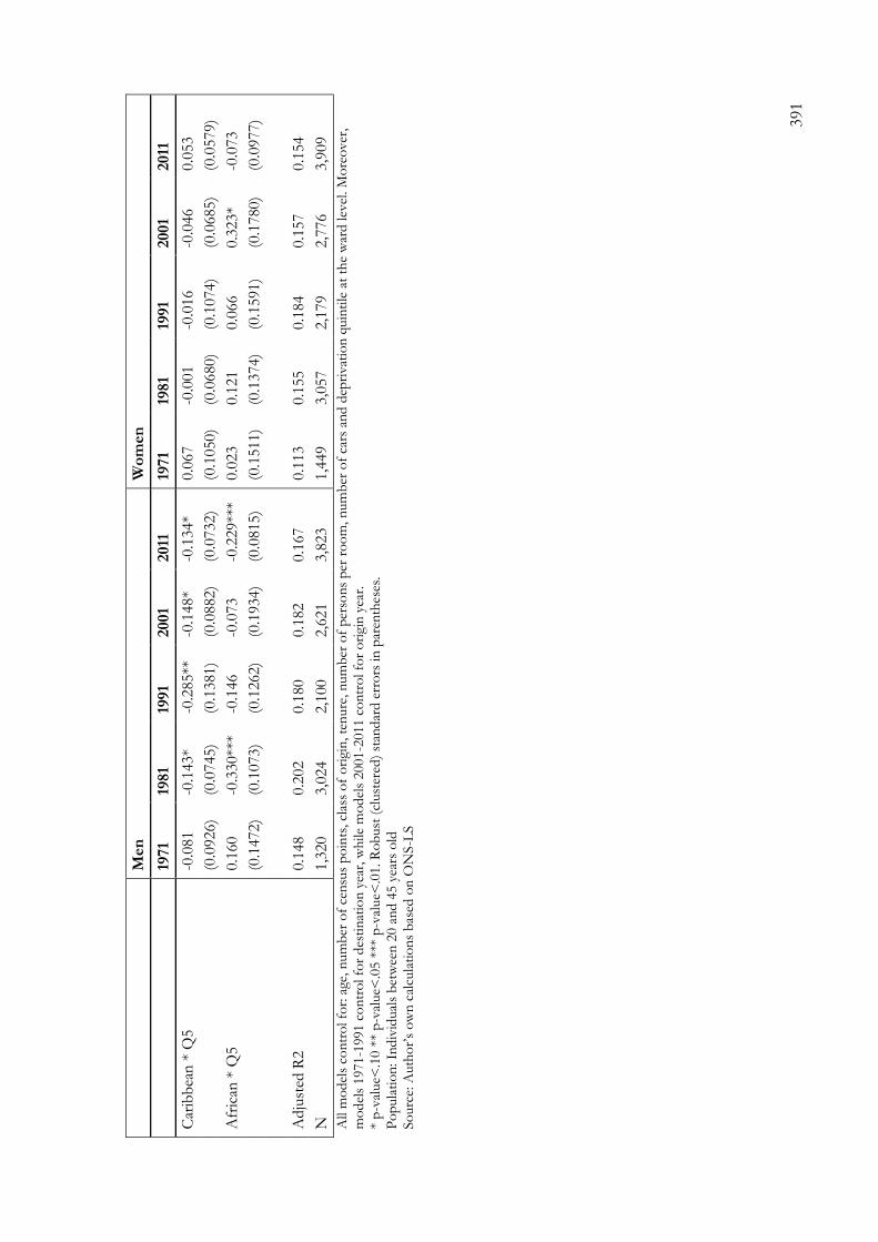
391

M

en

W

om

en

19

71

1981

1991

2001

2011

19

71

1981

1991

2001

2011

Car

ibb

ean

* Q

5

-0.0

81

-0.1

43*

-0.2

85**

-0

.148*

-0.1

34*

0.0

67

-0.0

01

-0.0

16

-0.0

46

0.0

53

(0

.0926)

(0.0

745)

(0.1

381)

(0.0

882)

(0.0

732)

(0.1

050)

(0.0

680)

(0.1

074)

(0.0

685)

(0.0

579)

Afr

ican

* Q

5

0.1

60

-0.3

30**

* -0

.146

-0.0

73

-0.2

29**

* 0.0

23

0.1

21

0.0

66

0.3

23*

-0.0

73

(0

.1472)

(0.1

073)

(0.1

262)

(0.1

934)

(0.0

815)

(0.1

511)

(0.1

374)

(0.1

591)

(0.1

780)

(0.0

977)

Adju

sted

R2

0.1

48

0.2

02

0.1

80

0.1

82

0.1

67

0.1

13

0.1

55

0.1

84

0.1

57

0.1

54

N

1,3

20

3,0

24

2,1

00

2,6

21

3,8

23

1,4

49

3,0

57

2,1

79

2,7

76

3,9

09

All

mo

del

s co

ntr

ol fo

r: a

ge, n

um

ber

of

cen

sus

po

ints

, cl

ass

of

ori

gin

, te

nure

, n

um

ber

of

per

son

s p

er r

oo

m, n

um

ber

of

cars

an

d d

epri

vat

ion

quin

tile

at

the

war

d lev

el. M

ore

over

, m

od

els

1971-1

991 c

on

tro

l fo

r d

esti

nat

ion

yea

r, w

hile

mo

del

s 2001-2

011 c

on

tro

l fo

r o

rigi

n y

ear.

*

p-v

alue<

.10 *

* p

-val

ue<

.05 *

** p

-val

ue<

.01. R

ob

ust

(cl

ust

ered

) st

and

ard

err

ors

in

par

enth

eses

. P

op

ula

tio

n: In

div

idual

s b

etw

een

20 a

nd

45 y

ears

old

So

urc

e: A

uth

or’

s o

wn

cal

cula

tio

ns

bas

ed o

n O

NS

-LS

392

Tab

le ‎1

0.7

: P

rob

abili

ty o

f b

ein

g in

a n

eigh

bo

urh

oo

d w

ith

a lo

w s

har

e o

f n

on

-wh

ites

(quin

tile

s 1-2

) fo

r in

div

idual

s ra

ised

in

dif

fere

nt

ori

gin

yea

rs (

1971-

1991)

and in

div

idual

s m

easu

red in

dif

fere

nt

des

tin

atio

n y

ears

(2001-2

011).

Tes

t fo

r C

hap

ter

6 (

men

an

d w

om

en p

oo

led).

19

71

1981

1991

NW

qu

inti

le (

ref.

Q1:

lo

wes

t sh

are

)

Q2

-0.0

55**

* -0

.063**

* -0

.110**

*

(0

.0029)

(0.0

032)

(0.0

091)

Q3

-0.1

48**

* -0

.176**

* -0

.289**

*

(0

.0070)

(0.0

083)

(0.0

207)

Q4

-0.1

71**

* -0

.219**

* -0

.390**

*

(0

.0102)

(0.0

119)

(0.0

266)

Q5

-0.1

89**

* -0

.298**

* -0

.447**

*

(0

.0143)

(0.0

161)

(0.0

299)

Eth

nic

gro

up

(re

f. w

hit

e B

riti

sh)

In

dia

n

-0.2

23**

* -0

.211**

* -0

.233**

*

(0

.0221)

(0.0

169)

(0.0

281)

Pak

ista

ni

-0.3

04**

* -0

.374**

* -0

.354**

*

(0

.0341)

(0.0

224)

(0.0

344)

Ban

glad

esh

i -0

.109

-0.4

06**

* -0

.283**

*

(0

.1299)

(0.0

386)

(0.0

442)

Car

ibb

ean

-0

.344**

* -0

.321**

* -0

.384**

*

(0

.0199)

(0.0

232)

(0.0

495)

Afr

ican

-0

.335**

* -0

.278**

* -0

.349**

*

(0

.0582)

(0.0

595)

(0.1

153)

Ed

ucati

on

(re

f. L

eve

l 1

or

less

)

Lev

el 2

+3

0.0

07**

* 0.0

07**

* 0.0

05

(0

.0018)

(0.0

020)

(0.0

040)

Lev

el 4

+

-0.0

09**

* -0

.018**

* -0

.033**

*

(0

.0026)

(0.0

029)

(0.0

061)

So

cia

l cla

ss (

ref.

Man

ual)

Pet

it B

ourg

eois

ie

0.0

06**

0.0

08**

0.0

12

(0

.0028)

(0.0

037)

(0.0

097)

Inte

rmed

iate

-0

.000

0.0

00

0.0

04

393

19

71

1981

1991

(0

.0026)

(0.0

028)

(0.0

049)

Ser

vic

e 0.0

03

-0.0

00

0.0

01

(0

.0021)

(0.0

023)

(0.0

045)

Part

ners

hip

(re

f. n

on

-wh

ite)

N

o p

artn

er

0.0

83**

* 0.0

57**

* -0

.038

(0

.0149)

(0.0

151)

(0.0

287)

Wh

ite

Bri

tish

0.1

23**

* 0.0

93**

* -0

.012

(0

.0148)

(0.0

151)

(0.0

287)

Oth

er

0.0

73**

* 0.0

38**

-0

.057

(0

.0166)

(0.0

178)

(0.0

385)

Adju

sted

R-s

quar

ed

0.1

25

0.1

92

0.2

52

Ob

serv

atio

ns

78,1

48

64,6

64

18,3

56

All

mo

del

s co

ntr

ol fo

r: a

ge, n

um

ber

of

cen

sus

po

ints

, cl

ass

of

ori

gin

, te

nure

, n

um

ber

of

per

son

s p

er r

oo

m, n

um

ber

of

cars

an

d d

epri

vat

ion

quin

tile

at

the

war

d lev

el. M

ore

over

, m

od

els

1971-1

991 c

on

tro

l fo

r d

esti

nat

ion

yea

r, w

hile

mo

del

s 2001-2

011 c

on

tro

l fo

r o

rigi

n y

ear.

*

p-v

alue<

.10 *

* p

-val

ue<

.05 *

** p

-val

ue<

.01. R

ob

ust

sta

nd

ard

err

ors

in

par

enth

eses

. P

op

ula

tio

n: In

div

idual

s b

etw

een

20 a

nd

55 y

ears

old

So

urc

e: A

uth

or’

s o

wn

cal

cula

tio

ns

bas

ed o

n O

NS

-LS

395

11 BIBLIOGRAPHY

Alba, Richard D., and John R. Logan. 1993. "Minority proximity to whites in suburbs: an

individual-level analysis of segregation." American Journal of Sociology 98(6):1388-427.

Alba, Richard D., John R. Logan, Brian J. Stults, Gilbert Marzan, and Wenquan Zhang. 1999.

"Immigrant groups in the suburbs: a reexamination of suburbanization and spatial

assimilation." American Sociological Review 64(3):446-60.

Alba, Richard, and Victor Nee. 1997. "Rethinking assimilation theory for a new era of

immigration." International Migration Review 31(4):826-74.

—. 2003. Remaking the American mainstream. Assimilation and contemporary immigration Cambridge:

Harvard University Press.

Alexander, Claire. 2002. "Beyond black: re-thinking the colour/culture divide." Ethnic and Racial

Studies 25(4):552-71.

Algan, Y., C. Dustmann, A. Glitz, and A. Manning. 2010. "The economic situation of first and

second-generation immigrants in France, Germany and the United Kingdom." Economic

Journal 120(542):F4-F30.

Allasino, E., E. Reyneri, A. Venturini, and G. Zincone. 2004. "Labour market discrimination

against migrant workers in Italy." in International Migration Papers. Geneva: ILO.

Apparicio, Philippe, Éric Fournier, and Denis Apparicio. 2012. "Geo-Segregation Analyzer: a

multi-platform application (version 1.0)." Montreal: Spatial Analysis and Regional

Economics Laboratory (SAREL), INRS Urbanisation Culture Société.

Bagguley, Paul. 2014. "Interculturalism: the new era of cohesion and diversity (book review)."

Ethnic and Racial Studies:1-2.

Becares, L., M. Stafford, J. Laurence, and J. Nazroo. 2011. "Composition, concentration and

deprivation: exploring their association with social cohesion among different ethnic groups

in the UK." Urban Studies 48(13):2771-87.

Bergström, Lina, and Maarten van Ham. 2012. "Understanding neighbourhood effects: selection

bias and residential mobility." Pp. 79-99 in Neighbourhood Effects Research: New Perspectives,

edited by Maarten van Ham, David Manley, Nick Bailey, Ludi Simpson, and Duncan

Maclennan: Springer Netherlands.

Bernardi, Fabrizio. 2012. "Social origins and inequality in educational returns in the labour market

in Spain." in EUI Working Papers: European University Institute.

396

Blau, Peter, and Otis Dudley Duncan. 1967. The American occupational structure. New York: Wiley.

Bolt, Gideon, A. Şule Özüekren, and Deborah Phillips. 2010. "Linking integration and residential

segregation." Journal of Ethnic and Migration Studies 36(2):169-86.

Bolt, Gideon, and Ronald Van Kempen. 2010. "Ethnic segregation and residential mobility:

relocations of minority ethnic groups in the Netherlands." Journal of Ethnic and Migration

Studies 36(2):333-54.

Boudon, Raymond. 1973. L' inégalité des chances: la mobilité sociale dans les sociétés industrielles. Paris:

Armand Collin.

Bowes, Alison, N. S. Dar, and D. F. Sim. 2002. "Differentiation in housing careers: the case of

Pakistanis in the UK." Housing Studies 17(3):381-99.

Bowes, Alison, Naira Dar, and Duncan Sim. 1997. "Tenure preference and housing strategy: an

exploration of Pakistani experiences." Housing Studies 12(1):63-84.

Boyle, Paul, Paul Norman, and Philip Rees. 2004. "Changing places. Do changes in the relative

deprivation of areas influence limiting long-term illness and mortality among non-migrant

people living in non-deprived households?" Social Science & Medicine 58(12):2459-71.

Brah, Avtar. 1993. "'Race' and 'culture' in the gendering of labour markets: South Asian young

Muslim women and the labour market." Journal of Ethnic and Migration Studies 19(3):441-58.

Breen, Richard (Ed.). 2004. Social mobility in Europe. Oxford: Oxford University Press.

Breen, Richard, and Jan O. Jonsson. 2005. "Inequality of opportunity in comparative perspective:

recent research on educational attainment and social mobility." Annual Review of Sociology

31(1):223-43.

Brinbaum, Yael, and Hector Cebolla-Boado. 2007. "The school careers of ethnic minority youth

in France: Success or disillusion?" Ethnicities 7(3):445-74.

Bukodi, Erzsebet, and John Goldthorpe. 2011. "Social class returns to higher education: chances

of access to the professional and managerial salariat for men in three British birth cohorts."

Longitudinal and Life Course Studies 2(2):185-201.

Burgess, Ernest (Ed.). 1925. The urban community. Chicago: The University of Chicago Press.

Cantle, Ted. 2012. Interculturalism: the new era of cohesion and diversity. Hampshire: Palgrave

Macmillan.

Carling, Alan. 2008. "The curious case of the mis-claimed myth claims: ethnic segregation,

polarisation and the future of Bradford." Urban Studies 45(3):553-89.

Carstairs, Vera, and Russell Morris. 1991. "Deprivation and Health in Scotland." Aberdeen.

Catney, Gemma. 2013. "Has neighbourhood ethnic segregation decreased?" in Dynamics of

Diversity: evidence from the 2011 Census, edited by ESRC-CoDE. Manchester.

397

Cheung, Sin Yi, and Anthony Heath. 2007a. "The comparative study of ethnic minority

disadvantage." in Unequal chances. Ethnic minorities in Western labour markets, edited by Sin Yi

Cheung and Anthony Heath. New York: Oxford University Press.

—. 2007b. "Nice work if you can get it: ethnic penalties in Great Britain." Pp. 507-50 in Unequal

chances. Ethnic minorities in Western labour markets, edited by Anthony Heath and Sin Yi Cheung.

New York: Oxford University Press.

Clark, K., and S. Drinkwater. 2002. "Enclaves, neighbourhood effects and employment

outcomes: ethnic minorities in England and Wales." Journal of Population Economics 15(1):5-29.

Clark, Ken, and Stephen Drinkwater. 2010. "Recent trends in minority ethnic entrepreneurship in

Britain." International Small Business Journal 28(2):136-46.

Crul, Maurice, and Hans Vermeulen. 2003. "The second generation in Europe." International

Migration Review 37(4):965-86.

Cutler, David M., Edward L. Glaeser, and Jacob L. Vigdor. 2008. "When are ghettos bad?

Lessons from immigrant segregation in the United States." Journal of Urban Economics

63(3):759-74.

Dale, Angela, Nusrat Shaheen, Virinder Kalra, and Edward Fieldhouse. 2002. "Routes into

education and employment for young Pakistani and Bangladeshi women in the UK." Ethnic

and Racial Studies 25(6):942-68.

de Palo, Domenico, Riccardo Faini, and Alessandra Venturini. 2006. "The social assimilation of

immigrants." in IZA Discussion Paper.

Dietz, Robert D. 2002. "The estimation of neighborhood effects in the social sciences: An

interdisciplinary approach." Social Science Research 31(4):539-75.

DiPrete, Thomas A., and Gregory M. Eirich. 2006. "Cumulative advantage as a mechanism for

inequality: a review of theoretical and empirical developments." Annual Review of Sociology

32(1):271-97.

Dobbs, Joy, Hazel Green, and Linda Zealey (Eds.). 2006. Focus on ethnicity and religion. Hampshire:

Palgrave Macmillan.

Duncan, Otis Dudley, and Beverly Duncan. 1955. "A methodological analysis of segregation

indexes." American Sociological Review 20(2):210-17.

—. 1955a. "Residential distribution and occupational stratification." American Journal of Sociology

60(5):493-503.

Dustmann, Christian. 2008. "Return migration, investment in children, and intergenerational

mobility: comparing sons of foreign- and native-born fathers." Journal of Human Resources

43(2):299-324.

398

Dustmann, Christian, Tommaso Frattini, and Gianandrea Lanzara. 2012. "Educational

achievement of second-generation immigrants: an international comparison." Economic Policy

27(69):143-85.

Erikson, Robert , and John Goldthorpe. 1992. The constant flux: a study of class mobility in industrial

societies. Oxford: Clarendon Press.

Evans, William N., Wallace E. Oates, and Robert M. Schwab. 1992. "Measuring peer group

effects: a study of teenage behavior." Journal of Political Economy 100(5):966-91.

Farley, Reynolds, and Richard Alba. 2002. "The new second generation in the United States."

International Migration Review 36(3):669-701.

Feng, Xiaoqi, Robin Flowerdew, and Zhiqiang Feng. 2013. "Does neighbourhood influence

ethnic inequalities in economic activity? Findings from the ONS Longitudinal Study." Journal

of Economic Geography.

Finney, Nissa. 2011. "Understanding ethnic differences in the migration of young adults within

Britain from a lifecourse perspective." Transactions of the Institute of British Geographers

36(3):455-70.

Finney, Nissa, and Ludi Simpson. 2008. "Internal migration and ethnic groups: evidence for

Britain from the 2001 Census." Population, Space and Place 14(2):63-83.

—. 2009a. "Population dynamics: the roles of natural change and migration in producing the

ethnic mosaic." Journal of Ethnic and Migration Studies 35(9):1479-96.

—. 2009b. 'Sleepwalking to segregation'?: Challenging myths about race and migration. Bristol: The Policy

Press.

Galster, George. 2003. "Investigating behavioural impacts of poor neighbourhoods: towards new

data and analytic strategies." Housing Studies 18(6):893-914.

Galster, George, Roger Andersson, Sako Musterd, and Timo M. Kauppinen. 2007a. "Does

neighborhood income mix affect earnings of adults? New evidence from Sweden." Journal of

Urban Economics 63(3):858-70.

Galster, George C. . 2010. "The mechanism(s) of neighborhood effects theory, evidence, and

policy implications." in ESRC Seminar: “Neighbourhood Effects: Theory & Evidence”. St. Andrews

University, Scotland, UK.

Galster, George, and Lina Hedman. 2013. "Measuring neighbourhood effects non-

experimentally: how much do alternative methods matter?" Housing Studies 28(3):473-98.

Galster, George, Dave E. Marcotte, Marv Mandell, Hal Wolman, and Nancy Augustine. 2007b.

"The Influence of neighborhood poverty during childhood on fertility, education, and

earnings outcomes." Housing Studies 22(5):723-51.

399

Goering, John M. 1978. "Neighborhood tipping and racial transition: a review of social science

evidence." Journal of the American Institute of Planners 44(1):68-78.

Goldthorpe, John. 2000. On sociology. Numbers, narratives, and the integration of research and theory.

Oxford: Oxford University Press.

Goldthorpe, John, and K. Hope. 1974. The social grading of occupations. Oxford: Clarendon Press.

Gordon, Milton M. 1964. Assimilation in American life: the role of race, religion, and national origins. New

York: Oxford University Press

Hattersley, Lin, and Rosemary Creeser. 1995. "‘Longitudinal Study 1971-1991 History,

organisation and quality of data." in Series LS.

Heath, Anthony, and Sin Yi Cheung. 2006. "Ethnic penalties in the labour market: employers and

discrimination." in Department for Work and Pensions. Research Report No 341. London.

— (Eds.). 2007. Unequal chances. Ethnic minorities in Western labour markets. New York: Oxford

University Press.

Heath, Anthony, and Neli Demireva. 2013. "Has multiculturalism failed in Britain?" Ethnic and

Racial Studies 37(1):161-80.

Heath, Anthony F., Catherine Rothon, and Elina Kilpi. 2008. "The second generation in Western

Europe: education, unemployment, and occupational attainment." Annual Review of Sociology

34(1):211-35.

Heath, Anthony, Stephen Fisher, Gemma Rosenblatt, David Sanders, and Maria Sobolewska.

2013. The political integration of ethnic minorities in Britain. Oxford: Oxford University Press.

Heath, Anthony, and Yaojun Li. 2010. "Struggling onto the ladder, climbing the rungs:

employment and class position of minority ethnic groups in Britain." Pp. 83-97 in Spatial and

social disparities. Understanding population trends and processes, edited by John Stillwell, Paul

Norman, Claudia Thomas, and Claudia Surridge. London: Springer.

Heath, Anthony, and Dorren McMahon. 2005. "Social mobility of ethnic minorities." Pp. 393-

413 in Ethnicity, social mobility and public policy, edited by Glenn C. Loury, Tariq Modood, and

Steven M. Teles. Cambridge: Cambridge University Press.

Heath, Anthony, and John Ridge. 1983. "Social mobility of ethnic minorities." Journal of Biosocial

Science 15(Supplement 8):169-84.

Heath, Anthony, and Soojin Yu. 2005. "Explaining ethnic minority disadvantage." in

Understanding Social Change, edited by Anthony Heath, John Ermisch, and Duncan Gallie.

Oxford: Oxford University Press.

Hessari, Ruth, and Dave Hill. 1990. Practical ideas for multicultural learning and teaching in the primary

classroom. London: Routledge.

400

Hout, Michael, and Thomas A. DiPrete. 2006. "What we have learned: RC28's contributions to

knowledge about social stratification." Research in Social Stratification and Mobility 24(1):1-20.

Iceland, John, Daniel H. Weinberg, and Erika Steinmetz. 2002. "Racial and ethnic residential

segregation in the United States: 1980-2000." U.S. Census Bureau, Series CENSR-3.

Washington, DC.

Jivraj, Stephen, and Omar Khan. 2013. "Ethnicity and deprivation in England: how likely are

ethnic minorities to live in deprived neighbourhoods?" in Dynamics of Diversity: evidence from the

2011 Census, edited by ESRC-CoDE: University of Manchester.

Johnston, Ron, James Forrest, and Michael Poulsen. 2002a. "Are there ethnic enclaves/ghettos in

English cities?" Urban Studies 39(4):591-618.

—. 2002b. "The ethnic geography of EthniCities: The `American model' and residential

concentration in London." Ethnicities 2(2):209-35.

Johnston, Ron, Michael Poulsen, and James Forrest. 2007. "The geography of ethnic residential

segregation: a comparative study of five countries." Annals of the Association of American

Geographers 97(4):713-38.

—. 2010. "Moving on from indices, refocusing on mix: on measuring and understanding ethnic

patterns of residential segregation." Journal of Ethnic and Migration Studies 36(4):697-706.

Jones, Colin , Mike Coombes, and Cecilia Wong. 2010. "Geography of housing market areas:

final report." edited by Department for Communities and Local Government.

Kalter, Frank, Nadia Granato, and Cornelia Kristen. 2007. "Disentangling recent trends of the

second generation´s structural assimilation in Germany." in From origin to destination. Trends

and mechanisms in social stratification research, edited by Stefani Scherer, Reinhard Pollak, Gunnar

Otte, and Markus Gangl. Chicago: The University of Chicago Press.

Kicinger, Anna. 2013. "Migration policy from the European perspective: a primer for forecasters

" in International migration and the future of populations and labour force resources in Europe, edited by

Marek Kupiszewski. Dordrecht: Springer.

Kim, Dae Young, and Veena S. Kulkarni. 2009. "The role of father's occupation on

intergenerational educational and occupational mobility: the case of second-generation

Chinese Americans in New York." Sociological Forum 24(1):104-34.

Knies, Gundi, Alita Nandi, and Lucinda Platt. 2013. "Life satisfaction, ethnicity and

neighbourhoods: is there an effect of neighbourhood ethnic composition on life

satisfaction?" in 4th Norface Migration Network Conference on "Migration: Global Development, New

Frontiers". London.

401

Kogan, Irena. 2006. "Labor markets and economic incorporation among recent immigrants in

Europe " Social Forces 85(2):697-721.

Kristen, Cornelia, and Nadia Granato. 2007. "The educational attainment of the second

generation in Germany: Social origins and ethnic inequality." Ethnicities 7(3):343-66.

Kuha, Jouni, and John H. Goldthorpe. 2010. "Path analysis for discrete variables: the role of

education in social mobility." Journal of the Royal Statistical Society: Series A (Statistics in Society)

173(2):351-69.

Lersch, Philipp M. 2013. "Place stratification or spatial assimilation? Neighbourhood quality

changes after residential mobility for migrants in Germany." Urban Studies 50(5):1011-29.

Li, Peter. 2004. "Social capital and economic outcomes for immigrants and ethnic minorities."

Journal of International Migration and Integration 5(2):171-90.

Lin, Nan 2001. Social capital: a theory of social structure and action. Cambridge:

Cambridge University Press.

Logan, John R. , and Brian Stults. 2011. "The persistence of segregation in the metropolis: new

findings from the 2010 Census." Census Brief prepared for Project US2010. Available at:

http://www.s4.brown.edu/us2010.

Logan, JohnR, BrianJ Stults, and Reynolds Farley. 2004. "Segregation of minorities in the

metropolis: two decades of change." Demography 41(1):1-22.

Ludwig, Jens , Jeffrey B. Liebman, Jeffrey R. Kling, Greg J. Duncan, Lawrence F. Katz,

Ronald C. Kessler, and Lisa Sanbonmatsu. 2008. "What can we learn about neighborhood

effects from the moving to opportunity experiment?" American Journal of Sociology 114(1):144-

88.

Luk, W. K. E. 2009. "Chinese ethnic settlements in Britain: spatial meanings of an orderly

distribution, 1981-2001." Journal of Ethnic and Migration Studies 35(4):575-99.

Massey, D. S. 1985. "Ethnic residential segregation: a theoretical synthesis and empirical review."

Sociology and social research 69(3):315-50.

—. 2012. "Reflections on the dimensions of segregation." Social Forces 91(1):39-43.

Massey, Douglas S., and Nancy A. Denton. 1985. "Spatial assimilation as a socioeconomic

outcome." American Sociological Review 50(1):94-106.

—. 1987. "Trends in the residential segregation of Blacks, Hispanics, and Asians: 1970-1980."

American Sociological Review 52(6):802-25.

—. 1988. "The dimensions of residential segregation." Social Forces 67(2):281-315.

—. 1989. "Hypersegregation in U.S. metropolitan areas: black and hispanic segregation along five

dimensions." Demography 26(3):373-91.

http://www.s4.brown.edu/us2010

402

McLoone, Philip. 2004. "Carstairs scores for Scottish postcode sectors from the 2001 Census." in

MRC Social & Public Health Sciences Unit, University of Glasgow.

Meer, Nasar, and Tariq Modood. 2013. "The 'civic re-balancing' of British multiculturalism, and

beyond..." in Challenging multiculturalism: European models of diversity, edited by Raymond Taras.

Edinburgh: Edinburgh University Press.

Modood, Tariq, and Nasar Meer. 2012. "Interculturalism, multiculturalism or both?" Political

Insight 3(1):30-33.

Musterd, Sako. 2005. "Social and ethnic segregation in Europe: levels, causes, and effects." Journal

of Urban Affairs 27(3):331-48.

Musterd, Sako, and Roger Andersson. 2006. "Employment, social mobility and neighbourhood

effects: the case of Sweden." International Journal of Urban and Regional Research 30(1):120-40.

Musterd, Sako, Wim Ostendorf, and Sjoerd De Vos. 2003. "Neighbourhood effects and social

mobility: a longitudinal analysis." Housing Studies 18(6):877-92.

Musterd, Sako, and Ronald Van Kempen. 2009. "Segregation and housing of minority ethnic

groups in Western European cities." Tijdschrift voor economische en sociale geografie 100(4):559-66.

Norman, Paul. 2010. "Identifying change over time in small area socio-economic deprivation."

Applied Spatial Analysis and Policy 3(2-3):107-38.

Norman, Paul, and Paul Boyle. 2014. "Are health inequalities between differently deprived areas

evident at different ages? A longitudinal study of census records in England and Wales,

1991–2001." Health & Place 26(0):88-93.

Norman, Paul, Paul Boyle, and Philip Rees. 2005. "Selective migration, health and deprivation: a

longitudinal analysis." Social Science & Medicine 60(12):2755-71.

Norman, Paul, and Mylène Riva. 2012. "Population health across space and time: the

geographical harmonisation of the Office for National Statistics Longitudinal Study for

England and Wales." Population, Space and Place 18(5):483-502.

Office for National Statistics. "A beginner's guide to UK geography."

—. 2010. "Standard Occupational Classification 2010. The National Statistics Socio-economic

Classification: (Rebased on the SOC2010) User Manual." Palgrave Macmillan.

Openshaw, S. 1984. The modifiable area unit problem. Norwick: Geo Books.

Özüekren, A. Sule, and Ronald van Kempen. 2002. "Housing careers of minority ethnic groups:

experiences, explanations and prospects." Housing Studies 17(3):365-79.

Panayi, Panikos. 2010. An immigration history of Britain: multicultural racism since 1800. Harlow:

Pearson Education Limited.

403

Pantazis, Christina, and Simon Pemberton. 2009. "From the ‘old’ to the ‘new’ suspect

community: examining the impacts of recent UK counter-terrorist legislation." British Journal

of Criminology 49(5):646-66.

Park, R. , and E. Burgess. 1969. Introduction to the science of sociology. Chicago: University of Chicago

Press.

Park, Robert. 1925. "The urban community as a spacial pattern and a moral order." in The urban

community, edited by Ernest Burgess. Chicago: The University of Chicago Press.

Peach, Ceri. 1998. "South Asian and Caribbean ethnic minority housing choice in Britain." Urban

Studies 35(10):1657-80.

—. 2005. "Social integration and social mobility: spatial segregation and intermarriage of the

Caribbean population in Britain." Pp. 178-203 in Ethnicity, social mobility and public policy, edited

by Glenn C. Loury, Tariq Modood, and Steven M. Teles. Cambridge: Cambridge University

Press.

Phillips, Deborah. 1998. "Black minority ethnic concentration, segregation and dispersal in

Britain." Urban Studies 35(10):1681-702.

—. 2006. "Parallel lives? Challenging discourses of British Muslim self-segregation." Environment

and Planning D: Society and Space 24(1):25-40.

Platt, Lucinda. 2005a. "The intergenerational social mobility of minority ethnic groups." Sociology

39(3):445-61.

—. 2005b. Migration and social mobility: the life chances of Britain's minority ethnic communities. Bristol:

Policy Press

—. 2007. "Making education count: the effects of ethnicity and qualifications on

intergenerational social class mobility." The Sociological Review 55:485-508.

Platt, Lucinda 2005. "New destinations? Assessing the post-migration social mobility of minority

ethnic groups in England and Wales." Social Policy & Administration 39(6):697-721.

Platt, Lucinda, Gundi Knies, and Alita Nandi. 2014. "Life satisfaction, ethnicity and

neighbourhoods: is there an effect of neighbourhood ethnic composition on life

satisfaction?" in CReAM Discussion Paper Series. London: Department of Economics,

University College London.

Platt, Lucinda, Simonetta Longhi, and Cheti Nicoletti. 2012. "Occupation and pay across the

generations: the labour market experience of four ethno-religious groups in Britain." in Social

stratitication: trends and processes, edited by Paul Lambert, Roxanne Connelly, Robert M.

Blackburn, and Vernon Gayle. Furnham: Ashgate Publishing Limited.

404

Portes, Alejandro. 1998. "Social capital: its origins and applications in modern sociology." Annual

Review of Sociology 24:1-24.

Portes, Alejandro, and Leif Jensen. 1989. "The enclave and the entrants: patterns of ethnic

enterprise in Miami before and after Mariel." American Sociological Review 54(6):929-49.

—. 1992. "Disproving the enclave hypothesis: reply." American Sociological Review 57(3):418-20.

Portes, Alejandro, and Min Zhou. 1993. "The new second generation: segmented assimilation

and its variants." The ANNALS of the American Academy of Political and Social Science 530(1):74-

96.

Poulsen, Michael, and Ron Johnston. 2006. "Ethnic residential segregation in England: getting

the right message across." Environment and Planning A.

Rattansi, Ali. 2011. Multiculturalism: a very short introduction. Oxford: Oxford University Press.

Rees, Phil, and Faisal Butt. 2004. "Ethnic change and diversity in England, 1981–2001." Area

36(2):174-86.

Robinson, Vaughan, and Rina Valeny. 2005. "Ethnic minorities, employment, self-employment,

and social mobility in poswar Britain." in Ethnicity, social moblity and public policy, edited by

Glenn C. Loury, Tariq Modood, and Steven M. Teles. Cambridge: Cambridge University

Press.

Röder, Antje, and Peter Mühlau. 2014. "Are they acculturating? Europe's immigrants and gender

egalitarianism." Social Forces.

Rodríguez Vignoli, Jorge. 2001. "Segregación residencial socioeconómica: ¿qué es?, ¿cómo se

mide?, ¿qué está pasando?, ¿importa?" in CEPAL. Serie Población y Desarrollo No. 16.

Safi, Mirna. 2009. "La dimension spatiale de l'intégration : évolution de la ségrégation des

populations immigrées en France entre 1968 et 1999." Revue française de sociologie 50(3):521-52.

Sanders, Jimy M., and Victor Nee. 1987. "Limits of ethnic solidarity in the enclave economy."

American Sociological Review 52(6):745-73.

—. 1992. "Problems in resolving the enclave economy debate." American Sociological Review

57(3):415-18.

Schaake, Karina, Jack Burgers, and Clara H. Mulder. 2013. "Ethnicity, education and income, and

residential mobility between neighbourhoods." Journal of Ethnic and Migration Studies

40(4):512-27.

Schaake, Karina, Jack Burgers, and ClaraH Mulder. 2010. "Ethnicity at the individual and

neighborhood level as an explanation for moving out of the neighborhood." Population

Research and Policy Review 29(4):593-608.

405

Silberman, Roxane, Richard Alba, and Irene Fournier. 2007. "Segmented assimilation in France?

Discrimination in the labour market against the second generation." Ethnic and Racial Studies

30(1):1-27.

Simpson, Ludi. 2007. "Ghettos of the mind: the empirical behaviour of indices of segregation

and diversity." Journal of the Royal Statistical Society: Series A (Statistics in Society) 170(2):405-24.

—. 2012. "More segregation or more mixing?" in Dynamics of Diversity: evidence from the 2011 Census,

edited by ESRC-CoDE: Centre on Dynamics of Ethnicity (CoDE).

—. 2013. "What makes ethnic group populations grow? Age structures and immigration." in

Dynamics of diversity: evidence from the 2011 Census, edited by ESRC-CoDE: University of

Manchester.

Simpson, Ludi, and Nissa Finney. 2009. "Spatial patterns of internal migration: evidence for

ethnic groups in Britain." Population, Space and Place 15(1):37-56.

South, Scott J., and Kyle D. Crowder. 1997. "Escaping distressed neighborhoods: individual,

community, and metropolitan influences." American Journal of Sociology 102(4):1040-84.

Sturgis, Patrick, Ian Brunton-Smith, Jouni Kuha, and Jonathan Jackson. 2013. "Ethnic diversity,

segregation and the social cohesion of neighbourhoods in London." Ethnic and Racial

Studies:1-21.

Sturgis, Patrick, Ian Brunton-Smith, Sanna Read, and Nick Allum. 2011. "Does ethnic diversity

erode trust? Putnam’s ‘hunkering down’ thesis reconsidered." British Journal of Political Science

41(01):57-82.

Sunak, Rishi, and Saratha Rajeswaran. 2014. "A portrait of modern Britain." London: Policy

Exchange.

UK Home Office. 2013. "Immigration Act 2014 - Immigration Bill: overview factsheet."

Urban, Susanne. 2009. "Is the neighbourhood effect an economic or an immigrant issue? a study

of the importance of the childhood neighbourhood for future integration into the labour

market." Urban Studies 46(3):583-603.

Uslaner, Eric. 2012. Segregation and mistrust: diversity, isolation and social cohesion. New York:

Cambridge University Press.

Van De Werfhorst, Herman G., and Frank Van Tubergen. 2007. "Ethnicity, schooling, and merit

in the Netherlands." Ethnicities 7(3):416-44.

Van Kempen, Ronald, and A. Şule Özüekren. 1998. "Ethnic segregation in cities: new forms and

explanations in a dynamic world." Urban Studies 35(10):1631-56.

van Oers, Ricky. 2014. Deserving citizenship: citizenship tests in Germany, the Netherlands and the United

Kingdom. Leiden: Martinus Nijhoff Publishers.

406

Van Tubergen, Frank, Ineke Maas, and Henk Flap. 2004. "The economic incorporation of

immigrants in 18 Western societies: origin, destination, and community effects." American

Sociological Review 69(5):704-27.

Vermeulen, Hans, and Joel Perlmann (Eds.). 2000. Immigrants, schooling and social mobility: does culture

make a difference? Basingstoke: Macmillan.

Wacquant, LoÏC J. D. 1993. "Urban outcasts: stigma and division in the Black American ghetto

and the French urban periphery*." International Journal of Urban and Regional Research 17(3):366-

83.

Wood, Martin, Jon Hales, Susan Purdon, Tanja Sejersen, and Oliver Hayllar. 2009. "A test for

racial discrimination in recruitment practice in British cities." in Department for Work and

Pensions Research Report.

Wray, Helena. 2011. Regulating marriage migration into the UK. Farnham: Ashgate Publishing Limited.

Wrench, J., and T. Modood. 2000. "The effectiveness of employment equality policies in relation

to immigrants and ethnic minorities in the UK." in Report commissioned by the International

Labour Office. International Migration Papers 38. Geneva.

Zhou, Min. 1997. "Segmented assimilation: issues, controversies, and recent research on the new

second generation." International Migration Review 31(4):975-1008.

Zuccotti, Carolina. 2014. "Do parents matter? Revisiting ethnic penalties in occupation among

second generation ethnic minorities in England and Wales." Sociology (online first).

Shaping Ethnic Inequalities - CADMUS, EUI Research ...

Documents

Transcript of Shaping Ethnic Inequalities - CADMUS, EUI Research ...