Growth, Employment and Inequalities in Africa Croissance ...
120
Volume 01 Congress of African Economists Growth, Employment and Inequalities in Africa Croissance, Emploi et Inégalités en Afrique Proceedings of the Fifth Congress of African Economists Les Actes du Cinquième Congrès des Economistes Africains Malabo, Equatorial Guinea 01 st - 04 th November 2017
-
Upload
khangminh22 -
Category
Documents
-
view
1 -
download
0
Transcript of Growth, Employment and Inequalities in Africa Croissance ...

Volume 01Congress of African Economists
Growth, Employment and Inequalities in AfricaCroissance, Emploi et Inégalités en Afrique
Proceedings of the Fifth Congress of African EconomistsLes Actes du Cinquième Congrès des Economistes Africains
Malabo, Equatorial Guinea01st- 04th November 2017

Growth, Employment and Inequalities in AfricaCroissance, Emploi et Inégalités en Afrique 3
Proceedings of the Fifth Congress of African EconomistsLes Actes du Cinquième Congrès des Economistes Africains
Malabo, Equatorial Guinea
01st- 04th November 2017 Volume 1
Growth, Employment and Inequalities in AfricaCroissance, Emploi et Inégalités en Afrique
Congress ofAfricanEconomists

4Proceedings of the Fifth Congress of African EconomistsLes Actes du Cinquième Congrès des Economistes Africains
Volume 1Growth, Employment and Inequalities in Africa
Croissance, Emploi et Inégalités en Afrique 5
Session 1: The Sources of Growth ............................................................................................. 7
A Reexamination of the Financial Development- Growth Nexus in Presence of Structural Breaks: The African Countries Experience .................................................................................. ...................8
La croissance économique en Afrique: les institutions importent-elles? ................................... .................32
Institutions and other determinants of total factor Productivity in Sub-Saharan Africa ............ .................43
Spurring Growth or Taming Fluctuations: A Developing Country Conundrum? .......................... .................63
Financial Innovation and Pro Poor & Inclusive Growth in Developing Countries: The role of Mobile Banking & Financial Services Development in Africa ...................................................... ...............86
Social Class, life chances and vulnerability to poverty in South Africa ..................................... ...............108
Session 2: Growth and Inequality in Africa ............................................................................ 149
Growth and inequality in Sub-Saharan Africa: Insight from a linked ABG method and CGE modeling.............. ............................................................................................................................... 150
Growth and Redistribution components of Poverty changes in Cote D’Ivoire ............................ ...............167
L’effet direct et indirect de l’inégalité de genre dans l’éducation sur le revenu par tête des pays de la CEMAC ..................................................................................................................................189
Initiative PPTE- Inégalité et croissance pro-pauvre en Afrique Subsaharienne ......................................... 209
Quel Niveau de transformation économique pour réduction des inégalités de revenue en Afrique?................. ..................................................................................................................................... 224
Table of Content / Table des Matières
Proceedings of the Fifth Congress of African Economists
Growth, Employment and Inequalities in Africa
Les Actes du Cinquième Congrès des Économistes Africains
Croissance, Emploi et Inégalités en Afrique
ISSN number: 1993-6177
© African Union Commission (AUC), February /Février 2018
All rights are reserved. No part of this publication may be reproduced or utilised in any form by any means, electronic or mechanical, including photocopying and recording, or by any information or storage and retrieval system, without permission in writing from the publisher. Opinions expressed are the responsibility of the individual authors and not of the AUC.
Tous droits réservés. Aucune partie de cette publication ne peut être reproduite ou utilisée sous aucunes formes ou par quelque procédé que ce soit, électronique ou mécanique, y compris des photocopies et des rapports, ou par aucun moyen de mise en mémoire d’information et de système de récupération sans la permission écrite de l’éditeur. Les opinions exprimées sont de la responsabilité des auteurs et non de celle de AUC.
Editorial BoardPr. Victor Harison,
Executive Editor,
Commissioner for Economic Affairs,
AUC
Dr. René N’Guettia Kouassi,
Director of Economic Affairs,
AUC
Layout Design & Print
AMEYIB Communication and Markeeting Plc
Dr. Ligane Massamba Sene
Policy Officer- Research and Economic Policy
Department of Economic Affairs,
AUC
Ms. Djeinaba Kane
Editorial Officer
Department of Economic Affairs,
AUC
Ms. Fatema Deme,
Department of Economic Affairs,
AUC
Ms. Kokobe George
Department of Economic Affairs,
AUC
Mr. Tesfahun Getu
Department of Economic Affairs,
AUC

6Proceedings of the Fifth Congress of African EconomistsLes Actes du Cinquième Congrès des Economistes Africains
Volume 1Growth, Employment and Inequalities in Africa
Croissance, Emploi et Inégalités en Afrique 7
The Sources of Growth
Les sources de croissance
SESSI
ON1
8Proceedings of the Fifth Congress of African EconomistsLes Actes du Cinquième Congrès des Economistes Africains
Volume 1Growth, Employment and Inequalities in Africa
Croissance, Emploi et Inégalités en Afrique 9
A Reexamination of the Financial Development- Growth Nexus in Presence of Structural Breaks: The African Countries ExperienceBy Chrysost BANGAKE, Université d’Artois & Laboratoire Lille Economie et Management (LEM)
IntroductionThe relationship between financial development and economic growth has been extensively studied in the economic literature both theoretically and empirically. Although this question dates back at least to Schumpeter (1911), the seminal contribution of King and Levine (1993b) revived a great interest and gave a boost to increasing academic researches. The question of causal relationship between financial development and economic growth is an important phenomenon for economic policy makers and has clear policy implications for developing countries. It is generally admitted that most of African countries have limited financial market linkages with the world economic. This situation has contributed to weak economic growth, a relatively low saving rate and capital flight from the region (Collier and Gunning, 1999). In the economics literature, the direction of causality between financial development and economic growth is crucial because two opposite streams of research have held different points of view: the supply-leading and demand-following hypothesis (Patrick, 1966). The supply-leading hypothesis argues that the financial development is a necessary pre-
condition for economic growth. The idea is that financial institutions and markets boost the supply and financial services, thus leading to improved real economic growth. However, the demand-following hypothesis assumes that finance is led by, rather than leads economic growth. In this approach, finance plays a minor role in economic growth and is merely considered a by-product or an outcome of growth. Although many empirical studies have examined the causal relationship between financial development and economic growth, the results are still ambiguous.
By and large, cross-section and panel data studies find positive effects of financial development on economic growth even after accounting for other determinant of growth as well as for potential biases induced by simultaneity, omitted variables and unobserved country-specific effect on the finance growth link (see for instance, King and Levine, 1993b; Levine et al., 2000; Beck et al. 2000, Baltagi et al, 2009; Rahaman, 2011 Kendall, 2012). In general, all these papers suggest that a well-developed financial market is growth-enhancing, and therefore consistent
with the proposition of “more finance, more growth”. However, the recent 2007-2008 global crisis has led both academics and policy makers to reconsider their prior conclusions. Moreover, the existing evidence also demonstrated that this relationship is very likely to be nonlinear where the effect of finance on growth may vary by stage and level of economic development (Deida, 2002; Rioja and Valev, 2004, Law and al, 2013, Law and Beck et al, 2014, Singh, 2014, Adeneyi, 2015, Ductor et Grechyna, 2015, Samargandi et al, 2015).
While these studies are highly interesting, they also have the drawback to occult structural breaks. It is well-know that erroneously omitted breaks do not disappear simply because one uses panel data. Lack of careful investigation of these potential structural breaks may thus lead to misspecification of the long-run properties of a dynamic and inadequate estimation and testing procedures (see for example Teng and Liang, 2007; Esso, 2010; Uddin et al, 2013). Indeed, the occurrence of certain events such economic crisis, financial deregulations, structural adjustments, energetic crisis could have affected the trend of behaviour of the financial development and economic growth in Africa. Regarding the existing literature, less attention has been paid on how the financial development and economic growth relationship evolves over time in Africa. This paper tries to fill this gap.
The purpose of this paper is to examine the short and long run causality relationship between financial development and economic growth in Africa for the period 1970-2015. The case of Africa is particularly interesting, since until recently, Africa had experienced uninterrupted growth for about two decades, and was for many years one of the highest growth regions of the world. For example, during the period 2001-2014, the average annual percentage growth in GDP was more than 5% (IMF, 2015). Despite the high level of economic growth, Africa countries are characterized by a low level of financial development. Besides, the previous studies that examine the interaction between financial development and economic growth on Africa countries assume homogeneity of parameters on panel data setting. Our study is similar to the papers by Esso (2010) and by Uddin et al (2013) but it differs from those previous works in four aspects.
First, we employ innovative recently developed panel
methods to test for unit roots, cointegration and Granger causality. Specifically, we employ Westerlund (2007) panel cointegration tests which do not impose common factor restriction and solve the problems of Pedroni’s (1999) residual-based tests being also robust to possible cross-country dependence. We also make use of Westerlund (2006) panel cointegration test allowing for multiple endogenous structural breaks, which can differ among series. However, given that this is an overly restrictive assumption in macroeconomics, we draw our empirical conclusions using bootstrap-based critical value. This method allows us to solve another problem of Pedroni’s (1999) cointegration test that cannot accommodate structural breaks. To the best of our knowledge, such an analysis has not performed to study the relationship between financial development and economic growth in Africa. Adoption of such new panel data methods within macropanel setting is preferred to the usual time series techniques to circumvent the well-know problems associated with the low power of traditional unit root cointegration tests in small sample sizes (as it is the case here with just forty observations).
The second contribution of this study is the use of Dynamic Ordinary Least Square (DOLS) estimator. The DOLS method allows for consistent and efficient estimators of the long-run relationship. It also deals with the endogeneity of regressors and accounts for integration and cointegration properties of data.
The third contribution consists in analyzing causality using Pooled Mean Group (PMG) estimator proposed by Pesaran et al. (1999). The Pooled Mean Group is an intermediate estimator that allows the short-term parameters to differ between groups while imposing the equality of the long-run coefficients between groups.1
The fourth contribution is to consider a mix of African countries comprising both civil law and common law countries. Indeed, recent economic research suggests that a variety of legal rules (e.g., those governing both investor protection and legal procedure) can influence the protection of outside investors and hence financial markets. For example, La Porta et al. (1998, 2008) show 1 Pesaran et al. (1999) argue that there are often good reasons to
expect the same long-run equilibrium relationships across countries, due to budget or solvency constraints, arbitrage conditions, or common technologies influencing all groups in a similar way. The reasons for assuming that short-run dynamics and error variance should be the same tend to be less compelling.

10Proceedings of the Fifth Congress of African EconomistsLes Actes du Cinquième Congrès des Economistes Africains
Volume 1Growth, Employment and Inequalities in Africa
Croissance, Emploi et Inégalités en Afrique 11
that English common law countries have generally the strongest legal protections of investors while civil law countries the weakest. We apply here La Porta et al. (1997, 1998)’s framework, by examining whether legal origins can significantly affect the impact of financial development on economic growth in African countries.
The paper is organized as follows. Section 2 briefly surveys the theoretical and empirical results linking financial development and economic growth. Section 3 introduces the empirical methodology whereas Section 4 presents and discusses the empirical results. Section 5 suggests some policy implications and offers some concluding remarks.
Development and economic growth for 32 African countries over the period from 1970 to 2009, using recently developed panel cointegration and causality tests. The countries are divided into two groups: civil law and common law countries. We show that there exists a long-run equilibrium relationship between financial development, economic growth, and auxiliaries’ variable in African countries. This result is robust to possible cross-country dependence and still holds when allowing for multiple endogenous structural breaks, which can differ among countries. Furthermore, our study confirms previous results of bidirectional causality between financial development and economic growth. Finally, there is a marked difference in the cointegration relationship when country groups are considered.
Our empirical findings have major policy implications as follows. First, given evidence of bi-directional causality between financial development was found, the implication is that policies designed to enhance efficiency of the financial sector and economic growth would be mutually beneficial. Such policies could entail consolidation and improvement on current growth and investment patterns in these economies to improve development of financial market which in turn will engender economic growth. Moreover, measures such as liberalization of the financial system and the consolidation of the banking system would have significant positive effect on the growth of these economies. Policymakers, especially in Africa countries, should enhance macroeconomic stability to increase investor confidence. Moreover, there is need for institutional and legal improvements that strengthen creditor and investor rights and contract
enforcement. In this context, for example, anti-competitive effects of subsidies and tax reductions implemented by government should be reduced.
Second, the results of the strong short-run and long-run causality tests for common law countries imply that in the countries with strong legal protection of investors increasing the financial development increases more growth, and vice versa. Therefore, civil law countries should encourage financial development through appropriate mix of taxes, legal and regulatory policies to remove barriers to financial markets operation and thus enhance their efficiency.
Third, our results also show that estimated structural break tests are associated globally and with great shocks i.e. mainly occurred during commodities crisis. It implies that commodities crisis have a significant impact on the finance development-growth nexus.
Financial development and growth in economic literature: an overviewTheoretical considerations
The relationship between financial development and economic growth has been comprehensively treated in the economic literature. The theoreotical foundation of this relationship dated back to the work of Schumpeter (1911). Later, others economists including McKinnon (1973), Shaw (1973), Kapur (1976), Mathieson (1980) have underlined the importance of the financial system in promoting economic growth. They advocated that financial development is seen as exerting positive effects on economic growth. The view that a liberalized financial system contributes to economic growth has policy implications for less-developed countries. In 1989 the World Bank described a developed financial sector as being a “cornerstone of a growing economy” (p. 1). The recent endogenous growth models have reinforced the point of view that financial intermediaries can boost economic growth through three main channels.
The first one through which financial development can affect growth is diversification or risk reduction. For example, Greenwood and Jovanovic (1990) show
that financial intermediaries allow better sharing of information and diversification of idiosyncratic risk. They highlight the capacity of financial institutions to acquire and analyze information about the state of technology and to channel investible funds into investment activities that yield the highest return. Similarly, King and Levine (1993b) show that financial institutions can boost the rate of technological innovations by identifying those entrepreneurs with the best chance of successfully identifying new goods and production processes. In a theoretical model, Levine (1991) shows that stock markets emerge to allocate risk. He also explores how the stock markets alter investment incentives in a way that changes steady state growth rate. In this approach stock markets accelerate growth for two reasons. First, they facilitate the trade of firms’ ownership without disrupting the productive processes occurring within firms. Second, they allow agents to diversify portfolios. Saint-Paul (1992) also highlights how financial markets can allow individuals to diversify their investment portfolio to insure themselves against negative demand shocks and, at the same time, choose the more productive technology. In a similar development, Bencivenga and Smith (1991) show how financial intermediaries eliminate liquidity risk and enable the economy to reduce the fraction of savings held in the form of unproductive liquid assets. In this way, improve on the composition of savings, which in turn affects the equilibrium growth rate.
The second channel is the intermediation efficiency, i.e. the transformation of savings into investment. Pagano (1993) suggests in a basic endogenous growth model that the development of financial sector through intermediation efficiency may positively affect economic growth, because it can raise the proportion of funneled savings to investment. According to Pagano (1993), financial development may also increase the social marginal productivity of capital, and has favorable influence on the private saving rate. Berthelemy and Varoudakis (1994) extend Pagano’s model and show that intermediation efficiency may be an increasing function of labor employed in the financial sector. They suggest that interaction between the real and financial sectors leads to multiple equilibria due to reciprocal externality between both sectors. Then, growth in the real sector causes the financial market to expand, thereby increasing banking competition and
efficiency. In return, the development of the banking sector raises the net yield on savings and enhanced capital accumulation and growth.
The third channel is the reduction of informational problems. Another role of financial development in economic growth process is to reduce asymmetric information, moral hazard and credit rationing problems between borrowers and lenders. According to Bencivenga and Smith (1998), when intermediation costs are high due to market imperfections, the financial equilibrium characterized by strong growth cannot be achieved. In the same vein, Zilibotti (1994) shows that for low levels of financial development, the costs of intermediation are high and the economy stays in the poverty trap. Blackburn and Hung (1998) and de la Fuente and Marin (1996) also show that financial intermediaries emerge endogenously to avoid the duplication of monitoring activities and negotiate contracts with innovators which induce optimal effort through a combination of incentives and monitoring.
By contrast, a few economists hold skeptical view on the decisive role played by financial development in the economic growth process. Robinson (1952, p. 52) questions this one-way causality, arguing that “by and large, it seems to be the case that where enterprise leads finance follows”. According to Lucas (1988) economists overstress the role of finance. Chandavarkar (1992, p. 134) argues that “none of the pioneers of development economics… even lists finance as a factor of development”. Moreover, the view that financial development fosters economic growth seems inconsistent with recent experience. The rapid growth of many Asian economies in the 1970s and 1980s has been accomplished with domestic financial sectors that could not be regarded as “developed”. Furthermore, many OECD countries engage on financial reforms in the 1980s, yet savings, investment and growth in them have not accelerated. In this regard, in 1993 the World Bank modified its policy recommendations regarding the role of finance sector in the process of economic development. It seems to endorse a more regulated approach, noting that “our judgment is that, in some cases, government intervention resulted in higher and more equal growth than otherwise would have occurred” (p. 6).

12Proceedings of the Fifth Congress of African EconomistsLes Actes du Cinquième Congrès des Economistes Africains
Volume 1Growth, Employment and Inequalities in Africa
Croissance, Emploi et Inégalités en Afrique 13
Empirical assessments
Since there is no general consensus among economists on the relationship between financial development and economic growth, one way to solve this controversy is to look at the issue empirically. The empirical literature on finance-growth nexus can be summarized as follows. A first stream of literature examines the correlation between financial development and economic growth using cross-section and panel data analysis. For example, King and Levine (1993a) investigate the relationship between four indicators for financial development and long-run growth using a cross-section of about 80 countries for the period 1960-1989. They find that financial development is strongly associated with economic growth. The authors claim that “data are consistent with Schumpeter’s view that the services provided by financial intermediaries stimulate long-run growth”. In the same vein, Levine and Zervos (1998) examined whether measures of stock market liquidity, size, volatility and international integration are robustly correlated with economic growth. They found a strong, positive link between financial development and economic growth. As their results suggest that financial factors are an integral part of the growth process, they conclude that banking development predicts economic growth. Using a GMM estimator, Levine et al. (2000) confirm that financial intermediary development exert a statistically significant and positive influence on economic growth. The authors therefore conclude to a strong, positive, correlation between financial intermediary development and economic growth.
Contrary to previous findings, De Gregorio and Guidotti (1995) find that the ratio between bank credit to private sector and GDP is negatively correlated with growth from a sample of 12 Latin America countries. They argue that this finding is the result of financial liberalization policy in poor regulatory environment. In the same vein, Ram (1999) shows from a sample of 95 countries that a negative correlation is more likely to happen in the relationship between financial development and economic growth. Ductor and Grechyna (2015) used cross-section and panel estimations to evaluate the interdependence between financial development and real sector output and the effect on economic growth over the period 1970-2010. The results show that the effect of financial development on economic growth
depends on the growth of private credit to the real output growth.
However, cross-sectional methodology has many drawbacks. Quah (1993) formally shows the lack of balanced paths across country – which violates the hypothesis of averaging and pooling of cross country data. Evan (1995) also points out the heterogeneity of slope coefficients across countries as a main limit of a cross-section analysis. Finally, Apergis, et al. (2007) show the inability to discuss the integration and cointegration properties of data. These difficulties lead some authors to use time series approach.
Arguing the merits of a time series approach, Shan (2005) proposed a VAR approach to re-examine the relationship between financial development and economic growth. Using quarterly time-series data from 10 OECD countries and China, he founds weak support for the hypothesis that financial development leads economic growth. Arestis and Demetriades (1997) use time series analysis and Johansen cointegration test for the USA and Germany and report mixed results. While in Germany financial development effects economic growth, in USA real GDP contributes to both banking system and stock market development. Neusser and Kugler (1998) study the finance–growth relationship by using financial sector GDP and manufacturing GDP as proxies for financial development and economic growth, respectively. The findings of their causality tests are consistent with the view that finance plays an important role in economic development. Similar findings are obtained by Demetriades and Luintel (1996), Luintel and Khan (1999), Xu (2000), and Rousseau and Vuthipadadorn (2005), Hsueh and Hu (2013). Hassan et al, (2011) examined the relationship between financial development and economic growth in low and middle income classified by geographic regions. Using VAR and Granger causality methods, the authors found a positive relationship between financial development and economic growth in developing countries. Moreover, short run multivariate analysis provides mixed results: a two-way causality relationship between finance and growth for most regions and one-way causality from growth to finance for the two poorest regions.
Previous researches on African countries provide mixed results. The majority of these studies mainly have used the residual-based cointegration test
associated with Engel and Granger (1987) and the maximum likelihood test based on Johansen (1988) and Johansen and Juselius (1990). For example, Ghali (1999) investigated empirically the question of whether financial development leads to economic growth in a small country like Tunisia. He shows the existence of a stable long-run relationship between the development of the financial sector and the evolution of per capita real output that is consistent with the view that financial development can be an engine of growth in this country. Ghirmay (2004) provides evidence of the existence of a long-run relationship between financial development and economic growth in 12 out of 13 sub-Sahara African countries. With respect to the direction of long-term causality, the results show that financial development plays a causal role on economic growth, again in eight of the countries. At the same time, evidence of bidirectional causal relationships is found in six countries. Applying cointegration and error-correction model on data for Kenya, South Africa and Tanzania, Odhiambo (2007) shows that, the direction of causality between finance and growth is sensitive to the choice of measures for financial development. In addition, the strength and clarity of the causality evidence is found to vary from country to country and over time. He finds that, on balance, a demand-following response is found to be stronger in Kenya and South Africa, whilst in Tanzania a supply-leading response is found to be dominant. Employing the same approach to study the relationship between financial depth, savings and economic growth in Kenya for the period 1969-2005, Odhiambo (2008) shows unidirectional causal flow from economic growth to financial development. The results also reveal that economic growth Granger causes savings, while savings drive the development of the financial sector in Kenya.
Baliamoune-Lutz (2008) investigated short-run dynamics and long-run relationship between income and financial development of the North African, specifically Algeria, Egypt and Morocco. Using cointegration and VECM models and four indicators of financial development, their results show long-run relationship between income and each of the financial development indicators except credit to private sector in Algeria.
Abu-Bader and Abu-Qarn (2008a) applied Granger technique to assess the causal relationship between
financial development and economic growth in Egypt during the period 1960-2001. They found that financial development causes economic growth through both increasing resources for investment and enhancing efficiency. Abu-Bader and Abu-Qarn (2008b) results strongly support the hypothesis that finance leads to growth in 5 out of 6 Middle Eastern and North African countries. Akinlo and Egbetunde (2010) re-examined the long-run and causal relationship between financial development and economic growth for ten countries in sub-Saharan Africa using cointegration and error-correction modeling techniques. They show that financial development Granger causes economic growth in Central African Republic, Congo Republic, Gabon and Nigeria while economic growth Granger causes financial development in Zambia. However, bidirectional relationship between financial development and economic growth was found in Kenya, Chad, South Africa, Sierra Leone and Swaziland. Aka (2010) suggests from a study on 22 African countries that, the causal relationship between financial development and growth is bidirectional, whereas only financial development causes global factor productivity. Ben Jedidia et al, (2014) used ARDL cointegration to assess the finance- growth relationship in Tunisia, they emphasized that domestic credit to private has a positive effect on economic growth. Furthermore, the study confirmed the view of bidirectional relationship between financial development and economic growth.
Ahmed and Mmolainyane (2014) used VECM modeling to examine the impact of financial integration on economic growth in Botswana. They do not find a direct, robust and statistically significant association between the both variable. However, their results show that financial integration is positively and significant correlated with financial development in the Botswana economy.
Moreover, the existing evidence also demonstrated that this relationship is very likely to be nonlinear where the effect of finance on growth may vary by stage and level of economic development. For example, Adeniyi et al, (2015) re-examined the relationship between financial development and economic growth in Nigeria for the period 1960-2010. They found that financial development negatively impacted growth but a sign reversal resulted on accounting for threshold effects.

14Proceedings of the Fifth Congress of African EconomistsLes Actes du Cinquième Congrès des Economistes Africains
Volume 1Growth, Employment and Inequalities in Africa
Croissance, Emploi et Inégalités en Afrique 15
One problem with the previous results for time series is that they cannot accommodate structural breaks. It is now convenient in times-series analysis to check whether models chosen for describing data are subject to structural breaks. The need to take account for structural breaks in financial development and economic growth comes from the possibility of external factors causing violent exogenous shocks. To solve this problem, Teng and Liang (2007) employed the unit root and tests and cointegration allowing for structural breaks to empirically examine the causality between financial development and economic growth for 11 emerging countries. They found that financial developing is positively and significantly related to economic growth in only half of the sample countries. Taking together, the analysis also indicated that the source of the mixed results on the finance-growth nexus may due to the length of data span and the different econometric procedure.
Esso (2010) analyzed the cointegration and causal relationship between financial development and economic growth for fourteen ECOWAS countries during the period 1960-2005. Using the Gregory and Hansen (1996a, 1996b) approach to cointegration with structural breaks, he found that there is a long-run relationship between financial development and economic growth in six countries, namely Burkina Faso, Cape Verde, Ivory Coast, Ghana, Liberia, and Sierra Leone. Furthermore, the study showed that financial development lead economic growth in Ghana and Mali while economic growth causes finance in Burkina Faso, Ivory Coast and Sierra Leone, and bidirectional causality in Cape Verde and Liberia.
In the same vein, Uddin et al (2013) used a simulation based ARDL bounds testing and Gregory and Hansen’s structural break cointegration approaches to examine the causal relationship between financial development and economic growth in Kenya. Cointegration is being found between the series in the presence of a structural break in 1992 while financial development has a positive influence on economic growth in the long run.
Unfortunately, most of these studies relied upon limited time series data, usually 30 to 45 observations, which reduces the power and sizes properties of conventional unit root and cointegration tests. Moreover, they did not take into account the endogeneity of regressors
in panel methods. Recent empirical studies on the relationship between financial development and growth have used panel causality and cointegration techniques to control for possible shortcomings of previous methodologies. Christopoulos and Tsionas (2004) investigate the long-run relationship between financial development and economic growth for 10 developing countries over the period 1970-2000. Using panel cointegration analysis, they found a unique cointegrating vector between financial development, growth and auxiliary variables. They also establish that the only cointegrating relationship implies unidirectional causality from financial development to growth. But on the one hand, the long-run relationship is estimated using Fully Modified OLS (FMOLS). Furthermore, work by Christopoulos and Tsionas (2004) lacks robustness since they use only one measure of financial development. Using the Geweke decomposition test on pooled data of 109 developing and developed countries from 1960 to 1994, Calderon and Liu (2003) find a bi-directional causality between financial development and economic growth. However, financial development contributes more to the causal relationships in developing countries than in developed countries. Apergis et al. (2007) check whether there exists a long-run relationship between financial development and economic growth. They use panel integration and cointegration techniques of 15 OECD and 50 non OECD countries over the period 1975-2000. Their results support a bi-directional causality between financial development and economic growth. This finding remains robust across various specifications of the sample. In the same vein, using PANIC (panel data analysis to the idiosyncratic and common components) analysis, Dufrénot et al. (2010) reappraise the finance-growth link on a sample of 89 developed and developing countries on the 1980-2006 period. Their empirical investigation suggests that, while financial intermediation variables positively influence growth in the OECD countries, it acts negatively on the economic growth of developing countries. These outcomes can also be explained by the use of different methodology according to the country groups. Indeed, in consideration of stationary properties of data, the authors use the Pooled Mean Group (PMG) estimator for OECD countries, whilst the GMM method is employed for non OECD countries. More recently, Bangake and Eggoh (2011) found from a
sample of 71 countries over the period 1960-2004 that the finance-growth relationship is more robust in high income countries than in low income countries. When considering both long-run and short-run causality, the authors show significant differences among country groups. While in low and middle income countries there is no supportive evidence of short-run causality between financial development and economic growth, in high income countries economic growth significantly affects financial development. Durusu-Ciftci et al, (2017) re-assessed the relationship between financial development and economic growth on the sample of 40 countries over the period 1989-2011 using Augmented Mean Group (AMG) and Common-Correlated Effects (CCE). They found that both credit market development and stock market development have positive long-run effects on steady-state level of GDP per capita. Furthermore, the contribution of the credit markets is substantially greater.
As far as Africa countries are concerned, panel data studies are quite limited. Allen and Ndikumana (2000) used panel data analysis to assess the financial intermediation and economic growth in Southern Africa. They found that financial development is positively correlated with the growth rate of real per capita GDP. Using panel data for 19 countries in sub-Saharan Africa, Fowewe (2008) analysed the effects of financial liberalization policies on the growth. The results show a significant positive relationship between economic growth and financial liberalization policies. Fowowe (2011) re-examined the causal relationship between financial development and economic growth using data for 17 countries in sub-Saharan Africa. The analysis is conducted using Pedroni panel cointegration and causality tests which take account of heterogeneity between countries. The results show that there is homogenous bi-directional causality between financial development and economic growth. The author also found that, there is no long-run relationship between both variables, using Pedroni cointegration test. Unfortunately as mentioned above a limitation of the Pedroni (1999) test is that it cannot accommodate structural breaks that have been a common place in financial development and economic growth relationship. Furthermore, work by Fowowe (2011) used bivariate panel causality tests and its results suffer from huge bias of omitted variables. Using panel GMM methodology, Assane
and Malamud (2010) examine relationship between legal origin, currency union, financial development and economic growth in 24 countries in sub-Saharan Africa from 1960 to 2000. Their results suggest that financial development contributes positively to economic growth in British legal origin SSA, while in French legal origin SSA, the currency union constraints tend to hinder financial development in CFA countries beyond the negative impacts of French legal origin. Abdullahi (2010) also suggest a long-run relationship between financial development and growth from a sample of 15 sub-Sahara African countries over the period of 1976-2005. More recently, Abdullahi and Wahid (2011) investigate the dynamic relationship between financial development and economic growth in a panel of a group of 7 African countries over the period of 1986-2007, using FMOLS estimator. They found that market-based financial system is important for explaining output growth through enhancing efficiency and productivity, while higher levels of banking system are positively associated with capital accumulation growth and lead to faster rates of economic growth. Unfortunately, their study is limited to seven African countries and does not analyze the causal relationship between financial development and economic growth.
To sum up, although the literature on the relationship between financial development and economic growth in Africa is quite vast, it provide mixed results and fails to reach a consensus as to the direction of causality. Besides, to our knowledge, none of the existing studies has considered the problem of structural breaks in a panel framework combined with the possible cross-country dependence, which instead we do in the following analysis.
Empirical methodology
Our examination of the relationship between economic growth, financial development, investment as ratio to GDP, government consumption, openness to trade and inflation rate is conducted in three steps. First, we test for the order of integration of the variables. Second, we employ panel cointegration tests to examine whether a long-run relationship exists among the variables and we compare the situation that assumes the existence of no breaks with that accounting for the possibility of multiple heterogeneous and endogenous structural breaks. Then, we estimate long-run coefficients using

16Proceedings of the Fifth Congress of African EconomistsLes Actes du Cinquième Congrès des Economistes Africains
Volume 1Growth, Employment and Inequalities in Africa
Croissance, Emploi et Inégalités en Afrique 17
appropriate methodology (Dynamic OLS, DOLS). And third, we use the Pooled Mean Group (PMG) approach of Pesaran, Shin and Smith (1999) to sort out the long-run versus short-run effects of the different countries respective relationship between financial development and economic growth, and we also evaluate the direction of causality among variables.
Panel unit root tests
Before proceeding to cointegration techniques, we need to determine the order of integration of each variable. One way to do so is to implement the panel unit root due to Im, Pesaran and Shin (hereafter IPS, 2003) and second generation test of panel unit root of Pesaran (2007). These tests are less restrictive and more powerful than the tests developed by Levin and Lin (2002) and Breitung (2000), 2 which do not allow for heterogeneity in the autoregressive coefficient. The tests proposed by IPS permit to solve Levin and Lin’s serial correlation problem by assuming heterogeneity between units in a dynamic panel framework. The basic equation for the panel unit root tests for IPS is as follows:
(1)
where stands for each variable under consideration in our model, is the individual fixed effect and p is selected to make the residuals uncorrelated over time. The null hypothesis is that for all versus the alternative hypothesis is that for some
and for
The IPS statistic is based on averaging individual Augmented Dickey-Fuller (ADF, hereinafter) statistics and can be written as follows:
(4)
where is the ADF t-statistic for country based on the country-specific ADF regression, as in Eq (1). The statistic has been shown to be normally distributed
under and the critical values for given values of and are provided in Im et al. (2003).
IPS’s test has the drawback of assuming that the cross-sections are independent; the same assumption is made in all first generation of panel unit root tests. 2 For a useful survey on panel unit root tests, see Banerjee (1999) and Hurlin and Mignon (2005).
However, it has been pointed out in the literature that cross-section dependence can arise due to unobserved common factors, externalities, regional and macroeconomic linkages, and unaccounted residual interdependence. Recently, some new panel unit root tests have emerged that address the question of the dependence and correlation given the prevalence of macroeconomic dynamics and linkages. These tests are called the second generation panel unit root tests. A well-known second generation test that is considered in this paper is Pesaran’s (2007) Cross-Sectional Augmented IPS (CIPS) test. To formulate a panel unit root test with cross-sectional dependence, Pesaran (2007) considers the following Cross-Sectional Augmented Dickey-Fuller (CADF) regression, estimating the OLS method for the cross-section in the panel:
(3)
where, , and is the -statistic of the in the above equation used for computing the individual ADF statistics. More importantly, Pesaran proposed the following test CIPS statistic that is based on the average of individual CADF statistics as follows:
(4)
The critical values for CIPS for various deterministic terms are tabulated by Pesaran (2007).
Panel cointegration tests without structural breaks
Once the order of integration has been defined, we apply Pedroni’s cointegration test methodology. Indeed, like the IPS test, the heterogeneous panel cointegration test advanced by Pedroni (1999, 2004) allows for cross-section dependence with different individual effects.
The empirical model of Pedroni’s cointegration test is based on the following equation:
(4)
for where N refers to the number of individual members in the panel and T refers to the number of observations over time. is real GDP per capita, is a measure of financial development, and a set of control variables. All variables are expressed in natural logarithms and are country and time fixed effects, respectively. denote the estimated residuals which represent deviations from the long-run relationship. The structure of estimated residuals is as follows:
1iti (6)
Pedroni has proposed seven different statistics to test panel data cointegration. Out of these seven statistics, four are based on pooling, what is referred to as the “Within” dimension and the last three are based on the “Between” dimension. Both kinds of tests focus on the null hypothesis of no cointegration. However, the distinction comes from the specification of the alternative hypothesis. For the tests based on “Within”, the alternative hypothesis is for all i, while concerning the last three test statistics which are based on the “Between” dimension, the alternative hypothesis is , for all
The finite sample distribution for the seven statistics has been tabulated by Pedroni via Monte Carlo simulations. The calculated statistic tests must be smaller than the tabulated critical value to reject the null hypothesis of the absence of cointegration.
A limitation of the tests proposed by Pedroni (1999) is that it based on the hypothesis of common factor restriction and that it does not take possible cross-country dependence into account. This hypothesis suggests that the long-run parameters for the variables in their levels are equal to the short-run parameters
for the variables in their first differences. A failure to satisfy the restriction can cause a significant loss of power for residual-based cointegration tests. In this paper, in addition to applying the Pedroni (1999) tests, we also use the panel cointegration tests proposed by Westerlund (2007) to examine the relationship between economic growth, financial development and auxiliary variables in African countries. The Westerlund (2007) tests avoid the problem of common factor restriction and are designed to test the null hypothesis of no cointegration by inferring whether the error-correction term in a conditional error-correction model is equal to zero. Therefore, a rejection of the null hypothesis of no error-correction can be viewed as a rejection of the null hypothesis of no cointegration. The error-correction tests assume the following data-generating process
(7)
where contains the deterministic components, denotes the natural logarithms of the real GDP and denotes a set of exogenous variables, including
financial development. Equation (7) can be rewritten as:
(8)
where The parameter determines the speed at which the system corrects back to the equilibrium after a sudden shock. If , then the model is error-correcting, implying that and are cointegrated. If , then there is no error correction and, thus no cointegration. The null hypothesis for all countries of the panel is: for all versus for for and for
. The alternative hypothesis allows differing across the cross-sectional units.
Westerlund (2007) proposed four different statistics to test panel cointegration, based on least squares estimates of and its ratio. While two of the four tests are panel tests with the alternative hypothesis that the whole panel is cointegrated ( for all), the other two tests are group-mean tests which test against the alternative hypothesis that for at least one cross-section unit there is evidence of cointegration ( for at least one ). The panel statistics denoted and test the null hypothesis of no cointegration against the simultaneous alternative
18Proceedings of the Fifth Congress of African EconomistsLes Actes du Cinquième Congrès des Economistes Africains
Volume 1Growth, Employment and Inequalities in Africa
Croissance, Emploi et Inégalités en Afrique 19
that the panel is cointegrated, whereas the group mean statistics and test the null hypothesis of no cointegration against the alternative that at least one element in the panel is cointegrated. The test proposed by Westerlund (2007) does not only allow for various forms of heterogeneity, but also provides p -values which are robust against cross-sectional dependencies via bootstrapping.
Panel cointegration tests with structural breaks
A limitation of the previous cointegration tests is that they cannot accommodate structural breaks. However, using a time series approach such structural breaks have been recently found by Esso (2010) in financial development and economic growth relationship for fifteen ECOWAS countries. Consequently, to deal with this issue, we use the panel cointegration test proposed by Westerlund (2006) that allows for multiple structural breaks to examine the relationship between economic growth, financial development and auxiliary variables in African countries.
Consider the following long-run model:
(9)
(10)
(11)
The index denotes structural breaks. One can allow for at most breaks or regimes that are located at dates ,where and . is the error-correction parameter measuring the speed of adjustment towards the long-run equilibrium. The location of the breaks are specified as a fixed fraction of such that and for .To ensure that the break date estimator works properly we set the minimum length of each sample segment equal to 0.15T and follow the advice of Bai and Perron (2003) and use the Schwartz Bayesian Criterion. The maximum number of allowable breaks is set equal to five.The null hypothesis of cointegration for all countries of the panel is:
versus
The alternative hypothesis allows differing across the cross-sectional units. Note that appropriate
critical values accommodating possible cross-country dependence are obtained via bootstrap simulations.
Long-run and short-run parameter estimates of the panel error-correction model
Although Pedroni (1999) and Westerlund (2007) methodologies allow us to test the presence of cointegration among a set of economic variables, they do not provide coefficient estimates either for the long-run or for the short run parameters of a panel error-correction model (PECM). In a panel framework, in presence of cointegration several estimators can be used: OLS, Fully Modified OLS (FMOLS), Dynamic OLS (DOLS) and Pooled Mean Group (PMG). Chen et al., (1999) analyzed the proprieties of the OLS estimator3 and suggest that alternatives, such as the FMOLS estimator or the DOLS estimators may be more promising in cointegrated panel regressions. However, Kao and Chiang (2000) showed that both the OLS and FMOLS exhibit small sample bias and that the DOLS estimator appears to outperform both estimators. 4In this paper, we consider two estimators to get the parameter estimates of the PVAR describing the linkage between financial development and economic growth in African countries: DOLS for the long-run parameters and PMG for the short and long-run parameters.
The Dynamic OLS (DOLS) estimator
To obtain an unbiased estimator of the long-run parameters and to achieve the endogeneity correction, DOLS estimator uses parametric adjustment to the errors by including the past and the future values of the differenced I (1) regressors. We obtained the Dynamic OLS estimator from the following equation:
(12)where , is the coefficient of a lead or lag of first differenced explanatory variables. The estimated coefficient of DOLS is given by:
(13)3 The following proprieties are examined by Chen et al. (1999): the
finite sample proprieties of the OLS estimator, the t-statistic, the bias-corrected OLS estimator, and the bias-corrected t-statistic.
4 See Kao and Chiang (2000) for more discussions on the advantages of these estimators.
where is vector of regressors, and ( ) is the transformed variable of .
The Pooled Mean Group (PMG) estimator and the test for causality
Our final step consists in implementing an alternative methodology, the PMG approach of Pesaran et al. (1999), to estimate the short and long-run parameters of the panel error-correction model (PECM), and then to test for causality between economic growth, financial development, investment ratio, government consumption, openness to rate and inflation rate. The PMG is an intermediate estimator between Mean Group (MG) estimator and Dynamic Fixed Effect (DFE) estimator, because it involves both pooling and averaging. One advantage of the PMG over the DOLS model is that it can allow the short-run dynamic specification to differ from country to country while the long-run coefficients are constrained to be the same, a restrictive assumption that we will test in our econometric investigation. Given that the variables are cointegrated, the PMG estimator is used in order to perform Granger-causality tests. First, the long-run model specified in Eq. (5) is estimated in order to obtain the residuals. Next, defining the lagged residuals from Eq. (5) as the error correction term, the following dynamic error correction model is estimated:
(14a)
(14b)
where is real GDP per capita; is a measure of financial development and is a set of control variables. 5 denotes the first-difference operator and p is the optimal lag length determined by the Schwarz Bayesian Criterion. 6The specification in Eq. (14) allows us to test for both short-run and long-run causality. For example, in the real GDP equation (Eq. 14a), short-run causality from financial development and control variables to real GDP are tested, respectively, based
5 All variables are expressed in natural logarithms.6 A maximum number of six lags were considered and the optimal
number of lags in the VAR system was determined via the Schwarz Bayesian Criterion. In order to avoid some endogeneity problem, the lags of explanatory (other than the lagged of the dependent variable) start at k=1 rather than k=0.
on and . In the financial development equation Eq. (14b), short-run
causality from real GDP and other control variables are tested, respectively, based on and . More generally, with respect to Eqs. (14a)-(14b), short-run causality is determined by the statistical significance of the partial F-statistic associated with the corresponding right hand side variables. The presence (or absence) of long-run causality can be established by examining the significance using a t-statistic on the coefficient , of the error correction term, in Eqs. (14a)-(14b).
Data and empirical resultsData
Annual data covering the period 1970 to 2015 were obtained from the World Development Indicators (WDI, 2017) for 34 African countries. 7 The Gross Domestic Product (GDP) per capita (constant 2010 US dollar) is the real sector’s indicator. Financial development is measured by three different variables in order to capture the variety of channels through which finance can affect growth: the first
one is the domestic credit to private sector by banks as percentage of GDP (Bank) that refers to financial resources provided to the private sector by other depository corporations, such as through loans, purchases of non-equity securities, and trade credits and other accounts receivable, that establish a claim for repayment. Since domestic credit is not provided only by the banking sector, we also use a broad measure of financial development like the domestic credit provided by the financial sector as ratio of GDP (Finance) includes all credit to various sectors on a gross basis, with the exception of credit to the central government, which is net. These two indicators measure the intermediation power of the economy. In addition, we use a third indicator, which
7 Algeria, Benin, Burkina Faso, Burundi, Cameroon, Central African Republic, Chad, Ivory Coast, Congo, Congo Democratic, Egypt, Ga-bon, Gambia, Ghana, Kenya, Lesotho, Madagascar, Malawi, Mali, Mauritania, Morocco, Niger, Nigeria, Rwanda, Senegal, Sierra Leone, South Africa, Sudan, Swaziland, Togo, Tunisia, Uganda, Zambia, Zimbabwe

20Proceedings of the Fifth Congress of African EconomistsLes Actes du Cinquième Congrès des Economistes Africains
Volume 1Growth, Employment and Inequalities in Africa
Croissance, Emploi et Inégalités en Afrique 21
is calculated as currency plus demand and interest-bearing liabilities of financial intermediaries and nonbank financial intermediaries, divided by GDP (M3/GDP). This is the broadest measure of financial depth used, since it includes all types of financial institutions (central bank, deposit money banks, and other financial institutions). Following the works by Beck et al. (2000) and Levine et al. (2000), we also use a set of
control variables: investment rate is defined by gross fixed capital formation divided by GDP (Investment), government expenditure as ratio to GDP (Government), the openness to trade as exports and imports divided by GDP (Trade), and finally inflation rate (Inflation) is the log difference of consumer price index. Table 1 presents data properties toward descriptive statistics of variables under consideration.
Table 1: Descriptive statistics, cross-section: 1970-2015
Variable N Mean Std. Dev. Minimum MaximumGDP per capita Growth (Y) 34 1.0274 1.293 -1.967 3.184Bank (B) 34 17.739 12.043 2.531 57.465Finance (F) 34 29.685 23.867 7.828 125.531M3/PIB (M) 34 27.605 15.699 10.391 75.407Investment (I) 34 19.261 5.415 11.510 31.140Government (G) 34 14.983 3.926 9.322 26.851Trade (T) 34 63.767 26.902 27.009 139.170Inflation (P) 34 10.968 6.767 4.645 30.432
On the period 1970-20015, the descriptive statistics show that GDP per capita growth is lower in African countries with regard to the world average on the same period (1.57%). The level of the financial development indicators is also still low compared to the average of OECD countries (>80%). Except the inflation rate which value remains higher with respect to the convergence criteria (for example, according to the convergence criteria of the ECOWAS, the inflation rate must be lower than 3%), the level of the other control variables is lower compared to the average of the OECD countries. The descriptive statistics indicate that most of the indicators are characterized by great variability across country and motivate the interest to have more homogeneous sub-groups. We present on Table A1 (see Appendix) the statistic on more homogenous sub-groups following legal tradition: civil law countries and common law countries. The comparison of descriptive statistics between country groups reveals that the financial development variables is statistically higher in common law countries since the statistic tests of means equality reject the null hypothesis of financial development level equality across countries. This result confirms common findings which suggest that common law countries exhibit significantly higher level of financial development compared to civil law countries. Our results also suggest that common law
countries have grown faster than civil law countries. Compared to the common law countries, GDP per capita in civil law countries has grown about 0.76 percentage point slower per year. This outcome is consistent with Mahoney (2001), who found that civil law countries have a delay of growth about 0.6%, with respect to common law countries from 1960 to 2000. Moreover, the recent ranking of Slate Afrique on economic growth in Africa reveals that nine of the ten countries which have better growth perspective are common law, whilst seven of the ten worst African economies are civil law. As soon as the control variables are concerned, both country groups have the same level of government expenditure and investment ratio, while openness to trade and inflation rate are higher in common law countries than civil law countries. Indeed, the gap in inflation rates is very large between both country groups: common law (15.55%) and civil law (7.26%). This result suggests that higher growth and financial development in common law countries are followed by a relatively high level of inflation, which can be a significant impediment for the economic development of these countries.
Results of unit roots and cointegration tests
Panel data integration of “first generation” (as IPS, 2003) assume cross-sectional interdependence among panel units (except for common time effects), whereas panel data unit root tests of the “second generation” (as Pesaran, 2007) allows for more general forms of cross-sectional dependency (not only limited to common time effect). Table 2 presents the results of the IPS (2003) and Pesaran’s (2007) panel unit root tests. It shows that the null hypothesis of the unit roots for the panel data for the measures of financial development, economic growth and all control variables cannot be rejected in level. However, this hypothesis is rejected when series are in first differences. These results strongly indicate that the variables in level are non-stationary and stationary in first-differences (at the 1% significance level). Results are qualitatively the same for the two groups of countries of our sample: common law countries and civil law countries. Therefore, we conclude that whether cross-sectional dependence is taken (or not) into account, all our series are non-stationary and integrated of order one.
Table 2: Panel unit root tests
Level First DifferenceIPS CIPS IPS CIPS
All countries (34)
GDP per capita (Y) -1.888 -2.563 -3.172*** -3.002***Bank (B) -2.049 -2.491 -2.956*** -3.187***Finance (F) -2.110 -2.185 -3.081*** -2.795***M3/PIB (M) -2.137 -2.519 -3.082*** -2.968***Investment (I) -2.083 -2.195 -3.616*** -3.247***Government (G) -2.214 -2.198 -3.289*** -2.941***Trade (T) -2.068 -2.231 -3.416*** -3.183***Inflation (P) -2.277* -1.822 -2.195*** -2.340**
Common law countries (14)
GDP per capita (Y) -1.928 -2.167 -3.025*** -3.558***Bank (B) -2.144 -2.531 -2.996*** -3.066***Finance (F) -2.011 -2.087 -3.095*** -2.814**M3/PIB (M) -2.199 -2.285 -3.215*** -3.291***Investment (I) -2.161 -1.936 -3.393*** -2.881**Government (G) -2.326 -2.094 -3.248*** -2.984***Trade (T) -2.001 -1.421 -3.318*** -3.242***Inflation (P) -2.045 -2.456 -2.670*** -2.970***
Civil law countries (20)
GDP per capita (Y) -2.064 -2.635 -3.066*** -2.875***Bank (B) -1.990 -2.277 -3.044*** -3.158***Finance (F) -2.099 -1.941 -3.065*** -2.853***M3/PIB (M) -2.004 -2.374 -3.056*** -2.964***Investment (I) -2.086 -2.377 -3.743*** -3.512***Government (G) -2.240 -1.792 -3.249*** -2.851***Trade (T) -1.991 -2.001 -3.519*** -3.079***Inflation (P) -2.305* -1.694 -2.709*** -2.865***
Notes: *, **, *** indicate rejection of the null hypothesis of non-stationary at 10, 5 and 1 percent level of significance.
22Proceedings of the Fifth Congress of African EconomistsLes Actes du Cinquième Congrès des Economistes Africains
Volume 1Growth, Employment and Inequalities in Africa
Croissance, Emploi et Inégalités en Afrique 23
Since all variables are I(1), the next step is to test whether a long-run relationship exists between then. Table 3 shows the results of Pedroni’s (1999) tests between GDP, financial development and auxiliary variables. We use four within-group tests (panel statistics based on estimators that pool the autoregressive coefficient across different countries for the unit root tests on the estimated residual) and three between-group tests (group statistics based
on estimators that average individually estimated
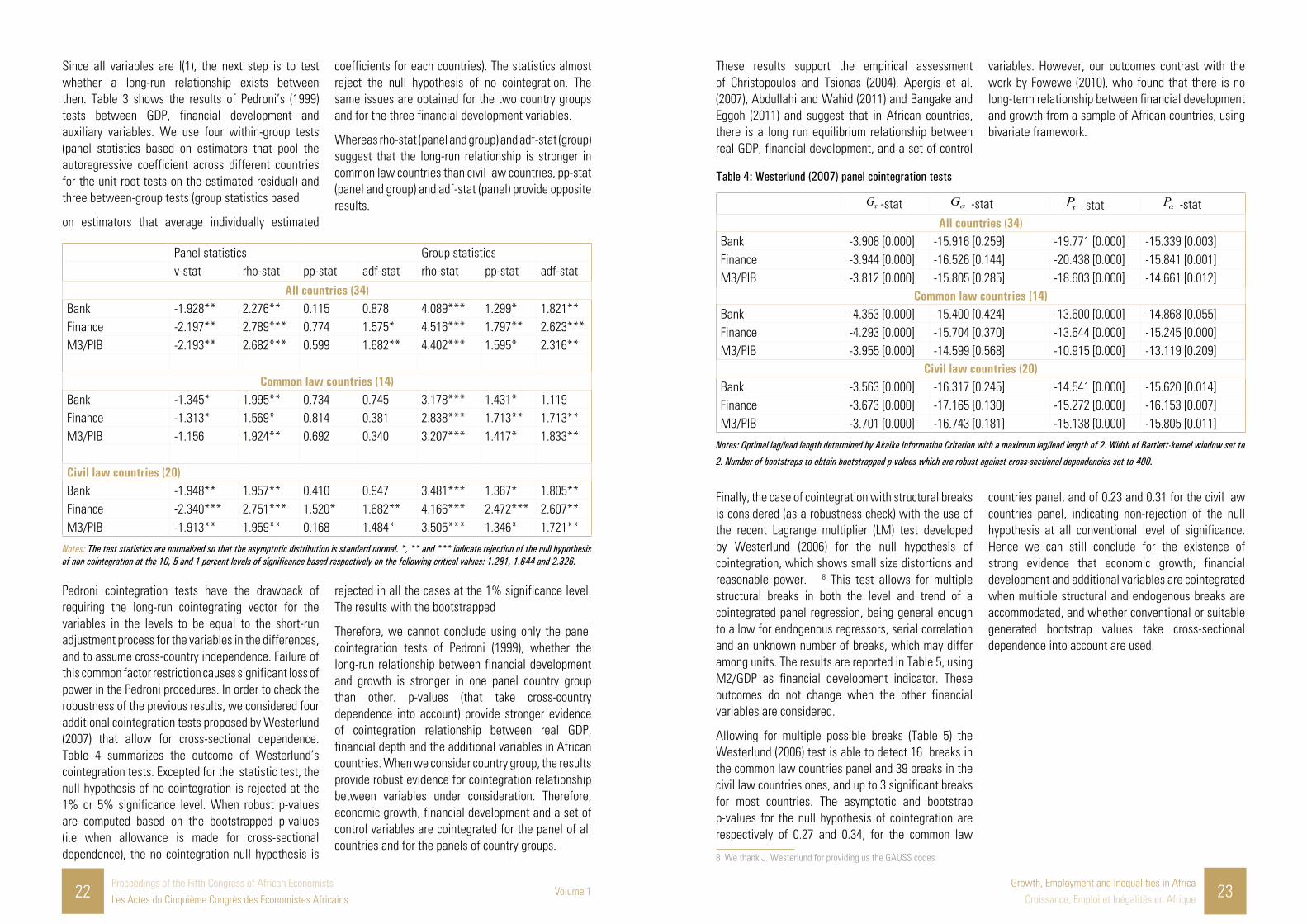
These results support the empirical assessment of Christopoulos and Tsionas (2004), Apergis et al. (2007), Abdullahi and Wahid (2011) and Bangake and Eggoh (2011) and suggest that in African countries, there is a long run equilibrium relationship between real GDP, financial development, and a set of control
variables. However, our outcomes contrast with the work by Fowewe (2010), who found that there is no long-term relationship between financial development and growth from a sample of African countries, using bivariate framework.
Table 4: Westerlund (2007) panel cointegration tests
-stat -stat -stat -statAll countries (34)
Bank -3.908 [0.000] -15.916 [0.259] -19.771 [0.000] -15.339 [0.003]Finance -3.944 [0.000] -16.526 [0.144] -20.438 [0.000] -15.841 [0.001]M3/PIB -3.812 [0.000] -15.805 [0.285] -18.603 [0.000] -14.661 [0.012]
Common law countries (14)Bank -4.353 [0.000] -15.400 [0.424] -13.600 [0.000] -14.868 [0.055]Finance -4.293 [0.000] -15.704 [0.370] -13.644 [0.000] -15.245 [0.000]M3/PIB -3.955 [0.000] -14.599 [0.568] -10.915 [0.000] -13.119 [0.209]
Civil law countries (20)Bank -3.563 [0.000] -16.317 [0.245] -14.541 [0.000] -15.620 [0.014]Finance -3.673 [0.000] -17.165 [0.130] -15.272 [0.000] -16.153 [0.007]M3/PIB -3.701 [0.000] -16.743 [0.181] -15.138 [0.000] -15.805 [0.011]
Notes: Optimal lag/lead length determined by Akaike Information Criterion with a maximum lag/lead length of 2. Width of Bartlett-kernel window set to
2. Number of bootstraps to obtain bootstrapped p-values which are robust against cross-sectional dependencies set to 400.
Finally, the case of cointegration with structural breaks is considered (as a robustness check) with the use of the recent Lagrange multiplier (LM) test developed by Westerlund (2006) for the null hypothesis of cointegration, which shows small size distortions and reasonable power. 8 This test allows for multiple structural breaks in both the level and trend of a cointegrated panel regression, being general enough to allow for endogenous regressors, serial correlation and an unknown number of breaks, which may differ among units. The results are reported in Table 5, using M2/GDP as financial development indicator. These outcomes do not change when the other financial variables are considered.
Allowing for multiple possible breaks (Table 5) the Westerlund (2006) test is able to detect 16 breaks in the common law countries panel and 39 breaks in the civil law countries ones, and up to 3 significant breaks for most countries. The asymptotic and bootstrap p-values for the null hypothesis of cointegration are respectively of 0.27 and 0.34, for the common law
8 We thank J. Westerlund for providing us the GAUSS codes
countries panel, and of 0.23 and 0.31 for the civil law countries panel, indicating non-rejection of the null hypothesis at all conventional level of significance. Hence we can still conclude for the existence of strong evidence that economic growth, financial development and additional variables are cointegrated when multiple structural and endogenous breaks are accommodated, and whether conventional or suitable generated bootstrap values take cross-sectional dependence into account are used.
coefficients for each countries). The statistics almost reject the null hypothesis of no cointegration. The same issues are obtained for the two country groups and for the three financial development variables.
Whereas rho-stat (panel and group) and adf-stat (group) suggest that the long-run relationship is stronger in common law countries than civil law countries, pp-stat (panel and group) and adf-stat (panel) provide opposite results.
Panel statistics Group statisticsv-stat rho-stat pp-stat adf-stat rho-stat pp-stat adf-stat
All countries (34)Bank -1.928** 2.276** 0.115 0.878 4.089*** 1.299* 1.821**Finance -2.197** 2.789*** 0.774 1.575* 4.516*** 1.797** 2.623***M3/PIB -2.193** 2.682*** 0.599 1.682** 4.402*** 1.595* 2.316**
Common law countries (14)Bank -1.345* 1.995** 0.734 0.745 3.178*** 1.431* 1.119Finance -1.313* 1.569* 0.814 0.381 2.838*** 1.713** 1.713**M3/PIB -1.156 1.924** 0.692 0.340 3.207*** 1.417* 1.833**
Civil law countries (20)Bank -1.948** 1.957** 0.410 0.947 3.481*** 1.367* 1.805**Finance -2.340*** 2.751*** 1.520* 1.682** 4.166*** 2.472*** 2.607**M3/PIB -1.913** 1.959** 0.168 1.484* 3.505*** 1.346* 1.721**
Notes: The test statistics are normalized so that the asymptotic distribution is standard normal. *, ** and *** indicate rejection of the null hypothesis of non cointegration at the 10, 5 and 1 percent levels of significance based respectively on the following critical values: 1.281, 1.644 and 2.326.
Pedroni cointegration tests have the drawback of requiring the long-run cointegrating vector for the variables in the levels to be equal to the short-run adjustment process for the variables in the differences, and to assume cross-country independence. Failure of this common factor restriction causes significant loss of power in the Pedroni procedures. In order to check the robustness of the previous results, we considered four additional cointegration tests proposed by Westerlund (2007) that allow for cross-sectional dependence. Table 4 summarizes the outcome of Westerlund’s cointegration tests. Excepted for the statistic test, the null hypothesis of no cointegration is rejected at the 1% or 5% significance level. When robust p-values are computed based on the bootstrapped p-values (i.e when allowance is made for cross-sectional dependence), the no cointegration null hypothesis is
rejected in all the cases at the 1% significance level. The results with the bootstrapped
Therefore, we cannot conclude using only the panel cointegration tests of Pedroni (1999), whether the long-run relationship between financial development and growth is stronger in one panel country group than other. p-values (that take cross-country dependence into account) provide stronger evidence of cointegration relationship between real GDP, financial depth and the additional variables in African countries. When we consider country group, the results provide robust evidence for cointegration relationship between variables under consideration. Therefore, economic growth, financial development and a set of control variables are cointegrated for the panel of all countries and for the panels of country groups.

24Proceedings of the Fifth Congress of African EconomistsLes Actes du Cinquième Congrès des Economistes Africains
Volume 1Growth, Employment and Inequalities in Africa
Croissance, Emploi et Inégalités en Afrique 25
Common law countries
Number of breaks
Years
Egypt Arab Rep. 1 1995Ghana 1 1991Gambia 1 1995Kenya 1 1995Lesotho 1 1996Malawi 2 1986 1995Nigeria 2 1986 1995Sudan 1 1986Sierra Leone 1 1986Swaziland 1 1986Uganda 1 1986South Africa 1 1986Zambia 1 1990Zimbabwe 1 1994
Civil law countries
Number of
breaksYears
Burundi 2 1980 1989Benin 2 1981 1990Burkina Faso 3 1976 1982 1990Central African Republic
3 1976 1983 1989
Ivory Coast 2 1979 1990Cameroon 3 1978 1983 1991Congo 1979 1990Congo Democratic
1980 1991
Algeria 2 1979 1990Gabon 2 1979 1990Morocco 2 1979 1989Madagascar 2 1979 1990Mali 2 1981 1991Mauritania 2 1979 1992Niger 2 1982 1989Rwanda 2 1981 1992Senegal 2 1979 1990Chad 2 1979 1990Togo 2 1983 1992Tunisia 2 1978 1989
Note: The breaks are estimated using the Bai and Perron (2003) procedure with a maximum number of five breaks for each country. The minimum
length of each break regime is set to 0.1T.
Compared to the existing studies, the estimated date of our structural breaks is roughly consistent with Teng and Liang (2010) who found two structural breaks in 11 emerging countries. Our results also are broadly in accordance with consistent with Esso (2010) that used the Gregory and Hansen (1996a; 1996b) testing approach to threshold cointegration for 15 African countries.
As far as the civil law countries are concerned, our study shows that the first structural breaks occurred in the 1970s or 1980s, while the second and the third structural breaks in the 1990s or 2000s. Roughly, our structural breaks are associated globally and with great shocks. They may reflect the energy crises triggered by the 1973 Arab oil embargo; the 1978 Iranian revolution, accompanied by escalating oil prices and a period of high inflation during the 1970s decade; the deep world-wide recession in the early 1980s; the 1987 wall Street stock market crash; the commodities crises of the 1980s due to the second oil shocks and to the start period of the economic liberalization within the context of structural adjustment in most of the Sub-Saharan African countries (Esso, 2010). Indeed, Africa countries faced to a serious economic crisis in the 1980s which is culminated in pronounced disequilibria in both the domestic and external sector. Moreover, for Algeria, Burkina Faso, Cameroon, Central African Republic, Chad, Ivory Coast, Morocco, Madagascar, Mauritania, Senegal and Tunisia, the first structural breaks appeared between 1976 and 1979 before the commodity crisis around the time of the second oil price shock in 1979 and the Iran-Iraq war in 1980. In Benin, Burundi, Mali, Niger, Rwanda, and Togo the first structural breaks occurred in early 1980 period of deep world-wide recession.
Concerning the common law countries, the results of the estimated date of structural breaks are almost different to those obtained in civil. For instance, for Malawi, Nigeria, Sudan, Sierra Leone, Swaziland, South Africa and Uganda, the first structural appeared in the 1980s during the commodity crisis of the 1980s. Except for South Africa, Nigeria and Sudan, most of these countries are largely monoculture and rely on one or two commodity exports. In this regard, a perennial balance of payment deficit, brought about largely by commodity price fluctuation and adverse terms of trade led these countries to be heavily indebted.
Results of DOLS and panel causality results
As mentioned above, we use two techniques to obtain the parameter estimates of the panel error-correction model for the relationship between financial development and economic growth and a set of control variables: DOLS for the long-run parameters and PMG for the short and long-run parameters. Table 6 presents the DOLS results. The estimated coefficients of the three indicators of financial development (Bank, Finance, and M3/GDP) are all positive and statistically significant for all countries at 1% level. Since the variables are expressed in natural logarithms, the coefficients can be interpreted as elasticities. Overall, the outcomes of this study show that there is strong long-run relationship between real GDP, financial development and the other control variables. The results on the global sample indicate that a 1% increase in financial development variables (Bank, Finance, and M3/GDP) increases economic growth respectively, by 0.403%, 0.433% and 0.620%. Accordingly, these findings suggest that high levels of financial depth are positively associated with faster economic growth in African countries. There is difference in results when country groups are considered. For instance, in common law countries, a 1% increase in financial development variables (Bank, Finance, and M3/GDP) increases economic growth respectively by 0.707%, 0.467% and 0.769%. As far as civil law countries are concerned, a 1% increase of financial development increases economic growth respectively, by 0.137%, 0.321% and 0.395%.
Compared to the results of other DOLS and FMOLS estimates using panel data in developing countries, the elasticity of financial development in African countries is within the range of these studies. For example, the financial development coefficients are larger than the 0.032, 0.027 and 0.024 (for liquid liability, bank credit and private credit, respectively) reported by Apergis et al. (2007) for a sample of non-OECD countries, and also the elasticity estimates obtained by Bangake and Eggoh (2011) for a sample of low income countries. Using FMOLS estimator for a panel of 15 sub-Sahara African countries from 1976-2005, Abdullahi (2010) also reported the estimate coefficients of 0.031 and 0.579 for private credit and domestic credit, respectively.
In addition, the coefficients of control variables have expected sign. The investment rate and the openness to trade are positively associated with economic growth,
while government expenditure as ratio to GDP has negative impact and inflation rate is insignificant, for the global sample. However, government expenditure exhibits non significant coefficient in common law countries, but a statistically negative impact in civil law countries. This outcome shows that government expenditures are more inefficiency in African civil law countries, which also record the most negative impact of inflation rate.

26Proceedings of the Fifth Congress of African EconomistsLes Actes du Cinquième Congrès des Economistes Africains
Volume 1Growth, Employment and Inequalities in Africa
Croissance, Emploi et Inégalités en Afrique 27
is associated with a more helpful government than the French civil law.
These results imply that in the countries with strong legal protection of investors, the long-run relationship between finance and growth is higher than in the countries with worst protection. These findings may be due to the fact that in common law countries with less-formal judicial procedures many reforms have been taken in the early 1980s (privatization, rationalization of the public sector, liberalization of exchange rate, and financial systems).
Thus, the flexibility of common law system has facilitated the development of financial intermediaries and the establishment of new financial institutions. On the other hand, civil law juridical proceedings and centralized administration have impeded financial development in African French legal origin countries. Furthermore, African civil law countries are characterized by a weak institutional framework which is not favorable to financial development.
After establishing that economic growth has a long-run relationship with financial development, we need to examine the causality between both variables. Table 7 reports (Panels A, B and C) the results of the short-run and long-run Granger-causality tests for each panel data set, using domestic credit to private sector by banks as percentage of GDP (Bank) as financial development variable. 9 The optimal lag structure of two years is chosen using the Schwarz Bayesian Criterion. In panel A which includes all countries of our sample, Eq. (14a) shows that financial development and investment ratio have a positive and statistically significant impact in the short-run on economic growth, whereas government ratio has negative impact. On the other hand, openness to trade and price level have insignificant impact on economic growth. The sum of the lagged coefficients is 0.081 and 0.052 for financial development variable and investment ratio respectively. This outcome highlights the importance of financial development in the economic growth process in African countries and supports the supply leading hypothesis. Moreover, the error correction term is statistically significant at 1% and denotes the speed of adjustment to long-run equilibrium. In term of
9 In order to check for robustness we present in the Appendix (see Tables A2 and A3) the results, based on the other financial development variables. Notice that the results are robust to various financial development indicators.
Eq. (14b), it appears that economic growth, investment ratio and government consumption have positive and significant impact on financial development in short-run at 5% significant level. The sum of lagged values of economic growth, investment ratio and government expenditure is 0.306, 0.061 and 0.144, respectively. This shows that economic activity is the main factor in financial development process and provides a strong support to demand following hypothesis. The statistically significance at 1% of the error correction term suggests that financial development responds to deviations from long-run equilibrium. Overall, our investigation provides a strong support to feedback relationship between financial development and economic growth: decreasing in financial development decreases growth and vice versa, and that increasing in financial development increases growth, and vice versa. Our results are in line with Apergis et al. (2007), Luintel and Khan (1999), Demetriades and Hussein (1996) who also show a bi-directional relationship between financial development and growth.
As far as the short-run dynamics is concerned, the Eq. (14a) shows that financial development and investment ratio have a positive and statistically significant impact on economic growth in common law countries, whilst financial development, government consumption and trade openness are significant in civil law countries. Thus, financial development policies can impulse growth in common law as well as civil law countries. With respect to Eq. (14b) economic growth and openness to trade have positive and significant impact in both country groups, whereas government ratio is only significant in civil law countries, and price level in common law countries. Concerning the long-run relationship, the error correction terms are statistically significant, but the speed of adjustment can vary according to the country groups. For example, the adjustment dynamic of economic growth is faster in common law than in civil law countries.
More importantly, our empirical results bring further evidence: the bi-directional causality is observed in all country groups, giving credence to both the supply-leading and the demand-following hypothesis. However, a strong support for short-run and long-run causality is found for common law countries. Due to their juridical system that offers better investor protection and government effectiveness, improvements in the financial system will have more
Table 6: Panel DOLS long-run estimatesBank (B) Finance M3/GDP
All countries (34)
Financial development 0.403***(0.023) 0.433*** (0.0204) 0.620*** (0.035)Investment (I) 0.501*** (0.026) 0.571*** (0.026) 0.458*** (0.026)Government (G) -0.368*** (0.036) -0.341*** (0.0370) -0.303*** (0.037)Trade (T) 0.390*** (0.041) 0.520*** (0.0418) 0.419*** (0.041)Inflation (P) -0.003 (0.008) -0.0015 (0.008) -0.0161** (0.008)Observations 1,394 1,394 1,394
Common law countries (14)
Financial development 0.707*** (0.042) 0.467*** (0.030) 0.769*** (0.052)Investment (I) 0.100*** (0.038) 0.343*** (0.035) 0.040 (0.052)Government (G) -0.159*** (0.051) -0.033 (0.049) -0.048 (-1.430)Trade (T) -0.110** (0.056) 0.185*** (0.053) -0.024 (0.056)Inflation (P) 0.0176 (0.019) 0.0378** (0.018) 0.013 (0.019)Observations 574 574 574
Civil law countries (20)
Financial development 0.137*** (0.028) 0.321*** (0.025) 0.395*** (0.045)Investment (I) 0.692*** (0.037) 0.626*** (0.036) 0.565*** (0.036)Government (G) -0.123** (0.050) -0.224*** (0.050) -0.173*** (0.051)Trade (T) 0.900*** (0.061) 0.884*** (0.060) 0.890*** (0.060)Inflation (P) -0.004 (0.008) -0.004 (0.008) -0.012 (0.008)Observations 820 820 820
Notes: t-statistics are in parentheses. *, ** and *** significant at 10,
5 and 1 percent.
There are interesting results when considering panels of country groups. For instance, in common law countries, a 1% increase in financial development indicators (Bank, Finance, and M3/GDP) increases economic growth by 0.707%, 0.467% and 0.769%, respectively. As far as civil law countries are concerned, a 1% increase in financial development variables (Bank, Finance, and M3/GDP) increases economic growth by 0.137%, 0.321% and 0.395%., respectively. Based on Fisher statistics, our results indicate that the null hypothesis of coefficients equality between common law and civil law countries is strongly rejected at 1% significance level. These outcomes provide overwhelming evidence in support the view that the positive long-run effects of financial development on growth is higher in African common law than in civil law countries.
What does difference in the finance-growth relationship, between common law and civil law
countries in Africa? La Porta et al. (2008, p. 298) formally established that: “compared to French civil law, common law is associated with (a) better investor protection, which in turn is associated with improved financial development, better access to finance, and higher ownership dispersion, (b) lighter government ownership and regulation, which are in turn associated with less corruption, better functioning labor markets, and smaller unofficial economies, and (c) less formalized and more independent judicial systems, which are in turn associated with more secure property rights and better contract enforcement”. Moreover, Djankov et al. (2007) show that private credit rises after improvements in creditor rights and in information sharing in a sample of 129 countries. Using firm perceptions on how helpful the government is to provide an alternative test of the theory of legal origin, Amin (2009) also finds from a sample of 48 countries, that the English common law

28Proceedings of the Fifth Congress of African EconomistsLes Actes du Cinquième Congrès des Economistes Africains
Volume 1Growth, Employment and Inequalities in Africa
Croissance, Emploi et Inégalités en Afrique 29
impact on economic growth than in civil law countries. Finally, our results suggest that financial development may be a good lever to enhance economic growth in African countries.
Similar results are often obtained in the literature and suggest a low effect of financial development on
economic growth in developed countries. For example, Apergis et al. (2007) find that the bi-directional causality between financial development and economic growth is higher in non-OECD countries, than OECD countries.
Table 7: Panel causality tests using banking sector ratio to GDP (Bank) as financial development variableDependant variables
Sources of causality
Short-run Long-runY ECT
Panel A – All countries(14a) Y - 7.72***
[0.081]3.97**[0.052]
2.65*[-0.038]
1.59[0.023]
0.48[-0.028]
-0.048***(-4.77)
(14b) 5.93**[0.306]
- 2.87* [0.061]
10.41***[0.144]
3.07*[0.152]
2.31[0.104]
-0.089***(-5.63)
Panel B – Common law countries(14a) Y - 9.78***
[0.107]4.82**[0.069]
1.08[-0.015]
0.98[0.029]
2.91*[-0.089]
-0.073***(-4.69)
(14b) 4.98**[0.373]
- 1.36[0.091]
1.81[0.061]
10.54***[0.201]
5.42**[0.221]
-0.124***(-4.13)
Panel C – Civil law countries(14a) Y - 3.86**
[0.094]2.79*[0.054]
3.07*[-0.065]
1.81[0.051]
1.57[-0.060]
-0.042***(-2.78)
(14b) 8.85***[0.268]
- 1.16[-0.018]
11.81***[0.209]
5.36**[0.127]
2.71*[0.182]
-0.084***(-5.26)
Notes: Partial F-statistics are reported with respect to short-run changes in the independent variables. ECT represents the coefficient of the error correction term. t-statistics are reported in parentheses. The sum of the lagged coefficients for the respective short-run changes is denotes in brackets
*** Significant at 1 percent and ** significant at 5 percent.
ConclusionThe aim of this study was to shed light on relationship between financial development, economic growth and auxiliaries’ variables for 32 African countries over the period from 1970 to 2015. We have made use of recent panel unit root tests, Pedroni (1999) and Westerlund (2006, 2007) panel cointegration and causality tests to analyse the nexus between financial development and growth. Since African countries differ in their level of financial development due to differences in policies and institutions, the sample is divided into two groups: civil law countries and common law countries. Our results reveal that there is a long-run equilibrium relationship between financial development, economic growth, and auxiliaries’ variables. Moreove r, we find that decreasing in financial development decreases growth and vice versa, and that increasing in financial development increases growth, and vice versa, and that this applies for both civil law countries and common law countries. In other words, both the financial and real sectors are complementary to each other. This result is robust to possible cross-country dependence and still holds when allowing for multiple endogenous structural breaks, which can differ among countries.
From a policy perspective, the results mean that adopting an apparently simple solution of improving financial development is not going to help with economic growth. What is necessary is to alter the relationship between financial development and economic growth. In this regard, one solution consists in focusing on financial development efficiency, that is, to promote faster economic growth. African countries might undertake financial reforms through financial liberalization, the promotion of saving for the modest households. Of course, this would require a mentality change and an access to the banking sector for the households with low income, this might be a choice that is necessary to make. It would also be interesting to improve access to credit for moderate income households through credits and microcredit loans to stimulate domestic consumption and investment in order to promote economic growth. Furthermore, our results also show that estimated structural break tests are associated globally and with great shocks i.e. mainly occurred during commodities crisis. It implies that commodities crisis have a significant impact on the finance development-growth nexus.

30Proceedings of the Fifth Congress of African EconomistsLes Actes du Cinquième Congrès des Economistes Africains
Volume 1Growth, Employment and Inequalities in Africa
Croissance, Emploi et Inégalités en Afrique 31
AppendixTable A1: Descriptive statistics, cross-section: 1970-2009; Sub-samples
Variable N Mean Std. Dev. Minimum MaximumCommon law countries
Growth 14 1.289 1.147 -0.806 3.260M2/gdp 14 27.915 12.555 14.0699 69.674M3/gdp 14 32.526 11.864 16.081 79.327Private 14 20.852 23.153 4.779 95.705Investment 14 19.058 4.381 10.561 37.913Government 14 15.685 3.505 10.241 20.636Openness 14 70.065 36.911 29.298 158.976Inflation 14 20.578 10.663 9.778 35.158
Civil law countries
Growth 18 0.624 1.065 -1.241 3.225M2/gdp 18 24.214 10.403 11.772 55.572M3/gdp 18 26.319 10.273 12.297 61.846Private 18 20.387 12.727 7.795 57.234Investment 18 19.007 4.773 11.272 31.479Government 18 14.487 3.926 9.931 27.535Openness 18 59.173 21.291 33.090 102.448Inflation 18 6.776 2.487 3.746 13.579
Equality tests: H0: mean difference=0
Growth 1.434 [0.080]M2/gdp 0.722 [0.237]M3/gdp 1.089 [0.142]Private 0.072 [0.471]
Table A2: Panel causality tests using m3/gdp as financial development variable
Dependant variables
Sources of causality
Short-run Long-runY ECT
Panel A – All countries(14a) Y - 3.86**
[0.075]
4.07**
[0.052]
3.22*
[-0.048]
1.07
[0.032]
1.23
[-0.021]
-0.049***
(-4.81)(14b) 7.34***
[0.372]
- 1.17
[0.042]
14.65***
[0.159]
3.98**
[0.123]
2.67
[0.278]
-0.141***
(-8.06)Panel B – Common law countries(14a) Y - 3.90**
[0.097]
3.02*
[0.055]
0.86
[-0.029]
1.48
[-0.021]
1.14
[-0.022]
-0.066***
(-2.88)
Dependant variables
Sources of causality
(14b) 4.34**
[0.451]
- 1.25
[0.049]
2.02
[0.093]
2.68*
[0.087]
6.08**
[-0.185]
-0.176***
(-4.14)Panel C – Civil law countries(14a) Y - 3.74**
[0.052]
3.88**
[0.053]
1.71
[-0.053]
1.38
[-0.037]
1.23
[-0.032]
-0.041***
(-3.71)(14b) 4.30**
[0.390]
- 1.31
[-0.064]
1.51
[0.076]
8.79***
[0.149]
2.67*
[0.028]
-0.138***
(-2.61)Notes: Partial F-statistics are reported with respect to short-run changes in the independent variables. ECT represents the coefficient of the error correction term. t-statistics are reported in parentheses. The sum of the lagged coefficients for the respective short-run changes is denotes in brackets *** Significant at 1 percent and ** significant at 5 percent.
Table A3: Panel causality tests using private/gdp as financial development variable
Dependant variables
Sources of causality
Short-run Long-runY ECT
Panel A – All countries(14a) Y - 8.21***
[0.081]
11.85***
[0.092]
5.84**
[-0.064]
0.46
[0.022]
0.81
[-0.038]
-0.055***
(-4.99)(14b) 2.96*
[0.279]
- 3.72**
[0.065]
8.20***
[0.152]
1.21
[-0.047]
1.29
[-0.188]
-0.108***
(-6.09)Panel B – Common law countries(14a) Y - 3.78**
[0.087]
4.24**
[0.133]
1.30
[-0.019]
1.33
[0.025]
1.35
[-0.094]
0.081***
(-2.54)(14b) 3.81**
[0.225]
- 4.27**
[0.088]
4.02**
[-0.059]
5.69**
[0.223]
2.02
[-0.237]
-0.178***
(-5.45)Panel C – Civil law countries(14a) Y - 3.52**
[0.046]
6.05**
[0.090]
3.64**
[-0.088]
1.09
[-0.014]
2.52
[-0.042]
-0.072***
(-3.75)(14b) 3.20*
[0.147]
- 3.67**
[0.098]
7.94***
[0.227]
1.36
[0.021]
1.65
[-0.239]
-0.069***
(-4.05)

32Proceedings of the Fifth Congress of African EconomistsLes Actes du Cinquième Congrès des Economistes Africains
Volume 1Growth, Employment and Inequalities in Africa
Croissance, Emploi et Inégalités en Afrique 33
La croissance économique en Afrique: les institutions importent-elles? Par Jacques Simon SONG, PhD en Economie, Université de Dschang, Cameroun
Introduction Disposer de bonnes institutions procure au moins deux avantages aux pays. Le premier avantage est la réduction des coûts de transaction, et le second est la garantie des discussions sans tyrannie. D’autres effets moins directs sont mentionnés dans la littérature tels les causes majeures de la croissance économique (Saima, 2015 ; Iqbal et Daly, 2014), les incitations dans les échanges humains (North, 1990), la protection des droits de propriété (Acemoglu et al., 2005), les activités entrepreneuriales et les innovations (Estrin et al., 2013).
Au cours de la dernière décennie, la croissance économique mondiale est restée instable (Banque Mondiale, 2015). Estimée à 1,6% en 2008, 4% en 2010 puis 2,2% en 2012 du fait de la baisse de la demande mondiale, de la crise dans la zone euro, à l’incertitude planant sur le mur budgétaire et le plafonnement de la dette aux Etats-Unis (Commission Economique pour l’Afrique, 2013). Dans l’Union Européenne, la croissance économique s’est contractée de 0,3% en 2012 contre 1,5 % en 2011 (Département des Affaires Economiques et Sociales DAES-ONU 2012). Les États-Unis ont enregistré une croissance de 2,1 % en 2012 du fait de la consommation privée, des investissements vigoureux ainsi qu’un meilleur environnement du crédit. En Asie Occidentale, le taux de croissance économique a chuté pour se situer à 3,3 % en 2012, contre 6,7%
en 2011. Cette baisse a été également observée en Amérique latine avec un taux de croissance de 3,1 % en 2012, contre 4,3% en 2011 (DAES, ONU 2012).
En Afrique, malgré les contrecoups de l’atonie de l’économie mondiale, la croissance économique est restée vigoureuse comparativement aux autres régions du monde du fait d’un environnement économique favorable. En Afrique, après deux décennies de stagnation, le taux de croissance économique est resté instable depuis le début du XXIe siècle (Banque Mondiale, 2015). Trois constats émergent : D’abord, la croissance économique est passée de 5,6% entre 2002 et 2008, à 2,2% en 2009 sous l’effet conjugué de la crise financière mondiale et de la flambée des prix de produits alimentaires. Ensuite, elle s’est établie à 4,6 % en 2010 pour fléchir de nouveau en 2011 en raison de la transition politique en Afrique du Nord. Enfin, elle a atteint 5% en 2012, en dépit de la récession économique mondiale et des incertitudes. Compte tenu du seuil de 4,8 % en 2013, de 5,1 % en 2014, et de 5,2 %, en 2015, les perspectives de croissance économique demeurent fermes du fait des efforts à bâtir des institutions solides, capables de soutenir et d’améliorer le cadre des actions des entreprises, de la gouvernance et de la gestion macroéconomique.
Dans les différentes sous-régions de l’Afrique, la croissance économique est restée peu constante
passant de 5,2% en 2008 à 5% en 2012 (Banque Mondiale, 2015). Au cours de la même période, le taux de croissance économique de l’Afrique Australe est passé de 4,9% à 3,51%, de 6,6% à 5,7% pour les pays de l’Afrique de l’Est, de 5,9% à 6,4% pour les pays de l’Afrique de l’Ouest, de 4,9% à 5,4% pour les pays de l’Afrique du Nord, et maintenu à 5% pour les pays de l’Afrique Centrale. Depuis 2013, on enregistre une croissance moyenne de l’ordre10 de 3%.
Cependant, certains pays enregistrent des taux de croissance élevés tels que le Rwanda (7,9%), l’Angola (7,5%), le Mozambique (7,5%), l’Ethiopie (7%), la Tanzanie (6,8%), la
Guinée Equatoriale (6,3%). Selon la CEDEAO (2016), la Côte d’Ivoire se démarque par ses performances avec des taux de croissance élevés de l’ordre de 10,7% (2012), 9,2% (2013), 8,5% (2014), 9,4% (2015).
En dépit de la relative croissance économique de l’Afrique comparativement aux autres régions, les explications sous-jacentes reposent sur les déficits, le poids de l’endettement, les infrastructures. Pourtant, les revers des politiques d’austérité ont fait émerger de nouvelles idées expliquant la relance économique non seulement par des facteurs économiques, mais aussi par des facteurs mésoéconomiques comme la qualité des institutions qui ont toujours été une priorité. Depuis l’avènement des Programmes d’Ajustement Structurels sous l’égide de la Banque Mondiale et du Fonds Monétaire International, les pays Africains ambitionnaient de créer les conditions d’une croissance économique propice, saine, durable, d’assoir les stratégies de bonne gouvernance, et d’assainir le paysage sociopolitique. Cette nécessité a conduit à reposer les termes du débat entre institutions et croissance économique afin d’assoir les stratégies de développement volontaristes sur des bases rigoureuses. Cependant, les divergences dans les déficits des États africains, les infrastructures, les incapacités à amortir les chocs extérieurs et notamment en matière de croissance économique persistent.
A titre illustratif, depuis 1996, les statistiques sur les indices de gouvernance définis par Kaufmann et al., (2010) et variant entre -2,5 (très faible performance) et 2,5 (très bonne performance) laissent entrevoir
10 Voir rapport de la Communauté Economique des Etats de l’Afrique de l’Ouest.
trois groupes de pays : Le premier groupe caractérisé de « bons élèves » avec un indice moyen positif qui fluctue entre 0,74 pour l’Ile Maurice et 0,22 pour les Seychelles (WGI, 2016)11 . Le deuxième groupe se compose des « élèves moyens ». En effet ce sont les pays qui ont un indice composite de qualité institutionnelle proche de 0. On y retrouve le Ghana (-0,06), la Tunisie (-0,12) et le Maroc (-0,22). Le troisième groupe est constitué de « mauvais élèves » en matière de gouvernance. Les pays présentant un indice composite de qualité institutionnelle supérieur à -1 ou à -2. Les pays comme la Somalie (-2,23), la République Démocratique du Congo (-1,76), le Soudan (-1,54) se trouvent dans cette catégorie. En général, les institutions sont relativement restées de mauvaise qualité. L’Afrique Australe se démarque (-0,11), suivie de l’Afrique du Nord (-0,57), de l’Afrique de l’Ouest (-0,63), de l’Afrique de l’Est (-1,03) et l’Afrique centrale occupe la dernière position (-1,05).
Cerner les écarts de croissance économique entre pays constitue un regain d’intérêt. Les faits esquissés ci-dessus induisent des questionnements sur la croissance économique et confirment à quelques exceptions près la considération des institutions en Afrique. Radu (2015) souligne qu’il est impossible d’analyser la situation économique d’un pays en prenant en compte les seuls facteurs du marché. L’ancrage théorique du rôle des institutions au processus de croissance économique remonte aux travaux de Wolf (1955), North et Thomas (1973) dont le regain d’intérêt au cours becomes pertinent that governments, and institutions around the continent need to reassess the approach employed when seeking productivity growth. In the past, a more attention has been placed on political institutions, and the engendering of democracy within in African states, in order to meet development goals. However, given these results, maybe, market based institutions, and more importantly, the de jure aspects of the market need to be paid more attention. That is, focusing on de facto objectives without tackling some of the fundamental economic and market based institutional underpinnings, which are often times very deep in nature would only lead to the same outcomes. Rather to attain sustainable growth in productivity on
11 Les indices de gouvernance retenus dans ce travail sont tirés de la base de Worldwide Governance Indicators, (2016). Il s’agit des in-dices de gouvernance de la Banque Mondiale définis par Kaufmann et al. (2010). Ils varient de -2,5 (très faible performance) à 2,5 (très bonne performance).

34Proceedings of the Fifth Congress of African EconomistsLes Actes du Cinquième Congrès des Economistes Africains
Volume 1Growth, Employment and Inequalities in Africa
Croissance, Emploi et Inégalités en Afrique 35
the continent, some of the attention placed on political institutions, need to be places in economic and market based institutions. This, per this paper, would lead to positive outcomes within a total factor productivity context. Positive TFP would subsequently help realise and attain the ‘catch-up’ that seems to have evaded many SSA countries.
des trois dernières décennies a conduit en mettre en exergue, leur nature et leurs rôles (Dias et Tebaldi, 2012). Ainsi, les institutions ont émergé comme une condition nécessaire du succès des économies (Clague et al., 1996 ). Toutefois, les effets des institutions au processus de croissance économique sont non consensuels. Certes, la littérature empirique souligne que les institutions peuvent stimuler la croissance économique (Efendic et al., 2011 ; Siddiqui et Masood, 2013 ; Adams et Osei-Opoku, 2015), l’entraver (Dollar et Kraay, 2000) et être sans effets sur celle-ci (Baume et Lake 2003 ; Doucouliagos et Ulubasoglu, 2008 ; Knutsen, 2010). Cette littérature est remise en cause du fait des composantes institutionnelles, des spécifications et des données utilisées.
L’objectif de cet article est d’analyser le rôle des institutions au processus de croissance économique en Afrique. Ce choix repose sur le fait que la qualité des institutions occupe de plus en plus une place importante dans les conditionnalités de l’aide des organismes internationaux. La Banque Mondiale dans son rapport économique pour l’Afrique publié en 2015 souligne que les pays de l’Afrique doivent bâtir des institutions solides pour soutenir et améliorer le cadre des actions des entreprises, de la gouvernance et de la gestion macroéconomique.
Trois contributions ressortent : Primo, cette étude se démarque par son aspect innovateur et instructif. En effet, les études existantes appréhendent la croissance économique par les seules institutions de droit de propriété. Pourtant, la croissance économique nécessite la mise en place d’autres types d’institutions économiques permettant de soutenir la dynamique de celle-ci, de renforcer la capacité de résistance aux chocs et de permettre une répartition socialement acceptable. Ainsi, nous déclinons quatre composantes institutionnelles suite à la classification de Rodrik (2005) à savoir : les institutions de création du marché, les institutions de stabilisation du marché, les institutions de régulation du marché,
et les institutions de légitimation du marché qui permettent de mieux appréhender la dynamique de la croissance économique, de renforcer la capacité de résistance aux chocs et de permettre une répartition socialement acceptable. Secundo, cette étude vient enrichir la littérature empirique traitant de la croissance économique dans une perspective institutionnelle. En effet, les travaux existant portent sur les échantillons qui intègrent les pays développés et pays en développement avec des environnements institutionnels différents. Par conséquent, les résultats sont biaisés. Ce problème se pose dans une moindre mesure lorsque l’analyse porte sur les pays d’un même continent comme l’Afrique. Or, au mieux de notre connaissance, il n’y a pas d’études empiriques qui établissent de telles corrélations. Tertio, l’étude est effectuée sur données de panel qui permettent de tenir compte de la dimension temporelle des données en plus de leur dimension transversale, de retracer la dynamique des comportements et leur éventuelle hétérogénéité, de réduire le risque de colinéarité entre les variables explicatives (Sevestre, 2002). Nos résultats économétriques montrent que les institutions importent au processus de croissance économique en Afrique.
À la suite de cette première section qui constitue l’introduction, le reste de l’article s’organise en quatre sections additionnelles : La deuxième section passe en revue les considérations théoriques et empiriques de la littérature. La troisième section esquisse le modèle empirique, l’approche méthodologique et les données. La quatrième section reporte et interprète les résultats. La cinquième section conclut, et propose des recommandations de politiques économiques.
Institutions et croissance économique : les enseignements de la littératureRevue de littérature théorique
La littérature traitant du rôle des institutions sur la croissance économique n’est pas récente. L’ancrage théorique remonte aux travaux de Wolf (1955). Par la suite, l’avènement de la Nouvelle Economie Institutionnelle a permis un développement des outils néoclassiques pour l’analyse du rôle des institutions dans la coordination et la réalisation des activités économiques. Ainsi, North et Thomas (1973), North (1990) ont souligné l’importance de l’environnement institutionnel et de l’arrangement institutionnel 12au processus de croissance économique. Cette distinction a induit une double approche dans l’appréhension des effets des institutions au processus de croissance économique. Une approche macroéconomique qui explore la nature et le rôle des institutions au processus de croissance économique (North, 2005), puis l’approche microéconomique qui porte sur l’étude des modes d’organisation des transactions et de leur efficacité comparée sur la croissance économique (Coase, 1991 ; Williamson, 2001). Ainsi, les économistes ont intégré dans leurs analyses, les droits de propriété (Clague et al., 1996), l’instabilité politique (Alesina et Perotti, 1996), la gouvernance (Kaufmann et Kraay, 2002 ). Toutefois, les institutions au côté d’autres facteurs comme l’éducation, les dépenses publiques sont apparues comme ayant des effets sur la croissance économique.
Selon North (1990), les institutions sont les règles du jeu dans une société, ou plus formellement, ce sont les contraintes humainement conçues qui déterminent les interactions humaines. Elles se déclinent en 12 L’environnement institutionnel renvoie aux règles qui délimitent
et soutiennent l’activité transactionnelle des acteurs, alors que l’arrangement institutionnel renvoie aux modes d’utilisation de ces règles par les acteurs, ou, plus exactement, aux modes d’organisa-tion des transactions dans le cadre de ces règles (Davis et North, 1971).
institutions informelles et institutions formelles. Ces dernières intègrent les institutions économiques des institutions politiques (North et Thomas, 1973). Selon Acemoglu et al., (2005), les institutions économiques définissent les règles régissant les interactions humaines dans le domaine économique, alors que les institutions politiques définissent ces règles dans le domaine politique. La littérature théorique repose sur le consensus faisant suite aux travaux de North (1990), les bonnes institutions importent à la croissance économique. Précisément, de meilleures institutions favorisent l’émergence d’un environnement garantissant la promotion de l’activité économique et l’adoption des innovations (Butkiewicz et Yanikkaya, 2006), permettent d’expliquer les divergences inter-pays (Lewis, 2010). Ces assertions sont confortées par la théorie des droits de propriété et la théorie de la régulation.
La théorie des droits de propriété13 distingue les bonnes institutions des mauvaises institutions en mettant en exergue leurs effets sur la croissance économique (Demsetz, 1967). Les bonnes institutions stimulent la croissance économique via la réduction des coûts de transaction, des défaillances du marché, de l’incertitude et du risque, garantissent l’appropriation des investissements ainsi que des droits de propriété, favorisent l’innovation et l’investissement (Acemoglu et Robinson, 2006). Ce qui à l’évidence n’est pas le cas pour les mauvaises institutions. La théorie de la régulation14 pose les jalons d’une co-évolution entre la sphère institutionnelle et la sphère économique. L’idée est que la régulation efficace s’accompagne d’une réduction des entraves existant sur les marchés et au sein de l’économie. Ainsi, elle améliore l’environnement institutionnel, stimule les investissements, augmente la propension à innover, et rend accessible les opportunités de l’économie.
A la suite des travaux de North (1990), d’autres auteurs ont exploré théoriquement les rôles des variables institutionnelles et trouvé des explications aux écarts de croissance économique entre pays par l’instabilité
13 La théorie des droits de propriété est liée à la théorie des external-ités et à la théorie des coûts de transaction.
14 La théorie de la régulation s’est constituée en rupture avec la théorie standard (Benassy et al., 1978 ; Aglietta, 1976)5, et trouve son inspiration dans la théorie marxiste, la théorie keynésienne, et dans l’institutionnalisme. La théorie de la régulation repose sur la volonté d’analyser la dynamique de l’accumulation du capital en liaison avec les formes institutionnelles qui servent de cadre aux comportements économiques.

36Proceedings of the Fifth Congress of African EconomistsLes Actes du Cinquième Congrès des Economistes Africains
Volume 1Growth, Employment and Inequalities in Africa
Croissance, Emploi et Inégalités en Afrique 37
politique, la démocratie (Barro, 1996), le respect des droits de propriété (Clague et al., 1996). Rodrik (1999), Kaufmann et Kraay (2002) soulignent qu’une bonne gouvernance est une condition nécessaire pour le succès des économies de marché.
Revue de littérature empirique
La littérature empirique sur la croissance économique peut être déclinée en trois. Premièrement, à travers les modèles exogènes notamment avec les travaux de Solow (1956). Par ailleurs, ces modèles exogènes n’intégraient pas une analyse détaillée du progrès technique et de l’innovation. Deuxièmement, les modèles endogènes qui ont expliqué la croissance économique par l’accumulation du capital humain (Lucas, 1988), l’innovation (Aghion et Howitt, 1992 ; Aghion et al., 2001), le commerce (Wacziarg et Welch, 2008), les dépenses gouvernementales, et le système financier (Tavares et Wacziarg, 2001). Toutefois, ces mécanismes n’ont pas permis de connaître l’origine de la croissance économique observée à long terme. Troisièmement, les institutions dont l’ancrage empirique repose sur les travaux de Mauro (1995), Knack et Keefer (1995) qui ont montré que les institutions de droit de propriété stimulent la croissance économique. Cependant, la littérature empirique est remise en cause du fait des spécifications, des données utilisées, et du type d’institutions utilisées. En effet, l’essentiel de la littérature repose sur des spécifications transversales basées sur les indicateurs de gouvernance, et sur les institutions de droits de propriété.
Sachs (1996), Dollar et Kraay (2003), Glaeser et al., (2004) utilisant des régressions transversales dans le cadre des échantillons composites, trouvent que les institutions de droits de propriété stimulent la croissance économique, bien que l’effet soit moindre en raison du problème de multicolinéarité. Jones et Romer (2009), faisant usage des spécifications réduites incluant les facteurs traditionnels de la croissance ainsi que les variables institutionnelles ont montré que les institutions contribuent davantage à l’amélioration de la croissance économique des pays développés. Les études faisant usage des données de panels ont émergé avec le travail séminal d’Arellano et Bond (1991). Dans cette perspective, Barro (1995) et Rodrik (1999) ont montré que la qualité des institutions approximée par les droits de propriété influe positivement sur les performances économiques.
Bhattacharyya (2009), utilisant une régression en panel dynamique trouve qu’en plus de l’éducation, les institutions contribuent à stimuler la croissance économique des pays développés et des pays en développement. Putterman (2013), Siddiqui et Masood (2013) utilisant une régression en panel dynamique ont trouvé que les perspectives de croissance économique résultent de l’efficience institutionnelle, et des capabilités sociales des pays.
Jerzmanowski (2006) met en exergue les effets de la qualité des institutions sur la croissance économique dans les pays développés et les pays en développement. Il trouve au travers des spécifications en panel que les institutions de droits de propriété stimulent relativement la croissance économique. De même, Hausmann et al., (2005), Efendic et al., (2011), approximant la qualité des institutions par les institutions de droits de propriété, trouvent que celles-ci au même titre que l’éducation influent positivement la croissance économique par le biais de l’adoption des innovations. Rodrik (2005) et Jellema et Roland (2011) ont trouvé que la protection des droits de propriété privée accroît le taux d’investissement et la productivité globale des facteurs, lesquels stimulent la croissance économique. Rodrik et al., (2004) ont montré que les institutions impactent significativement la croissance économique à travers l’investissement et le commerce. Yildrim et Gokalp (2016), dans un échantillon de 38 pays en développement, et faisant usage d’une régression en panel trouve que les institutions approximée par l’indice de l’indépendance du système judiciaire, et la cadre juridique ont des effets respectivement négatif, et positif sur la croissance économique.
Par ailleurs, Helliwell (1994), Dollar et Kraay (2000) montrent que la faible qualité des institutions contribue à entraver la croissance économique du fait des politiques distorsives et des inefficiences économiques. Svenson (1998) trouve que dans un environnement d’instabilité politique et de polarisation sociale, les gouvernants ont une faible propension à assurer la protection des droits de propriété privée, lesquels par conséquent contribuent à détériorer la croissance économique. Cependant, Baume et Lake (2003), Doucouliagos et Ulubasoglu (2008), Knutsen (2010) sont parvenus par usage des régressions transversales et en panel sur des
échantillons composés des pays développés et des pays en développement que les institutions n’ont pas d’effets statistiquement significatifs sur la croissance économique.
Investiguant les effets des institutions sur la croissance économique en Afrique, Adams et Osei-Opoku (2015) utilisent des régressions en panel dynamique sur la période 1980-2009. Ils trouvent que les institutions de régulation du marché du travail détériorent la croissance économique, et les institutions de régulation du marché du crédit stimulent la croissance économique en Afrique. Boudhiaf et Zribi (2014) ont trouvé en utilisant une régression en panel que les institutions de régulation du marché stimulent la croissance économique. Siong et al., (2013) analysant les effets des institutions sur la croissance économique par la causalité au sens de Granger sur données de panel pour la période 1990-2010. Ils trouvent que le cadre juridique, et la qualité de la bureaucratie institutions stimulent la croissance économique dans les pays à revenu élevé.
Le modèle empirique, la méthode d’estimation et les donnéesLe modèle de panel dynamique
Afin d’investiguer l’impact des institutions sur la croissance économique en Afrique, nous utilisons un modèle de panel dynamique. Plus précisément, nous utilisons un modèle de croissance endogène augmenté, dont la spécification est basée sur une combinaison des théories de la croissance proposées par Romer (1986), Lucas (1988), North (1981), et ancrée sur les travaux empiriques de Bhattacharyya (2009). Nous recourons à l’estimateur GMM en système sous une spécification en panel dynamique pour capturer l’effet retardé de la croissance économique sur son niveau courant, et corriger le biais d’endogénéité. L’équation à estimer est spécifiée ci-dessous
1- 12 (1)
La variable dépendante Yit est la croissance
économique approximée par l’indicateur de richesse PIB 15 /tête dont les données sont issues de la base World Development Indicators (WDI). Iit est une matrice de la qualité contemporaine des institutions économiques dont la spécification fait suite à la classification proposée par Rodrik (2005) à savoir : (i) des institutions de création du marché, (ii) des institutions de stabilisation du marché, (iii) des institutions de régulation du marché, et (iv) des institutions de légitimation du marché. Le choix de cette spécification institutionnelle repose sur le fait que la croissance économique requiert des institutions susceptibles de faciliter les échanges dans un monde caractérisé par l’imperfection de l’information, la maitrise des chocs aléatoires aux économies ainsi que le partage des charges socialement acceptables, et essentielles à l’occurrence des chocs. De plus, la classification adoptée couvre non seulement tous les aspects des institutions, et les distingue sur la base de leurs rôles dans le processus de croissance économique.
Les institutions de création du marché assurent la protection des droits de propriété et l’application des contrats. Nous les approximons par l’indice de structure légale et des droits de propriété utilisé par Jerzmanowski (2006). Les données sont issues de la base Fraser Institute. Les institutions de régulation du marché préviennent contre les défaillances du marché, et aident à soutenir l’élan de la croissance économique dans le temps. Nous les approximons par un indice de régulation composite du marché de crédit, du marché de travail, et des affaires, utilisé par Gwartney et Lawson (2005). Les données sont issues de la base Fraser Institute. Les institutions de stabilisation du marché renseignent sur l’élasticité des chocs, la réduction des pressions inflationnistes, minimisent la volatilité macroéconomique et informent sur l’occurrence des crises. Nous les approximons par l’indice de monnaie, lequel prend en compte la croissance moyenne annuelle de l’offre de monnaie, la variabilité standard de l’inflation, et le taux d’inflation récent. Cet indice a été utilisé par Bhattacharyya (2009). Les données sont issues de la base Fraser Institute. Les institutions de légitimation du marché garantissent la redistribution, la gestion du conflit, fournissent la protection sociale, et l’assurance en ce qui concerne l’occurrence, et l’étendue des chocs.
15 Produit intérieur Brut (constant 2005 us).

38Proceedings of the Fifth Congress of African EconomistsLes Actes du Cinquième Congrès des Economistes Africains
Volume 1Growth, Employment and Inequalities in Africa
Croissance, Emploi et Inégalités en Afrique 39
Nous les approximons par l’indice de démocratie utilisé par Rodrik (2005). Les données proviennent de la base des données Polity IV.
X’it est une matrice des variables de contrôle composée d’une part, de la variable éducation, approximée par le taux d’inscription dans le secondaire. En tant qu’instrument idéologique à la base de la formation d’une société idéale, elle prolifère, et légitimise les principes de révolution des communautés. D’autre part, la variable ouverture commerciale approximée par la somme des exportations et importations de biens et services en tant que pourcentage du PIB. i désigne les pays de l’échantillon (i = 1, 2, …, 39), t indique l’année, µi représente l’effet spécifique, t l’effet temporel, et it est le terme d’erreurs. Les sont les coefficients à estimer.
La technique d’estimation : la méthode des moments généralisés en système
Pour solutionner le problème d’endogéneité16 , de contrôler davantage les effets individuels et temporels, d’apporter les solutions aux problèmes de biais de simultanéité, de causalité bidirectionnelle et de variables omises, nous faisons recours à la Méthode des Moments Généralisés. En utilisant les valeurs retardées de la différence première de la variable endogène comme instruments, Arellano et Bond (1991) ont développé un estimateur consistant, nommé estimateur GMM en différence. Toutefois, Arellano et Bover (1995), Blundell et Bond (1998) ont démontré que lorsque la variable dépendante est persistante dans le temps, les valeurs retardées sont de très mauvais instruments. Par ailleurs, l’utilisation des conditions de moments additionnelles par ces auteurs a permis de développer un estimateur alternatif plus robuste qualifié d’estimateur GMM en système.
L’avantage de l’estimateur GMM en système repose sur le fait qu’elle permet de corriger l’endogéneité, de retracer la dynamique des comportements, et de leur éventuelle hétérogénéité, de procéder à des estimations dont les propriétés sont assimilées aux propriétés asymptotiques, et de réduire le risque de colinéarité entre variables explicatives. Si la méthode des moments généralisés en système (GMM-S) semble en théorie plus efficiente que la méthode des moments généralisés en différence, elle utilise 16 L’endogéneité peut résulter de l’omission de variables explicatives
pertinentes corrélées aux effets spécifiques
en revanche plus d’instruments que cette dernière, ce qui la rend particulièrement inappropriée lorsque la dimension individuelle est petite (Bowsher, 2002). Toutefois, la quasi-stationnarité des variables et l’absence d’autocorrélation des résidus garantissent l’obtention de ces estimateurs. Etant donné que les mesures des variables institutionnelles utilisées sont objectives, nous ne pouvons pas exclure les risques d’erreurs de mesure. Ainsi, les caractéristiques désirables de la méthode des moments généralisés en système permettent de s’attaquer aux problèmes de muticolinéarité, d’endogéneité et de biais de variables omises.
La procédure de Blundell et Bond (1998) consiste à estimer simultanément l’équation en différences et l’équation en niveau. De plus, les tests effectués par les auteurs à partir des simulations de Monte Carlo valident la robustesse de l’estimateur GMM en système comparativement à l’estimateur en différence. Sur la base de ces justifications, nous utilisons l’estimateur GMM en Système. De plus, pour résoudre le problème de la nature des instruments, il est judicieux d’introduire des variables qui n’ont rien en commun telles les variables institutionnelles, où de retarder certaines, où toutes les variables explicatives, et de tester leur validité par un test de Sargan et de Hansen (Roodman, 2009).
Les données
Les données sont issues des bases World Development Indicators de la Banque Mondiale pour les variables économiques, Fraser Institute et Polity IV pour les variables institutionnelles. L’échantillon d’analyse se compose uniquement des pays de l’Afrique pour un horizon temporel couvrant la période 1980-2010. Les statistiques descriptives et la matrice de corrélation des variables d’analyse sont contenues dans les tableaux 1 et 2. Les corrélations entre les institutions de stabilisation du marché et les institutions de création du marché d’une part, puis les institutions de légitimation du marché et les institutions de régulation du marché d’autre part, sont respectivement de 0,345 et 0,126. De même, la corrélation entre les variables éducation et commerce est de 0,397. Toutefois, les corrélations les plus importantes apparaissent entre les institutions de régulation du marché et les institutions de création du marché (0,458), les institutions de régulation du marché et les institutions
de stabilisation du marché (0,534), l’éducation et le commerce (0,667), puis le commerce et la croissance économique (0,527). Toutefois, les corrélations entre les variables d’analyse ne sont pas assez élevées pour parler de présomption de multicolinéarité.
Tableau 1 : Statistiques descriptives des variables d’analyse
Variables Observations Moyennes Ecart-Types Minimum Maximum
Institutions de Création du Marché
273 4,336114 1,422575 1,161 8,04667
Institutions de Stabilisation du Marché
273 6,014651 2,07985 0,05894 9,5785
Institutions de Régulation du Marché
273 5,536666 1,112327 2,77998 8,13903
Institutions de Légitimation du Marché
273 -1,578022 16,31952 -85,8 7
Log (PIB/tête) 273 6,466038 0,9620847 4,81874 8,962889Log(Education) 273 3,052901 0,7762514 0,910007 4,538259Log(Ouverture Commerciale)
273 4,080813 0,4474117 2,653277 5,252933
Source : Auteur
Tableau 2 : Matrice de corrélation des variables d’analyse
Log (PIB/tête)Log
(Education)Log (Ouvcom) ICM ISM IRM ILM
Log (PIB/tête) 1 Log(Education) 0,6677 1 Log (Ouvcom) 0,5271 0,3975 1 ICM 0,2894 0,2456 0,2554 1 ISM 0,1146 0,1630 0,1537 0,3453 1 IRM 0,1617 0,3737 0,2898 0,4580 0,5340 1 ILM 0,1465 0,1018 0,1941 0,1996 0,1845 0,1268 1
Note : ICM : Institutions de Création du Marché ; ISM : Institutions de Stabilisation du Marché ; IRM : Institutions de Régulation du Marché ; ILM :
Institutions de Légitimation du Marché. Ouvcom : Ouverture commerciale

40Proceedings of the Fifth Congress of African EconomistsLes Actes du Cinquième Congrès des Economistes Africains
Volume 1Growth, Employment and Inequalities in Africa
Croissance, Emploi et Inégalités en Afrique 41
Présentation et interprétation des résultatsNous estimons le modèle empirique esquissé ci-dessus sous huit spécifications tel que l’illustre le tableau 3 ci-dessous. Toutefois, les tests d’autocorrélation des erreurs montrent qu’il n’existe pas une autocorrélation d’ordre 2, justifiant ainsi une bonne spécification du modèle estimé. Les résultats indiquent un effet mémoire de la croissance économique et une pertinence simple des variables institutionnelles. Plus précisément, nous estimons individuellement l’effet de chacune des composantes institutionnelles sur la croissance économique (colonnes 1 à 4). Nous trouvons que les institutions de création du marché, les institutions de stabilisation du marché et les institutions de régulation du marché ont des effets positifs et statistiquement significatifs sur la croissance économique. Leurs impacts sur la croissance économique sont respectivement de 6,6%, 4,5% et 4,3%. Par contre les institutions de légitimation du marché détériorent la croissance économique, avec une incidence estimée à -1,2%. Les explications sous-jacentes reposent sur le fait que les institutions en Afrique favorisent l’émergence d’un marché aux activités productives, réduisent les coûts de transaction, et garantissent peu les interactions sociales.
Ces aspects engendrent relativement la croissance économique en dépit du respect relatif des droits de propriété et de l’incertitude. Ces résultats sont confortés par les assertions du « Public interest theory of regulation » de Pigou (1938) qui souligne que les marchés non régulés sont plus enclins aux défaillances et associés à des résultats économiques faibles. Ainsi, les institutions en Afrique contribuent à réduire les défaillances, favorisent l’entrée des investisseurs plus dynamiques et innovateurs, contribuant à accroître implicitement les rendements. Les résultats sont semblables à ceux de Bhattacharyya (2009) qui a trouvé d’une part que les institutions de création du marché et les institutions de stabilisation du marché stimulent la croissance économique, et d’autre part un effet négatif des institutions de légitimation du
marché sur celle-ci.
Afin de déterminer la pertinence relative des variables institutionnelles, nous les estimons de manière simultanée (colonne 5). Les résultats laissent entrevoir que seules les institutions de stabilisation du marché et les institutions de légitimation du marché ont des effets significatifs, respectivement positifs et négatifs sur la croissance économique au cours de la période d’étude. La magnitude des coefficients baisse moins considérablement. Lorsque nous associons à l’ensemble des variables institutionnelles, la variable de contrôle éducation (colonne 6), les résultats indiquent la pertinence des seules institutions de régulation du marché avec des effets positifs et statistiquement significatifs sur la croissance économique. De même, l’éducation impacte positivement et de manière significative la croissance économique. En ajoutant le commerce (colonne 7) à l’ensemble des variables institutions, seule la pertinence des institutions de légitimation du marché est avérée en termes de signe, et de significativité.
En estimant le modèle global (colonne 8) qui intègre à la fois les variables institutionnelles, l’éducation et commerce, les résultats indiquent une pertinence avérée en termes de signe et de significativité pour les institutions de création du marché, les institutions de stabilisation du marché, les institutions de légitimation et l’éducation. Les résultats obtenus sont conformes à ceux de Acemoglu et Johnson (2005). Les résultats trouvés sont peu conformes à ceux obtenus lorsque les estimations portent sur des variables isolées. Les coefficients conservent leurs incidences et leurs significativités pour ce qui est des institutions de légitimation du marché et des institutions de stabilisation du marché. Toutefois, lorsque nous intégrons dans les régressions les variables de contrôle éducation et commerce, seule la significativité de la variable éducation est avérée. Il ressort également que les institutions de création du marché, les institutions de stabilisation du marché, et les institutions de légitimation du marché stimulent la croissance économique des pays de l’échantillon.
Tableau 3 : Effets des institutions sur la croissance économique en Afrique
Variable dépendante : Croissance économique
1 2 3 4 5 6 7 8
Log (PIB/tête) it-1 1.002*** 1.023*** 1.023*** 1.025*** 1.047*** 0.884*** 1.020*** 0.890*** (0.000) (0.000) (0.000) (0.000) (0.000) (0.000) (0.000) (0.000)Institutions de Création du Marché
0.066** 0.046 0.003 0.073 0.103*
(0.045) (0.185) (0.376) (0.272) (0.057)Institutions de Stabilisation du Marché
0.045*** 0.040** 0.063** 0.024 0.034**
(0.000) (0.019) (0.041) (0.312) (0.880)Institutions de Régulation du Marché
0.043*** 0.021 0.075 0.028 0.033
(0.004) (0.252) (0.334) (0.453) (0.168)Institutions de Légitimation du Marché
0.002* 0.002* 0.001 0.002* 0.001**
(0.071) (0.070) (0.171) (0.087) (0.011)Log(Education) 0.298* 0.246** (0.078) (0.048)L o g ( O u v e r t u r e commerciale)
0.197 0.113
(0.364) (0.214)Constante -0.272** 0.403*** -0.36*** -0.128 -0.43*** -0.122 -0.885 -0.368 (0.047) (0.000) (0.000) (0.141) (0.000) (0.285) (0.317) (0.211)Observations / Pays
234/39 234/39 234/39 234/39 234/39 234/39 234/39 234/39
AR(1) 0.015 0.003 0.022 0.009 0.005 0.081 0.038 0.011AR(2) 0.449 0.085 0.639 0.967 0.055 0.235 0.121 0.289Test de Hansen 0.168 0.359 0.144 0.176 0.155 0.375 0.131 0.311N o m b r e d’instruments
11 11 11 11 13 11 12 13
Note: ***, ** et * désignent les significativités des nombres entre parenthèses aux seuils de 1%, 5% et 10% respectivement.
Source : Auteur
42Proceedings of the Fifth Congress of African EconomistsLes Actes du Cinquième Congrès des Economistes Africains
Volume 1Growth, Employment and Inequalities in Africa
Croissance, Emploi et Inégalités en Afrique 43
Conclusion et recommandations de politique économiqueLes institutions importent-elles au processus de croissance économique en Afrique ? La réponse à cette question a constitué l’objet de cet article. L’atteinte de cet objectif a conduit à esquisser les trends de croissance économique et des institutions en Afrique, de passer en revue la littérature, et de procéder à un examen empirique. A l’issue des investigations économétriques, deux principaux résultats ressortent. D’une part, les institutions sont indubitablement importantes au processus de croissance économique en Afrique au cours de la période d’étude. Prises de manière individuelle, les institutions de création du marché, les institutions de stabilisation du marché, les institutions de régulation du marché et les institutions de légitimation du marché ont des effets positifs et statistiquement significatifs sur la croissance économique. D’autre part, l’éducation stimule la croissance économique des pays de l’Afrique au cours de la période d’étude. La prise en compte simultanée des variables institutionnelles, et des variables de contrôle induit une relative conformité des résultats.
Sur la base des résultats obtenus, découlent trois recommandations de politique économique. Premièrement, l’assainissement de l’environnement institutionnel à travers la mise en place des règles économiques efficientes qui délimitent et soutiennent l’activité transactionnelle. Deuxièmement, la vulgarisation des politiques de bonne gouvernance afin d’éradiquer les inefficiences institutionnelles, de stimuler la compétitivité dans les systèmes
de marché, de garantir la protection des droits de propriété. Troisièmement, d’ériger des réformes axées sur l’optimisation institutionnelle afin d’améliorer les conditions socioéconomiques, d’assurer une bonne gestion des ressources naturelles, ainsi que la redistribution équitable des retombées du processus de croissance économique en Afrique.
Institutions and other determinants of total factor Productivity in Sub-Saharan Africa Par David O. FADIRAN, University of South Africa, Economics Department
Introduction Total factor productivity (TFP) is often considered in tandem with other factor inputs as drivers of growth. In sub-Saharan Africa (SSA) and other parts of the world, productivity growth is an avenue that has often been explored as a possible source of growth. This becomes even more pertinent when trying to decipher the sources of positive or negative growth, especially in the light of growth spurts experienced by many developing countries between 1990 and the mid-2000s. In the case of SSA, the available evidence suggests that other elements beyond mere factor accumulation most likely contribute to these growth patterns in terms of TFP at the aggregate level (Acemoglu & Zilbotti, 1999; Devarajan et al., 2003; Fosu, 2012). This suggests some saliency of TFP relative to normal factor productivity in SSA.
Factor productivity is often higher in more developed countries than in their less developed counterparts. Hall & Jones (1999) reported that workers in the USA had 35 times the output of workers in Niger. Not much has changed since then, as many developing and sub-Saharan African countries are still considerably less productive than their developed counterparts. The importance of total factor productivity as a stimulant in the performance of an economy is agreed upon in most of the literature on economic growth (Solow,
1956; Kydland & Prescott, 1982; Romer, 1990; Agion & Howitt, 1992). What is not always agreed upon is its importance relative to factor accumulation. Total factor productivity is defined as that portion of a country’s output which is not accounted for in the corresponding level of inputs employed in production. In other words, while the optimal utilisation of labour and capital is very important in any country, the degree of efficiency with which they are employed is what constitutes total productivity. This is also often referred to as technological progress. In simplistic terms this can be explained by extracting, from a production function, those changes in total output that are not solely due to increases in the corresponding production factors. Thus TFP indicates how efficiently production factors are being used in production. As such, the aim of any functional economic system should be to maximise efficiency in production through continued technological progress or growth in total factor productivity.
In the past, the standard neoclassical approach to economic theory viewed this phenomenon as exogenous to the system, thereby failing to create the necessary incentives for countries to seek ways to improve it (Ramsey, 1928; Solow, 1956; Samuelson, 1958). However, this idea has been challenged

44Proceedings of the Fifth Congress of African EconomistsLes Actes du Cinquième Congrès des Economistes Africains
Volume 1Growth, Employment and Inequalities in Africa
Croissance, Emploi et Inégalités en Afrique 45
successfully and it is now generally accepted that total factor productivity is, in fact, endogenous to a country’s production (Schumpeter, 1978; Romer, 1986; Lucas, 1988). It is therefore not surprising that, primarily as a consequence of the seminal work of Romer (1986), a number of studies have explored both the role of total factor productivity on growth, and the determinants of total factor productivity. While empirical evidence supporting the importance of the former has been quite conclusive, the same has not been true in terms of the latter. Exploring this aspect of TFP is therefore of great importance to many developing countries that continue to suffer as a result of the inefficient usage of resources. Accordingly, this study aims to explore the determinants of total factor productivity and their contribution to overall economic growth in greater depth. Some of these determinants have, in fact, been explored in the literature, and these include innovation, research and development incentives or subsidies, the abundance of skilled labour, changes in the size of the market, etc. (Romer, 1990; Aghion & Howitt, 1992; Hall & Jones, 1999; Comin, 2006; Akanbi, 2011). These determinants are not always mutually exclusive. For example, the link between innovation and institutions is a well-researched empirical area (Schumpeter, 1934; Park & Ginarte, 1997; Acemoglu 2008; Park 2008). This study however focuses on institutions as a possible determinant of TFP growth in Africa.
Along with other developing countries, the analysis of the role of institutions in SSA countries (and of other developing countries) by researchers have often used the rather broad but inadequate definition of institutions coined by North (1990), in which institutions are defined as humanly devised constraints that shape human interaction. In less formal terms, institutions are considered as rules of the game within a society aimed at structuring incentives in human exchange. While generally accepted, this broad definition highlights one of the primary obstacles encountered when analysing institutions, namely the failure to clearly indicate which specific institutions are being addressed in terms of the range of possible institution types (Aron, 2000). The research by Acemoglu et al (2001, 2005 & 2012), and Glaeser (2004), appropriately highlighted the flawed approach taken by some empirical studies by failing to recognise the endogeneity of institutions and the need to unbundle institutions into more understandable segments. For
example, many studies simply capture a particular country’s institutional environment as a composite of institutions (both political and economic/market) with several sub-categories. Because of this oversimplified clustering of many different types of institutions into one composite measure, it becomes virtually impossible to draw meaningful inferences from the evidence presented. Given these concerns, it would be useful to explore institutions from a narrower and more readily interpretable perspective, rather than to make use of a composite measure,17 even if this is at the risk of capturing only certain features of the institutional environment of a country.
For this study to make a significant contribution towards understanding the dynamics of TFP in SSA, the development of an adequate measure of the two variables of interest becomes very important. Once we have identified ideal proxies for institutions and for TFP, we will then be able to explore the significant role of institutions as one possible determinant of TFP growth in SSA. Accordingly, this study seeks to address two pertinent questions, namely: Do institutions play a significant role in determining TFP in SSA? And, how does the role of institutions compare to other core determinants found in the literature, such as human capital, research and development, infrastructure, financial development, macroeconomic stability, etc.
These questions contribute to the body of literature, especially in the case of SSA. It is particularly surprising that these questions have not yet been explored in any great depth, especially given the fact that, in the past decade, many African countries have experienced high growth spurts similar to that experienced by some Asian countries between 1980 and 2010. The majority of studies on TFP explored the possible role of TFP and its determinants in these growth spurts, but most have focused on Asia. The reason for the lack of empirical inquiry into the SSA environment is partly due to the lack of adequate data on variables such as labour force participation, research and development, and institutions. Additionally, even though the relevant data is now being collected by multilateral institutions such as the IMF and World Bank, the period of coverage is still very limited, thus severely restricting the capacity for empirical inquiry. Moreover, the role
17 For example, it becomes quite difficult to pinpoint which of the measures within the composite index is the source of the observed variation.
that institutions play has been examined within many different contexts on the continent. 18 Despite these studies there are many other aspects of the role of institutions within various contexts that still need to be appropriately categorised, TFP being one of them. The link between institutions and some of the core determinants of TFP, such as financial development, research and development, and GDP, has been well documented in the literature on institutions (Lynn et al, 1996; Nelson & Nelson 2002; Chinn & Ito, 2006; Acemoglu, 2008; Jones & Romer, 2010). This paper therefore fills an important gap in the literature.
The results obtained from the empirical estimations show that the two different types of institutions considered in this study show an important long-run link with TFP. However, it appears that market-based economic institutions feature stronger than political institutions in terms of economic growth. The results further suggest that, in the absence of institutions in the empirical models, some of the other core determinants of TFP appear to have inflated elasticities, but this diminishes in magnitude once institutions are controlled for. Finally, while not being the most strongly linked determinant to TFP, institutions do surface as one of the stronger determinants of TFP in the long-term.
The remainder of the study is arranged as follows: The next section discusses the theoretical framework underlying the study. Sections 3 and 4 contain the analysis of the data and a discussion of the empirical approach respectively, while section 5 analyses the results. The final section (6) contains our concluding remarks.
Theoretical framework Classical growth theory has always identified capital and labour as the main sources of output in an economy, while other sources of production were considered to be exogenous to the system. In essence, all factors, such as institutions, technological progress, total factor productivity, etc., were considered to be exogenous. In the neoclassical framework, however, growth is viewed as stemming from two possible sources namely, the accumulation of factors such
18 This includes the role of institutions in determining economic growth, conflict, foreign direct investment, and many other phe-nomena.
as labour and capital, as well as from growth in productivity. The combination of these two sources of growth comprises the notion of total factor productivity referred to in this analysis. In the past the issue of which of the two sources would be more important for economic growth, has been a point of contention. This study does not follow the same approach. The key point here is the determination of productivity. Whereas the relationship between factor accumulation and economic growth is well understood, the relative contribution of productivity to growth is not a well understood and theorised relationship. Furthermore, in terms of the primary focus of this study, total factor productivity is not readily measured in the literature.
Unlike theoretical support for determinants of TFP, the relationship between institutions and economic performance has been well theorised (North, 1989, 1990; Knaack & Keefer, 1995; Acemoglu et al, 2001; Glaeser et al, 2004). Similarly, the relationship between TFP and economic growth has been equally well examined (Solow, 1957; Fare, Grosskopf, Norris, & Zhang et al, 1994; Chen, 1997; Baier, Dwyer & Tamura, 2006; Griliches, 2007; McMillan & Rodrik, 2011). However, the relationship between institutions and total factor productivity has not been explored much. This relationship can be viewed as an expansion of the relationship between innovation, technological progress and economic performance. In this particular approach, institutions are viewed from the perspective of patent laws which govern ownership, and the ability to extract returns from research and development. This is in harmony with North’s (1989) approach in which institutions are viewed from a transactional perspective19.
Mehlum et al (2006) extends North’s institutional approach by categorising institutions into two types: producer-friendly institutions and grabber-friendly institutions. In the former case, production complements rent seeking in the economy (i.e. investment), while in the latter, production competes with rent seeking (i.e. loans/debts). In this parlance, political institutions are viewed as elements of a market system that either complement productivity or compete with it. An application of this relationship is found in the interdependence between innovation, 19 In terms of North’s discussion, interactions between individuals are
riddled with high levels of uncertainty, and as such necessitate the creation of institutions that would then ensure high levels of trust and confidence and low levels of uncertainty during interactions.

46Proceedings of the Fifth Congress of African EconomistsLes Actes du Cinquième Congrès des Economistes Africains
Volume 1Growth, Employment and Inequalities in Africa
Croissance, Emploi et Inégalités en Afrique 47
technological progress and institutions. Firms need to be assured of their ability to regain profits from the investments into research and development through the institutional environment. Innovating firms will then have the assurance that the rule of law will protect the use, by other parties, of their intellectual property rights, thus creating an environment where the benefits of innovation and new technological developments would contribute to their earnings. This will encourage continued investment in R&D, which, in turn, leads to technological progress and increased productivity in the economy.
Many other determinants of TFP have been examined in the literature, and the findings support the empirical evidence for the existence of a host of other macroeconomic variables that equally influence TFP in SSA. This includes variables such as trade openness, external debt, macroeconomic stability, policy syndromes, human capital, financial sector development, governance, economic growth, infrastructure, and research and development, among others (Edwards, 1998; Miller & Upadhyay, 2000; Olson et al, 2000; Akinlo, 2006; Bronzini & Piselli, 2009; Akanbi, 2011; Fosu, 2012). Given the large variety of macroeconomic variables linked to productivity, it is important to pinpoint those variables that feature consistently in the majority of these studies, and are relevant within the context of our study.
While the link between institutions and TFP is the primary focus in this study, this does not imply that the link with other potential determinants is of less importance. The role of R&D in enabling TFP growth has often been highlighted in endogenous growth models (Romer, 1990; Grossman & Helpman, 1991). However, the premise here is that increased R&D activities would serve to promote the diffusion of knowledge and innovation, which, in turn, would drive productivity growth. Likewise, human capital is believed to enhance productivity growth because higher levels of education will increase the ability to use and improve pre-existing technologies more efficiently (Lucas, 1988). When considering the link between public infrastructure and productivity growth, it goes without saying that better quality roads and road network systems would lead to greater productivity, or that improved access to electricity would enable manufacturing companies to be more productive. However, the empirical evidence underlying these supposedly obvious conjectures
remain controversial, and contrary to what might be expected, there seems to be very little consensus on this. This could be because the need for improved infrastructure in most developed countries is minimal in comparison to the majority of SSA countries where there are substantial gaps in the availability of infrastructure. Thus, despite the apparent lack of consensus, public infrastructure remains an important potential determinant worthy of consideration in the empirical analysis of the determinants of TFP growth in SSA. Against this background, the following model of the TFP is adopted in this study:
(1)
where is the total factor productivity, is the gross domestic product, is the price level (proxy for macroeconomic stability), is the total government expenditure (proxy for fiscal discipline),
is the trade openness (measured by the sum of exports and imports divided by GDP), is the total population, is the M2 money supply (proxy for financial development, measured as a ratio of GDP),
is the physical infrastructure index, is the index for human capital as measured in world Penn tables, is the level of research and development (measured by the total number of journals published),
is the level of institutions measured in terms of the polity index and the Fraser Institute property rights index, and are the cross-sections and time periods respectively.
Data analysisThe data used in this study – from 26 SSA countries and covering the period 1990 to 2011 – were obtained from the World Bank Development Indicators databank and the World Penn Tables respectively. All data were measured in real terms (2005 prices) and in US dollars. All variables are expressed in natural logarithms. In cases where variables have negative values, a general transformation (i.e. adding each series by a constant) was performed and thereafter the natural logarithm was taken. The time period covered is based on data availability. The data from most SSA countries are more reliable from 1990 onwards, and the time period was limited to 2011, based on the latest updated data from the Penn World Tables from which the variables human capital, price level, and government spending
were obtained.
Furthermore, given the paucity of data that cover extended periods of time in SSA, it is important to identify proxies that are both long-term and would still capture the macroeconomic phenomena relevant to this study. This requires narrowing down the variables of interest for our analysis, to those with available proxies, ample data points, and which are generally adequate for analysis in the context of the institutional determinants of TFP. The determinants we control for include the most common determinants of TFP as highlighted in the empirical literature.
Based on the above, the following provides a detailed explanation of how some variables used in the study were generated.
Measuring TFP
The issue of total factor productivity estimation has been the focus of many studies on factor productivity, thus providing a sound basis for further empirical investigation. For this reason not much attention is given in the present study to the estimation of productivity. Our primary aim here is to adopt the direct measurement approach and focus on the determination of TFP instead. In the past the residual approach was the more common measurement technique. The residual approach, formally known as the Solow residual, was developed by Solow in his seminal paper Solow (1957). However, this measurement approach requires that growth rates for factor inputs be accurately. Additionally, it can only be analysed in the presence of perfectly competitive factor markets within a neoclassical framework. In essence, accurately capturing TFP using the Solow residual approach is conditional upon some requirements that are difficult to accomplish in most sub-Saharan African countries.
To circumvent this problem, subsequent studies introduced an alternative approach to the growth accounting Solow residual approach. This approach involves the use of a direct measurement technique by extracting the “A” component from the traditional neoclassical production function. This measurement approach avoids many of the assumptions and conditions that are attached to the Solow residual approach. Studies which have employed it include works by Nadiri (1996), Hall & Jones (2002), and
Fedderke & Bogetic (2009). In these studies, the subject of concern is often the relationship between TFP and economic growth.
To capture TFP, we used the simple endogenous production function and solve for A, which in the past, from the perspective of the classical growth theory, was often considered to be an exogenous factor. Consider the simple Cobb-Douglas production function:
(2)
Solving for the changes in output not due to changes in factors inputs, we solve for the parameter A, which gives:
(3)
To calculate this for SSA, we need to obtain values for the coefficient of capital and labour in equation (2). In doing so, the production function was estimated for each country, and the estimated coefficients of capital and labour were then used to calculate “A” in equation (3). We used gross fixed capital information from the World Bank data bank as a measure for capital stock. In the absence of labour force data, the labour force participation rate was multiplied by the adult population in order to derive a proxy for employment. Given that the labour force participation data in Africa only becomes consistent post 1997, an extrapolation was carried out to obtain the rates for the year 1990 and onwards. 20
Measuring institutions
Institutions are important for economic growth, and this has been proven without reservation. Although such a consensus exists, questions pertaining to the type of institution, its nature and whether or not it is viewed as a ‘good’ or ‘bad’ institution, still abound. Furthermore, is a good or bad institution consistently good or bad in absolute terms across all different countries, regions and economic systems the world over? Moreover, the nature of institutions under consideration is often not clearly stated or consistently inferred, which leads to vagueness in the results obtained. Many previous institutional analyses were flawed due to these inherent ambiguities. These
20 Data on labour force participation from ILO and the World Bank are mostly available post 1996 and later for most of the countries in the data set. We intrapolate the data available back to 1970, but only use data from 1990 onwards for our analysis.

48Proceedings of the Fifth Congress of African EconomistsLes Actes du Cinquième Congrès des Economistes Africains
Volume 1Growth, Employment and Inequalities in Africa
Croissance, Emploi et Inégalités en Afrique 49
are pertinent issues that need consideration when analysing the role of institutions within any subject area. The lack of a clear stance on these subjects, make the accuracy of the inferences made from the empirical outcomes questionable. Although the focus on this study is mainly on the role that institutions play in determining productivity, we also attempt to address some of these concerns.
Admittedly, the institutions investigated in this study cover a wide spectrum (political and economic), and as such, we do not focus on any particular aspect of these institutions. A common problem when dealing with a wide array of institutions is to decide what constitutes a ’good’ or a ‘bad’ institution, and the answer to this question would vary significantly across different regions, countries, customs and economic systems. This can be problematic for empirical analysis as results may show institutions to be negatively linked with TFP and growth, which is contrary to what has been concluded in much of the growth literature. However, such an outcome would not be entirely implausible. For example, Kahn (2012) touched on this subject in a comprehensive analysis of various institutions and highlighted the differences in the dynamics observed when comparing developed and developing countries. The study suggested, for example, that some ’good’ institutions in the west may, in fact, have a detrimental impact on developing countries. This premise is based on the fact that institutions in developing countries, even though they appear good on paper, are prevented from operating efficiently due to the lack of the necessary infrastructure.
We allow for the possibility of such an outcome in this analysis. A common example from many SSA countries over the past decade can be seen in the interplay of democracy, voting rights and rotating governance. The rationale is that administrative changes in the polity are good for a good institutional environment. However, what has played out in some SSA countries such as Rwanda and the Seychelles, among others, is the voting (in free and fair elections) into power over several terms of the same administration ― something the global community often takes exception to. If viewed as a valid and democratic procedure, the outcome would be perceived as positive. However, it will most likely be construed as “bad” for the institutional environment, since it may be viewed as impacting negatively on institutions. From the local
voters’ perspective, however, it is seen as a positive institutional outcome.
To accommodate some of these concerns, we use three different measures of institutions to capture both political and market-based institutions. We employ the often-used Polity series and the Freedom House index as proxies for political institutions, and the property rights indices from the Fraser Institute to capture market-based institutions. The Polity IV index ranges from -10 to 10, with -10 signifying a complete absence of a fully democratic and free political system and 10 signalling the presence of such a system. The Freedom House index scale ranges from 1 to 7, with 7 representing the lowest degree of political freedom, and 1 representing the highest. As such, a negative coefficient on the Freedom House index for political rights would indicate a positive relationship between political rights and TFP. The Fraser Institute index, on the other hand, ranges from 0 to 10, with 0 representing the lowest level of freedom, and 10 representing the highest.
We decided on these three measures of institutions as they cover a relatively long time period for most SSA countries, while providing a proxy to examine both the political and the economic aspects of institutions, as well as the respective roles they play in determining TFP. Taking into account some of the findings in the literature, we expect to find a positive link between TFP and both the Polity IV and Fraser Institute indices. We also anticipate a negative sign on the coefficient linking the Freedom House index and TFP. 21
Measuring infrastructure
In order to capture infrastructure in a broader context and not to depend on single infrastructure stock alone, the study further generated a composite Physical Infrastructure Index (PII), which is based on three infrastructure stocks, namely roads, telecommunications and electricity. Following the lead in Akanbi (2015, 2013), Calderón and Servén’s (2004) approach was adopted in building an aggregate index that combines the three infrastructure stocks. Calderón and Servén’s idea was premised on the fact that many of the variations in a particular infrastructure stock across countries are explained by differences 21 A negative coefficient on the institutional factor is still a plausible
outcome, given the previous explanations i.e. (the backlog of infra-structure development which inhibits the ability to take advantage of sometimes positive institutional outcomes)
in these countries’ geographic and demographic characteristics. Therefore, to construct the PII, the first step was to take the residuals from the regression of a particular infrastructural stock and to measure each infrastructural stock22 respectively as the total road network per 1 000 km, the electricity generation per 1 000 people, and the number of telephone subscribers (main lines and mobile phones) per 1 000 people.
To aggregate the residual series derived from each regression, the Principal Component Analysis (PCA) was adopted and the first eigenvectors (loading matrix) from the principal component analysis were used as the required weights. This produced the following linear combination:
(4)
where are the eigenvectors (weights) from the PCA, and are the three synthetic infrastructure stocks (see detailed explanation in Akanbi 2015).
Other determinants
To capture some of the more common determinants such as research and development, human development and financial development, we used journal publications, the human capital index and domestic credit to GDP ratio respectively. We anticipate that the relationship between the three variables and TFP will be a positive one, given the findings in recent literature on the subject (Miller
& Upadhyay, 2000; Olson et al, 2000; Akinlo, 2006; Bronzini & Piselli, 2009; AW et al, 2009; Akanbi, 2011).
Empirical approachIn determining the ideal empirical approach for the analysis, a number of decisions had to be made. Given that we are dealing mainly with aggregated macroeconomic observations, the noise accompanying the macroeconomic data could potentially disturb the outcome. Additionally, issues of endogeneity are also relevant and had to be addressed. In this particular study, endogeneity could surface from a number of areas. Given the fact that the model uses the Cobb-Douglas production function, and that macroeconomic
22 Each infrastructural stock (i.e. roads, telecommunications and electricity) is regressed on the labour force, urbanisation ratio and land area.
variables make up the parameters, it is probable that several variables in the system may be jointly determined. For example, it is possible that a factor such as “good institutions” could be jointly determined with macroeconomic stability, and the same can be said for increases in government spending and the resultant changes in GDP. Therefore, in a model where variables are captured at the macro level and are therefore all endogenous, the possibility of bias due to endogeneity becomes very high. Consequently, many of the explanatory variables may be correlated with the error term. This means that the results obtained from estimating the production function using, for example, the OLS approach, may result in inconsistencies due to endogeneity emanating from simultaneity bias. Moreover, there is also the possibility of reverse causality arising from the performance of the explanatory variables due to changes in productivity. It has been shown that growth itself has a reinforcing impact on productivity (Olson et al, 2000).
With these concerns in mind, it was important to determine the best estimation technique for our purpose. A possible estimation technique would be to use an instrumental variables technique to account for all the endogenous variables, or any other technique that allows for the instrumentation of endogenous variables. The challenge arising from using any of these estimation techniques resides in the paucity of alternative measures to capture certain variables. This is a challenge peculiar to SSA. Obtaining adequate orthogonal proxies to instrument for all the endogenous variables would not be plausible in this case.
Given these considerations, an appropriate estimation of the elasticities of TFP requires the use of an estimator that accounts for the stated concerns without requiring instrumentation for the endogenous variables. Accordingly, we used an estimator that accounts for endogenous regressors, namely the Fully-modified OLS (FMOLS) estimation technique. This technique was developed by Pedroni (1996, 2000). The main strength of this technique is its ability to control for the endogeneity of the explanatory variables. Additionally, it allows for heterogeneity across cross-sectional units. The approach in this estimation technique is to use cointegrating vectors in dynamic panels, in panel unit root and within a panel cointegration framework. An added advantage of this approach is its ability to selectively pool the long-

50Proceedings of the Fifth Congress of African EconomistsLes Actes du Cinquième Congrès des Economistes Africains
Volume 1Growth, Employment and Inequalities in Africa
Croissance, Emploi et Inégalités en Afrique 51
run information contained in the data, while at the same time being able to tease out short-run dynamics and heterogeneous fixed effects between the cross-sectional units.
FMOLS estimation can either be pooled “within” or “between” dimensions of the panel. In our particular study, we were interested in the “between” dimensions of the panel, as this has been shown to help lower the distortion when dealing with small samples. Since our time period only covers 1990-2011 for (most of23) the 26 SSA countries, an FMOLS estimation approach more suited to small samples, seemed to be the better option. The FMOLS is constructed by adjusting for endogeneity and serial correlation in the original OLS estimator. Consider the OLS estimator for β:
(5)
where is the fixed effects panel regression, and are M x 1 integrated processes, integrated of order one, for all , where . In addition, and . The presence of endogenous variables in the system means that there is the possibility of inconsistent estimates due to the simultaneity bias. The fully modified estimator takes care of this problem by correcting for endogeneity and serial correlation in the OLS estimator above. The process of this correction is detailed in Pedroni (1996) and Kao et al (1999). Accordingly, the fully modified OLS estimator obtained is of the form:
(6)
where and the endogeneity and serial correlation correction terms respectively.
Panel attributes
Prior to embarking on the estimation, it was necessary to explore the properties of the panel data set, which would help to determine both the long-run memory and co-movement attributes of the data. The first step entailed testing the data set for unit roots. While unit root tests in panel analysis are not as accurate and consistent as unit root tests in time series, some unit root tests have, however, been developed and 23 Some of the data for some of the countries will be lost during the
process of obtaining cointegrating vectors.
are generally accepted in empirical studies related to economics. For this particular study we employed four different unit root tests in view of the risk of obtaining varying results from unit root tests. 24 The unit root tests we employed included the Augmented Dickey-Fuller approach, on which most other unit root tests are based. Specifically, we incorporated the Levin, Lin and Chu (LLC) unit root test developed by Levin et al (2002), and the Im, Pesaran and Shin unit root test developed by Im et al (2003). These two unit root tests are normally distributed. The two other unit root tests utilised are the Augmented Dickey-Fuller Fisher (ADF Fisher) unit root test developed by Maddala and Wu (1999), and the Fisher-Perron and Phillips (PP-Fisher) unit root test. 25 The last two Unit root tests have a chi-square distribution. All four Unit root tests test the null hypothesis of non-stationarity, which is the presence of a unit root. The only difference between these tests relates to the fact that the Levin, Lin and Chu test, tests for the presence of a common unit root, while the others test for the presence of an individual unit root.
To take advantage of the long-run dynamics of the series, one would need to explore the cointegration attributes of the data and test whether or not any form of long-run relationship exists between the series. Ideally, to test for the existence of cointegrating vectors between the variables considered, the traditional Pedroni approach would be the best option. This approach was developed by Pedroni et al (1999, 2004). The issue with this approach is the inherent limitation on the number of series that can be considered simultaneously for the existence of cointegration, which is 7. In this particular study the model had more than 7 series, and would therefore not be applicable. The Kao’s cointegration testing approach proved to be more suitable. This method is based on the cointegration testing technique originally developed by Engel and Granger (1987, 1991). This approach was developed by Kao (1999).
Empirical results and analysisSince the time series properties of the variables were unknown, the empirical analysis began by conducting
24 This is a common practice in empirical economics. 25 This was first provided in the Eviews 5 econometric package.
the above-mentioned panel unit root tests. The results of the unit root tests are presented in Table 1. For most of the variables, two or more of the four unit root tests accept the null hypothesis of unit root presence at the 5% significance level, with the exception of the Freedom House indicators. This means that traditional panel estimation techniques would likely suffer from spurious regression and thus provide uninterpretable results. A possible solution to this could be achieved by first differencing the series, and then estimate using an estimation technique such as OLS. There is substantial evidence to show that most of the series are stationary after taking their first difference, with the exception of human capital and population. However, first differencing the series before estimation, while avoiding spurious regression, would result in a loss of information on the long-run dynamics of the series.
The results of the cointegration tests are reported with the regression outputs in Tables 2, 3 and 4. The tests results suggest that cointegrating vectors do exists for all variables included in the regressions in Tables 2 and 3. In columns (1), (2), (3) and (4) of Tables 2 and 3, the results of the OLS estimates are presented. The first column is given without either the fixed or time effects; column (2) includes only time effects; column (3) includes only country effects, while the fourth column includes both time and cross-sectional fixed effects. These OLS results are expected to suffer from a simultaneity bias, and thus may lead to an overestimation of the elasticities. The results for the FMOLS estimation, as well as for the Kao cointegration test results are presented in columns (5) to (8) of the tables. The corresponding t-statistic of the Kao residual (cointegration test) is -7.342, which is well above the 1.98 95% critical value. This implies the existence of a long-run relationship between the explanatory variables and total factor productivity. In column (5), the FMOLS estimates of the model is once again presented without including any time or cross-country fixed effects. According to Kao et al (1999), the OLS elasticity estimates are often larger and thus more often overestimated than the FMOLS estimates, which corrects for serial correlation and endogeneity. In this particular case, when comparing across the two estimations without any fixed or time effects, it does seem to be the case. For example, the coefficient for Domestic credit are mostly larger in column (1) in comparison to column (5).
However, these results could be problematic as macroeconomic variables tend to increase over time, and an argument can be made that SSA countries are not completely homogenous (depending on the context of the analysis). As such, both time and fixed cross-country effects need to be included in the estimations to effectively analyse our data set. Column (6) includes a time effect, column (7) the fixed country effects, while column (8) includes both time and fixed effects. In Columns (5) to (8), we see that some of the explanatory variables have corresponding signs that do not agree with the literature. According to the estimates, financial development and trade have a negative and significant long-run effect on TFP in SSA.
For comparison we also regress all the explanatory variables, with the inclusion of institutions on TFP. The regression output is presented in Table 3. We immediately observe that the signs in both cases (Tables 2 & 3) remain mostly consistent. Secondly, we notice a significant decrease in the elasticities for some of the variables involved. For example, the journal (R&D) coefficient was 0.444, 0.222, 0.394 and 0.060 for the regressions in columns (5) to (8) of Table 2 respectively. However, once institutions are controlled for in Table 3, we see a decrease to 0.004, 0.002, 0.004 and 0.002 in columns (5) to (8) respectively. This suggests that empirical analysis in the absence of institutions may overcall the overall impact of some explanatory variables on TFP. In some instances it seems that the effects of a few of the explanatory variables are underestimated. However, there generally seems to be more overestimation than underestimation. Additionally, we also see in column (7) of both tables, that some of the variables which did not impact TFP in the absence of institutions now seem to have a significant correlation with TFP in the long-run. This suggests that the omission of institutions in TFP analysis may misrepresent the role of some of the more prominent factors. 26
26 Infrastructure, R&D, human capital, financial development, etc.

52Proceedings of the Fifth Congress of African EconomistsLes Actes du Cinquième Congrès des Economistes Africains
Volume 1Growth, Employment and Inequalities in Africa
Croissance, Emploi et Inégalités en Afrique 53
Tabl
e 1:
Pan
el un
it ro
ot te
sts
Varia
ble
LLC
ImPS
ADF-
Fish
erPP
-Fis
her
Varia
ble
LLC
ImPS
ADF-
Fish
erPP
-Fis
her
TFP
-1.6
56**
-1.4
74**
*64
.66
74.3
6**
∆TFP
-2.6
12**
*-7
.449
***
144*
**43
2***
(-0
.049
)(0
.07)
(0.1
12)
(0.0
23)
(0
.005
)(0
.00)
(0.0
0)(0
.00)
Polit
y13
.463
-0.1
9340
.48
301*
**∆P
olity
12.2
24-3
.062
***
67.5
6**
1072
***
(1
.00)
(0.4
23)
(0.8
29)
(0.0
0)
(1.0
0)(0
.001
)(0
.013
)(0
.00)
FH-C
ivil
Libe
rties
-2.2
07**
-2.0
93**
20.8
4**
78.8
3***
∆FH-
Civi
l lib
ertie
s16
.353
0.05
33.
058
33.2
7***
(0
.014
)(0
.018
)(0
.022
)(0
.00)
(1
.00)
(0.5
21)
(0.5
48)
(0.0
0)FI
-Pro
perty
righ
ts-0
.899
-0.0
2835
.00
75.5
7***
∆FI_
Prop
erty
righ
ts0.
254
-1.8
88**
56.0
7**
193*
**
(0.1
84)
(0.4
89)
(0.7
69)
(0.0
01)
(0
.60)
(0.0
30)
(0.0
47)
(0.0
0)Hc
-6.2
30**
*-0
.325
45.2
717
8***
∆Hc
6.28
72.
170
37.6
624
.966
(0
.00)
(0.3
73)
(0.7
34)
(0.0
0)
(1.0
0)(0
.985
)(0
.932
)(1
.00)
Dom
Cre
d0.
430
0.59
143
.21
53.7
3∆D
om C
red
-3.5
11**
*-6
.082
***
118*
**48
6***
(0
.667
)(0
.723
)(0
.741
)(0
.333
)
(0.0
0)(0
.00)
(0.0
0)(0
.00)
Ljou
rn0.
915
4.10
944
.23
37.6
1∆i
nfra
stru
ctur
e1.
536
-7.3
34**
*14
4***
1259
***
(0
.82)
(1.0
0)(0
.769
)(0
.933
)
(0.9
38)
(0.0
0)(0
.00)
(0.0
0)In
frast
ruct
ure
-2.2
27**
1.03
143
.75
60.9
9
-1.5
86*
-4.9
52**
*10
7***
326*
**
(0.0
13)
(0.8
49)
(0.7
85)
(0.1
84)
(0
.056
)(0
.00)
(0.0
0)(0
.00)
Trad
e-1
.936
**-2
.114
**70
.41*
*10
1***
∆tra
de-3
.976
***
-8.4
39**
*16
8***
717*
**
(0.0
26)
(0.0
17)
(0.0
45)
(0.0
0)
(0.0
0)(0
.00)
(0.0
0)(0
.00)
GDP_
lag
2.06
37.
651
11.4
215
.88
∆pop
ulat
ion
-10.
66**
*-6
.637
***
169*
**25
7***
(0
.98)
(1.0
0)(1
.00)
(1.0
0)
(0.0
0)(0
.00)
(0.0
0)(0
.00)
Popu
latio
n-0
.509
4.59
387
.08*
**14
8***
∆GDP
-2.4
43**
*-4
.005
***
119*
**64
.42
(0
.305
)(1
.00)
(0.0
02)
(0.0
0)
(0.0
07)
(0.0
0)(0
.00)
(0.1
16)
Pric
e le
vel
3.67
63.
078
17.0
925
.48
∆Pric
e le
vel
-3.1
05**
*-4
.090
***
86.4
0***
311*
**
(1.0
0)(0
.999
)(1
.00)
(0.9
99)
(0
.001
)(0
.00)
(0.0
02)
(0.0
0)Go
vt. S
pend
ing
-1.7
07**
-1.2
0657
.80
82.5
3***
∆Gov
t. Sp
endi
ng-2
.217
**-5
.978
***
125*
**41
7***
(0
.044
)(0
.114
)(0
.270
)(0
.005
)
0.01
3(0
.00)
(0.0
0)(0
.00)
Sour
ce: A
utho
rs’ c
ompu
tatio
n an
d an
alys
is of
resu
lts
Note
: P-v
alue
s in
par
enth
eses
. *, *
*, a
nd *
**, d
enot
es th
e 10
%, 5
% a
nd 1
% le
vels
of s
igni
fican
ce re
spec
tively
. FH-
Civil
Lib
ertie
s an
d FH
-Pro
perty
righ
ts a
re in
stitu
tiona
l ind
ices
from
the
Free
dom
Hou
se d
ata
set,
whi
le FI
-Pr
oper
ty ri
ghts
is th
e pr
oper
ty ri
ghts
inde
x fro
m th
e Fr
aser
Inst
itute
dat
a se
ries.
HC s
tand
s fo
r hum
an c
apita
l, Do
m c
red
for d
omes
tic c
redi
t to
GDP
ratio
. All
the
test
s ar
e ca
rried
out
to in
clude
indi
vidua
l fixe
d ef
fect
s an
d in
divid
ual t
rend
s. T
he sp
ecifi
ed la
gs fo
r all t
he v
aria
bles
are
2, e
xcep
t for
the
Free
dom
Hou
se a
nd F
rase
r Ins
titut
e in
dice
s, w
hich
are
ass
igne
d a
lag
of 1
, due
to th
e la
ck o
f ade
quat
e da
ta. I
n al
l the
four
diff
eren
t tes
ts, t
he n
ull
hypo
thes
es b
eing
test
ed is
that
of t
he p
rese
nce
of a
uni
t roo
t.
If we revert to the main regression results in Table 3 and focus on Column (7), which incorporates fixed country effects in its analysis, the results indicate that, with the exception of government spending, all the explanatory variables have a significant long-run relationship with productivity growth. While most of the theoretically-backed variables, such as infrastructure, research and development, as well as human capital, have positive and significant elasticities, some of them have signs contrary to expectations. A few of the variables have a negative sign. For example, financial development, population, trade, and the price level all have negative and significant coefficients. While a negative coefficient on price level is expected, and a negative coefficient on population could be ambiguous depending on the quality of the population, a negative coefficient on trade and financial development is puzzling. The literature suggest that trade and openness would have a positive impact on productivity (Melitz, 2003; Alcala & Ciccone, 2004; Melitz & Ottaviano, 2008; Topalova & Khandelwal, 2011). A possible reason for this contrary result may be the fact that trade activities within and across SSA countries remain in the primary goods sector, with some found in the manufactured goods sector where actual productivity could be measured. Similarly, the development of the financial system has not yet benefitted the majority of SSA citizens. Access to credit remains very tight, especially to small business owners who operate mainly in the informal sector where the majority of the population is found.
The main focus of this analysis lies in the role played by institutions, in their different forms, in determining TFP in SSA. Overall, while GDP and population are important factors when it comes to explaining TFP, the institutional impact at 0.056%, is one of the larger elasticities among the core determinants of TFP, falling behind human capital at 0.443%, and trade at -0.068%, but ahead of research and development, as well as of infrastructure (see column (7) of Table 3). If we consider column (8), which assumes both a time effect as well as heterogeneity between countries, and thus include both fixed time and cross-country effects, we see many of the core determinants becoming insignificant. Surprisingly, human capital seems to exhibit a negative yet significant relationship with TFP growth.27 This is quite puzzling, as the 27 Notice that the coefficient on human capital only becomes negative
in the presence of fixed time (period) effects.
literature on TFP suggests that human capital would be an important facet of productivity improvement (Rauch, 1991; Maudos et al, 1999; Miller & Upadhyay, 2000; Shapiro, 2006; Ciccone & Papaioannou, 2009; Teixeira & Fortuna, 2010). However, it is possible that, over the years post-independence, during which most education and a human capital metrics increased, many SSA countries have also experienced high levels of deterioration in infrastructure, civil unrest, and political instability. All these factors might contribute to the low quality of human capital, thus not reflecting positively on TFP in SSA.
To explore this further, we also employed a different measure of institutions which captures property rights rather than political rights, and used this as a proxy for the state of institutions across SSA. The measure used in this case is the Fraser Institute property rights measure. This measure captures market-based institutions as opposed to the political institutions captured by the Polity IV series. The results are presented in Table 4. The OLS estimates with fixed time effects, fixed country effects, and fixed time and country effects reported in columns (2) to (4), suggest that none of the core determinants of TFP (except for human capital in column (2)) are significant, while many of the other controlled variables are significant.

54Proceedings of the Fifth Congress of African EconomistsLes Actes du Cinquième Congrès des Economistes Africains
Volume 1Growth, Employment and Inequalities in Africa
Croissance, Emploi et Inégalités en Afrique 55
Tabl
e 2:
OLS
and
FM
OLS
estim
atio
n of
TFP
det
erm
inan
ts -
with
out i
nstit
utio
ns
Varia
ble
OLS
FMOL
S1
23
41
23
4R&
D0.
093
0.09
20.
001
0.00
00.
001
0.00
4-0
.001
0.00
1(0
.065
)(0
.069
)(0
.004
)(0
.004
)(0
.007
)(0
.005
)(0
.002
)(0
.002
)HC
-2.9
68**
*-2
.958
***
0.36
5**
0.33
0**
0.44
9**
-0.0
920.
367*
**-0
.323
**(0
.513
)(0
.529
)(0
.147
)(0
.168
)(0
.223
)(0
.408
)(0
.060
)(0
.147
)Do
m C
redi
t-0
.155
*-0
.143
-0.0
65**
*-0
.062
***
-0.0
81**
*-0
.031
**-0
.076
***
-0.0
32**
*(0
.092
)(0
.095
)(0
.011
)(0
.012
)(0
.017
)(0
.015
)(0
.004
)(0
.006
)In
frast
ruct
ure
0.26
40.
272
0.00
20.
000
-0.0
040.
035
-0.0
020.
013
(0.2
50)
(0.2
57)
(0.0
14)
(0.0
15)
(0.0
21)
(0.0
26)
(0.0
06)
(0.0
09)
Trad
e0.
386*
*0.
382*
*-0
.102
***
-0.1
04**
*-0
.087
***
-0.0
99**
*-0
.098
***
-0.0
98**
*(0
.172
)(0
.178
)(0
.021
)(0
.021
)(0
.030
)(0
.025
)(0
.008
)(0
.009
)GD
P la
gged
0.21
1**
0.19
00.
551*
**0.
541*
**0.
582
0.39
1***
0.54
1***
0.25
8***
(0.1
09)
(0.1
19)
(0.0
32)
(0.0
34)
(0.0
47)
(0.0
69)
(0.0
12)
(0.0
25)
Pop
-0.0
28-0
.006
-0.6
93**
*-0
.766
***
-0.7
15-0
.375
-0.6
44**
*-0
.052
(0.1
09)
(0.1
16)
(0.0
68)
(0.0
87)
(0.1
01)
(0.2
51)
(0.0
27)
(0.0
91)
Pric
e Le
vel
0.80
7***
0.98
7***
-0.0
07-0
.032
-0.0
24-0
.001
-0.0
11*
0.02
0***
(0.2
14)
(0.2
81)
(0.0
15)
(0.0
20)
(0.0
22)
(0.0
19)
(0.0
06)
(0.0
07)
Govt
Spe
nd0.
313*
0.31
3*-0
.019
-0.0
20-0
.008
-0.0
07-0
.022
***
-0.0
31**
*(0
.175
)(0
.181
)(0
.016
)(0
.016
)(0
.023
)(0
.026
)(0
.006
)(0
.009
)Ef
fect
sN
one
Tim
eCo
untry
Both
Non
eTi
me
Coun
tryBo
thR
squa
red
0.12
10.
126
0.99
70.
998
0.99
70.
998
0.99
70.
999
Obs.
521
521
521
521
487
487
487
487
Kao’
s Re
sidu
al T
est
Nul
l:N
o co
inte
grat
ion
t-sta
t-7
.342
457
P-va
lue:
0So
urce
: Aut
hors
’ com
puta
tion
and
anal
ysis
of re
sults
*
, **,
and
***
repr
esen
t 10%
, 5%
and
1%
sign
ifica
nce
levels
resp
ectiv
ely. S
tand
ard
erro
rs a
re in
par
enth
eses
. Ka
o’s r
esid
ual is
the
pane
l coi
nteg
ratio
n te
st fo
r the
exis
tenc
e of
coi
nteg
ratin
g eq
uatio
ns a
mon
g th
e va
riabl
es. N
ull
hypo
thes
is be
ing
test
ed b
y th
e co
inte
grat
ion
test
is n
o co
inte
grat
ion
On the other hand, examining the results derived from the FMOLS estimation, the regressions with fixed country effects, and fixed time and country effects in columns (7) and (8), show that market-based institutions are positively linked with TFP growth, while both research and development, and human capital are negatively linked with TFP in the long-run. Once again, trade, price level, population and government spending remain negatively linked, as in the case of Polity IV approach shown in Table 3. Both human capital and R&D remain negatively linked to TFP growth. The counterintuitive result from the R&D variable, indicates that the level of research and development in SSA countries have not yet been fully utilised in the production sector and therefore reflects negatively in the total productivity growth.
An interesting observation in the results is the magnitude of the two different types of institutions (political and economic institutions). If one considers the elasticities in Columns (7) and (8) of both Tables 3 and 4, we see that the magnitude for property rights exceeds that of political liberties in column (8),
while the opposite is true in column (7). 28 To explore this further, we conducted a regression controlling for both measures of institutions. The challenge with this is the lack of adequate observations to perform a cointegration analysis. The OLS estimates are, however, presented in Table A of the Appendix. The output suggests that market-based institutions might be more relevant for TFP determination, although in a detrimental way (see column (2)). However, once either fixed country effects, or both fixed time or country effects are included in the regression, none of all the core explanatory variables, including institutions, is significantly linked with TFP determination in the long-run.
As an additional test of the robustness of institutions in determining TFP, we employed one extra measure which captures political rights (Fh_Pr) index from the Freedom House. The Kao test for Fh_Pr reports a t-statistic of -1.35, and a corresponding p-value of 0.089. While this is not at the 5% level of significance, it is still within the 10% level of significance, and thus we can interpret the estimated elasticities with 90% confidence. The regression outcome is reported 28 However, in a similar manner to the previous results, the core
explanatory variables (human capital, R&D, and financial develop-ment) seem to be negatively correlated to TFP.
in Table B of the Appendix. For the most part, the OLS reports in columns (2) to (4) of all the different measures of institutions remain insignificant.
A comparison of the FMOLS output for the Fh_Pr estimates in Table B to those in Tables 3 and 4, reveals that on the whole, institutions continue to significantly affect TFP in the long-run (see column (7) across all the regression outcomes, while the results differ in column (8) of the regressions). The argument can be made for both homogeneity (column 6) and heterogeneity (columns 7 and 8). Similarly, many of the r-squared results reported for most of the OLS estimates, which included time (period) effects, are not much larger than those without, suggesting that the time effects might not be as important for the variables we employed, making a case for considering only fixed country effects. As such, we can consider both results of columns (6) to (8) as feasible representation of these economies.

56Proceedings of the Fifth Congress of African EconomistsLes Actes du Cinquième Congrès des Economistes Africains
Volume 1Growth, Employment and Inequalities in Africa
Croissance, Emploi et Inégalités en Afrique 57
Tabl
e 3:
OLS
& F
MOL
S es
timat
ion
of T
FP d
eter
min
ants
, usin
g po
lity
as p
roxy
for i
nstit
utio
ns
OL
S
FMOL
S
Varia
ble
12
34
1
23
4
Polit
y0.
951
2.26
9-0
.098
*-0
.062
-0.1
99**
-0.0
72-0
.095
***
-0.0
18
(1.0
18)
(1.4
58)
(0.0
57)
(0.0
82)
(0.0
84)
(0.0
66)
(0.0
21)
(0.0
19)
R&D
0.14
9**
0.14
8**
-0.0
02-0
.001
-0.0
06-0
.004
-0.0
06**
*-0
.006
***
(0
.062
)(0
.066
)(0
.004
)(0
.004
)(0
.007
)(0
.006
)(0
.002
)(0
.002
)HC
-2.0
83**
*-2
.102
***
0.11
10.
153
-0.1
98-1
.152
***
-0.2
11**
*-1
.198
***
(0
.473
)(0
.487
)(0
.145
)(0
.163
)(0
.230
)(0
.418
)(0
.057
)(0
.119
)Do
m C
redi
t0.
069
0.07
0-0
.029
***
-0.0
29**
*-0
.003
-0.0
44**
*-0
.013
***
-0.0
47**
*
(0.0
75)
(0.0
77)
(0.0
07)
(0.0
07)
(0.0
11)
(0.0
13)
(0.0
03)
(0.0
04)
Infra
stru
ctur
e0.
048
0.07
70.
024*
0.02
30.
012
0.00
30.
009*
*0.
000
(0
.241
)(0
.248
)(0
.014
)(0
.014
)(0
.019
)(0
.025
)(0
.005
)(0
.007
)Tr
ade
-0.0
30-0
.036
-0.1
27**
*-0
.124
***
-0.1
40**
*-0
.114
***
-0.1
36**
*-0
.094
***
(0
.166
)(0
.172
)(0
.019
)(0
.020
)(0
.028
)(0
.027
)(0
.007
)(0
.008
)GD
P la
gged
0.25
1***
0.25
6**
0.55
3***
0.54
6***
0.53
1***
0.33
4***
0.49
9***
0.23
8***
(0
.097
)(0
.106
)(0
.030
)(0
.032
)(0
.046
)(0
.071
)(0
.011
)(0
.020
)Po
p-0
.358
***
-0.3
67**
*-0
.641
***
-0.6
56**
*-0
.502
***
-0.2
94-0
.451
***
-0.2
40**
*
(0.1
04)
(0.1
10)
(0.0
68)
(0.0
86)
(0.1
07)
(0.2
93)
(0.0
26)
(0.0
83)
Pric
e Le
vel
0.29
4**
0.26
1-0
.018
-0.0
31*
-0.0
170.
038*
-0.0
12**
0.04
5***
(0
.206
)(0
.272
)(0
.014
)(0
.018
)(0
.020
)(0
.021
)(0
.005
)(0
.006
)Go
vt S
pend
0.36
40.
384*
*-0
.027
**-0
.025
*0.
005
-0.0
35-0
.012
**-0
.047
***
(0
.154
)(0
.160
)(0
.014
)(0
.015
)(0
.020
)(0
.026
)(0
.005
)(0
.007
)Ef
fect
sN
one
Tim
eCo
untry
Both
Non
eTi
me
Coun
tryBo
thR
squa
red
0.07
90.
092
0.99
70.
998
0.99
70.
998
0.99
70.
998
Obs.
419
419
419
419
332
332
332
332
Kao’
s Re
sidu
al T
est
Nul
l:N
o co
inte
grat
ion
t-sta
t-6
.406
56P-
valu
e:0
Sour
ce: A
utho
rs’ c
ompu
tatio
n an
d an
alys
is of
resu
lts
*, *
*, a
nd *
** re
pres
ent 1
0%, 5
% a
nd 1
% si
gnifi
canc
e lev
els re
spec
tively
. Sta
ndar
d er
rors
are
in p
aren
thes
es.
Kao’
s res
idua
l is th
e pa
nel c
oint
egra
tion
test
for t
he e
xiste
nce
of c
oint
egra
ting
equa
tions
am
ong
the
varia
bles
. Nul
l hy
poth
esis
bein
g te
sted
by
the
coin
tegr
atio
n te
st is
no
coin
tegr
atio
n
Tabl
e 4:
OLS
& F
MOL
S es
timat
ion
of T
FP d
eter
min
ants
, usin
g th
e Fr
aser
Inst
itute
pro
perty
righ
ts a
s pr
oxy
for i
nstit
utio
ns
OLS
FM
OLS
Varia
ble
12
34
1
23
4 Fi
_PR
-1.9
15**
-2.3
35**
*0.
091
-0.0
410.
308*
*0.
087
0.35
1***
0.21
0***
(0
.798
)(0
.916
)(0
.057
)(0
.064
)(0
.145
)(0
.148
)(0
.016
)(0
.000
)JO
URN
AL0.
041
0.04
10.
015
0.01
40.
015
0.03
10.
015*
**0.
022*
**
(0.1
40)
(0.1
44)
(0.0
10)
(0.0
10)
(0.0
25)
(0.0
20)
(0.0
03)
(0.0
00)
HC-2
.709
***
-2.6
66**
*-0
.420
***
-0.1
09-1
.455
***
-0.9
70-1
.499
***
-1.0
81**
*
(0.7
14)
(0.7
27)
(0.1
65)
(0.1
83)
(0.4
90)
(1.1
00)
(0.0
55)
(0.0
00)
Dom
Cre
dit
-0.6
69**
*-0
.548
**-0
.033
0.00
10.
026
0.02
00.
008
-0.0
51**
*
(0.2
24)
(0.2
39)
(0.0
25)
(0.0
26)
(0.0
47)
(0.0
51)
(0.0
05)
(0.0
00)
Infra
stru
ctur
e0.
627*
*0.
561*
0.00
60.
001
0.00
1-0
.018
-0.0
06**
-0.0
05**
*
(0.3
14)
(0.3
23)
(0.0
15)
(0.0
15)
(0.0
27)
(0.0
38)
(0.0
03)
(0.0
00)
Trad
e0.
772*
**0.
743*
**-0
.087
***
-0.0
87-0
.121
***
-0.0
89*
-0.1
31**
*-0
.063
***
(0
.240
)(0
.251
)(0
.028
)(0
.029
)(0
.049
)(0
.050
)(0
.006
)(0
.000
)GD
P la
gged
0.99
1***
0.80
9***
0.46
7***
0.50
3***
0.34
9***
0.35
9*0.
413*
**0.
546*
**
(0.2
86)
(0.3
24)
(0.0
58)
(0.0
59)
(0.1
04)
(0.2
00)
(0.0
12)
(0.0
00)
Pop
0.26
00.
329*
-0.4
46**
*-0
.202
**-0
.042
-2.9
65*
-0.0
63**
-0.9
13**
*
(0.1
60)
(0.1
86)
(0.0
79)
(0.1
04)
(0.2
39)
(1.7
00)
(0.0
27)
(0.0
00)
Pric
e Le
vel
0.95
0***
1.42
6***
-0.0
200.
051
-0.0
660.
069
-0.0
55**
*0.
069*
**
(0.3
12)
(0.5
40)
(0.0
21)
(0.0
34)
(0.0
48)
(0.0
46)
(0.0
05)
(0.0
00)
Govt
Spe
nd0.
734*
**0.
800*
**-0
.021
-0.0
260.
086*
0.02
30.
061*
**0.
031*
**
(0.2
70)
(0.2
78)
(0.0
23)
(0.0
23)
(0.0
48)
(0.0
48)
(0.0
05)
(0.0
00)
Effe
cts
Non
eTi
me
Coun
tryBo
thN
one
Tim
eCo
untry
Both
R sq
uare
d0.
270
0.28
60.
999
0.99
90.
999
1.00
00.
999
1.00
0ob
s29
929
929
929
920
819
820
819
8Ka
o’s
Resi
dual
Tes
tN
ull:
No
coin
tt-s
tat
-10.
3002
6P-
valu
e:0
So
urce
: Aut
hors
’ com
puta
tion
and
anal
ysis
of re
sults
Note
: *, *
*, a
nd *
** re
pres
ent 1
0%, 5
% a
nd 1
% si
gnifi
canc
e lev
els re
spec
tively
. Sta
ndar
d er
rors
are
in p
aren
thes
es. K
ao’s
resid
ual is
the
pane
l coi
nteg
ratio
n te
st fo
r the
exis
tenc
e of
coi
nteg
ratin
g eq
uatio
ns a
mon
g th
e va
riabl
es.
Null
hypo
thes
is be
ing
test
ed b
y th
e co
inte
grat
ion
test
is n
o co
inte
grat
ion

58Proceedings of the Fifth Congress of African EconomistsLes Actes du Cinquième Congrès des Economistes Africains
Volume 1Growth, Employment and Inequalities in Africa
Croissance, Emploi et Inégalités en Afrique 59
Conclusion and policy implicationsIn this paper, we explored the determinants of Total Factor Productivity in sub-Saharan Africa. Special attention is given to the role played by institutions, in addition to other core determinants such as R&D, human capital, infrastructure, financial development, trade, government spending, population, price level and GDP.
The results indicate that institutions play an important role in determining TFP in SSA. We find that in some cases, the role of determinants previously determined in the literature (i.e. R&D, human capital, financial development) had elasticities that were quite large in the absence of institutions. However, in the presence of institutions, some of the elasticities had slightly lesser values, indicating a relatively lesser role in determining productivity in SSA than had previously been determined. An interesting result is the consistently negative role played by trade and some of the other explanatory variables in determining productivity. This is contrary to the evidence in the TFP literature, as “openness” and “trade” are expected to be positive and significant in determining productivity, as suggested by earlier studies carried out in Asia and other non-African economies. However, given the position of SSA in the context of a globalised world, it is possible that trade impacts productivity in a negative manner, given that the manufacturing and industrial sectors in many countries in SSA are relatively underdeveloped. As such, products imported are often finished products, which might mean that the link between trade and productivity, which includes the import of intermediate products used in the production of final products, may not be as positive in SSA as in other more developed nations. This can have a detrimental impact on productivity.
We also explored possible differences in the elasticities attached to different institutional measures and types. We differentiated between political institutions and market-based economic institutions. Our results suggest that market-based economic institutions (property rights), might play a more significant role in determining productivity changes in SSA. This is an interesting outcome, given that, in the past, more
attention was given to political institutions in order to attain sustainable economic growth. Although political institutions remain a worthy cause, these results suggest that attention should also be given to market-based economic institutions as they may have an even more important role in improving productivity across SSA.
Finally, we are aware of the empirical and methodological concerns that come with such studies, for example, the use of FMOLS to counteract issues related to endogeneity which often limits the value of macroeconomic studies. Caution must therefore be taken in interpreting the OLS results, as well as the results obtained from the FMOLS estimates where the cointegration tests show a relatively low 90% level of confidence. In addition to this, this study gives an overview of the role played by institutions in determining TFP. The next step should be to conduct a country-specific analysis in which individual country characteristics can be well accounted for, thus allowing for more adequate country-specific policy recommendations.
AppendicesTable A: OLS estimation of TFP determinants, using both Fraser Institute Property rights and Polity IV as proxy for institutions
OLS
Variable 1 2 3 4
Polity 0.644 1.819 -0.141** -0.214**(1.434) 2.122 (0.070) (0.102)
Fi_Pr -4.560*** -5.534*** 0.159** 0.102(0.777) 0.919 (0.078) (0.086)
JOURNAL 0.270** 0.285** 0.015 0.022**(0.137) 0.140 (0.011) (0.011)
HC -1.962*** -1.829*** -0.708*** -0.523**(0.703) 0.709 (0.235) (0.247)
Dom Credit 0.271*** 0.288*** -0.022** -0.020*(0.095) 0.097 (0.010) (0.011)
Infrastructure 0.656** 0.696** 0.020 0.015(0.330) (0.334) 0.017 (0.017)
Trade 0.179 0.160 -0.078*** -0.086***(0.243) (0.250) (0.028) (0.030)
GDP lagged 0.191 0.249 0.373*** 0.397***(0.151) (0.183) (0.046) (0.048)
Pop -0.158 -0.248 -0.314*** -0.144(0.163) (0.199) (0.105) (0.133)
Price Level 0.391 0.049 0.001 0.023(0.332) (0.649) (0.024) (0.037)
Govt Spend 1.121*** 1.083*** -0.042* -0.038(0.258) (0.263) (0.025) (0.025)
Effects None Time Country BothR squared 0.257 0.289 0.999 0.999
Obs. 226 226 226 226Kao’s Residual Test Null: No cointegration t-stat -9.943615
*, **, and *** represent 10%, 5% and 1% significance levels respectively. Standard errors are in parentheses. Null hypothesis being tested by the
cointegration test is no cointegration

60Proceedings of the Fifth Congress of African EconomistsLes Actes du Cinquième Congrès des Economistes Africains
Volume 1Growth, Employment and Inequalities in Africa
Croissance, Emploi et Inégalités en Afrique 61
Tabl
e B:
OLS
& F
MOL
S es
timat
ion
of T
FP d
eter
min
ants
, usin
g Fr
eedo
m H
ouse
Pro
perty
righ
ts a
s pr
oxy
for i
nstit
utio
ns
OLS
FMOL
S
Varia
ble
12
34
12
34
Fh_C
L-0
.160
-0.2
580.
020
0.02
30.
024
0.00
90.
049*
**0.
033*
**(0
.225
)(0
.349
)(0
.012
)(0
.018
)(0
.052
)(0
.043
)(0
.008
)(0
.006
)JO
URN
AL0.
137*
*0.
130*
-0.0
020.
000
-0.0
05-0
.003
-0.0
12**
*-0
.011
***
(0.0
69)
(0.0
75)
(0.0
05)
(0.0
05)
(0.0
15)
(0.0
12)
(0.0
02)
(0.0
02)
HC-1
.942
***
-2.0
54**
*0.
138
0.24
0-0
.387
-0.7
61-0
.535
***
-1.3
11**
*(0
.550
)(0
.573
)(0
.158
)(0
.177
)(0
.665
)(1
.458
)(0
.104
)(0
.215
)Do
m C
redi
t0.
079
0.08
1-0
.035
***
-0.0
34**
*-0
.024
-0.0
77*
-0.0
12**
-0.0
64**
*(0
.084
)(0
.087
)(0
.008
)(0
.008
)(0
.032
)(0
.042
)(0
.005
)(0
.006
)In
frast
ruct
ure
-0.0
53-0
.032
0.02
20.
020
0.04
90.
022
0.02
9***
-0.0
20*
(0.2
69)
(0.2
79)
(0.0
15)
(0.0
15)
(0.0
48)
(0.0
80)
(0.0
07)
(0.0
12)
Trad
e-0
.065
-0.0
80-0
.131
***
-0.1
19**
*-0
.119
-0.0
88-0
.182
***
-0.1
60**
*(0
.190
)(0
.200
)(0
.021
)(0
.022
)(0
.088
)(0
.082
)(0
.014
)(0
.012
)GD
P la
gged
0.19
7*0.
226*
0.57
2***
0.57
4***
0.65
6***
1.10
5***
0.53
8***
0.40
9***
(0.1
12)
(0.1
21)
(0.0
33)
(0.0
36)
(0.1
23)
(0.3
25)
(0.0
19)
(0.0
48)
Pop
-0.3
24**
*-0
.354
***
-0.6
57**
*-0
.699
***
-0.5
32-0
.665
-0.2
76**
*-1
.673
***
(0.1
18)
(0.1
25)
(0.0
75)
(0.0
93)
(0.3
31)
(1.7
25)
(0.0
52)
(0.2
55)
Pric
e Le
vel
0.45
7**
0.34
5-0
.020
-0.0
36*
-0.0
38-0
.002
-0.0
15*
-0.0
03(0
.233
)(0
.308
)(0
.015
)(0
.019
)(0
.052
)(0
.061
)(0
.008
)(0
.009
)Go
vt S
pend
0.30
8*0.
348*
-0.0
24-0
.018
0.01
20.
028
-0.0
080.
016
(0.1
76)
(0.1
83)
(0.0
16)
(0.0
16)
(0.0
58)
(0.0
77)
(0.0
09)
(0.0
11)
Effe
cts
Non
eTi
me
Coun
tryBo
thN
one
Tim
eCo
untry
Both
R sq
uare
d0.
076
0.09
50.
998
0.99
80.
998
0.99
80.
998
0.99
9Ob
s.33
233
233
233
210
910
910
910
9Ka
o’s
Resi
dual
Tes
tN
ull:
No
coin
tt-s
tat
-4.4
0499
7P-
valu
e:0
*, *
*, a
nd *
** re
pres
ent 1
0%, 5
% a
nd 1
% si
gnifi
canc
e lev
els re
spec
tively
. Sta
ndar
d er
rors
are
in p
aren
thes
es. N
ull h
ypot
hesis
bein
g te
sted
by
the
coin
tegr
atio
n te
st is
no
coin
tegr
atio
n
Table C: List of Countries
Benin Ghana Rwanda
Botswana Kenya Senegal
Burundi Lesotho Sierra Leone
Cameroon Malawi South Africa
Central African Republic Mauritania Sudan
Congo, Republic Mauritius Swaziland
Cote d’Ivoire Mozambique Togo
Gabon Namibia Uganda
The Gambia Niger
62Proceedings of the Fifth Congress of African EconomistsLes Actes du Cinquième Congrès des Economistes Africains
Volume 1Growth, Employment and Inequalities in Africa
Croissance, Emploi et Inégalités en Afrique 63
Spurring Growth or Taming Fluctuations: A Developing Country Conundrum?By Ibrahima Sory KABA, UNU-MERIT, Maastricht University, Maastricht Graduate School of Governance
IntroductionPreferences modelisation has been one of the most buoyant exercises for macroeconomists throughout the last six and plus decades. The wide variety of these preferences reflect the structural difficulty to parameterize human behavior in general. Of the plethora of possible formulations, the Constant Relative Risk-Aversion (CRRA) and the Von NeumannMorgenstern preferences have perhaps been some of the most popular and used utility functions in applied macroeconomics in recent times. Von Neumann and Morgenstern (1953) in particular laid down the foundations for the expected utility theorization, by showing that, under certain axioms of rational behavior, a decision-maker (often a consumer) faced with probabilistic outcomes of different choices will behave as if he is maximizing the expected value of some function defined over the potential outcomes at some specified point in the future. These expected utilities have been used in some of the most seminal applied macroeconomic debates in recent years, such as the Real Business Cycle (RBC) theory of Kydland and Prescott (1982), the equity premium puzzle of Mehra and Prescott (1985), or the welfare cost of business cycles debate pioneered by Lucas (1987).29 However, on the specific issue of the welfare cost 29 The welfare costs of business cycles are defined by Imrohoroglu
(1989) as the percentage increase in consumption across all dates and states that would be necessary to make a representative consumer indifferent between a smooth consumption stream and one that is subject to aggregate fluctuation
of business cycles, a mounting body of research has challenged Lucas (1987) early findings, on several grounds, but particularly on his preferred model of consumers’ utility parameterization. The key message of Lucas (1987) was to conclude that as far as the postwar United States was concerned, consumers would sacrifice at most 0.1 percent of their lifetime consumption, leading him to focus his own research agenda on long-term economic growth rather than short-term aggregate fluctuations. Obstfeld (1994) argues that in a context of inter-temporal optimization, the weights consumers use to cumulate the per-period costs of risks with persistent effects, depend both on the inter-temporal subsitutability as well as on risk aversion. As such, in dynamic stochastic welfare comparisons, the intertemporal elasticity
of substitution (IES) should clearly be distinguished from the risk aversion parameter, if one wants to avoid misleading assessments of the impact of risk aversion on the welfare cost of consumptionrisk changes. Additionally, Obstfeld (1994) considers that when shocks are persistent over future periods, the discount rate of their static welfare costs increases with the degree of intertemporal substitutability. As such, a higher IES would imply a larger welfare cost of fluctuations for reasons that are not necessarily inherent to the risk aversion parameter. This is
the main reason why the recursive formulation of consumers’ preferences a` la Epstein and Zin (1989) does a better job in assessing the welfare cost of business cycles than the standard CRRA function, given that the later assumes that the IES is the inverse of the constant risk aversion parameter. This class of utility functions is specifically framed around two key components, as shown by Dolmas (1998): a time aggregator that characterizes the preferences in the total absence of uncertainty and a risk aggregator that outlines the certainty equivalent function that characterizes preferences over static gambles. The latest major contribution to the literature of welfare cost of business cycles using a recursive Epstein and Zin (1989) preference comes from Ellison and Sargent (2015), who investigate the question using a small noise expansion in a model built to account for fear of misspecification.30
Most of the estimates of the welfare cost of business cycles discussed or not mentioned at all in this paper have been for the postwar U.S. economy. Overall, one can reasonably argue over the true welfare cost of macroeconomic fluctuations in the United States to be relatively modest, if not negligible, as initially claimed by Lucas (1987). The low cost estimates obtained in most of the post-Lucas (1987) literature stems mainly from the fact that the U.S. economy since the 1950s has been relatively stable. What is less debatable however is the sheer magnitude of aggregate fluctuations in developing countries compared to the industrialized world. In particular, the volatility of output in developing countries ranges from two to six times that in the United States (Mendoza, 1995; Carmichael et al., 1999; Agenor et al., 2000). What about the welfare cost of macroeconomic fluctuations in developing countries? Few studies have really explored that question, with the noticeable exception of Pallage and Robe (2003). Using a three-model economy, encompassing a CRRA and an Epstein and Zin (1989) preferences, a Most of the estimates of the welfare cost of business cycles discussed or not mentioned at all in this paper have been for the postwar U.S. economy. Overall, one can reasonably argue over the true welfare cost of macroeconomic fluctuations in the United States to be relatively modest, if not negligible, as initially claimed 30 Houssa (2013) is another noticeable recent contribution as he
departs from the traditional estimation techniques with his use of Bayesian inference.
by Lucas (1987)31. The low cost estimates obtained in most of the post-Lucas (1987) literature stems mainly from the fact that the U.S. economy since the 1950s has been relatively stable. What is less debatable however is the sheer magnitude of aggregate fluctuations in developing countries compared to the industrialized world. In particular, the volatility of output in developing countries ranges from two to six times that in the United States (Mendoza, 1995; Carmichael et al., 1999; Agenor et al., 2000). What about the welfare cost of macroeconomic fluctuations in developing countries? Few studies have really explored that question, with the noticeable exception of Pallage and Robe (2003). Using a three-model economy, encompassing a CRRA and an Epstein and Zin (1989) preferences, a stationary auto-regressive and a finite-state Markov chain processes for per capita consumption, Pallage and Robe (2003) showed that the median welfare cost of business cycles in Africa is 10 to 30 times larger than that of the United States. Additionally, they argue that the welfare gain from eliminating aggregate fluctuations in Africa may be so large as to exceed that of receiving an additional 1 percent of growth forever, which suggests the crucial importance of macroeconomic stabilization policies in developing countries. We follow Pallage and Robe (2003) by focusing on 37 developing countries, of which 24 are located in sub-Saharan Africa and by estimating not only the welfare gains from stabilization but also those from growthenhancing.
Why are developing countries more prone to fluctuations? The literature has traditionally attributed the huge volatility of the developing world as seeming to stem from three main sources. First, they face bigger external shocks (capital flows, terms of trade, world interest rate). Second, they seem to experience more domestic shocks, often generated by the intrinsic instability of the development process and self-inflicted policy mistakes. Third, developing countries have weaker “shock stabilizers” in the forms of diversified financial markets and macroeconomic stabilization policies. The literature suggests three strategies to deal with volatility. First, reducing the level an variability of fiscal expenditures, keeping inflation low and stable, and avoiding price rigidity,
31 Congruent with that conclusion, the literature on international risk sharing shows that computational estimates of the welfare gains from better international insurance rely heavily on the underlying economy (Van Wincoop, 1994).

64Proceedings of the Fifth Congress of African EconomistsLes Actes du Cinquième Congrès des Economistes Africains
Volume 1Growth, Employment and Inequalities in Africa
Croissance, Emploi et Inégalités en Afrique 65
mostly that of the exchange rate (Loayza et al., 2007). Second, strengthening the economy’s shock absorbers, and allowing a floating exchange rate regime. Third, managing directly the shocks, following the Ehrlich and Becker (1972) classic “comprehensive insurance” framework.
Compared to the developed world, little attention has been given to the study of macroeconomic fluctuations in developing countries. While industrialized countries’ business cycles stylized facts are well-established, the set of empirical studies on the stylized facts of developing countries’ business cycles remains very limited. Those stylized facts have been originally surveyed by Agenor et al. (2000), Rand and Tarp (2002), Neumeyer and Perri (2005), Aguar and Gopinath (2007), and more recently by Male (2010), whose extension and generalization of the early stylized facts encompasses three main themes: the volatility, the persistence and the cyclicality. Regarding the first point, output is more volatile by a factor of two or three in developing countries than in developed countries. Consumption is on average 30% more volatile than output, while investment volatility is about two to four times the one of the output. Government expenditures and revenues are significantly more volatile in the developing countries and they are almost four times more volatile than the aggregate output. Investment volatility in developing countries is nearly two to three times higher than output volatility and of a similar level to that in the developed countries. Trade balance is around three times more volatile than output, with a higher magnitude in developing countries. Imports, exports and the terms of trade follow the similar pattern of trade balance. Regarding the second theme addressed by Male (2010), output and real exchange rates fluctuations are significantly persistent both in developed and developing countries, though the magnitude of that persistence of that persistence is somewhat lower in the latter. Prices and wages are significantly persistent in developing countries and this finding justifies the use of theoretical models with sticky prices and wages for the modeling of developing countries’ business cycles (Agenor et al., 2000; Male, 2010). As for the last point, output fluctuations in developing countries are strongly correlated with the economic activities in the developed countries. Real wages are countercyclical in developing and developed countries. There is a positive relationship
between output and both public and private consumption in developing countries. Investment is strongly procyclical. Government revenues are procyclical while its expenditures are significantly countercyclical. Broad money is countercyclical in the majority of developing countries. Imports and exports are strongly procyclical in the developed countries, and in the majority of the developing countries. Terms of trade are countercyclical for the developed countries while they are procyclical for the majority of developing countries. Finally, it is noticeable that nominal and real effective exchange rates are countercyclical in developed countries and both variables exhibit the same cyclical relationship in developing countries.
The single most important contribution of this paper is to bring into the fray the concept of structural breaks. While most of the previous literature – from Lucas (1987), to Imrohoroglu (1989) or Barlevy (2004), just to mention the few – have explored the question of the welfare cost of business cycles from a steady perspective, we argue that the consumption series do not evolve according to an ever-lasting uninterrupted trend. This idea is not entirely new. In fact the argument of structural breaks has been vividly put forward and explored recently in macroeconomic time series, especially for the gross domestic product series (Ben-David and Papell, 1995; Jones and Olken, 2008; Papell and Prodan, 2014). The intuition for this observation stems from the fact that growth often consists of qualitatively different episodes, such as crises, recoveries, periods of stagnation, and sudden accelerations. This prompted Pritchett (2000) to provide a classification of the postwar United States growth experiences into “Hills, Plateaus, Mountains, and Plains”. Ever since, a growing literature has analyzed the features and specifics of different types of growth episodes, often using statistical tests of structural stability – successively developed by Bai (1997), Bai and Perron (1998) and Bai (1999) – to define, locate and properly identify the episode of interest.
This paper therefore combines the structural break approach inspired from Andrews (1993), and the recursive preference specifications developed by Epstein and Zin (1989) to argue that the welfare gains for developing countries from increasing consumption growth forever consistently and robustly exceed the welfare gains from stabilizing consumption fluctuations entirely. This suggests that what appears to be at first
glance a developing-country connundrum between simultaneously controlling adverse fluctuations and improvong growth is not exactly as such. To make this case, we use an optimization model in which consumers are subject to aggregate shocks and ask what happens when consumption series feature trend-changing unknown structural breaks. The framework of the model builds on Obstfeld (1994), Dolmas (1998), Pallage and Robe (2003), and to some extent Bluhm et al. (2016). To get the discrete versions of the national per capita consumption series, we apply the finite state Markov-chain approximations to univariate and multivariate autoregressions developed by Tauchen (1986)32.
The remainder of the article is organized as the following: Section 2 discusses the theoretical framework underlying the analysis; Section 3 presents different estimations and the results of the calibrations; Section 4 provides the robustness checks; and Section 5 concludes.
Theoretical FrameworkModel Economy
The model used here is a refinement of Obstfeld (1994), Dolmas (1998), and to some extent Pallage and Robe (2003) as well as Houssa (2013). Unlike the original Lucas (1987)’s framework, the building blocks of the model borrow from the recursive preference a` la Epstein and Zin (1989) and a stationary auto-regressive process of order one for the consumption growth factor. To these ingredients, the structural breaks from Bai and Perron (1998) are added.
Consumption Process
The model is set in discrete time, which suggests that all variables mentioned are defined at specific dates (i.e., t = 0,1,2,...,T). For a per capita consumption stream { } let denote by Ψ = the growth factor of . In addition, let assume like Pallage and Robe (2003) that Ψt follows an auto- regressive process of order one of the form:
(1)
where ϕ 0 is the constant term of the auto-regressive 32 T auchen (1986) belongs to a class of econometric time series
approximations which also includes Rouwenhorst (1995), who proposes an alternative discretization methodology for highly persistent processes.
process, ϕ 1 its persistence parameter, and is the unconditional mean of the
process. Finally, t is the independently and identically distributed (i.i.d.) Gaussian white noise defined as
The process (1) is similar to the model in Dolmas (1998) and when the persistence parameter ϕ1 is not significantly different from zero, it becomes similar to the model poised by Obstfeld (1994). The common feature across all these specifications is to take stock of the random walk hypothesis for the consumption process, which is equivalent of saying that the natural logarithm of per capita consumption {lnCt} follows a random walk process.33
The original calculations of the welfare cost of business cycles by Lucas (1987) and Imrohoroglu (1989) heavily rely on the role of the consumers’ degree of risk aversion embedded in their preferences34. While Lucas (1987)’ calculations were based on a Constant Relative Risk Aversion (CRRA) utility function, Obstfeld (1994), and later on Dolmas (1998), Houssa (2013), and Ellison and Sargent (2015) adopted a martingale consumption process and recursive lifetime preferences a` la Epstein and Zin (1989). Assuming this new setting, Obstfeld (1994) considers that when shocks are permanent, then a fall in consumption today is expected to persist ad vitam æternam, and he found that the cost of business cycles can be as much as 1.8 percent of lifetime consumption35. Dolmas (1998) shows that the cost of fluctuations can be even larger – over 20 percent of lifetime consumption – when shocks are permanent and when individual preferences exhibit first-order risk aversion. Using Bayesian estimates for welfare effects of consumption fluctuations and economic growth, Houssa (2013) argues that a great deal of caution is needed when drawing conclusions from point estimates of welfare costs of business cycles. More recently, Ellison and Sargent (2015) combine the insights of de Santis (2007) on the double aggregate and idiosyncratic nature 33 The random walk hypothesis for consumption was first hypothe-
sized by Hall (1988), as an answer to the Lucas critique. It later got confirmed by further empirical studies (see, for example, Nelson and Plosser (1982), Ogaki (1992), and Cooley and Ogaki (1996)).
34 Lucas (1987)’s baseline formula for the welfare cost of business cycles is given by:; where σ is the standard deviation of the natural logarithm of per capita consumption and θ is a measure of the degree of risk aversion.
35 For all positive values of the positive mean adjusted growth rates that result holds. However, when the mean adjusted growth rate is negative, the opposite relationship could be true (Obstfeld, 1994).

66Proceedings of the Fifth Congress of African EconomistsLes Actes du Cinquième Congrès des Economistes Africains
Volume 1Growth, Employment and Inequalities in Africa
Croissance, Emploi et Inégalités en Afrique 67
of shocks and the intuition of Barillas et al. (2009) about the agents’ fear of model mispecification, and conclude that the welfare costs of business cycles are important and larger than previously thought by Lucas (1987). A specific mention has to be given to Alvarez and Jermann (2005) who took a completely different route to evaluate the welfare cost of business cycles. They used a nonparametric approach to evaluate the potential gains from stabilization policy, relating the marginal cost of business cycle risk to observed market prices without ever committing to a utility function and found much higher estimates than Lucas (1987).
By assuming that the economy is populated by a continuum of infinitely lived, identical individuals of mass one, the perfect example of recursive utility corresponds to the preferences `a la Epstein and Zin (1989) of the form:
(2)
which is an increasing, concave, and homogeneous function of degree one in per capita consumption Ct. The scalar β ∈ is a constant discount factor, γ (0 < γ 6= 1) the coefficient of relative risk aversion, and 1/θ (0 < θ 6= 1) the IES for the deterministic consumption paths. 36
Welfare Effects and Gains from Growth
) denotes the welfare effect of consumption fluctuations or the compensatory factor, which depends on the parameters of the auto-regressive process (1), the variance of the white noise error term, and the time-invariant long-term growth rate. As in Lucas (1987), λ is defined as the percentage increase in consumption, across all states and dates, required to leave the representative consumer indifferent between the risk-free and smooth trend of consumption and the consumption path subject to fluctuations. It could also be defined as the representative consumer’s willingness to pay in order to eliminate all volatility in consumption or as the welfare gain that would be obtained if consumption were to be completely stabilized. Equivalently, let
) denote the welfare gains from an additional one percent of yearly consumption growth. Just like , it measures the additional consumption, across all dates and states, that the representative 36 When the coefficient of relative risk aversion and the inter-tempo-
ral elasticity of substitution are identical (i.e., γ ≡ θ ) then the recursive function Ut takes the form of a CRRA preference: Ut =
agent would obtain if the trend growth g is increased by one percent.
The calculation of and follows from the value function iteration method employed in Dolmas (1998). The recursive utility function could be rewritten as:
(3)
where Ψ -1 , and v(Ψt) is a normalized value function defined as Ctv(Ψt) = V (Ct, Ψt) with V (Ct, Ψt) Ut. The stochastic consumption process in equation (1) is approximated by a finite state Markov chain process with the methodology proposed by Tauchen (1986). As such, the normalized value functions can be expressed in terms of discrete values of consumption growth across n states. Subsequently, the discrete normalized value functions are solved in an iterative way until successive values differ by no more than 108.37
After solving the normalized value functions, the welfare cost of consumption fluctuations gives:38
(4)
where is the normalized value function for the deterministic consumption path obtained by plugging the deterministic consumption growth factor Ψ in v(Ψt), and vsto is the corresponding value function for the stochastic consumption process. In particular, vsto is estimated as the weighted average of the normalized value functions across the n states where the weights are the invariant probabilities πj (for j = 1,...,n). Formally:
(5)
The computation of the welfare benefit of an additional one percent of yearly consumption growth is carried out in a similar fashion. The new process for consumption growth – identical to the one proposed in Pallage and Robe (2003) – can be written as:
(6)
After approximating this extended auto-regressive process by a finite-state Markov state, and solving for the corresponding value function vg(Ψt+1) together
37 In dynamic programming, and under Blackwell (1965)’ sufficient conditions, it could be shown that the value function iteration method ultimately leads to a unique solution, as argued by Stokey et al.
38 The value of λ is obtained by assuming the homogeneity of the utility consumption
with the new unconditional probability distribution πjg, the welfare gain of the additional percentage point of growth, ζ, is then:
, (7)
To define the finite state Markov chain, which stands as an approximation of the stochastic consumption process, two problems need first to be solved: finding the appropriate length p of the auto-regressive process and determining the right number of discrete states n. With respect to the lag length, we choose an AR(1), and calibrate the model for each country, to match moments of the real per capita consumption growth series. The mean growth rate of g, the persistence parameter ϕ1, and the residual variance
are all obtained from a standard AR(1) fit. When the persistence parameter ϕ1, is not statistically significant, the other parameters are re-estimated by regressing the consumption growth rate on a constant. All countries with a negative growth mean growth rate (g < 0) are not considered for the estimations, given that their consumption streams converge to zero. Table (1) summarizes the regression results for the remaining 37 countries. This approach borrows from Pallage and Robe (2003). The discretization of the autoregressive process in equation (1) is done following the methodology proposed by Tauchen (1986). He shows that a continuous autoregressive process can be approximated by a finite-state Markov chain. The approximation becomes arbitrarily close to the original process, the finer the grid of state variables is defined.39 This therefore requires identifying a certain space of state variables together with a transition probability matrix congruent with the features of the autoregressive process. As for the number of discrete states, n is chosen such that the new discretized variables mimic as much as possible the behavior of the original process.40
Structural Breaks
In macroeconomic time series such as the per capita consumption data used in this paper, the possibility of unexpected shifts in the mean or the variance in the 39 For highly persistent processes (i.e. ϕ1 > 0.9), Rouwenhorst (1995)
proposes a different discretization method, which will not used in this analysis. Appendix B provides the details for a univariate ap-proximation of an AR(1) process, as developed by Tauchen (1986).
40 As shown by Otrok et al. (2002), in general, a good approximation is found when the number of discrete states is set to be n = 19 for the AR(1) processes and n = 5p for the V AR(1) processes. We choose n = 50, just like Pallage and Robe (2003).
series exists and should be considered seriously. These unexpected shifts are referred to as structural breaks and could eventually lead to major forecasting errors and a likely unreliability of the model considered. In case the model is linear with a unique known break in the mean, the Chow test (Chow, 1960) has for decades been the classic test, while the Hartley test (Hartley, 1950) was the equivalent test in the situations where the single break in mean is not exactly known.
The method followed in this paper to identify the shifts constructs a test statistic for a structural break without imposing a known break date by combining the test statistics computed for each break date in the sample. It uses the maximum Wald test at the possible break dates. The limiting distribution of this supremum Wald test is known but nonstandard, and depends on an unknown break date, which is not identified under the null hypothesis of no structural break. . The main intuition behind the class of tests such as the supremum Wald statistic is to compare the maximum sample test with what could be expected under the null hypothesis (Quandt, 1960; Kim and Siegmund, 1989; Andrews, 1993).
Almost all the structural break tests proposed by the literature are to some degree a function of the sample statistics computed over a finite range of possible break dates. However, not all sample observations can be tested and registered as break dates given that there are often insufficient observations to estimate the parameters for dates too close to the start or to the end of the sample. This recurrent identification problem is taken care of by trimming, which discards the observations too near the beginning or the end of the sample from the set of possible break dates. Among others, Andrews (1993) recommends a symmetric trimming of 15% when there is no available information on good and reliable trimming values. The baseline structural change model of the per capita consumption series is the followwing:
Ct = ψ 0 + κ01(t ≤ T1) + κ 11(t > T1) + ψ 1Ct 1 + ν t (8)
where Ct is the per capita consumption at year t, T1 is the potential unique structural break of consumption, 1(·) is the classic indicator function, while p is the lag order as determined by the optimal AR(p) model, and νt is the error term. The iteration approach is used to determine the optimal lag, and when none of the candidate models is significant at the 10 percent

68Proceedings of the Fifth Congress of African EconomistsLes Actes du Cinquième Congrès des Economistes Africains
Volume 1Growth, Employment and Inequalities in Africa
Croissance, Emploi et Inégalités en Afrique 69
level, per capita consumption is directly regressed on the constant. Alternatively, the Akaike Information criterion (AIC) or the Bayesian Information Criterion (BIC) could have informed about the optimal lag. The structural break being unique, there is no need to add an additional requirement regarding the distance between different break points.
The partial structural change model of equation (8) formalizes the idea that the evolution of per capita consumption is potentially a function of time split into two sub-periods: the pre-structural break (t∈[t0,T1]) and the post-structural break (t∈]T1,T]), where t0 and T represent the initial and final dates of the series. The exact location of the breakpoint T1 is not known at first but estimated within the model. T1 is not assumed to specifically precede a slump or a spurt in consumption. Therefore, all the parameters of the model are unrestricted and allowed to be either positive, negative, or not significantly different from zero.
The sequential break search algorithm adopted here to estimate T1 draws indirectly from Andrews (1993) and to some extent from Bluhm et al. (2016), with the sole difference that the series are not identical and that the supremum Wald (sup-W) statistic here is not bootstrapped. First, the structural change model specified in equation (8) is estimated according to the iterative process previously described. The trimming algorithm ensures that 5% of the observations at the start and at the end of the sample are excluded, in order to avoid estimating spurious breaks. Second, the supremum Wald test statistic is computed, to test the null hypothesis of no structural change in the per capita consumption series (H0: κ0= κ1 = 0). if the sup-W test rejects the null hypothesis at the 10% significance level, the estimated break date T1 is recorded and the sample is split into a series running until the break, and a series starting right after the break. Appendix A provides the formal description of the break search algorithm inspired from Bluhm et al. (2016).
One thing that this paper will not do is to try define and characterize the structure and evolution of consumption before and after the break. This therefore allows for a higher degree of flexibility and assumes that the series could adopt all forms of growth regimes, as identified by Pritchett (2000). The main assumption underlying the framework here
is the random walk hypothesis, which is equivaent of assuming that the natural logarithm of per capita consumption {lnCt} follows a random walk process.41 Thus the consumption series are allowed to be the residuals of any type of growth model: neoclassical steady-state model, endogenous model, or any other empirically relevant standard growth model.
When confronted to the real data, the sequential algorithm for structural break estimation explained here identifies 25 statistically robust break dates for the sample of 37 developing countries covered. Although there is no special pattern regarding the location and distribution of the breaks, the earliest ones occur in 1976 (Bangladesh, Zambia), while the latest breaks happen in 2007 (Nigeria, Zimbabwe). The algorithm also identifies some historical shifts in national consumption series. Two of these historical breaks concern Bolivia, and Burkina Faso. Figure 1 below illustrates those breaks for Burkina Faso (Panel (a)) and Bolivia (Panel (b)). The figure displays the natural logarithm of per capita consumption from 1960 to 2014. The algorithm credibly identifies 1995 and 1984 as break dates for Burkina Faso and Bolivia respectively.
Burkina Faso like 13 other Western and Central sub-Saharan African countries belongs to the CFA Franc Zone, a seven decades old currency union dating back to the colonial era of the continent. 42The CFA Franc (CFAF) is convertible with the FrenchFranc/Euro at a fixed rate and is currently pegged against the Euro. Since its creation, the union has provided a remarkable macroeconomic stability to its member states, especially when it comes to moderate inflation rates (Elbadawi and Majd, 1996; Bleaney and Fielding, 2002). The only exception perhaps to this stability occurred in 1994 when the French authorities decided boldly a 50 percent devaluation of the CFA Franc, in a move to boost the sluggish growth and export competitiveness of the union. The side effect of this unprecedented policy change was a one-time surge in prices, which immediately led to a higher inflation across the union. 41 The random walk hypothesis for consumption was first hypothesized
by Hall (1988), as an answer to the Lucas critique. It later got confirmed by further empirical studies (see, for example, Nelson and Plosser (1982), Ogaki (1992), and Cooley and Ogaki (1996)).
42 The other 13 Member states of the CFA Franc Zone as it currently stands are: Benin, Cameroon, Central African Republic, Cˆote d’Ivoire, Chad, Equatorial Guinea, Gabon, Guinea-Bissau, Mali, Niger, Republic of Congo, and Togo.
43One of the countries that ended up bearing the heaviest toll of the devaluation was Burkina Faso. The effects of the devaluation for the country got amplified by a simultaneous sharp drop in the price of cotton, the first exported commodity of Burkina Faso, resulting in a severe deterioration of the terms of trade for the country. This qualifies 1995 as a credible breakpoint for the consumption series of Burkina Faso.
Panel (b) of Figure 1 indicates 1984 as the robust break date of Bolivia’s per capita consumption series. This coincide precisely with the start of the 1984-1985 hyperinflation of Bolivia, standing out as the most dramatic inflation phenomena of the time both in Latin America and in the world history. During the 12-month period between August 1984 and August 1985, the average price level increased by more than 20,000 percent, and from May 1985 to August 1985 alone, this figure jumped to an annualized rate of 60,000 percent. This eventually resulted in a change of government in early August 1985, voted in primarily for its comprehensive stabilization program. Ultimately, as in similar hyperinflation episodes, the end came abruptly, thanks in part to the proactive policies of the new government. Sachs (1987) provides a detailed analysis of the underlying causes of the Bolivian 1984-1985 hyperinflation as well as some tentative factors that resolved it. It is almost an evidence that a dramatic surge in inflation always leads to a drop in consumption, as shown by Panel (b) of Figure 1 below.
Figure 1: Structural Breaks in per Capita Consumption Series
7.4
1960
1963
1966
1969
1972
1975
1978
1981
1984
1987
1990
1993
1996
1999
2002
2005
2008
2011
2014
7.2
6.8
6.6
6.4
6.2
6
7
a) Burkina Faso43 Azam and Wane (2001) provide an in-depth analysis of the effects
of the 1994 CFAF devaluation on growth and poverty in the West-ern African Monetary Union (WAEMU).
1960
1963
1966
1969
1972
1975
1978
1981
1984
1987
1990
1993
1996
1999
2002
2005
2008
2011
2014
8.6
8.5
8.4
8.3
8.2
8.1
7.9
7.8
7.7
7.6
7.5
8
(b) Bolivia
Note: The ordinates on these two graphs display the natural logarithm of per capita consumption in Burkina Faso (Panel a) and in Bolivia (Panel b) respectively, from 1960 to 2014. The bold vertical lines coincide with the breakpoints: 1995 for Burkina Faso and 1984 for Bolivia.
Empirical AnalysisData and Calibration
In order to quantify the welfare loss brought about by macroeconomic fluctuations and the welfare gains from growth-enhancing in our sample of developing countries, we parameterize each of the recursive model, solve it numerically, calibrate it, and carry out few robustness checks. The data used for that purpose is the natural logarithm of the real per capita consumption at constant 2011 national prices. The aggregate consumption and the population data are all taken from the Penn World Table, version 9.0 (PWT 9.0), which also informs on the levels of relative income, output, inputs, and productivity for 182 countries between 1950 and 2014. 44This paper focuses on Low Income and Lower Middle Income countries, as classified by the World Bank. These countries are unsurprisingly located in sub-Saharan Africa in their vast majority, but also in Noth-Africa, Latin America, and Asia. These countries are more vulnerable to external shocks – compared to the developed economies – and have to some extent been exposed to abrupt consumption fluctuations in their recent pasts. Another reason to focus on this group of countries comes from the simple fact that they belong to the poorest group of countries 44 The Penn World Table comes from Feenstra et al. (2015)

70Proceedings of the Fifth Congress of African EconomistsLes Actes du Cinquième Congrès des Economistes Africains
Volume 1Growth, Employment and Inequalities in Africa
Croissance, Emploi et Inégalités en Afrique 71
in the world, hence the World Bank classification. Unsurprisingly therefore, concerns that volatility may be truly enormous should be most relevant to these economies (Agenor et al., 2000).
For all the 37 countries initially covered in the analysis, the data run from 1960 to 2014. Such long and uniform time-span helps the comparison between the cross-country estimates. A country is excluded from the sample if fewer than 22 consecutive years of data are available for that country. This criterion excludes many Low Income and Lower Middle Income economies from the general Penn World Table. The initial sample is reduced to 25 countries, after the structural break search algorithm is applied to the consumption series. As a shorthand, the model when the whole time-span is covered is referred to as the general model and as the reduced model when the structural break is found. Tables (1) and (4) summarize the results from estimating the autoregressive process from equation (1) and and the welfare gains and for the general model. Similarly, tables (2) and (6) summarize the results from estimating the autoregressive process from equation (1) and and the welfare gains and for the reduced or restricted model. Table (8) in the Appendix provides the summary statistics of the growth factors for each of the 37 countries included in the sample.
Main Results
To calibrate the preference parameters of the model, we rely on previous estimates. For yearly data and for developed and developing countries, the discount is often set to vary between 0.95 and 0.95. Therefore we chose the average 0.96 of the two as base value for all the computations. 45Regarding the relative risk aversion parameter ( ) and the Intertemporal Elasticity of Substitution (1/ )the results presented in this section are based on = 5.0 and = 2.5, which equally correspond to the values commonly used in empirical macroeconomics. However, there is no general consensus about the ”true” value of in the finance literature. To account for this uncertainty, Section (4) presents the results of the analysis for higher values of γ and θ. This whole exercise stems from the fact that neither the coefficient of relative risk aversion γ nor the
45 Ostry and Reinhart (1992) argue that the range of the discount rate may be somewhat broader in developing countries, with a lower bound of 0.945 in Africa. Marginally changing the value of the discount factor outside the initial interval does not alter the quality of the results.
coefficient of intertemporal elasticity of substitution 1θ has an undisputed standard value. γ is often in the range of {1.5,2,2.5,5,10}, which coincide with the recognized range by Mehra and Prescott (1985). Equivalently and in congruence with Obstfeld (1994), Dolmas (1998) and to some extent Ostry and Reinhart (1992) argue that θ is understood to belong to the set {1.5,2,2.5,5}. Technically, an increase in θ within the previous range (i.e., a decrease in the intertemporal elasticity of substitution) leads to a smaller cost of macroeconomic fluctuations. Intuitively, the agents with a high elasticity (henceforth a low θ) would love to adjust to shocks by substituting intertemporally. However, in the specific context of this model, they cannot do so given that consumption is in effect exogenous. Contrarily, low-elasticity individuals would not substitute much across time, suggesting that they should be less affected. In general, the higher is the representative consumer’s elasticity of intertemporal substitution, the costlier should be for him to depart from an optimal consumption stream that is induced by increased volatility.
Tables (1) and (2) present the estimates of the standard AR(1) fit from equation (1), for the general model without any structural break and for the restricted model with one structural break respectively, over the 1960-2014 period. Table (1) specifically provides the estimates for 37 countries, while table (2) deals with 21. This difference comes from the fact that all the countries for which the sructural break test fails to find a breakpoint have been dropped. For the rest, the estimation of the AR(1) process is made providing that there are enough years covered (at least 22 years) before and/or after the breakpoint. The estimations are done twice for Bolivia and the Philippines, both countries having more than 22 observations before and after their structural breaks. Table (10) in Appendix provides the estimates of the break dates, their supremum Wald test statistics as well as the corresponding p-values. In the two tables, ϕ0 is the constant term of the autoregressive process, ϕ1 its persistence parameter, g the mean growth rate of per capita consumption, and σ is the standard deviation of the residuals of the regressions. As stated previously, the regressions for which ϕ1 is not significant (at least at a 10 percent level) are then re-estimated directly on the constant term of the random process. The cost of fluctuations and the gains from growth
are subsequently estimated for the countries with a strictly positive mean growth rate. This criterion excludes some countries from the original sample. Tables (1) and (2) indicate that developing countries in general display larger shocks (materialized by a large σ). This is even more true for countries like Mauritania, Nigeria and Zimbabwe. This result is congruent with previous findings in the literature (Agenor et al., 2000; Mendoza, 1995). In general, ceteris paribus, a higher persistence of shocks automatically leads to larger effects of consumption volatility, as explicitly implied by the Lucas (1987)’s formula. This is largely implied by the fact that the more persistent the shocks are, the longer their effects last and the larger their induced welfare loss become.
Tacking stock of the estimates obtained previously, tables (4) and (6) display the point estimates of the cross-country welfare gains from eliminating consumption fluctuations (λ), the cross-country welfare gains from increasing consumption growth perpetually by one percent (ζ), as well as their difference (λ − ζ). The difference is meant to provide an indication on the policy priority for the government of the country concerned. Positive values of (λ−ζ) indicate that stabilization policies should have the priority while positive differences suggest that long-term growth-enhancing should top the national agendas. 46
The results for both the general and the restricted models show a remarkable consistency, in the sens that the difference between the gains from stabilization and the gains from growth-enhancing (λ−ζ) remains negative for all the countries included in the analysis. This is the case when the time-span is the same for all countries (1960-2014), as summarized by table (4). This holds even for countries with a higher cost of fluctuations compared to the rest of the sample. Zimbabwe has for example 5.06% of lifetime consumption as the welfare loss induced by consumption volatility and 10.71% as the gain from an additional 1% increase of lifetime consumption. Despite the sheer magnitude of the former number, it remains nearly half of the later. Table (6) gives an alternative time-span for each country in the sample, providing that the structural
46 One should note however that this comparison does not incorpo-rate the cost of implementing macroeconomic policies. Moreover, in the real world, it might not be feasible to entirely remove all consumption fluctuations or to indefinitely achieve an increase in long-term growth by one percent in a country, even in the most sophisticated environment.
break exists. Few countries, ranging from Benin, Chad, Congo, Guatemala, Guinea-Bissau, Lesotho, Malawi, Mauritania, Nepal, Rwanda, Syria, to Tanzania, are dropped from the original estimations. That is because their supremum Wald statistics are not significant at the 10% level. Further details about the breakpoints are provided by table (10) of the Appendix. Again, the results show that the welfare gains from increasing growth exceed the gains from stabilization. The results are at odds with the findings of Pallage and Robe (2003), who argue that for a large section of sub-Saharan African countries, the impetus should be directed towards eliminating the fluctuations at the expense of growth policies. This means that, just like the majority of developed countries, the developing economies would also highly gain from growth than from stabilization. This however does not suggest that macroeconomic stabilization policies should be discarded altogether. The question should rather be about the exact composition of the growth-stabilization mix, a question which goes beyond the scope of this paper

72Proceedings of the Fifth Congress of African EconomistsLes Actes du Cinquième Congrès des Economistes Africains
Volume 1Growth, Employment and Inequalities in Africa
Croissance, Emploi et Inégalités en Afrique 73
Table 1: Parameter Estimates for the AR(1) Process of the General Model Country ϕ0 ϕ1 g δε F-stat
Bangladesh 1.005216∗∗∗ (0.0062689) 0 ... 0.005216 0.0460672 ...Benin 1.00463∗∗∗ (0.0054408) 0 ... 0.00463 0.0399813 ...Bolivia 1.011858∗∗∗ (0.0053143) 0 ... 0.011858 0.0390519 ...Burkina Faso 1.299984∗∗∗ (0.1356263) −0.2805973∗∗ (0.1334356) 0.0151387 0.066718 4.42Burundi 1.017323∗∗∗ (0.0107213) 0 ... 0.017323 0.0787851 ...Cameroon 0.7724663∗∗∗ (0.1376411) 0.2332085∗ (0.1366002) 0.0074007 0.044121 2.91Chad 1.009766∗∗∗ (0.0159895) 0 ... 0.009766 0.1174985 ...Congo 0.7210207∗∗∗ (0.1347997) 0.2914929∗∗ (0.1323876) 0.0176619 0.0620041 4.85Coˆte d’Ivo-ire
1.007662∗∗∗ (0.0092907) 0 ... 0.007662 0.0682727 ...
Ethiopia 1.030977∗∗∗ (0.0106793) 0 ... 0.030977 0.0784764 ...Gambia 1.004744∗∗∗ (0.0126421) 0 ... 0.004744 0.0928998 ...Ghana 1.009596∗∗∗ (0.0099465) 0 ... 0.009596 0.0730914 ...Guatemala 0.3898643∗∗∗ (0.1120214) 0.6154658∗∗∗ (0.1105122) 0.01386118 0.0150477 31.02Guinea 1.010741∗∗∗ (0.0068184) 0 ... 0.010741 0.050105 ...Guinea Bissau
1.016483∗∗∗ (0.0112259) 0 ... 0.016483 0.0824929 ...
Haiti 1.007287∗∗∗ (0.0081285) 0 ... 0.007287 0.0597321 ...Honduras 1.01257∗∗∗ (0.004522) 0 ... 0.01257 0.0332295 ...India 1.029227∗∗∗ (0.0042146) 0 ... 0.029227 0.0309705 ...Indonesia 0.6251599∗∗∗ (0.13332) 0.3971639∗∗∗ (0.1284767) 0.0370313 0.0379693 9.56Kenya 1.008767∗∗∗ (0.0073411) 0 ... 0.008767 0.0539459 ...Lesotho 0.7727522∗∗∗ (0.138479) 0.2491918∗ (0.1341498) 0.0292272 0.0562424 3.45Malawi 1.31322∗∗∗ (0.1346211)Mauritania 0.75733256∗∗∗ (0.12380807) 0 (0.1185394) 0.04503367 0.1337729 5.39Morocco 1.02913∗∗∗ (0.0059189) 0 ... 0.02913 0.043495 ...Mozam-bique
1.018588∗∗∗ (0.0077086) 0 ... 0.018588 0.0566461 ...
Nepal 1.280896∗∗∗ (0.1378738) −0.258054∗ (0.1353266) 0.0181566 0.0378176 3.64Nicaragua 1.006948∗∗∗ (0.0088033) 0 ... 0.006948 0.0646911 ...Nigeria 1.302343∗∗∗ (0.1387341) −0.2714186∗∗ (0.1342966) 0.02432275 0.1360931 4.08Pakistan 1.022912∗∗∗ (0.0039915) 0 ... 0.022912 0.0293317 ...Philippines 0.3405808∗∗∗ (0.1077645) 0.6652003∗∗∗ (0.1059942) 0.017267 0.0132033 39.39Rwanda 1.011809∗∗∗ (0.0111339) 0 ... 0.011809 0.0818174 ...Syria 1.022631∗∗∗ (0.0158823) 0 ... 0.022631 0.1167106 ...Tanzania 1.023359∗∗∗ (0.0078047) 0 ... 0.023359 0.0573527 ...Togo 1.010119∗∗∗ (0.0098602) 0 ... 0.010119 0.0724572 ...Uganda 0.6870145∗∗∗ (0.1351479) 0.3211845∗∗ (0.1336203) 0.0120784 0.0483587 5.78Zambia 1.000783∗∗∗ (0.0120835) 0 ... 0.000783 0.0887954 ...Zimbabwe 1.033907∗∗∗ (0.0280905) 0 ... 0.033907 0.2064218 ...
Note:. The standard errors of the regression are in parentheses. ***, **, and * denote the significance at 1, 5 and 10 percent levels, respectively.
Tabl
e 2:
Par
amet
er E
stim
ates
for t
he A
R(1)
Pro
cess
of t
he R
estri
cted
Mod
el
Coun
tryϕ 0
ϕ 1g
δ εF-
stat
Bang
lade
sh1.
3074
54∗∗
∗(0
.006
2689
)−0
.287
1842
∗(0
.155
8646
)0.
0157
474
0.03
3662
73.
39Bo
livia
1.00
5632
∗∗∗
(0.0
1153
72)
0...
0.00
5632
0.05
6520
3...
0.41
1299
1∗∗
(0.1
6517
)0.
5964
864∗
∗∗(0
.162
5512
)0.
0192
943
0.01
1402
83.
39Bu
rkin
a Fa
so1.
3690
95∗∗
∗(0
.168
2504
)−0
.359
581∗
∗(0
.167
0314
)0.
0069
977
0.07
7970
94.
63Bu
rund
i1.
0055
35∗∗
∗(0
.011
1702
)0
...0.
0055
350.
0757
599
...Et
hiop
ia1.
0250
78∗∗
∗(0
.012
0703
)0
...0.
0250
780.
0809
699
...Ga
mbi
a1.
0012
89∗∗
∗(0
.014
8553
)0
...0.
0012
890.
0974
129
...Gh
ana
1.00
3176
∗∗∗
(0.0
1181
97)
0...
0.00
3176
0.07
6600
6...
Guin
ea1.
0030
25∗∗
∗(0
.005
5995
)0
...0.
0030
250.
0379
779
...Ha
iti1.
0023
21∗∗
∗(0
.010
3879
)0
...0.
0023
210.
0614
559
...Ho
ndur
as1.
0083
27∗∗
∗(0
.005
7436
)0
...0.
0083
270.
0363
255
...In
dia
1.02
2893
∗∗∗
(0.0
0441
62)
0...
0.02
2893
0.02
9624
5...
Indo
nesi
a0.
5872
137∗
∗∗(0
.176
7188
)0.
4334
813∗
∗(0
.169
4817
)0.
0365
301
0.04
5220
46.
54Ke
nya
1.00
5532
∗∗∗
(0.0
1100
75)
0...
0.00
5532
0.06
5121
...M
oroc
co1.
0279
71∗∗
∗(0
.007
3713
)0
...0.
0279
710.
0483
365
...M
ozam
biqu
e1.
0136
91∗∗
∗(0
.009
7531
)0
...0.
0136
910.
0632
076
...N
iger
ia1.
0258
19∗∗
∗(0
.020
6208
)0
...0.
0258
190.
1413
693
...Pa
kist
an1.
0225
87∗∗
∗(0
.004
4519
)0
...0.
0225
870.
0295
308
...Ph
ilipp
ines
0.31
6082
5∗∗
(0.1
5291
29)
0.68
6726
6(0
.151
1999
)0.
0089
669
0.01
4030
120
.63
0.47
3685
6∗∗
(0.1
7290
92)
0.53
6493
9 (0
.169
1086
)0.
0219
619
0.01
1753
110
.06
Togo
1.00
276∗
∗∗(0
.013
1069
)0
...0.
0027
60.
0775
414
...Ug
anda
0.37
7411
1∗(0
.211
0398
)0.
6277
505∗
∗∗0.
2118
162
0.01
3865
90.
0512
758.
78Zi
mba
bwe
1.00
9164
∗∗∗
(0.0
1371
73)
0...
0.00
9164
0.09
4041
...No
te:.
See
tabl
e (1
).Tab
le 3:
Welf
are
Cost
of F
luct
uatio
ns v
ersu
s Be
nefit
of E
xtra
1%
Gro
wth

74Proceedings of the Fifth Congress of African EconomistsLes Actes du Cinquième Congrès des Economistes Africains
Volume 1Growth, Employment and Inequalities in Africa
Croissance, Emploi et Inégalités en Afrique 75
Table 3: Welfare Cost of Fluctuations versus Benefit of Extra 1% Growth
Country λ(%) ζ(%) λ(%) − ζ(%)
Bangladesh 0.0705 18.8781 -18.8076Benin 0.0540 19.2232 -19.1692Bolivia 0.0412 15.6192 -15.5780Burkina Faso 0.0872 14.3926 -14.3054Burundi 0.1901 13.6915 -13.5014Cameroon 0.1119 17.6875 -17.5756Chad 0.9655 16.7701 -15.8046Congo 0.1782 13.5841 -13.4059Cˆote d’Ivoire 0.1620 17.5664 -17.4044Ethiopia 0.1391 10.3590 -10.2199Gambia 0.4783 19.2842 -18.8059Ghana 0.1859 16.6368 -16.4509Guatemala 0.0194 14.8381 -14.8187Guinea 0.0707 16.0959 -16.0252Guinea Bissau
0.2255 13.9706 -13.7451
Haiti 0.1161 17.7465 -17.6304Honduras 0.0292 15.3307 -15.3015India 0.0172 10.6733 -10.6561Indonesia 0.0789 9.3247 -9.2458Kenya 0.0878 16.999 -16.9112Lesotho 0.0997 10.6896 -10.5899Malawi 0.1133 16.7230 -16.6097Mauritania 1.2264 8.4115 -7.1851Morocco 0.0341 10.6958 -10.6617Mozambique 0.0751 13.2761 -13.201Nepal 0.0185 13.3935 -13.3750Nicaragua 0.1433 17.9326 -17.7893Nigeria 0.8508 11.9027 -11.0519Pakistan 0.0176 12.0804 -12.0628Philippines 0.0143 13.6705 -13.6562Rwanda 0.2487 15.6927 -15.4440Syria 0.6747 12.2885 -11.6138Tanzania 0.0692 11.9801 -11.9109Togo 0.1784 16.3978 -16.2194Uganda 0.1465 15.5591 -15.4126Zambia 0.4713 22.0174 -21.5461Zimbabwe 5.0637 10.7116 -5.6476
Note: λ represents the welfare cost of aggregate fluctuations, as a percentage of lifetime consumption, while ζ is the percentage gain of consumption from a 1% increase of its unconditional mean growth rate.
Table 5: Welfare Cost of Fluctuations versus Benefit of Extra 1% Growth
Country λ(%) ζ(%) λ(%) − ζ(%)
Bangladesh 0.0137 14.1661 -14.1524Bolivia 0.1076 18.6480 -18.5404
0.0085 13.0543 -13.0458Burkina Faso 0.1692 17.9130 -17.7438Burundi 0.2355 18.7421 -18.5066Ethiopia 0.1736 11.5914 -11.4178Gambia 0.6419 21.6847 -21.0428Ghana 0.2644 20.2158 -19.9514Guinea 0.0515 20.2486 -20.1971Haiti 0.1473 20.7643 -20.6170Honduras 0.0395 17.1991 -17.1596India 0.0180 12.0852 -12.0672Indonesia 0.1104 9.4082 -9.2978Kenya 0.1527 18.7190 -18.5663Morocco 0.0433 10.9329 -10.8896Mozambique 0.1108 14.9212 -14.8104Nigeria 1.3066 11.6478 -10.3412Pakistan 0.0180 12.6230 -12.6050Philippines 0.0251 16.8903 -16.8652
0.0074 12.3214 -12.3140Togo 0.2789 20.5020 -20.2231Uganda 0.5731 15.0101 -14.4370Zimbabwe 0.4335 16.9054 -16.4719Morocco 0.0341 10.6958 -10.6617Mozambique 0.0751 13.2761 -13.201Nepal 0.0185 13.3935 -13.3750Nicaragua 0.1433 17.9326 -17.7893Nigeria 0.8508 11.9027 -11.0519Pakistan 0.0176 12.0804 -12.0628Philippines 0.0143 13.6705 -13.6562Rwanda 0.2487 15.6927 -15.4440Syria 0.6747 12.2885 -11.6138Tanzania 0.0692 11.9801 -11.9109Togo 0.1784 16.3978 -16.2194Uganda 0.1465 15.5591 -15.4126Zambia 0.4713 22.0174 -21.5461Zimbabwe 5.0637 10.7116 -5.6476
Note: λ represents the welfare cost of aggregate fluctuations, as a percentage of lifetime consumption, while ζ is the percentage gain of consumption from a 1%
Robustness ChecksAlternative Values for the Parameters
As previously mentioned, there is not a real agreement regarding the exact magnitude of the relative risk aversion (γ) and the intertemporal elasticity of substitution (1/θ). The changes in the values of these parameters affect the estimates of the welfare costs of business cycles and the welfare gains from growth-enhancing. For example, for a given value of θ, the cost of fluctuations increases with the relative risk aversion parameter. This is a reflection of the risk-averse consumers’ preference for a smooth consumption stream. Consequently, the more risk averse a consumer is, the more welfare compensation he would request to offset the effects of volatility in consumption. Alternatively, when the degree of risk aversion γ is held constant, the cost of fluctuations decreases with θ. This captures the positive effect of the IES on the welfare cost of fluctuations when the shocks are persistent. In the presence of persistence shocks, the discount factor of static welfare costs of consumption fluctuations over time increases with the IES.47
Because of the lack of general agreement regarding the true empirical values of γ and θ, we will double the values of these parameters separately (from 5 to 10 for γ and from 2.5 to 5 for θ).48 The results obtained from doubling the value of γ (as shown by tables 12 and 14 in the Appendix) ceteris paribus, or those computed from doubling the value of θ (as displayed by Tables 16 and 18 in the Appendix), while keeping γ constant, show that the conclusions reached from the benchmark analysis remain robust to parameters shifting.
Additional Structural Break Tests
The supremum Wald (sup-W) statistic, chosen here as the benchmark test for validating the potential break dates, belongs to a wider class of statistical tests. 47 The result holds true providing that the mean adjusted growth rate
of consumption ( ) is positive. Otherwise, the opposite relationship is true (see (Obstfeld, 1994) for further discussions.
48 These are reasonable values, and Ogaki et al. (1996) find for exam-ple estimated values of θ ranging from 2.26 to 2.96 for developing countries, from 1.35 to 2.51 for lower-middle-income countries, from 1.26 to 2.38 for upper-middle-income countries, and from 1.21 to 2.29 for high income countries.

76Proceedings of the Fifth Congress of African EconomistsLes Actes du Cinquième Congrès des Economistes Africains
Volume 1Growth, Employment and Inequalities in Africa
Croissance, Emploi et Inégalités en Afrique 77
Prominent among them are the average Wald test, the average likelihood ratio (LR) test, the supremum LR test as well as the exponential versions of these tests. This diversity stems from the fact that the test at each possible break date is not predetermined and therefore could either be a Wald or a LR. While the supremum Wald test uses the maximum of the sample Wald tests, the supremum LR test uses the maximum of the sample LR tests. It is assumed that the supremum tests have much less power than average and exponential tests, in some specific circumstances (Andrews, 1993). The average test is more suited when the alternative hypothesis is a small change in parameter values at the potential structural break. Andrews and Ploberger (1994) provide further details regarding the properties of average and exponential tests.
The average Wald and likelihood ratio tests were conducted in addition to the benchmark supremum Wald test for the 25 identified structural break dates, and although the test statistics sometimes fail to reject the null hypothesis of no structural break in the consumption series (H0 : κ0 = κ1 = 0), most of these new statistics remain significant at the 10% level.
Concluding RemarksThis paper combines a robust recursive preference framework and a strong structural break algorithm to infer on the welfare costs of consumption fluctuations and the gains from consumption growth. It departs from the previous literature specifically on the ground of structural change, which is likely to arise in any aggregate time series, as acknowledged by the recent macroeconomic literature. All the 37 countries covered in this analysis belong to the Low Income and the Lower Middle Income categories of the World Bank’s classification, and cover Africa, Asia, Latin America, and South-East Asia to some extent. In addition to the large basket of developing countries covered, the time-span considered runs from 1960 to 2014.
At first, the results show that for all the countries concerned by the analysis and for a relatively long period of time – as the one considered here –, the welfare gains from a perpetual one percent increase of lifetime consumption growth transcends the welfare cost of aggregate consumption fluctuations. These results hold firmly when the analysis is repeated before and after structural breaks, given that the number of years covered exceed 22 years. To check for the robustness of the previous results, the coefficient of relative risk aversion and the intertemporal elasticity of substitution parameter are doubled separately. Additionally, alternative structural break tests are provided. Overall, the findings remain unchanged and the majority of the candidate breakpoints of the consumption series stand unaltered. Although the welfare gains from consumption stabilization and the welfare gains from consumption growth-enhancing are computed using point estimates, they show that growth-enhancing policies should still top the agendas of developing countries’ governments, as long advocated by the World Bank and other international organizations.
This paper, despite its contributions, leaves however many unanswered questions in the developing countries’ macroeconomic fluctuations’ debate. Is the amplitude of aggregate fluctuations mostly related to economic diversification–or lack thereof? And if so to which extent. Are domestic macroeconomic stabilization policies key to reducing aggregate consumption volatility? Can a developing country’s integration in the international capital markets help significantly contain consumption volatility? All these questions deserve serious considerations and
promise fruitful venues for further research.
Appendix: Estimation of Structural BreaksThis section underlines the sequential procedure for testing and dating the structural breaks in the consumption series. The procedure builds on Bluhm et al. (2016) , whose approach itself is a continuation of Bai (1997)’s sequential likelihood ratio tests for structural change.49 It assumes that the series under consideration are regime-wise trendstationary. Although this paper uses consumption rather than output series, we will adopt the same assumption. Therefore, the task of verifying this assumption will not be the focus of the paper, as testing for unit roots in the presence of structural breaks. The procedure displayed here is different from the Bluhm et al. (2016) approach on two grounds: the structural break is unique and the supremum Wald statistic (which tests the significance of of the break estimate) is not bootstrapped after the estimation. The four steps sequential procedure is therefore:
1. Determine the optimal lag length of the auto-regressive process (AR(p)) from equation (8). The iteration approach is used to determine the optimal lag, and when none of the candidate models is significant at the 10 percent level, per capita consumption is directly regressed on the constant. Alternatively, the Akaike Information criterion (AIC) or the Bayesian Information Criterion (BIC) could have informed about the optimal lag. Using the iterative approach, we find that pmax = 3.
2. Specify the structural change model applied to per capita consumption series of the form:
where Ct is the per capita consumption at year t, T1 is the potential unique structural break of consumption, 1(·) is the classic indicator function, while p is the lag order as determined by the optimal AR(p) model. The structural break being unique, there is no need to add an additional requirement regarding the distance between different break points.49 The extensions of these sequential likelihood ratio tests exist in
Bai and Perron (1998) and in Bai (1999).
1. Define the trimming parameter τ, where typically τ ∈ [0.05,0.25] of the data. Andrews (1993) recommends a symmetric trimming of 15% when there is no available information on good and reliable trimming values, while by default, τ = 0.05.
2. Compute the sup-W test statistic of the null of no break versus a break (H0 : κ0 = κ1 = 0). The supremum is chosen according to the following
where K the total number of parameters, SSRr and SSRu the sum of squared residuals and the sum of squared residuals from the regression imposing and without imposing H0 respectively.
Appendix: Markov-Chain ApproximationThe methodology for a finite state Markov-chain approximation to univariate and vector autoregressions was first developed by Tauchen (1986). His procedure for finding a discrete-valued Markov chain whose sample paths approximate well those of a vector autoregression draws from an additively separable intertemporal utility function equation for the asset price p of the form:
Z (9)
where u0(h) is the marginal utility of consumption, h is the dividend, β is the subjective rate of discount, and F(dh0|h) is the conditional distribution of the dividend. Defining the logarithm of the dividend as the state variable (y = log(h)), the law of motion is , where is a white noise. Tauchen (1986) assumes that the recursive utility function admits a unique solution for the asset price as a function p(y) of the logarithm of the dividend.50
Tauchen (1986)’s method proposes an algorithm for choosing the state variables and the transition probabilities, so that the resulting finite state Markov chain mimics closely an underlying continuous-valued 50 Such pricing functions date back to Lucas (1978), Brock (1982), and
others.

78Proceedings of the Fifth Congress of African EconomistsLes Actes du Cinquième Congrès des Economistes Africains
Volume 1Growth, Employment and Inequalities in Africa
Croissance, Emploi et Inégalités en Afrique 79
autoregression. For a state variable yt generated by the autoregressive scheme,
(10)
where t is a white noise process with a variance of . The distribution function of t is assumed to be
Pr[ ), where F is a cumulative distribution function (cdf) with unit variance. ˜yt denotes the discrete-valued process that approximates the continuous-valued of the AR(1) process, and ¯y1 < y¯2,...,< y¯N represent the values that y˜t may take. The Tauchen (1986)’s method for selecting the values ¯yj is to let ¯yN be a multiple m of the unconditional standard deviation . It is assumed that ¯y1 = −y¯N, while the remaining discrete values are equispaced over the interval[¯y1,y¯N].
The method for calculating the transition matrix pjk = Pr[˜yt = ¯yk|y˜t−1 = ¯yj] follows. Putting w = ¯yk − y¯k−1, and for each j, if k is between 2 and N − 1, setting
otherwise,
and
This assignment of the transition probabilities is equivalent of making the distribution of y˜t conditional on ˜yt−1 = ¯yj as a discrete approximation of the distribution of a certain random variable contingent on ¯yj and ε51 To assess the adequacy of the approximation of the transition probabilities, note that the discrete process ˜yt admits representation of the form, ˜
, with cov(˜ ) = 0, where λ¯ = cov(˜yt,y˜t−1)/var˜yt, and ). The parameters λ¯ and are functions of the second moments of the ˜yt process, and these moments can be computed from the transition matrix and the set {y¯j}.
51 This random variable is of the form: where λy¯j is fixed and is distributed at the white noise
Appendix: Descriptive StatisticsTable 7: Descriptive Statistics of Consumption Growth Factors (1960-2014)
Country Obs. Mean Std. Dev. Min Max
Bangladesh 54 1.005216 0.0460672 0.8464927 1.086463Benin 54 1.00463 0.0399813 0.8393903 1.085028Bolivia 54 1.011858 0.0390519 0.8786815 1.136234Burkina Faso 54 1.014325 0.0693802 0.8589628 1.287234Burundi 54 1.017323 0.0787851 0.8422803 1.278561Cameroon 54 1.007109 0.0449415 0.874505 1.106108Chad 54 1.009766 0.1174986 0.777664 1.689235Congo 54 1.015912 0.0649835 0.7975834 1.203761Cˆote d’Ivoire 54 1.007662 0.0682727 0.7591224 1.111583Ethiopia 54 1.030977 0.0784764 0.8008052 1.221531Gambia 54 1.004744 0.0928998 0.7305721 1.362432Ghana 54 1.009596 0.0730914 0.8256029 1.20319Guatemala 54 1.013591 0.0189034 0.9461869 1.050522Guinea 54 1.010741 0.050105 0.8882738 1.174274Guinea Bissau 54 1.016483 0.0824929 0.7541997 1.260783Haiti 54 1.007287 0.0597321 0.86766 1.163125Honduras 54 1.01257 0.0332295 0.9505893 1.123654India 54 1.029227 0.0309705 0.940853 1.082704Indonesia 54 1.036852 0.0409917 0.9209041 1.13411Kenya 54 1.008767 0.0539459 0.8916304 1.133386Lesotho 54 1.030701 0.0581526 0.9286685 1.236249Malawi 54 1.008736 0.072594 0.7929404 1.246934Mauritania 54 1.031884 0.1566281 0.5159126 1.654761Morocco 54 1.02913 0.043495 0.934367 1.152151Mozambique 54 1.018588 0.0566461 0.8890447 1.291605Nepal 54 1.018217 0.0387728 0.9292915 1.145406Nicaragua 54 1.006948 0.0646911 0.7463497 1.169188Nigeria 54 1.022942 0.140603 0.7857614 1.629491Pakistan 54 1.022912 0.0293318 0.9602338 1.095673Philippines 54 1.016854 0.0174161 0.962156 1.059689Rwanda 54 1.011809 0.0818174 0.6982229 1.168109Syria 54 1.022631 0.1167106 0.7924271 1.480501Tanzania 54 1.023359 0.0573527 0.9010585 1.300008Togo 54 1.010119 0.0724572 0.854517 1.220608Uganda 54 1.011078 0.0506233 0.8488763 1.216916Zambia 54 1.000783 0.0887954 0.8090424 1.35824Zimbabwe 54 1.033907 0.2064218 0.8062489 2.338038

80Proceedings of the Fifth Congress of African EconomistsLes Actes du Cinquième Congrès des Economistes Africains
Volume 1Growth, Employment and Inequalities in Africa
Croissance, Emploi et Inégalités en Afrique 81
Structural Breaks Estimates
Table 9: Estimated Structural Breaks: 37 Interruptions
Country Lag-length t0 T1 T Sup-W p-value
Bangladesh 2 1960 1976 2014 18.0713 0.0086Benin 1 1960 1989 2014 7.8929 0.2134Bolivia 1 1960 1984 2014 13.7829 0.0194Burkina Faso 1 1960 1995 2014 11.4547 0.0522Burundi 1 1960 2006 2014 17.3521 0.0040Cameroon 2 1960 1978 2014 29.3124 0.0000Chad 1 1960 2005 2014 7.1942 0.2748Congo 2 1960 1985 2014 4.7196 0.8366Cˆote d’Ivoire 1 1960 1980 2014 44.2737 0.0000Ethiopia 1 1960 2005 2014 18.3622 0.0025Gambia 1 1960 2003 2014 10.4158 0.0801Ghana 1 1960 2002 2014 11.2312 0.0573Guatemala 2 1960 1987 2014 11.6343 0.1188Guinea 1 1960 2006 2014 10.5098 0.0771Guinea Bissau 1 1960 1998 2014 7.2526 0.2691Haiti 1 1960 1995 2014 14.6280 0.0134Honduras 1 1960 2000 2014 12.2277 0.0378India 1 1960 2005 2014 18.2749 0.0026Indonesia 1 1960 1998 2014 13.6875 0.0540Kenya 1 1960 1995 2014 19.1033 0.0018Lesotho 1 1960 1979 2014 9.0464 0.1379Malawi 2 1960 2002 2014 11.2902 0.1347Mauritania 1 1960 1980 2014 3.5040 0.8103Morocco 2 1960 2003 2014 13.9874 0.0479Mozambique 1 1960 2002 2014 21.7556 0.0005Nepal 2 1960 1984 2014 6.9797 0.5263Nicaragua 1 1960 1978 2014 12.8617 0.0288Nigeria 2 1960 2007 2014 49.0393 0.0000Pakistan 1 1960 2004 2014 15.8126 0.0079Philippines 2 1960 1986 2014 12.9854 0.0712Rwanda 1 1960 2005 2014 7.7204 0.2274Syria 1 1960 1974 2014 7.7523 0.2247Tanzania 1 1960 1997 2014 6.6095 0.3366Togo 1 1960 1980 2014 11.5051 0.0512Uganda 2 1960 1994 2014 16.5071 0.0169Zambia 2 1960 1976 2014 15.1518 0.0298Zimbabwe 2 1960 2007 2014 27.7080 0.0001
Note:. The sequential algorithm identifies 37 breakpoints, of which only 25 are significant according to the supremum Wald test.
Higher Risk-Aversion Level
Table 11: Welfare Cost of Fluctuations versus Benefit of Extra 1% Growth
Country λ(%) ζ(%) λ(%) − ζ(%)
Bangladesh 0.1411 18.8995 -18.7584Benin 0.1081 19.2398 -19.1317Bolivia 0.0825 15.6298 -15.5473Burkina Faso 0.1623 14.4102 -14.2479Burundi 0.3811 13.7355 -13.3544Cameroon 0.2358 17.7246 -17.4888Chad 1.9577 17.0396 -15.0819Congo 0.3749 13.6313 -13.2564Cˆote d’Ivoire 0.3246 17.6126 -17.2880Ethiopia 0.2786 10.3845 -10.1059Gambia 0.9629 19.4331 -18.4702Ghana 0.3727 16.6875 -16.3148Guatemala 0.0196 14.8382 -14.8186Guinea 0.1415 16.1145 -15.9730Guinea Bissau 0.4524 14.0238 -13.5714Haiti 0.2325 17.7799 -17.5474Honduras 0.0585 15.3381 -15.2796India 0.0344 10.6766 -10.6422Indonesia 0.1700 9.3433 -9.1733Kenya 0.1758 17.0233 -16.8475Lesotho 0.2085 10.7112 -10.5027Malawi 0.2097 16.7488 -16.5391Mauritania 2.6126 8.6371 -6.0245Morocco 0.0682 10.7022 -10.6340Mozambique 0.1503 13.2930 -13.1427Nepal 0.0329 13.3966 -13.3637Nicaragua 0.2871 17.9743 -17.6872Nigeria 1.6151 12.0546 -10.4395Pakistan 0.0353 12.0840 -12.0487Philippines 0.0143 13.6705 -13.6562Rwanda 0.4990 15.7573 -15.2583Syria 1.3629 12.4329 -11.0700Tanzania 0.1385 11.9943 -11.8558Togo 0.3575 16.4458 -16.0883Uganda 0.3119 15.6044 -15.2925Zambia 0.9485 22.1818 -21.2333Zimbabwe 10.9784 11.7873 -0.8089
Note:. See table (4).

82Proceedings of the Fifth Congress of African EconomistsLes Actes du Cinquième Congrès des Economistes Africains
Volume 1Growth, Employment and Inequalities in Africa
Croissance, Emploi et Inégalités en Afrique 83
Table 13: Welfare Cost of Fluctuations versus Benefit of Extra 1% Growth
Country λ(%) ζ(%) λ(%) − ζ(%)Bangladesh 0.0233 14.1683 -14.1450Bolivia 0.2155 18.6803 -18.4648
0.0085 13.0543 -13.0458Burkina Faso 0.3083 17.9522 -17.6439Burundi 0.4725 18.8133 -18.3408Ethiopia 0.3480 11.6264 -11.2784Gambia 1.2951 21.9065 -20.6114Ghana 0.5305 20.3011 -19.7706Guinea 0.1031 20.2652 -20.1621Haiti 0.2951 20.8128 -20.5177Honduras 0.0791 17.2101 -17.1310India 0.0360 12.0889 -12.0529Indonesia 0.2374 9.4339 -9.1965Kenya 0.3059 18.7650 -18.4591Morocco 0.0866 10.9412 -10.8546Mozambique 0.2219 14.9487 -14.7268Nigeria 2.6647 11.9191 -9.2544Pakistan 0.0360 12.1661 -12.1301Philippines 0.0251 16.8903 -16.8652
0.0074 12.3214 -12.3140Togo 0.5597 20.5931 -20.0334Uganda 1.2454 15.2250 -13.9796Zimbabwe 0.8723 17.0259 -16.1536
Note:. See table (4).
Higher Intertemporal Elasticity of Substitution
Table 15: Welfare Cost of Fluctuations versus Benefit of Extra 1% Growth
Country λ(%) ζ(%) λ(%) − ζ(%)
Bangladesh 0.0553 12.6815 -12.6262Benin 0.0433 13.1133 -13.0700Bolivia 0.0270 9.1616 -9.1346Burkina Faso 0.0546 8.0495 -7.9949Burundi 0.1131 7.4560 -7.3429Cameroon 0.0810 11.2864 -11.2054Chad 0.6665 10.2976 -9.6311Congo 0.1029 7.3673 -7.2644Cˆote d’Ivoire 0.1177 11.1519 -11.0342Ethiopia 0.0711 4.9874 -4.9163Gambia 0.3828 13.1885 -12.8057Ghana 0.1283 10.1637 -10.0354Guatemala 0.0410 8.4576 -8.4166Guinea 0.0475 9.6215 -9.5740Guinea Bissau 0.1360 7.6886 -7.5526Haiti 0.0852 11.3524 -11.2672Honduras 0.0189 8.8911 -8.8722India 0.0089 5.1987 -5.1898Indonesia 0.0335 4.3201 -4.2866Kenya 0.0619 10.5405 -10.4786Lesotho 0.0499 5.2094 -5.1595Malawi 0.0795 10.2527 -10.1732Mauritania 0.5445 3.7617 -3.2172Morocco 0.0177 5.2139 -5.1962Mozambique 0.0439 7.1182 -7.0743Nepal 0.0112 7.2129 -7.2017Nicaragua 0.1063 11.5622 -11.4559Nigeria 0.4741 6.0638 -5.5897Pakistan 0.0098 6.1961 -6.1863Philippines 0.0270 7.4482 -7.4212Rwanda 0.1633 9.2307 -9.0674Syria 0.3749 6.3499 -5.9750Tanzania 0.0381 6.1219 -6.0838Togo 0.1216 9.9212 -9.7996Uganda 0.0933 9.1039 -9.0106Zambia 0.4524 17.1668 -16.7144Zimbabwe 2.5469 5.2144 -2.6675
Note:. See table (4).

84Proceedings of the Fifth Congress of African EconomistsLes Actes du Cinquième Congrès des Economistes Africains
Volume 1Growth, Employment and Inequalities in Africa
Croissance, Emploi et Inégalités en Afrique 85
Table 17: Welfare Cost of Fluctuations versus Benefit of Extra 1% Growth
Country λ(%) ζ(%) λ(%) − ζ(%)Bangladesh 0.0086 7.8549 -7.8463Bolivia 0.0832 12.4006 -12.3174
0.0152 6.9465 -6.9313Burkina Faso 0.1266 11.5398 -11.4132Burundi 0.1829 12.5141 -12.3312Ethiopia 0.0938 5.8390 -5.7452Gambia 0.6003 16.6220 -16.0217Ghana 0.2249 14.4308 -14.2059Guinea 0.0440 14.4781 -14.4341Haiti 0.1301 15.2146 -15.0845Honduras 0.0282 10.7533 -10.7251India 0.0100 6.1997 -6.1897Indonesia 0.0477 4.3722 -4.3245Kenya 0.1185 12.4864 -12.3679Morocco 0.0227 5.3760 -5.3533Mozambique 0.0701 8.5165 -8.4464Nigeria 0.7021 5.8770 -5.1749Pakistan 0.0100 6.2570 -6.2470Philippines 0.0657 10.4564 -10.3907
0.0123 6.3798 -6.3675Togo 0.2416 14.8341 -14.5925Uganda 0.3320 8.5822 -8.2502Zimbabwe 0.3029 10.4407 -10.1378
Note:. See table (4).
Financial Innovation and Pro Poor & Inclusive Growth in Developing Countries: The role of Mobile Banking & Financial Services Development in AfricaBy Christian Lambert NGUENA, PhD, Lecturer & Researcher, the University of Dschang
IntroductionIt is worldwide empirically and theoretically established that an important part of growth is supported by investment and business performance. To this major factor of economic development, we should mention the importance of a healthy and developed financial system. In Africa, the main concern is the inclusion and depth aspect of the financial system which tends to considerably explain the lower level of the contribution of the supply side of the economy (Ndebbio, 2004; Meisel & Mvogo, 2007; Nguena & Tsafack, 2015). In general mobile financial & banking services offer great potential to improve financial inclusion to the poor through inclusive financial services and particularly digital payment services (Gutierrez & Singh, 2013). With its main characteristics being instantaneity, cash holding free, privacy, security, perceived ease of use, compatibility, social influence …etc. mobile baking is assumed to be more suitable to “Homo Africanus” behaviour and can therefore improve the inclusiveness of the financial sector and unleash investments and economic development.
In Sub-Saharan Africa, we have 75% of the population which do not have access to any form of formal financial services; this situation which contribute to the success of informal finance like ROSCAS, is very important to be ignored according to the well documented literature on the positive link between a developed financial system and economic development (Roubini & Sala-i-Martin, 1992; King & Levine, 1993ab; Easterly, 1993; Pagano, 1993; Gertler & Rose, 1994; Levine , 1997; Beck et al., 2000; Khan & Senhadji, 2000; Thiel, 2001; Wachtel, 2001; Christopoulos & Tsionas, 2004; Levine, 2004; Auerbach & Saddiki, 2004; Deisting et al. 2012; Lansana, 2012; Mbate, 2013). The potential reasons of the failure of traditional financial system in terms of inclusion are mainly: the long distance to the nearest bank; the difficulty for the population to trust and the willingness to allow a third party like a bank to manage their very limited disposable income…etc.
Mobile finance & banking (also known as M-Banking, mbanking, SMS Banking) is a term used for performing account transactions, payments, credit applications

86Proceedings of the Fifth Congress of African EconomistsLes Actes du Cinquième Congrès des Economistes Africains
Volume 1Growth, Employment and Inequalities in Africa
Croissance, Emploi et Inégalités en Afrique 87
and other banking transactions through a mobile device such as a mobile phone with a link or not to a traditional banking account. The idea is that mobile financial services can work without a link to a traditional banking account while mobile banking services is related to banking account. All these new mode of financial attitude constitute what we call financial innovation. Mobile finance & banking has experienced a fast growth globally. According to Telecom Trends International Inc., today there are 1.3 billion mobile phones around the world which have emerged in the past 20 years, compared to the more than 2.5 billion landlines built over the last century. The number of mobile phones is expected to be 4.5 billion by 2016, compared to 1.5 billion TV sets in worldwide use today. In line with this trend, mobile banking seems the actual big trend after micro-finance that is gathering more than 90 million customers since 30 years. Based on this large potential, the rational question is how mobile finance & banking can be used in facilitating economic development, on the one hand, and mobilizing funds for use in economic development, e.g. through micro financial institutions, on the other hand. More specifically, how can these new financial modes help in term of inclusiveness of finance and thus improve reduction of poverty with an inclusive growth.
The mobile phone revolution is at the origin of the revolution in the lives of many Africans, providing not just telecommunications but also access to basic financial provision in the forms of phone-based money transfer and storage (Jonathan & Camilo, 2008; Ondiege, 2010; Demombynes & Thegeya, 2012; Nguena, 2012a; Nguena, 2015). In fact, the substantial penetration rates of mobile telephony that are transforming cell phones into pocket-banks in Africa is providing opportunities for countries on the continent to increase affordable and cost-effective means of bringing on board a large chunk of the population that hitherto has been excluded from formal financial services for decades (Tchouto & Nguena, 2015). This transformation has been appealing not only for banks and Micro Financial Institutions (MFIs) but also to financial regulators and governments, as well as development partners who are providing support to ameliorate the lives of Africans via sustained growth and poverty reduction policies. The Economist (2008) described the phenomenon with the following sentence:
“a device that was a yuppie toy not so long ago has now become a potent for economic development in the world’s poorest countries”. Consistent with Aker & Mbiti (2010, 208), at the Connect Africa summit in 2007, Paul Kagame president of Rwanda asserted: “in ten short years, what was once an object of luxury and privilege, the mobile phone has become a basic necessity in Africa”. These perceptions have been investigated by Asongu (2014a) who has found mobile phone penetration to mitigate African inequality, due to its positive correlation with informal financial sector development (Asongu, 2013a).
Against this background, while mobile banking has grown at a breathtaking pace in certain countries (e.g. Kenya), most African nations still need to take full advantage of the many benefits procured by these mobile banking services. Hence, a current policy challenge is to know why some African countries are more advanced in mobile phone penetration and mobile banking than others. There is a wealth of literature to substantiate the relevance of this empirical problem statement.
As emphasized by Maurer (2008) and confirmed in subsequent literature (Jonathan & Camilo, 2008; Thacker & Wright, 2012), scholarly research on the adoption and socioeconomic effects of mobile banking (payments) systems in the developing world is scarce52. From a broad point of view, most studies on mobile banking have been theoretical and qualitative in nature (Maurer, 2008; Jonathan & Camilo, 2008; Merritt, 2010; Thacker & Wright, 2012; Asongu, 2013a, 2014a). Moreover, the few existing empirical works hinge on country-specific and micro-level data (collected from surveys) for the most part (Demombynes & Thegeya, 2012)53. The purpose of this study is therefore to fill the existing gap by empirically check if mobile banking development matters for pro poor and inclusive growth 52 “Relative to the spread of some other technologies that have
been introduced in sub-Saharan Africa-improved seeds, solar cook stoves and agricultural technology-mobile phones adoption has occurred at a staggering rate on the continent. Yet few empirical economic studies have examined mobile phone adoption. This could be due to a variety of factors, including unreliable or nonex-istent data on individual level adoption (leading to measurement error)…” Aker & Mbiti (2010, 225).
53 As far as we have reviewed, one of the most exhaustive accounts of the ‘mobile phone’ development literature concludes: “Existing empirical evidence on the effect of mobile phone coverage and services suggest that the mobile phone can potentially serve as a tool for economic development in Africa. But this evidence while certainly encouraging remains limited” (Aker & Mbiti, 2010, 224).
in African developing countries.
This paper’s specific objectives are: to empirically determine the impact of mobile banking development on pro poor and inclusive economic growth and to empirically estimate the determinants of mobile banking development in Africa. To the best of our knowledge, the paper is seminal and uses newly available data from the World Bank on mobile phone penetration and mobile banking54. In essence, apart from some stylized fact for the case of African countries, the study does an in-depth of the distinguishing characteristics of mobile banking: ‘mobile phone used to pay bills’ and ‘mobile phone used to pay/received money’ and ‘internet users per head’. Additionally, the aspect of capitalism has been taken into account by considering the ‘economic freedom’ index.
The contribution of the paper to the literature is fourfold. First, we deviate from mainstream African mobile literature that is based on qualitative and microeconomic assessments (Maurer, 2008; Jonathan & Camilo, 2008; Merritt, 2010; Thacker & Wright, 2012; Demombynes & Thegeya, 2012). Hence, the paper complements existing literature with a macroeconomic empirical assessment of the impact of mobile banking development on pro poor & inclusive growth and on the determinants of the burgeoning mobile banking phenomenon. Secondly, the study uses the only mobile banking data available first published by the World Bank in 2013. Thus, we are able to steer clear of recent studies that have used mobile penetration as a proxy for mobile banking (Ondiege, 2010; Asongu, 2013a). Instead of using only mobile penetration data as a mobile banking proxy, we construct an indicator of mobile finance & banking using “mobile phone usage in the payment of bills”, “mobile usage in the sending/reception of money” and “Internet users per head”. Thirdly, the empirical study is contemporaneous by using current period data and questioning current financial innovation in comparison to the context of previous studies and therefore can been classified as participating to the new debate on finance and growth nexus. Fourthly, the context of cohabitation of a less developed financial system which is generally a more bank-based system than market-based system on the one hand and an increasing and rapid adoption of
54 http://blogs.worldbank.org/allaboutfinance/mobile-banking-who-driver-s-seat
financial innovations on the other hand for practically all African countries increase the importance of this study to the economic welfare objective.
The rest of the paper is organized as follow: the first section presents the literature review on mobile banking development, growth, poverty and income distribution; the second section focuses on mobile finance & banking stylized facts and benchmarking; the third is dedicated to the econometric methodology; the fourth section presents and discusses the results; the fifth and last section concludes the study.
Mobile finance & banking development, growth, poverty and income distribution: A selected literature review:Growth, poverty, and income distribution
This section present different cross-country investigation which verify the link between growth, poverty and income distribution. It is clear that effective pro-poor and inclusive growth policies may not have to only concentrate on economic growth, but it should also be combined with effective income redistribution policies; the link between growth and inequality are important from a policy standpoint. There is an intensive debate on this question since the 1950s.
Kuznets (1955) explores the relationship between per capita income and inequality in a cross-section of countries and finds that inequality increases, and then declines, as per capita income increases. Many other studies verify the same hypothesized relationship found by Kuznets. Using a more accurate database than the one used in previous studies as well as countries specific data, Deininger & Squire (1998) find no evidence of an inverted-U relationship between per capita income and inequality base on their sample. In
88Proceedings of the Fifth Congress of African EconomistsLes Actes du Cinquième Congrès des Economistes Africains
Volume 1Growth, Employment and Inequalities in Africa
Croissance, Emploi et Inégalités en Afrique 89
addition, the same authors do not find any absolute evidence of a positive relationship between economic growth and inequality. Rapid growth is associated with decreasing inequality as often as it is related to increasing inequality, or related to no changes at all.
In the same line, by implementing an empirical investigation based on household surveys for 67 developing and transnational economies covering the period 1981-1994, Ravallion & Chen (1997) find no correlation between marginal changes in inequality and polarization; income distribution enhanced as often as it worsened in growing economies, and negative economic growth is still more unfavorable to distribution than positive economic growth. For the specific case of the effect of economic growth on inequality, according to Goudie & Ladd (1999) firstly there is very small persuasive evidence on the fact that economic growth absolutely changes income distribution and, secondly in the context of nonexistence of a clear link, countries pursue an economic growth-oriented policy.
A small number of other studies focus the impact of inequality on poverty. By investigating the impact on poverty of initial and concomitant changes in inequality, Deininger & Squire (1998) find that the poorest 20% suffer the most from economic growth decreasing effects of inequality; additionally, initial inequality also hurts the poor via credit rationing and powerlessness to invest channels. Ravallion (2003) also demonstrate that the poor might have an increasing benefit from economic redistribution but suffer more than the rich from economic shrinkage.
On the other hand, while several studies argue in favor of a strong relationship, there are some countries where initially higher inequality may be less successful in terms of fighting poverty; for example, earlier models (Harrod-Domar model) find that greater inequality leads to higher growth rates. Using data on 45 countries covering the period 1966-1995 and various estimation methods, Forbes (2000) also challenges the belief on a negative link between inequality and economic growth; he shows that in the short and medium term, an increase in income inequality has a significant and positive effect on economic growth. In a political economy context, Alesina & Rodrik (1994) demonstrate that when income inequality
is high, it implies that the poor have less voice and accountability, and that the median voter will push for distortionary taxes, which will finally negatively impact savings and hamper growth.
Finally, this controversial literature review can allow us to consider different empirical models of checking the impact of mobile finance & banking development on pro poor and inclusive growth.
Mobile finance & banking development and pro-poor & inclusive growth
There are few studies that have investigated the role of mobile finance & banking development for economic development and poverty reduction.
Since a seminal paper by Hardy (1980) investigated the impact of telephones per capita on economic growth, a growing number of studies have attempted to identify telecommunications as an essential component of economic infrastructure, fostering productivity and economic growth. The implications of telecommunications infrastructure for economic development have evolved out of both direct and indirect benefits to economic growth of telecommunications expansion. For example, more efficient flow of information reduces communication and transaction costs, and accelerated information diffusion enhances market efficiency and competition as well as the potential for technological catch-up.
In the literature, the relationship between telecommunications investment and economic growth has been examined in various ways. Several studies have employed time series analysis such as Granger causality tests and modified Sims tests, and have focused on the strength and direction of the causal relationship between telecommunication infrastructure investment and economic growth. For instance, Cronin et al. (1991, 1993) and Wolde-Rufael (2007) confirm a two-way causal relationship in the U.S. between telecommunications infrastructure investment and economic growth. In a similar study, however, Beil et al. (2005) conduct Granger-Sims causality tests for a time series of 50 years in the U.S., and find a one-way causality from economic growth to telecommunications investment. Dutta (2001) applies Granger causality tests for a cross section of 30 developing and industrialized countries in three
different years, and finds a bi-directional causality for both developing and industrialized countries. Perkins et al (2005) also identify a bi-directional causality in South Africa using a PSS F-test (Pesaran et al., 2001).
On the other hand, a few studies have attempted to quantify the impact of telecommunications on economic growth by incorporating telecommunications infrastructure investment explicitly into a macro (aggregate) production function or a cross-country growth framework. Madden & Savage (2000) extend Mankiw et al. (1992) to develop a supply-side growth model where tele density (the number of main telephone lines per 100 persons) and the share of telecommunications investment in national income are controlled for as telecommunications capital proxies. Their results from data on 43 countries over 1975-1990 suggests a significant positive cross-country relationship between telecommunications capital and economic growth. In another study, Roller & Waverman (2001) endogenize telecommunications infrastructure into aggregate economic activity. They first specify a micro model of the demand for and supply of telecommunications infrastructure, and jointly estimate the micro model with the macro production function. They find a significant causal relationship between telecommunications infrastructure and aggregate output. More recently, Datta & Agarwal (2004) extended the cross-country growth framework of Barro (1991) and Levine & Renelt (1992) to examine the effects of telecommunications infrastructure on economic growth.
In a dynamic panel model built upon Islam (1995), they control for lagged real gross domestic product (GDP) per capita to test for convergence while testing separately the direction of causality between the teledensity and economic growth using the first-lagged values of teledensity.
While previous studies attest to the fact that telecommunications infrastructure investment is positively correlated with economic growth, far fewer studies have investigated how mobile telecommunications specifically has played a role in economic growth, especially in a region where a disproportionate rate of growth of mobile telecommunications is present relative to the level of land-line telephony. The growth of mobile telephony
in Africa, especially in sub-Saharan Africa, epitomizes such a case. Due to the highly investment-intensive nature of land-line telecommunications infrastructure deployment, Africa accounted for less than 2 percent of the main telephone lines worldwide in 2006 while Asia had a 48 percent share (International Telecommunication Union (ITU), 2007). However, the breakthroughs in mobile phone technology in the last decade, combined with relatively cheap mobile phone infrastructure, have led Africa to achieve a significant annual growth in mobile telephone penetration. For instance, the number of mobile subscribers in Africa became higher than the number of land-lines in 2001 (Gray, 2006) and the number of mobile subscribers in the region increased by 46.2 percent between 2001 and 2005 (ITU, 2007). In addition, mobile penetration in Africa by the end of 2006 was 22.0 subscribers per 100 persons while Asia had 29.3, and Africa was the only region where mobile telephone services generated more revenues than land-line telephone services in 2005, accounting for more than 60 percent of total telecommunications revenues in the region (ITU, 2007). The growth in mobile telephone subscriptions in sub-Saharan countries is shown in Figure 1 in the appendix.
Vodafone (2005) reported that, in a typical developing country, an increase of 10 mobile phones per 100 people boosts GDP growth by 6%. Ovum (2006) reports that the mobile services industry contributed $7.8 billion towards GDP in India. Enriquez et al. (2007) estimate the contribution of mobile operators and mobile-related companies and report that in China mobile-related companies contribute twice as much to GDP, as mobile operators. Deloitte (2008) reports that, in all 6 countries analyzed (Bangladesh, Malaysia, Pakistan, Serbia, Thailand, and Ukraine) mobile phones have a significant impact on GDP. Sang et al. (2012) find that mobile cellular phone expansion is an important determinant of the rate of economic growth in sub-Saharan Africa.
Overall, studies with an explicit focus on mobile finance & banking development and especially for the case of Africa are relatively missing in the literature. Additionally the majority of work focuses on the impact of telecommunication, mobile telephony, 3G technology, mobile data services, and mobile phone penetration on economic growth instead of focusing

90Proceedings of the Fifth Congress of African EconomistsLes Actes du Cinquième Congrès des Economistes Africains
Volume 1Growth, Employment and Inequalities in Africa
Croissance, Emploi et Inégalités en Afrique 91
on mobile finance & banking development and pro poor & inclusive growth. The need to empirically verify our research question for the case of African countries is therefore important to contribute to the existing literature.
Determinants of mobile finance & banking
The mobile money platform has become popular with the banks, underserved and the unbanked population. Acceptability of mobile money highly depends on how individual users perceive innovation attributes such as simplicity, convenience, security, cost, flexibility and accessibility (Porteous, 2007). Perceptions on an innovation have a direct impact on the intention to use and the actual usage of an innovation (Venkatesh, 2000). Mobile banking as a new technology in most parts of the world; can either be adopted or rejected by users depending on several factors that affect their perceptions (Ngugi et al., 2010). Adoption of new service or new technology in mobile banking has been addressed for years by academicians.
Gutierrez & Singh (2013), in a first attempt and by exploiting individual dimension of 37.000 individuals in 35 countries, explored statistically what factor are more associated with mobile banking usage. They mainly find that a supporting regulatory framework is associated with higher usage of mobile banking for the general population as well as for the unbanked.
Dzokoto & Mensah (2011) in their study to investigate the adoption of mobile money transfers, conducted interviews with 35 low-income clients, 35 middle class clients, 25 merchants and 25 market women who are Mobile Money vendors in Ghana. They find that customers value Mobile Money as safe, fast and convenient services and they identify the major challenges as lack of trust, literacy on technology (Dzokoto & Mensah, 2011).
A study by Rajnish et al, (2007) is critically examine the phenomenon of Mobile Commerce in a given business field and to scrutinize the potentials. The study concentrates on application and utilities of Mobile Banking in Germany. The customer acceptance of Mobile Banking was surveyed between 28.06.2005 and 21.07.2005 mainly in Hamburg. A total of 488 persons in the age-group of 18 to 65 years answered a 3-page long questionnaire giving information on
their perceived preferences and willingness to pay for 17 different financial services offered in Mobile Banking. The services were bundled into 3 groups: Mobile Accounting, Mobile Brokerage and Mobile Financial Information. The survey results and findings showed unambiguously that Mobile Banking staged a remarkable use and acceptance. The banks under review were seen to increasingly get forced to include mobile services in their product portfolios (Rajnish et al., 2007).
In South Africa, M-Pesa, a Vodacom and Nedbank partnership did not live up to expectations. In 2011, it had registered just over 100 000 users, a far cry from the 10 million, of the 13 million unbanked population, that it had expected to register within three years of the launch (AllAfrica.com, 2011). Despite partnering with local banks to offer mobile banking services it did not experience a breakthrough and adoption by the locals. According to the CEO of Vodacom at the time, the reason for the failure of M-Pesa in South Africa is due to the fact that the South African banking sector is more developed (All Africa.com, 2011).
A study to investigate the factors influencing mobile banking adoption by Korir (2012) was guided by four objectives ranging from age, cost, education and security of the platform under survey. The study targets a sample of 400 respondents in Garissa District who are customers of Kenya Commercial Bank Ltd. The findings of the study indicate that there was a need for banks to develop a technically, reliable and easy to understand mobile banking system besides being sensitive on cost effectiveness to their customers as it reveals that a few of them admitted that the cost of accessing mobile banking services was high. He noted that many behavioral implications have not been considered in depth as regards perception an attitude. (Korir, 2012).
A study by Thando (2013) examines the perception and adoption of mobile payment platforms (MPP) by entrepreneurs in Zimbabwe. It involves sampling a database of 1842 registered agents of the MPP that is supplied by Green Mobile, in Zimbabwe. Of the 1842 agents, 558 are informal entrepreneurs. These agents facilitate where customers could register to use the MPP. The research finds that most informal entrepreneurs have positive perceptions about the
service provider of the MPP; however, he suggests that the service providers need to direct more effort and time in educating the entrepreneurs about the functionality, and added benefits of using the platform (Thando, 2013).
Gakure et al. (2013) undertake a descriptive survey research to analyze the factors that contribute to the performance of the Mkesho in Nairobi Region. As per the survey M-Kesho Account was launched by M-Pesa and Equity as an accessible, affordable bank account that allows people to deposit and withdraw money from their account using an MPesa Account from their handset. The general objective of the study is to investigate factors contributing to low adoption of Mkesho services by subscribers. The total registered users of Mkesho during the survey period in May 2013 was about 700,000 people which formed the population in the survey. The research samples a total of 100 respondents representing 0.0142% of the population. The findings show that 80% of the respondents were not using the Mkesho services and only 20% of the subscribers were using the service. This implies that most customers had ceased to use the services of Mkesho thus leading towards the decline of the services. The findings also attribute the presence of other competitive and substitute products like Mshwari that is simple and easy to use, also the lack of awareness of Mkesho to the consumers as a cause for low adoption of Mkesho service. This shows that there are more underlying factors that affect adoption of mobile technology besides perception and attitudes.
This section has explored different theories advanced to explain the factor of mobile banking and penetration. A multitude of models have been proposed to better predict the adoption factors for these services however, it has highlighted that there is still a lot to be discovered on these technologies determinants especially for Africa.
Mobile finance & banking in Africa: stylized fact, statistical issues and benchmarkingDeveloping countries including African countries could use the opportunity of mobile banking by providing financial services to the unbanked individuals where the number of mobile phones is more than the number of bank accounts. Africa ranked among the largest continent in mobile penetration with a higher growth rate of mobile phone subscribers whereas there are a lower number of bank branches. Mobile banking is a cheap way to offer financial services in Africa. The fast-growing Smartphone market in Africa with prices bottoming out with more variants are adding with lower price points directly correlated with the growth of mobile banking. On the other hand, the broadband connectivity is limited and has still not reached to many places in Africa, and the Internet usage is much lesser compared to mobile phone diffusion.
The advancement of mobile communication and wireless technologies has made a rapid development in the sector of banking services using their mobile phones. A good system with much potential has the capacity to attract a huge block of customers to opt for banking services through their mobile phones. The dynamism in the present era of technology, where many other channels are available, this mobile banking system alone attracts more customers to connect to use mobile banking services. Recently, Africa has witnessed a very high growth of cellular phones usage that was around 650 million customers in 2012. The lower access rate of formal banking highlighted above and the important volume of immigrant transfer have contributed to unleash the increasing effective and potential demand of financial services innovation. The banking services started slowly in 2000 in Zambia, South Africa (which launched the biometrical payment system in 2012) and Philippines. There has been a rise of other countries such as Kenya with the launch of M-PESA (a money transfer through SMS) and

92Proceedings of the Fifth Congress of African EconomistsLes Actes du Cinquième Congrès des Economistes Africains
Volume 1Growth, Employment and Inequalities in Africa
Croissance, Emploi et Inégalités en Afrique 93
M-Shwari (a banking service without folders) in 2007;
Interestingly the provision rate of mobile banking (2.7%) appeared to be less than the one of traditional banking (5%) in this case. In fact the development of mobile banking can improve communication and information exchange, formal savings, remittances and reduce operating costs. More interestingly, the informal finance which appears to be important in the African context can be reabsorbed by the formal system and allow data availability and good investment and well informed governmental financial policy implementations.
However, recent studies of mobile banking adoption reveal that the adoption of mobile banking services are still very low compared to the other banking channels (Wessels & Drennan, 2010; Laukkanen & Kiviniemi, 2010; Zhou et al., 2010). Although, there are many advantages of mobile banking, when compared with developed countries like USA, UK, Finland, the adoption of mobile banking in Africa is at its infancy. Mobile banking has of-late attained greater significance in Africa and there is a lack of empirical studies related to the adoption of mobile banking and mobile phone penetration. Additionally, there are no theoretical studies applied to the African context about the subject.
In order to present the results of our benchmarking exercise, it is important to recognize that mobile penetration is a necessary but non-sufficient condition for mobile banking. Mobile penetration is influenced by regulation in the mobile phone market whereas mobile banking is influenced by regulations in the banking industry. However as shown in the figures in the appendix, the two are of course symbiotic and positively related.
Moreover, there is a mitigated link between mobile banking development indices and pro poor & inclusive growth in Africa. As shown in the figures in the appendix, depending of the proxy of mobile banking development, there is an either positive or negative link with pro poor & inclusive growth.
Considering this information and conjectures, we need to implement an econometric assessment of the situation.
Data, model and econometric Strategy:Data
We examine a sample of 54 African countries using data from African & Governance Development Indicators (ADI & GDI) and the Financial Development and Structure Database (FDSD) of the World Bank (WB). The mobile banking data is from the World Bank and the index of economic freedom is from the Heritage Foundation. The other database from Gate Foundation and Mastercard Foundation are not suitable to our investigation and not available for African countries.
• Principal Component Analysis
The potentially high degree of substitution between internet users, mobile bills and mobile send/received variables imply that some information could be redundant. Therefore, we employ Principal Component Analysis (PCA) to mitigate the redundancy of common information in the dependent variables. PCA is a widely employed statistical technique that is used to reduce a large group of correlated variables into a smaller set of uncorrelated variables which represent a substantial degree of variation in the original dataset. These common factors are called principal components (PCs). The criterion used to retain common factors is from Kaiser (1974) and Jolliffe (2002) who recommend only PCs which have eigenvalues greater than the mean value (greater than one). The underlying logic for using PCA is that, given the potentially high correlation (degree of substitution) between mobile banking and mobile phone penetration, more general policy implications maybe obtained if the dependent variables are represented by a common factor.
Without going into the depths of the PCA technique, as it can be seen from Table A5 in the appendix, the first principal component (PC) of both mobile bills and mobile send & received accounts for around 80% of the variation in all three constituents while it account for 69% for the case of internet user. The criteria applied to determine how many common factors to keep are taken from Kaiser (1974) and Jolliffe (2002). Kaiser recommends dropping factors with an eigenvalue less than one.
Models and methodology
In order to check the impact of mobile banking development on pro poor and inclusive growth and the determinants of mobile banking, we will use two different models.
The first model is based on the Cobb-Douglas function as follow:
(1)
Where the left side include variables on pro poor and inclusive economic growth such as GDP per capita growth, poverty index and GINI growth55; and the right side include variables on mobile banking (Mobile banking index, mobile bills, mobile sent/received, internet users) and other control variables identified in the literature as fundamental factor of inclusive and pro poor economic growth including Technological innovation; Economic policy; Business & Bank; Economic development & Physical Capital; External flows; Human Development; Institutional & Knowledge Economy areas.
The estimation approach for the first model follows the study conducted by Andrianaivo & Kpodar (2011) which are among the few panel data studies that focus on the effects of mobile Information and Communication Technologies (‘ICT’) on economic growth. In these papers, the issue of reverse causality between mobile telecoms expansion and economic growth is addressed by specifying a dynamic panel data model and estimating the parameters using either Generalized Method of Moments (GMM) techniques or Least Square Dummy Variables (LSDV).
The econometric approach undertusedaken is the dynamic panel data estimation method introduced by Arellano & Bond (1991). The choice of this approach is motivated by two main factors. First, this technique allows the potential endogeneity of mobile banking data to be addressed by using the lags of these variables as instruments. Secondly, a panel data technique allows the best exploitation of the information contained in the dataset such as the cross country variation in the
55 We have three models to estimate for robustness purposes; however, only relevant results according to our research question will be discussed.
sample (at a given point in time, different countries are characterized by different levels of mobile banking) and the time series variation (for each country, mobile data usage substantially varies over time).
For the second model, due to the cross-sectional structure of our data, we follow our theoretical model previously built and the empirical specification employed in the literature for this data structure (Andrés, 2006). The box in the appendix presents the main strands through which the determinants of mobile banking could be discussed.
(2)
Overall for this second model, the dependent variable include respectively “mobile banking index”, “internet users”, “mobile phone usage in the payment of bills” and “mobile phone usage in the sending/reception of money”. Like in the first model, independent variables (X is a vector of determinants; Y is the set of control variables) are constituted by characteristics identified in the literature and concerning Technological innovation (Gutierrez & Singh, 2013); Economic policy; Business & Bank; Economic development & Physical Capital; External flows; Household Development; Institutional Economy. All variables are expressed in logarithm form and to ensure a robustness analysis, we implement several estimation of different specification. is the constant; is the error term. For the second model, we use a cross sectional estimation method.
Presentation and discussion of estimation results:In this section, we present and discuss the results of our main empirical investigations concerning mobile banking development and pro poor & inclusive growth and further the determinants of mobile banking development.
Mobile finance & banking development and pro poor & inclusive growth
The results presented in table A1 in the appendix show that there is overall a positive impact of mobile

94Proceedings of the Fifth Congress of African EconomistsLes Actes du Cinquième Congrès des Economistes Africains
Volume 1Growth, Employment and Inequalities in Africa
Croissance, Emploi et Inégalités en Afrique 95
banking development on pro poor & inclusive growth. More specifically, mobile banking impact positively on GDP per capita with a higher rate when we consider our index; also independently of the proxy of mobile banking used the sign is positive. Additionally, there is a negative impact of both the mobile banking index and other proxies on GINI and poverty index. When we consider the economic freedom index, there is a positive impact on GDP per capita and negative impact on GINI growth.
The control variables also present in general the expected sign with an exception for the case of net interest margin, return on asset for the case of GDP per capita growth and public investment for the case of GINI growth. This may imply that business and bank activities/profit is not useful when we consider its importance in terms of pro poor and inclusive growth on the one hand and that states focusing on increasing investment cannot help have good results in terms of inequalities reduction.
Overall, our estimation present the sign expected and we can therefore extrapolate the usefulness of mobile banking development for the case of Africa; what is it about the determinants of the development of mobile finance & banking sector?
Mobile finance & banking determinants
The table A2 in the appendix presents results for the four different models when we consider the four different proxy variables of mobile finance & banking.
Overall, we can see that domestic credit, human capital, remittances, trade openness, CMP and infrastructure are key determinants of mobile banking development in Africa independently of the proxy used. Human development is the strongest positive determinants since its impact coefficient is the highest. The CMP is also important and is therefore legitimated as contributing to mobile finance & banking development in Africa.
In addition, some variables seem to be hampering mobile finance & banking development depending on the economic environment. These variables are: Net interest margin and return of asset. This could be explained by the fact that the way the traditional market is working and gaining profitability seems to
reduce the potential and development of the mobile banking sector. This ambiguous empirical result might mean that the hypothesis of banking development as a catalyzer of mobile banking should be relativized since it seems to be detrimental. In fact, we can see that the banking sector is more developed than the financial sector in Africa; however, we still have a low depth of mobile banking. Developing financial markets is an imperative in this context and should be encouraged by a clear State policy. This finding is a contribution to the recent applied literature on financial development in Africa since previous works have not highlighted this result. As a matter of fact, financial and stock market are less developed in almost all African countries. A study by Beck et al. (2011) shows that more banking and less stock market is one of the key features of the financial structure; this could be another reason why several African countries have a weak mobile banking market since their financial structure is more bank-based than market-based. In fact, we can see that this financial structure failed to improve mobile banking depth in Africa. For almost all these countries, there are several public and private banks but mobile banking depth remains low but stable. Hence, policy makers willing to boost mobile banking in Africa should strongly consider strengthening the development of stock markets.
Also, the urban population is instrumental to mobile finance & banking development in Africa. We can see that the urban population is a positive determinant of mobile banking when we consider the estimation with mobile banking index. This could be explained by the fact that this variable drives the demand of mobile banking assets in African countries.
Robustness check
In order to make sure that our results are robust, we implement additional estimations changing some variables by their proxy, changing the specification and estimation method. By changing the specification, we were guided by the maximization of the number of observation relatively to the one of the principal estimation. Practically, it consisted either to add control variables that might affect the dependent variable, or to remove some other control variables with the view to maximize the number of observations. Our results are conclusive since we have the same sign
and signification variable as in the principal results discussed. By changing some variables by their proxy, we were able to verify whether we have the same result independently to the fact that we use different measure for the same variable.
Overall, from the estimation results, we can see that results remain unchanged in terms of sign and significance of coefficients. In addition, overall our findings remain unchanged when controlling for mobile finance & banking development with alternative index.
Conclusion and policy recommendation:This paper uses a new database on mobile finance & banking across countries and several econometric technics to investigate the impact of mobile finance & banking on pro poor & inclusive growth and identify the main determinants of mobile finance & banking development in Africa.
The paper starts by using a theoretical framework and highlighting stylized facts. Mainly, the statistical analysis reveals that there is a positive link between mobile finance & banking development and pro poor & inclusive growth in Africa.
The estimation of our model of pro poor & inclusive growth using different specification show a positive impact of the mobile finance & banking index on both pro poor and inclusive economic growth in Africa.
Based on the result of this first analysis, the paper has gone further by undertaking several econometric analyses which yield the following key findings. Concerning mobile banking development determinants, we find that domestic credit, human capital, remittances, trade openness, CMP and infrastructure are key determinants of mobile banking development in Africa independently of the proxy used. Human development is the strongest positive determinants since its impact coefficient is the highest. The CMP is also important and is therefore legitimated as contributing to mobile finance & banking development in Africa.
Overall, African governments in their pursuit of good performance in terms of mobile banking development should implement policies mainly oriented toward domestic credit access facilitation, human capital development, remittances facilitation, trade openness, CMP and infrastructure development.

96Proceedings of the Fifth Congress of African EconomistsLes Actes du Cinquième Congrès des Economistes Africains
Volume 1Growth, Employment and Inequalities in Africa
Croissance, Emploi et Inégalités en Afrique 97
Appendices:Figure 1: Mobile sent/received & mobile phone penetration in Africa
Figure 2: Mobile bills & mobile phone penetration in Africa
Figure 3: Internet users & mobile phone penetra-tion in Africa
Figure 4: Mobile sent/received & mobile bills in Africa
Figure 5: Mobile sent/received & mobile banking in Africa Figure 6: Mobile bills & mobile banking in Africa
Mob
ile b
anki
ng (s
ent/
rece
ived
)In
tern
et u
sers
Mob
ile se
nt/ r
ecei
ved
Mob
ile b
ills
Mob
ile se
nt/r
ecei
ved
Mob
ile B
anki
ng (m
obile
bill
s)
0 4020
20
10
0
40
30
30
60
60
70
50
20
10
0
40
30
60
70
50
80 100 120 140 160 00
0
20
20
25
15
10
5
3020 251510
30 40 50 60 7020
5
0
5
4
3
2
1
0
-1
5
4
3
2
1
-2
40 60 100 120 140 160
Mobile phone penetration
Source: Authors calculation. Source: Authors calculation.
Source: Authors calculation. Source: Authors calculation.
Source: Authors calculation. Source: Authors calculation.
Mobile phone penetration Mobile bills
Mobile banking Mobile banking
Mobile phone penetration
Mobile banking (sent/received) =f (Mobile phone pentration)
Mobile banking =f (Mobile phone pentration)
Mobile sent/received =f (Mobile bills)
Mobile sent/received =f (Mobile banking)
Mobile bill =f (Mobile banking)
LInear(Mobile bill =f (Mobile banking))
Linear Mobile sent/received =f (Mobile banking))
Linear (Mobile sent/received =f (Mobile bills))
Linear Mobile banking =f (Mobile pentration))
Mobile banking (mobilebills) =f (Mobile phone pentration)
Linear (mobile bankingmobilebills) =f (Mobile phone pentration)
y=0,0633x + 5,0142R2=0,024
y=0,0015x - 0,0857R2=0,0014
y=0,0888x - 0,7672R2=0,8181
y=1,666x + 3,1734R2=0,4047
y=0,0137x + 4,0675R2=0,0077
0 80 100 120 140 160604020
0
-1
5
6
4
3
2
1
-2
0
-110 3020 2515105
y=0.2324x - 0.7633R2=0.81809
80
y = -0,0177x + 2,5813R² = 0,0004
-10
-5
0
5
10
15
0 10 15 20 25 30GD
P p
er
cap
ita
Mobile bills
GDP percapita =f(Mobilebills)
Linear(GDP percapita =f(Mobilebills))
y = 0,0061x + 2,4848R² = 0,0007
-10
-5
0
5
10
15
0 10 20 30 40 50 60 70GD
P p
er
cap
ita
Mobile sent/received
GDP percapita =f(Mobilesent/received)
Linear(GDP percapita =f(Mobilesent/received))
-10
-5
15
20
-2 -1 0 1 2 3 4 5
GD
P g
row
th
Mobile banking
GDPgrowth =f(Mobilebanking)
Linear(GDPgrowth =f(Mobilebanking))
y = -0,0604x + 4,9725R² = 0,004
-10
-5
0
5
10
15
20
0 5 10 15 20 25 30
GD
P g
row
th
Mobile bills
GDPgrowth=f(Mobile bills)
Linear(GDPgrowth=f(Mobile bills)) -10
-5
0
5
10
15
20
0 10 20 30 40 50 60 70
GD
P g
row
th
Mobile sent/received
GDPgrowth =f(Mobilesent/received)
Linear(GDPgrowth =f(Mobilesent/received))
y = 0,0235x + 2,5369R² = 7E-05
-10
-5
0
10
15
2 0 1 2 3 4 5
GD
P p
er
cap
ita
gro
wth
Mobile banking
GDP percapitagrowth =f(Mobilebanking)
Linear(GDP percapitagrowth =f(Mobilebanking))
5
-1 5
y = -0,3887x + 4,7669R² = 0,0175
10
5
0
y = -0,0392x + 5,1313R² = 0,0257
Figure 7: Mobile banking & pro poor growth in Africa Figure 8: Mobile bills & pro poor GDP in Africa
Figure 11: Mobile bills & pro poor GDP in Africa Figure 12: Mobile banking & pro poor GDP in Africa
Figure 9: Mobile sent/received & pro poor GDP in Africa Figure 10: Mobile banking & pro poor GDP in Africa
Source: Authors calculation. Source: Authors calculation.
Source: Authors calculation. Source: Authors calculation.
Source: Authors calculation. Source: Authors calculation.

98Proceedings of the Fifth Congress of African EconomistsLes Actes du Cinquième Congrès des Economistes Africains
Volume 1Growth, Employment and Inequalities in Africa
Croissance, Emploi et Inégalités en Afrique 99
Tabl
e A.
1: Im
pact
of m
obile
fina
nce
& b
anki
ng o
n pr
o po
or &
inclu
sive
grow
th (P
anel
data
est
imat
ion)
.
GDP
Per C
apita
gro
wth
GIN
I gro
wth
Pove
rty
Inte
rnet
use
rs0.
175*
*0.
043*
**---
-0.0
1***
-0.0
1***
----0
.52*
*---
(0.0
15)
(0.0
00)
(0.0
00)
(0.0
00)
(0.0
08)
Mob
ile b
illin
g0.
042*
*---
------
-0.9
7**
----0
.053
**---
(001
2)(0
.021
)(0
.019
)M
obile
S/R
---0.
007*
---0.
01**
*---
------
---(0
.086
)(0
.000
)M
obile
ban
king
-2
.65
0.42
2***
1.72
9***
------
-0.6
8**
----0
.001
(0.3
75)
(0.0
00)
(0.0
00)
(0.0
09)
(0.3
48)
Econ
omic
free
dom
(0.0
00)
1.05
8***
0.17
5***
----0
.009
***
0.12
4---
0.14
---(0
.000
)(0
.000
)(0
.245
)(0
.702
)
Econ
omic
pol
icy
Trad
e op
enne
ss1.
05**
*---
0.31
5-2
.377
-3.0
08-0
.22*
**0.
031
-0.0
08**
(0.0
00)
(0.1
12)
(0.4
33)
(0.1
99)
(0.0
08)
(0.3
42)
(0.0
22)
Fina
ncia
l ope
nnes
s
(0.4
28)
0.45
8---
0.15
5---
----0
.411
---0.
086
(0.4
55)
(0.1
83)
(0.1
75)
Mon
ey S
uppl
y-0
.11*
---0.
191*
------
0.52
9---
-1.0
01(0
.071
)(0
.076
)(0
.806
)(0
.444
)CM
P 0.
055*
*---
0.10
2*---
----0
.078
**---
-0.1
77(0
.004
)(0
.058
)(0
.016
)(0
.753
)Pu
blic
Inv
estm
ent
-1.0
1---
-0.9
71---
---1.
22**
*---
0.01
***
(0.2
39)
(0.3
54)
(0.0
00)
(0.0
07)
Busi
ness
/ Ba
nk
Net
Inte
rest
Mar
gin
(0.0
03)
-1.2
2**
-0.8
9*-2
.65
2.06
7-0
.093
-1.4
2**
1.08
30.
78**
*(0
.052
)(0
.185
)(0
.709
)(0
.808
)(0
.015
)(0
.301
)(0
.001
)
Dom
estic
cre
dit
-2.0
300.
104
-2.6
8---
----1
.68*
**---
-2.1
5**
(0.2
49)
(0.6
88)
(0.1
84)
(0.0
00)
(0.0
35)
Inte
rest
Rat
e Sp
read
---
---1.
058
------
3.08
2---
1.45
2(0
.866
)(0
.113
)(0
.682
)Ba
nk D
ensi
ty
10.6
***
3.89
**2.
96**
------
1.02
2---
0.17
5(0
.000
)(0
.012
)(0
.025
)(0
.529
)(0
337)
Retu
rn o
n As
sets
-1.5
50.
632
-9.6
***
------
0.32
8---
1.00
2(0
.539
)(0
.556
)(0
.008
)(0
.193
)(0
.997
)Re
turn
on
Equi
ty
0.15
0-0
.04
0.78
**---
----0
.017
----1
.447
(0.4
70)
(0.5
85)
(0.0
13)
(0.6
70)
(0.8
87)
Econ
omic
de
velo
pmen
t &
capi
tal
Infra
stru
ctur
e 5.
009
0.21
1.43
5*-2
.099
-1.0
93-0
.86*
**-0
.409
-1.5
5**
(0.9
22)
(0.2
35)
(0.0
64)
(0.2
22)
(0.6
03)
(0.0
00)
(0.1
89)
(0.0
26)
Popu
latio
n gr
owth
---
1.62
-35.
18---
---0.
448
---0.
117
(0.8
04)
(0.1
05)
(0.3
41)
(0.1
02)
Urba
n p
opul
atio
n ---
12.0
***
17.2
7***
------
1.54
7---
0.44
8(0
.000
)(0
.000
)(0
.391
)(0
.993
)
Exte
rnal
Flo
ws
Fore
ign
Inve
stm
ent
(0.1
33)
0.28
9---
1.09
**0.
306
0.13
9-0
.496
*0.
089
-1.0
08(0
.029
)(0
.312
)(0
.362
)(0
.062
)(0
.721
)(0
.229
)
Fore
ign
Aid
---01
222.
099
0.18
5-0
.051
-0.0
02-1
.04
-0.0
18(0
.288
)(0
.422
)(0
.285
)(0
.502
)(0
.989
)(0
.955
)(0
.575
)Re
mitt
ance
s ---
---0.
009
-0.1
87-0
.75*
**-0
.060
-0.0
09**
0.00
1(0
.339
)(0
.431
)(0
.000
)(0
.814
)(0
.017
)(0
.113
)

100Proceedings of the Fifth Congress of African EconomistsLes Actes du Cinquième Congrès des Economistes Africains
Volume 1Growth, Employment and Inequalities in Africa
Croissance, Emploi et Inégalités en Afrique 101
Hum
an
Deve
lopm
ent
Hum
an D
evel
opm
ent
(0.4
27)
0.05
62.
099
-0.0
81---
0.04
5---
1.89
---(0
.449
)(0
.966
)(0
.272
)(0
.978
)
Hous
ehol
d ex
pend
iture
------
1.00
70.
054
------
------
(0.1
09)
(0.8
39)
Dom
estic
Sav
ings
---
----0
.001
----0
.341
-0.2
86-0
.504
-0.7
77(0
255)
(0.1
52)
(0.2
21)
(0.3
48)
(0.9
69)
Net
tran
sfer
------
0.08
9---
----3
.098
----1
.55
(0.5
99)
(0.8
22)
(0.3
33)
Inst
itutio
nal
Econ
omy
Educ
atio
n -0
.099
0.00
6-1
.449
2.51
***
----1
.49*
**---
-0.6
46**
*(0
.437
)(0
.111
)(0
.118
)(0
.000
)(0
.000
)(0
.002
)Go
vern
ance
---
---1.
001
-3.6
270.
922
-17.
8***
1.00
1-2
.05*
**(0
.221
)(0
.736
)(0
.934
)(0
.003
)(0
.444
)(0
.001
)Co
nsta
nt
-28.
65-4
32**
*-4
68**
*-8
5.8*
**-2
16**
*-9
6.68
-12.
6**
88.1
2(0
.375
)(0
.000
)(0
.000
)(0
.000
)(0
.000
)(0
.109
)(0
.018
)(0
.447
)
LSDV
R²
0.98
10.
903
0.98
50.
901
0.80
90.
999
0.70
60.
802
With
in R
²0.
859
0.80
50.
960
0.80
10.
801
0.85
00.
622
0.70
2LS
DV F
ishe
r 41
.9**
*42
.4**
*98
.06*
**29
.95*
**29
.5**
*37
.5**
*18
.9**
*24
.7**
*Cr
oss
Sect
ions
630
637
3822
1822
Obse
rvat
ions
25
190
2525
123
814
510
914
5
Sour
ce: A
utho
r cal
cula
tion.
OLS
with
HAC
SE:
Ord
inar
y Le
ast S
quar
es w
ith H
eter
osce
dasc
ticity
and
Aut
ocor
rela
tion
Cons
isten
t Sta
ndar
d Er
rors
. **
*; *
*; *
: sig
nific
ant l
evels
at 1
0%, 5
% a
nd 1
% re
spec
tively
. LS
DV: L
east
Squa
res D
umm
y Va
riabl
e
Tabl
e A2
: Det
erm
inan
ts o
f Mob
ile fi
nanc
e &
ban
king
(Cro
ss-s
ectio
nal e
stim
atio
n).
Mob
ile b
illin
gM
obile
sen
t/re
ceiv
edIn
tern
et u
sers
Mob
ile b
anki
ng
Fina
ncia
l ope
nnes
s---
0.04
4---
-2.0
58---
0.04
5---
-0.0
01(0
.225
)(0
.805
)(0
.205
)(0
.119
)
Econ
omic
pol
icy
Trad
e op
enne
ss0.
045*
*---
0.00
2**
---0.
045*
*---
0.01
0**
---(0
.010
)(0
.050
)(0
.027
)(0
.013
)CM
P0.
094*
*---
0.25
3*---
1.05
5**
---0.
015*
*---
(0.0
14)
(0.0
72)
(0.0
48)
(0.0
43)
Publ
ic I
nves
tmen
t0.
0004
----0
.059
---0.
001
----0
.006
---(0
.991
)(0
.811
)(0
.257
)(0
.621
)
Busi
ness
/
Bank
Net
Inte
rest
Mar
gin
----0
.361
----0
.060
---0.
175
----0
.050
**(0
.378
)(0
.879
)(0
.448
)(0
.021
)Do
mes
tic c
redi
t---
-0.2
84---
1.46
7**
---1.
022
---0.
097*
(0.2
04)
(0.0
35)
(0.8
09)
(0.0
78)
Inte
rest
Rat
e Sp
read
-0
.208
---0.
102
---1.
001
---2.
006
---(0
.124
)(0
.805
)(0
.560
)(0
.117
)Ba
nk D
ensi
ty
----0
.708
----0
.403
----0
.008
----0
.205
**(0
.120
)(0
.277
)(0
.608
)(0
.034
)Re
turn
of A
sset
s1.
069
---1.
855
---0.
001
----1
.009
*---
(0.2
05)
(0.9
07)
(0.3
08)
(0.0
66)
Retu
rn o
f Equ
ity
----0
.170
---0.
022
----1
.008
----0
.051
(0.3
38)
(0.7
23)
(0.9
05)
(0.1
09)

102Proceedings of the Fifth Congress of African EconomistsLes Actes du Cinquième Congrès des Economistes Africains
Volume 1Growth, Employment and Inequalities in Africa
Croissance, Emploi et Inégalités en Afrique 103
Econ
omic
de
velo
pmen
t &
capi
tal
GDP
grow
th
0.12
2---
0.07
8---
----0
.001
0.04
4---
(0.6
69)
(0.2
44)
(0.8
03)
(0.4
77)
Popu
latio
n gr
owth
---
1.09
9---
1.00
1---
0.92
4---
0.30
5(0
.144
)(0
.703
)(0
.334
)(0
.112
)Ur
ban
pop
ulat
ion
---0.
802
---1.
077
---1.
001
---0.
455*
(0.3
38)
(0.2
01)
(0.1
29)
(0.0
72)
Infra
stru
ctur
e---
0.14
4**
---0.
082*
---0.
293*
*---
0.15
5*(0
.018
)(0
.065
)(0
.042
)(0
.084
)GD
P pe
r cap
ita g
row
th---
0.00
8---
0.17
7-0
.000
------
1.05
4(0
.188
)(0
.933
)(0
.449
)(0
.117
)
Exte
rnal
Flow
s
Fore
ign
Inve
stm
ent
-1.0
07---
-1.0
89---
0.00
1---
-0.0
42---
(0.2
33)
(0.9
24)
(0.1
55)
(0.4
15)
Fore
ign
Aid
---0.
071
---0.
048
----0
.188
---0.
001
(0.5
77)
(0.1
99)
(0.8
05)
(0.4
08)
Rem
ittan
ces
---0.
022*
*---
0.04
8***
---0.
122*
---0.
001*
*(0
.039
)(0
.000
)(0
.075
)(0
.028
)N
et tr
ansf
er1.
093
---1.
008
------
1.09
81.
001
---(0
.445
)(0
.551
)(0
.228
)(0
.198
)
Hum
an
Deve
lopm
ent
Hum
an D
evel
opm
ent
---2.
045*
---1.
682*
*5.
21**
4.65
**---
1.96
8**
(0.0
56)
(0.0
48)
(0.0
13)
(0.0
20)
(0.0
12)
Hous
ehol
d ex
pend
iture
---1.
244
---1.
0001
---0.
009
---0.
018
(0.5
33)
(0.4
44)
(0.2
10)
(0.2
27)
Dom
estic
Sav
ings
---
0.00
8---
0.16
6-0
.003
------
1.07
7(0
.288
)(0
.222
)(0
.589
)(0
.447
)In
stitu
tiona
l
econ
omy
Educ
atio
n -0
.024
---0.
065
------
-0.3
69-0
.003
0.04
0*(0
.277
)(0
.279
)(0
.364
)(0
.527
)(0
.052
)Go
vern
ance
---
0.10
0---
0.04
4-0
.369
------
---(0
.277
)(0
.111
)(0
.304
)
Cons
tant
-0
.572
11.0
7*3.
711
15.7
8**
-2.7
2***
-3.1
4***
-0.9
8***
1.32
0(0
.413
)(0
.077
)(0
.650
)(0
.031
)(0
.000
)(0
.007
)(0
.000
)(0
.107
)
Adju
sted
R²
0.42
00.
608
0.48
90.
169
-0.1
690.
397
0.03
0-0
.197
Fish
er
5.87
***
3.86
945
.1**
*0.
935
1.39
35.
31**
*3.
80**
3.10
8**
RAM
SEY
RESE
T 1.
968
n.a
1.08
34.
79**
0.33
61.
800
0.57
10.
230
(0.1
79)
(0.3
75)
(0.0
31)
(0.7
21)
(0.2
04)
(0.5
72)
(0.7
97)
Obse
rvat
ions
208
1718
1820
3420
Sour
ce: A
utho
r cal
cula
tion.
*,*
*,**
*, d
enot
e sig
nific
ance
leve
ls of
10%
, 5%
and
1%
resp
ectiv
ely. T
he re
gres
sions
are
bas
ed o
n he
tero
sced
astic
ity c
onsis
tent
stan
dard
erro
rs.

104Proceedings of the Fifth Congress of African EconomistsLes Actes du Cinquième Congrès des Economistes Africains
Volume 1Growth, Employment and Inequalities in Africa
Croissance, Emploi et Inégalités en Afrique 105
Table A.3: Mobile finance & banking development impact on inclusive / pro poor economic growth.
Variables category Proxy
Mobile Finance & Banking Development (4) Internet users / head, Mobile Billing, Mobile S/R, Mobile Banking
Economic policy (5) CMP, Trade openness, financial openness, public investment, M3
Business/Bank (6) Investment incentives (Domestic credit, NIM, IRS, Bank density, ROA, ROE)
Economic development and physical capital (3)
Market size, market growth, market structure (Infrastructure, Popg, Population)
Institutional Economy (3) Governance, Education (SSE).External Flows (3) FDI, Development Assistance, RemittancesHuman development (4) Net transfer, HDI, HHCExp, Domestic savings
Source: Author calculation. CMP: Credible Monetary Policy. Mobile S/R: Mobile phone used to send & receive money. M3: Money Supply. GFCF: Gross Fixed Capital Formation. NIM: Net Interest Margin. IRS: Interest Rate Spread. ROA: Return on Assets. ROE: Return on Equity. GDPg: GDP growth. Popg: Population growth. SSE: Secondary School Enrolment. Ubanpop: Urban population. FDI: Foreign Direct Investment. HDI: Human Development Index.
HHCExp: Household Consumption Expenditure.
Table A.4: Mobile finance & banking determinants
Variables category Proxy
Economic policy (4) CMP, Trade openness, financial openness, public in-vestment.
Business/Bank (7) Investment incentives (Domestic credit, NIM, IRS, Bank density, ROA, ROE)
Economic development and physical capital (6) Market size, market growth, market structure (Infra-structure, GDPg, GDP per capita growth, Inequality, Popg, Population)
Institutional Economy (3) Governance, Education (SSE).External Flows (3) FDI, Development Assistance, RemittancesHuman development (4) Net transfer, HDI, HHCExp, Domestic savings
Source: Author construction. CMP: Credible Monetary Policy. M3: Money Supply. GFCF: Gross Fixed Capital Formation. NIM: Net Interest Margin. IRS: Interest Rate Spread. ROA: Return on Assets. ROE: Return on Equity. GDPg: GDP growth. Popg: Population growth. SSE: Secondary School Enrolment.
Ubanpop: Urban population. FDI: Foreign Direct Investment. HDI: Human Development Index. HHCExp: Household Consumption Expenditure.
Table A.5: PCA result for the construction of the Mobile finance & banking index
Principal Compo-nents
Component Matrix (Loadings) ProportionCumulative
ProportionEigen Value
MBills MSR InternetFirst PC 0.805 0.809 0.690 0.896 0.896 1.596Second PC -0.805 0.809 0.690 0.156 1.000 0.386
Source: Author construction. PC: Principal Component. MBill: Mobile phone used to pay bills. MSR: Mobile phone used to send and receive money.
Internet: Internet users (per head).
Table A.6: Variable definitions of the full data base
Categories Variables Signs Definitions Source
Mobile
Banking / Technological innovation
Internet users / head
Internet Internet users (per head) ITU
Mobile Billing MBills Mobile phone used to pay bills (% of Adults) WDIMobile S/R MSR Mobile phone used to send & receive money (% of
Adults)WDI
Mobile Banking MB First principal component of MBills and MSR PCAEconomic freedom Ecofree Right to control his own labor and property (0-90) THF
Economic policy
Public Investment PUBIV Gross Public Investment (% of GDP) WDIFinancial openness Kaopen Economy capital account degree of openness Chin & ItoPublic spending PSpend Public spending on education, total (% of GDP) WDITrade openness Tropen Imports + Exports of Good & Services (% of GDP) WDIFinancial Depth M3 Money Supply (% of GDP) WDICredible Mon. Pol. CPM Quadratic function using current, high and low in-
flation (0-1)QUA
Domestic Invt. GFCF Gross Fixed Capital Formation (% of GDP) WDI
Business & Bank
Domestic credit BCRED Domestic credit to private sector by banks (% of GDP)
WDI
Interest Margin NIM Net Interest Margin (%) WDIInterest Spread IRS Interest Rate Spread (Lending rate minus Deposit
rate, %)WDI
Bank Density Bbrchs Commercial bank branches (per 100 000 adults) WDIBank Return 1 ROA Return on Assets (annual %) WDIBank Return 2 ROE Return on Equity (annual %) WDI
Economic development & Capital
Inclusive eco. prosp. GDPPC GDP per capita Growth (annual %) WDIEconomic Prosperity GDPG GDP Growth (annual %) WDIShared prosperity INEQ Gini index WDIPop. Growth Popg Population growth rate (annual %) WDIPopulation Pop Population ages 15-64 (% of total) WDIInfrastructure 1 Road Roads paved (% of total roads) WDIInfrastructure 2 Elec Electricity production from hydroelectric (% of total) WDIDomestic Invt. GFCF Gross Fixed Capital Formation (% of GDP) WDI
External flows
Foreign Invt. FDI Foreign Direct Investment net inflows (% of GDP) WDIRemittances Remi Remittance inflows (% of GDP) WDIForeign Aid NODA Net Official Development Assistance (% of GNI) WDI
Human De-velopment
Net transfers TRANS Net current transfers from abroad (constant LCU) WDIHuman dev. HDI Human Development Index WDIHC Expenditure HCE Household Final Consumption Expenditure (% of
GDP)WDI
Domestic Savings DSav Gross Domestic Savings (% of GDP) WDI
Institutional Economy
Governance Gov Voice and accountability WGIEducation Hucap Secondary School Enrolment (% of Gross) WDI
Source: Author calculation. Eco: Economic. Pop: population. Invt: Investment. HC: Household Consumption. THF: The Heritage Foundation. PCA: Principal Component Analysis. QUA; Quadratic transformation; CPM: Credible Monetary Policy; ITU: International Telecommunication Union. WDI:
World Development Indicators of the World Bank. WGI: World Governance Indicators. GNI: Gross National Income. S/R: Sending & Receiving.

106Proceedings of the Fifth Congress of African EconomistsLes Actes du Cinquième Congrès des Economistes Africains
Volume 1Growth, Employment and Inequalities in Africa
Croissance, Emploi et Inégalités en Afrique 107
BOX: Determinants of mobile banking
There are two main strands along which the determinants of mobile banking could be discussed. The first avenue takes into consideration the macroeconomic environment of the country; the second presents some statistics on the proliferation of mobile telephony in Africa. The first avenue is the characteristics of the macroeconomic context through which mobile banking is involved in Africa. The macroeconomic environment is favourable to the development of mobile banking because of the following reasons: Firstly from an international perspective, we have in Africa in general a less internationally connected and developed banking and financial system; Therefore, the virtual connexion offered by mobile telecommunications to households is an excellent alternative tools for banking and finance. Secondly, the context of increasing level of fund transfers from abroad to Africa can be mobilized by a well-established mobile banking given a higher level of mobile penetration. Thirdly, it can help boost the investment activities.
The second strand presents a picture of the proliferation of mobile banking with some statistics. The story of the growth of mobile phones in Africa is one of a tectonic and unexpected change in communications technology (Mbiti & Weil, 2011). From virtually unconnected in the 1990s, more than 60% of Africa now has mobile phone coverage and there are currently over ten times as many mobiles as landline phones in use (Aker & Mbiti, 2010). Aker & Mbiti have further stressed how African mobile phone coverage has progressed at a staggering rate over the past decade. In 1999, only 11% of the African population had mobile phone coverage, primarily in Sothern (Kenya and South Africa) and Northern (Egypt, Algeria, Libya, Morocco and Tunisia) Africa. By 2008, 60% of the population (477 million) could get a signal and an area of 11.2 million square kilometers (equivalent to the United Sates and Argentina combined) had mobile phone coverage. It was projected that by the turn of 2012, most villages in Africa would have had coverage with only a handful of countries relatively unconnected. Kenya has undergone a remarkable information and communication technology (ICT) revolution. At the turn of the 1990s, less than 3% of Kenyan households owned a telephone and less than 1 in 1000 Kenyan adults had mobile phone service (Demombynes & Thegeya, 2012). However, by the turn of 2011, 93 percent of Kenyan households owned a mobile phone. The M-PESA mobile-banking network is largely credited for this soar.
Source: Author base on literature review.
Social Class, life chances and vulnerability to poverty in South Africa By Rocco ZIZZAMIA, Southern Africa Labour and Development Research Unit (SALDRU), University of Cape Town, South Africa
IntroductionWhat defines the middle class? While seemingly countless interpretations exist, most definitions of what constitutes the middle class relate in some way to the degree of economic security and self-sufficiency that people experience. There is a common understanding that being middle class entails being free from poverty, which means being able to afford the basic things in life – not only today, but also tomorrow. It is actually this very confidence which many people will name first when being asked what makes them self-identify as middle class.56 It is about the freedom they have to decide what to spend their money on, and the stability needed to engage in mid- and long-term planning. It is also about the opportunities they are given to move ahead in life, which some people never get, and about the financial cushion that allows them to take risks and to cope with adverse shocks.57
This understanding of the middle class as an ‘empowered’ and economically secure part of society is indeed inherent to many of the expectations 56 See Phadi and Ceruti (2011) for a sociological study interviewing
2559 residents of Soweto. While interpretations of what consti-tuted ‘basic goods or needs’ differed considerably, the notion of economic security was pervasive amongst the heterogeneous group which self-identified as middle class.
57 Evidence from the psychological and health literature has shown that vulnerability to poverty can reduce the well-being of house-holds, even if a deterioration in material well-being does not materialise (Cafiero & Vakis, 2006). It is not only current income or consumption that matter for actual welfare, “but also the risks a household faces, as well as its (in)ability to prevent, mitigate and cope with these” (Klasen & Waibel, 2012: 17).
commonly placed on this class’s role in politics and economic development. Besides its purchasing power and potential to boost domestic consumption, the list of favourable value orientations often ascribed to the middle class is long. It includes traits such as a commitment to saving and investment, a belief in meritocracy, entrepreneurial spirit and the importance attached to education (Cárdenas et al. 2011). Broadly, in the tradition of modernisation theory, a sizeable and well-established middle class has been associated with a shift in public priorities away from a focus on ‘basic needs’ towards so-called ‘higher order’ goods, which may benefit the creation and consolidation of good institutions in general and democratic rule in particular (Inglehart 1990, Easterly 2001, Birdsall 2010). Sharply lower levels of economic scarcity and physiological insecurity are indispensable prerequisites – albeit no guarantees – for the middle class to live up to these ascribed tasks.
In face of the ambitious hopes placed in the middle class as torchbearers of both democracy and long-term economic growth, it is little wonder that upbeat stories about a rapidly expanding new middle class in Africa (AfDB 2011) have been excitedly embraced by the business community, policymakers and the media alike (Giesbert and Schotte 2016). However, much of this enthusiasm depends crucially upon the exact way in which the middle class is identified. In spite of a

108Proceedings of the Fifth Congress of African EconomistsLes Actes du Cinquième Congrès des Economistes Africains
Volume 1Growth, Employment and Inequalities in Africa
Croissance, Emploi et Inégalités en Afrique 109
considerable body of research highlighting the dynamic nature of poverty (see, e.g., Dercon, 2006; Klasen and Waibel, 2012), more than a few studies in the economics literature statically locate the middle class just above the poverty line (for an extensive review of different approaches, see Zizzamia et al., 2016). These studies fail to acknowledge that being able to afford a certain basket of goods at a given point in time provides an insufficient indication of whether the same will be true in the near future, and even those who are currently non-poor may face a non-negligible risk of falling into poverty. Similarly, not all households below the poverty line are alike. Poverty tends to be self-perpetuating, but while some households may have always been poor, others may have suffered some negative financial shock that only temporarily pushed them into poverty (Glewwe and Gibson, 2006).
Based on these considerations, in this paper, we link the demarcation of social strata to an in-depth analysis of poverty transitions. In doing so, our contribution is both conceptual and empirical:
The conceptual contribution consists in proposing a class schema with particular relevance for the emerging and developing country context marked by high economic insecurity. While the idea of defining the middle class using a vulnerability criterion is not novel (see López-Calva and Ortiz-Juarez, 2014), we aim to strengthen and expand existing approaches in the economics literature in three ways: First, to our knowledge, this paper is the first that incorporates the differentiation between the middle class and a non-poor but vulnerable group into a social stratification schema that additionally differentiates between transient and chronic poverty. Second, we argue that the simple modelling framework used by existing studies to derive a vulnerability index that identifies the middle class lacks robustness, as it ignores a number of important findings from the poverty dynamics literature. Following Cappellari and Jenkins (2002, 2004, 2008), we employ a multivariate regression model that explicitly allows for possible feedback effects from past poverty experiences and accounts for potential endogeneity of initial conditions, unobserved heterogeneity, and non-random panel attrition – four factors insufficiently addressed in existing studies when estimating poverty risks. Third, we show that traditional social stratification variables (such as education and occupation) and demographic characteristics (such as race, gender, and household
composition) are important predictors of poverty risks, which cannot be fully captured by current income or consumption levels alone. Therefore, we refrain from the definition of absolute monetary thresholds to identify class-layers and instead base our analysis directly on estimated risk cut-offs.
The empirical contribution consists in the application of the proposed conceptual framework to the South African case. The multivariate model of poverty transitions is fitted to four waves of panel data from the National Income Dynamics Study (NIDS) covering the period from 2008 to 2014/15. Four key findings emerge from this analysis: First, with an average population share close to 20 per cent between 2008 and 2014/15, the middle class that we identify is considerably smaller than the range of 30 to 55 per cent that other studies suggest (Visagie and Posel, 2013; Burger et al., 2014; Burger et al., 2015). Second, there is substantial genuine state dependence of poverty in South Africa. That is, the experience of poverty itself, independent of other household characteristics and resources, leads to a higher risk of future poverty. Third, we find that the transient poor, who were (temporarily) pushed into poverty but have above average chances of poverty exit, and the non-poor but vulnerable, who face above average risks of slipping into poverty, are highly similar in average household characteristics. For policy purposes, it may make sense to think of these two classes as one group that is characterised by comparatively high volatility and frequent movement into and out of poverty, which is clearly distinguishable from both the chronically poor and the stable middle class and elite – not only in terms of household characteristics, but likely also in policy needs.
The remainder of this paper is structured as follows: In Section 2 we provide a brief review of the existing literature, focusing on the interrelationship between class and social mobility. In Section 3 we develop our schema of social stratification based on a model of poverty transitions fitted to NIDS data. Section 4 profiles the five identified social classes for the South African case in terms of their relative size, growth, racial composition and other demographic characteristics, geographic location, labour market resources, and mobility patterns. Section 5 summarizes and concludes.
Enduring social inequality versus social mobility in class analysisTheories of class and social stratification generally seek to account for patterns of systematised and enduring social inequality, understood as a condition whereby actors have unequal access to desired (economic or non-economic) resources (Arthur, 2014; Southall, 2016; Vandecasteele, 2015). Despite this common ground, it is widely acknowledged that class remains a contested concept with multiple definitions, understandings, and applications (see inter alia Burger et al., 2014; Southall, 2016; Zizzamia et al., 2016 for an overview). In what follows, we briefly review some key approaches to the study of social class from the theoretical and empirical literature. We concentrate on studies that assess the interrelationship between class and social mobility and that are of specific relevance for the South African context. While our focus is on the economic literature, to which this paper aims to add, we also attempt to provide a conceptual bridge to some contributions from sociology.
The conceptual roots of most class analyses can be traced back to the writings of Karl Marx and Max Weber. Unlike Marx, for whom individual movements between the capitalist and the working class were limited and with negligible consequences for the underlying class schema, Weber considered political and economic advancement of the working class to be possible. Accordingly, he interposed a continuum of groups whose positions were determined not only by property ownership (or the lack of it), but also by other factors that determine someone’s life-time opportunities or ‘life chances’.
Located in the Weberian line of thought, in the sociological literature there has emerged a well-established tradition of class and social mobility research that is centred on Goldthorpe’s class schema.58
58 Goldthorpe (2000): (i) professional, administrative and managerial employees, higher grade; (ii) professional, administrative and managerial employees, lower grade; technicians, higher grade; (iii) routine non-manual employees, higher grade; (iv) small employers and self-employed workers; (v) supervisors of manual workers;
Goldthorpe’s seven defined occupational categories are ranked by the type of tasks and skill levels, such that workers within each category should typically be comparable in terms of their earnings, degree of employment security, promotion opportunities, and degree of task autonomy (Goldthorpe, 1980). While the schema has been mainly confined to developed country analyses, several authors have proposed similar occupation-based approaches for the specific South African context (see, e.g., Crankshaw, 1997; Garcia-Rivero et al., 2003; Seekings and Nattrass, 2005). Among these, for example, the class schema suggested by Southall (2016) additionally differentiates between employment in the private and public sector as two distinct sources of economic and political power.
An important disadvantage of these occupation-based approaches, however, is that they create a large and highly heterogeneous, non-classifiable “residual” group of households without any direct link to the labour market. Visagie and Posel (2014) circumvent this problem by using a much less fine-grained three-tier class schema, where South Africa’s “affluent” middle class is located in an income range equivalent to the expected income for households where the highest income earner is in an occupation that has typically been associated with the middle class.59 Households with incomes below or above this range are respectively considered as lower or upper class. The authors contrast this conceptualisation with a relative definition that identifies the middle class as the three middle quintiles of the national income distribution (as suggested by Easterly, 2001 and Solimano, 2008 in cross-national studies; similar measures had been suggested by Levy et al., 2014 and Finn et al., 2013 for South Africa specifically). While the latter can be useful to assess progress at the median and the inclusiveness of economic growth, the authors argue that the affluence measure captures “those in society who have achieved a standard of living associated with economic stability and prosperity” (Visagie and Posel, 2014: 166). Other scholars focusing on the emerging
technicians, lower grade; (vi) skilled manual workers; (vii) semi- and unskilled manual workers.
59 Middle class occupations include white collar professions such as managers, senior officials, legislators, professionals (e.g. teachers and nurses), associate professionals, technicians and clerks; whereas working class occupations would include plant and machinery operators, craft and related trade workers, skilled agriculture and fishery workers, service and market sales workers and all elementary occupations (Visagie, 2013a).

110Proceedings of the Fifth Congress of African EconomistsLes Actes du Cinquième Congrès des Economistes Africains
Volume 1Growth, Employment and Inequalities in Africa
Croissance, Emploi et Inégalités en Afrique 111
and developing countries context, similarly argued that those in the actual middle will likely still be poor in absolute terms and are “unlikely to be the middle class as either historically defined or understood” (Bhalla 2007, p. 94).
In view of the above, the definition of absolute class thresholds appears preferable. However, an important decision researchers are confronted with in this case is whether the middle class starts just where poverty ends (Banerjee and Duflo, 2008; Ravallion, 2010), or whether there should be some intermediate group that separates those who can satisfy their most basic needs (but remain on the verge of falling into poverty) from a more economically stable middle class (AfDB, 2011). Arguing in favour of the latter, López-Calva and Ortiz-Juarez (2014) proposed an approach to defining the middle class anchored in the notion of economic security. For a set of Latin American countries, they find that a minimum income level of $10 a day (in 2005 PPPs) is required for households to face a maximum risk to poverty of 10 per cent, which they consider the maximum acceptable degree of vulnerability for being considered middle class. Replicating the approach for South Africa, Zizzamia et al. (2016) locate the country’s middle class in an expenditure range of R3,104 to R10,387 (in January 2015 prices), equivalent to about $13 to $43.3 a day (in 2005 PPPs), which overlaps with Visagie and Posel’s (2014) affluence-based middle class definition. An important limitation to this approach, however, is that it assumes that the risk to poverty that a household faces can ultimately be summarised in an absolute income threshold. This simplifying assumption ignores that households with the same current income level can diverge substantially in their characteristics and associated poverty risks. A similar critique applies to Visagie and Posel’s (2014) affluence-thresholds.60
Alternatively, some scholars have used asset indices to proxy for both current household wealth and the ability to cope with negative economic shocks (for South Africa, e.g., see Udjo, 2008; McEwan et al., 2015). However, despite providing a comprehensive understanding of the standard of living of those in the middle class, these approaches remain silent 60 There is no guarantee that the household that falls within the
income bands defined by Visagie and Posel (2014) actually derive their income from the (relatively stable) occupations that have typically been associated with the middle class (compare Southall, 2016).
on the sources of wealth as they give no indication where the assets originally came from or how there were financed. Burger et al. (2015) partly overcome this shortcoming by proposing a combined multi-dimensional approach to defining the middle class that closely builds on Sen’s capability approach. However, the functionings used to operationalise the capabilities considered essential for being middle class tend to capture very basic needs rather than a situation of economic empowerment (see Zizzamia et al., 2016).61 Building on the idea that members of the same class should share common life chances, Schotte (2017) recently suggested another multidimensional approach that combines an asset index with a measure for subjective well-being and a measure of perceived chances for social upward mobility. In this paper, we build on this and other preceding work (López-Calva and Ortiz-Juarez, 2014; Zizzamia et al., 2016).
A model of multi-layered social classes in South AfricaIn what follows, we propose a multi-layered class schema for South Africa (see Figure 1), which takes expected upward and downward mobility and particularly vulnerability to poverty explicitly into consideration. The five defined classes diverge both in their absolute average standard of living and their risk of remaining in or falling into poverty.
61 The four core capabilities Burger et al. (2015) define for being con-sidered middle class include: (i) freedom from concern about sur-vival and meeting basic needs, (ii) financial discretion and buying power, (iii) labour market power, and (iv) access to information and the ability to process information. The four core fuctionings are: (i) adequate sanitation and clean water, (ii) ownership of a stove and fridge, (iii) at least one employed member of the household, and (iv) TV and radio ownership, and literacy.
Figure 1: Schema of social stratification based on current living standards and mobility patterns
General class structure according to absolute expenditure thresholds
Derivation of probability thresholds that allow for a finer subdivision of classes according to predicted poverty exit and entry rates
CLASS STRUCTURE
BELOW ! Chronic PoorPOOR Average probability of EXITING poverty
ABOVE ! TransitoryPoverty Threshold
ABOVE ! VulnerableMIDDLE CLASS # Average prob. of FALLING into poverty
BELOW ! Middle ClassElite Threshold
ELITE ! Elite
Source: Authors’ representation. Source: Authors’ representation.
Note: Solid lines denote absolute expenditure thresholds. Dashed lines denote probability thresholds.
We begin by assuming a standard division of society into three main classes: the poor or the lower class, the middle class, and the elite or the upper class. We understand the poor as those who are in an economically precarious situation in the present period, which does not allow them to satisfy their basic needs. In other words, the poor are those who fall below some commodity-based poverty line reflecting the average estimated cost of a consumption basket that is deemed to be adequate, with respect to both food and non-food components (see section 3.2 for details on the definition of the poverty line). Similarly, we understand the elite as those in society who enjoy a standard of living well above the national average (we arbitrarily fix the elite-threshold at two standard deviations above the average per capita household expenditure in our data).62
Taking on a dynamic perspective, we introduce two further sublayers (see Figure 1) that conceptually follow a similar idea as Sen’s capability approach to well-being (Sen 1993) or the Weberian concept of
62 The definition of the upper- or elite-threshold is not the focus of this paper. The size of the middle class can be expected to be relatively robust to minor variations in this threshold, given that it lies in the upper tail of the distribution. However, while we consid-er the exact cut-off point to be less of a concern, we believe the definition of an elite to be particularly relevant in the South African context, marked by an outstanding concentration of wealth at the top of the distribution, particularly in the top quintile (see Zizzamia et al., 2016).
shared ‘life chances’ (1968). Based on our model of poverty transitions presented below, for each person we can predict the propensity to remain in or fall into poverty within a two-year time horizon – conditional on the household characteristics and the observed poverty status at present. We believe that these forward looking scores provide a more comprehensive understanding of a person’s (medium term) welfare prospects, than what we could gain by focusing on reported expenditure levels exclusively. Based on these latent poverty propensities, we distinguish those with chances of exiting poverty below the observed average exit rate and thus comparatively high risk of poverty persistence – the chronically poor – from those with above average chances of making it out of poverty – the transient poor.63 Analogously, among the ones currently above the poverty line, we distinguish those who face an above average risk of slipping into poverty – the vulnerable – from the more secure ‘actual’ middle class with a risk to entering poverty below the observed average entry rate and thus better chances to sustain a living above subsistence.
63 Note that the extent of chronic poverty according to this relative, forward looking definition will be about five percentage points lower than what standard measures of chronic poverty – such as the spells (see, e.g., Bane and Ellwood, 1986) or the components approach (see Jalan and Ravallion, 1998) – suggest for South Africa.

112Proceedings of the Fifth Congress of African EconomistsLes Actes du Cinquième Congrès des Economistes Africains
Volume 1Growth, Employment and Inequalities in Africa
Croissance, Emploi et Inégalités en Afrique 113
Modelling poverty entry and exit probabilities
We examine the determinants of transitions into and out of poverty following an approach developed by Cappellari and Jenkins (2002, 2004, and 2008) drawing on Stewart and Staffield (1999). In order to simultaneously account for initial condition effects, unobserved heterogeneity, and non-random panel attrition, the authors suggest using a multivariate probit model that jointly estimates a system of three equations, including (1) a first-order Markov process of poverty transitions between two consecutive panel waves, and , (2) the poverty status at (in order to account for potential endogeneity of initial conditions), and (3) an equation for sample retention (to consider potential non-random attrition), allowing free correlation between the unobservables affecting each of these three processes. 64 By specifying the current poverty status to be a function of the realised discrete poverty outcome in the last period (following a standard approach pioneered by Heckman, 1981b), we allow the impact of the variables that explain current poverty to vary conditional on whether the individual or household was initially poor or not. This way, the specification provides estimates for both poverty persistence and entry rates.
For each individual, , define and to be binary variables summarising the individual’s poverty status at time and respectively (measured at the household level), equal to one if is poor an zero otherwise. Let be a binary variable summarising panel retention, taking a value of one if is observed at both and , and zero if only observed at (i.e. if attrited from the sample).
64 Controlling for the observed and unobserved determinants of initial poverty status is important in presence of state dependence; this is, if there are reasons to believe that households who have experienced poverty in the past face a higher risk to experience poverty in the future (Heckman 1981a) – for example due to a poverty- or risk-related change in behaviour, constraints relevant for future choices, the depreciation of human capital, and alike. The need to control for unobserved heterogeneity in this respect results from the fact that individuals or households with more favourable characteristics will tend to leave poverty earlier (Heckman 1981a). In practice, the initial poverty status can hardly be considered exogenous. In other words, those who are observed to be poor in the first wave of data tend to be a non-random sample of the population, given that individuals with a higher tendency to remain permanently poor are likely to be overrepresented in the sample (Cappellari and Jenkins 2004; 2008). In addition, endogenous selection may occur with regard to the sub-sample of individuals for whom the poverty status is observed at two consecutive points in time.
For each pair of consecutive waves, individuals can be characterised by the latent poverty propensities and , and a latent propensity of retention that take the form:
(1)
(2)
(3)
and
unobserved otherwise (4)
(5)
(6)
where are vectors of explanatory variables characterising individual i in her household in terms of base year vales, are vectors of parameter, and and are the error terms defined as the sum of a normal individual-specific effect ( ) plus a normal orthogonal white noise error ( ) where the latter follows a standard normal distribution. are binary indicator functions equal to one if the underlying latent propensity exceeds some unobserved value (which can be set to zero without loss of generality) and equal to zero otherwise. Note that for those individuals who drop out of the panel ( ), equation (4) if incidentally truncated, i.e. equation (6) describes a selection mechanism governing whether respondents enter the balanced 2-wave pooled panel and thus contribute to the estimation of poverty transitions.
For the model to be identified, exclusion restrictions are required. In other words, we will need to find a set of instrumental variables that affect the initial poverty status or panel retention (i.e. that enter equation (2) or (3)), but have no direct effect on poverty transitions (i.e. that are excludable from equation (1)). This is, we need to find variables entering but not (see Section 3.2 for details). An alternative sufficient condition for identification would be to constrain the
cross-equation correlations to zero from the outset. However, we follow Cappellari and Jenkins (2002, 2004, 2008) in estimating a general model with free correlation. This is we assume that the joint distribution of the unobservables ( ) is trivariate standard normal with zero means and an unrestricted (and estimable) correlation structure. There are thus three correlations of interest to be estimated:
the correlation between the unobservable factors affecting
the correlation between the unobservable factors affecting (7)
the correlation between the unobservable factors affecting
The estimate of the correlation coefficient () that summarises the association between the unobservable individual or household-specific factors determining current poverty (error term equation (1)) and base year poverty status (error term equation (2)) will provide a test for initial conditions exogeneity. Here, a positive (resp. negative) sign indicates that individuals or households who are more likely to be initially poor (due to unobservable factors, holding observable characteristics fixed), are more (resp. less) likely to be poor in the next period. Similarly, a positive (resp. negative) estimated correlation coefficient ( ) between the error terms of equations (2) and (3) provides information on whether individuals or households who were more likely to be initially poor had a higher (resp. lower) likelihood of remaining in the sample. Finally, the estimated correlation coefficient ( ) between the error terms of equations (1) and (3) tests for exogeneity of sample retention to poverty transitions, such that a positive (resp. negative) sign indicates that individuals or households who were more likely to be observed in two successive waves were more (resp. less) likely to either remain poor or fall into poverty.
The likelihood-ratio test of no correlation between the cross-equation error terms may allow for a simplification of the suggested model. Other things being equal, if , then there is no initial conditions problem, i.e. the initial poverty status may be
treated as exogenous. Likewise, if , then the process governing panel attrition can be ignored. In both cases, the model would then reduce to a bivariate probit regression. Lastly, if then poverty entry and exit equations may be estimated using simple univariate probit models (see Cappellari and Jenkins 2002, 2004, 2008).
The estimated parameter values allow predicting for each individual the poverty persistence rate, the probability of being poor in , conditional on being poor in , and the poverty entry rate, the probability of being poor in , conditional on being non-poor in , irrespective of the observed initial poverty status. The conditional probabilities are given by:
(8)
and
(9)
where denote respectively the cumulative density functions of the trivariate and the bivariate standard normal distribution (see Cappellari and Jenkins 2002, 2004, 2008).
Data, definitions and estimation
The econometric model specified above is fitted to panel data from the South African National Income Dynamics Study (NIDS) implemented by SALDRU at the University of Cape Town (SALDRU 2016a, b, c, d). NIDS is South Africa’s first national panel study, which started with a nationally representative sample of over 28,000 individuals in 7,300 households. At present, there are four waves of data available, which are each spaced approximately two years apart, with the first survey being conducted in 2008. Data from pairs of consecutive waves and were pooled, such that the determinants of poverty persistence and entry rates are derived by analysing transitions from 2008 to 2010/11, 2010/11 to 2012 and 2012 to 2014/15 controlling for period specific fixed effects.65
65 The post-stratified survey weights have been adjusted such that each period of wave-to-wave transitions accounts for the same share of observed transitions. This way, we aim to prevent our results to be over-proportionally influenced by transition periods for which more respondents could be tracked (note that attrition from the NIDS panel was highest in 2010). This adjustment is however found to have only a minor effect on the calculated average statistics (generally less than 0.5 percentage points difference).

114Proceedings of the Fifth Congress of African EconomistsLes Actes du Cinquième Congrès des Economistes Africains
Volume 1Growth, Employment and Inequalities in Africa
Croissance, Emploi et Inégalités en Afrique 115
Households were classified as being poor versus non-poor using Statistics South Africa’s (StatsSA) upper bound poverty line set at R992 (in January 2015 prices) per person per month, equivalent to about $5.5 a day (in 2011 PPPs). The line is one of three national poverty lines published by StatsSA in 2015 using a cost-of-basic-needs (CoBN) approach to capture different degrees of poverty. Among these, the food poverty line (FPL) is the level of consumption below which individuals are unable to purchase sufficient food to fulfil their caloric requirements, even if all expenditure is dedicated to food. The lower-bound poverty line (LBPL) allows for spending on non-food items, but requires that individuals sacrifice some food consumption in order to fulfil these non-food needs. Only at the upper-bound poverty line (UBPL), individuals can purchase both adequate food and non-food items. Given that we understand the satisfaction of basic needs a necessary condition for being considered middle class, we consider the UBPL the most adequate benchmark for our purposes.
Before moving on to the analysis, it is important to briefly highlight some of the limitation of the data at hand. The 2008 sample was drawn on a nationally representative basis and the poverty headcount (UBPL) calculated from this data based on per capita household income (56.7) or expenditure (60.1 per cent) closely matches official statistics (56.8 per cent).66 However, the poverty trends observed over subsequent waves should be treated with caution. Using household expenditure, poverty increased up to 2010/11 and decreased subsequently up to 2014/15, with the strongest fall observed from 2012 to 2014/15. This general trend is consistent across key variables and robust across subsamples.67 Nevertheless, the data may overstate the reduction in poverty over the last two years of NIDS, given that it was not mirrored by a major event at the macro-level.68 As discussed below, our model explicitly controls for the observable and unobservable factors that are associated with both poverty dynamics and penal retention. This way 66 Using the 2008-2009 living conditions survey, a poverty headcount
of 56.8 was estimated (http://www.statssa.gov.za/?page_id=739&id=1).
67 When using incomes instead of expenditures, an even stronger fall in the poverty headcount by more than ten percentage points between 2008 and 2014/15 is observed. A similar pattern emerges when restricting the sample to respondents that were successfully interviewed in all four waves.
68 By using a pooled panel of wave-to-wave transitions, the influence of the last survey wave should be limited.
we aim to limit the potential attrition bias resulting from the observation that NIDS over time may be capturing a certain section of the population that is somewhat more likely to be upwardly mobile. The observed dynamics in transitions matrices for the chances to exit poverty exit should thus be treated as an upper bound.
Before proceeding to the model, we aim to illustrate the relevance of issues such as state dependence, initial conditions, and selective attrition that have been ignored in previous attempts to define the middle class based on a vulnerability criterion. For this purpose, panel (a) of Table 1 shows the raw poverty transition matrix constructed using the restricted sample of individuals for whom two consecutive NIDS waves with non-missing expenditure data are available (74,217 observations).
Table 1: Poverty inflow and outflow rates (row %) between survey waves
Poverty status, year t-1
Poverty status, year t
Non-poor Poor Missing(a) Sample with non-missing expenditure at tNon-poor 73.97 26.03Poor 16.59 83.41All 35.55 64.45(b) All individualsNon-poor 55.34 19.47 25.19Poor 14.20 71.42 14.37All 29.05 52.67 18.28
Source: Author’s calculations using NIDS waves 1 to 4 pooled sample (post-stratified weights).
Notes: Respondents are classified as poor if their household’s per capita expenditure falls below the StatsSA UBPL of R992 (in January 2015 prices). Missing expenditure data at arise either from sample attrition or incomplete response (see text for further details). The post-stratified survey weights used here have not been corrected for panel attrition.
As can be seen, the chances of being poor in a given year (not controlling for anything) differ substantially depending on the previous period’s poverty status. Less than two in ten individuals who were poor in one wave were no longer poor in the next wave. By contrast, about seven in ten who were initially non-poor remained out of poverty. On average, the poverty rate
among the former is more than 50 percentage points higher that the poverty rate among the latter. Note that this measure does not yet control for unobserved heterogeneity between individuals, an issue that the applied modelling framework will specifically account for (Jenkins, 2011).
Panel (b) of Table 1 draws attention to the issue of non-random attrition because of sample drop-out or item non-response. The potential arises not so much from the fact that about 18 per cent of the full pooled sample (90,674 observations) are not being retained from one wave to the other, but more from the observation that retention rates differ by poverty status in , with the initially non-poor showing a higher propensity of attrition. This raises questions of representativeness of the sample of ‘stayers’. Our multivariate probit model allows for non-random retention and for its joint determination along with the initial conditions and poverty transition processes (Jenkins, 2011).
In proceeding to the endogenous switching regression, the choice of regressors follows the previous literature. Because the individual poverty status is identified using per capita household expenditure, all explanatory variables in our poverty transition equation (1) were also measured at the household level. They mostly summarize the demographic composition and labour market attachment of the household in which the individual lives. In this regard, the covariates either refer to the household head including demographics (age, age squared, gender, and race), level of education, and labour market status or occupation, or the household itself, including a set of variables capturing the composition and age structure of the household, the number of employed members and controls for geographic location. All variables were measured in the base year (wave ) prior to a potential poverty transition (experienced in wave ) and, in line with most of the poverty modelling literature, are thus assumed to be pre-determined. For this very reason, variables summarising the occurrence of economic shocks or other types of ‘trigger events’ are not used in this specification.
As explained in the previous section, statistical identification of the model parameters requires exclusion restrictions. Specifically, we need to find a set of instrumental variables that affect initial poverty status or sample retention, but have no direct effect
on poverty transitions. For the base-year poverty status, we follow the previous literature in using a set of instruments summarising both the mother’s and father’s highest level of education attained (also including variables to indicate missing information on the items of interest). We add controls for the kind of work usually done by the parent in the current or last job in order to separate these labour market effects likely adding to the current income situation from the factors determining the respondent’s parental background. Thus, the explanatory variables for initial conditions include all the variables to explain poverty transitions plus the parental background indicators, which are assumed to have a direct impact on the initial poverty status in the base-period, but not on poverty entry or exit in subsequent waves.
Following Cappellari and Jenkins (2002, 2004, and 2008) and Jenkins (2011), the set of instruments for sample retention includes a binary variable indicating whether the respondent is an original sample member (OSM) who has been in the NIDS panel since the first wave, or joined the survey later as temporary sample member (TSM) by moving in with or being born into an OSM household. Thus, the explanatory variables for the panel retention equation include all the variables to explain poverty transitions plus the sample membership control, which is assumed to affect panel retention or attrition, but be orthogonal to the poverty transition propensity.
Regarding the parental background indicators, the test results reported in Table 2 indicate that mother’s schooling is significantly correlated with the initial poverty status and excludable from the poverty transition equation, whereas father’s schooling does not satisfy the exclusion restriction. The variable for original sample membership can be excluded from the poverty transition equation, and is statistically significant in the sample retention equation.69 We are confident that the controls for mother’s schooling and original sample membership allow identifying the system of equations.
69 We tried adding a dummy variable to the set of instruments for whether the respondent was classified by the interviewer as friendly and very attentive, or not. However, this variable did not fulfil the exclusion restriction.
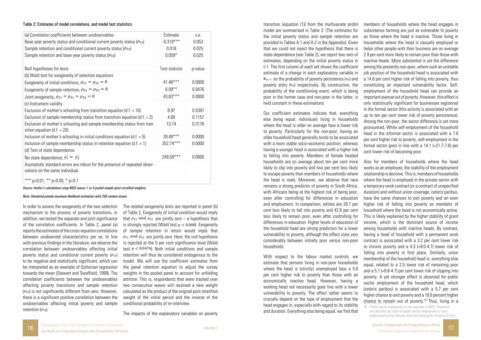
116Proceedings of the Fifth Congress of African EconomistsLes Actes du Cinquième Congrès des Economistes Africains
Volume 1Growth, Employment and Inequalities in Africa
Croissance, Emploi et Inégalités en Afrique 117
Table 2: Estimates of model correlations, and model test statistics
(a) Correlation coefficients between unobservables Estimate s.e.Base year poverty status and conditional current poverty status ( ) -0.319*** 0.053Sample retention and conditional current poverty status ( ) 0.018 0.025Sample retention and base year poverty status ( ) 0.059* 0.025
Null hypotheses for tests Test statistic p-value(b) Wald test for exogeneity of selection equationsExogeneity of initial conditions, 41.48*** 0.0000
Exogeneity of sample retention, 6.09** 0.0476
Joint exogeneity, 43.83*** 0.0000(c) Instrument validity Exclusion of mother’s schooling from transition equation (d.f. = 10) 8.97 0.5397Exclusion of sample membership status from transition equation (d.f. = 2) 4.69 0.1157Exclusion of mother’s schooling and sample membership status from tran-sition equation (d.f. = 20)
13.74 0.3176
Inclusion of mother’s schooling in initial conditions equation (d.f. = 5) 28.49*** 0.0000Inclusion of sample membership status in retention equation (d.f. = 1) 352.74*** 0.0000(d) Test of state dependence
No state dependence, 249.59*** 0.0000
Asymptotic standard errors are robust for the presence of repeated obser-vations on the same individual.
*** p<0.01, ** p<0.05, * p<0.1Source: Author’s calculations using NIDS waves 1 to 4 pooled sample (post-stratified weights).
Note: Simulated pseudo maximum likelihood estimation with 250 random draws.
The related exogeneity tests are reported in panel (b) of Table 2. Exogeneity of initial condition would imply that are jointly zero – a hypothesis that is strongly rejected (Wald test ). Exogeneity of sample retention in return would imply that
are jointly zero. Here, the null hypothesis is rejected at the 5 per cent significance level (Wald test ). Both initial conditions and sample retention will thus be considered endogenous to the model. We will use the coefficient estimates from the panel retention equation to adjust the survey weights in the pooled panel to account for unfolding attrition. This is, respondents that were tracked over two consecutive waves will received a new weight calculated as the product of the original post-stratified weight of the initial period and the inverse of the conditional probability of re-interview.
The impacts of the explanatory variables on poverty
In order to assess the exogeneity of the two selection mechanism to the process of poverty transitions, in addition, we tested the separate and joint significance of the correlation coefficients. In Table 2, panel (a) reports the estimates of the cross-equation correlations between unobserved characteristics per se. In line with previous findings in the literature, we observe the correlation between unobservables affecting initial poverty status and conditional current poverty ( ) to be negative and statistically significant, which can be interpreted as an example of Galtonian regression towards the mean (Stewart and Swaffield, 1999). The correlation coefficients between the unobservables affecting poverty transitions and sample retention ( ) is not significantly different from zero. However, there is a significant positive correlation between the unobservables affecting initial poverty and sample retention ( ).
transition (equation (1)) from the multivariate probit model are summarised in Table 3. (The estimates for the initial poverty status and sample retention are provided in Tables A.1 and A.2 in the Appendix). Given that we could not reject the hypothesis that there is state-dependence (see Table 2), we report two sets of estimates, depending on the initial poverty status in t-1. The first column of each set shows the coefficient estimate of a change in each explanatory variable in
on the probability of poverty persistence ( ) and poverty entry ( ) respectively. By construction, the probability of the conditioning event, which is being poor in the former case and non-poor in the latter, is held constant in these estimations.
Our coefficient estimates indicate that, everything else being equal, individuals living in households where the head is older on average face a lower risk to poverty. Particularly for the non-poor, having an older household head generally tends to be associated with a more stable socio-economic position, whereas having a younger head is associated with a higher risk to falling into poverty. Members of female headed households are on average about ten per cent more likely to slip into poverty and two per cent less likely to escape poverty than members of households where the head is male. Moreover, we observe that race remains a strong predictor of poverty in South Africa, with Africans being at the highest risk of being poor, even after controlling for differences in education and employment. In comparison, whites are 28.7 per cent less likely to fall into poverty and 42.6 per cent less likely to remain poor, even after controlling for differences in education. Higher levels of education of the household head are strong predictors for a lower vulnerability to poverty, although the effect sizes vary considerably between initially poor versus non-poor households.
With respect to the labour market controls, we estimate that persons living in non-poor households where the head is (strictly) unemployed face a 5.6 per cent higher risk to poverty than those with an economically inactive head. However, having a working head not necessarily goes line with a lower vulnerability to poverty. The effect rather seems to crucially depend on the type of employment that the head engages in, especially with regard to its stability and duration. Everything else being equal, we find that
members of households where the head engages in subsistence farming are just as vulnerable to poverty as those where the head is inactive. Those living in households where the head is casually employed or helps other people with their business are on average 2.9 per cent more likely to remain poor than those with inactive heads. More substantial is yet the difference among the presently non-poor, where such an unstable job position of the household head is associated with a 14.8 per cent higher risk of falling into poverty, thus constituting an important vulnerability factor. Self-employment of the household head can provide an important avenue out of poverty. However, this effect is only statistically significant for businesses registered in the formal sector (this activity is associated with an up to ten per cent lower risk of poverty persistence). Among the non-poor, the sector difference is yet more pronounced. While self-employment of the household head in the informal sector is associated with a 7.6 per cent higher risk to poverty, self-employment in the formal sector goes in line with a 14.1 (=21.7-7.6) per cent lower risk of becoming poor.
Also for members of households where the head works as an employee, the stability of the employment relationship is decisive. This is, members of households where the head is employed in the private sector with a temporary work contract (or a contract of unspecified duration) and without union coverage, ceteris paribus, have the same chances to exit poverty and an even higher risk of falling into poverty as members of household where the head is not economically active. This is likely explained by the higher stability of grant income, which is the dominant source of income among households with inactive heads. By contrast, having a head of household with a permanent work contract is associated with a 3.2 per cent lower risk to chronic poverty and a 4.3 (=9.0-4.7) lower risk of falling into poverty in first place. Similarly, union membership of the household head is, everything else equal, related to a 2.5 lower risk of remaining poor and a 5.1 (=9.8-4.7) per cent lower risk of slipping into poverty. A yet stronger effect is observed for public sector employment of the household head, which (ceteris paribus) is associated with a 5.7 per cent higher chance to exit poverty and a 10.6 percent higher chance to remain out of poverty.70 Thus, living in a 70 Public sector employment is not reported in NIDS. Therefore,
we calculate the share of public sector employment in total employment at the industry level (we distinguish 10 sectors) from

118Proceedings of the Fifth Congress of African EconomistsLes Actes du Cinquième Congrès des Economistes Africains
Volume 1Growth, Employment and Inequalities in Africa
Croissance, Emploi et Inégalités en Afrique 119
household where the head has a permanent job in the public sector with union coverage, would on average be associated with an 11.2 per cent lower risk to remain persistently poor and a 20.1 per cent lower risk of falling into poverty. This effect is likely explained by both higher wages and higher job security.
With respect to the household composition, as one may expect, larger households generally face a higher risk to poverty and particularly the presence of economically dependent household members goes in line with an elevated vulnerability to poverty. Among the non-poor, adding an additional member to the household is on average associated with a 3.7 per cent higher risk of falling into poverty. There is no statistically significant difference with respected to whether the additional household member is below 18 years old (eligibility threshold for child support grant) or a dependent member in working age. Among the poor, by contrast, large households with a high number of children are the most likely to remain chronically poor. This observation underscores the importance that child support programs have in South Africa.
Holding the household size, the number of employed household members has an important vulnerability reducing effect. Everything else equal, each household member who is working (excluding the household head, whose employment status has been assessed in detail above) goes in line with a 2.1 per cent lower average risk to remain poor and a 5.8 per cent lower average risk of falling into poverty. Given this difference in effect, in addition to the explanations suggested earlier, we may imagine that being poor can bring difficulties in finding good quality jobs, for example through social network effects, reducing in turn the probability of exiting poverty.
Despite the presence of a large and comparatively generous social pension program (with maximum benefits of R1500 a month), we find that an increase in the number of elderly household members, everything else equal, comes with a 5.7 per cent higher risk of falling into poor, but has a negligible effect on the likelihood of poverty persistence. We assume this result to be primarily driven by changes in the household composition and composition of income sources that tend to occur between periods and .
the Quarterly Labour Force Surveys (QLFS) by sub-period (2008, 2010/11, 2012, 2014/15) and use this as a proxy in the regression.
Households with a larger share of elderly members may be more likely to experience a loss in labour market income due to the retirement of respective members. Furthermore, some evidence suggests that household formation responses may play an important role. State transfers (particularly non-contributory old age pensions) tend to take on the function of a private safety net in South Africa, and may attract additional dependents to the households (Klasen and Woolard, 2009). However, more research would be needed to fully understand the mechanisms behind this result and particularly the differences observed between poor and non-poor households.
Table 3: Multivariate probit model: Poverty transitionsProbability of being poor in t conditional on poverty status in t-1
Poverty persistence Poverty entry
Average
Marginal Effect
Coeff.
Estimates.e.
Average Marginal
Effect
Coeff.
Estimates.e.
Characteristics of the household head (HoH) in t-1HoH age 0.001 0.006 (0.004) -0.005 -0.018** (0.008)HoH age squared (x0.01) -0.002 -0.009** (0.004) 0.000 -0.001 (0.008)HoH is female 0.017 0.070*** (0.024) 0.095 0.330*** (0.041)HoH race group (base: African)
Coloured -0.005 -0.022 (0.053) -0.121 -0.411*** (0.064)Asian/Indian -0.407 -1.278*** (0.153) -0.293 -1.144*** (0.116)White -0.426 -1.336*** (0.279) -0.287 -1.109*** (0.107)
HoH education (base: no schooling) Less than primary completed 0.011 0.050 (0.032) -0.110 -0.356*** (0.088)Primary completed 0.023 0.102** (0.044) -0.128 -0.415*** (0.096)Secondary not completed -0.027 -0.113*** (0.034) -0.202 -0.656*** (0.085)Secondary completed -0.067 -0.265*** (0.051) -0.288 -0.952*** (0.101)Tertiary -0.215 -0.752*** (0.078) -0.340 -1.147*** (0.107)
HoH employment status (base: inactive)Unemployed (discouraged) 0.021 0.094 (0.059) -0.066 -0.233** (0.110)Unemployed (strict) 0.002 0.007 (0.039) 0.056 0.194** (0.079)Subsistence farmer 0.010 0.045 (0.064) 0.003 0.010 (0.149)Casual worker/ helping others 0.029 0.127** (0.061) 0.148 0.511*** (0.181)Self-employed -0.021 -0.087 (0.054) 0.076 0.262*** (0.079)
Self-employed # Formala -0.066 -0.322* (0.174) -0.217 -0.493*** (0.134)Employee 0.000 0.001 (0.041) 0.047 0.161** (0.069)
Employee # Permanent contract -0.032 -0.128** (0.052) -0.090 -0.150** (0.061)Employee # Union member -0.025 -0.101* (0.062) -0.098 -0.178*** (0.057)Employee # Share public sectorb -0.057 -0.225** (0.093) -0.153 -0.372*** (0.093)
Characteristics of the household (HH) in t-1Composition of the HH
No. of HH members 0.007 0.027*** (0.008) 0.037 0.125*** (0.020)
No. of employed members (excl. HoH) -0.021 -0.087*** (0.015) -0.058 -0.208*** (0.029)
No. of children (<18 years) 0.024 0.099*** (0.011) 0.005 0.016 (0.025)No. of elderly members (60+ years) -0.002 -0.007 (0.021) 0.057 0.200*** (0.037)
HH has access to basic goods and services (shelter/water/sanitation/electricity)
-0.040 -0.165*** (0.032) -0.027 -0.095** (0.046)
Geographic location (base: traditional) c Urban -0.006 -0.026 (0.032) -0.058 -0.198*** (0.055)Farms 0.031 0.138*** (0.048) 0.060 0.205** (0.091)
Constant 0.825*** (0.123) 0.923*** (0.205)Province fixed effects YES YESTime fixed effects YES YESLog-likelihood -97,980,000Model chi2 (d.f.=174) 23,842Number of observations 67,117Asymptotic standard errors are robust for the presence of repeated observations on the same individual.
*** p<0.01, ** p<0.05, * p<0.1

120Proceedings of the Fifth Congress of African EconomistsLes Actes du Cinquième Congrès des Economistes Africains
Volume 1Growth, Employment and Inequalities in Africa
Croissance, Emploi et Inégalités en Afrique 121
equal, initially poor (non-poor) had a lower (higher) poverty propensity, indicating some regression towards the mean. Put simply, following an extreme random event, the next random event may likely be expected to be less extreme.
Predicted poverty transition probabilities and class thresholds
We use the estimates from the presented endogenous switching model to predict poverty exit and entry probabilities of initially poor versus non-poor individuals). These are evaluated against two probability thresholds, displayed in Table 4 panel (a), based on the actual observed rates of poverty exit and entry in our data. We observe that, on average, 16.52 per cent of the initially poor escaped poverty from one wave to the next in the pooled sample. This is set as the cut-off point separating the chronically poor from the transient poor. Analogously, we observe that the average probability of falling into poverty for those who were initially non-poor was 25.91 per cent in our pooled sample. This is set as the cut-off point separating vulnerable from the middle class.71
For comparative purposes, we also give an indication of the monetary thresholds associated with these probability cut-off points. We calculate the average monthly per capita household expenditure of those respondents with a predicted poverty transition probability that falls within the 95-per cent confidence interval of the respective probability threshold. We find that the average probability of exiting poverty is associated with a monetary threshold of R543 per person per month, which falls between StatsSA’s food poverty line (R441) and the lower bound poverty line (R647) (in January 2015 prices). The average probability of entering poverty is associated with a monetary threshold of R2,590 per person per month. Thus, on average, respondents living in households with expenditure levels above this threshold could be considered reasonably secure against falling into poverty.
71 Note the slight difference to the transition probabilities reported in Table 1, which arises from the use of attrition adjusted weights based on the results from the retention equation (see p.12 details).
Source: Author’s calculations using NIDS waves 1 to 4 pooled sample (post-stratified weights).
Notes: Simulated pseudo maximum likelihood estimation with 250
random draws.
a For self-employed, formal businesses are registered for income tax &/or VAT.
b The average share of public sector employment by industry and survey year has been calculated from the 2008, 2010/11, 2012, and 2014/2015 Quarterly Labour Force Surveys.
c In line with the 2011 census, three settlement types are distinguished in NIDS:
1. Urban - A continuously built-up area that is established through cities, towns, ‘townships’, small towns, and hamlets.
2. Traditional - Communally-owned land under the jurisdiction of traditional leaders. Settlements within these areas are villages.
3. Farms - Land allocated for and used for commercial farming including the structures and infrastructure on it. Those parts of the country falling under the jurisdiction of traditional authorities (or traditional chiefs) are considered as rural, mainly due to their lack of infrastructure due to past legacy.
In terms of geographic patterns, having access to basic services is associated with a four per cent lower risk to chronic poverty and 2.7 per cent lower risk to become poor. Despite many efforts to address the past, the spatial patterns of segregation remain visible in post-apartheid South Africa. For the initially non-poor, the risk to falling into poverty is about 5.8 per cent lower in urban than in the “deep rural” or “traditional” areas of the country, comprising traditional villages and communally-owned land, which includes those areas where the former “homelands” were located. The chances to escape poverty, however, are not significantly different between regions.
While the effects for most of the explanatory variables point into the same direction for both sets of estimates, the size of the effect on the poverty propensities differs importantly, depending on whether the individual was already poor in the initial period or not (a test of whether the two sets of coefficients are identical can be rejected at all common significance levels, compare Table 2). The results reported in Table 3 suggest that one of the channels through which a past poverty experience seems to increase the risk to future poverty is the depreciation of human capital, as well as potential signalling effects – in the sense that employers may consider past experiences of (long-term) unemployment as negative signals in a recruitment process with respect to the applicant’s capacity or productivity – and the potential acceptance of low quality job offers that may be associated with future unemployment spells. Yet, everything else
Table 4: Probability thresholds and associated monetary thresholds
(a) Probability threshold (%) (b) Associated monetary threshold
Mean Std. Err.[95% Conf.
Int.] Mean Std. Err.[95% Conf.
Int.]Average probability of EXITING poverty for those who were poor in the last period
16.52 0.16 16.21 16.84 543 6 532 555
Average probability of FALLING into poverty for those who were non-poor in the last pe-riod
25.91 0.36 25.21 26.61 2,590 85 2,422 2,757
Source: Author’s calculations using NIDS waves 1 to 4 pooled sample (post-stratified weights corrected for panel attrition).
Note: Poverty transition probabilities are predicted using parameter estimates from our regression model. The associated monetary thresholds are calculated as the average per capita household expenditure of those falling into the 95% confidence interval around the respective probability threshold. All monetary values are expressed in January 2015 Rands.
Using these monetary thresholds as cut-off points however would mask a substantial degree of variation in the predicted poverty transition probabilities among individuals living in households with similar current expenditure levels, as Table 5 illustrates. Although the transient poor tend on average to be better off than the chronically poor, members of both groups can be found anywhere below the poverty line, spanning the full range. Similarly, while the middle class is on average better off than the vulnerable, members of both groups can be located anywhere between the poverty line and the elite cut-off fixed at R10,484 per person per month.
Table 5: Monthly household expenditure per person by social class, 2008 to 2014/15
Min Max Median Mean [95% Conf. Interval]
Chronic Poor 29 992 342 390 388 391Transient Poor 24 991 617 617 613 620Vulnerable 992 10,418 1,586 2,045 2,024 2,066Middle class 993 10,470 3,319 3,987 3,946 4,029Elite 10,488 131,514 15,347 19,251 18,693 19,809
Source: Author’s calculations using NIDS waves 1 to 4 pooled sample (post-stratified weights corrected for panel attrition).
Note: All monetary values are expressed in January 2015 Rands.
In consequence, by applying a monetary threshold to distinguish those who are non-poor but vulnerable from those who are stably middle class, we would risk making two misclassification errors. First, there may be households that fall below the vulnerability thresholds, but have access to a relatively secure income flow, which will help them to sustain their living standard over time. As Table 6 illustrates, almost one in four out of ten individuals who would be classified as vulnerable by their income position, we would classify as middle class given their household characteristics. Second, there may be households for which we observe a current consumption level above the vulnerability threshold, potentially in reaction to some type of shock, but which face an elevated risk to poverty and will likely not be able to sustain their current living standard over time. This applies to two out of ten individuals who would be classified as middle class by their income position, but who we would consider to be vulnerable given their household characteristics. The same logic applies to the distinction between chronic versus transient poverty. For about one out of ten individuals with per capita household expenditures of less than R543 we would predict above average chances to exit poverty, while five out of ten individuals with expenditures above that threshold we would see at an above average risk to remain poor in the future.

122Proceedings of the Fifth Congress of African EconomistsLes Actes du Cinquième Congrès des Economistes Africains
Volume 1Growth, Employment and Inequalities in Africa
Croissance, Emploi et Inégalités en Afrique 123
Table 6: Classes identified by poverty propensity versus monetary thresholds, 2008 to 2014/15
Pooled Sample Probability Threshold
(two consecutive waves)
Chronic Transient VulnerableMiddle Class
Elite Total
Mon
etar
y
Chronic poor 88.72 11.28 0 0 0 100Transitory poor 58.39 41.61 0 0 0 100Vulnerable 0 0 60.44 39.56 0 100Middle class 0 0 18.53 81.47 0 100Elite 0 0 0 0 100 100Total 49.44 12.80 14.37 19.69 3.70 100
Source: Author’s calculations using NIDS waves 1 to 4 pooled sample (post-stratified weights corrected for panel attrition).
In Table 7 we compare the relative size of the five social classes, when using probability thresholds as opposed to monetary thresholds to distinguish the class sublayers. We observe that the middle class, which we identify using the latent poverty propensity, is about five percentage points larger (and the group of the vulnerable accordingly five smaller) than when a monetary threshold was applied. This is, by using a monetary threshold to identify the middle class, we risk missing out on a non-negligible share of the population, who falls below that threshold by still is relatively secure against falling into poverty. Despite the identified middle class being larger, on average, only 9.5 per cent (as compared to 9.7 per cent) fell below the poverty line within a two-year time horizon. In particular, by directly basing the classification on
the latent poverty propensity scores, we are better able to identify those with an elevated risk to poverty than by relying on monetary measures alone. Almost every second person who we classify as vulnerable actually fell into poverty within two-years’ time.
Table 7 also shows that the extent of chronic or extreme poverty would have been underestimated if a monetary threshold had been used. About 80 per cent of the poor in South Africa, equivalent to about 50 per cent of the population, have an average chance of exiting poverty of about ten percent, while the transient poor share has an average chance to exit poverty of about 40 per cent.
Table 7: Average class size and mobility patterns by identification method, 2008 to 2014/15
Probability Thresholds Monetary Thresholds
Population
Share (%)
Share (%)
that fell into poverty
Share (%)
that moved out of poverty
Population
Share (%)
Share (%)
that fell into poverty
Share (%)
that moved out of poverty
Chronic Poor 49.44 .. 10.63 43.21 .. 10.53
Transient Poor 12.80 .. 40.28 19.03 .. 31.02Vulnerable 14.37 49.72 .. 19.24 40.24 ..Middle class 19.69 9.54 .. 14.82 9.72 ..Elite 3.70 2.80 .. 3.70 2.80 ..
Source: Author’s calculations using NIDS waves 1 to 4 pooled sample (post-stratified weights corrected for panel attrition).
Note: All monetary values are expressed in January 2015 Rands.
Table 8 further illustrates the higher stability of the middle class that we identify using latent poverty propensity scores. We observe that using this approach, on average, about 71 per cent of those that the classify as middle class in one survey wave would still be classified as middle class two years later, while 12.1 had entered the group of the vulnerable. When a monetary boundary was applied, only 56.2 per cent of all middle class individuals would still enter this categorisation two years later, while 25 per cent had fallen below the vulnerability threshold.
Table 8: Stability of the middle class by identification method, 2008 to 2014/15Pooled Sample(two consecutive waves) Chronic Transient Vulnerable
Middle Class Elite Total
Middle class
(Probability Threshold)
2.15 7.39 12.11 70.95 7.40 100
Middle class
(Monetary Threshold)
4.06 5.65 25.02 56.20 9.07 100
Source: Author’s calculations using NIDS waves 1 to 4 pooled sample (post-stratified weights corrected for panel attrition).
from equation (10) and base year characteristics (the estimation results are reported in Table A.3 of the Appendix).
Third, using the same predictor variables as in the probability model, we fit a linear regression model to estimate a cross-sectional income equation (using expenditure as a proxy for permanent income) for the base year at the household level as:
(11)
where is the household per capita income in logarithmic scale at .
For each individual we then predict the per capita income in associated to each probability, using the coefficient estimates from equation (11) and initial household characteristics. To derive the vulnerability threshold, following López-Calva and Ortiz-Juarez (2014), we calculate the predicted average per capita income level associated with a predicted poverty propensity of 10 per cent, which is considered to present the maximum acceptable risk to poverty to be identified as middle class (the estimation results are reported in Table A.4 of the Appendix). To reduce the sensitivity of the calculated threshold to the 10 per cent cut-off point, and to have enough observations to get a more robust estimate of the mean income level associated with this probability estimate, we calculate
Sensitivity analysis and comparison to alternative approaches
As indicated in the introduction, the approach presented in this paper, in order to identify a South African middle class that is acceptably secure against falling into poverty, expands an approach that was pioneered by López-Calva and Ortiz-Juarez (2014). For comparative purposes, we replicate their approach here.72 We use a simple probit model to regress the poverty status at time against the same set of household-level characteristics observed at time but without distinguishing between initially poor versus non-poor households and without controlling for sample attrition. This is, only a single parameter vector, , will be estimated as:
and (10)
where the error term follows a standard normal distribution and denotes an indicator function which takes on the value of one if the corresponding latent variable exceeds some observed threshold (which can be set equal to zero without loss of generality), and zero otherwise. In a second step, for each individual we predict the probability of being poor in period based on the coefficient estimates 72 Note that this has been done before by Zizzamia et al. (2016),
though using a different poverty line and a different set of regressor variables and using only the first and the last waves of NIDS.

124Proceedings of the Fifth Congress of African EconomistsLes Actes du Cinquième Congrès des Economistes Africains
Volume 1Growth, Employment and Inequalities in Africa
Croissance, Emploi et Inégalités en Afrique 125
the vulnerability threshold as the mean predicted per capita income in for all individuals with a predicted poverty propensity in of 8 to 12 per cent.73 It may be worthwhile to note that by translating the ten per cent probability threshold to a monetary threshold, rather than directly working with the predicted poverty propensities, the approach will suffer from the same misclassification errors as outlined above. This is, some of those identified as middle class by their income level will face a predicted risk to poverty that exceeds the ten per cent cut-off point, and some of those classified as vulnerable will face a predicted risk to poverty of less than ten per cent.
Applying their approach to two waves of panel data from three Latin American countries (Chile, Mexico and Peru), López-Calva and Ortiz-Juarez’s (2014) find that a minimum income level of $10 a day (at purchasing power parities (PPP) at 2005 prices) is required to face a maximum risk to falling into poverty of ten per cent. This would translate to a monthly threshold of R2,657 in January 2015 prices if the 2011 PPP rate (5.07 Rand per Int. $) is applied (R2,397 if the 2005 PPP rate was applied). Replicating their approach for the South African context using the same explanatory variables as in the regression framework above, we estimate a monetary threshold for being middle class of R2,670, which is surprisingly close to the original thresholds suggested by López-Calva and Ortiz-Juarez (2014).74
However, a somewhat lower threshold of R2,409 is obtained once control variables for changes in the household size and changes in the number of employed household members from to are added to the regression, as done in the original paper.75
Using these monetary thresholds, the size of the middle class ranges between 14.4 and 16 per cent, as compared to 19.7 per cent using the approach presented in this paper. The share of the group of the vulnerable
73 The derived vulnerability threshold is relatively robust to the choice of the ±2 percentage-points probability interval around the 10-percent cut-off point and similar thresholds are obtained when using narrower bands.
74 The threshold is also quite close to the average income level that we observe at the probability threshold defined in this paper (R2,590). However, note that we are looking at actual income levels, whereas the approach suggested by López-Calva and Ortiz-Juarez (2014) looks at predicted income. The actual observed income for those with a predicted poverty propensity of 8 to 12 per cent using the simple probit model would have been R3,983.
75 We would caution against the use of these variables due to potential endogeneity concerns (all variables in the regression should be pre-determined).
in return is larger, ranging between 18.1 and 19.6 per cent, as compared to 14.4 per cent suggested by us (see Table 9). As explained above, this difference by approximately five percentage points primarily results from our model’s ability to identify households whose household characteristics enable them to maintain a level of economic stability, despite the fact that their observed consumption level falls below the R2,670 or R2,409 cut-off.
Table 9: Average class size by identification method, 2008 to 2014/15
Multivariate Probit
Simple probit
Simple probit with
change variables
Monetary threshold for being middle class
Probability Threshold
R2,670 R2,409
Poor 62.24 62.24 62.24Vulnerable 14.37 19.62 18.11Middle class 19.69 14.44 15.95Elite 3.70 3.70 3.70Total 100 100 100
Source: Author’s calculations using NIDS waves 1 to 4 pooled sample (post-stratified weights corrected for panel attrition).
Note: All monetary values are expressed in January 2015 Rands.
As a useful way of exploring how consequential the classificatory mismatch between the approaches is, in Table 10 we look at the share that feel into poverty (UBPL) and extreme poverty (FPL) out of the respectively identified vulnerable group and middle class. We observe that both our approach and the one by López-Calva and Ortiz-Juarez (2014) perform similarly well in terms of identifying a middle class which is fairly secure against falling into poverty. For both approaches, the middle class which is identified faces an average risk of about ten per cent to fall into poverty over time. It is worth noting that this similarity holds despite the larger size of the middle class that we identify. This middle class furthermore faces only half the risk of falling into extreme poverty (below the FPL), as compared to the middle class that would have been identified using conventional methods. In return, the vulnerable group that we identify faces an about ten percentage points higher risk of falling below the
UBPL, and an almost five percentage points higher risk to falling below the FPL, as compared to the one that would have been identified using the standard vulnerability approach.
Table 10: Average risk of falling into poverty by identification method, 2008 to 2014/15
Probability ThresholdMonetary Threshold
(R2,670)Monetary Threshold
(R2,409)
Poor UBPL
(R992)Poor FPL (R441)
Poor UBPL (R992)
Poor FPL (R441)
Poor UBPL (R992)
Poor FPL (R441)
t – 1
Vulnerable 49.72 17.86 40.21 13.20 41.40 13.45
Middle class
9.54 1.36 8.87 2.16 10.35 2.90
Source: Author’s calculations using NIDS waves 1 to 4 pooled sample (post-stratified weights corrected for panel attrition).
Class formations, social inequality and mobility in South AfricaIn this section, we provide a profile of the five identified social strata in South Africa – the chronically poor, the transient poor, the vulnerable, the middle class, and the elite – in terms of their relative size, growth performance, racial composition, and labour market resources.
Class characteristics and inequality patterns
As Figure 2 illustrates, we find that according to the suggested stratification schema, on average, about one in four (24 per cent) South Africans could be classified as stably middle class or elite between 2008 and 2014/15. Their combined share has remained relatively stable over this period. In addition, about 14 per cent of the population fell into the group of the vulnerable between 2008 and 2014/15. That is, a substantial share of the non-poor was still facing a considerable risk to falling into poverty. On the other hand, among the poor, about 80 per cent could be considered chronically poor (comprising half of the South African population), whereas the remaining 20 per cent (accounting for 13 per cent of the population between 2008 and 2014/15) could be classified as transient poor. The poverty reducing trend between 2012 and 2014/15 and associated growth in the share
of the vulnerable (and to a lesser extent the middle class) might in part be explained by changes in the NIDS sample (as explained in Section 3.2 above), and should therefore be interpreted with caution.
Figure 2: Class sizes, 2008 to 2014/15
Source: Author’s calculations using NIDS waves 1 to 4 pooled sample (post-stratified weights corrected for panel attrition).
0%
20%
40%
60%
80%
100%
2008 2010/11 2012 2014/15
Elite
Middle class
Vulnerable
Transient Poor
Chronic Poor
Source: Author’s calculations using NIDS waves 1 to 4 pooled sample
(post-stratified weights corrected for panel attrition).
Table 9 and Table 10 provide an overview of the key average characteristics of the household in general and the household head in particular among the five social classes. By construction, the characteristics closely mirror the determinants of poverty transitions reported in Table 3 above.
In terms of the household composition, an important observation from Table 9 is that larger households not only face a higher risk to experience a poverty spell, but poverty also tends to be more persistent.76 Specifically, those classified as chronically poor live in households that on average count seven members, which is about twice the size compared to those in the middle class. Of the seven members, about half (3.5) are below age 18 and three are below age 15. 76 This finding resonates with previous studies that exposed the
presence of dependants as an important risk factor of poverty entrance and poverty persistence (Finn and Leibbrandt, 2016; Woolard and Klasen, 2005).

126Proceedings of the Fifth Congress of African EconomistsLes Actes du Cinquième Congrès des Economistes Africains
Volume 1Growth, Employment and Inequalities in Africa
Croissance, Emploi et Inégalités en Afrique 127
Accordingly, we observe that poverty in general and chronic poverty in particular over-proportionally affects children in South Africa. About three out of four children (74.6 per cent) below age 15 live in poverty, with about two in three (64.9 per cent) growing up in a situation of persistent poverty. By contrast, only 14 per cent of all children below 15 years can be classified as stably middle class or elite. This is particularly worrisome as it has been shown that being raised in poverty places children at a higher risk for a number of factors – ranging from inadequate nutrition over decreased cognitive stimulation to violent crime and abuse – which can hamper the cognitive, social, and emotional development of the child and increase the risk to poverty in adulthood (Brooks-Gunn and Duncan, 1997).
In Table 9 we furthermore observe that most households, independent of their size, rely on a
single-income earner. The working poor thus not only have to take care of an importantly higher number of dependents, but average labour market earnings are also much lower. In return, poverty tends to be a more temporary phenomenon for those with access to (higher) earnings from the labour market. The close similarity between the transient poor and the vulnerable is striking both in terms of household composition and composition of income sources available to the household. Consistent with the existing literature, we moreover find that the middle class is the class that most heavily relies on the labour market for its welfare. Labour market income makes up 84.2 per cent of total household income in the middle class and 87.7 per cent of all individuals in the middle class live in households for which labour market earnings constitute the main source of income.
Table 9: Average household (HH) characteristics by social class, 2008 to 2014/15
Chronic
Poor
Transient
PoorVulnerable
Middle
ClassElite Total
Weighted share of respondents 49.4% 12.8% 14.4% 19.7% 3.7% 100%- As percentage of poor 79.4% 20.6% n.a. n.a. n.a. n.a.
Weighted share of respondents under 15 years old
64.9% 9.7% 11.4% 12.7% 1.3% 100%
Mean household expenditure per capita 390 617 2,045 3,987 19,251 2,063Median household expenditure per capita 342 617 1,586 3,319 15,347 658No. of members in HH 7.0 4.3 3.9 3.4 2.7 5.3No. of workers in HH 0.9 1.3 1.1 1.5 1.2 1.1Age composition
No. of children (<18 years) 3.5 1.4 1.5 1.1 0.5 2.3No. of members in working age (18-60
years) 3.1 2.7 2.2 2.1 1.8 2.7No. of elderly members (60+ years) 0.4 0.3 0.3 0.3 0.3 0.4
Income by source a Share of income derived from source
Labour 37.0% 68.0% 68.8% 84.2% 81.6% 56.6%Government grants 54.0% 25.1% 19.4% 6.5% 1.9% 33.9%Remittances 6.4% 5.4% 8.5% 2.9% 1.7% 5.7%Subsistence agriculture 0.9% 0.2% 0.4% 0.1% 0.1% 0.5%Investments 1.7% 1.3% 3.0% 6.3% 14.7% 3.3%
Mean income from source (if non-zero) Labour 3,414 5,237 6,887 16,091 38,347 3,414Government grants 1,688 1,240 1,195 1,486 1,326 1,688Remittances 1,357 1,055 1,811 1,966 16,249 1,357Subsistence agriculture 208 169 476 829 1,367 208Investments 1,684 1,446 2,989 11,395 17,008 1,684
Access to services House, cluster, town house 60.0% 74.2% 68.2% 79.7% 88.4% 67.9%Tap water in house/on plot 58.7% 87.8% 83.1% 97.4% 98.1% 75.0%Flush toilet in/outside house 31.6% 75.2% 66.9% 95.3% 97.9% 57.3%Access to electricity 76.8% 88.2% 88.4% 96.4% 97.3% 84.6%HH has access to basic goods and services (shelter/water/sanitation/electricity)
20.0% 57.4% 44.5% 74.7% 84.5% 41.4%
Geographic location b Traditional 55.8% 16.8% 26.5% 4.6% 3.0% 34.6%Urban 39.4% 78.2% 67.9% 91.7% 95.2% 60.8%Farms 4.8% 5.0% 5.5% 3.7% 1.8% 4.6%
Source: Author’s calculations using NIDS waves 1 to 4 pooled sample (post-stratified weights corrected for panel attrition).
Notes: All monetary values are expressed in January 2015 Rands.

128Proceedings of the Fifth Congress of African EconomistsLes Actes du Cinquième Congrès des Economistes Africains
Volume 1Growth, Employment and Inequalities in Africa
Croissance, Emploi et Inégalités en Afrique 129
a Imputes rental income has been excluded. Government grants include i) State old age pension, ii) Disability, iii) Child Support, iv) Foster Care, and v) Care dependency grant. Other income from government includes i) Unemployment Insurance Fund and ii) Workmen’s compensation. Investment Income includes i) Interest/dividend income, ii) Rental income, and iii) Private pensions and annuities.
b In line with the 2011 census, three settlement types are distinguished in NIDS:
1. Urban - A continuously built-up area that is established through cities, towns, ‘townships’, small towns, and hamlets.
2. Traditional - Communally-owned land under the jurisdiction of traditional leaders. Settlements within these areas are villages.
3. Farms - Land allocated for and used for commercial farming including the structures and infrastructure on it.
Those parts of the country falling under the jurisdiction of traditional authorities (or traditional chiefs) are considered as rural, mainly due to their lack of infrastructure due to past legacy.
Interestingly, in absolute terms, income from government grants is fairly stable across all five classes, being highest among the chronic poor, at R1,688 (though this income is shared among substantially larger households) and, strikingly, lowest among the vulnerable, at R1,240 (see Table 9). While fairly constant in absolute terms (probably because of very broad access to old age pensions), the relative importance of social grants in the lives of the poor evidently remains very significant. Specifically, the chronic poor derive more than half (54 per cent) of their income from government grants. By comparison, grant makes up one fourth (25.1 per cent) of the income of the transient poor and one fifth (19.4 per cent) of the income of the vulnerable. In the middle class, 6.5 per cent of total household income is derived from grants (see Table 9).
A key difference between the chronic poor and the transient poor seems to lie in their geographic location. While 55.8 per cent of South Africans classified as chronically poor reside in traditional areas, the same applies to only 16.8 per cent of those in the transient poor class. Similarly, 26.5 of those in the vulnerable group live in traditional areas, as compared to 4.6 per cent of those among the middle class. Relatedly, we observe that the chronic poor are the most deprived in terms of their access to basic goods and services. As reported in Table 9, only one out of five members of the chronic poor class had access to electricity, flowing water, a flushable toilet and formal housing, as compared to three out of five among the transient poor and three out of four among the middle class.
As Figure 3 displays, among South Africa’s nine provinces, KwaZulu-Natal has the highest incidence of chronic poverty and the second smallest middle class (after Limpopo). At the same time, however, KwaZulu-Natal also has the fourth largest elite (after Gauteng, the Western Cape, and Mpumalanga), indicating a substantial degree of local social inequality. Chronic poverty is lowest in the Western Cape and in Gauteng – which are also the two provinces with the strongest middle class and elite. While vulnerability is substantial in all provinces, including those provinces with low levels of chronic poverty, we observe a negative relationship between the extent of chronic and transient poverty across the provinces (see Figure 3).
Figure 3: Geographic split of South Africa’s five social classes, 2008 to 2014/15
0%
20%
40%
60%
80%
100%
Elite
Middle Class
Vulnerable
Transient Poor
Chronic Poor
Source: Authors’ calculations using NIDS waves 1 to 4 pooled sample (post-stratified weights).
Table 10 explores the average characteristics of the head of household by social class. With 42 years, household heads in the vulnerable class tend to be younger than those in the other classes, which may be associated with a less stable position in the labour market. With 50 years, household heads tend to be oldest among those living in chronic poverty. This may link to processes of household formation, where adult children or grandchildren co-reside with (grant-)parents that receive the old-age pension, thus forming larger, intergenerational households (see Klasen and Woolard, 2009).
Furthermore, seven out of ten chronically poor individuals live in households where the household head is female, as compared to five to six out of ten among the transient poor and vulnerable classes, and three out of ten among the middle class and elite. This reflects the higher incidence of poverty and vulnerability to poverty among single mothers in South Africa.
Given that race tends to be a strong predictor of poverty in South Africa, it is unsurprising that the chronically poor group is almost exclusively made up by Africans and Coloureds. These two groups also constitute the vast majority of the transient poor and the vulnerable. However, coloureds seem to be more heavily concentrated amongst the transient poor (note that this lower chance to be persistently poor was not statistically significant in the regression results) and the stable middle class, facing lower risks of downward mobility. Although Africans also constitute the largest proportion of the middle class – with a growing trend in recent years illustrated in Figure 4 – their share among the two top groups remains far from demographic representivity. That is, while Africans make up about 80 per cent of the total population, in 2014/15 they made up just above 50 per cent of the middle class. On the other hand, while whites constitute a mere 10 per cent of the South African population, almost one in three members of the middle class and two in three members of the elite are white.
Figure 4: Racial composition of South Africa’s five social classes, 2008 and 2014/15
0%10%20%30%40%50%60%70%80%90%
100%
2008 2014 2008 2014 2008 2014 2008 2014 2008 2014
Chronic Poor Transient Poor Vulnerable Middle Class Elite
White
Asian/Indian
Coloured
African
Source: Authors’ calculations using NIDS waves 1 to 4 pooled sample (post-stratified weights).
As one may expect, Table 10 reveals a strong relationship between the educational attainment of household heads and the incidence and persistence of poverty (similar patterns are observed when looking at individual education levels). Given that higher levels of education tend to be accompanied by a lower risk to poverty, heads of chronically poor households are on average the least educated with no more than five years of primary education, while the transient poor and the vulnerable tend to have some secondary
education. A household head in the middle class generally has completed secondary schooling, while those in the elite tend to have some tertiary education.
There is also a clear differentiation between classes in terms of access to the labour market: The more disadvantaged the class that a household belongs to, the more likely it is that the household head is unemployed or economically inactive. Only 30.8 of household heads amongst the chronically poor are in employment, with the remainder being economically
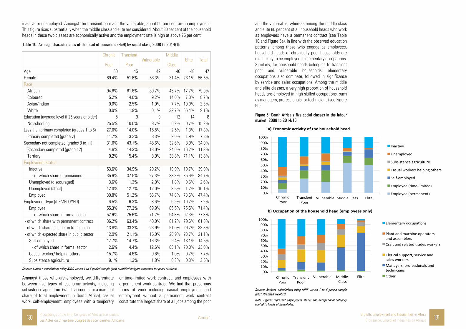
130Proceedings of the Fifth Congress of African EconomistsLes Actes du Cinquième Congrès des Economistes Africains
Volume 1Growth, Employment and Inequalities in Africa
Croissance, Emploi et Inégalités en Afrique 131
inactive or unemployed. Amongst the transient poor and the vulnerable, about 50 per cent are in employment. This figure rises substantially when the middle class and elite are considered. About 80 per cent of the household heads in these two classes are economically active and the employment rate is high at above 75 per cent.
Table 10: Average characteristics of the head of household (HoH) by social class, 2008 to 2014/15
Chronic
Poor
Transient
PoorVulnerable
Middle
ClassElite Total
Age 50 45 42 46 48 47Female 69.4% 51.6% 58.3% 31.4% 28.1% 56.5%Race
African 94.8% 81.6% 89.7% 45.7% 17.7% 79.9%Coloured 5.2% 14.0% 9.2% 14.0% 7.0% 8.7%Asian/Indian 0.0% 2.5% 1.0% 7.7% 10.0% 2.3%White 0.0% 1.9% 0.1% 32.7% 65.4% 9.1%
Education (average level if 25 years or older) 5 9 9 12 14 8No schooling 25.5% 10.0% 8.7% 0.2% 0.7% 15.2%
Less than primary completed (grades 1 to 6) 27.0% 14.0% 15.5% 2.5% 1.3% 17.8%Primary completed (grade 7) 11.7% 3.2% 8.3% 2.0% 1.9% 7.8%
Secondary not completed (grades 8 to 11) 31.0% 43.1% 45.6% 32.6% 8.9% 34.0%Secondary completed (grade 12) 4.6% 14.3% 13.0% 24.0% 16.2% 11.3%Tertiary 0.2% 15.4% 8.9% 38.8% 71.1% 13.8%
Employment status Inactive 53.6% 34.9% 29.2% 19.9% 19.7% 39.9% - of which share of pensioners 35.6% 37.5% 27.3% 33.3% 35.6% 34.7%
Unemployed (discouraged) 3.6% 1.3% 2.0% 1.8% 0.5% 2.6%Unemployed (strict) 12.0% 12.7% 12.0% 3.5% 1.2% 10.1%Employed 30.8% 51.2% 56.7% 74.8% 78.6% 47.4%
Employment type (if EMPLOYED) 6.5% 6.3% 8.6% 6.9% 10.2% 7.2%Employee 55.3% 77.3% 69.9% 85.5% 75.5% 71.4% - of which share in formal sector 52.6% 75.6% 71.2% 94.8% 92.3% 77.3%
- of which share with permanent contract 36.2% 63.4% 48.9% 81.2% 79.6% 61.8% - of which share member in trade union 13.8% 33.3% 23.9% 51.0% 29.7% 33.3% - of which expected share in public sector 12.9% 21.1% 15.0% 28.9% 23.7% 21.1%
Self-employed 17.7% 14.7% 16.3% 9.4% 18.1% 14.5% - of which share in formal sector 2.6% 14.4% 12.6% 63.1% 70.0% 23.0%
Casual worker/ helping others 15.7% 4.6% 9.6% 1.0% 0.7% 7.7%Subsistence agriculture 9.1% 1.3% 1.8% 0.3% 0.3% 3.5%
Source: Author’s calculations using NIDS waves 1 to 4 pooled sample (post-stratified weights corrected for panel attrition).
Amongst those who are employed, we differentiate between five types of economic activity, including subsistence agriculture (which accounts for a marginal share of total employment in South Africa), casual work, self-employment, employees with a temporary
or time-limited work contract, and employees with a permanent work contract. We find that precarious forms of work including casual employment and employment without a permanent work contract constitute the largest share of all jobs among the poor
and the vulnerable, whereas among the middle class and elite 80 per cent of all household heads who work as employees have a permanent contract (see Table 10 and Figure 5a). In line with the observed education patterns, among those who engage as employees, household heads of chronically poor households are most likely to be employed in elementary occupations. Similarly, for household heads belonging to transient poor and vulnerable households, elementary occupations also dominate, followed in significance by service and sales occupations. Among the middle and elite classes, a very high proportion of household heads are employed in high skilled occupations, such as managers, professionals, or technicians (see Figure 5b).
Figure 5: South Africa’s five social classes in the labour market, 2008 to 2014/15
a) Economic activity of the household head
b) Occupation of the household head (employees only)
0%10%20%30%40%50%60%70%80%90%
100%
ChronicPoor
TransientPoor
TransientPoor
Vulnerable Middle Class Elite
Inactive
Unemployed
Subsistence agriculture
Casual worker/ helping others
Self-employed
Employee (time-limited)
Employee (permanent)
0%10%20%30%40%50%60%70%80%90%
100%
Vulnerable Middle Class
Elite
Elementary occupations
Plant and machine operators,and assemblersCraft and related trades workers
Clerical support, service andsales workersManagers, professionals andtechniciansOtherChronic
Poor
Source: Authors’ calculations using NIDS waves 1 to 4 pooled sample (post-stratified weights).
Note: Figures represent employment status and occupational category limited to heads of households.

132Proceedings of the Fifth Congress of African EconomistsLes Actes du Cinquième Congrès des Economistes Africains
Volume 1Growth, Employment and Inequalities in Africa
Croissance, Emploi et Inégalités en Afrique 133
A dynamic perspective on the determinants of social class and inter-class transitions
The net changes in South Africa’s class structure reported above may mask a substantial degree of inter-class mobility. Tables 11 and 12 illustrate these mobility patterns.
In line with our classification schema, 80.5 per cent of those who were considered chronically poor remained poor from one survey wave to the other, 8.9 per cent improved their chances of exiting poverty and were considered transient poor, and only about one in ten individuals actually exited poverty. By contrast, approximately every fourth among the transient poor moved above the poverty line from one survey wave to the next. More than half the respondents in the vulnerable group slipped into poverty over time, with most of these seemingly falling into a trap of chronic
poverty. The middle class were largely stable, with about 71 per cent of all members maintaining their status over time. Of the less than 10 per cent who slipped below the poverty line, only a small fraction fell into a trap of chronic poverty. The elite was also largely stable at the top. In ten members of the elite, on average five were able to maintain their positions, while most of the rest entered the middle class. Very few of those among the elite fell into poverty or the vulnerable class. Table 12 also illustrates the importance of the overall macroeconomic framework in determining poverty risks. On average, more (less) respondents exited (fell into) poverty between 2012 and 2014/15 that in the years before between 2008 and 2012, which may partly be attributed the global economic crisis that hit South Africa in 2009/10.
Table 11: Movements across classes, 2008 to 2014/15
Pooled Sample wave t
(two consecutive waves) Chronic Transient VulnerableMiddle Class
Elite Total
wav
e t
-1
Chronic poor 80.46 8.91 8.97 1.53 0.14 100Transitory poor 23.57 36.15 23.44 16.46 0.37 100Vulnerable 29.43 20.28 31.8 17.23 1.25 100Middle class 2.15 7.39 12.11 70.95 7.4 100Elite 0.94 1.86 3.41 45.86 47.93 100Total 50.98 13.59 14.31 18.35 2.77 100
Source: Author’s calculations using NIDS waves 1 to 4 pooled sample (post-stratified weights corrected for panel attrition).
Table 12: Poverty entry and exit, 2008 to 2014/15
Share (%) by class that… Pooled 2008-2010 2010-2012 2012-20141) …exited poverty: Chronic Poor 10.64 8.37 8.58 14.98 Transient 40.27 31.21 40.22 46.392) …fell into poverty: Vulnerable 49.71 58.80 53.35 38.55
Middle class 9.54 9.79 9.83 9.09 Elite 2.80 4.94 2.52 1.61
Source: Author’s calculations using NIDS waves 1 to 4 pooled sample (post-stratified weights corrected for panel attrition).
An intuitive way of exploring the determinants of class membership and inter-class transitions is to examine the predicted probabilities of poverty entry and exit and associated expenditure levels for persons with different combinations of characteristics. The various predictions are summarised in Table 13, and
were derived using the point estimates of the poverty transition equation reported in Table 3 above. By construction, the estimates control for the selection biases associated with initial poverty status and retention.
Our reference person, case (1), can be seen to represent a ‘typical’ member of the middle class in South Africa. In line with the average class characteristics reported in Table 9 and Table 10 above, a typical middle class household has two working adults and one child, the head of household is male, African, 46 years old, has completed secondary education (12 years of schooling), is employed with a permanent work contract and union coverage, and resides in an urban area in Gauteng. Using the results from our multivariate probit model we predict that this reference person, if initially non-poor, faces a probability of falling into poverty over time of 8 per cent, and, in case of being initially poor, would have a probability of exiting poverty of 37.8 per cent.
For illustrative purposes, we predict the average per capita expenditure conditional on household characteristics for this middle-class reference person using the income model presented in section 3.4 (see Table A.4 Appendix). The predicted expenditure level for our middle-class reference person is R2,959 per month, which is about three times the basic-needs requirement captured by the poverty line (R992). A yet more stable job in the public sector would further half the risk to falling into poverty and raise the predicted chances of poverty exit to just below 50 per cent (case (2)).
In the following, we first investigate how the predicted poverty entry and exit probabilities and the expenditure level change, as we stepwise modify the reference person’s household characteristics (case (1)) to represent a ‘typical’ member of the vulnerable class (case (7)).77 Compared to the middle class, household heads in the vulnerable group are often somewhat younger and female, which leads to a moderate decline in the predicted expenditure level (from R2,959 to R2,495), but almost doubles the predicted likelihood of falling into poverty from 8 to 15.8 per cent. Reducing the level of education attained by the head to nine years of schooling (secondary education not completed) leads to a further contraction of the predicted expenditure level to R1,812 and an increase in the propensity to enter poverty to 24 per cent, which pushes the person from being middle class to the edge of entering the group of the vulnerable (note that the
77 As discussed in section 4.1, when taking a look at the average characteristics of the transient poor and the vulnerable, we observe striking similarities between the two groups.
probability cut-off value is fixed at an poverty entry rate of 25.9 per cent). Vulnerable households are moreover larger, normally counting two adults and two children, and often there is only a single earner. This is associated with an increase in the risk of slipping into poverty to 36.1 per cent, and a reduction in the probability of escaping poverty once having fallen to 22.6 per cent.
Higher job insecurity also presents an important source of vulnerability. Among the vulnerable and the transient poor class, time-limited work contracts and casual employment are more common, and a larger share is either unemployed or economically inactive. These less stable employment relationships are associated with an elevated risk to poverty. A typical member of the vulnerable class living in a household where the head has a time-limited work contract and no union coverage would face an average risk to poverty to 48.9 per cent – confirming that the vulnerable group is often only one income shock away from falling into poverty. In case of having fallen into poverty, this stylised person would have an average probability of exiting poverty of 16.3 per cent, indicating a substantial degree of poverty persistence that places the members of this stylised household just to the edge of chronic poverty. If the head loses her job and is forced to move into casual employment, the predicted risk to falling into poverty surges to 62.6 per cent and, once in poverty, the probability of escaping poverty is reduced to 13.4 per cent.
In line with the preceding simulations, we also investigate the effects of modifying the middle-class reference person’s characteristics to represent a ‘typical’ member of the elite in South Africa. Here we observe that, while higher levels of education and smaller household sizes play a role, race remains key in explaining elite status. Merely being white dramatically increases predicted per capita household expenditure, and decreases the probability of falling into poverty. Like middle class households, for an elite household, a job loss of the household head tends to go in line with a notable scaling down of living standards. However, this generally implies a descent into the middle class, leaving the household with a risk of falling into poverty of less than one per cent.

134Proceedings of the Fifth Congress of African EconomistsLes Actes du Cinquième Congrès des Economistes Africains
Volume 1Growth, Employment and Inequalities in Africa
Croissance, Emploi et Inégalités en Afrique 135
Table 13: Predicted poverty probabilities for persons with different combinations of characteristics
Predicted
per capita household expenditure
Predicted probability of FALLING into poverty
Predicted probability of EXITING poverty Class
(1) A typical middle class household has two working adults and one child, the head of household is male, African, 46 years old, has completed secondary education, is employed with a permanent work contract and union coverage, and resides in an urban area in Gauteng.
2,959 8.01% 37.82% Middle Class
(2) As (1), except household head employed in public sector
3,474 3.78% 46.60% Middle Class
Gradually adjust the characteristics in (1) to represent a typical member of the vulnerable group
(3) As (2), except household head is female and 42 years
2,495 15.84% 34.91% Middle Class
(4) As (3), except household head did not complete secondary schooling
1,812 24.04% 29.46% At the edge to vulnerability
(5) As (4), except one additional child in the household
1,570 28.65% 25.25% Vulnerable
(6) As (5), except only the household head is in employment
1,366 36.13% 22.55% Vulnerable
(7) As (6), except no union coverage of the household head
1,091 42.95% 19.62% At the edge to transient poverty
As in (7), but higher job insecurity (8) As (7), except household head has a time-
limited (i.e., non-permanent) work contract900 48.88% 16.27% At the edge
to chronic poverty
(9) As (8), except household head is in casual employment
706 62.60% 13.35% Chronic Poor
Gradually adjust the characteristics in (1) to represent a typical member of the elite
(10) As (1), except household head is 48 years old 2,995 7.48% 38.00% Middle Class(11) As (10), except household head has tertiary
education4,549 5.09% 57.22% Middle Class
(12) As (11), except household head is white 14,480 0.30% 93.55% Elite
Source: Own simulations based on coefficient estimates reported in Table 3.
Note: To be considered middle class, individuals must have a maximum predicted risk to falling into poverty of 25.89%. Transient poor have a chance of exiting poverty of 16.54% or above.
The distribution of risks and coping mechanism across class categories
This section analyses in greater depth the routes by which individuals and households move into and out of the middle class. Building on the conceptual foundations laid in the vulnerability literature – which, with few exceptions (see, for example, Azomahou and Yitbarek, 2015), is mostly agriculture-oriented and focusses on the occurrence of covariate weather-related shocks (see, e.g., Carter and May, 2001; Dercon, 2006; Klasen and Waibel, 2013; Ward, 2016) – we attempt to identify shocks and insurance mechanisms with particular relevance to inter-class transitions and stability in the South African urban setting.78
Our approach closely relates to the method developed by Bane and Ellwood (1986) in an analysis for the United States that has since been used repeatedly to study the determinants of poverty transitions and low income dynamics (see e.g. Jenkins and Schulter, 2003; Jenkins and Rigg 2001). Drawing on Jenkins (2011), we modify the original approach using a non-exhaustive compilation of not mutually exclusive trigger events that may explain middle class entries and exists. These events include variations in the number of employed household members and other sorts of changes in the household composition, changes in labour earnings and non-labour incomes, and changes in the geographic location. In addition, we look into the insurance mechanisms and financial instruments that can be associated with staying in the middle class.
To our knowledge, ours is the first study that uses this approach to provide an assessment of the events that may trigger middle class entries and exists. Through such an analysis, we aim to give an indication of the mechanisms that might improve economic stability in South Africa, with a view to allowing more people to join the ranks of an economically stable middle class. While the analysis of these associations is undoubtedly informative, we are aware that issues such as reverse causation, confounding shocks and simultaneity make identifying causal relations exceptionally difficult. Our aim is thus to provide a first idea of the potential mechanisms at play, and provide an understanding of the kinds of issues that will need to be taken up in further research.78 In South Africa, both subsistence agriculture and the informal
sector are very small relative to most countries in the developing world. See Chapter 3, Seekings and Nattrass (2005) for a historical account of the ‘deagrarianisation’ of South African society in the 1950s and 1960s.
For the correlation exercise presented in this section, we group together the middle class and elite, on the one hand, and the poor and vulnerable, on the other. In the following, for the sake of simplicity, we will use the term “middle class entries” to refer to entries into the middle class or elite from below and “middle class exits” to refer to falls out of the middle class or elite into poverty or vulnerability. All changes will refer to wave-to-wave transitions in the pooled panel dataset using the first four waves of NIDS. This means that, by construction, the analysis considers class transitions over intervals of approximately two years.
The tabulation of middle class entries by event type is shown in Table 14. In total, a share of 7.3 per cent of the individuals who were classified as poor or vulnerable in 2008, 2010, or 2012, entered into the middle class or elite within a two-year time span. This small share is primarily explained by the fact that the chronically poor, who constitute the largest group in the sample, on average had a chance of less than one per cent to move up into the middle class or elite. Middle class entries were considerably more common among the transient poor and the vulnerable (compare section 4.2).
We observe that more than every third middle class entry in our dataset can be associated with a rise in the number of workers present in the household. On average, those households who experienced this trigger event had an average likelihood to move into the middle class of 9.5 per cent, which is slightly higher compared to the unconditional average of 7.3 per cent. Some of these switches arise because a working adult joins the household (or the individual moved to another household with a larger number of working adults) and some arise because existing members find employment. The associated likelihood of entering the middle class is importantly higher in cases where the increase in the number of workers occurs without an accompanying change in the household size. While this conditional event tends to occur less frequently, those households for which we can assume that an existing member found a job on have an average chance of making it to the middle class of 14.5 per cent. In addition, increases in labour earnings (by at least 10 per cent), holding the number of workers in the household unchanged, can be associated with an average likelihood to enter the middle class of 9.8 per cent. By contrast, those who experienced an increase in their non-labour incomes, particularly government grants and remittances, will most likely not be middle

136Proceedings of the Fifth Congress of African EconomistsLes Actes du Cinquième Congrès des Economistes Africains
Volume 1Growth, Employment and Inequalities in Africa
Croissance, Emploi et Inégalités en Afrique 137
class entrants. While these increases may play an important role in buffering negative economic shocks and securing the lives of the poor and the vulnerable, they generally do not (and are not intended to) present an avenue into the middle class or elite.
With regard to the household composition, decreases in household size and changes from a female to a male household head are among the most frequently experienced events. Especially the latter tends to be associated with elevated chances to enter the middle class. We may note that there is some overlap between those who see a change in the household head from female to a male and those who see an increase in
the number workers. These would be cases in which either an existing male member found employment and took over the headship or a working male joined the household and became the head. While geographic movement from traditional to urban areas as well from other provinces of the country to Gauteng or the Western Cape appear much less frequently compared to other trigger events, those who move see their chances of entering the middle class increase considerably. One reason behind this pattern may be that people decide to move because they find new or better paying jobs in these areas.
Table 14: Events associated with entries into the middle class (or elite), 2008 to 2014/15
Entries into the middle class (or elite) from below Number of cases
Weighted Share (%)
Individuals, who were poor or vulnerable to poverty in t-1: 57,571Entries into middle class from below between t-1 and t: 2,850 7.26
Event prevalenceMiddle class entries conditional on event
Middle class entries associated
with event Household event type Number
of casesWeighted Share (%)
Number of cases
Weighted Share (%)
Weighted Share (%)
Labour market events§Rise in the number of workers 17,268 31.69 1,062 9.54 41.66§Rise in the number of workers
(household size constant)
5,993 12.05 487 14.51 24.07
§Rise in labour income (≥10%)
(number of workers constant)
5,975 10.99 540 9.84 14.90
Non-labour income events§Rise in income from public grants
(≥10%) 4,762 7.75 74 1.25 1.34
§Rise in income from remittances (≥10%)
286 0.57 11 6.42 0.50
Demographic events§Change in the household head
(from female to male)
7,069 13.05 871 18.09 32.52
§Decrease in the household size 18,116 29.51 1,265 9.27 37.71§Movement from traditional to urban
area1,736 2.49 248 15.42 5.30
§Movement to Gauteng or Western Cape from other provinces
787 1.26 162 22.94 3.98
Source: Author’s calculations using NIDS waves 1 to 4 pooled sample (post-stratified weights corrected for panel attrition).
Mirroring the analysis of the potential determinants of middle class entry, in Table 15 we report the correlations between middle class exits and specified trigger events. We observe that 30.2 per cent of all middle class exists are associated with a fall in the number of workers present in the household. Holding the household size constant, the associated risk is somewhat higher at 31.4 per cent. By contrast, cuts in labour earnings (by at least 10 per cent), while holding the number of workers unchanged, do not seem to be a driving force behind exits out of the middle class. Similarly, we also cannot relate the observed middle class exists to a decline in non-labour income sources.
In terms of demographic trigger events, changes from a male to a female household head can be associated
with about every third middle class exit. This event often coincides with the loss of an adult working household member. Overall, 20.4 per cent of all middle class (or elite) households experienced an increase in household size and, of those who did, more than every third household fell into poverty or vulnerability. It is worth noting that this effect would be more moderate if adult equivalence scales were used in measuring poverty instead of a per capita poverty measure. Despite the negative association between household size and risk to poverty, the death of a household member can trigger a fall out of the middle class, especially when the deceased household member brought in income in the form of labour earnings. However, life insurance can help to moderate this negative shock.
Table 15: Events associated with exits out of the middle class (or elite), 2008 to 2014/15
Exits out of the middle class (or elite) into poverty or vulnerability Number of cases
Weighted Share (%)
Individuals, who were middle class (or elite) in : 7,052Exits out of the middle class (or elite) between and 1,709 18.81
Event prevalence Middle class exit conditional on event
Middle class exit associated with
eventHousehold event type Number of
casesWeighted Share (%) Number of
casesWeighted Share (%)
Weighted Share (%)
Labour market events§Fall in the number of workers 1,648 21.25 577 30.17 34.09§Fall in the number of workers
(household size constant)767 9.46 251 31.35 15.77
§Fall in labour income (≥10%) (number of workers constant)
1,115 17.37 276 18.30 16.90
Non-labour income events§Fall in income from public
grants (≥10%) 80 0.36 43 34.21 0.66
§Death of a non-resident family member, who assisted financially
247 3.24 73 14.82 2.55
Demographic events§Change in household head
(from male to female)
1,175 16.82 522 34.34 30.70
§Increase in the household size 1,638 20.38 707 35.46 38.41§Birth of a child (0 to 2 years) 994 11.98 472 40.96 26.10§Death of a household member 306 3.82 93 22.72 4.61§Death of a household member
(with life insurance)
125 1.58 24 7.69 0.65
Source: Author’s calculations using NIDS waves 1 to 4 pooled sample (post-stratified weights corrected for panel attrition).

138Proceedings of the Fifth Congress of African EconomistsLes Actes du Cinquième Congrès des Economistes Africains
Volume 1Growth, Employment and Inequalities in Africa
Croissance, Emploi et Inégalités en Afrique 139
Finally, the association between the chances of staying in the middle class and the possession of selected insurance mechanisms and credit instruments is reported in Table 16. Among the formal insurance mechanisms, health and life insurance is widely used and can be respectively related to 42.8 and 45.5 per cent of the cases where individuals stayed in the middle class. Individuals in possession of a private pension, retirement annuity, unit trusts, stocks and/or shares also have above average chances of staying in the middle class. Regarding ex-post consumption smoothing strategies, personal loans from banks are the most frequently used instrument. Having access to a bank loan importantly increases the chances of staying in the middle class. However, access to these financial services is limited to a relatively small portion of the population, mostly concentrated amongst the elite and upper end of the middle class. The observed higher financial stability among this group may thus simply reflect their rather elevated economic standing and is not necessarily a direct outcome of the possession of financial assets and insurance mechanisms
In contrast, belonging to a Stokvel or savings club appears insufficient to buffer larger economic shocks and does not relate to a higher likelihood of staying in the middle class. Also informal loans from family members or friends appear insufficient to keep someone in the middle class. These instruments, however, tend to be concentrated amongst the lower middle class and may thus primarily reflect the already compromised economic position of this group. Unfortunately, we did not observe sufficient cases to give an indication of the stabilising effect which loans from micro-lenders or from informal money lenders could have. Also asset sales, which may offer a potential coping strategy for households without access to financial markets, were barely observed in the data at hand. Clearly, more work will need to be done in investigating the effectiveness of various formal and informal risk coping mechanisms in South Africa. The existing quantitative data, however, is ill-suited to answering these more complex questions, especially for those informal coping strategies which are the main form of insurance amongst the lower social classes. There is significant scope for further research - both quantitative and qualitative – in identifying what kinds of coping mechanisms are being used, and which of these have the scope to be
strengthened and improved to improve the economic security of those who fall outside of the stable middle class.
Table 16: Instruments associated with staying in the middle class (or elite), 2008 to 2014/15
Staying in the middle class (or elite) Number of cases
Weighted Share (%)
Individuals, who were middle class (or elite) in : 7,052Continuance in the middle class (or elite) be-tween and
5,343 81.19
Event prevalenceMiddle class persistence
conditional on eventMiddle class persistence
associated with event Household event type Number
of casesWeighted Share (%)
Number of cases
Weighted Share (%)
Weighted Share (%)
Insurance mechanisms§Have a health insurance 2,573 38.72 2,196 89.72 42.78§Have a life insurance 3,023 42.09 2,496 87.79 45.52§Have a pension/retire-
ment annuity572 9.59 493 91.93 10.86
§Have unit trusts, stocks and shares
160 2.77 154 97.79 3.34
§Belong to a Stokvel/ Savings Club
232 2.94 165 78.35 2.83
Credit instruments§Personal loan from bank
(in and not in )520 7.72 441 89.04 8.46
§Loan from a family mem-ber/friend
(in and not in )
84 1.46 62 83.89 1.51
Source: Author’s calculations using NIDS waves 1 to 4 pooled sample (post-stratified weights corrected for panel attrition).
Notes: Insurance mechanisms are identified ex ante (in ), while credit instruments are identified ex post (in ).

140Proceedings of the Fifth Congress of African EconomistsLes Actes du Cinquième Congrès des Economistes Africains
Volume 1Growth, Employment and Inequalities in Africa
Croissance, Emploi et Inégalités en Afrique 141
term. In addition to the provision of basic services for ensuring that their health, education and nutritional needs are met, for many of South Africa’s chronic poor, cash transfers (currently in the form of pensions, disability grants and child support grants) will remain an indispensable source of income, which has the crucial advantage of being highly predictable and dependable (Dercon, 2001; Mkandawire, 2005).
Last but not least, our analysis also indicates that the poor and the vulnerable are not only more exposed to several risk factors, but they also seem to be disproportionately deprived in terms of their access to effective insurance mechanisms and coping strategies to deal with socio-economic shocks. Noting the importance of trigger events and the inadequacy of existing coping mechanisms opens the possibility of improving the efficiency of targeted social protection measures. However, for this to be accomplished, policy makers will require a closer investigation into the distribution, frequency and intensity of poverty triggering events as well as their interrelationship with social class. In addition, more work will need to be done in investigating the effectiveness of informal coping strategies (which are the main forms of insurance amongst poor) given that existing quantitative data has been shown to be ill-suited to answering these more complex questions.
ConclusionGiven the social stratification schema derived in this paper, we argue that only one in four South Africans can be considered stably middle class or elite, whereas the other three are either poor or face an elevated risk of falling into poverty. The size of the middle class is thus considerably smaller and growth has been more sluggish than suggested by other studies. Consistent with the existing empirical evidence, we find that there has been rapid growth in the African share of the middle class. However, despite this change in racial composition, Africans are still underrepresented in the middle class relative to their share in the overall population, and race remains a strong predictor of poverty in South Africa, with Africans being at the highest risk to (chronic) poverty even after controlling for differences in education and employment. Members of larger, female headed, or non-urban households also face a higher vulnerability to poverty and lower chances to enter the middle class.
A higher level of education of the household head and having access to stable labour market income, by contrast, are key determinants for households to achieve economic stability in South Africa. From this we may conclude that improving access to quality higher and tertiary education, easing labour market access, and improving both the quantity and quality of employment opportunities would be important prerequisites to spur the growth of a larger and more stable middle class in South Africa. In this regard – given that casual and precarious forms of work do little in reducing poverty risks – policymakers are likely to face an important trade-off between flexible labour market arrangements to foster job creation, and the creation of fewer, but better and more stable jobs that will allow more South Africans to escape poverty over the longer term.
While the transient poor and the vulnerable classes may importantly benefit from these measures, there is also a substantial share of the population that must be considered as chronically poor. Characterised by exceptionally low levels of human capital and financial assets as well as their geographical isolation from markets and employment opportunities, members of this class are unlikely candidates for fruitful integration into the productive economy in the short
Appendix Table A1: Multivariate Probit model: Initial Poverty Status
Dependent variable: Poverty status in t-1 (binary)
Estimate s.e.
Characteristics of the individual in t-1
Mother education (base: no schooling)
0-7 years -0.151*** (0.051)8-11 years -0.254*** (0.059)matric + -0.321*** (0.087)Don’t know -0.101* (0.052)Missing 0.037 (0.095)
Father education (base: no schooling)
0-7 years -0.125** (0.059)8-11 years -0.011 (0.063)matric + -0.262*** (0.079)Don’t know 0.007 (0.043)Missing 0.072 (0.067)
Kind of work usually done by mother (base: never worked)
Elementary 0.004 (0.041)Non-Elementary -0.148** (0.061)Don’t know 0.095 (0.076)Missing -0.013 (0.088)
Kind of work usually done by father (base: never worked)
Elementary -0.172*** (0.054)Non-Elementary -0.242*** (0.044)Don’t know -0.111** (0.044)Missing -0.263*** (0.060)
Characteristics of the head of household (HoH) in t-1
HoH age -0.003 (0.004)HoH age squared (x0.01) -0.008* (0.004)HoH is female 0.185*** (0.024)
HoH race group (base: African)
Coloured -0.295*** (0.049)Asian/Indian -1.713*** (0.090)White -1.310*** (0.127)
HoH education (base: no schooling)
Less than primary completed
-0.172*** (0.040)
Primary completed -0.261*** (0.049)Secondary not com-
pleted-0.587*** (0.040)
Secondary completed -1.035*** (0.050)Tertiary -1.358*** (0.055)
HoH employment status (base: inactive)
Unemployed (discour-aged)
-0.062 (0.065)
Unemployed (strict) 0.112*** (0.042)Subsistence farmer -0.033 (0.068)Casual worker/ help-
ing others 0.255*** (0.060)
Self-employed -0.217*** (0.047)Self-employed #
Formala-0.703*** (0.144)
Employee -0.043 (0.038)Employee # Perma-
nent contract-0.308*** (0.039)
Employee # Union member
-0.299*** (0.039)
Employee # Share public sectorb
-0.599*** (0.066)
Characteristics of the household (HH) in t-1
Composition of the HH No. of HH members 0.201*** (0.011)No. of employed members (excl. HoH)
-0.191*** (0.017)
No. of children (<18 years)
0.065*** (0.014)
No. of elderly mem-bers (60+ years)
-0.056** (0.024)

142Proceedings of the Fifth Congress of African EconomistsLes Actes du Cinquième Congrès des Economistes Africains
Volume 1Growth, Employment and Inequalities in Africa
Croissance, Emploi et Inégalités en Afrique 143
HH has access to basic goods and services (shelter/water/sani-tation/electricity)
-0.395*** (0.029)
Geographic location (base: traditional)
Urban -0.079** (0.032)Farms 0.356*** (0.051)
Constant 0.969*** (0.123)Province fixed effects YESTime fixed effects YESLog-likelihood -97,980,000Model chi2 (d.f.=174) 23,842Number of observations 67,117
Robust standard errors clustered at the individual level.
*** p<0.01, ** p<0.05, * p<0.1
Source: Author’s calculations using NIDS waves 1 to 4 pooled sample (post-stratified weights).
Notes: Simulated pseudo maximum likelihood estimation with 250 random draws.
a For self-employed, formal businesses are registered for income tax &/or VAT.
b The average share of public sector employment by industry and survey year has been calculated from the 2008, 2010/11, 2012, and 2014/2015 Quarterly Labour Force Surveys.
Table A2: Multivariate Probit model: Panel retention
Dependent variable: Sample member in t (binary) Estimate s.e.
Characteristics of the individual in t-1
Cooperative during interview
0.456*** (0.038)
Original sample mem-ber
0.842*** (0.045)
Characteristics of the head of household (HoH) in t-1
HoH age -0.001 (0.007)HoH age squared (x0.01)
-0.003 (0.007)
HoH is female -0.057 (0.038)HoH race group (base: African)
Coloured -0.237*** (0.083)Asian/Indian -0.414*** (0.156)White 0.022 (0.110)
HoH education (base: no schooling)
Less than primary completed
0.123** (0.055)
Primary completed 0.045 (0.069)Secondary not com-
pleted-0.020 (0.054)
Secondary com-pleted
-0.057 (0.081)
Tertiary -0.023 (0.088)HoH employment sta-tus (base: inactive)
Unemployed (dis-couraged)
0.393*** (0.093)
Unemployed (strict) -0.015 (0.066)Subsistence farmer -0.058 (0.077)Casual worker/
helping others-0.048 (0.088)
Self-employed -0.077 (0.074)Self-employed #
Formala-0.121 (0.168)
Employee 0.007 (0.066)Employee # Per-
manent contract 0.172** (0.076)
Employee # Union member
-0.051 (0.095)
Employee # Share public sectorb
-0.440*** (0.136)
Characteristics of the household (HH) in t-1
Composition of the HH No. of HH mem-
bers-0.192*** (0.013)
No. of employed members (excl. HoH)
0.195*** (0.023)
No. of children (<18 years)
0.281*** (0.019)
No. of elderly members (60+ years)
0.024 (0.034)
HH has access to basic goods and services (shel-ter/water/sanita-tion/electricity)
-0.060 (0.044)
Geographic location (base: traditional)
Urban -0.112** (0.057)Farms -0.031 (0.089)
Constant 0.957*** (0.216)Province fixed effects YESTime fixed effects YESLog-likelihood -97,980,000Model chi2 (d.f.=174) 23,842Number of observa-tions
67,117
Robust standard errors clustered at the individual level.
*** p<0.01, ** p<0.05, * p<0.1
Source: Author’s calculations using NIDS waves 1 to 4 pooled sample (post-stratified weights).
Notes: Simulated pseudo maximum likelihood estimation with 250 random draws.
a For self-employed, formal businesses are registered for income tax &/or VAT.
b The average share of public sector employment by industry and survey year has been calculated from the 2008, 2010/11, 2012, and
2014/2015 Quarterly Labour Force Surveys.
Table A3: Simple probit model of current poverty status
Dependent variable: Poverty status in t (binary)
(1) (2)
Estimate s.e. Estimate s.e.
Characteristics of the head of household (HoH) in t-1HoH age -0.001 0.001 -0.001 0.001HoH age squared (x0.01) -0.001 0.002 -0.001 0.002HoH is female 0.058*** 0.010 0.049*** 0.011HoH race group (base: African)
Coloured -0.081*** 0.019 -0.072*** 0.017Asian/Indian -0.419*** 0.026 -0.410*** 0.029White -0.374*** 0.046 -0.314*** 0.043

144Proceedings of the Fifth Congress of African EconomistsLes Actes du Cinquième Congrès des Economistes Africains
Volume 1Growth, Employment and Inequalities in Africa
Croissance, Emploi et Inégalités en Afrique 145
HoH education (base: no schooling)
Less than primary completed
-0.014 0.016 -0.016 0.016
Primary completed -0.010 0.018 -0.015 0.019Secondary not completed -0.090*** 0.015 -0.096*** 0.016Secondary completed -0.184*** 0.020 -0.177*** 0.020Tertiary -0.287*** 0.026 -0.262*** 0.025
HoH employment status (base: inactive)
Unemployed (discouraged)
0.005 0.024 0.003 0.022
Unemployed (strict) 0.026 0.016 0.033** 0.017Subsistence farmer -0.001 0.029 -0.025 0.032Casual worker/ helping
others 0.081*** 0.028 0.087*** 0.028Self-employed 0.002 0.018 0.009 0.017
Self-employed # Formala -0.168*** 0.054 -0.176*** 0.046
Employee 0.005 0.016 0.024 0.016Employee # Permanent
contract -0.055*** 0.018 -0.048*** 0.018Employee # Union
member -0.060*** 0.017 -0.051*** 0.016Employee # Share
public sectorb-0.117*** 0.026 -0.108*** 0.025
Characteristics of the household (HH) in t-1
Composition of the HH No. of HH members 0.025*** 0.004 0.060*** 0.005No. of employed
members (excl. HoH) -0.041*** 0.007 -0.080*** 0.008No. of children (<18
years) 0.024*** 0.006 0.002 0.006No. of elderly members
(60+ years) 0.011 0.009 -0.001 0.01HH has access to basic goods and services (shelter/water/sanitation/electricity) -0.249*** 0.06 -0.316*** 0.069Geographic location (base: traditional)
Urban -0.133** 0.063 -0.112 0.073Farms 0.217** 0.088 0.300*** 0.098
Change in HH characteristics from t-1 to t
Change in no. of HH members
0.058*** 0.002
Change in no. of employed members (excl. HoH)
-0.055*** 0.006
Province fixed effects YES YESTime fixed effects YES YESR-squared 0.36 0.42Number of observations 67,117 67,117
*** p<0.01, ** p<0.05, * p<0.1
Source: Author’s calculations using NIDS waves 1 to 4 pooled sample (post-stratified weights).
a For self-employed, formal businesses are registered for income tax &/or VAT.
b The average share of public sector employment by industry and survey year has been calculated from the 2008, 2010/11, 2012, and 2014/2015
Quarterly Labour Force Surveys.
Table A4: Linear model of logarithmised per capita household expenditure
Dependent Variable: Log. per capita household expenditure in t Estimate s.e.
Characteristics of the head of household (HoH) in tHoH age 0.005 (0.003)HoH age squared (x0.01) 0.001 (0.003)HoH is female -0.146*** (0.020)HoH race group (base: African)
Coloured 0.286*** (0.062)Asian/Indian 0.958*** (0.104)White 1.158*** (0.066)
HoH education (base: no schooling) Less than primary completed 0.099*** (0.034)Primary completed 0.157*** (0.038)Secondary not completed 0.356*** (0.031)Secondary completed 0.676*** (0.044)Tertiary 1.094*** (0.048)
HoH employment status (base: inactive) Unemployed (discouraged) -0.008 (0.055)Unemployed (strict) -0.090*** (0.031)Subsistence farmer -0.002 (0.045)Casual worker/ helping others -0.128*** (0.037)Self-employed 0.180*** (0.035)
Self-employed # Formala 0.547*** (0.102)Employee 0.115*** (0.028)
Employee # Permanent contract 0.193*** (0.027)Employee # Union member 0.224*** (0.035)Employee # Share public sectorb 0.161*** (0.051)

146Proceedings of the Fifth Congress of African EconomistsLes Actes du Cinquième Congrès des Economistes Africains
Volume 1Growth, Employment and Inequalities in Africa
Croissance, Emploi et Inégalités en Afrique 147
Characteristics of the household (HH) in t Composition of the HH
No. of HH members -0.128*** (0.011)No. of employed members (excl. HoH) 0.139*** (0.013)No. of children (<18 years) -0.015 (0.012)No. of elderly members (60+ years) 0.050*** (0.018)
HH has access to basic goods and services (shelter/water/sanita-tion/electricity)
0.273*** (0.032)
Geographic location (base: traditional) Urban 0.063* (0.035)Farms -0.155*** (0.047)
Constant 6.287*** (0.099)Province fixed effects YESTime fixed effects YESR-squared 0.6978F-Test ( d.f.=39) 338.99Number of observations 19,315
*** p<0.01, ** p<0.05, * p<0.1
Source: Author’s calculations using NIDS waves 1 to 4 pooled sample (post-stratified weights).
Note: The regression is estimated at the household level.
a For self-employed, formal businesses are registered for income tax &/or VAT.
b The average share of public sector employment by industry and survey year has been calculated from the 2008, 2010/11, 2012, and 2014/2015
Quarterly Labour Force Surveys.

148Proceedings of the Fifth Congress of African EconomistsLes Actes du Cinquième Congrès des Economistes Africains
Volume 1Growth, Employment and Inequalities in Africa
Croissance, Emploi et Inégalités en Afrique 149
SESSI
ON2
Growth and Inequality in Africa
Croissance et inégalité en Afrique
Growth and inequality in Sub-Saharan Africa: Insight from a linked ABG method and CGE modeling By Dr. Ligane Massamba SENE, PhD, Policy Officer, Economic Policy and Research, AUC
IntroductionAfrica has the highest poverty rate in the world and is the second most inequitable region after the Latin America. Giving the relation between growth and inequality, there is timely research question to undertake detailed analyses on inequality across and within countries and to find out the growth strategies that lead to a more equal distribution of wealth.
This paper uses a new representation of inequality developed by (Chauvel, 2014) in order to shed a new light on income distribution in Sub-Africa. In this framework, inequality is then considered as anisotropic and varies along the income side. This is contrary to the traditional approaches that consider inequality as stable and relying only on partial summary statistics like the Gini coefficient. The study uses survey data from a sample of 10 African countries, with a particular focus on West African countries79, to assess the inequality disparities along the income scale, between countries and over time.
The growth realized in the continent did not translate into equal distribution of wealth and an interesting research question could focus on identifying alternative sources of growth that could generate a high poverty 79 Many empirical analyses focused on the Southern African region
where we have six countries among the continent’s top ten most unequal countries in the world (ADB, 2012).
reduction and a more equal distribution of wealth80.
The second part of the paper tackles this question by using Senegal as a study country. It applies a Quasi-Dynamic Computable General Equilibrium (CGE) model linked to a micro-simulation module to identify the economic sectors that when driving growth have the highest impact on poverty reduction and inequality. Despite the long debate and the huge literature about growth-inequality linkage, no consensus and clear relationship have been found. I contribute to this debate by turning our attention to the possibility that the growth-inequality relationship is defined in local domains along the income scale and by considering the fact that the pattern of growth might be an important explanatory factor. I explore the impact on inequality in the different parts of the income distribution in order to better take into account the complex nature of the inequality-growth nexus. This investigation could help to see the conditions in which economic growth impacts on inequality and poverty. The analyses of growth-poverty-inequality linkage for Senegal serve as a touchstone for future research including several countries.
Different sector-led growth profiles might have 80 The GINI coefficient increases from 0.42 to 0.46 over the period
2000 to 2010 (ADB, 2012).

150Proceedings of the Fifth Congress of African EconomistsLes Actes du Cinquième Congrès des Economistes Africains
Volume 1Growth, Employment and Inequalities in Africa
Croissance, Emploi et Inégalités en Afrique 151
heterogeneous effects on inequality at the median, the top and bottom ends of the income distribution. Moreover, determining the condition under which economic growth impacts inequality requires an in-deep country specific analysis in a general equilibrium framework in order to integrate all the spillover effects in the economy. However, many of the previous studies on poverty-growth-inequality linkage use cross-countries data that often lead to limited and broad conclusions by failing to account for the idiosyncratic factors, and by using samples which include countries at various stages of economic development. A complex and unknown inequality shape combined with an inappropriate choice of growth profile might lead to sub-optimal development policies.
The rest of the paper is organized as follows. In section 2, I provide some background knowledge on the issue of anisotropic inequality and growth-poverty-inequality linkage. Section 3 presents the methodology I used to address the research questions. Section 4.1 and 4.2 presents the pattern of inequality along the income scale and over time for selected countries in Africa. Section 4.3 identifies the growth profiles that have the highest impacts on poverty and inequality taking into account the heterogeneity along the income scale.
Background Poverty-inequality-growth linkage
It is widely recognized that Sub-Saharan Africa is one of the most unequal region in the world. The Gini coefficient is estimated at 0.46 and is the highest, behind Latin America (Table 1). However, beyond this general statistic, there might exist different levels and structures of inequality between countries and between the individuals within each country. This calls for a deep analysis of the structure and the evolution of inequality over the years and along the income scale. Besides, the adopted framework allows analyzing how inequality responds to the different economic growth profiles. While there is a consensus that growth is a necessary condition for poverty reduction (Ravaillon and Chen 1997; Deininger and Squire 1997; Fan, Hazell and Thorat, 2000; Ravallion, 2004; Fields, 2001; Kraay, 2006), the relationship between inequality and growth was subject to controversial debate in the literature
that makes the link between the two factors not clear. For instance, a cross-country study by Ravallion (2004) finds that a one percent increase in income level results in a poverty reduction of between 0.6 and 4.3 percent. Likewise, Kraay (2006) found that growth in average incomes can explain 70 and 97 percent of changes in poverty headcounts in developing countries in the short and long-run.
Regarding growth-inequality linkage, Kuznets (1955) identifies an inverted U shape of inequalities over time. However, this relationship was criticized by some authors (Ravallion and Chen 1997; Atkinson, 1999; Arjona, Ladaique and Pearson, 2001) who cast doubt on the direction of the causation and the robustness of the relation. Pardo-Beltran (2002) finds a negative and non-linear effect of growth on inequality. While Hausman and Gavin (1996) showed that the volatility of growth increases income inequality measured as the ratio of the income received by the richest 20 percent of the population to the income received by the poorest 40 percent.
In contrast to the growth-poverty nexus, the literature review shows that there is little consensus regarding growth-inequality linkage. However, my study investigates whether this relationship might depend on the pattern of growth, the parts of the income distribution that is considered and on the shape of inequality. In fact, different growth sources might have heterogeneous effects on inequality at the different parts of the income distribution because they affect household income differently and are not all growth-neutral. The link between inequality and growth can be multidimensional. Nevertheless, this paper focuses on one direction of the interaction that is how growth might impact income inequality. There have been many indexes used in the literature to measure inequality at the top and bottom of the distribution, such as the quintile ratios, namely Q5/Q3 and Q3/Q1 and the percentile ratios, namely P90/P50 and P50/P1 or P90/P70 and P10/P30. However, the choice of these indexes might be arbitrary and might lead to various results. The Alpha Beta Gamma method (ABG) defined in section 3 allows a straightforward combination of the information along the income scale without losing generality.
This paper sheds a light on the difference of
structure of inequalities between and within selected sub-Saharan African countries by taking into account the heterogeneity in the income distribution. In a second step, this contribution investigates whether or not it is the source of growth that is crucial in determining the effects on inequality. Our framework allows identifying the growth profiles that lead to more egalitarian economies.
Table 1: Income Inequalities in the world
Regions Gini GE(0)* 90th/10th percentile ratio
Middle East and North Africa
0.37 0.25 5.12
Sub-Saharan Africa 0.46 0.31 6.63Latin America 0.50 0.50 14.42
South Asia 0.33 0.18 4.12East Asia 0.39 0.25 4.92
Europe and Central Asia 0.31 0.16 4.17High-income OCDE 0.31 0.17 4.09
Note *: Mean log deviation.Source: World Bank, 2005; AFD, 2007
PSE is growth and the structural transformation of the economy through the consolidation of the actual growth engines and the development of new sectors that are able to create wealth, employment, and social inclusion. The plan also seeks to promote sectors that have the strongest export capacity and are attractive for investments (Senegal Emergent Plan, 2014). This new development strategy looking ahead to 2035 comes in addition to the large set of initiatives undertaken by the government like the establishment of the SCA (Accelerated Growth Strategy) at broader level or the implementation of agricultural development initiatives such as the Great Offensive for Food and Abundance (GOANA), the program return to Agriculture (REVA), the agro - Sylvo - Pastoral Orientation Law (LOASP) and more recently the National Program of Agricultural Investment (PNIA), within the Comprehensive African Agricultural Development Program (CAADP).
The implication of an agriculture-led growth is not documented so far, nor has been empirical evidence on the impacts of non-farm sectors on the welfare of both non-agricultural households and agricultural households.
On one hand, although occupying a high share of employment, Agriculture81 in Senegal contributes
81 In the broad sens including Livestock, fisheries and forestry along the paper
Agricultural sector in the case study country, Senegal
Determining the extent to which different growth profiles affects household welfare and anisotropic inequality can be helpful for designing development policies. I use Senegal as a case study in order to better understand the potentials for inequality reduction and poverty reduction by assessing the complex impacts of each specific sector-led growth on inequality along the income scale. The ABG method is used in order to have a comprehensive measure of inequality.
In Senegal, as in many sub-Saharan countries, there has not been sufficient work in the sense of investigating the linkages between the several household groups and economic sectors and the various economic mechanisms that are specific to the each sector. The study provides insight on the extent different sector-led growth affect local inequality and household welfare. I will show how these effects vary, in the context of the structural transformation and growth promoted by the Senegalese Emergency Plan (PSE). In fact, the Senegalese government has recently started a new challenge that is the one of rapid progress toward successful economic emergence. This latter is the new reference framework for economic and social policy in the medium and long-term. One of the three axes of the new released

152Proceedings of the Fifth Congress of African EconomistsLes Actes du Cinquième Congrès des Economistes Africains
Volume 1Growth, Employment and Inequalities in Africa
Croissance, Emploi et Inégalités en Afrique 153
weakly to the national GDP contrary to Services sector. On the other hand, it is widely recognized that the Services sector drives growth, but poverty and inequality are still persistent, and at the current path of the economy it is difficult to imagine that figures will change much better over the next decades. Therefore, an interesting research question is to identify the growth profiles that have higher contribution to poverty and inequality reductions.
The general equilibrium modelling part wants to shed a light on the heterogeneity on the effects of different growth profiles on anisotropic inequality and poverty. The characteristics of the economic sectors are not identical and the patterns that ensure their linkages to populations are quite different. Thus, inequality and poverty impacts of various growth strategies deserve to be analyzed by considering the full range of general equilibrium effects. Further, the analyses of the sector-led growth and inequality linkages will be extended to remaining countries once I have built an appropriate micro-simulated CGE model for each country.
Beyond the macro-economic models that are based on national accounts, it is important to explore growth-poverty-inequality linkage from household surveys. As pointed out by Bourguignon et al. (2008), linked micro-macro can help to deal with the limitations of single and pure micro (respectively macro model) that when taken solely, only provides partial responses of policies at the macro level (respectively the micro level).
The Table 2 presents the structure of the Senegalese economy. The primary sector employs the most of the individuals (47.4%), but account for only 16% of the GDP. The agricultural sector is confronted with many difficulties, including an overall yield decline owing to the soil degradation, the dependence on rain, the successions of sub-optimal government policies, and the difficulties facing the main fertilizer provider, the Chemical Industry of Senegal (ICS), etc. Services account for a large share of the GDP (60%), despite the fact that the primary sector is the first source of employment in rural areas. The country’s key export sectors are in the Industry (mainly chemical industry that includes fertilizer and phosphate extraction). Besides, the Food processing with 14.8% and primary sector82 with 11.2% have a significant part in the national export level.
82 Especially the fishing sector, the groundnut and vegetable sectors
Table 2: The general structure of the economy
Sectors GDP share Employment share
Export share Import share
Primary sector 16.1 47.4 11.2 7.0
Agriculture - crop 7.0 26.4 3.2 6.1
Food Ag. 5.6 17.2 1.2 5.7
Industrial Ag. 1.4 9.2 2.0 0.3
Livestock 5.1 16.5 0.0 0.3
Forestry 1.1 2.5 0.1 0.1
Fishing 2.8 2.1 7.9 0.6
Secondary sector 23.9 14.7 64.1 85.3
Mining 2.2 0.9 8.9 9.9
Food processing 5.8 5.2 14.8 17.6
Industry 10.0 3.8 34.8 52.3
Other industries 6.0 4.8 5.6 5.5
Tertiary sector 60.0 37.9 24.7 7.7
Trade 16.7 25.8 0.0 0.0
Telecommunication 7.3 0.2 5.4 1.3
Business services 5.3 3.5 6.2 3.1
Health and Educa-tion
4.4 2.8 0.7 1.3
Other services 26.4 5.7 12.4 1.9
Note: GDP, employment, export and import shares from the SAM are presentedSource: Author
index in the population expressed as the Gini index. The Alpha, Beta and Gamma (ABG) method estimates three parameters of inequalities, compatible with the Pareto properties of the tails. These parameters provide the level-specific measures of inequality at the median (alpha), the top (beta) and the bottom (gamma).
Starting from the CF distribution (see Champernowne, 1937; Fisk, 1961; Dagum, 2006), the ABG method is based on the expression of power of income (measured as the logarithm of the medianized revenue) as a function of the logit of the rank quantile in the distribution, = logit () = log (/) where is the proportion of individuals (1 - ) having income above the income of the individual .
(1)
The use of the CGE allows integrating all relevant economic aspects, especially existing spillover effects in the economy and resource re-allocation. My analyses give valuable information on the responsiveness of inequality and poverty to growth driven by a specific sector, as many policies are formulated by targeting specific sectoral programs.
MethodologyInequality analyses
To assess inequality I used a new method develop by Chauvel (2014) that relies on the fact that inequality is anisotropic and its intensity is variable along the income scale. This method differs from the traditional one that only considers a constant general inequality

154Proceedings of the Fifth Congress of African EconomistsLes Actes du Cinquième Congrès des Economistes Africains
Volume 1Growth, Employment and Inequalities in Africa
Croissance, Emploi et Inégalités en Afrique 155
With expressing the local inequality at level through the divergence between the median and log-income and is defined as follows
ISO(X) = alpha + beta B(X) + gamma G(X) (2)
Where
And and
Figure 1: theta1 and theta2 functions
Source: Adapted from Chauvel (2014)
The coefficient alpha of the inequality level near to the median corresponds to the constant term in the equation (2). The uses of the two tangents hyperbolic related functions and allow the parameter beta to measure additional inequality at the top and gamma the additional inequality at the bottom. When beta and gamma are equal to zero, the distribution is a CF of coefficient alpha that will correspond to the Gini index. Otherwise, the inequality is considered as non-stable along the income scale. The coefficient beta is positive when the rich are richer than in the CF distribution of coefficient alpha and gamma is positive when the poor are poorer than in the CF distribution of coefficient alpha (For more information see Chauvel, 2014).
To assess poverty impact, the calculated poverty indexes are the Foster-Greer-Thorbecke (FGT) family of poverty measures.
(3)
For the FGT index collapses to the headcount
ratio that quantifies the proportion of the population that is poor, but does not show how poor the poor are.
gives the poverty gap index ( ) that measures the extent to which individuals fall below the poverty line as a proportion of the poverty line. The poverty line corresponds to the level of expenditure that allows households to meet nutritional needs and essential non-food consumption.
CGE modeling and micro-simulation
As explained previously, I use Senegal as a case study to see how different sources of growth might have different impacts on both poverty and anisotropic inequality. A dynamic extension of the standard model developed by the International Food Policy Research Institute (IFPRI) is constructed for Senegal (see Lofgren and Robinson, 2002 and Thurlow, 2004). The model is built for Senegal and calibrated using the 2011 agricultural Social Accounting Matrix (SAM) that I also constructed. The simulations are run over a ten year period from 2011 to 2020 at the midterm of the Sustainable Development Goals (SDGs)83.
Households are disaggregated based on their location, activity, and initial poverty status (Rural agricultural poor, rural agricultural rich, rural non-agricultural poor, rural non-agricultural rich, urban agricultural poor, urban agricultural rich, urban non-agricultural poor, and urban non-agricultural rich). Their consumption levels result from the maximization of a Stone-Geary utility function. The aggregated domestic output is allocated between domestic sales and exports using a constant elasticity of transformation (CET) to reflect the imperfect transformability between these two types of sales. An Armington function (Armington, 1969) is used to model imperfect substitutability between domestic outputs supplied for the domestic market and imports (See Lofgren, 2002 and Thurlow, 2004 for more details on the CGE model)84. Labor is disaggregated into four categories: unskilled labor, primary labor, secondary labor, and tertiary labor. Further explanation of the core model can be found in the above-mentioned documents.
To assess the impact on poverty and inequalities, I use a micro simulation that I calibrated to household 83 The new Sustainable Development Goals aim to end poverty
by 2030 and replaced the Millennium Development Goals from January 2016
84 The Armington and CET elasticities are borrowed from the GTAP.
survey ESPS II85. Endogenous changes in consumption resulting from the CGE model are passed down to the household by mapping each of the households in the micro simulation model to their corresponding household in the CGE model86.
Data Source
The study relies on data from household surveys available for different countries. These surveys are representative at the national level and collected detailed information on household characteristics (employment, housing, income, education, health, etc.). The source of these surveys is indicated in Table 3 for each country.
Table 3: Data source for income inequality analyses
Country Survey Used Year
Senegal
ESAM I: The Senegalese Household Survey I 1994
ESPS I : Poverty Monitoring survey I 2005
ESPS II : Poverty Monitoring survey II 2011
Uganda UNHS: Uganda National Household Survey 2005
Burkina FasoEPI: Priority Survey 1994
ILCS: Integrated Living Conditions Survey 2009
Cameroon ECAM III : Households Survey 2007
Ghana GLSS : Living Standards Survey III 1992
GLSS : Living Standards Survey V 2006
MaliHousehold survey 1989
ELIM: Integrated Household survey 2006
NigerECVAM : Vvulnerabilityandhouseholdfood insecuri-ty
2005
Togo QUIBB 2006
Ivory Coast Living Standards Survey 1993
Living Standards Survey 2008
Congo ECOM: Household poverty monitoring survey 2005
85 Poverty Monitoring Survey86 See (Colombo, 2010) for explanation of survey data and CGE model
linkages.
Results and DiscussionInequality and poverty
While there are many studies describing poverty, this study primarily focuses on inequality. The analyses of the isographs (Figure 2) and their summary in the ABG parameters (Table 4) show some heterogeneity between countries in both the level and the shape of inequality along the income scale, especially at the top income extremity. The isographs are not flat or constant over the income scale, revealing therefore the existence of local inequality. The difference of the parameters Beta and Gamma from zero indicates the limit of the Gini indicator.

156Proceedings of the Fifth Congress of African EconomistsLes Actes du Cinquième Congrès des Economistes Africains
Volume 1Growth, Employment and Inequalities in Africa
Croissance, Emploi et Inégalités en Afrique 157
Figure 2: Shape of inequality across countries
-5
iso_SN_ 2011 iso_BF_ 2009iso_CAM_ 2007iso_CG_ 2005iso_ML_ 2006iso_TG_ 2006
iso_CI_ 2008iso_UG_ 2005iso_GH_ 2006iso_NG_ 2005
5545
353
54
0 5
Note: SN = Senegal; BF = Burkina Faso; CI = Ivory Coast; CAM = Cameroon; UG = Uganda; CG= Congo Democratic; GH = Ghana; ML= Mali; NG = Niger; TG = TogoSource: Author
Table 4: Parameter values from the ABG method
Countries Year Alpha Beta Gamma
Senegal 2011 0.5061 0.0035 -0.1243(0.0005) (0.0022) (0.0012)
Uganda 2005 0.4289 0.0421 -0.09210.0001) (0.0003) (0.0004)
Burkina Faso 2009 0.4401 0.0436 -0.1068(0.0001) (0.0004) (0.0003)
Cameroon 2007 0.4967 -0.0517 -0.1290(0.0002) (0.0005) (0.0009)
Ghana 2006 0.4946 -0.0372 -0.0564(0.0001) (0.0006) (0.0003)
Mali 2006 0.4306 0.0827 -0.0769(0.0003) (0.0011) (0.0007)
Niger 2005 0.3913 -0.0322 -0.0523(0.0002) (0.0006) (0.0005)
Togo 2006 0.5101 0.0063 -0.1523(0.0002) (0.0008) (0.0005)
Ivory Coast 2008 0.4921 -0.0520 -0.0564(0.0001) (0.0005) (0.0003)
Congo 2005 0.4399 0.0347 -0.0283(0.0003) (0.0008) (0.0009)
Note: Standard errors in parentheses.
Source: Author
Considering the latest available household surveys, countries in our study are classified according to the sign of the parameters beta and gamma. Although the years of the different surveys are not the same, it is still insightful to compare the shape of inequality as I believe that inequality structure does not change drastically in the very short term.
All the countries have a negative gamma. However, the coefficient Beta allows the classification of the countries in two groups. Cameroon, Ghana, Niger, and Ivory Coast (Group N) have a negative beta while Senegal, Uganda, Burkina Faso, Mali, Togo, and Congo (Group P) have a positive one. In the first group countries have an isograph in the form of an inverted U with the peak observed around the zero and those in the second group have isograph with a positive slope. A positive Beta reveals more inequality at the top of the income distribution than at the median.
The country typology reveals that despite being on the
same continent and having similar economic structure, there are significant variations across countries in the structure of the inequality. Senegal and Togo have the highest inequality at the median of the distribution, Ghana and Ivory Coast have the highest inequality among the poor households (alpha + gamma), while Burkina Faso and Mali tend to have the highest level of inequality when considering the richest households (alpha + gamma).

158Proceedings of the Fifth Congress of African EconomistsLes Actes du Cinquième Congrès des Economistes Africains
Volume 1Growth, Employment and Inequalities in Africa
Croissance, Emploi et Inégalités en Afrique 159
Table 5: Classification of the countries following the
shape of their isograph
Beta Negative Beta Positive
Gamma negative
Group N
Cameroon
Ghana
Niger
Ivory Cost
Group P
Senegal
Uganda
Burkina Faso
Mali
Togo
Congo Source: Author
Dynamic inequalities for selected countries
A description of the temporal variation of the shape of inequality for some countries (two countries selected from each group) would allow seeing in detail potential heterogeneity in the change of the structure of inequality between the two last decades. The figure 3 shows the changes and the persistent problem of inequality along the income scale over the years for the selected countries. The shape of inequality has changed less in Ivory Coast between the 1990’s and the 2000’s. In Senegal the inequality has increased over the years at the lower and middle level of income while the isograph decreased at the top. Senegal has observed a change in its shape of inequality that appears to be increasing throughout the mid-nighties and started charting an inverted U shaped type in the mid-twenties. Ghana and Mali show opposite patterns with either an observed widening or compression of inequality at the ends of the distribution over the years. Income inequality in Ghana has substantially increased at the low level of the income and has not changed much at the top while in Mali only inequality at the upper tail has changed drastically. Therefore, in Mali the increase of overall inequality is due to the diverging effect at the upper tail from the 1900’s to the 2000’s while in Ghana it comes from the diverging effect at the lower tail between the two periods. The differences of the inequality structures indicate that there should be no blueprints of the development policies’ looking at the issue of inequality in Africa, each country deserves to be treated separately.
Figure 3: Dynamic of inequality
Source: Author
The engines for poverty and inequality reduction: Application to Senegal
A prominent debate is to identify the sectors and corresponding growth profiles that have the potential to be panaceas for both poverty reduction and income inequalities. This question is discussed in what follows by using Senegal as a case study country. The analysis will be extended to cover other countries in our future research, as there are no universal
policy prescriptions and because of the existence of idiosyncratic characteristics of the growth-poverty-inequality linkages in each country. Moreover, the previous section has shown significant differences in the structure of inequality between African countries showing potential limitations of cross-countries studies analyzing the issue of inequality in Africa. The evidence from this analysis has the potential to contribute to development policy making and designing an optimal policy strategy in order to achieve development targets in terms of poverty alleviation and inclusive growth.
Using the quasi-dynamic CGE modeling framework linked to the ABG method, I simulate an additional slight growth of the GDP from the baseline (Business As Usual – BAU) value of 3.7 % to 4% through different scenarios where I assume that this additional growth is led by a specific sector. The size of the simulation here is not crucial as different shifts will generate the same mechanisms in the economy.
The figure 4 shows the initial income distribution in 2011 in Senegal assuming that the income generating process follows a Singh-Maddala distribution. The latter is a generalized Pareto distribution and is considered as providing a better fit for income distribution than distributions like Gamma or Log-normal (Singh and Maddala, 1976; Mac Donald and Ransom, 1979). Poverty headcount is estimated at 46.7% at the national level and is heterogeneous across locations with a widespread rural poverty (57.1%). The capital Dakar shows highest income variance compared to the rural areas and other urban locations. In the rural areas, poverty is not a marginal phenomenon as poor individuals are clustered around the poverty line. This indicates a difficulty in promoting policies that try to directly identify and target these poor individuals due to the concentration of individuals around the poverty line. In fact, there are many non-poor individuals that are closer to the poverty line as well as many poor individuals are not severely affected by poverty. These two groups might have the same characteristics.

160Proceedings of the Fifth Congress of African EconomistsLes Actes du Cinquième Congrès des Economistes Africains
Volume 1Growth, Employment and Inequalities in Africa
Croissance, Emploi et Inégalités en Afrique 161
Figure 4: Income distribution across strata in 2011
Note: Z2 = measures the intensity of poverty reduction. dak = Dakar; rur = rural areas; second = other urban centers.
Source: Author
The impact on poverty and inequality in each sector-led growth depends on the income and price effects. For each household, the significant part of the change in income can be expressed as a weighted sum of the factor earning from different sources. The importance of the direct income effect on poverty and inequality changes for a given household type following a production shift in each single sector, will depend on the propensity of the sector to use a given factor and on the share of this factor income distributed to the household group. The importance of the price effect for the households depends on the weight of the product that is produced by the sector driving growth in the composition of the household consumption basket. Furthermore, poverty and inequality tend to decrease more if the experienced growth is inclusive and associated with an equitable income distribution in the population.
In addition to these effects that are directly related to the sector that is assumed to be affected by growth, generated through sectoral productivity improvement, we have indirect effects that will determine the final size of the changes. These indirect effects depend on both production and consumption linkages between the targeted sector and the rest of the economy. A sector with important backward and forward linkages might have larger spillover effects. Agriculture-led
growth has the largest impact on poverty with 8.74% reduction of the poverty rate in 2020 compared to its initial level. Agribusiness and Livestock follow with (respectively) poverty change of 6.62% and 5.96%. However, some simulations where growth is led by non-agricultural sectors show also significant impacts on poverty reduction, especially for trade and telecommunication.
Figure 5: Change in poverty across the sector specific led
growth
8.74%
5.96%5.24%
6.62%
4.62%5.73%
2.55% 2.86%
5.71%
2.67%
Poverty reduction
SIMAGRI_FOOD SIM_LIVESTOCk SIM_FISH SIM_AGRIBUS SIM_INDUS
SIM_TRADE SIM_TOURISM SIM_FINANCIAL SIM_TELECOM SIM_SOCIAL
Source: Author
Inequality achieved in 2020 and resulting from each sector-led growth can be compared to the initial inequality level. Our simulations show that agriculture-led growth generate the highest reduction of the inequality level compared to the case where growth is led by non-agricultural sectors. While some non-agricultural sectors might increase the level of inequality. The observed poverty reduction effects of the different sources of growth are partially related to the resulting income distribution. Figure 6 summarizes quantitatively the results by giving the change in the inequality level in the median, upper tail and bottom side of the income distribution. For the different simulations, the reduction of inequality along the income scale is calculated as follows:
• Reduction of inequality at the median:
• Reduction of inequality at the top:
• Reduction of inequality at the bottom:
Considering inequality at the median, only growth led by the primary sector e.g agriculture (namely agriculture-crop, livestock, fish, forestery), agribusiness and trade has reducing effects. Promoting growth profile led by
these sectors can help reduce inequalities instead of empowering relatively a certain class of individuals and impoverishing the weaker population. For the remaining sectors, the simulations show a potential tradeoff between growth and inequality.
Results also show that only agriculture and agribusiness tend to overcome inequality along all the income scale (median, upper tail and lower tail). The livestock, fishing sector, industry and financial sectors tend to reduce inequality at the top of the income distribution, but increase the one at the bottom while trade, tourism, telecommunication, and social services have the opposite effect by reducing inequality at the bottom and increasing the one among the richest households.
The difference observed in inequality reduction between the growth profiles is due to the difference in income source between households and on the extent to which some sectors are linked to the household groups and to the poorest within each household group.
The simulations assume the same level of government payments to household compared to the baseline simulation. Therefore, the changes in household income will come from other sources. Household income is affected following the changes in wage and quantity of the different labor categories, on

162Proceedings of the Fifth Congress of African EconomistsLes Actes du Cinquième Congrès des Economistes Africains
Volume 1Growth, Employment and Inequalities in Africa
Croissance, Emploi et Inégalités en Afrique 163
agricultural and non-agricultural capital, on land, the change of intra-household transfers, and the variation of transfer from the rest of the word. Wage and employment variation in the productive sector induces changes in the salaries of the workers associated with the concerned sectors and in turn change of household income. For example, professionals are more represented in the urban non-agricultural households, while unskilled labor is predominant in
the other household groups, especially for rural and agricultural households (see Table 6). Secondary labor is the second more represented in the urban non-agricultural household group. Thus, variation in the quantity and wage of this type of labor tends to have repercussions on the income of urban non-agricultural household compared to the other household groups and compared to unskilled and primary labor.
Table 6: Distribution of the household labor income across the labor categories (%)
Households Unskilled labor Primary labor Secondary labor Tertiary labor
Rural agricultural poor 70.1 9.8 5.8 14.3Rural agricultural rich 76.4 5.2 2.7 15.8
Rural non-agricultural poor 50.0 17.2 4.8 28.0Rural non-agricultural rich 55.2 7.6 6.1 31.1
Urban agricultural poor 45.7 15.5 4.8 34.0Urban agricultural rich 41.8 14.4 3.3 40.5
Urban non-agricultural poor 25.5 19.4 12.7 42.3Urban non-agricultural rich 13.6 11.6 16.4 58.4
Source: Author
For a better understanding of these linkages between sectors and households, I compute an interdependence index through the different factors. These relationships help understand the direct effects of sector-led growth scenarios. To take into account the heterogeneity within the agriculture sector, I consider the disaggregation into different crops which are further subdivided into the 14 geographical regions to cover heterogeneity in resource endowments, crop patterns, and farming activities.
Where
indicates the extent to which the household groups are linked to the factors. This index evaluates the importance of the income from factor in the total factor income of the household .
And =
Where is the average price of factor the index for sectors, the wage distortion factor for factor f in activity the quantity demanded of factor f from activity a.
considers the intensity of the sector in the use of .
Our calculations of the interdependence
coefficients87 show that in general, rural agricultural households are linked to agricultural sector and the degree of this relationship is higher for the poor households. Unskilled labor and agricultural capital are mainly at the base of this relation and allow the differentiation from the other sectors. Particularly through the capital factor, the rural and agricultural households are more linked to the fishing sector and through unskilled labor to the livestock sector. Rural and non-agricultural households are linked to the agricultural sector through income from unskilled workers and slightly to services through professional labor and capital with a weaker linkage for the poor. Urban and non-agricultural households are more linked to the services mainly through professional workers and capital. This latter is more related to the richest than to the poor. The interdependence metrics also reavel that the non-agricultural and the richest households in urban areas are less linked to agriculture than the poor ones. In both urban and rural areas rich households are more associated with land. Trade that is associated with transaction costs is linked to rural households and urban poor households,
87 The complete matrix of interdenpendancy coefficients is available upon request.
mainly through unskilled labor. For urban and rich households this occurs through professional labor and capital. These various linkages will determine the way growth profiles affect poverty reduction and inequality along the income scale. Growth in labor intensive sectors has more impact on poverty and inequality than growth in the capital intensive sectors. Results show that to reduce inequality along the income
scale, future growth should be driven by agriculture and agribusiness. In addition, productivity growth in staple crop and livestock sub-sectors might lead to the highest impacts on poverty and inequality given their relative strong linkages with the poorest households, based on the calculated interdependence metrics.
Figure 6: Reduction of inequality at the median, the top and the bottom
1.7%
0.2%$LEM" 0.7%
-0.4% 0.2%-0.8% -0.5% -0.2%
-1.4%
Reduction of inequality at the median
SIMAGRI_FOOD SIM_LIVESTOCK SIM_FISH SIM_AGRIBUS SIM_INDUSTRY
SIM_TRADE SIM_TOURISM SIM_FINANCIAL SIM_TELECOM SIM_SOCIAL
0.91%
0.33% 0.37%0.14%
0.35%
-0.08%-0.49%
0.59%
-0.30% -0.26%
Reduction of inequality at the top
SIMAGRI_FOOD SIM_LIVESTOCK SIM_FISH SIM_AGRIBUS SIM_INDUSTRY
SIM_TRADE SIM_TOURISM SIM_FINANCIAL SIM_TELECOM SIM_SOCIAL
0.35%
-0.37%-0.62%
0.16%
-0.73%
0.34% 0.41%
-0.73%
0.29%0.08%
Reduction of inequality at the bottom
SIMAGRI_FOOD SIM_LIVESTOCK SIM_FISH SIM_AGRIBUS SIM_INDUSTRY
SIM_TRADE SIM_TOURISM SIM_FINANCIAL SIM_TELECOM SIM_SOCIAL
Source: Author

164Proceedings of the Fifth Congress of African EconomistsLes Actes du Cinquième Congrès des Economistes Africains
Volume 1Growth, Employment and Inequalities in Africa
Croissance, Emploi et Inégalités en Afrique 165
Besides, I calculate a difference in difference indexes to see how the gap between inequalities at the top (respectively inequality at the bottom) is reduced between the additional growth scenarios and the initial situation. These differences are expressed as follows:
• Reduction in the difference between inequality at the top and inequality at the median:
• Reduction in the difference between inequality at the bottom and inequality at the median
Agriculture is likely to create more homogenous and constant inequality profile along the income as agriculture-led growth close the gap between
inequality at the top and bottom ends and the inequality level evaluated at the median.
It is insightful to identify how the different growth profiles impact on inequality by controlling for all the scale of income. Effort to reach a specific level of targeted growth within formulated policy goals might be insufficient if they do not consider income asymmetries. The findings suggest that examining the level of growth and not its profile, and conducting analyses by using a single non-elastic measurement of inequality might be inappropriate when capturing the effect of growth on inequality. The majority of the results shows evidence that policies that aim to boost the agricultural sector are the most egalitarian.
Figure 7: Reduction in the difference between inequality at the top (respectively at the bottom) and inequality at the
median
23.0%
1&LEM" -5.6%
15.4%
-14.3%
6.5%-6.6%
-19.5%
1.8%
-20.4%
Reduction in the difference between inequality atthe top and inequality at the median
13.5%
5.0% 5.9% 5.2% 2.2%
1$L,M"
-9.0%
EL'M"
-3.9%
-11.2%
SIMAGRI_FOOD SIM_LIVESTOCK SIM_FISH SIM_AGRIBUS SIM_INDUSTRY
SIM_TRADE SIM_TOURISM SIM_FINANCIAL SIM_TELECOM SIM_SOCIAL
SIMAGRI_FOOD SIM_LIVESTOCK SIM_FISH SIM_AGRIBUS SIM_INDUSTRY
SIM_TRADE SIM_TOURISM SIM_FINANCIAL SIM_TELECOM SIM_SOCIAL
Reduction in the difference between inequality atthe bottom and inequality at the median
Source: Author
ConclusionAfrica’s remarkable economic growth in recent years did not automatically translate into considerable welfare improvement and negatively affected the distribution of wealth. This poor performance have led the problem of inequality at the forefront of public debate. Yet, there is still much to be learned about inequality in Africa and the complex relationships between growth-poverty-inequality.
The paper uses a sample on Sub-African countries and shows heterogeneity in the temporal change of the structure of inequality and in the shape with strong variations at the different levels of the income scale. The use of the Alpha Beta Gamma method shows that there is a limitation to focus on the single summary statistics. Policies that attempt to reduce inequality should not only lies on broad measurement indexes generally expressed at the median of the income distribution, but should also look at the income distribution at the extremes. Based on the pattern of the isographs and structure of inequality I classified countries in two different groups.
Further, using Senegal as a case study country the results show that only growth led by the primary sector, agribusiness and trade have reducing effects on inequality measured at the median level. For the remaining sectors, the simulations show the potential trade-off between growth and inequality. Results also show that only agriculture and agribusiness tend to reduce inequality along all the income scale (median, upper tail and lower tail). Growth driven by these key sectors can make the majority of the people benefit from income growth. The livestock, fishing sector, industry and financial sectors tend to reduce inequality at the top of the income distribution, but increase the one at the bottom while trade, tourism, telecommunication, and social services have the opposite effect by reducing inequality at the bottom and increasing the one among the richest households.
As for Senegal, similar study will be conducted in other countries using the same anisotropic concepts of inequality. Governments should have a sequential approach to tackle inequalities by promoting growth-led by the appropriate sectors for each income class. African countries should increase the efficiency of
public expenditures and devote sufficient resources towards fostering the development of the key sectors like agricultural sector as committed in the Maputo declaration on agriculture and food Security.
At the statistical level, providing disaggregated and broad measures of inequalities like the one proposed in this paper can help better assess the progress achieved in the fight against inequality and related policy outcomes. At this end, the development of national statistical systems should be supported in order to produce timely and comprehensive data and measures of inequality.

166Proceedings of the Fifth Congress of African EconomistsLes Actes du Cinquième Congrès des Economistes Africains
Volume 1Growth, Employment and Inequalities in Africa
Croissance, Emploi et Inégalités en Afrique 167
Growth and Redistribution components of Poverty changes in Cote D’IvoireBy Mahuman Thierry HOUNSA, School of Economics, College of Business and Economics, University of Rwanda
IntroductionDevelopment policies include, to a large extent, poverty reduction goals, improving people’s living conditions, and reducing inequality. Poverty reduction can be achieved by a strong and sustained economic growth, as well as an income redistribution policy. Indeed, it is generally accepted that economic growth is followed by an improvement of people’s well-being. However, the relationship between poverty and economic growth is not always obvious. Indeed, some countries experience increases in poverty at times of economic growth. This situation is at the heart of debates in the literature on the relationship between the two phenomena.
It can occur that growth is more advantageous for the rich rather than the poor, which induces an increase in inequality. Rising inequality may therefore be a factor behind the ineffectiveness of economic growth in reducing poverty. As far as a decline of poverty depends at the same time of economic growth and the way the incomes of growth are redistributed, It is important to create an effective nexus between economic growth, poverty and inequalities. This can be achieved through a pro-poor growth. We need a pro-poor growth, which induces the growth of incomes for the population living below the poverty line and which translates into a reduction of income disparities between the poor and the rest of the population. Growth is pro-poor if it is more profitable to the poor than to the non-poor (Kakwani and Pernia, 2000). The aim of this paper is to
assess the pro-poorness of economic growth in Côte d’Ivoire between 2008 and 2015.
In Côte d’Ivoire, the 2010 post-election crisis has led to a worsening of poverty due to the economic recession and the destruction of the productive apparatus. However, since the end of the post-election crisis, significant progress has been recorded. The economic growth rate was 8.3% in 2014 and was estimated to 9.4% in 2015. In this study, we question the impact of such economic performance on the households’ well-being.
The overall objective of this study is to review the link between economic growth, poverty and inequality in Côte d’Ivoire. Specifically, it is question of measuring the impact of economic growth and inequality on the poverty variation and testing whether the 2008-2015 growth in Côte d’Ivoire is pro-poor or not.
The rest of the paper is organized as follows. In section 2, we present a review of previous studies. Section 3 discusses the methodology. Section 4 describes the poverty profile in Côte d’Ivoire. In section 5, we give the empirical results and section 6 concludes.
Literature reviewThe definition and the measurement of poverty is at the heart of ideological debates. Although there is no
single definition of poverty, it can be regarded as a state of deprivation which does not allow people to live with dignity. Poverty is linked not only to the lack of financial resources but also to failure to meet basic needs. In the literature there are two main approaches to poverty namely the monetary approach supported by the welfarists, and the non-monetary approach. The monetary approach is dominant in the literature.
The utilitarian approach (also known as the monetary approach) considers welfare as the level of satisfaction achieved by an individual. This level of satisfaction is a function of goods and services consumed by the individual. Therefore, there is a need to construct indicators of the satisfaction level. The indicators used are monetary indicators and are based either on income or expenditure. This raises the problem of setting the poverty line that allows classifying an individual as poor or not. The question is what is the threshold for considering an individual or a household as poor? To this question, two types of responses are made. This difference lies in the type of poverty line chosen: this threshold can be defined in absolute terms (for example $1 per day) or in relative terms, which is, in comparison with an average or median income (e.g. 50% of median income).
Non utilitarians define welfare regardless of individual perceptions drawing on what they think to be desirable for the individual from a social point of view. In terms of welfare measure, they then use selective indicators turning to certain goods judged socially useful, notably a balanced diet compared to nutritional consumption standards. For non utilitarians, poverty is a multidimensional phenomenon and should not be only limited to monetary appearance. We can refer to the famous “capability approach” of Amartya SEN (Nobel Prize of Economics in 1998): “be poor it is not only to have low monetary means, it is more fundamentally to be deprived of real freedoms”. In this, exclusion in all its forms, which is to say not to be able to participate to social life is included in the notion of poverty. A series of variables (not always measurable), should be considered to evaluate the poverty of an individual, a group or a country. However, in this study the analysis is focused on the concept of monetary poverty.
Given the extent of poverty in the world, many researchers these last years are interested in the determinants of poverty and the mechanisms of
fight against this phenomenon. Among the identified means in order to stop poverty in the world, economic growth and income redistribution are top listed. Several studies then focused on the potential impact of economic growth and income redistribution on poverty. This part shows an outline of literature about this matter.
Relationship between Economic growth and poverty and pro-poor growth notion
ØPro-poor growth notion
The concept of pro-poor growth arouses since some years a lot of interest among economists. This interest comes from the fact that economic growth is often seen as a mean for reducing poverty. If economists generally agree about the role that economic growth could play in the reduction of poverty, it does not exist an agreement about the definition to give to the concept of pro-poor growth.
In the literature, there are two definitions of pro-poor growth, which are the relative approach and the absolute approach.
The first approach notably proposed by Kakwani and Pernia (2000), White and Anderson (2001), gives a definition of pro-poor growth which takes inequalities dimension into account. According to the relative approach, growth is pro-poor if it is more profitable to the poor than to the non poor. In case of negative economic growth, growth is pro-poor if poor people lose fewer incomes than non-poor people. This approach takes the way incomes are distributed between poor people and rich people into account. It stands out from the trickle-down growth theory according to which economic growth is profitable firstly to rich people then only to poor people when rich people start spending their profits. According to the trickle-down theory poor people benefit less from growth than rich people. The problem posed by the relative approach is that a country should prefer a policy leading to an average growth of 2% whereas poor people income followed a growth of 3% to another policy marked by an average growth of 7% and a growth of poor people income of 4%. Although the distribution of growth in the first policy is more profitable to poor people, the second policy makes poor people and non-poor people become richer at the same time.

168Proceedings of the Fifth Congress of African EconomistsLes Actes du Cinquième Congrès des Economistes Africains
Volume 1Growth, Employment and Inequalities in Africa
Croissance, Emploi et Inégalités en Afrique 169
In order to remedy the relative approach limits, Ravallion and Chen (2003) say that economic growth is pro-poor if it leads to a poverty reduction. Then an economic growth can be considered as pro-poor when it is followed by an increase of poor people average income. The absolute approach of pro-poor growth does not consider the evolution of inequalities following the process of growth. The only thing that is considered is the evolution of poor people average income. But one more time again, this approach underlines some problems. To see this, a global economic growth of 6% but which only results in a growth of poor people income of 0.1% will be considered as pro-poor growth in the absolute approach. As a response to the limits of the two previous approaches, Osmani (2005) thinks that growth is pro-poor if it allows the reduction of poverty and inequalities at the same time.
ØRelationship between Economic Growth and Inequality
Dollar and Kraay (2000, 2002) think that economic growth is profitable to poor people. They come to this conclusion after observing in a sample of 92 countries, that in average the revenue of the poorest quintile grows at the same rhythm as the average revenue. One of the implications of that study is that to reduce poverty, we have to promote economic growth. But Kakwani and Pernia (2000) question this result and argue that the concept and measures of the revenue, poverty and inequalities differ across countries of the sample used. The results found seem not to be robust. Moreover, regressions on many countries only give average trends and situations can be totally different from a country to another. Kraay (2004) examines the potential way by which economic growth affects poverty. The three main sources of pro-poor growth identified are: a high growth rate of the average income, a big sensibility of poverty to the growth of average income and a growth of relative incomes allowing the reduction of poverty. Kraay (2004) decomposes the poverty variations in these three components with the Datt and Ravallion (1992) approach on a sample of developing countries by considering data from 1980 to 1990. Results show that in the long run, the average revenue growth is the first explanatory factor of variations observed in poverty indexes. This result shows the importance of macroeconomic policies of growth promotion in poverty reduction.
Ravallion (2004) also thinks that a high economic growth rate is the first source of poverty reduction. He identifies the initial level of inequalities and the way inequalities vary over time as factors which can explain how a same economic growth rate can lead to different rates of poverty reduction. Concerning the first factor, Ravallion (1997) and Kraay (2004) already showed that more the initial level of inequalities is high; weaker will be the reduction of poverty in period of economic growth. Two types of arguments can back this viewpoint. The first is that a high level of inequalities results in a weaker economic growth (Ravallion 1997, 2001) and consequently a weak reduction of poverty rate. The second argument is more direct in the way that if the level of inequalities is high, poor people will receive relatively fewer profits than rich people in period of economic growth.
Some economists like Bhagwati (1988) also say that economic growth can be a source of impoverishment (immiserizing growth). We don’t go in detail into this idea because the empirical predominant result in the literature is that economic growth has a positive impact on poverty reduction.
In order to measure the pro-poor growth, different indicators have been proposed in the literature.
ØPro-poor growth indicators
Kakwani and Pernia (2000) develop a Pro-Poor Growth Index (PPGI) and apply it to Laos, Korea and Thailand. This index links the total reduction of poverty and the reduction of poverty that we would have experienced if there was a growth without any modification of inequalities. PPGI is higher than 1 if growth has been pro-poor, varies between 0 and 1 in case of trickle-down and is negative when growth leads to an increase of poverty.
Results show that Laos and Thailand have experienced the phenomenon of trickle-down. The economic growth of these two countries has been followed by a worse of inequalities, which reduced the effect of economic growth on poverty reduction. However, the economic growth of Korea has been followed by a drop of inequalities. Poor people then benefited more from the incomes of the economic growth than rich people and this economic growth was pro-poor in the relative approach.
In response to the limits of PPGI notably the non-satisfaction of the monotony criterion, Kakwani and Son (2008) propose the Poverty Equivalent Growth Rate (PEGR). The PEGR is the growth rate which would have led to the same reduction of poverty if the economic growth left constant inequalities; this is to say if the economic growth benefits everyone in an equitable way.
Ravallion and Chen (2003) measure the rate of pro-poverty of growth by using the Growth Incidence Curve (GIC) which gives the growth rates by quantile of the income distribution. Kakwani, Khandker and Son (2004) later show theoretically and through an empirical example that the measure proposed by Ravallion and Chen (2003) breaks axiom 1 that they stated themselves. Another limit of the GIC is that it is only defined for the Watts’s index of poverty.
Son (2003), proposes a Poverty Growth Curve (PGC) in order to measure the pro-poverty of economic growth. He estimates that the PGC is better than the GIC of Ravallion and Chen (2003) because data required for its calculations lead to less measurement errors. Applying the PGC to Thailand data, Son (2003) finds that over the periods 1988-1990 and 1990-1992 poverty decreased but the economic growth was not pro-poor according to the Kakwani approach. However, over the periods 1992-1994 and 1994-1996 the economic growth was pro-poor in the relative approach. The financial crisis of which Thailand was victim put an end to these successive periods of reduction of poverty. Indeed, between 1996-1998 and 1998-2000 poverty increased because of a negative economic growth rate and the crisis gravely got in touch with poor people more than no poor people. Son (2003) then applies his methodology to 87 countries by using data from the World Bank. In the majority of cases, the PGC allowed to draw a conclusion concerning the nature of economic growth.
Esso (2011) uses the two previous methodologies to test the pro-poverty of the economic growth between 1992 and 2002 by using data from the Living Standards Measurement Survey in Côte d’Ivoire. The PGC and the GIC show that Côte d’Ivoire experienced the phenomenon of trickle-down: the economic growth was more profitable for rich people than to poor people.
The Economic Growth-Inequality Relationship
In a pioneer paper, Kuznets (1955) questioned himself on the nature of the relation between economic growth and inequalities through a study turning to some industrialized countries. He finds that this relation follows an inverted U shape. Otherwise during the first steps of development, inequalities increase as the income per capita increases. Once the economy is advanced enough and industrialized, inequalities start decreasing and economic growth slows down at the same time.
This assumption has been validated by some studies notably Kravis (1960), Oshima (1962), Adelman and Morris (1971), Paukert (1973), Ahluwalia (1974, 1976), Robinson (1976), and Ram (1988). These studies essentially focused on cross-countries data. But Ahluwalia (1976), himself recognizes that the data used are not always suitable for international comparison.
Many studies then put in question the relation between economic growth and inequalities such as specified by Kuznets (Anand and Kanbur 1984, Fields 1989, Oshima 1994, Deininger and Squire 1996). Ravallion (1995) then thinks that economic growth doesn’t have any impact on inequalities. On the contrary, it allows the reduction of poverty. Ravallion and Chen (1996) using data from more than 100 Living Standards Measurement Surveys in a study about more than 40 countries over the period 1987 to 1993 invalidate the Kuznets’s curve. On the considered sample, Ravallion and Chen (1996) find that economic growth is not followed by an increase of inequalities. From an updated version of this sample, Ravallion (2001) equally finds a very low correlation (-0.09) between annual changes of Gini index logarithm and the variations of households’ revenue logarithm. Deininger and Squire (1998) in a study about many countries show that inequalities reduce the revenue growth of the poorest groups of the population without affecting the revenue growth of the richest groups. Inequalities are then harmful to poor people. Moreover the initial level of inequalities negatively affects long run growth. On the contrary data don’t permit to conclude to an impact of growth on inequalities.
Dollar and Kraay (2002) consider a larger sample and

170Proceedings of the Fifth Congress of African EconomistsLes Actes du Cinquième Congrès des Economistes Africains
Volume 1Growth, Employment and Inequalities in Africa
Croissance, Emploi et Inégalités en Afrique 171
use some econometric methods allowing correction of probable endogeneity of income. Their results equally show that economic growth doesn’t have any impact on income inequalities measured by the proportion of revenue held by the poorest quintile. Dollar and Kraay (2002) also show that macroeconomic policies of growth promotion such as a low inflation and trade openess only have few effects on income distribution. As far as Ravallion (2001) is concerned, many reasons can explain the fact that these policies don’t have any impact on inequalities. Firstly, it is about measurement errors of inequalities. Another reason is that data used correspond to the averages of different countries. At last, inequalities are lowly correlated to economic reforms because of the initial level of inequalities prevailing before the reforms. If the proportion of the national income returning to poor people doesn’t vary proportionally to the growth of average income, then rich people income increases more greatly than those of poor people in period of economic growth for a given level of inequalities. The economic growth then would not be pro-poor according to the relative sense because it doesn’t have any impact on inequalities.
Concerning the impact of inequalities on economic growth, the agreement is less clear. Theoretically inequalities can be an obstacle to economic growth because of the credit market imperfections (Ravallion 2001, 2004). Credit market imperfections prevent individuals to seize opportunities resulting from growth process in order to invest in physical and human capital (Benabou, 1996; Aghion and al., 1999). With a decreasing capital marginal productivity, losses experienced by poor people are more significant. Then, higher will be the proportion of poor people in the economy, lower will be the economic growth rate. Empirically, some studies showed that countries with a high level of inequalities witnessed the lowest economic growth rates. Ravallion (2001) finds that inequalities slow down the rhythm of poverty reduction. Indeed, the median headcount ratio is seven times higher in countries where the growth of the average income is followed by a decrease of inequalities measured by Gini index than in countries where the income growth is followed by an increase of inequalities.
But this result doesn’t mean any decrease of inequalities implies an increase of economic growth.
Banerjee and Duflo (2000) then show that any change (decrease or increase) of inequalities is harmful to economic growth when they adopt a non-linear specification of the growth-inequalities relation. This situation can intervene if the decrease of inequalities is done to the detriment of other factors which imply economic growth.
The growth-poverty-inequalities triangle and decomposition methods
The link between growth, poverty and inequalities is very often analyzed through decomposition methods. Those methods allow the evaluation of the contribution of economic growth and inequalities to the variation of poverty. Among the decomposition approaches proposed in the literature, the most used are those of Kakwani (1993, 1997, 2000); Datt and Ravallion (1992) and Shorrocks (1999).
Kakwani (1993) presents a static approach which permits to calculate poverty elasticities to average income and inequalities. He applies this methodology to the data from the 1985 LSMS in Côte d’Ivoire. The major drawback of this approach is that it doesn’t consider the time dimension of the variation of poverty.
The approach of Datt and Ravallion (1992) propose a dynamic decomposition of poverty in three elements: (1) the growth effect which evaluates poverty change that would be obtained with an unchanged relative distribution of income, (2) the redistribution effect which measures poverty change attributable to a variation of Lorenz curve when the average income is constant, (3) a residual which is the interaction between growth and redistribution effects. But the residual of the Datt and Ravallion decomposition is hardly interpretable (Kakwani,1997). Indeed, this residual can be big and most of the time difficult to be explained insofar as only the average income and inequality are supposed to explain poverty change. The contribution of Kakwani (1997) then comes to get rid of the residual in the dynamic decomposition of poverty. The approach of Kakwani (1997) is axiomatic and is a particular case of the Shorrocks method (1999) focused on the Shapley’s value.
Boccanfuso and Kaboré (2003) apply the different decomposition methods to data from Senegal and Burkina Faso. Results show for these two countries
that the growth component has a positive impact on the poverty reduction. On the contrary, the inequality component has a negative effect on poverty which is higher than the growth effect.
Epo and Baye (2007) apply the decomposition method based on the Shapley’s value to data from Cameroon. They show that the growth component is more significant than the inequality component in the poverty reduction. This result is as valid in rural place as in urban place.
Balaro (2005) explores parameterization methods of Lorenz curves, notably those based on, generalized quadratic and Beta functional forms from data of the survey Questionnaire Unifié des Indicateurs du Bien-être (QUIB) in Benin. The results showed that the persistence of poverty observed during years 2000, in spite of the exceptional economic growth performances of years 1990, comes from the specificity of the economic growth process which increased inequality rather than decreasing it. We are in presence of an unequal growth which is not pro-poor. The increase of inequality comes from the growth model and the impact of reforms and macroeconomic policies applied. It is not probable that economic growth can alone reduce poverty and socio-economic inequality in Benin.
In Côte d’Ivoire, Kouadio, Mamadou and Ouattara (2012) use data from Living Standards Measurement Survey between 1988 and 2002 and show through decomposition approaches that growth of average income does not always imply a poverty reduction.
MethodologyThe Lorenz Curve
The Lorenz curve is a graphical index which permits to appreciate inequality in the income distribution. Lorenz curve L(p) represents the proportion of the total revenue held by the poorest p individuals.
Given:
x, a positive random variable representing the income of a population;
f (x), the probability density function of x;
F (x), the cumulative distribution function of x;
F-1 (.) the inverse of F or quantile function;
Lorenz’s curve is then:
where µ is the expected value of x.
Proof: The proportion of individuals whose revenue is less than y is p(y)= F(y). The part of the total revenue held by this proportion is:
=
Now p=F(y) what implies y=F-1(p). So q(y) can be rewritten in this way:
Applying the change u=F(v) which implies v=F-1(u) and du= f(v) dv, we have the Lorenz curve:
The Lorenz’s curve is increasing and convex. More the Lorenz curve is convex; more the income distribution is unequal.
The Lorenz curve has the following properties:
Theorem: The function L(p) defined and continuous on the interval [0,1] admitting a second derivative is a Lorenz curve if and only if :
There are two main approaches to estimate a Lorenz curve. The first one consists in assuming a probability distribution over the empirical distribution of incomes in order to compute the Lorenz curve from the estimated density. The second approach consists in parameterising a functional form of Lorenz curve and estimating the parameters from the observed data. It

172Proceedings of the Fifth Congress of African EconomistsLes Actes du Cinquième Congrès des Economistes Africains
Volume 1Growth, Employment and Inequalities in Africa
Croissance, Emploi et Inégalités en Afrique 173
is this last approach that we use.
Balaro (2005) counts ten different specifications in functional forms for Lorenz curves. For Datt (1998), among the different proposed specifications, those which lead to best results are the generalized quadratic specification proposed by Villasenor and Arnold (1984) and the Beta specification proposed by Kakwani (1980). Our study focused on these two specifications.
Among the two taken specifications, quadratic Lorenz’s curve has the advantage that poverty indexes are easily calculable. For instance, the headcount ratio calculation formula from a Beta Lorenz’s curve presents a nonlinear equation that can be solved only by algorithms.
Poverty indexes and elasticities
The Lorenz curve is most used in the literature to
analyze poverty and inequalities. It is possible from Lorenz curve to estimate poverty and inequalities indexes. In this study we will be interested in FGT poverty indexes. FGT indexes are defined as follow:
x represents the household consumption, f(x) its density, z is the poverty line and α is a positive parameter which represents the aversion degree to inequality. FGT indexes are calculated for α=0, 1, 2, what respectively defines the headcount index (H), the poverty gap index (PG) and the squared poverty gap (SPG).
The following table presents poverty indexes calculation formulas from the two taken specifications and the functional forms.
Table 1: Poverty measures for alternative parameterizations of the Lorenz curve
Source: Datt (1998)
Theoretically, so that a Lorenz’s curve is validated, it should fill the 4 conditions presented in the previous theorem. It is then important to verify whether the estimated Lorenz’s curve respects the regularity conditions which have been presented. For this, there is a link between these conditions and the estimated coefficients.
Table 2: Conditions of validity for alternative parameterizations of the Lorenz curve
Source: Datt (1998)
Once these conditions have been respected, it is possible to estimate poverty elasticities with respect to the mean income and to Gini index like in the following table:
Table 1: Elasticities of Poverty measures
Source: Datt (1998)
- Kakwani decomposition and pro-poor growth index
Kakwani (1997, 2000) proposes an exact decomposition of poverty change in an economic growth component and an inequality component. We assume that the measure of poverty θ is totally determined by the poverty line z, the mean income µ and the parameters of the Lorenz curve L. Then θ= θ(z,µ, L(p)). Between two dates i and j, it is possible to observe a variation θij in the poverty index θ:
θij = θ(z, µj , Lj (p)) - θ(z, µi , Li(p))
The growth effect Gij is the poverty variation if the mean income varies but with an unchanged Lorenz curve. Moreover, the inequality effect Iij is the poverty variation if the Lorenz curve varies with a constant mean income. Focusing on three axioms, Kakwani (1997, 2000) shows that the different components can be estimated in the

174Proceedings of the Fifth Congress of African EconomistsLes Actes du Cinquième Congrès des Economistes Africains
Volume 1Growth, Employment and Inequalities in Africa
Croissance, Emploi et Inégalités en Afrique 175
following way:
We note that:
Given , the economic growth rate between the two periods, the poverty elasticity with respect to the economic growth rate is:
Moreover, we can define the elasticity of income effect η and redistributive effect with respect to the economic growth rate:
With δ= η+
δ is the poverty variation following an economic growth of 1%, η is the poverty variation following an economic growth of 1% if growth has been done without any variation of relative inequalities. The
elasticity η is still negative because the income effect and the economic growth rate have opposed signs. If is negative, in case of positive (negative) growth then growth implies a change in income distribution in favor of (in disfavor of) poor people: growth is pro-poor. We then deduct the relative pro-poor growth index:
If ϕ is higher (less) than the unit during an episode of positive (negative) growth, then growth is pro-poor in the relative sense. We say that growth has been pro-poor during an episode of negative growth if poor people lose proportionally less revenue than rich people after a reduction of the mean income.
Poverty profile in Côte d’IvoireThe profile of poverty and inequalities in Côte d’Ivoire is done through data from the Living Standards Measurement Survey. The literature having shown that data about household income are generally little reliable, poverty is analyzed by considering annual expenditures per capita. The poverty line in 2015 is 269,075 FCFA per capita and per year versus 241,145 FCFA per capita and per year in 2008.
Evolution of poverty indicators
Data of the 2015 LSMS show an improvement of Ivorian’s living conditions between 2008 and 2015. Indeed, the headcount ratio (P0), poverty gap (P1) and squared poverty gap (P2) decreased between 2008 and 2015.
Table 4: Compared evolution of FGT indexes between 2008 and 2015
Year Poverty Indexes Value (%) Standard deviation 95% Confidence interval
2008
P0 48.94 0.006 [47.71 ; 50.17]
P1 18.19 0.003 [17.57 ; 18.81]
P2 9.13 0.002 [8.72 ; 9.54]
2015
P0 46.34 0.003 [45.78 ; 46.90]
P1 16.34 0.001 [16.10 ; 16.59]
P2 8.02 0.0008 [7.86 ; 8.17]Source: Author’s calculations based on data from the Côte d’Ivoire LSMS
In 2015, 46.34% of Ivorians are under the poverty line, corresponding to a drop of 2.6 compared with 2008. But, it is important to underline that the drop of the headcount ratio was not sufficient to compensate for the quick increase of the population and there are about 935,500 poor people more in 2015 than in 2008 in Côte d’Ivoire. The other poverty indexes significantly decreased. The poverty gap index (P1) which measures the relative gap between the average expenditures of poor people and the poverty line moved from 18.19% in 2008 to 16.34% in 2015. The squared poverty gap (P2) which measures inequality in the distribution of expenditures among poor people moved from 9.13% in 2008 to 8.02% in 2015.
Table 5: Significance test of the difference between poverty indexes
Hypothesis P-valueH0 : ∆P0= 0 against H1 : ∆P0 ≠ 0 0.0002H0 : ∆P1= 0 against H1 : ∆P1 ≠ 0 0.0000H0 : ∆P2= 0 against H1 : ∆P2 ≠ 0 0.0000
Source: Author’s calculations based on data from the Côte d’Ivoire
LSMS
Poverty geography
ØRural poverty and urban poverty
The analysis following the residence place shows that in spite of a drop of the headcount ratio, in rural area, poverty is still a phenomenon essentially rural.
Table 6: Poverty indexes per living place
Poverty Indexes
Urban Area Rural Area2008 2015 2008 2015
P0 (%) 29.45 35.92 62.45 56.80P1 (%) 9.05 11.21 24.53 21.50P2 (%) 4.07 5.02 12.63 11.03
Source: Author’s calculations based on data from the Côte d’Ivoire LSMS
In 2015, about 57% of people living in rural zone are poor. On the contrary in urban zone, hardly 36% of residents are under the poverty line. Poverty is then more widespread and marked in rural place than in urban place. This conclusion is reinforced by the contribution of different places to national poverty which shows that more than 61% of poor people live in rural place.
Table 7: Contribution of residence places to national poverty
Area P0 (%) Popu-lation Share (%)
Absolute Contri-bution (%)
Relative Contri-bution (%)
Urban 35.92 50.1 18 38.84Rural 56.80 49.9 28.34 61.16Côte d’Ivoire
46.34 100 46.34 100
Source: Author’s calculations based on data from the Côte d’Ivoire
2015 LSMS
The calculation of contributions to national poverty is done by a decomposition of FGT indexes. We assume that the population can be subdivided into G groups. FGT indexes can then be written like this:
Where is the proportion of group g in the total population; is the FGT index in the group g;
is the absolute contribution of the group g to the total poverty and ) is the relative contribution of group g to the total poverty.
ØContribution of regions to poverty
At the level of regions, there are some high disparities when it comes to poverty. Poverty rate varies from 22.69% in the district of Abidjan to 72% in the region of Kabadougou as we can see in the table in appendix A.
In 2015, in the 33 regions that the country contains, 27 regions have a poverty rate higher than the national average which is 46.34%. In these 27 regions, 10 have a poverty rate higher of more than 10 points of percentage than the national poverty rate.
The 33 regions of the country can be gathered together in 3 main categories according to the headcount ratio of poverty:
− Regions of high poverty (poverty rate higher than 60%). Those regions are 9, namely: Iffou ; Tonkpi; Belier; Bounkani; Tchologo; Bagoue; Bafing ; Folon; Kabadougou.

176Proceedings of the Fifth Congress of African EconomistsLes Actes du Cinquième Congrès des Economistes Africains
Volume 1Growth, Employment and Inequalities in Africa
Croissance, Emploi et Inégalités en Afrique 177
− Regions of moderate poverty (poverty rate between 40% and 60%). Those regions are 20, namely: Cavally, Guemon, Sud-comoe, Grands-ponts, Indenie-djuablin, Agneby-tiassa, Loh-djiboua, Gbokle, Gontougo, La me, Goh, Marahoue, Poro, Moronou, Worodougou, Haut-Sassandra, Gbeke, Bere, Hambol, N’zi.
− Regions of low poverty,( poverty rate less than 40%). Those regions are 4, namely: the district of Abidjan; San-Pedro; Nawa and the district of Yamoussoukro.
Despite the fact that the independent district of Abidjan has the lowest rate of poverty, it is also the region which has the highest relative contribution to national poverty. Indeed, this region shelters more than 11% of poor people living in Côte d’Ivoire. This situation apparently paradoxical can be explained by the high demographic weight of Abidjan which shelters more than the fifth of Côte d’Ivoire population.
Poverty and socio-demographic group of the household head
The analysis following the sex of the household head shows that 45.95% of people living in households led by women are poor versus 46.43% for people living in
households led by men. This difference is low and is not significant from a statistic view on the contrary to the situation of 2008. Concerning the poverty gap and the squared poverty gap, there is no significant difference between the calculated indexes according to the sex of the household head. The sex of the household head then does not have a significant impact on the state of poverty of individuals.
Table 8: FGT indexes according to the sex of the household head
P o v e r t y Indexes
Household Head sex P-value of H0 : ∆P=0Male Female
P0 (%) 46.43 45.95 0.52P1 (%) 16.31 16.47 0.63P2 (%) 8.03 7.95 0.68
Source: Author’s calculations based on data from the Côte d’Ivoire 2015 LSMS
When we focus on the education level of the household head, it comes that households where the head has a high level of education are less attained by poverty.
Table 9: Poverty rate according to the education level of
the household head
Educational level P0 (%) Population Share (%)
Absolute Contribu-tion (%)
Relative Contribu-tion (%)
None 55 55.68 30.62 66.08Primary 44.32 17.16 7.61 16.41Secondary 34.26 20.98 7.19 15.51University 8.94 5.13 0.46 0.99Côte d’Ivoire 46.34 100 46.34 100
Source: Author’s calculations based on data from the Côte d’Ivoire 2015 LSMS
Poverty is more widespread in households led by individuals with no level of education (55%) with a total contribution of 66%. The majority of poor people (66%) live in households whose head have no level of education. Concerning households led by people with a primary or secondary level of education, we notice that respectively 44% and 34% of individuals living in these households are poor. Poverty rate falls to 9% for
households led by people who have attained university. These results enlighten the positive role of education in poverty reduction and constitute an argument for the important place which should be given to education in the conception of poverty reduction policies.
Poverty and socio-economic group of the household head
Concerning the sector of activity of the household head, the situation is far to be uniform as far as poverty rate is concerned, as we can see in the following table.
Table 10: Poverty rate according to the socio-professional category of the household head
Socio-Professional Category
P0 (%) Population Share (%)
Absolute Contribu-tion (%)
Relative Contribu-tion (%)
Not employed 50.02 22.28 11.14 24.05Public Sector 16.60 3.71 0.62 1.33Private Sector 33.17 19.35 6.42 13.85Self-employment 36.52 18.80 6.86 14.81Agriculture 59.39 35.86 21.30 45.95Côte d’Ivoire 46.34 100 46.34 100
Source: Author’s calculations based on data from the Côte d’Ivoire 2015 LSMS
It is important to notice that households where heads work in agriculture have the highest rate of poverty (59%). Moreover, 46% of poor people live in households where the head has an agricultural activity. The raison which justifies this fact is that agricultural sector is a sector with low productivity. The lowest rate of poverty is observed for public sector employees.
Poverty and household size
Particularly dealing with the household size, it comes that large households are the most attained by poverty.
Table 11: Poverty rate according to the household size
Household Size Headcount ratio (%) Standard deviation 95% Confidence interval
2 individuals or less 12.07 0.0046 [11.17 ; 12.97]3 to 4 individuals 35.47 0.0048 [34.52 ; 36.42]5 to 7 individuals 57.16 0.0048 [56.22 ; 58.10]8 individuals and more 75.87 0.0061 [74.68 ; 77.06]
Source: Author’s calculations based on data from the Côte d’Ivoire 2015 LSMS
In the national view, the mean size of households is 3.45 people whereas poor households have an average of 4.93 people. The demographic factor is then very important in the explanation of poverty.
Empirical resultsPoverty and inequality measures for alternative parameterizations of the Lorenz curve
The estimation of the two functional forms (generalized quadratic and beta) permits us to calculate poverty and inequality measures in 2008 and 2015. The following table presents these indexes in the national plan and by place of residence.

178Proceedings of the Fifth Congress of African EconomistsLes Actes du Cinquième Congrès des Economistes Africains
Volume 1Growth, Employment and Inequalities in Africa
Croissance, Emploi et Inégalités en Afrique 179
Table 12: Poverty and inequality measures in 2008
Empirical indexes Quadratic functional form Beta functional form
Urban Rural National Urban Rural National Urban Rural NationalP0 0.29 0.62 0.49 0.3 0.62 0.48 0.31 0.61 0.48P1 0.09 0.25 0.18 0.09 0.24 0.18 0.1 0.25 0.19P2 0.04 0.13 0.09 0.04 0.13 0.09 0.04 0.13 0.1Gini 0.41 0.38 0.42 0.41 0.38 0.42 0.41 0.38 0.42
Source: Author’s calculations based on data from the Côte d’Ivoire 2008 LSMS
P0, P1 and P2 are respectively the headcount ratio, the poverty gap and the squared poverty gap. Gini is the Gini index which measures the inequality.
Empirical indexes are indexes calculated from observed data. The other indexes come from parametric Lorenz’s curve estimation.
Table 13: Poverty and inequality measures in 2015
Empirical indexes Quadratic functional form Beta functional form
Urban Rural National Urban Rural National Urban Rural NationalP0 0.36 0.57 0.46 0.35 0.56 0.45 0.35 0.55 0.45P1 0.11 0.22 0.16 0.11 0.21 0.16 0.12 0.22 0.17P2 0.05 0.11 0.08 0.05 0.11 0.08 0.05 0.11 0.09Gini 0.39 0.38 0.4 0.4 0.38 0.4 0.39 0.38 0.4
Source: Author’s calculations based on data from the Côte d’Ivoire 2015 LSMS
The calculation of poverty indexes from parametric Lorenz’s curve gives some results very close to empirical values obtained from observed data. This shows that the functional forms used adapt well to the data.
Generalized quadratic and Beta Lorenz curves estimated in 2008 and 2015 per residence place and at the national plan respect all the validity conditions presented in the methodology part. In order to choose one of these two functional forms, we use a criterion which permit to assess the quality of regressions namely the sum of squared residuals. Focusing on this criterion, the generalized quadratic form suits better the data than the Beta specification. Indeed, as at the national level as in the residence place, the sum of squared residuals for the generalized quadratic form is less than the sum of squared residuals for the corresponding Beta specification. This result is valid in 2008 and in 2015. In the following, analysis are based on the results obtained from the generalized quadratic form of Lorenz’s curve.
In view of these results, we notice that the headcount
ratio of poverty moved from 0.48 in 2008 to 0.45 in 2015 at national plan (quadratic specification). The poverty gap moved from 0.18 to 0.16 and the squared poverty gap moved to 0.08 in 2015 from a value of 0.09 in 2008. Concerning the Gini index, it moved from 0.42 to 0.40.
The analysis according to the residence place shows that 35% of individuals living in urban place are poor versus a rate of 56% for those who live in rural place for the year 2015. In 2008, these numbers were respectively 30% for urban place and 62% for rural place. We then notice a drop of rural poverty and an increase of urban poverty. Poverty gap and squared poverty gap also follow the same trend. Concerning inequality, it stayed stable in rural place and slightly decreased in urban place.
At the sectors level, estimations didn’t permit to validate the generalized quadratic form of Lorenz curve per sector of activity because the first condition of validity is not respected. So, we only present here poverty indexes obtained from Beta specification.
Table 14: Sectorial indexes of poverty in 2008
Empirical indexes Beta functional form Agriculture Manufacturing Trade Services Agriculture Manufacturing Trade ServicesP0 0.64 0.33 0.33 0.2 0.63 0.33 0.33 0.23P1 0.25 0.1 0.1 0.06 0.25 0.11 0.11 0.07P2 0.13 0.05 0.05 0.03 0.13 0.05 0.05 0.03Gini 0.37 0.41 0.38 0.41 0.37 0.41 0.39 0.4
Source: Author’s calculation, Beta estimation
In 2008, people whose the head of household works in agricultural sector are the poorest (63%). In industrial sector and trade, poverty rate is 33% and in services, this rate is only 23%. On the contrary concerning inequalities, agricultural sector is the less unequal with a Gini’s index of 0.37 versus 0.41 in industrial sector.
Table 15: Sectorial indexes of poverty in 2015
Empirical indexes Beta functional form
Agriculture Manufacturing Trade Services Agriculture Manufacturing Trade ServicesP0 0.58 0.33 0.38 0.29 0.56 0.33 0.38 0.29P1 0.21 0.1 0.11 0.08 0.22 0.11 0.12 0.09P2 0.11 0.05 0.05 0.03 0.11 0.05 0.05 0.04Gini 0.39 0.38 0.37 0.43 0.37 0.37 0.37 0.4
Source: Author’s calculation, Beta estimation
In 2015, agricultural sector remains the poorest, even if the headcount ratio (56%) is decreasing compared with the poverty rate of 2008. Agricultural sector is followed by trade sector of which the poverty rate of 38% is increasing compared with its level of 2008. The poverty rate of people working in industrial sector remained constant at 29%. Services sector remains the less poor with a poverty rate of 29%.
Sectorial disparities when it comes to poverty can be explained by the low productivity and the lowness of revenues of the agricultural sector and the important place of informal sector in this sector.
Impact of economic growth and inequalities in poverty variation: an approach by decomposition methods
We use the decomposition method of Kakwani (2000) in order to evaluate the impact of economic growth and inequalities on poverty variation. The method assumes that poverty variation is the sum of two opposite effects: an economic growth effect due to an increase of the mean income when inequalities stay unchanged and a redistributive effect due to the reduction of inequalities when the mean income stays
unchanged.
Kakwani’s method requires a unique poverty line for the two dates. We consider the poverty line of 2008 (241,145 FCFA) and deflate per capita expenditures of households in 2015 by the ratio of the two poverty lines.
The following table presents the results of the decomposition per place of residence and at the national plan.

180Proceedings of the Fifth Congress of African EconomistsLes Actes du Cinquième Congrès des Economistes Africains
Volume 1Growth, Employment and Inequalities in Africa
Croissance, Emploi et Inégalités en Afrique 181
Table 16: Poverty variation decomposition in growth effect and inequalities effect
Urban Area Rural Area National P0 P1 P2 P0 P1 P2 P0 P1 P2
Growth Effect (%) 6.6 2.84 1.5 -5.65 -3.21 -2.01 -0.57 -0.3 -0.17
Inequalities ef-fect (%)
-1.15 -0.67 -0.42 -0.34 0.25 0.4 -2.31 -1.51 -0.95
Overall Variation (%)
5.45 2.16 1.08 -5.99 -2.97 -1.61 -2.88 -1.8 -1.13
Source: author’s calculation, quadratic estimation
At the national plan, the decomposition shows that the observed poverty reduction is due to the two combined effects of economic growth and inequalities. Both of the economic growth and inequalities had a positive effect on poverty drop, but the inequality effect is higher than the economic growth effect for the different poverty indexes at the national plan. While in rural area, the growth effect is higher than the inequality effect. Concerning rural poverty rate, the observed drop is due to the redistribution effect and the growth effect which dominates. Dealing with rural poverty gap and rural squared poverty gap, the inequality effect has a positive sign, which shows that it contributes to the increase of these indexes. However, the growth effect has a positive impact on the decrease of the rural poverty gap and rural squared poverty gap which dominates the negative effect of the inequalities component. The positive sign of the inequalities component means that in rural place, inequalities among poor people increased.
In urban areas, the growth component has a positive sign, which means that it contributes to the aggravation of poverty. The negative effect of the growth component dominates the positive effect of the inequalities component, which results in an increase of urban poverty indexes. The aggravation of urban poverty is the result of the decrease of households consumption. The decrease of urban households consumption can be due to the decrease of revenues following the lack of jobs in urban areas. Both in urban and rural areas, fight against poverty should be done by an improvement of the population living standards.
Table 17: Sectorial decomposition of Poverty variation
Growth effect (%) Inequalities effect (%) Overall variation (%)
P0 P1 P2 P0 P1 P2 P0 P1 P2Agriculture -6.36 -3.8 -2.43 -0.8 0.44 0.62 -7.16 -3.35 -1.81Industrie 4.45 2.01 1.11 -4.48 -2.43 -1.39 -0.03 -0.42 -0.29Commerce 6.68 3.07 1.69 -2.24 -1.9 -1.21 4.44 1.17 0.48Services 6.53 2.67 1.33 -0.6 -0.27 -0.17 5.93 2.39 1.16
Source: Author’s calculation, Beta estimation
The sectorial decomposition of poverty variation shows that economic growth permitted to reduce poverty only in agricultural sector. In the other sectors, the growth component tends to imply an increase of poverty. This result is in accordance with the decomposition per place of residence results in the sense that agriculture is the main activity of rural place.
Generally, the inequality effect has a positive impact on the poverty rate reduction whatever the considered sector. Apart from the industrial sector, the growth effect dominates the inequality effect in absolute value.
Poverty elasticities to economic growth and inequalities
In this section, we apply the Kakwani (1993) method to the 2015 LSMS data in order to calculate poverty measures’ elasticities to economic growth and inequalities. Later, we derive the marginal rate of substitution between economic growth and inequalities. The marginal rate of substitution between economic growth and inequalities represents the increase percentage of the mean income needful to maintain poverty index constant following a 1% increase of the Gini index. These rates are calculated as the ratio of the elasticity to inequality on the elasticity
to economic growth preceded by the negative sign.
The following table presents poverty indexes elasticities with respect to the mean income and to Gini index per place of residence and at the national plan.
Table 18: Elasticities of poverty measures to economic growth and inequalities
Elasticity with respect to mean
incomeElasticity with respect to Gini
indexMarginal rate of substitution
Urban Rural National Urban Rural National Urban Rural NationalP0 -1.54 -1.14 -1.29 1.09 0.19 0.56 0.71 0.16 0.44P1 -2.12 -1.59 -1.75 3.2 1.42 2.2 1.51 0.89 1.25P2 -2.65 -1.91 -2.14 5.28 2.64 3.8 1.99 1.38 1.78
Source: author’s calculations, quadratic form estimation
In rural place, urban place and at the national plan, different poverty indexes elasticities with respect to mean
income are all higher than 1 in absolute value. This fact shows the high sensibility of poverty to economic growth. An economic growth of 1% which doesn’t modify inequalities will be followed by a decrease more than proportionally of poverty measures. For instance an economic growth of 1% which doesn’t modify inequalities at the national plan will lead to a decrease of 1.29% of the headcount ratio, a decrease of 1.75% of poverty gap and a reduction of 2.14% of squared poverty gap.
Moreover, urban poverty is more sensitive to economic growth and inequality than rural poverty whatever the considered poverty index. To illustrate this, an economic growth of 1% in urban place which doesn’t affect inequalities will imply a reduction of 1.54% of urban poverty rate versus a reduction of 1.14% for rural poverty for the same level of growth in rural place.
In view of these elasticities, we notice that if the economic policy goal is to reduce the headcount ratio, then it is better to choose economic growth policies rather than a policy of reduction of inequalities. Indeed, whatever the considered place and at the national plan, headcount ratio elasticities to the mean income are higher than headcount ratio elasticities to Gini’s index. On the contrary, if the goal is the reduction of poverty gap or squared poverty gap, it is better to
choose a redistributive policy.
We also need to note that elasticities with respect to the mean income and to Gini index are a monotone growing function of the aversion to inequality index. This means that if growth doesn’t modify Gini’s index, it will be more profitable for extremely poor households in comparison with less poor households.
The marginal rates of substitution also vary in a monotone way with the aversion to inequality. If the Gini index increases of 1% at the national plan, we need 0.44% of economic growth to maintain unchanged headcount ratio, 1.25 for poverty gap and 1.78 for squared poverty gap. Concerning the rural/urban stratum, the marginal rates of substitution are higher in urban place than in rural place. Then, if the growth process implies an increase of inequalities, we need more economic growth to maintain the headcount ratio, poverty gap and squared poverty gap stable in urban place than in rural place.

182Proceedings of the Fifth Congress of African EconomistsLes Actes du Cinquième Congrès des Economistes Africains
Volume 1Growth, Employment and Inequalities in Africa
Croissance, Emploi et Inégalités en Afrique 183
Table 19: Sectorial poverty elasticities to economic growth and inequalities
Elasticity with respect to
mean incomeElasticity with respect to
Gini indexMarginal rate of substitu-
tion
P0 P1 P2 P0 P1 P2 P0 P1 P2Agriculture -1.06 -1.53 -1.87 0.15 1.36 2.54 0.14 0.88 1.36Manufactur-ing
-1.53 -2.03 -2.41 1.05 3.08 5.03 0.69 1.52 2.09
Trade -1.48 -2.06 -2.51 0.82 2.69 4.49 0.55 1.3 1.79Services -1.61 -2.25 -2.77 1.54 4.09 6.54 0.95 1.82 2.36
Source: author’s calculations, Beta form estimation
In a sectorial view, it is suitable to note that elasticities with respect to the mean income and to Gini index are a growing monotone function of the aversion to inequality index for all the sectors. Whatever the considered sector, elasticities to the mean income are higher than 1 in absolute value. Poverty in the different sectors of activity is then highly elastic to the mean income. Services sector shows the difference as the sector with the highest elasticities to the mean income and inequality in absolute value compared with other sectors. With the purpose of decreasing sectorial poverty, Government policies should then focus on this sector. Concerning agricultural sector, it is the sector which has the lowest mean income and inequality elasticities. This could explain the persistence of poverty in this sector.
Sectorial elasticities inform us about the fact that the headcount ratio is more elastic to economic growth than to inequality for sectors. However, concerning poverty gap and squared poverty gap, some higher drops will be recorded by inequalities reduction policies than by growth policies. This result is the same like the one obtained at the national plan and per place of residence.
The marginal rates of substitution vary in a monotone way with the aversion to inequality index. For instance, we respectively need 0.14%, 0.88% and 1.36% of economic growth in order to maintain respectively headcount ratio, poverty gap and squared poverty gap stable after an increase of 1% of Gini index in agricultural sector. Services sector is the sector which records the highest marginal rates of substitution. This sector is followed by the manufacturing sector, trade and then the agricultural sector, in that order. We then need more economic growth in order to maintain
poverty indexes unchanged in services sector after an increase of 1% of Gini’s index in the other sectors.
ØPro-poor growth index
We calculate pro-poor growth indexes in order to determine how Côte d’Ivoire economic growth was profitable to poor people. The calculation of the pro-poor growth index was done from the generalized quadratic specification.
Table 20 : Pro-poor growth index
Poverty Measures
η εPro-poor growth in-dex
Urban AreaP0 -0.55 0.1 0.83P1 -0.24 0.06 0.76P2 -0.13 0.04 0.72Rural AreaP0 -0.6 -0.04 1.06P1 -0.34 0.03 0.92P2 -0.21 0.04 0.8Côte d’ivoireP0 -0.57 -2.33 5.09P1 -0.29 -1.53 6.22P2 -0.18 -0.96 6.48
Source: Author’s calculations
Results show that economic growth was pro-poor in the relative sense in Côte d’Ivoire. Poor people took more advantage of the results of growth than the non-poor. In urban place where we observed a reduction of the mean income, poor people were less attained by the reduction of revenue than the non-poor. In
rural place, the economic growth certainly was more profitable for poor people than the non-poor, but this was only for poor people who are not far from poverty line. Insofar as we go far from poverty line and we go close to extreme poverty, the benefits of growth that households receive decrease.
The result whereby Côte d’Ivoire economic growth would have been pro-poor in the relative sense is confirmed by the Growth Incidence Curve (GIC).
This curve shows the growth rate of income for the different quantiles of the distribution. The GIC is globally decreasing, which shows that poorest income progressed more rapidly than the ones of the richest people. Economic growth was then pro-poor in the relative sense because it was more profitable to poor people than to rich people.
Figure 1: Growth Incidence Curve
Source: Author
Targeting policies
When it comes to reduce poverty, it is sometimes important to simulate first the impact of some specific policies on poverty indexes. We consider here two types of targeting policies, namely a transfer policy of a constant amount and a transfer policy proportional to the revenue.
The transfer policy of a constant amount assumes that the Government transfers a constant amount (for instance 1,000FCFA) to each member of a group. Duclos (2002) shows that the marginal reduction of FGT indexes after a constant transfer of one monetary unit from the Government can be written in this way:
Government transfer should then be done for the group having the highest marginal decrease after the transfer.
It can also be interesting to consider a Government transfer proportional to the revenue. The Government for instance can decide to give to each member of a group a transfer equivalent to 1% of his initial revenue. Such a transfer has the advantage to leave inequalities unchanged. Duclos (2002) also calculated the marginal impact of a transfer proportional to the revenue, which can be written in this way:
Concerning targeting policies per place of residence, results in appendix B show that the interventions of the Government should be focused on rural place in

184Proceedings of the Fifth Congress of African EconomistsLes Actes du Cinquième Congrès des Economistes Africains
Volume 1Growth, Employment and Inequalities in Africa
Croissance, Emploi et Inégalités en Afrique 185
order to obtain a highest reduction of national poverty. This result is true for poverty headcount ratio, poverty gap and squared poverty gap and also whatever the type of considered transfer (constant transfer or transfer proportional to the revenue).
ConclusionOur study had as principal goal to enlighten the role of economic growth and inequalities in poverty variation. The functional forms estimation of Lorenz’s curves and the decompositions methods showed that the observed reduction of poverty indexes is essentially due to inequalities reduction. The economic growth effect is relatively low and needs to be improved.
Economic growth had a relatively low impact in the reduction of poverty from 2008 to 2015 and in some cases had a negative impact on the reduction of poverty, notably in urban place. Economic policies should then focus on the improvement of the role of growth in the reduction of poverty without neglecting the role of inequalities. With the purpose of reducing poverty headcount ratio, economic growth appears as the best tool of economic policy. On the contrary, if we consider poverty gap and squared poverty gap, redistributive policies should be privileged. Targeting policies showed that rural place should be a priority zone of intervention for the Government.
Appendix A: Poverty rates by region
RegionsHeadcount ratio (%)
Population share (%)
Absolute Contribution (%)
Relative Contribution (%)
Abidjan 22.69 18.98 4.31 9.3Haut-Sassandra 54.89 6.3 3.46 7.46Poro 54.04 3.4 1.84 3.97Gbeke 54.94 4.5 2.47 5.34Indenie-Djuablin 48.68 2.5 1.22 2.63Tonkpi 60.55 4.4 2.66 5.75Yamoussoukro 39.36 1.6 0.63 1.36Gontougo 51.22 2.9 1.49 3.21San-Pedro 35.38 3.6 1.27 2.75Kabadougou 71.72 0.8 0.57 1.24N’zi 59.05 1.1 0.65 1.4Marahoue 53.57 3.8 2.04 4.39Sud-Comoe 46.77 2.8 1.31 2.83Worodougou 54.53 1.2 0.65 1.41
Loh-Djiboua 49.57 3.2 1.59 3.42
Agneby-tiassa 49.53 2.7 1.34 2.89Goh 53.27 3.8 2.02 4.37Cavally 41.01 2 0.82 1.77Bafing 69.24 0.8 0.55 1.2Bagoue 68.49 1.7 1.16 2.51Belier 61.83 1.5 0.93 2Bere 55.81 1.7 0.95 2.05Bounkani 61.83 1.2 0.74 1.6Folon 70.06 0.4 0.28 0.6Gbokle 51.01 1.8 0.92 1.98Grands-ponts 48.85 3.32 1.62 3.5Guemon 42.85 4.1 1.76 3.79Hambol 56.15 1.9 1.07 2.3Iffou 60.47 1.4 0.85 1.83La me 52.68 2.3 1.21 2.61Nawa 37.42 4.6 1.72 3.71Tchologo 65.6 2.1 1.38 2.97Moronou 54.08 1.6 0.87 1.87Côte d’Ivoire 46.34 100 46.34 100
Source: Author’s calculations based on data from the Côte d’Ivoire 2015 LSMS

186Proceedings of the Fifth Congress of African EconomistsLes Actes du Cinquième Congrès des Economistes Africains
Volume 1Growth, Employment and Inequalities in Africa
Croissance, Emploi et Inégalités en Afrique 187
B: Lorenz curves and targeting policies
General quadratic Lorenz curves
Regression output : Quadratic lorenz curves, 2008. Dependant Variable= L(1-L).
Regression method: OLS without intercept
Independents VariablesCoefficients and (p-value)
Urban area Rural area Côte d’Ivoire
P2 - L 0.825 (0.000) 0.880 (0.000) 0.835 (0.000)
L(P-1) -0.929 (0.000) -1.107 (0.000) -0.817 (0.000)
P-L 0.210 (0.000) 0.195 (0.000) 0.218 (0.000)
Adjusted R2 1 1 1Source: Author’s calculations based on data from the Côte d’Ivoire 2008 LSMS
Regression output: Quadratic lorenz curves, 2015. Dependant Variable= L(1-L).
Regression method: OLS without intercept
Independents VariablesCoefficients and (p-value)
Urban area Rural area Côte d’Ivoire
P2 - L 0.847 (0.000) 0.907 (0.000) 0.869 (0.000)
L(P-1) -0.942 (0.000) -1.145 (0.000) -0.968 (0.000)
P-L 0.228 (0.000) 0.169 (0.000) 0.201 (0.000)
Adjusted R2 1 1 1Source: Author’s calculations based on data from the Côte d’Ivoire 2015 LSMS
Beta Lorenz Curves
Regression output : Beta lorenz curves, 2008. Dependant Variable= log(P-L).
Regression method: OLS
Coefficients and (p-value)
Log(P) Log(1-P) InterceptAdjusted
R2
Agriculture 0.953 (0.000) 0.531 (0.000) -0.370 (0.000) 0.9997
Manufacturing 0.973 (0.000) 0.525 (0.000) -0.258 (0.000) 0.998
Trade 0.983 (0.000) 0.575 (0.000) -0.259 (0.000) 0.987
Services 0.970 (0.000) 0.505 (0.000) -0.292 (0.000) 0.9969
Côte d’Ivoire 0.978 (0.000) 0.507 (0.000) -0.245 (0.000) 0.9983
Source: Author’s calculations based on data from the Côte d’Ivoire 2008 LSMS
Regression output : Beta lorenz curves, 2015. Dependant Variable= log(P-L).
Regression method: OLS
Coefficients and (p-value)
Log(P) Log(1-P) InterceptAdjusted
R2
Agriculture 0.960 (0.000) 0.557 (0.000) -0.328 (0.000) 0.9943
Manufacturing 0.960 (0.000) 0.574 (0.000) -0.319 (0.000) 0.9983
Trade 0.962 (0.000) 0.552 (0.000) -0.345 (0.000) 0.9974
Services 0.973 (0.000) 0.524 (0.000) -0.290 (0.000) 0.9971
Côte d’Ivoire 0.970 (0.000) 0.540 (0.000) -0.268 (0.000) 0.9964
Source: Author’s calculations based on data from the Côte d’Ivoire 2015 LSMS
Targeting policies
Transfert of a constant amount of 1000F (%) Proportional Transfert (1%) (%)
Parameter (alpha) 0 1 2 0 1 2
Rural area -0.13 -0.12 -0.09 -0.32 -0.18 -0.1
Urban area -0.12 -0.07 -0.05 -0.29 -0.12 -0.06
Target Rural Rural Rural Rural Rural Rural
Source: Author’s calculations based on data from the Côte d’Ivoire 2015 LSMS

188Proceedings of the Fifth Congress of African EconomistsLes Actes du Cinquième Congrès des Economistes Africains
Volume 1Growth, Employment and Inequalities in Africa
Croissance, Emploi et Inégalités en Afrique 189
L’effet direct et indirect de l’inégalité de genre dans l’éducation sur le revenu par tête des pays de la CEMAC By Giscard ASSOUMOU-ELLA, CIREGED, Université Omar Bongo, Gabon
Introduction Dans la littérature récente, il est démontré que l’inégalité de genre dans l’éducation a un impact négatif sur la croissance économique (Knowles et al. 2000, Lagerlöf, 2003, Klasen et Lamanna, 2009). Certaines études sur cette question concernent un ou plusieurs pays en développement (Qureshi et al. 2011; Tansel et Gungor, 2013). D’autres analysent se basent spécifiquement sur les pays africains (Seguino et Were, 2013; Licumba et al. 2015). Toutes concluent qu’un niveau élevé d’inégalités de genre dans l’éducation a une influence négative sur la croissance économique. A contrario, les liens sont mis en évidence dans la littérature pour montrer l’effet bénéfique de l’égalité de genre dans l’éducation sur la croissance. Elle augmenterait le stock de capital humain (Bonque Mondiale, 2001; Knowles et al. 2002), rendrait le marché du travail plus compétitif (Seguino, 2000) et pourrait permettre l’augmentation du stock de capital physique. En revanche, l’inégalité de genre pourrait augmenter le taux de fécondité et la mortalité infantile, tout en réduisant l’éducation des générations futures (Galor et Weil, 1996; Lagerlöf, 1999; Banque Mondiale, 2001). En outre, le maintien des femmes en dehors du système éducatif rendrait le monde moins juste et moins sécurisé et réduirait le bien-être global (Sen, 1999). De ce fait, l’éducation pour tous fait partie
des points importants des objectifs du Millénaire pour le développement (OMD). Les pays de la Communauté économique et monétaire d’Afrique centrale (CEMAC : Gabon, Cameroun, République Centrafricaine, Tchad, République du Congo et Guinée Equatoriale) 88 se sont engagés à atteindre cet objectif éducatif. Cependant, alors que les femmes représentent en moyenne 50% de la population totale de la CEMAC, (50% de la population totale du Cameroun, Congo, République Centrafricaine et Tchad et 49% de celle du Gabon en 2014), les inégalités de genre en général et l’inégalité de genre dans l’éducation en particulier, restent élevées dans cette région. Au cours des dix dernières années, l’effectif scolaire au niveau tertiaire mesuré par d’indice d’égalité de genre (IEG) évolue de 0,63 à 0,79 au Cameroun, de 0,13 à 0,75 au Congo, de 0,06 à 0,36 en République Centrafricaine, de 0,06 à 0,23 au Tchad et de 0,28 à 0,68 au Gabon. En d’autres termes, 79 filles contre 100 garçons sont inscrites au Cameroun, 75 filles contre 100 garçons au Congo, 36 filles contre 100 garçons en République Centrafricaine, 23 filles contre 100 garçons au Tchad et 68 filles contre 100 garçons au Gabon. 89
Dans ce contexte, le présent article a pour ambition 88 Pour des raisons de disponibilité des données, la Guinée Equato-
riale n’est pas prise en compte dans l’analyse. 89 Les données sont tirées de Gender Statistics.
d’évaluer les effets direct et indirect de l’inégalité de genre dans l’éducation sur le niveau du PIB par habitant des pays de la CEMAC.
Plusieurs raisons justifient pourquoi l’inégalité de genre pourrait entraver le PIB par habitant dans cette région. Cette dernière décennie, ces pays ont connu une croissance économique remarquable et stable. Au moins trois pays ont un taux de croissance moyen supérieur à 3% entre 2000 et 2014. 90 Cependant, cette croissance dépend fortement des ressources naturelles. En effet, des six pays de la région, cinq sont exportateurs de pétrole. Cette dépendance aux ressources naturelles a des répercussions sur le marché du travail. La diversification économique aiderait ces pays à renforcer la résilience aux chocs. Durant les chocs des prix du pétrole de 1996-1998 et 2008, la croissance du PIB réel de la CEMAC est passée de 10,8% en 1997 à 3,2% en 1999 et de 4,2% en 2008 à 1,0% en 2009 (FMI, 2015). Dans ce contexte, la forte baisse actuelle des prix du pétrole pourrait avoir un impact négatif sur les économies de la CEMAC ; ce qui renforce la nécessité, pour les pays de cette communauté, de diversifier les sources de la croissance. De ce fait, une main-d’œuvre éduquée, y compris celle féminine, serait essentielle pour sortir de la dépendance aux exportations afin d’arriver à une croissance durable.
En outre, de nombreux pays de la région sont touchés par les instabilités politiques résultant de la forte présence des inégalités, y compris les inégalités dans l’éducation, qui peuvent avoir un effet négatif sur le revenu national. Trois pays de l’échantillon sont concernés : le Congo, le Tchad et la République Centrafricaine. Ces deux derniers cas sont particulièrement révélateurs. Le Tchad a subi une succession de rébellions et de putschs militaires depuis 1966 qui ont conduit à une constitution (dislocation) de dizaines de groupes politico-militaires. Sa frontière orientale avec le Soudan a été le tremplin de beaucoup de rébellions. La République Centrafricaine, quant à elle, a été déchirée par des mutineries, des putschs militaires et des interventions étrangères au cours des deux dernières décennies. La dernière crise entre les groupes armés réunis dans les mouvements dénommés Seleka et Anti Balaka en est une parfaite illustration (GABAC, 2016).
90 Les données sont tirées de World Development Indicators.
Enfin, à notre connaissance, aucune étude antérieure sur les effets direct et indirect des inégalités de genre dans l’éducation sur le PIB par habitant ne s’intéresse spécifiquement aux pays de la CEMAC. Nous souhaitons, de ce fait, enrichir la littérature en analysant ce volet.
Dans la littérature empirique, l’inégalité de genre dans l’éducation est mesurée en termes de ratio homme-femme du nombre total des années d’étude (Klasen, 2002), de taux d’enrôlement homme-femme (Hill et King, 1995; Brummet, 2008), etc. Compte tenu de la disponibilité des données dans les pays de la CEMAC, nous adoptons la dernière approche et mesurons l’inégalité de genre par l’indice d’égalité de genre dans l’éducation. L’Organisation des Nations Unies pour l’éducation, la science et la culture (UNESCO) calcule cet indicateur pour les inscriptions au niveau primaire, secondaire et tertiaire. Un IEG inférieur à 1 indique qu’il y a proportionnellement moins de filles que de garçons dans le système éducatif, et inversement. L’égalité parfaite en termes de taux d’enrôlement est représentée par un IEG égal à 1.
Dans beaucoup d’études empiriques, il est observé que les problèmes d’endogénéité et de colinéarité affectent les résultats des analyses sur l’inégalité entre les sexes, à l’instar de Barro et Lee (1994), Barro et Sala-i-Martin (1995). Par conséquent, il est important d’utiliser une approche qui résout ces problèmes (Brummet, 2008). Pour cela, comme Dollar et Gatti (1999) ; Baliamoune-Lutz et McGillivray (2009); Qureshi et al. (2011), nous estimons un modèle de panel en utilisant les variables instrumentales et l’estimateur GMM en système de Blundel et Bond (1998). Ces estimateurs permettent de corriger le biais d’endogénéité et de variables omises.
Les contributions de l’étude sont empiriques et théorique. Théoriquement, s’inspirant du modèle de Solow (1957) tout en incluant le fait que les femmes représentent 50% de la population totale de la CEMAC, on peut voir que la production de la CEMAC avec égalité de genre dans l’éducation est supérieure à la production avec inégalité de genre. Ce résultat théorique est vérifié empiriquement. En effet, les résultats obtenus montrent qu’une augmentation de l’indice d’égalité de genre au primaire-secondaire et tertiaire accroit le PIB par habitant. En outre,

190Proceedings of the Fifth Congress of African EconomistsLes Actes du Cinquième Congrès des Economistes Africains
Volume 1Growth, Employment and Inequalities in Africa
Croissance, Emploi et Inégalités en Afrique 191
l’étude établit un lien clairement négatif entre l’instabilité politique, les chocs pétroliers, la fertilité des adolescents et le PIB par habitant ; le canal de transmission étant l’augmentation des inégalités de genre dans l’éducation. Enfin, l’étude montre que la diminution des inégalités de genre sur le marché du travail, les IDE et les dépenses publiques ont un effet bénéfique sur la production à travers leurs retombées positives sur l’indice d’égalité de genre dans l’éducation.
Le document est organisé comme suit : la section 2 présente l’état de l’art sur le lien entre inégalité de genre dans l’éducation et croissance économique. La section 3 présente le modèle théorique de référence. Dans les sections 4 et 5, sont présentés : l’analyse descriptive des données, la modélisation économétrique et les résultats. Enfin, la section 6 conclue.
Revue de la littérature Plusieurs études récentes ont montré l’importance de l’éducation dans la promotion de la croissance économique des pays en développement (Gyimah-Brempong et al. 2006 ; Hanushek et Woessmann, 2012 ; Eggoh et al. 2015). Cependant, cet effet dépendrait de sa qualité et de l’égalité entre les sexes qui amélioraient l’effet bénéfique de l’éducation sur la croissance. L’objectif de cette section est de présenter cette littérature.
L’intérêt d’analyser la relation entre croissance et inégalité remonte au travail de Kuznets (1955) qui avait trouvé une relation sous forme de U inversé entre la croissance et les inégalités de revenu. Selon cette relation, la croissance économique permet de réduire les inégalités à moyen et long terme. Dans les années 1970, Chenery et al. (1974) fournissent une nouvelle façon d’appréhender ce lien. Contrairement à Kuznets, ils montrent que la croissance profite plus aux riches ; d’où la nécessité d’une réaffectation des investissements pour une meilleure redistribution de la richesse nationale (McKinley, 2009). D’autres aspects, à l’instar des inégalités de genre, des inégalités de développement entre secteurs et régions, ont été introduits dans le débat.
Concerne spécifiquement l’inégalité de genre dans
l’éducation, Lagerlöf (1999 ; 2003) établit un lien entre l’inégalité entre les sexes dans l’éducation, la fertilité et la croissance économique. A l’aide d’un modèle à générations imbriquées, l’auteur montre que l’inégalité entre les sexes conduit à une fertilité élevée et à une faible croissance économique. La conséquence ultime est «la trappe à la pauvreté» justifiant l’intervention du gouvernement. Les résultats d’Agénor et al. (2010), l’étude d’Agénor et al. (2015) basée sur l’Inde et les travaux d’Agénor et Canuto (2015) basés sur le Brésil vont dans le même sens. A l’aide d’un modèle de croissance endogène avec générations imbriquées, les auteurs montrent que l’égalité entre les sexes dans l’éducation améliore les capacités humaines de la génération suivante. En effet, l’égalité scolaire homme-femme améliore le pouvoir de négociation des femmes ainsi que leur pouvoir d’achat. De ce fait, elles pourraient prendre en charge la scolarité de leurs enfants. C’est la transmission intergénérationnelle des effets de productivité.
Les premiers travaux empiriques sur l’inégalité de genre et la croissance économique ont souffert de problèmes de multi-colinéarité. Nous les mentionnons pour montrer l’évolution de la recherche empirique sur cette question. Ainsi, Barro et Lee (1994), Barro et Sala-i-Martin (1995) incluent les taux de scolarisation des femmes et des hommes dans les mêmes régressions et trouvent un résultat contre-intuitif ; l’éducation des femmes au primaire et secondaire impactant négativement la croissance économique. A cet effet, ils suggèrent qu’une grande différence entre les taux de scolarisation des hommes et des femmes représente une augmentation des inégalités et est associée à une faible croissance économique. Cependant, ce résultat pourrait être la conséquence de la colinéarité. En effet, dans la plupart des pays, les effectifs scolaires des hommes et des femmes sont corrélés ; rendant difficile l’identification empirique des effets liés à chaque effectif. Le soupçon de multi-colinéarité est possible par le fait que, dans certaines spécifications, l’éducation des hommes semble avoir un impact négatif sur la croissance, tandis que dans d’autres, c’est plutôt l’éducation des femmes qui semble avoir cet effet. En outre, les écarts-types sont grands dans toutes les régressions où les deux variables sont incluses. C’est pourquoi, contrairement aux travaux précédents, Hill et King (1995) utilisent le niveau du PIB et le taux de scolarisation homme-femme pour résoudre ce
problème de colinéarité. Ils constatent que le faible taux de scolarisation des femmes par rapport aux hommes a un impact négatif sur le PIB. En outre, Dollar et Gatti (1999) examinent la relation entre l’inégalité entre les sexes dans l’éducation et la croissance. Ils contrôlent l’endogénéité potentielle entre l’éducation et la croissance économique à l’aide de variables instrumentales. Ils trouvent que l’augmentation des effectifs féminins dans l’enseignement secondaire a un effet positif sur la croissance, alors que celle des hommes a un impact négatif. Lorsqu’ils utilisent l’échantillon mondial, les deux variables deviennent non significatives. En les divisant en deux groupes (les pays ayant initialement des taux de scolarisation élevés et les autres), ils trouvent que la promotion de l’éducation des femmes dans le deuxième groupe n’a pas d’effet significatif sur la croissance. Si la même politique est mise en œuvre dans le premier groupe, l’impact devient significatif et positif.
L’existence de nouvelles bases de données permettant de quantifier les inégalités a favorisé l’émergence de plusieurs études empiriques, en particulier l’économétrie des données de panel (Klasen et Lamanna, 2009). La multi-colinéarité dans les régressions est également examinée dans cette littérature récente. Ainsi, Brummet (2008) veut résoudre ce problème en utilisant les ratios de l’inégalité entre les sexes et non les taux d’inscription et trouve qu’un niveau élevé d’inégalités entre les sexes dans l’éducation a un effet négatif sur la croissance économique. De plus, ce résultat est robuste non seulement en introduisant d’autres variables, mais aussi en modifiant la spécification de l’inégalité entre les sexes. Contrairement à Brummet (2008), Klasen et Lamanna (2009) étudient l’effet combiné de l’inégalité homme-femme dans l’éducation et dans le marché du travail sur la croissance économique. Ils constatent que cette combinaison a un effet négatif sur la croissance. En utilisant les données de panel, ils comparent les résultats de différentes régions et constatent que le coût combiné de l’inégalité de genre dans l’éducation et le marché du travail serait de 0,9 et 1,6 pour le Moyen-Orient et l’Afrique du Nord ; une différence de coût de 0,9 et 1,6 par rapport à l’Asie de l’Est.
Certaines études récentes concernent un ou plusieurs pays en développement (Qureshi et al. 2011;
Tansel et Gungor, 2013) et d’autres se focalisent spécifiquement sur les pays africains (Baliamoune-Lutz et McGillivray, 2009 ; Seguino et Were, 2013 ; Bandara, 2015; Licumba et al. 2015). En utilisant la méthode des moments généralisés (GMM), Qureshi et al. (2011) suggèrent que l’inégalité entre les sexes a un effet défavorable sur la croissance économique du Pakistan via son impact négatif sur la productivité du capital physique et sur la disponibilité de la main-d’œuvre qualifiée. Cet impact négatif sur la croissance est également rendu possible via l’effet positif de l’inégalité sur le taux de croissance de la population. En utilisant les données provinciales, Tansel et Gungor (2013) trouvent également une relation négative entre inégalité de genre et croissance économique en Turquie. En ce qui concerne spécifiquement les pays africains, en utilisant les panels dynamiques inspirés de la méthode d’Arellano-Bond (1991) pour la période allant de 1974 à 2001, Baliamoune-Lutz et McGillivray (2009) soutiennent que les inégalités de genre ont un effet négatif sur la croissance économique dans 31 pays d’Afrique subsaharienne et dans 10 pays arabes. Seguino et Were (2013) soutiennent que l’investissement public dans l’éducation et une banque centrale soutenant l’activité sont deux politiques qui peuvent promouvoir l’égalité entre les sexes et la croissance économique en Afrique subsaharienne. Dans la même perspective, Licumba et al. (2015) trouvent un effet positif de l’égalité des sexes sur la croissance économique dans cinq pays d’Afrique australe entre 1970 et 2010. Bandara (2015), quant à lui, calcule un indicateur appelé «écart entre sexes dans le travail effectif» qui est « l’effet combiné des inégalités de genre dans l’éducation et dans le marché du travail ». L’auteur soutient que cet indicateur a un impact négatif sur la production par travailleur dans les pays africains et réduit la croissance économique.
Le cadre théorique de référence Le cadre théorique de référence est le modèle de Solow (1957). A l’instar du FMI (2015), nous retenons une fonction de production Cobb-Douglas avec les rendements d’échelle constants et une concurrence parfaite. Dans ce context, la production des pays de la CEMAC peut s’écrire :
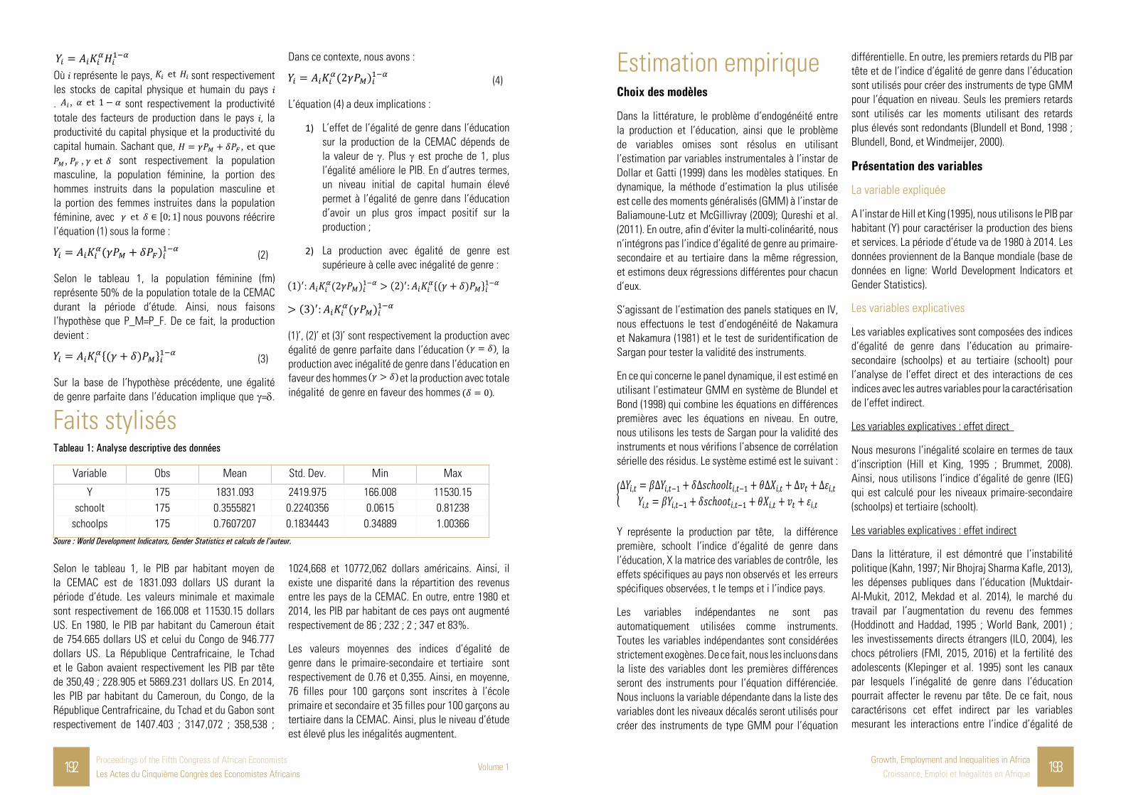
192Proceedings of the Fifth Congress of African EconomistsLes Actes du Cinquième Congrès des Economistes Africains
Volume 1Growth, Employment and Inequalities in Africa
Croissance, Emploi et Inégalités en Afrique 193
Où représente le pays, sont respectivement les stocks de capital physique et humain du pays . sont respectivement la productivité totale des facteurs de production dans le pays , la productivité du capital physique et la productivité du capital humain. Sachant que,
sont respectivement la population masculine, la population féminine, la portion des hommes instruits dans la population masculine et la portion des femmes instruites dans la population féminine, avec nous pouvons réécrire l’équation (1) sous la forme :
(2)
Selon le tableau 1, la population féminine (fm) représente 50% de la population totale de la CEMAC durant la période d’étude. Ainsi, nous faisons l’hypothèse que P_M=P_F. De ce fait, la production devient :
(3)
Sur la base de l’hypothèse précédente, une égalité de genre parfaite dans l’éducation implique que γ=δ.
Dans ce contexte, nous avons :
(4)
L’équation (4) a deux implications :
1) L’effet de l’égalité de genre dans l’éducation sur la production de la CEMAC dépends de la valeur de γ. Plus γ est proche de 1, plus l’égalité améliore le PIB. En d’autres termes, un niveau initial de capital humain élevé permet à l’égalité de genre dans l’éducation d’avoir un plus gros impact positif sur la production ;
2) La production avec égalité de genre est supérieure à celle avec inégalité de genre :
(1)’, (2)’ et (3)’ sont respectivement la production avec égalité de genre parfaite dans l’éducation , la production avec inégalité de genre dans l’éducation en faveur des hommes et la production avec totale inégalité de genre en faveur des hommes .
Faits stylisés Tableau 1: Analyse descriptive des données
Variable Obs Mean Std. Dev. Min Max
Y 175 1831.093 2419.975 166.008 11530.15schoolt 175 0.3555821 0.2240356 0.0615 0.81238
schoolps 175 0.7607207 0.1834443 0.34889 1.00366 Soure : World Development Indicators, Gender Statistics et calculs de l’auteur.
Selon le tableau 1, le PIB par habitant moyen de la CEMAC est de 1831.093 dollars US durant la période d’étude. Les valeurs minimale et maximale sont respectivement de 166.008 et 11530.15 dollars US. En 1980, le PIB par habitant du Cameroun était de 754.665 dollars US et celui du Congo de 946.777 dollars US. La République Centrafricaine, le Tchad et le Gabon avaient respectivement les PIB par tête de 350,49 ; 228.905 et 5869.231 dollars US. En 2014, les PIB par habitant du Cameroun, du Congo, de la République Centrafricaine, du Tchad et du Gabon sont respectivement de 1407.403 ; 3147,072 ; 358,538 ;
1024,668 et 10772,062 dollars américains. Ainsi, il existe une disparité dans la répartition des revenus entre les pays de la CEMAC. En outre, entre 1980 et 2014, les PIB par habitant de ces pays ont augmenté respectivement de 86 ; 232 ; 2 ; 347 et 83%.
Les valeurs moyennes des indices d’égalité de genre dans le primaire-secondaire et tertiaire sont respectivement de 0.76 et 0,355. Ainsi, en moyenne, 76 filles pour 100 garçons sont inscrites à l’école primaire et secondaire et 35 filles pour 100 garçons au tertiaire dans la CEMAC. Ainsi, plus le niveau d’étude est élevé plus les inégalités augmentent.
Estimation empiriqueChoix des modèles
Dans la littérature, le problème d’endogénéité entre la production et l’éducation, ainsi que le problème de variables omises sont résolus en utilisant l’estimation par variables instrumentales à l’instar de Dollar et Gatti (1999) dans les modèles statiques. En dynamique, la méthode d’estimation la plus utilisée est celle des moments généralisés (GMM) à l’instar de Baliamoune-Lutz et McGillivray (2009); Qureshi et al. (2011). En outre, afin d’éviter la multi-colinéarité, nous n’intégrons pas l’indice d’égalité de genre au primaire-secondaire et au tertiaire dans la même régression, et estimons deux régressions différentes pour chacun d’eux.
S’agissant de l’estimation des panels statiques en IV, nous effectuons le test d’endogénéité de Nakamura et Nakamura (1981) et le test de suridentification de Sargan pour tester la validité des instruments.
En ce qui concerne le panel dynamique, il est estimé en utilisant l’estimateur GMM en système de Blundel et Bond (1998) qui combine les équations en différences premières avec les équations en niveau. En outre, nous utilisons les tests de Sargan pour la validité des instruments et nous vérifions l’absence de corrélation sérielle des résidus. Le système estimé est le suivant :
Y représente la production par tête, la différence première, schoolt l’indice d’égalité de genre dans l’éducation, X la matrice des variables de contrôle, les effets spécifiques au pays non observés et les erreurs spécifiques observées, t le temps et i l’indice pays.
Les variables indépendantes ne sont pas automatiquement utilisées comme instruments. Toutes les variables indépendantes sont considérées strictement exogènes. De ce fait, nous les incluons dans la liste des variables dont les premières différences seront des instruments pour l’équation différenciée. Nous incluons la variable dépendante dans la liste des variables dont les niveaux décalés seront utilisés pour créer des instruments de type GMM pour l’équation
différentielle. En outre, les premiers retards du PIB par tête et de l’indice d’égalité de genre dans l’éducation sont utilisés pour créer des instruments de type GMM pour l’équation en niveau. Seuls les premiers retards sont utilisés car les moments utilisant des retards plus élevés sont redondants (Blundell et Bond, 1998 ; Blundell, Bond, et Windmeijer, 2000).
Présentation des variables
La variable expliquée
A l’instar de Hill et King (1995), nous utilisons le PIB par habitant (Y) pour caractériser la production des biens et services. La période d’étude va de 1980 à 2014. Les données proviennent de la Banque mondiale (base de données en ligne: World Development Indicators et Gender Statistics).
Les variables explicatives
Les variables explicatives sont composées des indices d’égalité de genre dans l’éducation au primaire-secondaire (schoolps) et au tertiaire (schoolt) pour l’analyse de l’effet direct et des interactions de ces indices avec les autres variables pour la caractérisation de l’effet indirect.
Les variables explicatives : effet direct
Nous mesurons l’inégalité scolaire en termes de taux d’inscription (Hill et King, 1995 ; Brummet, 2008). Ainsi, nous utilisons l’indice d’égalité de genre (IEG) qui est calculé pour les niveaux primaire-secondaire (schoolps) et tertiaire (schoolt).
Les variables explicatives : effet indirect
Dans la littérature, il est démontré que l’instabilité politique (Kahn, 1997; Nir Bhojraj Sharma Kafle, 2013), les dépenses publiques dans l’éducation (Muktdair-Al-Mukit, 2012, Mekdad et al. 2014), le marché du travail par l’augmentation du revenu des femmes (Hoddinott and Haddad, 1995 ; World Bank, 2001) ; les investissements directs étrangers (ILO, 2004), les chocs pétroliers (FMI, 2015, 2016) et la fertilité des adolescents (Klepinger et al. 1995) sont les canaux par lesquels l’inégalité de genre dans l’éducation pourrait affecter le revenu par tête. De ce fait, nous caractérisons cet effet indirect par les variables mesurant les interactions entre l’indice d’égalité de

194Proceedings of the Fifth Congress of African EconomistsLes Actes du Cinquième Congrès des Economistes Africains
Volume 1Growth, Employment and Inequalities in Africa
Croissance, Emploi et Inégalités en Afrique 195
genre aux niveaux primaire-secondaire et tertiaire, et les vecteurs de transmission ci-dessus listés. Ainsi, nous avons :
- schoolps*instability et schoolt*instability, respectivement les interactions entre les instabilités politiques dans la CEMAC et l’indice d’égalité de genre dans l’éducation aux niveaux primaire-secondaire et tertiaire. En effet, des études récentes ont montré que l’instabilité politique affecte la croissance économique (Aisen et Veiga, 2011; Bonnal et Yaya, 2015; Tabassam et al. 2016) via son impact négatif sur l’éducation (Kahn, 1997; Nir Bhojraj Sharma Kafle, 2013). A cet effet, nous créons une variable muette qui prend la valeur 1 l’année où le pays a connu une guerre ou un coup d’état militaire et 0 sinon. Nous multiplions, par la suite, cette variable par les indices d’égalité de genre comme mentionné précédemment. Trois pays de l’échantillon ont connu des instabilités politiques pendant la période d’étude : le Tchad, la République Centrafricaine et le Congo. Le Tchad a connu trois coups d’état militaires (ou tentative de coups d’état militaires) et trois rébellions qui ont déstabilisé ce pays et ont fait de nombreuses victimes. En République Centrafricaine, après des mutineries dans l’armée en avril, mai et novembre 1996, l’ancien président André Kolingba fait un coup d’état en mai 2001. En 2003, François Bozizé renverse le président Patassé et se proclame président de la République. En 2012, la coalition rebelle de la Seleka dénonce le non-respect des accords de paix signés en 2007 et 2011 et reprend les armes. En 2013, les rebelles prennent le palais présidentiel et s’emparent du pouvoir. Le Congo a connu des conflits et des troubles entre 1993 et 2002 qui ont entraîné 400 000 morts ; soit plus de 10% de sa population. De juillet 1993 à 1994, ce pays a connu une guerre civile opposant trois clans : les partisans du président Lissouba, ceux de l’ancien président Sassou-Nguesso et les partisans de Bernard Kolélas ;
-schoolps*g et schoolt*g : respectivement les interactions entre les dépenses publiques et l’indice d’égalité de genre dans l’éducation aux niveaux primaire-secondaire et tertiaire. En effet, il existe une abondante littérature récente qui montre l’effet positif des dépenses publiques dans l’éducation sur la croissance économique (Muktdair-Al-Mukit, 2012, Mekdad et al. 2014). Les pays en développement ont une faible dotation en capital humain. En
conséquence, investir dans le système éducatif peut contribuer à augmenter leurs stocks de capital humain et à promouvoir la croissance économique (Teles et Andrade, 2015) ;
-schoolps*ratio et schoolt*ratio : respectivement les interactions entre l’écart entre les sexes sur le marché du travail (mesuré par le rapport entre le taux d’activité des femmes et celui des hommes) et l’indice d’égalité de genre dans l’éducation aux niveaux primaire-secondaire et tertiaire. Il est démontré dans la littérature que plus les femmes travaillent et ont un revenu, plus elles investissent dans l’éducation de leurs enfants (Hoddinott and Haddad, 1995 ; World Bank, 2001 ; Korinek, 2005). De ce fait, l’emploi des femmes pourrait influencer le revenu par tête via son impact positif sur l’accessibilité des filles à l’éducation.
-schoolps*fdi et schoolt*fdi : respectivement les interactions entre les investissements directs étrangers et l’indice d’égalité de genre dans l’éducation aux niveaux primaire-secondaire et tertiaire. Il a été démontré que l’arrivée massive d’IDE dans certains pays en développement a des effets bénéfiques sur l’employabilité des femmes (ILO, 2004). L’emploi des femmes donne un revenu supplémentaire à ces dernières. Ce qui leur permet de scolariser leurs enfants et améliore la scolarité des filles. Il s’en suit un effet bénéfique sur le produit par tête.
-schoolps*oilchoc et schoolt*oilchoc : respectivement les interactions entre les années durant lesquelles les chocs pétroliers ont eu lieu et l’indice d’égalité de genre dans l’éducation aux niveaux primaire-secondaire et tertiaire. En effet, au cours des chocs pétroliers de 1996-1998, 2008 et 2014, le prix du pétrole a baissé en moyenne respectivement de -55 ; -67 et -77% ;
-schoolps*adofertility et schoolt*adofertility : respectivement les interactions entre le taux de fécondité des adolescents et l’indice d’égalité de genre dans l’éducation aux niveaux primaire-secondaire et tertiaire. En effet, la fertilité des adolescents peut avoir une incidence sur la croissance économique par le canal du capital humain. Après avoir interviewé 2795 femmes de 1979 à 1991, Klepinger et al. (1995) démontrent qu’avoir un enfant avant l’âge de 20 ans réduit considérablement la scolarité de près de trois ans. Selon le tableau 1, il y a dans la CEMAC
en moyenne 157 naissances pour 1000 femmes (âgés de 15 à 19 ans). Le nombre minimal est de 93 naissances pour 1000 adolescents et le maximal de 218 naissances. En 2014, le Cameroun enregistre 106 naissances pour 1000 adolescents, 119 naissances au Congo, 93 naissances en République Centrafricaine, 137 naissances au Tchad et 102 naissances au Gabon.
Les variables de contrôle
Cette sous-section est consacrée à la présentation des variables de contrôle.
- Mortalité infantile (mort) : la mortalité est un facteur qui détermine l’état du système de santé d’un pays. En conséquence, elle peut influencer la croissance économique (Kalemli-Ozcan, 2002, Lehmijoki et Palokangas, 2011). Dans cette étude, nous utilisons la mortalité infantile. Selon le tableau 1, pour 1000 naissances dans la CEMAC, une moyenne de 84 enfants décède avant l’âge de 1 an. Le nombre minimum est de 34 décès pour 1000 naissances et le maximum de 126 décès. En 2014, le Cameroun a enregistré 58 décès pour 1000 naissances, 34 décès au Congo, 93 décès en République Centrafricaine, 87 décès au Tchad et 37 décès au Gabon.
- L’interaction entre les termes de l’échange et l’ouverture commerciale (somme des exportations et des importations sur le PIB réel) (tot*ouv) : plusieurs études récentes ont démontré que les termes de l’échange influencent la croissance économique (Eicher et al. 2008). De ce fait, les pays de l’échantillon ayant des économies ouvertes, il semble nécessaire d’introduire cette variable parmi les celles explicatives.
- Investissement privé (inv) : en dehors du capital humain, le capital physique est également un facteur déterminant de la croissance économique. De nombreuses études récentes montrent l’effet positif de l’investissement sur la croissance (Khan et Rehinart, 1990, Bint-e-Ajaz et Ellahi, 2012, Yovo, 2017). En conséquence, nous l’intégrons comme variable explicative.
- Variables commerciales : la théorie économique soutient que le commerce extérieur est un déterminant important de la croissance économique (Yanikkaya, 2003, Khan, 2014, Brueckner et Lederman, 2015, Were, 2015) ; l’un des canaux de transmission étant
l’éducation (Korinek, 2005 ; Fukase, 2010; Mamoon and Murshed, 2012). Les pays de la CEMAC ont des économies extraverties et tirent la majeure partie de leur revenu des exportations de matières premières. En outre, les importations représentent une part importante de la consommation des ménages dans ces pays. Dans ces conditions, hormis les termes de l’échange et l’indice d’ouverture commerciale, nous utilisons deux autres variables pour caractériser le commerce extérieur : les exportations (x) et les importations (m).
- La dévaluation de 1994 (dev) : selon la théorie économique, la dévaluation stimulerait les exportations. Osundina et Osundina (2014) démontrent que la dévaluation du Naira en 2014 aurait réduit les importations et augmenté les exportations et le taux d’intérêt de l’économie nigériane. Shahzad et Afzal (2013) trouvent un résultat similaire pour le Pakistan et le Bangladesh. Le FCFA a été dévalué en 1994 pour stimuler les exportations des pays qui utilisent cette monnaie et qui étaient en crise. En conséquence, nous créons une variable muette qui prend la valeur 1 en 1994 et zéro les autres années.
Les variables instrumentales
Pour corriger les biais d’endogénéité et de variables omises, nous avons utilisé les variables instrumentales suivantes pour les estimations en IV :
- L’instabilité politique (instability) : des études récentes ont montré que l’instabilité politique affecte la croissance économique (Aisen et Veiga, 2011; Bonnal et Yaya, 2015; Tabassam et al. 2016) via son impact négatif sur l’éducation (Kahn, 1997; Nir Bhojraj Sharma Kafle, 2013). A cet effet, nous créons une variable muette qui prend la valeur 1 l’année où le pays a connu une guerre ou un coup d’état militaire et 0 sinon.
- Taux de fécondité des adolescents (adofert) : la fertilité des adolescents peut avoir une incidence sur la croissance économique par le canal du capital humain. Après avoir interviewé 2795 femmes de 1979 à 1991, Klepinger et al. (1995) démontrent qu’avoir un enfant avant l’âge de 20 ans réduit considérablement la scolarité de près de trois ans.
- Interaction entre les dépenses publiques dans

196Proceedings of the Fifth Congress of African EconomistsLes Actes du Cinquième Congrès des Economistes Africains
Volume 1Growth, Employment and Inequalities in Africa
Croissance, Emploi et Inégalités en Afrique 197
l’éducation et les chocs pétroliers (gedu*oilshock) : il existe une abondante littérature récente qui montre l’effet positif des dépenses publiques dans l’éducation sur la croissance économique (Muktdair-Al-Mukit, 2012, Mekdad et al. 2014). La volatilité des dépenses publiques due aux fluctuations des cours du pétrole est un canal de transmission majeure dans les pays de la CEMAC (FMI, 2016). Ainsi, pour tenir compte de l’effet des chocs pétroliers sur l’indice d’égalité de genre, nous avons créé la variable gedu*oilshock qui est une multiplication des dépenses publiques dans l’éducation (gedu) par la variable choc pétrolier (oilshock). Dans la construction de cette variable, le choc pétrolier est mesuré par la variation en pourcentage du prix international du pétrole multipliée par la part du revenu tiré du pétrole dans le PIB (FMI, 2015).
Nous considérons également les FDI et l’écart entre les sexes sur le marché du travail (mesuré par le rapport entre le taux d’activité des femmes et celui des hommes) comme des instruments dans les estimations en IV en effet direct. En effet indirect, le choix des instruments tient compte de la variable qui a été multipliée à l’indice d’égalité de genre dans l’éducation. Par exemple, si c’est l’interaction entre les IDE et l’indice d’égalité de genre dans l’éducation, la variable IDE est enlevée parmi les instruments.
Interprétation des résultats et recommandations de politiques économiques
L’effet direct de l’indice des inégalités de genre dans l’éducation sur le PIB par habitant
Le modèle empirique est présenté en Log-niveau. Ainsi, on interprète les résultats comme le changement en pourcentage du PIB par habitant lorsque l’indice d’égalité de genre augmente d’une unité, toutes choses égales par ailleurs : lorsque le niveau de l’indice d’égalité de genre augmente d’une unité, le PIB par habitant augmente donc de 100 × le coefficient estimé. Ce raisonnement est aussi valable pour les variables de contrôle. Dans la base de données Gender Statistics, on remarque que les indices d’égalité de genre au primaire-secondaire et au tertiaire sont systématiquement inférieurs à 1 durant toute la période d’étude dans tous les pays de l’échantillon. Ainsi, une augmentation de ces indices signifie qu’ils tendent vers la valeur 1 (l’égalité
parfaite homme-femme) et traduit une diminution des inégalités. On s’attend donc à ce que l’augmentation de l’indice d’égalité de genre au primaire-secondaire et au tertiaire puisse entrainer une augmentation du PIB par habitant des pays de la CEMAC comme l’indique le modèle théorique de référence (cf. section 3).
Les estimations sont faites en statique et en dynamique. Selon les résultats obtenus (cf. tableaux 2 et 4), en statique, une augmentation de l’indice d’égalité de genre au primaire-secondaire d’une unité accroit le PIB par habitant de 112.8 %. Alors qu’une augmentation de l’indice d’égalité de genre au tertiaire d’une unité accroit le PIB par habitant de 164.8 %. En dynamique, une augmentation de l’indice d’égalité de genre au primaire-secondaire d’une unité aux années t-1 et t accroit le PIB par habitant respectivement de 53.3 et 18.8 %. Alors qu’une augmentation de l’indice d’égalité de genre au tertiaire d’une unité à l’année t-2 accroit le PIB par habitant de 35.85 % ; les autres années n’étant pas significatives. Ainsi, les résultats empiriques vont dans le même sens que le résultat théorique. Une réduction des inégalités de genre dans l’éducation accroit la production des pays de la CEMAC. En effet, comme le montrent les récentes études sur d’autres pays africains (Baliamoune-Lutz et McGillivray, 2009 ; Seguino et Were, 2013 ; Bandara, 2015; Licumba et al. 2015), une augmentation des inégalités a tendance à avoir un effet négatif sur la croissance économique, alors qu’une diminution de ces dernières a un effet positif sur la croissance. En CEMAC, les femmes représentant en moyenne 50 % de la population totale, une diminution des inégalités de genre dans l’éducation signifie, de facto, augmentation du stock de capital humain. Plusieurs études récentes ont montré l’importance du capital humain dans la promotion de la croissance économique des pays en développement (Gyimah-Brempong et al. 2006 ; Hanushek et Woessmann, 2012 ; Eggoh et al. 2015). C’est pourquoi l’augmentation du stock de capital humain dans la CEMAC se traduit par celle de la production par tête.
S’agissant des variables de contrôle, l’augmentation de la mortalité infantile a des effets dommageables sur la production par tête. En effet, son signe est significatif et négatif en statique et en dynamique. Elle permet d’approximer l’état du système sanitaire des pays de la CEMAC. De ce fait, on peut en déduire que ces pays
ont des systèmes de santé peu développés et non favorable à la production des biens et services. L’effet combiné entre les termes de l’échange et l’ouverture commerciale a un impact positif sur la production par tête. Il en va de même pour les exportations. Les importations, quant à elles, ont un effet négatif sur la production. Ce qui signifie que les pays de la CEMAC importent plus de biens de consommation, dont l’achat représente une sortie de capitaux sans contrepartie, que de biens d’investissement pouvant permettre l’augmentation de la production. Cela est d’autant plus soutenable que la variable investissement a un signe positif et significatif sur la production en statique. Enfin, la dévaluation de 1914 semble avoir eu un effet défavorable sur la production par tête des pays de la CEMAC. Ainsi, l’effet bénéfique de l’augmentation des exportations (Shahzad and Afzal 2013 ; Osundina and Osundina, 2014) a été inférieur à l’effet négatif inhérent à la perte du pouvoir d’achat des agents économiques suite à la hausse du prix des importations.
L’effet indirect de l’indice des inégalités de genre dans l’éducation sur le PIB par habitant
Les effets indirects sont également calculés en statique et en dynamique. Ce sont les vecteurs de transmission par lesquels la situation du genre dans l’éducation influence la production.
A cet effet, l’interaction entre l’instabilité politique et l’indice d’égalité de genre dans l’éducation a un effet négatif sur la production de la CEMAC en statique et en dynamique. L’impact négatif sur la production vient du fait que l’instabilité politique accroit les inégalités de genre dans l’éducation (Kahn, 1997; Nir Bhojraj Sharma Kafle, 2013). En effet, le Congo, la Centrafrique et le Tchad ont connu des troubles politiques durant la période d’étude souvent liés au manque de démocratie et à la mauvaise répartition des richesses.
L’interaction entre les dépenses publiques et l’indice d’égalité de genre dans l’éducation a un effet positif et significatif sur la production par tête en statique et en dynamique. En effet, les dépenses publiques dans l’éducation sont susceptibles de faire baisser les inégalités de genre. Ce qui a, par conséquent, un effet bénéfique sur le niveau de la production comme démontré un peu plus haut. Ce résultat va dans le même sens que ceux de Muktdair-Al-Mukit, 2012 ;
Mekdad et al. 2014 qui montrent l’effet positif des dépenses publiques dans l’éducation sur la croissance économique.
L’interaction entre l’indice d’égalité de genre dans l’éducation et l’écart entre les sexes sur le marché du travail (mesuré par le rapport entre le taux d’activité des femmes et celui des hommes) a un effet positif et significatif sur la production par tête en statique et en dynamique. En effet, il est démontré dans la littérature que plus les femmes travaillent et ont un revenu, plus elles investissent dans l’éducation de leurs enfants (Hoddinott and Haddad, 1995 ; World Bank, 2001). L’augmentation du ratio d’activité femmes-hommes sur le marché du travail entraine une augmentation de l’emploi des femmes, et donc de leur revenu. Ce qui se traduit par l’accroissement de l’investissement dans la scolarisation des enfants, quelque soit leur sexe. L’ultime effet sera la réduction des inégalités de genre dans l’éducation qui aura des retombées bénéfiques sur le produit par tête.
L’interaction entre l’indice d’égalité de genre dans l’éducation et les flux d’investissements directs étrangers a un effet positif et significatif sur la production par tête en statique et en dynamique. En effet, dans la littérature, il est démontré que le commerce international et la globalisation caractérisée, entre autres, par l’arrivée massive d’IDE dans certains pays en développement ont des effets bénéfiques sur l’employabilité des femmes. Selon l’ILO (2004), l’implantation des firmes multinationales dans les pays en développement peut conduire à des changements dans les entreprises locales et les institutions traditionnelles. Par exemple, les pratiques de gestion des pays développés pourraient être introduites dans les pays en développement ; conduisant à plus d’égalité de genre dans les filiales locales des multinationales. Ainsi, en ce qui concerne les pratiques de discrimination qui peuvent être observées dans les entreprises locales, les femmes ayant un niveau d’éducation plus élevé pourraient choisir de travailler dans ces filiales. A moyen et long terme, les pratiques des firmes multinationales sont progressivement introduites dans la gestion des entreprises locales ; conduisant à plus d’égalité de genre sur le marché du travail. Comme nous l’avons vu précédemment, l’augmentation du revenu des femmes conduit à celle de l’investissement dans l’éducation

198Proceedings of the Fifth Congress of African EconomistsLes Actes du Cinquième Congrès des Economistes Africains
Volume 1Growth, Employment and Inequalities in Africa
Croissance, Emploi et Inégalités en Afrique 199
des enfants. De ce fait, l’entrée d’IDE a un effet bénéfique sur la production par tête des pays de la CEMAC via l’indice d’égalité de genre.
L’interaction entre le choc pétrolier, l’indice d’égalité de genre et la variation des dépenses publiques a un effet significatif et négatif sur la production par tête en dynamique. En effet, la volatilité des dépenses publiques due aux fluctuations des cours du pétrole est un canal de transmission majeure dans les pays de la CEMAC (FMI, 2016). De ce fait, la baisse des dépenses publiques en éducation a des effets dommageables sur l’indice d’égalité de genre dans l’éducation. Par conséquent, elle affecte négativement la production par ce canal.
Enfin, l’interaction entre la fertilité des adolescents et l’indice d’égalité de genre dans l’éducation à un impact négatif et significatif sur la production par tête en statique et en dynamique. Selon Klepinger et al. (1995), avoir des enfants très tôt réduit la scolarisation des adolescents. Dans le tableau 1, il est montré qu’en CEMAC, on a en moyenne 157 naissances pour 1000 adolescentes (l’âge compris entre 15 et 19 ans). Cette fertilité des adolescents baisse le stock de capital humain en affectant négativement la scolarisation des jeunes filles mères. Ce qui a des retombées négatives sur la production par tête.
Recommandations de politiques économiques
Les résultats montrent que l’augmentation de l’indice d’égalité de genre pourrait avoir un effet bénéfique sur la production par tête des pays de la CEMAC. Les pays de cette Communauté sont fortement dépendants des matières premières. De ce fait, ils doivent diversifier les sources de la croissance en mettant un accent particulier dans la lutte contre les inégalités dans l’éducation. En effet, une croissance soutenable nécessite un capital humain abondant et bien formé ; y compris le capital humain féminin. En outre, selon l’indice du développement humain (IDH), la santé est un élément primordial pour le développement et le bien-être des populations. Par conséquent, les pays de la CEMAC doivent, non seulement investir dans l’éducation, mais aussi dans la santé afin d’accroitre la production par tête ; tout en adoptant la démocratie et une meilleure répartition des richesses comme mode de gouvernance. En effet, l’étude montre que
l’instabilité politique pourrait affecter la production via son impact négatif sur l’indice d’égalité de genre. Le Congo, la Centrafrique et le Tchad sont impactés par ce phénomène. Même si le Gabon et le Cameroun semblent épargnés, la stabilité politique dans ces pays est précaire. En effet, les élections sont souvent suivies de contestations et de soupçons de fraude dans les deux pays précités. La mission d’observation de l’Union Européenne sur l’élection présidentielle du 27 août 2016 au Gabon écrit ceci dans son rapport à la page 33 : « Une escalade progressive des tensions a eu lieu à partir de la soirée du 27 août, date du scrutin. L’apogée des tensions s’est manifestée le 31 août immédiatement après l’annonce des résultats, que l’opposition a jugé manipulés. Les manifestations de rue à travers le pays ont abouti à de graves violences, dont l’incendie partiel de l’Assemblée nationale et de certaines installations extérieures du Sénat. Selon les autorités, huit cents personnes ont été arrêtées à Libreville et trois cents dans le reste du pays. Entre les chiffres officiels et ceux de l’opposition, le décompte des victimes variait entre 5 et 100. » Ainsi, l’exemple précédent montre que la stabilité dans certains pays de la CEMAC n’est qu’apparente et précaire. De ce fait, ces pays doivent instaurer des démocraties véritables ; gages de stabilité durable et de prospérité. S’agissant de l’effet négatif de la fertilité des adolescents, des enseignements et campagnes d’éducation sexuelle devraient être mises en œuvre dans les établissements primaires et secondaires afin de prévenir tout comportement à risque. Ces campagnes doivent également permettre de sensibiliser les adultes des sanctions pénales encourues en cas de détournement des mineures. Les jeunes filles mères devraient être bien suivies et encadrées afin qu’elles n’abandonnent pas leur scolarité. En outre, un bon climat des affaires doit être mis en œuvre pour attirer les IDE. L’objectif ultime est de diversifier les économies afin de les rendre moins dépendantes des matières premières. Ce qui permettra une réduction de l’exposition aux chocs internationaux. Les externalités positives des IDE sont également visibles dans l’employabilité des femmes et les techniques managériales modernes. Toute chose qui aura un effet bénéfique sur le produit intérieur brut des pays de la CEMAC.
Conclusion Les contributions de l’étude sont empiriques et théorique. Théoriquement, s’inspirant du modèle de Solow (1957) tout en incluant le fait que les femmes représentent 50% de la population totale de la CEMAC, on peut voir que la production de la CEMAC avec égalité de genre dans l’éducation est supérieure à la production avec inégalité de genre. Ce résultat théorique est vérifié empiriquement. En effet, les résultats obtenus montrent qu’une augmentation de l’indice d’égalité de genre au primaire-secondaire et tertiaire accroit le PIB par habitant. En conséquence, les pays de la CEMAC doivent mettre en œuvre des politiques visant à réduire les inégalités de genre dans l’éducation pour avoir une croissance économique soutenable. En effet, ces pays, qui exportent principalement des matières premières, y compris le pétrole, sont exposés aux chocs des prix internationaux. Ainsi, les exportations plus diversifiées et à forte valeur ajoutée, telles que celles dérivées d’un capital humain bien formé et abondant, permettraient à ces pays de réduire leur niveau d’exposition. En outre, l’étude établit un lien clairement négatif entre l’instabilité politique, les chocs pétroliers, la fertilité des adolescents et le PIB par habitant ; le canal de transmission étant l’augmentation des inégalités de genre dans l’éducation. En effet, le Congo, la République Centrafricaine et le Tchad ont connu des instabilités politiques pendant la période d’étude, souvent liées au manque de démocratie et à la mauvaise répartition de la richesse. Bien que le Gabon et le Cameroun semblent épargnés, la stabilité politique dans ces pays est précaire. Les élections sont souvent suivies de contestations populaires et de soupçons de fraude dans les deux pays ci-dessus mentionnés. En conséquence, ces pays doivent établir de véritables démocraties pour assurer une stabilité et une prospérité durables. Enfin, l’étude montre que la diminution des inégalités de genre sur le marché du travail, les IDE et les dépenses publiques ont un effet bénéfique sur la production à travers leurs retombées positives sur l’indice d’égalité de genre dans l’éducation.

200Proceedings of the Fifth Congress of African EconomistsLes Actes du Cinquième Congrès des Economistes Africains
Volume 1Growth, Employment and Inequalities in Africa
Croissance, Emploi et Inégalités en Afrique 201
AnnexesTableau 2 : Effet direct de l’indice des inégalités de genre dans l’éducation sur le PIB par habitant en statique
Dependent variables
(1)
Per capita GDP
(2)
Per capita
GDPschoolt 1.648***
(0.371)
----
schoolps ---- 1.128***
(0.505)mortality -0.027***
(0.001)
-0.024***
(0.004)lot*ouv 0.006***
(0.001)
0.004***
(0.000)inv 2.77***
(0.000)
4.33***
(0.000)x 8.13***
(0.000)
1.14***
(0.000)m -3.85***
(0.000)
-4.12***
(0.000)dev -0.161
(0.151)
-0.165
(0.157)cst 8.141***
(0.279)
7.544***
(0.738) Adjusted R2 0.91 0.91
Obs. 175 175----Non disponible.
*Significatif à 10%**Significatif à 5%.
***Significatif à 1%.
Tabl
eau
3 : E
ffet
indi
rect
de
l’ind
ice d
es in
égal
ités
de g
enre
dan
s l’é
duca
tion
sur l
e PI
B pa
r hab
itant
en
stat
ique
Depe
nden
t va
riabl
es(1
)
Per c
apita
GD
P
(2)
Per c
apita
GDP
(3)
Per c
apita
GDP
(4)
Per c
apita
GDP
(5)
Per c
apita
GDP
(6)
Per c
apita
GDP
(7)
Per c
apita
GDP
(8)
Per c
apita
GDP
(9)
Per c
apita
GDP
(10)
Per c
apita
GDP
(11)
Per c
apita
GDP
(12)
Per c
apita
GDP
scho
olt*
inst
a-bi
lity
-5.4
47**
*
(1.8
49)
----
----
----
----
----
----
----
----
----
----
----
scho
olps
*ins
ta-
bilit
y---
--0
.837
**
(0.4
53)
----
----
----
----
----
----
----
----
----
----
scho
olt*
g---
----
-2.
76**
*
(0.0
00)
----
----
----
----
----
----
----
----
----
scho
olps
*g---
----
----
-1.
24**
*
(0 .0
00)
----
----
----
----
----
----
----
----
scho
olt*
ratio
----
----
----
----
0.03
7***
(0.0
09)
----
----
----
----
----
----
----
scho
olps
*rat
io---
----
----
----
----
-0.
012*
*
(0.0
06)
----
----
----
----
----
----
sch
oolt*
fdi
----
----
----
----
----
----
-0.9
99
(0.2
89)
----
----
----
----
----
scho
olps
*fdi
----
----
----
----
----
----
----
0.06
9***
(0.0
31)
----
----
----
----
scho
olt*
oilc
hoc
----
----
----
----
----
----
----
----
-0.1
01
(0.1
25)
----
----
----
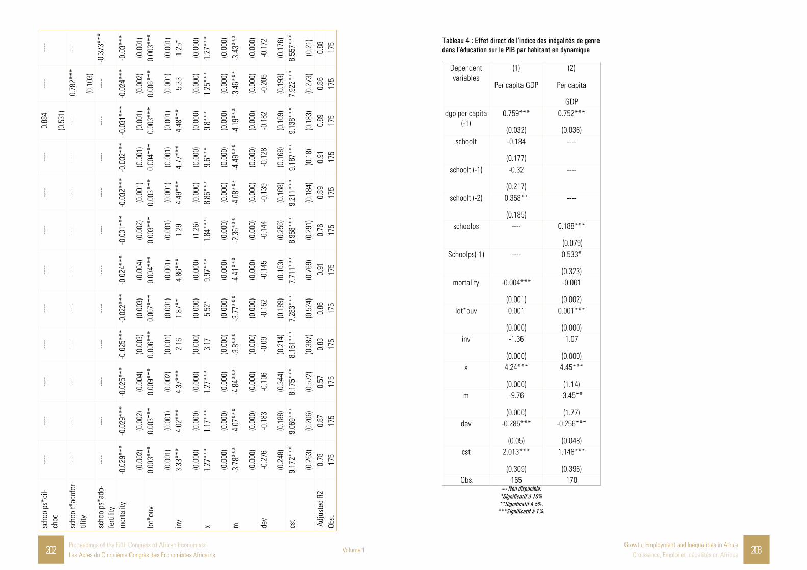
202Proceedings of the Fifth Congress of African EconomistsLes Actes du Cinquième Congrès des Economistes Africains
Volume 1Growth, Employment and Inequalities in Africa
Croissance, Emploi et Inégalités en Afrique 203
scho
olps
*oil-
choc
----
----
----
----
----
----
----
----
----
0.88
4
(0.5
31)
----
----
scho
olt*
adof
er-
tility
----
----
----
----
----
----
----
----
----
----
-0.7
82**
*
(0.1
03)
----
scho
olps
*ado
-fe
rtilit
y---
----
----
----
----
----
----
----
----
----
----
--0
.373
***
mor
talit
y-0
.029
***
(0.0
02)
-0.0
29**
*
(0.0
02)
-0.0
25**
*
(0.0
04)
-0.0
25**
*
(0.0
03)
-0.0
22**
*
(0.0
03)
-0.0
24**
*
(0.0
04)
-0.0
31**
*
(0.0
02)
-0.0
32**
*
(0.0
01)
-0.0
32**
*
(0.0
01)
-0.0
31**
*
(0.0
01)
-0.0
24**
*
(0.0
02)
-0.0
3***
(0.0
01)
lot*
ouv
0.00
3***
(0.0
01)
0.00
3***
(0.0
01)
0.00
9***
(0.0
02)
0.00
6***
(0.0
01)
0.00
7***
(0.0
01)
0.00
4***
(0.0
01)
0.00
3***
(0.0
01)
0.00
3***
(0.0
01)
0.00
4***
(0.0
01)
0.00
3***
(0.0
01)
0.00
6***
(0.0
01)
0.00
3***
(0.0
01)
inv
3.33
***
(0.0
00)
4.02
***
(0.0
00)
4.37
***
(0.0
00)
2.16
(0.0
00)
1.87
**
(0.0
00)
4.86
***
(0.0
00)
1.29
(1.2
6)
4.49
***
(0.0
00)
4.77
***
(0.0
00)
4.48
***
(0.0
00)
5.33
(0.0
00)
1.25
*
(0.0
00)
x1.
27**
*
(0.0
00)
1.17
***
(0.0
00)
1.27
***
(0.0
00)
3.17
(0.0
00)
5.52
*
(0.0
00)
9.97
***
(0.0
00)
1.84
***
(0.0
00)
8.86
***
(0.0
00)
9.6*
**
(0.0
00)
9.8*
**
(0.0
00)
1.25
***
(0.0
00)
1.27
***
(0.0
00)
m-3
.78*
**
(0.0
00)
-4.0
7***
(0.0
00)
-4.8
4***
(0.0
00)
-3.8
***
(0.0
00)
-3.7
7***
(0.0
00)
-4.4
1***
(0.0
00)
-2.3
6***
(0.0
00)
-4.0
8***
(0.0
00)
-4.4
9***
(0.0
00)
-4.1
9***
(0.0
00)
-3.4
6***
(0.0
00)
-3.4
3***
(0.0
00)
dev
-0.2
76
(0.2
48)
-0.1
83
(0.1
88)
-0.1
06
(0.3
44)
-0.0
9
(0.2
14)
-0.1
52
(0.1
89)
-0.1
45
(0.1
63)
-0.1
44
(0.2
56)
-0.1
39
(0.1
68)
-0.1
28
(0.1
68)
-0.1
82
(0.1
69)
-0.2
05
(0.1
93)
-0.1
72
(0.1
76)
cst
9.17
2***
(0.2
63)
9.06
9***
(0.2
06)
8.17
5***
(0.5
72)
8.16
1***
(0.3
87)
7.28
3***
(0.5
24)
7.71
1***
(0.7
69)
8.95
8***
(0.2
91)
9.21
1***
(0.1
84)
9.18
7***
(0.1
8)
9.13
8***
(0.1
83)
7.92
2***
(0.2
73)
8.55
7***
(0.2
1) A
djus
ted
R20.
78
0.87
0.
57
0.83
0.86
0
.91
0.76
0.
890.
910.
89
0.86
0.
88
Obs.
175
175
175
175
175
175
175
175
175
175
175
175 Tableau 4 : Effet direct de l’indice des inégalités de genre
dans l’éducation sur le PIB par habitant en dynamique
Dependent variables
(1)
Per capita GDP
(2)
Per capita
GDPdgp per capita
(-1)0.759***
(0.032)
0.752***
(0.036)schoolt -0.184
(0.177)
----
schoolt (-1) -0.32
(0.217)
----
schoolt (-2) 0.358**
(0.185)
----
schoolps ---- 0.188***
(0.079)Schoolps(-1) ---- 0.533*
(0.323)mortality -0.004***
(0.001)
-0.001
(0.002)lot*ouv 0.001
(0.000)
0.001***
(0.000)inv -1.36
(0.000)
1.07
(0.000)x 4.24***
(0.000)
4.45***
(1.14)m -9.76
(0.000)
-3.45**
(1.77)dev -0.285***
(0.05)
-0.256***
(0.048)cst 2.013***
(0.309)
1.148***
(0.396) Obs. 165 170
---- Non disponible.*Significatif à 10%**Significatif à 5%.
***Significatif à 1%.

204Proceedings of the Fifth Congress of African EconomistsLes Actes du Cinquième Congrès des Economistes Africains
Volume 1Growth, Employment and Inequalities in Africa
Croissance, Emploi et Inégalités en Afrique 205
Tabl
eau
5 : E
ffet
indi
rect
de
l’ind
ice d
es in
égal
ités
de g
enre
dan
s l’é
duca
tion
sur l
e PI
B pa
r hab
itant
en
dyna
miq
ue
Depe
nden
t va
riabl
es(1
)
Per c
apita
GD
P
(2)
Per c
apita
GDP
(3)
Per c
apita
GDP
(4)
Per c
apita
GDP
(5)
Per c
apita
GDP
(6)
Per c
apita
GDP
(7)
Per c
apita
GDP
(8)
Per c
apita
GDP
(9)
Per c
apita
GDP
(10)
Per c
apita
GDP
(11)
Per c
apita
GDP
(12)
Per c
apita
GDP
Per c
apita
GDP
(-1)
0.82
2***
(0.0
27)
0.80
8***
(0.0
28)
0.84
1***
(0.0
3)
0.85
3***
(0.0
37)
0.84
***
(0.0
27)
0.79
9***
(0.0
29)
0.85
2***
(0.0
26)
0.84
9***
(0.0
27)
0.80
2***
(0.0
31)
0.77
8***
(0.0
31)
0.81
***
(0.0
42)
0.78
5***
(0.0
27)
scho
olt*
inst
abili
ty-0
.279
*
(0.1
63)
----
----
----
----
----
----
----
----
----
----
----
scho
olt*
inst
abili
-ty
(-1)
0.25
2
(0.2
1)
----
----
----
----
----
----
----
----
----
----
----
scho
olt*
inst
abili
-ty
(-2)
0.01
5
(0.1
66)
----
----
----
----
----
----
----
----
----
----
----
scho
olps
*ins
ta-
bilit
y---
--0
.062
(0.0
54)
----
----
----
----
----
----
----
----
----
----
scho
olps
*ins
tabi
l-ity
(-1)
----
0.08
1
(0.0
53)
----
----
----
----
----
----
----
----
----
----
scho
olt*
g---
----
-2.
44**
*
(1.1
3)
----
----
----
----
----
----
----
----
----
scho
olt*
g(-1
)---
----
--4
.1
(1.2
3)
----
----
----
----
----
----
----
----
----
scho
olt*
g(-2
)---
----
-9.
29
(1.2
3)
----
----
----
----
----
----
----
----
----
scho
olps
*g---
----
----
-2.
19**
*
(0.0
00)
----
----
----
----
----
----
----
----
scho
olps
*g(-1
)---
----
----
--3
.72
(0.0
00)
----
----
----
----
----
----
----
----
scho
olt*
ratio
----
----
----
----
-0.0
01
(0.0
01)
----
----
----
----
----
----
----
scho
olt*
ratio
(-1)
----
----
----
----
-0.0
02
(0.0
02)
----
----
----
----
----
----
----
scho
olt*
ratio
(-2)
----
----
----
----
0.00
3*
(0.0
02)
----
----
----
----
----
----
----
scho
olps
*rat
io---
----
----
----
----
-0.
001*
**
(0.0
01)
----
----
----
----
----
----
scho
olps
*rat
io(-1
)---
----
----
----
----
-0.
003
(0.0
03)
----
----
----
----
----
----
scho
olt*
fdi
----
----
----
----
----
----
-0.0
15
(0.0
04)
----
----
----
----
----
scho
olt*
fdi(-
1)---
----
----
----
----
----
-0.
01*
(0.0
05)
----
----
----
----
----
scho
olt*
fdi(-
2)---
----
----
----
----
----
-0.
008*
(0.0
05)
----
----
----
----
----

206Proceedings of the Fifth Congress of African EconomistsLes Actes du Cinquième Congrès des Economistes Africains
Volume 1Growth, Employment and Inequalities in Africa
Croissance, Emploi et Inégalités en Afrique 207
scho
olps
*fdi
----
----
----
----
----
----
-0.0
04
(0.0
02)
----
----
----
----
scho
olps
*fdi
(-1)
----
----
----
----
----
----
----
0.00
6***
(0.0
01)
----
----
----
----
scho
olt*
oilc
ho-
c*dg
----
----
----
----
----
----
----
----
-2.2
5
(2.1
8)
----
----
----
scho
olt*
oilc
ho-
c*dg
(-1)
----
----
----
----
----
----
----
----
7.26
(2.7
5)
----
----
----
scho
olt*
oilc
ho-
c*dg
(-2)
----
----
----
----
----
----
----
----
-3.6
9*
(2.2
1)
----
----
----
scho
olps
*oilc
ho-
c*dg
----
----
----
----
----
----
----
----
----
-1.2
4*
(0.0
00)
----
----
scho
olps
*oilc
ho-
c*dg
(-1)
----
----
----
----
----
----
----
----
----
1.89
(1.0
3)
----
----
scho
olt*
adof
er-
tility
----
----
----
----
----
----
----
----
----
----
0.00
5
(0.0
18)
----
scho
olt*
adof
ertil
-ity
(-1)
----
----
----
----
----
----
----
----
----
----
-0.0
35*
(0.0
19)
----
scho
olt*
adof
ertil
-ity
(-2)
----
----
----
----
----
----
----
----
----
----
-0.0
21
(0.0
21)
----
scho
olps
*ado
fer-
tility
----
----
----
----
----
----
----
----
----
----
----
-0.0
29**
*
(0.0
14)
scho
olps
*ado
fer-
tility
(-1)
----
----
----
----
----
----
----
----
----
----
----
-0.0
16
(0.0
14)
mor
talit
y-0
.004
***
(0.0
01)
-0.0
04**
*
(0.0
01)
-0.0
03**
*
(0.0
01)
-0.0
04**
*
(0.0
01)
-0.0
03**
*
(0.0
01)
-0.0
01
(0.0
01)
-0.0
03**
*
(0.0
01)
-0.0
03**
*
(0.0
01)
-0.0
03**
*
(0.0
01)
-0.0
04**
*
(0.0
01)
-0.0
05**
*
(0.0
01)
-0.0
05**
*
(0.0
01)
lot*
ouv
0.00
1***
(0.0
00)
0.00
1***
(0.0
00)
0.00
1
(0.0
00)
0.00
1
(0.0
00)
0.00
1***
(0.0
00)
0.00
1***
(0.0
01)
0.00
1***
(0.0
01)
0.00
1*
(0.0
01)
0.00
1***
(0.0
00)
0.00
1***
(0.0
00)
0.00
1***
(0.0
00)
0.00
1***
(0.0
00)
inv
9.41
(0.0
00)
9.29
(2.1
1)
4.08
*
(2.1
7)
6.03
***
(2.1
5)
1.02
(2.0
9)
2.16
(3.1
1)
1.41
(1.8
5)
1.85
(1.7
9)
6.93
(2.0
9)
1.31
(2.0
2)
1.24
(2.1
6)
6.16
(1.9
6)x
3.18
***
(0.0
00)
3.45
***
(0.0
00)
2.68
***
(0.0
00)
3.34
***
(1.0
4)
3.44
***
(0.0
00)
3.65
***
(0.0
00)
3.37
***
(0.0
00)
3.58
***
(0.0
00)
3.57
***
(0.0
00)
3.56
***
(0.0
00)
3.39
***
(0.0
00)
4.41
***
(0.0
00)
m-3
.07*
(1.7
1)
-3.0
9*
(1.6
9)
-3.4
7***
(1.1
7)
-3.3
6**
(1.7
3)
-3.5
4**
(1.7
9)
-4.0
7***
(1.5
6)
-3.3
5**
(1.7
1)
-4.2
7***
(1.6
5)
-2.8
7*
(1.7
9)
-3.4
4**
(1.7
3)
-5.7
3***
*
(1.8
7)
-5.9
3***
(1.6
8)de
v-0
.244
***
(0.0
44)
-0.2
38**
*
(0.0
44)
-0.2
25**
*
(0.0
51)
-0.2
05**
*
(0.0
52)
-0.2
73**
*
(0.0
42)
-0.2
52**
*
(0.0
53)
-0.2
35**
*
(0.0
45)
-0.2
47**
*
(0.0
44)
-.024
5***
(0.0
44)
-0.2
41**
*
(0.0
43)
-0.2
66**
*
(0.0
65)
-0.2
45**
*
(0.0
38)
cst
1.51
5***
(0.2
75)
1.62
3***
(0.2
8)
1.38
1***
(0.1
8)
1.41
7***
(0.2
52)
1.37
8***
(0.2
61)
1.09
5***
(0.4
)
1.25
1***
(0.2
67)
1.29
9***
(0.2
71)
1.59
2***
(0.3
03)
1.85
***
(0.2
97)
1.63
6***
(0.2
3)
1.76
1***
(0.2
57)
Obs.
16
5 17
0 16
5 17
0 16
5 17
0 16
5 17
0 16
0 16
5 16
0 16
5 ---
- Non
disp
onib
le.
*Sig
nific
atif
à 10
%**
Sign
ifica
tif à
5%
.**
*Sig
nific
atif
à 1%
.

208Proceedings of the Fifth Congress of African EconomistsLes Actes du Cinquième Congrès des Economistes Africains
Volume 1Growth, Employment and Inequalities in Africa
Croissance, Emploi et Inégalités en Afrique 209
Initiative PPTE- Inégalité et croissance pro-pauvre en Afrique Subsaharienne Par Fousseini NAPO, Docteur en Sciences Economiques, Membre du Centre de Recherche et de Formation en Sciences Economiques et de Gestion (CERFEG)
IntroductionLa question de l’évolution de la pauvreté et les inégalités grandissantes au cours de ces dernières années dans les pays en développement interpelle les acteurs du développement sur les effets des mesures d’allègements de la dette extérieure sur la croissance économique et la réduction de la pauvreté. D’après la Banque mondiale (BM), le ratio de la population pauvre disposant de moins de 1,25 dollars US par jour (PPA) en Afrique subsaharienne en 2010 est de 48,5%. Le cas du Togo illustre bien cet état de choses, d’après le rapport du Programme des Nations Unies pour le Développement (PNUD) sur le profil de la pauvreté au Togo, l’incidence de la pauvreté extrême est en effet passée de 28,6 % en 2006 à 30,4 % de la population en 2011 soit une hausse de près de deux points en moins de six ans ; ce taux est plus sévère en milieu rural avec des chiffres 38,8 % en 2006 et 43,4% en 2011, pourtant il fait partie des pays admis à l’assistance au titre d’Initiative des Pays Pauvres Très Endettés (IPPTE). Or, le but ultime de la communauté internationale à travers ces programmes de réduction de dettes est l’amélioration des conditions de vie des populations pauvres et vulnérables. La BM et le Fonds Monétaire International (FMI) dans le souci de concilier les liens entre l’allègement de la dette extérieure et la réduction de la pauvreté, ont suggéré que les réductions de dettes obtenues grâce à l’application de l’initiative PPTE soient intégrées à des efforts plus significatifs de réduction de la pauvreté. Il s’agissait notamment
d’accroître les liens entre croissance et réduction de la pauvreté tout en accordant une attention particulière aux impératifs de bonne gestion (Joseph, 2000). De ce fait, l’efficacité des mesures d’allègements de la dette extérieure à travers leurs effets directs ou indirects sur la réduction de la pauvreté dans les pays bénéficiaires doit être au centre des politiques publiques.
En effet, le fait d’évaluer avec précision l’impact de l’aide à l’investissement au titre de l’initiative PPTE sur les améliorations des situations économiques des pays bénéficiaires est très complexe. Ceci étant, l’allègement de la dette bilatérale et la dette multilatérale est une des réponses à l’amélioration du bien-être individuel et collectif. Toutefois, partant du postulat qu’une augmentation de la croissance économique entraînerait une diminution de la pauvreté, suscite plusieurs questions à savoir : quel est l’impact de l’initiative PPTE sur la croissance économique dans les pays de l’Afrique subsaharienne post-achèvement ? Quel en est le résultat final sur l’incidence de la réduction de la pauvreté par le biais des dépenses de consommation finale des ménages ? Autrement dit, est-ce que les mesures d’allègements de la dette extérieure contribuent à la réduction des inégalités et la pauvreté monétaire dans les pays post-achèvement ? C’est sur cet ensemble de questions que nous avons choisi de travailler dans cette recherche à travers une analyse empirique.
Objectifs
L’objectif principal de cette recherche est d’analyser empiriquement les effets des mesures d’allégements de la dette extérieure sur les dépenses de consommation finale des ménages.
Il s’agit spécifiquement de : (i) analyser les effets de l’aide au titre de l’initiative PPTE sur l’augmentation des dépenses de consommation finale des ménages en termes de réduction de la pauvreté monétaire à partir des effets de croissance et d’inégalités ; (ii) analyser les raisons de l’inefficacité de l’initiative PPTE à partir de ses effets de croissance et d’inégalité.
Hypothèses de recherche
Pour atteindre nos objectifs, nous formulons les hypothèses de recherche suivantes :
H1: L’initiative PPTE est favorable à la croissance économique mais n’entraine pas l’augmentation des dépenses de consommation finale des ménages dans les pays post-achèvement.
H2: : Les effets d’inégalités dépassent les effets de croissance des pays post-achèvement.
La suite de cette recherche est organisée comme suit : la section 2 est consacrée à l’examen de la revue de la littérature théorique et empirique. La méthodologie de l’étude et la méthode d’estimation économétrique sont présentées dans la section 3. La section 4, se réfère aux interprétations et à la discussion des résultats de nos estimations. Enfin, la section 5 est consacrée à la conclusion.
La revue de la littératureCette section a pour objectif de présenter une revue théorique et empirique de l’impact de l’initiative PPTE sur les consommateurs africains à partir des effets d’inégalité et de croissance.
Lien théorique
Initiative PPTE : effet d’inégalité dans la théorie de la croissance pro-pauvre
L’analyse des effets de la croissance sur le niveau des inégalités de revenus est issue de l’hypothèse
de Kuznets (1955). D’après cette hypothèse, un niveau élevé d’inégalités résulte du processus de croissance lui-même. En effet, ces théoriciens du « trickle-down development » supposent alors que l’objectif de la réduction de la pauvreté est atteint au terme d’un processus inhérent à l’accélération de la croissance. D’où, la réduction des inégalités et la croissance découlent du processus de croissance. Ainsi, les politiques relatives à la croissance en faveur des pauvres sont fortement liées aux questions de l’amélioration de l’équité et de la résorption des trappes à inégalités, car elles visent à offrir aux pauvres les opportunités de participer à la croissance économique et de bénéficier de ses avantages. Dans cette recherche, nous considérons qu’une croissance est pro-pauvre lorsqu’elle permet d’augmenter le revenu des plus démunis plus que proportionnellement par rapport à celui de la moyenne de la population, ce qui permet de garantir une réduction significative des inégalités (Ravallion et Chen, 2002 ; Son, 2004). Autrement dit, cette croissance pro-pauvre résulte également de l’augmentation des dépenses de consommation finale des ménages. En outre, elles montrent que la croissance du revenu moyen induit une augmentation proportionnelle des revenus des pauvres. Sous cette hypothèse, il va de soi que l’aide au titre de l’initiative PPTE est mécaniquement bonne pour les pauvres, puisqu’il a été prouvé qu’elle est bonne pour la croissance.
Par contre, Ravaillon (1997) montre que la réduction de la pauvreté dépend à la fois du niveau initial des inégalités et de la croissance du revenu moyen. En effet, le niveau des inégalités peut affecter la pauvreté d’une façon directe ou d’une façon indirecte. Lorsque les inégalités initiales sont très élevées, l’effet de la croissance économique sur le revenu des pauvres se réduit. Dans certains cas, lorsque les inégalités sont extrêmement élevées le taux de réduction de la pauvreté peut être inélastique à la croissance économique. Cet effet est appelé « Argument de l’élasticité de la croissance ». Ainsi, le taux de réduction de la pauvreté est directement proportionnel au taux de croissance corrigé par la distribution. Comment peut-on mesurer cette variation de réduction de pauvreté et d’inégalité ?
Selon Daymon et Gimet (2007), on utilise un seuil de pauvreté relatif afin d’évaluer la variation de la

210Proceedings of the Fifth Congress of African EconomistsLes Actes du Cinquième Congrès des Economistes Africains
Volume 1Growth, Employment and Inequalities in Africa
Croissance, Emploi et Inégalités en Afrique 211
pauvreté même si le niveau de vie des pauvres a augmenté. Pour le faire, on considère que l’élasticité croissance de la pauvreté ( ) peut se décomposer en deux effets : un effet croissance ( ) et un effet inégalité ( ). On alors :
[1.1]
: L’indice de pauvreté à la période t; : Le revenu moyen de la distribution à la période t ; : La distribution de revenu à la période t,
> 0 signifie que la croissance a été favorable aux riches en l’absence de toute amélioration du revenu moyen pro-riche. En revanche, si < 0, la variation de la distribution s’est faite en faveur des pauvres (pro-pauvres), ce qui a donc réduit la pauvreté globale ( ). En somme l’aide au titre de l’initiative PPTE a un effet positif sur la croissance. Ainsi, l’effet de redistribution de revenu pourra permettre la réduction des écarts des inégalités de revenu au sein des populations et par conséquent permettra de réduire la pauvreté.
Il est alors intéressant de voir comment se positionnent aujourd’hui des pays de l’Afrique subsaharienne par rapport à cette théorie afin de déterminer si la croissance est une condition suffisante à la réduction des inégalités et de la pauvreté au sein des pays assistés sous l’aide au titre de l’initiative PPTE.
Lien empirique
Initiative PPTE et croissance économique
L’analyse de la relation entre la réduction de la dette extérieure et la croissance économique dans les pays en développement à faible revenu n’a été que très peu fait l’objet d’études empiriques. En effet, les quelques travaux existants portant sur les PFR donnent les résultats inquiétants. Partant des travaux empiriques d’Arslanalp et Henry (2004, 2005, 2006), Depetris et Kraay (2005, 2008), Presbitero (2009), Johansson (2010), l’efficacité de l’initiative PPTE à travers ses effets directs sur la croissance économique dans les pays à faible revenu (PFR) a été révélée non significative.
Sur cette question de l’efficacité de l’aide au titre de l’initiative PPTE dans les PFR, les résultats d’Arslanalp et Henry (2004, 2005, 2006) suggèrent que la croissance
économique des PFR bénéficiant de ces initiatives n’a pas été supérieure à celle des autres PFR. Selon, les auteurs, l’aide au titre de l’initiative PPTE ne peut pas générer d’importants gains d’efficacité lorsque la croissance économique du pays débiteur souffre du surendettement. Ils trouvent que ce résultat ne concorde pas avec ceux de l’analyse faite sur un échantillon de 16 pays à revenu intermédiaire ayant bénéficié des accords de Brady dans les années 1990 et qui ont pu enregistrer de meilleures performances économiques par rapport au groupe de pays n’ayant pas conclu ces accords de réduction du stock de dettes d’origine bancaire. En conclusion, les auteurs tirent deux enseignements : i) si ces pays ont pu réaliser de meilleures performances économiques avec les accords de Brady, c’est que la croissance économique de ces pays était confrontée au problème de surendettement ; ii) pour les PPTE, leur croissance économique n’est pas liée aux problèmes de surendettement, ils sont plutôt confrontés aux problèmes de manque d’infrastructures et d’institutions de qualité. D’où il est probable que les mesures d’allègement de la dette (IPPTE et Initiative de l’allégement de la dette multilatérale (IADM)) ne puissent pas stimuler la croissance économique et l’investissement dans les PFR.
De leur côté, Depetris et Kraay (2005, 2008) en s’intéressant à l’analyse de l’impact direct de l’aide au titre de l’initiative PPTE sur la croissance économique dans les PFR, utilisent un échantillon de 62 pays à faible revenu dont 38 pays actuellement éligibles à l’initiative PPTE sur la période de 1989-2003. Les résultats de leur étude ne trouvent aucun effet significatif de la réduction de la dette sur la croissance économique et sur l’investissement ou sur la qualité des politiques économiques et les institutions dans ces pays. Ce résultat est confirmé deux ans plus tard par les travaux de Presbitero (2009) qui utilisent la même méthodologie, mais sur une période beaucoup plus longue allant jusqu’à 2007.
Johansson (2010) en utilisant les données relatives aux valeurs actuelles de la réduction de dette développées par Depetris et Kraay (2005) et à travers une régression de croissance ne trouve aucun effet positif de la réduction de la dette sur la croissance économique dans 118 PED dont 40 à faible revenu couvrant de 1989-2004. Ses résultats montrent que les effets des interactions de cette variable avec des
mesures reflétant respectivement le poids de la dette, le développement institutionnel et l’appartenance ou non au groupe des PPTE se sont également révélés non significatifs (Abdelhafidh, (2010)). En outre, l’effet de l’allègement de la dette ne s’est révélé positif et significatif que dans une régression relative à l’investissement et uniquement pour les pays ne faisant pas partie des PPTE.
Abdelhafidh (2010) étudie l’effet de la réduction de la dette extérieure sur la croissance économique dans un échantillon de 26 pays africains à faible revenu durant la période 1989-2008. A l’aide des données de panel, il emploie des spécifications déduites des travaux portant sur les déterminants de la croissance et distingue entre les effets liés aux annulations et remises des dettes et les effets liés à d’autres instruments de réduction. Les résultats de son étude réussissent à détecter à l’aide de la technique des GMM en système, les effets significatifs de la réduction de la dette sur la croissance économique. Mais ils ne concernent que les réductions à travers des annulations et ne sont positifs que lorsque la dette dépasse les 408.53 % du PIB. Ses résultats montrent aussi que le surendettement ne se trouve résolu que lorsque le montant de cette forme d’allègement est supérieur à 6,67% du PIB. Il conclut que ce sont des seuils qui n’ont été observés dans aucun pays de l’échantillon et qui semblent très difficile à atteindre dans le contexte actuel. Les conclusions des travaux d’Abdelhafidh (2010), confirment l’hypothèse selon laquelle les mesures d’allègement de la dette extérieure des PPTE n’exercent pas d’effets positifs sur la croissance économique de ces derniers. L’efficacité de ces mesures d’allègement de dette dans les PFR éligibles au programme laisse pessimiste. C’est ce qui sera confirmé par les travaux de Martin (2013) ; en comparant les performances économiques entre les PFR bénéficiant des mesures d’allègements de dettes et celles des autres pays non admis IPPTE montre que les mesures d’allègement de la dette extérieure n’ont pas eu d’effets positifs sur l’investissement public et sur la croissance économique dans les pays bénéficiaires. Selon Martin, l’hypothèse concernant les avantages dont devraient bénéficier les PPTE en raison de l’allègement de la dette extérieure semble être dans le doute. Quels effets peuvent-elles avoir sur le bien-être des populations des pays bénéficiaires ?
L’impact de l’initiative PPTE sur les consommateurs africains
L’évaluation de l’impact des mesures d’allègements de la dette extérieure sur la réduction de la pauvreté reste un défi majeur auquel les pays pauvres doivent faire face. Toutefois, il serait intéressant dans notre recherche de montrer les effets de la réduction ou de l’annulation de la dette extérieure sur la vie des consommateurs. Comme nous l’avons déjà souligné précédemment, jusqu’alors très peu d’études ont porté sur l’impact de l’allègement de la dette sur la vie des consommateurs dans les PFR en particulier les consommateurs africains où se trouve la majorité des pays admis au programme de l’aide au titre de l’initiative PPTE. Nous illustrons ici le cas précis de l’Ouganda, l’un des premiers pays africains sélectionné pour la réduction de la dette et considéré comme le « bon élève ». D’après l’histoire, l’Ouganda aurait commencé à recevoir un allègement de sa dette au titre de l’initiative PPTE en 1997 en échange de sa promesse de réallouer les économies réalisées vers des efforts de réduction de la pauvreté à travers son Fonds de Réduction de la Pauvreté. A ce titre, il met en place le programme de l’éducation gratuite c’est-à-dire l’éducation primaire pour tous. C’est ainsi que l’Ouganda réussit à faire passer au cours de la période de 1996 à 1997 le nombre d’inscriptions des enfants à l’éducation primaire de 2,6 à 5,3 millions. En 2002, ce chiffre s’est élevé à 7,3 millions, filles et garçons allant à l’école en égale proportion. L’Ouganda a aussi utilisé l’allègement de la dette pour accroitre les dépenses dans d’autres secteurs qui profitent directement aux consommateurs. Ceux-ci comprennent entre autres l’eau, l’assainissement et les transports. C’est ainsi qu’au niveau national l’accès à l’eau et l’assainissement s’est amélioré passant de 40% en 1997 à 52% en 2001. Au niveau des transports, on note une maintenance régulière des pistes rurales passant de 20% du système routier en 1997 à 60% en 2001. Du côté de la santé, on observe également une augmentation significative de 20% des dépenses de santé et des projets concernant les maladies sexuellement transmissibles en particulier le VIH / SIDA.
Les fonds des mesures d’allègement de la dette a permis une amélioration des institutions juridiques telles que l’égalité des sexes, le droit et la justice de

212Proceedings of the Fifth Congress of African EconomistsLes Actes du Cinquième Congrès des Economistes Africains
Volume 1Growth, Employment and Inequalities in Africa
Croissance, Emploi et Inégalités en Afrique 213
l’Ouganda. Eu égard à ces améliorations de l’Ouganda, d’autres pays de la sous-région se sont engagés à utiliser les fonds disponibles grâce à l’allègement de la dette en faveur de la santé, de l’éducation, et des services sociaux. L’augmentation effective des dépenses de santé après la fin de la première phase de l’initiative PPTE (le point de décision) de certains pays confirme globalement cette hypothèse : Mozambique 23%, Burkina Faso 24%, Cameroun 25%, Mali 7%, Mauritanie 43%. Au plan macro les dépenses de santé de 26 pays ayant franchi la première phase de l’initiative PPTE (le point de décision) en juillet 2002 représentaient 8,5% des dépenses publique et 1,8 % du PIB. La Zambie a supprimé les frais scolaires au niveau de l’éducation primaire, tout comme la Tanzanie qui s’est engagée à utiliser les ressources additionnelles issues de l’allègement de la dette de la part du Royaume-Uni pour financer son programme de l’éducation secondaire gratuite. Le Mozambique signe un accord avec le Royaume-Uni qui devrait lui permettre d’obtenir les fonds pour la santé, l’éducation et les infrastructures de développement. De même le Togo admis à l’Initiative PPTE en 2010, emboîte les pas au programme de l’éducation primaire pour tous, décrétant en 2011 l’éducation primaire gratuite. A travers ces programmes, il semble bon que les mesures d’allègements de la dette extérieure donnent une bouffée d’oxygène aux politiques macroéconomiques qui sembleraient améliorer les conditions de vie des consommateurs vulnérables de ces pays.
Malgré ces quelques faits positifs des politiques publiques, on note cependant une importante détérioration des termes de l’échange commerciaux des principaux produits d’exportation de l’Ouganda, en particulier le café. Au cours de l’année 2002-2003 les recettes à l’exportation étaient estimées à 1,007 milliards de dollars US, mais au lendemain point d’achèvement (après la fin de la deuxième phase au titre de l’initiative PPTE) les recettes sont estimées seulement à 726 millions de dollars US, soit une chute de 28 %. Ceci a eu un impact direct sur les revenus des petits producteurs qui constituent la majorité des consommateurs ougandais. Cette détérioration des revenus d’exportations affectent négativement les conditions de bien-être des consommateurs. Toutefois, ce qui est clair à travers cette analyse, c’est que les mesures d’allègements de la dette extérieure ne peuvent pas résoudre à elles seules le problème
de la pauvreté dans les pays pauvres en particulier l’Afrique. Bien que le niveau de bien-être dépend non seulement du niveau de revenu ou de la consommation mais aussi d’autres facteurs tels que la qualité de l’alimentation, le fait de pouvoir s’habiller selon les normes sociales en vigueur, l’accès aux soins de santé de qualité, l’accès à une éducation de qualité, les structures familiales (Herrera et al. (2006)).
Approche méthodologiqueCette partie décrit intégralement une démarche logique dans le but de détecter les effets de l’aide au titre de l’initiative PPTE sur l’augmentation des dépenses de consommation finale des ménages en termes de réduction de la pauvreté monétaire. L’introduction des montants annulés et réduits comme nouveaux fonds dont bénéficie ses pays dans ce modèle prend la forme d’un choc extérieur exogène.
Spécifications économétriques
Afin d’examiner économétriquement l’impact de l’aide au titre de l’initiative PPTE sur l’augmentation des dépenses de consommation finale des ménages dans les pays de l’Afrique subsaharienne, nous construisons un modèle structurel composé de plusieurs équations simultanées. Le modèle structurel retenu se base sur l’existence d’une relation triangulaire entre la croissance économique, les inégalités et les dépenses de consommation. Ce modèle comporte une équation de base dérivant des équations de croissance comme celles de Barro (1991, 2001), Mankiw, Romer et Weil (1992). Ainsi, nous considérons dans ce modèle les indicateurs d’allègements de la dette extérieure comme un choc extérieur exogène. Il s’agit donc d’examiner leurs effets sur les dépenses de consommation finale des ménages dans les PPTE tout en tenant compte de leurs effets simultanés sur la croissance économique et sur les inégalités. A partir de cette équation de base nous formulons d’autres équations qui permettent de déterminer des canaux de transmissions par lesquels l’aide au titre de l’initiative PPTE impacte des dépenses de consommation finale des ménages.
La structure du modèle se présente comme suit :
[1.2]
[1.3]
[1.4]
Avec : le vecteur des variables de réduction et d’annulation de la dette extérieure au titre de l’initiative PPTE ; est le vecteur des variables spécifiques au taux de croissance (notamment : taux d’inflation (Infl), ouverture commerciale (ouvcom), investissement domestique en pourcentage du PIB (Invesd % PIB), aide publique au développement (aide) et la corruption (corrup)). est le vecteur des variables spécifiques aux inégalités (taux de croissance de la population (tcpop), montants de l’aide officielle externe par personne (maih), aide publique au développement (aide), corruption (corrup), Accès aux soins médicaux des enfants est en % des enfants âgés de 12 à 23 mois contre la rougeole, diphtérie, la coqueluche et le tétanos (asme), Le pourcentage de la population urbaine dans la population totale (urba). le vecteur des variables spécifiques aux dépenses de consommation finale des ménages (Le pourcentage de la population urbaine dans la population totale (urba), taux d’inflation (Infl), Montants de l’aide officielle externe par personne (maih), Accès des filles à l’éducation secondaire (afieS), Accès aux soins médicaux des enfants est en % des enfants âgés de 12 à 23 mois contre la rougeole, diphtérie, la coqueluche et le tétanos (asme). Les variables tcpib, Ing, dcfm représentent respectivement le taux de croissance du PIB ; les inégalités de revenus (coefficient de GINI) et les dépenses de consommation finale de ménages (proxy de la pauvreté monétaire). En outre, représentent les termes d’erreur de chaque équation. i est l’indice pays et t représente l’indice temporel. De plus, nous limitons le nombre de variables explicatives de chaque équation afin de maximiser le nombre de degrés de liberté. Cela est très important pour la validité statistique des résultats surtout lorsque le nombre d’observations est faible (Forbes, (2000)). Concernant l’ensemble des variables explicatives, elles se répartissent selon les objectifs théoriques de chacune des trois équations ci-dessus.
Par ailleurs, la première équation est construite à partir des modèles standards de croissance (Barro, 2001). Elle est enrichie par l’introduction des montants de dettes extérieures réduites et annulées, tout comme l’introduction de l’aide publique au développement dans l’équation de croissance de Clements et al. (2004). Elle explique l’équation de croissance et renferme les
indicateurs des inégalités, l’indicateur de mesures d’allègement de dettes et les variables de contrôle.
La deuxième explique les inégalités. La variable à expliquer est le coefficient de GINI : il est la meure la plus utilisée empiriquement pour étudier les inégalités de revenus dans la société.
Enfin, l’équation trois explique l’évolution des dépenses de consommation finale des ménages. A ce titre nous utilisons dans cette recherche les dépenses de consommation finale des ménages en pourcentage du PIB pour capter la pauvreté monétaire. Cet indicateur est disponible pour les PFR dans la base de la Banque Mondiale. La croissance économique, les inégalités, les variables réduction de dette et les variables de contrôles sont testées dans cette équation de dépense de consommation.
A partir de ce système d’équations simultanées, nous déterminons l’effet total et indépendant des mesures d’allègements de la dette extérieure selon les équations réduites suivantes.
Ici, β représente l’effet total des mesures d’allègements de dette sur la croissance :
[1.5]
Et 𝛂 est l’effet total des mesures d’allègements de la dette extérieure sur les inégalités. L’équation déduite à partir de β se présente comme suit :
[1.6]
Enfin, l’effet total de ces mesures d’allègements de dettes sur les dépenses de consommation finale des ménages sous l’hypothèse de la combinaison des deux équations réduites se présente comme suit :
[1.7]
Afin de tenir compte des caractéristiques des différentes mesures d’allègements de la dette extérieure ( les interactions des variables d’annulation et réduction de stock de dette) d’origine publique et décidées par les créanciers dans ce contexte des PFR nous amène à remplacer l’équation [1.4] par l’équation [1.8] ci-après dans le système à équation simultané précédent.

214Proceedings of the Fifth Congress of African EconomistsLes Actes du Cinquième Congrès des Economistes Africains
Volume 1Growth, Employment and Inequalities in Africa
Croissance, Emploi et Inégalités en Afrique 215
[1.8]
En effet, le modèle ci-après montre le circuit de transmission des effets des mesures d’allègements de la dette sur l’augmentation des dépenses de consommation finale des ménages due à l’augmentation de la croissance économique et aux réductions des inégalités.
Ces canaux de transmissions des effets positifs de l’aide à l’investissement au titre de l’initiative PPTE montrent que l’effet de croissance se traduit par le coefficient de force γ_3 de l’équation de croissance et l’effet d’inégalité est transmis par le coefficient de force λ_3 de l’équation d’inégalité. L’effet total conjugué des mesures d’allègements de la dette extérieure s’impose par le coefficient β de l’équation [1.5]. Sans doute ces trois effets qui entraineraient une amélioration du panier de la ménagère par l’augmentation du revenu des ménages. Cette augmentation des revenus améliore le bien-être des pauvres, qui se traduit par l’augmentation de leurs dépenses de consommation finale dans les ménages. Le résultat de ce mécanisme est le plus attendu de la communauté internationale dans la politique internationale de l’initiative PPTE.
Méthode d’estimation économétrique
La prise en compte des problèmes d’endogénéité et de simultanéité a pour nécessité l’utilisation de plusieurs méthodes. A l’instar les doubles moindres carrées (2SLS), la Méthode des Moments Généralisés (GMM) et les triples moindres carrés (3SLS).
Le processus de la méthode des doubles moindres carrés (2SLS) se fait en deux étapes et utilise les moindres carrés ordinaires (MCO). Elle consiste à dériver la forme réduite d’un modèle à partir de sa forme structurelle. Cependant, l’estimateur GMM a été à l’origine développé par Holtz-Eakin et al., (1988) et Arellano et Bond (1991). En effet, il existe deux types d’estimateurs : l’estimateur GMM en différences premières et l’estimateur GMM en système. L’estimateur GMM tout comme 2SLS permettent d’éliminer les biais générés par l’omission de certaines variables explicatives et aussi l’utilisation des variables instrumentales permettant d’estimer plus rigoureusement les paramètres. Cependant, les deux estimateurs (2SLS et GMM) présentent des limites en termes de biais de simultanéité. Pour résoudre ce problème de biais de simultanéité, Holtz-Eakin et al., (1988) proposent l’utilisation de la méthode des triples
moindres carrés (3SLS).
Afin de remédier aux problèmes d’endogénéité et de simultanéité, nous utilisons trois techniques d’estimation. Ces méthodes s’appuient sur les techniques des triples moindres carrés appliquée à un panel non cylindré de 28 pays de l’Afrique subsaharienne post-achèvement tout en faisant varier les spécifications temporelles et individuelles.
La première technique d’estimation est celle de la méthode des triples moindres carrés (3SLS) en coupe transversale. Cette méthode a été largement utilisée dans les études empiriques notamment chez Lahimer (2009), Gakpa (2012). Le mécanisme de base de cette méthode consiste à estimer simultanément les équations du système. C’est-à-dire que les 3SLS est une méthode systémique, pour laquelle tous les paramètres du modèle sont estimés conjointement. Cette technique permet de remédier aux problèmes d’endogénéité et de simultanéité. Elle procède en trois temps : d’abord estimer chaque équation par les doubles moindres carrés (2SLS) ; ensuite, générer les résidus à partir des résultats de la première étape puis les utiliser pour estimer le lien entre les aléas des différentes équations et enfin, appliquer les moindres carrés généralisés pour estimer globalement l’ensemble du modèle en tenant compte de l’information dérivée à la deuxième étape.
La seconde technique s’applique à la méthode d’estimation des triples moindres carrés avec moyenne temporelle (time average three stage least squared, TA3SLS). Cette technique d’estimation permet de tenir compte des différences inter-pays en travaillant sur les moyennes et peut être interpréter comme étant l’effet de long terme.
Enfin, la dernière technique se réfère à la méthode des triples moindres carrés pondérés que nous dénommerons « 3SLS-P ». Cette technique d’estimations permet d’éliminer les différences structurelles entre les pays en centrant les données par rapport à leurs moyennes. Le fait de centrer les données par rapport à leurs moyennes, pourrait capturer toute la variance de la variable explicative et conduire à l’ignorance des effets des variables instrumentales. Cette méthode nous donne des estimateurs de court terme. Ces deux dernières techniques ont été utilisées dans les études empiriques de Lahimer en 2009.
Tableau I.1 : description des variables et leurs sources
Catégories Définition des variables et sources
La croissance économique
Il s’agit du taux de croissance du PIB par habitant (tcpib). Il est le taux de variation du PIB par habitant. Les données proviennent d’IMD, BM-2016.
Développement institutionnel
Degré de liberté de la corruption (corrup): mesure le degré de liberté face à la corruption. Il est exprimé sur une échelle de [0 à 100] dont un degré proche de 100 signifie que la corruption est faible et qu’elle n’exerce pas une limitation sur la liberté individuelle. Un degré proche de 0 signifie que la corruption est grande et qu’elle limite fortement la liberté des individus. Les données proviennent de la Base de données de l’Université de Sherbrooke. www.perspectives.usherbrooke.ca
Politique économique
Montants de l’aide officielle externe par personne (maih), il permet d’évaluer si les moyens mis à la disposition des gouvernements sont mis en œuvre pour réduire la pauvreté. Investissement domestique en % PIB (Invesd % PIB), montre la participation des nationaux à la production nationale; Inflation (Infl) indique la stabilité économique. Accès aux soins médicaux des enfants est en % des enfants âgés de 12 à 23 mois contre la rougeole, diphtérie, la coqueluche et le tétanos (asme). Cet indicateur fait ressortir la notion de l’équité à travers un ensemble de variables de vulnérabilité sociale indiquant également à l’accessibilité des structures de base, ouverture commerciale (Ouvcom). Source : IMD, BM-2016.
Variables de réduction de la dette extérieure
Dons, annulations de la dette extérieure et réductions des stocks de dettes extérieures (lnandette), il s’agit des données sur les montants de réductions et d’annulations de la dette extérieure en logarithme. Source : IMD, BM-2016.
Variable proxy de la pauvreté monétaire
Les dépenses de consommation finale des ménages en pourcentage PIB (dcfm/PIB) sont considérées ici comme un indicateur du bien-être. Dans ce contexte, elles expliquent le niveau de la pauvreté et prend en compte toutes les dépenses dites courantes des ménages. Cette variable peut s’interpréter comme suit : plus les dépenses de consommation finale des ménages sont élevées moins la pauvreté est importante, et vice versa. Source : Ils proviennent de la Base de données de l’Université de Sherbrooke. www.perspectives.usherbrooke.ca
Variables d’inégalités
Les inégalités de revenus mesurées par le coefficient de GINI (Ing), elles représentent dans cette recherche à la fois une variable exogène et endogène. Cet indicateur joue un rôle important dans la réduction des inégalités et permet de capitaliser les inégalités qui existent dans une société. Aide internationale (aide) et Accès des filles à l’éducation secondaire (afieS) sont également des déterminants de la croissance et des inégalités. Source : IMD, BM-2016
Capital humain
Taux de croissance de la population (tcpop), il mesure la proportion du nombre d’individus issus des naissances et des immigrations. Elle permet d’identifier les mesures de l’effort à faire en matière de la variation du capital. Le pourcentage de la population urbaine dans la population totale (urba), cette variable indique les phases du développement des pays. Source : IMD, BM-2016.
Source : Elaboré par l’auteur

216Proceedings of the Fifth Congress of African EconomistsLes Actes du Cinquième Congrès des Economistes Africains
Volume 1Growth, Employment and Inequalities in Africa
Croissance, Emploi et Inégalités en Afrique 217
La liste des pays de l’échantillon
Dans cette recherche, l’échantillon retenu est composé de 28 pays de l’Afrique subsaharienne post-achèvement. Tous ces pays ont rempli les conditions requises pour bénéficier de l’aide au titre de l’initiative PPTE. Globalement, l’étude couvre une période de 26 ans et s’intéresse à la période allant de 1989 à 2015 prenant en compte toutes les annulations et les réductions de stocks de dettes extérieures. En outre, le choix des pays est essentiellement basé sur la disponibilité des données. Ces pays sont entre autres : Benin, Burkina Faso, Burundi, Cameroun, République centrafricaine, République du Congo, République Démocratique du Congo, Côte d’Ivoire, Comores, Ethiopie, Gambie, Ghana, Guinée, Guinée-Bissau, Liberia, Madagascar, Malawi, Mali, Mauritanie, Mozambique, Niger, Ouganda, Rwanda, Sénégal, Sierra Leone, Tanzanie, Togo, Zambie.
Interprétations et discussions des résultatsEquation de la croissance économique
Le tableau I.2 ci-dessous présente les résultats économétriques de l’équation des déterminants de la croissance économique. Ces résultats montrent qu’à long terme la variable des montants de stock de dettes extérieures annulés et réduites a un effet négatif sur la croissance économique dans les pays étudiés et significatif au seuil de 10 %. Elle est statistiquement significative à 1 % dans les estimateurs des triples moindres carrés en coupe transversale (3SLS) avec un effet positif. C’est cette croissance qui est parfois observée dans certains pays post-PPTE. Par contre, à court terme avec l’estimateur des triples moindres carrés pondéré (3SLS-P) ces montants ont un effet positif sur la croissance mais non significatif. Par ailleurs, l’effet négatif de ces montants de stocks des dettes annulés et réduites sur la croissance économique à long termes valide l’hypothèse du syndrome hollandais dans les pays « post-achèvement
». D’une part, ce résultat suggérait la mauvaise gestion des montants de dette convertis dans les différents secteurs porteurs de croissance. D’autres parts, les opérations comptables liées à l’initiative PPTE et les conditionnalités des bailleurs multilatéraux notamment le FMI et la Banque Mondiale sont contraires aux intérêts des populations des pays bénéficiaires.
Ces conditionnalités issues de l’annulation de la dette ne sont pas favorables à la croissance dans la mesure où les pays bénéficiaires ne sont plus incités à assainir les finances publiques pour une meilleure gestion et d’orientation des politiques publiques dans le sens de booster la croissance pour un développement durable au lendemain du point d’achèvement. En outre, ces mesures donneraient plus aux pouvoirs publics les possibilités d’extorsion de fonds public et pire encore l’orientation de ces fonds dans les secteurs non promoteurs. Cet effet réducteur (l’effet négatif) sur la croissance réside dans la formulation des instruments ou des conditionnalités qui accompagnent les initiatives. Par contre, la deuxième catégorie de variable d’intérêt est l’inégalité (Ing). Elle est statistiquement significative à long termes au seuil de 1%. Son signe négatif permet de conclure qu’une hausse de l’indice de l’inégalité de 1 % baisserait la croissance de 19.7 % avec (TA3SLS). La tendance de ces résultats est conforme aux conclusions de plusieurs études empiriques, celles de : Deininger et Squire (1998) qui trouvent qu’il est égal à 0,047. Ceux de Lahimer (2010) montrent qu’une augmentation de l’indice de GINI de 1 point baisserait la croissance de 0,13 point dans la méthode (TA3SLS) et de 0,63 point dans la méthode (3SLS-P). Forbes trouve en 2000 que l’ampleur de l’effet des inégalités sur la croissance est de 0,0036 ; et les résultats de Mbabazi et al., (2002) indiquent qu’il est de l’ordre de 0,04.
Tableau I.2 : Estimations des déterminants de la croissance 3SLS 3SLS-P TA3SLS
Ing -0.119 -0.66 -0.002 -0.83-
0.197*** -3.41lanandette 0.474*** 2.92 0.008 0.64 - 0.435* -1.86corrup -0.045 -1.12 0.002* 1.65 0.053 1.52Infl 0.061 1.44 -0.001 -1.42 - 0.007 -0.95maih 0.011 1.05 0.001 0.54 0.032** 2.16ouvcom -0.045** -2.37 -0.006 -1.19Invesdpib 0.163** 2.33 0.005 1.40 0.042 0.74aid 0.0003 0.59 2.82-6*** 4.09 0.001* 1.68Cons -1.822 -0.19 0.682 0.24 12.81** 2.45Obs 71 131 28RMSE 2.7343 6.4733 1.4583Chi2 30.29 36.62 34.13Prob 0.0002 0.0000 0.0000R² 0.2615 0.0748 0.1149 Note : (***) significatif au seuil de 1%, (**) significatif au seuil de 5% et (*) significatif au seuil de 10%.
Source: Estimation de l’auteur à partir du logiciel Stata 13.0
Equation des inégalités
L’appréciation de l’effet de l’aide au titre de l’initiative PPTE nous conduit à analyser l’impact de la variable regroupant des montants moyens de dons et de dettes extérieures annulés et réduites (lnandette) sur les inégalités. Il faut rappeler que les caractéristiques institutionnelles des pays de l’étude expliquent une grande partie de la manière dont les revenus sont distribués au sein de la population. Ils sont donc une partie indéniable dans le processus de compréhension des niveaux d’inégalités initiales et de leurs variations. Nous trouvons dans nos estimations que la variable des montants moyens de dons et de dettes extérieures annulés et réduites est statistiquement significative dans le court terme (3SLS-P) au seuil de 1%. A partir de cet estimateur des triples moindres carrés pondéré, il est suggéré que l’augmentation des montants moyens de dons et de dettes extérieures annulés et réduites de 1 point impliquerait une augmentation du coefficient de GINI (inégalité) de 3.131 point (colonne 3) du tableau I.3. Autrement dit, ils accroissent des inégalités au taux de 313.1% point à court terme. Ce qui ne correspond pas aux attentes car cette variable (GINI) mesure l’équité sociale et monétaire qui considère le degré de répartition du revenu national. L’accès difficile aux ressources financière des populations
démunies ne permet pas de réduire les inégalités de revenu. Sur le plan institutionnel et sociologique ce résultat montre également que la corruption affecte directement les interactions entre les agents économiques tels que la réalisation de contrat, les droits de propriété, les procédures administratives et le fonctionnement du secteur public dans l’utilisation de ses fonds convertis par les créanciers dans l’investissement du développement et sociaux. Ainsi, une bonne orientation de ses fonds serait synonyme d’une plus grande égalité au niveau de l’accès aux opportunités. Cet état de fait traduit également la présence d’une mauvaise gouvernance institutionnelle et financière dans les pays bénéficiaires de l’initiative PPTE. Par ailleurs, la théorie économique montre que la mauvaise qualité institutionnelle accompagnée de corruption est susceptible d’augmenter des inégalités dans les pays récipiendaires en favorisant les agents économiques les plus nantis. Les résultats du modèle vont dans ce sens si nous considérons l’indicateur de la corruption (colonne 1) du tableau I.3. Dans ce sens, elle augmente les inégalités au sein de la société. Ceci pourrait être expliqué par la mauvaise justice dans le règlement des conflits entre les agents économiques dans les pays concernés. Ainsi, une amélioration de l’efficacité des services gouvernementaux et de l’Etat de droit constituerait des facteurs favorables à la

218Proceedings of the Fifth Congress of African EconomistsLes Actes du Cinquième Congrès des Economistes Africains
Volume 1Growth, Employment and Inequalities in Africa
Croissance, Emploi et Inégalités en Afrique 219
réduction des inégalités à travers une redistribution plus juste et équitable des ressources nationales.
Le montant de l’aide publique par habitant est négativement corrélé aux inégalités dans le court terme au seuil de 10 %. Une hausse de 1 % de l’aide publique par habitant entrainerait une réduction de 3.5 % des inégalités. Cela peut s’expliquer, du fait que l’effet de l’aide par habitant affecte directement les interactions entre les acteurs économiques. Ce qui est conforme aux résultats trouvés par Anatole (2012) pour les pays de l’Afrique subsaharienne. Où, il trouve que l’aide publique au développement par habitant est négative et significative dans la méthode SUR (Seemingly Unrelated Regression) et des triples moindres carrées. Une aide internationale bien orientée réduit des inégalités dans les pays bénéficiaires. La variable relative à l’accès aux soins médicaux des enfants (asme) est positivement corrélée aux inégalités au seuil de 10 % dans la méthode 3SLS en coupe transversale.
Concernant certaines de nos variables de contrôles, elles sont aussi significatives. Le taux d’urbanisation
est significatif et de signe positif dans la méthode des 3SLS. Ainsi, une hausse de 1% de cette variable accroit des inégalités dans les milieux urbains de 24.06 % à court terme. Ce résultat montre que les populations rurales espérant avoir une meilleure vie, quittent les campagnes vers les villes où les salaires sont plus élevés, mais malheureusement se retrouvent frappés par la marginalisation dans l’accès aux opportunités. Par conséquent, cette augmentation de la population urbaine provoque une augmentation des inégalités au sein de notre échantillon.
L’accès aux opportunités à des structures de base de soins médicaux impliquerait une augmentation des inégalités entre des citoyens dans la société. Le résultat traduirait que la majorité des enfants âgés de 12 à 23 mois n’arrivent pas à bénéficier des soins médicaux définis faute de moyens financiers des parents. Cet indicateur fait ressortir la notion de l’équité à travers un ensemble de variables de vulnérabilité sociale indiquant également l’accessibilité des structures de base dans les pays.
Tableau I.3 : Estimations des déterminants des inégalités
3SLS 3SLS-P TA3SLS tcpib -0.4095 -0.71 24.0594 1.16 -3.22621** -2.74Lnandette 0.2482 0.60 3.13176*** 2.81 -1.6976 -1.53tcpop 0.4297 0.45 45.7877 1.59 -0.81955 -0.32maih -0.03519* -1.80 0.103591 1.60aid -0.00087 -0.87corrup -0.1624** -2.21 0.2352 1.16asme 0.126** 3.03urba 0.0169 0.26 0.24062* 1.91 -0.03359 -0.38Cons 32.7020 4.28 53.2650 0.14 66.3421*** 3.30Obs 71 131 28RMSE 5.3765 771.4626 6.3623Chi2 17.57 24.89 12.97Prob 0.0141 0.0001 0.043R² 0.1850 0.1724 -0.0880 Note : (***) significatif au seuil de 1%, (**) significatif au seuil de 5% et (*) significatif au seuil de 10%.
Source: Estimation de l’auteur à partir du logiciel Stata 13.0
Equation de dépenses de consommation finale
des ménages
Dans cette partie, l’analyse des résultats de l’équation de dépenses de consommation finale des ménages se concentre sur l’étude des effets des mesures d’allègements de la dette extérieure, de la croissance économique, des inégalités et sur quelques variables de contrôles. La variable des inégalités présente des effets mitigés sur les dépenses de consommation finale des ménages. En effet, avec les estimateurs des triples moindres carrés en coupe transversale (3SLS), elle est significative et du signe positif. Autrement dit, elle entrainerait une augmentation du pouvoir d’achat des ménages de 70.6 % pour une hausse de 1% des écarts de l’inégalité. Ce résultat suggérait la concentration de l’accumulation de capital chez les plus nantis entrainant la hausse des dépenses globales de consommation finale des ménages. En revanche, la corrélation entre le coefficient de GINI et les dépenses de consommation finale des ménages est négative dans le long terme (TA3SLS) et dans le court terme (3SLS-P). L’effet obtenu n’est pas conforme aux attentes. Ainsi, plus les inégalités sont élevés plus
la baisse des dépenses de consommation finale des ménages en Afrique subsaharienne est importante.
Par ailleurs, la réduction du stock des montants de la dette annulés et réduites au titre de l’initiative PPTE agit négativement et significativement sur les dépenses de consommation finale des ménages dans le long-terme (TA3SLS) au seuil de 1% et par conséquent entraineraient une augmentation du degré de la pauvreté monétaire (colonne 1) du tableau I.4. A ce titre le modèle montre que les réductions des stocks de dettes ne favorisent pas directement à l’augmentation des dépenses de consommation finale des ménages et par conséquent ne réduit pas la pauvreté. Ceci nous interpelle de nouveau sur le contenu des conditionnalités des mesures d’allègements de la dette extérieure, du fait que la variable de réduction de stock dettes n’est pas significative dans de long-terme. La non-significativité des effets de réduction des stocks de dettes sur les dépenses de consommation finale des ménages dans le long terme est certainement due à l’importance des caractéristiques internes des pays dans les processus de redistribution et d’ajustement.
Tableau I.4: des déterminants des dépenses de consommation finale des ménages
3SLS 3SLS-P TA3SLS tcpib -0.8802 -0.70 8.4297 0.13 0.04142 0.02Ing 0.7066* 1.79 -2.878*** -3.56 -0.4892 -0.71lnandette -0.2958 -0.39 -3.3355 -0.95 -7.8968*** -3.35urba -0.0989 -0.76 0.0760 0.20 -0.11411 -0.58Infl 0.1487 0.97 0.0204 0.29 0.0118 1.49maih -0.0959*** -3.30 -0.0792 -1.37 0.0754 0.57afieS 0.0886* 1.72 -0.03277 -0.17asme 0.03520 0.48 0.0281 0.24 -0.0044 -0.02Cons 61.4561*** 4.04 116118.94 13.33 233.669*** 4.23Obs 71 131 28RMSE 8.4115 2484.722 9.7864Chi2 41.08 57.03 18.17Prob 0.0000 0.0000 0.0200R² 0.2383 -0.9454 0.3967 Note : (***) significatif au seuil de 1%, (**) significatif au seuil de 5% et (*) significatif au seuil de 10%.
Source: Estimation de l’auteur à partir du logiciel Stata 13.0.
Les résultats montrent que les montants de l’aide officielle externe par personne (maih) sont statistiquement significatifs en coupe transversale.
En terme monétaire cette variable n’améliore pas les conditions de vie des populations. C’est ainsi que les moyens mis à la disposition des gouvernements

220Proceedings of the Fifth Congress of African EconomistsLes Actes du Cinquième Congrès des Economistes Africains
Volume 1Growth, Employment and Inequalities in Africa
Croissance, Emploi et Inégalités en Afrique 221
ne sauraient être totalement investis pour réduire la pauvreté dans les pays bénéficiaires. Les résultats montrent que les montants de l’aide officielle externe par personne ont un impact sur la réduction des dépenses de consommation finale des ménages de - 9.59 (colonne 1) du tableau I.4.
Dans les études économétriques, les modèles à équations simultanées permettent d’analyser les effets directs et les effets totaux de chaque variable sur la variable d’intérêt. Dans notre cas, les mesures d’allègements de la dette extérieure au titre de l’initiative PPTE affectent la croissance économique qui à son tour impacte les inégalités et la pauvreté. Dans un autre canal, les mesures d’allègements de la dette agissent directement sur les inégalités et les dépenses de consommation finale des ménages qui elles-mêmes affectent la croissance économique. Afin de prendre en compte de toutes ses interactions à partir de l’effet total des mesures d’allègements de dette sur le triangle croissance, inégalités et dépenses de consommation nous recourons aux modèles réduits de nos équations estimés. A ce titre, l’effet total des mesures d’allègement de la dette sur les dépenses de consommation finale des ménages en termes d’incidence de la pauvreté monétaire se décompose en trois effets, dont deux indirects à travers respectivement la croissance et les inégalités, et un direct. Le résultat final dépend non seulement du signe et de l’ampleur de chaque effet mais aussi de l’importance de chacun de ces facteurs dans l’équation de dépenses de consommation finale des ménages.
Le tableau I.5 présente l’effet total des mesures d’allègements de dette extérieure sur la croissance économique, les inégalités et les dépenses de consommation finale des ménages tout en prenant en compte les méthodes d’estimations et des différentes hypothèses.
Globalement, les résultats montrent que les mesures d’allègements de la dette extérieure au titre de l’initiative PPTE entraineraient une augmentation de la croissance économique en Afrique subsaharienne. L’impact de ces mesures d’allègements sur la croissance aura un effet réel et durable si les ressources obtenues au titre de l’aide à l’initiative PPTE ou d’investissement soient bien orientées. En effet, les résultats du calcul de l’effet total de long terme (TA3SLS), de court terme
(3SLS-P) et en coupe transversale montrent clairement qu’il s’agit d’un effet favorable à la réduction des dépenses de consommation finale des ménages. Les effets de l’aide au titre de l’initiative PPTE sur la réduction de la pauvreté sont négatifs car l’effet inégalité dépasse l’effet croissance et par conséquent compromet les efforts d’augmentation des dépenses de consommation finale des ménages en termes de lutte contre la pauvreté. Même si à court terme, l’effet total des mesures de réduction de dettes accroit la croissance, il est évident que cette dernière n’est pas pro-pauvre, dans la mesure où, il réduits les dépenses de consommation final des ménages (colonne 1 et 2 du tableau I.5). En effet, l’effet total calculé ici sur la croissance dépend de l’ampleur et du signe des effets cumulés des différents indicateurs utilisés pour le compte des mesures d’allègements de la dette extérieure sur la croissance et les inégalités, de l’ampleur et du signe de la double causalité entre la croissance et les inégalités et enfin de l’élasticité des revenus des pauvres et du système de distribution.
Tableau I.5: Effet total des mesures d’allègements de la dette sur la croissance, les inégalités et les dépenses de consommation finale des ménages 3SLS 3SLS-P TA3SLSEffet total sur la croissance (β) 0.46723 0.00165 -0.02240Effet total sur les inégalités (α) 0.05686 3.17162 -1.62500Effet total sur l’incidence les dépenses - 0.6687 -12.4495 -7.10278Note : les effets totaux des mesures d’allègements de la dette extérieure sur la pauvreté, la croissance et les inégalités sont calculés à partir des estimations trouvées dans les tableaux (I. 2, 3, 4) et en fonction des formules [1.5], [1.6] et [1.7].
Source: Elaboré par l’auteur à partir des estimations.
Nos résultats montrent à long termes une situation positive des mesures d’allègements de la dette extérieure sur la réduction des inégalités et ceci pour deux raisons : d’abord la négligence des effets individuels dus aux caractéristiques structurelles des pays et ensuite l’accumulation compensatoire des effets directs des montants de dons et d’annulations et celui des réductions de stocks de la dettes extérieure (somme des deux effets) dans les équations réduites. Sous ces conditions, les mesures d’allègements de dettes réduisent les inégalités, indirectement à travers la croissance économique. Par la suite, la réduction des inégalités se répercutera sur l’amélioration du pouvoir d’achat des ménages dû à l’augmentation des dépenses de consommation finale des ménages et entrainerait la baisse de l’incidence de la pauvreté monétaire. C’est ce qui est difficile à observer dans le contexte actuel dans ces pays.
L’observation faite à partir du long terme sur la nature des coefficients de nos variables relatifs au taux de croissance du PIB, aux réductions des stocks de dette extérieure annulés et réduites nous permet de calculer des seuils pour observer les effets positifs de la croissance, l’incidence des mesures d’allègements de la dette sur la pauvreté monétaire au sens de l’amélioration du panier de la ménagère. En effet, sur cette base nous déduisons que l’impact de la croissance sur les dépenses de consommation finale des ménages sur le court terme en projection du long terme est donné par le tableau I.6 ci-dessous.
Tableau I.6: Transmission des effets croisés de l’aide au titre de l’Initiative PPTER² Number of groups 28 Number of obs 131
Wald chi2(7) = 22.13
Prob > chi2 = 0.0024
within = 0.0464between = 0.5212Overall = 0.2861
Coef. Std. Err. Z P>IzI [95% Conf Interval]tcpib 217.016*** 70.199 3.09 0.002 79.4271 354.60Ing -0.0193 0.1597 -0.12 0.904 -0.3325 0.2938lnandette 0.1772 2.0427 0.09 0.931 -3.8264 4.1810lnandette*tcpib -0.7040 *** 0.2249 -3.13 0.002 -1.1448 -.26328asme 0.1745 ** 0.0829 2.10 0.035 0.0119 0.3372urba -0.4591 0.3059 -1.50 0.133 -1.0589 0.1405aid -0.0002 0.0002 -0.95 0.341 -0.0004 0.0001Cos 6404.3*** 769.18 8.33 0.000 4896.8 7911.9Note : (***) significatif au seuil de 1%, (**) significatif au seuil de 5% et (*) significatif au seuil de 10%.
Source: Elaboré par l’auteur à partir du logiciel Stata 13.0..

222Proceedings of the Fifth Congress of African EconomistsLes Actes du Cinquième Congrès des Economistes Africains
Volume 1Growth, Employment and Inequalities in Africa
Croissance, Emploi et Inégalités en Afrique 223
Les équations suivantes montrent l’impact de l’aide au titre de l’initiative PPTE :
Imptcpib = 217.016 – 0.7040 lnandette
Pour que cet effet soit bénéfique sur les dépenses de consommation finale des ménages en pourcentage du PIB (réduire la pauvreté monétaire), il faut que :
lnandette >217.016 / 0.7040 = 308.2613 point dcfm
Ceci, montre qu’un montant annuel moyen de dettes extérieures annulés et réduites supérieure ou égal à 308.2613 point des dépenses de consommation finale des ménages (dcfm % PIB) peut permettre de résoudre le problème de pauvreté auquel font face les pays de notre échantillon. Autrement dit, si un pays arrive à capitaliser le profit de cet indicateur dans le sens de la contribution du panier de la ménagère à hauteur de 308.2613 point dans les dépenses de consommation des ménages, sans doute réduirait la pauvreté monétaire.
Cependant, la nature et l’orientation des aides à l’investissement au titre de l’Initiative PPTE ajoutées aux problèmes de gouvernance, il sera difficile d’envisager l’existence de ces retombées positives sur l’amélioration des conditions de vie des populations. Si nous nous referons au coefficient de l’aide publique au développement, bien qu’il soit positif, nous trouvons comme Johansson (2010), un effet non significatif à long terme (TA3SLS). Il s’agit d’un résultat pouvant être expliqué par la non prise en compte de la qualité des politiques économiques (Burnside et Dollar (2000)) ou par le fait que l’effet de l’aide s’exerce dans le long terme (Minoiu et Reddy, (2010)).
ConclusionL’objet de cette recherche a été de faire ressortir l’effet de l’aide au titre de l’initiative PPTE sur l’augmentation des dépenses de consommation finale des ménages en termes de réduction de la pauvreté monétaire dans les pays de l’Afrique subsaharienne post-achèvement. Par ailleurs, nous avons proposé un raisonnement en système d’équation simultané avec les données de panel non-cylindré. Ce raisonnement a permis de trouver plusieurs résultats importants quant aux politiques de développement des pays étudiés. Les résultats ont montré que les effets des mesures d’allègements de la dette sur les dépenses de consommation finale des ménages s’effectuent sur deux canaux : Premièrement, en favorisant la croissance économique, les mesures d’allègements de la dette devraient contribuer à l’amélioration du bien-être global des ménages et réduire par conséquent la pauvreté. Deuxièmement, les mesures d’allègements de la dette affecteraient la réduction de la pauvreté à travers leurs effets sur la distribution des revenus. En effet, à partir des effets individuels, le modèle montre que les montants des stocks de la dette extérieure annulés et réduites au titre de l’initiative PPTE favoriseraient directement à l’augmentation des inégalités. L’augmentation des inégalités dans le cas des pays du panel est le résultat de la relation entre les institutions et les acteurs économiques souvent associés à la corruption. En outre, les estimations montrent que l’effet des inégalités sur la croissance est négatif et linéaire.
Par ailleurs, l’analyse de l’effet total des mesures d’allègements de la dette extérieure sur la pauvreté montre qu’il existe une compensation entre les effets favorables à la croissance et à la baisse des inégalités et par conséquent devrait améliorer le bien-être des populations. Force est de constater, que les proportions des profits des montants des dons et d’annulations et les montants de réduction des stocks de dette extérieure à la participation aux dépenses de consommation finale des ménages nécessaire au recul de la pauvreté monétaire ne sont pas vérifiées, ce qui suscite de nombreuses questions face à la qualité des politiques économiques et celles des canaux de transmission. Nous pouvons tout de même supposer que le recul de la pauvreté et le développement en Afrique subsaharienne post-achèvement ne sont pas liés aux montants de dettes extérieures annulées et réduites.
Quel Niveau de transformation économique pour réduction des inégalités de revenue en Afrique? Par Edém Komi Afawoubo DJAHINI, Doctorant, Département d’économie, Université de Lomé (Togo)
IntroductionDe fortes inégalités de revenus sont moralement injustes et compromettent les performances économiques des pays (Wright, 2000). En effet, les conséquences des inégalités de revenus sur les performances économiques des pays paraissent énormes surtout dans une perspective de long terme. Traditionnellement, la théorie économique identifie trois canaux aux travers desquels la recrudescence des inégalités peut freiner les performances économiques d’un pays.
Le premier canal repose sur la thèse de l’instabilité socio-politique qu’engendreraient les inégalités de revenus dans la mesure où les populations les plus pauvres seraient tentées de poursuivre leurs objectifs économiques et politiques par des voies anormales. Ainsi, les pauvres seraient amenés à participer activement aux mouvements de violence politique susceptibles d’engendrer de l’instabilité politique qui crée de l’incertitude et limite les investissements et par conséquence, la croissance économique (Perotti, 1996 ; Alesina et Perotti, 1994 ; Alesina et al. 1996).
Le deuxième canal de transmission des effets des inégalités de revenus sur les performances économiques des pays est la thèse du capital humain. En effet, les inégalités de revenus priveraient les couches les plus pauvres à avoir accès aux services
de santé et surtout d’accéder à une éducation de qualité (Galor et Zeira, 1993 ; Perotti 1993). Ceci réduirait non seulement la productivité économique des pauvres mais aussi forcerait les pouvoirs publics à débourser des ressources importantes pour financer des services sociaux à la couche la plus défavorisée de la population alors même que sa contribution aux activités économiques reste marginale.
Le troisième canal de transmission des effets néfastes des inégalités de revenu sur l’activité économique repose sur les répercussions de ces inégalités sur le secteur financier. Selon Stiglitz et al. (2009), l’accroissement des inégalités de revenus et de richesses peut conduire à l’instabilité financière. L’accroissement des inégalités équivaut en réalité, à un transfert de revenus des classes moyennes et pauvres avec une propension marginale à consommer plus élevée, vers les riches dont la propension marginale à épargner est bien plus importante. Par conséquence, l’accroissement des inégalités de revenu a un effet réducteur sur la demande globale et donc limiterait le bon fonctionnement du secteur financier à mesure que les entreprises auront du mal à rembourser les crédits contractés91. Ainsi, les inégalités de revenu peuvent être dommageables à l’économie même dans une perspective de court terme.91 Du fait de la faiblesse de la demande, les entreprises ne feront
pas suffisamment de recettes pour faire face à leurs échéances

224Proceedings of the Fifth Congress of African EconomistsLes Actes du Cinquième Congrès des Economistes Africains
Volume 1Growth, Employment and Inequalities in Africa
Croissance, Emploi et Inégalités en Afrique 225
Dans ces conditions, réduire les inégalités devrait constituer un objectif prioritaire de la politique économique. Pour les économies africaines, la question de la réduction des inégalités est très importante pour deux raisons fondamentales. Premièrement, le continent a besoin d’une croissance soutenue pour éradiquer l’extrême pauvreté et asseoir les bases d’un développement équitable. En effet, le niveau de pauvreté reste encore élevé en Afrique Sub-saharienne, même si le taux de pauvreté a chuté ces dernières années, passant de 56,8% en 1990 à 42,7% en 2012. Parallèlement, le nombre d’africains au sud du Sahara vivant en dessous du seuil de l’extrême pauvreté a progressé, passant de 290 millions en 1990 à 376 millions en 1999 puis à 414 millions en 2010 (CEA, UA, BAD et PNUD 2015). En outre, le rythme de réduction de la pauvreté est plus faible en ASS que dans les autres mondes en développement. Alors que le niveau de réduction de la prévalence de la pauvreté est marginal en ASS, les autres régions en développement ont connu une plus forte réduction de leur incidence de pauvreté. En effet, selon les données de la Banque Mondiale, entre 1990 et 2012, le taux de pauvreté évalué par le nombre de personne vivant avec moins de 1,90 dollars américains par jour, s’est réduit de seulement 24,9% dans les pays en développement de l’ASS alors que cette réduction a été 2,6 fois plus forte dans les pays en développent de l’Amérique Latine et Caraïbe (65% de réduction) et 3,5 fois plus importante dans les pays en développement de l’Asie de l’Est et Pacifique (88,1%). Le taux de pauvreté est 5,9 fois plus élevé en ASS que dans les pays en développement de l’Asie de l’Est et Pacifique en 2012 (respectivement 42,7% et 7,2%) alors qu’il y était moins élevée de près de quatre points de pourcentage que dans ces pays il y a deux décennies (56,8% contre 60,6% en 1990 respectivement pour l’ASS et l’Asie de l’Est et Pacifique).
Deuxièmement, les inégalités de revenu semblent prendre une allure inquiétante sur le continent où elles sont en progression faisant de la région l’une des plus inégalitaires au monde. En matière des inégalités de revenu, la situation du continent reste préoccupante (PNUD 2014), même si les inégalités sont en baisse de 4,3 pour cent entre la période de 1990-1999 et 2000-2009 sur le continent qui est la deuxième région après l’Amérique Latine, où les inégalités sont les plus prononcées au monde. Sur la période allant de 2000
à 2009, l’indice de Gini en Afrique est de 43,9 points contre 37,5 et 32,5 points respectivement pour régions d’Asie et d’Europe.
Le continent peine donc à assurer un niveau de développement social et humain alors même qu’il connaît un regain de croissance économique surtout au cours de la dernière décennie. En 2015, l’ASS est restée derrière l’Asie de l’Est et Pacifique, la deuxième zone la plus dynamique en termes de croissance économique avec un taux de croissance de 3,6% plus importante que la croissance de 3,1% réalisée au niveau mondiale et bien loin devant la zone Euro avec ses 1,5% de croissance (AfDB, OECD et UNDP, 2016).
Le faible niveau de développement social et humain (avec notamment la persistance de l’extrême pauvreté et des inégalités de revenu) en ASS montre bien les limites de la croissance économique du continent à générer suffisamment d’emplois à sa jeune92 population évaluée à près de 200 millions, faisant de la région, celle ayant la population la plus jeune du monde (CEA 2013). Cette situation est sans doute, l’un des paradoxes économiques les plus frappants de la dernière décennie (CEA et CUA 2014). Ce paradoxe peut s’expliquer en autres, par les principaux moteurs de la croissance économique du continent. En effet, la forte croissance économique qu’ont connue les économies africaines, provient essentiellement du prix relativement élevé des produits de base, de la hausse de la demande intérieure sous l’impulsion de l’accroissement des investissements dans l’infrastructure et l’énergie, et par l’amélioration de la gouvernance et de la gestion économiques (CEA et CUA 2014 ; Agbor et Taïwo 2014 ; WEF 2013). De ce fait, la croissance économique en Afrique n’a pu être inclusive pour générer suffisamment d’emplois à cause notamment de la contribution assez marginale du secteur industrielle à cette croissance et de la conjoncture internationale marquée par une forte volatilité des prix des produits de base dont est tributaire la plupart des économies africaines. La forte volatilité des prix des produits de base ne peut en effet favoriser la mise en place d’aucun programme de développement et surtout, hypothèque grandement la viabilité de l’économie africaine à long terme en raison d’une part, de la baisse des rendements dans le secteur agricole sous l’effet conjugué des problèmes fonciers
92 Jeunes âgés de 15 à 24 ans
et du réchauffement climatique, et d’autre part, de l’épuisement des ressources non renouvelables dont l’exploitation est limitée par les réserves disponibles (CEA et CUA 2013).
Pour répondre au défi du développement économique et social, le continent doit changer radicalement la structure de son économie en l’orientant vers la production de biens et services à forte teneur de valeur ajoutée (WEF 2013, 2015 ; CEA et CUA 2014 ; CEA, UA, BAD et PNUD 2015). La transformation économique qui est la réallocation des ressources des secteurs les moins productifs vers les secteurs les plus productifs, est un impératif pour les économies africaines dominées par le secteur primaire. L’enjeu pour le continent est de donner vie à son secteur industriel en réallouant les ressources du secteur agricole vers le secteur manufacturier. L’industrialisation, compte tenu de ses atouts semble être la solution aux problèmes économiques du continent. En effet, l’histoire des pays développés et des pays émergents fournit un des éléments de preuve que l’industrialisation est la base de tout développement économique et qu’aucun développement économique ne peut être atteint sur la base d’une industrie faible (Lall 1999). En outre, de la littérature économique, il ressort l’existence d’un lien étroit entre le niveau d’industrialisation, la croissance économique et le développement économique (Alfaro 2003 ; Barrios et al. 2004).
Si la transformation économique devra conduire à terme à une réduction des inégalités de revenu, son effet sur les inégalités ne devrait pas être linéaire. Comme l’a montré Lewis (1954), la transformation structurelle devrait être accompagnée dans un premier temps, par l’accroissement des inégalités avant d’être suivie par une phase de décroissance des inégalités.
Cet article fait l’hypothèse qu’il existe un seuil de transformation économique à partir duquel celle-ci va avoir des effets réducteurs sur les inégalités de revenus. L’objectif principal de cet article est d’identifier le niveau de transformation économique que devrait atteindre les pays africains pour pouvoir réduire les inégalités de revenus.
Pour ce faire, nous avons adopté le Panel Smooth Transmission Regression (PSTR) de González et al. (2005) que nous avons appliqué à un échantillon de 19 pays africains sur la période de 1960 à 2012. Les
résultats révèlent que la transformation économique ne commencera par réduire les inégalités de revenu que si elle atteint un niveau minimal de 10,08%. En dessous de ce niveau de transformation économique, les inégalités de revenu s’accroissent avec le processus de transformation économique. En conséquence, les économies africaines doivent accélérer leur processus de transformation économique afin de dépasser le seuil et réduire les inégalités de revenu pour asseoir les bases d’une croissance durable, inclusive et équitable.
La principale contribution de cet article est qu’elle a exploré l’un des canaux par lequel les inégalités de revenu peuvent être éliminées de façon durable à travers une croissance soutenue, durable et inclusive. En effet, la vaste littérature relative à la question des inégalités a dans sa grande majorité, traité du rôle que peut jouer la taxation dans la réduction des inégalités (Stewart, Brown and Cobham 2009 ; Ilaboya et Ohonba 2013) ou celui que peut jouer la fourniture des services sociaux dans la lutte contre les inégalités de revenu en Afrique. Cet article se veut à notre connaissance, l’un des tous premiers à aborder le rôle de la transformation économique dans la lutte contre les inégalités de revenu en Afrique. A notre connaissance, en dehors Galbraith (2008) qui a analysé cette relation, très peu d’études se sont intéressées à la relation entre la transformation économique et les inégalités de revenus. Dans le contexte spécifique des pays africains, aucune étude n’a à notre connaissance, abordé cette relation. Cet article ne s’est pas seulement contenté d’analyser la relation entre la transformation économique et les inégalités de revenu en Afrique mais il a déterminé le seuil de transformation économique requis pour la réduction des inégalités en Afrique.
Le reste de l’article est structuré comme suit : la deuxième section présente les notions de transformation économique et des inégalités de revenu, la troisième section présente la méthodologie adoptée, la quatrième section présente les principaux résultats et la cinquième section conclut puis donne les implications de politique économique.

226Proceedings of the Fifth Congress of African EconomistsLes Actes du Cinquième Congrès des Economistes Africains
Volume 1Growth, Employment and Inequalities in Africa
Croissance, Emploi et Inégalités en Afrique 227
Transformation économique et inégalité de revenusLa transformation économique
La transformation économique est l’un des plus importants aspects du développement économique. Conçue comme la réallocation de l’activité économique des secteurs à faibles productivités vers les secteurs où elles sont plus élevées, elle est souvent caractérisée par (i) l’augmentation de la part du secteur manufacturier et des services à forte valeur ajoutée dans le PIB, couplée avec une baisse soutenue de la part de l’agriculture dans le PIB et ; (ii) la baisse de la part de l’emploi agricole et le transfert des travailleurs vers des secteurs plus productifs (BAD 2013 ; Bustos, Caprettini et Ponticelli 2013 ; Eberhardt et Vollrath 2014).
La nature et le rôle de la transformation économique peuvent être appréhendés à travers plusieurs approches. L’une des plus célèbres est celle basée sur la reconnaissance du changement structurel comme des changements durables et permanents de la structure des systèmes économiques (Chenery, Robinson et Syrquin 1986 ; Syrquin, 2007 ; UNIDO 2009).
Traditionnellement, l’analyse du processus de la transformation structurelle est associée à la théorie de la croissance économique. Selon Kuznets (1971), il ne peut y avoir de croissance économique sans la transformation structurelle. Selon Pasinetti (1981), la croissance a pour soubassement les changements structurels de l’économie que Schumpeter (1939) lie aux innovations qui auraient des implications réelles sur la croissance économique.
Deux théories fondamentales permettent d’expliquer les transformations de la structure des économies. La première est basée sur les cycles conjoncturels de l’économiste russe Kondratiev et la seconde se rapporte à la répartition de l’économe en trois secteurs (Šipilova 2013).
Suivant la première approche, cinq grands changements à savoir le manufactory (1785-1835), steam engines (1830-1890), machine building (1880-1940), mass production (1930-1990), information technology (depuis le milieu des années 1980) peuvent être identifiés. Selon Spilover (2013), l’économie moderne se situerait au cinquième stade de développement signifiant que les principaux moteurs de la croissance économique seraient la connaissance et l’information technologiques, qui permettront in fine un changement de la structure de l’économie en faveur des services.
La seconde approche est basée sur la répartition de l’économie en trois secteurs à savoir, les secteurs primaire (agriculture), secondaire (manufacturier) et tertiaire (services), par Clark et Fourastié. Dans son analyse de la dynamique transformationnelle des économies, Fourastié a montré que le développement prend place à mesure que la société migre d’une société agraire où la majeure partie de la population est employée dans l’extraction des matières premières et la production des produits agricoles, vers une société industrielle dans laquelle la majeur partie de la population économiquement active est employée dans le traitement et la transformation des produits de base en produits finis, et après, vers une société post industrielle dans laquelle la grande partie des travailleurs est engagée dans la fourniture de divers services à forte teneur de valeurs ajoutées (Clark 1940 ; Fourastié 1985). Suivant cette approche, la structure des économies développées contemporaines dans lesquelles le secteur des services prend de plus en plus d’importance peut être comprise. Toutefois, pour Baumol et certains auteurs comme Bonatti et Felice, l’importance de plus en plus croissante du secteur des services dans le processus de la croissance économique avec un niveau de productivité plus faible comparativement au secteur manufacturier, crée des conditions moins favorables à une croissance soutenue (Baumol 1967; Bonatti, Felice 2008).
Dans les économies post industrielles, le savoir et la technologie deviennent les moteurs de la productivité et donc du développement économique. Leur importance dans le processus de développement a été analysée par Pasinetti (1981) à travers les modèles de changements structurels. Cette analyse a été aussi faite à travers les modèles de croissance endogène développés par Romer (1986).
Comme implication, l’analyse des mutations des ressources à travers celle de la structure de l’économie s’est modernisée. Ainsi, la structure d’une économie renseigne-t-elle sur sa soutenabilité et son efficience à mesure qu’elle occupe une certaine place dans l’économie mondiale. Les avancées technologiques et les besoins des sociétés deviennent plus complexes et induisent ainsi des changements dans les parts des secteurs de l’économie. Ce qui veut dire que la viabilité d’une économie ne peut être atteinte que si le changement structurel débouche sur la production des biens innovants qui peuvent être compétitifs non seulement sur le marché local mais aussi sur le plan international (Šipilova, 2013).
Alors même que le processus de transformation consiste dans les sociétés peu industrialisées à faire migrer l’activité économique du secteur primaire vers les secteurs secondaire et tertiaire, dans les sociétés post industrielles il consiste à orienter l’activité économique vers les secteurs intensifs en savoir-faire et vers les secteurs de haute technologie. Ainsi, l’analyse du processus de transformation économique sera différente selon que l’on considère une économie post ou pré industrielle. En Afrique, la transformation structurelle devrait consister à migrer l’activité économique du secteur primaire vers le secteur manufacturier puisque le secteur manufacturier y est à l’étape embryonnaire.
Les inégalités de revenus
Les inégalités de revenu constituent un indicateur de la répartition des richesses à travers la société. Depuis plusieurs décennies, les chercheurs tentent de comprendre comment elles apparaissent et s’entretiennent ainsi que leurs effets sur l’activité économique.
La relation entre les inégalités de revenu et les performances économiques est loin d’être évidente mais deux grandes tendances dominent la littérature (Aghion et Williamson 1998).
La première soutient que les inégalités de revenus seraient nécessaires pour inciter les agents économiques dans les systèmes capitalistes. Les inégalités de revenus encourageraient donc la croissance économique. Cette conception assez classique, n’a pas été confirmée par les travaux
empiriques. Plusieurs études dont Alesina et Rodrik (1994), Persson et Tabellini (1994), puis Perotti (1996) ont trouvé une corrélation négative entre la croissance économique et les inégalités de revenu sur la période allant de 1960 à 1985. Cette relation négative entre les inégalités des revenus et la croissance économique est plus importante pour les pays développés que pour ceux en développement. Persson et Tabellini (1994) sont allés plus loin dans leur analyse et ont eu recours aux séries temporelles pour neuf pays développés sur la période allant de 1830 à 1985. Ils trouvent que les inégalités de revenus impactent négativement la croissance économique à tous les niveaux de développement économique. Benabou (1996) analyse la situation de la Corée du Sud et des Philippines qui avaient des situations économiques semblables au début des années 1960, même si ces deux pays avaient des situations bien différentes en ce qui concernent les inégalités de revenus mesurées par l’indice de Gini. Sur les trente années suivantes, contrairement à ceux que prédisent la théorie classique, le pays le moins équitable a connu une croissance faible que le pays le plus équitable. En effet, le niveau d’output s’est quintuplé en Corée du Sud alors qu’il s’est à peine doublé aux Philippines. Plus récemment, Cingano (2014) trouve que la réduction des inégalités se traduirait par un gain de croissance économique dans les pays de l’OCDE.
La deuxième conception de la relation entre la croissance économique et les inégalités de revenus analyse elle, les effets qu’aurait la croissance économique sur les inégalités de revenus. Cette relation obéit à l’hypothèse de Kuznets. A l’aide des régressions du produit national brut (PNB) sur la distribution de revenu à travers un nombre important de pays, Kuznets (1955) trouve une relation en U inversée entre le PNB et les inégalités de revenus. Cela suggère que des niveaux faible et élevé de revenus sont associés à de niveaux faibles d’inégalités alors que de revenus moyens sont associés à de fortes inégalités de revenu. Ainsi, les inégalités de revenus devraient s’accroître dans les premières étapes du processus de développement des économies et décroître plus tard avec la baisse de l’emploi rural. Cette hypothèse de Kuznets a été vérifiée par les faits non seulement aux Etats-Unis mais aussi dans les pays de l’OCDE.

228Proceedings of the Fifth Congress of African EconomistsLes Actes du Cinquième Congrès des Economistes Africains
Volume 1Growth, Employment and Inequalities in Africa
Croissance, Emploi et Inégalités en Afrique 229
Relations entre transformation économique et inégalités de revenus.
L’analyse de la relation entre les inégalités de revenu et la transformation économique remonte à la seconde moitié du 20e avec le modèle à deux secteurs de Lewis (1954). Ce modèle considère deux secteurs, le secteur agricole et le secteur industriel. On assume qu’au début du processus de développement, l’économie est essentiellement agricole avec une forte offre de travail.
Comme l’offre de terre est fixe et l’offre de travail agricole varie, la production agricole augmente à mesure que le travail augmente. Mais, le rendement du secteur agricole baisse. Dans ces conditions, le supplément du travail n’améliore pas le produit agricole et la productivité marginale du travail est nulle. Cette situation indique l’existence d’un surplus d’offre de travail et comme la rémunération dépend de la productivité marginale, les salaires resteront constants à mesure que le surplus d’offre du travail persiste. Ces salaires correspondent aux revenus de subsistance (Gillis, 1992).
Suivant le modèle à deux secteurs, l’industrialisation marque le début du processus de développement et s’accompagnera d’une phase d’augmentation des inégalités de revenus puis d’une phase de réduction des inégalités de revenus. En effet, les industries ont besoin des travailleurs et compte tenu de l’existence du surplus de l’offre de travail dans le secteur agricole, les industries attirent les travailleurs du secteur agricole en leur offrant un salaire légèrement supérieur à celui offert par le secteur de l’agriculture. Aussi longtemps qu’il existerait le surplus du travail dans le secteur agricole, les inégalités de revenu vont se creuser dans l’économie à mesure que les travailleurs migrent du secteur agricole vers le secteur industriel. Il en est ainsi parce que la hausse de la quantité du travail associée à la faiblesse des coûts du travail dans le secteur industriel remonte la quantité d’output de ce secteur. Dans ces conditions, les propriétaires des industries réalisent d’énormes profits au dépend des travailleurs dont les salaires resteront constants jusqu’à ce que le travail ne devienne rare. Ainsi, bien que les travailleurs gagnent plus que le salaire de subsistance en migrant vers le secteur industriel, ce qui devrait conduire à une réduction des inégalités
de revenu, les immenses profits réalisés par les industriels sont plus importants et conduisent à un accroissement des inégalités de revenu.
Lorsque le travail cesse d’être abondant dans le secteur agricole, les demandes de travail supplémentaires du secteur industriel vont conduire à une hausse des salaires dans ce secteur alors même que travailler dans le secteur de l’agriculture devient mieux rémunéré à cause de la baisse de l’offre de travail dudit secteur. Ainsi, il y aura une amélioration du niveau général des revenus dans l’économie. Le point à partir duquel le travail devient rare dans le secteur agricole constitue le point de départ de la tendance vers la parité des revenus. A partir de ce point, il est plus intéressant de travailler dans le secteur agricole car : (i) les travailleurs du secteur industriel ne vont pas produire leur propre nourriture, entraînant ainsi la hausse de la demande des produits agricoles et par conséquent, les prix des produits agricoles vont augmenter ; (ii) la hausse du ratio terre par travailleur dans le secteur de l’agriculture va conduire à une hausse de la productivité marginale du travail agricole qui implique une amélioration des rémunérations du secteur de l’agriculture. Pour que le secteur industriel attire les travailleurs du secteur agricole, il doit proposer un salaire bien plus important que celui offert par ce dernier (Gillis, 1992). La hausse de la demande du travail dans le secteur industriel s’accompagnera d’une augmentation de revenus et conduira ainsi à la réduction des inégalités de revenu au sein de l’économie. Ainsi, la transformation économique devrait s’accompagner dans sa première phase d’une dégradation du niveau des inégalités avant de s’accompagner dans une seconde phase d’une réduction des inégalités de revenus. Cette relation entre l’inégalité de revenu et la transformation économique est compatible avec l’hypothèse de courbe en U inversée de Kuznets (1955).
Approche méthodologique Le cadre théorique d’analyse
Dans cette sous-section, nous proposons un modèle assez simple pour illustrer les effets de la transformation économique sur les inégalités de
revenu. Considérons une économie composée de deux secteurs d’activité : un secteur traditionnel (agricole) et un secteur moderne (manufacturier). Trois facteurs de production à savoir la terre arable (T), le capital (K) et la main d’œuvre (L) permettent d’assurer l’activité de production.
Avec une quantité fixe, la terre arable n’est utilisée que pour les fins de production agricole. Le capital quant à lui, est spécifique à la production manufacturière et sa quantité disponible est définie par son stock. Enfin, la main d’œuvre dont l’offre est le fait des agents résidents dans l’économie, est utilisé dans les deux secteurs d’activité.
La technologie de production est de type Cobb-Douglas aussi bien dans le secteur moderne que dans le secteur traditionnel. Ainsi, la production agricole est définie comme suit :
(1)
Où désigne la production agricole, le progrès technique dans le secteur agricole, T la surface de terre arable utilisée pour la production, la quantité de main d’œuvre utilisée pour la production des biens agricoles.
De même, la production manufacturière est définie par l’équation (2) suivante :
(2)
Où désigne la production manufacturière, le progrès technique dans le secteur manufacturier, K le stock de capital utilisé, la quantité de main d’œuvre utilisée pour la production manufacturière. Notons que le stock de main d’œuvre disponible dans l’économie est :
La productivité marginale du travail ( ) étant donnée par la dérivée première de la fonction de production par rapport au facteur travail, nous obtenons respectivement pour les secteurs agricole et manufacturier :
(3a) et (3b)
Le comportement de ces fonctions de productivités marginales qui représentent les rémunérations du
facteur travail dont nous souhaitons avoir l’évolution à mesure que la structure de l’économie se transforme, permet d’identifier trois principales zones de production dont deux sont d’inefficacité productive. La première zone d’inefficacité est caractérisée par une utilisation du facteur travail en-dessous de sa valeur optimale et une forte croissance de la productivité marginale du facteur travail. La productivité marginale du travail y est croissante et il est utile d’augmenter le nombre d’ouvriers pour rendre la production plus efficace. Dans la seconde zone d’inefficacité productive où la productivité marginale du travail est décroissante et négative, la main d’œuvre est sous employée et il faudrait réduire sa quantité pour rendre la production plus efficace.
Alors que l’industrialisation africaine serait proche du premier cas, l’agriculture du continent pourrait se classer dans la seconde zone d’inefficacité avec plus de 60% de la population active (PNUD, 2014). Dans ces conditions, la main d’œuvre doit migrer du secteur agricole vers le secteur manufacturier pour une plus grande efficacité de la production des deux secteurs. La productivité marginale du travail agricole étant faible, la rémunération dans ce secteur restera faible et le secteur manufacturier attirera les travailleurs à mesure que le salaire qu’il leur propose soit légèrement supérieur à celui offert par le secteur agricole. Cette situation offre des supers profits aux détenteurs de capital dans le secteur manufacturier et creuse les inégalités par rapport aux agriculteurs et aux travailleurs du secteur manufacturier (Gillis, 1992). Mais à mesure que les travailleurs migrent vers le secteur manufacturier, la main d’œuvre cessera d’être abondante dans le secteur agricole, les niveaux de rémunérations deviendront de plus en plus importants dans le secteur sous l’effet conjugué de la hausse de la productivité marginale du travail dans le secteur agricole et de la hausse de la demande des produits agricoles induite par le développement du secteur manufacturier. Le secteur agricole devient attractif en termes de rémunération et obligera les industriels à proposer un salaire équivalent à la productivité marginale du travail dans le secteur manufacturier pour attirer les travailleurs du secteur agricole qui désormais, est tout aussi rentable que le secteur manufacturier.
En somme, la transformation économique ne

230Proceedings of the Fifth Congress of African EconomistsLes Actes du Cinquième Congrès des Economistes Africains
Volume 1Growth, Employment and Inequalities in Africa
Croissance, Emploi et Inégalités en Afrique 231
commencera par faire baisser les inégalités de revenu que si elle atteint un seuil donné comme l’hypothèse de Kuznets le laisse envisager.
Comme nous l’avons montré dans cette sous-section, la relation entre la transformation économique et les inégalités de revenu en Afrique n’est pas linéaire. La sous-section suivante présente le modèle économétrique théorique utilisée dans le présent article pour déterminer empiriquement le seuil de transformation économique à partir duquel les inégalités de revenu vont commencer par être réduite en Afrique. De fait, le modèle économétrique le plus approprié pour analyser la relation entre la transformation économique et les inégalités de revenu, est celui qui devrait permettre de déterminer le niveau de transformation économique à partir duquel les inégalités de revenu vont commencer par baisser.
Le modèle économétrique théorique
Cet article adopte comme modèle théorique, le PSTR (Panel Smooth Transmission Regression) proposé par González et al. (2005). Mondjeli et Tsopmo (2015) exposent succinctement le PSTR qui n’est qu’une extension du PTR (Panel Treshold Regression) de Hansen (1999). La forme théorique du PSTR est :
(4)
Où les indices i et t désignent respectivement les dimensions individuelle et temporelle. la variable dépendante, un vecteur d’effets fixes individuels,
un vecteur de variables explicatives, la fonction de transition qui dépend de la variable de transition , du paramètre de seuil et d’un paramètre de lissage ( est une perturbation aléatoire iid, et désignent respectivement le vecteur des paramètres des modèle linéaire et non linéaire. La fonction indicatrice du modèle PSTR est la fonction de transition qui est continue et intégrable sur l’intervalle. Cette fonction permet au système de transiter progressivement d’un régime à un autre. Afin de définir la forme fonctionnelle de la fonction de transition, González et al. (2005), comme Granger et Teräsvirta (1993), Teräsvirta (1994), Jansen et Teräsvirta (1996), suggèrent de retenir la forme logistique d’ordre suivante :
(5)
Avec est un vecteur regroupant les paramètres du seuil et représente le paramètre de lissage dont la pente décrit le lissage de la transmission d’un régime à un autre. Lorsque
, la fonction de transition se rapproche d’une fonction indicatrice qui prend la valeur 1 si . Si , la fonction de transition devient un panel linéaire homogène à effets fixes. Ibarra et Trupkin (2011) ont montré que si est suffisamment élevé alors le PSTR est réduit à un modèle à seuil à deux régimes. Dans ce cas, l’effet direct de la variable d’intérêt sur la variable endogène est pour les individus dont la variable d’intérêt est au-dessus du seuil et pour ceux dont la variable d’intérêt est supérieure au seuil. En tenant compte de la fonction de transition décrite en (5), l’équation (4) devient :
(6)
La spécification du modèle
L’objectif du présent article est de déterminer le niveau de transformation économique à partir duquel le niveau des inégalités de revenus va commencer par être réduit en Afrique. Pour ce faire, la variable endogène est l’indice de Gini qui est l’une des mesures des inégalités de revenus des plus utilisées (Ilaboya et Ohonba 2013). L’indice de Gini mesure la différence entre les revenus et ceux qui auraient prévalu en cas d’une répartition égalitaire des richesses. Elle a une valeur comprise entre 0 et 100 où la valeur la plus élevée traduit une société inégalitaire.
La variable d’intérêt est la transformation économique captée dans cet article par l’indice transformation structurelle (ISC) communément utilisé dans la littérature (OECD 1994 ; Connolly et Lewis 2010 ; Šipilova 2013). L’ISC mesure le changement structurel de l’économie sur une période spécifique, évalue la part des différentes industries dans le total de la production nominale, réelle, de l’emploi ou encore de l’investissement. Nous considérons l’aspect de la production réelle. L’ISC est calculé comme suit :
(7)
Où est la part moyenne de l’industrie dans l’économie au temps t, P est le nombre d’années de retard considéré. Cet indice a une valeur comprise entre 0 et 100 ; où 0 indique que l’économie ne s’est
pas transformée et 100 indique une transformation complète de l’économie (OECD 1994; Productivity Comission 1998). L’ISC est sensible aux éléments suivants :
i. Le niveau d’agrégation des secteurs
L’indice de transformation structurelle est d’autant plus précis que les industries sont désagrégées (Productivity Comission 1998 ; Šipilova 2013)
ii. La période considérée pour l’analyse
L’indice de transformation structurelle peut être calculé en considérant de différents intervalles temporaires : annuel, quinquennal etc. La compilation annuelle peut exhiber des dispersions considérables reflétant les influences conjoncturelles des activités et peut masquer les effets de long terme, (Productivity Comission 1998). Nous avons opté pour la compilation des sous-périodes pour lesquelles les données sont disponibles dans la mesure où les données relatives à l’indice de Gini ne sont disponibles que pour certaines années seulement.
iii. Le mouvement des prix
L’un des choix les plus importants à opérer pour le calcul de l’indice de transformation structurelle est l’évaluation des outputs à prix constants ou à prix courants. Cet article opte pour l’évaluation à prix constants pour annihiler l’effet de l’inflation afin de capter uniquement les changements en volume.
Les variables suivantes sont utilisées comme variables de contrôle : le développement financier, le revenu par tête, le niveau d’éducation, le taux de pauvreté, la taille de la population, et la croissance économique.
Capté par le crédit domestique accordé au secteur privé en pourcentage du PIB, le développement financier permet de capter l’influence des conditions d’accès au crédit sur les inégalités de revenus.
Le revenu par tête est capté par le PIB par tête et permet de voir si le niveau de vie de la population influe sur le niveau des inégalités de revenus.
L’éducation s’avère être un important outil de lutte contre les inégalités de revenus surtout dans une perspective de long terme. Elle est captée par le taux d’accession au lycée.
Le taux de pauvreté est capté par le pourcentage de la population qui vit en dessous du seuil 1.25$ américain par jour.
La taille de la population est mesurée par le nombre de personnes qui habitent le pays. Elle peut être un facteur de prospérité économique ou constituer un véritable défi pour l’activité économique.
Enfin, la croissance économique captée par le taux de croissance du PIB, permet de mesurer l’effet de l’amélioration du cadre macroéconomique sur les inégalités de revenus.
Les stratégies d’estimation
La procédure d’estimation s’articule autour de trois étapes principales. Dans la première étape, on procède au test de linéarité ou d’homogénéité. La seconde étape vise à déterminer le nombre de régimes du modèle PSTR. La troisième étape enfin procède à l’estimation du modèle PSTR à l’issue de laquelle on obtient niveau optimal de transformation économique requise pour que les inégalités de revenus commencent par baisser.
Le test de linéarité ou d’homogénéité
L’idée est de montrer qu’il existe une relation non linéaire entre la transformation économique et le niveau des inégalités de revenus. Ainsi, avons-nous conduit un test de linéarité dont l’hypothèse nulle est contre l’hypothèse alternative . Toutefois, ce test n’est pas standard dans la mesure où sous l’hypothèse nulle, le modèle PSTR contient des paramètres de nuisance non identifiés (Hansen, 1999). A l’instar de Seleteng et al. (2013), nous adoptons la solution développée par Luukkonen et al. (1988) qui proposent de remplacer la fonction de transition
par le développement limité de premier ordre de Taylor au point et l’hypothèse nulle devient . Réécrite, l’équation (3) devient :
(8)
où les vecteurs de paramètres sont des multiples de et où est le résidu du développement de Taylor. L’hypothèse nulle du test de linéarité devient : . L’hypothèse de linéarité est testée à partir des tests standards. Nous avons recours à la statistique de

232Proceedings of the Fifth Congress of African EconomistsLes Actes du Cinquième Congrès des Economistes Africains
Volume 1Growth, Employment and Inequalities in Africa
Croissance, Emploi et Inégalités en Afrique 233
Wald ( ) qui s’écrit de la façon suivante :
(9)
Où désignent respectivement la somme des carrés des résidus du panel sous l’hypothèse nulle (modèle de panel linéaire avec effets individuels) et la somme des carrés des résidus du panel sous l’hypothèse alternative (modèle PSTR avec m régimes). Lorsque la taille de l’échantillon est faible, Gonzàlez et al. (2005) suggèrent d’utiliser la statistique de Fisher
définie comme suit :
(10)
Avec k le nombre de variables explicatives. suit une loi de Fisher à degrés de liberté ( )). Sous l’hypothèse nulle, tous les tests de linéarité suivent une chi-deux à degrés de liberté ( ).
Le test du nombre de régimes ou du nombre de fonctions de transition
Il s’agit de tester le nombre de régimes ou de manière équivalente le nombre de fonctions de transition. Cela consiste à vérifier l’hypothèse nulle selon laquelle le modèle PSTR a une seule fonction de transition ( ) contre l’hypothèse alternative que le modèle PSTR possède au minimum deux fonctions de transition ( ). Les décisions du test s’appuient sur les statistiques . Si les coefficients sont statistiquement significatifs au seuil critique de 5%, on rejette l’hypothèse nulle et on admet qu’il existe au moins deux fonctions de transition. Dans le cas contraire, on ne rejette pas l’hypothèse nulle et on
conclut que le modèle possède deux régimes et par conséquence un seuil.
Données
Les données utilisées viennent de deux sources : la base de données de la Banque Mondiale (BM) sur les indicateurs de développement et la base de données sur les inégalités d’UNU-WIDER. A l’exception des données relatives aux inégalités de revenu, toutes les autres variables proviennent des données de la BM de 2015 (WDI 2015). La base de données d’UNU-WIDER sur les inégalités de revenu de 2014 (WIID 2014) dont proviennent les coefficients de Gini reportent les indices de Gini obtenus dans différents pays à travers des enquêtes et consignées dans de plusieurs bases de données. Cette base est la seule qui nous donne la possibilité d’avoir les coefficients de Gini d’un grand nombre de pays africains. Le principal critère de sélection de l’échantillon est l’existence des coefficients de Gini au moins quatre différentes années à partir des années 1960. Le nombre de pays contenus dans l’échantillon est seulement de 19 sur les 54 que compte le continent, à cause du manque de données sur les inégalités de revenu. Le nombre d’observations n’étant pas identique pour tous les pays, nous sommes en face des panels non cylindrés.
Analyse des résultatsAnalyse descriptive
Les statistiques descriptives des deux variables clés (Gini et ICS) se résument comme ceci :
Tableau 2: Statistiques descriptivesVariables Moyenne Ecart type Minimum Maximum ObservationsGini 47.49027 10.69488 28.9 70 113ISC 4.254443 4.974808 0 27.56886 113
Source : Auteurs
Le tableau 1 révèle l’existence d’importantes inégalités de revenus couplées avec de faibles niveaux de transformation économique. Le niveau moyen de l’indice de Gini est de 47.5 montrant qu’en moyenne seulement 52.5% de la population se partage les richesses nationales. Le pays le plus équitable a un indice de Gini de 28.9%, ce qui est largement au-dessus du niveau de 20% généralement souhaitable.
Dans le pays le plus inégalitaire, près de 70% de la population n’a pas accès aux ressources nationales.
Quant à l’indice de transformation économique, il reste moyennement faible. Alors que le pays ayant connu la plus forte transformation économique n’a qu’un indice de 27.6%, certains pays continuent par dépendre de leurs activités traditionnelles. En
moyenne, les économies de l’échantillon n’ont changé que de 4.25%.
Pour vérifier l’existence d’une quelconque relation entre ces deux indices, nous avons procédé au calcul du coefficient de corrélation entre ces deux indices. Le coefficient de corrélation est une assez faible avec une valeur de 0.0759, laissant ainsi perplexe quant à la conclusion d’un lien linéaire entre ces deux variables. Le coefficient de corrélation suggérait plutôt l’existence d’une relation non linéaire entre ces deux variables.
Les résultats des tests
Les résultats des tests [LM]_w et [LM]_F conduisent au rejet de l’hypothèse nulle au seuil de 5%. Cela traduit l’existence d’une relation non linéaire entre la transformation économique et les inégalités de revenus en Afrique. Un tel résultat implique que le nombre de régimes du processus soit déterminé. Le test du nombre de régime conclut à l’existence d’une seule fonction de transition (deux régimes) puisque l’hypothèse nulle est acceptée pour un seuil de 5%.
Ce résultat conforte l’hypothèse d’un seuil au-dessus duquel, la transformation économique entraîner une réduction des inégalités de revenu.
Résultats du modèle PSTR
Les résultats du modèle PSTR sont consignés dans le tableau 2 ci-dessous. La première colonne reporte les variables, la deuxième colonne reporte les coefficients lorsque l’estimation est faite avec des valeurs de l’indice de transformation économique inférieures à la valeur du seuil et la troisième colonne reporte ceux obtenus avec des valeurs supérieures à celle du seuil.
Il semble exister conformément à l’hypothèse de Kuznets (1955), un seuil minimal de transformation économique pour la réduction des inégalités de revenus en Afrique. Les résultats révèlent en effet, que le taux de transformation économique requis pour que les inégalités commencent par baisser est de 10,8%. En dessous de ce seuil, les inégalités de revenu s’accroissent avec la transformation de la structure des économies. Toute augmentation de l’indice de transformation économique de 1% se traduira par un accroissement des inégalités de 1.3892%. Mais au-delà du seuil, l’augmentation de l’indice de 1% induit
une réduction des inégalités de revenu de 0.8183% (1,3892-2,2273). Ce résultat, conforme aux prédictions du modèle à deux secteurs de Lewis (1954), conforte l’hypothèse de Kuznets (1955) et appelle les économies africaines à accélérer le processus de transformation structurelle de leurs économies en les orientant vers la production des produits à fortes teneurs de valeur ajoutée. Ils révèlent également qu’en dessous du seuil, le revenu par tête nourrit les inégalités de revenu comme prédit par Kuznets (1955) et qu’au-dessus du seuil, l’économie va générer suffisamment de ressources pour réduire les inégalités. Ce même résultat est obtenu pour le taux de croissance économique et conforte la position selon laquelle la forte dépendance des économies africaines vis-à-vis des produits de base est dangereuse pour leur viabilité à long terme et ne peut conduire à faire face aux défis du développement et de lutte contre la pauvreté (WEF, 2013).
Alors que la population a un effet non significatif sur les inégalités de revenus dans les premières phases du processus de transformation économique, son effet devient négatif et significatif lorsque le seuil optimal de transformation économique est dépassé. Cela veut dire qu’à partir du seuil de 10.8%, l’augmentation de la population conduira à une réduction des inégalités. Ceci se justifierait par le fait qu’à la base du retournement, se trouve la rareté de la main d’œuvre agricole étant donné que ce secteur deviendra aussi rentable que les secteurs modernes. Ainsi, une augmentation de la population va nourrir les secteurs modernes en facteurs travail. Toutefois, il convient de rappeler que pour que la population ne serve efficacement les secteurs modernes, elle devrait être entretenue nécessitant ainsi d’importants investissements en soins de santé, éducation et tout autre service de base nécessaire au développement efficace du capital humain.
Le taux de pauvreté indépendamment du régime de transformation économique, augmente les inégalités de revenus en Afrique. Cela montre bien la nécessité d’éradiquer le phénomène de pauvreté qui sévit dans les pays africains.
Le développement financier et le niveau d’éducation n’ont pas d’effets sur les inégalités de revenus en Afrique. Ces deux derniers résultats sont assez

234Proceedings of the Fifth Congress of African EconomistsLes Actes du Cinquième Congrès des Economistes Africains
Volume 1Growth, Employment and Inequalities in Africa
Croissance, Emploi et Inégalités en Afrique 235
surprenants mais laisseraient croire à l’existence d’une relation plutôt non linéaire entre ces facteurs et les inégalités de revenu en Afrique. Aussi, le choix des indicateurs utilisés pour capter ces deux variables peut-il être avancé pour justifier ces résultats. En effet, le développement financier est capté par le ratio de crédit accordé au secteur privé alors que ces crédits sont généralement de court terme et sont souvent utilisés pour acheter des biens importés (automobiles essentiellement). De ce fait, les crédits n’entretiennent pas le processus de transformation économique en Afrique parce qu’ils ne servent pas à financer ni directement le processus de transformation économique par l’investissement dans les projets d’industrialisation, ni indirectement par la demande des biens locaux. Quant à l’éducation, elle est captée par le taux d’accession au lycée. Or, l’éducation secondaire en Afrique n’est pas une formation pratique et ne peut contribuer à fournir une main d’œuvre opérationnelle et qualifiée aux secteurs modernes en Afrique. De ce fait, son effet sur les inégalités ne peut qu’être marginal.
Tableau 2 : Tableau des résultats du modèle PSTR93 Estimation (1) Estimation (2)
Seuil 10,8%Revenu par tête 0.0048***
(2.95)-0.0047***(3.05)
Développement fi-nancier
0.1215(1.03)
0.1354(1.14)
Taux de croissance 0.5083*(1.78)
-0.5142*(1.79)
Population (en ln) 2.59e-07(-1.35)
-2.8e-07*(1.79)
Taux de pauvreté 0.2003*(1.89)
0.2101*(-2.04)
Education 0.0337(0.66)
0.0385(0.70)
Indice de transfor-mation structurelle
1.3892*(1.80)
-2.2273**(-2.20)
Constante 51.8672***(5.94)
55.6698***(6.73)
Les valeurs en parenthèses sont les statistiques. ***, **, et * dénotent respectivement la significativité à 1%, 5% et 10%.
Sources : estimation des auteurs
93 La variable dépendante est la mesure des inégalités de revenus captée par l’indice de Gini
Conclusion et implications de politique économiqueLa lutte contre les inégalités de revenu constitue un objectif prioritaire pour les économies africaines qui continuent d’abriter la population la plus pauvre au monde et où les inégalités de revenu continuent de croître (PNUD 2014).
Pour répondre à ce double défi de réduction des inégalités de revenu et de pauvreté, le continent a besoin de transformer la structure de son économie en l’orientant vers la production des biens à fortes teneurs de valeurs ajoutées (WEF 2013). Pourtant, le processus de transformation économique doit dans un premier temps, entretenir les inégalités avant de commencer par les réduire conformément à l’hypothèse de Kuznets (1955) et aux prédictions de Lewis (1954). Cet article s’est donné pour objectif de vérifier la validité de ces arguments pour les économies africaines puis de déterminer le niveau optimal de transformation économique nécessaire pour que les inégalités de revenus commencent par être réduites à mesure que les économies africaines se transforment. Pour ce faire, nous avons adopté et appliqué le modèle PSTR à un échantillon de 19 pays africains sur la période de 1960 à 2012. Les résultats révèlent que la transformation économique ne commencera par réduire les inégalités de revenus que s’il atteint un niveau minimal de 10,8%. Les économies africaines doivent donc, pour réduire les inégalités de revenu et asseoir les bases pour une croissance inclusive, durable et équitable, doivent accélérer le processus de transformation de leurs économies.
Pour réussir la transformation structurelle des économies africaines, des actions fortes doivent être menées. Ainsi, les économies africaines doivent :
Repenser leur participation au commerce international
Dans un environnement mondial marqué par une concurrence de plus en plus exacerbée par la mondialisation, le continent ne peut réussir la transformation de la structure de ses économies sans
une politique commerciale réfléchie et adéquate. En effet, comme le soulignent Jouanjean, Mendez-Parra et te Velde (2015), une importance capitale a été toujours accordée à la politique commerciale au nombre des politiques mises en œuvre pour promouvoir la transformation économique. L’utilisation de la politique commerciale aux fins de la transformation de la structure des économies n’est pas nouvelle. Déjà, dans les années 1959, partant du principe que l’évolution des termes de références n’augure pas des perspectives de développement des pays exportateurs des ressources naturelles (Prebisch, 1959), la politique des Industrialisations par substitution aux importations (ISI) et le protectionnisme ont tenté de changer la structure des exportations de ces pays sur une base industrielle. Mais à la suite du consensus de Washington qui suggérait que le marché soit le principal guide de l’activité économique, des politiques commerciales plus ou moins libérales ont été adoptées par bien de pays pour changer la structure de leurs économies. Plus récemment, des pays qualifiés d’émergents aujourd’hui, ont réussi à travers des politiques commerciales bien appropriées, à réorienter la structure de leurs économies vers des secteurs à forte valeur ajoutée. L’exemple contemporain le plus attrayant est celui de la Chine (plus généralement les pays de l’Asie et Pacifique) qui a su tirer parti de son intégration au commerce international pour réaliser de performances économiques remarquables (Ferreira et al. 2013).
Théoriquement, Jouanjean, Mendez-Parra et te Velde (2015) identifient les principaux canaux par lesquels la politique commerciale peut affecter la transformation économique que nous pouvons résumer en ces points : (i) une allocation plus efficiente des facteurs de production, (ii) un accroissement de la concurrence, (iii) un accroissement de la taille du marché ou encore, (iv) l’acquisition de nouvelles compétences et technologies.
Il convient donc que le continent repense sa participation au commerce international, en faisant usage au besoin, des dérogations concédées par l’Organisation. Aussi, les pays africains doivent-ils accélérer et encourager l’intégration économique effective de leurs économies.
Promouvoir le développement du capital humain
Il est généralement admis en théorie du développement économique que la qualité des ressources humaines d’un pays a une incidence significative sur son évolution et sa croissance économique. La base de capital humain d’un pays mesurée par le niveau d’éducation de ses citoyens n’est pas seulement un indicateur de la phase de développement économique du pays mais mieux, le potentiel de la croissance future. C’est la ressource nationale qui détermine en grande partie le succès d’un pays en termes de PIB, d’environnement d’investissement et, en fin de compte, facilite sa transformation économique dans un environnement économique mondial concurrentiel croissant. Selon Lucas (1988), la création du capital humain à travers l’éducation génère des différences de productivité et de progrès technologique. La disponibilité de main-d’œuvre hautement qualifiée contribue au développement de la recherche et du développement pour propulser l’innovation technologique et la croissance de la productivité (Romer, 1990), qui font partie des plus importants moteurs de la transformation économique. Les économies africaines doivent donc mettre l’accent sur l’éducation en l’orientant surtout vers des formations professionnelles de qualité pour soutenir le processus de la transformation structurelle des économies africaines. Comme le souligne Baah-Boateng (2013), l’éducation constitue le principal moteur de la transformation économique en Afrique.
Promouvoir le développement financier et encourager les investissements privés
Le développement financier est une condition nécessaire pour le processus de transformation structurel. Bien d’études dont Schumpeter (1911) et Beji et Belhadj (2014) soulignent le rôle crucial du développement financier dans la mobilisation des ressources et dans leurs allocations efficaces au sein de l’économie. Généralement, un système de financement efficace pourrait transférer efficacement les fonds des épargnants aux investisseurs et assurer l’efficacité des investissements
Rendre les institutions plus efficaces
Les institutions jouent un rôle fondamental dans le développement économique. Alia (2014) souligne que le rôle fondamental des institutions et des

236Proceedings of the Fifth Congress of African EconomistsLes Actes du Cinquième Congrès des Economistes Africains
Volume 1Growth, Employment and Inequalities in Africa
Croissance, Emploi et Inégalités en Afrique 237
changements institutionnels dans le processus de développement économique a longtemps été reconnu dans la littérature (North 1971, Acemoglu, Simon et James, 2001). De bonnes institutions encouragent l’accumulation du capital physique et humain ainsi que le développement et l’adoption de meilleures technologies essentielles une amélioration de la productivité et facilite la réallocation des facteurs de productions vers les secteurs les plus productifs (Aron, 2000). Par contre, de faibles institutions faibles découragent les investissements, en particulier les investissements étrangers et limitent l’innovation nationale.
Annexe : Liste des pays inclus dans l’échantillon
Afrique du Sud Cote D’Ivoire MadagascarBotswana Egypte MalawiBurkina Faso Ethiopie MarocBurundi Gabon NigériaCameroun Ghana SénégalCentre Afrique Guinée UgandaCote D’Ivoire Kenya

African Union CommissionP.O.Box: 3243 Addis Ababa, Ethiopia
E.mail: [email protected]: http://www.au.int