Inequalities in Access to Employment and the Impact on Wellbeing:

A Criterion for Spatial Planning?

Ken Gibb Department of Urban Studies,

University of Glasgow, Glasgow, Scotland G12 8RS g.pryce@lbss.gla.ac.uk

Liv Osland

Stord/Haugesund University College, Bjørnsonsgt 45, N-5528 Haugesund, Norway

liv.osland@hsh.no

and

Gwilym Pryce Department of Urban Studies,

University of Glasgow, Glasgow, Scotland G12 8RS g.pryce@lbss.gla.ac.uk

Preliminary Draft : Please do not quote

Abstract: This paper attempts to address three questions: (1) How unequal is access to employment and the wellbeing associated with it? (2) What is the money value consumers place on access to employment? and (3) How does the inequality of access to employment correspond to the geographical pattern of variation in social deprivation? On the basis that house prices, once adjusted for property type and size, reflect variation in quality of life across space, econometric estimates of the impact of employment access on house prices can be used to simulate the impact on inequality of wellbeing. With this rationale in mind, we use the Osland and Pryce (2009) house price model to derive an appropriate measure of Access Welfare – the wellbeing associated with living a given distance to employment – and to put a money value on that welfare. The model also allows us to incorporate the negative externalities associated with living in close proximity to centres of employment, and the complexities that arise from the existence of multiple employment centres of varying size. We use Gini and Atkinson coefficients and kernel density estimation to analyse the inequalities observed and compare the spatial distribution of the access welfare variable with the spatial pattern of deprivation.

1

Introduction

How can we measure the inequality in wellbeing that arises from unequal access to

employment? It is a slippery question because poor access to employment may affect

other variables, such as the ability to find work, or at least affect how easy it is to find

the job that best matches one’s skills. And if land prices are higher the better the

access to employment, there may be vicious circles at work as those on low wages are

screened out of the best placed housing. In the long term, however, how much those

on high wages will outbid those on low wages for a house with easy access will

reflect the increase in welfare associated with proximity to employment centres. It

follows that the value of a dwelling, once other factors have been controlled for (such

as property attributes, size, and access to amenities such as good schooling, shopping

facilities and leisure), should rise and fall with the value of employment access.

The problem is complicated, as we shall see, by the existence of multiple employment

centres of variable size, and negative externalities (pollution, noise and congestion)

which diminish the quality of life for those who live in the immediate vicinity of

employment centres. Our goal is to account for such complexities using a gravity

based hedonic model with non-monotonic distance effects and derive a measure that

captures the wellbeing associated with location at a given distance from employment.

We call this “Access Welfare” and attempt to ascribe to it a meaningful scale by

estimating its monetary value. We also seek to gauge how unequal this form of

wellbeing is by applying kernel density estimation techniques and estimating Gini and

Atkinson coefficients for the respective measures. Finally, we investigate whether

there is any correspondence between Access Wellbeing and the geographical pattern

of social deprivation. Our results show a stark negative relationship between the two,

2

raising important questions about the priorities of planning policy and whether

equality of access (based on models of the kind proposed here) could be of value in

routine strategic planning decisions.

The paper is structured as follows. Section 1 reviews the existing literature. Section 2

states our research questions. Section 3 summarises the main methodological

challenges and how our econometric strategy attempts to address them. We also, in

this section, summarise our approach to measuring inequality. Section 5 describes our

data and section 6 presents the results of our regression analysis, and our attempts to

investigate the three research questions listed above. Section 7 concludes.

1. Literature Review

Urban space, inequality and employment

This short, selective literature review attempts to cover and then synthesise findings

from three broad urban literatures: spatial/skills mismatch; the urban land rent

gradient and the empirical analysis if inequality across urban space. These three

literatures correspond directly to the principal goals of the paper: the inequality of

access to employment across urban space, the money value placed on that access and

the urban spatial relationship between employment and wider inequality.

Spatial Mismatch

The spatial mismatch literature originated in the pioneering work of Kain (1968) and

has generated extensive empirical investigation that was then pooled together for

review by Wheeler, 1990; Jencks and Mayer, 1990; Holzer, 1991; Ihlanfeldt, 1992;

Kain, 1992; Mayer, 1996; Ihlanfeldt and Sjoquist, 1998; Preston and McLafferty,

1999; Kain, 2004; Houston, 2005; Ihlanfeldt, 2006; and Gobillon et al, 2007.

3

Spatial mismatch as an idea was originally developed by Kain in order to ‘describe a

broad set of geographical barriers to employment for African-American inner city

residents’ (Preston and McLafferty, 1999, p.388). Suburbanisation of jobs and

residential segregation or sorting into predominantly inner city housing created

difficult trade-offs between housing costs, transport and acceptable wages which in

turn led to higher degrees of inner city i.e. black worklessness and further reinforcing

of ethnic spatial segregation and inequality over space. Subsequent research has

sought confirmatory evidence of these forces in terms of employment outcomes, as

well as examining other racial groups such as American Hispanics, minority women

and wider gender issues, class distinctions and evidence of spatial mismatch in other

parts of the world and not just metropolitan America. The empirical evidence broadly

supports the thesis but varies considerably in magnitude across time and space and

sub-population (Kain, 1992; Ihlanfeldt and Sjoquist, 1998; Preston and McLafferty,

1999; Gobillon et al, 2007).

There has also been a broadening to examine labour market skills levels (i.e. a skills

mismatch) as the key source of endemic unemployment in for instance UK cities

experiencing economic restructuring in the 1980s and after (Turok and Webster,

1998, Turok and Edge, 1999; Houston, 2005). Papers have also contributed to policy

analysis in response to the mismatch focusing on housing market discrimination,

labour market information and search policies and a series of initiatives to weaken the

commuting cost constraint. Of course, these analyses are founded on different

conceptualisations of urban labour markets, for instance the extent to which the labour

market is segmented or in fact can draw in mobile labour from across the metropolitan

system (Morrison, 2005). In this regard the Gobillon et al (2007) paper is particularly

useful in that it expressly tries to moves beyond empirical confirmation of one form or

another of the hypothesis and instead attempts to understand the underlying process of

mismatch, identifying seven mechanisms of mismatch (p.2408-09):

1. workers may refuse a job that involves excessive commutes and are costly

relative to the expected wage

2. worker job search efficiency may decrease with distance to the job

3. workers who live far away form jobs may not search sufficiently intensively

4. workers may incur high search costs that lead them to restrict their search

space to their own neighbourhood

4

5. employers may discriminate against residentially segregated potential workers

6. employers may refuse to hire or offer lower wages to long commuters because

of concerns about lower productivity

7. suburban employers may think their customers will discriminate against

minority workers from the city.

Gobillon, et al, find, in their empirical review of these mechanisms, that ‘there is

some clear evidence supporting the effect of commuting costs and customer

discrimination on unemployment. There is also suggestive evidence that the increase

ein search costs and the decrease in search efficiency with distance can cause

unemployment. However, it appears that the search incentive, productivity and

redlining assumptions have not [yet] been empirically investigated’ (p.2419).

Land Rent Gradients

The land rent gradient i.e. the spatial shape or pattern of a standardised unit of land

over urban space has been widely discussed in the literature both as a textbook

stalwart of monocentric access-space trade-off (and polycentric applications of)

explanations of the urban economy and how it allocates land to different uses across

space, but also in terms of empirical outcomes (Alonso, 1964; Muth, 1969; Mills,

1972; Evans, 1985; McDonald, 1997; Anas et al, 1998; O’Flaherty, 2005; Arnott and

McMillan, 2006; McDonald and McMillen, 2007).

The essence of the basic model is that derived from a monocentric model wherein

different land use shave different bid-rent functions over urban space, rents, land

values (and standardised house prices) will fall at a diminishing rate from the city

centre (e.g. Evans, 1986, p.24). Better access to services in the city centre requires

accepting higher per unit land costs (O’Flaherty, 2005, argues that rents are the costs

that you impose on other people by your impact on the rationing of space – p.121).

Rather pragmatically Evans argues that while the Alonso/Muth/Mills trade-off model

does a good job explaining the spatial rent gradient in most large cities it is les

effective elsewhere in part because of the well known restrictiveness of the model’s

assumptions.

5

The empirical evidence on the shape and existence of well-behaved land rent

gradients (with monocentric assumptions) is not straightforward because of the lack

of good data (McDonald and McMillen, 2007, p.149). McMillen (2006, p.136) argues

that the moncentric model also suffers because of its static nature and that the age or

vintage of cities matters fundamentally - ‘densities reflect the past, whereas land

values reflect expectations about the future’. Moreover, polycentricism and the

changing pattern of urban employment and the decentralisation of specific sectors

such as manufacturing and even a range of economic services – captured in Garreau’s

Edge City concept, brings the two dimensional rent gradient concept into some

disrepute and indicates that the empirical researcher may need to uncover and

investigate a larger number of rent gradients associated with employment subcentres,

residential neighbourhoods and transport nodes across cities and metropolitan regions

(Anas et al, 1998). A key issue is whether individual sub-centres are substitutes for

each other (and hence have their own rent gradient) or complement each other and

hence occupy the same rent gradient (Anas et al, p.1441-42). Theoretical studies

suggest that employment subcentres arise where built up areas become sufficiently

large and have tipped into high congestion costs, incentivising firms to leave the CBD

(McDonald and McMillen, 2007, p.171).

The loss of the tractability of the monocentric model implies a much more fuzzy and

context contingent set of relationships between land rents and urban space. McDonald

and McMillen report a series of studies that go beyond CBS employment centres,

again partly hamstrung by lack of good data and that decentralisation is dynamic and

frustrates employment sub centre definition (p.165), but evidence does exist that

tracks for instance office rents across space in Los Angeles (Sivitanidou, 1995) which

suggest higher local office rents where there is good access to transport, closeness to

high visual amenities, lower crime, more retail space and land use regulation (quoted

in McDonald and McMillen, 2007, p.166). However, it should be noted that in terms

of measuring empirical rent gradients, McMillen (2007, p.136) argues that traditional

monocentric models can accommodate employment sub-centres, as their effects are

‘more marginal and can be handled by introducing additional explanatory variables’.

The Spatial Distribution of Urban Economic Inequality

6

A core idea of the trade-off model is that higher income groups have an elastic

income demand for space and consequently households are sorted by space with

higher income groups suburbanising (although there are many contemporary cities

and nations where higher income groups are found in city centres – Meen and Meen,

2003). We have already seen one interpretation of the spatial mismatch hypothesis as

a dynamic residential sorter by minority status or skill level. Anas (2006, p.542) also

points out that agglomeration processes can create ‘voluntary ghettos’ segregating

because proximity of like economic agents may reduce costs e.g. a Chinatown.

Schelling has also identified self-organising processes where economic agents tip into

segregated use of space (Meen and Meen, 2003; Meen et al, 2005). Of course, what

begins as a voluntary process may cease to be and become involuntary over time as a

city’s economy changes. Spatial patterns of segregation may therefore also reflect

market imperfections, market failures and the consequences of policy.

In the UK researchers have grown familiar with indices of multiple deprivation

drawing on increasingly sophisticated data and modes of analysis (but normally

including employment, occupational status and material income as key domains of

deprivation at the relevant sub-local authority geography). At the same time, urban

geographers have spent more than 50 years fine-tuning spatial distributional analysis

with tools such as indices of dissimilarity or isolation, again made easier to use and

more tractable with developments in data and computing packages.

2. Research Questions We seek to investigate the following research questions:

1. How unequal is the wellbeing derived from access to employment across the city?

That is, we seek to estimate the distribution of “Access Welfare” across locations

in Glasgow, and to use standard measures, such as Gini and Atkinson coefficients,

to gauge how unequal that distribution is across space.

7

2. What is the money value placed on access to employment

We seek to estimate the financial value that society places on being located in

close proximity to employment, mindful of the fact that there may be offsetting

factors at work (i.e. negative as well as positive effects on wellbeing associated

with living near a centre of employment – see methods section below).

3. How does the inequality of access to employment correspond to the geographical

pattern of variation in social deprivation?

In other words, who receives the most welfare gains from access to employment,

the poor or the rich? This is an important question because it potentially relates

planning decisions to social and economic inequality. It also connects our results

to the predictions of urban economic theory which traditionally places higher

income households further from employment nodes.

3. Methods

Methodological Issues:

If we ask how the distribution of Access Welfare varies by income group, we

must be aware that employment access may itself affect earning potential. So the

direction of causation may run two ways. In the long run, the earning potential

associated with locating in a particular area will be reflected in the price of housing in

that area, so the geographical pattern of house prices observed in a given moment

should indeed reveal wellbeing if house prices are approximately in equilibrium.

8

Nevertheless we should describe our results with caution because of the dynamic and

circular relationship with income.

A second cause for concern arises from the fact that planners have limited

control of the location of firms. They can zone land use and direct planning

permissions but cannot force firms to locate in a particular area – they may simply

relocate in a different city. One factor affecting the location decision of firms is the

pool of skilled labour. A second is the proximity to market – other things being equal,

firms seek where the demand for their goods can be realised. This in turn is affected

by the location of high earners so it may be that employment location follows income

rather than the other way round. Consequently, we do not present our analysis of the

correspondence between Access Welfare and income as a strictly causal one, rather

we simply describe the pattern observed.

Another theme in the literature, which we shall overlook here, is the role of

transport. The assumption seems to be that space does distribute attributes and

services unequally and that transport is the solution in some instances. Germany has a

regional planning strategy that is based around no one being more than a limited

commuting time from an urban centre for example. This policy is said to have evened

out economic development and house prices (refs?).

In terms of our present study, the issue is whether simple distance to

employment is an adequate proxy for accessibility. Glasgow has a complex mesh of

roads, railways, bus routes and cycle lanes and so there will inevitably be errors and

biases associated with using simple Euclidian distance as a measure of access. There

is, however, a strong counter argument to attempting to use a measure based on

commuting time or travel costs rather than distance. The very complexity of the

transport network is likely to frustrate meaningful measurement. Idiosyncrasies in

9

transport access may be so localised that they will escape any attempt to capture them

in a single measure. As a result, modelling transport access may lead to greater bias,

or at least offer little gain, compared to simple distance measures. As noted above,

there is research that suggests that linear distance may be a surprisingly good

approximation of journey times in large samples.

One obvious concern, regarding the use of a hedonic model to simulate the

house price effects of access to employment, is whether analysis of house price data

can capture significant information about spatial inequality in employment in areas

dominated by social renting. This is especially important as spatial concentration of

social housing is associated with a variety of disadvantages (income, employment,

obstacles to employment such as disability etc. – see Hills 2007). One important

development that goes some way to ameliorate this concern is the advent of Right to

Buy. Because social housing can now be purchased and resold into owner occupancy,

areas that were exclusively social renting (and remain primarily so) will now be

represented in a dataset of private house transactions, and the price differentials in

those sales will allow us to pick up variations in quality of life, holding constant the

type and size of property. Inevitably, however, such sales are sparse relative to areas

that are dominated by owner occupancy or private renting1 and there may be sample

selection problems. However, it is anticipated that the geographical variation in access

to employment and other drivers of wellbeing will be so pronounced that it will

dominate the loss of precision that arises from sparse observations.

1 Dwellings used for private renting also enter databases on house transactions because private landlords buy and sell properties.

10

Econometric Strategy

To address the problem of multiple employment nodes and the complication that the

effects of distance may not be linear or even monotonic, we need to find a way of

modelling the relationship between access to employment and house prices that does

not impose linearity or monotonicity, and that captures the effect of proximity to

many employment centres, each of varying size in terms of numbers employed.

Our approach is to use the regression model of Osland and Pryce (2009) which relates

the price of homogenous housing at a given location to the gravity based access

variable, Sj, where Sj = ΣjLjγvj

θexp[σvj]. In the current paper, we interpret this variable

as an indicator of the wellbeing or welfare that arises from access to employment. We

there describe Sj as our Access Welfare variable. Note that by estimating the values of

parameters g, q and s, we are able to take into account the non-monotonic effect of

distance on welfare – that is, S can rise with proximity to employment nodes but then

decline as one approaches close proximity.

Of course, to isolate the effect of distance to employment, we need to control

for dwelling heterogeneity (house prices in one area may be more expensive not

because of access to employment but because of larger or better quality housing). We

attempt to control for such effects by including a range of house characteristics in the

model plus distance to the central business district (CBD) which is assumed to be the

locus of a variety of important amenities including shopping facilities and leisure

attractions, which have an impact on wellbeing (and hence the value of housing in

close proximity) above and beyond the effect of access to employment.

11

We use the log of house prices (because house prices tend to be approximately

log-normal, that is, while selling prices are certainly not normally distributed, the

distribution of the log of house prices is close to normal). This leaves us with the

following model:

ln(P) = a0 + b ·A + a1 ΣjLjγvj

θexp[σvj]

+ a2CBD +a3 Seas_d + a4 D+i Subm_d +a5 SPerf + ε (1)

where P = observed selling price at location i, A is a vector of attributes of dwelling at

location i, and CBD is the distance to the central business district. CBD is included to

test whether there are any effects of proximity to CBD other than distance to

employment centre effect (Osland and Thorsen, 2008). The model is adjusted for time

of sale, and hence, seasonal dummies Seas_d are included. Subm_d denotes the

inclusion of submarket dummies. The area is divided into four submarkets: the West

End, East End, South Side and North Side. In our regression models we include a

dummy variable for each of these submarkets except the West End (Subm_d). The

variable SPerf denotes school performance, and has been shown to be of importance

in the housing submarket literature (see for instance Goodman and Thibodeau 1998).

The main challenge here is to estimate the access parameters γ, θ, and σ, which we

achieve using Maximum Likelihood methods. If one assumes monotonic distance

effects on the house price gradient, then this is equivalent to imposing the restriction θ

= 0, and the model reduces to Sj = ΣjLjγ exp[σvj], which is similar to the O&T (Osland

and Thorsen 2008) regression model. More details are given in Osland and Pryce

12

(2009) on the estimation process where a variety of regression models are estimated.

In the current paper we use the OLS results for sake of simplicity.

Measuring Inequality:

We employ three methods to measure inequality of access: kernel density

estimation, Gini coefficients and Atkinson coefficients. Kernel density estimation is a

non-parametric approach to estimating the probability density function of a variable.

The probability density function is a mathematical representation of the distribution of

a variable. It is similar to a histogram except that the vertical axis is standardised to

ensure that the area under the distribution equals one. Also, the density curve is more

precise than a histogram in the sense that it shows the shape of the distribution as a

continuous line rather than as a series of discrete columns.2 We estimate the shape of

the distribution using kernel density methods which are non-parametric and so do not

assume a particular shape to the distribution (i.e. it means that we do not have to

assume that employment access is normally distributed, for example). In terms of our

current requirements, kernel density estimation allows us to simulate the shape of the

distribution and hence helps us visualise how unequal access to employment actually

is. If there is complete equality in access, then the density function will appear as a

single spike – every observation will have the same value. The greater the inequality

in access, the more spread out the distribution will be.

2 For more details, see an introductory statistics text, such as Moore and McCabe (2003 pp. 66-68, 82-83, 310-312).

13

The Gini coefficient takes on a value between zero and one, and can be

represented as a percentage (Johnson, 1973; Lambert 1993; De Maio 2007). If access

to employment is perfectly equally distributed, the Gini coefficient will equal zero. In

a perfectly unequal society, where all access to employment is owned by one person,

the coefficient will equal one. The standard Gini measure of inequality is applied to

the Access Welfare variable.

Atkinson coefficients allow one to specify a sensitivity value, e, to capture

how concerned the researcher is about those in the sample with lowest value of the

variable in question (in this case, the Access Welfare variable). e can be specified to

lie at any point range zero to infinity, the higher the value, the greater the sensitivity

of the index to inequalities at the bottom of the Access Welfare distribution. Atkinson

coefficients are conventionally computed for a variety of values of e, typically e = 0.5,

1, 1.5 and 2 (De Maio, 2007, p. 850). We apply the standard Atkinson measures of

inequality to the Access Welfare variable.

5. Data

The variables of our model are summarised below in Table 1. As outlined

before, in line with many hedonic studies we include four types of variables: Type of

dwelling, internal characteristics of the houses, external characteristics, size of houses

and lots, seasonal dummies, a number of neighbourhood and submarket variables. The

house price data were supplied by Glasgow Solicitors Property centre, a consortium

of over 200 real estate agents across the Strathclyde city region, and are comprised of

6,269 dwelling transactions in Glasgow in 2007. This comprises a fairly large dataset,

given that we are going to perform a spatial econometric analysis. The dataset has a

relatively dense spatial distribution. A large proportion of the data lies within about 10

14

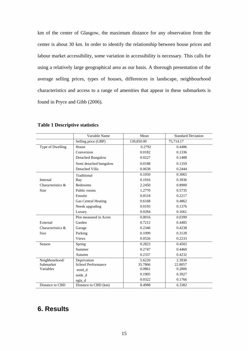
km of the center of Glasgow, the maximum distance for any observation from the

center is about 30 km. In order to identify the relationship between house prices and

labour market accessibility, some variation in accessibility is necessary. This calls for

using a relatively large geographical area as our basis. A thorough presentation of the

average selling prices, types of houses, differences in landscape, neighbourhood

characteristics and access to a range of amenities that appear in these submarkets is

found in Pryce and Gibb (2006).

Table 1 Descriptive statistics

Variable Name Mean Standard Deviation Selling price (GBP) 139,850.00 75,714.17 Type of Dwelling House 0.2792 0.4486 Conversion 0.0182 0.1336 Detached Bungalow 0.0227 0.1488 Semi detached bungalow 0.0188 0.1359 Detached Villa 0.0638 0.2444 Traditional 0.1050 0.3065 Internal Bay 0.1916 0.3936 Characteristics & Bedrooms 2.2450 0.8900 Size Public rooms 1.2770 0.5735 Ensuite 0.0518 0.2217 Gas Central Heating 0.6168 0.4862 Needs upgrading 0.0193 0.1376 Luxury 0.0284 0.1661 Plot measured in Acres 0.0016 0.0399 External Garden 0.7212 0.4485 Characteristics & Garage 0.2346 0.4238 Size Parking 0.1099 0.3128 Views 0.0526 0.2233 Season Spring 0.2823 0.4502 Summer 0.2747 0.4460 Autumn 0.2337 0.4232 Neighbourhood/ Submarket

Deprivation School Performance

5.6220 35.7866

2.3930 22.8057

Variables eend_d 0.0861 0.2806 sside_d 0.1905 0.3927 ngla_d 0.0322 0.1766 Distance to CBD Distance to CBD (km) 8.4988 6.3382

6. Results

15

Regression Results

The specification of the Access Welfare variable makes the hedonic house

price model (1) non-linear in its parameters. For this reason maximum likelihood

estimations have first been performed to obtain optimal values of the parameters. In

this way, all the parameters have been estimated simultaneously as against a more

stepwise procedure found in for instance Adair et al. (2000). Thereafter we have

performed least squares estimation of (1) which is based on imputed values of the

estimated parameters found in the Access Welfare variable. This explains the ordinary

least squares results documented in Table 2.

The estimation results found in Osland and Pryce (2009) clearly showed that

the Access Welfare variable contributes significantly to explain variation in housing

prices in the Glasgow area. The variable is most significant when monotonicity is not

imposed. To provide evidence for this result, Osland and Pryce (2009) followed a

spatial econometric approach as recommended by Florax et al. (2003). This means

that the paper started with some relatively simple model specifications. These model

alternatives were then thoroughly tested for various spatially related

misspecifications. Regardless of which spatial model we used (i.e. spatial error

model, spatial lag model or a more comprehensive spatial Durbin model), regardless

of estimation method and number of neighbours included in the weights matrices, the

variable labour market accessibility with a non-monotonic distance effect was

important for explaining variation in housing prices. Tests for spatial effects showed

that a spatial error model probably is the most correct specification of (1). This may

imply that the ordinary least squares estimator is unbiased. It should, however, be

noted that there are relatively large variations in the values of the estimated elasticities

16

of employment accessibility in the OLS-model and the spatial error model. This

warrants a careful interpretation of the results found in this paper.

Table 2 Regression Results ------------------------------------------------------------------------------ Linear regression Number of obs = 6269 F( 28, 6240) = 400.69 Prob > F = 0.0000 R-squared = 0.6103 Root MSE = .30549 ------------------------------------------------------------------------------ | Robust sellingpln | Coef. Std. Err. t P>|t| [95% Conf. Interval] -------------+---------------------------------------------------------------- hous_all | .2196775 .0131007 16.77 0.000 .1939956 .2453595 convsn_d | .3695046 .0261976 14.10 0.000 .3181483 .4208608 bundet_d | .3158067 .0284138 11.11 0.000 .260106 .3715075 bunsd_d | .1641338 .0214784 7.64 0.000 .1220287 .2062389 vildet_d | .1380729 .0181949 7.59 0.000 .1024046 .1737412 trad | .0718791 .0184767 3.89 0.000 .0356584 .1080997 bay | .1095154 .0095229 11.50 0.000 .0908471 .1281836 bedrooms | .1849854 .0072579 25.49 0.000 .1707574 .1992134 publicro | .1635422 .0104666 15.63 0.000 .1430241 .1840603 ensuite | .1097422 .0153395 7.15 0.000 .0796715 .139813 gch_d | .0415696 .0084399 4.93 0.000 .0250244 .0581147 needsupg | -.1107956 .0253196 -4.38 0.000 -.1604307 -.0611605 luxury | .1359236 .0227219 5.98 0.000 .0913809 .1804663 acre | .336311 .0927142 3.63 0.000 .1545592 .5180628 garden_d | .0458404 .0104032 4.41 0.000 .0254466 .0662341 garage_d | .0990781 .0112651 8.80 0.000 .0769946 .1211616 parking | .0369223 .0163794 2.25 0.024 .0048129 .0690316 views | .068451 .0230265 2.97 0.003 .0233112 .1135909 spring | .0361596 .0102335 3.53 0.000 .0160985 .0562208 summer | .0539391 .0100373 5.37 0.000 .0342625 .0736156 autumn | .0436298 .0114168 3.82 0.000 .021249 .0660107 deprivtn | -.0170906 .0027176 -6.29 0.000 -.0224179 -.0117632 schoolpe~100 | .2208635 .0231542 9.54 0.000 .1754733 .2662537 eend_d | -.1587008 .0134379 -11.81 0.000 -.1850437 -.1323578 sside_d | -.1387943 .0097877 -14.18 0.000 -.1579815 -.1196071 ngla_d | -.2118817 .0210185 -10.08 0.000 -.2530852 -.1706781 cbdkm | -.0057795 .0012065 -4.79 0.000 -.0081447 -.0034143 VS_431_E12 | .0161653 .0006758 23.92 0.000 .0148405 .0174901 _cons | 10.81296 .0321817 336.00 0.000 10.74987 10.87604 ------------------------------------------------------------------------------

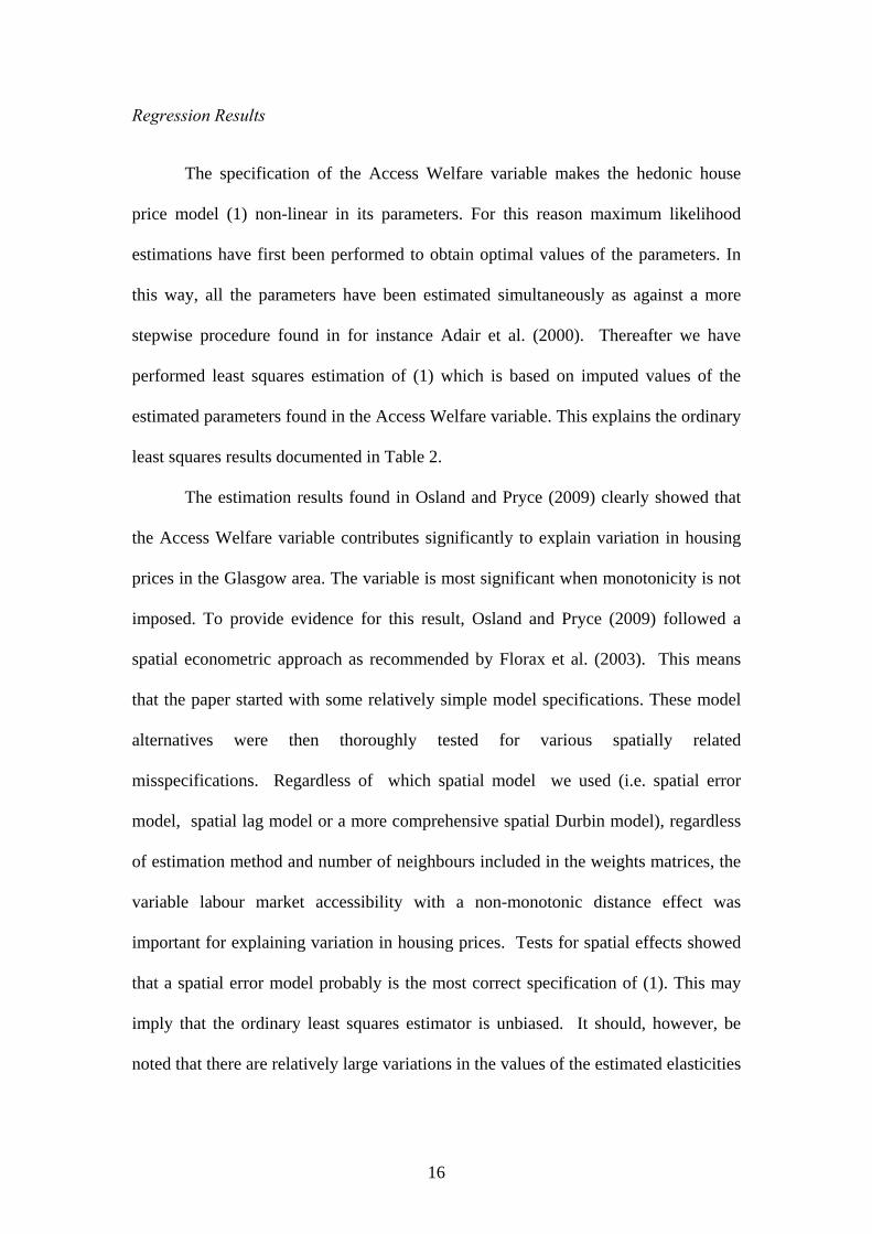
The estimated accessibility measure is plotted against distance to nearest employment

centre below (where employment = 100 and then when employment = 1,000). The

plots reveal clear evidence of non-monotonicity in the impact of access to

employment on house prices.

17

0.0

5.1

.15

S_0

p1_4

p6_m

0p00

7_n1

00_E

12

0 1000 2000 3000DIST

No. employees at employment node = 100Access Welfare Variable & Distance to Employment Node

0.0

5.1

.15

.2S

_0p1

_4p6

_m0p

007_

n100

0_E

12

0 1000 2000 3000DIST

No. employees at employment node = 1000Access Welfare Variable & Distance to Employment Node

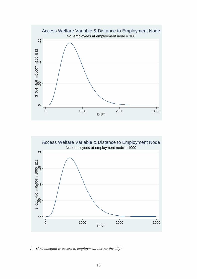
1. How unequal is access to employment across the city?

18

Our first task is to estimate the distribution of “Access Welfare” across locations in

Glasgow, and to use standard measures, such as Gini and Atkinson coefficients, to

gauge how unequal that distribution is. We have created a variable that captures the

benefits of access to employment while taking into account the undesirable effects of

being located too close to an employment node. We call it the Access Welfare

Variable and have estimated its kernel density function in Figure 1 below for Glasgow

(dropping out repeat postcodes). While no household has zero welfare, over 7 per cent

of people have access welfare values less than 1, and a further 11 per cent have values

less than 10, either because they are located very near employment centres (and

therefore suffer from noise, pollution and congestion) or very far from employment

nodes. Access to employment is highly unequal with the average variation in Access

Welfare coming in at around 90% of the mean (as shown by the coefficient of

variation). The Gini coefficient of .48 (relative to a value of zero in a world of equal

access and a value of 1 in a world of perfect unequal access) paints a similar picture,

as do the Atkinson coefficients.

19

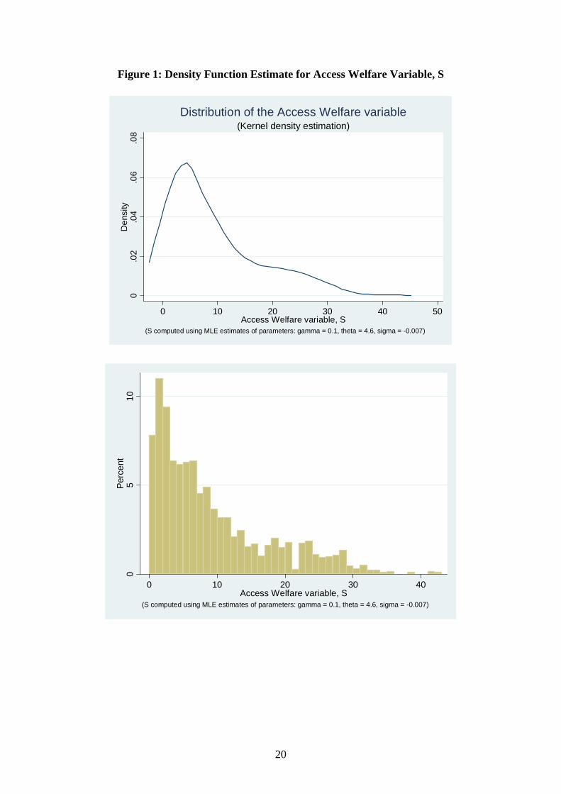
Figure 1: Density Function Estimate for Access Welfare Variable, S

0.0

2.0

4.0

6.0

8D

ensi

ty

0 10 20 30 40 50Access Welfare variable, S

(S computed using MLE estimates of parameters: gamma = 0.1, theta = 4.6, sigma = -0.007)

(Kernel density estimation)Distribution of the Access Welfare variable

05

10P

erce

nt

0 10 20 30 40Access Welfare variable, S

(S computed using MLE estimates of parameters: gamma = 0.1, theta = 4.6, sigma = -0.007)

20

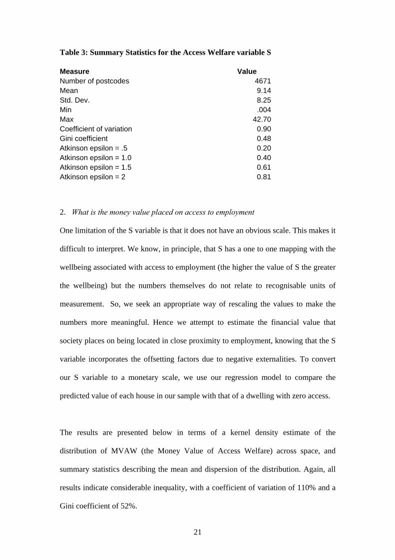
Table 3: Summary Statistics for the Access Welfare variable S

Measure Value Number of postcodes 4671 Mean 9.14 Std. Dev. 8.25Min .004 Max 42.70Coefficient of variation 0.90Gini coefficient 0.48Atkinson epsilon = .5 0.20Atkinson epsilon = 1.0 0.40Atkinson epsilon = 1.5 0.61Atkinson epsilon = 2 0.81

2. What is the money value placed on access to employment

One limitation of the S variable is that it does not have an obvious scale. This makes it

difficult to interpret. We know, in principle, that S has a one to one mapping with the

wellbeing associated with access to employment (the higher the value of S the greater

the wellbeing) but the numbers themselves do not relate to recognisable units of

measurement. So, we seek an appropriate way of rescaling the values to make the

numbers more meaningful. Hence we attempt to estimate the financial value that

society places on being located in close proximity to employment, knowing that the S

variable incorporates the offsetting factors due to negative externalities. To convert

our S variable to a monetary scale, we use our regression model to compare the

predicted value of each house in our sample with that of a dwelling with zero access.

The results are presented below in terms of a kernel density estimate of the

distribution of MVAW (the Money Value of Access Welfare) across space, and

summary statistics describing the mean and dispersion of the distribution. Again, all

results indicate considerable inequality, with a coefficient of variation of 110% and a

Gini coefficient of 52%.

21

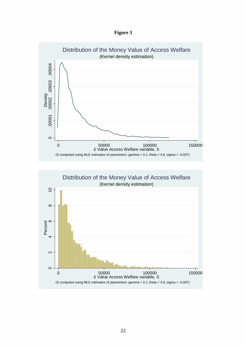
Figure 3

0.0

0001

.000

02.0

0003

.000

04D

ensi

ty

0 50000 100000 150000£ Value Access Welfare variable, S

(S computed using MLE estimates of parameters: gamma = 0.1, theta = 4.6, sigma = -0.007)

(Kernel density estimation)Distribution of the Money Value of Access Welfare

02

46

810

Per

cent

0 50000 100000 150000£ Value Access Welfare variable, S

(S computed using MLE estimates of parameters: gamma = 0.1, theta = 4.6, sigma = -0.007)

(Kernel density estimation)Distribution of the Money Value of Access Welfare

22

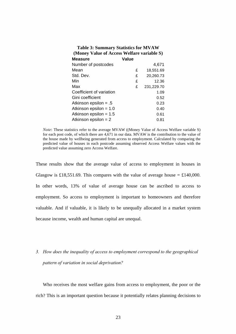
Table 3: Summary Statistics for MVAW (Money Value of Access Welfare variable S)

Measure Value Number of postcodes 4,671 Mean £ 18,551.69 Std. Dev. £ 20,260.73 Min £ 12.36 Max £ 231,229.70 Coefficient of variation 1.09Gini coefficient 0.52Atkinson epsilon = .5 0.23Atkinson epsilon = 1.0 0.40Atkinson epsilon = 1.5 0.61Atkinson epsilon = 2 0.81

Note: These statistics refer to the average MVAW ((Money Value of Access Welfare variable S) for each post code, of which there are 4,671 in our data. MVAW is the contribution to the value of the house made by wellbeing generated from access to employment. Calculated by comparing the predicted value of houses in each postcode assuming observed Access Welfare values with the predicted value assuming zero Access Welfare.

These results show that the average value of access to employment in houses in

Glasgow is £18,551.69. This compares with the value of average house = £140,000.

In other words, 13% of value of average house can be ascribed to access to

employment. So access to employment is important to homeowners and therefore

valuable. And if valuable, it is likely to be unequally allocated in a market system

because income, wealth and human capital are unequal.

3. How does the inequality of access to employment correspond to the geographical

pattern of variation in social deprivation?

Who receives the most welfare gains from access to employment, the poor or the

rich? This is an important question because it potentially relates planning decisions to

23

social and economic inequality. It also connects our results to the predictions of urban

economic theory which traditionally places higher income households further from

employment nodes.

We interpolate our results across space using nearest neighbour methods to

give a complete unbroken 3D surface of the Money Value of Access Welfare

covering areas of both high and low deprivation. We apply the same GIS techniques

to derive a surface of deprivation (the peaks represent highly deprived areas).

Figure 4: Geographical Distribution of the Money Value of the Access Welfare Variable

Surface Estimate in Cartesian Space using Nearest Neighbour interpolation

Key:

Figure 5: Geographical Distribution of the Unemployment Rate

24

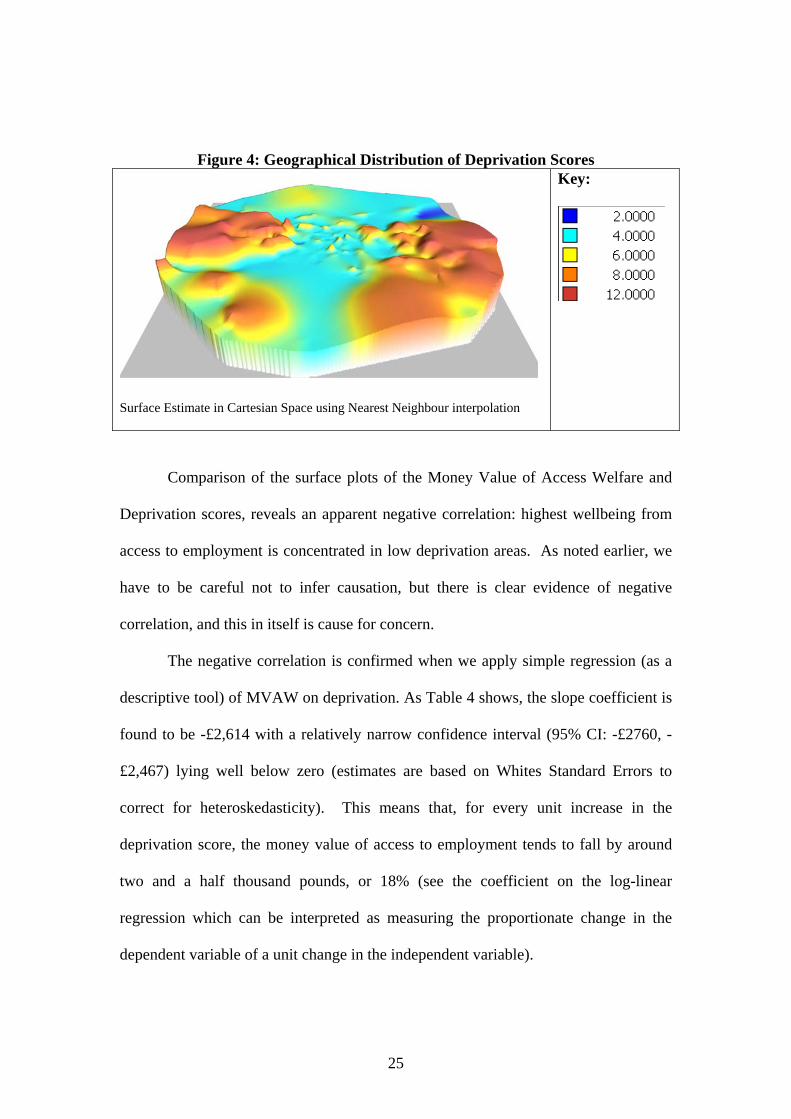
Figure 4: Geographical Distribution of Deprivation Scores

Surface Estimate in Cartesian Space using Nearest Neighbour interpolation

Key:

Comparison of the surface plots of the Money Value of Access Welfare and

Deprivation scores, reveals an apparent negative correlation: highest wellbeing from

access to employment is concentrated in low deprivation areas. As noted earlier, we

have to be careful not to infer causation, but there is clear evidence of negative

correlation, and this in itself is cause for concern.

The negative correlation is confirmed when we apply simple regression (as a

descriptive tool) of MVAW on deprivation. As Table 4 shows, the slope coefficient is

found to be -£2,614 with a relatively narrow confidence interval (95% CI: -£2760, -

£2,467) lying well below zero (estimates are based on Whites Standard Errors to

correct for heteroskedasticity). This means that, for every unit increase in the

deprivation score, the money value of access to employment tends to fall by around

two and a half thousand pounds, or 18% (see the coefficient on the log-linear

regression which can be interpreted as measuring the proportionate change in the

dependent variable of a unit change in the independent variable).

25

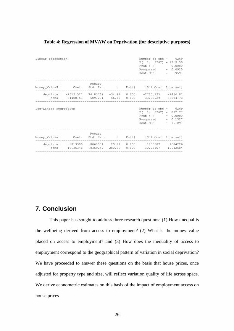
Table 4: Regression of MVAW on Deprivation (for descriptive purposes)

Linear regression Number of obs = 6269 F( 1, 6267) = 1219.59 Prob > F = 0.0000 R-squared = 0.0925 Root MSE = 19591 ------------------------------------------------------------------------------ | Robust Money_Valu~S | Coef. Std. Err. t P>|t| [95% Conf. Interval] -------------+---------------------------------------------------------------- deprivtn | -2613.527 74.83769 -34.92 0.000 -2760.235 -2466.82 _cons | 34400.53 609.201 56.47 0.000 33206.29 35594.78 ------------------------------------------------------------------------------ Log-Linear regression Number of obs = 6269 F( 1, 6267) = 882.77 Prob > F = 0.0000 R-squared = 0.1327 Root MSE = 1.1097 ------------------------------------------------------------------------------ | Robust Money_Valu~n | Coef. Std. Err. t P>|t| [95% Conf. Interval] -------------+---------------------------------------------------------------- deprivtn | -.1813906 .0061051 -29.71 0.000 -.1933587 -.1694226 _cons | 10.35346 .0369247 280.39 0.000 10.28107 10.42584 ------------------------------------------------------------------------------

7. Conclusion This paper has sought to address three research questions: (1) How unequal is

the wellbeing derived from access to employment? (2) What is the money value

placed on access to employment? and (3) How does the inequality of access to

employment correspond to the geographical pattern of variation in social deprivation?

We have proceeded to answer these questions on the basis that house prices, once

adjusted for property type and size, will reflect variation quality of life across space.

We derive econometric estimates on this basis of the impact of employment access on

house prices.

26

Our approach has been novel in that we have sought to address both the highly

non-linear relationship between wellbeing and distance to employment, and the

existence of multiple centres of employment nodes, each of a different size. We are

aware that this study is nevertheless a static one and therefore cannot tackle the

difficult problems of causality and simultaneous determination. We are also aware of

multiple sources of imprecision and bias in our model (not least the relatively sparse

observations on house prices in the most deprived areas) but we believe that our key

results (the inequality of access and the negative correlation with deprivation) are so

pronounced that they are unlikely to be overturned by using more precise and

complete data.

It is beyond the scope of this paper to estimate what proportion of the

mismatch between those who need work (unemployment tends to be highest in highly

deprived areas) and where work is located is due to the sorting process of the market

and what proportion is due to the cumulative history of planning decisions

(particularly the construction of peripheral social housing estates in the 1960s). The

two are inevitably interlaced. Nevertheless, our results highlight the potency of this

mismatch, and the extent to which it has persisted in the face of Glasgow’s long

recovery from deindustrialisation (Turok et al).

Our results emphasise the need for improved access to employment for the

poorest households. Note, however, that new private housing estates are themselves

likely to lie on the periphery, and so the real implication of our results is not so much

the infusion of social mix into new development but how to increase social mix in

established areas of the city that have good access to employment.

Our findings also raise the question of whether a model of this kind might

provide a useful input into strategic planning generally. While the model has its

27

limitations, it does make explicit the implications for equality of access of the

juxtaposition of residential and employment location. Our findings highlight

important questions about the priorities of planning policy and whether equality of

access (based on models of the kind proposed here) should be an active ingredient of

strategic planning decisions.

Finally, our model could be used to simulate the impact on inequality and

spatial mismatch of new developments, such as the construction of a new factory. It is

a fairly easy application of the model to enter hypothetical increases in employment in

particular postcodes and estimate the effect on Access Welfare and the corresponding

Gini and Atkinson coefficients.

28

References

Adair A, S McGreal, A Smyth, J Cooper, and T Ryley, 2000, House prices and accessibility: the testing of Relationships within the Belfast urban area, Housing studies, 15, 699-716.

Alonso W, 1964, Location and land use. Toward a general theory of land, Harvard University Press, Cambridge, Massachusetts.

Anselin L, 1988, Spatial econometrics: methods and models. Kluwer Academic Publishers, London.

Anselin, L. and J. Le Gallo, 2006, Interpolation in Spatial Hedonic Models, Spatial Economic Analysis, 1(1), 32-52.

Anselin, L. and N. Lozano-Gracia, 2008, Errors in variables and spatial effects in hedonic house price models of ambient air quality, Empirical Economics, 3, 5-34.

Anselin, L., 2006, Spatial econometrics, Ch. 26 in Palgrave Handbook of Econometrics, Mills TC and Patterson K (eds), volume 1, Palgrave Macmillan.

Bartik, T.J. and V.K. Smith, 1987, Urban Amenities and Public Policy, Handbook of Regional and Urban Economics, Vol. 2, Elsevier.

Beckman, M.J., 1973, Equilibrium models of residential land use. Regional and Urban Economics, 3, 361-368.

Bell , K.P. and N.E. Bockstael, 2000, Applying the Generalized-Moments Estimation approach to spatial problems involving microlevel data. The Review of Economics and Statistics, 82(1), 72-82.

Bivand, R. E.J. Pebesma and V. Gómez-Rubio, 2008, Applied spatial analysis with R. Springer.

Clapp, J.M. Rodriguez,M. Pace, R.K., 2001, Residential Land Values and the Decentralization of Jobs, Journal of Real Estate Finance and Economics, 22, 1, 43-61.

Crane, R., 1996, The influence of uncertain job location on urban form and the journey to work, Journal of Urban Economics, 37, pp. 342–356.

De Maio, F. (2007) Income Inequality Measures, Journal of Epidemiology and Community Health 2007;61:849–852

Dunse, N. and Jones, C. 1998, A hedonic price model of office rents, Journal of Property Valuation and Investments, 16, 3, 297-312.

Duranton, G. and Overman, H.G., 2005, Testing for localisation using micro-geographic data. Review of Economic Studies, 72, 4, 1077-1106.

29

Fingleton, B. (2006), A crosss-sectional analysis of residential property prices: the effects of income, commuting, shooling, the housing stock and spatial interaction in the English regions, Papers in Regional Science, 85(3), 339-361.

Fingleton, B. (2008), Housing supply, housing demand and affordability. Urban Studies, 45(8), 1545-1563.

Florax R.J.G.M. and T. De Graaf ,2004, The performance of diagnostic tests for spatial dependence in linear regression models: a meta analysis of simulation studies. Ch. 2 in Advances in Spatial Econometrics. Methodology, Tools and Applications, Anselin, L. Florax, R.J.G.M. and Rey, S.J. (eds.), Springer.

Florax R.J.G.M., H. Folmer and S.J. Rey, Specification searches in spatial econometrics: the relevance of Hendry’s methodology, Regional Science and Urban Economics, 2003, 22, 5, 557-579.

Fujita, M., 1989, Urban Economic Theory, Cambridge University Press, Cambridge.

Glaeser, E.L. and Kohlase, J.E., 2004, Cities, regions and the decline of transport costs, Papers in Regional Science, Journal of the Regional Science Association International, 83, 1, pp. 197-228.

Goodman, A.C. and Thibodeau, T.G., 1998, Housing market segmentation. Journal of Housing Economics, 7, pp. 121–143.

Grieson, R.E. and Murray, M.P., On the possibility and optimality of positive rent gradients, Journal of Urban Economics, 9, 3, pp. 275-285.

Guiliano, G, and K Small, 1991, Subcenters in the Los Angeles region, Regional Science and Urban Economics, 21, 163-182.

Heikkila E, P Gordon, J I Kim, R B Peiser, H W Richardson, 1989, What happened to the CBD-distance gradient?: land values in a polycentric city, Environment and Planning A 21 221-232.

J. Yinger, J., 1992,Urban models with more than one employment center, Journal of Urban Economics 31 (1992) (2), pp. 181–205.

Johnson, H. G. (1973) The Theory of Income Distribution, Gray-Mills Publishing, London.

Kelejian, H.H. and I.R. Prucha, 1999, A generalized moments estimator for the autoregressive parameter in a spatial model, International Economic Review, 40, 2, 509-533.

Lambert, P. (1993) The Distribution and Redistribution of Income: A Mathematical Analysis, Second Ed., Manchester University Press, Manchester.

LeSage, J. and R.K. Pace, 2009, Introduction to Spatial Econometrics, CRC Press.

Levin, E.J. and Pryce, G. (2007) A Statistical Explanation for Extreme Bids in the House Market, Urban Studies, 44(12), pp.2339-2355.

30

Li M. M. and H. J. Brown, 1980, Micro-neighbourhood externalities and hedonic prices, Land Economics, 56 125-140.

Maclennan, D. and Tu, Y., 1996, Economic perspectives on the structure of local housing markets, Housing Studies, 11, 387-406.

Maclennan, D., Munro, M., and Wood, G., 1987, Housing choice and the structure of urban housing markets, in Turner, B., Kemeny, J. and Lundquist (Eds) Between State and Market Housing in the Post-industrial Era, Almquist and Hicksell International, Gothenburg.

McMillen, D P, 2003, The return of centralization to Chicago: using repeat sales to identify changes in house price distance gradients, Regional Science and Urban Economics, 33, 287-304.

Moore, D. S. and McCabe, G. P. (2003) Introduction to the Practice of Statistics, 4th Edition, Freeman, New York.

Muth, R, 1969, Cities and Housing, Chicago, University of Chicago Press.

Osland, L, I Thorsen, and J P Gitlesen, 2007, ”Housing price gradients in a geography with one dominating center”, Journal of Real Estate Research, 29, 321-346

Osland, L. and I. Thorsen, 2008, Effects on housing prices of urban attraction and labor market accessibility, Environment and Planning A, 40,10, pp 2490 – 2509

Osland, L., (in print), An application of spatial econometrics in relation to hedonic house price modelling. Journal of Real Estate Research.

Papageorgiou G.J. and E. Casetti, 1971, Spatial equilibrium residential land values in a multicentric setting, Journal of Regional Science 11, pp. 385–389.

Pryce, G and Gibb, K., 2006, Submarket Dynamics of Time to Sale, Real Estate Economics, 34(3), pp.377-415.

Pryce, G. and Oates, S. , 2008, Rhetoric in the Language of Real Estate Marketing, Housing Studies, 23(2), pp.319-348.

Richardson, H W, P Gordon, M-J Jun, H Heikkila, P Reiser, D Dale-Johnson, 1990, ”Residential property values, the CBD, and multiple nodes: further analysis”, Environment and Planning A 22 829-833

Richardson, H W,1988, Monocentric vs. Policentric Models: The Future of Urban Economics in Regional Science, The Annals of Regional Science, vol. 22, issue 2, 1-12

Romanos, M.C., 1977, Household location in a linear multi-center metropolitan area, Regional Science and Urban Economics 7, pp. 233–250.

31

Ross, S. and J. Yinger, 1995, Comparative static analysis of open urban models with a full labor market and suburban employment, Regional Science and Urban Economics 25, pp. 575–605.

Waddell, P, B J L Berry, and I Hoch, 1993, Residential property values in a multinodal urban area: new evidence on the implicit price of location, Journal of Real Estate Finance and Economics, 22 829-833

Watkins, C. 2001. The Definition and Identification of Housing Submarkets. Environment and Planning A 33: 2235–2253.

Wheaton, W.C., 2004, Commuting, congestion, and employment dispersal in cities with mixed land use, Journal of Urban Economics, 55(3), 417-438.

Yiu C.Y. and C.S. Tam, 2004, A review of recent empirical studies of property price gradients, Journal of Real Estate Literature 12, 3, pp. 307–322.

Yiu, C.Y. and Tam, C.S., 2007, Housing price gradient with two workplaces – empirical study in Hong Kong, Regional Science and Urban Economics, 37, 413-429.

32

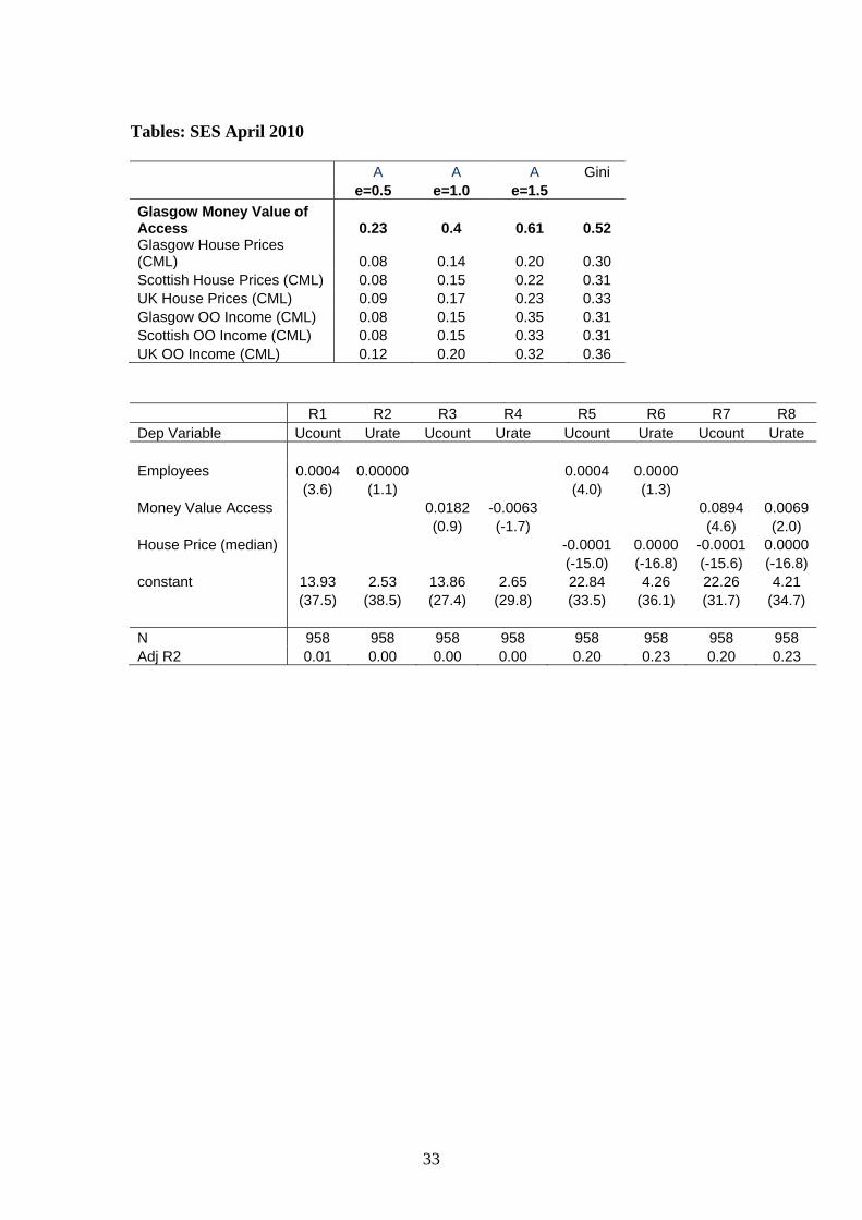
Tables: SES April 2010

A A A Gini e=0.5 e=1.0 e=1.5

Glasgow Money Value of Access 0.23 0.4 0.61 0.52 Glasgow House Prices (CML) 0.08 0.14 0.20 0.30 Scottish House Prices (CML) 0.08 0.15 0.22 0.31 UK House Prices (CML) 0.09 0.17 0.23 0.33 Glasgow OO Income (CML) 0.08 0.15 0.35 0.31 Scottish OO Income (CML) 0.08 0.15 0.33 0.31 UK OO Income (CML) 0.12 0.20 0.32 0.36

R1 R2 R3 R4 R5 R6 R7 R8 Dep Variable Ucount Urate Ucount Urate Ucount Urate Ucount Urate Employees 0.0004 0.00000 0.0004 0.0000 (3.6) (1.1) (4.0) (1.3) Money Value Access 0.0182 -0.0063 0.0894 0.0069 (0.9) (-1.7) (4.6) (2.0) House Price (median) -0.0001 0.0000 -0.0001 0.0000 (-15.0) (-16.8) (-15.6) (-16.8) constant 13.93 2.53 13.86 2.65 22.84 4.26 22.26 4.21 (37.5) (38.5) (27.4) (29.8) (33.5) (36.1) (31.7) (34.7) N 958 958 958 958 958 958 958 958 Adj R2 0.01 0.00 0.00 0.00 0.20 0.23 0.20 0.23

33

34