AN EXAMINATION OF WAGE INEQUALITIES IN CHILE

Estudios Públicos, 85 (verano 2002).

STUDY

AN EXAMINATION OF WAGEINEQUALITIES IN CHILE

Harald Beyerand Carmen Le Foulon

HARALD BEYER. Investigador y Coordinador Académico del Centro de Estudios Pú-blicos. Ingeniero Comercial, Universidad de Chile. Candidato a Doctor en Economía de laUniversidad de California, Los Ángeles.

CARMEN LE FOULON. Ingeniera Comercial, Pontificia Universidad Católica de Chile.Magister en Economía Aplicada mención Políticas Públicas, PUC. Investigadora del Centrode Estudios Públicos.

Chile has one of the highest levels of wage inequality in the world,and has had for decades. Nonetheless, this paper argues that if thewage distribution is examined in its entirety, instead of concentra-ting on specific indicators such as the Gini coefficient or the coeffi-cient of variation of wages, significant changes in wage inequalitycan be seen over the years. In particular, all the action on inequalityis occurring in the upper part of the wage distribution.The authors show that wage inequality grew significantly during the1960s, reflecting increases in the variance of wages both betweenand within different skill groups. The fact that this occurred moreforcefully in the public sector, leads one to speculate about thepossible role played by labor unions in this phenomenon.The two ensuing decades saw significant falls in real wages for allwage earners, reflecting the high inflation rates of the 1970s and theeffects of the recessions of 1975 and 1982-83 on the real wages ofChilean white-collar and manual workers. These falls were much

Translated by Timothy Ennis

2 ESTUDIOS PÚBLICOS

steeper among groups in the middle of the wage distribution. Theleast affected groups were the top wage earners. This helps to ex-plain an increase in wage dispersion between skill groups which iscompensated by a reduction in the intra-group wage dispersion. As aresult, during these two decades, the more permanent levels of wagedispersion are not very different from those seen back in 1970.Finally, wage dispersion narrowed slightly in the 1990s, but notenough to compensate for the increases in inequality that occurredduring the 1960s.In their analysis, the authors highlight what has been happening withwage-earners who are high-school graduates. These have seen adrastic fall in their wages relative to those with only primaryschooling. Whereas in the 1960s high-school graduates earned morethan twice the wages of someone with primary education, the diffe-rence today is no more than 35%. On the other hand, the returns tohigher education have grown significantly during the same period,and the educational differences between high and middle wagegroups have widened. All of this goes a long way to explaining whywage inequalities have not decreased over the last four decades,despite the population’s average level of schooling rising from sevenyears in the early 1960s to 11 in the late 1990s.

1. Introduction

here are a variety of indicators that show Latin America to be themost unequal region of the world, even more so than Africa. Some of thedifferences can be explained by differences in regional development levelsor by methodological considerations in collecting the basic information onwhich the indicators are constructed. However, once such differences arecontrolled for, we find that Latin America has a Gini coefficient (a traditio-nal indicator of inequality that takes values between zero and 1, zero indica-ting absolute equality) which is, on average, 10 points higher than would bethe case if our countries were located in another region of the world. Mo-reover, Chile is in the more unequal half of the Latin American region,which suggests that the issue of inequality will not easily disappear fromour country’s political agenda nor from that of the region as a whole.Underlying this concern about inequality there is a clear desire to overcomepoverty as quickly as possible. If Chile had its current per-capita incomebut the same level of inequality as the Republic of Korea, its poverty levelwould be no higher than 16%; in other words there would be nearly onemillion fewer poor people in our country.

T

HARALD BEYER, CARMEN LE FOULON 3

Making our country more equal is an objective that cannot be aban-doned. But to achieve it, we need to correctly understand the origins of ourinequality. The distributional conflicts that intensified in our country follo-wing the Great Depression of 1929-32 spawned numerous policies thatbecame a burden on productive activity. Chile’s per-capita income grew ata rate of 1.9% per year in real terms, between 1945 and 1970, while per-capita income in the rest of Latin America expanded at 3% per year and theworld economy grew at an annual rate of 4%. Nonetheless, this sacrifice interms of economic growth did not produce significant changes in incomeinequality. Although the data are too disperse to reach a definitive conclu-sion, everything seems to suggest that inequality by the end of the 1960swas not very different from the situation in the early 1940s. Slow growthlifted few people out of poverty; frustrations grew and society polarized.The 1970s and 1980s were marked by deep divisions among the Chileanpeople, and the country endured deep crisis. Structural economic changefailed to raise Chile’s per-capita income, which in the late 1980s was just11% higher than in 1970, while inequality had increased.

Trade liberalization had given people access to more and betterproducts, however. The proportion of households with at least one automo-bile had risen from 7.3% in 1970 to 21.3% by 1990. In the same period oftime, the proportion with a television set had risen from 10.3% to 78.6%,and homes with a refrigerator had grown from 14.4% to 44.9%. The possi-bility of obtaining more material goods clearly increased the welfare ofChilean families, but it was essential for prosperity to be maintained overtime. Democracy needed to be strengthened and, clearly, economic growthcould contribute enormously to that. The structural reforms introduced bythe authoritarian government followed by responsible economic leadershipduring the 1990s, supported by positive international conditions and a rela-tively harmonious political climate, were among the many factors that ena-bled Chile’s economy to grow as never before in our history. Between 1985and 1998, the income of Chilean families practically doubled. Between1987 and 1998, two million Chileans ceased to be poor. Yet this rapidgrowth was not accompanied by a reduction in income inequality, and soonthe “development model” began to be questioned. Doubts have been rein-forced by the country’s sluggish economic performance since 1998 and thepersistent unemployment that has accompanied it.

It cannot be denied that the desire for equality is latent among theChilean people, but there is no wish to sacrifice economic progress. Thesetwo demands are confused and intermixed among the population. Naturally,our political leaders see sharp inequalities in income and want to correct


them; but efforts to do so, unless well thought out, often end up undermi-ning economic growth (Alesina and Rodrick, 1994), and hence also taxrevenue and State action targeting the poorer segments of the population.The risks of redistributive adventures may have a very high social cost;hence the importance of correctly evaluating the policies to be pursued. It isessential to have a clear view of the country’s distributive reality and thechanges that have occurred in recent decades. This is the subject of thisarticle. We aim to delve deeper into the trend of inequality over the last 40years. Taking advantage of employment surveys carried out by the Univer-sity of Chile, we will concentrate on wage inequality. Of course, we are notthe first authors to look at this evidence (see Beyer et al., 1999; Bravo andMarinovic, 1998; Ruiz-Tagle, 1999, among others), but we believe we cancontribute a useful and also new perspective. In the following section webriefly review a number of studies that are relevant to research on incomeinequality in Chile. The third section explains the origin of the figures usedin this study and makes a preliminary assessment of them. The fourth sec-tion takes an original look at the trend of wage inequality in Chile, and thefifth offers some conclusions.

2. A review of the literature

Income inequality has increasingly been attracting economists’ at-tention. The ultimate cause of this interest stems from the clear tendencytowards greater inequality that can be seen in the developed world, especia-lly in the United States and the United Kingdom (Gottschalk and Smeeding,1997). Research into this subject is assisted by increasing availability ofinformation. The Chilean economy has continued to change in recent deca-des, but a long-term view suggests that the changes have been less signifi-cant than might be suggested by studying a few years in isolation (Cowanand De Gregorio, 1998). Naturally, however, opinions tend to differ in thisarea, depending on the emphasis placed by the observer. Some analystsclaim that significant changes have taken place in the income distribution inChile1 in the long-term, but not in the medium and short-term (Marcel andSolimano, 1993; Contreras, 1996; Valdés, 1999). An interesting paper inthis category is that by Ruiz-Tagle (1999), who sets up confidence intervalsto analyze the trend of inequality between 1957 and 1998. He concludes

1 Long-term analysis refers to Greater Santiago rather than to Chile as a whole, andis based on University of Chile employment surveys.


2 Differences in the Gini coefficient are statistically significant at 1% with respect to1965, and at the 5% level with respect to 1970.

3 The wage rate that divides the lowest paid 10% of the population from the remai-ning 90%, measured in terms of the hourly wage.

4 This phenomenon did not extend nationwide. The CASEN surveys suggest thatwage dispersion in the 1990s actually increased slightly (see Beyer, 2001).

5 In Chile, according to national accounts, wage incomes account for about 47% ofnational income (assuming indirect taxes are paid by capital and labor in proportion to theirshare of national income). Nonetheless, this factor underestimates the true share of labor: itdoes not consider the income of independent workers, nor does it take account of the fact thata large proportion of capital incomes are, strictly speaking, payments to labor. Profits earnedby small and medium-sized businesses are an example of this.

6 For a more detailed analysis, see Beyer (2000).7 Cowan and De Gregorio (1996), Beyer (1997), Contreras (1996), Valdés (1999).

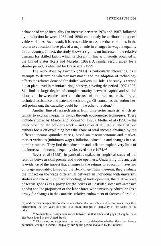
that changes from one year to another are not usually significant, as theyfall within the confidence interval. Table 1 shows the trend of severalinequality indicators in recent decades for Greater Santiago. Unfortunatelyit is impossible to make long-term comparisons at the national level. Theimpression is that at the end of the last century inequality in Chile wassomewhat greater than in the 1960s,2 but no different from the levels pre-vailing in 1980. On the other hand, in 1985 and 1990 the income distribu-tion was significantly more unequal than in the late 1990s. Inequality grewin the 1980s as a result of a sharp rise in unemployment in those years and asignificant drop in real wages, which, despite impinging on all socialgroups, had more serious effects on people with low-incomes (see figure 1).

Between 1981 and 1985 the hourly wage in the 10th percentile3 fellby 39%, whereas the equivalent fall in percentile 90 was just 21%. In 1990,the hourly wage in percentile 90 exceeded its real value in 1981 by 12%,while that of percentile 10 was still 13% below its 1981 level. The stronggrowth of the 1990s facilitated a rapid increase in wages at the lower levels,thereby reducing wage dispersion among the inhabitants of Santiago.4 No-netheless, this dispersion was greater in the late 1990s than in the early1980s. It is worth asking whether this emphasis on people’s labor incomeshas any justification; after all, income from capital is also a major propor-tion of national income.5 The fact that income from capital is distributedunequally is not in dispute; but it is not distributed very differently in Chilethan elsewhere in the world. What is clear is that labor incomes are distribu-ted much more unequally than in other countries.6 So it seems reasonableto focus the analysis on labor incomes.

This unequal distribution of labor incomes is magnified at the house-hold level by factors that often are specific to our country.7 For example,the female market-market participation rate, which is surprisingly low in


TABLE N° 1: HOUSEHOLD INCOME DISTRIBUTION: GREATER SANTIAGO

(Ranked by per-capita income)

1965 1970 1980 1985 1990 1994 1998

Quintile 1 5.9 5.5 5.0 4.2 4.3 5.2 4.8

Quintile 2 11.6 9.3 8.7 8.4 8.1 9.6 8.7

Quintile 3 14.9 14.3 12.5 12.2 11.7 12.2 12.9

Quintile 4 19.7 19.6 20.3 20.7 18.3 19.0 20.7

Quintile 5 47.9 51.3 53.4 54.5 57.6 53.9 52.9

Gini 0.414 0.441 0.469 0.485 0.507 0.466 0.468

Ratio 8.1 9.3 10.6 13.0 13.5 10.4 11.1

Source: Prepared by the authors on the basis of employment surveys conducted inthe month of June by the Department of Economics of the University of Chile. Figures arethree-year averages centered on the year indicated.

FIGURE N° 1: TREND OF HOURLY WAGE

(Male wage-earners)

0

50

100

150

200

250

300

350

400

Percentil 10 Percentil 50 Percentil 90

1957

1960

1962

1966

1968

1970

1972

1974

1976

1978

1980

1982

1984

1986

1988

1990

1992

1994

1996

1998

Percentil 90Percentil 50Percentil 10


8 This claim is not so obvious, but the empirical evidence suggests that investmentsin human capital yield varying returns.

9 This result is not that surprising, considering that inequality among the highest10% of the income distribution is similar to that in the other 90%. The result merely corrobo-rates this.

10 Through the Mincerian income equation they decompose the variance, calculatingthe percentage that is attributable to observable variables (education and potential experien-

Chile, is significantly correlated with education levels. As a result, thepoorest households on average have fewer income-earners per family mem-ber than those with higher incomes, thereby accentuating the income diffe-rences between the poor and the rich. The likelihood of unemployment isalso correlated with an individual’s education level. In the absence of gene-rous unemployment insurance schemes, the effect of these differences in theunemployment rate magnify individual income inequalities in the house-hold. Of course, differences in the fertility rate, which are also correlatedwith education, explain significant differences in family size, which meansthat economic differences between high- and low-income families increasein per-capita income terms. Analysis of the determination of labor incomesis usually based on the theory of human capital originally developed byBecker (1964) and Mincer (1974), or on further elaborations of those theo-retical developments. This theory assumes that a worker’s productivity, andhence income, is determined by his or her level of human capital; this, inturn, is based on skills acquired in formal education and those acquiredinformally (through work). Labor incomes therefore depend on the endow-ment of productive characteristics and their market return,8 which makeseducation an essential element in explaining changes in the income distribu-tion.

The evidence in this field is interesting. Montenegro (1998) investi-gates whether there are differences in returns according to income percenti-le, and finds higher returns to education among the higher income groups.9

The evidence suggests that returns to education vary significantly from onelevel of education to another, so assuming a unique average private rate ofreturn for all Chilean education would be mistaken (Beyer, 2000). Specifi-cally, returns rise with years of education, such that university education hasa greater marginal impact on wages than basic education. Similarly, Contre-ras (1996) shows that part of the differences in the trend of poverty andinequality is explained by regional differences in the return to education forthe different education levels.

Bravo and Marinovic (1999) and find that wage inequality has in-creased, and they separate changes in the distribution of labor income intochanges in observable and non-observable variables.10 They show that the


ce) and the percentages attributable to non-observable variables in different years; they thendifferentiate the two years in order to attribute changes in inequality to one factor or theother.

11 Nonetheless, complementarities between skilled labor and physical capital havealso been found in the United States.

12 Of course, as we pointed out earlier, it is debatable whether there has been apermanent change in income inequality during the period analyzed by the authors.

behavior of wage inequality (an increase between 1974 and 1987, followedby a reduction between 1987 and 1996) can mostly be attributed to obser-vable variables. As a result, it is reasonable to assume that variations in thereturn to education have played a major role in changes in wage inequalityin our country. In fact, the study shows a significant increase in the relativedemand for skilled labor, which is closely in line with results obtained inthe United States (Katz and Murphy, 1992). A similar result, albeit for ashorter period, is obtained by Bravo et al (1999).

The work done by Pavcnik (2000) is particularly interesting, as itattempts to determine whether investment and the adoption of technologyaffects the relative demand for skilled workers in Chile. The study is carriedout at plant level in manufacturing industry, covering the period 1997-1986.She finds a large degree of complementarity between capital and skilledlabor, and between the latter and the use of imported materials, foreigntechnical assistance and patented technology. Of course, as the author her-self points out, the causality could be in the other direction.11

Another line of research arises from time-series analysis, which at-tempts to explain inequality trends through econometric techniques. Theseinclude studies by Marcel and Solimano (1993), Meller et al (1996) – thelatter based on the previous work – and Beyer et al (1999). The first twoauthors focus on explaining how the share of total income obtained by thedifferent income quintiles varies, based on macroeconomic and market-market variables (minimum wage), inflation, education and changes in eco-nomic structure. They find that education and inflation explain very little ofthe increase in income inequality observed since 1974.12

Beyer et al (1999), in particular, makes an empirical study of therelation between skill premia and trade openness. Underlying this analysisis evidence of the impact that changes in the returns to education have hadon wage inequality. Based on the Heckscher-Ohlin theorem, they evaluatethe impact on the wage differential between an individual with universitystudies and one with primary schooling, of trade openness, the relative priceof textile goods (as a proxy for the prices of unskilled intensive-intensivegoods) and the proportion of the labor force with university education (as aproxy for changes in the countries relative endowment of factors of produc-


13 This variable is obtained by estimating a Mincerian human capital model, withthe natural logarithm of the hourly wage as dependent variable and a series of variables thathave been shown to affect individual wages in other studies. The estimation includes dummyeducational variables. The variable in question is constructed by taking the difference bet-ween the coefficient of the “complete university education” dummy and the “complete prima-ry education” dummy.

tion).13 They find a positive relation between trade openness and the wagedifferential, whereby additional openness is found to have increased wageinequality in Chile. Possibly hiding behind this relation is technologicalchange biased in favor of skilled labor, or some change in the productivestructure of the economy. The fall in the prices of unskilled intensive-intensive goods reduces the relative wage of the less skilled, in keepingwith Heckscher-Ohlin. The increasing percentage of university graduates inthe labor force reduces their relative wage.

Given the importance of education in income, and hence its influen-ce on the income distribution, De Gregorio and Lee (1999) attempt tounravel the relationship between the two, using panel data taken from asample of countries between 1960 and 1990. One of their conclusions isthat higher population education levels reduce income inequality. The op-posite occurs if there is greater dispersion in education. In addition, inkeeping with other studies, they find that social policies do affect the inco-me distribution. Another result, also highlighted in Beyer (2000), is confir-mation of the existence of a Kuznets curve, in which the relation between acountry’s income level and its inequality displays an inverted U-shape.Nonetheless, they suggest that the majority of income inequality cannot beexplained either by education or by social expenditure, or by the country’sdevelopment level.

This review of the literature reveals that there is still a long way togo in understanding the causes behind the unequal distribution of laborincomes in Chile. As this is a situation that we also tend to share with therest of the Latin American region, there are clearly common elements thatshould help us understand this uncomfortable distributive reality. In thenext section we review Chilean experience over the last few decades. Ouraim is basically to describe the changes that have occurred in wage inequa-lity, rather than explain the high levels of inequality which seem always tohave been with us to a greater or lesser extent.

3. The Data

As a source of information, this study uses the employment andunemployment survey for Greater Santiago that the Department of Econo-


mics of the University of Chile has been conducting ever since 1957. Ouranalysis studies the period from 1957 through 1999. Although the survey iscarried out four times a year in March, June, September and December, wework with the June sample which provides additional data on labor andhousehold incomes. The survey gathers information from about 11,000people, both those active in the labor market and retirees. Our study onlyconsiders wage earners which the survey classifies as white-collar and ma-nual workers. The analysis focuses on men, since female labor marketparticipation is relatively low and has undergone significant changes duringthe period,14 both of which could affect and bias our comparisons. Natura-lly, the analysis excludes observations for which information on the varia-bles studied is incomplete. These considerations ultimately result in a sam-ple covering an average of 1,700 male wage earners in the period underanalysis.15

In this study we attempt to explain the trend of the natural logarithmof the hourly wage.16 For this purpose we use information covering thewhole wage distribution and focus our analysis on the path of percentiles10, 50 and 90, which we take to represent the incomes of lower-income,middle-income, and higher-income workers, respectively.

Wages have been corrected for variations in inflation and are deno-minated in pesos at June 2000 prices. The deflator used was the consumerprice index furnished by the National Institute of Statistics. For the period1970-1978, we further apply the Cortázar and Marshall (1980) correction.This study does not break down inflation for the period 1971-1972.17 Inorder to ensure reliable indices for June 1971 and 1972, we use the correc-tion proposed by Yáñez (1978), but as the latter is smaller than the Cortázarand Marshall version, we adjusted the Yáñez indices by the monthly diffe-rence between the two.18

Table 2 shows a number of indicators of the evolution of incomesand inequality in recent decades, based on data for greater Santiago. Thebehavior of the average annual percentage change in income has variedfrom decade to decade and between groups. In the 1960s, incomes increa-

14 See annex 1.15 Annex 2 displays the total observations for each year and the sample used.16 The hourly wage is defined as a worker’s total monthly income divided by the

number of hours worked per month, the latter being approximated as the number of hoursworked in the week multiplied by four.

17 “ […] due to the absence of primary information that would make it possible todescribe the differential effect of parallel markets in the various months”, Cortázar andMarshall (1980).

18 Annex 3 shows the corresponding values.


sed for all groups, but more for those earning higher incomes. In the en-suing decades, real wages fell in both the 1970s and 1980s, with wages ofmiddle-income white-collar workers and those of manual workers decliningmost. Incomes grew again in the 1990s, but with the opposite pattern to thatseen in the 1970s, namely, a smaller increase among higher income groups.These different patterns in income behavior generate different trends ininequality, measured in terms of the standard deviation of incomes, coeffi-cient of variation and differences between the income percentiles.

4. What has happened with the wage distribution?

We saw in figure 1 that real wages in Chile display a rising trendover the last four decades, but with significant fluctuations, and sharp fallsin some periods. Growth has not been uniform throughout the wage distri-bution. The highest skilled workers have obtained the largest increase –more than tripling their incomes since the start of the period – while theleast skilled have experienced more modest growth, with incomes doublingsince the early 1960s. This can be seen more clearly in figure 2 whichrecords changes in the logarithm of the hourly wage for all income percenti-les.

Without doubt there has been a major increase in wage levels for allincome groups, but particularly those in the highest 25% of the distribution.While in percentile 50 the real hourly wage increased by about 120% overfour decades, or at an average annual rate of 2%, the wages among the top10% of the distribution grew on average by 200%, or at an annual rate of

TABLE N° 2: INDICATORS OF INCOME CHANGES AND INEQUALITY

Annual average percentage change Average for the ten years

Income Income Income Std. Dev. Coefficient Difference Difference Differencepercentile 10 percentile 50 percentile 90 logarithm of variation percentiles percentiles percentiles

hourly wage hourly wage 50-10 90-50 90-10

1960-1969 3.07 3.30 5.17 0.81 1.45 0.81 1.22 2.031970-1979 –2.37 –2.85 –1.45 0.83 1.29 0.84 1.26 2.101980-1989 –1.12 –2.03 –0.96 0.89 1.46 0.81 1.43 2.241989-1999 5.02 4.26 3.50 0.83 1.45 0.74 1.35 2.09

Source: Prepared by the authors on the basis of University of Chile Surveys ofEmployment and Unemployment.


FIGURE N° 2: VARIATIONS IN THE LOGARITHM OF THE HOURLY WAGE

(Whole distribution: 1960-1999)

19 It should be recalled that the figure measures differences in the logarithm of thehourly wage for each income percentile, with the percentage differences calculated as follo-ws: (exp(x)-1)*100, where x represents the difference in natural logarithms of the hourlywage. This value is measured on vertical axis of figure 2.

1 4 7 10 13 16 19 22 25 28 31 34 37 40 43 46 49 52 55 58 61 64 67 70 73 76 79 82 85 88 91 94 97

1,4

1,2

1

0,8

0,6

0,4

0,2

0

2.8%.19 Consequently, during the last four decades dispersion has increa-sed in the upper part of the Chilean wage distribution. In the lower part ofthe distribution, as a result of the slightly larger wage increases among lowincome-income groups than among middle-income groups, the earnings dis-tribution has narrowed. So, in the context of a generalized increase in wagesin recent decades, there is a slightly larger increase at the extremes, especia-lly among the highest income groups. The net result is that wage differencesin the lower part of the distribution have narrowed whereas differentials inthe upper part have widened.

This distributional reality is the result of a series of changes thathave taken place over four decades, with considerable variation from onedecade to the next, as shown by figure 3. Thus, it is surprising to see that inthe 1960s there was a significant increase in wage dispersion, in the contextof a general increase in wage levels. Whereas hourly wages in the lowerpart of the wage distribution grew at an annual average of 3%, wagesamong groups in the upper half of the annual distribution grew by 6% peryear. This suggests that the relatively greater inequality seen in the 1990s


compared to the early 1960s, cannot be attributed to economic changesintroduced after the military coup of 1973, or to the sharp economic down-turns of 1975 and 1982-83 (which did indeed increase inequality, especiallythrough their effects on unemployment, but for a limited period only). Ins-tead, it is the result of forces that were already present in the 1960s.

The high levels of inflation of the 1970s and the economic contrac-tion in the middle of that decade caused real wages to fall significantlyacross all income groups. Although it is more difficult to discern a pattern

FIGURE N° 3: VARIATIONS IN THE LOGARITHM OF THE HOURLY WAGE FOR DIFFERENT

SUBPERIODS

1960-70 1970-80

1980-90 1990-99

0

0.1

0.2

0.3

0.4

0.5

0.6

0.7

0.8

0.9

1 4 7 10 13 16 19 22 25 28 31 34 37 40 43 46 49 52 55 58 61 64 67 70 73 76 79 82 85 88 91 94 97

-0.5

-0.45

-0.4

-0.35

-0.3

-0.25

-0.2

-0.15

-0.1

-0.05

0

1 4 7 10 13 16 19 22 25 28 31 34 37 40 43 46 49 52 55 58 61 64 6

-0.2

-0.1

0

0.1

0.2

0.3

0.4

0.5

1 4 7 10 13 16 19 22 25 28 31 34 37 40 43 46 49 52 55 58 61 64 67 70 73 76 79 82 85 88 91 94 97

0

0.1

0.2

0.3

0.4

0.5

0.6

0.7

0.8

0.9

1 4 7 10 13 16 19 22 25 28 31 34 37 40 43 46 49 52 55 58 61 64


in this case, it can be argued that the worst hit were very low-income groupsand those located around the third quartile (i.e. percentile 75) of the wagedistribution. In the 1980s, on the other hand, the fall in real wages affecteda broad group of wage earners, with only the extremes of the distributionbucking the trend. For those concerned, the drop in real wages was less thanin the 1970s, and it is notable that the lowest paid managed to defendthemselves from the fall in wages experience by middle-income groups.Possibly this was the result of the relatively inauspicious way in which thedecade had begun (in the 1970s there was a major deterioration in realwages), or that the various employment programs of the 1980s established awage floor that prevented further wage cuts. Lastly, the 1990s show notonly a substantial increase in wages for all white-collar and manual workersin Greater Santiago, but there was also a narrowing of the upper half of thewage distribution, which suggests that strong economic growth not only hasa significant effect on the population through its impact on wages, but itmay also have a significant redistributive effect.20

What underlies these changes in wage inequality? To answer thisquestion, we firstly estimate a regression of the natural logarithm of thehourly wage on a series of independent variables covering individual cha-racteristics that traditionally are considered as explanatory variables for thebehavior of wages in empirical human capital models. Specifically, ourregression includes a series of dummy variables that reflect the educationallevel attained by the interviewee.21 These variables have been fully interac-ted with the apparent experience of the individual and the square of thatexperience. The regression also included dummy variables controlling forthe economic sector in which the individual works, and for the institutionalnature of the employer (public or private). Estimates for different yearsenable us to evaluate whether changes in the wage distribution stem fromchanges between skill groups or within the different groups. The wagespredicted from these regressions are used to estimate changes betweengroups, while the residuals are used to estimate changes within the differentgroups. Table 3 provides results of this exercise.

20 Clearly, there is no conclusive evidence that economic growth reduces incomeinequalities. In fact, the nationwide CASEN survey does not show the same behavior. Onecould surmise, however, that economic growth has helped consolidate Chile’s higher educa-tion system. This in turn, has led to an increase in the supply of workers with highereducation, attracted by the high returns to this type of education. This could result in anincipient moderation in wage increases among the higher wage groups, which largely consistof university graduates, and hence a reduction in wage differences.

21 There are seven educational categories: without education, primary incomplete,primary complete (eight years), high-school incomplete, high-school complete, university andspecial education. In the regression we omitted the “without education” category.


22 Again it is worth remembering that following the crises, especially in 1982-83,wage inequality increased sharply, but this seems to relate more to transitory rather thanpermanent changes. Accordingly, if we consider the changes in wage inequality around thebeginning or end of the decade in years, apart from 1999 perhaps, that are reasonable fromthe economic point of view, we can gain a better idea of the factors behind these changes.

23 Recall that our regression included different educational categories, experience,experience squared (the latter two fully interacted with educational variables), the economicactivity in which the person works, whether the person worked in a public or private institu-tion, and lastly, whether the interviewee was a head of household.

The figures show that the largest increase in wage inequality occu-rred in the 1960s.22 The variance of wages grew significantly between 1960and 1970 by 46%. This major increase in wage dispersion during the 1960sstems firstly from changes in the variance within the different skill groups.The variance of residuals increases from 0.265 to 0.402, in other words by52%. There was a notable increase in the variance between skill groups: thevariance of predicted wages increases from 0.262 to 0.368, i.e. 40.5%,between 1960 and 1970. The increase in wage inequality during the 1960s,therefore, is mainly the result of the greater dispersion within the differentskill groups.23

An aspect that we would like to draw attention to in this analysis isthe behavior of the public sector (probably one ought to speak more genera-

TABLE N° 3: WAGE DISTRIBUTION IN CHILE: VARIOUS INDICATORS

1960 1970 1980 1990 1999

Actual wages50-10 0.829 0.916 0.866 0.706 0.75490-50 1.005 1.281 1.386 1.556 1.32590-10 1.834 2.197 2.252 2.262 2.079

Variance 0.527 0.770 0.769 0.799 0.674

Predicted wages50-10 0.490 0.545 0.482 0.368 0.45690-50 0.821 1.074 1.169 1.399 1.19590-10 1.311 1.619 1.651 1.767 1.651

Variance 0.262 0.368 0.390 0.424 0.334

Residual50-10 0.599 0.692 0.756 0.703 0.67590-50 0.651 0.769 0.718 0.786 0.71890-10 1.250 1.461 1.474 1.489 1.393

Variance 0.265 0.402 0.379 0.375 0.340

Source. See text.


TABLE N° 4: VARIANCE OF WAGES (IN NATURAL LOGARITHMS) IN THE PUBLIC AND

PRIVATE SECTORS

1960 1970 1980 1990 1999

PublicVariance 0.4893 0.8260 0.8329 0.8045 0.7311

Proportion 23.36% 23.58% 15.54% 10.56% 7.00%

PrivateVariance 0.4820 0.6646 0.7527 0.7856 0.6573

Proportion 76.64% 76.42% 84.46% 89.44% 93.00%

Source: Prepared by the authors on the basis of University of Chile Surveys ofEmployment and Unemployment

24 The survey distinguishes between fiscal institutions, public-sector bodies and pu-blic firms. We have grouped the whole public sector in a single category.

25 For further detail on this see Coloma and Rojas (2000).

lly of the unionized sector) in the 1960s. Table 4 shows not only thevariance of wages in the public24 and private sector throughout the variousyears analyzed, but also the proportion of wage earners in Greater Santiagoworking in the public and private sectors.

The increase of nearly 70% in the variance of wages in the publicsector explains much of the increase in wage inequality during the 1960s. Incontrast, the variance of wages in the private sector increased by just 38%.The increase in wage dispersion in the public sector was so strong that itwas never matched in the private sector throughout the period analyzed.Throughout the period public-sector wage dispersion remained higher thanin the private sector. A possible explanation for the behavior of wages inthe 1960s relates to the growing power that labor legislation was giving tothe unions.25 The public sector was no exception to this trend, so it shouldnot be surprising that while private sector wages grew at 4% per year in the1960s, public-sector wages rose at an annual rate of 5.3%. This reflects thepressure-group power enjoyed by public-sector workers. Unfortunately, theavailable information does not enable us to directly confirm whether theincrease in wage dispersion in the 1960s stems from the growing power ofunions, but the data presented are certainly consistent with this possibility.It may seem strange that unions have the capacity to increase wage disper-sion when usually they are expected to reduce it; but if unionized workersbasically come from the higher part of the wage distribution, income diffe-


26 Strictly speaking, union activity was suspended between 1973 and 1979.

rences between those who earn more and those who earn less are liable tobecome more pronounced in the presence of unions.

The authoritarian government drastically reduced the power of theunions, especially in the public sector, where employment was also cut backsharply.26 Curiously, this does not seem to have translated into a reductionin wage dispersion in the public sector, which is suggestive of wage inertiain this sector. The usual pattern of raising public-sector workers wages inequal proportions, in the absence of wage negotiations, may explain thisinertia. Nonetheless, as wage dispersion in the public sector remained hig-her than in the private sector, the fall (increase) in the proportion of workersworking in the public sector (private) should have caused a smaller varianceof wages. This effect can be seen in a reduction in the variance of theresiduals, i.e. the variance within the different skill groups. The effect ismore than compensated by a major increase in the variance between skillgroups (the variance of predicted wages rises significantly between 1970and 1980, and from then to 1990), shown in table 4 as an increase in theprivate-sector wage variance.

The increase in the wage variance is basically explained by an in-crease in dispersion in the upper part of the distribution. Figure 4 shows the

FIGURE N° 4: TREND OF DIFFERENCES BETWEEN WAGE DISTRIBUTION PERCENTILES

(Differences of natural logarithm of the wage)

0.6000

0.7000

0.8000

0.9000

1.0000

1.1000

1.2000

1.3000

1.4000

1.5000

1.6000

1.7000

diferencia percentil 90-50

diferencia percentil 50-10

1960

1962

1964

1966

1968

1970

1972

1974

1976

1978

1980

1982

1984

1986

1988

1990

1992

1994

1996

1998

difference percentile 50-10

difference percentile 90-50

0


evolution of differentials between percentiles 90 and 50 and between per-centiles 50 and 10. It is clear that whereas in the 1970s and 1980s, thedifference between percentiles 50 and 10 tends to diminish, the differentialbetween percentiles 90 and 50 tends to increase.

Lastly, the 1990s saw a reduction both in the variance of predictedwages and in the variance of residuals, suggesting a reduction in the varian-ce between skill groups, and within the different groups. Based on thesefigures we can distinguish three periods during the four decades. Firstly, the1960s saw a major increase in variance both between and within skillgroups. The two following decades display a weakening of the variancewithin skill groups but a slight increase between them. The final decaderecords a slight reduction in variance both between school groups andwithin them.

Figures 5, 6 and 7 summaries the reality described above. It shouldbe recalled that the regression used to construct table 3 included variouseducation categories among the independent variables, including primary,secondary (high-school) and university education. The figures show thechanges in wages experienced by white-collar and manual workers withdifferent levels of schooling in the periods defined earlier. The comparisonis made between the percentiles of each wage distribution, i.e. the distribu-tion of individuals with university, high-school and primary education res-pectively. To minimize possible errors arising from the small size of eachsample, we use three-year averages to carry out this exercise. The figuresshow the middle year in each case; thus, 1970 indicates that the average of1969, 1970 and 1971 has been taken to construct the 100 wage percentilesin each educational group. Figure 5, which corresponds to the 1960s, allowsus to clearly verify that in that period wage dispersion increased within eacheducational group, and in general the higher percentiles saw their wagesrise relatively more than the lower percentiles. This is particularly so bet-ween wage-earners with secondary and those with primary education. Atthe same time, the wages earned by university graduates grew faster thanamong other educational groups, thereby increasing the variance of wagesbetween educational groups. During 1970-1988, all groups saw their realwages decline. The wages of individuals with more education fell less,thereby increasing dispersion between skill groups. But among wage ear-ners with high-school and primary education, wage dispersion actually na-rrowed. Those earning most in each of the groups saw their wages fallrelatively more than those earning less. Naturally, no-one is better off, butwage differentials have narrowed. This is consistent with the smaller varian-


FIGURE N° 5: TREND OF HOURLY WAGE:1958-1970

(By percentile and educational category)



0

0.2

0.4

0.6

0.8

1

1.2

1 4 7 10 13 16 19 22 25 28 31 34 37 40 43 46 49 52 55 58 61 64 67 70 73 76 79 82 85 88 9

Básica Media Universitaria

-1.2

-1

-0.8

-0.6

-0.4

-0.2

01 5 9 13 17 21 25 29 33 37 41 45 49 53 57 61 65 69 73 77 81 85 89


1,2

1,0

0,8

0,6

0,4

0,2

0

0

–0,2

–0,4

–0,6

–0,8

–1,0

–1,2

Primary Secondary University


ce seen in the second period within the different skill groups. Lastly, figure7 shows that wage dispersion diminished in all educational groups in theperiod 1988-98. In addition, the earnings of university trained professionalsgrew more slowly than those of other wage-earners, so the variance bothbetween and within the different skill groups decreases. Figure 8 shows thechanges in the wage distribution for the four decades analyzed.




-0.2

0

0.2

0.4

0.6

0.8

1

1.2

1 5 9 13 17 21 25 29 33 37 41 45 49 53 57 61 65 69 73 77 81 85 89


1,2

1,0

0,8

0,6

0,4

0,2

0,0

–0,2


FIGURE N° 7: TREND OF HOURLY WAGE:1988 - 1998

(By percentile and educational category

0

0.2

0.4

0.6

0.8

1

1.2

1 4 7 10 13 16 19 22 25 28 31 34 37 40 43 46 49 52 55 58 61 64 67 70 73 76 79 82 85 88 91 9

Básica Media UniversitariaBásica Media Universitaria

1,2

1,0

0,8

0,6

0,4

0,2



The overall picture to emerge from these four decades is surprising.Part of the greater variance between skill groups is explained by the slowgrowth of earnings among individuals with high-school education.27 Mo-reover, in the upper percentiles of the distribution of wage earners with

27 We say “part of the increase in the variance” because we are not considering allthe independent variables included in the regression.


28 Bravo and Marinovic (1999), for example, argue that there has been an increasein the relative demand for skilled workers in Chile.

secondary education, wage increases over the 40-year period are slightlynegative. Of course supply factors play a role here. As figure 9 shows, theproportion of high-school educated individuals has risen significantly overthe last 40 years. But the proportion of the population with higher educationhas also grown significantly, without showing through in the trend of wagesin this group (although at the end of the period it seems to be making itseffects felt). Accordingly, there are demand factors that also explain therelative deterioration in the earnings of high-school educated workers.28

People with primary schooling that earn most have also seen their wagesdeteriorate compared to individuals with higher education, but to a relative-ly small extent. From the standpoint of the individual deciding whether ornot to invest in education, the secondary education “project” seems veryunattractive unless the higher education alternative is considered at thesame time. Thus it should not be surprising that the demand for secondaryschool students, including those going through technical-professional edu-

FIGURE N° 9: EDUCATION LEVEL OF WAGE-EARNERS IN GREATER SANTIAGO

��

��

��

��

��

��

��

��

0%

20%

40%

60%

80%

100%

58 70 88 98

Sin Educación Básica Incompleta Básica Completa�� Media Incompleta

�� Media Completa UniversitariaSecondary incomplete

Without education Primary incomplete

Secondary complete

Primary complete

Universitary

1958 1970 1988 1998

100%

80%

60%

40%

20%

0%


FIGURE N°10: DIFFERENCES IN LOG OF WAGES OF WORKERS WITH SECONDARY AND

BASIC EDUCATION

(Corrected for experience)

0

0.2

0.4

0.6

0 8

1

1.2

1 4

1957 1960 1962 1966 1968 1970 1972 1974 1976 1978 1980 1982 1984 1986 1988 1990 1992 1994 1996 1998

1,4

1,2

1,0

0,8

0,6

0,4

0,2

0,0

cation, should be for higher education. Figure 10 shows how wage differen-tials between individuals with high-school education and those with basiceducation have narrowed.

In the 1960s an individual with high-school education typically ear-ned more than twice the wage of someone who left the formal educationsystem after primary school.29 In the 1990s, they were earning just 35%more. What has been happening, then, is a convergence of the wages ofindividuals with high-school education towards those of individuals withprimary education. In other words, the labor market distinguishes less andless between secondary school and basic education graduates. This is aphenomenon peculiar to the last two decades; whereas the 1960s clearlysaw wage inequality climb to levels it would maintain during the two follo-wing decades, the determinants of this inequality are changing. In the 1960sthere was a considerable increase in the variance both between skill groupsand within the each of the groups; in the subsequent decades this gives wayto a further increase in the variance between groups, largely resulting fromslower wage growth among workers with secondary education, and a na-rrowing of the intra-group variance, which is incomplete because of thelarger wage dispersion among university professionals towards the end of

29 To reach this conclusion on the basis of the graph, recall that the graph representsthe difference between the natural logarithm of the wage of an individual with secondaryschooling and another with primary. Thus, the wage ratio is obtained by estimating ex, wherex represents the difference in the logarithms mentioned.


the 1990s, compared to the early 1960s.30 Although the 1990s show areduction in both the inter-group and intra-group variances, this is insuffi-cient to compensate for the changes that took place in the preceding deca-des.

Another way of looking at changes in the wage distribution thatenriches the above analysis is to determine the contribution to the trend ofwage inequality made by changes in observed quantities, observed pricesand unobserved prices. This alternative is particularly attractive in the caseof Chile, where the simple human capital model generally captures thebehavior of wages quite well.31

To perform this exercise we use a methodology originally developedby Juhn et al (1993). The key is to isolate the different effects, namelyobserved quantities, observed prices and non-observed prices. We start witha simple human capital model, such as represented in equation (1).

(1) Yit = Xit b + uit

Where Yit is the logarithm of the hourly wage of individual i in yeart. Xit represents a matrix of individual characteristics, including experience,education and marital status. Lastly, uit covers the unobserved part of thewage equation. For analytical purposes, we want to break this factor downinto two elements: the individual percentile in the residual distribution whi-ch we shall call qit, and the distribution function of the residuals fromequation (1) which we call Ft( ). Using the definition of the cumulativedistribution function, we then have

(2) uit = Ft-1(qit|Xit)

Where Ft-1( × |Xit) is the inverse of the cumulative distribution of

residuals for workers with characteristics Xit in year t. In this framework,changes in wage inequality stem from three sources: changes in the distribu-tion of the X, changes in the b, and changes in the distribution of theresiduals. If we define an average price for the observables throughout theperiod (‘b) and also an average cumulative distribution for the period (‘F( ×|Xit)), then we can decompose the wage equation into different componentsas follows:

30 Of course, the increase in the proportion of university professionals also has aninfluence.

31 Typically, a regression with the natural logarithm of the hourly wage as dependentvariable, and education (or various educational categories), experience, experience squared,as independent variables, explains around 40% of the variation in individual wages.


(3) Yit = Xit’b + Xit (b -’b) +’F-1(qit | Xit) + [F-1(qit | Xit) -’F-1(qit | Xit)] .

The first term of equation (3) captures the effect of a change in thedistribution of the X, while holding prices constant. The second term captu-res the effect of a change in the b, holding the X constant. The final termcaptures the effect of changes in the distribution of the residuals from thewage equation. This decomposition makes it possible to reconstruct theshape that the wage distribution would adopt if any of its components wereheld constant. Specifically, if we left observable prices and the distributionof residuals constant, the wage equation would be determined by

(4) Yit1 = Xit’b +’F-1(qit | Xit).

Calculating the distribution of Yit1 for each year would enable us to

attribute changes in inequality to changes in observable quantities. Analo-gously, if we want both observable prices and quantities to vary over time,but not the distribution of the residuals, we can estimate the wage equationas follows:

(5) Yit2 = Xit b +’F-1(qit | Xit).

If we proceed in this way, the difference between Yit2 and Yit

1 can beattributed to changes in observable prices. Any additional change in inequa-lity that results from comparing the effective distribution with Yit

2 shouldbe attributed to changes in the distribution of non-observables. This is theexercise we carry out below. The average b correspond to different periodsanalyzed. Table 5 gives the results of this decomposition for the last fourdecades. Tables 6, 7 and 8 show the results for different periods.

Table 5, corroborates what we have been saying. Wage dispersionincreased significantly over the last four decades, widening the differentialin hourly wage between an individual in percentile 90 and someone inpercentile 10 by 40%. The difference between percentiles 90 and 50 increa-sed by 47%. The wage of an individual in percentile 90 rises from just oversix times higher than someone in percentile 10 to nearly nine times higher.This increase is explained exclusively by the behavior of the upper part ofthe distribution, given that the wage differential between percentiles 50 and10 narrowed by 6.3%. The main factors behind this increase in wage dis-persion are observable prices, in other words the premium paid to observa-ble skills such as education. This increased premium is concentrated parti-cularly in the upper part of the distribution, and in fact its trend in the lower


TABLE N° 5: BREAKDOWN OF SOURCES OF CHANGES IN THE WAGE DISTRIBUTION:

PERIOD 1958-1998*

Period 1958-1998

Percentiles Effective difference Quantities Prices Nonobservables

90-10 0.333 0.046 0.170 0.11650-10 –0.054 –0.102 –0.127 0.18990-50 0.386 0.161 0.298 –0.073

* Corresponds to middle year of three-year averages.


PERIOD1958-1970*

Period 1958-1970


90-10 0.334 0.075 0.134 0.12550-10 0.028 –0.060 0.025 0.06390-50 0.305 0.135 0.109 0.062



PERIOD1970-1988*

Period 1970-1988


90-10 0.170 –0.033 0.138 0.06550-10 –0.087 –0.139 0.010 0.04290-50 0.257 0.106 0.128 0.023



part of the distribution contributes to reducing wage dispersion. Observablequantities do not seem to have had a major effect on wage dispersion,although the behavior of these quantities varies significantly within thedistribution. While the trend of quantities (years of schooling, for example)helps to compress the lower part of the wage distribution, it magnifies wageinequalities in the upper part of the distribution. This suggests that educa-tional differences between wage earners in percentile 90 and those in per-centile 50 widened during the period under analysis, unlike educationaldifferences between percentiles 90 and 10. This suggests the existence ofsome type of barrier to increasing education among middle-income groups.Lastly, there seems to have been a non-negligible increase in the premiumto non-observable skills which is particularly noticeable in the lower part ofthe distribution. This is compensated, however, by a reduction in premia toobservable skills and by smaller differences in quantities.

Table 6 summarizes the changes that took place in the 1960s andshows that they were of a similar magnitude to changes that occurred in thefour decades analyzed. There are significant differences, however, withrespect to table 5. Dispersion is slightly less in the upper part of the wagedistribution. At the same time the increase in the premium to observableskills is a significantly less, and the increase is distributed rather morehomogeneously throughout the distribution. Lastly, the increase in the pre-mium to non-observable skills is greater in this decade than in the fourdecades taken together. The period 1970-1988 has its own peculiarities.Wage differentials increase still further between percentiles 90 and 10,mainly because of greater dispersion in the upper part of the distributionwhich, in turn, is explained almost equally by changes in observable quanti-ties and by further increases in premia to observable skills. The final periodshows a decline in wage inequality in Greater Santiago of a similar magni-


PERIOD1988-1998*

Period 1988-1998*


90-10 –0.179 0.029 –0.116 –0.09250-10 0.000 0.071 –0.027 –0.04390-50 –0.179 –0.042 –0.089 –0.049



tude to the increase recorded during the two preceding decades. The reduc-tion in wage dispersion in the 1990s is explained exclusively by a na-rrowing of the 90-50 percentile differential. In this case, a narrowing of thepremium paid to observable skills plays a very important role.

Changes in wage inequality display different characteristics overtime. Changes in the premium to non-observable skills have been essentialin explaining changes in wage dispersion, and the effect on wage inequalityof premia paid to non-observable skills has been considerable, especially inthe 1960s. This phenomenon is compatible with the hypothesis that growingunion power may have served to increase wage inequality, which the lawsgranting such power possibly were intended to correct. All of this suggeststhat changes in wage inequality are complex, difficult to explain and impos-sible to attribute to a single factor. It should also be mentioned that changesin observable quantities also help to explain changes in wage inequality. Inour opinion, these quantities are fundamentally explained by education andexperience. In what follows, we want to refer to the behavior of education,in which there are some interesting elements. Figure 11 shows the trend inaverage schooling among wage earners in Greater Santiago. Averageschooling has increased by a slightly over four years during these fourdecades, rising from an average of 6.8 years in the early 1960s to 11.2 yearstoday. Initially this increase in the average schooling of wage earners seemsto have been the result of a significant increase in schooling among a smallsegment of the population, accompanied also by an increase in the disper-sion of education, as shown in figure 12.

During the last few decades alone educational differences among thepopulation have reduced significantly. Nonetheless, this seems to be theresult of having managed to increase the education level of those with least

FIGURE N° 11: AVERAGE SCHOOLING OF MALE WAGE EARNERS IN GREATER

SANTIAGO

12

10

8

6

4

2

0

1957

1961

1966

1969

1972

1975

1978

1981

1984

1987

1990

1993

1996

1999


FIGURE N° 12: DISPERSION OF HIGH-SCHOOL EDUCATION MEASURED BY STANDARD

DEVIATION

3.5

3.6

3.7

3.8

3.9

4

4.1

4.2

4.3

4.4

4.5

1957

1961

1966

1969

1972

1975

1978

1981

1984

1987

1990

1993

1996

1999

1957

1961

1966

1969

1972

1975

1978

1981

1984

1987

1990

1993

1996

1999

4,5

4,4

4,3

4,2

4,1

4,0

3,9

3,8

3,7

3,6

3,5

schooling. Table 9 clearly shows that the average years of schooling hasincreased significantly for all groups. The largest increase occurred in thelowest income groups in the distribution.32 This has enabled them to closethe educational gap with respect to wage earners located around the 50thpercentile. Nonetheless, the gap between wage earners located around per-centile 50 and those in the region of percentile 90 has not closed; in fact ithas actually widened. Differences of just under five years of schooling in1958 have grown to seven years today. But, perhaps most importantly,whereas percentile 50 still remains at high-school education levels, wageearners in percentile 90 have gone beyond this level of schooling to com-plete higher education courses. This magnifies wage differentials betweenthe two groups not only because of the effect on incomes of having comple-ted more years of schooling, but also because there are significant differen-ces in the returns to each education level in Chile.33 Accordingly, for analy-tical purposes, two effects on income can be distinguished as a result ofthe increased level of schooling. The first stems from the change in quantity– in the number of years’ difference – which can be referred to as a “purequantity” change. The second stems from the fact that an additional year ofeducation generates a larger wage differential if it involves moving from

32 It is not particularly surprising, therefore, that these groups have experiencedgreater wage increases than middle income groups.

33 Returns differ and display a rising structure; in other words, the returns to primaryeducation are smaller than those to secondary education, and these in turn are less than thoseobtained from university education. See Beyer (2000) for a more detailed analysis of thisresult.


TABLE N° 9: YEARS OF SCHOOLING AMONG DIFFERENT GROUPS OF THE WAGE

DISTRIBUTION

Percentile 10 Percentile 50 Percentile 90

1958 3.5 6.3 11.11998 8.7 9.5 16.5

primary school to high-school education, and particularly from secondary tohigher education, than if the additional year occurs within the same educa-tion level. We shall refer to this as a “level effect” to distinguish it from the“pure quantity” effect. Applying this distinction it is very likely that therelatively major impact of changes in observable quantities on wage diffe-rences (recall table 5) is biased, because it includes a level effect which,strictly speaking, relates more to what we understand as a return to educa-tion rather than increase in years of schooling. This suggests that suchincreases will do little to reduce educational inequalities unless the returnsto the different types of education are made more uniform or the schoolinglevel of middle-income groups in the wage distribution is raised well be-yond secondary education. The challenges are enormous in either case.

5. Conclusions

We have attempted to make an exhaustive analysis of the changesthat have occurred in the wage distribution in Chile over the last fourdecades. Our analysis stands alongside those of other authors that haveundertaken similar tasks. Some of the results obtained have been surprising– particularly the fact that wage inequality increased significantly in the1960s. The data analyzed do not tell us for certain what it was in thatdecade that caused such a large increase in wage inequality, but it is notablethat it was spearheaded by the public sector. It is reasonable to speculatethat the growing power acquired by unions in this period was behind theincrease. Insofar as labor unions consist of workers located in the upperpart of the wage distribution, an increase in their bargaining power couldlead to greater wage inequality. Nonetheless, we wish to leave this merelyas a possible explanation, rather than as a confirmed statement. In the twofollowing decades, inequality remained at similar levels to those prevailingby 1970, with transitory but significant increases during periods of econo-mic crisis. In the 1990s, on the other hand, wage inequality decreased, butnot enough to offset the changes that had occurred in the 1960s.


ANNEX 1:Trend of female labor market participation rate

0%

10%

20%

30%

40%

50%

60%

1957

1960

1962

1966

1968

1970

1972

1974

1976

1978

1980

1982

1984

1986

1988

1990

1992

1994

1996

It is noteworthy that the changes recorded in the wage distributionare concentrated in the upper part of the distribution. In the lower part,wage differentials actually narrowed, especially as result of the sharp in-crease in schooling among the lowest paid. Differences in schooling in theupper part of the distribution, on the other hand, actually increase. Theimpact of this on wage dispersion is also magnified, because wage earnersin the upper part of the wage distribution progressed from high-schooleducation to university education in the last four decades, while those inpercentile 50 are still not competing high-school. As the premium to high-school education fell significantly in the same period, while the return totertiary education increased, the impacts on wage dispersion are enormous.

The situation of high-school educated wage earners is particularlyworrying. Their wages seem to have leveled out with those of workers onlywith basic education. The effect is so strong that wage earners with this typeof education that earn most have seen their real wages fall in the last fourdecades. It is clear that the labor market distinguishes less and less betweenworkers with basic education and high-school graduates. This raises a cha-llenge that cannot be eluded. The demand for young people with highereducation will continue to grow. Moreover, those who do not see highereducation as a possibility will not have much incentive to complete high-school, which will make it more difficult to reduce the still large educatio-nal differences that exist among Chilean people. Will wage differentials inChile narrow? Unless educational differences narrow and differences in thereturns to the different types of education become more uniform, this goalwill be impossible to achieve. Changes in wage inequality will inevitably belinked to what happens with education in Chile.


ANNEX 2:

Total Hombres Empleados Obreros Total muestra

1957 10.756 4.902 792 1.124 1.6071958 10.556 4.797 646 1.107 1.3741960 10.197 4.575 689 999 1.3401961 11.312 5.135 789 1.013 1.4481962 12.360 5.647 825 1.096 1.5851965 14.759 6.885 996 1.452 2.0381966 14.680 6.889 1.027 1.434 2.0431967 15.944 7.432 1.176 1.577 2.2241968 14.834 6.939 1.147 1.300 1.9881969 14.167 6.585 1.105 1.240 1.8971970 14.536 6.816 1.186 1.276 1.9311971 15.976 7.541 1.446 1.117 2.1421972 14.659 6.949 1.370 1.051 2.0401973 14.977 7.163 1.386 1.103 2.1281974 12.831 6.166 946 1.181 1.6191975 14.539 7.039 1.159 1.218 1.7851976 13.824 6.558 960 1.203 1.5821977 14.230 6.692 1.043 1.323 1.8671978 14.643 6.951 1.081 1.293 1.8401979 14.627 6.999 1.094 1.295 1.8811980 12.699 6.066 919 1.163 1.6611981 12.833 6.096 940 1.246 1.8021982 12.801 6.009 956 1.266 1.4851983 12.473 5.942 918 1.273 1.4571984 12.520 5.983 882 1.223 1.5911985 12.625 5.988 934 1.245 1.6801986 12.381 5.800 931 1.181 1.6211987 12.273 5.817 956 1.170 1.6651988 12.115 5.802 909 1.188 1.6811989 11.806 5.597 973 1.181 1.6571990 11.716 5.590 988 1.135 1.6061991 11.939 5.757 1.051 1.140 1.6931992 11.507 5.567 986 1.182 1.6711993 11.287 5.405 1.025 1.158 1.6981994 11.456 5.476 1.098 1.142 1.5901995 11.184 5.301 1.032 1.036 1.5261996 11.235 5.422 1.085 1.076 1.4901997 5.371 608 989 1.5371998 11.268 5.456 930 1.205 1.3691999 11.297 635 954 1.231 1.280

Total number of observations and sample used


ANNEX 3:Adjustment to convert to pesos at June 2000 prices

1957 2.754.569,601958 2.291.639,921959 1.637.941,081960 1.499.700,081961 1.378.530,451962 1.243.338,771963 848.031,501964 572.121,451965 438.701,471966 360.348,751967 303.087,801968 239.695,231969 180.544,311970 137.739,401971 106.385,401972 65.620,081973 12.898,571974 1.651,681975 317,871976 97,311977 44,081978 29,431979 21,831980 15,811981 13,071982 12,541983 9,481984 7,951985 5,881986 5,011987 4,211988 3,641989 3,141990 2,511991 2,031992 1,771993 1,571994 1,391995 1,291996 1,191997 1,131998 1,081999 1,04


BIBLIOGRAPHY

Alesina, Alberto and Danny Rodrik. 1994. “Distributive Politics and Economic Growth”.Quarterly Journal of Economics, Vol. 109, N° 2 (May).

Becker, Gary. 1964. Human Capital. Chicago: University of Chicago Press, 3rd edition,1993.

Beyer, Harald. 1997. “Distribución del Ingreso: Antecedentes para la Discusión”. Estudios

Públicos, 65 (summer).Beyer, Harald; Patricio Rojas and Rodrigo Vergara. 1999. “Trade Liberalization and Wage

Inequality in Chile”. Journal of Economic Development, June.Beyer, Harald. 2000. “Educación y Desigualdad de Ingresos: Una Nueva Mirada”. Estudios

Públicos, 77 (summer).Beyer, Harald. 2001. “Salario Mínimo y Desempleo”. Working Papers, March, Centro de

Estudios Públicos.Bravo, David and Alejandra Marinovic. 1999. “Wage Inequality in Chile: 40 Years of Evi-

dence”. Mimeo, Department of Economics, University of Chile.Bravo, David; Dante Contreras and Tomás Rau. 1999. “Wage Inequality and Labor Markets

in Chile 1990-1996: A Non-Parametric Approach”, Mimeo, Department of Econo-mics, University of Chile.

Coloma, Fernando and Patricio Rojas. 2000. “Evolución del Mercado Laboral en Chile:Reformas y Resultados”. In Felipe Larraín and Rodrigo Vergara (eds.), La Transfor-

mación Económica de Chile. Santiago: Centro de Estudios Públicos.Contreras, Dante. 1964. “Pobreza y Desigualdad en Chile: 1987-1992. Discurso, Metodología

y Evidencia Empírica”. Estudios Públicos, 64 (spring).Cortázar, René and Jorge Marshall. 1980. “Índice de Precios al Consumidor en Chile: 1970-

1978”. Colección Estudios Cieplan, 4.Cowan, Kevin and José De Gregorio. 1996. “Distribución y Pobreza en Chile: ¿Estamos mal?

¿Ha Habido Progresos? ¿Hemos Retrocedido?” Estudios Públicos, 64 (spring).De Gregorio, José and Jong-Wha Lee. 1999. “Education and Income Distribution: New

Evidence from Cross Country Data”. Working paper N° 55, Serie Económica, Cen-ter for Applied Economics, Department of Industrial Engineering, University ofChile.

Engel, Eduardo; Alex Galetovic and Claudio Raddatz. 1997. “Reforma Tributaria y Disitribu-ción del Ingreso en Chile”. Working paper N° 40, Serie Económica, Center forApplied Economics, Department of Industrial Engineering, University of Chile.

Gottschalk, P. and T. Smeeding. 1997. “Cross-National Comparisons of Earnings and IncomeInequality”. Journal of Economic Literature, 35.

Juhn, C.; K. Murphy and B. Pierce. 1993. “Wage Inequality and the Rise in Returns to Skill”.Journal of Political Economy, Vol. 111, N° 3 (June).

Marcel, Mario and Andrés Solimano. 1993. “Developmentalism, Socialism and Free MarketReform: Three Decades of Income Distribution in Chile”. Policy Research Working

Papers, World Bank.Meller, Patricio; Raúl O’Ryan and Andrés Solimano. 1996. “Growth, Equity, and the Envi-

ronment in Chile: Issues and Evidence”. World Development, Vol. 24, N° 2.Mincer, Jacob. 1974. Schooling, Experience and Earnings. New York: National Bureau of

Economic Research.Montenegro, Claudio. 1998. “The Structures of Wages in Chile 1960-1996: An Application

of Quantile Regression”. Estudios de Economía, Vol. 25, N° 1.


Pavcnik, Nina. 2000. “What Explains Skill Upgrading in Less Developed Countries?” Wor-

king Paper Series N° 7846, National Bureau of Economic Research.Ruiz-Tagle, Jaime. 1999. “Chile: 40 años de Desigualdad de Ingresos”. Working paper N°

165 (November), Department of Economics, University of Chile.Yañez, José. 1978. “Una Corrección del Índice de Precios al Consumidor durante el Período

1971-1973”. Comentarios sobre la Situación Económica. Current affairs workshop,Department of Economics, University of Chile.

AN EXAMINATION OF WAGE INEQUALITIES IN CHILE

Documents

Transcript of AN EXAMINATION OF WAGE INEQUALITIES IN CHILE