6.12 Linear Algebra

(b) Show that the mapping T : Mnn

Mnn

given by T (A) = A – AT is a linear operator

on Mnn

.

5. Let P be a fixed non-singular matrix in Mnn

. Show that the mapping T : Mnn

Mnn

given

by T (A) = P–1 AP is a linear operator.

6. Let V and W be vector spaces. Show that a function T : V W is a linear transformation if

and only if T ( v1 + v

2) =

T(v

1) + T(v

2), for all v

1, v

2 V and all .

7. Let T1, T

2 : V W be linear transformations. Define

T1 + T

2 : V W by (T

1 + T

2)(v) = T

1(v) + T

2(v), v V

Also, define

cT1 : V W by (cT

1)(v) = c (T

1(v)), v V

Show that T1 + T

2 and cT are linear transformations.

ANSWERS

1. (a) Yes (b) No (c) No (d) No (e) Yes (f ) No (g) No

6.2 THE MATRIX OF A LINEAR TRANSFORMATION

In this section we will show that a linear transformation between finite-dimensional vector spaces

is uniquely determined if we know its action on an ordered basis for the domain. We will also show

that every linear transformation between finite-dimensional vector spaces has a unique matrix ABC

with respect to the ordered bases B and C chosen for the domain and codomain, respectively.

A Linear Transformation is Determined by its Action on a Basis

One of the most useful properties of linear transformations is that, if we know how a linear map

T : V W acts on a basis of V, then we know how it acts on the whole of V.

THEOREM 6.4 Let B = {v1, v

2, ..., v

n} be an ordered basis for a vector space V. Let W be a

vector space, and let w1, w

2, ..., w

n be any n (not necessarily distinct) vectors in W. Then there

is one and only one linear transformation T : V W satisfying T(v1) = w

1, T(v

2) = w

2, ..., T(v

n) = w

n.

In other words, a linear transformation is determined by its action on a basis.

Proof Let v be any vector in V. Since B = {v1, v

2, ..., v

n} is an ordered basis for V, there exist

unique scalars a1, a

2, ..., a

n in such that v = a

1 v

1 + a

2 v

2 + ... + a

n v

n.

Define a function T : V W by

T (v) = a1 w

1 + a

2 w

2 + ... + a

n w

n

Since the scalars ai’s are unique, T is well-defined. We will show that T is a linear transformation.

Let x and y be two vectors in V. Then

x = b1 v

1 + b

2 v

2 + ... + b

n v

n

6.13Linear Transformations

and y = c1 v

1 + c

2 v

2 + ... + c

n v

n

for some unique bi’s and c

i’s in . Then, by definition of T, we have

T (x) = b1 w

1 + b

2 w

2 + ... + b

n w

n

T (y) = c1 w

1 + c

2 w

2 + ... + c

n w

n

T(x) + T(y) = (b1 w

1 + b

2 w

2 + ... + b

n w

n) + (c

1 w

1 + c

2 w

2 + ... + c

n w

n)

= (b1 + c

1)w

1 + (b

2 + c

2)w

2 + ... + (b

n + c

n)w

n

However, x + y = (b1 v

1 + b

2 v

2 + ... + b

n v

n) + (c

1 v

1 + c

2 v

2 + ... + c

n v

n)

= (b1 + c

1)v

1 + (b

2 + c

2)v

2 + ... + (b

n + c

n)v

n

T (x + y) = (b1 + c

1)w

1 + (b

2 + c

2)w

2 + ... + (b

n + c

n)w

n,

again by definition of T. Hence, T(x + y) = T(x) + T(y). Next, for any scalar c ,

c x = c (b1 v

1 + b

2 v

2 + ... + b

n v

n) = (cb

1)v

1 + (cb

2)v

2 + ... + (cb

n)v

n

T(cx) = (cb1)w

1 + (cb

2)w

2 + ... + (cb

n)w

n

= c(b1 w

1) + c (b

2 w

2) + ... +c(b

n w

n)

= c(b1 w

1 + b

2 w

2 + ... + b

n w

n)

= cT (x)

Hence T is a linear transformation.

To prove the uniqueness, let L : V W be another linear transformation satisfying

L (v1) = w

1, L (v

2) = w

2, ..., L (v

n) = w

n

If v V, then v = a1 v

1 + a

2 v

2 + ... + a

n v

n, for unique scalars a

1, a

2, ..., a

n . But then

L (v) = L(a1 v

1 + a

2 v

2 + ... + a

n v

n)

= a1

L (v1) + a

2 L (v

2) + ... + a

n L (v

n) ( L is a L.T.)

= a1 w

1 + a

2 w

2 + ... + a

n w

n = T (v)

L = T and hence T is uniquely determined.

EXAMPLE 14 Suppose L : 3 2 is a linear transformation with

L([1, –1, 0]) = [2, 1], L([0, 1, –1]) = [–1, 3] and L([0, 1, 0]) = [0, 1].

Find L([–1, 1, 2]). Also, give a formula for L([x, y, z]), for any [x, y, z] 3.

[Delhi Univ. GE-2, 2017]

SOLUTION To find L([–1, 1, 2]), we need to express the vector v = [–1, 1, 2] as a linear

combination of vectors v1 = [1, –1, 0], v

2 = [0, 1, –1] and v

3 = [0, 1, 0]. That is, we need to find

constants a1, a

2 and a

3 such that

v = a1

v1 + a

2 v

2 + a

3 v

3,

which leads to the linear system whose augmented matrix is

6.14 Linear Algebra

1 0 0 1

1 1 1 1

0 1 0 2

We transform this matrix to reduced row echelon form :

2 2 1

1 0 0 1 1 0 0 1

1 1 1 1 0 1 1 0

0 1 0 2 0 1 0 2

R R R

3 3 2

1 0 0 1

0 1 1 0

0 0 1 2

R R R

2 2 3

1 0 0 1

0 1 0 2

20 0 1

R R R

This gives a1

= –1, a2 = –2, and a

3 = 2. So,

v = – v1 – 2v

2 + 2v

3

L(v) = L(– v1 – 2v

2 + 2v

3)

= L(– v1) – 2L(v

2) + 2L(v

3)

= –[2, 1] – 2[–1, 3] + 2[0, 1] = [0, –5]

i.e., L([–1, 1, 2]) = [0, –5]

To find L([x, y, z]) for any [x, y, z] 3, we row reduce

1 0 0 1 0 0

1 1 1 to obtain 0 1 0

0 1 0 0 0 1

x x

y z

z x y z

Thus, [x, y, z] = x v

1 – z

v

2 + (x + y + z)

v

3

L([x, y, z]) = L(x v

1 – z

v

2 + (x + y + z)

v

3)

= x L(v

1) – z

L(v

2) + (x + y + z)L(v

3)

= x[2, 1] – z[–1, 3] + (x + y + z) [0, 1]

= [2x + z, 2x + y – 2z].

EXAMPLE 15 Suppose L : 2 2 is a linear operator and L([1, 1]) = [1, –3] and

L([–2, 3]) = [–4, 2]. Express L([1, 0]) and L([0, 1]) as linear combinations of the vectors

[1, 0] and [0, 1]. [Delhi Univ. GE-2, 2019]

SOLUTION To find L([1, 0]) and L([0, 1]), we first express the vectors v1 = [1, 0] and

v2 = [0, 1] as linear combinations of vectors w

1 = [1, 1] and w

2 = [–2, 3]. To do this, we row

reduce the augmented matrix

6.15Linear Transformations

[w1 w

2 | v

1 v

2] =

1 2 1 0

1 3 0 1

Thus, we row reduce

2 2 11 2 1 0 1 2 1 0

1 3 0 1 0 5 1 1

R R R

2 2

1

51 2 1 0

0 1 1/ 5 1/ 5

R R

1 1 2

2 1 0 3/ 5 2 / 5

0 1 1/ 5 1/ 5

R R R

v1

= 3

5w

1 –

1

5w

2 and v

2 =

2

5w

1 +

1

5w

2

This gives L(v1) =

3

5L (w

1) –

1

5L (w

2)

= 3

5L([1, 1]) –

1

5L([–2, 3])

= 3

5[1, –3] –

1

5[–4, 2] =

7 11 7 11, [1, 0] [0, 1]

5 5 5 5

and L(v2) =

2

5L (w

1) +

1

5L (w

2)

= 2

5L([1, 1]) +

1

5L([–2, 3])

= 2

5[1, –3] +

1

5[–4, 2] =

2 4 2 4, [1, 0] [0, 1].

5 5 5 5

The Matrix of a Linear Transformation

We now show that any linear transformation on a finite-dimensional vector space can be expressed

as a matrix multiplication. This will enable us to find the effect of any linear transformation by

simply using matrix multiplication.

Let V and W be non-trivial vector spaces, with dim V = n and dim W = m. Let B = {v1, v

2, ..., v

n}

and C = {w1, w

2, ..., w

m} be ordered bases for V and W, respectively. Let T : V W be a linear

transformation. For each v in V, the coordinate vectors for v and T (v) with respect to ordered

bases B and C are [v]B and [T (v)]

C, respectively. Our goal is to find an m × n matrix A = (a

i j)

(1 i m ; 1 j n ) such that

A[v]B

= [T(v)]C

...(1)

6.16 Linear Algebra

holds for all vectors v in V. Since Equation (1) must hold for all vectors in V, it must hold, in

particular, for the basis vectors in B, that is,

A[v1]B = [T(v

1)]

C, A[v

2]B = [T(v

2)]

C, ...., A[v

n]B = [T(v

n)]

C...(2)

But [v1]B =

1

0,

0

[v

2]B =

0

1,

0

...., [v

n]B =

0

0,

1

A[v1]B

=

11 12 1 11

21 22 2 21

1 2 1

1

0

0

n

n

m m mn m

a a a a

a a a a

a a a a

A[v2]B

=

11 12 1 12

21 22 2 22

1 2 2

0

1

0

n

n

m m mn m

a a a a

a a a a

a a a a

A[vn]B

=

11 12 1 1

21 22 2 2

1 2

0

0

1

n n

n n

m m mn mn

a a a a

a a a a

a a a a

Substituting these results into (2), we obtain

11

21

1m

a

a

a

= [T(v

1)]

C,

12

22

2m

a

a

a

= [T(v

2)]

C, ......,

1

2

n

n

mn

a

a

a

= [T(v

n)]

C,

This shows that the successive columns of A are the coordinate vectors of T(v1), T(v

2), ..., T(v

n)

with respect to the ordered basis C. Thus, the matrix A is given by

A = [[T(v1)]

C [T(v

2)]

C [T(v

n)]

C]

We will call this matrix as the matrix of T relative to the bases B and C and will denote it by the

symbol ABC

or [T ]BC

. Thus,

ABC

= [[T(v1)]

C [T(v

2)]

C ... T(v

n)]

C]

From (1), the matrix ABC

satisfies the property

ABC

[v]B

= [T(v)]C for all v V.

We have thus proved :

6.17Linear Transformations

THEOREM 6.5 Let V and W be non-trivial vector spaces, with dim(V) = n and dim(W) = m.

Let B = {v1, v

2, ..., v

n} and C = {w

1, w

2, ..., w

m} be ordered bases for V and W, respectively. Let

T : V W be a linear transformation. Then there is a unique m × n matrix ABC

such that

ABC

[v]B = [T [v]]

C, for all v V. (That is A

BC times the coordinatization of v with respect to B

gives the coordinatization of T (v) with respect to C).

Furthermore, for 1 i n, the ith column of ABC

= [T [vi]]

C.

EXAMPLE 16 Let T : 3 3 be the linear operator given by T ([x1, x

2, x

3]) = [3x

1 + x

2,

x1 + x

3, x

1 – x

3]. Find the matrix for T with respect to the standard basis for 3.

SOLUTION The standard basis for 3 is B = {e1 = [1, 0, 0], e

2 = [0, 1, 0], e

3 = [0, 0, 1]}.

Substituting each standard basis vector into the given formula for T shows that

T(e1) = [3, 1, 1], T(e

2) = [1, 0, 0], T(e

3) = [0, 1, –1]

Since the coordinate vector of any element [x1, x

2, x

3] in 3 with respect to the standard basis

{e1, e

2, e

3} is

1

2

3

,

x

x

x

we have

[T(e1)]

B=

3

1 ,

1

[T(e2)]

B =

1

0 ,

0

[T(e3)]

B =

0

1

1

Thus, the matrix ABB

for T with respect to the standard basis is :

ABB

= [[T(e1)]

B [T(e

2)]

B [T(e

3)]

B]

=

3 1 0

1 0 1

1 0 1

.

EXAMPLE 17 Let T : P3 3 be the linear transformation given by T (ax3 + bx2 + cx + d )

= [4a – b + 3c + 3d, a + 3b – c + 5d, –2a – 7b + 5c – d]. Find the matrix for T with respect to the

standard bases B = {x3, x2, x, 1} for P3 and C = {e

1, e

2, e

3} for 3.

SOLUTION Substituting each standard basis vector in B into the given formula for T shows that

T(x3) = [4, 1, –2], T (x2) = [–1, 3, –7], T (x) = [3, –1, 5] and T (1) = [3, 5, –1]. Since we are using

the standard basis C for 3,

[T (x3)]C

=

4

1 ,

2

[T (x2)]C =

1

3 ,

7

[T (x)]C =

3

1 ,

5

[T (1)]C =

3

5

1

Thus, the matrix of T with respect to the bases B and C is:

ABC

= [ [T (x3)]C [T (x2)]

C [T (x)]

C [T (1)]

C] =

4 1 3 3

1 3 1 5

2 7 5 1

.

6.18 Linear Algebra

EXAMPLE 18 Let T : P3 P

2 be the linear transformation given by T (p) = p, where p P

3.

Find the matrix for T with respect to the standard bases for P3 and P

2. Use this matrix to calculate

T(4x3 – 5x2 + 6x – 7) by matrix multiplication.

SOLUTION The standard basis for P3

is B = {x3, x2, x, 1}, and the standard basis for P2

is

C = {x2, x, 1}. Computing the derivative of each polynomial in the standard bases B for P3 shows

that

T(x3) = 3x2, T(x2) = 2x, T(x) = 1, and T(1) = 0.

We convert these resulting polynomials in P2 to vectors in 3 :

3x2 [3, 0, 0] ; 2x [0, 2, 0] ; 1 [0, 0, 1] ; and 0 [0, 0, 0].

Using each of these vectors as columns yields

ABC

=

3 0 0 0

0 2 0 0 .

0 0 1 0

We will compute T (4x3 – 5x2 + 6x – 7) using this matrix. Now,

[4x3 – 5x2 + 6x – 7]B

=

4

5

6

7

Hence,

[T(4x3 – 5x2 + 6x – 7)]C

= ABC

[4x3 – 5x2 + 6x – 7]B =

43 0 0 0 12

50 2 0 0 10 .

60 0 1 0 6

7

Converting back from C-coordinates to polynomials gives

T (4x3 – 5x2 + 6x – 7) = 12x2 – 10x + 6.

EXAMPLE 19 Let T : 3 2 be the linear transformation given by T ([x1, x

2, x

3]) = [–2x

1 + 3x

3,

x1 + 2x

2 – x

3]. Find the matrix for T with respect to the ordered bases B = {[1, –3, 2], [–4, 13, –3],

[2, –3, 20]} for 3 and C = {[–2, –1], [5, 3]} for 2. [Delhi Univ. GE-2, 2019(Modified)]

SOLUTION By definition, the matrix ABC

of T with respect to the ordered bases B and C is given

by ABC

= [[T(v1)]

C [T(v

2)]

C [T(v

3)]

C], where v

1 = [1, –3, 2], v

2 = [–4, 13, –3], and v

3 = [2, –3, 20]

are the basis vectors in B. Substituting each basis vector in B into the given formula for T shows that

T(v1) = [4, –7], T(v

2) = [–1, 25], T(v

3) = [56, –24]

Next, we must find the coordinate vector of each of these images in 2 with respect to the C

basis. To do this, we use the Coordinatization Method. Thus, we must row reduce matrix

[w1 w

2 | T (v

1) T (v

2) T (v

3)],

where w1 = [–2, –1], w

2 = [5, 3] are the basis vectors in C. Thus, we row reduce

6.19Linear Transformations

2 5 4 1 56 1 0 47 128 288 to obtain

1 3 7 25 24 0 1 18 51 104

Hence [T (v1)]

C =

47,

18

[T (v2)]

C =

128,

51

[T (v3)]

C =

288

104

The matrix of T with respect to the bases B and C is ABC

= 47 128 288

18 51 104

.

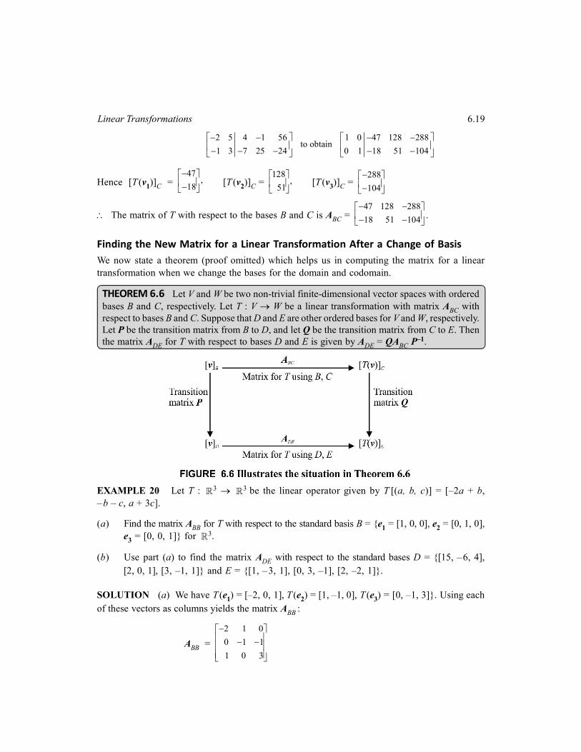
Finding the New Matrix for a Linear Transformation After a Change of Basis

We now state a theorem (proof omitted) which helps us in computing the matrix for a linear

transformation when we change the bases for the domain and codomain.

THEOREM 6.6 Let V and W be two non-trivial finite-dimensional vector spaces with ordered

bases B and C, respectively. Let T : V W be a linear transformation with matrix ABC

with

respect to bases B and C. Suppose that D and E are other ordered bases for V and W, respectively.

Let P be the transition matrix from B to D, and let Q be the transition matrix from C to E. Then

the matrix ADE

for T with respect to bases D and E is given by ADE

= QABC

P–1.

EXAMPLE 20 Let T : 3 3 be the linear operator given by T [(a, b, c)] = [–2a + b,

–b – c, a + 3c].

(a) Find the matrix ABB

for T with respect to the standard basis B = {e1 = [1, 0, 0], e

2 = [0, 1, 0],

e3 = [0, 0, 1]} for 3.

(b) Use part (a) to find the matrix ADE

with respect to the standard bases D = {[15, –6, 4],

[2, 0, 1], [3, –1, 1]} and E = {[1, –3, 1], [0, 3, –1], [2, –2, 1]}.

SOLUTION (a) We have T (e1) = [–2, 0, 1], T (e

2) = [1, –1, 0], T (e

3) = [0, –1, 3]}. Using each

of these vectors as columns yields the matrix ABB

:

ABB

=

2 1 0

0 1 1

1 0 3

6.20 Linear Algebra

(b) To find ADE

, we make use of the following relationship :

ADE

= QABB

P –1, ...(1)

where P is the transition matrix from B to D and Q is the transition matrix from B to E. Since P–1 is

the transition matrix from D to B and B is the standard basis for 3, it is given by

P –1 =

15 2 3

6 0 1

4 1 1

To find Q, we first find Q –1, the transition matrix from E to B, which is given by

Q –1 =

1 0 2

3 3 2

1 1 1

It can be easily checked that

Q = (Q –1)–1 =

1 2 6

1 1 4

0 1 3

Hence, using Eq. (1), we obtain

ADE

= Q ABB

P –1 =

1 2 6 2 1 0 15 2 3

1 1 4 0 1 1 6 0 1

0 1 3 1 0 3 4 1 1

=

202 32 43

146 23 31 .

83 14 18

EXAMPLE 21 Let T : P3 3 be the linear transformation given by T (ax3 + bx2 + cx + d )

= [c + d, 2b, a – d].

(a) Find the matrix ABC

for T with respect to the standard bases B (for P3) and C (for 3).

(b) Use part (a) to find the matrix ADE

for T with respect to the standard bases D = {x3 + x2,

x2 + x, x + 1, 1} for P3

and E = {[–2, 1, –3], [1, –3, 0], [3, –6, 2]} for 3.

SOLUTION (a) To find the matrix ABC

for T with respect to the standard bases B = {x3, x2, x, 1}

for P3 and C = {e

1 = [1, 0, 0], e

2 = [0, 1, 0], e

3 = [0, 0, 1]} for 3, we first need to find T (v) for

each v B. By definition of T, we have

T (x3) = [0, 0, 1], T (x2) = [0, 2, 0], T (x) = [1, 0, 0] and T (1) = [1, 0, –1]

Since we are using the standard basis C for 3, the matrix ABC

for T is the matrix whose columns

are these images. Thus

ABC

=

0 0 1 1

0 2 0 0

1 0 0 1

(b) To find ADE

, we make use of the following relationship :

ADE

= QABC

P –1 ...(1)

6.21Linear Transformations

where P is the transition matrix from B to D and Q is the transition matrix C to E. Since P is the

transition matrix from B to D, therefore P–1 is the transition matrix from D to B. To compute

P –1, we need to convert the polynomials in D into vectors in 4. This is done by converting each

polynomial ax3 + bx2 + cx + d in D to [a, b, c, d]. Thus

(x3 + x2) [1, 1, 0, 0] ; (x2 + x) [0, 1, 1, 0] ; (x + 1) [0, 0, 1, 1] ; (1) [0, 0, 0, 1]

Since B is the standard basis for 3, the transition matrix (P–1) from D to B is obtained by using

each of these vectors as columns :

P–1 =

1 0 0 0

1 1 0 0

0 1 1 0

0 0 1 1

To find Q, we first find Q–1, the transition matrix from E to C, which is the matrix whose columns

are the vectors in E.

Q –1 =

2 1 3

1 3 6

3 0 2

Q = (Q –1)–1 =

12 1 3 6 2 3

1 3 6 16 5 9

3 0 2 9 3 5

Hence, ADE

= QABC

P–1 =

1 0 0 06 2 3 0 0 1 1

1 1 0 016 5 9 0 2 0 0

0 1 1 09 3 5 1 0 0 1

0 0 1 1

=

1 10 15 9

1 26 41 25 .

1 15 23 14

6.3 LINEAR OPERATORS AND SIMILARITY

In this section we will show that any two matrices for the same linear operator (on a finite-dimensional

vector space) with respect to different ordered bases are similar.

Let V be a finite-dimensional vector space with ordered bases B and C, and let T : V V be a

linear operator. Then we can find two matrices, ABB

and ACC

, for T with respect to ordered bases

B and C, respectively. We will show that ABB

and ACC

are similar. To prove this, let P denote the

transition matrix (PCB) from B to C. Then by Theorem 6.6, we have

ACC

= P ABB

P–1 ABB

= P –1 ACC

P

This shows that the matrices ABB

and ACC

are similar. We have thus proved the following:

THEOREM 6.7 Let V be a finite-dimensional vector space with ordered bases B and C. Let T

be a linear operator on V. Then the matrix ABB

for T with respect to the basis B is similar to the

matrix ACC

for T with respect to the basis C. More specifically, if P is the transition matrix from

B to C, then ABB

= P–1 ACC

P.