arX

iv:h

ep-p

h/01

0826

4v1

31

Aug

200

1

hep-ph/0108264LU TP 01–21August 2001

PYTHIA 6.2Physics and Manual

Torbjorn Sjostrand, Leif Lonnblad

Department of Theoretical Physics,Lund University, Solvegatan 14A,

S-223 62 Lund, Sweden

Stephen Mrenna

Physics Department,University of California at Davis,

One Shields Avenue,Davis, CA 95616, USA

*......**:::!!:::::::::::*

*::::::!!::::::::::::::**::::::::!!::::::::::::::::**:::::::::!!:::::::::::::::::**:::::::::!!:::::::::::::::::**::::::::!!::::::::::::::::*!

*::::::!!::::::::::::::* !!!! *:::!!:::::::::::* !!!! !* -><- * !!!! !! !!!! !! !!!! !!!! ep !!!! !!!! pp !!!! e+e- !!!! !!!!

Abstract

The Pythia program can be used to generate high-energy-physics ‘events’,i.e. sets of outgoing particles produced in the interactions between two in-coming particles. The objective is to provide as accurate as possible arepresentation of event properties in a wide range of reactions, with empha-sis on those where strong interactions play a role, directly or indirectly, andtherefore multihadronic final states are produced. The physics is then notunderstood well enough to give an exact description; instead the programhas to be based on a combination of analytical results and various QCD-based models. This physics input is summarized here, for areas such as hardsubprocesses, initial- and final-state parton showers, beam remnants and un-derlying events, fragmentation and decays, and much more. Furthermore,extensive information is provided on all program elements: subroutines andfunctions, switches and parameters, and particle and process data. Thisshould allow the user to tailor the generation task to the topics of interest.

The information in this edition of the manual refers to Pythia version6.200, of 31 August 2001.

The official reference to the latest published version isT. Sjostrand, P. Eden, C. Friberg, L. Lonnblad, G. Miu, S. Mrenna andE. Norrbin, Computer Physics Commun. 135 (2001) 238.

Preface

The Pythia program is frequently used for event generation in high-energy physics. Theemphasis is on multiparticle production in collisions between elementary particles. Thisin particular means hard interactions in e+e−, pp and ep colliders, although also otherapplications are envisaged. The program is intended to generate complete events, in asmuch detail as experimentally observable ones, within the bounds of our current under-standing of the underlying physics. Many of the components of the program representsoriginal research, in the sense that models have been developed and implemented for anumber of aspects not covered by standard theory.

Historically, the family of event generators from the Lund group was begun withJetset in 1978. The Pythia program followed a few years later. With time, the twoprograms so often had to be used together that it made sense to merge them. There-fore Pythia 5.7 and Jetset 7.4 were the last versions to appear individually; as ofPythia 6.1 all the code is collected under the Pythia heading. At the same time, theSPythia sideline of Pythia was reintegrated. Both programs have a long history, andseveral manuals have come out. The most recent one is

T. Sjostrand, P. Eden, C. Friberg, L. Lonnblad, G. Miu, S. Mrenna and E. Norrbin,Computer Physics Commun. 135 (2001) 238,

so please use this for all official references. Additionally remember to cite the original lit-erature on the physics topics of particular relevance for your studies. (There is no reasonto omit references to good physics papers simply because some of their contents have alsobeen made available as program code.)

Event generators often have a reputation for being ‘black boxes’; if nothing else, thisreport should provide you with a glimpse of what goes on inside the program. Some suchunderstanding may be of special interest for new users, who have no background in thefield. An attempt has been made to structure the report sufficiently well so that many ofthe sections can be read independently of each other, so you can pick the sections thatinterest you. We have tried to keep together the physics and the manual sections onspecific topics, where practicable.

A large number of persons should be thanked for their contributions. Bo Anderssonand Gosta Gustafson are the originators of the Lund model, and strongly influenced theearly development of the programs. Hans-Uno Bengtsson is the originator of the Pythia

program. Mats Bengtsson is the main author of the final-state parton-shower algorithm.Patrik Eden has contributed an improved popcorn scenario for baryon production. Chris-ter Friberg has helped develop the expanded photon physics machinery, Emanuel Norrbinthe new matrix-element matching of the final-state parton shower algorithm and the han-dling of low-mass strings, and Gabriela Miu the matching of initial-state showers. PeterSkands has contributed the code for lepton-number-violating decays in supersymmetry.

Further comments on the programs and smaller pieces of code have been obtained fromusers too numerous to be mentioned here, but who are all gratefully acknowledged. Towrite programs of this size and complexity would be impossible without a strong supportand user feedback. So, if you find errors, please let us know.

The moral responsibility for any remaining errors clearly rests with the authors. How-ever, kindly note that this is a ‘University World’ product, distributed ‘as is’, free ofcharge, without any binding guarantees. And always remember that the program doesnot represent a dead collection of established truths, but rather one of many possibleapproaches to the problem of multiparticle production in high-energy physics, at thefrontline of current research. Be critical!

Contents

1 Introduction 1

2 Physics Overview 92.1 Hard Processes and Parton Distributions . . . . . . . . . . . . . . . . . . . 92.2 Initial- and Final-State Radiation . . . . . . . . . . . . . . . . . . . . . . . 132.3 Beam Remnants and Multiple Interactions . . . . . . . . . . . . . . . . . . 162.4 Hadronization . . . . . . . . . . . . . . . . . . . . . . . . . . . . . . . . . . 17

3 Program Overview 213.1 Update History . . . . . . . . . . . . . . . . . . . . . . . . . . . . . . . . . 213.2 Program Installation . . . . . . . . . . . . . . . . . . . . . . . . . . . . . . 243.3 Program Philosophy . . . . . . . . . . . . . . . . . . . . . . . . . . . . . . 263.4 Manual Conventions . . . . . . . . . . . . . . . . . . . . . . . . . . . . . . 273.5 Getting Started with the Simple Routines . . . . . . . . . . . . . . . . . . 283.6 Getting Started with the Event Generation Machinery . . . . . . . . . . . 33

4 Monte Carlo Techniques 404.1 Selection From a Distribution . . . . . . . . . . . . . . . . . . . . . . . . . 404.2 The Veto Algorithm . . . . . . . . . . . . . . . . . . . . . . . . . . . . . . 424.3 The Random Number Generator . . . . . . . . . . . . . . . . . . . . . . . . 44

5 The Event Record 485.1 Particle Codes . . . . . . . . . . . . . . . . . . . . . . . . . . . . . . . . . . 485.2 The Event Record . . . . . . . . . . . . . . . . . . . . . . . . . . . . . . . . 565.3 How The Event Record Works . . . . . . . . . . . . . . . . . . . . . . . . . 595.4 The HEPEVT Standard . . . . . . . . . . . . . . . . . . . . . . . . . . . . 62

6 The Old e+e− Annihilation Routines 666.1 Annihilation Events in the Continuum . . . . . . . . . . . . . . . . . . . . 666.2 Decays of Onia Resonances . . . . . . . . . . . . . . . . . . . . . . . . . . . 756.3 Routines and Common Block Variables . . . . . . . . . . . . . . . . . . . . 766.4 Examples . . . . . . . . . . . . . . . . . . . . . . . . . . . . . . . . . . . . 83

7 Process Generation 857.1 Parton Distributions . . . . . . . . . . . . . . . . . . . . . . . . . . . . . . 857.2 Kinematics and Cross Section for a 2 → 2 Process . . . . . . . . . . . . . . 917.3 Resonance Production . . . . . . . . . . . . . . . . . . . . . . . . . . . . . 937.4 Cross-section Calculations . . . . . . . . . . . . . . . . . . . . . . . . . . . 987.5 2 → 3 and 2 → 4 Processes . . . . . . . . . . . . . . . . . . . . . . . . . . . 1047.6 Resonance Decays . . . . . . . . . . . . . . . . . . . . . . . . . . . . . . . . 1057.7 Nonperturbative Processes . . . . . . . . . . . . . . . . . . . . . . . . . . . 108

8 Physics Processes 1168.1 The Process Classification Scheme . . . . . . . . . . . . . . . . . . . . . . . 1168.2 QCD Processes . . . . . . . . . . . . . . . . . . . . . . . . . . . . . . . . . 1258.3 Physics with Incoming Photons . . . . . . . . . . . . . . . . . . . . . . . . 1308.4 Electroweak Gauge Bosons . . . . . . . . . . . . . . . . . . . . . . . . . . . 1368.5 Higgs Production . . . . . . . . . . . . . . . . . . . . . . . . . . . . . . . . 1408.6 Non-Standard Physics . . . . . . . . . . . . . . . . . . . . . . . . . . . . . 1458.7 Supersymmetry . . . . . . . . . . . . . . . . . . . . . . . . . . . . . . . . . 1538.8 Polarization . . . . . . . . . . . . . . . . . . . . . . . . . . . . . . . . . . . 1578.9 Main Processes by Machine . . . . . . . . . . . . . . . . . . . . . . . . . . 157

9 The Process Generation Program Elements 1609.1 The Main Subroutines . . . . . . . . . . . . . . . . . . . . . . . . . . . . . 1609.2 Switches for Event Type and Kinematics Selection . . . . . . . . . . . . . . 1649.3 The General Switches and Parameters . . . . . . . . . . . . . . . . . . . . 1719.4 Further Couplings . . . . . . . . . . . . . . . . . . . . . . . . . . . . . . . . 1949.5 Supersymmetry Common Blocks and Routines . . . . . . . . . . . . . . . . 1989.6 General Event Information . . . . . . . . . . . . . . . . . . . . . . . . . . . 2039.7 How to Generate Weighted Events . . . . . . . . . . . . . . . . . . . . . . 2089.8 How to Run with Varying Energies . . . . . . . . . . . . . . . . . . . . . . 2129.9 How to Include External Processes . . . . . . . . . . . . . . . . . . . . . . 2159.10 Interfaces to Other Generators . . . . . . . . . . . . . . . . . . . . . . . . . 2359.11 Other Routines and Common Blocks . . . . . . . . . . . . . . . . . . . . . 239

10 Initial- and Final-State Radiation 25610.1 Shower Evolution . . . . . . . . . . . . . . . . . . . . . . . . . . . . . . . . 25610.2 Final-State Showers . . . . . . . . . . . . . . . . . . . . . . . . . . . . . . . 25910.3 Initial-State Showers . . . . . . . . . . . . . . . . . . . . . . . . . . . . . . 26910.4 Routines and Common Block Variables . . . . . . . . . . . . . . . . . . . . 279

11 Beam Remnants and Underlying Events 28811.1 Beam Remnants . . . . . . . . . . . . . . . . . . . . . . . . . . . . . . . . . 28811.2 Multiple Interactions . . . . . . . . . . . . . . . . . . . . . . . . . . . . . . 29111.3 Pile-up Events . . . . . . . . . . . . . . . . . . . . . . . . . . . . . . . . . . 29911.4 Common Block Variables . . . . . . . . . . . . . . . . . . . . . . . . . . . . 300

12 Fragmentation 30612.1 Flavour Selection . . . . . . . . . . . . . . . . . . . . . . . . . . . . . . . . 30612.2 String Fragmentation . . . . . . . . . . . . . . . . . . . . . . . . . . . . . . 31212.3 Independent Fragmentation . . . . . . . . . . . . . . . . . . . . . . . . . . 31912.4 Other Fragmentation Aspects . . . . . . . . . . . . . . . . . . . . . . . . . 322

13 Particles and Their Decays 32913.1 The Particle Content . . . . . . . . . . . . . . . . . . . . . . . . . . . . . . 32913.2 Masses, Widths and Lifetimes . . . . . . . . . . . . . . . . . . . . . . . . . 33013.3 Decays . . . . . . . . . . . . . . . . . . . . . . . . . . . . . . . . . . . . . . 332

14 The Fragmentation and Decay Program Elements 33714.1 Definition of Initial Configuration or Variables . . . . . . . . . . . . . . . . 33714.2 The Physics Routines . . . . . . . . . . . . . . . . . . . . . . . . . . . . . . 34014.3 The General Switches and Parameters . . . . . . . . . . . . . . . . . . . . 34214.4 Further Parameters and Particle Data . . . . . . . . . . . . . . . . . . . . 35714.5 Miscellaneous Comments . . . . . . . . . . . . . . . . . . . . . . . . . . . . 36414.6 Examples . . . . . . . . . . . . . . . . . . . . . . . . . . . . . . . . . . . . 366

15 Event Study and Analysis Routines 37015.1 Event Study Routines . . . . . . . . . . . . . . . . . . . . . . . . . . . . . 37015.2 Event Shapes . . . . . . . . . . . . . . . . . . . . . . . . . . . . . . . . . . 37515.3 Cluster Finding . . . . . . . . . . . . . . . . . . . . . . . . . . . . . . . . . 37915.4 Event Statistics . . . . . . . . . . . . . . . . . . . . . . . . . . . . . . . . . 38415.5 Routines and Common Block Variables . . . . . . . . . . . . . . . . . . . . 38515.6 Histograms . . . . . . . . . . . . . . . . . . . . . . . . . . . . . . . . . . . 395

16 Summary and Outlook 399

References 400

Subprocess Summary Table 414

Index of Subprograms and Common Block Variables 417

1 Introduction

Multiparticle production is the most characteristic feature of current high-energy physics.Today, observed particle multiplicities are typically between ten and a hundred, and withfuture machines this range will be extended upwards. The bulk of the multiplicity is foundin jets, i.e. in collimated bunches of hadrons (or decay products of hadrons) producedby the hadronization of partons, i.e. quarks and gluons. (For some applications it willbe convenient to extend the parton concept also to some non-coloured but showeringparticles, such as electrons and photons.)

The Complexity of High-Energy Processes

To first approximation, all processes have a simple structure at the level of interactionsbetween the fundamental objects of nature, i.e. quarks, leptons and gauge bosons. Forinstance, a lot can be understood about the structure of hadronic events at LEP just fromthe ‘skeleton’ process e+e− → Z0 → qq. Corrections to this picture can be subdivided,arbitrarily but conveniently, into three main classes.

Firstly, there are bremsstrahlung-type modifications, i.e. the emission of additionalfinal-state particles by branchings such as e → eγ or q → qg. Because of the largenessof the strong coupling constant αs, and because of the presence of the triple gluon ver-tex, QCD emission off quarks and gluons is especially prolific. We therefore speak about‘parton showers’, wherein a single initial parton may give rise to a whole bunch of par-tons in the final state. Also photon emission may give sizeable effects in e+e− and epprocesses. The bulk of the bremsstrahlung corrections are universal, i.e. do not dependon the details of the process studied, but only on one or a few key numbers, such as themomentum transfer scale of the process. Such universal corrections may be included toarbitrarily high orders, using a probabilistic language. Alternatively, exact calculationsof bremsstrahlung corrections may be carried out order by order in perturbation the-ory, but rapidly the calculations then become prohibitively complicated and the answerscorrespondingly lengthy.

Secondly, we have ‘true’ higher-order corrections, which involve a combination of loopgraphs and the soft parts of the bremsstrahlung graphs above, a combination needed tocancel some divergences. In a complete description it is therefore not possible to considerbremsstrahlung separately, as assumed here. The necessary perturbative calculations areusually very difficult; only rarely have results been presented that include more than onenon-‘trivial’ order, i.e. more than one loop. As above, answers are usually very lengthy,but some results are sufficiently simple to be generally known and used, such as therunning of αs, or the correction factor 1 + αs/π + · · · in the partial widths of Z0 → qqdecay channels. For high-precision studies it is imperative to take into account the resultsof loop calculations, but usually effects are minor for the qualitative aspects of high-energyprocesses.

Thirdly, quarks and gluons are confined. In the two points above, we have used aperturbative language to describe the short-distance interactions of quarks, leptons andgauge bosons. For leptons and colourless bosons this language is sufficient. However, forquarks and gluons it must be complemented with the structure of incoming hadrons, anda picture for the hadronization process, wherein the coloured partons are transformedinto jets of colourless hadrons, photons and leptons. The hadronization can be furthersubdivided into fragmentation and decays, where the former describes the way the creationof new quark-antiquark pairs can break up a high-mass system into lower-mass ones,ultimately hadrons. (The word ‘fragmentation’ is also sometimes used in a broader sense,but we will here use it with this specific meaning.) This process is still not yet understoodfrom first principles, but has to be based on models. In one sense, hadronization effectsare overwhelmingly large, since this is where the bulk of the multiplicity comes from. In

1

another sense, the overall energy flow of a high-energy event is mainly determined by theperturbative processes, with only a minor additional smearing caused by the hadronizationstep. One may therefore pick different levels of ambition, but in general detailed studiesrequire a detailed modelling of the hadronization process.

The simple structure that we started out with has now become considerably morecomplex — instead of maybe two final-state partons we have a hundred final particles.The original physics is not gone, but the skeleton process has been dressed up and is nolonger directly visible. A direct comparison between theory and experiment is thereforecomplicated at best, and impossible at worst.

Event Generators

It is here that event generators come to the rescue. In an event generator, the objectivestrived for is to use computers to generate events as detailed as could be observed by aperfect detector. This is not done in one step, but rather by ‘factorizing’ the full prob-lem into a number of components, each of which can be handled reasonably accurately.Basically, this means that the hard process is used as input to generate bremsstrahlungcorrections, and that the result of this exercise is thereafter left to hadronize. This soundsa bit easier than it really is — else this report would be a lot thinner. However, the basicidea is there: if the full problem is too complicated to be solved in one go, try to subdivideit into smaller tasks of manageable proportions. In the actual generation procedure, moststeps therefore involve the branching of one object into two, or at least into a very smallnumber, with the daughters free to branch in their turn. A lot of book-keeping is involved,but much is of a repetitive nature, and can therefore be left for the computer to handle.

As the name indicates, the output of an event generator should be in the form of‘events’, with the same average behaviour and the same fluctuations as real data. Inthe data, fluctuations arise from the quantum mechanics of the underlying theory. Ingenerators, Monte Carlo techniques are used to select all relevant variables according tothe desired probability distributions, and thereby ensure randomness in the final events.Clearly some loss of information is entailed: quantum mechanics is based on amplitudes,not probabilities. However, only very rarely do (known) interference phenomena appearthat cannot be cast in a probabilistic language. This is therefore not a more restrainingapproximation than many others.

Once there, an event generator can be used in many different ways. The five mainapplications are probably the following:

• To give physicists a feeling for the kind of events one may expect/hope to find, andat what rates.

• As a help in the planning of a new detector, so that detector performance is opti-mized, within other constraints, for the study of interesting physics scenarios.

• As a tool for devising the analysis strategies that should be used on real data, sothat signal-to-background conditions are optimized.

• As a method for estimating detector acceptance corrections that have to be appliedto raw data, in order to extract the ‘true’ physics signal.

• As a convenient framework within which to interpret the observed phenomena interms of a more fundamental underlying theory (usually the Standard Model).

Where does a generator fit into the overall analysis chain of an experiment? In ‘reallife’, the machine produces interactions. These events are observed by detectors, and theinteresting ones are written to tape by the data acquisition system. Afterwards the eventsmay be reconstructed, i.e. the electronics signals (from wire chambers, calorimeters, andall the rest) may be translated into a deduced setup of charged tracks or neutral energydepositions, in the best of worlds with full knowledge of momenta and particle species.Based on this cleaned-up information, one may proceed with the physics analysis. In theMonte Carlo world, the role of the machine, namely to produce events, is taken by the

2

event generators described in this report. The behaviour of the detectors — how particlesproduced by the event generator traverse the detector, spiral in magnetic fields, showerin calorimeters, or sneak out through cracks, etc. — is simulated in programs such asGeant [Bru89]. Traditionally, this latter activity is called event simulation, which issomewhat unfortunate since the same words could equally well be applied to what, here,we call event generation. A more appropriate term is detector simulation. Ideally, theoutput of this simulation has exactly the same format as the real data recorded by thedetector, and can therefore be put through the same event reconstruction and physicsanalysis chain, except that here we know what the ‘right answer’ should be, and so cansee how well we are doing.

Since the full chain of detector simulation and event reconstruction is very time-consuming, one often does ‘quick and dirty’ studies in which these steps are skippedentirely, or at least replaced by very simplified procedures which only take into accountthe geometric acceptance of the detector and other trivial effects. One may then use theoutput of the event generator directly in the physics studies.

There are still many holes in our understanding of the full event structure, despitean impressive amount of work and detailed calculations. To put together a generatortherefore involves making a choice on what to include, and how to include it. At best,the spread between generators can be used to give some impression of the uncertaintiesinvolved. A multitude of approximations will be discussed in the main part of this report,but already here is should be noted that many major approximations are related to thealmost complete neglect of the second point above, i.e. of the non-‘trivial’ higher-ordereffects. It can therefore only be hoped that the ‘trivial’ higher order parts give the bulk ofthe experimental behaviour. By and large, this seems to be the case; for e+e− annihilationit even turns out to be a very good approximation.

The necessity to make compromises has one major implication: to write a good eventgenerator is an art, not an exact science. It is therefore essential not to blindly trustthe results of any single event generator, but always to make several cross-checks. Inaddition, with computer programs of tens of thousands of lines, the question is not whetherbugs exist, but how many there are, and how critical their positions. Further, an eventgenerator cannot be thought of as all-powerful, or able to give intelligent answers to ill-posed questions; sound judgement and some understanding of a generator are necessaryprerequisites for successful use. In spite of these limitations, the event generator approachis the most powerful tool at our disposal if we wish to gain a detailed and realisticunderstanding of physics at current or future high-energy colliders.

The Origins of the JETSET and PYTHIA Programs

Over the years, many event generators have appeared. Surveys of generators for e+e−

physics in general and LEP in particular may be found in [Kle89, Sjo89, Kno96, Lon96],for high-energy hadron–hadron (pp) physics in [Ans90, Sjo92, Kno93, LHC00], and forep physics in [HER92, HER99]. We refer the reader to those for additional details andreferences. In this particular report, the two closely connected programs Jetset andPythia, now merged under the Pythia label, will be described.

Jetset has its roots in the efforts of the Lund group to understand the hadroniza-tion process, starting in the late seventies [And83]. The so-called string fragmentationmodel was developed as an explicit and detailed framework, within which the long-rangeconfinement forces are allowed to distribute the energies and flavours of a parton config-uration among a collection of primary hadrons, which subsequently may decay further.This model, known as the Lund string model, or ‘Lund’ for short, contained a number ofspecific predictions, which were confirmed by data from PETRA and PEP, whence themodel gained a widespread acceptance. The Lund string model is still today the mostelaborate and widely used fragmentation model at our disposal. It remains at the heart

3

of the Pythia program.In order to predict the shape of events at PETRA/PEP, and to study the fragmentation

process in detail, it was necessary to start out from the partonic configurations thatwere to fragment. The generation of complete e+e− hadronic events was therefore added,originally based on simple γ exchange and first-order QCD matrix elements, later extendedto full γ∗/Z0 exchange with first-order initial-state QED radiation and second-order QCDmatrix elements. A number of utility routines were also provided early on, for everythingfrom event listing to jet finding.

By the mid-eighties it was clear that the matrix-element approach had reached thelimit of its usefulness, in the sense that it could not fully describe the multijet topologies ofthe data. (Later on, the use of optimized perturbation theory was to lead to a resurgenceof the matrix-element approach, but only for specific applications.) Therefore a parton-shower description was developed [Ben87a] as an alternative to the matrix-element one.The combination of parton showers and string fragmentation has been very successful,and forms the main approach to the description of hadronic Z0 events.

In recent years, the Jetset part of the code has been a fairly stable product, coveringthe four main areas of fragmentation, final-state parton showers, e+e− event generationand general utilities.

The successes of string fragmentation in e+e− made it interesting to try to extend thisframework to other processes, and explore possible physics consequences. Therefore anumber of other programs were written, which combined a process-specific description ofthe hard interactions with the general fragmentation framework of Jetset. The Pythia

program evolved out of early studies on fixed-target proton–proton processes, addressedmainly at issues related to string drawing.

With time, the interest shifted towards higher energies, first to the SPS pp collider,and later to the Tevatron, SSC and LHC, in the context of a number of workshops inthe USA and Europe. Parton showers were added, for final-state radiation by makinguse of the Jetset routine, for initial-state one by the development of the concept of‘backwards evolution’, specifically for Pythia [Sjo85]. Also a framework was developedfor minimum-bias and underlying events [Sjo87a].

Another main change was the introduction of an increasing number of hard processes,within the Standard Model and beyond. A special emphasis was put on the search forthe Standard Model Higgs, in different mass ranges and in different channels, with duerespect to possible background processes.

The bulk of the machinery developed for hard processes actually depended little on thechoice of initial state, as long as the appropriate parton distributions were there for theincoming partons and particles. It therefore made sense to extend the program from beingonly a pp generator to working also for e+e− and ep. This process was only completed in1991, again spurred on by physics workshop activities. Currently Pythia should thereforework equally well for a selection of different possible incoming beam particles.

An effort independent of the Lund group activities got going to include supersymmetricevent simulation in Pythia. This resulted in the SPythia program.

While Jetset was independent of Pythia until 1996, their ties had grown muchstronger over the years, and the border-line between the two programs had become moreand more artificial. It was therefore decided to merge the two, and also include theSPythia extensions, starting from Pythia 6.1. The different origins in part still arereflected in this manual, but the strive is towards a seamless merger.

The tasks of including new processes, and of improving the simulation of parton show-ers and other aspects of already present processes, are never-ending. Work thereforecontinues apace.

4

About this Report

As we see, Jetset and Pythia started out as very ideologically motivated programs, de-veloped to study specific physics questions in enough detail that explicit predictions couldbe made for experimental quantities. As it was recognized that experimental imperfec-tions could distort the basic predictions, the programs were made available for general useby experimentalists. It thus became feasible to explore the models in more detail thanwould otherwise have been possible. As time went by, the emphasis came to shift some-what, away from the original strong coupling to a specific fragmentation model, towards adescription of high-energy multiparticle production processes in general. Correspondingly,the use expanded from being one of just comparing data with specific model predictions,to one of extensive use for the understanding of detector performance, for the deriva-tion of acceptance correction factors, for the prediction of physics at future high-energyaccelerators, and for the design of related detectors.

While the ideology may be less apparent, it is still there, however. This is not some-thing unique to the programs discussed here, but inherent in any event generator, or atleast any generator that attempts to go beyond the simple parton level skeleton descrip-tion of a hard process. Do not accept the myth that everything available in Monte Carloform represents ages-old common knowledge, tested and true. Ideology is present bycommissions or omissions in any number of details. A programs like Pythia representsa major amount of original physics research, often on complicated topics where no simpleanswers are available. As a (potential) program user you must be aware of this, so thatyou can form your own opinion, not just about what to trust and what not to trust, butalso how much to trust a given prediction, i.e. how uncertain it is likely to be. Pythia

is particularly well endowed in this respect, since a number of publications exist wheremost of the relevant physics is explained in considerable detail. In fact, the problem mayrather be the opposite, to find the relevant information among all the possible places.One main objective of the current report is therefore to collect much of this informationin one single place. Not all the material found in specialized papers is reproduced, by awide margin, but at least enough should be found here to understand the general pictureand to know where to go for details.

The current report is therefore intended to update and extend the previous round ofpublished physics descriptions and program manuals [Sjo86, Sjo87, Ben87, Sjo94, Mre97,Sjo01]. Make all references to the most recent published one in [Sjo01]. Further speci-fication could include a statement of the type ‘We use Pythia version X.xxx’. (If youare a LATEX fan, you may want to know that the program name in this report has beengenerated by the command \textscPythia.) Kindly do not refer to Pythia as ‘un-published’, ‘private communication’ or ‘in preparation’: such phrases are incorrect andonly create unnecessary confusion.

In addition, remember that many of the individual physics components are docu-mented in separate publications. If some of these contain ideas that are useful to you,there is every reason to cite them. A reasonable selection would vary as a function of thephysics you are studying. The criterion for which to pick should be simple: imagine thata Monte Carlo implementation had not been available. Would you then have cited a givenpaper on the grounds of its physics contents alone? If so, do not punish the extra effortof turning these ideas into publicly available software. (Monte Carlo manuals are goodfor nothing in the eyes of many theorists, so often only the acceptance of ‘mainstream’publications counts.) Here follows a list of some main areas where the Pythia programscontain original research:

• The string fragmentation model [And83, And98].• The string effect [And80].• Baryon production (diquark/popcorn) [And82, And85, Ede97].• Small-mass string fragmentation [Nor98].

5

• Fragmentation of multiparton systems [Sjo84].• Colour rearrangement [Sjo94a] and Bose-Einstein effects [Lon95].• Fragmentation effects on αs determinations [Sjo84a].• Initial-state parton showers [Sjo85, Miu99].• Final-state parton showers [Ben87a, Nor01].• Photon radiation from quarks [Sjo92c]• Deeply Inelastic Scattering [And81a, Ben88].• Photoproduction [Sch93a], γγ [Sch94a] and γ∗p/γ∗γ/γ∗γ∗ [Fri00] physics.• Parton distributions of the photon [Sch95, Sch96].• Colour flow in hard scatterings [Ben84].• Elastic and diffractive cross sections [Sch94].• Minijets (multiple parton–parton interactions) [Sjo87a].• Rapidity gaps [Dok92].• Jet clustering in k⊥ [Sjo83].In addition to a physics survey, the current report also contains a complete manual

for the program. Such manuals have always been updated and distributed jointly withthe programs, but have grown in size with time. A word of warning may therefore be inplace. The program description is fairly lengthy, and certainly could not be absorbed inone sitting. This is not even necessary, since all switches and parameters are providedwith sensible default values, based on our best understanding (of the physics, and of whatyou expect to happen if you do not specify any options). As a new user, you can thereforedisregard all the fancy options, and just run the program with a minimum ado. Lateron, as you gain experience, the options that seem useful can be tried out. No single useris ever likely to find need for more than a fraction of the total number of possibilitiesavailable, yet many of them have been added to meet specific user requests.

In some instances, not even this report will provide you with all the information youdesire. You may wish to find out about recent versions of the program, know about relatedsoftware, pick up a few sample main programs to get going, or get hold of related physicspapers. Some such material can be found on the Pythia web page:

http://www.thep.lu.se/∼torbjorn/Pythia.html .

Disclaimer

At all times it should be remembered that this is not a commercial product, developedand supported by professionals. Instead it is a ‘University World’ product, developed bya very few physicists (mainly the current first author) originally for their own needs, andsupplied to other physicists on an ‘as-is’ basis, free of charge. No guarantees are thereforegiven for the proper functioning of the program, nor for the validity of physics results.In the end, it is always up to you to decide for yourself whether to trust a given resultor not. Usually this requires comparison either with analytical results or with results ofother programs, or with both. Even this is not necessarily foolproof: for instance, if anerror is made in the calculation of a matrix element for a given process, this error will bepropagated both into the analytical results based on the original calculation and into allthe event generators which subsequently make use of the published formulae. In the end,there is no substitute for a sound physics judgement.

This does not mean that you are all on your own, with a program nobody feels respon-sible for. Attempts are made to check processes as carefully as possible, to write programsthat do not invite unnecessary errors, and to provide a detailed and accurate documen-tation. All of this while maintaining the full power and flexibility, of course, since thephysics must always take precedence in any conflict of interests. If nevertheless any errorsor unclarities are found, please do communicate them to e-mail torbjorn@thep.lu.se, or toanother person in charge. For instance, all questions on the supersymmetric machinery

6

are better directed to mrenna@physics.ucdavis.edu. Every attempt will be made to solveproblems as soon as is reasonably possible, given that this support is by a few persons,who mainly have other responsibilities.

However, in order to make debugging at all possible, we request that any samplecode you want to submit as evidence be completely self-contained, and peeled off from allirrelevant aspects. Use simple write statements or the Pythia histogramming routines tomake your point. Chances are that, if the error cannot be reproduced by fifty lines of code,in a main program linked only to Pythia, the problem is sitting elsewhere. Numerouserrors have been caused by linking to other (flawed) libraries, e.g. collaboration-specificframeworks for running Pythia. Then you should put the blame elsewhere.

Appendix: The Historical Pythia

The ‘Pythia’ label may need some explanation.The myth tells how Apollon, the God of Wisdom, killed the powerful dragon-like

monster Python, close to the village of Delphi in Greece. To commemorate this victory,Apollon founded the Pythic Oracle in Delphi, on the slopes of Mount Parnassos. Heremen could come to learn the will of the Gods and the course of the future. The oracleplays an important role in many of the other Greek myths, such as those of Heracles andof King Oedipus.

Questions were to be put to the Pythia, the ‘Priestess’ or ‘Prophetess’ of the Oracle. Infact, she was a local woman, usually a young maiden, of no particular religious schooling.Seated on a tripod, she inhaled the obnoxious vapours that seeped up through a crevice inthe ground. This brought her to a trance-like state, in which she would scream seeminglyrandom words and sounds. It was the task of the professional priests in Delphi to recordthose utterings and edit them into the official Oracle prophecies, which often took theform of poems in perfect hexameter. In fact, even these edited replies were often less thaneasy to interpret. The Pythic oracle acquired a reputation for ambiguous answers.

The Oracle existed already at the beginning of the historical era in Greece, and wasuniversally recognized as the foremost religious seat. Individuals and city states came toconsult, on everything from cures for childlessness to matters of war. Lavish gifts allowedthe temple area to be built and decorated. Many states supplied their own treasury halls,where especially beautiful gifts were on display. Sideshows included the Omphalos, astone reputedly marking the centre of the Earth, and the Pythic games, second only tothe Olympic ones in importance.

Strife inside Greece eventually led to a decline in the power of the Oracle. A seriousblow was dealt when the Oracle of Zeus Ammon (see below) declared Alexander the Greatto be the son of Zeus. The Pythic Oracle lived on, however, and was only closed by aRoman Imperial decree in 390 ad, at a time when Christianity was ruthlessly destroyingany religious opposition. Pythia then had been at the service of man and Gods for amillennium and a half.

The role of the Pythic Oracle prophecies on the course of history is nowhere betterdescribed than in ‘The Histories’ by Herodotus [Herbc], the classical and captivatingdescription of the Ancient World at the time of the Great War between Greeks andPersians. Especially famous is the episode with King Croisus of Lydia. Contemplating awar against the upstart Persian Empire, he resolves to ask an oracle what the outcomeof a potential battle would be. However, to have some guarantee for the veracity of anyprophecy, he decides to send embassies to all the renowned oracles of the known World.The messengers are instructed to inquire the various divinities, on the hundredth dayafter their departure, what King Croisus is doing at that very moment. From the Pythiathe messengers bring back the reply

I know the number of grains of sand as well as the expanse of the sea,And I comprehend the dumb and hear him who does not speak,

7

There came to my mind the smell of the hard-shelled turtle,Boiled in copper together with the lamb,With copper below and copper above.

The veracity of the Pythia is thus established by the crafty ruler, who had waited untilthe appointed day, slaughtered a turtle and a lamb, and boiled them together in a coppercauldron with a copper lid. Also the Oracle of Zeus Ammon in the Libyan desert is ableto give a correct reply (lost to posterity), while all others fail. King Croisus now sends asecond embassy to Delphi, inquiring after the outcome of a battle against the Persians.The Pythia answers

If Croisus passes over the Halys he will dissolve a great Empire.

Taking this to mean he would win, the King collects his army and crosses the border river,only to suffer a crushing defeat and see his Kingdom conquered. When the victorious KingCyrus allows Croisus to send an embassy to upbraid the Oracle, the God Apollon answersthrough his Prophetess that he has correctly predicted the destruction of a great empire— Croisus’ own — and that he cannot be held responsible if people choose to interpretthe Oracle answers to their own liking.

The history of the Pythia program is neither as long nor as dignified as that ofits eponym. However, some points of contact exist. You must be very careful whenyou formulate the questions: any ambiguities will corrupt the reply you get. And youmust be even more careful not to misinterpret the answers; in particular not to pick theinterpretation that suits you before considering the alternatives. Finally, even a perfectGod has servants that are only human: a priest might mishear the screams of the Pythiaand therefore produce an erroneous oracle reply; the current author might unwittingly leta bug free in the program Pythia.

8

2 Physics Overview

In this section we will try to give an overview of the main physics features of Pythia, andalso to introduce some terminology. The details will be discussed in subsequent sections.

For the description of a typical high-energy event, an event generator should containa simulation of several physics aspects. If we try to follow the evolution of an event insome semblance of a time order, one may arrange these aspects as follows:

1. Initially two beam particles are coming in towards each other. Normally each par-ticle is characterized by a set of parton distributions, which defines the partonicsubstructure in terms of flavour composition and energy sharing.

2. One shower initiator parton from each beam starts off a sequence of branchings,such as q → qg, which build up an initial-state shower.

3. One incoming parton from each of the two showers enters the hard process, wherethen a number of outgoing partons are produced, usually two. It is the nature ofthis process that determines the main characteristics of the event.

4. The hard process may produce a set of short-lived resonances, like the Z0/W± gaugebosons, whose decay to normal partons has to be considered in close association withthe hard process itself.

5. The outgoing partons may branch, just like the incoming did, to build up final-stateshowers.

6. In addition to the hard process considered above, further semihard interactions mayoccur between the other partons of two incoming hadrons.

7. When a shower initiator is taken out of a beam particle, a beam remnant is leftbehind. This remnant may have an internal structure, and a net colour charge thatrelates it to the rest of the final state.

8. The QCD confinement mechanism ensures that the outgoing quarks and gluons arenot observable, but instead fragment to colour neutral hadrons.

9. Normally the fragmentation mechanism can be seen as occurring in a set of separatecolour singlet subsystems, but interconnection effects such as colour rearrangementor Bose–Einstein may complicate the picture.

10. Many of the produced hadrons are unstable and decay further.Conventionally, only quarks and gluons are counted as partons, while leptons and

photons are not. If pushed ad absurdum this may lead to some unwieldy terminology. Wewill therefore, where it does not matter, speak of an electron or a photon in the ‘partonic’substructure of an electron, lump branchings e → eγ together with other ‘parton shower’branchings such as q → qg, and so on. With this notation, the division into the aboveseven points applies equally well to an interaction between two leptons, between a leptonand a hadron, and between two hadrons.

In the following sections, we will survey the above ten aspects, not in the same orderas given here, but rather in the order in which they appear in the program execution, i.e.starting with the hard process.

2.1 Hard Processes and Parton Distributions

In the original Jetset code, only two hard processes are available. The first and mainone is e+e− → γ∗/Z0 → qq. Here the ‘∗’ of γ∗ is used to denote that the photon must beoff the mass shell. The distinction is of some importance, since a photon on the mass shellcannot decay. Of course also the Z0 can be off the mass shell, but here the distinction isless relevant (strictly speaking, a Z0 is always off the mass shell). In the following we maynot always use ‘∗’ consistently, but the rule of thumb is to use a ‘∗’ only when a process isnot kinematically possible for a particle of nominal mass. The quark q in the final stateof e+e− → γ∗/Z0 → qq may be u, d, s, c, b or t; the flavour in each event is picked at

9

random, according to the relative couplings, evaluated at the hadronic c.m. energy. Alsothe angular distribution of the final qq pair is included. No parton-distribution functionsare needed.

The other original Jetset process is a routine to generate ggg and γgg final states,as expected in onium 1−− decays such as Υ. Given the large top mass, toponium de-cays weakly much too fast for these processes to be of any interest, so therefore no newapplications are expected.

2.1.1 Hard Processes

The current Pythia contains a much richer selection, with around 240 different hardprocesses. These may be classified in many different ways.

One is according to the number of final-state objects: we speak of ‘2 → 1’ processes,‘2 → 2’ ones, ‘2 → 3’ ones, etc. This aspect is very relevant from a programming pointof view: the more particles in the final state, the more complicated the phase space andtherefore the whole generation procedure. In fact, Pythia is optimized for 2 → 1 and2 → 2 processes. There is currently no generic treatment of processes with three or moreparticles in the final state, but rather a few different machineries, each tailored to thepole structure of a specific class of graphs.

Another classification is according to the physics scenario. This will be the main themeof section 8. The following major groups may be distinguished:

• Hard QCD processes, e.g. qg → qg.• Soft QCD processes, such as diffractive and elastic scattering, and minimum-bias

events. Hidden in this class is also process 96, which is used internally for themerging of soft and hard physics, and for the generation of multiple interactions.

• Heavy-flavour production, both open and hidden, e.g. gg → tt and gg → J/ψg.• Prompt-photon production, e.g. qg → qγ.• Photon-induced processes, e.g. γg → qq.• Deeply Inelastic Scattering, e.g. qℓ→ qℓ.• W/Z production, such as the e+e− → γ∗/Z0 or qq → W+W−.• Standard model Higgs production, where the Higgs is reasonably light and narrow,

and can therefore still be considered as a resonance.• Gauge boson scattering processes, such as WW → WW, when the Standard Model

Higgs is so heavy and broad that resonant and non-resonant contributions have tobe considered together.

• Non-standard Higgs particle production, within the framework of a two-Higgs-doublet scenario with three neutral (h0, H0 and A0) and two charged (H±) Higgsstates. Normally associated with Susy (see below), but does not have to be.

• Production of new gauge bosons, such as a Z′, W′ and R (a horizontal boson,coupling between generations).

• Technicolor production, as an alternative scenario to the standard picture of elec-troweak symmetry breaking by a fundamental Higgs.

• Compositeness is a possibility not only in the Higgs sector, but may also apply tofermions, e.g. giving d∗ and u∗ production. At energies below the threshold for newparticle production, contact interactions may still modify the standard behaviour.

• Left–right symmetric models give rise to doubly charged Higgs states, in fact oneset belonging to the left and one to the right SU(2) gauge group. Decays involveright-handed W’s and neutrinos.

• Leptoquark (LQ) production is encountered in some beyond-the-standard-model sce-narios.

• Supersymmetry (Susy) is probably the favourite scenario for physics beyond thestandard model. A rich set of processes are allowed, even if one obeys R-parity

10

conservation. The supersymmetric machinery and process selection is inheritedfrom SPythia [Mre97], however with many improvements in the event generationchain. Many different Susy scenarios have been proposed, and the program isflexible enough to allow input from several of these, in addition to the ones providedinternally.

• The possibility of extra dimensions at low energies has been a topic of much study inrecent years, but has still not settled down to some standard scenarios. Its inclusioninto Pythia is also only in a very first stage.

This is by no means a survey of all interesting physics. Also, within the scenarios studied,not all contributing graphs have always been included, but only the more importantand/or more interesting ones. In many cases, various approximations are involved in thematrix elements coded.

2.1.2 Resonance Decays

As we noted above, the bulk of the processes above are of the 2 → 2 kind, with veryfew leading to the production of more than two final-state particles. This may be seenas a major limitation, and indeed is so at times. However, often one can come quite farwith only one or two particles in the final state, since showers will add the required extraactivity. The classification may also be misleading at times, since an s-channel resonanceis considered as a single particle, even if it is assumed always to decay into two final-stateparticles. Thus the process e+e− → W+W− → q1q

′1 q2q

′2 is classified as 2 → 2, although

the decay treatment of the W pair includes the full 2 → 4 matrix elements (in the doublyresonant approximation, i.e. excluding interference with non-WW four-fermion graphs).

Particles which admit this close connection between the hard process and the subse-quent evolution are collectively called resonances in this manual. It includes all particlesin mass above the b quark system, such as t, Z0, W±, h0, supersymmetric particles, andmany more. Typically their decays are given by electroweak physics, or physics beyondthe Standard Model. What characterizes a (Pythia) resonance is that partial widthsand branching ratios can be calculated dynamically, as a function of the actual massof a particle. Therefore not only do branching ratios change between an h0 of nominalmass 100 GeV and one of 200 GeV, but also for a Higgs of nominal mass 200 GeV, thebranching ratios would change between an actual mass of 190 GeV and 210 GeV, say.This is particularly relevant for reasonably broad resonances, and in threshold regions.For an approach like this to work, it is clearly necessary to have perturbative expressionsavailable for all partial widths.

Decay chains can become quite lengthy, e.g. for supersymmetric processes, but followa straight perturbative pattern. If the simulation is restricted to only some set of decays,the corresponding cross section reduction can easily be calculated. (Except in some rarecases where a nontrivial threshold behaviour could complicate matters.) It is thereforestandard in Pythia to quote cross sections with such reductions already included. Notethat the branching ratios of a particle is affected also by restrictions made in the secondaryor subsequent decays. For instance, the branching ratio of h0 → W+W−, relative toh0 → Z0Z0 and other channels, is changed if the allowed W decays are restricted.

The decay products of resonances are typically quarks, leptons, or other resonances,e.g. W → qq′ or h0 → W+W−. Ordinary hadrons are not produced in these decays,but only in subsequent hadronization steps. In decays to quarks, parton showers areautomatically added to give a more realistic multijet structure, and one may also allowphoton emission off leptons. If the decay products in turn are resonances, further decaysare necessary. Often spin information is available in resonance decay matrix elements.This means that the angular orientations in the two decays of a W+W− pair are properlycorrelated. In other cases, the information is not available, and then resonances decayisotropically.

11

Of course, the above ‘resonance’ terminology is arbitrary. A ρ, for instance, couldalso be called a resonance, but not in the above sense. The width is not perturbativelycalculable, it decays to hadrons by strong interactions, and so on. From a practical pointof view, the main dividing line is that the values of — or a change in — branchingratios cannot affect the cross section of a process. For instance, if one wanted to considerthe decay Z0 → cc, with a D meson producing a lepton, not only would there thenbe the problem of different leptonic branching ratios for different D’s (which means thatfragmentation and decay treatments would no longer decouple), but also that of additionalcc pair production in parton-shower evolution, at a rate that is unknown beforehand. Inpractice, it is therefore next to impossible to force D decay modes in a consistent manner.

2.1.3 Parton Distributions

The cross section for a process ij → k is given by

σij→k =∫

dx1

∫

dx2 f1i (x1) f

2j (x2) σij→k . (1)

Here σ is the cross section for the hard partonic process, as codified in the matrix elementsfor each specific process. For processes with many particles in the final state it wouldbe replaced by an integral over the allowed final-state phase space. The fai (x) are theparton-distribution functions, which describe the probability to find a parton i insidebeam particle a, with parton i carrying a fraction x of the total a momentum. Actually,parton distributions also depend on some momentum scale Q2 that characterizes the hardprocess.

Parton distributions are most familiar for hadrons, such as the proton. Hadrons areinherently composite objects, made up of quarks and gluons. Since we do not understandQCD, a derivation from first principles of hadron parton distributions does not yet exist,although some progress is being made in lattice QCD studies. It is therefore necessaryto rely on parameterizations, where experimental data are used in conjunction with theevolution equations for the Q2 dependence, to pin down the parton distributions. Severaldifferent groups have therefore produced their own fits, based on slightly different sets ofdata, and with some variation in the theoretical assumptions.

Also for fundamental particles, such as the electron, is it convenient to introduce partondistributions. The function f e

e (x) thus parameterizes the probability that the electron thattakes part in the hard process retains a fraction x of the original energy, the rest beingradiated (into photons) in the initial state. Of course, such radiation could equally well bemade part of the hard interaction, but the parton-distribution approach usually is muchmore convenient. If need be, a description with fundamental electrons is recovered forthe choice f e

e (x,Q2) = δ(x− 1). Note that, contrary to the proton case, electron partondistributions are calculable from first principles, and reduce to the δ function above forQ2 → 0.

The electron may also contain photons, and the photon may in its turn contain quarksand gluons. The internal structure of the photon is a bit of a problem, since the photoncontains a point-like part, which is perturbatively calculable, and a resolved part (withfurther subdivisions), which is not. Normally, the photon parton distributions are there-fore parameterized, just as the hadron ones. Since the electron ultimately contains quarksand gluons, hard QCD processes like qg → qg therefore not only appear in pp collisions,but also in ep ones (‘resolved photoproduction’) and in e+e− ones (‘doubly resolved 2γevents’). The parton distribution function approach here makes it much easier to reuseone and the same hard process in different contexts.

There is also another kind of possible generalization. The two processes qq → γ∗/Z0,studied in hadron colliders, and e+e− → γ∗/Z0, studied in e+e− colliders, are really specialcases of a common process, ff → γ∗/Z0, where f denotes a fundamental fermion, i.e. a

12

quark, lepton or neutrino. The whole structure is therefore only coded once, and thenslightly different couplings and colour prefactors are used, depending on the initial stateconsidered. Usually the interesting cross section is a sum over several different initialstates, e.g. uu → γ∗/Z0 and dd → γ∗/Z0 in a hadron collider. This kind of summation isalways implicitly done, even when not explicitly mentioned in the text.

2.2 Initial- and Final-State Radiation

In every process that contains coloured and/or charged objects in the initial or final state,gluon and/or photon radiation may give large corrections to the overall topology of events.Starting from a basic 2 → 2 process, this kind of corrections will generate 2 → 3, 2 → 4,and so on, final-state topologies. As the available energies are increased, hard emissionof this kind is increasingly important, relative to fragmentation, in determining the eventstructure.

Two traditional approaches exist to the modelling of perturbative corrections. One isthe matrix-element method, in which Feynman diagrams are calculated, order by order.In principle, this is the correct approach, which takes into account exact kinematics,and the full interference and helicity structure. The only problem is that calculationsbecome increasingly difficult in higher orders, in particular for the loop graphs. Only inexceptional cases have therefore more than one loop been calculated in full, and oftenwe do not have any loop corrections at all at our disposal. On the other hand, we haveindirect but strong evidence that, in fact, the emission of multiple soft gluons plays asignificant role in building up the event structure, e.g. at LEP, and this sets a limit tothe applicability of matrix elements. Since the phase space available for gluon emissionincreases with the available energy, the matrix-element approach becomes less relevantfor the full structure of events at higher energies. However, the perturbative expansionis better behaved at higher energy scales, owing to the running of αs. As a consequence,inclusive measurements, e.g. of the rate of well-separated jets, should yield more reliableresults at high energies.

The second possible approach is the parton-shower one. Here an arbitrary number ofbranchings of one parton into two (or more) may be combined, to yield a description ofmultijet events, with no explicit upper limit on the number of partons involved. This ispossible since the full matrix-element expressions are not used, but only approximationsderived by simplifying the kinematics, and the interference and helicity structure. Partonshowers are therefore expected to give a good description of the substructure of jets, but inprinciple the shower approach has limited predictive power for the rate of well-separatedjets (i.e. the 2/3/4/5-jet composition). In practice, shower programs may be matched tofirst-order matrix elements to describe the hard-gluon emission region reasonably well, inparticular for the e+e− annihilation process. Nevertheless, the shower description is notoptimal for absolute αs determinations.

Thus the two approaches are complementary in many respects, and both have founduse. However, because of its simplicity and flexibility, the parton-shower option is gener-ally the first choice, while the matrix elements one is mainly used for αs determinations,angular distribution of jets, triple-gluon vertex studies, and other specialized studies. Ob-viously, the ultimate goal would be to have an approach where the best aspects of thetwo worlds are harmoniously married. This is currently a topic of quite some study.

2.2.1 Matrix elements

Matrix elements are especially made use of in the older Jetset-originated implementationof the process e+e− → γ∗/Z0 → qq.

For initial-state QED radiation, a first order (un-exponentiated) description has beenadopted. This means that events are subdivided into two classes, those where a photon

13

is radiated above some minimum energy, and those without such a photon. In the latterclass, the soft and virtual corrections have been lumped together to give a total event ratethat is correct up to one loop. This approach worked fine at PETRA/PEP energies, butdoes not do so well for the Z0 line shape, i.e. in regions where the cross section is rapidlyvarying and high precision is strived for.

For final-state QCD radiation, several options are available. The default is the parton-shower one (see below), but the matrix-elements options are also frequently used. In thedefinition of 3- or 4-jet events, a cut is introduced whereby it is required that any twopartons have an invariant mass bigger than some fraction of the c.m. energy. 3-jet eventswhich do not fulfil this requirement are lumped with the 2-jet ones. The first-order matrix-element option, which only contains 3- and 2-jet events therefore involves no ambiguities.In second order, where also 4-jets have to be considered, a main issue is what to do with4-jet events that fail the cuts. Depending on the choice of recombination scheme, wherebythe two nearby partons are joined into one, different 3-jet events are produced. Thereforethe second-order differential 3-jet rate has been the subject of some controversy, and theprogram actually contains two different implementations.

By contrast, the normal Pythia event generation machinery does not contain any fullhigher-order matrix elements, with loop contributions included. There are several caseswhere higher-order matrix elements are included at the Born level. Consider the case ofresonance production at a hadron collider, e.g. of a W, which is contained in the lowest-order process qq′ → W. In an inclusive description, additional jets recoiling against the Wmay be generated by parton showers. Pythia also contains the two first-order processesqg → Wq′ and qq′ → Wg. The cross sections for these processes are divergent when thep⊥ → 0. In this region a correct treatment would therefore have to take into account loopcorrections, which are not available in Pythia.

Even without having these accessible, we know approximately what the outcomeshould be. The virtual corrections have to cancel the p⊥ → 0 singularities of the realemission. The total cross section of W production therefore receives finite O(αs) cor-rections to the lowest-order answer. These corrections can often be neglected to firstapproximation, except when high precision is required. As for the shape of the W p⊥spectrum, the large cross section for low-p⊥ emission has to be interpreted as allowingmore than one emission to take place. A resummation procedure is therefore necessaryto have matrix element make sense at small p⊥. The outcome is a cross section below thenaive one, with a finite behaviour in the p⊥ → 0 limit.

Depending on the physics application, one could then use Pythia in one of twoways. In an inclusive description, which is dominated by the region of reasonably smallp⊥, the preferred option is lowest-order matrix elements combined with parton showers,which actually is one way of achieving the required resummation. For W production asbackground to some other process, say, only the large-p⊥ tail might be of interest. Thenthe shower approach may be inefficient, since only few events will end up in the interestingregion, while the matrix-element alternative allows reasonable cuts to be inserted fromthe beginning of the generation procedure. (One would probably still want to add showersto describe additional softer radiation, at the cost of some smearing of the original cuts.)Furthermore, and not less importantly, the matrix elements should give a more preciseprediction of the high-p⊥ event rate than the approximate shower procedure.

In the particular case considered here, that of W production, and a few similar pro-cesses, actually the shower has been improved by a matching to first-order matrix ele-ments, thus giving a decent description over the whole p⊥ range. This does not providethe first-order corrections to the total W production rate, however, nor the possibility toselect only a high-p⊥ tail of events.

14

2.2.2 Parton showers

The separation of radiation into initial- and final-state showers is arbitrary, but veryconvenient. There are also situations where it is appropriate: for instance, the processe+e− → Z0 → qq only contains final-state QCD radiation (QED radiation, however, ispossible both in the initial and final state), while qq → Z0 → e+e− only contains initial-state QCD one. Similarly, the distinction of emission as coming either from the q or fromthe q is arbitrary. In general, the assignment of radiation to a given mother parton is agood approximation for an emission close to the direction of motion of that parton, butnot for the wide-angle emission in between two jets, where interference terms are expectedto be important.

In both initial- and final-state showers, the structure is given in terms of branchingsa → bc, specifically e → eγ, q → qg, q → qγ, g → gg, and g → qq. (Further branchings,like γ → e+e− and γ → qq, could also have been added, but have not yet been of interest.)Each of these processes is characterized by a splitting kernel Pa→bc(z). The branching rateis proportional to the integral

∫

Pa→bc(z) dz. The z value picked for a branching describesthe energy sharing, with daughter b taking a fraction z and daughter c the remaining 1−zof the mother energy. Once formed, the daughters b and c may in turn branch, and so on.

Each parton is characterized by some virtuality scale Q2, which gives an approximatesense of time ordering to the cascade. In the initial-state shower, Q2 values are graduallyincreasing as the hard scattering is approached, while Q2 is decreasing in the final-stateshowers. Shower evolution is cut off at some lower scale Q0, typically around 1 GeV forQCD branchings. From above, a maximum scale Qmax is introduced, where the showersare matched to the hard interaction itself. The relation between Qmax and the kinematicsof the hard scattering is uncertain, and the choice made can strongly affect the amountof well-separated jets.

Despite a number of common traits, the initial- and final-state radiation machineriesare in fact quite different, and are described separately below.

Final-state showers are time-like, i.e. partons have m2 = E2 − p2 ≥ 0. The evolutionvariable Q2 of the cascade is therefore in Pythia associated with the m2 of the branchingparton, but this choice is not unique. Starting from Q2

max, an original parton is evolveddownwards in Q2 until a branching occurs. The selected Q2 value defines the mass of thebranching parton, and the z of the splitting kernel the parton energy division betweenits daughters. These daughters may now, in turn, evolve downwards, in this case withmaximum virtuality already defined by kinematics, and so on down to the Q0 cut-off.

In QCD showers, corrections to the leading-log picture, so-called coherence effects,lead to an ordering of subsequent emissions in terms of decreasing angles. This doesnot follow automatically from the mass-ordering constraint, but is implemented as anadditional requirement on allowed emissions. Photon emission is not affected by angularordering. It is also possible to obtain non-trivial correlations between azimuthal angles inthe various branchings, some of which are implemented as options. Finally, the theoreticalanalysis strongly suggests the scale choice αs = αs(p

2⊥) = αs(z(1 − z)m2), and this is the

default in the program.The final-state radiation machinery is normally applied in the c.m. frame of the hard

scattering or a decaying resonance. The total energy and momentum of that subsystem ispreserved, as is the direction of the outgoing partons (in their common rest frame), whereapplicable.

In contrast to final-state showers, initial-state ones are space-like. This means that,in the sequence of branchings a → bc that lead up from the shower initiator to the hardinteraction, particles a and b have m2 = E2 − p2 < 0. The ‘side branch’ particle c, whichdoes not participate in the hard scattering, may be on the mass shell, or have a time-likevirtuality. In the latter case a time-like shower will evolve off it, rather like the final-stateradiation described above. To first approximation, the evolution of the space-like main

15

branch is characterized by the evolution variable Q2 = −m2, which is required to bestrictly increasing along the shower, i.e. Q2

b > Q2a. Corrections to this picture have been

calculated, but are basically absent in Pythia.Initial-state radiation is handled within the backwards evolution scheme. In this ap-

proach, the choice of the hard scattering is based on the use of evolved parton distributions,which means that the inclusive effects of initial-state radiation are already included. Whatremains is therefore to construct the exclusive showers. This is done starting from thetwo incoming partons at the hard interaction, tracing the showers ‘backwards in time’,back to the two shower initiators. In other words, given a parton b, one tries to find theparton a that branched into b. The evolution in the Monte Carlo is therefore in termsof a sequence of decreasing space-like virtualities Q2 and increasing momentum fractionsx. Branchings on the two sides are interleaved in a common sequence of decreasing Q2

values.In the above formalism, there is no real distinction between gluon and photon emission.

Some of the details actually do differ, as will be explained in the full description.The initial- and final-state radiation shifts around the kinematics of the original hard

interaction. In Deeply Inelastic Scattering, this means that the x and Q2 values that canbe derived from the momentum of the scattered lepton do not automatically agree withthe values originally picked. In high-p⊥ processes, it means that one no longer has twojets with opposite and compensating p⊥, but more complicated topologies. Effects of anyoriginal kinematics selection cuts are therefore smeared out, an unfortunate side-effect ofthe parton-shower approach.

2.3 Beam Remnants and Multiple Interactions

In a hadron–hadron collision, the initial-state radiation algorithm reconstructs one showerinitiator in each beam. This initiator only takes some fraction of the total beam energy,leaving behind a beam remnant which takes the rest. For a proton beam, a u quark ini-tiator would leave behind a ud diquark beam remnant, with an antitriplet colour charge.The remnant is therefore colour-connected to the hard interaction, and forms part ofthe same fragmenting system. It is further customary to assign a primordial transversemomentum to the shower initiator, to take into account the motion of quarks inside theoriginal hadron, at least as required by the uncertainty principle by the proton size, prob-ably augmented by unresolved (i.e. not simulated) soft shower activity. This primordialk⊥ is selected according to some suitable distribution, and the recoil is assumed to betaken up by the beam remnant.

Often the remnant is more complicated, e.g. a gluon initiator would leave behind a uudproton remnant system in a colour octet state, which can conveniently be subdivided intoa colour triplet quark and a colour antitriplet diquark, each of which are colour-connectedto the hard interaction. The energy sharing between these two remnant objects, and theirrelative transverse momentum, introduces additional degrees of freedom, which are notunderstood from first principles.

Naıvely, one would expect an ep event to have only one beam remnant, and an e+e−

event none. This is not always correct, e.g. a γγ → qq interaction in an e+e− event wouldleave behind the e+ and e− as beam remnants, and a qq → gg interaction in resolvedphotoproduction in an e+e− event would leave behind one e± and one q or q in eachremnant. Corresponding complications occur for photoproduction in ep events.

There is another source of beam remnants. If parton distributions are used to resolvean electron inside an electron, some of the original energy is not used in the hard in-teraction, but is rather associated with initial-state photon radiation. The initial-stateshower is in principle intended to trace this evolution and reconstruct the original elec-tron before any radiation at all took place. However, because of cut-off procedures, somesmall amount may be left unaccounted for. Alternatively, you may have chosen to switch

16

off initial-state radiation altogether, but still preserved the resolved electron parton dis-tributions. In either case the remaining energy is given to a single photon of vanishingtransverse momentum, which is then considered in the same spirit as ‘true’ beam rem-nants.

So far we have assumed that each event only contains one hard interaction, i.e. thateach incoming particle has only one parton which takes part in hard processes, and that allother constituents sail through unaffected. This is appropriate in e+e− or ep events, butnot necessarily so in hadron–hadron collisions. Here each of the beam particles containsa multitude of partons, and so the probability for several interactions in one and thesame event need not be negligible. In principle these additional interactions could arisebecause one single parton from one beam scatters against several different partons fromthe other beam, or because several partons from each beam take place in separate 2 → 2scatterings. Both are expected, but combinatorics should favour the latter, which is themechanism considered in Pythia.

The dominant 2 → 2 QCD cross sections are divergent for p⊥ → 0, and drop rapidlyfor larger p⊥. Probably the lowest-order perturbative cross sections will be regularizedat small p⊥ by colour coherence effects: an exchanged gluon of small p⊥ has a largetransverse wave function and can therefore not resolve the individual colour charges ofthe two incoming hadrons; it will only couple to an average colour charge that vanishesin the limit p⊥ → 0. In the program, some effective p⊥min scale is therefore introduced,below which the perturbative cross section is either assumed completely vanishing or atleast strongly damped. Phenomenologically, p⊥min comes out to be a number of the orderof 1.5–2.0 GeV.

In a typical ‘minimum-bias’ event one therefore expects to find one or a few scatteringsat scales around or a bit above p⊥min, while a high-p⊥ event also may have additionalscatterings at the p⊥min scale. The probability to have several high-p⊥ scatterings in thesame event is small, since the cross section drops so rapidly with p⊥.

The understanding of multiple interaction is still very primitive. Pythia thereforecontains several different options, with a fairly simple one as default. The options differ inparticular on the issue of the ‘pedestal’ effect: is there an increased probability or not foradditional interactions in an event which is known to contain a hard scattering, comparedwith one that contains no hard interactions?

2.4 Hadronization

QCD perturbation theory, formulated in terms of quarks and gluons, is valid at shortdistances. At long distances, QCD becomes strongly interacting and perturbation theorybreaks down. In this confinement regime, the coloured partons are transformed intocolourless hadrons, a process called either hadronization or fragmentation. In this paperwe reserve the former term for the combination of fragmentation and the subsequent decayof unstable particles.

The fragmentation process has yet to be understood from first principles, starting fromthe QCD Lagrangian. This has left the way clear for the development of a number ofdifferent phenomenological models. Three main schools are usually distinguished, stringfragmentation (SF), independent fragmentation (IF) and cluster fragmentation (CF), butmany variants and hybrids exist. Being models, none of them can lay claims to being‘correct’, although some may be better founded than others. The best that can be aimedfor is internal consistency, a good representation of existing data, and a predictive powerfor properties not yet studied or results at higher energies.

17

2.4.1 String Fragmentation

The original Jetset program is intimately connected with string fragmentation, in theform of the time-honoured ‘Lund model’. This is the default for all Pythia applications,but independent fragmentation options also exist, for applications where one wishes tostudy the importance of string effects.

All current models are of a probabilistic and iterative nature. This means that thefragmentation process as a whole is described in terms of one or a few simple underlyingbranchings, of the type jet → hadron + remainder-jet, string → hadron + remainder-string, and so on. At each branching, probabilistic rules are given for the production ofnew flavours, and for the sharing of energy and momentum between the products.

To understand fragmentation models, it is useful to start with the simplest possiblesystem, a colour-singlet qq 2-jet event, as produced in e+e− annihilation. Here latticeQCD studies lend support to a linear confinement picture (in the absence of dynamicalquarks), i.e. the energy stored in the colour dipole field between a charge and an antichargeincreases linearly with the separation between the charges, if the short-distance Coulombterm is neglected. This is quite different from the behaviour in QED, and is related tothe presence of a triple-gluon vertex in QCD. The details are not yet well understood,however.

The assumption of linear confinement provides the starting point for the string model.As the q and q partons move apart from their common production vertex, the physicalpicture is that of a colour flux tube (or maybe a colour vortex line) being stretched betweenthe q and the q. The transverse dimensions of the tube are of typical hadronic sizes,roughly 1 fm. If the tube is assumed to be uniform along its length, this automaticallyleads to a confinement picture with a linearly rising potential. In order to obtain a Lorentzcovariant and causal description of the energy flow due to this linear confinement, the moststraightforward way is to use the dynamics of the massless relativistic string with notransverse degrees of freedom. The mathematical, one-dimensional string can be thoughtof as parameterizing the position of the axis of a cylindrically symmetric flux tube. Fromhadron spectroscopy, the string constant, i.e. the amount of energy per unit length, isdeduced to be κ ≈ 1 GeV/fm. The expression ‘massless’ relativistic string is somewhatof a misnomer: κ effectively corresponds to a ‘mass density’ along the string.

Let us now turn to the fragmentation process. As the q and q move apart, the potentialenergy stored in the string increases, and the string may break by the production of anew q′q′ pair, so that the system splits into two colour-singlet systems qq′ and q′q. If theinvariant mass of either of these string pieces is large enough, further breaks may occur.In the Lund string model, the string break-up process is assumed to proceed until onlyon-mass-shell hadrons remain, each hadron corresponding to a small piece of string witha quark in one end and an antiquark in the other.

In order to generate the quark–antiquark pairs q′q′ which lead to string break-ups, theLund model invokes the idea of quantum mechanical tunnelling. This leads to a flavour-independent Gaussian spectrum for the p⊥ of q′q′ pairs. Since the string is assumed tohave no transverse excitations, this p⊥ is locally compensated between the quark and theantiquark of the pair. The total p⊥ of a hadron is made up out of the p⊥ contributionsfrom the quark and antiquark that together form the hadron. Some contribution of verysoft perturbative gluon emission may also effectively be included in this description.

The tunnelling picture also implies a suppression of heavy-quark production, u : d : s :c ≈ 1 : 1 : 0.3 : 10−11. Charm and heavier quarks hence are not expected to be producedin the soft fragmentation, but only in perturbative parton-shower branchings g → qq.

When the quark and antiquark from two adjacent string breaks are combined to forma meson, it is necessary to invoke an algorithm to choose between the different allowedpossibilities, notably between pseudoscalar and vector mesons. Here the string modelis not particularly predictive. Qualitatively one expects a 1 : 3 ratio, from counting

18

the number of spin states, multiplied by some wave-function normalization factor, whichshould disfavour heavier states.

A tunnelling mechanism can also be used to explain the production of baryons. Thisis still a poorly understood area. In the simplest possible approach, a diquark in acolour antitriplet state is just treated like an ordinary antiquark, such that a string canbreak either by quark–antiquark or antidiquark–diquark pair production. A more complexscenario is the ‘popcorn’ one, where diquarks as such do not exist, but rather quark–antiquark pairs are produced one after the other. This latter picture gives a less strongcorrelation in flavour and momentum space between the baryon and the antibaryon of apair.

In general, the different string breaks are causally disconnected. This means that it ispossible to describe the breaks in any convenient order, e.g. from the quark end inwards.One therefore is led to write down an iterative scheme for the fragmentation, as follows.Assume an initial quark q moving out along the +z axis, with the antiquark going outin the opposite direction. By the production of a q1q1 pair, a meson with flavour contentqq1 is produced, leaving behind an unpaired quark q1. A second pair q2q2 may now beproduced, to give a new meson with flavours q1q2, etc. At each step the produced hadrontakes some fraction of the available energy and momentum. This process may be iterateduntil all energy is used up, with some modifications close to the q end of the string inorder to make total energy and momentum come out right.

The choice of starting the fragmentation from the quark end is arbitrary, however.A fragmentation process described in terms of starting at the q end of the system andfragmenting towards the q end should be equivalent. This ‘left–right’ symmetry constrainsthe allowed shape of the fragmentation function f(z), where z is the fraction of theremaining light-cone momentum E ± pz (+ for the q jet, − for the q one) taken byeach new particle. The resulting ‘Lund symmetric fragmentation function’ has two freeparameters, which are determined from data.

If several partons are moving apart from a common origin, the details of the stringdrawing become more complicated. For a qqg event, a string is stretched from the qend via the g to the q end, i.e. the gluon is a kink on the string, carrying energy andmomentum. As a consequence, the gluon has two string pieces attached, and the ratio ofgluon to quark string force is 2, a number which can be compared with the ratio of colourcharge Casimir operators, NC/CF = 2/(1 − 1/N2

C) = 9/4. In this, as in other respects,the string model can be viewed as a variant of QCD where the number of colours NC

is not 3 but infinite. Note that the factor 2 above does not depend on the kinematicalconfiguration: a smaller opening angle between two partons corresponds to a smallerstring length drawn out per unit time, but also to an increased transverse velocity of thestring piece, which gives an exactly compensating boost factor in the energy density perunit string length.

The qqg string will fragment along its length. To first approximation this meansthat there is one fragmenting string piece between q and g and a second one between gand q. One hadron is straddling both string pieces, i.e. sitting around the gluon corner.The rest of the particles are produced as in two simple qq strings, but strings boostedwith respect to the overall c.m. frame. When considered in detail, the string motionand fragmentation is more complicated, with the appearance of additional string regionsduring the time evolution of the system. These corrections are especially important forsoft and collinear gluons, since they provide a smooth transition between events wheresuch radiation took place and events where it did not. Therefore the string fragmentationscheme is ‘infrared safe’ with respect to soft or collinear gluon emission.

For events that involve many partons, there may be several possible topologies fortheir ordering along the string. An example would be a qqg1g2 (the gluon indices are hereused to label two different gluon-momentum vectors), where the string can connect thepartons in either of the sequences q−g1−g2−q and q−g2−g1−q. The matrix elements

19

that are calculable in perturbation theory contain interference terms between these twopossibilities, which means that the colour flow is not always well-defined. Fortunately, theinterference terms are down in magnitude by a factor 1/N2

C, where NC = 3 is the numberof colours, so approximate recipes can be found. In the leading log shower description,on the other hand, the rules for the colour flow are well-defined.

A final comment: in the argumentation for the importance of colour flows there isa tacit assumption that soft-gluon exchanges between partons will not normally messup the original colour assignment. Colour rearrangement models provide toy scenarioswherein deviations from this rule could be studied. Of particular interest has been theprocess e+e− → W+W− → q1q2q3q4, where the original singlets q1q2 and q3q4 couldbe rearranged to q1q4 and q3q2. So far, there are no experimental evidence for dramaticeffects of this kind, but the more realistic models predict effects sufficiently small that thesehave not been ruled out. Another example of nontrivial effects is that of Bose–Einsteincorrelations between identical final-state particles, which reflect the true quantum natureof the hadronization process.

2.4.2 Decays

A large fraction of the particles produced by fragmentation are unstable and subsequentlydecay into the observable stable (or almost stable) ones. It is therefore important to in-clude all particles with their proper mass distributions and decay properties. Althoughinvolving little deep physics, this is less trivial than it may sound: while a lot of ex-perimental information is available, there is also very much that is missing. For charmmesons, it is necessary to put together measured exclusive branching ratios with someinclusive multiplicity distributions to obtain a consistent and reasonably complete set ofdecay channels, a rather delicate task. For bottom even less is known, and for some Bbaryons only a rather simple phase-space type of generator has been used for hadronicdecays.

Normally it is assumed that decay products are distributed according to phase space,i.e. that there is no dynamics involved in their relative distribution. However, in manycases additional assumptions are necessary, e.g. for semileptonic decays of charm andbottom hadrons one needs to include the proper weak matrix elements. Particles mayalso be produced polarized and impart a non-isotropic distribution to their decay products.Many of these effects are not at all treated in the program. In fact, spin information isnot at all carried along, but has to be reconstructed explicitly when needed.

This normal decay treatment makes use of a set of tables where branching ratiosand decay modes are stored. It encompasses all hadrons made out of d, u, s, c and bquarks, and also the leptons. The decay products are hadrons, leptons and photons.Some bb states are sufficiently heavy that they are allowed to decay to partonic states,like Υ → ggg, which subsequently fragment, but these are exceptions.

You may at will change the particle properties, decay channels or branching ratios ofthe above particles. There is no censorship what is allowed or not allowed, beyond energy–momentum and (electrical and colour) charge conservation. There is also no impact e.g. onthe cross section of processes, since there is no way of knowing e.g. if the restriction to onespecific decay of a particle is because that decay is of particular interest to us, or becauserecent measurement have shown that this indeed is the only channel. Furthermore, thenumber of particles produced of each species in the hadronization process is not knownbeforehand, and so cannot be used to correctly bias the preceding steps of the generationchain. All of this contrasts with the class of ‘resonances’ described above, in section 2.1.2.

20

3 Program Overview

This section contains a diverse collection of information. The first part is an overview ofprevious Jetset and Pythia versions. The second gives instructions for installation ofthe program and describes its philosophy: how it is constructed and how it is supposedto be used. It also contains some information on how to read this manual. The third andfinal part contains several examples of pieces of code or short programs, to illustrate thegeneral style of program usage. This last part is mainly intended as an introduction forcompletely new users, and can be skipped by more experienced ones.

The combined Pythia package is completely self-contained. Interfaces to externallydefined subprocesses, parton-distribution function libraries, τ decay libraries, and a timeroutine are provided, however, plus a few other optional interfaces.

Many programs written by other persons make use of Pythia, especially the stringfragmentation machinery. It is not the intention to give a complete list here. A majority ofthese programs are specific to given collaborations, and therefore not publicly distributed.Below we give a list of a few public programs from the ‘Lund group’, which may have asomewhat wider application. None of them are supported by the Pythia author team,so any requests should be directed to the persons mentioned.

• Ariadne is a generator for dipole emission, written mainly by L. Lonnblad [Pet88].• Aroma is a generator for heavy-flavour processes in leptoproduction, written by

G. Ingelman and G. Schuler [Ing88].• Fritiof is a generator for hadron–hadron, hadron–nucleus and nucleus–nucleus

collisions [Nil87].• Lepto is a leptoproduction event generator, written mainly by G. Ingelman [Ing80].

It can generate parton configurations in Deeply Inelastic Scattering according to anumber of possibilities.

• Pompyt is a generator for pomeron interactions written by G. Ingelman and col-laborators [Bru96].

One should also note that a version of Pythia has been modified to include the effectsof longitudinally polarized incoming protons. This is the work of St. Gullenstern et al.[Gul93].

3.1 Update History

For the record, in Tables 1 and 2 we list the official main versions of Jetset and Pythia,respectively, with some brief comments.

All versions preceding Pythia 6.1 should now be considered obsolete, and are nolonger maintained. For stable applications, the earlier combination Jetset 7.4 andPythia 5.7 could still be used, however. (A note on backwards compatibility: per-sons who have code that relies on the old /LUJETS/ single precision commonblock couldeasily write a translation routine to copy the /PYJETS/ double precision information to/LUJETS/. In fact, among the old Jetset 7 routines, only LUGIVE and LULOGO routineshave access to some Pythia commonblocks, and therefore these are the only ones thatneed to be modified if one, for some reason, would like to combine Pythia 6 with the oldJetset 7 routines.)

The move from Jetset 7.4 and Pythia 5.7 to Pythia 6.1 was a major one. Forreasons of space, individual points are therefore not listed separately below, but only themain ones. The Pythia web page contains complete update notes, where all changes aredocumented by topic and subversion.

The main new features of Pythia 6.1, either present from the beginning or addedlater on, include:

• Pythia and Jetset have been merged.

21

Table 1: The main versions of Jetset, with their date of appearance, publishedmanuals, and main changes from previous versions.

No. Date Publ. Main new or improved features

1 Nov 78 [Sjo78] single-quark jets

2 May 79 [Sjo79] heavy-flavour jets

3.1 Aug 79 — 2-jets in e+e−, preliminary 3-jets

3.2 Apr 80 [Sjo80] 3-jets in e+e− with full matrix elements,

toponium → ggg decays

3.3 Aug 80 — softer fragmentation spectrum

4.1 Apr 81 — baryon production and diquark fragmentation,

fourth-generation quarks, larger jet systems

4.2 Nov 81 — low-p⊥ physics

4.3 Mar 82 [Sjo82] 4-jets and QFD structure in e+e−,

Jul 82 [Sjo83] event-analysis routines

5.1 Apr 83 — improved string fragmentation scheme, symmetric

fragmentation, full 2nd order QCD for e+e−

5.2 Nov 83 — momentum-conservation schemes for IF,

initial-state photon radiation in e+e−

5.3 May 84 — ‘popcorn’ model for baryon production

6.1 Jan 85 — common blocks restructured, parton showers

6.2 Oct 85 [Sjo86] error detection

6.3 Oct 86 [Sjo87] new parton-shower scheme

7.1 Feb 89 — new particle codes and common block structure,

more mesons, improved decays, vertex information,

Abelian gluon model, Bose–Einstein effects

7.2 Nov 89 — interface to new standard common block,

photon emission in showers

7.3 May 90 [Sjo92d] expanded support for non-standard particles

7.4 Dec 93 [Sjo94] updated particle data and defaults

• All real variables are declared in double precision.• The internal mapping of particle codes has changed.• The supersymmetric process machinery of SPythia has been included and further

improved, with several new processes.• Many new processes of beyond-the-standard-model physics, in areas such as techni-

color and doubly-charged Higgses.• An expanded description of QCD processes in virtual-photon interactions, combined

with a new machinery for the flux of virtual photons from leptons.• Initial-state parton showers are matched to the next-to-leading order matrix ele-

ments for gauge boson production.• Final-state parton showers are matched to a number of different first-order matrix

elements for gluon emission, including full mass dependence.• The hadronization description of low-mass strings has been improved, with conse-

quences especially for heavy-flavour production.

22

Table 2: The main versions of Pythia, with their date of appearance, publishedmanuals, and main changes from previous versions.

No. Date Publ. Main new or improved features

1 Dec 82 [Ben84] synthesis of predecessors Compton, Highpt and

Kassandra

2 —

3.1 —

3.2 —

3.3 Feb 84 [Ben84a] scale-breaking parton distributions

3.4 Sep 84 [Ben85] more efficient kinematics selection

4.1 Dec 84 initial- and final-state parton showers, W and Z

4.2 Jun 85 multiple interactions

4.3 Aug 85 WW, WZ, ZZ and R processes

4.4 Nov 85 γW, γZ, γγ processes

4.5 Jan 86 H0 production, diffractive and elastic events

4.6 May 86 angular correlation in resonance pair decays

4.7 May 86 Z′0 and H+ processes

4.8 Jan 87 [Ben87] variable impact parameter in multiple interactions

4.9 May 87 gH+ process

5.1 May 87 massive matrix elements for heavy quarks

5.2 Jun 87 intermediate boson scattering

5.3 Oct 89 new particle and subprocess codes, new common block

structure, new kinematics selection, some

lepton–lepton and lepton–hadron interactions,

new subprocesses

5.4 Jun 90 s-dependent widths, resonances not on the mass shell,

new processes, new parton distributions

5.5 Jan 91 improved e+e− and ep, several new processes

5.6 Sep 91 [Sjo92d] reorganized parton distributions, new processes,

user-defined external processes

5.7 Dec 93 [Sjo94] new total cross sections, photoproduction, top decay

6.1 Mar 97 [Sjo01] merger with Jetset, double precision, supersymmetry,

technicolor, extra dimensions, etc. new processes,

improved initial- and final-state showers,

baryon production, virtual photon processes

6.1 Aug 01 this user processes, lepton number violation

23

• An alternative baryon production model has been introduced.• Colour rearrangement is included as a new option, and several alternative Bose-

Einstein descriptions are added.By comparison, the move from Pythia 6.1 to Pythia 6.2 was rather less dramatic.

Again update notes tell the full story. Some of the main new features, which partly breakbackwards compatibility, are:

• A new machinery to handle user-defined external processes, according to the stan-dard in [Boo01]. The old machinery is no longer available. Some of the alternativesfor the FRAME argument in the PYINIT call have also been renamed to make way fora new ’USER’ option.

• The maximum size of the decay channel table has been increased from 4000 to 8000,affecting the MDME, BRAT and KFDP arrays in the PYDAT3 common block.

• Lepton-number-violating decay channels have been included for supersymmetricparticles [Ska01]. Thus the decay tables have grown considerably longer.

• The PYSHOW timelike showering routine has been expanded to allow showering insidesystems consisting of up to seven particles, which can be made use of in someresonance decays and in user-defined processes.

• Some exotic particles and QCD effective states have been moved from temporaryflavour codes to a PDG-consistent naming, and a few new codes have been intro-duced.

• The maximum number of documentation lines in the beginning of the event recordhas been expanded from 50 to 100.

• The default parton distribution set for the proton is now CTEQ 5L.• The default Standard Model Higgs mass has been changed to 115 GeV.

3.2 Program Installation

The Pythia ‘master copy’ is the one found on the web page

http://www.thep.lu.se/∼torbjorn/Pythia.html

There you have, for several subversions xx:

pythia62xx.f the Pythia 6.2xx code,pythia62xx.tex this Pythia manual, andpythia62xx.update plain text update notes to the manual.

In addition to these, one may also find older versions of the program and manuals, samplemain programs and other pieces of related software, and other physics papers.

The program is written essentially entirely in standard Fortran 77, and should run onany platform with such a compiler. To a first approximation, program compilation shouldtherefore be straightforward.

Unfortunately, experience with many different compilers has been uniform: the op-tions available for obtaining optimized code may actually produce erroneous code (e.g.operations inside DO loops are moved out before them, where some of the variables havenot yet been properly set). Therefore the general advice is to use a low optimization level.Note that this is often not the default setting.

SAVE statements have been included in accordance with the Fortran standard.All default settings and particle and process data are stored in BLOCK DATA PYDATA.

This subprogram must be linked for a proper functioning of the other routines. On someplatforms this is not done automatically but must be forced by you, e.g. by having a line

EXTERNAL PYDATA

24

at the beginning of your main program. This applies in particular if Pythia is main-tained as a library from which routines are to be loaded only when they are needed. Inthis connection we note that the library approach does not give any significant spaceadvantages over a loading of the packages as a whole, since a normal run will call on mostof the routines anyway, directly or indirectly.

With the move towards higher energies, e.g. for LHC applications, single-precision (32bit) real arithmetic has become inappropriate. Therefore a declaration IMPLICIT DOUBLEPRECISION(A-H,O-Z) at the beginning of each subprogram is inserted to ensure double-precision (64 bit) real arithmetic. Remember that this also means that all calls to Pythia

routines have to be done with real variables declared correspondingly in the user-writtencalling program. An IMPLICIT INTEGER(I-N) is also included to avoid problems on somecompilers. Integer functions beginning with PY have to be declared explicitly. In total,therefore all routines begin with

C...Double precision and integer declarations.IMPLICIT DOUBLE PRECISION(A-H, O-Z)IMPLICIT INTEGER(I-N)INTEGER PYK,PYCHGE,PYCOMP

and you are recommended to do the same in your main programs. Note that, in runningtext and in description of commonblock default valuess, the more cumbersome double-precision notation is not always made explicit, but code examples should be correct.

On a machine where DOUBLE PRECISION would give 128 bits, it may make sense touse compiler options to revert to 64 bits, since the program is anyway not constructed tomake use of 128 bit precision.

Fortran 77 makes no provision for double-precision complex numbers. Therefore com-plex numbers have been used only sparingly. However, some matrix element expressions,mainly for supersymmetric and technicolor processes, simplify considerably when writtenin terms of complex variables. In order to achieve a uniform precision, such variableshave been declared COMPLEX*16, and are manipulated with functions such as DCMPLXand DCONJG. Affected are PYSIGH, PYWIDT and several of the supersymmetry routines.Should the compiler not accept this deviation from the standard, or some simple equiv-alent thereof (like DOUBLE COMPLEX instead of COMPLEX*16) these code pieces could berewritten to ordinary COMPLEX, also converting the real numbers involved to and fromsingle precision, with some drop in accuracy for the affected processes. PYRESD alreadycontains some ordinary COMPLEX variables, and should not cause any problems.

Several compilers report problems when an odd number of integers precede a double-precision variable in a commonblock. Therefore an extra integer has been introduced aspadding in a few instances, e.g. NPAD, MSELPD and NGENPD.

Since Fortran 77 provides no date-and-time routine, PYTIME allows a system-specificroutine to be interfaced, with some commented-out examples given in the code. Thisroutine is only used for cosmetic improvements of the output, however, so can be left atthe default with time 0 given.

A test program, PYTEST, is included in the Pythia package. It is disguised as asubroutine, so you have to run a main program

CALL PYTEST(1)END

This program will generate over a thousand events of different types, under a variety ofconditions. If Pythia has not been properly installed, this program is likely to crash, orat least generate a number of erroneous events. This will then clearly be marked in theoutput, which otherwise will just contain a few sample event listings and a table of thenumber of different particles produced. To switch off the output of normal events and

25

final table, use PYTEST(0) instead of PYTEST(1). The final tally of errors detected shouldread 0.

For a program written to run Pythia 5 and Jetset 7, most of the conversion requiredfor Pythia 6 is fairly straightforward, and can be automatized. Both a simple Fortranroutine and a more sophisticated Perl [Gar98] script exist to this end, see the Pythia

web page. Some manual checks and interventions may still be required.

3.3 Program Philosophy

The Monte Carlo program is built as a slave system, i.e. you, the user, have to supplythe main program. From this the various subroutines are called on to execute specifictasks, after which control is returned to the main program. Some of these tasks may bevery trivial, whereas the ‘high-level’ routines by themselves may make a large number ofsubroutine calls. Many routines are not intended to be called directly by you, but onlyfrom higher-level routines such as PYEXEC, PYEEVT, PYINIT or PYEVNT.

Basically, this means that there are three ways by which you communicate with theprograms. First, by setting common block variables, you specify the details of how theprograms should perform specific tasks, e.g. which subprocesses should be generated,which particle masses should be assumed, which coupling constants used, which fragmen-tation scenarios, and so on with hundreds of options and parameters. Second, by callingsubroutines you tell the programs to generate events according to the rules establishedabove. Normally there are few subroutine arguments, and those are usually related todetails of the physical situation, such as what c.m. energy to assume for events. Third,you can either look at the common block PYJETS to extract information on the generatedevent, or you can call on various functions and subroutines to analyse the event furtherfor you.

It should be noted that, while the physics content is obviously at the centre of at-tention, the Pythia package also contains a very extensive setup of auxiliary serviceroutines. The hope is that this will provide a comfortable working environment, wherenot only events are generated, but where you also linger on to perform a lot of the subse-quent studies. Of course, for detailed studies, it may be necessary to interface the outputdirectly to a detector simulation program.

The general rule is that all routines have names that are six characters long, beginningwith PY. There are three exceptions the length rules: PYK, PYP and PYR. The former twofunctions are strongly coupled to the K and P matrices in the PYJETS common block, thelatter is very frequently used. Also common block names are six characters long and startwith PY. There are three integer functions, PYK,PYCHGE and PYCOMP. In all routines wherethey are to be used, they have to be declared INTEGER.

On the issue of initialization, the routines of different origin and functionality behavequite differently. Routines that are intended to be called from many different places, suchas showers, fragmentation and decays, require no specific initialization (except for theone implied by the presence of BLOCK DATA PYDATA, see above), i.e. each event and eachtask stands on its own. Current common block values are used to perform the tasks inspecific ways, and those rules can be changed from one event to the next (or even withinthe generation of one and the same event) without any penalty. The random-numbergenerator is initialized at the first call, but usually this is transparent.

In the core process generation machinery (e.g. selection of the hard process kinematics),on the other hand, a sizeable amount of initialization is performed in the PYINIT call, andthereafter the events generated by PYEVNT all obey the rules established at that point.This improves the efficiency of the generation process, and also ties in with the MonteCarlo integration of the process cross section over many events. Therefore common blockvariables that specify methods and constraints to be used have to be set before the PYINITcall and then not be changed afterwards, with few exceptions. Of course, it is possible

26

to perform several PYINIT calls in the same run, but there is a significant time overheadinvolved, so this is not something one would do for each new event. The two older separateprocess generation routines PYEEVT (and some of the routines called by it) and PYONIAalso contain some elements of initialization, where there are a few advantages if events aregenerated in a coherent fashion. The cross section is not as complicated here, however, sothe penalty for reinitialization is small, and also does not require any special user calls.

Apart from writing a title page, giving a brief initialization information, printing errormessages if need be, and responding to explicit requests for listings, all tasks of theprogram are performed ‘silently’. All output is directed to unit MSTU(11), by default 6,and it is up to you to set this unit open for write. The only exceptions are PYRGET, PYRSETand PYUPDA where, for obvious reasons, the input/output file number is specified at eachcall. Here you again have to see to it that proper read/write access is set.

The programs are extremely versatile, but the price to be paid for this is having alarge number of adjustable parameters and switches for alternative modes of operation.No single user is ever likely to need more than a fraction of the available options. Sinceall these parameters and switches are assigned sensible default values, there is no reasonto worry about them until the need arises.

Unless explicitly stated (or obvious from the context) all switches and parameters canbe changed independently of each other. One should note, however, that if only a fewswitches/parameters are changed, this may result in an artificially bad agreement withdata. Many disagreements can often be cured by a subsequent retuning of some otherparameters of the model, in particular those that were once determined by a comparisonwith data in the context of the default scenario. For example, for e+e− annihilation, sucha retuning could involve one QCD parameter (αs or Λ), the longitudinal fragmentationfunction, and the average transverse momentum in fragmentation.

The program contains a number of checks that requested processes have been imple-mented, that flavours specified for jet systems make sense, that the energy is sufficient toallow hadronization, that the memory space in PYJETS is large enough, etc. If anythinggoes wrong that the program can catch (obviously this may not always be possible), anerror message will be printed and the treatment of the corresponding event will be cutshort. In serious cases, the program will abort. As long as no error messages appear onthe output, it may not be worthwhile to look into the rules for error checking, but if butone message appears, it should be enough cause for alarm to receive prompt attention.Also warnings are sometimes printed. These are less serious, and the experienced usermight deliberately do operations which go against the rules, but still can be made tomake sense in their context. Only the first few warnings will be printed, thereafter theprogram will be quiet. By default, the program is set to stop execution after ten errors,after printing the last erroneous event.

It must be emphasized that not all errors will be caught. In particular, one tricky ques-tion is what happens if an integer-valued common block switch or subroutine/functionargument is used with a value that is not defined. In some subroutine calls, a promptreturn will be expedited, but in most instances the subsequent action is entirely unpre-dictable, and often completely haywire. The same goes for real-valued variables that areassigned values outside the physically sensible range. One example will suffice here: ifPARJ(2) is defined as the s/u suppression factor, a value > 1 will not give more profuseproduction of s than of u, but actually a spillover into c production. Users, beware!

3.4 Manual Conventions

In the manual parts of this report, some conventions are used. All names of subprograms,common blocks and variables are given in upper-case ‘typewriter’ style, e.g. MSTP(111)=0.Also program examples are given in this style.

If a common block variable must have a value set at the beginning of execution, then

27

a default value is stored in the block data subprogram PYDATA. Such a default value isusually indicated by a ‘(D=. . . )’ immediately after the variable name, e.g.MSTJ(1) : (D=1) choice of fragmentation scheme.

All variables in the fragmentation-related common blocks (with very few exceptions,clearly marked) can be freely changed from one event to the next, or even within thetreatment of one single event; see discussion on initialization in the previous section. Inthe process generation machinery common blocks the situation is more complicated. Thevalues of many switches and parameters are used already in the PYINIT call, and cannotbe changed after that. The problem is mentioned in the preamble to the afflicted commonblocks, which in particular means /PYPARS/ and /PYSUBS/. For the variables which maystill be changed from one event to the next, a ‘(C)’ is added after the ‘(D=. . . )’ statement.

Normally, variables internal to the program are kept in separate common blocks andarrays, but in a few cases such internal variables appear among arrays of switches andparameters, mainly for historical reasons. These are denoted by ‘(R)’ for variables youmay want to read, because they contain potentially interesting information, and by ‘(I)’for purely internal variables. In neither case may the variables be changed by you.

In the description of a switch, the alternatives that this switch may take are oftenenumerated, e.g.MSTJ(1) : (D=1) choice of fragmentation scheme.

= 0 : no jet fragmentation at all.= 1 : string fragmentation according to the Lund model.= 2 : independent fragmentation, according to specification in MSTJ(2) and

MSTJ(3).If you then use any value other than 0, 1 or 2, results are undefined. The action couldeven be different in different parts of the program, depending on the order in which thealternatives are identified.

It is also up to you to choose physically sensible values for parameters: there is nocheck on the allowed ranges of variables. We gave an example of this at the end of thepreceding section.

Subroutines you are expected to use are enclosed in a box at the point where they aredefined:

CALL PYLIST(MLIST)

This is followed by a description of input or output parameters. The difference betweeninput and output is not explicitly marked, but should be obvious from the context. Infact, the event-analysis routines of section 15.5 return values, while all the rest only haveinput variables.

Routines that are only used internally are not boxed in. However, we use boxes for allcommon blocks, so as to enhance the readability.

In running text, often specific switches and parameters will be mentioned, without areference to the place where they are described further. The Index at the very end of thedocument allows you to find this place. Tables 3 and 4 gives a brief summary of almostall common blocks and the variables stored there. Often names for switches begin withMST and parameters with PAR. No common block variables begin with PY. There is thusno possibility to confuse an array element with a function or subroutine call.

3.5 Getting Started with the Simple Routines

Normally Pythia is expected to take care of the full event generation process. At times,however, one may want to access the more simple underlying routines, which allow a large

28

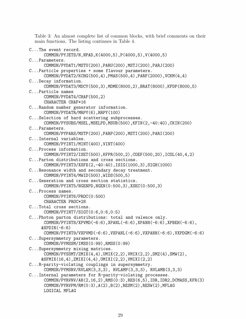
Table 3: An almost complete list of common blocks, with brief comments on theirmain functions. The listing continues in Table 4.

C...The event record.COMMON/PYJETS/N,NPAD,K(4000,5),P(4000,5),V(4000,5)

C...Parameters.COMMON/PYDAT1/MSTU(200),PARU(200),MSTJ(200),PARJ(200)

C...Particle properties + some flavour parameters.COMMON/PYDAT2/KCHG(500,4),PMAS(500,4),PARF(2000),VCKM(4,4)

C...Decay information.COMMON/PYDAT3/MDCY(500,3),MDME(8000,2),BRAT(8000),KFDP(8000,5)

C...Particle namesCOMMON/PYDAT4/CHAF(500,2)CHARACTER CHAF*16

C...Random number generator information.COMMON/PYDATR/MRPY(6),RRPY(100)

C...Selection of hard scattering subprocesses.COMMON/PYSUBS/MSEL,MSELPD,MSUB(500),KFIN(2,-40:40),CKIN(200)

C...Parameters.COMMON/PYPARS/MSTP(200),PARP(200),MSTI(200),PARI(200)

C...Internal variables.COMMON/PYINT1/MINT(400),VINT(400)

C...Process information.COMMON/PYINT2/ISET(500),KFPR(500,2),COEF(500,20),ICOL(40,4,2)

C...Parton distributions and cross sections.COMMON/PYINT3/XSFX(2,-40:40),ISIG(1000,3),SIGH(1000)

C...Resonance width and secondary decay treatment.COMMON/PYINT4/MWID(500),WIDS(500,5)

C...Generation and cross section statistics.COMMON/PYINT5/NGENPD,NGEN(0:500,3),XSEC(0:500,3)

C...Process names.COMMON/PYINT6/PROC(0:500)CHARACTER PROC*28

C...Total cross sections.COMMON/PYINT7/SIGT(0:6,0:6,0:5)

C...Photon parton distributions: total and valence only.COMMON/PYINT8/XPVMD(-6:6),XPANL(-6:6),XPANH(-6:6),XPBEH(-6:6),

&XPDIR(-6:6)COMMON/PYINT9/VXPVMD(-6:6),VXPANL(-6:6),VXPANH(-6:6),VXPDGM(-6:6)

C...Supersymmetry parameters.COMMON/PYMSSM/IMSS(0:99),RMSS(0:99)

C...Supersymmetry mixing matrices.COMMON/PYSSMT/ZMIX(4,4),UMIX(2,2),VMIX(2,2),SMZ(4),SMW(2),

&SFMIX(16,4),ZMIXI(4,4),UMIXI(2,2),VMIXI(2,2)C...R-parity-violating couplings in supersymmetry.

COMMON/PYMSRV/RVLAM(3,3,3), RVLAMP(3,3,3), RVLAMB(3,3,3)C...Internal parameters for R-parity-violating processes.

COMMON/PYRVNV/AB(2,16,2),RMS(0:3),RES(6,5),IDR,IDR2,DCMASS,KFR(3)COMMON/PYRVPM/RM(0:3),A(2),B(2),RESM(2),RESW(2),MFLAGLOGICAL MFLAG

29

Table 4: Continuation of Table 3.

C...Parameters for Gauss integration of supersymmetric widths.COMMON/PYINTS/XXM(20)COMMON/PYG2DX/X1

C...Histogram information.COMMON/PYBINS/IHIST(4),INDX(1000),BIN(20000)

C...HEPEVT commonblock.PARAMETER (NMXHEP=4000)COMMON/HEPEVT/NEVHEP,NHEP,ISTHEP(NMXHEP),IDHEP(NMXHEP),

&JMOHEP(2,NMXHEP),JDAHEP(2,NMXHEP),PHEP(5,NMXHEP),VHEP(4,NMXHEP)DOUBLE PRECISION PHEP,VHEP

C...User process initialization commonblock.INTEGER MAXPUPPARAMETER (MAXPUP=100)INTEGER IDBMUP,PDFGUP,PDFSUP,IDWTUP,NPRUP,LPRUPDOUBLE PRECISION EBMUP,XSECUP,XERRUP,XMAXUPCOMMON/HEPRUP/IDBMUP(2),EBMUP(2),PDFGUP(2),PDFSUP(2),

&IDWTUP,NPRUP,XSECUP(MAXPUP),XERRUP(MAXPUP),XMAXUP(MAXPUP),&LPRUP(MAXPUP)

C...User process event common block.INTEGER MAXNUPPARAMETER (MAXNUP=500)INTEGER NUP,IDPRUP,IDUP,ISTUP,MOTHUP,ICOLUPDOUBLE PRECISION XWGTUP,SCALUP,AQEDUP,AQCDUP,PUP,VTIMUP,SPINUPCOMMON/HEPEUP/NUP,IDPRUP,XWGTUP,SCALUP,AQEDUP,AQCDUP,IDUP(MAXNUP),

&ISTUP(MAXNUP),MOTHUP(2,MAXNUP),ICOLUP(2,MAXNUP),PUP(5,MAXNUP),&VTIMUP(MAXNUP),SPINUP(MAXNUP)

flexibility to ‘do it yourself’. We therefore start with a few cases of this kind, at the sametime introducing some of the more frequently used utility routines.

As a first example, assume that you want to study the production of uu 2-jet systemsat 20 GeV energy. To do this, write a main program

IMPLICIT DOUBLE PRECISION(A-H, O-Z)CALL PY2ENT(0,2,-2,20D0)CALL PYLIST(1)END

and run this program, linked together with Pythia. The routine PY2ENT is specificallyintended for storing two entries (partons or particles). The first argument (0) is a com-mand to perform fragmentation and decay directly after the entries have been stored, thesecond and third that the two entries are u (2) and u (−2), and the last that the c.m.energy of the pair is 20 GeV, in double precision. When this is run, the resulting event isstored in the PYJETS common block. This information can then be read out by you. Nooutput is produced by PY2ENT itself, except for a title page which appears once for everyPythia run.

Instead the second command, to PYLIST, provides a simple visible summary of theinformation stored in PYJETS. The argument (1) indicates that the short version shouldbe used, which is suitable for viewing the listing directly on an 80-column terminal screen.It might look as shown here.

Event listing (summary)

30

I particle/jet KS KF orig p_x p_y p_z E m

1 (u) A 12 2 0 0.000 0.000 10.000 10.000 0.0062 (ubar) V 11 -2 0 0.000 0.000 -10.000 10.000 0.0063 (string) 11 92 1 0.000 0.000 0.000 20.000 20.0004 (rho+) 11 213 3 0.098 -0.154 2.710 2.856 0.8855 (rho-) 11 -213 3 -0.227 0.145 6.538 6.590 0.7816 pi+ 1 211 3 0.125 -0.266 0.097 0.339 0.1407 (Sigma0) 11 3212 3 -0.254 0.034 -1.397 1.855 1.1938 (K*+) 11 323 3 -0.124 0.709 -2.753 2.968 0.8469 p~- 1 -2212 3 0.395 -0.614 -3.806 3.988 0.938

10 pi- 1 -211 3 -0.013 0.146 -1.389 1.403 0.14011 pi+ 1 211 4 0.109 -0.456 2.164 2.218 0.14012 (pi0) 11 111 4 -0.011 0.301 0.546 0.638 0.13513 pi- 1 -211 5 0.089 0.343 2.089 2.124 0.14014 (pi0) 11 111 5 -0.316 -0.197 4.449 4.467 0.13515 (Lambda0) 11 3122 7 -0.208 0.014 -1.403 1.804 1.11616 gamma 1 22 7 -0.046 0.020 0.006 0.050 0.00017 K+ 1 321 8 -0.084 0.299 -2.139 2.217 0.49418 (pi0) 11 111 8 -0.040 0.410 -0.614 0.751 0.13519 gamma 1 22 12 0.059 0.146 0.224 0.274 0.00020 gamma 1 22 12 -0.070 0.155 0.322 0.364 0.00021 gamma 1 22 14 -0.322 -0.162 4.027 4.043 0.00022 gamma 1 22 14 0.006 -0.035 0.422 0.423 0.00023 p+ 1 2212 15 -0.178 0.033 -1.343 1.649 0.93824 pi- 1 -211 15 -0.030 -0.018 -0.059 0.156 0.14025 gamma 1 22 18 -0.006 0.384 -0.585 0.699 0.00026 gamma 1 22 18 -0.034 0.026 -0.029 0.052 0.000

sum: 0.00 0.000 0.000 0.000 20.000 20.000

(A few blanks have been removed between the columns to make it fit into the formatof this text.) Look in the particle/jet column and note that the first two lines are theoriginal u and u. The parentheses enclosing the names, ‘(u)’ and ‘(ubar)’, are there asa reminder that these partons actually have been allowed to fragment. The partons arestill retained so that event histories can be studied. Also note that the KF (flavour code)column contains 2 in the first line and −2 in the second. These are the codes actuallystored to denote the presence of a u and a u, cf. the PY2ENT call, while the names writtenare just conveniences used when producing visible output. The A and V near the end of theparticle/jet column indicate the beginning and end of a string (or cluster, or independentfragmentation) parton system; any intermediate entries belonging to the same systemwould have had an I in that column. (This gives a poor man’s representation of anup-down arrow, l.)

In the orig (origin) column, the zeros indicate that u and u are two initial entries.The subsequent line, number 3, denotes the fragmenting uu string system as a whole, andhas origin 1, since the first parton of this string system is entry number 1. The particlesin lines 4–10 have origin 3 to denote that they come directly from the fragmentation ofthis string. In string fragmentation it is not meaningful to say that a particle comes fromonly the u quark or only the u one. It is the string system as a whole that gives a ρ+, aρ−, a π+, a Σ0, a K∗+, a p−, and a π−. Note that some of the particle names are againenclosed in parentheses, indicating that these particles are not present in the final stateeither, but have decayed further. Thus the π− in line 13 and the π0 in line 14 have origin5, as an indication that they come from the decay of the ρ− in line 5. Only the namesnot enclosed in parentheses remain at the end of the fragmentation/decay chain, and

31

are thus experimentally observable. The actual status code used to distinguish betweendifferent classes of entries is given in the KS column; codes in the range 1–10 correspondto remaining entries, and those above 10 to those that have fragmented or decayed.

The columns with p x, p y, p z, E and m are quite self-explanatory. All momenta,energies and masses are given in units of GeV, since the speed of light is taken to be c = 1.Note that energy and momentum are conserved at each step of the fragmentation/decayprocess (although there exist options where this is not true). Also note that the z axisplays the role of preferred direction, along which the original partons are placed. The finalline is intended as a quick check that nothing funny happened. It contains the summedcharge, summed momentum, summed energy and invariant mass of the final entries at theend of the fragmentation/decay chain, and the values should agree with the input impliedby the PY2ENT arguments. (In fact, warnings would normally appear on the output ifanything untoward happened, but that is another story.)

The above example has illustrated roughly what information is to be had in the eventrecord, but not so much about how it is stored. This is better seen by using a 132-columnformat for listing events. Try e.g. the following program

IMPLICIT DOUBLE PRECISION(A-H, O-Z)CALL PY3ENT(0,1,21,-1,30D0,0.9D0,0.7D0)CALL PYLIST(2)CALL PYEDIT(3)CALL PYLIST(2)END

where a 3-jet dgd event is generated in the first executable line and listed in the second.This listing will contain the numbers as directly stored in the common block PYJETS

COMMON/PYJETS/N,NPAD,K(4000,5),P(4000,5),V(4000,5)

For particle I, K(I,1) thus gives information on whether or not a parton or particle hasfragmented or decayed, K(I,2) gives the particle code, K(I,3) its origin, K(I,4) andK(I,5) the position of fragmentation/decay products, and P(I,1)–P(I,5) momentum,energy and mass. The number of lines in current use is given by N, i.e. 1 ≤ I ≤ N. TheV matrix contains decay vertices; to view those PYLIST(3) has to be used. NPAD is adummy, needed to avoid some compiler troubles. It is important to learn the rules forhow information is stored in PYJETS.

The third executable line in the program illustrates another important point aboutPythia: a number of routines are available for manipulating and analyzing the eventrecord after the event has been generated. Thus PYEDIT(3) will remove everything exceptstable charged particles, as shown by the result of the second PYLIST call. More advancedpossibilities include things like sphericity or clustering routines. Pythia also containssome simple routines for histogramming, used to give self-contained examples of analysisprocedures.

Apart from the input arguments of subroutine calls, control on the doings of Pythiamay be imposed via many common blocks. Here sensible default values are always pro-vided. A user might want to switch off all particle decays by putting MSTJ(21)=0 orincrease the s/u ratio in fragmentation by putting PARJ(2)=0.40D0, to give but two ex-amples. It is by exploring the possibilities offered here that Pythia can be turned intoan extremely versatile tool, even if all the nice physics is already present in the defaultvalues.

As a final, semi-realistic example, assume that the p⊥ spectrum of π+ particles is tobe studied in 91.2 GeV e+e− annihilation events, where p⊥ is to be defined with respectto the sphericity axis. Using the internal routines for simple histogramming, a completeprogram might look like

32

C...Double precision and integer declarations.IMPLICIT DOUBLE PRECISION(A-H, O-Z)IMPLICIT INTEGER(I-N)INTEGER PYK,PYCHGE,PYCOMP

C...Common blocks.COMMON/PYJETS/N,NPAD,K(4000,5),P(4000,5),V(4000,5)

C...Book histograms.CALL PYBOOK(1,’pT spectrum of pi+’,100,0D0,5D0)

C...Number of events to generate. Loop over events.NEVT=100DO 110 IEVT=1,NEVT

C...Generate event. List first one.CALL PYEEVT(0,91.2D0)IF(IEVT.EQ.1) CALL PYLIST(1)

C...Find sphericity axis.CALL PYSPHE(SPH,APL)

C...Rotate event so that sphericity axis is along z axis.CALL PYEDIT(31)

C...Loop over all particles, but skip if not pi+.DO 100 I=1,N

IF(K(I,2).NE.211) GOTO 100

C...Calculate pT and fill in histogram.PT=SQRT(P(I,1)**2+P(I,2)**2)CALL PYFILL(1,PT,1D0)

C...End of particle and event loops.100 CONTINUE110 CONTINUE

C...Normalize histogram properly and list it.CALL PYFACT(1,20D0/NEVT)CALL PYHIST

END

Study this program, try to understand what happens at each step, and run it to checkthat it works. You should then be ready to look at the relevant sections of this reportand start writing your own programs.

3.6 Getting Started with the Event Generation Machinery

A run with the full Pythia event generation machinery has to be more strictly organizedthan the simple examples above, in that it is necessary to initialize the generation beforeevents can be generated, and in that it is not possible to change switches and parametersfreely during the course of the run. A fairly precise recipe for how a run should bestructured can therefore be given.

33

Thus, the nowadays normal usage of Pythia can be subdivided into three steps.1. The initialization step. It is here that all the basic characteristics of the coming

generation are specified. The material in this section includes the following.• Declarations for double precision and integer variables and integer functions:

IMPLICIT DOUBLE PRECISION(A-H, O-Z)IMPLICIT INTEGER(I-N)INTEGER PYK,PYCHGE,PYCOMP

• Common blocks, at least the following, and maybe some more:COMMON/PYJETS/N,NPAD,K(4000,5),P(4000,5),V(4000,5)COMMON/PYDAT1/MSTU(200),PARU(200),MSTJ(200),PARJ(200)COMMON/PYSUBS/MSEL,MSELPD,MSUB(500),KFIN(2,-40:40),CKIN(200)COMMON/PYPARS/MSTP(200),PARP(200),MSTI(200),PARI(200)

• Selection of required processes. Some fixed ‘menus’ of subprocesses can beselected with different MSEL values, but with MSEL=0 it is possible to compose‘a la carte’, using the subprocess numbers. To generate processes 14, 18 and29, for instance, one needs

MSEL=0MSUB(14)=1MSUB(18)=1MSUB(29)=1

• Selection of kinematics cuts in the CKIN array. To generate hard scatteringswith 5 GeV ≤ p⊥ ≤ 10 GeV, for instance, use

CKIN(3)=5D0CKIN(4)=10D0

Unfortunately, initial- and final-state radiation will shift around the kinematicsof the hard scattering, making the effects of cuts less predictable. One thereforealways has to be very careful that no desired event configurations are cut out.

• Definition of underlying physics scenario, e.g. Higgs mass.• Selection of parton-distribution sets, Q2 definitions, and all other details of the

generation.• Switching off of generator parts not needed for toy simulations, e.g. fragmen-

tation for parton level studies.• Initialization of the event generation procedure. Here kinematics is set up,

maxima of differential cross sections are found for future Monte Carlo gen-eration, and a number of other preparatory tasks carried out. Initializationis performed by PYINIT, which should be called only after the switches andparameters above have been set to their desired values. The frame, the beamparticles and the energy have to be specified, e.g.

CALL PYINIT(’CMS’,’p’,’pbar’,1800D0)

• Any other initial material required by you, e.g. histogram booking.2. The generation loop. It is here that events are generated and studied. It includes

the following tasks:• Generation of the next event, with

CALL PYEVNT

• Printing of a few events, to check that everything is working as planned, withCALL PYLIST(1)

• An analysis of the event for properties of interest, either directly reading out in-formation from the PYJETS common block or making use of the utility routinesin Pythia.

• Saving of events on disk or tape, or interfacing to detector simulation.3. The finishing step. Here the tasks are:

34

• Printing a table of deduced cross sections, obtained as a by-product of theMonte Carlo generation activity, with the command

CALL PYSTAT(1)

• Printing histograms and other user output.To illustrate this structure, imagine a toy example, where one wants to simulate the

production of a 300 GeV Higgs particle. In Pythia, a program for this might looksomething like the following.

C...Double precision and integer declarations.IMPLICIT DOUBLE PRECISION(A-H, O-Z)IMPLICIT INTEGER(I-N)INTEGER PYK,PYCHGE,PYCOMP

C...Common blocks.COMMON/PYJETS/N,NPAD,K(4000,5),P(4000,5),V(4000,5)COMMON/PYDAT1/MSTU(200),PARU(200),MSTJ(200),PARJ(200)COMMON/PYDAT2/KCHG(500,4),PMAS(500,4),PARF(2000),VCKM(4,4)COMMON/PYDAT3/MDCY(500,3),MDME(8000,2),BRAT(8000),KFDP(8000,5)COMMON/PYSUBS/MSEL,MSELPD,MSUB(500),KFIN(2,-40:40),CKIN(200)COMMON/PYPARS/MSTP(200),PARP(200),MSTI(200),PARI(200)

C...Number of events to generate. Switch on proper processes.NEV=1000MSEL=0MSUB(102)=1MSUB(123)=1MSUB(124)=1

C...Select Higgs mass and kinematics cuts in mass.PMAS(25,1)=300D0CKIN(1)=290D0CKIN(2)=310D0

C...For simulation of hard process only: cut out unnecessary tasks.MSTP(61)=0MSTP(71)=0MSTP(81)=0MSTP(111)=0

C...Initialize and list partial widths.CALL PYINIT(’CMS’,’p’,’p’,14000D0)CALL PYSTAT(2)

C...Book histogram.CALL PYBOOK(1,’Higgs mass’,50,275D0,325D0)

C...Generate events. Look at first few.DO 200 IEV=1,NEVCALL PYEVNTIF(IEV.LE.3) CALL PYLIST(1)

C...Loop over particles to find Higgs and histogram its mass.DO 100 I=1,N

35

IF(K(I,1).LT.20.AND.K(I,2).EQ.25) HMASS=P(I,5)100 CONTINUE

CALL PYFILL(1,HMASS,1D0)200 CONTINUE

C...Print cross sections and histograms.CALL PYSTAT(1)CALL PYHIST

END

Here 102, 123 and 124 are the three main Higgs production graphs gg → h, ZZ → h,and WW → h, and MSUB(ISUB)=1 is the command to switch on process ISUB. Fullfreedom to combine subprocesses ‘a la carte’ is ensured by MSEL=0; ready-made ‘menus’can be ordered with other MSEL numbers. The PMAS command sets the mass of the Higgs,and the CKIN variables the desired mass range of the Higgs — a Higgs with a 300 GeVnominal mass actually has a fairly broad Breit–Wigner type mass distribution. The MSTPswitches that come next are there to modify the generation procedure, in this case toswitch off initial- and final-state radiation, multiple interactions among beam jets, andfragmentation, to give only the ‘parton skeleton’ of the hard process. The PYINIT callinitializes Pythia, by finding maxima of cross sections, recalculating the Higgs decayproperties (which depend on the Higgs mass), etc. The decay properties can be listedwith PYSTAT(2).

Inside the event loop, PYEVNT is called to generate an event, and PYLIST(1) to listthe event. The information used by PYLIST(1) is the event record, stored in the commonblock PYJETS. Here one finds all produced particles, both final and intermediate ones, withinformation on particle species and event history (K array), particle momenta (P array)and production vertices (V array). In the loop over all particles produced, 1 through N,the Higgs particle is found by its code, K(I,2)=25, and its mass is stored in P(I,5).

After all events have been generated, PYSTAT(1) gives a summary of the number ofevents generated in the various allowed channels, and the inferred cross sections.

In the run above, a typical event listing might look like the following.

Event listing (summary)

I particle/jet KF p_x p_y p_z E m

1 !p+! 2212 0.000 0.000 8000.000 8000.000 0.9382 !p+! 2212 0.000 0.000-8000.000 8000.000 0.938

======================================================================3 !g! 21 -0.505 -0.229 28.553 28.558 0.0004 !g! 21 0.224 0.041 -788.073 788.073 0.0005 !g! 21 -0.505 -0.229 28.553 28.558 0.0006 !g! 21 0.224 0.041 -788.073 788.073 0.0007 !H0! 25 -0.281 -0.188 -759.520 816.631 300.0278 !W+! 24 120.648 35.239 -397.843 424.829 80.0239 !W-! -24 -120.929 -35.426 -361.677 391.801 82.57910 !e+! -11 12.922 -4.760 -160.940 161.528 0.00111 !nu_e! 12 107.726 39.999 -236.903 263.302 0.00012 !s! 3 -62.423 7.195 -256.713 264.292 0.19913 !cbar! -4 -58.506 -42.621 -104.963 127.509 1.350

======================================================================14 (H0) 25 -0.281 -0.188 -759.520 816.631 300.02715 (W+) 24 120.648 35.239 -397.843 424.829 80.023

36

16 (W-) -24 -120.929 -35.426 -361.677 391.801 82.57917 e+ -11 12.922 -4.760 -160.940 161.528 0.00118 nu_e 12 107.726 39.999 -236.903 263.302 0.00019 s A 3 -62.423 7.195 -256.713 264.292 0.19920 cbar V -4 -58.506 -42.621 -104.963 127.509 1.35021 ud_1 A 2103 -0.101 0.176 7971.328 7971.328 0.77122 d V 1 -0.316 0.001 -87.390 87.390 0.01023 u A 2 0.606 0.052 -0.751 0.967 0.00624 uu_1 V 2203 0.092 -0.042-7123.668 7123.668 0.771

======================================================================sum: 2.00 0.00 0.00 0.00 15999.98 15999.98

The above event listing is abnormally short, in part because some columns of informationwere removed to make it fit into this text, in part because all initial- and final-state QCDradiation, all non-trivial beam jet structure, and all fragmentation was inhibited in thegeneration. Therefore only the skeleton of the process is visible. In lines 1 and 2 onerecognizes the two incoming protons. In lines 3 and 4 are incoming partons before initial-state radiation and in 5 and 6 after — since there is no such radiation they coincide here.Line 7 shows the Higgs produced by gg fusion, 8 and 9 its decay products and 10–13 thesecond-step decay products. Up to this point lines give a summary of the event history,indicated by the exclamation marks that surround particle names (and also reflected inthe K(I,1) code, not shown). From line 14 onwards come the particles actually producedin the final states, first in lines 14–16 particles that subsequently decayed, which havetheir names surrounded by brackets, and finally the particles and partons left in the end,including beam remnants. Here this also includes a number of unfragmented partons,since fragmentation was inhibited. Ordinarily, the listing would have gone on for a fewhundred more lines, with the particles produced in the fragmentation and their decayproducts. The final line gives total charge and momentum, as a convenient check thatnothing unexpected happened. The first column of the listing is just a counter, the secondgives the particle name and information on status and string drawing (the A and V), thethird the particle-flavour code (which is used to give the name), and the subsequentcolumns give the momentum components.

One of the main problems is to select kinematics efficiently. Imagine for instance thatone is interested in the production of a single Z with a transverse momentum in excess of50 GeV. If one tries to generate the inclusive sample of Z events, by the basic productiongraphs qq → Z, then most events will have low transverse momenta and will have to bediscarded. That any of the desired events are produced at all is due to the initial-stategeneration machinery, which can build up transverse momenta for the incoming q andq. However, the amount of initial-state radiation cannot be constrained beforehand. Toincrease the efficiency, one may therefore turn to the higher-order processes qg → Zqand qq → Zg, where already the hard subprocess gives a transverse momentum to theZ. This transverse momentum can be constrained as one wishes, but again initial- andfinal-state radiation will smear the picture. If one were to set a p⊥ cut at 50 GeV forthe hard-process generation, those events where the Z was given only 40 GeV in the hardprocess but got the rest from initial-state radiation would be missed. Not only thereforewould cross sections come out wrong, but so might the typical event shapes. In the end,it is therefore necessary to find some reasonable compromise, by starting the generationat 30 GeV, say, if one knows that only rarely do events below this value fluctuate up to50 GeV. Of course, most events will therefore not contain a Z above 50 GeV, and one willhave to live with some inefficiency. It is not uncommon that only one event out of tencan be used, and occasionally it can be even worse.

If it is difficult to set kinematics, it is often easier to set the flavour content of a process.In a Higgs study, one might wish, for example, to consider the decay h0 → Z0Z0, witheach Z0 → e+e− or µ+µ−. It is therefore necessary to inhibit all other h0 and Z0 decay

37

channels, and also to adjust cross sections to take into account this change, all of whichis fairly straightforward. The same cannot be said for decays of ordinary hadrons, wherethe number produced in a process is not known beforehand, and therefore inconsistencieseasily can arise if one tries to force specific decay channels.

In the examples given above, all run-specific parameters are set in the code (in themain program; alternatively it could be in a subroutine called by the main program).This approach is allowing maximum flexibility to change parameters during the courseof the run. However, in many experimental collaborations one does not want to allowthis freedom, but only one set of parameters, to be read in from an external file at thebeginning of a run and thereafter never changed. This in particular applies when Pythia

is to be linked with other libraries, such as Geant [Bru89] and detector-specific software.While a linking of a normal-sized main program with Pythia is essentially instantaneouson current platforms (typically less than a second), this may not hold for other libraries.For this purpose one then needs a parser of Pythia parameters, the core of which canbe provided by the PYGIVE routine.

As an example, consider a main program of the form

C...Double precision and integer declarations.IMPLICIT DOUBLE PRECISION(A-H, O-Z)IMPLICIT INTEGER(I-N)INTEGER PYK,PYCHGE,PYCOMP

C...Input and output strings.CHARACTER FRAME*12,BEAM*12,TARGET*12,PARAM*100

C...Read parameters for PYINIT call.READ(*,*) FRAME,BEAM,TARGET,ENERGY

C...Read number of events to generate, and to print.READ(*,*) NEV,NPRT

C...Loop over reading and setting parameters/switches.100 READ(*,’(A)’,END=200) PARAM

CALL PYGIVE(PARAM)GOTO 100

C...Initialize PYTHIA.200 CALL PYINIT(FRAME,BEAM,TARGET,ENERGY)

C...Event generation loopDO 300 IEV=1,NEVCALL PYEVNTIF(IEV.LE.NPRT) CALL PYLIST(1)

300 CONTINUE

C...Print cross sections.CALL PYSTAT(1)

END

and a file indata with the contents

CMS,p,p,14000.1000,3! below follows commands sent to PYGIVE

38

MSEL=0 ! Mix processes freelyMSUB(102)=1 ! g + g -> h0MSUB(123)=1 ! Z0 + Z0 -> h0MSUB(124)=1 ! W+ + W- -> h0PMAS(25,1)=300. ! Higgs massCKIN(1)=290. ! lower cutoff on massCKIN(2)=310. ! upper cutoff on massMSTP(61)=0 ! no initial-state showersMSTP(71)=0 ! no final-state showersMSTP(81)=0 ! no multiple interactionsMSTP(111)=0 ! no hadronization

Here the text following the exclamation marks is interpreted as a comment by PYGIVE, andthus purely intended to allow better documentation of changes. The main program couldthen be linked to Pythia, to an executable a.out, and run e.g. with a Unix commandline

a.out < indata > output

to produce results on the file output. Here the indata could be changed without requiringa recompilation. Of course, the main program would have to be more realistic, e.g. withevents saved to disk or tape, but the principle should be clear.

39

4 Monte Carlo Techniques

Quantum mechanics introduces a concept of randomness in the behaviour of physicalprocesses. The virtue of event generators is that this randomness can be simulated bythe use of Monte Carlo techniques. In the process, the program authors have to use someingenuity to find the most efficient way to simulate an assumed probability distribution.A detailed description of possible techniques would carry us too far, but in this sectionsome of the most frequently used approaches are presented, since they will appear indiscussions in subsequent sections. Further examples may be found e.g. in [Jam80].

First of all one assumes the existence of a random number generator. This is a (For-tran) function which, each time it is called, returns a number R in the range between 0and 1, such that the inclusive distribution of numbers R is flat in the range, and such thatdifferent numbers R are uncorrelated. The random number generator that comes withPythia is described at the end of this section, and we defer the discussion until then.

4.1 Selection From a Distribution

The situation that is probably most common is that we know a function f(x) which isnon-negative in the allowed x range xmin ≤ x ≤ xmax. We want to select an x ‘at random’so that the probability in a small interval dx around a given x is proportional to f(x) dx.Here f(x) might be a fragmentation function, a differential cross section, or any of anumber of distributions.

One does not have to assume that the integral of f(x) is explicitly normalized to unity:by the Monte Carlo procedure of picking exactly one accepted x value, normalization isimplicit in the final result. Sometimes the integral of f(x) does carry a physics contentof its own, as part of an overall weight factor we want to keep track of. Consider, forinstance, the case when x represents one or several phase-space variables and f(x) adifferential cross section; here the integral has a meaning of total cross section for theprocess studied. The task of a Monte Carlo is then, on the one hand, to generate eventsone at a time, and, on the other hand, to estimate the total cross section. The discussionof this important example is deferred to section 7.4.

If it is possible to find a primitive function F (x) which has a known inverse F−1(x),an x can be found as follows (method 1):

∫ x

xmin

f(x) dx = R∫ xmax

xmin

f(x) dx

=⇒ x = F−1(F (xmin) +R(F (xmax) − F (xmin))) . (2)

The statement of the first line is that a fraction R of the total area under f(x) should beto the left of x. However, seldom are functions of interest so nice that the method aboveworks. It is therefore necessary to use more complicated schemes.

Special tricks can sometimes be found. Consider e.g. the generation of a Gaussianf(x) = exp(−x2). This function is not integrable, but if we combine it with the sameGaussian distribution of a second variable y, it is possible to transform to polar coordinates

f(x) dx f(y) dy = exp(−x2 − y2) dx dy = r exp(−r2) dr dϕ , (3)

and now the r and ϕ distributions may be easily generated and recombined to yield x.At the same time we get a second number y, which can also be used. For the generationof transverse momenta in fragmentation, this is very convenient, since in fact we want toassign two transverse degrees of freedom.

If the maximum of f(x) is known, f(x) ≤ fmax in the x range considered, a hit-or-missmethod will always yield the correct answer (method 2):

40

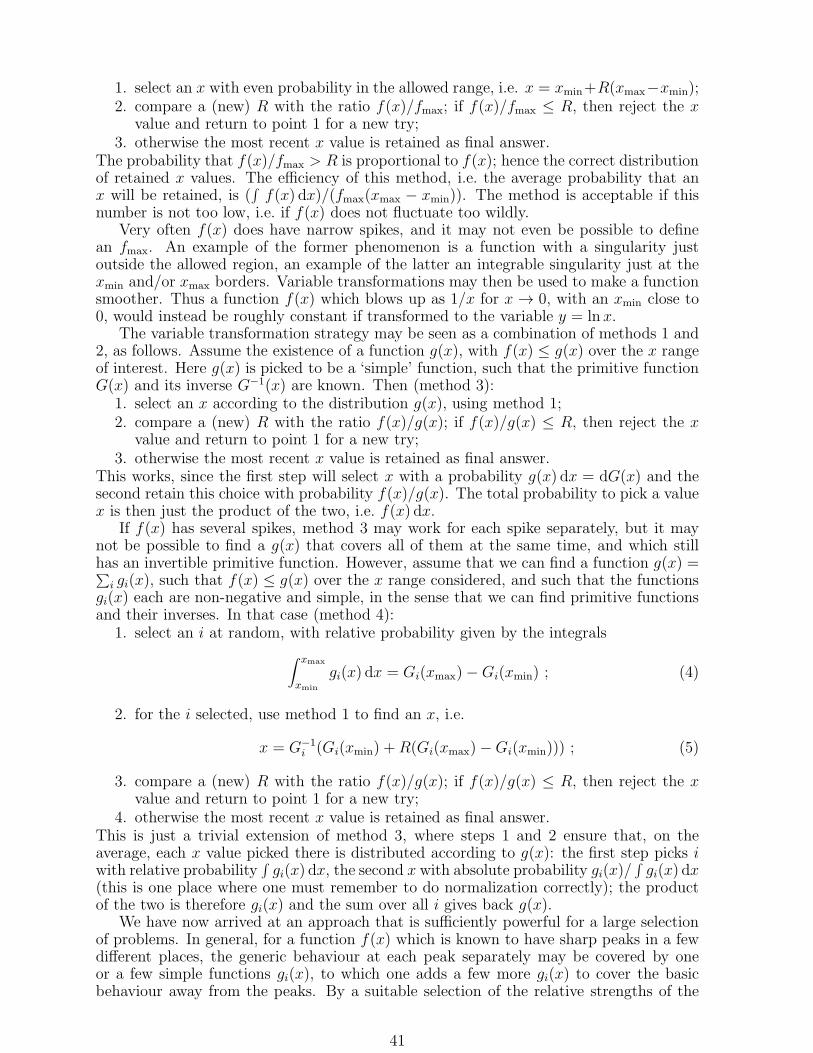
1. select an x with even probability in the allowed range, i.e. x = xmin+R(xmax−xmin);2. compare a (new) R with the ratio f(x)/fmax; if f(x)/fmax ≤ R, then reject the x

value and return to point 1 for a new try;3. otherwise the most recent x value is retained as final answer.

The probability that f(x)/fmax > R is proportional to f(x); hence the correct distributionof retained x values. The efficiency of this method, i.e. the average probability that anx will be retained, is (

∫

f(x) dx)/(fmax(xmax − xmin)). The method is acceptable if thisnumber is not too low, i.e. if f(x) does not fluctuate too wildly.

Very often f(x) does have narrow spikes, and it may not even be possible to definean fmax. An example of the former phenomenon is a function with a singularity justoutside the allowed region, an example of the latter an integrable singularity just at thexmin and/or xmax borders. Variable transformations may then be used to make a functionsmoother. Thus a function f(x) which blows up as 1/x for x → 0, with an xmin close to0, would instead be roughly constant if transformed to the variable y = ln x.

The variable transformation strategy may be seen as a combination of methods 1 and2, as follows. Assume the existence of a function g(x), with f(x) ≤ g(x) over the x rangeof interest. Here g(x) is picked to be a ‘simple’ function, such that the primitive functionG(x) and its inverse G−1(x) are known. Then (method 3):

1. select an x according to the distribution g(x), using method 1;2. compare a (new) R with the ratio f(x)/g(x); if f(x)/g(x) ≤ R, then reject the x

value and return to point 1 for a new try;3. otherwise the most recent x value is retained as final answer.

This works, since the first step will select x with a probability g(x) dx = dG(x) and thesecond retain this choice with probability f(x)/g(x). The total probability to pick a valuex is then just the product of the two, i.e. f(x) dx.

If f(x) has several spikes, method 3 may work for each spike separately, but it maynot be possible to find a g(x) that covers all of them at the same time, and which stillhas an invertible primitive function. However, assume that we can find a function g(x) =∑

i gi(x), such that f(x) ≤ g(x) over the x range considered, and such that the functionsgi(x) each are non-negative and simple, in the sense that we can find primitive functionsand their inverses. In that case (method 4):

1. select an i at random, with relative probability given by the integrals

∫ xmax

xmin

gi(x) dx = Gi(xmax) −Gi(xmin) ; (4)

2. for the i selected, use method 1 to find an x, i.e.

x = G−1i (Gi(xmin) +R(Gi(xmax) −Gi(xmin))) ; (5)

3. compare a (new) R with the ratio f(x)/g(x); if f(x)/g(x) ≤ R, then reject the xvalue and return to point 1 for a new try;

4. otherwise the most recent x value is retained as final answer.This is just a trivial extension of method 3, where steps 1 and 2 ensure that, on theaverage, each x value picked there is distributed according to g(x): the first step picks iwith relative probability

∫

gi(x) dx, the second x with absolute probability gi(x)/∫

gi(x) dx(this is one place where one must remember to do normalization correctly); the productof the two is therefore gi(x) and the sum over all i gives back g(x).

We have now arrived at an approach that is sufficiently powerful for a large selectionof problems. In general, for a function f(x) which is known to have sharp peaks in a fewdifferent places, the generic behaviour at each peak separately may be covered by oneor a few simple functions gi(x), to which one adds a few more gi(x) to cover the basicbehaviour away from the peaks. By a suitable selection of the relative strengths of the

41

different gi’s, it is possible to find a function g(x) that matches well the general behaviourof f(x), and thus achieve a reasonable Monte Carlo efficiency.

The major additional complication is when x is a multidimensional variable. Usuallythe problem is not so much f(x) itself, but rather that the phase-space boundaries maybe very complicated. If the boundaries factorize it is possible to pick phase-space pointsrestricted to the desired region. Otherwise the region may have to be inscribed in a hyper-rectangle, with points picked within the whole hyper-rectangle but only retained if theyare inside the allowed region. This may lead to a significant loss in efficiency. Variabletransformations may often make the allowed region easier to handle.

There are two main methods to handle several dimensions, each with its set of vari-ations. The first method is based on a factorized ansatz, i.e. one attempts to find afunction g(x) which is everywhere larger than f(x), and which can be factorized intog(x) = g(1)(x1) g

(2)(x2) · · · g(n)(xn), where x = (x1, x2, . . . , xn). Here each g(j)(xj) may

in its turn be a sum of functions g(j)i , as in method 4 above. First, each xj is selected

independently, and afterwards the ratio f(x)/g(x) is used to determine whether to retainthe point.

The second method is useful if the boundaries of the allowed region can be written ina form where the maximum range of x1 is known, the allowed range of x2 only dependson x1, that of x3 only on x1 and x2, and so on until xn, whose range may depend on allthe preceding variables. In that case it may be possible to find a function g(x) that canbe integrated over x2 through xn to yield a simple function of x1, according to which x1 isselected. Having done that, x2 is selected according to a distribution which now dependson x1, but with x3 through xn integrated over. In particular, the allowed range for x2 isknown. The procedure is continued until xn is reached, where now the function dependson all the preceding xj values. In the end, the ratio f(x)/g(x) is again used to determinewhether to retain the point.

4.2 The Veto Algorithm

The ‘radioactive decay’ type of problems is very common, in particular in parton showers,but it is also used, e.g. in the multiple interactions description in Pythia. In this kindof problems there is one variable t, which may be thought of as giving a kind of time axisalong which different events are ordered. The probability that ‘something will happen’(a nucleus decay, a parton branch) at time t is described by a function f(t), which isnon-negative in the range of t values to be studied. However, this naıve probability ismodified by the additional requirement that something can only happen at time t if itdid not happen at earlier times t′ < t. (The original nucleus cannot decay once againif it already did decay; possibly the decay products may decay in their turn, but that isanother question.)

The probability that nothing has happened by time t is expressed by the functionN (t) and the differential probability that something happens at time t by P(t). Thebasic equation then is

P(t) = −dNdt

= f(t)N (t) . (6)

For simplicity, we shall assume that the process starts at time t = 0, with N (0) = 1.The above equation can be solved easily if one notes that dN /N = d lnN :

N (t) = N (0) exp

−∫ t

0f(t′) dt′

= exp

−∫ t

0f(t′) dt′

, (7)

and thus

P(t) = f(t) exp

−∫ t

0f(t′) dt′

. (8)

42

With f(t) = c this is nothing but the textbook formulae for radioactive decay. In partic-ular, at small times the correct decay probability, P(t), agrees well with the input one,f(t), since the exponential factor is close to unity there. At larger t, the exponentialgives a dampening which ensures that the integral of P(t) never can exceed unity, evenif the integral of f(t) does. The exponential can be seen as the probability that nothinghappens between the original time 0 and the final time t. In the parton-shower language,this corresponds to the so-called Sudakov form factor.

If f(t) has a primitive function with a known inverse, it is easy to select t valuescorrectly:

∫ t

0P(t′) dt′ = N (0) −N (t) = 1 − exp

−∫ t

0f(t′) dt′

= 1 −R , (9)

which has the solution

F (0) − F (t) = lnR =⇒ t = F−1(F (0) − lnR) . (10)

If f(t) is not sufficiently nice, one may again try to find a better function g(t), withf(t) ≤ g(t) for all t ≥ 0. However to use method 3 with this g(t) would not work, sincethe method would not correctly take into account the effects of the exponential term inP(t). Instead one may use the so-called veto algorithm:

1. start with i = 0 and t0 = 0;2. add 1 to i and select ti = G−1(G(ti−1) − lnR), i.e. according to g(t), but with the

constraint that ti > ti−1,3. compare a (new) R with the ratio f(ti)/g(ti); if f(ti)/g(ti) ≤ R, then return to

point 2 for a new try;4. otherwise ti is retained as final answer.It may not be apparent why this works. Consider, however, the various ways in which

one can select a specific time t. The probability that the first try works, t = t1, i.e. thatno intermediate t values need be rejected, is given by

P0(t) = exp

−∫ t

0g(t′) dt′

g(t)f(t)

g(t)= f(t) exp

−∫ t

0g(t′) dt′

, (11)

where the exponential times g(t) comes from eq. (8) applied to g, and the ratio f(t)/g(t)is the probability that t is accepted. Now consider the case where one intermediate timet1 is rejected and t = t2 is only accepted in the second step. This gives

P1(t) =∫ t

0dt1 exp

−∫ t1

0g(t′) dt′

g(t1)

[

1 − f(t1)

g(t1)

]

exp

−∫ t

t1g(t′) dt′

g(t)f(t)

g(t), (12)

where the first exponential times g(t1) gives the probability that t1 is first selected, thesquare brackets the probability that t1 is subsequently rejected, the following piece theprobability that t = t2 is selected when starting from t1, and the final factor that t isretained. The whole is to be integrated over all possible intermediate times t1. Theexponentials together give an integral over the range from 0 to t, just as in P0, and thefactor for the final step being accepted is also the same, so therefore one finds that

P1(t) = P0(t)∫ t

0dt1 [g(t1) − f(t1)] . (13)

This generalizes. In P2 one has to consider two intermediate times, 0 ≤ t1 ≤ t2 ≤ t3 = t,and so

P2(t) = P0(t)∫ t

0dt1 [g(t1) − f(t1)]

∫ t

t1dt2 [g(t2) − f(t2)]

= P0(t)1

2

(∫ t

0[g(t′) − f(t′)] dt′

)2

. (14)

43

The last equality is most easily seen if one also considers the alternative region 0 ≤ t2 ≤t1 ≤ t, where the roles of t1 and t2 have just been interchanged, and the integral thereforehas the same value as in the region considered. Adding the two regions, however, theintegrals over t1 and t2 decouple, and become equal. In general, for Pi, the i intermediatetimes can be ordered in i! different ways. Therefore the total probability to accept t, inany step, is

P(t) =∞∑

i=0

Pi(t) = P0(t)∞∑

i=0

1

i!

(∫ t

0[g(t′) − f(t′)] dt′

)i

= f(t) exp

−∫ t

0g(t′) dt′

exp∫ t

0[g(t′) − f(t′)] dt′

= f(t) exp

−∫ t

0f(t′) dt′

, (15)

which is the desired answer.If the process is to be stopped at some scale tmax, i.e. if one would like to remain

with a fraction N (tmax) of events where nothing happens at all, this is easy to include inthe veto algorithm: just iterate upwards in t at usual, but stop the process if no allowedbranching is found before tmax.

Usually f(t) is a function also of additional variables x. The methods of the precedingsection are easy to generalize if one can find a suitable function g(t, x) with f(t, x) ≤g(t, x). The g(t) used in the veto algorithm is the integral of g(t, x) over x. Each timea ti has been selected also an xi is picked, according to g(ti, x) dx, and the (t, x) point isaccepted with probability f(ti, xi)/g(ti, xi).

4.3 The Random Number Generator

In recent years, progress has been made in constructing portable generators with largeperiods and other good properties; see the review [Jam90]. Therefore the current versioncontains a random number generator based on the algorithm proposed by Marsaglia,Zaman and Tsang [Mar90]. This routine should work on any machine with a mantissaof at least 48 digits, i.e. on computers with a 64-bit (or more) representation of doubleprecision real numbers. Given the same initial state, the sequence will also be identicalon different platforms. This need not mean that the same sequence of events will begenerated, since the different treatments of roundoff errors in numerical operations willlead to slightly different real numbers being tested against these random numbers in IFstatements. Also code optimization may lead to a divergence of the event sequence.

Apart from nomenclature issues, the coding of PYR as a function rather than a sub-routine, and the extension to double precision, the only difference between our code andthe code given in [Jam90] is that slightly different algorithms are used to ensure that therandom number is not equal to 0 or 1 within the machine precision. Further developmentsof the algorithm has been proposed [Lus94] to remove residual possibilities of small long-range correlations, at the price of a slower generation procedure. However, given thatPythia is using random numbers for so many different tasks, without any fixed cycle,this has been deemed unnecessary.

The generator has a period of over 1043, and the possibility to obtain almost 109

different and disjoint subsequences, selected by giving an initial integer number. Theprice to be paid for the long period is that the state of the generator at a given momentcannot be described by a single integer, but requires about 100 words. Some of theseare real numbers, and are thus not correctly represented in decimal form. The old-styleprocedure, which made it possible to restart the generation from a seed value written tothe run output, is therefore not convenient. The CERN library implementation keepstrack of the number of random numbers generated since the start. With this value saved,

44

in a subsequent run the random generator can be asked to skip ahead the correspondingnumber of random numbers. Pythia is a heavy user of random numbers, however:typically 30% of the full run time is spent on random number generation. Of this, half isoverhead coming from the function call administration, but the other half is truly relatedto the speed of the algorithm. Therefore a skipping ahead would take place with 15% ofthe time cost of the original run, i.e. an uncomfortably high figure.

Instead a different solution is chosen here. Two special routines are provided forwriting and reading the state of the random number generator (plus some initializationinformation) on a sequential file, in a platform-dependent internal representation. The fileused for this purpose has to be specified by you, and opened for read and write. A stateis written as a single record, in free format. It is possible to write an arbitrary number ofstates on a file, and a record can be overwritten, if so desired. The event generation loopmight then look something like:

1. save the state of the generator on file (using flag set in point 3 below),2. generate an event,3. study the event for errors or other reasons why to regenerate it later; set flag to

overwrite previous generator state if no errors, otherwise set flag to create newrecord;

4. loop back to point 1.With this procedure, the file will contain the state before each of the problematical events.These events can therefore be generated in a shorter run, where further information canbe printed. (Inside Pythia, some initialization may take place in connection with thevery first event generated in a run, so it may be necessary to generate one ordinaryevent before reading in a saved state to generate the interesting events.) An alternativeapproach might be to save the state every 100 events or so. If the events are subsequentlyprocessed through a detector simulation, you may have to save also other sets of seeds,naturally.

Unfortunately, the procedure is not always going to work. For instance, if cross sectionmaximum violations have occured before the interesting event in the original run, there isa possibility that another event is picked in the re-started one, where the maximum weightestimate has not been updated. Another problem is the multiple interaction machinery,where some of the options contain an element of learning, which again means that theevent sequence may be broken.

In addition to the service routines, the common block which contains the state of thegenerator is available for manipulation, if you so desire. In particular, the initial seedvalue is by default 19780503, i.e. different from the Marsaglia/CERN default 54217137.It is possible to change this value before any random numbers have been generated, or toforce re-initialization in mid-run with any desired new seed.

It should be noted that, of course, the appearance of a random number generatorpackage inside Pythia does in no way preclude the use of other routines. You can easilyrevert to having PYR as nothing but an interface to an arbitrary external random numbergenerator; e.g. to call a routine RNDM all you need to have is

FUNCTION PYR(IDUMMY)IMPLICIT DOUBLE PRECISION(A-H, O-Z)

100 PYR=RNDM(IDUMMY)IF(PYR.LE.0D0.OR.PYR.GE.1D0) GOTO 100RETURNEND

The random generator subpackage consists of the following components.

R = PYR(IDUMMY)

45

Purpose: to generate a (pseudo)random number R uniformly in the range 0<R<1, i.e.excluding the endpoints.

IDUMMY : dummy input argument; normally 0.

CALL PYRGET(LFN,MOVE)

Purpose: to dump the current state of the random number generator on a separate file,using internal representation for real and integer numbers. To be precise, thefull contents of the PYDATR common block are written on the file, with theexception of MRPY(6).

LFN : (logical file number) the file number to which the state is dumped. You mustassociate this number with a true file (with a platform-dependent name), andsee to it that this file is open for write.

MOVE : choice of adding a new record to the file or overwriting old record(s). Normallyonly options 0 or −1 should be used.

= 0 (or > 0) : add a new record to the end of the file.= -1 : overwrite the last record with a new one (i.e. do one BACKSPACE before

the new write).= −n : back up n records before writing the new record. The records following

after the new one are lost, i.e. the last n old records are lost and one newadded.

CALL PYRSET(LFN,MOVE)

Purpose: to read in a state for the random number generator, from which the subsequentgeneration can proceed. The state must previously have been saved by aPYRGET call. Again the full contents of the PYDATR common block are read,with the exception of MRPY(6).

LFN : (logical file number) the file number from which the state is read. You mustassociate this number with a true file previously written with a PYRGET call,and see to it that this file is open for read.

MOVE : positioning in file before a record is read. With zero value, records are read oneafter the other for each new call, while non-zero values may be used to navigateback and forth, and e.g. return to the same initial state several times.

= 0 : read the next record.= +n : skip ahead n records before reading the record that sets the state of the

random number generator.= −n : back up n records before reading the record that sets the state of the

random number generator.

COMMON/PYDATR/MRPY(6),RRPY(100)

Purpose: to contain the state of the random number generator at any moment (forcommunication between PYR, PYRGET and PYRSET), and also to provide youwith the possibility to initialize different random number sequences, and toknow how many numbers have been generated.

MRPY(1) : (D=19780503) the integer number that specifies which of the possible subse-quences will be initialized in the next PYR call for which MRPY(2)=0. Allowedvalues are 0≤MRPY(1)≤900 000 000, the original Marsaglia (and CERN library)seed is 54217137. The MRPY(1) value is not changed by any of the Pythia

routines.

46

MRPY(2) : (D=0) initialization flag, put to 1 in the first PYR call of run. A re-initializationof the random number generator can be made in mid-run by resetting MRPY(2)to 0 by hand. In addition, any time the counter MRPY(3) reaches 1000000000,it is reset to 0 and MRPY(2) is increased by 1.

MRPY(3) : (R) counter for the number of random numbers generated from the beginningof the run. To avoid overflow when very many numbers are generated, MRPY(2)is used as described above.

MRPY(4), MRPY(5) : I97 and J97 of the CERN library implementation; part of the stateof the generator.

MRPY(6) : (R) current position, i.e. how many records after beginning, in the file; usedby PYRGET and PYRSET.

RRPY(1) - RRPY(97) : the U array of the CERN library implementation; part of thestate of the generator.

RRPY(98) - RRPY(100) : C, CD and CM of the CERN library implementation; the firstpart of the state of the generator, the latter two constants calculated at ini-tialization.

47

5 The Event Record

The event record is the central repository for information about the particles produced inthe current event: flavours, momenta, event history, and production vertices. It plays avery central role: without a proper understanding of what the record is and how informa-tion is stored, it is meaningless to try to use Pythia. The record is stored in the commonblock PYJETS. Almost all the routines that the user calls can be viewed as performingsome action on the record: fill a new event, let partons fragment or particles decay, boostit, list it, find clusters, etc.

In this section we will first describe the KF flavour code, subsequently the PYJETScommon block, and then give a few comments about the role of the event record in theprograms.

To ease the interfacing of different event generators, a HEPEVT standard common blockstructure for the event record has been agreed on. For historical reasons the standardcommon blocks are not directly used in Pythia, but a conversion routine comes with theprogram, and is described at the end of this section.

5.1 Particle Codes

The Particle Data Group particle code [PDG88, PDG92, PDG00] is used consistentlythroughout the program. Almost all known discrepancies between earlier versions of thePDG standard and the Pythia usage have now been resolved. The one known exception isthe (very uncertain) classification of f0(980), with f0(1370) also affected as a consequence.There is also some slight mixup in the technicolor sector between π′0

tc and ηtc. Theseshould not be major problems. The PDG standard, with the local Pythia extensions, isreferred to as the KF particle code. This code you have to be thoroughly familiar with. Itis described below.

The KF code is not convenient for a direct storing of masses, decay data, or otherparticle properties, since the KF codes are so spread out. Instead a compressed code KCbetween 1 and 500 is used here. A particle and its antiparticle are mapped to the sameKC code, but else the mapping is unique. Normally this code is only used at very specificplaces in the program, not visible to the user. If need be, the correspondence can alwaysbe obtained by using the function PYCOMP, i.e. KC = PYCOMP(KF). This mapping is nothardcoded, but can be changed by user intervention, e.g. by introducing new particleswith the PYUPDA facility. It is therefore not intended that you should ever want or needto know any KC codes at all. It may be useful to know, however, that for codes smallerthan 80, KF and KC agree. Normally a user would never do the inverse mapping, but wenote that this is stored as KF = KCHG(KC,4), making use of the KCHG array in the PYDAT2common block. Of course, the sign of a particle could never be recovered by this inverseoperation.

The particle names printed in the tables in this section correspond to the ones obtainedwith the routine PYNAME, which is used extensively, e.g. in PYLIST. Greek charactersare spelt out in full, with a capital first letter to correspond to a capital Greek letter.Generically the name of a particle is made up of the following pieces:

1. The basic root name. This includes a * for most spin 1 (L = 0) mesons and spin3/2 baryons, and a ′ for some spin 1/2 baryons (where there are two states to bedistinguished, cf. Λ–Σ0). The rules for heavy baryon naming are in accordance withthe 1986 Particle Data Group conventions [PDG86]. For mesons with one unit oforbital angular momentum, K (D, B, . . . ) is used for quark-spin 0 and K* (D*, B*,. . . ) for quark-spin 1 mesons; the convention for ‘*’ may here deviate slightly fromthe one used by the PDG.

2. Any lower indices, separated from the root by a . For heavy hadrons, this is theadditional heavy-flavour content not inherent in the root itself. For a diquark, it is

48

Table 5: Quark and lepton codes.

KF Name Printed KF Name Printed

1 d d 11 e− e-

2 u u 12 νe nu e

3 s s 13 µ− mu-

4 c c 14 νµ nu mu

5 b b 15 τ− tau-

6 t t 16 ντ nu tau

7 b′ b’ 17 τ ′ tau’

8 t′ t’ 18 ν ′τ nu’ tau

9 19

10 20

the spin.3. The characters ‘bar’ for an antiparticle, wherever the distinction between particle

and antiparticle is not inherent in the charge information.4. Charge information: ++, +, 0, −, or −−. Charge is not given for quarks or diquarks.

Some neutral particles which are customarily given without a 0 also here lack it,such as neutrinos, g, γ, and flavour-diagonal mesons other than π0 and ρ0. Notethat charge is included both for the proton and the neutron. While non-standard,it is helpful in avoiding misunderstandings when looking at an event listing.

Below follows a list of KF particle codes. The list is not complete; a more extensive onemay be obtained with CALL PYLIST(11). Particles are grouped together, and the basicrules are described for each group. Whenever a distinct antiparticle exists, it is given thesame KF code with a minus sign (whereas KC codes are always positive).

1. Quarks and leptons, Table 5.This group contains the basic building blocks of matter, arranged according tofamily, with the lower member of weak isodoublets also having the smaller code(thus d precedes u). A fourth generation is included as part of the scenarios forexotic physics. The quark codes are used as building blocks for the diquark, mesonand baryon codes below.

2. Gauge bosons and other fundamental bosons, Table 6.This group includes all the gauge and Higgs bosons of the standard model, as wellas some of the bosons appearing in various extensions of it. They correspond toone extra U(1) and one extra SU(2) group, a further Higgs doublet, a graviton,a horizontal gauge boson R (coupling between families), and a (scalar) leptoquarkLQ.

3. Exotic particle codes.The positions 43–80 are used as temporary sites for exotic particles that eventuallymay be shifted to a separate code sequence. Currently this list is empty. The onesnot in use are at your disposal (but with no guarantees that they will remain so).

4. Various special codes, Table 7.In a Monte Carlo, it is always necessary to have codes that do not correspond toany specific particle, but are used to lump together groups of similar particles fordecay treatment (nowadays largely obsolete), to specify generic decay products (alsoobsolete), or generic intermediate states in external processes, or additional eventrecord information from jet searches. These codes, which again are non-standard,are found between numbers 81 and 100.

49

Table 6: Gauge boson and other fundamental boson codes.

KF Name Printed KF Name Printed

21 g g 31

22 γ gamma 32 Z′0 Z’0

23 Z0 Z0 33 Z′′0 Z"0

24 W+ W+ 34 W′+ W’+

25 h0 h0 35 H0 H0

26 36 A0 A0

27 37 H+ H+

28 38

29 39 G Graviton

30 40

41 R0 R0

42 LQ LQ

Table 7: Various special codes.

KF Printed Meaning

81 specflav Spectator flavour; used in decay-product listings

82 rndmflav A random u, d, or s flavour; possible decay product

83 phasespa Simple isotropic phase-space decay

84 c-hadron Information on decay of generic charm hadron

85 b-hadron Information on decay of generic bottom hadron

86

87

88

89 (internal use for unspecified resonance data)

90 system Intermediate pseudoparticle in external process

91 cluster Parton system in cluster fragmentation

92 string Parton system in string fragmentation

93 indep. Parton system in independent fragmentation

94 CMshower Four-momentum of time-like showering system

95 SPHEaxis Event axis found with PYSPHE

96 THRUaxis Event axis found with PYTHRU

97 CLUSjet Jet (cluster) found with PYCLUS

98 CELLjet Jet (cluster) found with PYCELL

99 table Tabular output from PYTABU

100

50

Table 8: Diquark codes. For brevity, diquarks containing c or b quarks are notlisted, but are defined analogously.

KF Name Printed KF Name Printed

1103 dd1 dd 1

2101 ud0 ud 0 2103 ud1 ud 1

2203 uu1 uu 1

3101 sd0 sd 0 3103 sd1 sd 1

3201 su0 su 0 3203 su1 su 1

3303 ss1 ss 1

5. Diquark codes, Table 8.A diquark made up of a quark with code i and another with code j, where i ≥ j,and with total spin s, is given the code

KF = 1000i+ 100j + 2s+ 1 , (16)

i.e. the tens position is left empty (cf. the baryon code below). Some of the mostfrequently used codes are listed in the table. All the lowest-lying spin 0 and 1diquarks are included in the program.

6. Meson codes, Tables 9 and 10.A meson made up of a quark with code i and an antiquark with code −j, j 6= i,and with total spin s, is given the code

KF = 100 max(i, j) + 10 min(i, j) + 2s+ 1 sign(i− j) (−1)max(i,j) , (17)

assuming it is not orbitally or radially excited. Note the presence of an extra − signif the heaviest quark is a down-type one. This is in accordance with the particle–antiparticle distinction adopted in the 1986 Review of Particle Properties [PDG86].It means for example that a B meson contains a b antiquark rather than a b quark.The flavour-diagonal states are arranged in order of ascending mass. Thus theobvious generalization of eq. (17) to KF = 110i+ 2s+ 1 is only valid for charm andbottom. The lighter quark states can appear mixed, e.g. the π0 (111) is an equalmixture of dd (naively code 111) and uu (naively code 221).The standard rule of having the last digit of the form 2s+1 is broken for the K0

S–K0L

system, where it is 0, and this convention should carry over to mixed states in theB meson system, should one choose to define such. For higher multiplets with thesame spin, ±10000, ±20000, etc., are added to provide the extra distinction needed.Some of the most frequently used codes are given below.The full lowest-lying pseudoscalar and vector multiplets are included in the program,Table 9.Also the lowest-lying orbital angular momentum L = 1 mesons are included, Table10: one pseudovector multiplet obtained for total quark-spin 0 (L = 1, S = 0 ⇒J = 1) and one scalar, one pseudovector and one tensor multiplet obtained for totalquark-spin 1 (L = 1, S = 1 ⇒ J = 0, 1 or 2), where J is what is conventionallycalled the spin s of the meson. Any mixing between the two pseudovector multipletsis not taken into account. Please note that some members of these multiplets havestill not been found, and are included here only based on guesswork. Even for knownones, the information on particles (mass, width, decay modes) is highly incomplete.Only two radial excitations are included, the ψ′ = ψ(2S) and Υ′ = Υ(2S).

7. Baryon codes, Table 11.A baryon made up of quarks i, j and k, with i ≥ j ≥ k, and total spin s, is given

51

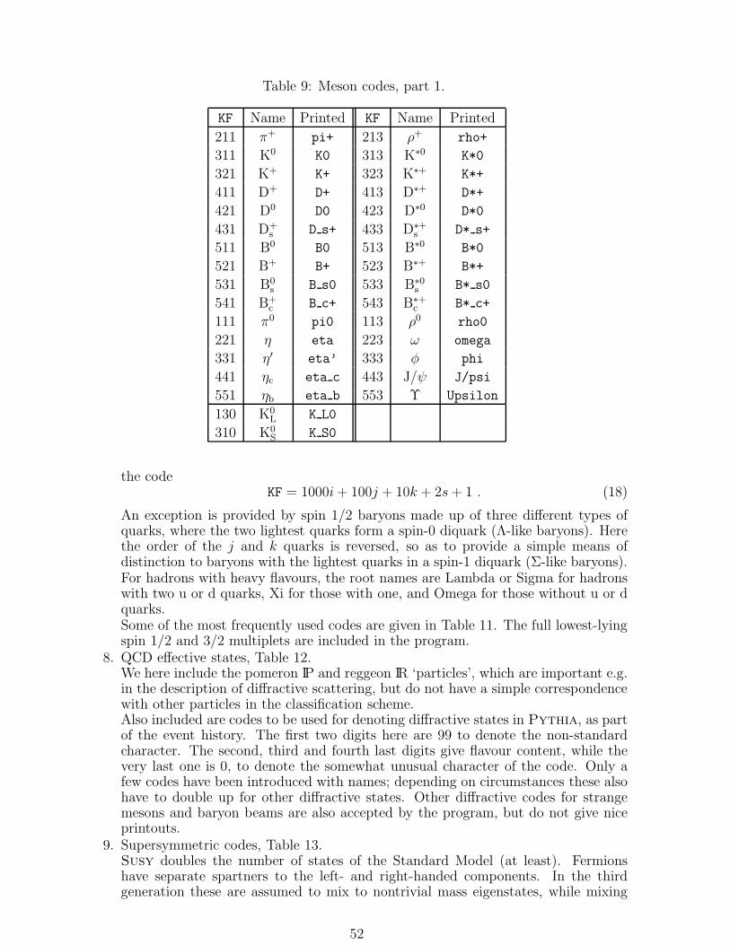
Table 9: Meson codes, part 1.

KF Name Printed KF Name Printed

211 π+ pi+ 213 ρ+ rho+

311 K0 K0 313 K∗0 K*0

321 K+ K+ 323 K∗+ K*+

411 D+ D+ 413 D∗+ D*+

421 D0 D0 423 D∗0 D*0

431 D+s D s+ 433 D∗+

s D* s+

511 B0 B0 513 B∗0 B*0

521 B+ B+ 523 B∗+ B*+

531 B0s B s0 533 B∗0

s B* s0

541 B+c B c+ 543 B∗+

c B* c+

111 π0 pi0 113 ρ0 rho0

221 η eta 223 ω omega

331 η′ eta’ 333 φ phi

441 ηc eta c 443 J/ψ J/psi

551 ηb eta b 553 Υ Upsilon

130 K0L K L0

310 K0S K S0

the codeKF = 1000i+ 100j + 10k + 2s+ 1 . (18)

An exception is provided by spin 1/2 baryons made up of three different types ofquarks, where the two lightest quarks form a spin-0 diquark (Λ-like baryons). Herethe order of the j and k quarks is reversed, so as to provide a simple means ofdistinction to baryons with the lightest quarks in a spin-1 diquark (Σ-like baryons).For hadrons with heavy flavours, the root names are Lambda or Sigma for hadronswith two u or d quarks, Xi for those with one, and Omega for those without u or dquarks.Some of the most frequently used codes are given in Table 11. The full lowest-lyingspin 1/2 and 3/2 multiplets are included in the program.

8. QCD effective states, Table 12.We here include the pomeron IP and reggeon IR ‘particles’, which are important e.g.in the description of diffractive scattering, but do not have a simple correspondencewith other particles in the classification scheme.Also included are codes to be used for denoting diffractive states in Pythia, as partof the event history. The first two digits here are 99 to denote the non-standardcharacter. The second, third and fourth last digits give flavour content, while thevery last one is 0, to denote the somewhat unusual character of the code. Only afew codes have been introduced with names; depending on circumstances these alsohave to double up for other diffractive states. Other diffractive codes for strangemesons and baryon beams are also accepted by the program, but do not give niceprintouts.

9. Supersymmetric codes, Table 13.Susy doubles the number of states of the Standard Model (at least). Fermionshave separate spartners to the left- and right-handed components. In the thirdgeneration these are assumed to mix to nontrivial mass eigenstates, while mixing

52

Table 10: Meson codes, part 2. For brevity, states with b quark are omitted fromthis listing, but are defined in the program.

KF Name Printed KF Name Printed

10213 b1 b 1+ 10211 a+0 a 0+

10313 K01 K 10 10311 K∗0

0 K* 00

10323 K+1 K 1+ 10321 K∗+

0 K* 0+

10413 D+1 D 1+ 10411 D∗+

0 D* 0+

10423 D01 D 10 10421 D∗0

0 D* 00

10433 D+1s D 1s+ 10431 D∗+

0s D* 0s+

10113 b01 b 10 10111 a0

0 a 00

10223 h01 h 10 10221 f00 f 00

10333 h′01 h’ 10 10331 f ′00 f’ 00

10443 h01c h 1c0 10441 χ0

0c chi 0c0

20213 a+1 a 1+ 215 a+

2 a 2+

20313 K∗01 K* 10 315 K∗0

2 K* 20

20323 K∗+1 K* 1+ 325 K∗+

2 K* 2+

20413 D∗+1 D* 1+ 415 D∗+

2 D* 2+

20423 D∗01 D* 10 425 D∗0

2 D* 20

20433 D∗+1s D* 1s+ 435 D∗+

2s D* 2s+

20113 a01 a 10 115 a0

2 a 20

20223 f01 f 10 225 f02 f 20

20333 f ′01 f’ 10 335 f ′02 f’ 20

20443 χ01c chi 1c0 445 χ0

2c chi 2c0

100443 ψ′ psi’

100553 Υ′ Upsilon’

is not included in the first two. Note that all sparticle names begin with a tilde.Default masses are arbitrary and branching ratios not set at all. This is taken careof at initialization if IMSS(1) is positive.

10. Technicolor codes, Table 14.A set of colourless and coloured technihadrons have been included, the latter specif-ically for the case of Topcolor assisted Technicolor. Where unclear, indices 1 or 8denote the colour multiplet. Then there are coloured technirhos and technipions thatcan mix with the Coloron (or V8) associated with the breaking of SU(3)2×SU(3)3to ordinary SU(3)C (where the 2 and 3 indices refer to the first two and the thirdgeneration, respectively).The ηtc belongs to an older iteration of Technicolor modelling than the rest. It wasoriginally given the 3000221 code, and thereby now comes to clash with the π′0

tc ofthe current main scenario. Since the ηtc is one-of-a-kind, it was deemed better tomove it to make way for the π′0

tc. This leads to a slight inconsistency with the PDGcodes.

11. Excited fermion codes, Table 15.A first generation of excited fermions are included.

12. Exotic particle codes, Table 16.This section includes the excited graviton, as the first (but probably not last) man-ifestation of the possibility of large extra dimensions. Although it is not yet in the

53

Table 11: Baryon codes. For brevity, some states with b quarks or multiple c onesare omitted from this listing, but are defined in the program.

KF Name Printed KF Name Printed

1114 ∆− Delta-

2112 n n0 2114 ∆0 Delta0

2212 p p+ 2214 ∆+ Delta+

2224 ∆++ Delta++

3112 Σ− Sigma- 3114 Σ∗− Sigma*-

3122 Λ0 Lambda0

3212 Σ0 Sigma0 3214 Σ∗0 Sigma*0

3222 Σ+ Sigma+ 3224 Σ∗+ Sigma*+

3312 Ξ− Xi- 3314 Ξ∗− Xi*-

3322 Ξ0 Xi0 3324 Ξ∗0 Xi*0

3334 Ω− Omega-

4112 Σ0c Sigma c0 4114 Σ∗0

c Sigma* c0

4122 Λ+c Lambda c+

4212 Σ+c Sigma c+ 4214 Σ∗+

c Sigma* c+

4222 Σ++c Sigma c++ 4224 Σ∗++

c Sigma* c++

4132 Ξ0c Xi c0

4312 Ξ′0c Xi’ c0 4314 Ξ∗0

c Xi* c0

4232 Ξ+c Xi c+

4322 Ξ′+c Xi’ c+ 4324 Ξ∗+

c Xi* c+

4332 Ω0c Omega c0 4334 Ω∗0

c Omega* c0

5112 Σ−b Sigma b- 5114 Σ∗−

b Sigma* b-

5122 Λ0b Lambda b0

5212 Σ0b Sigma b0 5214 Σ∗0

b Sigma* b0

5222 Σ+b Sigma b+ 5224 Σ∗+

b Sigma* b+

Table 12: QCD effective states.

KF Printed Meaning

110 reggeon reggeon IR

990 pomeron pomeron IP

9900110 rho diff0 Diffractive π0/ρ0/γ state

9900210 pi diffr+ Diffractive π+ state

9900220 omega di0 Diffractive ω state

9900330 phi diff0 Diffractive φ state

9900440 J/psi di0 Diffractive J/ψ state

9902110 n diffr Diffractive n state

9902210 p diffr+ Diffractive p state

54

Table 13: Supersymmetric codes.

KF Name Printed KF Name Printed

1000001 dL ∼d L 2000001 dR ∼d R

1000002 uL ∼u L 2000002 uR ∼u R

1000003 sL ∼s L 2000003 sR ∼s R

1000004 cL ∼c L 2000004 cR ∼c R

1000005 b1 ∼b 1 2000005 b2 ∼b 2

1000006 t1 ∼t 1 2000006 t2 ∼t 2

1000011 eL ∼e L- 2000011 eR ∼e R-

1000012 νeL ∼nu eL 2000012 νeR ∼nu eR

1000013 µL ∼mu L- 2000013 µR ∼mu R-

1000014 νµL ∼nu muL 2000014 νµR ∼nu muR

1000015 τ1 ∼tau L- 2000015 τ2 ∼tau R-

1000016 ντL ∼nu tauL 2000016 ντR ∼nu tauR

1000021 g ∼g 1000025 χ03 ∼chi 30

1000022 χ01 ∼chi 10 1000035 χ0

4 ∼chi 40

1000023 χ02 ∼chi 20 1000037 χ+

2 ∼chi 2+

1000024 χ+1 ∼chi 1+ 1000039 G ∼Gravitino

Table 14: Technicolor codes.

KF Name Printed KF Name Printed

3000111 π0tc pi tc0 3100021 V8,tc V8 tc

3000211 π+tc pi tc+ 3100111 π0

22,1,tc pi 22 1 tc

3000221 π′0tc pi’ tc0 3200111 π0

22,8,tc pi 22 8 tc

3000113 ρ0tc rho tc0 3100113 ρ011,tc rho 11 tc

3000213 ρ+tc rho tc+ 3200113 ρ012,tc rho 12 tc

3000223 ω0tc omega tc0 3300113 ρ021,tc rho 21 tc

3000331 ηtc eta tc0 3400113 ρ022,tc rho 22 tc

Table 15: Excited fermion codes.

KF Name Printed KF Name Printed

4000001 u∗ d* 4000011 e∗ e*-

4000002 d∗ u* 4000012 ν∗e nu* e0

55

Table 16: Exotic particle codes.

KF Name Printed KF Name Printed

5000039 G∗ Graviton*

9900012 νRe nu Re 9900023 Z0R Z R0

9900014 νRµ nu Rmu 9900024 W+R W R+

9900016 νRτ nu Rtau 9900041 H++L H L++

9900042 H++R H R++

PDG standard, we assume that such states will go in a new series of numbers.Included is also a set of particles associated with an extra SU(2) gauge group forrighthanded states, as required in order to obtain a left–right symmetric theory athigh energies. This includes righthanded (Majorana) neutrinos, righthanded Z0

R andW±

R gauge bosons, and both left- and righthanded doubly charged Higgses. Such ascenario would also contain other Higgs states, but these do not bring anything newrelative to the ones already introduced, from an observational point of view. Herethe first two digits are 99 to denote the non-standard character.

A hint on large particle numbers: if you want to avoid mistyping the number of zeros,it may pay off to define a statement like

PARAMETER (KSUSY1=1000000,KSUSY2=2000000,KTECHN=3000000,&KEXCIT=4000000,KDIMEN=5000000)

at the beginning of your program and then refer to particles as KSUSY1+1 = dL and soon. This then also agrees with the internal notation (where feasible).

5.2 The Event Record

Each new event generated is in its entirety stored in the common block PYJETS, whichthus forms the event record. Here each parton or particle that appears at some stageof the fragmentation or decay chain will occupy one line in the matrices. The differentcomponents of this line will tell which parton/particle it is, from where it originates, itspresent status (fragmented/decayed or not), its momentum, energy and mass, and thespace–time position of its production vertex. Note that K(I,3)–K(I,5) and the P and Vvectors may take special meaning for some specific applications (e.g. sphericity or clusteranalysis), as described in those connections.

The event history information stored in K(I,3)–K(I,5) should not be taken too lit-erally. In the particle decay chains, the meaning of a mother is well-defined, but thefragmentation description is more complicated. The primary hadrons produced in stringfragmentation come from the string as a whole, rather than from an individual parton.Even when the string is not included in the history (see MSTU(16)), the pointer fromhadron to parton is deceptive. For instance, in a qgq event, those hadrons are pointingtowards the q (q) parton that were produced by fragmentation from that end of the string,according to the random procedure used in the fragmentation routine. No particles pointto the g. This assignment seldom agrees with the visual impression, and is not intendedto.

The common block PYJETS has expanded with time, and can now house 4000 entries.This figure may seem ridiculously large, but actually the previous limit of 2000 wasoften reached in studies of high-p⊥ processes at the LHC (and SSC). This is becausethe event record contains not only the final particles, but also all intermediate partonsand hadrons, which subsequently showered, fragmented or decayed. Included are also awealth of photons coming from π0 decays; the simplest way of reducing the size of the

56

event record is actually to switch off π0 decays by MDCY(PYCOMP(111),1)=0. Also notethat some routines, such as PYCLUS and PYCELL, use memory after the event record properas a working area. Still, to change the size of the common block, upwards or downwards,is easy: just do a global substitute in the common block and change the MSTU(4) value tothe new number. If more than 10000 lines are to be used, the packing of colour informationshould also be changed, see MSTU(5).

COMMON/PYJETS/N,NPAD,K(4000,5),P(4000,5),V(4000,5)

Purpose: to contain the event record, i.e. the complete list of all partons and particles(initial, intermediate and final) in the current event. (By parton we heremean the subclass of particles that carry colour, for which extra colour flowinformation is then required. Normally this means quarks and gluons, whichcan fragment to hadrons, but also squarks and other exotic particles fall inthis category.)

N : number of lines in the K, P and V matrices occupied by the current event. Nis continuously updated as the definition of the original configuration and thetreatment of fragmentation and decay proceed. In the following, the individualparton/particle number, running between 1 and N, is called I.

NPAD : dummy to ensure an even number of integers before the double precision reals,as required by some compilers.

K(I,1) : status code KS, which gives the current status of the parton/particle stored inthe line. The ground rule is that codes 1–10 correspond to currently existingpartons/particles, while larger codes contain partons/particles which no longerexist, or other kinds of event information.

= 0 : empty line.= 1 : an undecayed particle or an unfragmented parton, the latter being either

a single parton or the last one of a parton system.= 2 : an unfragmented parton, which is followed by more partons in the same

colour-singlet parton system.= 3 : an unfragmented parton with special colour flow information stored in

K(I,4) and K(I,5), such that adjacent partons along the string neednot follow each other in the event record.

= 4 : a particle which could have decayed, but did not within the allowedvolume around the original vertex.

= 5 : a particle which is to be forced to decay in the next PYEXEC call, in thevertex position given (this code is only set by user intervention).

= 11 : a decayed particle or a fragmented parton, the latter being either a singleparton or the last one of a parton system, cf. =1.

= 12 : a fragmented parton, which is followed by more partons in the samecolour-singlet parton system, cf. =2. Further, a B meson which decayedas a B one, or vice versa, because of B–B mixing, is marked with thiscode rather than =11.

= 13 : a parton which has been removed when special colour flow informationhas been used to rearrange a parton system, cf. =3.

= 14 : a parton which has branched into further partons, with special colour-flow information provided, cf. =3.

= 15 : a particle which has been forced to decay (by user intervention), cf. =5.= 21 : documentation lines used to give a compressed story of the event at the

beginning of the event record.= 31 : lines with information on sphericity, thrust or cluster search.= 32 : tabular output, as generated by PYTABU.

57

= 41 : junction (currently not fully implemented).< 0 : these codes are never used by the program, and are therefore usually

not affected by operations on the record, such as PYROBO, PYLIST andevent-analysis routines (the exception is some PYEDIT calls, where linesare moved but not deleted). Such codes may therefore be useful in someconnections.

K(I,2) : particle KF code, as described in section 5.1.K(I,3) : line number of parent particle, where known, otherwise 0. Note that the

assignment of a particle to a given parton in a parton system is unphysical,and what is given there is only related to the way the fragmentation wasgenerated.

K(I,4) : normally the line number of the first daughter; it is 0 for an undecayed particleor unfragmented parton.For K(I,1) = 3, 13 or 14, instead, it contains special colour-flow information(for internal use only) of the formK(I,4) = 200000000*MCFR + 100000000*MCTO + 10000*ICFR + ICTO,where ICFR and ICTO give the line numbers of the partons from which thecolour comes and to where it goes, respectively; MCFR and MCTO originallyare 0 and are set to 1 when the corresponding colour connection has been tracedin the PYPREP rearrangement procedure. (The packing may be changed withMSTU(5).) The ‘from’ colour position may indicate a parton which branchedto produce the current parton, or a parton created together with the currentparton but with matched anticolour, while the ‘to’ normally indicates a partonthat the current parton branches into. Thus, for setting up an initial colourconfiguration, it is normally only the ‘from’ part that is used, while the ‘to’part is added by the program in a subsequent call to parton-shower evolution(for final-state radiation; it is the other way around for initial-state radiation).Note: normally most users never have to worry about the exact rules forcolour-flow storage, since this is used mainly for internal purposes. However,when it is necessary to define this flow, it is recommended to use the PYJOINroutine, since it is likely that this would reduce the chances of making a mis-take.

K(I,5) : normally the line number of the last daughter; it is 0 for an undecayed particleor unfragmented parton.For K(I,1) = 3, 13 or 14, instead, it contains special colour-flow information(for internal use only) of the formK(I,5) = 200000000*MCFR + 100000000*MCTO + 10000*ICFR + ICTO,where ICFR and ICTO give the line numbers of the partons from which theanticolour comes and to where it goes, respectively; MCFR and MCTO orig-inally are 0 and are set to 1 when the corresponding colour connection hasbeen traced in the PYPREP rearrangement procedure. For further discussion,see K(I,4).

P(I,1) : px, momentum in the x direction, in GeV/c.P(I,2) : py, momentum in the y direction, in GeV/c.P(I,3) : pz, momentum in the z direction, in GeV/c.P(I,4) : E, energy, in GeV.P(I,5) : m, mass, in GeV/c2. In parton showers, with space-like virtualities, i.e. where

Q2 = −m2 > 0, one puts P(I,5)= −Q.V(I,1) : x position of production vertex, in mm.V(I,2) : y position of production vertex, in mm.V(I,3) : z position of production vertex, in mm.V(I,4) : time of production, in mm/c (≈ 3.33 × 10−12 s).V(I,5) : proper lifetime of particle, in mm/c (≈ 3.33 × 10−12 s). If the particle is not

58

expected to decay, V(I,5)=0. A line with K(I,1)=4, i.e. a particle that couldhave decayed, but did not within the allowed region, has the proper non-zeroV(I,5).In the absence of electric or magnetic fields, or other disturbances, the decayvertex VP of an unstable particle may be calculated asVP(j) = V(I,j) + V(I,5)*P(I,j)/P(I,5), j = 1–4.

5.3 How The Event Record Works

The event record is the main repository for information about an event. In the generationchain, it is used as a ‘scoreboard’ for what has already been done and what remains todo. This information can be studied by you, to access information not only about thefinal state, but also about what came before.

5.3.1 A simple example

The first example of section 3.5 may help to clarify what is going on. When PY2ENT iscalled to generate a qq pair, the quarks are stored in lines 1 and 2 of the event record,respectively. Colour information is set to show that they belong together as a coloursinglet. The counter N is also updated to the value of 2. At no stage is a previouslygenerated event removed. Lines 1 and 2 are overwritten, but lines 3 onwards still containwhatever may have been there before. This does not matter, since N indicates where the‘real’ record ends.

As PYEXEC is called, explicitly by you or indirectly by PY2ENT, the first entry is con-sidered and found to be the first parton of a system. Therefore the second entry is alsofound, and these two together form a colour singlet parton system, which may be allowedto fragment. The ‘string’ that fragments is put in line 3 and the fragmentation productsin lines 4 through 10 (in this particular case). At the same time, the q and q in the firsttwo lines are marked as having fragmented, and the same for the string. At this stage, Nis 10. Internally in PYEXEC there is another counter with the value 2, which indicates howfar down in the record the event has been studied.

This second counter is gradually increased by one. If the entry in the correspondingline can fragment or decay, then fragmentation or decay is performed. The fragmenta-tion/decay products are added at the end of the event record, and N is updated accordingly.The entry is then also marked as having been treated. For instance, when line 3 is con-sidered, the ‘string’ entry of this line is seen to have been fragmented, and no action istaken. Line 4, a ρ+, is allowed to decay to π+π0; the decay products are stored in lines 11and 12, and line 4 is marked as having decayed. Next, entry 5 is allowed to decay. Theentry in line 6, π+, is a stable particle (by default) and is therefore passed by without anyaction being taken.

In the beginning of the process, entries are usually unstable, and N grows faster thanthe second counter of treated entries. Later on, an increasing fraction of the entries arestable end products, and the roles are now reversed, with the second counter growingfaster. When the two coincide, the end of the record has been reached, and the processcan be stopped. All unstable objects have now been allowed to fragment or decay. Theyare still present in the record, so as to simplify the tracing of the history.

Notice that PYEXEC could well be called a second time. The second counter would thenstart all over from the beginning, but slide through until the end without causing anyaction, since all objects that can be treated already have been. Unless some of the relevantswitches were changed meanwhile, that is. For instance, if π0 decays were switched offthe first time around but on the second, all the π0’s found in the record would be allowedto decay in the second call. A particle once decayed is not ‘undecayed’, however, so if theπ0 is put back stable and PYEXEC is called a third time, nothing will happen.

59

5.3.2 Complete PYTHIA events

In a full-blown event generated with Pythia, the usage of PYJETS is more complicated,although the general principles survive. PYJETS is used extensively by many of the gener-ation routines; indeed it provides the bridge between many of them. The Pythia eventlisting begins (optionally) with a few lines of event summary, specific to the hard processsimulated and thus not described in the overview above. These specific parts are coveredin the following.

In most instances, only the particles actually produced are of interest. ForMSTP(125)=0, the event record starts off with the parton configuration existing afterhard interaction, initial- and final-state radiation, multiple interactions and beam rem-nants have been considered. The partons are arranged in colour singlet clusters, orderedas required for string fragmentation. Also photons and leptons produced as part of thehard interaction (e.g. from qq → gγ or uu → Z0 → e+e−) appear in this part of the eventrecord. These original entries appear with pointer K(I,3)=0, whereas the products of thesubsequent fragmentation and decay have K(I,3) numbers pointing back to the line ofthe parent.

The standard documentation, obtained with MSTP(125)=1, includes a few lines at thebeginning of the event record, which contain a brief summary of the process that has takenplace. The number of lines used depends on the nature of the hard process and is storedin MSTI(4) for the current event. These lines all have K(I,1)=21. For all processes, lines1 and 2 give the two incoming particles. When listed with PYLIST, these two lines will beseparated from subsequent ones by a sequence of ‘======’ signs, to improve readability.For diffractive and elastic events, the two outgoing states in lines 3 and 4 complete thelist. Otherwise, lines 3 and 4 contain the two partons that initiate the two initial-stateparton showers, and 5 and 6 the end products of these showers, i.e. the partons thatenter the hard interaction. With initial-state radiation switched off, lines 3 and 5 andlines 4 and 6 are identical. For a simple 2 → 2 hard scattering, lines 7 and 8 give thetwo outgoing partons/particles from the hard interaction, before any final-state radiation.For 2 → 2 processes proceeding via an intermediate resonance such as γ∗/Z0, W± or h0,the resonance is found in line 7 and the two outgoing partons/particles in 8 and 9. Insome cases one of these may be a resonance in its own right, or both of them, so thatfurther pairs of lines are added for subsequent decays. If the decay of a given resonancehas been switched off, then no decay products are listed either in this initial summaryor in the subsequent ordinary listing. Whenever partons are listed, they are assumed tobe on the mass shell for simplicity. The fact that effective masses may be generated byinitial- and final-state radiation is taken into account in the actual parton configurationthat is allowed to fragment, however. The listing of the event documentation closes withanother line made up of ‘======’ signs.

A few examples may help clarify the picture. For a single diffractive event pp → pdiffrp,the event record will start withI K(I,1) K(I,2) K(I,3) comment1 21 2212 0 incoming p2 21 -2212 0 incoming p========================= not part of record; appears in listings3 21 9902210 1 outgoing pdiffr

4 21 -2212 2 outgoing p========================= again not part of record

The typical QCD 2 → 2 process would beI K(I,1) K(I,2) K(I,3) comment1 21 2212 0 incoming p2 21 -2212 0 incoming p=========================

60

3 21 2 1 u picked from incoming p4 21 -1 2 d picked from incoming p5 21 21 3 u evolved to g at hard scattering6 21 -1 4 still d at hard scattering7 21 21 0 outgoing g from hard scattering8 21 -1 0 outgoing d from hard scattering=========================

Note that, where well defined, the K(I,3) code does contain information as to whichside the different partons come from, e.g. above the gluon in line 5 points back to the uin line 3, which points back to the proton in line 1. In the example above, it would havebeen possible to associate the scattered g in line 7 with the incoming one in line 5, butthis is not possible in the general case, consider e.g. gg → gg.

A special case is provided by W+W− or Z0Z0 fusion to an h0. Then the virtual W’s orZ’s are shown in lines 7 and 8, the h0 in line 9, and the two recoiling quarks (that emittedthe bosons) in 10 and 11, followed by the Higgs decay products. Since the W’s and Z’s arespace-like, what is actually listed as the mass for them is −

√−m2. Thus W+W− fusion

to an h0 in process 8 (not process 124, which is lengthier) might look likeI K(I,1) K(I,2) K(I,3) comment1 21 2212 0 first incoming p2 21 2212 0 second incoming p=========================3 21 2 1 u picked from first p4 21 21 2 g picked from second p5 21 2 3 still u after initial-state radiation6 21 -4 4 g evolved to c7 21 24 5 space-like W+ emitted by u quark8 21 -24 6 space-like W− emitted by c quark9 21 25 0 Higgs produced by W+W− fusion10 21 1 5 u turned into d by emission of W+

11 21 -3 6 c turned into s by emission of W−

12 21 23 9 first Z0 coming from decay of h0

13 21 23 9 second Z0 coming from decay of h0

14 21 12 12 νe from first Z0 decay15 21 -12 12 νe from first Z0 decay16 21 5 13 b quark from second Z0 decay17 21 -5 13 b antiquark from second Z0 decay=========================

Another special case is when a spectrum of virtual photons are generated inside alepton beam, i.e. when PYINIT is called with one or two ’gamma/lepton’ arguments.Then the documentation section is expanded to reflect the new layer of administration.Positions 1 and 2 contain the original beam particles, e.g. e and p (or e+ and e−). Inposition 3 (and 4 for e+e−) is (are) the scattered outgoing lepton(s). Thereafter comesthe normal documentation, but starting from the photon rather than a lepton. For ep,this means 4 and 5 are the γ∗ and p, 6 and 7 the shower initiators, 8 and 9 the incomingpartons to the hard interaction, and 10 and 11 the outgoing ones. Thus the documentationis 3 lines longer (4 for e+e−) than normally.

After these lines with the initial information, the event record looks the same asfor MSTP(125)=0, i.e. first comes the parton configuration to be fragmented and, afteranother separator line ‘======’ in the output (but not the event record), the productsof subsequent fragmentation and decay chains. This ordinary listing begins in positionMST(4)+1. The K(I,3) pointers for the partons, as well as leptons and photons producedin the hard interaction, are now pointing towards the documentation lines above, however.In particular, beam remnants point to 1 or 2, depending on which side they belong to, and

61

partons emitted in the initial-state parton showers point to 3 or 4. In the second exampleabove, the partons produced by final-state radiation will be pointing back to 7 and 8; asusual, it should be remembered that a specific assignment to 7 or 8 need not be unique.For the third example, final-state radiation partons will come both from partons 10 and11 and from partons 16 and 17, and additionally there will be a neutrino–antineutrinopair pointing to 14 and 15.

A hadronic event may contain several (semi)hard interactions, in the multiple inter-actions scenario. The hardest interaction of an event is shown in the initial section of theevent record, while further ones are not. Therefore these extra partons, documented inthe main section of the event, do not have a documentation copy to point back to, andso are assigned K(I,3)=0.

There exists a third documentation option, MSTP(125)=2. Here the history of initial-and final-state parton branchings may be traced, including all details on colour flow. Thisinformation has not been optimized for user-friendliness, and cannot be recommended forgeneral usage. With this option, the initial documentation lines are the same. They arefollowed by blank lines, K(I,1)=0, up to line 100 (can be changed in MSTP(126)). Fromline 101 onwards each parton with K(I,1)= 3, 13 or 14 appears with special colour-flowinformation in the K(I,4) and K(I,5) positions. For an ordinary 2 → 2 scattering,the two incoming partons at the hard scattering are stored in lines 101 and 102, andthe two outgoing in 103 and 104. The colour flow between these partons has to bechosen according to the proper relative probabilities in cases when many alternatives arepossible, see section 8.2.1. If there is initial-state radiation, the two partons in lines 101and 102 are copied down to lines 105 and 106, from which the initial-state showers arereconstructed backwards step by step. The branching history may be read by noting that,for a branching a→ bc, the K(I,3) codes of b and c point towards the line number of a.Since the showers are reconstructed backwards, this actually means that parton b wouldappear in the listing before parton a and c, and hence have a pointer to a position belowitself in the list. Associated time-like partons c may initiate time-like showers, as maythe partons of the hard scattering. Again a showering parton or pair of partons will becopied down towards the end of the list and allowed to undergo successive branchingsc → de, with d and e pointing towards c. The mass of time-like partons is properlystored in P(I,5); for space-like partons −

√−m2 is stored instead. After this section,

containing all the branchings, comes the final parton configuration, properly arranged incolour, followed by all subsequent fragmentation and decay products, as usual.

5.4 The HEPEVT Standard

A set of common blocks was developed and agreed on within the framework of the 1989LEP physics study, see [Sjo89]. This standard defines an event record structure whichshould make the interfacing of different event generators much simpler.

It would be a major work to rewrite Pythia to agree with this standard event recordstructure. More importantly, the standard only covers quantities which can be definedunambiguously, i.e. which are independent of the particular program used. There arethus no provisions for the need for colour-flow information in models based on string frag-mentation, etc., so the standard common blocks would anyway have to be supplementedwith additional event information. For the moment, the adopted approach is therefore toretain the PYJETS event record, but supply a routine PYHEPC which can convert to or fromthe standard event record. Owing to a somewhat different content in the two records,some ambiguities do exist in the translation procedure. PYHEPC has therefore to be usedwith some judgement.

In this section, the standard event structure is first presented, i.e. the most importantpoints in [Sjo89] are recapitulated. Thereafter the conversion routine is described, withparticular attention to ambiguities and limitations.

62

The standard event record is stored in two common blocks. The second of these isspecifically intended for spin information. Since Pythia never (explicitly) makes use ofspin information, this latter common block is not addressed here. A third common blockfor colour flow information has been discussed, but never formalized. Note that a CALLPYLIST(5) can be used to obtain a simple listing of the more interesting information inthe event record.

In order to make the components of the standard more distinguishable in your pro-grams, the three characters HEP (for High Energy Physics) have been chosen to be a partof all names.

Originally it was not specified whether real variables should be in single or doubleprecision. At the time, this meant that single precision became the default choice, butsince then the trend has been towards increasing precision. In connection with the 1995LEP 2 workshop, it was therefore agreed to adopt DOUBLE PRECISION real variables aspart of the standard, and also to extend the size from 2000 to 4000 entries [Kno96]. If, forsome reason, one would want to revert to single precision, this would only require trivialchanges to the code of the PYHEPC conversion routine described below.

PARAMETER (NMXHEP=4000)COMMON/HEPEVT/NEVHEP,NHEP,ISTHEP(NMXHEP),IDHEP(NMXHEP),&JMOHEP(2,NMXHEP),JDAHEP(2,NMXHEP),PHEP(5,NMXHEP),VHEP(4,NMXHEP)DOUBLE PRECISION PHEP, VHEP

Purpose: to contain an event record in a Monte Carlo-independent format.NMXHEP: maximum numbers of entries (particles) that can be stored in the common

block. The default value of 4000 can be changed via the parameter construc-tion. In the translation, it is checked that this value is not exceeded.

NEVHEP: is normally the event number, but may have special meanings, according tothe description below:

> 0 : event number, sequentially increased by 1 for each call to the main eventgeneration routine, starting with 1 for the first event generated.

= 0 : for a program which does not keep track of event numbers, as some ofthe Pythia routines.

= -1 : special initialization record; not used by Pythia.= -2 : special final record; not used by Pythia.

NHEP: the actual number of entries stored in the current event. These are found in thefirst NHEP positions of the respective arrays below. Index IHEP, 1≤IHEP≤NHEP,is used below to denote a given entry.

ISTHEP(IHEP): status code for entry IHEP, with the following meanings:= 0 : null entry.= 1 : an existing entry, which has not decayed or fragmented. This is the main

class of entries, which represents the ‘final state’ given by the generator.= 2 : an entry which has decayed or fragmented and is therefore not appearing

in the final state, but is retained for event history information.= 3 : a documentation line, defined separately from the event history. This

could include the two incoming reacting particles, etc.= 4 - 10 : undefined, but reserved for future standards.= 11 - 200 : at the disposal of each model builder for constructs specific to his

program, but equivalent to a null line in the context of any other program.= 201 - : at the disposal of users, in particular for event tracking in the detector.

IDHEP(IHEP) : particle identity, according to the PDG standard. The four additionalcodes 91–94 have been introduced to make the event history more legible, seesection 5.1 and the MSTU(16) description of how daughters can point back to

63

them.JMOHEP(1,IHEP) : pointer to the position where the mother is stored. The value is 0 for

initial entries.JMOHEP(2,IHEP) : pointer to position of second mother. Normally only one mother

exists, in which case the value 0 is to be used. In Pythia, entries withcodes 91–94 are the only ones to have two mothers. The flavour con-tents of these objects, as well as details of momentum sharing, have to befound by looking at the mother partons, i.e. the two partons in positionsJMOHEP(1,IHEP) and JMOHEP(2,IHEP) for a cluster or a shower system, andthe range JMOHEP(1,IHEP)–JMOHEP(2,IHEP) for a string or an independentfragmentation parton system.

JDAHEP(1,IHEP) : pointer to the position of the first daughter. If an entry has notdecayed, this is 0.

JDAHEP(2,IHEP) : pointer to the position of the last daughter. If an entry has notdecayed, this is 0. It is assumed that daughters are stored sequentially, sothat the whole range JDAHEP(1,IHEP)–JDAHEP(2,IHEP) contains daughters.This variable should be set also when only one daughter is present, as inK0 → K0

S decays, so that looping from the first daughter to the last one workstransparently. Normally daughters are stored after mothers, but in backwardsevolution of initial-state radiation the opposite may appear, i.e. that mothersare found below the daughters they branch into. Also, the two daughters thenneed not appear one after the other, but may be separated in the event record.

PHEP(1,IHEP) : momentum in the x direction, in GeV/c.PHEP(2,IHEP) : momentum in the y direction, in GeV/c.PHEP(3,IHEP) : momentum in the z direction, in GeV/c.PHEP(4,IHEP) : energy, in GeV.PHEP(5,IHEP) : mass, in GeV/c2. For space-like partons, it is allowed to use a negative

mass, according to PHEP(5,IHEP)= −√−m2.

VHEP(1,IHEP) : production vertex x position, in mm.VHEP(2,IHEP) : production vertex y position, in mm.VHEP(3,IHEP) : production vertex z position, in mm.VHEP(4,IHEP) : production time, in mm/c (≈ 3.33 × 10−12 s).

This completes the brief description of the standard. In Pythia, the routine PYHEPCis provided as an interface.

CALL PYHEPC(MCONV)

Purpose: to convert between the PYJETS event record and the HEPEVT event record.MCONV : direction of conversion.

= 1 : translates the current PYJETS record into the HEPEVT one, while leavingthe original PYJETS one unaffected.

= 2 : translates the current HEPEVT record into the PYJETS one, while leavingthe original HEPEVT one unaffected.

The conversion of momenta is trivial: it is just a matter of exchanging the order of theindices. The vertex information is but little more complicated; the extra fifth componentpresent in PYJETS can be easily reconstructed from other information for particles whichhave decayed. (Some of the advanced features made possible by this component, such asthe possibility to consider decays within expanding spatial volumes in subsequent PYEXECcalls, cannot be used if the record is translated back and forth, however.) Also, theparticle codes K(I,2) and IDHEP(I) are identical, since they are both based on the PDGcodes.

64

The remaining, non-trivial areas deal with the status codes and the event history. Inmoving from PYJETS to HEPEVT, information on colour flow is lost. On the other hand, theposition of a second mother, if any, has to be found; this only affects lines with K(I,2)=91–94. Also, for lines with K(I,1)= 13 or 14, the daughter pointers have to be found. Byand large, however, the translation from PYJETS to HEPEVT should cause little problem,and there should never be any need for user intervention. (We assume that Pythia is runwith the default MSTU(16)=1 mother pointer assignments, otherwise some discrepancieswith respect to the proposed standard event history description will be present.)

In moving from HEPEVT to PYJETS, information on a second mother is lost. Anycodes IDHEP(I) not equal to 1, 2 or 3 are translated into K(I,1)=0, and so all entrieswith K(I,1)≥ 30 are effectively lost in a translation back and forth. All entries withIDHEP(I)=2 are translated into K(I,1)=11, and so entries of type K(I,1) = 12, 13, 14or 15 are never found. There is thus no colour-flow information available for partonswhich have fragmented. For partons with IDHEP(I)=1, i.e. which have not fragmented,an attempt is made to subdivide the partonic system into colour singlets, as requiredfor subsequent string fragmentation. To this end, it is assumed that partons are storedsequentially along strings. Normally, a string would then start at a q (q) or qq (qq) entry,cover a number of intermediate gluons, and end at a q (q) or qq (qq) entry. Particlescould be interspersed in this list with no adverse effects, i.e. a u − g − γ − u sequencewould be interpreted as a u− g−u string plus an additional photon. A closed gluon loopwould be assumed to be made up of a sequential listing of the gluons, with the stringcontinuing from the last gluon up back to the first one. Contrary to the previous, openstring case, the appearance of any particle but a gluon would therefore signal the end ofthe gluon loop. For example, a g − g − g − g sequence would be interpreted as one singlefour-gluon loop, while a g − g − γ − g − g sequence would be seen as composed of two2-gluon systems.

If these interpretations, which are not unique, are not to your liking, it is up to youto correct them, e.g. by using PYJOIN to tell exactly which partons should be joined, inwhich sequence, to give a string. Calls to PYJOIN (or the equivalent) are also necessary ifPYSHOW is to be used to have some partons develop a shower.

For practical applications, one should note that e+e− events, which have been allowedto shower but not to fragment, do have partons arranged in the order assumed above,so that a translation to HEPEVT and back does not destroy the possibility to performfragmentation by a simple PYEXEC call. Also the hard interactions in hadronic eventsfulfil this condition, while problems may appear in the multiple interaction scenario,where several closed gg loops may appear directly following one another, and thus wouldbe interpreted as a single multigluon loop after translation back and forth.

65

6 The Old e+e− Annihilation Routines

From the Jetset package, Pythia inherits routines for the dedicated simulation of twohard processes in e+e− annihilation. The process of main interest is e+e− → γ∗/Z0 → qq.The description provided by the PYEEVT routine has been a main staple from PETRA daysup to the LEP1 era. Nowadays it is superseded by process 1 of the main Pythia eventgeneration machinery, see section 8.4.2. This latter process offers a better description offlavour selection, resonance shape and initial-state radiation. It can also, optionally, beused with the second-order matrix element machinery documented in this section. Forbackwards compatibility, however, the old routines have still been retained here. Thereare also a few features found in the routines in this section, and not in the other ones,such as polarized incoming beams.

For the process e+e− → γ∗/Z0 → qq, higher-order QCD corrections can be obtainedeither with parton showers or with second-order matrix elements. The details of theparton-shower evolution are given in section 10, while this section contains the matrix-element description, including a summary of the older algorithm for initial-state photonradiation used here.

The other standalone hard process in this section is Υ decay to ggg or γgg, which isbriefly commented on.

The main sources of information for this chapter are refs. [Sjo83, Sjo86, Sjo89].

6.1 Annihilation Events in the Continuum

The description of e+e− annihilation into hadronic events involves a number of compo-nents: the s dependence of the total cross section and flavour composition, multipartonmatrix elements, angular orientation of events, initial-state photon bremsstrahlung andeffects of initial-state electron polarization. Many of the published formulae have beenderived for the case of massless outgoing quarks. For each of the components described inthe following, we will begin by discussing the massless case, and then comment on whatis done to accommodate massive quarks.

6.1.1 Electroweak cross sections

In the standard theory, fermions have the following couplings (illustrated here for the firstgeneration):

eν = 0, vν = 1, aν = 1,

ee = −1, ve = −1 + 4 sin2θW , ae = −1,

eu = 2/3, vu = 1 − 8 sin2θW/3, aν = 1,

ed = −1/3, vd = −1 + 4 sin2θW/3, ad = −1,

with e the electric charge, and v and a the vector and axial couplings to the Z0. Therelative energy dependence of the weak neutral current to the electromagnetic one is givenby

χ(s) =1

16 sin2θW cos2θW

s

s−m2Z + imZΓZ

, (19)

where s = E2cm. In this section the electroweak mixing parameter sin2θW and the Z0 mass

mZ and width ΓZ are considered as constants to be given by you (while the full Pythiaevent generation machinery itself calculates an s-dependent width).

Although the incoming e+ and e− beams are normally unpolarized, we have includedthe possibility of polarized beams, following the formalism of [Ols80]. Thus the incominge+ and e− are characterized by polarizations P± in the rest frame of the particles:

P± = P±T s± + P±

L p± , (20)

66

where 0 ≤ P±T ≤ 1 and −1 ≤ P±

L ≤ 1, with the constraint

(P±)2 = (P±T )2 + (P±

L )2 ≤ 1 . (21)

Here s± are unit vectors perpendicular to the beam directions p±. To be specific, wechoose a right-handed coordinate frame with p± = (0, 0,∓1), and standard transversepolarization directions (out of the machine plane for storage rings) s± = (0,±1, 0), thelatter corresponding to azimuthal angles ϕ± = ±π/2. As free parameters in the program

we choose P+L , P−

L , PT =√

P+T P

−T and ∆ϕ = (ϕ+ + ϕ−)/2.

In the massless QED case, the probability to produce a flavour f is proportional toe2f , i.e up-type quarks are four times as likely as down-type ones. In lowest-order mass-less QFD (Quantum Flavour Dynamics; part of the Standard Model) the correspondingrelative probabilities are given by [Ols80]

hf(s) = e2e (1 − P+L P

−L ) e2f + 2ee

ve(1 − P+L P

−L ) − ae(P

−L − P+

L )

ℜχ(s) efvf +

+

(v2e + a2e)(1 − P+L P

−L ) − 2veae(P

−L − P+

L )

|χ(s)|2

v2f + a2f

, (22)

where ℜχ(s) denotes the real part of χ(s). The hf(s) expression depends both on the svalue and on the longitudinal polarization of the e± beams in a non-trivial way.

The cross section for the process e+e− → γ∗/Z0 → ff may now be written as

σf(s) =4πα2

em

3sRf(s) , (23)

where Rf gives the ratio to the lowest-order QED cross section for the process e+e− →µ+µ−,

Rf(s) = NC RQCD hf(s) . (24)

The factor of NC = 3 counts the number of colour states available for the qq pair. TheRQCD factor takes into account QCD loop corrections to the cross section. For nf effectiveflavours (normally nf = 5)

RQCD ≈ 1 +αs

π+ (1.986 − 0.115nf)

(

αs

π

)2

+ · · · (25)

in the MS renormalization scheme [Din79]. Note that RQCD does not affect the relativequark-flavour composition, and so is of peripheral interest here. (For leptons the NC

and RQCD factors would be absent, i.e. NC RQCD = 1, but leptonic final states are notgenerated by this routine.)

Neglecting higher-order QCD and QFD effects, the corrections for massive quarks are

given in terms of the velocity βf of a fermion with mass mf , βf =√

1 − 4m2f /s, as follows.

The vector quark current terms in hf (proportional to e2f , efvf , or v2f ) are multiplied by athreshold factor βf(3 − β2

f )/2, while the axial vector quark current term (proportional toa2f ) is multiplied by β3

f . While inclusion of quark masses in the QFD formulae decreasesthe total cross section, first-order QCD corrections tend in the opposite direction [Jer81].Naıvely, one would expect one factor of βf to get cancelled. So far, the available optionsare either to include threshold factors in full or not at all.

Given that all five quarks are light at the scale of the Z0, the issue of quark massesis not really of interest at LEP. Here, however, purely weak corrections are important, inparticular since they change the b quark partial width differently from that of the otherones [Kuh89]. No such effects are included in the program.

67

6.1.2 First-order QCD matrix elements

The Born process e+e− → qq is modified in first-order QCD by the probability for the q orq to radiate a gluon, i.e. by the process e+e− → qqg. The matrix element is convenientlygiven in terms of scaled energy variables in the c.m. frame of the event, x1 = 2Eq/Ecm,x2 = 2Eq/Ecm, and x3 = 2Eg/Ecm, i.e. x1 + x2 + x3 = 2. For massless quarks the matrixelement reads [Ell76]

1

σ0

dσ

dx1 dx2=αs

2πCF

x21 + x22(1 − x1)(1 − x2)

, (26)

where σ0 is the lowest-order cross section, CF = 4/3 is the appropriate colour factor, andthe kinematically allowed region is 0 ≤ xi ≤ 1, i = 1, 2, 3. By kinematics, the xk variablefor parton k is related to the invariant mass mij of the other two partons i and j byyij = m2

ij/E2cm = 1 − xk.

The strong coupling constant αs is in first order given by

αs(Q2) =

12π

(33 − 2nf) ln(Q2/Λ2). (27)

Conventionally Q2 = s = E2cm; we will return to this issue below. The number of flavours

nf is 5 for LEP applications, and so the Λ value determined is Λ5 (while e.g. most DeeplyInelastic Scattering studies refer to Λ4, the energies for these experiments being belowthe bottom threshold). The αs values are matched at flavour thresholds, i.e. as nf ischanged the Λ value is also changed. It is therefore the derivative of αs that changes ata threshold, not αs itself.

In order to separate 2-jets from 3-jets, it is useful to introduce jet-resolution param-eters. This can be done in several different ways. Most famous are the y and (ǫ, δ)procedures. We will only refer to the y cut, which is the one used in the program. Herea 3-parton configuration is called a 2-jet event if

mini,j

(yij) = mini,j

(

m2ij

E2cm

)

< y . (28)

The cross section in eq. (26) diverges for x1 → 1 or x2 → 1 but, when first-orderpropagator and vertex corrections are included, a corresponding singularity with oppositesign appears in the qq cross section, so that the total cross section is finite. In analyticalcalculations, the average value of any well-behaved quantity Q can therefore be calculatedas

〈Q〉 =1

σtotlimy→0

(

Q(2parton) σ2parton(y) +∫

yij>yQ(x1, x2)

dσ3partondx1 dx2

dx1 dx2

)

, (29)

where any explicit y dependence disappears in the limit y → 0.In a Monte Carlo program, it is not possible to work with a negative total 2-jet rate,

and thus it is necessary to introduce a fixed non-vanishing y cut in the 3-jet phase space.Experimentally, there is evidence for the need of a low y cut, i.e. a large 3-jet rate. ForLEP applications, the recommended value is y = 0.01, which is about as far down as onecan go and still retain a positive 2-jet rate. With αs = 0.12, in full second-order QCD(see below), the 2 : 3 : 4 jet composition is then approximately 11% : 77% : 12%.

Note, however, that initial-state QED radiation may occasionally lower the c.m. energysignificantly, i.e. increase αs, and thereby bring the 3-jet fraction above unity if y is keptfixed at 0.01 also in those events. Therefore, at PETRA/PEP energies, y values slightlyabove 0.01 are needed. In addition to the y cut, the program contains a cut on the

68

invariant mass mij between any two partons, which is typically required to be larger than2 GeV. This cut corresponds to the actual merging of two nearby parton jets, i.e. where atreatment with two separate partons rather than one would be superfluous in view of thesmearing arising from the subsequent fragmentation. Since the cut-off mass scale

√yEcm

normally is much larger, this additional cut only enters for events at low energies.For massive quarks, the amount of QCD radiation is slightly reduced [Iof78]:

1

σ0

dσ

dx1 dx2=

αs

2πCF

x21 + x22(1 − x1)(1 − x2)

− 4m2q

s

(

1

1 − x1+

1

1 − x2

)

− 2m2q

s

(

1

(1 − x1)2+

1

(1 − x2)2

)

− 4m4q

s2

(

1

1 − x1+

1

1 − x2

)2

. (30)

Properly, the above expression is only valid for the vector part of the cross section, witha slightly different expression for the axial part, but here the one above is used for it all.In addition, the phase space for emission is reduced by the requirement

(1 − x1)(1 − x2)(1 − x3)

x23≥ m2

q

s. (31)

For b quarks at LEP energies, these corrections are fairly small.

6.1.3 4-jet matrix elements

Two new event types are added in second-order QCD, e+e− → qqgg and e+e− → qqq′q′.The 4-jet cross section has been calculated by several groups [Ali80a, Gae80, Ell81, Dan82],which agree on the result. The formulae are too lengthy to be quoted here. In one of thecalculations [Ali80a], quark masses were explicitly included, but here only the masslessexpressions are included, as taken from [Ell81]. Here the angular orientation of the eventhas been integrated out, so that five independent internal kinematical variables remain.These may be related to the six yij and the four yijk variables, yij = m2

ij/s = (pi + pj)2/s

and yijk = m2ijk/s = (pi + pj + pk)

2/s, in terms of which the matrix elements are given.The original calculations were for the pure γ-exchange case; it has been pointed out

[Kni89] that an additional contribution to the e+e− → qqq′q′ cross section arises from theaxial part of the Z0. This term is not included in the program, but fortunately it is finiteand small.

Whereas the way the string, i.e. the fragmenting colour flux tube, is stretched isuniquely given in qqg event, for qqgg events there are two possibilities: q − g1 − g2 − qor q − g2 − g1 − q. A knowledge of quark and gluon colours, obtained by perturbationtheory, will uniquely specify the stretching of the string, as long as the two gluons do nothave the same colour. The probability for the latter is down in magnitude by a factor1/N2

C = 1/9. One may either choose to neglect these terms entirely, or to keep them for thechoice of kinematical setup, but then drop them at the choice of string drawing [Gus82].We have adopted the latter procedure. Comparing the two possibilities, differences aretypically 10–20% for a given kinematical configuration, and less for the total 4-jet crosssection, so from a practical point of view this is not a major problem.

In higher orders, results depend on the renormalization scheme; we will use MSthroughout. In addition to this choice, several possible forms can be chosen for αs, allof which are equivalent to that order but differ in higher orders. We have picked therecommended standard [PDG88]

αs(Q2) =

12π

(33 − 2nf) ln(Q2/Λ2MS

)

1 − 6153 − 19nf(33 − 2nf)2

ln(ln(Q2/Λ2MS

))

ln(Q2/Λ2MS

)

. (32)

69

6.1.4 Second-order 3-jet matrix elements

As for first order, a full second-order calculation consists both of real parton emissionterms and of vertex and propagator corrections. These modify the 3-jet and 2-jet crosssections. Although there was some initial confusion, everybody soon agreed on the sizeof the loop corrections [Ell81, Ver81, Fab82]. In analytic calculations, the procedureof eq. (29), suitably expanded, can therefore be used unambiguously for a well-behavedvariable.

For Monte Carlo event simulation, it is again necessary to impose some finite jet-resolution criterion. This means that four-parton events which fail the cuts should bereassigned either to the 3-jet or to the 2-jet event class. It is this area that caused quite alot of confusion in the past [Kun81, Got82, Ali82, Zhu83, Gut84, Gut87, Kra88], and wherefull agreement does not exist. Most likely, agreement will never be reached, since thereare indeed ambiguous points in the procedure, related to uncertainties on the theoreticalside, as follows.

For the y-cut case, any two partons with an invariant mass m2ij < yE2

cm should berecombined into one. If the four-momenta are simply added, the sum will correspondto a parton with a positive mass, namely the original mij. The loop corrections aregiven in terms of final massless partons, however. In order to perform the (partial)cancellation between the four-parton real and the 3-parton virtual contributions, it istherefore necessary to get rid of the bothersome mass in the four-parton states. Severalrecombinations are used in practice, which go under names such as ‘E’, ‘E0’, ‘p’ and‘p0’ [OPA91]. In the ‘E’-type schemes, the energy of a recombined parton is given byEij = Ei + Ej , and three-momenta may have to be adjusted accordingly. In the ‘p’-type schemes, on the other hand, three-momenta are added, pij = pi + pj , and thenenergies may have to be adjusted. These procedures result in different 3-jet topologies,and therefore in different second-order differential 3-jet cross sections.

Within each scheme, a number of lesser points remain to be dealt with, in particularwhat to do if a recombination of a nearby parton pair were to give an event with a non-qqgflavour structure.

This code contains two alternative second-order 3-jet implementations, GKS andERT(Zhu). The latter is the recommended one and default. Other parameterizationshave also been made available that run together with Jetset 6 (but not adopted to thecurrent program), see [Sjo89, Mag89].

The GKS option is based on the GKS [Gut84] calculation, where some of the originalmistakes in FKSS [Fab82] have been corrected. The GKS formulae have the advantage ofgiving the second-order corrections in closed analytic form, as not-too-long functions ofx1, x2, and the y cut. However, it is today recognized, also by the authors, that importantterms are still missing, and that the matrix elements should therefore not be taken tooseriously. The option is thus kept mainly for backwards compatibility.

The ERT(Zhu) generator [Zhu83] is based on the ERT matrix elements [Ell81], witha Monte Carlo recombination procedure suggested by Kunszt [Kun81] and developed byAli [Ali82]. It has the merit of giving corrections in a convenient, parameterized form.For practical applications, the main limitation is that the corrections are only given fordiscrete values of the cut-off parameter y, namely y = 0.01, 0.02, 0.03, 0.04, and 0.05. Atthese y values, the full second-order 3-jet cross section is written in terms of the ‘ratiofunction’ R(X, Y ; y), defined by

1

σ0

dσtot3

dX dY=αs

πA0(X, Y )

1 +αs

πR(X, Y ; y)

, (33)

where X = x1 − x2 = xq − xq, Y = x3 = xg, σ0 is the lowest-order hadronic crosssection, and A0(X, Y ) the standard first-order 3-jet cross section, cf. eq. (26). By MonteCarlo integration, the value of R(X, Y ; y) is evaluated in bins of (X, Y ), and the resultparameterized by a simple function F (X, Y ; y). Further details are found in [Sjo89].

70

6.1.5 The matrix-element event generator scheme

The program contains parameterizations, separately, of the total first-order 3-jet rate, thetotal second-order 3-jet rate, and the total 4-jet rate, all as functions of y (with αs as aseparate prefactor). These parameterizations have been obtained as follows:

• The first-order 3-jet matrix element is almost analytically integrable; some smallfinite pieces were obtained by a truncated series expansion of the relevant integrand.

• The GKS second-order 3-jet matrix elements were integrated for 40 different y-cutvalues, evenly distributed in ln y between a smallest value y = 0.001 and the kine-matical limit y = 1/3. For each y value, 250 000 phase-space points were generated,evenly in d ln(1 − xi) = dxi/(1 − xi), i = 1, 2, and the second-order 3-jet rate inthe point evaluated. The properly normalized sum of weights in each of the 40 ypoints were then fitted to a polynomial in ln(y−1 − 2). For the ERT(Zhu) matrixelements the parameterizations in eq. (33) were used to perform a correspondingMonte Carlo integration for the five y values available.

• The 4-jet rate was integrated numerically, separately for qqgg and qqq′q′ events, bygenerating large samples of 4-jet phase-space points within the boundary y = 0.001.Each point was classified according to the actual minimum y between any twopartons. The same events could then be used to update the summed weights for40 different counters, corresponding to y values evenly distributed in ln y betweeny = 0.001 and the kinematical limit y = 1/6. In fact, since the weight sums for largey values only received contributions from few phase-space points, extra (smaller)subsamples of events were generated with larger y cuts. The summed weights,properly normalized, were then parameterized in terms of polynomials in ln(y−1−5).Since it turned out to be difficult to obtain one single good fit over the whole rangeof y values, different parameterizations are used above and below y = 0.018. Asoriginally given, the qqq′q′ parameterization only took into account four q′ flavours,i.e. secondary bb pairs were not generated, but this has been corrected for LEP.

In the generation stage, each event is treated on its own, which means that the αs andy values may be allowed to vary from event to event. The main steps are the following.

1. The y value to be used in the current event is determined. If possible, this isthe value given by you, but additional constraints exist from the validity of theparameterizations (y ≥ 0.001 for GKS, 0.01 ≤ y ≤ 0.05 for ERT(Zhu)) and anextra (user-modifiable) requirement of a minimum absolute invariant mass betweenjets (which translates into varying y cuts due to the effects of initial-state QEDradiation).

2. The αs value is calculated.3. For the y and αs values given, the relative two/three/four-jet composition is deter-

mined. This is achieved by using the parameterized functions of y for 3- and 4-jetrates, multiplied by the relevant number of factors of αs. In ERT(Zhu), where thesecond-order 3-jet rate is available only at a few y values, intermediate results areobtained by linear interpolation in the ratio of second-order to first-order 3-jet rates.The 3-jet and 4-jet rates are normalized to the analytically known second-order to-tal event rate, i.e. divided by RQCD of eq. (25). Finally, the 2-jet rate is obtainedby conservation of total probability.

4. If the combination of y and αs values is such that the total 3- plus 4-jet fraction islarger than unity, i.e. the remainder 2-jet fraction negative, the y-cut value is raised(for that event), and the process is started over at point 3.

5. The choice is made between generating a 2-, 3- or 4-jet event, according to therelative probabilities.

6. For the generation of 4-jets, it is first necessary to make a choice between qqggand qqq′q′ events, according to the relative (parameterized) total cross sections. Aphase-space point is then selected, and the differential cross section at this point is

71

evaluated and compared with a parameterized maximum weight. If the phase-spacepoint is rejected, a new one is selected, until an acceptable 4-jet event is found.

7. For 3-jets, a phase-space point is first chosen according to the first-order cross sec-tion. For this point, the weight

W (x1, x2; y) = 1 +αs

πR(x1, x2; y) (34)

is evaluated. Here R(x1, x2; y) is analytically given for GKS [Gut84], while it isapproximated by the parameterization F (X, Y ; y) of eq. (33) for ERT(Zhu). Again,linear interpolation of F (X, Y ; y) has to be applied for intermediate y values. Theweight W is compared with a maximum weight

Wmax(y) = 1 +αs

πRmax(y) , (35)

which has been numerically determined beforehand and suitably parameterized. Ifthe phase-space point is rejected, a new point is generated, etc.

8. Massive matrix elements are not available for second-order QCD (but are in thefirst-order option). However, if a 3- or 4-jet event determined above falls outside thephase-space region allowed for massive quarks, the event is rejected and reassignedto be a 2-jet event. (The way the yij and yijk variables of 4-jet events shouldbe interpreted for massive quarks is not even unique, so some latitude has beentaken here to provide a reasonable continuity from 3-jet events.) This procedureis known not to give the expected full mass suppression, but is a reasonable firstapproximation.

9. Finally, if the event is classified as a 2-jet event, either because it was initially soassigned, or because it failed the massive phase-space cuts for 3- and 4-jets, thegeneration of 2-jets is trivial.

6.1.6 Optimized perturbation theory

Theoretically, it turns out that the second-order corrections to the 3-jet rate are large. It istherefore not unreasonable to expect large third-order corrections to the 4-jet rate. Indeed,the experimental 4-jet rate is much larger than second order predicts (when fragmentationeffects have been included), if αs is determined based on the 3-jet rate [Sjo84a, JAD88].

The only consistent way to resolve this issue is to go ahead and calculate the full nextorder. This is a tough task, however, so people have looked at possible shortcuts. Forexample, one can try to minimize the higher-order contributions by a suitable choice ofthe renormalization scale [Ste81] — ‘optimized perturbation theory’. This is equivalentto a different choice for the Q2 scale in αs, a scale which is not unambiguous anyway.Indeed the standard value Q2 = s = E2

cm is larger than the natural physical scale ofgluon emission in events, given that most gluons are fairly soft. One could therefore pickanother scale, Q2 = fs, with f < 1. The O(αs) 3-jet rate would be increased by sucha scale change, and so would the number of 4-jet events, including those which collapseinto 3-jet ones. The loop corrections depend on the Q2 scale, however, and compensatethe changes above by giving a larger negative contribution to the 3-jet rate.

The possibility of picking an optimized scale f is implemented as follows [Sjo89].Assume that the differential 3-jet rate at scale Q2 = s is given by the expression

R3 = r1αs + r2α2s , (36)

where R3, r1 and r2 are functions of the kinematical variables x1 and x2 and the y cut,as implied by the second-order formulae above, see e.g. eq. (33). When the coupling ischosen at a different scale, Q′2 = fs, the 3-jet rate has to be changed to

R′3 = r′1α

′s + r2α

′2s , (37)

72

where r′1 = r1,

r′2 = r2 + r133 − 2nf

12πln f , (38)

and α′s = αs(fs). Since we only have the Born term for 4-jets, here the effects of a scale

change come only from the change in the coupling constant. Finally, the 2-jet cross sectioncan still be calculated from the difference between the total cross section and the 3- and4-jet cross sections.

If an optimized scale is used in the program, the default value is f = 0.002, which isfavoured by the studies in ref. [Bet89]. (In fact, it is also possible to use a correspondinglyoptimized RQCD factor, eq. (25), but then the corresponding f is chosen independentlyand much closer to unity.) The success of describing the jet rates should not hide the factthat one is dabbling in (educated, hopefully) guesswork, and that any conclusions basedon this method have to be taken with a pinch of salt.

One special problem associated with the use of optimized perturbation theory is thatthe differential 3-jet rate may become negative over large regions of the (x1, x2) phasespace. This problem already exists, at least in principle, even for a scale f = 1, since r2 isnot guaranteed to be positive definite. Indeed, depending on the choice of y cut, αs valueand recombination scheme, one may observe a small region of negative differential 3-jetrate for the full second-order expression. This region is centred around qqg configurations,where the q and q are close together in one hemisphere and the g is alone in the other, i.e.x1 ≈ x2 ≈ 1/2. It is well understood why second-order corrections should be negative inthis region [Dok89]: the q and q of a qqg state are in a relative colour octet state, and thusthe colour force between them is repulsive, which translates into a negative second-orderterm.

However, as f is decreased below unity, r′2 receives a negative contribution from the ln fterm, and the region of negative differential cross section has a tendency to become larger,also after taking into account related changes in αs. In an event-generator framework,where all events are supposed to come with unit weight, it is clearly not possible tosimulate negative cross sections. What happens in the program is therefore that no 3-jetevents at all are generated in the regions of negative differential cross section, and thatthe 3-jet rate in regions of positive cross sections is reduced by a constant factor, chosenso that the total number of 3-jet events comes out as it should. This is a consequenceof the way the program works, where it is first decided what kind of event to generate,based on integrated 3-jet rates in which positive and negative contributions are added upwith sign, and only thereafter the kinematics is chosen.

Based on our physics understanding of the origin of this negative cross section, theapproach adopted is as sensible as any, at least to that order in perturbation theory (whatone might strive for is a properly exponentiated description of the relevant region). It cangive rise to funny results for low f values, however, as observed by OPAL [OPA92] forthe energy–energy correlation asymmetry.

6.1.7 Angular orientation

While pure γ exchange gives a simple 1 + cos2 θ distribution for the q (and q) direction inqq events, Z0 exchange and γ∗/Z0 interference results in a forward–backward asymmetry.If one introduces

h′f(s) = 2ee

ae(1 − P+L P

−L ) − ve(P

−L − P+

L )

ℜχ(s)efaf

+

2veae(1 − P+L P

−L ) − (v2e + a2e)(P

−L − P+

L )

|χ(s)|2 vfaf , (39)

then the angular distribution of the quark is given by

dσ

d(cos θf)∝ hf(s)(1 + cos2 θf) + 2h′f(s) cos θf . (40)

73

The angular orientation of a 3- or 4-jet event may be described in terms of three anglesχ, θ and ϕ; for 2-jet events only θ and ϕ are necessary. From a standard orientation, withthe q along the +z axis and the q in the xz plane with px > 0, an arbitrary orientation maybe reached by the rotations +χ in azimuthal angle, +θ in polar angle, and +ϕ in azimuthalangle, in that order. Differential cross sections, including QFD effects and arbitrary beampolarizations have been given for 2- and 3-jet events in refs. [Ols80, Sch80]. We use theformalism of ref. [Ols80], with translation from their terminology according toχ→ π− χand ϕ− → −(ϕ+ π/2). The resulting formulae are tedious, but straightforward to apply,once the internal jet configuration has been chosen. 4-jet events are approximated by 3-jetones, by joining the two gluons of a qqgg event and the q′ and q′ of a qqq′q′ event into oneeffective jet. This means that some angular asymmetries are neglected [Ali80a], but thatweak effects are automatically included. It is assumed that the second-order 3-jet eventshave the same angular orientation as the first-order ones, some studies on this issue maybe found in [Kor85]. Further, the formulae normally refer to the massless case; only forthe QED 2- and 3-jet cases are mass corrections available.

The main effect of the angular distribution of multijet events is to smear the lowest-order result, i.e. to reduce any anisotropies present in 2-jet systems. In the parton-showeroption of the program, only the initial qq axis is determined. The subsequent showerevolution then de facto leads to a smearing of the jet axis, although not necessarily in fullagreement with the expectations from multijet matrix-element treatments.

6.1.8 Initial-state radiation

Initial-state photon radiation has been included using the formalism of ref. [Ber82]. Hereeach event contains either no photon or one, i.e. it is a first-order non-exponentiateddescription. The main formula for the hard radiative photon cross section is

dσ

dxγ=αem

π

(

lns

m2e

− 1

)

1 + (1 − xγ)2

xγσ0(s) , (41)

where xγ is the photon energy fraction of the beam energy, s = (1 − xγ)s is the squaredreduced hadronic c.m. energy, and σ0 is the ordinary annihilation cross section at thereduced energy. In particular, the selection of jet flavours should be done according toexpectations at the reduced energy. The cross section is divergent both for xγ → 1 andxγ → 0. The former is related to the fact that σ0 has a 1/s singularity (the real photonpole) for s → 0. An upper cut on xγ can here be chosen to fit the experimental setup.The latter is a soft photon singularity, which is to be compensated in the no-radiationcross section. A requirement xγ > 0.01 has therefore been chosen so that the hard-photon fraction is smaller than unity. In the total cross section, effects from photonswith xγ < 0.01 are taken into account, together with vertex and vacuum polarizationcorrections (hadronic vacuum polarizations using a simple parameterization of the morecomplicated formulae of ref. [Ber82]).

The hard photon spectrum can be integrated analytically, for the full γ∗/Z0 structureincluding interference terms, provided that no new flavour thresholds are crossed and thatthe RQCD term in the cross section can be approximated by a constant over the rangeof allowed s values. In fact, threshold effects can be taken into account by standardrejection techniques, at the price of not obtaining the exact cross section analytically, butonly by an effective Monte Carlo integration taking place in parallel with the ordinaryevent generation. In addition to xγ , the polar angle θγ and azimuthal angle ϕγ of thephotons are also to be chosen. Further, for the orientation of the hadronic system, achoice has to be made whether the photon is to be considered as having been radiatedfrom the e+ or from the e−.

Final-state photon radiation, as well as interference between initial- and final-stateradiation, has been left out of this treatment. The formulae for e+e− → µ+µ− cannot

74

be simply taken over for the case of outgoing quarks, since the quarks as such only livefor a short while before turning into hadrons. Another simplification in our treatment isthat effects of incoming polarized e± beams have been completely neglected, i.e. neitherthe effective shift in azimuthal distribution of photons nor the reduction in polarization isincluded. The polarization parameters of the program are to be thought of as the effectivepolarization surviving after initial-state radiation.

6.1.9 Alternative matrix elements

The program contains two sets of ‘toy model’ matrix elements, one for an Abelian vectorgluon model and one for a scalar gluon model. Clearly both of these alternatives arealready excluded by data, and are anyway not viable alternatives for a consistent theoryof strong interactions. They are therefore included more as references to show how wellthe characteristic features of QCD can be measured experimentally.

Second-order matrix elements are available for the Abelian vector gluon model. Theseare easily obtained from the standard QCD matrix elements by a substitution of theCasimir group factors: CF = 4/3 → 1, NC = 3 → 0, and TR = nf/2 → 3nf . First-ordermatrix elements contain only CF ; therefore the standard first-order QCD results may berecovered by a rescaling of αs by a factor 4/3. In second order the change of NC to 0means that g → gg couplings are absent from the Abelian model, while the change of TRcorresponds to an enhancement of the g → q′q′ coupling, i.e. to an enhancement of theqqq′q′ 4-jet event rate.

The second-order corrections to the 3-jet rate turn out to be strongly negative — ifαs is fitted to get about the right rate of 4-jet events, the predicted differential 3-jet rateis negative almost everywhere in the (x1, x2) plane. Whether this unphysical behaviourwould be saved by higher orders is unclear. It has been pointed out that the rate canbe made positive by a suitable choice of scale, since αs runs in opposite directions in anAbelian model and in QCD [Bet89]. This may be seen directly from eq. (38), where theterm 33 = 11NC is absent in the Abelian model, and therefore the scale-dependent termchanges sign. In the program, optimized scales have not been implemented for this toymodel. Therefore the alternatives provided for you are either to generate only 4-jet events,or to neglect second-order corrections to the 3-jet rate, or to have the total 3-jet rate setvanishing (so that only 2- and 4-jet events are generated). Normally we would expect theformer to be the one of most interest, since it is in angular (and flavour) distributionsof 4-jet events that the structure of QCD can be tested. Also note that the ‘correct’running of αs is not included; you are expected to use the option where αs is just givenas a constant number.

The scalar gluon model is even more excluded than the Abelian vector one, sincedifferences appear already in the 3-jet matrix element [Lae80]:

dσ

dx1 dx2∝ x23

(1 − x1)(1 − x2)(42)

when only γ exchange is included. The axial part of the Z0 gives a slightly differentshape; this is included in the program but does not make much difference. The angularorientation does include the full γ∗/Z0 interference [Lae80], but the main interest is in the3-jet topology as such [Ell79]. No higher-order corrections are included. It is recommendedto use the option of a fixed αs also here, since the correct running is not available.

6.2 Decays of Onia Resonances

Many different possibilities are open for the decay of heavy JPC = 1−− onia resonances.Of special interest are the decays into three gluons or two gluons plus a photon, since

75

these offer unique possibilities to study a ‘pure sample’ of gluon jets. A routine for thispurpose is included in the program. It was written at a time where the expectations wereto find toponium at PETRA energies. Given the large value of the top mass, weak decaysdominate, to the extent that the top quark decays weakly even before a bound toponiumstate is formed, and thus the routine will be of no use for top. The charm system, on theother hand, is far too low in mass for a jet language to be of any use. The only applicationis therefore likely to be for Υ, which unfortunately also is on the low side in mass.

The matrix element for qq → ggg is (in lowest order) [Kol78]

1

σggg

dσgggdx1 dx2

=1

π2 − 9

(

1 − x1x2x3

)2

+(

1 − x2x1x3

)2

+(

1 − x3x1x2

)2

, (43)

where, as before, xi = 2Ei/Ecm in the c.m. frame of the event. This is a well-definedexpression, without the kind of singularities encountered in the qqg matrix elements. Inprinciple, no cuts at all would be necessary, but for reasons of numerical simplicity weimplement a y cut as for continuum jet production, with all events not fulfilling this cutconsidered as (effective) gg events. For ggg events, each gg invariant mass is required tobe at least 2 GeV.

Another process is qq → γgg, obtained by replacing a gluon in qq → ggg by a photon.This process has the same normalized cross section as the one above, if e.g. x1 is taken torefer to the photon. The relative rate is [Kol78]

σγggσggg

=36

5

e2q αem

αs(Q2). (44)

Here eq is the charge of the heavy quark, and the scale in αs has been chosen as the massof the onium state. If the mass of the recoiling gg system is lower than some cut-off (bydefault 2 GeV), the event is rejected.

In the present implementation the angular orientation of the ggg and γgg events isgiven for the e+e− → γ∗ → onium case [Kol78] (optionally with beam polarization effectsincluded), i.e. weak effects have not been included, since they are negligible at around10 GeV.

It is possible to start a perturbative shower evolution from either of the two statesabove. However, for Υ the phase space for additional evolution is so constrained that notmuch is to be gained from that. We therefore do not recommend this possibility. Theshower generation machinery, when starting up from a γgg configuration, is constructedsuch that the photon energy is not changed. This means that there is currently nopossibility to use showers to bring the theoretical photon spectrum in better agreementwith the experimental one.

In string fragmentation language, a ggg state corresponds to a closed string trianglewith the three gluons at the corners. As the partons move apart from a common origin,the string triangle expands. Since the photon does not take part in the fragmentation,the γgg state corresponds to a double string running between the two gluons.

6.3 Routines and Common Block Variables

6.3.1 e+e− continuum event generation

The only routine a normal user will call to generate e+e− continuum events is PYEEVT.The other routines listed below, as well as PYSHOW (see section 10.4), are called by PYEEVT.

CALL PYEEVT(KFL,ECM)

76

Purpose: to generate a complete event e+e− → γ∗/Z0 → qq → parton shower → hadronsaccording to QFD and QCD cross sections. As an alternative to parton show-ers, second-order matrix elements are available for qq + qqg + qqgg + qqq′q′

production.KFL : flavour of events generated.

= 0 : mixture of all allowed flavours according to relevant probabilities.= 1 - 8 : primary quarks are only of the specified flavour KFL.

ECM : total c.m. energy of system.Remark: Each call generates one event, which is independent of preceding ones, with

one exception, as follows. If radiative corrections are included, the shape ofthe hard photon spectrum is recalculated only with each PYXTEE call, whichnormally is done only if KFL, ECM or MSTJ(102) is changed. A change of e.g.the Z0 mass in mid-run has to be followed either by a user call to PYXTEE orby an internal call forced e.g. by putting MSTJ(116)=3.

SUBROUTINE PYXTEE(KFL,ECM,XTOT) : to calculate the total hadronic cross section, in-cluding quark thresholds, weak, beam polarization, and QCD effects and ra-diative corrections. In the process, variables necessary for the treatment ofhard photon radiation are calculated and stored.

KFL, ECM : as for PYEEVT.XTOT : the calculated total cross section in nb.

SUBROUTINE PYRADK(ECM,MK,PAK,THEK,PHIK,ALPK) : to describe initial-state hard γradiation.

SUBROUTINE PYXKFL(KFL,ECM,ECMC,KFLC) : to generate the primary quark flavour incase this is not specified by you.

SUBROUTINE PYXJET(ECM,NJET,CUT) : to determine the number of jets (2, 3 or 4) to begenerated within the kinematically allowed region (characterized by CUT = ycut)in the matrix-element approach; to be chosen such that all probabilities arebetween 0 and 1.

SUBROUTINE PYX3JT(NJET,CUT,KFL,ECM,X1,X2) : to generate the internal momentumvariables of a 3-jet event, qqg, according to first- or second-order QCD matrixelements.

SUBROUTINE PYX4JT(NJET,CUT,KFL,ECM,KFLN,X1,X2,X4,X12,X14) : to generate theinternal momentum variables for a 4-jet event, qqgg or qqq′q′, according tosecond-order QCD matrix elements.

SUBROUTINE PYXDIF(NC,NJET,KFL,ECM,CHI,THE,PHI) : to describe the angular orien-tation of the jets. In first-order QCD the complete QED or QFD formulae areused; in second order 3-jets are assumed to have the same orientation as infirst, and 4-jets are approximated by 3-jets.

6.3.2 A routine for onium decay

In PYONIA we have implemented the decays of heavy onia resonances into three gluons ortwo gluons plus a photon, which are the dominant non-background-like decays of Υ.

CALL PYONIA(KFL,ECM)

Purpose: to simulate the process e+e− → γ∗ → 1−− onium resonance → (ggg or ggγ) →shower → hadrons.

KFL : the flavour of the quark giving rise to the resonance.= 0 : generate ggg events alone.= 1 - 8 : generate ggg and ggγ events in mixture determined by the squared

charge of flavour KFL, see eq. (44). Normally KFL= 5.

77

ECM : total c.m. energy of system.

6.3.3 Common block variables

The status codes and parameters relevant for the e+e− routines are found in the com-mon block PYDAT1. This common block also contains more general status codes andparameters, described elsewhere.

COMMON/PYDAT1/MSTU(200),PARU(200),MSTJ(200),PARJ(200)

Purpose: to give access to a number of status codes and parameters regulating theperformance of the e+e− event generation routines.

MSTJ(101) : (D=5) gives the type of QCD corrections used for continuum events.= 0 : only qq events are generated.= 1 : qq + qqg events are generated according to first-order QCD.= 2 : qq + qqg + qqgg + qqq′q′ events are generated according to second-order

QCD.= 3 : qq + qqg + qqgg + qqq′q′ events are generated, but without second-order

corrections to the 3-jet rate.= 5 : a parton shower is allowed to develop from an original qq pair, see

MSTJ(38) - MSTJ(50) for details.= -1 : only qqg events are generated (within same matrix-element cuts as for

=1). Since the change in flavour composition from mass cuts or radiativecorrections is not taken into account, this option is not intended forquantitative studies.

= -2 : only qqgg and qqq′q′ events are generated (as for =2). The same warningas for =-1 applies.

= -3 : only qqgg events are generated (as for =2). The same warning as for =-1applies.

= -4 : only qqq′q′ events are generated (as for =2). The same warning as for=-1 applies.

Note 1: MSTJ(101) is also used in PYONIA, with≤ 4 : ggg+γgg events are generated according to lowest-order matrix elements.≥ 5 : a parton shower is allowed to develop from the original ggg or ggγ con-

figuration, see MSTJ(38) - MSTJ(50) for details.Note 2: The default values of fragmentation parameters have been chosen to

work well with the default parton-shower approach above. If any ofthe other options are used, or if the parton shower is used in non-defaultmode, it is normally necessary to retune fragmentation parameters. Asan example, we note that the second-order matrix-element approach(MSTJ(101)=2) at PETRA/PEP energies gives a better description whenthe a and b parameters of the symmetric fragmentation function are setto a =PARJ(41)=1, b =PARJ(42)=0.7, and the width of the transversemomentum distribution to σ =PARJ(21)=0.40. In principle, one alsoought to change the joining parameter to PARJ(33)=PARJ(35)=1.1 topreserve a flat rapidity plateau, but if this should be forgotten, it doesnot make too much difference. For applications at TRISTAN or LEP,one has to change the matrix-element approach parameters even more,to make up for additional soft gluon effects not covered in this approach.

MSTJ(102) : (D=2) inclusion of weak effects (Z0 exchange) for flavour production, angu-lar orientation, cross sections and initial-state photon radiation in continuumevents.

78

= 1 : QED, i.e. no weak effects are included.= 2 : QFD, i.e. including weak effects.= 3 : as =2, but at initialization in PYXTEE the Z0 width is calculated from

sin2θW , αem and Z0 and quark masses (including bottom and top thresh-old factors for MSTJ(103) odd), assuming three full generations, and theresult is stored in PARJ(124).

MSTJ(103) : (D=7) mass effects in continuum matrix elements, in the form MSTJ(103)= M1 +2M2 +4M3, where Mi = 0 if no mass effects and Mi = 1 if mass effectsshould be included. Here;

M1 : threshold factor for new flavour production according to QFD result;M2 : gluon emission probability (only applies for |MSTJ(101)|≤ 1, otherwise

no mass effects anyhow);M3 : angular orientation of event (only applies for |MSTJ(101)|≤ 1 and

MSTJ(102)=1, otherwise no mass effects anyhow).MSTJ(104) : (D=5) number of allowed flavours, i.e. flavours that can be produced in a

continuum event if the energy is enough. A change to 6 makes top productionallowed above the threshold, etc. Note that in qqq′q′ events only the first fiveflavours are allowed in the secondary pair, produced by a gluon breakup.

MSTJ(105) : (D=1) fragmentation and decay in PYEEVT and PYONIA calls.= 0 : no PYEXEC calls, i.e. only matrix-element and/or parton-shower treat-

ment, and collapse of small jet systems into one or two particles (inPYPREP).

= 1 : PYEXEC calls are made to generate fragmentation and decay chain.= -1 : no PYEXEC calls and no collapse of small jet systems into one or two

particles (in PYPREP).MSTJ(106) : (D=1) angular orientation in PYEEVT and PYONIA.

= 0 : standard orientation of events, i.e. q along +z axis and q along −z axisor in xz plane with px > 0 for continuum events, and g1g2g3 or γg2g3 inxz plane with g1 or γ along the +z axis for onium events.

= 1 : random orientation according to matrix elements.MSTJ(107) : (D=0) radiative corrections to continuum events.

= 0 : no radiative corrections.= 1 : initial-state radiative corrections (including weak effects for MSTJ(102)=

2 or 3).MSTJ(108) : (D=2) calculation of αs for matrix-element alternatives. The MSTU(111)

and PARU(112) values are automatically overwritten in PYEEVT or PYONIA callsaccordingly.

= 0 : fixed αs value as given in PARU(111).= 1 : first-order formula is always used, with ΛQCD given by PARJ(121).= 2 : first- or second-order formula is used, depending on value of MSTJ(101),

with ΛQCD given by PARJ(121) or PARJ(122).MSTJ(109) : (D=0) gives a possibility to switch from QCD matrix elements to some

alternative toy models. Is not relevant for shower evolution, MSTJ(101)=5,where one can use MSTJ(49) instead.

= 0 : standard QCD scenario.= 1 : a scalar gluon model. Since no second-order corrections are available in

this scenario, one can only use this with MSTJ(101) = 1 or -1. Also notethat the event-as-a-whole angular distribution is for photon exchangeonly (i.e. no weak effects), and that no higher-order corrections to thetotal cross section are included.

= 2 : an Abelian vector gluon theory, with the colour factors CF = 1 (= 4/3in QCD), NC = 0 (= 3 in QCD) and TR = 3nf (= nf/2 in QCD).If one selects αAbelian = (4/3)αQCD, the 3-jet cross section will agree

79

with the QCD one, and differences are to be found only in 4-jets. TheMSTJ(109)=2 option has to be run with MSTJ(110)=1 and MSTJ(111)=0;if need be, the latter variables will be overwritten by the program.Warning: second-order corrections give a large negative contribution tothe 3-jet cross section, so large that the whole scenario is of doubtful use.In order to make the second-order options work at all, the 3-jet crosssection is here by hand set exactly equal to zero for MSTJ(101)=2. It ishere probably better to use the option MSTJ(101)=3, although this is nota consistent procedure either.

MSTJ(110) : (D=2) choice of second-order contributions to the 3-jet rate.= 1 : the GKS second-order matrix elements.= 2 : the Zhu parameterization of the ERT matrix elements, based on the pro-

gram of Kunszt and Ali, i.e. in historical sequence ERT/Kunszt/Ali/Zhu.The parameterization is available for y = 0.01, 0.02, 0.03, 0.04 and 0.05.Values outside this range are put at the nearest border, while those in-side it are given by a linear interpolation between the two nearest points.Since this procedure is rather primitive, one should try to work at one ofthe values given above. Note that no Abelian QCD parameterization isavailable for this option.

MSTJ(111) : (D=0) use of optimized perturbation theory for second-order matrix ele-ments (it can also be used for first-order matrix elements, but here it onlycorresponds to a trivial rescaling of the αs argument).

= 0 : no optimization procedure; i.e. Q2 = E2cm.

= 1 : an optimized Q2 scale is chosen as Q2 = fE2cm, where f =PARJ(128) for

the total cross section R factor, while f =PARJ(129) for the 3- and 4-jetrates. This f value enters via the αs, and also via a term proportionalto α2

s ln f . Some constraints are imposed; thus the optimized ‘3-jet’ con-tribution to R is assumed to be positive (for PARJ(128)), the total 3-jetrate is not allowed to be negative (for PARJ(129)), etc. However, there isno guarantee that the differential 3-jet cross section is not negative (andtruncated to 0) somewhere (this can also happen with f = 1, but is thenless frequent). The actually obtained f values are stored in PARJ(168)and PARJ(169), respectively. If an optimized Q2 scale is used, then theΛQCD (and αs) should also be changed. With the value f = 0.002, ithas been shown [Bet89] that a ΛQCD = 0.100 GeV gives a reasonableagreement; the parameter to be changed is PARJ(122) for a second-orderrunning αs. Note that, since the optimized Q2 scale is sometimes belowthe charm threshold, the effective number of flavours used in αs may wellbe 4 only. If one feels that it is still appropriate to use 5 flavours (onechoice might be as good as the other), it is necessary to put MSTU(113)=5.

MSTJ(115) : (D=1) documentation of continuum or onium events, in increasing order ofcompleteness.

= 0 : only the parton shower, the fragmenting partons and the generatedhadronic system are stored in the PYJETS common block.

= 1 : also a radiative photon is stored (for continuum events).= 2 : also the original e+e− are stored (with K(I,1)=21).= 3 : also the γ or γ∗/Z0 exchanged for continuum events, the onium state for

resonance events is stored (with K(I,1)=21).MSTJ(116) : (D=1) initialization of total cross section and radiative photon spectrum

in PYEEVT calls.= 0 : never; cannot be used together with radiative corrections.= 1 : calculated at first call and then whenever KFL or MSTJ(102) is changed

or ECM is changed by more than PARJ(139).

80

= 2 : calculated at each call.= 3 : everything is re-initialized in the next call, but MSTJ(116) is afterwards

automatically put =1 for use in subsequent calls.MSTJ(119) : (I) check on need to re-initialize PYXTEE.MSTJ(120) : (R) type of continuum event generated with the matrix-element option

(with the shower one, the result is always =1).= 1 : qq.= 2 : qqg.= 3 : qqgg from Abelian (QED-like) graphs in matrix element.= 4 : qqgg from non-Abelian (i.e. containing triple-gluon coupling) graphs in

matrix element.= 5 : qqq′q′.

MSTJ(121) : (R) flag set if a negative differential cross section was encountered in thelatest PYX3JT call. Events are still generated, but maybe not quite accordingto the distribution one would like (the rate is set to zero in the regions ofnegative cross section, and the differential rate in the regions of positive crosssection is rescaled to give the ‘correct’ total 3-jet rate).

PARJ(121) : (D=1.0 GeV) Λ value used in first-order calculation of αs in the matrix-element alternative.

PARJ(122) : (D=0.25 GeV) Λ values used in second-order calculation of αs in the matrix-element alternative.

PARJ(123) : (D=91.187 GeV) mass of Z0 as used in propagators for the QFD case.PARJ(124) : (D=2.489 GeV) width of Z0 as used in propagators for the QFD case.

Overwritten at initialization if MSTJ(102)=3.PARJ(125) : (D=0.01) ycut, minimum squared scaled invariant mass of any two partons

in 3- or 4-jet events; the main user-controlled matrix-element cut. PARJ(126)provides an additional constraint. For each new event, it is additionallychecked that the total 3- plus 4-jet fraction does not exceed unity; if so theeffective y cut will be dynamically increased. The actual y-cut value is storedin PARJ(150), event by event.

PARJ(126) : (D=2. GeV) minimum invariant mass of any two partons in 3- or 4-jetevents; a cut in addition to the one above, mainly for the case of a radiativephoton lowering the hadronic c.m. energy significantly.

PARJ(127) : (D=1. GeV) is used as a safety margin for small colour-singlet jet systems,cf. PARJ(32), specifically qq′ masses in qqq′q′ 4-jet events and gg mass inonium γgg events.

PARJ(128) : (D=0.25) optimized Q2 scale for the QCD R (total rate) factor for theMSTJ(111)=1 option is given by Q2 = fE2

cm, where f =PARJ(128). For variousreasons the actually used f value may be increased compared with the nominalone; while PARJ(128) gives the nominal value, PARJ(168) gives the actual onefor the current event.

PARJ(129) : (D=0.002) optimized Q2 scale for the 3- and 4-jet rate for the MSTJ(111)=1option is given by Q2 = fE2

cm, where f =PARJ(129). For various reasons theactually used f value may be increased compared with the nominal one; whilePARJ(129) gives the nominal value, PARJ(169) gives the actual one for thecurrent event. The default value is in agreement with the studies of Bethke[Bet89].

PARJ(131), PARJ(132) : (D=2*0.) longitudinal polarizations P+L and P−

L of incominge+ and e−.

PARJ(133) : (D=0.) transverse polarization PT =√

P+T P

−T , with P+

T and P−T transverse

polarizations of incoming e+ and e−.PARJ(134) : (D=0.) mean of transverse polarization directions of incoming e+ and e−,

81

∆ϕ = (ϕ+ + ϕ−)/2, with ϕ the azimuthal angle of polarization, leading to ashift in the ϕ distribution of jets by ∆ϕ.

PARJ(135) : (D=0.01) minimum photon energy fraction (of beam energy) in initial-stateradiation; should normally never be changed (if lowered too much, the fractionof events containing a radiative photon will exceed unity, leading to problems).

PARJ(136) : (D=0.99) maximum photon energy fraction (of beam energy) in initial-stateradiation; may be changed to reflect actual trigger conditions of a detector (butmust always be larger than PARJ(135)).

PARJ(139) : (D=0.2 GeV) maximum deviation of Ecm from the corresponding value atlast PYXTEE call, above which a new call is made if MSTJ(116)=1.

PARJ(141) : (R) value of R, the ratio of continuum cross section to the lowest-ordermuon pair production cross section, as given in massless QED (i.e. three timesthe sum of active quark squared charges, possibly modified for polarization).

PARJ(142) : (R) value of R including quark-mass effects (for MSTJ(102)=1) and/or weakpropagator effects (for MSTJ(102)=2).

PARJ(143) : (R) value of R as PARJ(142), but including QCD corrections as given byMSTJ(101).

PARJ(144) : (R) value of R as PARJ(143), but additionally including corrections frominitial-state photon radiation (if MSTJ(107)=1). Since the effects of heavyflavour thresholds are not simply integrable, the initial value of PARJ(144) isupdated during the course of the run to improve accuracy.

PARJ(145) - PARJ(148) : (R) absolute cross sections in nb as for the cases PARJ(141)- PARJ(144) above.

PARJ(150) : (R) current effective matrix element cut-off ycut, as given by PARJ(125),PARJ(126) and the requirements of having non-negative cross sections for 2-,3- and 4-jet events. Not used in parton showers.

PARJ(151) : (R) value of c.m. energy ECM at last PYXTEE call.PARJ(152) : (R) current first-order contribution to the 3-jet fraction; modified by mass

effects. Not used in parton showers.PARJ(153) : (R) current second-order contribution to the 3-jet fraction; modified by

mass effects. Not used in parton showers.PARJ(154) : (R) current second-order contribution to the 4-jet fraction; modified by

mass effects. Not used in parton showers.PARJ(155) : (R) current fraction of 4-jet rate attributable to qqq′q′ events rather than

qqgg ones; modified by mass effects. Not used in parton showers.PARJ(156) : (R) has two functions when using second-order QCD. For a 3-jet event,

it gives the ratio of the second-order to the total 3-jet cross section in thegiven kinematical point. For a 4-jet event, it gives the ratio of the modified4-jet cross section, obtained when neglecting interference terms whose colourflow is not well defined, to the full unmodified one, all evaluated in the givenkinematical point. Not used in parton showers.

PARJ(157) - PARJ(159) : (I) used for cross-section calculations to include mass thresh-old effects to radiative photon cross section. What is stored is basic crosssection, number of events generated and number that passed cuts.

PARJ(160) : (R) nominal fraction of events that should contain a radiative photon.PARJ(161) - PARJ(164) : (I) give shape of radiative photon spectrum including weak

effects.PARJ(168) : (R) actual f value of current event in optimized perturbation theory for R;

see MSTJ(111) and PARJ(128).PARJ(169) : (R) actual f value of current event in optimized perturbation theory for 3-

and 4-jet rate; see MSTJ(111) and PARJ(129).PARJ(171) : (R) fraction of cross section corresponding to the axial coupling of quark

pair to the intermediate γ∗/Z0 state; needed for the Abelian gluon model 3-jet

82

matrix element.

6.4 Examples

An ordinary e+e− annihilation event in the continuum, at a c.m. energy of 91 GeV, maybe generated with

CALL PYEEVT(0,91D0)

In this case a qq event is generated, including weak effects, followed by parton-showerevolution and fragmentation/decay treatment. Before a call to PYEEVT, however, a numberof default values may be changed, e.g. MSTJ(101)=2 to use second-order QCD matrixelements, giving a mixture of qq, qqg, qqgg, and qqq′q′ events, MSTJ(102)=1 to have QEDonly, MSTJ(104)=6 to allow tt production as well, MSTJ(107)=1 to include initial-statephoton radiation (including a treatment of the Z0 pole), PARJ(123)=92.0 to change theZ0 mass, PARJ(81)=0.3 to change the parton-shower Λ value, or PARJ(82)=1.5 to changethe parton-shower cut-off. If initial-state photon radiation is used, some restrictions applyto how one can alternate the generation of events at different energies or with differentZ0 mass, etc. These restrictions are not there for efficiency reasons (the extra time forrecalculating the extra constants every time is small), but because it ties in with thecross-section calculations (see PARJ(144)).

Most parameters can be changed independently of each other. However, if just oneor a few parameters/switches are changed, one should not be surprised to find a ratherbad agreement with the data, like e.g. a too low or high average hadron multiplicity. Itis therefore usually necessary to retune one parameter related to the perturbative QCDdescription, like αs or Λ, one of the two parameters a and b of the Lund symmetricfragmentation function (since they are so strongly correlated, it is often not necessaryto retune both of them), and the average fragmentation transverse momentum — seeNote 2 of the MSTJ(101) description for an example. For very detailed studies it may benecessary to retune even more parameters.

The three-gluon and gluon–gluon–photon decays of Υ may be simulated by a call

CALL PYONIA(5,9.46D0)

A typical program for analysis of e+e− annihilation events at 200 GeV might looksomething like

IMPLICIT DOUBLE PRECISION(A-H, O-Z)IMPLICIT INTEGER(I-N)INTEGER PYK,PYCHGE,PYCOMPCOMMON/PYJETS/N,NPAD,K(4000,5),P(4000,5),V(4000,5)COMMON/PYDAT1/MSTU(200),PARU(200),MSTJ(200),PARJ(200)COMMON/PYDAT2/KCHG(500,4),PMAS(500,4),PARF(2000),VCKM(4,4)COMMON/PYDAT3/MDCY(500,3),MDME(8000,2),BRAT(8000),KFDP(8000,5)MDCY(PYCOMP(111),1)=0 ! put pi0 stableMSTJ(107)=1 ! include initial-state radiationPARU(41)=1D0 ! use linear sphericity..... ! other desired changesCALL PYTABU(10) ! initialize analysis statisticsDO 100 IEV=1,1000 ! loop over eventsCALL PYEEVT(0,200D0) ! generate new eventIF(IEV.EQ.1) CALL PYLIST(2) ! list first eventCALL PYTABU(11) ! save particle composition

! statisticsCALL PYEDIT(2) ! remove decayed particles

83

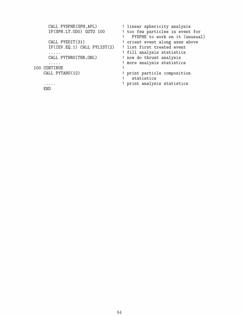
CALL PYSPHE(SPH,APL) ! linear sphericity analysisIF(SPH.LT.0D0) GOTO 100 ! too few particles in event for

! PYSPHE to work on it (unusual)CALL PYEDIT(31) ! orient event along axes aboveIF(IEV.EQ.1) CALL PYLIST(2) ! list first treated event..... ! fill analysis statisticsCALL PYTHRU(THR,OBL) ! now do thrust analysis..... ! more analysis statistics

100 CONTINUE !CALL PYTABU(12) ! print particle composition

! statistics..... ! print analysis statisticsEND

84

7 Process Generation

Much can be said about the processes in Pythia and the way they are generated. There-fore the material has been split into three sections. In the current one the philosophyunderlying the event generation scheme is presented. Here we provide a generic descrip-tion, where some special cases are swept under the carpet. In the next section, theexisting processes are enumerated, with some comments about applications and limita-tions. Finally, in the third section the generation routines and common block switchesare described.

The section starts with a survey of parton distributions, followed by a detailed descrip-tion of the simple 2 → 2 and 2 → 1 hard subprocess generation schemes, including pairsof resonances. This is followed by a few comments on more complicated configurations,and on nonperturbative processes.

7.1 Parton Distributions

The parton distribution function fai (x,Q2) parameterizes the probability to find a partoni with a fraction x of the beam energy when the beam particle a is probed by a hardscattering at virtuality scale Q2. Usually the momentum-weighted combination xfai (x,Q2)is used, for which the normalization condition

∑

i

∫ 10 dx xf

ai (x,Q2) ≡ 1 normally applies.

The Q2 dependence of parton distributions is perturbatively calculable, see section 10.3.1.The parton distributions in Pythia come in many shapes, as shown in the following.

7.1.1 Baryons

For protons, many sets exist on the market. These are obtained by fits to experimentaldata, constrained so that the Q2 dependence is in accordance with the standard QCDevolution equations. The current default in Pythia is GRV 94L [Glu95], a simple leading-order fit. Several other sets are found in Pythia. The complete list is:

• EHLQ sets 1 and 2 [Eic84];• DO sets 1 and 2 [Duk82];• the GRV 92L (updated version) fit [Glu92];• the CTEQ 3L, CTEQ 3M and CTEQ 3D fits [Lai95];• the GRV 94L, GRV 94M and GRV 94D fits [Glu95]; and• the CTEQ 5L and CTEQ 5M1 fits [Lai00].

Of these, EHLQ, DO, GRV 92L, CTEQ 3L, GRV94L and CTEQ5L are leading-orderparton distributions, while CTEQ 3D and GRV94D are in the next-to-leading-order DISscheme and the rest in the next-to-leading order MS scheme. The EHLQ and DO setsare by now rather old, and are kept mainly for backwards compatibility. Since only Born-level matrix elements are included in the program, there is no particular reason to usehigher-order parton distributions — the resulting combination is anyway only good toleading-order accuracy. (Some higher-order corrections are effectively included by theparton-shower treatment, but there is no exact match.)

There is a steady flow of new parton-distribution sets on the market. To keep trackof all of them is a major work on its own. Therefore Pythia contains an interface to anexternal library of parton distribution functions, Pdflib [Plo93]. This is a truly ency-clopedic collection of almost all proton, pion and photon parton distributions proposedsince the late 70’s. Three dummy routines come with the Pythia package, so as to avoidproblems with unresolved external references if Pdflib is not linked. One should alsonote that Pythia does not check the results, but assumes that sensible answers will bereturned, also outside the nominal (x,Q2) range of a set. Only the sets that come withPythia have been suitably modified to provide reasonable answers outside their nominaldomain of validity.

85

From the proton parton distributions, those of the neutron are obtained by isospinconjugation, i.e. fn

u = fpd and fn

d = fpu .

The program does allow for incoming beams of a number of hyperons: Λ0, Σ−,0,+,Ξ−,0 and Ω−. Here one has essentially no experimental information. One could imagineto construct models in which valence s quarks are found at larger average x values thanvalence u and d ones, because of the larger s-quark mass. However, hyperon beams is alittle-used part of the program, included only for a few specific studies. Therefore a simpleapproach has been taken, in which an average valence quark distribution is constructed asfval = (fp

u,val +fpd,val)/3, according to which each valence quark in a hyperon is assumed to

be distributed. Sea-quark and gluon distributions are taken as in the proton. Any protonparton distribution set may be used with this procedure.

7.1.2 Mesons and photons

Data on meson parton distributions are scarce, so only very few sets have been con-structed, and only for the π±. Pythia contains the Owens set 1 and 2 parton distribu-tions [Owe84], which for a long time were essentially the only sets on the market, and themore recent dynamically generated GRV LO (updated version) [Glu92a]. The latter oneis the default in Pythia. Further sets are found in Pdflib and can therefore be used byPythia, just as described above for protons.

Like the proton was used as a template for simple hyperon sets, so also the pion isused to derive a crude ansatz for K±/K0

S/K0L. The procedure is the same, except that now

fval = (fπ+

u,val + fπ+

d,val)/2.

Sets of photon parton distributions have been obtained as for hadrons; an additionalcomplication comes from the necessity to handle the matching of the vector meson dom-inance (VMD) and the perturbative pieces in a consistent manner. New sets have beenproduced where this division is explicit and therefore especially well suited for applicationsto event generation[Sch95]. The Schuler and Sjostand set 1D is the default. Although thevector-meson philosophy is at the base, the details of the fits do not rely on pion data,but only on F γ

2 data. Here follows a brief summary of relevant details.Real photons obey a set of inhomogeneous evolution equations, where the inhomoge-

neous term is induced by γ → qq branchings. The solution can be written as the sum oftwo terms,

f γa (x,Q2) = f γ,NPa (x,Q2;Q2

0) + f γ,PTa (x,Q2;Q20) , (45)

where the former term is a solution to the homogeneous evolution with a (nonperturba-tive) input at Q = Q0 and the latter is a solution to the full inhomogeneous equationwith boundary condition f γ,PTa (x,Q2

0;Q20) ≡ 0. One possible physics interpretation is to

let f γ,NPa correspond to γ ↔ V fluctuations, where V = ρ0, ω, φ, . . . is a set of vector

mesons, and let f γ,PTa correspond to perturbative (‘anomalous’) γ ↔ qq fluctuations. Thediscrete spectrum of vector mesons can be combined with the continuous (in virtualityk2) spectrum of qq fluctuations, to give

f γa (x,Q2) =∑

V

4παem

f 2V

f γ,Va (x,Q2) +αem

2π

∑

q

2e2q

∫ Q2

Q20

dk2

k2f γ,qqa (x,Q2; k2) , (46)

where each component f γ,V and f γ,qq obeys a unit momentum sum rule.In sets 1 the Q0 scale is picked at a low value, 0.6 GeV, where an identification of the

nonperturbative component with a set of low-lying mesons appear natural, while sets 2use a higher value, 2 GeV, where the validity of perturbation theory is better established.The data are not good enough to allow a precise determination of ΛQCD. Therefore weuse a fixed value Λ(4) = 200 MeV, in agreement with conventional results for protondistributions. In the VMD component the ρ0 and ω have been added coherently, so thatuu : dd = 4 : 1 at Q0.

86

Unlike the p, the γ has a direct component where the photon acts as an unresolvedprobe. In the definition of F γ

2 this adds a component Cγ, symbolically

F γ2 (x,Q2) =

∑

q

e2q[

f γq + f γq]

⊗ Cq + f γg ⊗ Cg + Cγ . (47)

Since Cγ ≡ 0 in leading order, and since we stay with leading-order fits, it is permissibleto neglect this complication. Numerically, however, it makes a non-negligible difference.We therefore make two kinds of fits, one DIS type with Cγ = 0 and one ms type includingthe universal part of Cγ.

When jet production is studied for real incoming photons, the standard evolutionapproach is reasonable also for heavy flavours, i.e. predominantly the c, but with a lowercut-off Q0 ≈ mc for γ → cc. Moving to Deeply Inelastic Scattering, eγ → eX , there isan extra kinematical constraint: W 2 = Q2(1 − x)/x > 4m2

c. It is here better to use the‘Bethe-Heitler’ cross section for γ∗γ → cc. Therefore each distribution appears in twovariants. For applications to real γ’s the parton distributions are calculated as the sum ofa vector-meson part and an anomalous part including all five flavours. For applicationsto DIS, the sum runs over the same vector-meson part, an anomalous part and possiblya Cγ part for the three light flavours, and a Bethe-Heitler part for c and b.

In version 2 of the SaS distributions, which are the ones found here, the extensionfrom real to virtual photons was improved, and further options made available [Sch96].The resolved components of the photon are dampened by phenomenologically motivatedvirtuality-dependent dipole factors, while the direct ones are explicitly calculable. Thuseq. (46) generalizes to

f γ⋆

a (x,Q2, P 2) =∑

V

4παem

f 2V

(

m2V

m2V + P 2

)2

f γ,Va (x,Q2; Q20)

+αem

2π

∑

q

2e2q

∫ Q2

Q20

dk2

k2

(

k2

k2 + P 2

)2

f γ,qqa (x,Q2; k2) . (48)

In addition to the introduction of the dipole form factors, note that the lower input scalefor the VMD states is here shifted from Q2

0 to some Q20 ≥ Q2

0. This is based on a studyof the evolution equation [Bor93] that shows that the evolution effectively starts ‘later’ inQ2 for a virtual photon. Equation (48) is one possible answer. It depends on both Q2 andP 2 in a non-trivial way, however, so that results are only obtained by a time-consumingnumerical integration rather than as a simple parametrization. Therefore several otheralternatives are offered, that are in some sense equivalent, but can be given in simplerform.

In addition to the SaS sets, Pythia also contains the Drees–Grassie set of partondistributions [Dre85] and, as for the proton, there is an interface to the Pdflib library[Plo93]. These calls are made with photon virtuality P 2 below the hard process scale Q2.Further author-recommended constrains are implemented in the interface to the GRS set[Glu99] which, along with SaS, is among the few also to define parton distributions ofvirtual photons. However, these sets do not allow a subdivision of the photon partondistributions into one VMD part and one anomalous part. This subdivision is necessary asophisticated modelling of γp and γγ events, see above and section 7.7.2. As an alterna-tive, for the VMD part alone, the ρ0 parton distribution can be found from the assumedequality

f ρ0

i = fπ0

i =1

2(fπ

+

i + fπ−

i ) . (49)

Thus any π+ parton distribution set, from any library, can be turned into a VMD ρ0 set.The ω parton distribution is assumed the same, while the φ and J/ψ ones are handled in

87

the very crude approximation fφs,val = fπ+

u,val and fφsea = fπ+

sea . The VMD part needs to becomplemented by an anomalous part to make up a full photon distribution. The latter isfully perturbatively calculable, given the lower cut-off scale Q0. The SaS parameterizationof the anomalous part is therefore used throughout for this purpose. The Q0 scale can beset freely in the PARP(15) parameter.

The f γ,anomi distribution can be further decomposed, by the flavour and the p⊥ ofthe original branching γ → qq. The flavour is distributed according to squared charge(plus flavour thresholds for heavy flavours) and the p⊥ according to dp2⊥/p

2⊥ in the range

Q0 < p⊥ < Q. At the branching scale, the photon only consists of a qq pair, with xdistribution ∝ x2 + (1 − x)2. A component f γ,qqa (x,Q2; k2), characterized by its k ≈ p⊥and flavour, then is evolved homogeneously from p⊥ to Q. For theoretical studies it isconvenient to be able to access a specific component of this kind. Therefore also leading-order parameterizations of these decomposed distributions are available [Sch95].

7.1.3 Leptons

Contrary to the hadron case, there is no necessity to introduce the parton-distributionfunction concept for leptons. A lepton can be considered as a point-like particle, withinitial-state radiation handled by higher-order matrix elements. However, the partondistribution function approach offers a slightly simplified but very economical descriptionof initial-state radiation effects for any hard process, also those for which higher-ordercorrections are not yet calculated.

Parton distributions for electrons have been introduced in Pythia, and are used alsofor muons and taus, with a trivial substitution of masses. Alternatively, one is free touse a simple ‘unresolved’ e, f e

e (x,Q2) = δ(x − 1), where the e retains the full originalmomentum.

Electron parton distributions are calculable entirely from first principles, but differentlevels of approximation may be used. The parton-distribution formulae in Pythia arebased on a next-to-leading-order exponentiated description, see ref. [Kle89], p. 34. Theapproximate behaviour is

f ee (x,Q2) ≈ β

2(1 − x)β/2−1 ;

β =2αem

π

(

lnQ2

m2e

− 1

)

. (50)

The form is divergent but integrable for x → 1, i.e. the electron likes to keep most of theenergy. To handle the numerical precision problems for x very close to unity, the partondistribution is set, by hand, to zero for x > 1−10−10, and is rescaled upwards in the range1− 10−7 < x < 1− 10−10, in such a way that the total area under the parton distributionis preserved:

(

f ee (x,Q2)

)

mod=

f ee (x,Q2) 0 ≤ x ≤ 1 − 10−7

1000β/2

1000β/2 − 1f ee (x,Q2) 1 − 10−7 < x < 1 − 10−10

0 x > 1 − 10−10 .

(51)

A separate issue is that electron beams may not be monochromatic, more so than forother particles because of the small electron mass. In storage rings the main mechanism issynchrotron radiation. For future high-luminosity linear colliders, the beam–beam interac-tions at the collision vertex may induce a quite significant energy loss — ‘beamstrahlung’.Note that neither of these are associated with any off-shellness of the electrons, i.e. theresulting spectrum only depends on x and not Q2. Examples of beamstrahlung spectra

88

are provided by the Circe program [Ohl97], with a sample interface on the Pythia

webpages.The branchings e → eγ, which are responsible for the softening of the f e

e partondistribution, also gives rise to a flow of photons. In photon-induced hard processes, thef eγ parton distribution can be used to describe the equivalent flow of photons. In the next

section, a complete differential photon flux machinery is introduced. Here some simplerfirst-order expressions are introduced, for the flux integrated up to a hard interaction scaleQ2. There is some ambiguity in the choice of Q2 range over which emissions should beincluded. The naıve (default) choice is

f eγ(x,Q2) =

αem

2π

1 + (1 − x)2

xln

(

Q2

m2e

)

. (52)

Here it is assumed that only one scale enters the problem, namely that of the hardinteraction, and that the scale of the branching e → eγ is bounded from above by thehard interaction scale. For a pure QCD or pure QED shower this is an appropriateprocedure, cf. section 10.1.3, but in other cases it may not be optimal. In particular, forphotoproduction the alternative that is probably most appropriate is [Ali88]:

f eγ(x,Q2) =

αem

2π

1 + (1 − x)2

xln

(

Q2max(1 − x)

m2e x

2

)

. (53)

Here Q2max is a user-defined cut for the range of scattered electron kinematics that is

counted as photoproduction. Note that we now deal with two different Q2 scales, onerelated to the hard subprocess itself, which appears as the argument of the parton dis-tribution, and the other related to the scattering of the electron, which is reflected inQ2

max.Also other sources of photons should be mentioned. One is the beamstahlung pho-

tons mentioned above, where again Circe provides sample parameterizations. Another,particularly interesting one, is laser backscattering, wherein an intense laser pulse is shotat an incoming high-energy electron bunch. By Compton backscattering this gives riseto a photon energy spectrum with a peak at a sigificant fraction of the original electronenergy [Gin82]. Both of these sources produce real photons, which can be consideredas photon beams of variable energy (see subsection 9.8), decoupled from the productionprocess proper.

In resolved photoproduction or resolved γγ interactions, one has to include the partondistributions for quarks and gluons inside the photon inside the electron. This is best donewith the machinery of the next section. However, as an older and simpler alternative, f e

q,g

can be obtained by a numerical convolution according to

f eq,g(x,Q

2) =∫ 1

x

dxγxγ

f eγ(xγ , Q

2) f γq,g

(

x

xγ, Q2

)

, (54)

with f eγ as discussed above. The necessity for numerical convolution makes this parton

distribution evaluation rather slow compared with the others; one should therefore onlyhave it switched on for resolved photoproduction studies.

One can obtain the positron distribution inside an electron, which is also the electronsea parton distribution, by a convolution of the two branchings e → eγ and γ → e+e−;the result is [Che75]

f e−

e+ (x,Q2) =1

2

αem

2π

(

lnQ2

m2e

− 1

)21

x

(

4

3− x2 − 4

3x3 + 2x(1 + x) ln x

)

. (55)

89

Finally, the program also contains the distribution of a transverse W− inside an elec-tron

f eW(x,Q2) =

αem

2π

1

4 sin2θW

1 + (1 − x)2

xln

(

1 +Q2

m2W

)

. (56)

7.1.4 Equivalent photon flux in leptons

With the ’gamma/lepton’ option of a PYINIT call, an ep or e+e− event (or correspondingprocesses with muons) is factorized into the flux of virtual photons and the subsequentinteractions of such photons. While real photons always are transverse, the virtual photonsalso allow a longitudinal component. This corresponds to cross sections

dσ(ep → eX) =∑

ξ=T,L

∫ ∫

dy dQ2 f ξγ/e(y,Q2) dσ(γ∗ξp → X) (57)

and

dσ(ee → eeX) =∑

ξ1,ξ2=T,L

∫ ∫ ∫

dy1 dQ21 dy2 dQ2

2 fξ1γ/e(y1, Q

21)f

ξ2γ/e(y2, Q

22) dσ(γ∗ξ1γ

∗ξ2→ X) .

(58)For ep events, this factorized ansatz is perfectly general, so long as azimuthal distributionsin the final state are not studied in detail. In e+e− events, it is not a good approximationwhen the virtualities Q2

1 and Q22 of both photons become of the order of the squared

invariant mass W 2 of the colliding photons [Sch98]. In this region the cross sectionhave terms that depend on the relative azimuthal angle of the scattered leptons, and thetransverse and longitudinal polarizations are non-trivially mixed. However, these termsare of order Q2

1Q22/W

2 and can be neglected whenever at least one of the photons has lowvirtuality compared to W 2.

When Q2/W 2 is small, one can derive [Bon73, Bud75, Sch98]

fTγ/l(y,Q

2) =αem

2π

(

(1 + (1 − y)2

y

1

Q2− 2m2

l y

Q4

)

, (59)

fLγ/l(y,Q

2) =αem

2π

2(1 − y)

y

1

Q2, (60)

where l = e±, µ± or τ±. In fTγ/l the second term, proportional to m2

l /Q4, is not leading log

and is therefore often omitted. Clearly it is irrelevant at large Q2, but around the lowercut-off Q2

min it significantly dampens the small-y rise of the first term. (Note that Q2min

is y-dependent, so properly the dampening is in a region of the (y,Q2) plane.) Overall,under realistic conditions, it reduces event rates by 5–10% [Sch98, Fri93].

The y variable is defined as the light-cone fraction the photon takes of the incominglepton momentum. For instance, for l+l− events,

yi =qikjkikj

, j = 2(1) for i = 1(2) , (61)

where the ki are the incoming lepton four-momenta and the qi the four-momenta of thevirtual photons.

Alternatively, the energy fraction the photon takes in the rest frame of the collisioncan be used,

xi =qi(k1 + k2)

ki(k1 + k2), i = 1, 2 . (62)

90

The two are simply related,

yi = xi +Q2i

s, (63)

with s = (k1 + k2)2. (Here and in the following formulae we have omitted the lepton and

hadron mass terms when it is not of importance for the argumentation.) Since the Jaco-bian d(yi, Q

2i )/d(xi, Q

2i ) = 1, either variable would be an equally valid choice for covering

the phase space. Small xi values will be of less interest for us, since they lead to smallW 2, so yi/xi ≈ 1 except in the high-Q2 tail, and often the two are used interchangeably.

Unless special Q2 cuts are imposed, cross sections obtained with fT,Lγ/l (x,Q2) dx rather

than fT,Lγ/l (y,Q2) dy differ only at the per mil level. For comparisons with experimental

cuts, it is sometimes relevant to know which of the two is being used in an analysis.In the ep kinematics, the x and y definitions give that

W 2 = xs = ys−Q2 . (64)

The W 2 expression for l+l− is more complicated, especially because of the dependence onthe relative azimuthal angle of the scattered leptons, ϕ12 = ϕ1 − ϕ2:

W 2 = x1x2s+2Q2

1Q22

s− 2

√

1 − x1 −Q2

1

s

√

1 − x2 −Q2

2

sQ1Q2 cosϕ12

= y1y2s−Q21 −Q2

2 +Q2

1Q22

s− 2

√

1 − y1√

1 − y2Q1Q2 cosϕ12 . (65)

The lepton scattering angle θi is related to Q2i as

Q2i =

x2i1 − xi

m2i + (1 − xi)

(

s− 2

(1 − xi)2m2i − 2m2

j

)

sin2(θi/2) , (66)

with m2i = k2i = k′2i and terms of O(m4) neglected. The kinematical limits thus are

(Q2i )min ≈ x2i

1 − xim2i , (67)

(Q2i )max ≈ (1 − xi)s , (68)

unless experimental conditions reduce the θi ranges.In summary, we will allow the possibility of experimental cuts in the xi, yi, Q

2i , θi

and W 2 variables. Within the allowed region, the phase space is Monte Carlo sampledaccording to

∏

i(dQ2i /Q

2i ) (dxi/xi) dϕi, with the remaining flux factors combined with the

cross section factors to give the event weight used for eventual acceptance or rejection.This cross section in its turn can contain the parton densities of a resolved virtual photon,thus offering an effective convolution that gives partons inside photons inside electrons.

7.2 Kinematics and Cross Section for a 2 → 2 Process

In this section we begin the description of kinematics selection and cross-section calcula-tion. The example is for the case of a 2 → 2 process, with final-state masses assumed tobe vanishing. Later on we will expand to finite fixed masses, and to resonances.

Consider two incoming beam particles in their c.m. frame, each with energy Ebeam.The total squared c.m. energy is then s = 4E2

beam. The two partons that enter thehard interaction do not carry the total beam momentum, but only fractions x1 and x2,respectively, i.e. they have four-momenta

p1 = Ebeam(x1; 0, 0, x1) ,

p2 = Ebeam(x2; 0, 0,−x2) . (69)

91

There is no reason to put the incoming partons on the mass shell, i.e. to have time-likeincoming four-vectors, since partons inside a particle are always virtual and thus space-like. These space-like virtualities are introduced as part of the initial-state parton-showerdescription, see section 10.3.3, but do not affect the formalism of this section, whereforemassless incoming partons is a sensible ansatz. The one example where it would beappropriate to put a parton on the mass shell is for an incoming lepton beam, but evenhere the massless kinematics description is adequate as long as the c.m. energy is correctlycalculated with masses.

The squared invariant mass of the two partons is defined as

s = (p1 + p2)2 = x1 x2 s . (70)

Instead of x1 and x2, it is often customary to use τ and either y or xF:

τ = x1x2 =s

s; (71)

y =1

2lnx1x2

; (72)

xF = x1 − x2 . (73)

In addition to x1 and x2, two additional variables are needed to describe the kinematicsof a scattering 1 + 2 → 3 + 4. One corresponds to the azimuthal angle ϕ of the scatteringplane around the beam axis. This angle is always isotropically distributed for unpolarizedincoming beam particles, and so need not be considered further. The other variable canbe picked as θ, the polar angle of parton 3 in the c.m. frame of the hard scattering. Theconventional choice is to use the variable

t = (p1 − p3)2 = (p2 − p4)

2 = − s2

(1 − cos θ) , (74)

with θ defined as above. In the following, we will make use of both t and θ. It is alsocustomary to define u,

u = (p1 − p4)2 = (p2 − p3)

2 = − s2

(1 + cos θ) , (75)

but u is not an independent variable since

s + t+ u = 0 . (76)

If the two outgoing particles have masses m3 and m4, respectively, then the four-momenta in the c.m. frame of the hard interaction are given by

p3,4 =

(

s± (m23 −m2

4)

2√s

,±√s

2β34 sin θ, 0,±

√s

2β34 cos θ

)

, (77)

where

β34 =

√

√

√

√

(

1 − m23

s− m2

4

s

)2

− 4m2

3

s

m24

s. (78)

Then t and u are modified to

t, u = −1

2

(s−m23 −m2

4) ∓ s β34 cos θ

, (79)

92

withs+ t+ u = m2

3 +m24 . (80)

The cross section for the process 1 + 2 → 3 + 4 may be written as

σ =∫ ∫ ∫

dx1 dx2 dt f1(x1, Q2) f2(x2, Q

2)dσ

dt

=∫ ∫ ∫

dτ

τdy dt x1f1(x1, Q

2) x2f2(x2, Q2)

dσ

dt. (81)

The choice of Q2 scale is ambiguous, and several alternatives are available in theprogram. For massless outgoing particles the default is the squared transverse momentum

Q2 = p2⊥ =s

4sin2 θ =

tu

s, (82)

which is modified to

Q2 =1

2(m2

⊥3 +m2⊥4) =

1

2(m2

3 +m24) + p2⊥ =

1

2(m2

3 +m24) +

tu−m23m

24

s(83)

when masses are introduced in the final state. The mass term is selected such that,for m3 = m4 = m, the expression reduces to the squared transverse mass, Q2 = m2

⊥ =m2+p2⊥. For cases with spacelike virtual incoming photons, of virtuality Q2

i = −m2i = |p2i |,

a further generalization to

Q2 =1

2(Q2

1 +Q22 +m2

3 +m24) + p2⊥ (84)

is offered.The dσ/dt expresses the differential cross section for a scattering, as a function of the

kinematical quantities s, t and u. It is in this function that the physics of a given processresides.

The performance of a machine is measured in terms of its luminosity L, which isdirectly proportional to the number of particles in each bunch and to the bunch crossingfrequency, and inversely proportional to the area of the bunches at the collision point.For a process with a σ as given by eq. (81), the differential event rate is given by σL, andthe number of events collected over a given period of time

N = σ∫

L dt . (85)

The program does not calculate the number of events, but only the integrated crosssections.

7.3 Resonance Production

The simplest way to produce a resonance is by a 2 → 1 process. If the decay of theresonance is not considered, the cross-section formula does not depend on t, but takes theform

σ =∫ ∫ dτ

τdy x1f1(x1, Q

2) x2f2(x2, Q2) σ(s) . (86)

Here the physics is contained in the cross section σ(s). The Q2 scale is usually taken tobe Q2 = s.

93

In published formulae, cross sections are often given in the zero-width approximation,i.e. σ(s) ∝ δ(s − m2

R), where mR is the mass of the resonance. Introducing the scaledmass τR = m2

R/s, this corresponds to a delta function δ(τ − τR), which can be used toeliminate the integral over τ .

However, what we normally want to do is replace the δ function by the appropriateBreit–Wigner shape. For a resonance width ΓR this is achieved by the replacement

δ(τ − τR) → s

π

mRΓR(sτ −m2

R)2 +m2RΓ2

R

. (87)

In this formula the resonance width ΓR is a constant.An improved description of resonance shapes is obtained if the width is made s-

dependent (occasionally also referred to as mass-dependent width, since s is not always theresonance mass), see e.g. [Ber89]. To first approximation, this means that the expressionmRΓR is to be replaced by sΓR/mR, both in the numerator and the denominator. Anintermediate step is to perform this replacement only in the numerator. This is convenientwhen not only s-channel resonance production is simulated but also non-resonance t- oru-channel graphs are involved, since mass-dependent widths in the denominator here maygive an imperfect cancellation of divergences. (More about this below.)

To be more precise, in the program the quantity HR(s) is introduced, and the Breit–Wigner is written as

δ(τ − τR) → s

π

HR(sτ)

(sτ −m2R)2 +H2

R(sτ). (88)

The HR factor is evaluated as a sum over all possible final-state channels, HR =∑

f H(f)R .

Each decay channel may have its own s dependence, as follows.A decay to a fermion pair, R → ff, gives no contribution below threshold, i.e. for

s < 4m2f . Above threshold, H

(f)R is proportional to s, multiplied by a threshold factor

β(3 − β2)/2 for the vector part of a spin 1 resonance, by β3 for the axial vector part,

by β3 for a scalar resonance and by β for a pseudoscalar one. Here β =√

1 − 4m2f /s.

For the decay into unequal masses, e.g. of the W+, corresponding but more complicatedexpressions are used.

For decays into a quark pair, a first-order strong correction factor 1 + αs(s)/π is

included in H(f)R . This is the correct choice for all spin 1 colourless resonances, but

is here used for all resonances where no better knowledge is available. Currently themajor exception is top decay, where the factor 1−2.5αs(s)/π is used to approximate loopcorrections [Jez89]. The second-order corrections are often known, but then are specific toeach resonance, and are not included. An option exists for the γ/Z0/Z′0 resonances, wherethreshold effects due to qq bound-state formation are taken into account in a smeared-out,average sense, see eq. (137).

For other decay channels, not into fermion pairs, the s dependence is typically morecomplicated. An example would be the decay h0 → W+W−, with a nontrivial thresholdand a subtle energy dependence above that [Sey95a]. Since a Higgs with mh < 2mW

could still decay in this channel, it is in fact necessary to perform a two-dimensionalintegral over the W± Breit–Wigner mass distributions to obtain the correct result (andthis has to be done numerically, at least in part). Fortunately, a Higgs particle lighter than2mW is sufficiently narrow that the integral only needs to be performed once and for allat initialization (whereas most other partial widths are recalculated whenever needed).Channels that proceed via loops, such as h → gg, also display complicated thresholdbehaviours.

The coupling structure within the electroweak sector is usually (re)expressed in terms

94

of gauge boson masses, αem and sin2θW , i.e. factors of GF are replaced according to

√2GF =

π αem

sin2θW m2W

. (89)

Having done that, αem is allowed to run [Kle89], and is evaluated at the s scale. Therebythe relevant electroweak loop correction factors are recovered at the mW/mZ scale. How-ever, the option exists to go the other way and eliminate αem in favour of GF. Currentlysin2θW is not allowed to run.

For Higgs particles and technipions, fermion masses enter not only in the kinematicsbut also as couplings. The latter kind of quark masses (but not the former, at least not inthe program) are running with the scale of the process, i.e. normally the resonance mass.The expression used is [Car96]

m(Q2) = m0

(

ln(k2m20/Λ

2)

ln(Q2/Λ2)

)12/(33−2nf )

. (90)

Here m0 is the input mass at a reference scale km0, defined in the ms scheme. Typicalchoices are either k = 1 or k = 2; the latter would be relevant if the reference scale ischosen at the QQ threshold. Both Λ and nf are as given in αs.

In summary, we see that an s dependence may enter several different ways into the

H(f)R expressions from which the total HR is built up.

When only decays to a specific final state f are considered, the HR in the denominatorremains the sum over all allowed decay channels, but the numerator only contains the

H(f)R term of the final state considered.

If the combined production and decay process i → R → f is considered, the same sdependence is implicit in the coupling structure of i→ R as one would have had in R → i,i.e. to first approximation there is a symmetry between couplings of a resonance to theinitial and to the final state. The cross section σ is therefore, in the program, written inthe form

σi→R→f(s) ∝π

s

H(i)R (s)H

(f)R (s)

(s−m2R)2 +H2

R(s). (91)

As a simple example, the cross section for the process e−νe → W− → µ−νµ can be writtenas

σ(s) = 12π

s

H(i)W (s)H

(f)W (s)

(s−m2W)2 +H2

W(s), (92)

where

H(i)W (s) = H

(f)W (s) =

αem(s)

24 sin2θWs . (93)

If the effects of several initial and/or final states are studied, it is straightforward tointroduce an appropriate summation in the numerator.

The analogy between the H(f)R and H

(i)R cannot be pushed too far, however. The

two differ in several important aspects. Firstly, colour factors appear reversed: the decayR → qq contains a colour factor NC = 3 enhancement, while qq → R is instead suppressedby a factor 1/NC = 1/3. Secondly, the 1 + αs(s)/π first-order correction factor for thefinal state has to be replaced by a more complicated K factor for the initial state. Thisfactor is not known usually, or it is known (to first non-trivial order) but too lengthy tobe included in the program. Thirdly, incoming partons as a rule are space-like. All thethreshold suppression factors of the final-state expressions are therefore irrelevant when

production is considered. In sum, the analogy between H(f)R and H

(i)R is mainly useful

as a consistency cross-check, while the two usually are calculated separately. Exceptions

95

include the rather messy loop structure involved in gg → h0 and h0 → gg, which is onlycoded once.

It is of some interest to consider the observable resonance shape when the effects ofparton distributions are included. In a hadron collider, to first approximation, partondistributions tend to have a behaviour roughly like f(x) ∝ 1/x for small x — this is whyf(x) is replaced by xf(x) in eq. (81). Instead, the basic parton-distribution behaviouris shifted into the factor of 1/τ in the integration phase space dτ/τ , cf. eq. (86). Whenconvoluted with the Breit–Wigner shape, two effects appear. One is that the overallresonance is tilted: the low-mass tail is enhanced and the high-mass one suppressed. Theother is that an extremely long tail develops on the low-mass side of the resonance: whenτ → 0, eq. (91) with HR(s) ∝ s gives a σ(s) ∝ s ∝ τ , which exactly cancels the 1/τfactor mentioned above. Naıvely, the integral over y,

∫

dy = − ln τ , therefore gives a netlogarithmic divergence of the resonance shape when τ → 0. Clearly, it is then necessaryto consider the shape of the parton distributions in more detail. At not-too-small Q2, theevolution equations in fact lead to parton distributions more strongly peaked than 1/x,typically with xf(x) ∝ x−0.3, and therefore a divergence like τ−0.3 in the cross-sectionexpression. Eventually this divergence is regularized by a closing of the phase space,i.e. that HR(s) vanishes faster than s, and by a less drastic small-x parton-distributionbehaviour when Q2 ≈ s→ 0.

The secondary peak at small τ may give a rather high cross section, which can evenrival that of the ordinary peak around the nominal mass. This is the case, for instance,with W production. Such a peak has never been observed experimentally, but this is notsurprising, since the background from other processes is overwhelming at low s. Thus alepton of one or a few GeV of transverse momentum is far more likely to come from thedecay of a charm or bottom hadron than from an extremely off-shell W of a mass of afew GeV. When resonance production is studied, it is therefore important to set limitson the mass of the resonance, so as to agree with the experimental definition, at least tofirst approximation. If not, cross-section information given by the program may be veryconfusing.

Another problem is that often the matrix elements really are valid only in the resonanceregion. The reason is that one usually includes only the simplest s-channel graph in thecalculation. It is this ‘signal’ graph that has a peak at the position of the resonance, whereit (usually) gives much larger cross sections than the other ‘background’ graphs. Awayfrom the resonance position, ‘signal’ and ‘background’ may be of comparable order, orthe ‘background’ may even dominate. There is a quantum mechanical interference whensome of the ‘signal’ and ‘background’ graphs have the same initial and final state, and thisinterference may be destructive or constructive. When the interference is non-negligible,it is no longer meaningful to speak of a ‘signal’ cross section. As an example, consider thescattering of longitudinal W’s, W+

L W−L → W+

L W−L , where the ‘signal’ process is s-channel

exchange of a Higgs. This graph by itself is ill-behaved away from the resonance region.Destructive interference with ‘background’ graphs such as t-channel exchange of a Higgsand s- and t-channel exchange of a γ/Z is required to save unitarity at large energies.

In e+e− colliders, the f ee parton distribution is peaked at x = 1 rather than at x = 0.

The situation therefore is the opposite, if one considers e.g. Z0 production in a machinerunning at energies above mZ: the tail towards lower masses is suppressed and the onetowards higher masses enhanced, with a sharp secondary peak at around the nominalenergy of the machine. Also in this case, an appropriate definition of cross sectionstherefore is necessary — with additional complications due to the interference between γ∗

and Z0. When other processes are considered, problems of interference with backgroundappears also here. Numerically the problems may be less pressing, however, since thesecondary peak is occurring in a high-mass region, rather than in a more complicatedlow-mass one. Further, in e+e− there is little uncertainty from the shape of the partondistributions.

96

In 2 → 2 processes where a pair of resonances are produced, e.g. e+e− → Z0h0, crosssection are almost always given in the zero-width approximation for the resonances. Heretwo substitutions of the type

1 =∫

δ(m2 −m2R) dm2 →

∫

1

π

mRΓR(m2 −m2

R)2 +m2RΓ2

R

dm2 (94)

are used to introduce mass distributions for the two resonance masses, i.e. m23 and m2

4.In the formula, mR is the nominal mass and m the actually selected one. The phase-space integral over x1, x1 and t in eq. (81) is then extended to involve also m2

3 and m24.

The effects of the mass-dependent width is only partly taken into account, by replacingthe nominal masses m2

3 and m24 in the dσ/dt expression by the actually generated ones

(also e.g. in the relation between t and cos θ), while the widths are evaluated at thenominal masses. This is the equivalent of a simple replacement of mRΓR by sΓR/mR inthe numerator of eq. (87), but not in the denominator. In addition, the full thresholddependence of the widths, i.e. the velocity-dependent factors, is not reproduced.

There is no particular reason why the full mass-dependence could not be introduced,except for the extra work and time consumption needed for each process. In fact, thematrix elements for several γ∗/Z0 and W± production processes do contain the full ex-pressions. On the other hand, the matrix elements given in the literature are often validonly when the resonances are almost on the mass shell, since some graphs have beenomitted. As an example, the process qq → e−νeµ

+νµ is dominated by qq → W−W+

when each of the two lepton pairs is close to mW in mass, but in general also receivescontributions e.g. from qq → Z0 → e+e−, followed by e+ → νeW

+ and W+ → µ+νµ. Thelatter contributions are neglected in cross sections given in the zero-width approximation.

Widths may induce gauge invariance problems, in particular when the s-channel graphinterferes with t- or u-channels. Then there may be an imperfect cancellation of contri-butions at high energies, leading to an incorrect cross section behaviour. The underlyingreason is that a Breit-Wigner corresponds to a resummation of terms of different ordersin coupling constants, and that therefore effectively the s-channel contributions are calcu-lated to higher orders than the t- or u-channel ones, including interference contributions.A specific example is e+e− → W+W−, where s-channel γ∗/Z∗ exchange interferes witht-channel νe exchange. In such cases, a fixed width is used in the denominator. Onecould also introduce procedures whereby the width is made to vanish completely at highenergies, and theoretically this is the cleanest, but the fixed-width approach appears goodenough in practice.

Another gauge invariance issue is when two particles of the same kind are producedin a pair, e.g. gg → tt. Matrix elements are then often calculated for one commonmt mass, even though in real life the masses m3 6= m4. The proper gauge invariantprocedure to handle this would be to study the full six-fermion state obtained after thetwo t → bW → bfifj decays, but that may be overkill if indeed the t’s are close tomass shell. Even when only equal-mass matrix elements are available, Breit-Wigners aretherefore used to select two separate masses m3 and m4. From these two masses, anaverage mass m is constructed so that the β34 velocity factor of eq. (78) is retained,

β34(s, m2, m2) = β34(s, m

23, m

24) ⇒ m2 =

m23 +m2

4

2− (m2

3 −m24)

2

4s. (95)

This choice certainly is not unique, but normally should provide a sensible behaviour,also around threshold. The approach may well break down when either or both particlesare far away from mass shell. Furthermore, the preliminary choice of scattering angle θis also retained. Instead of the correct t and u of eq. (79), modified

t, u = −1

2

(s− 2m2) ∓ s β34 cos θ

= (t, u) − (m23 −m2

4)2

4s(96)

97

can then be obtained. The m2, t and u are now used in the matrix elements to decidewhether to retain the event or not.

Processes with one final-state resonance and another ordinary final-state product, e.g.qg → W+q′, are treated in the same spirit as the 2 → 2 processes with two resonances,except that only one mass need be selected according to a Breit–Wigner.

7.4 Cross-section Calculations

In the program, the variables used in the generation of a 2 → 2 process are τ , y andz = cos θ. For a 2 → 1 process, the z variable can be integrated out, and need thereforenot be generated as part of the hard process, except when the allowed angular range ofdecays is restricted. In unresolved lepton beams, i.e. when f e

e (x) = δ(x−1), the variablesτ and/or y may be integrated out. We will cover all these special cases towards the endof the section, and here concentrate on ‘standard’ 2 → 2 and 2 → 1 processes.

7.4.1 The simple 2 → 2 processes

In the spirit of section 4.1, we want to select simple functions such that the true τ , y andz dependence of the cross sections is approximately modelled. In particular, (almost) allconceivable kinematical peaks should be represented by separate terms in the approximateformulae. If this can be achieved, the ratio of the correct to the approximate cross sectionswill not fluctuate too much, but allow reasonable Monte Carlo efficiency.

Therefore the variables are generated according to the distributions hτ (τ), hy(y) andhz(z), where normally

hτ (τ) =c1I1

1

τ+c2I2

1

τ 2+c3I3

1

τ(τ + τR)+c4I4

1

(sτ −m2R)2 +m2

RΓ2R

+c5I5

1

τ(τ + τR′)+c6I6

1

(sτ −m2R′)2 +m2

R′Γ2R′

, (97)

hy(y) =c1I1

(y − ymin) +c2I2

(ymax − y) +c3I3

1

cosh y, (98)

hz(z) =c1I1

+c2I2

1

a− z+c3I3

1

a+ z+c4I4

1

(a− z)2+c5I5

1

(a + z)2. (99)

Here each term is separately integrable, with an invertible primitive function, such thatgeneration of τ , y and z separately is a standard task, as described in section 4.1. In thefollowing we describe the details of the scheme, including the meaning of the coefficientsci and Ii, which are separate for τ , y and z.

The first variable to be selected is τ . The range of allowed values, τmin ≤ τ ≤ τmax,is generally constrained by a number of user-defined requirements. A cut on the allowedmass range is directly reflected in τ , a cut on the p⊥ range indirectly. The first two termsof hτ are intended to represent a smooth τ dependence, as generally obtained in processeswhich do not receive contributions from s-channel resonances. Also s-channel exchangeof essentially massless particles (γ, g, light quarks and leptons) are accounted for, sincethese do not produce any separate peaks at non-vanishing τ . The last four terms ofhτ are there to catch the peaks in the cross section from resonance production. Theseterms are only included when needed. Each resonance is represented by two pieces, a firstto cover the interference with graphs which peak at τ = 0, plus the variation of partondistributions, and a second to approximate the Breit–Wigner shape of the resonance itself.The subscripts R and R′ denote values pertaining to the two resonances, with τR = m2

R/s.Currently there is only one process where the full structure with two resonances is used,namely ff → γ∗/Z0/Z′0. Otherwise either one or no resonance peak is taken into account.

98

The kinematically allowed range of y values is constrained by τ , |y| ≤ −12

ln τ , andyou may impose additional cuts. Therefore the allowed range ymin ≤ y ≤ ymax is onlyconstructed after τ has been selected. The first two terms of hy give a fairly flat y depen-dence — for processes which are symmetric in y ↔ −y, they will add to give a completelyflat y spectrum between the allowed limits. In principle, the natural subdivision wouldhave been one term flat in y and one forward–backward asymmetric, i.e. proportional toy. The latter is disallowed by the requirement of positivity, however. The y − ymin andymax − y terms actually used give the same amount of freedom, but respect positivity.The third term is peaked at around y = 0, and represents the bias of parton distributionstowards this region.

The allowed z = cos θ range is naıvely −1 ≤ z ≤ 1. However, most cross sections aredivergent for z → ±1, so some kind of regularization is necessary. Normally one requiresp⊥ ≥ p⊥min, which translates into z2 ≤ 1 − 4p2⊥min/(τs) for massless outgoing particles.Since again the limits depend on τ , the selection of z is done after that of τ . Additionalrequirements may constrain the range further. In particular, a p⊥max constraint may splitthe allowed z range into two, i.e. z−min ≤ z ≤ z−max or z+min ≤ z ≤ z+max. An un-splitrange is represented by z−max = z+min = 0. For massless outgoing particles the parametera = 1 in hz, such that the five terms represent a piece flat in angle and pieces peaked as 1/t,1/u, 1/t2, and 1/u2, respectively. For non-vanishing masses one has a = 1 + 2m2

3m24/s

2.In this case, the full range −1 ≤ z ≤ 1 is therefore available — physically, the standard tand u singularities are regularized by the masses m3 and m4.

For each of the terms, the Ii coefficients represent the integral over the quantitymultiplying the coefficient ci; thus, for instance:

hτ : I1 =∫

dτ

τ= ln

(

τmax

τmin

)

,

I2 =∫

dτ

τ 2=

1

τmin− 1

τmax;

hy : I1 =∫

(y − ymin) dy =1

2(ymax − ymin)2 ;

hz : I1 =∫

dz = (z−max − z−min) + (z+max − z+min),

I2 =∫ dz

a− z= ln

(

(a− z−min)(a− z+min)

(a− z−max)(a− z−min)

)

. (100)

The ci coefficients are normalized to unit sum for hτ , hy and hz separately. Theyhave a simple interpretation, as the probability for each of the terms to be used in thepreliminary selection of τ , y and z, respectively. The variation of the cross section overthe allowed phase space is explored in the initialization procedure of a Pythia run, andbased on this knowledge the ci are optimized so as to give functions hτ , hy and hz thatclosely follow the general behaviour of the true cross section. For instance, the coefficientc4 in hτ is to be made larger the more the total cross section is dominated by the regionaround the resonance mass.

The phase-space points tested at initialization are put on a grid, with the number ofpoints in each dimension given by the number of terms in the respective h expression,and with the position of each point given by the median value of the distribution of oneof the terms. For instance, the dτ/τ distribution gives a median point at

√τminτmax, and

dτ/τ 2 has the median 2τminτmax/(τmin + τmax). Since the allowed y and z ranges dependon the τ value selected, then so do the median points defined for these two variables.

With only a limited set of phase-space points studied at the initialization, the ‘optimal’set of coefficients is not uniquely defined. To be on the safe side, 40% of the total weight istherefore assigned evenly between all allowed ci, whereas the remaining 60% are assigned

99

according to the relative importance surmised, under the constraint that no coefficient isallowed to receive a negative contribution from this second piece.

After a preliminary choice has been made of τ , y and z, it is necessary to find theweight of the event, which is to be used to determine whether to keep it or generateanother one. Using the relation dt = s β34 dz/2, eq. (81) may be rewritten as

σ =∫ ∫ ∫

dτ

τdy

sβ342

dz x1f1(x1, Q2) x2f2(x2, Q

2)dσ

dt

=π

s

∫

hτ (τ) dτ∫

hy(y) dy∫

hz(z) dz β34x1f1(x1, Q

2) x2f2(x2, Q2)

τ 2hτ (τ) hy(y) 2hz(z)

s2

π

dσ

dt

=

⟨

π

s

β34τ 2hτ (τ) hy(y) 2hz(z)

x1f1(x1, Q2) x2f2(x2, Q

2)s2

π

dσ

dt

⟩

. (101)

In the middle line, a factor of 1 = hτ/hτ has been introduced to rewrite the τ integral interms of a phase space of unit volume:

∫

hτ (τ) dτ = 1 according to the relations above.Correspondingly for the y and z integrals. In addition, factors of 1 = s/(τs) and 1 = π/πare used to isolate the dimensionless cross section (s2/π) dσ/dt. The content of the lastline is that, with τ , y and z selected according to the expressions hτ (τ), hy(y) and hz(z),respectively, the cross section is obtained as the average of the final expression over allevents. Since the h’s have been picked to give unit volume, there is no need to multiplyby the total phase-space volume.

As can be seen, the cross section for a given Monte Carlo event is given as the productof four factors, as follows:

1. The π/s factor, which is common to all events, gives the overall dimensions of thecross section, in GeV−2. Since the final cross section is given in units of mb, theconversion factor of 1 GeV−2 = 0.3894 mb is also included here.

2. Next comes the Jacobian, which compensates for the change from the original tothe final phase-space volume.

3. The parton-distribution function weight is obtained by making use of the partondistribution libraries in Pythia or externally. The x1 and x2 values are obtainedfrom τ and y via the relations x1,2 =

√τ exp(±y).

4. Finally, the dimensionless cross section (s2/π) dσ/dt is the quantity that has to becoded for each process separately, and where the physics content is found.

Of course, the expression in the last line is not strictly necessary to obtain the crosssection by Monte Carlo integration. One could also have used eq. (81) directly, selectingphase-space points evenly in τ , y and t, and averaging over those Monte Carlo weights.Clearly this would be much simpler, but the price to be paid is that the weights ofindividual events could fluctuate wildly. For instance, if the cross section contains anarrow resonance, the few phase-space points that are generated in the resonance regionobtain large weights, while the rest do not. With our procedure, a resonance wouldbe included in the hτ (τ) factor, so that more events would be generated at around theappropriate τR value (owing to the hτ numerator in the phase-space expression), but withthese events assigned a lower, more normal weight (owing to the factor 1/hτ in the weightexpression). Since the weights fluctuate less, fewer phase-space points need be selected toget a reasonable cross-section estimate.

In the program, the cross section is obtained as the average over all phase-space pointsgenerated. The events actually handed on to you should have unit weight, however (anoption with weighted events exists, but does not represent the mainstream usage). Atinitialization, after the ci coefficients have been determined, a search inside the allowedphase-space volume is therefore made to find the maximum of the weight expression inthe last line of eq. (101). In the subsequent generation of events, a selected phase-space

100

point is then retained with a probability equal to the weight in the point divided bythe maximum weight. Only the retained phase-space points are considered further, andgenerated as complete events.

The search for the maximum is begun by evaluating the weight in the same grid ofpoints as used to determine the ci coefficients. The point with highest weight is used asstarting point for a search towards the maximum. In unfortunate cases, the convergencecould be towards a local maximum which is not the global one. To somewhat reducethis risk, also the grid point with second-highest weight is used for another search. Afterinitialization, when events are generated, a warning message will be given by default atany time a phase-space point is selected where the weight is larger than the maximum,and thereafter the maximum weight is adjusted to reflect the new knowledge. This meansthat events generated before this time have a somewhat erroneous distribution in phasespace, but if the maximum violation is rather modest the effects should be negligible. Theestimation of the cross section is not affected by any of these considerations, since themaximum weight does not enter into eq. (101).

For 2 → 2 processes with identical final-state particles, the symmetrization factor of1/2 is explicitly included at the end of the dσ/dt calculation. In the final cross section,a factor of 2 is retrieved because of integration over the full phase space (rather thanonly half of it). That way, no special provisions are needed in the phase-space integrationmachinery.

7.4.2 Resonance production

We have now covered the simple 2 → 2 case. In a 2 → 1 process, the t integral is absent,and the differential cross section dσ/dt is replaced by σ(s). The cross section may nowbe written as

σ =∫ ∫ dτ

τdy x1f1(x1, Q

2) x2f2(x2, Q2) σ(s)

=π

s

∫

hτ (τ) dτ∫

hy(y) dyx1f1(x1, Q

2) x2f2(x2, Q2)

τ 2hτ (τ) hy(y)

s

πσ(s)

=

⟨

π

s

1

τ 2hτ (τ) hy(y)x1f1(x1, Q

2) x2f2(x2, Q2)s

πσ(s)

⟩

. (102)

The structure is thus exactly the same, but the z-related pieces are absent, and the roleof the dimensionless cross section is played by (s/π)σ(s).

If the range of allowed decay angles of the resonance is restricted, e.g. by requiringthe decay products to have a minimum transverse momentum, effectively this translatesinto constraints on the z = cos θ variable of the 2 → 2 process. The difference is that theangular dependence of a resonance decay is trivial, and that therefore the z-dependentfactor can be easily evaluated. For a spin-0 resonance, which decays isotropically, therelevant weight is simply (z−max−z−min)/2+(z+max−z+min)/2. For a transversely polarizedspin-1 resonance the expression is, instead,

3

8(z−max − z−min) +

3

8(z+max − z+min) +

1

8(z−max − z−min)3 +

1

8(z+max − z+min)3 . (103)

Since the allowed z range could depend on τ and/or y (it does for a p⊥ cut), the factorhas to be evaluated for each individual phase-space point and included in the expressionof eq. (102).

For 2 → 2 processes where either of the final-state particles is a resonance, or both, anadditional choice has to be made for each resonance mass, eq. (94). Since the allowed τ ,y and z ranges depend on m2

3 and m24, the selection of masses have to precede the choice

101

of the other phase-space variables. Just as for the other variables, masses are not selecteduniformly over the allowed range, but are rather distributed according to a functionhm(m2) dm2, with a compensating factor 1/hm(m2) in the Jacobian. The functional formpicked is normally

hm(m2) =c1I1

1

π

mRΓR(m2 −m2

R)2 +m2RΓ2

R

+c2I2

+c3I3

1

m2+c4I4

1

m4. (104)

The definition of the Ii integrals is analogous to the one before. The ci coefficients are notfound by optimization, but predetermined, normally to c1 = 0.8, c2 = c3 = 0.1, c4 = 0.Clearly, had the phase space and the cross section been independent of m2

3 and m24, the

optimal choice would have been to put c1 = 1 and have all other ci vanishing — then the1/hm factor of the Jacobian would exactly have cancelled the Breit–Wigner of eq. (94)in the cross section. The second and the third terms are there to cover the possibilitythat the cross section does not die away quite as fast as given by the naıve Breit–Wignershape. In particular, the third term covers the possibility of a secondary peak at smallm2, in a spirit slightly similar to the one discussed for resonance production in 2 → 1processes.

The fourth term is only used for processes involving γ∗/Z0 production, where the γpropagator guarantees that the cross section does have a significant secondary peak form2 → 0. Therefore here the choice is c1 = 0.4, c2 = 0.05, c3 = 0.3 and c4 = 0.25.

A few special tricks have been included to improve efficiency when the allowed massrange of resonances is constrained by kinematics or by user cuts. For instance, if a pairof equal or charge-conjugate resonances are produced, such as in e+e− → W+W−, use ismade of the constraint that the lighter of the two has to have a mass smaller than halfthe c.m. energy.

7.4.3 Lepton beams

Lepton beams have to be handled slightly differently from what has been described so far.One also has to distinguish between a lepton for which parton distributions are includedand one which is treated as an unresolved point-like particle. The necessary modificationsare the same for 2 → 2 and 2 → 1 processes, however, since the t degree of freedom isunaffected.

If one incoming beam is an unresolved lepton, the corresponding parton-distributionpiece collapses to a δ function. This function can be used to integrate out the y variable:δ(x1,2 − 1) = δ(y ± (1/2) ln τ). It is therefore only necessary to select the τ and the zvariables according to the proper distributions, with compensating weight factors, andonly one set of parton distributions has to be evaluated explicitly.

If both incoming beams are unresolved leptons, both the τ and the y variables aretrivially given: τ = 1 and y = 0. Parton-distribution weights disappear completely. Fora 2 → 2 process, only the z selection remains to be performed, while a 2 → 1 process iscompletely specified, i.e. the cross section is a simple number that only depends on thec.m. energy.

For a resolved electron, the f ee parton distribution is strongly peaked towards x = 1.

This affects both the τ and the y distributions, which are not well described by eitherof the pieces in hτ (τ) or hy(y) in processes with interacting e±. (Processes which involvee.g. the γ content of the e are still well simulated, since f e

γ is peaked at small x.)If both parton distributions are peaked close to 1, the hτ (τ) expression in eq. (99)

is therefore increased with one additional term of the form hτ (τ) ∝ 1/(1 − τ), withcoefficients c7 and I7 determined as before. The divergence when τ → 1 is cut off by ourregularization procedure for the f e

e parton distribution; therefore we only need considerτ < 1 − 2 × 10−10.

102

Correspondingly, the hy(y) expression is expanded with a term 1/(1−exp(y−y0)) whenincoming beam number 1 consists of a resolved e±, and with a term 1/(1− exp(−y− y0))when incoming beam number 2 consists of a resolved e±. Both terms are present foran e+e− collider, only one for an ep one. The coefficient y0 = −(1/2) ln τ is the naıvekinematical limit of the y range, |y| < y0. From the definitions of y and y0 it is easyto see that the two terms above correspond to 1/(1 − x1) and 1/(1 − x2), respectively,and thus are again regularized by our parton-distribution function cut-off. Therefore theintegration ranges are y < y0−10−10 for the first term and y > −y0 +10−10 for the secondone.

7.4.4 Mixing processes

In the cross-section formulae given so far, we have deliberately suppressed a summationover the allowed incoming flavours. For instance, the process ff → Z0 in a hadron colliderreceives contributions from uu → Z0, dd → Z0, ss → Z0, and so on. These contributionsshare the same basic form, but differ in the parton-distribution weights and (usually) in afew coupling constants in the hard matrix elements. It it therefore convenient to generatethe terms together, as follows:

1. A phase-space point is picked, and all common factors related to this choice areevaluated, i.e. the Jacobian and the common pieces of the matrix elements (e.g. fora Z0 the basic Breit–Wigner shape, excluding couplings to the initial flavour).

2. The parton-distribution-function library is called to produce all the parton distri-butions, at the relevant x and Q2 values, for the two incoming beams.

3. A loop is made over the two incoming flavours, one from each beam particle. For eachallowed set of incoming flavours, the full matrix-element expression is constructed,using the common pieces and the flavour-dependent couplings. This is multipliedby the common factors and the parton-distribution weights to obtain a cross-sectionweight.

4. Each allowed flavour combination is stored as a separate entry in a table, togetherwith its weight. In addition, a summed weight is calculated.

5. The phase-space point is kept or rejected, according to a comparison of the summedweight with the maximum weight obtained at initialization. Also the cross-sectionMonte Carlo integration is based on the summed weight.

6. If the point is retained, one of the allowed flavour combinations is picked accordingto the relative weights stored in the full table.

Generally, the flavours of the final state are either completely specified by those ofthe initial state, e.g. as in qg → qg, or completely decoupled from them, e.g. as inff → Z0 → f ′f

′. In neither case need therefore the final-state flavours be specified in the

cross-section calculation. It is only necessary, in the latter case, to include an overallweight factor, which takes into account the summed contribution of all final states thatare to be simulated. For instance, if only the process Z0 → e+e− is studied, the relevantweight factor is simply Γee/Γtot. Once the kinematics and the incoming flavours havebeen selected, the outgoing flavours can be picked according to the appropriate relativeprobabilities.

In some processes, such as gg → gg, several different colour flows are allowed, eachwith its own kinematical dependence of the matrix-element weight, see section 8.2.1. Eachcolour flow is then given as a separate entry in the table mentioned above, i.e. in total anentry is characterized by the two incoming flavours, a colour-flow index, and the weight.For an accepted phase-space point, the colour flow is selected in the same way as theincoming flavours.

The program can also allow the mixed generation of two or more completely differentprocesses, such as ff → Z0 and qq → gg. In that case, each process is initialized separately,with its own set of coefficients ci and so on. The maxima obtained for the individual cross

103

sections are all expressed in the same units, even when the dimensionality of the phasespace is different. (This is because we always transform to a phase space of unit volume,∫

hτ (τ) dτ ≡ 1, etc.) The above generation scheme need therefore only be generalized asfollows:

1. One process is selected among the allowed ones, with a relative probability given bythe maximum weight for this process.

2. A phase-space point is found, using the distributions hτ (τ) and so on, optimized forthis particular process.

3. The total weight for the phase-space point is evaluated, again with Jacobians, matrixelements and allowed incoming flavour combinations that are specific to the process.

4. The point is retained with a probability given by the ratio of the actual to themaximum weight of the process. If the point is rejected, one has to go back to step1 and pick a new process.

5. Once a phase-space point has been accepted, flavours may be selected, and the eventgenerated in full.

It is clear why this works: although phase-space points are selected among the allowedprocesses according to relative probabilities given by the maximum weights, the probabil-ity that a point is accepted is proportional to the ratio of actual to maximum weight. Intotal, the probability for a given process to be retained is therefore only proportional tothe average of the actual weights, and any dependence on the maximum weight is gone.

In γp and γγ physics, the different components of the photon give different final states,see section 7.7.2. Technically, this introduces a further level of administration, since eachevent class contains a set of (partly overlapping) processes. From an ideological point ofview, however, it just represents one more choice to be made, that of event class, beforethe selection of process in step 1 above. When a weighting fails, both class and processhave to be picked anew.

7.5 2 → 3 and 2 → 4 Processes

The Pythia machinery to handle 2 → 1 and 2 → 2 processes is fairly sophisticated andgeneric. The same cannot be said about the generation of hard scattering processes withmore than two final-state particles. The number of phase-space variables is larger, and itis therefore more difficult to find and transform away all possible peaks in the cross sectionby a suitably biased choice of phase-space points. In addition, matrix-element expressionsfor 2 → 3 processes are typically fairly lengthy. Therefore Pythia only contains a verylimited number of 2 → 3 and 2 → 4 processes, and almost each process is a special case ofits own. It is therefore less interesting to discuss details, and we only give a very genericoverview.

If the Higgs mass is not light, interactions among longitudinal W and Z gauge bosonsare of interest. In the program, 2 → 1 processes such as W+

L W−L → h0 and 2 → 2

ones such as W+L W−

L → Z0LZ0

L are included. The former are for use when the h0 still isreasonably narrow, such that a resonance description is applicable, while the latter areintended for high energies, where different contributions have to be added up. Since theprogram does not contain WL or ZL distributions inside hadrons, the basic hard scatteringhas to be convoluted with the q → q′WL and q → qZL branchings, to yield effective 2 → 3and 2 → 4 processes. However, it is possible to integrate out the scattering angles of thequarks analytically, as well as one energy-sharing variable [Cha85]. Only after an eventhas been accepted are these other kinematical variables selected. This involves furtherchoices of random variables, according to a separate selection loop.

In total, it is therefore only necessary to introduce one additional variable in the basicphase-space selection, which is chosen to be s′, the squared invariant mass of the full2 → 3 or 2 → 4 process, while s is used for the squared invariant mass of the inner

104

2 → 1 or 2 → 2 process. The y variable is coupled to the full process, since parton-distribution weights have to be given for the original quarks at x1,2 =

√τ ′ exp (±y). The

t variable is related to the inner process, and thus not needed for the 2 → 3 processes.The selection of the τ ′ = s′/s variable is done after τ , but before y has been chosen. Toimprove the efficiency, the selection is made according to a weighted phase space of theform

∫

hτ ′(τ′) dτ ′, where

hτ ′(τ′) =

c1I1

1

τ ′+c2I2

(1 − τ/τ ′)3

τ ′2+c3I3

1

τ ′(1 − τ ′), (105)

in conventional notation. The ci coefficients are optimized at initialization. The c3 term,peaked at τ ′ ≈ 1, is only used for e+e− collisions. The choice of hτ ′ is roughly matchedto the longitudinal gauge-boson flux factor, which is of the form

(

1 +τ

τ ′

)

ln(

τ

τ ′

)

− 2(

1 − τ

τ ′

)

. (106)

For a light h the effective W approximation above breaks down, and it is necessaryto include the full structure of the qq′ → qq′h0 (i.e. ZZ fusion) and qq′ → q′′q′′′h0 (i.e.WW fusion) matrix elements. The τ ′, τ and y variables are here retained, and selectedaccording to standard procedures. The Higgs mass is represented by the τ choice; normallythe h0 is so narrow that the τ distribution effectively collapses to a δ function. In addition,the three-body final-state phase space is rewritten as

(

5∏

i=3

1

(2π)3d3pi2Ei

)

(2π)4δ(4)(p3+p4+p5−p1−p2) =1

(2π)5π2

4√λ⊥34

dp2⊥3

dϕ3

2πdp2⊥4

dϕ4

2πdy5 ,

(107)where λ⊥34 = (m2

⊥34−m2⊥3−m2

⊥4)2−4m2

⊥3m2⊥4. The outgoing quarks are labelled 3 and 4,

and the outgoing Higgs 5. The ϕ angles are selected isotropically, while the two transversemomenta are picked, with some foreknowledge of the shape of the W/Z propagators inthe cross sections, according to h⊥(p2⊥) dp2⊥, where

h⊥(p2⊥) =c1I1

+c2I2

1

m2R + p2⊥

+c3I3

1

(m2R + p2⊥)2

, (108)

with mR the W or Z mass, depending on process, and c1 = c2 = 0.05, c3 = 0.9. Withinthe limits given by the other variable choices, the rapidity y5 is chosen uniformly. A finalchoice remains to be made, which comes from a twofold ambiguity of exchanging thelongitudinal momenta of partons 3 and 4 (with minor modifications if they are massive).Here the relative weight can be obtained exactly from the form of the matrix elementitself.

7.6 Resonance Decays

Resonances (see section 2.1.2) can be made to decay in two different routines. Oneis the standard decay treatment (in PYDECY) that can be used for any unstable particle,where decay channels are chosen according to fixed probabilities, and decay angles usuallyare picked isotropically in the rest frame of the resonance, see section 13.3. The moresophisticated treatment (in PYRESD) is the default one for resonances produced in Pythia,and is described here. The ground rule is that everything in mass up to and including bhadrons is decayed with the simpler PYDECY routine, while heavier particles are handledwith PYRESD. This also includes the γ∗/Z0, even though here the mass in principle couldbe below the b threshold. Other resonances include, e.g., t, W±, h0, Z′0, W′±, H0, A0,H±, and technicolor and supersymmetric particles.

105

7.6.1 The decay scheme

In the beginning of the decay treatment, either one or two resonances may be present,the former represented by processes such as qq′ → W+ and qg → W+q′, the latter byqq → W+W−. If the latter is the case, the decay of the two resonances is considered inparallel (unlike PYDECY, where one particle at a time is made to decay).

First the decay channel of each resonance is selected according to the relative weights

H(f)R , as described above, evaluated at the actual mass of the resonance, rather than at

the nominal one. Threshold factors are therefore fully taken into account, with channelsautomatically switched off below the threshold. Normally the masses of the decay prod-ucts are well-defined, but e.g. in decays like h0 → W+W− it is also necessary to selectthe decay product masses. This is done according to two Breit–Wigners of the type ineq. (94), multiplied by the threshold factor, which depends on both masses.

Next the decay angles of the resonance are selected isotropically in its rest frame.Normally the full range of decay angles is available, but in 2 → 1 processes the decayangles of the original resonance may be restrained by user cuts, e.g. on the p⊥ of the decayproducts. Based on the angles, the four-momenta of the decay products are constructedand boosted to the correct frame. As a rule, matrix elements are given with quark andlepton masses assumed vanishing. Therefore the four-momentum vectors constructed atthis stage are actually massless for all quarks and leptons.

The matrix elements may now be evaluated. For a process such as qq → W+W− →e+νeµ

−νµ, the matrix element is a function of the four-momenta of the two incomingfermions and of the four outgoing ones. An upper limit for the event weight can beconstructed from the cross section for the basic process qq → W+W−, as already used toselect the two W momenta. If the weighting fails, new resonance decay angles are pickedand the procedure is iterated until acceptance.

Based on the accepted set of angles, the correct decay product four-momenta are con-structed, including previously neglected fermion masses. Quarks and, optionally, leptonsare allowed to radiate, using the standard final-state showering machinery, with maximumvirtuality given by the resonance mass.

In some decays new resonances are produced, and these are then subsequently allowedto decay. Normally only one resonance pair is considered at a time, with the possibility offull correlations. In a few cases triplets can also appear, but such configurations currentlyare considered without inclusion of correlations. Also note that, in a process like qq →Z0h0 → Z0W+W− → 6 fermions, the spinless nature of the h0 ensures that the W± decaysare decoupled from that of the Z0 (but not from each other).

7.6.2 Cross-section considerations

The cross section for a process which involves the production of one or several resonancesis always reduced to take into account channels not allowed by user flags. This is trivialfor a single s-channel resonance, cf. eq. (91), but can also be included approximately ifseveral layers of resonance decays are involved. At initialization, the ratio between theuser-allowed width and the nominally possible one is evaluated and stored, starting fromthe lightest resonances and moving upwards. As an example, one first finds the reductionfactors for W+ and for W− decays, which need not be the same if e.g. W+ is allowed todecay only to quarks and W− only to leptons. These factors enter together as a weightfor the h0 → W+W− channel, which is thus reduced in importance compared with otherpossible Higgs decay channels. This is also reflected in the weight factor of the h0 itself,where some channels are open in full, others completely closed, and finally some (like theone above) open but with reduced weight. Finally, the weight for the process qq → Z0h0

is evaluated as the product of the Z0 weight factor and the h0 one. The standard crosssection of the process is multiplied with this weight.

106

Since the restriction on allowed decay modes is already included in the hard processcross section, mixing of different event types is greatly simplified, and the selection of decaychannel chains is straightforward. There is a price to be paid, however. The reductionfactors evaluated at initialization all refer to resonances at their nominal masses. Forinstance, the W reduction factor is evaluated at the nominal W mass, even when thatfactor is used, later on, in the description of the decay of a 120 GeV Higgs, where at leastone W would be produced below this mass. We know of no case where this approximationhas any serious consequences, however.

The weighting procedure works because the number of resonances to be produced,directly or in subsequent decays, can be derived recursively already from the start. Itdoes not work for particles which could also be produced at later stages, such as theparton-shower evolution and the fragmentation. For instance, D0 mesons can be producedfairly late in the event generation chain, in unknown numbers, and so weights could notbe introduced to compensate, e.g. for the forcing of decays only into π+K−.

One should note that this reduction factor is separate from the description of theresonance shape itself, where the full width of the resonance has to be used. This widthis based on the sum of all possible decay modes, not just the simulated ones. Pythia

does allow the possibility to change also the underlying physics scenario, e.g. to includethe decay of a Z0 into a fourth-generation neutrino.

Normally the evaluation of the reduction factors is straightforward. However, fordecays into a pair of equal or charge-conjugate resonances, such as Z0Z0 or W+W−, it ispossible to pick combinations in such a way that the weight of the pair does not factorizeinto a product of the weight of each resonance itself. To be precise, any decay channelcan be given seven different status codes:

• −1: a non-existent decay mode, completely switched off and of no concern to us;• 0: an existing decay channel, which is switched off;• 1: a channel which is switched on;• 2: a channel switched on for particles, but off for antiparticles;• 3: a channel switched on for antiparticles, but off for particles;• 4: a channel switched on for one of the particles or antiparticles, but not for both;• 5: a channel switched on for the other of the particles or antiparticles, but not for

both.The meaning of possibilities 4 and 5 is exemplified by the statement ‘in a W+W− pair,one W decays hadronically and the other leptonically’, which thus covers the cases whereeither W+ or W− decays hadronically.

Neglecting non-existing channels, each channel belongs to either of the classes above.If we denote the total branching ratio into channels of type i by ri, this then translatesinto the requirement r0 + r1 + r2 + r3 + r4 + r5 = 1. For a single particle the weight factoris r1 + r2 + r4, and for a single antiparticle r1 + r3 + r4. For a pair of identical resonances,the joint weight is instead

(r1 + r2)2 + 2(r1 + r2)(r4 + r5) + 2r4r5 , (109)

and for a resonance–antiresonance pair

(r1 + r2)(r1 + r3) + (2r1 + r2 + r3)(r4 + r5) + 2r4r5 . (110)

If some channels come with a reduced weight because of restrictions on subsequent decaychains, this may be described in terms of properly reduced ri, so that the sum is less thanunity. For instance, in a tt → bW+ bW− process, the W decay modes may be restrictedto W+ → qq and W− → e−νe, in which case (

∑

ri)t ≈ 2/3 and (∑

ri)t ≈ 1/9. With index± denoting resonance/antiresonance, eq. (110) then generalizes to

(r1 + r2)+(r1 + r3)

− + (r1 + r2)+(r4 + r5)

− + (r4 + r5)+(r1 + r3)

− + r+4 r−5 + r+5 r

−4 . (111)

107

7.7 Nonperturbative Processes

A few processes are not covered by the discussion so far. These are the ones that dependon the details of hadronic wave functions, and therefore are not strictly calculable pertur-batively (although perturbation theory may often provide some guidance). What we haveprimarily in mind is elastic scattering, diffractive scattering and low-p⊥ ‘minimum-bias’events in hadron–hadron collisions, but one can also find corresponding processes in γpand γγ interactions. The description of these processes is rather differently structuredfrom that of the other ones, as is explained below. Models for ‘minimum-bias’ eventsare discussed in detail in section 11.2, to which we refer for details on this part of theprogram.

7.7.1 Hadron–hadron interactions

In hadron–hadron interactions, the total hadronic cross section for AB → anything, σABtot ,is calculated using the parameterization of Donnachie and Landshoff [Don92]. In thisapproach, each cross section appears as the sum of one pomeron term and one reggeonone

σABtot (s) = XAB sǫ + Y AB s−η , (112)

where s = E2cm. The powers ǫ = 0.0808 and η = 0.4525 are expected to be universal,

whereas the coefficients XAB and Y AB are specific to each initial state. (In fact, the high-energy behaviour given by the pomeron term is expected to be the same for particle and

antiparticle interactions, i.e. XAB = XAB.) Parameterizations not provided in [Don92]have been calculated in the same spirit, making use of quark counting rules [Sch93a].

The total cross section is subdivided according to

σABtot (s) = σABel (s) + σABsd(XB)(s) + σABsd(AX)(s) + σABdd (s) + σABnd (s) . (113)

Here ‘el’ is the elastic process AB → AB, ‘sd(XB)’ the single diffractive AB → XB,‘sd(AX)’ the single diffractive AB → AX , ‘dd’ the double diffractive AB → X1X2, and‘nd’ the non-diffractive ones. Higher diffractive topologies, such as central diffraction, arecurrently neglected. In the following, the elastic and diffractive cross sections and eventcharacteristics are described, as given in the model by Schuler and Sjostrand [Sch94,Sch93a]. The non-diffractive component is identified with the ‘minimum bias’ physicsalready mentioned, a practical but not unambiguous choice. Its cross section is given by‘whatever is left’ according to eq. (113), and its properties are discussed in section 11.2.

At not too large squared momentum transfers t, the elastic cross section can be ap-proximated by a simple exponential fall-off. If one neglects the small real part of the crosssection, the optical theorem then gives

dσeldt

=σ2tot

16πexp(Belt) , (114)

and σel = σ2tot/16πBel. The elastic slope parameter is parameterized by

Bel = BABel (s) = 2bA + 2bB + 4sǫ − 4.2 , (115)

with s given in units of GeV and Bel in GeV−2. The constants bA,B are bp = 2.3, bπ,ρ,ω,φ =1.4, bJ/ψ = 0.23. The increase of the slope parameter with c.m. energy is faster thanthe logarithmically one conventionally assumed; that way the ratio σel/σtot remains well-behaved at large energies.

108

The diffractive cross sections are given by

dσsd(XB)(s)

dt dM2=

g3IP16π

βAIP β2BIP

1

M2exp(Bsd(XB)t)Fsd ,

dσsd(AX)(s)

dt dM2=

g3IP16π

β2AIP βBIP

1

M2exp(Bsd(AX)t)Fsd ,

dσdd(s)

dt dM21 dM2

2

=g23IP16π

βAIP βBIP1

M21

1

M22

exp(Bddt)Fdd . (116)

The couplings βAIP are related to the pomeron term XABsǫ of the total cross sectionparameterization, eq. (112). Picking a reference scale

√sref = 20 GeV, the couplings are

given by βAIPβBIP = XAB sǫref . The triple-pomeron coupling is determined from single-diffractive data to be g3IP ≈ 0.318 mb1/2; within the context of the formulae in thissection.

The spectrum of diffractive masses M is taken to begin 0.28 GeV ≈ 2mπ above themass of the respective incoming particle and extend to the kinematical limit. The simpledM2/M2 form is modified by the mass-dependence in the diffractive slopes and in the Fsd

and Fdd factors (see below).The slope parameters are assumed to be

Bsd(XB)(s) = 2bB + 2α′ ln(

s

M2

)

,

Bsd(AX)(s) = 2bA + 2α′ ln(

s

M2

)

,

Bdd(s) = 2α′ ln

(

e4 +ss0

M21M

22

)

. (117)

Here α′ = 0.25 GeV−2 and conventionally s0 is picked as s0 = 1/α′. The term e4 in Bdd isadded by hand to avoid a breakdown of the standard expression for large values of M2

1M22 .

The bA,B terms protect Bsd from breaking down; however a minimum value of 2 GeV−2

is still explicitly required for Bsd, which comes into play e.g. for a J/ψ state (as part of aVMD photon beam).

The kinematical range in t depends on all the masses of the problem. In terms ofthe scaled variables µ1 = m2

A/s, µ2 = m2B/s, µ3 = M2

(1)/s (= m2A/s when A scatters

elastically), µ4 = M2(2)/s (= m2

B/s when B scatters elastically), and the combinations

C1 = 1 − (µ1 + µ2 + µ3 + µ4) + (µ1 − µ2)(µ3 − µ4) ,

C2 =√

(1 − µ1 − µ2)2 − 4µ1µ2

√

(1 − µ3 − µ4)2 − 4µ3µ4 ,

C3 = (µ3 − µ1)(µ4 − µ2) + (µ1 + µ4 − µ2 − µ3)(µ1µ4 − µ2µ3) , (118)

one has tmin < t < tmax with

tmin = −s2

(C1 + C2) ,

tmax = −s2

(C1 − C2) = −s2

4C3

C1 + C2=s2C3

tmin. (119)

The Regge formulae above for single- and double-diffractive events are supposed tohold in certain asymptotic regions of the total phase space. Of course, there will bediffraction also outside these restrictive regions. Lacking a theory which predicts differen-tial cross sections at arbitrary t and M2 values, the Regge formulae are used everywhere,

109

but fudge factors are introduced in order to obtain ‘sensible’ behaviour in the full phasespace. These factors are:

Fsd =

(

1 − M2

s

)(

1 +cresM

2res

M2res +M2

)

,

Fdd =

(

1 − (M1 +M2)2

s

)(

sm2p

sm2p +M2

1 M22

)

×(

1 +cresM

2res

M2res +M2

1

)(

1 +cresM

2res

M2res +M2

2

)

. (120)

The first factor in either expression suppresses production close to the kinematical limit.The second factor in Fdd suppresses configurations where the two diffractive systemsoverlap in rapidity space. The final factors give an enhancement of the low-mass region,where a resonance structure is observed in the data. Clearly a more detailed modellingwould have to be based on a set of exclusive states rather than on this smeared-outaveraging procedure. A reasonable fit to pp/pp data is obtained for cres = 2 and Mres =2 GeV, for an arbitrary particle A which is diffractively excited we use MA

res = mA−mp +2 GeV.

The diffractive cross-section formulae above have been integrated for a set of c.m.energies, starting at 10 GeV, and the results have been parameterized. The form ofthese parameterizations is given in ref. [Sch94], with explicit numbers for the pp/pp case.Pythia also contains similar parameterizations for πp (assumed to be same as ρp andωp), φp, J/ψp, ρρ (ππ etc.), ρφ, ρJ/ψ, φφ, φJ/ψ and J/ψJ/ψ.

The processes above do not obey the ordinary event mixing strategy. First of all, sincetheir total cross sections are known, it is possible to pick the appropriate process from thestart, and then remain with that choice. In other words, if the selection of kinematicalvariables fails, one would not go back and pick a new process, the way it was done insection 7.4.4. Second, it is not possible to impose any cuts or restrain allowed incomingor outgoing flavours: if not additional information were to be provided, it would makethe whole scenario ill-defined. Third, it is not recommended to mix generation of theseprocesses with that of any of the other ones: normally the other processes have so smallcross sections that they would almost never be generated anyway. (We here exclude thecases of ‘underlying events’ and ‘pile-up events’, where mixing is provided for, and evenis a central part of the formalism, see sections 11.2 and 11.3.)

Once the cross-section parameterizations has been used to pick one of the processes,the variables t and M are selected according to the formulae given above.

A ρ0 formed by γ → ρ0 in elastic or diffractive scattering is polarized, and thereforeits decay angular distribution in ρ0 → π+π− is taken to be proportional to sin2 θ, wherethe reference axis is given by the ρ0 direction of motion.

A light diffractive system, with a mass less than 1 GeV above the mass of the in-coming particle, is allowed to decay isotropically into a two-body state. Single-resonancediffractive states, such as a ∆+, are therefore not explicitly generated, but are assumeddescribed in an average, smeared-out sense.

A more massive diffractive system is subsequently treated as a string with the quantumnumbers of the original hadron. Since the exact nature of the pomeron exchanged betweenthe hadrons is unknown, two alternatives are included. In the first, the pomeron isassumed to couple to (valence) quarks, so that the string is stretched directly between thestruck quark and the remnant diquark (antiquark) of the diffractive state. In the second,the interaction is rather with a gluon, giving rise to a ‘hairpin’ configuration in which thestring is stretched from a quark to a gluon and then back to a diquark (antiquark). Bothof these scenarios could be present in the data; the default choice is to mix them in equalproportions.

110

There is experimental support for more complicated scenarios [Ing85], wherein thepomeron has a partonic substructure, which e.g. can lead to high-p⊥ jet production inthe diffractive system. The full machinery, wherein a pomeron spectrum is convolutedwith a pomeron-proton hard interaction, is not available in Pythia. (But is found in thePompyt program [Bru96].)

7.7.2 Photoproduction and γγ physics

The photon physics machinery in Pythia has been largely expanded in recent years.Historically, the model was first developed for photoproduction, i.e. a real photon ona hadron target [Sch93, Sch93a]. Thereafter γγ physics was added in the same spirit[Sch94a, Sch97]. Only recently also virtual photons have been added to the description[Fri00], including the nontrivial transition region between real photons and Deeply Inelas-tic Scattering (DIS). In this section we partly trace this evolution towards more complexconfigurations.

The total γp and γγ cross sections can again be parameterized in a form like eq. (112),which is not so obvious since the photon has more complicated structure than an ordinaryhadron. In fact, the structure is still not so well understood. The model we outline is theone studied by Schuler and Sjostrand [Sch93, Sch93a], and further updated in [Fri00]. Inthis model the physical photon is represented by

|γ〉 =√

Z3 |γB〉 +∑

V=ρ0,ω,φ,J/ψ

e

fV|V 〉 +

∑

q

e

fqq|qq〉 +

∑

ℓ=e,µ,τ

e

fℓℓ|ℓ+ℓ−〉 . (121)

By virtue of this superposition, one is led to a model of γp interactions, where threedifferent kinds of events may be distinguished:

• Direct events, wherein the bare photon |γB〉 interacts directly with a parton fromthe proton. The process is perturbatively calculable, and no parton distributionsof the photon are involved. The typical event structure is two high-p⊥ jets and aproton remnant, while the photon does not leave behind any remnant.

• VMD events, in which the photon fluctuates into a vector meson, predominantly aρ0. All the event classes known from ordinary hadron–hadron interactions may thusoccur here, such as elastic, diffractive, low-p⊥ and high-p⊥ events. For the latter,one may define (VMD) parton distributions of the photon, and the photon alsoleaves behind a beam remnant. This remnant is smeared in transverse momentumby a typical ‘primordial k⊥’ of a few hundred MeV.

• Anomalous or GVMD (Generalized VMD) events, in which the photon fluctuatesinto a qq pair of larger virtuality than in the VMD class. The initial parton distri-bution is perturbatively calculable, as is the subsequent QCD evolution. It gives riseto the so-called anomalous part of the parton distributions of the photon, whenceone name for the class. As long as only real photons were considered, it made senseto define the cross section of this event class to be completely perturbatively calcu-lable, given some lower p⊥ cut-off. Thus only high-p⊥ events could occur. However,alternatively, one may view these states as excited higher resonances (ρ′ etc.), thusthe GVMD name. In this case one is lead to a picture which also allows a low-p⊥cross section, uncalculable in perturbation theory. The reality may well interpo-late between these two extreme alternatives, but the current framework more leanstowards the latter point of view. Either the q or the q plays the role of a beamremnant, but this remnant has a larger p⊥ than in the VMD case, related to thevirtuality of the γ ↔ qq fluctuation.

The |ℓ+ℓ−〉 states can only interact strongly with partons inside the hadron at higherorders, and can therefore be neglected in the study of hadronic final states.

In order that the above classification is smooth and free of double counting, onehas to introduce scales that separate the three components. The main one is k0, which

111

separates the low-mass vector meson region from the high-mass |qq〉 one, k0 ≈ mφ/2 ≈ 0.5GeV. Given this dividing line to VMD states, the anomalous parton distributions areperturbatively calculable. The total cross section of a state is not, however, since thisinvolves aspects of soft physics and eikonalization of jet rates. Therefore an ansatz ischosen where the total cross section of a state scales like k2V /k

2⊥, where the adjustable

parameter kV ≈ mρ/2 for light quarks. The k⊥ scale is roughly equated with half themass of the GVMD state. The spectrum of GVMD states is taken to extend over a rangek0 < k⊥ < k1, where k1 is identified with the p⊥min(s) cut-off of the perturbative jetspectrum in hadronic interactions, p⊥min(s) ≈ 1.5 GeV at typical energies, see section11.2 and especially eq. (189). Above that range, the states are assumed to be sufficientlyweakly interacting that no eikonalization procedure is required, so that cross sections canbe calculated perturbatively without any recourse to pomeron phenomenology. There issome arbitrariness in that choice, and some simplifications are required in order to obtaina manageable description.

The VMD and GVMD/anomalous events are together called resolved ones. In termsof high-p⊥ jet production, the VMD and anomalous contributions can be combined intoa total resolved one, and the same for parton-distribution functions. However, the twoclasses differ in the structure of the underlying event and possibly in the appearance ofsoft processes.

In terms of cross sections, eq. (121) corresponds to

σγptot(s) = σγpdir(s) + σγpVMD(s) + σγpanom(s) . (122)

The direct cross section is, to lowest order, the perturbative cross section for the twoprocesses γq → qg and γg → qq, with a lower cut-off p⊥ > k1, in order to avoid double-counting with the interactions of the GVMD states. Properly speaking, this should bemultiplied by the Z3 coefficient,

Z3 = 1 −∑

V=ρ0,ω,φ,J/ψ

(

e

fV

)2

−∑

q

(

e

fqq

)2

−∑

ℓ=e,µ,τ

(

e

fℓℓ

)2

, (123)

but normally Z3 is so close to unity as to make no difference.The VMD factor (e/fV )2 = 4παem/f

2V gives the probability for the transition γ → V .

The coefficients f 2V /4π are determined from data to be (with a non-negligible amount of

uncertainty) 2.20 for ρ0, 23.6 for ω, 18.4 for φ and 11.5 for J/ψ. Together these numbersimply that the photon can be found in a VMD state about 0.4% of the time, dominatedby the ρ0 contribution. All the properties of the VMD interactions can be obtained byappropriately scaling down V p physics predictions. Thus the whole machinery developedin the previous section for hadron–hadron interactions is directly applicable. Also partondistributions of the VMD component inside the photon are obtained by suitable rescaling.

The contribution from the ‘anomalous’ high-mass fluctuations to the total cross sectionis obtained by a convolution of the fluctuation rate

∑

q

(

e

fqq

)2

≈ αem

2π

(

2∑

q

e2q

)

∫ k1

k0

dk2⊥k2⊥

, (124)

which is to be multiplied by the abovementioned reduction factor k2V /k2⊥ for the total

cross section, and all scaled by the assumed real vector meson cross section.As an illustration of this scenario, the phase space of γp events may be represented

by a (k⊥, p⊥) plane. Two transverse momentum scales are distinguished: the photon res-olution scale k⊥ and the hard interaction scale p⊥. Here k⊥ is a measure of the virtualityof a fluctuation of the photon and p⊥ corresponds to the most virtual rung of the ladder,possibly apart from k⊥. As we have discussed above, the low-k⊥ region corresponds to

112

VMD and GVMD states that encompasses both perturbative high-p⊥ and nonperturba-tive low-p⊥ interactions. Above k1, the region is split along the line k⊥ = p⊥. Whenp⊥ > k⊥ the photon is resolved by the hard interaction, as described by the anomalouspart of the photon distribution function. This is as in the GVMD sector, except that weshould (probably) not worry about multiple parton–parton interactions. In the comple-mentary region k⊥ > p⊥, the p⊥ scale is just part of the traditional evolution of the partondistributions of the proton up to the scale of k⊥, and thus there is no need to introduce aninternal structure of the photon. One could imagine the direct class of events as extendingbelow k1 and there being the low-p⊥ part of the GVMD class, only appearing when a hardinteraction at a larger p⊥ scale would not preempt it. This possibility is implicit in thestandard cross section framework.

In γγ physics [Sch94a, Sch97], the superposition in eq. (121) applies separately foreach of the two incoming photons. In total there are therefore 3 × 3 = 9 combinations.However, trivial symmetry reduces this to six distinct classes, written in terms of the totalcross section (cf. eq. (122)) as

σγγtot(s) = σγγdir×dir(s) + σγγVMD×VMD(s) + σγγGVMD×GVMD(s)

+ 2σγγdir×VMD(s) + 2σγγdir×GVMD(s) + 2σγγVMD×GVMD(s) . (125)

A parameterization of the total γγ cross section is found in [Sch94a, Sch97].The six different kinds of γγ events are thus:• The direct×direct events, which correspond to the subprocess γγ → qq (or ℓ+ℓ−).

The typical event structure is two high-p⊥ jets and no beam remnants.• The VMD×VMD events, which have the same properties as the VMD γp events.

There are four by four combinations of the two incoming vector mesons, with oneVMD factor for each meson.

• The GVMD×GVMD events, wherein each photon fluctuates into a qq pair of largervirtuality than in the VMD class. The ‘anomalous’ classification assumes that oneparton of each pair gives a beam remnant, whereas the other (or a daughter par-ton thereof) participates in a high-p⊥ scattering. The GVMD concept implies thepresence also of low-p⊥ events, like for VMD.

• The direct×VMD events, which have the same properties as the direct γp events.• The direct×GVMD events, in which a bare photon interacts with a parton from

the anomalous photon. The typical structure is then two high-p⊥ jets and a beamremnant.

• The VMD×GVMD events, which have the same properties as the GVMD γp events.Like for photoproduction events, this can be illustrated in a parameter space, but now

three-dimensional, with axes given by the k⊥1, k⊥2 and p⊥ scales. Here each k⊥i is ameasure of the virtuality of a fluctuation of a photon, and p⊥ corresponds to the mostvirtual rung on the ladder between the two photons, possibly excepting the endpointk⊥i ones. So, to first approximation, the coordinates along the k⊥i axes determine thecharacters of the interacting photons while p⊥ determines the character of the interactionprocess. Double counting should be avoided by trying to impose a consistent classification.Thus, for instance, p⊥ > k⊥i with k⊥1 < k0 and k0 < k⊥2 < k1 gives a hard interactionbetween a VMD and a GVMD photon, while k⊥1 > p⊥ > k⊥2 with k⊥1 > k1 and k⊥2 <k0 is a single-resolved process (direct×VMD; with p⊥ now in the parton distributionevolution).

In much of the literature, where a coarser classification is used, our direct×direct iscalled direct, our direct×VMD and direct×GVMD is called single-resolved since theyboth involve one resolved photon which gives a beam remnant, and the rest are calleddouble-resolved since both photons are resolved and give beam remnants.

If the photon is virtual, it has a reduced probability to fluctuate into a vector mesonstate, and this state has a reduced interaction probability. This can be modelled by a

113

traditional dipole factor (m2V /(m

2V +Q2))2 for a photon of virtuality Q2, where mV → 2k⊥

for a GVMD state. Putting it all together, the cross section of the GVMD sector ofphotoproduction then scales like

∫ k21

k20

dk2⊥k2⊥

k2Vk2⊥

(

4k2⊥4k2⊥ +Q2

)2

. (126)

For a virtual photon the DIS process γ∗q → q is also possible, but by gauge invarianceits cross section must vanish in the limit Q2 → 0. At large Q2, the direct processes canbe considered as the O(αs) correction to the lowest-order DIS process, but the directones survive for Q2 → 0. There is no unique prescription for a proper combination atall Q2, but we have attempted an approach that gives the proper limits and minimizesdouble-counting. For large Q2, the DIS γ∗p cross section is proportional to the structurefunction F2(x,Q

2) with the Bjorken x = Q2/(Q2 +W 2). Since normal parton distributionparameterizations are frozen below some Q0 scale and therefore do not obey the gaugeinvariance condition, an ad hoc factor (Q2/(Q2 + m2

ρ))2 is introduced for the conversion

from the parameterized F2(x,Q2) to a σγ

∗pDIS:

σγ∗p

DIS ≃(

Q2

Q2 +m2ρ

)24π2αem

Q2F2(x,Q

2) =4π2αemQ

2

(Q2 +m2ρ)

2

∑

q

e2q

xq(x,Q2) + xq(x,Q2)

.

(127)Here mρ is some nonperturbative hadronic mass parameter, for simplicity identified withthe ρ mass. One of the Q2/(Q2 + m2

ρ) factors is required already to give finite σγptot forconventional parton distributions, and could be viewed as a screening of the individualpartons at small Q2. The second factor is chosen to give not only a finite but actually avanishing σγ

∗pDIS for Q2 → 0 in order to retain the pure photoproduction description there.

This latter factor thus is more a matter of convenience, and other approaches could havebeen pursued.

In order to avoid double-counting between DIS and direct events, a requirement p⊥ >max(k1, Q) is imposed on direct events. In the remaining DIS ones, denoted lowest order

(LO) DIS, thus p⊥ < Q. This would suggest a subdivision σγ∗p

LODIS = σγ∗p

DIS − σγ∗p

direct, with

σγ∗p

DIS given by eq. (127) and σγ∗p

direct by the perturbative matrix elements. In the limitQ2 → 0, the DIS cross section is now constructed to vanish while the direct is not, so thiswould give σγ

∗pLODIS < 0. However, here we expect the correct answer not to be a negative

number but an exponentially suppressed one, by a Sudakov form factor. This modifiesthe cross section:

σγ∗p

LODIS = σγ∗p

DIS − σγ∗p

direct −→ σγ∗p

DIS exp

(

−σγ∗pdirect

σγ∗p

DIS

)

. (128)

Since we here are in a region where the DIS cross section is no longer the dominant one,this change of the total DIS cross section is not essential.

The overall picture, from a DIS perspective, now requires three scales to be kepttrack of. The traditional DIS region is the strongly ordered one, Q2 ≫ k2⊥ ≫ p2⊥, whereDGLAP-style evolution [Alt77, Gri72] is responsible for the event structure. As always,ideology wants strong ordering, while the actual classification is based on ordinary orderingQ2 > k2⊥ > p2⊥. The region k2⊥ > max(Q2, p2⊥) is also DIS, but of the O(αs) direct kind.The region where k⊥ is the smallest scale corresponds to non-ordered emissions, that thengo beyond DGLAP validity, while the region p2⊥ > k2⊥ > Q2 cover the interactions of aresolved virtual photon. Comparing with the plane of real photoproduction, we concludethat the whole region p⊥ > k⊥ involves no double-counting, since we have made noattempt at a non-DGLAP DIS description but can choose to cover this region entirely by

114

the VMD/GVMD descriptions. Actually, it is only in the corner p⊥ < k⊥ < min(k1, Q)that an overlap can occur between the resolved and the DIS descriptions. Some furtherconsiderations show that usually either of the two is strongly suppressed in this region,except in the range of intermediate Q2 and rather small W 2. Typically, this is the regionwhere x ≈ Q2/(Q2 +W 2) is not close to zero, and where F2 is dominated by the valence-quark contribution. The latter behaves roughly ∝ (1 − x)n, with an n of the order of 3or 4. Therefore we will introduce a corresponding damping factor to the VMD/GVMDterms.

In total, we have now arrived at our ansatz for all Q2:

σγ∗p

tot = σγ∗p

DIS exp

(

−σγ∗pdirect

σγ∗p

DIS

)

+ σγ∗p

direct +

(

W 2

Q2 +W 2

)n(

σγ∗p

VMD + σγ∗p

GVMD

)

, (129)

with four main components. Most of these in their turn have a complicated internalstructure, as we have seen.

Turning to γ∗γ∗ processes, finally, the parameter space is now five-dimensional: Q1,Q2, k⊥1, k⊥2 and p⊥. As before, an effort is made to avoid double-counting, by havinga unique classification of each region in the five-dimensional space. Remaining double-counting is dealt with as above. In total, our ansatz for γ∗γ∗ interactions at all Q2 contains13 components: 9 when two VMD, GVMD or direct photons interact, as is already allowedfor real photons, plus a further 4 where a ‘DIS photon’ from either side interacts with aVMD or GVMD one. With the label resolved used to denote VMD and GVMD, one canwrite

σγ∗γ∗

tot (W 2, Q21, Q

22) = σγ

∗γ∗

DIS×res exp

(

− σγ∗γ∗

dir×res

σγ∗γ∗

DIS×res

)

+ σγ∗γ∗

dir×res

+ σγ∗γ∗

res×DIS exp

(

− σγ∗γ∗

res×dir

σγ∗γ∗

res×DIS

)

+ σγ∗γ∗

res×dir (130)

+ σγ∗γ∗

dir×dir +

(

W 2

Q21 +Q2

2 +W 2

)3

σγ∗γ∗

res×res

Most of the 13 components in their turn have a complicated internal structure, as we haveseen.

An important note is that the Q2 dependence of the DIS and direct photon interactionsis implemented in the matrix element expressions, i.e. in processes such as γ∗γ∗ → qq orγ∗q → qg the photon virtuality explicitly enters. This is different from VMD/GVMD,where dipole factors are used to reduce the total cross sections and the assumed flux ofpartons inside a virtual photon relative to those of a real one, but the matrix elementsthemselves contain no dependence on the virtuality either of the partons or of the photonitself. Typically results are obtained with the SaS 1D parton distributions for the virtualtransverse photons [Sch95, Sch96], since these are well matched to our framework, e.g.allowing a separation of the VMD and GVMD/anomalous components. Parton distribu-tions of virtual longitudinal photons are by default given by some Q2-dependent factortimes the transverse ones. The new set by Chyla [Chy00] allows more precise modellinghere, but first indications are that many studies will not be sensitive to the detailed shape.

The photon physics machinery is of considerable complexity, and so the above is onlya brief summary. Further details can be found in the literature quoted above. Some topicsare also covered in other places in this manual, e.g. the flux of transverse and longitudinalphotons in subsection 7.1.4, scale choices for parton density evaluation in subsection 7.2,and further aspects of the generation machinery and switches in subsection 8.3.

115

8 Physics Processes

In this section we enumerate the physics processes that are available in Pythia, introduc-ing the ISUB code that can be used to select desired processes. A number of commentsare made about the physics scenarios involved, in particular with respect to underly-ing assumptions and domain of validity. The section closes with a survey of interestingprocesses by machine.

8.1 The Process Classification Scheme

A wide selection of fundamental 2 → 1 and 2 → 2 tree processes of the Standard Model(electroweak and strong) has been included in Pythia, and slots are provided for manymore, not yet implemented. In addition, ‘minimum-bias’-type processes (like elastic scat-tering), loop graphs, box graphs, 2 → 3 tree graphs and many non-Standard Modelprocesses are included. The classification is not always unique. A process that proceedsonly via an s-channel state is classified as a 2 → 1 process (e.g. qq → γ∗/Z0 → e+e−),but a 2 → 2 cross section may well have contributions from s-channel diagrams (gg → ggobtains contributions from gg → g∗ → gg). Also, in the program, 2 → 1 and 2 → 2graphs may sometimes be convoluted with two 1 → 2 splittings to form effective 2 → 3or 2 → 4 processes (W+W− → h0 is folded with q → q′′W+ and q′ → q′′′W− to giveqq′ → q′′q′′′h0).

The original classification and numbering scheme feels less relevant today than whenoriginally conceived. In those days, the calculation of 2 → 3 or 2 → 4 matrix elements wassufficiently complicated that one would wish to avoid it if at all possible, e.g. by having inmind to define effective parton densities for all standard model particles, such as the W±.Today, the improved computational techniques and increased computing power impliesthat people would be willing to include a branching q → qW as part of the hard process,i.e. not try to factor it off in some approximation. With the large top mass and large Higgsmass limits, there is also a natural subdivision, such that the b quark is the heaviest objectfor which the parton distribution concept makes sense. Therefore most of the preparedbut empty slots are likely to remain empty, or be reclaimed for other processes.

It is possible to select a combination of subprocesses to simulate, and also afterwardsto know which subprocess was actually selected in each event. For this purpose, allsubprocesses are numbered according to an ISUB code. The list of possible codes is givenin Tables 17, 18, 19, 20, 21, 22, 23 and 24. Only processes marked with a ‘+’ sign in thefirst column have been implemented in the program to date. Although ISUB codes wereoriginally designed in a logical fashion, we must admit that subsequent developments ofthe program have tended to obscure the structure. For instance, the process numbers forHiggs production are spread out, in part as a consequence of the original classification, inpart because further production mechanisms have been added one at a time, in whateverfree slots could be found. At some future date the subprocess list will therefore be re-organized. In the thematic descriptions that follow the main tables, the processes ofinterest are repeated in a more logical order. If you want to look for a specific process, itwill be easier to find it there.

In the following, fi represents a fundamental fermion of flavour i, i.e. d, u, s, c, b, t,b′, t′, e−, νe, µ

−, νµ, τ−, ντ , τ′− or ν ′τ . A corresponding antifermion is denoted by f i. In

several cases, some classes of fermions are explicitly excluded, since they do not coupleto the g or γ (no e+e− → gg, e.g.). When processes have only been included for quarks,while leptons might also have been possible, the notation qi is used. A lepton is denotedby ℓ; in a few cases neutrinos are also lumped under this heading. In processes wherefermion masses are explicitly included in the matrix elements, an F or Q is used to denotean arbitrary fermion or quark. Flavours appearing already in the initial state are denotedby indices i and j, whereas new flavours in the final state are denoted by k and l.

116

Table 17: Subprocess codes, part 1. First column is ‘+’ for processes implementedand blank for those that are only foreseen. Second is the subprocess number ISUB,and third the description of the process. The final column gives references fromwhich the cross sections have been obtained. See text for further information.

In No. Subprocess Reference

+ 1 fif i → γ∗/Z0 [Eic84]

+ 2 fifj → W+ [Eic84]

+ 3 fif i → h0 [Eic84]

4 γW+ → W+

+ 5 Z0Z0 → h0 [Eic84, Cha85]

6 Z0W+ → W+

7 W+W− → Z0

+ 8 W+W− → h0 [Eic84, Cha85]

+ 10 fifj → fkfl (QFD) [Ing87a]

+ 11 fifj → fifj (QCD) [Com77, Ben84, Eic84, Chi90]

+ 12 fif i → fkfk [Com77, Ben84, Eic84, Chi90]

+ 13 fif i → gg [Com77, Ben84]

+ 14 fif i → gγ [Hal78, Ben84]

+ 15 fif i → gZ0 [Eic84]

+ 16 fifj → gW+ [Eic84]

17 fif i → gh0

+ 18 fif i → γγ [Ber84]

+ 19 fif i → γZ0 [Eic84]

+ 20 fifj → γW+ [Eic84, Sam91]

21 fif i → γh0

+ 22 fif i → Z0Z0 [Eic84, Gun86]

+ 23 fifj → Z0W+ [Eic84, Gun86]

+ 24 fif i → Z0h0 [Ber85]

+ 25 fif i → W+W− [Bar94, Gun86]

+ 26 fifj → W+h0 [Eic84]

27 fif i → h0h0

+ 28 fig → fig [Com77, Ben84]

+ 29 fig → fiγ [Hal78, Ben84]

+ 30 fig → fiZ0 [Eic84]

+ 31 fig → fkW+ [Eic84]

32 fig → fih0

+ 33 fiγ → fig [Duk82]

+ 34 fiγ → fiγ [Duk82]

+ 35 fiγ → fiZ0 [Gab86]

+ 36 fiγ → fkW+ [Gab86]

37 fiγ → fih0

38 fiZ0 → fig

39 fiZ0 → fiγ

117

Table 18: Subprocess codes, part 2. Comments as before.

In No. Subprocess Reference

40 fiZ0 → fiZ

0

41 fiZ0 → fkW

+

42 fiZ0 → fih

0

43 fiW+ → fkg

44 fiW+ → fkγ

45 fiW+ → fkZ

0

46 fiW+ → fkW

+

47 fiW+ → fkh

0

48 fih0 → fig

49 fih0 → fiγ

50 fih0 → fiZ

0

51 fih0 → fkW

+

52 fih0 → fih

0

+ 53 gg → fkfk [Com77, Ben84]

+ 54 gγ → fkfk [Duk82]

55 gZ0 → fkfk56 gW+ → fkf l57 gh0 → fkfk

+ 58 γγ → fkfk [Bar90]

59 γZ0 → fkfk60 γW+ → fkf l61 γh0 → fkfk62 Z0Z0 → fkfk63 Z0W+ → fkf l64 Z0h0 → fkfk65 W+W− → fkfk66 W+h0 → fkf l67 h0h0 → fkfk

+ 68 gg → gg [Com77, Ben84]

+ 69 γγ → W+W− [Kat83]

+ 70 γW+ → Z0W+ [Kun87]

+ 71 Z0Z0 → Z0Z0 (longitudinal) [Abb87]

+ 72 Z0Z0 → W+W− (longitudinal) [Abb87]

+ 73 Z0W+ → Z0W+ (longitudinal) [Dob91]

74 Z0h0 → Z0h0

75 W+W− → γγ

+ 76 W+W− → Z0Z0 (longitudinal) [Ben87b]

+ 77 W+W± → W+W± (longitudinal) [Dun86, Bar90a]

78 W+h0 → W+h0

79 h0h0 → h0h0

+ 80 qiγ → qkπ± [Bag82]

118

Table 19: Subprocess codes, part 3. Comments as before

In No. Subprocess Reference

+ 81 fif i → QkQk [Com79]

+ 82 gg → QkQk [Com79]

+ 83 qifj → Qkfl [Dic86]

+ 84 gγ → QkQk [Fon81]

+ 85 γγ → FkFk [Bar90]

+ 86 gg → J/ψg [Bai83]

+ 87 gg → χ0cg [Gas87]

+ 88 gg → χ1cg [Gas87]

+ 89 gg → χ2cg [Gas87]

+ 91 elastic scattering [Sch94]

+ 92 single diffraction (AB → XB) [Sch94]

+ 93 single diffraction (AB → AX) [Sch94]

+ 94 double diffraction [Sch94]

+ 95 low-p⊥ production [Sjo87a]

+ 96 semihard QCD 2 → 2 [Sjo87a]

+ 99 γ∗q → q

101 gg → Z0

+ 102 gg → h0 [Eic84]

+ 103 γγ → h0 [Dre89]

+ 104 gg → χ0c [Bai83]

+ 105 gg → χ2c [Bai83]

+ 106 gg → J/ψγ [Dre91]

+ 107 gγ → J/ψg [Ber81]

+ 108 γγ → J/ψγ [Jun97]

+ 110 fif i → γh0 [Ber85a]

+ 111 fif i → gh0 [Ell88]

+ 112 fig → fih0 [Ell88]

+ 113 gg → gh0 [Ell88]

+ 114 gg → γγ [Con71, Ber84, Dic88]

+ 115 gg → gγ [Con71, Ber84, Dic88]

116 gg → γZ0

117 gg → Z0Z0

118 gg → W+W−

119 γγ → gg

+ 121 gg → QkQkh0 [Kun84]

+ 122 qiqi → QkQkh0 [Kun84]

+ 123 fifj → fifjh0 (ZZ fusion) [Cah84]

+ 124 fifj → fkflh0 (W+W− fusion) [Cah84]

+ 131 fiγ∗T → fig [Alt78]

+ 132 fiγ∗L → fig [Alt78]

+ 133 fiγ∗T → fiγ [Alt78]

119

Table 20: Subprocess codes, part 4. Comments as before.

In No. Subprocess Reference

+ 134 fiγ∗L → fiγ [Alt78]

+ 135 gγ∗T → fif i [Alt78]

+ 136 gγ∗L → fif i [Alt78]

+ 137 γ∗Tγ∗T → fifi [Bai81]

+ 138 γ∗Tγ∗L → fifi [Bai81]

+ 139 γ∗Lγ∗T → fifi [Bai81]

+ 140 γ∗Lγ∗L → fif i [Bai81]

+ 141 fif i → γ/Z0/Z′0 [Alt89]

+ 142 fifj → W′+ [Alt89]

+ 143 fifj → H+ [Gun87]

+ 144 fifj → R [Ben85a]

+ 145 qiℓj → LQ [Wud86]

+ 146 eγ → e∗ [Bau90]

+ 147 dg → d∗ [Bau90]

+ 148 ug → u∗ [Bau90]

+ 149 gg → ηtc [Eic84, App92]

+ 151 fif i → H0 [Eic84]

+ 152 gg → H0 [Eic84]

+ 153 γγ → H0 [Dre89]

+ 156 fif i → A0 [Eic84]

+ 157 gg → A0 [Eic84]

+ 158 γγ → A0 [Dre89]

+ 161 fig → fkH+ [Bar88]

+ 162 qig → ℓkLQ [Hew88]

+ 163 gg → LQLQ [Hew88, Eic84]

+ 164 qiqi → LQLQ [Hew88]

+ 165 fif i → fkfk (via γ∗/Z0) [Eic84, Lan91]

+ 166 fifj → fkf l (via W±) [Eic84, Lan91]

+ 167 qiqj → qkd∗ [Bau90]

+ 168 qiqj → qku∗ [Bau90]

+ 169 qiqi → e±e∗∓ [Bau90]

+ 171 fif i → Z0H0 [Eic84]

+ 172 fifj → W+H0 [Eic84]

+ 173 fifj → fifjH0 (ZZ fusion) [Cah84]

+ 174 fifj → fkflH0 (W+W− fusion) [Cah84]

+ 176 fif i → Z0A0 [Eic84]

+ 177 fifj → W+A0 [Eic84]

+ 178 fifj → fifjA0 (ZZ fusion) [Cah84]

+ 179 fifj → fkflA0 (W+W− fusion) [Cah84]

+ 181 gg → QkQkH0 [Kun84]

+ 182 qiqi → QkQkH0 [Kun84]

120

Table 21: Subprocess codes, part 5. Comments as before.

In No. Subprocess Reference

+ 183 fif i → gH0 [Ell88]

+ 184 fig → fiH0 [Ell88]

+ 185 gg → gH0 [Ell88]

+ 186 gg → QkQkA0 [Kun84]

+ 187 qiqi → QkQkA0 [Kun84]

+ 188 fif i → gA0 [Ell88]

+ 189 fig → fiA0 [Ell88]

+ 190 gg → gA0 [Ell88]

+ 191 fif i → ρ0tc [Eic96]

+ 192 fifj → ρ±tc [Eic96]

+ 193 fif i → ω0tc [Eic96]

+ 194 fif i → fkfk [Eic96, Lan99]

+ 195 fifj → fkfl [Eic96, Lan99]

+ 201 fif i → eLe∗L [Bar87, Daw85]

+ 202 fif i → eRe∗R [Bar87, Daw85]

+ 203 fif i → eLe∗R + e∗LeR [Bar87]

+ 204 fif i → µLµ∗L [Bar87, Daw85]

+ 205 fif i → µRµ∗R [Bar87, Daw85]

+ 206 fif i → µLµ∗R + µ∗

LµR [Bar87]

+ 207 fif i → τ1τ∗1 [Bar87, Daw85]

+ 208 fif i → τ2τ∗2 [Bar87, Daw85]

+ 209 fif i → τ1τ∗2 + τ ∗1 τ2 [Bar87]

+ 210 fifj → ℓLν∗ℓ + ℓ∗Lνℓ [Daw85]

+ 211 fifj → τ1ν∗τ + τ ∗1 ντ [Daw85]

+ 212 fifj → τ2ντ∗ + τ ∗2 ντ [Daw85]

+ 213 fif i → νℓν∗ℓ [Bar87, Daw85]

+ 214 fif i → ντ ν∗τ [Bar87, Daw85]

+ 216 fif i → χ1χ1 [Bar86a]

+ 217 fif i → χ2χ2 [Bar86a]

+ 218 fif i → χ3χ3 [Bar86a]

+ 219 fif i → χ4χ4 [Bar86a]

+ 220 fif i → χ1χ2 [Bar86a]

+ 221 fif i → χ1χ3 [Bar86a]

+ 222 fif i → χ1χ4 [Bar86a]

+ 223 fif i → χ2χ3 [Bar86a]

+ 224 fif i → χ2χ4 [Bar86a]

+ 225 fif i → χ3χ4 [Bar86a]

+ 226 fif i → χ±1 χ

∓1 [Bar86b]

+ 227 fif i → χ±2 χ

∓2 [Bar86b]

+ 228 fif i → χ±1 χ

∓2 [Bar86b]

121

Table 22: Subprocess codes, part 6. Comments as before.

In No. Subprocess Reference

+ 229 fifj → χ1χ±1 [Bar86a, Bar86b]

+ 230 fifj → χ2χ±1 [Bar86a, Bar86b]

+ 231 fifj → χ3χ±1 [Bar86a, Bar86b]

+ 232 fifj → χ4χ±1 [Bar86a, Bar86b]

+ 233 fifj → χ1χ±2 [Bar86a, Bar86b]

+ 234 fifj → χ2χ±2 [Bar86a, Bar86b]

+ 235 fifj → χ3χ±2 [Bar86a, Bar86b]

+ 236 fifj → χ4χ±2 [Bar86a, Bar86b]

+ 237 fifi → gχ1 [Daw85]

+ 238 fifi → gχ2 [Daw85]

+ 239 fifi → gχ3 [Daw85]

+ 240 fifi → gχ4 [Daw85]

+ 241 fifj → gχ±1 [Daw85]

+ 242 fifj → gχ±2 [Daw85]

+ 243 fifi → gg [Daw85]

+ 244 gg → gg [Daw85]

+ 246 fig → qiLχ1 [Daw85]

+ 247 fig → qiRχ1 [Daw85]

+ 248 fig → qiLχ2 [Daw85]

+ 249 fig → qiRχ2 [Daw85]

+ 250 fig → qiLχ3 [Daw85]

+ 251 fig → qiRχ3 [Daw85]

+ 252 fig → qiLχ4 [Daw85]

+ 253 fig → qiRχ4 [Daw85]

+ 254 fig → qjLχ±1 [Daw85]

+ 256 fig → qjLχ±2 [Daw85]

+ 258 fig → qiLg [Daw85]

+ 259 fig → qiRg [Daw85]

+ 261 fifi → t1t∗1 [Daw85]

+ 262 fifi → t2t∗2 [Daw85]

+ 263 fifi → t1t∗2 + t∗1t2 [Daw85]

+ 264 gg → t1t∗1 [Daw85]

+ 265 gg → t2t∗2 [Daw85]

+ 271 fifj → qiLqjL [Daw85]

+ 272 fifj → qiRqjR [Daw85]

+ 273 fifj → qiLqjR + qiRqjL [Daw85]

+ 274 fifj → qiLq∗j L [Daw85]

+ 275 fifj → qiRq∗jR [Daw85]

+ 276 fifj → qiLq∗jR + qiRq∗

j L [Daw85]

+ 277 fifi → qjLq∗j L [Daw85]

122

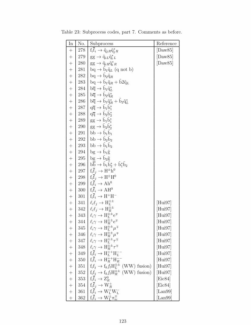
Table 23: Subprocess codes, part 7. Comments as before.

In No. Subprocess Reference

+ 278 fifi → qjRq∗jR [Daw85]

+ 279 gg → qiLq∗i L [Daw85]

+ 280 gg → qiRq∗i R [Daw85]

+ 281 bq → b1qL (q not b)

+ 282 bq → b2qR+ 283 bq → b1qR + b2qL+ 284 bq → b1q

∗L

+ 285 bq → b2q∗R

+ 286 bq → b1q∗R + b2q

∗L

+ 287 qq → b1b∗1

+ 288 qq → b2b∗2

+ 289 gg → b1b∗1

+ 290 gg → b2b∗2

+ 291 bb → b1b1

+ 292 bb → b2b2

+ 293 bb → b1b2

+ 294 bg → b1g

+ 295 bg → b2g

+ 296 bb → b1b∗2 + b∗

1b2

+ 297 fifj → H±h0

+ 298 fifj → H±H0

+ 299 fifi → Ah0

+ 300 fifi → AH0

+ 301 fifi → H+H−

+ 341 ℓiℓj → H±±L [Hui97]

+ 342 ℓiℓj → H±±R [Hui97]

+ 343 ℓiγ → H±±L e∓ [Hui97]

+ 344 ℓiγ → H±±R e∓ [Hui97]

+ 345 ℓiγ → H±±L µ∓ [Hui97]

+ 346 ℓiγ → H±±R µ∓ [Hui97]

+ 347 ℓiγ → H±±L τ∓ [Hui97]

+ 348 ℓiγ → H±±R τ∓ [Hui97]

+ 349 fifi → H++L H−−

L [Hui97]

+ 350 fifi → H++R H−−

R [Hui97]

+ 351 fifj → fkflH±±L (WW) fusion) [Hui97]

+ 352 fifj → fkflH±±R (WW) fusion) [Hui97]

+ 353 fifi → Z0R [Eic84]

+ 354 fifj → W+R [Eic84]

+ 361 fifi → W+L W−

L [Lan99]

+ 362 fifi → W±Lπ

∓tc [Lan99]

123

Table 24: Subprocess codes, part 8. Comments as before.

In No. Subprocess Reference

+ 363 fif i → π+tcπ

−tc [Lan99]

+ 364 fif i → γπ0tc [Lan99]

+ 365 fif i → γπ′0tc [Lan99]

+ 366 fif i → Z0π0tc [Lan99]

+ 367 fif i → Z0π′0tc [Lan99]

+ 368 fif i → W±π∓tc [Lan99]

+ 370 fifj → W±L Z0

L [Lan99]

+ 371 fifj → W±L π

0tc [Lan99]

+ 372 fifj → π±tcZ

0L [Lan99]

+ 373 fifj → π±tcπ

0tc [Lan99]

+ 374 fifj → γπ±tc [Lan99]

+ 375 fifj → Z0π±tc [Lan99]

+ 376 fifj → W±π0tc [Lan99]

+ 377 fifj → W±π′0tc [Lan99]

+ 391 ff → G∗ [Ran99]

+ 392 gg → G∗ [Ran99]

+ 393 qq → gG∗ [Ran99, Bij01]

+ 394 qg → qG∗ [Ran99, Bij01]

+ 395 gg → gG∗ [Ran99, Bij01]

In supersymmetric processes, antiparticles of sfermions are denoted by ∗, i.e. t∗ rather

than the more correct but cumbersome t or t.Charge-conjugate channels are always assumed included as well (where separate), and

processes involving a W+ also imply those involving a W−. Wherever Z0 is written, it isunderstood that γ∗ and γ∗/Z0 interference should be included as well (with possibilitiesto switch off either, if so desired). In some cases this is not fully implemented, see furtherbelow. Correspondingly, Z′0 denotes the complete set γ∗/Z0/Z′0 (or some subset of it).Thus the notation γ is only used for a photon on the mass shell.

In the last column of the tables below, references are given to works from whichformulae have been taken. Sometimes these references are to the original works on thesubject, sometimes only to the place where the formulae are given in the most convenientor accessible form, or where chance lead us. Apologies to all matrix-element calculatorswho are not mentioned. However, remember that this is not a review article on physicsprocesses, but only a way for readers to know what is actually found in the program, forbetter or worse. In several instances, errata have been obtained from the authors. Oftenthe formulae given in the literature have been generalized to include trivial radiativecorrections, Breit–Wigner line shapes with s-dependent widths (see section 7.3), etc.

The following sections contain some useful comments on the processes included in theprogram, grouped by physics interest rather than sequentially by ISUB or MSEL code (see9.2 for further information on the MSEL code). The different ISUB and MSEL codes that canbe used to simulate the different groups are given. ISUB codes within brackets indicatethe kind of processes that indirectly involve the given physics topic, although only as partof a larger whole. Some obvious examples, such as the possibility to produce jets in justabout any process, are not spelled out in detail.

124

The text at times contains information on which special switches or parameters are ofparticular interest to a given process. All these switches are described in detail in sections9.3 9.4 and 9.5, but are alluded to here so as to provide a more complete picture of thepossibilities available for the different subprocesses. However, the list of possibilities iscertainly not exhausted by the text below.

8.2 QCD Processes

Obviously most processes in Pythia contain QCD physics one way or another, so theabove title should not be overstressed. One example: a process like e+e− → γ∗/Z0 → qqis also traditionally called a QCD event, but is here book-kept as γ∗/Z0 production. Inthis section we discuss scatterings between coloured partons, plus a few processes thatare close relatives to other processes of this kind.

8.2.1 QCD jets

MSEL = 1, 2ISUB = 11 qiqj → qiqj

12 qiqi → qkqk13 qiqi → gg

28 qig → qig

53 gg → qkqk68 gg → gg

96 semihard QCD 2 → 2No higher-order processes are explicitly included, nor any higher-order loop corrections

to the 2 → 2 processes. However, by initial- and final-state QCD radiation, multijet eventsare being generated, starting from the above processes. The shower rate of multijetproduction is clearly uncertain by some amount, especially for well-separated jets.

A string-based fragmentation scheme such as the Lund model needs cross sections forthe different colour flows; these have been calculated in [Ben84] and differ from the usualcalculations by interference terms of the order 1/N2

C . By default, the standard colour-summed QCD expressions for the differential cross sections are used. In this case, theinterference terms are distributed among the various colour flows according to the polestructure of the terms. However, the interference terms can be excluded, by changingMSTP(34)

As an example, consider subprocess 28, qg → qg. The total cross section for thisprocess, obtained by summing and squaring the Feynman s-, t-, and u-channel graphs, is[Com77]

2

(

1 − us

t2

)

− 4

9

(

s

u+u

s

)

− 1 . (131)

(An overall factor πα2s/s

2 is ignored.) Using the identity of the Mandelstam variables forthe massless case, s+ t+ u = 0, this can be rewritten as

s2 + u2

t2− 4

9

(

s

u+u

s

)

. (132)

On the other hand, the cross sections for the two possible colour flows of this subprocessare [Ben84]

A :4

9

(

2u2

t2− u

s

)

;

125

B :4

9

(

2s2

t2− s

u

)

. (133)

Colour configuration A is one in which the original colour of the q annihilates with theanticolour of the g, the g colour flows through, and a new colour–anticolour is createdbetween the final q and g. In colour configuration B, the gluon anticolour flows through,but the q and g colours are interchanged. Note that these two colour configurations havedifferent kinematics dependence. For MSTP(34)=0, these are the cross sections actuallyused.

The sum of the A and B contributions is

8

9

s2 + u2

t2− 4

9

(

s

u+u

s

)

. (134)

The difference between this expression and that of [Com77], corresponding to the inter-ference between the two colour-flow configurations, is then

1

9

s2 + u2

t2, (135)

which can be naturally divided between colour flows A and B:

A :1

9

u2

t2;

B :1

9

s2

t2. (136)

For MSTP(34)=1, the standard QCD matrix element is therefore used, with the samerelative importance of the two colour configurations as above. Similar procedures arefollowed also for the other QCD subprocesses.

All the matrix elements in this group are for massless quarks (although final-statequarks are of course put on the mass shell). As a consequence, cross sections are divergentfor p⊥ → 0, and some kind of regularization is required. Normally you are expected toset the desired p⊥min value in CKIN(3).

The new flavour produced in the annihilation processes (ISUB = 12 and 53) is deter-mined by the flavours allowed for gluon splitting into quark–antiquark; see switch MDME.

Subprocess 96 is special among all the ones in the program. In terms of the basiccross section, it is equivalent to the sum of the other ones, i.e. 11, 12, 13, 28, 53 and 68.The phase space is mapped differently, however, and allows p⊥ as input variable. Thisis especially useful in the context of the multiple interactions machinery, see subsection11.2, where potential scatterings are considered in order of decreasing p⊥, with a formfactor related to the probability of not having another scattering with a p⊥ larger thanthe considered one. You are not expected to access process 96 yourself. Instead it isautomatically initialized and used either if process 95 is included or if multiple interactionsare switched on. The process will then appear in the maximization information output,but not in the cross section table at the end of a run. Instead, the hardest scatteringgenerated within the context of process 95 is reclassified as an event of the 11, 12, 13, 28,53 or 68 kinds, based on the relative cross section for these in the point chosen. Furthermultiple interactions, subsequent to the hardest one, also do not show up in cross sectiontables.

126

8.2.2 Heavy flavours

MSEL = 4, 5, 6, 7, 8ISUB = 81 qiqi → QkQk

82 gg → QkQk

(83) qifj → Qkfl(84) gγ → QkQk

(85) γγ → FkFkThe matrix elements in this group differ from the corresponding ones in the group

above in that they correctly take into account the quark masses. As a consequence, thecross sections are finite for p⊥ → 0. It is therefore not necessary to introduce any specialcuts.

The two first processes that appear here are the dominant lowest-order QCD graphsin hadron colliders — a few other graphs will be mentioned later, such as process 83.

The choice of flavour to produce is according to a hierarchy of options:1. if MSEL=4-8 then the flavour is set by the MSEL value;2. else if MSTP(7)=1-8 then the flavour is set by the MSTP(7) value;3. else the flavour is determined by the heaviest flavour allowed for gluon splitting into

quark–antiquark; see switch MDME.Note that only one heavy flavour is allowed at a time; if more than one is turned on inMDME, only the heaviest will be produced (as opposed to the case for ISUB = 12 and 53above, where more than one flavour is allowed simultaneously).

The lowest-order processes listed above just represent one source of heavy-flavour pro-duction. Heavy quarks can also be present in the parton distributions at the Q2 scaleof the hard interaction, leading to processes like Qg → Qg, so-called flavour excitation,or they can be created by gluon splittings g → QQ in initial- or final-state shower evo-lution. The implementation and importance of these various production mechanisms isdiscussed in detail in [Nor98]. In fact, as the c.m. energy is increased, these other pro-cesses gain in importance relative to the lowest-order production graphs above. As asexample, only 10%–20% of the b production at LHC energies come from the lowest-ordergraphs. The figure is even smaller for charm, while it is well above 50% for top. At LHCenergies, the specialized treatment described in this section is therefore only of interestfor top (and potential fourth-generation quarks) — the higher-order corrections can herebe approximated by an effective K factor, except possibly in some rare corners of phasespace.

For charm and bottom, on the other hand, it is necessary to simulate the full eventsample (within the desired kinematics cuts), and then only keep those events that containb/c, be that either from lowest-order production, or flavour excitation, or gluon splitting.Obviously this may be a time-consuming enterprise — although the probability for a high-p⊥ event at collider energies to contain (at least) one charm or bottom pair is fairly large,most of these heavy flavours are carrying a small fraction of the total p⊥ flow of the jets,and therefore do not survive normal experimental cuts. We note that the lowest-orderproduction of charm or bottom with processes 12 and 53, as part of the standard QCDmix, is now basically equivalent with that offered by processes 81 and 82. For 12 vs. 81this is rather trivial, since only s-channel gluon exchange is involved, but for process 53it requires a separate evaluation of massive matrix elements for c and b in the flavourloop. This is performed by retaining the s and θ values already preliminarily selected forthe massless kinematics, and recalculating t and u with mass effects included. Some ofthe documentation information in PARI does not properly reflect this recalculation, butthat is purely a documentation issue. Also process 96, used internally for the total QCDjet cross section, includes c and b masses. Only the hardest interaction in a multipleinteractions scenario may contain c/b, however, for technical reasons, so that the total

127

rate may be underestimated. (Quite apart from other uncertainties, of course.)As an aside, it is not only for the lowest-order graphs that events may be generated

with a guaranteed heavy-flavour content. One may also generate the flavour excitationprocess by itself, in the massless approximation, using ISUB = 28 and setting the KFINarray appropriately. No trick exists to force the gluon splittings without introducingundesirable biases, however. In order to have it all, one therefore has to make a full QCDjets run, as already noted.

Also other processes can generate heavy flavours, all the way up to top, but thenwithout a proper account of masses. By default, top production is switched off in thoseprocesses where a new flavour pair is produced at a gluon or photon vertex, i.e. 12, 53, 54,58, 96 and 135–140, while charm and bottom is allowed. These defaults can be changedby setting the MDME(IDC,1) values of the appropriate g or γ ‘decay channels’, see furtherbelow.

The cross section for a heavy quark pair close to threshold can be modified accordingto the formulae of [Fad90], see MSTP(35). Here threshold effects due to QQ bound-stateformation are taken into account in a smeared-out, average sense. Then the naıve crosssection is multiplied by the squared wave function at the origin. In a colour-singlet channelthis gives a net enhancement of the form

|Ψ(s)(0)|2 =X(s)

1 − exp(−X(s)), where X(s) =

4

3

παs

β, (137)

where β is the quark velocity, while in a colour octet channel there is a net suppressiongiven by

|Ψ(8)(0)|2 =X(8)

exp(−X(8)) − 1, where X(8) =

1

6

παs

β. (138)

The αs factor in this expression is related to the energy scale of bound-state formation;it is selected independently from the one of the standard production cross section. Thepresence of a threshold factor affects the total rate and also kinematical distributions.

Heavy flavours, i.e. top and fourth generation, are assumed to be so short-lived thatthey decay before they have time to hadronize. This means that the light quark in thedecay Q → W±q inherits the colour of the heavy one. The current Pythia descriptionrepresents a change of philosophy compared to older versions, formulated at a time whenthe top was thought to be much lighter than we now know it to be. For event shapes thedifference between the two time orderings normally has only marginal effects [Sjo92a].

It should be noted that cross section calculations are different in the two cases. Thetop (or a fourth generation fermion) is assumed short-lived, and is treated like a resonancein the sense of section 7.6.2, i.e. the cross-section is reduced so as only to correspond tothe channels left open by you. This also includes the restrictions on secondary decays,i.e. on the decays of a W+ or a H+ produced in the top decay. For b and c quarks, whichare long-lived enough to form hadrons, no such reduction takes place. Branching ratiosthen have to be folded in by hand to get the correct cross sections. The logic behind thisdifference is that when hadronization takes place, one would normally decay the D0 andD+ meson according to different branching ratios. But which D mesons are to be formedis not known at the bottom quark creation, so one could not weight for that. For a tquark, which decays rapidly, this ambiguity does not exist, and so a reduction factor canbe introduced directly coupled to the t quark production process.

This rule about cross-section calculations applies to all the processes explicitly set upto handle heavy flavour creation. In addition to the ones above, this means all the ones inTables 17–24 where the fermion final state is given as capital letters (‘Q’ and ‘F’) and alsoflavours produced in resonance decays (Z0, W±, h0, etc., including processes 165 and 166).However, heavy flavours could also be produced in a process such as 31, qig → qkW

±,where qk could be a top quark. In this case, the thrust of the description is clearly on

128

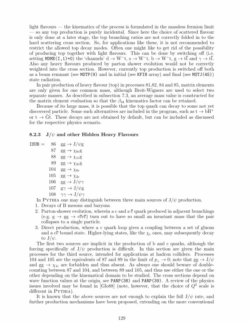
light flavours — the kinematics of the process is formulated in the massless fermion limit— so any top production is purely incidental. Since here the choice of scattered flavouris only done at a later stage, the top branching ratios are not correctly folded in to thehard scattering cross section. So, for applications like these, it is not recommended torestrict the allowed top decay modes. Often one might like to get rid of the possibilityof producing top together with light flavours. This can be done by switching off (i.e.setting MDME(I,1)=0) the ‘channels’ d → W−t, s → W−t, b → W−t, g → tt and γ → tt.Also any heavy flavours produced by parton shower evolution would not be correctlyweighted into the cross section. However, currently top production is switched off bothas a beam remnant (see MSTP(9) and in initial (see KFIN array) and final (see MSTJ(45))state radiation.

In pair production of heavy flavour (top) in processes 81,82, 84 and 85, matrix elementsare only given for one common mass, although Breit-Wigners are used to select twoseparate masses. As described in subsection 7.3, an average mass value is constructed forthe matrix element evaluation so that the β34 kinematics factor can be retained.

Because of its large mass, it is possible that the top quark can decay to some not yetdiscovered particle. Some such alternatives are included in the program, such as t → bH+

or t → Gt. These decays are not obtained by default, but can be included as discussedfor the respective physics scenario.

8.2.3 J/ψ and other Hidden Heavy Flavours

ISUB = 86 gg → J/ψg

87 gg → χ0cg

88 gg → χ1cg

89 gg → χ2cg

104 gg → χ0c

105 gg → χ2c

106 gg → J/ψγ

107 gγ → J/ψg

108 γγ → J/ψγIn Pythia one may distinguish between three main sources of J/ψ production.

1. Decays of B mesons and baryons.2. Parton-shower evolution, wherein a c and a c quark produced in adjacent branchings

(e.g. g → gg → cccc) turn out to have so small an invariant mass that the paircollapses to a single particle.

3. Direct production, where a c quark loop gives a coupling between a set of gluonsand a cc bound state. Higher-lying states, like the χc ones, may subsequently decayto J/ψ.

The first two sources are implicit in the production of b and c quarks, although theforcing specifically of J/ψ production is difficult. In this section are given the mainprocesses for the third source, intended for applications at hadron colliders. Processes104 and 105 are the equivalents of 87 and 89 in the limit of p⊥ → 0; note that gg → J/ψand gg → χ1c are forbidden and thus absent. As always one should beware of double-counting between 87 and 104, and between 89 and 105, and thus use either the one or theother depending on the kinematical domain to be studied. The cross sections depend onwave function values at the origin, see PARP(38) and PARP(39). A review of the physicsissues involved may be found in [Glo88] (note, however, that the choice of Q2 scale isdifferent in Pythia).

It is known that the above sources are not enough to explain the full J/ψ rate, andfurther production mechanisms have been proposed, extending on the more conventional

129

treatment here [Can97].While programmed for the charm system, it would be straightforward to apply these

processes instead to bottom mesons. One needs to change the codes of states produced,which is achieved by KFPR(ISUB,1)=KFPR(ISUB,1)+110 for the processes ISUB above,and changing the values of the wave functions at the origin, PARP(38) and PARP(39).

8.2.4 Minimum bias

MSEL = 1, 2ISUB = 91 elastic scattering

92 single diffraction (AB → XB)

93 single diffraction (AB → AX)

94 double diffraction

95 low-p⊥ productionThese processes are briefly discussed in section 7.7. They are mainly intended for

interactions between hadrons, although one may also consider γp and γγ interactions inthe options where the incoming photon(s) is (are) assumed resolved.

Uncertainties come from a number of sources, e.g. from the parameterizations of thevarious cross sections and slope parameters.

In diffractive scattering, the structure of the selected hadronic system may be regulatedwith MSTP(101). No high-p⊥ jet production in diffractive events is included so far.

The subprocess 95, low-p⊥ events, is somewhat unique in that no meaningful physicalborder-line to high-p⊥ events can be defined. Even if the QCD 2 → 2 high-p⊥ processesare formally switched off, some of the generated events will be classified as belonging tothis group, with a p⊥ spectrum of interactions to match the ‘minimum-bias’ event sample.The generation of such jets is performed with the help of the auxiliary subprocess 96, seesubsection 8.2.1. Only with the option MSTP(82)=0 will subprocess 95 yield strictly low-p⊥ events, events which will then probably not be compatible with any experimental data.A number of options exist for the detailed structure of low-p⊥ events, see in particularMSTP(81) and MSTP(82). Further details on the model(s) for minimum-bias events arefound in section 11.2.

8.3 Physics with Incoming Photons

With recent additions, the machinery for photon physics has become rather extensive[Fri00]. The border between the physics of real photon interactions and of virtual photonones is now bridged by a description that continuously interpolates between the twoextremes, as summarized in section 7.7.2. Furthermore, the ’gamma/lepton’ option (wherelepton is to be replaced by e-, e+, mu-, mu+, tau- or tau+ as the case may be) in a PYINITcall gives access to an internally generated spectrum of photons of varying virtuality.The CKIN(61) - CKIN(78) variables can be used to set experimentally motivated x andQ2 limits on the photon fluxes. With this option, and the default MSTP(14)=30, oneautomatically obtains a realistic first approximation to ‘all’ QCD physics of γ∗p and γ∗γ∗

interactions. The word ‘all’ clearly does not mean that a perfect description is guaranteed,or that all issues are addressed, but rather that the intention is to simulate all processesthat give a significant contribution to the total cross section in whatever Q2 range is beingstudied: jets, low-p⊥ events, elastic and diffractive scattering, etc.

The material to be covered encompasses many options, several of which have beensuperseded by further developments but have been retained for backwards compatibility.Therefore it is here split into three sections. The first covers the physics of real photonsand the subsequent one that of (very) virtual ones. Thereafter, in the final section, thethreads are combined into a machinery applicable at all Q2.

130

8.3.1 Photoproduction and γγ physics

MSEL = 1, 2, 4, 5, 6, 7, 8ISUB = 33 qiγ → qig

34 fiγ → fiγ

54 gγ → qkqk58 γγ → fkfk80 qiγ → qkπ

±

84 gγ → QkQk

85 γγ → FkFkAn (almost) real photon has both a point-like component and a hadron-like one. This

means that several classes of processes may be distinguished, see section 7.7.2.1. The processes listed above are possible when the photon interacts as a point-like

particle, i.e. couples directly to quarks and leptons.2. When the photon acts like a hadron, i.e. is resolved in a partonic substructure,

then high-p⊥ parton–parton interactions are possible, as described in sections 8.2.1and 8.4.1. These interactions may be further subdivided into VMD and anomalous(GVMD) ones [Sch93, Sch93a].

3. A hadron-like photon can also produce the equivalent of the minimum bias processesof section 8.2.4. Again, these can be subdivided into VMD and GVMD (anomalous)ones.

For γp events, we believe that the best description can be obtained when three separateevent classes are combined, one for direct, one for VMD and one for GVMD/anomalousevents, see the detailed description in [Sch93, Sch93a]. These correspond to MSTP(14)being 0, 2 and 3, respectively. The direct component is high-p⊥ only, while VMD andGVMD contain both high-p⊥ and low-p⊥ events. The option MSTP(14)=1 combines theVMD and GVMD/anomalous parts of the photon into one single resolved photon concept,which therefore is less precise than the full subdivision.

When combining three runs to obtain the totality of γp interactions, to the best ofour knowledge, it is necessary to choose the p⊥ cut-offs with some care, so as to representthe expected total cross section.

• The direct processes by themselves only depend on the CKIN(3) cut-off of the gener-ation. In older program versions the preferred value was 0.5 GeV [Sch93, Sch93a]. Inthe more recent description in [Fri00], also eikonalization of direct with anomalousinteractions into the GVMD event class is considered. That is, given a branchingγ → qq, direct interactions are viewed as the low-p⊥ events and anomalous ones ashigh-p⊥ events that have to merge smoothly. Then the CKIN(3) cut-off is increasedto the p⊥min of multiple interactions processes, see PARP(81) (or PARP(82), depend-ing on minijet unitarization scheme). See MSTP(18) for a possibility to switch backto the older behaviour. However, full backwards compatibility cannot be assured,so the older scenarios are better simulated by using an older Pythia version.

• The VMD processes work as ordinary hadron–hadron ones, i.e. one obtains bothlow- and high-p⊥ events by default, with dividing line set by p⊥min above.

• Also the GVMD processes work like the VMD ones. Again this is a change fromprevious versions, where the anomalous processes only contained high-p⊥ physicsand the low-p⊥ part was covered in the direct event class. See MSTP(15)=5 for apossibility to switch back to the older behaviour, with comments as above for thedirect class. A GVMD state is book-kept as a diffractive state in the event listing,even when it scatters ‘elastically’, since the subsequent hadronization descriptionsare very similar.

The processes in points 1 and 2 can be simulated with a photon beam, i.e. when’gamma’ appears as argument in the PYINIT call. It is then necessary to use option

131

MSTP(14) to switch between a point-like and a resolved photon — it is not possible tosimulate the two sets of processes in a single run. This would be the normal mode ofoperation for beamstrahlung photons, which have Q2 = 0 but with a nontrivial energyspectrum that would be provided by some external routine.

For bremsstrahlung photons, the x and Q2 spectrum can be simulated internally, withthe ’gamma/lepton’ argument in the PYINIT call. This is the recommended procedure,wherein direct and resolved processes can be mixed. An older — now not recommended— alternative is to use a parton-inside-electron structure function concept, obtainablewith a simple ’e-’ (or other lepton) argument in PYINIT. To access these quark andgluon distributions inside the photon (itself inside the electron), MSTP(12)=1 must thenbe used. Also the default value MSTP(11)=1 is required for the preceding step, that offinding photons inside the electron. Also here the direct and resolved processes may begenerated together. However, this option only works for high-p⊥ physics. It is not possibleto have also the low-p⊥ physics (including multiple interactions in high-p⊥ events) for anelectron beam. Kindly note that subprocess 34 contains both the scattering of an electronoff a photon and the scattering of a quark (inside a photon inside an electron) off a photon;the former can be switched off with the help of the KFIN array.

If you are only concerned with standard QCD physics, the option MSTP(14)=10or the default MSTP(14)=30 gives an automatic mixture of the VMD, direct andGVMD/anomalous event classes. The mixture is properly given according to the rel-ative cross sections. Whenever possible, this option is therefore preferable in terms ofuser-friendliness. However, it can only work because of a completely new layer of admin-istration, not found anywhere else in Pythia. For instance, a subprocess like qg → qgis allowed in several of the classes, but appears with different sets of parton distributionsand different p⊥ cut-offs in each of these, so that it is necessary to switch gears betweeneach event in the generation. It is therefore not possible to avoid a number of restrictionson what you can do in this case:

• The MSTP(14)=10 and =30 options can only be used for incoming photon beams,with or without convolution with the bremsstrahlung spectrum, i.e. when ’gamma’or ’gamma/lepton’ is the argument in the PYINIT call.

• The machinery has only been set up to generate standard QCD physics, specificallyeither ‘minimum-bias’ one or high-p⊥ jets. There is thus no automatic mixing ofprocesses only for heavy-flavour production, say, or of some exotic particle. Forminimum bias, you are not allowed to use the CKIN variables at all. This is not amajor limitation, since it is in the spirit of minimum-bias physics not to impose anyconstraints on allowed jet production. (If you still do, these cuts will be ineffectivefor the VMD processes but take effect for the other ones, giving inconsistencies.) Theminimum-bias physics option is obtained by default; by switching from MSEL=1 toMSEL=2 also the elastic and diffractive components of the VMD and GVMD parts areincluded. High-p⊥ jet production is obtained by setting the CKIN(3) cut-off largerthan the p⊥min(W 2) of the multiple interactions scenario. For lower input CKIN(3)values the program will automatically switch back to minimum-bias physics.

• Multiple interactions become possible in both the VMD and GVMD sector, withthe average number of interactions given by the ratio of the jet to the total crosssection. Currently only the simpler default scenario MSTP(82)=1 is implemented,however, i.e. the more sophisticated variable-impact-parameter ones need furtherphysics studies and model development.

• Some variables are internally recalculated and reset, notably CKIN(3). This is be-cause it must have values that depend on the component studied. It can thereforenot be modified without changing PYINPR and recompiling the program, which ob-viously is a major exercise.

• Pileup events are not at all allowed.Also, a warning about the usage of Pdflib for photons. So long as MSTP(14)=1, i.e.

132

the photon is not split up, Pdflib is accessed by MSTP(56)=2 and MSTP(55) as the partondistribution set. However, when the VMD and anomalous pieces are split, the VMD partis based on a rescaling of pion distributions by VMD factors (except for the SaS sets, thatalready come with a separate VMD piece). Therefore, to access Pdflib for MSTP(14)=10,it is not correct to set MSTP(56)=2 and a photon distribution in MSTP(55). Instead, oneshould put MSTP(56)=2, MSTP(54)=2 and a pion distribution code in MSTP(53), whileMSTP(55) has no function. The anomalous part is still based on the SaS parameterization,with PARP(15) as main free parameter.

Currently, hadrons are not defined with any photonic content. None of the processesare therefore relevant in hadron–hadron collisions. In ep collisions, the electron can emitan almost real photon, which may interact directly or be resolved. In e+e− collisions, onemay have direct, singly-resolved or doubly-resolved processes.

The γγ equivalent to the γp description involves six different event classes, see section7.7.2. These classes can be obtained by setting MSTP(14) to 0, 2, 3, 5, 6 and 7, respectively.If one combines the VMD and anomalous parts of the parton distributions of the photon,in a more coarse description, it is enough to use the MSTP(14) options 0, 1 and 4. Thecut-off procedures follows from the ones used for the γp ones above.

As with γp events, the options MSTP(14)=10 or MSTP(14)=30 give a mixture of the sixpossible γγ event classes. The same complications and restrictions exist here as alreadylisted above.

Process 54 generates a mixture of quark flavours; allowed flavours are set by the gluonMDME values. Process 58 can generate both quark and lepton pairs, according to theMDME values of the photon. Processes 84 and 85 are variants of these matrix elements,with fermion masses included in the matrix elements, but where only one flavour canbe generated at a time. This flavour is selected as described for processes 81 and 82in section 8.2.2, with the exception that for process 85 the ‘heaviest’ flavour allowed forphoton splitting takes to place of the heaviest flavour allowed for gluon splitting. Sincelepton KF codes come after quark ones, they are counted as being ‘heavier’, and thus takeprecedence if they have been allowed.

Process 80 is a higher twist one. The theory for such processes is rather shaky, soresults should not be taken too literally. The messy formulae given in [Bag82] havenot been programmed in full, instead the pion form factor has been parameterized asQ2Fπ(Q2) ≈ 0.55/ lnQ2, with Q in GeV.

8.3.2 Deeply Inelastic Scattering and γ∗γ∗ physics

MSEL = 1, 2, 35, 36, 37, 38ISUB = 10 fifj → fkfl

83 qifj → Qkfl99 γ∗q → q

131 fiγ∗T → fig

132 fiγ∗L → fig

133 fiγ∗T → fiγ

134 fiγ∗L → fiγ

135 gγ∗T → fifi136 gγ∗L → fifi137 γ∗Tγ

∗T → fif i

138 γ∗Tγ∗L → fif i

139 γ∗Lγ∗T → fif i

140 γ∗Lγ∗L → fif i

Among the processes in this section, 10 and 83 are intended to stand on their own,

133

while the rest are part of the newer machinery for γ∗p and γ∗γ∗ physics. We thereforeseparate the description in this section into these two main parts.

The Deeply Inelastic Scattering (DIS) processes, i.e. t-channel electroweak gauge bosonexchange, are traditionally associated with interactions between a lepton or neutrino anda hadron, but processes 10 and 83 can equally well be applied for qq scattering in hadroncolliders (with a cross section much smaller than corresponding QCD processes, however).If applied to incoming e+e− beams, process 10 corresponds to Bhabha scattering.

For process 10 both γ, Z0 and W± exchange contribute, including interference betweenγ and Z0. The switch MSTP(21) may be used to restrict to only some of these, e.g. neutralor charged current only.

The option MSTP(14)=10 (see previous section) has now been extended so that it alsoworks for DIS of an electron off a (real) photon, i.e. process 10. What is obtained isa mixture of the photon acting as a vector meson and it acting as an anomalous state.This should therefore be the sum of what can be obtained with MSTP(14)=2 and =3. Itis distinct from MSTP(14)=1 in that different sets are used for the parton distributions— in MSTP(14)=1 all the contributions to the photon distributions are lumped together,while they are split in VMD and anomalous parts for MSTP(14)=10. Also the beamremnant treatment is different, with a simple Gaussian distribution (at least by default)for MSTP(14)=1 and the VMD part of MSTP(14)=10, but a powerlike distribution dk2⊥/k

2⊥

between PARP(15) and Q for the anomalous part of MSTP(14)=10.To access this option for e and γ as incoming beams, it is only necessary to set

MSTP(14)=10 and keep MSEL at its default value. Unlike the corresponding option for γpand γγ, no cuts are overwritten, i.e. it is still your responsibility to set these appropriately.

Cuts especially appropriate for DIS usage include either CKIN(21)-CKIN(22) orCKIN(23)-CKIN(24) for the x range (former or latter depending on which side is theincoming real photon), CKIN(35)-CKIN(36) for the Q2 range, and CKIN(39)-CKIN(40)for the W 2 range.

In principle, the DIS x variable of an event corresponds to the x value stored inPARI(33) or PARI(34), depending on which side the incoming hadron is on, while theDIS Q2 = −t =-PARI(15). However, just like initial- and final-state radiation can shiftjet momenta, they can modify the momentum of the scattered lepton. Therefore the DISx and Q2 variables are not automatically conserved. An option, on by default, exists inMSTP(23), where the event can be ‘modified back’ so as to conserve x and Q2, but thisoption is rather primitive and should not be taken too literally.

Process 83 is the equivalent of process 10 for W± exchange only, but with the heavy-quark mass included in the matrix element. In hadron colliders it is mainly of interest forthe production of very heavy flavours, where the possibility of producing just one heavyquark is kinematically favoured over pair production. The selection of the heavy flavouris already discussed in section 8.2.2.

Turning to the other processes, part of the γ∗p and γ∗γ∗ process-mixing machineries,99 has close similarities with the above discussed 10 one. Whereas 10 would simulate thefull process eq → eq, 99 assumes a separate machinery for the flux of virtual photons,e → eγ∗ and only covers the second half of the process, γ∗q → q. One limitation of thisfactorization is that only virtual photons are considered in process 99, not contributionsfrom the Z0 neutral current or the W± charged current.

Note that 99 has no correspondence in the real-photon case, but has to vanish inthis limit by gauge invariance, or indeed by simple kinematics considerations. This, plusthe desire to avoid double-counting with real-photon physics processes, is why the crosssection for this process is explicitly made to vanish for photon virtuality Q2 → 0, eq. (127),also when parton distributions have not been constructed to fulfil this, see MSTP(19). (Nosuch safety measures are present in 10, again illustrating how the two are intended mainlyto be used at large or at small Q2, respectively.)

For a virtual photon, processes 131–136 may be viewed as first-order corrections to

134

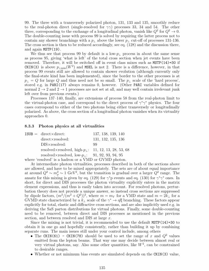
99. The three with a transversely polarized photon, 131, 133 and 135, smoothly reduceto the real-photon direct (single-resolved for γγ) processes 33, 34 and 54. The otherthree, corresponding to the exchange of a longitudinal photon, vanish like Q2 for Q2 → 0.The double-counting issue with process 99 is solved by requiring the latter process not tocontain any shower branchings with a p⊥ above the lower p⊥ cut-off of processes 131-136.The cross section is then to be reduced accordingly, see eq. (128) and the discussion there,and again MSTP(19).

We thus see that process 99 by default is a low-p⊥ process in about the same senseas process 95, giving ‘what is left’ of the total cross section when jet events have beenremoved. Therefore, it will be switched off in event class mixes such as MSTP(14)=30 ifCKIN(3) is above p⊥min(W

2) and MSEL is not 2. There is a difference, however, in thatprocess 99 events still are allowed to contain shower evolution (although currently onlythe final-state kind has been implemented), since the border to the other processes is atp⊥ = Q for large Q and thus need not be so small. The p⊥ scale of the ‘hard process’,stored e.g. in PARI(17) always remains 0, however. (Other PARI variables defined fornormal 2 → 2 and 2 → 1 processes are not set at all, and may well contain irrelevant junkleft over from previous events.)

Processes 137–140, finally, are extensions of process 58 from the real-photon limit tothe virtual-photon case, and correspond to the direct process of γ∗γ∗ physics. The fourcases correspond to either of the two photons being either transversely or longitudinallypolarized. As above, the cross section of a longitudinal photon vanishes when its virtualityapproaches 0.

8.3.3 Photon physics at all virtualities

ISUB = direct×direct: 137, 138, 139, 140

direct×resolved: 131, 132, 135, 136

DIS×resolved: 99

resolved×resolved, high-p⊥: 11, 12, 13, 28, 53, 68

resolved×resolved, low-p⊥: 91, 92, 93, 94, 95where ‘resolved’ is a hadron or a VMD or GVMD photon.

At intermediate photon virtualities, processes described in both of the sections aboveare allowed, and have to be mixed appropriately. The sets are of about equal importanceat around Q2 ∼ m2

ρ ∼ 1 GeV2, but the transition is gradual over a larger Q2 range. Theansatz for this mixing is given by eq. (129) for γ∗p events and eq. (130) for γ∗γ∗ ones. Inshort, for direct and DIS processes the photon virtuality explicitly enters in the matrixelement expressions, and thus is easily taken into account. For resolved photons, pertur-bation theory does not provide a unique answer, so instead cross sections are suppressedby dipole factors, (m2/(m2 +Q2))2, where m = mV for a VMD state and m = 2k⊥ for aGVMD state characterized by a k⊥ scale of the γ∗ → qq branching. These factors appearexplicitly for total, elastic and diffractive cross sections, and are also implicitly used e.g. inderiving the SaS parton distributions for virtual photons. Finally, some double-countingneed to be removed, between direct and DIS processes as mentioned in the previoussection, and between resolved and DIS at large x.

Since the mixing is not trivial, it is recommended to use the default MSTP(14)=30 toobtain it in one go and hopefully consistently, rather than building it up by combiningseparate runs. The main issues still under your control include, among others

• The CKIN(61) - CKIN(78) should be used to set the range of x and Q2 valuesemitted from the lepton beams. That way one may decide between almost real orvery virtual photons, say. Also some other quantities, like W 2, can be constrainedto desirable ranges.

• Whether or not minimum bias events are simulated depends on the CKIN(3) value,

135

just like in hadron physics. The only difference is that the initialization energy scaleWinit is selected in the allowed W range rather than to be the full c.m. energy.For a high CKIN(3), CKIN(3)> p⊥min(W

2init), only jet production is included. Then

further CKIN values can be set to constrain e.g. the rapidity of the jets produced.For a low CKIN(3), CKIN(3)< p⊥min(W

2init), like the default value CKIN(3) = 0,

low-p⊥ physics is switched on together with jet production, with the latter properlyeikonalized to be lower than the total one. The ordinary CKIN cuts, not related tothe photon flux, cannot be used here.For a low CKIN(3), when MSEL=2 instead of the default =1, also elastic and diffractiveevents are simulated.

• The impact of resolved longitudinal photons is not unambiguous, e.g. only recentlythe first parameterization of parton distributions appeared [Chy00]. Different simplealternatives can be probed by changing MSTP(17) and associated parameters.

• The choice of scales to use in parton distributions for jet rates is always ambiguous,but depends on even more scales for virtual photons than in hadronic collisions.MSTP(32) allows a choice between several alternatives.

• The matching of p⊥ generation by shower evolution to that by primordial k⊥ is ageneral problem, for photons with an additional potential source in the γ∗ → qqvertex. MSTP(66) offer some alternatives.

• PARP(15) is the k0 parameter separating VMD from GVMD.• PARP(18) is the kρ parameter in GVMD total cross sections.• MSTP(16) selects the momentum variable for an e → eγ∗ branching.• MSTP(18) regulates the choice of p⊥min for direct processes.• MSTP(19) regulates the choice of partonic cross section in process 99, γ∗q → q.• MSTP(20) regulates the suppression of the resolved cross section at large x.

The above list is not complete, but gives some impression what can be done.

8.4 Electroweak Gauge Bosons

This section covers the production and/or exchange of γ, Z0 and W± gauge bosons, singlyand in pairs. The topic of longitudinal gauge-boson scattering at high energies is deferredto the Higgs section, since the presence or absence of a Higgs here makes a big difference.

8.4.1 Prompt photon production

MSEL = 10ISUB = 14 qiqi → gγ

18 fifi → γγ

29 qig → qiγ

114 gg → γγ

115 gg → gγIn hadron colliders, processes ISUB = 14 and 29 give the main source of single-γ

production, with ISUB = 115 giving an additional contribution which, in some kinematicsregions, may become important. For γ-pair production, the process ISUB = 18 is oftenovershadowed in importance by ISUB = 114.

Another source of photons is bremsstrahlung off incoming or outgoing quarks. Thishas to be treated on an equal footing with QCD parton showering. For time-like parton-shower evolution, i.e. in the final-state showering and in the side branches of the initial-state showering, photon emission may be switched on or off with MSTJ(41). Photonradiation off the space-like incoming quark legs is not yet included, but should be oflesser importance for production at reasonably large p⊥ values. Radiation off an incomingelectron is included in a leading-log approximation.

136

Warning: the cross sections for the box graphs 114 and 115 become very complicated,numerically unstable and slow when the full quark mass dependence is included. For quarkmasses much below the s scale, the simplified massless expressions are therefore used— a fairly accurate approximation. However, there is another set of subtle numericalcancellations between different terms in the massive matrix elements in the region ofsmall-angle scattering. The associated problems have not been sorted out yet. Thereare therefore two possible solutions. One is to use the massless formulae throughout.The program then becomes faster and numerically stable, but does not give, for example,the characteristic dip (due to destructive interference) at top threshold. This is thecurrent default procedure, with five flavours assumed, but this number can be changedin MSTP(38). The other possibility is to impose cuts on the scattering angle of the hardprocess, see CKIN(27) and CKIN(28), since the numerically unstable regions are when| cos θ| is close to unity. It is then also necessary to change MSTP(38) to 0.

8.4.2 Single W/Z production

MSEL = 11, 12, 13, 14, 15, (21)

ISUB = 1 fifi → γ∗/Z0

2 fifj → W+

15 fifi → g(γ∗/Z0)

16 fifj → gW+

19 fifi → γ(γ∗/Z0)

20 fifj → γW+

30 fig → fi(γ∗/Z0)

31 fig → fkW+

35 fiγ → fi(γ∗/Z0)

36 fiγ → fkW+

(141) fifi → γ/Z0/Z′0

This group consists of 2 → 1 processes, i.e. production of a single resonance, and2 → 2 processes, where the resonance is recoiling against a jet or a photon. The process141, which also is listed here, is described further elsewhere.

With initial-state showers turned on, the 2 → 1 processes also generate additional jets;in order to avoid double-counting, the corresponding 2 → 2 processes should therefore notbe turned on simultaneously. The basic rule is to use the 2 → 1 processes for inclusivegeneration of W/Z, i.e. where the bulk of the events studied have p⊥ ≪ mW/Z. With theintroduction of explicit matrix-element-inspired corrections to the parton shower [Miu99],also the high-p⊥ tail is well described in this approach, thus offering an overall gooddecription of the full p⊥ spectrum of gauge bosons [Bal01].

If one is interested in the high-p⊥ tail only, however, the generation efficiency will below. It is here better to start from the 2 → 2 matrix elements and add showers to these.However, the 2 → 2 matrix elements are divergent for p⊥ → 0, and should not be useddown to the low-p⊥ region, or one may get unphysical cross sections. As soon as thegenerated 2 → 2 cross section corresponds to a non-negligible fraction of the total 2 → 1one, say 10%–20%, Sudakov effects are likely to be affecting the shape of the p⊥ spectrumto a corresponding extent, and results should not be trusted.

The problems of double-counting and Sudakov effects apply not only to W/Z produc-tion in hadron colliders, but also to a process like e+e− → Z0γ, which clearly is part ofthe initial-state radiation corrections to e+e− → Z0 obtained for MSTP(11)=1. As is thecase for Z production in association with jets, the 2 → 2 process should therefore only beused for the high-p⊥ region.

The Z0 of subprocess 1 includes the full interference structure γ∗/Z0; via MSTP(43)

137

you can select to produce only γ∗, only Z0, or the full γ∗/Z0. The same holds true for theZ′0 of subprocess 141; via MSTP(44) any combination of γ∗, Z0 and Z′0 can be selected.Thus, subprocess 141 with MSTP(44)=4 is essentially equivalent to subprocess 1 withMSTP(43)=3; however, process 141 also includes the possibility of a decay into Higgses.Also processes 15, 19, 30 and 35 contain the full mixture of γ∗/Z0, with MSTP(43) availableto change this.

Note that process 1, with only qq → γ∗ → ℓ+ℓ− allowed, and studied in the regionwell below the Z0 mass, is what is conventionally called Drell–Yan. This latter processtherefore does not appear under a separate heading, but can be obtained by a suitablesetting of switches and parameters.

A process like fifj → γW+ is only included in the limit that the γ is emitted in the‘initial state’, while the possibility of a final-state radiation off the W+ decay products isnot explicitly included (but can be obtained implicitly by the parton-shower machinery)and various interference terms are not at all present. Some caution must therefore beexercised; see also section 8.4.3 for related comments.

For the 2 → 1 processes, the Breit–Wigner includes an s-dependent width, whichshould provide an improved description of line shapes. In fact, from a line-shape pointof view, process 1 should provide a more accurate simulation of e+e− annihilation eventsthan the dedicated e+e− generation scheme of PYEEVT (see section 6.1). Another differ-ence is that PYEEVT only allows the generation of γ∗/Z0 → qq, while process 1 additionallycontains γ∗/Z0 → ℓ+ℓ− and γ∗/Z0 → νν. The parton-shower and fragmentation descrip-tions are the same, but the process 1 implementation only contains a partial interface tothe first- and second-order matrix-element options available in PYEEVT, see MSTP(48).

All processes in this group have been included with the correct angular distributionin the subsequent W/Z → ff decays. In process 1 also fermion mass effects have been in-cluded in the angular distributions, while this is not the case for the other ones. Normallymass effects are not large anyway.

The process e+e− → e+e−Z0 can be simulated in two different ways. One is to makeuse of the e ‘sea’ distribution inside e, i.e. have splittings e → γ → e. This can beobtained, together with ordinary Z0 production, by using subprocess 1, with MSTP(11)=1and MSTP(12)=1. Then the contribution of the type above is 5.0 pb for a 500 GeV e+e−

collider, compared with the correct 6.2 pb [Hag91]. Alternatively one may use process 35,with MSTP(11)=1 and MSTP(12)=0. This process has a singularity in the forward direction,regularized by the electron mass and also sensitive to the virtuality of the photon. It istherefore among the few where the incoming masses have been included in the matrixelement expression. Nevertheless, it may be advisable to set small lower cut-offs, e.g.CKIN(3)=CKIN(5)=0.01, if one should experience problems (e.g. at higher energies).

Process 36, fγ → f ′W± may have corresponding problems; except that in e+e− theforward scattering amplitude for eγ → νW is killed (radiation zero), which means thatthe differential cross section is vanishing for p⊥ → 0. It is therefore feasible to use thedefault CKIN(3) and CKIN(5) values in e+e−, and one also comes closer to the correctcross section.

The process gg → Z0bb, formerly available as process 131, has been removedfrom the current version, since the implementation turned out to be slow and un-stable. However, process 1 with incoming flavours set to be bb (by KFIN(1,5)=KFIN(1,-5)=KFIN(2,5)=KFIN(2,-5)=1 and everything else =0) provides an alternativedescription, where the additional bb are generated by g → bb branchings in the initial-state showers. (Away from the low-p⊥ region, process 30 with KFIN values as above exceptthat also incoming gluons are allowed, offers yet another description. Here it is in termsof gb → Z0b, with only one further g → bb branching constructed by the shower.) Atfirst glance, the shower approach would seem less reliable than the full 2 → 3 matrix ele-ment. The relative lightness of the b quark will generate large logs of the type ln(m2

Z/m2b),

however, that ought to be resummed [Car00]. This is implicit in the parton-density ap-

138

proach of incoming b quarks but absent from the lowest-order gg → Z0bb matrix elements.Therefore actually the shower approach may be the more accurate of the two. Within thegeneral range of uncertainty of any leading-order description, at least it is not any worse.

8.4.3 W/Z pair production

MSEL = 15ISUB = 22 fif i → (γ∗/Z0)(γ∗/Z0)

23 fifj → Z0W+

25 fif i → W+W−

69 γγ → W+W−

70 γW+ → Z0W+

In this section we mainly consider the production of W/Z pairs by fermion–antifermionannihilation, but also include two processes which involve γ/W beams. Scatterings be-tween gauge-boson pairs, i.e. processes like W+W− → Z0Z0, depend so crucially on theassumed Higgs scenario that they are considered separately in section 8.5.2.

The cross sections used for the above processes are those derived in the narrow-widthlimit, but have been extended to include Breit–Wigner shapes with mass-dependentwidths for the final-state particles. In process 25, the contribution from Z0 exchangeto the cross section is now evaluated with the fixed nominal Z0 mass and width in thepropagator. If instead the actual mass and the running width were to be used, it gives adiverging cross section at large energies, by imperfect gauge cancellation.

However, one should realize that other graphs, not included here, can contribute inregions away from the W/Z mass. This problem is especially important if several flavourscoincide in the four-fermion final state. Consider, as an example, e+e− → µ+µ−νµνµ. Notonly would such a final state receive contributions from intermediate Z0Z0 and W+W−

states, but also from processes e+e− → Z0 → µ+µ−, followed either by µ+ → µ+Z0 →µ+νµνµ, or by µ+ → νµW+ → νµµ

+νµ. In addition, all possible interferences shouldbe considered. Since this is not done, the processes have to be used with some soundjudgement. Very often, one may wish to constrain a lepton pair mass to be close to mZ,in which case a number of the possible ‘other’ processes are negligible.

For the W pair production graph, one experimental objective is to do precision mea-surements of the cross section near threshold. Then also other effects enter. One such isCoulomb corrections, induced by photon exchange between the two W’s and their decayproducts. The gauge invariance issues induced by the finite W lifetime are not yet fullyresolved, and therefore somewhat different approximate formulae may be derived [Kho96].The options in MSTP(40) provide a reasonable range of uncertainty.

Of the above processes, the first contains the full fif i → (γ∗/Z0)(γ∗/Z0) structure,obtained by a straightforward generalization of the formulae in ref. [Gun86] (done by oneof the Pythia authors). Of course, the possibility of there being significant contributionsfrom graphs that are not included is increased, in particular if one γ∗ is very light andtherefore could be a bremsstrahlung-type photon. It is possible to use MSTP(43) to recoverthe pure Z0 case, i.e. fif i → Z0Z0 exclusively. In processes 23 and 70, only the pure Z0

contribution is included.Full angular correlations are included for the first three processes, i.e. the full 2 → 2 →

4 matrix elements are included in the resonance decays, including the appropriate γ∗/Z0

interference in process 22. In the latter two processes no spin information is currentlypreserved, i.e. the W/Z bosons are allowed to decay isotropically.

We remind you that the mass ranges of the two resonances may be set with theCKIN(41) - CKIN(44) parameters; this is particularly convenient, for instance, to pickone resonance almost on the mass shell and the other not.

139

8.5 Higgs Production

A fair fraction of all the processes in Pythia deal with Higgs production in one form oranother. This multiplication is caused by the need to consider production by several differ-ent processes, depending on Higgs mass and machine type. Further, the program containsa full two-Higgs-multiplet scenario, as predicted for example in the Minimal Supersym-metric extension of the Standard Model (MSSM). Therefore the continued discussion is,somewhat arbitrarily, subdivided into a few different scenarios. Doubly-charged Higgsparticles appear in left–right symmetric models, and are covered in section 8.6.3.

8.5.1 Light Standard Model Higgs

MSEL = 16, 17, 18ISUB = 3 fifi → h0

24 fifi → Z0h0

26 fifj → W+h0

102 gg → h0

103 γγ → h0

110 fifi → γh0

111 fifi → gh0

112 fig → fih0

113 gg → gh0

121 gg → QkQkh0

122 qiqi → QkQkh0

123 fifj → fifjh0 (Z0Z0 fusion)

124 fifj → fkflh0 (W+W− fusion)

In this section we discuss the production of a reasonably light Standard Model Higgs,below 700 GeV, say, so that the narrow width approximation can be used with someconfidence. Below 400 GeV there would certainly be no trouble, while above that thenarrow width approximation is gradually starting to break down.

In a hadron collider, the main production processes are 102, 123 and 124, i.e. gg, Z0Z0

and W+W− fusion. In the latter two processes, it is also necessary to take into accountthe emission of the space-like W/Z bosons off quarks, which in total gives the 2 → 3processes above.

Further processes of lower cross sections may be of interest because of easier signals.For instance, processes 24 and 26 give associated production of a Z or a W together withthe h0. There is also the processes 3 (see below), 121 and 122, which involve productionof heavy flavours.

Process 3 contains contributions from all flavours, but is completely dominated by thesubprocess tt → h0, i.e. by the contribution from the top sea distributions. Assuming,of course, that parton densities for top quarks are available, which is no longer the casein current parameterizations. This process is by now known to overestimate the crosssection for Higgs production as compared with a more careful calculation based on thesubprocess gg → tth0, process 121. The difference between the two is that in process 3the t and t are added by the initial-state shower, while in 121 the full matrix elementis used. The price to be paid is that the complicated multibody phase space in process121 makes the program run slower than with most other processes. As usual, it would bedouble-counting to include the same flavour both with 3 and 121. Process 122 is similarin structure to 121, but is less important. In both process 121 and 122 the producedquark is assumed to be a t; this can be changed in KFPR(121,2) and KFPR(122,2) beforeinitialization, however. For b quarks it could well be that process 3 with bb → h0 is more

140

reliable than process 121 with gg → bbh0 [Car00]; see the discussion on Z0bb final statesin section 8.4.2. Thus it would make sense to run with all quarks up to and including bsimulated in process 3 and then consider t quarks separately in process 121. Assumingno t parton densities, this would actually be the default behaviour, meaning that the twocould be combined in the same run without doublecounting.

The two subprocess 112 and 113, with a Higgs recoiling against a quark or gluonjet, are also effectively generated by initial-state corrections to subprocess 102. Thus, inorder to avoid double-counting, just as for the case of Z0/W+ production, section 8.4.2,these subprocesses should not be switched on simultaneously. Process 111, qq → gh0 isdifferent, in the sense that it proceeds through an s-channel gluon coupling to a heavy-quark loop, and that therefore the emitted gluon is necessary in the final state in order toconserve colours. It is not to be confused with a gluon-radiation correction to the Born-level process 3, qq → h0, since process 3 vanishes for massless quarks while process 111 ismainly intended for such. The lack of a matching Born-level process shows up by process111 being vanishing in the p⊥ → 0 limit. Numerically it is of negligible importance, exceptat very large p⊥ values. Process 102, possibly augmented by 111, should thus be usedfor inclusive production of Higgs, and 111–113 for the study of the Higgs subsample withhigh transverse momentum.

A warning is that the matrix-element expressions for processes 111–113 are verylengthy and the coding therefore more likely to contain some errors and numerical in-stabilities than for most other processes. Therefore the full expressions are only availableby setting the non-default value MSTP(38)=0. Instead the default is based on the sim-plified expressions obtainable if only the top quark contribution is considered, in themt → ∞ limit [Ell88]. As a slight improvement, this expression is rescaled by the ratioof the gg → h0 cross sections (or, equivalently, the h → gg partial widths) of the full cal-culation and that in the mt → ∞ limit. Simple checks show that this approach normallyagrees with the full expressions to within ∼ 20%, which is small compared with otheruncertainties. The agreement is worse for process 111 alone, about a factor of 2, but thisprocess is small anyway. We also note that the matrix element correction factors, used inthe initial-state parton shower for process 102, subsection 10.3.5, are based on the samemt → ∞ limit expressions, so that the high-p⊥ tail of process 102 is well matched to thesimple description of process 112 and 113.

In e+e− annihilation, associated production of an h0 with a Z0, process 24, is usuallythe dominant one close to threshold, while the Z0Z0 and W+W− fusion processes 123 and124 win out at high energies. Process 103, γγ fusion, may also be of interest, in particularwhen the possibilities of beamstrahlung photons and backscattered photons are included(see subsection 7.1.3). Process 110, which gives an h0 in association with a γ, is a loopprocess and is therefore suppressed in rate. It would have been of interest for a h0 massabove 60 GeV at LEP 1, since its phase space suppression there is less severe than for theassociated production with a Z0. Now it is not likely to be of any further interest.

The branching ratios of the Higgs are very strongly dependent on the mass. In prin-ciple, the program is set up to calculate these correctly, as a function of the actual Higgsmass, i.e. not just at the nominal mass. However, higher-order corrections may at timesbe important and not fully unambiguous; see for instance MSTP(37).

Since the Higgs is a spin-0 particle it decays isotropically. In decay processes suchas h0 → W+W−/Z0Z0 → 4 fermions angular correlations are included [Lin97]. Also inprocesses 24 and 26, Z0 and W± decay angular distributions are correctly taken intoaccount.

141

8.5.2 Heavy Standard Model Higgs

ISUB = 5 Z0Z0 → h0

8 W+W− → h0

71 Z0Z0 → Z0Z0 (longitudinal)

72 Z0Z0 → W+W− (longitudinal)

73 Z0W+ → Z0W+ (longitudinal)

76 W+W− → Z0Z0 (longitudinal)

77 W+W± → W+W± (longitudinal)Processes 5 and 8 are the simple 2 → 1 versions of what is now available in 123 and

124 with the full 2 → 3 kinematics. For low Higgs masses processes 5 and 8 overestimatethe correct cross sections and should not be used, whereas good agreement between the2 → 1 and 2 → 3 descriptions is observed when heavy Higgs production is studied.

The subprocesses 5 and 8, V V → h0, which contribute to the processes V V → V ′V ′,show a bad high-energy behaviour. Here V denotes a longitudinal intermediate gaugeboson, Z0 or W±. This can be cured only by the inclusion of all V V → V ′V ′ graphs, asis done in subprocesses 71, 72, 73, 76 and 77. In particular, subprocesses 5 and 8 giverise to a fictitious high-mass tail of the Higgs. If this tail is thrown away, however, theagreement between the s-channel graphs only (subprocesses 5 and 8) and the full set ofgraphs (subprocesses 71 etc.) is very good: for a Higgs of nominal mass 300 (800) GeV, acut at 600 (1200) GeV retains 95% (84%) of the total cross section, and differs from theexact calculation, cut at the same values, by only 2% (11%) (numbers for SSC energies).With this prescription there is therefore no need to use subprocesses 71 etc. rather thansubprocesses 5 and 8.

For subprocess 77, there is an option, see MSTP(45), to select the charge combinationof the scattering W’s: like-sign, opposite-sign (relevant for Higgs), or both.

Process 77 contains a divergence for p⊥ → 0 due to γ-exchange contributions. Thisleads to an infinite total cross section, which is entirely fictitious, since the simple parton-distribution function approach to the longitudinal W flux is not appropriate in this limit.For this process, it is therefore necessary to make use of a cut, e.g. p⊥ > mW.

For subprocesses 71, 72, 76 and 77, an option is included (see MSTP(46)) wherebyyou can select only the s-channel Higgs graph; this will then be essentially equivalent torunning subprocess 5 or 8 with the proper decay channels (i.e. Z0Z0 or W+W−) set viaMDME. The difference is that the Breit–Wigners in subprocesses 5 and 8 contain a mass-dependent width, whereas the width in subprocesses 71–77 is calculated at the nominalHiggs mass; also, higher-order corrections to the widths are treated more accurately insubprocesses 5 and 8. Further, processes 71–77 assume the incoming W/Z to be on themass shell, with associated kinematics factors, while processes 5 and 8 have W/Z correctlyspace-like. All this leads to differences in the cross sections by up to a factor of 1.5.

In the absence of a Higgs, the sector of longitudinal Z and W scattering will becomestrongly interacting at energies above 1 TeV. The models proposed by Dobado, Herreroand Terron [Dob91] to describe this kind of physics have been included as alternativematrix elements for subprocesses 71, 72, 73, 76 and 77, selectable by MSTP(46). Fromthe point of view of the general classification scheme for subprocesses, this kind of modelsshould appropriately be included as separate subprocesses with numbers above 100, butthe current solution allows a more efficient reuse of existing code. By a proper choice ofparameters, it is also here possible to simulate the production of a techni-ρ (see subsection8.6.7).

Currently, the scattering of transverse gauge bosons has not been included, neither thatof mixed transverse–longitudinal scatterings. These are expected to be less important athigh energies, and do not contain an h0 resonance peak, but need not be entirely negligiblein magnitude. As a rule of thumb, processes 71–77 should not be used for V V invariant

142

masses below 500 GeV.The decay products of the longitudinal gauge bosons are correctly distributed in angle.

8.5.3 Extended neutral Higgs sector

MSEL = 19ISUB = h0 H0 A0

3 151 156 fifi → X

102 152 157 gg → X

103 153 158 γγ → X

111 183 188 qq → gX

112 184 189 qg → qX

113 185 190 gg → gX

24 171 176 fifi → Z0X

26 172 177 fifj → W+X

123 173 178 fifj → fifjX (ZZ fusion)

124 174 179 fifj → fkflX (W+W− fusion)

121 181 186 gg → QkQkX

122 182 187 qiqi → QkQkXIn Pythia, the particle content of a two-Higgs-doublet scenario is included: two

neutral scalar particles, 25 and 35, one pseudoscalar one, 36, and a charged doublet, ±37.(Of course, these particles may also be associated with corresponding Higgs states inlarger multiplets.) By convention, we choose to call the lighter scalar Higgs h0 and theheavier H0. The pseudoscalar is called A0 and the charged H±. Charged-Higgs productionis covered in section 8.5.4.

A number of h0 processes have been duplicated for H0 and A0. The correspondencebetween ISUB numbers is shown in the table above: the first column of ISUB numberscorresponds to X = h0, the second to X = H0, and the third to X = A0. Note that severalof these processes are not expected to take place at all, owing to vanishing Born termcouplings. We have still included them for flexibility in simulating arbitrary couplingsat the Born or loop level, or for the case of mixing between the scalar and pseudoscalarsectors.

A few Standard Model Higgs processes have no correspondence in the scheme above.These include

• 5 and 8, which anyway have been superseded by 123 and 124;• 71, 72, 73, 76 and 77, which deal with what happens if there is no light Higgs, and

so is a scenario complementary to the one above, where several light Higgses areassumed; and

• 110, which is mainly of interest in Standard Model Higgs searches.The processes 111–113, 183–185 and 188–190 have only been worked out in full detail

for the Standard Model Higgs case, and not when e.g. squark loop contributions need beconsidered. The approximate procedure outlined in subsection 8.5.1, based on combiningthe kinematics shape from simple expressions in the mt → ∞ limit with a normalizationderived from the gg → X cross section, should therefore be viewed as a first ansatz only.In particular, it is not recommended to try the non-default MSTP(38)=0 option, which isincorrect beyond the Standard Model.

In processes 121, 122, 181, 182, 186 and 187 the recoiling heavy flavour is assumed tobe top, which is the only one of interest in the Standard Model, and the one where theparton-distribution-function approach invoked in processes 3, 151 and 156 is least reliable.However, it is possible to change the quark flavour in 121 etc.; for each process ISUB thisflavour is given by KFPR(ISUB,2). This may become relevant if couplings to bb states are

143

enhanced, e.g. if tan β ≫ 1 in the MSSM. The matrix elements in this group are basedon scalar Higgs couplings; differences for a pseudoscalar Higgs remains to be worked out.

By default, the h0 has the couplings of the Standard Model Higgs, while the H0

and A0 have couplings set in PARU(171) - PARU(178) and PARU(181) - PARU(190),respectively. The default values for the H0 and A0 have no deep physics motivation,but are set just so that the program will not crash due to the absence of any couplingswhatsoever. You should therefore set the above couplings to your desired values if youwant to simulate either H0 or A0. Also the couplings of the h0 particle can be modified,in PARU(161) - PARU(165), provided that MSTP(4) is set to 1.

For MSTP(4)=2, the mass of the h0 (in PMAS(25,1)) and the tan β value (in PARU(141))are used to derive the masses of the other Higgses, as well as all Higgs couplings.PMAS(35,1) - PMAS(37,1) and PARU(161) - PARU(195) are overwritten accordingly.The relations used are the ones of the Born-level MSSM [Gun90]. Loop corrections tothose expressions have been calculated within specific supersymmetric scenarios, and areknown to have a non-negligible effects on the resulting phenomenology. By switching onsupersymmetry simulation and setting parameters appropriately, one will gain access tothese mass formulae, see section 9.5.

Note that not all combinations of mh and tanβ are allowed; for MSTP(4)=2 the re-quirement of a finite A0 mass imposes the constraint

mh < mZtan2 β − 1

tan2 β + 1, (139)

or, equivalently,

tan2 β >mZ +mh

mZ −mh. (140)

If this condition is not fulfilled, the program will crash.A more realistic approach to the Higgs mass spectrum is to include radiative correc-

tions to the Higgs potential. Such a machinery has never been implemented as such inPythia, but appears as part of the Supersymmetry framework described in subsection 8.7.At tree level, the minimal set of inputs would be IMSS(1)=1 to switch on Susy, RMSS(5)to set the tanβ value (this overwrites the PARU(141) value when Susy is switched on)and RMSS(19) to set A0 mass. However, the significant radiative corrections depend onthe properties of all particles that couple to the Higgs boson, and the user may want tochange the default values of the relevant RMSS inputs. In practice, the most importantare those related indirectly to the physical masses of the third generation supersymmetricquarks and the Higgsino: RMSS(10) to set the left–handed doublet Susy mass parame-ter, RMSS(11) to set the right stop mass parameter, RMSS(12) to set the right sbottommass parameter, RMSS(4) to set the Higgsino mass and a portion of the squark mixing,and RMSS(16) and RMSS(17) to set the stop and bottom trilinear couplings, respectively,which specifies the remainder of the squark mixing. From these inputs, the Higgs massesand couplings would be derived. Note that switching on Susy also implies that Super-symmetric decays of the Higgs particles become possible if kinematically allowed. If youdo not want this to happen, you may want to increase the Susy mass parameters. (UseCALL PYSTAT(2) after initialization to see the list of branching ratios.)

Pair production of Higgs states may be a relevant source, see section 8.5.5 below.Finally, heavier Higgses may decay into lighter ones, if kinematically allowed, in pro-

cesses like A0 → Z0h0 or H+ → W+h0. Such modes are included as part of the generalmixture of decay channels, but they can be enhanced if the uninteresting channels areswitched off.

144

8.5.4 Charged Higgs sector

MSEL = 23ISUB = 143 fifj → H+

161 fig → fkH+

A charged Higgs doublet, H±, is included in the program. This doublet may be theone predicted in the MSSM scenario, see section 8.5.3, or in any other scenario. The tan βparameter, which is relevant also for charged Higgs couplings, is set via PARU(141) or, ifSusy is switched on, via RMSS(5).

The basic subprocess for charged Higgs production in hadron colliders is ISUB = 143.However, this process is dominated by tb → H+, and so depends on the choice of t partondistribution, if at all present. A better representation is provided by subprocess 161,fg → f ′H+; i.e. actually bg → tH+. It is therefore recommended to use 161 and not 143;to use both would be double-counting.

Pair production of Higgs states may be a relevant source, see section 8.5.5 below.A major potential source of charged Higgs production is top decay. It is possible to

switch on the decay channel t → bH+. Top will then decay to H+ a fraction of the time,whichever way it is produced. The branching ratio is automatically calculated, based onthe tanβ value and masses. It is possible to only have the H+ decay mode switched on,in which case the cross section is reduced accordingly.

8.5.5 Higgs pairs

ISUB = (141) fifi → γ/Z0/Z′0

297 fifj → H±h0

298 fifj → H±H0

299 fifi → Ah0

300 fifi → AH0

301 fifi → H+H−

The subprocesses 297–301 give the production of a pair of Higgses via the s-channelexchange of a γ∗/Z0 or a W± state.

Note that Higgs pair production is still possible through subprocess 141, as part of thedecay of a generic combination of γ∗/Z0/Z′0. Thus it can be used to simulate Z0 → h0A0

and Z0 → H0A0 for associated neutral Higgs production. The fact that we here make useof the Z′0 can easily be discounted, either by letting the relevant couplings vanish, or bythe option MSTP(44)=4.

Similarly the decay γ∗/Z0/Z′0 → H+H− allows the production of a pair of chargedHiggs particles. This process is especially important in e+e− colliders. The coupling ofthe γ∗ to H+H− is determined by the charge alone (neglecting loop effects), while the Z0

coupling is regulated by PARU(142), and that of the Z′0 by PARU(143). The Z′0 piececan be switched off, e.g. by MSTP(44)=4. An ordinary Z0, i.e. particle code 23, cannot bemade to decay into a Higgs pair, however.

The advantage of the explicit pair production processes is the correct implementationof the pair threshold.

8.6 Non-Standard Physics

The number of possible non-Standard Model scenarios is essentially infinite, but many ofthe studied scenarios still share a lot of aspects. For instance, new W′ and Z′ gauge bosonscan arise in a number of different ways. Therefore it still makes sense to try to cover a fewbasic classes of particles, with enough freedom in couplings that many kinds of detailedscenarios can be accommodated by suitable parameter choices. We have already seen one

145

example of this, in the extended Higgs sector above. In this section a few other kinds ofnon-standard generic physics are discussed. Supersymmetry is covered separately in thefollowing section, since it is such a large sector by itself.

8.6.1 Fourth-generation fermions

MSEL = 7, 8, 37, 38ISUB = 1 fifi → γ∗/Z0

2 fifj → W+

81 qiqi → QkQk

82 gg → QkQk

83 qifj → Qkfl84 gγ → QkQk

85 γγ → FkFk141 fifi → γ/Z0/Z′0

142 fifj → W′+

The prospects of a fourth generation currently seem rather dim, but the appropriateflavour content is still found in the program. In fact, the fourth generation is included onan equal basis with the first three, provided MSTP(1)=4. Also processes other than theones above can therefore be used, e.g. all other processes with gauge bosons, includingnon-standard ones such as the Z′0. We therefore do not repeat the descriptions foundelsewhere, e.g. how to set only the desired flavour in processes 81–85. Note that it may beconvenient to set CKIN(1) and other cuts such that the mass of produced gauge bosonsis enough for the wanted particle production — in principle the program will cope evenwithout that, but possibly at the expense of very slow execution.

8.6.2 New gauge bosons

MSEL = 21, 22, 24ISUB = 141 fifi → γ/Z0/Z′0

142 fifj → W′+

144 fifj → RThe Z′0 of subprocess 141 contains the full γ∗/Z0/Z′0 interference structure for cou-

plings to fermion pairs. With MSTP(44) it is possible to pick only a subset, e.g. only thepure Z′0 piece. The couplings of the Z′0 to quarks and leptons in the first generation canbe set via PARU(121) - PARU(128), in the second via PARJ(180) - PARJ(187) and inthe third via PARJ(188) - PARJ(195). The eight numbers correspond to the vector andaxial couplings of down-type quarks, up-type quarks, leptons and neutrinos, respectively.The default corresponds to the same couplings as that of the Standard Model Z0, withaxial couplings af = ±1 and vector couplings vf = af − 4ef sin2θW . This implies a reso-nance width that increases linearly with the mass. By a suitable choice of the parameters,it is possible to simulate just about any imaginable Z′0 scenario, with full interference ef-fects in cross sections and decay angular distributions. Note that also the possibility of ageneration dependence has been included for the Z′0, which is normally not the case.

The coupling to the decay channel Z′0 → W+W− is regulated by PARU(129) -PARU(130). The former gives the strength of the coupling, which determines the rate. Thedefault, PARU(129)=1., corresponds to the ‘extended gauge model’ of [Alt89], wherein theZ0 → W+W− coupling is used, scaled down by a factor m2

W/m2Z′, to give a Z′0 partial

width into this channel that again increases linearly. If this factor is cancelled, by havingPARU(129) proportional to m2

Z′/m2W, one obtains a partial width that goes like the fifth

146

power of the Z′0 mass, the ‘reference model’ of [Alt89]. In the decay angular distributionone could imagine a much richer structure than is given by the one parameter PARU(130).

Other decay modes include Z′0 → Z0h0, predicted in left–right symmetric models (seePARU(145) and ref. [Coc91]), and a number of other Higgs decay channels, see sections8.5.3 and 8.5.4.

The W′± of subprocess 142 so far does not contain interference with the StandardModel W± — in practice this should not be a major limitation. The couplings of the W′

to quarks and leptons are set via PARU(131) - PARU(134). Again one may set vectorand axial couplings freely, separately for the qq′ and the ℓνℓ decay channels. The defaultscorrespond to the V − A structure of the Standard Model W, but can be changed tosimulate a wide selection of models. One possible limitation is that the same Cabibbo–Kobayashi–Maskawa quark mixing matrix is assumed as for the standard W.

The coupling W′ → Z0W can be set via PARU(135) - PARU(136). Further commentson this channel as for Z′; in particular, default couplings again agree with the ‘extendedgauge model’ of [Alt89]. A W′ → Wh0 channel is also included, in analogy with theZ′0 → Z0h0 one, see PARU(146).

The R boson (particle code 41) of subprocess 144 represents one possible scenario for ahorizontal gauge boson, i.e. a gauge boson that couples between the generations, inducingprocesses like sd → R0 → µ−e+. Experimental limits on flavour-changing neutral currentsforces such a boson to be fairly heavy. The model implemented is the one described in[Ben85a].

A further example of new gauge groups follows right after this.

8.6.3 Left–Right Symmetry and Doubly Charged Higgses

ISUB = 341 ℓiℓj → H±±L

342 ℓiℓj → H±±R

343 ℓiγ → H±±L e∓

344 ℓiγ → H±±R e∓

345 ℓiγ → H±±L µ∓

346 ℓiγ → H±±R µ∓

347 ℓiγ → H±±L τ∓

348 ℓiγ → H±±R τ∓

349 fifi → H++L H−−

L

350 fifi → H++R H−−

R

351 fifj → fkflH±±L (WW fusion)

352 fifj → fkflH±±R (WW fusion)

353 fifi → Z0R

354 fifi → W±R

At current energies, the world is lefthanded, i.e. the Standard Model contains anSU(2)L group. Left–right symmetry at some larger scale implies the need for an SU(2)Rgroup. Thus the particle content is expanded by righthanded Z0

R and W±R and righthanded

neutrinos. The Higgs fields have to be in a triplet representation, leading to doubly-charged Higgs particles, one set for each of the two SU(2) groups. Also the number ofneutral and singly-charged Higgs states is increased relative to the Standard Model, but asearch for the lowest-lying states of this kind is no different from e.g. the freedom alreadyaccorded by the MSSM Higgs scenarios.

Pythia implements the scenario of [Hui97]. The expanded particle content withdefault masses is:

147

KF name m (GeV)9900012 νRe 5009900014 νRµ 5009900016 νRτ 5009900023 Z0

R 12009900024 W+

R 7509900041 H++

L 2009900042 H++

R 200The main decay modes implemented areH++L → W+

LW+L , ℓ

+i ℓ

+j (i, j generation indices); and

H++R → W+

RW+R, ℓ

+i ℓ

+j .

The physics parameters of the scenario are found in PARP(181) - PARP(192).The W±

R has been implemented as a simple copy of the ordinary W±, with the ex-ception that it couple to righthanded neutrinos instead of the ordinary lefthanded ones.Thus the standard CKM matrix is used in the quark sector, and the same vector andaxial coupling strengths, leaving only the mass as free parameter. The Z0

R implemen-tation (without interference with γ or the ordinary Z0) allows decays both to left- andrighthanded neutrinos, as well as other fermions, according to one specific model ansatz[Fer00]. Obviously both the W±

R and the Z0R descriptions are likely to be simplifications,

but provide a starting point.The righthanded neutrinos can be allowed to decay further [Riz81, Fer00]. Assuming

them to have a mass below that of W+R, they decay to three-body states via a virtual

W+R, νRℓ → ℓ+ff

′and νRℓ → ℓ−ff ′, where both choices are allowed owing to the Majorana

character of the neutrinos. If there is a significant mass splitting, also sequential decaysνRℓ → ℓ±ℓ′∓ν ′Rℓ are allowed. Currently the decays are isotropic in phase space. If theneutrino masses are close to or above the WR ones, this description has to be substitutedby a sequential decay via a real WR (not implemented, but actually simpler to do thanthe one here).

8.6.4 Leptoquarks

MSEL = 25ISUB = 145 qiℓj → LQ

162 qg → ℓLQ

163 gg → LQLQ

164 qiqi → LQLQ

Several processes that can generate a leptoquark have been included. Currently onlyone leptoquark has been implemented, as particle 42, denoted LQ. The leptoquark isassumed to carry specific quark and lepton quantum numbers, by default u quark pluselectron. These flavour numbers are conserved, i.e. a process such as ue− → LQ → dνeis not allowed. This may be a bit restrictive, but it represents one of many leptoquarkpossibilities. The spin of the leptoquark is assumed to be zero, i.e. its decay is isotropical.

Although only one leptoquark is implemented, its flavours may be changed arbitrarilyto study the different possibilities. The flavours of the leptoquark are defined by thequark and lepton flavours in the decay mode list. Since only one decay channel is allowed,this means that the quark flavour is stored in KFDP(MDCY(42,2),1) and the lepton onein KFDP(MDCY(42,2),2). The former must always be a quark, while the latter couldbe a lepton or an antilepton; a charge-conjugate partner is automatically defined by theprogram. At initialization, the charge is recalculated as a function of the flavours defined;also the leptoquark name is redefined to be of the type ’LQ (q)(l)’, where actual quark(q) and lepton (l) flavours are displayed.

The LQ → qℓ vertex contains an undetermined Yukawa coupling strength, which

148

affects both the width of the leptoquark and the cross section for many of the productiongraphs. This strength may be changed in PARU(151). The definition of PARU(151)corresponds to the k factor of [Hew88], i.e. to λ2/(4παem), where λ is the Yukawa couplingstrength of [Wud86]. Note that PARU(151) is thus quadratic in the coupling.

The leptoquark is likely to be fairly long-lived, in which case it has time to fragmentinto a mesonic- or baryonic-type state, which would decay later on. This is a bit tedious tohandle; therefore the leptoquark is always assumed to decay before fragmentation. Thismay give some imperfections in the event generation, but should not be off by much inthe final analysis [Fri97].

Inside the program, the leptoquark is treated as a resonance. Since it carries colour,some extra care is required. In particular, it is not allowed to put the leptoquark stable,by modifying either MDCY(42,1) or MSTP(41): then the leptoquark would be handedundecayed to Pythia, which would try to fragment it (as it does with any other colouredobject), and most likely crash.

8.6.5 Compositeness and anomalous couplings

ISUB = 11 fifj → fifj (QCD)

12 fifi → fkfk20 fifj → γW+

165 fifi → fkfk (via γ∗/Z0)

166 fifj → fkf l (via W±)Some processes have been set up to allow anomalous coupling to be introduced, in

addition to the Standard Model ones. These can be switched on by MSTP(5)≥ 1; thedefault MSTP(5)=0 corresponds to the Standard Model behaviour.

In processes 11 and 12, the quark substructure is included in the left–left isoscalarmodel [Eic84, Chi90] for MSTP(5)=1, with compositeness scale Λ given in PARU(155)(default 1000 GeV) and sign η of interference term in PARU(156) (default +1; only otheralternative −1). The above model assumes that only u and d quarks are composite(at least at the scale studied); with MSTP(5)=2 compositeness terms are included in theinteractions between all quarks.

The processes 165 and 166 are basically equivalent to 1 and 2, i.e. γ∗/Z0 and W±

exchange, respectively, but a bit less fancy (no mass-dependent width etc.). The reason forthis duplication is that the resonance treatment formalism of processes 1 and 2 could noteasily be extended to include other than s-channel graphs. In processes 165 and 166, onlyone final-state flavour is generated at the time; this flavour should be set in KFPR(165,1)and KFPR(166,1), respectively. For process 166 one gives the down-type flavour, andthe program will associate the up-type flavour of the same generation. Defaults are11 in both cases, i.e. e+e− and e+νe (e−νe) final states. While MSTP(5)=0 gives theStandard Model results, MSTP(5)=1 contains the left–left isoscalar model (which does notaffect process 166), and MSTP(5)=3 the helicity-non-conserving model (which affects both)[Eic84, Lan91]. Both models above assume that only u and d quarks are composite; withMSTP(5)= 2 or 4, respectively, contact terms are included for all quarks in the initial state.Parameters are PARU(155) and PARU(156), as above.

Note that processes 165 and 166 are book-kept as 2 → 2 processes, while 1 and 2 are2 → 1 ones. This means that the default Q2 scale in parton distributions is p2⊥ for theformer and s for the latter. To make contact between the two, it is recommended to setMSTP(32)=4, so as to use s as scale also for processes 165 and 166.

In process 20, for Wγ pair production, it is possible to set an anomalous magneticmoment for the W in PARU(153) (= η = κ−1; where κ = 1 is the Standard Model value).The production process is affected according to the formulae of [Sam91], while W decaycurrently remains unaffected. It is necessary to set MSTP(5)=1 to enable this extension.

149

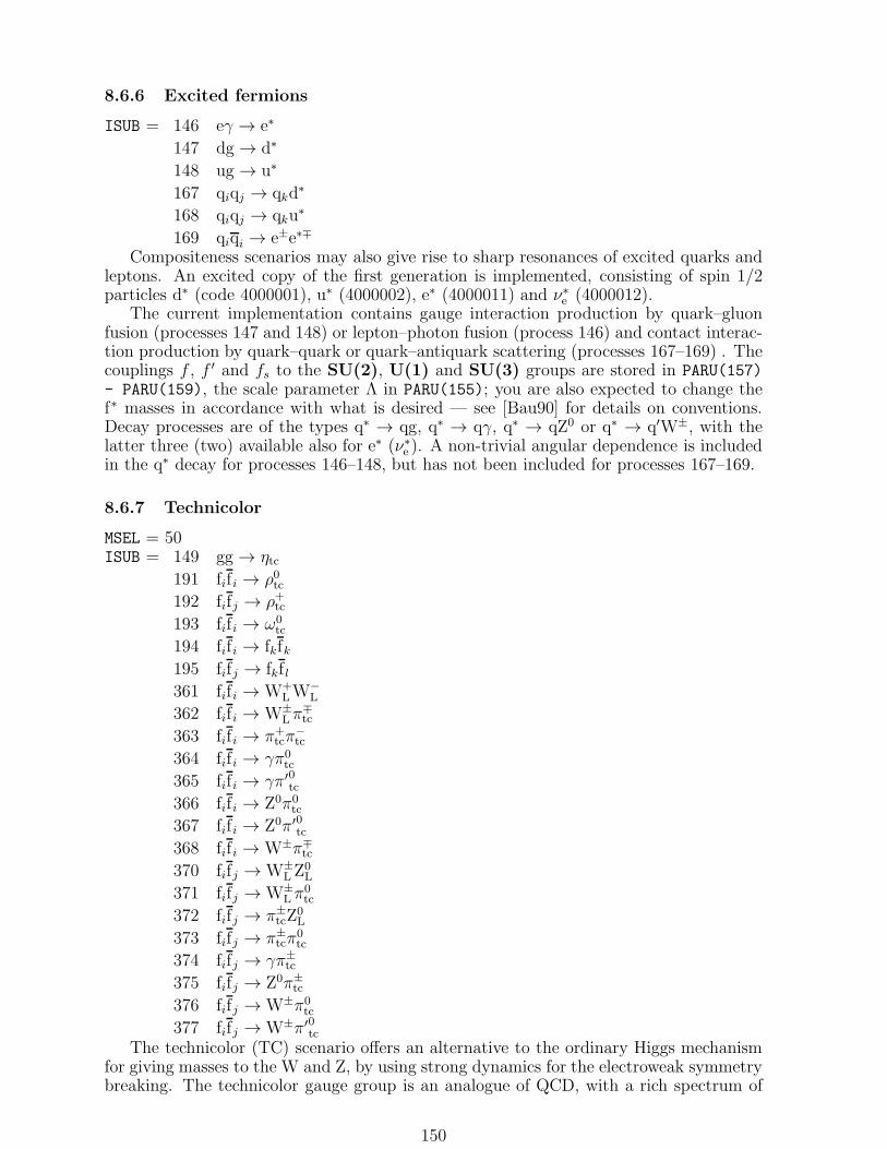
8.6.6 Excited fermions

ISUB = 146 eγ → e∗

147 dg → d∗

148 ug → u∗

167 qiqj → qkd∗

168 qiqj → qku∗

169 qiqi → e±e∗∓

Compositeness scenarios may also give rise to sharp resonances of excited quarks andleptons. An excited copy of the first generation is implemented, consisting of spin 1/2particles d∗ (code 4000001), u∗ (4000002), e∗ (4000011) and ν∗e (4000012).

The current implementation contains gauge interaction production by quark–gluonfusion (processes 147 and 148) or lepton–photon fusion (process 146) and contact interac-tion production by quark–quark or quark–antiquark scattering (processes 167–169) . Thecouplings f , f ′ and fs to the SU(2), U(1) and SU(3) groups are stored in PARU(157)- PARU(159), the scale parameter Λ in PARU(155); you are also expected to change thef∗ masses in accordance with what is desired — see [Bau90] for details on conventions.Decay processes are of the types q∗ → qg, q∗ → qγ, q∗ → qZ0 or q∗ → q′W±, with thelatter three (two) available also for e∗ (ν∗e ). A non-trivial angular dependence is includedin the q∗ decay for processes 146–148, but has not been included for processes 167–169.

8.6.7 Technicolor

MSEL = 50ISUB = 149 gg → ηtc

191 fifi → ρ0tc192 fifj → ρ+tc193 fifi → ω0

tc

194 fifi → fkfk195 fifj → fkf l361 fifi → W+

L W−L

362 fifi → W±Lπ

∓tc

363 fifi → π+tcπ

−tc

364 fifi → γπ0tc

365 fifi → γπ′0tc

366 fifi → Z0π0tc

367 fifi → Z0π′0tc

368 fifi → W±π∓tc

370 fifj → W±L Z0

L

371 fifj → W±L π

0tc

372 fifj → π±tcZ

0L

373 fifj → π±tcπ

0tc

374 fifj → γπ±tc

375 fifj → Z0π±tc

376 fifj → W±π0tc

377 fifj → W±π′0tc

The technicolor (TC) scenario offers an alternative to the ordinary Higgs mechanismfor giving masses to the W and Z, by using strong dynamics for the electroweak symmetrybreaking. The technicolor gauge group is an analogue of QCD, with a rich spectrum of

150

technimesons made out of techniquarks. An effective Lagrangian can be derived for thelightest resonances. In TC, the breaking of a chiral symmetry in the new, strongly inter-acting gauge theory generates the Goldstone bosons necessary for electroweak symmetrybreaking. Thus three of the technipions assume the role of the longitudinal componentsof the W and Z bosons, but many other states remain as separate particles: technipions(πtc), technirhos (ρtc), techniomegas (ωtc), etc. The mass hierarchies, however, are unlikeQCD because of the behaviour of the gauge couplings in realistic models of extendedTC (ETC). The difficulties of ETC in explaining the top quark mass while suppressingFCNC’s is circumvented by the addition of topcolor interactions, which provide the bulkof mt.

No fully realistic model has been found so far, however, so any phenomenology hasto be taken as indicative only. As experimental constraints have accumulated, also thesophistication of model building has had to follow suit. The processes represented herecorrespond to several generations of development. Thus processes 149, 191, 192 and 193should nowadays be considered as obsolete and superseded by the other processes 194,195 and 361–377.

In section 8.5.2 it is discussed how processes 71–77, in some of its options, can be usedto simulate a scenario with techni-ρ resonances in longitudinal gauge boson scattering.

Process 149 is that of the production of a techni-η, particle code KF = 3000331. Thisparticle has zero spin, is a singlet under electroweak SU(2)×U(1), but carries octetcolour charge. It is one of the possible techni-π particles; the name techni-η is part of asub-classification not used by all authors.

The techni-η couples to ordinary fermions according to the fermion squared mass. Thedominant decay mode is therefore tt, if allowed. The coupling to a gg state is roughlycomparable with that to bb. Production at hadron colliders is therefore predominantlythrough gg fusion, as implemented in process 149.

The two main free parameters are the techni-η mass and the decay constant Fπ. Thelatter appears inversely quadratically in all the partial widths. Also the total cross sectionis affected, since the cross section is proportional to the gg partial width. Fπ is storedin PARP(46) and has the default value 123 GeV, which is the number predicted in somemodels.

All the other processes refer to ETC models, where hard mass contributions to tech-nipion masses make decays like ρtc → πtcπtc kinematically inaccessible. Instead, decayslike ρewtc → πew

tc WL, for example, dominate, where ew denotes constituent technifermionswith only electroweak quantum numbers and WL is a longitudinal W bosons. As a result,the ew technirho and techniomega tend to have small total widths.

Effective couplings are derived in the valence technifermion approximation, and thetechniparticle decays can be calculated directly [Eic96, Lan99]. Technirhos and tech-niomegas are produced through kinematic mixing with gauge bosons, leading to finalstates containing Standard Model particles and/or pseudo-Goldstone bosons (technipi-ons).

As an additional possibility, SUc(3) non-singlet states are included along with thecoloron of topcolor assisted technicolor. In this case, coloured technirhos (and the coloron)can have substantial total widths and enhanced couplings to bottom and top quarks.

The expanded particle content with default masses is:KF name m (GeV)3000111 π0

tc 1103000211 π+

tc 1103000221 π′0

tc 1103000113 ρ0tc 2103000213 ρ+tc 2103000223 ω0

tc 210The ρtc and ω0

tc masses are not pole masses. Parameters regulating production and decay

151

rates are stored in PARP(137) - PARP(150).Processes 191, 192 and 193 are based on s-channel production of the respective res-

onance [Eic96]. All decay modes implemented can be simulated separately or in com-bination, in the standard fashion. These include pairs of fermions, of gauge bosons, oftechnipions, and of mixtures of gauge bosons and technipions

Process 194 is intended to more accurately represent the mixing between the γ∗, Z0, ρ0tcand ω0

tc particles in the Drell-Yan process [Lan99]. Process 195 is the analogous chargedchannel process including W± and ρ±tc mixing. By default, the final state fermions are e+e−

and e±νe, respectively. These can be changed through the parameters KFPR(194,1) andKFPR(195,1), respectively (where the KFPR value should represent a charged fermion).

Processes 361–368 give the pair production of technipions and gauge bosons by ρ0tc/ω0tc

exchange, with processes 370–377 corresponding pair production by ρ±tc exchange. Itis worth mentioning that the decay products of the W and Z bosons are distributedaccording to phase space, regardless of their designation as longitudinal WL/ZL or ordinarytransverse gauge bosons. The exact meaning of longitudinal or transverse polarizationsin this case requires more thought from the side of the model authors.

The possibility of coloured technihadrons has been included, specifically for the caseof Topcolor assisted Technicolor. The main effects of these particles are indirect, in thatthey modify the underlying two-parton QCD processes much like compositeness terms,except that resonances are visible. More details will be forthcoming. The parameterdependence of the ‘model’ is included in the tangent of the mixing angle PARP(155)and a mass parameter PARP(156). Similar to compositeness, the effects of these coloredtechnihadrons are simulated by setting MSTP(5)=5.

8.6.8 Extra Dimensions

ISUB = 391 ff → G∗

392 gg → G∗

393 qq → gG∗

394 qg → qG∗

395 gg → gG∗

In recent years, the area of observable consequences of extra dimensions has attracteda strong interest. The field is still in rapid development, so there still does not exist a‘standard phenomenology’. The topic is also fairly new in Pythia, and currently only afirst scenario is available.

The G∗, temporarily introduced as new particle code 41, is intended to represent thelowest excited graviton state in a Randall-Sundrum scenario [Ran99] of extra dimensions.The lowest-order production processes by fermion or gluon fusion are found in 391 and392. The further processes 393–395 are intended for the high-p⊥ tail in hadron colliders.As usual, it would be double-counting to have both sets of processes switched on at thesame time. Processes 391 and 392, with initial-state showers switched on, are appropriatefor the full cross section at all p⊥ values, and gives a reasonable description also of thehigh-p⊥ tail. Processes 393–395 could be useful e.g. for the study of invisible decays ofthe G∗, where a large p⊥ imbalance would be required. It also serves to test/confirm theshower expectations of different p⊥ spectra for different production processes [Bij01].

Decay channels of the G∗ to ff, gg, γγ, Z0Z0 and W+W− contribute to the totalwidth. The correct angular distributions are included for decays to a fermion pair in thelowest-order processes, whereas other decays currently are taken to be isotropic.

The G∗ mass is to be considered a free parameter. The other degree of freedom in thisscenario is a dimensionless coupling, see PARP(50).

152

8.7 Supersymmetry

MSEL = 39–45ISUB = 201–296 (see tables at the beginning of the chapter)

Pythia simulates the Minimal Supersymmetric Standard Model (MSSM), based onan effective Lagrangian of softly-broken Susy with parameters defined at the weak scale,which is typically between mZ and 1 TeV. The MSSM particle spectrum is minimal in thesense that it includes only the partners of all Standard Model particles (presently withoutmassive neutrinos), two Higgs doublets with partners, and the gravitino.

Each SM fermion has a scalar partner with the same quantum numbers. For countingpurposes, the fermion states ψL and ψR are separate particles with scalar partners φL andφR. Each SM gauge boson has a fermion partner with the same quantum numbers. TheHiggs sector is extended to two complex scalar doublets — one Higgs Hu which couplesonly to up-type fermions and one Hd which couples only to down-type fermions — leadingto 3 additional physical Higgs bosons H0, A0 and H± to complement the SM Higgs h0.Fermion higgsino partners are added for the two scalar doublets. Additionally, a lightgravitino G is included to allow studies of gauge mediated dynamical Susy breaking[Din96].

Because of the large Yukawa couplings and the running masses for coloured particles,the interaction and mass eigenstates for the third generation sfermions can be significantlymixed. We denote the top and bottom squark mass eigenstates t1,t2,b1, and b2 to distin-guish them from the nearly degenerate eigenstates for the lighter squarks. In addition,the tau slepton mass eigenstates are τ1 and τ2. The subscript 1 or 2 refers to the lightestand heaviest state respectively. In SUGRA inspired models, in the absence of mixingso that interaction eigenstates are the same as mass eigenstates, the right eigenstate islighter than the left. In this case, for example, b1 = bR and b2 = bL. For completeness,we include the sterile νR particles. The mixing of the partners to the electroweak gaugebosons (gauginos) and the two Higgs doublets (higgsinos) lead to the mass eigenstates forneutralino χ0

i and chargino χ±i particles.

The particle partners and KF codes are listed in Table 13. Note that, at times, an-tiparticles of scalar particles are denoted by ∗, i.e. t∗ rather than the more correct but

cumbersome t or t.Once the parameters of the softly-broken Susy Lagrangian are specified, the inter-

actions are fixed, and the sparticle masses can be calculated [Hab85]. The masses ofthe scalar partners to fermions, sfermions, depend on soft scalar masses, trilinear cou-plings, the Higgsino mass µ, and tan β, the ratio of Higgs vacuum expectation values〈Hu〉/〈Hd〉. The masses of the fermion partners to the gauge and Higgs bosons, theneutralinos and charginos, depend on soft gaugino masses, µ, and tan β. Finally, theproperties of the Higgs scalar sector is calculated from the input pseudoscalar Higgs bo-son mass mA, tan β, µ, trilinear couplings and the sparticle properties in an effectivepotential approach [Car95]. Of course, these calculations also depend on SM parameters(mt, mZ, αs, etc.). Any modifications to these quantities from virtual MSSM effects arenot taken into account. In principle, the sparticle masses also acquire loop correctionsthat depend on all MSSM masses.

Several models exist for deriving the rich set of directly measurable mass and mixingparameters from the assumed soft Susy breaking scenario with a much smaller set of freeparameters. One example is Supergravity (SUGRA) inspired models, where the num-ber of free parameters is reduced by imposing universality and exploiting the apparentunification of gauge couplings. Five parameters fixed at the gauge coupling unificationscale, tanβ,M0, m1/2, A0, and sign(µ), are then related to the mass parameters at thescale of EWSB by renormalization group equations (see e.g. [Pie97]). Isasusy/Isajet[Bae93] and Susygen [Kat98] numerically solve these equations to determine the massparameters. Alternatively, they can input a general set of parameters. Pythia operates

153

in the second manner, with a slightly more general set of input parameters. There arethree reasons for this: (1) programs already exist to calculate the SUGRA inspired massparameters, (2) approximate analytic formulae [Dre95] also exist which reproduce theoutput of Isasusy within ≃ 10%, and (3) we desire to study a much richer phenomenol-ogy than that possible in SUGRA inspired models. The Pythia input parameters aredescribed in detail later, in section 9.5.

R-parity conservation is assumed (at least on the time and distance scale of a typ-ical collider experiment), and only lowest order, sparticle pair production processes areincluded. Only those processes with e+e−, µ+µ−, or quark and gluon initial states aresimulated. Tables 21, 22 and 23 list available Susy processes. In processes 210 and 213,ℓ refers to both e and µ. For ease of readability, we have removed the subscript L on ν.tit

∗i , τiτ

∗j and τiν

∗τ production correctly account for sfermion mixing. Several processes are

conspicuously absent from the table. For example, processes 255 and 257 would simulatethe associated production of right handed squarks with charginos. Since the right handedsquark only couples to the higgsino component of the chargino, the interaction strengthis proportional to the quark mass, so these processes can be ignored.

Likewise, only R-parity conserving decays are allowed, so that one sparticle is stable,either the lightest neutralino, the gravitino, or a sneutrino. Susy decays of the top quarkare included, but all other SM particle decays are unaltered.

The decays of superpartners are calculated using the formulae of refs. [Gun88, Bar86a,Bar86b, Bar95]. All decays are spin averaged. For simplicity, the kinematics of three bodydecays of neutralinos, charginos, and the gluino are sampled using only the phase spaceweight. Decays involving b and t use the formulae of [Bar95], so they are valid for largevalues of tanβ. The one loop decays χj → χiγ and t → cχ1 are also included.

One difference between the Susy simulation and the other parts of the program isthat it is not beforehand known which sparticles may be stable. Normally this wouldmean either the χ0

1 or the gravitino G, but in principle also other sparticles could bestable. The ones found to be stable have their MWID(KC) and MDCY(KC,1) values set zeroat initialization. If several PYINIT calls are made in the same run, with different Susy

parameters, the ones set zero above are not necessarily set back to nonzero values, sincemost original values are not saved anywhere. As an exception to this rule, the PYMSINSusy initialization routine, called by PYINIT, does save and restore the MWID(KC) andMDCY(KC,1) values of the lightest Susy particle. It is therefore possible to combine severalPYINIT calls in a single run, provided that only the lightest Susy particle is stable. Ifthis is not the case, MWID(KC) and MDCY(KC,1) values may have to be reset by hand, orelse some particles that ought to decay will not do that.

Various improvements to the simulation are being implemented in stages. Some ofthese can have a significant impact on the collider phenomenology. Among these are:the generalization to complex-valued soft Susy-breaking parameters in the neutralinoand chargino sector; the same in the Higgs sector, which removes the possibility of CP-even or CP-odd labels; the calculation of neutralino and chargino decay rates which areaccurate for large tanβ; and matrix element weighting of particle distributions in three-body decays.

Recently, several improvements have been introduced to the supersymmetric machin-ery:

• Complex phases in the neutralino, chargino, and gluino sector. The parameters M1,M2, M3, and µ (specifically RMSS(1) - RMSS(4)) now refer only to the modulus ofthese parameters. Phases are specified by the parameters RMSS(30) - RMSS(33),respectively. Chargino and neutralino masses and mixing angles now differ fromthe case with vanishing phases, and the production cross sections and decay ratesincluding pairs of neutralinos and charginos have been modified accordingly. Gluinodecays to neutralinos and charginos are also affected (but the effect on gluino +neutralino/chargino production has not yet been simulated).

154

The PYSSMT commonblock has been expanded toCOMMON/PYSSMT/ZMIX(4,4),UMIX(2,2),VMIX(2,2),SMZ(4),SMW(2),&SFMIX(16,4),ZMIXI(4,4),UMIXI(2,2),VMIXI(2,2)

where ZMIX, UMIX, VMIX give the real and ZMIXI, UMIXI, VMIXI the imaginaryparts of the complex mixing matrices.

• Matrix Element weighting in 3-body sparticle decays. This replaces the older ap-proach based purely on phase space. The matrix element includes the dependenceon complex phases.

• Large tanβ corrections to Higgs boson properties have been included. The arrayvalues RMSS(40) and RMSS(41) are used for temporary storage of the corrections∆mt and ∆mb. The updated version of SubHpole, written by Carena et al, alsoincludes some bug fixes, so that it is generally better behaved.

• More flexibility in the treatment of stops, sbottoms and staus. With the flagIMSS(5)=1, the properties of the third generation sparticles can be specified by theirmixing angle and mass eigenvalues (instead of being derived from the soft Susy-breaking parameters). The parameters RMSS(26) - RMSS(28) specify the mixingangle (in radians) for the sbottom, stop, and stau. The parameters RMSS(10) -RMSS(14) specify the two stop masses, the one sbottom mass (the other being fixedby the other parameters) and the two stau masses. Note that the masses RMSS(10),RMSS(11) and RMSS(13) correspond to the left-left entries of the diagonalized ma-trices, while RMSS(12) and RMSS(14) correspond to the right-right entries. Notethat these entries need not be ordered in mass. Also, one technical change hasarisen with the stau sector. Previously, it was assumed that the soft Susy-breakingparameters associated with the stau included D-terms. This is no longer the case,and is more consistent with the treatment of the stop and sbottom.

8.7.1 SUSY examples

The Susy routines and commonblock variables are described in section 9.5. To illustratethe usage of the switches and parameters, we give three simple examples.

Example 1: Light StopThe first example is an MSSM model with a light neutralino χ1 and a light stop t1, sothat t → t1χ1 can occur. The input parameters areIMSS(1)=1, RMSS(1)=70., RMSS(2)=70., RMSS(3)=225., RMSS(4)=-40., RMSS(5)=1.5,RMSS(6)=100., RMSS(7)=125., RMSS(8)=250., RMSS(9)=250., RMSS(10)=1500.,RMSS(11)=1500., RMSS(12)=-128., RMSS(13)=100., RMSS(14)=125., RMSS(15)=800.,RMSS(16)=800., RMSS(17)=0., and RMSS(19)=400.0.The top mass is fixed at 175 GeV, PMAS(6,1)=175.0. The resulting model has Mt1 = 55GeV and Mχ1

= 38 GeV. IMSS(1)=1 turns on the MSSM simulation. By default, thereare no intrinsic relations between the gaugino masses, so M1 = 70 GeV, M2 = 70 GeV,and M3 = 225 GeV. The pole mass of the gluino is slightly higher than the parameterM3, and the decay g → t∗1t + t1t occurs almost 100% of the time.

Example 2: Approximate SUGRAThe second example is an approximate SUGRA model. The input parameters areIMSS(1)=2, RMSS(1)=200., RMSS(4)=1., RMSS(5)=10., RMSS(8)=800., andRMSS(16)=0.0.The resulting model has MdL

= 901 GeV, MuR = 890 GeV, Mt1 = 538 GeV, MeL = 814GeV, Mg = 560 GeV, Mχ1

= 80 GeV, Mχ±

1= 151 GeV, Mh = 110 GeV, and MA = 883

GeV. It corresponds to the choice M0=800 GeV, M1/2 =200 GeV, tanβ = 10, A0 = 0, andsign(µ) > 0. The output is similar to an Isasusy run, but there is not exact agreement.

Example 3: Isasusy ModelThe final example demonstrates how to convert the output of an Isasusy run using thesame SUGRA inputs into the Pythia format. This assumes that you already made an

155

Isasusy run, e.g. with the equivalents of the input parameters above. From the outputof this run you can now extract those physical parameters that need to be handed toPythia, in the above exampleIMSS(1)=1, IMSS(3)=1, RMSS(1)=83.81, RMSS(2)=168.90, RMSS(3)=581.83,RMSS(4)=283.37, RMSS(5)=10., RMSS(6)=813.63, RMSS(7)=804.87, RMSS(8)=917.73,RMSS(9)=909.89, RMSS(10)=772.87, RMSS(11)=901.52, RMSS(12)=588.33,RMSS(13)=813.63, RMSS(14)=804.87, RMSS(15)=610.54, RMSS(16)=422.35,RMSS(17)=600., and RMSS(19)=858.412.

8.7.2 Lepton number violation

The most general SUSY Lagrangian contains both lepton and baryon number violatingcouplings, customarily forbidden by the introduction of R parity to avoid problems withproton decay. This is not the only possible choice, but certainly the simplest. On theother hand, the violation of baryon or lepton number is allowed without resulting inproton decay, and both give rise to very distinct phenomenologies, most notably theconsequences of a decaying LSP and the removal of the cosmological constraint that theLSP should be neutral.

In the current version of Pythia, decays of supersymmetric particles to SM parti-cles via two different lepton number violating couplings can be invoked (Details aboutthe implementation and tests can be found in [Ska01], to which references concering L-violation in Pythia can be made). These couplings, λ and λ′, correspond to the twolepton number violating terms possible in the most general supersymmetric Lagrangian,usually denoted LLE and LQD respectively. They are Yuakawa-type trilinear couplingscarrying three generation indices, i, j, and k. The LLE coupling (λijk) is antisymmetricin i and j whereas no similar constraint applies to the LQD coupling (λ′ijk).

Complete matrix elements for all two-body sfermion and three-body neutralino andchargino decays are included (as given in [Dre00]). Lepton number violating decays of thegluino are not yet implemented. This should not lead to a large source of error since thegluino, being heavy in most scenarios, often has a number of other, unsuppressed decaymodes available, keeping the probability that it branches into an L-violating mode smallas long as the L-violating couplings are small compared with the gauge couplings.

The existence of R-odd couplings also allows for single sparticle production, i.e. thereis no requirement that SUSY particles should be produced in pairs. These productioncross sections are likewise not yet included in the program. For low-mass sparticles, theassociated error is estimated to be negligible, as long as the L-violating couplings aresmaller than the gauge couplings. For higher mass sparticles, the reduction of the phasespace for pair production becomes an important factor, and single sparticle productioncould dominate even for very small values of the L-violating couplings. The total SUSYproduction cross sections, as calculated by Pythia in its current form are thus underes-timated, possibly quite severely for heavy-mass sparticles.

Three possibilities exist for the initializations of the couplings. The first, selectedby setting IMSS(51)=1 for LLE and IMSS(52)=1 for LQD type couplings, sets all thecouplings, independent of generation, to a common value of 10−RMSS(51) or 10−RMSS(52), asthe case may be.

Setting IMSS(51)=2 and/or IMSS(52)=2 causes the couplings to be initialized (inPYINIT) to so-called ‘natural’ generation-hierarchical values, as proposed in [Hin93].These values, inspired by the structure of the Yukawa couplings in the SM, are definedby:

|λijk|2 = (RMSS(51))2meimejmek

|λ′ijk|2 = (RMSS(52))2meimqjmdk; m ≡ m

v=

m

126GeV(141)

where mqj is the arithmetic mean of muj and mdj .

156

The third option available is to set IMSS(51)=3 and/or IMSS(52)=3, in which caseall the relevant couplings are zero by default (but the lepton number violating processesare turned on) and the user is expected to enter all non-zero coupling values by hand.RVLAM(i,j,k) contains the λijk and RVLAMP(i,j,k) contains the λ′ijk couplings.

8.8 Polarization

In most processes, incoming beams are assumed unpolarized. However, especially for e+e−

linear collider studies, polarized beams would provide further important information onmany new physics phenomena, and at times help to suppress backgrounds. Therefore a fewprocess cross sections are now available also for polarized incoming beams. The averagepolarization of the two beams is then set by PARJ(131) and PARJ(132), respectively. Insome cases, noted below, MSTP(50) need also be switched on to access the formulae forpolarized beams.

Process 25, W+W− pair production, allows polarized incoming lepton beam particles.The polarization effects are included both in the production matrix elements and in theangular distribution of the final four fermions. Note that the matrix element used [Mah98]is for on-shell W production, with a suppression factor added for finite width effects.This polarized cross section expression, evaluated at vanishing polarization, disagreeswith the standard unpolarized one, which presumably is the more accurate of the two.The difference can be quite significant below threshold and at very high energies. Thiscan be traced to the simplified description of off-shell W’s in the polarized formulae.Good agreement is obtained either by switching off the W width with MSTP(42)=0 or byrestricting the W mass ranges (with CKIN(41) - CKIN(44)) to be close to on-shell. It istherefore necessary to set MSTP(50)=1 to switch from the default standard unpolarizedformulae to the polarized ones.

Also many Susy production processes now include the effects from polarization of theincoming fermion beams. This applies for scalar pair production, with the exception ofsneutrino pair production and h0A0 and H0A0 production, this omission being an oversightat the time of this release, but easily remedied in the future.

The effect of polarized photons is included in the process γγ → FkFk, process 85. Herethe array values PARJ(131) and PARJ(132) are used to define the average longitudinalpolarization of the two photons.

8.9 Main Processes by Machine

In the previous section we have already commented on which processes have limitedvalidity, or have different meanings (according to conventional terminology) in differentcontexts. Let us just repeat a few of the main points to be remembered for differentmachines.

8.9.1 e+e− collisions

The main annihilation process is number 1, e+e− → Z0, where in fact the full γ∗/Z0

interference structure is included. This process can be used, with some confidence, forc.m. energies from about 4 GeV upwards, i.e. at DORIS/CESR, PETRA/PEP, TRISTAN,LEP, and any future linear colliders. (To get below 10 GeV, you have to change PARP(2),however.) This is the default process obtained when MSEL=1, i.e. when you do not changeanything yourself.

Process 141 contains a Z′0, including full interference with the standard γ∗/Z0. Withthe value MSTP(44)=4 in fact one is back at the standard γ∗/Z0 structure, i.e. the Z′0

piece has been switched off. Even so, this process may be useful, since it can simulatee.g. e+e− → h0A0. Since the h0 may in its turn decay to Z0Z0, a decay channel of

157

the ordinary Z0 to h0A0, although physically correct, would be technically confusing. Inparticular, it would be messy to set the original Z0 to decay one way and the subsequentones another. So, in this sense, the Z′0 could be used as a copy of the ordinary Z0, butwith a distinguishable label.

The process e+e− → Υ does not exist as a separate process in Pythia, but can besimulated by using PYONIA, see section 6.2.

At LEP 2 and even higher energy machines, the simple s-channel process 1 loses outto other processes, such as e+e− → Z0Z0 and e+e− → W+W−, i.e. processes 22 and 25.The former process in fact includes the structure e+e− → (γ∗/Z0)(γ∗/Z0), which meansthat the cross section is singular if either of the two γ∗/Z0 masses is allowed to vanish. Amass cut therefore needs to be introduced, and is actually also used in other processes,such as e+e− → W+W−.

For practical applications, both with respect to cross sections and to event shapes,it is imperative to include initial-state radiation effects. Therefore MSTP(11)=1 is thedefault, wherein exponentiated electron-inside-electron distributions are used to give themomentum of the actually interacting electron. By radiative corrections to process 1,such processes as e+e− → γZ0 are therefore automatically generated. If process 19 wereto be used at the same time, this would mean that radiation were to be double-counted.In the alternative MSTP(11)=0, electrons are assumed to deposit their full energy in thehard process, i.e. initial-state QED radiation is not included. This option is very useful,since it often corresponds to the ‘ideal’ events that one wants to correct back to.

Resolved electrons also means that one may have interactions between photons. Thisopens up the whole field of γγ processes, which is described in section 8.3. In particular,with ’gamma/e+’,’gamma/e-’ as beam and target particles in a PYINIT call, a flux ofphotons of different virtualities is convoluted with a description of direct and resolvedphoton interaction processes, including both low-p⊥ and high-p⊥ processes. This machin-ery is directed to the description of the QCD processes, and does e.g. not address theproduction of gauge bosons or other such particles by the interactions of resolved pho-tons. For the latter kind of applications, a simpler description of partons inside photonsinside electrons may be obtained with the MSTP(12)=1 options and e± as beam and targetparticles.

The thrust of the Pythia programs is towards processes that involve hadron pro-duction, one way or another. Because of generalizations from other areas, also afew completely non-hadronic processes are available. These include Bhabha scattering,e+e− → e+e− in process 10, and photon pair production, e+e− → γγ in process 18. How-ever, note that the precision that could be expected in a Pythia simulation of thoseprocesses is certainly far less than that of dedicated programs. For one thing, electroweakloop effects are not included. For another, nowhere is the electron mass taken into account,which means that explicit cut-offs at some minimum p⊥ are always necessary.

8.9.2 Lepton–hadron collisions

The main option for photoproduction and Deeply Inelastic Scattering (DIS) physics isprovided by the ’gamma/lepton’ option as beam or target in a PYINIT call, see section8.3. The Q2 range to be covered, and other kinematics constraints, can be set by CKINvalues. By default, when the whole Q2 range is populated, obviously photoproductiondominates.

The older DIS process 10, ℓq → ℓ′q′, includes γ0/Z0/W± exchange, with full interfer-ence, as described in section 8.3.2. The Z0/W± contributions are not implemented in the’gamma/lepton’ machinery. Therefore process 10 is still the main option for physics atvery high Q2, but has been superseded for lower Q2. Radiation off the incoming lepton legis included by MSTP(11)=1 and off the outgoing one by MSTJ(41)=2 (both are default).Note that both QED and QCD radiation (off the e and the q legs, respectively) are al-

158

lowed to modify the x and Q2 values of the process, while the conventional approach inthe literature is to allow only the former. Therefore an option (on by default) has beenadded to preserve these values by a post-facto rescaling, MSTP(23)=1. Further commentson HERA applications are found in [Sjo92b].

8.9.3 Hadron–hadron collisions

The default is to include QCD jet production by 2 → 2 processes, see section 8.2.1. Sincethe differential cross section is divergent for p⊥ → 0, a lower cut-off has to be introduced.Normally that cut-off is given by the user-set p⊥min value in CKIN(3). If CKIN(3) ischosen smaller than a given value of the order of 2 GeV (see PARP(81) and PARP(82)),then low-p⊥ events are also switched on. The jet cross section is regularized at low p⊥, soas to obtain a smooth joining between the high-p⊥ and the low-p⊥ descriptions, see furthersection 11.2. As CKIN(3) is varied, the jump from one scenario to another is abrupt, interms of cross section: in a high-energy hadron collider, the cross section for jets downto a p⊥min scale of a few GeV can well reach values much larger than the total inelastic,non-diffractive cross section. Clearly this is nonsense; therefore either p⊥min should bepicked so large that the jet cross section be only a fraction of the total one, or else oneshould select p⊥min = 0 and make use of the full description.

If one switches to MSEL=2, also elastic and diffractive processes are switched on, seesection 8.2.4. However, the simulation of these processes is fairly primitive, and shouldnot be used for dedicated studies, but only to estimate how much they may contaminatethe class of non-diffractive minimum bias events.

Most processes can be simulated in hadron colliders, since the bulk of Pythia pro-cesses can be initiated by quarks or gluons. However, there are limits. Currently we in-clude no photon or lepton parton distributions, which means that a process like γq → γqis not accessible. Further, the possibility of having Z0 and W± interacting in processessuch as 71–77 has been hardwired process by process, and does not mean that there is ageneric treatment of Z0 and W± distributions.

The emphasis in the hadron–hadron process description is on high energy hadron col-liders. The program can be used also at fixed-target energies, but the multiple interactionmodel for underlying events then breaks down and should not be used. The limit of ap-plicability is somewhere at around 100 GeV. Only with the simpler model obtained forMSTP(82)=1 can one go arbitrarily low.

159

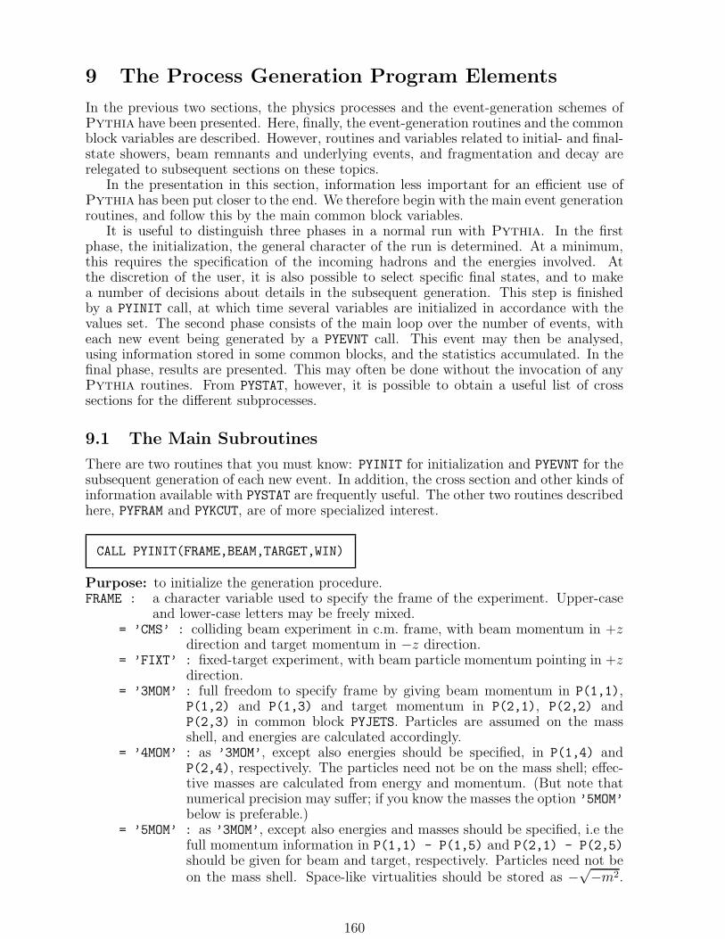
9 The Process Generation Program Elements

In the previous two sections, the physics processes and the event-generation schemes ofPythia have been presented. Here, finally, the event-generation routines and the commonblock variables are described. However, routines and variables related to initial- and final-state showers, beam remnants and underlying events, and fragmentation and decay arerelegated to subsequent sections on these topics.

In the presentation in this section, information less important for an efficient use ofPythia has been put closer to the end. We therefore begin with the main event generationroutines, and follow this by the main common block variables.

It is useful to distinguish three phases in a normal run with Pythia. In the firstphase, the initialization, the general character of the run is determined. At a minimum,this requires the specification of the incoming hadrons and the energies involved. Atthe discretion of the user, it is also possible to select specific final states, and to makea number of decisions about details in the subsequent generation. This step is finishedby a PYINIT call, at which time several variables are initialized in accordance with thevalues set. The second phase consists of the main loop over the number of events, witheach new event being generated by a PYEVNT call. This event may then be analysed,using information stored in some common blocks, and the statistics accumulated. In thefinal phase, results are presented. This may often be done without the invocation of anyPythia routines. From PYSTAT, however, it is possible to obtain a useful list of crosssections for the different subprocesses.

9.1 The Main Subroutines

There are two routines that you must know: PYINIT for initialization and PYEVNT for thesubsequent generation of each new event. In addition, the cross section and other kinds ofinformation available with PYSTAT are frequently useful. The other two routines describedhere, PYFRAM and PYKCUT, are of more specialized interest.

CALL PYINIT(FRAME,BEAM,TARGET,WIN)

Purpose: to initialize the generation procedure.FRAME : a character variable used to specify the frame of the experiment. Upper-case

and lower-case letters may be freely mixed.= ’CMS’ : colliding beam experiment in c.m. frame, with beam momentum in +z

direction and target momentum in −z direction.= ’FIXT’ : fixed-target experiment, with beam particle momentum pointing in +z

direction.= ’3MOM’ : full freedom to specify frame by giving beam momentum in P(1,1),

P(1,2) and P(1,3) and target momentum in P(2,1), P(2,2) andP(2,3) in common block PYJETS. Particles are assumed on the massshell, and energies are calculated accordingly.

= ’4MOM’ : as ’3MOM’, except also energies should be specified, in P(1,4) andP(2,4), respectively. The particles need not be on the mass shell; effec-tive masses are calculated from energy and momentum. (But note thatnumerical precision may suffer; if you know the masses the option ’5MOM’below is preferable.)

= ’5MOM’ : as ’3MOM’, except also energies and masses should be specified, i.e thefull momentum information in P(1,1) - P(1,5) and P(2,1) - P(2,5)should be given for beam and target, respectively. Particles need not beon the mass shell. Space-like virtualities should be stored as −

√−m2.

160

Especially useful for physics with virtual photons. (The virtuality couldbe varied from one event to the next, but then it is convenient to initializefor the lowest virtuality likely to be encountered.) Four-momentum andmass information must match.

= ’USER’ : a run primarily intended to involve external, user-defined processes,see subsection 9.9. Information on incoming beam particles and energiesis read from the HEPRUP common block. In this option, the BEAM, TARGETand WIN arguments are dummy.

= ’NONE’ : there will be no initialization of any processes, but only of resonancewidths and a few other process-independent variables. Subsequent tosuch a call, PYEVNT cannot be used to generate events, so this option ismainly intended for those who will want to construct their own eventsafterwards, but still want to have access to some of the Pythia facilities.In this option, the BEAM, TARGET and WIN arguments are dummy.

BEAM, TARGET : character variables to specify beam and target particles. Upper-caseand lower-case letters may be freely mixed. An antiparticle can be denoted by‘bar’ at the end of the name (‘∼’ is a valid alternative for reasons of backwardscompatibility). It is also possible to leave out the underscore (‘ ’) directly after‘nu’ in neutrino names, and the charge for proton and neutron. The argumentsare dummy when the FRAME argument above is either ’USER’ or ’NONE’.

= ’e-’ : electron.= ’e+’ : positron.= ’nu e’ : νe.= ’nu ebar’ : νe.= ’mu-’ : µ−.= ’mu+’ : µ+.= ’nu mu’ : νµ.= ’nu mubar’ : νµ.= ’tau-’ : τ−.= ’tau+’ : τ+.= ’nu tau’ : ντ .= ’nu taubar’ : ντ .= ’gamma’ : photon (real, i.e. on the mass shell).= ’gamma/e-’ : photon generated by the virtual-photon flux in an electron beam;

WIN below refers to electron, while photon energy and virtuality variesbetween events according to what is allowed by CKIN(61) - CKIN(78).

= ’gamma/e+’ : as above for a positron beam.= ’gamma/mu-’ : as above for a µ− beam.= ’gamma/mu+’ : as above for a µ+ beam.= ’gamma/tau-’ : as above for a τ− beam.= ’gamma/tau+’ : as above for a τ+ beam.= ’pi0’ : π0.= ’pi+’ : π+.= ’pi-’ : π−.= ’n0’ : neutron.= ’nbar0’ : antineutron.= ’p+’ : proton.= ’pbar-’ : antiproton.= ’K+’ : K+ meson; since parton distributions for strange hadrons are not avail-

able, very simple and untrustworthy recipes are used for this and subse-quent hadrons, see subsection 7.1.

= ’K-’ : K− meson.= ’KS0’ : K0

S meson.

161

= ’KL0’ : K0L meson.

= ’Lambda0’ : Λ baryon.= ’Sigma-’ : Σ− baryon.= ’Sigma0’ : Σ0 baryon.= ’Sigma+’ : Σ+ baryon.= ’Xi-’ : Ξ− baryon.= ’Xi0’ : Ξ0 baryon.= ’Omega-’ : Ω− baryon.= ’pomeron’ : the pomeron IP; since pomeron parton distribution functions have

not been defined this option can not be used currently.= ’reggeon’ : the reggeon IR, with comments as for the pomeron above.

WIN : related to energy of system, exact meaning depends on FRAME.FRAME=’CMS’ : total energy of system (in GeV).FRAME=’FIXT’ : momentum of beam particle (in GeV/c).FRAME=’3MOM’, ’4MOM’, ’5MOM’ : dummy (information is taken from the P vec-

tors, see above).FRAME=’USER’ : dummy (information is taken from the HEPRUP common block, see

above).FRAME=’NONE’ : dummy (no information required).

CALL PYEVNT

Purpose: to generate one event of the type specified by the PYINIT call. (This is themain routine, which calls a number of other routines for specific tasks.)

CALL PYSTAT(MSTAT)

Purpose: to print out cross-sections statistics, decay widths, branching ratios, statuscodes and parameter values. PYSTAT may be called at any time, after thePYINIT call, e.g. at the end of the run, or not at all.

MSTAT : specification of desired information.= 1 : prints a table of how many events of the different kinds that have been

generated and the corresponding cross sections. All numbers alreadyinclude the effects of cuts required by you in PYKCUT.Note that no errors are given on the cross sections. In most cases across section is obtained by Monte Carlo integration during the courseof the run. (Exceptions include e.g. total and elastic hadron–hadroncross sections, which are parameterized and thus known from the veryonset.) A rule of thumb would then be that the statistical error of agiven subprocess scales like δσ/σ ≈ 1/

√n, where n is the number of

events generated of this kind. In principle, the numerator of this relationcould be decreased by making use of the full information accumulatedduring the run, i.e. also on the cross section in those phase space pointsthat are eventually rejected. This is actually the way the cross sectionitself is calculated. However, once you introduce further cuts so thatonly some fraction of the generated events survive to the final analysis,you would be back to the simple 1/

√n scaling rule for that number of

surviving events. Statistical errors are therefore usually better evaluatedwithin the context of a specific analysis. Furthermore, systematic errorsoften dominate over the statistical ones.Also note that runs with very few events, in addition to having largeerrors, tend to have a bias towards overestimating the cross sections.

162

In a typical case, the average cross section obtained with many runsof only one event each may be twice that of the correct answer of asingle run with many events. The reason is a ‘quit while you are ahead’phenomenon, that an upwards fluctuation in the differential cross sectionin an early try gives an acceptable event and thus terminates the run,while a downwards one leads to rejection and a continuation of the run.

= 2 : prints a table of the resonances defined in the program, with their par-ticle codes (KF), and all allowed decay channels. (If the number of gen-erations in MSTP(1) is 3, however, channels involving fourth-generationparticles are not displayed.) For each decay channel is shown the se-quential channel number (IDC) of the Pythia decay tables, the decayproducts (usually two but sometimes three), the partial decay width,branching ratio and effective branching ratio (in the event some channelshave been excluded by you).

= 3 : prints a table with the allowed hard interaction flavours KFIN(I,J) forbeam and target particles.

= 4 : prints a table of the kinematical cuts CKIN(I) set by you in the currentrun.

= 5 : prints a table with all the values of the status codes MSTP(I) and theparameters PARP(I) used in the current run.

= 6 : prints a table of all subprocesses implemented in the program.= 7 : prints two tables related to R-violating supersymmetry. The first is a

collection of semi-inclusive branching ratios where the entries have theform ~chi 10 --> nu + q + q where a sum has been performed overall lepton and quark flavours. In the rightmost coloumn of the table, thenumber of modes that went into the sum is given. The purpose of thistable is to give a quick overview of the branching fractions, since thereare currently more than 1200 individual R-violating processes includedin the generator. Note that only the pure 1 → 3 parts of the 3-bodymodes are included in this sum. If a process can also proceed via twosuccessive 1 → 2 branchings (i.e. the intermediate resonance is on shell)the product of these branchings should be added to the number givenin this table. A small list at the bottom of the table shows the totalnumber of R-violating processes in the generator, the number with non-zero branching ratios in the current run, and the number with branchingratios larger than 10−3. The second table which is printed by this callmerely lists the R-violating λ, λ′, and λ′′ couplings.

CALL PYFRAM(IFRAME)

Purpose: to transform an event listing between different reference frames, if so desired.The use of this routine assumes you do not do any boosts yourself.

IFRAME : specification of frame the event is to be boosted to.= 1 : frame specified by you in the PYINIT call.= 2 : c.m. frame of incoming particles.= 3 : hadronic c.m. frame of lepton–hadron interaction events. Mainly in-

tended for Deeply Inelastic Scattering, but can also be used in photo-production. Is not guaranteed to work with the ’gamma/lepton’ options,however, and so of limited use. Note that both the lepton and any pho-tons radiated off the lepton remain in the event listing, and have to beremoved separately if you only want to study the hadronic subsystem.

163

CALL PYKCUT(MCUT)

Purpose: to enable you to reject a given set of kinematic variables at an early stage of thegeneration procedure (before evaluation of cross sections), so as not to spendunnecessary time on the generation of events that are not wanted. The routinewill not be called unless you require is by setting MSTP(141)=1, and never if‘minimum-bias’-type events (including elastic and diffractive scattering) are tobe generated as well. Furthermore it is never called for user-defined externalprocesses. A dummy routine PYKCUT is included in the program file, so as toavoid unresolved external references when the routine is not used.

MCUT : flag to signal effect of user-defined cuts.= 0 : event is to be retained and generated in full.= 1 : event is to be rejected and a new one generated.

Remark : at the time of selection, several variables in the MINT and VINT arrays inthe PYINT1 common block contain information that can be used to make thedecision. The routine provided in the program file explicitly reads the variablesthat have been defined at the time PYKCUT is called, and also calculates somederived quantities. The information available includes subprocess type ISUB,Ecm, s, t, u, p⊥, x1, x2, xF, τ , y, τ ′, cos θ, and a few more. Some of these maynot be relevant for the process under study, and are then set to zero.

9.2 Switches for Event Type and Kinematics Selection

By default, if Pythia is run for a hadron collider, only QCD 2 → 2 processes are gener-ated, composed of hard interactions above p⊥min =PARP(81), with low-p⊥ processes addedon so as to give the full (parameterized) inelastic, non-diffractive cross section. In an e+e−

collider, γ∗/Z0 production is the default, and in an ep one it is Deeply Inelastic Scattering.With the help of the common block PYSUBS, it is possible to select the generation of an-other process, or combination of processes. It is also allowed to restrict the generation tospecific incoming partons/particles at the hard interaction. This often automatically alsorestricts final-state flavours but, in processes such as resonance production or QCD/QEDproduction of new flavours, switches in the Pythia program may be used to this end; seesection 14.4.

The CKIN array may be used to impose specific kinematics cuts. You should here bewarned that, if kinematical variables are too strongly restricted, the generation time perevent may become very long. In extreme cases, where the cuts effectively close the fullphase space, the event generation may run into an infinite loop. The generation of 2 → 1resonance production is performed in terms of the s and y variables, and so the rangesCKIN(1) - CKIN(2) and CKIN(7) - CKIN(8) may be arbitrarily restricted without asignificant loss of speed. For 2 → 2 processes, cos θ is added as a third generation variable,and so additionally the range CKIN(27) - CKIN(28) may be restricted without any lossof efficiency..

Effects from initial- and final-state radiation are not included, since they are not knownat the time the kinematics at the hard interaction is selected. The sharp kinematical cut-offs that can be imposed on the generation process are therefore smeared, both by QCDradiation and by fragmentation. A few examples of such effects follow.

• Initial-state radiation implies that each of the two incoming partons has a non-vanishing p⊥ when they interact. The hard scattering subsystem thus receives a nettransverse boost, and is rotated with respect to the beam directions. In a 2 → 2process, what typically happens is that one of the scattered partons receives anincreased p⊥, while the p⊥ of the other parton is reduced.

• Since the initial-state radiation machinery assigns space-like virtualities to the in-

164

coming partons, the definitions of x in terms of energy fractions and in terms ofmomentum fractions no longer coincide, and so the interacting subsystem may re-ceive a net longitudinal boost compared with naıve expectations, as part of theparton-shower machinery.

• Initial-state radiation gives rise to additional jets, which in extreme cases may bemistaken for either of the jets of the hard interaction.

• Final-state radiation gives rise to additional jets, which smears the meaning of thebasic 2 → 2 scattering. The assignment of soft jets is not unique. The energy of ajet becomes dependent on the way it is identified, e.g. what jet cone size is used.

• The beam remnant description assigns primordial k⊥ values, which also gives anet p⊥ shift of the hard-interaction subsystem; except at low energies this effectis overshadowed by initial-state radiation, however. Beam remnants may also addfurther activity under the ‘perturbative’ event.

• Fragmentation will further broaden jet profiles, and make jet assignments and energydeterminations even more uncertain.

In a study of events within a given window of experimentally defined variables, it is upto you to leave such liberal margins that no events are missed. In other words, cuts haveto be chosen such that a negligible fraction of events migrate from outside the simulatedregion to inside the interesting region. Often this may lead to low efficiency in terms ofwhat fraction of the generated events are actually of interest to you. See also section 3.6.

In addition to the variables found in PYSUBS, also those in the PYPARS common blockmay be used to select exactly what one wants to have simulated. These possibilities willbe described in the following section.

The notation used above and in the following is that ‘ ’ denotes internal variables inthe hard scattering subsystem, while ‘∗’ is for variables in the c.m. frame of the event asa whole.

COMMON/PYSUBS/MSEL,MSELPD,MSUB(500),KFIN(2,-40:40),CKIN(200)

Purpose: to allow you to run the program with any desired subset of processes, or restrictflavours or kinematics. If the default values, denoted below by (D=. . . ), arenot satisfactory, they must be changed before the PYINIT call.

MSEL : (D=1) a switch to select between full user control and some preprogrammedalternatives.

= 0 : desired subprocesses have to be switched on in MSUB, i.e. full user control.= 1 : depending on incoming particles, different alternatives are used.

Lepton–lepton: Z or W production (ISUB = 1 or 2).Lepton–hadron: Deeply Inelastic Scattering (ISUB = 10; this option isnow out of date for most applications, superseded by the ’gamma/lepton’machinery).Hadron–hadron: QCD high-p⊥ processes (ISUB = 11, 12, 13, 28, 53,68); additionally low-p⊥ production if CKIN(3)<PARP(81) or PARP(82),depending on MSTP(82) (ISUB = 95). If low-p⊥ is switched on, the otherCKIN cuts are not used.A resolved photon counts as hadron. When the photon is not resolved,the following cases are possible.Photon–lepton: Compton scattering (ISUB = 34).Photon–hadron: photon-parton scattering (ISUB = 33, 34, 54).Photon–photon: fermion pair production (ISUB = 58).When photons are given by the ’gamma/lepton’ argument in the PYINITcall, the outcome depends on the MSTP(14) value. Default is a mixtureof many kinds of processes, as described in section 8.3.

165

= 2 : as MSEL = 1 for lepton–lepton, lepton–hadron and unresolved photons.For hadron–hadron (including resolved photons) all QCD processes, in-cluding low-p⊥, single and double diffractive and elastic scattering, areincluded (ISUB = 11, 12, 13, 28, 53, 68, 91, 92, 93, 94, 95). The CKINcuts are here not used.For photons given with the ’gamma/lepton’ argument in the PYINIT call,the above processes are replaced by other ones that also include the pho-ton virtuality in the cross sections. The principle remains to include bothhigh- and low-p⊥ processes, however.

= 4 : charm (cc) production with massive matrix elements (ISUB = 81, 82, 84,85).

= 5 : bottom (bb) production with massive matrix elements (ISUB = 81, 82,84, 85).

= 6 : top (tt) production with massive matrix elements (ISUB = 81, 82, 84,85).

= 7 : fourth generation b′ (b′b′) production with massive matrix elements

(ISUB = 81, 82, 84, 85).= 8 : fourth generation t′ (t′t

′) production with massive matrix elements (ISUB

= 81, 82, 84, 85).= 10 : prompt photons (ISUB = 14, 18, 29).= 11 : Z0 production (ISUB = 1).= 12 : W± production (ISUB = 2).= 13 : Z0 + jet production (ISUB = 15, 30).= 14 : W± + jet production (ISUB = 16, 31).= 15 : pair production of different combinations of γ, Z0 and W± (except γγ;

see MSEL = 10) (ISUB = 19, 20, 22, 23, 25).= 16 : h0 production (ISUB = 3, 102, 103, 123, 124).= 17 : h0Z0 or h0W± (ISUB = 24, 26).= 18 : h0 production, combination relevant for e+e− annihilation (ISUB = 24,

103, 123, 124).= 19 : h0, H0 and A0 production, excepting pair production (ISUB = 24, 103,

123, 124, 153, 158, 171, 173, 174, 176, 178, 179).= 21 : Z′0 production (ISUB = 141).= 22 : W′± production (ISUB = 142).= 23 : H± production (ISUB = 143).= 24 : R0 production (ISUB = 144).= 25 : LQ (leptoquark) production (ISUB = 145, 162, 163, 164).= 35: single bottom production by W exchange (ISUB = 83).= 36: single top production by W exchange (ISUB = 83).= 37: single b′ production by W exchange (ISUB = 83).= 38: single t′ production by W exchange (ISUB = 83).= 39: all MSSM processes except Higgs production.= 40: squark and gluino production (ISUB = 243, 244, 258, 259, 271–280).= 41: stop pair production (ISUB = 261–265).= 42: slepton pair production (ISUB = 201–214).= 43: squark or gluino with chargino or neutralino, (ISUB = 237–242, 246–256).= 44: chargino–neutralino pair production (ISUB = 216–236).= 45: sbottom production (ISUB = 281–296).= 50: pair production of technipions and gauge bosons by π0,±

tc /ω0tc exchange

(ISUB = 361–377).

MSUB : (D=500*0) array to be set when MSEL=0 (for MSEL≥ 1 relevant entries are set inPYINIT) to choose which subset of subprocesses to include in the generation.

166

The ordering follows the ISUB code given in section 8.1 (with comments asgiven there).

MSUB(ISUB) = 0 : the subprocess is excluded.MSUB(ISUB) = 1 : the subprocess is included.Note: when MSEL=0, the MSUB values set by you are never changed by Pythia.

If you want to combine several different ‘subruns’, each with its ownPYINIT call, into one single run, it is up to you to remember not onlyto switch on the new processes before each new PYINIT call, but also toswitch off the old ones that are no longer desired.

KFIN(I,J) : provides an option to selectively switch on and off contributions to the crosssections from the different incoming partons/particles at the hard interaction.In combination with the Pythia resonance decay switches, this also allowsyou to set restrictions on flavours appearing in the final state.

I : is 1 for beam side of event and 2 for target side.J : enumerates flavours according to the KF code; see section 5.1.KFIN(I,J) = 0 : the parton/particle is forbidden.KFIN(I,J) = 1 : the parton/particle is allowed.Note: By default, the following are switched on: d, u, s, c, b, e−, νe, µ

−, νµ,τ−, ντ , g, γ, Z0, W+ and their antiparticles. In particular, top is off, andhas to be switched on explicitly if needed.

CKIN : kinematics cuts that can be set by you before the PYINIT call, and that affectthe region of phase space within which events are generated. Some cuts are‘hardwired’ while most are ‘softwired’. The hardwired ones are directly relatedto the kinematical variables used in the event selection procedure, and there-fore have negligible effects on program efficiency. The most important of theseare CKIN(1) - CKIN(8), CKIN(27) - CKIN(28), and CKIN(31) - CKIN(32).The softwired ones are most of the remaining ones, that cannot be fully takeninto account in the kinematical variable selection, so that generation in con-strained regions of phase space may be slow. In extreme cases the phase spacemay be so small that the maximization procedure fails to find any allowedpoints at all (although some small region might still exist somewhere), andtherefore switches off some subprocesses, or aborts altogether.

CKIN(1), CKIN(2) : (D=2.,-1. GeV) range of allowed m =√s values. If CKIN(2)< 0.,

the upper limit is inactive.CKIN(3), CKIN(4) : (D=0.,-1. GeV) range of allowed p⊥ values for hard 2 → 2 pro-

cesses, with transverse momentum p⊥ defined in the rest frame of the hardinteraction. If CKIN(4)< 0., the upper limit is inactive. For processes that aresingular in the limit p⊥ → 0 (see CKIN(6)), CKIN(5) provides an additionalconstraint. The CKIN(3) and CKIN(4) limits can also be used in 2 → 1 → 2processes. Here, however, the product masses are not known and hence are as-sumed to be vanishing in the event selection. The actual p⊥ range for massiveproducts is thus shifted downwards with respect to the nominal one.

CKIN(5) : (D=1. GeV) lower cut-off on p⊥ values, in addition to the CKIN(3) cut above,for processes that are singular in the limit p⊥ → 0 (see CKIN(6)).

CKIN(6) : (D=1. GeV) hard 2 → 2 processes, which do not proceed only via an inter-mediate resonance (i.e. are 2 → 1 → 2 processes), are classified as singular inthe limit p⊥ → 0 if either or both of the two final-state products has a massm <CKIN(6).

CKIN(7), CKIN(8) : (D=-10.,10.) range of allowed scattering subsystem rapidities y =y∗ in the c.m. frame of the event, where y = (1/2) ln(x1/x2). (Following thenotation of this section, the variable should be given as y∗, but because of itsfrequent use, it was called y in section 7.2.)

167

CKIN(9), CKIN(10) : (D=-40.,40.) range of allowed (true) rapidities for the productwith largest rapidity in a 2 → 2 or a 2 → 1 → 2 process, defined in the c.m.frame of the event, i.e. max(y∗3, y

∗4). Note that rapidities are counted with sign,

i.e. if y∗3 = 1 and y∗4 = −2 then max(y∗3, y∗4) = 1.

CKIN(11), CKIN(12) : (D=-40.,40.) range of allowed (true) rapidities for the prod-uct with smallest rapidity in a 2 → 2 or a 2 → 1 → 2 process, definedin the c.m. frame of the event, i.e. min(y∗3, y

∗4). Consistency thus requires

CKIN(11)≤CKIN(9) and CKIN(12)≤CKIN(10).CKIN(13), CKIN(14) : (D=-40.,40.) range of allowed pseudorapidities for the product

with largest pseudorapidity in a 2 → 2 or a 2 → 1 → 2 process, defined inthe c.m. frame of the event, i.e. max(η∗3, η

∗4). Note that pseudorapidities are

counted with sign, i.e. if η∗3 = 1 and η∗4 = −2 then max(η∗3, η∗4) = 1.

CKIN(15), CKIN(16) : (D=-40.,40.) range of allowed pseudorapidities for the productwith smallest pseudorapidity in a 2 → 2 or a 2 → 1 → 2 process, definedin the c.m. frame of the event, i.e. min(η∗3, η

∗4). Consistency thus requires

CKIN(15)≤CKIN(13) and CKIN(16)≤CKIN(14).CKIN(17), CKIN(18) : (D=-1.,1.) range of allowed cos θ∗ values for the product with

largest cos θ∗ value in a 2 → 2 or a 2 → 1 → 2 process, defined in the c.m.frame of the event, i.e. max(cos θ∗3, cos θ∗4).

CKIN(19), CKIN(20) : (D=-1.,1.) range of allowed cos θ∗ values for the product withsmallest cos θ∗ value in a 2 → 2 or a 2 → 1 → 2 process, defined in thec.m. frame of the event, i.e. min(cos θ∗3, cos θ∗4). Consistency thus requiresCKIN(19)≤CKIN(17) and CKIN(20)≤CKIN(18).

CKIN(21), CKIN(22) : (D=0.,1.) range of allowed x1 values for the parton on side 1that enters the hard interaction.

CKIN(23), CKIN(24) : (D=0.,1.) range of allowed x2 values for the parton on side 2that enters the hard interaction.

CKIN(25), CKIN(26) : (D=-1.,1.) range of allowed Feynman-x values, where xF = x1−x2.

CKIN(27), CKIN(28) : (D=-1.,1.) range of allowed cos θ values in a hard 2 → 2 scatter-

ing, where θ is the scattering angle in the rest frame of the hard interaction.CKIN(31), CKIN(32) : (D=2.,-1. GeV) range of allowed m′ =

√s′ values, where m′ is

the mass of the complete three- or four-body final state in 2 → 3 or 2 → 4processes (while m, constrained in CKIN(1) and CKIN(2), here correspondsto the one- or two-body central system). If CKIN(32)< 0., the upper limit isinactive.

CKIN(35), CKIN(36) : (D=0.,-1. GeV2) range of allowed |t| = −t values in 2 → 2processes. Note that for Deeply Inelastic Scattering this is nothing but theQ2 scale, in the limit that initial- and final-state radiation is neglected. IfCKIN(36)< 0., the upper limit is inactive.

CKIN(37), CKIN(38) : (D=0.,-1. GeV2) range of allowed |u| = −u values in 2 → 2processes. If CKIN(38)< 0., the upper limit is inactive.

CKIN(39), CKIN(40) : (D=4., -1. GeV2) the W 2 range allowed in DIS processes, i.e.subprocess number 10. If CKIN(40)< 0., the upper limit is inactive. Here W 2

is defined in terms of W 2 = Q2(1− x)/x. This formula is not quite correct, inthat (i) it neglects the target mass (for a proton), and (ii) it neglects initial-state photon radiation off the incoming electron. It should be good enough forloose cuts, however. These cuts are not checked if process 10 is called for twolepton beams.

CKIN(41) - CKIN(44) : (D=12.,-1.,12.,-1. GeV) range of allowed mass values of thetwo (or one) resonances produced in a ‘true’ 2 → 2 process, i.e. one not (only)proceeding through a single s-channel resonance (2 → 1 → 2). (These are theones listed as 2 → 2 in the tables in section 8.1.) Only particles with a width

168

above PARP(41) are considered as bona fide resonances and tested against theCKIN limits; particles with a smaller width are put on the mass shell withoutapplying any cuts. The exact interpretation of the CKIN variables depends onthe flavours of the two produced resonances.For two resonances like Z0W+ (produced from fifj → Z0W+), which are notidentical and which are not each other’s antiparticles, one hasCKIN(41)< m1 <CKIN(42), andCKIN(43)< m2 <CKIN(44),where m1 and m2 are the actually generated masses of the two resonances,and 1 and 2 are defined by the order in which they are given in the productionprocess specification.For two resonances like Z0Z0, which are identical, or W+W−, which are eachother’s antiparticles, one instead hasCKIN(41)< min(m1, m2) <CKIN(42), andCKIN(43)< max(m1, m2) <CKIN(44).In addition, whatever limits are set on CKIN(1) and, in particular, on CKIN(2)obviously affect the masses actually selected.

Note 1: If MSTP(42)=0, so that no mass smearing is allowed, the CKIN values haveno effect (the same as for particles with too narrow a width).

Note 2: If CKIN(42)<CKIN(41) it means that the CKIN(42) limit is inactive;correspondingly, if CKIN(44)<CKIN(43) then CKIN(44) is inactive.

Note 3: If limits are active and the resonances are identical, it is up to you toensure that CKIN(41)≤CKIN(43) and CKIN(42)≤CKIN(44).

Note 4: For identical resonances, it is not possible to preselect which of the res-onances is the lighter one; if, for instance, one Z0 is to decay to leptonsand the other to quarks, there is no mechanism to guarantee that thelepton pair has a mass smaller than the quark one.

Note 5: The CKIN values are applied to all relevant 2 → 2 processes equally, whichmay not be what one desires if several processes are generated simulta-neously. Some caution is therefore urged in the use of the CKIN(41) -CKIN(44) values. Also in other respects, you are recommended to takeproper care: if a Z0 is only allowed to decay into bb, for example, settingits mass range to be 2–8 GeV is obviously not a good idea.

CKIN(45) - CKIN(48) : (D=12.,-1.,12.,-1. GeV) range of allowed mass values of the two(or one) secondary resonances produced in a 2 → 1 → 2 process (like gg →h0 → Z0Z0) or even a 2 → 2 → 4 (or 3) process (like qq → Z0h0 → Z0W+W−).Note that these CKIN values only affect the secondary resonances; the primaryones are constrained by CKIN(1), CKIN(2) and CKIN(41) - CKIN(44) (indi-rectly, of course, the choice of primary resonance masses affects the allowedmass range for the secondary ones). What is considered to be a resonance isdefined by PARP(41); particles with a width smaller than this are automat-ically put on the mass shell. The description closely parallels the one givenfor CKIN(41) - CKIN(44). Thus, for two resonances that are not identical oreach other’s antiparticles, one hasCKIN(45)< m1 <CKIN(46), andCKIN(47)< m2 <CKIN(48),where m1 and m2 are the actually generated masses of the two resonances, and1 and 2 are defined by the order in which they are given in the decay channelspecification in the program (see e.g. output from PYSTAT(2) or PYLIST(12)).For two resonances that are identical or each other’s antiparticles, one insteadhasCKIN(45)< min(m1, m2) <CKIN(46), andCKIN(47)< max(m1, m2) <CKIN(48).

169

Notes 1 - 5: as for CKIN(41) - CKIN(44), with trivial modifications.Note 6: Setting limits on secondary resonance masses is possible in any of the

channels of the allowed types (see above). However, so far only h0 → Z0Z0

and h0 → W+W− have been fully implemented, such that an arbitrarymass range below the naıve mass threshold may be picked. For otherpossible resonances, any restrictions made on the allowed mass range arenot reflected in the cross section; and further it is not recommendable topick mass windows that make a decay on the mass shell impossible.

CKIN(49) - CKIN(50) : allow minimum mass limits to be passed from PYRESD toPYOFSH. They are used for tertiary and higher resonances, i.e. those not con-trolled by CKIN(41)-CKIN(48). They should not be touched by the user.

CKIN(51) - CKIN(56) : (D=0.,-1.,0.,-1.,0.,-1. GeV) range of allowed transverse mo-menta in a true 2 → 3 process. This means subprocesses such as 121–124 forh0 production, and their H0, A0 and H±± equivalents. CKIN(51) - CKIN(54)corresponds to p⊥ ranges for scattered partons, in order of appearance, i.e.CKIN(51) - CKIN(52) for the parton scattered off the beam and CKIN(53) -CKIN(54) for the one scattered off the target. CKIN(55) and CKIN(56) heresets p⊥ limits for the third product, the h0, i.e. the CKIN(3) and CKIN(4)values have no effect for this process. Since the p⊥ of the Higgs is not one ofthe primary variables selected, any constraints here may mean reduced MonteCarlo efficiency, while for these processes CKIN(51) - CKIN(54) are ‘hard-wired’ and therefore do not cost anything. As usual, a negative value impliesthat the upper limit is inactive.

CKIN(61) - CKIN(78) : allows to restrict the range of kinematics for the photons gen-erated off the lepton beams with the ’gamma/lepton’ option of PYINIT. Ineach quartet of numbers, the first two corresponds to the range allowed onincoming side 1 (beam) and the last two to side 2 (target). The cuts are onlyapplicable for a lepton beam. Note that the x and Q2 (P 2) variables are thebasis for the generation, and so can be restricted with no loss of efficiency. Forleptoproduction (i.e. lepton on hadron) the W is uniquely given by the one xvalue of the problem, so here also W cuts are fully efficient. The other cutsmay imply a slowdown of the program, but not as much as if equivalent cutsonly are introduced after events are fully generated. See [Fri00] for details.

CKIN(61) - CKIN(64) : (D=0.0001,0.99,0.0001,0.99) allowed range for the energy frac-tions x that the photon take of the respective incoming lepton energy. Thesefractions are defined in the c.m. frame of the collision, and differ from energyfractions as defined in another frame. (Watch out at HERA!) In order to avoidsome technical problems, absolute lower and upper limits are set internally at0.0001 and 0.9999.

CKIN(65) - CKIN(68) : (D=0.,-1.,0.,-1. GeV2) allowed range for the spacelike virtualityof the photon, conventionally called either Q2 or P 2, depending on process. Anegative number means that the upper limit is inactive, i.e. purely given bykinematics. A nonzero lower limit is implicitly given by kinematics constraints.

CKIN(69) - CKIN(72) : (D=0.,-1.,0.,-1.) allowed range of the scattering angle θ of thelepton, defined in the c.m. frame of the event. (Watch out at HERA!) Anegative number means that the upper limit is inactive, i.e. equal to π.

CKIN(73) - CKIN(76) : (D=0.0001,0.99,0.0001,0.99) allowed range for the light-conefraction y that the photon take of the respective incoming lepton energy. Thelight-cone is defined by the four-momentum of the lepton or hadron on theother side of the event (and thus deviates from true light-cone fraction bymass effects that normally are negligible). The y value is related to the x andQ2 (P 2) values by y = x +Q2/s if mass terms are neglected.

CKIN(77), CKIN(78) : (D=2.,-1. GeV) allowed range for W , i.e. either the photon–

170

hadron or photon–photon invariant mass. A negative number means that theupper limit is inactive.

9.3 The General Switches and Parameters

The PYPARS common block contains the status code and parameters that regulate theperformance of the program. All of them are provided with sensible default values, so thata novice user can neglect them, and only gradually explore the full range of possibilities.Some of the switches and parameters in PYPARS will be described later, in the shower andbeam remnants sections.

COMMON/PYPARS/MSTP(200),PARP(200),MSTI(200),PARI(200)

Purpose: to give access to status code and parameters that regulate the performance ofthe program. If the default values, denoted below by (D=. . . ), are not satis-factory, they must in general be changed before the PYINIT call. Exceptions,i.e. variables that can be changed for each new event, are denoted by (C).

MSTP(1) : (D=3) maximum number of generations. Automatically set ≤ 4.MSTP(2) : (D=1) calculation of αs at hard interaction, in the routine PYALPS.

= 0 : αs is fixed at value PARU(111).= 1 : first-order running αs.= 2 : second-order running αs.

MSTP(3) : (D=2) selection of Λ value in αs for MSTP(2)≥ 1.= 1 : Λ is given by PARP(1) for hard interactions, by PARP(61) for space-like

showers, by PARP(72) for time-like showers not from a resonance decay,and by PARJ(81) for time-like ones from a resonance decay (including e.g.γ/Z0 → qq decays, i.e. conventional e+e− physics). This Λ is assumedto be valid for 5 flavours; for the hard interaction the number of flavoursassumed can be changed by MSTU(112).

= 2 : Λ value is chosen according to the parton-distribution-function para-meterizations. The choice is always based on the proton parton-distribution set selected, i.e. is unaffected by pion and photon parton-distribution selection. All the Λ values are assumed to refer to 4 flavours,and MSTU(112) is set accordingly. This Λ value is used both for the hardscattering and the initial- and final-state radiation. The ambiguity in thechoice of the Q2 argument still remains (see MSTP(32), MSTP(64) andMSTJ(44)). This Λ value is used also for MSTP(57)=0, but the sensiblechoice here would be to use MSTP(2)=0 and have no initial- or final-stateradiation. This option does not change the PARJ(81) value of timelikeparton showers in resonance decays, so that LEP experience on this spe-cific parameter is not overwritten unwittingly. Therefore PARJ(81) canbe updated completely independently.

= 3 : as =2, except that here also PARJ(81) is overwritten in accordance withthe Λ value of the proton parton-distribution-function set.

MSTP(4) : (D=0) treatment of the Higgs sector, predominantly the neutral one.= 0 : the h0 is given the Standard Model Higgs couplings, while H0 and A0 cou-

plings should be set by you in PARU(171) - PARU(175) and PARU(181)- PARU(185), respectively.

= 1 : you should set couplings for all three Higgses, for the h0 in PARU(161) -PARU(165), and for the H0 and A0 as above.

= 2 : the mass of h0 in PMAS(25,1) and the tan β value in PARU(141) are usedto derive H0, A0 and H± masses, and h0, H0, A0 and H± couplings, using

171

the relations of the Minimal Supersymmetric extension of the StandardModel at Born level [Gun90]. Existing masses and couplings are overwrit-ten by the derived values. See section 8.5.3 for discussion on parameterconstraints.

= 3: as =2, but using relations at the one-loop level. This option is not yetimplemented as such. However, if you initialize the Susy machinery withIMSS(1)=1, then the Susy parameters will be used to calculate also Higgsmasses and couplings. These are stored in the appropriate slots, and thevalue of MSTP(4) is overwritten to 1.

MSTP(5) : (D=0) presence of anomalous couplings in processes. See section 8.6.5 forfurther details.

= 0 : absent.= 1 : left–left isoscalar model, with only u and d quarks composite (at the

probed scale).= 2 : left–left isoscalar model, with all quarks composite.= 3 : helicity-non-conserving model, with only u and d quarks composite (at

the probed scale).= 4 : helicity-non-conserving model, with all quarks composite.= 5 : coloured technihadrons, affecting the standard QCD 2 → 2 cross sections,

see subsection 8.6.7 and parameters PARP(155) and PARP(156).MSTP(7) : (D=0) choice of heavy flavour in subprocesses 81–85. Does not apply for

MSEL=4-8, where the MSEL value always takes precedence.= 0 : for processes 81–84 (85) the ‘heaviest’ flavour allowed for gluon (photon)

splitting into a quark–antiquark (fermion–antifermion) pair, as set in theMDME array. Note that ‘heavy’ is defined as the one with largest KF code,so that leptons take precedence if they are allowed.

= 1 - 8 : pick this particular quark flavour; e.g., MSTP(7)=6 means that top willbe produced.

= 11 - 18 : pick this particular lepton flavour. Note that neutrinos are not possi-ble, i.e. only 11, 13, 15 and 17 are meaningful alternatives. Lepton pairproduction can only occur in process 85, so if any of the other processeshave been switched on they are generated with the same flavour as wouldbe obtained in the option MSTP(7)=0.

MSTP(8) : (D=0) choice of electroweak parameters to use in the decay widths of reso-nances (W, Z, h, . . . ) and cross sections (production of W’s, Z’s, h’s, . . . ).

= 0 : everything is expressed in terms of a running αem(Q2) and a fixed sin2θW ,i.e. GF is nowhere used.

= 1 : a replacement is made according to αem(Q2) →√

2GFm2W sin2θW/π in

all widths and cross sections. If GF and mZ are considered as given, thismeans that sin2θW and mW are the only free electroweak parameter.

= 2 : a replacement is made as for =1, but additionally sin2θW is constrainedby the relation sin2θW = 1 −m2

W/m2Z. This means that mW remains as

a free parameter, but that the sin2θW value in PARU(102) is never used,except in the vector couplings in the combination v = a−4 sin2θW e. Thislatter degree of freedom enters e.g. for forward-backward asymmetries inZ0 decays.

Note: This option does not affect the emission of real photons in the initial andfinal state, where αem is always used. However, it does affect also purelyelectromagnetic hard processes, such as qq → γγ.

MSTP(9) : (D=0) inclusion of top (and fourth generation) as allowed remnant flavour q′

in processes that involve q → q′ + W branchings as part of the overall process,and where the matrix elements have been calculated under the assumptionthat q′ is massless.

172

= 0 : no.= 1 : yes, but it is possible, as before, to switch off individual channels by the

setting of MDME switches. Mass effects are taken into account, in a crudefashion, by rejecting events where kinematics becomes inconsistent whenthe q′ mass is included.

MSTP(11) : (D=1) use of electron parton distribution in e+e− and ep interactions.= 0 : no, i.e. electron carries the whole beam energy.= 1 : yes, i.e. electron carries only a fraction of beam energy in agreement with

next-to-leading electron parton-distribution function, thereby includingthe effects of initial-state bremsstrahlung.

MSTP(12) : (D=0) use of e− (‘sea’, i.e. from e → γ → e), e+, quark and gluon distributionfunctions inside an electron.

= 0 : off.= 1 : on, provided that MSTP(11)≥ 1. Quark and gluon distributions are ob-

tained by numerical convolution of the photon content inside an electron(as given by the bremsstrahlung spectrum of MSTP(11)=1) with the quarkand gluon content inside a photon. The required numerical precision isset by PARP(14). Since the need for numerical integration makes this op-tion somewhat more time-consuming than ordinary parton-distributionevaluation, one should only use it when studying processes where it isneeded.

Note: for all traditional photoproduction/DIS physics this option is supersededby the ’gamma/lepton’ option for PYINIT calls, but can still be of use forsome less standard processes.

MSTP(13) : (D=1) choice of Q2 range over which electrons are assumed to radiate pho-tons; affects normalization of e− (sea), e+, γ, quark and gluon distributionsinside an electron for MSTP(12)=1.

= 1 : range set by Q2 argument of parton-distribution-function call, i.e. by Q2

scale of the hard interaction. Therefore parton distributions are propor-tional to ln(Q2/m2

e).= 2 : range set by the user-determined Q2

max, given in PARP(13). Parton distri-butions are assumed to be proportional to ln((Q2

max/m2e)(1−x)/x2). This

is normally most appropriate for photoproduction, where the electron issupposed to go undetected, i.e. scatter less than Q2

max.Note: the choice of effective range is especially touchy for the quark and gluon

distributions. An (almost) on-the-mass-shell photon has a VMD piecethat dies away for a virtual photon. A simple convolution of distribu-tion functions does not take this into account properly. Therefore thecontribution from Q values above the ρ mass should be suppressed. Achoice of Qmax ≈ 1 GeV is then appropriate for a photoproduction limitdescription of physics. See also note for MSTP(12).

MSTP(14) : (D=30) structure of incoming photon beam or target. Historically, numbersup to 10 were set up for real photons, and subsequent ones have been addedalso to allow for virtual photon beams. The reason is that the existing optionsspecify e.g. direct×VMD, summing over the possibilities of which photon isdirect and which VMD. This is allowed when the situation is symmetric, i.e.for two incoming real photons, but not if one is virtual. Some of the new optionsagree with previous ones, but are included to allow a more consistent pattern.Further options above 25 have been added also to include DIS processes.

= 0 : a photon is assumed to be point-like (a direct photon), i.e. can onlyinteract in processes which explicitly contain the incoming photon, suchas fiγ → fig for γp interactions. In γγ interactions both photons aredirect, i.e the main process is γγ → fif i.

173

= 1 : a photon is assumed to be resolved, i.e. can only interact through itsconstituent quarks and gluons, giving either high-p⊥ parton–parton scat-terings or low-p⊥ events. Hard processes are calculated with the use ofthe full photon parton distributions. In γγ interactions both photons areresolved.

= 2 : a photon is assumed resolved, but only the VMD piece is included in theparton distributions, which therefore mainly are scaled-down versionsof the ρ0/π0 ones. Both high-p⊥ parton–parton scatterings and low-pTevents are allowed. In γγ interactions both photons are VMD-like.

= 3 : a photon is assumed resolved, but only the anomalous piece of the photonparton distributions is included. (This event class is called either anoma-lous or GVMD; we will use both interchangeably, though the former ismore relevant for high-p⊥ phenomena and the latter for low-p⊥ ones.) Inγγ interactions both photons are anomalous.

= 4 : in γγ interactions one photon is direct and the other resolved. A typicalprocess is thus fiγ → fig. Hard processes are calculated with the useof the full photon parton distributions for the resolved photon. Bothpossibilities of which photon is direct are included, in event topologiesand in cross sections. This option cannot be used in configurations withonly one incoming photon.

= 5 : in γγ interactions one photon is direct and the other VMD-like. Bothpossibilities of which photon is direct are included, in event topologiesand in cross sections. This option cannot be used in configurations withonly one incoming photon.

= 6 : in γγ interactions one photon is direct and the other anomalous. Bothpossibilities of which photon is direct are included, in event topologiesand in cross sections. This option cannot be used in configurations withonly one incoming photon.

= 7 : in γγ interactions one photon is VMD-like and the other anomalous.Only high-p⊥ parton–parton scatterings are allowed. Both possibilitiesof which photon is VMD-like are included, in event topologies and incross sections. This option cannot be used in configurations with onlyone incoming photon.

= 10 : the VMD, direct and anomalous/GVMD components of the photon areautomatically mixed. For γp interactions, this means an automatic mix-ture of the three classes 0, 2 and 3 above [Sch93, Sch93a], for γγ onesa mixture of the six classes 0, 2, 3, 5, 6 and 7 above [Sch94a]. Variousrestrictions exist for this option, as discussed in section 8.3.1.

= 11 : direct×direct (see note 5); intended for virtual photons.= 12 : direct×VMD (i.e. first photon direct, second VMD); intended for virtual

photons.= 13 : direct×anomalous; intended for virtual photons.= 14 : VMD×direct; intended for virtual photons.= 15 : VMD×VMD; intended for virtual photons.= 16 : VMD×anomalous; intended for virtual photons.= 17 : anomalous×direct; intended for virtual photons.= 18 : anomalous×VDM; intended for virtual photons.= 19 : anomalous×anomalous; intended for virtual photons.= 20 : a mixture of the nine above components, 11–19, in the same spirit as =10

provides a mixture for real gammas (or a virtual gamma on a hadron).For gamma-hadron, this option coincides with =10.

= 21 : direct×direct (see note 5).= 22 : direct×resolved.

174

= 23 : resolved×direct.= 24 : resolved×resolved.= 25 : a mixture of the four above components, offering a simpler alternative

to =20 in cases where the parton distributions of the photon have notbeen split into VMD and anomalous components. For γ-hadron, onlytwo components need be mixed.

= 26 : DIS×VMD/p.= 27 : DIS×anomalous.= 28 : VMD/p×DIS.= 29 : anomalous×DIS.= 30 : a mixture of all the 4 (for γ∗p) or 13 (for γ∗γ∗) components that are

available, i.e. (the relevant ones of) 11–19 and 26–29 above; is as =20with the DIS processes mixed in.

Note 1: The MSTP(14) options apply for a photon defined by a ’gamma’ or’gamma/lepton’ beam in the PYINIT call, but not to those photons im-plicitly obtained in a ’lepton’ beam with the MSTP(12)=1 option. Thislatter approach to resolved photons is more primitive and is no longerrecommended for QCD processes.

Note 2: for real photons our best understanding of how to mix event classes isprovided by the option 10 above, which also can be obtained by combin-ing three (for γp) or six (for γγ) separate runs. In a simpler alternativethe VMD and anomalous classes are joined into a single resolved class.Then γp physics only requires two separate runs, with 0 and 1, and γγphysics requires three, with 0, 1 and 4.

Note 3: most of the new options from 11 onwards are not needed and there-fore not defined for ep collisions. The recommended ’best’ value thus isMSTP(14)=30, which also is the new default value.

Note 4: as a consequence of the appearance of new event classes, the MINT(122)and MSTI(9) codes are not the same for γ∗γ∗ events as for γp, γ∗p orγγ ones. Instead the code is 3(i1 − 1) + i2, where i is 1 for direct, 2 forVMD and 3 for anomalous/GVMD and indices refer to the two incomingphotons. For γ∗p code 4 is DIS, and for γ∗γ∗ codes 10–13 corresponds tothe MSTP(14) codes 26–29. As before, MINT(122) and MSTI(9) are onlydefined when several processes are to be mixed, not when generating oneat a time. Also the MINT(123) code is modified (not shown here).

Note 5: The direct×direct event class excludes lepton pair production when runwith the default MSEL=1 option (or MSEL=2), in order not to confuseusers. You can obtain lepton pairs as well, e.g. by running with MSEL=0and switching on the desired processes by hand.

Note 6: For all non-QCD processes, a photon is assumed unresolved whenMSTP(14)= 10, 20 or 25. In principle, both the resolved and directpossibilities ought to be explored, but this mixing is not currently im-plemented, so picking direct at least will explore one of the two mainalternatives rather than none. Resolved processes can be accessed by themore primitive machinery of having a lepton beam and MSTP(12)=1.

MSTP(15) : (D=0) possibility to modify the nature of the anomalous photon component(as used with the appropriate MSTP(14) options), in particular with respectto the scale choices and cut-offs of hard processes. These options are mainlyintended for comparative studies and should not normally be touched. Someof the issues are discussed in [Sch93a], while others have only been used forinternal studies and are undocumented.

= 0 : none, i.e. the same treatment as for the VMD component.= 1 : evaluate the anomalous parton distributions at a scale Q2/PARP(17)2.

175

= 2 : as =1, but instead of PARP(17) use either PARP(81)/PARP(15) orPARP(82)/PARP(15), depending on MSTP(82) value.

= 3 : evaluate the anomalous parton distribution functions of the photon asf γ,anom(x,Q2, p20) − f γ,anom(x,Q2, r2Q2) with r =PARP(17).

= 4 : as =3, but instead of PARP(17) use either PARP(81)/PARP(15) orPARP(82)/PARP(15), depending on MSTP(82) value.

= 5 : use larger p⊥min for the anomalous component than for the VMD one,but otherwise no difference.

MSTP(16) : (D=1) choice of definition of the fractional momentum taken by a photonradiated off a lepton. Enters in the flux factor for the photon rate, and therebyin cross sections.

= 0 : x, i.e. energy fraction in the rest frame of the event.= 1 : y, i.e. light-cone fraction.

MSTP(17) : (D=4) possibility of a extrafactor for processes involving resolved virtualphotons, to approximately take into account the effects of longitudinal pho-tons. Given on the formR = 1 + PARP(165) r(Q2, µ2) fL(y,Q2)/fT (y,Q2).Here the 1 represents the basic transverse contribution, PARP(165) is somearbitrary overall factor, and fL/fT the (known) ratio of longitudinal to trans-verse photon flux factors. The arbitrary function r depends on the photonvirtuality Q2 and the hard scale µ2 of the process. See [Fri00] for a discussionof the options.

= 0 : No contribution, i.e. r = 0.= 1 : r = 4µ2Q2/(µ2 +Q2)2.= 2 : r = 4Q2/(µ2 +Q2).= 3 : r = 4Q2/(m2

ρ +Q2).

= 4 : r = 4m2VQ

2/(m2V + Q2)2, where mV is the vector meson mass for VMD

and 2k⊥ for GVMD states. Since there is no µ dependence here (as wellas for =3 and =5) also minimum-bias cross sections are affected, whereµ would be vanishing. Currently the actual vector meson mass in theVMD case is replaced by mρ, for simplicity.

= 5 : r = 4Q2/(m2V +Q2), with mV and comments as above.

Note: For a photon given by the ’gamma/lepton’ option in the PYINIT call, they spectrum is dynamically generated and y is thus known from event toevent. For a photon beam in the PYINIT call, y is unknown from theonset, and has to be provided by you if any longitudinal factor is to beincluded. So long as these values, in PARP(167) and PARP(168), are attheir default values, 0, it is assumed they have not been set and thus theMSTP(17) and PARP(165) values are inactive.

MSTP(18) : (D=3) choice of p⊥min for direct processes.= 1 : same as for VMD and GVMD states, i.e. the p⊥min(W 2) scale. Primarily

intended for real photons.= 2 : p⊥min is chosen to be PARP(15), i.e. the original old behaviour proposed in

[Sch93, Sch93a]. In that case, also parton distributions, jet cross sectionsand αs values were dampened for small p⊥, so it may not be easy toobtain full backwards compatibility with this option.

= 3 : as =1, but if the Q scale of the virtual photon is above the VMD/GVMDp⊥min(W

2), p⊥min is chosen equal to Q. This is part of the strategy tomix in DIS processes at p⊥ below Q, e.g. in MSTP(14)=30.

MSTP(19) : (D=4) choice of partonic cross section in the DIS process 99.= 0 : QPM answer 4π2αem/Q

2 ∑

q e2q(xq(x,Q

2) + xq(x,Q2)) (with parton dis-tributions frozen below the lowest Q allowed in the parameterization).Note that this answer is divergent for Q2 → 0 and thus violates gauge

176

invariance.= 1 : QPM answer is modified by a factor Q2/(Q2 + m2

ρ) to provide a finite

cross section in the Q2 → 0 limit. A minimal regularization recipe.= 2 : QPM answer is modified by a factor Q4/(Q2+m2

ρ)2 to provide a vanishing

cross section in the Q2 → 0 limit. Appropriate if one assumes thatthe normal photoproduction description gives the total cross section forQ2 = 0, without any DIS contribution.

= 3 : as = 2, but additionally suppression by a parameterized factor f(W 2, Q2)(different for γ∗p and γ∗γ∗) that avoids double-counting the direct-process region where p⊥ > Q. Shower evolution for DIS events is thenalso restricted to be at scales below Q, whereas evolution all the way upto W is allowed in the other options above.

= 4 : as = 3, but additionally include factor 1/(1 − x) for conversion from F2

to σ. This is formally required, but is only relevant for small W 2 andtherefore often neglected.

MSTP(20) : (D=3) suppression of resolved (VMD or GVMD) cross sections, introducedto compensate for an overlap with DIS processes in the region of intermediateQ2 and rather small W 2.

= 0 : no; used as is.

> 1 : yes, by a factor (W 2/(W 2 + Q21 + Q2

2))MSTP(20) (where Q2

i = 0 for anincoming hadron).

Note: the suppression factor is joined with the dipole suppression stored inVINT(317) and VINT(318).

MSTP(21) : (D=1) nature of fermion–fermion scatterings simulated in process 10 by t-channel exchange.

= 0 : all off (!).= 1 : full mixture of γ∗/Z0 neutral current and W± charged current.= 2 : γ neutral current only.= 3 : Z0 neutral current only.= 4 : γ∗/Z0 neutral current only.= 5 : W± charged current only.

MSTP(22) : (D=0) special override of normal Q2 definition used for maximum of parton-shower evolution, intended for Deeply Inelastic Scattering in lepton–hadronevents, see section 10.4.

MSTP(23) : (D=1) for Deeply Inelastic Scattering processes (10 and 83), this optionallows the x and Q2 of the original hard scattering to be retained by thefinal electron when showers are considered (with warnings as below; partlyobsolete).

= 0 : no correction procedure, i.e. x and Q2 of the scattered electron differfrom the originally generated x and Q2.

= 1 : post facto correction, i.e. the change of electron momentum, by initialand final QCD radiation, primordial k⊥ and beam remnant treatment,is corrected for by a shuffling of momentum between the electron andhadron side in the final state. Only process 10 is corrected, while process83 is not.

= 2 : as =1, except that both process 10 and 83 are treated. This option isdangerous, especially for top, since it may well be impossible to ‘correct’in process 83: the standard DIS kinematics definitions are based on theassumption of massless quarks. Therefore infinite loops are not excluded.

Note 1: the correction procedure will fail for a fraction of the events, which arethus rejected (and new ones generated in their place). The correction op-tion is not unambiguous, and should not be taken too seriously. For very

177

small Q2 values, the x is not exactly preserved even after this procedure.Note 2: This switch does not affect the recommended DIS description obtained

with a ’gamma/lepton’ beam/target in PYINIT, where x and Q2 are al-ways conserved.

MSTP(31) : (D=1) parameterization of total, elastic and diffractive cross sections.= 0 : everything is to be set by you yourself in the PYINT7 common block. For

photoproduction, additionally you need to set VINT(281). Normally youwould set these values once and for all before the PYINIT call, but if yourun with variable energies (see MSTP(171)) you can also set it before eachnew PYEVNT call.

= 1 : Donnachie–Landshoff for total cross section [Don92], and Schuler–Sjostrand for elastic and diffractive cross sections [Sch94, Sch93a].

MSTP(32) : (D=8) Q2 definition in hard scattering for 2 → 2 processes. For resonanceproduction Q2 is always chosen to be s = m2

R, where mR is the mass of the res-onance. For gauge boson scattering processes V V → V V the W or Z0 squaredmass is used as scale in parton distributions. See PARP(34) for a possibility tomodify the choice below by a multiplicative factor.The newer options 6–10 are specifically intended for processes with incomingvirtual photons. These are ordered from a ‘minimal’ dependence on the virtu-alities to a ‘maximal’ one, based on reasonable kinematics considerations. Theold default value MSTP(32)=2 forms the starting point, with no dependenceat all, and the new default is some intermediate choice. Notation is that P 2

1

and P 22 are the virtualities of the two incoming particles, p⊥ the transverse

momentum of the scattering process, and m3 and m4 the masses of the twooutgoing partons. For a direct photon, P 2 is the photon virtuality and x = 1.For a resolved photon, P 2 still refers to the photon, rather than the unknownvirtuality of the reacting parton in the photon, and x is the momentum fractiontaken by this parton.

= 1 : Q2 = 2stu/(s2 + t2 + u2).= 2 : Q2 = (m2

⊥3 +m2⊥4)/2 = p2⊥ + (m2

3 +m24)/2.

= 3 : Q2 = min(−t,−u).= 4 : Q2 = s.= 5 : Q2 = −t.= 6 : Q2 = (1 + x1P

21 /s+ x2P

22 /s)(p

2⊥ +m2

3/2 +m24/2).

= 7 : Q2 = (1 + P 21 /s+ P 2

2 /s)(p2⊥ +m2

3/2 +m24/2).

= 8 : Q2 = p2⊥ + (P 21 + P 2

2 +m23 +m2

4)/2.= 9 : Q2 = p2⊥ + P 2

1 + P 22 +m2

3 +m24.

= 10 : Q2 = s (the full energy-squared of the process).Note: options 6 and 7 are motivated by assuming that one wants a scale that

interpolates between t for small t and u for small u, such asQ2 = −tu/(t+u). When kinematics for the 2 → 2 process is constructed as if anincoming photon is massless when it is not, it gives rise to a mismatchfactor 1+P 2/s (neglecting the other masses) in thisQ2 definition, which isthen what is used in option 7 (with the neglect of some small cross-termswhen both photons are virtual). When a virtual photon is resolved, thevirtuality of the incoming parton can be anything from xP 2 and upwards.So option 6 uses the smallest kinematically possible value, while 7 is morerepresentative of the typical scale. Option 8 and 9 are more handwavingextensions of the default option, with 9 specially constructed to ensurethat the Q2 scale is always bigger than P 2.

MSTP(33) : (D=0) inclusion of K factors in hard cross sections for parton–parton inter-actions (i.e. for incoming quarks and gluons).

= 0 : none, i.e. K = 1.

178

= 1 : a common K factor is used, as stored in PARP(31).= 2 : separate factors are used for ordinary (PARP(31)) and colour annihilation

graphs (PARP(32)).= 3 : A K factor is introduced by a shift in the αs Q

2 argument, αs =αs(PARP(33)Q

2).MSTP(34) : (D=1) use of interference term in matrix elements for QCD processes, see

section 8.2.1.= 0 : excluded (i.e. string-inspired matrix elements).= 1 : included (i.e. conventional QCD matrix elements).Note: for the option MSTP(34)=1, i.e. interference terms included, these terms

are divided between the different possible colour configurations accordingto the pole structure of the (string-inspired) matrix elements for thedifferent colour configurations.

MSTP(35) : (D=0) threshold behaviour for heavy-flavour production, i.e. ISUB = 81, 82,84, 85, and also for Z and Z′ decays. The non-standard options are mainlyintended for top, but can be used, with less theoretical reliability, also forcharm and bottom (for Z and Z′ only top and heavier flavours are affected).The threshold factors are given in eqs. (137) and (138).

= 0 : naıve lowest-order matrix-element behaviour.= 1 : enhancement or suppression close to threshold, according to the colour

structure of the process. The αs value appearing in the threshold factor(which is not the same as the αs of the lowest-order 2 → 2 process) istaken to be fixed at the value given in PARP(35). The threshold factorused in an event is stored in PARI(81).

= 2 : as =1, but the αs value appearing in the threshold factor is taken to

be running, with argument Q2 = mQ

√

(m− 2mQ)2 + Γ2Q. Here mQ is

the nominal heavy-quark mass, ΓQ is the width of the heavy-quark-massdistribution, and m is the invariant mass of the heavy-quark pair. TheΓQ value has to be stored by you in PARP(36). The regularization of αs

at low Q2 is given by MSTP(36).MSTP(36) : (D=2) regularization of αs in the limit Q2 → 0 for the threshold factor ob-

tainable in the MSTP(35)=2 option; see MSTU(115) for a list of the possibilities.MSTP(37) : (D=1) inclusion of running quark masses in Higgs production (qq → h0)

and decay (h0 → qq) couplings, obtained by calls to the PYMRUN function.Also included for charged Higgs and technipion production and decay.

= 0 : not included, i.e. fixed quark masses are used according to the values inthe PMAS array.

= 1 : included, with running starting from the value given in the PMAS array, ata Q0 scale of PARP(37) times the quark mass itself, up to a Q scale givenby the Higgs mass. This option only works when αs is allowed to run(so one can define a Λ value). Therefore it is only applied if additionallyMSTP(2)≥ 1.

MSTP(38) : (D=5) handling of quark loop masses in the box graphs gg → γγ and gg →gγ, and in the Higgs production loop graphs qq → gh0, qg → qh0 and gg →gh0, and their equivalents with H0 or A0 instead of h0.

= 0 : for gg → γγ and gg → gγ the program will for each flavour automat-ically choose the massless approximation for light quarks and the fullmassive formulae for heavy quarks, with a dividing line between lightand heavy quarks that depends on the actual s scale. For Higgs produc-tion, all quark loop contributions are included with the proper masses.This option is then correct only in the Standard Model Higgs scenario,and should not be used e.g. in the MSSM.

≥1 : for gg → γγ and gg → gγ the program will use the massless approxima-

179

tion throughout, assuming the presence of MSTP(38) effectively masslessquark species (however, at most 8). Normally one would use =5 for theinclusion of all quarks up to bottom, and =6 to include top as well. ForHiggs production, the approximate expressions derived in the mt → ∞limit are used, rescaled to match the correct gg → h0/H0/A0 cross sec-tions. This procedure should work, approximately, also for non-standardHiggs particles.

Warning: for =0, numerical instabilities may arise in gg → γγ and gg → gγ forscattering at small angles. You are therefore recommended in this caseto set CKIN(27) and CKIN(28) so as to exclude the range of scatteringangles that is not of interest anyway. Numerical problems may also occurfor Higgs production with =0, and additionally the lengthy expressionsmake the code error-prone.

MSTP(39) : (D=2) choice of Q2 scale for parton distributions and initial state partonshowers in processes gg → QQh or qq → QQh.

= 1 : m2Q.

= 2 : max(m2⊥Q, m

2⊥Q

) = m2Q + max(p2⊥Q, p

2⊥Q

).

= 3 : m2h, where mh is the actual Higgs mass of the event, fluctuating from one

event to the next.= 4 : s = (ph + pQ + pQ)2.

= 5 : m2h, where mh is the nominal, fixed Higgs mass.

MSTP(40) : (D=0) option for Coulomb correction in process 25, W+W− pair production,see [Kho96]. The value of the Coulomb correction factor for each event is storedin VINT(95).

= 0 : ‘no Coulomb’. Is the often-used reference point.= 1 : ‘unstable Coulomb’, gives the correct first-order expression valid in the

non-relativistic limit. Is the reasonable option to use as a ‘best bet’description of LEP 2 physics.

= 2 : ‘second-order Coulomb’ gives the correct second-order expression validin the non-relativistic limit. In principle this is even better than =1, butthe differences are negligible and computer time does go up because ofthe need for a numerical integration in the weight factor.

= 3 : ‘dampened Coulomb’, where the unstable Coulomb expression has beenmodified by a (1 − β)2 factor in front of the arctan term. This is in-tended as an alternative to =1 within the band of our uncertainty in therelativistic limit.

= 4 : ‘stable Coulomb’, i.e. effects are calculated as if the W’s were stable. Isincorrect, and mainly intended for comparison purposes.

Note : Unfortunately the W’s at LEP 2 are not in the non-relativistic limit,so the separation of Coulomb effects from other radiative corrections isnot gauge invariant. The options above should therefore be viewed asindicative only, not as the ultimate answer.

MSTP(41) : (D=2) master switch for all resonance decays (Z0, W±, t, h0, Z′0, W′±, H0,A0, H±, LQ, R0, d∗, u∗, . . . ).

= 0 : all off.= 1 : all on.= 2 : on or off depending on their individual MDCY values.Note: also for MSTP(41)=1 it is possible to switch off the decays of specific

resonances by using the MDCY(KC,1) switches in Pythia. However, sincethe MDCY values are overwritten in the PYINIT call when MSTP(41)=1 (or0), individual resonances should then be switched off after the PYINITcall.

180

Warning: for top, leptoquark and other colour-carrying resonances it is danger-ous to switch off decays if one later on intends to let them decay (withPYEXEC); see section 8.6.4.

MSTP(42) : (D=1) mass treatment in 2 → 2 processes, where the final-state resonanceshave finite width (see PARP(41)). (Does not apply for the production of a singles-channel resonance, where the mass appears explicitly in the cross section ofthe process, and thus is always selected with width.)

= 0 : particles are put on the mass shell.= 1 : mass generated according to a Breit–Wigner.

MSTP(43) : (D=3) treatment of Z0/γ∗ interference in matrix elements. So far imple-mented in subprocesses 1, 15, 19, 22, 30 and 35; in other processes what iscalled a Z0 is really a Z0 only, without the γ∗ piece.

= 1 : only γ∗ included.= 2 : only Z0 included.= 3 : complete Z0/γ∗ structure (with interference) included.

MSTP(44) : (D=7) treatment of Z′0/Z0/γ∗ interference in matrix elements.= 1 : only γ∗ included.= 2 : only Z0 included.= 3 : only Z′0 included.= 4 : only Z0/γ∗ (with interference) included.= 5 : only Z′0/γ∗ (with interference) included.= 6 : only Z′0/Z0 (with interference) included.= 7 : complete Z′0/Z0/γ∗ structure (with interference) included.

MSTP(45) : (D=3) treatment of WW → WW structure (ISUB = 77).= 1 : only W+W+ → W+W+ and W−W− → W−W− included.= 2 : only W+W− → W+W− included.= 3 : all charge combinations WW → WW included.

MSTP(46) : (D=1) treatment of V V → V ′V ′ structures (ISUB = 71–77), where V repre-sents a longitudinal gauge boson.

= 0 : only s-channel Higgs exchange included (where existing). With this op-tion, subprocesses 71–72 and 76–77 will essentially be equivalent to sub-processes 5 and 8, respectively, with the proper decay channels (i.e. onlyZ0Z0 or W+W−) set via MDME. The description obtained for subprocesses5 and 8 in this case is more sophisticated, however; see section 8.5.2.

= 1 : all graphs contributing to V V → V ′V ′ processes are included.= 2 : only graphs not involving Higgs exchange (either in s, t or u channel) are

included; this option then gives the naıve behaviour one would expect ifno Higgs exists, including unphysical unitarity violations at high energies.

= 3 : the strongly interacting Higgs-like model of Dobado, Herrero and Ter-ron [Dob91] with Pade unitarization. Note that to use this option itis necessary to set the Higgs mass to a large number like 20 TeV (i.e.PMAS(25,1)=20000). The parameter ν is stored in PARP(44), but shouldnot have to be changed.

= 4 : as =3, but with K-matrix unitarization [Dob91].= 5 : the strongly interacting QCD-like model of Dobado, Herrero and Terron

[Dob91] with Pade unitarization. The parameter ν is stored in PARP(44),but should not have to be changed. The effective techni-ρ mass in thismodel is stored in PARP(45); by default it is 2054 GeV, which is theexpected value for three technicolors, based on scaling up the ordinary ρmass appropriately.

= 6 : as =5, but with K-matrix unitarization [Dob91]. While PARP(45) still isa parameter of the model, this type of unitarization does not give rise toa resonance at a mass of PARP(45).

181

MSTP(47) : (D=1) (C) angular orientation of decay products of resonances (Z0, W±, t,h0, Z′0, W′±, etc.), either when produced singly or in pairs (also from an h0

decay), or in combination with a single quark, gluon or photon.= 0 : independent decay of each resonance, isotropic in c.m. frame of the res-

onance.= 1 : correlated decay angular distributions according to proper matrix ele-

ments, to the extent these are implemented.MSTP(48) : (D=0) (C) switch for the treatment of γ∗/Z0 decay for process 1 in e+e−

events.= 0 : normal machinery.= 1 : if the decay of the Z0 is to either of the five lighter quarks, d, u, s, c or b,

the special treatment of Z0 decay is accessed, including matrix elementoptions, according to section 6.1.This option is based on the machinery of the PYEEVT and associated rou-tines when it comes to the description of QCD multijet structure and theangular orientation of jets, but relies on the normal PYEVNT machinery foreverything else: cross section calculation, initial state photon radiation,flavour composition of decays (i.e. information on channels allowed), etc.The initial state has to be e+e−; forward-backward asymmetries wouldnot come out right for quark-annihilation production of the γ∗/Z0 andtherefore the machinery defaults to the standard one in such cases.You can set the behaviour for the MSTP(48) option using the normalmatrix element related switches. This especially means MSTJ(101) forthe selection of first- or second-order matrix elements (=1 and =2, respec-tively). Further selectivity is obtained with the switches and parametersMSTJ(102) (for the angular orientation part only), MSTJ(103) (except theproduction threshold factor part), MSTJ(106), MSTJ(108) - MSTJ(111),PARJ(121), PARJ(122), and PARJ(125) - PARJ(129). Informationcan be read from MSTJ(120), MSTJ(121), PARJ(150), PARJ(152) -PARJ(156), PARJ(168), PARJ(169), PARJ(171).The other e+e− switches and parameters should not be touched. In mostcases they are simply not accessed, since the related part is handled bythe PYEVNT machinery instead. In other cases they could give incor-rect or misleading results. Beam polarization as set by PARJ(131) -PARJ(134), for instance, is only included for the angular orientation, butis missing for the cross section information. PARJ(123) and PARJ(124)for the Z0 mass and width are set in the PYINIT call based on the inputmass and calculated widths.The cross section calculation is unaffected by the matrix element ma-chinery. Thus also for negative MSTJ(101) values, where only specific jetmultiplicities are generated, the PYSTAT cross section is the full one.

MSTP(49) : (D=1) assumed variation of the Higgs width to boson pairs, as a function of

the actual mass m =√s and the nominal mass mh. The switch applies both

to h0, H0, A0 and H± decays.= 0 : the width is proportional to m3; thus the high-mass tail of the Breit-

Wigner is enhanced.= 1 : the width is proportional to m2

hm. For a fixed Higgs mass mh this meansa width variation across the Breit-Wigner more in accord with otherresonances (such as the Z0). This alternative gives more emphasis tothe low-mass tail, where the parton distributions are peaked (for hadroncolliders). This option is favoured by resummation studies [Sey95a].

Note 1: the partial width of a Higgs to a fermion pair is always taken to beproportional to the actual Higgs mass m, irrespectively of MSTP(49).

182

Note 2: this switch does not affect processes 71–77, where a fixed Higgs width isused in order to control cancellation of divergences.

MSTP(50) : (D=0) Switch to allow or not longitudinally polarized incoming beams, withthe two polarizations stored in PARJ(131) and PARJ(132), respectively. Mostcross section expressions with polarization reduce to the unpolarized behaviourfor the default PARJ(131)=PARJ(132)=0, and then this switch is not imple-mented. Currently it is only used in process 25, ff → W+W−, for reasonsexplained in subsection 8.8.

= 0 : no polarization effects, no matter what PARJ(131) and PARJ(132) valuesare set.

= 1 : include polarization information in the cross section of the process andfor angular correlations.

MSTP(51) : (D=7) choice of proton parton-distribution set; see also MSTP(52).= 1 : CTEQ 3L (leading order).= 2 : CTEQ 3M (MS).= 3 : CTEQ 3D (DIS).= 4 : GRV 94L (leading order).= 5 : GRV 94M (MS).= 6 : GRV 94D (DIS).= 7 : CTEQ 5L (leading order).= 8 : CTEQ 5M1 (MS; slightly update version of CTEQ 5M).= 11 : GRV 92L (leading order).= 12 : EHLQ set 1 (leading order; 1986 updated version).= 13 : EHLQ set 2 (leading order; 1986 updated version).= 14 : Duke–Owens set 1 (leading order).= 15 : Duke–Owens set 2 (leading order).= 16 : simple ansatz with all parton distributions of the form c/x, with c some

constant; intended for internal debug use only.Note 1: distributions 11–15 are obsolete and should not be used for current

physics studies. They are only implemented to have some sets in commonbetween Pythia 5 and 6, for cross-checks.

Note 2: since all parameterizations have some region of applicability, the par-ton distributions are assumed frozen below the lowest Q2 covered bythe parameterizations. In some cases, evolution is also frozed above themaximum Q2.

MSTP(52) : (D=1) choice of proton parton-distribution-function library.= 1 : the internal Pythia one, with parton distributions according to the

MSTP(51) above.= 2 : the Pdflib one [Plo93], with the Pdflib (version 4) NGROUP and NSET

numbers to be given as MSTP(51) = 1000×NGROUP + NSET.Note: to make use of option 2, it is necessary to link Pdflib. Additionally,

on most computers, the three dummy routines PDFSET, STRUCTM and(for virtual photons) STRUCTP at the end of the Pythia file should beremoved or commented out.

Warning: For external parton distribution libraries, Pythia does not checkwhether MSTP(51) corresponds to a valid code, or if special x and Q2 re-strictions exist for a given set, such that crazy values could be returned.This puts an extra responsibility on you.

MSTP(53) : (D=3) choice of pion parton-distribution set; see also MSTP(54).= 1 : Owens set 1.= 2 : Owens set 2.= 3 : GRV LO (updated version).

MSTP(54) : (D=1) choice of pion parton-distribution-function library.

183

= 1 : the internal Pythia one, with parton distributions according to theMSTP(53) above.

= 2 : the Pdflib one [Plo93], with the Pdflib (version 4) NGROUP and NSETnumbers to be given as MSTP(53) = 1000×NGROUP + NSET.

Note: to make use of option 2, it is necessary to link Pdflib. Additionally,on most computers, the three dummy routines PDFSET, STRUCTM andSTRUCTP at the end of the Pythia file should be removed or commentedout.

Warning: For external parton distribution libraries, Pythia does not checkwhether MSTP(53) corresponds to a valid code, or if special x and Q2 re-strictions exist for a given set, such that crazy values could be returned.This puts an extra responsibility on you.

MSTP(55) : (D=5) choice of the parton-distribution set of the photon; see also MSTP(56)and MSTP(60).

= 1 : Drees–Grassie.= 5 : SaS 1D (in DIS scheme, with Q0 = 0.6 GeV).= 6 : SaS 1M (in ms scheme, with Q0 = 0.6 GeV).= 7 : SaS 2D (in DIS scheme, with Q0 = 2 GeV).= 8 : SaS 2M (in ms scheme, with Q0 = 2 GeV).= 9 : SaS 1D (in DIS scheme, with Q0 = 0.6 GeV).= 10 : SaS 1M (in ms scheme, with Q0 = 0.6 GeV).= 11 : SaS 2D (in DIS scheme, with Q0 = 2 GeV).= 12 : SaS 2M (in ms scheme, with Q0 = 2 GeV).Note 1: sets 5–8 use the parton distributions of the respective set, and nothing

else. These are appropriate for most applications, e.g. jet production inγp and γγ collisions. Sets 9–12 instead are appropriate for γ∗γ processes,i.e. DIS scattering on a photon, as measured in F γ

2 . Here the anomalouscontribution for c and b quarks are handled by the Bethe-Heitler for-mulae, and the direct term is artificially lumped with the anomalousone, so that the event simulation more closely agrees with what willbe experimentally observed in these processes. The agreement with theF γ2 parameterization is still not perfect, e.g. in the treatment of heavy

flavours close to threshold.Note 2: Sets 5–12 contain both VMD pieces and anomalous pieces, separately

parameterized. Therefore the respective piece is automatically called,whatever MSTP(14) value is used to select only a part of the allowedphoton interactions. For other sets (set 1 above or Pdflib sets), usuallythere is no corresponding subdivision. Then an option like MSTP(14)=2(VMD part of photon only) is based on a rescaling of the pion distribu-tions, while MSTP(14)=3 gives the SaS anomalous parameterization.

Note 3: Formally speaking, the k0 (or p0) cut-off in PARP(15) need not be set inany relation to the Q0 cut-off scales used by the various parameteriza-tions. Indeed, due to the familiar scale choice ambiguity problem, therecould well be some offset between the two. However, unless you knowwhat you are doing, it is recommended that you let the two agree, i.e.set PARP(15)=0.6 for the SaS 1 sets and =2. for the SaS 2 sets.

MSTP(56) : (D=1) choice of photon parton-distribution-function library.= 1 : the internal Pythia one, with parton distributions according to the

MSTP(55) above.= 2 : the Pdflib one [Plo93], with the Pdflib (version 4) NGROUP and NSET

numbers to be given as MSTP(55) = 1000×NGROUP + NSET. When theVMD and anomalous parts of the photon are split, like for MSTP(14)=10,it is necessary to specify pion set to be used for the VMD component, in

184

MSTP(53) and MSTP(54), while MSTP(55) here is irrelevant.= 3 : when the parton distributions of the anomalous photon are requested,

the homogeneous solution is provided, evolved from a starting valuePARP(15) to the requested Q scale. The homogeneous solution is nor-malized so that the net momentum is unity, i.e. any factors of αem/2πand charge have been left out. The flavour of the original q is given inMSTP(55) (1, 2, 3, 4 or 5 for d, u, s, c or b); the value 0 gives a mixtureaccording to squared charge, with the exception that c and b are onlyallowed above the respective mass threshold (Q > mq). The four-flavourΛ value is assumed given in PARP(1); it is automatically recalculated for3 or 5 flavours at thresholds. This option is not intended for standardevent generation, but is useful for some theoretical studies.

Note: to make use of option 2, it is necessary to link Pdflib. Additionally,on most computers, the three dummy routines PDFSET, STRUCTM andSTRUCTP at the end of the Pythia file should be removed or commentedout.

Warning: For external parton-distribution libraries, Pythia does not checkwhether MSTP(55) corresponds to a valid code, or if special x and Q2 re-strictions exist for a given set, such that crazy values could be returned.This puts an extra responsibility on you.

MSTP(57) : (D=1) choice of Q2 dependence in parton-distribution functions.= 0 : parton distributions are evaluated at nominal lower cut-off value Q2

0, i.e.are made Q2-independent.

= 1 : the parameterized Q2 dependence is used.= 2 : the parameterized parton-distribution behaviour is kept at large Q2 and

x, but modified at small Q2 and/or x, so that parton distributions vanishin the limit Q2 → 0 and have a theoretically motivated small-x shape[Sch93a]. This option is only valid for the p and n. It is obsolete withinthe current ’gamma/lepton’ framework.

= 3 : as =2, except that also the π± is modified in a corresponding manner. AVMD photon is not mapped to a pion, but is treated with the same pho-ton parton distributions as for other MSTP(57) values, but with properlymodified behaviour for small x or Q2. This option is obsolete within thecurrent ’gamma/lepton’ framework.

MSTP(58) : (D=min(5, 2×MSTP(1))) maximum number of quark flavours used in partondistributions, and thus also for initial-state space-like showers. If some distri-butions (notably t) are absent in the parameterization selected in MSTP(51),these are obviously automatically excluded.

MSTP(59) : (D=1) choice of electron-inside-electron parton distribution.= 1 : the recommended standard for LEP 1, next-to-leading exponentiated, see

[Kle89], p. 34.= 2 : the recommended ‘β’ scheme for LEP 2, also next-to-leading exponenti-

ated, see [Bee96], p. 130.MSTP(60) : (D=7) extension of the SaS real-photon distributions to off-shell photons,

especially for the anomalous component. See [Sch96] for an explanation ofthe options. The starting point is the expression in eq. (48), which requiresa numerical integration of the anomalous component, however, and thereforeis not convenient. Approximately, the dipole damping factor can be removedand compensated by a suitably shifted lower integration limit, whereafter theintegral simplifies. Different ‘goodness’ criteria for the choice of the shiftedlower limit is represented by the options 2–7 below.

= 1 : dipole dampening by integration; very time-consuming.= 2 : P 2

0 = max(Q20, P

2).

185

= 3 : P ′20 = Q2

0 + P 2.= 4 : Peff that preserves momentum sum.= 5 : Pint that preserves momentum and average evolution range.= 6 : Peff , matched to P0 in P 2 → Q2 limit.= 7 : Pint, matched to P0 in P 2 → Q2 limit.

MSTP(61) : (D=1) (C) master switch for initial-state QCD and QED radiation.= 0 : off.= 1 : on.

MSTP(62) - MSTP(69) : (C) further switches for initial-state radiation, see section 10.4.MSTP(71) : (D=1) (C) master switch for final-state QCD and QED radiation.

= 0 : off.= 1 : on.Note: additional switches (e.g. for conventional/coherent showers) are available

in MSTJ(38) - MSTJ(50) and PARJ(80) - PARJ(90), see section 10.4.MSTP(81) : (D=1) master switch for multiple interactions.

= 0 : off.= 1 : on.

MSTP(82) - MSTP(86) : further switches for multiple interactions, see section 11.4.MSTP(91) - MSTP(94) : switches for beam remnant treatment, see section 11.4.MSTP(101) : (D=3) (C) structure of diffractive system.

= 1 : forward moving diquark + interacting quark.= 2 : forward moving diquark + quark joined via interacting gluon (‘hairpin’

configuration).= 3 : a mixture of the two options above, with a fraction PARP(101) of the

former type.MSTP(102) : (D=1) (C) decay of a ρ0 meson produced by ‘elastic’ scattering of an incom-

ing γ, as in γp → ρ0p, or the same with the hadron diffractively excited.= 0 : the ρ0 is allowed to decay isotropically, like any other ρ0.= 1 : the decay ρ0 → π+π− is done with an angular distribution proportional

to sin2 θ in its rest frame, where the z axis is given by the direction ofmotion of the ρ0. The ρ0 decay is then done as part of the hard process,i.e. also when MSTP(111)=0.

MSTP(110) : (D=0) switch to allow some or all resonance widths to be modified by thefactor PARP(110). This is not intended for serious physics studies. The mainapplication is rather to generate events with an artificially narrow resonancewidth in order to study the detector-related smearing effects on the mass res-olution.

> 0 : rescale the particular resonance with KF = MSTP(110). If the resonancehas an antiparticle, this one is affected as well.

= -1 : rescale all resonances, except t, t, Z0 and W±.= -2 : rescale all resonances.Warning: Only resonances with a width evaluated by PYWIDT are affected, and

preferentially then those with MWID value 1 or 3. For other resonancesthe appearance of effects or not depends on how the cross sections havebeen implemented. So it is important to check that indeed the massdistribution is affected as expected. Also beware that, if a sequentialdecay chain is involved, the scaling may become more complicated. Fur-thermore, depending on implementational details, a cross section may ormay not scale with PARP(110) (quite apart from differences related tothe convolution with parton distributions etc.). All in all, it is then anoption to be used only with open eyes, and for very specific applications.

MSTP(111) : (D=1) (C) master switch for fragmentation and decay, as obtained with aPYEXEC call.

186

= 0 : off.= 1 : on.= -1 : only choose kinematical variables for hard scattering, i.e. no jets are de-

fined. This is useful, for instance, to calculate cross sections (by MonteCarlo integration) without wanting to simulate events; information ob-tained with PYSTAT(1) will be correct.

MSTP(112) : (D=1) (C) cuts on partonic events; only affects an exceedingly tiny fractionof events. Normally this concerns what happens in the PYPREP routine, if acolour singlet subsystem has a very small invariant mass and attempts tocollapse it to a single particle fail, see section 12.4.1.

= 0 : no cuts (can be used only with independent fragmentation, at least inprinciple).

= 1 : string cuts (as normally required for fragmentation).MSTP(113) : (D=1) (C) recalculation of energies of partons from their momenta and

masses, to be done immediately before and after fragmentation, to partly com-pensate for some numerical problems appearing at high energies.

= 0 : not performed.= 1 : performed.

MSTP(115) : (D=0) (C) choice of colour rearrangement scenario for process 25, W+W−

pair production, when both W’s decay hadronically. (Also works for process22, Z0Z0 production, except when the Z’s are allowed to fluctuate to very smallmasses.) See section 12.4.2 for details.

= 0 : no reconnection.= 1 : scenario I, reconnection inspired by a type I superconductor, with the

reconnection probability related to the overlap volume in space and timebetween the W+ and W− strings. Related parameters are found inPARP(115) - PARP(119), with PARP(117) of special interest.

= 2 : scenario II, reconnection inspired by a type II superconductor, with re-connection possible when two string cores cross. Related parameter inPARP(115).

= 3 : scenario II’, as model II but with the additional requirement that a re-connection will only occur if the total string length is reduced by it.

= 5 : the GH scenario, where the reconnection can occur that reduces the totalstring length (λ measure) most. PARP(120) gives the fraction of suchevent where a reconnection is actually made; since almost all events couldallow a reconnection that would reduce the string length, PARP(120) isalmost the same as the reconnection probability.

= 11 : the intermediate scenario, where a reconnection is made at the ‘origin’ ofevents, based on the subdivision of all radiation of a qq system as comingeither from the q or the q. PARP(120) gives the assumed probability thata reconnection will occur. A somewhat simpleminded model, but notquite unrealistic.

= 12 : the instantaneous scenario, where a reconnection is allowed to occur be-fore the parton showers, and showering is performed inside the recon-nected systems with maximum virtuality set by the mass of the recon-nected systems. PARP(120) gives the assumed probability that a recon-nection will occur. Is completely unrealistic, but useful as an extremeexample with very large effects.

MSTP(121) : (D=0) calculation of kinematics selection coefficients and differential crosssection maxima for included (by you or default) subprocesses.

= 0 : not known; to be calculated at initialization.= 1 : not known; to be calculated at initialization; however, the maximum

value then obtained is to be multiplied by PARP(121) (this may be useful

187

if a violation factor has been observed in a previous run of the same kind).= 2 : known; kinematics selection coefficients stored by you in COEF(ISUB,J)

(J = 1–20) in common block PYINT2 and maximum of the correspondingdifferential cross section times Jacobians in XSEC(ISUB,1) in commonblock PYINT5. This is to be done for each included subprocess ISUBbefore initialization, with the sum of all XSEC(ISUB,1) values, except forISUB = 95, stored in XSEC(0,1).

MSTP(122) : (D=1) initialization and differential cross section maximization print-out.Also, less importantly, level of information on where in phase space a crosssection maximum has been violated during the run.

= 0 : none.= 1 : short message at initialization; only when an error (i.e. not a warning) is

generated during the run.= 2 : detailed message, including full maximization., at initialization; always

during run.MSTP(123) : (D=2) reaction to violation of maximum differential cross section or to oc-

curence of negative differential cross sections (except when allowed for externalprocesses, i.e. when IDWTUP < 0).

= 0 : stop generation, print message.= 1 : continue generation, print message for each subsequently larger violation.= 2 : as =1, but also increase value of maximum.

MSTP(124) : (D=1) (C) frame for presentation of event.= 1 : as specified in PYINIT.= 2 : c.m. frame of incoming particles.= 3 : hadronic c.m. frame for DIS events, with warnings as given for PYFRAM.

MSTP(125) : (D=1) (C) documentation of partonic process, see section 5.3.2 for de-tails.

= 0 : only list ultimate string/particle configuration.= 1 : additionally list short summary of the hard process.= 2 : list complete documentation of intermediate steps of parton-shower evo-

lution.MSTP(126) : (D=100) number of lines at the beginning of event record that are reserved

for event-history information; see section 5.3.2. This value should never bereduced, but may be increased at a later date if more complicated processesare included.

MSTP(127) : (D=0) possibility to continue run even if none of the requested processeshave non-vanishing cross sections.

= 0 : no, the run will be stopped in the PYINIT call.= 1 : yes, the PYINIT execution will finish normally, but with the flag

MSTI(53)=1 set to signal the problem. If nevertheless PYEVNT is calledafter this, the run will be stopped, since no events can be generated. Ifinstead a new PYINIT call is made, with changed conditions (e.g. mod-ified supersymmetry parameters in a SUSY run), it may now becomepossible to initialize normally and generate events.

MSTP(128) : (D=0) storing of copy of resonance decay products in the documentationsection of the event record, and mother pointer (K(I,3)) relation of the actualresonance decay products (stored in the main section of the event record) tothe documentation copy.

= 0 : products are stored also in the documentation section, and each productstored in the main section points back to the corresponding entry in thedocumentation section.

= 1 : products are stored also in the documentation section, but the productsstored in the main section point back to the decaying resonance copy in

188

the main section.= 2 : products are not stored in the documentation section; the products stored

in the main section point back to the decaying resonance copy in the mainsection.

MSTP(129) : (D=10) for the maximization of 2 → 3 processes (ISET(ISUB)=5) eachphase-space point in τ , y and τ ′ is tested MSTP(129) times in the other dimen-sions (at randomly selected points) to determine the effective maximum in the(τ , y, τ ′) point.

MSTP(131) : (D=0) master switch for pile-up events, i.e. several independent hadron–hadron interactions generated in the same bunch–bunch crossing, with theevents following one after the other in the event record. See subsection 11.3for details.

= 0 : off, i.e. only one event is generated at a time.= 1 : on, i.e. several events are allowed in the same event record. Information

on the processes generated may be found in MSTI(41) - MSTI(50).MSTP(132) - MSTP(134) : further switches for pile-up events, see section 11.4.MSTP(141) : (D=0) calling of PYKCUT in the event-generation chain, for inclusion of

user-specified cuts.= 0 : not called.= 1 : called.

MSTP(142) : (D=0) calling of PYEVWT in the event-generation chain, either to giveweighted events or to modify standard cross sections. See PYEVWT descriptionin section 9.1 for further details.

= 0 : not called.= 1 : called; the distribution of events among subprocesses and in kinematics

variables is modified by the factor WTXS, set by you in the PYEVWT call,but events come with a compensating weight PARI(10)=1./WTXS, suchthat total cross sections are unchanged.

= 2 : called; the cross section itself is modified by the factor WTXS, set by youin the PYEVWT call.

MSTP(151) : (D=0) introduce smeared position of primary vertex of events.= 0 : no, i.e. the primary vertex of each event is at the origin.= 1 : yes, with Gaussian distributions separately in x, y, z and t. The re-

spective widths of the Gaussians have to be given in PARP(151) -PARP(154). Also pile-up events obtain separate primary vertices. Noprovisions are made for more complicated beam-spot shapes, e.g. with aspread in z that varies as a function of t. Note that a large beam spotcombined with some of the MSTJ(22) options may lead to many particlesnot being allowed to decay at all.

MSTP(171) : (D=0) possibility of variable energies from one event to the next. Forfurther details see section 9.8.

= 0 : no; i.e. the energy is fixed at the initialization call.= 1 : yes; i.e. a new energy has to be given for each new event.Warning: Variable energies cannot be used in conjunction with the internal

generation of a virtual photon flux obtained by a PYINIT call with’gamma/lepton’ argument. The reason is that a variable-energy ma-chinery is now used internally for the γ-hadron or γγ subsystem, withsome information saved at initialization for the full energy.

MSTP(172) : (D=2) options for generation of events with variable energies, applicablewhen MSTP(171)=1.

= 1 : an event is generated at the requested energy, i.e. internally a loop isperformed over possible event configurations until one is accepted. If therequested c.m. energy of an event is below PARP(2) the run is aborted.

189

Cross-section information can not be trusted with this option, since itdepends on how you decided to pick the requested energies.

= 2 : only one event configuration is tried. If that is accepted, the event isgenerated in full. If not, no event is generated, and the status codeMSTI(61)=1 is returned. You are then expected to give a new energy,looping until an acceptable event is found. No event is generated if therequested c.m. energy is below PARP(2), instead MSTI(61)=1 is set tosignal the failure. In principle, cross sections should come out correctlywith this option.

MSTP(173) : (D=0) possibility for you to give in an event weight to compensate for abiased choice of beam spectrum.

= 0 : no, i.e. event weight is unity.= 1 : yes; weight to be given for each event in PARP(173), with maximum

weight given at initialization in PARP(174).MSTP(181) : (R) Pythia version number.MSTP(182) : (R) Pythia subversion number.MSTP(183) : (R) last year of change for Pythia.MSTP(184) : (R) last month of change for Pythia.MSTP(185) : (R) last day of change for Pythia.

PARP(1) : (D=0.25 GeV) nominal ΛQCD used in running αs for hard scattering (seeMSTP(3)).

PARP(2) : (D=10. GeV) lowest c.m. energy for the event as a whole that the programwill accept to simulate.

PARP(13) : (D=1. GeV2) Q2max scale, to be set by you for defining maximum scale

allowed for photoproduction when using the option MSTP(13)=2.PARP(14) : (D=0.01) in the numerical integration of quark and gluon parton distribu-

tions inside an electron, the successive halvings of evaluation-point spacing isinterrupted when two values agree in relative size, |new−old|/(new+old), tobetter than PARP(14). There are hardwired lower and upper limits of 2 and 8halvings, respectively.

PARP(15) : (D=0.5 GeV) lower cut-off p0 used to define minimum transverse momentumin branchings γ → qq in the anomalous event class of γp interactions, i.e. setsthe dividing line between the VMD and GVMD event classes.

PARP(16) : (D=1.) the anomalous parton-distribution functions of the photon are takento have the charm and bottom flavour thresholds at virtuality PARP(16)×m2

q.PARP(17) : (D=1.) rescaling factor used for the Q argument of the anomalous parton

distributions of the photon, see MSTP(15).PARP(18) : (D=0.4 GeV) scale kρ, such that the cross sections of a GVMD state of scale

k⊥ is suppressed by a factor k2ρ/k2⊥ relative to those of a VMD state. Should

be of order mρ/2, with some finetuning to fit data.PARP(31) : (D=1.5) common K factor multiplying the differential cross section for hard

parton–parton processes when MSTP(33)=1 or 2, with the exception of colourannihilation graphs in the latter case.

PARP(32) : (D=2.0) special K factor multiplying the differential cross section in hardcolour annihilation graphs, including resonance production, when MSTP(33)=2.

PARP(33) : (D=0.075) this factor is used to multiply the ordinary Q2 scale in αs at thehard interaction for MSTP(33)=3. The effective K factor thus obtained is inaccordance with the results in [Ell86], modulo the danger of doublecountingbecause of parton-shower corrections to jet rates.

PARP(34) : (D=1.) the Q2 scale defined by MSTP(32) is multiplied by PARP(34) whenit is used as argument for parton distributions and αs at the hard interaction.It does not affect αs when MSTP(33)=3, nor does it change the Q2 argument

190

of parton showers.PARP(35) : (D=0.20) fix αs value that is used in the heavy-flavour threshold factor when

MSTP(35)=1.PARP(36) : (D=0. GeV) the width ΓQ for the heavy flavour studied in processes ISUB

= 81 or 82; to be used for the threshold factor when MSTP(35)=2.PARP(37) : (D=2.) for MSTP(37)=1 this regulates the point at which the reference

on-shell quark mass in Higgs and technicolor couplings is assumed definedin PYMRUN calls; specifically the running quark mass is assumed to coincidewith the fix one at an energy scale PARP(37) times the fix quark mass, i.e.mrunning(PARP(37)×mfix) = mfix. See discussion at eq. 90 on ambiguity ofPARP(37) choice.

PARP(38) : (D=0.70 GeV3) the squared wave function at the origin, |R(0)|2, of the J/ψwave function. Used for processes 86 and 106–108. See ref. [Glo88].

PARP(39) : (D=0.006 GeV3) the squared derivative of the wave function at the origin,|R′(0)|2/m2, of the χc wave functions. Used for processes 87–89 and 104–105.See ref. [Glo88].

PARP(41) : (D=0.020 GeV) in the process of generating mass for resonances, and op-tionally to force that mass to be in a given range, only resonances with a totalwidth in excess of PARP(41) are generated according to a Breit–Wigner shape(if allowed by MSTP(42)), while narrower resonances are put on the mass shell.

PARP(42) : (D=2. GeV) minimum mass of resonances assumed to be allowed whenevaluating total width of h0 to Z0Z0 or W+W− for cases when the h0 is so lightthat (at least) one Z/W is forced to be off the mass shell. Also generally usedas safety check on minimum mass of resonance. Note that some CKIN valuesmay provide additional constraints.

PARP(43) : (D=0.10) precision parameter used in numerical integration of width for achannel with at least one daughter off the mass shell.

PARP(44) : (D=1000.) the ν parameter of the strongly interacting Z/W model ofDobado, Herrero and Terron [Dob91].

PARP(45) : (D=2054. GeV) the effective techni-ρ mass parameter of the strongly inter-acting model of Dobado, Herrero and Terron [Dob91]; see MSTP(46)=5. Onphysical grounds it should not be chosen smaller than about 1 TeV or largerthan about the default value.

PARP(46) : (D=123. GeV) the Fπ decay constant that appears inversely quadraticallyin all techni-η partial decay widths [Eic84, App92].

PARP(47) : (D=246. GeV) vacuum expectation value v used in the DHT scenario[Dob91] to define the width of the techni-ρ; this width is inversely propor-tional v2.

PARP(48) : (D=50.) the Breit-Wigner factor in the cross section is set to vanish formasses that deviate from the nominal one by more than PARP(48) times thenominal resonance width (i.e. the width evaluated at the nominal mass). Isused in most processes with a single s-channel resonance, but there are someexceptions, notably γ∗/Z0 and W±. The reason for this option is that theconventional Breit-Wigner description is at times not really valid far awayfrom the resonance position, e.g. because of interference with other graphsthat should then be included. The wings of the Breit-Wigner can therefore beremoved.

PARP(50) : (D=0.054) dimensionless coupling, which enters quadratically in all partialwidths of the excited graviton G∗ resonance, is κmG∗ =

√2x1k/MPl, where

x1 ≈ 3.83 is the first zero of the J1 Bessel function and MPl is the modifiedPlanck mass scale [Ran99, Bij01].

PARP(61) - PARP(65) : (C) parameters for initial-state radiation, see section 10.4.PARP(71) - PARP(72) : (C) parameter for final-state radiation, see section 10.4.

191

PARP(81) - PARP(90) : parameters for multiple interactions, see section 11.4.PARP(91) - PARP(100) : parameters for beam remnant treatment, see section 11.4.PARP(101) : (D=0.50) fraction of diffractive systems in which a quark is assumed kicked

out by the pomeron rather than a gluon; applicable for option MSTP(101)=3.PARP(102) : (D=0.28 GeV) the mass spectrum of diffractive states (in single and double

diffractive scattering) is assumed to start PARP(102) above the mass of theparticle that is diffractively excited. In this connection, an incoming γ istaken to have the selected VMD meson mass, i.e. mρ, mω, mφ or mJ/ψ.

PARP(103) : (D=1.0 GeV) if the mass of a diffractive state is less than PARP(103) abovethe mass of the particle that is diffractively excited, the state is forced todecay isotropically into a two-body channel. In this connection, an incomingγ is taken to have the selected VMD meson mass, i.e. mρ, mω, mφ or mJ/ψ.If the mass is higher than this threshold, the standard string fragmentationmachinery is used. The forced two-body decay is always carried out, also whenMSTP(111)=0.

PARP(104) : (D=0.8 GeV) minimum energy above threshold for which hadron–hadrontotal, elastic and diffractive cross sections are defined. Below this energy, analternative description in terms of specific few-body channels would have beenrequired, and this is not modelled in Pythia.

PARP(110) : (D=1.) a rescaling factor for resonance widths, applied when MSTP(110 isswitched on.

PARP(111) : (D=2. GeV) used to define the minimum invariant mass of the remnanthadronic system (i.e. when interacting partons have been taken away), togetherwith original hadron masses and extra parton masses. For a hadron or resolvedphoton beam, this also implies a further contraint that the x of an interactingparton be below 1 − 2 × PARP(111)/Ecm.

PARP(115) : (D=1.5 fm) (C) the average fragmentation time of a string, giving theexponential suppression that a reconnection cannot occur if strings decayedbefore crossing. Is implicitly fixed by the string constant and the fragmentationfunction parameters, and so a significant change is not recommended.

PARP(116) : (D=0.5 fm) (C) width of the type I string, giving the radius of the Gaussiandistribution in x and y separately.

PARP(117) : (D=0.6) (C) kI, the main free parameter in the reconnection probabilityfor scenario I; the probability is given by PARP(117) times the overlap volume,up to saturation effects.

PARP(118), PARP(119) : (D=2.5,2.0) (C) fr and ft, respectively, used in the MonteCarlo sampling of the phase space volume in scenario I. There is no real reasonto change these numbers.

PARP(120) : (D=1.0) (D) (C) fraction of events in the GH, intermediate and instanta-neous scenarios where a reconnection is allowed to occur. For the GH one afurther suppression of the reconnection rate occurs from the requirement ofreduced string length in a reconnection.

PARP(121) : (D=1.) the maxima obtained at initial maximization are multiplied by thisfactor if MSTP(121)=1; typically PARP(121) would be given as the product ofthe violation factors observed (i.e. the ratio of final maximum value to initialmaximum value) for the given process(es).

PARP(122) : (D=0.4) fraction of total probability that is shared democratically betweenthe COEF coefficients open for the given variable, with the remaining fractiondistributed according to the optimization results of PYMAXI.

PARP(131) : parameter for pile-up events, see section 11.4.PARP(137) : (D=200.000 GeV) MV , vector mass parameter for technivector decays to

transverse gauge bosons and technipions.PARP(138) : (D=200.000 GeV) MA, axial mass parameter for technivector decays to

192

transverse gauge bosons and technipions.PARP(139) : (D=0.33300) sinχ′, where χ′ is the mixing angle between the π′0

tc interactionand mass eigenstates.

PARP(140) : (D=0.05000) isospin violating ρ0tc/ω0tc mixing amplitude.

PARP(141) : (D= 0.33333) sinχ, where χ is the mixing angle between technipion inter-action and mass eigenstates.

PARP(142) : (D=82.0000 GeV) FT , the technipion decay constant.PARP(143) : (D= 1.3333) QU , charge of up-type technifermion; the down-type tech-

nifermion has a charge QD = QU − 1.PARP(144) : (D= 4.0000) NTC , number of technicolors; fixes the relative values of gem

and getc.PARP(145) : (D= 1.0000) Cc, coefficient of the technipion decays to charm; appears

squared in the decay rate.PARP(146) : (D= 1.0000) Cb, coefficient of the technipion decays to bottom; appears

squared in the decay rate.PARP(147) : (D= 0.0182) Ct, coefficient of the technipion decays to top, estimated to

be mb/mt; appears squared in the decay rate.PARP(148) : (D= 1.0000) Cτ , coefficient of the technipion decays to τ ; appears squared

in the decay rate.PARP(149) : (D=0.00000) Cπ, coefficient of technipion decays to gg.PARP(150) : (D=1.33333) Cπ′, coefficient of π′0

tc decays to gg.PARP(151) - PARP(154) : (D=4*0.) (C) regulate the assumed beam-spot size. For

MSTP(151)=1 the x, y, z and t coordinates of the primary vertex of each eventare selected according to four independent Gaussians. The widths of theseGaussians are given by the four parameters, where the first three are in unitsof mm and the fourth in mm/c.

PARP(155) : (D=0.3651480) parameter in the scenario with coloured technihadrons de-scribed in subsection 8.6.7 and switched on with MSTP(5)=5. The sign ofPARP(155) is used to fix one of two models. For PARP(155)> 0, the couplingof the V8 to light quarks is suppressed by PARP(155)2 whereas the coupling toheavy (b and t) quarks is enhanced by 1/PARP(155)2. For PARP(155)< 0, thecouplings to quarks is universal, and given by 1/PARP(155)2.

PARP(156) : (D=200 GeV) mass parameter in the scenario with coloured technihadronsdescribed in subsection 8.6.7 and switched on with MSTP(5)=5. It sets thescale for the decay of technirhos into technipions, thereby affecting the widthof the resonances.

PARP(161) - PARP(164) : (D=2.20, 23.6, 18.4, 11.5) couplings f 2V /4π of the photon to

the ρ0, ω, φ and J/ψ vector mesons.PARP(165) : (D=0.5) a simple multiplicative factor applied to the cross section for the

transverse resolved photons to take into account the effects of longitudinalresolved photons, see MSTP(17). No preferred value, but typically one could usePARP(165)=1 as main contrast to the no-effect =0, with the default arbitrarilychosen in the middle.

PARP(167), PARP(168) : (D=2*0) the longitudinal energy fraction y of an incomingphoton, side 1 or 2, used in the R expression given for MSTP(17) to evalu-ate fL(y,Q2)/fT (y,Q2). Need not be supplied when a photon spectrum isgenerated inside a lepton beam, but only when a photon is directly given asargument in the PYINIT call.

PARP(171) : to be set, event-by-event, when variable energies are allowed, i.e. whenMSTP(171)=1. If PYINIT is called with FRAME=’CMS’ (=’FIXT’), PARP(171)multiplies the c.m. energy (beam energy) used at initialization. For the options’3MOM’, ’4MOM’ and ’5MOM’, PARP(171) is dummy, since there the momentaare set in the P array. It is also dummy for the ’USER’ option, where the choice

193

of variable energies is beyond the control of Pythia.PARP(173) : event weight to be given by you when MSTP(173)=1.PARP(174) : (D=1.) maximum event weight that will be encountered in PARP(173)

during the course of a run with MSTP(173)=1; to be used to optimize theefficiency of the event generation. It is always allowed to use a larger boundthan the true one, but with a corresponding loss in efficiency.

PARP(181) - PARP(189) : (D = 0.1, 0.01, 0.01, 0.01, 0.1, 0.01, 0.01, 0.01, 0.3) Yukawacouplings of leptons to H++, assumed same for H++

L and H++R . Is a symmetric

3 × 3 array, where PARP(177+3*i+j) gives the coupling to a lepton pair withgeneration indices i and j. Thus the default matrix is dominated by thediagonal elements and especially by the ττ one.

PARP(190) : (D=0.64) gL = e/ sin θW .PARP(191) : (D=0.64) gR, assumed same as gL.PARP(192) : (D=5 GeV) vL vacuum expectation value of the left-triplet. The corre-

sponding vR is assumed given by vR =√

2MWR/gR and is not stored explicitly.

9.4 Further Couplings

In this section we collect information on the two routines for running αs and αem, andon other couplings of standard and non-standard particles found in the PYDAT1 commonblock. Although originally begun for applications within the traditional particle sector,this section has rapidly expanded towards the non-standard aspects, and is thus more ofinterest for applications to specific processes. It could therefore equally well have beenput somewhere else in this manual. Several other couplings indeed appear in the PARParray in the PYPARS common block, see section 9.3, and the choice between the two haslargely been dictated by availability of space.

ALEM = PYALEM(Q2)

Purpose: to calculate the running electromagnetic coupling constant αem. Expressionsused are described in ref. [Kle89]. See MSTU(101), PARU(101), PARU(103) andPARU(104).

Q2 : the momentum transfer scale Q2 at which to evaluate αem.

ALPS = PYALPS(Q2)

Purpose: to calculate the running strong coupling constant αs, e.g. in matrix elementsand resonance decay widths. (The function is not used in parton showers,however, where formulae rather are written in terms of the relevant Λ values.)The first- and second-order expressions are given by eqs. (27) and (32). SeeMSTU(111) - MSTU(118) and PARU(111) - PARU(118) for options.

Q2 : the momentum transfer scale Q2 at which to evaluate αs.

PM = PYMRUN(KF,Q2)

Purpose: to give running masses of d, u, s, c, b and t quarks according to eq. 90. Forall other particles, the PYMASS function is called by PYMRUN to give the normalmass. Such running masses appear e.g. in couplings of fermions to Higgs andtechnipion states.

KF : flavour code.Q2 : the momentum transfer scale Q2 at which to evaluate αs.

194

Note: The nominal values, valid at a reference scaleQ2

ref = max((PARP(37)mnominal)2, 4Λ2),

are stored in PARF(91)-PARF(96).

COMMON/PYDAT1/MSTU(200),PARU(200),MSTJ(200),PARJ(200)

Purpose: to give access to a number of status codes and parameters which regulate theperformance of the program as a whole. Here only those related to couplingsare described; the main description is found in section 14.3.

MSTU(101) : (D=1) procedure for αem evaluation in the PYALEM function.= 0 : αem is taken fixed at the value PARU(101).= 1 : αem is running with the Q2 scale, taking into account corrections from

fermion loops (e, µ, τ , d, u, s, c, b).= 2 : αem is fixed, but with separate values at low and high Q2. For Q2 be-

low (above) PARU(104) the value PARU(101) (PARU(103)) is used. Theformer value is then intended for real photon emission, the latter forelectroweak physics, e.g. of the W/Z gauge bosons.

MSTU(111) : (I, D=1) order of αs evaluation in the PYALPS function. Is overwritten inPYEEVT, PYONIA or PYINIT calls with the value desired for the process understudy.

= 0 : αs is fixed at the value PARU(111). As extra safety, Λ =PARU(117) is setin PYALPS so that the first-order running αs agrees with the desired fixedαs for the Q2 value used.

= 1 : first-order running αs is used.= 2 : second-order running αs is used.

MSTU(112) : (D=5) the nominal number of flavours assumed in the αs expression, withrespect to which Λ is defined.

MSTU(113) : (D=3) minimum number of flavours that may be assumed in αs expression,see MSTU(112).

MSTU(114) : (D=5) maximum number of flavours that may be assumed in αs expression,see MSTU(112).

MSTU(115) : (D=0) treatment of αs singularity for Q2 → 0 in PYALPS calls. (Relevante.g. for QCD 2 → 2 matrix elements in the p⊥ → 0 limit, but not for showers,where PYALPS is not called.)

= 0 : allow it to diverge like 1/ ln(Q2/Λ2).= 1 : soften the divergence to 1/ ln(1 +Q2/Λ2).= 2 : freeze Q2 evolution below PARU(114), i.e. the effective argument is

max(Q2,PARU(114)).MSTU(118) : (I) number of flavours nf found and used in latest PYALPS call.

PARU(101) : (D=0.00729735=1/137.04) αem, the electromagnetic fine structure constantat vanishing momentum transfer.

PARU(102) : (D=0.232) sin2θW , the weak mixing angle of the standard electroweakmodel.

PARU(103) : (D=0.007764=1/128.8) typical αem in electroweak processes; used forQ2 >PARU(104) in the option MSTU(101)=2 of PYALEM. Although it can tech-nically be used also at rather small Q2, this αem value is mainly intended forhigh Q2, primarily Z0 and W± physics.

PARU(104) : (D=1 GeV2) dividing line between ‘low’ and ‘high’ Q2 values in the optionMSTU(101)=2 of PYALEM.

PARU(105) : (D=1.16639E-5 GeV−2) GF, the Fermi constant of weak interactions.PARU(108) : (I) the αem value obtained in the latest call to the PYALEM function.

195

PARU(111) : (D=0.20) fix αs value assumed in PYALPS when MSTU(111)=0 (and also inparton showers when αs is assumed fix there).

PARU(112) : (I, D=0.25 GeV) Λ used in running αs expression in PYALPS. LikeMSTU(111), this value is overwritten by the calling physics routines, and istherefore purely nominal.

PARU(113) : (D=1.) the flavour thresholds, for the effective number of flavours nf touse in the αs expression, are assumed to sit at Q2 =PARU(113)×m2

q, where mq

is the quark mass. May be overwritten from the calling physics routine.PARU(114) : (D=4 GeV2) Q2 value below which the αs value is assumed constant for

MSTU(115)=2.PARU(115) : (D=10.) maximum αs value that PYALPS will ever return; is used as a last

resort to avoid singularities.PARU(117) : (I) Λ value (associated with MSTU(118) effective flavours) obtained in latest

PYALPS call.PARU(118) : (I) αs value obtained in latest PYALPS call.PARU(121) - PARU(130) : couplings of a new Z′0; for fermion default values are given

by the Standard Model Z0 values, assuming sin2θW = 0.23. Since a genera-tion dependence is now allowed for the Z′0 couplings to fermions, the vari-ables PARU(121) - PARU(128) only refer to the first generation, with thesecond generation in PARJ(180) - PARJ(187) and the third in PARJ(188)- PARJ(195) following exactly the same pattern. Note that e.g. the Z′0 widthcontains squared couplings, and thus depends quadratically on the values be-low.

PARU(121), PARU(122) : (D=-0.693,-1.) vector and axial couplings of down typequarks to Z′0.

PARU(123), PARU(124) : (D=0.387,1.) vector and axial couplings of up typequarks to Z′0.

PARU(125), PARU(126) : (D=-0.08,-1.) vector and axial couplings of leptons toZ′0.

PARU(127), PARU(128) : (D=1.,1.) vector and axial couplings of neutrinos to Z′0.PARU(129) : (D=1.) the coupling Z ′0 → W+W− is taken to be PARU(129)×(the

Standard Model Z0 → W+W− coupling)×(mW/mZ′)2. This gives aZ′0 → W+W− partial width that increases proportionately to the Z′0

mass.PARU(130) : (D=0.) in the decay chain Z′0 → W+W− → 4 fermions, the angular

distribution in the W decays is supposed to be a mixture, with fraction1-PARU(130) corresponding to the same angular distribution between thefour final fermions as in Z0 → W+W− (mixture of transverse and lon-gitudinal W’s), and fraction PARU(130) corresponding to h0 → W+W−

the same way (longitudinal W’s).PARU(131) - PARU(136) : couplings of a new W′±; for fermions default values are given

by the Standard Model W± values (i.e. V − A). Note that e.g. the W′±

width contains squared couplings, and thus depends quadratically on the valuesbelow.

PARU(131), PARU(132) : (D=1.,-1.) vector and axial couplings of a quark–antiquark pair to W′±; is further multiplied by the ordinary CKM factors.

PARU(133), PARU(134) : (D=1.,-1.) vector and axial couplings of a lepton-neutrino pair to W′±.

PARU(135) : (D=1.) the coupling W′± → Z0W± is taken to be PARU(135)×(theStandard Model W± → Z0W± coupling)×(mW/mW ′)2. This gives aW′± → Z0W± partial width that increases proportionately to the W′

mass.PARU(136) : (D=0.) in the decay chain W′± → Z0W± → 4 fermions, the angular

196

distribution in the W/Z decays is supposed to be a mixture, with fraction1-PARU(136) corresponding to the same angular distribution betweenthe four final fermions as in W± → Z0W± (mixture of transverse andlongitudinal W/Z’s), and fraction PARU(136) corresponding to H± →Z0W± the same way (longitudinal W/Z’s).

PARU(141) : (D=5.) tanβ parameter of a two Higgs doublet scenario, i.e. the ratioof vacuum expectation values. This affects mass relations and couplings inthe Higgs sector. If the Supersymmetry simulation is switched on, IMSS(5)nonvanishing, PARU(141) will be overwritten by RMSS(5) at initialization, soit is the latter varaible that should be set.

PARU(142) : (D=1.) the Z0 → H+H− coupling is taken to be PARU(142)×(the MSSMZ0 → H+H− coupling).

PARU(143) : (D=1.) the Z′0 → H+H− coupling is taken to be PARU(143)×(the MSSMZ0 → H+H− coupling).

PARU(145) : (D=1.) quadratically multiplicative factor in the Z′0 → Z0h0 partial widthin left–right-symmetric models, expected to be unity (see [Coc91]).

PARU(146) : (D=1.) sin(2α) parameter, enters quadratically as multiplicative factor inthe W′± → W±h0 partial width in left–right-symmetric models (see [Coc91]).

PARU(151) : (D=1.) multiplicative factor in the LQ → qℓ squared Yukawa coupling,and thereby in the LQ partial width and the qℓ → LQ and other cross sections.Specifically, λ2/(4π) =PARU(151)×αem, i.e. it corresponds to the k factor of[Hew88].

PARU(153) : (D=0.) anomalous magnetic moment of the W± in process 20; η = κ− 1,where η = 0 (κ = 1) is the Standard Model value.

PARU(155) : (D=1000. GeV) compositeness scale Λ.PARU(156) : (D=1.) sign of interference term between standard cross section and com-

posite term (η parameter); should be ±1.PARU(157) - PARU(159) : (D=3*1.) strength of SU(2), U(1) and SU(3) couplings,

respectively, in an excited fermion scenario; cf. f , f ′ and fs of [Bau90].PARU(161) - PARU(168) : (D=5*1.,3*0.) multiplicative factors that can be used to

modify the default couplings of the h0 particle in Pythia. Note that the fac-tors enter quadratically in the partial widths. The default values correspondto the couplings given in the minimal one-Higgs-doublet Standard Model, andare therefore not realistic in a two-Higgs-doublet scenario. The default val-ues should be changed appropriately by you. Also the last two default valuesshould be changed; for these the expressions of the minimal supersymmetricStandard Model (MSSM) are given to show parameter normalization. Alter-natively, the Susy machinery can generate all the couplings for IMSS(1), seeMSTP(4).

PARU(161) : h0 coupling to down type quarks.PARU(162) : h0 coupling to up type quarks.PARU(163) : h0 coupling to leptons.PARU(164) : h0 coupling to Z0.PARU(165) : h0 coupling to W±.PARU(168) : h0 coupling to H± in γγ → h0 loops, in MSSM sin(β − α) +

cos(2β) sin(β + α)/(2 cos2θW ).PARU(171) - PARU(178) : (D=7*1.,0.) multiplicative factors that can be used to mod-

ify the default couplings of the H0 particle in Pythia. Note that the factorsenter quadratically in partial widths. The default values for PARU(171) -PARU(175) correspond to the couplings given to h0 in the minimal one-Higgs-doublet Standard Model, and are therefore not realistic in a two-Higgs-doubletscenario. The default values should be changed appropriately by you. Alsothe last two default values should be changed; for these the expressions of the

197

minimal supersymmetric Standard Model (MSSM) are given to show param-eter normalization. Alternatively, the Susy machinery can generate all thecouplings for IMSS(1), see MSTP(4).

PARU(171) : H0 coupling to down type quarks.PARU(172) : H0 coupling to up type quarks.PARU(173) : H0 coupling to leptons.PARU(174) : H0 coupling to Z0.PARU(175) : H0 coupling to W±.PARU(176) : H0 coupling to h0h0, in MSSM cos(2α) cos(β+α)−2 sin(2α) sin(β+α).PARU(177) : H0 coupling to A0A0, in MSSM cos(2β) cos(β + α).PARU(178) : H0 coupling to H± in γγ → H0 loops, in MSSM cos(β − α) −

cos(2β) cos(β + α)/(2 cos2θW ).PARU(181) - PARU(190) : (D=3*1.,2*0.,2*1.,3*0.) multiplicative factors that can be

used to modify the default couplings of the A0 particle in Pythia. Notethat the factors enter quadratically in partial widths. The default values forPARU(181) - PARU(183) correspond to the couplings given to h0 in the min-imal one-Higgs-doublet Standard Model, and are therefore not realistic in atwo-Higgs-doublet scenario. The default values should be changed appropri-ately by you. PARU(184) and PARU(185) should be vanishing at the tree level,in the absence of CP violating phases in the Higgs sector, and are so set; nor-malization of these couplings agrees with what is used for h0 and H0. Alsothe other default values should be changed; for these the expressions of theMinimal Supersymmetric Standard Model (MSSM) are given to show param-eter normalization. Alternatively, the Susy machinery can generate all thecouplings for IMSS(1), see MSTP(4).

PARU(181) : A0 coupling to down type quarks.PARU(182) : A0 coupling to up type quarks.PARU(183) : A0 coupling to leptons.PARU(184) : A0 coupling to Z0.PARU(185) : A0 coupling to W±.PARU(186) : A0 coupling to Z0h0 (or Z∗ to A0h0), in MSSM cos(β − α).PARU(187) : A0 coupling to Z0H0 (or Z∗ to A0H0), in MSSM sin(β − α).PARU(188) : As PARU(186), but coupling to Z′0 rather than Z0.PARU(189) : As PARU(187), but coupling to Z′0 rather than Z0.PARU(190) : A0 coupling to H± in γγ → A0 loops, 0 in MSSM.

PARU(191) - PARU(195) : (D=4*0.,1.) multiplicative factors that can be used to mod-ify the couplings of the H± particle in Pythia. Currently only PARU(195) isin use. See above for related comments.

PARU(195) : H± coupling to W±h0 (or W∗± to h±h0), in MSSM cos(β − α).

PARJ(180) - PARJ(187) : couplings of the second generation fermions to the Z ′0, fol-lowing the same pattern and with the same default values as the first one inPARU(121) - PARU(128).

PARJ(188) - PARJ(195) : couplings of the third generation fermions to the Z ′0, fol-lowing the same pattern and with the same default values as the first one inPARU(121) - PARU(128).

9.5 Supersymmetry Common Blocks and Routines

The parameters available to the Susy user are stored in the common block PYMSSM. Ingeneral, options are set by the IMSS array, while real valued parameters are set by RMSS.The entries IMSS(0) and RMSS(0) are not used, but are available for compatibility withthe C programming language.

198

COMMON/PYMSSM/IMSS(0:99),RMSS(0:99)

Purpose: to give access to parameters that allow the simulation of the MSSM.IMSS(1) : (D=0) level of MSSM simulation.

= 0 : No MSSM simulation.= 1 : A general MSSM simulation. The parameters of the model are set by

the array RMSS.= 2 : An approximate SUGRA simulation using the analytic formulae of

[Dre95] to reduce the number of free parameters. In this case, onlyfive input parameters are used. RMSS(1) is the common gaugino massm1/2, RMSS(8) is the common scalar mass m0, RMSS(4) fixes the sign ofthe higgsino mass µ, RMSS(16) is the common trilinear coupling A, andRMSS(5) is tan β = v2/v1.

IMSS(2) : (D=0) treatment of U(1), SU(2), and SU(3) gaugino mass parame-ters.

= 0 : The gaugino parameters M1,M2 and M3 are set by RMSS(1), RMSS(2),and RMSS(3), i.e. there is no forced relation between them.

= 1 : The gaugino parameters are fixed by the relation (3/5)M1/α1 =M2/α2 = M3/α3 = X and the parameter RMSS(1). If IMSS(1)=2, thenRMSS(1) is treated as the common gaugino mass m1/2 and RMSS(20) isthe GUT scale coupling constant αGUT , so that X = m1/2/αGUT .

= 2 : M1 is set by RMSS(1), M2 by RMSS(2) and M3 = M2α3/α2. In such ascenario, the U(1) gaugino mass behaves anomalously.

IMSS(3) : (D=0) treatment of the gluino mass parameter.= 0 : The gluino mass parameter M3 is used to calculate the gluino pole mass

with the formulae of [Kol96]. The effects of squark loops can significantlyshift the mass.

= 1 : M3 is the gluino pole mass. The effects of squark loops are assumed tohave been included in this value.

IMSS(4) : (D=1) treatment of the Higgs sector.= 0 : The Higgs sector is determined by the approximate formulae of [Car95]

and the pseudoscalar mass MA set by RMSS(19).= 1 : The Higgs sector is determined by the exact formulae of [Car95] and the

pseudoscalar mass MA set by RMSS(19). The pole mass for MA is notthe same as the input parameter.

= 2 : The Higgs sector is fixed by the mixing angle α set by RMSS(18) and themass values PMAS(I,1), where I=25,35,36, and 37.

IMSS(5) : (D=0) allows you to set the t, b and τ masses and mixing by hand.= 0 : no, the program calculates itself.= 1 : yes, calculate from given input. The parameters RMSS(26) - RMSS(28)

specify the mixing angle (in radians) for the sbottom, stop, and stau.The parameters RMSS(10) - RMSS(14) specify the two stop masses, theone sbottom mass (the other being fixed by the other parameters) andthe two stau masses. Note that the masses RMSS(10), RMSS(11) andRMSS(13) correspond to the left-left entries of the diagonalized matrices,while RMSS(12) and RMSS(14) correspond to the right-right entries. Notethat these entries need not be ordered in mass.

IMSS(7) : (D=0) treatment of the scalar masses in an extension of SUGRA models. Thepresence of additional U(1) symmetries at high energy scales can modify theboundary conditions for the scalar masses at the unification scale.

= 0 : No additional D–terms are included. In SUGRA models, all scalars havethe mass m0 at the unification scale.

199

= 1 : RMSS(23) - RMSS(25) are the values of DX , DY and DS at the unifi-cation scale in the model of [Mar94]. The boundary conditions for thescalar masses are shifted based on their quantum numbers under theadditional U(1) symmetries.

IMSS(8) : (D=1) treatment of the τ mass eigenstates.= 0 : The τ mass eigenstates are calculated using the parameters

RMSS(13,14,17).= 1 : The τ mass eigenstates are identical to the interaction eigenstates, so

they are treated identically to e and µ .IMSS(9) : (D=0) treatment of the right handed squark mass eigenstates for the first two

generations.= 0 : The qR masses are fixed by RMSS(9). dR and uR are identical except for

Electroweak D–term contributions.= 1 : The masses of dR and uR are fixed by RMSS(9) and RMSS(22) respectively.

IMSS(10) : (D=0) allowed decays for χ2.= 0 : The second lightest neutralino χ2 decays with a branching ratio calcu-

lated from the MSSM parameters.= 1 : χ2 is forced to decay only to χ1γ, regardless of the actual branching ratio.

This can be used for detailed studies of this particular final state.IMSS(11) : (D=0) choice of the lightest superpartner (LSP).

= 0 : χ1 is the LSP.= 1 : χ1 is the next to lightest superparter (NLSP) and the gravitino is the

LSP. The χ1 decay length is calculated from the gravitino mass set byRMSS(21) and the χ1 mass and mixing.

IMSS(51) : (D=0) Lepton number violation on/off (LLE type couplings).= 0 : All LLE couplings off. LLE decay channels off.= 1 : All LLE couplings set to common value given by 10-RMSS(51).= 2 : LLE couplings set to generation-hierarchical ‘natural’ values with com-

mon normalization RMSS(51) (see section 8.7.2).= 3 : All LLE couplings set to zero, but LLE decay channels not switched

off. Non-zero couplings should be entered individually into the arrayRVLAM(I,J,K).

IMSS(52) : (D=0) Lepton number violation on/off (LQD type couplings).= 0 : All LQD couplings off. LQD decay channels off.= 1 : All LQD couplings set to common value given by 10-RMSS(52).= 2 : LQD couplings set to generation-hierarchical ‘natural’ values with com-

mon normalization RMSS(52) (see section 8.7.2).= 3 : All LQD couplings set to zero, but LQD decay channels not switched

off. Non-zero couplings should be entered individually into the arrayRVLAMP(I,J,K).

IMSS(53) : Reserved for baryon number violation.

RMSS(1) : (D=80. GeV) If IMSS(1)=1 M1, then U(1) gaugino mass. If IMSS(1)=2,then the common gaugino mass m1/2.

RMSS(2) : (D=160. GeV) M2, the SU(2) gaugino mass.RMSS(3) : (D=500. GeV) M3, the SU(3) (gluino) mass parameter.RMSS(4) : (D=800. GeV) µ, the higgsino mass parameter. If IMSS(1)=2, only the sign

of µ is used.RMSS(5) : (D=2.) tan β, the ratio of Higgs expectation values.RMSS(6) : (D=250. GeV) Left slepton mass MℓL

. The sneutrino mass is fixed by a sumrule.

RMSS(7) : (D=200. GeV) Right slepton mass MℓR.

RMSS(8) : (D=800. GeV) Left squark mass MqL . If IMSS(1)=2, the common scalar

200

mass m0.RMSS(9) : (D=700. GeV) Right squark mass MqR . MdR

when IMSS(9)=1.RMSS(10) : (D=800. GeV) Left squark mass for the third generation MqL . When

IMSS(5)=1, it is instead the t2 mass, and MqL is a derived quantity.RMSS(11) : (D=700. GeV) Right sbottom mass MbR

. When IMSS(5)=1, it is instead

the b1 mass.RMSS(12) : (D=500. GeV) Right stop mass MtR If negative, then it is assumed that

M2tR< 0. When IMSS(5)=1, it is instead the t1 mass.

RMSS(13) : (D=250. GeV) Left stau mass MτL .RMSS(14) : (D=200. GeV) Right stau mass MτR .RMSS(15) : (D=800. GeV) Bottom trilinear coupling Ab. When IMSS(5)=1, it is a

derived quantity.RMSS(16) : (D=400. GeV) Top trilinear coupling At. If IMSS(1)=2, the common trilin-

ear coupling A. When IMSS(5)=1, it is a derived quantity.RMSS(17) : (D=0.) Tau trilinear coupling Aτ . When IMSS(5)=1, it is a derived quantity.RMSS(18) : (D=0.1) Higgs mixing angle α. This is only used when all of the Higgs

parameters are set by you, i.e IMSS(4)=2.RMSS(19) : (D=850. GeV) Pseudoscalar Higgs mass parameter MA.RMSS(20) : (D=0.041) GUT scale coupling constant αGUT.RMSS(21) : (D=1.0 eV) The gravitino mass. Note nonconventional choice of units for

this particular mass.RMSS(22) : (D=800. GeV) uR mass when IMSS(9)=1.RMSS(23) : (D=104 GeV2) DX contribution to scalar masses when IMSS(7)=1.RMSS(24) : (D=104 GeV2) DY contribution to scalar masses when IMSS(7)=1.RMSS(25) : (D=104 GeV2) DS contribution to scalar masses when IMSS(7)=1.RMSS(26) : (D=0.0 radians) when IMSS(5)=1 it is the sbottom mixing angle.RMSS(27) : (D=0.0 radians) when IMSS(5)=1 it is the stop mixing angle.RMSS(28) : (D=0.0 radians) when IMSS(5)=1 it is the stau mixing angle.RMSS(29) : (D=2.4 × 1018 GeV) The Planck mass, used for calculating decays to light

gravitinos.RMSS(30) - RMSS(33) : (D=0.0,0.0,0.0,0.0) complex phases for the mass parameters

in RMSS(1) - RMSS(4), where the latter represent the moduli of the massparameters for the case of nonvanishing phases.

RMSS(40), RMSS(41) : used for temporary storage of the corrections ∆mt and ∆mb,respectively, in the calculation of Higgs properties.

RMSS(51) : (D=0.0) when IMSS(51)=1 it is the negative logarithm of the common valuefor all lepton number violating λ couplings (LLE). When IMSS(51)=2 it is theconstant of proportionality for generation-hierarchical λ couplings. See section8.7.2.

RMSS(52) : (D=0.0) when IMSS(52)=1 it is the negative logarithm of the common valuefor all lepton number violating λ couplings (LQD). When IMSS(52)=2 it isthe constant of proportionality for generation-hierarchical λ′ couplings. Seesection 8.7.2.

RMSS(53) : (D=0.0) Reserved for baryon number violation.

COMMON/PYSSMT/ZMIX(4,4),UMIX(2,2),VMIX(2,2),SMZ(4),SMW(2),&SFMIX(16,4),ZMIXI(4,4),UMIXI(2,2),VMIXI(2,2)

Purpose: to provide information on the neutralino, chargino, and sfermion mixing pa-rameters. The variables should not be changed by you.

ZMIX(4,4) : the real part of the neutralino mixing matrix in the Bino–neutral Wino–Up

201

higgsino–Down higgsino basis.UMIX(2,2) : the real part of the chargino mixing matrix in the charged Wino–charged

higgsino basis.VMIX(2,2) : the real part of the charged conjugate chargino mixing matrix in the wino–

charged higgsino basis.SMZ(4) : the signed masses of the neutralinos.SMW(2) : the signed masses of the charginos.SFMIX(16,4) : the sfermion mixing matrices T in the L–R basis, identified by the corre-

sponding fermion, i.e. SFMIX(6,I) is the stop mixing matrix. The four entriesfor each sfermion are T11,T12,T21, and T22.

ZMIXI(4,4) : the imaginary part of the neutralino mixing matrix in the Bino–neutralWino–Up higgsino–Down higgsino basis.

UMIXI(2,2) : the imaginary part of the chargino mixing matrix in the charged Wino–charged higgsino basis.

VMIXI(2,2) : the imaginary part of the charged conjugate chargino mixing matrix inthe wino–charged higgsino basis.

COMMON/PYMSRV/RVLAM(3,3,3), RVLAMP(3,3,3), RVLAMB(3,3,3)

Purpose: to provide information on lepton and baryon number violating couplings.RVLAM(3,3,3) : the lepton number violating λijk couplings. See IMSS(51), RMSS(51).RVLAMP(3,3,3) : the lepton number violating λ′ijk couplings. See IMSS(52), RMSS(52).RVLAMB(3,3,3) : the baryon number violating λ′′ijk couplings. Currently not used.

The following subroutines and functions need not be accessed by the user, but aredescribed for completeness.

SUBROUTINE PYAPPS : uses approximate analytic formulae to determine the full set ofMSSM parameters from SUGRA inputs.

SUBROUTINE PYGLUI : calculates gluino decay modes.SUBROUTINE PYGQQB : calculates three body decays of gluinos into neutralinos or

charginos and third generation fermions. These routines are valid for largevalues of tan β.

SUBROUTINE PYCJDC : calculates the chargino decay modes.SUBROUTINE PYHEXT : calculates the non–Standard Model decay modes of the Higgs

bosons.SUBROUTINE PYHGGM : determines the Higgs boson mass spectrum using several inputs.SUBROUTINE PYINOM : finds the mass eigenstates and mixing matrices for the charginos

and neutralinos.SUBROUTINE PYMSIN : initializes the MSSM simulation.SUBROUTINE PYNJDC : calculates neutralino decay modes.SUBROUTINE PYPOLE : computes the Higgs boson masses using a renormalization group

improved leading–log approximation and two-loop leading–log corrections.SUBROUTINE PYRNMT : determines the running mass of the top quark.SUBROUTINE PYSFDC : calculates sfermion decay modes.SUBROUTINE PYSUBH : computes the Higgs boson masses using only renormalization

group improved formulae.SUBROUTINE PYTBDY : samples the phase space for three body decays of neutralinos,

charginos, and the gluino.SUBROUTINE PYTHRG : computes the masses and mixing matrices of the third generation

sfermions.SUBROUTINE PYRVSF : R-violating sfermion decay widths.SUBROUTINE PYRVNE : R-violating neutralino decay widths.SUBROUTINE PYRVCH : R-violating chargino decay widths.

202

SUBROUTINE PYRVGW : calculates R-violating 3-body widths using PYRVI1, PYRVI2,PYRVI3, PYRVG1, PYRVG2, PYRVG3, PYRVG4, PYRVR, and PYRVS.

FUNCTION PYRVSB : calculates R-violating 2-body widths.

9.6 General Event Information

When an event is generated with PYEVNT, some information on it is stored in the MSTIand PARI arrays of the PYPARS common block (often copied directly from the internalMINT and VINT variables). Further information is stored in the complete event record; seesection 5.2.

Part of the information is only relevant for some subprocesses; by default everythingirrelevant is set to 0. Kindly note that, like the CKIN constraints described in section 9.2,kinematical variables normally (i.e. where it is not explicitly stated otherwise) refer to thenaıve hard scattering, before initial- and final-state radiation effects have been included.

COMMON/PYPARS/MSTP(200),PARP(200),MSTI(200),PARI(200)

Purpose: to provide information on latest event generated or, in a few cases, on statisticsaccumulated during the run.

MSTI(1) : specifies the general type of subprocess that has occurred, according to theISUB code given in section 8.1.

MSTI(2) : whenever MSTI(1) (together with MSTI(15) and MSTI(16)) are not enoughto specify the type of process uniquely, MSTI(2) provides an ordering of thedifferent possibilities. This is particularly relevant for the different colour-flowtopologies possible in QCD 2 → 2 processes. With i =MSTI(15), j =MSTI(16)and k =MSTI(2), the QCD possibilities are, in the classification scheme of[Ben84] (cf. section 8.2.1):

ISUB = 11, i = j, qiqi → qiqi;k = 1 : colour configuration A.k = 2 : colour configuration B.

ISUB = 11, i 6= j, qiqj → qiqj ;k = 1 : only possibility.

ISUB = 12, qiqi → qlql;k = 1 : only possibility.

ISUB = 13, qiqi → gg;k = 1 : colour configuration A.k = 2 : colour configuration B.

ISUB = 28, qig → qig;k = 1 : colour configuration A.k = 2 : colour configuration B.

ISUB = 53, gg → qlql;k = 1 : colour configuration A.k = 2 : colour configuration B.

ISUB = 68, gg → gg;k = 1 : colour configuration A.k = 2 : colour configuration B.k = 3 : colour configuration C.

ISUB = 83, fq → f ′Q (by t-channel W exchange; does not distinguish colour flowsbut result of user selection);k = 1 : heavy flavour Q is produced on side 1.k = 2 : heavy flavour Q is produced on side 2.

MSTI(3) : the number of partons produced in the hard interactions, i.e. the number n

203

of the 2 → n matrix elements used; it is sometimes 3 or 4 when a basic 2 → 1or 2 → 2 process has been folded with two 1 → 2 initial branchings (likeqiqj → qkqlh

0).MSTI(4) : number of documentation lines at the beginning of the common block PYJETS

that are given with K(I,1)=21; 0 for MSTP(125)=0.MSTI(5) : number of events generated to date in current run. In runs with the variable-

energy option, MSTP(171)=1 and MSTP(172)=2, only those events that survive(i.e. that do not have MSTI(61)=1) are counted in this number. That is,MSTI(5) may be less than the total number of PYEVNT calls.

MSTI(6) : current frame of event, cf. MSTP(124).MSTI(7), MSTI(8) : line number for documentation of outgoing partons/particles from

hard scattering for 2 → 2 or 2 → 1 → 2 processes (else = 0).MSTI(9) : event class used in current event for γp or γγ events. The code depends on

which process is being studied.= 0 : for other processes than the ones listed above.For γp or γ∗p events, generated with the MSTP(14)=10 or MSTP(14)=30 options:= 1 : VMD.= 2 : direct.= 3 : anomalous.= 4 : DIS (only for γ∗p, i.e. MSTP(14)=30).For real γγ events, i.e. MSTP(14)=10:= 1 : VMD×VMD.= 2 : VMD×direct.= 3 : VMD×anomalous .= 4 : direct×direct.= 5 : direct×anomalous.= 6 : anomalous×anomalous.For virtual γ∗γ∗ events, i.e. MSTP(14)=30, where the two incoming photons are not

equivalent and the order therefore matters:= 1 : direct×direct.= 2 : direct×VMD.= 3 : direct×anomalous.= 4 : VMD×direct.= 5 : VMD×VMD.= 6 : VMD×anomalous.= 7 : anomalous×direct.= 8 : anomalous×VMD.= 9 : anomalous×anomalous.= 10 : DIS×VMD.= 11 : DIS×anomalous.= 12 : VMD×DIS.= 13 : anomalous×DIS.

MSTI(10) : is 1 if cross section maximum was violated in current event, and 0 if not.MSTI(11) : KF flavour code for beam (side 1) particle.MSTI(12) : KF flavour code for target (side 2) particle.MSTI(13), MSTI(14) : KF flavour codes for side 1 and side 2 initial-state shower initia-

tors.MSTI(15), MSTI(16) : KF flavour codes for side 1 and side 2 incoming partons to the

hard interaction.MSTI(17), MSTI(18) : flag to signal if particle on side 1 or side 2 has been scattered

diffractively; 0 if no, 1 if yes.MSTI(21) - MSTI(24) : KF flavour codes for outgoing partons from the hard interaction.

The number of positions actually used is process-dependent, see MSTI(3); trail-

204

ing positions not used are set = 0. For events with many outgoing partons,e.g. in external processes, also MSTI(25) and MSTI(26) could be used.

MSTI(25), MSTI(26) : KF flavour codes of the products in the decay of a single s-channelresonance formed in the hard interaction. Are thus only used when MSTI(3)=1and the resonance is allowed to decay.

MSTI(31) : number of hard or semi-hard scatterings that occurred in the current eventin the multiple-interaction scenario; is = 0 for a low-p⊥ event.

MSTI(32) : information on whether a reconnection occurred in the current event; is 0normally but 1 in case of reconnection.

MSTI(41) : the number of pile-up events generated in the latest PYEVNT call (includingthe first, ‘hard’ event).

MSTI(42) - MSTI(50) : ISUB codes for the events 2–10 generated in the pile-up-eventsscenario. The first event ISUB code is stored in MSTI(1). If MSTI(41) isless than 10, only as many positions are filled as there are pile-up events. IfMSTI(41) is above 10, some ISUB codes will not appear anywhere.

MSTI(51) : normally 0 but set to 1 if a UPEVNT call did not return an event, such thatPYEVNT could not generate an event. For further details, see section 9.9.

MSTI(52) : counter for the number of times the current event configuration failed in thegeneration machinery. For accepted events this is always 0, but the countercan be used inside UPEVNT to check on anomalous occurrences. For furtherdetails, see section 9.9.

MSTI(53) : normally 0, but 1 if no processes with non-vanishing cross sections werefound in a PYINIT call, for the case that MSTP(127)=1.

MSTI(61) : status flag set when events are generated. It is only of interest for runs withvariable energies, MSTP(171)=1, with the option MSTP(172)=2.

= 0 : an event has been generated.= 1 : no event was generated, either because the c.m. energy was too low or

because the Monte Carlo phase space point selection machinery rejectedthe trial point. A new energy is to be picked by you.

MSTI(71), MSTI(72) : KF code for incoming lepton beam or target particles, when aflux of virtual photons are generated internally for ’gamma/lepton’ beams,while MSTI(11) and MSTI(12) is then the photon code.

PARI(1) : total integrated cross section for the processes under study, in mb. Thisnumber is obtained as a by-product of the selection of hard-process kinematics,and is thus known with better accuracy when more events have been generated.The value stored here is based on all events until the latest one generated.

PARI(2) : for unweighted events, MSTP(142)=0 or =2, it is the ratio PARI(1)/MSTI(5),i.e. the ratio of total integrated cross section and number of events generated.Histograms should then be filled with unit event weight and, at the end of therun, multiplied by PARI(2) and divided by the bin width to convert resultsto mb/(dimension of the horizontal axis). For weighted events, MSTP(142)=1,MSTI(5) is replaced by the sum of PARI(10) values. Histograms should thenbe filled with event weight PARI(10) and, as before, be multiplied by PARI(2)and divided by the bin width at the end of the run. In runs with the variable-energy option, MSTP(171)=1 and MSTP(172)=2, only those events that survive(i.e. that do not have MSTI(61)=1) are counted.

PARI(7) : an event weight, normally 1 and thus uninteresting, but for external processeswith IDWTUP=-1, -2 or -3 it can be −1 for events with negative cross section,with IDWTUP=4 it can be an arbitrary non-negative weight of dimension mb,and with IDWTUP=-4 it can be an arbitrary weight of dimension mb. (Thedifference being that in most cases a rejection step is involved to bring theaccepted events to a common weight normalization, up to a sign, while no

205

rejection need be involved in the last two cases.)PARI(9) : is weight WTXS returned from PYEVWT call when MSTP(142)≥ 1, otherwise is

1.PARI(10) : is compensating weight 1./WTXS that should be associated to events when

MSTP(142)=1, else is 1.PARI(11) : Ecm, i.e. total c.m. energy (except when using the ’gamma/lepton’ machin-

ery, see PARI(101).PARI(12) : s, i.e. squared total c.m. energy (except when using the ’gamma/lepton’

machinery, see PARI(102).PARI(13) : m =

√s, i.e. mass of the hard-scattering subsystem.

PARI(14) : s of the hard subprocess (2 → 2 or 2 → 1).PARI(15) : t of the hard subprocess (2 → 2 or 2 → 1 → 2).PARI(16) : u of the hard subprocess (2 → 2 or 2 → 1 → 2).PARI(17) : p⊥ of the hard subprocess (2 → 2 or 2 → 1 → 2), evaluated in the rest frame

of the hard interaction.PARI(18) : p2⊥ of the hard subprocess; see PARI(17).PARI(19) : m′, the mass of the complete three- or four-body final state in 2 → 3 or

2 → 4 processes (while m, given in PARI(13), here corresponds to the one- ortwo-body central system). Kinematically m ≤ m′ ≤ Ecm.

PARI(20) : s′ = m′2; see PARI(19).PARI(21) : Q of the hard-scattering subprocess. The exact definition is process-

dependent, see MSTP(32).PARI(22) : Q2 of the hard-scattering subprocess; see PARI(21).PARI(23) : Q of the outer hard-scattering subprocess. Agrees with PARI(21) for a 2 → 1

or 2 → 2 process. For a 2 → 3 or 2 → 4 W/Z fusion process, it is set by theW/Z mass scale, and for subprocesses 121 and 122 by the heavy-quark mass.

PARI(24) : Q2 of the outer hard-scattering subprocess; see PARI(23).PARI(25) : Q scale used as maximum virtuality in parton showers. Is equal to PARI(23),

except for Deeply Inelastic Scattering processes when MSTP(22)≥ 1.PARI(26) : Q2 scale in parton showers; see PARI(25).PARI(31), PARI(32) : the momentum fractions x of the initial-state parton-shower ini-

tiators on side 1 and 2, respectively.PARI(33), PARI(34) : the momentum fractions x taken by the partons at the hard

interaction, as used e.g. in the parton-distribution functions.PARI(35) : Feynman-x, xF = x1 − x2 =PARI(33)−PARI(34).PARI(36) : τ = s/s = x1 x2 =PARI(33)×PARI(34).PARI(37) : y = (1/2) ln(x1/x2), i.e. rapidity of the hard-interaction subsystem in the

c.m. frame of the event as a whole.PARI(38) : τ ′ = s′/s =PARI(20)/PARI(12).PARI(39), PARI(40) : the primordial k⊥ values selected in the two beam remnants.PARI(41) : cos θ, where θ is the scattering angle of a 2 → 2 (or 2 → 1 → 2) interaction,

defined in the rest frame of the hard-scattering subsystem.PARI(42) : x⊥, i.e. scaled transverse momentum of the hard-scattering subprocess, x⊥ =

2p⊥/Ecm = 2PARI(17)/PARI(11).PARI(43), PARI(44) : xL3 and xL4, i.e. longitudinal momentum fractions of the two

scattered partons, in the range −1 < xL < 1, in the c.m. frame of the event asa whole.

PARI(45), PARI(46) : x3 and x4, i.e. scaled energy fractions of the two scattered par-tons, in the c.m. frame of the event as a whole.

PARI(47), PARI(48) : y∗3 and y∗4, i.e. rapidities of the two scattered partons in the c.m.frame of the event as a whole.

PARI(49), PARI(50) : η∗3 and η∗4, i.e. pseudorapidities of the two scattered partons inthe c.m. frame of the event as a whole.

206

PARI(51), PARI(52) : cos θ∗3 and cos θ∗4, i.e. cosines of the polar angles of the two scat-tered partons in the c.m. frame of the event as a whole.

PARI(53), PARI(54) : θ∗3 and θ∗4, i.e. polar angles of the two scattered partons, definedin the range 0 < θ∗ < π, in the c.m. frame of the event as a whole.

PARI(55), PARI(56) : azimuthal angles φ∗3 and φ∗

4 of the two scattered partons, definedin the range −π < φ∗ < π, in the c.m. frame of the event as a whole.

PARI(61) : multiple interaction enhancement factor for current event. A large valuecorresponds to a central collision and a small value to a peripheral one.

PARI(65) : sum of the transverse momenta of partons generated at the hardest interac-tion of the event, excluding initial- and final-state radiation, i.e. 2×PARI(17).Only intended for 2 → 2 or 2 → 1 → 2 processes, i.e. not implemented for2 → 3 ones.

PARI(66) : sum of the transverse momenta of all partons generated at the hardest inter-action, including initial- and final-state radiation, resonance decay products,and primordial k⊥.

PARI(67) : scalar sum of transverse momenta of partons generated at hard interactions,excluding the hardest one (see PARI(65)), and also excluding all initial- andfinal-state radiation. Is non-vanishing only in the multiple-interaction scenario.

PARI(68) : sum of transverse momenta of all partons generated at hard interactions,excluding the hardest one (see PARI(66)), but including initial- and final-stateradiation associated with those further interactions. Is non-vanishing only inthe multiple-interaction scenario. Since showering has not yet been added tothose additional interactions, it currently coincides with PARI(67).

PARI(69) : sum of transverse momenta of all partons generated in hard interactions(PARI(66) + PARI(68)) and, additionally, of all beam remnant partons.

PARI(71), PARI(72) : sum of the momentum fractions x taken by initial-state parton-shower initiators on side 1 and and side 2, excluding those of the hardestinteraction. Is non-vanishing only in the multiple-interaction scenario.

PARI(73), PARI(74) : sum of the momentum fractions x taken by the partons at thehard interaction on side 1 and side 2, excluding those of the hardest interaction.Is non-vanishing only in the multiple-interaction scenario.

PARI(75), PARI(76) : the x value of a photon that branches into quarks or gluons,i.e. x at interface between initial-state QED and QCD cascades, for the oldphotoproduction machinery..

PARI(77), PARI(78) : the χ values selected for beam remnants that are split into twoobjects, describing how the energy is shared (see MSTP(92) and MSTP(94)); isvanishing if no splitting is needed.

PARI(81) : size of the threshold factor (enhancement or suppression) in the latest eventwith heavy-flavour production; see MSTP(35).

PARI(91) : average multiplicity n of pile-up events, see MSTP(133). Only relevant forMSTP(133)= 1 or 2.

PARI(92) : average multiplicity 〈n〉 of pile-up events as actually simulated, i.e. withmultiplicity = 0 events removed and the high-end tail truncated. Only relevantfor MSTP(133)= 1 or 2.

PARI(93) : for MSTP(133)=1 it is the probability that a beam crossing will produce a pile-up event at all, i.e. that there will be at least one hadron–hadron interaction;for MSTP(133)=2 the probability that a beam crossing will produce a pile-up event with one hadron–hadron interaction of the desired rare type. Seesubsection 11.3.

PARI(101) : c.m. energy for the full collision, while PARI(11) gives the γ-hadron orγγ subsystem energy; used for virtual photons generated internally with the’gamma/lepton’ option.

PARI(102) : full squared c.m. energy, while PARI(12) gives the subsystem squared en-

207

ergy; used for virtual photons generated internally with the ’gamma/lepton’option.

PARI(103), PARI(104) : x values, i.e. respective photon energy fractions of the incom-ing lepton in the c.m. frame of the event; used for virtual photons generatedinternally with the ’gamma/lepton’ option.

PARI(105), PARI(106) : Q2 or P 2, virtuality of the respective photon (thus the squareof VINT(3), VINT(4)); used for virtual photons generated internally with the’gamma/lepton’ option.

PARI(107), PARI(108) : y values, i.e. respective photon light-cone energy fraction ofthe incoming lepton; used for virtual photons generated internally with the’gamma/lepton’ option.

PARI(109), PARI(110) : θ, scattering angle of the respective lepton in the c.m.frame of the event; used for virtual photons generated internally with the’gamma/lepton’ option.

PARI(111), PARI(112) : φ, azimuthal angle of the respective scattered lepton in thec.m. frame of the event; used for virtual photons generated internally with the’gamma/lepton’ option.

PARI(113), PARI(114): the R factor defined at MSTP(17), giving a cross section en-hancement from the contribution of resolved longitudinal photons.

9.7 How to Generate Weighted Events

By default Pythia generates unweighted events, i.e. all events in a run are on an equalfooting. This means that corners of phase space with low cross sections are poorly popu-lated, as it should be. However, sometimes one is interested in also exploring such corners,in order to gain a better undestanding of physics. A typical example would be the jetcross section in hadron collisions, which is dropping rapidly with increasing jet p⊥, andwhere it is interesting to trace this drop over several orders of magnitude. Experimen-tally this may be solved by prescaling events rates already at the trigger level, so thatall high-p⊥ events are saved but only a fraction of the lower-p⊥ ones. In this section weoutline procedures to generate events in a similar manner.

Basically two approaches can be used. One is to piece together results from differentsubruns, where each subrun is restricted to some specific region of phase space. Withineach subrun all events then have the same weight, but subruns have to be combinedaccording to their relative cross sections. The other approach is to let each event come withan associated weight, that can vary smoothly as a function of p⊥. These two alternativescorrespond to stepwise or smoothly varying prescaling factors in the experimementalanalogue. We describe them one after the other.

The phase space can be sliced in many different ways. However, for the jet rate andmany other processes, the most natural variable would be p⊥ itself. (For production ofa lepton pair by s-channel resonances, the invariant mass would be a better choice.) Itis not possible to specify beforehand the jet p⊥’s an event will contain, since this is acombination of the p⊥ of the hard scattering process with additional showering activity,with hadronization, with underlying event and with the jet clustering approach actuallyused. However, one would expect a strong correlation between the p⊥ scale and the jetp⊥’s. Therefore the full p⊥ range can be subdivided into a set of ranges by using theCKIN(3) and CKIN(4) variables as lower and upper limits. This could be done e.g. foradjacent non-overlapping bins 10–20,20–40,40–70, etc.

Only if one would like to cover also very small p⊥ is there a problem with this strategy:since the naive jet cross section is divergent for p⊥ → 0, a unitarization procedure is im-plied by setting CKIN(3)=0 (or some other low value). This unitarization then disregardsthe actual CKIN(3) and CKIN(4) values and generates events over the full phase space.In order not to doublecount, then events above the intended upper limit of the first bin

208

have to be removed by brute force.A simple but complete example of a code performing this task (with some primitive

histogramming) is the following:

C...All real arithmetic in double precision.IMPLICIT DOUBLE PRECISION(A-H, O-Z)

C...Three Pythia functions return integers, so need declaring.INTEGER PYK,PYCHGE,PYCOMP

C...EXTERNAL statement links PYDATA on most platforms.EXTERNAL PYDATA

C...The event record.COMMON/PYJETS/N,NPAD,K(4000,5),P(4000,5),V(4000,5)

C...Selection of hard scattering subprocesses.COMMON/PYSUBS/MSEL,MSELPD,MSUB(500),KFIN(2,-40:40),CKIN(200)

C...Parameters.COMMON/PYPARS/MSTP(200),PARP(200),MSTI(200),PARI(200)

C...Bins of pT.DIMENSION PTBIN(10)DATA PTBIN/0D0,10D0,20D0,40D0,70D0,110D0,170D0,250D0,350D0,1000D0/

C...Main parameters of run: c.m.\ energy and number of events per bin.ECM=2000D0NEV=1000

C...Histograms.CALL PYBOOK(1,’dn_ev/dpThat’,100,0D0,500D0)CALL PYBOOK(2,’dsigma/dpThat’,100,0D0,500D0)CALL PYBOOK(3,’log10(dsigma/dpThat)’,100,0D0,500D0)CALL PYBOOK(4,’dsigma/dpTjet’,100,0D0,500D0)CALL PYBOOK(5,’log10(dsigma/dpTjet)’,100,0D0,500D0)CALL PYBOOK(11,’dn_ev/dpThat, dummy’,100,0D0,500D0)CALL PYBOOK(12,’dn/dpTjet, dummy’,100,0D0,500D0)

C...Loop over pT bins and initialize.DO 300 IBIN=1,9CKIN(3)=PTBIN(IBIN)CKIN(4)=PTBIN(IBIN+1)CALL PYINIT(’CMS’,’p’,’pbar’,ECM)

C...Loop over events. Remove unwanted ones in first pT bin.DO 200 IEV=1,NEV

CALL PYEVNTPTHAT=PARI(17)IF(IBIN.EQ.1.AND.PTHAT.GT.PTBIN(IBIN+1)) GOTO 200

C...Store pThat. Cluster jets and store variable number of pTjet.CALL PYFILL(1,PTHAT,1D0)CALL PYFILL(11,PTHAT,1D0)CALL PYCELL(NJET)DO 100 IJET=1,NJETCALL PYFILL(12,P(N+IJET,5),1D0)

100 CONTINUE

C...End of event loop.

209

200 CONTINUE

C...Normalize cross section to pb/GeV and add up.FAC=1D9*PARI(1)/(DBLE(NEV)*5D0)CALL PYOPER(2,’+’,11,2,1D0,FAC)CALL PYOPER(4,’+’,12,4,1D0,FAC)

C...End of loop over pT bins.300 CONTINUE

C...Take logarithm and plot.CALL PYOPER(2,’L’,2,3,1D0,0D0)CALL PYOPER(4,’L’,4,5,1D0,0D0)CALL PYNULL(11)CALL PYNULL(12)CALL PYHIST

END

The alternative to slicing the phase space is to used weighted events. This is possibleby making use of the PYEVWT routine:

CALL PYEVWT(WTXS)

Purpose: to allow you to reweight event cross sections, by process type and kinematicsof the hard scattering. There exists two separate modes of usage, described inthe following.For MSTP(142)=1, it is assumed that the cross section of the process is correctlygiven by default in Pythia, but that one wishes to generate events biased toa specific region of phase space. While the WTXS factor therefore multipliesthe naıve cross section in the choice of subprocess type and kinematics, theproduced event comes with a compensating weight PARI(10)=1./WTXS, whichshould be used when filling histograms etc. In the PYSTAT(1) table, the crosssections are unchanged (up to statistical errors) compared with the standardcross sections, but the relative composition of events may be changed and needno longer be in proportion to relative cross sections. A typical example of thisusage is if one wishes to enhance the production of high-p⊥ events; then aweight like WTXS= (p⊥/p⊥0)

2 (with p⊥0 some fixed number) might be appro-priate. See PARI(2) for a discussion of overall normalization issues.For MSTP(142)=2, on the other hand, it is assumed that the true cross sec-tion is really to be modified by the multiplicative factor WTXS. The generatedevents therefore come with unit weight, just as usual. This option is reallyequivalent to replacing the basic cross sections coded in Pythia, but allowsmore flexibility: no need to recompile the whole of Pythia.The routine will not be called unless MSTP(142)≥ 1, and never if ‘minimum-bias’-type events (including elastic and diffractive scattering) are to be gen-erated as well. Further, cross sections for additional multiple interactions orpile-up events are never affected. A dummy routine PYEVWT is included in theprogram file, so as to avoid unresolved external references when the routine isnot used.

WTXS: multiplication factor to ordinary event cross section; to be set (by you) inPYEVWT call.

Remark : at the time of selection, several variables in the MINT and VINT arrays in

210

the PYINT1 common block contain information that can be used to make thedecision. The routine provided in the program file explicitly reads the variablesthat have been defined at the time PYEVWT is called, and also calculates somederived quantities. The given list of information includes subprocess type ISUB,Ecm, s, t, u, p⊥, x1, x2, xF, τ , y, τ ′, cos θ, and a few more. Some of these maynot be relevant for the process under study, and are then set to zero.

Warning: the weights only apply to the hard scattering subprocesses. There is no way toreweight the shape of initial- and final-state showers, fragmentation, or otheraspects of the event.

There are some limitations to the facility. PYEVWT is called at an early stage of thegeneration process, when the hard kinematics is selected, well before the full event isconstructed. It then cannot be used for low-p⊥, elastic or diffractive events, for which nohard kinematics has been defined. If such processes are included, the event weighting isswitched off. Therefore it is no longer an option to run with CKIN(3)=0.

Which weight expression to use may take some trial and error. In the above case, areasonable ansatz seems to be a weight behaving like p6⊥, where four powers of p⊥ aremotivated by the partonic cross section behaving like 1/p4⊥, and the remaining two by thefall-off of parton densities. An example for the same task as above one would then be:

C...All real arithmetic in double precision.IMPLICIT DOUBLE PRECISION(A-H, O-Z)

C...Three Pythia functions return integers, so need declaring.INTEGER PYK,PYCHGE,PYCOMP

C...EXTERNAL statement links PYDATA on most platforms.EXTERNAL PYDATA

C...The event record.COMMON/PYJETS/N,NPAD,K(4000,5),P(4000,5),V(4000,5)

C...Selection of hard scattering subprocesses.COMMON/PYSUBS/MSEL,MSELPD,MSUB(500),KFIN(2,-40:40),CKIN(200)

C...Parameters.COMMON/PYPARS/MSTP(200),PARP(200),MSTI(200),PARI(200)

C...Main parameters of run: c.m.\ energy, pTmin and number of events.ECM=2000D0CKIN(3)=5D0NEV=10000

C...Histograms.CALL PYBOOK(1,’dn_ev/dpThat’,100,0D0,500D0)CALL PYBOOK(2,’dsigma/dpThat’,100,0D0,500D0)CALL PYBOOK(3,’log10(dsigma/dpThat)’,100,0D0,500D0)CALL PYBOOK(4,’dsigma/dpTjet’,100,0D0,500D0)CALL PYBOOK(5,’log10(dsigma/dpTjet)’,100,0D0,500D0)

C...Initialize with weighted events.MSTP(142)=1CALL PYINIT(’CMS’,’p’,’pbar’,ECM)

C...Loop over events; read out pThat and event weight.DO 200 IEV=1,NEVCALL PYEVNTPTHAT=PARI(17)WT=PARI(10)

211

C...Store pThat. Cluster jets and store variable number of pTjet.CALL PYFILL(1,PTHAT,1D0)CALL PYFILL(2,PTHAT,WT)CALL PYCELL(NJET)DO 100 IJET=1,NJET

CALL PYFILL(4,P(N+IJET,5),WT)100 CONTINUE

C...End of event loop.200 CONTINUE

C...Normalize cross section to pb/GeV, take logarithm and plot.FAC=1D9*PARI(2)/5D0CALL PYFACT(2,FAC)CALL PYFACT(4,FAC)CALL PYOPER(2,’L’,2,3,1D0,0D0)CALL PYOPER(4,’L’,4,5,1D0,0D0)CALL PYHIST

END

C*************************************************************

SUBROUTINE PYEVWT(WTXS)

C...Double precision and integer declarations.IMPLICIT DOUBLE PRECISION(A-H, O-Z)IMPLICIT INTEGER(I-N)INTEGER PYK,PYCHGE,PYCOMP

C...Commonblock.COMMON/PYINT1/MINT(400),VINT(400)

C...Read out pThat^2 and set weight.PT2=VINT(48)WTXS=PT2**3

RETURNEND

Note that, in PYEVWT one cannot look for p⊥ in PARI(17), since this variable is only setat the end of the event generation. Instead the internal VINT(48) is used. The dummycopy of the PYEVWT routine found in the Pythia code shows what is available and howto access this.

9.8 How to Run with Varying Energies

It is possible to use Pythia in a mode where the energy can be varied from one event tothe next, without the need to re-initialize with a new PYINIT call. This allows a significantspeed-up of execution, although it is not as fast as running at a fixed energy. It can notbe used for everything — we will come to the fine print at the end — but it should beapplicable for most tasks.

The master switch to access this possibility is in MSTP(171). By default it is off,so you must set MSTP(171)=1 before initialization. There are two submodes of running,

212

with MSTP(172) being 1 or 2. In the former mode, Pythia will generate an event at therequested energy. This means that you have to know which energy you want beforehand.In the latter mode, Pythia will often return without having generated an event — withflag MSTI(61)=1 to signal that — and you are then requested to give a new energy. Theenergy spectrum of accepted events will then, in the end, be your naive input spectrumweighted with the cross-section of the processes you study. We will come back to this.

The energy can be varied, whichever frame is given in the PYINIT call. (Except for’USER’, where such information is fed in via the HEPEUP common block and thus beyondthe control of Pythia.) When the frame is ’CMS’, PARP(171) should be filled with thefractional energy of each event, i.e. Ecm =PARP(171)×WIN, where WIN is the nominalc.m. energy of the PYINIT call. Here PARP(171) should normally be smaller than unity,i.e. initialization should be done at the maximum energy to be encountered. For the’FIXT’ frame, PARP(171) should be filled by the fractional beam energy of that one,i.e. Ebeam =PARP(171)×WIN. For the ’3MOM’, ’4MOM’ and ’5MOM’ options, the two four-momenta are given in for each event in the same format as used for the PYINIT call. Notethat there is a minimum c.m. energy allowed, PARP(2). If you give in values below this, theprogram will stop for MSTP(172)=1, and will return with MSTI(61)=1 for MSTP(172)=1.

To illustrate the use of the MSTP(172)=2 facility, consider the case of beamstrahlungin e+e− linear colliders. This is just for convenience; what is said here can be translatedeasily into other situations. Assume that the beam spectrum is given by D(z), where zis the fraction retained by the original e after beamstrahlung. Therefore 0 ≤ z ≤ 1 andthe integral of D(z) is unity. This is not perfectly general; one could imagine branchingse− → e−γ → e−e+e−, which gives a multiplication in the number of beam particles. Thiscould either be expressed in terms of a D(z) with integral larger than unity or in termsof an increased luminosity. We will assume the latter, and use D(z) properly normalized.Given a nominal s = 4E2

beam, the actual s′ after beamstrahlung is given by s′ = z1z2s.For a process with a cross section σ(s) the total cross section is then

σtot =∫ 1

0

∫ 1

0D(z1)D(z2)σ(z1z2s) dz1 dz2 . (142)

The cross section σ may in itself be an integral over a number of additional phase spacevariables. If the maximum of the differential cross section is known, a correct procedureto generate events is

1. pick z1 and z2 according to D(z1) dz1 and D(z2) dz2, respectively;2. pick a set of phase space variables of the process, for the given s′ of the event;3. evaluate σ(s′) and compare with σmax;4. if event is rejected, then return to step 1 to generate new variables;5. else continue the generation to give a complete event.

You as a user are assumed to take care of step 1, and present the resulting kinematicswith incoming e+ and e− of varying energy. Thereafter Pythia will do steps 2–5, andeither return an event or put MSTI(61)=1 to signal failure in step 4.

The maximization procedure does search in phase space to find σmax, but it does notvary the s′ energy in this process. Therefore the maximum search in the PYINIT callshould be performed where the cross section is largest. For processes with increasingcross section as a function of energy this means at the largest energy that will ever beencountered, i.e. s′ = s in the case above. This is the ‘standard’ case, but often oneencounters other behaviours, where more complicated procedures are needed. One suchcase would be the process e+e− → Z∗0 → Z0h0, which is known to have a cross sectionthat increases near the threshold but is decreasing asymptotically. If one already knowsthat the maximum, for a given Higgs mass, appears at 300 GeV, say, then the PYINITcall should be made with that energy, even if subsequently one will be generating eventsfor a 500 GeV collider.

213

In general, it may be necessary to modify the selection of z1 and z2 and assign acompensating event weight. For instance, consider a process with a cross section behavingroughly like 1/s. Then the σtot expression above may be rewritten as

σtot =∫ 1

0

∫ 1

0

D(z1)

z1

D(z2)

z2z1z2σ(z1z2s) dz1 dz2 . (143)

The expression z1z2σ(s′) is now essentially flat in s′, i.e. not only can σmax be found ata convenient energy such as the maximum one, but additionally the Pythia generationefficiency (the likelihood of surviving step 4) is greatly enhanced. The price to be paid isthat z has to be selected according to D(z)/z rather than according to D(z). Note thatD(z)/z is not normalized to unity. One therefore needs to define

ID =∫ 1

0

D(z)

zdz , (144)

and a properly normalized

D′(z) =1

IDD(z)

z. (145)

Then

σtot =∫ 1

0

∫ 1

0D′(z1)D

′(z2) I2D z1z2σ(z1z2s) dz1 dz2 . (146)

Therefore the proper event weight is I2D z1z2. This weight should be stored by you, for each

event, in PARP(173). The maximum weight that will be encountered should be storedin PARP(174) before the PYINIT call, and not changed afterwards. It is not necessaryto know the precise maximum; any value larger than the true maximum will do, butthe inefficiency will be larger the cruder the approximation. Additionally you must putMSTP(173)=1 for the program to make use of weights at all. Often D(z) is not knownanalytically; therefore ID is also not known beforehand, but may have to be evaluated (byyou) during the course of the run. Then you should just use the weight z1z2 in PARP(173)and do the overall normalization yourself in the end. Since PARP(174)=1 by default, inthis case you need not set this variable specially. Only the cross sections are affected bythe procedure selected for overall normalization, the events themselves still are properlydistributed in s′ and internal phase space.

Above it has been assumed tacitly that D(z) → 0 for z → 0. If not, D(z)/z isdivergent, and it is not possible to define a properly normalized D′(z) = D(z)/z. If thecross section is truly diverging like 1/s, then a D(z) which is nonvanishing for z → 0does imply an infinite total cross section, whichever way things are considered. In caseslike that, it is necessary to impose a lower cut on z, based on some physics or detectorconsideration. Some such cut is anyway needed to keep away from the minimum c.m.energy required for Pythia events, see above.

The most difficult cases are those with a very narrow and high peak, such as theZ0. One could initialize at the energy of maximum cross section and use D(z) as is,but efficiency might turn out to be very low. One might then be tempted to do morecomplicated transforms of the kind illustrated above. As a rule it is then convenient towork in the variables τz = z1z2 and yz = (1/2) ln(z1/z2), cf. section 7.2.

Clearly, the better the behaviour of the cross section can be modelled in the choiceof z1 and z2, the better the overall event generation efficiency. Even under the best ofcircumstances, the efficiency will still be lower than for runs with fix energy. There is also anon-negligible time overhead for using variable energies in the first place, from kinematicsreconstruction and (in part) from the phase space selection. One should therefore not usevariable energies when not needed, and not use a large range of energies

√s′ if in the end

only a smaller range is of experimental interest.

214

This facility may be combined with most other aspects of the program. For instance,it is possible to simulate beamstrahlung as above and still include bremsstrahlung withMSTP(11)=1. Further, one may multiply the overall event weight of PARP(173) with akinematics-dependent weight given by PYEVWT, although it is not recommended (since thechances of making a mistake are also multiplied). However, a few things do not work.

• It is not possible to use pile-up events, i.e. you must have MSTP(131)=0.• The possibility of giving in your own cross-section optimization coefficients, optionMSTP(121)=2, would require more input than with fixed energies, and this optionshould therefore not be used. You can still use MSTP(121)=1, however.

• The multiple interactions scenario with MSTP(82)≥ 2 only works approximately forenergies different from the initialization one. If the c.m. energy spread is smaller thana factor 2, say, the approximation should be reasonable, but if the spread is largerone may have to subdivide into subruns of different energy bins. The initializationshould be made at the largest energy to be encountered — whenever multiple inter-actions are possible (i.e. for incoming hadrons and resolved photons) this is wherethe cross sections are largest anyway, and so this is no further constraint. Thereis no simple possibility to change PARP(82) during the course of the run, i.e. anenergy-independent p⊥0 must be assumed. The default option MSTP(82)=1 worksfine, i.e. does not suffer from the constraints above. If so desired, p⊥min =PARP(81)can be set differently for each event, as a function of c.m. energy. Initializationshould then be done with PARP(81) as low as it is ever supposed to become.

9.9 How to Include External Processes

Despite a large repertory of processes in Pythia, the number of interesting missing onesclearly is even larger, and with time this discrepancy is likely to increase. There areseveral reasons why it is not practicable to imagine a Pythia which has ‘everything’.One is the amount of time it takes to implement a process for the few Pythia authors,compared with the rate of new cross section results produced by the rather larger matrix-element calculations community. Another is the length of currently produced matrix-element expressions, which would make the program very bulky. A third argument isthat, whereas the phase space of 2 → 1 and 2 → 2 processes can be set up once and forall according to a reasonably flexible machinery, processes with more final-state particlesare less easy to generate. To achieve a reasonable efficiency, it is necessary to tailor thephase-space selection procedure to the dynamics of the given process, and to the desiredexperimental cuts.

At times, simple solutions may be found. Some processes may be seen just as trivialmodifications of already existing ones. For instance, you might want to add some extraterm, corresponding to contact interactions, to the matrix elements of a Pythia 2 → 2process. In that case it is not necessary to go through the machinery below, but insteadyou can use the PYEVWT routine (subsection 9.7) to introduce an additional weight for theevent, defined as the ratio of the modified to the unmodified differential cross sections.If you use the option MSTP(142)=2, this weight is considered as part of the ‘true’ crosssection of the process, and the generation is changed accordingly.

A Pythia expert could also consider implementing a new process along the lines ofthe existing ones, hardwired in the code. Such a modification would have to be portedanytime the Pythia program is upgraded, however.

The recommended solution, if a desired process is missing, is instead to include itinto Pythia as an ‘external’ process. In this section we will describe how it is possibleto specify the parton-level state of some hard-scattering process in a common block.(‘Parton-level’ is not intended to imply a restriction to quarks and gluons as interactingparticles, but only that quarks and gluons are given rather than the hadrons they willproduce in the observable final state.) Pythia will read this common block, and add

215

initial- and final-state showers, beam remnants and underlying events, fragmentation anddecays, to build up an event in as much detail as an ordinary Pythia one. Anothercommon block is to be filled with information relevant for the run as a whole, wherebeams and processes are specified.

Such a facility has been available since long, and has been used e.g. together with theCompHEP package. CompHEP [Puk99] is mainly intended for the automatic compu-tation of matrix elements, but also allows the sampling of phase space according to thesematrix elements and thereby the generation of weighted or unweighted events. Theseevents can be saved on disk and thereafter read back in to Pythia for subsequent con-sideration [Bel00].

At the Les Houches 2001 workshop it was decided to develop a common standard,that could be used by all matrix-elements-based generators to feed information into anycomplete event generator [Boo01]. It is similar to, but in its details different from, theapproach previously implemented in Pythia. Furthermore, it uses the same namingconvention: all names in commonblocks end with UP, short for User(-defined) Process.This produces some clashes. Therefore the old facility, existing up to and includingPythia 6.1, has been completely removed and replaced by the new one. The new codeis still under development, and not all particulars have yet been implemented. In thedescription below we will emphasize current restrictions to the standard, as well as thesolutions to aspects not specified by the standard.

In particular, even with the common block contents defined, it is not clear where theyare to be filled, i.e. how the external supplier of parton-level events should synchronizewith Pythia. The solution adopted here — recommended in the standard — is to intro-duce two subroutines, UPINIT and UPEVNT. The first is called by PYINIT at initializationto obtain information about the run itself, and the other called by PYEVNT each timea new event configuration is to be fed in. We begin by describing these two steps andtheir related common blocks, before proceeding with further details and examples. Thedescription is cast in a Pythia-oriented language, but for the common block contents itclosely matches the generator-neutral standard in [Boo01]. Restrictions to or extensionsof the standard should be easily recognized, but in case you are vitally dependent onfollowing the standard exactly, you should of course check [Boo01].

If you want to provide routines based on this standard, free to be used by a largercommunity, please inform torbjorn@thep.lu.se. The intention is to create a list of linksto such routines, accessible from the standard Pythia webpage, if there is interest.

9.9.1 Run information

When PYINIT is called in the main program, with ’USER’ as first argument (which makesthe other arguments dummy), it signals that external processes are to be implemented.Then PYINIT, as part of its initialization tasks, will call the routine UPINIT.

CALL UPINIT

Purpose: routine to be provided by you when you want to implement external processes,wherein the contents of the HEPRUP common block are set. This informationspecifies the character of the run, both beams and processes, see further below.

Note 1: alternatively, the HEPRUP common block could be filled already before PYINITis called, in which case UPINIT could be empty. We recommend UPINIT as thelogical place to collect the relevant information, however.

Note 2: a dummy copy of UPINIT is distributed with the program, in order to avoidpotential problems with unresolved external references. This dummy shouldnot be linked when you supply your own UPINIT routine.

216

INTEGER MAXPUPPARAMETER (MAXPUP=100)INTEGER IDBMUP,PDFGUP,PDFSUP,IDWTUP,NPRUP,LPRUPDOUBLE PRECISION EBMUP,XSECUP,XERRUP,XMAXUPCOMMON/HEPRUP/IDBMUP(2),EBMUP(2),PDFGUP(2),PDFSUP(2),&IDWTUP,NPRUP,XSECUP(MAXPUP),XERRUP(MAXPUP),XMAXUP(MAXPUP),&LPRUP(MAXPUP)

Purpose: to contain the initial information necessary for the subsequent generation ofcomplete events from externally provided parton configurations. The IDBMUP,EBMUP, PDFGUP and PDFSUP variables specify the nature of the two incomingbeams. IDWTUP is a master switch, selecting the strategy to be used to mixdifferent processes. NPRUP gives the number of different external processesto mix, and XSECUP, XERRUP, XMAXUP and LPRUP information on each of these.The contents in this common block must remain unchanged by the user duringthe course of the run, once set in the initialization stage.This common block should be filled in the UPINIT routine or, alternatively,before the PYINIT call. During the run, Pythia may update the XMAXUPvalues as required.

MAXPUP : the maximum number of distinguishable processes that can be defined. (Eachprocess in itself could consist of several subprocesses that have been distin-guished in the parton-level generator, but where this distinction is not carriedalong.)

IDBMUP : the PDG codes of the two incoming beam particles (or, in alternative termi-nology, the beam and target particles).In Pythia, this replaces the information normally provided by the BEAM andTARGET arguments of the PYINIT call. Only particles which are acceptableBEAM or TARGET arguments may also be used in IDBMUP. The ’gamma/lepton’options are not available.

EBMUP : the energies, in GeV, of the two incoming beam particles. The first (second)particle is taken to travel in the +z (−z) direction.The standard also allows non-collinear and varying-energy beams to be speci-fied, see ISTUP = -9 below, but this is not yet implemented in Pythia.

PDFGUP, PDFSUP : the author group (PDFGUP) and set (PDFSUP) of the parton distribu-tions of the two incoming beams, as used in the generation of the parton-levelevents. Numbers are based on the Pdflib [Plo93] lists. This enumerationmay not always be up to date, but it provides the only unique integer labelsfor parton distributions that we have. Where no codes are yet assigned tothe parton distribution sets used, one should do as best as one can, and beprepared for more extensive user interventions to interpret the information.For lepton beams, or when the information is not provided for other reasons,one should put PDFGUP = PDFSUP = -1.By knowing which set has been used, it is possible to reweight cross sectionsevent by event, to correspond to another set.Note that Pythia does not access the PDFGUP or PDFSUP values in its descrip-tion of internal processes or initial-state showers. If you want this to happen,you have to manipulate the MSTP(51) - MSTP(56) switches. For instance,to access Pdflib for protons, put MSTP(51) = 1000*PDFGUP + PDFSUP andMSTP(52) = 2 in UPINIT. (And remove the dummy Pdflib routines, as de-scribed for MSTP(52).) Also note that PDFGUP and PDFSUP allow an inde-pendent choice of parton distributions on the two sides of the event, whereasPythia only allows one single choice for all protons, another for all pions and

217

a third for all photons.IDWTUP : master switch dictating how event weights and cross sections should be in-

terpreted. Several different models are presented in detail below. There willbe tradeoffs between these, e.g. a larger flexibility to mix and re-mix severaldifferent processes could require a larger administrative machinery. Thereforethe best strategy would vary, depending on the format of the input providedand the output desired. In some cases, parton-level configurations have al-ready been generated with one specific model in mind, and then there may beno choice.IDWTUP significantly affects the interpretation of XWGTUP, XMAXUP and XSECUP,as described below, but the basic nomenclature is the following. XWGTUP is theevent weight for the current parton-level event, stored in the HEPEUP commonblock. For each allowed external process i, XMAXUP(i) gives the maximumevent weight that could be encountered, while XSECUP(i) is the cross sectionof the process. Here i is an integer in the range between 1 and NPRUP; see theLPRUP description below for comments on alternative process labels.

= 1 : parton-level events come with a weight when input to Pythia, but arethen accepted or rejected, so that fully generated events at output have acommon weight, customarily defined as +1. The event weight XWGTUP isa non-negative dimensional quantity, in pb (converted to mb in Pythia),with a mean value converging to the total cross section of the respectiveprocess. For each process i, the XMAXUP(i) value provides an upper esti-mate of how large XWGTUP numbers can be encountered. There is no needto supply an XSECUP(i) value; the cross sections printed with PYSTAT(1)are based entirely on the averages of the XWGTUP numbers (with a smallcorrection for the fraction of events that PYEVNT fails to generate in fullfor some reason).The strategy is that PYEVNT selects which process i should be generatednext, based on the relative size of the XMAXUP(i) values. The UPEVNTroutine has to fill the HEPEUP common block with a parton-level eventof the requested type, and give its XWGTUP event weight. The event isaccepted by PYEVNT with probability XWGTUP/XMAXUP(i). In case of re-jection, PYEVNT selects a new process i and asks for a new event. Thisensures that processes are mixed in proportion to their average XWGTUPvalues.This model presumes that UPEVNT is able to return a parton-level eventof the process type requested by PYEVNT. It works well if each process isassociated with an input stream of its own, either a subroutine generat-ing events ‘on the fly’ or a file of already generated events. It works lesswell if parton-level events from different processes already are mixed ina single file, and therefore cannot easily be returned in the order wantedby PYEVNT. In the latter case one should either use another model or elseconsider reducing the level of ambition: even if you have mixed severaldifferent subprocesses on a file, maybe there is no need for Pythia toknow this finer classification, in which case we may get back to a situationwith one ‘process’ per external file. Thus the subdivision into processesshould be a matter of convenience, not a straight jacket. Specifically, theshower and hadronization treatment of a parton-level event is indepen-dent of the process label assigned to it.If the events of some process are already available unweighted, then acorrect mixing of this process with others is ensured by putting XWGTUP= XMAXUP(i), where both of these numbers now is the total cross sectionof the process.

218

Each XMAXUP(i) value must be known from the very beginning, e.g. froman earlier exploratory run. If a larger value is encountered during thecourse of the run, a warning message will be issued and the XMAXUP(i)value (and its copy in XSEC(ISUB,1)) increased. Events generated be-fore this time will have been incorrectly distributed, both in the processcomposition and in the phase space of the affected process, so that abad estimate of XMAXUP(i) may require a new run with a better startingvalue.The model described here agrees with the one used for internal Pythiaprocesses, and these can therefore freely be mixed with the external ones.Internal processes are switched on with MSUB(ISUB) = 1, as usual, eitherbefore the PYINIT call or in the UPINIT routine. One cannot use MSEL toselect a predefined set of processes, for technical reasons, wherefore MSEL= 0 is hardcoded when external processes are included.A reweighting of events is feasible, e.g. by including a kinematics-dependent K factor into XWGTUP, so long as XMAXUP(i) is also properlymodified to take this into account. Optionally it is also possible to pro-duce events with non-unit weight, making use the PYEVWT facility, see sub-section 9.7. This works exactly the same way as for internal Pythia pro-cesses, except that the event information available inside PYEVWT wouldbe different for external processes. You may therefore wish to access theHEPEUP common block inside your own copy of PYEVWT, where you cal-culate the event weight.In summary, this option provides maximal flexibility, but at the price ofpotentially requiring the administration of several separate input streamsof parton-level events.

= -1 : same as = 1 above, except that event weights may be either positive ornegative on input, and therefore can come with an output weight of +1or −1. This weight is uniquely defined by the sign of XWGTUP. It is alsostored in PARI(7). The need for negative-weight events arises in somenext-to-leading-order calculations, but there are inherent dangers, dis-cussed in subsection 9.9.4 below.In order to allow a correct mixing between processes, a process of inde-terminate cross section sign has to be split up in two, where one alwaysgives a positive or vanishing XWGTUP, and the other always gives it neg-ative or vanishing. The XMAXUP(i) value for the latter process shouldgive the most negative XWGTUP that will be encountered. PYEVNT selectswhich process i that should be generated next, based on the relative sizeof the |XMAXUP(i)| values. A given event is accepted with probability|XWGTUP|/|XMAXUP(i)|.

= 2 : parton-level events come with a weight when input to Pythia, butare then accepted or rejected, so that events at output have a com-mon weight, customarily defined as +1. The non-negative eventweight XWGTUP and its maximum value XMAXUP(i) may or may notbe dimensional quantities; it does not matter since only the ratioXWGTUP/XMAXUP(i) will be used. Instead XSECUP(i) contains the processcross section in pb (converted to mb in Pythia). It is this cross sectionthat appears in the PYSTAT(1) table, only modified by the small fractionof events that PYEVNT fails to generate in full for some reason.The strategy is that PYEVNT selects which process i should be generatednext, based on the relative size of the XSECUP(i) values. The UPEVNTroutine has to fill the HEPEUP common block with a parton-level eventof the requested type, and give its XWGTUP event weight. The event is

219

accepted by PYEVNT with probability XWGTUP/XMAXUP(i). In case of re-jection, the process number i is retained and PYEVNT asks for a new eventof this kind. This ensures that processes are mixed in proportion to theirXSECUP(i) values.This model presumes that UPEVNT is able to return a parton-level eventof the process type requested by PYEVNT, with comments exactly as forthe = 1 option.If the events of some process are already available unweighted, then acorrect mixing of this process with others is ensured by putting XWGTUP= XMAXUP(i).Each XMAXUP(i) and XSECUP(i) value must be known from the verybeginning, e.g. from an earlier integration run. If a larger value is en-countered during the course of the run, a warning message will be issuedand the XMAXUP(i) value increased. This will not affect the process com-position, but events generated before this time will have been incorrectlydistributed in the phase space of the affected process, so that a bad esti-mate of XMAXUP(i) may require a new run with a better starting value.While the generation model is different from the normal internal Pythiaone, it is sufficiently close that internal processes can be freely mixedwith the external ones, exactly as described for the = 1 option. In sucha mix, internal processes are selected according to their equivalents ofXMAXUP(i) and at rejection a new i is selected, whereas external onesare selected according to XSECUP(i) with i retained when an event isrejected.A reweighting of individual events is no longer simple, since this wouldchange the XSECUP(i) value nontrivially. Thus a new integration runwith the modified event weights would be necessary to obtain newXSECUP(i) and XMAXUP(i) values. An overall rescaling of each processseparately can be obtained by modifying the XSECUP(i) values accord-ingly, however, e.g. by a relevant K factor.In summary, this option is similar to the = 1 one. The input ofXSECUP(i) allows good cross section knowledge also in short test runs,but at the price of a reduced flexibility to reweight events.

= -2 : same as = 2 above, except that event weights may be either positive ornegative on input, and therefore can come with an output weight of +1or −1. This weight is uniquely defined by the sign of XWGTUP. It is alsostored in PARI(7). The need for negative-weight events arises in somenext-to-leading-order calculations, but there are inherent dangers, dis-cussed in subsection 9.9.4 below.In order to allow a correct mixing between processes, a process of inde-terminate cross section sign has to be split up in two, where one alwaysgives a positive or vanishing XWGTUP, and the other always gives it neg-ative or vanishing. The XMAXUP(i) value for the latter process shouldgive the most negative XWGTUP that will be encountered, and XSECUP(i)should give the integrated negative cross section. PYEVNT selects whichprocess i that should be generated next, based on the relative size ofthe |XSECUP(i)| values. A given event is accepted with probability|XWGTUP|/|XMAXUP(i)|.

= 3 : parton-level events come with unit weight when input to Pythia, XWGTUP= 1, and are thus always accepted. This makes the XMAXUP(i) superflu-ous, while XSECUP(i) should give the cross section of each process.The strategy is that that the next process type i is selected by the userinside UPEVNT, at the same time as the HEPEUP common block is filled

220

with information about the parton-level event. This event is then un-conditionally accepted by PYEVNT, except for the small fraction of eventsthat PYEVNT fails to generate in full for some reason.This model allows UPEVNT to read events from a file where different pro-cesses already appear mixed. Alternatively, you are free to devise andimplement your own mixing strategy inside UPEVNT, e.g. to mimic theones already outlined for PYEVNT in = 1 and = 2 above.The XSECUP(i) values should be known from the beginning, in order forPYSTAT(1) to produce a sensible cross section table. This is the onlyplace where it matters, however. That is, the processing of events insidePythia is independent of this information.In this model it is not possible to mix with internal Pythia processes,since not enough information is available to perform such a mixing.A reweighting of events is completely in the hands of the UPEVNT author.In the case that all events are stored in a single file, and all are to behanded on to PYEVNT, only a common K factor applied to all processeswould be possible.In summary, this option puts more power — and responsibility — in thehands of the author of the parton-level generator. It is very convenientfor the processing of unweighted parton-level events stored in a singlefile. The price to be paid is a reduced flexibility in the reweighting ofevents, or in combining processes at will.

= -3 : same as = 3 above, except that event weights may be either +1 or −1.This weight is uniquely defined by the sign of XWGTUP. It is also storedin PARI(7). The need for negative-weight events arises in some next-to-leading-order calculations, but there are inherent dangers, discussed insubsection 9.9.4 below.Unlike the = -1 and = -2 options, there is no need to split a process intwo, each with a definite XWGTUP sign, since PYEVNT is not responsible forthe mixing of processes. It may well be that the parton-level-generatorauthor has enforced such a split, however, to solve a corresponding mixingproblem inside UPEVNT. Information on the relative cross section in thenegative- and positive-weight regions may also be useful to understandthe character and validity of the calculation (large cancellations meanstrouble!).

= 4 : parton-level events come with a weight when input to Pythia, and thisweight is to be retained unchanged at output. The event weight XWGTUP isa non-negative dimensional quantity, in pb (converted to mb in Pythia,and as such also stored in PARI(7)), with a mean value converging tothe total cross section of the respective process. When histogrammingresults, one of these event weights would have to be used.The strategy is exactly the same as = 3 above, except that the eventweight is carried along from UPEVNT to the PYEVNT output. Thus againall control is in the hands of the UPEVNT author.A cross section can be calculated from the average of the XWGTUP values,as in the = 1 option, and is displayed by PYSTAT(1). Here it is of purelyinformative character, however, and does not influence the generationprocedure. Neither XSECUP(i) or XMAXUP(i) needs to be known or sup-plied.In this model it is not possible to mix with internal Pythia processes,since not enough information is available to perform such a mixing.A reweighting of events is completely in the hands of the UPEVNT author,and is always simple, also when events appear sequentially stored in a

221

single file.In summary, this option allows maximum flexibility for the parton-level-generator author, but potentially at the price of spending a significantamount of time processing events of very small weight. Then again, insome cases it may be an advantage to have more events in the tails of adistribution in order to understand those tails better.

= -4 : same as = 4 above, except that event weights in XWGTUP may be eitherpositive or negative. In particular, the mean value of XWGTUP is con-verging to the total cross section of the respective process. The need fornegative-weight events arises in some next-to-leading-order calculations,but there are inherent dangers, discussed in subsection 9.9.4 below.Unlike the = -1 and = -2 options, there is no need to split a process intwo, each with a definite XWGTUP sign, since PYEVNT does not have to mixprocesses. However, as for option = -3, such a split may offer advantagesin understanding the character and validity of the calculation.

NPRUP : the number of different external processes, with information stored in the firstNPRUP entries of the XSECUP, XERRUP, XMAXUP and LPRUP arrays.

XSECUP : cross section for each external process, in pb. This information is mandatoryfor IDWTUP = ±2, helpful for ±3, and not used for the other options.

XERRUP : the statistical error on the cross section for each external process, in pb.Pythia will never make use of this information, but if it is available anywayit provides a helpful service to the user of parton-level generators.Note that, if a small number nacc of events pass the experimental selectioncuts, the statistical error on this cross section is limited by δσ/σ ≈ 1/

√nacc,

irrespectively of the quality of the original integration. Furthermore, at leastin hadronic physics, systematic errors from parton distributions and higherorders typically are much larger than the statistical errors.

XMAXUP : the maximum event weight XWGTUP that is likely to be encountered for eachexternal process. For IDWTUP = ±1 it has dimensions pb, while the dimen-sionality need not be specified for ±2. For the other IDWTUP options it is notused.

LPRUP : a unique integer identifier of each external process, free to be picked by you foryour convenience. This code is used in the IDPRUP identifier of which processoccured.In Pythia, an external process is thus identified by three different integers.The first is the Pythia process number, ISUB. This number is assigned byPYINIT at the beginning of each run, by scanning the ISET array for unusedprocess numbers, and reclaiming such in the order they are found. The sec-ond is the sequence number i, running from 1 through NPRUP, used to findinformation in the cross section arrays. The third is the LPRUP(i) number,which can be anything that the user wants to have as a unique identifier, e.g.in a larger database of processes. For Pythia to handle conversions, the twoKFPR numbers of a given process ISUB are overwritten with the second andthird numbers above. Thus the first external process will land in ISUB = 4(currently), and could have LPRUP(1) = 13579. In a PYSTAT(1) call, it wouldbe listed as User process 13579.

9.9.2 Event information

Inside the event loop of the main program, PYEVNT will be called to generate the next event,as usual. When this is to be an external process, the parton-level event configuration andthe event weight is found by a call from PYEVNT to UPEVNT.

222

CALL UPEVNT

Purpose: routine to be provided by you when you want to implement external processes,wherein the contents of the HEPEUP common block are set. This informationspecifies the next parton-level event, and some additional event information,see further below. How UPEVNT is expected to solve its task depends on themodel selected in IDWTUP, see above. Specifically, note that the process typeIDPRUP has already been selected for some IDWTUP options (and then cannotbe overwritten), while it remains to be chosen for others.

Note : a dummy copy of UPEVNT is distributed with the program, in order to avoidpotential problems with unresolved external references. This dummy shouldnot be linked when you supply your own UPEVNT routine.

INTEGER MAXNUPPARAMETER (MAXNUP=500)INTEGER NUP,IDPRUP,IDUP,ISTUP,MOTHUP,ICOLUPDOUBLE PRECISION XWGTUP,SCALUP,AQEDUP,AQCDUP,PUP,VTIMUP,SPINUPCOMMON/HEPEUP/NUP,IDPRUP,XWGTUP,SCALUP,AQEDUP,AQCDUP,IDUP(MAXNUP),&ISTUP(MAXNUP),MOTHUP(2,MAXNUP),ICOLUP(2,MAXNUP),PUP(5,MAXNUP),&VTIMUP(MAXNUP),SPINUP(MAXNUP)

Purpose : to contain information on the latest external process generated in UPEVNT.A part is one-of-a-kind numbers, like the event weight, but the bulk of theinformation is a listing of incoming and outgoing particles, with history, colour,momentum, lifetime and spin information.

MAXNUP : the maximum number of particles that can be specified by the external process.The maximum of 500 is more than Pythia is set up to handle. By default,MSTP(126) = 100, at most 96 particles could be specified, since 4 additionalentries are needed in Pythia for the two beam particles and the two initiatorsof initial-state radiation. If this default is not sufficient, MSTP(126) would haveto be increased at the beginning of the run.

NUP : the number of particle entries in the current parton-level event, stored in theNUP first entries of the IDUP, ISTUP, MOTHUP, ICOLUP, PUP, VTIMUP and SPINUParrays.The special value NUP = 0 is used to denote the case where UPEVNT is unableto provide an event, at least of the type requested by PYEVNT, e.g. because allevents available in a file have already been read. For such an event also theerror flag MSTI(51) = 1 instead of the normal = 0.

IDPRUP : the identity of the current process, as given by the LPRUP codes.When IDWTUP = ±1 or ±2, IDPRUP is selected by PYEVNT and already set whenentering UPEVNT. Then UPEVNT has to provide an event of the specified processtype, but cannot change IDPRUP. When IDWTUP = ±3 or ±4, UPEVNT is free toselect the next process, and then should set IDPRUP accordingly.

XWGTUP : the event weight. The precise definition of XWGTUP depends on the value of theIDWTUP master switch. For IDWTUP = 1 or = 4 it is a dimensional quantity, inpb, with a mean value converging to the total cross section of the respectiveprocess. For IDWTUP = 2 the overall normalization is irrelevant. For IDWTUP= 3 only the value +1 is allowed. For negative IDWTUP also negative weightsare allowed, although positive and negative weights cannot appear mixed inthe same process for IDWTUP = -1 or = -2.

SCALUP : scale Q of the event, as used in the calculation of parton distributions (fac-torization scale). If the scale has not been defined, this should be denoted by

223

using the value -1.In Pythia, this is input to PARI(21) - PARI(26) (and internally VINT(51) -VINT(56)) When SCALUP is non-positive, the invariant mass of the parton-levelevent is instead used as scale. Either of these comes to set the maximum vir-tuality in the initial-state parton showers. The same scale is also used for thefirst final-state shower, i.e. the one associated with the hard scattering. As ininternal events, PARP(67) and PARP(71) offer multiplicative factors, wherebythe respective initial- or final-state showering Q2

max scale can be modified rel-ative to the scale above. Any subsequent final-state showers are assumed tocome from resonance decays, where the resonance mass always sets the scale.

AQEDUP : the QED coupling αem used for this event. If αem has not been defined, thisshould be denoted by using the value -1.In Pythia, this value is stored in VINT(57). It is not used anywhere, however.

AQCDUP : the QCD coupling αs used for this event. If αs has not been defined, thisshould be denoted by using the value -1.In Pythia, this value is stored in VINT(58). It is not used anywhere, however.

IDUP(i) : particle identity code, according to the PDG convention, for particle i. As anextension to this standard, IDUP(i) = 0 can be used to designate an interme-diate state of undefined (and possible non-physical) character, e.g. a subsystemwith a mass to be preserved by parton showers.In the Pythia event record, this corresponds to the KF = K(I,2) code. Butnote that, here and in the following, the positions i in HEPEUP and I in PYJETSare likely to be different, since Pythia normally stores more information inthe beginning of the event record. Since K(I,2) = 0 is forbidden, the IDUP(i)= 0 code is mapped to K(I,2) = 90.

ISTUP(i) : status code of particle i.= -1 : an incoming particle of the hard-scattering process.

In Pythia, currently it is presumed that the first two particles, i = 1and = 2, are of this character, and none of the others. If not, the programexecution will stop. This is a restriction relative to the standard, whichallows more possibilities. It is also presumed that these two particlesare given with vanishing masses and parallel to the respective incomingbeam direction, i.e. E = pz for the first and E = −pz for the second. Theassignment of spacelike virtualities and nonvanishing p⊥’s from initial-state radiation and primordial k⊥’s is the prerogative of Pythia.

= 1 : an outgoing final-state particle.Such a particle can, of course, be processed further by Pythia, to addshowers and hadronization, or perform decays of any leftover resonances.

= 2 : an intermediate resonance, whose mass should be preserved by partonshowers. For instance, in a process such as e+e− → Z0h0 → qq bb, theZ0 and h0 should both be flagged this way, to denote that the qq and bbsystems should have their individual masses preserved. In a more com-plex example, du → W−Z0g → ℓ−νℓ qq g, both the W− and Z0 particlesand the W−Z0 pseudoparticle (with IDUP(i) = 0) could be given withstatus 2.Often mass preservation is correlated with colour singlet subsystems, butthis need not be the case. In e+e− → tt → bW+ bW−, the b and b wouldbe in a colour singlet state, but not with a preserved mass. Instead thet = bW+ and t = bW− masses would be preserved, i.e. when b radiatesb → bg the recoil is taken by the W+. Exact mass preservation also bythe hadronization stage is only guaranteed for colour singlet subsystems,however, at least for string fragmentation, since it is not possible to de-fine a subset of hadrons that uniquely belong only with a single coloured

224

particle.The assignment of intermediate states is not always quantum mechan-ically well-defined. For instance, e+e− → µ−µ+νµνµ can proceed boththrough a W+W− and a Z0Z0 intermediate state, as well as through othergraphs, which can interfere with each other. It is here the responsibilityof the matrix-element-generator author to pick one of the alternatives,according to some convenient recipe. One option might be to performtwo calculations, one complete to select the event kinematics and calcu-late the event weight, and a second with all interference terms neglectedto pick the event history according to the relative weight of each graph.Often one particular graph would dominate, because a certain pairing ofthe final-state fermions would give invariant masses on or close to someresonance peaks.In Pythia, the identification of an intermediate resonance is not onlya matter of preserving a mass, but also of improving the modelling ofthe final-state shower evolution, since matrix-element-correction factorshave been calculated for a variety of possible resonance decays and im-plemented in the respective parton shower description, see subsection10.2.6.

= 3 : an intermediate resonance, given for documentation only, without anydemand that the mass should be preserved in subsequent showers.In Pythia, currently particles defined with this option are not treatedany differently from the ones with = 2.

= -2 : an intermediate space-like propagator, defining an x and a Q2, in theDeeply Inelastic Scattering terminology, which should be preserved.In Pythia, currently this option is not defined and should not be used.If it is, the program execution will stop.

= -9 : an incoming beam particle at time t = −∞. Such beams are not requiredin most cases, since the HEPRUP common block normally contains theinformation. The exceptions are studies with non-collinear beams andwith varying-energy beams (e.g. from beamstrahlung, subsection 7.1.3),where HEPRUP does not supply sufficient flexibility. Information givenwith = -9 overwrites the one given in HEPRUP.This is an optional part of the standard, since it may be difficult tocombine with some of the IDWTUP options.Currently it is not recognized by Pythia. If it is used, the programexecution will stop.

MOTHUP(1,i), MOTHUP(2,i) : position of the first and last mother of particle i. Decayproducts will normally have only one mother. Then either MOTHUP(2,i) = 0or MOTHUP(2,i) = MOTHUP(1,i). Particles in the outgoing state of a 2 → nprocess have two mothers. This scheme does not limit the number of mothers,so long as these appear consecutively in the listing, but in practice there willlikely never be more than two mothers per particle.As has already been mentioned for ISTUP(i) = 2, the definition of history isnot always unique. Thus, in a case like e+e− → µ+µ−γ, proceeding via anintermediate γ∗/Z0, the squared matrix element contains an interference termbetween initial- and final-state emission of the photon. This ambiguity has tobe resolved by the matrix-elements-based generator.In Pythia, only information on the first mother survives into K(I,3). This isadequate for resonance decays, while particles produced in the primary 2 → nprocess are given mother code 0, as is customary for internal processes. Itimplies that two particles are deemed to have the same mothers if the first oneagrees; it is difficult to conceive of situations where this would not be the case.

225

Furthermore, it is assumed that the MOTHUP(1,i) < i, i.e. that mothers arestored ahead of their daughters, and that all daughters of a mother are listedconsecutively, i.e. without other particles interspersed.Pythia has a limit of at most seven particles coming from the same mother,for the final-state parton shower algorithm to work. In fact, the shower isoptimized for a primary 2 → 2 process followed by some sequence of 1 → 2resonance decays. Then colour coherence with the initial state, matrix-elementmatching to gluon emission in resonance decays, and other sophisticated fea-tures are automatically included. By contrast, the description of emission insystems with three or more partons is less sophisticated. Apart from problemswith the algorithm itself, more information would be needed to do a good jobthan is provided by the standard. Specifically, there is a significant dangerof doublecounting or gaps between the radiation already covered by matrixelements and the one added by the shower. The omission from HEPEUP of in-termediate resonances known to be there, so that e.g. two consecutive 1 → 2decays are bookkept as a single 1 → 3 branching, is a simple way to reducethe reliability of your studies!

ICOLUP(1,i), ICOLUP(2,i) : integer tags for the colour flow lines passing through thecolour and anticolour, respectively, of the particle. Any particle with colour(anticolour), such as a quark (antiquark) or gluon, will have the first (second)number nonvanishing.The tags can be viewed as a numbering of different colours in theNC → ∞ limitof QCD. Any nonzero integer can be used to represent a different colour, butthe standard recommends to stay with positive numbers larger than MAXNUPto avoid confusion between colour tags and the position labels i of particles.The colour and anticolour of a particle is defined with the respect to the phys-ical time ordering of the process, so as to allow a unique definition of colourflow also through intermediate particles. That is, a quark always has a non-vanishing colour tag ICOLUP(1,i), whether it is in the initial, intermediateor final state. A simple example would be qq → tt → bW+bW−, where thesame colour label is to be used for the q, the t and the b. Correspondingly,the q, t and b share another colour label, now stored in the anticolour positionICOLUP(2,i).The colour label in itself does not distinguish between the colour or the an-ticolour of a given kind; that information appears in the usage either of theICOLUP(1,i) or of the ICOLUP(2,i) position for the colour or anticolour, re-spectively. Thus, in a W+ → ud decay, the u and d would share the samecolour label, but stored in ICOLUP(1,i) for the u and in ICOLUP(2,i) for thed.In general, several colour flows are possible in a given subprocess. This leadsto ambiguities, of a character similar to the ones for the history above, and asis discussed in subsection 8.2.1. Again it is up to the author of the matrix-elements-based generator to find a sensible solution. It is useful to note thatall interference terms between different colour flow topologies vanish in theNC → ∞ limit of QCD. One solution would then be to use a first calculationin standard QCD to select the momenta and find the weight of the process,and a second with NC → ∞ to pick one specific colour topology according tothe relative probabilities in this limit.The above colour scheme also allows for baryon number violating processes.Such a vertex would show up by ‘dangling’ colour lines, when the ICOLUP andMOTHUP information is correlated. For instance, in u → dd the u inherits anexisting colour label, while the two d’s are produced with two different newlabels.

226

Several examples of colour assignments, both with and without baryon numberviolation, are given in [Boo01].In Pythia, baryon number violation is not yet implemented. It will requiresubstantial extra work, and is not imminent.

PUP(1,i), PUP(2,i), PUP(3,i), PUP(4,i), PUP(5,i) : the particle momentum vec-tor (px, py, pz, E,m), with units of GeV. A spacelike virtuality is denoted by anegative sign on the mass.Apart from the index order, this exactly matches the P momentum conventionsin PYJETS.Pythia is forgiving when it comes to using other masses than its own, e.g.for quarks. Thus the external process can be given directly with the mb usedin the calculation, without any worry how this matches the Pythia default.However, remember that the two incoming particles with ISTUP(i) = -1 haveto be massless.

VTIMUP(i) : invariant lifetime cτ in mm, i.e. distance from production to decay. Oncethe primary vertex has been selected, the subsequent decay vertex positionsin space and time can be constructed step by step, by also making use of themomentum information. Propagation in vacuum, without any bending e.g. bymagnetic fields, has to be assumed.This exactly corresponds to the V(I,5) component in PYJETS. Note that it isused in Pythia to track colour singlet particles through distances that mightbe observable in a detector. It is not used to trace the motion of coloured par-tons at fm scales, through the hadronization process. Also note that Pythia

will only use this information for intermediate resonances, not for the initial-and final-state particles. For instance, for an undecayed τ−, the lifetime isselected as part of the τ− decay process, not based on the VTIMUP(i) value.

SPINUP(i) : cosine of the angle between the spin vector of a particle and its three-momentum, specified in the lab frame, i.e. the frame where the event as awhole is defined. This scheme is neither general nor complete, but it is chosenas a sensible compromise.The main foreseen application is τ ’s with a specific helicity. Typically a rel-ativistic τ− (τ+) coming from a W− (W+) decay would have helicity andSPINUP(i) = −1 (+1). This could be changed by the boost from the W restframe to the labe frame, however. The use of a real number, rather than aninteger, allows for an extension to the non-relativistic case.Particles which are unpolarized or have unknown polarization should be givenSPINUP(i) = 9.Explicit spin information is not used anywhere in Pythia. It is implicit inmany production and decay matrix elements, which often contain more cor-relation information than could be conveyed by the simple spin numbers dis-cussed here. Correspondingly, it is to be expected that the external generatoralready performed the decays of the W’s, the Z’s and the other resonances,so as to include the full spin correlations. If this is not the case, such reso-nances will normally be decayed isotropically. Some correlations could appearin decay chains: the Pythia decay t → bW+ is isotropic, but the subequentW+ → q1q2 decay contains implicit W helicity information from the t decay.Also τ decays performed by Pythia would be isotropic. An interface routinePYTAUD (see subsection 14.2) can be used to link to external τ decay generators,but is based on defining the τ in the rest frame of the decay that produces it,and so is not directly applicable here. In some future, it will be rewritten tomake use of the SPINUP(i) information. In the meantime, and of course alsoafterwards, a valid option is to perform the τ decays yourself before passing‘parton-level’ events to Pythia.

227

9.9.3 An example

To exemplify the above discussion, consider the explicit case of qq or gg → tt →bW+bW− → bq1q2 bq3q4. These two processes are already available in Pythia, butwithout full spin correlations. One might therefore wish to include them from some ex-ternal generator. A physics analysis would then most likely involve angular correlationsintended to set limits on (or reveal traces of) anomalous couplings. However, so as togive a simple self-contained example, instead consider the analysis of the charged mul-tiplicity distribution. This actually offers a simple first cross-check between the internaland external implementations of the same process. The main program might then looksomething like

IMPLICIT DOUBLE PRECISION(A-H, O-Z)IMPLICIT INTEGER(I-N)

C...User process event common block.INTEGER MAXNUPPARAMETER (MAXNUP=500)INTEGER NUP,IDPRUP,IDUP,ISTUP,MOTHUP,ICOLUPDOUBLE PRECISION XWGTUP,SCALUP,AQEDUP,AQCDUP,PUP,VTIMUP,SPINUPCOMMON/HEPEUP/NUP,IDPRUP,XWGTUP,SCALUP,AQEDUP,AQCDUP,IDUP(MAXNUP),

&ISTUP(MAXNUP),MOTHUP(2,MAXNUP),ICOLUP(2,MAXNUP),PUP(5,MAXNUP),&VTIMUP(MAXNUP),SPINUP(MAXNUP)SAVE /HEPEUP/

C...PYTHIA common block.COMMON/PYJETS/N,NPAD,K(4000,5),P(4000,5),V(4000,5)SAVE /PYJETS/

C...Initialize.CALL PYINIT(’USER’,’ ’,’ ’,0D0)

C...Book histogram. Reset event counter.CALL PYBOOK(1,’Charged multiplicity’,100,-1D0,199D0)NACC=0

C...Event loop; check that not at end of run; list first events.DO 100 IEV=1,1000CALL PYEVNTIF(NUP.EQ.0) GOTO 110NACC=NACC+1IF(IEV.LE.3) CALL PYLIST(7)IF(IEV.LE.3) CALL PYLIST(2)

C...Analyze event; end event loop.CALL PYEDIT(3)CALL PYFILL(1,DBLE(N),1D0)

100 CONTINUE

C...Statistics and histograms.110 CALL PYSTAT(1)

CALL PYFACT(1,1D0/DBLE(NACC))CALL PYHIST

228

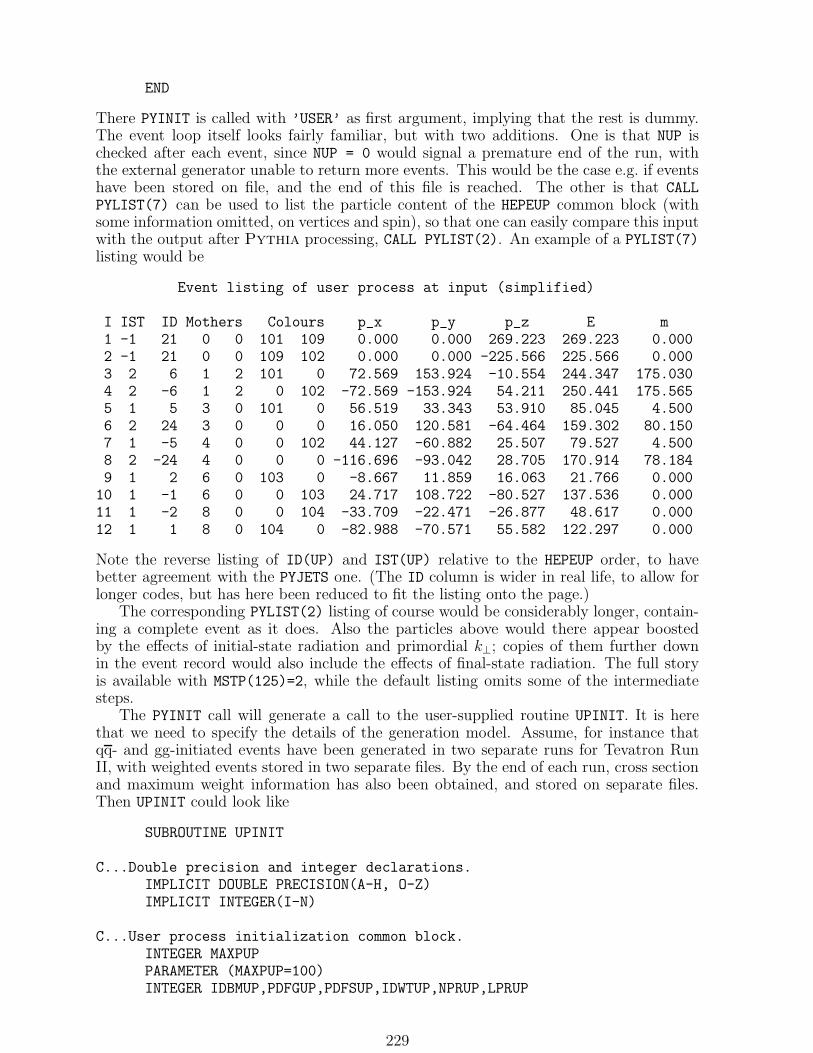
END

There PYINIT is called with ’USER’ as first argument, implying that the rest is dummy.The event loop itself looks fairly familiar, but with two additions. One is that NUP ischecked after each event, since NUP = 0 would signal a premature end of the run, withthe external generator unable to return more events. This would be the case e.g. if eventshave been stored on file, and the end of this file is reached. The other is that CALLPYLIST(7) can be used to list the particle content of the HEPEUP common block (withsome information omitted, on vertices and spin), so that one can easily compare this inputwith the output after Pythia processing, CALL PYLIST(2). An example of a PYLIST(7)listing would be

Event listing of user process at input (simplified)

I IST ID Mothers Colours p_x p_y p_z E m1 -1 21 0 0 101 109 0.000 0.000 269.223 269.223 0.0002 -1 21 0 0 109 102 0.000 0.000 -225.566 225.566 0.0003 2 6 1 2 101 0 72.569 153.924 -10.554 244.347 175.0304 2 -6 1 2 0 102 -72.569 -153.924 54.211 250.441 175.5655 1 5 3 0 101 0 56.519 33.343 53.910 85.045 4.5006 2 24 3 0 0 0 16.050 120.581 -64.464 159.302 80.1507 1 -5 4 0 0 102 44.127 -60.882 25.507 79.527 4.5008 2 -24 4 0 0 0 -116.696 -93.042 28.705 170.914 78.1849 1 2 6 0 103 0 -8.667 11.859 16.063 21.766 0.00010 1 -1 6 0 0 103 24.717 108.722 -80.527 137.536 0.00011 1 -2 8 0 0 104 -33.709 -22.471 -26.877 48.617 0.00012 1 1 8 0 104 0 -82.988 -70.571 55.582 122.297 0.000

Note the reverse listing of ID(UP) and IST(UP) relative to the HEPEUP order, to havebetter agreement with the PYJETS one. (The ID column is wider in real life, to allow forlonger codes, but has here been reduced to fit the listing onto the page.)

The corresponding PYLIST(2) listing of course would be considerably longer, contain-ing a complete event as it does. Also the particles above would there appear boostedby the effects of initial-state radiation and primordial k⊥; copies of them further downin the event record would also include the effects of final-state radiation. The full storyis available with MSTP(125)=2, while the default listing omits some of the intermediatesteps.

The PYINIT call will generate a call to the user-supplied routine UPINIT. It is herethat we need to specify the details of the generation model. Assume, for instance thatqq- and gg-initiated events have been generated in two separate runs for Tevatron RunII, with weighted events stored in two separate files. By the end of each run, cross sectionand maximum weight information has also been obtained, and stored on separate files.Then UPINIT could look like

SUBROUTINE UPINIT

C...Double precision and integer declarations.IMPLICIT DOUBLE PRECISION(A-H, O-Z)IMPLICIT INTEGER(I-N)

C...User process initialization common block.INTEGER MAXPUPPARAMETER (MAXPUP=100)INTEGER IDBMUP,PDFGUP,PDFSUP,IDWTUP,NPRUP,LPRUP

229

DOUBLE PRECISION EBMUP,XSECUP,XERRUP,XMAXUPCOMMON/HEPRUP/IDBMUP(2),EBMUP(2),PDFGUP(2),PDFSUP(2),

&IDWTUP,NPRUP,XSECUP(MAXPUP),XERRUP(MAXPUP),XMAXUP(MAXPUP),&LPRUP(MAXPUP)SAVE /HEPRUP/

C....Pythia common block - needed for setting PDF’s; see below.COMMON/PYPARS/MSTP(200),PARP(200),MSTI(200),PARI(200)SAVE /PYPARS/

C...Set incoming beams: Tevatron Run II.IDBMUP(1)=2212IDBMUP(2)=-2212EBMUP(1)=1000D0EBMUP(2)=1000D0

C...Set PDF’s of incoming beams: CTEQ 5L.C...Note that Pythia will not look at PDFGUP and PDFSUP.

PDFGUP(1)=4PDFSUP(1)=46PDFGUP(2)=PDFGUP(1)PDFSUP(2)=PDFSUP(1)

C...Set use of CTEQ 5L in internal Pythia code.MSTP(51)=7

C...If you want Pythia to use PDFLIB, you have to set it by hand.C...(You also have to ensure that the dummy routinesC...PDFSET, STRUCTM and STRUCTP in Pythia are not linked.)C MSTP(52)=2C MSTP(51)=1000*PDFGUP(1)+PDFSUP(1)

C...Decide on weighting strategy: weighted on input, cross section known.IDWTUP=2

C...Number of external processes.NPRUP=2

C...Set up q qbar -> t tbar.OPEN(21,FILE=’qqtt.info’,FORM=’unformatted’,ERR=100)READ(21,ERR=100) XSECUP(1),XERRUP(1),XMAXUP(1)LPRUP(1)=661OPEN(22,FILE=’qqtt.events’,FORM=’unformatted’,ERR=100)

C...Set up g g -> t tbar.OPEN(23,FILE=’ggtt.info’,FORM=’unformatted’,ERR=100)READ(23,ERR=100) XSECUP(2),XERRUP(2),XMAXUP(2)LPRUP(2)=662OPEN(24,FILE=’ggtt.events’,FORM=’unformatted’,ERR=100)

RETURNC...Stop run if file operations fail.

100 WRITE(*,*) ’Error! File open or read failed. Program stopped.’

230

STOP

END

Here unformatted read/write is used to reduce the size of the event files, but at the price ofa platform dependence. Formatted files are preferred if they are to be shipped elsewhere.The rest should be self-explanatory.

Inside the event loop of the main program, PYEVNT will call UPEVNT to obtain the nextparton-level event. In its simplest form, only a single READ statement would be necessaryto read information on the next event, e.g. what is shown in the event listing earlier inthis subsection, with a few additions. Then the routine could look like

SUBROUTINE UPEVNT

C...Double precision and integer declarations.IMPLICIT DOUBLE PRECISION(A-H, O-Z)IMPLICIT INTEGER(I-N)

C...User process event common block.INTEGER MAXNUPPARAMETER (MAXNUP=500)INTEGER NUP,IDPRUP,IDUP,ISTUP,MOTHUP,ICOLUPDOUBLE PRECISION XWGTUP,SCALUP,AQEDUP,AQCDUP,PUP,VTIMUP,SPINUPCOMMON/HEPEUP/NUP,IDPRUP,XWGTUP,SCALUP,AQEDUP,AQCDUP,IDUP(MAXNUP),

&ISTUP(MAXNUP),MOTHUP(2,MAXNUP),ICOLUP(2,MAXNUP),PUP(5,MAXNUP),&VTIMUP(MAXNUP),SPINUP(MAXNUP)SAVE /HEPEUP/

C...Pick file to read from, based on requested event type.IUNIT=22IF(IDPRUP.EQ.662) IUNIT=24

C...Read event from this file. (Except that NUP and IDPRUP are known.)NUP=12READ(IUNIT,ERR=100,END=100) XWGTUP,SCALUP,AQEDUP,AQCDUP,

&(IDUP(I),ISTUP(I),MOTHUP(1,I),MOTHUP(2,I),ICOLUP(1,I),&ICOLUP(2,I),(PUP(J,I),J=1,5),VTIMUP(I),SPINUP(I),I=1,NUP)

C...Return, with NUP=0 if read failed.RETURN

100 NUP=0RETURNEND

However, in reality one might wish to save disk space by not storing redundant informa-tion. The XWGTUP and SCALUP numbers are vital, while AQEDUP and AQCDUP are purelyinformational and can be omitted. In a gg → tt → bW+bW− → bq1q2 bq3q4 event,only the q1, q2, q3 and q4 flavours need be given, assuming that the particles are alwaysstored in the same order. For a qq initial state, the q flavour should be added to the list.The ISTUP, MOTHUP and ICOLUP information is the same in all events of a given process,except for a twofold ambiguity in the colour flow for gg initial states. All VTIMUP vanishand the SPINUP are uninteresting since spins have already been taken into account by thekinematics of the final fermions. (It would be different if one of the W’s decayed leptoni-cally to a τ .) Only the PUP values of the six final fermions need be given, since the other

231

momenta and masses can be reconstructed from this, remembering that the two initialpartons are massless and along the beam pipe. The final fermions are on the mass shell,so their masses need not be stored event by event, but can be read from a small table.The energy of a particle can be reconstructed from its momentum and mass. Overalltransverse momentum conservation removes two further numbers. What remains is thus5 integers and 18 real numbers, where the reals could well be stored in single precision.Of course, the code needed to unpack information stored this way would be lengthy buttrivial. Even more compact storage strategies could be envisaged, e.g. only to save theweight and the seed of a dedicated random-number generator, to be used to generate thenext parton-level event. It is up to you to find the optimal balance between disk spaceand coding effort.

9.9.4 Further comments

This section contains additional information on a few different topics: cross section in-terpretation, negative-weight events, relations with other Pythia switches and routines,and error conditions.

In several IDWTUP options, the XWGTUP variable is supposed to give the differentialcross section of the current event, times the phase-space volume within which events aregenerated, expressed in picobarns. (Converted to millibarns inside Pythia.) This meansthat, in the limit that many events are generated, the average value of XWGTUP givesthe total cross section of the simulated process. Of course, the tricky part is that thedifferential cross section usually is strongly peaked in a few regions of the phase space,such that the average probability to accept an event, 〈XWGTUP〉/XMAXUP(i) is small. Itmay then be necessary to find a suitable set of transformed phase-space coordinates, forwhich the correspondingly transformed differential cross section is better behaved.

To avoid unclarities, here is a more formal version of the above paragraph. Call dXthe differential phase space, e.g. for a 2 → 2 process dX = dx1 dx2 dt, where x1 and x2are the momentum fractions carried by the two incoming partons and t the Mandelstamvariable of the scattering (see subsection 7.2). Call dσ/dX the differential cross sectionof the process, e.g. for 2 → 2: dσ/dX =

∑

ij fi(x1, Q2) fj(x2, Q

2) dσij/dt, i.e. the prod-uct of parton distributions and hard-scattering matrix elements, summed over all allowedincoming flavours i and j. The physical cross section that one then wants to generateis σ =

∫

(dσ/dX) dX , where the integral is over the allowed phase-space volume. Theevent generation procedure consists of selecting an X uniformly in dX and then evalu-ating the weight dσ/dX at this point. XWGTUP is now simply XWGTUP= dσ/dX

∫

dX , i.e.the differential cross section times the considered volume of phase space. Clearly, whenaveraged over many events, XWGTUP will correctly estimate the desired cross section. IfXWGTUP fluctuates too much, one may try to transform to new variables X ′, where eventsare now picked accordingly to dX ′ and XWGTUP= dσ/dX ′

∫

dX ′.A warning. It is important that X is indeed uniformly picked within the allowed phase

space, alternatively that any Jacobians are properly taken into account. For instance, inthe case above, one approach would be to pick x1, x2 and t uniformly in the ranges0 < x1 < 1, 0 < x2 < 1, and −s < t < 0, with full phase space volume

∫

dX = s. Thecross section would only be non-vanishing inside the physical region given by −sx1x2 < t(in the massless case), i.e. Monte Carlo efficiency is likely to be low. However, if one wereto choose t values only in the range −s < t < 0, small s values would be favoured, sincethe density of selected t values would be larger there. Without the use of a compensatingJacobian s/s, an incorrect answer would be obtained. Alternatively, one could start out

with a phase space like dX = dx1 dx2 d(cos θ), where the limits decouple. Of course, the

cos θ variable can be translated back into a t, which will then always be in the desiredrange −s < t < 0. The transformation itself here gives the necessary Jacobian.

232

At times, it is convenient to split a process into a discrete set of subprocesses for theparton-level generation, without retaining these in the IDPRUP classification. For instance,the cross section above contains a summation over incoming partons. An alternativewould then have been to let each subprocess correspond to one unique combination ofincoming flavours. When an event of process type i is to be generated, first a specificsubprocess ik is selected with probability f ik, where

∑

k fik = 1. For this subprocess an

XWGTUPk is generated as above, except that there is no longer a summation over incomingflavours. Since only a fraction f ik of all events now contain this part of the cross section,a compensating factor 1/f ik is introduced, i.e. XWGTUP=XWGTUPk/f ik. Further, one has todefine XMAXUP(i)= maxk XMAXUPik/f ik and XSECUP(i)=

∑

k XSECUPik. The generationefficiency will be maximized for the f ik coefficients selected proportional to XMAXUPik, butthis is no requirement.

The standard allows external parton-level events to come with negative weights, unlikethe case for internal Pythia processes. In order to avoid indiscriminate use of this option,some words of caution are in place. In next-to-leading-order calculations, events withnegative weights may occur as part of the virtual corrections. In any physical observablequantity, the effect of such events should cancel against the effect of real events withone more parton in the final state. For instance, the next-to-leading order calculation ofgluon scattering contains the real process gg → ggg, with a positive divergence in the softand collinear regions, while the virtual corrections to gg → gg are negatively divergent.Neglecting the problems of outgoing gluons collinear with the beams, and those of softgluons, two nearby outgoing gluons in the gg → ggg process can be combined into oneeffective one, such that the divergences can be cancelled.

If rather widely separated gluons can be combined, the remaining negative contribu-tions are not particularly large. Different separation criteria could be considered; one

example would be ∆R =√

(∆η)2 + (∆ϕ)2 ≈ 1. The recombination of well separatedpartons is at the price of an arbitrariness in the choice of clustering algorithm, whentwo gluons of nonvanishing invariant mass are to be combined into one massless one, asrequired to be able to compare with the kinematics of the massless gg → gg process whenperforming the divergence cancellations. Alternatively, if a smaller ∆R cut is used, wherethe combining procedure is less critical, there will be more events with large positive andnegative weights that are to cancel.

Without proper care, this cancellation could easily be destroyed by the subsequentshowering description, as follows. The standard for external processes does not provideany way to pass information on the clustering algorithm used, so the showering routinewill have to make its own choice what region of phase space to populate with radiation.One choice could be to allow a cone defined by the nearest colour-connected parton (seesubsection 10.1.3 for a discussion). There could then arise a significant mismatch inshower description between events where two gluons are just below or just above the ∆Rcut for being recombined, equivalently between gg → gg and gg → ggg events. Most ofthe phase space may be open for the former, while only the region below ∆R may be itfor the latter. Thus the average ‘two-parton’ events may end up containing significantlymore jet activity than the corresponding ‘three-parton’ ones. The smaller the ∆R cut,the more severe the mismatch, both on an event-by-event basis and in terms of the eventrates involved.

One solution would be to extend the standard also to specify which clustering algo-rithm has been used in the matrix-element calculation, and with what parameter values.Any shower emission that would give rise to an extra jet, according to this algorithm,would be vetoed. If a small ∆R cut is used, this is almost equivalent to allowing noshower activity at all. (That would still leave us with potential mismatch problems in thehadronization description. Fortunately the string fragmentation approach is very pow-erful in this respect, with a smooth transition between two almost parallel gluons and asingle one with the full energy [Sjo84].) But we know that the unassisted matrix-element

233

description cannot do a good job of the internal structure of jets on an event-by-eventbasis, since multiple-gluon emission is the norm in this region. Therefore a ∆R ∼ 1 willbe required, to let the matrix elements describe the wide-angle emission and the showersthe small-angle one. This again suggests a picture with only a small contribution fromnegative-weight events. In summary, the appearance of a large fraction of negative-weightevents should be a sure warning sign that physics is likely to be incorrectly described.

The above example illustrates that it may, at times, be desirable to sidestep the stan-dard and provide further information directly in the Pythia common blocks. (Currentlythere is no exact match to the clustering task mentioned above, but there are a few sim-pler ways to intervene in the shower evolution.) Then it is useful to note that, apart fromthe hard-process generation machinery itself, the external processes are handled almostexactly as the internal ones. Thus essentially all switches and parameter values related toshowers, underlying events and hadronization can be modified at will. This even appliesto alternative listing modes of events and history pointers, as set by MSTP(128). Alsosome of the information on the hard scattering is available, such as MSTI(3), MSTI(21)- MSTI(26), and PARI(33) - PARI(38). Before using them, however, it is prudent tocheck that your variables of interest do work as intended for the particular process youstudy. Several differences do remain between internal and external processes, in particularrelated to final-state showers and resonance decays. For internal processes, the PYRESDroutine will perform a shower (if relevant) directly after each decay. A typical examplewould be that a t → bW decay is immediately followed by a shower, which could changethe momentum of the W before it decays in its turn. For an external process, this decaychain would presumably already have been carried out. When the equivalent shower tothe above is performed, it is therefore now necessary also to boost the decay products ofthe W. The special sequence of showers and boosts for external processes is administratedby the PYADSH routine.

You are free to make use of whatever tools you want in your UPINIT and UPEVNTroutines, and normally there would be little or no contact with the rest of Pythia, exceptas described above. However, several Pythia tools can be used, if you so wish. Oneattractive possibility is to use PYPDFU for parton-distribution-function evaluation. Otherpossible tools could be PYR for random-number generation, PYALPS for αs evaluation,PYALEM for evaluation of a running αem, and maybe a few more.

We end with a few comments on anomalous situations. As already described, you mayput NUP=0 inside UPEVNT, e.g. to signal the end of the file from which events are read. Ifthe program encounters this value at a return from UPEVNT, then it will also exit fromPYEVNT, without incrementing the counters for the number of events generated. It is thenup to you to have a check on this condition in your main event-generation loop. This youdo either by looking at NUP or at MSTI(51); the latter is set to 1 if no event was generated.

It may also happen that a parton-level configuration fails elsewhere in the PYEVNTcall. For instance, the beam-remnant treatment occasionally encounters situations itcannot handle, wherefore the parton-level event is rejected and a new one generated.This happens also with ordinary (not user-defined) events, and usually comes about asa consequence of the initial-state radiation description leaving too little energy for theremnant. If the same hard scattering were to be used as input for a new initial-stateradiation and beam-remnant attempt, it could then work fine. There is a possibility togive events that chance, as follows. MSTI(52) counts the number of times a hard-scatteringconfiguration has failed to date. If you come in to UPEVNT with MSTI(52) non-vanishing,this means that the latest configuration failed. So long as the contents of the HEPEUPcommon block are not changed, such an event may be given another try. For instance, aline

IF(MSTI(52).GE.1.AND.MSTI(52).LE.4) RETURN

at the beginning of UPEVNT will give each event up to five tries; thereafter a new one

234

would be generated as usual. Note that the counter for the number of events is updatedat each new try. The fraction of failed configurations is given in the bottom line of thePYSTAT(1) table.

The above comment only refers to very rare occurrences (less than one in a hundred),which are not errors in a strict sense; for instance, they do not produce any error messageson output. If you get warnings and error messages that the program does not understandthe flavour codes or cannot reconstruct the colour flows, it is due to faults of yours, andgiving such events more tries is not going to help.

9.10 Interfaces to Other Generators

In the previous section an approach to including external processes in Pythia was ex-plained. While general enough, it may not always be the optimal choice. In particular, fore+e− annihilation events one may envisage some standard cases where simpler approachescould be pursued. A few such standard interfaces are described in this section.

In e+e− annihilation events, a convenient classification of electroweak physics is by thenumber of fermions in the final state. Two fermions from Z0 decay is LEP1 physics, fourfermions can come e.g. from W+W− or Z0Z0 events at LEP2, and at higher energies sixfermions are produced by three-gauge-boson production or top-antitop. Often interferenceterms are non-negligible, requiring much more complex matrix-element expressions thanare normally provided in Pythia. Dedicated electroweak generators often exist, however,and the task is therefore to interface them to the generic parton showering and hadroniza-tion machinery available in Pythia. In the LEP2 workshop [Kno96] one possible strategywas outlined to allow reasonably standardized interfaces between the electroweak and theQCD generators. The LU4FRM routine was provided for the key four-fermion case. Thisroutine is now included here, in slightly modified form, together with two new siblings fortwo and six fermions. The former is trivial and included mainly for completeness, whilethe latter is rather more delicate.

In final states with two or three quark–antiquark pairs, the colour connection is notunique. For instance, a udud final state could either stem from a W+W− or a Z0Z0

intermediate state, or even from interference terms between the two. In order to showerand fragment the system, it is then necessary to pick one of the two alternatives, e.g.according to the relative matrix element weight of each alternative, with the interferenceterm dropped. Some different such strategies are proposed as options below.

Note that here we discuss purely perturbative ambiguities. One can imagine colourreconnection at later stages of the process, e.g. if the intermediate state indeed is W+W−,a soft-gluon exchange could still result in colour singlets uu and dd. We are then no longerspeaking of ambiguities related to the hard process itself but rather to the possibility ofnonperturbative effects. This is an interesting topic in itself, addressed in section 12.4.2but not here.

The fermion-pair routines are not set up to handle QCD four-jet events, i.e. events ofthe types qqgg and qqq′q′ (with q′q′ coming from a gluon branching). Such events aregenerated in normal parton showers, but not necessarily at the right rate (a problem thatmay be especially interesting for massive quarks like b). Therefore one would like to starta QCD final-state parton shower from a given four-parton configuration. Already sometime ago, a machinery was developed to handle this kind of occurrences [And98a]. Thisapproach has now been adapted to Pythia, in a somewhat modified form, see section10.2.7. The main change is that, in the original work, the colour flow was picked in aseparate first step (not discussed in the publication, since it is part of the standard 4-parton configuration machinery of PYEEVT), which reduces the number of allowed qqggparton-shower histories. In the current implementation, more geared towards completelyexternal generators, no colour flow assumptions are made, meaning a few more possibleshower histories to pick between. Another change is that mass effects are better respected

235

by the z definition. The code contains one new user routine, PY4JET, two new auxiliaryones, PY4JTW and PY4JTS, and significant additions to the PYSHOW showering routine.

CALL PY2FRM(IRAD,ITAU,ICOM)

Purpose: to allow a parton shower to develop and partons to hadronize from a two-fermion starting point. The initial list is supposed to be ordered such that thefermion precedes the antifermion. In addition, an arbitrary number of photonsmay be included, e.g. from initial-state radiation; these will not be affected bythe operation and can be put anywhere. The scale for QCD (and QED) final-state radiation is automatically set to be the mass of the fermion-antifermionpair. (It is thus not suited for Bhabha scattering.)

IRAD : final-state QED radiation.= 0 : no final-state photon radiation, only QCD showers.= 1 : photon radiation inside each final fermion pair, also leptons, in addition

to the QCD one for quarks.ITAU : handling of τ lepton decay (where Pythia does not include spin effects, al-

though some generators provide the helicity information that would allow amore sophisticated modelling).

= 0 : τ ’s are considered stable (and can therefore be decayed afterwards).= 1 : τ ’s are allowed to decay.

ICOM : place where information about the event (flavours, momenta etc.) is stored atinput and output.

= 0 : in the HEPEVT commonblock (meaning that information is automaticallytranslated to PYJETS before treatment and back afterwards).

= 1 : in the PYJETS commonblock. All fermions and photons can be givenwith status code K(I,1)=1, flavour code in K(I,2) and five-momentum(momentum, energy, mass) in P(I,J). The V vector and remaining com-ponents in the K one are best put to zero. Also remember to set the totalnumber of entries N.

CALL PY4FRM(ATOTSQ,A1SQ,A2SQ,ISTRAT,IRAD,ITAU,ICOM)

Purpose: to allow a parton shower to develop and partons to hadronize from a four-fermion starting point. The initial list of fermions is supposed to be orderedin the sequence fermion (1) – antifermion (2) – fermion (3) – antifermion (4).The flavour pairs should be arranged so that, if possible, the first two couldcome from a W+ and the second two from a W−; else each pair should haveflavours consistent with a Z0. In addition, an arbitrary number of photons maybe included, e.g. from initial-state radiation; these will not be affected by theoperation and can be put anywhere. Since the colour flow need not be unique,three real and one integer numbers are providing further input. Once the colourpairing is determined, the scale for final-state QCD (and QED) radiation isautomatically set to be the mass of the fermion-antifermion pair. (This is therelevant choice for normal fermion pair production from resonance decay, butis not suited e.g. for γγ processes dominated by small-t propagators.) Thepairing is also meaningful for QED radiation, in the sense that a four-leptonfinal state is subdivided into two radiating subsystems in the same way. Onlyif the event consists of one lepton pair and one quark pair is the informationsuperfluous.

ATOTSQ : total squared amplitude for the event, irrespective of colour flow.A1SQ : squared amplitude for the configuration with fermions 1 + 2 and 3 + 4 as the

236

two colour singlets.A2SQ : squared amplitude for the configuration with fermions 1 + 4 and 3 + 2 as the

two colour singlets.ISTRAT : the choice of strategy to select either of the two possible colour configurations.

Here 0 is supposed to represent a reasonable compromize, while 1 and 2 areselected so as to give the largest reasonable spread one could imagine.

= 0 : pick configurations according to relative probabilities A1SQ : A2SQ.= 1 : assign the interference contribution to maximize the 1 + 2 and 3 + 4

pairing of fermions.= 2 : assign the interference contribution to maximize the 1 + 4 and 3 + 2

pairing of fermions.IRAD : final-state QED radiation.

= 0 : no final-state photon radiation, only QCD showers.= 1 : photon radiation inside each final fermion pair, also leptons, in addition

to the QCD one for quarks.ITAU : handling of τ lepton decay (where Pythia does not include spin effects, al-

though some generators provide the helicity information that would allow amore sophisticated modelling).

= 0 : τ ’s are considered stable (and can therefore be decayed afterwards).= 1 : τ ’s are allowed to decay.

ICOM : place where information about the event (flavours, momenta etc.) is stored atinput and output.

= 0 : in the HEPEVT commonblock (meaning that information is automaticallytranslated to PYJETS before treatment and back afterwards).

= 1 : in the PYJETS commonblock. All fermions and photons can be givenwith status code K(I,1)=1, flavour code in K(I,2) and five-momentum(momentum, energy, mass) in P(I,J). The V vector and remaining com-ponents in the K one are best put to zero. Also remember to set the totalnumber of entries N.

Comment : Also colour reconnection phenomena can be studied with the PY4FRM rou-tine. MSTP(115) can be used to switch between the scenarios, with defaultbeing no reconnection. Other reconnection parameters also work as normally,including that MSTI(32) can be used to find out whether a reconnection oc-cured or not. In order for the reconnection machinery to work, the event recordis automatically compelemented with information on the W+W− or Z0Z0 pairthat produced the four fermions, based on the rules described above.We remind that the four first parameters of the PY4FRM call are supposed toparameterize an ambiguity on the perturbative level of the process, which hasto be resolved before parton showers are performed. The colour reconnectiondiscussed here is (in most scenarios) occuring on the nonperturbative level,after the parton showers.

CALL PY6FRM(P12,P13,P21,P23,P31,P32,PTOP,IRAD,ITAU,ICOM)

Purpose: to allow a parton shower to develop and partons to hadronize from a six-fermion starting point. The initial list of fermions is supposed to be orderedin the sequence fermion (1) – antifermion (2) – fermion (3) – antifermion (4)– fermion (5) – antifermion (6). The flavour pairs should be arranged so that,if possible, the first two could come from a Z0, the middle two from a W+

and the last two from a W−; else each pair should have flavours consistentwith a Z0. Specifically, this means that in a tt event, the t decay productswould be found in 1 (b) and 3 and 4 (from the W+ decay) and the t ones in

237

2 (b) and 5 and 6 (from the W− decay). In addition, an arbitrary number ofphotons may be included, e.g. from initial-state radiation; these will not beaffected by the operation and can be put anywhere. Since the colour flow neednot be unique, further input is needed to specify this. The number of possibleinterference contributions being much larger than for the four-fermion case, wehave not tried to implement different strategies. Instead six probabilities maybe input for the different pairings, that you e.g. could pick as the six possiblesquared amplitudes, or according to some more complicated scheme for howto handle the interference terms. The treatment of final-state cascades mustbe quite different for top events and the rest. For a normal three-boson event,each fermion pair would form one radiating system, with scale set equal to thefermion-antifermion invariant mass. (This is the relevant choice for normalfermion pair production from resonance decay, but is not suited e.g. for γγprocesses dominated by small-t propagators.) In the top case, on the otherhand, the b (b) would be radiating with a recoil taken by the W+ (W−) insuch a way that the t (t) mass is preserved, while the W dipoles would radiateas normal. Therefore you need also supply a probability for the event to be atop one, again e.g. based on some squared amplitude.

P12, P13, P21, P23, P31, P32 : relative probabilities for the six possible pairings offermions with antifermions. The first (second) digit tells which antifermionthe first (second) fermion is paired with, with the third pairing given by elim-ination. Thus e.g. P23 means the first fermion is paired with the second an-tifermion, the second fermion with the third antifermion and the third fermionwith the first antifermion. Pairings are only possible between quarks and lep-tons separately. The sum of probabilities for allowed pairings is automaticallynormalized to unity.

PTOP : the probability that the configuration is a top one; a number between 0 and 1.In this case, it is important that the order described above is respected, withthe b and b coming first. No colour ambiguity exists if the top interpretationis selected, so then the P12 - P32 numbers are not used.

IRAD : final-state QED radiation.= 0 : no final-state photon radiation, only QCD showers.= 1 : photon radiation inside each final fermion pair, also leptons, in addition

to the QCD one for quarks.ITAU : handling of τ lepton decay (where Pythia does not include spin effects, al-

though some generators provide the helicity information that would allow amore sophisticated modelling).

= 0 : τ ’s are considered stable (and can therefore be decayed afterwards).= 1 : τ ’s are allowed to decay.

ICOM : place where information about the event (flavours, momenta etc.) is stored atinput and output.

= 0 : in the HEPEVT commonblock (meaning that information is automaticallytranslated to PYJETS before treatment and back afterwards).

= 1 : in the PYJETS commonblock. All fermions and photons can be givenwith status code K(I,1)=1, flavour code in K(I,2) and five-momentum(momentum, energy, mass) in P(I,J). The V vector and remaining com-ponents in the K one are best put to zero. Also remember to set the totalnumber of entries N.

CALL PY4JET(PMAX,IRAD,ICOM)

Purpose: to allow a parton shower to develop and partons to hadronize from a qqgg

238

or qqq′q′ original configuration. The partons should be ordered exactly as in-dicated above, with the primary qq pair first and thereafter the two gluonsor the secondary q′q′ pair. (Strictly speaking, the definition of primary andsecondary fermion pair is ambiguous. In practice, however, differences in topo-logical variables like the pair mass should make it feasible to have some sensiblecriterion on an event by event basis.) Within each pair, fermion should precedeantifermion. In addition, an arbitrary number of photons may be included, e.g.from initial-state radiation; these will not be affected by the operation and canbe put anywhere. The program will select a possible parton shower historyfrom the given parton configuration, and then continue the shower from thereon. The history selected is displayed in lines NOLD+1 to NOLD+6, where NOLD isthe N value before the routine is called. Here the masses and energies of inter-mediate partons are clearly displayed. The lines NOLD+7 and NOLD+8 containthe equivalent on-mass-shell parton pair from which the shower is started.

PMAX : the maximum mass scale (in GeV) from which the shower is started in thosebranches that are not already fixed by the matrix-element history. If PMAXis set zero (actually below PARJ(82), the shower cutoff scale), the showerstarting scale is instead set to be equal to the smallest mass of the virtualpartons in the reconstructed shower history. A fixed PMAX can thus be used toobtain a reasonably exclusive set of four-jet events (to that PMAX scale), withlittle five-jet contamination, while the PMAX=0 option gives a more inclusiveinterpretation, with five- or more-jet events possible. Note that the showeris based on evolution in mass, meaning the cut is really one of mass, not ofp⊥, and that it may therefore be advantageous to set up the matrix elementscuts accordingly if one wishes to mix different event classes. This is not arequirement, however.

IRAD : final-state QED radiation.= 0 : no final-state photon radiation, only QCD showers.= 1 : photon radiation inside each final fermion pair, also leptons, in addition

to the QCD one for quarks.ICOM : place where information about the event (flavours, momenta etc.) is stored at

input and output.= 0 : in the HEPEVT commonblock (meaning that information is automatically

translated to PYJETS before treatment and back afterwards).= 1 : in the PYJETS commonblock. All fermions and photons can be given

with status code K(I,1)=1, flavour code in K(I,2) and five-momentum(momentum, energy, mass) in P(I,J). The V vector and remaining com-ponents in the K one are best put to zero. Also remember to set the totalnumber of entries N.

9.11 Other Routines and Common Blocks

The subroutines and common blocks that you will come in direct contact with havealready been described. A number of other routines and common blocks exist, and thosenot described elsewhere are here briefly listed for the sake of completeness. The PYG***routines are slightly modified versions of the SAS*** ones of the SaSgam library. Thecommon block SASCOM is renamed PYINT8. If you want to use the parton distributionsfor standalone purposes, you are encouraged to use the original SaSgam routines ratherthan going the way via the Pythia adaptations.

SUBROUTINE PYINRE : to initialize the widths and effective widths of resonances.SUBROUTINE PYINBM(CHFRAM,CHBEAM,CHTARG,WIN) : to read in and identify the beam

(CHBEAM) and target (CHTARG) particles and the frame (CHFRAM) as given in thePYINIT call; also to save the original energy (WIN).

239

SUBROUTINE PYINKI(MODKI) : to set up the event kinematics, either at initialization(MODKI=0) or for each separate event, the latter when the program is run withvarying kinematics (MODKI=1).

SUBROUTINE PYINPR : to set up the partonic subprocesses selected with MSEL. For γpand γγ, also the MSTP(14) value affects the choice of processes. In particular,options such as MSTP(14)=10 and =30 sets up the several different kinds ofprocesses that need to be mixed, with separate cuts for each.

SUBROUTINE PYXTOT : to give the parameterized total, double diffractive, single diffrac-tive and elastic cross sections for different energies and colliding hadrons orphotons.

SUBROUTINE PYMAXI : to find optimal coefficients COEF for the selection of kinematicalvariables, and to find the related maxima for the differential cross section timesJacobian factors, for each of the subprocesses included.

SUBROUTINE PYPILE(MPILE) : to determine the number of pile-up events, i.e. eventsappearing in the same beam–beam crossing.

SUBROUTINE PYSAVE(ISAVE,IGA) : saves and restores parameters and cross section val-ues between the several γp and γγ components of mixing options such asMSTP(14)=10 and =30. The options for ISAVE are (1) a complete save of allparameters specific to a given component, (2) a partial save of cross-sectioninformation, (3) a restoration of all parameters specific to a given component,(4) as 3 but preceded by a random selection of component, and (5) a summa-tion of component cross sections (for PYSTAT). The subprocess code in IGA isthe one described for MSTI(9); it is input for options 1, 2 and 3 above, outputfor 4 and dummy for 5.

SUBROUTINE PYGAGA(IGA) : to generate photons according to the virtual photon fluxaround a lepton beam, for the ’gamma/lepton’ option in PYINIT.

IGA = 1 : call at initialization to set up x and Q2 limits etc.IGA = 2 : call at maximization step to give estimate of maximal photon flux factor.IGA = 3 : call at the beginning of the event generation to select the kinematics of

the photon emission and to give the flux factor.IGA = 4 : call at the end of the event generation to set up the full kinematics of

the photon emission.SUBROUTINE PYRAND : to generate the quantities characterizing a hard scattering on the

parton level, according to the relevant matrix elements.SUBROUTINE PYSCAT : to find outgoing flavours and to set up the kinematics and colour

flow of the hard scattering.SUBROUTINE PYRESD(IRES) : to allow resonances to decay, including chains of successive

decays and parton showers. Normally only two-body decays of each resonance,but a few three-body decays are also implemented.

IRES : The standard call from PYEVNT, for the hard process, has IRES=0, andthen finds resonances to be treated based on the subprocess number ISUB.In case of a nonzero IRES only the resonance in position IRES of the eventrecord is considered. This is used by PYEVNT and PYEXEC to decay leftoverresonances. (Example: a b → W + t branching may give a t quark asbeam remnant.)

SUBROUTINE PYMULT(MMUL) : to generate semi-hard interactions according to the multi-ple interaction formalism.

SUBROUTINE PYREMN(IPU1,IPU2) : to add on target remnants and include primordialk⊥.

SUBROUTINE PYDIFF : to handle diffractive and elastic scattering events.SUBROUTINE PYDISG : to set up kinematics, beam remnants and showers in the 2 → 1

DIS process γ∗f → f. Currently initial-state radiation is not yet implemented,while final-state is.

240

SUBROUTINE PYDOCU : to compute cross sections of processes, based on current MonteCarlo statistics, and to store event information in the MSTI and PARI arrays.

SUBROUTINE PYWIDT(KFLR,SH,WDTP,WDTE) : to calculate widths and effective widths ofresonances. Everything is given in dimensions of GeV.

SUBROUTINE PYOFSH(MOFSH,KFMO,KFD1,KFD2,PMMO,RET1,RET2) : to calculate partialwidths into channels off the mass shell, and to select correlated masses ofresonance pairs.

SUBROUTINE PYKLIM(ILIM) : to calculate allowed kinematical limits.SUBROUTINE PYKMAP(IVAR,MVAR,VVAR) : to calculate the value of a kinematical variable

when this is selected according to one of the simple pieces.SUBROUTINE PYSIGH(NCHN,SIGS) : to give the differential cross section (multiplied by

the relevant Jacobians) for a given subprocess and kinematical setup.SUBROUTINE PYPDFL(KF,X,Q2,XPQ) : to give parton distributions for p and n in the

option with modified behaviour at small Q2 and x, see MSTP(57).SUBROUTINE PYPDFU(KF,X,Q2,XPQ) : to give parton-distribution functions (multiplied

by x, i.e. xfi(x,Q2)) for an arbitrary particle (of those recognized by Pythia).

Generic driver routine for the following, specialized ones.KF : flavour of probed particle, according to KF code.X : x value at which to evaluate parton distributions.Q2 : Q2 scale at which to evaluate parton distributions.XPQ : array of dimensions XPQ(-25:25), which contains the evaluated parton

distributions xfi(x,Q2). Components i ordered according to standard

KF code; additionally the gluon is found in position 0 as well as 21 (forhistorical reasons).

Note: the above set of calling arguments is enough for a real photon, but hasto be complemented for a virtual one. This is done by VINT(120).

SUBROUTINE PYPDEL(KFA,X,Q2,XPEL) : to give e/µ/τ parton distributions.SUBROUTINE PYPDGA(X,Q2,XPGA) : to give the photon parton distributions for sets other

than the SaS ones.SUBROUTINE PYGGAM(ISET,X,Q2,P2,IP2,F2GM,XPDFGM) : to construct the SaS F2 and

parton distributions of the photon by summing homogeneous (VMD) and in-homogeneous (anomalous) terms. For F2, c and b are included by the Bethe-Heitler formula; in the ‘ms’ scheme additionally a Cγ term is added. IP2 setstreatment of virtual photons, with same code as MSTP(60). Calls PYGVMD,PYGANO, PYGBEH, and PYGDIR.

SUBROUTINE PYGVMD(ISET,KF,X,Q2,P2,ALAM,XPGA,VXPGA) : to evaluate the partondistributions of a VMD photon, evolved homogeneously from an initial scaleP 2 to Q2.

SUBROUTINE PYGANO(KF,X,Q2,P2,ALAM,XPGA,VXPGA) : to evaluate the parton distribu-tions of the anomalous photon, inhomogeneously evolved from a scale P 2

(where it vanishes) to Q2.SUBROUTINE PYGBEH(KF,X,Q2,P2,PM2,XPBH) : to evaluate the Bethe-Heitler cross sec-

tion for heavy flavour production.SUBROUTINE PYGDIR(X,Q2,P2,AK0,XPGA) : to evaluate the direct contribution, i.e. the

Cγ term, as needed in ‘ms’ parameterizations.SUBROUTINE PYPDPI(X,Q2,XPPI) : to give pion parton distributions.SUBROUTINE PYPDPR(X,Q2,XPPR) : to give proton parton distributions. Calls several

auxiliary routines: PYCTEQ, PYGRVL, PYGRVM, PYGRVD, PYGRVV, PYGRVW, PYGRVS,PYCT5L, PYCT5M and PYPDPO.

FUNCTION PYHFTH(SH,SQM,FRATT) : to give heavy-flavour threshold factor in matrix el-ements.

SUBROUTINE PYSPLI(KF,KFLIN,KFLCH,KFLSP) : to give hadron remnant or remnantsleft behind when the reacting parton is kicked out.

241

FUNCTION PYGAMM(X) : to give the value of the ordinary Γ(x) function (used in someparton-distribution parameterizations).

SUBROUTINE PYWAUX(IAUX,EPS,WRE,WIM) : to evaluate the two auxiliary functions W1

and W2 appearing in some cross section expressions in PYSIGH.SUBROUTINE PYI3AU(EPS,RAT,Y3RE,Y3IM) : to evaluate the auxiliary function I3 ap-

pearing in some cross section expressions in PYSIGH.FUNCTION PYSPEN(XREIN,XIMIN,IREIM) : to calculate the real and imaginary part of

the Spence function [Hoo79].SUBROUTINE PYQQBH(WTQQBH) : to calculate matrix elements for the two processes gg →

QQh0 and qq → QQh0.SUBROUTINE PYRECO(IW1,IW2,NSD1,NAFT1)) : to perform nonperturbative reconnec-

tion among strings in W+W− and Z0Z0 events. The physics of this routine isdescribed as part of the fragmentation story, section 12.4.2, but for technicalreasons the code is called directly in the event generation sequence.

BLOCK DATA PYDATA : to give sensible default values to all status codes and parameters.

COMMON/PYINT1/MINT(400),VINT(400)

Purpose: to collect a host of integer- and real-valued variables used internally in the pro-gram during the initialization and/or event generation stage. These variablesmust not be changed by you.

MINT(1) : specifies the general type of subprocess that has occurred, according to theISUB code given in section 8.1.

MINT(2) : whenever MINT(1) (together with MINT(15) and MINT(16)) are not sufficientto specify the type of process uniquely, MINT(2) provides an ordering of thedifferent possibilities, see MSTI(2). Internally and temporarily, in process 53MINT(2) is increased by 2 or 4 for c or b, respectively.

MINT(3) : number of partons produced in the hard interactions, i.e. the number n ofthe 2 → n matrix elements used; is sometimes 3 or 4 when a basic 2 → 1 or2 → 2 process has been convoluted with two 1 → 2 initial branchings (likeqq′ → q′′q′′′h0).

MINT(4) : number of documentation lines at the beginning of the common block PYJETSthat are given with K(I,1)=21; 0 for MSTP(125)=0.

MINT(5) : number of events generated to date in current run. In runs with the variable-energy option, MSTP(171)=1 and MSTP(172)=2, only those events that survive(i.e. that do not have MSTI(61)=1) are counted in this number. That is,MINT(5) may be less than the total number of PYEVNT calls.

MINT(6) : current frame of event (see MSTP(124) for possible values).MINT(7), MINT(8) : line number for documentation of outgoing partons/particles from

hard scattering for 2 → 2 or 2 → 1 → 2 processes (else = 0).MINT(10) : is 1 if cross section maximum was violated in current event, and 0 if not.MINT(11) : KF flavour code for beam (side 1) particle.MINT(12) : KF flavour code for target (side 2) particle.MINT(13), MINT(14) : KF flavour codes for side 1 and side 2 initial-state shower initia-

tors.MINT(15), MINT(16) : KF flavour codes for side 1 and side 2 incoming partons to the

hard interaction. (For use in PYWIDT calls, occasionally MINT(15)=1 signals thepresence of an as yet unspecified quark, but the original value is then restoredafterwards.)

MINT(17), MINT(18) : flag to signal if particle on side 1 or side 2 has been scattereddiffractively; 0 if no, 1 if yes.

MINT(19), MINT(20) : flag to signal initial-state structure with parton inside photon

242

inside electron on side 1 or side 2; 0 if no, 1 if yes.MINT(21) - MINT(24) : KF flavour codes for outgoing partons from the hard interaction.

The number of positions actually used is process-dependent, see MINT(3); trail-ing positions not used are set = 0. For events with many outgoing partons,e.g. in external processes, also MINT(25) and MINT(26) could be used.

MINT(25), MINT(26) : KF flavour codes of the products in the decay of a single s-channelresonance formed in the hard interaction. Are thus only used when MINT(3)=1and the resonance is allowed to decay.

MINT(31) : number of hard or semi-hard scatterings that occurred in the current eventin the multiple-interaction scenario; is = 0 for a low-p⊥ event.

MINT(32) : information on whether a nonperturbative colour reconnection occurred inthe current event; is 0 normally but 1 in case of reconnection.

MINT(41), MINT(42) : type of incoming beam or target particle; 1 for lepton and 2 forhadron. A photon counts as a lepton if it is not resolved (direct or DIS) andas a hadron if it is resolved (VMD or GVMD).

MINT(43) : combination of incoming beam and target particles. A photon counts as ahadron.

= 1 : lepton on lepton.= 2 : lepton on hadron.= 3 : hadron on lepton.= 4 : hadron on hadron.

MINT(44) : as MINT(43), but a photon counts as a lepton.MINT(45), MINT(46) : structure of incoming beam and target particles.

= 1 : no internal structure, i.e. a lepton or photon carrying the full beam en-ergy.

= 2 : defined with parton distributions that are not peaked at x = 1, i.e. ahadron or a resolved (VMD or GVMD) photon.

= 3 : defined with parton distributions that are peaked at x = 1, i.e. a resolvedlepton.

MINT(47) : combination of incoming beam- and target-particle parton-distribution func-tion types.

= 1 : no parton distribution either for beam or target.= 2 : parton distributions for target but not for beam.= 3 : parton distributions for beam but not for target.= 4 : parton distributions for both beam and target, but not both peaked at

x = 1.= 5 : parton distributions for both beam and target, with both peaked at x =

1.= 6 : parton distribution is peaked at x = 1 for target and no distribution at

all for beam.= 7 : parton distribution is peaked at x = 1 for beam and no distribution at

all for target.MINT(48) : total number of subprocesses switched on.MINT(49) : number of subprocesses that are switched on, apart from elastic scattering

and single, double and central diffractive.MINT(50) : combination of incoming particles from a multiple interactions point of

view.= 0 : the total cross section is not known; therefore no multiple interactions

are possible.= 1 : the total cross section is known; therefore multiple interactions are possi-

ble if switched on. Requires beams of hadrons, VMD photons or GVMDphotons.

MINT(51) : internal flag that event failed cuts.

243

= 0 : no problem.= 1 : event failed; new one to be generated.= 2 : event failed; no new event is to be generated but instead control is to be

given back to used. Is intended for user-defined processes, when NUP=0.MINT(52) : internal counter for number of lines used (in /PYJETS/) before multiple in-

teractions are considered.MINT(53) : internal counter for number of lines used (in /PYJETS/) before beam rem-

nants are considered.MINT(55) : the heaviest new flavour switched on for QCD processes, specifically the

flavour to be generated for ISUB = 81, 82, 83 or 84.MINT(56) : the heaviest new flavour switched on for QED processes, specifically for ISUB

= 85. Note that, unlike MINT(55), the heaviest flavour may here be a lepton,and that heavy means the one with largest KF code.

MINT(57) : number of times the beam remnant treatment has failed, and the same basickinematical setup is used to produce a new parton shower evolution and beamremnant set. Mainly used in leptoproduction, for the option when x and Q2

are to be preserved.MINT(61) : internal switch for the mode of operation of resonance width calculations in

PYWIDT for γ∗/Z0 or γ∗/Z0/Z′0.= 0 : without reference to initial-state flavours.= 1 : with reference to given initial-state flavours.= 2 : for given final-state flavours.

MINT(62) : internal switch for use at initialization of h0 width.= 0 : use widths into ZZ∗ or WW∗ calculated before.= 1 : evaluate widths into ZZ∗ or WW∗ for current Higgs mass.

MINT(63) : internal switch for use at initialization of the width of a resonance definedwith MWID(KC)=3.

= 0 : use existing widths, optionally with simple energy rescaling.= 1 : evaluate widths at initialization, to be used subsequently.

MINT(65) : internal switch to indicate initialization without specified reaction.= 0 : normal initialization.= 1 : initialization with argument ’none’ in PYINIT call.

MINT(71) : switch to tell whether current process is singular for p⊥ → 0 or not.= 0 : non-singular process, i.e. proceeding via an s-channel resonance or with

both products having a mass above CKIN(6).= 1 : singular process.

MINT(72) : number of s-channel resonances that may contribute to the cross section.MINT(73) : KF code of first s-channel resonance; 0 if there is none.MINT(74) : KF code of second s-channel resonance; 0 if there is none.MINT(81) : number of selected pile-up events.MINT(82) : sequence number of currently considered pile-up event.MINT(83) : number of lines in the event record already filled by previously considered

pile-up events.MINT(84) : MINT(83) + MSTP(126), i.e. number of lines already filled by previously con-

sidered events plus number of lines to be kept free for event documentation.MINT(91) : is 1 for a lepton–hadron event and 0 else. Used to determine whether a

PYFRAM(3) call is possible.MINT(92) : is used to denote region in (x,Q2) plane when MSTP(57)=2, according to

numbering in [Sch93a]. Simply put, 0 means that the modified proton partondistributions were not used, 1 large x and Q2, 2 small Q2 but large x, 3 smallx but large Q2 and 4 small x and Q2.

MINT(93) : is used to keep track of parton distribution set used in the latest STRUCTMcall to Pdflib. The code for this set is stored in the form MINT(93) =

244

1000000×NPTYPE + 1000×NGROUP + NSET. The stored previous value is com-pared with the current new value to decide whether a PDFSET call is needed toswitch to another set.

MINT(101), MINT(102) : is normally 1, but is 4 when a resolved photon (appearing onside 1 or 2) can be represented by either of the four vector mesons ρ0, ω, φand J/ψ.

MINT(103), MINT(104) : KF flavour code for the two incoming particles, i.e. the sameas MINT(11) and MINT(12). The exception is when a resolved photon is rep-resented by a vector meson (a ρ0, ω, φ or J/ψ). Then the code of the vectormeson is given.

MINT(105) : is either MINT(103) or MINT(104), depending on which side of the eventcurrently is being studied.

MINT(107), MINT(108) : if either or both of the two incoming particles is a photon,then the respective value gives the nature assumed for that photon. The codefollows the one used for MSTP(14):

= 0 : direct photon.= 1 : resolved photon.= 2 : VMD-like photon.= 3 : anomalous photon.= 4 : DIS photon.

MINT(109) : is either MINT(107) or MINT(108), depending on which side of the eventcurrently is being studied.

MINT(111) : the frame given in PYINIT call, 0–5 for ’NONE’, ’CMS’, ’FIXT’, ’3MOM’,’4MOM’ and ’5MOM’, respectively, and 11 for ’USER’.

MINT(121) : number of separate event classes to initialize and mix.= 1 : the normal value.= 2 - 13 : for γp/γ∗p/γγ/γ∗γ/γ∗γ∗ interaction when MSTP(14) is set to mix dif-

ferent photon components.MINT(122) : event class used in current event for γp or γγ events generated with one

of the MSTP(14) options mixing several event classes; code as described forMSTI(9).

MINT(123) : event class used in the current event, with the same list of possibilitiesas for MSTP(14), except that options 1, 4 or 10 do not appear. = 8 denotesDIS×VMD/p or vice verse, = 9 DIS*GVMD or vice versa. Apart from a dif-ferent coding, this is exactly the same information as is available in MINT(122).

MINT(141), MINT(142) : for ’gamma/lepton’ beams, KF code for incoming lepton beamor target particles, while MINT(11) and MINT(12) is then the photon code.A nonzero value is the main check whether the photon emission machineryshould be called at all.

MINT(143) : the number of tries before a successful kinematics configuration is found inPYGAGA, used for ’gamma/lepton’ beams. Used for the cross section updatingin PYRAND.

VINT(1) : Ecm, c.m. energy.VINT(2) : s (= E2

cm) squared mass of complete system.VINT(3) : mass of beam particle. Can be negative to denote a spacelike particle, e.g. a

γ∗.VINT(4) : mass of target particle. Can be negative to denote a spacelike particle, e.g. a

γ∗.VINT(5) : absolute value of momentum of beam (and target) particle in c.m. frame.VINT(6) - VINT(10) : θ, ϕ and β for rotation and boost from c.m. frame to user-

specified frame.VINT(11) : τmin.

245

VINT(12) : ymin.VINT(13) : cos θmin for cos θ ≤ 0.VINT(14) : cos θmin for cos θ ≥ 0.VINT(15) : x2⊥min.VINT(16) : τ ′min.VINT(21) : τ .VINT(22) : y.VINT(23) : cos θ.VINT(24) : ϕ (azimuthal angle).VINT(25) : x2⊥.VINT(26) : τ ′.VINT(31) : τmax.VINT(32) : ymax.VINT(33) : cos θmax for cos θ ≤ 0.VINT(34) : cos θmax for cos θ ≥ 0.VINT(35) : x2⊥max.VINT(36) : τ ′max.VINT(41), VINT(42) : the momentum fractions x taken by the partons at the hard

interaction, as used e.g. in the parton-distribution functions.VINT(43) : m =

√s, mass of hard-scattering subsystem.

VINT(44) : s of the hard subprocess (2 → 2 or 2 → 1).VINT(45) : t of the hard subprocess (2 → 2 or 2 → 1 → 2).VINT(46) : u of the hard subprocess (2 → 2 or 2 → 1 → 2).VINT(47) : p⊥ of the hard subprocess (2 → 2 or 2 → 1 → 2), i.e. transverse momentum

evaluated in the rest frame of the scattering.VINT(48) : p2⊥ of the hard subprocess; see VINT(47).VINT(49) : m′, the mass of the complete three- or four-body final state in 2 → 3 or

2 → 4 processes.VINT(50) : s′ = m′2; see VINT(49).VINT(51) : Q of the hard subprocess. The exact definition is process-dependent, see

MSTP(32).VINT(52) : Q2 of the hard subprocess; see VINT(51).VINT(53) : Q of the outer hard-scattering subprocess, used as scale for parton distribu-

tion function evaluation. Agrees with VINT(51) for a 2 → 1 or 2 → 2 process.For a 2 → 3 or 2 → 4 W/Z fusion process, it is set by the W/Z mass scale,and for subprocesses 121 and 122 by the heavy-quark mass.

VINT(54) : Q2 of the outer hard-scattering subprocess; see VINT(53).VINT(55) : Q scale used as maximum virtuality in parton showers. Is equal to VINT(53),

except for DIS processes when MSTP(22)> 0.VINT(56) : Q2 scale in parton showers; see VINT(55).VINT(57) : αem value of hard process.VINT(58) : αs value of hard process.VINT(59) : sin θ (cf. VINT(23)); used for improved numerical precision in elastic and

diffractive scattering.VINT(63), VINT(64) : nominal m2 values, i.e. without final-state radiation effects, for

the two (or one) partons/particles leaving the hard interaction. For elasticVMD and GVMD events, this equals VINT(69)2 or VINT(70)2, and for diffrac-tive events it is above that.

VINT(65) : pinit, i.e. common nominal absolute momentum of the two partons enteringthe hard interaction, in their rest frame.

VINT(66) : pfin, i.e. common nominal absolute momentum of the two partons leavingthe hard interaction, in their rest frame.

246

VINT(67), VINT(68) : mass of beam and target particle, as VINT(3) and VINT(4),except that an incoming γ is assigned the ρ0, ω or φ mass. (This also appliesfor a GVMD photon, where the mass of the VMD state with the equivalentflavour content is chosen.) Used for elastic scattering γp → ρ0p and othersimilar processes.

VINT(69), VINT(70) : the actual mass of a VMD or GVMD state; agrees with the abovefor VMD but is selected as a larger number for GVMD, using the approximateassociation m = 2k⊥. Thus the mass selection for a GVMD state is accordingto dm2/(m2 + Q2)2 between limits 2k0 < m < 2k1 = 2p⊥min(W

2). Requiredfor elastic and diffractive events.

VINT(71) : p⊥min of process, i.e. CKIN(3) or CKIN(5), depending on which is larger, andwhether the process is singular in p⊥ → 0 or not.

VINT(73) : τ = m2/s value of first resonance, if any; see MINT(73).VINT(74) : mΓ/s value of first resonance, if any; see MINT(73).VINT(75) : τ = m2/s value of second resonance, if any; see MINT(74).VINT(76) : mΓ/s value of second resonance, if any; see MINT(74).VINT(80) : correction factor (evaluated in PYOFSH) for the cross section of resonances

produced in 2 → 2 processes, if only some mass range of the full Breit–Wignershape is allowed by user-set mass cuts (CKIN(2), CKIN(45) - CKIN(48)).

VINT(95) : the value of the Coulomb factor in the current event, see MSTP(40). ForMSTP(40)=0 it is = 1, else it is > 1.

VINT(97) : an event weight, normally 1 and thus uninteresting, but for external processeswith IDWTUP=-1, -2 or -3 it can be −1 for events with negative cross section,with IDWTUP=4 it can be an arbitrary non-negative weight of dimension mb,and with IDWTUP=-4 it can be an arbitrary weight of dimension mb. (Thedifference being that in most cases a rejection step is involved to bring theaccepted events to a common weight normalization, up to a sign, while norejection need be involved in the last two cases.)

VINT(98) : is sum of VINT(100) values for current run.VINT(99) : is weight WTXS returned from PYEVWT call when MSTP(142)≥ 1, otherwise is

1.VINT(100) : is compensating weight 1./WTXS that should be associated with events when

MSTP(142)=1, otherwise is 1.VINT(108) : ratio of maximum differential cross section observed to maximum differen-

tial cross section assumed for the generation; cf. MSTP(123).VINT(109) : ratio of minimal (negative!) cross section observed to maximum differential

cross section assumed for the generation; could only become negative if crosssections are incorrectly included.

VINT(111) - VINT(116) : for MINT(61)=1 gives kinematical factors for the differentpieces contributing to γ∗/Z0 or γ∗/Z0/Z′0 production, for MINT(61)=2 givessum of final-state weights for the same; coefficients are given in the order pureγ∗, γ∗–Z0 interference, γ∗–Z′0 interference, pure Z0, Z0–Z′0 interference andpure Z′0.

VINT(117) : width of Z0; needed in γ∗/Z0/Z′0 production.VINT(120) : mass of beam or target particle, i.e. coincides with VINT(3) or VINT(4),

depending on which side of the event is considered. Is used to bring informationon the user-defined virtuality of a photon beam to the parton distributions ofthe photon.

VINT(131) : total cross section (in mb) for subprocesses allowed in the pile-up eventsscenario according to the MSTP(132) value.

VINT(132) : n =VINT(131)×PARP(131) of pile-up events, cf. PARI(91).VINT(133) : 〈n〉 =

∑

i iPi/∑

i Pi of pile-up events as actually simulated, i.e. 1 ≤ i ≤ 200(or smaller), see PARI(92).

247

VINT(134) : number related to probability to have an event in a beam–beam crossing; isexp(−n)

∑

i ni/i! for MSTP(133)=1 and exp(−n)

∑

i ni/(i−1)! for MSTP(133)=2,

cf. PARI(93).VINT(138) : size of the threshold factor (enhancement or suppression) in the latest event

with heavy-flavour production; see MSTP(35).VINT(141), VINT(142) : x values for the parton-shower initiators of the hardest inter-

action; used to find what is left for multiple interactions.VINT(143), VINT(144) : 1−∑i xi for all scatterings; used for rescaling each new x-value

in the multiple-interaction parton-distribution-function evaluation.VINT(145) : estimate of total parton–parton cross section for multiple interactions; used

for MSTP(82)≥ 2.VINT(146) : common correction factor fc in the multiple-interaction probability; used

for MSTP(82)≥ 2 (part of e(b), see eq. (202)).VINT(147) : average hadronic matter overlap; used for MSTP(82)≥ 2 (needed in evalua-

tion of e(b), see eq. (202)).VINT(148) : enhancement factor for current event in the multiple-interaction probability,

defined as the actual overlap divided by the average one; used for MSTP(82)≥ 2(is e(b) of eq. (202)).

VINT(149) : x2⊥ cut-off or turn-off for multiple interactions. For MSTP(82)≤ 1 it is4p2⊥min/W

2, for MSTP(82)≥ 2 it is 4p2⊥0/W2. For hadronic collisions, W 2 = s,

but in photoproduction or γγ physics the W 2 scale refers to the hadronicsubsystem squared energy. This may vary from event to event, so VINT(149)needs to be recalculated.

VINT(150) : probability to keep the given event in the multiple-interaction scenario withvarying impact parameter, as given by the exponential factor in eq. (204).

VINT(151), VINT(152) : sum of x values for all the multiple-interaction partons.VINT(153) : current differential cross section value obtained from PYSIGH; used in mul-

tiple interactions only.VINT(154) : current p⊥min(s) or p⊥min(W 2), used for multiple interactions and also as

upper cut-off k1 if the GVMD k⊥ spectrum. See comments at VINT(149).VINT(155), VINT(156) : the x value of a photon that branches into quarks or gluons,

i.e. x at interface between initial-state QED and QCD cascades, in the oldphotoproduction machinery.

VINT(157), VINT(158) : the primordial k⊥ values selected in the two beam remnants.VINT(159), VINT(160) : the χ values selected for beam remnants that are split into two

objects, describing how the energy is shared (see MSTP(92) and MSTP(94)); is0 if no splitting is needed.

VINT(161) - VINT(200) : sum of Cabibbo–Kobayashi–Maskawa squared matrix ele-ments that a given flavour is allowed to couple to. Results are stored in formatVINT(180+KF) for quark and lepton flavours and antiflavours (which need notbe the same; see MDME(IDC,2)). For leptons, these factors are normally unity.

VINT(201) - VINT(220) : additional variables needed in phase-space selection for 2 →3 processes with ISET(ISUB)=5. Below indices 1, 2 and 3 refer to scatteredpartons 1, 2 and 3, except that the q four-momentum variables are q1 + q2 →q′1 + q′2 + q′3. All kinematical variables refer to the internal kinematics of the3-body final state — the kinematics of the system as a whole is described byτ ′ and y, and the mass distribution of particle 3 (a resonance) by τ .

VINT(201) : m1.VINT(202) : p2⊥1.VINT(203) : ϕ1.VINT(204) : M1 (mass of propagator particle).VINT(205) : weight for the p2⊥1 choice.VINT(206) : m2.

248

VINT(207) : p2⊥2.VINT(208) : ϕ2.VINT(209) : M2 (mass of propagator particle).VINT(210) : weight for the p2⊥2 choice.VINT(211) : y3.VINT(212) : y3max.VINT(213) : ǫ = ±1; choice between two mirror solutions 1 ↔ 2.VINT(214) : weight associated to ǫ-choice.VINT(215) : t1 = (q1 − q′1)

2.VINT(216) : t2 = (q2 − q′2)

2.VINT(217) : q1q

′2 four-product.

VINT(218) : q2q′1 four-product.

VINT(219) : q′1q′2 four-product.

VINT(220) :√

(m2⊥12 −m2

⊥1 −m2⊥2)

2 − 4m2⊥1m

2⊥2, where m⊥12 is the transverse

mass of the q′1q′2 system.

VINT(221) - VINT(225) : θ, ϕ and β for rotation and boost from c.m. frame to hadronicc.m. frame of a lepton–hadron event.

VINT(231) : Q2min scale for current parton-distribution function set.

VINT(232) : valence quark distribution of a VMD photon; set in PYPDFU and used inPYPDFL.

VINT(281) : for resolved photon events, it gives the ratio between the total γX crosssection and the total π0X cross section, where X represents the target particle.

VINT(283), VINT(284) : virtuality scale at which a GVMD/anomalous photon on thebeam or target side of the event is being resolved. More precisely, it givesthe k2⊥ of the γ → qq vertex. For elastic and diffractive scatterings, m2/4 isstored, where m is the mass of the state being diffracted. For clarity, we pointout that elastic and diffractive events are characterized by the mass of thediffractive states but without any primordial k⊥, while jet production involvesa primordial k⊥ but no mass selection. Both are thus not used at the sametime, but for GVMD/anomalous photons, the standard (though approximate)identification k2⊥ = m2/4 ensures agreement between the two applications.

VINT(285) : the CKIN(3) value provided by you at initialization; subsequently CKIN(3)may be overwritten (for MSTP(14)=10) but VINT(285) stays.

VINT(289) : squared c.m. energy found in PYINIT call.VINT(290) : the WIN argument of a PYINIT call.VINT(291) - VINT(300) : the two five-vectors of the two incoming particles, as recon-

structed in PYINKI. These may vary from one event to the next.VINT(301) - VINT(320) : used when a flux of virtual photons is being generated by

the PYGAGA routine, for ’gamma/lepton’ beams.VINT(301) : c.m. energy for the full collision, while VINT(1) gives the γ-hadron or

γγ subsystem energy.VINT(302) : full squared c.m. energy, while VINT(2) gives the subsystem squared

energy.VINT(303), VINT(304) : mass of the beam or target lepton, while VINT(3) or

VINT(4) give the mass of a photon emitted off it.VINT(305), VINT(306) : x values, i.e. respective photon energy fractions of the

incoming lepton in the c.m. frame of the event.VINT(307), VINT(308) : Q2 or P 2, virtuality of the respective photon (thus the

square of VINT(3), VINT(4)).VINT(309), VINT(310) : y values, i.e. respective photon light-cone energy fraction

of the lepton.VINT(311), VINT(312) : θ, scattering angle of the respective lepton in the c.m.

frame of the event.

249

VINT(315), VINT(316): the R factor defined at MSTP(17), giving a cross sectionenhancement from the contribution of resolved longitudinal photons.

VINT(317) : dipole suppression factor in PYXTOT for current event.VINT(318) : dipole suppression factor in PYXTOT at initialization.VINT(313), VINT(314) : φ, azimuthal angle of the respective scattered lepton in

the c.m. frame of the event.VINT(319) : photon flux factor in PYGAGA for current event.VINT(320) : photon flux factor in PYGAGA at initialization.

COMMON/PYINT2/ISET(500),KFPR(500,2),COEF(500,20),ICOL(40,4,2)

Purpose: to store information necessary for efficient generation of the different subpro-cesses, specifically type of generation scheme and coefficients of the Jacobian.Also to store allowed colour-flow configurations. These variables must not bechanged by you.

ISET(ISUB) : gives the type of kinematical-variable selection scheme used for subprocessISUB.

= 0 : elastic, diffractive and low-p⊥ processes.= 1 : 2 → 1 processes (irrespective of subsequent decays).= 2 : 2 → 2 processes (i.e. the bulk of processes).= 3 : 2 → 3 processes (like qq′ → q′′q′′′h0).= 4 : 2 → 4 processes (like qq′ → q′′q′′′W+W−).= 5 : ‘true’ 2 → 3 processes, one method.= 8 : 2 → 1 process γ∗fi → fi where, unlike the 2 → 1 processes above, s = 0.= 9 : 2 → 2 in multiple interactions (p⊥ as kinematics variable).= 11 : a user-defined process.= -1 : legitimate process which has not yet been implemented.= -2 : ISUB is an undefined process code.

KFPR(ISUB,J) : give the KF flavour codes for the products produced in subprocess ISUB.If there is only one product, the J=2 position is left blank. Also, quarks andleptons assumed massless in the matrix elements are denoted by 0. The mainapplication is thus to identify resonances produced (Z0, W±, h0, etc.). Forexternal processes, KFPR instead stores information on process numbers in thetwo external classifications, see subsection 9.9.

COEF(ISUB,J) : factors used in the Jacobians in order to speed up the selection of kine-matical variables. More precisely, the shape of the cross section is given asthe sum of terms with different behaviour, where the integral over the allowedphase space is unity for each term. COEF gives the relative strength of theseterms, normalized so that the sum of coefficients for each variable used is unity.Note that which coefficients are indeed used is process-dependent.

ISUB : standard subprocess code.J = 1 : τ selected according 1/τ .J = 2 : τ selected according to 1/τ 2.J = 3 : τ selected according to 1/(τ(τ + τR)), where τR = m2

R/s is τ value ofresonance; only used for resonance production.

J = 4 : τ selected according to Breit–Wigner of form 1/((τ − τR)2 + γ2R), whereτR = m2

R/s is τ value of resonance and γR = mRΓR/s is its scaled masstimes width; only used for resonance production.

J = 5 : τ selected according to 1/(τ(τ + τR′)), where τR′ = m2R′/s is τ value

of second resonance; only used for simultaneous production of two reso-nances.

J = 6 : τ selected according to second Breit–Wigner of form 1/((τ − τR′)2 +γ2R′),

250

where τR′ = m2R′/s is τ value of second resonance and γR′ = mR′ΓR′/s is

its scaled mass times width; is used only for simultaneous production oftwo resonances, like γ∗/Z0/Z′0.

J = 7 : τ selected according to 1/(1 − τ); only used when both parton distribu-tions are peaked at x = 1.

J = 8 : y selected according to y − ymin.J = 9 : y selected according to ymax − y.J = 10 : y selected according to 1/ cosh(y).J = 11 : y selected according to 1/(1−exp(y−ymax)); only used when beam parton

distribution is peaked close to x = 1.J = 12 : y selected according to 1/(1 − exp(ymin − y)); only used when target

parton distribution is peaked close to x = 1.J = 13 : z = cos θ selected evenly between limits.J = 14 : z = cos θ selected according to 1/(a − z), where a = 1 + 2m2

3m24/s

2, m3

and m4 being the masses of the two final-state particles.J = 15 : z = cos θ selected according to 1/(a+ z), with a as above.

J = 16 : z = cos θ selected according to 1/(a− z)2, with a as above.

J = 17 : z = cos θ selected according to 1/(a+ z)2, with a as above.J = 18 : τ ′ selected according to 1/τ ′.J = 19 : τ ′ selected according to (1 − τ/τ ′)3/τ ′2.J = 20 : τ ′ selected according to 1/(1− τ ′); only used when both parton distribu-

tions are peaked close to x = 1.ICOL : contains information on different colour-flow topologies in hard 2 → 2 pro-

cesses.

COMMON/PYINT3/XSFX(2,-40:40),ISIG(1000,3),SIGH(1000)

Purpose: to store information on parton distributions, subprocess cross sections anddifferent final-state relative weights. These variables must not be changed byyou.

XSFX : current values of parton-distribution functions xf(x) on beam and target side.ISIG(ICHN,1) : incoming parton/particle on the beam side to the hard interaction for

allowed channel number ICHN. The number of channels filled with relevantinformation is given by NCHN, one of the arguments returned in a PYSIGH call.Thus only 1 ≤ICHN≤NCHN is filled with relevant information.

ISIG(ICHN,2) : incoming parton/particle on the target side to the hard interaction forallowed channel number ICHN. See also comment above.

ISIG(ICHN,3) : colour-flow type for allowed channel number ICHN; see MSTI(2) list. Seealso above comment. For ‘subprocess’ 96 uniquely, ISIG(ICHN,3) is also usedto translate information on what is the correct subprocess number (11, 12, 13,28, 53 or 68); this is used for reassigning subprocess 96 to either of these.

SIGH(ICHN) : evaluated differential cross section for allowed channel number ICHN, i.e.matrix-element value times parton distributions, for current kinematical setup(in addition, Jacobian factors are included in the numbers, as used to speedup generation). See also comment for ISIG(ICHN,1).

COMMON/PYINT4/MWID(500),WIDS(500,5)

Purpose: to store character of resonance width treatment and partial and effective decaywidths for the different resonances. These variables must not be changed byyou.

251

MWID(KC) : gives the character of particle with compressed code KC, mainly as usedin PYWIDT to calculate widths of resonances (not necessarily at the nominalmass).

= 0 : an ordinary particle; not to be treated as resonance.= 1 : a resonance for which the partial and total widths (and hence branching

ratios) are dynamically calculated in PYWIDT calls; i.e. special code has toexist for each such particle. The effects of allowed/unallowed secondarydecays are included, both in the relative composition of decays and inthe process cross section.

= 2 : The total width is taken to be the one stored in PMAS(KC,2) and therelative branching ratios the ones in BRAT(IDC) for decay channels IDC.There is then no need for any special code in PYWIDT to handle a res-onance. During the run, the stored PMAS(KC,2) and BRAT(IDC) valuesare used to calculate the total and partial widths of the decay channels.Some extra information and assumptions are then used. Firstly, thestored BRAT values are assumed to be the full branching ratios, includ-ing all possible channels and all secondary decays. The actual relativebranching fractions are modified to take into account that the simula-tion of some channels may be switched off (even selectively for a particleand an antiparticle), as given by MDME(IDC,1), and that some secondarychannels may not be allowed, as expressed by the WIDS factors. This alsogoes into process cross sections. Secondly, it is assumed that all widthsscale like

√s/m, the ratio of the actual to the nominal mass. A further

nontrivial change as a function of the actual mass can be set for eachchannel by the MDME(IDC,2) value, see section 14.4.

= 3 : a hybrid version of options 1 and 2 above. At initialization the PYWIDTcode is used to calculate PMAS(KC,2) and BRAT(IDC) at the nominalmass of the resonance. Special code must then exist in PYWIDT for theparticle. The PMAS(KC,2) and BRAT(IDC) values overwrite the defaultones. In the subsequent generation of events, the simpler scheme ofoption 2 is used, thus saving some execution time.

Note: the Z and Z′ cannot be used with options 2 and 3, since the more com-plicated interference structure implemented for those particles is onlyhandled correctly for option 1.

WIDS(KC,J) : gives the dimensionless suppression factor to cross sections caused by theclosing of some secondary decays, as calculated in PYWIDT. It is defined as theratio of the total width of channels switched on to the total width of all pos-sible channels (replace width by squared width for a pair of resonances). Theon/off status of channels is set by the MDME switches; see section 14.4. Theinformation in WIDS is used e.g. in cross-section calculations. Values are builtup recursively from the lightest particle to the heaviest one at initialization,with the exception that W and Z are done already from the beginning (sincethese often are forced off the mass shell). WIDS can go wrong in case youhave perverse situations where the branching ratios vary rapidly as a func-tion of energy, across the resonance shape. This then influences process crosssections.

KC : standard KC code for resonance considered.J = 1 : suppression when a pair of resonances of type KC are produced to-

gether. When an antiparticle exists, the particle–antiparticle pair (suchas W+W−) is the relevant combination, else the particle–particle one(such as Z0Z0).

J = 2 : suppression for a particle of type KF when produced on its own, or to-gether with a particle of another type.

252

J = 3 : suppression for an antiparticle of type KF when produced on its own, ortogether with a particle of another type.

J = 4 : suppression when a pair of two identical particles are produced, for aparticle which has a nonidentical antiparticle (e.g. W+W+).

J = 5 : suppression when a pair of two identical antiparticles are produced, fora particle which has a nonidentical antiparticle (e.g. W−W−).

COMMON/PYINT5/NGENPD,NGEN(0:500,3),XSEC(0:500,3)

Purpose: to store information necessary for cross-section calculation and differentialcross-section maximum violation. These variables must not be changed byyou.

NGEN(ISUB,1) : gives the number of times that the differential cross section (times Ja-cobian factors) has been evaluated for subprocess ISUB, with NGEN(0,1) thesum of these.

NGEN(ISUB,2) : gives the number of times that a kinematical setup for subprocess ISUBis accepted in the generation procedure, with NGEN(0,2) the sum of these.

NGEN(ISUB,3) : gives the number of times an event of subprocess type ISUB is generated,with NGEN(0,3) the sum of these. Usually NGEN(ISUB,3) = NGEN(ISUB,2),i.e. an accepted kinematical configuration can normally be used to produce anevent.

XSEC(ISUB,1) : estimated maximum differential cross section (times the Jacobian fac-tors used to speed up the generation process) for the different subprocesses inuse, with XSEC(0,1) the sum of these (except low-p⊥, i.e. ISUB = 95). For ex-ternal processes special rules may apply, see subsection 9.9. In particular, neg-ative cross sections and maxima may be allowed. In this case, XSEC(ISUB,1)stores the absolute value of the maximum, since this is the number that allowsthe appropriate mixing of subprocesses.

XSEC(ISUB,2) : gives the sum of differential cross sections (times Jacobian factors) forthe NGEN(ISUB,1) phase-space points evaluated so far.

XSEC(ISUB,3) : gives the estimated integrated cross section for subprocess ISUB, basedon the statistics accumulated so far, with XSEC(0,3) the estimated total crosssection for all subprocesses included (all in mb). This is exactly the informationobtainable by a PYSTAT(1) call.

Warning : For γp and γγ events, when several photon components are mixed (seeMSTP(14)), a master copy of these numbers for each component is stored in thePYSAVE routine. What is then visible after each event is only the numbers forthe last component considered, not the full statistics. A special PYSAVE call,perfomed e.g. in PYSTAT, is required to obtain the sum of all the components.

COMMON/PYINT6/PROC(0:500)CHARACTER PROC*28

Purpose: to store character strings for the different possible subprocesses; used whenprinting tables.

PROC(ISUB) : name for the different subprocesses, according to ISUB code. PROC(0)denotes all processes.

COMMON/PYINT7/SIGT(0:6,0:6,0:5)

Purpose: to store information on total, elastic and diffractive cross sections. These

253

variables should only be set by you for the option MSTP(31)=0; else they shouldnot be touched. All numbers are given in mb.

SIGT(I1,I2,J) : the cross section, both total and subdivided by class (elastic, diffractiveetc.). For a photon to be considered as a VMD meson the cross sections areadditionally split into the contributions from the various meson states.

I1, I2 : allowed states for the incoming particle on side 1 and 2, respectively.= 0 : sum of all allowed states. Except for a photon to be considered as

a VMD meson this is the only nonvanishing entry.= 1 : the contribution from the ρ0 VMD state.= 2 : the contribution from the ω VMD state.= 3 : the contribution from the φ VMD state.= 4 : the contribution from the J/ψ VMD state.= 5, 6 : reserved for future use.

J : the total and partial cross sections.= 0 : the total cross section.= 1 : the elastic cross section.= 2 : the single diffractive cross section AB → XB.= 3 : the single diffractive cross section AB → AX .= 4 : the double diffractive cross section.= 5 : the inelastic, non-diffractive cross section.

Warning: If you set these values yourself, it is important that they are internallyconsistent, since this is not explicitly checked by the program. Thus thecontributions J=1–5 should add up to the J=0 one and, for VMD photons,the contributions I=1–4 should add up to the I=0 one.

COMMON/PYINT8/XPVMD(-6:6),XPANL(-6:6),XPANH(-6:6),XPBEH(-6:6),&XPDIR(-6:6)

Purpose: to store the various components of the photon parton distributions when thePYGGAM routine is called.

XPVMD(KFL) : gives distributions of the VMD part (ρ0, ω and φ).XPANL(KFL) : gives distributions of the anomalous part of light quarks (d, u and s).XPANH(KFL) : gives distributions of the anomalous part of heavy quarks (c and b).XPBEH(KFL) : gives Bethe-Heitler distributions of heavy quarks (c and b). This provides

an alternative to XPANH, i.e. both should not be used at the same time.XPDIR(KFL) : gives direct correction to the production of light quarks (d, u and s). This

term is nonvanishing only in the ms scheme, and is applicable for F γ2 rather

than for the parton distributions themselves.

COMMON/PYINT9/VXPVMD(-6:6),VXPANL(-6:6),VXPANH(-6:6),VXPDGM(-6:6)

Purpose: to give the valence parts of the photon parton distributions (x-weighted, asusual) when the PYGGAM routine is called. Companion to /PYINT8/, whichgives the total parton distributions.

VXPVMD(KFL) : valence distributions of the VMD part; matches XPVMD in /PYINT8/.VXPANL(KFL) : valence distributions of the anomalous part of light quarks; matches

XPANL in /PYINT8/.VXPANH(KFL) : valence distributions of the anomalous part of heavy quarks; matches

XPANH in /PYINT8/.VXPDGM(KFL) : gives the sum of valence distributions parts; matches XPDFGM in the

PYGGAM call.

254

Note 1: the Bethe-Heitler and direct contributions in XPBEH(KFL) and XPDIR(KFL) in/PYINT8/ are pure valence-like, and therefore are not duplicated here.

Note 2: the sea parts of the distributions can be obtained by taking the appropriatedifferences between the total distributions and the valence distributions.

255

10 Initial- and Final-State Radiation

Starting from the hard interaction, initial- and final-state radiation corrections may beadded. This is normally done by making use of the parton-shower language — only for thee+e− → qq process does Pythia offer a matrix-element option (described in section 6.1).The algorithms used to generate initial- and final-state showers are rather different, andare therefore described separately below, starting with the conceptually easier final-stateone. Before that, some common elements are introduced.

The main references for final-state showers is [Ben87a, Nor01] and for initial-state ones[Sjo85, Miu99].

10.1 Shower Evolution

In the leading-logarithmic picture, a shower may be viewed as a sequence of 1 → 2branchings a → bc. Here a is called the mother and b and c the two daughters. Eachdaughter is free to branch in its turn, so that a tree-like structure can evolve. We will usethe word ‘parton’ for all the objects a, b and c involved in the branching process, i.e. notonly for quarks and gluons but also for leptons and photons. The branchings included inthe program are q → qg, g → gg, g → qq, q → qγ and ℓ → ℓγ. Photon branchings, i.e.γ → qq and γ → ℓℓ, have not been included so far, since they are reasonably rare andsince no urgent need for them has been perceived.

A word on terminology may be in place. The algorithms described here are customarilyreferred to as leading-log showers. This is correct insofar as no explicit corrections fromhigher orders are included, i.e. there are no O(α2

s ) terms in the splitting kernels, neitherby new 1 → 3 processes nor by corrections to the 1 → 2 ones. However, it is grosslymisleading if leading-log showers are equated with leading-log analytical calculations. Inparticular, the latter contain no constraints from energy–momentum conservation: theradiation off a quark is described in the approximation that the quark does not loseany energy when a gluon is radiated, so that the effects of multiple emissions factorize.Therefore energy–momentum conservation is classified as a next-to-leading-log correction.In a Monte Carlo shower, on the other hand, energy–momentum conservation is explicitbranching by branching. By including coherence phenomena and optimized choices of αs

scales, further information on higher orders is inserted. While the final product is stillnot certified fully to comply with a NLO/NLL standard, it is well above the level of anunsophisticated LO/LL analytic calculation.

10.1.1 The evolution equations

In the shower formulation, the kinematics of each branching is given in terms of twovariables, Q2 and z. Slightly different interpretations may be given to these variables,and indeed this is one main area where the various programs on the market differ. Q2

has dimensions of squared mass, and is related to the mass or transverse momentum scaleof the branching. z gives the sharing of the a energy and momentum between the twodaughters, with parton b taking a fraction z and parton c a fraction 1− z. To specify thekinematics, an azimuthal angle ϕ of the b around the a direction is needed in addition;in the simple discussions ϕ is chosen to be isotropically distributed, although options fornon-isotropic distributions currently are the defaults.

The probability for a parton to branch is given by the evolution equations (also calledDGLAP or Altarelli–Parisi [Gri72, Alt77]). It is convenient to introduce

t = ln(Q2/Λ2) ⇒ dt = d ln(Q2) =dQ2

Q2, (147)

256

where Λ is the QCD Λ scale in αs. Of course, this choice is more directed towards theQCD parts of the shower, but it can be used just as well for the QED ones. In terms ofthe two variables t and z, the differential probability dP for parton a to branch is now

dPa =∑

b,c

αabc2π

Pa→bc(z) dt dz . (148)

Here the sum is supposed to run over all allowed branchings, for a quark q → qg andq → qγ, and so on. The αabc factor is αem for QED branchings and αs for QCD ones (tobe evaluated at some suitable scale, see below).

The splitting kernels Pa→bc(z) are

Pq→qg(z) = CF1 + z2

1 − z,

Pg→gg(z) = NC(1 − z(1 − z))2

z(1 − z),

Pg→qq(z) = TR (z2 + (1 − z)2) ,

Pq→qγ(z) = e2q1 + z2

1 − z,

Pℓ→ℓγ(z) = e2ℓ1 + z2

1 − z, (149)

with CF = 4/3, NC = 3, TR = nf/2 (i.e. TR receives a contribution of 1/2 for eachallowed qq flavour), and e2q and e2ℓ the squared electric charge (4/9 for u-type quarks, 1/9for d-type ones, and 1 for leptons).

Persons familiar with analytical calculations may wonder why the ‘+ prescriptions’and δ(1 − z) terms of the splitting kernels in eq. (149) are missing. These complicationsfulfil the task of ensuring flavour and energy conservation in the analytical equations. Thecorresponding problem is solved trivially in Monte Carlo programs, where the shower evo-lution is traced in detail, and flavour and four-momentum are conserved at each branching.The legacy left is the need to introduce a cut-off on the allowed range of z in splittings, soas to avoid the singular regions corresponding to excessive production of very soft gluons.

Also note that Pg→gg(z) is given here with a factor NC in front, while it is sometimesshown with 2NC . The confusion arises because the final state contains two identical par-tons. With the normalization above, Pa→bc(z) is interpreted as the branching probabilityfor the original parton a. On the other hand, one could also write down the probabilitythat a parton b is produced with a fractional energy z. Almost all the above kernels can beused unchanged also for this purpose, with the obvious symmetry Pa→bc(z) = Pa→cb(1−z).For g → gg, however, the total probability to find a gluon with energy fraction z is thesum of the probability to find either the first or the second daughter there, and that givesthe factor of 2 enhancement.

10.1.2 The Sudakov form factor

The t variable fills the function of a kind of time for the shower evolution. In final-stateshowers, t is constrained to be gradually decreasing away from the hard scattering, ininitial-state ones to be gradually increasing towards the hard scattering. This does notmean that an individual parton runs through a range of t values: in the end, each partonis associated with a fixed t value, and the evolution procedure is just a way of pickingthat value. It is only the ensemble of partons in many events that evolves continuouslywith t, cf. the concept of parton distributions.

257

For a given t value we define the integral of the branching probability over all allowedz values,

Ia→bc(t) =∫ z+(t)

z−(t)dz

αabc2π

Pa→bc(z) . (150)

The naıve probability that a branching occurs during a small range of t values, δt, is givenby

∑

b,c Ia→bc(t) δt, and thus the probability for no emission by 1 −∑

b,c Ia→bc(t) δt.If the evolution of parton a starts at a ‘time’ t0, the probability that the parton has

not yet branched at a ‘later time’ t > t0 is given by the product of the probabilities thatit did not branch in any of the small intervals δt between t0 and t. In other words, lettingδt→ 0, the no-branching probability exponentiates:

Pno−branching(t0, t) = exp

−∫ t

t0dt′

∑

b,c

Ia→bc(t′)

= Sa(t) . (151)

Thus the actual probability that a branching of a occurs at t is given by

dPadt

= −dPno−branching(t0, t)

dt=

∑

b,c

Ia→bc(t)

exp

−∫ t

t0dt′

∑

b,c

Ia→bc(t′)

. (152)

The first factor is the naıve branching probability, the second the suppression dueto the conservation of total probability: if a parton has already branched at a ‘time’t′ < t, it can no longer branch at t. This is nothing but the exponential factor thatis familiar from radioactive decay. In parton-shower language the exponential factorSa(t) = Pno−branching(t0, t) is referred to as the Sudakov form factor [Sud56].

The ordering in terms of increasing t above is the appropriate one for initial-stateshowers. In final-state showers the evolution is from an initial tmax (set by the hardscattering) and towards smaller t. In that case the integral from t0 to t in eqs. (151) and(152) is replaced by an integral from t to tmax. Since, by convention, the Sudakov factoris still defined from the lower cut-off t0, i.e. gives the probability that a parton startingat scale t will not have branched by the lower cut-off scale t0, the no-branching factor isactually Pno−branching(tmax, t) = Sa(tmax)/Sa(t).

We note that the above structure is exactly of the kind discussed in section 4.2. Theveto algorithm is therefore extensively used in the Monte Carlo simulation of partonshowers.

10.1.3 Matching to the hard scattering

The evolution in Q2 is begun from some maximum scale Q2max for final-state parton

showers, and is terminated at (a possibly different) Q2max for initial-state showers. In

general Q2max is not known. Indeed, since the parton-shower language does not guarantee

agreement with higher-order matrix-element results, neither in absolute shape nor nor-malization, there is no unique prescription for a ‘best’ choice. Generically Qmax shouldbe of the order of the hard-scattering scale, i.e. the largest virtuality should be associatedwith the hard scattering, and initial- and final-state parton showers should only involvevirtualities smaller than that. This may be viewed just as a matter of sound book-keeping:in a 2 → n graph, a 2 → 2 hard-scattering subgraph could be chosen several differentways, but if all the possibilities were to be generated then the cross section would bedouble-counted. Therefore one should define the 2 → 2 ‘hard’ piece of a 2 → n graph asthe one that involves the largest virtuality.

Of course, the issue of double-counting depends a bit on what processes are actuallygenerated in the program. If one considers a qqg final state in hadron colliders, this couldcome either as final-state radiation off a qq pair, or by a gluon splitting in a qq pair, or

258

many other ways, so that the danger of double-counting is very real. On the other hand,consider the production of a low-p⊥, low-mass Drell–Yan pair of leptons, together with twoquark jets. Such a process in principle could proceed by having a γ∗ emitted off a quarkleg, with a quark–quark scattering as hard interaction. However, since this process is notincluded in the program, there is no actual danger of (this particular) double-counting,and so the scale of evolution could be picked larger than the mass of the Drell–Yan pair,as we shall see.

For most 2 → 2 scattering processes in Pythia, the Q2 scale of the hard scatteringis chosen to be Q2

hard = p2⊥ (when the final-state particles are massless, otherwise massesare added). In final-state showers, where Q is associated with the mass of the branchingparton, transverse momenta generated in the shower are constrained by p⊥ < Q/2. Anordering that the shower p⊥ should be smaller than the hard-scattering p⊥ thereforecorresponds roughly to Q2

max = 4Q2hard, which is the default assumption. The constraints

are slightly different for initial-state showers, where the spacelike virtuality Q2 attachesbetter to p2⊥, and therefore Q2

max = Q2hard is a sensible default. We iterate that these

limits, set by PARP(71) and PARP(67), respectively, are imagined sensible when there isa danger of doublecounting; if not, large values could well be relevant to cover a widerrange of topologies, but always with some caution. (See also MSTP(68).)

The situation is rather better for the final-state showers in the decay of any colour-singlet particles, or coloured but reasonably long-lived ones, such as the Z0 or the h0,either as part of a hard 2 → 1 → 2 process, or anywhere else in the final state. Then weknow that Qmax has to be put equal to the particle mass. It is also possible to match theparton-shower evolution to the first-order matrix-element results.

QCD processes such as qg → qg pose a special problem when the scattering angle issmall. Coherence effects (see below) may then restrict the emission further than whatis just given by the Qmax scale introduced above. This is most easily viewed in the restframe of the 2 → 2 hard scattering subprocess. Some colours flow from the initial tothe final state. The radiation associated with such a colour flow should be restrictedto a cone with opening angle given by the difference between the original and the finalcolour directions; there is one such cone around the incoming parton for initial stateradiation and one around the outgoing parton for final state radiation. Colours that areannihilated or created in the process effectively correspond to an opening angle of 180

and therefore the emission is not constrained for these. For a gluon, which have twocolours and therefore two different cones, a random choice is made between the two forthe first branching. Further, coherence effects also imply azimuthal anisotropies of theemission inside the allowed cones.

Finally, we note that there can be some overlap between descriptions of the same pro-cess. Section 8.4.2 gives two examples. One is the correspondence between the descriptionof a single W or Z with additional jet production by showering, or the same picture ob-tained by using explicit matrix elements to generate at least one jet in association withthe W/Z. The other is the generation of Z0bb final states either starting from bb → Z0,or from bg → Z0b or from gg → bbZ0. As a rule of thumb, to be used with commonsense, one would start from as low an order as possible for an inclusive description, wherethe low-p⊥ region is likely to generate most of the cross section, whereas higher-ordertopologies are more relevant for studies of exclusive event samples at high p⊥.

10.2 Final-State Showers

Final-state showers are time-like, i.e. all virtualities m2 = E2 − p2 ≥ 0. The maxi-mum allowed virtuality scale Q2

max is set by the hard-scattering process, and thereafterthe virtuality is decreased in each subsequent branching, down to the cut-off scale Q2

0.This cut-off scale is used to regulate both soft and collinear divergences in the emissionprobabilities.

259

The main points of the Pythia showering algorithm are as follows.• It is a leading-log algorithm, of the improved, coherent kind, i.e. with angular or-

dering.• It can be used for an arbitrary initial pair of partons or, in fact, for any number

between one and seven given entities (including hadrons and gauge bosons) althoughonly quarks, gluons, leptons, squarks and gluinos can initiate a shower.

• The pair of showering partons may be given in any frame, but the evolution iscarried out in the c.m. frame of the showering partons.

• Energy and momentum are conserved exactly at each step of the showering process.• If the initial pair comes from the decay of a known resonance, an additional rejection

technique is used in the gluon emission off a parton of the pair, so as to reproducethe lowest-order differential 3-jet cross section.

• In subsequent branchings, angular ordering (coherence effects) is imposed.• Gluon helicity effects, i.e. correlations between the production plane and the decay

plane of a gluon, can be included.• The first-order αs expression is used, with the Q2 scale given by (an approximation

to) the squared transverse momentum of a branching. The default ΛQCD, whichshould not be regarded as a proper ΛMS, is 0.29 GeV.

• The parton shower is by default cut off at a mass scale of 1 GeV.Let us now proceed with a more detailed description.

10.2.1 The choice of evolution variable

In the Pythia shower algorithm, the evolution variable Q2 is associated with the squaredmass of the branching parton, Q2 = m2

a for a branching a → bc. As a consequence,t = ln(Q2/Λ2) = ln(m2

a/Λ2). This Q2 choice is not unique, and indeed other programs

have other definitions: Herwig uses Q2 ≈ m2/(2z(1 − z)) [Mar88] and Ariadne Q2 =p2⊥ ≈ z(1−z)m2 [Pet88]. Below we will also modify the Q2 choice to give a better accountof mass effects, e.g. for b quarks.

With Q a mass scale, the lower cut-off Q0 is one in mass. To be more precise, in aQCD shower, the Q0 parameter is used to derive effective masses

meff ,g =1

2Q0 ,

meff ,q =

√

m2q +

1

4Q2

0 , (153)

where the mq have been chosen as typical kinematical quark masses, see section 13.2.1.A parton cannot branch unless its mass is at least the sum of the lightest pair of alloweddecay products, i.e. the minimum mass scale at which a branching is possible is

mmin,g = 2meff ,g = Q0 ,

mmin,q = meff ,q +meff ,g ≥ Q0 . (154)

The above masses are used to constrain the allowed range of Q2 and z values. However,once it has been decided that a parton cannot branch any further, that parton is put onthe mass shell, i.e. ‘final-state’ gluons are massless.

When also photon emission is included, a separate Q0 scale is introduced for the QEDpart of the shower, and used to calculate cut-off masses by analogy with eqs. (153) and(154) above [Sjo92c]. By default the two Q0 scales are chosen equal, and have the value1 GeV. If anything, one would be inclined to allow a cut-off lower for photon emissionthan for gluon one. In that case the allowed z range of photon emission would be larger

260

than that of gluon emission, and at the end of the shower evolution only photon emissionwould be allowed.

Photon and gluon emission differ fundamentally in that photons appear as physicalparticles in the final state, while gluons are confined. For photon emission off quarks,however, the confinement forces acting on the quark may provide an effective photonemission cut-off at larger scales than the bare quark mass. Soft and collinear photonscould also be emitted by the final-state charged hadrons [Bar94a]; the matching betweenemission off quarks and off hadrons is a delicate issue, and we therefore do not attemptto address the soft-photon region.

For photon emission off leptons, there is no need to introduce any collinear emissioncut-off beyond what is given by the lepton mass, but we keep the same cut-off approachas for quarks, although at a smaller scale. However, note that, firstly, the program isnot aimed at high-precision studies of lepton pairs (where interference terms betweeninitial- and final-state radiation also would have to be included), and, secondly, mostexperimental procedures would include the energy of collinear photons into the effectiveenergy of a final-state lepton.

10.2.2 The choice of energy splitting variable

The final-state radiation machinery is always applied in the c.m. frame of the hard scat-tering, from which normally emerges a pair of evolving partons. Occasionally there maybe one evolving parton recoiling against a non-evolving one, as in qq → gγ, where onlythe gluon evolves in the final state, but where the energy of the photon is modified by thebranching activity of the gluon. (With only one evolving parton and nothing else, it wouldnot be possible to conserve energy and momentum when the parton is assigned a mass.)Thus, before the evolution is performed, the parton pair is boosted to their common c.m.frame, and rotated to sit along the z axis. After the evolution, the full parton shower isrotated and boosted back to the original frame of the parton pair.

The interpretation of the energy and momentum splitting variable z is not unique,and in fact the program allows the possibility to switch between four different alternatives[Ben87a], ‘local’ and ‘global’ z definition combined with ‘constrained’ or ‘unconstrained’evolution. In all four of them, the z variable is interpreted as an energy fraction, i.e.Eb = zEa and Ec = (1 − z)Ea. In the ‘local’ choice of z definition, energy fractions aredefined in the rest frame of the grandmother, i.e. the mother of parton a. The preferredchoice is the ‘global’ one, in which energies are always evaluated in the c.m. frame ofthe hard scattering. The two definitions agree for the branchings of the partons thatemerge directly from the hard scattering, since the hard scattering itself is considered tobe the ‘mother’ of the first generation of partons. For instance, in Z0 → qq the Z0 isconsidered the mother of the q and q, even though the branching is not handled by theparton-showering machinery. The ‘local’ and ‘global’ definitions diverge for subsequentbranchings, where the ‘global’ tends to allow more shower evolution.

In a branching a→ bc the kinematically allowed range of z = za values, z− < z < z+,is given by

z± =1

2

1 +m2b −m2

c

m2a

± |pa|Ea

√

(m2a −m2

b −m2c)

2 − 4m2bm

2c

m2a

. (155)

With ‘constrained’ evolution, these bounds are respected in the evolution. The cut-offmasses meff ,b and meff ,c are used to define the maximum allowed z range, within whichza is chosen, together with the ma value. In the subsequent evolution of b and c, onlypairs of mb and mc are allowed for which the already selected za fulfils the constraints ineq. (155).

261

For ‘unconstrained’ evolution, which is the preferred alternative, one may start off byassuming the daughters to be massless, so that the allowed z range is

z± =1

2

1 ± |pa|Ea

θ(ma −mmin,a)

, (156)

where θ(x) is the step function, θ(x) = 1 for x > 0 and θ(x) = 0 for x < 0. The decay

kinematics into two massless four-vectors p(0)b and p(0)c is now straightforward. Once mb

and mc have been found from the subsequent evolution, subject only to the constraintsmb < zaEa, mc < (1 − za)Ea and mb +mc < ma, the actual massive four-vectors may bedefined as

pb,c = p(0)b,c ± (rcp

(0)c − rbp

(0)b ) , (157)

where

rb,c =m2a ± (m2

c −m2b) −

√

(m2a −m2

b −m2c)

2 − 4m2bm

2c

2m2a

. (158)

In other words, the meaning of za is somewhat reinterpreted post facto. Needless to say,the ‘unconstrained’ option allows more branchings to take place than the ‘constrained’one. In the following discussion we will only refer to the ‘global, unconstrained’ z choice.

10.2.3 First branchings and matrix-element matching

The final-state evolution is normally started from some initial parton pair 1 + 2, at aQ2

max scale determined by deliberations already discussed. When the evolution of parton1 is considered, it is assumed that parton 2 is massless, so that the parton 1 energy andmomentum are simple functions of its mass (and of the c.m. energy of the pair, whichis fixed), and hence also the allowed z1 range for splittings is a function of this mass,eq. (156). Correspondingly, parton 2 is evolved under the assumption that parton 1 ismassless. After both partons have been assigned masses, their correct energies may befound, which are smaller than originally assumed. Therefore the allowed z ranges haveshrunk, and it may happen that a branching has been assigned a z value outside thisrange. If so, the parton is evolved downwards in mass from the rejected mass value; ifboth z values are rejected, the parton with largest mass is evolved further. It may alsohappen that the sum of m1 and m2 is larger than the c.m. energy, in which case the onewith the larger mass is evolved downwards. The checking and evolution steps are iterateduntil an acceptable set of m1, m2, z1 and z2 has been found.

The procedure is an extension of the veto algorithm, where an initial overestimationof the allowed z range is compensated by rejection of some branchings. One should note,however, that the veto algorithm is not strictly applicable for the coupled evolution in twovariables (m1 and m2), and that therefore some arbitrariness is involved. This is manifestin the choice of which parton will be evolved further if both z values are unacceptable, orif the mass sum is too large.

For quark and lepton pairs which come from the decay of a colour-singlet particle, thefirst branchings are matched to the explicit first-order matrix elements for gauge bosondecays.

The matching is based on a mapping of the parton-shower variables on to the 3-jetphase space. To produce a 3-jet event, γ∗/Z0 → q(p1)q(p2)g(p3), in the shower language,one will pass through an intermediate state, where either the q or the q is off the massshell. If the former is the case then

m2 = (p1 + p3)2 = E2

cm(1 − x2) ,

z =E1

E1 + E3=

x1x1 + x3

=x1

2 − x2, (159)

262

where xi = 2Ei/Ecm. The q emission case is obtained with 1 ↔ 2. The parton-showersplitting expression in terms of m2 and z, eq. (148), can therefore be translated into thefollowing differential 3-jet rate:

1

σ

dσPSdx1 dx2

=αs

2πCF

1

(1 − x1)(1 − x2)×

×

1 − x1x3

(

1 +(

x12 − x2

)2)

+1 − x2x3

(

1 +(

x22 − x1

)2)

, (160)

where the first term inside the curly bracket comes from emission off the quark and thesecond term from emission off the antiquark. The corresponding expression in matrix-element language is

1

σ

dσME

dx1 dx2=αs

2πCF

1

(1 − x1)(1 − x2)

x21 + x22

. (161)

With the kinematics choice of Pythia, the matrix-element expression is always smallerthan the parton-shower one. It is therefore possible to run the shower as usual, but toimpose an extra weight factor dσME/dσPS, which is just the ratio of the expressions incurly brackets. If a branching is rejected, the evolution is continued from the rejectedQ2 value onwards (the veto algorithm). The weighting procedure is applied to the firstbranching of both the q and the q, in each case with the (nominal) assumption that noneof the other partons branch (neither the sister nor the daughters), so that the relationsof eq. (159) are applicable.

If a photon is emitted instead of a gluon, the emission rate in parton showers is givenby

1

σ

dσPSdx1 dx2

=αem

2π

1

(1 − x1)(1 − x2)×

×

e2q1 − x1x3

(

1 +(

x12 − x2

)2)

+ e2q1 − x2x3

(

1 +(

x22 − x1

)2)

, (162)

and in matrix elements by [Gro81]

1

σ

dσME

dx1 dx2=αem

2π

1

(1 − x1)(1 − x2)

(

eq1 − x1x3

− eq1 − x2x3

)2(

x21 + x22)

. (163)

As in the gluon emission case, a weighting factor dσME/dσPS can therefore be applied wheneither the original q (ℓ) or the original q (ℓ) emits a photon. For a neutral resonance,such as Z0, where eq = −eq, the above expressions simplify and one recovers exactly thesame ratio dσME/dσPS as for gluon emission.

Compared with the standard matrix-element treatment, a few differences remain. Theshower one automatically contains the Sudakov form factor and an αs running as a functionof the p2⊥ scale of the branching. The shower also allows all partons to evolve further,which means that the naıve kinematics assumed for a comparison with matrix elementsis modified by subsequent branchings, e.g. that the energy of parton 1 is reduced whenparton 2 is assigned a mass. All these effects are formally of higher order, and so donot affect a first-order comparison. This does not mean that the corrections need besmall, but experimental results are encouraging: the approach outlined does as good asexplicit second-order matrix elements for the description of 4-jet production, better insome respects (like overall rate) and worse in others (like some angular distributions).

263

10.2.4 Subsequent branches and angular ordering

The shower evolution is (almost) always done on a pair of partons, so that energy andmomentum can be conserved. In the first step of the evolution, the two original partonsthus undergo branchings 1 → 3 + 4 and 2 → 5 + 6. As described above, the allowed m1,m2, z1 and z2 ranges are coupled by kinematical constraints. In the second step, the pair3 + 4 is evolved and, separately, the pair 5 + 6. Considering only the former (the latter

is trivially obtained by symmetry), the partons thus have nominal initial energies E(0)3 =

z1E1 and E(0)4 = (1−z1)E1, and maximum allowed virtualities mmax,3 = min(m1, E

(0)3 ) and

mmax,4 = min(m1, E(0)4 ). Initially partons 3 and 4 are evolved separately, giving masses

m3 and m4 and splitting variables z3 and z4. If m3 + m4 > m1, the parton of 3 and 4that has the largest ratio of mi/mmax,i is evolved further. Thereafter eq. (157) is used toconstruct corrected energies E3 and E4, and the z values are checked for consistency. Ifa branching has to be rejected because the change of parton energy puts z outside theallowed range, the parton is evolved further.

This procedure can then be iterated for the evolution of the two daughters of parton3 and for the two of parton 4, etc., until each parton reaches the cut-off mass mmin. Thenthe parton is put on the mass shell.

The model, as described so far, produces so-called conventional showers, whereinmasses are strictly decreasing in the shower evolution. Emission angles are decreasingonly in an average sense, however, which means that also fairly ‘late’ branchings can givepartons at large angles. Theoretical studies beyond the leading-log level show that thisis not correct [Mue81], but that destructive interference effects are large in the region ofnon-ordered emission angles. To a good first approximation, these so-called coherenceeffects can be taken into account in parton shower programs by requiring a strict order-ing in terms of decreasing emission angles. (Actually, the fact that the shower describedhere is already ordered in mass implies that the additional cut on angle will be a bit toorestrictive. While effects from this should be small at current energies, some deviationsbecome visible at very high energies.)

The coherence phenomenon is known already from QED. One manifestation is theChudakov effect [Chu55], discovered in the study of high-energy cosmic γ rays impingingon a nuclear target. If a γ is converted into a highly collinear e+e− pair inside theemulsion, the e+ and e− in their travel through the emulsion ionize atoms and therebyproduce blackening. However, near the conversion point the blackening is small: the e+

and e− then are still close together, so that an atom traversed by the pair does not resolvethe individual charges of the e+ and the e−, but only feels a net charge close to zero. Onlylater, when the e+ and e− are separated by more than a typical atomic radius, are thetwo able to ionize independently of each other.

The situation is similar in QCD, but is further extended, since now also gluons carrycolour. For example, in a branching q0 → qg the q and g share the newly created pairof opposite colour–anticolour charges, and therefore the q and g cannot emit subsequentgluons incoherently. Again the net effect is to reduce the amount of soft gluon emission:since a soft gluon (emitted at large angles) corresponds to a large (transverse) wavelength,the soft gluon is unable to resolve the separate colour charges of the q and the g, andonly feels the net charge carried by the q0. Such a soft gluon g′ (in the region θq0g′ > θqg)could therefore be thought of as being emitted by the q0 rather than by the q–g system.If one considers only emission that should be associated with the q or the g, to a goodapproximation, there is a complete destructive interference in the regions of non-decreasingopening angles, while partons radiate independently of each other inside the regions ofdecreasing opening angles (θqg′ < θqg and θgg′ < θqg), once azimuthal angles are averagedover. The details of the colour interference pattern are reflected in non-uniform azimuthalemission probabilities.

The first branchings of the shower are not affected by the angular-ordering requirement

264

— since the evolution is performed in the c.m. frame of the original parton pair, where theoriginal opening angle is 180, any angle would anyway be smaller than this — but hereinstead the matrix-element matching procedure is used, where applicable. Subsequently,each opening angle is compared with that of the preceding branching in the shower.

For a branching a→ bc the kinematical approximation

θa ≈p⊥bEb

+p⊥cEc

≈√

za(1 − za)ma

(

1

zaEa+

1

(1 − za)Ea

)

=1

√

za(1 − za)

ma

Ea(164)

is used to derive the opening angle (this is anyway to the same level of approximationas the one in which angular ordering is derived). With θb of the b branching calculatedsimilarly, the requirement θb < θa can be reduced to

zb(1 − zb)

m2b

>1 − zazam2

a

. (165)

Since photons do not obey angular ordering, the check on angular ordering is notperformed when a photon is emitted. When a gluon is emitted in the branching after aphoton, its emission angle is restricted by that of the preceding QCD branching in theshower, i.e. the photon emission angle does not enter.

10.2.5 Other final-state shower aspects

The electromagnetic coupling constant for the emission of photons on the mass shell isαem = αem(Q2 = 0) ≈ 1/137. For the strong coupling constant several alternatives areavailable, the default being the first-order expression αs(p

2⊥), where p2⊥ is defined by the

approximate expression p2⊥ ≈ z(1 − z)m2. Studies of next-to-leading-order correctionsfavour this choice [Ama80]. The other alternatives are a fixed αs and an αs(m

2).With the default choice of p2⊥ as scale in αs, a further cut-off is introduced on the

allowed phase space of gluon emission, not present in the options with fixed αs or withαs(m

2), nor in the QED shower. A minimum requirement, to ensure a well-defined αs,is that p⊥/Λ > 1.1, but additionally Pythia requires that p⊥ > Q0/2. This latterrequirement is not a necessity, but it makes sense when p⊥ is taken to be the preferred scaleof the branching process, rather than e.g.m. It reduces the allowed z range, compared withthe purely kinematical constraints. Since the p⊥ cut is not present for photon emission,the relative ratio of photon to gluon emission off a quark is enhanced at small virtualitiescompared with naıve expectations; in actual fact this enhancement is largely compensatedby the running of αs, which acts in the opposite direction. The main consequence, however,is that the gluon energy spectrum is peaked at around Q0 and rapidly vanishes for energiesbelow that, whilst the photon spectrum extends all the way to zero energy.

Previously it was said that azimuthal angles in branchings are chosen isotropically.In fact, it is possible to include some effects of gluon polarization, which correlate theproduction and the decay planes of a gluon, such that a g → gg branching tends to takeplace in the production plane of the gluon, while a decay out of the plane is favoured forg → qq. The formulae are given e.g. in ref. [Web86], as simple functions of the z valueat the vertex where the gluon is produced and of the z value when it branches. Alsocoherence phenomena lead to non-isotropic azimuthal distributions [Web86]. In eithercase the ϕ azimuthal variable is first chosen isotropically, then the weight factor due topolarization times coherence is evaluated, and the ϕ value is accepted or rejected. In caseof rejection, a new ϕ is generated, and so on.

While the rule is to have an initial pair of partons, there are a few examples whereone or three partons have to be allowed to shower. If only one parton is given, it is notpossible to conserve both energy and momentum. The choice has been made to conserve

265

energy and jet direction, but the momentum vector is scaled down when the radiatingparton acquires a mass. The ‘rest frame of the system’, used e.g. in the z definition, istaken to be whatever frame the jet is given in.

In Υ → ggg decays and other configurations (e.g. from external processes) with threeor more primary parton, one is left with the issue how the kinematics from the on-shellmatrix elements should be reinterpreted for an off-shell multi-parton configuration. Wehave made the arbitrary choice of preserving the direction of motion of each parton inthe rest frame of the system, which means that all three-momenta are scaled down bythe same amount, and that some particles gain energy at the expense of others. Massmultiplets outside the allowed phase space are rejected and the evolution continued.

Finally, it should be noted that two toy shower models are included as options. Oneis a scalar gluon model, in which the q → qg branching kernel is replaced by Pq→qg(z) =23(1−z). The couplings of the gluon, g → gg and g → qq, have been left as free parameters,

since they depend on the colour structure assumed in the model. The spectra are flat inz for a spin 0 gluon. Higher-order couplings of the type g → ggg could well contributesignificantly, but are not included. The second toy model is an Abelian vector one. In thisoption g → gg branchings are absent, and g → qq ones enhanced. More precisely, in thesplitting kernels, eq. (149), the Casimir factors are changed as follows: CF = 4/3 → 1,NC = 3 → 0, TR = nf/2 → 3nf . When using either of these options, one should beaware that also a number of other components in principle should be changed, from therunning of αs to the whole concept of fragmentation. One should therefore not take themtoo seriously.

10.2.6 Merging with massive matrix elements

The matching to first-order matrix-elements is well-defined for massless quarks, and wasoriginally used unchanged for massive ones. A first attempt to include massive matrixelements did not compensate for mass effects in the shower kinematics, and thereforecame to exaggerate the suppression of radiation off heavy quarks [Nor01, Bam00]. Nowthe shower has been modified to solve this issue, and also improved and extended to coverbetter a host of different reactions [Nor01].

The starting point is the calculation of processes a→ bc and a→ bcg, where the ratio

WME(x1, x2) =1

σ(a→ bc)

dσ(a→ bcg)

dx1 dx2(166)

gives the process-dependent differential gluon-emission rate. Here the phase space vari-ables are x1 = 2Eb/ma and x2 = 2Ec/ma, expressed in the rest frame of particle a. Usingthe standard model and the minimal supersymmetric extension thereof as templates, awide selection of colour and spin structures have been addressed, as shown in Table 25.When allowed, processes have been calculated for an arbitrary mixture of ‘parities’, i.e.without or with a γ5 factor, like in the vector/axial vector structure of γ∗/Z0. Variouscombinations of 1 and γ5 may also arise e.g. from the wave functions of the sfermion part-ners to the left- and right-handed fermion states. In cases where the correct combinationis not provided, an equal mixture of the two is assumed as a reasonable compromize. Allthe matrix elements are encoded in the new function PYMAEL(NI,X1,X2,R1,R2,ALPHA),where NI distinguishes the matrix elements, ALPHA is related to the γ5 admixture and themass ratios r1 = mb/ma and r2 = mc/ma are free parameters. This routine is called byPYSHOW, but might also have an interest on its own.

In order to match to the singularity structure of the massive matrix elements, theevolution variable Q2 is changed from m2 to m2 −m2

on−shell, i.e. 1/Q2 is the propagatorof a massive particle [Nor01]. For the shower history b → bg this gives a differential

266

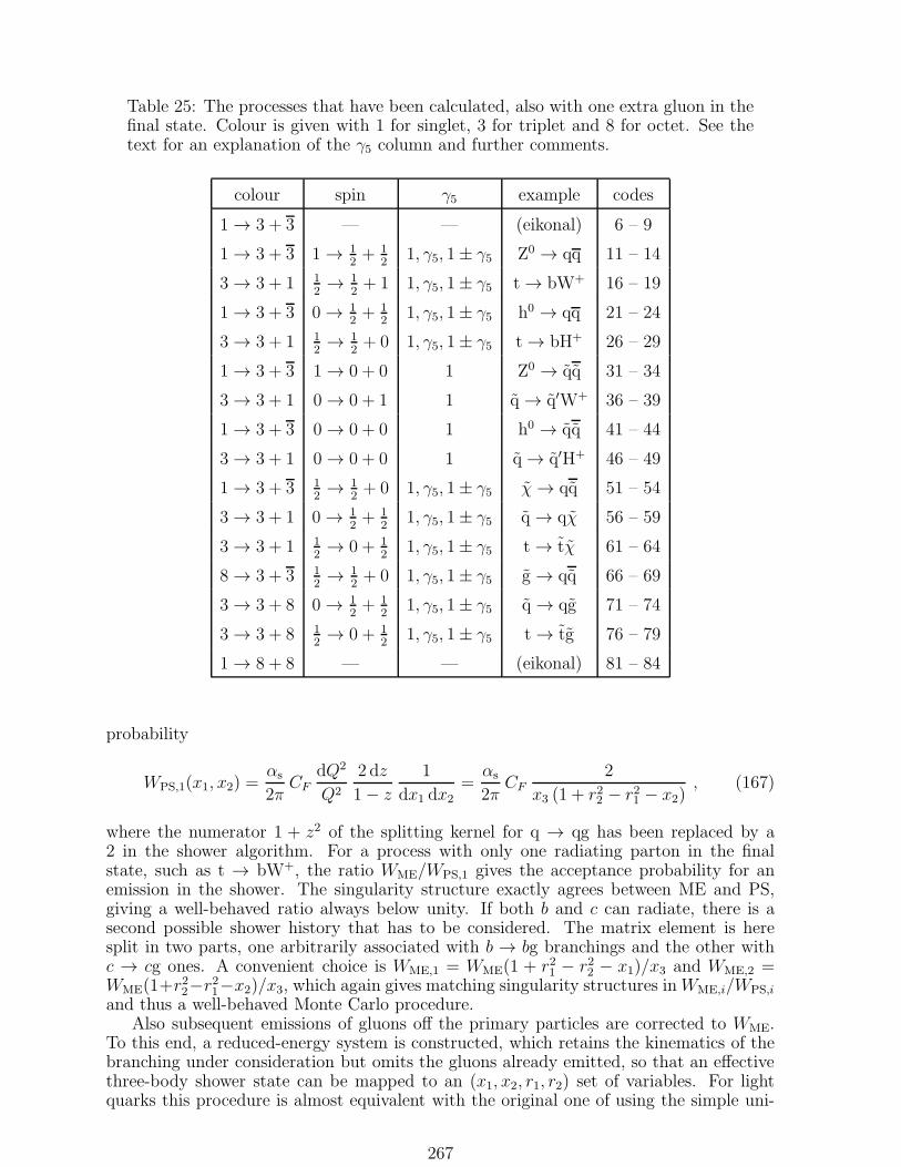
Table 25: The processes that have been calculated, also with one extra gluon in thefinal state. Colour is given with 1 for singlet, 3 for triplet and 8 for octet. See thetext for an explanation of the γ5 column and further comments.

colour spin γ5 example codes

1 → 3 + 3 — — (eikonal) 6 – 9

1 → 3 + 3 1 → 12

+ 12

1, γ5, 1 ± γ5 Z0 → qq 11 – 14

3 → 3 + 1 12→ 1

2+ 1 1, γ5, 1 ± γ5 t → bW+ 16 – 19

1 → 3 + 3 0 → 12

+ 12

1, γ5, 1 ± γ5 h0 → qq 21 – 24

3 → 3 + 1 12→ 1

2+ 0 1, γ5, 1 ± γ5 t → bH+ 26 – 29

1 → 3 + 3 1 → 0 + 0 1 Z0 → qq 31 – 34

3 → 3 + 1 0 → 0 + 1 1 q → q′W+ 36 – 39

1 → 3 + 3 0 → 0 + 0 1 h0 → qq 41 – 44

3 → 3 + 1 0 → 0 + 0 1 q → q′H+ 46 – 49

1 → 3 + 3 12→ 1

2+ 0 1, γ5, 1 ± γ5 χ→ qq 51 – 54

3 → 3 + 1 0 → 12

+ 12

1, γ5, 1 ± γ5 q → qχ 56 – 59

3 → 3 + 1 12→ 0 + 1

21, γ5, 1 ± γ5 t → tχ 61 – 64

8 → 3 + 3 12→ 1

2+ 0 1, γ5, 1 ± γ5 g → qq 66 – 69

3 → 3 + 8 0 → 12

+ 12

1, γ5, 1 ± γ5 q → qg 71 – 74

3 → 3 + 8 12→ 0 + 1

21, γ5, 1 ± γ5 t → tg 76 – 79

1 → 8 + 8 — — (eikonal) 81 – 84

probability

WPS,1(x1, x2) =αs

2πCF

dQ2

Q2

2 dz

1 − z

1

dx1 dx2=αs

2πCF

2

x3 (1 + r22 − r21 − x2), (167)

where the numerator 1 + z2 of the splitting kernel for q → qg has been replaced by a2 in the shower algorithm. For a process with only one radiating parton in the finalstate, such as t → bW+, the ratio WME/WPS,1 gives the acceptance probability for anemission in the shower. The singularity structure exactly agrees between ME and PS,giving a well-behaved ratio always below unity. If both b and c can radiate, there is asecond possible shower history that has to be considered. The matrix element is heresplit in two parts, one arbitrarily associated with b → bg branchings and the other withc → cg ones. A convenient choice is WME,1 = WME(1 + r21 − r22 − x1)/x3 and WME,2 =WME(1+r22−r21−x2)/x3, which again gives matching singularity structures in WME,i/WPS,i

and thus a well-behaved Monte Carlo procedure.Also subsequent emissions of gluons off the primary particles are corrected to WME.

To this end, a reduced-energy system is constructed, which retains the kinematics of thebranching under consideration but omits the gluons already emitted, so that an effectivethree-body shower state can be mapped to an (x1, x2, r1, r2) set of variables. For lightquarks this procedure is almost equivalent with the original one of using the simple uni-

267

versal splitting kernels after the first branching. For heavy quarks it offers an improvedmodelling of mass effects also in the collinear region.

Some further changes have been introduced, a few minor as default and some moresignificant ones as non-default options [Nor01]. This includes the description of coherenceeffects and αs arguments, in general and more specifically for secondary heavy flavourproduction by gluon splittings. The problem in the latter area is that data at LEP1 showa larger rate of secondary charm and bottom production than predicted in most showerdescriptions [Bam00, Man00], or in analytical studies [Sey95]. This is based on applyingthe same kind of coherence considerations to g → qq branchings as to g → gg, whichis not fully motivated by theory. In the lack of an unambiguous answer, it is thereforehelpful to allow options that can explore the range of uncertainty.

Further issues remain to be addressed, e.g. radiation off particles with non-negligiblewidth. In general, however, the new shower should allow an improved description of gluonradiation in many different processes.

10.2.7 Matching to four-parton events

The shower routine, as described above, is optimized for two objects forming the showeringsystem, within which energy and momentum should be conserved. However, occasionallymore than two initial objects are given, e.g. if one would like to consider the subclassof e+e− → qqgg events in order to study angular correlations as a test of the couplingstructure of QCD. Such events are generated in the showering of normal e+e− → qqevents, but not with high efficiency within desired cuts, and not with the full angularstructure included in the shower. Therefore four-parton matrix elements may be therequired starting point but, in order to ‘dress up’ these partons, one nevertheless wishes toadd shower emission. A possibility to start from three partons has existed since long, butonly with [And98a] was an approach for four parton introduced, and with the possibilityto generalize to more partons, although this latter work has not yet been done.

The basic idea is to cast the output of matrix element generators in the form of aparton-shower history, that then can be used as input for a complete parton shower. Inthe shower, that normally would be allowed to develop at random, some branchings arenow fixed to their matrix-element values while the others are still allowed to evolve inthe normal shower fashion. The preceding history of the event is also in these randombranchings then reflected e.g. in terms of kinematical or dynamical (e.g. angular ordering)constraints.

Consider e.g. the qqgg case. The matrix-element expression contains contributionsfrom five graphs, and from interferences between them. The five graphs can also be readas five possible parton-shower histories for arriving at the same four-parton state, buthere without the possibility of including interferences. The relative probability for eachof these possible shower histories can be obtained from the rules of shower branchings.For example, the relative probability for the history where e+e− → q(1)q(2), followed byq(1) → q(3)g(4) and g(4) → g(5)g(6), is given by:

P = P1→34P4→56 =1

m21

4

3

1 + z2341 − z34

· 1

m24

3(1 − z56(1 − z56))

2

z56(1 − z56)(168)

where the probability for each branching contains the mass singularity, the colour factorand the momentum splitting kernel. The masses are given by

m21 = p21 = (p3 + p5 + p6)

2 , (169)

m24 = p24 = (p5 + p6)

2 ,

268

and the z values by

zbc = za→bc =m2a

λ

EbEa

− m2a − λ+m2

b −m2c

2λ(170)

with λ =√

(m2a −m2

b −m2c)

2 − 4m2b m

2c .

We here assume that the on-shell mass of quarks can be neglected. The form of theprobability then matches the expression used in the parton-shower algorithm.

Variants on the above probabilities are imaginable. For instance, in the spirit of thematrix-element approach we have assumed a common αs for all graphs, which thus neednot be shown, whereas the parton-shower language normally assumes αs to be a functionof the transverse momentum of each branching. One could also include information onazimuthal anisotropies.

The relative probability P for each of the five possible parton-shower histories canbe used to select one of the possibilities at random. (A less appealing alternative wouldbe a ‘winner takes all’ strategy, i.e. selecting the configuration with the largest P.) Theselection fixes the values of the m, z and ϕ at two vertices. The azimuthal angle ϕis defined by the daughter parton orientation around the mother direction. When theconventional parton-shower algorithm is executed, these values are then forced on theotherwise random evolution. This forcing cannot be exact for the z values, since thefinal partons given by the matrix elements are on the mass shell, while the correspondingpartons in the parton shower might be virtual and branch further. The shift betweenthe wanted and the obtained z values are rather small, very seldom above 10−6. Moresignificant are the changes of the opening angle between two daughters: when daughtersoriginally assumed massless are given a mass the angle between them tends to be reduced.This shift has a non-negligible tail even above 0.1 radians. The ‘narrowing’ of jets bythis mechanism is compensated by the broadening caused by the decay of the massivedaughters, and thus overall effects are not so dramatic.

All other branchings of the parton shower are selected at random according to thestandard evolution scheme. There is an upper limit on the non-forced masses from internallogic, however. For instance, for four-parton matrix elements, the singular regions aretypically avoided with a cut y > 0.01, where y is the square of the minimal scaled invariantmass between any pair of partons. Larger y values could be used for some purposes, whilesmaller ones give so large four-jet rates that the need to include Sudakov form factorscan no longer be neglected. The y > 0.01 cut roughly corresponds to m > 9 GeV atLEP 1 energies, so the hybrid approach must allow branchings at least below 9 GeVin order to account for the emission missing from the matrix-element part. Since no 5-parton emission is generated by the second-order matrix elements, one could also allowa threshold higher than 9 GeV in order to account for this potential emission. However,if any such mass is larger than one of the forced masses, the result would be a differenthistory than the chosen one, and one would risk some doublecounting issues. So, as analternative, one could set the minimum invariant mass between any of the four originalpartons as the maximum scale of the subsequent shower evolution.

10.3 Initial-State Showers

The initial-state shower algorithm in Pythia is not quite as sophisticated as the final-stateone. This is partly because initial-state radiation is less well understood theoretically,partly because the programming task is more complicated and ambiguous. Still, theprogram at disposal is known to do a reasonably good job of describing existing data,such as Z0 production properties at hadron colliders [Sjo85]. It can be used both for QCDshowers and for photon emission off leptons (e, µ or τ ; relative to earlier versions, the

269

description of incoming µ and τ are better geared to represent the differences in leptonmass, and the lepton-inside-lepton parton distributions are properly defined).

10.3.1 The shower structure

A fast hadron may be viewed as a cloud of quasi-real partons. Similarly a fast leptonmay be viewed as surrounded by a cloud of photons and partons; in the program the twosituations are on an equal footing, but here we choose the hadron as example. At eachinstant, an individual parton can initiate a virtual cascade, branching into a number ofpartons. This cascade can be described in terms of a tree-like structure, composed ofmany subsequent branchings a → bc. Each branching involves some relative transversemomentum between the two daughters. In a language where four-momentum is conservedat each vertex, this implies that at least one of the b and c partons must have a space-likevirtuality, m2 < 0. Since the partons are not on the mass shell, the cascade only lives afinite time before reassembling, with those parts of the cascade that are most off the massshell living the shortest time.

A hard scattering, e.g. in deeply inelastic leptoproduction, will probe the hadron at agiven instant. The probe, i.e. the virtual photon in the leptoproduction case, is able toresolve fluctuations in the hadron up to the Q2 scale of the hard scattering. Thus probesat different Q2 values will seem to see different parton compositions in the hadron. Thechange in parton composition with t = ln(Q2/Λ2) is given by the evolution equations

dfb(x, t)

dt=∑

a,c

∫

dx′

x′fa(x

′, t)αabc2π

Pa→bc

(

x

x′

)

. (171)

Here the fi(x, t) are the parton-distribution functions, expressing the probability of findinga parton i carrying a fraction x of the total momentum if the hadron is probed at virtualityQ2. The Pa→bc(z) are given in eq. (149). As before, αabc is αs for QCD shower and αem

for QED ones.Eq. (171) is closely related to eq. (148): dPa describes the probability that a given

parton a will branch (into partons b and c), dfb the influx of partons b from the branchingsof partons a. (The expression dfb in principle also should contain a loss term for partonsb that branch; this term is important for parton-distribution evolution, but does notappear explicitly in what we shall be using eq. (171) for.) The absolute form of hadronparton distributions cannot be predicted in perturbative QCD, but rather have to beparameterized at some Q0 scale, with the Q2 dependence thereafter given by eq. (171).Available parameterizations are discussed in section 7.1. The lepton and photon partondistributions inside a lepton can be fully predicted, but here for simplicity are treated onequal footing with hadron parton distributions.

If a hard interaction scatters a parton out of the incoming hadron, the ‘coherence’[Gri83] of the cascade is broken: the partons can no longer reassemble completely backto the cascade-initiating parton. In this semiclassical picture, the partons on the ‘mainchain’ of consecutive branchings that lead directly from the initiating parton to the scat-tered parton can no longer reassemble, whereas fluctuations on the ‘side branches’ to thischain may still disappear. A convenient description is obtained by assigning a space-likevirtuality to the partons on the main chain, in such a way that the partons on the sidebranches may still be on the mass shell. Since the momentum transfer of the hard processcan put the scattered parton on the mass shell (or even give it a time-like virtuality, sothat it can initiate a final-state shower), one is then guaranteed that no partons have aspace-like virtuality in the final state. (In real life, confinement effects obviously implythat partons need not be quite on the mass shell.) If no hard scattering had taken place,the virtuality of the space-like parton line would still force the complete cascade to re-assemble. Since the virtuality of the cascade probed is carried by one single parton, it is

270

possible to equate the space-like virtuality of this parton with the Q2 scale of the cascade,to be used e.g. in the evolution equations. Coherence effects [Gri83, Bas83] guarantee thatthe Q2 values of the partons along the main chain are strictly ordered, with the largestQ2 values close to the hard scattering.

Further coherence effects have been studied [Cia87], with particular implications forthe structure of parton showers at small x. None of these additional complications areimplemented in the current algorithm, with the exception of a few rather primitive optionsthat do not address the full complexity of the problem.

Instead of having a tree-like structure, where all legs are treated democratically, thecascade is reduced to a single sequence of branchings a → bc, where the a and b partonsare on the main chain of space-like virtuality, m2

a,b < 0, while the c partons are on themass shell and do not branch. (Later we will include the possibility that the c partonsmay have positive virtualities, m2

c > 0, which leads to the appearance of time-like ‘final-state’ parton showers on the side branches.) This truncation of the cascade is only possiblewhen it is known which parton actually partakes in the hard scattering: of all the possiblecascades that exist virtually in the incoming hadron, the hard scattering will select one.

To obtain the correct Q2 evolution of parton distributions, e.g., it is essential that allbranches of the cascade be treated democratically. In Monte Carlo simulation of space-likeshowers this is a major problem. If indeed the evolution of the complete cascade is to befollowed from some small Q2

0 up to the Q2 scale of the hard scattering, it is not possibleat the same time to handle kinematics exactly, since the virtuality of the various partonscannot be found until after the hard scattering has been selected. This kind of ‘forwardevolution’ scheme therefore requires a number of extra tricks to be made to work. Further,in this approach it is not known e.g. what the s of the hard scattering subsystem will beuntil the evolution has been carried out, which means that the initial-state evolution andthe hard scattering have to be selected jointly, a not so trivial task.

Instead we use the ‘backwards evolution’ approach [Sjo85], in which the hard scatteringis first selected, and the parton shower that preceded it is subsequently reconstructed.This reconstruction is started at the hard interaction, at the Q2

max scale, and thereafterstep by step one moves ‘backwards’ in ‘time’, towards smaller Q2, all the way back tothe parton-shower initiator at the cut-off scale Q2

0. This procedure is possible if evolvedparton distributions are used to select the hard scattering, since the fi(x,Q

2) containthe inclusive summation of all initial-state parton-shower histories that can lead to theappearance of an interacting parton i at the hard scale. What remains is thus to selectan exclusive history from the set of inclusive ones.

10.3.2 Longitudinal evolution

The evolution equations, eq. (171), express that, during a small increase dt there is aprobability for parton a with momentum fraction x′ to become resolved into parton bat x = zx′ and another parton c at x′ − x = (1 − z)x′. Correspondingly, in backwardsevolution, during a decrease dt a parton b may be ‘unresolved’ into parton a. The relativeprobability dPb for this to happen is given by the ratio dfb/fb. Using eq. (171) one obtains

dPb =dfb(x, t)

fb(x, t)= |dt|

∑

a,c

∫

dx′

x′fa(x

′, t)

fb(x, t)

αabc2π

Pa→bc

(

x

x′

)

. (172)

Summing up the cumulative effect of many small changes dt, the probability for no radi-ation exponentiates. Therefore one may define a form factor

Sb(x, tmax, t) = exp

−∫ tmax

tdt′

∑

a,c

∫

dx′

x′fa(x

′, t′)

fb(x, t′)

αabc(t′)

2πPa→bc

(

x

x′

)

= exp

−∫ tmax

tdt′

∑

a,c

∫

dzαabc(t

′)

2πPa→bc(z)

x′fa(x′, t′)

xfb(x, t′)

, (173)

271

giving the probability that a parton b remains at x from tmax to a t < tmax.It may be useful to compare this with the corresponding expression for forward evolu-

tion, i.e. with Sa(t) in eq. (151). The most obvious difference is the appearance of partondistributions in Sb. Parton distributions are absent in Sa: the probability for a givenparton a to branch, once it exists, is independent of the density of partons a or b. Theparton distributions in Sb, on the other hand, express the fact that the probability fora parton b to come from the branching of a parton a is proportional to the number ofpartons a there are in the hadron, and inversely proportional to the number of partons b.Thus the numerator fa in the exponential of Sb ensures that the parton composition ofthe hadron is properly reflected. As an example, when a gluon is chosen at the hard scat-tering and evolved backwards, this gluon is more likely to have been emitted by a u thanby a d if the incoming hadron is a proton. Similarly, if a heavy flavour is chosen at thehard scattering, the denominator fb will vanish at the Q2 threshold of the heavy-flavourproduction, which means that the integrand diverges and Sb itself vanishes, so that noheavy flavour remain below threshold.

Another difference between Sb and Sa, already touched upon, is that the Pg→gg(z)splitting kernel appears with a normalization 2NC in Sb but only with NC in Sa, sincetwo gluons are produced but only one decays in a branching.

A knowledge of Sb is enough to reconstruct the parton shower backwards. At eachbranching a→ bc, three quantities have to be found: the t value of the branching (whichdefines the space-like virtuality Q2

b of parton b), the parton flavour a and the splittingvariable z. This information may be extracted as follows:

1. If parton b partook in the hard scattering or branched into other partons at a scaletmax, the probability that b was produced in a branching a→ bc at a lower scale t is

dPbdt

= −dSb(x, tmax, t)

dt=

(

∑

a,c

∫

dzαabc(t

′)

2πPa→bc(z)

x′fa(x′, t′)

xfb(x, t′)

)

Sb(x, tmax, t) .

(174)If no branching is found above the cut-off scale t0 the iteration is stopped and partonb is assumed to be massless.

2. Given the t of a branching, the relative probabilities for the different allowed branch-ings a→ bc are given by the z integrals above, i.e. by

∫

dzαabc(t)

2πPa→bc(z)

x′fa(x′, t)

xfb(x, t). (175)

3. Finally, with t and a known, the probability distribution in the splitting variablez = x/x′ = xb/xa is given by the integrand in eq. (175).

In addition, the azimuthal angle ϕ of the branching is selected isotropically, i.e. no spinor coherence effects are included in this distribution.

The selection of t, a and z is then a standard task of the kind than can be performedwith the help of the veto algorithm. Specifically, upper and lower bounds for parton dis-tributions are used to find simple functions that are everywhere larger than the integrandsin eq. (175). Based on these simple expressions, the integration over z may be carried out,and t, a and z values selected. This set is then accepted with a weight given by a ratio ofthe correct integrand in eq. (175) to the simple approximation used, both evaluated forthe given set. Since parton distributions, as a rule, are not in a simple analytical form,it may be tricky to find reasonably good bounds to parton distributions. It is necessaryto make different assumptions for valence and sea quarks, and be especially attentiveclose to a flavour threshold ([Sjo85]). An electron distribution inside an electron behavesdifferently from parton distributions encountered in hadrons, and has to be consideredseparately.

A comment on soft gluon emission. Nominally the range of the z integral in Sb isx ≤ z ≤ 1. The lower limit corresponds to x′ = x/z = 1, and parton distributions vanish

272

in this limit, wherefore no problems are encountered here. At the upper cut-off z = 1 thesplitting kernels Pq→qg(z) and Pg→gg diverge. This is the soft gluon singularity: the energycarried by the emitted gluon is vanishing, xg = x′ − x = (1 − z)x′ = (1 − z)x/z → 0 forz → 1. In order to calculate the integral over z in Sb, an upper cut-off zmax = x/(x+ xǫ)is introduced, i.e. only branchings with z ≤ zmax are included in Sb. Here xǫ is a smallnumber, typically chosen so that the gluon energy is above 2 GeV when calculated in therest frame of the hard scattering. That is, the gluon energy xg

√s/2 ≥ xǫ

√s/2 = 2 GeV/γ,

where γ is the boost factor of the hard scattering. The average amount of energy carriedaway by gluons in the range xg < xǫ, over the given range of t values from ta to tb, may beestimated [Sjo85]. The finally selected z value may thus be picked as z = zhard〈zsoft(ta, tb)〉,where zhard is the originally selected z value and zsoft is the correction factor for soft gluonemission.

In QED showers, the smallness of αem means that one can use rather smaller cut-offvalues without obtaining large amounts of emission. A fixed small cut-off xγ > 10−10 istherefore used to avoid the region of very soft photons. As has been discussed in section7.1.3, the electron distribution inside the electron is cut off at xe < 1−10−10, for numericalreasons, so the two cuts are closely matched.

The cut-off scale Q0 may be chosen separately for QCD and QED showers, just as infinal-state radiation. The defaults are 1 GeV and 0.001 GeV, respectively. The formeris the typical hadronic mass scale, below which radiation is not expected resolvable; thelatter is of the order of the electron mass.

Normally QED and QCD showers do not appear mixed. The most notable exceptionis resolved photoproduction (in ep) and resolved γγ events (in e+e−), i.e. shower historiesof the type e → γ → q. Here the Q2 scales need not be ordered at the interface, i.e.the last e → eγ branching may well have a larger Q2 than the first q → qg one, and thebranching γ → q does not even have a strict parton-shower interpretation for the vectordominance model part of the photon parton distribution. This kind of configurationsis best described by the ’gamma/lepton’ machinery for having a flux of virtual photonsinisde the lepton, see section 7.1.4. In this case, no initial-state radiation has currentlybeen implemented for the electron (or µ or τ). The one inside the virtual-photon systemis considered with the normal algorithm, but with the lower cut-off scale modified by thephoton virtuality, see MSTP(66).

An older description still lives on, although no longer as the recommended one. There,these issues are currently not addressed in full. Rather, based on the x selected for theparton (quark or gluon) at the hard scattering, the xγ is selected once and for all in therange x < xγ < 1, according to the distribution implied by eq. (54). The QCD partonshower is then traced backwards from the hard scattering to the QCD shower initiator att0. No attempt is made to perform the full QED shower, but rather the beam remnanttreatment (see section 11.1) is used to find the q (or g) remnant that matches the q (org) QCD shower initiator, with the electron itself considered as a second beam remnant.

10.3.3 Transverse evolution

We have above seen that two parton lines may be defined, stretching back from thehard scattering to the initial incoming hadron wavefunctions at small Q2. Specifically,all parton flavours i, virtualities Q2 and energy fractions x may be found. The exactkinematical interpretation of the x variable is not unique, however. For partons withsmall virtualities and transverse momenta, essentially all definitions agree, but differencesmay appear for branchings close to the hard scattering.

In first-order QED [Ber85] and in some simple QCD toy models [Got86], one may showthat the ‘correct’ choice is the ‘s approach’. Here one requires that s = x1x2s, both at thehard scattering scale and at any lower scale, i.e. s(Q2) = x1(Q

2) x2(Q2) s, where x1 and

x2 are the x values of the two resolved partons (one from each incoming beam particle) at

273

the given Q2 scale. In practice this means that, at a branching with the splitting variablez, the total s has to be increased by a factor 1/z in the backwards evolution. It also meansthat branchings on the two incoming legs have to be interleaved in a single monotonicsequence of Q2 values of branchings. A problem with this x interpretation is that it is notquite equivalent with an ms definition of parton densities [Col00], or any other standarddefinition. In practice, effects should not be large from this mismatch.

For a reconstruction of the complete kinematics in this approach, one should startwith the hard scattering, for which s has been chosen according to the hard scatteringmatrix element. By backwards evolution, the virtualities Q2

1 = −m21 and Q2

2 = −m22 of

the two interacting partons are reconstructed. Initially the two partons are considered intheir common c.m. frame, coming in along the ±z directions. Then the four-momentumvectors have the non-vanishing components

E1,2 =s± (Q2

2 −Q21)

2√s

,

pz1 = −pz2 =

√

(s+Q21 +Q2

2)2 − 4Q2

1Q22

4s, (176)

with (p1 + p2)2 = s.

If, say, Q21 > Q2

2, then the branching 3 → 1 + 4, which produced parton 1, is the onethat took place closest to the hard scattering, and the one to be reconstructed first. Withthe four-momentum p3 known, p4 = p3 − p1 is automatically known, so there are fourdegrees of freedom. One corresponds to a trivial azimuthal angle around the z axis. Thez splitting variable for the 3 → 1+4 vertex is found as the same time as Q2

1, and providesthe constraint (p3 + p2)

2 = s/z. The virtuality Q23 is given by backwards evolution of

parton 3.One degree of freedom remains to be specified, and this is related to the possibility

that parton 4 initiates a time-like parton shower, i.e. may have a non-zero mass. Themaximum allowed squared mass m2

max,4 is found for a collinear branching 3 → 1 + 4. Interms of the combinations

s1 = s+Q22 +Q2

1 ,

s3 =s

z+Q2

2 +Q23 ,

r1 =√

s21 − 4Q22Q

21 ,

r3 =√

s23 − 4Q22Q

23 , (177)

one obtains

m2max,4 =

s1s3 − r1r32Q2

2

−Q21 −Q2

3 , (178)

which, for the special case of Q22 = 0, reduces to

m2max,4 =

Q21

z−Q2

3

s

s+Q21

− s

s/z +Q23

. (179)

These constraints on m4 are only the kinematical ones, in addition coherence phenomenacould constrain the mmax,4 values further. Some options of this kind are available; thedefault one is to require additionally that m2

4 ≤ Q21, i.e. lesser than the space-like virtuality

of the sister parton.With the maximum virtuality given, the final-state showering machinery may be used

to give the development of the subsequent cascade, including the actual mass m24, with

274

0 ≤ m24 ≤ m2

max,4. The evolution is performed in the c.m. frame of the two ‘resolved’partons, i.e. that of partons 1 and 2 for the branching 3 → 1 + 4, and parton 4 is assumedto have a nominal energy Enom,4 = (1/z− 1)

√s/2. (Slight modifications appear if parton

4 has a non-vanishing mass mq or mℓ.)Using the relation m2

4 = (p3 − p1)2, the momentum of parton 3 may now be found as

E3 =1

2√s

s

z+Q2

2 −Q21 −m2

4

,

pz3 =1

2pz1s3 − 2E2E3 ,

p2⊥,3 =

m2max,4 −m2

4

(s1s3 + r1r3)/2 −Q22(Q

21 +Q2

3 +m24)

r21. (180)

The requirement that m24 ≥ 0 (or ≥ m2

f for heavy flavours) imposes a constraint onallowed z values. This constraint cannot be included in the choice of Q2

1, where it logicallybelongs, since it also depends on Q2

2 and Q23, which are unknown at this point. It is fairly

rare (in the order of 10% of all events) that an unallowed z value is generated, and when ithappens it is almost always for one of the two branchings closest to the hard interaction:for Q2

2 = 0 eq. (179) may be solved to yield z ≤ s/(s+Q21 −Q2

3), which is a more severecut for s small and Q2

1 large. Therefore an essentially bias-free way of coping is to redocompletely any initial-state cascade for which this problem appears.

This completes the reconstruction of the 3 → 1 + 4 vertex. The subsystem made outof partons 3 and 2 may now be boosted to its rest frame and rotated to bring partons 3and 2 along the ±z directions. The partons 1 and 4 now have opposite and compensatingtransverse momenta with respect to the event axis. When the next vertex is considered,either the one that produces parton 3 or the one that produces parton 2, the 3–2 subsystemwill fill the function the 1–2 system did above, e.g. the role of s = s12 in the formulae aboveis now played by s32 = s12/z. The internal structure of the 3–2 system, i.e. the branching3 → 1 + 4, appears nowhere in the continued description, but has become ‘unresolved’.It is only reflected in the successive rotations and boosts performed to bring back thenew endpoints to their common rest frame. Thereby the hard scattering subsystem 1–2builds up a net transverse momentum and also an overall rotation of the hard scatteringsubsystem.

After a number of steps, the two outermost partons have virtualities Q2 < Q20 and

then the shower is terminated and the endpoints assigned Q2 = 0. Up to small correctionsfrom primordial k⊥, discussed in section 11.1, a final boost will bring the partons fromtheir c.m. frame to the overall c.m. frame, where the x values of the outermost partonsagree also with the light-cone definition.

10.3.4 Other initial-state shower aspects

In the formulae above, Q2 has been used as argument for αs, and not only as the space-likevirtuality of partons. This is one possibility, but in fact loop calculations tend to indicatethat the proper argument for αs is not Q2 but p2⊥ = (1 − z)Q2 [Bas83]. The variablep⊥ does have the interpretation of transverse momentum, although it is only exactly sofor a branching a → bc with a and c massless and Q2 = −m2

b , and with z interpretedas light-cone fraction of energy and momentum. The use of αs((1 − z)Q2) is default inthe program. Indeed, if one wanted to, the complete shower might be interpreted as anevolution in p2⊥ rather than in Q2.

Angular ordering is included in the shower evolution by default. However, as alreadymentioned, the physics is much more complicated than for timelike showers, and so thisoption should only be viewed as a first approximation. In the code the quantity ordered

275

is an approximation of p⊥/p ≈ sin θ. (An alternative would have been p⊥/pL ≈ tan θ, butthis suffers from instability problems.)

In flavour excitation processes, a c (or b) quark enters the hard scattering and shouldbe reconstructed by the shower as coming from a g → cc (or g → bb) branching. Herean x value for the incoming c above Q2

c/(Q2c +m2

c), where Q2c is the spacelike virtuality of

the c, does not allow a kinematical reconstruction of the gluon branching with an xg < 1,and is thus outside the allowed phase space. Such events (with some safety margin) arerejected. Currently they will appear in PYSTAT(1) listings in the ‘Fraction of events thatfail fragmentation cuts’, which is partly misleading, but has the correct consequence ofsuppressing the physical cross section. Further, the Q2 value of the backwards evolutionof a c quark is by force kept above m2

c , so as to ensure that the branching g → cc is not‘forgotten’ by evolving Q2 below Q2

0. Thereby the possibility of having a c in the beamremnant proper is eliminated [Nor98]. Warning: as a consequence, flavour excitation isnot at all possible too close to threshold. If the KFIN array in PYSUBS is set so as to requirea c (or b) on either side, and the phase space is closed for such a c to come from a g → ccbranching, the program will enter an infinite loop.

For proton beams, say, any c or b quark entering the hard scattering has to come froma preceding gluon splitting. This is not the case for a photon beam, since a photon has ac and b valence quark content. Therefore the above procedure need not be pursued there,but c and b quarks may indeed appear as beam remnants.

As we see, the initial-state showering algorithm leads to a net boost and rotation ofthe hard scattering subsystems. The overall final state is made even more complex by theadditional final-state radiation. In principle, the complexity is very physical, but it maystill have undesirable side effects. One such, discussed further in section 9.2, is that it isvery difficult to generate events that fulfil specific kinematics conditions, since kinematicsis smeared and even, at times, ambiguous.

A special case is encountered in Deeply Inelastic Scattering in ep collisions. Here theDIS x and Q2 values are defined in terms of the scattered electron direction and energy,and therefore are unambiguous (except for issues of final-state photon radiation close tothe electron direction). Neither initial- nor final-state showers preserve the kinematics ofthe scattered electron, however, and hence the DIS x and Q2 are changed. In principle,this is perfectly legitimate, with the caveat that one then also should use different sets ofparton distributions than ones derived from DIS, since these are based on the kinematicsof the scattered lepton and nothing else. Alternatively, one might consider showeringschemes that leave x and Q2 unchanged. In [Ben88] detailed modifications are presentedthat make a preservation possible when radiation off the incoming and outgoing electronis neglected, but these are not included in the current version of Pythia. Instead thecurrent ’gamma/lepton’ machinery explicitly separates off the e → eγ vertex from thecontinued fate of the photon.

The only reason for using the older machinery, such as process 10, is that this is stillthe only place where weak charged and neutral current effects can be considered. Whatis available there, as an option, is a simple machinery which preserves x and Q2 from theeffects of QCD radiation, and also from those of primordial k⊥ and the beam remnanttreatment, as follows. After the showers have been generated, the four-momentum ofthe scattered lepton is changed to the expected one, based on the nominal x and Q2

values. The azimuthal angle of the lepton is maintained when the transverse momentumis adjusted. Photon radiation off the lepton leg is not fully accounted for, i.e. it is assumedthat the energy of final-state photons is added to that of the scattered electron for thedefinition of x and Q2 (this is the normal procedure for parton-distribution definitions).

The change of three-momentum on the lepton side of the event is balanced by thefinal state partons on the hadron side, excluding the beam remnant but including all thepartons both from initial- and final-state showering. The fraction of three-momentumshift taken by each parton is proportional to its original light-cone momentum in the

276

direction of the incoming lepton, i.e. to E ∓ pz for a hadron moving in the ± direction.This procedure guarantees momentum but not energy conservation. For the latter, oneadditional degree of freedom is needed, which is taken to be the longitudinal momentumof the initial state shower initiator. As this momentum is modified, the change is sharedby the final state partons on the hadron side, according to the same light-cone fractionsas before (based on the original momenta). Energy conservation requires that the totalchange in final state parton energies plus the change in lepton side energy equals thechange in initiator energy. This condition can be turned into an iterative procedure tofind the initiator momentum shift.

Sometimes the procedure may break down. For instance, an initiator with x > 1 maybe reconstructed. If this should happen, the x and Q2 values of the event are preserved,but new initial and final state showers are generated. After five such failures, the eventis completely discarded in favour of a new kinematical setup.

Kindly note that the four-momentum of intermediate partons in the shower historyare not being adjusted. In a listing of the complete event history, energy and momentumneed then not be conserved in shower branchings. This mismatch could be fixed up, ifneed be.

The scheme presented above should not be taken too literally, but is rather intendedas a contrast to the more sophisticated schemes already on the market, if one would liketo understand whether the kind of conservation scheme chosen does affect the observablephysics.

10.3.5 Matrix-element matching

In Pythia 6.1, matrix-element matching was introduced for the initial-state shower de-scription of initial-state radiation in the production of a single colour-singlet resonance,such as γ∗/Z0/W± [Miu99]. The basic idea is to map the kinematics between the PS andME descriptions, and to find a correction factor that can be applied to hard emissions inthe shower so as to bring agreement with the matrix-element expression. The Pythia

shower kinematics definitions are based on Q2 as the spacelike virtuality of the partonproduced in a branching and z as the factor by which the s of the scattering subsystemis reduced by the branching. Some simple algebra then shows that the two qq′ → gW±

emission rates disagree by a factor

Rqq′→gW(s, t) =(dσ/dt)ME

(dσ/dt)PS=t2 + u2 + 2m2

Ws

s2 +m4W

, (181)

which is always between 1/2 and 1. The shower can therefore be improved in two ways,relative to the old description. Firstly, the maximum virtuality of emissions is raised fromQ2

max ≈ m2W to Q2

max = s, i.e. the shower is allowed to populate the full phase space.Secondly, the emission rate for the final (which normally also is the hardest) q → qgemission on each side is corrected by the factor R(s, t) above, so as to bring agreementwith the matrix-element rate in the hard-emission region. In the backwards evolutionshower algorithm [Sjo85], this is the first branching considered.

The other possible O(αs) graph is qg → q′W±, where the corresponding correctionfactor is

Rqg→q′W(s, t) =(dσ/dt)ME

(dσ/dt)PS=

s2 + u2 + 2m2W t

(s−m2W)2 +m4

W

, (182)

which lies between 1 and 3. A probable reason for the lower shower rate here is that theshower does not explicitly simulate the s-channel graph qg → q∗ → q′W. The g → qqbranching therefore has to be preweighted by a factor of 3 in the shower, but otherwisethe method works the same as above. Obviously, the shower will mix the two alternativebranchings, and the correction factor for a final branching is based on the current type.

277

The reweighting procedure prompts some other changes in the shower. In particular,u < 0 translates into a constraint on the phase space of allowed branchings, not previouslyimplemented. Here u = Q2 − sold(1 − z)/z = Q2 − snew(1 − z), where the associationwith the u variable is relevant if the branching is reinterpreted in terms of a 2 → 2scattering. Usually such a requirement comes out of the kinematics, and therefore isimposed eventually anyway. The corner of emissions that do not respect this requirementis that where the Q2 value of the spacelike emitting parton is little changed and thez value of the branching is close to unity. (That is, such branchings are kinematicallyallowed, but since the mapping to matrix-element variables would assume the first partonto have Q2 = 0, this mapping gives an unphysical u, and hence no possibility to impose amatrix-element correction factor.) The correct behaviour in this region is beyond leading-log predictivity. It is mainly important for the hardest emission, i.e. with largest Q2.The effect of this change is to reduce the total amount of emission by a non-negligibleamount when no matrix-element correction is applied. (This can be confirmed by usingthe special option MSTP(68)=-1.) For matrix-element corrections to be applied, thisrequirement must be used for the hardest branching, and then whether it is used or notfor the softer ones is less relevant.

Our published comparisons with data on the p⊥W spectrum show quite a good agree-ment with this improved simulation [Miu99]. A worry was that an unexpectedly largeprimordial k⊥, around 4 GeV, was required to match the data in the low-p⊥Z region.However, at that time we had not realized that the data were not fully unsmeared. Therequired primordial k⊥ therefore drops by about a factor of two [Bal01]. This number isstill uncomfortably large, but not too dissimilar from what is required in various resum-mation descriptions.

The method can also be used for initial-state photon emission, e.g. in the processe+e− → γ∗/Z0. There the old default Q2

max = m2Z allowed no emission at large p⊥,

p⊥ >∼mZ at LEP2. This is now corrected by the increased Q2max = s, and using the R of

eq. (181) with mW → mZ.The above method does not address the issue of next-to-leading order corrections to

the total W cross section. Rather, the implicit assumption is that such corrections, comingmainly from soft- and virtual-gluon effects, largely factorize from the hard-emission effects.That is, that the p⊥ shape obtained in our approach will be rather unaffected by next-to-leading order corrections (when used both for the total and the high-p⊥ cross section).A rescaling by a common K factor could then be applied by hand at the end of theday. However, the issue is not clear. Alternative approaches have been proposed, wheremore sophisticated matching procedures are used also to get the next-to-leading ordercorrections to the cross section integrated into the shower formalism [Mre99].

A matching can also be attempted for other processes than the ones above. Currentlya matrix-element correction factor is also used for g → gg and q → gq branchings in thegg → h0 process, in order to match on to the gg → gh0 and qg → qh0 matrix elements[Ell88]. The loop integrals of Higgs production are quite complex, however, and thereforeonly the expressions obtained in the limit of a heavy top quark is used as a starting pointto define the ratios of gg → gh0 and qg → qh0 to gg → h0 cross sections. (Whereasthe gg → h0 cross section by itself contains the complete expressions.) In this limit, thecompact correction factors

Rgg→gh0(s, t) =(dσ/dt)ME

(dσ/dt)PS=

s4 + t4 + u4 +m8h

2(s2 −m2h(s−m2

h))2(183)

and

Rqg→qh0(s, t) =(dσ/dt)ME

(dσ/dt)PS=

s2 + u2

s2 + (s−m2h)2

(184)

can be derived. Even though they are clearly not as reliable as the above expressions forγ∗/Z0/W±, they should hopefully represent an improved description relative to having no

278

correction factor at all. For this reason they are applied not only for the standard modelHiggs, but for all the three Higgs states h0, H0 and A0. The Higgs correction factors arealways in the comfortable range between 1/2 and 1.

Note that a third process, qq → gh0 does not fit into the pattern of the other two. Theabove process cannot be viewed as a showering correction to a lowest-order qq → h0 one:since the q is assumed (essentially) massless there is no pointlike coupling. The graphabove instead again involved a top loop, coupled to the initial state by a single s-channelgluon. The final-state gluon is necessary to balance colours in the process, and thereforethe cross section is vanishing in the p⊥ → 0 limit.

10.4 Routines and Common Block Variables

In this section we collect information on how to use the initial- and final-state showeringroutines. Of these PYSHOW for final-state radiation is the more generally interesting, sinceit can be called to let a user-defined parton configuration shower. PYSSPA, on the otherhand, is so intertwined with the general structure of a Pythia event that it is of littleuse as a stand-alone product.

CALL PYSHOW(IP1,IP2,QMAX)

Purpose: to generate time-like parton showers, conventional or coherent. The perfor-mance of the program is regulated by the switches MSTJ(38) - MSTJ(50) andparameters PARJ(80) - PARJ(90). In order to keep track of the colour flowinformation, the positions K(I,4) and K(I,5) have to be organized properlyfor showering partons. Inside the Pythia programs, this is done automati-cally, but for external use proper care must be taken.

IP1 > 0, IP2 = 0 : generate a time-like parton shower for the parton in line IP1 incommon block PYJETS, with maximum allowed mass QMAX. With only oneparton at hand, one cannot simultaneously conserve both energy and momen-tum: we here choose to conserve energy and jet direction, while longitudinalmomentum (along the jet axis) is not conserved.

IP1 > 0, IP2 > 0 : generate time-like parton showers for the two partons in lines IP1and IP2 in the common block PYJETS, with maximum allowed mass for eachparton QMAX. For shower evolution, the two partons are boosted to their c.m.frame. Energy and momentum is conserved for the pair of partons, althoughnot for each individually. One of the two partons may be replaced by a nonra-diating particle, such as a photon or a diquark; the energy and momentum ofthis particle will then be modified to conserve the total energy and momentum.

IP1 > 0, -7 ≤ IP2 < 0 : generate time-like parton showers for the -IP2 (at most 7)partons in lines IP1, IP1+1, . . . IPI-IP2-1 in the common block PYJETS, withmaximum allowed mass for each parton QMAX. The actions for IP2=-1 andIP2=-2 correspond to what is described above, but additionally larger num-bers may be used to generate the evolution starting from three or more givenpartons. Then the partons are boosted to their c.m. frame, the direction ofthe momentum vector is conserved for each parton individually and energyfor the system as a whole. It should be understood that the uncertainty inthis option is larger than for two-parton systems, and that a number of thesophisticated features (such as coherence with the incoming colour flow) arenot implemented.

IP1 > 0, IP2 = -8 : generate a four-parton system, where a history starting from twopartons has already been constructed as discussed in subsection 10.2.7. In-cluding intermediate partons this requires 8 lines, whence the IP2 value. This

279

option is used in PY4JET, whereas you would normally not want to use thisoption directly yourself.

QMAX : the maximum allowed mass of a radiating parton, i.e. the starting value for thesubsequent evolution. (In addition, the mass of a single parton may not exceedits energy, the mass of a parton in a system may not exceed the invariant massof the system.)

FUNCTION PYMAEL(NI,X1,X2,R1,R2,ALPHA)

Purpose: returns the ratio of the first-order gluon emission rate normalized to the lowest-order event rate, eq. (166). An overall factor CFαs/2π is omitted, since therunning of αs probably is done better in shower language anyway.

NI : code of the matrix element to be used, see Table 25. In each group of fourcodes in that table, the first is for the 1 case, the second for the γ5 one, thethird for an arbitrary mixture, see ALPHA below, and the last for 1 ± γ5.

X1, X2 : standard energy fractions of the two daughters.R1, R2 : mass of the two daughters normalized to the mother mass.ALPHA: fraction of the no-γ5 (i.e. vector/scalar/...) part of the cross section; a free

parameter for the third matrix element option of each group in Table 25 (13,18, 23, 28, . . . ).

SUBROUTINE PYADSH(NFIN)

Purpose: to administrate a sequence of final-state showers for external processes, wherethe order normally is that all resonances have decayed before showers areconsidered, and therefore already existing daughters have to be boosted whentheir mothers radiate or take the recoil from radiation.

NFIN : line in the event record of the last final-state entry to consider.

SUBROUTINE PYSSPA(IPU1,IPU2)

Purpose: to generate the space-like showers of the initial-state radiation.IPU1, IPU2 : positions of the two partons entering the hard scattering, from which the

backwards evolution is initiated.

SUBROUTINE PYMEMX(MECOR,WTFF,WTGF,WTFG,WTGG)

Purpose: to set the maximum of the ratio of the correct matrix element to the oneimplied by the spacelike parton shower.

MECOR : kind of hard scattering process, 1 for f + f → γ∗/Z0/W±/ . . . vector gaugebosons, 2 for g + g → h0/H0/A0.

WTFF, WTGF, WTFG, WTGG : maximum weights for f → f (+g/γ), g/γ → f (+f), f →g/γ (+f) and g → g (+g), respectively.

SUBROUTINE PYMEWT(MECOR,IFLCB,Q2,Z,PHIBR,WTME)

Purpose: to calculate the ratio of the correct matrix element to the one implied by thespacelike parton shower.

MECOR : kind of hard scattering process, 1 for f + f → γ∗/Z0/W±/ . . . vector gauge

280

bosons, 2 for g + g → h0/H0/A0.IFLCB : kind of branching, 1 for f → f (+g/γ), 2 for g/γ → f (+f), 3 for f → g/γ (+f)

and 4 for g → g (+g).Q2, Z : Q2 and z values of shower branching under consideration.PHIBR : ϕ azimuthal angle of the shower branching; may be overwritten inside routine.WTME : calculated matrix element correction weight, used in the acceptance/rejection

of the shower branching under consideration.

COMMON/PYDAT1/MSTU(200),PARU(200),MSTJ(200),PARJ(200)

Purpose: to give access to a number of status codes and parameters which regulate theperformance of Pythia. Most parameters are described in section 14.3; hereonly those related to PYSHOW are described.

MSTJ(38) : (D=0) matrix element code NI for PYMAEL; as in MSTJ(47). If nonzero, theMSTJ(38) value overrides MSTJ(47), but is then set =0 in the PYSHOW call. Theusefulness of this switch lies in processes where sequential decays occur andthus there are several showers, each requiring its matrix element. ThereforeMSTJ(38) can be set in the calling routine when it is known, and when not setone defaults back to the attempted matching procedure of MSTJ(47)=3 (e.g.).

MSTJ(40) : (D=0) possibility to suppress the branching probability for a branching q →qg (or q → qγ) of a quark produced in the decay of an unstable particlewith width Γ, where this width has to be specified by you in PARJ(89). Thealgorithm used is not exact, but still gives some impression of potential effects.This switch ought to have appeared at the end of the current list of showerswitches (after MSTJ(50)), but because of lack of space it appears immediatelybefore.

= 0 : no suppression, i.e. the standard parton-shower machinery.= 1 : suppress radiation by a factor χ(ω) = Γ2/(Γ2 + ω2), where ω is the

energy of the gluon (or photon) in the rest frame of the radiating dipole.Essentially this means that hard radiation with ω > Γ is removed.

= 2 : suppress radiation by a factor 1 − χ(ω) = ω2/(Γ2 + ω2), where ω is theenergy of the gluon (or photon) in the rest frame of the radiating dipole.Essentially this means that soft radiation with ω < Γ is removed.

MSTJ(41) : (D=2) type of branchings allowed in shower.= 0 : no branchings at all, i.e. shower is switched off.= 1 : QCD type branchings of quarks and gluons.= 2 : also emission of photons off quarks and leptons; the photons are assumed

on the mass shell.= 10 : as =2, but enhance photon emission by a factor PARJ(84). This option

is unphysical, but for moderate values, PARJ(84)≤ 10, it may be usedto enhance the prompt photon signal in qq events. The normalization ofthe prompt photon rate should then be scaled down by the same factor.The dangers of an improper use are significant, so do not use this optionif you do not know what you are doing.

MSTJ(42) : (D=2) branching mode, especially coherence level, for time-like show-ers.

= 1 : conventional branching, i.e. without angular ordering.= 2 : coherent branching, i.e. with angular ordering.= 3 : in a branching a → bg, where mb is nonvanishing, the decay angle is re-

duced by a factor (1 + (m2b/m

2a)(1− z)/z)−1, thereby taking into account

mass effects in the decay [Nor01]. Therefore more branchings are accept-able from an angular ordering point of view. In the definition of the angle

281

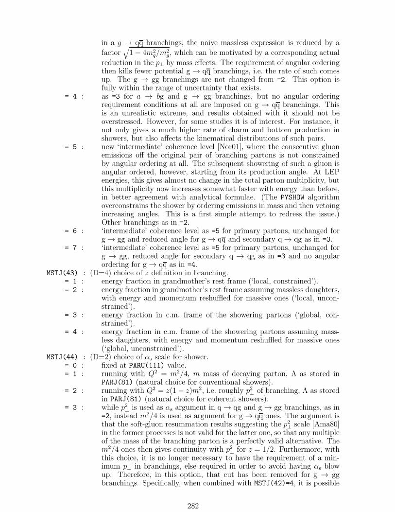
in a g → qq branchings, the naive massless expression is reduced by a

factor√

1 − 4m2q/m

2g, which can be motivated by a corresponding actual

reduction in the p⊥ by mass effects. The requirement of angular orderingthen kills fewer potential g → qq branchings, i.e. the rate of such comesup. The g → gg branchings are not changed from =2. This option isfully within the range of uncertainty that exists.

= 4 : as =3 for a → bg and g → gg branchings, but no angular orderingrequirement conditions at all are imposed on g → qq branchings. Thisis an unrealistic extreme, and results obtained with it should not beoverstressed. However, for some studies it is of interest. For instance, itnot only gives a much higher rate of charm and bottom production inshowers, but also affects the kinematical distributions of such pairs.

= 5 : new ‘intermediate’ coherence level [Nor01], where the consecutive gluonemissions off the original pair of branching partons is not constrainedby angular ordering at all. The subsequent showering of such a gluon isangular ordered, however, starting from its production angle. At LEPenergies, this gives almost no change in the total parton multiplicity, butthis multiplicity now increases somewhat faster with energy than before,in better agreement with analytical formulae. (The PYSHOW algorithmoverconstrains the shower by ordering emissions in mass and then vetoingincreasing angles. This is a first simple attempt to redress the issue.)Other branchings as in =2.

= 6 : ‘intermediate’ coherence level as =5 for primary partons, unchanged forg → gg and reduced angle for g → qq and secondary q → qg as in =3.

= 7 : ‘intermediate’ coherence level as =5 for primary partons, unchanged forg → gg, reduced angle for secondary q → qg as in =3 and no angularordering for g → qq as in =4.

MSTJ(43) : (D=4) choice of z definition in branching.= 1 : energy fraction in grandmother’s rest frame (‘local, constrained’).= 2 : energy fraction in grandmother’s rest frame assuming massless daughters,

with energy and momentum reshuffled for massive ones (‘local, uncon-strained’).

= 3 : energy fraction in c.m. frame of the showering partons (‘global, con-strained’).

= 4 : energy fraction in c.m. frame of the showering partons assuming mass-less daughters, with energy and momentum reshuffled for massive ones(‘global, unconstrained’).

MSTJ(44) : (D=2) choice of αs scale for shower.= 0 : fixed at PARU(111) value.= 1 : running with Q2 = m2/4, m mass of decaying parton, Λ as stored in

PARJ(81) (natural choice for conventional showers).= 2 : running with Q2 = z(1 − z)m2, i.e. roughly p2⊥ of branching, Λ as stored

in PARJ(81) (natural choice for coherent showers).= 3 : while p2⊥ is used as αs argument in q → qg and g → gg branchings, as in

=2, instead m2/4 is used as argument for g → qq ones. The argument isthat the soft-gluon resummation results suggesting the p2⊥ scale [Ama80]in the former processes is not valid for the latter one, so that any multipleof the mass of the branching parton is a perfectly valid alternative. Them2/4 ones then gives continuity with p2⊥ for z = 1/2. Furthermore, withthis choice, it is no longer necessary to have the requirement of a min-imum p⊥ in branchings, else required in order to avoid having αs blowup. Therefore, in this option, that cut has been removed for g → ggbranchings. Specifically, when combined with MSTJ(42)=4, it is possible

282

to reproduce the simple 1+cos2 θ angular distribution of g → gg branch-ings, which is not possible in any other approach. (However it may givetoo high a charm and bottom production rate in showers [Nor01].)

= 4 : p2⊥ as in =2, but scaled down by a factor (1 −m2b/m

2a)

2 for a branchinga → bg with b massive, in an attempt better to take into account themass effect on kinematics.

= 5 : as for =4 for q → qg, unchanged for g → gg and as =3 for g → qq.MSTJ(45) : (D=5) maximum flavour that can be produced in shower by g → qq; also

used to determine the maximum number of active flavours in the αs factor inparton showers (here with a minimum of 3).

MSTJ(46) : (D=3) nonhomogeneous azimuthal distributions in a shower branching.= 0 : azimuthal angle is chosen uniformly.= 1 : nonhomogeneous azimuthal angle in gluon decays due to a kinematics-

dependent effective gluon polarization. Not meaningful for scalar model,i.e. then same as =0.

= 2 : nonhomogeneous azimuthal angle in gluon decay due to interference withnearest neighbour (in colour). Not meaningful for Abelian model, i.e.then same as =0.

= 3 : nonhomogeneous azimuthal angle in gluon decay due to both polarization(=1) and interference (=2). Not meaningful for Abelian model, i.e. thensame as =1. Not meaningful for scalar model, i.e. then same as =2.

MSTJ(47) : (D=3) matrix-element-motivated corrections to the gluon shower emissionrate in generic processes of the type a → bcg. Also, in the massless fermionapproximation, with an imagined vector source, to the lowest-order qqγ, ℓ+ℓ−γor ℓνℓγ matrix elements, i.e. more primitive than for QCD radiation.

= 0 : no corrections.= 1 - 5 : yes; try to match to the most relevant matrix element and default back

to an assumed source (e.g. a vector for a qq pair) if the correct motherparticle cannot be found.

= 6 - : yes, match to the specific matrix element code NI = MSTJ(47) of thePYMAEL function; see Table 25.

Warning : since a process may contain sequential decays involving several differentkinds of matrix elements, it may be dangerous to fix MSTJ(47) to aspecialized value > 5; see MSTJ(38) above.

MSTJ(48) : (D=0) possibility to impose maximum angle for the first branching in ashower.

= 0 : no explicit maximum angle.= 1 : maximum angle given by PARJ(85) for single showering parton, by

PARJ(85) and PARJ(86) for pair of showering partons.MSTJ(49) : (D=0) possibility to change the branching probabilities according to some

alternative toy models (note that the Q2 evolution of αs may well be different inthese models, but that only the MSTJ(44) options are at your disposal).

= 0 : standard QCD branchings.= 1 : branchings according to a scalar gluon theory, i.e. the splitting kernels

in the evolution equations are, with a common factor αs/(2π) omitted,Pq→qg = (2/3)(1 − z), Pg→gg = PARJ(87), Pg→qq = PARJ(88) (for eachseparate flavour). The couplings of the gluon have been left as free pa-rameters, since they depend on the colour structure assumed. Note that,since a spin 0 object decays isotropically, the gluon splitting kernels con-tain no z dependence.

= 2 : branchings according to an Abelian vector gluon theory, i.e. the colourfactors are changed (compared with QCD) according to CF = 4/3 → 1,NC = 3 → 0, TR = 1/2 → 3. Note that an Abelian model is not

283

expected to contain any coherence effects between gluons, so that oneshould normally use MSTJ(42)=1 and MSTJ(46)= 0 or 1. Also, αs isexpected to increase with increasing Q2 scale, rather than decrease. Nosuch αs option is available; the one that comes closest is MSTJ(44)=0, i.e.a fix value.

MSTJ(50) : (D=3) possibility to introduce colour coherence effects in the first branchingof a final state shower; mainly of relevance for QCD parton–parton scatteringprocesses.

= 0 : none.= 1 : impose an azimuthal anisotropy.= 2 : restrict the polar angle of a branching to be smaller than the scattering

angle of the relevant colour flow.= 3 : both azimuthal anisotropy and restricted polar angles.Note: for subsequent branchings the (polar) angular ordering is automatic

(MSTP(42)=2) and MSTJ(46)=3).

PARJ(80) : (D=0.5) ‘parity’ mixing parameter, α value for the PYMAEL routine, to beused when MSTJ(38) is nonvanishing.

PARJ(81) : (D=0.29 GeV) Λ value in running αs for parton showers (see MSTJ(44)).This is used in all user calls to PYSHOW, in the PYEEVT/PYONIA e+e− routines,and in a resonance decay. It is not intended for other timelike showers, however,for which PARP(72) is used.

PARJ(82) : (D=1.0 GeV) invariant mass cut-off mmin of parton showers, below whichpartons are not assumed to radiate. For Q2 = p2⊥ (MSTJ(44)=2) PARJ(82)/2additionally gives the minimum p⊥ of a branching. To avoid infinite αs values,one must have PARJ(82)> 2×PARJ(81) for MSTJ(44)≥ 1 (this is automaticallychecked in the program, with 2.2×PARJ(81) as the lowest value attainable).

PARJ(83) : (D=1.0 GeV) invariant mass cut-off mmin used for photon emission in partonshowers, below which quarks are not assumed to radiate. The function ofPARJ(83) closely parallels that of PARJ(82) for QCD branchings, but there isa priori no requirement that the two be equal. The cut-off for photon emissionoff leptons is given by PARJ(90).

PARJ(84) : (D=1.) used for option MSTJ(41)=10 as a multiplicative factor in the promptphoton emission rate in final state parton showers. Unphysical but usefultechnical trick, so beware!

PARJ(85), PARJ(86) : (D=10.,10.) maximum opening angles allowed in the firstbranching of parton showers; see MSTJ(48).

PARJ(87) : (D=0.) coupling of g → gg in scalar gluon shower, see MSTJ(49)=1.PARJ(88) : (D=0.) coupling of g → qq in scalar gluon shower (per quark species), see

MSTJ(49)=1.PARJ(89) : (D=0. GeV) the width of the unstable particle studied for the MSTJ(40)>0

options; to be set by you (separately for each PYSHOW call, if need be).PARJ(90) : (D=0.0001 GeV) invariant mass cut-off mmin used for photon emission in

parton showers, below which leptons are not assumed to radiate, cf. PARJ(83)for radiation off quarks. By making this separation of cut-off values, photonemission off leptons becomes more realistic, covering a larger part of the phasespace. The emission rate is still not well reproduced for lepton-photon invariantmasses smaller than roughly twice the lepton mass itself.

COMMON/PYPARS/MSTP(200),PARP(200),MSTI(200),PARI(200)

Purpose: to give access to status code and parameters which regulate the performanceof Pythia. Most parameters are described in section 9.3; here only those

284

related to PYSSPA and PYSHOW are described.MSTP(22) : (D=0) special override of normal Q2 definition used for maximum of parton-

shower evolution. This option only affects processes 10 and 83 (Deeply InelasticScattering) and only in lepton–hadron events.

= 0 : use the scale as given in MSTP(32).= 1 : use the DIS Q2 scale, i.e. −t.= 2 : use the DIS W 2 scale, i.e. (−t)(1 − x)/x.

= 3 : use the DIS Q×W scale, i.e. (−t)√

(1 − x)/x.

= 4 : use the scale Q2(1−x) max(1, ln(1/x)), as motivated by first order matrixelements [Ing80, Alt78].

Note: in all of these alternatives, a multiplicative factor is introduced byPARP(67) and PARP(71), as usual.

MSTP(61) : (D=1) master switch for initial-state QCD and QED radiation.= 0 : off.= 1 : on.

MSTP(62) : (D=3) level of coherence imposed on the space-like parton-shower evolu-tion.

= 1 : none, i.e. neither Q2 values nor angles need be ordered.= 2 : Q2 values at branches are strictly ordered, increasing towards the hard

interaction.= 3 : Q2 values and opening angles of emitted (on-mass-shell or time-like) par-

tons are both strictly ordered, increasing towards the hard interaction.MSTP(63) : (D=2) structure of associated time-like showers, i.e. showers initiated by

emission off the incoming space-like partons.= 0 : no associated showers are allowed, i.e. emitted partons are put on the

mass shell.= 1 : a shower may evolve, with maximum allowed time-like virtuality set by

the phase space only.= 2 : a shower may evolve, with maximum allowed time-like virtuality set by

phase space or by PARP(71) times the Q2 value of the space-like partoncreated in the same vertex, whichever is the stronger constraint.

= 2 : a shower may evolve, with maximum allowed time-like virtuality set byphase space, but further constrained to evolve within a cone with openingangle (approximately) set by the opening angle of the branching wherethe showering parton was produced.

MSTP(64) : (D=2) choice of αs and Q2 scale in space-like parton showers.= 0 : αs is taken to be fix at the value PARU(111).= 1 : first-order running αs with argument PARP(63)Q2.= 2 : first-order running αs with argument PARP(64)k2⊥ =PARP(64)(1 − z)Q2.

MSTP(65) : (D=1) treatment of soft gluon emission in space-like parton-shower evolu-tion.

= 0 : soft gluons are entirely neglected.= 1 : soft gluon emission is resummed and included together with the hard

radiation as an effective z shift.MSTP(66) : (D=5) choice of lower cut-off for initial-state QCD radiation in VMD or

anomalous photoproduction events, and matching to primordial k⊥.= 0 : the lower Q2 cutoff is the standard one in PARP(62)2.= 1 : for anomalous photons, the lower Q2 cut-off is the larger of PARP(62)2

and VINT(283) or VINT(284), where the latter is the virtuality scale forthe γ → qq vertex on the appropriate side of the event. The VINT valuesare selected logarithmically even between PARP(15)2 and the Q2 scale ofthe parton distributions of the hard process.

285

= 2 : extended option of the above, intended for virtual photons. For VMDphotons, the lower Q2 cut-off is the larger of PARP(62)2 and the P 2

int

scale of the SaS parton distributions. For anomalous photons, the lowercut-off is chosen as for =1, but the VINT(283) and VINT(284) are hereselected logarithmically even between P 2

int and the Q2 scale of the partondistributions of the hard process.

= 3 : the k⊥ of the anomalous/GVMD component is distributed like 1/k2⊥ be-tween k0 and p⊥min(W 2). Apart from the change of the upper limit, thisoption works just like =1.

= 4 : a stronger damping at large k⊥, like dk2⊥/(k2⊥ + Q2/4)2 with k0 < k⊥ <

p⊥min(W2). Apart from this, it works like =1.

= 5 : a k⊥ generated as in =4 is added vectorially with a standard Gaussiank⊥ generated like for VMD states. Ensures that GVMD has typical k⊥’sabove those of VMD, in spite of the large primordial k⊥’s implied byhadronic physics. (Probably attributable to a lack of soft QCD radiationin parton showers.)

MSTP(67) : (D=2) possibility to introduce colour coherence effects in the first branchingof the backwards evolution of an initial state shower; mainly of relevance forQCD parton–parton scattering processes.

= 0 : none.= 2 : restrict the polar angle of a branching to be smaller than the scattering

angle of the relevant colour flow.Note 1: azimuthal anisotropies have not yet been included.Note 2: for subsequent branchings, MSTP(62)=3 is used to restrict the (polar)

angular range of branchings.MSTP(68) : (D=1) choice of maximum virtuality scale and matrix-element matching

scheme for initial-state radiation.= 0 : maximum shower virtuality is the same as the Q2 choice for the parton

distributions, see MSTP(32). (Except that the multiplicative extra factorPARP(34) is absent and instead PARP(67) can be used for this purpose.)No matrix-element correction.

= 1 : as =0 for most processes, but new scheme for processes 1, 2, 141, 142,144 and 102, i.e. single s-channel colourless gauge boson and Higgs pro-duction: γ∗/Z0, W±, Z′0, W′±, R and h0. Here the maximum scale ofshower evolution is s, the total squared energy. The nearest branchingon either side of the hard scattering is corrected by the ratio of the first-order matrix-element weight to the parton-shower one, so as to obtain animproved description. For gauge boson production, this branching canbe of the types q → q + g, f → f + γ, g → q + q or γ → f + f, while forHiggs production it is g → g + g. See section 10.3.5 for a detailed de-scription. Note that the improvements apply both for incoming hadronand lepton beams.

= 2 : the maximum scale for initial-state shower evolution is always selected tobe s, except for the 2 → 2 QCD processes 11, 12, 13, 28, 53 and 68. TheQCD exception is to avoid the double-counting issues that could easilyarise here. Based on the experience in [Miu99], there is reason to assumethat this does give an improved qualitative description of the high-p⊥ tail,although the quantitative agreement is currently beyond our control. Nomatrix-element corrections, even for the processes in =1.

= -1 : as =0, except that there is no requirement on u being negative.MSTP(69) : (D=0) possibility to change Q2 scale for parton distributions from the

MSTP(32) choice, especially for e+e−.= 0 : use MSTP(32) scale.

286

= 1 : in lepton-lepton collisions, the QED lepton-inside-lepton parton distri-butions are evaluated with s, the full squared c.m. energy, as scale.

= 2 : s is used as parton distribution scale also in other processes.MSTP(71) : (D=1) master switch for final-state QCD and QED radiation.

= 0 : off.= 1 : on.

PARP(61) : (D=0.25 GeV) Λ value used in space-like parton shower (see MSTP(64)).This value may be overwritten, see MSTP(3).

PARP(62) : (D=1. GeV) effective cut-off Q or k⊥ value (see MSTP(64)), below whichspace-like parton showers are not evolved.

PARP(63) : (D=0.25) in space-like shower evolution the virtuality Q2 of a parton ismultiplied by PARP(63) for use as a scale in αs and parton distributions whenMSTP(64)=1.

PARP(64) : (D=1.) in space-like parton-shower evolution the squared transverse mo-mentum evolution scale k2⊥ is multiplied by PARP(64) for use as a scale in αs

and parton distributions when MSTP(64)=2.PARP(65) : (D=2. GeV) effective minimum energy (in c.m. frame) of time-like or on-shell

parton emitted in space-like shower; see also PARP(66). For a hard subprocessmoving in the rest frame of the hard process, this number is reduced roughlyby a factor 1/γ for the boost to the hard scattering rest frame.

PARP(66) : (D=0.001) effective lower cut-off on 1 − z in space-like showers, in additionto the cut implied by PARP(65).

PARP(67) : (D=1.) the Q2 scale of the hard scattering (see MSTP(32)) is multipliedby PARP(67) to define the maximum parton virtuality allowed in space-likeshowers. This does not apply to s-channel resonances, where the maximumvirtuality is set by m2. The current default is based on arguments from amatching of scales in heavy-flavour production [Nor98], and other values suchas 4 (the previous default) could be imagined from other arguments or in otherprocesses.

PARP(68) : (D=0.001 GeV) lower Q cut-off for QED space-like showers. Comes in ad-dition to a hardcoded cut that the Q2 is at least 2m2

e , 2m2µ or 2m2

τ , as the casemay be.

PARP(71) : (D=4.) the Q2 scale of the hard scattering (see MSTP(32)) is multipliedby PARP(71) to define the maximum parton virtuality allowed in time-likeshowers. This does not apply to s-channel resonances, where the maximumvirtuality is set by m2. Like for PARP(67) this number is uncertain.

PARP(72) : (D=0.25 GeV) Λ value used in running αs for timelike parton showers, exceptfor showers in the decay of a resonance. (Resonance decay, e.g. γ∗/Z0 decay,is instead set by PARJ(81).)

287

11 Beam Remnants and Underlying Events

Each incoming beam particle may leave behind a beam remnant, which does not take partin the initial-state radiation or hard scattering process. If nothing else, the remnants needbe reconstructed and connected to the rest of the event. In hadron–hadron collisions, thecomposite nature of the two incoming beam particles implies the additional possibilitythat several parton pairs undergo separate hard or semi-hard scatterings, ‘multiple inter-actions’. This may give a non-negligible contribution to the ‘underlying event’ structure,and thus to the total multiplicity. Finally, in high-luminosity colliders, it is possible tohave several collisions between beam particles in one and the same beam crossing, i.e.pile-up events, which further act to build up the general particle production activity thatis to be observed by detectors. These three aspects are described in turn, with emphasison the middle one, that of multiple interactions within a single hadron–hadron collision.

The main reference on the multiple interactions model is [Sjo87a].

11.1 Beam Remnants

The initial-state radiation algorithm reconstructs one shower initiator in each beam. (Ifinitial-state radiation is not included, the initiator is nothing but the incoming partonto the hard interaction.) Together the two initiators delineate an interaction subsystem,which contains all the partons that participate in the initial-state showers, in the hardinteraction, and in the final-state showers. Left behind are two beam remnants which,to first approximation, just sail through, unaffected by the hard process. (The issue ofadditional interactions is covered in the next section.)

A description of the beam remnant structure contains a few components. First, giventhe flavour content of a (colour-singlet) beam particle, and the flavour and colour of theinitiator parton, it is possible to reconstruct the flavour and colour of the beam remnant.Sometimes the remnant may be represented by just a single parton or diquark, but oftenthe remnant has to be subdivided into two separate objects. In the latter case it isnecessary to share the remnant energy and momentum between the two. Due to Fermimotion inside hadron beams, the initiator parton may have a ‘primordial k⊥’ transversemomentum motion, which has to be compensated by the beam remnant. If the remnantis subdivided, there may also be a relative transverse momentum. In the end, total energyand momentum has to be conserved. To first approximation, this is ensured within eachremnant separately, but some final global adjustments are necessary to compensate forthe primordial k⊥ and any effective beam remnant mass.

Consider first a proton (or, with trivial modifications, any other baryon or antibaryon).• If the initiator parton is a u or d quark, it is assumed to be a valence quark, and

therefore leaves behind a diquark beam remnant, i.e. either a ud or a uu diquark,in a colour antitriplet state. Relative probabilities for different diquark spins arederived within the context of the non-relativistic SU(6) model, i.e. flavour SU(3)times spin SU(2). Thus a ud is 3/4 ud0 and 1/4 ud1, while a uu is always uu1.

• An initiator gluon leaves behind a colour octet uud state, which is subdivided into acolour triplet quark and a colour antitriplet diquark. SU(6) gives the appropriatesubdivision, 1/2 of the time into u + ud0, 1/6 into u + ud1 and 1/3 into d + uu1.

• A sea quark initiator, such as an s, leaves behind a uuds four-quark state. The PDGflavour coding scheme and the fragmentation routines do not foresee such a state, sotherefore it is subdivided into a meson plus a diquark, i.e. 1/2 into us+ud0, 1/6 intous + ud1 and 1/3 into ds + uu1. Once the flavours of the meson are determined, thechoice of meson multiplet is performed as in the standard fragmentation description.

• Finally, an antiquark initiator, such as an s, leaves behind a uuds four-quark state,which is subdivided into a baryon plus a quark. Since, to first approximation, thess pair comes from the branching g → ss of a colour octet gluon, the subdivision

288

uud + s is not allowed, since it would correspond to a colour-singlet ss. Thereforethe subdivision is 1/2 into ud0s + u, 1/6 into ud1s + u and 1/3 into uu1s + d. Abaryon is formed among the ones possible for the given flavour content and diquarkspin, according to the relative probabilities used in the fragmentation. One couldargue for an additional weighting to count the number of baryon states available fora given diquark plus quark combination, but this has not been included.

One may note that any u or d quark taken out of the proton is automatically assumedto be a valence quark. Clearly this is unrealistic, but not quite as bad as it might seem.In particular, one should remember that the beam remnant scenario is applied to theinitial-state shower initiators at a scale of Q0 ≈ 1 GeV and at an x value usually muchlarger than the x at the hard scattering. The sea quark contribution therefore normallyis negligible.

For a meson beam remnant, the rules are in the same spirit, but somewhat easier, sinceno diquark or baryons need be taken into account. Thus a valence quark (antiquark)initiator leaves behind a valence antiquark (quark), a gluon initiator leaves behind avalence quark plus a valence antiquark, and a sea quark (antiquark) leaves behind ameson (which contains the partner to the sea parton) plus a valence antiquark (quark).

A resolved photon is similar in spirit to a meson. A VMD photon is associated witheither ρ0, ω, φ or J/ψ, and so corresponds to a well-defined valence flavour content. Sincethe ρ0 and ω are supposed to add coherently, the uu : dd mixing is in the ratio 4 : 1.Similarly a GVMD state is characterized by its qq classification, in rates according to e2qtimes a mass suppression for heavier quarks.

In the older photon physics options, where a quark content inside an electron is ob-tained by a numerical convolution, one does not have to make the distinction betweenvalence and sea flavour. Thus any quark (antiquark) initiator leaves behind the matchingantiquark (quark), and a gluon leaves behind a quark + antiquark pair. The relativequark flavour composition in the latter case is assumed proportional to e2q among light

flavours, i.e. 2/3 into u + u, 1/6 into d + d, and 1/6 into s + s. If one wanted to, one couldalso have chosen to represent the remnant by a single gluon.

If no initial-state radiation is assumed, an electron (or, in general, a lepton or aneutrino) leaves behind no beam remnant. Also when radiation is included, one wouldexpect to recover a single electron with the full beam energy when the shower initiator isreconstructed. This does not have to happen, e.g. if the initial-state shower is cut off ata non-vanishing scale, such that some of the emission at low Q2 values is not simulated.Further, for purely technical reasons, the distribution of an electron inside an electron,f ee (x,Q2), is cut off at x = 1−10−10. This means that always, when initial-state radiation

is included, a fraction of at least 10−10 of the beam energy has to be put into one singlephoton along the beam direction, to represent this not simulated radiation. The physicsis here slightly different from the standard beam remnant concept, but it is handled withthe same machinery. Beam remnants can also appear when the electron is resolved withthe use of parton distributions, but initial-state radiation is switched off. Conceptually,this is a contradiction, since it is the initial-state radiation that builds up the partondistributions, but sometimes the combination is still useful. Finally, since QED radiationhas not yet been included in events with resolved photons inside electrons, also in thiscase effective beam remnants have to be assigned by the program.

The beam remnant assignments inside an electron, in either of the cases above, is asfollows.

• An e− initiator leaves behind a γ remnant.• A γ initiator leaves behind an e− remnant.• An e+ initiator leaves behind an e− + e− remnant.• A q (q) initiator leaves behind a q + e− (q + e−) remnant.• A g initiator leaves behind a g + e− remnant. One could argue that, in agreement

289

with the treatment of photon beams above, the remnant should be q + q + e−. Theprogram currently does not allow for three beam remnant objects, however.

It is customary to assign a primordial transverse momentum to the shower initiator,to take into account the motion of quarks inside the original hadron, basically as requiredby the uncertainty principle. A number of the order of 〈k⊥〉 ≈ mp/3 ≈ 300 MeV couldtherefore be expected. However, in hadronic collisions much higher numbers than that areoften required to describe data, typically of the order of or even above 1 GeV [EMC87,Bal01] if a Gaussian parameterization is used. (This number is now the default.) Thus, aninterpretation as a purely nonperturbative motion inside a hadron is difficult to maintain.

Instead a likely culprit is the initial-state shower algorithm. This is set up to cover theregion of hard emissions, but may miss out on some of the softer activity, which inherentlyborders on nonperturbative physics. By default, the shower does not evolve down to scalesbelow Q0 = 1 GeV. Any shortfall in shower activity around or below this cutoff then hasto be compensated by the primordial k⊥ source, which thereby largely loses its originalmeaning. One specific reason for such a shortfall is that the current initial-state showeralgorithm does not include non-order emissions in Q2, as is predicted to occur especiallyat small x and Q2 within the BFKL/CCFM framework [Lip76, Cia87].

By the hard scattering and initial-state radiation machinery, the shower initiator hasbeen assigned some fraction x of the four-momentum of the beam particle, leaving behind1− x to the remnant. If the remnant consists of two objects, this energy and momentumhas to be shared, somehow. For an electron in the old photoproduction machinery, thesharing is given from first principles: if, e.g., the initiator is a q, then that q was producedin the sequence of branchings e → γ → q, where xγ is distributed according to theconvolution in eq. (54). Therefore the q remnant takes a fraction χ = (xγ − x)/(1− x) ofthe total remnant energy, and the e takes 1 − χ.

For the other beam remnants, the relative energy-sharing variable χ is not known fromfirst principles, but picked according to some suitable parameterization. Normally severaldifferent options are available, that can be set separately for baryon and meson beams,and for hadron + quark and quark + diquark (or antiquark) remnants. In one extremeare shapes in agreement with naıve counting rules, i.e. where energy is shared evenlybetween ‘valence’ partons. For instance, P(χ) = 2 (1 − χ) for the energy fraction takenby the q in a q + qq remnant. In the other extreme, an uneven distribution could beused, like in parton distributions, where the quark only takes a small fraction and mostis retained by the diquark. The default for a q + qq remnant is of an intermediate type,

P(χ) ∝ (1 − χ)3

4

√

χ2 + c2min

, (185)

with cmin = 2〈mq〉/Ecm = (0.6 GeV)/Ecm providing a lower cut-off. The default when ahadron is split off to leave a quark or diquark remnant is to use the standard Lund sym-metric fragmentation function. In general, the more uneven the sharing of the energy, theless the total multiplicity in the beam remnant fragmentation. If no multiple interactionsare allowed, a rather even sharing is needed to come close to the experimental multiplicity(and yet one does not quite make it). With an uneven sharing there is room to generatemore of the total multiplicity by multiple interactions [Sjo87a].

In a photon beam, with a remnant q + q, the χ variable is chosen the same way itwould have been in a corresponding meson remnant.

Before the χ variable is used to assign remnant momenta, it is also necessary toconsider the issue of primordial k⊥. The initiator partons are thus assigned each a k⊥value, vanishing for an electron or photon inside an electron, distributed either accordingto a Gaussian or an exponential shape for a hadron, and according to either of theseshapes or a power-like shape for a quark or gluon inside a photon (which may in its turnbe inside an electron). The interaction subsystem is boosted and rotated to bring it from

290

the frame assumed so far, with each initiator along the ±z axis, to one where the initiatorshave the required primordial k⊥ values.

The p⊥ recoil is taken by the remnant. If the remnant is composite, the recoil isevenly split between the two. In addition, however, the two beam remnants may begiven a relative p⊥, which is then always chosen as for qiqi pairs in the fragmentationdescription.

The χ variable is interpreted as a sharing of light-cone energy and momentum, i.e.E + pz for the beam moving in the +z direction and E − pz for the other one. When thetwo transverse masses m⊥1 and m⊥2 of a composite remnant have been constructed, thetotal transverse mass can therefore be found as

m2⊥ =

m2⊥1

χ+

m2⊥2

1 − χ, (186)

if remnant 1 is the one that takes the fraction χ. The choice of a light-cone interpretationto χ means the definition is invariant under longitudinal boosts, and therefore does notdepend on the beam energy itself. A χ value close to the naıve borders 0 or 1 can leadto an unreasonably large remnant m⊥. Therefore an additional check is introduced, thatthe remnant m⊥ be smaller than the naıve c.m. frame remnant energy, (1 − x)Ecm/2. Ifthis is not the case, a new χ and a new relative transverse momentum is selected.

Whether there is one remnant parton or two, the transverse mass of the remnant isnot likely to agree with 1−x times the mass of the beam particle, i.e. it is not going to bepossible to preserve the energy and momentum in each remnant separately. One thereforeallows a shuffling of energy and momentum between the beam remnants from each of thetwo incoming beams. This may be achieved by performing a (small) longitudinal boost ofeach remnant system. Since there are two boost degrees of freedom, one for each remnant,and two constraints, one for energy and one for longitudinal momentum, a solution maybe found.

Under some circumstances, one beam remnant may be absent or of very low energy,while the other one is more complicated. One example is Deeply Inelastic Scattering in epcollisions, where the electron leaves no remnant, or maybe only a low-energy photon. It isclearly then not possible to balance the two beam remnants against each other. Therefore,if one beam remnant has an energy below 0.2 of the beam energy, i.e. if the initiator partonhas x > 0.8, then the two boosts needed to ensure energy and momentum conservationare instead performed on the other remnant and on the interaction subsystem. If there isa low-energy remnant at all then, before that, energy and momentum are assigned to theremnant constituent(s) so that the appropriate light-cone combination E±pz is conserved,but not energy or momentum separately. If both beam remnants have low energy, butboth still exist, then the one with lower m⊥/E is the one that will not be boosted.

11.2 Multiple Interactions

In this section we present the model [Sjo87a] used in Pythia to describe the possibilitythat several parton pairs undergo hard interactions in a hadron–hadron collision, andthereby contribute to the overall event activity, in particular at low p⊥. The same modelis also used to describe the VMD γp events, where the photon interacts like a hadron. Itshould from the onset be made clear that this is not an easy topic. In fact, in the fullevent generation process, probably no other area is as poorly understood as this one. Thewhole concept of multiple interactions has been very controversial, with contradictoryexperimental conclusions [AFS87], but a recent CDF study [CDF97] has now started tobring more general acceptance.

The multiple interactions scenario presented here [Sjo87a] was the first detailed modelfor this kind of physics, and is still one of the very few available. We will present tworelated but separate scenarios, one ‘simple’ model and one somewhat more sophisticated.

291

In fact, neither of them are all that simple, which may make the models look unattractive.However, the world of hadron physics is complicated, and if we err, it is most likely inbeing too unsophisticated. The experience gained with the model(s), in failures as wellas successes, could be used as a guideline in the evolution of yet more detailed models.

Our basic philosophy will be as follows. The total rate of parton–parton interactions,as a function of the transverse momentum scale p⊥, is assumed to be given by pertur-bative QCD. This is certainly true for reasonably large p⊥ values, but here we shall alsoextend the perturbative parton–parton scattering framework into the low-p⊥ region. Aregularization of the divergence in the cross section for p⊥ → 0 has to be introduced,however, which will provide us with the main free parameter of the model. Since eachincoming hadron is a composite object, consisting of many partons, there should existthe possibility of several parton pairs interacting when two hadrons collide. It is notunreasonable to assume that the different pairwise interactions take place essentially in-dependently of each other, and that therefore the number of interactions in an event isgiven by a Poissonian distribution. This is the strategy of the ‘simple’ scenario.

Furthermore, hadrons are not only composite but also extended objects, meaning thatcollisions range from very central to rather peripheral ones. Reasonably, the average num-ber of interactions should be larger in the former than in the latter case. Whereas theassumption of a Poissonian distribution should hold for each impact parameter separately,the distribution in number of interactions should be widened by the spread of impact pa-rameters. The amount of widening depends on the assumed matter distribution inside thecolliding hadrons. In the ‘complex’ scenario, different matter distributions are thereforeintroduced.

11.2.1 The basic cross sections

The QCD cross section for hard 2 → 2 processes, as a function of the p2⊥ scale, is givenby

dσ

dp2⊥=∑

i,j,k

∫

dx1

∫

dx2

∫

dt fi(x1, Q2) fj(x2, Q

2)dσkijdt

δ

(

p2⊥ − tu

s

)

, (187)

cf. section 7.2. Implicitly, from now on we are assuming that the ‘hardness’ of processesis given by the p⊥ scale of the scattering. For an application of the formula above to smallp⊥ values, a number of caveats could be made. At low p⊥, the integrals receive majorcontributions from the small-x region, where parton distributions are poorly understoodtheoretically (Regge limit behaviour, dense packing problems etc. [Lev90]) and not yetmeasured. Different sets of parton distributions can therefore give numerically ratherdifferent results for the phenomenology of interest. One may also worry about higher-order corrections to the jet rates, K factors, beyond what is given by parton-showercorrections — one simple option we allow here is to evaluate αs of the hard scatteringprocess at an optimized scale, such as αs(0.075p2⊥) [Ell86].

The hard scattering cross section above some given p⊥min is given by

σhard(p⊥min) =∫ s/4

p2⊥min

dσ

dp2⊥dp2⊥ . (188)

Since the differential cross section diverges roughly like dp2⊥/p4⊥, σhard is also divergent for

p⊥min → 0. We may compare this with the total inelastic, non-diffractive cross sectionσnd(s) — elastic and diffractive events are not the topic of this section. At current colliderenergies σhard(p⊥min) becomes comparable with σnd for p⊥min ≈ 1.5–2 GeV. This neednot lead to contradictions: σhard does not give the hadron–hadron cross section but theparton–parton one. Each of the incoming hadrons may be viewed as a beam of partons,with the possibility of having several parton–parton interactions when the hadrons pass

292

through each other. In this language, σhard(p⊥min)/σnd(s) is simply the average numberof parton–parton scatterings above p⊥min in an event, and this number may well be largerthan unity.

While the introduction of several interactions per event is the natural consequence ofallowing small p⊥min values and hence large σhard ones, it is not the solution of σhard(p⊥min)being divergent for p⊥min → 0: the average s of a scattering decreases slower with p⊥min

than the number of interactions increases, so naıvely the total amount of scattered partonicenergy becomes infinite. One cut-off is therefore obtained via the need to introduce propermulti-parton correlated parton distributions inside a hadron. This is not a part of thestandard perturbative QCD formalism and is therefore not built into eq. (188). In practice,even correlated parton-distribution functions seems to provide too weak a cut, i.e. one islead to a picture with too little of the incoming energy remaining in the small-angle beamjet region [Sjo87a].

A more credible reason for an effective cut-off is that the incoming hadrons are colourneutral objects. Therefore, when the p⊥ of an exchanged gluon is made small and thetransverse wavelength correspondingly large, the gluon can no longer resolve the indi-vidual colour charges, and the effective coupling is decreased. This mechanism is not incontradiction to perturbative QCD calculations, which are always performed assumingscattering of free partons (rather than partons inside hadrons), but neither does presentknowledge of QCD provide an understanding of how such a decoupling mechanism wouldwork in detail. In the simple model one makes use of a sharp cut-off at some scale p⊥min,while a more smooth dampening is assumed for the complex scenario.

One key question is the energy-dependence of p⊥min; this may be relevant e.g. for com-parisons of jet rates at different Tevatron energies, and even more for any extrapolation toLHC energies. The problem actually is more pressing now than at the time of the originalstudy [Sjo87a], since nowadays parton distributions are known to be rising more steeplyat small x than the flat xf(x) behaviour normally assumed for small Q2 before HERA.This translates into a more dramatic energy dependence of the multiple-interactions ratefor a fixed p⊥min.

The larger number of partons should also increase the amount of screening, however, asconfirmed by toy simulations [Dis01]. As a simple first approximation, p⊥min is assumed toincrease in the same way as the total cross section, i.e. with some power ǫ ≈ 0.08 [Don92]that, via reggeon phenomenology, should relate to the behaviour of parton distributionsat small x and Q2. Thus the default in Pythia is

p⊥min(s) = (1.9 GeV)(

s

1 TeV2

)0.08

(189)

for the simple model, with the same ansatz for p⊥0 in the impact-parameter-dependentapproach, except that then 1.9 GeV → 2.1 GeV. At any energy scale, the simplest criterionto fix p⊥min is to require the average charged multiplicity to agree with the experimentallydetermined one. In general, there is quite a strong dependence of the multiplicity onp⊥min, with a lower p⊥min corresponding to more multiple interactions and therefore ahigher multiplicity. This is the way the 1.9 GeV and 2.1 GeV numbers are fixed, basedon a comparison with UA5 data in the energy range 200–900 GeV [UA584]. The energydependence inside this range is also consistent with the chosen ansatz. However, clearly,neither the experimental nor the theoretical precision is high enough to make too strongstatements. It should also be remembered that the p⊥min values are determined within thecontext of a given calculation of the QCD jet cross section, and given model parameterswithin the multiple interactions scenario. If anything of this is changed, e.g. the partondistributions used, then p⊥min ought to be retuned accordingly.

293

11.2.2 The simple model

In an event with several interactions, it is convenient to impose an ordering. The logicalchoice is to arrange the scatterings in falling sequence of x⊥ = 2p⊥/Ecm. The ‘first’ scat-tering is thus the hardest one, with the ‘subsequent’ (‘second’, ‘third’, etc.) successivelysofter. It is important to remember that this terminology is in no way related to anypicture in physical time; we do not know anything about the latter. In principle, all thescatterings that occur in an event must be correlated somehow, naıvely by momentumand flavour conservation for the partons from each incoming hadron, less naıvely by var-ious quantum mechanical effects. When averaging over all configurations of soft partons,however, one should effectively obtain the standard QCD phenomenology for a hard scat-tering, e.g. in terms of parton distributions. Correlation effects, known or estimated, canbe introduced in the choice of subsequent scatterings, given that the ‘preceding’ (harder)ones are already known.

With a total cross section of hard interactions σhard(p⊥min) to be distributed amongσnd(s) (non-diffractive, inelastic) events, the average number of interactions per event isjust the ratio n = σhard(p⊥min)/σnd(s). As a starting point we will assume that all hadroncollisions are equivalent (no impact parameter dependence), and that the different parton–parton interactions take place completely independently of each other. The number ofscatterings per event is then distributed according to a Poissonian with mean n. A fitto SppS collider multiplicity data [UA584] gave p⊥min ≈ 1.6 GeV, which corresponds ton ≈ 1. For Monte Carlo generation of these interactions it is useful to define

f(x⊥) =1

σnd(s)

dσ

dx⊥, (190)

with dσ/dx⊥ obtained by analogy with eq. (187). Then f(x⊥) is simply the probabilityto have a parton–parton interaction at x⊥, given that the two hadrons undergo a non-diffractive, inelastic collision.

The probability that the hardest interaction, i.e. the one with highest x⊥, is at x⊥1, isnow given by

f(x⊥1) exp

−∫ 1

x⊥1

f(x′⊥) dx′⊥

, (191)

i.e. the naıve probability to have a scattering at x⊥1 multiplied by the probability thatthere was no scattering with x⊥ larger than x⊥1. This is the familiar exponential damp-ening in radioactive decays, encountered e.g. in parton showers in section 10.1.2. Usingthe same technique as in the proof of the veto algorithm, section 4.2, the probability tohave an i:th scattering at an x⊥i < x⊥i−1 < · · · < x⊥1 < 1 is found to be

f(x⊥i)1

(i− 1)!

(∫ 1

x⊥i

f(x′⊥) dx′⊥

)i−1

exp

−∫ 1

x⊥i

f(x′⊥) dx′⊥

. (192)

The total probability to have a scattering at a given x⊥, irrespectively of it being thefirst, the second or whatever, obviously adds up to give back f(x⊥). The multiple inter-action formalism thus retains the correct perturbative QCD expression for the scatteringprobability at any given x⊥.

With the help of the integral

F (x⊥) =∫ 1

x⊥f(x′⊥) dx′⊥ =

1

σnd(s)

∫ s/4

sx2⊥/4

dσ

dp2⊥dp2⊥ (193)

(where we assume F (x⊥) → ∞ for x⊥ → 0) and its inverse F−1, the iterative procedureto generate a chain of scatterings 1 > x⊥1 > x⊥2 > · · · > x⊥i is given by

x⊥i = F−1(F (x⊥i−1) − lnRi) . (194)

294

Here the Ri are random numbers evenly distributed between 0 and 1. The iterativechain is started with a fictitious x⊥0 = 1 and is terminated when x⊥i is smaller thanx⊥min = 2p⊥min/Ecm. Since F and F−1 are not known analytically, the standard vetoalgorithm is used to generate a much denser set of x⊥ values, whereof only some areretained in the end. In addition to the p2⊥ of an interaction, it is also necessary to generatethe other flavour and kinematics variables according to the relevant matrix elements.

Whereas the ordinary parton distributions should be used for the hardest scattering,in order to reproduce standard QCD phenomenology, the parton distributions to be usedfor subsequent scatterings must depend on all preceding x values and flavours chosen. Wedo not know enough about the hadron wave function to write down such joint probabilitydistributions. To take into account the energy ‘already’ used in harder scatterings, a con-servative approach is to evaluate the parton distributions, not at xi for the i:th scatteredparton from hadron, but at the rescaled value

x′i =xi

∑i−1j=1 xj

. (195)

This is our standard procedure in the program; we have tried a few alternatives withoutfinding any significantly different behaviour in the final physics.

In a fraction exp(−F (x⊥min)) of the events studied, there will be no hard scatteringabove x⊥min when the iterative procedure in eq. (194) is applied. It is therefore alsonecessary to have a model for what happens in events with no (semi)hard interactions.The simplest possible way to produce an event is to have an exchange of a very softgluon between the two colliding hadrons. Without (initially) affecting the momentumdistribution of partons, the ‘hadrons’ become colour octet objects rather than coloursinglet ones. If only valence quarks are considered, the colour octet state of a baryon canbe decomposed into a colour triplet quark and an antitriplet diquark. In a baryon-baryoncollision, one would then obtain a two-string picture, with each string stretched from thequark of one baryon to the diquark of the other. A baryon-antibaryon collision would giveone string between a quark and an antiquark and another one between a diquark and anantidiquark.

In a hard interaction, the number of possible string drawings are many more, and theoverall situation can become quite complex when several hard scatterings are present inan event. Specifically, the string drawing now depends on the relative colour arrangement,in each hadron individually, of the partons that are about to scatter. This is a subjectabout which nothing is known. To make matters worse, the standard string fragmentationdescription would have to be extended, to handle events where two or more valence quarkshave been kicked out of an incoming hadron by separate interactions. In particular, theposition of the baryon number would be unclear. We therefore here assume that, followingthe hardest interaction, all subsequent interactions belong to one of three classes.

• Scatterings of the gg → gg type, with the two gluons in a colour-singlet state, suchthat a double string is stretched directly between the two outgoing gluons, decoupledfrom the rest of the system.

• Scatterings gg → gg, but colour correlations assumed to be such that each of thegluons is connected to one of the strings ‘already’ present. Among the different pos-sibilities of connecting the colours of the gluons, the one which minimizes the totalincrease in string length is chosen. This is in contrast to the previous alternative,which roughly corresponds to a maximization (within reason) of the extra stringlength.

• Scatterings gg → qq, with the final pair again in a colour-singlet state, such that asingle string is stretched between the outgoing q and q.

By default, the three possibilities are assumed equally probable. Note that the total jetrate is maintained at its nominal value, i.e. scatterings such as qg → qg are included in

295

the cross section, but are replaced by a mixture of gg and qq events for string drawingissues. Only the hardest interaction is guaranteed to give strings coupled to the beamremnants. One should not take this approach to colour flow too seriously — clearly itis a simplification — but the overall picture does not tend to be very dependent on theparticular choice you make.

Since a gg → gg or qq scattering need not remain of this character if initial- andfinal-state showers were to be included (e.g. it could turn into a qg-initiated process),radiation is only included for the hardest interaction. In practice, this is not a seriousproblem: except for the hardest interaction, which can be hard because of experimentaltrigger conditions, it is unlikely for a parton scattering to be so hard that radiation playsa significant role.

In events with multiple interactions, the beam remnant treatment is slightly modified.First the hard scattering is generated, with its associated initial- and final-state radia-tion, and next any additional multiple interactions. Only thereafter are beam remnantsattached to the initiator partons of the hardest scattering, using the same machineryas before, except that the energy and momentum already taken away from the beamremnants also include that of the subsequent interactions.

11.2.3 A model with varying impact parameters

Up to this point, it has been assumed that the initial state is the same for all hadron col-lisions, whereas in fact each collision also is characterized by a varying impact parameterb. Within the classical framework of the model reviewed here, b is to be thought of as adistance of closest approach, not as the Fourier transform of the momentum transfer. Asmall b value corresponds to a large overlap between the two colliding hadrons, and hencean enhanced probability for multiple interactions. A large b, on the other hand, corre-sponds to a grazing collision, with a large probability that no parton–parton interactionsat all take place.

In order to quantify the concept of hadronic matter overlap, one may assume a spheri-cally symmetric distribution of matter inside the hadron, ρ(x) d3x = ρ(r) d3x. For simplic-ity, the same spatial distribution is taken to apply for all parton species and momenta.Several different matter distributions have been tried, and are available. We will hereconcentrate on the most extreme one, a double Gaussian

ρ(r) ∝ 1 − β

a31exp

−r2

a21

+β

a32exp

−r2

a22

. (196)

This corresponds to a distribution with a small core region, of radius a2 and containing afraction β of the total hadronic matter, embedded in a larger hadron of radius a1. Whileit is mathematically convenient to have the origin of the two Gaussians coinciding, thephysics could well correspond to having three disjoint core regions, reflecting the presenceof three valence quarks, together carrying the fraction β of the proton momentum. Onecould alternatively imagine a hard hadronic core surrounded by a pion cloud. Such detailswould affect e.g. the predictions for the t distribution in elastic scattering, but are not ofany consequence for the current topics. To be specific, the values β = 0.5 and a2/a1 = 0.2have been picked as default values. It should be noted that the overall distance scalea1 never enters in the subsequent calculations, since the inelastic, non-diffractive crosssection σnd(s) is taken from literature rather than calculated from the ρ(r).

Compared to other shapes, like a simple Gaussian, the double Gaussian tends to givelarger fluctuations, e.g. in the multiplicity distribution of minimum bias events: a collisionin which the two cores overlap tends to have a strongly increased activity, while ones wherethey do not are rather less active. One also has a biasing effect: hard processes are morelikely when the cores overlap, thus hard scatterings are associated with an enhanced

296

multiple interaction rate. This provides one possible explanation for the experimental‘pedestal effect’.

For a collision with impact parameter b, the time-integrated overlap O(b) between thematter distributions of the colliding hadrons is given by

O(b) ∝∫

dt∫

d3x ρ(x, y, z) ρ(x+ b, y, z + t)

∝ (1 − β)2

2a21exp

− b2

2a21

+2β(1 − β)

a21 + a22exp

− b2

a21 + a22

+β2

2a22exp

− b2

2a22

.(197)

The necessity to use boosted ρ(x) distributions has been circumvented by a suitable scaletransformation of the z and t coordinates.

The overlap O(b) is obviously strongly related to the eikonal Ω(b) of optical models. Wehave kept a separate notation, since the physics context of the two is slightly different: Ω(b)is based on the quantum mechanical scattering of waves in a potential, and is normallyused to describe the elastic scattering of a hadron-as-a-whole, while O(b) comes from apurely classical picture of point-like partons distributed inside the two colliding hadrons.Furthermore, the normalization and energy dependence is differently realized in the twoformalisms.

The larger the overlap O(b) is, the more likely it is to have interactions between partonsin the two colliding hadrons. In fact, there should be a linear relationship

〈n(b)〉 = kO(b) , (198)

where n = 0, 1, 2, . . . counts the number of interactions when two hadrons pass eachother with an impact parameter b. The constant of proportionality, k, is related to theparton–parton cross section and hence increases with c.m. energy.

For each given impact parameter, the number of interactions is assumed to be dis-tributed according to a Poissonian. If the matter distribution has a tail to infinity (as thedouble Gaussian does), events may be obtained with arbitrarily large b values. In orderto obtain finite total cross sections, it is necessary to assume that each event containsat least one semi-hard interaction. The probability that two hadrons, passing each otherwith an impact parameter b, will actually undergo a collision is then given by

Pint(b) = 1 − exp(−〈n(b)〉) = 1 − exp(−kO(b)) , (199)

according to Poissonian statistics. The average number of interactions per event at impactparameter b is now

〈n(b)〉 =〈n(b)〉Pint(b)

=kO(b)

1 − exp(−kO(b)), (200)

where the denominator comes from the removal of hadron pairs which pass without col-liding, i.e. with n = 0.

The relationship 〈n〉 = σhard/σnd was earlier introduced for the average number of in-teractions per non-diffractive, inelastic event. When averaged over all impact parameters,this relation must still hold true: the introduction of variable impact parameters may givemore interactions in some events and less in others, but it does not affect either σhard orσnd. For the former this is because the perturbative QCD calculations only depend onthe total parton flux, for the latter by construction. Integrating eq. (200) over b, one thenobtains

〈n〉 =

∫ 〈n(b)〉 Pint(b) d2b∫ Pint(b) d2b

=

∫

kO(b) d2b∫

(1 − exp(−kO(b))) d2b=σhardσnd

. (201)

For O(b), σhard and σnd given, with σhard/σnd > 1, k can thus always be found (numeri-cally) by solving the last equality.

297

The absolute normalization of O(b) is not interesting in itself, but only the relativevariation with impact parameter. It is therefore useful to introduce an ‘enhancementfactor’ e(b), which gauges how the interaction probability for a passage with impactparameter b compares with the average, i.e.

〈n(b)〉 = kO(b) = e(b) 〈kO(b)〉 . (202)

The definition of the average 〈kO(b)〉 is a bit delicate, since the average number of inter-actions per event is pushed up by the requirement that each event contain at least oneinteraction. However, an exact meaning can be given [Sjo87a].

With the knowledge of e(b), the f(x⊥) function of the simple model generalizes to

f(x⊥, b) = e(b) f(x⊥) . (203)

The naıve generation procedure is thus to pick a b according to the phase space d2b, findthe relevant e(b) and plug in the resulting f(x⊥, b) in the formalism of the simple model.If at least one hard interaction is generated, the event is retained, else a new b is to befound. This algorithm would work fine for hadronic matter distributions which vanishoutside some radius, so that the d2b phase space which needs to be probed is finite. Sincethis is not true for the distributions under study, it is necessary to do better.

By analogy with eq. (191), it is possible to ask what the probability is to find thehardest scattering of an event at x⊥1. For each impact parameter separately, the proba-bility to have an interaction at x⊥1 is given by f(x⊥, b), and this should be multiplied bythe probability that the event contains no interactions at a scale x′⊥ > x⊥1, to yield thetotal probability distribution

dPhardest

d2b dx⊥1= f(x⊥1, b) exp

−∫ 1

x⊥1

f(x′⊥, b) dx′⊥

= e(b) f(x⊥1) exp

−e(b)∫ 1

x⊥1

f(x′⊥) dx′⊥

. (204)

If the treatment of the exponential is deferred for a moment, the distribution in b and x⊥1

appears in factorized form, so that the two can be chosen independently of each other.In particular, a high-p⊥ QCD scattering or any other hard scattering can be selectedwith whatever kinematics desired for that process, and thereafter assigned some suitable‘hardness’ x⊥1. With the b chosen according to e(b) d2b, the neglected exponential can nowbe evaluated, and the event retained with a probability proportional to it. From the x⊥1

scale of the selected interaction, a sequence of softer x⊥i values may again be generatedas in the simple model, using the known f(x⊥, b). This sequence may be empty, i.e. theevent need not contain any further interactions.

It is interesting to understand how the algorithm above works. By selecting b accordingto e(b) d2b, i.e. O(b) d2b, the primary b distribution is maximally biased towards smallimpact parameters. If the first interaction is hard, by choice or by chance, the integralof the cross section above x⊥1 is small, and the exponential close to unity. The rejectionprocedure is therefore very efficient for all standard hard processes in the program — onemay even safely drop the weighting with the exponential completely. The large e(b) valueis also likely to lead to the generation of many further, softer interactions. If, on the otherhand, the first interaction is not hard, the exponential is no longer close to unity, and manyevents are rejected. This pulls down the efficiency for ‘minimum bias’ event generation.Since the exponent is proportional to e(b), a large e(b) leads to an enhanced probabilityfor rejection, whereas the chance of acceptance is larger with a small e(b). Among eventswhere the hardest interaction is soft, the b distribution is therefore biased towards largervalues (smaller e(b)), and there is a small probability for yet softer interactions.

To evaluate the exponential factor, the program pretabulates the integral of f(x⊥) atthe initialization stage, and further increases the Monte Carlo statistics of this tabulation

298

as the run proceeds. The x⊥ grid is concentrated towards small x⊥, where the integralis large. For a selected x⊥1 value, the f(x⊥) integral is obtained by interpolation. Aftermultiplication by the known e(b) factor, the exponential factor may be found.

In this section, nothing has yet been assumed about the form of the dσ/dp⊥ spectrum.Like in the impact parameter independent case, it is possible to use a sharp cut-off atsome given p⊥min value. However, now each event is required to have at least one inter-action, whereas before events without interactions were retained and put at p⊥ = 0. It istherefore aesthetically more appealing to assume a gradual turn-off, so that a (semi)hardinteraction can be rather soft part of the time. The matrix elements roughly diverge likeαs(p

2⊥) dp2⊥/p

4⊥ for p⊥ → 0. They could therefore be regularized as follows. Firstly, to

remove the 1/p4⊥ behaviour, multiply by a factor p4⊥/(p2⊥ + p2⊥0)

2. Secondly, replace thep2⊥ argument in αs by p2⊥ + p2⊥0. If one has included a K factor by a rescaling of the αs

argument, as mentioned earlier, replace 0.075 p2⊥ by 0.075 (p2⊥ + p2⊥0).With these substitutions, a continuous p⊥ spectrum is obtained, stretching from p⊥ = 0

to Ecm/2. For p⊥ ≫ p⊥0 the standard perturbative QCD cross section is recovered,while values p⊥ ≪ p⊥0 are strongly damped. The p⊥0 scale, which now is the main freeparameter of the model, in practice comes out to be of the same order of magnitude asthe sharp cut-off p⊥min did, i.e. 1.5–2 GeV, but typically about 10% higher.

Above we have argued that p⊥min and p⊥0 should only have a slow energy dependence,and even allowed for the possibility of fixed values. For the impact parameter independentpicture this works out fine, with all events being reduced to low-p⊥ two-string ones whenthe c.m. energy is reduced. In the variable impact parameter picture, the whole formalismonly makes sense if σhard > σnd, see e.g. eq. (201). Since σnd does not vanish withdecreasing energy, but σhard would do that for a fixed p⊥0, this means that p⊥0 has tobe reduced significantly at low energies, even more than implied by our assumed energydependence. The more ‘sophisticated’ model of this section therefore makes sense atcollider energies, whereas it is not well suited for applications at fixed-target energies.There one should presumably attach to a picture of multiple soft Pomeron exchanges.

11.3 Pile-up Events

In high luminosity colliders, there is a non-negligible probability that one single bunchcrossing may produce several separate events, so-called pile-up events. This in particularapplies to future pp colliders like LHC, but one could also consider e.g. e+e− colliderswith high rates of γγ collisions. The program therefore contains an option, currently onlyapplicable to hadron–hadron collisions, wherein several events may be generated and putone after the other in the event record, to simulate the full amount of particle productiona detector might be facing.

The program needs to know the assumed luminosity per bunch–bunch crossing, ex-pressed in mb−1. Multiplied by the cross section for pile-up processes studied, σpile, thisgives the average number of collisions per beam crossing, n. These pile-up events aretaken to be of the minimum bias type, with diffractive and elastic events included or not(and a further subdivision of diffractive events into single and double). This means thatσpile may be either σtot, σtot − σel or σtot − σel − σdiffr. Which option to choose dependson the detector: most detectors would not be able to observe elastic pp scattering, andtherefore it would be superfluous to generate that kind of events. In addition, we allow forthe possibility that one interaction may be of a rare kind, selected freely by you. There isno option to generate two ‘rare’ events in the same crossing; normally the likelihood forthat kind of occurrences should be small.

If only minimum bias type events are generated, i.e. if only one cross section is involvedin the problem, then the number of events in a crossing is distributed according to aPoissonian with the average number n as calculated above. The program actually willsimulate only those beam crossings where at least one event occurs, i.e. not consider

299

the fraction exp(−n) of zero-event crossings. Therefore the actually generated averagenumber of pile-up events is 〈n〉 = n/(1 − exp(−n)).

Now instead consider the other extreme, where one event is supposed be rare, with across section σrare much smaller than σpile, i.e. f ≡ σrare/σpile ≪ 1. The probability thata bunch crossing will give i events, whereof one of the rare kind, now is

Pi = f i exp(−n)ni

i!= f n exp(−n)

ni−1

(i− 1)!. (205)

The naıve Poissonian is suppressed by a factor f , since one of the events is rare ratherthan of the normal kind, but enhanced by a factor i, since any one of the i events maybe the rare one. As the equality shows, the probability distribution is now a Poissonianin i− 1: in a beam crossing which produces one rare event, the multiplicity of additionalpile-up events is distributed according to a Poissonian with average number n. The totalaverage number of events thus is 〈n〉 = n + 1.

Clearly, for processes with intermediate cross sections, nσrare/σpile ≃ 1, also the aver-age number of events will be intermediate, and it is not allowed to assume only one eventto be of the ‘rare’ type. We do not consider that kind of situations.

Each pileup event can be assigned a separate collision vertex within the envelopeprovided by the colliding beams, see MSTP(151). Only simple Gaussian shapes in spaceand time are implemented internally, however. If this is too restrictive, you would haveto assign interaction points yourself, and then shift each event separately by the requiredamount in space and time.

When the pile-up option is used, one main limitation is that event records may becomevery large when several events are put one after the other, so that the space limit in thePYJETS common block is reached. It is possible to expand the dimension of the commonblock, see MSTU(4) and MSTU(5), but only up to about 20 000 entries, which might notalways be enough, e.g. for LHC. Simplifications like switching off π0 decay may help keepdown the size, but also has its limits.

For practical reasons, the program will only allow a n up to 120. The multiplicitydistribution is truncated above 200, or when the probability for a multiplicity has fallenbelow 10−6, whichever occurs sooner. Also low multiplicities with probabilities below 10−6

are truncated.

11.4 Common Block Variables

Of the routines used to generate beam remnants, multiple interactions and pile-up events,none are intended to be called directly by the user. The only way to regulate these aspectsis therefore via the variables in the PYPARS common block.

COMMON/PYPARS/MSTP(200),PARP(200),MSTI(200),PARI(200)

Purpose: to give access to a number of status codes and parameters which regulate theperformance of Pythia. Most parameters are described in section 9.3; hereonly those related to beam remnants, multiple interactions and pile-up eventsare described. If the default values, below denoted by (D=. . . ), are not satis-factory, they must in general be changed before the PYINIT call. Exceptions,i.e. variables which can be changed for each new event, are denoted by (C).

MSTP(81) : (D=1) master switch for multiple interactions.= 0 : off.= 1 : on.

300

MSTP(82) : (D=1) structure of multiple interactions. For QCD processes, used downto p⊥ values below p⊥min, it also affects the choice of structure for the onehard/semi-hard interaction.

= 0 : simple two-string model without any hard interactions. Toy model only!= 1 : multiple interactions assuming the same probability in all events, with

an abrupt p⊥min cut-off at PARP(81). (With a slow energy dependencegiven by PARP(89) and PARP(90).)

= 2 : multiple interactions assuming the same probability in all events, with acontinuous turn-off of the cross section at p⊥0 =PARP(82). (With a slowenergy dependence given by PARP(89) and PARP(90).)

= 3 : multiple interactions assuming a varying impact parameter and ahadronic matter overlap consistent with a Gaussian matter distribution,with a continuous turn-off of the cross section at p⊥0 =PARP(82). (Witha slow energy dependence given by PARP(89) and PARP(90).)

= 4 : multiple interactions assuming a varying impact parameter and ahadronic matter overlap consistent with a double Gaussian matter dis-tribution given by PARP(83) and PARP(84), with a continuous turn-offof the cross section at p⊥0 =PARP(82). (With a slow energy dependencegiven by PARP(89) and PARP(90).)

Note 1: For MSTP(82)≥ 2 and CKIN(3)>PARP(82) (modulo the slow energy de-pendence noted above), cross sections given with PYSTAT(1) may besomewhat too large, since (for reasons of efficiency) the probability factorthat the hard interaction is indeed the hardest in the event is not includedin the cross sections. It is included in the event selection, however, so theevents generated are correctly distributed. For CKIN(3) values a coupleof times larger than PARP(82) this ceases to be a problem.

Note 2: The PARP(81) and PARP(82) values are sensitive to the choice of partondistributions, ΛQCD, etc., in the sense that a change in the latter variablesleads to a net change in the multiple interaction rate, which has to becompensated by a retuning of PARP(81) or PARP(82) if one wants to keepthe net multiple interaction structure the same. The default PARP(81)and PARP(82) values are consistent with the other default values give,i.e. parton distributions of the proton etc.

MSTP(83) : (D=100) number of Monte Carlo generated phase-space points per bin(whereof there are 20) in the initialization (in PYMULT) of multiple interac-tions for MSTP(82)≥ 2.

MSTP(86) : (D=2) requirements on multiple interactions based on the hardness scale ofthe main process.

= 1 : the main collision is harder than all the subsequent ones. This is the oldbehaviour, preserved for reasons of backwards compatibility, and most ofthe time quite sensible, but with dangers as follows.The traditional multiple interactions procedure is to let the main inter-action set the upper p⊥ scale for subsequent multiple interactions. ForQCD, this is a matter of avoiding double-counting. Other processes nor-mally are hard, so the procedure is then also sensible. However, for a softmain interaction, further softer interactions are hardly possible, i.e. mul-tiple interactions are more or less killed. Such a behaviour could be moti-vated by the rejected events instead appearing as part of the interactionsunderneath a normal QCD hard interaction, but in practice the lattermechanism is not implemented. (And would have been very inefficientto work with, had it been.) For MSTP(82)≥ 3 it is even worse, since alsothe events themselves are likely to be rejected in the impact-parameterselection stage. Thus the spectrum of main events that survive is biased,

301

with the low-p⊥, soft tail suppressed. Furthermore, even when events arerejected by the impact parameter procedure, this is not reflected in thecross section for the process, as it should have been. Results may thusbe misleading.

= 2 : when the main process is of the QCD jets type (the same as those inmultiple interactions) subsequent jets are requested to be softer, but forother processes no such requirement exists.

= 3 : no requirements at all that multiple interactions have to be softer thanthe main interactions (of dubious use for QCD processes but intendedfor cross-checks).

Note: process cross sections are unreliable whenever the main process does re-strict subsequent interactions, and the main process can become soft.For QCD jet studies in this region it is then better to put CKIN(3)=0and get the ‘correct’ total cross section.

MSTP(91) : (D=1) (C) primordial k⊥ distribution in hadron. See MSTP(93) for pho-ton.

= 0 : no primordial k⊥.= 1 : Gaussian, width given in PARP(91), upper cut-off in PARP(93).= 2 : exponential, width given in PARP(92), upper cut-off in PARP(93).

MSTP(92) : (D=3) (C) energy partitioning in hadron or resolved photon remnant, whenthis remnant is split into two jets. (For a splitting into a hadron plus a jet, seeMSTP(94).) The energy fraction χ taken by one of the two objects, with con-ventions as described for PARP(94) and PARP(96), is chosen according to thedifferent distributions below. Here cmin = 0.6 GeV/Ecm ≈ 2〈mq〉/Ecm.

= 1 : 1 for meson or resolved photon, 2(1− χ) for baryon, i.e. simple countingrules.

= 2 : (k + 1)(1 − χ)k, with k given by PARP(94) or PARP(96).

= 3 : proportional to (1 − χ)k/ 4

√

χ2 + c2min, with k given by PARP(94) orPARP(96).

= 4 : proportional to (1 − χ)k/√

χ2 + c2min, with k given by PARP(94) orPARP(96).

= 5 : proportional to (1 − χ)k/(χ2 + c2min)b/2, with k given by PARP(94) orPARP(96), and b by PARP(98).

MSTP(93) : (D=1) (C) primordial k⊥ distribution in photon, either it is one of the in-coming particles or inside an electron.

= 0 : no primordial k⊥.= 1 : Gaussian, width given in PARP(99), upper cut-off in PARP(100).= 2 : exponential, width given in PARP(99), upper cut-off in PARP(100).= 3 : power-like of the type dk2⊥/(k

2⊥0 +k2⊥)2, with k⊥0 in PARP(99) and upper

k⊥ cut-off in PARP(100).= 4 : power-like of the type dk2⊥/(k

2⊥0 + k2⊥), with k⊥0 in PARP(99) and upper

k⊥ cut-off in PARP(100).= 5 : power-like of the type dk2⊥/(k

2⊥0 + k2⊥), with k⊥0 in PARP(99) and upper

k⊥ cut-off given by the p⊥ of the hard process or by PARP(100), whicheveris smaller.

Note: for options 1 and 2 the PARP(100) value is of minor importance, oncePARP(100)≫PARP(99). However, options 3 and 4 correspond to distri-butions with infinite 〈k2⊥〉 if the k⊥ spectrum is not cut off, and thereforethe PARP(100) value is as important for the overall distribution as isPARP(99).

MSTP(94) : (D=3) (C) energy partitioning in hadron or resolved photon remnant, whenthis remnant is split into a hadron plus a remainder-jet. The energy fraction

302

chi is taken by one of the two objects, with conventions as described below orfor PARP(95) and PARP(97).

= 1 : 1 for meson or resolved photon, 2(1− χ) for baryon, i.e. simple countingrules.

= 2 : (k + 1)(1 − χ)k, with k given by PARP(95) or PARP(97).= 3 : the χ of the hadron is selected according to the normal fragmentation

function used for the hadron in jet fragmentation, see MSTJ(11). Thepossibility of a changed fragmentation function shape in diquark frag-mentation (see PARJ(45)) is not included.

= 4 : as =3, but the shape is changed as allowed in diquark fragmentation (seePARJ(45)); this change is here also allowed for meson production. (Thisoption is not so natural for mesons, but has been added to provide thesame amount of freedom as for baryons).

MSTP(131) : (D=0) master switch for pile-up events, i.e. several independent hadron–hadron interactions generated in the same bunch–bunch crossing, with theevents following one after the other in the event record.

= 0 : off, i.e. only one event is generated at a time.= 1 : on, i.e. several events are allowed in the same event record. Information

on the processes generated may be found in MSTI(41) - MSTI(50).MSTP(132) : (D=4) the processes that are switched on for pile-up events. The first event

may be set up completely arbitrarily, using the switches in the PYSUBS commonblock, while all the subsequent events have to be of one of the ‘inclusive’processes which dominate the cross section, according to the options below. Itis thus not possible to generate two rare events in the pile-up option.

= 1 : low-p⊥ processes (ISUB = 95) only. The low-p⊥ model actually used, bothin the hard event and in the pile-up events, is the one set by MSTP(81)etc. This means that implicitly also high-p⊥ jets can be generated in thepile-up events.

= 2 : low-p⊥ + double diffractive processes (ISUB = 95 and 94).= 3 : low-p⊥ + double diffractive + single diffractive processes (ISUB = 95, 94,

93 and 92).= 4 : low-p⊥ + double diffractive + single diffractive + elastic processes, to-

gether corresponding to the full hadron–hadron cross section (ISUB = 95,94, 93, 92 and 91).

MSTP(133) : (D=0) multiplicity distribution of pile-up events.= 0 : selected by you, before each PYEVNT call, by giving the MSTP(134) value.= 1 : a Poissonian multiplicity distribution in the total number of pile-up

events. This is the relevant distribution if the switches set for thefirst event in PYSUBS give the same subprocesses as are implied byMSTP(132). In that case the mean number of events per beam cross-ing is n = σpile×PARP(131), where σpile is the sum of the cross sectionfor allowed processes. Since bunch crossing which do not give any eventsat all (probability exp(−n)) are not simulated, the actual average numberper PYEVNT call is 〈n〉 = n/(1 − exp(−n)).

= 2 : a biased distribution, as is relevant when one of the events to be generatedis assumed to belong to an event class with a cross section much smallerthan the total hadronic cross section. If σrare is the cross section for thisrare process (or the sum of the cross sections of several rare processes)and σpile the cross section for the processes allowed by MSTP(132), thendefine n = σpile×PARP(131) and f = σrare/σpile. The probability that abunch crossing will give i events is then Pi = f i exp(−n)ni/i!, i.e. thenaıve Poissonian is suppressed by a factor f since one of the events willbe rare rather than frequent, but enhanced by a factor i since any of the

303

i events may be the rare one. Only beam crossings which give at leastone event of the required rare type are simulated, and the distributionabove normalized accordingly.

Note: for practical reasons, it is required that n < 120, i.e. that an averagebeam crossing does not contain more than 120 pile-up events. The mul-tiplicity distribution is truncated above 200, or when the probabilityfor a multiplicity has fallen below 10−6, whichever occurs sooner. Alsolow multiplicities with probabilities below 10−6 are truncated. See alsoPARI(91) - PARI(93).

MSTP(134) : (D=1) a user selected multiplicity, i.e. total number of pile-up events, to begenerated in the next PYEVNT call when MSTP(133)=0. May be reset for eachnew event, but must be in the range 1 ≤MSTP(134)≤ 200.

PARP(81) : (D=1.9 GeV) effective minimum transverse momentum p⊥min for multipleinteractions with MSTP(82)=1, at the reference energy scale PARP(89), withthe degree of energy rescaling given by PARP(90).

PARP(82) : (D=2.1 GeV) regularization scale p⊥0 of the transverse momentum spec-trum for multiple interactions with MSTP(82)≥ 2, at the reference energy scalePARP(89), with the degree of energy rescaling given by PARP(90). (Currentdefault based on the MSTP(82)=4 option, without any change of MSTP(2) orMSTP(33).)

PARP(83), PARP(84) : (D=0.5, 0.2) parameters of an assumed double Gaussian matterdistribution inside the colliding hadrons for MSTP(82)=4, of the form given ineq. (196), i.e. with a core of radius PARP(84) of the main radius and containinga fraction PARP(83) of the total hadronic matter.

PARP(85) : (D=0.33) probability that an additional interaction in the multiple inter-action formalism gives two gluons, with colour connections to ‘nearest neigh-bours’ in momentum space.

PARP(86) : (D=0.66) probability that an additional interaction in the multiple interac-tion formalism gives two gluons, either as described in PARP(85) or as a closedgluon loop. Remaining fraction is supposed to consist of quark–antiquarkpairs.

PARP(87), PARP(88) : (D=0.7, 0.5) in order to account for an assumed dominance ofvalence quarks at low transverse momentum scales, a probability is introducedthat a gg-scattering according to naıve cross section is replaced by a qq one; thisis used only for MSTP(82)≥ 2. The probability is parameterized as P = a(1 −(p2⊥/(p

2⊥ + b2)2), where a =PARP(87) and b =PARP(88)×PARP(82) (including

the slow energy rescaling of the p⊥0 parameter).PARP(89) : (D=1000. GeV) reference energy scale, at which PARP(81) and PARP(82)

give the p⊥min and p⊥0 values directly. Has no physical meaning in itself, but isused for convenience only. (A form p⊥min = PARP(81)EPARP(90)

cm would have beenequally possible but then with a less transparent meaning of PARP(81).) Forstudies of the p⊥min dependence at some specific energy it may be convenientto choose PARP(89) equal to this energy.

PARP(90) : (D=0.16) power of the energy-rescaling term of the p⊥min and p⊥0 parame-ters, which are assumed proportional to EPARP(90)

cm . The default value is inspiredby the rise of the total cross section by the pomeron term, sǫ = E2ǫ

cm = E2·0.08cm ,

which is not inconsistent with the small-x behaviour. It is also reasonablyconsistent with the energy-dependence implied by a comparison with the UA5multiplicity distributions at 200 and 900 GeV [UA584]. PARP(90) = 0 is anallowed value, i.e. it is possible to have energy-independent parameters.

PARP(91) : (D=1. GeV/c) (C) width of Gaussian primordial k⊥ distribution insidehadron for MSTP(91)=1, i.e. exp(−k2⊥/σ2) k⊥ dk⊥ with σ =PARP(91) and

304

〈k2⊥〉 =PARP(91)2.PARP(92) : (D=0.40 GeV/c) (C) width parameter of exponential primordial k⊥ distribu-

tion inside hadron for MSTP(91)=2, i.e. exp(−k⊥/σ) k⊥ dk⊥ with σ =PARP(92)

and 〈k2⊥〉 = 6×PARP(92)2. Thus one should put PARP(92)≈PARP(91)/√

6 tohave continuity with the option above.

PARP(93) : (D=5. GeV/c) (C) upper cut-off for primordial k⊥ distribution insidehadron.

PARP(94) : (D=1.) (C) for MSTP(92)≥ 2 this gives the value of the parameter k forthe case when a meson or resolved photon remnant is split into two fragments(which is which is chosen at random).

PARP(95) : (D=0.) (C) for MSTP(94)=2 this gives the value of the parameter k for thecase when a meson or resolved photon remnant is split into a meson and aspectator fragment jet, with χ giving the energy fraction taken by the meson.

PARP(96) : (D=3.) (C) for MSTP(92)≥ 2 this gives the value of the parameter k for thecase when a nucleon remnant is split into a diquark and a quark fragment,with χ giving the energy fraction taken by the quark jet.

PARP(97) : (D=1.) (C) for MSTP(94)=2 this gives the value of the parameter k for thecase when a nucleon remnant is split into a baryon and a quark jet or a mesonand a diquark jet, with χ giving the energy fraction taken by the quark jet ormeson, respectively.

PARP(98) : (D=0.75) (C) for MSTP(92)=5 this gives the power of an assumed basic 1/χb

behaviour in the splitting distribution, with b =PARP(98).PARP(99) : (D=1. GeV/c) (C) width parameter of primordial k⊥ distribution inside

photon; exact meaning depends on MSTP(93) value chosen (cf. PARP(91) andPARP(92) above).

PARP(100) : (D=5. GeV/c) (C) upper cut-off for primordial k⊥ distribution inside pho-ton.

PARP(131) : (D=0.01 mb−1) in the pile-up events scenario, PARP(131) gives the assumedluminosity per bunch–bunch crossing, i.e. if a subprocess has a cross sectionσ, the average number of events of this type per bunch–bunch crossing isn = σ×PARP(131). PARP(131) may be obtained by dividing the integratedluminosity over a given time (1 s, say) by the number of bunch–bunch crossingsthat this corresponds to. Since the program will not generate more than 200pile-up events, the initialization procedure will crash if n is above 120.

305

12 Fragmentation

The main fragmentation option in Pythia is the Lund string scheme, but independentfragmentation options are also available. These latter options should not be taken tooseriously, since we know that independent fragmentation does not provide a consistentalternative, but occasionally one may like to compare string fragmentation with somethingelse.

The subsequent four sections give further details; the first one on flavour selection,which is common to the two approaches, the second on string fragmentation, the thirdon independent fragmentation, while the fourth and final contains information on a fewother issues.

The Lund fragmentation model is described in [And83], where all the basic ideas arepresented and earlier papers [And79, And80, And82, And82a] summarized. The detailsgiven there on how a multiparton jet system is allowed to fragment are out of date,however, and for this one should turn to [Sjo84]. Also the ‘popcorn’ baryon productionmechanism is not covered, see [And85], and [Ede97] for a more sophisticated version. Themost recent comprehensive description of the Lund model is found in [And98]. Reviewsof fragmentation models in general may be found in [Sjo88, Sjo89].

12.1 Flavour Selection

In either string or independent fragmentation, an iterative approach is used to describethe fragmentation process. Given an initial quark q = q0, it is assumed that a new q1q1

pair may be created, such that a meson q0q1 is formed, and a q1 is left behind. This q1

may at a later stage pair off with a q2, and so on. What need be given is thus the relativeprobabilities to produce the various possible qiqi pairs, uu, dd, ss, etc., and the relativeprobabilities that a given qi−1qi quark pair combination forms a specific meson, e.g. forud either π+, ρ+ or some higher state.

In Pythia, it is assumed that the two aspects can be factorized, i.e. that it is possiblefirst to select a qiqi pair, without any reference to allowed physical meson states, andthat, once the qi−1qi flavour combination is given, it can be assigned to a given mesonstate with total probability unity. Corrections to this factorized ansatz will come in thebaryon sector.

12.1.1 Quark flavours and transverse momenta

In order to generate the quark–antiquark pairs qiqi which lead to string breakups, theLund model invokes the idea of quantum mechanical tunnelling, as follows. If the qi andqi have no (common) mass or transverse momentum, the pair can classically be created atone point and then be pulled apart by the field. If the quarks have mass and/or transversemomentum, however, the qi and qi must classically be produced at a certain distance sothat the field energy between them can be transformed into the sum of the two transversemasses m⊥. Quantum mechanically, the quarks may be created in one point (so as to keepthe concept of local flavour conservation) and then tunnel out to the classically allowedregion. In terms of a common transverse mass m⊥ of the qi and the qi, the tunnellingprobability is given by

exp

(

−πm2⊥

κ

)

= exp

(

−πm2

κ

)

exp

(

−πp2⊥

κ

)

. (206)

The factorization of the transverse momentum and the mass terms leads to a flavour-independent Gaussian spectrum for the px and py components of qiqi pairs. Since thestring is assumed to have no transverse excitations, this p⊥ is locally compensated between

306

the quark and the antiquark of the pair. The p⊥ of a meson qi−1qi is given by the vectorsum of the p⊥:s of the qi−1 and qi constituents, which implies Gaussians in px and py with

a width√

2 that of the quarks themselves. The assumption of a Gaussian shape may bea good first approximation, but there remains the possibility of non-Gaussian tails, thatcan be important in some situations.

In a perturbative QCD framework, a hard scattering is associated with gluon radiation,and further contributions to what is naıvely called fragmentation p⊥ comes from unre-solved radiation. This is used as an explanation why the experimental 〈p⊥〉 is somewhathigher than obtained with the formula above.

The formula also implies a suppression of heavy quark production u : d : s : c ≈1 : 1 : 0.3 : 10−11. Charm and heavier quarks are hence not expected to be produced in thesoft fragmentation. Since the predicted flavour suppressions are in terms of quark masses,which are notoriously difficult to assign (should it be current algebra, or constituent, ormaybe something in between?), the suppression of ss production is left as a free parameterin the program: uu : dd : ss = 1 : 1 : γs, where by default γs = 0.3. At least qualitatively,the experimental value agrees with theoretical prejudice. There is no production at all ofheavier flavours in the fragmentation process, but only in the hard process or as part ofthe shower evolution.

12.1.2 Meson production

Once the flavours qi−1 and qi have been selected, a choice is made between the possiblemultiplets. The relative composition of different multiplets is not given from first princi-ples, but must depend on the details of the fragmentation process. To some approximationone would expect a negligible fraction of states with radial excitations or non-vanishingorbital angular momentum. Spin counting arguments would then suggest a 3:1 mixturebetween the lowest lying vector and pseudoscalar multiplets. Wave function overlap ar-guments lead to a relative enhancement of the lighter pseudoscalar states, which is morepronounced the larger the mass splitting is [And82a].

In the program, six meson multiplets are included. If the nonrelativistic classificationscheme is used, i.e. mesons are assigned a valence quark spin S and an internal orbitalangular momentum L, with the physical spin s denoted J , J = L+S, then the multipletsare:

• L = 0, S = 0, J = 0: the ordinary pseudoscalar meson multiplet;• L = 0, S = 1, J = 1: the ordinary vector meson multiplet;• L = 1, S = 0, J = 1: an axial vector meson multiplet;• L = 1, S = 1, J = 0: the scalar meson multiplet;• L = 1, S = 1, J = 1: another axial vector meson multiplet; and• L = 1, S = 1, J = 2: the tensor meson multiplet.

Each multiplet has the full five-flavour setup of 5 × 5 states included in the program.Some simplifications have been made; thus there is no mixing included between the twoaxial vector multiplets.

In the program, the spin S is first chosen to be either 0 or 1. This is done according toparameterized relative probabilities, where the probability for spin 1 by default is takento be 0.5 for a meson consisting only of u and d quark, 0.6 for one which contains s aswell, and 0.75 for quarks with c or heavier quark, in accordance with the deliberationsabove.

By default, it is assumed that L = 0, such that only pseudoscalar and vector mesonsare produced. For inclusion of L = 1 production, four parameters can be used, one togive the probability that a S = 0 state also has L = 1, the other three for the probabilitythat a S = 1 state has L = 1 and J either 0, 1, or 2.

For the flavour-diagonal meson states uu, dd and ss, it is also necessary to include

307

mixing into the physical mesons. This is done according to a parameterization, based onthe mixing angles given in the Review of Particle Properties [PDG88]. In particular, thedefault choices correspond to

η =1

2(uu + dd) − 1√

2ss ;

η′ =1

2(uu + dd) +

1√2

ss ;

ω =1√2

(uu + dd)

φ = ss . (207)

In the π0 − η − η′ system, no account is therefore taken of the difference in masses, anapproximation which seems to lead to an overestimate of η′ rates [ALE92]. Thereforeparameters have been introduced to allow an additional ‘brute force’ suppression of η andη′ states.

12.1.3 Baryon production

The mechanism for meson production follows rather naturally from the simple picture ofa meson as a short piece of string between two q/q endpoints. There is no unique recipe togeneralize this picture to baryons. The program actually contains three different scenarios:diquark, simple popcorn, and advanced popcorn. In the diquark model the baryon andantibaryon are always produced as nearest neighbours along the string, while mesons may(but need not) be produced in between in the popcorn scenarios. The simpler popcornalternative admits at most one intermediate meson, while the advanced one allows many.Further differences may be found, but several aspects are also common between the threescenarios. Below they are therefore described in order of increasing sophistication. Finallythe application of the models to baryon remnant fragmentation, where a diquark originallysits at one endpoint of the string, is discussed.

Diquark pictureBaryon production may, in its simplest form, be obtained by assuming that any flavour

qi given above could represent either a quark or an antidiquark in a colour triplet state.Then the same basic machinery can be run through as above, supplemented with theprobability to produce various diquark pairs. In principle, there is one parameter for eachdiquark, but if tunnelling is still assumed to give an effective description, mass relationscan be used to reduce the effective number of parameters. There are three main onesappearing in the program:

• the relative probability to pick a qq diquark rather than a q;• the extra suppression associated with a diquark containing a strange quark (over

and above the ordinary s/u suppression factor γs); and• the suppression of spin 1 diquarks relative to spin 0 ones (apart from the factor of

3 enhancement of the former based on counting the number of spin states).The extra strange diquark suppression factor comes about since what appears in theexponent of the tunnelling formula is m2 and not m, so that the diquark and the strangequark suppressions do not factorize.

Only two baryon multiplets are included, i.e. there are no L = 1 excited states. Thetwo multiplets are:

• S = J = 1/2: the ‘octet’ multiplet of SU(3);• S = J = 3/2: the ‘decuplet’ multiplet of SU(3).

In contrast to the meson case, different flavour combinations have different numbers ofstates available: for uuu only ∆++, whereas uds may become either Λ, Σ0 or Σ∗0.

308

An important constraint is that a baryon is a symmetric state of three quarks, ne-glecting the colour degree of freedom. When a diquark and a quark are joined to form abaryon, the combination is therefore weighted with the probability that they form a sym-metric three-quark state. The program implementation of this principle is to first selecta diquark at random, with the strangeness and spin 1 suppression factors above included,but then to accept the selected diquark with a weight proportional to the number ofstates available for the quark-diquark combination. This means that, were it not for thetunnelling suppression factors, all states in the SU(6) (flavour SU(3) times spin SU(2))56-multiplet would become equally populated. Of course also heavier baryons may comefrom the fragmentation of e.g. c quark jets, but although the particle classification schemeused in the program is SU(10), i.e. with five flavours, all possible quark-diquark combi-nations can be related to SU(6) by symmetry arguments. As in the case for mesons, onecould imagine an explicit further suppression of the heavier spin 3/2 baryons.

In case of rejection, one again chooses between a diquark or a quark. If choosingdiquark, a new baryon is selected and tested, etc. (In versions earlier than Pythia 6.106,the algorithm was instead to always produce a new diquark if the previous one had beenrejected. However, the probability that a quark will produce a baryon and a antidiquarkis then flavour independent, which is not in agreement with the model.) Calling thetunnelling factor for diquark D TD, the number of spin states σD and the SU(6) factorfor D and a quark q SUD,q, the model prediction for the (q → B + D)/(q → M + q′)ratio is

Sq =P (qq)

P (q)

∑

D

TDσDSUD,q . (208)

(Neglecting this flavour dependence e.g. leads to an enhancement of the Ω− relative toprimary proton production with approximately a factor 1.2, using Jetset 7.4 defaultvalues.) Since the chosen algorithm implies the normalization

∑

D TDσD = 1 and SUD,q ≤1, the final diquark production rate is somewhat reduced from the P (qq)/P (q) input value.

When a diquark has been fitted into a symmetrical three-particle state, it shouldnot suffer any further SU(6) suppressions. Thus the accompanying antidiquark should‘survive’ with probability 1. When producing a quark to go with a previously produceddiquark, this is achieved by testing the configuration against the proper SU(6) factor,but in case of rejection keep the diquark and pick a new quark, which then is tested, etc.

There is no obvious corresponding algorithm available when a quark from one side anda diquark from the other are joined to form the last hadron of the string. In this case thequark is a member of a pair, in which the antiquark already has formed a specific hadron.Thus the quark flavour cannot be reselected. One could consider the SU(6) rejectionas a major joining failure, and restart the fragmentation of the original string, but thenthe already accepted diquark does suffer extra SU(6) suppression. In the program thejoining of a quark and a diquark is always accepted.

Simple popcornA more general framework for baryon production is the ‘popcorn’ one [And85], in

which diquarks as such are never produced, but rather baryons appear from the successiveproduction of several qiqi pairs. The picture is the following. Assume that the original qis red r and the q is r. Normally a new q1q1 pair produced in the field would also be rr,so that the q1 is pulled towards the q end and vice versa, and two separate colour-singletsystems qq1 and q1q are formed. Occasionally, the q1q1 pair may be e.g. gg (g = green),in which case there is no net colour charge acting on either q1 or q1. Therefore, the paircannot gain energy from the field, and normally would exist only as a fluctuation. If q1

moves towards q and q1 towards q, the net field remaining between q1 and q1 is bb (b =blue; g+r = b if only colour triplets are assumed). In this central field, an additional q2q2

pair can be created, where q2 now is pulled towards qq1 and q2 towards qq1, with no netcolour field between q2 and q2. If this is all that happens, the baryon B will be made up

309

out of q1, q2 and some q4 produced between q and q1, and B of q1, q2 and some q5, i.e.the B and B will be nearest neighbours in rank and share two quark pairs. Specifically,q1 will gain energy from q2 in order to end up on mass shell, and the tunnelling formulafor an effective q1q2 diquark is recovered.

Part of the time, several bb colour pair productions may take place between the q1

and q1, however. With two production vertices q2q2 and q3q3, a central meson q2q3 maybe formed, surrounded by a baryon q4q1q2 and an antibaryon q3q1q5. We call this aBMB configuration to distinguish it from the q4q1q2 + q2q1q5 BB configuration above.For BMB the B and B only share one quark–antiquark pair, as opposed to two forBB configurations. The relative probability for a BMB configuration is given by theuncertainty relation suppression for having the q1 and q1 sufficiently far apart that ameson may be formed in between. The suppression of the BMB system is estimated by

|∆F |2 ≈ exp(−2µ⊥M⊥/κ) (209)

where µ⊥ and M⊥ is the transverse mass of q1 and the meson, respectively. Strictlyspeaking, also configurations like BMMB, BMMMB, etc. should be possible, but sincethe total invariant M⊥ grows rapidly with the number of mesons, the probability for thisis small in the simple model. Further, since larger masses corresponds to longer stringpieces, the production of pseudoscalar mesons is favoured over that of vector ones. If onlyBB and BMB states are included, and if the probability for having a vector meson Mis not suppressed extra, two partly compensating errors are made (since a vector mesontypically decays into two or more pseudoscalar ones).

In total, the flavour iteration procedure therefore contains the following possible sub-processes (plus, of course, their charge conjugates):

• q1 → q2 + (q1q2) meson;• q1 → q2q3 + (q1q2q3) baryon;• q1q2 → q3 + (q1q2q3) baryon;• q1q2 → q1q3 + (q2q3) meson;

with the constraint that the last process cannot be iterated to obtain several mesons inbetween the baryon and the antibaryon.

When selecting flavours for qq → M + qq′, the quark coming from the accepted qqis kept, and the other member of qq′, as well as the spin of qq′, is chosen with weightstaking SU(6) symmetry into account. Thus the flavour of qq is not influenced by SU(6)factors for qq′, but the flavour of M is.

Unfortunately, the resulting baryon production model has a fair number of parame-ters, which would be given by the model only if quark and diquark masses were knownunambiguously. We have already mentioned the s/u ratio and the qq/q one; the latterhas to be increased from 0.09 to 0.10 for the popcorn model, since the total number ofpossible baryon production configurations is lower in this case (the particle produced be-tween the B and B is constrained to be a meson). With the improved SU(6) treatmentintroduced in Pythia 6.106, a rejected q → B+ qq may lead to the splitting q → M + q′

instead. This calls for an increase of the qq/q input ratio by approximately 10%. For thepopcorn model, exactly the same parameters as already found in the diquark model areneeded to describe the BB configurations. For BMB configurations, the square root of asuppression factor should be applied if the factor is relevant only for one of the B and B,e.g. if the B is formed with a spin 1 ‘diquark’ q1q2 but the B with a spin 0 diquark q1q3.Additional parameters include the relative probability for BMB configurations, which isassumed to be roughly 0.5 (with the remaining 0.5 being BB), a suppression factor forhaving a strange meson M between the B and B (as opposed to having a lighter non-strange one) and a suppression factor for having a ss pair (rather than a uu one) sharedbetween the B and B of a BMB configuration. The default parameter values are basedon a combination of experimental observation and internal model predictions.

310

In the diquark model, a diquark is expected to have exactly the same transverse mo-mentum distribution as a quark. For BMB configurations the situation is somewhat moreunclear, but we have checked that various possibilities give very similar results. The op-tion implemented in the program is to assume no transverse momentum at all for the q1q1

pair shared by the B and B, with all other pairs having the standard Gaussian spectrumwith local momentum conservation. This means that the B and B p⊥:s are uncorrelatedin a BMB configuration and (partially) anticorrelated in the BB configurations, with thesame mean transverse momentum for primary baryons as for primary mesons.

Advanced popcornIn [Ede97], a revised popcorn model is presented, where the separate production of

the quarks in an effective diquark is taken more seriously. The production of a qq pairwhich breaks the string is in this model determined by eq. (206), also when ending up in adiquark. Furthermore, the popcorn model is re-implemented in such a way that eq (209)could be used explicitly in the Monte Carlo. The two parameters

βq ≡ 2 〈µ⊥q〉 /κ, or βu and ∆β ≡ βs − βu, (210)

then govern both the diquark and the intermediate meson production. In this algorithm,configurations like BMMB etc. are considered in a natural way. The more independentproduction of the diquark partons implies a moderate suppression of spin 1 diquarks.Instead the direct suppression of spin 3/2 baryons, in correspondence to the suppressionof vector mesons relative to pseudo-scalar ones, is assumed to be important. Consequently,a suppression of Σ-states relative to Λ0 is derived from the spin 3/2 suppression parameter.

Several new routines have been added, and the diquark code has been extended withinformation about the curtain quark flavour, i.e. the qq pair that is shared between thebaryon and antibaryon, but this is not visible externally. Some parameters are no longerused, while others have to be given modified values. This is described in section 14.3.1.

Baryon remnant fragmentationOccasionally, the endpoint of a string is not a single parton, but a diquark or an-

tidiquark, e.g. when a quark has been kicked out of a proton beam particle. One couldconsider fairly complex schemes for the resulting fragmentation. One such [And81] wasavailable in Jetset version 6 but is no longer found here. Instead the same basic schemeis used as for diquark pair production above. Thus a qq diquark endpoint is let to frag-ment just as would a qq produced in the field behind a matching qq flavour, i.e. eitherthe two quarks of the diquark enter into the same leading baryon, or else a meson isfirst produced, containing one of the quarks, while the other is contained in the baryonproduced in the next step.

Similarly, the revised algorithm for baron production can be applied to endpoint di-quarks, though this must be made with some care [Ede97]. The suppression factor forpopcorn mesons is derived from the assumption of colour fluctuations violating energyconservation and thus being suppressed by the Heisenberg uncertainty principle. Whensplitting an original diquark into two more independent quarks, the same kind of energyshift does not obviously emerge. One could still expect large separations of the diquarkconstituents to be suppressed, but the shape of this suppression is beyond the scope of themodel. For simplicity, the same kind of exponential suppression as in the ”true popcorn”case is implemented in the program. However, there is little reason for the strength ofthe suppression to be exactly the same in the different situations. Thus the leading rankmeson production in a diquark jet is governed by a new β parameter, which is independentof the popcorn parameters βu and ∆β in eq. (210). Furthermore, in the process (originaldiquark → baryon+q) the spin 3/2 suppression should not apply at full strength. Thissuppression factor stems from the normalization of the overlapping q and q wavefunctionsin a newly produced qq pair, but in the process considered here, two out of three valencequarks already exist as an initial condition of the string.

311

12.2 String Fragmentation

An iterative procedure can also be used for other aspects of the fragmentation. This ispossible because, in the string picture, the various points where the string break by theproduction of qq pairs are causally disconnected. Whereas the space–time picture in thec.m. frame is such that slow particles (in the middle of the system) are formed first, thisordering is Lorentz frame dependent and hence irrelevant. One may therefore make theconvenient choice of starting an iteration process at the ends of the string and proceedingtowards the middle.

The string fragmentation scheme is rather complicated for a generic multiparton state.In order to simplify the discussion, we will therefore start with the simple qq process, andonly later survey the complications that appear when additional gluons are present. (Thisdistinction is made for pedagogical reasons, in the program there is only one general-purpose algorithm).

12.2.1 Fragmentation functions

Assume a qq jet system, in its c.m. frame, with the quark moving out in the +z directionand the antiquark in the −z one. We have discussed how it is possible to start the flavouriteration from the q end, i.e. pick a q1q1 pair, form a hadron qq1, etc. It has also beennoted that the tunnelling mechanism is assumed to give a transverse momentum p⊥ foreach new qiqi pair created, with the p⊥ locally compensated between the qi and the qimember of the pair, and with a Gaussian distribution in px and py separately. In theprogram, this is regulated by one parameter, which gives the root-mean-square p⊥ of aquark. Hadron transverse momenta are obtained as the sum of p⊥:s of the constituent qiand qi+1, where a diquark is considered just as a single quark.

What remains to be determined is the energy and longitudinal momentum of thehadron. In fact, only one variable can be selected independently, since the momentum ofthe hadron is constrained by the already determined hadron transverse mass m⊥,

(E + pz)(E − pz) = E2 − p2z = m2⊥ = m2 + p2x + p2y . (211)

In an iteration from the quark end, one is led (by the desire for longitudinal boost invari-ance and other considerations) to select the z variable as the fraction of E + pz taken bythe hadron, out of the available E + pz. As hadrons are split off, the E + pz (and E − pz)left for subsequent steps is reduced accordingly:

(E + pz)new = (1 − z)(E + pz)old ,

(E − pz)new = (E − pz)old −m2

⊥

z(E + pz)old. (212)

The fragmentation function f(z), which expresses the probability that a given z ispicked, could in principle be arbitrary — indeed, several such choices can be used insidethe program, see below.

If one, in addition, requires that the fragmentation process as a whole should lookthe same, irrespectively of whether the iterative procedure is performed from the q endor the q one, ‘left–right symmetry’, the choice is essentially unique [And83a]: the ‘Lundsymmetric fragmentation function’,

f(z) ∝ 1

zzaα

(

1 − z

z

)aβ

exp

(

−bm2⊥

z

)

. (213)

There is one separate parameter a for each flavour, with the index α corresponding to the‘old’ flavour in the iteration process, and β to the ‘new’ flavour. It is customary to put

312

all aα,β the same, and thus arrive at the simplified expression

f(z) ∝ z−1(1 − z)a exp(−bm2⊥/z) . (214)

In the program, only two separate a values can be given, that for quark pair productionand that for diquark one. In addition, there is the b parameter, which is universal.

The explicit mass dependence in f(z) implies a harder fragmentation function forheavier hadrons. The asymptotic behaviour of the mean z value for heavy hadrons is

〈z〉 ≈ 1 − 1 + a

bm2⊥

. (215)

Unfortunately it seems this predicts a somewhat harder spectrum for B mesons thanobserved in data. However, Bowler [Bow81] has shown, within the framework of theArtru–Mennessier model [Art74], that a massive endpoint quark with mass mQ leads toa modification of the symmetric fragmentation function, due to the fact that the stringarea swept out is reduced for massive endpoint quarks, compared with massless ditto.The Artru–Mennessier model in principle only applies for clusters with a continuous massspectrum, and does not allow an a term (i.e. a ≡ 0); however, it has been shown [Mor89]that, for a discrete mass spectrum, one may still retain an effective a term. In the programan approximate form with an a term has therefore been used:

f(z) ∝ 1

z1+rQbm2Q

zaα(

1 − z

z

)aβ

exp

(

−bm2⊥

z

)

. (216)

In principle the prediction is that rQ ≡ 1, but so as to be able to extrapolate smoothlybetween this form and the original Lund symmetric one, it is possible to pick rQ separatelyfor c and b hadrons.

For future reference we note that the derivation of f(z) as a by-product also gives theprobability distribution in proper time τ of qiqi breakup vertices. In terms of Γ = (κτ)2,this distribution is

P(Γ) dΓ ∝ Γa exp(−bΓ) dΓ , (217)

with the same a and b as above. The exponential decay allows an interpretation in termsof an area law for the colour flux [And98].

Many different other fragmentation functions have been proposed, and a few are avail-able as options in the program.

• The Field-Feynman parameterization [Fie78],

f(z) = 1 − a + 3a(1 − z)2 , (218)

with default value a = 0.77, is intended to be used only for ordinary hadrons madeout of u, d and s quarks.

• Since there are indications that the shape above is too strongly peaked at z = 0,instead a shape like

f(z) = (1 + c)(1 − z)c (219)

may be used.• Charm and bottom data clearly indicate the need for a harder fragmentation func-

tion for heavy flavours. The best known of these is the Peterson/SLAC formula[Pet83]

f(z) ∝ 1

z(

1 − 1z − ǫQ

1 − z

)2 , (220)

where ǫQ is a free parameter, expected to scale between flavours like ǫQ ∝ 1/m2Q.

313

• As a crude alternative, that is also peaked at z = 1, one may use

f(z) = (1 + c)zc . (221)

• In [Ede97], it is argued that the quarks responsible for the colour fluctuations instepwise diquark production cannot move along the light-cones. Instead there is anarea of possible starting points for the colour fluctuation, which is essentially givenby the proper time of the vertex squared. By summing over all possible startingpoints, one obtains the total weight for the colour fluctuation. The result is arelative suppression of diquark vertices at early times, which is found to be of theform 1 − exp(−ρΓ), where Γ ≡ κ2τ 2 and ρ ≈ 0.7GeV−2. This result, and especiallythe value of ρ, is independent of the fragmentation function, f(z), used to reach aspecific Γ-value. However, if using a f(z) which implies a small average value 〈Γ〉,the program implementation is such that a large fraction of the q → B+qq attemptswill be rejected. This dilutes the interpretation of the input P (qq)/P (q) parameter,which needs to be significantly enhanced to compensate for the rejections.A property of the Lund Symmetric Fragmentation Function is that the first verticesproduced near the string ends have a lower 〈Γ〉 than central vertices. Thus an effectof the low-Γ suppression is a relative reduction of the leading baryons. The effect issmaller if the baryon is very heavy, as the large mass implies that the first vertexalmost reaches the central region. Thus the leading baryon suppression effect isreduced for c- and b jets.

12.2.2 Joining the jets

The f(z) formula above is only valid, for the breakup of a jet system into a hadron plusa remainder-system, when the remainder mass is large. If the fragmentation algorithmwere to be used all the way from the q end to the q one, the mass of the last hadronto be formed at the q end would be completely constrained by energy and momentumconservation, and could not be on its mass shell. In theory it is known how to take sucheffects into account [Ede00], but the resulting formulae are wholly unsuitable for MonteCarlo implementation.

The practical solution to this problem is to carry out the fragmentation both from theq and the q end, such that for each new step in the fragmentation process, a random choiceis made as to from what side the step is to be taken. If the step is on the q side, then zis interpreted as fraction of the remaining E + pz of the system, while z is interpreted asE−pz fraction for a step from the q end. At some point, when the remaining mass of thesystem has dropped below a given value, it is decided that the next breakup will producetwo final hadrons, rather than a hadron and a remainder-system. Since the momenta oftwo hadrons are to be selected, rather than that of one only, there are enough degrees offreedom to have both total energy and total momentum completely conserved.

The mass at which the normal fragmentation process is stopped and the final twohadrons formed is not actually a free parameter of the model: it is given by the require-ment that the string everywhere looks the same, i.e. that the rapidity spacing of the finaltwo hadrons, internally and with respect to surrounding hadrons, is the same as elsewherein the fragmentation process. The stopping mass, for a given setup of fragmentation pa-rameters, has therefore been determined in separate runs. If the fragmentation parametersare changed, some retuning should be done but, in practice, reasonable changes can bemade without any special arrangements.

Consider a fragmentation process which has already split off a number of hadrons fromthe q and q sides, leaving behind a a qiqj remainder system. When this system breaks bythe production of a qnqn pair, it is decided to make this pair the final one, and producethe last two hadrons qiqn and qnqj , if

((E + pz)(E − pz))remaining = W 2rem < W 2

min . (222)

314

The Wmin is calculated according to

Wmin = (Wmin0 +mqi +mqj + kmqn) (1 ± δ) . (223)

Here Wmin0 is the main free parameter, typically around 1 GeV, determined to give a flatrapidity plateau (separately for each particle species), while the default k = 2 correspondsto the mass of the final pair being taken fully into account. Smaller values may also beconsidered, depending on what criteria are used to define the ‘best’ joining of the q andthe q chain. The factor 1±δ, by default evenly distributed between 0.8 and 1.2, signifies asmearing of the Wmin value, to avoid an abrupt and unphysical cut-off in the invariant massdistribution of the final two hadrons. Still, this distribution will be somewhat differentfrom that of any two adjacent hadrons elsewhere. Due to the cut there will be no tail upto very high masses; there are also fewer events close to the lower limit, where the twohadrons are formed at rest with respect to each other.

This procedure does not work all that well for heavy flavours, since it does not fullytake into account the harder fragmentation function encountered. Therefore, in additionto the check above, one further test is performed for charm and heavier flavours, as follows.If the check above allows more particle production, a heavy hadron qiqn is formed, leavinga remainder qnqj. The range of allowed z values, i.e. the fraction of remaining E+pz thatmay be taken by the qiqn hadron, is constrained away from 0 and 1 by the qiqn mass andminimal mass of the qnqj system. The limits of the physical z range is obtained whenthe qnqj system only consists of one single particle, which then has a well-determined

transverse mass m(0)⊥ . From the z value obtained with the infinite-energy fragmentation

function formulae, a rescaled z′ value between these limits is given by

z′ =1

2

1 +m2

⊥in

W 2rem

− m(0)2⊥nj

W 2rem

+

√

√

√

√

√

1 − m2⊥in

W 2rem

− m(0)2⊥nj

W 2rem

2

− 4m2

⊥in

W 2rem

m(0)2⊥nj

W 2rem

(2z − 1)

. (224)

From the z′ value, the actual transverse mass m⊥nj ≥ m(0)⊥nj of the qnqj system may be

calculated. For more than one particle to be produced out of this system, the requirement

m2⊥nj = (1 − z′)

(

W 2rem − m2

⊥in

z′

)

> (mqj +Wmin0)2 + p2⊥ (225)

has to be fulfilled. If not, the qnqj system is assumed to collapse to one single particle.The consequence of the procedure above is that, the more the infinite energy fragmen-

tation function f(z) is peaked close to z = 1, the more likely it is that only two particlesare produced. The procedure above has been constructed so that the two-particle fractioncan be calculated directly from the shape of f(z) and the (approximate) mass spectrum,but it is not unique. For the symmetric Lund fragmentation function, a number of alter-natives tried all give essentially the same result, whereas other fragmentation functionsmay be more sensitive to details.

Assume now that two final hadrons have been picked. If the transverse mass of theremainder-system is smaller than the sum of transverse masses of the final two hadrons,the whole fragmentation chain is rejected, and started over from the q and q endpoints.This does not introduce any significant bias, since the decision to reject a fragmentationchain only depends on what happens in the very last step, specifically that the next-to-laststep took away too much energy, and not on what happened in the steps before that.

If, on the other hand, the remainder-mass is large enough, there are two kinematicallyallowed solutions for the final two hadrons: the two mirror images in the rest frame of theremainder-system. Also the choice between these two solutions is given by the consistencyrequirements, and can be derived from studies of infinite energy jets. The probability for

315

the reverse ordering, i.e. where the rapidity and the flavour orderings disagree, is givenby the area law as

Preverse =1

1 + eb∆where ∆ = Γ2 − Γ1 =

√

(W 2rem −m2

⊥in +m2⊥nj)

2 − 4m2⊥inm

2⊥nj .

(226)For the Lund symmetric fragmentation function, b is the familiar parameter, whereas forother functions the b value becomes an effective number to be fitted to the behaviourwhen not in the joining region.

When baryon production is included, some particular problems arise (also see section12.1.3). First consider BB situations. In the naıve iterative scheme, away from the middleof the event, one already has a quark and is to chose a matching diquark flavour or theother way around. In either case the choice of the new flavour can be done taking intoaccount the number of SU(6) states available for the quark-diquark combination. For acase where the final qnqn breakup is an antidiquark-diquark one, the weights for formingqiqn and qnqi enter at the same time, however. We do not know how to handle thisproblem; what is done is to use weights as usual for the qiqn baryon to select qn, but thenconsider qnqi as given (or the other way around with equal probability). If qnqi turnsout to be an antidiquark-diquark combination, the whole fragmentation chain is rejected,since we do not know how to form corresponding hadrons. A similar problem arises, andis solved in the same spirit, for a BMB configuration in which the B (or B) was chosenas third-last particle. When only two particles remain to be generated, it is obviously toolate to consider having a BMB configuration. This is as it should, however, as can befound by looking at all possible ways a hadron of given rank can be a baryon.

While some practical compromises have to be accepted in the joining procedure, thefact that the joining takes place in different parts of the string in different events meansthat, in the end, essentially no visible effects remain.

12.2.3 String motion and infrared stability

We have now discussed the SF scheme for the fragmentation of a simple qq jet system.In order to understand how these results generalize to arbitrary jet systems, it is firstnecessary to understand the string motion for the case when no fragmentation takesplace. In the following we will assume that quarks as well as gluons are massless, but allarguments can be generalized to massive quarks without too much problem.

For a qq event viewed in the c.m. frame, with total energy W , the partons startmoving out back-to-back, carrying half the energy each. As they move apart, energyand momentum is lost to the string. When the partons are a distance W/κ apart, allthe energy is stored in the string. The partons now turn around and come togetheragain with the original momentum vectors reversed. This corresponds to half a periodof the full string motion; the second half the process is repeated, mirror-imaged. Forfurther generalizations to multiparton systems, a convenient description of the energyand momentum flow is given in terms of ‘genes’ [Art83], infinitesimal packets of the four-momentum given up by the partons to the string. Genes with pz = E, emitted from the qend in the initial stages of the string motion above, will move in the q direction with thespeed of light, whereas genes with pz = −E given up by the q will move in the q direction.Thus, in this simple case, the direction of motion for a gene is just opposite to that ofa free particle with the same four-momentum. This is due to the string tension. If thesystem is not viewed in the c.m. frame, the rules are that any parton gives up genes withfour-momentum proportional to its own four-momentum, but the direction of motion ofany gene is given by the momentum direction of the genes it meets, i.e. that were emittedby the parton at the other end of that particular string piece. When the q has lost allits energy, the q genes, which before could not catch up with q, start impinging on it,

316

and the q is pulled back, accreting q genes in the process. When the q and q meet in theorigin again, they have completely traded genes with respect to the initial situation.

A 3-jet qqg event initially corresponds to having a string piece stretched between q andg and another between g and q. Gluon four-momentum genes are thus flowing towardsthe q and q. Correspondingly, q and q genes are flowing towards the g. When the gluonhas lost all its energy, the g genes continue moving apart, and instead a third string regionis formed in the ‘middle’ of the total string, consisting of overlapping q and q genes. Thetwo ‘corners’ on the string, separating the three string regions, are not of the gluon-kinktype: they do not carry any momentum.

If this third region would only appear at a time later than the typical time scale forfragmentation, it could not affect the sharing of energy between different particles. Thisis true in the limit of high energy, well separated partons. For a small gluon energy,on the other hand, the third string region appears early, and the overall drawing of thestring becomes fairly 2-jet-like, since the third string region consists of q and q genesand therefore behaves exactly as a sting pulled out directly between the q and q. Inthe limit of vanishing gluon energy, the two initial string regions collapse to naught, andthe ordinary 2-jet event is recovered [Sjo84]. Also for a collinear gluon, i.e. θqg (or θqg)small, the stretching becomes 2-jet-like. In particular, the q string endpoint first movesout a distance pq/κ losing genes to the string, and then a further distance pg/κ, a firsthalf accreting genes from the g and the second half re-emitting them. (This latter halfactually includes yet another string piece; a corresponding piece appears at the q end,such that half a period of the system involves five different string regions.) The end resultis, approximately, that a string is drawn out as if there had only been a single parton withenergy |pq + pg|, such that the simple 2-jet event again is recovered in the limit θqg → 0.These properties of the string motion are the reason why the string fragmentation schemeis ‘infrared safe’ with respect to soft or collinear gluon emission.

The discussions for the 3-jet case can be generalized to the motion of a string with qand q endpoints and an arbitrary number of intermediate gluons. For n partons, whereofn− 2 gluons, the original string contains n− 1 pieces. Anytime one of the original gluonshas lost its energy, a new string region is formed, delineated by a pair of ‘corners’. Asthe extra ‘corners’ meet each other, old string regions vanish and new are created, so thathalf a period of the string contains 2n2 − 6n + 5 different string regions. Each of theseregions can be understood simply as built up from the overlap of (opposite-moving) genesfrom two of the original partons, according to well specified rules.

12.2.4 Fragmentation of multiparton systems

The full machinery needed for a multiparton system is very complicated, and is describedin detail in [Sjo84]. The following outline is far from complete, and is complicated nonethe-less. The main message to be conveyed is that a Lorentz covariant algorithm exists forhandling an arbitrary parton configuration, but that the necessary machinery is morecomplex than in either cluster or independent fragmentation.

Assume n partons, with ordering along the string, and related four-momenta, givenby q(p1)g(p2)g(p3) · · · g(pn−1)q(pn). The initial string then contains n− 1 separate pieces.The string piece between the quark and its neighbouring gluon is, in four-momentum

space, spanned by one side with four-momentum p(1)+ = p1 and another with p

(1)− = p2/2.

The factor of 1/2 in the second expression comes from the fact that the gluon shares itsenergy between two string pieces. The indices ‘+’ and ‘−’ denotes direction towards theq and q end, respectively. The next string piece, counted from the quark end, is spanned

by p(2)+ = p2/2 and p

(2)− = p3/2, and so on, with the last one being p

(n−1)+ = pn−1/2 and

p(n−1)− = pn.

For the algorithm to work, it is important that all p(i)± be light-cone-like, i.e. p

(i)2± = 0.

317

Since gluons are massless, it is only the two endpoint quarks which can cause problems.The procedure here is to create new p± vectors for each of the two endpoint regions,defined to be linear combinations of the old p± ones for the same region, with coefficientsdetermined so that the new vectors are light-cone-like. De facto, this corresponds toreplacing a massive quark at the end of a string piece with a massless quark at the end ofa somewhat longer string piece. With the exception of the added fictitious piece, whichanyway ends up entirely within the heavy hadron produced from the heavy quark, thestring motion remains unchanged by this.

In the continued string motion, when new string regions appear as time goes by, the

first such string regions that appear can be represented as being spanned by one p(j)+

and another p(k)− four-vector, with j and k not necessarily adjacent. For instance, in

the qgq case, the ‘third’ string region is spanned by p(1)+ and p

(3)− . Later on in the string

evolution history, it is also possible to have regions made up of two p+ or two p− momenta.These appear when an endpoint quark has lost all its original momentum, has accretedthe momentum of an gluon, and is now re-emitting this momentum. In practice, these

regions may be neglected. Therefore only pieces made up by a (p(j)+ , p

(k)− ) pair of momenta

are considered in the program.The allowed string regions may be ordered in an abstract parameter plane, where the

(j, k) indices of the four-momentum pairs define the position of each region along thetwo (parameter plane) coordinate axes. In this plane the fragmentation procedure canbe described as a sequence of steps, starting at the quark end, where (j, k) = (1, 1), andending at the antiquark one, (j, k) = (n−1, n−1). Each step is taken from an ‘old’ qi−1qi−1

pair production vertex, to the production vertex of a ‘new’ qiqi pair, and the string piecebetween these two string breaks represent a hadron. Some steps may be taken withinone and the same region, while others may have one vertex in one region and the othervertex in another region. Consistency requirements, like energy-momentum conservation,dictates that vertex j and k region values be ordered in a monotonic sequence, and thatthe vertex positions are monotonically ordered inside each region. The four-momentum ofeach hadron can be read off, for p+ (p−) momenta, by projecting the separation between

the old and the new vertex on to the j (k) axis. If the four-momentum fraction of p(i)±

taken by a hadron is denoted x(i)± , then the total hadron four-momentum is given by

p =j2∑

j=j1

x(j)+ p

(j)+ +

k2∑

k=k1

x(k)− p

(k)− + px1e

(j1k1)x + py1e

(j1k1)y + px2e

(j2k2)x + py2e

(j2k2)y , (227)

for a step from region (j1, k1) to region (j2, k2). By necessity, x(j)+ is unity for a j1 < j < j2,

and correspondingly for x(k)− .

The (px, py) pairs are the transverse momenta produced at the two string breaks,and the (ex, ey) pairs four-vectors transverse to the string directions in the regions of therespective string breaks:

e(jk)2x = e(jk)2y = −1 ,

e(jk)x e(jk)y = e(jk)x,y p(j)+ = e(jk)x,y p

(k)− = 0 . (228)

The fact that the hadron should be on mass shell, p2 = m2, puts one constraint onwhere a new breakup may be, given that the old one is already known, just as eq. (211)did in the simple 2-jet case. The remaining degree of freedom is, as before, to be given bythe fragmentation function f(z). The interpretation of the z is only well-defined for a stepentirely constrained to one of the initial string regions, however, which is not enough. Inthe 2-jet case, the z values can be related to the proper times of string breaks, as follows.The variable Γ = (κτ)2, with κ the string tension and τ the proper time between the

318

production vertex of the partons and the breakup point, obeys an iterative relation of thekind

Γ0 = 0 ,

Γi = (1 − zi)

(

Γi−1 +m2

⊥i

zi

)

. (229)

Here Γ0 represents the value at the q and q endpoints, and Γi−1 and Γi the values atthe old and new breakup vertices needed to produce a hadron with transverse mass m⊥i,and with the zi of the step chosen according to f(zi). The proper time can be definedin an unambiguous way, also over boundaries between the different string regions, so formultijet events the z variable may be interpreted just as an auxiliary variable needed todetermine the next Γ value. (In the Lund symmetric fragmentation function derivation,the Γ variable actually does appear naturally, so the choice is not as arbitrary as it mayseem here.) The mass and Γ constraints together are sufficient to determine where thenext string breakup is to be chosen, given the preceding one in the iteration scheme.Actually, several ambiguities remain, but are of no importance for the overall picture.

The algorithm for finding the next breakup then works something like follows. Picka hadron, p⊥, and z, and calculate the next Γ. If the old breakup is in the region (j, k),and if the new breakup is also assumed to be in the same region, then the m2 and Γ

constraints can be reformulated in terms of the fractions x(j)+ and x

(k)− the hadron must

take of the total four-vectors p(j)+ and p

(k)− :

m2 = c1 + c2x(j)+ + c3x

(k)− + c4x

(j)+ x

(k)− ,

Γ = d1 + d2x(j)+ + d3x

(k)− + d4x

(j)+ x

(k)− . (230)

Here the coefficients cn are fairly simple expressions, obtainable by squaring eq. (227),while dn are slightly more complicated in that they depend on the position of the oldstring break, but both the cn and the dn are explicitly calculable. What remains is an

equation system with two unknowns, x(j)+ and x

(k)− . The absence of any quadratic terms is

due to the fact that all p(i)2± = 0, i.e. to the choice of a formulation based on light-cone-like

longitudinal vectors. Of the two possible solutions to the equation system (elimination ofone variable gives a second degree equation in the other), one is unphysical and can bediscarded outright. The other solution is checked for whether the x± values are actuallyinside the physically allowed region, i.e. whether the x± values of the current step, pluswhatever has already been used up in previous steps, are less than unity. If yes, a solutionhas been found. If no, it is because the breakup could not take place inside the regionstudied, i.e. because the equation system was solved for the wrong region. One thereforehas to change either index j or index k above by one step, i.e. go to the next neareststring region. In this new region, a new equation system of the type in eq. (230) may bewritten down, with new coefficients. A new solution is found and tested, and so on untila physically acceptable solution is found. The hadron four-momentum is now given byan expression of the type (227). The breakup found forms the starting point for the newstep in the fragmentation chain, and so on. The final joining in the middle is done as inthe 2-jet case, with minor extensions.

12.3 Independent Fragmentation

The independent fragmentation (IF) approach dates back to the early seventies [Krz72],and gained widespread popularity with the Field-Feynman paper [Fie78]. Subsequently,IF was the basis for two programs widely used in the early PETRA/PEP days, the Hoyeret al. [Hoy79] and the Ali et al. [Ali80] programs. Pythia has as (non-default) options awide selection of independent fragmentation algorithms.

319

12.3.1 Fragmentation of a single jet

In the IF approach, it is assumed that the fragmentation of any system of partons can bedescribed as an incoherent sum of independent fragmentation procedures for each partonseparately. The process is to be carried out in the overall c.m. frame of the jet system,with each jet fragmentation axis given by the direction of motion of the correspondingparton in that frame.

Exactly as in string fragmentation, an iterative ansatz can be used to describe thesuccessive production of one hadron after the next. Assume that a quark is kicked out bysome hard interaction, carrying a well-defined amount of energy and momentum. Thisquark jet q is split into a hadron qq1 and a remainder-jet q1, essentially collinear witheach other. New quark and hadron flavours are picked as already described. The sharingof energy and momentum is given by some probability distribution f(z), where z is thefraction taken by the hadron, leaving 1 − z for the remainder-jet. The remainder-jet isassumed to be just a scaled-down version of the original jet, in an average sense. Theprocess of splitting off a hadron can therefore be iterated, to yield a sequence of hadrons.In particular, the function f(z) is assumed to be the same at each step, i.e. independentof remaining energy. If z is interpreted as the fraction of the jet E + pL, i.e. energy pluslongitudinal momentum with respect to the jet axis, this leads to a flat central rapidityplateau dn/dy for a large initial energy.

Fragmentation functions can be chosen among those listed above for string fragmen-tation, but also here the default is the Lund symmetric fragmentation function.

The normal z interpretation means that a choice of a z value close to 0 corresponds to aparticle moving backwards, i.e. with pL < 0. It makes sense to allow only the production ofparticles with pL > 0, but to explicitly constrain z accordingly would destroy longitudinalinvariance. The most straightforward way out is to allow all z values but discard hadronswith pL < 0. Flavour, transverse momentum and E + pL carried by these hadrons are‘lost’ for the forward jet. The average energy of the final jet comes out roughly rightthis way, with a spread of 1–2 GeV around the mean. The jet longitudinal momentumis decreased, however, since the jet acquires an effective mass during the fragmentationprocedure. For a 2-jet event this is as it should be, at least on average, because also themomentum of the compensating opposite-side parton is decreased.

Flavour is conserved locally in each qiqi splitting, but not in the jet as a whole. Firstof all, there is going to be a last meson qn−1qn generated in the jet, and that will leavebehind an unpaired quark flavour qn. Independent fragmetation does not specify the fateof this quark. Secondly, also a meson in the middle of the flavour chain may be selectedwith such a small z value that it obtains pL < 0 and is rejected. Thus a u quark jet ofcharge 2/3 need not only gives jets of charge 0 or 1, but also of −1 or +2, or even higher.Like with the jet longitudinal momentum above, one could imagine this compensated byother jets in the event.

It is also assumed that transverse momentum is locally conserved, i.e. the net p⊥of the qiqi pair as a whole is assumed to be vanishing. The p⊥ of the qi is taken tobe a Gaussian in the two transverse degrees of freedom separately, with the transversemomentum of a hadron obtained by the sum of constituent quark transverse momenta.The total p⊥ of a jet can fluctuate for the same two reasons as discussed above for flavour.Furthermore, in some scenarios one may wish to have the same p⊥ distribution for thefirst-rank hadron qq1 as for subsequent ones, in which case also the original q should beassigned an unpaired p⊥ according to a Gaussian.

Within the IF framework, there is no unique recipe for how gluon jet fragmentationshould be handled. One possibility is to treat it exactly like a quark jet, with the initialquark flavour chosen at random among u, u, d, d, s and s, including the ordinary s quarksuppression factor. Since the gluon is supposed to fragment more softly than a quarkjet, the fragmentation function may be chosen independently. Another common option

320

is to split the g jet into a pair of parallel q and q ones, sharing the energy, e.g. as in aperturbative branching g → qq, i.e. f(z) ∝ z2 + (1 − z)2. The fragmentation functioncould still be chosen independently, if so desired. Further, in either case the fragmentationp⊥ could be chosen to have a different mean.

12.3.2 Fragmentation of a jet system

In a system of many jets, each jet is fragmented independently. Since each jet by itselfdoes not conserve the flavour, energy and momentum, as we have seen, then neither doesa system of jets. At the end of the generation, special algorithms are therefore used topatch this up. The choice of approach has major consequences, e.g. for event shapes andαs determinations [Sjo84a].

Little attention is usually given to flavour conservation, and we only offer one scheme.When the fragmentation of all jets has been performed, independently of each other,the net initial flavour composition, i.e. number of u quarks minus number of u quarksetc., is compared with the net final flavour composition. In case of an imbalance, theflavours of the hadron with lowest three-momentum are removed, and the imbalance isre-evaluated. If the remaining imbalance could be compensated by a suitable choice ofnew flavours for this hadron, flavours are so chosen, a new mass is found and the newenergy can be evaluated, keeping the three-momentum of the original hadron. If theremoval of flavours from the hadron with lowest momentum is not enough, flavours areremoved from the one with next-lowest momentum, and so on until enough freedom isobtained, whereafter the necessary flavours are recombined at random to form the newhadrons. Occasionally one extra qiqi pair must be created, which is then done accordingto the customary probabilities.

Several different schemes for energy and momentum conservation have been devised.One [Hoy79] is to conserve transverse momentum locally within each jet, so that the finalmomentum vector of a jet is always parallel with that of the corresponding parton. Thenlongitudinal momenta may be rescaled separately for particles within each jet, such thatthe ratio of rescaled jet momentum to initial parton momentum is the same in all jets.Since the initial partons had net vanishing three-momentum, so do now the hadrons. Therescaling factors may be chosen such that also energy comes out right. Another commonapproach [Ali80] is to boost the event to the frame where the total hadronic momentumis vanishing. After that, energy conservation can be obtained by rescaling all particlethree-momenta by a common factor.

The number of possible schemes is infinite. Two further options are available in theprogram. One is to shift all particle three-momenta by a common amount to give netvanishing momentum, and then rescale as before. Another is to shift all particle three-momenta, for each particle by an amount proportional to the longitudinal mass withrespect to the imbalance direction, and with overall magnitude selected to give momentumconservation, and then rescale as before. In addition, there is a choice of whether to treatseparate colour singlets (like qq′ and q′q in a qqq′q′ event) separately or as one single bigsystem.

A serious conceptual weakness of the IF framework is the issue of Lorentz invariance.The outcome of the fragmentation procedure depends on the coordinate frame chosen,a problem circumvented by requiring fragmentation always to be carried out in the c.m.frame. This is a consistent procedure for 2-jet events, but only a technical trick formultijets.

It should be noted, however, that a Lorentz covariant generalization of the independentfragmentation model exists, in which separate ‘gluon-type’ and ‘quark-type’ strings areused, the Montvay scheme [Mon79]. The ‘quark string’ is characterized by the ordinarystring constant κ, whereas a ‘gluon string’ is taken to have a string constant κg. If κg > 2κit is always energetically favourable to split a gluon string into two quark ones, and the

321

ordinary Lund string model is recovered. Otherwise, for a 3-jet qqg event the threedifferent string pieces are joined at a junction. The motion of this junction is given by thecomposant of string tensions acting on it. In particular, it is always possible to boost anevent to a frame where this junction is at rest. In this frame, much of the standard naıveIF picture holds for the fragmentation of the three jets; additionally, a correct treatmentwould automatically give flavour, momentum and energy conservation. Unfortunately,the simplicity is lost when studying events with several gluon jets. In general, each eventwill contain a number of different junctions, resulting in a polypod shape with a numberof quark and gluons strings sticking out from a skeleton of gluon strings. With the shiftof emphasis from three-parton to multi-parton configurations, the simple option existingin Jetset 6.3 therefore is no longer included.

A second conceptual weakness of IF is the issue of collinear divergences. In a parton-shower picture, where a quark or gluon is expected to branch into several reasonablycollimated partons, the independent fragmentation of one single parton or of a bunch ofcollinear ones gives quite different outcomes, e.g. with a much larger hadron multiplicityin the latter case. It is conceivable that a different set of fragmentation functions could beconstructed in the shower case in order to circumvent this problem (local parton–hadronduality [Dok89] would correspond to having f(z) = δ(z − 1)).

12.4 Other Fragmentation Aspects

Here some further aspects are considered.

12.4.1 Small mass systems

A hadronic event is conventionally subdivided into sets of partons that form separatecolour singlets. These sets are represented by strings, that e.g. stretch from a quark endvia a number of intermediate gluons to an antiquark end. Three string mass regions maybe distinguished for the hadronization.

1. Normal string fragmentation. In the ideal situation, each string has a large invariantmass. Then the standard iterative fragmentation scheme above works well. Inpractice, this approach can be used for all strings above some cut-off mass of a fewGeV.

2. Cluster decay. If a string is produced with a small invariant mass, maybe onlytwo-body final states are kinematically accessible. The traditional iterative Lundscheme is then not applicable. We call such a low-mass string a cluster, and considerit separately from above. The modelling is still intended to give a smooth match onto the standard string scheme in the high-cluster-mass limit [Nor98].

3. Cluster collapse. This is the extreme case of the above situation, where the stringmass is so small that the cluster cannot decay into two hadrons. It is then assumedto collapse directly into a single hadron, which inherits the flavour content of thestring endpoints. The original continuum of string/cluster masses is replaced by adiscrete set of hadron masses. Energy and momentum then cannot be conservedinside the cluster, but must be exchanged with the rest of the event [Nor98].

String systems below a threshold mass are handled by the cluster machinery. In it, anattempt is first made to produce two hadrons, by having the string break in the middleby the production of a new qq pair, with flavours and hadron spins selected accordingto the normal string rules. If the sum of the hadron masses is larger than the clustermass, repeated attempts can be made to find allowed hadrons; the default is two tries. Ifan allowed set is found, the angular distribution of the decay products in the cluster restframed is picked isotropically near the threshold, but then gradually more elongated alongthe string direction, to provide a smooth match to the string description at larger masses.

322

This also includes a forward–backward asymmetry, so that each hadron is preferentiallyin the same hemisphere as the respective original quark it inherits.

If the attempts to find two hadrons fail, one single hadron is formed from the givenflavour content. The basic strategy thereafter is to exchange some minimal amount ofenergy and momentum between the collapsing cluster and other string pieces in the neigh-bourhood. The momentum transfer can be in either direction, depending on whether thehadron is lighter or heavier than the cluster it comes from. When lighter, the excess mo-mentum is split off and put as an extra ‘gluon’ on the nearest string piece, where ‘nearest’is defined by a space–time history-based distance measure. When the hadron is heavier,momentum is instead borrowed from the endpoints of the nearest string piece.

The free parameters of the model can be tuned to data, especially to the significantasymmetries observed between the production of D and D mesons in π−p collisions, withhadrons that share some of the π− flavour content very much favoured at large xF in theπ− fragmentation region [Ada93]. These spectra and asymmetries are closely related tothe cluster collapse mechanism, and also to other effects of the colour topology of theevent (‘beam drag’) [Nor98]. The most direct parameters are the choice of compensationscheme (MSTJ(16)), the number of attempts to find a kinematically valid two-body de-cay (MSTJ(16)) and the border between cluster and string descriptions (PARJ(32)). Alsomany other parameters enter the description, however, such as the effective charm mass(PMAS(4,1)), the quark constituent masses (PARF(101) - PARF(105)), the beam rem-nant structure (MSTP(91) - MSTP(94) and PARP(91) - PARP(100)) and the standardstring fragmentation parameters.

The cluster collapse is supposed to be a part of multiparticle production. It is notintended for exclusive production channels, and may there give quite misleading results.For instance, a cc quark pair produced in a γγ collision could well be collapsed to asingle J/ψ if the invariant mass is small enough, even though the process γγ → J/ψ intheory is forbidden by spin–parity–charge considerations. Furthermore, properties suchas strong isospin are not considered in the string fragmentation picture (only its thirdcomponent, i.e. flavour conservation), neither when one nor when many particles areproduced. For multiparticle states this should matter little, since the isospin then will beduly randomized, but properly it would forbid the production of several one- or two-bodystates that currently are generated.

12.4.2 Interconnection Effects

The widths of the W, Z and t are all of the order of 2 GeV. A standard model Higgs witha mass above 200 GeV, as well as many supersymmetric and other beyond the standardmodel particles would also have widths in the multi-GeV range. Not far from threshold,the typical decay times τ = 1/Γ ≈ 0.1 fm ≪ τhad ≈ 1 fm. Thus hadronic decay systemsoverlap, between a resonance and the underlying event, or between pairs of resonances,so that the final state may not contain independent resonance decays.

So far, studies have mainly been performed in the context of W pair production atLEP2. Pragmatically, one may here distinguish three main eras for such interconnection:

1. Perturbative: this is suppressed for gluon energies ω > Γ by propagator/timescaleeffects; thus only soft gluons may contribute appreciably.

2. Nonperturbative in the hadroformation process: normally modelled by a colourrearrangement between the partons produced in the two resonance decays and inthe subsequent parton showers.

3. Nonperturbative in the purely hadronic phase: best exemplified by Bose–Einsteineffects; see next section.

The above topics are deeply related to the unsolved problems of strong interactions:confinement dynamics, 1/N2

C effects, quantum mechanical interferences, etc. Thus theyoffer an opportunity to study the dynamics of unstable particles, and new ways to probe

323

confinement dynamics in space and time [Gus88, Sjo94], but they also risk to limit or evenspoil precision measurements.

The reconnection scenarios outlined in [Sjo94a] are now available, plus also an optionalong the lines suggested in [Gus94]. Currently they can only be invoked in process 25,e+e− → W+W− → q1q2q3q4, which is the most interesting one for the foreseeable future.(Process 22, e+e− → γ∗/Z0 γ∗/Z0 → q1q1q2q2 can also be used, but the travel distance iscalculated based only on the Z0 propagator part. Thus, the description in scenarios I, IIand II′ below would not be sensible e.g. for a light-mass γ∗γ∗ pair.) If normally the eventis considered as consisting of two separate colour singlets, q1q2 from the W+ and q3q4

from the W−, a colour rearrangement can give two new colour singlets q1q4 and q3q2. Ittherefore leads to a different hadronic final state, although differences usually turn outto be subtle and difficult to isolate [Nor97]. When also gluon emission is considered, thenumber of potential reconnection topologies increases.

Since hadronization is not understood from first principles, it is important to rememberthat we deal with model building rather than exact calculations. We will use the standardLund string fragmentation model [And83] as a starting point, but have to extend itconsiderably. The string is here to be viewed as a Lorentz covariant representation of alinear confinement field.

The string description is entirely probabilistic, i.e. any negative-sign interference ef-fects are absent. This means that the original colour singlets q1q2 and q3q4 may transmuteto new singlets q1q4 and q3q2, but that any effects e.g. of q1q3 or q2q4 dipoles are absent.In this respect, the nonperturbative discussion is more limited in outlook than a corre-sponding perturbative one. However, note that dipoles such as q1q3 do not correspond tocolour singlets, and can therefore not survive in the long-distance limit of the theory, i.e.they have to disappear in the hadronization phase.

The imagined time sequence is the following. The W+ and W− fly apart from theircommon production vertex and decay at some distance. Around each of these decay ver-tices, a perturbative parton shower evolves from an original qq pair. The typical distancethat a virtual parton (of mass m ∼ 10 GeV, say, so that it can produce separate jets inthe hadronic final state) travels before branching is comparable with the average W+W−

separation, but shorter than the fragmentation time. Each W can therefore effectivelybe viewed as instantaneously decaying into a string spanned between the partons, from aquark end via a number of intermediate gluons to the antiquark end. The strings expand,both transversely and longitudinally, at a speed limited by that of light. They eventuallyfragment into hadrons and disappear. Before that time, however, the string from theW+ and the one from the W− may overlap. If so, there is some probability for a colourreconnection to occur in the overlap region. The fragmentation process is then modified.

The Lund string model does not constrain the nature of the string fully. At oneextreme, the string may be viewed as an elongated bag, i.e. as a flux tube without anypronounced internal structure. At the other extreme, the string contains a very thin core,a vortex line, which carries all the topological information, while the energy is distributedover a larger surrounding region. The latter alternative is the chromoelectric analogueto the magnetic flux lines in a type II superconductor, whereas the former one is moreakin to the structure of a type I superconductor. We use them as starting points for twocontrasting approaches, with nomenclature inspired by the superconductor analogy.

In scenario I, the reconnection probability is proportional to the space–time volumeover which the W+ and W− strings overlap, with saturation at unit probability. Thisprobability is calculated as follows. In the rest frame of a string piece expanding alongthe ±z direction, the colour field strength is assumed to be given by

Ω(x, t) = exp

−(x2 + y2)/2r2had

θ(t− |x|) exp

−(t2 − z2)/τ 2frag

. (231)

The first factor gives a Gaussian fall-off in the transverse directions, with a string widthrhad ≈ 0.5 fm of typical hadronic dimensions. The time retardation factor θ(t − |x|)

324

ensures that information on the decay of the W spreads outwards with the speed of light.The last factor gives the probability that the string has not yet fragmented at a givenproper time along the string axis, with τfrag ≈ 1.5 fm. For a string piece e.g. from the W+

decay, this field strength has to be appropriately rotated, boosted and displaced to theW+ decay vertex. In addition, since the W+ string can be made up of many pieces, thestring field strength Ω+

max(x, t) is defined as the maximum of all the contributing Ω+’s inthe given point. The probability for a reconnection to occur is now given by

Precon = 1 − exp(

−kI∫

d3xdt Ω+max(x, t) Ω−

max(x, t))

, (232)

where kI is a free parameter. If a reconnection occurs, the space–time point for thisreconnection is selected according to the differential probability Ω+

max(x, t) Ω−max(x, t). This

defines the string pieces involved and the new colour singlets.In scenario II it is assumed that reconnections can only take place when the core

regions of two string pieces cross each other. This means that the transverse extent ofstrings can be neglected, which leads to considerable simplifications compared with theprevious scenario. The position of a string piece at time t is described by a one-parameterset x(t, α), where 0 ≤ α ≤ 1 is used to denote the position along the string. To findwhether two string pieces i and j from the W+ and W− decays cross, it is sufficient tosolve the equation system x+

i (t, α+) = x−j (t, α−) and to check that this (unique) solution is

in the physically allowed domain. Further, it is required that neither string piece has hadtime to fragment, which gives two extra suppression factors of the form exp−τ 2/τ 2frag,with τ the proper lifetime of each string piece at the point of crossing, i.e. as in scenario I.If there are several string crossings, only the one that occurs first is retained. The II′

scenario is a variant of scenario II, with the requirement that a reconnection is allowedonly if it leads to a reduction of the string length.

Other models include a simplified implementation of the ‘GH’ model [Gus94], wherethe reconnection is selected solely based on the criterion of a reduced string length. The‘instantaneous’ and ‘intermediate’ scenarios are two toy models. In the former (which isequivalent to that in [Gus88]) the two reconnected systems q1q4 and q3q2 are immediatelyformed and then subsequently shower and fragment independently of each other. In thelatter, a reconnection occurs between the shower and fragmentation stages. One has tobear in mind that the last two ‘optimistic’ (from the connectometry point of view) toyapproaches are oversimplified extremes and are not supposed to correspond to the truenature. These scenarios may be useful for reference purposes, but are essentially alreadyexcluded by data.

While interconnection effects are primarily viewed as hadronization physics, their im-plementation is tightly coupled to the event generation of a few specific processes, and notto the generic handronization machinery. Therefore the relevant main switch MSTP(115)and parameters PARP(115) - PARP(120) are described in subsection 9.3.

12.4.3 Bose–Einstein effects

A crude option for the simulation of Bose–Einstein effects is included since long, but isturned off by default. In view of its shortcomings, alternative descriptions have beenintroduced that try to overcome at least some of them [Lon95].

The detailed BE physics is not that well understood, see e.g. [Lor89]. What is offeredis an algorithm, more than just a parameterization (since very specific assumptions andchoices have been made), and yet less than a true model (since the underlying physicspicture is rather fuzzy). In this scheme, the fragmentation is allowed to proceed as usual,and so is the decay of short-lived particles like ρ. Then pairs of identical particles, π+

say, are considered one by one. The Qij value of a pair i and j is evaluated,

Qij =√

(pi + pj)2 − 4m2 , (233)

325

where m is the common particle mass. A shifted (smaller) Q′ij is then to be found such

that the (infinite statistics) ratio f2(Q) of shifted to unshifted Q distributions is given bythe requested parameterization. The shape may be chosen either exponential or Gaussian,

f2(Q) = 1 + λ exp (−(Q/d)r) , r = 1 or 2 . (234)

(In fact, the distribution has to dip slightly below unity at Q values outside the Boseenhancement region, from conservation of total multiplicity.) If the inclusive distributionof Qij values is assumed given just by phase space, at least at small relative momentumthen, with d3p/E ∝ Q2 dQ/

√Q2 + 4m2, then Q′

ij is found as the solution to the equation

∫ Qij

0

Q2 dQ√Q2 + 4m2

=∫ Q′

ij

0f2(Q)

Q2 dQ√Q2 + 4m2

. (235)

The change of Qij can be translated into an effective shift of the three-momenta of thetwo particles, if one uses as extra constraint that the total three-momentum of each pairbe conserved in the c.m. frame of the event. Only after all pairwise momentum shiftshave been evaluated, with respect to the original momenta, are these momenta actuallyshifted, for each particle by the (three-momentum) sum of evaluated shifts. The totalenergy of the event is slightly reduced in the process, which is compensated by an overallrescaling of all c.m. frame momentum vectors. It can be discussed which are the particlesto involve in this rescaling. Currently the only exceptions to using everything are leptonsand neutrinos coming from resonance decays (such as W’s) and photons radiated byleptons (also in initial state radiation). Finally, the decay chain is resumed with morelong-lived particles like π0.

Two comments can be made. The Bose–Einstein effect is here interpreted almost as aclassical force acting on the ‘final state’, rather than as a quantum mechanical phenomenonon the production amplitude. This is not a credo, but just an ansatz to make thingsmanageable. Also, since only pairwise interactions are considered, the effects associatedwith three or more nearby particles tend to get overestimated. (More exact, but alsomore time-consuming methods may be found in [Zaj87].) Thus the input λ may haveto be chosen smaller than what one wants to get out. (On the other hand, many of thepairs of an event contains at least one particle produced in some secondary vertex, like aD decay. This reduces the fraction of pairs which may contribute to the Bose–Einsteineffects, and thus reduces the potential signal.) This option should therefore be used withcaution, and only as a first approximation to what Bose–Einstein effects can mean.

Probably the largest weakness of the above approach is the issue how to conserve thetotal four-momentum. It preserves three-momentum locally, but at the expense of notconserving energy. The subsequent rescaling of all momenta by a common factor (in therest frame of the event) to restore energy conservation is purely ad hoc. For studies of asingle Z0 decay, it can plausibly be argued that such a rescaling does minimal harm. Thesame need not hold for a pair of resonances. Indeed, studies [Lon95] show that this globalrescaling scheme, which we will denote BE0, introduces an artificial negative shift in thereconstructed W mass, making it difficult (although doable) to study the true BE effectsin this case. This is one reason to consider alternatives.

The global rescaling is also running counter to our philosophy that BE effects shouldbe local. To be more specific, we assume that the energy density of the string is a fixedquantity. To the extent that a pair of particles have their four-momenta slightly shifted,the string should act as a ‘commuting vessel’, providing the difference to other particlesproduced in the same local region of the string. What this means in reality is still notcompletely specified, so further assumptions are necessary. In the following we discussfour possible algorithms, whereof the last two are based strictly on the local conservationaspect above, while the first two are attempting a slightly different twist to the locality

326

concept. All are based on calculating an additional shift δrlk for some pairs of particles,where particles k and l need not be identical bosons. In the end each particle momentumwill then be shifted to p′

i = pi +∑

j 6=i δpji + α

∑

k 6=i δrki , with the parameter α adjusted

separately for each event so that the total energy is conserved.In the first approach we emulate the criticism of the global event weight methods with

weights always above unity, as being intrinsically unstable. It appears more plausible thatweights fluctuate above and below unity. For instance, the simple pair symmetrizationweight is 1+cos(∆x ·∆p), with the 1+λ exp(−Q2R2) form only obtained after integrationover a Gaussian source. Non-Gaussian sources give oscillatory behaviours

If weights above unity correspond to a shift of pairs towards smaller relative Q values,the below-unity weights instead give a shift towards larger Q. One therefore is lead to apicture where very nearby identical particles are shifted closer, those somewhat furtherare shifted apart, those even further yet again shifted closer, and so on. Probably theoscillations dampen out rather quickly, as indicated both by data and by the global modelstudies. We therefore simplify by simulating only the first peak and dip. Furthermore, toinclude the desired damping and to make contact with our normal generation algorithm(for simplicity), we retain the Gaussian form, but the standard f2(Q) = 1+λ exp(−Q2R2)is multiplied by a further factor 1+αλ exp(−Q2R2/9). The factor 1/9 in the exponential,i.e. a factor 3 difference in the Q variable, is consistent with data and also with what onemight expect from a dampened cos form, but should be viewed more as a simple ansatzthan having any deep meaning.

In the algorithm, which we denote BE3, δrji is then non-zero only for pairs of identical

bosons, and is calculated in the same way as δpji , with the additional factor 1/9 in theexponential. As explained above, the δrji shifts are then scaled by a common factor αthat ensures total energy conservation. It turns out that the average α needed is ≈ −0.2.The negative sign is exactly what we want to ensure that δrji corresponds to shifting apair apart, while the order of α is consistent with the expected increase in the numberof affected pairs when a smaller effective radius R/3 is used. One shortcoming of themethod, as implemented here, is that the input f2(0) is not quite 2 for λ = 1 but rather(1 + λ)(1 + αλ) ≈ 1.6. This could be solved by starting off with an input λ somewhatabove unity.

The second algorithm, denoted BE32, is a modification of the BE3 form intended togive f2(0) = 1 + λ. The ansatz is

f2(Q) =

1 + λ exp(−Q2R2)

1 + αλ exp(−Q2R2/9)(

1 − exp(−Q2R2/4))

, (236)

applied to identical pairs. The combination exp(−Q2R2/9) (1 − exp(−Q2R2/4)) can beviewed as a Gaussian, smeared-out representation of the first dip of the cos function. Asa technical trick, the δrji are found as in the BE3 algorithm and thereafter scaled down bythe 1 − exp(−Q2R2/4) factor. (This procedure does not quite reproduce the formalismof eq. (235), but comes sufficiently close for our purpose, given that the ansatz form initself is somewhat arbitrary.) One should note that, even with the above improvementrelative to the BE3 scheme, the observable two-particle correlation is lower at small Qthan in the BE0 algorithm, so some further tuning of λ could be required. In this scheme,〈α〉 ≈ −0.25.

In the other two schemes, the original form of f2(Q) is retained, and the energy isinstead conserved by picking another pair of particles that are shifted apart appropriately.That is, for each pair of identical particles i and j, a pair of non-identical particles, k andl, neither identical to i or j, is found in the neighbourhood of i and j. For each shift δpji , acorresponding δrlk is found so that the total energy and momentum in the i, j, k, l system isconserved. However, the actual momentum shift of a particle is formed as the composantof many contributions, so the above pair compensation mechanism is not perfect. Themismatch is reflected in a non-unit value α used to rescale the δrlk terms.

327

The k, l pair should be the particles ‘closest’ to the pair affected by the BE shift, in thespirit of local energy conservation. One option would here have been to ‘look behind thescenes’ and use information on the order of production along the string. However, oncedecays of short-lived particles are included, such an approach would still need arbitraryfurther rules. We therefore stay with the simplifying principle of only using the producedparticles.

Looking at W+W− (or Z0Z0) events and a pair i, j with both particles from the sameW, it is not obvious whether the pair k, l should also be selected only from this W or if allpossible pairs should be considered. Below we have chosen the latter as default behaviour,but the former alternative is also studied below.

One obvious measure of closeness is small invariant mass. A first choice would thenbe to pick the combination that minimizes the invariant mass mijkl of all four particles.However, such a procedure does not reproduce the input f2(Q) shape very well: both thepeak height and peak width are significantly reduced, compared with what happens inthe BE0 algorithm. The main reason is that either of k or l may have particles identicalto itself in its local neighbourhood. The momentum compensation shift of k is at random,more or less, and therefore tends to smear the BE signal that could be introduced relativeto k’s identical partner. Note that, if k and its partner are very close in Q to startwith, the relative change δQ required to produce a significant BE effect is very small,approximately δQ ∝ Q. The momentum compensation shift on k can therefore easilybecome larger than the BE shift proper.

It is therefore necessary to disfavour momentum compensation shifts that break upclose identical pairs. One alternative would have been to share the momentum conser-vation shifts suitably inside such pairs. We have taken a simpler course, by introducinga suppression factor 1 − exp(−Q2

kR2) for particle k, where Qk is the Q value between k

and its nearest identical partner. The form is fixed such that a Qk = 0 is forbidden andthen the rise matches the shape of the BE distribution itself. Specifically, in the thirdalgorithm, BEm, the pair k, l is chosen so that the measure

Wijkl =(1 − exp(−Q2

kR2))(1 − exp(−Q2

lR2))

m2ijkl

(237)

is maximized. The average α value required to rescale for the effect of multiple shifts is0.73, i.e. somewhat below unity.

The BEλ algorithm is inspired by the so-called λ measure [And89] (not the be confusedwith the λ parameter of f2(Q)). It corresponds to a string length in the Lund stringfragmentation framework. It can be shown that partons in a string are colour-connectedin a way that tends to minimize this measure. The same is true for the ordering of theproduced hadrons, although with large fluctuations. As above, having identical particlesnearby to k, l gives undesirable side effects. Therefore the selection is made so that

Wijkl =(1 − exp(−Q2

kR2))(1 − exp(−Q2

lR2))

min(12 permutations)(mijmjkmkl, mijmjlmlk, . . .)(238)

is maximized. The denominator is intended to correspond to exp(λ). For cases whereparticles i and j comes from the same string, this would favour compensating the energyusing particles that are close by and in the same string. We find 〈α〉 ≈ 0.73, as above.

The main switches and parameters affecting the Bose–Einstein algorithm are MSTJ(51)- MSTJ(57) and PARJ(91) - PARJ(96).

328

13 Particles and Their Decays

Particles are the building blocks from which events are constructed. We here use theword ‘particle’ in its broadest sense, i.e. including partons, resonances, hadrons, and soon, subgroups we will describe in the following. Each particle is characterized by somequantities, such as charge and mass. In addition, many of the particles are unstable andsubsequently decay. This section contains a survey of the particle content of the programs,and the particle properties assumed. In particular, the decay treatment is discussed. Someparticle and decay properties form part already of the hard subprocess description, andare therefore described in sections 6, 7 and 8.

13.1 The Particle Content

In order to describe both current and potential future physics, a number of differentparticles are needed. A list of some particles, along with their codes, is given in section5.1. Here we therefore emphasize the generality rather than the details.

Four full generations of quarks and leptons are included in the program, althoughindications from LEP strongly suggest that only three exist in Nature. The PDG namingconvention for the fourth generation is to repeat the third one but with a prime: b′, t′ τ ′

and ν ′τ . Quarks may appear either singly or in pairs; the latter are called diquarks andare characterized by their flavour content and their spin. A diquark is always assumed tobe in a colour antitriplet state.

The colour neutral hadrons may be build up from the five lighter coloured quarks (anddiquarks). Six full meson multiplets are included and two baryon ones, see section 12.1.In addition, K0

S and K0L are considered as separate particles coming from the ‘decay’ of

K0 and K0

(or, occasionally, produced directly).Other particles from the Standard Model include the gluon g, the photon γ, the

intermediate gauge bosons Z0 and W±, and the standard Higgs h0. Non-standard particlesinclude additional gauge bosons, Z′0 and W′±, additional Higgs bosons H0, A0 and H±,a leptoquark LQ a horizontal gauge boson R0, technicolor and supersymmetric particles,and more.

From the point of view of usage inside the programs, particles may be subdivided intothree classes, partly overlapping.

1. A parton is generically any object which may be found in the wave function of theincoming beams, and may participate in initial- or final-state showers. This includeswhat is normally meant by partons, i.e. quarks and gluons, but here also leptons andphotons. In a few cases other particles may be classified as partons in this sense.

2. A resonance is an unstable particle produced as part of the hard process, and wherethe decay treatment normally is also part of the hard process. Resonance partialwidths are perturbatively calculable, and therefore it is possible to dynamicallyrecalculate branching ratios as a function of the mass assigned to a resonance. Res-onances includes particles like the Z0 and other massive gauge bosons and Higgsparticles, in fact everything with a mass above the b quark and additionally also alighter γ∗.

3. Hadrons and their decay products, i.e. mesons and baryons produced either in thefragmentation process, in secondary decays or as part of the beam remnant treat-ment, but not directly as part of the hard process (except in a few special cases).Hadrons may be stable or unstable. Branching ratios are not assumed perturbativelycalculable, and can therefore be set freely. Also leptons and photons produced indecays belong to this class. In practice, this includes everything up to and includingb quarks in mass (except a light γ∗, see above).

Usually the subdivision above is easy to understand and gives you the control youwould expect. Thus the restriction on the allowed decay modes of a resonance will directly

329

affect the cross section of a process, while this is not the case for an ordinary hadron,since in the latter case there is no precise theory knowledge on the set of decay modesand branching ratios.

13.2 Masses, Widths and Lifetimes

13.2.1 Masses

Quark masses are not particularly well defined. In the program it is necessary to makeuse of three kinds of masses, kinematical, running current algebra ones and constituentones. The first ones are relevant for the kinematics in hard processes, e.g. in gg → cc,and are partly fixed by such considerations [Nor98]. The second define couplings to Higgsparticles, and also other mass-related couplings in models for physics beyond the standardmodel. Both these kinds directly affect cross sections in processes. Constituent masses,finally, are used to derive the masses of hadrons, for some not yet found ones, and e.g. togauge the remainder mass below which the final two hadrons are to be produced in stringfragmentation.

The first set of values are the ones stored in the standard mass array PMAS. The start-ing values of the running masses are stored in PARF(91) - PARF(96), with the runningcalculated in the PYMRUN function. Constituent masses are also stored in the PARF array,above position 101. We maintain this distinction for the five first flavours, and partly fortop, using the following values by default:quark kinematical current algebra mass constituent mass

d 0.33 GeV 0.0099 GeV 0.325 GeV

u 0.33 GeV 0.0056 GeV 0.325 GeV

s 0.5 GeV 0.199 GeV 0.5 GeV

c 1.5 GeV 1.35 GeV 1.6 GeV

b 4.8 GeV 4.5 GeV 5.0 GeV

t 175 GeV 165 GeV —For top no constituent mass is defined, since it does not form hadrons. For hypotheticalfourth generation quarks only one set of mass values is used, namely the one in PMAS.Constituent masses for diquarks are defined as the sum of the respective quark masses.The gluon is always assumed massless.

Particle masses, when known, are taken from ref. [PDG96]. Hypothesized particles,such as fourth generation fermions and Higgs bosons, are assigned some not unreasonableset of default values, in the sense of where you want to search for them in the not toodistant future. Here it is understood that you will go in and change the default valuesaccording to your own opinions at the beginning of a run.

The total number of hadrons in the program is very large, whereof some are not yetdiscovered (like charm and bottom baryons). There the masses are built up, when needed,from the constituent masses. For this purpose one uses formulae of the type [DeR75]

m = m0 +∑

i

mi + km2d

∑

i<j

〈σi · σj〉mimj

, (239)

i.e. one constant term, a sum over constituent masses and a spin-spin interaction term foreach quark pair in the hadron. The constants m0 and k are fitted from known masses,treating mesons and baryons separately. For mesons with orbital angular momentumL = 1 the spin-spin coupling is assumed vanishing, and only m0 is fitted. One may alsodefine ‘constituent diquarks masses’ using the formula above, with a k value 2/3 that ofbaryons. The default values are:

330

multiplet m0 k

pseudoscalars and vectors 0. 0.16 GeV

axial vectors (S = 0) 0.50 GeV 0.

scalars 0.45 GeV 0.

axial vectors (S = 1) 0.55 GeV 0.

tensors 0.60 GeV 0.

baryons 0.11 GeV 0.048 GeV

diquarks 0.077 GeV 0.048 GeV.Unlike earlier versions of the program, the actual hadron values are hardcoded, i.e. areunaffected by any change of the charm or bottom quark masses.

13.2.2 Widths

A width is calculated perturbatively for those resonances which appear in the Pythia

hard process generation machinery. The width is used to select masses in hard processesaccording to a relativistic Breit–Wigner shape. In many processes the width is allowedto be s-dependent, see section 7.3.

Other particle masses, as discussed so far, have been fixed at their nominal value. Wenow have to consider the mass broadening for short-lived particles such as ρ, K∗ or ∆.Compared to the Z0, it is much more difficult to describe the ρ resonance shape, sincenonperturbative and threshold effects act to distort the naıve shape. Thus the ρ mass islimited from below by its decay ρ → ππ, but also from above, e.g. in the decay φ → ρπ.Normally thus the allowed mass range is set by the most constraining decay chains. Somerare decay modes, specifically ρ0 → ηγ and a2 → η′π, are not allowed to have full impact,however. Instead one accepts an imperfect rendering of the branching ratio, as some low-mass ρ0/a2 decays of the above kind are rejected in favour of other decay channels. Insome decay chains, several mass choices are coupled, like in a2 → ρπ, where also the a2

has a non-negligible width. Finally, there are some extreme cases, like the f0, which has anominal mass below the KK threshold, but a tail extending beyond that threshold, andtherefore a non-negligible branching ratio to the KK channel.

In view of examples like these, no attempt is made to provide a full description. Insteada simplified description is used, which should be enough to give the general smearing ofevents due to mass broadening, but maybe not sufficient for detailed studies of a specificresonance. By default, hadrons are therefore given a mass distribution according to anon-relativistic Breit–Wigner

P(m) dm ∝ 1

(m−m0)2 + Γ2/4dm . (240)

Leptons and resonances not taken care of by the hard process machinery are distributedaccording to a relativistic Breit–Wigner

P(m2) dm2 ∝ 1

(m2 −m20)

2 +m20Γ

2dm2 . (241)

Here m0 and Γ are the nominal mass and width of the particle. The Breit–Wigner shapeis truncated symmetrically, |m − m0| < δ, with δ arbitrarily chosen for each particle sothat no problems are encountered in the decay chains. It is possible to switch off the massbroadening, or to use either a non-relativistic or a relativistic Breit–Wigners everywhere.

The f0 problem has been ‘solved’ by shifting the f0 mass to be slightly above the KKthreshold and have vanishing width. Then kinematics in decays f0 → KK is reasonablywell modelled. The f0 mass is too large in the f0 → ππ channel, but this does not reallymatter, since one anyway is far above threshold here.

331

13.2.3 Lifetimes

Clearly the lifetime and the width of a particle are inversely related. For practical applica-tions, however, any particle with a non-negligible width decays too close to its productionvertex for the lifetime to be of any interest. In the program, the two aspects are thereforeconsidered separately. Particles with a non-vanishing nominal proper lifetime τ0 = 〈τ〉are assigned an actual lifetime according to

P(τ) dτ ∝ exp(−τ/τ0) dτ , (242)

i.e. a simple exponential decay is assumed. Since the program uses dimensions where thespeed of light c ≡ 1, and space dimensions are in mm, then actually the unit of cτ0 is mmand of τ0 itself mm/c ≈ 3.33 × 10−12 s.

If a particle is produced at a vertex v = (x, t) with a momentum p = (p, E) and alifetime τ , the decay vertex position is assumed to be

v′ = v + τp

m, (243)

where m is the mass of the particle. With the primary interaction (normally) in theorigin, it is therefore possible to construct all secondary vertices in parallel with theordinary decay treatment.

The formula above does not take into account any detector effects, such as a magneticfield. It is therefore possible to stop the decay chains at some suitable point, and leaveany subsequent decay treatment to the detector simulation program. One may selectthat particles are only allowed to decay if they have a nominal lifetime τ0 shorter thansome given value or, alternatively, if their decay vertices x′ are inside some spherical orcylindrical volume around the origin.

13.3 Decays

Several different kinds of decay treatment are used in the program, depending on thenature of the decay. Not discussed here are the decays of resonances which are handledas part of the hard process.

13.3.1 Strong and electromagnetic decays

The decays of hadrons containing the ‘ordinary’ u, d and s quarks into two or threeparticles are known, and branching ratios may be found in [PDG96]. (At least for thelowest-lying states; the four L = 1 meson multiplets are considerably less well known.)We normally assume that the momentum distributions are given by phase space. Thereare a few exceptions, where the phase space is weighted by a matrix-element expression,as follows.

In ω and φ decays to π+π−π0, a matrix element of the form

|M|2 ∝ |pπ+ × pπ−|2 (244)

is used, with the pπ the pion momenta in the rest frame of the decay. (Actually, what iscoded is the somewhat more lengthy Lorentz invariant form of the expression above.)

Consider the decay chain P0 → P1+V → P1+P2+P3, with P representing pseudoscalarmesons and V a vector one. Here the decay angular distribution of the V in its rest frameis

|M|2 ∝ cos2 θ02 , (245)

where θ02 is the angle between P0 and P2. The classical example is D → K∗π → Kππ. Ifthe P1 is replaced by a γ, the angular distribution in the V decay is instead ∝ sin2 θ02.

332

In Dalitz decays, π0 or η → e+e−γ, the mass m∗ of the e+e− pair is selected accordingto

P(m∗2) dm∗2 ∝ dm∗2

m∗2

(

1 +2m2

e

m∗2

)

√

1 − 4m2e

m∗2

(

1 − m∗2

m2π,η

)31

(m2ρ −m∗2)2 +m2

ρΓ2ρ

.

(246)The last factor, the VMD-inspired ρ0 propagator, is negligible for π0 decay. Once the m∗

has been selected, the angular distribution of the e+e− pair is given by

|M|2 ∝ (m∗2−2m2e)

(pγpe+)2 + (pγpe−)2

+4m2e

(pγpe+)(pγpe−) + (pγpe+)2 + (pγpe−)2

.

(247)Also a number of simple decays involving resonances of heavier hadrons, e.g. Σ0

c →Λ+

c π− or B∗− → B−γ are treated in the same way as the other two-particle decays.

13.3.2 Weak decays of the τ lepton

For the τ lepton, an explicit list of decay channels has been put together, which includeschannels with up to five final-state particles, some of which may be unstable and subse-quently decay to produce even larger total multiplicities.

The leptonic decays τ− → ντℓ−νℓ, where ℓ is e or µ, are distributed according to the

standard V −A matrix element

|M|2 = (pτpνℓ)(pℓpντ ) . (248)

(The corresponding matrix element is also used in µ decays, but normally the µ is assumedstable.)

In τ decays to hadrons, the hadrons and the ντ are distributed according to phasespace times the factor xν (3 − xν), where xν = 2Eν/mτ in the rest frame of the τ . Thelatter factor is the ντ spectrum predicted by the parton level V −A matrix element, andtherefore represents an attempt to take into account that the ντ should take a largermomentum fraction than given by phase space alone.

The probably largest shortcoming of the τ decay treatment is that no polarizationeffects are included, i.e. the τ is always assumed to decay isotropically. Usually this isnot correct, since a τ is produced polarized in Z0 and W± decays. The PYTAUD routineprovides a generic interface to an external τ decay library, such as Tauola [Jad91], wheresuch effects could be handled (see also MSTJ(28)).

13.3.3 Weak decays of charm hadrons

The charm hadrons have a mass in an intermediate range, where the effects of the naıveV − A weak decay matrix element is partly but not fully reflected in the kinematics offinal-state particles. Therefore different decay strategies are combined. We start withhadronic decays, and subsequently consider semileptonic ones.

For the four ‘main’ charm hadrons, D+, D0, D+s and Λ+

c , a number of branching ratiosare already known. The known branching ratios have been combined with reasonableguesses, to construct more or less complete tables of all channels. For hadronic decays ofD0 and D+, where rather much is known, all channels have an explicitly listed particlecontent. However, only for the two-body decays and some three-body decays is resonanceproduction properly taken into account. It means that the experimentally measuredbranching ratio for a Kππ decay channel, say, is represented by contributions from adirect Kππ channel as well as from indirect ones, such as K∗π and Kρ. For a channel likeKππππ, on the other hand, not all possible combinations of resonances (many of whichwould have to be off mass shell to have kinematics work out) are included. This is more or

333

less in agreement with the philosophy adopted in the PDG tables [PDG92]. For D+s and

Λ+c knowledge is rather incomplete, and only two-body decay channels are listed. Final

states with three or more hadron are only listed in terms of a flavour content.The way the program works, it is important to include all the allowed decay channels

up to a given multiplicity. Channels with multiplicity higher than this may then begenerated according to a simple flavour combination scheme. For instance, in a D+

s decay,the normal quark content is ssud, where one s is the spectator quark and the others comefrom the weak decay of the c quark. The spectator quark may also be annihilated, like inD+

s → ud. The flavour content to make up one or two hadrons is therefore present fromthe onset. If one decides to generate more hadrons, this means new flavour-antiflavourpairs have to be generated and combined with the existing flavours. This is done usingthe same flavour approach as in fragmentation, section 12.1.

In more detail, the following scheme is used.1. The multiplicity is first selected. The D+

s and Λ+c multiplicity is selected according

to a distribution described further below. The program can also be asked to generatedecays of a predetermined multiplicity.

2. One of the non-spectator flavours is selected at random. This flavour is allowedto ‘fragment’ into a hadron plus a new remaining flavour, using exactly the sameflavour generation algorithm as in the standard jet fragmentation, section 12.1.

3. Step 2 is iterated until only one or two hadrons remain to be generated, depending onwhether the original number of flavours is two or four. In each step one ‘unpaired’flavour is replaced by another one as a hadron is ‘peeled off’, so the number ofunpaired flavours is preserved.

4. If there are two flavours, these are combined to form the last hadron. If there arefour, then one of the two possible pairings into two final hadrons is selected atrandom. To find the hadron species, the same flavour rules are used as when finalflavours are combined in the joining of two jets.

5. If the sum of decay product masses is larger than the mass of the decaying particle,the flavour selection is rejected and the process is started over at step 1. Normallya new multiplicity is picked, but for D0 and D+ the old multiplicity is retained.

6. Once an acceptable set of hadrons has been found, these are distributed accordingto phase space.

The picture then is one of a number of partons moving apart, fragmenting almost likejets, but with momenta so low that phase-space considerations are enough to give theaverage behaviour of the momentum distribution. Like in jet fragmentation, endpointflavours are not likely to recombine with each other. Instead new flavour pairs are createdin between them. One should also note that, while vector and pseudoscalar mesons areproduced at their ordinary relative rates, events with many vectors are likely to fail instep 5. Effectively, there is therefore a shift towards lighter particles, especially at largemultiplicities.

When a multiplicity is to be picked, this is done according to a Gaussian distribution,centered at c+nq/4 and with a width

√c, with the final number rounded off to the nearest

integer. The value for the number of quarks nq is 2 or 4, as described above, and

c = c1 ln(

m−∑

mq

c2

)

, (249)

where m is the hadron mass and c1 and c2 have been tuned to give a reasonable descriptionof multiplicities. There is always some lower limit for the allowed multiplicity; if a numbersmaller than this is picked the choice is repeated. Since two-body decays are explicitlyenumerated for D+

s and Λ+c , there the minimum multiplicity is three.

Semileptonic branching ratios are explicitly given in the program for all the four par-ticles discussed here, i.e. it is never necessary to generate the flavour content using the

334

fragmentation description. This does not mean that all branching ratios are known; a fairamount of guesswork is involved for the channels with higher multiplicities, based on aknowledge of the inclusive semileptonic branching ratio and the exclusive branching ratiosfor low multiplicities.

In semileptonic decays it is not appropriate to distribute the lepton and neutrinomomenta according to phase space. Instead the simple V −A matrix element is used, inthe limit that decay product masses may be neglected and that quark momenta can bereplaced by hadron momenta. Specifically, in the decay H → ℓ+νℓh, where H is a charmhadron and h and ordinary hadron, the matrix element

|M|2 = (pHpℓ)(pνph) (250)

is used to distribute the products. It is not clear how to generalize this formula whenseveral hadrons are present in the final state. In the program, the same matrix elementis used as above, with ph replaced by the total four-momentum of all the hadrons. Thistends to favour a low invariant mass for the hadronic system compared with naıve phasespace.

There are a few charm hadrons, such as Ξc and Ωc, which decay weakly but are so rarethat little is known about them. For these a simplified generic charm decay treatment isused. For hadronic decays only the quark content is given, and then a multiplicity and aflavour composition is picked at random, as already described. Semileptonic decays areassumed to produce only one hadron, so that V −A matrix element can be simply applied.

13.3.4 Weak decays of bottom hadrons

Some exclusive branching ratios now are known for B decays. In this version, the B0,B+, B0

s and Λ0b therefore appear in a similar vein to the one outlined above for D+

s andΛ+

c above. That is, all leptonic channels and all hadronic two-body decay channels areexplicitly listed, while hadronic channels with three or more particles are only given interms of a quark content. The Bc is exceptional, in that either the bottom or the charmquark may decay first, and in that annihilation graphs may be non-negligible. Leptonicand semileptonic channels are here given in full, while hadronic channels are only listedin terms of a quark content, with a relative composition as given in [Lus91]. No separatebranching ratios are set for any of the other weakly decaying bottom hadrons, but insteada pure ‘spectator quark’ model is assumed, where the decay of the b quark is the same in allhadrons and the only difference in final flavour content comes from the spectator quark.Compared to the charm decays, the weak decay matrix elements are given somewhatlarger importance in the hadronic decay channels.

In semileptonic decays b → cℓ−νℓ the c quark is combined with the spectator antiquarkor diquark to form one single hadron. This hadron may be either a pseudoscalar, a vectoror a higher resonance (tensor etc.). The relative fraction of the higher resonances has beenpicked to be about 30%, in order to give a leptonic spectrum in reasonable experimentwith data. (This only applies to the main particles B0, B+, B0

s and Λ0b; for the rest the

choice is according to the standard composition in the fragmentation.) The overall processis therefore H → hℓ−νℓ, where H is a bottom antimeson or a bottom baryon (rememberthat B is the one that contains a b quark), and the matrix element used to distributemomenta is

|M|2 = (pHpν)(pℓph) . (251)

Again decay product masses have been neglected in the matrix element, but in the branch-ing ratios the τ−ντ channel has been reduced in rate, compared with e−νe and µ−νµ ones,according to the expected mass effects. No CKM-suppressed decays b → uℓ−νℓ are cur-rently included.

In most multibody hadronic decays, e.g. b → cdu, the c quark is again combinedwith the spectator flavour to form one single hadron, and thereafter the hadron and the

335

two quark momenta are distributed according to the same matrix element as above, withℓ− ↔ d and νℓ ↔ u. The invariant mass of the two quarks is calculated next. If thismass is so low that two hadrons cannot be formed from the system, the two quarks arecombined into one single hadron. Else the same kind of approach as in hadronic charmdecays is adopted, wherein a multiplicity is selected, a number of hadrons are formed andthereafter momenta are distributed according to phase space. The difference is that herethe charm decay product is distributed according to the V −A matrix element, and onlythe rest of the system is assumed isotropic in its rest frame, while in charm decays allhadrons are distributed isotropically.

Note that the c quark and the spectator are assumed to form one colour singlet andthe du another, separate one. It is thus assumed that the original colour assignments ofthe basic hard process are better retained than in charm decays. However, sometimesthis will not be true, and with about 20% probability the colour assignment is flippedaround so that cu forms one singlet. (In the program, this is achieved by changing theorder in which decay products are given.) In particular, the decay b → csc is allowed togive a cc colour-singlet state part of the time, and this state may collapse to a single J/ψ.Two-body decays of this type are explicitly listed for B0, B+, B0

s and Λ0b; while other J/ψ

production channels appear from the flavour content specification.

The B0–B0

and B0s–B

0s systems mix before decay. This is optionally included. With a

probability

Pflip = sin2

(

x τ

2 〈τ〉

)

(252)

a B is therefore allowed to decay like a B, and vice versa. The mixing parameters are by

default xd = 0.7 in the B0–B0

system and xs = 10 in the B0s–B

0s one.

In the past, the generic B meson and baryon decay properties were stored for ‘particle’85, now obsolete but not yet removed. This particle contains a description of the free bquark decay, with an instruction to find the spectator flavour according to the particlecode of the actual decaying hadron.

13.3.5 Other decays

For onia spin 1 resonances, decay channels into a pair of leptons are explicitly given.Hadronic decays of the J/ψ are simulated using the flavour generation model introducedfor charm. For Υ a fraction of the hadronic decays is into qq pairs, while the rest is intoggg or ggγ, using the matrix elements of eq. (43). The ηc and ηb are both allowed to decayinto a gg pair, which then subsequently fragments. In Υ and ηb decays the partons areallowed to shower before fragmentation, but energies are too low for showering to haveany impact.

Default branching ratios are given for resonances like the Z0, the W±, the t or the h0.When Pythia is initialized, these numbers are replaced by branching ratios evaluatedfrom the given masses. For Z0 and W± the branching ratios depend only marginally on themasses assumed, while effects are large e.g. for the h0. In fact, branching ratios may varyover the Breit–Wigner resonance shape, something which is also taken into account inthe PYRESD description. Therefore the simpler resonance treatment of PYDECY is normallynot so useful, and should be avoided. When it is used, a channel is selected according tothe given fixed branching ratios. If the decay is into a qq pair, the quarks are allowed toshower and subsequently the parton system is fragmented.

336

14 The Fragmentation and Decay Program Elements

In this section we collect information on most of the routines and common block variablesfound in the fragmentation and decay descriptions of Pythia, plus a number of relatedlow-level tasks.

14.1 Definition of Initial Configuration or Variables

With the use of the conventions described for the event record, it is possible to specify anyinitial jet/particle configuration. This task is simplified for a number of often occurringsituations by the existence of the filling routines below. It should be noted that manyusers do not come in direct contact with these routines, since that is taken care of byhigher-level routines for specific processes, particularly PYEVNT and PYEEVT.

Several calls to the routines can be combined in the specification. In case one call isenough, the complete fragmentation/decay chain may be simulated at the same time. Ateach call, the value of N is updated to the last line used for information in the call, so ifseveral calls are used, they should be made with increasing IP number, or else N shouldbe redefined by hand afterwards.

The routine PYJOIN is very useful to define the colour flow in more complicated partonconfigurations; thereby one can bypass the not so trivial rules for how to set the K(I,4)and K(I,5) colour-flow information.

The routine PYGIVE contains a facility to set various commonblock variables in acontrolled and documented fashion.

CALL PY1ENT(IP,KF,PE,THE,PHI)

Purpose: to add one entry to the event record, i.e. either a parton or a particle.IP : normally line number for the parton/particle. There are two exceptions.

If IP=0, line number 1 is used and PYEXEC is called.If IP<0, line -IP is used, with status code K(-IP,2)=2 rather than 1; thus aparton system may be built up by filling all but the last parton of the systemwith IP<0.

KF : parton/particle flavour code.PE : parton/particle energy. If PE is smaller than the mass, the parton/particle is

taken to be at rest.THE, PHI : polar and azimuthal angle for the momentum vector of the parton/particle.

CALL PY2ENT(IP,KF1,KF2,PECM)

Purpose: to add two entries to the event record, i.e. either a 2-parton system or twoseparate particles.

IP : normally line number for the first parton/particle, with the second in line IP+1.There are two exceptions.If IP=0, lines 1 and 2 are used and PYEXEC is called.If IP<0, lines -IP and -IP+1 are used, with status code K(I,1)=3, i.e. withspecial colour connection information, so that a parton shower can be generatedby a PYSHOW call, followed by a PYEXEC call, if so desired (only relevant forpartons).

KF1, KF2 : flavour codes for the two partons/particles.PECM : (= Ecm) the total energy of the system.Remark: the system is given in the c.m. frame, with the first parton/particle going out

in the +z direction.

337

CALL PY3ENT(IP,KF1,KF2,KF3,PECM,X1,X3)

Purpose: to add three entries to the event record, i.e. either a 3-parton system or threeseparate particles.

IP : normally line number for the first parton/particle, with the other two in IP+1and IP+2. There are two exceptions.If IP=0, lines 1, 2 and 3 are used and PYEXEC is called.If IP<0, lines -IP through -IP+2 are used, with status code K(I,1)=3, i.e.with special colour connection information, so that a parton shower can begenerated by a PYSHOW call, followed by a PYEXEC call, if so desired (onlyrelevant for partons).

KF1, KF2, KF3: flavour codes for the three partons/particles.PECM : (Ecm) the total energy of the system.X1, X3 : xi = 2Ei/Ecm, i.e. twice the energy fraction taken by the i’th parton. Thus

x2 = 2 − x1 − x3, and need not be given. Note that not all combinations of xiare inside the physically allowed region.

Remarks : the system is given in the c.m. frame, in the xz-plane, with the first partongoing out in the +z direction and the third one having px > 0. A system mustbe given in the order of colour flow, so qgq and qgq are allowed but qqg not.Thus x1 and x3 come to correspond to what is normally called x1 and x2, i.e.the scaled q and q energies.

CALL PY4ENT(IP,KF1,KF2,KF3,KF4,PECM,X1,X2,X4,X12,X14)

Purpose: to add four entries to the event record, i.e. either a 4-parton system or fourseparate particles (or, for qqq′q′ events, two 2-parton systems).

IP : normally line number for the first parton/particle, with the other three in linesIP+1, IP+2 and IP+3. There are two exceptions.If IP=0, lines 1, 2, 3 and 4 are used and PYEXEC is called.If IP<0, lines -IP through -IP+3 are used, with status code K(I,1)=3, i.e.with special colour connection information, so that a parton shower can begenerated by a PYSHOW call, followed by a PYEXEC call, if so desired (onlyrelevant for partons).

KF1,KF2,KF3,KF4 : flavour codes for the four partons/particles.PECM : (= Ecm) the total energy of the system.X1,X2,X4 : xi = 2Ei/Ecm, i.e. twice the energy fraction taken by the i’th parton. Thus

x3 = 2 − x1 − x2 − x4, and need not be given.X12,X14 : xij = 2pipj/E

2cm, i.e. twice the four-vector product of the momenta for partons

i and j, properly normalized. With the masses known, other xij may beconstructed from the xi and xij given. Note that not all combinations of xiand xij are inside the physically allowed region.

Remarks: the system is given in the c.m. frame, with the first parton going out in the+z direction and the fourth parton lying in the xz-plane with px > 0. Thesecond parton will have py > 0 and py < 0 with equal probability, with thethird parton balancing this py (this corresponds to a random choice betweenthe two possible stereoisomers). A system must be given in the order of colourflow, e.g. qggq and qq′q′q.

CALL PYJOIN(NJOIN,IJOIN)

Purpose: to connect a number of previously defined partons into a string configuration.

338

Initially the partons must be given with status codes K(I,1)= 1, 2 or 3. Af-terwards the partons all have status code 3, i.e. are given with full colour-flowinformation. Compared to the normal way of defining a parton system, thepartons need therefore not appear in the same sequence in the event record asthey are assumed to do along the string. It is also possible to call PYSHOW forall or some of the entries making up the string formed by PYJOIN.

NJOIN: the number of entries that are to be joined by one string.IJOIN: an one-dimensional array, of size at least NJOIN. The NJOIN first numbers

are the positions of the partons that are to be joined, given in the order thepartons are assumed to appear along the string. If the system consists entirelyof gluons, the string is closed by connecting back the last to the first entry.

Remarks: only one string (i.e. one colour singlet) may be defined per call, but one is atliberty to use any number of PYJOIN calls for a given event. The program willcheck that the parton configuration specified makes sense, and not take anyaction unless it does. Note, however, that an initially sensible parton config-uration may become nonsensical, if only some of the partons are reconnected,while the others are left unchanged.

CALL PYGIVE(CHIN)

Purpose: to set the value of any variable residing in the commmonblocks PYJETS,PYDAT1, PYDAT2, PYDAT3, PYDAT4, PYDATR, PYSUBS, PYPARS, PYINT1, PYINT2,PYINT3, PYINT4, PYINT5, PYINT6, PYINT7, PYINT8, PYMSSM or PYMSRV. Thisis done in a more controlled fashion than by directly including the commonblocks in your program, in that array bounds are checked and the old andnew values for the variable changed are written to the output for reference.An example how PYGIVE can be used to parse input from a file is given insubsection 3.6.

CHIN : character expression of length at most 100 characters, with requests for vari-ables to be changed, stored in the formvariable1=value1;variable2=value2;variable3=value3. . . .Note that an arbitrary number of instructions can be stored in one call ifseparated by semicolons, and that blanks may be included anyplace. An ex-clamation mark is recognized as the beginning of a comment, which is not to beprocessed. Normal parsing is resumed at the next semicolon (if any remain).An example would beCALL PYGIVE(’MSEL=16!Higgs production;PMAS(25,1)=115.!h0 mass’)The variablei may be any single variable in the Pythia common blocks, andthe valuei must be of the correct integer, real or character (without extraquotes) type. Array indices and values must be given explicitly, i.e. cannotbe variables in their own right. The exception is that the first index can bepreceded by a C, signifying that the index should be translated from normal KFto compressed KC code with a PYCOMP call; this is allowed for the KCHG, PMAS,MDCY, CHAF and MWID arrays.If a valuei is omitted, i.e. with the construction variable=, the current valueis written to the output, but the variable itself is not changed.The writing of info can be switched off by MSTU(13)=0.

Remark : The checks on array bounds are hardwired into this routine. Therefore, if youchange array dimensions and MSTU(3), MSTU(6) and/or MSTU(7), as allowedby other considerations, these changes will not be known to PYGIVE. Normallythis should not be a problem, however.

339

14.2 The Physics Routines

Once the initial parton/particle configuration has been specified and default parametervalues changed, if so desired, only a PYEXEC call is necessary to simulate the whole frag-mentation and decay chain. Therefore a normal user will not directly see any of the otherroutines in this section. Some of them could be called directly, but the danger of faultyusage is then non-negligible.

The PYTAUD routine provides an optional interface to an external τ decay library, wherepolarization effects could be included. It is up to you to write the appropriate calls, asexplained at the end of this section.

CALL PYEXEC

Purpose: to administrate the fragmentation and decay chain. PYEXEC may be called sev-eral times, but only entries which have not yet been treated (more precisely,which have 1 ≤K(I,1)≤ 10) can be affected by further calls. This may applyif more partons/particles have been added by you, or if particles previouslyconsidered stable are now allowed to decay. The actions that will be taken dur-ing a PYEXEC call can be tailored extensively via the PYDAT1–PYDAT3 commonblocks, in particular by setting the MSTJ values suitably.

SUBROUTINE PYPREP(IP) : to rearrange parton shower end products (marked withK(I,1)=3) sequentially along strings; also to (optionally) allow small partonsystems to collapse into two particles or one only, in the latter case with energyand momentum to be shuffled elsewhere in the event; also to perform checksthat e.g. flavours of colour-singlet systems make sense.

SUBROUTINE PYSTRF(IP) : to generate the fragmentation of an arbitrary colour-singletparton system according to the Lund string fragmentation model. One of theabsolutely central routines of Pythia.

SUBROUTINE PYINDF(IP) : to handle the fragmentation of a parton system accordingto independent fragmentation models, and implement energy, momentum andflavour conservation, if so desired. Also the fragmentation of a single parton,not belonging to a parton system, is considered here (this is of course physicalnonsense, but may sometimes be convenient for specific tasks).

SUBROUTINE PYDECY(IP) : to perform a particle decay, according to known branchingratios or different kinds of models, depending on our level of knowledge. Var-ious matrix elements are included for specific processes.

SUBROUTINE PYKFDI(KFL1,KFL2,KFL3,KF) : to generate a new quark or diquark flavourand to combine it with an existing flavour to give a hadron.

KFL1: incoming flavour.KFL2: extra incoming flavour, e.g. for formation of final particle, where the

flavours are completely specified. Is normally 0.KFL3: newly created flavour; is 0 if KFL2 is non-zero.KF: produced hadron. Is 0 if something went wrong (e.g. inconsistent com-

bination of incoming flavours).SUBROUTINE PYPTDI(KFL,PX,PY) : to give transverse momentum, e.g. for a qq pair cre-

ated in the colour field, according to independent Gaussian distributions in pxand py.

SUBROUTINE PYZDIS(KFL1,KFL3,PR,Z) : to generate the longitudinal scaling variable zin jet fragmentation, either according to the Lund symmetric fragmentationfunction, or according to a choice of other shapes.

SUBROUTINE PYBOEI : to include Bose–Einstein effects according to a simple parameteri-zation. By default, this routine is not called. If called from PYEXEC, this is

340

done after the decay of short-lived resonances, but before the decay of long-lived ones. This means the routine should never be called directly by you, norwould effects be correctly simulated if decays are switched off. See MSTJ(51)- MSTJ(57) for switches of the routine.

FUNCTION PYMASS(KF) : to give the mass for a parton/particle.SUBROUTINE PYNAME(KF,CHAU) : to give the parton/particle name (as a string of type

CHARACTER CHAU*16). The name is read out from the CHAF array.FUNCTION PYCHGE(KF) : to give three times the charge for a parton/particle. The value

is read out from the KCHG(KC,1) array.FUNCTION PYCOMP(KF) : to give the compressed parton/particle code KC for a given KF

code, as required to find entry into mass and decay data tables. Also checkswhether the given KF code is actually an allowed one (i.e. known by the pro-gram), and returns 0 if not. Note that KF may be positive or negative, whilethe resulting KC code is never negative.Internally PYCOMP uses a binary search in a table, with KF codes arranged inincreasing order, based on the KCHG(KC,4) array. This table is constructedthe first time PYCOMP is called, at which time MSTU(20) is set to 1. In case of auser change of the KCHG(KC,4) array one should reset MSTU(20)=0 to force are-initialization at the next PYCOMP call (this is automatically done in PYUPDAcalls). To speed up execution, the latest (KF,KC) pair is kept in memory andchecked before the standard binary search.

SUBROUTINE PYERRM(MERR,MESSAG) : to keep track of the number of errors and warningsencountered, write out information on them, and abort the program in case oftoo many errors.

FUNCTION PYANGL(X,Y) : to calculate the angle from the x and y coordinates.SUBROUTINE PYLOGO : to write a title page for the Pythia programs. Called by

PYLIST(0).SUBROUTINE PYTIME(IDATI) : to give the date and time, for use in PYLOGO and else-

where. Since Fortran 77 does not contain a standard way of obtaining thisinformation, the routine is dummy, to be replaced by you. Some commented-out examples are given, e.g. for Fortran 90 or the GNU Linux libU77. Theoutput is given in an integer array ITIME(6), with components year, month,day, hour, minute and second. If there should be no such information availableon a system, it is acceptable to put all the numbers above to 0.

CALL PYTAUD(ITAU,IORIG,KFORIG,NDECAY)

Purpose: to act as an interface between the standard decay routine PYDECY and a user-supplied τ lepton decay library such as Tauola [Jad91]. The latter librarywould normally know how to handle polarized τ ’s, given the τ helicity as input,so one task of the interface routine is to construct the τ polarization/helicityfrom the information available. Input to the routine (from PYDECY) is providedin the first three arguments, while the last argument and some event recordinformation have to be set before return. To use this facility you have to setthe switch MSTJ(28), include your own interface routine PYTAUD and see to itthat the dummy routine PYTAUD is not linked. The dummy routine is thereonly to avoid unresolved external references when no user-supplied interface islinked.

ITAU : line number in the event record where the τ is stored. The four-momentumof this τ has first been boosted back to the rest frame of the decaying motherand thereafter rotated to move out along the +z axis. It would have beenpossible to also perform a final boost to the rest frame of the τ itself, but

341

this has been avoided so as not to suppress the kinematics aspect of close-to-threshold production (e.g. in B decays) vs. high-energy production (e.g.in real W decays). The choice of frame should help the calculation of thehelicity configuration. After the PYTAUD call the τ and its decay products willautomatically be rotated and boosted back. However, seemingly, the eventrecord does not conserve momentum at this intermediate stage.

IORIG : line number where the mother particle to the τ is stored. Is 0 if the mother isnot stored. This does not have to mean the mother is unknown. For instance,in semileptonic B decays the mother is a W± with known four-momentumpW = pτ +pντ , but there is no W line in the event record. When several copiesof the mother is stored (e.g. one in the documentation section of the eventrecord and one in the main section), IORIG points to the last. If a branchingslike τ → τγ occurs, the ‘grandmother’ is given, i.e. the mother of the direct τbefore branching.

KFORIG : flavour code for the mother particle. Is 0 if the mother is unknown. The motherwould typically be a resonance such as γ∗/Z0 (23), W± (±24), h0 (25), or H±

(±37). Often the helicity choice would be clear just by the knowledge of thismother species, e.g., W± vs. H±. However, sometimes further complicationsmay exist. For instance, the KF code 23 represents a mixture of γ∗ and Z0; aknowledge of the mother mass (in P(IORIG,5)) would here be required to makethe choice of helicities. Further, a W± or Z0 may either be (predominantly)transverse or longitudinal, depending on the production process under study.

NDECAY : the number of decay products of the τ ; to be given by the user routine. Youmust also store the KF flavour codes of those decay products in the posi-tions K(I,2), N+1≤I≤N+NDECAY, of the event record. The corresponding five-momentum (momentum, energy and mass) should be stored in the associatedP(I,J) positions, 1≤J≤5. The four-momenta are expected to add up to thefour-momentum of the τ in position ITAU. You should not change the N valueor any of the other K or V values (neither for the τ nor for its decay products)since this is automatically done in PYDECY.

14.3 The General Switches and Parameters

The common block PYDAT1 contains the main switches and parameters for the fragmen-tation and decay treatment, but also for some other aspects. Here one may control indetail what the program is to do, if the default mode of operation is not satisfactory.

COMMON/PYDAT1/MSTU(200),PARU(200),MSTJ(200),PARJ(200)

Purpose: to give access to a number of status codes and parameters which regulate theperformance of the program as a whole. Here MSTU and PARU are related toutility functions, as well as a few parameters of the Standard Model, while MSTJand PARJ affect the underlying physics assumptions. Some of the variables inPYDAT1 are described elsewhere, and are therefore here only reproduced asreferences to the relevant sections. This in particular applies to many couplingconstants, which are found in section 9.4, and switches of the older dedicatede+e− machinery, section 6.3.

MSTU(1) - MSTU(3) : variables used by the event study routines, section 15.1.MSTU(4) : (D=4000) number of lines available in the common block PYJETS. Should

always be changed if the dimensions of the K and P arrays are changed byyou, but should otherwise never be touched. Maximum allowed value is 10000,unless MSTU(5) is also changed.

342

MSTU(5) : (D=10000) is used in building up the special colour-flow information storedin K(I,4) and K(I,5) for K(I,3)= 3, 13 or 14. The generic form for j= 4 or5 isK(I,j)= 2×MSTU(5)2×MCFR+MSTU(5)2×MCTO+MSTU(5)×ICFR+ICTO,with notation as in section 5.2. One should always have MSTU(5)≥MSTU(4).On a 32 bit machine, values MSTU(5)> 20000 may lead to overflow problems,and should be avoided.

MSTU(6) : (D=500) number of KC codes available in the KCHG, PMAS, MDCY, and CHAFarrays; should be changed if these dimensions are changed.

MSTU(7) : (D=8000) number of decay channels available in the MDME, BRAT and KFDParrays; should be changed if these dimensions are changed.

MSTU(10) : (D=2) use of parton/particle masses in filling routines (PY1ENT, PY2ENT,PY3ENT, PY4ENT).

= 0 : assume the mass to be zero.= 1 : keep the mass value stored in P(I,5), whatever it is. (This may be used

e.g. to describe kinematics with off-mass-shell partons).= 2 : find masses according to mass tables as usual.

MSTU(11) - MSTU(12) : variables used by the event study routines, section 15.1.MSTU(13) : (D=1) writing of information on variable values changed by a PYGIVE

call.= 0 : no information is provided.= 1 : information is written to standard output.

MSTU(14) : variable used by the event study routines, section 15.1.MSTU(15) : (D=0) decides how PYLIST shows empty lines, which are interspersed among

ordinary particles in the event record.= 0 : do not print lines with K(I,1)≤ 0.= 1 : do not print lines with K(I,1)< 0.= 2 : print all lines.

MSTU(16) : (D=1) choice of mother pointers for the particles produced by a fragmentingparton system.

= 1 : all primary particles of a system point to a line with KF = 92 or 93, forstring or independent fragmentation, respectively, or to a line with KF =91 if a parton system has so small a mass that it is forced to decay intoone or two particles. The two (or more) shower initiators of a showeringparton system point to a line with KF = 94. The entries with KF = 91–94in their turn point back to the predecessor partons, so that the KF =91–94 entries form a part of the event history proper.

= 2 : although the lines with KF = 91–94 are present, and contain the correctmother and daughter pointers, they are not part of the event historyproper, in that particles produced in string fragmentation point directlyto either of the two endpoint partons of the string (depending on the sidethey were generated from), particles produced in independent fragmen-tation point to the respective parton they were generated from, particlesin small mass systems point to either endpoint parton, and shower initia-tors point to the original on-mass-shell counterparts. Also the daughterpointers bypass the KF = 91–94 entries. In independent fragmentation,a parton need not produce any particles at all, and then have daughterpointers 0.

Note : MSTU(16) should not be changed between the generation of an event andthe translation of this event record with a PYHEPC call, since this maygive an erroneous translation of the event history.

MSTU(17) : (D=0) storage option for MSTU(90) and associated information on z valuesfor heavy-flavour production.

343

= 0 : MSTU(90) is reset to zero at each PYEXEC call. This is the appropriatecourse if PYEXEC is only called once per event, as is normally the casewhen you do not yourself call PYEXEC.

= 1 : you have to reset MSTU(90) to zero yourself before each new event. Thisis the appropriate course if several PYEXEC calls may appear for one event,i.e. if you call PYEXEC directly.

MSTU(19) : (D=0) advisory warning for unphysical flavour setups in PY2ENT, PY3ENT orPY4ENT calls.

= 0 : yes.= 1 : no; MSTU(19) is reset to 0 in such a call.

MSTU(20) : (D=0) flag for the initialization status of the PYCOMP routine. A value 0indicates that tables should be (re)initialized, after which it is set 1. In caseyou change the KCHG(KC,4) array you should reset MSTU(20)=0 to force are-initialization at the next PYCOMP call.

MSTU(21) : (D=2) check on possible errors during program execution. Obviously noguarantee is given that all errors will be caught, but some of the most trivialuser-caused errors may be found.

= 0 : errors do not cause any immediate action, rather the program will try tocope, which may mean e.g. that it runs into an infinite loop.

= 1 : parton/particle configurations are checked for possible errors. In caseof problem, an exit is made from the misbehaving subprogram, but thegeneration of the event is continued from there on. For the first MSTU(22)errors a message is printed; after that no messages appear.

= 2 : parton/particle configurations are checked for possible errors. In case ofproblem, an exit is made from the misbehaving subprogram, and sub-sequently from PYEXEC. You may then choose to correct the error, andcontinue the execution by another PYEXEC call. For the first MSTU(22)errors a message is printed, after that the last event is printed and exe-cution is stopped.

MSTU(22) : (D=10) maximum number of errors that are printed.MSTU(23) : (I) count of number of errors experienced to date.MSTU(24) : (R) type of latest error experienced; reason that event was not generated in

full. Is reset at each PYEXEC call.= 0 : no error experienced.= 1 : program has reached end of or is writing outside PYJETS memory.= 2 : unknown flavour code or unphysical combination of codes; may also be

caused by erroneous string connection information.= 3 : energy or mass too small or unphysical kinematical variable setup.= 4 : program is caught in an infinite loop.= 5 : momentum, energy or charge was not conserved (even allowing for ma-

chine precision errors, see PARU(11)); is evaluated only after event hasbeen generated in full, and does not apply when independent fragmenta-tion without momentum conservation was used.

= 6 : error call from outside the fragmentation/decay package (e.g. the e+e−

routines).= 7 : inconsistent particle data input in PYUPDA (MUPDA = 2,3) or other

PYUPDA-related problem.= 8 : problems in more peripheral service routines.= 9 : various other problems.

MSTU(25) : (D=1) printing of warning messages.= 0 : no warnings are written.= 1 : first MSTU(26) warnings are printed, thereafter no warnings appear.

MSTU(26) : (D=10) maximum number of warnings that are printed.

344

MSTU(27) : (I) count of number of warnings experienced to date.MSTU(28) : (R) type of latest warning given, with codes parallelling those for MSTU(24),

but of a less serious nature.MSTU(31) : (I) number of PYEXEC calls in present run.MSTU(32) - MSTU(33) : variables used by the event study routines, section 15.1.MSTU(41) - MSTU(63) : switches for event-analysis routines, see section 15.5.MSTU(70) - MSTU(80) : variables used by the event study routines, section 15.1.MSTU(90) : number of heavy-flavour hadrons (i.e. hadrons containing charm or bottom)

produced in the fragmentation stage of the current event, for which the posi-tions in the event record are stored in MSTU(91) - MSTU(98) and the z valuesin the fragmentation in PARU(91) - PARU(98). At most eight values will bestored (normally this is no problem). No z values can be stored for those heavyhadrons produced when a string has so small mass that it collapses to one ortwo particles, nor for those produced as one of the final two particles in thefragmentation of a string. If MSTU(17)=1, MSTU(90) should be reset to zeroby you before each new event, else this is done automatically.

MSTU(91) - MSTU(98) : the first MSTU(90) positions will be filled with the line numbersof the heavy-flavour hadrons produced in the current event. See MSTU(90)for additional comments. Note that the information is corrupted by calls toPYEDIT with options 0–5 and 21–23; calls with options 11–15 work, however.

MSTU(101) - MSTU(118) : switches related to couplings, see section 9.4.MSTU(121) - MSTU(125) : internally used in the advanced popcorn code, see subsection

14.3.1.MSTU(131) - MSTU(140) : internally used in the advanced popcorn code, see subsection

14.3.1.MSTU(161), MSTU(162) : information used by event-analysis routines, see section 15.5.

PARU(1) : (R) π ≈ 3.141592653589793.PARU(2) : (R) 2π ≈ 6.283185307179586.PARU(3) : (D=0.197327) conversion factor for GeV−1 → fm or fm−1 → GeV.PARU(4) : (D=5.06773) conversion factor for fm → GeV−1 or GeV → fm−1.PARU(5) : (D=0.389380) conversion factor for GeV−2 → mb or mb−1 → GeV2.PARU(6) : (D=2.56819) conversion factor for mb → GeV−2 or GeV2 → mb−1.PARU(11) : (D=0.001) relative error, i.e. non-conservation of momentum and energy di-

vided by total energy, that may be attributable to machine precision problemsbefore a physics error is suspected (see MSTU(24)=5).

PARU(12) : (D=0.09 GeV2) effective cut-off in squared mass, below which partons maybe recombined to simplify (machine precision limited) kinematics of stringfragmentation. (Default chosen to be of the order of a light quark mass, orhalf a typical light meson mass.)

PARU(13) : (D=0.01) effective angular cut-off in radians for recombination of partons,used in conjunction with PARU(12).

PARU(21) : (I) contains the total energy W of all first generation partons/particles aftera PYEXEC call; to be used by the PYP function for I>0, J= 20–25.

PARU(41) - PARU(63) : parameters for event-analysis routines, see section 15.5.PARU(91) - PARU(98) : the first MSTU(90) positions will be filled with the fragmenta-

tion z values used internally in the generation of heavy-flavour hadrons —how these are translated into the actual energies and momenta of the observedhadrons is a complicated function of the string configuration. The particlewith z value stored in PARU(i) is to be found in line MSTU(i) of the eventrecord. See MSTU(90) and MSTU(91) - MSTU(98) for additional comments.

PARU(101) - PARU(195) : various coupling constants and parameters related to cou-plings, see section 9.4.

345

MSTJ(1) : (D=1) choice of fragmentation scheme.= 0 : no jet fragmentation at all.= 1 : string fragmentation according to the Lund model.= 2 : independent fragmentation, according to specification in MSTJ(2) and

MSTJ(3).MSTJ(2) : (D=3) gluon jet fragmentation scheme in independent fragmentation.

= 1 : a gluon is assumed to fragment like a random d, u or s quark or antiquark.= 2 : as =1, but longitudinal (see PARJ(43), PARJ(44) and PARJ(59)) and

transverse (see PARJ(22)) momentum properties of quark or antiquarksubstituting for gluon may be separately specified.

= 3 : a gluon is assumed to fragment like a pair of a d, u or s quark andits antiquark, sharing the gluon energy according to the Altarelli-Parisisplitting function.

= 4 : as =3, but longitudinal (see PARJ(43), PARJ(44) and PARJ(59)) andtransverse (see PARJ(22)) momentum properties of quark and antiquarksubstituting for gluon may be separately specified.

MSTJ(3) : (D=0) energy, momentum and flavour conservation options in independentfragmentation. Whenever momentum conservation is described below, energyand flavour conservation is also implicitly assumed.

= 0 : no explicit conservation of any kind.= 1 : particles share momentum imbalance compensation according to their

energy (roughly equivalent to boosting event to c.m. frame). This issimilar to the approach in the Ali et al. program [Ali80].

= 2 : particles share momentum imbalance compensation according to theirlongitudinal mass with respect to the imbalance direction.

= 3 : particles share momentum imbalance compensation equally.= 4 : transverse momenta are compensated separately within each jet, longi-

tudinal momenta are rescaled so that ratio of final jet to initial partonmomentum is the same for all the jets of the event. This is similar to theapproach in the Hoyer et al. program [Hoy79].

= 5 : only flavour is explicitly conserved.= 6 - 10 : as =1 - 5, except that above several colour singlet systems that fol-

lowed immediately after each other in the event listing (e.g. qqqq) weretreated as one single system, whereas here they are treated as separatesystems.

= -1 : independent fragmentation, where also particles moving backwards withrespect to the jet direction are kept, and thus the amount of energy andmomentum mismatch may be large.

MSTJ(11) : (D=4) choice of longitudinal fragmentation function, i.e. how large a fractionof the energy available a newly-created hadron takes.

= 1 : the Lund symmetric fragmentation function, see PARJ(41) - PARJ(45).= 2 : choice of some different forms for each flavour separately, see PARJ(51)

- PARJ(59).= 3 : hybrid scheme, where light flavours are treated with symmetric Lund

(=1), but charm and heavier can be separately chosen, e.g. according tothe Peterson/SLAC function (=2).

= 4 : the Lund symmetric fragmentation function (=1), for heavy endpointquarks modified according to the Bowler (Artru–Mennessier, Morris)space–time picture of string evolution, see PARJ(46).

= 5 : as =4, but with possibility to interpolate between Bowler and Lund sep-arately for c and b; see PARJ(46) and PARJ(47).

MSTJ(12) : (D=2) choice of baryon production model.= 0 : no baryon-antibaryon pair production at all; initial diquark treated as a

346

unit.= 1 : diquark-antidiquark pair production allowed; diquark treated as a unit.= 2 : diquark-antidiquark pair production allowed, with possibility for diquark

to be split according to the ‘popcorn’ scheme.= 3 : as =2, but additionally the production of first rank baryons may be sup-

pressed by a factor PARJ(19).= 4 : as =2, but diquark vertices suffer an extra suppression of the form 1 −

exp(ρΓ), where ρ ≈ 0.7GeV−2 is stored in PARF(192).= 5 : Advanced version of the popcorn model. Independent of PARJ(3-7).

Instead depending on PARJ(8-10). When using this option PARJ(1)needs to enhanced by approx. a factor 2 (i.e. it losses a bit of its normalmeaning), and PARJ(18) is suggested to be set to 0.19. See section 14.3.1for further details.

MSTJ(13) : (D=0) generation of transverse momentum for endpoint quark(s) of singlequark jet or qq jet system (in multijet events no endpoint transverse momen-tum is ever allowed for).

= 0 : no transverse momentum for endpoint quarks.= 1 : endpoint quarks obtain transverse momenta like ordinary qq pairs pro-

duced in the field (see PARJ(21)); for 2-jet systems the endpoints obtainbalancing transverse momenta.

MSTJ(14) : (D=1) treatment of a colour-singlet parton system with a low invariantmass.

= 0 : no precautions are taken, meaning that problems may occur in PYSTRF(or PYINDF) later on. Warning messages are issued when low massesare encountered, however, or when the flavour or colour configurationappears to be unphysical.

= 1 : small parton systems are allowed to collapse into two particles or, failingthat, one single particle. Normally all small systems are treated this way,starting with the smallest one, but some systems would require more workand are left untreated; they include diquark-antidiquark pairs below thetwo-particle threshold. See further MSTJ(16) and MSTJ(17).

= -1 : special option for PYPREP calls, where no precautions are taken (as for=0), but, in addition, no checks are made on the presence of small-masssystems or unphysical flavour or colour configurations; i.e. PYPREP onlyrearranges colour strings.

MSTJ(15) : (D=0) production probability for new flavours.= 0 : according to standard Lund parameterization, as given by PARJ(1) -

PARJ(20).= 1 : according to probabilities stored in PARF(201) - PARF(1960); note that

no default values exist here, i.e. PARF must be set by you. The MSTJ(12)switch can still be used to set baryon production mode, with the modifi-cation that MSTJ(12)=2 here allows an arbitrary number of mesons to beproduced between a baryon and an antibaryon (since the probability fordiquark → meson + new diquark is assumed independent of prehistory).

MSTJ(16) : (D=2) mode of cluster treatment (where a cluster is a low-mass string thatcan fragment to two particles at the most).

= 0 : old scheme. Cluster decays (to two hadrons) are isotropic. In clustercollapses (to one hadron), energy-momentum compensation is to/fromthe parton or hadron furthest away in mass.

= 1 : intermediate scheme. Cluster decays are anisotropic in a way that isintended to mimic the Gaussian p⊥ suppression and string ‘area law’of suppressed rapidity orderings of ordinary string fragmentation. Incluster collapses, energy-momentum compensation is to/from the string

347

piece most closely moving in the same direction as the cluster. Excessenergy is put as an extra gluon on this string piece, while a deficit istaken from both endpoints of this string piece as a common fraction oftheir original momentum.

= 2 : new default scheme. Essentially as =1 above, except that an energydeficit is preferentially taken from the endpoint of the string piece thatis moving closest in direction to the cluster.

MSTJ(17) : (D=2) number of attempts made to find two hadrons that have a combinedmass below the cluster mass, and thus allow a cluster to decay to two hadronsrather than collapse to one. Thus the larger MSTJ(17), the smaller the fractionof collapses. At least one attempt is always made, and this was the old defaultbehaviour.

MSTJ(21) : (D=2) form of particle decays.= 0 : all particle decays are inhibited.= 1 : a particle declared unstable in the MDCY vector, and with decay channels

defined, may decay within the region given by MSTJ(22). A particlemay decay into partons, which then fragment further according to theMSTJ(1) value.

= 2 : as =1, except that a qq parton system produced in a decay (e.g. of a Bmeson) is always allowed to fragment according to string fragmentation,rather than according to the MSTJ(1) value (this means that momentum,energy and charge are conserved in the decay).

MSTJ(22) : (D=1) cut-off on decay length for a particle that is allowed to decay accordingto MSTJ(21) and the MDCY value.

= 1 : a particle declared unstable is also forced to decay.= 2 : a particle is decayed only if its average proper lifetime is smaller than

PARJ(71).= 3 : a particle is decayed only if the decay vertex is within a distance PARJ(72)

of the origin.= 4 : a particle is decayed only if the decay vertex is within a cylindrical volume

with radius PARJ(73) in the xy-plane and extent to ±PARJ(74) in the zdirection.

MSTJ(23) : (D=1) possibility of having a shower evolving from a qq pair created as decayproducts. This switch only applies to decays handled by PYDECY rather thanPYRESD, and so is of less relevance today.

= 0 : never.= 1 : whenever the decay channel matrix-element code is MDME(IDC,2)= 4, 32,

33, 44 or 46, the two first decay products (if they are partons) are allowedto shower, like a colour-singlet subsystem, with maximum virtuality givenby the invariant mass of the pair.

MSTJ(24) : (D=2) particle masses.= 0 : discrete mass values are used.= 1 : particles registered as having a mass width in the PMAS vector are given a

mass according to a truncated Breit–Wigner shape, linear in m, eq. (240).= 2 : as =1, but gauge bosons (actually all particles with |KF| ≤ 100) are

distributed according to a Breit–Wigner quadratic in m, as obtainedfrom propagators.

= 3 : as =1, but Breit–Wigner shape is always quadratic in m, eq. (241).MSTJ(26) : (D=2) inclusion of B–B mixing in decays.

= 0 : no.= 1 : yes, with mixing parameters given by PARJ(76) and PARJ(77). Mixing

decays are not specially marked.= 2 : yes, as =1, but a B (B) that decays as a B (B) is marked as K(I,1)=12

348

rather than the normal K(I,1)=11.MSTJ(28) : (D=0) call to an external τ decay library like Tauola. For this option to

be meaningful, it is up to you to write the appropriate interface and includethat in the routine PYTAUD, as explained in section 14.2.

= 0 : not done, i.e. the internal PYDECY treatment is used.= 1 : done whenever the τ mother particle species can be identified, else the

internal PYDECY treatment is used. Normally the mother particle shouldalways be identified, but it is possible for you to remove event historyinformation or to add extra τ ’s directly to the event record, and then themother is not known.

= 2 : always done.MSTJ(38) - MSTJ(50) : switches for time-like parton showers, see section 10.4.MSTJ(51) : (D=0) inclusion of Bose–Einstein effects.

= 0 : no effects included.= 1 : effects included according to an exponential parameterization f2(Q) =

1+PARJ(92)× exp(−Q/PARJ(93)), where f2(Q) represents the ratio ofparticle production at Q with Bose–Einstein effects to that without, andthe relative momentum Q is defined by Q2(p1, p2) = −(p1 − p2)

2 = (p1 +p2)

2 − 4m2. Particles with width broader than PARJ(91) are assumed tohave time to decay before Bose–Einstein effects are to be considered.

= 2 : effects included according to a Gaussian parameterization f2(Q) =1+PARJ(92)× exp(−(Q/PARJ(93))2), with notation and comments asabove.

MSTJ(52) : (D=3) number of particle species for which Bose–Einstein correlations areto be included, ranged along the chain π+, π−, π0, K+, K−, K0

L, K0S, η and

η′. Default corresponds to including all pions (π+, π−, π0), 7 to including allKaons as well, and 9 is maximum.

MSTJ(53) : (D=0) In e+e− → W+W−, e+e− → Z0Z0, or if PARJ(94)> 0 and there areseveral strings in the event, apply BE algorithm

= 0 : on all pion pairs.= 1 : only on pairs were both pions come from the same W/Z/string.= 2 : only on pairs were the pions come from different W/Z/strings.= -2 : when calculating balancing shifts for pions from same W/Z/string, only

consider pairs from this W/Z/string.Note: if colour reconnections has occurred in an event, the distinction between

pions coming from different W/Z’s is lost.MSTJ(54) : (D=2) Alternative local energy compensation. (Notation in brackets refer

to the one used in [Lon95].)= 0 : global energy compensation (BE0).= 1 : compensate with identical pairs by negative BE enhancement with a third

of the radius (BE3).= 2 : ditto, but with the compensation constrained to vanish at Q = 0, by an

additional 1 − exp(−Q2R2/4) factor (BE32).= -1 : compensate with pair giving the smallest invariant mass (BEm).= -2 : compensate with pair giving the smallest string length (BEλ).

MSTJ(55) : (D=0) Calculation of difference vector.= 0 : in the lab frame.= 1 : in the c.m. of the given pair.

MSTJ(56) : (D=0) In e+e− → W+W− or e+e− → Z0Z0 include distance betweenW/Z’s.

= 0 : radius is the same for all pairs.= 1 : radius for pairs from different W/Z’s is R+ δRWW (R+ δRZZ), where δR

is the generated distance between the decay vertices. (When considering

349

W or Z pairs with an energy well above threshold, this should give morerealistic results.)

MSTJ(57) : (D=1) Penalty for shifting particles with close-by identical neighbours inlocal energy compensation, MSTJ(54) < 0.

= 0 : no penalty.= 1 : penalty.

MSTJ(91) : (I) flag when generating gluon jet with options MSTJ(2)= 2 or 4 (then =1,else =0).

MSTJ(92) : (I) flag that a qq or gg pair or a ggg triplet created in PYDECY should beallowed to shower, is 0 if no pair or triplet, is the entry number of the firstparton if a pair indeed exists, is the entry number of the first parton, with a− sign, if a triplet indeed exists.

MSTJ(93) : (I) switch for PYMASS action. Is reset to 0 in PYMASS call.= 0 : ordinary action.= 1 : light (d, u, s, c, b) quark masses are taken from PARF(101) - PARF(105)

rather than PMAS(1,1) - PMAS(5,1). Diquark masses are given as sumof quark masses, without spin splitting term.

= 2 : as =1. Additionally the constant terms PARF(121) and PARF(122) aresubtracted from quark and diquark masses, respectively.

MSTJ(101) - MSTJ(121) : switches for e+e− event generation, see section 6.3.

PARJ(1) : (D=0.10) is P(qq)/P(q), the suppression of diquark-antidiquark pair produc-tion in the colour field, compared with quark–antiquark production.

PARJ(2) : (D=0.30) is P(s)/P(u), the suppression of s quark pair production in the fieldcompared with u or d pair production.

PARJ(3) : (D=0.4) is (P(us)/P(ud))/(P(s)/P(d)), the extra suppression of strange di-quark production compared with the normal suppression of strange quarks.

PARJ(4) : (D=0.05) is (1/3)P(ud1)/P(ud0), the suppression of spin 1 diquarks comparedwith spin 0 ones (excluding the factor 3 coming from spin counting).

PARJ(5) : (D=0.5) parameter determining relative occurrence of baryon production byBMB and by BB configurations in the simple popcorn baryon productionmodel, roughly P(BMB)/(P(BB) + P(BMB)) = PARJ(5)/(0.5+PARJ(5)).This and subsequent baryon parameters are modified in the advanced popcornscenario, see subsection 14.3.1.

PARJ(6) : (D=0.5) extra suppression for having a ss pair shared by the B and B of aBMB situation.

PARJ(7) : (D=0.5) extra suppression for having a strange meson M in a BMB config-uration.

PARJ(8) - PARJ(10) : used in the advanced popcorn scenario, see subsection 14.3.1.PARJ(11) - PARJ(17) : parameters that determine the spin of mesons when formed in

fragmentation or decays.PARJ(11) : (D=0.5) is the probability that a light meson (containing u and d

quarks only) has spin 1 (with 1-PARJ(11) the probability for spin 0).PARJ(12) : (D=0.6) is the probability that a strange meson has spin 1.PARJ(13) : (D=0.75) is the probability that a charm or heavier meson has spin 1.PARJ(14) : (D=0.) is the probability that a spin = 0 meson is produced with an

orbital angular momentum 1, for a total spin = 1.PARJ(15) : (D=0.) is the probability that a spin = 1 meson is produced with an

orbital angular momentum 1, for a total spin = 0.PARJ(16) : (D=0.) is the probability that a spin = 1 meson is produced with an

orbital angular momentum 1, for a total spin = 1.PARJ(17) : (D=0.) is the probability that a spin = 1 meson is produced with an

orbital angular momentum 1, for a total spin = 2.

350

Note : the end result of the numbers above is that, with i = 11, 12 or 13,depending on flavour content,P(S = 0, L = 0, J = 0) = (1 − PARJ(i)) × (1 − PARJ(14)),P(S = 0, L = 1, J = 1) = (1 − PARJ(i)) × PARJ(14),P(S = 1, L = 0, J = 1) =

PARJ(i) × (1 − PARJ(15) − PARJ(16) − PARJ(17)),P(S = 1, L = 1, J = 0) = PARJ(i) × PARJ(15),P(S = 1, L = 1, J = 1) = PARJ(i) × PARJ(16),P(S = 1, L = 1, J = 2) = PARJ(i) × PARJ(17),where S is the quark ‘true’ spin and J is the total spin, usually calledthe spin s of the meson.

PARJ(18) : (D=1.) is an extra suppression factor multiplying the ordinary SU(6) weightfor spin 3/2 baryons, and hence a means to break SU(6) in addition to the dy-namic breaking implied by PARJ(2), PARJ(3), PARJ(4), PARJ(6) and PARJ(7).

PARJ(19) : (D=1.) extra baryon suppression factor, which multiplies the ordinarydiquark-antidiquark production probability for the breakup closest to theendpoint of a string, but leaves other breaks unaffected. Is only used forMSTJ(12)=3.

PARJ(21) : (D=0.36 GeV) corresponds to the width σ in the Gaussian px and py trans-verse momentum distributions for primary hadrons. See also PARJ(22) -PARJ(24).

PARJ(22) : (D=1.) relative increase in transverse momentum in a gluon jet generatedwith MSTJ(2)= 2 or 4.

PARJ(23), PARJ(24) : (D=0.01, 2.) a fraction PARJ(23) of the Gaussian transversemomentum distribution is taken to be a factor PARJ(24) larger than input inPARJ(21). This gives a simple parameterization of non-Gaussian tails to theGaussian shape assumed above.

PARJ(25) : (D=1.) extra suppression factor for η production in fragmentation; if an ηis rejected a new flavour pair is generated and a new hadron formed.

PARJ(26) : (D=0.4) extra suppression factor for η′ production in fragmentation; if an η′

is rejected a new flavour pair is generated and a new hadron formed.PARJ(31) : (D=0.1 GeV) gives the remaining W+ below which the generation of a single

jet is stopped. (It is chosen smaller than a pion mass, so that no hadronsmoving in the forward direction are missed.)

PARJ(32) : (D=1. GeV) is, with quark masses added, used to define the minimumallowable energy of a colour-singlet parton system.

PARJ(33) - PARJ(34) : (D=0.8 GeV, 1.5 GeV) are, together with quark masses, usedto define the remaining energy below which the fragmentation of a partonsystem is stopped and two final hadrons formed. PARJ(33) is normally used,except for MSTJ(11)=2, when PARJ(34) is used.

PARJ(36) : (D=2.) represents the dependence on the mass of the final quark pair fordefining the stopping point of the fragmentation. Is strongly correlated to thechoice of PARJ(33) - PARJ(35).

PARJ(37) : (D=0.2) relative width of the smearing of the stopping point energy.PARJ(39) : (D=0.08 GeV−2) refers to the probability for reverse rapidity ordering of the

final two hadrons, according to eq. (226), for MSTJ(11)=2 (for other MSTJ(11)values PARJ(42) is used).

PARJ(41), PARJ(42) : (D=0.3, 0.58 GeV−2) give the a and b parameters of the sym-metric Lund fragmentation function for MSTJ(11)=1, 4 and 5 (and MSTJ(11)=3for ordinary hadrons).

PARJ(43), PARJ(44) : (D=0.5, 0.9 GeV−2) give the a and b parameters as above forthe special case of a gluon jet generated with IF and MSTJ(2)= 2 or 4.

PARJ(45) : (D=0.5) the amount by which the effective a parameter in the Lund flavour

351

dependent symmetric fragmentation function is assumed to be larger than thenormal a when diquarks are produced. More specifically, referring to eq. (213),aα =PARJ(41) when considering the fragmentation of a quark and = PARJ(41)+ PARJ(45) for the fragmentation of a diquark, with corresponding expressionfor aβ depending on whether the newly created object is a quark or diquark (foran independent gluon jet generated with MSTJ(2)= 2 or 4, replace PARJ(41)by PARJ(43)). In the popcorn model, a meson created in between the baryonand antibaryon has aα = aβ =PARJ(41) + PARJ(45).

PARJ(46), PARJ(47) : (D=2*1.) modification of the Lund symmetric fragmentationfor heavy endpoint quarks according to the recipe by Bowler, available whenMSTJ(11)= 4 or 5 is selected. The shape is given by eq. (216). If MSTJ(11)=4then rQ =PARJ(46) for both c and b, while if MSTJ(11)=5 then rc =PARJ(46)and rb =PARJ(47). PARJ(46) and PARJ(47) thus provide a possibility tointerpolate between the ‘pure’ Bowler shape, r = 1, and the normal Lundone, r = 0. The additional modifications made in PARJ(43) - PARJ(45) areautomatically taken into account, if necessary.

PARJ(51) - PARJ(55) : (D=3*0.77, −0.05, −0.005) give a choice of four possible waysto parameterize the fragmentation function for MSTJ(11)=2 (and MSTJ(11)=3for charm and heavier). The fragmentation of each flavour KF may be chosenseparately; for a diquark the flavour of the heaviest quark is used. Withc =PARJ(50+KF), the parameterizations are:0 ≤ c ≤ 1 : Field-Feynman, f(z) = 1 − c+ 3c(1 − z)2;−1 ≤ c < 0 : Peterson/SLAC, f(z) = 1/(z(1 − 1/z − (−c)/(1 − z))2);c > 1 : power peaked at z = 0, f(z) = (1 − z)c−1;c < −1 : power peaked at z = 1, f(z) = z−c−1.

PARJ(59) : (D=1.) replaces PARJ(51) - PARJ(53) for gluon jet generated withMSTJ(2)= 2 or 4.

PARJ(61) - PARJ(63) : (D=4.5, 0.7, 0.) parameterizes the energy dependence of theprimary multiplicity distribution in phase-space decays. The former two cor-respond to c1 and c2 of eq. (249), while the latter allows a further additiveterm in the multiplicity specifically for onium decays.

PARJ(64) : (0.003 GeV) minimum kinetic energy in decays (safety margin for numericalprecision errors). When violated, typically new masses would be selected ifparticles have a Breit-Wigner width, or a new decay channel where that isrelevant.

PARJ(65) : (D=0.5 GeV) mass which, in addition to the spectator quark or diquarkmass, is not assumed to partake in the weak decay of a heavy quark in ahadron. This parameter was mainly intended for top decay and is currentlynot in use.

PARJ(66) : (D=0.5) relative probability that colour is rearranged when two singlets areto be formed from decay products. Only applies for MDME(IDC,2)= 11–30, i.e.low-mass phase-space decays.

PARJ(71) : (D=10 mm) maximum average proper lifetime cτ for particles allowed todecay in the MSTJ(22)=2 option. With the default value, K0

S, Λ, Σ−, Σ+, Ξ−,Ξ0 and Ω− are stable (in addition to those normally taken to be stable), butcharm and bottom do still decay.

PARJ(72) : (D=1000 mm) maximum distance from the origin at which a decay is allowedto take place in the MSTJ(22)=3 option.

PARJ(73) : (D=100 mm) maximum cylindrical distance ρ =√x2 + y2 from the origin

at which a decay is allowed to take place in the MSTJ(22)=4 option.PARJ(74) : (D=1000 mm) maximum z distance from the origin at which a decay is

allowed to take place in the MSTJ(22)=4 option.

PARJ(76) : (D=0.7) mixing parameter xd = ∆M/Γ in B0–B0

system.

352

PARJ(77) : (D=10.) mixing parameter xs = ∆M/Γ in B0s–B

0s system.

PARJ(80) - PARJ(90) : parameters for time-like parton showers, see section 10.4.PARJ(91) : (D=0.020 GeV) minimum particle width in PMAS(KC,2), above which par-

ticle decays are assumed to take place before the stage where Bose–Einsteineffects are introduced.

PARJ(92) : (D=1.) nominal strength of Bose–Einstein effects for Q = 0, see MSTJ(51).This parameter, often denoted λ, expresses the amount of incoherence in parti-cle production. Due to the simplified picture used for the Bose–Einstein effects,in particular for effects from three nearby identical particles, the actual λ ofthe simulated events may be larger than the input value.

PARJ(93) : (D=0.20 GeV) size of the Bose–Einstein effect region in terms of the Qvariable, see MSTJ(51). The more conventional measure, in terms of theradius R of the production volume, is given by R = h/PARJ(93)≈ 0.2fm×GeV/PARJ(93)=PARU(3)/PARJ(93).

PARJ(94) : (D=0.0 GeV) Increase radius for pairs from different W/Z/strings.< 0 : if MSTJ(56) = 1, the radius for pairs from different W/Z’s is increased

to R + δRWW + PARU(3)/abs(PARJ(94)).> 0 : the radius for pairs from different strings is increased to

R + PARU(3)/PARJ(94).PARJ(95) : (R) Set to the energy imbalance after the BE algorithm, before rescaling of

momenta.PARJ(96) : (R) Set to the α needed to retain energy-momentum conservation in each

event for relevant models.PARJ(121) - PARJ(171) : parameters for e+e− event generation, see section 6.3.PARJ(180) - PARJ(195) : various coupling constants and parameters related to cou-

plings, see section 9.4.

14.3.1 The advanced popcorn code for baryon production

In section 12.1.3 a new advanced popcorn code for baryon production model was presented,based on [Ede97]. It partly overwrites and redefines the meaning of some of the parametersabove. Therefore the full description of these new options are given separately in thissection, together with a listing of the new routines involved.

In order to use the new options, a few possibilities are open.• Use of the old diquark and popcorn models, MSTJ(12) = 1 and 2, is essentially

unchanged. Note, however, that PARJ(19) is available for an ad-hoc suppression offirst-rank baryon production.

• Use of the old popcorn model with new SU(6) weighting:• Set MSTJ(12)=3.• Increase PARJ(1) by approximately a factor 1.2 to retain about the same ef-

fective baryon production rate as in MSTJ(12)=2.• Note: the new SU(6) weighting e.g. implies that the total production rate of

charm and bottom baryons is reduced.• Use of the old flavour model with new SU(6) treatment and modified fragmentation

function for diquark vertices (which softens baryon spectra):• Set MSTJ(12)=4.• Increase PARJ(1) by about a factor 1.7 and PARJ(5) by about a factor 1.2 to

restore the baryon and popcorn rates of the MSTJ(12)=2 default.• Use of the new flavour model (automatically with modified diquark fragmentation

function.)• Set MSTJ(12)=5.• Increase PARJ(1) by approximately a factor 2.

353

• Change PARJ(18) from 1 to approx. 0.19.• Instead of PARJ(3) - PARJ(7), tune PARJ(8), PARJ(9), PARJ(10) andPARJ(18). (Here PARJ(10) is used only in collisions having remnants of baryonbeam particles.)

• Note: the proposed parameter values are based on a global fit to all baryonproduction rates. This e.g. means that the proton rate is lower than in theMSTJ(12)=2 option, with current data somewhere in between. The PARJ(1)value would have to be about 3 times higher in MSTJ(12)=5 than in =2 to havethe same total baryon production rate (=proton+neutron), but then otherbaryon rates would not match at all.

• The new options MSTJ(12)=4 and =5 (and, to some extent, =3) soften baryon spectrain such a way that PARJ(45) (the change of a for diquarks in the Lund symmetricfragmentation function) is available for a retune. It affects i.e. baryon-antibaryonrapidity correlations and the baryon excess over antibaryons in quark jets.

The changes in and additions to the commonblocks are as follows.MSTU(121) - MSTU(125) : Internal flags and counters; only MSTU(123) may be touched

by you.MSTU(121) : Popcorn meson counter.MSTU(122) : Points at the proper diquark production weights, to distinguish be-

tween ordinary popcorn and rank 0 diquark systems. Only needed ifMSTJ(12)=5.

MSTU(123) : Initialization flag. If MSTU(123) is 0 in a PYKFDI call, PYKFIN iscalled and MSTU(123) set to 1. Would need to be reset by you if flavourparameters are changed in the middle of a run.

MSTU(124) : First parton flavour in decay call, stored to easily find random flavourpartner in a popcorn system.

MSTU(125) : Maximum number of popcorn mesons allowed in decay flavour gen-eration. If a larger popcorn system passes the fake string suppressions,the error KF=0 is returned and the flavour generation for the decay isrestarted.

MSTU(131) - MSTU(140) : Store of popcorn meson flavour codes in decay algorithm.Purely internal.

MSTJ(12) : (D=2) Main switch for choice of baryon production model. Suppression ofrank 1 baryons by a parameter PARJ(19) is no longer governed by the MSTJ(12)switch, but instead turned on by setting PARJ(19)<1. Three new options areavailable:

= 3 : as =2, but additionally the production of first rank baryons may be sup-pressed by a factor PARJ(19).

= 4 : as =2, but diquark vertices suffers an extra suppression of the form 1 −exp(ρΓ), where ρ ≈ 0.7GeV−2 is stored in PARF(192).

= 5 : Advanced version of the popcorn model. Independent of PARJ(3-7).Instead depending on PARJ(8-10). When using this option PARJ(1)needs to enhanced by approx. a factor 2 (i.e. it losses a bit of its normalmeaning), and PARJ(18) is suggested to be set to 0.19.

PARJ(8), PARJ(9) : (D=0.6, 1.2 GeV−1) The new popcorn parameters βu and δβ =βs − βu. Used to suppress popcorn mesons of total invariant mass M⊥ byexp(−βq ∗M⊥). Larger PARJ(9) leads to a stronger suppression of popcornsystems surrounded by an ss pair, and also a little stronger suppression ofstrangeness in diquarks.

PARJ(10) : (D=0.6 GeV−1) Corresponding parameter for suppression of leading rankmesons of transverse mass M⊥ in the fragmentation of diquark jets, used if

354

MSTJ(12)=5. The treatment of original diquarks is flavour independent, i.e.PARJ(10) is used even if the diquark contains s or heavier quarks.

PARF(131) - PARF(190) : Different diquark and popcorn weights, calculated in PYKFIN,which is automatically called from PYKFDI.

PARF(131) : Popcorn ratio BMB/BB in the old model.PARF(132-134) : Leading rank meson ratio MB/B in the old model, for original

diquark with 0, 1 and 2 s-quarks, respectively.PARF(135-137) : Colour fluctuation quark ratio, i.e. the relative probability that

the heavier quark in a diquark fits into the baryon at the opposite sideof the popcorn meson. For sq, original sq and original cq diquarks, re-spectively.

PARF(138) : The extra suppression of strange colour fluctuation quarks, due to therequirement of surrounding a popcorn meson. (In the old model, it issimply PARJ(6).)

PARF(139) : Preliminary suppression of a popcorn meson in the new model. Asystem of N popcorn mesons is started with weight proportional toPARF(139)N . It is then tested against the correct weight, derived fromthe mass of the system. For strange colour fluctuation quarks, the weightis PARF(138)*PARF(139).

PARF(140) : Preliminary suppression of leading rank mesons in diquark strings,irrespective of flavour. Corresponds to PARF(139).

PARF(141-145) : Maximal SU(6) factors for different types of diquarks.PARF(146) : Σ/Λ suppression if MSTJ(12)=5, derived from PARJ(18).PARF(151-190) : Production ratios for different diquarks. Stored in four groups,

handling q → BB, q → BM...B, qq → MB and finally qq → MB inthe case of original diquarks. In each group is stored:

1 : s/u colour fluctuation ratio.2,3 : s/u ratio for the vertex quark if the colour fluctuation quarkis light or strange, respectively.4 : q/q′ vertex quark ratio if the colour fluctuation quark is lightand = q.5-7 : (spin 1)/(spin 0) ratio for su, us and ud, where the first flavouris the colour fluctuation quark.8-10 : Unused.

PARF(191) : (D=0.2) Non-constituent mass in GeV of a ud0 diquark. Used in combi-nation with diquark constituent mass differences to derive relative productionrates for different diquark flavours in the MSTJ(12)=5 option.

PARF(192) : (D=0.5) Parameter for the low-Γ suppression of diquark vertices in theMSTJ(12)≥ 4 options. PARF(192) represents e−ρ, i.e. the suppression is of theform 1-PARF(192)Γ, Γ in GeV2.

PARF(193,194) : (I) Store of some popcorn weights used by the present popcorn system.PARF(201-1400) : (I) Weights for every possible popcorn meson construction in the

MSTJ(12)=5 option. Calculated from input parameters and meson masses inPYKFIN. When q1q2 → M + q1q3, the weights for M and the new diquark de-pends not only on q1 and q2. It is also important if this is a ‘true’ popcornsystem, or a system which started with a diquark at the string end, and if Mis the final meson of the popcorn system, i.e. if the q1q3 diquark will go into abaryon or not. With five possible flavours for q1 and q2 this gives 80 differentsituations when selecting M and q3. However, quarks heavier than s only existin the string endpoints, and if more popcorn mesons are to be produced, theq1q3 diquark does not influence the weights and the q1 dependence reduces towhat β factor (PARJ(8-10)) that is used. Then 40 distinct situations remains,

355

i.e.:‘true popcorn’ final meson q1 q2

YES YES d,u,s d,u,sNO <s,s d,u,s

NO YES d,u,s,>s d,u,s,c,bNO 1 case d,u,s,c,b

This table also shows the order in which the situations are stored. E.g. situa-tion no. 1 is ‘YES,YES,d,d’, situation no.11 is ‘YES,NO,< s,u’.In every situation q3 can be d, u or s. if q3 = q2 there are in the programthree possible flavour mixing states available for the meson. This gives fivepossible meson flavours, and for each one of them there are six possible L, Sspin states. Thus 30 PARF positions are reserved for each situation, and theseare used as follows:For each spin multiplet (in the same order as in PARF(1-60)) five positionsare reserved. First are stored the weights for the the q3 6= q2 mesons, with q3

in increasing order. If q2 > s, this occupies three spots, and the final two areunused. If q2 ≤ s, the final three spots are used for the diagonal states whenq3 = q2.

In summary, all commonblock variables are completely internal, except MSTU(123),MSTJ(12), PARJ(8) - PARJ(10) and PARF(191), PARF(192). Among these, PARF(191)and PARF(192) should not need to be changed. MSTU(123) should be 0 when starting,and reset to 0 whenever changing a switch or parameter which influences flavour weightWith MSTJ(12)=4, PARJ(5) may need to increase. With MSTJ(12)=5, a preliminarytune suggests PARJ(8) = 0.6, PARJ(9) = 1.2, PARJ(10) = 0.6, PARJ(1) = 0.20 andPARJ(18)=0.19.

Three new subroutines are added, but are only needed for internal use.SUBROUTINE PYKFIN : to calculate a large set of diquark and popcorn weights from input

parameters. Is called from PYKFDI if MSTU(123)=0. Sets MSTU(123) to 1.SUBROUTINE PYNMES(KFDIQ) : to calculate number of popcorn mesons to be generated

in a popcorn system, or the number of leading rank mesons when fragment-ing a diquark string. Stores the number in MSTU(121). Always returns 0 ifMSTJ(12)< 2. Returns 0 or 1 if MSTJ(12)< 5.

KFDIQ : Flavour of the diquark in a diquark string. If starting a popcorn systeminside a string, KFDIQ is 0.

SUBROUTINE PYDCYK(KFL1,KFL2,KFL3,KF) : to generate flavours in the phase spacemodel of hadron decays, and in cluster decays. Is essentially the same asa PYKFDI call, but also takes into account the effects of string dynamics inflavour production in the MSTJ(12)≥ 4 options. This is done in order to get areasonable interpretation of the input parameters also for hadron decays withthese options.

KFL1,KFL2,KFL3,KF : See SUBROUTINE PYKFDI.

Internally the diquark codes have been extended to store the necessary further popcorninformation. As before, an initially existing diquark has a code of the type 1000qa+100qb+2s+ 1, where qa > qb. Diquarks created in the fragmentation process now have the longercode 10000qc + 1000qa + 100qb + 2s+ 1, i.e. one further digit is set. Here qc is the curtainquark, i.e. the flavour of the quark-antiquark pair that is shared between the baryonand the antibaryon, either qa or qb. The non-curtain quark, the other of qa and qb, mayhave its antiquark partner in a popcorn meson. In case there are no popcorn mesonsthis information is not needed, but is still set at random to be either of qa and qb. Theextended code is used internally in PYSTRF and PYDECY and in some routines called bythem, but is not visible in any event listings.

356

14.4 Further Parameters and Particle Data

The PYUPDA routine is the main tool for updating particle data tables. The followingcommon blocks are maybe of a more peripheral interest, with the exception of the MDCYarray, which allows a selective inhibiting of particle decays, and setting masses of not yetdiscovered particles, such as PMAS(25,1), the (Standard Model) Higgs mass.

CALL PYUPDA(MUPDA,LFN)

Purpose: to give you the ability to update particle data, or to keep several versions ofmodified particle data for special purposes (e.g. bottom studies).

MUPDA : gives the type of action to be taken.= 1 : write a table of particle data, that you then can edit at leisure. For ordi-

nary listing of decay data, PYLIST(12) should be used, but that listingcould not be read back in by the program.For each compressed flavour code KC = 1–500, one line is written con-taining the corresponding uncompressed KF flavour code (1X,I9) inKCHG(KC,4), the particle and antiparticle names (2X,A16,2X,A16) inCHAF, the electric (I3), colour charge (I3) and particle/antiparticle dis-tinction (I3) codes in KCHG, the mass (F12.5), the mass width (F12.5),maximum broadening (F12.5) and average proper lifetime (1P,E13.5) inPMAS, the resonance width treatment (I3) in MWID and the on/off decayswitch (I3) in MDCY(KC,1).After a KC line follows one line for each possible decay channel, containingthe MDME codes (10X,2I5), the branching ratio (F12.6) in BRAT, and theKFDP codes for the decay products (5I10), with trailing 0’s if the numberof decay products is smaller than 5.

= 2 : read in particle data, as written with =1 and thereafter edited by you, anduse this data subsequently in the current run. This also means e.g. themapping between the full KF and compressed KC flavour codes. Readingis done with fixed format, which means that you have to preserve theformat codes described for =1 during the editing. A number of checkswill be made to see if input looks reasonable, with warnings if not. Ifsome decay channel is said not to conserve charge, it should be takenseriously. Warnings that decay is kinematically unallowed need not be asserious, since that particular decay mode may not be switched on unlessthe particle mass is increased.

= 3 : read in particle data, like option 2, but use it as a complement to ratherthan a replacement of existing data. The input file should therefore onlycontain new particles and particles with changed data. New particlesare added to the bottom of the KC and decay channel tables. Changedparticles retain their KC codes and hence the position of particle data,but their old decay channels are removed, this space is recuperated, andnew decay channels are added at the end. Thus also the decay channelnumbers of unchanged particles are affected.

= 4 : write current particle data as data lines, which can be edited into BLOCKDATA PYDATA for a permanent replacement of the particle data. Thisoption is intended for the program author only, not for you.

LFN : the file number which the data should be written to or read from. You mustsee to it that this file is properly opened for read or write (since the definitionof file names is platform dependent).

357

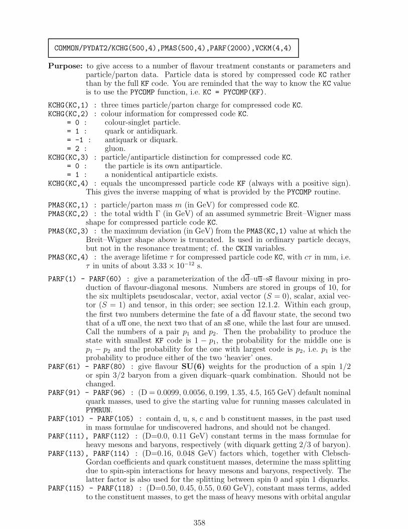
COMMON/PYDAT2/KCHG(500,4),PMAS(500,4),PARF(2000),VCKM(4,4)

Purpose: to give access to a number of flavour treatment constants or parameters andparticle/parton data. Particle data is stored by compressed code KC ratherthan by the full KF code. You are reminded that the way to know the KC valueis to use the PYCOMP function, i.e. KC = PYCOMP(KF).

KCHG(KC,1) : three times particle/parton charge for compressed code KC.KCHG(KC,2) : colour information for compressed code KC.

= 0 : colour-singlet particle.= 1 : quark or antidiquark.= -1 : antiquark or diquark.= 2 : gluon.

KCHG(KC,3) : particle/antiparticle distinction for compressed code KC.= 0 : the particle is its own antiparticle.= 1 : a nonidentical antiparticle exists.

KCHG(KC,4) : equals the uncompressed particle code KF (always with a positive sign).This gives the inverse mapping of what is provided by the PYCOMP routine.

PMAS(KC,1) : particle/parton mass m (in GeV) for compressed code KC.PMAS(KC,2) : the total width Γ (in GeV) of an assumed symmetric Breit–Wigner mass

shape for compressed particle code KC.PMAS(KC,3) : the maximum deviation (in GeV) from the PMAS(KC,1) value at which the

Breit–Wigner shape above is truncated. Is used in ordinary particle decays,but not in the resonance treatment; cf. the CKIN variables.

PMAS(KC,4) : the average lifetime τ for compressed particle code KC, with cτ in mm, i.e.τ in units of about 3.33 × 10−12 s.

PARF(1) - PARF(60) : give a parameterization of the dd–uu–ss flavour mixing in pro-duction of flavour-diagonal mesons. Numbers are stored in groups of 10, forthe six multiplets pseudoscalar, vector, axial vector (S = 0), scalar, axial vec-tor (S = 1) and tensor, in this order; see section 12.1.2. Within each group,the first two numbers determine the fate of a dd flavour state, the second twothat of a uu one, the next two that of an ss one, while the last four are unused.Call the numbers of a pair p1 and p2. Then the probability to produce thestate with smallest KF code is 1 − p1, the probability for the middle one isp1 − p2 and the probability for the one with largest code is p2, i.e. p1 is theprobability to produce either of the two ‘heavier’ ones.

PARF(61) - PARF(80) : give flavour SU(6) weights for the production of a spin 1/2or spin 3/2 baryon from a given diquark–quark combination. Should not bechanged.

PARF(91) - PARF(96) : (D = 0.0099, 0.0056, 0.199, 1.35, 4.5, 165 GeV) default nominalquark masses, used to give the starting value for running masses calculated inPYMRUN.

PARF(101) - PARF(105) : contain d, u, s, c and b constituent masses, in the past usedin mass formulae for undiscovered hadrons, and should not be changed.

PARF(111), PARF(112) : (D=0.0, 0.11 GeV) constant terms in the mass formulae forheavy mesons and baryons, respectively (with diquark getting 2/3 of baryon).

PARF(113), PARF(114) : (D=0.16, 0.048 GeV) factors which, together with Clebsch-Gordan coefficients and quark constituent masses, determine the mass splittingdue to spin-spin interactions for heavy mesons and baryons, respectively. Thelatter factor is also used for the splitting between spin 0 and spin 1 diquarks.

PARF(115) - PARF(118) : (D=0.50, 0.45, 0.55, 0.60 GeV), constant mass terms, addedto the constituent masses, to get the mass of heavy mesons with orbital angular

358

momentum L = 1. The four numbers are for pseudovector mesons with quarkspin 0, and for scalar, pseudovector and tensor mesons with quark spin 1,respectively.

PARF(121), PARF(122) : (D=0.1, 0.2 GeV) constant terms, which are subtracted forquark and diquark masses, respectively, in defining the allowed phase space inparticle decays into partons (e.g. B0 → cdud).

PARF(201) - PARF(1960) : (D=1760*0) relative probabilities for flavour production inthe MSTJ(15)=1 option; to be defined by you before any Pythia calls. (Thestandard meaning is changed in the advanced baryon popcorn code, describedin subsection 14.3.1, where many of the PARF numbers are used for other pur-poses.)The index in PARF is of the compressed form120 + 80×KTAB1+25×KTABS+KTAB3.Here KTAB1 is the old flavour, fixed by preceding fragmentation history, whileKTAB3 is the new flavour, to be selected according to the relevant relativeprobabilities (except for the very last particle, produced when joining two jets,where both KTAB1 and KTAB3 are known). Only the most frequently ap-pearing quarks/diquarks are defined, according to the code 1 = d, 2 = u,3 = s, 4 = c, 5 = b, 6 = t (obsolete!), 7 = dd1, 8 = ud0, 9 = ud1, 10 = uu1,11 = sd0, 12 = sd1, 13 = su0, 14 = su1, 15 = ss1, 16 = cd0, 17 = cd1, 18 = cu0,19 = cu1, 20 = cs0, 21 = cs1, 22 = cc1. These are thus the only possibilitiesfor the new flavour to be produced; for an occasional old flavour not on thislist, the ordinary relative flavour production probabilities will be used.Given the initial and final flavour, the intermediate hadron that is producedis almost fixed. (Initial and final diquark here corresponds to ‘popcorn’ pro-duction of mesons intermediate between a baryon and an antibaryon). Theadditional index KTABS gives the spin type of this hadron, with0 = pseudoscalar meson or Λ-like spin 1/2 baryon,1 = vector meson or Σ-like spin 1/2 baryon,2 = tensor meson or spin 3/2 baryon.(Some meson multiplets, not frequently produced, are not accessible by thisparameterization.)Note that some combinations of KTAB1, KTAB3 and KTABS do not cor-respond to a physical particle (a Λ-like baryon must contain three differ-ent quark flavours, a Σ-like one at least two), and that you must see toit that the corresponding PARF entries are vanishing. One additional com-plication exist when KTAB3 and KTAB1 denote the same flavour content(normally KTAB3=KTAB1, but for diquarks the spin freedom may giveKTAB3=KTAB1±1): then a flavour neutral meson is to be produced, andhere dd, uu and ss states mix (heavier flavour states do not, and these aretherefore no problem). For these cases the ordinary KTAB3 value gives thetotal probability to produce either of the mesons possible, while KTAB3=23gives the relative probability to produce the lightest meson state (π0, ρ0, a0

2),KTAB3=24 relative probability for the middle meson (η, ω, f02), and KTAB3 =25 relative probability for the heaviest one (η′, φ, f ′0

2 ). Note that, for simplic-ity, these relative probabilities are assumed the same whether initial and finaldiquark have the same spin or not; the total probability may well be assumeddifferent, however.As a general comment, the sum of PARF values for a given KTAB1 need notbe normalized to unity, but rather the program will find the sum of relevantweights and normalize to that. The same goes for the KTAB3=23–25 weights.This makes it straightforward to use one common setup of PARF values andstill switch between different MSTJ(12) baryon production modes, with the

359

exception of the advanced popcorn scenarios.

VCKM(I,J) : squared matrix elements of the Cabibbo-Kobayashi-Maskawa flavour mix-ing matrix.

I : up type generation index, i.e. 1 = u, 2 = c, 3 = t and 4 = t′.J : down type generation index, i.e. 1 = d, 2 = s, 3 = b and 4 = b′.

COMMON/PYDAT3/MDCY(500,3),MDME(8000,2),BRAT(8000),KFDP(8000,5)

Purpose: to give access to particle decay data and parameters. In particular, theMDCY(KC,1) variables may be used to switch on or off the decay of a givenparticle species, and the MDME(IDC,1) ones to switch on or off an individualdecay channel of a particle. For quarks, leptons and gauge bosons, a numberof decay channels are included that are not allowed for on-mass-shell particles,see MDME(IDC,2)=102. These channels are not directly used to perform de-cays, but rather to denote allowed couplings in a more general sense, and toswitch on or off such couplings, as described elsewhere. Particle data is storedby compressed code KC rather than by the full KF code. You are remindedthat the way to know the KC value is to use the PYCOMP function, i.e. KC =PYCOMP(KF).

MDCY(KC,1) : switch to tell whether a particle with compressed code KC may be allowedto decay or not.

= 0 : the particle is not allowed to decay.= 1 : the particle is allowed to decay (if decay information is defined below for

the particle).Warning: these values may be overwritten for resonances in a PYINIT call, based

on the MSTP(41) option you have selected. If you want to allow resonancedecays in general but switch off the decay of one particular resonance,this is therefore better done after the PYINIT call.

MDCY(KC,2) : gives the entry point into the decay channel table for compressed particlecode KC. Is 0 if no decay channels have been defined.

MDCY(KC,3) : gives the total number of decay channels defined for compressed particlecode KC, independently of whether they have been assigned a non-vanishingbranching ratio or not. Thus the decay channels are found in positionsMDCY(KC,2) to MDCY(KC,2)+MDCY(KC,3)-1.

MDME(IDC,1) : on/off switch for individual decay channel IDC. In addition, a channelmay be left selectively open; this has some special applications in the eventgeneration machinery. Effective branching ratios are automatically recalcu-lated for the decay channels left open. Also process cross sections are affected;see section 7.6.2. If a particle is allowed to decay by the MDCY(KC,1) value,at least one channel must be left open by you. A list of decay channels withcurrent IDC numbers may be obtained with PYLIST(12).

= -1 : this is a non-Standard Model decay mode, which by default is assumednot to exist. Normally, this option is used for decays involving fourthgeneration or H± particles.

= 0 : channel is switched off.= 1 : channel is switched on.= 2 : channel is switched on for a particle but off for an antiparticle. It is also

on for a particle which is its own antiparticle, i.e. here it means the sameas =1.

= 3 : channel is switched on for an antiparticle but off for a particle. It is offfor a particle which is its own antiparticle.

360

= 4 : in the production of a pair of equal or charge conjugate resonances inPythia, say h0 → W+W−, either one of the resonances is allowed todecay according to this group of channels, but not both. If the two par-ticles of the pair are different, the channel is on. For ordinary particles,not resonances, this option only means that the channel is switched off.

= 5 : as =4, but an independent group of channels, such that in a pair of equalor charge conjugate resonances the decay of either resonance may bespecified independently. If the two particles in the pair are different, thechannel is off. For ordinary particles, not resonances, this option onlymeans that the channel is switched off.

Warning: the two values -1 and 0 may look similar, but in fact are quite different.In neither case the channel so set is generated, but in the latter case thechannel still contributes to the total width of a resonance, and thus affectsboth simulated line shape and the generated cross section when Pythia

is run. The value 0 is appropriate to a channel we assume exists, even ifwe are not currently simulating it, while -1 should be used for channelswe believe do not exist. In particular, you are warned unwittingly to setfourth generation channels 0 (rather than -1), since by now the supportfor a fourth generation is small.

Remark: all the options above may be freely mixed. The difference, for those caseswhere both make sense, between using values 2 and 3 and using 4 and5 is that the latter automatically include charge conjugate states, e.g.h0 → W+W− → e+νedu or due−νe, but the former only one of them. Incalculations of the joint branching ratio, this makes a factor 2 difference.

Example: to illustrate the above options, consider the case of a W+W− pair. Onemight then set the following combination of switches for the W:channel value comment

ud 1 allowed for W+ and W− in any combination,

us 0 never produced but contributes to W width,

cd 2 allowed for W+ only,

cs 3 allowed for W− only, i.e. properly W− → cs,

tb 0 never produced but contributes to W width

if the channel is kinematically allowed,

νee+ 4 allowed for one of W+ or W−, but not both,

νµµ+ 4 allowed for one of W+ or W−, but not both,

and not in combination with νee+,

νττ+ 5 allowed for the other W, but not both,

νχχ− −1 not produced and does not contribute to W width.

A W+W− final state ud + cs is allowed, but not its charge conjugateud + cs, since the latter decay mode is not allowed for a W+. Thecombination νee

+ + νττ− is allowed, since the two channels belong to

different groups, but not νee+ + νµµ

−, where both belong to the same.Both ud+νττ

− and ud+ντ τ+ are allowed, since there is no clash. The full

rulebook, for this case, is given by eq. (111). A term r2i means channeli is allowed for W+ and W− simultaneously, a term rirj that channelsi and j may be combined, and a term 2rirj that channels i and j maybe combined two ways, i.e. that also a charge conjugate combination isallowed.

MDME(IDC,2) : information on special matrix-element treatment for decay channel IDC.Is mainly intended for the normal-particle machinery in PYDECY, so many of

361

the codes are superfluous in the more sophisticated resonance decay treatmentby PYRESD, see section 2.1.2. In addition to the outline below, special rulesapply for the order in which decay products should be given, so that matrixelements and colour flow is properly treated. One such example is the weakmatrix elements, which only will be correct if decay products are given in theright order. The program does not police this, so if you introduce channels ofyour own and use these codes, you should be guided by the existing particledata.

= 0 : no special matrix-element treatment; partons and particles are copieddirectly to the event record, with momentum distributed according tophase space.

= 1 : ω and φ decays into three pions, eq. (244).= 2 : π0 or η Dalitz decay to γe+e−, eq. (246).= 3 : used for vector meson decays into two pseudoscalars, to signal non-

isotropic decay angle according to eq. (245), where relevant.= 4 : decay of a spin 1 onium resonance to three gluons or to a photon and

two gluons, eq. (43). The gluons may subsequently develop a shower ifMSTJ(23)=1.

= 11 : phase-space production of hadrons from the quarks available.= 12 : as =11, but for onia resonances, with the option of modifying the multi-

plicity distribution separately.= 13 : as =11, but at least three hadrons to be produced (useful when the two-

body decays are given explicitly).= 14 : as =11, but at least four hadrons to be produced.= 15 : as =11, but at least five hadrons to be produced.= 22 - 30 : phase-space production of hadrons from the quarks available, with

the multiplicity fixed to be MDME(IDC,2)-20, i.e. 2–10.= 31 : two or more quarks and particles are distributed according to phase space.

If three or more products, the last product is a spectator quark, i.e. sittingat rest with respect to the decaying hadron.

= 32 : a qq or gg pair, distributed according to phase space (in angle), andallowed to develop a shower if MSTJ(23)=1.

= 33 : a triplet qXq, where X is either a gluon or a colour-singlet particle; thefinal particle (q) is assumed to sit at rest with respect to the decayinghadron, and the two first particles (q and X) are allowed to develop ashower if MSTJ(23)=1. Nowadays superfluous.

= 41 : weak decay, where particles are distributed according to phase space,multiplied by a factor from the expected shape of the momentum spec-trum of the direct product of the weak decay (the ντ in τ decay).

= 42 : weak decay matrix element for quarks and leptons. Products may begiven either in terms of quarks or hadrons, or leptons for some channels.If the spectator system is given in terms of quarks, it is assumed tocollapse into one particle from the onset. If the virtual W decays intoquarks, these quarks are converted to particles, according to phase spacein the W rest frame, as in =11. Is intended for τ , charm and bottom.

= 43 : as =42, but if the W decays into quarks, these will either appear as jetsor, for small masses, collapse into a one- or two-body system. Nowadayssuperfluous.

= 44 : weak decay matrix element for quarks and leptons, where the spectatorsystem may collapse into one particle for a small invariant mass. Ifthe first two decay products are a qq′ pair, they may develop a partonshower if MSTJ(23)=1. Was intended for top and beyond, but is nowadayssuperfluous.

362

= 46 : W (KF = 89) decay into qq′ or ℓνℓ according to relative probabilities givenby couplings (as stored in the BRAT vector) times a dynamical phase-spacefactor given by the current W mass. In the decay, the correct V − Aangular distribution is generated if the W origin is known (heavy quarkor lepton). This is therefore the second step of a decay with MDME=45. Aqq′ pair may subsequently develop a shower if MSTJ(23)=1. Was intendedfor top and beyond, but is nowadays superfluous.

= 48 : as =42, but require at least three decay products.= 50 : (default behaviour, also obtained for any other code value apart from

the ones listed below) do not include any special threshold factors. Thatis, a decay channel is left open even if the sum of daughter nominalmasses is above the mother actual mass, which is possible if at least oneof the daughters can be pushed off the mass shell. Is intended for decaytreatment in PYRESD with PYWIDT calls, and has no special meaning forordinary PYDECY calls.

= 51 : a step threshold, i.e. a channel is switched off when the sum of daughternominal masses is above the mother actual mass. Is intended for decaytreatment in PYRESD with PYWIDT calls, and has no special meaning forordinary PYDECY calls.

= 52 : a β-factor threshold, i.e.√

(1 −m21/m

2 −m22/m

2)2 − 4m21m

22/m

4, assum-ing that the values stored in PMAS(KC,2) and BRAT(IDC) did not includeany threshold effects at all. Is intended for decay treatment in PYRESDwith PYWIDT calls, and has no special meaning for ordinary PYDECY calls.

= 53 : as =52, but assuming that PMAS(KC,2) and BRAT(IDC) did include thethreshold effects, so that the weight should be the ratio of the β valueat the actual mass to that at the nominal one. Is intended for decaytreatment in PYRESD with PYWIDT calls, and has no special meaning forordinary PYDECY calls.

= 101 : this is not a proper decay channel, but only to be considered as a con-tinuation line for the decay product listing of the immediately precedingchannel. Since the KFDP array can contain five decay products per chan-nel, with this code it is possible to define channels with up to ten decayproducts. It is not allowed to have several continuation lines after eachother.

= 102 : this is not a proper decay channel for a decaying particle on the mass shell(or nearly so), and is therefore assigned branching ratio 0. For a particleoff the mass shell, this decay mode is allowed, however. By includingthis channel among the others, the switches MDME(IDC,1) may be usedto allow or forbid these channels in hard processes, with cross sectionsto be calculated separately. As an example, γ → uu is not possible for amassless photon, but is an allowed channel in e+e− annihilation.

BRAT(IDC) : give branching ratios for the different decay channels. In principle, thesum of branching ratios for a given particle should be unity. Since the pro-gram anyway has to calculate the sum of branching ratios left open by theMDME(IDC,1) values and normalize to that, you need not explicitly ensure thisnormalization, however. (Warnings are printed in PYUPDA(2) or PYUPDA(3)calls if the sum is not unity, but this is entirely intended as a help for findinguser mistypings.) For decay channels with MDME(IDC,2)> 80 the BRAT valuesare dummy.

KFDP(IDC,J) : contain the decay products in the different channels, with five positionsJ= 1–5 reserved for each channel IDC. The decay products are given follow-ing the standard KF code for partons and particles, with 0 for trailing empty

363

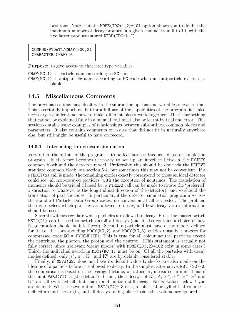
positions. Note that the MDME(IDC+1,2)=101 option allows you to double themaximum number of decay product in a given channel from 5 to 10, with thefive latter products stored KFDP(IDC+1,J).

COMMON/PYDAT4/CHAF(500,2)CHARACTER CHAF*16

Purpose: to give access to character type variables.

CHAF(KC,1) : particle name according to KC code.CHAF(KC,2) : antiparticle name according to KC code when an antiparticle exists, else

blank.

14.5 Miscellaneous Comments

The previous sections have dealt with the subroutine options and variables one at a time.This is certainly important, but for a full use of the capabilities of the program, it is alsonecessary to understand how to make different pieces work together. This is somethingthat cannot be explained fully in a manual, but must also be learnt by trial and error. Thissection contains some examples of relationships between subroutines, common blocks andparameters. It also contains comments on issues that did not fit in naturally anywhereelse, but still might be useful to have on record.

14.5.1 Interfacing to detector simulation

Very often, the output of the program is to be fed into a subsequent detector simulationprogram. It therefore becomes necessary to set up an interface between the PYJETScommon block and the detector model. Preferrably this should be done via the HEPEVTstandard common block, see section 5.4, but sometimes this may not be convenient. If aPYEDIT(2) call is made, the remaining entries exactly correspond to those an ideal detectorcould see: all non-decayed particles, with the exception of neutrinos. The translation ofmomenta should be trivial (if need be, a PYROBO call can be made to rotate the ‘preferred’z direction to whatever is the longitudinal direction of the detector), and so should thetranslation of particle codes. In particular, if the detector simulation program also usesthe standard Particle Data Group codes, no conversion at all is needed. The problemthen is to select which particles are allowed to decay, and how decay vertex informationshould be used.

Several switches regulate which particles are allowed to decay. First, the master switchMSTJ(21) can be used to switch on/off all decays (and it also contains a choice of howfragmentation should be interfaced). Second, a particle must have decay modes definedfor it, i.e. the corresponding MDCY(KC,2) and MDCY(KC,3) entries must be non-zero forcompressed code KC = PYCOMP(KF). This is true for all colour neutral particles exceptthe neutrinos, the photon, the proton and the neutron. (This statement is actually notfully correct, since irrelevant ‘decay modes’ with MDME(IDC,2)=102 exist in some cases.)Third, the individual switch in MDCY(KC,1) must be on. Of all the particles with decaymodes defined, only µ±, π±, K± and K0

L are by default considered stable.Finally, if MSTJ(22) does not have its default value 1, checks are also made on the

lifetime of a particle before it is allowed to decay. In the simplest alternative, MSTJ(22)=2,the comparison is based on the average lifetime, or rather cτ , measured in mm. Thus ifthe limit PARJ(71) is (the default) 10 mm, then decays of K0

S, Λ, Σ−, Σ+, Ξ−, Ξ0 andΩ− are all switched off, but charm and bottom still decay. No cτ values below 1 µmare defined. With the two options MSTJ(22)= 3 or 4, a spherical or cylindrical volume isdefined around the origin, and all decays taking place inside this volume are ignored.

364

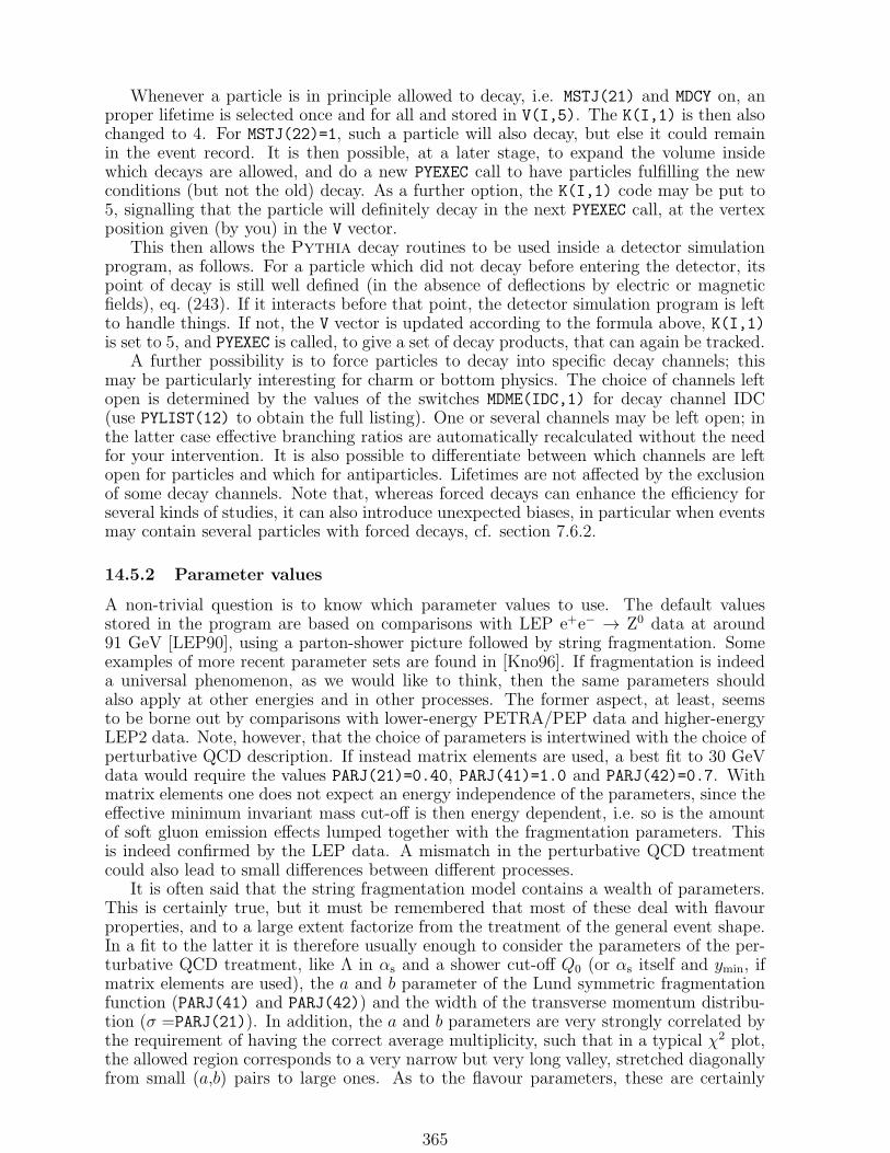
Whenever a particle is in principle allowed to decay, i.e. MSTJ(21) and MDCY on, anproper lifetime is selected once and for all and stored in V(I,5). The K(I,1) is then alsochanged to 4. For MSTJ(22)=1, such a particle will also decay, but else it could remainin the event record. It is then possible, at a later stage, to expand the volume insidewhich decays are allowed, and do a new PYEXEC call to have particles fulfilling the newconditions (but not the old) decay. As a further option, the K(I,1) code may be put to5, signalling that the particle will definitely decay in the next PYEXEC call, at the vertexposition given (by you) in the V vector.

This then allows the Pythia decay routines to be used inside a detector simulationprogram, as follows. For a particle which did not decay before entering the detector, itspoint of decay is still well defined (in the absence of deflections by electric or magneticfields), eq. (243). If it interacts before that point, the detector simulation program is leftto handle things. If not, the V vector is updated according to the formula above, K(I,1)is set to 5, and PYEXEC is called, to give a set of decay products, that can again be tracked.

A further possibility is to force particles to decay into specific decay channels; thismay be particularly interesting for charm or bottom physics. The choice of channels leftopen is determined by the values of the switches MDME(IDC,1) for decay channel IDC(use PYLIST(12) to obtain the full listing). One or several channels may be left open; inthe latter case effective branching ratios are automatically recalculated without the needfor your intervention. It is also possible to differentiate between which channels are leftopen for particles and which for antiparticles. Lifetimes are not affected by the exclusionof some decay channels. Note that, whereas forced decays can enhance the efficiency forseveral kinds of studies, it can also introduce unexpected biases, in particular when eventsmay contain several particles with forced decays, cf. section 7.6.2.

14.5.2 Parameter values

A non-trivial question is to know which parameter values to use. The default valuesstored in the program are based on comparisons with LEP e+e− → Z0 data at around91 GeV [LEP90], using a parton-shower picture followed by string fragmentation. Someexamples of more recent parameter sets are found in [Kno96]. If fragmentation is indeeda universal phenomenon, as we would like to think, then the same parameters shouldalso apply at other energies and in other processes. The former aspect, at least, seemsto be borne out by comparisons with lower-energy PETRA/PEP data and higher-energyLEP2 data. Note, however, that the choice of parameters is intertwined with the choice ofperturbative QCD description. If instead matrix elements are used, a best fit to 30 GeVdata would require the values PARJ(21)=0.40, PARJ(41)=1.0 and PARJ(42)=0.7. Withmatrix elements one does not expect an energy independence of the parameters, since theeffective minimum invariant mass cut-off is then energy dependent, i.e. so is the amountof soft gluon emission effects lumped together with the fragmentation parameters. Thisis indeed confirmed by the LEP data. A mismatch in the perturbative QCD treatmentcould also lead to small differences between different processes.

It is often said that the string fragmentation model contains a wealth of parameters.This is certainly true, but it must be remembered that most of these deal with flavourproperties, and to a large extent factorize from the treatment of the general event shape.In a fit to the latter it is therefore usually enough to consider the parameters of the per-turbative QCD treatment, like Λ in αs and a shower cut-off Q0 (or αs itself and ymin, ifmatrix elements are used), the a and b parameter of the Lund symmetric fragmentationfunction (PARJ(41) and PARJ(42)) and the width of the transverse momentum distribu-tion (σ =PARJ(21)). In addition, the a and b parameters are very strongly correlated bythe requirement of having the correct average multiplicity, such that in a typical χ2 plot,the allowed region corresponds to a very narrow but very long valley, stretched diagonallyfrom small (a,b) pairs to large ones. As to the flavour parameters, these are certainly

365

many more, but most of them are understood qualitiatively within one single framework,that of tunnelling pair production of flavours.

Since the use of independent fragmentation has fallen in disrespect, it should bepointed out that the default parameters here are not particularly well tuned to the data.This especially applies if one, in addition to asking for independent fragmentation, alsoasks for another setup of fragmentation functions, i.e. other than the standard Lundsymmetric one. In particular, note that most fits to the popular Peterson/SLAC heavy-flavour fragmentation function are based on the actual observed spectrum. In a MonteCarlo simulation, one must then start out with something harder, to compensate for theenergy lost by initial-state photon radiation and gluon bremsstrahlung. Since indepen-dent fragmentation is not collinear safe (i.e, the emission of a collinear gluon changes theproperties of the final event), the tuning is strongly dependent on the perturbative QCDtreatment chosen. All the parameters needed for a tuning of independent fragmentationare available, however.

14.6 Examples

A 10 GeV u quark jet going out along the +z axis is generated with

CALL PY1ENT(0,2,10D0,0D0,0D0)

Note that such a single jet is not required to conserve energy, momentum or flavour. Inthe generation scheme, particles with negative pz are produced as well, but these areautomatically rejected unless MSTJ(3)=-1. While frequently used in former days, theone-jet generation option is not of much current interest.

In e.g. a leptoproduction event a typical situation could be a u quark going out inthe +z direction and a ud0 target remnant essentially at rest. (Such a process can besimulated by Pythia, but here we illustrate how to do part of it yourself.) The simplestprocedure is probably to treat the process in the c.m. frame and boost it to the lab frameafterwards. Hence, if the c.m. energy is 20 GeV and the boost βz = 0.996 (correspondingto xB = 0.045), then

CALL PY2ENT(0,2,2101,20D0)CALL PYROBO(0,0,0D0,0D0,0D0,0D0,0.996D0)

The jets could of course also be defined and allowed to fragment in the lab frame with

CALL PY1ENT(-1,2,223.15D0,0D0,0D0)CALL PY1ENT(2,12,0.6837D0,3.1416D0,0D0)CALL PYEXEC

Note here that the target diquark is required to move in the backwards direction withE−pz = mp(1−xB) to obtain the correct invariant mass for the system. This is, however,only an artefact of using a fixed diquark mass to represent a varying target remnant mass,and is of no importance for the fragmentation. If one wants a nicer-looking event record,it is possible to use the following

CALL PY1ENT(-1,2,223.15D0,0D0,0D0)MSTU(10)=1P(2,5)=0.938D0*(1D0-0.045D0)CALL PY1ENT(2,2101,0D0,0D0,0D0)MSTU(10)=2CALL PYEXEC

A 30 GeV uug event with Eu = 8 GeV and Eu = 14 GeV is simulated with

366

CALL PY3ENT(0,2,21,-2,30D0,2D0*8D0/30D0,2D0*14D0/30D0)

The event will be given in a standard orientation with the u quark along the +z axisand the u in the ±z,+x half plane. Note that the flavours of the three partons have tobe given in the order they are found along a string, if string fragmentation options areto work. Also note that, for 3-jet events, and particularly 4-jet ones, not all setups ofkinematical variables x lie within the kinematically allowed regions of phase space.

All common block variables can obviously be changed by including the correspondingcommon block in the user-written main program. Alternatively, the routine PYGIVE canbe used to feed in values, with some additional checks on array bounds then performed.A call

CALL PYGIVE(’MSTJ(21)=3;PMAS(C663,1)=210.;CHAF(401,1)=funnyino;’//&’PMAS(21,4)=’)

will thus change the value of MSTJ(21) to 3, the value of PMAS(PYCOMP(663),1) =PMAS(136,1) to 210., the value of CHAF(401,1) to ’funnyino’, and print the currentvalue of PMAS(21,4). Since old and new values of parameters changed are written to out-put, this may offer a convenient way of documenting non-default values used in a givenrun. On the other hand, if a variable is changed back and forth frequently, the resultingvoluminous output may be undesirable, and a direct usage of the common blocks is thento be recommended (the output can also be switched off, see MSTU(13)).

A general rule of thumb is that none of the physics routines (PYSTRF, PYINDF, PYDECY,etc.) should ever be called directly, but only via PYEXEC. This routine may be calledrepeatedly for one single event. At each call only those entries that are allowed to fragmentor decay, and have not yet done so, are treated. Thus

CALL PY2ENT(1,1,-1,20D0) ! fill 2 partons without fragmentingMSTJ(1)=0 ! inhibit jet fragmentationMSTJ(21)=0 ! inhibit particle decayMDCY(PYCOMP(111),1)=0 ! inhibit pi0 decayCALL PYEXEC ! will not do anythingMSTJ(1)=1 !CALL PYEXEC ! partons will fragment, no decaysMSTJ(21)=2 !CALL PYEXEC ! particles decay, except pi0CALL PYEXEC ! nothing new can happenMDCY(PYCOMP(111),1)=1 !CALL PYEXEC ! pi0:s decay

A partial exception to the rule above is PYSHOW. Its main application is for internaluse by PYEEVT, PYDECY, and PYEVNT, but it can also be directly called by you. Note thata special format for storing colour-flow information in K(I,4) and K(I,5) must then beused. For simple cases, the PY2ENT can be made to take care of that automatically, bycalling with the first argument negative.

CALL PY2ENT(-1,1,-2,80D0) ! store d ubar with colour flowCALL PYSHOW(1,2,80D0) ! shower partonsCALL PYEXEC ! subsequent fragmentation/decay

For more complicated configurations, PYJOIN should be used.It is always good practice to list one or a few events during a run to check that the

program is working as intended. With

CALL PYLIST(1)

367

all particles will be listed and in addition total charge, momentum and energy of sta-ble entries will be given. For string fragmentation these quantities should be conservedexactly (up to machine precision errors), and the same goes when running independentfragmentation with one of the momentum conservation options. PYLIST(1) gives a formatthat comfortably fits in an 80 column window, at the price of not giving the completestory. With PYLIST(2) a more extensive listing is obtained, and PYLIST(3) also givesvertex information. Further options are available, like PYLIST(12), which gives a list ofparticle data.

An event, as stored in the PYJETS common block, will contain the original partons andthe whole decay chain, i.e. also particles which subsequently decayed. If parton showersare used, the amount of parton information is also considerable: first the on-shell partonsbefore showers have been considered, then a K(I,1)=22 line with total energy of theshowering subsystem, after that the complete shower history tree-like structure, startingoff with the same initial partons (now off-shell), and finally the end products of the showerrearranged along the string directions. This detailed record is useful in many connections,but if one only wants to retain the final particles, superfluous information may be removedwith PYEDIT. Thus e.g.

CALL PYEDIT(2)

will leave you with the final charged and neutral particles, except for neutrinos.The information in PYJETS may be used directly to study an event. Some useful

additional quantities derived from these, such as charge and rapidity, may easily be foundvia the PYK and PYP functions. Thus electric charge =PYP(I,6) (as integer, three timescharge =PYK(I,6)) and true rapidity y with respect to the z axis = PYP(I,17).

A number of utility (MSTU, PARU) and physics (MSTJ, PARJ) switches and parametersare available in common block PYDAT1. All of these have sensible default values. Particledata is stored in common blocks PYDAT2, PYDAT3 and PYDAT4. Note that the data in thearrays KCHG, PMAS, MDCY CHAF and MWID is not stored by KF code, but by the compressedcode KC. This code is not to be learnt by heart, but instead accessed via the conversionfunction PYCOMP, KC = PYCOMP(KF).

In the particle tables, the following particles are considered stable: the photon, e±,µ±, π±, K±, K0

L, p, p, n, n and all the neutrinos. It is, however, always possible to inhibitthe decay of any given particle by putting the corresponding MDCY value zero or negative,e.g. MDCY(PYCOMP(310),1)=0 makes K0

S and MDCY(PYCOMP(3122),1)=0 Λ stable. It isalso possible to select stability based on the average lifetime (see MSTJ(22)), or based onwhether the decay takes place within a given spherical or cylindrical volume around theorigin.

The Field-Feynman jet model [Fie78] is available in the program by changing thefollowing values: MSTJ(1)=2 (independent fragmentation), MSTJ(3)=-1 (retain parti-cles with pz < 0; is not mandatory), MSTJ(11)=2 (choice of longitudinal fragmenta-tion function, with the a parameter stored in PARJ(51) - PARJ(53)), MSTJ(12)=0 (nobaryon production), MSTJ(13)=1 (give endpoint quarks p⊥ as quarks created in the field),MSTJ(24)=0 (no mass broadening of resonances), PARJ(2)=0.5 (s/u ratio for the produc-tion of new qq pairs), PARJ(11)=PARJ(12)=0.5 (probability for mesons to have spin 1)and PARJ(21)=0.35 (width of Gaussian transverse momentum distribution). In additiononly d, u and s single quark jets may be generated following the FF recipe. Today the FF‘standard jet’ concept is probably dead and buried, so the numbers above should morebe taken as an example of the flexibility of the program, than as something to apply inpractice.

A wide range of independent fragmentation options are implemented, to be accessedwith the master switch MSTJ(1)=2. In particular, with MSTJ(2)=1 a gluon jet is assumedto fragment like a random d, d, u, u, s or s jet, while with MSTJ(2)=3 the gluon is splitinto a dd, uu or ss pair of jets sharing the energy according to the Altarelli-Parisi splitting

368

function. Whereas energy, momentum and flavour is not explicitly conserved in indepen-dent fragmentation, a number of options are available in MSTJ(3) to ensure this ‘postfacto’, e.g. MSTJ(3)=1 will boost the event to ensure momentum conservation and then(in the c.m. frame) rescale momenta by a common factor to obtain energy conservation,whereas MSTJ(3)=4 rather uses a method of stretching the jets in longitudinal momentumalong the respective jet axis to keep angles between jets fixed.

369

15 Event Study and Analysis Routines

After an event has been generated, one may wish to list it, or process it further in variousways. The first section below describes some simple study routines of this kind, while thesubsequent ones describe more sophisticated analysis routines.

To describe the complicated geometries encountered in multihadronic events, a numberof event measures have been introduced. These measures are intended to provide a globalview of the properties of a given event, wherein the full information content of the eventis condensed into one or a few numbers. A steady stream of such measures are proposedfor different purposes. Many are rather specialized or never catch on, but a few becomestandards, and are useful to have easy access to. Pythia therefore contains a number ofroutines that can be called for any event, and that will directly access the event recordto extract the required information.

In the presentation below, measures have been grouped in three kinds. The first con-tains simple event shape quantities, such as sphericity and thrust. The second is jet findingalgorithms. The third is a mixed bag of particle multiplicities and compositions, factorialmoments and energy–energy correlations, put together in a small statistics package.

None of the measures presented here are Lorentz invariant. The analysis will beperformed in whatever frame the event happens to be given in. It it therefore up to youto decide whether the frame in which events were generated is the right one, or whetherevents beforehand should be boosted, e.g. to the c.m. frame. You can also decide whichparticles you want to have affected by the analysis.

15.1 Event Study Routines

After a PYEVNT call, or another similar physics routine call, the event generated is stored inthe PYJETS common block, and whatever physical variable is desired may be constructedfrom this record. An event may be rotated, boosted or listed, and particle data may belisted or modified. Via the functions PYK and PYP the values of some frequently appearingvariables may be obtained more easily. As described in subsequent sections, also moredetailed event shape analyses may be performed simply.

CALL PYROBO(IMI,IMA,THE,PHI,BEX,BEY,BEZ)

Purpose: to perform rotations and Lorentz boosts (in that order, if both in the samecall) of jet/particle momenta and vertex position variables.

IMI, IMA : range of entries affected by transformation, IMI≤I≤IMA. If 0 or below, IMIdefaults to 1 and IMA to N. Lower and upper bounds given by positive MSTU(1)and MSTU(2) override the IMI and IMA values, and also the 1 to N constraint.

THE, PHI : standard polar coordinates θ, ϕ, giving the rotated direction of a momentumvector initially along the +z axis.

BEX, BEY, BEZ : gives the direction and size β of a Lorentz boost, such that a particleinitially at rest will have p/E =β afterwards.

Remark: all entries in the range IMI–IMA (or modified as described above) are affected,unless the status code of an entry is K(I,1)≤ 0.

CALL PYEDIT(MEDIT)

Purpose: to exclude unstable or undetectable jets/particles from the event record. Onemay also use PYEDIT to store spare copies of events (specifically initial partonconfiguration) that can be recalled to allow e.g. different fragmentation schemesto be run through with one and the same parton configuration. Finally, an

370

event which has been analyzed with PYSPHE, PYTHRU or PYCLUS (see section15.5) may be rotated to align the event axis with the z direction.

MEDIT : tells which action is to be taken.= 0 : empty (K(I,1)=0) and documentation (K(I,1)>20) lines are removed.

The jets/particles remaining are compressed in the beginning of thePYJETS common block and the N value is updated accordingly. The eventhistory is lost, so that information stored in K(I,3), K(I,4) and K(I,5)is no longer relevant.

= 1 : as =0, but in addition all jets/particles that have fragmented/decayed(K(I,1)>10) are removed.

= 2 : as =1, but also all neutrinos and unknown particles (i.e. compressed codeKC= 0) are removed.

= 3 : as =2, but also all uncharged, colour neutral particles are removed, leavingonly charged, stable particles (and unfragmented partons, if fragmenta-tion has not been performed).

= 5 : as =0, but also all partons which have branched or been rearranged in aparton shower and all particles which have decayed are removed, leavingonly the fragmenting parton configuration and the final-state particles.

= 11 : remove lines with K(I,1)<0. Update event history information (inK(I,3) - K(I,5)) to refer to remaining entries.

= 12 : remove lines with K(I,1)=0. Update event history information (inK(I,3) - K(I,5)) to refer to remaining entries.

= 13 : remove lines with K(I,1)= 11, 12 or 15, except for any line withK(I,2)=94. Update event history information (in K(I,3) - K(I,5)) torefer to remaining entries. In particular, try to trace origin of daughters,for which the mother is decayed, back to entries not deleted.

= 14 : remove lines with K(I,1)= 13 or 14, and also any line with K(I,2)=94.Update event history information (in K(I,3) - K(I,5)) to refer to re-maining entries. In particular, try to trace origin of rearranged jets backthrough the parton-shower history to the shower initiator.

= 15 : remove lines with K(I,1)>20. Update event history information (inK(I,3) - K(I,5)) to refer to remaining entries.

= 16 : try to reconstruct missing daughter pointers of decayed particles from themother pointers of decay products. These missing pointers typically comefrom the need to use K(I,4) and K(I,5) also for colour flow information.

= 21 : all partons/particles in current event record are stored (as a spare copy)in bottom of common block PYJETS (is e.g. done to save original partonsbefore calling PYEXEC).

= 22 : partons/particles stored in bottom of event record with =21 are placed inbeginning of record again, overwriting previous information there (so thate.g. a different fragmentation scheme can be used on the same partons).Since the copy at bottom is unaffected, repeated calls with =22 can bemade.

= 23 : primary partons/particles in the beginning of event record are marked asnot fragmented or decayed, and number of entries N is updated accord-ingly. Is simpe substitute for =21 plus =22 when no fragmentation/decayproducts precede any of the original partons/particles.

= 31 : rotate largest axis, determined by PYSPHE, PYTHRU or PYCLUS, to sit alongthe z direction, and the second largest axis into the xz plane. For PYCLUSit can be further specified to +z axis and xz plane with x > 0, respec-tively. Requires that one of these routines has been called before.

= 32 : mainly intended for PYSPHE and PYTHRU, this gives a further alignment ofthe event, in addition to the one implied by =31. The ‘slim’ jet, defined

371

as the side (z > 0 or z < 0) with the smallest summed p⊥ over squareroot of number of particles, is rotated into the +z hemisphere. In theopposite hemisphere (now z < 0), the side of x > 0 and x < 0 whichhas the largest summed |pz| is rotated into the z < 0, x > 0 quadrant.Requires that PYSPHE or PYTHRU has been called before.

Remark: all entries 1 through N are affected by the editing. For options 0–5 lower andupper bounds can be explicitly given by MSTU(1) and MSTU(2).

CALL PYLIST(MLIST)

Purpose: to list an event, jet or particle data, or current parameter values.MLIST : determines what is to be listed.

= 0 : writes a title page with program version number and last date of change;is mostly for internal use.

= 1 : gives a simple list of current event record, in an 80 column format suitablefor viewing directly in a terminal window. For each entry, the followinginformation is given: the entry number I, the parton/particle name (seebelow), the status code (K(I,1)), the flavour code KF (K(I,2)), the linenumber of the mother (K(I,3)), and the three-momentum, energy andmass (P(I,1) - P(I,5)). If MSTU(3) is non-zero, lines immediately afterthe event record proper are also listed. A final line contains informationon total charge, momentum, energy and invariant mass.The particle name is given by a call to the routine PYNAME. For an entrywhich has decayed/fragmented (K(I,1)= 11–20), this particle name isgiven within parentheses. Similarly, a documentation line (K(I,1)= 21–30) has the name enclosed in expression signs (!. . . !) and an event/jetaxis information line the name within inequality signs (<. . .>). If thelast character of the name is a ‘?’, it is a signal that the complete namehas been truncated to fit in, and can therefore not be trusted; this isvery rare. For partons which have been arranged along strings (K(I,1)=1, 2, 11 or 12), the end of the parton name column contains informationabout the colour string arrangement: an A for the first entry of a string,an I for all intermediate ones, and a V for the final one (a poor man’srendering of a vertical doublesided arrow, l).It is possible to insert lines just consisting of sequences of ====== toseparate different sections of the event record, see MSTU(70) - MSTU(80).

= 2 : gives a more extensive list of the current event record, in a 132 col-umn format, suitable for wide terminal windows. For each entry, thefollowing information is given: the entry number I, the parton/particlename (with padding as described for =1), the status code (K(I,1)), theflavour code KF (K(I,2)), the line number of the mother (K(I,3)), thedecay product/colour-flow pointers (K(I,4), K(I,5)), and the three-momentum, energy and mass (P(I,1) - P(I,5)). If MSTU(3) is non-zero, lines immediately after the event record proper are also listed. Afinal line contains information on total charge, momentum, energy andinvariant mass. Lines with only ====== may be inserted as for =1.

= 3 : gives the same basic listing as =2, but with an additional line for eachentry containing information on production vertex position and time(V(I,1) - V(I,4)) and, for unstable particles, proper lifetime (V(I,5)).

= 5 : gives a simple listing of the event record stored in the HEPEVT commonblock. This is mainly intended as a tool to check how conversion with thePYHEPC routine works. The listing does not contain vertex information,

372

and the flavour code is not displayed as a name.= 7 : gives a simple listing of the parton-level event record for an external

process, as stored in the HEPEUP common block. This is mainly intendedas a tool to check how reading from HEPEUP input works. The listingdoes not contain lifetime or spin information, and the flavour code is notdisplayed as a name. It also does not show other HEPEUP numbers, suchas the event weight.

= 11 : provides a simple list of all parton/particle codes defined in the program,with KF code and corresponding particle name. The list is grouped byparticle kind, and only within each group in ascending order.

= 12 : provides a list of all parton/particle and decay data used in the pro-gram. Each parton/particle code is represented by one line containingKF flavour code, KC compressed code, particle name, antiparticle name(where appropriate), electrical and colour charge and peresence or not ofan antiparticle (stored in KCHG), mass, resonance width and maximumbroadening, average proper lifetime (in PMAS) and whether the particleis considered stable or not (in MDCY). Immediately after a particle, eachdecay channel gets one line, containing decay channel number (IDC readfrom MDCY), on/off switch for the channel, matrix element type (MDME),branching ratio (BRAT), and decay products (KFDP). The MSTU(1) andMSTU(2) flags can be used to set the range of KF codes for which parti-cles are listed.

= 13 : gives a list of current parameter values for MSTU, PARU, MSTJ and PARJ,and the first 200 entries of PARF. This is useful to keep check of whichdefault values were changed in a given run.

Remark: for options 1–3 and 12 lower and upper bounds of the listing can be explicitlygiven by MSTU(1) and MSTU(2).

KK = PYK(I,J)

Purpose: to provide various integer-valued event data. Note that many of the optionsavailable (in particular I> 0, J≥ 14) which refer to event history will not workafter a PYEDIT call. Further, the options 14–18 depend on the way the eventhistory has been set up, so with the explosion of different allowed formats theseoptions are no longer as safe as they may have been. For instance, option 16can only work if MSTU(16)=2.

I=0, J= : properties referring to the complete event.= 1 : N, total number of lines in event record.= 2 : total number of partons/particles remaining after fragmentation and de-

cay.= 6 : three times the total charge of remaining (stable) partons and particles.

I>0, J= : properties referring to the entry in line no. I of the event record.= 1 - 5 : K(I,1) - K(I,5), i.e. parton/particle status KS, flavour code KF and

origin/decay product/colour-flow information.= 6 : three times parton/particle charge.= 7 : 1 for a remaining entry, 0 for a decayed, fragmented or documentation

entry.= 8 : KF code (K(I,2)) for a remaining entry, 0 for a decayed, fragmented or

documentation entry.= 9 : KF code (K(I,2)) for a parton (i.e. not colour neutral entry), 0 for a

particle.= 10 : KF code (K(I,2)) for a particle (i.e. colour neutral entry), 0 for a parton.

373

= 11 : compressed flavour code KC.= 12 : colour information code, i.e. 0 for colour neutral, 1 for colour triplet, -1

for antitriplet and 2 for octet.= 13 : flavour of ‘heaviest’ quark or antiquark (i.e. with largest code) in hadron

or diquark (including sign for antiquark), 0 else.= 14 : generation number. Beam particles or virtual exchange particles are

generation 0, original jets/particles generation 1 and then 1 is added foreach step in the fragmentation/decay chain.

= 15 : line number of ancestor, i.e. predecessor in first generation (generation 0entries are disregarded).

= 16 : rank of a hadron in the jet it belongs to. Rank denotes the orderingin flavour space, with hadrons containing the original flavour of the jethaving rank 1, increasing by 1 for each step away in flavour ordering. Alldecay products inherit the rank of their parent. Whereas the meaningof a first-rank hadron in a quark jet is always well-defined, the definitionof higher ranks is only meaningful for independently fragmenting quarkjets. In other cases, rank refers to the ordering in the actual simulation,which may be of little interest.

= 17 : generation number after a collapse of a parton system into one particle,with 0 for an entry not coming from a collapse, and -1 for entry withunknown history. A particle formed in a collapse is generation 1, andthen one is added in each decay step.

= 18 : number of decay/fragmentation products (only defined in a collectivesense for fragmentation).

= 19 : origin of colour for showering parton, 0 else.= 20 : origin of anticolour for showering parton, 0 else.= 21 : position of colour daughter for showering parton, 0 else.= 22 : position of anticolour daughter for showering parton, 0 else.

PP = PYP(I,J)

Purpose: to provide various real-valued event data. Note that some of the optionsavailable (I> 0, J= 20–25), which are primarily intended for studies of systemsin their respective c.m. frame, requires that a PYEXEC call has been made forthe current initial parton/particle configuration, but that the latest PYEXECcall has not been followed by a PYROBO one.

I=0, J= : properties referring to the complete event.= 1 - 4 : sum of px, py, pz and E, respectively, for the stable remaining entries.= 5 : invariant mass of the stable remaining entries.= 6 : sum of electric charge of the stable remaining entries.

I>0, J= : properties referring to the entry in line no. I of the event record.= 1 - 5 : P(I,1) - P(I,5), i.e. normally px, py, pz, E and m for jet/particle.= 6 : electric charge e.= 7 : squared momentum |p|2 = p2x + p2y + p2z.= 8 : absolute momentum |p|.= 9 : squared transverse momentum p2⊥ = p2x + p2y.= 10 : transverse momentum p⊥.= 11 : squared transverse mass m2

⊥ = m2 + p2x + p2y.= 12 : transverse mass m⊥.= 13 - 14 : polar angle θ in radians (between 0 and π) or degrees, respectively.= 15 - 16 : azimuthal angle ϕ in radians (between −π and π) or degrees, respec-

tively.

374

= 17 : true rapidity y = (1/2) ln((E + pz)/(E − pz)).= 18 : rapidity yπ obtained by assuming that the particle is a pion when calcu-

lating the energy E, to be used in the formula above, from the (assumedknown) momentum p.

= 19 : pseudorapidity η = (1/2) ln((p+ pz)/(p− pz)).= 20 : momentum fraction xp = 2|p|/W , where W is the total energy of the

event, i.e. of the initial jet/particle configuration.= 21 : xF = 2pz/W (Feynman-x if system is studied in the c.m. frame).= 22 : x⊥ = 2p⊥/W .= 23 : xE = 2E/W .= 24 : z+ = (E + pz)/W .= 25 : z− = (E − pz)/W .

COMMON/PYDAT1/MSTU(200),PARU(200),MSTJ(200),PARJ(200)

Purpose: to give access to a number of status codes that regulate the behaviour of theevent study routines. The main reference for PYDAT1 is in section 14.3.

MSTU(1),MSTU(2) : (D=0,0) can be used to replace the ordinary lower and upper limits(normally 1 and N) for the action of PYROBO, and most PYEDIT and PYLISTcalls. Are reset to 0 in a PYEXEC call.

MSTU(3) : (D=0) number of lines with extra information added after line N. Is reset to0 in a PYEXEC call, or in an PYEDIT call when particles are removed.

MSTU(11) : (D=6) file number to which all program output is directed. It is your re-sponsibility to see to it that the corresponding file is also opened for output.

MSTU(12) : (D=1) writing of title page (version number and last date of change forPythia) on output file.

= 0 : not done.= 1 : title page is written at first occasion, at which time MSTU(12) is set =0.

MSTU(32) : (I) number of entries stored with PYEDIT(21) call.MSTU(33) : (I) if set 1 before a PYROBO call, the V vectors (in the particle range to be

rotated/boosted) are set 0 before the rotation/boost. MSTU(33) is set back to0 in the PYROBO call.

MSTU(70) : (D=0) the number of lines consisting only of equal signs (======) that are in-serted in the event listing obtained with PYLIST(1), PYLIST(2) or PYLIST(3),so as to distinguish different sections of the event record on output. At most10 such lines can be inserted; see MSTU(71) - MSTU(80). Is reset at PYEDITcalls with arguments 0–5.

MSTU(71) - MSTU(80) : line numbers below which lines consisting only of equal signs(======) are inserted in event listings. Only the first MSTU(70) of the 10allowed positions are enabled.

15.2 Event Shapes

In this section we study general event shape variables: sphericity, thrust, Fox-Wolframmoments, and jet masses. These measures are implemented in the routines PYSPHE,PYTHRU, PYFOWO and PYJMAS, respectively.

Each event is assumed characterized by the particle four-momentum vectors pi =(pi, Ei), with i = 1, 2, · · · , n an index running over the particles of the event.

375

15.2.1 Sphericity

The sphericity tensor is defined as [Bjo70]

Sαβ =

∑

i

pαi pβi

∑

i

|pi|2, (253)

where α, β = 1, 2, 3 corresponds to the x, y and z components. By standard diagonaliza-tion of Sαβ one may find three eigenvalues λ1 ≥ λ2 ≥ λ3, with λ1 + λ2 + λ3 = 1. Thesphericity of the event is then defined as

S =3

2(λ2 + λ3) , (254)

so that 0 ≤ S ≤ 1. Sphericity is essentially a measure of the summed p2⊥ with respect tothe event axis; a 2-jet event corresponds to S ≈ 0 and an isotropic event to S ≈ 1.

The aplanarity A, with definition A = 32λ3, is constrained to the range 0 ≤ A ≤ 1

2.

It measures the transverse momentum component out of the event plane: a planar eventhas A ≈ 0 and an isotropic one A ≈ 1

2.

Eigenvectors vj can be found that correspond to the three eigenvalues λj of the spheric-ity tensor. The v1 one is called the sphericity axis (or event axis, if it is clear from thecontext that sphericity has been used), while the sphericity event plane is spanned by v1

and v2.The sphericity tensor is quadratic in particle momenta. This means that the sphericity

value is changed if one particle is split up into two collinear ones which share the originalmomentum. Thus sphericity is not an infrared safe quantity in QCD perturbation theory.A useful generalization of the sphericity tensor is

S(r)αβ =

∑

i

|pi|r−2 pαi pβi

∑

i

|pi|r, (255)

where r is the power of the momentum dependence. While r = 2 thus corresponds tosphericity, r = 1 corresponds to linear measures calculable in perturbation theory [Par78]:

S(1)αβ =

∑

i

pαi pβi

|pi|∑

i

|pi|. (256)

Eigenvalues and eigenvectors may be defined exactly as before, and therefore alsoequivalents of S and A. These have no standard names; we may call them linearizedsphericity Slin and linearized aplanarity Alin. Quantities derived from the linear matrixthat are standard in the literature are instead the combinations [Ell81]

C = 3(λ1λ2 + λ1λ3 + λ2λ3) , (257)

D = 27λ1λ2λ3 . (258)

Each of these is constrained to be in the range between 0 and 1. Typically, C is used tomeasure the 3-jet structure and D the 4-jet one, since C is vanishing for a perfect 2-jetevent and D is vanishing for a planar event. The C measure is related to the secondFox-Wolfram moment (see below), C = 1 −H2.

376

Noninteger r values may also be used, and corresponding generalized sphericity andaplanarity measures calculated. While perturbative arguments favour r = 1, we know thatthe fragmentation ‘noise’, e.g. from transverse momentum fluctuations, is proportionatelylarger for low momentum particles, and so r > 1 should be better for experimental eventaxis determinations. The use of too large an r value, on the other hand, puts all theemphasis on a few high-momentum particles, and therefore involves a loss of information.It should then come as no surprise that intermediate r values, of around 1.5, gives the bestperformance for event axis determinations in 2-jet events, where the theoretical meaning ofthe event axis is well-defined. The gain in accuracy compared with the more conventionalchoices r = 2 or r = 1 is rather modest, however.

15.2.2 Thrust

The quantity thrust T is defined by [Bra64]

T = max|n|=1

∑

i

|n · pi|∑

i

|pi|, (259)

and the thrust axis v1 is given by the n vector for which maximum is attained. Theallowed range is 1/2 ≤ T ≤ 1, with a 2-jet event corresponding to T ≈ 1 and an isotropicevent to T ≈ 1/2.

In passing, we note that this is not the only definition found in the literature. Thedefinitions agree for events studied in the c.m. frame and where all particles are detected.However, a definition like

T = 2 max|n|=1

∣

∣

∣

∣

∣

∑

i

θ(n · pi)pi∣

∣

∣

∣

∣

∑

i

|pi|= 2 max

θi=0,1

∣

∣

∣

∣

∣

∑

i

θi pi

∣

∣

∣

∣

∣

∑

i

|pi|(260)

(where θ(x) is the step function, θ(x) = 1 if x > 0, else θ(x) = 0) gives different resultsthan the one above if e.g. only charged particles are detected. It would even be possibleto have T > 1; to avoid such problems, often an extra fictitious particle is introduced tobalance the total momentum [Bra79].

Eq. (259) may be rewritten as

T = maxǫi=±1

∣

∣

∣

∣

∣

∑

i

ǫi pi

∣

∣

∣

∣

∣

∑

i

|pi|. (261)

(This may also be viewed as applying eq. (260) to an event with 2n particles, n carryingthe momenta pi and n the momenta −pi, thus automatically balancing the momentum.)To find the thrust value and axis this way, 2n−1 different possibilities would have to betested. The reduction by a factor of 2 comes from T being unchanged when all ǫi → −ǫi.Therefore this approach rapidly becomes prohibitive. Other exact methods exist, which‘only’ require about 4n2 combinations to be tried.

In the implementation in Pythia, a faster alternative method is used, in which thethrust axis is iterated from a starting direction n(0) according to

n(j+1) =

∑

i

ǫ(n(j) · pi)pi∣

∣

∣

∣

∣

∑

i

ǫ(n(j) · pi)pi∣

∣

∣

∣

∣

(262)

377

(where ǫ(x) = 1 for x > 0 and ǫ(x) = −1 for x < 0). It is easy to show that the relatedthrust value will never decrease, T (j+1) ≥ T (j). In fact, the method normally convergesin 2–4 iterations. Unfortunately, this convergence need not be towards the correct thrustaxis but is occasionally only towards a local maximum of the thrust function [Bra79]. Weknow of no foolproof way around this complication, but the danger of an error may belowered if several different starting axes n(0) are tried and found to agree. These n(0) aresuitably constructed from the n′ (by default 4) particles with the largest momenta in theevent, and the 2n

′−1 starting directions∑

i ǫi pi constructed from these are tried in fallingorder of the corresponding absolute momentum values. When a predetermined numberof the starting axes have given convergence towards the same (best) thrust axis this oneis accepted.

In the plane perpendicular to the thrust axis, a major [MAR79] axis and value maybe defined in just the same fashion as thrust, i.e.

Ma = max|n|=1,n·v1=0

∑

i

|n · pi|∑

i

|pi|. (263)

In a plane more efficient methods can be used to find an axis than in three dimensions[Wu79], but for simplicity we use the same method as above. Finally, a third axis, theminor axis, is defined perpendicular to the thrust and major ones, and a minor value Mi

is calculated just as thrust and major. The difference between major and minor is calledoblateness, O = Ma −Mi. The upper limit on oblateness depends on the thrust value ina not so simple way. In general O ≈ 0 corresponds to an event symmetrical around thethrust axis and high O to a planar event.

As in the case of sphericity, a generalization to arbitrary momentum dependence mayeasily be obtained, here by replacing the pi in the formulae above by |pi|r−1 pi. Thispossibility is included, although so far it has not found any experimental use.

15.2.3 Fox-Wolfram moments

The Fox-Wolfram moments Hl, l = 0, 1, 2, . . ., are defined by [Fox79]

Hl =∑

i,j

|pi| |pj|E2

vis

Pl(cos θij) , (264)

where θij is the opening angle between hadrons i and j and Evis the total visible energyof the event. Note that also autocorrelations, i = j, are included. The Pl(x) are theLegendre polynomials,

P0(x) = 1 ,

P1(x) = x ,

P2(x) =1

2(3x2 − 1) ,

P3(x) =1

2(5x3 − 3x) ,

P4(x) =1

8(35x4 − 30x2 + 3) . (265)

To the extent that particle masses may be neglected, H0 ≡ 1. It is customary to normalizethe results to H0, i.e. to give Hl0 = Hl/H0. If momentum is balanced then H1 ≡ 0. 2-jetevents tend to give Hl ≈ 1 for l even and ≈ 0 for l odd.

378

15.2.4 Jet masses

The particles of an event may be divided into two classes. For each class a squared invari-ant mass may be calculated, M2

1 and M22 . If the assignment of particles is adjusted such

that the sum M21 +M2

2 is minimized, the two masses thus obtained are called heavy andlight jet mass, MH and ML. It has been shown that these quantities are well behaved inperturbation theory [Cla79]. In e+e− annihilation, the heavy jet mass obtains a contribu-tion from qqg 3-jet events, whereas the light mass is non-vanishing only when 4-jet eventsalso are included. In the c.m. frame of an event one has the limits 0 ≤M2

H ≤ E2cm/3.

In general, the subdivision of particles tends to be into two hemispheres, separated bya plane perpendicular to an event axis. As with thrust, it is time-consuming to find theexact solution. Different approximate strategies may therefore be used. In the program,the sphericity axis is used to perform a fast subdivision into two hemispheres, and thusinto two preliminary jets. Thereafter one particle at a time is tested to determine whetherthe sum M2

1 + M22 would be decreased if that particle were to be assigned to the other

jet. The procedure is stopped when no further significant change is obtained. Often theoriginal assignment is retained as it is, i.e. the sphericity axis gives a good separation.This is not a full guarantee, since the program might get stuck in a local minimum whichis not the global one.

15.3 Cluster Finding

Global event measures, like sphericity or thrust, can only be used to determine the jet axesfor back-to-back 2-jet events. To determine the individual jet axes in events with threeor more jets, or with two (main) jets which are not back-to-back, cluster algorithms arecustomarily used. In these, nearby particles are grouped together into a variable numberof clusters. Each cluster has a well-defined direction, given by a suitably weighted averageof the constituent particle directions.

The cluster algorithms traditionally used in e+e− and in pp physics differ in severalrespects. The former tend to be spherically symmetric, i.e. have no preferred axis in space,and normally all particles have to be assigned to some jet. The latter pick the beam axisas preferred direction, and make use of variables related to this choice, such as rapidityand transverse momentum; additionally only a fraction of all particles are assigned tojets.

This reflects a difference in the underlying physics: in pp collisions, the beam remnantsfound at low transverse momenta are not related to any hard processes, and therefore onlyprovide an unwanted noise to many studies. (Of course, also hard processes may produceparticles at low transverse momenta, but at a rate much less than that from soft or semi-hard processes.) Further, the kinematics of hard processes is, to a good approximation,factorized into the hard subprocess itself, which is boost invariant in rapidity, and parton-distribution effects, which determine the overall position of a hard scattering in rapidity.Hence rapidity, azimuthal angle and transverse momentum is a suitable coordinate frameto describe hard processes in.

In standard e+e− annihilation events, on the other hand, the hard process c.m. frametends to be almost at rest, and the event axis is just about randomly distributed in space,i.e. with no preferred role for the axis defined by the incoming e±. All particle productionis initiated by and related to the hard subprocess. Some of the particles may be less easyto associate to a specific jet, but there is no compelling reason to remove any of themfrom consideration.

This does not mean that the separation above is always required. 2γ events in e+e−

may have a structure with ‘beam jets’ and ‘hard scattering’ jets, for which the pp typealgorithms might be well suited. Conversely, a heavy particle produced in pp collisionscould profitably be studied, in its own rest frame, with e+e− techniques.

379

In the following, particles are only characterized by their three-momenta or, alter-natively, their energy and direction of motion. No knowledge is therefore assumed ofparticle types, or even of mass and charge. Clearly, the more is known, the more so-phisticated clustering algorithms can be used. The procedure then also becomes moredetector-dependent, and therefore less suitable for general usage.

Pythia contains two cluster finding routines. PYCLUS is of the e+e− type and PYCELLof the pp one. Each of them allows some variations of the basic scheme.

15.3.1 Cluster finding in an e+e− type of environment

The usage of cluster algorithms for e+e− applications started in the late 1970’s. A numberof different approaches were proposed [Bab80], see review in [Mor98]. Of these, we willhere only discuss those based on binary joining. In this kind of approach, initially eachfinal-state particle is considered to be a cluster. Using some distance measure, the twonearest clusters are found. If their distance is smaller than some cut-off value, the twoclusters are joined into one. In this new configuration, the two clusters that are nownearest are found and joined, and so on until all clusters are separated by a distancelarger than the cut-off. The clusters remaining at the end are often also called jets. Notethat, in this approach, each single particle belongs to exactly one cluster. Also note thatthe resulting jet picture explicitly depends on the cut-off value used. Normally the numberof clusters is allowed to vary from event to event, but occasionally it is more useful tohave the cluster algorithm find a predetermined number of jets (like 3).

The obvious choice for a distance measure is to use squared invariant mass, i.e. fortwo clusters i and j to define the distance to be

m2ij = (Ei + Ej)

2 − (pi + pj)2 . (266)

(Equivalently, one could have used the invariant mass as measure rather than its square;this is just a matter of convenience.) In fact, a number of people (including one ofthe authors) tried this measure long ago and gave up on it, since it turns out to havesevere instability problems. The reason is well understood: in general, particles tend tocluster closer in invariant mass in the region of small momenta. The clustering processtherefore tends to start in the center of the event, and only subsequently spread outwardsto encompass also the fast particles. Rather than clustering slow particles around thefast ones (where the latter naıvely should best represent the jet directions), the invariantmass measure will tend to cluster fast particles around the slow ones.

Another instability may be seen by considering the clustering in a simple 2-jet event.By the time that clustering has reached the level of three clusters, the ‘best’ the clusteringalgorithm can possibly have achieved, in terms of finding three low-mass clusters, is tohave one fast cluster around each jet, plus a third slow cluster in the middle. In thelast step this third cluster would be joined with one of the fast ones, to produce twofinal asymmetric clusters: one cluster would contain all the slow particles, also those thatvisually look like belonging to the opposite jet. A simple binary joining process, with nopossibility to reassign particles between clusters, is therefore not likely to be optimal.

The solution adopted [Sjo83] is to reject invariant mass as distance measure. Instead ajet is defined as a collection of particles which have a limited transverse momentum withrespect to a common jet axis, and hence also with respect to each other. This picture isclearly inspired by the standard fragmentation picture, e.g. in string fragmentation. Adistance measure dij between two particles (or clusters) with momenta pi and pj shouldthus not depend critically on the longitudinal momenta but only on the relative transversemomentum. A number of such measures were tried, and the one eventually selected was

d2ij =1

2(|pi| |pj| − pi · pj)

4 |pi| |pj|(|pi| + |pj |)2

=4 |pi|2 |pj|2 sin2(θij/2)

(|pi| + |pj |)2. (267)

380

For small relative angle θij , where 2 sin(θij/2) ≈ sin θij and cos θij ≈ 1, this measurereduces to

dij ≈|pi × pj||pi + pj |

, (268)

where ‘×’ represents the cross product. We therefore see that dij in this limit has thesimple physical interpretation as the transverse momentum of either particle with respectto the direction given by the sum of the two particle momenta. Unlike the approximateexpression, however, dij does not vanish for two back-to-back particles, but is here morerelated to the invariant mass between them.

The basic scheme is of the binary joining type, i.e. initially each particle is assumed tobe a cluster by itself. Then the two clusters with smallest relative distance dij are foundand, if dij < djoin, with djoin some predetermined distance, the two clusters are joined toone, i.e. their four-momenta are added vectorially to give the energy and momentum ofthe new cluster. This is repeated until the distance between any two clusters is > djoin.The number and momenta of these final clusters then represent our reconstruction of theinitial jet configuration, and each particle is assigned to one of the clusters.

To make this scheme workable, two further ingredients are necessary, however. Firstly,after two clusters have been joined, some particles belonging to the new cluster mayactually be closer to another cluster. Hence, after each joining, all particles in the eventare reassigned to the closest of the clusters. For particle i, this means that the distancedij to all clusters j in the event has to be evaluated and compared. After all particles havebeen considered, and only then, are cluster momenta recalculated to take into accountany reassignments. To save time, the assignment procedure is not iterated until a stableconfiguration is reached, but, since all particles are reassigned at each step, such aniteration is effectively taking place in parallel with the cluster joining. Only at the veryend, when all dij > djoin, is the reassignment procedure iterated to convergence — stillwith the possibility to continue the cluster joining if some dij should drop below djoin dueto the reassignment.

Occasionally, it may occur that the reassignment step leads to an empty cluster, i.e.one to which no particles are assigned. Since such a cluster has a distance dij = 0 toany other cluster, it is automatically removed in the next cluster joining. However, itis possible to run the program in a mode where a minimum number of jets is to bereconstructed. If this minimum is reached with one cluster empty, the particle is foundwhich has largest distance to the cluster it belongs to. That cluster is then split intotwo, namely the large-distance particle and a remainder. Thereafter the reassignmentprocedure is continued as before.

Secondly, the large multiplicities normally encountered means that, if each particleinitially is to be treated as a separate cluster, the program will become very slow. There-fore a smaller number of clusters, for a normal e+e− event typically 8–12, is constructedas a starting point for the iteration above, as follows. The particle with the highest mo-mentum is found, and thereafter all particles within a distance dij < dinit from it, wheredinit ≪ djoin. Together these are allowed to form a single cluster. For the remainingparticles, not assigned to this cluster, the procedure is iterated, until all particles havebeen used up. Particles in the central momentum region, |p| < 2dinit are treated sep-arately; if their vectorial momentum sum is above 2dinit they are allowed to form onecluster, otherwise they are left unassigned in the initial configuration. The value of dinit,as long as reasonably small, has no physical importance, in that the same final clusterconfiguration will be found as if each particle initially is assumed to be a cluster by itself:the particles clustered at this step are so nearby anyway that they almost inevitably mustenter the same jet; additionally the reassignment procedure allows any possible ‘mistake’to be corrected in later steps of the iteration.

Thus the jet reconstruction depends on one single parameter, djoin, with a clearcutphysical meaning of a transverse momentum ‘jet-resolution power’. Neglecting smearing

381

from fragmentation, dij between two clusters of equal energy corresponds to half theinvariant mass of the two original partons. If one only wishes to reconstruct well separatedjets, a large djoin should be chosen, while a small djoin would allow the separation of closejets, at the cost of sometimes artificially dividing a single jet into two. In particular, bquark jets may here be a nuisance. The value of djoin to use for a fixed jet-resolution powerin principle should be independent of the c.m. energy of events, although fragmentationeffects may give a contamination of spurious extra jets that increases slowly with Ecm forfixed djoin. Therefore a djoin = 2.5 GeV was acceptable at PETRA/PEP, while 3–4 GeVmay be better for applications at LEP and beyond.

This completes the description of the main option of the PYCLUS routine. Variationsare possible. One such is to skip the reassignment step, i.e. to make use only of the simplebinary joining procedure, without any possibility to reassign particles between jets. (Thisoption is included mainly as a reference, to check how important reassignment really is.)The other main alternative is to replace the distance measure used above with the oneused in the JADE algorithm [JAD86].

The JADE cluster algorithm is an attempt to save the invariant mass measure. Thedistance measure is defined to be

yij =2EiEj(1 − cos θij)

E2vis

. (269)

Here Evis is the total visible energy of the event. The usage of E2vis in the denominator

rather than E2cm tends to make the measure less sensitive to detector acceptance correc-

tions; in addition the dimensionless nature of yij makes it well suited for a comparison ofresults at different c.m. energies. For the subsequent discussions, this normalization willbe irrelevant, however.

The yij measure is very closely related to the squared mass distance measure: the twocoincide (up to the difference in normalization) if mi = mj = 0. However, consider a pairof particles or clusters with non-vanishing individual masses and a fixed pair mass. Then,the larger the net momentum of the pair, the smaller the yij measure. This somewhattends to favour clustering of fast particles, and makes the algorithm less unstable thanthe one based on true invariant mass.

The successes of the JADE algorithm are well known: one obtains a good agreementbetween the number of partons generated on the matrix-element (or parton-shower) leveland the number of clusters reconstructed from the hadrons, such that QCD aspects like therunning of αs can be studied with a small dependence on fragmentation effects. Of course,the insensitivity to fragmentation effects depends on the choice of fragmentation model.Fragmentation effects are small in the string model, but not necessarily in independentfragmentation scenarios. Although independent fragmentation in itself is not credible,this may be seen as a signal for caution.

One should note that the JADE measure still suffers from some of the diseases of thesimple mass measure (without reassignments), namely that particles which go in oppositedirections may well be joined into the same cluster. Therefore, while the JADE algorithmis a good way to find the number of jets, it is inferior to the standard dij measure for adetermination of jet directions and energies [Bet92]. The dij measure also gives narrowerjets, which agree better with the visual impression of jet structure.

Later, the ‘Durham algorithm’ was introduced [Cat91], which works as the JADE onebut with a distance measure

yij =2 min(E2

i , E2j )(1 − cos θij)

E2cm

. (270)

Like the dij measure, this is a transverse momentum, but yij has the geometrical inter-pretation as the transverse momentum of the softer particle with respect to the direction

382

of the harder one, while dij is the transverse momentum of either particle with respectto the common direction given by the momentum vector sum. The two definitions agreewhen one cluster is much softer than the other, so the soft gluon exponentiation provenfor the Durham measure also holds for the dij one.

The main difference therefore is that the standard PYCLUS option allows reassignments,while the Durham algorithm does not. The latter is therefore more easily calculableon the perturbative parton level. This point is sometimes overstressed, and one couldgive counterexamples why reassignments in fact may bring better agreement with theunderlying perturbative level. In particular, without reassignments, one will make therecombination that seems the ‘best’ in the current step, even when that forces you tomake ‘worse’ choices in subsequent steps. With reassignments, it is possible to correct formistakes due to the too local sensitivity of a simple binary joining scheme.

15.3.2 Cluster finding in a pp type of environment

The PYCELL cluster finding routines is of the kind pioneered by UA1 [UA183], and com-monly used in pp physics. It is based on a choice of pseudorapidity η, azimuthal angle ϕand transverse momentum p⊥ as the fundamental coordinates. This choice is discussed inthe introduction to cluster finding above, with the proviso that the theoretically preferredtrue rapidity has to be replaced by pseudorapidity, to make contact with the real-lifedetector coordinate system.

A fix detector grid is assumed, with the pseudorapidity range |η| < ηmax and the fullazimuthal range each divided into a number of equally large bins, giving a rectangulargrid. The particles of an event impinge on this detector grid. For each cell in (η,ϕ) space,the transverse energy (normally ≈ p⊥) which enters that cell is summed up to give a totalcell E⊥ flow.

Clearly the model remains very primitive in a number of respects, compared with areal detector. There is no magnetic field allowed for, i.e. also charged particles move instraight tracks. The dimensions of the detector are not specified; hence the positions ofthe primary vertex and any secondary vertices are neglected when determining which cella particle belongs to. The rest mass of particles is not taken into account, i.e. what is used

is really p⊥ =√

p2x + p2y, while in a real detector some particles would decay or annihilate,

and then deposit additional amounts of energy.To take into account the energy resolution of the detector, it is possible to smear the

E⊥ contents, bin by bin. This is done according to a Gaussian, with a width assumedproportional to the

√E⊥ of the bin. The Gaussian is cut off at zero and at some prede-

termined multiple of the unsmeared E⊥, by default twice it. Alternatively, the smearingmay be performed in E rather than in E⊥. To find the E, it is assumed that the fullenergy of a cell is situated at its center, so that one can translate back and forth withE = E⊥ cosh ηcenter.

The cell with largest E⊥ is taken as a jet initiator if its E⊥ is above some threshold.A candidate jet is defined to consist of all cells which are within some given radius Rin the (η,ϕ) plane, i.e. which have (η − ηinitiator)

2 + (ϕ − ϕinitiator)2 < R2. Coordinates

are always given with respect to the center of the cell. If the summed E⊥ of the jet isabove the required minimum jet energy, the candidate jet is accepted, and all its cells areremoved from further consideration. If not, the candidate is rejected. The sequence isnow repeated with the remaining cell of highest E⊥, and so on until no single cell fulfilsthe jet initiator condition.

The number of jets reconstructed can thus vary from none to a maximum given bypurely geometrical considerations, i.e. how many circles of radius R are needed to coverthe allowed (η,ϕ) plane. Normally only a fraction of the particles are assigned to jets.

One could consider to iterate the jet assignment process, using the E⊥-weighted centerof a jet to draw a new circle of radius R. In the current algorithm there is no such iteration

383

step. For an ideal jet assignment it would also be necessary to improve the treatmentwhen two jet circles partially overlap.

A final technical note. A natural implementation of a cell finding algorithm is basedon having a two-dimensional array of E⊥ values, with dimensions to match the detectorgrid. Very often most of the cells would then be empty, in particular for low-multiplicityevents in fine-grained calorimeters. Our implementation is somewhat atypical, since cellsare only reserved space (contents and position) when they are shown to be non-empty.This means that all non-empty cells have to be looped over to find which are within therequired distance R of a potential jet initiator. The algorithm is therefore faster than theordinary kind if the average cell occupancy is low, but slower if it is high.

15.4 Event Statistics

All the event-analysis routines above are defined on an event-by-event basis. Once found,the quantities are about equally often used to define inclusive distributions as to selectspecific classes of events for continued study. For instance, the thrust routine might beused either to find the inclusive T distribution or to select events with T < 0.9. Othermeasures, although still defined for the individual event, only make sense to discuss interms of averages over many events. A small set of such measures is found in PYTABU.This routine has to be called once after each event to accumulate statistics, and once inthe end to print the final tables. Of course, among the wealth of possibilities imaginable,the ones collected here are only a small sample, selected because the authors at somepoint have found a use for them.

15.4.1 Multiplicities

Three options are available to collect information on multiplicities in events. One gives theflavour content of the final state in hard interaction processes, e.g. the relative compositionof dd/uu/ss/cc/bb in e+e− annihilation events. Additionally it gives the total partonmultiplicity distribution at the end of parton showering. Another gives the inclusive rateof all the different particles produced in events, either as intermediate resonances or asfinal-state particles. The number is subdivided into particles produced from fragmentation(primary particles) and those produced in decays (secondary particles).

The third option tabulates the rate of exclusive final states, after all allowed decayshave occurred. Since only events with up to 8 final-state particles are analyzed, this isclearly not intended for the study of complete high-energy events. Rather the main ap-plication is for an analysis of the decay modes of a single particle. For instance, the decaydata for D mesons is given in terms of channels that also contain unstable particles, suchas ρ and η, which decay further. Therefore a given final state may receive contributionsfrom several tabulated decay channels; e.g. Kππ from K∗π and Kρ, and so on.

15.4.2 Energy-Energy Correlation

The Energy-Energy Correlation is defined by [Bas78]

EEC(θ) =∑

i<j

2EiEjE2

vis

δ(θ − θij) , (271)

and its Asymmetry by

EECA(θ) = EEC(π − θ) − EEC(θ) . (272)

Here θij is the opening angle between the two particles i and j, with energies Ei andEj . In principle, normalization should be to Ecm, but if not all particles are detected

384

it is convenient to normalize to the total visible energy Evis. Taking into account theautocorrelation term i = j, the total EEC in an event then is unity. The δ functionpeak is smeared out by the finite bin width ∆θ in the histogram, i.e., it is replaced by acontribution 1/∆θ to the bin which contains θij .

The formulae above refer to an individual event, and are to be averaged over all eventsto suppress statistical fluctuations, and obtain smooth functions of θ.

15.4.3 Factorial moments

Factorial moments may be used to search for intermittency in events [Bia86]. The wholefield has been much studied in past years, and a host of different measures have beenproposed. We only implement one of the original prescriptions.

To calculate the factorial moments, the full rapidity (or pseudorapidity) and azimuthalranges are subdivided into bins of successively smaller size, and the multiplicity distri-butions in bins is studied. The program calculates pseudorapidity with respect to the zaxis; if desired, one could first find an event axis, e.g. the sphericity or thrust axis, andsubsequently rotate the event to align this axis with the z direction.

The full rapidity range |y| < ymax (or pseudorapidity range |η| < ηmax) and azimuthalrange 0 < ϕ < 2π are subdivided into my and mϕ equally large bins. In fact, thewhole analysis is performed thrice: once with mϕ = 1 and the y (or η) range graduallydivided into 1, 2, 4, 8, 16, 32, 64, 128, 256 and 512 bins, once with my = 1 and the ϕrange subdivided as above, and finally once with my = mϕ according to the same binarysequence. Given the multiplicity nj in bin j, the i:th factorial moment is defined by

Fi = (mymϕ)i−1∑

j

nj(nj − 1) · · · (nj − i + 1)

n(n− 1) · · · (n− i + 1). (273)

Here n =∑

j nj is the total multiplicity of the event within the allowed y (or η) limits.The calculation is performed for the second through the fifth moments, i.e. F2 throughF5.

The Fi as given here are defined for the individual event, and have to be averaged overmany events to give a reasonably smooth behaviour. If particle production is uniformand uncorrelated according to Poissonian statistics, one expects 〈Fi〉 ≡ 1 for all momentsand all bin sizes. If, on the other hand, particles are locally clustered, factorial momentsshould increase when bins are made smaller, down to the characteristic dimensions of theclustering.

15.5 Routines and Common Block Variables

The six routines PYSPHE, PYTHRU, PYCLUS, PYCELL, PYJMAS and PYFOWO give you the possi-bility to find some global event shape properties. The routine PYTABU performs a statisticalanalysis of a number of different quantities like particle content, factorial moments andthe energy–energy correlation.

Note that, by default, all remaining partons/particles except neutrinos are used in theanalysis. Neutrinos may be included with MSTU(41)=1. Also note that axes determinedare stored in PYJETS, but are not proper four-vectors and, as a general rule (with someexceptions), should therefore not be rotated or boosted.

CALL PYSPHE(SPH,APL)

Purpose: to diagonalize the momentum tensor, i.e. find the eigenvalues λ1 > λ2 > λ3,with sum unity, and the corresponding eigenvectors.

385

Momentum power dependence is given by PARU(41); default corresponds tosphericity, PARU(41)=1. gives measures linear in momenta. Which particles(or partons) are used in the analysis is determined by the MSTU(41) value.

SPH : 32(λ2 + λ3), i.e. sphericity (for PARU(41)=2.).

= -1. : analysis not performed because event contained less than two particles(or two exactly back-to-back particles, in which case the two transversedirections would be undefined).

APL : 32λ3, i.e. aplanarity (for PARU(41)=2.).

= -1. : as SPH=-1.Remark: the lines N+1 through N+3 (N-2 through N for MSTU(43)=2) in PYJETS will,

after a call, contain the following information:K(N+i,1) = 31;K(N+i,2) = 95;K(N+i,3) : i, the axis number, i = 1, 2, 3;K(N+i,4), K(N+i,5) = 0;P(N+i,1) - P(N+i,3) : the i’th eigenvector, x, y and z components;P(N+i,4) : λi, the i’th eigenvalue;P(N+i,5) = 0;V(N+i,1) - V(N+i,5) = 0.Also, the number of particles used in the analysis is given in MSTU(62).

CALL PYTHRU(THR,OBL)

Purpose: to find the thrust, major and minor axes and corresponding projected mo-mentum quantities, in particular thrust and oblateness. The performance ofthe program is affected by MSTU(44), MSTU(45), PARU(42) and PARU(48). Inparticular, PARU(42) gives the momentum dependence, with the default value=1 corresponding to linear dependence. Which particles (or partons) are usedin the analysis is determined by the MSTU(41) value.

THR : thrust (for PARU(42)=1.).= -1. : analysis not performed because event contained less than two particles.= -2. : remaining space in PYJETS (partly used as working area) not large enough

to allow analysis.OBL : oblateness (for PARU(42)=1.).

= -1., -2. : as for THR.Remark: the lines N+1 through N+3 (N-2 through N for MSTU(43)=2) in PYJETS will,

after a call, contain the following information:K(N+i,1) = 31;K(N+i,2) = 96;K(N+i,3) : i, the axis number, i = 1, 2, 3;K(N+i,4), K(N+i,5) = 0;P(N+i,1) - P(N+i,3) : the thrust, major and minor axis, respectively, fori = 1, 2 and 3;P(N+i,4) : corresponding thrust, major and minor value;P(N+i,5) = 0;V(N+i,1) - V(N+i,5) = 0.Also, the number of particles used in the analysis is given in MSTU(62).

CALL PYCLUS(NJET)

Purpose: to reconstruct an arbitrary number of jets using a cluster analysis methodbased on particle momenta.

386

Three different distance measures are available, see section 15.3. The choiceis controlled by MSTU(46). The distance scale djoin, above which two clustersmay not be joined, is normally given by PARU(44). In general, djoin may bevaried to describe different ‘jet-resolution powers’; the default value, 2.5 GeV,is fairly well suited for e+e− physics at 30–40 GeV. With the alternative massdistance measure, PARU(44) can be used to set the absolute maximum clustermass, or PARU(45) to set the scaled one, i.e. in y = m2/E2

cm, where Ecm is thetotal invariant mass of the particles being considered.It is possible to continue the cluster search from the configuration alreadyfound, with a new higher djoin scale, by selecting MSTU(48) properly. InMSTU(47) one can also require a minimum number of jets to be reconstructed;combined with an artificially large djoin this can be used to reconstruct a pre-determined number of jets.Which particles (or partons) are used in the analysis is determined by theMSTU(41) value, whereas assumptions about particle masses is given byMSTU(42). The parameters PARU(43) and PARU(48) regulate more technicaldetails (for events at high energies and large multiplicities, however, the choiceof a larger PARU(43) may be necessary to obtain reasonable reconstructiontimes).

NJET : the number of clusters reconstructed.= -1 : analysis not performed because event contained less than MSTU(47) (nor-

mally 1) particles, or analysis failed to reconstruct the requested numberof jets.

= -2 : remaining space in PYJETS (partly used as working area) not large enoughto allow analysis.

Remark: if the analysis does not fail, further information is found in MSTU(61) -MSTU(63) and PARU(61) - PARU(63). In particular, PARU(61) contains theinvariant mass for the system analyzed, i.e. the number used in determiningthe denominator of y = m2/E2

cm. PARU(62) gives the generalized thrust, i.e.the sum of (absolute values of) cluster momenta divided by the sum of par-ticle momenta (roughly the same as multicity [Bra79]). PARU(63) gives theminimum distance d (in p⊥ or m) between two clusters in the final clusterconfiguration, 0 in case of only one cluster.Further, the lines N+1 through N+NJET (N-NJET+1 through N for MSTU(43)=2)in PYJETS will, after a call, contain the following information:K(N+i,1) = 31;K(N+i,2) = 97;K(N+i,3) : i, the jet number, with the jets arranged in falling order of abso-lute momentum;K(N+i,4) : the number of particles assigned to jet i;K(N+i,5) = 0;P(N+i,1) - P(N+i,5) : momentum, energy and invariant mass of jet i;V(N+i,1) - V(N+i,5) = 0.Also, for a particle which was used in the analysis, K(I,4)= i, where I is theparticle number and i the number of the jet it has been assigned to. Unde-cayed particles not used then have K(I,4)=0. An exception is made for lineswith K(I,1)=3 (which anyhow are not normally interesting for cluster search),where the colour-flow information stored in K(I,4) is left intact.MSTU(3) is only set equal to the number of jets for positive NJET andMSTU(43)=1.

CALL PYCELL(NJET)

387

Purpose: to provide a simpler cluster routine more in line with what is currently usedin the study of high-p⊥ collider events.A detector is assumed to stretch in pseudorapidity between -PARU(51) and+PARU(51) and be segmented in MSTU(51) equally large η (pseudorapidity)bins and MSTU(52) ϕ (azimuthal) bins. Transverse energy E⊥ for undecayedentries are summed up in each bin. For MSTU(53) non-zero, the energy issmeared by calorimetric resolution effects, cell by cell. This is done accord-ing to a Gaussian distribution; if MSTU(53)=1 the standard deviation for theE⊥ is PARU(55)×√

E⊥, if MSTU(53)=2 the standard deviation for the E isPARU(55)×

√E, E⊥ and E expressed in GeV. The Gaussian is cut off at 0 and

at a factor PARU(56) times the correct E⊥ or E. Cells with an E⊥ below agiven threshold PARU(58) are removed from further consideration; by defaultPARU(58)=0. and thus all cells are kept.All bins with E⊥ >PARU(52) are taken to be possible initiators of jets, andare tried in falling E⊥ sequence to check whether the total E⊥ summed over

cells no more distant than PARU(54) in√

(∆η)2 + (∆ϕ)2 exceeds PARU(53).If so, these cells define one jet, and are removed from further consideration.Contrary to PYCLUS, not all particles need be assigned to jets. Which particles(or partons) are used in the analysis is determined by the MSTU(41) value.

NJET : the number of jets reconstructed (may be 0).= -2 : remaining space in PYJETS (partly used as working area) not large enough

to allow analysis.Remark: the lines N+1 through N+NJET (N-NJET+1 through N for MSTU(43)=2) in PYJETS

will, after a call, contain the following information:K(N+i,1) = 31;K(N+i,2) = 98;K(N+i,3) : i, the jet number, with the jets arranged in falling order in E⊥;K(N+i,4) : the number of particles assigned to jet i;K(N+i,5) = 0;V(N+i,1) - V(N+i,5) = 0.Further, for MSTU(54)=1P(N+i,1), P(N+i,2) = position in η and ϕ of the center of the jet initiatorcell, i.e. geometrical center of jet;P(N+i,3), P(N+i,4) = position in η and ϕ of the E⊥-weighted center of thejet, i.e. the center of gravity of the jet;P(N+i,5) = sum E⊥ of the jet;while for MSTU(54)=2P(N+i,1) - P(N+i,5) : the jet momentum vector, constructed from thesummed E⊥ and the η and ϕ of the E⊥-weighted center of the jet as(px, py, pz, E,m) = E⊥(cosϕ, sinϕ, sinh η, cosh η, 0);and for MSTU(54)=3P(N+i,1) - P(N+i,5) : the jet momentum vector, constructed by addingvectorially the momentum of each cell assigned to the jet, assuming that all theE⊥ was deposited at the center of the cell, and with the jet mass in P(N+i,5)calculated from the summed E and p as m2 = E2 − p2x − p2y − p2z.Also, the number of particles used in the analysis is given in MSTU(62), andthe number of cells hit in MSTU(63).MSTU(3) is only set equal to the number of jets for positive NJET andMSTU(43)=1.

CALL PYJMAS(PMH,PML)

388

Purpose: to reconstruct high and low jet mass of an event. A simplified algorithm isused, wherein a preliminary division of the event into two hemispheres is donetransversely to the sphericity axis. Then one particle at a time is reassignedto the other hemisphere if that reduces the sum of squares of the two jetmasses, m2

H+m2L. The procedure is stopped when no further significant change

(see PARU(48)) is obtained. Often, the original assignment is retained as itis. Which particles (or partons) are used in the analysis is determined bythe MSTU(41) value, whereas assumptions about particle masses is given byMSTU(42).

PMH : heavy jet mass (in GeV).= -2. : remaining space in PYJETS (partly used as working area) not large enough

to allow analysis.PML : light jet mass (in GeV).

= -2. : as for PMH=-2.Remark: After a successful call, MSTU(62) contains the number of particles used in the

analysis, and PARU(61) the invariant mass of the system analyzed. The latternumber is helpful in constructing scaled jet masses.

CALL PYFOWO(H10,H20,H30,H40)

Purpose: to do an event analysis in terms of the Fox-Wolfram moments. The momentsHi are normalized to the lowest one, H0. Which particles (or partons) are usedin the analysis is determined by the MSTU(41) value.

H10 : H1/H0. Is = 0 if momentum is balanced.H20 : H2/H0.H30 : H3/H0.H40 : H4/H0.Remark: the number of particles used in the analysis is given in MSTU(62).

CALL PYTABU(MTABU)

Purpose: to provide a number of event-analysis options which can be be used on eachnew event, with accumulated statistics to be written out on request. Whenerrors are quoted, these refer to the uncertainty in the average value for theevent sample as a whole, rather than to the spread of the individual events,i.e. errors decrease like one over the square root of the number of eventsanalyzed. For a correct use of PYTABU, it is not permissible to freely mixgeneration and analysis of different classes of events, since only one set ofstatistics counters exists. A single run may still contain sequential ‘subruns’,between which statistics is reset. Whenever an event is analyzed, the numberof particles/partons used is given in MSTU(62).

MTABU : determines which action is to be taken. Generally, a last digit equal to 0indicates that the statistics counters for this option is to be reset; since thecounters are reset (by DATA statements) at the beginning of a run, this is notused normally. Last digit 1 leads to an analysis of current event with respectto the desired properties. Note that the resulting action may depend on howthe event generated has been rotated, boosted or edited before this call. Thestatistics accumulated is output in tabular form with last digit 2, while it isdumped in the PYJETS common block for last digit 3. The latter option maybe useful for interfacing to graphics output.

Warning: this routine cannot be used on weighted events, i.e. in the statistics calculationall events are assumed to come with the same weight.

389

= 10 : statistics on parton multiplicity is reset.= 11 : the parton content of the current event is analyzed, classified according

to the flavour content of the hard interaction and the total number of par-tons. The flavour content is assumed given in MSTU(161) and MSTU(162);these are automatically set e.g. in PYEEVT and PYEVNT calls.

= 12 : gives a table on parton multiplicity distribution.= 13 : stores the parton multiplicity distribution of events in /PYJETS/, using

the following format:N = total number of different channels found;K(I,1) = 32;K(I,2) = 99;K(I,3), K(I,4) = the two flavours of the flavour content;K(I,5) = total number of events found with flavour content of K(I,3)and K(I,4);P(I,1) - P(I,5) = relative probability to find given flavour content anda total of 1, 2, 3, 4 or 5 partons, respectively;V(I,1) - V(I,5) = relative probability to find given flavour content anda total of 6–7, 8–10, 11–15, 16–25 or above 25 partons, respectively.In addition, MSTU(3)=1 andK(N+1,1) = 32;K(N+1,2) = 99;K(N+1,5) = number of events analyzed.

= 20 : statistics on particle content is reset.= 21 : the particle/parton content of the current event is analyzed, also for parti-

cles which have subsequently decayed and partons which have fragmented(unless this has been made impossible by a preceding PYEDIT call). Par-ticles are subdivided into primary and secondary ones, the main principlebeing that primary particles are those produced in the fragmentation ofa string, while secondary come from decay of other particles.

= 22 : gives a table of particle content in events.= 23 : stores particle content in events in /PYJETS/, using the following format:

N = number of different particle species found;K(I,1) = 32;K(I,2) = 99;K(I,3) = particle KF code;K(I,5) = total number of particles and antiparticles of this species;P(I,1) = average number of primary particles per event;P(I,2) = average number of secondary particles per event;P(I,3) = average number of primary antiparticles per event;P(I,4) = average number of secondary antiparticles per event;P(I,5) = average total number of particles or antiparticles per event.In addition, MSTU(3)=1 andK(N+1,1) = 32;K(N+1,2) = 99;K(N+1,5) = number of events analyzed;P(N+1,1) = average primary multiplicity per event;P(N+1,2) = average final multiplicity per event;P(N+1,3) = average charged multiplicity per event.

= 30 : statistics on factorial moments is reset.= 31 : analyzes the factorial moments of the multiplicity distribution in differ-

ent bins of rapidity and azimuth. Which particles (or partons) are usedin the analysis is determined by the MSTU(41) value. The selection be-tween usage of true rapidity, pion rapidity or pseudorapidity is regulated

390

by MSTU(42). The z axis is assumed to be event axis; if this is not desir-able find an event axis e.g. with PYSPHE or PYTHRU and use PYEDIT(31).Maximum (pion-, pseudo-) rapidity, which sets the limit for the rapidityplateau or the experimental acceptance, is given by PARU(57).

= 32 : prints a table of the first four factorial moments for various bins of pseu-dorapidity and azimuth. The moments are properly normalized so thatthey would be unity (up to statistical fluctuations) for uniform and un-correlated particle production according to Poissonian statistics, but in-creasing for decreasing bin size in case of ‘intermittent’ behaviour. Theerror on the average value is based on the actual statistical sample (i.e.does not use any assumptions on the distribution to relate errors to theaverage values of higher moments). Note that for small bin sizes, wherethe average multiplicity is small and the factorial moment therefore onlyvery rarely is non-vanishing, moment values may fluctuate wildly and theerrors given may be too low.

= 33 : stores the factorial moments in /PYJETS/, using the format:N = 30, with I = i = 1–10 corresponding to results for slicing the rapidityrange in 2i−1 bins, I = i = 11–20 to slicing the azimuth in 2i−11 bins,and I = i = 21–30 to slicing both rapidity and azimuth, each in 2i−21

bins;K(I,1) = 32;K(I,2) = 99;K(I,3) = number of bins in rapidity;K(I,4) = number of bins in azimuth;P(I,1) = rapidity bin size;P(I,2) - P(I,5) = 〈F2〉–〈F5〉, i.e. mean of second, third, fourth andfifth factorial moment;V(I,1) = azimuthal bin size;V(I,2) - V(I,5) = statistical errors on 〈F2〉–〈F5〉.In addition, MSTU(3) = 1 andK(31,1) = 32;K(31,2) = 99;K(31,5) = number of events analyzed.

= 40 : statistics on energy–energy correlation is reset.= 41 : the energy–energy correlation EEC of the current event is analyzed.

Which particles (or partons) are used in the analysis is determined bythe MSTU(41) value. Events are assumed given in their c.m. frame. Theweight assigned to a pair i and j is 2EiEj/E

2vis, where Evis is the sum

of energies of all analyzed particles in the event. Energies are deter-mined from the momenta of particles, with mass determined accordingto the MSTU(42) value. Statistics is accumulated for the relative angleθij , ranging between 0 and 180 degrees, subdivided into 50 bins.

= 42 : prints a table of the energy–energy correlation EEC and its asymmetryEECA, with errors. The definition of errors is not unique. In our ap-proach each event is viewed as one observation, i.e. an EEC and EECAdistribution is obtained by summing over all particle pairs of an event,and then the average and spread of this event-distribution is calculated inthe standard fashion. The quoted error is therefore inversely proportionalto the square root of the number of events. It could have been possibleto view each single particle pair as one observation, which would havegiven somewhat lower errors, but then one would also be forced to do acomplicated correction procedure to account for the pairs in an event notbeing uncorrelated (two hard jets separated by a given angle typically

391

corresponds to several pairs at about that angle). Note, however, thatin our approach the squared error on an EECA bin is smaller than thesum of the squares of the errors on the corresponding EEC bins (as itshould be). Also note that it is not possible to combine the errors of twonearby bins by hand from the information given, since nearby bins arecorrelated (again a trivial consequence of the presence of jets).

= 43 : stores the EEC and EECA in /PYJETS/, using the format:N = 25;K(I,1) = 32;K(I,2) = 99;P(I,1) = EEC for angles between I-1 and I, in units of 3.6;P(I,2) = EEC for angles between 50-I and 51-I, in units of 3.6;P(I,3) = EECA for angles between I-1 and I, in units of 3.6;P(I,4), P(I,5) : lower and upper edge of angular range of bin I, ex-pressed in radians;V(I,1) - V(I,3) : errors on the EEC and EECA values stored inP(I,1) - P(I,3) (see =42 for comments);V(I,4), V(I,5) : lower and upper edge of angular range of bin I, ex-pressed in degrees.In addition, MSTU(3)=1 andK(26,1) = 32;K(26,2) = 99;K(26,5) = number of events analyzed.

= 50 : statistics on complete final states is reset.= 51 : analyzes the particle content of the final state of the current event record.

During the course of the run, statistics is thus accumulated on how oftendifferent final states appear. Only final states with up to 8 particlesare analyzed, and there is only reserved space for up to 200 differentfinal states. Most high energy events have multiplicities far above 8,so the main use for this tool is to study the effective branching ratiosobtained with a given decay model for e.g. charm or bottom hadrons.Then PY1ENT may be used to generate one decaying particle at a time,with a subsequent analysis by PYTABU. Depending on at what level thisstudied is to be carried out, some particle decays may be switched off,like π0.

= 52 : gives a list of the (at most 200) channels with up to 8 particles in thefinal state, with their relative branching ratio. The ordering is accordingto multiplicity, and within each multiplicity according to an ascendingorder of KF codes. The KF codes of the particles belonging to a givenchannel are given in descending order.

= 53 : stores the final states and branching ratios found in /PYJETS/, using theformat:N = number of different explicit final states found (at most 200);K(I,1) = 32;K(I,2) = 99;K(I,5) = multiplicity of given final state, a number between 1 and 8;P(I,1) - P(I,5), V(I,1) - V(I,3) : the KF codes of the up to 8particles of the given final state, converted to real numbers, with trailingzeroes for positions not used;V(I,5) : effective branching ratio for the given final state.In addition, MSTU(3)=1 andK(N+1,1) = 32;K(N+1,2) = 99;

392

K(N+1,5) = number of events analyzed;V(N+1,5) = summed branching ratio for finals states not given above,either because they contained more than 8 particles or because all 200channels have been used up.

COMMON/PYDAT1/MSTU(200),PARU(200),MSTJ(200),PARJ(200)

Purpose: to give access to a number of status codes and parameters which regulate theperformance of fragmentation and event analysis routines. Most parametersare described in section 14.3; here only those related to the event-analysisroutines are described.

MSTU(41) : (D=2) partons/particles used in the event-analysis routines PYSPHE, PYTHRU,PYCLUS, PYCELL, PYJMAS, PYFOWO and PYTABU (PYTABU(11) excepted).

= 1 : all partons/particles that have not fragmented/decayed.= 2 : ditto, with the exception of neutrinos and unknown particles.= 3 : only charged, stable particles, plus any partons still not fragmented.

MSTU(42) : (D=2) assumed particle masses, used in calculating energies E2 = p2 +m2,as subsequently used in PYCLUS, PYJMAS and PYTABU (in the latter also forpseudorapidity, pion rapidity or true rapidity selection).

= 0 : all particles are assumed massless.= 1 : all particles, except the photon, are assumed to have the charged pion

mass.= 2 : the true masses are used.

MSTU(43) : (D=1) storing of event-analysis information (mainly jet axes), in PYSPHE,PYTHRU, PYCLUS and PYCELL.

= 1 : stored after the event proper, in positions N+1 through N+MSTU(3). If sev-eral of the routines are used in succession, all but the latest informationis overwritten.

= 2 : stored with the event proper, i.e. at the end of the event listing, with Nupdated accordingly. If several of the routines are used in succession, allthe axes determined are available.

MSTU(44) : (D=4) is the number of the fastest (i.e. with largest momentum) particlesused to construct the (at most) 10 most promising starting configurations forthe thrust axis determination.

MSTU(45) : (D=2) is the number of different starting configurations above, which haveto converge to the same (best) value before this is accepted as the correctthrust axis.

MSTU(46) : (D=1) distance measure used for the joining of clusters in PYCLUS.= 1 : dij, i.e. approximately relative transverse momentum. Anytime two clus-

ters have been joined, particles are reassigned to the cluster they now areclosest to. The distance cut-off djoin is stored in PARU(44).

= 2 : distance measure as in =1, but particles are never reassigned to new jets.= 3 : JADE distance measure yij, but with dimensions to correspond approx-

imately to total invariant mass. Particles may never be reassigned be-tween clusters. The distance cut-off mmin is stored in PARU(44).

= 4 : as =3, but a scaled JADE distance yij is used instead of mij . The distancecut-off ymin is stored in PARU(45).

= 5 : Durham distance measure yij, but with dimensions to correspond ap-proximately to transverse momentum. Particles may never be reassignedbetween clusters. The distance cut-off p⊥min is stored in PARU(44).

= 6 : as =5, but a scaled Durham distance yij is used instead of p⊥ij. Thedistance cut-off ymin is stored in PARU(45).

393

MSTU(47) : (D=1) the minimum number of clusters to be reconstructed by PYCLUS.MSTU(48) : (D=0) mode of operation of the PYCLUS routine.

= 0 : the cluster search is started from scratch.= 1 : the clusters obtained in a previous cluster search on the same event (with

MSTU(48)=0) are to be taken as the starting point for subsequent clusterjoining. For this call to have any effect, the joining scale in PARU(44) orPARU(45) must have been changed. If the event record has been modifiedafter the last PYCLUS call, or if any other cluster search parameter settinghas been changed, the subsequent result is unpredictable.

MSTU(51) : (D=25) number of pseudorapidity bins that the range between -PARU(51)and +PARU(51) is divided into to define cell size for PYCELL.

MSTU(52) : (D=24) number of azimuthal bins, used to define the cell size for PYCELL.MSTU(53) : (D=0) smearing of correct energy, imposed cell-by-cell in PYCELL, to simulate

calorimeter resolution effects.= 0 : no smearing.= 1 : the transverse energy in a cell, E⊥, is smeared according to a Gaussian

distribution with standard deviation PARU(55)×√E⊥, where E⊥ is given

in GeV. The Gaussian is cut off so that 0 < E⊥smeared <PARU(56)×E⊥true.= 2 : as =1, but it is the energy E rather than the transverse energy E⊥ that

is smeared.MSTU(54) : (D=1) form for presentation of information about reconstructed clusters in

PYCELL, as stored in PYJETS according to the MSTU(43) value.= 1 : the P vector in each line contains η and ϕ for the geometric origin of the

jet, η and ϕ for the weighted center of the jet, and jet E⊥, respectively.= 2 : the P vector in each line contains a massless four-vector giving the direc-

tion of the jet, obtained as(px, py, pz, E,m) = E⊥(cosϕ, sinϕ, sinh η, cosh η, 0),where η and ϕ give the weighted center of a jet and E⊥ its transverseenergy.

= 3 : the P vector in each line contains a massive four-vector, obtained byadding the massless four-vectors of all cells that form part of the jet, andcalculating the jet mass from m2 = E2 − p2x − p2y − p2z. For each cell, thetotal E⊥ is summed up, and then translated into a massless four-vectorassuming that all the E⊥ was deposited in the center of the cell.

MSTU(61) : (I) first entry for storage of event-analysis information in last event analyzedwith PYSPHE, PYTHRU, PYCLUS or PYCELL.

MSTU(62) : (R) number of particles/partons used in the last event analysis with PYSPHE,PYTHRU, PYCLUS, PYCELL, PYJMAS, PYFOWO or PYTABU.

MSTU(63) : (R) in a PYCLUS call, the number of preclusters constructed in order to speedup analysis (should be equal to MSTU(62) if PARU(43)=0.). In a PYCELL call,the number of cells hit.

MSTU(161), MSTU(162) : hard flavours involved in current event, as used in an analysiswith PYTABU(11). Either or both may be set 0, to indicate the presence ofone or none hard flavours in event. Is normally set by high-level routines, likePYEEVT or PYEVNT, but can also be set by you.

PARU(41) : (D=2.) power of momentum-dependence in PYSPHE, default corresponds tosphericity, =1. to linear event measures.

PARU(42) : (D=1.) power of momentum-dependence in PYTHRU, default corresponds tothrust.

PARU(43) : (D=0.25 GeV) maximum distance dinit allowed in PYCLUS when formingstarting clusters used to speed up reconstruction. The meaning of the param-eter is in p⊥ for MSTU(46)≤ 2 or ≥ 5 and in m else. If =0., no preclustering is

394

obtained. If chosen too large, more joining may be generated at this stage thanis desirable. The main application is at high energies, where some speedup isimperative, and the small details are not so important anyway.

PARU(44) : (D=2.5 GeV) maximum distance djoin, below which it is allowed to join twoclusters into one in PYCLUS. Is used for MSTU(46)≤ 3 and =5, i.e. both for p⊥and mass distance measure.

PARU(45) : (D=0.05) maximum distance yjoin = m2/E2vis or ditto with m2 → p2⊥, below

which it is allowed to join two clusters into one in PYCLUS for MSTU(46)=4,=6.

PARU(48) : (D=0.0001) convergence criterion for thrust (in PYTHRU) or generalized thrust(in PYCLUS), or relative change of m2

H + m2L (in PYJMAS), i.e. when the value

changes by less than this amount between two iterations the process is stopped.PARU(51) : (D=2.5) defines maximum absolute pseudorapidity used for detector as-

sumed in PYCELL.PARU(52) : (D=1.5 GeV) gives minimum E⊥ for a cell to be considered as a potential

jet initiator by PYCELL.PARU(53) : (D=7.0 GeV) gives minimum summed E⊥ for a collection of cells to be

accepted as a jet.

PARU(54) : (D=1.) gives the maximum distance in R =√

(∆η)2 + (∆ϕ)2 from cellinitiator when grouping cells to check whether they qualify as a jet.

PARU(55) : (D=0.5) when smearing the transverse energy (or energy, see MSTU(53))in PYCELL, the calorimeter cell resolution is taken to be PARU(55)×√

E⊥ (or

PARU(55)×√E) for E⊥ (or E) in GeV.

PARU(56) : (D=2.) maximum factor of upward fluctuation in transverse energy or en-ergy in a given cell when calorimeter resolution is included in PYCELL (seeMSTU(53)).

PARU(57) : (D=3.2) maximum rapidity (or pseudorapidity or pion rapidity, dependingon MSTU(42)) used in the factorial moments analysis in PYTABU.

PARU(58) : (D=0. GeV) in a PYCELL call, cells with a transverse energy E⊥ belowPARP(58) are removed from further consideration. This may be used to rep-resent a threshold in an actual calorimeter, or may be chosen just to speed upthe algorithm in a high-multiplicity environment.

PARU(61) : (I) invariant mass W of a system analyzed with PYCLUS or PYJMAS, withenergies calculated according to the MSTU(42) value.

PARU(62) : (R) the generalized thrust obtained after a successful PYCLUS call, i.e. ratioof summed cluster momenta and summed particle momenta.

PARU(63) : (R) the minimum distance d between two clusters in the final cluster config-uration after a successful PYCLUS call; is 0 if only one cluster left.

15.6 Histograms

The GBOOK package was written in 1979, at a time when HBOOK [Bru87] was notavailable in Fortran 77. It has been used since as a small and simple histogrammingprogram. For this version of Pythia the program has been updated to run togetherwith Pythia in double precision. Only the one-dimensional histogram part has beenretained, and subroutine names have been changed to fit Pythia conventions. Thesemodified routines are now distributed together with Pythia. They would not be used forfinal graphics, but may be handy for simple checks, and are extensively used to providefree-standing examples of analysis programs, to be found on the Pythia web page.

There is a maximum of 1000 histograms at your disposal, numbered in the range 1to 1000. Before a histogram can be filled, space must be reserved (booked) for it, andhistogram information provided. Histogram contents are stored in a commonblock of

395

dimension 20000, in the order they are booked. Each booked histogram requires NX+28numbers, where NX is the number of x bins and the 28 include limits, under/overflow andthe title. If you run out of space, the program can be recompiled with larger dimensions.The histograms can be manipulated with a few routines. Histogram output is ‘line printer’style, i.e. no graphics.

CALL PYBOOK(ID,TITLE,NX,XL,XU)

Purpose: to book a one-dimensional histogram.ID : histogram number, integer between 1 and 1000.TITLE : histogram title, at most 60 characters.NX : number of bins in the histogram; integer between 1 and 100.XL, XU : lower and upper bound, respectively, on the x range covered by the histogram.

CALL PYFILL(ID,X,W)

Purpose: to fill a one-dimensional histogram.ID : histogram number.X : x coordinate of point.W : weight to be added in this point.

CALL PYFACT(ID,F)

Purpose: to rescale the contents of a histogram.ID : histogram number.F : rescaling factor, i.e. a factor that all bin contents (including overflow etc.) are

multiplied by.Remark: a typical rescaling factor could be f = 1/(bin size * number of events) =

NX/(XU-XL) * 1/(number of events).

CALL PYOPER(ID1,OPER,ID2,ID3,F1,F2)

Purpose: this is a general-purpose routine for editing one or several histograms, whichall are assumed to have the same number of bins. Operations are carried outbin by bin, including overflow bins etc.

OPER: gives the type of operation to be carried out, a one-character string or aCHARACTER*1 variable.

= ’+’, ’-’, ’*’, ’/’ : add, subtract, multiply or divide the contents in ID1 andID2 and put the result in ID3. F1 and F2, if not 1D0, give factors bywhich the ID1 and ID2 bin contents are multiplied before the indicatedoperation. (Division with vanishing bin content will give 0.)

= ’A’, ’S’, ’L’ : for ’S’ the square root of the content in ID1 is taken (result0 for negative bin contents) and for ’L’ the 10-logarithm is taken (anonpositive bin content is before that replaced by 0.8 times the smallestpositive bin content). Thereafter, in all three cases, the content is mul-tiplied by F1 and added with F2, and the result is placed in ID3. ThusID2 is dummy in these cases.

= ’M’ : intended for statistical analysis, bin-by-bin mean and standard deviationof a variable, assuming that ID1 contains accumulated weights, ID2 accu-mulated weight*variable and ID3 accumulated weight*variable-squared.

396

Afterwards ID2 will contain the mean values (=ID2/ID1) and ID3 the

standard deviations (=√

ID3/ID1 − (ID2/ID1)2). In the end, F1 multi-plies ID1 (for normalization purposes), while F2 is dummy.

ID1, ID2, ID3 : histogram numbers, used as described above.F1, F2 : factors or offsets, used as described above.

CALL PYHIST

Purpose: to print all histograms that have been filled, and thereafter reset their bincontents to 0.

CALL PYPLOT(ID)

Purpose: to print out a single histogram.ID : histogram to be printed.

CALL PYNULL(ID)

Purpose: to reset all bin contents, including overflow etc., to 0.ID : histogram to be reset.

CALL PYDUMP(MDUMP,LFN,NHI,IHI)

Purpose: to dump the contents of existing histograms on an external file, from whichthey could be read in to another program.

MDUMP : the action to be taken.= 1 : dump histograms, each with the first line giving histogram number and

title, the second the number of x bins and lower and upper limit, thethird the total number of entries and under-, inside- and overflow, andsubsequent ones the bin contents grouped five per line. If NHI=0 all exist-ing histograms are dumped and IHI is dummy, else the NHI histogramswith numbers IHI(1) through IHI(NHI) are dumped.

= 2 : read in histograms dumped with MDUMP=1 and book and fill histogramsaccording to this information. (With modest modifications this optioncould instead be used to write the info to HBOOK/HPLOT format, orwhatever.) NHI and IHI are dummy.

= 3 : dump histogram contents in column style, where the first column con-tains the x values (average of respective bin) of the first histogram, andsubsequent columns the histogram contents. All histograms dumpedthis way must have the same number of x bins, but it is not checkedwhether the x range is also the same. If NHI=0 all existing histogramsare dumped and IHI is dummy, else the NHI histograms with numbersIHI(1) through IHI(NHI) are dumped. A file written this way can beread e.g. by Gnuplot [Gnu99].

LFN : the file number to which the contents should be written. You must see to itthat this file is properly opened for write (since the definition of file names isplatform dependent).

NHI : number of histograms to be dumped; if 0 then all existing histograms aredumped.

IHI : array containing histogram numbers in the first NHI positions for NHI nonzero.

397

COMMON/PYBINS/IHIST(4),INDX(1000),BIN(20000)

Purpose: to contain all information on histograms.IHIST(1) : (D=1000) maximum allowed histogram number, i.e. dimension of the INDX

array.IHIST(2) : (D=20000) size of histogram storage, i.e. dimension of the BIN array.IHIST(3) : (D=55) maximum number of lines per page assumed for printing histograms.

18 lines are reserved for title, bin contents and statistics, while the rest can beused for the histogram proper.

IHIST(4) : internal counter for space usage in the BIN array.INDX : gives the initial address in BIN for each histogram. If this array is expanded,

also IHIST(1) should be changed.BIN : gives bin contents and some further histogram information for the booked

histograms. If this array is expanded, also IHIST(2) should be changed.

398

16 Summary and Outlook

A complete description of the Pythia program would have to cover four aspects:1. the basic philosophy and principles underlying the programs;2. the detailed physics scenarios implemented, with all the necessary compromises and

approximations;3. the structure of the implementation, including program flow, internal variable names

and programming tricks; and4. the manual, which describes how to use the programs.

Of these aspects, the first has been dealt with in reasonable detail. The second is unevenlycovered: in depth for aspects which are not discussed anywhere else, more summarily forareas where separate up-to-date papers already exist. The third is not included at all, but‘left as an exercise’ for the reader, to figure out from the code itself. The fourth, finally,should be largely covered, although many further comments could have been made, inparticular about the interplay between different parts of the programs. Still, in the end,no manual, however complete, can substitute for ‘hands on’ experience.

The Pythia program is continuously being developed. We are aware of many short-comings, some of which hopefully will be addressed in the future. Mainly this is a matterof including new interesting physics scenarios and improving the existing ones, but alsosome cleanup and reorganization would be appropriate. No timetable is set up for such fu-ture changes, however. After all, this is not a professionally maintained software product,but part of a small physics research project. Very often, developments of the programshave come about as a direct response to the evolution of the physics stage, i.e. experi-mental results and studies for future accelerators. Hopefully, the program will keep onevolving in step with the new challenges opening up.

In the longer future, a radically new version of the program is required. Given thedecisions by the big laboratories and collaborations to discontinue the use of Fortranand instead adopt C++, it is natural to attempt to move also event generators in thatdirection. User-friendly interfaces will have to hide the considerable underlying complexityfrom the non-expert. The Pythia 7 project got going in the beginning of 1998, and isan effort to reformulate the event generation process in object oriented language. Evenif much of the physics will be carried over unchanged, none of the existing code willsurvive. The structure of the event record and the whole administrative apparatus iscompletely different from the current one, in order to allow a much more general andflexible formulation of the event generation process. A strategy document [Lon99] wasfollowed by a first ‘proof of concept version’ in June 2000 [Ber01], containing the genericevent generation machinery, some processes, and the string fragmentation routines. Inthe next few years, the hope is to produce useful versions, even if still limited in scope.Due to the considerable complexity of the undertaking, it will still be several years beforethe C++ version of Pythia will contain more and better physics than the Fortran one.The two versions therefore will coexist for several years, with the Fortran one used forphysics ‘production’ and the C++ one for exploration of the object-oriented approachthat will be standard at the LHC.

399

References

[Abb87] A. Abbasabadi and W. Repko, Phys. Lett. B199 (1987) 286; Phys. Rev. D37(1988) 2668;W. Repko and G.L. Kane, private communication

[Ada93] WA82 Collaboration, M. Adamovich et al., Phys. Lett. B305 (1993) 402;E769 Collaboration, G.A. Alves et al., Phys. Rev. Lett. 72 (1994) 812;E791 Collaboration, E.M. Aitala et al., Phys. Lett. B371 (1996) 157

[AFS87] AFS Collaboration, T. Akesson et al., Z. Phys. C34 (1987) 163;UA2 Collaboration, J. Alitti et al., Phys. Lett. B268 (1991) 145;L. Keeble (CDF Collaboration), FERMILAB-CONF-92-161-E (1992)

[ALE92] ALEPH Collaboration, D. Buskulic et al., Phys. Lett. B292 (1992) 210

[Ali80] A. Ali, J.G. Korner, G. Kramer and J. Willrodt, Nucl. Phys. B168 (1980)409;A. Ali, E. Pietarinen, G. Kramer and J. Willrodt, Phys. Lett. B93 (1980)155

[Ali80a] A. Ali, J.G. Korner, Z. Kunszt, E. Pietarinen, G. Kramer, G. Schierholz andJ. Willrodt, Nucl. Phys. B167 (1980) 454

[Ali82] A. Ali, Phys. Lett. B110 (1982) 67;A. Ali and F. Barreiro, Phys. Lett. B118 (1982) 155; Nucl. Phys. B236(1984) 269

[Ali88] A. Ali et al., in ‘Proceedings of the HERA Workshop’, ed. R.D. Peccei (DESY,Hamburg, 1988), Vol. 1, p. 395;M. Bilenky and G. d’Agostini, private communication (1991)

[Alt77] G. Altarelli and G. Parisi, Nucl. Phys. B126 (1977) 298

[Alt78] G. Altarelli and G. Martinelli, Phys. Lett. 76B (1978) 89 ;A. Mendez, Nucl. Phys. B145 (1978) 199;R. Peccei and R. Ruckl, Nucl. Phys. B162 (1980) 125;Ch. Rumpf, G. Kramer and J. Willrodt, Z. Phys. C7 (1981) 337

[Alt89] G. Altarelli, B. Mele and M. Ruiz-Altaba, Z. Phys. C45 (1989) 109

[Ama80] D. Amati, A. Bassetto, M. Ciafaloni, G. Marchesini and G. Veneziano, Nucl.Phys. B173 (1980) 429;G. Curci, W. Furmanski and R. Petronzio, Nucl. Phys. B175 (1980) 27

[And79] B. Andersson, G. Gustafson and C. Peterson, Z. Phys. C1 (1979) 105;B. Andersson and G. Gustafson, Z. Phys. C3 (1980) 22;B. Andersson, G. Gustafson and T. Sjostrand, Z. Phys. C6 (1980) 235; Z.Phys. C12 (1982) 49

[And80] B. Andersson, G. Gustafson and T. Sjostrand, Phys. Lett. B94 (1980) 211

[And81] B. Andersson, G. Gustafson, I. Holgersson and O. Mansson, Nucl. Phys.B178 (1981) 242

[And81a] B. Andersson, G. Gustafson, G. Ingelman and T. Sjostrand, Z. Phys. C9(1981) 233

400

[And82] B. Andersson, G. Gustafson and T. Sjostrand, Nucl. Phys. B197 (1982) 45

[And82a] B. Andersson and G. Gustafson, LU TP 82-5 (1982)

[And83] B. Andersson, G. Gustafson, G. Ingelman and T. Sjostrand, Phys. Rep. 97(1983) 31

[And83a] B. Andersson, G. Gustafson and B. Soderberg, Z. Phys. C20 (1983) 317

[And85] B. Andersson, G. Gustafson and T. Sjostrand, Physica Scripta 32 (1985) 574

[And89] B. Andersson, P. Dahlqvist and G. Gustafson, Z. Phys. C44 (1989) 455;B. Andersson, G. Gustafson, A. Nilsson and C. Sjogren, Z. Phys. C49 (1991)79

[And98] B. Andersson, ‘The Lund Model’ (Cambridge University Press, 1998)

[And98a] J. Andre and T. Sjostrand, Phys. Rev. D57 (1998) 5767

[Ans90] F. Anselmo et al., in ‘Large Hadron Collider Workshop’, eds. G. Jarlskog andD. Rein, CERN 90-10 (Geneva,1990), Vol. II, p. 130

[App92] T. Appelquist and G. Triantaphyllou, Phys. Pev. Lett. 69 (1992) 2750

[Art74] X. Artru and G. Mennessier, Nucl. Phys. B70 (1974) 93

[Art83] X. Artru, Phys. Rep. 97 (1983) 147

[Bab80] J.B. Babcock and R.E. Cutkosky, Nucl. Phys. B176 (1980) 113;J. Dorfan, Z. Phys. C7 (1981) 349;H.J. Daum, H. Meyer and J. Burger, Z. Phys. C8 (1981) 167;K. Lanius, H.E. Roloff and H. Schiller, Z. Phys. C8 (1981) 251;M.C. Goddard, Rutherford preprint RL-81-069 (1981);A. Backer, Z. Phys. C12 (1982) 161

[Bae93] H. Baer, F.E. Paige, S.D. Protopopescu and X. Tata, in ‘Workshop on Physicsat Current Accelerators and Supercolliders’, eds. J.L. Hewett, A.R. White andD. Zeppenfeld, ANL-HEP-CP-93-92 (Argonne, 1993), p. 703;H. Baer, F.E. Paige, S.D. Protopopescu and X. Tata, hep-ph/0001086

[Bag82] J.A. Bagger and J.F. Gunion, Phys. Rev. D25 (1982) 2287

[Bai81] V.N. Baier, E.A. Kuraev, V.S. Fadin and V.A. Khoze, Phys. Rep. 78 (1981)293

[Bai83] R. Baier and R. Ruckl, Z. Phys. C19 (1983) 251

[Lip76] L.N. Lipatov, Sov. J. Nucl. Phys. 23 (1976) 338;E.A. Kuraev, L.N. Lipatov and V.S. Fadin, Sov. Phys. JETP 45 (1977) 199;I. Balitsky and L.N. Lipatov, Sov. J. Nucl. Phys. 28 (1978) 822V.S. Fadin and L.N. Lipatov, Nucl.Phys. B477 (1996) 767

[Bal01] C. Balazs, J. Huston and I. Puljak, Phys. Rev. D63 (2001) 014021

[Bam00] P. Bambade et al., in ‘Reports of the Working Groups on Precision Calcula-tions for LEP2 Physics’, eds. S. Jadach, G. Passarino and R. Pittau, CERN2000-009, p. 137

401

[Bar86a] A. Bartl, H. Fraas, W. Majerotto, Nucl. Phys. B278 (1986) 1

[Bar86b] A. Bartl, H. Fraas, W. Majerotto, Z. Phys. C30 (1986) 441

[Bar87] A. Bartl, H. Fraas, W. Majerotto, Z. Phys. C34 (1987) 411

[Bar88] R.M. Barnett, H.E. Haber and D.E. Soper, Nucl. Phys. B306 (1988) 697

[Bar90] T.L. Barklow, SLAC-PUB-5364 (1990)

[Bar90a] V.Barger, K. Cheung, T. Han and R.J.N. Phillips, Phys. Rev. D42 (1990)3052

[Bar94] D. Bardin, M. Bilenky, D. Lehner, A. Olchevski and T. Riemann, Nucl. PhysB, Proc. Suppl. 37B (1994) 148;D. Bardin, private communication

[Bar94a] E. Barberio and Z. Was, Computer Physics Commun. 79 (1994) 291

[Bar95] A. Bartl, W. Majerotto, and W. Porod, Z. Phys.C68 (1995) 518

[Bas78] C. Basham, L. Brown, S. Ellis and S. Love, Phys. Rev. Lett. 41 (1978) 1585

[Bas83] A. Bassetto, M. Ciafaloni and G, Marchesini, Phys. Rep. 100 (1983) 202

[Bau90] U. Baur, M. Spira and P. M. Zerwas, Phys. Rev. D42 (1990) 815

[Bee96] W. Beenakker et al., in ‘Physics at LEP2’, eds. G. Altarelli, T. Sjostrand andF. Zwirner, CERN 96-01 (Geneva, 1996), Vol. 1, p. 79

[Bel00] A.S. Belyaev et al., talk at the ACAT2000 Workshop, Fermilab, October16–20, 2000 [hep-ph/0101232]

[Ben84] H.-U. Bengtsson, Computer Physics Commun. 31 (1984) 323

[Ben84a] H.-U. Bengtsson and G. Ingelman, LU TP 84-3, Ref.TH.3820-CERN (1984)

[Ben85] H.-U. Bengtsson and G. Ingelman, Computer Physics Commun. 34 (1985)251

[Ben85a] H.-U. Bengtsson, W.-S. Hou, A. Soni and D.H. Stork, Phys. Rev. Lett. 55(1985) 2762

[Ben87] H.-U. Bengtsson and T. Sjostrand, Computer Physics Commun. 46 (1987)43

[Ben87a] M. Bengtsson and T. Sjostrand, Phys. Lett. B185 (1987) 435; Nucl. Phys.B289 (1987) 810

[Ben87b] M. C. Bento and C. H. Llewellyn Smith, Nucl. Phys. B289 (1987) 36

[Ben88] M. Bengtsson and T. Sjostrand, Z. Phys. C37 (1988) 465

[Ber81] E.L. Berger and D. Jones, Phys. Rev. D23 (1981) 1521

[Ber82] F.A. Berends, R. Kleiss and S. Jadach, Nucl. Phys. B202 (1982) 63; Com-puter Physics Commun. 29 (1983) 185

[Ber84] E. L. Berger, E. Braaten and R. D. Field, Nucl. Phys. B239 (1984) 52

402

[Ber85] F.A. Berends and R. Kleiss, Nucl. Phys. B260 (1985) 32

[Ber85a] L. Bergstrom and G. Hulth, Nucl. Phys. B259 (1985) 137

[Ber89] F.A. Berends et al., in ‘Z Physics at LEP 1’, eds. G. Altarelli, R. Kleiss andC. Verzegnassi, CERN 89-08 (Geneva, 1989), Vol. 1, p. 89

[Ber01] M. Bertini, L. Lonnblad and T. Sjostrand, Computer Physics Commun. 134(2001) 365

[Bet89] S. Bethke, Z. Phys. C43 (1989) 331

[Bet92] S. Bethke, Z. Kunszt, D.E. Soper and W.J. Stirling, Nucl. Phys. B370 (1992)310

[Bia86] A. Bia las and R. Peschanski, Nucl. Phys. B273 (1986) 703

[Bij01] J. Bijnens, P. Eerola, M. Maul, A. Mansson and T. Sjostrand, Phys. Lett.B503 (2001) 341

[Bjo70] J.D. Bjorken and S.J. Brodsky, Phys. Rev. D1 (1970) 1416

[Bon73] G. Bonneau, M. Gourdin and F. Martin, Nucl. Phys.B54 (1973) 573

[Boo01] E. Boos et al., in preparation, to appear in the proceedings of the Workshopon Physics at TeV Colliders, Les Houches, France, 21 May – 1 June 2001

[Bor93] F.M. Borzumati and G.A. Schuler, Z. Phys. C58 (1993) 139

[Bow81] M.G. Bowler, Z. Phys. C11 (1981) 169

[Bra64] S. Brandt, Ch. Peyrou, R. Sosnowski and A. Wroblewski, Phys. Lett. 12(1964) 57;E. Fahri, Phys. Rev. Lett. 39 (1977) 1587

[Bra79] S. Brandt and H.D. Dahmen, Z. Phys. C1 (1979) 61

[Bru87] R. Brun and D. Lienart, ‘HBOOK User Guide’, CERN program library longwrite-up Y250 (1987);R. Brun and N. Cremel Somon, ‘HPLOT User Guide’, CERN program librarylong write-up Y251 (1988)

[Bru89] R. Brun et al., GEANT 3, CERN report DD/EE/84-1 (1989)

[Bru96] P. Bruni, A. Edin and G. Ingelman, in preparation (draft ISSN 0418-9833)

[Bud75] V.M. Budnev, I.F. Ginzburg, G.V. Meledin and V.G. Serbo,Phys. Rep 15 (1975) 181

[Cah84] R.N. Cahn and S. Dawson, Phys. Lett. 136B (1984) 196;R.N. Cahn, Nucl. Phys. B255 (1985) 341;G. Altarelli, B. Mele and F. Pitolli, Nucl. Phys. B287 (1987) 205

[Can97] B. Cano-Coloma and M.A. Sanchis-Lozano, Nucl. Phys. B508 (1997) 753;A. Edin, G. Ingelman and J. Rathsman, Phys. Rev. D56 (1997) 7317

[Car95] M. Carena, J.–R. Espinosa, M. Quiros and C.E.M. Wagner, Phys. Lett. B355(1995) 209;M. Carena, M. Quiros and C.E.M. Wagner, Nucl. Phys. B461 (1996) 407

403

[Car96] M. Carena et al., in ‘Physics at LEP2’, eds. G. Altarelli, T. Sjostrand andF. Zwirner, CERN 96-01 (Geneva, 1996), Vol. 1, p. 351

[Car00] M. Carena et al., ‘Report of the Tevatron Higgs Working Group’,FERMILAB-CONF-00-279-T [hep-ph/0010338];M. Spira, talk at the Workshop on Physics at TeV Colliders, Les Houches, 21May – 1 June 2001

[Cat91] S. Catani, Yu. L. Dokshitzer, M. Olsson, G. Turnock and B.R. Webber, Phys.Lett. B269 (1991) 432

[CDF97] CDF Collaboration, F. Abe et al., Phys. Rev. Lett. 79 (1997) 584.

[Chi90] P. Chiappetta and M. Perrottet, in ‘Large Hadron Collider Workshop’, eds.G. Jarlskog and D. Rein, CERN 90-10 (Geneva, 1990), Vol. II, p. 806

[Cha85] M. Chanowitz and M.K. Gaillard, Nucl. Phys. B261 (1985) 379

[Che75] M.-S. Chen and P. Zerwas, Phys. Rev. D12 (1975) 187;P. Zerwas, private communication (1991)

[Chu55] A.E. Chudakov, Izv. Akad. Nauk SSSR, Ser. Fiz. 19 (1955) 650

[Chy00] J. Chyla, Phys. Lett. B488 (2000) 289

[Cia87] M. Ciafaloni, Nucl. Phys. B296 (1987) 249;S. Catani, F. Fiorani and G. Marchesini, Nucl. Phys. B336 (1990) 18;G. Marchesini and B.R. Webber, Nucl. Phys. B349 (1991) 617

[Cla79] L. Clavelli, Phys. Lett. B85 (1979) 111;A.V. Smilga, Nucl. Phys. B161 (1979) 449;L. Clavelli and D. Wyler, Phys. Lett. 103B (1981) 383

[Coc91] D. Cocolicchio, F. Feruglio, G.L. Fogli and J. Terron, Phys. Lett. B255 (1991)599;F. Feruglio, private communication (1990)

[Col00] J. Collins, JHEP 05 (2000) 004;Y. Chen, J. Collins and N. Tkachuk, hep-ph/0105291

[Com77] B.L. Combridge, J. Kripfganz and J. Ranft, Phys. Lett. 70B (1977) 234;R. Cutler and D. Sivers, Phys. Rev. D17 (1978) 196

[Com79] B.L. Combridge, Nucl. Phys. B151 (1979) 429

[Con71] V. Constantini, B. de Tollis and G. Pistoni, Nuovo Cim. 2A (1971) 733

[Dan82] D. Danckaert, P. De Causmaecker, R. Gastmans, W. Troost and T.T. Wu,Phys. Lett. B114 (1982) 203

[Daw85] S. Dawson, E. Eichten and C. Quigg, Phys. Rev. D31 (1985) 1581

[DeR75] A. De Rujula, H. Georgi and S.L Glashow, Phys. Rev. D12 (1975) 147

[Dic86] D.A. Dicus and S.S.D. Willenbrock, Phys. Rev. D34 (1986) 155

[Dic88] D.A. Dicus and S.S.D. Willenbrock, Phys. Rev. D37 (1988) 1801

404

[Din79] M. Dine and J. Sapirstein, Phys. Rev. Lett. 43 (1979) 668;K.G. Chetyrkin et al., Phys. Lett. B85 (1979) 277;W. Celmaster and R.J. Gonsalves, Phys. Rev. Lett. 44 (1980) 560

[Din96] M. Dine, A.E. Nelson, Y. Nir, and Y. Shirman, Phys. Rev. D53 (1996) 2658

[Dis01] J. Dischler and T. Sjostrand, EPJdirect C2 (2001) 1

[Dob91] A. Dobado, M.J. Herrero and J. Terron, Z. Phys. C50 (1991) 205, ibid. 465

[Dok89] Yu.L. Dokshitzer, V.A. Khoze and S.I. Troyan, in ‘Perturbative QCD’, ed.A.H. Mueller (World Scientific, Singapore, 1989), p. 241

[Dok92] Yu.L. Dokshitzer, V.A. Khoze and T. Sjostrand, Phys. Lett. B274 (1992)116

[Don92] A. Donnachie and P.V. Landshoff, Phys. Lett. B296 (1992) 227

[Dre85] M. Drees and K. Grassie, Z. Phys. C28 (1985) 451

[Dre89] M. Drees, J. Ellis and D. Zeppenfeld, Phys. Lett. B223 (1989) 454

[Dre91] M. Drees and C.S. Kim, Z. Phys. C53 (1991) 673.

[Dre95] M. Drees and S.P. Martin, in ‘Electroweak symmetry breaking and newphysics at the TeV scale’, eds. T.L. Barklow et al., p. 146 [hep-ph/9504324]

[Dre00] H. Dreiner, P. Richardson and M. H. Seymour, JHEP 0004 (2000) 008 [hep-ph/9912407]

[Duk82] D.W. Duke and J.F. Owens, Phys. Rev. D26 (1982) 1600

[Dun86] M.J. Duncan, G.L. Kane and W.W. Repko, Nucl. Phys. B272 (1986) 517

[Ede97] P. Eden and G. Gustafson, Z. Phys. C75 (1997) 41;P. Eden, LUTP 96–29 [hep-ph/9610246]

[Ede00] P. Eden, JHEP 05 (2000) 029

[Eic84] E. Eichten, I. Hinchliffe, K. Lane and C. Quigg, Rev. Mod. Phys. 56 (1984)579; Rev. Mod. Phys. 58 (1985) 1065

[Eic96] E. Eichten and K. Lane, Phys. Lett. B388 (1996) 803;E. Eichten, K. Lane and J. Womersley, Phys. Lett. B405 (1997) 305

[Eij90] B. van Eijk and R. Kleiss, in ‘Large Hadron Collider Workshop’, eds. G.Jarlskog and D. Rein, CERN 90-10 (Geneva, 1990), Vol. II, p. 183

[Ell76] J. Ellis, M.K. Gaillard and G.G. Ross, Nucl. Phys. B111 (1976) 253

[Ell79] J. Ellis and I. Karliner, Nucl. Phys. B148 (1979) 141

[Ell81] R.K. Ellis, D.A. Ross and A.E. Terrano, Nucl. Phys. B178 (1981) 421

[Ell86] R.K. Ellis and J.C. Sexton, Nucl. Phys. B269 (1986) 445

[Ell88] R.K. Ellis, I. Hinchliffe, M. Soldate and J.J. van der Bij, Nucl. Phys. B297(1988) 221

405

[EMC87] EMC Collaboration, M. Arneodo et al., Z. Physik C36 (1987) 527;L. Apanasevich et al., Phys. Rev. D59 (1999) 074007

[Fab82] K. Fabricius, G. Kramer, G. Schierholz and I. Schmitt, Z. Phys. C11 (1982)315

[Fad90] V. Fadin, V. Khoze and T. Sjostrand, Z. Phys. C48 (1990) 613

[Fer00] A. Ferrari et al., Phys. Rev. D62 (2000) 013001;A. Ferrari, private communication

[Fie78] R.D. Field and R.P. Feynman, Nucl. Phys. B136 (1978) 1

[Fon81] M. Fontannaz, B. Pire and D. Schiff, Z. Phys. C11 (1981) 211

[Fox79] G.C. Fox and S. Wolfram, Nucl. Phys. B149 (1979) 413

[Fri93] S. Frixione, M.L. Mangano, P. Nason and G. Ridolfi, Phys. Lett. B319 (1993)339

[Fri97] C. Friberg, E. Norrbin and T. Sjostrand, Phys. Lett. B403 (1997) 329

[Fri00] C. Friberg and T. Sjostrand, Eur. Phys. J. C13 (2000) 151, JHEP 09 (2000)010, Phys. Lett. B492 (2000) 123

[Gab86] E. Gabrielli, Mod. Phys. Lett. A1 (1986) 465

[Gae80] K.J.F. Gaemers and J.A.M. Vermaseren, Z. Phys. C7 (1980) 81

[Gar98] L. Garren, http://www-pat.fnal.gov/mcgen/lund/convert.pl

[Gas87] R. Gastmans, W. Troost and T.T. Wu, Phys. Lett. B184 (1987) 257

[Gin82] I.F. Ginzburg, G.L. Kotkin, V.G. Serbo and V.I. Telnov, JETP Lett. 34(1982) 491, Nucl. Instrum. Meth. 205 (1983) 47

[Glo88] E.W.N. Glover, A.D. Martin and W.J. Stirling, Z. Phys. C38 (1988) 473

[Glu92] M. Gluck, E. Reya and A. Vogt, Z. Phys. C53 (1992) 127

[Glu92a] M. Gluck, E. Reya and A. Vogt, Z. Phys. C53 (1992) 651

[Glu95] M. Gluck, E. Reya and A. Vogt, Z. Phys. C67 (1995) 433

[Glu99] M. Gluck, E. Reya and I. Schienbein, Phys. Rev. D60 (1999) 054019, ErratumPhys. Rev. D62 (2000) 019902

[Gnu99] Gnuplot website at www.gnuplot.org

[Got82] T.D. Gottschalk, Phys. Lett. B109 (1982) 331;T.D. Gottschalk and M.P. Shatz, Phys. Lett. B150 (1985) 451, CALT-68-1172 (1984)

[Got86] T.D. Gottschalk, Nucl. Phys. B277 (1986) 700

[Gri72] V.N. Gribov and L.N. Lipatov, Sov. J. Nucl. Phys. 15 (1972) 438, ibid. 75;Yu. L. Dokshitzer, Sov. J. Phys. JETP 46 (1977) 641

[Gri83] L.V. Gribov, E.M. Levin and M.G. Ryskin, Phys. Rep. 100 (1983) 1

406

[Gro81] T.R. Grose and K.O. Mikaelian, Phys. Rev. D23 (1981) 123

[Gul93] St. Gullenstern, P. Gornicki, L. Mankiewicz and A. Schafer, Nucl. Phys. A560(1993) 494

[Gun86] J.F. Gunion and Z. Kunszt, Phys. Rev. D33 (1986) 665;errata as private communication from the authors

[Gun87] J.F. Gunion, H.E. Haber, F.E. Paige, W.-K. Tung and S.S.D. Willenbrock,Nucl. Phys. B294 (1987) 621

[Gun88] J. Gunion and H. Haber, Phys. Rev. D37 (1988) 2515

[Gun90] J.F. Gunion, H.E. Haber, G. Kane and S. Dawson, The Higgs Hunter’s Guide(Addison-Wesley, 1990);A. Djouadi, private communication (1991)

[Gus82] G. Gustafson, Z. Phys. C15 (1982) 155

[Gus88] G. Gustafson, U. Pettersson and P. Zerwas, Phys. Lett. B209 (1988) 90

[Gus94] G. Gustafson and J. Hakkinen, Z. Phys. C64 (1994) 659.

[Gut84] F. Gutbrod, G. Kramer and G. Schierholz, Z. Phys. C21 (1984) 235

[Gut87] F. Gutbrod, G. Kramer, G. Rudolph and G. Schierholz, Z. Phys. C35 (1987)543

[Hab85] H.E. Haber and G.L. Kane, Phys. Rep. 117 (1985) 75.

[Hag91] K. Hagiwara, H. Iwasaki, A. Miyamoto, H. Murayama and D. Zeppenfeld,Nucl. Phys. B365 (1991) 544

[Hal78] F. Halzen and D. M. Scott, Phys. Rev. D18 (1978) 3378

[Herbc] Herodotus of Halicarnassus, ‘The Histories’ (circa 430 bc),translation to English e.g. by A. de Selincourt (1954), available in PenguinClassics

[HER92] ‘Physics at HERA’, eds. W Buchmuller and G. Ingelman (DESY, Hamburg,1992), Vol. 3

[HER99] ‘Monte Carlo Generators for HERA Physics’, eds. A.T. Doyle, G. Grind-hammer, G. Ingelman and H. Jung, DESY-Proc-1999-02 (DESY, Hamburg,1999)

[Hew88] J.L. Hewett and S. Pakvasa, Phys. Rev. D37 (1988) 3165, and private com-munication from the authors

[Hin93] I. Hinchliffe and T. Kaeding, Phys. Rev. D47 (1993) 279

[Hoo79] G. ’t Hooft and M. Veltman, Nucl. Phys. B153 (1979) 365

[Hoy79] P. Hoyer, P. Osland, H.G. Sander, T.F. Walsh and P.M. Zerwas, Nucl. Phys.B161 (1979) 349

407

[Hui97] K. Huitu, J. Maalampi, A. Pietila and M. Raidal, Nucl. Phys. B487 (1997)27 and private communication;G. Barenboim, K. Huitu, J. Maalampi and M. Raidal, Phys. Lett. B394(1997) 132

[Ing80] G. Ingelman and T. Sjostrand, LUTP 80-12 (1980);G. Ingelman, A. Edin and J. Rathsman, Computer Physics Commun. 101(1997) 108

[Ing85] G. Ingelman and P.E. Schlein, Phys. Lett. 152B (1985) 256

[Ing87] G. Ingelman, Computer Physics Commun. 46 (1987) 217

[Ing87a] G. Ingelman et al., in ‘Proceedings of the HERA Workshop’, ed. R.D. Peccei(DESY, Hamburg, 1988), Vol. 1, p. 3

[Ing88] G. Ingelman and G.A. Schuler, Z. Phys. C40 (1988) 299;G. Ingelman and G.A. Schuler, in ‘Physics at HERA’, eds. W. Buchmullerand G. Ingelman (DESY, Hamburg, 1992), Vol. 3, p. 1346

[Iof78] B.L. Ioffe, Phys. Lett. 78B (1978) 277

[JAD86] JADE Collaboration, W. Bartel et al., Z. Phys. C33 (1986) 23;S. Bethke, Habilitation thesis, LBL 50-208 (1987)

[JAD88] JADE Collaboration, S. Bethke et al., Phys. Lett. B213 (1988) 235;TASSO Collaboration, W. Braunschweig et al., Phys. Lett. 214B (1988) 286

[Jad91] S. Jadach, Z. Was and J.H. Kuhn, Computer Physics Commun. 64 (1991)275;M. Jezabek, Z. Was, S. Jadach and J.H. Kuhn, Computer Physics Commun.70 (1992) 69;S. Jadach, Z. Was, R. Decker and J.H. Kuhn, Computer Physics Commun.76 (1993) 361

[Jam80] F. James, Rep. Prog. Phys. 43 (1980) 1145

[Jam90] F. James, Computer Physics Commun. 60 (1990) 329

[Jer81] J. Jersak, E. Laermann and P.M. Zerwas, Phys. Rev. D25 (1982) 1218

[Jez89] M. Jezabek and J.H. Kuhn, Nucl. Phys. B314 (1989) 1

[Jol99] A. Joly, J. Gascon, P. Taras, Eur. Phys. J. C6 (1999) 413.

[Jun97] H. Jung, private communication;H. Kharraziha, private communication

[Kat83] M. Katuya, Phys. Lett. 124B (1983) 421

[Kat98] S. Katsanevas and P. Morawitz, Computer Physics Commun. 112 (1998) 227

[Kho96] V.A. Khoze and T. Sjostrand, Z. Phys. C70 (1996) 625.

[Kle89] R. Kleiss et al., in ‘Z physics at LEP 1’, eds. G. Altarelli, R. Kleiss andC. Verzegnassi, CERN 89-08 (Geneva, 1989), Vol. 3, p. 143

[Kni89] B.A. Kniehl and J.H. Kuhn, Phys. Lett. B224 (1989) 229

408

[Kno93] I.G. Knowles and S.D. Protopopescu, in ‘Workshop on Physics at CurrentAccelerators and Supercolliders’, eds. J.L. Hewett, A.R. White and D. Zep-penfeld, ANL-HEP-CP-93-92 (Argonne, 1993), p. 651

[Kno96] I.G. Knowles et al., in ‘Physics at LEP2’, eds. G. Altarelli, T. Sjostrand andF. Zwirner, CERN 96–01 (Geneva, 1996), Vol. 2, p. 103

[Kol78] K. Koller and T.F. Walsh, Nucl. Phys. B140 (1978) 449

[Kol96] C. Kolda and S.P. Martin, Phys. Rev. D53 (1996) 3871

[Kor85] J.G. Korner and G. Schuler, Z. Phys. C26 (1985) 559

[Kra88] G. Kramer and B. Lampe, Z. Phys. C39 (1988) 101; Fortschr. Phys. 37 (1989)161

[Krz72] A. Krzywicki and B. Petersson, Phys. Rev. D6 (1972) 924;J. Finkelstein and R.D. Peccei, Phys. Rev. D6 (1972) 2606;F. Niedermayer, Nucl. Phys. B79 (1974) 355;A. Casher, J. Kogut and L. Susskind, Phys. Rev. D10 (1974) 732

[Kuh89] J.H. Kuhn et al., in ‘Z Physics at LEP 1’, eds. G. Altarelli, R. Kleiss and C.Verzegnassi, CERN 89-08 (Geneva, 1989), Vol. 1, p. 267

[Kun81] Z. Kunszt, Phys. Lett. B99 (1981) 429; Phys. Lett. B107 (1981) 123

[Kun84] Z. Kunszt, Nucl. Phys. B247 (1984) 339

[Kun87] Z. Kunszt et al., in ‘Proceedings of the Workshop on Physics at Future Ac-celerators’, ed. J.H. Mulvey, CERN 87-08 (1987), Vol. I, p. 123, and privatecommunication

[Lae80] E. Laermann, K.H. Streng and P.M. Zerwas, Z. Phys. C3 (1980) 289; ErratumZ. Phys. C52 (1991) 352

[Lai95] CTEQ Collaboration, H.L. Lai et al., Phys. Rev. D51 (1995) 4763

[Lai00] CTEQ Collaboration, H.L. Lai et al., Eur. Phys. J. C12 (2000) 375

[Lan91] K. Lane, private communication (1991)

[Lan99] K. Lane, Phys. Rev. D60 (1999) 075007;S. Mrenna, Phys. Lett. B461 (1999) 352

[LEP90] OPAL Collaboration, M.Z. Akrawy et al., Z. Phys C47 (1990) 505;L3 Collaboration, B. Adeva et al., Z. Phys. C55 (1992) 39;ALEPH Collaboration, D. Buskulic et al., Z. Phys. C55 (1992) 209

[Lev90] E.M. Levin and M.G. Ryskin, Phys. Rep. 189 (1990) 267

[LHC00] ‘Proceedings of the Workshop on Standard Model Physics (and more) at theLHC’, eds. G. Altarelli and M.L. Mangano, CERN 2000–004 (Geneva, 2000)

[Lin97] O. Linossier and R. Zitoun, internal ATLAS note and private communication;V. Barger et al., Phys. Rev. D49 (1994) 79

[Lon95] L. Lonnblad and T. Sjostrand, Phys. Lett. B351 (1995) 293, Eur. Phys. J.C2 (1998) 165

409

[Lon96] L. Lonnblad et al., in ‘Physics at LEP2’, eds. G. Altarelli, T. Sjostrand andF. Zwirner, CERN 96–01 (Geneva, 1996), Vol. 2, p. 187

[Lon99] L. Lonnblad, Computer Physics Commun. 118 (1999) 213

[Lor89] B. Lorstad, Int. J. of Mod. Phys. A4 (1989) 2861

[Lus91] M. Lusignoli and M. Masetti, Z. Physik C51 (1991) 549

[Lus94] M. Luscher, Computer Physics Commun. 79 (1994) 100;F. James, Computer Physics Commun. 79 (1994) 111

[Mag89] N. Magnussen, Ph.D. Thesis, University of Wuppertal WUB-DI 88-4 andDESY F22-89-01 (1989);G. Kramer and N. Magnussen, Z. Phys. C49 (1991) 301

[Mah98] G. Mahlon and S. Parke, Phys. Rev. D58 (1998) 054015

[Man00] M.L. Mangano, in International Europhysics Conference on High EnergyPhysics, eds. K. Huitu et al. (IOP Publishing, Bristol, 2000), p. 33

[MAR79] MARK J Collaboration, D.P. Barber et al., Phys. Rev. Lett. 43 (1979) 830

[Mar88] G. Marchesini and B.R. Webber, Nucl. Phys. B310 (1988) 571;G. Marchesini, B.R. Webber, M.H. Seymour, G. Abbiendi, L. Stanco and I.G.Knowles, Computer Physics Commun. 67 (1992) 465

[Mar90] G. Marsaglia, A. Zaman and W.-W. Tsang, Stat. Prob. Lett. 9 (1990) 35

[Mar94] S.P. Martin and M.T. Vaughn, Phys. Rev. D50 (1994) 2282

[Miu99] G. Miu and T. Sjostrand, Phys. Lett. B449 (1999) 313

[Mon79] I. Montvay, Phys. Lett. B84 (1979) 331

[Mor89] D.A. Morris, Nucl. Phys. B313 (1989) 634

[Mor98] S. Moretti, L. Lonnblad and and T. Sjostrand, JHEP 08 (1998) 001

[Mre97] S. Mrenna, Computer Physics Commun. 101 (1997) 232

[Mre99] S. Mrenna, UCD-99-4 [hep-ph/9902471]

[Mue81] A.H. Mueller, Phys. Lett. 104B (1981) 161;B.I. Ermolaev, V.S. Fadin, JETP Lett. 33 (1981) 269

[Nil87] B. Nilsson-Almqvist and E. Stenlund, Computer Physics Commun. 43 (1987)387;H. Pi, Computer Physics Commun. 71 (1992) 173

[Nor97] E. Norrbin and T. Sjostrand, Phys. Rev. D55 (1997) R5;V.A. Khoze and T. Sjostrand, Eur. Phys. J. C6 (1999) 271, EPJdirect C1(2000) 1.

[Nor98] E. Norrbin and T. Sjostrand, Phys. Lett. B442 (1998) 407, Eur. Phys. J.C17 (2000) 137

[Nor01] E. Norrbin and T. Sjostrand, Nucl. Phys. B603 (2001) 297

410

[Ohl97] T. Ohl, Computer Physics Commun.101 (1997) 269

[Ols80] H.A. Olsen, P. Osland and I. Øverbø, Nucl. Phys. B171 (1980) 209

[OPA91] OPAL Collaboration, M.Z. Akrawy et al., Z. Phys. C49 (1991) 375

[OPA92] OPAL Collaboration, P.D. Acton et al., Phys. Lett. B276 (1992) 547

[Owe84] J.F. Owens, Phys. Rev. D30 (1984) 943

[Par78] G. Parisi, Phys. Lett. 74B (1978) 65;J.F. Donoghue, F.E. Low and S.Y. Pi, Phys. Rev. D20 (1979) 2759

[PDG86] Particle Data Group, M. Aguilar-Benitez et al., Phys. Lett. B170 (1986) 1

[PDG88] Particle Data Group, G. P. Yost et al., Phys. Lett. B204 (1988) 1

[PDG92] Particle Data Group, K. Hikasa et al., Phys. Rev. D45 (1992) S1

[PDG96] Particle Data Group, R.M. Barnett et al., Phys. Rev. D54 (1996) 1

[PDG00] Particle Data Group, D.E. Groom et al., Eur. Phys. J. C15 (2000) 1

[Pet83] C. Peterson, D. Schlatter, I. Schmitt and P. Zerwas, Phys. Rev. D27 (1983)105

[Pet88] U. Pettersson, LU TP 88-5 (1988);L. Lonnblad and U. Pettersson, LU TP 88-15 (1988);L. Lonnblad, Computer Physics Commun. 71 (1992) 15

[Pie97] D.M. Pierce, J.A. Bagger, K. Matchev and R. Zhang, Nucl. Phys. B491(1997) 3

[Plo93] H. Plothow-Besch, Computer Physics Commun. 75 (1993) 396, Int. J. Mod.Phys. A10 (1995) 2901, http://consult.cern.ch/writeup/pdflib/

[Puk99] A. Pukhov et al., preprint INP MSU 98-41/542 [hep-ph/9908288]

[Ran99] L. Randall and R. Sundrum, Phys. Rev. Lett. 83 (1999) 3370;B.C. Allanach, K. Odagiri, M.A. Parker and B.R. Webber, JHEP 0009 (2000)019

[Riz81] T. Rizzo and G. Senjanovic, Phys. Rev. D24 (1981) 704

[Sam91] M.A. Samuel, G. Li, N. Sinha, R. Sinha and M.K. Sundaresan, Phys. Rev.Lett. 67 (1991) 9; ERRATUM ibid. 2920

[Sch80] G. Schierholz and D.H. Schiller, DESY 80/88 (1980);J.G. Korner and D.H. Schiller, DESY 81-043 (1981);K. Koller, D.H. Schiller and D. Wahner, Z. Phys. C12 (1982) 273

[Sch92] G.A. Schuler and J. Terron, in ‘Physics at HERA’, eds. W. Buchmuller andG. Ingelman (DESY, Hamburg, 1992), Vol. 1, p. 599

[Sch93] G.A. Schuler and T. Sjostrand, Phys. Lett. B300 (1993) 169

[Sch93a] G.A. Schuler and T. Sjostrand, Nucl. Phys. B407 (1993) 539

[Sch94] G.A. Schuler and T. Sjostrand, Phys. Rev. D49 (1994) 2257

411

[Sch94a] G.A. Schuler and T. Sjostrand, in ‘Workshop on Two-Photon Physics fromDAPHNE to LEP200 and Beyond’, eds. F. Kapusta and J. Parisi (WorldScientific, Singapore, 1994), p. 163

[Sch95] G.A. Schuler and T. Sjostrand, Z. Phys. C68 (1995) 607.

[Sch96] G.A. Schuler and T. Sjostrand, Phys. Lett. B376 (1996) 193.

[Sch97] G.A. Schuler and T. Sjostrand, Z. Phys. C73 (1997) 677

[Sch98] G.A. Schuler, Computer Physics Commun. 108 (1998) 279

[Sey95] M.H. Seymour, Nucl. Phys. B436 (1995) 163;D.J. Miller and M.H. Seymour, Phys. Lett. B435 (1998) 213

[Sey95a] M.H. Seymour, Phys. Lett. B354 (1995) 409

[Sjo78] T. Sjostrand, B. Soderberg, LU TP 78-18 (1978)

[Sjo79] T. Sjostrand, LU TP 79-8 (1979)

[Sjo80] T. Sjostrand, LU TP 80-3 (1980)

[Sjo82] T. Sjostrand, Computer Physics Commun. 27 (1982) 243

[Sjo83] T. Sjostrand, Computer Physics Commun. 28 (1983) 229

[Sjo84] T. Sjostrand, Phys. Lett. 142B (1984) 420, Nucl. Phys. B248 (1984) 469

[Sjo84a] T. Sjostrand, Z. Phys. C26 (1984) 93;M. Bengtsson, T. Sjostrand and M. van Zijl, Phys. Lett. B179 (1986) 164

[Sjo85] T. Sjostrand, Phys. Lett. 157B (1985) 321;M. Bengtsson, T. Sjostrand and M. van Zijl, Z. Phys. C32 (1986) 67

[Sjo86] T. Sjostrand, Computer Physics Commun. 39 (1986) 347

[Sjo87] T. Sjostrand and M. Bengtsson, Computer Physics Commun. 43 (1987) 367

[Sjo87a] T. Sjostrand and M. van Zijl, Phys. Rev. D36 (1987) 2019

[Sjo88] T. Sjostrand, Int. J. Mod. Phys. A3 (1988) 751

[Sjo89] T. Sjostrand et al., in ‘Z physics at LEP 1’, eds. G. Altarelli, R. Kleiss andC. Verzegnassi, CERN 89-08 (Geneva, 1989), Vol. 3, p. 143

[Sjo92] T. Sjostrand, in ‘1991 CERN School of Computing’, ed. C. Verkerk, CERN92-02 (Geneva, 1992), p. 227

[Sjo92a] T. Sjostrand and P.M. Zerwas, in ‘e+e− Collisions at 500 GeV: The PhysicsPotential’, ed P.M. Zerwas, DESY 92-123 (Hamburg, 1992), Part A, p. 463;T. Sjostrand, in ‘Proceedings of the 1992 Workshops on High-Energy Physicswith Colliding Beams’, ed. J. Rogers, SLAC Report-428 (Stanford, 1993),Vol. 2, p. 445;V.A. Khoze and T. Sjostrand, Phys. Lett. B328 (1994) 466

[Sjo92b] T. Sjostrand, in ‘Physics at HERA’, eds. W Buchmuller and G. Ingelman(DESY, Hamburg, 1992), Vol. 3, p. 1405

412

[Sjo92c] T. Sjostrand, in ‘Workshop on Photon Radiation from Quarks’, ed. S.Cartwright, CERN 92-04 (Geneva, 1992), p. 89 and p. 103

[Sjo92d] T. Sjostrand, CERN-TH.6488/92 (1992)

[Sjo94] T. Sjostrand, Computer Physics Commun. 82 (1994) 74

[Sjo94a] T. Sjostrand and V.A. Khoze, Z. Phys. C62 (1994) 281, Phys. Rev. Lett. 72(1994) 28

[Sjo01] T. Sjostrand, P. Eden, C. Friberg, L. Lonnblad, G. Miu, S. Mrenna and E.Norrbin, Computer Physics Commun. 135 (2001) 238

[Ska01] P. Z. Skands, Master’s Thesis, Niels Bohr Inst., Copenhagen University (2001)

[Ste81] P.M. Stevenson, Phys. Rev. D23 (1981) 2916

[Sud56] V.V. Sudakov, Zh.E.T.F. 30 (1956) 87 (Sov. Phys. J.E.T.P. 30 (1956) 65)

[UA183] UA1 Collaboration, G. Arnison et al., Phys. Lett. 123B (1983) 115;UA1 Collaboration, C. Albajar et al., Nucl. Phys. B309 (1988) 405

[UA584] UA5 Collaboration, G.J. Alner et al., Phys. Lett. 138B (1984) 304;UA5 Collaboration, R.E. Ansorge et al., Z. Phys. C43 (1989) 357

[Ver81] J.A.M. Vermaseren, K.J.F. Gaemers and S.J. Oldham, Nucl. Phys. B187(1981) 301

[Web86] B.R. Webber, Ann. Rev. Nucl. Part. Sci. 36 (1986) 253

[Wu79] S.L. Wu and G. Zobernig, Z. Phys. C2 (1979) 107

[Wud86] J. Wudka, Phys. Lett. 167B (1986) 337

[Zaj87] W.A. Zajc, Phys. Rev. D35 (1987) 3396

[Zhu83] R.-y. Zhu, Ph. D. Thesis (M.I.T.), MIT-LNS Report RX-1033 (1983); CaltechReport CALT-68-1306; in Proceedings of the 1984 DPF conference, Santa Fe,p. 229; in Proceedings of 1985 DPF conference, Oregon, p. 552

413

Subprocess Summary Table

This index is intended to give a quick reference to the different physics processes imple-mented in the program. Further details are to be found elsewhere in the manual, especiallyin section 8. A trailing ’+’ on a few Susy processes indicates inclusion of charge-conjugatemodes as well.

No. Subprocess

Hard QCD processes:

11 fifj → fifj

12 fif i → fkfk

13 fif i → gg

28 fig → fig

53 gg → fkfk

68 gg → gg

Soft QCD processes:

91 elastic scattering

92 single diffraction (XB)

93 single diffraction (AX)

94 double diffraction

95 low-p⊥ production

Open heavy flavour:

(also fourth generation)

81 fif i → QkQk

82 gg → QkQk

83 qifj → Qkfl

84 gγ → QkQk

85 γγ → FkFk

Closed heavy flavour:

86 gg → J/ψg

87 gg → χ0cg

88 gg → χ1cg

89 gg → χ2cg

104 gg → χ0c

105 gg → χ2c

106 gg → J/ψγ

107 gγ → J/ψg

108 γγ → J/ψγ

No. Subprocess

W/Z production:

1 fif i → γ∗/Z0

2 fifj → W±

22 fif i → Z0Z0

23 fifj → Z0W±

25 fif i → W+W−

15 fif i → gZ0

16 fifj → gW±

30 fig → fiZ0

31 fig → fkW±

19 fif i → γZ0

20 fifj → γW±

35 fiγ → fiZ0

36 fiγ → fkW±

69 γγ → W+W−

70 γW± → Z0W±

Prompt photons:

14 fif i → gγ

18 fif i → γγ

29 fig → fiγ

114 gg → γγ

115 gg → gγ

Deeply Inel. Scatt.:

10 fifj → fkfl

99 γ∗q → q

Photon-induced:

33 fiγ → fig

34 fiγ → fiγ

54 gγ → fkfk

58 γγ → fkfk

131 fiγ∗T → fig

No. Subprocess

132 fiγ∗L → fig

133 fiγ∗T → fiγ

134 fiγ∗L → fiγ

135 gγ∗T → fif i

136 gγ∗L → fifi

137 γ∗Tγ∗T → fif i

138 γ∗Tγ∗L → fif i

139 γ∗Lγ∗T → fif i

140 γ∗Lγ∗L → fif i

80 qiγ → qkπ±

Light SM Higgs:

3 fifi → h0

24 fifi → Z0h0

26 fifj → W±h0

102 gg → h0

103 γγ → h0

110 fifi → γh0

111 fifi → gh0

112 fig → fih0

113 gg → gh0

121 gg → QkQkh0

122 qiqi → QkQkh0

123 fifj → fifjh0

124 fifj → fkflh0

Heavy SM Higgs:

5 Z0Z0 → h0

8 W+W− → h0

71 Z0LZ0

L → Z0LZ0

L

72 Z0LZ0

L → W+L W−

L

73 Z0LW±

L → Z0LW±

L

76 W+L W−

L → Z0LZ0

L

77 W±L W±

L → W±L W±

L

414

No. Subprocess

BSM Neutral Higgses:

151 fif i → H0

152 gg → H0

153 γγ → H0

171 fif i → Z0H0

172 fifj → W±H0

173 fifj → fifjH0

174 fifj → fkflH0

181 gg → QkQkH0

182 qiqi → QkQkH0

183 fif i → gH0

184 fig → fiH0

185 gg → gH0

156 fif i → A0

157 gg → A0

158 γγ → A0

176 fif i → Z0A0

177 fifj → W±A0

178 fifj → fifjA0

179 fifj → fkflA0

186 gg → QkQkA0

187 qiqi → QkQkA0

188 fif i → gA0

189 fig → fiA0

190 gg → gA0

Charged Higgs:

143 fifj → H+

161 fig → fkH+

Higgs pairs:

297 fifj → H±h0

298 fifj → H±H0

299 fif i → A0h0

300 fif i → A0H0

301 fif i → H+H−

No. Subprocess

New gauge bosons:

141 fif i → γ/Z0/Z′0

142 fifj → W′+

144 fifj → R

Leptoquarks:

145 qiℓj → LQ

162 qg → ℓLQ

163 gg → LQLQ

164 qiqi → LQLQ

Technicolor:

149 gg → ηtc

191 fif i → ρ0tc192 fifj → ρ+tc193 fif i → ω0

tc

194 fif i → fkfk

195 fifj → fkf l

361 fif i → W+L W−

L

362 fif i → W±L π

∓tc

363 fif i → π+tcπ

−tc

364 fif i → γπ0tc

365 fif i → γπ′0tc

366 fif i → Z0π0tc

367 fif i → Z0π′0tc

368 fif i → W±π∓tc

370 fifj → W±L Z0

L

371 fifj → W±L π

0tc

372 fifj → π±tcZ

0L

373 fifj → π±tcπ

0tc

374 fifj → γπ±tc

375 fifj → Z0π±tc

376 fifj → W±π0tc

377 fifj → W±π′0tc

No. Subprocess

Compositeness:

146 eγ → e∗

147 dg → d∗

148 ug → u∗

167 qiqj → d∗qk

168 qiqj → u∗qk

169 qiqi → e±e∗∓

165 fif i(→ γ∗/Z0) → fkfk

166 fifj(→ W±) → fkf l

Left–right symmetry:

341 ℓiℓj → H±±L

342 ℓiℓj → H±±R

343 ℓ±i γ → H±±L e∓

344 ℓ±i γ → H±±R e∓

345 ℓ±i γ → H±±L µ∓

346 ℓ±i γ → H±±R µ∓

347 ℓ±i γ → H±±L τ∓

348 ℓ±i γ → H±±R τ∓

349 fif i → H++L H−−

L

350 fif i → H++R H−−

R

351 fifj → fkflH±±L

352 fifj → fkflH±±R

353 fif i → Z0R

354 fifj → W±R

Extra Dimensions:

391 ff → G∗

392 gg → G∗

393 qq → gG∗

394 qg → qG∗

395 gg → gG∗

415

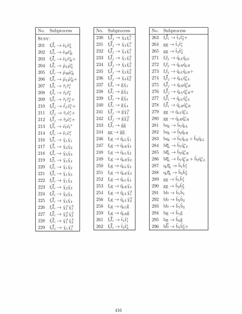
No. Subprocess

Susy:

201 fif i → eLe∗L202 fif i → eRe∗R203 fif i → eLe∗R+

204 fif i → µLµ∗L

205 fif i → µRµ∗R

206 fif i → µLµ∗R+

207 fif i → τ1τ∗1

208 fif i → τ2τ∗2

209 fif i → τ1τ∗2 +

210 fifj → ℓLν∗ℓ+

211 fifj → τ1ν∗τ+

212 fifj → τ2ν∗τ+

213 fif i → νℓνℓ∗

214 fif i → ντ ν∗τ

216 fif i → χ1χ1

217 fif i → χ2χ2

218 fif i → χ3χ3

219 fif i → χ4χ4

220 fif i → χ1χ2

221 fif i → χ1χ3

222 fif i → χ1χ4

223 fif i → χ2χ3

224 fif i → χ2χ4

225 fif i → χ3χ4

226 fif i → χ±1 χ

∓1

227 fif i → χ±2 χ

∓2

228 fif i → χ±1 χ

∓2

229 fifj → χ1χ±1

No. Subprocess

230 fifj → χ2χ±1

231 fifj → χ3χ±1

232 fifj → χ4χ±1

233 fifj → χ1χ±2

234 fifj → χ2χ±2

235 fifj → χ3χ±2

236 fifj → χ4χ±2

237 fif i → gχ1

238 fif i → gχ2

239 fif i → gχ3

240 fif i → gχ4

241 fifj → gχ±1

242 fifj → gχ±2

243 fif i → gg

244 gg → gg

246 fig → qiLχ1

247 fig → qiRχ1

248 fig → qiLχ2

249 fig → qiRχ2

250 fig → qiLχ3

251 fig → qiRχ3

252 fig → qiLχ4

253 fig → qiRχ4

254 fig → qjLχ±1

256 fig → qjLχ±2

258 fig → qiLg

259 fig → qiRg

261 fif i → t1t∗1

262 fif i → t2t∗2

No. Subprocess

263 fif i → t1t∗2+

264 gg → t1t∗1

265 gg → t2t∗2

271 fifj → qiLqjL

272 fifj → qiRqjR

273 fifj → qiLqjR+

274 fifj → qiLq∗j L

275 fifj → qiRq∗jR

276 fifj → qiLq∗jR+

277 fif i → qjLq∗j L

278 fif i → qjRq∗jR

279 gg → qiLq∗i L

280 gg → qiRq∗i R

281 bqi → b1qiL

282 bqi → b2qiR

283 bqi → b1qiR + b2qiL

284 bqi → b1q∗i L

285 bqi → b2q∗i R

286 bqi → b1q∗i R + b2q

∗i L

287 qiqi → b1b∗1

288 qiqi → b2b∗2

289 gg → b1b∗1

290 gg → b2b∗2

291 bb → b1b1

292 bb → b2b2

293 bb → b1b2

294 bg → b1g

295 bg → b2g

296 bb → b1b∗2+

416

Index of Subprograms and Common Block Variables

This index is not intended to be complete, but gives the page where the main descriptionbegins of a subroutine, function, block data, common block, variable or array. For commonblock variables also the name of the common block is given. When some components ofan array are described in a separate place, a special reference (indented with respect tothe main one) is given for these components.

AQCDUP in HEPEUP 224AQEDUP in HEPEUP 224BRAT in PYDAT3 363CHAF in PYDAT4 364CKIN in PYSUBS 167COEF in PYINT2 250EBMUP in HEPRUP 217HEPEUP common block 223HEPEVT common block 63HEPRUP common block 217ICOL in PYINT2 251ICOLUP in HEPEUP 226IDBMUP in HEPRUP 217IDPRUP in HEPEUP 223IDUP in HEPEUP 224IDWTUP in HEPRUP 218IMSS in PYMSSM 199ISET in PYINT2 250ISIG in PYINT3 251ISTUP in HEPEUP 224K in PYJETS 57KCHG in PYDAT2 358KFDP in PYDAT3 363KFIN in PYSUBS 167KFPR in PYINT2 250LPRUP in HEPRUP 222MAXNUP in HEPEUP 223MAXPUP in HEPRUP 217MDCY in PYDAT3 360MDME in PYDAT3 360MINT in PYINT1 242MOTHUP in HEPEUP 225MRPY in PYDATR 46MSEL in PYSUBS 165MSTI in PYPARS 203MSTJ in PYDAT1, main 345MSTJ(38) - MSTJ(50) 281MSTJ(101) - MSTJ(121) 78

MSTP in PYPARS, main 171MSTP(22) 285MSTP(61) - MSTP(71) 285MSTP(81) - MSTP(94) 300MSTP(131) - MSTP(134) 303

MSTU in PYDAT1, main 342MSTU(1) and some more 375MSTU(41) - MSTU(63) 393MSTU(101) - MSTU(118) 195MSTU(161) - MSTU(162) 394

MSUB in PYSUBS 166MWID in PYINT4 251N in PYJETS 57NGEN in PYINT5 253NPRUP in HEPRUP 222NUP in HEPEUP 223P in PYJETS 58PARF in PYDAT2 358PARI in PYPARS 205PARJ in PYDAT1, main 350PARJ(80) - PARJ(90) 284PARJ(121) - PARJ(171) 81PARJ(180) - PARJ(195) 198

PARP in PYPARS, main 190PARP(61) - PARP(72) 287PARP(81) - PARP(100) 304PARP(131) 305

PARU in PYDAT1, main 345PARU(41) - PARU(63) 394PARU(101) - PARU(195) 195

PDFGUP in HEPRUP 217PDFSUP in HEPRUP 217PMAS in PYDAT2 358PROC in PYINT6 253PUP in HEPEUP 227PY1ENT subroutine 337PY2ENT subroutine 337PY3ENT subroutine 338PY4ENT subroutine 338PY2FRM subroutine 236PY4FRM subroutine 236PY6FRM subroutine 237PY4JET subroutine 238PYADSH function 280PYALEM function 194PYALPS function 194PYANGL function 341PYBINS common block 398

417

PYBOEI subroutine 340PYBOOK subroutine 396PYCELL subroutine 387PYCHGE function 341PYCLUS subroutine 386PYCOMP function 341PYDAT1 common block 342PYDAT2 common block 358PYDAT3 common block 360PYDAT4 common block 364PYDATA block data 242PYDATR common block 46PYDCYK subroutine 356PYDECY subroutine 340PYDIFF subroutine 240PYDISG subroutine 240PYDOCU subroutine 240PYDUMP subroutine 397PYEDIT subroutine 370PYEEVT subroutine 76PYERRM subroutine 341PYEVNT subroutine 162PYEVWT subroutine 210PYEXEC subroutine 340PYFACT subroutine 396PYFILL subroutine 396PYFOWO subroutine 389PYFRAM subroutine 163PYGAGA subroutine 240PYGAMM function 241PYGANO function 241PYGBEH function 241PYGDIR function 241PYGGAM function 241PYGIVE subroutine 339PYGVMD function 241PYHEPC subroutine 64PYHFTH function 241PYHIST subroutine 397PYI3AU subroutine 242PYINBM subroutine 239PYINDF subroutine 340PYINIT subroutine 160PYINKI subroutine 240PYINPR subroutine 240PYINRE subroutine 239PYINT1 common block 242PYINT2 common block 250PYINT3 common block 251PYINT4 common block 251PYINT5 common block 253

PYINT6 common block 253PYINT7 common block 253PYINT8 common block 254PYINT9 common block 254PYJETS common block 57PYJMAS subroutine 388PYJOIN subroutine 338PYK function 373PYKCUT subroutine 164PYKFDI subroutine 340PYKFIN subroutine 356PYKLIM subroutine 241PYKMAP subroutine 241PYLIST subroutine 372PYLOGO subroutine 341PYMAEL function 280PYMASS function 341PYMAXI subroutine 240PYMEMX subroutine 280PYMEWT subroutine 280PYMRUN function 194PYMSRV common block 202PYMSSM common block 199PYMULT subroutine 240PYNAME subroutine 341PYNMES subroutine 356PYNULL subroutine 397PYONIA subroutine 77PYOPER subroutine 396PYOFSH subroutine 241PYP function 374PYPARS common block 171, 203PYPDEL subroutine 241PYPDFL subroutine 241PYPDFU subroutine 241PYPDGA subroutine 241PYPDPI subroutine 241PYPDPR subroutine 241PYPILE subroutine 240PYPLOT subroutine 397PYPREP subroutine 340PYPTDI subroutine 340PYQQBH subroutine 242PYR function 45PYRGET subroutine 46PYRSET subroutine 46PYRADK subroutine 77PYRAND subroutine 240PYRECO subroutine 242PYREMN subroutine 240PYRESD subroutine 240

418

PYROBO subroutine 370PYSAVE subroutine 240PYSCAT subroutine 240PYSHOW subroutine 279PYSIGH subroutine 241PYSPEN function 242PYSPHE subroutine 385PYSPLI subroutine 241PYSSMT common block 201PYSSPA subroutine 280PYSTAT subroutine 162PYSTRF subroutine 340PYSUBS common block 165PYTABU subroutine 389PYTAUD subroutine 341PYTEST subroutine 25PYTHRU subroutine 386PYTIME subroutine 341PYUPDA subroutine 357PYWAUX subroutine 242PYWIDT subroutine 241PYX3JT subroutine 77PYX4JT subroutine 77PYXDIF subroutine 77PYXJET subroutine 77PYXKFL subroutine 77PYXTEE subroutine 77PYXTOT subroutine 240PYZDIS subroutine 340RMSS in PYMSSM 200RRPY in PYDATR 47RVLAM in PYMSRV 202RVLAMB in PYMSRV 202RVLAMP in PYMSRV 202SCALUP in HEPEUP 223

SFMIX in PYSSMT 202SIGH in PYINT3 251SIGT in PYINT7 254SMW in PYSSMT 202SMZ in PYSSMT 202SPINUP in HEPEUP 227UPEVNT subroutine 223UPINIT subroutine 216V in PYJETS 58VCKM in PYDAT2 360VINT in PYINT1 245VTIMUP in HEPEUP 227VXPANH in PYINT9 254VXPANL in PYINT9 254VXPDGM in PYINT9 254VXPVMD in PYINT9 254WIDS in PYINT4 252XERRUP in HEPRUP 222XMAXUP in HEPRUP 222XPANH in PYINT8 254XPANL in PYINT8 254XPBEH in PYINT8 254XPDIR in PYINT8 254XPVMD in PYINT8 254XSEC in PYINT5 253XSECUP in HEPRUP 222XSFX in PYINT3 251XWGTUP in HEPEUP 223UMIX in PYSSMT 202UMIXI in PYSSMT 202VMIX in PYSSMT 202VMIXI in PYSSMT 202ZMIX in PYSSMT 201ZMIXI in PYSSMT 202

419