THE GENERAL COMMON EXACT SOLUTIONS OF COUPLED LINEAR MATRIX AND MATRIX DIFFERENTIAL EQUATIONS
13
The 2nd International Conference on Research and Education in Mathematics (ICREM 2) – 2005 75 THE GENERAL COMMON EXACT SOLUTIONS OF COUPLED LINEAR MATRIX AND MATRIX DIFFERENTIAL EQUATIONS Adem Kilicman and Zeyad Abdel Aziz Al Zhour Department of Mathematics and Institute for Mathematical Research University Putra Malaysia (UPM), Malaysia 43400 , Serdang , Selangor , Darul Ehsan , Malaysia. Email: [email protected] , [email protected] Abstract: System of matrix and matrix differential equations play an important role in system theory, control theory, stability theory of differential equations communication systems and many other subjects. In this paper, based on the connection between the Kronecker products and Vector- operation, we present the general common exact solutions of coupled linear matrix equations E YB B XA A = + 2 1 2 1 , F YD D XC C = + 2 1 2 1 and coupled linear matrix differential equations D t CY B t AX t X ) ( ) ( ) ( ' + = , B t AY D t CX t Y ) ( ) ( ) ( ' + = . Several special cases of these systems are also considered; we prove the existence and uniqueness solution of each case, which includes the well-known coupled Sylvester matrix equations, as a special case. Keywords: Kronecker product (sum), Vector – operator, Matrix equations, Matrix differential equations, Sylvester Equation, Exponential matrix, , Cosh . ) ( A Sinh ) ( A 1. Introduction There are many books and papers, e.g. [3, 4, 5, 7, 8] devoted to the analysis, existence, uniqueness and representation of the solution and also to the numerical algorithm to solve various types of matrix equations. Most of the existing results, however, are connected with particular systems of such matrix and matrix differential equations. Systems of matrix and matrix differential equations have been widely used in stability theory of differential equations, in the perturbation analysis of linear and non-linear matrix equations and other fields of pure and applied mathematics and also recently in the context of the analysis and numerical simulation of descriptor systems. In matrix theory, the Kronecker product and vector operator affirming their capability of solving some matrix equations and matrix differential equations. In the recent paper, we use the Kronecker products of matrices and vector operator to solve the coupled matrix and matrix differential equations. This method is easy to understand, simple to use and accurate. Furthermore, we discuss several special cases of these systems, and then we prove the existence and uniqueness of the solution of each case. The need to compute the e , cosh( and sinh( are due its appearance in the solutions of coupled matrix and matrix differential equations. A ) A ) A We use the following notations: • the derivative of matrix function and − ) ( ' t X ) (t X − I the identity matrix..
Transcript of THE GENERAL COMMON EXACT SOLUTIONS OF COUPLED LINEAR MATRIX AND MATRIX DIFFERENTIAL EQUATIONS

The 2nd International Conference on Research and Education in Mathematics (ICREM 2) – 2005 75
THE GENERAL COMMON EXACT SOLUTIONS OF COUPLED LINEAR MATRIX AND MATRIX DIFFERENTIAL EQUATIONS
Adem Kilicman and Zeyad Abdel Aziz Al Zhour
Department of Mathematics and Institute for Mathematical Research University Putra Malaysia (UPM), Malaysia
43400 , Serdang , Selangor , Darul Ehsan , Malaysia. Email: [email protected] , [email protected]
Abstract: System of matrix and matrix differential equations play an important role in system theory, control theory, stability theory of differential equations communication systems and many other subjects. In this paper, based on the connection between the Kronecker products and Vector- operation, we present the general common exact solutions of coupled linear matrix equations
EYBBXAA =+ 2121 ,
FYDDXCC =+ 2121 and coupled linear matrix differential equations
DtCYBtAXtX )()()(' += ,
BtAYDtCXtY )()()(' += . Several special cases of these systems are also considered; we prove the existence and uniqueness solution of each case, which includes the well-known coupled Sylvester matrix equations, as a special case.
Keywords: Kronecker product (sum), Vector – operator, Matrix equations, Matrix differential equations, Sylvester Equation, Exponential matrix, , Cosh . )(ASinh )(A
1. Introduction There are many books and papers, e.g. [3, 4, 5, 7, 8] devoted to the analysis, existence, uniqueness and representation of the solution and also to the numerical algorithm to solve various types of matrix equations. Most of the existing results, however, are connected with particular systems of such matrix and matrix differential equations. Systems of matrix and matrix differential equations have been widely used in stability theory of differential equations, in the perturbation analysis of linear and non-linear matrix equations and other fields of pure and applied mathematics and also recently in the context of the analysis and numerical simulation of descriptor systems.
In matrix theory, the Kronecker product and vector operator affirming their capability
of solving some matrix equations and matrix differential equations.
In the recent paper, we use the Kronecker products of matrices and vector operator to solve the coupled matrix and matrix differential equations. This method is easy to understand, simple to use and accurate. Furthermore, we discuss several special cases of these systems, and then we prove the existence and uniqueness of the solution of each case. The need to compute thee , cosh( and sinh( are due its appearance in the solutions of coupled matrix and matrix differential equations.
A )A )A
We use the following notations:
• the derivative of matrix function and −)(' tX )(tX −I the identity matrix..

The 2nd International Conference on Research and Education in Mathematics (ICREM 2) – 2005 76
• the set of all m matrices over −nmM , n× M and when m = n , we write instead of .
nM
nmM ,
• , , Vec , TA 1−A )(A )(Aσ , tr , det( , )(A )A −)(Arank the transpose, inverse of vector operator, eigenvalues, trace, determinant and rank of matrix A , respectively.
2. Some Notations and Preliminary Results
Consider matrices ( ) mij MaA ∈= , ( ) nkl MbB ∈= . Let ( ) mnijij MBaBA ∈=⊗ , BA⊕
be the Kronecker product and Kronecker sum of mnM∈nm BIIA ⊗+⊗= )()( A and B ,
respectively, and VecA the ( )1,1 2,,
mT
mmm Maa ∈L22212 ,,,, maaa L1 ,,m L2111 ,,, aaa= L
vector – operator of . The Kronecker product and vector-operator are related by A
(see, eg., [1,5,7, 8])
Vec (1) VecXABAXB T )()( ⊗=
for any matrices , andnmMA ,∈ qpMB ,∈ pnMX ,∈ .
For any compatibly matrices A , B , and , we shall make frequent use the following properties of the Kronecker product, Kronecker sum and vector – operator that will be useful in our investigation of the solution of matrix and matrix differential equations:
C D
(i) BDACDCBA ⊗=⊗⊗ ))(( (2)
(ii) (3) BABA eee ⊗=⊕ )(
(iii) If { miA i ,...,2,1:)( }== λσ are the eigenvalues of and A { }njB j ,...,2,1:)( == µσ are the eigenvalues of B . Then
(i) { }njmiBA ji ,...,2,1,,...,2,1:)( ===⊗ µλσ . (4)
(ii). { }njmiBA ji ,...,2,1,,...,2,1:)( ==+=⊕ µλσ . (5)
(iv) If is analytic function on the region containing the eigenvalues of f A .Then
and )()( AfIAIf ⊗=⊗ IAfIAf ⊗=⊗ )()( . (6)
Some special cases include (iv):
(i) For , we have AeAf =)(
e and e . (7) IAeIA ⊗=⊗ AeIAI ⊗=⊗
(ii) For , we have )sinh()( AAf =
IAIA ⊗=⊗ )sinh()sinh( and sinh( )sinh() AIAI ⊗=⊗ . (8)
(iii) For , we have )cosh()( AAf =
IAIA ⊗=⊗ )cosh()cosh( and )cosh()cosh( AIAI ⊗=⊗ . (9)
Here, ∑∞
=
=
0 !k
kA
kAe , { }AA eeA −−=
21)sinh( and { }AA eeA −+=
21)cosh( . (10)

The 2nd International Conference on Research and Education in Mathematics (ICREM 2) – 2005 77
For any matrix mMA∈ , the spectral representation of and e assures that: Ae At
e and (11) ∑=
=n
i
iTii
A eyx0
λ ∑=
=n
i
tiTii
At ee yx0
λ
where{ }nλλ ,,1 L are the eigenvalues of A ,{ }nxx ,,1 L be the eigenvectors corresponding to the eigenvalues { }nλλ ,,L1 and { be the eigenvectors of matrix . }nyy ,,1 L
TA
3. Coupled Linear Matrix Differential Equations
In this section we use the Kronecker product and −Vec notation to solve the coupled linear matrix differential equations:
, Y (12) DtCYBtAXtX )()()(' += BtAYDtCXt )()()(' +=
Here, , CAAC = DBBD = , EtX =)( 0 , Y Ft =)( 0 , nd are given constant matrices and ,
EDCBA ,,,, a nMF ∈)(tX nMtY ∈)( are the unknown matrices to be solved.
First, let us introduce the simplest forms of linear matrix differential equations:
(i) , (13) ) CtX =)( 0()(' tAXtX =
Here, A and are given constant matrices. The unique solution of the matrix differential equation defined in (13) is given by
nMC ∈
(14) CtX ttAe )0()( −=
(ii) , BtXtAXtX )()()(' += CtX =)( 0 (15)
Here, , and are given constant matrices. If we use the notation, then we get,
nMA∈−
mMB∈ mnMC ,∈Vec
Vec )( )= . (16) =))(( ' tX () tVecXIBAI nT
m ⊗+⊗ ()( tVecXABT ⊕
Let , , )()( '' tVecXtx = ABH T ⊕= )()( tVecXtx = and VecCc = . Then (16) can be written as follows:
, )(.)(' txHtx = ctx =)( 0 (17)
The unique solution of the matrix differential equation defined in (15) is given by
. (18) )()( 00 ..)( ttBttA eCetX −−=
3.1. Theorem: The general exact solution of coupled linear matrix differential equations defined in (12) is given by
{ }VecFttCDVecEttCDtVecX TTttABTe )])([sinh()])([cosh()( 00))(( 0 −⊗+−⊗= −⊗
{ }VecFttCDVecEttCDtVecY TTttABTe )])([cosh()])([sinh()( 00))(( 0 −⊗+−⊗= −⊗
; (19)
(20)
Proof: If we use the Vec notation, we have the following system: −(.)
. (21)
⊗⊗⊗⊗
=
)()(
)()(
'
'
tVecYtVecX
ABCDCDAB
tVecYtVecX
TT
TT
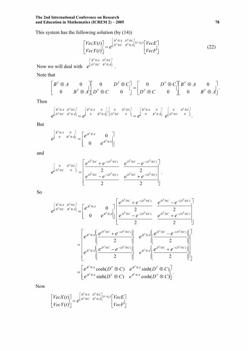
The 2nd International Conference on Research and Education in Mathematics (ICREM 2) – 2005 78
This system has the following solution (by (14))
(22)
=
−
⊗⊗⊗⊗
VecFVecE
tVecYtVecX tt
ABCDCDAB
TT
TT
e)( 0
)()(
Now we will deal with e .
⊗⊗⊗⊗
ABCDCDAB
TT
TT
Note that
⊗⊗
⊗⊗
00
00
CDCD
ABAB
T
T
T
T
⊗⊗
⊗⊗
=AB
ABCD
CDT
T
T
T
00
00
.
Then
⊗⊗⊗⊗
ABCDCDAB
TT
TT
e
⊗⊗
+
⊗⊗
= 00
00
CDCD
ABAB
T
T
T
T
e
⊗⊗
= ABAB
T
T
e 00
e .
⊗⊗0
0CD
CDT
T
But
=
⊗
⊗
⊗⊗
AB
ABAB
AB
T
TT
T
eee
000
0
and
+−
−+
=⊗−⊗⊗−⊗
⊗−⊗⊗−⊗
⊗⊗
22
22)()(
)()(
00
CDCDCDCD
CDCDCDCD
CDCD
TTTT
TTTT
eeee
eeeeT
T
e .
So
⊗⊗⊗⊗
ABCDCDAB
TT
TT
e
=
⊗
⊗
AB
AB
T
T
ee
00
+−
−+
⊗−⊗⊗−⊗
⊗−⊗⊗−⊗
22
22)()(
)()(
CDCDCDCD
CDCDCDCD
TTTT
TTTT
eeee
eeee
+
−
−
+
⊗−⊗⊗
⊗−⊗⊗
⊗−⊗⊗
⊗−⊗⊗
22
22)()(
)()(
CDCDAB
CDCDAB
CDCDAB
CDCDAB
TTT
TTT
TTT
TTT
eeeee
eeeeee
e=
= .
⊗⊗⊗⊗
⊗⊗
⊗⊗
)cosh()sinh()sinh()cosh(
CDeCDCDCD
TABTAB
TABTAB
TT
TT
eee
Now
=
−
⊗⊗⊗⊗
VecFVecE
tVecYtVecX tt
ABCDCDAB
TT
TT
e)( 0
)()(

The 2nd International Conference on Research and Education in Mathematics (ICREM 2) – 2005 79
−⊗−⊗−⊗−⊗=
−⊗−⊗
−⊗−⊗
))(cosh())(sinh())(sinh())(cosh(
0))((
0))((
0))((
0))((
00
00
ttCDettCDttCDttCD
TttABTttAB
TttABTttAB
TT
TT
eee
VecFVecE
(23)
This gives the following general solution:
{ }VecFttCDVecEttCDtVecX TTttABTe )])([sinh()])([cosh()( 00))(( 0 −⊗+−⊗= −⊗ ,
and
{ }VecFttCDVecEttCDtVecY TTttABTe )])([cosh()])([sinh()( 00))(( 0 −⊗+−⊗= −⊗ .
Now we discuss some special cases of Theorem (3.1), as in the following corollaries:
3.2. Corollary: Consider the coupled matrix differential equations:
DtYBtXtX )()()(' += , Y (24) BtYDtXt )()()(' +=
Here, DBBD = , YEX =)0( , F=)0( a , and ndEDB , nMF ∈ . Then the general exact solution of (24) is given by
{ } BteDtFDtEtX )sinh()cosh()( += , { } BteDtFDtEt )cosh()sinh()( +=Y (25)
Proof: Set and t in (19) and (20), we have nICA == 00 =
{ }VecFtIDVecEtIDtVecX nT
nTtIB n
Te ])[sinh(])[cosh()( )( ⊗+⊗= ⊗
= { }VecFItDVecEItDI nT
nT
ntBTe ][sinh][cosh)( ⊗+⊗⊗
{ }VecEItD nTtBTe ⊗cosh= { }VecFItD n
TtBTe ⊗+ sinh
{ }VecEIDt nTBte ⊗])[cosh(= { }VecFIDt n
TBte ⊗+ ])[sinh( BteDtEtX )cosh()( = BteDtF )sinh(+ { } BteDtFDtE )sinh()cosh( += .
Similarly, Y . { } BteDtFDtEt )cosh()sinh()( +=
3.3. Corollary: Consider the coupled matrix differential equations:
)()()(' tCYtAXtX += , Y (26) )()()(' tAYtCXt +=
Here, , YCAAC = EX =)0( , F=)0( a , and ndECA , nMF ∈ . Then the general exact solution of (26) is given by
{ }FCtECttX Ate ).sinh().cosh()( += , { }FCtECtt Ate ).cosh().sinh()( +=Y (27)
Proof: By taking nIBD == and 00 =t in (19) and (20), we have
{ }VecFtCIVecEtCItVecX nntAIne ])[sinh(])[cosh()( )( ⊗+⊗= ⊗
= { }VecFCtIVecECtII nnAt
n e )]sinh([)]cosh([ ⊗+⊗⊗
= +⊗⊗ VecECtII nAt
n e ))cosh()(( VecFCtII nAt
n e ))sinh()(( ⊗⊗
= +⊗ VecECtI Atn e )]cosh([ VecFCtI At
n e )]sinh([ ⊗
= +)).cosh(( ECtVec Ate )).sinh(( FCtVec Ate

The 2nd International Conference on Research and Education in Mathematics (ICREM 2) – 2005 80
= +ECtVec Ate ).cosh(( )).sinh( FCtAte
{ }FCtECttX Ate ).sinh().cosh()( +=
Similarly, Y . { }FCtECtt Ate ).cosh().sinh()( +=
3.4. Corollary: Consider the coupled matrix differential equations:
)()()(' tYtXtX += , Y (28) )()()(' tYtXt +=
Here, , Y and EX =)0( F=)0( E and nMF ∈ . Then the general exact solution of (28) is given by
{ })sinh()cosh()( tFtEtX te += , { })sinh()sinh()( tFtEt te +=Y (29)
Proof: Set in (25), we have nIBD ==
{ } tInetFtEtX )sinh()cosh()( += { })sinh()cosh( tFtE += nt Ie
= { })sinh()cosh( tFtEte +
Similarly, { })sinh()sinh()( tFtEt te +=Y .
3.5. Corollary: Consider the coupled matrix differential equations:
)()()(' tYBtXtX += , Y (30) BtYtXt )()()(' +=
Here, , Y and andEX =)0( F=)0( EB, nMF ∈ . Then the general exact solution of (30) is given by
{ } BtetFtEtX )sinh()cosh()( += , { } BtetFtEt )cosh()sinh()( +=Y (31)
Proof: Follows immediately by setting nID = in (25).
3.6. Corollary: Consider coupled matrix differential equations:
DtYtXtX )()()(' += , Y (32) )()()(' tYDtXt +=
Here, Y and andEX =)0( , F=)0( ED, nMF ∈ . Then the general exact solution of (32) is given by
{ })sinh()cosh()( DtFDtEtX te += , { })cosh()sinh()( DtFDtEet t +=Y (33)
Proof: Follows immediately by setting nIB = in (25).
4. Coupled Linear Matrix Equations
In this section we use the Kronecker product and −Vec notation to solve and prove the existence and uniqueness solution of the coupled linear matrix equations:
EYBBXAA =+ 2121 , C FYDDXC =+ 2121 (34)
Here,C , C , , , are given constant matrices and
1111 CDD = 2222 CDD = 1111 ,,, DCBA EDCBA ,,,, 2222 nMF ∈X , are the unknown matrices . nMY ∈
Knowledge of the Kronecker product and its applications facilitates our analysis of matrix equations, since the Kronecker product can be used to give a convenient representation for linear matrix equations.

The 2nd International Conference on Research and Education in Mathematics (ICREM 2) – 2005 81
The simplest matrix equation is:
CAXB = (35)
Here, , , C are given constant matrices and is the unknown matrix to be solved . The matrix equation in (35) can be written by using the Vec notation as:
nMA∈ mMB∈ mnM ,∈ mnMX ,∈−(.)
VecCVecXABT =⊗ )( (36)
This system has a unique solution if and only if is invertible if and only if and )( ABT ⊗ AB are invertible.
Now if is not invertible, we consider the rank of the augmented matrix: )( ABT ⊗
]:[ VecCABT ⊗VecXABT =⊗ )(
. If this rank is equal to the rank of the matrix ( , then the system has a solution; otherwise the system has no solution.
)ABT ⊗VecC
The matrix equation in (35) can be generalized as:
∑=
=p
iii CXBA
1 (37)
Here, , ni MA ∈ mi MB ∈ ),...,2,1( pi = and mnMC ,∈ are given constant matrices. Similarly, the general matrix equation in (37) can be written by using the −(.)Vec notation as:
VecCVecXABp
ii
Ti =⊗∑
=1)( (38)
The unique solution is obtained if and only if is invertible, otherwise we
consider a rank argument.
∑=
⊗p
ii
Ti AB
1
)(
An important particular case of (37) is the Sylvester matrix equation:
CXBAX =+ (39)
Here, , and C are given constant matrices, in which the Kronecker sum, frequently turns up. By using the
nMA∈ mMB∈ mnM ,∈−(.)Vec notation in (39), we have
VecCVecXABT =⊕ )( (40)
The system in (40) has a unique solution if and only if is invertible, that is if and only if non of the eigenvalues of ( is zero. So Sylvester matrix equation has a unique solution if and only if and (
)( ABT ⊕)ABT ⊕)BA − have no common eigenvalue if and only if
φσσ =−∩ )()( BA . If on the other hand and A )( B− have an eigenvalue in common, then the existence of the solution depends on the rank of the augmented matrix: [ . If the rank of this matrix is equal to the rank of the matrix , then the solutions exist, otherwise they do not.
]:VecCABT ⊕)( ABT ⊕
4.1. Lemma: Let nMA∈ , and mMB∈ mnMC ,∈ and all eigenvalues of and ( are negatives. Then the unique solution of the matrix equation defined in (39) is
A )B−

The 2nd International Conference on Research and Education in Mathematics (ICREM 2) – 2005 82
∫∞
−=0
... dtCX BtAt ee (41)
As a special case of the matrix equation in (39), set AB −= and , then the following matrix equation:
0=C
XAAX = (42)
has an infinity solutions and the solutions are all matrices which commute with A , for example, are solutions of the matrix equation defined in (37). ,....2,1: == kAX k
Another important particular case of the matrix equation defined in (37) is the following one:
XXAAX α=− (43)
Here, and , which has a non-trivial solution if and only if nMA∈ mMB∈
{ })(:) AA i σλα ∈∈ ( ATσ ⊕− ji λλ −= . Hence, the matrix equation defined in (43) has
a non-trivial solution if and only if ji λλα −= for some ji , .
The previous matrix equations have been considered in several references ( see ,e.g., [5, 8, 10] ).
4.2. Lemma: Let and such thatCBA ,, mMD∈ CAAC = . Then T is invertible if
and only if is invertible.
=
DCBA
CBAD −
Proof: First we prove the lemma for the case when is invertible. It easy to verify that A
− −
n
n
ICAI
1
0
DCBA
=
EBA
0 (44)
Here, is called the Schur complement of in BCADE 1−−= A T . Note that
− −
n
n
ICAI
1
0
EBA
0
is invertible with inverse and T is invertible if and
only if is invertible . Then is invertible if and only if
−
n
n
ICAI
1
0
EB
=
DCBA
A0
E is invertible.
In fact, if E is invertible, then is the inverse of matrix .
−−
−−−
1
111
0 EBEAA
EBA
0
Conversely, suppose is invertible with
as its inverse; then
EBA
0
SRQP
EBA
0
SRQP
=
SRQP
EBA
0
=
n
n
II0
0.
So

The 2nd International Conference on Research and Education in Mathematics (ICREM 2) – 2005 83
++ESER
BSAQBRAP
++
=SERBRAQEPBPA
=
n
n
II0
0.
Since and 0=RA A is invertible, then 0=R , nIPAAP == and , so nISEES == PA =−1 and . We conclude that S=−1E T is invertible if and only if
BCAD 1−− is invertible if and only if is invertible (Since ).
BACAAD 1−− CBADBCAAAD −=−= −1
CAAC =
Finally, the general case (when A is not necessarily invertible) follows by the fact that the set of invertible matrices is dense in (see e.g., [9]). nM
4.3. Lemma: Let and such thatCBA ,, mMD∈ DCCD = . Then T is invertible if
and only if is invertible.
=
DCBA
BCAD −
Proof: When is invertible. It easy to verify that D
DCBA
− −
n
n
ICDI
1
0
=
DBF
0 (45)
Here, is the Schur complement of in CBDAF 1−−= D T .
Proof: Follows by the similar argument of the proof in Lemma (4.2).
4.4. Theorem: The coupled linear matrix equations defined in (34) has a unique solution if and only if is invertible. 11221122 CBCBDADA TTTT ⊗−⊗
Proof: By using the Vec notation, we get −
VecEVecYBBVecXAA TT =⊗+⊗ )()( 1212 (46)
VecFVecYDDVecXCC TT =⊗+⊗ )()( 1212 (47)
This system is equivalent to the following one:
=
⊗⊗⊗⊗
VecFVecE
VecYVecX
DDCCBBAA
TT
TT
1212
1212 (48)
The system defined in (48) has a unique solution if and only if is
invertible if and only if is invertible if and only if is invertible (By Lemma (4.3))
⊗⊗⊗⊗
1212
1212
DDCCBBAA
TT
TT
)1C⊗)(())(( 2121212 CBBDDAA TTTT ⊗−⊗⊗
112 CBT ⊗21122 CBDADA TTT −⊗
Now we discuss some special cases of Theorem (4.4)
4.5. Corollary: Let are given constant matrices such thatECBA ,,, , nMF ∈ BAAB = . Then the coupled linear matrix equations
EBYCAXC =+ , FAYCBXC =+ (49)
has a unique solution if and only if ( is invertible. )() 222 BACT −⊗

The 2nd International Conference on Research and Education in Mathematics (ICREM 2) – 2005 84
Proof: Follows immediately by setting =A =1A 1D , =B =1B and 1C=C 222 BCA == 2D= in Theorem (4.4).
4.6. Corollary: Let ndEDCBA ,,,, a nMF ∈ be given constant matrices such that CD DC= . Then the coupled linear matrix equations
EBYAX =+ , CX FDY =+ (50)
has a unique solution if and only if BCAD − is invertible.
Proof: Set , , C , 1AA = 1BB = 1C= 1DD = and nI 2222 DCBA ==== in Theorem
(4.4).Then the system defined in (50) has a unique solution if and only if BCIADI nn ⊗−⊗ is invertible if and only if )( BCADI n −⊗ is invertible if and only if is invertible. BC−AD
4.7. Corollary: Let ndEDCBA ,,,, a nMF ∈ be given constant matrices such that CD DC= . Then the coupled linear matrix equations
EYBXA =+ , FYDXC =+ (51)
has a unique solution if and only if CBDA − is invertible.
Proof: Set , , C , 2AA = 2BB = 3C= 2DD = and nI 1111 DCBA ==== in Theorem
(4.4). Then the system defined in (51) has a unique solution if and only if is invertible if and only if ( is invertible if and
only if is invertible. n
TTn
TT ICBIDA ⊗−⊗CBDA −
nT ICBDA ⊗− )
4.8. Corollary: Let ndEDCBA ,,,, a nMF ∈ be given constant matrices. Then the coupled Sylvester linear matrix equations
EYBAX =+ , CX FYD =+ (52)
has a unique solution if and only if is invertible if and only if the
matrix is non-singular, in this case, the unique solution is given by
CBAD TT ⊗−⊗
⊗⊗⊗⊗
=IDCIIBAI
H T
T
=
−
VecFVecE
HVecYVecX 1 (53)
Proof: Follows immediately by setting 1AA = , 2BB = , 1CC = , 2DD = and
nI 1212 DCBA ==== in Theorem ( 4.4).
4.9. Corollary: Let ndEDCBA ,,,, a nMF ∈ be given constant matrices. Then the coupled linear matrix equations
EBYXA =+ , FDYXC =+ (54)
has a unique solution if and only if is invertible . BCDA TT ⊗−⊗
Proof: Follows immediately by setting 2AA = , 1BB = , 2CC = , 1DD = and
nI 2121 DCBA ==== in Theorem ( 4.4).

The 2nd International Conference on Research and Education in Mathematics (ICREM 2) – 2005 85
4.10. Theorem: Let and ECBA ,,, nMF ∈ be given constant matrices such that BAAB = . Then the coupled linear matrix equations
EBYCAXC =+ , FAYCBXC =+ (55)
has a unique solution if and only if C , BA + and BA − are invertible matrices, in this case, the unique solution is given by
{ 111 )()()()(21 −−− −−+++= CFEBAFEBAX } (56)
{ 111 )()()()(21 −−− −−−++= CFEBAFEBAY } (57)
Proof: By using the Vec notation, the system becomes −
VecEVecYBCVecXAC TT =⊗+⊗ )()(
VecFVecYACVecXBC TT =⊗+⊗ )()(
This system is equivalent to the following one:
=
⊗⊗⊗⊗
VecFVecE
VecYVecX
ACBCBCAC
TT
TT
(58)
The system defined in (58) has a unique solution if and only if is
invertible. One can easily show that:
⊗⊗⊗⊗
ACBCBCAC
TT
TT
⊗⊗⊗⊗
ACBCBCAC
TT
TTT
T
T
UBAC
BACU
−⊗+⊗
=)(0
0)( (59)
Here, U =
−
nn
nn
IIII
21 is a unitary matrix. So
⊗⊗⊗⊗
ACBCBCAC
TT
TT
)( BACT +⊗
is invertible if and only if if and only if
and C are invertible matrices if and only if ,
−⊗+⊗
)(00)(
BACBAC
T
T
C)( BAT −⊗ BA + and BA − are invertible matrices. Note that
1−
⊗⊗⊗⊗
ACBCBCAC
TT
TT1
11
)(00)(
)( −
−
−
−⊗+⊗
= UBAC
BACU
T
TT
TT
T
UBAC
BACU
−⊗+⊗
=−−
−−
11
11
)()(00)()(
− nn
nn
IIII
21
=
−⊗+⊗
−−
−−
11
11
)()(00)()(
BACBAC
T
T
−
nn
nn
IIII
{ } { }{ } {
−++⊗−−+⊗−−+⊗−++⊗
=−−−−−−
−−−−−−
111111
111111
)()()()()()()()()()()()(
21
BABACBABACBABACBABAC
TT
TT
} (60)

The 2nd International Conference on Research and Education in Mathematics (ICREM 2) – 2005 86
Then
⊗⊗⊗⊗
=
−
VecFVecE
ACBCBCAC
VecYVecX
TT
TT 1
(61)
This gives:
{ } { }( )VecFBABACVecEBABACVecX TT 111111 )()()()()()(21 −−−−−− −−+⊗+−++⊗=
{ } { }( )111111 )()()()(21 −−−−−− −−++−++ FCBABAECBABAVec=
{ }1111 )()()()(21 −−−− −−+++ CFEBACFEBAVec=
Hence, { } 111 )()()()(21 −−− −−+++= CFEBAFEBAX .
Similarly, { } 111 )()()()(21 −−− −−−++= CFEBAFEBAY .
4.11. Theorem: Let and ECBA ,,, nMF ∈ be given constant matrices such that BAAB = . Then the coupled linear matrix equations
ECYBCXA =+ , CXB FCYA =+ (62)
has a unique solution if and only if C , BA + and BA − are invertible matrices, in this cas, the unique solution is given by
{ })))(())((21 111 −−− −−+++= BAFEBAFECX (63)
{ })))(())((21 111 −−− −−−++= BAFEBAFECY (64)
Proof: Follows by the similar argument of the proof in Theorem (4.10).
4.12. Corollary: Let and EBA ,, nMF ∈ be given constant matrices such that BAAB = . Then the coupled linear matrix equations
EBYAX =+ , FAYBX =+ (65)
has a unique solution if and only if BA + and BA − are invertible matrices, in this case, the unique solution is given by
{ )()()()(21 11 FEBAFEBAX −−+++= −− } (66)
{ )()()()(21 11 FEBAFEBAY −−−++= −− } (67)
Proof: Follows immediately by setting C nI= in (56) and (57).
4.13. Corollary: Let and EBA ,, nMF ∈ be given constant matrices such that BAAB = . Then the coupled linear matrix equations
EYBXA =+ , FYAXB =+ (68)
The 2nd International Conference on Research and Education in Mathematics (ICREM 2) – 2005 87
has a unique solution If and only if BA + and BA − are invertible matrices, in this case, the unique solution is given by
{ )))(())((21 11 −− −−+++= BAFEBAFEX } (69)
{ )))(())((21 11 −− −−−++= BAFEBAFEY } (70)
Proof: Follows immediately by setting nIC = in (63) and (64).
Acknowledgment This research is supported by University Putra Malaysia (UPM) under the Grant IRPA 09-02-04-0259-EA001.
References [1]. Al Zhour Zeyad , “ Kronecker Products and Some Applications”, M.Sc. Thesis, Al Al-
Bayt University, July (1997).
[2]. J.B. Barlow, M. M. Monahemi and D.P.O. Leary, “ Constrained Matrix Sylvester Equations”, SIAM. J. Matrix. Anal. Appl.13 (1992) 1-9.
[3]. S. Barnett, “ Introduction to Mayhematical Control Theory”, Oxford university Press, Oxford, (1975).
[4]. F. Ding and T. Chen, , Iterative Least-Square Solutions of Coupled Sylvester Matrix Equations, Sys. and Control Letters 54 (2005) 95-107.
[5]. A.Graham, “ Kronecker Product and Matrix Calculus with Applications”, 1st edition. Ellis Horwood Ltd., Chichester, UK (1981).
[6]. V. Hernandez and M. Gasso, Explicit Solution of the matrix Equation , Lin. Alg. and its Appl. 121 (1989) 333-344. ECXDAXB =−
[7]. R. Horn and C. Johnson, “ Topics in Matrix Analysis”, 1st edition, Cambridge University Press, Cambridge, UK (1991).
[8]. R. Horn and C. Johnson, “Matrix Analysis”,1st edition, Cambridge University Press, Cambridge, UK (1985).
[9]. D. Hua, On the Symmetric Solutions of Linear Matrix Equations, Lin. Alg. and its Appl.131 (1990) 1-7.
[10]. C.G. Khatri and S. K. Mitra, Hermitian and Nonnegative Definite Solutions of Linear Matrix Equations, SIAM J. Appl. Math. 31 (1976) 578-585.
[11]. S.K. Mitra, Common Solutions to a pair of Linear Matrix Equations and
111 CXBA =
222 CXBA = , Proc. Cmbridge Philos. Soc., 74, (1973), 213-216.
[12]. A. Navarra, P.L. Odell and D.M. Young, A Representation of the General Common Solution to the Matrix Equations 111 CXBA = and 222 CXBA = with Applications, Computer and Math. Appl. 41 (2001) 929-935.
[13]. J.M. Ortiga, “ Matrix Theory”, 2nd edition, Plenum Press, NewYork and London, (1987).