On the Causal Relationship between Trade Openness and Government Size: Evidence from 23 OECD...

research paper series Internationalisation of Economic Policy

Research Paper 2004/14

On the Causal Relationship between Trade-Openness and Government Size:

Evidence from 23 OECD Countries

by

Hassan Molana, Catia Montagna and Mara Violato

The Centre acknowledges financial support from The Leverhulme Trust under Programme Grant F114/BF

The Authors

Hassan Molana is Professor of Economics in the Department of Economic Studies, University

of Dundee; Catia Montagna is a Reader in Economics in the Department of Economic Studies,

University of Dundee and an External Research Fellow at GEP; Mara Violato is a PhD student

in the Department of Economic Studies, University of Dundee.

Acknowledgements We thank participants at the Third GEP Post-Graduate Conference for helpful comments and Richard Kneller for a stimulating discussion. The usual disclaimer applies. The British Academy Research Grant (Ref SG-32914) is gratefully acknowledged.

On the Causal Relationship between Trade-Openness and Government Size:

Evidence from 23 OECD Countries*

by

Hassan Molana†, Catia Montagna†‡, and Mara Violato

Abstract

In the literature on the effects of economic globalisation, the compensation hypothesis predicts a positive relationship between trade openness and the size of the public sector, as governments perform a risk mitigating role in the face of internationally generated risk and economic dislocations. Statistically, support for the compensation hypothesis should entail a positive causality running from trade-openness to government size. We use time series data − for 23 industrialised OECD countries over the 1948-1998 period − to test this hypothesis within the framework proposed by Sims and Granger. Our findings fail to provide overwhelming support for it.

Keywords: globalisation; trade-openness; government size; welfare state; causality; cointegration

JEL Classification: F15, H5, H11

Outline

1. Introduction

2. Data, Methodology and Results

3. Conclusions

Non-Technical Summary

In recent years economists and political scientists have increasingly focused their attention on the relationship between a country’s government size and its degree of international economic openness. One of the dominant views that emerges from this literature is the so called efficiency hypothesis which suggests that economic globalisation inevitably strengthens the need to roll back government programmes, since: (i) public expenditure and the taxation necessary to finance it damage the international ‘competitiveness’ of national firms and industries, and (ii) the threat of international relocation of increasingly mobile capital, firms and jobs, undermines the revenue raising ability of governments. This view is however somewhat at odds with the concomitant occurrence of two major trends that have characterised the post World War II period, namely: (1) the process of international economic integration that has resulted in rapid and progressive increases in cross border flows of goods, services, capital and technology; and (2) the expansion of government sectors both in industrialised and in developing countries and, particularly in the former, the growing role of the state as provider of social insurance.

In a seminal contribution, Rodrik uses cross-country data to investigate the nature of the relationship between ‘trade-openness’ and ‘government size’ and finds that there is a strong positive causation from the former to the latter. Challenging the view that regards markets and governments as substitutes, Rodrik takes this evidence to suggest that there may be a degree of complementary between them. In particular, he contends that the causal relationship between trade-openness and government size can be explained by what has become known as the ‘compensation hypothesis’. His basic argument is that the increased volatility brought about by growing exposure to, and dependence on, developments in the rest of the world creates incentives for governments to provide social insurance against internationally generated risk and economic dislocations.

The aim of this paper is to go beyond the cross-country evidence and use time series data for a number of countries to further examine the link between trade-openness and government size in each country. If the compensation hypothesis holds then we should observe that both openness to international trade and share of government in the economy have systematically increased over time and we should also find that the former has caused the latter and not vice versa. We use annual data over the period 1948-1998 for 23 OECD countries and find that data fails to provide an overwhelming support for a positive causality from international trade openness to the size of the government sector; only for few countries in our sample do we find robust evidence for the existence of a causal relationship that is consistent with the ‘risk compensation’ hypothesis. These results question the universality of any single explanation of the link between the size of government and the extent of openness to trade in a country and beg a careful scrutiny of both the theoretical processes underlying such a link as well as the appropriateness of the measurements which approximate openness and government size.

1

1. INTRODUCTION In recent years economists and political scientists have increasingly focused their attention

on the relationship between a country’s government size in general, and its welfare state

provision in particular, and its degree of international economic openness.

One of the dominant views that emerges from this literature − particularly amongst

economists, see for instance Alesina and Perotti (1997) − is the so called efficiency

hypothesis which suggests that economic globalisation inevitably strengthens the need to

roll back government programmes, since: (i) public expenditure and the taxation necessary

to finance it damage the international ‘competitiveness’ of national firms and industries,

and (ii) the threat of international relocation of increasingly mobile capital, firms and jobs,

undermines the revenue raising ability of governments.

This conventional wisdom is however somewhat at odds with the concomitant

occurrence of two major trends that have characterised the post World War II period,

namely: (1) the process of international economic integration that has resulted in rapid and

progressive increases in cross border flows of goods, services, capital and technology; and

(2) the expansion of government sectors both in industrialised and in developing countries

and, particularly in the former, the growing role of the state as provider of social insurance.

In his seminal contribution, Rodrik (1997a, 1998) uses cross-country data to

investigate the nature of the relationship between ‘trade-openness’ and ‘government size’ −

measured, respectively, by (Imports+Exports)/GDP averaged over the period 1980-1989

and Government Consumption/GDP averaged over the period 1990-1992 − and finds that

there is a strong positive causation from the former to the latter. Challenging the view that

regards markets and governments as substitutes, Rodrik takes this evidence to suggest that

there may be a degree of complementary between them. In particular, he contends that the

causal relationship between trade-openness and government size can be explained by what

has become known as the ‘compensation hypothesis’. His basic argument is that the

increased volatility brought about by growing exposure to, and dependence on,

developments in the rest of the world creates incentives for governments to provide social

insurance against internationally generated risk and economic dislocations1.

1 Cameron (1978) was amongst the first to point to the positive relationship between openness and

government size. He suggested that more open economies, due to higher rates of industrial concentration, were more likely to develop strong labour movements exerting stronger pressure on governments to provide social transfers.

2

The aim of this paper is to go beyond the cross-country evidence and use time series

data for a number of countries to further examine the link between trade-openness and

government size in each country. Following Rodrik’s argument, if the compensation

hypothesis holds then, provided that (i) openness does increase exposure to external risk

and (ii) governments do fulfil the risk mitigating role, we ought to find a positive causal

relationship from trade-openness to government size. In other words, when – for each

country in the sample – we observe that both openness to international trade and share of

government in the economy have systematically increased over time, the compensation

hypothesis implies that we should also find that the former has caused the latter and not

vice versa.

There are three main advantages in testing the direction of causality by using time

series data for a number of individual countries. First, data are more homogenous and there

is no need to control for country specific factors which account for inter-country

heterogeneities – see Rodrik (1998) for an extensive list. As a result, the time-series

causality tests proposed by Granger and Sims should give robust results. Second, time

series data sets overcome the lack of time dimension of cross-country data, and the fact that

any inference based on the latter is specific to the underlying period. This is particularly

important in this context because, as Garrett (2001) argues, in so far as the relationship

between trade-openness and government size is an effect of globalisation, it ought to be

considered as a process rather than a steady-state and a distinction ought to be allowed

between the short-run and long-run relationships between these two variables. Using cross-

country data sets, Garrett compares the results of regressions based on levels (averaged

over the 1985-1995 period) with those based on changes (measured as the difference

between 1970-1984 averages and 1985-1995 averages). His results confirm the importance

of this distinction: whilst the regressions based on levels support Rodrik’s finding that

more open countries have larger governments, those based on changes indicate that

government size grew less quickly in those countries in which trade-openness grew faster.

This throws doubt on the robustness of Rodrik’s finding. The third advantage of time series

data is that it allows us to use the results derived from individual country data to obtain the

response of government size to a change in degree of openness and compare this response

across countries over a similar time period.

We use annual data over the period 1948-1998 for 23 OECD countries and find that

data do not fully support a unique hypothesis; only for few countries in our sample do we

find robust evidence for the existence of a causal relationship that is consistent with the

3

‘risk compensation’ hypothesis. These results question the universality of any single

explanation of the link between the size of government and the extent of openness to trade

in a country and beg a careful scrutiny of both the theoretical processes underlying such a

link as well as the appropriateness of the measurements which approximate openness and

government size.

Section 2 explains our data and methodology and reports the results of the causality

tests. Section 3 concludes the paper. For convenience, all tables reporting the results are

given at the end of the paper.

2. DATA, METHODOLOGY AND RESULTS Data are from International Finance Statistic and Government Finance Statistic (IMF

publications) and cover (with annual frequency over the period 1948-1998) the following

23 OECD countries, where the number in parentheses is our reference number for that

country2: Australia (1), Austria (2), Belgium (3), Canada (4), Denmark (5), Finland (6),

France (7), Germany (8), Greece (9), Iceland (10), Ireland (11), Italy (12), Japan (13),

Luxembourg (14), Netherlands (15), New Zealand (16), Norway (17), Portugal (18), Spain

(19), Sweden (20), Switzerland (21), United Kingdom (22), and United States (23).

Our measures of ‘openness’ and ‘government size’ are as those used by Rodrik

(1998) and Garrett (2001), that is (Imports+Exports)/GDP and Government

Consumption/GDP, henceforth denoted by X and Y respectively. To have a basic idea of

how these countries compare, in Tables 1 and 2 we plot scatter diagrams using average data

as that used in Rodrik’s study − i.e. average Y over a number of years plotted against

average X over the previous decade − for four decades: 1955-1964, 1965-1974, 1975-1984

and 1985-1994. Table 1 shows that an individual country’s position over time is not

immutable, as some countries have changed their position from one decade to the next.

Figures in Table 2 repeat those in Table 1 but exclude Luxemburg (country No 14), which

may be considered as an outlier, and add a polynomial and a linear fit which are shown by

the solid and broken lines respectively3. These graphs clearly indicate that the nature of the

relationship between openness and government size across the countries in the sample has

changed over the four decades under consideration and support Garrett’s concern regarding

2 These are the industrialised countries for which data for longest common period exists. 3 Different functional forms were tried but a 3rd order polynomial was chosen on the basis of statistical

superiority. Table A in the Appendix shows how the fits are affected when Luxemburg is not excluded.

4

the importance of treating the effects of globalisation as a process by distinguishing

between the short-run and the long-run relationships.

One way to accommodate Garrett’s point and also test for the existence and

direction of causality between openness (X) and government size (Y) in each country is to

use the routine bivariate vector autoregression (VAR) analysis − see, for example, Harvey

(1990) and Enders (1995) for technical details. The results of the analysis are reported in

Table 3, where the name and reference number of the countries are given in the first

column. The second column shows the behaviour of openness and government size for

each country over the 1948-1998 period and indicates that both variables have been

growing in most countries. The rest of the columns in Table 3 give the results of VAR

analysis.

Before estimating the VAR system, we used standard statistical techniques to

determine the trending nature of X and Y and found that in all countries both variables are

I(1) and first difference stationary4. This confirms that, in all the countries, both openness

and government size have a stochastic trend which in most cases has led to a significant and

persistent growth over the sample period. Given this result, we then used the Johansen’s

procedure to investigate whether these two variables are cointegrated in any of the countries

and found that the hypothesis of existence of a cointegration between Y and X could not be

rejected only in a small number of countries. The result of cointegration tests are shown in

the first line in column three of Table 3, where for those countries for which cointegration

cannot be rejected we also give the estimated coefficient, i.e. ( )ˆ (0)t tY X Iθ− ∼ where θ̂ is

the coefficient estimated by applying Johansen’s decomposition.

We then proceeded to test for Granger causality as follows. In the absence of

cointegration, we estimated the unrestricted VAR system below

( )

( )

1

1

,

,

q

t i t i i t i ti

q

t i t i i t i ti

Y Y X U

X Y X V

∆ α ∆ β ∆

∆ γ ∆ φ ∆

− −=

− −=

= + +

= + +

∑

∑ (1)

where ∆ is the first difference operator, U and V are random disturbances, ( , , , )i i i iα β γ φ are

the parameters to be estimated and q is the appropriate lag-length chosen on the basis of 4 These and the subsequent test results are not reported in the paper but are available on request from the

authors.

5

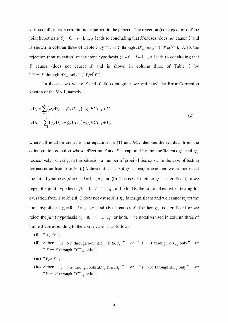
various information criteria (not reported in the paper). The rejection (non-rejection) of the

joint hypothesis 0, 1,...,i i qβ = = leads to concluding that X causes (does not cause) Y and

is shown in column three of Table 3 by “ through onlyt iX Y X∆ −⇒ ” (“ X ⇒Y ”). Also, the

rejection (non-rejection) of the joint hypothesis 0, 1,...,i i qγ = = leads to concluding that

Y causes (does not cause) X and is shown in column three of Table 3 by

“ through onlyt iY X Y∆ −⇒ ” (“Y ⇒ X ”).

In those cases where Y and X did cointegrate, we estimated the Error Correction

version of the VAR, namely

( )

( )

11

11

,

,

q

t i t i i t i y t ti

q

t i t i i t i x t ti

Y Y X ECT U

X Y X ECT V

∆ α ∆ β ∆ η

∆ γ ∆ φ ∆ η

− − −=

− − −=

= + + +

= + + +

∑

∑ (2)

where all notation are as in the equations in (1) and ECT denotes the residual from the

cointegration equation whose effect on Y and X is captured by the coefficients yη and xη

respectively. Clearly, in this situation a number of possibilities exist. In the case of testing

for causation from X to Y: (i) X does not cause Y if yη is insignificant and we cannot reject

the joint hypothesis 0, 1,...,i i qβ = = ; and (ii) X causes Y if either yη is significant, or we

reject the joint hypothesis 0, 1,...,i i qβ = = , or both. By the same token, when testing for

causation from Y to X: (iii) Y does not cause X if xη is insignificant and we cannot reject the

joint hypothesis 0, 1,...,i i qγ = = ; and (iv) Y causes X if either xη is significant or we

reject the joint hypothesis 0, 1,...,i i qγ = = , or both. The notation used in column three of

Table 3 corresponding to the above cases is as follows:

(i) “ X ⇒Y ”;

(ii) either “ 1 through both & t i tX Y X ECT∆ − −⇒ ”, or “ through onlyt iX Y X∆ −⇒ ”, or “ 1 through onlytX Y ECT −⇒ ”;

(iii) “Y ⇒ X ”;

(iv) either “ 1 through both & t i tY X Y ECT∆ − −⇒ ”, or “ through onlyt iY X Y∆ −⇒ ”, or “ 1 through onlytY X ECT −⇒ ”.

6

In addition to checking for Granger causality from X to Y and vice versa, we also

carried out a version of Sims’ causality test by investigating the extent of correlation

between the residuals of the ARIMA models fitted to X and Y (regressions are not reported

here). Denoting these residuals by x and y and the correlation coefficient by ρ, we

calculated the correlations between lagged, current and future x and y, denoted respectively

by ( ) ( ) ( )1 1, , ,ˆ ˆ ˆ, andx y x y x yρ ρ ρ− +

in column three of Table 3. These correlations provide a

measure of causation from past X to current Y, instantaneous causation between X and Y,

and causation from Y to future X (or from past Y to current X), respectively. On the null

hypothesis ρ = 0, the estimator ( )ˆ 0,1/a

N Tρ ∼ , where T is the number of observations.

Given the sample size used, ρ = 0 can be safely rejected at 5% critical level if ˆ 0.29ρ > .

A few points are worth highlighting. First, the results of the causality tests are far

from supporting a universal hypothesis: (i) only 3 out of 23 countries − Japan, Norway and

the UK − satisfy the relationship between trade-openness and government size which is

consistent with Rodrik’s findings; (ii) in 6 countries − Denmark, Finland, Germany, Italy,

Portugal and USA − the causality runs from government size to trade-openness; (iii) of the

5 countries which exhibit instantaneous causality between the two variables − Belgium,

Greece, Italy, Portugal and Sweden − only Greece and Portugal show a positive relationship

between trade-openness and government size; (iv) in 5 countries − Australia, Austria,

Canada, Luxemburg and New Zealand − the causality runs in both directions; and finally

(v) in 6 of the countries − France, Iceland, Ireland, Netherlands, Spain and Switzerland −

we have been unable to find any indication of significant interaction between trade-

openness and government size.

Second, regardless of the direction of causality, the distinction between the short-

run and long-run nature of the relationship between the two variables, as emphasised by

Garrett (2001), seems to be very relevant. Within the time series context, given that in all

of the countries considered both trade-openness and government size are first difference

stationary, the existence of a long-run relationship between these variables will manifest

itself through cointegration between their levels. Only for five of the countries − Australia,

Austria, Denmark, Luxembourg and New Zealand − we could not reject the existence of a

cointegration relationship and in all cases the coefficient estimates suggest the existence of

a plausible positive long-run relationship between trade-openness and government.

However, in none of these countries does the direction of causality conform to Rodrik’s

7

compensation hypothesis. As Rodrik himself points out, exposure to trade could be the

result of government policy and it is possible that this is what our analysis is capturing.

Third, a clear indication of a negative causation, e.g. a negative and significant

instantaneous causality as in Belgium, Italy and Sweden, could suggest that the effect of the

factors underlying the efficiency hypothesis dominates those underlying the compensation

hypothesis.

Forth, the fact that only 5 out of 23 countries favour the existence of a long-run

relationship strengthens Garrett’s point that the link between openness and government size

should be seen as a dynamic process and therefore may not be best captured by static

regressions based on cross-country data which is averaged over a number of years.

Garrett’s approach, however, is to replace the levels with changes while still maintaining a

single data point for each country in the sample. Our results show that the dynamics of the

relationship between trade-openness and government size varies considerably across

countries. In order to provide some indication of the magnitude and pattern of the effect of

these variables on each other within the VAR framework, in the last two columns of Table

3 we plot the accumulated responses of ∆Y (or Y) and ∆X (or X) to a unit impulse to ∆X (or

X) and ∆Y (or Y)5. For each country, these graphs are based on the multipliers obtained

from the estimated coefficients of the general VAR system – which we have used to

construct the test statistics for Granger causality, reported in column three – and hence

disregard the results of the causality tests. They should therefore be interpreted as if a two-

way Granger causality between X on Y existed and are useful for a preliminary

investigation, in different countries, of: (i) how rapidly the effects of the shocks settle; (ii)

whether these effects are in the same or in the opposite direction; and (iii) how the

magnitude of the effect of a unit shock to X on Y compares to that of Y on X. On the whole,

it is clear that countries differ in this respect and disregarding these differences and simply

representing each country in the panel by one data point could severely bias the results.

3. CONCLUSIONS The analysis carried out in this paper fails to provide an overwhelming support for a

positive causality from international trade openness to the size of the government sector.

An extreme conclusion that can be drawn from these results is a refusal of the universal

5 We have chosen a unit shock in order to make the results comparable both between the two variables in a

country and across different countries for the same variable. Note that the shock affects the level when the variables cointegrate.

8

validity of the ‘compensation hypothesis’. Alternatively, these findings could simply be

taken to suggest that trade openness is not the main force driving the (risk-mitigating)

growth in the size of governments. Despite Rodrik’s (1997b) suggestion that increasing

openness in capital and financial markets, by constraining the revenue raising ability of

governments, undermines the positive relationship between government size and openness,

some have argued that capital mobility is associated with more public spending (Quinn,

1997). Thus, the bivariate VAR may not be strictly suitable in that the past values of trade

openness and government expenditure may not provide the appropriate information set on

the basis of which the compensation hypothesis could be verified and we would need to

expand the system to include the additional relevant variables. Along similar lines, it could

be the case that government consumption may not be the component of government budget

that is most responsive to openness. For instance, it could be argued that – particularly for

mature industrial economies – a more suitable measure is welfare spending. However, time

series data on capital mobility, FDI and components of government budget do not exist for

a sufficiently long period for individual countries and further research ought to use the

panel − pooled time series cross section − approach.

As Rodrik points out, a direct test of the compensation hypothesis is to examine

whether openness raises exposure to risk − reflected, for instance, in an increase in

consumption volatility and uneven income distribution − which is then dampened by a

larger government size. Again, availability of time series data for individual countries is an

obstacle and our parallel research on these issues relies on the panel approach. Our

preliminary results in this direction indicate that other variables have a significant role to

play and that the compensation hypothesis may not be the main or the sole factor

underlying the growth of government size6.

6 One direction that is worth investigation is the suggested link between government size and the extent, depth

and composition of industrialisation as new sectors displace the more traditional ones in the economy – see Iversen and Cusack (2000) and Iversen (2001) for an exposition.

9

Table 1. Relationship between trade-openness and government size over four decades in 23 OECD countries 1965-1968, 23 OECD Countries

G

over

nmen

t Siz

e (A

vera

ge 1

965-

1968

)

Trade Openness (Average 1955-1964)

0 .5 1 1.5 20

.1

.2

.3

1 2 34 5

678

9 101112

1314

1516

1718

19

20

21

2223

1975-1978, 23 OECD Countries

G

over

nmen

t Siz

e (A

vera

ge 1

975-

1978

)


0 .5 1 1.5 20

.1

.2

.3

1 2 34

5

678

9 101112

1314

1516

17

18

19

20

21

2223


G

over

nmen

t Siz

e (A

vera

ge 1

985-

1988

)


0 .5 1 1.5 20

.1

.2

.3

1 23

4

5

67 89 10 1112

13

141516

17

1819

20

21

2223


G

over

nmen

t Siz

e (A

vera

ge 1

995-

1998

)


0 .5 1 1.5 20

.1

.2

.3

1 2

3

4

5

67

8

9

10

1112

13

141516

171819

20

21

22

23

10

Table 2. Relationship between trade-openness and government size over four decades in 22 OECD countries*

1965-1968, Excluding Luxemburg (country no. 14)

0

0.1

0.2

0.3

0 0.2 0.4 0.6 0.8 1 1.2 1.4


Gov

enm

ent S

ize

(Ave

rage

196

5-19

68)


0

0.1

0.2

0.3

0 0.2 0.4 0.6 0.8 1 1.2 1.4


Gov

enm

ent S

ize

(Ave

rage

197

5-19

78)


0

0.1

0.2

0.3

0 0.2 0.4 0.6 0.8 1 1.2 1.4


Gov

enm

ent S

ize

(Ave

rage

198

5-19

88)


0

0.1

0.2

0.3

0 0.2 0.4 0.6 0.8 1 1.2 1.4


Gov

enm

ent S

ize

(Ave

rage

199

5-19

98)

* The solid and broken lines represent 2 3ˆ ˆˆ ˆ ˆt t t tY a b X c X d X= + + + and ˆˆ ˆt tY a b X= + fits respectively.

11

Table 3. Causality analysis of the relationship between trade-openness and government size in 23 OECD countries

Australia (1)

sample: 1949-1998

.08

.12

.16

.20

.2

.3

.4

.5

.6

50 55 60 65 70 75 80 85 90 95

Y1 X1

Cointegration: ( )0.64 ~ (0)t tY X I−

Causality: through onlyt iX Y X∆ −⇒

1through onlytY X ECT −⇒

( ) ( ) ( )1 1, , ,ˆ ˆ ˆ.333; .003; .131x y x y x yρ ρ ρ− +

= = − = −

Response of Y to a shock to X

.00

.02

.04

.06

.08

.10

.12

.14

5 10 15 20 25

Response of X to a shock to Y

-1.0

-0.5

0.0

0.5

1.0

1.5

2.0

5 10 15 20 25

Austria (2)

sample: 1948-1998

.10

.12

.14

.16

.18

.20

.22

0.0

0.2

0.4

0.6

0.8

1.0

50 55 60 65 70 75 80 85 90 95

Y2 X2


Causality: 1through onlytX Y ECT −⇒

1 through both & t i tY X Y ECT∆ − −⇒

( ) ( ) ( )1 1, , ,ˆ ˆ ˆ.200; .236; .113x y x y x yρ ρ ρ− +

= = − = −


.00

.01

.02

.03

.04

.05

.06

.07

.08

.09

5 10 15 20 25


-2

0

2

4

6

8

5 10 15 20 25

Belgium

(3)

sample: 1953-1997

.10

.12

.14

.16

.18

.20

0.4

0.6

0.8

1.0

1.2

1.4

1.6

50 55 60 65 70 75 80 85 90 95

Y3 X3

Cointegration: None

Causality: X ⇒Y

Y ⇒ X

( ) ( ) ( )1 1, , ,ˆ ˆ ˆ.080; .491; .214x y x y x yρ ρ ρ− +

= = − =

Response of ∆Y to a shock to ∆X

.00

.01

.02

.03

.04

5 10 15 20 25

Response of ∆X to a shock to ∆Y

0

1

2

3

4

5

5 10 15 20 25

(i) The number in parentheses after the country name in column 1 is the reference number of the country, used in Figures in Table 1. (ii) For each country (j), the figure in column 2 depicts openness − Xj =(Imports+Expots)/GDP − and government size − Yj =Government Consumption/GDP − using independent scales measured on the right and the left axes, respectively. (iii) In the third column, X⇒ Y (Y⇒ X ) denotes the existence of Granger causation from X to Y (Y to X) and ⇒ indicates the lack of such causation. ECT is the error correction term. ( ) ( ) ( )1 1, , ,ˆ ˆ ˆ, andx y x y x yρ ρ ρ

− + are the estimated correlation coefficients

between the residuals of ARIMA models fitted to X and Y, denoted by x and y, and correspond to Sims’ concept of causality. If statistically significant, these respectively indicate causation from past X to current Y, instantaneous causation between X and Y, or causation from past Y to current X. The 5% critical value of ρ is ±0.29. (iv) The figures in the last two columns are the accumulated response of Y and X to a one unit shock to X and Y using the underlying general VAR specification. They give an indication of the way a change in one of the variables affects the other variable regardless of the causality tests.

12

Table 3 continued

Canada (4)

sample: 1948-1998

.00

.05

.10

.15

.20

.25

0.0

0.2

0.4

0.6

0.8

1.0

50 55 60 65 70 75 80 85 90 95

Y4 X4

Cointegration: None


through onlyt iY X Y∆ −⇒

( ) ( ) ( )1 1, , ,ˆ ˆ ˆ.118; .226; .113x y x y x yρ ρ ρ− +

= − = − = −


.00

.04

.08

.12

.16

.20

5 10 15 20 25


-0.8

-0.4

0.0

0.4

0.8

1.2

5 10 15 20 25

Denm

ark*(5)

sample: 1950-1998

.10

.15

.20

.25

.30

.50

.55

.60

.65

.70

.75

50 55 60 65 70 75 80 85 90 95

Y5 X5


Causality: X ⇒Y


( ) ( ) ( )1 1, , ,ˆ ˆ ˆ.103; .089; .145x y x y x yρ ρ ρ− +

= − = − = −


.00

.01

.02

.03

.04

.05

.06

.07

.08

5 10 15 20 25


0.0

0.4

0.8

1.2

1.6

2.0

2.4

2.8

5 10 15 20 25

Finland (6)

sample: 1950-1997

.10

.15

.20

.25

.3

.4

.5

.6

.7

.8

50 55 60 65 70 75 80 85 90 95

Y6 X6

Cointegration: None

Causality: X ⇒Y


( ) ( ) ( )1 1, , ,ˆ ˆ ˆ.154; .207; .014x y x y x yρ ρ ρ− +

= − = − =


.00

.01

.02

.03

.04

.05

5 10 15 20 25


-1

0

1

2

3

4

5 10 15 20 25

France (7)

sample: 1950-1998

.12

.16

.20

.24

.28

.20

.25

.30

.35

.40

.45

.50

50 55 60 65 70 75 80 85 90 95

Y7 X7

Cointegration: None

Causality: X ⇒Y

Y ⇒ X

( ) ( ) ( )1 1, , ,ˆ ˆ ˆ.249; .084; .109x y x y x yρ ρ ρ− +

= = − = −


.00

.02

.04

.06

.08

.10

.12

5 10 15 20 25


.00

.05

.10

.15

.20

.25

.30

5 10 15 20 25

* The results for Denmark are obtained by including a dummy for period 1950-1970 to account for the difference in pre and post 1970 behaviour.

13

Table 3 continued

Germ

any (8)

sample: 1950-1998

.12

.14

.16

.18

.20

.22

.2

.3

.4

.5

.6

.7

.8

50 55 60 65 70 75 80 85 90 95

Y8 X8

Cointegration: None

Causality: X ⇒Y


( ) ( ) ( )1 1, , ,ˆ ˆ ˆ.185; .043; .116x y x y x yρ ρ ρ− +

= − = = −


-.04

-.02

.00

.02

.04

.06

.08

.10

5 10 15 20 25 30 35 40 45 50


-2

-1

0

1

2

3

4

5 10 15 20 25 30 35 40 45 50

Greece (9)

sample: 1948-1998

.10

.12

.14

.16

.18

.20

.22

.1

.2

.3

.4

.5

.6

50 55 60 65 70 75 80 85 90 95

Y9 X9

Cointegration: None

Causality: X ⇒Y

Y ⇒ X

( ) ( ) ( )1 1, , ,ˆ ˆ ˆ.073; .415; .166x y x y x yρ ρ ρ− +

= = = −


.00

.01

.02

.03

.04

.05

.06

.07

.08

5 10 15 20 25


-.5

-.4

-.3

-.2

-.1

.0

5 10 15 20 25

Iceland (10)

sample: 1950-1998

.04

.08

.12

.16

.20

.24

0.4

0.5

0.6

0.7

0.8

0.9

1.0

50 55 60 65 70 75 80 85 90 95

Y10 X10

Cointegration: None

Causality: X ⇒Y

Y ⇒ X

( ) ( ) ( )1 1, , ,ˆ ˆ.251; .195; .016x y x y x yρ ρ ρ− +

= − = − = −


-.016

-.014

-.012

-.010

-.008

-.006

-.004

-.002

.000

5 10 15 20 25


.0

.1

.2

.3

.4

.5

.6

.7

.8

5 10 15 20 25

Ireland (11)

sample: 1948-1997

.10

.12

.14

.16

.18

.20

0.6

0.8

1.0

1.2

1.4

1.6

50 55 60 65 70 75 80 85 90 95

Y11 X11

Cointegration: None

Causality: X ⇒Y

Y ⇒ X

( ) ( ) ( )1 1, , ,ˆ ˆ ˆ.265; .105; .134x y x y x yρ ρ ρ− +

= = − = −


.000

.001

.002

.003

.004

.005

.006

5 10 15 20 25


-2.4

-2.0

-1.6

-1.2

-0.8

-0.4

0.0

5 10 15 20 25

14

Table 3 continued

Italy (12)

sample: 1951-1997

.10

.12

.14

.16

.18

.20

.25

.30

.35

.40

.45

.50

50 55 60 65 70 75 80 85 90 95

Y12 X12

Cointegration: None

Causality: X ⇒Y

Y ⇒ X

( ) ( ) ( )1 1, , ,ˆ ˆ ˆ.014; .333; .302x y x y x yρ ρ ρ− +

= − = − = −


-.032

-.028

-.024

-.020

-.016

-.012

-.008

-.004

.000

5 10 15 20 25


-.4

-.3

-.2

-.1

.0

5 10 15 20 25

Japan (13)

sample: 1952-1998

.07

.08

.09

.10

.11

.12

.16

.20

.24

.28

.32

50 55 60 65 70 75 80 85 90 95

Y13 X13

Cointegration: None


Y ⇒ X

( ) ( ) ( )1 1, , ,ˆ ˆ ˆ.410; .062; .137x y x y x yρ ρ ρ− +

= = − =


.00

.02

.04

.06

.08

.10

5 10 15 20 25


0.0

0.2

0.4

0.6

0.8

1.0

5 10 15 20 25

Luxem

bourg (14)

sample: 1950-1997

.08

.10

.12

.14

.16

1.0

1.2

1.4

1.6

1.8

2.0

50 55 60 65 70 75 80 85 90 95

Y14 X14



1 through both & t i tY X Y ECT∆ − −⇒

( ) ( ) ( )1 1, , ,ˆ ˆ ˆ.186; .268; .051x y x y x yρ ρ ρ− +

= = − = −


.00

.01

.02

.03

.04

.05

.06

5 10 15 20 25


-1

0

1

2

3

4

5

5 10 15 20 25

Netherlands (15)

sample: 1950-1998

.12

.14

.16

.18

.20

0.8

0.9

1.0

1.1

1.2

1.3

50 55 60 65 70 75 80 85 90 95

Y15 X15

Cointegration: None

Causality: X ⇒Y

Y ⇒ X

( ) ( ) ( )1 1, , ,ˆ ˆ ˆ.107; .169; .217x y x y x yρ ρ ρ− +

= − = = −


.000

.001

.002

.003

.004

.005

5 10 15 20 25


-3

-2

-1

0

1

2

3

5 10 15 20 25

15

Table 3 continued

N. Z

ealand (16)

sample: 1950-1997

.10

.12

.14

.16

.18

.20

.4

.5

.6

.7

.8

50 55 60 65 70 75 80 85 90 95

Y16 X16




( ) ( ) ( )1 1, , ,ˆ ˆ ˆ.036; .014; .057x y x y x yρ ρ ρ− +

= − = − = −


.00

.02

.04

.06

.08

.10

.12

5 10 15 20 25


0.0

0.4

0.8

1.2

1.6

2.0

2.4

5 10 15 20 25

Norw

ay (17)

sample: 1949-1998

.08

.12

.16

.20

.24

0.6

0.7

0.8

0.9

1.0

50 55 60 65 70 75 80 85 90 95

Y17 X17

Cointegration: None


Y ⇒ X

( ) ( ) ( )1 1, , ,.224; .274; .064x y x y x yρ ρ ρ− +

= = − = −


.00

.02

.04

.06

.08

.10

.12

.14

5 10 15 20 25


-2.5

-2.0

-1.5

-1.0

-0.5

0.0

5 10 15 20 25

Portugal (18)

sample: 1953-1998

.08

.12

.16

.20

.24

.3

.4

.5

.6

.7

.8

.9

50 55 60 65 70 75 80 85 90 95

Y18 X18

Cointegration: None

Causality: X ⇒Y


( ) ( ) ( )1 1, , ,.038; .872; .131x y x y x yρ ρ ρ− +

= = = −


.000

.005

.010

.015

.020

.025

.030

5 10 15 20 25


-3.5

-3.0

-2.5

-2.0

-1.5

-1.0

-0.5

0.0

5 10 15 20 25

Spain (19)

sample: 1954-1998

.06

.08

.10

.12

.14

.16

.18

.1

.2

.3

.4

.5

.6

50 55 60 65 70 75 80 85 90 95

Y19 X19

Cointegration: None

Causality: X ⇒Y

Y ⇒ X

( ) ( ) ( )1 1, , ,ˆ ˆ ˆ.058; .097; .085x y x y x yρ ρ ρ− +

= − = − = −


-1.0

-0.5

0.0

0.5

1.0

1 2 3 4 5 6 7 8 9 10


-1.0

-0.5

0.0

0.5

1.0

1 2 3 4 5 6 7 8 9 10

16

Table 3 continued

Sweden (20)

sample: 1950-1998

.12

.16

.20

.24

.28

.32

.4

.5

.6

.7

.8

.9

50 55 60 65 70 75 80 85 90 95

Y20 X20

Cointegration: None

Causality: X ⇒Y

Y ⇒ X

( ) ( ) ( )1 1, , ,ˆ ˆ ˆ.045; .339; .108x y x y x yρ ρ ρ− +

= = − = −


-.04

.00

.04

.08

.12

.16

.20

5 10 15 20 25


-1

0

1

2

3

4

5

6

5 10 15 20 25

Switzerland (21)

sample: 1948-1998

.08

.10

.12

.14

.16

.4

.5

.6

.7

.8

50 55 60 65 70 75 80 85 90 95

Y21 X21

Cointegration: None

Causality: X ⇒Y

Y ⇒ X

( ) ( ) ( )1 1, , ,ˆ ˆ ˆ.123; .196; .040x y x y x yρ ρ ρ− +

= = − = −


.00

.01

.02

.03

.04

.05

.06

5 10 15 20 25


-1.2

-0.8

-0.4

0.0

0.4

0.8

5 10 15 20 25

U.K

. (22)

sample: 1948-1998

.14

.16

.18

.20

.22

.24

.35

.40

.45

.50

.55

.60

50 55 60 65 70 75 80 85 90 95

Y22 X22

Cointegration: None


Y ⇒ X

( ) ( ) ( )1 1, , ,ˆ ˆ ˆ.143; .078; .159x y x y x yρ ρ ρ− +

= = − =


.00

.02

.04

.06

.08

.10

.12

.14

.16

5 10 15 20 25


0.0

0.2

0.4

0.6

0.8

1.0

1.2

1.4

5 10 15 20 25

U.S.A

. (23)

sample: 1949-1998

.10

.12

.14

.16

.18

.20

.22

.08

.12

.16

.20

.24

.28

50 55 60 65 70 75 80 85 90 95

Y23 X23

Cointegration: None

Causality: X ⇒Y


( ) ( ) ( )1 1, , ,ˆ ˆ ˆ.152; .232; .121x y x y x yρ ρ ρ− +

= = − = −


.00

.05

.10

.15

.20

.25

.30

5 10 15 20 25


-.6

-.5

-.4

-.3

-.2

-.1

.0

5 10 15 20 25

17

APPENDIX: Table A . Relationship between trade-openness and government size over four decades in 23 OECD countries*


0

0.1

0.2

0.3

0 0.2 0.4 0.6 0.8 1 1.2 1.4 1.6 1.8


Gov

enm

ent S

ize

(Ave

rage

196

5-19

68)


0

0.1

0.2

0.3

0 0.2 0.4 0.6 0.8 1 1.2 1.4 1.6 1.8


Gov

enm

ent S

ize

(Ave

rage

197

5-19

78)


0

0.1

0.2

0.3

0 0.2 0.4 0.6 0.8 1 1.2 1.4 1.6 1.8


Gov

enm

ent S

ize

(Ave

rage

198

5-19

88)


0

0.1

0.2

0.3

0 0.2 0.4 0.6 0.8 1 1.2 1.4 1.6 1.8 2


Gov

enm

ent S

ize

(Ave

rage

199

5-19

98)

* The solid and broken lines represent 2 3ˆ ˆˆ ˆ ˆt t t tY a b X c X d X= + + + and ˆˆ ˆt tY a b X= + fits respectively.

18

REFERENCES Alesina, A. and R. Perotti (1997). “The Welfare State and Competitiveness”, American

Economic Review, 87, 921-39.

Cameron, D. R. (1978). “The Expansion of the Public Economy: A Comparative Analysis”, American Political Science Review, vol. 72, pp.237-269.

Enders, W. (1995). Applied Econometric Time Series, John Wiley & Sons.

Garrett, G. (1995). “Capital Mobility, Trade and the Domestic Politics of Economic Policy”, International Organization, vol. 49, no.4, pp.657-687.

Garrett, G. (1998). Partisan Politics in the Global Economy, Cambridge: Cambridge University Press.

Garrett, G. (2001). “Globalization and Government Spending Around the World”, Studies in Comparative International Development, vol. 35, no.4, pp. 3-29.

Harvey, A.C. (1990). The Econometric Analysis of Time Series, Second edition, LSE Handbooks in Economics, Phillip Allan.

Iversen, T. (2001). “The Dynamics of Welfare State Expansion: Trade Openness, De-industrialization, and Partisan Politics”, in The new Politics of the Welfare State, P. Pierson (ed.), Oxford University Press.

Iversen, T. and Cusack T.R. (2000). “The Causes of Welfare State Expansion”, World Politics, 52, 313-349.

Quinn, D. (1997). “The Correlates of Changes in International Financial Regulation”, American Political Science Review, 91, 531-552.

Rodrik, D. (1997a). “Trade, Social Insurance, and the Limits to Globalization”, NBER, Working Paper 5905.

Rodrik, D. (1997b). Has globalization gone too far?, Washington: Institute for International Economics.

Rodrik, D. (1998). “Why do more open economies have bigger governments?”, Journal of Political Economy, vol. 106, no.5, pp.997-1032.

On the Causal Relationship between Trade Openness and Government Size: Evidence from 23 OECD...

Documents

Transcript of On the Causal Relationship between Trade Openness and Government Size: Evidence from 23 OECD...