Optimization of Steel-Concrete Composite I-Girder Bridges
137
Renata Ligocki Pedro Optimization of Steel-Concrete Composite I-Girder Bridges Brazil 2017
-
Upload
khangminh22 -
Category
Documents
-
view
1 -
download
0
Transcript of Optimization of Steel-Concrete Composite I-Girder Bridges

Renata Ligocki Pedro
Optimization of Steel-Concrete CompositeI-Girder Bridges
Brazil2017

Renata Ligocki Pedro
Optimization of Steel-Concrete Composite I-GirderBridges
Master’s Thesis presented as a par-tial requirement for obtaining a Mas-ter’s degree in Civil Engineeringfrom the Federal University of SantaCatarina
Federal University of Santa CatarinaDepartment of Civil Engineering
Graduation program in Civil EngineeringAdvisor: Prof. Leandro Fleck Fadel MiguelCo-advisor: Prof. Rafael Holdorf Lopez
Brazil2017


Ficha de identificação da obra elaborada pelo autor, através do Programa de Geração Automática da Biblioteca Universitária da UFSC.
Ligocki Pedro, Renata Optimization of Steel-Concrete Composite IGirder Bridges / Renata Ligocki Pedro ; orientador,Leandro Fleck Fadel Miguel, coorientador, RafaelHoldorf Lopez, 2017. 135 p.
Dissertação (mestrado) - Universidade Federal deSanta Catarina, Centro Tecnológico, Programa de PósGraduação em Engenharia Civil, Florianópolis, 2017.
Inclui referências.
1. Engenharia Civil. 2. Estrutura Mista. 3.Ponte. 4. Otimização. 5. Método dos ElementosFinitos. I. Fleck Fadel Miguel, Leandro. II.Holdorf Lopez, Rafael. III. Universidade Federal deSanta Catarina. Programa de Pós-Graduação emEngenharia Civil. IV. Título.
Renata Ligocki Pedro
Optimization of Steel-Concrete Composite I-GirderBridges
Esta Dissertação foi julgada adequada para obtenção do Título de"Mestre", e aprovada em sua forma final pelo Programa de Pós-graduaçãoem Engenharia Civil
Florianópolis, 29 de Maio de 2017:
Prof. Dr. Glicério TrichêsCoordenador do Curso
Prof. Dr. Leandro Fleck Fadel MiguelOrientador
Prof. Dr. Rafael Holdorf LopezCo-Orientador
Banca Examinadora:
Prof. Roberto Caldas de Andrade Pinto, PhD.Universidade Federal de Santa Catarina
Prof. Dr. José Carlos de Carvalho PereiraUniversidade Federal de Santa Catarina
Prof. Dr. Ricardo Hallal FakuryUniversidade Federal de Minas Gerais
(vídeo-conferência)


Acknowledgments
This work was carried out during the years 2015-2017 at the CivilEngineering Department, Federal University of Santa Catarina. It is apleasure to thank those who made this dissertation possible.
First, I am forever indebted to my parents, for their supportthroughout my entire life. Without them I couldn’t have achieved anyof my dreams. My warmest gratitude also goes to my sister, who sharedher experience and let me learn through her difficulties.
I am deeply grateful to my advisor Professor Leandro Fleck FadelMiguel. Without his continuous enthusiasm and encouragement thisstudy couldn’t have reached its completion. Also, I’d like to thank myco-advisor, Professor Rafael Holdorf Lopez, who shared his knowledgeabout optimization tools and turned this study possible.
I want to express my gratitude to the other contributors of thisthesis: Professor Daniel Loriggio, for teaching me even more aboutbridges structural behavior; Professors Ricardo Hallal Fakury, JoséCarlos de Carvalho Pereira and Roberto Caldas de Andrade Pinto, forsharing their knowledge and improving this work.
I also owe a great debt of gratitude to Professor Cláudio CezarZimmerman and the PET group, for helping me start in the engineeringuniverse, navigating with me through all the different fields, learningtogether, and making me the person and professional that I am today.
I cannot forget to thank my colleagues: Juliano Demarche, forsharing his knowledge in Finite Element Models, facilitating my learningin the matter; Rafael Souza, for always being prompt to help me inanything that I needed.


“We build too many walls and not enough bridges.“Isaac Newton

AbstractThis work presents an efficient two-stage optimization approach to thedesign of steel-concrete composite I-girder bridges. In the first step,a simplified structural model, usually adopted by bridge designers, isemployed aiming to locate the global optimum region and provide astarting point to the local search. Then, a finite element model (FEM) isused to refine and improve the optimization. Through this procedure, it ispossible to combine the low computational cost required on the first stagewith the accuracy provided on the second one. For illustration purposes,a numerical example of a composite bridge designed by Pinho & Bellei(2007) and studied by Leitão et al. (2011) is assessed. The objectivefunction is based on the economic cost of the structure. Due to the non-convex nature of the problem and to the presence of discrete variables,the first stage optimization is conducted through five well-known meta-heuristic algorithms: Backtracking Search Algorithm (BSA), FireflyAlgorithm (FA), Genetic Algorithm (GA), Imperialist CompetitiveAlgorithm (ICA) and Search Group Algorithm (SGA). The SGA ischosen to pursue the second stage because a statistical analysis hasdemonstrated that it achieved the best performance. It is shown thatthe proposed scheme is able to reduce the structural cost in up to 7.43%already in the first stage and can reach up to 9.17% of saving costs inthe end of the optimization procedure.
Key-words: Composite Structure. Bridge. Optimization. Finite Ele-ment Method.


Resumo ExpandidoPontes são estruturas importantes para travessia de rios e vales. Elascomeçaram a ser construídas em 62 a.C. em Roma, usando a técnicade arcos de pedra. Com o passar do tempo, as técnicas e os materiaisempregados em pontes foram evoluindo, de arco em pedra para madeiratreliçada, chegando até a tecnologia de pontes pênseis e estaiadas. Aspontes mistas de aço e concreto surgiram em 1930, com a laje de concretoarmado e as vigas em seção I ou caixão.
As pontes mistas de seção I são muito econômicas para estruturas retascom vãos pequenos (20 a 50m). Essa estrutura tem sua importânciacomprovada pela quantidade de trabalhos na área. - Madrazo-Aguirre,Ruiz-Teran & Wadee (2015), Liu et al. (2014), Zhou et al. (2016), Liuet al. (2009), Ellobody (2014), Oehlers (1990), Gocál & Ďuršová (2012),Pinho & Bellei (2007), Fernandes (2008), Klinsky (1999), Leitão et al.(2011), Vitório (2015) e Fabeane (2015). Porém, nenhum desses estudosfocam na otimização completa da estrutura.
Na área de otimização de pontes, há também um grande número detrabalhos na literatura. Alguns autores optaram por otimizar os cabosde pontes estaiadas - Lute, Upadhyay & Singh (2009), Cai & Aref (2015),Martins, Simões & Negrão (2015), Baldomir et al. (2010) e Hassan (2013).Outros estudaram a otimização de pontes de grandes vãos - Kusano etal. (2014) -, pontes de treliça metálica - Cheng (2010) e Cheng, Qian& Sun (2013) -, pontes de concreto protendido - Martí et al. (2013) eKaveh, Maniat & Naeini (2016) - e pontes de pilares altos - Martínezet al. (2011). Na otimização de pontes mistas, pode-se citar o trabalhode Gocál & Ďuršová (2012), que realizou um estudo paramétrico paraotimizar a disposição transversal das vigas. Logo, é importante reiterarque não foi encontrado nenhum trabalho de otimização da estruturacompleta de pontes mistas. Além disso, a importância do tema é tambémcontabilizada na separação entre a eficiência do projeto e a experiência
do projetista. Baseado na otimização de outras estruturas, espera-seobter uma redução de até 10% do custo da ponte.
Assim, o principal objetivo desta dissertação é otimizar o projeto depontes mistas de aço e concreto. Para isso, é proposta uma metodologiade otimização dividida em dois estágios. Na primeira etapa, um modeloestrutural simplificado, usualmente adotado por projetistas, é utilizadopara achar a região ótima, assim como para indicar um ponto inicial paraa busca seguinte. No segundo estágio, um modelo de elementos finitosutilizando barras e cascas é incorporado para melhorar a otimização.Essa estratégia é empregada para combinar o benefício de cada estágiona resolução desse problema. Enquanto que o primeiro estágio tem umcusto computacional baixo, podendo ser repetido inúmeras vezes, asegunda etapa é mais precisa estruturalmente. Logo, com a combinaçãodos dois modelos, o projeto pode ser otimizado de forma precisa comum tempo computacional razoável.
Ainda, para resolver esse problema, é preciso definir o método de oti-mização. Por causa da complexidade do problema e da presença devariáveis discretas, optou-se por utilizar algoritmos heurísticos. Comonão existe um algoritmo universal, foram testados estatisticamentecinco algoritmos heurísticos conhecidos: Backtracking Search Algorithm(BSA), Firefly Algorithm (FA), Genetic Algorithm (GA), ImperialistCompetitive Algorithm (ICA) e Search Group Algorithm (SGA). Dentreeles, o SGA foi o que teve a melhor performance para resolver essaotimização.
Com a escolha do SGA, a otimização em duas etapas foi realizada. Foi,então, otimizada uma ponte mista bi-apoiada com 40m de vão livre e13m de largura. Na primeira etapa, atingiu-se um custo de U$119.796,43e na segunda, U$117.884,93. Comparando esses resultados com umaponte de mesmas características projetada manualmente por Pinho &

Bellei (2007), alcançou-se uma redução de 9,17%.
Os resultados alcançados mostram que a metodologia proposta é eficientena redução de custo da ponte. Outros estudos devem ser efetuados, taiscomo o da influência da passagem dinâmica de veículos, para aumentara confiança estrutural.
Palavras-chave: Estrutura Mista. Ponte. Otimização. Método dosElementos Finitos.

List of Figures
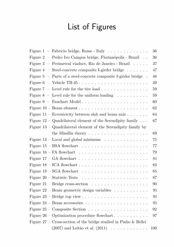
Figure 1 – Fabricio bridge, Rome - Italy . . . . . . . . . . . . . 36Figure 2 – Pedro Ivo Campos bridge, Florianópolis - Brazil . . 36Figure 3 – Perimetral viaduct, Rio de Janeiro - Brazil . . . . . 37Figure 4 – Steel-concrete composite I-girder bridge . . . . . . . 47Figure 5 – Parts of a steel-concrete composite I-girder bridge . 48Figure 6 – Vehicle TB-45 . . . . . . . . . . . . . . . . . . . . . . 49Figure 7 – Level rule for the tire load . . . . . . . . . . . . . . . 59Figure 8 – Level rule for the uniform loading . . . . . . . . . . 59Figure 9 – Fauchart Model . . . . . . . . . . . . . . . . . . . . . 60Figure 10 – Beam element . . . . . . . . . . . . . . . . . . . . . . 62Figure 11 – Eccentricity between slab and beam axis . . . . . . . 64Figure 12 – Quadrilateral element of the Serendipity family . . . 67Figure 13 – Quadrilateral element of the Serendipity family by
the Mindlin theory . . . . . . . . . . . . . . . . . . . 69Figure 14 – Local and global minimum . . . . . . . . . . . . . . 75Figure 15 – BSA flowchart . . . . . . . . . . . . . . . . . . . . . 77Figure 16 – FA flowchart . . . . . . . . . . . . . . . . . . . . . . 79Figure 17 – GA flowchart . . . . . . . . . . . . . . . . . . . . . . 81Figure 18 – ICA flowchart . . . . . . . . . . . . . . . . . . . . . . 83Figure 19 – SGA flowchart . . . . . . . . . . . . . . . . . . . . . 85Figure 20 – Statistic Tests . . . . . . . . . . . . . . . . . . . . . 87Figure 21 – Bridge cross-section . . . . . . . . . . . . . . . . . . 90Figure 22 – Beam geometric design variables . . . . . . . . . . . 91Figure 23 – Bridge top view . . . . . . . . . . . . . . . . . . . . . 91Figure 24 – Beam accessories . . . . . . . . . . . . . . . . . . . . 91Figure 25 – Composite Section . . . . . . . . . . . . . . . . . . . 92Figure 26 – Optimization procedure flowchart . . . . . . . . . . . 97Figure 27 – Cross-section of the bridge studied in Pinho & Bellei
(2007) and Leitão et al. (2011) . . . . . . . . . . . . 100

Figure 28 – SAP2000 model . . . . . . . . . . . . . . . . . . . . . 101Figure 29 – Stress distribution . . . . . . . . . . . . . . . . . . . 104Figure 30 – Stress distribution (zoom) . . . . . . . . . . . . . . . 104Figure 31 – Convergence history comparison of all the algorithms
used . . . . . . . . . . . . . . . . . . . . . . . . . . . 106Figure 32 – Results of the ANOVA test for 200,000 OFEs . . . . 107Figure 33 – Comparison of the means of the algorithms . . . . . 108Figure 34 – Convergence history of the two-stage based optimization111Figure 35 – Rüsch’s table 14 . . . . . . . . . . . . . . . . . . . . 132Figure 36 – Rüsch’s table 27 . . . . . . . . . . . . . . . . . . . . 133Figure 37 – Rüsch’s table 98 - part 1 . . . . . . . . . . . . . . . . 134Figure 38 – Rüsch’s table 98 - part 2 . . . . . . . . . . . . . . . . 135
List of Tables
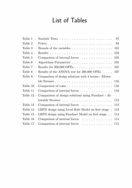
Table 1 – Statistic Tests . . . . . . . . . . . . . . . . . . . . . . 87Table 2 – Prices . . . . . . . . . . . . . . . . . . . . . . . . . . . 94Table 3 – Bounds of the variables . . . . . . . . . . . . . . . . . 101Table 4 – Results . . . . . . . . . . . . . . . . . . . . . . . . . . 103Table 5 – Comparison of internal forces . . . . . . . . . . . . . 103Table 6 – Algorithms Parameters . . . . . . . . . . . . . . . . . 105Table 7 – Results for 200,000 OFEs . . . . . . . . . . . . . . . . 105Table 8 – Results of the ANOVA test for 200,000 OFEs . . . . 107Table 9 – Comparison of design solutions with 4 beams - Allowa-
ble Stresses . . . . . . . . . . . . . . . . . . . . . . . . 110Table 10 – Comparison of costs . . . . . . . . . . . . . . . . . . . 110Table 11 – Comparison of internal forces . . . . . . . . . . . . . 110Table 12 – Comparison of design solutions using Fauchart - Al-
lowable Stresses . . . . . . . . . . . . . . . . . . . . . 112Table 13 – Comparison of internal forces . . . . . . . . . . . . . 112Table 14 – LRFD design using Level Rule Model on first stage . 113Table 15 – LRFD design using Fauchart Model on first stage . . 114Table 16 – Comparison of internal forces . . . . . . . . . . . . . 114Table 17 – Comparison of internal forces . . . . . . . . . . . . . 115


List of abbreviations and acronyms
AASHTO American Association of State Highway and Trans-portation Officials
ABNT Brazilian Association of Technical Standards
ACO Ant Colony Optimization
ANOVA Analysis of Variance
BSA Backtracking Search Algorithm
CBO Colliding Bodies Optimization
CFRP Carbon Fiber Reinforced Polymeric
DOF Degrees of Freedom
FA Firefly Algorithm
FEM Finite Element Model
FM Fauchart Model
GA Genetic Algorithm
IBGE Brazilian Institute of Statistics and Geography
ICA Imperialist Competitive Algorithm
LR Level Rule
NBR Brazilian Standard
OFE Objective Function Evaluation
SA Simulated Annealing
SD Standard Deviation

SGA Search Group Algorithm
SVM Support Vector Machine

List of symbols
Capital Latin Symbols
A Axle load
As Reinforcement section area
Ass Stiffener area
At Area of the stiffener
Atmin Minimum area of the stiffener
Bbridge Width of the bridge
B Strain-displacement matrix
Bb Bending strain-displacement matrix
Bs Transverse shear strain-displacement matrix
Cost Cost function
C Matrix of constitutive relations
Cb Bending constitutive matrix
Cs Transverse shear constitutive matrix
Dc Depth of the web in compression in the elastic range
E Elastic modulus
F Random value
Fcr Critical buckling stress for plates
Fsa Stiffener allowable stress

Fv Allowable shear stress on the beam web
Fve Shear stress on the transversal stiffener
G Shear modulus
Is Inertia of the longitudinal stiffener
Ismin Minimum inertia of the longitudinal stiffener
It Inertia of the transversal stiffener
Itmin Minimum inertia of the transversal stiffener
Iy Moments of inertia about the minor principal axis ofthe cross-section
Iyc Moment of inertia of the compression flange of a steelsection about the vertical axis in the plane of the web
J Objective function
Jt Torsional inertia
Kb Plate bending stiffness matrix
Kg Stiffness global matrix
Km Membrane stiffness matrix
Kp Plate stiffness matrix
Ks Plate transverse shear stiffness matrix
Kshell Shell stiffness matrix
L Matrix of differential operators
Lb Bridge free span
M Bending moment
Mn Nominal flexural resistance based on the tensionflange
Mu Moment due to factored loads
N Matrix of shape functions
Na(ξ, η) Parametric coordinates matrix
NA Neutral axis
Ni Shape functions
OFEmaxFEM Maximum objective function evaluations for the FEMmodel
OFEmaxSM Maximum objective function evaluations for eachiteration of the simplified model
P Tire load
Pop Population created in the Initialization process
Rij Former jth column of the search group matrix
S Project admissible region
Tb Bending subdivision of the transformation matrix
TB Transformation matrix
T.C.n Total cost of the nth empire
TM Mindlin transformation matrix
Ts Shear subdivision of the transformation matrix
V Design shear force on the support
Vd1 Shear due to the factored loads considering the pre-sence of a transversal stiffener
Vn Nominal shear resistance
Vn,sup Support stiffener nominal shear resistance
Vu Shear due to the factored loads
X∗k Final population of the kth iteration of the simplifiedmodel
Xk Population of the kth iteration of the simplified model
X∗opt Best individual of each iteration of the simplifiedmodel
Lower Case Latin Symbols
a Polynomial parameters vector
ai Polynomial parameters
b2 Width between beams
bs Beam top flange width
bsa Support stiffener width
bsl Longitudinal stiffener width
bst Transversal stiffener width
bu Width of the bottom flange of the beam
c Factor
d Vector of nodal DOF
d0 Distance between the support and the first transversalstiffener
d1 Distance between each transversal stiffener
dcomp Distance from compression face to centroid of tensionreinforcement
diaf Profile of diaphragms
dstud Stud diameter
dvq Possible discrete values for the variables
e Eccentricity between slab and beam axis
f Nodal forces vector
fbi Bottom flange maximum stress
fbs Top flange maximum stress
f ′c Concrete 28-day compressive strength
fc Slab maximum stress
fcomp Compression-flange stress at the section under consi-deration
fg Force global vector
fp Surface tractions vector
fq Body forces vector
fv Beam web maximum stress
fy Steel yield strength
fya Allowable yield strength of the steel
gj Inequality restrictions
h Deck thickness
hj Equality restrictions
hstud Stud height
hv Beam web height
itmaxSM Maximum iterations of the simplified model
j Factor
k Factor defined by the slab height
kb Mindlin curvature sub-vector
kM Mindlin curvature and transverse shear strain vector
ks Mindlin transverse shear strain sub-vector
kt Torsional spring constant
kv Vertical spring constant
m(x) Uniform distributed torsion moment
ndiaf Number of diaphragms used
npop,FEM Size of the population used in the FEM model
npop,SM Size of the population used in the simplified model
oldP Historical population
p Surface tractions vector
p Bridge uniform load
p(x) Uniform loading
p∗i Standard bound
pi Given structural response
q Body forces vector
rdiaf Radius of gyration of the diaphragm section
rij Cartesian distance between the two fireflies
t Plate height
ts Beam top flange thickness
tsa Support stiffener thickness
tsl Longitudinal stiffener thickness
tst Transversal stiffener thickness
tu Thickness of the bottom flange of the beam
tw Beam web thickness
u Displacements vector
u(x) Displacements function
u(ξ, η) Parametric displacement u
u(ξ, η) Parametric displacements vector
ui Translation in direction x
uxb Beam nodal displacement in x
uxp Plate nodal displacement in x
uzb Beam nodal displacement in z
uzp Plate nodal displacement in z
v(x) Displacements function
v(ξ, η) Parametric displacement v
vi Translation in direction y
w Vertical displacement
w(x) Displacements function
wi Translation in direction z
wpar Positive weight parameter
x Design variables
x∗ Optimum design
xd Discrete variables
xnewj Perturbed individual
xk Continuous variables
xki Members of the simplified model population
x∗optF EM Best individual found in the FEM model stage
x∗optSM Optimum design of the first stage
Greek Symbols
αFA Randomization parameter
αi Polynomial parameters
αSGA Parameter that controls the size of the perturbation
β0 Attractiveness at r = 0
γ Light absorption coefficient
∆ Deflection
δd Virtual nodal DOF vector
δu Virtual displacement vector
δε Virtual strain vector
δεb(ξ, η, z) Bending virtual strain vector
δεs(ξ, η) Transversal shear virtual strain vector
ε Strain vector
εb Vector of strains
εr Random variable
εr Random vector
εs Vector of shear deformations
εx Strain in the x direction
εy Strain in the y direction
εz Strain in the z direction
η Parametric coordinate
θ Torsion angle
θx(x) Displacements function
θxi Rotation around the x axis
θyb Beam nodal rotation around y
θyi Rotation around the y axis
θyp Plate nodal rotation around y
θzi Rotation around the z axis
λxy Shear deformation in the xy plane
λxz Shear deformation in the xz plane
λyz Shear deformation in the yz plane
ν Poisson coefficient
ξ Parametric coordinate
ξ1 Positive number which is considered to be less than 1
ρ Reinforcement steel rate

σ Stress vector
σc Slab normal stress
τR Concrete shear stress resistance
τs Slab shear stress
ϕ Impact factor
Summary
List of Figures . . . . . . . . . . . . . . . . . . . . . . . . . . . 17List of Tables . . . . . . . . . . . . . . . . . . . . . . . . . . . . 191 Introduction . . . . . . . . . . . . . . . . . . . . . . . . . . . 35
1.1 Motivation . . . . . . . . . . . . . . . . . . . . . . . . . 351.2 Literature Review . . . . . . . . . . . . . . . . . . . . . 381.3 Scope and Objective of the Study . . . . . . . . . . . . . 411.4 Organization of the Text . . . . . . . . . . . . . . . . . . 42
2 Steel-Concrete Composite I-Girder Bridges . . . . . . . . . 452.1 Bridge Structural Design . . . . . . . . . . . . . . . . . . 45
2.1.1 Loads . . . . . . . . . . . . . . . . . . . . . . . . 472.1.2 Design Constraints - Allowable Stresses . . . . . 492.1.3 Design Constraints - Limit and Resistance Factor
Design . . . . . . . . . . . . . . . . . . . . . . . . 552.2 Structural Analysis . . . . . . . . . . . . . . . . . . . . . 57
2.2.1 Simplified Models . . . . . . . . . . . . . . . . . 582.2.2 Finite Element Model (FEM) . . . . . . . . . . . 61
3 Fundamentals of Optimization . . . . . . . . . . . . . . . . 733.1 General Concepts . . . . . . . . . . . . . . . . . . . . . . 733.2 Algorithms . . . . . . . . . . . . . . . . . . . . . . . . . 76
3.2.1 Backtracking Search Algorithm (BSA) . . . . . . 763.2.2 Firefly Algorithm (FA) . . . . . . . . . . . . . . . 783.2.3 Genetic Algorithm (GA) . . . . . . . . . . . . . . 783.2.4 Imperialist Competitive Algorithm (ICA) . . . . 803.2.5 Search Group Algorithm (SGA) . . . . . . . . . . 81
3.3 Statistic Tests . . . . . . . . . . . . . . . . . . . . . . . . 834 Steel-Concrete Composite I-Girder Bridge Optimization . . 89
4.1 Optimization Problem . . . . . . . . . . . . . . . . . . . 894.2 Two-Stage Based Optimization Approach . . . . . . . . 94
5 Numerical Example . . . . . . . . . . . . . . . . . . . . . . . 99
5.1 Structure Studied . . . . . . . . . . . . . . . . . . . . . . 995.2 Mechanical Model Validation . . . . . . . . . . . . . . . 1005.3 Assessment of the Heuristic Algorithms . . . . . . . . . 1055.4 Two-stage Bridge Optimization . . . . . . . . . . . . . . 108
5.4.1 Allowable Stresses . . . . . . . . . . . . . . . . . 1095.4.2 Limit and Resistance Factor Design . . . . . . . 111
6 Concluding Remarks and Future Developments . . . . . . . 1176.1 Concluding Remarks . . . . . . . . . . . . . . . . . . . . 1176.2 Future Studies . . . . . . . . . . . . . . . . . . . . . . . 119
References . . . . . . . . . . . . . . . . . . . . . . . . . . . . . 121
Annex 129Annex A Rüsch’s tables . . . . . . . . . . . . . . . . . . . . . 131

35
Chapter 1
Introduction
1.1 Motivation
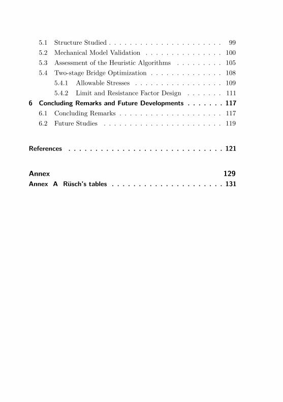
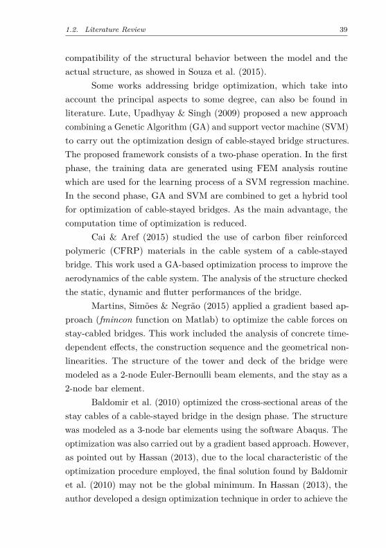
Historically, bridges arose by the necessity of people to cross riversand valleys. The ancient Romans are recognized as the first builders ableto construct bridges with reasonable spans and withstanding conditionsthat would damage previous designs. Their oldest bridge is the so-calledFabricio Bridge (Figure 1), located in Rome. It still is in existence untiltoday, presenting a 24.5m span.
The iron was first employed in 1779, in a 31m span arch structurein England. Since then, the materials and techniques used in the cons-truction evolved significantly. The modern suspension bridges and thefirst concrete bridges started to be designed in the 19th century. Amongthe former, the Brooklyn Bridge was constructed in 1870, presenting480m of free span. The 20th century consolidated the use of cable-stayedstructures, which becomes economical for big spans.
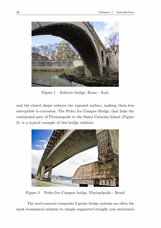
Within this context, the steel-concrete composite bridges startedto be designed in the 30’s of the last century. They are formed with aconcrete deck and steel beams, which can be I-sections or box girders.According to Chen, Duan & Altman (2000), the latter are usuallyemployed in the construction of urban highway, horizontally curved andlong-span bridges. They have higher flexural capacity, torsional rigidity
36 Chapter 1. Introduction
Figure 1 – Fabricio bridge, Rome - Italy
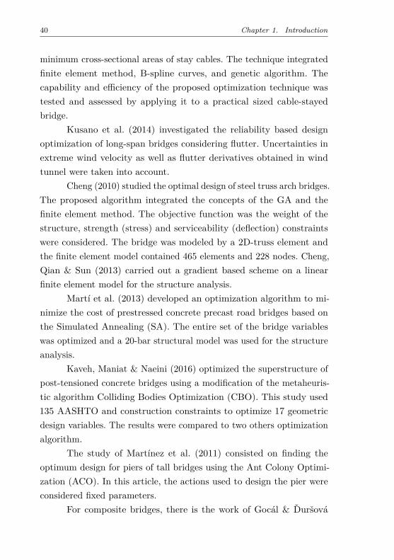
and the closed shape reduces the exposed surface, making them lesssusceptible to corrosion. The Pedro Ivo Campos Bridge, that links thecontinental part of Florianópolis to the Santa Catarina Island (Figure2), is a typical example of this bridge solution.
Figure 2 – Pedro Ivo Campos bridge, Florianópolis - Brazil
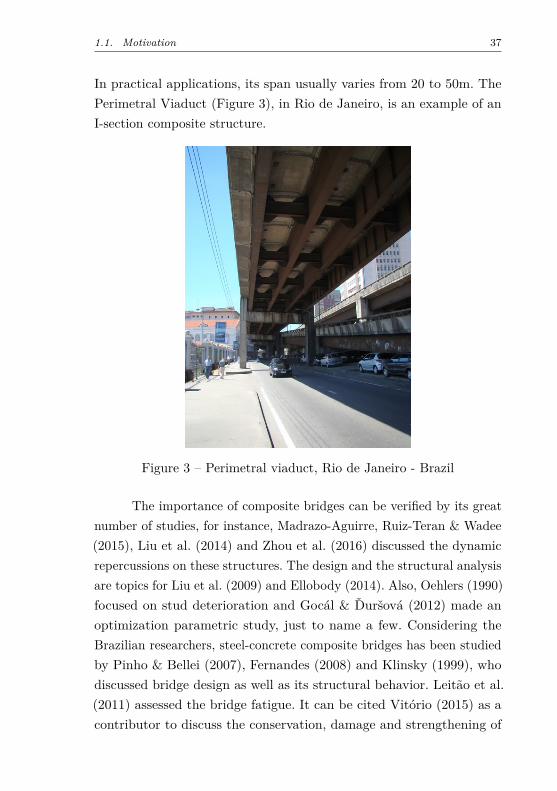
The steel-concrete composite I-girder bridge systems are often themost economical solution to simply supported straight axis structures.
1.1. Motivation 37
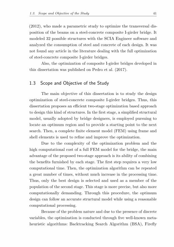
In practical applications, its span usually varies from 20 to 50m. ThePerimetral Viaduct (Figure 3), in Rio de Janeiro, is an example of anI-section composite structure.
Figure 3 – Perimetral viaduct, Rio de Janeiro - Brazil
The importance of composite bridges can be verified by its greatnumber of studies, for instance, Madrazo-Aguirre, Ruiz-Teran & Wadee(2015), Liu et al. (2014) and Zhou et al. (2016) discussed the dynamicrepercussions on these structures. The design and the structural analysisare topics for Liu et al. (2009) and Ellobody (2014). Also, Oehlers (1990)focused on stud deterioration and Gocál & Ďuršová (2012) made anoptimization parametric study, just to name a few. Considering theBrazilian researchers, steel-concrete composite bridges has been studiedby Pinho & Bellei (2007), Fernandes (2008) and Klinsky (1999), whodiscussed bridge design as well as its structural behavior. Leitão et al.(2011) assessed the bridge fatigue. It can be cited Vitório (2015) as acontributor to discuss the conservation, damage and strengthening of
38 Chapter 1. Introduction
these structures. Also, Fabeane (2015) with main focus on optimizationdirectrixes.
Despite the reasonable amount of research, those investigationsare not dealing with full optimization studies. In addition, even consi-dering the relative simple configuration of composite bridges, the finalsolution strongly depends on the engineer experience due to the greatnumber of design variables. Therefore, it is intended to achieve bettereconomical solutions with the help of optimization procedures.
1.2 Literature Review
The structural optimization is a very relevant field and has beena growing focus on research. Initial emphasis had been given to trussstructures and some important advances were carried out - Tang, Tong& Gu (2005), Kelesoglu (2007), Rahami, Kaveh & Gholipour (2008),Torii, Lopez & Biondini (2012), Miguel, Lopez & Miguel (2013), Wang& Ohmori (2013) and Torii, Lopez & Miguel (2014), just to name afew. However, it is essential to note that the main focus of these studieswas the implementation and development of different optimizationprocedures applied only to academic examples of truss structures.
In the context of industrial application of complex 3D structureswith a large number of members and subjected to several constraintsimposed by standard design codes, the number of existing studies in theliterature is reduced - Shea & Smith (2006), Guo & Li (2011), Kripka,Medeiros & Lemonge (2015), Munck et al. (2015), Huang et al. (2015),Kaveh & Behnam (2013), Sharafi, Teh & Hadi (2014), Kociecki & Adeli(2013), Kravanja et al. (2013), Poitras, Lefrançois & Cormier (2011),Kaveh & Abadi (2010), Lopez, Luersen & Cursi (2009), Haftka (1989),Kodiyalam & Vanderplaats (1989), Vanderplaats (1999), Arora (2004),Taniwaki & Ohkubo (2004), Bhatti (1999), Balling, Briggs & Gillman(2006), Lee & Geem (2005), Bartholomew & Morris (1976), Furukawaet al. (1989), Qin (1992) and Yang (1997). The main issues are relatedto constructive feasibility of the optimum algorithm solution and the
1.2. Literature Review 39
compatibility of the structural behavior between the model and theactual structure, as showed in Souza et al. (2015).
Some works addressing bridge optimization, which take intoaccount the principal aspects to some degree, can also be found inliterature. Lute, Upadhyay & Singh (2009) proposed a new approachcombining a Genetic Algorithm (GA) and support vector machine (SVM)to carry out the optimization design of cable-stayed bridge structures.The proposed framework consists of a two-phase operation. In the firstphase, the training data are generated using FEM analysis routinewhich are used for the learning process of a SVM regression machine.In the second phase, GA and SVM are combined to get a hybrid toolfor optimization of cable-stayed bridges. As the main advantage, thecomputation time of optimization is reduced.
Cai & Aref (2015) studied the use of carbon fiber reinforcedpolymeric (CFRP) materials in the cable system of a cable-stayedbridge. This work used a GA-based optimization process to improve theaerodynamics of the cable system. The analysis of the structure checkedthe static, dynamic and flutter performances of the bridge.
Martins, Simões & Negrão (2015) applied a gradient based ap-proach (fmincon function on Matlab) to optimize the cable forces onstay-cabled bridges. This work included the analysis of concrete time-dependent effects, the construction sequence and the geometrical non-linearities. The structure of the tower and deck of the bridge weremodeled as a 2-node Euler-Bernoulli beam elements, and the stay as a2-node bar element.
Baldomir et al. (2010) optimized the cross-sectional areas of thestay cables of a cable-stayed bridge in the design phase. The structurewas modeled as a 3-node bar elements using the software Abaqus. Theoptimization was also carried out by a gradient based approach. However,as pointed out by Hassan (2013), due to the local characteristic of theoptimization procedure employed, the final solution found by Baldomiret al. (2010) may not be the global minimum. In Hassan (2013), theauthor developed a design optimization technique in order to achieve the
40 Chapter 1. Introduction
minimum cross-sectional areas of stay cables. The technique integratedfinite element method, B-spline curves, and genetic algorithm. Thecapability and efficiency of the proposed optimization technique wastested and assessed by applying it to a practical sized cable-stayedbridge.
Kusano et al. (2014) investigated the reliability based designoptimization of long-span bridges considering flutter. Uncertainties inextreme wind velocity as well as flutter derivatives obtained in windtunnel were taken into account.
Cheng (2010) studied the optimal design of steel truss arch bridges.The proposed algorithm integrated the concepts of the GA and thefinite element method. The objective function was the weight of thestructure, strength (stress) and serviceability (deflection) constraintswere considered. The bridge was modeled by a 2D-truss element andthe finite element model contained 465 elements and 228 nodes. Cheng,Qian & Sun (2013) carried out a gradient based scheme on a linearfinite element model for the structure analysis.
Martí et al. (2013) developed an optimization algorithm to mi-nimize the cost of prestressed concrete precast road bridges based onthe Simulated Annealing (SA). The entire set of the bridge variableswas optimized and a 20-bar structural model was used for the structureanalysis.
Kaveh, Maniat & Naeini (2016) optimized the superstructure ofpost-tensioned concrete bridges using a modification of the metaheuris-tic algorithm Colliding Bodies Optimization (CBO). This study used135 AASHTO and construction constraints to optimize 17 geometricdesign variables. The results were compared to two others optimizationalgorithm.
The study of Martínez et al. (2011) consisted on finding theoptimum design for piers of tall bridges using the Ant Colony Optimi-zation (ACO). In this article, the actions used to design the pier wereconsidered fixed parameters.
For composite bridges, there is the work of Gocál & Ďuršová
1.3. Scope and Objective of the Study 41
(2012), who made a parametric study to optimize the transversal dis-position of the beams on a steel-concrete composite I-girder bridge. Itmodeled 32 possible structures with the SCIA Engineer software andanalyzed the consumption of steel and concrete of each design. It wasnot found any article in the literature dealing with the full optimizationof steel-concrete composite I-girder bridges.
Also, the optimization of composite I-girder bridges developed inthis dissertation was published on Pedro et al. (2017).
1.3 Scope and Objective of the Study
The main objective of this dissertation is to study the designoptimization of steel-concrete composite I-girder bridges. Thus, thisdissertation proposes an efficient two-stage optimization based approachto design this kind of structures. In the first stage, a simplified structuralmodel, usually adopted by bridge designers, is employed pursuing tolocate an optimum region and to provide a starting point to the nextsearch. Then, a complete finite element model (FEM) using frame andshell elements is used to refine and improve the optimization.
Due to the complexity of the optimization problem and thehigh computational cost of a full FEM model for the bridge, the mainadvantage of the proposed two-stage approach is its ability of combiningthe benefits furnished by each stage. The first step requires a very lowcomputational time. Then, the optimization algorithm can be repeateda great number of times, without much increase in the processing time.Thus, only the best design is selected and used as a member of thepopulation of the second stage. This stage is more precise, but also morecomputationally demanding. Through this procedure, the optimumdesign can follow an accurate structural model while using a reasonablecomputational processing.
Because of the problem nature and due to the presence of discretevariables, the optimization is conducted through five well-known meta-heuristic algorithms: Backtracking Search Algorithm (BSA), Firefly
42 Chapter 1. Introduction
Algorithm (FA), Genetic Algorithm (GA), Imperialist CompetitiveAlgorithm (ICA) and Search Group Algorithm (SGA). The latter wasrecently developed by Gonçalves, Lopez & Miguel (2015) which isshowing very promising results in different engineering applications.To assess the algorithm that better suits the problem, a performanceanalysis through statistics tests is carried out.
Specific objectives can be also listed:
• to develop an efficient optimization tool to be used as an accessoryto steel-concrete composite I-girder bridge designers;
• to compare, statistically, the efficiency of five well known meta-heuristic algorithms for the steel-concrete composite I-girder bridgeoptimization;
• to compare the simple model usually adopted by designers with amore refined methodology;
• to assess the influence of a most modern design philosophy (Loadand Resistance Factor Design vs Allowable Stress Desing ) on theoptimum results.
1.4 Organization of the Text
The dissertation is divided in 6 chapters. This, which is the firstone, aims to introduce and to delimit the research scope.
The second chapter presents a general description of steel-concretecomposite I-girder bridges and describes the general methodology usedto its structural design.
The third chapter presents an overview on engineering optimi-zation. The main definitions are presented, as well as the heuristicalgorithms used in this dissertation. Finally the statistic tests used tocompare the efficiency between algorithms are explained.
The fourth chapter details the steel-concrete optimization pro-blem. It shows its variables and formulations as well as the optimizationapproach to find the optimum solution.
1.4. Organization of the Text 43
The fifth chapter presents the numerical examples used to testthe optimization approach developed. For this purpose, a compositebridge previously studied in Pinho & Bellei (2007) and Leitão et al.(2011) is assessed. Firstly, a validation procedure is carried out aimingto guarantee the appropriate behavior of the FEM bridge model. Then,the composite bridge is optimized by five heuristic algorithms. Thisoptimization is pursued using the Level Rule and its objective is to assessthe best algorithm for this specific problem. Afterwards, the compositebridge is designed using the proposed two-stage based optimizationapproach. In this part, two classical simplified models (Level Ruleand Fauchart) are used to compare its performance. Finally, becausethe original design was studied prior the newest AASHTO standardit employed the Allowable Stress Desing (ASD) approach, the bridgeis also optimized through the Limit and Resistance Factor Design(LRFD) method, to demonstrate the influence of a most modern designphilosophy on the obtained results.
Finally, the sixth chapter presents the concluding remarks andthe suggestions for future developments of this work.

45
Chapter 2
Steel-Concrete CompositeI-Girder Bridges
This chapter presents a general description of steel-concrete com-posite I-girder bridges as well as describes the general methodologyused to its structural design. First, the loads acting on the structure aredetailed. Then, the structural constraints imposed by AASHTO (2002)are described. Finally, the two structural models used to represent thebridge are discussed. For further details on this subject, the reader isreferred to Pinho & Bellei (2007), Chen, Duan & Altman (2000) andthe references therein.
2.1 Bridge Structural Design
The steel-concrete composite I-girder bridges are usually cons-tructed adopting rolled or built-up (plate girder) I-sections. Due to itslimited dimensions, rolled I-sections are most applicable to shorter span(up to 30m) bridges. Plate girders are composed by top and bottomflanges welded to a web plate with dimensions determined accordingto the specific design. Therefore, higher transversal sections can beconstructed, allowing their use to longer span bridges (above 30m).
This plate girder feature provides to the bridge designer flexibility
46 Chapter 2. Steel-Concrete Composite I-Girder Bridges
to determine the flanges and web plates dimensions efficiently. Theymust present adequate strength without resulting in any additionalmanufacturing difficulties. Depending on the web slenderness, it must beemployed web transverse and longitudinal stiffeners. The former providesa tension-field action increasing the post-buckling shear strength andthe latter allows developing inelastic flexural buckling strength. Then,the engineer must define the cross sectional dimensions that meets safetyand constructional requirements while looking to its minimum weight.
According to Chen, Duan & Altman (2000), simple rules can beused as a first attempt to determine web and flange dimensions:
• Webs: The web mainly provides shear strength for the girder. Theweb height is commonly taken as 1/18 to 1/20 of the girder spanlength for highway bridges and slightly less for railway bridges.Since the web contributes little to the bending resistance, itsthickness should be as small as local buckling tolerance allows.Transverse stiffeners increase shear resistance by providing tensionfield action and are usually placed near the supports and large con-centrated loads. Longitudinal stiffeners increase flexure resistanceof the web by controlling lateral web deflection and preventingthe web bending buckling. They are, therefore, attached to thecompression side. It is usually recommended that sufficient webthickness be used to eliminate the need for longitudinal stiffe-ners as they can create difficulty in fabrication. Bearing stiffenersare also required at the bearing supports and concentrated loadlocations and are designed as compression members.
• Flanges: The flanges provide bending strength. The width andthickness are usually determined by choosing the area of theflanges within the limits of the width-to-thickness ratio and therequirement as specified in the design specifications to preventlocal buckling. Lateral bracing of the compression flanges is usuallyneeded to prevent lateral torsional buckling during various loadstages.
2.1. Bridge Structural Design 47
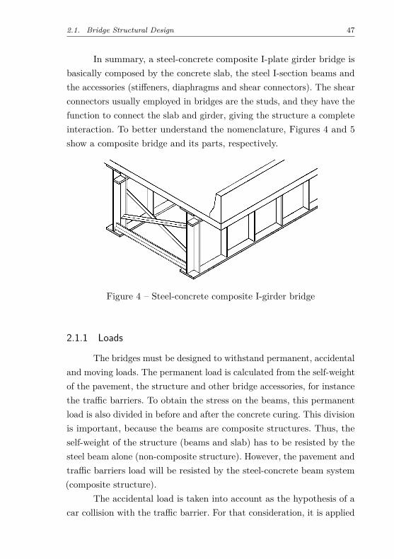
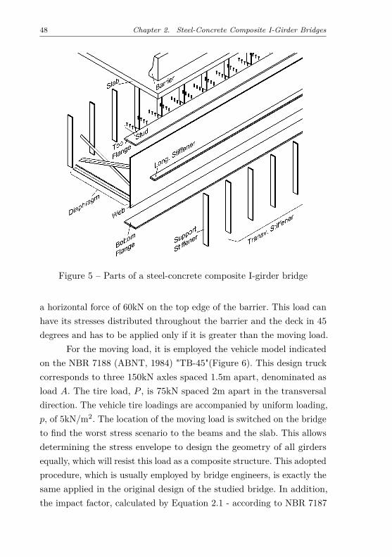
In summary, a steel-concrete composite I-plate girder bridge isbasically composed by the concrete slab, the steel I-section beams andthe accessories (stiffeners, diaphragms and shear connectors). The shearconnectors usually employed in bridges are the studs, and they have thefunction to connect the slab and girder, giving the structure a completeinteraction. To better understand the nomenclature, Figures 4 and 5show a composite bridge and its parts, respectively.
Figure 4 – Steel-concrete composite I-girder bridge
2.1.1 Loads
The bridges must be designed to withstand permanent, accidentaland moving loads. The permanent load is calculated from the self-weightof the pavement, the structure and other bridge accessories, for instancethe traffic barriers. To obtain the stress on the beams, this permanentload is also divided in before and after the concrete curing. This divisionis important, because the beams are composite structures. Thus, theself-weight of the structure (beams and slab) has to be resisted by thesteel beam alone (non-composite structure). However, the pavement andtraffic barriers load will be resisted by the steel-concrete beam system(composite structure).
The accidental load is taken into account as the hypothesis of acar collision with the traffic barrier. For that consideration, it is applied
48 Chapter 2. Steel-Concrete Composite I-Girder Bridges
Figure 5 – Parts of a steel-concrete composite I-girder bridge
a horizontal force of 60kN on the top edge of the barrier. This load canhave its stresses distributed throughout the barrier and the deck in 45degrees and has to be applied only if it is greater than the moving load.
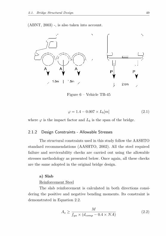
For the moving load, it is employed the vehicle model indicatedon the NBR 7188 (ABNT, 1984) "TB-45"(Figure 6). This design truckcorresponds to three 150kN axles spaced 1.5m apart, denominated asload A. The tire load, P , is 75kN spaced 2m apart in the transversaldirection. The vehicle tire loadings are accompanied by uniform loading,p, of 5kN/m2. The location of the moving load is switched on the bridgeto find the worst stress scenario to the beams and the slab. This allowsdetermining the stress envelope to design the geometry of all girdersequally, which will resist this load as a composite structure. This adoptedprocedure, which is usually employed by bridge engineers, is exactly thesame applied in the original design of the studied bridge. In addition,the impact factor, calculated by Equation 2.1 - according to NBR 7187
2.1. Bridge Structural Design 49
(ABNT, 2003) -, is also taken into account.
Figure 6 – Vehicle TB-45
ϕ = 1.4− 0.007× Lb[m] (2.1)
where ϕ is the impact factor and Lb is the span of the bridge.
2.1.2 Design Constraints - Allowable Stresses
The structural constraints used in this study follow the AASHTOstandard recommendations (AASHTO, 2002). All the steel requiredfailure and serviceability checks are carried out using the allowablestresses methodology as presented below. Once again, all these checksare the same adopted in the original bridge design.
a) SlabReinforcement SteelThe slab reinforcement is calculated in both directions consi-
dering the positive and negative bending moments. Its constraint isdemonstrated in Equation 2.2.
As ≥M
fya × (dcomp − 0.4×NA) (2.2)
50 Chapter 2. Steel-Concrete Composite I-Girder Bridges
where As is the reinforcement section area; M is the greatest bendingmoment on the slab; fya is the allowable yield strength of the steel;dcomp is the distance from compression face to centroid of tension rein-forcement; NA is the section neutral axis.
ShearThe shear stress in the slab is calculated in the moving load most
critical position and is verified by Equation 2.3.
τs ≤ τR × k(1.2 + 40ρ) + 0.15σc (2.3)
where τs is the slab shear stress; τR is the concrete shear stress resistance;k is a factor defined by the slab height; ρ is the reinforcement steel rate;σc is the slab normal stress.
Maximum DeflectionThe maximum vertical deflection is calculated (considering a
linear elastic model) in mid-span for the central slab and in the edgefor the lateral cantilever. Their corresponding limit values are definedin Equation 2.4 and 2.5, respectively.
∆ ≤ Lb800 (2.4)
∆ ≤ Lb300 (2.5)
where ∆ is deflection in mid-span or in the edge of the lateral cantilever;Lb is the span length.
b) GirdersAllowable StressEquations 2.6, 2.7, 2.8 and 2.9 are applied to define the allowable
stresses in the structure.
fbs ≤ 0.55× fy (2.6)
2.1. Bridge Structural Design 51
fbi ≤ 0.55× fy (2.7)
fv ≤ 0.33× fy (2.8)
fc ≤ 0.40× f ′c (2.9)
where fbs, fbi and fc are the maximum normal stresses on the top andbottom flange and slab, respectively; fv is the maximum shear stresson the beam web; fy is the yield strength of the steel; f ′c is the 28-daycompressive concrete strength.
As explained in Section 2.1.1, the self-weight of the structure(beams and deck) has to be resisted by the steel beam alone (non-composite structure). However, the pavement and traffic barriers loadwill be resisted by the steel-concrete beam system (composite structure).
Maximum DeflectionThe maximum deflection is calculated in mid-span with corres-
ponding value defined by Equation 2.10.
∆ ≤ Lb800 (2.10)
Again, the girder deflections must be verified at the constructionstage (non-composite structure) as well as in the final composite confi-guration.
c) AccessoriesShear ConnectorThe number of studs, used as shear connectors, is determined
based on fatigue considerations and the shear stress on the bridge section.In addition, it has two size constraints to be followed (Equations 2.11and 2.12)
hstud ≥ 4× dstud (2.11)
52 Chapter 2. Steel-Concrete Composite I-Girder Bridges
dstud ≤ 2.5× ts (2.12)
where hstud and dstud are the height and diameter of the stud; ts is thebeam top flange thickness.
Support StiffenerThe support stiffener is defined by the following constraints.
bsa ≤bs − tw
2 (2.13)
tsa ≥bsa12
√fy
22.8[ kNcm2 ](2.14)
Fsa ≥V
Ass(2.15)
where bsa and tsa are the width and thickness of the support stiffener;bs is the beam top flange width; tw is the beam web thickness; Fsa isthe stiffener allowable stress; V is the design shear force on the support;Ass is the area of the stiffener.
Transversal StiffenerThe transversal stiffeners shall be employed when the following
Equations 2.16, 2.17 and 2.18 are satisfied.
tw ≤hv150 (2.16)
fv ≥ Fve (2.17)
Fve ≤ Fv (2.18)
where hv is the beam web height; Fve is the shear stress on the transversalstiffener; Fv is the allowable shear stress on the beam web.
2.1. Bridge Structural Design 53
When the use of transversal stiffeners is necessary, its size isdefined following the constraints in Equations 2.19, 2.20, 2.21, 2.22 and2.23.
bst ≥ 5 + hv30[cm] (2.19)
bst ≥bs4 (2.20)
tst ≥bst16 (2.21)
At ≥ Atmin = [0.15hvtw
(1− c) fvFv− 18] fy
Fcrt2w (2.22)
It ≥ Itmin = d1 × t3w × j (2.23)
where bst and tst are the width and thickness of the transversal stiffener;At and Atmin are the area and the minimum area of the stiffener; cis a factor equal 1 for a pair of stiffeners; Fcr is the critical bucklingstress for plates; It and Itmin are the inertia and the minimum inertiaof the stiffener; d1 is the distance between each transversal stiffener; jis a factor defined by j = 2.5(hv
d1)2 − 2 ≥ 0.5.
Longitudinal StiffenerSimilarly as for the transversal stiffener, the algorithm first detects
the necessity of the longitudinal stiffener using Equations 2.24 and 2.25.
tw ≤hv170 (2.24)
tw ≤ hv√fbs
600 (2.25)
If the use is necessary, then the stiffener is defined following theconstraints in Equations 2.26, 2.27, 2.28 and 2.29.
bsl ≥ 5 + hv30[cm] (2.26)
54 Chapter 2. Steel-Concrete Composite I-Girder Bridges
bsl ≥bs4 (2.27)
tsl ≥bsl16 (2.28)
Is ≥ Ismin = hv × t3w[2.4 d21h2v
− 0.13] (2.29)
where bsl and tsl are the width and thickness of the longitudinal stiffener;Is and Ismin are the inertia and the minimum inertia of the stiffener.
When using this stiffener it is important to check the beam webusing the constrains defined by Equations 2.30 and 2.31.
tw ≤hv340 (2.30)
tw ≤ hv√fbs
1200 (2.31)
DiaphragmThe diaphragms are checked by its slenderness and maximum
spacing (Equations 2.32, 2.33 and 2.34).
ndiaf ≥Lb7.6 + 1 (2.32)
rdiaf ≥12b2
120 (2.33)
rdiaf ≥√b22 + (ts + hv + ti)2
200 (2.34)
where ndiaf is the number of diaphragms used; rdiaf is the perpendicularradius of gyration of the diaphragm section; b2 is the width betweenbeams.
2.1. Bridge Structural Design 55
2.1.3 Design Constraints - Limit and Resistance Factor Design
Aiming to consider the influence of the design methodology inthe optimum results, it will be also employed the AASHTO (2012)LRFD based approach. The checks for failure and serviceability of thismethodology are listed below.
a) SlabReinforcement SteelThe slab reinforcement is calculated in both directions consi-
dering the positive and negative bending moments. Its constraint isdemonstrated in Equation 2.35.
As ≥Mu
fy × (dcomp − 0.4×NA) (2.35)
where Mu is the moment due to factored loads.
b) GirderLimit and Resistance Factor DesignEquations 2.36 to 2.40 are applied to define the structure.
Mu ≤Mn (2.36)
Iyc ≤ 0.9× Iy (2.37)
Iyc ≥ 0.1× Iy (2.38)
bs2ts≤ 1.38
√√√√ Es
fcomp√
2Dc
tw
(2.39)
Vd1 ≤ Vn (2.40)
where Mn is the nominal flexural resistance based on the tension flange;Iyc is the moment of inertia of the compression flange of a steel section
56 Chapter 2. Steel-Concrete Composite I-Girder Bridges
about the vertical axis in the plane of the web; Iy is the moments ofinertia about the minor principal axis of the cross-section; fcomp isthe compression-flange stress at the section under consideration; Dc
is the depth of the web in compression in the elastic range; Vd1 is theshear due to the factored loads considering the presence of a transversalstiffener; Vn is the nominal shear resistance.
c) AccessoriesSupport StiffenerThe support stiffener shall be employed when the following Equa-
tion is satisfied:
Vu ≥ Vn (2.41)
After verifying its need, it is defined by the following constraints.
Vu ≤ Vn,sup (2.42)
bsa ≥ 0.25× bs (2.43)
bsa ≤ 0.48× tsa
√Esfy
(2.44)
bsa ≤ 16× tsa (2.45)
bsa ≥ 2× 2.54 + hv30[cm] (2.46)
where Vu is the shear due to the factored loads; Vn,sup is the supportstiffener nominal shear resistance.
Transversal StiffenerThe transversal stiffeners, as the support stiffener, also shall be
employed when the Equation 2.41 is satisfied. Its design follows the
2.2. Structural Analysis 57
same rules as the support stiffener.
Longitudinal StiffenerSimilarly as for the other stiffeners, the algorithm first detects
the necessity of the longitudinal stiffener using Equation 2.47.
2Dc
tw≥ 6.77
√Es
fcomp(2.47)
If the use is necessary, then the stiffener is defined following theconstraints in Equations 2.48, 2.49, 2.50 and 2.51.
bsl ≥ 5 + hv30[cm] (2.48)
bsl ≥bs4 (2.49)
tsl ≥bsl16 (2.50)
tw ≥ hv340 (2.51)
d) Other verificationsThe slab and girder maximum deflection, slab shear, shear connec-
tors and diaphragms are calculated in the same way as in the AllowableStress methodology.
2.2 Structural Analysis
There are different structural analyses techniques available tobridge engineers accomplish the structural design. They vary from simplecode recommendations to more complex procedures. Usually, this choiceis based on the engineer preference and his experience.
58 Chapter 2. Steel-Concrete Composite I-Girder Bridges
For instance, AASHTO (2012) suggests the application of sim-plified formulas when the structure is inside predetermined intervals.Nevertheless, whether these conditions are not valid it is recommended,for example, the application of the Level Rule, which will be explainedin Section 2.2.1.
In addition, other structural analyses’ simplified procedures com-mon for bridge engineers are the Engesser-Courbon, the Leonhardtand the Fauchart approaches. The first considers that the girders areconnected through a rigid beam, while the second takes into account thegrid effect. The Fauchart Method is adopted in the present dissertation.Differently from the previous schemes, it does not consider the existenceof beams connecting the bridge girders. More details on this approachwill be given in Section 2.2.1.
A more refined model to determine the stress distribution onthe structure can be constructed using the Finite Element Method(FEM). Despite it being a more complex methodology, requiring acareful engineering interpretation, it is expected to achieve more preciseresults. This method, also used in this dissertation, is described inSection 2.2.2.
2.2.1 Simplified Models
The simplified static models are usually employed by bridge de-signers. The deck stresses are found using Rüsch’s tables (RÜSCH,1965), which are added to the Annex. To determine the load in girdersoriginated from the vehicle model many different methodologies can beapplied. This dissertation will use the conventional Level Rule and theFauchart model, both described below.
a) Level Rule (LR)The level rule is used by many designers, being the most simplified
way to determine the girders loads. This method was chosen becauseit is applicable in all situations, not being limited by the range ofapplicability of AASHTO approximate formulas, and was the one used
2.2. Structural Analysis 59
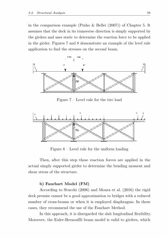
in the comparison example (Pinho & Bellei (2007)) of Chapter 5. Itassumes that the deck in its transverse direction is simply supported bythe girders and uses static to determine the reaction force to be appliedin the girder. Figures 7 and 8 demonstrate an example of the level ruleapplication to find the stresses on the second beam.
Figure 7 – Level rule for the tire load
Figure 8 – Level rule for the uniform loading
Then, after this step these reaction forces are applied in theactual simply supported girder to determine the bending moment andshear stress of the structure.
b) Fauchart Model (FM)According to Stucchi (2006) and Moura et al. (2016) the rigid
deck premise cannot be a good approximation to bridges with a reducednumber of cross-beams or when it is employed diaphragms. In thesecases, they recommend the use of the Fauchart Method.
In this approach, it is disregarded the slab longitudinal flexibility.Moreover, the Euler-Bernoullli beam model is valid to girders, which
60 Chapter 2. Steel-Concrete Composite I-Girder Bridges
are considered self-supported and with constant moment of inertia.From that, the first equations can be drawn. Equation 2.52 states
that the girder element alone have to obey the differential equation ofthe elastic line:
d4w
dx4 = p(x)EIy
(2.52)
where w is the vertical displacement in each x point; E is the elasticmodulus; Iy is the cross sectional inertia; p(x) is the uniform loading.
The girder also is governed by the torsion differential equation(Equation 2.53):
d2θ
dx2 = m(x)GJt
(2.53)
where θ is the torsion angle in each x point; G is the shear modulus; Jtis the torsional inertia; m(x) is the uniform distributed torsion moment.
Using the Fourier series, these differential equations are transfor-med in algebraic equations. After all the mathematical manipulations itresults in Equations 2.54 and 2.55.
kv = EIy( πLb
)4 (2.54)
kt = GJt(π
Lb)2 (2.55)
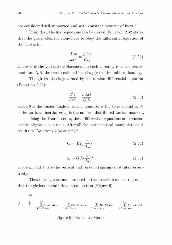
where kv and kt are the vertical and torsional spring constants, respec-tively.
Those spring constants are used in the structure model, represen-ting the girders in the bridge cross section (Figure 9).
Figure 9 – Fauchart Model
2.2. Structural Analysis 61
From this model it is possible to obtain the influence lines andthe resultant forces for each load configuration.
2.2.2 Finite Element Model (FEM)
It was developed an in-house Matlab FEM code to representthe bridge structure. For further details on this subject, the reader isreferred to Ferreira (2008) and Vaz (2011) and the references therein.
The girders are modeled using a 2-node, 6-DOF, Euler-Bernoulliframe element. The bridge deck is represented through a 4-node rec-tangular shell element. It is a composition of a membrane and a plateelement. The eccentricity between the slab mid-surface and the beamaxis is considered by introducing a rigid link.
This section describes the methodology used for each element ofthe model.
a) Frame ElementThe girders are modeled using a 2-node, 6-DOF per node (3
translations and 3 rotations), Euler-Bernoulli frame element. It is em-ployed linear polynomials to represent longitudinal displacements u(x)and torsion rotations θx(x) whereas cubic polynomials to describe thetransversal displacements v(x) and w(x), as shown in Equations 2.56and 2.57: u(x) = α1 + α2x
θx(x) = α1 + α2x(2.56)
v(x) = α3 + α4x+ α5x2 + α6x
3
w(x) = α3 + α4x+ α5x2 + α6x
3
dv(x)dx = θz(x)dw(x)dx = θy(x)
(2.57)
where u(x), θx(x), v(x), w(x), θz(x) and θy(x)are the displacementsfunction; αi for i = 1...6 are the polynomial parameters.
62 Chapter 2. Steel-Concrete Composite I-Girder Bridges
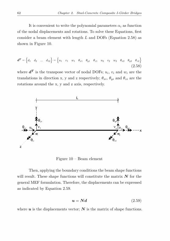
It is convenient to write the polynomial parameters αi as functionof the nodal displacements and rotations. To solve these Equations, firstconsider a beam element with length L and DOFs (Equation 2.58) asshown in Figure 10.
dT =d1 d2 ... d12
=
u1 v1 w1 θx1 θy1 θz1 u2 v2 w2 θx2 θy2 θz2
(2.58)
where dT is the transpose vector of nodal DOFs; ui, vi and wi are thetranslations in direction x, y and z respectively; θxi, θyi and θzi are therotations around the x, y and z axis, respectively.
Figure 10 – Beam element
Then, applying the boundary conditions the beam shape functionswill result. These shape functions will constitute the matrix N for thegeneral MEF formulation. Therefore, the displacements can be expressedas indicated by Equation 2.59.
u = Nd (2.59)
where u is the displacements vector; N is the matrix of shape functions.
2.2. Structural Analysis 63
Then, the strain can be obtained from Equation 2.59, makingthe derivative of matrix N in x. It results in Equation 2.60.
ε = Lu = LNd = Bd (2.60)
where ε is the strain vector; L is the matrix containing the differentialoperators; B is the strain-displacement matrix, that contains the spatialderivatives of the x variable.
The stresses in the element are obtained through the Hooke’sLaw (Equation 2.61).
σ = Cε (2.61)
where σ is the stress vector; C is the matrix of constitutive relations,which for an isotropic material depends only of: E, elastic modulus andν, Poisson coefficient.
Therefore, using the matrices N , B and C and applying thePrinciple of Virtual Work (Equation 2.62), the stiffness matrix K andthe equivalent nodal forces vector ff are determined.
∫ V
0δεtσdV =
∫ V
0δutqdV +
∫ Γ
0δutpdΓ + δdtf (2.62)
where q, p and f are the body forces, the surface tractions and thenodal forces vectors, respectively; δε is the virtual strain vector; δu isthe virtual displacement vector; δd is the virtual nodal displacementsvector.
The virtual strain vector and the virtual displacement vector canbe written according to Equations 2.63 and 2.64.
δu = Nδd (2.63)
δε = Bδd (2.64)
64 Chapter 2. Steel-Concrete Composite I-Girder Bridges
Thus, substituting these expressions and the Equations 2.59, 2.60and 2.61 in Equation 2.62, it is found the Equation 2.65.
δdt
∫ V
0BtCBdV d = δdt(
∫ V
0N tqdV +
∫ Γ
0N tpdΓ + f) (2.65)
Because the virtual nodal displacements vector is arbitrary, itmay be eliminated, resulting in Equation 2.66.
Kd = fq + fp + f (2.66)
where fq, fp are the equivalent nodal forces vector corresponding tothe body and surface tractions while f is the nodal forces vector itself.
The stiffness matrices and force vectors of each element arecombined adequately to properly form the structure global matrix Kg
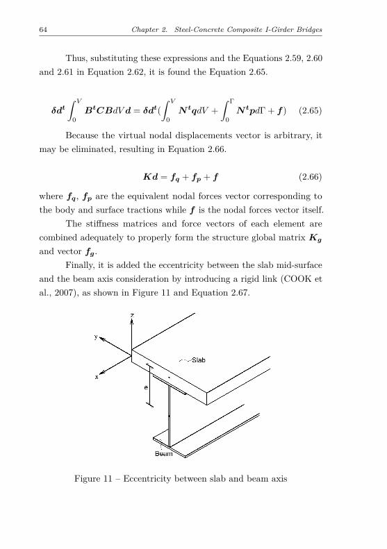
and vector fg.Finally, it is added the eccentricity between the slab mid-surface
and the beam axis consideration by introducing a rigid link (COOK etal., 2007), as shown in Figure 11 and Equation 2.67.
Figure 11 – Eccentricity between slab and beam axis
2.2. Structural Analysis 65
uxb
uzb
θyb
= TB
uxp
uzp
θyp
(2.67)
TB =
1 0 −e0 1 00 0 1
(2.68)
where uxb is the beam nodal displacement in x; uzb is the beam nodaldisplacement in z; θyb is the beam nodal rotation around y; uxp is theplate nodal displacement in x; uzp is the plate nodal displacement inz; θyp is the plate nodal rotation around y; TB is the transformationmatrix relating the beam nodal displacements and rotations with theshell nodal displacements and rotations; e is the eccentricity betweenslab and beam axis.
b) Shell ElementThe bridge deck is represented by a 4-node rectangular shell
element. It is a composition of a membrane and a plate element. Theplate is designed by the Mindlin theory, which makes the followingconsiderations:
• a normal to the shell mid-section, straight line keeps being straightafter the forces application. However, it does not necessarily keepbeing perpendicular to the surface;
• there is only vertical displacements, w(x, y, z);
• the strain, εz, is zero at any plate point.
The plate displacements are defined by Equation 2.69. From that,the strain matrix (Equation 2.70) can be deduced and simplified by
66 Chapter 2. Steel-Concrete Composite I-Girder Bridges
Equation 2.71. u(x, y, z) = zθy
v(x, y, z) = −zθxw(x, y, z) = 0
(2.69)
εx
εy
λxy
λyz
λxz
=
z 0 0 0 00 z 0 0 00 0 z 0 00 0 0 1 00 0 0 0 1
θy,x
−θx,yθy,y − θx,xw,y − θxw,x + θy
(2.70)
εb
εs
= TMkM =
[Tb 00 Ts
] kb
ks
(2.71)
where u, v and w are the displacements in the x, y and z directions,respectively; θx and θy are the rotations around the x and y axis,respectively; εx and εy are the strains in the directions indicated by theindex; λxy, λyz and λxz are the transverse shear deformations in theplane indicated by the index; εb and εs represents the vector of strainsand shear deformations; TM is the Mindlin transformation matrix,subdivided in Tb and Ts; kM is the Mindlin curvature and transverseshear strain vector, subdivided in kb and ks.
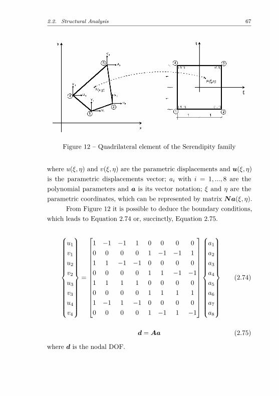
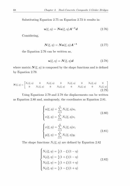
To continue the deductions of the finite element it is chosen touse the isoparametric element of the Serendipity family. A isoparametricelement uses the same shape functions for kinematic purposes and forgeometric measurements. Thus, the field that describes the Cartesiancoordinates of a quadrilateral element must be a 4th term polynomialwith parametric coordinates (Figure 12 and Equation 2.72 or, in short,Equation 2.73 ). u(ξ, η) = a1 + a2ξ + a3η + a4ξη
v(ξ, η) = a5 + a6ξ + a7η + a8ξη(2.72)
u(ξ, η) = Na(ξ, η)a (2.73)
2.2. Structural Analysis 67
Figure 12 – Quadrilateral element of the Serendipity family
where u(ξ, η) and v(ξ, η) are the parametric displacements and u(ξ, η)is the parametric displacements vector; ai with i = 1, ..., 8 are thepolynomial parameters and a is its vector notation; ξ and η are theparametric coordinates, which can be represented by matrix Na(ξ, η).
From Figure 12 it is possible to deduce the boundary conditions,which leads to Equation 2.74 or, succinctly, Equation 2.75.
u1
v1
u2
v2
u3
v3
u4
v4
=
1 −1 −1 1 0 0 0 00 0 0 0 1 −1 −1 11 1 −1 −1 0 0 0 00 0 0 0 1 1 −1 −11 1 1 1 0 0 0 00 0 0 0 1 1 1 11 −1 1 −1 0 0 0 00 0 0 0 1 −1 1 −1
a1
a2
a3
a4
a5
a6
a7
a8
(2.74)
d = Aa (2.75)
where d is the nodal DOF.
68 Chapter 2. Steel-Concrete Composite I-Girder Bridges
Substituting Equation 2.75 on Equation 2.73 it results in:
u(ξ, η) = Na(ξ, η)A−1d (2.76)
Considering,
N(ξ, η) = Na(ξ, η)A−1 (2.77)
the Equation 2.76 can be written as,
u(ξ, η) = N(ξ, η)d (2.78)
where matrix N(ξ, η) is composed by the shape functions and is definedby Equation 2.79.
N(ξ, η) =[N1(ξ, η) 0 N2(ξ, η) 0 N3(ξ, η) 0 N4(ξ, η) 0
0 N1(ξ, η) 0 N2(ξ, η) 0 N3(ξ, η) 0 N4(ξ, η)
](2.79)
Using Equations 2.79 and 2.78 the displacements can be writtenas Equation 2.80 and, analogously, the coordinates as Equation 2.81.
u(ξ, η) =4∑i=1
Ni(ξ, η)ui
v(ξ, η) =4∑i=1
Ni(ξ, η)vi(2.80)
x(ξ, η) =
4∑i=1
Ni(ξ, η)xi
y(ξ, η) =4∑i=1
Ni(ξ, η)yi(2.81)
The shape functions Ni(ξ, η) are defined by Equation 2.82
N1(ξ, η) = 14 (1− ξ)(1− η)
N2(ξ, η) = 14 (1 + ξ)(1− η)
N3(ξ, η) = 14 (1 + ξ)(1 + η)
N4(ξ, η) = 14 (1− ξ)(1 + η)
(2.82)
2.2. Structural Analysis 69
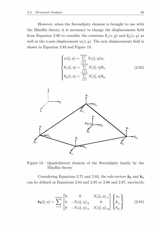
However, when the Serendipity element is brought to use withthe Mindlin theory, it is necessary to change the displacements fieldfrom Equation 2.80 to consider the rotations θx(x, y) and θy(x, y) aswell as the z-axis displacement w(x, y). The new displacements field isshown in Equation 2.83 and Figure 13.
w(ξ, η) =nnos∑i=1
Ni(ξ, η)wi
θx(ξ, η) =nnos∑i=1
Ni(ξ, η)θxi
θy(ξ, η) =nnos∑i=1
Ni(ξ, η)θyi
(2.83)
Figure 13 – Quadrilateral element of the Serendipity family by theMindlin theory
Considering Equations 2.71 and 2.83, the sub-vectors kb and ks
can be defined as Equations 2.84 and 2.85 or 2.86 and 2.87, succinctly.
kb(ξ, η) =nnos∑i=1
0 0 Ni(ξ, η),x0 −Ni(ξ, η),y 00 −Ni(ξ, η),x Ni(ξ, η),y
wi
θxi
θyi
(2.84)
70 Chapter 2. Steel-Concrete Composite I-Girder Bridges
ks(ξ, η) =nnos∑i=1
[Ni(ξ, η),x 0 Ni(ξ, η)Ni(ξ, η),y −Ni(ξ, η) 0
] wi
θxi
θyi
(2.85)
kb(ξ, η) = Bb(ξ, η)d (2.86)
ks(ξ, η) = Bs(ξ, η)d (2.87)
whereBb is the bending strain-displacement matrix;Bs is the transverseshear strain-displacement matrix.
Using Equations 2.86 and 2.87 the compatibility Equation 2.71can be rewritten as: εb(ξ, η, z) = zBb(ξ, η)d
εs(ξ, η) = Bs(ξ, η)d(2.88)
Considering those Equations and the Hooke Law, Equation 2.89is obtained. σb(ξ, η, z) = zCbBb(ξ, η)d
σs(ξ, η) = CsBs(ξ, η)d(2.89)
where Cb is the bending constitutive matrix; Cs is the transverse shearconstitutive matrix.
Then, using the Principle of Virtual Work it is possible to obtainthe stiffness matrix. For that, the virtual strains will be:δεb(ξ, η, z) = zBb(ξ, η)δd
δεs(ξ, η) = Bs(ξ, η)δd(2.90)
where δεb(ξ, η, z) is the bending virtual strain vector; δεs(ξ, η) is thetransversal shear virtual strain vector; δd is the vector of virtual nodalDOF.
2.2. Structural Analysis 71
Applying the Principle of Virtual Work separately for bendingand shear it is obtained:∫
V
δεtbσbdv +
∫V
δεtsσsdv = δdtf (2.91)
δdt(∫A
Bb(ξ, η)t∫ t
2
−t2
z2CbdtBb(ξ, η)dA
+∫A
Bs(ξ, η)t∫ t
2
−t2
CsdtBs(ξ, η)dA)d = δdtf
(2.92)
where the integrals in V and A are volume and area integrals; t is theplate height; f is the forces vector.
As δd is arbitrary, it can be eliminated from Equation 2.92.Considering that Db = t3
12Cb and Ds = tCs and integrating in theheight, it results in:
(∫A
Bb(ξ, η)tDbBb(ξ, η)dA+∫A
Bs(ξ, η)tDsBs(ξ, η)dA)d = f
(2.93)Or, in short:
(Kb +Ks)d = f (2.94)
whereKb is the plate bending stiffness matrix;Ks is the plate transverseshear stiffness matrix.
It is important to highlight that, as Bb and Bs are functions ofparametric variables ξ and η, the integrations of Equation 2.93 will bemade using the Gaussian quadrature.
The plate stiffness matrix is, then, found combining both thebending and transverse shear stiffness matrices, as shown in Equation2.95.
Kp =[Kb 00 Ks
](2.95)

72 Chapter 2. Steel-Concrete Composite I-Girder Bridges
The membrane element follows the same deduction logic as theplate, however it is modelled considering the plane displacements uiand vi. Then, to obtain the shell element matrix, the membrane andplate elements are combined in Equation 2.96. For the final element therotation around the slab perpendicular axis is disregarded.
Kshell =[Km 0
0 Kp
](2.96)
where Kshell is the shell stiffness matrix (20x20); Km is the membranestiffness matrix (8x8); Kp is the plate stiffness matrix (12x12).
73
Chapter 3
Fundamentals of Optimization
This chapter describes an overview on engineering optimization.Firstly, general concepts of optimization are shown. Then, the heuristicalgorithms employed in this dissertation are detailed. Finally, the statis-tic tests used to compare the efficiency between algorithms are explained.For further details on the matter, the reader is referred to Arora (2004),Civicioglu (2013), Yang (2010), Holland (1975), Atashpaz-Gargari &Lucas (2007), Gonçalves, Lopez & Miguel (2015), Schervish (2012) andthe references therein.
3.1 General Concepts
The practical use of optimization processes begins with the defi-nition of, at least, one objective, which is the performance mode thatthe system will be analyzed. It can be, for example, a structure costminimization. This objective is dependent of certain system characte-ristics, which are called design variables. The optimization goal is tofind the design variable values that give the best value for the objective.Sometimes these variables are limited to certain values which results ina restricted optimization problem. Thereby, an optimization problemcan be divided in the following elements:
• Objective function: function associated with the analyzed system
74 Chapter 3. Fundamentals of Optimization
parameters and used to measure its performance. Mathematicallyit can be described as the function J proving the system perfor-mance value associated with n parameters with real values. Asan example it can be considered the concrete volume of a bridgebeam;
• Design variables: parameters that define the system, which can bemodified by the designer to improve its performance. In mathema-tics, it can be considered the vector x = (x1, ..., xn) with n realadjustable parameters. This value is associated with the region V .In the previous example, the design variables x1 and x2 can bethe height and width of the beam cross section, respectively;
• Restrictions: limitations to the designers choices. In general, itis a not empty sub-domain of V , here called S. In the beamproblem a relation between design variables can be imposed, suchas 0, 5 ≤ x2
x1≤ 1, 0.
Then, an optimization problem can be described as Equation 3.1.
x∗ = argminJ(x) : x ∈ S (3.1)
where J is the function to be minimized; x are the design variables;S = gj(x) ≤ 0, 1 ≤ i ≤ nc, hj(x) = 0, 1 ≤ j ≤ ne is the projectadmissible region, gj and hj are the inequality and equality restrictions,respectively.
The problem consists in identifying the J global minimum, findinga x∗ ∈ S that J(x∗)∀x ∈ S. Note that if neither the J nor the S areconvex there can be a local minimum, x∗ ∈ S that J(x∗) ≤ J(x)∀x ∈S/ ‖ x− x∗ ‖≤ ε, ε > 0.
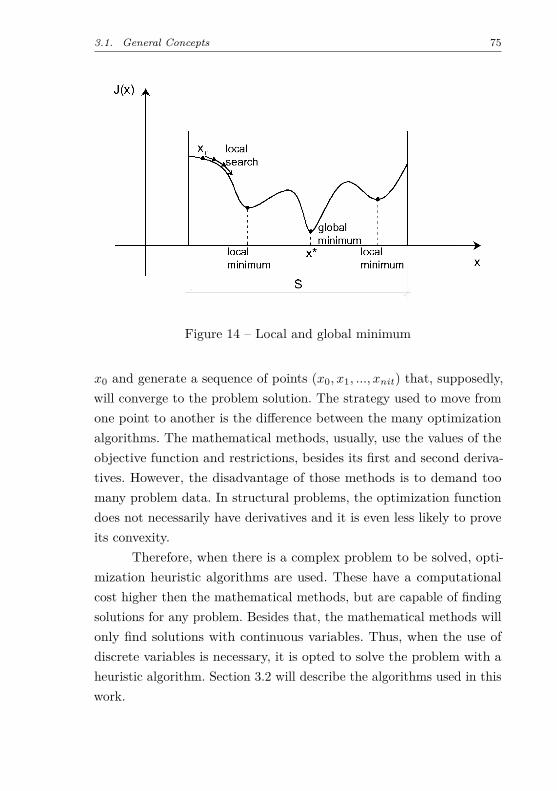
In general situations there can be many local and global mini-mums. Figure 14 shows an example of an one variable function with twolocal minimums and only one global minimum. Between the minimums,the one with the smaller value of J is the global minimum.
It is important to highlight that, generally, optimization algo-rithms are iterative. They begin with a design variable initial value
3.1. General Concepts 75
Figure 14 – Local and global minimum
x0 and generate a sequence of points (x0, x1, ..., xnit) that, supposedly,will converge to the problem solution. The strategy used to move fromone point to another is the difference between the many optimizationalgorithms. The mathematical methods, usually, use the values of theobjective function and restrictions, besides its first and second deriva-tives. However, the disadvantage of those methods is to demand toomany problem data. In structural problems, the optimization functiondoes not necessarily have derivatives and it is even less likely to proveits convexity.
Therefore, when there is a complex problem to be solved, opti-mization heuristic algorithms are used. These have a computationalcost higher then the mathematical methods, but are capable of findingsolutions for any problem. Besides that, the mathematical methods willonly find solutions with continuous variables. Thus, when the use ofdiscrete variables is necessary, it is opted to solve the problem with aheuristic algorithm. Section 3.2 will describe the algorithms used in thiswork.

76 Chapter 3. Fundamentals of Optimization
3.2 Algorithms
The algorithms used in this study are well known optimizationheuristic algorithms: Backtracking Search Algorithm (BSA), FireflyAlgorithm (FA), Genetic Algorithm (GA), Imperialist CompetitiveAlgorithm (ICA) and Search Group Algorithm (SGA). The operationof each one will be detailed in the next subsections.
3.2.1 Backtracking Search Algorithm (BSA)
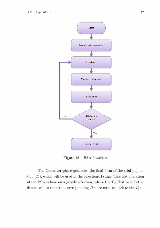
The Backtracking Search Algorithm (BSA) is an evolutionaryalgorithm created by Civicioglu (2013). It is a population based ite-rative algorithm divided into five processes: Initialization, Selection-I,Mutation, Crossover and Selection-II.
Algorithm 1 shows the BSA general structure.
Algorithm 1 General Structure of BSAprocedure BSA
Initializationloop:Selection-IMutationCrossoverSlection-IIgo to loop until stopping conditions are metend
After the initialization of the population, the Selection-I stagedetermines the historical population of the algorithm. Then, the Muta-tion generates a new population, which is based on the results of thetwo previous stages, as shown in Equation 3.2,
Mutant = Pop+ F (oldP − P ) (3.2)
where Pop is the population created in the Initialization process; oldP isthe historical population; F is a random value to control the amplitudeof (oldP − P ).
3.2. Algorithms 77
Figure 15 – BSA flowchart
The Crossover phase generates the final form of the trial popula-tion (Ti), which will be used in the Selection-II stage. This last operationof the BSA is base on a greedy selection, where the Tis that have betterfitness values than the corresponding Pis are used to update the Pis.
78 Chapter 3. Fundamentals of Optimization
3.2.2 Firefly Algorithm (FA)
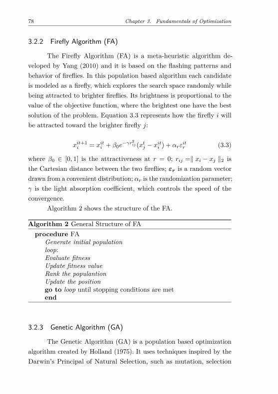
The Firefly Algorithm (FA) is a meta-heuristic algorithm de-veloped by Yang (2010) and it is based on the flashing patterns andbehavior of fireflies. In this population based algorithm each candidateis modeled as a firefly, which explores the search space randomly whilebeing attracted to brighter fireflies. Its brightness is proportional to thevalue of the objective function, where the brightest one have the bestsolution of the problem. Equation 3.3 represents how the firefly i willbe attracted toward the brighter firefly j:
xit+1i = xiti + β0e
−γr2ij (xtj − xiti ) + αrε
itr (3.3)
where β0 ∈ [0, 1] is the attractiveness at r = 0; rij =‖ xi − xj ‖2 isthe Cartesian distance between the two fireflies; εr is a random vectordrawn from a convenient distribution; αr is the randomization parameter;γ is the light absorption coefficient, which controls the speed of theconvergence.
Algorithm 2 shows the structure of the FA.
Algorithm 2 General Structure of FAprocedure FA
Generate initial populationloop:Evaluate fitnessUpdate fitness valueRank the populantionUpdate the positiongo to loop until stopping conditions are metend
3.2.3 Genetic Algorithm (GA)
The Genetic Algorithm (GA) is a population based optimizationalgorithm created by Holland (1975). It uses techniques inspired by theDarwin’s Principal of Natural Selection, such as mutation, selection
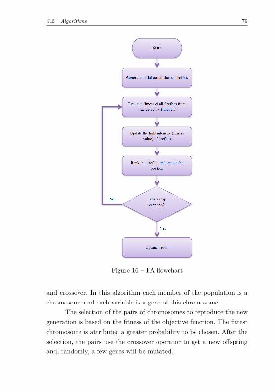
3.2. Algorithms 79
Figure 16 – FA flowchart
and crossover. In this algorithm each member of the population is achromosome and each variable is a gene of this chromosome.
The selection of the pairs of chromosomes to reproduce the newgeneration is based on the fitness of the objective function. The fittestchromosome is attributed a greater probability to be chosen. After theselection, the pairs use the crossover operator to get a new offspringand, randomly, a few genes will be mutated.
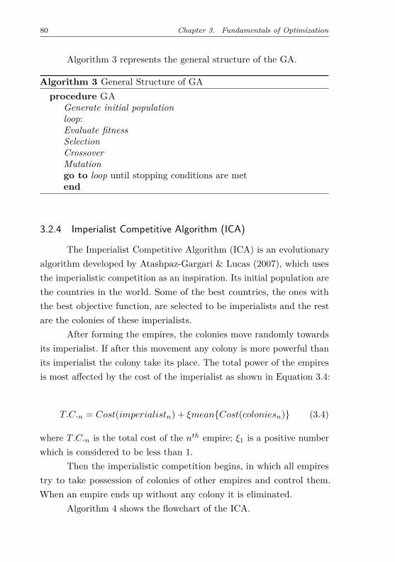
80 Chapter 3. Fundamentals of Optimization
Algorithm 3 represents the general structure of the GA.
Algorithm 3 General Structure of GAprocedure GA
Generate initial populationloop:Evaluate fitnessSelectionCrossoverMutationgo to loop until stopping conditions are metend
3.2.4 Imperialist Competitive Algorithm (ICA)
The Imperialist Competitive Algorithm (ICA) is an evolutionaryalgorithm developed by Atashpaz-Gargari & Lucas (2007), which usesthe imperialistic competition as an inspiration. Its initial population arethe countries in the world. Some of the best countries, the ones withthe best objective function, are selected to be imperialists and the restare the colonies of these imperialists.
After forming the empires, the colonies move randomly towardsits imperialist. If after this movement any colony is more powerful thanits imperialist the colony take its place. The total power of the empiresis most affected by the cost of the imperialist as shown in Equation 3.4:
T.C.n = Cost(imperialistn) + ξmeanCost(coloniesn) (3.4)
where T.C.n is the total cost of the nth empire; ξ1 is a positive numberwhich is considered to be less than 1.
Then the imperialistic competition begins, in which all empirestry to take possession of colonies of other empires and control them.When an empire ends up without any colony it is eliminated.
Algorithm 4 shows the flowchart of the ICA.
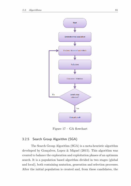
3.2. Algorithms 81
Figure 17 – GA flowchart
3.2.5 Search Group Algorithm (SGA)
The Search Group Algorithm (SGA) is a meta-heuristic algorithmdeveloped by Gonçalves, Lopez & Miguel (2015). This algorithm wascreated to balance the exploration and exploitation phases of an optimumsearch. It is a population based algorithm divided in two stages (globaland local), both containing mutation, generation and selection processes.After the initial population is created and, from these candidates, the
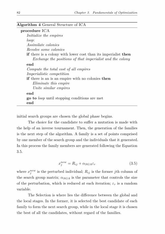
82 Chapter 3. Fundamentals of Optimization
Algorithm 4 General Structure of ICAprocedure ICA
Initialize the empiresloop:Assimilate coloniesRevolve some coloniesif there is a colony with lower cost than its imperialist then
Exchange the positions of that imperialist and the colonyendCompute the total cost of all empiresImperialistic competitionif there is an is an empire with no colonies then
Eliminate this empireUnite similar empires
endgo to loop until stopping conditions are metend
initial search groups are chosen the global phase begins.The choice for the candidate to suffer a mutation is made with
the help of an inverse tournament. Then, the generation of the familiesis the next step of the algorithm. A family is a set of points comprisedby one member of the search group and the individuals that it generated.In this process the family members are generated following the Equation3.5.
xnewj = Rij + αSGAεr (3.5)
where xnewj is the perturbed individual; Rij is the former jth column ofthe search group matrix; αSGA is the parameter that controls the sizeof the perturbation, which is reduced at each iteration; εr is a randomvariable.
The Selection is where lies the difference between the global andthe local stages. In the former, it is selected the best candidate of eachfamily to form the next search group, while in the local stage it is chosenthe best of all the candidates, without regard of the families.
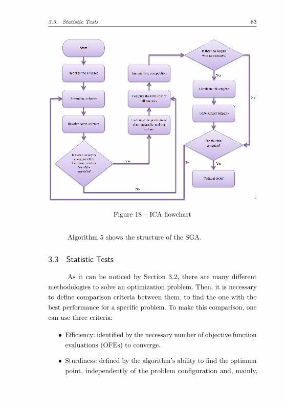
3.3. Statistic Tests 83
Figure 18 – ICA flowchart
Algorithm 5 shows the structure of the SGA.
3.3 Statistic Tests
As it can be noticed by Section 3.2, there are many differentmethodologies to solve an optimization problem. Then, it is necessaryto define comparison criteria between them, to find the one with thebest performance for a specific problem. To make this comparison, onecan use three criteria:
• Efficiency: identified by the necessary number of objective functionevaluations (OFEs) to converge.
• Sturdiness: defined by the algorithm’s ability to find the optimumpoint, independently of the problem configuration and, mainly,
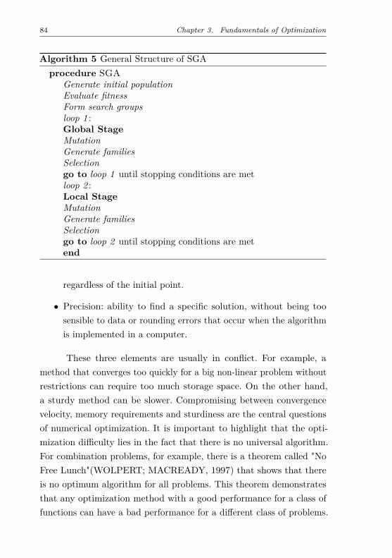
84 Chapter 3. Fundamentals of Optimization
Algorithm 5 General Structure of SGAprocedure SGA
Generate initial populationEvaluate fitnessForm search groupsloop 1 :Global StageMutationGenerate familiesSelectiongo to loop 1 until stopping conditions are metloop 2 :Local StageMutationGenerate familiesSelectiongo to loop 2 until stopping conditions are metend
regardless of the initial point.
• Precision: ability to find a specific solution, without being toosensible to data or rounding errors that occur when the algorithmis implemented in a computer.
These three elements are usually in conflict. For example, amethod that converges too quickly for a big non-linear problem withoutrestrictions can require too much storage space. On the other hand,a sturdy method can be slower. Compromising between convergencevelocity, memory requirements and sturdiness are the central questionsof numerical optimization. It is important to highlight that the opti-mization difficulty lies in the fact that there is no universal algorithm.For combination problems, for example, there is a theorem called "NoFree Lunch"(WOLPERT; MACREADY, 1997) that shows that thereis no optimum algorithm for all problems. This theorem demonstratesthat any optimization method with a good performance for a class offunctions can have a bad performance for a different class of problems.
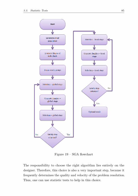
3.3. Statistic Tests 85
Figure 19 – SGA flowchart
The responsibility to choose the right algorithm lies entirely on thedesigner. Therefore, this choice is also a very important step, because itfrequently determines the quality and velocity of the problem resolution.Thus, one can use statistic tests to help in this choice.
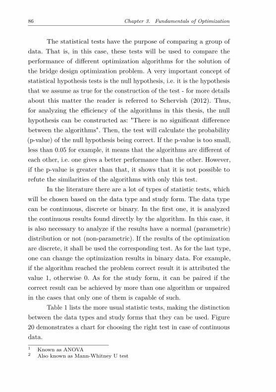
86 Chapter 3. Fundamentals of Optimization
The statistical tests have the purpose of comparing a group ofdata. That is, in this case, these tests will be used to compare theperformance of different optimization algorithms for the solution ofthe bridge design optimization problem. A very important concept ofstatistical hypothesis tests is the null hypothesis, i.e. it is the hypothesisthat we assume as true for the construction of the test - for more detailsabout this matter the reader is referred to Schervish (2012). Thus,for analyzing the efficiency of the algorithms in this thesis, the nullhypothesis can be constructed as: "There is no significant differencebetween the algorithms". Then, the test will calculate the probability(p-value) of the null hypothesis being correct. If the p-value is too small,less than 0.05 for example, it means that the algorithms are different ofeach other, i.e. one gives a better performance than the other. However,if the p-value is greater than that, it shows that it is not possible torefute the similarities of the algorithms with only this test.
In the literature there are a lot of types of statistic tests, whichwill be chosen based on the data type and study form. The data typecan be continuous, discrete or binary. In the first one, it is analyzedthe continuous results found directly by the algorithm. In this case, itis also necessary to analyze if the results have a normal (parametric)distribution or not (non-parametric). If the results of the optimizationare discrete, it shall be used the corresponding test. As for the last type,one can change the optimization results in binary data. For example,if the algorithm reached the problem correct result it is attributed thevalue 1, otherwise 0. As for the study form, it can be paired if thecorrect result can be achieved by more than one algorithm or unpairedin the cases that only one of them is capable of such.
Table 1 lists the more usual statistic tests, making the distinctionbetween the data types and study forms that they can be used. Figure20 demonstrates a chart for choosing the right test in case of continuousdata.1 Known as ANOVA2 Also known as Mann-Whitney U test
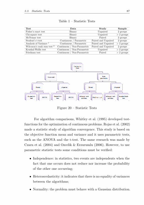
3.3. Statistic Tests 87
Table 1 – Statistic Tests
Test Data Study SampleFisher’s exact test Binary Unpaired 2 groupsChi-square test Binary Unpaired > 2 groupsMcNemar test Binary Paired 2 groupsStudent’s t-test Continuous / Parametric Paired and Unpaired 2 groupsAnalysis of Variance 1 Continuous / Parametric Paired and Unpaired > 2 groupsWilcoxon’s rank sum test 2 Continuous / Non-Parametric Paired and Unpaired 2 groupsKruskal-Wallis test Continuous / Non-Parametric Unpaired > 2 groupsFriedman test Continuous / Non-Parametric Paired > 2 groups
Figure 20 – Statistic Tests
For algorithm comparisons, Whitley et al. (1995) developed test-functions for the optimization of continuous problems. Rojas et al. (2002)made a statistic study of algorithm convergence. This study is based onthe objective function mean and variance and it uses parametric tests,such as the ANOVA and the t-test. The same research was made byCzarn et al. (2004) and Ozcelik & Erzurumlu (2006). However, to useparametric statistic tests some conditions must be verified:
• Independence: in statistics, two events are independents when thefact that one occurs does not reduce nor increase the probabilityof the other one occurring;
• Heteroscedasticity: it indicates that there is no equality of variancesbetween the algorithms;
• Normality: the problem must behave with a Gaussian distribution.
88 Chapter 3. Fundamentals of Optimization
As each algorithm is run without interaction with each other, theindependence criterion is guaranteed. The other two can be confirmedby some tests. The heteroscedasticity can be checked using the Levene’stest. For the normality it can be chosen one of the following:
• Kolmogorov-Smirnov;
• Shapiro-Wilk;
• D’Agostino-Pearson.
However, those three conditions will hardly be met at the sametime. Because of that, García et al. (2007) used non-parametric statisticprocedures in the comparison of algorithms results. This author con-cluded that, even without meeting the normality condition, the resultsof parametric and non-parametric are similar. García et al. (2007) alsosuggested that non-parametric analysis be chosen in the case of multiobjective functions.
89
Chapter 4
Steel-Concrete CompositeI-Girder Bridge Optimization
This chapter describes the steel-concrete composite I-girder opti-mization problem. The first section shows its variables and formulations.The second section describes the optimization approach developed tosolve this problem.
4.1 Optimization Problem
The steel-concrete composite I-girder bridge system studied inthe present dissertation corresponds to a simply supported straight axisstructure. In practical applications, its span usually varies from 20 to50m (PINHO; BELLEI, 2007). Figure 21 shows a typical cross-sectionfor this structure.
The final cost of the bridge is influenced by more than twentyvariables, which can be grouped as follows:
1. Geometric values (see Figures 21, 22, 23 and 24): medium thicknessof the deck, considering its haunch (h), width between beams(b2), width and thickness of the top flange of the beam (bs andts), height and thickness of the beam web (hv and tw), width
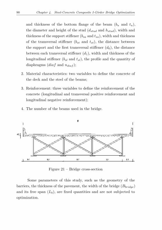
90 Chapter 4. Steel-Concrete Composite I-Girder Bridge Optimization
and thickness of the bottom flange of the beam (bu and tu),the diameter and height of the stud (dstud and hstud), width andthickness of the support stiffener (bsa and tsa), width and thicknessof the transversal stiffener (bst and tst), the distance betweenthe support and the first transversal stiffener (d0), the distancebetween each transversal stiffener (d1), width and thickness of thelongitudinal stiffener (bsl and tsl), the profile and the quantity ofdiaphragms (diaf and ndiaf );
2. Material characteristics: two variables to define the concrete ofthe deck and the steel of the beams;
3. Reinforcement: three variables to define the reinforcement of theconcrete (longitudinal and transversal positive reinforcement andlongitudinal negative reinforcement);
4. The number of the beams used in the bridge.
Figure 21 – Bridge cross-section
Some parameters of this study, such as the geometry of thebarriers, the thickness of the pavement, the width of the bridge (Bbridge)and its free span (Lb), are fixed quantities and are not subjected tooptimization.
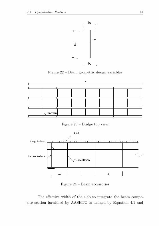
4.1. Optimization Problem 91
Figure 22 – Beam geometric design variables
Figure 23 – Bridge top view
Figure 24 – Beam accessories
The effective width of the slab to integrate the beam compo-site section furnished by AASHTO is defined by Equation 4.1 and
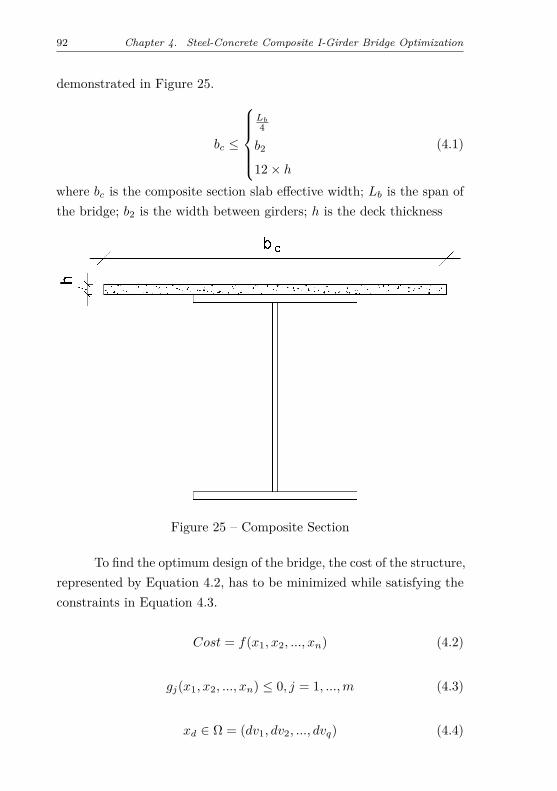
92 Chapter 4. Steel-Concrete Composite I-Girder Bridge Optimization
demonstrated in Figure 25.
bc ≤
Lb
4
b2
12× h
(4.1)
where bc is the composite section slab effective width; Lb is the span ofthe bridge; b2 is the width between girders; h is the deck thickness
Figure 25 – Composite Section
To find the optimum design of the bridge, the cost of the structure,represented by Equation 4.2, has to be minimized while satisfying theconstraints in Equation 4.3.
Cost = f(x1, x2, ..., xn) (4.2)
gj(x1, x2, ..., xn) ≤ 0, j = 1, ...,m (4.3)
xd ∈ Ω = (dv1, dv2, ..., dvq) (4.4)
4.1. Optimization Problem 93
xmin ≤ xk ≤ xmax (4.5)
where Cost is the cost function; gj are the constraints of the problem;xd are the discrete variables; dvq are the possible discrete values for thevariables; xk are the continuous variables.
The objective function of this analysis is the cost of the bridge.It is shown in Equation 4.6:
Cost =t∑i=1
pi ×mi (4.6)
where pi are the unit prices; mi are the measurements of the units; t isthe total number of construction units.
This function considers the cost of the materials (concrete, steeland reinforcement). These prices are obtained by a survey of costs of civilconstruction conducted by Caixa Econômica Federal (Federal EconomicFund) and IBGE (Brazilian Institute of Statistics and Geography) everymonth in Brazil (Caixa Econômica Federal, 2015). The data used isfrom June 2015 and are given in Table 2. The prices are converted todollar currency with the exchange price of November 19th 2015, which isR$3.75. Since the cost of the studs are much inferior when compared tothe whole structure, its unit cost was simplified taken to be the same asthe structural steel employed for the bridge. Despite their importance,the bridge construction costs, for instance, the beams erection costsas well as the form-work cost of the top slab were not included in theEquation 4.6. Then, this assessment would be interesting in furtherinvestigations.
The constraints herein applied, which were previously describedin Section 2.1.2, are based on AASHTO standards (AASHTO, 2002;AASHTO, 2012).
A penalization scheme is used to transform the constrained opti-mization problem given by Equation 4.3 into an unconstrained problem.It consists in summing a penalization proportional to the violation to
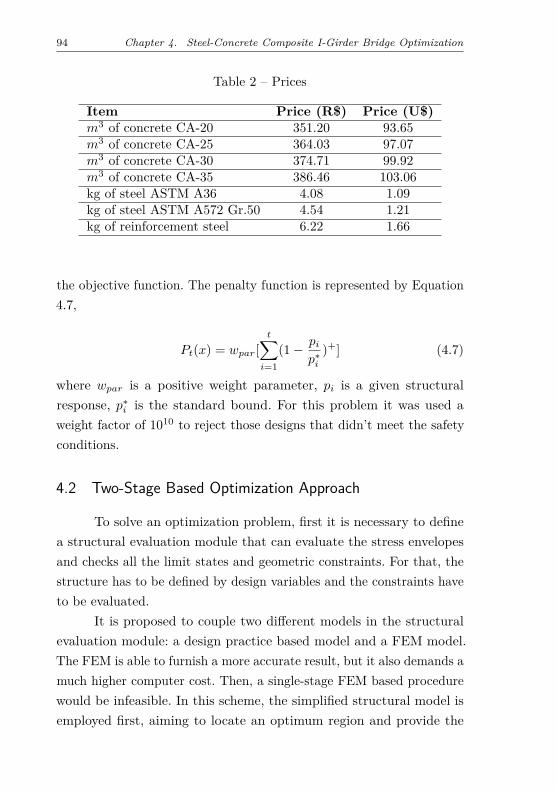
94 Chapter 4. Steel-Concrete Composite I-Girder Bridge Optimization
Table 2 – Prices
Item Price (R$) Price (U$)m3 of concrete CA-20 351.20 93.65m3 of concrete CA-25 364.03 97.07m3 of concrete CA-30 374.71 99.92m3 of concrete CA-35 386.46 103.06kg of steel ASTM A36 4.08 1.09kg of steel ASTM A572 Gr.50 4.54 1.21kg of reinforcement steel 6.22 1.66
the objective function. The penalty function is represented by Equation4.7,
Pt(x) = wpar[t∑i=1
(1− pip∗i
)+] (4.7)
where wpar is a positive weight parameter, pi is a given structuralresponse, p∗i is the standard bound. For this problem it was used aweight factor of 1010 to reject those designs that didn’t meet the safetyconditions.
4.2 Two-Stage Based Optimization Approach
To solve an optimization problem, first it is necessary to definea structural evaluation module that can evaluate the stress envelopesand checks all the limit states and geometric constraints. For that, thestructure has to be defined by design variables and the constraints haveto be evaluated.
It is proposed to couple two different models in the structuralevaluation module: a design practice based model and a FEM model.The FEM is able to furnish a more accurate result, but it also demands amuch higher computer cost. Then, a single-stage FEM based procedurewould be infeasible. In this scheme, the simplified structural model isemployed first, aiming to locate an optimum region and provide the
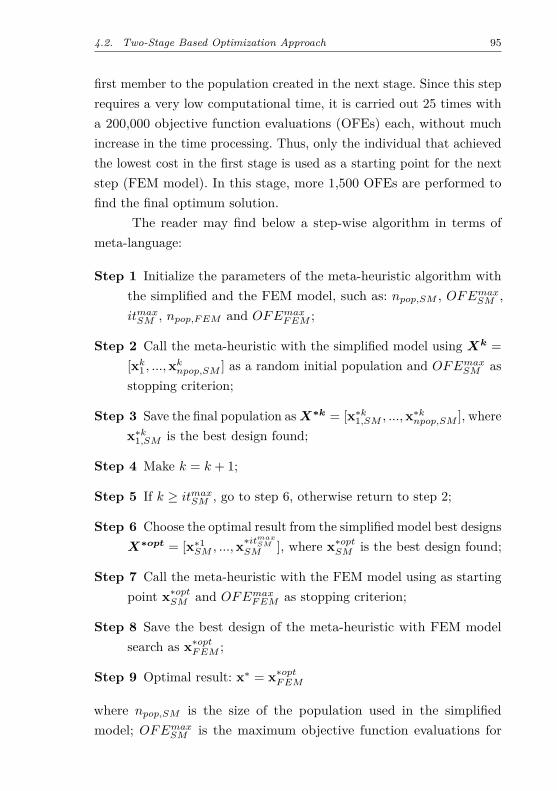
4.2. Two-Stage Based Optimization Approach 95
first member to the population created in the next stage. Since this steprequires a very low computational time, it is carried out 25 times witha 200,000 objective function evaluations (OFEs) each, without muchincrease in the time processing. Thus, only the individual that achievedthe lowest cost in the first stage is used as a starting point for the nextstep (FEM model). In this stage, more 1,500 OFEs are performed tofind the final optimum solution.
The reader may find below a step-wise algorithm in terms ofmeta-language:
Step 1 Initialize the parameters of the meta-heuristic algorithm withthe simplified and the FEM model, such as: npop,SM , OFEmaxSM ,itmaxSM , npop,FEM and OFEmaxFEM ;
Step 2 Call the meta-heuristic with the simplified model using Xk =[xk1 , ...,xknpop,SM ] as a random initial population and OFEmaxSM asstopping criterion;
Step 3 Save the final population asX∗k = [x∗k1,SM , ...,x∗knpop,SM ], wherex∗k1,SM is the best design found;
Step 4 Make k = k + 1;
Step 5 If k ≥ itmaxSM , go to step 6, otherwise return to step 2;
Step 6 Choose the optimal result from the simplified model best designsX∗opt = [x∗1SM , ...,x
∗itmaxSM
SM ], where x∗optSM is the best design found;
Step 7 Call the meta-heuristic with the FEM model using as startingpoint x∗optSM and OFEmaxFEM as stopping criterion;
Step 8 Save the best design of the meta-heuristic with FEM modelsearch as x∗optFEM ;
Step 9 Optimal result: x∗ = x∗optFEM
where npop,SM is the size of the population used in the simplifiedmodel; OFEmaxSM is the maximum objective function evaluations for
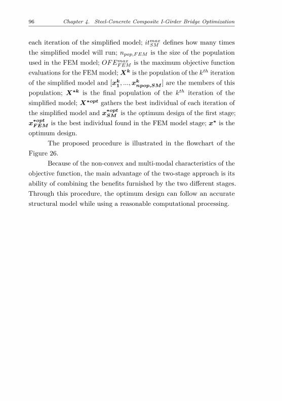
96 Chapter 4. Steel-Concrete Composite I-Girder Bridge Optimization
each iteration of the simplified model; itmaxSM defines how many timesthe simplified model will run; npop,FEM is the size of the populationused in the FEM model; OFEmaxFEM is the maximum objective functionevaluations for the FEM model;Xk is the population of the kth iterationof the simplified model and [xk
1 , ...,xknpop,SM ] are the members of this
population; X∗k is the final population of the kth iteration of thesimplified model; X∗opt gathers the best individual of each iteration ofthe simplified model and x∗opt
SM is the optimum design of the first stage;x∗opt
F EM is the best individual found in the FEM model stage; x∗ is theoptimum design.
The proposed procedure is illustrated in the flowchart of theFigure 26.
Because of the non-convex and multi-modal characteristics of theobjective function, the main advantage of the two-stage approach is itsability of combining the benefits furnished by the two different stages.Through this procedure, the optimum design can follow an accuratestructural model while using a reasonable computational processing.
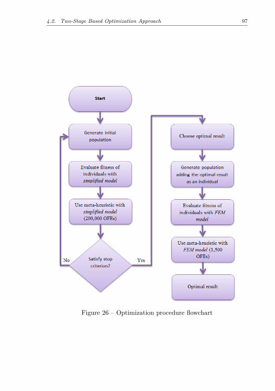
4.2. Two-Stage Based Optimization Approach 97
Figure 26 – Optimization procedure flowchart

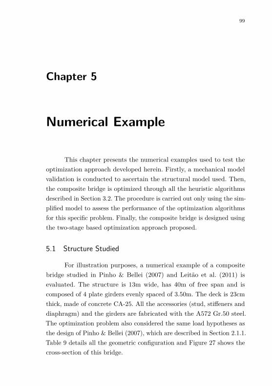
99
Chapter 5
Numerical Example
This chapter presents the numerical examples used to test theoptimization approach developed herein. Firstly, a mechanical modelvalidation is conducted to ascertain the structural model used. Then,the composite bridge is optimized through all the heuristic algorithmsdescribed in Section 3.2. The procedure is carried out only using the sim-plified model to assess the performance of the optimization algorithmsfor this specific problem. Finally, the composite bridge is designed usingthe two-stage based optimization approach proposed.
5.1 Structure Studied
For illustration purposes, a numerical example of a compositebridge studied in Pinho & Bellei (2007) and Leitão et al. (2011) isevaluated. The structure is 13m wide, has 40m of free span and iscomposed of 4 plate girders evenly spaced of 3.50m. The deck is 23cmthick, made of concrete CA-25. All the accessories (stud, stiffeners anddiaphragm) and the girders are fabricated with the A572 Gr.50 steel.The optimization problem also considered the same load hypotheses asthe design of Pinho & Bellei (2007), which are described in Section 2.1.1.Table 9 details all the geometric configuration and Figure 27 shows thecross-section of this bridge.
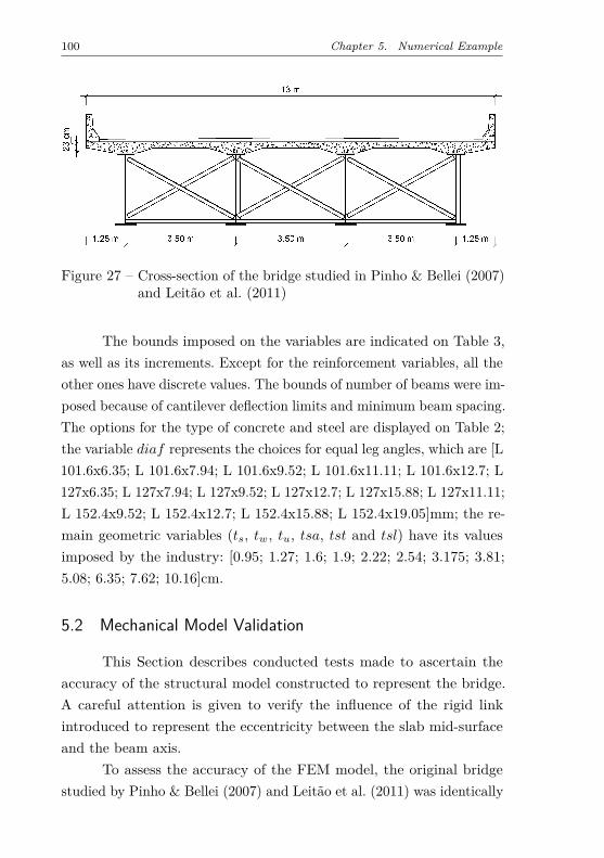
100 Chapter 5. Numerical Example
Figure 27 – Cross-section of the bridge studied in Pinho & Bellei (2007)and Leitão et al. (2011)
The bounds imposed on the variables are indicated on Table 3,as well as its increments. Except for the reinforcement variables, all theother ones have discrete values. The bounds of number of beams were im-posed because of cantilever deflection limits and minimum beam spacing.The options for the type of concrete and steel are displayed on Table 2;the variable diaf represents the choices for equal leg angles, which are [L101.6x6.35; L 101.6x7.94; L 101.6x9.52; L 101.6x11.11; L 101.6x12.7; L127x6.35; L 127x7.94; L 127x9.52; L 127x12.7; L 127x15.88; L 127x11.11;L 152.4x9.52; L 152.4x12.7; L 152.4x15.88; L 152.4x19.05]mm; the re-main geometric variables (ts, tw, tu, tsa, tst and tsl) have its valuesimposed by the industry: [0.95; 1.27; 1.6; 1.9; 2.22; 2.54; 3.175; 3.81;5.08; 6.35; 7.62; 10.16]cm.
5.2 Mechanical Model Validation
This Section describes conducted tests made to ascertain theaccuracy of the structural model constructed to represent the bridge.A careful attention is given to verify the influence of the rigid linkintroduced to represent the eccentricity between the slab mid-surfaceand the beam axis.
To assess the accuracy of the FEM model, the original bridgestudied by Pinho & Bellei (2007) and Leitão et al. (2011) was identically
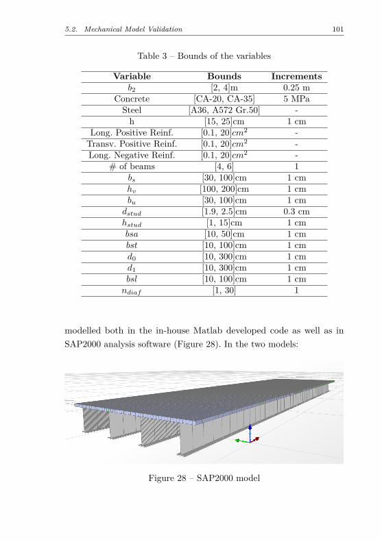
5.2. Mechanical Model Validation 101
Table 3 – Bounds of the variables
Variable Bounds Incrementsb2 [2, 4]m 0.25 m
Concrete [CA-20, CA-35] 5 MPaSteel [A36, A572 Gr.50] -h [15, 25]cm 1 cm
Long. Positive Reinf. [0.1, 20]cm2 -Transv. Positive Reinf. [0.1, 20]cm2 -Long. Negative Reinf. [0.1, 20]cm2 -
# of beams [4, 6] 1bs [30, 100]cm 1 cmhv [100, 200]cm 1 cmbu [30, 100]cm 1 cmdstud [1.9, 2.5]cm 0.3 cmhstud [1, 15]cm 1 cmbsa [10, 50]cm 1 cmbst [10, 100]cm 1 cmd0 [10, 300]cm 1 cmd1 [10, 300]cm 1 cmbsl [10, 100]cm 1 cmndiaf [1, 30] 1
modelled both in the in-house Matlab developed code as well as inSAP2000 analysis software (Figure 28). In the two models:
Figure 28 – SAP2000 model
102 Chapter 5. Numerical Example
• the bridge deck was represented through 8320, 25x25cm, 4-node,rectangular shell elements;
• each girder was modelled using 640 2-node, 6-DOF, Euler-Bernoulliframe elements (because of its small influence, the shear deforma-tion is not taken into account);
• the eccentricity between the slab mid-surface and the beam axiswas considered by introducing a rigid link.
Then, structure is subjected to five random load cases, which arelisted below. In each one of them, both models (Matlab and SAP2000)were compared to assess the precision of the response values.
• Load Case 1: uniform distributed load of 10kN/m2 on the entirebridge slab;
• Load Case 2: concentrated load of 100kN applied at the midspan of the first girder;
• Load Case 3: only the uniform distributed load part of themoving load (5kN/m2 on some parts of the slab);
• Load Case 4: concentrated load part of the moving load (6 loadsof 60kN);
• Load Case 5: the moving load.
The results of internal forces and displacements in the secondgirder are shown in Table 4. Based on that, it is possible to conclude thatthe in-house Matlab model employed in the present work is accurate andcorrect (and it is fully in accordance with a very robust computationalpackage SAP2000) to be used in the optimization problem.
Table 5 compares the internal forces found by the FEM modelwith those furnished by the Level Rule and Fauchart procedures. Thedifference between bending moments and shear considering the simpli-fied and FEM model were quite large. Note that the design practice
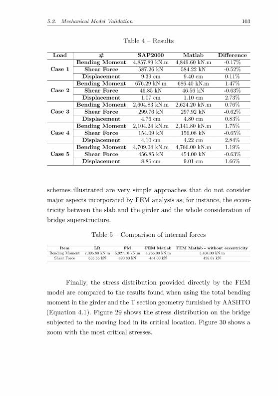
5.2. Mechanical Model Validation 103
Table 4 – Results
Load # SAP2000 Matlab Difference
Case 1Bending Moment 4,857.89 kN.m 4,849.60 kN.m -0.17%
Shear Force 587.26 kN 584.22 kN -0.52%Displacement 9.39 cm 9.40 cm 0.11%
Case 2Bending Moment 676.29 kN.m 686.40 kN.m 1.47%
Shear Force 46.85 kN 46.56 kN -0.63%Displacement 1.07 cm 1.10 cm 2.73%
Case 3Bending Moment 2,604.83 kN.m 2,624.20 kN.m 0.76%
Shear Force 299.76 kN 297.92 kN -0.62%Displacement 4.76 cm 4.80 cm 0.83%
Case 4Bending Moment 2,104.24 kN.m 2,141.80 kN.m 1.75%
Shear Force 154.09 kN 156.08 kN -0.65%Displacement 4.10 cm 4.22 cm 2.84%
Case 5Bending Moment 4,709.04 kN.m 4,766.00 kN.m 1.19%
Shear Force 456.85 kN 454.00 kN -0.63%Displacement 8.86 cm 9.01 cm 1.66%
schemes illustrated are very simple approaches that do not considermajor aspects incorporated by FEM analysis as, for instance, the eccen-tricity between the slab and the girder and the whole consideration ofbridge superstructure.
Table 5 – Comparison of internal forces
Item LR FM FEM Matlab FEM Matlab - without eccentricityBending Moment 7,095.80 kN.m 5,927.10 kN.m 4,766.00 kN.m 5,404.00 kN.m
Shear Force 635.55 kN 490.80 kN 454.00 kN 428.07 kN
Finally, the stress distribution provided directly by the FEMmodel are compared to the results found when using the total bendingmoment in the girder and the T section geometry furnished by AASHTO(Equation 4.1). Figure 29 shows the stress distribution on the bridgesubjected to the moving load in its critical location. Figure 30 shows azoom with the most critical stresses.
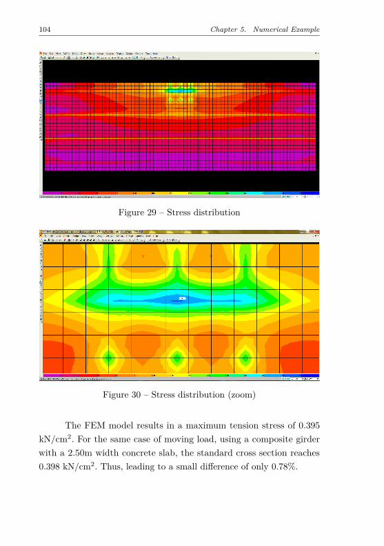
104 Chapter 5. Numerical Example
Figure 29 – Stress distribution
Figure 30 – Stress distribution (zoom)
The FEM model results in a maximum tension stress of 0.395kN/cm2. For the same case of moving load, using a composite girderwith a 2.50m width concrete slab, the standard cross section reaches0.398 kN/cm2. Thus, leading to a small difference of only 0.78%.
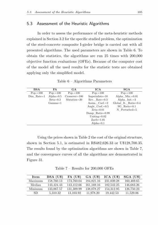
5.3. Assessment of the Heuristic Algorithms 105
5.3 Assessment of the Heuristic Algorithms
In order to assess the performance of the meta-heuristic methodsexplained in Section 3.2 for the specific studied problem, the optimizationof the steel-concrete composite I-girder bridge is carried out with allpresented algorithms. The used parameters are shown in Table 6. Toobtain the statistics, the algorithms are run 25 times with 200,000objective function evaluations (OFEs). Because of the computer costof the model all the used results for the statistic tests are obtainedapplying only the simplified model.
Table 6 – Algorithms Parameters
BSA FA GA ICA SGAPop.=100 Pop.=100 Pop.=100 Pop.=100 Pop.=100
Dim_Rate=1 Alpha=0.5 Crossover=100 Imperialists=10 Alpha_Min.=0.01Beta=0.2 Mutation=20 Rev._Rate=0.3 Alpha_Init.=3Gamma=1 Assim._Coef.=2 Global_It._Ratio=0.4
Angle_Coef.=0.5 SG_Ratio=0.1Zeta=0.01 N_Perturbed=5
Damp_Ratio=0.99Uniting=0.02Zarib=1.05Alpha=0.1
Using the prices shown in Table 2 the cost of the original structure,shown in Section 5.1, is estimated in R$482,626.33 or U$128,700.35.The results found by the optimization algorithms are shown in Table 7,and the convergence curves of all the algorithms are demonstrated inFigure 31.
Table 7 – Results for 200,000 OFEs
Item BSA (U$) FA (U$) GA (U$) ICA (U$) SGA (U$)Maximum 158,760.13 173,760.04 184,821.16 231,039.28 160,469.65Median 143,424.43 143,412.66 161,169.16 182,542.25 146,683.26Minimum 133,067.57 131,309.99 138,078.27 154,312.95 126,750.23
SD 5,310.32 13,103.92 11,978.20 19,442.53 11,529.06
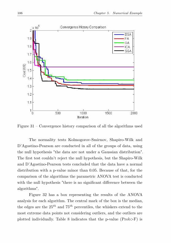
106 Chapter 5. Numerical Example
Figure 31 – Convergence history comparison of all the algorithms used
The normality tests Kolmogorov-Smirnov, Shapiro-Wilk andD’Agostino-Pearson are conducted in all of the groups of data, usingthe null hypothesis "the data are not under a Gaussian distribution".The first test couldn’t reject the null hypothesis, but the Shapiro-Wilkand D’Agostino-Pearson tests concluded that the data have a normaldistribution with a p-value minor than 0.05. Because of that, for thecomparison of the algorithms the parametric ANOVA test is conductedwith the null hypothesis "there is no significant difference between thealgorithms".
Figure 32 has a box representing the results of the ANOVAanalysis for each algorithm. The central mark of the box is the median,the edges are the 25th and 75th percentiles, the whiskers extend to themost extreme data points not considering outliers, and the outliers areplotted individually. Table 8 indicates that the p-value (Prob>F) is
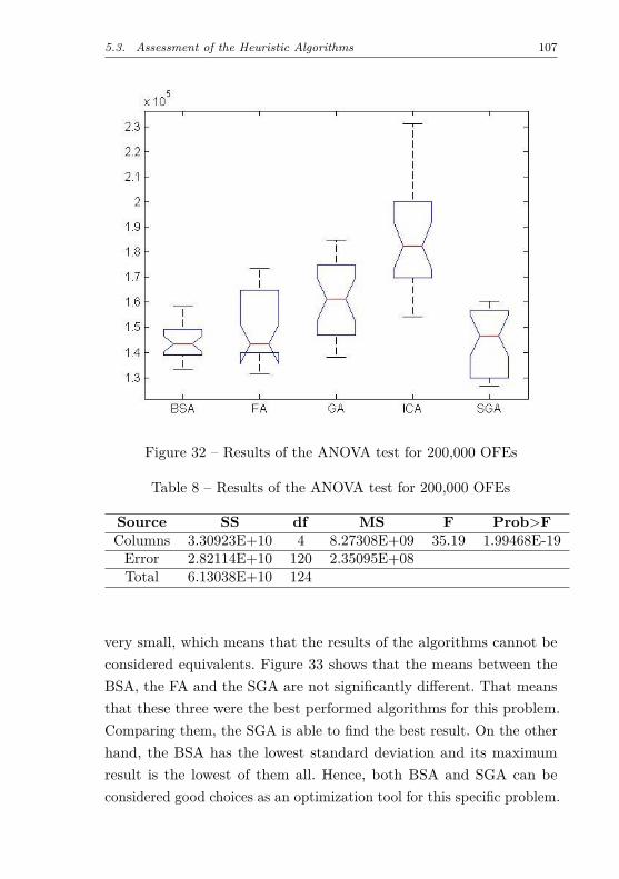
5.3. Assessment of the Heuristic Algorithms 107
Figure 32 – Results of the ANOVA test for 200,000 OFEs
Table 8 – Results of the ANOVA test for 200,000 OFEs
Source SS df MS F Prob>FColumns 3.30923E+10 4 8.27308E+09 35.19 1.99468E-19Error 2.82114E+10 120 2.35095E+08Total 6.13038E+10 124
very small, which means that the results of the algorithms cannot beconsidered equivalents. Figure 33 shows that the means between theBSA, the FA and the SGA are not significantly different. That meansthat these three were the best performed algorithms for this problem.Comparing them, the SGA is able to find the best result. On the otherhand, the BSA has the lowest standard deviation and its maximumresult is the lowest of them all. Hence, both BSA and SGA can beconsidered good choices as an optimization tool for this specific problem.
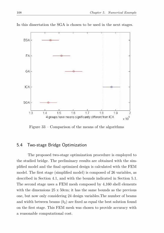
108 Chapter 5. Numerical Example
In this dissertation the SGA is chosen to be used in the next stages.
Figure 33 – Comparison of the means of the algorithms
5.4 Two-stage Bridge Optimization
The proposed two-stage optimization procedure is employed tothe studied bridge. The preliminary results are obtained with the sim-plified model and the final optimized design is calculated with the FEMmodel. The first stage (simplified model) is composed of 26 variables, asdescribed in Section 4.1, and with the bounds indicated in Section 5.1.The second stage uses a FEM mesh composed by 4,160 shell elementswith the dimensions 25 x 50cm; it has the same bounds as the previousone, but now only considering 24 design variables.The number of beamsand width between beams (b2) are fixed as equal the best solution foundon the first stage. This FEM mesh was chosen to provide accuracy witha reasonable computational cost.
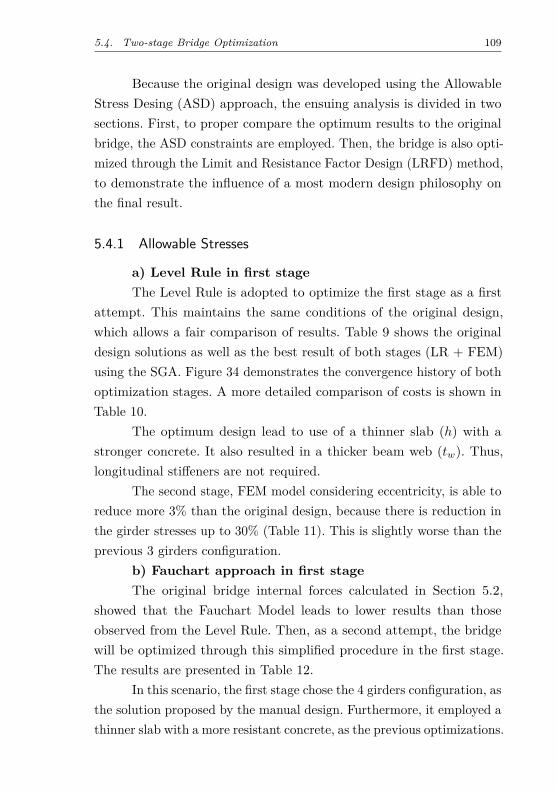
5.4. Two-stage Bridge Optimization 109
Because the original design was developed using the AllowableStress Desing (ASD) approach, the ensuing analysis is divided in twosections. First, to proper compare the optimum results to the originalbridge, the ASD constraints are employed. Then, the bridge is also opti-mized through the Limit and Resistance Factor Design (LRFD) method,to demonstrate the influence of a most modern design philosophy onthe final result.
5.4.1 Allowable Stresses
a) Level Rule in first stageThe Level Rule is adopted to optimize the first stage as a first
attempt. This maintains the same conditions of the original design,which allows a fair comparison of results. Table 9 shows the originaldesign solutions as well as the best result of both stages (LR + FEM)using the SGA. Figure 34 demonstrates the convergence history of bothoptimization stages. A more detailed comparison of costs is shown inTable 10.
The optimum design lead to use of a thinner slab (h) with astronger concrete. It also resulted in a thicker beam web (tw). Thus,longitudinal stiffeners are not required.
The second stage, FEM model considering eccentricity, is able toreduce more 3% than the original design, because there is reduction inthe girder stresses up to 30% (Table 11). This is slightly worse than theprevious 3 girders configuration.
b) Fauchart approach in first stageThe original bridge internal forces calculated in Section 5.2,
showed that the Fauchart Model leads to lower results than thoseobserved from the Level Rule. Then, as a second attempt, the bridgewill be optimized through this simplified procedure in the first stage.The results are presented in Table 12.
In this scenario, the first stage chose the 4 girders configuration, asthe solution proposed by the manual design. Furthermore, it employed athinner slab with a more resistant concrete, as the previous optimizations.
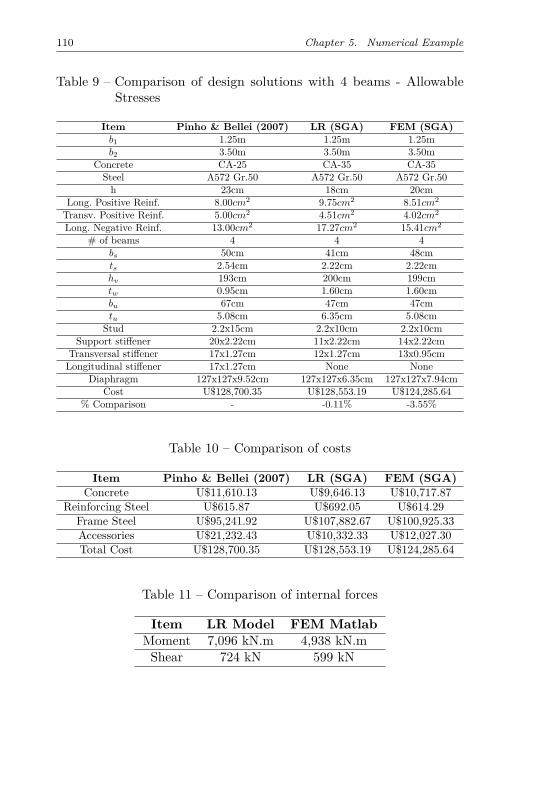
110 Chapter 5. Numerical Example
Table 9 – Comparison of design solutions with 4 beams - AllowableStresses
Item Pinho & Bellei (2007) LR (SGA) FEM (SGA)b1 1.25m 1.25m 1.25mb2 3.50m 3.50m 3.50m
Concrete CA-25 CA-35 CA-35Steel A572 Gr.50 A572 Gr.50 A572 Gr.50h 23cm 18cm 20cm
Long. Positive Reinf. 8.00cm2 9.75cm2 8.51cm2
Transv. Positive Reinf. 5.00cm2 4.51cm2 4.02cm2
Long. Negative Reinf. 13.00cm2 17.27cm2 15.41cm2
# of beams 4 4 4bs 50cm 41cm 48cmts 2.54cm 2.22cm 2.22cmhv 193cm 200cm 199cmtw 0.95cm 1.60cm 1.60cmbu 67cm 47cm 47cmtu 5.08cm 6.35cm 5.08cm
Stud 2.2x15cm 2.2x10cm 2.2x10cmSupport stiffener 20x2.22cm 11x2.22cm 14x2.22cm
Transversal stiffener 17x1.27cm 12x1.27cm 13x0.95cmLongitudinal stiffener 17x1.27cm None None
Diaphragm 127x127x9.52cm 127x127x6.35cm 127x127x7.94cmCost U$128,700.35 U$128,553.19 U$124,285.64
% Comparison - -0.11% -3.55%
Table 10 – Comparison of costs
Item Pinho & Bellei (2007) LR (SGA) FEM (SGA)Concrete U$11,610.13 U$9,646.13 U$10,717.87
Reinforcing Steel U$615.87 U$692.05 U$614.29Frame Steel U$95,241.92 U$107,882.67 U$100,925.33Accessories U$21,232.43 U$10,332.33 U$12,027.30Total Cost U$128,700.35 U$128,553.19 U$124,285.64
Table 11 – Comparison of internal forces
Item LR Model FEM MatlabMoment 7,096 kN.m 4,938 kN.mShear 724 kN 599 kN
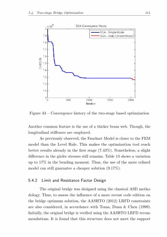
5.4. Two-stage Bridge Optimization 111
Figure 34 – Convergence history of the two-stage based optimization
Another common feature is the use of a thicker beam web. Though, thelongitudinal stiffeners are employed.
As previously observed, the Fauchart Model is closer to the FEMmodel than the Level Rule. This makes the optimization tool reachbetter results already in the first stage (7.43%). Nonetheless, a slightdifference in the girder stresses still remains. Table 13 shows a variationup to 17% in the bending moment. Thus, the use of the more refinedmodel can still guarantee a cheaper solution (9.17%).
5.4.2 Limit and Resistance Factor Design
The original bridge was designed using the classical ASD metho-dology. Thus, to assess the influence of a more recent code edition onthe bridge optimum solution, the AASHTO (2012) LRFD constraintsare also considered, in accordance with Toma, Duan & Chen (1999).Initially, the original bridge is verified using the AASHTO LRFD recom-mendations. It is found that this structure does not meet the support
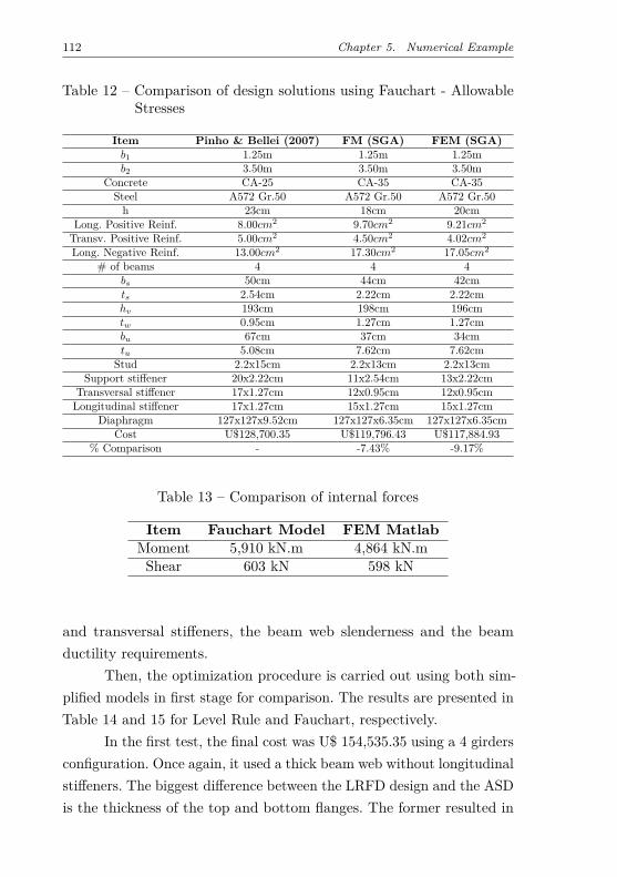
112 Chapter 5. Numerical Example
Table 12 – Comparison of design solutions using Fauchart - AllowableStresses
Item Pinho & Bellei (2007) FM (SGA) FEM (SGA)b1 1.25m 1.25m 1.25mb2 3.50m 3.50m 3.50m
Concrete CA-25 CA-35 CA-35Steel A572 Gr.50 A572 Gr.50 A572 Gr.50h 23cm 18cm 20cm
Long. Positive Reinf. 8.00cm2 9.70cm2 9.21cm2
Transv. Positive Reinf. 5.00cm2 4.50cm2 4.02cm2
Long. Negative Reinf. 13.00cm2 17.30cm2 17.05cm2
# of beams 4 4 4bs 50cm 44cm 42cmts 2.54cm 2.22cm 2.22cmhv 193cm 198cm 196cmtw 0.95cm 1.27cm 1.27cmbu 67cm 37cm 34cmtu 5.08cm 7.62cm 7.62cm
Stud 2.2x15cm 2.2x13cm 2.2x13cmSupport stiffener 20x2.22cm 11x2.54cm 13x2.22cm
Transversal stiffener 17x1.27cm 12x0.95cm 12x0.95cmLongitudinal stiffener 17x1.27cm 15x1.27cm 15x1.27cm
Diaphragm 127x127x9.52cm 127x127x6.35cm 127x127x6.35cmCost U$128,700.35 U$119,796.43 U$117,884.93
% Comparison - -7.43% -9.17%
Table 13 – Comparison of internal forces
Item Fauchart Model FEM MatlabMoment 5,910 kN.m 4,864 kN.mShear 603 kN 598 kN
and transversal stiffeners, the beam web slenderness and the beamductility requirements.
Then, the optimization procedure is carried out using both sim-plified models in first stage for comparison. The results are presented inTable 14 and 15 for Level Rule and Fauchart, respectively.
In the first test, the final cost was U$ 154,535.35 using a 4 girdersconfiguration. Once again, it used a thick beam web without longitudinalstiffeners. The biggest difference between the LRFD design and the ASDis the thickness of the top and bottom flanges. The former resulted in
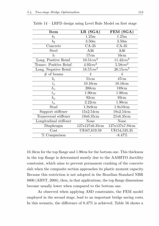
5.4. Two-stage Bridge Optimization 113
Table 14 – LRFD design using Level Rule Model on first stage
Item LR (SGA) FEM (SGA)b1 1.25m 1.25mb2 3.50m 3.50m
Concrete CA-35 CA-35Steel A36 A36h 17cm 16cm
Long. Positive Reinf. 10.51cm2 11.42cm2
Transv. Positive Reinf. 4.92cm2 5.58cm2
Long. Negative Reinf. 18.57cm2 20.15cm2
# of beams 4 4bs 51cm 47cmts 10.16cm 10.16cmhv 200cm 189cmtw 1.90cm 1.90cmbu 92cm 93cmtu 2.22cm 1.90cm
Stud 1.9x9cm 1.9x10cmSupport stiffener 15x2.54cm 18x2.54cm
Transversal stiffener 19x6.35cm 21x6.35cmLongitudinal stiffener None None
Diaphragm 127x127x6.35cm 127x127x7.94cmCost U$167,619.59 U$154,535.35
% Comparison - -8.47%
10.16cm for the top flange and 1.90cm for the bottom one. This thicknessin the top flange is determined mostly due to the AASHTO ductilityconstraint, which aims to prevent permanent crashing of the concreteslab when the composite section approaches its plastic moment capacity.Because this restriction is not adopted in the Brazilian Standard NBR8800 (ABNT, 2008), then, in that applications, the top flange dimensionsbecome usually lower when compared to the bottom one.
As observed when applying ASD constraints, the FEM modelemployed in the second stage, lead to an important bridge saving costs.In this scenario, the difference of 8.47% is achieved. Table 16 shows a
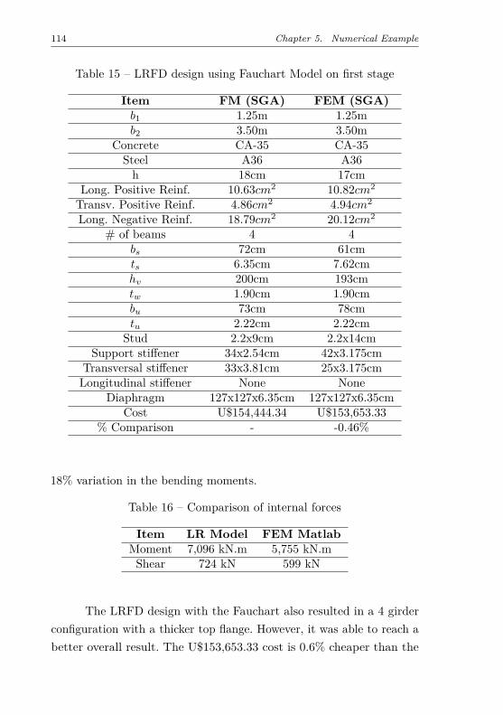
114 Chapter 5. Numerical Example
Table 15 – LRFD design using Fauchart Model on first stage
Item FM (SGA) FEM (SGA)b1 1.25m 1.25mb2 3.50m 3.50m
Concrete CA-35 CA-35Steel A36 A36h 18cm 17cm
Long. Positive Reinf. 10.63cm2 10.82cm2
Transv. Positive Reinf. 4.86cm2 4.94cm2
Long. Negative Reinf. 18.79cm2 20.12cm2
# of beams 4 4bs 72cm 61cmts 6.35cm 7.62cmhv 200cm 193cmtw 1.90cm 1.90cmbu 73cm 78cmtu 2.22cm 2.22cm
Stud 2.2x9cm 2.2x14cmSupport stiffener 34x2.54cm 42x3.175cm
Transversal stiffener 33x3.81cm 25x3.175cmLongitudinal stiffener None None
Diaphragm 127x127x6.35cm 127x127x6.35cmCost U$154,444.34 U$153,653.33
% Comparison - -0.46%
18% variation in the bending moments.
Table 16 – Comparison of internal forces
Item LR Model FEM MatlabMoment 7,096 kN.m 5,755 kN.mShear 724 kN 599 kN
The LRFD design with the Fauchart also resulted in a 4 girderconfiguration with a thicker top flange. However, it was able to reach abetter overall result. The U$153,653.33 cost is 0.6% cheaper than the

5.4. Two-stage Bridge Optimization 115
results using the first model (LR). On the other hand, in this scenario,both the Fauchart and FEM models are quite similar. Table 17 showslittle variation in internal forces.
Table 17 – Comparison of internal forces
Item Fauchart Model FEM MatlabMoment 5,691 kN.m 5,732 kN.mShear 581 kN 565 kN
Due to these differences, the AASHTO LRFD resulted in amore expensive result than that previously best solution. Even so, theproposed two-stage optimization approach could improve the resultfound when employing only the simplified approach.

117
Chapter 6
Concluding Remarks and FutureDevelopments
6.1 Concluding Remarks
This dissertation presented an efficient two-stage optimizationbased approach to design steel-concrete composite I-girder bridges.In the first step, a simplified structural model usually adopted bybridge designers was employed aiming to locate an optimum region andto provide a starting point to the next stage. Then, a finite elementmodel (FEM) was used to refine and improve the optimization. Themain advantage of this procedure was that it allows combining the lowcomputational cost required on first stage with the accuracy providedon second stage.
Despite it was conceived to steel-concrete composite I-girder brid-ges, the main idea of combining a simplified structural analysis procedurewith a FEM model, in a context of an optimization procedure, is generaland it can be adapted to other kinds of structural engineering problems.One of the crucial parts in this scheme is finding an adequate balance(accuracy versus computational time required) between the structuralanalysis modules chosen for both stages. This will be determinant onthe success of the optimization final result. Indeed, this will depend on
118 Chapter 6. Concluding Remarks and Future Developments
the particular problem and must be carefully assessed and examined bythe researcher. Note that this is an incipient idea and further studiesmust be encouraged, due to the promising achieved results.
Due to its non-convex nature and to the presence of discretevariables, the problem required the utilization of a global optimizationalgorithm. Then, the performance of five well-known meta-heuristicalgorithms for this specific problem was evaluated: Backtracking SearchAlgorithm (BSA), Firefly Algorithm (FA), Genetic Algorithm (GA),Imperialist Competitive Algorithm (ICA) and Search Group Algorithm(SGA). Then, another contribution was the assessment of five modernoptimization algorithms for a real world structural problem. The use ofstatistic tests provided additional information, supporting to correctlychoose the best algorithm for the study (BSA and SGA).
For illustration purposes, a numerical example of a compositebridge studied in Pinho & Bellei (2007) and Leitão et al. (2011) wasassessed. It was verified that when using a more accurate simplifiedmodel in the first stage, with a closer behavior of FEM model, betterresults can be achieved. In addition, the optimum values had beenimproved with FEM because it provided lower internal forces to thegirders (a bending moment reduction around 30%). When using theLevel Rule in the first stage, the proposed scheme was able to reduce0.11% of the structural cost, reaching up to 3.55% of saving costs inthe end of the optimization procedure, when compared to the solutiondesigned manually by a senior engineer. On the other hand, in thescenario using the Fauchart approach, which is closer to the FEMmodel, the optimization was able to reduce to 7.43% of the structuralcost in the first stage, reaching up to 9.17%. Furthermore, the optimalsolution reached here is feasible to a direct industrial application. Then,the obtained results showed that the proposed method is very promisingand further efforts must be carried out.
Finally, it is important to emphasize that the proposed schemehas shown a valuable tool to assist the engineer (not to substitute) in hisday-to-day practice. For instance, the designer can define the variables

6.2. Future Studies 119
of his preferences and use the optimization procedure as a starting pointto his own design.
6.2 Future Studies
Despite the promising results found in this dissertation, morestudies should be made to improve the work. Among them:
• The consideration of dynamic loads;
• Other types of bridges should be added to the optimization process;
• Girders with different sizes should be used to optimize even morethe structure;
• Consideration of fabrication costs.

121
References
AASHTO. Standard specifications for highway bridges. [S.l.]: AmericanAssociation of State Highway and Transportation Officials, 2002.
AASHTO. Standard specifications for highway bridges. [S.l.]: AmericanAssociation of State Highway and Transportation Officials, 2012.
ABNT. NBR 7188 – carga móvel em ponte rodoviária e passarela depedestre. Associação Brasileira de Normas Técnicas, Rio de Janeiro,Brazil. (In portuguese), 1984.
ABNT. NBR 7187 – reinforced and pre-stressed concrete bridge design.Associação Brasileira de Normas Técnicas, Rio de Janeiro, Brazil. (Inportuguese), 2003.
ABNT. NBR 8800 – projeto de estruturas de aço e de estruturasmistas de aço e concreto de edifícios. Associação Brasileira de NormasTécnicas, Rio de Janeiro, Brazil. (In portuguese), 2008.
ARORA, J. Introduction to optimum design. [S.l.]: Academic Press,2004.
ATASHPAZ-GARGARI, E.; LUCAS, C. Imperialist competitivealgorithm: an algorithm for optimization inspired by imperialisticcompetition. In: IEEE. Evolutionary computation, 2007. CEC 2007.IEEE Congress on. [S.l.], 2007. p. 4661–4667.
BALDOMIR, A.; HERNANDEZ, S.; NIETO, F.; JURADO, J. Cableoptimization of a long span cable stayed bridge in la coruña (spain).Advances in Engineering Software, Elsevier, v. 41, n. 7, p. 931–938,2010.
BALLING, R. J.; BRIGGS, R. R.; GILLMAN, K. Multiple optimumsize/shape/topology designs for skeletal structures using a geneticalgorithm. Journal of Structural Engineering, American Society of CivilEngineers, v. 132, n. 7, p. 1158–1165, 2006.
BARTHOLOMEW, P.; MORRIS, A. A unified approach tofully-stressed design. Engineering Optimization, Taylor & Francis, v. 2,n. 1, p. 3–15, 1976.
122 References
BHATTI, M. A. A mathematica based environment for analysis andoptimum design of composite structures. Computer Aided OptimumDesign of Structures VI, Computational Mechanics, p. 301, 1999.
CAI, H.; AREF, A. J. On the design and optimization of hybrid carbonfiber reinforced polymer-steel cable system for cable-stayed bridges.Composites Part B: Engineering, Elsevier, v. 68, p. 146–152, 2015.
Caixa Econômica Federal. Sinapi: índices da construção civil. Rio deJaneiro: CAIXA, 2015.
CHEN, W.-F.; DUAN, L.; ALTMAN, S. Bridge Engineering Handbook.[S.l.]: CRC Press, 2000.
CHENG, B.; QIAN, Q.; SUN, H. Steel truss bridges with weldedbox-section members and bowknot integral joints, part ii: Minimumweight optimization. Journal of Constructional Steel Research, Elsevier,v. 80, p. 475–482, 2013.
CHENG, J. Optimum design of steel truss arch bridges using a hybridgenetic algorithm. Journal of Constructional Steel Research, Elsevier,v. 66, n. 8, p. 1011–1017, 2010.
CIVICIOGLU, P. Backtracking search optimization algorithmfor numerical optimization problems. Applied Mathematics andComputation, Elsevier, v. 219, n. 15, p. 8121–8144, 2013.
COOK, R. D.; MALKUS, D. S.; PLESHA, M. E.; WITT, R. J.Concepts and applications of finite element analysis. [S.l.]: John Wiley& Sons, 2007.
CZARN, A.; MACNISH, C.; VIJAYAN, K.; TURLACH, B.; GUPTA,R. Statistical exploratory analysis of genetic algorithms. EvolutionaryComputation, IEEE Transactions on, IEEE, v. 8, n. 4, p. 405–421, 2004.
ELLOBODY, E. Finite Element Analysis and Design of Steel andSteel–Concrete Composite Bridges. [S.l.]: Butterworth-Heinemann,2014.
FABEANE, R. Pontes mistas de aço-concreto: estudo de diretrizes paradimensionamento otimizado. Dissertation — Universidade de PassoFundo, 2015.
FERNANDES, W. L. Software para análise e dimensionamento devigas mistas aço-concreto em pontes rodoviárias. Programa de Pós
References 123
Graduação em Engenharia Civil. Departamento de Engenharia Civil,Escola de Minas, Universidade Federal de Ouro Preto., 2008.
FERREIRA, A. J. MATLAB codes for finite element analysis: solidsand structures. [S.l.]: Springer Science & Business Media, 2008. v. 157.
FURUKAWA, K.; SUGIMOTO, H.; INOUE, K.; YAMADA, Y.Optimization of cable prestresses of cable stayed bridges based onminimum strain energy criterion. In: ASCE. Computer Utilization inStructural Engineering. [S.l.], 1989. p. 227–236.
GARCÍA, S.; MOLINA, D.; LOZANO, M.; HERRERA, F. Anexperimental study on the use of non-parametric tests for analyzing thebehaviour of evolutionary algorithms in optimization problems. In:Proceedings of the Spanish Congress on Metaheuristics, Evolutionaryand Bioinspired Algorithms (MAEB’2007). [S.l.: s.n.], 2007. p. 275–285.
GOCÁL, J.; ĎURŠOVÁ, A. Optimisation of transversal dispositionof steel and concrete composite road bridges. Procedia Engineering,Elsevier, v. 40, p. 125–130, 2012.
GONÇALVES, M. S.; LOPEZ, R. H.; MIGUEL, L. F. F. Search groupalgorithm: a new metaheuristic method for the optimization of trussstructures. Computers & Structures, Elsevier, v. 153, p. 165–184, 2015.
GUO, H.; LI, Z. Structural topology optimization of high-voltagetransmission tower with discrete variables. Structural andMultidisciplinary Optimization, Springer, v. 43, n. 6, p. 851–861, 2011.
HAFTKA, R. T. Integrated nonlinear structural analysis and design.AIAA journal, v. 27, n. 11, p. 1622–1627, 1989.
HASSAN, M. Optimization of stay cables in cable-stayed bridges usingfinite element, genetic algorithm, and b-spline combined technique.Engineering Structures, Elsevier, v. 49, p. 643–654, 2013.
HOLLAND, J. H. Adaptation in natural and artificial systems. [S.l.]:University of Michigan Press, 1975.
HUANG, M.; LI, Q.; CHAN, C.; LOU, W.; KWOK, K.; LI, G.Performance-based design optimization of tall concrete framedstructures subject to wind excitations. Journal of Wind Engineeringand Industrial Aerodynamics, Elsevier, v. 139, p. 70–81, 2015.
124 References
KAVEH, A.; ABADI, A. S. M. Cost optimization of a composite floorsystem using an improved harmony search algorithm. Journal ofConstructional Steel Research, Elsevier, v. 66, n. 5, p. 664–669, 2010.
KAVEH, A.; BEHNAM, A. Design optimization of reinforced concrete3d structures considering frequency constraints via a charged systemsearch. Scientia Iranica, Elsevier, v. 20, n. 3, p. 387–396, 2013.
KAVEH, A.; MANIAT, M.; NAEINI, M. A. Cost optimum designof post-tensioned concrete bridges using a modified colliding bodiesoptimization algorithm. Advances in Engineering Software, Elsevier,v. 98, p. 12–22, 2016.
KELESOGLU, O. Fuzzy multiobjective optimization of truss-structuresusing genetic algorithm. Advances in Engineering Software, Elsevier,v. 38, n. 10, p. 717–721, 2007.
KLINSKY, G. E. R. G. Uma contribuição ao estudo das pontes emvigas mistas. Tese (Doutorado) — Universidade de São Paulo, 1999.
KOCIECKI, M.; ADELI, H. Two-phase genetic algorithm for sizeoptimization of free-form steel space-frame roof structures. Journal ofConstructional Steel Research, Elsevier, v. 90, p. 283–296, 2013.
KODIYALAM, S.; VANDERPLAATS, G. N. Shape optimizationof three-dimensional continuum structures via force approximationtechniques. AIAA journal, v. 27, n. 9, p. 1256–1263, 1989.
KRAVANJA, S.; TURKALJ, G.; ŠILIH, S.; ŽULA, T. Optimal designof single-story steel building structures based on parametric minlpoptimization. Journal of constructional steel research, Elsevier, v. 81, p.86–103, 2013.
KRIPKA, M.; MEDEIROS, G. F.; LEMONGE, A. C. Use ofoptimization for automatic grouping of beam cross-section dimensionsin reinforced concrete building structures. Engineering Structures,Elsevier, v. 99, p. 311–318, 2015.
KUSANO, I.; BALDOMIR, A.; JURADO, J. A.; HERNÁNDEZ, S.Reliability based design optimization of long-span bridges consideringflutter. Journal of Wind Engineering and Industrial Aerodynamics,Elsevier, v. 135, p. 149–162, 2014.
LEE, K. S.; GEEM, Z. W. A new meta-heuristic algorithm forcontinuous engineering optimization: harmony search theory and
References 125
practice. Computer methods in applied mechanics and engineering,Elsevier, v. 194, n. 36, p. 3902–3933, 2005.
LEITÃO, F.; SILVA, J. D.; VELLASCO, P. d. S.; ANDRADE, S.D.; LIMA, L. D. Composite (steel–concrete) highway bridge fatigueassessment. Journal of Constructional Steel Research, Elsevier, v. 67,n. 1, p. 14–24, 2011.
LIU, K.; REYNDERS, E.; ROECK, G. D.; LOMBAERT, G.Experimental and numerical analysis of a composite bridge forhigh-speed trains. Journal of sound and vibration, Elsevier, v. 320, n. 1,p. 201–220, 2009.
LIU, X.; FAN, J.; NIE, J.; LI, G. Behavior of composite rigid framebridge under bi-directional seismic excitations. Journal of Traffic andTransportation Engineering (English Edition), Elsevier, v. 1, n. 1, p.62–71, 2014.
LOPEZ, R.; LUERSEN, M.; CURSI, E. Optimization of laminatedcomposites considering different failure criteria. Composites Part B:Engineering, Elsevier, v. 40, n. 8, p. 731–740, 2009.
LUTE, V.; UPADHYAY, A.; SINGH, K. K. Computationally efficientanalysis of cable-stayed bridge for ga-based optimization. EngineeringApplications of Artificial Intelligence, Elsevier, v. 22, n. 4, p. 750–758,2009.
MADRAZO-AGUIRRE, F.; RUIZ-TERAN, A. M.; WADEE, M. A.Dynamic behaviour of steel–concrete composite under-deck cable-stayedbridges under the action of moving loads. Engineering Structures,Elsevier, v. 103, p. 260–274, 2015.
MARTÍ, J. V.; GONZALEZ-VIDOSA, F.; YEPES, V.; ALCALÁ,J. Design of prestressed concrete precast road bridges with hybridsimulated annealing. Engineering Structures, Elsevier, v. 48, p. 342–352,2013.
MARTÍNEZ, F. J.; GONZÁLEZ-VIDOSA, F.; HOSPITALER, A.;ALCALÁ, J. Design of tall bridge piers by ant colony optimization.Engineering Structures, Elsevier, v. 33, n. 8, p. 2320–2329, 2011.
MARTINS, A.; SIMÕES, L.; NEGRÃO, J. Optimization of cable forceson concrete cable-stayed bridges including geometrical nonlinearities.Computers & Structures, Elsevier, v. 155, p. 18–27, 2015.
126 References
MIGUEL, L. F. F.; LOPEZ, R. H.; MIGUEL, L. F. F. Multimodal size,shape, and topology optimisation of truss structures using the fireflyalgorithm. Advances in Engineering Software, Elsevier, v. 56, p. 23–37,2013.
MOURA, M. W.; FERREIRA, M. W.; REAL, M. d. V.; SANTOS,G. C. Comparação do método de fauchart e do método dos elementosfinitos na avaliação da distribuição de esforços transversais em pontesrodoviárias. IX Congresso Brasileiro de Pontes e Estruturas, Rio deJaneiro, Brasil, 2016.
MUNCK, M. D.; SUTTER, S. D.; VERBRUGGEN, S.; TYSMANS, T.;COELHO, R. F. Multi-objective weight and cost optimization of hybridcomposite-concrete beams. Composite Structures, Elsevier, v. 134, p.369–377, 2015.
OEHLERS, D. J. Deterioration in strength of stud connectors incomposite bridge beams. Journal of structural engineering, AmericanSociety of Civil Engineers, v. 116, n. 12, p. 3417–3431, 1990.
OZCELIK, B.; ERZURUMLU, T. Comparison of the warpageoptimization in the plastic injection molding using anova, neuralnetwork model and genetic algorithm. Journal of materials processingtechnology, Elsevier, v. 171, n. 3, p. 437–445, 2006.
PEDRO, R. L.; DEMARCHE, J.; MIGUEL, L. F. F.; LOPEZ, R. H.An efficient approach for the optimization of simply supportedsteel-concrete composite i-girder bridges. Advances in EngineeringSoftware, Elsevier, X, n. X, p. X–X, 2017.
PINHO, F. O.; BELLEI, I. H. Pontes e viadutos em vigas mistas. [S.l.]:Instituto Brasileiro de Siderurgia, 2007.
POITRAS, G.; LEFRANÇOIS, G.; CORMIER, G. Optimization ofsteel floor systems using particle swarm optimization. Journal ofConstructional Steel Research, Elsevier, v. 67, n. 8, p. 1225–1231, 2011.
QIN, C. Optimization of cable-stretching planning in the constructionof cable-stayed bridges. Engineering optimization, Taylor & Francis,v. 19, n. 1, p. 1–20, 1992.
RAHAMI, H.; KAVEH, A.; GHOLIPOUR, Y. Sizing, geometry andtopology optimization of trusses via force method and genetic algorithm.Engineering Structures, Elsevier, v. 30, n. 9, p. 2360–2369, 2008.
References 127
ROJAS, I.; GONZÁLEZ, J.; POMARES, H.; MERELO, J.; CASTILLO,P.; ROMERO, G. Statistical analysis of the main parameters involvedin the design of a genetic algorithm. Systems, Man, and Cybernetics,Part C: Applications and Reviews, IEEE Transactions on, IEEE, v. 32,n. 1, p. 31–37, 2002.
RÜSCH, H. Berechnungstafeln für rechtwinklige Fahrbahnplatten vonStraßenbrücken. [S.l.]: Ernst, 1965.
SCHERVISH, M. J. Theory of statistics. [S.l.]: Springer Science &Business Media, 2012.
SHARAFI, P.; TEH, L. H.; HADI, M. N. Shape optimization ofthin-walled steel sections using graph theory and aco algorithm. Journalof Constructional Steel Research, Elsevier, v. 101, p. 331–341, 2014.
SHEA, K.; SMITH, I. F. Improving full-scale transmission towerdesign through topology and shape optimization. Journal of structuralengineering, American Society of Civil Engineers, v. 132, n. 5, p.781–790, 2006.
SOUZA, R. R.; MIGUEL, L. F. F.; LOPEZ, R. H.; MIGUEL, L. F. F.;TORII, A. J. A procedure for the size, shape and topology optimizationof transmission line tower structures. Engineering Structures, Elsevier,X, n. X, p. X–X, 2015.
STUCCHI, F. R. Pontes e Grandes Estruturas. [S.l.]: Escola Politécnica,Universidade de São Paulo, 2006.
TANG, W.; TONG, L.; GU, Y. Improved genetic algorithm for designoptimization of truss structures with sizing, shape and topologyvariables. International Journal for Numerical Methods in Engineering,Wiley Online Library, v. 62, n. 13, p. 1737–1762, 2005.
TANIWAKI, K.; OHKUBO, S. Optimal synthesis method fortransmission tower truss structures subjected to static and seismicloads. Structural and Multidisciplinary Optimization, Springer, v. 26,n. 6, p. 441–454, 2004.
TOMA, S.; DUAN, L.; CHEN, W. F. Bridge structures. In: .Structural Engineering Handbook Ed. [S.l.: s.n.], 1999.
TORII, A. J.; LOPEZ, R. H.; BIONDINI, F. An approach toreliability-based shape and topology optimization of truss structures.Engineering Optimization, Taylor & Francis, v. 44, n. 1, p. 37–53, 2012.
128 References
TORII, A. J.; LOPEZ, R. H.; MIGUEL, L. F. Modeling of globaland local stability in optimization of truss-like structures using frameelements. Structural and Multidisciplinary Optimization, Springer, p.1–12, 2014.
VANDERPLAATS, G. Structural design optimization status anddirection. Journal of Aircraft, v. 36, n. 1, p. 11–20, 1999.
VAZ, L. E. Método dos elementos finitos em análise de estruturas.Campus, 2011.
VITÓRIO, J. A. P. Pontes metálicas e mistas tópicos de conservação,danos e reforços estruturais. 2015.
WANG, H.; OHMORI, H. Elasto-plastic analysis based trussoptimization using genetic algorithm. Engineering Structures, Elsevier,v. 50, p. 1–12, 2013.
WHITLEY, D.; BEVERIDGE, R.; GRAVES, C.; MATHIAS, K. Testdriving three 1995 genetic algorithms: new test functions and geometricmatching. Journal of Heuristics, Springer, v. 1, n. 1, p. 77–104, 1995.
WOLPERT, D. H.; MACREADY, W. G. No free lunch theorems foroptimization. Evolutionary Computation, IEEE Transactions on, IEEE,v. 1, n. 1, p. 67–82, 1997.
YANG, R. Multidiscipline topology optimization. Computers &Structures, Elsevier, v. 63, n. 6, p. 1205–1212, 1997.
YANG, X.-S. Firefly algorithm. Engineering Optimization, WileyOnline Library, p. 221–230, 2010.
ZHOU, H.; SHI, G.; WANG, Y.; CHEN, H.; ROECK, G. D. Fatigueevaluation of a composite railway bridge based on fracture mechanicsthrough global–local dynamic analysis. Journal of Constructional SteelResearch, Elsevier, v. 122, p. 1–13, 2016.

Annex


131
Annex A
Rüsch’s tables
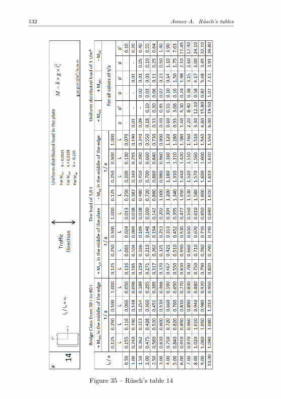
132 Annex A. Rüsch’s tables
Figure 35 – Rüsch’s table 14
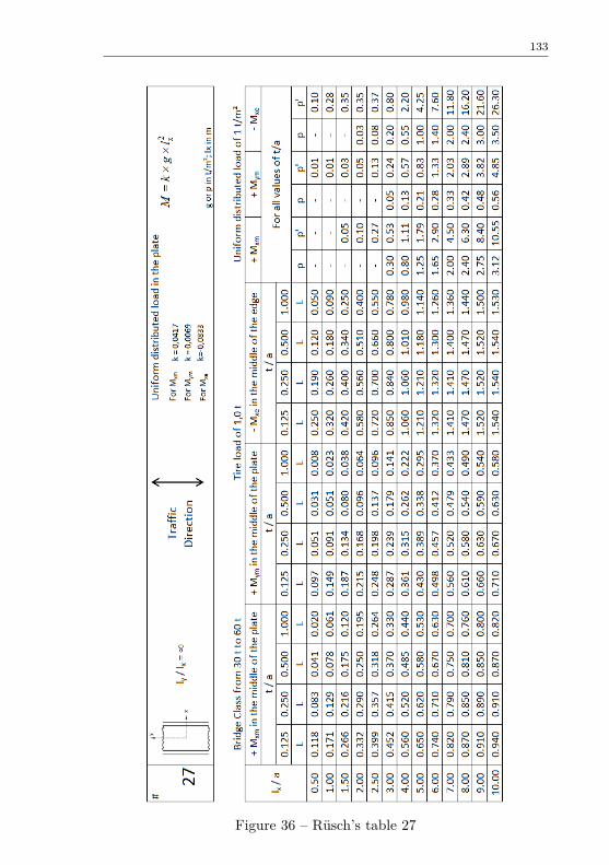
133
Figure 36 – Rüsch’s table 27
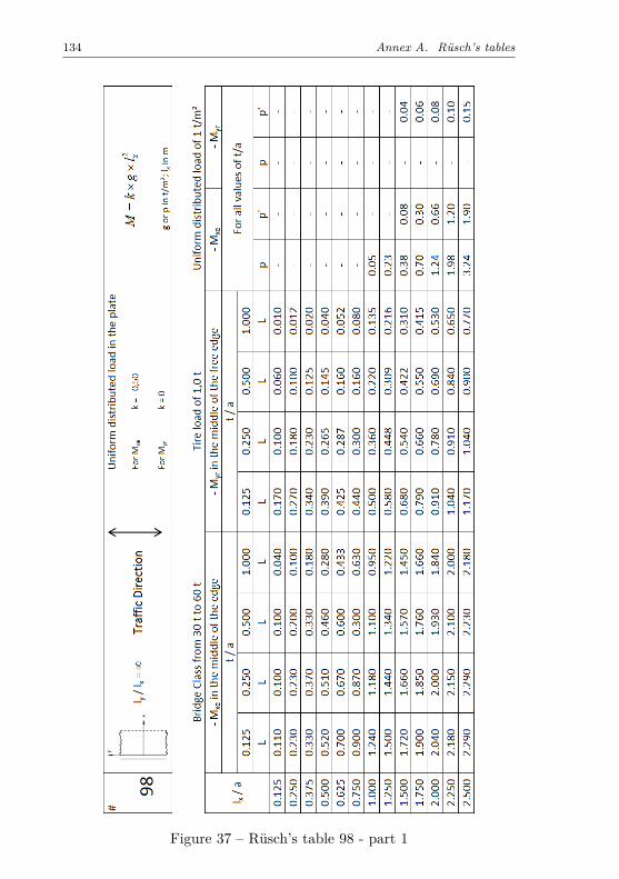
134 Annex A. Rüsch’s tables
Figure 37 – Rüsch’s table 98 - part 1
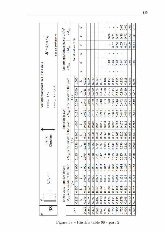
135
Figure 38 – Rüsch’s table 98 - part 2


![คาน[Beam or Girder] - Tumcivil](https://static.fdokumen.com/doc/165x107/63166eeac72bc2f2dd051417/beam-or-girder-tumcivil.jpg)