AC BRIDGES - Government Polytechnic Deogarh

CLASS NOTES ON ELECTRICAL MEASUREMENTS & INSTRUMENTATION

AC BRIDGES

2.1 General form of A.C. bridge

AC bridge are similar to D.C. bridge in topology(way of connecting).It consists of four arm

AB,BC,CD and DA .Generally the impedance to be measured is connected between ‘A’ and ‘B’.

A detector is connected between ‘B’ and ’D’. The detector is used as null deflection instrument.

Some of the arms are variable element. By varying these elements, the potential values at ‘B’ and

‘D’ can be made equal. This is called balancing of the bridge.

Fig. 2.1 General form of A.C. bridge

At the balance condition, the current through detector is zero.

4

.

2

.

3

.

1

.

II

II

=

=∴

4

.

3

.

2

.

1

.

I

I

I

I=∴ (2.1)

2020


At balance condition,

Voltage drop across ‘AB’=voltage drop across ‘AD’.

2

.

1

.

EE =

(2.2)

Similarly, Voltage drop across ‘BC’=voltage drop across ‘DC’

4

.

3

.

EE =

4

.

4

.

3

.

3

.

ZIZI =∴ (2.3)

From Eqn. (2.2), we have

1

.

2

.

2

.

1

.

Z

Z

I

I=∴ (2.4)

From Eqn. (2.3), we have

3

.

4

.

4

.

3

.

Z

Z

I

I=∴ (2.5)

From equation -2.1, it can be seen that, equation -2.4 and equation-2.5 are equal.

3

.

4

.

1

.

2

.

Z

Z

Z

Z=∴

3

.

2

.

4

.

1

.

ZZZZ =∴

Products of impedances of opposite arms are equal.

33224411 θθθθ ∠∠=∠∠∴ ZZZZ

32324141 θθθθ +∠=+∠⇒ ZZZZ

41 ZZ = 32 ZZ

3241 θθθθ +=+

2

.

2

.

1

.

1

.

ZIZI =∴

2020


∗ For balance condition, magnitude on either side must be equal.

∗ Angle on either side must be equal.

Summary

For balance condition,

• 3

.

1

.

II = , 4

.

2

.

II =

• 41 ZZ = 32 ZZ

• 3241 θθθθ +=+

• 2

.

1

.

EE = & 4

.

3

.

EE =

2.2 Types of detector

The following types of instruments are used as detector in A.C. bridge.

• Vibration galvanometer

• Head phones (speaker)

• Tuned amplifier

2.2.1 Vibration galvanometer

Between the point ‘B’ and ‘D’ a vibration galvanometer is connected to indicate the bridge

balance condition. This A.C. galvanometer which works on the principle of resonance. The

A.C. galvanometer shows a dot, if the bridge is unbalanced.

2.2.2 Head phones

Two speakers are connected in parallel in this system. If the bridge is unbalanced, the

speaker produced more sound energy. If the bridge is balanced, the speaker do not produced

any sound energy.

2.2.3 Tuned amplifier

If the bridge is unbalanced the output of tuned amplifier is high. If the bridge is balanced,

output of amplifier is zero.

2020


2.3 Measurements of inductance

2.3.1 Maxwell’s inductance bridge

The choke for which R1 and L1 have to measure connected between the points ‘A’ and

‘B’. In this method the unknown inductance is measured by comparing it with the standard

inductance.

Fig. 2.2 Maxwell’s inductance bridge

L2 is adjusted, until the detector indicates zero current.

Let R1= unknown resistance

L1= unknown inductance of the choke.

L2= known standard inductance

R1,R2,R4= known resistances.

2020


Fig 2.3 Phasor diagram of Maxwell’s inductance bridge

At balance condition, 3

.

2

.

4

.

1

.

ZZZZ =

322411 )()( RjXLRRjXLR +=+

322411 )()( RjwLRRjwLR +=+

32324141 RjwLRRRjwLRR +=+

Comparing real part,

3241 RRRR =

4

321

R

RRR =∴ (2.6)

Comparing the imaginary parts,

3241 RwLRwL =

4

321

R

RLL = (2.7)

Q-factor of choke, 324

432

1

1

RRR

RRWL

R

WLQ ==

2

2

R

WLQ = (2.8)

2020


Advantages

Expression for R1 and L1 are simple.

Equations area simple

They do not depend on the frequency (as w is cancelled)

R1 and L1 are independent of each other.

Disadvantages

Variable inductor is costly.

Variable inductor is bulky.

2.3.2 Maxwell’s inductance capacitance bridge

Unknown inductance is measured by comparing it with standard capacitance. In this bridge,

balance condition is achieved by varying ‘C4’.

Fig 2.4 Maxwell’s inductance capacitance bridge

2020


At balance condition, Z1Z4=Z3Z2 (2.9)

44

44

444 1

1

1||

jwCR

jwCR

jwCRZ

+

×

==

44

4

44

44

11 CjwR

R

CjwR

RZ

+=

+= (2.10)

∴Substituting the value of Z4 from eqn. (2.10) in eqn. (2.9) we get

3244

411

1)( RR

CjwR

RjwLR =

+×+

Fig 2.5 Phasor diagram of Maxwell’s inductance capacitance bridge

)1()( 4432411 CjwRRRRjwLR +=+

3244324141 RRRjwCRRRjwLRR +=+

Comparing real parts,

3241 RRRR =

2020


4

321

R

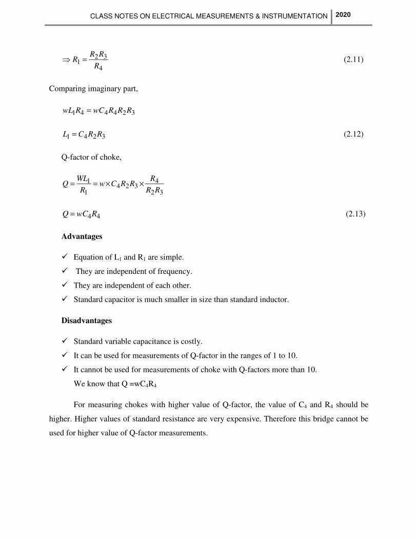
RRR =⇒ (2.11)

Comparing imaginary part,

324441 RRRwCRwL =

3241 RRCL =

(2.12)

Q-factor of choke,

32

4324

1

1

RR

RRRCw

R

WLQ ××==

44RwCQ = (2.13)

Advantages

Equation of L1 and R1 are simple.

They are independent of frequency.

They are independent of each other.

Standard capacitor is much smaller in size than standard inductor.

Disadvantages

Standard variable capacitance is costly.

It can be used for measurements of Q-factor in the ranges of 1 to 10.

It cannot be used for measurements of choke with Q-factors more than 10.

We know that Q =wC4R4

For measuring chokes with higher value of Q-factor, the value of C4 and R4 should be

higher. Higher values of standard resistance are very expensive. Therefore this bridge cannot be

used for higher value of Q-factor measurements.

2020


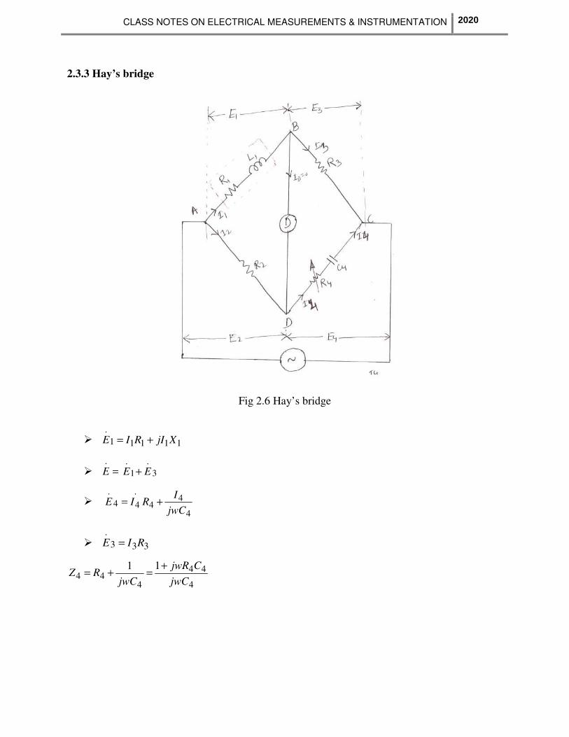
2.3.3 Hay’s bridge

Fig 2.6 Hay’s bridge

11111

.

XjIRIE +=

=.

E 3

.

1

.

EE +

4

44

.

44

.

jwC

IRIE +=

333

.

RIE =

4

44

444

11

jwC

CjwR

jwCRZ

+=+=

2020


Fig 2.7 Phasor diagram of Hay’s bridge

At balance condition, Z1Z4=Z3Z2

324

4411 )

1)(( RR

jwC

CjwRjwLR =

++

3424411 )1)(( RCjwRCjwRjwLR =++

32444122

11441 RRjwCRCLwjjwLRRjwCR =+++

32411444412

1 )()( RRjwCwLRRwCjRCLwR =++−

Comparing the real term,

04412

1 =− RCLwR

4412

1 RCLwR = (2.14)

2020


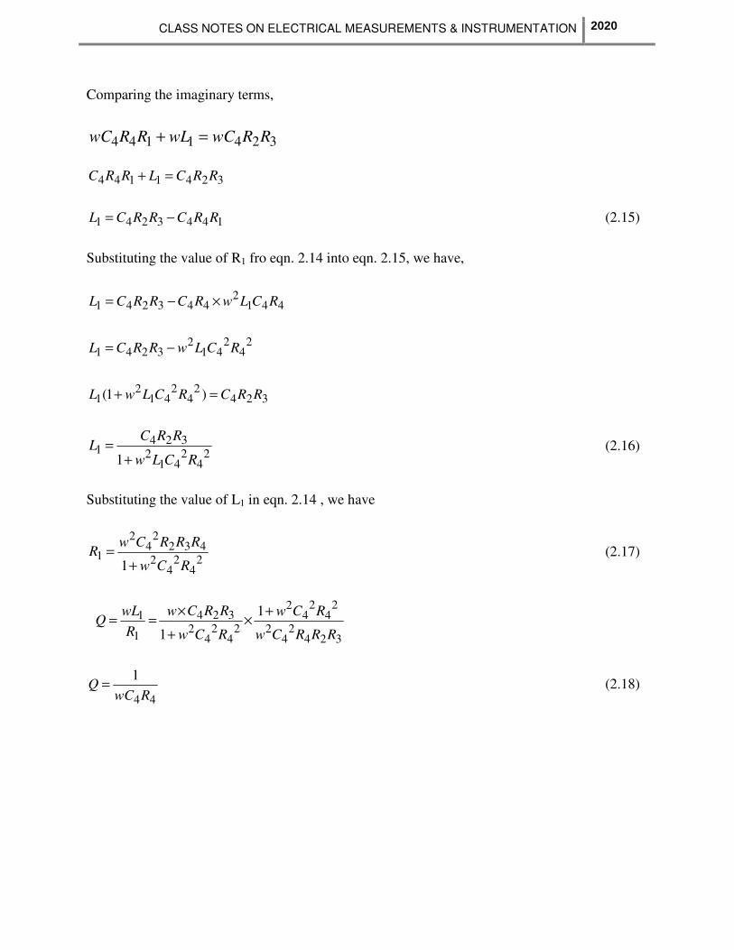
Comparing the imaginary terms,

3241144 RRwCwLRRwC =+

3241144 RRCLRRC =+

1443241 RRCRRCL −= (2.15)

Substituting the value of R1 fro eqn. 2.14 into eqn. 2.15, we have,

4412

443241 RCLwRCRRCL ×−=

24

241

23241 RCLwRRCL −=

3242

42

412

1 )1( RRCRCLwL =+

24

241

2324

11 RCLw

RRCL

+= (2.16)

Substituting the value of L1 in eqn. 2.14 , we have

24

24

2432

24

2

11 RCw

RRRCwR

+= (2.17)

3242

42

24

24

2

24

24

2324

1

1 1

1 RRRCw

RCw

RCw

RRCw

R

wLQ

+×

+

×==

44

1

RwCQ = (2.18)

2020


Advantages

Fixed capacitor is cheaper than variable capacitor.

This bridge is best suitable for measuring high value of Q-factor.

Disadvantages

Equations of L1and R1 are complicated.

Measurements of R1 and L1 require the value of frequency.

This bridge cannot be used for measuring low Q- factor.

2.3.4 Owen’s bridge

Fig 2.8 Owen’s bridge

11111 XjIRIE +=

I4 leads E4 by 900

2020


=.

E 3

.

1

.

EE +

2

2222

.

jwC

IRIE +=

Fig 2.9 Phasor diagram of Owen’s bridge

Balance condition, 3

.

2

.

4

.

1

.

ZZZZ =

2

22

222

11

jwC

RjwC

jwCRZ

+=+=

2

322

411

)1(1)(

jwC

RCjwR

jwCjwLR

×+=×+∴

)1()( 2243112 CjwRCRjwLRC +=+

4322432121 CRCjwRCRCjwLCR +=+

Comparing real terms,

4321 CRCR =

2020


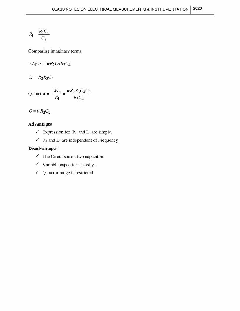
2

431

C

CRR =

Comparing imaginary terms,

432221 CRCwRCwL =

4321 CRRL =

Q- factor =43

2432

1

1

CR

CCRwR

R

WL=

22CwRQ =

Advantages

Expression for R1 and L1 are simple.

R1 and L1 are independent of Frequency.

Disadvantages

The Circuits used two capacitors.

Variable capacitor is costly.

Q-factor range is restricted.

2020


2.3.5 Anderson’s bridge

Fig 2.10 Anderson’s bridge

111111

.

)( XjIrRIE ++=

CEE =3

CC ErIE +=.

4

.

CIII += 42

−−−

=+ EEE 42

−−−

=+ EEE 31

2020


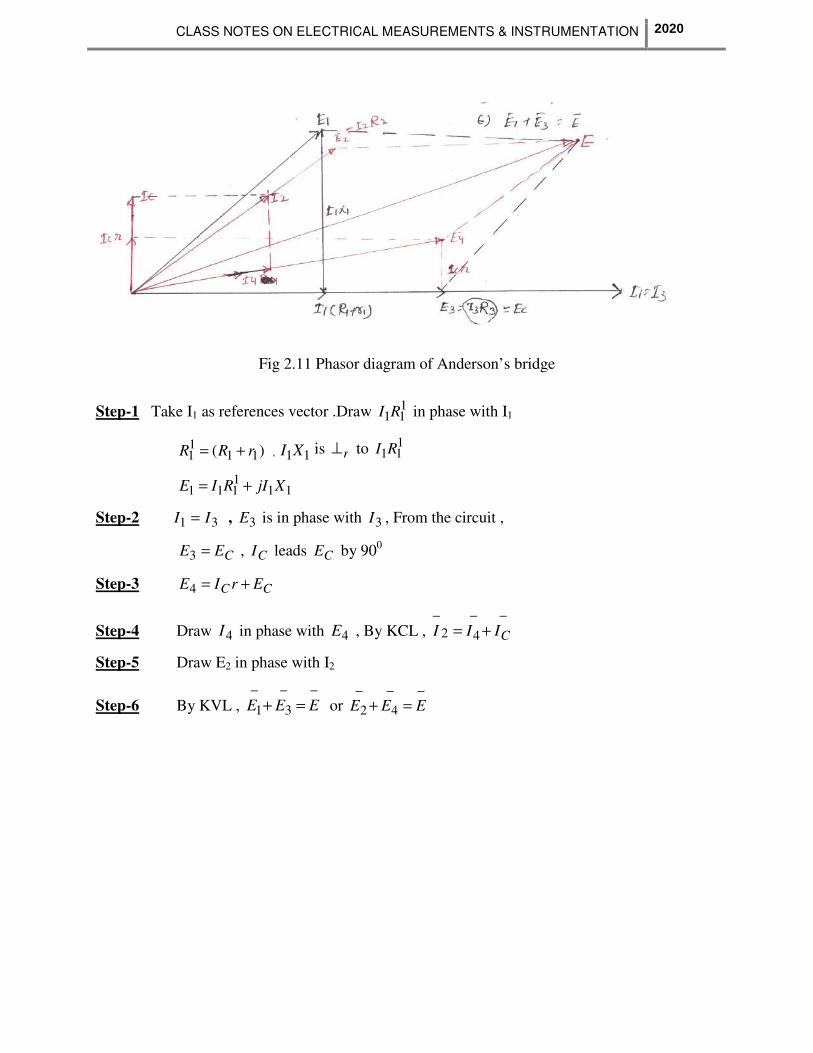
Fig 2.11 Phasor diagram of Anderson’s bridge

Step-1 Take I1 as references vector .Draw 111RI in phase with I1

)( 1111 rRR += , 11XI is r⊥ to 1

11RI

111111 XjIRIE +=

Step-2 31 II = , 3E is in phase with 3I , From the circuit ,

CEE =3 , CI leads CE by 900

Step-3 CC ErIE +=4

Step-4 Draw 4I in phase with 4E , By KCL , −−−

+= CIII 42

Step-5 Draw E2 in phase with I2

Step-6 By KVL , −−−

=+ EEE 31 or −−−

=+ EEE 42

2020


Fig 2.12 Equivalent delta to star conversion for the loop MON

)(11 4

4

4

47

rRjwC

rjwCR

jwcrR

rRZ

++=

++

×=

)(11

1

4

4

4

4

6rRjwC

R

jwcrR

jwCR

Z++

=++

×=

))(1

()(1

)(4

423

4

41

11

rRjwC

rjwCRRR

rRjwC

RjwLR

+++=

++×+

++

+++=

++

+⇒

)(1

))(1(

)(1

)(

4

4423

4

4111

rRjwC

jwCrRrRjwCRR

rRjwC

RjwLR

344323241411 )( RjwCrRRrRjCwRRRRjwLRR +++=+⇒

2020


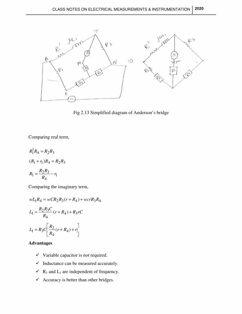
Fig 2.13 Simplified diagram of Anderson’s bridge

Comparing real term,

32411 RRRR =

32411 )( RRRrR =+

14

321 r

R

RRR −=

Comparing the imaginary term,

4343241 )( RwcrRRrRwCRRwL ++=

rCRRrR

CRRL 34

4

321 )( ++=

++= rRr

R

RCRL )( 4

4

231

Advantages

Variable capacitor is not required.

Inductance can be measured accurately.

R1 and L1 are independent of frequency.

Accuracy is better than other bridges.

2020


Disadvantages

Expression for R1 and L1 are complicated.

This is not in the standard form A.C. bridge.

2.4 Measurement of capacitance and loss angle. (Dissipation factor)

2.4.1 Dissipation factors (D)

A practical capacitor is represented as the series combination of small resistance and

ideal capacitance.

From the vector diagram, it can be seen that the angle between voltage and current is slightly less

than 900. The angle ‘δ ’ is called loss angle.

Fig 2.14 Condensor or capacitor

Fig 2.15 Representation of a practical capacitor

2020


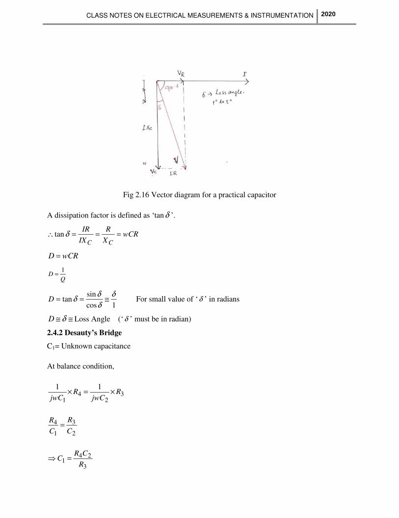
Fig 2.16 Vector diagram for a practical capacitor

A dissipation factor is defined as ‘tanδ ’.

wCRX

R

IX

IR

CC

===∴ δtan

wCRD =

QD

1=

1cos

sintan

δδδ

δ ≅==D For small value of ‘δ ’ in radians

≅≅ δD Loss Angle (‘δ ’ must be in radian)

2.4.2 Desauty’s Bridge

C1= Unknown capacitance

At balance condition,

32

41

11R

jwCR

jwC×=×

2

3

1

4

C

R

C

R=

3

241

R

CRC =⇒

2020


Fig 2.17 Desauty’s bridge

Fig 2.18 Phasor diagram of Desauty’s bridge

2020


2.4.3 Modified desauty’s bridge

Fig 2.19 Modified Desauty’s bridge

Fig 2.20 Phasor diagram of Modified Desauty’s bridge

2020


)( 1111 rRR +=

)( 2212 rRR +=

At balance condition, )1

()1

(2

1234

1

11

jwCRRR

jwCR +=+

)2

3123

1

44

11

jwC

RRR

jwC

RRR +=+

Comparing the real term, 1234

11 RRRR =

4

1231

1R

RRR =

4

3221

)(

R

RrRrR

+=+

Comparing imaginary term,

2

3

1

4

wC

R

wC

R=

3

241

R

CRC =

Dissipation factor D=wC1r1

Advantages

r1 and c1 are independent of frequency.

They are independent of each other.

Source need not be pure sine wave.

2.4.4 Schering bridge

41111 XjIrIE −=

C2 = C4= Standard capacitor (Internal resistance=0)

C4= Variable capacitance.

C1= Unknown capacitance.

r1= Unknown series equivalent resistance of the capacitor.

2020


R3=R4= Known resistor.

Fig 2.21 Schering bridge

1

11

111

11

jwC

rjwC

jwCrZ

+=+=

44

4

44

44

411

1

RjwC

R

jwCR

jwCR

Z+

=+

×=

2020


Fig 2.22 Phasor diagram of Schering bridge


.

2

.

4

.

1

.

ZZZZ =

2

3

44

4

1

11

1

1

jwC

R

RjwC

R

jwC

rjwC=

+×

+

)1()1( 44132411 rjwCCRCRrjwC +=+

134413241122 CRRjwCCRCRrjwCCR +=+

Comparing the real part,

3

241

R

CRC =∴

Comparing the imaginary part,

14342411 CRRwCCRrwC =

2

341

C

RCr =

Dissipation factor of capacitor,

2020


2

34

3

2411

C

RC

R

CRwrwCD ××==

44RwCD =∴

Advantages

In this type of bridge, the value of capacitance can be measured accurately.

It can measure capacitance value over a wide range.

It can measure dissipation factor accurately.

Disadvantages

It requires two capacitors.

Variable standard capacitor is costly.

2.5 Measurements of frequency

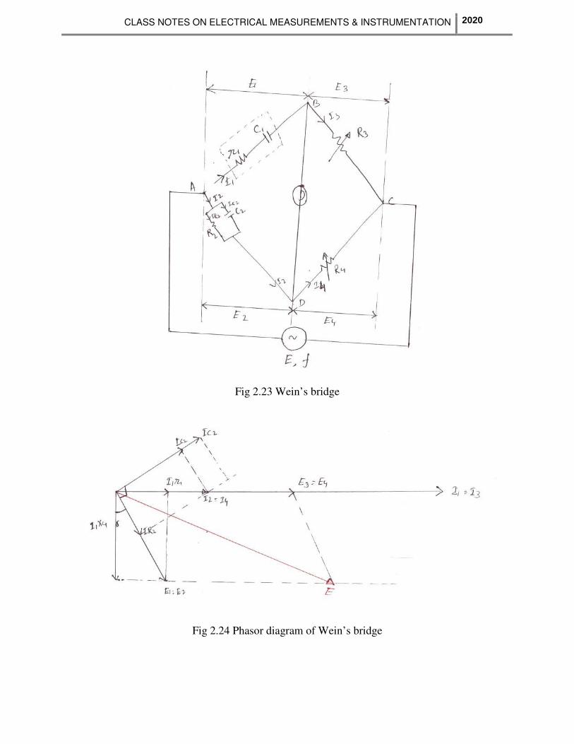
2.5.1 Wein’s bridge

Wein’s bridge is popularly used for measurements of frequency of frequency. In this bridge, the

value of all parameters are known. The source whose frequency has to measure is connected as

shown in the figure.

1

11

111

11

jwC

rjwC

jwCrZ

+=+=

22

22

1 RjwC

RZ

+=


.

2

.

4

.

1

.

ZZZZ =

322

24

1

11

1

1R

RjwC

RR

jwC

rjwC×

+=×

+

13242211 )1)(1( jwCRRRRjwCrjwC ×=++

[ ]4

3212121

211221

R

RRjwCRrCCwrjwCRjwC =−++

2020


Fig 2.23 Wein’s bridge

Fig 2.24 Phasor diagram of Wein’s bridge

2020


Comparing real term,

01 21212 =− RrCCw

121212 =RrCCw

2121

2 1

RrCCw =

2121

1

RrCCw = ,

21212

1

RrCCf

Π=

NOTE

The above bridge can be used for measurements of capacitance. In such case, r1 and C1 are

unknown and frequency is known. By equating real terms, we will get R1 and C1. Similarly by

equating imaginary term, we will get another equation in terms of r1 and C1. It is only used for

measurements of Audio frequency.

A.F=20 HZ to 20 KHZ

R.F=>> 20 KHZ

Comparing imaginary term,

4

3211122

R

RRwCrwCRwC =+

4

3211122

R

RRCrCRC =+ …………………………………..(2.19)

21221

1

RrCwC =

Substituting in eqn. (2.19), we have

14

32

2122

122 C

R

RR

RrCw

rRC =+

Multiplying 32

4

RR

R in both sides, we have

132

4

222

32

422

1C

RR

R

RCwRR

RRC =×+×

2020


3222

24

3

421

RRCw

R

R

RCC +=

122112 =RCrCw

+

==

3222

24

3

4222

212221

11

RRCw

R

R

RCRCw

CRCwr

+

=

32

4

3

422

22

1

RR

R

R

RRCw

+

=∴

22

22

2

4

31

1

1

RRCw

R

Rr

+=∴

)1

(

1

22

22

24

31

RRCw

R

Rr

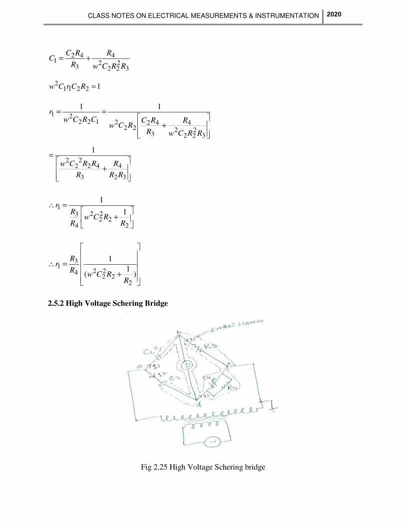
2.5.2 High Voltage Schering Bridge

Fig 2.25 High Voltage Schering bridge

2020


(1) The high voltage supply is obtained from a transformer usually at 50 HZ.

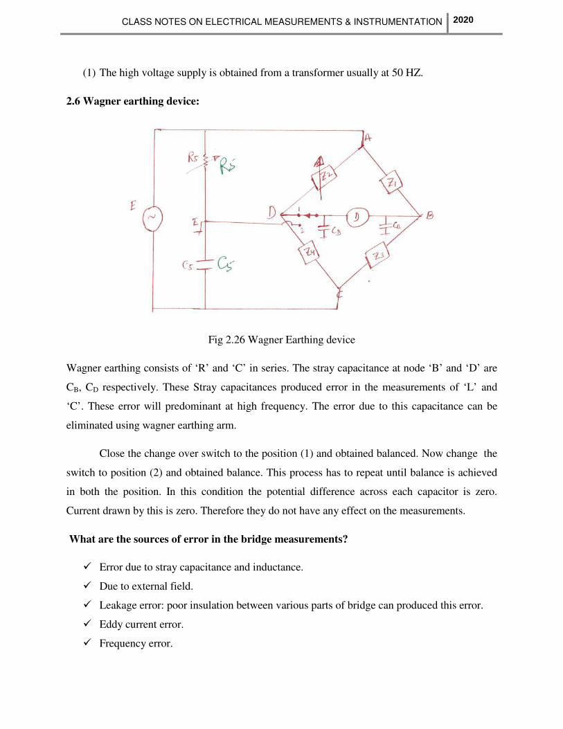
2.6 Wagner earthing device:

Fig 2.26 Wagner Earthing device

Wagner earthing consists of ‘R’ and ‘C’ in series. The stray capacitance at node ‘B’ and ‘D’ are

CB, CD respectively. These Stray capacitances produced error in the measurements of ‘L’ and

‘C’. These error will predominant at high frequency. The error due to this capacitance can be

eliminated using wagner earthing arm.

Close the change over switch to the position (1) and obtained balanced. Now change the

switch to position (2) and obtained balance. This process has to repeat until balance is achieved

in both the position. In this condition the potential difference across each capacitor is zero.

Current drawn by this is zero. Therefore they do not have any effect on the measurements.

What are the sources of error in the bridge measurements?

Error due to stray capacitance and inductance.

Due to external field.

Leakage error: poor insulation between various parts of bridge can produced this error.

Eddy current error.

Frequency error.

2020


Waveform error (due to harmonics)

Residual error: small inductance and small capacitance of the resistor produce this error.

Precaution

The load inductance is eliminated by twisting the connecting the connecting lead.

In the case of capacitive bridge, the connecting lead are kept apart.(d

rAC

∈∈=

0Q )

In the case of inductive bridge, the various arm are magnetically screen.

In the case of capacitive bridge, the various arm are electro statically screen to reduced

the stray capacitance between various arm.

To avoid the problem of spike, an inter bridge transformer is used in between the source

and bridge.

The stray capacitance between the ends of detector to the ground, cause difficulty in

balancing as well as error in measurements. To avoid this problem, we use wagner

earthing device.

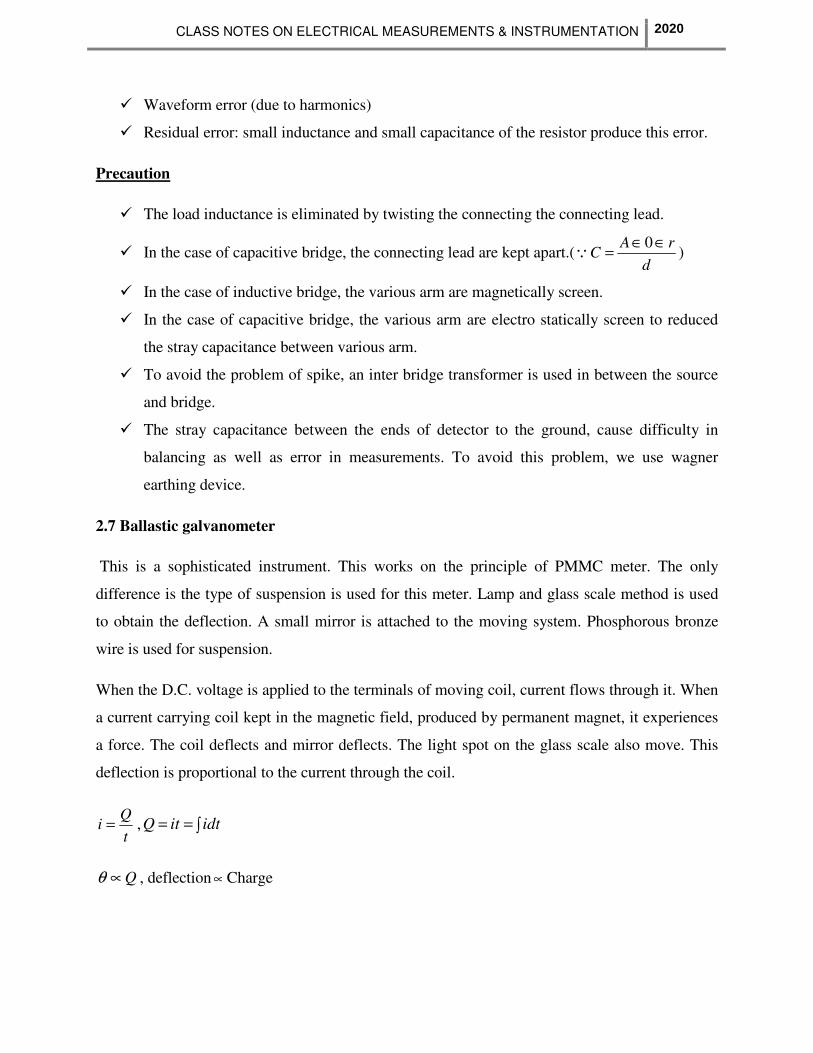
2.7 Ballastic galvanometer

This is a sophisticated instrument. This works on the principle of PMMC meter. The only

difference is the type of suspension is used for this meter. Lamp and glass scale method is used

to obtain the deflection. A small mirror is attached to the moving system. Phosphorous bronze

wire is used for suspension.

When the D.C. voltage is applied to the terminals of moving coil, current flows through it. When

a current carrying coil kept in the magnetic field, produced by permanent magnet, it experiences

a force. The coil deflects and mirror deflects. The light spot on the glass scale also move. This

deflection is proportional to the current through the coil.

t

Qi = , ∫== idtitQ

Q∝θ , deflection ∝ Charge

2020


Fig 2.27 Ballastic galvanometer

2.8 Measurements of flux and flux density (Method of reversal)

D.C. voltage is applied to the electromagnet through a variable resistance R1 and a reversing

switch. The voltage applied to the toroid can be reversed by changing the switch from position 2

to position ‘1’. Let the switch be in position ‘2’ initially. A constant current flows through the

toroid and a constant flux is established in the core of the magnet.

A search coil of few turns is provided on the toroid. The B.G. is connected to the search

coil through a current limiting resistance. When it is required to measure the flux, the switch is

changed from position ‘2’ to position ‘1’. Hence the flux reduced to zero and it starts increasing

in the reverse direction. The flux goes from + φ to - φ , in time ‘t’ second. An emf is induced in

the search coil, science the flux changes with time. This emf circulates a current through R2 and

B.G. The meter deflects. The switch is normally closed. It is opened when it is required to take

the reading.

2020


2.8.1 Plotting the BH curve

The curve drawn with the current on the X-axis and the flux on the Y-axis, is called

magnetization characteristics. The shape of B-H curve is similar to shape of magnetization

characteristics. The residual magnetism present in the specimen can be removed as follows.

Fig 2.28 BH curve

Fig 2.29 Magnetization characteristics

2020


Close the switch ‘S2’ to protect the galvanometer, from high current. Change the switch

S1 from position ‘1’ to ‘2’ and vice versa for several times.

To start with the resistance ‘R1’ is kept at maximum resistance position. For a particular value of

current, the deflection of B.G. is noted. This process is repeated for various value of current. For

each deflection flux can be calculated.( A

Bφ

= )

Magnetic field intensity value for various current can be calculated.().The B-H curve can be

plotted by using the value of ‘B’ and ‘H’.

2.8.2 Measurements of iron loss:

Let RP= pressure coil resistance

RS = resistance of coil S1

E= voltage reading= Voltage induced in S2

I= current in the pressure coil

VP= Voltage applied to wattmeter pressure coil.

W= reading of wattmeter corresponding voltage V

W1= reading of wattmeter corresponding voltage E

PEW

VW

→

→

1

V

WEW

V

E

W

W ×=⇒= 1

1

W1=Total loss=Iron loss+ Cupper loss.

The above circuit is similar to no load test of transformer.

In the case of no load test the reading of wattmeter is approximately equal to iron loss. Iron loss

depends on the emf induced in the winding. Science emf is directly proportional to flux. The

voltage applied to the pressure coil is V. The corresponding of wattmeter is ‘W’. The iron loss

corresponding E is V

WEE = . The reading of the wattmeter includes the losses in the pressure

coil and copper loss of the winding S1. These loses have to be subtracted to get the actual iron

loss.

2020


2.9 Galvanometers

D-Arsonval Galvanometer

Vibration Galvanometer

Ballistic C

2.9.1 D-arsonval galvanometer (d.c. galvanometer)

Fig 2.30 D-Arsonval Galvanometer

Galvanometer is a special type of ammeter used for measuring µ A or mA. This is a

sophisticated instruments. This works on the principle of PMMC meter. The only difference is

the type of suspension used for this meter. It uses a sophisticated suspension called taut

suspension, so that moving system has negligible weight.

Lamp and glass scale method is used to obtain the deflection. A small mirror is attached

to the moving system. Phosphors bronze is used for suspension.

2020


When D.C. voltage is applied to the terminal of moving coil, current flows through it.

When current carrying coil is kept in the magnetic field produced by P.M. , it experiences a

force. The light spot on the glass scale also move. This deflection is proportional to the current

through the coil. This instrument can be used only with D.C. like PMMC meter.

The deflecting Torque,

TD=BINA

TD=GI, Where G=BAN

TC=KSθ =Sθ

At balance, TC=TD ⇒ Sθ =GI

S

GI=∴θ

Where G= Displacements constant of Galvanometer

S=Spring constant

2.9.2 Vibration Galvanometer (A.C. Galvanometer )

The construction of this galvanometer is similar to the PMMC instrument except for the moving

system. The moving coil is suspended using two ivory bridge pieces. The tension of the system

can be varied by rotating the screw provided at the top suspension. The natural frequency can be

varied by varying the tension wire of the screw or varying the distance between ivory bridge

piece.

When A.C. current is passed through coil an alternating torque or vibration is produced. This

vibration is maximum if the natural frequency of moving system coincide with supply frequency.

Vibration is maximum, science resonance takes place. When the coil is vibrating , the mirror

oscillates and the dot moves back and front. This appears as a line on the glass scale. Vibration

galvanometer is used for null deflection of a dot appears on the scale. If the bridge is unbalanced,

a line appears on the scale

2020


Fig 2.31 Vibration Galvanometer

Example 2.2-In a low- Voltage Schering bridge designed for the measurement of

permittivity, the branch ‘ab’ consists of two electrodes between which the specimen under

test may be inserted, arm ‘bc’ is a non-reactive resistor R3 in parallel with a standard

capacitor C3, arm CD is a non-reactive resistor R4 in parallel with a standard capacitor C4,

arm ‘da’ is a standard air capacitor of capacitance C2. Without the specimen between the

electrode, balance is obtained with following values , C3=C4=120 pF, C2=150 pF,

R3=R4=5000Ω.With the specimen inserted, these values become C3=200 pF,C4=1000

pF,C2=900 pF and R3=R4=5000Ω. In such test w=5000 rad/sec. Find the relative

permittivity of the specimen?

Sol: Relative permittivity( rε ) =mediumair with measured ecapacitanc

mediumgiven with measured ecapacitanc

2020


Fig 2.32 Schering bridge

)(3

421

R

RCC =

Let capacitance value C0, when without specimen dielectric.

Let the capacitance value CS when with the specimen dielectric.

pFR

RCC 150

5000

5000150)(

3

420 =×==

pFR

RCCS 900

5000

5000900)(

3

42 =×==

6150

900

0

===C

CSrε

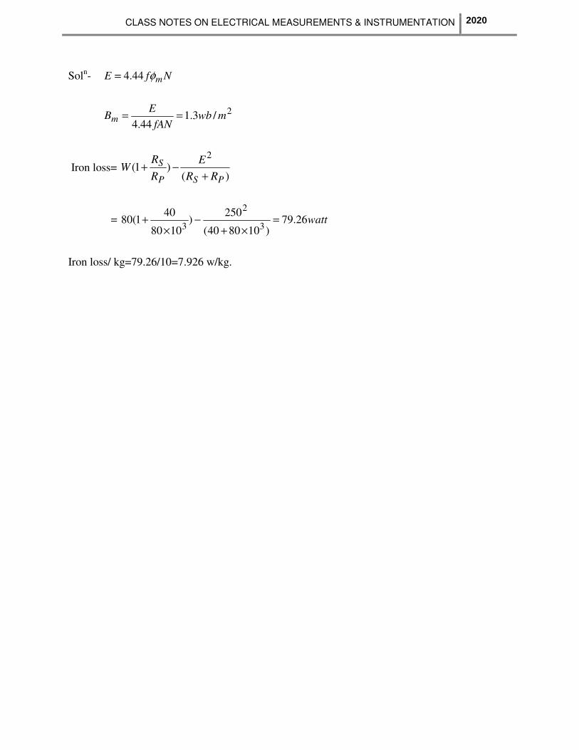
Example 2.3- A specimen of iron stamping weighting 10 kg and having a area of 16.8 cm2 is

tested by an episten square. Each of the two winding S1 and S2 have 515 turns. A.C. voltage

of 50 HZ frequency is given to the primary. The current in the primary is 0.35 A. A

voltmeter connected to S2 indicates 250 V. Resistance of S1 and S2 each equal to 40 Ω.

Resistance of pressure coil is 80 kΩ. Calculate maximum flux density in the specimen and

iron loss/kg if the wattmeter indicates 80 watt?

2020


Soln- NfE mφ44.4=

2/3.144.4

mwbfAN

EBm ==

Iron loss= )(

)1(2

PSP

S

RR

E

R

RW

+−+

= watt26.79)108040(

250)

1080

401(80

3

2

3=

×+−

×+

Iron loss/ kg=79.26/10=7.926 w/kg.

2020

AC BRIDGES - Government Polytechnic Deogarh

Documents

Transcript of AC BRIDGES - Government Polytechnic Deogarh