Parametric evolution for a deformed cavity

PHYSICAL REVIEW E, VOLUME 63, 046207

Parametric evolution for a deformed cavity

Doron Cohen,1 Alex Barnett,1 and Eric J. Heller1,2

1Department of Physics, Harvard University, Cambridge, Massachusetts 021382Department of Chemistry and Chemical Biology, Harvard University, Cambridge, Massachusetts 02138

~Received 31 August 2000; published 27 March 2001!

We consider a classically chaotic system that is described by a HamiltonianH(Q,P;x), where (Q,P)describes a particle moving inside a cavity, andx controls a deformation of the boundary. The quantumeigenstates of the system areun(x)&. We describe how the parametric kernelP(num)5u^n(x)um(x0)&u2, alsoknown as the local density of states, evolves as a function ofdx5x2x0. We illuminate the nonunitary natureof this parametric evolution, the emergence of nonperturbative features, the final nonuniversal saturation, andthe limitations of random-wave considerations. The parametric evolution is demonstrated numerically for twodistinct representative deformation processes.

DOI: 10.1103/PhysRevE.63.046207 PACS number~s!: 05.45.Mt, 03.65.2w, 73.23.2b

ia

av-d-

-itie

thu

acic

sy

ns

e-ra

f-

e

be

ehe

s:

.lear

t inumas in

be

oftion

so-

ae

mee-but

I. INTRODUCTION

A. The local density of states

Consider a system that is described by an HamiltonH(Q,P;x), where (Q,P) are canonical variables andx is aconstant parameter. Our interest in this paper is in the cwhere (Q,P) describe the motion of a particle inside a caity, and x controls the deformation of the confining bounary. The one-dimensional~1D! version of a cavity, alsoknown as a ‘‘potential well,’’ is illustrated in Fig. 1. However, we are mainly interested in the case of chaotic cavin d.1 dimensions. Cavities ind52 dimensions, alsoknown as billiard systems, are prototype examples instudies of classical and quantum chaos, and we shallthem for the purpose of numerical illustrations.

The eigenstates of the quantized Hamiltonian areun(x)&and the corresponding eigenenergies areEn(x). The eigenen-ergies are assumed to be ordered, and the mean level spwill be denoted byD. We are interested in the parametrkernel

P~num!5u^n~x!um~x0!&u25tr~rnrm!. ~1!

In the equation aboverm(Q,P) andrn(Q,P) are the Wignerfunctions that correspond to the eigenstatesum(x0)& andun(x)&, respectively. The trace stands fordQdP/(2p\)d in-tegration. The differencex2x0 will be denoted bydx. Weassume a dense spectrum, so that our interest is in ‘‘clacally small’’ but ‘‘quantum mechanically large’’ energscales. It is important to realize that the kernelP(num) has awell defined classical limit. The classical approximation~seeremark@1#! is obtained by using microcanonical distributioinstead of Wigner functions.

Fixing n, the vectorP(num) describes the shape of thnth eigenstate in theH05H(Q,P;x0) representation. By averaging over several eigenstates one obtains the aveshape of the eigenstate~ASOE!. We can also identifyP(num) as the local density of states~LDOS!, by regarding itas a function ofn, wherem is considered to be a fixed reerence state. In the latter case an average over fewm states isassumed. We shall denote the LDOS byP(r ), wherer 5(n2m). The ASOE is justP(2r ). Note that the ASOE and th

1063-651X/2001/63~4!/046207~12!/$20.00 63 0462

n

se

s

ese

ing

si-

ge

LDOS are given by the same function. One would have tomore careful with these definitions ifH0 were integrablewhile H nonintegrable.

A few words are in order regarding the definition of thLDOS, and its importance in physical applications. TLDOS, also known as strength function@4–6#, describes anenergy distribution. Conventionally it is defined as follow

r~E!521

p^muIm G~E!um&5(

nP~num!d~E2En!,

~2!

whereG(E)51/(E2H1 i0) is the retarded Green functionWe are interested in chaotic systems, so it should be cthat ourP(r ) is related by trivial change of variable (E°r )to the above definedr(E). Our P(r ) also incorporates anaverage over the reference state. The LDOS is importanstudies of either chaotic or complex conservative quantsystems that are encountered in nuclear physics as wellatomic and molecular physics. Related applications mayfound in mesoscopic physics. Going fromH0 to H may sig-nify a physical change of an external field, or switching ona perturbation, or a sudden change of an effective interac~as in molecular dynamics@7#!. The so-called ‘‘line shape’’of the LDOS is important for the understanding of the as

FIG. 1. The shape of a cavity ind dimensions is defined by itsd21 boundary. The confining potential isV(Q). The figure illus-tratesV(Q) for one dimension well. It also can be regarded ascross section of thed.1 cavity. The kinetic energy of the particlis E5

12 mv2. The walls of the cavity exert a field of forcef on the

bouncing particle. The hard wall limit corresponds tof→` andV0→`. For theoretical considerations it is convenient to assuthat f and V0 are large but finite. Mathematically it is also convnient to think of the embedding space as having some hugefinite volume~not illustrated!.

©2001 The American Physical Society07-1

Oil-f

eoas

ieived

hin

ts

ha

r-nyt

ricgy

sstre

nisasrk

ho

-

assreth

ie

ma

s.

-v

lls.allne

f(

PEheiledourd-

n-edaterity

utens,

ea-tive

ourex--ther

erot

areirl

t

in

DORON COHEN, ALEX BARNETT, AND ERIC J. HELLER PHYSICAL REVIEW E63 046207

ciated dynamics. It is also important to realize that the LDis the Fourier transform of the so-called ‘‘survival probabity amplitude’’ @7# ~see Ref.@8# for concise presentation othis point!.

B. Parametric evolution

Textbook @9# formulations of perturbation theory can bapplied in order to find the LDOS. Partial summationsdiagrams to infinite order can be used in order to getimproved Lorentzian-type approximation. However, motextbooks do not illuminate the limitations and the subtletwhich are involved in using the conventional perturbatschemes. It is therefore interesting to take a somewhatferent approach to the study of LDOS. The roots of talternate approach can be traced back to the work of Wig@10# regarding a simple banded random matrix~BRM! modelH5E1dxB. Here E is a diagonal matrix whose elemenare the ordered energies$En%, andB is a banded matrix. Thestudy of this model can be motivated by the realization tin generic circumstances it is possible to writeH(Q,P;x)'H0(Q,P)1dxF(Q,P). Using a simple semiclassical agument@11# it turns out that the matrix representation of agenericF, in the eigenbasis that is determined by the chaoHamiltonianH0, is a banded matrix.

The important ingredient~from our point of view! in theoriginal work by Wigner, is the emphasis on the parametevolution~PE! of the LDOS. The LDOS describes an enerdistribution: Fordx50 the kernelP(r ) is simply a Kronekerdelta function. Asdx becomes larger, the width as well athe whole profile of this distribution ‘‘evolves.’’ Wigner harealized that for his BRM model there are three parameregimes. For very smalldx we have the standard perturbativstructure where most of the probability is concentrated ir50. For largerdx we have a Lorentzian lineshape. But thLorentzian line shape does not persist if we further incredx. Instead we get a semicircle line shape. Many woabout the LDOS have followed@4–6#, but the issue of PEhas not been further discussed there. The emphasis in tworks is mainly on the case whereH0 is an integrable ornoninteracting system, whileH is possibly~but not necessarily ! chaotic due to some added perturbation term.

The line of study which is pursued in the present work hbeen originated and motivated by studies of quantum dipation@12–14#. Understanding PE can be regarded as a pliminary stage in the analysis of the energy spreading procin driven mesoscopic systems. Note that the LDOS givesenergy redistribution due to a ‘‘sudden’’~very fast! changeof the Hamiltonian. Unlike the common approach for studof LDOS, we assume bothH and H0 to be chaotic. Bothcorrespond to the same parametrically dependent HatonianH(Q,P;x), and there is nothing special in choosingparticular valuex5x0 as a starting point for the PE analysi

C. Main results

The theory of PE, as discussed in general in Refs.@12–14#and in particular in Refs.@8,15# takes us beyond the randommatrix-theory considerations of Wigner. There appear fi

04620

S

fnts

if-ser

t

ic

-

ic

es

se

si-

e-sse

s

il-

e

~rather than two! different parametric scales~see remark@2#!.These are summarized by Table I.

In the present paper we consider cavities with hard waWe are going to explain that because of the ‘‘hard wlimit’’ there are onlytwo independent parametric scales: Ois dxc

qm and the others~see remark@3#! coincide withdxNU .Assuming thatdxc

qm anddxNU are well separated, it followsthat there arethreedistinct parametric regimes in the PE oour system. These are the standard perturbative regimedx!dxc

qm), the core-tail regime (dxcNU!dx!dxqm), and the

nonuniversal regime (dx@dxNU).The exploration of the three parametric regimes in the

of a deformed cavity with hard walls is the main issue of tpresent paper. To the best of our knowledge such detaexploration has not been practical in the past. We oweability to carry out this task to a powerful technique for fining clusters of billiard eigenstates@19,20#. There are alsosome secondary issues that we are going to address.

~a! In the strict limit of hard walls the PE becomes nounitarity. We shall use the 1D well example in order to shlight on this confusing issue. In particular we demonstrthat any truncation of the PE equation leads to false unitadue to a finite-size edge effect.

~b! For special deformations, namely, those that constitlinear combination of translations, rotations, and dilatiothe parametric scalesdxc

qm anddxNU coincide. Consequentlythere is no longer distinct core-tail regime, and the PE ftures a quite sharp transition from the standard perturbaregime to the nonuniversal regime.

~c! In the nonuniversal regime we demonstrate thatnumerical results are in accordance with our theoreticalpectation@8#. Namely, the width of the LDOS profile is determined by time-domain semiclassical considerations, rathen by phase-space or random-wave considerations.

~d! The last section puts our specific study in a largcontext. We explain why Wigner’s scenario of PE is nfollowed once hard walls are considered.

II. CAVITY SYSTEM

We consider a particle moving inside ad-dimensionalcavity whose volume isV. The kinetic energy of the particleis E5 1

2 mv2, wherem is its mass, andv is its velocity. It is

TABLE I. The parametric scales in the general theory of PElisted ~left column! along with the questions that motivate theintroduction. The distributionP(r ) may contain perturbative tairegions~for dx!dxprt), and nonperturbative core regions~for dx.dxc

qm). Nonuniversal ~system specific! features may manifesthemselves in the core structure fordx@dxNU . In generic examplesdx@dxSC allows a classical approximation forP(r ). We are goingto explain that only two independent parametric scales survivethe hard wall limit.

dxccl Is it possible to linearizeH(x1dx)?

dxcqm Is it possible to use standard perturbation theory?

dxprt Do perturbative tail regions survive?dxNU Do nonuniversal core features show up?dxSC Is it possible to use semiclassical approximation?

7-2

st

m

ioli

n

aionoci

llth

is

i

dgof

e

e-

h

ry

a

ea

e

e

-if itf

tox-

lace

n-

nglikerd

l

atin

-by

nce

Defor

PARAMETRIC EVOLUTION FOR A DEFORMED CAVITY PHYSICAL REVIEW E63 046207

assumed that this motion is classically chaotic. The ballimean free path isl bl . One can use the estimatel bl;V/A,whereA is the total area of the walls. The associated tiscale istbl5 l bl /v.

The penetration distance upon a collision isl 5E/ f , wheref is the force that is exerted by the wall. Upon quantizatwe have an additional length scale, which is the De BrogwavelengthlB52p\/(mv). We shall distinguish betweethe hard walls case where we assumel ,lB! l bl , and softwalls for which lB! l . Note that taking\→0 implies softwalls.

There is a class of special deformations that are shpreserving. These are generated by translations, rotatand dilations of the cavity. A general deformation needpreserve the billiard shape nor its volume. We can speany deformation by a functionD(s), wheres specifies thelocation of a wall element on the boundary~surface! of thecavity, andD(s)dx is the normal displacement of this waelement. In many practical cases it is possible to useconventionuD(s)u;1. With this conventiondx has units oflength, and its value has the meaning of typical wall dplacement.

The eigenenergies of a particle inside the cavity aregeneral x dependent, and can be written asEn5(\kn)2/(2m). The mean level spacing is

D5\v32p

Vd

1

VlBd21 ~3!

whereVd52p,4p, . . . , for d52,3, . . . . In ournumericalstudy we shall consider a quarter stadium with curved eof radius 1 and straight edge of length 1. The ‘‘volume’’the quarter stadium isV511p/4. The ‘‘area’’ of its bound-ary A541p/2 is just the perimeter. We shall look on thparametric evolution of eigenstates aroundk;400 where themean level spacing ink units is D5D/(\v)'0.0088.

III. PARAMETRIC EVOLUTION

Consider the quantum-mechanical statec5um(x0)&. Wecan writec5(nan(x)un(x)&. The parametric kernel can bwritten asP(num)5uan(x)u2. It is a standard exercise to obtain ~from dc/dx50 and differentiating by parts! the fol-lowing equation for the amplitudes:

dan

dx52

i

\ (m

Wnm~x!am . ~4!

In order to getP(num) one should solve this equation witthe initial conditionsan(x0)5dnm . The transitions betweenlevels are induced by the matrix elements

Wnm5i\

En2EmS ]H

]x Dnm

~5!

and we use the ‘‘gauge’’ conventionWnm50 for n5m.~Only one parameter is being changed and therefore Berphase is not an issue.!

04620

ic

e

ne

pens,t

fy

e

-

n

e

’s

Equation~4! is a possible starting point for constructingperturbation theory for the PE ofP(r ) ~see Ref.@14# formore details!. As an input for this equation we need thmatrix elements of]H/]x. These can be calculated usingsimple boundary integral formula@16# whose simplest deri-vation @14# is as follows: The position of the particle in thvicinity of a wall element isQ5(z,s), wheres is a surfacecoordinate andz is a perpendicular ‘‘radial’’ coordinate. Wetake f 5` so that

]H]x

52D~s!V0d~z!. ~6!

The logarithmic derivative of the wave function on thboundary isw(s)/c(s), wherew(s)5n•¹c, andn is a unitvector in thez direction. Forz.0 the wave functionc(Q) isa decaying exponential. IfV0 is large enough, then the exponential decay is fast, and we can treat the boundary aswere locally flat. It follows that the logarithmic derivative othe wave function on the boundary should be equal2A2mV0/\. Consequently one obtains the following epression for the matrix elements:

S ]H]x D

nm

52\2

2m R wn~s!wm~s!D~s!ds. ~7!

In the one-dimensional case the boundary integral is repby the sum(swn(s)wm(s)D(s) where s51,2 are the twoturning points of the potential well.

IV. HARD WALLS AND NONUNITARITY

For the purpose of the following argumentation it is covenient to takef 5`, but to keepV0 large but finite. Math-ematically it is also convenient to think of the embeddispace as having some huge but finite volume. We wouldto illuminate a subtlety which is associated with the hawall limit V0→`. For any finiteV0 the parametric kernesatisfies

(n

P~num!5ptotal ~8!

with ptotal51. This follows from the fact thatun(x)& is acomplete orthonormal basis for anyx. However, for hardwalls (V05`) this statement is not true. This implies thfor hard walls the PE is nonunitary. We are going to explathis point below.

Let us denote the volume of the original cavity byV0 andof the deformed cavity byV. The volume shared by the deformed and the undeformed cavities will be denotedV0ùV and we shall use the notationh5(V0ùV)/V0. For thepurpose of the following argument let us consider a referestatem whose energyEm is well belowV0. Let us also as-sume that the wall displacement is large compared toBroglie wavelength. Consequently the expressionP(num) has the following semiclassical structure:

P~num!'h3 f ~En2Em!1~12h!3g~En2Ec!, ~9!

7-3

edc

in

nee

le

t

texweq.

us

.

hheh

one

v

ndiso-t

theel

s

u-


whereEc5(V01Em);V0. The above result can be deducby assuming that the wave functions look ergodic in spabut still that they are characterized by a well-definedlocalwavelength. An equivalent derivation is obtained by usthe phase-space picture of Ref.@8#. Both f andg in the aboveexpression have unit normalization, and thereforeptotal51for any finiteV0. However, for hard walls (V05`) we haveEc5` and thereforeptotal5h. We may say the the operatioof taking the hard wall limit does not commute with thsummation in Eq.~8!. An analogous statement can be drived regarding the summation(mP(num), with the respec-tive definitionh5(V0ùV)/V.

The correctness of the above observation becomestrivial if we consider Eq.~4! with expressions~5! and ~7!substituted for the matrix elements. Looking at Eq.~5! withEq. ~7! it seems as if the matrixWnm is Hermitian, andtherefore should generate unitary PE. But this statemenmathematically correct only for~any! finite truncationN ofthe PE equation. ForN5` the matrixWnm becomes non-Hermitian. It turns out that for any finiteN, there is a pile-upof probability in the edges of the spreading profile, duefinite-size effect. We shall demonstrate this effect in the nsection using a simple 1D example. In other words, ifsolve Eq.~4! for hard-walled cavity, we get as a result E~9! with Ec5EN . For N5` we get Ec5` and thereforeptotal5h in accordance with the conclusion of the previoparagraph.

Thus if eitherV0,` or N,` then we have unitary PEBut for hard walls, meaningV05` with N5`, we havenonunitary PE. The lost probability is associated with tsecond term in Eq.~9!. This term is peaked around a higenergyEc . For hard wallsEc5` and consequently somprobability is lost. The above picture is supported by tsimple pedagogical example of the next section.

V. PARAMETRIC EVOLUTION FOR A 1D BOX

Consider a 1D box with hard walls, where the free motiof the particle is within 0,Q,a. The eigenstates of thHamiltonian are

un~a!&→~21!nA2

asin~knQ!, ~10!

wherekn5n3(p/a) is the wave number, andn51,2, . . . ,is the level index. The phase factor (21)n has been intro-duced for convenience. We consider now the parametric elution as a function ofa. One easily obtains

^n~a!um~a0!&5~21!nAhsin~phn!

p

2m

h2n22m2, ~11!

whereh[a0 /a is assumed to be smaller than 1, correspoing to expansion of the box. The probability kernelP(num)5u^num&u2. One can verify that the parametric evlution in the a0°a direction is unitary, meaning tha(nP(num)51. On the other hand, in thea°a0 direction the

04620

e,

g

-

ss

is

ot

e

e

o-

-

parametric evolution is nonunitary, because(mP(num)5h.The profile ofP(num) for fixed n is illustrated by a dashedline in Fig. 2.

We can restore unitarity by makingV0 large but finite. Insuch case, a variation of the above calculation leads tofollowing picture: Consider the overlap of a reference levn(a) with the levelsm(a0). As in the caseV05` there is aprobability h which is located in the levels whose energieare Em'En . But now the ‘‘lost’’ probability (12h) is lo-cated in the levels whose energies areEm'En1V0. Thus wehave(mP(num)51 rather than(mP(num)5h.

We again consider the caseV05`. The normal derivative

on the boundary iswn(a)5A(2/a)kn . Hence we can easilyget the following result:

1

\Wnm5

2 i

kn22km

2wn~a!wm~a!52 i

1

a

2nm

n22m2. ~12!

FIG. 2. ~a! An image of the kernelP(num) for 13% expansionof the box ~i.e., a/a051.13). The kernel has been calculated nmerically using Eq.~13! with finite truncationN5256. ~b! Theprofile of a representative row ofP(num). The dashed line is theN5` analytical result using Eq.~11!.

7-4

n

-

1Dise

e

wloty

io

i

n

ldnrevo

in

ia-

a(-

nsvity

r-t the

bil-zed

the

as

te

ton-

-

esla-

f


It is more convenient to usea5 ln(a) for parametrization.Hence the equation that describes the parametric evolutio

dan

da52(

m

2nm

n22m2am . ~13!

For any finite truncationN,` this equation manifestly generates unitary parametric evolution. It is only forN5` thatit becomes equivalent to the nonunitary evolution of thebox. Again, one can wonder where the ‘‘lost’’ probabilitylocated ifN,`. The answer is illustrated in Fig. 2. We sethat the ‘‘lost’’ probability piles up at the edge of the~trun-cated! tail.

VI. MATRIX ELEMENTS FOR CHAOTIC CAVITY

It is possible to use semiclassical considerations@11# inorder to determine the band profile of the matrix Eq.~7!. Theapplication to the cavity example has been introduced in R@14#, and numerically demonstrated in Ref.@17#. The accu-racy of this semiclassical estimate is remarkable. Heresummarize the recipe. First one should generate a very~ergodic! trajectory, and define for it the fluctuating quanti

F~ t !52]H]x

5(col

2mv cos~ucol!Dcold~ t2tcol!, ~14!

wheretcol is the time of a collision,Dcol stands forD(s) atthe point of the collision, andv cos(ucol) is the normal com-ponent of the particle’s velocity. Each delta spike~for softwalls it is actually a narrow rectangular spike! corresponds toone collision. Now one can calculate the correlation functC(t) of the fluctuating quantityF(t), and its Fourier trans-form C(v). The semiclassical estimate for the band profile

K US ]H]x D

nmU2L '

D

2p\CS En2Em

\ D ~15!

Reference@18# contains a systematic study of the functioC(v). For largev, meaningv@1/tbl , one can use

C~v!'2m2v3^ucosuu3&1

V R @D~s!#2ds, ~16!

where the geometric factor isucos(u)u3&51,4/3p, . . . , ford51,2, . . . . Alengthy calculation@14# reveals that Eq.~15!with ~16! substituted, is an exact global result if we couassume that the cavity eigenfunctions look similar to ‘‘radom waves,’’ and that different wave functions are uncorlated. However, it turns out that to take this random waresult as a global approximation is an oversimplification. Fv!1/tbl , using the semiclassical recipe and assumstrongly chaotic cavity, one obtains

C~v!'C~`!3~tblv!g ~17!

with g54 for dilations and translations,g52 for rotations,andg50 for normal deformations. We use the term ‘‘specdeformations’’ @18# in order to distinguish those deforma

04620

is

f.

eng

n

s

--erg

l

tions that have the propertyC(v)→0 in the limit v→0.Any combination of dilations, translations, and rotations isspecial deformation. Around the bouncing frequencyv;1/tbl) the functionC(v) typically displays some nonuniversal ~system and deformation specific! structure. This istrue for any typical deformation, but for some deformatiothe nonuniversal features are more pronounced. If the cahas bouncing ball modes, we may get also a modified~non-universal! behavior in the small frequency limit. For the pupose of general discussion it is convenient to assume thainterpolation between Eqs.~17! and ~16! is smooth, but inactual numerical calculation the actualC(v) is computed~see below!.

As a numerical example we have picked the stadiumliard. We have found the eigenstates of a desymmetri~quarter! stadium as described in Ref.@17#. We have selectedthose eigenstates whose eigenenergieskn are in the vicinityof k5400. Our two representative deformations are~a! rota-tion around the stadium center and~b! generic~nonspecial!deformation involving the curved edge. In the latter casecurved edge of the quarter stadium (0,s,p/2) is pushedoutwards withD(s)5@cos(s)#2, while for the straight edgesD(s)50. ~The corners50 is the 90° intersection of thecurved edge with the long straight edge!. The respectiveband profiles are displayed in Fig. 3. The band profile hbeen defined as

B~k!51

4k2 K U R wn~s!wm~s! D~s!dsU2L , ~18!

wherek5(kn2km) is the distance from the diagonal. Nothat B(k) is just a scaled version of the semiclassicalC(v)as implied by Eq.~15! with ~7!. The remarkable agreemenof B(k) with the semiclassical calculation has been demstrated in Refs.@17,18#.

It is important to realize that in the hard wall limit~whichis assumed here! the matrix (]H/]x)nm is not a banded matrix. It would become banded if we were assumingsoftwalls.For soft wallsC(v) becomes vanishingly small forv@v/ l .The bandwidth in energy units isDb5\v/ l , and in dimen-sionless units it is

b5Db

D5

VllB

d21. ~19!

Unless stated otherwise we haveb5`.

VII. PARAMETRIC EVOLUTION—NUMERICALRESULTS

The parametric evolution ofP(r ) for rotation and for ge-neric deformation of the stadium is illustrated by the imagof Fig. 4 and by the plots of Fig. 5 and Fig. 6. The calcution of eachP(r ) profile is carried out as follows: Givendxwe use the method which is described in Ref.@20# in order tocalculate the matrixP(num). Then we plot the elements oP(num) versusk5@kn(x)2km(0)#. In order to obtain the

7-5

du

m

thoif

o(

e

ss

thned

a

ea

tedree


average profile the plot is smeared using standard proce~see remark@21#!. The transformation fromk to r 5(n2m) is done using the relation~see remark@21#!:

k5D•r 21

dk3

dVV . ~20!

AboveD is the mean level spacing of the$kn% spectrum, anddV is the volume change that is associated with the defortion ~it is approximately proportional todx). If the deforma-tion is volume preserving~as in the case of rotation! then thesecond term equals zero. But for the generic deformationwe have picked in our second numerical example, the vume is not preserved, and the systematic ‘‘downward’’ shof the levels should be taken into account.

Looking first at the case of rotation, we clearly see twparametric regimes: The standard perturbative regimedx,0.2) and the nonuniversal regime (dx.0.2). Let us clarify

FIG. 3. Band profiles for deformations of the quarter stadiumdefined by Eq.~18!. ~a! Rotation around the stadium center.~b!Generic ~nonspecial! deformation involving displacement of thcurved edge. It is important to notice that for the special deform

tion we haveC(v)→0 in the limit v→0.

04620

re

a-

atl-t

this observation. We see that fordx,0.2 most of the prob-ability is well concentrated inr 50. This implies that we canuse standard perturbation theory in order to estimate thr50 probabilities. On the other hand, fordx.0.2 the pertur-bative nature ofP(r ) is destroyed. NowP(r ) becomessmoother, and eventually~for dx.0.5) there is a very goodfitting with Lorentzian~see lower plot in Fig. 5!.

The qualitative explanation for the Lorentzian profile is afollows. Fordx.0.5 the typical displacement of the walls iof the order oflB . Therefore theun(x)& eigenstates becomeuncorrelated with theum(0)& eigenstates. ConsequentlyP(r )becomesdx independent. The Lorentzian profile agrees withe assumption of uncorrelated random waves as explaiin the Appendix.

s

-

FIG. 4. Each column is an image ofP(r ) versusk for a differ-ent value ofdx. There are 41 columns. The valuedx;1 corre-sponds roughly tolB displacement of the boundary.~a! is for rota-tion and ~b! is for generic deformation. Note that ther 50component is excluded from the image. Instead we have plotover the image anr 50 line wherever this component contains mothan 50% of the probability. In the lower figure this line cannot bresolved from the developing core region.

7-6

erp4

s

is

--


Let us now look at the case of generic deformation. Hwe clearly see three parametric regimes: The standardturbative regime (dx,0.004), the core-tail regime (0.00,dx,0.2), and the nonuniversal regime (dx.0.2). Let usclarify this observation. As in the case of rotation there istandard perturbative regime (dx,0.004) where most of the

FIG. 5. Representative plots ofP(r ) for the case of rotation.~a!is for 0.0010<dx<0.2512. Ther 50 component is excluded. In~b!the fitted Lorentzian is indistinguishable from the actual profile.

04620

eer-

a

probability is well concentrated inr 50. For larger deforma-tion, namely fordx.0.004, standard perturbation theoryno longer applicable because then5m level is mixed non-perturbatively with other~neighboring! levels. As a resultP(r ) contains a nonperturbative ‘‘core’’ component. However, for 0.004,dx,0.2 we definitely do not get a Lorent

FIG. 6. Representative plots ofP(r ) for the case of genericdeformation.~a! is for 0.0010<dx<0.2512. In~b! a fitted Lorent-zian is overlayed for the purpose of comparison.

7-7

y

ealn.tont

x

he-

hethsp

r

in

-

eth

e

nt.

nd-

grd to

ase,ller

nd

ueall

ngin-

n,on

ed.

re,ere

xingales.

n

al-

s at


zian. Rather the tails ofP(r ) keep growing in the same waas in the standard perturbative regime.

In the case of the generic deformation, as in the casrotation, we enter the nonuniversal regime, and eventu~for dx.0.6) we get a smooth Lorentzian-like distributioHowever, the Lorentzian-like distribution is not identicalthat of the rotation case. Also the similarity to proper Lorezian is far from being satisfactory~see lower plot in Fig. 6!.This means that the random-wave picture of the Appendian oversimplification.

In the following sections we are going to summarize ttheoretical considerations@8# that explain the observed parametric scenario. In particular we are going to illuminate tway in which nonperturbative features emerge; to clarifycrossover to the nonuniversal regime; and to explain thecific nature of the nonuniversal distribution.

VIII. THE STANDARD PERTURBATIVE REGIME

Standard perturbation theory gives the following first oder expression for the LDOS

P~num!'dnm1dx2u~]H/]x!nmu2

~En2Em!2. ~21!

This expression is most straightforwardly obtained byspecting Eqs.~4! and~5!. We can define the~total! transitionprobability as

p~dx!5(r 5” 0

P~r !. ~22!

Using Eq. ~21! combined with~15! we get the followingestimate:

p~dx!'dx231

\2Euvu.D/\

dv

2p

C~v!

v2. ~23!

Standard perturbation theory is applicable as long asp(dx)!1. This can be converted into an equivalent inequalitydx!dxc

qm. By this definitiondxcqm is the parametric deforma

tion which is needed in order to mix the initial levelm withother levelsn5” m.

If we use Eq.~23! for a special deformation, then we havg.1, and consequently the integral is not sensitive toexclusion of theur u,D region. As a result we havedxc

qm

}\. Using Eq.~17! with ~16! we get

dxcqmuspecial5S l bl

1

V R @D~s!#2dsD 21/2

3lB . ~24!

In the case of generic deformation, Eq.~24! is not validbecause the value of the integral in Eq.~23! is predominantlydetermined by thev;D/\ lower cutoff rather than by aneffectivev;1/tbl lower cutoff. As a result one obtains

dxcqmugeneric5S l H

1

V R @D~s!#2dsD 21/2

3lB , ~25!

04620

ofly

-

is

ee-

-

-

e

where l H5vtH is the length which is associated with thHeisenberg timetH52p\/D.

It is illuminating to use the conventionD(s);1, such thatdx measures the typical displacement of a wall elemeWith this convention we get from Eqs.~24!,~25! the follow-ing:

dxcqmuspecial'lB , ~26!

dxcqmugeneric5S lB

d21

AeffD 1/2

3lB , ~27!

dxcqmudiffractive;lB . ~28!

In the generic case the effective area of the deformed bouary Aeff may be smaller than the total areaA of the boundary.The effective areaAeff can be formally defined by comparinEq. ~27! with Eq. ~25!. Equation~28! has been added fosake of completeness of our presentation. It corresponthe diffractive limit Aeff→lB

d21 . Note that this limit is be-yond the scope of the present study. Thus in the generic cthe wall displacement needed to mix levels is much smathan lB . In the generic casedxc

qm}\ (d11)/2 rather thandxc

qm}\. What happens with perturbation theory beyodxc

qm? This is the subject of the next section.

IX. THE CORE-TAIL REGIME

For dx.dxcqm standard perturbation theory diverges d

to the nonperturbative mixing of neighboring levels on smscale: Oncedx becomes of the order ofdxc

qm several levelsare mixed, and asdx becomes larger, more levels are beimixed nonperturbatively. Consequently it is natural to distguish betweencore and tail regions @13–15#. Most of thespreading probability is contained within the core regiowhich implies a natural extension of first-order perturbatitheory ~FOPT!: The first step is to transform Eq.~4! into anew basis where transitions within the core are eliminatThe second step is to use FOPT~in the new basis! in order toanalyze the core-to-tail transitions. Details of this proceduwhich is in the spirit of degenerate perturbation theory, wdiscussed in Ref.@14#. The most important~and nontrivial!consequence of this procedure is the observation that mion small scales does not affect the transitions on large scTherefore we have in the tail regionP(num)}dx2 ratherthan P(num)}dx. The validity of this observation has beenumerically illustrated in Ref.@15#.

Following the above reasoning we define thetail regionas consists of those levels whose ‘‘occupation’’ can be cculated using perturbation theory, while thecore is the non-perturbative component in the vicinity ofr 50. Assumingthat only one scale characterize the core width, one arrivethe following practical approximation

Pprt~r !5D

2p\CS En2Em

\ D dx2

@G~dx!#21~En2Em!2.

~29!

7-8

-

etntt’

v

heic

en

tyr

in

-f

volei-a-h

or

-

lss

soi

tu

is

e-


It is implicit in this definition that (En2Em) should be re-garded as a function ofr 5(n2m). The parameterG(dx) isdetermined~for a given dx) such thatPprt(r ) has a unitnormalization. One may say thatG(dx) regularizes the behavior aroundr 50. For generic deformation we get

G~dx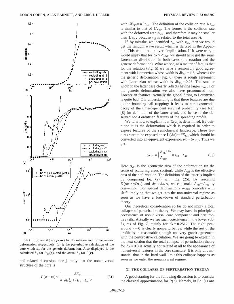![b0D'S dx

dxcqmD 2

3D. ~30!

The core is defined as the regionur u,b0, and the outer(ur u.b0) regions are the tails. Fordx!dxc

qm we getb0!1and the core-tail structure Eq.~29! becomes equivalent to thstandard perturbative result Eq.~21!. It should be clear thathe core-tail structure is a generalization of Wigner’s Lorezian. It is indeed a Lorentzian in the special case of a ‘‘flaband profile.

We turn now to analyze our numerical results. We haverified ~see, e.g., Fig. 7! that for dx,0.2 we have goodagreement with perturbation theory irrespective of whetwe have a core component~which is the case for the generdeformation! or not ~which is the case for the rotation!. Aswe come closer todx;0.2 the agreement becomes worsand for dx.0.3 we have a total collapse of perturbatiotheory. In Fig. 8 we display the total transition probabilip(dx) as a function ofdx. This plot should be used in ordeto numerically determine the value ofdxc

qm, say as the valuewherep(dx)51/2.

Figure 8 also displays comparison with the correspondperturbative calculation@using Eq. ~22! with ~29!#. Theagreement~for dx,dxc

qm) in case of the rotation is remarkable. For larger values ofdx one observes a linear drop othe total probability due to the nonunitary nature of the elution. ~This drop is clearly linear in a linear-linear scawhich is not displayed.! The eventual rise of the total transtion probability ~beyond 1) in case of the generic deformtion, reflects numerical errors in the determination of tsmall k overlaps. See Ref.@20# for further details.

The lower subfigure in Fig. 8 displays the calculated cwidth b0 for the generic deformation. Recall thatb0 is deter-mined, givendx, such thatPprt(r ) of Eq. ~29! is normalized.Also calculated is the widthbc of the region that contains50% of the probability. The widthbc is calculated for bothPprt(r ) and P(r ). Note thatbc51 in the standard perturbative regime. The determination ofdxc

qm for the generic de-formation becomes more convenient by using this plot. Athe crossover~at dxNU;0.2) to the nonuniversal regime imost pronounced.

X. NONUNIVERSAL REGIME

The validity of Eq.~29! as a global approximation relieon the assumption that the core is characterized only byscale~which is b0). But this assumption ceases to be truedx is large enough. We have explained in Ref.@8# that thewidth of thecoredefines a ‘‘window’’ through which we canview the ‘‘landscape’’ of the semiclassical analysis. Asdxbecomes larger, this ‘‘window’’ becomes wider, and evenally some of semiclassical structure is exposed. This

04620

-’

e

r

,

g

-

e

e

o

nef

-is

marked by the nonuniversal parametric scaledxNU . For dxlarger thandxNU , the nonuniversal structure of the coreexposed.

What is the semiclassical structure of the LDOS? Timdomain semiclassical considerations@See Eq.~10! of Ref. @8#

FIG. 7. Comparison between the perturbative calculationPprt(r )and the actualP(r ). ~a! is for the rotation and~b! is for the genericdeformation,~c! is the same as~b!, giving a zoom over the ‘‘birth’’of the nonperturbative semiclassical saturation profile.

7-9

l

r

n-ite

ate-

t

on-ndue

tial

-

tofea-

ed

astion

tala

rba-ub-

e

inoryof

m-as

er

cee


and related discussion there# imply that the nonuniversastructure of the core is

P~n2m!'1

p

dESC

dESC2 1~En2Em!2

~31!

FIG. 8. ~a! and~b! arep(dx) for the rotation and for the generideformation respectively.~c! is the perturbative calculation of thcore width b0 for the generic deformation. Also displayed is thcalculatedbc for Pprt(r ), and the actualbc for P(r ).

04620

with dESC5\/tcol . The definition of the collision rate 1/tcolis similar to that of 1/tbl . The former is the collision ratewith the deformed areaAdfr , and therefore it may be smallethan 1/tbl , becausetbl is related to the total areaA.

If, by mistake, we identifiedtcol with tbl , then we wouldget the random wave result which is derived in the Appedix. This would be an over simplification. If it were true,would imply that fordx.dxNU we should have got the samLorentzian distribution in both cases~the rotation and thegeneric deformation!. What we see, as a matter of fact, is thfor the rotation~Fig. 5! we have a reasonably good agrement with Lorentzian whose width isdkSC51.5, whereas forthe generic deformation~Fig. 6! there is rough agreemenwith Lorentzian whose width isdkSC50.26. The smallerwidth in the latter case clearly reflects having largertcol . Forthe generic deformation we also have pronounced nLorentzian features. Actually the global fitting to Lorentziais quite bad. Our understanding is that these features areto the bouncing-ball trapping: It leads to non-exponendecay of the time-dependent survival probability~see Ref.@8# for definition of the latter term!, and hence to the observed non-Lorentzian features of the spreading profile.

We turn now to explain howdxNU is determined. By defi-nition it is the deformation which is required in orderexpose features of the semiclassical landscape. Thesetures start to be exposed onceG(dx);dESC which should beconverted into an equivalent expressiondx;dxNU . Thus weget

dxNU5S Adfr

AeffD 1/2

3lB;lB . ~32!

Here Adfr is the geometric area of the deformation~in thesense of scattering cross section!, while Aeff is the effectivearea of the deformation. The definition of the latter is impliby comparing Eq. ~27! with Eq. ~25!. By rescalingD(s)°aD(s) and dx°dx/a, we can makeAeff5Adfr byconvention. For special deformationsdxNU coincides withdxc

qm implying that we get into the non-universal regimesoon as we have a breakdown of standard perturbatheory.

Our theoretical consideration so far do not imply a tocollapse of perturbation theory. We may have in principlecoexistence of nonuniversal core component and pertutive tails. Actually we see such coexistence in the lower sfigures of Fig. 7, mainly fordx50.2512. The right peakaroundk50 is clearly nonperturbative, while the rest of thprofile is in reasonable~though not very good! agreementwith the perturbative calculation. We are going to explainthe next section that the total collapse of perturbation thefor dx.0.3 is actually not related at all to the appearancenonuniversal features in the core structure. It is only circustantial that in the hard wall limit this collapse happenssoon as we enter the nonuniversal regime.

XI. THE COLLAPSE OF PERTURBATION THEORY

A good starting for the following discussion is to considthe classical approximation forP(r ). Namely, in Eq.~1! one

7-10

ce

f

o

i--

y

is

ncrd

’’al

ft

tu

mro

mhe

n

i-

-n

-

s-es-

t is

al

isthe

nrge


approximatesrn(Q,P) andrm(Q,P) by microcanonical dis-tributions. A phase-space illustration of the energy surfawhich supportrn(Q,P) andrm(Q,P) can be found in Fig. 1of Ref. @8#. The classicalP(num) equals to the overlap othese surfaces.

If we were dealing with a generic system we could intrduce a linearized version of the HamiltonianH(Q,P;x)5H0(Q,P)1dxF(Q,P;dx50), where F(Q,P;x)5]H/]x. By definition this linearization is a good approxmation provideddx!dxc

cl , wheredxccl is the classical corre

lation scale ofF(Q,P;x) with respect tox. In the classicallinear regime the classicalP(r ) has the scaling propertP(r )51/dxP(r /dx). See Ref.@15# for details.

An equivalent definition of dxccl in the quantum-

mechanical case is obtained by looking on thex dependenceof the matrix elements ofF(Q,P;x) in somefixed basis.Again we definedxc

cl as the respective correlation scale. Itquite clear that for cavity with soft walls we have

dxccl5 l @soft walls#, ~33!

where l 5E/ f has been defined as the penetration distaupon collision. From a purely classical point of view the hawall limit l→0 is a nonlinear limit. But this is not truequantum mechanically. Here we have

dxccl;lB @hard walls# ~34!

for l ,lB . The terminology ‘‘classical correlation scalewhile referring todxc

cl becomes misleading here, but we shkeep using it anyway.

The theory of the core-tail structure@14# is valid only inthe linear regimedx!dxc

cl . Let us assume for a moment sowalls. We can ask isdx!dxc

cl a sufficient condition for hav-ing a core-tail structure? The answer is definitely not. Perbation theory has a final collapse once the core widthb0(dx)becomes of the order of the band widthb. This defines aparametric scaledxprt . For dx.dxprt the LDOS becomespurely nonperturbative. In Wigner’s theory of randobanded matrices this corresponds to the crossover fLorentzian to semicircle line shape.

However, in the limit of hard walls the above mechanisof collapse becomes irrelevant because the band widtinfinite (b5`). On the other hand we still have to satisfy thinequalitydx!dxc

cl . Thus, fordx.lB we expect a total col-lapse of perturbation theory, as indeed observed in themerical study.

ACKNOWLEDGMENTS

This work was funded by ITAMP and the National Scence Foundation.

APPENDIX: OVERLAP OF UNCORRELATED RANDOMWAVES

It is possible to estimate the overlapu^num&u2 if we as-sume thatun& and um& are uncorrelatedrandom superpositions of plane waves: A random superposition of pla

04620

s

-

e

l

r-

m

is

u-

e

waves is characterized by the correlation function

^cR~x1!cR~x2!&51

V cos~kux22x1u!,

where cos(kr)[êxp(ik•r )&V is a generalized Bessel function ~for further details see Appendix D of Ref.@14#!. As-suming that the wave function ofun& is uncorrelated with thewave function ofum& one obtains

û^num&u2&5S 1

VD 2E E cos~knux22x1u!

3cos~kmux22x1u!dx1dx2 .

The integration is over the whole volume of the cavity. Uing the definition of the cos function we can cast this exprsion into the form u^num&u2&5^ f (q)&q where the average isover the differenceq5(k22k1), with all possible orienta-tions for uk1u5km and for uk2u5kn . The function f (q) isdefined as

f ~q!5U E eiq•xdxU2

.

The functionf (q) depends mainly onq5uqu. We can obtainan estimate forf (q) by considering a spherical cavityuxu,R with the same volume. Using spherical coordinates istraightforward to obtain

f ~q!'S FTF 1

d21~R22x2!(d21)/2G D 2

,

where FT is a Fourier transform fromx to q. For q!1/R wehave simply f (q)5(V)2. For q@1/R we have f (q)5(V)2/(Rq)d11. This is because of the singularity atx56R. The average overq can be done using again sphericcoordinate. We haveq'@(Dk)212k2(12cosu)#1/2, whereDk5ukn2kmu, and we can transform thedu integration intoa dq integration

^ f ~q!&q5Vd22

Vd21

3E qdq

k2 S A@q22~Dk!2#@~2k!22q2#

2k2 D d23

f ~q!,

where Vd is the solid angle ind dimensions. There is nopoint in trying to carry an exact integration. Rather, itimportant to observe that a practical approximation foroverlap is

û^num&u2&'S 1

kRD d21 1

11@R•~kn2km!#2.

In the latter expression we have neglected thed-dependentnormalization prefactor. It is a ‘‘practical’’ approximatiosince it gives the correct behavior for both small and lavalues ofDk. The interpolation aroundDk;1/R cannot betrusted.

7-11

all

ce-

e-eth

x-

g

it

idth

,

.

,

-A

.

s-

.

is-eveleanu-


@1# The classical approximation forP(num) works well for er-godic eigenstates. As explained later in the text we actuconsider the averaged profile. Namely,P(num) is regarded asa function ofr 5n2m, and it is averaged over the referenstatem. With this procedure the effect of the minority of nonergodic eigenstates can be neglected in the classical limit.

@2# The two parametric scales of Wigner’s RMT model corrspond todxc

qm and dxprt of Table I. Consequently there arthree parametric regimes in Wigner’s theory. These arestandard perturbative regime (dx!dxc

qm), the Lorentzian re-gime (dxc

qm!dx!dxprt), and the semi-circle regime (dx@dxprt). As an artifact of this RMT model, there actually eists a forth regime~Anderson strong localization regime! thatin the present context does not have a semiclassical analo

@3# As explained in Ref.@8# the generic hierarchy isdxNU!dxprt

!dxSC!dxccl . This hierarchy is realized in the classical lim

~small\) where we have soft walls~see Sec. II!. The hard walllimit is nongeneric, and these four parametric scales coincIn the present paper we assume hard walls unless stated owise.

@4# G. Casati, B. V. Chirikov, I. Guarneri, and F. M. IzrailevPhys. Rev. E48, R1613~1993!; Phys. Lett. A223, 430~1996!.

@5# V. V. Flambaum, A. A. Gribakina, G. F. Gribakin, and M. GKozlov, Phys. Rev. A50, 267 ~1994!.

@6# G. Casati, B. V. Chirikov, I. Guarneri, and F. M. IzrailevPhys. Lett. A223, 430 ~1996!; F. Borgonovi, I. Guarneri, andF. M. Izrailev, Phys. Rev. E57, 5291~1998!.

@7# E. Heller inChaos and Quantum Physics, Proceedings of Session LII of the Les-Houches Summer School, edited byVoros and M.-J. Giannoni~North-Holland, Amsterdam, 1990!.

@8# D. Cohen and E. J. Heller, Phys. Rev. Lett.84, 2841~2000!.

04620

y

e

.

e.er-

.

@9# C. Cohen-Tannoudji, J. Dupont-Roc, and G. Grynberg,Atom-photon Interactions: Basic Processes and Applications~Wiley,New York, 1992!.

@10# E. Wigner, Ann. Math.62, 548 ~1955!; 65, 203 ~1957!.@11# M. Feingold and A. Peres, Phys. Rev. A34, 591 ~1986!; M.

Feingold, D. Leitner, and M. Wilkinson, Phys. Rev. Lett.66,986 ~1991!; M. Wilkinson, M. Feingold, and D. Leitner, JPhys. A24, 175~1991!; M. Feingold, A. Gioletta, F. M. Izrai-lev, and L. Molinari, Phys. Rev. Lett.70, 2936~1993!.

@12# D. Cohen, Phys. Rev. Lett.82, 4951~1999!.@13# D. Cohen, inProceedings of the International School of Phy

ics ‘‘Enrico Fermi’’ Course CXLIII, edited by G. Casati, I.Guarneri, and U. Smilansky~IOS Press, Amsterdam, 2000!.

@14# D. Cohen, Ann. Phys.~N.Y.! 283, 175 ~2000!.@15# D. Cohen and T. Kottos, Phys. Rev. E~to be published!.@16# M. V. Berry and M. Wilkinson, Proc. R. Soc. London392, 15

~1984!.@17# A. Barnett, D. Cohen, and E. J. Heller, Phys. Rev. Lett.85,

1412 ~2000!.@18# A. Barnett, D. Cohen, and E. J. Heller, J. Phys. A~to be pub-

lished!.@19# E. Vergini and M. Saraceno, Phys. Rev. E52, 2204~1995!; E.

Vergini, Ph. D. thesis, Universidad de Buenos Aires, 1995@20# A. Barnett, Ph.D. thesis, Harvard, 2000.@21# In order to find the average profile we divide thek axis into

small bins. We find the averageP(num) value in each bin. Inorder to getP(r ) we resample the average profile. The dtance between the sampling points is equal to the mean lspacing. We are not interested in features on scale of the mlevel spacing. Therefore the transformation from the continous variablek to the integer variabler should not be consid-ered as problematic.

7-12

Parametric evolution for a deformed cavity

Documents

Transcript of Parametric evolution for a deformed cavity