arX

iv:a

stro

-ph/

9903

048v

1 2

Mar

199

9

Accepted for publication in ApJ

Profile instabilities of the millisecond pulsar PSR J1022+1001

Michael Kramer1,2, Kiriaki M. Xilouris3, Fernando Camilo 4, David J. Nice5, Donald C. Backer1,

Christoph Lange2, Duncan R. Lorimer2,3, Oleg Doroshenko6, Shauna Sallmen1

ABSTRACT

We present evidence that the integrated profiles of some millisecond pulsars exhibit

severe changes that are inconsistent with the moding phenomenon as known from slowly

rotating pulsars. We study these profile instabilities in particular for PSR J1022+1001

and show that they occur smoothly, exhibiting longer time constants than those associ-

ated with moding. In addition, the profile changes of this pulsar seem to be associated

with a relatively narrow-band variation of the pulse shape. Only parts of the integrated

profile participate in this process which suggests that the origin of this phenomenon is

intrinsic to the pulsar magnetosphere and unrelated to the interstellar medium. A po-

larization study rules out profile changes due to geometrical effects produced by any sort

of precession. However, changes are observed in the circularly polarized radiation com-

ponent. In total we identify four recycled pulsars which also exhibit instabilities in the

total power or polarization profiles due to an unknown phenomenon (PSRs J1022+1001,

J1730−2304, B1821−24, J2145−0750).

The consequences for high precision pulsar timing are discussed in view of the stan-

dard assumption that the integrated profiles of millisecond pulsars are stable. As a

result we present a new method to determine pulse times-of-arrival that involves an

adjustment of relative component amplitudes of the template profile. Applying this

method to PSR J1022+1001, we obtain an improved timing solution with a proper mo-

tion measurement of −17 ± 2 mas/yr in ecliptic longitude. Assuming a distance to the

pulsar as inferred from the dispersion measure this corresponds to an one-dimensional

space velocity of 50 km s−1.

1Astronomy Department, University of California, Berkeley, CA 94720, USA

2Max-Planck-Institut fur Radioastronomie, Auf dem Hugel 69, 53121 Bonn, Germany

3National Astronomy and Ionosphere Center, Arecibo Observatory, P.O. Box 995, Arecibo, PR 00613, USA

4Nuffield Radio Astronomy Laboratories, Jodrell Bank, Macclesfield, Cheshire SK11 9DL, England; Marie Curie

Fellow

5Joseph Henry Laboratories and Physics Department, Princeton University, Princeton, NJ 08544, USA

6Astro Space Center of P.N. Lebedev Physical Institute, Academy of Science, Leninski pr. 53, Moscow 117924,

Russia

– 2 –

Subject headings: Pulsars: millisecond pulsars – normal pulsars – profile stability – pre-

cession – mode changing – timing precision – PSRs J1022+1001, 1730−2304, B1821−24,

J2145−0750

1. Introduction

The discovery of millisecond pulsars (MSPs, Backer et al. 1982), opened new ways to study

the emission mechanism of pulsars. Although pulse periods and surface magnetic fields are several

orders of magnitude smaller than those of slowly rotating (’normal’) pulsars, the emission patterns

show some remarkable similarities (Kramer et al. 1998, hereafter KXL98; Xilouris et al. 1998,

hereafter XKJ98; Jenet et al. 1998). This suggests that the same emission process might work in

both types of objects despite orders of magnitude difference in the size of their magnetospheres.

A systematic study of the emission properties of MSPs and a comparison of the results with

characteristics of normal pulsars can thus lead to new important insight in the emission physics

of pulsars. In this paper we investigate unexpected profile instabilities seen for some MSPs and

compare them to profile changes known for normal pulsars.

The profile changes described here have consequences for high precision timing of MSPs, in

which integrated profiles are cross-correlated with a standard template to measure pulse times of

arrival. This procedure implicitly assumes that the shape of the integrated profile does not vary.

This premise has never been tested thoroughly for MSPs. The only systematic search we are aware

of was an analysis of the planet pulsar PSR B1257+12 which was searched, unsuccessfully, for shape

changes (Kaspi & Wolszczan 1993).

Recently, Backer & Sallmen (1997) noticed a significant change in the profile of the isolated

millisecond pulsar PSR B1821−24 in about 25% of all observations on time scales of a few hours

and possibly days. Even earlier Camilo (1995) described observations of PSR J1022+1001 which

show profile changes on apparently shorter time scales, i.e. hours or less. These are the first cases

in which such instabilities of profiles averaged over many pulse periods have been reported.

The plan of the paper is as follows. After briefly reviewing what is known about the profile

stability of normal pulsars in the next section, we present observations of PSR J1022+1001 and

investigate a large data set with respect to pulse shape changes in time, frequency and polarization.

In Sect. 3.5 we study the consequences for high precision timing and present a method to compensate

for the profile changes when measuring pulse times-of-arrival. Possible explanations for the observed

profile changes are discussed in Sect. 4, in view of additional sources showing a similar phenomenon.

A summary of this work is made in Sect. 5.

– 3 –

2. Profile stability of normal pulsars

Since the discovery of pulsars it has been known that individual pulses are highly variable in

shape and intensity. Nevertheless, summing a sufficiently large number of pulses leads generally to a

very stable pulse profile. Systematic studies of the stability of integrated profiles were carried out by

Helfand, Manchester & Taylor (1975) and recently by Rankin & Rathnasree (1995). These studies

show that a number of a few thousand pulses added together are very often enough to produce

a final stable waveform which does not differ from a high signal-to-noise ratio (S/N) template by

more than 0.1% or even less.

Despite this stability of pulse profiles, a small sample of normal pulsars shows distinct pulse

shape changes on time scales of minutes. This behaviour was first noticed by Backer (1970) and

is nowadays well known as mode changing. In a mode change the pulsar switches from one stable

profile to another on a time scale of less than a pulse period, remains in that mode for typically

hundreds of periods, before it returns back to the original pulse shape or switches to another mode.

This immediate switch from one mode to the next is a common phenomenon and is often associated

with a sudden change in pulse intensity (Rankin 1986). Interestingly, Suleymanova, Izvekova &

Rankin (1996) report that a mode switch in PSR B0943+10 is preceded by a decline in intensity

for one mode, although again a so called “burst” and “quiet” mode can be distinguished.

Rankin (1986) noted that mode-changing is often observed for such sources which exhibit rather

complex profiles showing both the so-called “cone” and “core” components (cf. Rankin 1983; Lyne

& Manchester 1988). The mode changing manifests itself as a reorganization of core and cone

emission and thus usually affects the whole profile (often including polarization properties) rather

than only certain pulse longitudes. A rare counter-example might be PSR J0538+2817 (Anderson

et al. 1996).

A phenomenon related to mode changing might be nulling, i.e. the absence of any pulsed

emission for a certain number of periods. There are no clear and unequivocal explanations for the

origin of nulling or mode changing which is normally interpreted as a re-arrangement in the structure

of the emitting region. Some studies report a possible relationship between mode changing and

change in emission height (e.g. Bartel et al. 1982). Other interpretations invoke a large variation

in the absorption properties of the magnetosphere above the polar cap (e.g. Zhang et al. 1997). In

any case, mode changing will increase the number of pulses that must be added before reaching a

final waveform. However, even for pulsars which show mode changes a maximum number of ∼ 104

pulses is typically sufficient for a stable average pulse shape to emerge from the process of adding

seemingly random pulses (Helfand, Manchester & Taylor 1975; Rankin & Rathnasree 1995). In

contrast, the profile changes of PSR J1022+1001 which we study in this paper, are on much longer

time scales, i.e. hundreds of thousands of periods or more as discussed below.

– 4 –

3. The changing profile of PSR J1022+1001

Soon after the discovery of PSR J1022+1001 (Camilo et al. 1996), we included it as part of our

regular timing programme at Effelsberg. The first high S/N profile was obtained in 1994 August

(Fig. 1a). Comparison with another high S/N profile in 1994 October (Fig. 1b) clearly demonstrated

that the resolved pulse peaks differ significantly in their relative amplitudes. Observations at other

telescopes confirmed this result which will be discussed in detail in the following.

3.1. Observations and data reduction

The majority of the data presented in this paper were obtained at 1410 MHz with the Effelsberg

100-m radiotelescope of the Max-Planck-Institut fur Radioastronomie, Bonn, Germany. Besides the

Effelsberg Pulsar Observing System (EPOS) described by KXL98, we also made measurements with

the Effelsberg-Berkeley-Pulsar-Processor (EBPP) — a coherent de-disperser that has operating in

parallel with EPOS since 1996 October.

The EBPP provides 32 channels for each polarization with a total bandwidth of up to 112

MHz depending on observing frequency, dispersion measure and number of Stokes parameters

recorded. For PSR J1022+1001 a bandwidth of 56 MHz can be obtained when recording only the

two orthogonal (left- and right hand) circularly polarized signals (LHC and RHC). In polarization

mode, i.e. also recording the polarization cross-products, a bandwidth of 28 MHz can be used. Each

channel is coherently de-dispersed on-line (assuming a dispersion measure of DM= 10.25 pc cm−3)

and folded with the topocentric pulse period. Individual sub-integrations typically last for 2 min,

before they are transferred to disk. A more detailed description of the EBPP can be found in

Backer et al. (1997) and Kramer et al. (1999).

In order to monitor the gain stability and polarization characteristics of the observing system,

we also performed regular calibration measurements using a switchable noise diode. The signal

from this noise diode is injected into the waveguide following the antenna horn and was itself

compared to the flux density of known continuum calibrators during regularly performed pointing

observations. Switching on the noise diode regularly after observations of pulsars allowed monitoring

of gain differences in the LHC and RHC signal paths. Use of this procedure, along with parallel

observations by two independent data acquisition systems, allows us to exclude an instrumental

origin of the observed profile changes. As a demonstration we show a three hour observation of

PSR J1022+1001 in Fig. 2, where each profile corresponds to an integration time of about 40 min.

The total power profile (right column) was obtained after appropriately weighting and adding the

LHC and RHC profiles shown in the first two columns. In order to guide the eye, we have drawn

a dashed horizontal line at the amplitude of the trailing pulse peak, which was normalized to

unity. Error bars are based on a worst-case analysis, combining 3σ values calculated from off-pulse

data with the (unlikely) assumption that the gain difference has (still) an uncertainty of about 20%.

Inspecting the time evolution of the shown profiles, we see that the RHC profile remains unchanged

– 5 –

during the whole measurement. At the same time the LHC profile undergoes clear changes. At the

beginning of the observations, the trailing pulse peak is the dominant feature in the LHC profile,

it then weakens gradually with time, until it becomes of equal amplitude to the first pulse peak.

The resulting (total power) profiles reflect exactly this trend.

The measurement presented in Fig. 2 clearly demonstrates that the observed profile changes

are not of instrumental origin, owing to the lack of any instrumental effect which could explain the

shown evolution on the observed short time scales. Moreover, a correlation between profile shape

and source elevation or hour angle is not present. We also searched for a possible relation between

profile changes and pulse intensity. In Fig. 2 we thus indicate the flux density measured for the

corresponding profiles (with an estimated uncertainty of less than 10%). Clearly, the profile changes

are uncorrelated with changes in intensity. Instead, the observed intensity change is presumably

caused by interstellar scintillation – a common phenomenon seen in low dispersion measure pulsars

(Rickett 1970).

3.2. Profile changes with time

A simple comparison of measured pulse profiles normalized to each of the two pulse peaks

provides first clues as to whether the profile is changing as a whole or stable parts are present.

In Fig. 3 we present pulse profiles obtained at 1.410 MHz at different epochs. Normalizing to the

leading pulse peak, the profile apparently changes over all pulse longitudes, i.e. including the depth

of the saddle region and the width of the profile itself. Normalizing the same profiles to the trailing

pulse peak seems to cause mainly changes in the first profile part while the trailing one remains

stable. The picture seems also to apply to the 430-MHz data obtained by Camilo (1995) and can

be confirmed, as discussed later, by the timing behaviour of this pulsar.

Although our data sometimes suggest that variations on time scales of a few minutes are

present, we need higher S/N data to confirm this impression. Instead, we reliably study here

profile variations visible on longer time scales by adding about 6 · 104 to 8 · 104 pulses each (i.e. 10

to 16 min). Although this corresponds to a much larger number of pulses than needed to reach

a stable profile for normal pulsars even in the presence of moding (cf. Sect. 2), we still observe a

smoothly varying set of pulse shapes. In order to demonstrate that the involved time scales are

highly variable, we calculated the amplitude ratio of the leading and trailing pulse peaks at 1410

MHz as the most easily accessible parameter to describe the profile changes. In order to use a

large homogeneous data set, we analyzed EPOS data, which were obtained with a bandwidth of

40 MHz, a time resolution of 25.8µs (cf. KXL98) and an integration time as quoted above. We

estimated uncertainties in the amplitude ratio using the same worst-case analysis as described

before. The mean value of the component ratio (amplitude of the leading pulse peak divided

by that of the second one) for the whole data set covering about four years of observations is

0.975± 0.009. Two examples of observations of comparable duration are shown in Fig. 4 where we

plot the amplitude ratio as a function of time. During the first measurement the profile appears

– 6 –

to be stable. In the second observation profile changes are evident. This is consistent with the

results of an unsuccessful search for periodicities or typical time scales in the amplitude ratio data

by computing Lomb periodograms of the unequally sampled data set. Using a method described

by Press et al. (1992) we investigated time scales ranging from several hours, over days to months

without obtaining significant results.

In order to model the profile changes in detail, we fit the integrated profiles to a sum of

Gaussian components, defined as

I(φ) =n

∑

i=1

a3i−2 exp

{

−

(

φ − a3i−1 − φ0

a3i

)2}

, (1)

where φ0 is a fiducial point. As shown by KXL98 PSR J1022+1001 is well described by a sum of

n = 5 components (cf. Fig. 5). We applied this method to the whole data set, varying amplitude,

positions, and widths of the components. We then developed a model using the median values of

component position and width, and found that, surprisingly, this model fits all observed profiles

well with only adjustments to the relative amplitudes of the components. Of the profiles studied,

only 5% of the fits would have been rejected by the criteria of Kramer et al. (1994). According to

these, the significance level of the null-hypothesis that the post-fit residuals in the on-pulse region

and the data in an off-pulse region of similar size are drawn from the same parent-distribution,

must not be less than 95%. Most of the rare cases, where these criteria were not fullfilled, were

profiles with very high S/N, indicating a refined model would be needed to perfectly describe the

best data.

The summarized results of our Gaussian fitting procedure are presented as a set of histograms

in Figures 6 and 7 and Table 1. Figure 6 shows the occurrence of amplitudes for each of the five

components (for a numbering see Fig. 5). All profiles were normalized to the trailing peak of the

profile, so that the amplitude of the fifth component is always close to unity. Whilst the range

of amplitudes is well confined for the first component, the amplitudes for the second and fourth

component show a broad distribution. In particular the amplitudes of the third component exhibit

a large scatter which is also demonstrated by the summary of the results in Table 1. Inspecting

Fig. 5, it is clear that the amplitude, p, of the first pulse peak is made up by a combination of

intensities from component 2 and 3, scaling as p = 0.75a4 + 0.95a7. The quantity p is is also

displayed in Fig. 6, showing a very broad distribution reflecting the observed changes in amplitude

ratio.

We can now test numerically as to whether only parts of the leading profile are changing by

repeating the above analysis, but this time allowing additionally for a fit in the relative spacing of

the components. The intriguing result is presented in Fig. 7, which shows the distributions of the

resulting centroids (relative to the fiducial point) for each component, and Table 1. Interestingly,

the scatter in the central position gradually decreases from the leading to the trailing part. At the

same time, the corresponding amplitude histogram is almost identical to Fig. 6 (not shown). This

result indeed suggests that the trailing part of the profile is more stable than the leading one, which

– 7 –

undergoes significant profile changes.

3.3. Profile changes with frequency

Although profiles of normal pulsars are well known to change significantly with observing

frequency, MSPs show often a much smaller profile development (XKJ98). In contrast, the profiles

of PSR J1022+1001 show strong changes with frequency, which are inconsistent with the canonical

behaviour of normal pulsars (cf. Rankin 1983, Lyne & Manchester 1988).

3.3.1. Large frequency scale

Comparing the average pulse profiles of PSR J1022+1001 over a wide range of frequencies

(cf. Sayer, Nice & Taylor 1997, Camilo et al. 1996, Kijak et al. 1997, Sallmen 1998, KXL98,

Kramer et al. 1999) it becomes clear that profile changes at frequencies other than 400 or 1400

MHz are more difficult to recognize (but nevertheless possible). Only around these two frequencies

both prominent pulse peaks are of comparable (although nevertheless changing) amplitude. It has

to be addressed by simultaneous multi-frequency observations as to whether the profile changes

at different frequencies occur simultaneously. This might, however, be a difficult task given the

discovered phenomenon discussed below.

3.3.2. Small frequency scale

For almost all cases, EPOS and EBPP, both operating in parallel, yielded identical pulse

profiles. However, at a few occasions the EBPP profiles differed slightly from those obtained with

EPOS. The causes are discovered profile variations across the observing bandpass: while EPOS

always uses a fixed bandwidth of 40 MHz, the bandwidth of the EBPP for PSR J1022+1001 at

1410 MHz is 56 MHz in total power mode and 28 MHz in polarization mode. When profile changes

happen on frequency intervals smaller than this, the obtained profile depends on the exact location

and size of the bandwidth used. This is what we observe as demonstrated by a contour plot (Fig. 8),

where we show the intensity as a function of pulse longitude and observing frequency. In order to

produce this plot we have added 12 min of EBPP total power data folding with the topocentric pulse

period. From 30 frequency channels (or 52.5 MHz, i.e. two channels were excised due to technical

reasons) each two adjacent ones were collapsed to produce a reliable S/N ratio. All resulting 15

profiles were normalized to the second pulse peak, indicated by the dashed vertical line at 60◦

longitude. Contour levels were chosen such that solid lines reflect an increase of 3σ (computed

from off-pulse data) from the unit amplitude of the trailing pulse peak. Conversely, the dotted

lines denote 3σ decreases with respect to the trailing pulse peak. Additionally, we overlay a sample

of corresponding profiles as insets whose vertical position reflects their actual observing frequency.

– 8 –

Their horizontal position is arbitrarily chosen for reasons of clarity. The longitude ranges covered

in the contour plot and the pulse profiles are identical. Evidently, a significant profile change is

occurring on a small frequency scale of the order of 8 MHz, which however also varies for different

observations.

Obviously, the profile observed over a large bandwidth is an average of the individual profiles

within the band. Depending on the relative occurrence and strength of the various pulse shapes,

which is additionally modulated by interstellar scintillation, a whole variety of pulse shapes and

time scales can be created.

3.4. Polarization structure

The polarization of PSR J1022+1001 has been already discussed by XKJ98 (see also Sall-

men 1998 and Stairs 1998). Here we concentrate on the impact of the profile changes on the

polarization characteristics, since it is already clear from Fig. 2 that some changes are to be ex-

pected. In Fig. 9 we present polarization data obtained with the EBPP at 1410 MHz for two

typical pulse shapes. In the left panel the leading pulse peak is weaker, whereas in the right panel

the amplitude ratio is reversed. The linearly polarized intensity (and thus its position angle) is

very similar in both measurements, but the circular polarization shows distinct differences. In the

right profile we observe significant circular power with positive sense, coinciding with the leading

resolved peak of the pulse profile. This feature of circular polarization is not present in the left

profile. Similarly, the saddle region of the right profile shows a dip in circular power, while at

the same longitude the left profile shows significant circular power with negative sense. Since the

position angle swing appears to be identical in both measurements, it rules out some obvious effects

due to changes in the viewing geometry. In fact, the strange notch appearing at the maximum of

circular power is prominent in both profiles and seems to describe a resolvable jump by about ∼ 70

deg above the otherwise fairly regular S-like swing. We stress, that the two profiles shown in Fig. 9

represent only two typical pulse profiles. Various states between two extremes can be observed.

The Gaussian components used to model the profile show a distinct correspondence to the

polarization structure: the first component coincides with the unpolarized leading part of the

profile. The second component corresponds to the first linearly polarized feature, whilst the third

component resembles the first large peak in circular polarization. The fourth component coincides

with the second peak in linearly polarized intensity, and the fifth Gaussian clearly agrees with the

trailing prominent pulse peak. This correspondence between Gaussian components and polarization

features, along with the success of the Gaussian model for the various profiles of this and other

pulsars (e.g. Kramer et al. 1994, KXL98), strongly suggests that the Gaussian components have

some physical meaning, and are not just a mathematical convenience used to describe profiles.

– 9 –

3.5. Timing solution

We have undertaken timing observations of PSR J1022+1001 at several observatories and

several observing frequencies over a span of four years. In many cases the timing measurements

were derived from the same data as used in the profile shape study described above. Data were

collected at the 300 m telescope at Arecibo7 (May to November 1994; 430 MHz), the 100 m telescope

at Effelsberg (December 1994 to July 1998; 1400 MHz); the 76 m Lovell telescope at Jodrell Bank

(April 1995 to July 1997; 600 and 1400 MHz); and the 42 m telescope at Green Bank (July 1994

to May 1998; 370, 600, and 800 MHz). At each observatory, data were folded with the topocentric

pulse period, de-dispersed (on- or off-line), and recorded, along with the observation start time.

Times of arrival were calculated by cross-correlating the data profiles with a standard template.

For the Green Bank and Jodrell Bank data, a template with fixed shape was used. For the Arecibo

and Effelsberg data, the model of five Gaussian components with fixed width and separation but

freely varying amplitudes was used. The Arecibo data were not calibrated (left- and right-hand

circular polarizations were summed with arbitrary weights), and systematic trends were evident

in the residual arrival times, even after allowing Gaussian component amplitudes to vary. The

trends were reduced somewhat by fitting the residuals to a linear function of the amplitudes of the

five Gaussian components and removing the resulting function from the data. These procedures

had the net effect of reducing the rms residual arrival times from 25µs to 17µs for two minute

integrations. Still, some systematics remained, typically drifts of order 20µs over time spans of 2

hours (Figure 10).

An alternative scheme for timing the Arecibo data, in which a conventional fixed-template

scheme was used, but only that part of the profile from the central saddle point through the

trailing edge were given weight in the fit, gave results very similar to those of the five-Gaussian fit.

We view this as further evidence that the trailing edge of the profile is relatively stable, while the

leading profile is variable.

A total of 4277 times of arrival (TOA) were measured. These were fit to a model of pulsar

spin-down, astrometry, and orbital elements using the tempo program. Root-mean-square (RMS)

residual arrival times after the fit were of order 15-20 µs for the Arecibo, Jodrell Bank, and Effels-

berg data sets, and 40-100 µs for the Green Bank data (Figure 11). To partially compensate for

systematic uncertainties, the Arecibo TOAs were given uniform weights in the fit (equivalent to a

timing uncertainty of 17 µs), and systematic terms (of order 10 µs) were added in quadrature to the

uncertainties of TOAs from other observatories. The resulting fits had reduced χ2 values close to

1 for each observatory, and the overall fit had a reduced χ2 of 1.09 for the full data set. Our best

estimates of timing parameters are listed in Table 2. To guard against remaining systematic errors,

we separately analyzed several subsets of the data and incorporated the spread in parameters thus

7The Arecibo Observatory, a facility of the National Astronomy and Ionosphere Center, is operated by Cornell

University under a cooperative agreement with the National Science Foundation.

– 10 –

derived into the uncertainties in Table 2. Particular data sets considered included the individual

sets from Green Bank, Jodrell Bank, and Effelsberg; a smoothed data set (in which all TOAs from

a given day were averaged); and a data set which excluded all earth-pulsar lines-of-sight which

passed within 30◦ of the Sun. We recommend that the uncertainties thus derived be treated as 1σ

values.

Because this pulsar is close to the ecliptic, the uncertainty in ecliptic latitude, as determined

by timing, is much greater than the uncertainty in ecliptic longitude. To minimize covariance

between fit parameters, the pulsar’s position and proper motion are thus best presented in ecliptic

coordinates. The ecliptic coordinates given in Table 2 are based on the reference frame of the DE

200 ephemeris of the Jet Propulsion Laboratory, rotated by 23◦26′21.4119′′ about the direction of

the equinox.

The proper motion of this pulsar has not been previously reported. The measured proper mo-

tion in ecliptic longitude, µλ, translates to a one-dimensional space motion of 50 km s−1, assuming

a distance of 0.6 kpc, as inferred from the dispersion measure. This is typical of the velocities of

millisecond pulsars (e.g. Lorimer 1995, Cordes & Chernoff 1998).

4. Discussion

For PSR J1022+1001 we clearly demonstrated the existence of highly unusual changes in

pulse shape and polarization which cannot be explained by instrumental effects. Studies of other

MSPs reveal that PSR J1022+1001 is not the only source for which such behaviour can be observed.

Backer & Sallmen (1997) have already discussed a similar phenomenon for PSR B1821−24. Another

MSP where we find profile changes is PSR J1730−2304 (see Fig. 12). Its usual weakness at 1410

MHz (cf. KXL98) prevents a data analysis as possible for PSR J1022+1001, but similar profile

changes have also been observed at the Parkes telescope (Camilo et al. in prep.). Very recently,

Vivekanand, Ables & McConnell (1998) also described small profile changes of PSR J0437−4715

at 327 MHz. Although they observed this highly polarized pulsar only with a single polarization,

and although Sandhu et al. (1997) demonstrate that measurements of this pulsar are difficult to

calibrate, Vivekanand et al. argue that these pulse variations are real. In any case, the low time

resolution of their observed profiles prevents a detailed analysis.

It was already noted by XKJ98 that for some MPSs profile changes can be prominent in the

polarization characteristics whereas the total intensity remains mostly unchanged. As an intriguing

example we refer to PSR J2145−0750, for which XKJ98 measured at 1410 MHz a high degree of

polarization and a well defined, flat position angle (see their Fig. 1). Recent results indicate that for

most of the time, the profile seems in fact to be weakly polarized with a highly disturbed position

angle swing (Sallmen 1998, Stairs 1998). However, a profile very similar to XKJ98’s 1410 MHz

observation has been observed by Sallmen (1998) also at 800 MHz.

As it is apparently the case for PSRs J1022+1001 and B1821−24, only certain parts of the pro-

– 11 –

file seem to actually change. Thus, we can exclude any propagation effect due to the interstellar or

interplanetary medium since it should affect all parts of the profile simultaneously. When we com-

pare the properties of this ’strange’ sample of MSPs, we notice that PSRs J0437−4715, J1022+1001

and J2145−0750 have an orbiting companion while both PSRs J1730−2304 and B1821−24 are iso-

lated pulsars. The existence of a binary companion is therefore certainly unrelated to the observed

phenomenon. The pulse periods of the pulsars range from 3.05 ms (PSR B1821−24) to 16.45 ms

(PSR J1022+1001), and their profiles are not only vastly different in shape and frequency develop-

ment (KXL98 and XKJ98), but also dissimilar in their polarization structure (XKJ98). While, for

instance, in the cases of PSRs J1730−2304 and B1821−24 a highly linearly polarised component

seems to change in intensity, it is a weakly polarised component in the case of PSR J1022+1001.

An other promiment example where profile changes for a recycled pulsar have been noticed,

are those of the binary pulsar PSR B1913+16 which were described by Weisberg, Romani & Tay-

lor (1989), Cordes, Wasserman & Blaskiewicz (1990) and Kramer (1998). The observed secular,

small change in the amplitude ratio and now also separation of the components is evidently caused

by geodetic precession of the neutron star. However, the time scales of the profiles changes discussed

here are by far shorter and also the amplitudes involved are dramatically larger. In combination

with the stable polarization angle swing (at least for PSR J1022+1001), we can certainly exclude

a precession effect for the profile changes of our studied sample.

The most simple explanation for the observations would be if we had discovered a mode

change as long known for normal pulsars. Although mode changes are not understood even for

slowly rotating pulsars, we would not have to invoke previously unknown effects. Comparing the

number of normal pulsars known when Backer (1970) discovered mode changing, we note that it

is similar to the number of MSPs known now. However, if the profile changes were just another

aspect of the mode changing for normal pulsars, we would expect similarly that even in such a case

a large number of typically 104 pulses should be sufficient to average out any random fluctuation

in the individual pulses, i.e. producing a stable waveform. For PSR J1022+1001 this would mean

to obtain a non-changing pulse profile already after only 3 min of integration time, in contrast to

what is observed, which is a pulse shape changing smoothly on much longer time-scales. Besides,

except for the case of PSR J0437−4715 reported by Vivekanand et al. (1998), the pulse shape

changes discussed here seem to appear only in certain parts of the profile while others are obviously

unaffected. This together with the obvious lack of a relation between pulse shape and intensity is

unusual for the moding behaviour as seen in slowly rotating pulsars.

Most important, however, is that the “classical” mode changing does not provide an expla-

nation for the extraordinary narrow-band variation of the profile of PSR J1022+1001, which is

most reminiscent of a scintillation pattern. Since we excluded propagation effects caused by the

interstellar medium, the data could be interpreted as a magnetospheric propagation effect but also

in the context of a previously unnoticed narrow-band property of the emission process. The latter

would be a surprising result since most of the previous pulsar studies favour a broad band emis-

sion process (e.g. Lyne & Smith 1998). We note here that Smirnova & Shabanova (1992) describe

– 12 –

simultaneous observations of PSR B0950+08 at very low frequencies of 60 MHz and 102 MHz.

Observing with only one linear polarization they report a previously unnoticed profile change of

this source which does not seem to occur at both frequencies at the same time. Similar to our

observations, they noticed a narrow-band variation of the pulse profile at both frequencies with a

characteristic bandwidth of 30–40 kHz. Arguing that recording only one linear polarization is not

responsible for this effect, they also consider a narrow band property of the emission process or

a scintillation effect of spatially separate sources of emission. Smirnova & Shabanova favour the

latter explanation and give estimates for the separation of the emission regions. Applying similar

calculations to our case, we however easily derive differences in emission height which are larger

than the light-cylinder radius of PSR J1022+1001.

It is interesting to note that the profile changes of PSR J1022+1001 bear certain similarities

to the behaviour of the well known mode-changing pulsar PSR B0329+54 (Bartel et al. 1982).

McKinnon & Hankins (1993) pointed out that “gated” pulse profiles of PSR B0329+54 produced

by single pulses sorted according to their intensity, revealed a shift in the pulse longitude of the core

component depending on its intensity. In order to explain this effect, they considered a different

emission height for strong and weak pulses as well as a circular motion of the core component around

an axis off-center to the magnetic axis. The profile changes in PSR J1022+1001 could be explained

in a similar manner, assuming that a core component moves, for instance, on an annulus whose

center is displaced from the magnetic axis but closer to the emission region of the leading pulse peak.

Those profiles with an amplitude ratio larger than unity (cf. Sect. 3.2) are then produced when the

core component is positioned in such a way that it adds to the observed intensity of the first pulse

peak. Most of the time, however, it will be away from the first pulse peak, leading to an average

amplitude ratio lower than unity as observed. Since core components are mostly associated with

circular polarization rather than linear, this simple picture also provides an explanation why only

the circular polarization is changing whereas the linear remains unchanged. A rough estimate for

the displacement can be calculated by using Eqn. (5) of McKinnon & Hankins (1993), a lower limit

for the magnetic inclination angle α of 60◦ (XKJ98) and the spacing of the centroids of components

3 and 5 of ∆t ∼ 0.55ms (Fig. 7). This results in a displacement of ∼ 1.2km, which corresponds

interestingly to the radius of a dipolar polar cap for PSR J1022+1001. A movement of the core

on a circular path would, however, imply a typical time scale for the profile changes, which is not

observed. If the motion of the core component happens instead in an irregular manner, obvious

time scales might not be present. Nevertheless, fluctuation spectra of observed single pulses may

be able to resolve a possible movement of the core. Those results should be frequency independent,

since all profile changes should obviously occur simultaneously over a wide range of frequencies.

Single pulse studies also offer a chance to detect possible correlations between the intensity of

single pulses and the resulting average pulse profile as in the cases of PSR B0329+54 (McKinnon

& Hankins 1993) or PSR J0437−4715 (Jenet et al. 1998). We note that a preliminary analysis of

recent Arecibo data at 430 MHz suggest that “giant pulses” for PSR J1022+1001 occur – if present

at all – much less than once per 104 stellar rotations, which is already much less than observed

for the Crab pulsar (e.g. Lundgren et al. 1995) or PSR B1937+21 (e.g. Sallmen & Backer 1995;

– 13 –

Cognard et al. 1996).

Although this above simple picture can apparently explain some of the observed features at

least qualitatively, it bears the fundamental problem that we still would not know what causes this

motion of individual components. The E × B-drift considered by McKinnon & Hankins (1993)

would presumably cause a regular motion. Similarly, the model provides unfortunately no direct

explanation of the observed narrow-band variation of the pulse profile. Actually, if we are deal-

ing with the same emission mechanism as for normal pulsars (see KXL98, XKJ98 and Jenet et

al. 1998) and if we cannot explain the data by the known moding behaviour, then we are left

with a propagation effect in the pulsar magnetosphere. This might be combined with different

emission altitudes for different parts of the profile and/or differential absorption properties of the

magnetosphere above the polar cap. Indeed, one could interpret the position angle swing of PSR

J1022+1001 as the composition of two separate S-swings which are delayed to each other and thus

represent (independent) emission from different altitudes. In that case, the “notch” in the swing

would mark the longitude where the trailing part of the pulse starts to dominate over the leading

one. Applying, however, the model derived by Blaskiewicz, Cordes & Wasserman (1991) to estimate

the emission height based on polarization properties, we would derive a negative emission altitude

for the trailing profile part. More conventionally we could use the spreads in the centroids, ∆t,

of the fitted Gaussian components as an estimator for a change in emission height, ∆r. A rough

estimate is given by ∆r = c∆t/(1+sin α), where α is the magnetic inclination angle and c the speed

of light (see eg. McKinnon & Hankins 1993). Using the largest spread as found for component 1

(i.e. 0.082 ms, cf. Tab. 1), and again α = 60◦ (XKJ98), we derive a change of ∆r ∼ 130 km. This

value is still smaller than the light cylinder radius of 785 km.

Although we can apparently construct a simple phenomenological model which can explain

some observations qualitatively, a propagation effect in the pulsar magnetosphere might be still

the most probable explanation for the observed phenomena. In conclusion, we believe that this

interpretation and the reason for the observed narrow-band variation of the pulse shape should be

addressed with future simultaneous multi-frequency observations of these interesting sources. Only

such observations have the potential to distinguish between a propagation effect in the pulsar mag-

netosphere, which can be expected to be frequency dependent, and those involving a reformation

of the emitting regions, which should produce frequency independent properties.

5. Summary

Focussing in particular on PSR J1022+1001, we have demonstrated that a sample of MSPs

shows distinct and unusual profile changes. We argued that these profile changes are not caused by

instrumental effects or represent a propagation effect in the interstellar or interplanetary medium.

In fact, we conclude that the observed variations in pulse shapes (in time and frequency) are

intrinsic to the pulsars and that they are not consistent with the mode changing effect known for

normal pulsars.

– 14 –

We have shown that the profile changes can have a significant impact regarding the apparent

timing stability of MSPs. We suggest the usual template matching procedure to be extended by

allowing for variations of the amplitudes of different profile component. As demonstrated for PSR

J1022+1001 this procedure improves the timing accuracy significantly and has led to the first proper

motion measurement for this pulsar.

We are indebted to all people involved in the project to monitor millisecond pulsars in Ef-

felsberg, in particular to Axel Jessner and Alex Wolszczan. MK acknowledges the receipt of the

Otto-Hahn Prize, during whose tenure this paper was written, and the warm hospitality of the

Astronomy Department at UC Berkeley. FC is a Marie Curie Fellow.

– 15 –

REFERENCES

Anderson S., Cadwell B. J., Jacoby B. A., Wolszczan A., Foster R. S., Kramer M., 1996, ApJ, 468,

L55

Backer D. C., Sallmen S. T., 1997, Astron. J., 114, 1539

Backer D. C., 1970, Nature, 228, 1297

Backer D. C., Kulkarni S. R., Heiles C., Davis M. M., Goss W. M., 1982, Nature, 300, 615

Backer D. C., Dexter M. R., Zepka A., Ng D., Werthimer D. J., Ray P. S., Foster R. S., 1997,

Publ.Astr. Soc. Pacific, 109, 61

Bartel N., Morris D., Sieber W., Hankins T. H., 1982, Astrophys. J., 258, 776

Blaskiewicz M., Cordes J. M., Wasserman I., 1991, Astrophys. J., 370, 643

Camilo F., 1995, PhD thesis, Princeton University

Camilo F., Nice D. J., Shrauner J. A., Taylor J. H., 1996, Astrophys. J., 469, 819

Cognard I., Shrauner J. A., Taylor J. H., Thorsett S. E., 1996, ApJ, 457, L81

Cordes J. M., Chernoff D. F., 1998, Astrophys. J., 515, 315

Cordes J. M., Wasserman I., Blaskiewicz M., 1990, Astrophys. J., 349, 546

Helfand D. J., Manchester R. N., Taylor J. H., 1975, Astrophys. J., 198, 661

Jenet F., Anderson S., Kaspi V., Prince T., Unwin S., 1998, Astrophys. J., 498, 365

Kaspi V. M., Wolszczan A., 1993, in Phillips J. A., Thorsett S. E., Kulkarni S. R., eds, Planets

Around Pulsars. Astronomical Society of the Pacific Conference Series, p. 81

Kijak J., Kramer M., Wielebinski R., Jessner A., 1997, Astr. Astrophys., 318, L63

Kramer M., 1998, Astrophys. J., 509, 856

Kramer M.,

Wielebinski R., Jessner A., Gil J. A., Seiradakis J. H., 1994, Astr.Astrophys. Suppl. Ser.,

107, 515

Kramer M., Xilouris K. M., Lorimer D. R., Doroshenko O., Jessner A., Wielebinski R., Wol-

szczan A., Camilo F., 1998, Astrophys. J., 501, 270

Kramer M., Lange C., Lorimer D., Backer D., Xilouris K., Jessner A., Wielebinski R., 1999, in

preparation

– 16 –

Lorimer D. R., 1995, Mon. Not. R. astr. Soc., 274, 300

Lundgren S. C., Cordes J. M., Ulmer M., Matz S. M., Lomatch S., Foster R. S., Hankins T., 1995,

Astrophys. J., 453, 433

Lyne A. G., Manchester R. N., 1988, Mon. Not. R. astr. Soc., 234, 477

Lyne A. G., Smith F. G., 1998, Pulsar Astronomy. Cambridge University Press

McKinnon M., Hankins T., 1993, Astr.Astrophys., 269, 325

Press W. H., Teukolsky S. A., Vetterling W. T., Flannery B. P., 1992, Numerical Recipes: The Art

of Scientific Computing, 2nd edition. Cambridge University Press, Cambridge

Rankin J. M., Rathnasree N., 1995, Astrophys. J., 452, 814

Rankin J. M., 1983, Astrophys. J., 274, 333

Rankin J. M., 1986, Astrophys. J., 301, 901

Rickett B. J., 1970, Mon.Not. R. astr. Soc., 150, 67

Sallmen S., Backer D. C., 1995, in Fruchter A. S., Tavani M., Backer D. C., eds, Millisecond Pulsars:

A Decade of Surprise. Astron. Soc. Pac. Conf. Ser. Vol. 72, p. 340

Sallmen S., 1998, PhD thesis, University of California at Berkeley

Sandhu J. S., Bailes M., Manchester R. N., Navarro J., Kulkarni S. R., Anderson S. B., 1997, ApJ,

478, L95

Sayer R. W., Nice D. J., Taylor J. H., 1997, Astrophys. J., 474, 426

Smirnova T. V., Shabanova T., 1992, Sov. Astron., 36, 628

Stairs I., 1998, PhD thesis, Princeton University

Suleymanova S., Izvekova V., Rankin J., 1996, in Johnston S., Walker M. A., Bailes M., eds,

Pulsars: Problems and Progress, IAU Colloquium 160. Astronomical Society of the Pacific,

San Francisco, p. 223

Vivekanand M., Ables J., McConnell D., 1998, Astrophys. J., 501, 823

Weisberg J. M., Romani R. W., Taylor J. H., 1989, Astrophys. J., 347, 1030

Xilouris K., Kramer M., Jessner A., von Hoensbroech A., Lorimer D., Wielebinski R., Wolszczan A.,

Camilo F., 1998, Astrophys. J., 501, 286

Zhang B., Qiao G. J., Lin W. P., Han J. L., 1997, Astrophys. J., 478, 313

This preprint was prepared with the AAS LATEX macros v4.0.

– 17 –

−6 −4 −2 0 2 4 6Pulse phase [ms]

0.0

0.2

0.4

0.6

0.8

1.0

Rel

ativ

e flu

x de

nsity

−6 −4 −2 0 2 4 6Pulse phase [ms]

MJD 49575 MJD 49651

Fig. 1.— Typical profile changes of PSR J1022+1001 as seen during the first measurements

obtained in Effelsberg at 1410 MHz. The error bars are conservative, being the result of 3σ values

calculated from off-pulse data and a performed worst-case analysis (see text for details). The

profiles are significantly different.

– 18 –

−2 −1 0 1 2 3Pulse phase (ms)

0

20

40

60

80

−2 −1 0 1 2 3

0

20

40

60

80

−2 −1 0 1 2 3

0

20

40

60

80

Rel

ativ

e flu

x de

nist

y (a

rbitr

ary

units

)

−2 −1 0 1 2 3

0

20

40

60

80

−2 −1 0 1 2 3

0

20

40

60

80

LHC

−2 −1 0 1 2 3Pulse phase (ms)

−2 −1 0 1 2 3

−2 −1 0 1 2 3

−2 −1 0 1 2 3

−2 −1 0 1 2 3

RHC

−2 −1 0 1 2 3Pulse phsae (ms)

0.0

0.2

0.4

0.6

0.8

1.0

−2 −1 0 1 2 3

0.00.2

0.4

0.60.8

1.0

−2 −1 0 1 2 3

0.0

0.2

0.4

0.6

0.8

1.0

Nor

mal

ized

flux

den

isty

(ar

bitr

ary

units

)

−2 −1 0 1 2 3

0.00.2

0.4

0.60.8

1.0

−2 −1 0 1 2 3

0.0

0.2

0.40.6

0.81.0

Total intensity

4.3 mJy

5.5 mJy

5.8 mJy

4.3 mJy

3.7 mJy

MJD 50828.06108

MJD 50828.08920

MJD 50828.11720

MJD 50828.14641

MJD 50828.17660

Fig. 2.— Change of integrated profiles for PSR J1022+1001 during a 3.3h observation showing

LHC (first column) and RHC (second column) signals and the total power profile (third column)

after correctly adding the two polarizations. While LHC and RHC profiles are scaled to the same

arbitrary flux units, the total power profiles were scaled to unity amplitude of the trailing pulse peak

(dashed horizontal line). The error bars are conservative, being the result of a worst-case analysis

(see text for details). Measured flux densities noted for each corresponding profile demonstrate

that the profile changes are unrelated to pulse intensity.

– 19 –

0 10 20 30 40 50 60 70 80 90 100Longitude (deg)

0.0

0.2

0.4

0.6

0.8

1.0

Flu

x de

nsity

(ar

bitr

ary

units

)

0.0

0.2

0.4

0.6

0.8

1.0

Flu

x de

nsity

(ar

bitr

ary

units

)

used for normalization

used for normalization

Fig. 3.— Same set of pulse profiles of PSR J1022+1001 observed at 1410 MHz, normalized to the

leading (bottom panel) and trailing (top panel) pulse peak.

– 20 –

268.8 268.9 269.00.4

0.6

0.8

1.0

1.2

1.4

1.6

Com

pone

nt a

mpl

itude

rat

io

1328.0 1328.1 1328.2MJD−49500

0.4

0.6

0.8

1.0

1.2

1.4

1.6

Com

pone

nt a

mpl

itude

rat

io

Fig. 4.— Ratio of pulse peak amplitudes (amplitude of leading peak divided by that of trailing

one) as a function of time for two different observations of similar length. The difference in the

time scale of the profile changes is clearly visible.

– 21 –

−50 −40 −30 −20 −10 0 10 20 30 40 50Pulse Longitude (deg)

−10.0

40.0

90.0

Rel

ativ

e flu

x de

nsity

1

2

3

4

5

Fig. 5.— Example of a profile observed for PSR 1022+1001 at 1410 MHz separated into five

Gaussian components. Adjusting only their relative amplitudes describes all observed different

pulse shapes with surprising accuracy.

– 22 –

0.0 0.1 0.2 0.3 0.4 0.5 0.6 0.7 0.8 0.9 1.0 1.1Amplitude

0

10

20

30

Num

ber

0

10

20

30N

umbe

r

Comp 1

Comp 2

Comp 3Comp 4

Comp 2 + 3

Comp 5

Fig. 6.— Statistical results of fitting a model of five Gaussian components to the profiles observed

at 1410 MHz (see text). During these fits only the amplitudes of the Gaussians were adjusted.

Obtained amplitude distributions are shown (see Fig. 5 for component numbering). The right

distribution in the bottom panel reflects an appropriate linear combination of the second and third

component, corresponding to the first pulse peak (see text).

– 23 –

−0.8 −0.6 −0.4 −0.2 0.0 0.2 0.4 0.6 0.8Centroid pulse phase (ms)

0

20

40

60

80

Num

ber

Comp 2

Comp 3

Comp 4

Comp 1

Comp 5

Fig. 7.— Statistical results of fitting a model of five Gaussian components to the profiles observed

at 1410 MHz (see text). During these fits the amplitudes and centroids of the Gaussians were

adjusted. Obtained centroid distributions are shown (see Fig. 5 for component numbering).

– 24 –

Fig. 8.— Contour plot of pulse intensity as a function of pulse longitude and observing frequency

covering a bandwidth of 52.5 MHz centered at 1410 MHz. Solid (dotted) contour lines reflect an

increase (decrease) of 3σ from the unit amplitude of the trailing pulse peak (dashed contours). A

sample of measured profiles is shown as insets whose vertical position corresponds to their actual

observing frequency. The longitude ranges of the contour plot and shown pulse profiles are identical.

– 25 –

0 20 40 60Longitude (deg)

−90

−60

−30

0

30

60

90

Pos

ition

ang

le (

deg)

−0.4

−0.2

0.0

0.2

0.4

0.6

0.8

1.0

Rel

ativ

e in

tens

ity

0 20 40 60 80Longitude (deg)

Fig. 9.— Polarization characteristics observed for different pulse shapes at 1410 MHz. While

the linear polarization (dashed line) is essentially unchanged, significant differences in circular

polarization (dotted line) like a sense reversal at position of the first pulse peak are visible in the

right plot while missing on the left.

– 26 –

Fig. 10.— Residual arrival times of the first five epochs of Arecibo data. Trends evident in the

data include drifts in arrival times as well as overall offsets from zero. As discussed in the text,

these artifacts are likely instrumental in nature.

– 27 –

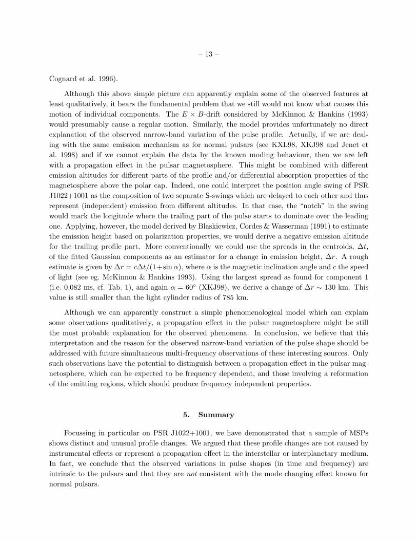
Fig. 11.— Residual arrival times of all data points.

Table 1: Statistical results of fitting a model of five Gaussian components to profiles observed at

1410 MHz. In the first case (second and third column) only the relative amplitudes were adjusted,

while in the second also the Gaussian centroids were varied (fourth and fifth column). For the

amplitudes, which are quoted in units of the trailing pulse peak, we list variances and their ratio

to the mean amplitudes. For the centroids of the components in units of milliseconds (relative to

the fiducial point), we quote variances and their values normalized to the (fixed) width of each

component.

Amplitudes Centroids

Comp σ σ/mean σ (ms) σ/width

I. 0.027 0.128 0.082 0.053

II. 0.059 0.134 0.057 0.059

III. 0.090 0.160 0.017 0.031

IV. 0.052 0.122 0.014 0.039

V. 0.042 0.043 0.004 0.009

– 28 –

−80 −40 0 40 80 120Pulse longitude (deg)

Flu

x de

nsity

(ar

bitr

ary

units

)F

lux

dens

ity (

arbi

trar

y un

its)

J1730−2304MJD 50351

MJD 49769

Fig. 12.— Two profiles of PSR J1730−2304 measured in Effelsberg at 1410 MHz at different

epochs. Error bars reflect 3σ values calculated from off-pulse data. A clear change in the profile is

visible.

– 29 –

Table 2: Timing parameters of PSR J1022+1001. Numbers in parentheses are 1σ uncertainties

derived from a combination of all four available data sets.

Ecliptic Longitude, λ (deg) . . . . . . . . . . 153.8659226(8)

Ecliptic Latitude, β (deg) . . . . . . . . . . . . −0.0641(1)

Proper Motion in λ, µλ (mas/yr) . . . . −17(2)

Period (ms) . . . . . . . . . . . . . . . . . . . . . . . . . 16.4529296832030(4)

Period derivative (10−20) . . . . . . . . . . . . 4.341(4)

Epoch of period (MJD) . . . . . . . . . . . . . . 50250

Dispersion measurea(pc cm−3) . . . . . . . 10.246

Projected semi-major axis (light s) . . . 16.765409(2)

Eccentricity . . . . . . . . . . . . . . . . . . . . . . . . . 0.00009735(8)

Time of periastron passage (MJD) . . . 50246.716(2)

Orbital Period (days) . . . . . . . . . . . . . . . . 7.805130162(6)

Angle of periastron (degrees) . . . . . . . . 97.67(7)

Right Ascensionb . . . . . . . . . . . . . . . . . . . . . 10h22m57.s997(9)

Declinationb . . . . . . . . . . . . . . . . . . . . . . . . . . 10◦01′52.′′1(3)

aHeld fixedbCalculated from λ and β