arX

iv:a

stro

-ph/

9801

177v

1 1

9 Ja

n 19

98

The characteristics of millisecond pulsar emission:

I. Spectra, pulse shapes and the beaming fraction

Michael Kramer1, Kiriaki M. Xilouris2, Duncan R. Lorimer1, Oleg Doroshenko1, Axel Jessner1,

Richard Wielebinski1, Alexander Wolszczan3, Fernando Camilo 4

ABSTRACT

The extreme physical conditions in millisecond pulsar magnetospheres as well as

their different evolutionary history compared to “normal pulsars” raise the question

as to whether these objects also differ in their radio emission properties. We have

monitored a large sample of millisecond pulsars for a period of three years using the

100-m Effelsberg radio telescope in order to compare the radio emission properties of

these two pulsar populations. Our sample comprises a homogeneous data set of very

high quality.

With some notable exceptions, our findings suggest that the two groups of objects

share many common properties. A comparison of the spectral indices between samples

of normal and millisecond pulsars demonstrates that millisecond pulsar spectra are not

significantly different from those of normal pulsars. This is contrary to what has pre-

viously been thought. There is evidence, however, that millisecond pulsars are slightly

less luminous and less efficient radio emitters compared to normal pulsars. We confirm

recent suggestions that a diversity exists among the luminosities of millisecond pulsars

with the isolated millisecond pulsars being less luminous than the binary millisecond

pulsars, implying an influence of the different evolutionary history on the emission

properties. There are indications that old millisecond pulsars exhibit somewhat flatter

spectra than the presumably younger ones.

Contrary to common belief, we present evidence that the millisecond pulsar profiles

are only marginally more complex than those found among the normal pulsar popula-

tion. Moreover, the development of the profiles with frequency is rather slow, suggesting

very compact magnetospheres. The profile development seems to anti-correlate with the

companion mass and the spin period, again suggesting that the amount of mass trans-

fer in a binary system might directly influence the emission properties. The angular

radius of radio beams of millisecond pulsars does not follow the scaling predicted from

1Max-Planck-Institut fur Radioastronomie, Auf dem Hugel 69, 53121 Bonn, Germany

2National Astronomy and Ionosphere Center, Arecibo Observatory, P.O. Box 995, Arecibo, PR 00613, USA

3Department of Astronomy and Astrophysics, Penn State University, University Park, PA 16802, USA

4Nuffield Radio Astronomy Laboratories, Jodrell Bank, Macclesfield, Cheshire SK11 9DL, England; Marie Curie

Fellow

– 2 –

a canonical pulsar model which is applicable for normal pulsars. Instead they are sys-

tematically smaller, supporting the concept of a critical rotational period below which

such a scaling ceases to exist. The smaller inferred luminosity and narrower emission

beams will need to be considered in future calculations of the birth-rate of the Galactic

population.

Subject headings: Pulsars: millisecond pulsars – normal pulsars – sub-millisecond pul-

sars – emission mechanism – birth-rates

1. Introduction

At the time of the discovery of the first millisecond pulsar B1937+21 by Backer et al. (1982)

around 350 pulsars were known. While most of these had periods around one second, the period of

PSR B1937+21 was a mere 1.6 ms, immediately raising the question in what respect such objects

differ from long period pulsars. Like the original binary pulsar, B1913+16 with a period of 59 ms,

it was proposed that millisecond pulsars originate in binary systems in which a slowly rotating

neutron star gets spun-up by mass transfer from the binary companion (Alpar et al. 1982). This

idea is supported by the fact that 80% of all millisecond pulsars found in the Galactic plane are

members of binary systems. These binary systems can be divided into three groups, depending on

the mass of the companion star (Camilo 1996), viz: low-mass (presumably Helium) white dwarfs,

high-mass (presumably Carbon-Oxygen) white dwarfs and other neutron stars. The progenitors

are therefore thought to be either low-mass or high-mass X-ray binary systems. It seems fairly

well established that millisecond pulsars are recycled pulsars originating from interacting binary

systems. As the exact definition of “millisecond pulsars” in terms of period is somewhat arbitrary,

it seems reasonable to treat all recycled pulsars as one class, referring to them as MSPs in the

following.

Since the special evolutionary history distinguishes MSPs from long period pulsars, it is con-

sequently interesting to compare the observed properties of these two classes of objects. The most

obvious difference between the two classes is, of course, the observed range of pulse periods. The

average period of slowly rotating pulsars (hereafter referred to as ‘normal’ pulsars) is about 0.7

s. Rapidly rotating pulsars exhibit pulse periods between 1.5 ms and about 60 ms. The period

derivatives of MSPs are a few orders of magnitude smaller than those of normal pulsars, i.e., of the

order of 10−19 or smaller compared to typically 10−15 for normal pulsars. The derived characteristic

ages, τ = P/2P , are of the order of 109 yr for MSPs and thus much larger than 106 yr typically

found for normal pulsars, indicating that MSPs represent an old population. Similarly, calculating

the surface magnetic field for MSPs, i.e., B = 3.2 · 1019√

PP Gauss if P is measured in seconds

(Manchester & Taylor 1977), we find typically values of the order of only 108 to 109 Gauss. An

outstanding mystery is how the magnetic field decreases from 1012 Gauss for normal pulsars by

– 3 –

three to four orders of magnitude during or after the recycling process (e.g., Bhattacharya & van

den Heuvel 1991; Phinney & Kulkarni 1994).

For normal pulsars, the magnetic field seems to maintain a dipolar form even at distances

of a few stellar radii above the neutron star surface (Phillips 1992; Xilouris et al. 1996; Kramer

et al. 1997). For MSPs it has been suggested that flux expulsion as a result of a pre-recycling

spin-down (e.g., Srinivasan et al. 1990; Jahan Miri & Bhattacharya 1994), or the spin-up process of

accreting mass on the neutron star surface itself (e.g., Romani 1990; Geppert & Urpin 1996) could

not only reduce the magnetic field strength, but could also have an impact on the magnetic field

structure by disturbing the previously present dipolar field. Moreover, near the surface of MSPs,

magnetic multipoles might be present (cf. Ruderman 1991; Arons 1993) which could increase the

actual magnetic field strength over the 108 Gauss inferred from the spin down rates which are

dominated by the field structure near the light cylinder (cf. Krolik 1991).

Despite these differences in the observational properties of MSPs and normal pulsars, it is

often believed that the emission mechanism responsible for the observed radio emission is the same

for both types of pulsars (e.g., Manchester 1992; Gil & Krawczyk 1997). However, there has been

no systematic comparison of the emission properties of MSPs and normal pulsars. In a series

of papers, we focus on this question which also constrains models of the emission mechanism of

normal pulsars. If the same emission theory applies for normal pulsars and MSPs, it implies that

the responsible radiation process has to work over three to four orders of magnitude in spin period

and magnetic field, ruling out models which depend very much on these parameters (see Melrose

1992). In fact, even if the emission process turns out to be the same for MSPs and normal pulsars,

the special evolutionary history of MSPs can be expected to have a certain impact on the observed

emission properties, so that it is important to separate such possible effects.

In the past, relatively little work has been done to compare spectral properties of MSPs and

normal pulsars. This was primarily due to the small size of the sample — only 5 MSPs were known

in the Galactic disk prior to 1990. The first careful study of MSP spectra was presented by Foster,

Fairhead, & Backer (1991), obtaining multi-frequency flux densities for four objects. Recently,

large-area surveys at Parkes, Arecibo, Jodrell Bank and Green Bank have been very successful

at finding MSPs and, as a result, over 35 are presently known in the Galactic disk. Lorimer et

al. (1995b) collected data for 20 MSPs mainly from the literature and compared them with a sample

of normal pulsars, while Bailes et al. (1997) compared the luminosities of isolated and binary MSPs.

Navarro & Manchester (1996) presented high-quality data for PSR J0437−4715 and demonstrated

that MSP profiles can exhibit an unusually large number of components. As pointed out by Backer

(1995), a systematic study of the complexity of MSP profiles however has not yet been undertaken.

Similarly, due to the limited resolution in many of the previously published MSP profiles, it has

been difficult to investigate the general width of MSP profiles, which is necessary when making

inferences about the intrinsic size of the emission beam.

In this paper we present data obtained over three years during a monitoring project of MSPs

– 4 –

at 1400 MHz. We used the Effelsberg 100-m radio telescope of the MPIfR and could thus observe

all MSPs with declinations greater than −29◦ which were strong enough to obtain data of high

quality. As a result, we present profiles of 27 MSPs, of which 24 are located in the Galactic disk,

so that our sample contains about 60% of all known Galactic disk MSPs. Most of the profiles are

of high quality both in signal-to-noise ratio and time resolution, thus allowing much more detailed

studies than previously possible. Therefore, in this and subsequent papers (Xilouris et al. 1998a,

hereafter paper II; Xilouris, Kramer & von Hoensbroech 1998b, hereafter paper III; Kramer et

al. 1998) we investigate the largest homogeneous sample of MSP data studied to date.

We investigate the spectra and observed luminosity distributions of MSPs. Attempting to

infer the structure and size of the emission beam, we then study the profile properties of MSPs.

Searching for possible differences, a detailed comparison with the properties of normal pulsars is

made (cf., Manchester & Taylor 1977; Rankin 1983; Lyne & Manchester 1988; Taylor, Manchester,

& Lyne 1993; Malofeev et al. 1994; Lorimer et al. 1995a; Seiradakis et al. 1995, Xilouris et al. 1996,

Kijak et al. 1997b). This study is complemented by the subsequent papers mentioned above to

investigate the polarisation properties of MSPs, the stability of their pulse profiles and the emission

height of their radio emission.

2. Instrumental set-up and data reduction

The data presented here were obtained during a project which was initiated to obtain pulse

time-of-arrival measurements for a number of MSPs during the upgrade of the Arecibo telescope5

(Wolszczan 1996, Kramer et al. 1996). Since April 1994 we have made regular observations using

the 100-m radio telescope in Effelsberg near Bonn. In order to study the polarisation characteristics,

all four Stokes parameters were recorded.

We used a highly sensitive 1.4 GHz HEMT receiver installed in the prime focus of the telescope,

which is tunable between 1.3 GHz and 1.7 GHz. The set noise temperature of this system is 25 K

at median elevations. The antenna gain at these frequencies is 1.5 K/Jy, independent of elevation.

We obtained left-hand (LHC ≡ A) and right-hand (RHC ≡ B) circularly polarised signals across

a 40 MHz bandwidth usually centered at 1.41 GHz, but sometimes also tuned to 1.71 GHz. The

LHC and RHC signals were mixed down to an intermediate frequency of 150 MHz and fed into

a passive (‘adding’) polarimeter providing the complex (undetected) outputs of A, B, A − B and

A− iB (for a detailed description of this polarimeter and its calibration see Hoensbroech & Xilouris

1997b). Each output was then split into 60 contiguous channels, each of 666 kHz bandwidth, by

four 60 × 0.666 = 40 MHz filter banks. The individually detected filter outputs were delayed

according to a pre-calculated delay time of the signals caused by dispersion due to the interstellar

medium. Finally, the filter outputs were added on-line and these incoherently de-dispersed signals

5The Arecibo telescope is operated by Cornell University for the National Science Foundation.

– 5 –

were transferred to the Effelsberg Pulsar Observing System (EPOS) backend.

All four data streams could be sampled by the backend with a maximum resolution of 0.2

µs. However, the pulse period was typically divided into 1024 phase bins. The data were folded

according to the computed topocentric pulse period which was updated every five seconds. Until the

beginning of 1995 the topocentric period was calculated using Tempo (Taylor & Weisberg 1989),

while later on we used Timapr developed by Doroshenko & Kopeikin (1995) for computational

convenience. A sub-integration of 15 s was finally transferred to disk for off-line reduction.

In order to monitor the gain stability and polarisation characteristics of EPOS, we performed

regular calibration measurements using a switchable noise diode. The signal from this noise diode

was injected into the waveguide following the antenna horn and was itself compared to the flux

density of known continuum calibrators (Ott et al. 1994) during regularly performed pointing

observations. Switching on the noise diode regularly after observations of pulsars allowed us to

monitor gain differences in LHC and RHC signal paths and to calibrate the pulse energies by

comparing these to the noise diode output. Using this reliable method, we obtained a large number

of flux density measurements presented in the following section.

3. Millisecond pulsar flux densities

In Table 1 we present the results of flux density measurements for 23 pulsars. These mea-

surements were performed repeatedly at 1.41 and 1.71 GHz, and therefore we quote an effective

frequency νeff representing the weighted mean of the centre frequencies used. The error introduced

by this procedure is at most 6% (for a steep spectral index of −3) and thus is much smaller than the

uncertainties due to interstellar scintillation. In order to give an impression about the amplitude of

any remaining uncertainties due to scintillation, we additionally quote the median of the measured

flux densities which can be directly compared to the mean value.

In the following we compare the spectra and luminosities of MSPs and normal pulsars. As we

will see, one has to take into account that the sample of MSPs was solely discovered during low

frequency surveys, which favoured nearby MSPs due to severe dispersion and scattering limitations.

In contrast, the sample of normal pulsars includes a large number of sources found in the previous

high frequency surveys by Johnston et al. (1992) and Clifton et al. (1992), which in turn favoured flat

spectrum, high luminosity sources (Lorimer et al. 1995b). In order to construct a more homogeneous

set of sources which can then be compared, we can restrict the studied samples to those pulsars

whose distance is not larger than 1.5 kpc, since we can reasonably assume that for a comparison of

normal pulsars and MSPs the population of MSPs has been sufficiently sampled out to this distance

(Lyne et al. 1998). Additionally, it will be useful to compare the results obtained for this set of

data with those of an analysis of MSPs and normal pulsars detected in a single survey. Evidently,

the recent Parkes 436 MHz southern sky survey (Manchester et al. 1996; Lyne et al. 1998) provides

such a homogeneous sample to verify our results.

– 6 –

3.1. Spectra of MSPs

Using the flux densities which we have measured at 1.4/1.7 GHz presented in Table 1, we have

used power law fits to calculate spectral indices based on our flux densities and those published

for lower frequencies. Corresponding references and resulting spectral indices are given in Table 1.

We also included data presented by Foster et al. (1991), and the recent observations of four MSPs

(J1022+1001, J1713+0747, B1855+09 and J2145−0750) at 4.85 GHz by Kijak et al. (1997a). If

estimated uncertainties for flux densities found in the literature were not specified, we assumed a

typical error of at least 30% due to the expected severe scintillation effects. In cases where we believe

that scintillation imposes an even larger uncertainty, we accounted for this effect by increasing the

estimated error. Additionally, for those pulsars which are not included in our sample but discussed

in the literature, we derived spectral indices for 11 further MSPs located in the Galactic disk (second

part of Table 1). Our subsequent analysis does not include PSRs J2019+2425 and J2322+2057,

although we present pulse profiles for these sources. For both these objects the number of flux

density measurements was too small to derive a reliable mean value for 1.4/1.7 GHz. Presently

only flux densities at 430 MHz are given in the literature (Nice, Taylor, & Fruchter 1993; Nice &

Taylor 1995).

In order to compare the spectra for Galactic disk MSPs and normal pulsars, we used a set

of spectral indices for 346 normal pulsars which was derived from data presented by Malofeev et

al. (1994), Lorimer et al. (1995b) and also Taylor et al. (1995). We find that the average spectrum

of MSPs seems to be steeper than that of normal pulsars, i.e. we derive a mean spectral index of

−1.8 ± 0.1 for a set of 32 MSPs located in the Galactic disk and a mean index of −1.60 ± 0.04 for

normal pulsars in the same frequency range. 6 The median values for both samples are −1.8 and

−1.7, respectively. Although the mean spectrum for MSPs seems to be somewhat steeper, both

distributions appear very similar. A Kolmogorov-Smirnov (KS) test yields a probability of 36%

that they are drawn from the same parent distribution.

However, as already discussed, the sample of normal pulsars is obviously biased towards distant,

flat spectrum sources. Removing this bias by restricting the compared data sets to those sources

which are closer than 1.5 kpc, we actually find mean spectral indices which are essentially the same,

i.e. −1.6 ± 0.2 (MSPs) and −1.7 ± 0.1 (normal pulsars) with median values of −1.65 and −1.66,

respectively. Comparing these distributions of 18 MSPs and 55 normal pulsars (Fig. 1), we find

an even higher KS-probability of 50% that the underlying parent distribution is the same. As a

final confirmation, we compare the spectral indices of nearby MSPs and normal pulsars detected

by the Parkes survey. In this case, we obtain mean spectral indices of −1.8 ± 0.2 (MSPs) and

−1.7± 0.1 (normal pulsars) and a KS-probability of 53% that both distributions are the same. We

thus conclude that there is no apparent difference in the spectra of normal pulsars and MSPs. This

is somewhat contrary to the first spectral study of 4 MSPs (Foster et al. 1991) in which MSP spectra

6Errors quoted here correspond to the mean standard deviation of the mean.

– 7 –

appeared to be steeper on average than normal pulsars. The larger sample of objects available to

us shows that steep spectra MSPs are the exception rather than the rule.

Obtaining more data at high and low frequencies in the future, i.e., above 2 GHz and below

400 MHz, will provide interesting information, particularly if MSP spectra also show the typical

steepening at a few GHz and a low frequency turn-over, which are both often observed for normal

pulsars (Malofeev et al. 1994). Indeed, the spectrum of B1937+21 presented by Foster et al. (1991)

indicates a low-frequency turn-over.

3.2. Luminosities of MSPs

For birth-rate studies of MSPs it is particularly important to compare their luminosities to

those of normal pulsars. Since we can estimate the uncertainties of our homogeneous sample of flux

densities obtained at 1.4/1.7 GHz better than those of values published for 400 MHz by various

authors, we compare distance-corrected flux densities observed at 1.4 GHz for both MSPs and

normal pulsars. This is possible since we have seen that the spectra of MSPs and normal pulsars

are essentially the same. Consequently, we calculate values S × d2, i.e. flux density measured in

mJy (Table 1) times square of the distance in kpc2. We find that MSPs are apparently one order of

magnitude less luminous than normal pulsars (see Fig. 2). The mean value of log(S×d2[

mJy kpc2]

)

is only 0.5±0.2 for our sample of 31 MSPs located in the Galactic disk7 compared to 1.50±0.04 for

369 normal pulsars (Lorimer et al. 1995b; Taylor et al. 1995). This is the reason why MSPs appear

as relatively weak sources at high radio frequencies, so that only a small number of them could be

detected at frequencies as high as 4.85 GHz (Kijak et al. 1997a). Removing the obvious bias from

both samples by restricting our analysis to all those sources which are closer than 1.5 kpc, we note

that this difference in luminosity becomes less prominent (Fig. 3). We now find mean values for

log(S×d2) of 0.0±0.1 (18 MSPs) and 0.57±0.09 (55 normal pulsars). The corresponding medians

are 0.1 (MSP) and 0.5 (normal), respectively. Performing a Kolmogorov-Smirnov test on both

samples, we find that both distributions are similar with a probability of 13%. It is interesting

that besides a deviating mean value for the luminosity there seems to be a lack of highly luminous

sources, i.e. log(S × d2) > 1, found for MSPs relative to normal pulsars. This could be an artifact

due to the smaller number of MSPs in our sample or perhaps due to a possible remaining small

difference in the spectral distribution of both samples. However, relying completely on published

flux densities we find a similar trend in the (usually) quoted 400-MHz luminosities. It therefore

seems that, although normal pulsars and MSPs have fairly similar luminosity distributions, MSPs

tend to be slightly weaker sources on the average. In order to verify this result we have performed

the same analysis on nearby sources detected in the Parkes survey. The derived values are −0.3±0.3

and 0.5± 0.1 for the mean logarithm of S × d2 of MSPs and normal pulsars, while we find medians

7We did not include PSR J0218+4232 because for this object the distance information is very uncertain (Navarro

et al. 1995).

– 8 –

of 0.1 (MSP) and 0.6 (normal), respectively. A KS-probability of only 4.8% is found that both

distributions are drawn from the same parent distribution. Summarising, we have indications that

the luminosity distributions of both types of pulsars are slightly different.

3.3. Relationships to other parameters

Any difference in the emission properties of MSPs and normal pulsars could have its origin

in the assumed special evolutionary history of MSPs or the significant difference in period and

magnetic field (see also paper II).

It is therefore interesting that although we have only seven (out of nine) isolated MSPs (includ-

ing the planetary system B1257+12 ) in our flux density sample, we can confirm the observation

by Bailes et al. (1997), that isolated MSPs tend to exhibit lower luminosities than binary MSPs.

The mean value of log(S × d2) for isolated MSPs is only −0.1 ± 0.4 and thus lower than that for

the rest of the sample, 0.6 ± 0.1. Restricting the sample to those sources within a distance of 1.5

kpc, we still find a difference in the mean value for isolated MSPs (−0.5 ± 0.3) and binary MSPs

(0.2± 0.1). In contrast, the mean spectral index for isolated MSPs appears to be the same as that

for the whole sample, −1.7 ± 0.1.

Investigating possible relationships of the spectral properties of MSPs to spin parameters like

period, magnetic field, spin down luminosity (∝ PP−3) or accelerating potential (∝ B/P 2, e.g., Ru-

derman & Sutherland 1975), we could not find significant correlations. Calculating these values we

have used intrinsic period derivatives, i.e., observed values of P were corrected for kinematic effects

whose importance for pulsars was first pointed out by Shklovskii (1970). As a result, measured

spin-down rates can be biased by proper motion and Galactic acceleration (see Damour & Taylor

1991), which can become a significant effect for MSPs (Camilo, Thorsett, & Kulkarni 1994). For

those sources where no velocity information was available, after Camilo et al. (1994) we assumed a

transverse speed of 75 km/s. We note in passing, that there might be a tendency for the spectral

index of MSPs to correlate with the characteristic age of MSPs, i.e., younger MSPs tend to have

a steeper spectrum than older MSPs. We find that Galactic disk MSPs with a characteristic age

between 108 yr and 109 yr have a mean spectral index of −2.5 ± 0.3, while those with a charac-

teristic age between 109 yr and 1010 yr exhibit a mean spectral index −1.9 ± 0.2. MSPs with a

characteristic age larger than 1010 yr in comparison show a mean index of −1.4 ± 0.2. This trend

would be in apparent contrast to that observed for normal pulsars (Johnston et al. 1992; Lorimer

et al. 1995b). As new sources are discovered, it will be interesting to see whether this tendency still

holds. However, the lack of any significant correlation between spectral properties and observed

spin parameters is similar to the observations made for normal pulsars assuming a canonical pulsar

model (Malofeev 1996).

Investigating the radio efficiency of MSPs and normal pulsars we have compared the ratio of

spin down luminosity, E = 3.95 ·1046PP−3 erg/s where P is measured in seconds (e.g., Manchester

– 9 –

& Taylor 1977), and observed radio luminosity. The distribution of the logarithm of this ratio,

S × d2/E, expressed in units of mJy kpc2 erg−1 s is presented in Fig. 4 for both MSPs and normal

pulsars. Again we have restricted both samples to sources closer than 1.5 kpc to remove the bias

previously discussed. It is evident that MSPs are much less efficient radio pulsars than slow rotating

ones. The mean value of log(S × d2/E) found for MSPs and normal pulsars is −33.3 ± 0.2 and

−31.5 ± 0.1, respectively, while the mean value of log E itself is found to be 33.2 ± 0.1 (MSP) and

32.0 ± 0.1 (normal), respectively.

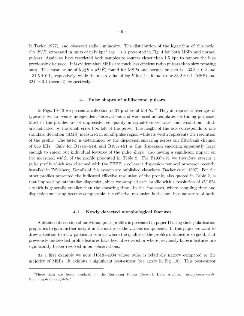
4. Pulse shapes of millisecond pulsars

In Figs. 10–13 we present a collection of 27 profiles of MSPs. 8 They all represent averages of

typically ten to twenty independent observations and were used as templates for timing purposes.

Most of the profiles are of unprecedented quality in signal-to-noise ratio and resolution. Both

are indicated by the small error box left of the pulse. The height of the box corresponds to one

standard deviation (RMS) measured in an off-pulse region while its width represents the resolution

of the profile. The latter is determined by the dispersion smearing across one filterbank channel

of 666 kHz. Only for B1744−24A and B1937+21 is this dispersion smearing apparently large

enough to smear out individual features of the pulse shape, also having a significant impact on

the measured width of the profile presented in Table 2. For B1937+21 we therefore present a

pulse profile which was obtained with the EBPP, a coherent dispersion removal processor recently

installed in Effelsberg. Details of this system are published elsewhere (Backer et al. 1997). For the

other profiles presented the indicated effective resolution of the profile, also quoted in Table 2, is

that imposed by interstellar dispersion, since we sampled each profile with a resolution of P/1024

s which is generally smaller than the smearing time. In the few cases, where sampling time and

dispersion smearing become comparable, the effective resolution is the sum in quadrature of both.

4.1. Newly detected morphological features

A detailed discussion of individual pulse profiles is presented in paper II using their polarisation

properties to gain further insight in the nature of the various components. In this paper we want to

draw attention to a few particular sources where the quality of the profiles obtained is so good, that

previously undetected profile features have been discovered or where previously known features are

significantly better resolved in our observations.

As a first example we note J1518+4904 whose pulse is relatively narrow compared to the

majority of MSPs. It exhibits a significant post-cursor (see arrow in Fig. 10). This post-cursor

8These data are freely available in the European Pulsar Network Data Archive: http://www.mpifr-

bonn.mpg.de/pulsar/data/

– 10 –

follows the midpoint of the main profile after about 25◦ and seems to be connected to it by low

intensity emission. Details can be better seen in Fig. 14 where we plot the bottom of the profile

magnified.

Another post-cursor is detected for J1730−2304, which is separated from the midpoint of the

profile by about 120◦ (cf. arrow in Fig. 11). We could not detect any emission connecting main

pulse and post-cursor (see Fig. 14).

Another interesting case is J1744−1134 which exhibits a pre-cursor preceding the main pulse

by about 124◦ (or following the main pulse by about 236◦ as in Fig. 11). Inspecting the magnified

profile in Fig. 14 we also note the possible existence of a feature following the profile by about 80◦.

Further observations are required to establish the existence of this post-cursor.

While the existence of the pre-cursors of J2145−0750 is well known (Lorimer 1994), we can

confirm the pre-cursor of B1953+29 first observed by Thorsett & Stinebring (1990, cf. Fig. 12).

We finally draw the attention to J2317+1439. For this pulsar we detect a prominent post-cursor,

following the midpoint of the profile by about 70◦ but connected to the main profile by low level

emission. Additionally, we note the possible existence of a weak interpulse preceding the main pulse

by about 150◦.

4.2. Complexity of pulse profiles

The complicated profiles of some of the first discovered MSPs (e.g., B1953+29, B1957+20)

created the impression that MSP profiles are much more complex than those of normal pulsars

which would be tempting to relate to the evolution history of MSPs by a possible disturbance of

the magnetic field structure due to mass accretion (Ruderman 1991). As now about 40 MSPs are

known in the Galactic plane, it seems adequate to re-examine this issue again in the light of a much

larger sample presented here.

A measure of the complexity of pulse profiles is obviously given by the number of Gaussian

components needed to obtain a representation of the pulse profile. Using a method described by

Kramer et al. (1994), which assures that random noise features are not misinterpreted as spurious

pulse components, we follow Foster et al. (1991) and have separated the pulse shapes into individual

Gaussian components. For each profile, the components obtained are indicated by the dashed lines

in Fig. 10–13. In order to compare them to a large sample of normal pulsars, we applied the

same component separation method to 180 profiles of normal pulsars presented by Seiradakis et

al. (1995). Since all profiles were observed at the same frequency using the identical observing

system EPOS and by applying the same time resolution, both samples are ideal for a comparison

of the profiles of normal pulsars and MSPs. Additionally, due to the very interesting shape of PSR

J0437−4715, we included the 1520 MHz profile presented by Bell et al. (1997) in our analysis which

is comparable in quality and resolution to the Effelsberg data.

– 11 –

Separating MSP profiles into components we find that they exhibit on average 4.2±0.4 Gaussian

components. For normal pulsars we derive a mean number of components, which is smaller by one

unit, 3.0±0.1. The sample of normal pulsars contains a large number of profiles with more than five

components. This is mostly due to the existence of multi-component interpulses (e.g., B1929+10)

but also due to such complex profiles as B0740−28 (cf. Kramer 1996) or B1237+25, B1742−30

and B1952+29 (Seiradakis et al. 1995). On the other hand, the sample of MSPs contains the very

complex profiles of J0437−4715 (12 components) and J1012+5307 (9 components). Comparing the

medians of the number of components, we however, find the same result, i.e., a median of 4 for MSPs

compared to 3 for normal pulsars. Fig. 5 shows the distribution of both samples, demonstrating

that the majority of MSP profiles can be described by only three to four components.

It is important to note that in the analysis described we included components representing

interpulses or post- and pre-cursors. While only about 2% of all normal pulsars are known to

exhibit interpulses or pre/post-cursors (Lyne & Manchester 1988; Seiradakis et al. 1995; Taylor

et al. 1995), about 36% of all Galactic MSPs known either emit a post- or pre-cursor, or exhibit

an interpulse. This apparent characteristic of MSPs has been noted before in particular for the

occurrence of interpulses, albeit in a much smaller sample (Ruderman 1991). This is an important

distinction between these two classes of objects, which also accounts for some of the difference in the

complexity. In summary, we conclude that the difference in the complexity of pulse shapes of MSPs

and normal pulsars is surprisingly small (i.e., only one Gaussian component). Simultaneously, we

consider the peculiar large number of MSP interpulses and pre/post-cursor as an important clue in

deciphering the circumstances in their very compact magnetospheres (cf. paper II).

4.3. Shape of the emission beams

If the emission beam of radio pulsars is confined to the open field line region, simple scaling

arguments based on the opening angle of the last open field lines (Goldreich & Julian 1969) sug-

gest that the radiation beam of MSPs should be larger than that of normal pulsars. As a first

approximation for the size of the beam one can study the observed profile widths which are listed

in Table 2 for our sample of MSPs. These widths were obtained using the technique described by

Kramer et al. (1994) and are quoted for a 50% and 10% intensity level, which refer to the peak

of the outermost resolved components. Quoted 10%- and 50%-widths, W10 and W50, represent

only the value measured for the main pulse, i.e., possible interpulses are not included. Post- and

pre-cursors are only considered in the calculations if their intensity exceeds the 10% intensity level.

Additionally, we present the equivalent pulse width, Weq, defined as the width of a box-car like

pulse shape of the same energy and amplitude as measured for the real pulse. Generally, a large

ratio of W50/Weq indicates the presence of prominent outer components. All widths and their cor-

responding uncertainty, which is mainly determined by the dispersion smearing, are quoted in both

units of degrees of longitude and milliseconds. Additionally, we used the value of W10 to derive the

duty cycle of the pulsed emission.

– 12 –

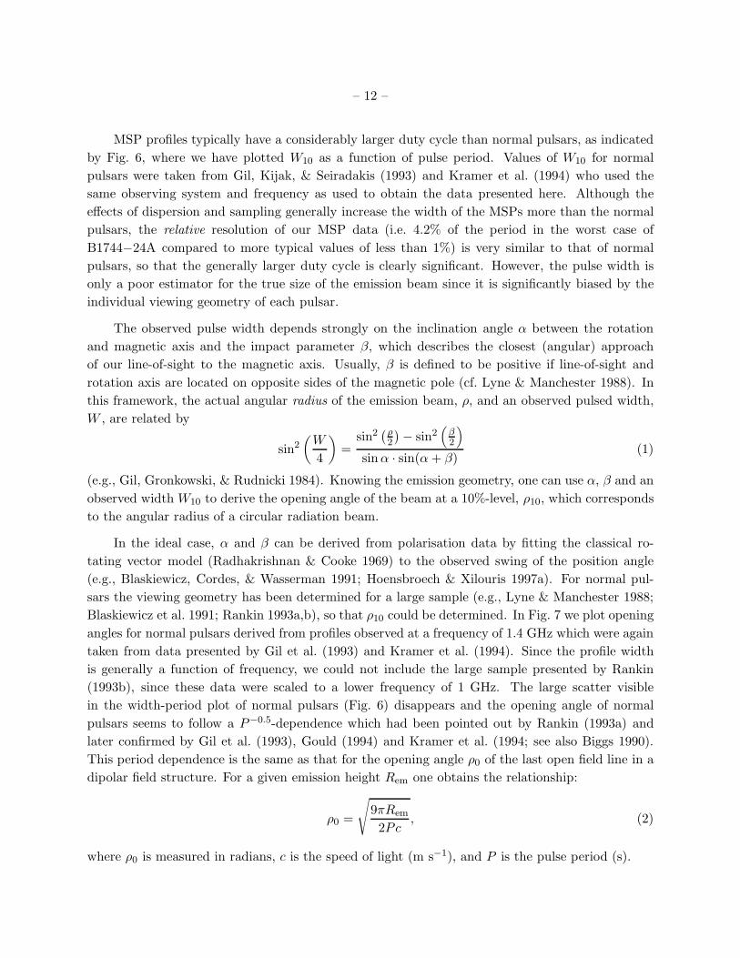
MSP profiles typically have a considerably larger duty cycle than normal pulsars, as indicated

by Fig. 6, where we have plotted W10 as a function of pulse period. Values of W10 for normal

pulsars were taken from Gil, Kijak, & Seiradakis (1993) and Kramer et al. (1994) who used the

same observing system and frequency as used to obtain the data presented here. Although the

effects of dispersion and sampling generally increase the width of the MSPs more than the normal

pulsars, the relative resolution of our MSP data (i.e. 4.2% of the period in the worst case of

B1744−24A compared to more typical values of less than 1%) is very similar to that of normal

pulsars, so that the generally larger duty cycle is clearly significant. However, the pulse width is

only a poor estimator for the true size of the emission beam since it is significantly biased by the

individual viewing geometry of each pulsar.

The observed pulse width depends strongly on the inclination angle α between the rotation

and magnetic axis and the impact parameter β, which describes the closest (angular) approach

of our line-of-sight to the magnetic axis. Usually, β is defined to be positive if line-of-sight and

rotation axis are located on opposite sides of the magnetic pole (cf. Lyne & Manchester 1988). In

this framework, the actual angular radius of the emission beam, ρ, and an observed pulsed width,

W , are related by

sin2

(

W

4

)

=sin2

(ρ2

)

− sin2(

β2

)

sin α · sin(α + β)(1)

(e.g., Gil, Gronkowski, & Rudnicki 1984). Knowing the emission geometry, one can use α, β and an

observed width W10 to derive the opening angle of the beam at a 10%-level, ρ10, which corresponds

to the angular radius of a circular radiation beam.

In the ideal case, α and β can be derived from polarisation data by fitting the classical ro-

tating vector model (Radhakrishnan & Cooke 1969) to the observed swing of the position angle

(e.g., Blaskiewicz, Cordes, & Wasserman 1991; Hoensbroech & Xilouris 1997a). For normal pul-

sars the viewing geometry has been determined for a large sample (e.g., Lyne & Manchester 1988;

Blaskiewicz et al. 1991; Rankin 1993a,b), so that ρ10 could be determined. In Fig. 7 we plot opening

angles for normal pulsars derived from profiles observed at a frequency of 1.4 GHz which were again

taken from data presented by Gil et al. (1993) and Kramer et al. (1994). Since the profile width

is generally a function of frequency, we could not include the large sample presented by Rankin

(1993b), since these data were scaled to a lower frequency of 1 GHz. The large scatter visible

in the width-period plot of normal pulsars (Fig. 6) disappears and the opening angle of normal

pulsars seems to follow a P−0.5-dependence which had been pointed out by Rankin (1993a) and

later confirmed by Gil et al. (1993), Gould (1994) and Kramer et al. (1994; see also Biggs 1990).

This period dependence is the same as that for the opening angle ρ0 of the last open field line in a

dipolar field structure. For a given emission height Rem one obtains the relationship:

ρ0 =

√

9πRem

2Pc, (2)

where ρ0 is measured in radians, c is the speed of light (m s−1), and P is the pulse period (s).

– 13 –

While the P−0.5-dependence of the opening angle has been independently determined, the

details of the scaling law (e.g., the actual scaling factor or a possible bi-modality of the distribution)

differ slightly among the various authors. In any case, the relation obtained and the maximum

possible value for ρ of 90◦, corresponding to a duty cycle of unity and thus continuous emission,

limit the period to a minimum value possible theoretically for pulsed emission. In other words,

if the scaling law derived for normal pulsars applies also to MSPs, a detection of MSPs with

periods below this critical period might not be possible. For a frequency of 1.4 GHz, Gould

(1994) derives a lower bound for the opening angles given by ρ5 = 5.4◦ · P−0.5 measured at a

5%-intensity level, while Gil et al. (1993) present ρ10 = (4.9◦ ± 0.5◦) · P−0.48±0.03 and Kramer et

al. (1994) ρ10 = (5.3◦ ± 0.3◦) · P−0.45±0.04 for a lower bound valid at a 10%-intensity level. These

scaling laws would imply a minimum possible period between 1 ms and 4 ms, which would be

just consistent with the shortest periods actually observed. Moreover it would suggest that, if the

neutron star equation-of-state allows the existence of sub-millisecond pulsars, such objects might

exhibit substantially different emission properties. Obviously, it is very interesting to see whether

the scaling laws obviously present for normal pulsars are also valid for MSPs. In the following we

therefore attempt to derive the opening angle of the beam for a number of MSPs.

The polarisation data of MSPs presented in paper II are used to model the observed position

angle swing in order to obtain information about the viewing geometry and the emission heights

(paper III). For fourteen sources, fits assuming the classical rotating-vector-model are made and

α and β determined. Corresponding values derived for the opening angle are presented in Table 3

and plotted in Fig. 7 as a function of period. The viewing geometry for B1534+12 presented by

Arzoumanian et al. (1996) and that presented for B1855+09 by Segelstein et al. (1986) are consistent

with the results of paper III by yielding the same opening angles within the uncertainties. For PSR

B1913+16, Cordes, Wasserman, & Blaskiewicz (1990) find constraints for the angles α and β, from

which we can derive ρ10 = 21 ± 4◦.

Although fitting the position angle swing is certainly the best way to obtain estimates of

the individual α and β values (cf. Lyne & Manchester 1988; Rankin 1990), the results might be

sometimes only poorly constrained (e.g., Hoensbroech & Xilouris 1997a). In fact, the uncertainties

of ρ10 presented in Table 3 and Fig. 7 for both normal pulsars and MSPs reflect only the estimated

error in the used pulse width. However, very often the derived opening angles agree within these

uncertainties if values for α and β are used which were derived independently by various authors

(see, e.g., Kramer et al. 1994). Nevertheless, we tried to find a second way to get an estimate for

the opening angle which is independent of derived values for α and β. We developed a new method

to constrain the actual value of ρ statistically. This is described in the following.

For an observed width of the pulse profile, a certain combination of α and β (or α and σ ≡ α+β

as used hereafter) leads to a value of ρ fulfilling Eq. (1). The angles α and σ are both defined in the

interval [0;π]. One can thus test how often a certain value for ρ could explain the observed width

for the given parameter space. While we cannot make any ad hoc assumption about the distribution

of α, σ as a purely geometrical factor of the relative orientation of pulsar and Earth, should be

– 14 –

distributed uniformly, so that the observed distribution is derived by weighting the possible ρ

values by a factor sinσ. For a given profile width we find typical probability distributions p(ρ)

as presented in Fig. 8. The most likely value for the opening angle is given by the peak of the

distribution function. In the following, we however use the typically larger expectation value 〈ρ〉

given by 〈ρ〉 =∫

p(ρ′) ρ′ dρ′. We can also derive an upper limit of ρ which is valid with a certain

probability. For a probability of 68%, such upper limit ρmax is given by∫ ρmax

0 p(ρ′) dρ′ = 0.68.

Both values are presented for a number of MSPs in Table 3 and Fig. 7. The expectation value 〈ρ〉

is plotted as a triangle while its error bar indicates the upper limit ρmax, i.e. with a probability

of 68% the actual value of ρ is smaller than the one indicated. We stress that these statistical

estimates do not depend on the determination of α and β.

In Fig. 7 we compare the opening angles of normal pulsars and MSPs. We have plotted the

lower bound ρ = 5.4 · P−0.5 derived by Gould (1994, dashed line). Additionally, we indicate the

maximum possible value of ρ of 90◦ by a dotted line. Assuming dipolar magnetic field lines (Eq. 2),

we have marked the region of opening angles which corresponds to the interior of a neutron star of

10 km radius. With the same assumption one can use Eq. (2) to translate the opening angle into

an emission height in units of fraction of the light cylinder radius, RLC = c P/2π. A corresponding

scale is indicated on the right hand side of the plot.

It is obvious from our sample of 27 MSPs that three sources have statistical values larger than

predicted by the scaling law derived from the sample of normal pulsars (J0621+1002, B1802−07

and J2145−0750), while only five MSPs (i.e. B1620−26, J1730−2304, B1744−24A, B1913+16 and

B1953+29) exhibit opening angles which are consistent with this scaling law. In fact, the large

majority of opening angles derived for MSPs are significantly smaller than expected (note the

logarithmic scale). A similar statement has been already made for the pulse width of B1937+21

by Chen & Ruderman (1993; see also Backer 1995) although we have demonstrated that the pulse

width itself is only a poor estimator to learn more about the size of the emission beam. Here we have

derived opening angles and thus attempted to remove geometrical effects which are always present.

For three sources (J1640+2224, J1744−1134 and J2317+1439) the derived values are not only

smaller than expected but they even indicate that the emission takes place inside the neutron star.

For the other sources, the indicated emission heights are substantially closer to the neutron star

than those derived for normal pulsars. However, due to the compactness of MSP magnetospheres,

the emission height is nevertheless at a significant fraction of the light cylinder radius, i.e. at 10% to

50% compared to the at most few percent observed for normal pulsars (e.g., Cordes 1978; Matese

& Whitmire 1980; Cordes & Stinebring 1984; Blaskiewicz et al. 1991; Phillips 1992; Xilouris et

al. 1996).

4.4. Frequency development of pulse profiles

Normal pulsar profiles very often show a distinct profile development with frequency which

can be used for a classification scheme, such as the one devised by Rankin (1983). Comparing the

– 15 –

frequency development of pulse profiles of normal pulsars and MSPs between 400 MHz and 1400

MHz, one gets the impression that MSP profiles change much less with frequency than normal

pulsars. A detailed discussion of individual MSP profiles and their frequency development is given

in paper II. Here we just want to investigate whether this tendency is related to the assumed

evolutionary history of MSPs. In such a case, the profiles could be affected by the amount of mass

transferred from the binary companion since the transferred mass could have altered the dipolar

magnetic field structure of the progenitor and thus the profile development compared to normal

pulsars (Ruderman 1991).

In order to quantify the profile development of MSPs we have used the results of the component

separations (see Sect. 4.2) to produce noise-free templates. These templates were modified by

adjusting the individual components to match the profiles observed at lower frequencies (in cases

where low-frequency data were available in digital form, these data were used; for references see

Table 1). The normalised difference in the area defined by the two pulse shapes, κ, was finally used

as the parameter describing the profile change, i.e.

κ =n

∑

i=1

∣

∣

∣

∣

∣

ti(ν1)∑n

j=1 tj(ν1)−

ti(ν2)∑n

j=1 tj(ν2)

∣

∣

∣

∣

∣

. (3)

The noise-free templates obtained for frequencies ν1 and ν2, are represented by n samples, t1, ...tn.

While ν1 was 1.41 GHz, ν2 was generally taken to be 400 MHz (Table 1). A value close to unity

means a large development in frequency while a value close to zero means a small change in the

profiles. The parameter, κ, could be determined for those profiles of MSPs in the Galactic disk

for which profiles of considerably good resolution and quality at low and high frequencies were

available. Profiles of B1937+21 were excluded since they are affected by interstellar scattering at

low frequencies (Thorsett & Stinebring 1990).

Since high-mass binary pulsars are expected to have accreted a smaller amount of mass than

low-mass binary pulsars with large inferred amounts of accreted mass (e.g., Phinney & Kulkarni

1994), we plotted κ versus the companion mass (Fig. 9). In cases where the inclination of the

binary system is not known, we assumed the most probable angle of 60◦ to calculate the mass of

the companion. We observe a slight tendency for systems with less massive companions to show

more profile development with frequency than those with more massive companions. The mean

value of κ for systems with companion masses mc ≤ 0.45M⊙ is 0.37 ± 0.05 (12 sources) but only

0.22 ± 0.05 for those with mc > 0.45M⊙ (6 sources, Fig. 9).

It can be expected that the final spin period of a recycled pulsar is related to the companion

mass (e.g., van den Heuvel & Bitzaraki 1995). Studying κ as a function of pulse period we see, in

fact, essentially the same tendency. Distinguishing between sources with spin periods smaller and

larger than 10 ms (now also including isolated MSPs with reasonably resolved profiles), we find a

mean κ of 0.35 ± 0.05 for P ≤ 10 ms (16 sources) and 0.21 ± 0.03 for P > 10 ms (8 sources). It

will be interesting to see whether this apparent tendency remains valid as more MSPs in massive

binary systems and with larger spin periods are discovered.

– 16 –

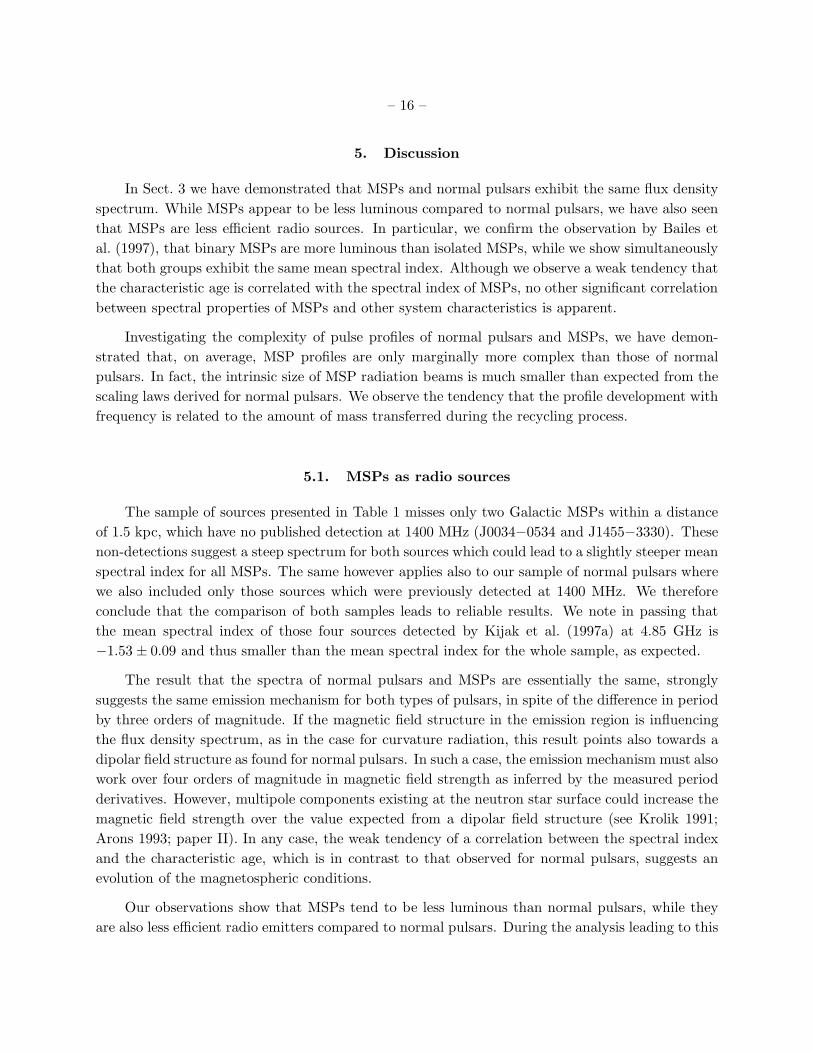
5. Discussion

In Sect. 3 we have demonstrated that MSPs and normal pulsars exhibit the same flux density

spectrum. While MSPs appear to be less luminous compared to normal pulsars, we have also seen

that MSPs are less efficient radio sources. In particular, we confirm the observation by Bailes et

al. (1997), that binary MSPs are more luminous than isolated MSPs, while we show simultaneously

that both groups exhibit the same mean spectral index. Although we observe a weak tendency that

the characteristic age is correlated with the spectral index of MSPs, no other significant correlation

between spectral properties of MSPs and other system characteristics is apparent.

Investigating the complexity of pulse profiles of normal pulsars and MSPs, we have demon-

strated that, on average, MSP profiles are only marginally more complex than those of normal

pulsars. In fact, the intrinsic size of MSP radiation beams is much smaller than expected from the

scaling laws derived for normal pulsars. We observe the tendency that the profile development with

frequency is related to the amount of mass transferred during the recycling process.

5.1. MSPs as radio sources

The sample of sources presented in Table 1 misses only two Galactic MSPs within a distance

of 1.5 kpc, which have no published detection at 1400 MHz (J0034−0534 and J1455−3330). These

non-detections suggest a steep spectrum for both sources which could lead to a slightly steeper mean

spectral index for all MSPs. The same however applies also to our sample of normal pulsars where

we also included only those sources which were previously detected at 1400 MHz. We therefore

conclude that the comparison of both samples leads to reliable results. We note in passing that

the mean spectral index of those four sources detected by Kijak et al. (1997a) at 4.85 GHz is

−1.53 ± 0.09 and thus smaller than the mean spectral index for the whole sample, as expected.

The result that the spectra of normal pulsars and MSPs are essentially the same, strongly

suggests the same emission mechanism for both types of pulsars, in spite of the difference in period

by three orders of magnitude. If the magnetic field structure in the emission region is influencing

the flux density spectrum, as in the case for curvature radiation, this result points also towards a

dipolar field structure as found for normal pulsars. In such a case, the emission mechanism must also

work over four orders of magnitude in magnetic field strength as inferred by the measured period

derivatives. However, multipole components existing at the neutron star surface could increase the

magnetic field strength over the value expected from a dipolar field structure (see Krolik 1991;

Arons 1993; paper II). In any case, the weak tendency of a correlation between the spectral index

and the characteristic age, which is in contrast to that observed for normal pulsars, suggests an

evolution of the magnetospheric conditions.

Our observations show that MSPs tend to be less luminous than normal pulsars, while they

are also less efficient radio emitters compared to normal pulsars. During the analysis leading to this

– 17 –

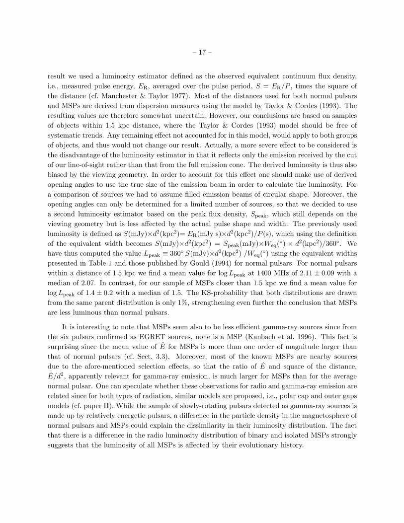
result we used a luminosity estimator defined as the observed equivalent continuum flux density,

i.e., measured pulse energy, ER, averaged over the pulse period, S = ER/P , times the square of

the distance (cf. Manchester & Taylor 1977). Most of the distances used for both normal pulsars

and MSPs are derived from dispersion measures using the model by Taylor & Cordes (1993). The

resulting values are therefore somewhat uncertain. However, our conclusions are based on samples

of objects within 1.5 kpc distance, where the Taylor & Cordes (1993) model should be free of

systematic trends. Any remaining effect not accounted for in this model, would apply to both groups

of objects, and thus would not change our result. Actually, a more severe effect to be considered is

the disadvantage of the luminosity estimator in that it reflects only the emission received by the cut

of our line-of-sight rather than that from the full emission cone. The derived luminosity is thus also

biased by the viewing geometry. In order to account for this effect one should make use of derived

opening angles to use the true size of the emission beam in order to calculate the luminosity. For

a comparison of sources we had to assume filled emission beams of circular shape. Moreover, the

opening angles can only be determined for a limited number of sources, so that we decided to use

a second luminosity estimator based on the peak flux density, Speak, which still depends on the

viewing geometry but is less affected by the actual pulse shape and width. The previously used

luminosity is defined as S(mJy)×d2(kpc2)= ER(mJy s)×d2(kpc2)/P (s), which using the definition

of the equivalent width becomes S(mJy)×d2(kpc2) = Speak(mJy)×Weq(◦) × d2(kpc2)/360◦. We

have thus computed the value Lpeak ≡ 360◦ S(mJy)×d2(kpc2) /Weq(◦) using the equivalent widths

presented in Table 1 and those published by Gould (1994) for normal pulsars. For normal pulsars

within a distance of 1.5 kpc we find a mean value for log Lpeak at 1400 MHz of 2.11 ± 0.09 with a

median of 2.07. In contrast, for our sample of MSPs closer than 1.5 kpc we find a mean value for

log Lpeak of 1.4 ± 0.2 with a median of 1.5. The KS-probability that both distributions are drawn

from the same parent distribution is only 1%, strengthening even further the conclusion that MSPs

are less luminous than normal pulsars.

It is interesting to note that MSPs seem also to be less efficient gamma-ray sources since from

the six pulsars confirmed as EGRET sources, none is a MSP (Kanbach et al. 1996). This fact is

surprising since the mean value of E for MSPs is more than one order of magnitude larger than

that of normal pulsars (cf. Sect. 3.3). Moreover, most of the known MSPs are nearby sources

due to the afore-mentioned selection effects, so that the ratio of E and square of the distance,

E/d2, apparently relevant for gamma-ray emission, is much larger for MSPs than for the average

normal pulsar. One can speculate whether these observations for radio and gamma-ray emission are

related since for both types of radiation, similar models are proposed, i.e., polar cap and outer gaps

models (cf. paper II). While the sample of slowly-rotating pulsars detected as gamma-ray sources is

made up by relatively energetic pulsars, a difference in the particle density in the magnetosphere of

normal pulsars and MSPs could explain the dissimilarity in their luminosity distribution. The fact

that there is a difference in the radio luminosity distribution of binary and isolated MSPs strongly

suggests that the luminosity of all MSPs is affected by their evolutionary history.

– 18 –

5.2. The beam structure of MSPs

It has been suggested that the overall dipolar field apparently observed for normal pulsars

(e.g., Phillips & Wolszczan 1992; Kramer et al. 1997) could be distorted by the existence of magnetic

multipoles in cases of MSPs which could be enhanced by mass accretion from a binary companion.

Disturbance of a dipolar field structure or the existence of magnetic multipoles in the emission

region should be reflected by overall shape of pulse profiles, their frequency development, and in

particular in the polarisation properties which are discussed in detail in paper II.

5.2.1. Complexity of pulse profiles

The previously observed apparent large complexity of MSP profiles was attributed to a de-

viation of the magnetic field structure from a dipolar form (Krolik 1991). However, we have

demonstrated that the majority of MSP profiles are actually only marginally more complex. Since

most of the profiles used to derive this result are in general of very high resolution already, we

do not expect the observable complexity to change significantly even if a coherent de-dispersion

technique is used (cf. profile of B1937+21 and also Backer 1995).

We believe that the impression created after the discovery of only a few MSPs, was mainly due

to the much larger duty cycle seen (see Table 2). In contrast to the average 3% found for normal

pulsars (Taylor et al. 1995), we observe a mean duty cycle of 21% for MSPs. Therefore, for MSPs

one immediately observes a “blown-up” version of the pulse shape, enabling an easier identification

of various components. Zooming in on the profiles of normal pulsars as done by Seiradakis et

al. (1995) or Kijak et al. (1997b), can lead to similar results for normal pulsars. Therefore, the

complexity of MSP profiles alone does not obviously provide any clue as to whether higher order

magnetic multipoles exist in the emission region. In fact, if the number of components is related to

the size of the polar cap, one would expect a considerably larger number of components for MSPs

even in cases of a dipolar field, since the polar cap scales as P−0.5. This is however not the case.

As already discussed, a perplexing large number of interpulses and pre-/post-cursors makes up for

some of the one unit difference derived in the mean number of components of normal pulsars and

MSPs. Therefore, even if a dipolar field near the neutron star or in the emission region exists, the

full open field line region might not be illuminated. In any case, the large number of additional

pulse features appearing in addition to the main pulse is an important significant difference in the

properties of MSP and normal pulsar emission. Combined with the relatively normal complexity of

MSP profiles, it possibly suggests that their origin is due to additional radiation beams, e.g., due

to outer gap emission (e.g., Cheng et al. 1986). We discuss this possibility further in paper II.

– 19 –

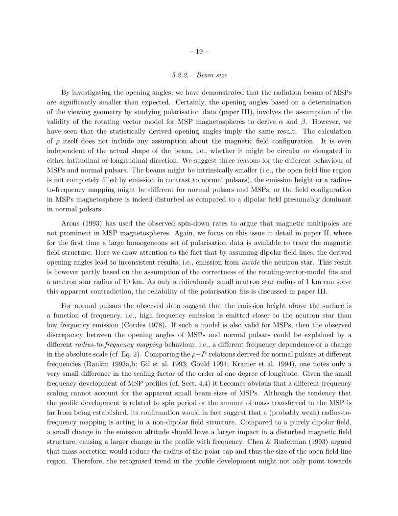
5.2.2. Beam size

By investigating the opening angles, we have demonstrated that the radiation beams of MSPs

are significantly smaller than expected. Certainly, the opening angles based on a determination

of the viewing geometry by studying polarisation data (paper III), involves the assumption of the

validity of the rotating vector model for MSP magnetospheres to derive α and β. However, we

have seen that the statistically derived opening angles imply the same result. The calculation

of ρ itself does not include any assumption about the magnetic field configuration. It is even

independent of the actual shape of the beam, i.e., whether it might be circular or elongated in

either latitudinal or longitudinal direction. We suggest three reasons for the different behaviour of

MSPs and normal pulsars. The beams might be intrinsically smaller (i.e., the open field line region

is not completely filled by emission in contrast to normal pulsars), the emission height or a radius-

to-frequency mapping might be different for normal pulsars and MSPs, or the field configuration

in MSPs magnetosphere is indeed disturbed as compared to a dipolar field presumably dominant

in normal pulsars.

Arons (1993) has used the observed spin-down rates to argue that magnetic multipoles are

not prominent in MSP magnetospheres. Again, we focus on this issue in detail in paper II, where

for the first time a large homogeneous set of polarisation data is available to trace the magnetic

field structure. Here we draw attention to the fact that by assuming dipolar field lines, the derived

opening angles lead to inconsistent results, i.e., emission from inside the neutron star. This result

is however partly based on the assumption of the correctness of the rotating-vector-model fits and

a neutron star radius of 10 km. As only a ridiculously small neutron star radius of 1 km can solve

this apparent contradiction, the reliability of the polarisation fits is discussed in paper III.

For normal pulsars the observed data suggest that the emission height above the surface is

a function of frequency, i.e., high frequency emission is emitted closer to the neutron star than

low frequency emission (Cordes 1978). If such a model is also valid for MSPs, then the observed

discrepancy between the opening angles of MSPs and normal pulsars could be explained by a

different radius-to-frequency mapping behaviour, i.e., a different frequency dependence or a change

in the absolute scale (cf. Eq. 2). Comparing the ρ−P -relations derived for normal pulsars at different

frequencies (Rankin 1993a,b; Gil et al. 1993; Gould 1994; Kramer et al. 1994), one notes only a

very small difference in the scaling factor of the order of one degree of longitude. Given the small

frequency development of MSP profiles (cf. Sect. 4.4) it becomes obvious that a different frequency

scaling cannot account for the apparent small beam sizes of MSPs. Although the tendency that

the profile development is related to spin period or the amount of mass transferred to the MSP is

far from being established, its confirmation would in fact suggest that a (probably weak) radius-to-

frequency mapping is acting in a non-dipolar field structure. Compared to a purely dipolar field,

a small change in the emission altitude should have a larger impact in a disturbed magnetic field

structure, causing a larger change in the profile with frequency. Chen & Ruderman (1993) argued

that mass accretion would reduce the radius of the polar cap and thus the size of the open field line

region. Therefore, the recognised trend in the profile development might not only point towards

– 20 –

the modification of a dipolar field structure by mass accretion, but could also offer an explanation

for the smaller beam sizes. In any case, it seems necessary to include additional independent

information to decide whether a multipole or disturbed dipolar magnetic field or systematically

unfilled emission beams are present. A major step in this direction is taken in papers II and III,

where we focus on the possible impact of gravitational bending and magnetic field sweep back.

The latter effects are apparently not important for the emission of normal pulsars (e.g., Phillips

1992; Kramer et al. 1997), but they might become relevant if the emission simultaneously takes

place close to the neutron star surface and at a significant fraction of the light cylinder radius as

indicated by Fig. 7.

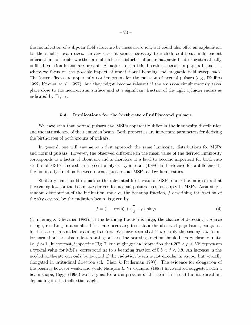
5.3. Implications for the birth-rate of millisecond pulsars

We have seen that normal pulsars and MSPs apparently differ in the luminosity distribution

and the intrinsic size of their emission beam. Both properties are important parameters for deriving

the birth-rates of both groups of pulsars.

In general, one will assume as a first approach the same luminosity distributions for MSPs

and normal pulsars. However, the observed difference in the mean value of the derived luminosity

corresponds to a factor of about six and is therefore at a level to become important for birth-rate

studies of MSPs. Indeed, in a recent analysis, Lyne et al. (1998) find evidence for a difference in

the luminosity function between normal pulsars and MSPs at low luminosities.

Similarly, one should reconsider the calculated birth-rates of MSPs under the impression that

the scaling law for the beam size derived for normal pulsars does not apply to MSPs. Assuming a

random distribution of the inclination angle α, the beaming fraction, f describing the fraction of

the sky covered by the radiation beam, is given by

f = (1 − cos ρ) + (π

2− ρ) sin ρ (4)

(Emmering & Chevalier 1989). If the beaming fraction is large, the chance of detecting a source

is high, resulting in a smaller birth-rate necessary to sustain the observed population, compared

to the case of a smaller beaming fraction. We have seen that if we apply the scaling law found

for normal pulsars also to fast rotating pulsars, the beaming fraction should be very close to unity,

i.e. f ≈ 1. In contrast, inspecting Fig. 7, one might get an impression that 20◦ < ρ < 50◦ represents

a typical value for MSPs, corresponding to a beaming fraction of 0.5 < f < 0.9. An increase in the

needed birth-rate can only be avoided if the radiation beam is not circular in shape, but actually

elongated in latitudinal direction (cf. Chen & Ruderman 1993). The evidence for elongation of

the beam is however weak, and while Narayan & Vivekanand (1983) have indeed suggested such a

beam shape, Biggs (1990) even argued for a compression of the beam in the latitudinal direction,

depending on the inclination angle.

– 21 –

6. Summary

The study of the characteristics of MSP radio emission of which the present work is the first

of a series of papers, was motivated by the question, in what respect do MSPs differ from normal

pulsars. The fact that both populations exhibit identical flux density spectra points towards the

same emission mechanism, which is further supported by the results presented in paper II. At the

same time, the radio output of MSPs seems to be affected by their particular evolutionary history,

i.e., the entire sample tends to be less luminous and in fact less efficient radio emitters compared

to normal pulsars. It is particularly interesting that, compared to the luminosity distribution of

normal pulsars within a distance of 1.5 kpc (Fig. 3), we are apparently missing some high luminosity

MSPs, although they should be the easiest to detect. Although no significant correlations between

spectral parameters and intrinsic spin parameters are observed, we note a weak tendency for old

MSPs to exhibit flatter spectra than MSPs with smaller intrinsic ages.

Although remarkable exceptions to the rule are observed, the pulse profiles of MSPs are only

slightly more complex than for the normal pulsars. These profiles do not change significantly with

frequency (for a detailed discussion see paper II), but we have indications that a measure of profile

change is actually related to the amount of mass transferred onto the neutron star during a spin-

up episode, or to the spin period. Moreover, the angular beam radii inferred from the observed

pulse shapes imply that the emission beam of rapidly-rotating pulsars is smaller than expected

from our knowledge of normal pulsars. If the neutron star equation-of-state allows the existence of

sub-millisecond pulsars, their detection will thus not be prevented by a beam size being too large

as it would have been implied from simply scaling the trend seen in normal pulsars.

The present data suggest that, although MSPs and normal pulsars exhibit the same emission

physics, they show pronounced differences probably related to the different evolutionary history.

In paper II we elaborate on these aspects further and again raise the question about the origin of

these differences in light of the additional data.

We strongly suggest that birth-rate calculations of MSP be reconsidered given the data dis-

cussed here.

We are grateful to the operators and engineers in Effelsberg for their support during this

project. It is also a pleasure to thank Norbert Wex for extremely helpful discussions leading to

the results presented in Sect. 4.3. We thank Alexis v. Hoensbroech, Jarek Kijak and Christoph

Lange for their help with the observations. FC gratefully acknowledges the support of the European

Commission through a Marie Curie fellowship, under contract no. ERBFMBICT961700. This work

was in part supported by the European Commission under the HCM Network Contract Nr. ERB

CHRX CT960633, i.e., the European Pulsar Network.

– 22 –

REFERENCES

Alpar, M. A., Cheng, A. F., Ruderman, M. A., & Shaham, J. 1982, Nature, 300, 728

Arons, J. 1993, ApJ, 408, 160

Arzoumanian, Z., Phillips, J. A., Taylor, J. H., & Wolszczan, A. 1996, ApJ, 470, 1111

Backer, D. C. 1995, J. Astrophys. Astr., 16, 165

Backer, D. C., Kulkarni, S. R., Heiles, C., Davis, M. M., & Goss, W. M. 1982, Nature, 300, 615

Backer, D. C., Dexter, M. R., Zepka, A., Werthimer, D. J., Ray, P. S., & Foster, R. S. 1997, PASP,

109, 61

Bailes, M., et al. 1994, ApJ, 425, L41

Bailes, M., et al. 1997, ApJ, 481, 386

Bell, J. F., Bailes, M., Manchester, R. N., Lyne, A. G., Camilo, F., & Sandhu, J. S. 1997, MNRAS,

286, 463

Biggs, J. D. 1990, MNRAS, 245, 514

Bhattacharya, D., & van den Heuvel, E. P. J. 1991, Phys. Rep., 203, 1

Blaskiewicz, M., Cordes, J. M., & Wasserman, I. 1991, ApJ, 370, 643

Boriakoff, V., Buccheri, R., & Fauci, F. 1983, Nature, 304, 417

Camilo, F. 1996, in Proc. IAU Colloq. 160, Pulsars: Problems & Progress, ed. S. Johnston,

M. Walker, M. Bailes, (San Francsico: PASP), p. 539

Camilo, F., Nice, D. J., & Taylor, J. H. 1993, ApJ, 412, L37

Camilo, F., Thorsett, S. E., & Kulkarni, S. R. 1994 ApJ, 421, L15

Camilo, F., Nice, D. J., & Taylor, J. H. 1996a, ApJ, 461, 812

Camilo, F., Nice, D. J., Shrauner, J. A., & Taylor, J. H. 1996b, ApJ, 469, 819

Chen, K., & Ruderman, M. 1993, ApJ, 408, 179

Cheng, K. S., Ho, C., & Ruderman, M. 1986, ApJ, 300, 500

Clifton, T. R., Lyne, A. G., Jones, A. W., McKenna, J., & Ashworth, M. 1992, MNRAS, 254, 177

Cordes, J. M. 1978, ApJ, 222, 1006

Cordes, J. M., & Stinebring, D. R. 1984, ApJ, 277, L53

– 23 –

Cordes, J. M., Wasserman, I., & Blaskiewicz, M. 1990, ApJ, 349, 546

D’Amico, N., Bailes, M., Lyne, A. G., Manchester, R. N., Johnston, S., & Fruchter, A. S. 1993,

MNRAS, 260, L7

Damour, T., & Taylor, J. H. 1991, ApJ, 366, 501

Doroshenko, O. V., & Kopeikin, S. M. 1995, MNRAS, 274, 1029

Emmering, R. T., & Chevalier, R. A. 1989, ApJ, 345, 931

Foster, R. S., Fairhead, L., & Backer, D. C. 1991, ApJ, 378, 687

Foster, R. S., Wolszczan, A., & Camilo, F. 1993, ApJ, 410, L91

Foster, R. S., Cadwell, B. J., Wolszczan, A., & Anderson, S. B. 1995, ApJ, 454, 826

Fruchter, A. S., Stinebring, D. R., & Taylor, J. H. 1988, Nature, 333, 237

Fruchter, A. S., et al. 1990, ApJ, 351, 642

Geppert, U., & Urpin, V. 1996, MNRAS, 278, 471

Gil, J. A., Gronkowski, P., & Rudnicki, W. 1984, A&A, 132, 312

Gil, J. A., Kijak, J., & Seiradakis, J. H. 1993, A&A, 272, 268

Gil, J. A., & Krawczyk, A. 1997, MNRAS, 285, 561

Goldreich, P., & Julian, W. H. 1969, ApJ, 157, 869

Gould, D. M. 1994, PhD-thesis, University of Manchester

Hoensbroech, A. von, & Xilouris, K. M. 1997a, A&A, 324, 981

Hoensbroech, A. von, & Xilouris, K. M. 1997b, A&AS, 126, 121

Jahan Miri, M., & Bhattacharya, D. 1994, MNRAS, 269, 455

Johnston, S., Lyne, A. G., Manchester, R. N., Kniffen, D. A., D’Amico, N., Lim, J., & Ashworth,

M. 1992, MNRAS, 255, 401

Johnston, S., et al. 1993, Nature, 361, 613

Kanbach, G., et al. 1996, A&AS, 120, 461

Kijak, J., Kramer, M., Wielebinski, R., & Jessner, A. 1997a, A&A, 318, L63

Kijak, J., Kramer, M., Wielebinski, R., & Jessner, A. 1997b, A&A, in press

– 24 –

Kramer, M. 1996, in Proc. IAU Colloq. 160, Pulsars: Problems & Progress, ed. S. Johnston,

M. Walker, M. Bailes, (San Francisco: PASP), p. 215

Kramer, M., Wielebinski, R., Jessner, A., Gil, J. A., & Seiradakis, J. H. 1994, A&AS, 107, 515

Kramer, M., Doroshenko, O., Jessner, A., Wielebinski, R., Wolszczan, A., Camilo, F., Taylor,

J. H., & Xilouris, K. M. 1996, in Proc. IAU Colloq. 160, Pulsars: Problems & Progress, ed.

S. Johnston, M. Walker, M. Bailes, (San Francisco: PASP), p. 95

Kramer, M., Xilouris, K. M., Jessner, A., Wielebinski, R., Lorimer, D. R., & Lyne, A. G. 1997,

A&A, 322, 846

Kramer, M., Xilouris, K. M., Camilo, F., Doroshenko, O., Nice, D. J., Jessner, A., Backer,

D.C. 1998, in preparation

Krolik, J. 1991, ApJ, 373, L69

Lorimer, D. R. 1994, PhD-thesis, University of Manchester

Lorimer, D. R., et al. 1995a, ApJ, 439, 933

Lorimer, D. R., Yates, J. A., Lyne, A. G., & Gould, D. M. 1995b, MNRAS, 273, 411

Lorimer, D. R., Lyne, A. G., Bailes, M., Manchester, R. N., D’Amico, N., Stapper, B. W., Johnston,

S., & Camilo, F. 1996, MNRAS, 283, 1383

Lundgren, S. C., Zepka, A., & Cordes, J. M. 1995, ApJ, 453, 419

Lyne, A. G., & Manchester, R. N. 1988, MNRAS, 234, 477

Lyne, A. G., Biggs, J. D., Brinklow, A., McKenna, J., & Ashworth, M. 1988, Nature, 332, 45

Lyne, A. G., et al. 1998, MNRAS, in press

Malofeev, V. M. 1996, in Proc. IAU Colloq. 160, Pulsars: Problems & Progress, ed. S. Johnston,

M. Walker, M. Bailes, (San Francisco: PASP), p. 271

Malofeev, V. M., Gil, J. A., Jessner, A., Malov, I. F., Seiradakis, J. H., Sieber, W., & Wielebinski,

R. 1994, A&A, 285, 201

Manchester, R. N. 1992, in Proc. of IAU Colloq. 128, ed. T. Hankins, J.M. Rankin, J. A. Gil,

(Zielona Gora: Pedagogical University Press), p. 206

Manchester, R. N., & Taylor, J. H. 1977, Pulsars, (San Francisco: Freeman)

Manchester, R. N., & Johnston, S. 1995, ApJ, 441, L65

Manchester, R. N., et al. 1996, MNRAS, 279, 1235

– 25 –

Matese, J. J., & Whitmire, D. P. 1980, ApJ, 235, 587

Melrose, D. B. 1992, Phil. Trans. Roy. Soc. Lond., A341, 105

Narayan, R., & Vivekanand, M. 1983, A&A, 122, 45

Navarro, J., de Bruyn, A. G., Frail, D. A., Kulkarni, S. R., & Lyne, A. G. 1995, ApJ, 455, L55

Navarro, J., & Manchester, R. N. 1996, Proc. IAU Colloq. 160, Pulsars: Problems & Progress,

eds. S. Johnston, M. Walker, M. Bailes, PASP, p. 249

Nicastro, L., Lyne, A. G., Lorimer, D. R., Harrison, P. A., Bailes, M., & Skidmore, B. D. 1995,

MNRAS, 273, L68

Nice, D. J. 1992, PhD-thesis, Princeton University

Nice, D. J., Taylor, J. H., & Fruchter, A. S. 1993, ApJ, 402, L49

Nice, D. J., & Taylor, J. H. 1995, ApJ, 441, 429

Nice, D. J., Sayer, R. W., & Taylor, J. H. 1996, ApJ, 466, L87

Ott, M., Witzel, A., Quirrenbach, A., Krichbaum, T. P., Standke, K. J., Schalinski, C. J., &

Hummel, C. A. 1994, A&A, 284, 331

Phillips, J. A. 1992, ApJ, 385, 282

Phillips, J. A., & Wolszczan, A. 1992, ApJ, 385, 273

Phinney, E. S., & Kulkarni, S. R. 1994, ARA&A, 32, 591

Radhakrishnan, V., & Cooke, D. J. 1969, Astrophys. Lett., 3, 225

Rankin, J. M. 1983, ApJ, 274, 333

Rankin, J. M. 1990, ApJ, 352, 247

Rankin, J. M. 1993a, ApJ, 405, 285

Rankin, J. M. 1993b, ApJS, 85, 145

Romani, R. W. 1990, Nature, 347, 741

Ruderman, M. 1991, ApJ, 382, 576

Ruderman, M. A., & Sutherland, P. G. 1975, ApJ, 196, 51

Sayer, R. W., Nice, D. J., & Taylor, J. H. 1997, ApJ, 474, 426

– 26 –

Segelstein, D. J., Rawley, L. A., Stinebring, D. R., Fruchter, A. S., & Taylor, J. H. 1986, Nature,

322, 714

Seiradakis, J. H., Gil, J. A., Graham, D. A., Jessner, A., Kramer, M., Malofeev, V. M., Sieber, W.,

& Wielebinski, R. 1995, A&AS, 111, 205

Shklovskii, I. S. 1970, Sov. Astron., 13, 562

Srinivasan, G., Bhattacharya, D., Muslimov, A. G., & Tsygan, A. I. 1990, Curr. Sci., 59, 31

Stappers, B. W., et al. 1996, ApJ, 465, L119

Taylor, J. H., & Weisberg, J. M. 1982, ApJ, 253, 908

Taylor, J. H., & Weisberg, J. M. 1989, ApJ, 345, 434

Taylor, J. H., & Cordes, J. M. 1993, ApJ, 411, 674

Taylor, J. H., Manchester, R., & Lyne, A.G. 1993, ApJS, 88, 529

Taylor, J.H., Manchester, R. N., Lyne, A. G., & Camilo, F. 1995, unpublished (available at

ftp://pulsar.princeton.edu/pub/catalog)

Thorsett, S. E., & Stinebring, D. R. 1990, ApJ, 361, 644

Van den Heuvel, E. P. J., & Bitzaraki, O. 1995, A&A, 297, L41

Wolszczan, A. 1991, Nature, 350, 688

Wolszczan, A. 1996, in Proc. IAU Colloq. 160, Sydney 1996: Pulsars: Problems & Progress, ed.

S. Johnston, M. Walker, M. Bailes, (San Francisco: PASP), p. 91

Wolszczan, A., & Frail, D. A. 1992 Nature, 355, 145

Xilouris, K. M., Kramer, M., Jessner, A., Wielebinski, R., & Timofeev, M. 1996, A&A, 309, 481

Xilouris, K. M., Kramer, M., Jessner, A., Hoensbroech, A. v., Lorimer, D. R.,Wielebinski, R.,

Wolszczan, A., & Camilo, F. 1998a, ApJ, in press (paper II)

Xilouris, K. M., Kramer, M., Hoensbroech, A. v. 1998b, in preparation (paper III)

This preprint was prepared with the AAS LATEX macros v4.0.

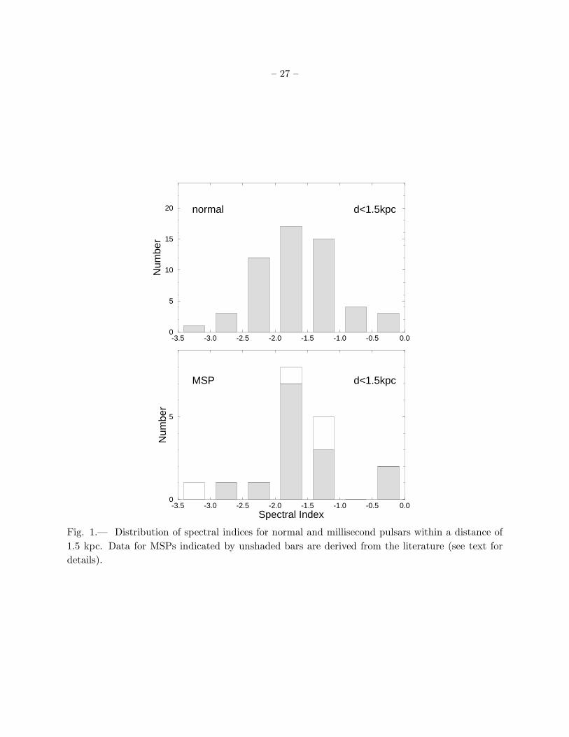
– 27 –

-3.5 -3.0 -2.5 -2.0 -1.5 -1.0 -0.5 0.0Spectral Index

0

5

Num

ber

-3.5 -3.0 -2.5 -2.0 -1.5 -1.0 -0.5 0.00

5

10

15

20

Num

ber

MSP

normal d<1.5kpc

d<1.5kpc

Fig. 1.— Distribution of spectral indices for normal and millisecond pulsars within a distance of

1.5 kpc. Data for MSPs indicated by unshaded bars are derived from the literature (see text for

details).

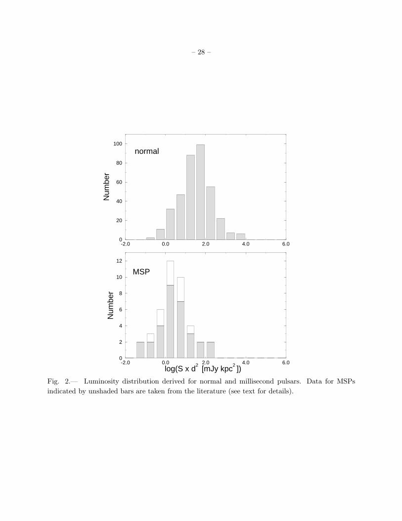
– 28 –

-2.0 0.0 2.0 4.0 6.0log(S x d

2 [mJy kpc

2 ])

0

2

4

6

8

10

12

Num

ber

-2.0 0.0 2.0 4.0 6.00

20

40

60

80

100

Num

ber

normal

MSP

Fig. 2.— Luminosity distribution derived for normal and millisecond pulsars. Data for MSPs

indicated by unshaded bars are taken from the literature (see text for details).

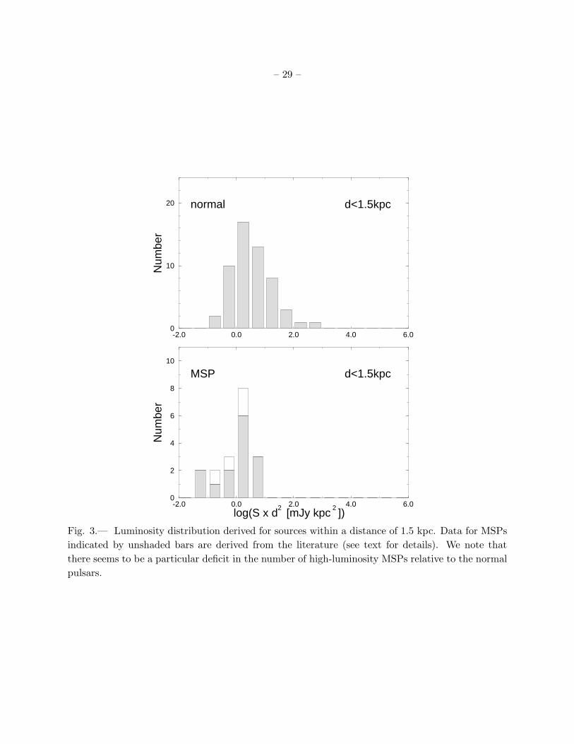
– 29 –

-2.0 0.0 2.0 4.0 6.0log(S x d

2 [mJy kpc

2 ])

0

2

4

6

8

10

Num

ber

-2.0 0.0 2.0 4.0 6.00

10

20

Num

ber

normal

MSP

d<1.5kpc

d<1.5kpc

Fig. 3.— Luminosity distribution derived for sources within a distance of 1.5 kpc. Data for MSPs

indicated by unshaded bars are derived from the literature (see text for details). We note that

there seems to be a particular deficit in the number of high-luminosity MSPs relative to the normal

pulsars.

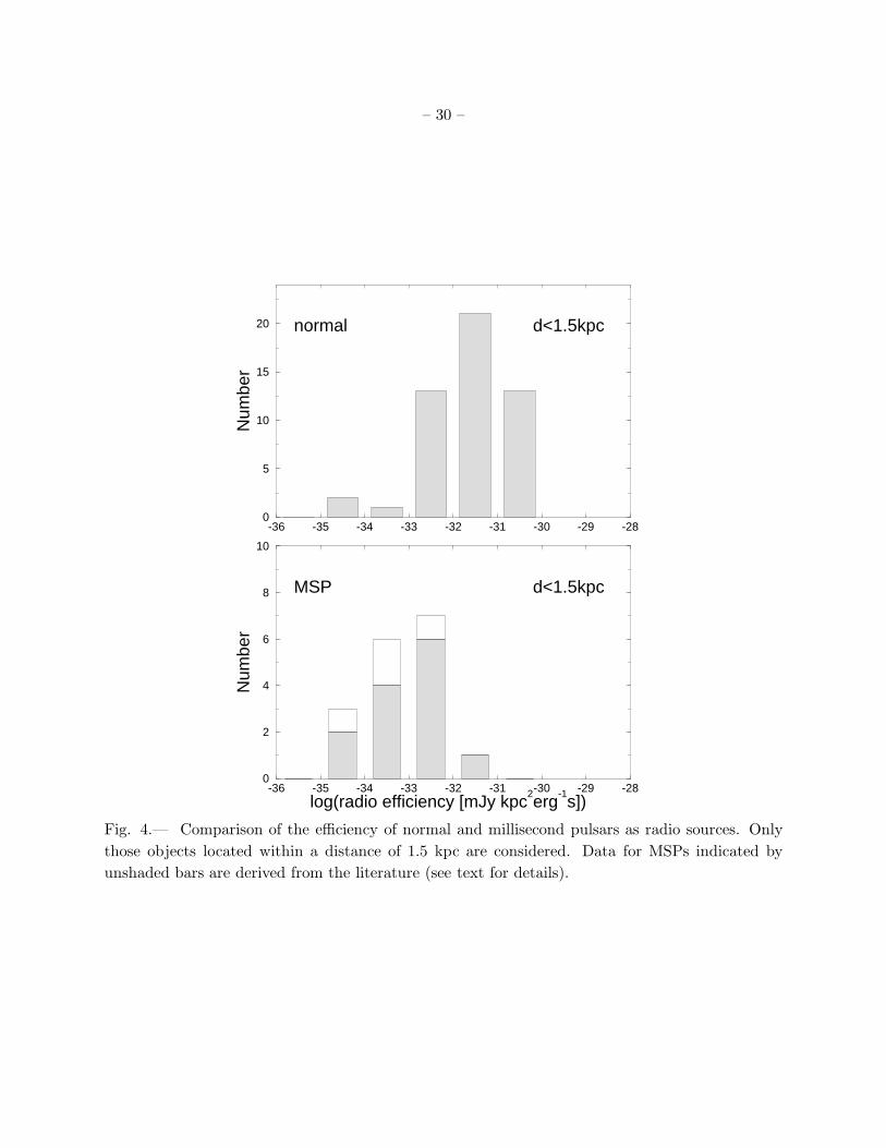
– 30 –

-36 -35 -34 -33 -32 -31 -30 -29 -28log(radio efficiency [mJy kpc

2erg

-1s])

0

2

4

6

8

10

Num

ber

-36 -35 -34 -33 -32 -31 -30 -29 -280

5

10

15

20

Num

ber

normal

MSP

d<1.5kpc

d<1.5kpc

Fig. 4.— Comparison of the efficiency of normal and millisecond pulsars as radio sources. Only

those objects located within a distance of 1.5 kpc are considered. Data for MSPs indicated by

unshaded bars are derived from the literature (see text for details).

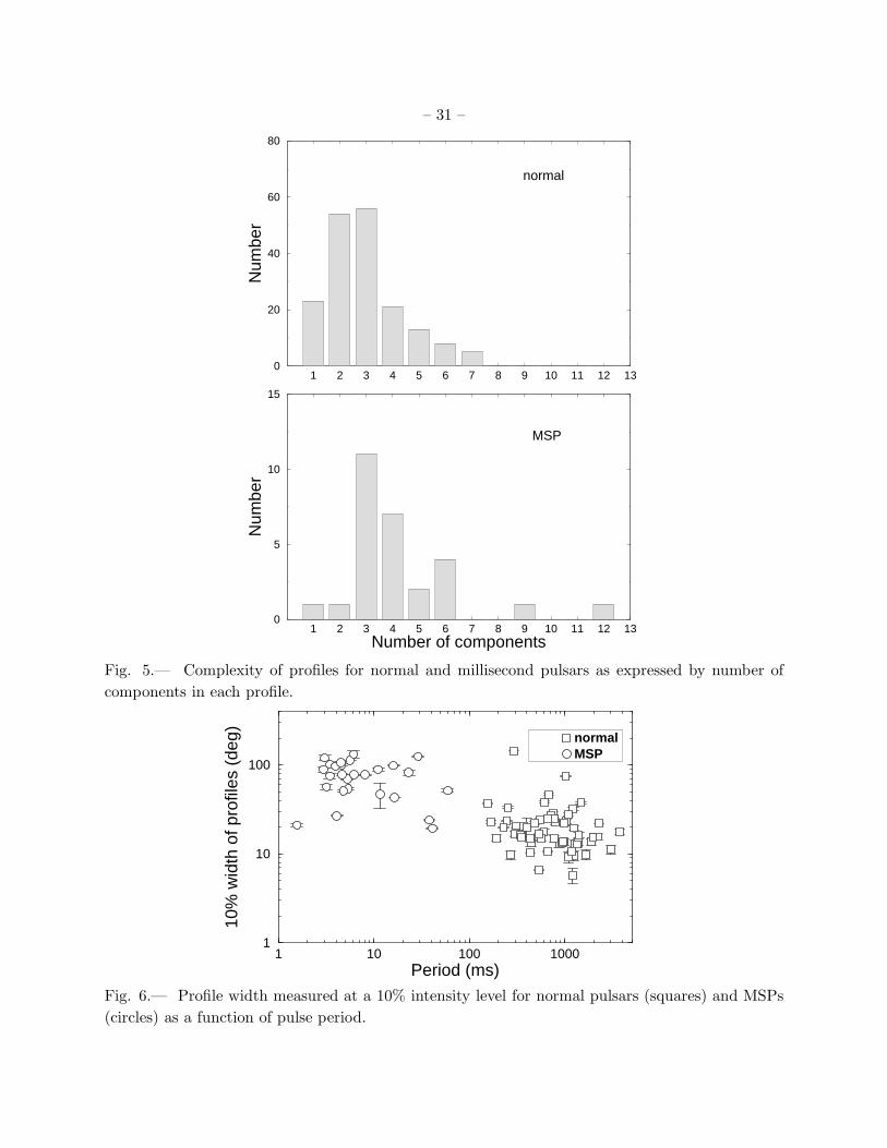
– 31 –

1 2 3 4 5 6 7 8 9 10 11 12 13Number of components

0

5

10

15

Num

ber

1 2 3 4 5 6 7 8 9 10 11 12 130

20

40

60

80

Num

ber

normal

MSP

Fig. 5.— Complexity of profiles for normal and millisecond pulsars as expressed by number of

components in each profile.

1 10 100 1000Period (ms)

1

10

100

10%

wid

th o

f pro

files

(de

g) normalMSP

Fig. 6.— Profile width measured at a 10% intensity level for normal pulsars (squares) and MSPs

(circles) as a function of pulse period.

– 32 –

1 10 100 1000Period (ms)

1

10

100

10%

ope

ning

ang

le (

deg)

normalMSPMSP expected5.4*P(s)

-0.5

Neutron star interior

0.005

0.01

0.05

0.1

0.5

Rem

\ RLC

0.001

Fig. 7.— Opening angles derived for a 10% intensity level for normal pulsars (squares) and MSPs

(circles) as a function of pulse period. For normal pulsars, the opening angles scale with P−0.5

as indicated by the dashed line derived by Gould (1994). MSPs seem not to follow the same

scaling, which is supported by the determined upper limits also presented. The triangles mark the

expectation value, 〈ρ〉, while the upper bar indicates an upper limit valid with 68% probability (see

text for details). Assuming dipolar magnetic field lines, we have marked the region of opening angles

which corresponds to the interior of a neutron star of 10 km radius. With the same assumption

one can translate an opening angle into an emission height in units of fraction of the light cylinder.

A corresponding scale is indicated on the right border of the plot. The maximum possible value of

the opening angle of 90◦ is marked by a dotted line.

– 33 –

0 10 20 30 40 50 60 70 80 90opening angle (deg)

0.00

0.01

0.02

0.03

0.04

prob

abili

ty<ρ>

Fig. 8.— Probability distribution for the occurrence of values for the opening angle ρ derived for

J1744−1134 with a 10%-profile width of 26.8◦. For this case, the most likely value of ρ given by

the peak of the probability function is 13.8◦. The expectation value 〈ρ〉 is marked at 42.2◦. With

a probability of 68% the true value of ρ is smaller than 55.4◦ (shaded area). These values are to

be compared to an opening angle derived from polarisation measurements of 18.1◦.

0.0 0.5 1.0 1.5 Companion mass (M Sun)

0.0

0.2

0.4

0.6

0.8

1.0

Pro

file

chan

ge, κ

Fig. 9.— Parameter describing the profile development between 400 MHz and 1400 MHz (for

definition see text) as a function of companion mass.

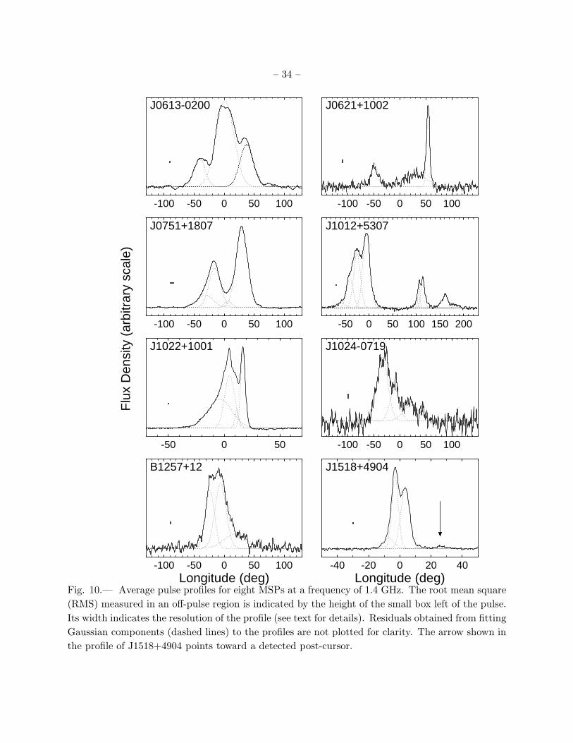
– 34 –

-100 -50 0 50 100Longitude (deg)

-50 0 50

-100 -50 0 50 100

-100 -50 0 50 100

-40 -20 0 20 40Longitude (deg)

-100 -50 0 50 100

-50 0 50 100 150 200

-100 -50 0 50 100

Flu

x D

ensi

ty (

arbi

trar

y sc

ale)

J0613-0200

J0751+1807

J1022+1001

B1257+12

J0621+1002

J1012+5307

J1024-0719

J1518+4904

Fig. 10.— Average pulse profiles for eight MSPs at a frequency of 1.4 GHz. The root mean square

(RMS) measured in an off-pulse region is indicated by the height of the small box left of the pulse.

Its width indicates the resolution of the profile (see text for details). Residuals obtained from fitting

Gaussian components (dashed lines) to the profiles are not plotted for clarity. The arrow shown in

the profile of J1518+4904 points toward a detected post-cursor.

– 35 –

0 50 100 150 200 250Longitude (deg)

-60 -40 -20 0 20 40 60

-60 -40 -20 0 20 40 60

-20 -10 0 10 20

-100 -50 0 50 100Longitude (deg)

-100 -50 0 50 100 150

-100 -50 0 50 100

-100 -50 0 50 100

Flu

x D

ensi

ty (

arbi

trar

y sc

ale)

B1534+12

J1640+2224

J1713+0747

J1744-1134

B1620-26

J1643-1224

J1730-2304

B1744-24A

Fig. 11.— Average pulse profiles for eight MSPs at a frequency of 1.4 GHz. The arrows shown for

J1730−2304 and J1744−1134 point toward detected post-cursor and pre-cursor, respectively.

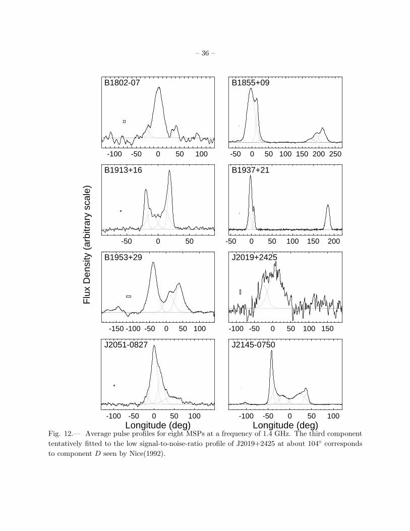
– 36 –

-100 -50 0 50 100Longitude (deg)

-100 -50 0 50 100 150

-50 0 50 100 150 200

-50 0 50 100 150 200 250-100 -50 0 50 100

-100 -50 0 50 100Longitude (deg)

-150 -100 -50 0 50 100

-50 0 50

Flu

x D

ensi

ty (

arbi

trar

y sc

ale)

B1802-07

B1913+16

B1953+29

J2051-0827

B1855+09

B1937+21

J2019+2425

J2145-0750

Fig. 12.— Average pulse profiles for eight MSPs at a frequency of 1.4 GHz. The third component

tentatively fitted to the low signal-to-noise-ratio profile of J2019+2425 at about 104◦ corresponds

to component D seen by Nice(1992).

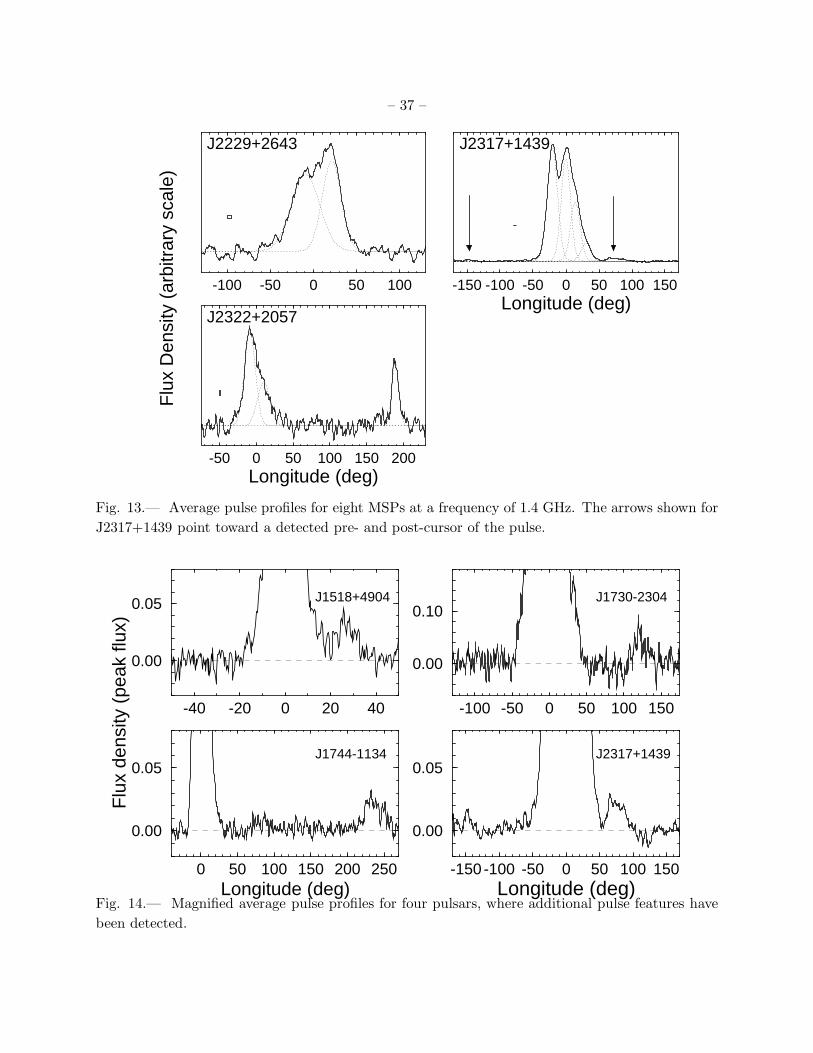
– 37 –

-150 -100 -50 0 50 100 150Longitude (deg)

-100 -50 0 50 100

-50 0 50 100 150 200Longitude (deg)

Flu

x D

ensi

ty (

arbi

trar

y sc

ale)

J2229+2643 J2317+1439

J2322+2057

Fig. 13.— Average pulse profiles for eight MSPs at a frequency of 1.4 GHz. The arrows shown for

J2317+1439 point toward a detected pre- and post-cursor of the pulse.

-150 -100 -50 0 50 100 150Longitude (deg)

0.00

0.05

-100 -50 0 50 100 150

0.00

0.10

-40 -20 0 20 40

0.00

0.05

0 50 100 150 200 250Longitude (deg)

0.00

0.05

J1518+4904 J1730-2304

J1744-1134 J2317+1439

Flu

x de

nsity

(pe

ak fl

ux)

Fig. 14.— Magnified average pulse profiles for four pulsars, where additional pulse features have

been detected.

– 38 –

Table 1. Flux densities and spectral indices for 34 millisecond pulsars. The flux density data

presented for the first 23 sources were derived from our measurements, while for 11 sources we

collected data from the literature. Besides the period of the pulsar (column 2), we quote the

corresponding frequency in column 3. The mean flux density and its uncertainty is shown in

column 4. Additionally, we present the median of all measured flux values, which is to be

compared with the mean value. The spectral index is derived by using published lower frequency

data (for references see column 7) which is indicated in column 6.

PSR P νeff Smean Smedian spectral index Ref.

(ms) (GHz) (mJy) (mJy) α

J0613−0200 3.062 1.410 1.4 ± 0.2 1.5 −1.9 ± 0.4 1

J0751+1807 3.479 1.435 3.2 ± 0.7 2.9 −0.9 ± 0.3 2

J1012+5307 5.256 1.410 3 ± 1 1.9 −1.8 ± 0.4 3

J1022+1001 16.453 1.443 3.0 ± 0.4 2.5 −1.7 ± 0.1 4, 5

J1024−0719 5.162 1.410 0.66 ± 0.04 0.66 −1.5 ± 0.2 6

B1257+12 6.219 1.410 2 ± 1 2 −1.9 ± 0.5 7

J1518+4904 40.935 1.410 4 ± 2 2.5 −0.5 ± 0.5 26, 30

B1534+12 37.904 1.530 0.6 ± 0.2 0.4 −3.0 ± 0.4 8

B1620−26 11.076 1.460 1.6 ± 0.3 1.7 −2.5 ± 0.2 9, 10

J1640+2224 3.163 1.472 2 ± 1 1 −0.3 ± 0.5 11

J1643−1224 4.621 1.410 4.8 ± 0.6 4.5 −2.4 ± 0.3 1

J1713+0747 4.570 1.510 8 ± 2 5 −1.5 ± 0.1 12

J1730−2304 8.123 1.410 4 ± 3 2 −1.8 ± 0.3 1

J1744−1134 4.075 1.470 3 ± 1 2 −1.6 ± 0.3 6

B1802−07 23.101 1.410 1.0 ± 0.5 1.0 −1.0 ± 0.5 13

B1855+09 5.362 1.470 5 ± 1 4 −1.3 ± 0.2 10, 14

B1913+16 59.030 1.560 0.9 ± 0.2 0.9 −1.4 ± 0.3 15, 27

B1937+21 1.558 1.579 10 ± 1 9 −2.3 ± 0.2 10

B1953+29 6.133 1.410 1.1 ± 0.2 1.1 −2.2 ± 0.3 16

J2051−0827 4.509 1.410 2.8 ± 0.6 2.5 −1.8 ± 0.3 17

J2145−0750 16.052 1.510 8 ± 2 7 −1.6 ± 0.1 18

J2229+2643 2.978 1.430 0.9 ± 0.2 0.8 −2.2 ± 0.5 19

J2317+1439 3.445 1.496 4 ± 1 2 −1.4 ± 0.3 20

J0218+4232 2.323 1.410 0.9 ± 0.2 − −2.8 ± 0.2 21

J0437−4715 5.757 1.460 142 ± 53 − −1.8 ± 0.2 22, 23

J0621+1002 28.853 0.800 1.9 ± 0.3 − −2.5 ± 1.4 4

J0711−6830 5.491 1.400 1.6 ± 0.3 − −1.4 ± 0.2 6

J1045−4509 7.474 1.520 3 ± 1 − −1.5 ± 0.3 18

J1603−7202 14.841 1.400 3.0 ± 0.5 − −1.3 ± 0.3 24

J1804−2717 9.343 1.400 0.4 ± 0.2 − −3.2 ± 0.5 24

J1911−1114 3.625 1.400 0.5 ± 0.2 − −3.3 ± 0.4 24

B1957+20 1.607 1.400 0.4 ± 0.2 − −3.5 ± 0.5 25, 30

J2124−3358 4.931 1.400 1.6 ± 0.4 − −1.1 ± 0.4 6

J2129−5721 3.726 1.400 1.4 ± 0.2 − −1.0 ± 0.4 24

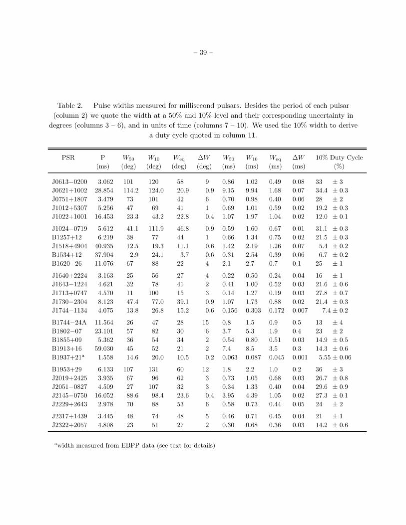
– 39 –

Table 2. Pulse widths measured for millisecond pulsars. Besides the period of each pulsar

(column 2) we quote the width at a 50% and 10% level and their corresponding uncertainty in

degrees (columns 3 – 6), and in units of time (columns 7 – 10). We used the 10% width to derive

a duty cycle quoted in column 11.

PSR P W50 W10 Weq ∆W W50 W10 Weq ∆W 10% Duty Cycle

(ms) (deg) (deg) (deg) (deg) (ms) (ms) (ms) (ms) (%)

J0613−0200 3.062 101 120 58 9 0.86 1.02 0.49 0.08 33 ± 3

J0621+1002 28.854 114.2 124.0 20.9 0.9 9.15 9.94 1.68 0.07 34.4 ± 0.3

J0751+1807 3.479 73 101 42 6 0.70 0.98 0.40 0.06 28 ± 2

J1012+5307 5.256 47 69 41 1 0.69 1.01 0.59 0.02 19.2 ± 0.3

J1022+1001 16.453 23.3 43.2 22.8 0.4 1.07 1.97 1.04 0.02 12.0 ± 0.1

J1024−0719 5.612 41.1 111.9 46.8 0.9 0.59 1.60 0.67 0.01 31.1 ± 0.3

B1257+12 6.219 38 77 44 1 0.66 1.34 0.75 0.02 21.5 ± 0.3

J1518+4904 40.935 12.5 19.3 11.1 0.6 1.42 2.19 1.26 0.07 5.4 ± 0.2

B1534+12 37.904 2.9 24.1 3.7 0.6 0.31 2.54 0.39 0.06 6.7 ± 0.2

B1620−26 11.076 67 88 22 4 2.1 2.7 0.7 0.1 25 ± 1

J1640+2224 3.163 25 56 27 4 0.22 0.50 0.24 0.04 16 ± 1

J1643−1224 4.621 32 78 41 2 0.41 1.00 0.52 0.03 21.6 ± 0.6

J1713+0747 4.570 11 100 15 3 0.14 1.27 0.19 0.03 27.8 ± 0.7

J1730−2304 8.123 47.4 77.0 39.1 0.9 1.07 1.73 0.88 0.02 21.4 ± 0.3

J1744−1134 4.075 13.8 26.8 15.2 0.6 0.156 0.303 0.172 0.007 7.4 ± 0.2

B1744−24A 11.564 26 47 28 15 0.8 1.5 0.9 0.5 13 ± 4

B1802−07 23.101 57 82 30 6 3.7 5.3 1.9 0.4 23 ± 2

B1855+09 5.362 36 54 34 2 0.54 0.80 0.51 0.03 14.9 ± 0.5

B1913+16 59.030 45 52 21 2 7.4 8.5 3.5 0.3 14.3 ± 0.6

B1937+21a 1.558 14.6 20.0 10.5 0.2 0.063 0.087 0.045 0.001 5.55 ± 0.06

B1953+29 6.133 107 131 60 12 1.8 2.2 1.0 0.2 36 ± 3

J2019+2425 3.935 67 96 62 3 0.73 1.05 0.68 0.03 26.7 ± 0.8

J2051−0827 4.509 27 107 32 3 0.34 1.33 0.40 0.04 29.6 ± 0.9

J2145−0750 16.052 88.6 98.4 23.6 0.4 3.95 4.39 1.05 0.02 27.3 ± 0.1

J2229+2643 2.978 70 88 53 6 0.58 0.73 0.44 0.05 24 ± 2

J2317+1439 3.445 48 74 48 5 0.46 0.71 0.45 0.04 21 ± 1

J2322+2057 4.808 23 51 27 2 0.30 0.68 0.36 0.03 14.2 ± 0.6

awidth measured from EBPP data (see text for details)

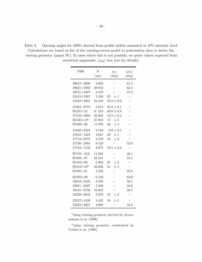
– 40 –

Table 3. Opening angles for MSPs derived from profile widths measured at 10% intensity level.

Calculations are based on fits of the rotating-vector-model to polarisation data to derive the

viewing geometry (paper IV). In cases where this is not possible, we quote values expected from

statistical arguments, 〈ρ10〉 (see text for details).

PSR P ρ10 〈ρ10〉

(ms) (deg) (deg)

J0613−0200 3.062 − 61.5

J0621+1002 28.854 − 62.4

J0751+1807 3.479 − 57.2

J1012+5307 5.256 35 ± 1 −

J1022+1001 16.453 25.0 ± 0.6 −

J1024−0719 5.612 25.8 ± 0.1 −

B1257+12 6 .219 40.0 ± 0.9 −

J1518+4904 40.935 10.5 ± 0.4 −

B1534+12a 37.904 17 ± 5 −

B1620−26 11.076 46 ± 3 −

J1640+2224 3.163 6.9 ± 0.1 −

J1643−1224 4.621 23 ± 1 −

J1713+0747 4.570 54 ± 3 −

J1730−2304 8.123 − 52.0

J1744−1134 4.075 18.1 ± 0.4 −

B1744−24A 11.564 − 46.1

B1802−07 23.101 − 53.1

B1855+09 5.362 27 ± 2 −

B1913+16b 59.030 21 ± 4 −

B1937+21 1.558 − 35.8

B1953+29 6.133 − 63.9

J2019+2425 3.935 − 56.1

J2051−0827 4.509 − 58.6

J2145−0750 16.052 − 56.7

J2229+2643 2.978 25 ± 3 −

J2317+1439 3.445 10 ± 1 −

J2322+2057 4.808 − 43.3

ausing viewing geometry derived by Arzou-

manian et al. (1996)

busing viewing geometry constrained by

Cordes et al. (1990)