The Atmospheric Dynamics of Pulsar Companions Adam S ...
318
The Atmospheric Dynamics of Pulsar Companions Adam S. Jermyn Thesis Mentor: E. S. Phinney Option Representative: Lynne Hillenbrand Division of Physics, Mathematics, and Astronomy California Institute of Technology June 10, 2015
-
Upload
khangminh22 -
Category
Documents
-
view
0 -
download
0
Transcript of The Atmospheric Dynamics of Pulsar Companions Adam S ...
The Atmospheric Dynamics of Pulsar Companions
Adam S. Jermyn
Thesis Mentor: E. S. PhinneyOption Representative: Lynne Hillenbrand
Division of Physics, Mathematics, and AstronomyCalifornia Institute of Technology
June 10, 2015

i
Curiosity demands that we ask questions, that we try to put thingstogether and try to understand this multitude of aspects as perhaps resultingfrom the action of a relatively small number of elemental things and forcesacting in an infinite variety of combinations.
– Richard P. Feynman

Acknowledgements
Except where otherwise noted, and to the best of my knowledge, all work presentedhere is my own. Getting to this point, however, is something for which I am deeplyindebted to those around me. Professor Sterl Phinney, my thesis mentor, taught methat intuition is more useful than precision, and patiently introduced me to the artof astronomy. Dr. Ravishankar Sundaraman, my collaborator and co-conspirator,showed me that numerical methods can be elegant as well as useful. Professor JasonAlicea, my adviser, introduced me to the subtle world of statistical physics, and gaveme an appreciation for the many mysteries therein. Dr. Milo Lin, my friend andcolleague, brought me into the fold of proteins and biophysics, and in so doing gaveme my first taste of emergence. Dr. Frank Rice, my laboratory instructor, impressedupon me the importance of always being grounded in experiment and observation.Professor Gil Refael, the leader of nights of free-wheeling physics and Thai food, gaveme the firm belief that any problem in Nature may be solved with enough of both.My friend Nicholas Schiefer gave me a little nudge towards astronomy in just theright way, and lent me an ear at all of the right times, and for that I will always begrateful. Of my professors and friends at Caltech, Tom Tombrello is the one I’ll nevertruly be able to thank. My adviser and advocate till the day he passed away, hebelieved in me even when I didn’t, and helped me find my way by gently pointing outthe doors he had opened all around me. The other person I cannot thank properly ismy grandfather Robert Katz, who passed away in May of 2014. He told me storiesabout the world through science and art and history, and in doing so piqued mycuriosity. Finally, I would like to thank Mom and Dad. You set me on my way inthis adventure.

Abstract

iv
Pulsars emit radiation over an extremely wide frequency range, from radio through
gamma1. Recently, systems in which this radiation significantly alters the atmospheres
of low-mass pulsar companions have been discovered2. These systems, ranging from
ones with highly anisotropic heating to those with transient X-ray emissions, represent
an exciting opportunity to investigate pulsars through the changes they induce in their
companions. In this work, we present both analytic and numerical work investigating
these phenomena, with a particular focus on atmospheric heat transport, transient
phenomena, and the possibility of deep heating via gamma rays. We find that certain
classes of binary systems may explain decadal-timescale X-ray transient phenomena3,
as well as the formation of so-called redback companion systems4. We also posit an
explanation for the formation of high-eccentricity millisecond pulsars with white dwarf
companions5. In addition, we examine the temperature anisotropy induced by the1A. Smith David. “Gamma Ray Pulsars with the Fermi LAT”. in: 3rd Fermi Symposium. May
2011. url: http://fermi.gsfc.nasa.gov/science/mtgs/symposia/2011/program/session14/Smith_FermiPSRs.pdf; H. et al Anderhub. “Search for Very High Energy Gamma-ray Emissionfrom Pulsar-Pulsar Wind Nebula Systems with the MAGIC Telescope”. In: The AstrophysicalJournal 710.1 (2010), p. 828. url: http://stacks.iop.org/0004-637X/710/i=1/a=828; T.Padmanabhan. Theoretical Astrophysics. Vol. 2. ISBN: 978-0521566315. Cambridge UniversityPress, 2001. Chap. 6.
2Mallory S. E. Roberts. Surrounded by Spiders! New Black Widows and Redbacks in the GalacticField. 2012. eprint: arXiv:1210.6903. url: http://arxiv.org/abs/1210.6903; M. T. Reynoldset al. “The light curve of the companion to PSR B1957+20”. In: Monthly Notices of the RoyalAstronomical Society 379.3 (2007), pp. 1117–1122. doi: 10.1111/j.1365-2966.2007.11991.x.eprint: http://arxiv.org/abs/0705.2514. url: http://mnras.oxfordjournals.org/content/379/3/1117.abstract.
3M. Linares. “X-Ray States of Redback Millisecond Pulsars”. In: The Astrophysical Journal 795,72 (Nov. 2014), p. 72. doi: 10.1088/0004-637X/795/1/72. arXiv: 1406.2384 [astro-ph.HE].
4P. Podsiadlowski, S. Rappaport, and E. D. Pfahl. “Evolutionary Sequences for Low- andIntermediate-Mass X-Ray Binaries”. In: The Astrophysical Journal 565 (Feb. 2002), pp. 1107–1133. doi: 10 . 1086 / 324686. eprint: astro - ph / 0107261; P. Podsiadlowski. “Irradiation-driven mass transfer low-mass X-ray binaries”. In: Nature 350 (Mar. 1991), pp. 136–138. doi:10.1038/350136a0.
5B. Knispel et al. “Einstein@Home Discovery of a PALFA Millisecond Pulsar in an EccentricBinary Orbit”. In: ArXiv e-prints (Apr. 2015). arXiv: 1504.03684 [astro-ph.HE].

v
Pulsar in its companion, and demonstrate that this may be used to infer properties
of both the companion and the Pulsar wind. Finally, we explore the possibility of
spontaneously generated banded winds in rapidly rotating convecting objects.

Contents
Acknowledgements i
Abstract ii
Definition of Symbols ix
List of Figures xvii
Motivation 1
I Physics 5
1 Geometry and Optical Depth 6
2 One-Dimensional Model 142.1 Equations of Stellar Structure . . . . . . . . . . . . . . . . . . . . . . 142.2 Simulations . . . . . . . . . . . . . . . . . . . . . . . . . . . . . . . . 182.3 Luminosity and Radial Variation . . . . . . . . . . . . . . . . . . . . 28
3 Higher Dimensional Models 363.1 Zero-Wind Analytic Model . . . . . . . . . . . . . . . . . . . . . . . . 39
3.1.1 Iterative Method . . . . . . . . . . . . . . . . . . . . . . . . . 403.1.2 Eigenfunction Expansion . . . . . . . . . . . . . . . . . . . . . 42
3.2 Zero-Divergence Wind Model . . . . . . . . . . . . . . . . . . . . . . 46
4 Review of Fluid Mechanics 494.1 Microscopic Viscosity . . . . . . . . . . . . . . . . . . . . . . . . . . . 494.2 Reynolds Number . . . . . . . . . . . . . . . . . . . . . . . . . . . . . 544.3 Rayleigh Number . . . . . . . . . . . . . . . . . . . . . . . . . . . . . 57
vi
CONTENTS vii
4.4 Richardson Number . . . . . . . . . . . . . . . . . . . . . . . . . . . . 594.5 Rossby Number . . . . . . . . . . . . . . . . . . . . . . . . . . . . . . 614.6 Mach Number . . . . . . . . . . . . . . . . . . . . . . . . . . . . . . . 62
5 Stability and Turbulence 655.1 Sheared Convection . . . . . . . . . . . . . . . . . . . . . . . . . . . . 66
5.1.1 Shear-dominated flow . . . . . . . . . . . . . . . . . . . . . . . 695.1.2 Convection-dominated flow . . . . . . . . . . . . . . . . . . . . 725.1.3 Mixed shear-convective flow . . . . . . . . . . . . . . . . . . . 73
5.2 Non-Convective Shear . . . . . . . . . . . . . . . . . . . . . . . . . . 75
6 Global Wind Patterns 796.1 Turbulent Zonal Flow . . . . . . . . . . . . . . . . . . . . . . . . . . . 796.2 Alternative Patterns . . . . . . . . . . . . . . . . . . . . . . . . . . . 82
6.2.1 Large Rossby Number . . . . . . . . . . . . . . . . . . . . . . 836.2.2 Small Rossby Number . . . . . . . . . . . . . . . . . . . . . . 88
6.3 Deciding . . . . . . . . . . . . . . . . . . . . . . . . . . . . . . . . . . 926.4 Convective Reynold’s Stress . . . . . . . . . . . . . . . . . . . . . . . 1006.5 Summary of Results . . . . . . . . . . . . . . . . . . . . . . . . . . . 104
7 Higher Dimensional Models with Transport 1107.1 Radiative Stars . . . . . . . . . . . . . . . . . . . . . . . . . . . . . . 1117.2 Convective Stars . . . . . . . . . . . . . . . . . . . . . . . . . . . . . 1157.3 Crossover Behavior . . . . . . . . . . . . . . . . . . . . . . . . . . . . 117
8 Time Dependence 1258.1 Assumptions and Computational Methods . . . . . . . . . . . . . . . 1258.2 Fully Radiative Stars . . . . . . . . . . . . . . . . . . . . . . . . . . . 1298.3 Fully Convective Stars . . . . . . . . . . . . . . . . . . . . . . . . . . 1328.4 Mixed Stars . . . . . . . . . . . . . . . . . . . . . . . . . . . . . . . . 138
II Applications in Astronomy 144
9 X-Ray Binaries 1459.1 Accretion rate . . . . . . . . . . . . . . . . . . . . . . . . . . . . . . . 1459.2 Pre-Roche Expansion . . . . . . . . . . . . . . . . . . . . . . . . . . . 1479.3 Post-Roche Accretion . . . . . . . . . . . . . . . . . . . . . . . . . . . 1529.4 Critical Accretion Dynamics . . . . . . . . . . . . . . . . . . . . . . . 158

CONTENTS viii
9.5 Limit Cycles . . . . . . . . . . . . . . . . . . . . . . . . . . . . . . . . 163
10 Accretion Induced Collapse 173
11 Spotted Black Widows 17911.1 Setup . . . . . . . . . . . . . . . . . . . . . . . . . . . . . . . . . . . . 18011.2 Main Sequence Solutions . . . . . . . . . . . . . . . . . . . . . . . . . 18311.3 Brown Dwarfs . . . . . . . . . . . . . . . . . . . . . . . . . . . . . . . 190
12 Banded Stars 198
Appendices 204
A Viscosity Code 204
B Acorn Stellar Integration Code 207B.1 Opal and Ferguson Opacity Table Parser . . . . . . . . . . . . . . . . 207B.2 Stellar Integration Code . . . . . . . . . . . . . . . . . . . . . . . . . 211
C Gob Stellar Integration Code 239
D Anisotropy Code 266
E Reference Stellar Models 271
Bibliography 291

ix
Definition of Symbols
Symbol Name Definition/Value/[Units]log Logarithm base 10ln Logarithm base eG Newton’s Constant 6.673× 10⁻⁸erg cm
g2
M Solar Mass 1.98855× 1033gR Solar Radius 6.955× 10¹⁰mL Solar Luminosity 3.83× 1033erg/smp Proton Mass 1.6605× 10⁻²⁴ga Radiation Constant 7.57× 10⁻¹⁵ erg
cm3K4
c Speed of Light 2.99792458× 1010cm/skB Boltzmann Constant 1.38065× 10⁻¹⁶erg/Kσ Stefan-Boltzmann Constant 5.6703× 10⁻⁵erg/s/cm2/K4
Ry Rydberg - Hydrogen Ionization Energy 2.179872× 10⁻¹¹ergq Electron Charge Magnitude 4.80321× 10⁻¹⁰√erg · cmM Stellar Mass [M]Mp Pulsar Mass [M]Σ Column Density [g/cm2]Σh Heating Column Density [g/cm2]κ Mass Attenuation Coefficient [cm2/g]R Stellar Radius [R]R0 Orbital Radius [cm]Rb Roche Lobe Radius [cm]P Orbital Period [s]Pp Pulsar Rotation Period [s]ω Pulsar frequency [rad/s]z Depth [cm]g Acceleration due to Gravity GM
R2
P Pressure [erg/cm3]ρ Density [g/cm3]T Temperature [K]u Specific Internal Energy [erg/cm3]s Specific Entropy [erg/K/cm3]Fb Flux due to Nuclear Processes [erg/cm2/s]Lin Luminosity due to Nuclear Processes [erg/s]Fr Radiative Flux 4acT 3
3κρ ∂zT
Le External Luminosity [erg/s]k Thermal Conductivity [erg/cm/s/K]krad Radiative Thermal Conductivity 4acT 3
3ρκcv Specific Heat Capacity (Constant Volume) [kB/µ]cp Specific Heat Capacity (Constant Pressure) γcvγ Adiabatic Index cp
cv
µ Mean Free Particle Mass ρkTp
vs Speed of Sound√
γpρ
hs Pressure Scale Height dzd ln p = p
ρg

x
Symbol Name Definition/Value/[Units]∇ Temperature Gradient d lnT
d lnP∇rad Radiative Temperature Gradient 3κpFbr2
4acGMT 4
∇ad Adiabatic Temperature Gradient 1− 1γ
l Convective Length-scale [cm]ℵ Convective Scale Factor l/hsΓ Convective Efficiency∇conv Convective Gradientvc Convective Speed [cm/s]Fc Convective Flux Fnet − Frv0 Wind Speedvφ Circumferential Wind Speed∇c Circumferential Temperature Gradient ∂φ lnT∆z Region Thickness [cm]τt Cooling Time Heat Content
Non-Transient Flux = cpT (∆z)Fb
= γp(∆z)Fb
τw Wind Circulation Time 2πrvw
ν Kinematic Viscosity [cm2/s]N Brunt-Vaisala Frequency
√g∂z ln ρ or
√g∂zs/γ
Ri Richardson Number N2
(dv/dz)2
Ric Critical Richardson NumberRe Reynolds Number vd/ν with characteristic flow diameter dRec Critical Reynolds Numberβ Thermal Expansion Coefficient [K−1]α Thermal Diffusivity k
cp
Ra Rayleigh Number βgl3∆Tαν
Rac Critical Rayleigh Number ∼ 103
Pe Péclet Number vlα
r Spherical Radial Coordinateθ Spherical Polar Angleφ Spherical Azimuthal/Cylindrical Polar Angles Cylindrical Radial Angle

List of Figures
1.1 Depiction of a pulsar and its companion. Note that none of thedepictions are to scale. The companion orbits with angular velocityequal to its rotational angular velocities due to tidal locking effects.The pular and companion are separated by a distance Ro. Their massesare Mp and M respectively. The star has radius R. The heating zoneis, for any kind of radiation, the region of unit optical depth giventhat the radiation is incident from one side and that the source is farenough away that it may be viewed as a planar wavefront. . . . . . . 8
1.2 log κ−1 is plotted versus logE. The former is measured in g/cm2 andthe latter in eV. Data was extracted manually from plots in the ParticleData Group book6, and so has some uncertainty associated with theconversion process. . . . . . . . . . . . . . . . . . . . . . . . . . . . . 10
1.3 log Σ is plotted versus logE. The former is measured in g/cm2 andthe latter in eV. . . . . . . . . . . . . . . . . . . . . . . . . . . . . . . 11
2.1 The vertical axis is log ρ (with ρ measured in g/cm3), the horizontal islog T (with T measured in K), and the color represents log κ (with κmeasured in cm2/g. White regions are those without data. . . . . . . 19
6´J. et al Beringer. “Particle Data Group”. In: Phys. Rev. D 86 (2012), p. 010001.
xi
LIST OF FIGURES xii
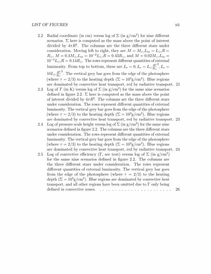
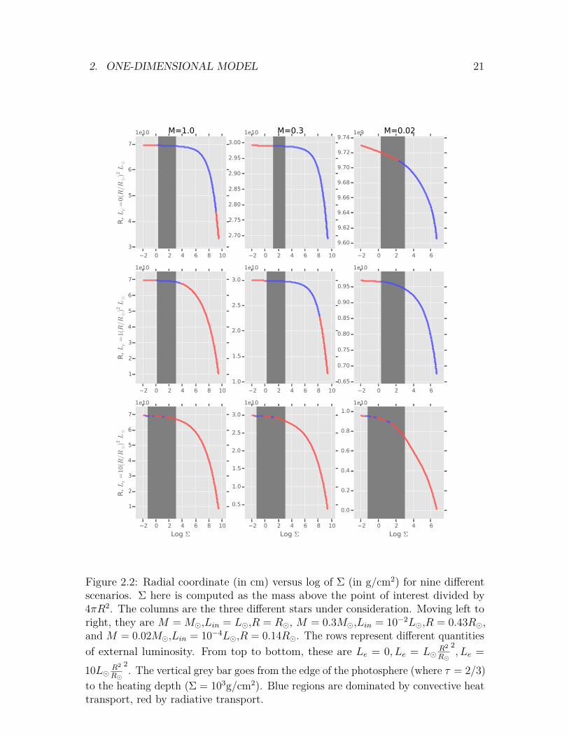
2.2 Radial coordinate (in cm) versus log of Σ (in g/cm2) for nine differentscenarios. Σ here is computed as the mass above the point of interestdivided by 4πR2. The columns are the three different stars underconsideration. Moving left to right, they are M = M,Lin = L,R =R, M = 0.3M,Lin = 10−2L,R = 0.43R, and M = 0.02M,Lin =10−4L,R = 0.14R. The rows represent different quantities of externalluminosity. From top to bottom, these are Le = 0, Le = L
R2
R
2, Le =
10L R2
R
2. The vertical grey bar goes from the edge of the photosphere(where τ = 2/3) to the heating depth (Σ = 103g/cm2). Blue regionsare dominated by convective heat transport, red by radiative transport. 21
2.3 Log of T (in K) versus log of Σ (in g/cm2) for the same nine scenariosdefined in figure 2.2. Σ here is computed as the mass above the pointof interest divided by 4πR2. The columns are the three different starsunder consideration. The rows represent different quantities of externalluminosity. The vertical grey bar goes from the edge of the photosphere(where τ = 2/3) to the heating depth (Σ = 103g/cm2). Blue regionsare dominated by convective heat transport, red by radiative transport. 23
2.4 Log of pressure scale height versus log of Σ (in g/cm2) for the same ninescenarios defined in figure 2.2. The columns are the three different starsunder consideration. The rows represent different quantities of externalluminosity. The vertical grey bar goes from the edge of the photosphere(where τ = 2/3) to the heating depth (Σ = 103g/cm2). Blue regionsare dominated by convective heat transport, red by radiative transport. 24
2.5 Log of convective efficiency (Γ, see text) versus log of Σ (in g/cm2)for the same nine scenarios defined in figure 2.2. The columns arethe three different stars under consideration. The rows representdifferent quantities of external luminosity. The vertical grey bar goesfrom the edge of the photosphere (where τ = 2/3) to the heatingdepth (Σ = 103g/cm2). Blue regions are dominated by convective heattransport, and all other regions have been omitted due to Γ only beingdefined in convective zones. . . . . . . . . . . . . . . . . . . . . . . . 26

LIST OF FIGURES xiii
2.6 The vertical axis is log ρ (with ρ measured in g/cm3), the horizontalis log T (with T measured in K), and the color represents log κ (withκ measured in cm2/g. White regions are those without data. Thenine stellar models defined in figure 2.2 are plotted as tracks on topof the opacity. The terminus marker indicates which track is which:the three sizes of markers correspond in increasing order to the threestellar masses under consideration, and the three kinds of markerscorrespond in order of increasing number of sides to increasing externalillumination. Blue regions are dominated by convective heat transport,red by radiative transport. . . . . . . . . . . . . . . . . . . . . . . . . 27
2.7 The log of f is plotted versus log(Le/Li,old) with β = 4 + 2/3 in orangeand β = 0 in blue. These solutions were determined numerically inMathematica. . . . . . . . . . . . . . . . . . . . . . . . . . . . . . . . 33
4.1 The vertical axis is log ρ (with ρ measured in g/cm3), the horizontal islog T (with T measured in K), and the color represents log ν (with νmeasured in cm2/s. White regions are those without data. . . . . . . 52
4.2 The vertical axis is log ρ (with ρ measured in g/cm3), the horizontal islog T (with T measured in K), and the color represents the log of theanisotropy factor A. White regions are those without data. . . . . . . 55
4.3 The vertical axis is log ρ (with ρ measured in g/cm3), the horizontal islog T (with T measured in K), and the color represents the log of theanisotropy factor A. White regions are those without data. . . . . . . 56
8.1 ∆T/T0 (top) and L/L (bottom) versus log Σ (in g/cm2) for a star ofmass M, radius R, and luminosity 100L. The external heat wasput in at Σ = 103g/cm2 and linearly increased from zero to 100Lover the course of 108s, which is where the simulation ends. Colorrepresents time, with the simulation beginning at violet and endingwith red. . . . . . . . . . . . . . . . . . . . . . . . . . . . . . . . . . . 130
8.2 ∆T/T0 (top) and L/L (bottom) versus log Σ (in g/cm2) for a star ofmassM, radius R, and luminosity 100L. The external heat was putin at Σ = 103g/cm2 and linearly increased from zero to 100L over thecourse of 108s, after which the simulation continued for another 108sto allow for equilibration. Color represents time, with the simulationbeginning at violet and ending with red. . . . . . . . . . . . . . . . . 131

LIST OF FIGURES xiv
8.3 ∆T/T0 (top) and L/L (bottom) versus log Σ (in g/cm2) for a star ofmass M, radius R, and luminosity 100L. The external heat wasput in at Σ = 103g/cm2 and linearly decreased from 100L to zeroover the course of 108s. Color represents time, with the simulationbeginning at violet and ending with red. . . . . . . . . . . . . . . . . 133
8.4 ∆T/T0 (top) and L/L (bottom) versus log Σ (in g/cm2) for a star ofmass 0.3M, radius 2.65R, and luminosity 0.1L. The external heatwas put in at Σ = 103g/cm2 and linearly decreased from 0.1L to zeroover the course of 108s. Color represents time, with the simulationbeginning at violet and ending with red. . . . . . . . . . . . . . . . . 134
8.5 ∆T/T0 (top) and L/L (bottom) versus log Σ (in g/cm2) for a starof mass 0.3M, radius 2.65R, and luminosity 0.1L. The externalheat was put in at Σ = 103g/cm2 and linearly decreased from 0.1Lto zero over the course of 108s. The simulation was then run for anadditional 108s with no external heating. Color represents time, withthe simulation beginning at violet and ending with red. . . . . . . . . 135
8.6 ∆T/T0 (top) and L/L (bottom) versus log Σ (in g/cm2) for a starof mass 0.3M, radius 2.65R, and luminosity 0.1L. The externalheat was put in at Σ = 103g/cm2 and linearly decreased from Lto zero over the course of 108s. The simulation was then run for anadditional 108s with no external heating. Color represents time, withthe simulation beginning at violet and ending with red. . . . . . . . . 136
8.7 ∆T/T0 (top) and L/L (bottom) versus log Σ (in g/cm2) for a star ofmass M, radius R, and luminosity L. The external heat was putin at Σ = 103g/cm2 and linearly decreased from L to zero over thecourse of 108s. Color represents time, with the simulation beginningat violet and ending with red. . . . . . . . . . . . . . . . . . . . . . . 140
8.8 ∆T/T0 (top) and L/L (bottom) versus log Σ (in g/cm2) for a starof mass 0.3M, radius 2.65R, and luminosity 0.1L. The externalheat was put in at Σ = 103g/cm2 and linearly decreased from 10Lto zero over the course of 108s. The simulation was then run for anadditional 108s with no external heating. Color represents time, withthe simulation beginning at violet and ending with red. . . . . . . . . 141

LIST OF FIGURES xv
8.9 ∆T/T0 (top) and L/L (bottom) versus log Σ (in g/cm2) for a star ofmass M, radius R, and luminosity L. The external heat was putin at Σ = 103g/cm2 and linearly decreased from L to zero over thecourse of 108s. It was then run for another 108s at that value. Colorrepresents time, with the simulation beginning at violet and endingwith red. . . . . . . . . . . . . . . . . . . . . . . . . . . . . . . . . . . 142
8.10 ∆T/T0 (top) and L/L (bottom) versus log Σ (in g/cm2) for a star ofmass M, radius R, and luminosity L. The external heat was putin at Σ = 103g/cm2 and immediately decreased from L to zero overthe course of 108s before being run for another 109s. Color representstime, with the simulation beginning at violet and ending with red. . . 143
9.1 The vertical axis is logP in seconds, the horizontal axis is the com-panion mass M in solar masses, and the color represents the log ofthe expansion timescale hs/R in seconds. The four different plotscorrespond to four different pulsar luminosities. . . . . . . . . . . . . 153
9.2 The vertical axis is logP in seconds, the horizontal axis is the com-panion mass M in solar masses, and the color represents the log ofτdisk/τexp. The four plots correspond to different pulsar luminosities. . 157
9.3 The vertical axis is logP in seconds, the horizontal axis is the com-panion mass M in solar masses, and the color represents the log ofthe ratio of the quick contraction length to the scale height. The fourplots correspond to different pulsar luminosities. . . . . . . . . . . . . 161
9.4 The vertical axis is logP in seconds, the horizontal axis is the com-panion mass M in solar masses, and the color represents the log of thecontraction timescale. The four plots correspond to different pulsarluminosities. . . . . . . . . . . . . . . . . . . . . . . . . . . . . . . . . 162
9.5 The vertical axis is logP in seconds, the horizontal axis is the com-panion mass M in solar masses, and the color represents the log of theratio of the critical disk viscous timescale to the contraction timescale.The four plots correspond to different pulsar luminosities. . . . . . . . 164
9.6 The vertical axis is logP in seconds, the horizontal axis is the com-panion mass M in solar masses, and the color represents the type oflimit cycle. Blue is type 1, Green is type 2, Maroon is type 3. Thefour plots correspond to different pulsar luminosities. . . . . . . . . . 169

LIST OF FIGURES xvi
10.1 The vertical axis is M/M, the horizontal axis is Mc/M, with bothaxes log-scaled. The color represents the ratio Rmax/30R, the denom-inator being the approximate Roche radius for the period and massrange of interest, and the numerator being the post-expansion radiusof the red giant of interest. . . . . . . . . . . . . . . . . . . . . . . . . 177
11.1 The vertical axis is P in seconds, the horizontal axis is the companionmass in solar masses, with both axes log-scaled. The color representsthe log of the day/night flux ratio logFday/Fnight. The four differentplots correspond to four different pulsar luminosities. The black linecorresponds to the Roche cutoff. . . . . . . . . . . . . . . . . . . . . . 186
11.2 The vertical axis is P in seconds, the horizontal axis is the companionmass in solar masses, with both axes log-scaled. The color representsthe log of the day/night flux ratio log ∆F/F . The four differentplots correspond to four different pulsar luminosities. The black linecorresponds to the Roche cutoff. The white regions above the Rochecutoff have ∆F = 0 due to heat bottling. . . . . . . . . . . . . . . . . 187
11.3 The vertical axis is P in seconds, the horizontal axis is the companionmass in solar masses, with both axes log-scaled. The color representsthe log of the day/night flux ratio logFday/(Fi+Fe). The four differentplots correspond to four different pulsar luminosities. The black linecorresponds to the Roche cutoff. . . . . . . . . . . . . . . . . . . . . . 188
11.4 The vertical axis is P in seconds, the horizontal axis is the companionmass in solar masses, with both axes log-scaled. The color representsthe log of the day/night flux ratio logW/(Fi + Fe). The four differentplots correspond to four different pulsar luminosities. The black linecorresponds to the Roche cutoff. Note that the white region above theRoche cutoff corresponds to the case W = 0 . . . . . . . . . . . . . . 189
11.5 The vertical axis is P in seconds, the horizontal axis is the companionmass in solar masses, with both axes log-scaled. The color representsthe log of the day/night flux ratio logFnight/Fi. The four differentplots correspond to four different pulsar luminosities. The black linecorresponds to the Roche cutoff. . . . . . . . . . . . . . . . . . . . . . 191
11.6 Top: ∆F/Fe is shown as a function of logχ. Bottom: logFday/Fnightis shown as a function of logχ. . . . . . . . . . . . . . . . . . . . . . . 194

List of Tables
6.1 Computed parameterization of circumferential heat transport by winds.The first column specifies what case is under consideration. All pos-sible cases are enumerated here. The remaining columns specify y, aprefactor on the transport as well as q, a, b, the exponents on ∆T/T ,l/2πR, and Ro respectively. Note that factors of γ and ℵ have beenneglected in assembling this table. . . . . . . . . . . . . . . . . . . . . 105
6.2 Critical thermal anisotropy values are listed for each case of interest.Note that factors of γ and ℵ have been neglected in assembling thistable. . . . . . . . . . . . . . . . . . . . . . . . . . . . . . . . . . . . . 107
xvii

Motivation
If you haven’t found something strange during the day, it hasn’t been muchof a day.
– John Archibald Wheeler
Pulsars, highly magnetic compact stellar remnants, exhibit some of the most un-usual behaviors in the universe by virtue of existing at length and energy scales wheregeneral relativity and quantum field theory are both relevant. Pulsar gravitationalfields are typically so strong that in binary pairs they emit significant gravitationalradiation. The magnetic field near a pulsar’s surface is strong enough that the indexof refraction of the vacuum deviates significantly from unity, and particle pair creationhelps create an ionized wind which travels relativistically away from the pulsar7.
Most of what is known of pulsars comes from radio timing data8. Pulsars may bethought of as spherical magnetic dipoles approximately 10km in radius with surfacemagnetic fields between 108Gauss and 1015Gauss, spinning with periods betweenmillisecond and second timescales9. As a result of the large electric fields created bythe rotating magnetic dipole moment, particles are created and carry energy, bothkinetic and in the form of a Poynting flux, away from the pulsar. As these particlesmove they also radiate gamma-rays. Observationally, this means that pulsars appearin a wide band of radio frequencies as a periodic short pulse, while also being activethrough very high energies. The timing of these pulses has informed much of what iscurrently known about pulsars.
7Padmanabhan, op. cit.8Dipankar Bhattacharya. “The Evolution of the Magnetic Fields of Neutron Stars”. In: J.
Astrophys. Astr. 16 (Mar. 1994), pp. 217–232. url: http://www.ias.ac.in/jarch/jaa/16/217-232.pdf.
9Idem, “The Evolution of the Magnetic Fields of Neutron Stars”; José A. Pons et al. “Evidencefor Heating of Neutron Stars by Magnetic-Field Decay”. In: Phys. Rev. Lett. 98 (7 Feb. 2007),p. 071101. doi: 10.1103/PhysRevLett.98.071101. eprint: http://arxiv.org/pdf/astro-ph/0607583.pdf?origin=publication_detail. url: http://link.aps.org/doi/10.1103/PhysRevLett.98.071101.
1
2
More specifically, pulsars have masses and radii in a very small range constrainedby models of the degenerate nuclear equation of state10. From dispersion delay dataat different frequencies it is possible to determine the electron column density inthe interstellar medium between Earth and the pulsar, which can give a distanceestimate11. Measurement of the pulse period gives the angular frequency ω. Combinedwith the mass and radius this gives the rotational energy of the pulsar:
E = 12Iω
2 = 15MR2ω2 (1)
Measurement of the rate at which the pulse period changes gives ω, which then givesthe rate at which the pulsar rotational energy changes:
E = 25MR2ωω (2)
Equating this with the energy loss rate of a magnetic dipole then gives the surfacedipole magnetic field. Measurement of ω can also give insight into the mechanismstransferring angular momentum to or from the pulsar by giving an estimate of thebraking index12.
While these techniques give significant insight into the properties of the pulsar,they give very little information regarding the surrounding environment. In particular,the properties of the pulsar wind are currently not very well known. While it isknown that some fraction of the outgoing electromagnetic flux must be convertedinto a particle flux at the light cylinder of radius
Rl = c
ω, (3)
little is known of the nature of this conversion and the effect it has on the radiationportion of the energy flux. Recently, a number of binary systems composed of apulsar and star orbiting it have been discovered in which the pulsar wind causesobservable changes in the companion star13. If the companion star has a mass less
10Padmanabhan, op. cit.; J. M. Lattimer and M. Prakash. “Neutron Star Structure and theEquation of State”. In: The Astrophysical Journal 550.1 (2001), p. 426. eprint: http://arxiv.org/abs/astro-ph/0002232. url: http://stacks.iop.org/0004-637X/550/i=1/a=426.
11Andrea N Lommen and Paul Demorest. “Pulsar timing techniques”. In: Classical and QuantumGravity 30.22 (2013), p. 224001. eprint: http://arxiv.org/abs/1309.1767. url: http://stacks.iop.org/0264-9381/30/i=22/a=224001.
12Padmanabhan, op. cit.13R. P. Breton et al. “Discovery of the Optical Counterparts to Four Energetic Fermi Millisecond
Pulsars”. In: The Astrophysical Journal 769 (2013), p. 108. url: http://arxiv.org/abs/1302.1790.

3
than the 0.08M minimum required to sustain fusion, the system is known as a BlackWidow14, and if the pulsar wind heats the companion and causes it to swell to fill itsRoche lobe, the system is known as a Redback15.
In the vast majority of Black Widows, even heating is seen on the pulsar-facingside16. There is one, however, known as PSR J1544-4937, in which the heatingappears to be highly concentrated towards a small set of points on the companion.This indicates effects involving the interaction between the wind and the companionmagnetosphere.
In the case of Redbacks, it is possible that Roche lobe-filling companions canbegin an accretion process onto the pulsar as a result of heating from the wind. Ifthis occurs, the system can become an X-ray binary. There are several known casesof X-ray binaries which turn on and off on timescales of ∼ 10yrs17. This may be dueto the accretion disk burying the magnetic field of the pulsar, allowing the companionto cool and thereby halting the accretion process18. Under this model, when theaccretion rate drops sufficiently the process begins again.
Both kinds of systems offer an opportunity to learn more about the pulsar wind,in particular as the effects of the wind on the companion are strongly influenced byits composition. For typical low-frequency radiation (anything ranging up to X-raysin energy), the region which the wind heats is in the upper atmosphere of the star,near the photosphere. The result is that the radiation is just re-radiated withoutsignificantly altering the structure of the atmosphere. The net effect is a rise in
14Roberts, op. cit.; D. J. Stevenson. “The search for brown dwarfs”. In: Annual Review ofAstronomy and Astrophysics 29 (1991), pp. 163–193. doi: 10.1146/annurev.aa.29.090191.001115.
15Hai-Liang Chen et al. “Formation of Black Widows and Redbacks—Two Distinct Populations ofEclipsing Binary Millisecond Pulsars”. In: The Astrophysical Journal 775.1 (2013), p. 27. eprint:http://arxiv.org/abs/1308.4107. url: http://stacks.iop.org/0004-637X/775/i=1/a=27.
16Reynolds et al., op. cit.; Roger W. Romani et al. “PSR J1311–3430: A Heavyweight Neutron Starwith a Flyweight Helium Companion”. In: The Astrophysical Journal Letters 760.2 (2012), p. L36.eprint: http://arxiv.org/abs/1210.6884. url: http://stacks.iop.org/2041-8205/760/i=2/a=L36; M. H. van Kerkwijk, R. P. Breton, and S. R. Kulkarni. “Evidence for a Massive NeutronStar from a Radial-velocity Study of the Companion to the Black-widow Pulsar PSR B1957+20”.In: The Astrophysical Journal 728.2 (2011), p. 95. eprint: http://arxiv.org/abs/1009.5427.url: http://stacks.iop.org/0004-637X/728/i=2/a=95.
17Icdem, B. and Baykal, A. “Viscous timescale in high mass X-ray binaries”. In: Astronomy andAstrophysics 529 (2011), A7. doi: 10.1051/0004-6361/201015810. eprint: http://arxiv.org/abs/1102.4203. url: http://dx.doi.org/10.1051/0004-6361/201015810.
18J. Hessels. “M28I and J1023+0038: The Missing Links Go Missing, but Provide a New Link”. In:NS Workshop. Dec. 2013. url: http://www.astro.uni-bonn.de/NS2013-2/Hessel_M28i.pdf.

4
temperature on the near-side according to the Stefan-Boltzmann law:
4πR2σT 4new = 4πR2σT 4
old + Le. (4)
The far-side does not heat at all, as there is no time to move the absorbed heataround the star before reemission occurs.
When the radiation is higher in energy, or is made of massive particles, thesituation is somewhat different. High energy radiation can penetrate quite deep intothe star, as will be discussed later. Massive particles can likewise make it quite far,particularly if they are uncharged. Charged massive particles are, however, limited bythe ionization zone in how far they may travel. Regardless of the specific form of theexternal heating, when it occurs at depth the picture is very different. In particular,the heat has some time to be redistributed within the star rather than immediatelyescaping to the near-side. The formal statement of this effect is that the time it takesfor the heat to be nontrivially redistributed is now comparable to or shorter thanthe radiative relaxation time. Profound structural changes in the stellar atmospheremay occur, including the excitation of gravity waves, strong zonal winds, tropicalhurricanes, and the inducement of swelling in the deeper regions of the atmosphere.This last symptom of external heating may be responsible for the observed Roche-lobefilling in certain Redback systems, with the eponymous thermal difference on thesurface between the two sides of the star being due to the non-penetrative flux of thePulsar wind.
As these phenomena couple heat transport, fluid mechanics, orbital mechanics,and various pieces of thermodynamic microphysics, we will discuss the physics first,and then the astronomy. Along the way, we will use examples from astronomy toillustrate relations, gain intuition, and build models, but only at the end will theastrophysical phenomena of interest be discussed in full.

Part I
Physics
5

1
Geometry and Optical Depth
6

1. GEOMETRY AND OPTICAL DEPTH 7
, .There is geometry in the humming of the strings, there is music in the spacing of thespheres.
– Pythagoras
The geometry of the situations of interest is outlined in Fig. 1.1. The companionstar and pulsar orbit their center of mass with angular velocity Ω. The companion istidally locked, and hence Ω is also its rotation rate. The pulsar, on the other hand,has rotation rate ω Ω. The two objects are separated by distance Ro, and havemasses Mp and M for the pulsar and companion respectively. The star has radius R.Note that the relative distances depicted are not shown to scale. The heating zone is,for any kind of radiation, the region surrounding the surface of unit optical depth. Inthe cases of interest the source is positioned on one side of the companion and is farenough away that it may be viewed as roughly a planar wavefront.
To determine where the heating zone lies, we must examine the optical depthassociated with various kinds of radiation incident on the surface of the star. Below10keV, the chief scattering processes are resonant absorption and Rayleigh scatter-ing1. Above this scale, Compton scattering becomes the dominant process,untilapproximately 1MeV ∼ 2me, at which point the dominant process is pair production.This state of affairs continues to arbitrarily high energies once the electron-positronpair production threshold is crossed. The use of the pair production decay channel,however, means that there will be more particles present after the initial scattering,and these may continue moving through the star for some distance before furtherscattering thermalizes them. If the resulting particles have energies above somecritical level, the dominant process once all channels and possibilities are accountedfor will continue to be pair production.
The net result of all of this is that for incident radiation below a critical energy, asingle scattering event suffices and the cross-section directly gives the depth at whichthe radiation deposits heat. This gives
Σ = 1κ, (1.1)
where κ is the mass attenuation coefficient corresponding to the material and particlekind. Above the critical energy, the resulting particles from the first scattering continueto produce further particles until their descendents drop below the critical energyand produce heat. At each stage in the shower, additional particles are producedwith energies approximately two times lower than what they started with, so if Eγ
1J. et al Beringer. “Particle Data Group”. In: Phys. Rev. D 86 (2012), p. 010001.

1. GEOMETRY AND OPTICAL DEPTH 8
R
Ro
Mp M
Ω
Heating Zone
Pulsar Companion Star
Ωω
Figure 1.1: Depiction of a pulsar and its companion. Note that none of the depictionsare to scale. The companion orbits with angular velocity equal to its rotationalangular velocities due to tidal locking effects. The pular and companion are separatedby a distance Ro. Their masses are Mp and M respectively. The star has radius R.The heating zone is, for any kind of radiation, the region of unit optical depth giventhat the radiation is incident from one side and that the source is far enough awaythat it may be viewed as a planar wavefront.

1. GEOMETRY AND OPTICAL DEPTH 9
is the energy of the photon and Ecrit is the critical energy, a total of approximatelylog2(Eγ/Ecrit) are created. If the scattering cross-section at each stage is roughlyconstant, as is expected in the case of energies above GeV scales2, then this meansthat the column density at which heat is produced should be
Σ = 1κ
(1 + log2
EγEcrit
),
The critical energy is given approximately3 in gases by
Ecrit = 710MeVZ + 0.92 ,
where Z is the number of protons in a nucleus. For hydrogen this simplifies to
Ecrit = 370MeV.
Plots of κ−1 and the corresponding Σ are shown in Fig. 1.2 and Fig. 1.3 respectively.For hydrogen, the value of κ−1 is approximately 100g/cm2 for all energies beyond
Ecrit which have been measured5, going up through 100GeV. Thus
Σ = 100 gcm2
(1 + log2
Eγ370MeV
).
Typical pulsar photon energies in the upper end of the spectrum are of order hundredsof GeV6. Substituting this in gives roughly
Σh = 103 gcm2 . (1.2)
This is the column density at which a stellar companion transforms the pulsar’sgamma rays into heat, and we will use this value in calculations involving the heatingdepth. To most appropriately model the physical process of particle showers andabsorption, we will treat the incident luminosity as following
Le(Σ) = Lee−Σ/Σh , (1.3)
2Ibid.3Ibid.5Ibid.6A. Smith David. “Gamma Ray Pulsars with the Fermi LAT”. in: 3rd Fermi Symposium. May
2011. url: http://fermi.gsfc.nasa.gov/science/mtgs/symposia/2011/program/session14/Smith_FermiPSRs.pdf; H. et al Anderhub. “Search for Very High Energy Gamma-ray Emissionfrom Pulsar-Pulsar Wind Nebula Systems with the MAGIC Telescope”. In: The AstrophysicalJournal 710.1 (2010), p. 828. url: http://stacks.iop.org/0004-637X/710/i=1/a=828.

1. GEOMETRY AND OPTICAL DEPTH 10
Figure 1.2: log κ−1 is plotted versus logE. The former is measured in g/cm2 and thelatter in eV. Data was extracted manually from plots in the Particle Data Groupbook4, and so has some uncertainty associated with the conversion process.

1. GEOMETRY AND OPTICAL DEPTH 11
Figure 1.3: log Σ is plotted versus logE. The former is measured in g/cm2 and thelatter in eV.
where Le measures only the high-energy photons. Low energy photons are ignored,as they are absorbed and reemitted soon thereafter in the photosphere.
Armed with this information regarding the structure of the heating zone, wecan in principle take a three-dimensional model of a star and compute the spatialdependence of the heating. Again, in principle, this may be used to compute theresulting effects on the star. For the purposes of gaining physical intuition, however,this is not the most effective way to proceed, for there are many simplifications whichmay save substantially on computational effort and may make clearer the relevantphysics.
The most basic model for the companion star which captures some of the physicsof interest is to treat it as one-dimensional, and ignore the azimuthal symmetrybreaking which results from the tidal locking. In this case, the star is parametrized bya series of functions of the radial coordinate, such as temperature, pressure, and so on.Though this model neglects a significant physical asymmetry, it is advantageous in itsmathematical and computational simplicity, and so will be our starting point. Withinthe context of this model, we will treat all physical quantities as their averages overthe angular coordinates, such that the externally incident flux will sum up to thesame total luminosity. As a result, this model is often referred to as the plane-parallelor isotropic atmosphere, for in it there is only one coordinate (depth) which matters.

1. GEOMETRY AND OPTICAL DEPTH 12
After this model, the next modification will be to examine higher-dimensionalmodels. We will examine both two-dimensional models which add just the azimuthalcoordinate φ and fully three dimensional models. In the former, we will treat allquantities as their average over the spherical polar angle θ, while the latter holds thefull dimensionality of the system.
Beyond spatial dimensions, there is also the question of time. Initially we willconsider all solutions in the steady-state. After this, we will shift to considering thetime-dependence of these models, and exa mine both the stability of the steady-statesolutions and the means by which they are reached.

1. GEOMETRY AND OPTICAL DEPTH 13
ReferencesAnderhub, H. et al. “Search for Very High Energy Gamma-ray Emission from Pulsar-
Pulsar Wind Nebula Systems with the MAGIC Telescope”. In: The AstrophysicalJournal 710.1 (2010), p. 828. url: http://stacks.iop.org/0004-637X/710/i=1/a=828 (cit. on p. 9).
Beringer, J. et al. “Particle Data Group”. In: Phys. Rev. D 86 (2012), p. 010001(cit. on pp. 7, 9).
Smith David, A. “Gamma Ray Pulsars with the Fermi LAT”. In: 3rd Fermi Symposium.May 2011. url: http://fermi.gsfc.nasa.gov/science/mtgs/symposia/2011/program/session14/Smith_FermiPSRs.pdf (cit. on p. 9).

2
One-Dimensional Model
There is a computer disease that anybody who works with computers knowsabout. It’s a very serious disease and it interferes completely with thework. The trouble with computers is that you "play" with them!
– Richard P. Feynman1
2.1 Equations of Stellar StructureIn the isotropic steady-state model, we treat all quantities in the companion asfunctions of r, the distance from its center. No other independent variable enters inthis model, as t is forbidden by the steady-state assumption and θ and φ are forbiddenby the isotropy assumption. Thus we write temperature as T (r), pressure as P (r),and so on.
To a very good approximation, we may neglect the variation in the compositionof the star with position. That is, we treat all compositional variables as globalconstants, such that X(r) = X0, the hydrogen mass fraction in the star, and likewisefor all other such quantities. In making this approximation we mainly lose accuracy incalculating the properties of convection zones, though there our accuracy is primarilylimited by the uncertainty in the choice of mixing length, and so this loss is acceptable.
The remaining spatial variables are then only thermodynamic ones. Of these,one might pick as "fundamental" ones the pressure, temperature, density, and mean
1Richard P. Feynman. Los Alamos From Below. https : / / www . youtube . com / watch ?v = 0ogSC6JKkrY. Feb. 6, 1975. url: http : / / calteches . library . caltech . edu / 34 / 3 /FeynmanLosAlamos.htm.
14

2. ONE-DIMENSIONAL MODEL 15
molecular weight2. All other quantities of interest may be derived from these. Wemay, however, eliminate µ, for it is a direct function of T . This follows from thefact that we have held compositional variables fixed, such that µ varies only throughionization.3. This variation occurs mainly when kBT is comparable to 13.6eV , and isgenerally taken to happen between 103.8K and 104.1K. The value of 13.6eV , of course,is the ionization energy of hydrogen.
Using the equation of state, we may eliminate yet another function, to reducethe total count of "fundamental" thermodynamic variables at each point to two. Theequation of state is most generally written as
P = f(ρ, T ), (2.1)
though it is usually well approximated by the form
µP = ρkBT + 13aT
4, (2.2)
where the second term is included to accommodate radiation pressure. At lowtemperatures the second term may be dropped, yielding the familiar ideal gas law.Regardless of the specific form, we will use the equation of state to eliminate thedensity from consideration, and hence write
ρ = g(P, T ). (2.3)
Our ability to write it in this form comes from P being monotonic in ρ and T . Wechoose ρ rather than T or P because we generally wish to compute heat transportproperties in terms of temperature, and in hydrostatic equilibrium the pressure iscomputable by a straightforward integral. As a result, we are left with two basicfunctions, P (r) and T (r), which fully characterize the star to within our variousapproximations.
It will often be more convenient to replace r with m, the mass above a particularradius, as the independent variable. As m is monotonically decreasing with r thisis a perfectly well-defined transformation. We thus write P = P (m), T = T (m). Inthis language, the condition of hydrostatic equilibrium may be cast into a convenientform, as
dP
dr= −ρg → dP
dm= g
4πr2 . (2.4)
Now over the depth ranges of interest, as will be verified later, r varies only slightlyrelative to R. As a result, we may neglect its variation in computing quantities
2Other valid choices include specific energy, specific entropy, sound speed, etc.3At high pressures it may also depend on pressure, and indeed we will account for this

2. ONE-DIMENSIONAL MODEL 16
in which r appears as a multiplicative factor. This is known as the thin-envelopeassumption, and has several useful implications. For instance, we may approximatethe gravity of the star as being fixed at
g ≡ GM
R2 . (2.5)
As a result, we may write the condition of hydrostatic equilibrium as
dP
dm= GM
4πR4 . (2.6)
Using the boundary condition P (r =∞) = 0,m(r =∞) = 0 we find
P (m) = GMm
4πR4 . (2.7)
Note that we may also use the variable
Σ ≡ m
4πR2 (2.8)
as the independent variable. Given that this is the form in which we know the heatingdepth, we will often switch to using this rather than m.
Given T (m), in addition to what we have found so far, we will know the structureof the star to within the bounds of our approximations. As a result, we know thatT (m) must depend in some fashion on the luminosity of the star and on the externalillumination we hope to investigate, for these quantities appear nowhere else and theyseem quite important. To that end, consider the outer boundary condition on thestar. There are a variety of models for this4, but most treat the low-m regime bysome gas-radiation dilution model and use this to find the optical depth along theradial direction. From there, it is typically asserted that
L = 4πR2σT 4 (2.9)
at the place where the optical depth τ = 2/3. This is just an application of theStephan-Boltzmann radiation law to a gray-body atmosphere, with an effectivetreatment for the differing rates at which different frequencies of radiation escape atlow optical depth. We will not go into the specific details of the model we used, andmerely state that they are those described in Ref.5.
4B. Paczyński. “Envelopes of Red Supergiants”. In: Acta Astronomica 19 (1969), p. 1.5Ibid.

2. ONE-DIMENSIONAL MODEL 17
From this upper boundary condition on T , we may integrate towards higher musing the equation
dT
dm=(d lnTd lnP
)T
P
dP
dm= ∇T
P
dP
dm, (2.10)
where the second equality defines the symbol ∇ and where the derivative with respectto lnP is taken along the radial direction. This last point is not relevant in anisotropic star, where ∇T and ∇p are aligned, but will become important when wemove to higher dimensional models.
Of course, there is no physical content in Eq. (2.10): it is simply a true statementregarding differentiable functions. The reason we bother to cast the problem in thisform is that ∇ may often be expressed simply. In regions of the star where heat istransported radiatively,
∇ = ∇rad = 3κPL16πacGMT 4 , (2.11)
where κ is the Rosseland mean opacity of the stellar material, and is generally afunction of P and T . On the other hand, when the region of interest is unstable againstconvection, the thermal gradient ∇ is somewhat more complicated. If convection isefficient, then the convective gradient matches the adiabatic gradient, such that
∇ = ∇ad = d lnTd lnP
∣∣∣∣∣s
. (2.12)
This gradient is typically 0.4 for monatomic gas and for fully ionized gas, and dropsto 0.1 − 0.2 in the ionization zone. If, on the other hand, convection is inefficient,then matters become somewhat more complex, as then both radiation and convectioncontribute nontrivially to thermal transport. The full solution for the convectivegradient in this case is somewhat complicated, and involves the root of a cubic witha closed form which does not yield much intuition. Various methods of numericalsolution have been developed6, and will be employed in the next section. As will beshown later, however, convection is usually highly efficient in the cases of interest,and so setting ∇ = ∇ad in convecting regions is generally accurate.
It is worth noting that the question of convective stability is much simpler in starsthan in other contexts. The microscopic viscosity of stellar atmospheres is generallyfar too low to stop convection7. This is a statement about the typically large value ofthe Rayleigh number whenever the radiative gradient exceeds the adiabatic one. Thus
6Ibid.7This will be discussed at length when we examine the properties of fluids in motion for higher
dimensional heat transport

2. ONE-DIMENSIONAL MODEL 18
in the absence of shear turbulence the primary criterion determining if convectionoccurs is
∇rad > ∇ad. (2.13)
If this condition is satisfied then convection occurs. Loosely speaking this criterionmay be thought of as indicating that the temperature gradient needed to carry thethermal flux through radiation is too high relative to the buoyancy experienced byan adiabatically expanding packet of gas. The result is a convective instability.
The only remaining piece of physics we need to compute stellar structures withthe above equations is κ. This we take from tables such that those of OPAL8 andFerguson9, as discussed in Appendix B.1. A plot of the opacities produced by thesetables at X = 0.7, Y = 0.27, Z = 0.03 is shown in figure 2.1.
2.2 SimulationsArmed with the equations of stellar structure, we may simulate a variety of starsnumerically to see how they respond to different amounts of external illumination. Thepurpose of these initial simulations is to gain intuition for the relevant phenomenology,and to determine reasonable ranges for the various parameters such as temperature,pressure, and so on.
Initially, all simulations were done using a modified version of the Gob softwarepackage, originally written for Red Giant envelope integration10. The original andmodified codes may be found in Appendix C. A modern code known as Acorn wasthen written as part of this thesis to incorporate recent advances in low-temperaturestellar opacity models. In addition, it uses a much finer adaptive mass grid, resultingin more accurate and smoother stellar profiles11. This code was then verified inthe high-temperature limit against Gob, and the microphysical inputs were verifiedindependently in the low-temperature limit. The details of this code may be found inAppendix B.2, with details on the opacity tables and associated interpolation routinesin Appendix B.1. The code solves precisely the same equations as Gob12, with the
8C. A. Iglesias and F. J. Rogers. “Updated Opal Opacities”. In: The Astrophysical Journal 464(June 1996), p. 943. doi: 10.1086/177381.
9Jason W. Ferguson et al. “Low-Temperature Opacities”. In: The Astrophysical Journal 623.1(2005), p. 585. url: http://stacks.iop.org/0004-637X/623/i=1/a=585.
10Paczyński, op. cit.11The smoothness of the resulting profiles is particularly important, as we will use the output
from the steady-state code as the input to the transient code, which requires evaluating numericalderivatives in mass.
12Paczyński, op. cit.

2. ONE-DIMENSIONAL MODEL 19
3 4 5 6 7 8 9log T
−10
−8
−6
−4
−2
0
2
4
6
log ρ
−4
−3
−2
−1
0
1
2
3
4
5
log κ
Figure 2.1: The vertical axis is log ρ (with ρ measured in g/cm3), the horizontal islog T (with T measured in K), and the color represents log κ (with κ measured incm2/g. White regions are those without data.

2. ONE-DIMENSIONAL MODEL 20
addition of the thin envelope assumption, such that M −m and r are taken not tochange, except where they appear explicitly as parameters for differentiation.
Though Acorn only computes stellar envelopes, this is more than enough toexamine the vicinity of Σh. The heat input was modeled by changing the luminosityof the star as a function of column density, according to
L(Σ) = Lin + Lee−Σ/Σh . (2.14)
A value of Σh = 103g/cm2 was used here, as per the discussion in Chapter 1.To begin with, we consider models where the external illumination is imposed
whilst holding the star’s radius and intrinsic luminosity fixed. The following threerepresentative models for companion stars were chosen for the simulations:
• The Sun: M = M,Lin = L,R = R
• Low-mass nuclear-burning: M = 0.3M,Lin = 10−2L,R = 0.43R
• Brown dwarf: M = 0.02M,Lin = 10−4L,R = 0.14R
The full output from Acorn for each of these cases for a variety of external luminositiesmay be found in Appendix E.
The first aspect of these models worth investigating is the region of validity ofthe thin-envelope approximation, which is the assumption that r ≈ R everywhere inthe envelope. To see where this holds, we have plotted the radius as a function of Σin figure 2.2. For the 1M star, the thin-envelope approximation is good down toΣ = 106g/cm2 or so, where deviations reach roughly 10%. For the 0.3M star, theapproximation is valid everywhere with no external heating, down to Σ = 107g/cm2 forLe = Li, and to Σ = 106g/cm2 for Le = 10Li. For both of these stars, deviations growrapidly past the regime of validity. Finally, for the 0.02M star, the approximation istypically only valid within 10% down to Σh. Past this, however, deviations grow muchmore slowly than for the other two stars, and so the approximation may be safelyused down to around 105g/cm2, where deviations reach 15%. Fortunately there areno phenomena which are both sensitive to the high-Σ failure of this approximationand are of significant quantitative interest, so this approximation is a safe one tomake. Subsequent plots will be truncated in their range of Σ to that in which theapproximation is valid to within 50%.
We now turn to the thermal structure of the star. Figure 2.3 shows the log oftemperature versus the log of column density for nine scenarios. The three stars ofinterest are represented by the columns, while three different external luminositiesare represented by the rows. The top row has no external illumination, the middle
2. ONE-DIMENSIONAL MODEL 21
−2 0 2 4 6 8 10
3
4
5
6
7
R, Le=0(R/R⊙)
2L⊙
1e10 M=1.0
−2 0 2 4 6 8 10
1
2
3
4
5
6
7
R, Le=1(R/R
⊙)2L⊙
1e10
−2 0 2 4 6 8 10
Log Σ
1
2
3
4
5
6
7
R, Le=10(R/R
⊙)2L⊙
1e10
−2 0 2 4 6 8 10
2.70
2.75
2.80
2.85
2.90
2.95
3.00
1e10 M=0.3
−2 0 2 4 6 8 10
1.0
1.5
2.0
2.5
3.0
1e10
−2 0 2 4 6 8 10
Log Σ
0.5
1.0
1.5
2.0
2.5
3.0
1e10
−2 0 2 4 6
9.60
9.62
9.64
9.66
9.68
9.70
9.72
9.741e9 M=0.02
−2 0 2 4 6
0.65
0.70
0.75
0.80
0.85
0.90
0.95
1e10
−2 0 2 4 6
Log Σ
0.0
0.2
0.4
0.6
0.8
1.0
1e10
Figure 2.2: Radial coordinate (in cm) versus log of Σ (in g/cm2) for nine differentscenarios. Σ here is computed as the mass above the point of interest divided by4πR2. The columns are the three different stars under consideration. Moving left toright, they are M = M,Lin = L,R = R, M = 0.3M,Lin = 10−2L,R = 0.43R,and M = 0.02M,Lin = 10−4L,R = 0.14R. The rows represent different quantitiesof external luminosity. From top to bottom, these are Le = 0, Le = L
R2
R
2, Le =
10L R2
R
2. The vertical grey bar goes from the edge of the photosphere (where τ = 2/3)to the heating depth (Σ = 103g/cm2). Blue regions are dominated by convective heattransport, red by radiative transport.

2. ONE-DIMENSIONAL MODEL 22
row has the illumination equal to LR2/R2, and the bottom row has it equal to ten
times that. Note that for each mass, the radius was held constant. As a result, thetop row represents a nearly unmodified system, while the bottom row represents asystem dominated by the external heating.
Looking first at the sun, we see that adding external heating begins by shuttingdown convection at the base of the envelope, and eventually leads to almost completelyradiative transport at high external luminosity. The only regions which remainconvective are those in the vicinity of the ionization zone, where the adiabaticgradient is very low to begin with. This may be understood as a result of the externalheat decreasing the temperature gradient between the core and the heating depth,while increasing it between this depth and the surface. In the former region thissuffices to switch the transport from convective to radiative, while the latter is verystable against convection and so remains radiative. That the effect of the heating isso much deeper than the heating depth may be viewed as due to the imposition of adifferent boundary condition at this depth. In particular, the fact that we maintain afixed radius as we vary the flux means that the surface temperature scales as L1/4
net .In the 0.3M star we see the same thing, though with convection holding on in alarger region in the middle plot. In the 0.02M star, the same process is evidentlyoccurring, though the transition to radiative transport is not apparent until the finalplot. This is as we expect: at the lower temperatures which dominate in these stars,radiative transport is less efficient and so the need for convective heat transport isgreater.
One interesting feature of note is the change in thermal gradient between T = 104Kand T = 104.5K. This occurs when the ionization zone is convective, which it almostalways is, and results from a decrease in the adiabatic gradient within the zone. Thereason this feature is not visible in each of the nine scenarios plotted in figure 2.3 isthat in not all scenarios does the ionization zone fall within the envelope.
The next aspect of these models worth examining is the pressure scale height, hs.This sets the characteristic length scale for turbulence, wind shearing, and convectivemotion, and so will be of interest at every stage of our analysis. The log of this heightis shown in figure 2.4. In each of the models, hs increases monotonically into the starpast the photosphere, starting around 106.5cm near the surface and reaching valuesonly a few orders of magnitude smaller than R at the base of the envelope. In general,we expect hs to follow a power-law as a function of Σ, and indeed this is what we see.Deviations from this are typically due to changes in the mode of heat transport, orto the ionization of material at various points.
Now we may also compute the efficiency of convection, Γ, defined as the ratioof the heat carried by a convecting gas packet to the heat lost radiatively along the

2. ONE-DIMENSIONAL MODEL 23
−2 0 2 4 6 8 10
3.5
4.0
4.5
5.0
5.5
6.0
6.5
Log T
, Le=0(R/R
⊙)2L⊙
M=1.0
−2 0 2 4 6 8
4.0
4.5
5.0
5.5
6.0
Log T
, Le=1(R/R
⊙)2L⊙
−2 0 2 4 6 8
Log Σ
4.0
4.5
5.0
5.5
6.0
Log T
, Le=10(R/R
⊙)2L⊙
−2 0 2 4 6 8 10
3.5
4.0
4.5
5.0
5.5
M=0.3
−2 0 2 4 6 8 10
3.5
4.0
4.5
5.0
5.5
6.0
−2 0 2 4 6 8
Log Σ
4.0
4.5
5.0
5.5
6.0
−2 0 2 4 6
3.2
3.4
3.6
3.8
4.0
M=0.02
−2 0 2 4 6
4.0
4.5
5.0
5.5
−2 −1 0 1 2 3 4 5
Log Σ
4.0
4.2
4.4
4.6
4.8
5.0
5.2
Figure 2.3: Log of T (in K) versus log of Σ (in g/cm2) for the same nine scenariosdefined in figure 2.2. Σ here is computed as the mass above the point of interestdivided by 4πR2. The columns are the three different stars under consideration.The rows represent different quantities of external luminosity. The vertical greybar goes from the edge of the photosphere (where τ = 2/3) to the heating depth(Σ = 103g/cm2). Blue regions are dominated by convective heat transport, red byradiative transport.

2. ONE-DIMENSIONAL MODEL 24
−2 0 2 4 6 8 106.5
7.0
7.5
8.0
8.5
9.0
9.5
10.0
Log h
s, Le=0(R/R⊙)
2L⊙
M=1.0
−2 0 2 4 6 8
7.0
7.5
8.0
8.5
9.0
9.5
10.0
Log h
s, Le=1(R/R
⊙)2L⊙
−2 0 2 4 6 8
Log Σ
7.5
8.0
8.5
9.0
9.5
10.0
Log h
s, Le=10(R/R
⊙)2L⊙
−2 0 2 4 6 8 106.0
6.5
7.0
7.5
8.0
8.5
9.0
M=0.3
−2 0 2 4 6 8 10
6.5
7.0
7.5
8.0
8.5
9.0
9.5
−2 0 2 4 6 8
Log Σ
7.0
7.5
8.0
8.5
9.0
9.5
−2 0 2 4 6
6.5
7.0
7.5
M=0.02
−2 0 2 4 6
7.0
7.5
8.0
8.5
9.0
−2 −1 0 1 2 3 4 5
Log Σ
7.4
7.6
7.8
8.0
8.2
8.4
8.6
8.8
Figure 2.4: Log of pressure scale height versus log of Σ (in g/cm2) for the samenine scenarios defined in figure 2.2. The columns are the three different stars underconsideration. The rows represent different quantities of external luminosity. Thevertical grey bar goes from the edge of the photosphere (where τ = 2/3) to the heatingdepth (Σ = 103g/cm2). Blue regions are dominated by convective heat transport, redby radiative transport.

2. ONE-DIMENSIONAL MODEL 25
way. While a variety of expressions exist for this, we will make use of the one used inthe Gob stellar integration code13. The results of doing so are shown in figure 2.5.This quantity is of interest because it is a good indicator of the extent to which thebalance between convection and radiation has been altered by the external heating,as well as because it indicates the extent to which the convective gradient deviatesfrom the adiabatic one. In each of the unperturbed stars, convection is either highlyefficient at the heating depth or becomes very efficient close to the heating depth. Inshallower regions the efficiency decreases until convection ceases, with a sharp drop inefficiency at the boundary. Importantly, the region over which the efficiency is low isvery small, as the slope of Γ with respect to Σ is large near the radiative-convectivetransition. In the perturbed stars, convection does not always occur in the sameregion, as the additional heat may turn it off in the vicinity of the surface, but whereit does occur all of the same statements regarding its efficiency hold.
Finally, it is also useful to examine how κ varies through each of the stellar modelsof interest, and so this is shown in figure 2.6. Referencing figure 2.1, we see a fewpoints worthy of discussion. First, many of the stellar tracks go outside of the knownopacity data. In most of these cases the stars are convective, with highly efficientconvection, and so the opacity is irrelevant. In every combination of the two low-massstars with the two lowest-heating values, however, we get a radiative region outsideof the known opacity data. In each case the issue arises because ρ is too large. Theopacity tables are internally stored using ρ/T 3 and T as the independent variables14.Below 106K the tables form a rectangular grid in these variables. As a result, thesetracks have exceeded the maximum value of ρ/T 3 for which we have data, whileremaining in an acceptable temperature range. The simulation code in these casessimply returns the opacity at the correct temperature and maximum value of ρ/T 3
for which data exists. Fortunately, however, examination of the corresponding regionsin figure 2.3 indicates that these regions are actually quite small in pressure-space,and only appear stretched in this plot out because ρ changes more rapidly here.
The second feature worth noting is that the convergence of the various trackscorresponding to the radiative atmospheres supports our conclusions regarding thedecay of heating into radiative zones. Likewise, the lack of convergence between theanalogous convective envelopes supports our conclusions regarding the continuation ofheating into convection zones. Additionally, the vast majority of each track, whethermeasured by pressure-space or arc-length in log ρ, log T space, is spent in regions
13Ibid.14The first of these, ρ/T 3, is often called R, and usually defined with ρ measured in units of
1g/cm3 and T measured in units of 106K.

2. ONE-DIMENSIONAL MODEL 26
−2 0 2 4 6 8 10
−4
−2
0
2
4
6
8
Log Γ
, Le=0(R/R⊙)
2L⊙
M=1.0
−2 0 2 4 6 8
−4
−3
−2
−1
0
1
2
3
Log Γ
, Le=1(R/R
⊙)2L⊙
−2 0 2 4 6 8
Log Σ
−8
−7
−6
−5
−4
−3
−2
−1
Log Γ
, Le=10(R/R
⊙)2L⊙
−2 0 2 4 6 8 10
0
2
4
6
8
10
12
M=0.3
−2 0 2 4 6 8 10
−4
−2
0
2
4
6
8
−2 0 2 4 6 8
Log Σ
−8
−7
−6
−5
−4
−3
−2
−1
−2 0 2 4 60
2
4
6
8
10
M=0.02
−2 0 2 4 6
−4
−2
0
2
4
6
8
−2 −1 0 1 2 3 4 5
Log Σ
−8
−7
−6
−5
−4
−3
−2
−1
Figure 2.5: Log of convective efficiency (Γ, see text) versus log of Σ (in g/cm2) for thesame nine scenarios defined in figure 2.2. The columns are the three different starsunder consideration. The rows represent different quantities of external luminosity.The vertical grey bar goes from the edge of the photosphere (where τ = 2/3) tothe heating depth (Σ = 103g/cm2). Blue regions are dominated by convective heattransport, and all other regions have been omitted due to Γ only being defined inconvective zones.

2. ONE-DIMENSIONAL MODEL 27
3.0 3.5 4.0 4.5 5.0 5.5 6.0 6.5 7.0
log T
−10
−8
−6
−4
−2
0
log ρ
−3
−2
−1
0
1
2
3
4
5
log κ
Figure 2.6: The vertical axis is log ρ (with ρ measured in g/cm3), the horizontal islog T (with T measured in K), and the color represents log κ (with κ measured incm2/g. White regions are those without data. The nine stellar models defined infigure 2.2 are plotted as tracks on top of the opacity. The terminus marker indicateswhich track is which: the three sizes of markers correspond in increasing order to thethree stellar masses under consideration, and the three kinds of markers correspond inorder of increasing number of sides to increasing external illumination. Blue regionsare dominated by convective heat transport, red by radiative transport.

2. ONE-DIMENSIONAL MODEL 28
where∂κ
∂T
∣∣∣∣∣ < 0. (2.15)
This fact will become relevant later in the next section. Finally, the fact that theminimum in κ lies at temperatures comparable to those in the ionization zone meansthat ∇rad tends to peak where ∇ad is at a minimum, which encourages the formationof a convection region around the ionization zone. This is seen even in the case ofheavy external illumination, which generally pushes stars towards radiative transporteven at depths much below where the additional heat is deposited.
2.3 Luminosity and Radial VariationThe simulations in the previous section were done with the radius and internalluminosity of the star fixed. To be completely accurate, we should really do aboundary condition matching between the photosphere and the nuclear burningregion, as is done in codes like MESA15. Instead, we will perform a much simplerprocess, which consists of identifying roughly what the temperature change in thebulk of the star is, and using that, along with the dependence of nuclear burningon temperature, to estimate the balance between changing radius, changing surfacetemperature, and changing internal luminosity.
To begin, let Pb be the pressure at which the star changes from being convectiveto being radiative. We usually expect stars to be convective for P < Pb and radiativefor P > Pb
16. This is obviously not always the case, as there can be small regionswhere convection turns on and off, but as a coarse view of things this is a goodapproximation. Note that for fully radiative stars Pb = 0 and for fully convectivestars Pb = Pcore ≈ 2gsurfM
4πR2 . The mixed case, where 0 < Pb < Pcore, arises for stars ofmass M ∈ [0.43, 2]M17.
15Bill Paxton et al. “Modules for Experiments in Stellar Astrophysics (MESA): Planets, Oscillations,Rotation, and Massive Stars”. In: The Astrophysical Journal Supplement Series 208.1 (2013), p. 4.url: http://stacks.iop.org/0067-0049/208/i=1/a=4.
16The reason we expect convection on top is that ∇rad decreases rapidly with temperature. Inan efficient convection zone T ∝ P∇ad , where ∇ad is usually around 0.4 except in the ionizationzone, where it drops to 0.1. ∇rad, on the other hand, usually goes roughly as PT−5 ∝ P 1−5∇ad
in the star’s interior. When we look past the ionization zone, the exponent is negative, and so∇rad eventually drops below ∇ad at high pressure. There may of course be brief changes betweenconvective and radiative heat transport in the ionization zone, but below that region our argumentsshould hold. Note that in computing ∇rad we have factored in the approximate dependence of theopacity on temperature and pressure.
17Maurizio Salaris and Cassisi Santi. Evolution of stars and stellar populations. Vol. 1. ISBN:

2. ONE-DIMENSIONAL MODEL 29
If the star’s surface heats up by an amount ∆T , we may ask how much of a changethis causes in the matter below. In the radiation region, we know that
dT
dP= 3κL
16πacGmT 3 , (2.16)
where m is the mass below the pressure of interest. If we perturb this equation byletting T → T + δT , and assume that T (P ) is a solution to the equation, then
d(δT )dP
= dT
dP
(∂ ln κ∂T
∣∣∣∣∣P
− 3 1T
)δT. (2.17)
Now κ usually decreases with increasing temperature, at least once you look deeperthan the upper envelope, so the perturbation decreases exponentially as one goes tohigher pressures. This is consistent with the valve modelof radiative zones18. Forfully radiative stars, then, we expect as a result that keeping R and Lin fixed isappropriate.
In the convecting region things are somewhat more complicated. We know thatT ∝ P∇c ≈ P∇ad . If the temperature at some pressure P0 is increased by T0, then thetemperature changes all the way from P0 to Pb following the convective gradient. Forstars which have some nontrivial convection zone, let ∆T0 be the temperature changeat P0, where we now restrict P0 < Pb and pick P0 at the lowest possible pressurebelow the photosphere. Recall that the radius of the star obeys
dr
dm= 1
4πr2ρ. (2.18)
This may also be written asdr3
dm= 3
4πρ. (2.19)
Differentiating with respect to time gives
d
dm
(dr3
dt
)= −3
4πρ
(d ln ρdt
)= −dr
3
dm
(d ln ρdt
). (2.20)
At fixed pressure, d ln ρ = −d lnT , neglecting the small space occupied by theionization zone, so
d ln ρdt
= −d lnTdt
. (2.21)
0-470-09220-3. John Wiley Sons, 2005, pp. 138–140.18H. Ritter, Z.-Y. Zhang, and U. Kolb. “Irradiation and mass transfer in low-mass compact
binaries”. In: Astronomy and Astrophysics 360 (Aug. 2000), p. 969. eprint: astro-ph/0005480.

2. ONE-DIMENSIONAL MODEL 30
As a result,d
dm
(dr3
dt
)= dr3
dm
d lnTdt
. (2.22)
Integrating assuming fixed radius at the base of the convection zone allows us to write
dVcdt
= Vcd lnTdt
, (2.23)
ord lnVcdt
= d lnTdt
, (2.24)
where Vc is the volume of the convection zone. Integrating with respect to time yields
∆ lnVc = ∆ lnT. (2.25)
If the position of the base of the convection zone is fixed and near the core, then thisreduces to
∆ lnR = 13∆ lnT. (2.26)
In the case of fully convective stars a fixed base is a fine assumption: ∇rad is somuch greater than ∇ad that Pb is just the core pressure. In the case of fully radiativestars, we are likewise fine: increasing T just lowers ∇rad, reinforcing the fact that∇rad < ∇ad. Thus we do not expect that if Vc is zero for some T , it will becomenonzero at a larger T . Between these two cases, we may compute the change that atemperature perturbation has on the convective-radiative boundary.
Suppose that T (P ) is the unperturbed state and δT (P ) is the perturbation. Then
∇ad = ∇rad (P ′b, T + δT ) = ∇rad (Pb, T ) , (2.27)
and so∴ ∂P∇raddPb + ∂T∇rad∂PTdPb + ∂T∇radδT = 0. (2.28)
From this it follows that
dPbdT
= −PT
(∂lnT∇rad
∂ln p∇rad +∇∂lnT∇rad
)= −P
T
(−3 + ∂lnT ln κ
1 +∇ (−3 + ∂lnT ln κ)
). (2.29)
As ∇ = ∇ad at the transition point, this simplifies to
dPbdT
= −PT
(−3 + ∂lnT ln κ
1 +∇ad (−3 + ∂lnT ln κ)
). (2.30)

2. ONE-DIMENSIONAL MODEL 31
Now ∂lnT ln κ (holding P fixed) at high temperature and pressure is generally around−3, and ∇ad under the same conditions is usually around 0.4, so this expression isactually negative, with magnitude roughly given by −4P/T . Thus
∇b ≡ −d lnPbd lnT ≈ 4. (2.31)
As lnT changes by the same amount everywhere in the convection zone, we maysubstitute T0 for T and obtain the same result. This is consistent with what we seein the top-left and middle-left of Figure 2.3, where log T changes by one near thebase of the sun’s envelope and logPb changes by five or so towards the surface.
We may now examine the behavior of the radius of the base of the convectionzone. Let this radius be Rbase, the initial temperature at P0 be T0,i, and the finaltemperature at P0 be T0,f . Using this, we write
dRbase
d lnT0= dRbase
d lnPbd lnPbd lnT0
= −∇adhsd lnPfd lnT0
= ∇ad∇bhs. (2.32)
Recalling that hs is a function only of T , we may find hs at the base using onlyknowledge of the way the temperature at the base of the convection zone changes.That is,
d lnTbd lnT0
= ∂ lnTb∂ lnT0
∣∣∣∣∣Pb
+ ∂ lnTb∂ lnPb
∣∣∣∣∣T0
d lnPbd lnT0
∣∣∣∣∣T0
= 1−∇ad∇b. (2.33)
Thusdhsd lnT0
= hs (1−∇ad∇b) , (2.34)
and hence
hs,f = hs,i
(T0,f
T0,i
)1−∇ad∇b. (2.35)
Now the difference between Ri,0 and Rf, 0 is given by
Ri,0 −Rf,0 =∫ Pf
P0
dr
dPdP = hs,i
∇ad
1−(P0,i
Pb,i
)∇ad
, (2.36)

2. ONE-DIMENSIONAL MODEL 32
so putting it all together we find
dR
d lnT0= ∂R
∂Vc
∣∣∣∣∣Rbase
dVcd lnT0
+ dRbase
d lnT0(2.37)
= ∂R
∂Vc
∣∣∣∣∣Rbase
(Vc − 4πR2
basedRbase
d lnT0
)+ dRbase
d lnT0(2.38)
= R
3Vc
(Vc − 4πR2
basedRbase
d lnT0
)+ dRbase
d lnT0(2.39)
= R
3 + dRbase
d lnT0
(1− R2
baseR2
)(2.40)
= R
3 +∇ad (Ri,0 −Rf,0)(T0,f
T0,i
)1−∇ad∇b (1− R2
baseR2
). (2.41)
Past the initial small changes in temperature, the second term is negligible, so wefind that we are actually justified in writing
∆ lnR = 13∆ lnT (2.42)
for convecting stars. To combine the cases of convection and radiation, we write
∆ lnR = min( 1
12 ln PbP0,13∆ lnT
). (2.43)
The picture, then, is that fully radiative stars have fixed R,Lin, and fully convectivestars have ∆ lnR = 1
3∆ lnT . To determine the change in Lin for a fully convectivestar, we note that nuclear burning typically scales as T β for some β > 0. Thus wemay write the energy balance in such a star as
4πR2σT 4surf,new = Le + Lin,old
(Tsurf,new
Tsurf,old
)β, (2.44)
where we have made use of the fact that the surface temperature ratio between theperturbed and unperturbed cases is the same as the core temperature ratio betweenthe two cases. Substituting in what we know for the dependence of R on T gives
4πR2oldσT
4+2/3surf,newT
−2surf,old = Le + Li,old
(Tsurf,new
Tsurf,old
)β. (2.45)

2. ONE-DIMENSIONAL MODEL 33
- -
[/]
[]
β=/
β=
Figure 2.7: The log of f is plotted versus log(Le/Li,old) with β = 4 + 2/3 in orangeand β = 0 in blue. These solutions were determined numerically in Mathematica.
Using Li,old = 4πR2oldσT
4surf,old and letting f ≡ Tsurf,new/Tsurf,old, we find
LeLi,old
= f 4+2/3 − fβ. (2.46)
Fully convective stars tend to be cooler ones, for which β ≈ 4, so we may numericallysolve this for a variety of cases. The results of this are shown in orange in figure 2.7.Note that when the impact on nuclear burning is included in the solution, the resultexceeds what we would otherwise find. This aligns with our intuition that heatingthe star causes it to burn faster, which causes it to heat more. The trend is close tolinear, past Le = Li,old, with a slope of roughly 1/6, so loosely speaking T ∝ L1/6
e ,R ∝ L1/6
e , and Lin ∝ L2/3e . In the case that the convection zone goes deep into the
star but does not reach near the nuclear burning region, we expect instead that Linwill be constant and that R ∝ T ∝ (Le + Lin)3/14, as plotted in blue in figure 2.7.
Note that if β > 14/3 then Eq. (2.46) has no solutions. This reflects the fact thatin such a system, heating the star causes the nuclear burning rate to go up fasterthan the surface flux can accommodate, further heating the star. The end of such aprocess occurs by weakening the coupling between the surface and the core of the starby turning off convection in the vicinity of the core. Further note that if the star is

2. ONE-DIMENSIONAL MODEL 34
not heated by nuclear burning, the only thermodynamically allowed equilibrium hasthe external illumination only stemming the loss of heat, not raising the temperature.
It appears, in summary, that the only stars which will respond to the externalillumination by swelling are those which are nuclear burning and mostly convective,and that the response is greatest in those which are convective all the way down tothe nuclear burning regions. In these, the swelling is increased by the fact that thenuclear burning increases in extent to match the hotter core temperatures.
In the next several chapters we will move to higher-dimensional models andperform the same kind of analysis to determine what, if any, impact the anisotropyin the external heating has, and how this impact depends on the parameters of thesystem.

2. ONE-DIMENSIONAL MODEL 35
ReferencesFerguson, Jason W. et al. “Low-Temperature Opacities”. In: The Astrophysical Journal
623.1 (2005), p. 585. url: http://stacks.iop.org/0004-637X/623/i=1/a=585(cit. on p. 18).
Feynman, Richard P. Los Alamos From Below. https://www.youtube.com/watch?v=0ogSC6JKkrY. Feb. 6, 1975. url: http://calteches.library.caltech.edu/34/3/FeynmanLosAlamos.htm (cit. on p. 14).
Iglesias, C. A. and F. J. Rogers. “Updated Opal Opacities”. In: The AstrophysicalJournal 464 (June 1996), p. 943. doi: 10.1086/177381 (cit. on p. 18).
Paczyński, B. “Envelopes of Red Supergiants”. In: Acta Astronomica 19 (1969), p. 1(cit. on pp. 16–18, 25).
Paxton, Bill et al. “Modules for Experiments in Stellar Astrophysics (MESA): Plan-ets, Oscillations, Rotation, and Massive Stars”. In: The Astrophysical JournalSupplement Series 208.1 (2013), p. 4. url: http://stacks.iop.org/0067-0049/208/i=1/a=4 (cit. on p. 28).
Ritter, H., Z.-Y. Zhang, and U. Kolb. “Irradiation and mass transfer in low-masscompact binaries”. In: Astronomy and Astrophysics 360 (Aug. 2000), p. 969. eprint:astro-ph/0005480 (cit. on p. 29).
Salaris, Maurizio and Cassisi Santi. Evolution of stars and stellar populations. Vol. 1.ISBN: 0-470-09220-3. John Wiley Sons, 2005, pp. 138–140 (cit. on p. 28).

3
Higher Dimensional Models
All of the analysis thus far has been one dimensional. We now describe a frameworkfor computing higher dimensional steady state effects in certain limits. Recall that inhydrostatic equilibrium,
∇p = ρ (c− g) , (3.1)
where c captures all rotational acceleration effects. We also have that in steady stateand without any input heating or winds, the thermal flux obeys
∇ · F = 0. (3.2)
In the presence of an input heat power density ε, this changes to
∇ · F = ε. (3.3)
The boundary condition on this equation at the star’s edge is a free one, with theflux at r =∞ dropping to zero. This results from the thermal flux proceeding out ofthe star at the photosphere with no reflection. The star’s photospheric temperatureis determined by
σT 4 = F · n (3.4)
at the photosphere’s base, usually defined as the point where τ = 2/3. Finally, ifwinds are introduced, the flux divergence becomes1
∇ · F = ε− cpTv · (∇ lnT −∇ad∇ ln p) . (3.5)1Rudolf Kippenhahn, Alfred Weigert, and Achim Weiss. Stellar Structure and Evolution. Springer,
2012. isbn: 978-3-642-30304-3.
36

3. HIGHER DIMENSIONAL MODELS 37
Note that F includes convective and radiative effects only. Further note that ε mustinclude the effects of viscous dissipation on the winds in order for this formalism tobe self-consistent.
In general, we expect that we may write the thermal flux in terms of the tempera-ture distribution as
F = −k∇T, (3.6)
where k may depend on the temperature, the pressure, and the gradients thereof.Note that this holds even for convective flux, though in the case of convection thethermal conductivity will be a rank two tensor, reflecting the potentially anisotropicnature of the thermal diffusion supported by convection. It is tempting to arguethat this anisotropy may be handled by superposing an advective flow on top of theunderlying convection cell, and this is mathematically a valid option, but it leads tomultiple different advective terms of distinct physical origin, which is not an appealingsolution. Thus we will not hide from the complexity of anisotropic thermal conductionby convection. Generally speaking the convective conductivity along ∇p will be givenby the usual expression, but with ∇ computed taking into account the angle α ofmisalignment between the temperature and pressure gradients. More formally, ∇may be defined in this context as
∇ ≡ ∂ lnT∂ ln p , (3.7)
where the partial derivatives are taken following the pressure gradient. The transversecomponents of the convective conductivity are then given by the transverse size ofthe convection cell, as will be discussed in a later chapter. Qualitatively, everythingelse remains the same for the convective aspect of the flow2.
In the case where k is a nontrivial tensor, it is not generally possible to avoidusing T as an intermediate result. Having said this, there are several things we candetermine which at least constrain the form of k. First, k must be invertible, as thenull space of k must consist solely of the trivial vector, or else arbitrary temperaturegradients along a given axis could result in no flux. Additionally, when ∇T and ∇palign, the flux is entirely along the preferred direction this picks out. Similarly, if ∇Tis perpendicular to ∇p, the flux is entirely along ∇T . Thus k must be diagonal in
2Pierre Lesaffre et al. “A two-dimensional mixing length theory of convective transport”. In:Monthly Notices of the Royal Astronomical Society (2013). doi: 10.1093/mnras/stt317. eprint:http://mnras.oxfordjournals.org/content/early/2013/03/20/mnras.stt317.full.pdf+html. url: http://mnras.oxfordjournals.org/content/early/2013/03/20/mnras.stt317.abstract.

3. HIGHER DIMENSIONAL MODELS 38
any orthonormal basis which has one basis element parallel to the pressure gradient.In this basis, k−1 is just the element-wise reciprocal of k along the diagonal.
In the case where k may vary spatially and is a scalar, ∇× F may be nonzero.In particular,
∇× F = −k∇×∇T −∇k ×∇T = −∇k ×∇T = ∇ ln k × F , (3.8)
which allows F to be computed without computing T as an intermediate result, solong as the functional form of k is known.
In general, a vector field may be written as the sum of a field with zero curl anda field with zero divergence. Suppose that
∇ ·G = 0 (3.9)
and∇×H = 0. (3.10)
Then we writeF = G+H . (3.11)
Thus all said we have, in the special case where k is a scalar,
∇ ·H = ε (3.12)∇×H = 0 (3.13)
∇ ·G = 0 (3.14)(∇−∇ ln k)×G = ∇ ln k ×H . (3.15)
The solution for H is given by the familiar electrostatics Green’s function as
H(r) =∫d3r′ ε(r′)(r − r′)
4π |r − r′|3. (3.16)
In the case where winds are important, the appropriate substitution of must be madeto incorporate them into Eq. (3.16). Given k, then, this serves as the source termwhich determines G.
There are several options to complete the solution given k. One is to directlyinvert the differential operator acting on G. This may be done, for instance, viaeigenfunction expansion into either a plane wave basis or a vector spherical harmonicbasis. Another solution involves numerical inversion of the differential operator overa spatial grid. Direct exact solutions, however, are of limited utility due to the factthat k is ultimately a nonlinear and non-local function of F . Even if this were not
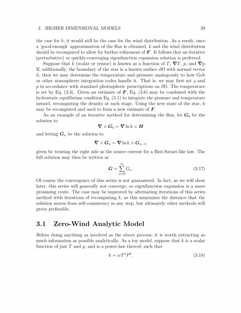
3. HIGHER DIMENSIONAL MODELS 39
the case for k, it would still be the case for the wind distribution. As a result, oncea ’good-enough’ approximation of the flux is obtained, k and the wind distributionshould be recomputed to allow for further refinement of F . It follows that an iterative(perturbative) or quickly-converging eigenfunction expansion solution is preferred.
Suppose that k (scalar or tensor) is known as a function of T , ∇T , p, and ∇p.If, additionally, the boundary of the star is a known surface ∂Ω with normal vectorn, then we may determine the temperature and pressure analogously to how Gobor other atmospheric integration codes handle it. That is, we may first set ρ andp in accordance with standard photospheric prescriptions on ∂Ω. The temperatureis set by Eq. (3.4). Given an estimate of F , Eq. (3.6) may be combined with thehydrostatic equilibrium condition Eq. (3.1) to integrate the pressure and temperatureinward, recomputing the density at each stage. Using the new state of the star, kmay be recomputed and used to form a new estimate of F .
As an example of an iterative method for determining the flux, let G0 be thesolution to
∇×G0 = ∇ ln k ×Hand letting Gn be the solution to
∇×Gn = ∇ ln k ×Gn−1,
given by treating the right side as the source current for a Biot-Savart-like law. Thefull solution may then be written as
G =∞∑n=0
Gn. (3.17)
Of course the convergence of this series is not guaranteed. In fact, as we will showlater, this series will generally not converge, so eigenfunction expansion is a morepromising route. The case may be improved by alternating iterations of this seriesmethod with iterations of recomputing k, as this minimizes the distance that thesolution moves from self-consistency in any step, but ultimately other methods willprove preferable.
3.1 Zero-Wind Analytic ModelBefore doing anything as involved as the above process, it is worth extracting asmuch information as possible analytically. As a toy model, suppose that k is a scalarfunction of just T and p, and is a power-law thereof, such that
k = wT aP b. (3.18)

3. HIGHER DIMENSIONAL MODELS 40
The former assumption amounts to specifying that we are in the radiative zone,while the latter amounts to specifying that we don’t cross between regions withsubstantively different power laws. This is actually not very constraining, as may beseen in figure 2.1. Furthermore, suppose that we neglect all wind effects. In latersections we will remove this assumption.
Take the external heating to be put in at a point, which by choice of axis we setto be at rh = rhz. Eq. (3.16) then gives
H(r) = 14π
(Lir
r2 + Le(r − rh)|r − rh|3
). (3.19)
The source term leading to G0 is then
∇ ln k ×H = (a∇ lnT + b∇ ln p)×H . (3.20)
To leading order, ∇T is parallel to H (treating G0 as a perturbation), so
∇ ln k ×H = b∇ ln p×H = b
hsg ×H . (3.21)
Rotational effects are a perturbation on g so we take g to be −r. As a result,
∇ ln k ×H = − b
hsr × 1
4π
(Lir
r2 + Le(r − rh)|r − rh|3
)= bLer × rh
4πhs |r − rh|3= −brhLeφ
4πhs |r − rh|3.
(3.22)
3.1.1 Iterative MethodNow suppose we adopt the iterative scheme described earlier. Then
∇×G0 = − brhLeφ
4πhs |r − rh|3, (3.23)
where the scale height is to be evaluated at the sample place as the curl, given byr. Outside of the star this quantity diverges, and so the curl of G0 becomes zero.Note that the nonzero circulating flux outside of the star is not unphysical, thoughthe representation of the flux in this manner is somewhat nonstandard. For a simpleexample, consider a planar light emitter which emits collimated light normal to itssurface, with flux which varies along the plane. The curl of the flux field above thissurface is evidently nonzero.

3. HIGHER DIMENSIONAL MODELS 41
From symmetry considerations it is evident that G0 describes a circulating fluxbetween the heating point and the opposing point on the star. The net flux transporteddue to all G terms is zero due to their uniformly vanishing divergences. The primaryeffect of these flux loops then is to change the distribution of heat in the interior. Inparticular, suppose that b ≥ 03. The circulating flux lines then proceed toward thepoint rh outside the star and away from it within the star.
We may compute the net flux which is transported from one side to the otherwithin the star. To do so, first note that G0 may be written as a curl of anothervector field due to its vanishing divergence. This vector field may be written as
A0(r) =∫d3r′
∇×G0
4π |r − r′| =∫d3r′
−brhLeφ(4π)2hs |r − rh|3 |r − r′|
. (3.24)
From symmetry considerations we know that this will go along −φ at r. Themagnitude will be dominated by contributions near rh, and so may be estimated as
A0 ≈brhLe
(4π)2hs |r − rh|(3.25)
up to corrections of order unity given roughly by the log of the ratio of r − rh to thesize of the heating region, which in practice will be finite. Note that the scale heighthere is that at rh. The integrated flux through the star is therefore
Lint = −∫d2rz ·G0 = −
∫ 2π
0dφrA0 · φ = 2πrbrhLe
(4π)2hs√r2 + r2
h
. (3.26)
In general we expect rh ≈ r so
Lint ≈rb
8√
2πhsLe. (3.27)
In general, hs r and b is of order unity, so this significantly exceeds the inputluminosity, and indeed indicates that the circulating flux significantly exceeds theconservative flux H. This indicates that the curl operator has eigenvalues whichare typically much less than those of the ∇ ln k× operator, invalidating an iterativemethod of this form. This result is more general than the specific form of k used.To see this, suppose we let b depend on P and T . None of the above results changeso long as |br/hs| 1, for we only relied on local properties of b until performing
3This will generally be true, as can be seen by noting that at fixed T , ρ ∝ P , and by examiningfigure 2.1. Note that k ∝ κP .
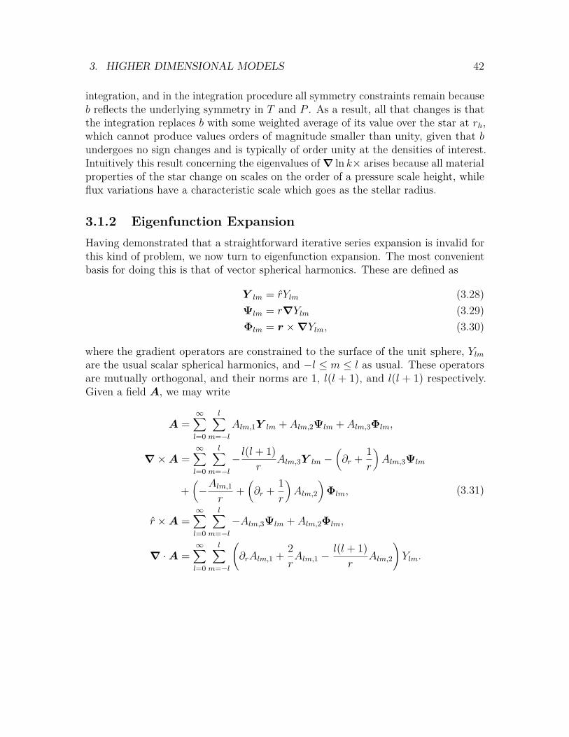
3. HIGHER DIMENSIONAL MODELS 42
integration, and in the integration procedure all symmetry constraints remain becauseb reflects the underlying symmetry in T and P . As a result, all that changes is thatthe integration replaces b with some weighted average of its value over the star at rh,which cannot produce values orders of magnitude smaller than unity, given that bundergoes no sign changes and is typically of order unity at the densities of interest.Intuitively this result concerning the eigenvalues of ∇ ln k× arises because all materialproperties of the star change on scales on the order of a pressure scale height, whileflux variations have a characteristic scale which goes as the stellar radius.
3.1.2 Eigenfunction ExpansionHaving demonstrated that a straightforward iterative series expansion is invalid forthis kind of problem, we now turn to eigenfunction expansion. The most convenientbasis for doing this is that of vector spherical harmonics. These are defined as
Y lm = rYlm (3.28)Ψlm = r∇Ylm (3.29)Φlm = r ×∇Ylm, (3.30)
where the gradient operators are constrained to the surface of the unit sphere, Ylmare the usual scalar spherical harmonics, and −l ≤ m ≤ l as usual. These operatorsare mutually orthogonal, and their norms are 1, l(l + 1), and l(l + 1) respectively.Given a field A, we may write
A =∞∑l=0
l∑m=−l
Alm,1Y lm + Alm,2Ψlm + Alm,3Φlm,
∇×A =∞∑l=0
l∑m=−l
− l(l + 1)r
Alm,3Y lm −(∂r + 1
r
)Alm,3Ψlm
+(−Alm,1
r+(∂r + 1
r
)Alm,2
)Φlm,
r ×A =∞∑l=0
l∑m=−l
−Alm,3Ψlm + Alm,2Φlm,
∇ ·A =∞∑l=0
l∑m=−l
(∂rAlm,1 + 2
rAlm,1 −
l(l + 1)r
Alm,2
)Ylm.
(3.31)
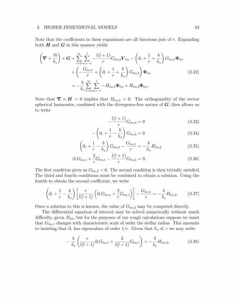
3. HIGHER DIMENSIONAL MODELS 43
Note that the coefficients in these expansions are all functions just of r. Expandingboth H and G in this manner yields(
∇ + rb
hs
)×G =
∞∑l=0
l∑m=−l
− l(l + 1)r
Glm,3Y lm −(∂r + 1
r+ b
hs
)Glm,3Ψlm
+(−Glm,1
r+(∂r + 1
r+ b
hs
)Glm,2
)Φlm
= − b
hs
∞∑l=0
l∑m=−l
−Hlm,3Ψlm +Hlm,2Φlm.
(3.32)
Note that ∇ ×H = 0 implies that Hlm,3 = 0. The orthogonality of the vectorspherical harmonics, combined with the divergence-free nature of G, then allows usto write
− l(l + 1)r
Glm,3 = 0 (3.33)
−(∂r + 1
r− b
hs
)Glm,3 = 0 (3.34)(
∂r + 1r− b
hs
)Glm,2 −
Glm,1
r= − b
hsHlm,2 (3.35)
∂rGlm,1 + 2rGlm,1 −
l(l + 1)r
Glm,2 = 0. (3.36)
The first condition gives us Glm,3 = 0. The second condition is then trivially satisfied.The third and fourth conditions must be combined to obtain a solution. Using thefourth to obtain the second coefficient, we write(
∂r + 1r− b
hs
)[r
l(l + 1)
(∂rGlm,1 + 2
rGlm,1
)]− Glm,1
r= − b
hsHlm,2. (3.37)
Once a solution to this is known, the value of Glm,2 may be computed directly.The differential equation of interest may be solved numerically without much
difficulty, given Hlm, but for the purposes of our rough calculations suppose we insistthat Glm,1 changes with characteristic scale of order the stellar radius. This amountsto insisting that ∂r has eigenvalues of order 1/r. Given that hs r we may write
− b
hs
(r
l(l + 1)∂rGlm,1 + 2l(l + 1)Glm,1
)= − b
hsHlm,2, (3.38)

3. HIGHER DIMENSIONAL MODELS 44
orr
l(l + 1)∂rGlm,1 + 2l(l + 1)Glm,1 = Hlm,2. (3.39)
To simplify matters somewhat, we consider a modified version of the input heatingconsidered earlier. In this case, the input heat takes on the form
ε = δ(r − rh)4πr2
h
[Le,0Y00 + Le,1 (Y1,−1 − Y1,1)] . (3.40)
This qualitatively reproduces the expected heating behavior, with preferential heatingon one side but without any net cooling, so long as Le,0 >
√6Le,1. The heating all
occurs at a radius rh, with maximum heating on the positive x side. The source term∇ ln k ×H is not impacted in any way by the Y0,0 term, as this term produces aradial flux field. The remaining terms give rise to a flux field which contributes tothe source term. The equations governing this field are given by
∂rH1,±1,1 + 2rH1,±1,1 −
2rH1,±1,2 = δ(r − rh)
4πr2h
(∓Le,1) , (3.41)
H1,±1,3 = 0 (3.42)
−H1,±1,1
r+(∂r + 1
r
)H1,±1,2 = 0. (3.43)
The first of these relations arises from the divergence condition H , while the secondtwo arise from the requirement that the curl of H vanish. The general solution tothis set of equations is
H1,±1,1 = A
r3 +B + ∓Le,1(r3 + 2r3h)Θ(r − rh)
12πr3r2h
(3.44)
H1,±1,2 = − A
2r3 +B + ∓Le,1(r3 − r3h)Θ(r − rh)
12πr3r2h
(3.45)
H1,±1,3 = 0, (3.46)where Θ(x) is the Heaviside step function and the constants A and B are to be fixedby boundary condition considerations. In this case, we want the flux to drop to zeroat infinity, and we want it to be finite at finite radius. As a result, both constants arezero and we have
H1,±1,1 = ∓Le,1(r3 + 2r3h)Θ(r − rh)
12πr3r2h
(3.47)
H1,±1,2 = ∓Le,1(r3 − r3h)Θ(r − rh)
12πr3r2h
(3.48)
H1,±1,3 = 0. (3.49)

3. HIGHER DIMENSIONAL MODELS 45
Using this to solve for G1,±1,1 in the simplified differential equation gives
G1,±1,1 = ∓Le,1(r − rh)2(r + 2rh)Θ(r − rh)12πr3r2
h
, (3.50)
where we have already imposed the condition that this converge at the origin. Toobtain the flux from one side of the star to the other from this, we note that Glm,1doesn’t contribute to the flux through a slice of the star which cuts it in half. The onlysuch contribution arises from the angular terms. We already know that Glm,3 = 0, sowe just need to compute Glm,2. This may be done as described previously, yielding
G1,±1,2 = ∓Le,112πr2r2
h
((r − rh)2(r + 2rh)δ(r − rh)
2 + (r3 − r3h)Θ(r − rh)r
). (3.51)
Only the portion of the vector field directed along φ contributes to the flux throughthe plane separating the two halves of the star, and this is given by
G±φ = ±√
32π
Le,112πr2r2
h
((r − rh)2(r + 2rh)δ(r − rh)
2 + (r3 − r3h)Θ(r − rh)r
), (3.52)
where we have set φ = π/2. Integrating this over the plane of interest then yields
L =∫ R
0dr∫ π/2
0d(cos θ)r(Gφ −G−φ) = 4
∫ R
0rGφ = (R− rh)2(R + 2rh)
2√
6π3/2Rr2h
Le,1, (3.53)
where R is the stellar radius and L is the total power flowing from one side of the starto the other as a result of the circulation field. In typical situations, R− rh R, so
L ≈ Le,1120
(1− rh
R
)2. (3.54)
By comparison, the flux due to the curl-free term is given by the incident flux timesthe ratio of the solid angle that the plane of interest sweeps as seen from the heatingpoint, which is roughly 2π/3, to the total solid angle of 4π, so in most cases thisterm dominates over the circulation term. One important consequence of Eq. (3.54)is that as the heat is deposited deeper, the flux which manages to find its way to theopposing side increases as expected.
Interestingly, this result is independent of a, b. So long as they do not varysubstantially on a spherical shell, this independence should hold. Additionally, notethat the situation in any case is very different from that of an isotropic star, whereinhalf of the heating flux is present on each side. This is a result of the fact that

3. HIGHER DIMENSIONAL MODELS 46
a spherically symmetric shell of heating cannot alter the flux inside it, while ananisotropic heating shell can.
It is worth noting two effects which we have not considered here. The first isthe potential for a more complex thermal conductivity structure due to convection,and the second is that of wind transport/dissipation. In the case of the former,the key effect will be the potential for significantly greater conductivity gradientsmisaligned with the thermal gradient. In the case of the latter, the key effect will beadditional heating terms, manifesting as regions of nonzero ε, even when no heatingis present at those locations. Finally, rotation plays a role in determining how thesecomplications alter the situation. Estimating the significance of these effects is thesubject of subsequent sections.
3.2 Zero-Divergence Wind ModelSuppose that we insist that the flux divergence be made zero by wind transport. Thisrepresents the opposite limit of the previous section solution. This condition meansthat we require
ε = cpTv · (∇ lnT −∇ad∇ ln p) . (3.55)Recall that cp = γcv and that up to factors of order unity cv = kBT/µ, so
ε = γpv · (∇ lnT −∇ad∇ ln p) . (3.56)
This relation would be precisely correct if we neglected convection in computing F .This is not how we are treating the heat flux, however, so we need to correct thisrelation by subtracting out the convective term. The convective term arises from gastraveling in a circulatory fashion up and down a pressure gradient. As a result, thissubtraction may be done by requiring v ⊥ ∇p. This is essentially the geostrophicflow condition. One might object to this requirement by citing Kelvin-Helmholtzinstability, but such processes separate in our treatment to convection and advection,as in a convective roll. Likewise one might object to this requirement by arguing thatwinds can move along pressure gradients in radiative regions. While this is true, suchwinds cannot be driven by thermal processes, as the region must, by definition, bestable against convection. Objections case aside, we impose this requirement, andthe criterion reduces to
ε = γpv ·∇ lnT ∼ Σghsv · eT , (3.57)
where eT is the unit vector along the thermal gradient. The approximate form comesfrom noting that if the flux has zero divergence except in the core, then the thermal

3. HIGHER DIMENSIONAL MODELS 47
gradient must be purely radial. Now we know that neglecting viscous losses,
ε ≈ Le2πR2 [1− exp (−Σ/Σh)] , (3.58)
where we are taking the illumination to occur on one side only. As a result,
v · eT ≈Lehs
2πgΣR2 [1− exp (−Σ/Σh)] . (3.59)
Usually R ∼ 1010cm, hs ∼ 107cm, g ∼ 104cm/s2, Le ∼ 1033erg/s, and Σh = 103g/cm2,so this has a maximum value of
v · eT ∼ 1012cm/s. (3.60)
This is an absurd value, greater than the speed of light, and indicates a breakdown inthe assumption that the divergence of the flux remains zero. In particular, it arisesfrom the characteristic scale over which T changes in the absence of a flux divergencebeing much greater than the characteristic scale over which ε changes. As the windclearly cannot move enough heat to keep the divergence at zero, the temperatureprofile will shift to accommodate the shorter length scale.
Evidently the true steady state, if one exists, lies somewhere in between the twomodels considered thus far. The star likely adjusts its radial transport to handlemuch of the flux divergence, and then sets up some non-radial flux transport, whichthen allows the wind to move non-radially to dissipate some of the flux divergence.As a result, the star must exhibit some anisotropy, but it is possible that below acertain depth winds succeed in isotropizing the thermal structure. This model willserve as a template for subsequent analyses.

3. HIGHER DIMENSIONAL MODELS 48
ReferencesKippenhahn, Rudolf, Alfred Weigert, and Achim Weiss. Stellar Structure and Evolu-
tion. Springer, 2012. isbn: 978-3-642-30304-3 (cit. on p. 36).Lesaffre, Pierre et al. “A two-dimensional mixing length theory of convective trans-
port”. In: Monthly Notices of the Royal Astronomical Society (2013). doi: 10.1093/mnras/stt317. eprint: http://mnras.oxfordjournals.org/content/early/2013/03/20/mnras.stt317.full.pdf+html. url: http://mnras.oxfordjournals.org/content/early/2013/03/20/mnras.stt317.abstract(cit. on p. 37).

4
Review of Fluid Mechanics
Big whirls have little whirls that feed on their velocity,and little whirls have lesser whirls and so on to viscosity.
– Lewis Fry Richardson
To understand how wind flow works in stars, it is worth reviewing the basic fluidmechanics involved. In general, fluid mechanics problems are exceedingly difficult tosolve, either analytically or numerically. As a result, we will exploit the fact that suchproblems may often be broadly characterized by only a few dimensionless numbers.This reduces the complexity of the problems, and allows us to reduce many scenariosto the same mathematics. Before discussing these numbers, however, we must addressa dimensionful property of fluids: viscosity.
4.1 Microscopic ViscosityIntuitively viscosity is a measure of the resistance of a fluid to shearing. The termusually refers to a material property, rather than a property of fluid flow. As bothnotions are important, viscosity as a material property and viscosity as a property offluid flow, we will use "microscopic viscosity" to denote the material property and"turbulent viscosity" or "effective viscosity" to denote the flow property. The latterwill be discussed at length later in this chapter, while here we will focus on the former.
In this analysis, we take the companion stars of interest to be primarily hydrogen,with some helium present in small quantities. At temperatures higher than thosein the ionization zone, in the regime where µ = 1
2mp, the Spitzer estimate gives the
49

4. REVIEW OF FLUID MECHANICS 50
microscopic viscosity as1
ν = 5.2× 10⁻¹⁵ T5/2
ρ ln Λcm2
s , (4.1)
where T is made dimensionless by dividing out by K, and likewise for ρ by dividingout by g/cm3. The quantity ln Λ is given by2
ln Λ =
−17.4 + 1.5 lnT − 0.5 ln ρ T < 1.1× 10⁵K−12.7 + lnT − 0.5 ln ρ T > 1.1× 10⁵K
, (4.2)
where everything is in the same units as before.To obtain a broader range of microscopic viscosities, we turn to tables of this
value at various temperatures and pressures3. The results, computed for a mixtureof 85% hydrogen and 15% helium, indicate that ρν is roughly constant, rangingfrom 3 × 10⁶g/cm/s to 3 × 10⁷g/cm/s. The tabulated data allows us to computeν for temperatures ranging from 3600K up to 105K, and pressures ranging from103erg/cm3 up to 1011erg/cm3. Between this and the Spitzer estimate, then, wehave covered the entire range of interest for stellar atmospheres except for very lowtemperatures in the outer regions of brown dwarfs. These regions, however, are not ofmuch interest, as the transport phenomena of interest occur much deeper in the star.Furthermore, unlike the case for opacity, the underlying physics behind microscopicviscosities is not expected to change significantly at these lower temperatures. Thusreasonable extensions of the low-temperature viscosity model may be used, with theunderstanding that they are only accurate as order-of-magnitude estimates.
Next we consider the viscosity of radiation, which was not included in either thedata table nor the Spitzer estimate. The radiative viscosity is given by4
νrad = aT 4
cκρ. (4.3)
This is usually much smaller even than the microscopic viscosity of hydrogen. To seethis, we may non-dimensionalize T , κ, and ρ and evaluate the constant factors to find
νrad ≈ 3× 10⁻⁵T 45 ρ−10 κ−1
0cm2
s , (4.4)
1Daniel Kagan and J. Craig Wheeler. “The Role of the Magnetorotational Instability in theSun”. In: The Astrophysical Journal 787.1 (2014), p. 21. url: http://stacks.iop.org/0004-637X/787/i=1/a=21.
2Ibid.3F. N. Edmonds Jr. “The Coefficients of Viscosity and Thermal Conductivity in the Hydrogen
Convection Zone.” In: The Astrophysical Journal 125 (Mar. 1957), p. 535. doi: 10.1086/146327.4Rudolf Kippenhahn, Alfred Weigert, and Achim Weiss. Stellar Structure and Evolution. Springer,
2012. isbn: 978-3-642-30304-3.

4. REVIEW OF FLUID MECHANICS 51
where factors with subscripts are given numerically by the quantity divided by ten tothe power of the subscript in the C.G.S.K unit system as usual. While this is muchless than the microscopic viscosity over the entire range of tabulated data, at hightemperatures it will overtake the Spitzer data due to a higher power of T appearingin the numerator.
To compute ν over the entire range of available data, an interpolation code waswritten which makes use of both the Spitzer form and the data tables. It returns anerror whenever the data is outside of the range of validity of both, taking the Spitzerformula to be only valid above the ionization temperature 104.1K. In places whereboth sources contained valid data, the tabulated version was used. In addition, itcomputes the radiative viscosity and adds it to the viscosity obtained from the othersources. The radiation merely provides an additional avenue for momentum transport,and so linear combination is appropriate. The full code may be found in Appendix A.The output from this code is shown in figure 4.1. Following the trajectories shown inthe one-dimensional modeling chapter, we see that the viscosity is typically between1cm2/s and 104cm2/s, with higher temperature stars reaching at most 105cm2/s.
The one remaining question needed to determine the viscous microphysics ofinterest is that of the impact of magnetic fields. At temperatures where the ionizationfraction is low, the magnetic field by and large does not interact with the gas, andso at low temperatures the above results are accurate independent of the magneticfield. The remaining effect of interest then is that of the solar magnetic field onmomentum transport in plasma. Once ionization occurs, the magnetic field canintroduce preferred directions of momentum transport, significantly altering the shearproperties of the medium. This occurs when the thermal gyroradius is less than themean free path of the ions. The intuition behind this is that it occurs when themagnetic field has a chance to order the system in between randomizing collisions.
Detailed calculations of this effect have been done5, with the result that theanisotropy in the viscosity is of order
t−2ci ω
−2ci , (4.5)
where tci is the self-collision time for positive ions and ωci is the gyrofrequency of thesesame ions in the magnetic field. Both quantities are to be computed assuming thermalequilibrium. More specifically, the quantity in Eq. (4.5) gives the approximate ratio ofthe visocosity of a velocity gradient perpendicular to the velocity, holding the velocityperpendicular to the magnetic field, to the viscosity in the absence of a magnetic
5Jr. Lyman Spitzer. Physics of Fully Ionized Gases. Vol. 1. ISBN 978-0-486-44982-1. Dover,2006.

4. REVIEW OF FLUID MECHANICS 52
3 4 5 6 7 8log T
−10
−8
−6
−4
−2
0
2
4
6
log ρ
0
2
4
6
8
10
12
14
log ν
Figure 4.1: The vertical axis is log ρ (with ρ measured in g/cm3), the horizontal islog T (with T measured in K), and the color represents log ν (with ν measured incm2/s. White regions are those without data.

4. REVIEW OF FLUID MECHANICS 53
field. If this quantity exceeds unity then the magnetic field may be ignored, and theanisotropy disappears.
To compute the anisotropy, then, we note that tci is given by the mean free pathof the ions divided by their typical thermal velocities. Thus
tci = λ√〈v2〉
= ν
〈v2〉. (4.6)
Note that in the final equality here, ν is the non-magnetic microscopic viscosity. Thethermal gyroradius is given by
rg =muc
√〈v2〉
qB, (4.7)
Thus
ωci =
√〈v2〉rg
= qB
muc. (4.8)
As a result, the anisotropy factor is
1t2ciω
2ci
= m2uc
2〈v2〉2
q2B2ν2 = 9k2BT
2c2
q2B2ν2 = 9p2µ2c2
ρ2q2B2ν2 . (4.9)
To produce a factor which has the appropriate temperature dependence at lowtemperatures, we note that the anisotropy only impacts the ionized portion of the gas.As a result, we may separate the gas into its ionized and neutral portions, computetheir viscosities, and then add them. The corrected anisotropy factor is then
m−1p
(2µ−mp + 2mp − µ
t2ciω2ci
). (4.10)
As an estimate of the magnitude of the anisotropy factor when µ = mp/2, we maytake typical values of ν to be ∼ ρ−1107g/cm/s, and hence
1t2ciω
2ci
∼ 9p2µ2c2
q2B21014 ∼p2µ2c2
q2B21013 ∼4× 10⁻²¹p2
B2 . (4.11)
where all units have been omitted for clarity. As usual all quantities are in measuredC.G.S.K units. In most stars of interest, g ∼ 104cm/s2, so near the surface this maybe written as
1t2ciω
2ci
∼ 4× 10⁻¹³Σ2
B2 . (4.12)

4. REVIEW OF FLUID MECHANICS 54
As a quick estimate, suppose we plug in the sun’s magnetic field of ∼ 10−2G. Thisyields an anisotropy factor of 4×10⁻⁹Σ2. Thus the viscosity is significantly anisotropicfor Σ < 6 × 10³g/cm2. The viscosity code in Appendix A is capable of computingthe minimum B field requires to induce significant anisotropy. In convection zonesthis is often irrelevant: the convective viscosity far exceeds the molecular viscosity.In radiative zones, the microscopic viscosity will play a role in determining thecharacteristic scale of turbulence6. In cases where the microscopic viscosity doesmatter in a regime in which there is magnetically-induced anisotropy, we will holdthe field to be that inside a dipole, aligned with the star’s rotation axis, and sothe microscopic viscosity is just multiplied by the anisotropy factor. The code inAppendix A accepts an optional argument specifying this factor. In its absence,isotropy is assumed.
The anisotropy factor is shown for B = 10−2G in figure 4.2 and B = 103G infigure 4.3. In the first case the anisotropy is minimal for most density-temperaturecombinations of interest, while the latter shows significant anisotropy in a wide enoughrange of densities and temperatures that most scenarios of interest are covered. Theregions of greatest anisotropy are subject to some numerical noise, resulting from abreakdown in the assumption that all ionization is hydrogen ionization.
4.2 Reynolds NumberThe first of our dimensionless numbers is the Reynolds number, defined as
Re ≡ vl
ν, (4.13)
where v is a characteristic velocity scale for a shear flow, l is a characteristic lengthscale, and ν is the viscosity of the fluid. The precise meaning of ν in this context issomewhat complex, so we will discuss it further later on. The Reynolds number innon-stratified flow is the quantity which determines whether or not a flow is shearturbulent. Barring stabilizing factors which will be discussed below, the flow isturbulent when
Re > Recfor some critical Reynolds number Rec. Typical values of this number are of order103.
6This is a result of our use of the more modern Richardson criterion modified to incorporate theeffect turbulence plays in aiding thermal diffusion.

4. REVIEW OF FLUID MECHANICS 55
3 4 5 6 7 8log T
−10
−8
−6
−4
−2
0
2
4
6
log ρ
−3.6
−3.2
−2.8
−2.4
−2.0
−1.6
−1.2
−0.8
−0.4
0.0
log A
Figure 4.2: The vertical axis is log ρ (with ρ measured in g/cm3), the horizontal islog T (with T measured in K), and the color represents the log of the anisotropyfactor A. White regions are those without data.
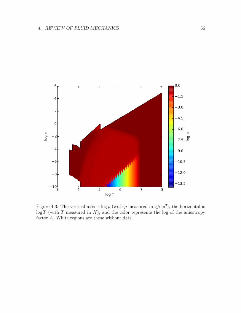
4. REVIEW OF FLUID MECHANICS 56
3 4 5 6 7 8log T
−10
−8
−6
−4
−2
0
2
4
6
log ρ
−13.5
−12.0
−10.5
−9.0
−7.5
−6.0
−4.5
−3.0
−1.5
0.0
log A
Figure 4.3: The vertical axis is log ρ (with ρ measured in g/cm3), the horizontal islog T (with T measured in K), and the color represents the log of the anisotropyfactor A. White regions are those without data.

4. REVIEW OF FLUID MECHANICS 57
4.3 Rayleigh NumberIn addition to shear instability, it is possible for a fluid to be convectively unstable.This instability is quantified by the Rayleigh number, defined as
Ra ≡ βgl3∆Tαν
, (4.14)
where β is the thermal expansion coefficient and α is as defined previously. Convectiveinstability occurs when ∇rad > ∇ad and the Rayleigh number exceeds the criticalRayleigh number Rac, typically of order 103. The former condition is necessary foradiabatic expansion to lead to growing buoyant perturbations, while the latter isnecessary for this expansion to not be overcome by viscous dissipation.
We claim that the Rayleigh number is typically so large that whenever the formercondition is satisfied in a star the latter is as well. To begin, we write the Rayleighnumber as
Ra ≈ βgℵ3h3sT∆ lnTαν
. (4.15)
Over a scale height, which is roughly what we expect the convection cell size to be,P changes by a factor of e and, we expect T to change by a multiplicative factor ofsimilar magnitude. Thus ∆ lnT is of order unity, so
Ra ≈ βgℵ3h3sT
αν. (4.16)
Now β is typically of order T−1, equaling
β = 1V
(∂V
∂T
)p
∼ 1T
so long as the ideal gas law holds. This only fails in the ionization zone, where β willbe somewhat lower. Keeping this in mind, we find
Ra ≈ ξgℵ3h3s
αν, (4.17)
where ξ is the dimensionless constant giving the ratio of β to T−1. Typical scaleheights are around 300km, and typical values of g are around 104cm/s2, so
Ra ≈ 3× 1026 ξℵ3
αν, (4.18)

4. REVIEW OF FLUID MECHANICS 58
with all remaining quantities given in the usual c.g.s.k unit system. Now
α = kradρcp
, (4.19)
soRa ≈ 3× 1026 ξℵ3ρcp
kradν. (4.20)
We expect cp to be of order kB/µ ≈ ρ108erg/K/cm3, so
Ra ≈ 2× 1034 ξℵ3
kradν. (4.21)
Typical values of ℵ are between unity and two. Taking the lower end gives
Ra ≈ 2× 1034 ξ
kradν. (4.22)
As was argued earlier, the maximum value of ν for the stellar models of interest isaround 105cms, so in a worst case scenario
Ra ≈ 2× 1029 ξ
krad. (4.23)
Now krad may be computed directly as
krad = 4acT 3
3ρκ , (4.24)
where κ is within a few orders of magnitude of 1cm2/g. Thus
krad = 108T34ρ1, (4.25)
where T4 is T/104K and ρ1 is ρcm3/g. It follows that, again in a worst case,
Ra ≈ 2× 10²¹ ξρ1
T 34. (4.26)
Even supposing that ξ and ρ1 are both quite a few orders of magnitude below unity,and taking T to be 106K, the Rayleigh number still exceeds its critical value. Thuswe are safe assuming that whenever convection is indicated by the thermal gradientcriterion it occurs.

4. REVIEW OF FLUID MECHANICS 59
4.4 Richardson NumberThe next dimensionless number of interest is the Richardson number, defined as
Ri ≡ N2
(dv/dz)2 , (4.27)
whereN2 = g
d ln ρdz
(4.28)
defines the Brunt-Vaisala frequency N and dv/dz is the vertical velocity shear. TheRichardson number quantifies the competition between buoyant stabilizing forces andshear instability. In particular, an oft-cited7 necessary but not sufficient criterion forinstability is that
Ri < Ric ≈ 0.25. (4.29)
There is, however, significant evidence, both experimental and theoretical, againstthis criterion8. There are two problems. The first is that turbulence mixes the fluid,which counteracts the entropic stratification that would otherwise stabilize it. Asa result, the fluid is actually unstable over a wider range of parameter space thanthis criterion indicates. The second is that more modern experimental evidencesuggests that even when this mixing is minimal, the critical value should be closer to
7Richard Lyons, A. H. Panopsky, and Sarah Wollaston. “The Critical Richardson Number andIts Implications for Forecast Problems”. In: Journal of Applied Meteorology 3 (Jan. 1964), pp. 136–142. url: http://journals.ametsoc.org/doi/pdf/10.1175/1520-0450(1964)003%3C0136:TCRNAI%3E2.0.CO;2.
8E. Schatzman, J.P. Zahn, and P. Morel. “Shear turbulence beneath the solar tachocline”. In:Astronomy and Astrophysics (Oct. 2000). eprint: http://arxiv.org/pdf/astro-ph/0010543v1.pdf; E. C. Itsweire, K. N. Helland, and C. W. Van Atta. “The evolution of grid-generatedturbulence in a stably stratified fluid”. In: Journal of Fluid Mechanics 162 (Jan. 1986), pp. 299–338.issn: 1469-7645. doi: 10.1017/S0022112086002069. url: http://journals.cambridge.org/article_S0022112086002069; A. Maeder. “Stellar rotation: Evidence for a large horizontalturbulence and its effects on evolution”. In: Astronomy and Astrophysics 399.1 (2003), pp. 263–269.doi: 10.1051/0004-6361:20021731. eprint: http://arxiv.org/abs/astro-ph/0301258. url:http://dx.doi.org/10.1051/0004- 6361:20021731; Prat, V. and Lignières, F. “Turbulenttransport in radiative zones of stars”. In: Astronomy and Astrophysics 551 (2013), p. L3. doi:10.1051/0004- 6361/201220577. eprint: http://arxiv.org/abs/1301.4151. url: http://dx.doi.org/10.1051/0004-6361/201220577; S. Mathis, A. Palacios, and J.-P. Zahn. “Onshear-induced turbulence in rotating stars”. In: Astronomy and Astrophysics 425.1 (2004), pp. 243–247. doi: 10.1051/0004-6361:20040279. eprint: http://arxiv.org/abs/astro-ph/0403580.url: http://dx.doi.org/10.1051/0004-6361:20040279.

4. REVIEW OF FLUID MECHANICS 60
unity than to 0.259. In convection zones this may be remedied by setting the criticalRichardson number to
Ric = max(
1, 1Pe
), (4.30)
where Pe is the Péclet number, defined in this context as
Pe = vcl
α(4.31)
and α is the thermal diffusivity. Outside of convective layers, the criterion maybe modified by replacing the Péclet as written above with one computed usingthe characteristic velocity and length scale of turbulent eddies.10 In both cases,this criterion takes into account the action of heat transport to lower buoyanteffects. Notice that this criterion in the non-convecting case presumes the existenceof turbulence from the start, and is primarily making a statement regarding thecharacteristic scale of the turbulence. This, in effect, neglects the microscopic viscosityof the fluid, which is akin to arguing that
ν v∆z, (4.32)
where v and ∆z are the maximum turbulence speed and size allowed by the modifiedRichardson criterion. This condition is satisfied by taking
ν
v∆z ≤1
Rec 1. (4.33)
Should this condition fail, the flow cannot be turbulent anyway via the Reynoldscriterion, as the turbulence velocity and length scale cannot be smaller than those ofthe shear which produces it, and so it suffices to require both the Reynolds criterionand the Richardson criterion, without having an additional condition regarding themicroscopic viscosity.
At this stage it is worth introducing the idea of an effective viscosity. This isthe viscosity that one would measure in a turbulent flow by using the definition ofviscosity as the force per unit area per unit shear across a fluid. A key property of aneffective viscosity, as will be discussed at length in the following sections, is that itis dependent on the length scale over which the shear occurs. In the context of theReynolds criterion, the question of stability becomes one of the effective viscosity of
9V. M. Canuto. “Turbulence in Stars. II. Shear, Stable Stratification, and Radiative Losses”.In: The Astrophysical Journal 508.2 (1998), p. 767. url: http://stacks.iop.org/0004-637X/508/i=2/a=767.
10Ibid.

4. REVIEW OF FLUID MECHANICS 61
any non-shear turbulent processes. In the context of the Richardson criterion, whatoccurs is the production in any Reynolds-unstable flow of turbulence up to a criticaleffective viscosity scale, defined by the criterion, and it is this effective viscosity whichis seen by the large-scale flow. Thus the Richardson criterion is perhaps better viewedas setting a viscosity scale than making definitive statements about flow stability.
This is not the end of the story of the Richardson criterion, however. The actualRichardson criterion must account for the fact that in a stratified flow, there isa difference between the horizontal turbulent viscosity and the vertical turbulentviscosity. In order to accommodate this, we use as our criterion11:
v∆z(krad + νh)
N2T + v∆z
νhN2µ <
(dv
dz
)2
, (4.34)
where v and ∆z are the speed and size of the largest eddies which are isotropic,νh is the turbulent viscosity for horizontal motions, krad is the thermal diffusivitydue to radiation transport, and NT and Nµ partition the Brunt-Vaisala frequencyinto pieces corresponding to the thermal and chemical gradients respectively. Thistakes into account all of the effects discussed thus far. We will examine in detail thecomputation of this criterion in the section on vertical shear.
4.5 Rossby NumberThe next dimensionless number of interest is the Rossby number, which determinesthe circumstances under which the Coriolis force has a significant impact on themotion of a fluid. Given a characteristic speed v and a characteristic length scale x,the Rossby number is defined as
Ro ≡ v
2xΩ sin θ , (4.35)
where Ω and θ are defined as usual. Note that v is defined in a reference framerotating at Ω, as fluid at rest in the rotating frame does not experience a Coriolisforce. When this number is large relative to unity, the Coriolis force is negligible andso may be neglected. In the opposing limit, the Coriolis force dominates the flow,and geostrophic balance is likely. When the Rossby number is of order unity, theCoriolis force must typically be taken into account, but need not be the dominanteffect. We will usually use x = R, such that the Rossby number refers to motionaround the star.
11S. Mathis, A. Palacios, and J.-P. Zahn, op. cit.

4. REVIEW OF FLUID MECHANICS 62
4.6 Mach NumberThe final dimensionless number of interest is the Mach number, defined as the ratioof the flow speed to the fluid’s sound speed. That is,
Ma ≡ v
vs. (4.36)
The sound speed is generally given as
vs =√P
ρ, (4.37)
whereγ = cp
cv(4.38)
is the adiabatic index of the fluid. For a monatomic gas outside of the ionizationzone, this is 5/3. Inside the ionization zone, it falls to roughly unity12. From ourperspective, the Mach number is important primarily because for Ma > 1, turbulentlosses become extreme, so we may safely assume that v < vs.
12Donald D. Clayton. Principles of Stellar Evolution and Nucleosynthesis. Vol. 1. ISBN: 978-0521566315. University of Chicago Press, 1968.

4. REVIEW OF FLUID MECHANICS 63
ReferencesA. Maeder. “Stellar rotation: Evidence for a large horizontal turbulence and its
effects on evolution”. In: Astronomy and Astrophysics 399.1 (2003), pp. 263–269.doi: 10.1051/0004-6361:20021731. eprint: http://arxiv.org/abs/astro-ph/0301258. url: http://dx.doi.org/10.1051/0004-6361:20021731 (cit. onp. 59).
Canuto, V. M. “Turbulence in Stars. II. Shear, Stable Stratification, and RadiativeLosses”. In: The Astrophysical Journal 508.2 (1998), p. 767. url: http://stacks.iop.org/0004-637X/508/i=2/a=767 (cit. on p. 60).
Clayton, Donald D. Principles of Stellar Evolution and Nucleosynthesis. Vol. 1. ISBN:978-0521566315. University of Chicago Press, 1968 (cit. on p. 62).
Edmonds Jr., F. N. “The Coefficients of Viscosity and Thermal Conductivity inthe Hydrogen Convection Zone.” In: The Astrophysical Journal 125 (Mar. 1957),p. 535. doi: 10.1086/146327 (cit. on p. 50).
Itsweire, E. C., K. N. Helland, and C. W. Van Atta. “The evolution of grid-generatedturbulence in a stably stratified fluid”. In: Journal of Fluid Mechanics 162 (Jan.1986), pp. 299–338. issn: 1469-7645. doi: 10.1017/S0022112086002069. url:http://journals.cambridge.org/article_S0022112086002069 (cit. on p. 59).
Kagan, Daniel and J. Craig Wheeler. “The Role of the Magnetorotational Instabilityin the Sun”. In: The Astrophysical Journal 787.1 (2014), p. 21. url: http ://stacks.iop.org/0004-637X/787/i=1/a=21 (cit. on p. 50).
Kippenhahn, Rudolf, Alfred Weigert, and Achim Weiss. Stellar Structure and Evolu-tion. Springer, 2012. isbn: 978-3-642-30304-3 (cit. on p. 50).
Lyman Spitzer, Jr. Physics of Fully Ionized Gases. Vol. 1. ISBN 978-0-486-44982-1.Dover, 2006 (cit. on p. 51).
Lyons, Richard, A. H. Panopsky, and Sarah Wollaston. “The Critical RichardsonNumber and Its Implications for Forecast Problems”. In: Journal of AppliedMeteorology 3 (Jan. 1964), pp. 136–142. url: http://journals.ametsoc.org/doi/pdf/10.1175/1520-0450(1964)003%3C0136:TCRNAI%3E2.0.CO;2 (cit. onp. 59).
Prat, V. and Lignières, F. “Turbulent transport in radiative zones of stars”. In:Astronomy and Astrophysics 551 (2013), p. L3. doi: 10 . 1051 / 0004 - 6361 /201220577. eprint: http://arxiv.org/abs/1301.4151. url: http://dx.doi.org/10.1051/0004-6361/201220577 (cit. on p. 59).
S. Mathis, A. Palacios, and J.-P. Zahn. “On shear-induced turbulence in rotating stars”.In: Astronomy and Astrophysics 425.1 (2004), pp. 243–247. doi: 10.1051/0004-

4. REVIEW OF FLUID MECHANICS 64
6361:20040279. eprint: http://arxiv.org/abs/astro- ph/0403580. url:http://dx.doi.org/10.1051/0004-6361:20040279 (cit. on pp. 59, 61).
Schatzman, E., J.P. Zahn, and P. Morel. “Shear turbulence beneath the solartachocline”. In: Astronomy and Astrophysics (Oct. 2000). eprint: http://arxiv.org/pdf/astro-ph/0010543v1.pdf (cit. on p. 59).

5
Stability and Turbulence
When I meet God, I am going to ask him two questions: Why relativity?And why turbulence? I really believe he will have an answer for the first.
– Werner Heisenberg
The key problem of interest in this chapter is that of determining the local flowpatterns that stars may exhibit, with a particular eye to questions of viscous andturbulent losses as well as flow stability. In the fluid mechanics discussed thus far, onlyone kind of instability was considered at a time. This turns out to be insufficientlygeneral. In the various stellar models under consideration, Σh is sometimes within theunperturbed convection zone and sometimes not. The latter case may be analyzed byonly considering shear instability, but the former requires understanding how shearand convective instabilities interact. To understand this, we will consider a model ofshear flow with convection and analyze it in general. We will then proceed to lookat the case of shear flow alone, as the difference in stability criteria between verticaland horizontal shear is significant there. The next chapter will then take a broaderview of wind in stars, and will piece together a global picture from these local parts.
In analyzing the stability of different kinds of flows in this chapter we will keepthe thin-envelope approximation made in our earlier one-dimensional model. This isjustified by the same reasoning used there, and allows us to assume that the regions ofinterest are always thin relative to R. This means that g is a constant in the regionsof interest, and that the curvature of these regions may be neglected. It further tellsus that the pressure in each region is just what is required to hold up the materialabove it.
In addition to the above conditions, we take the shear in all cases to be an amountv0 over a convective mixing length l = ℵhs, where ℵ > 1 is of order unity. Whenconvection occurs, we will take its eddy velocity to be vc.
65

5. STABILITY AND TURBULENCE 66
5.1 Sheared ConvectionIn the analysis to follow, we work within a single convection cell of linear dimensionl. Additionally, we take the forces resulting from microscopic viscosity to be smallrelative to those resulting from the buoyancy which drives convection. This is justifiedby our argument in the previous chapter that in stars the Rayleigh number is largerelative to its critical value.
Note that since, by assumption, the flow is convectively unstable, the Richardsoncriterion is automatically satisfied: N2 < 0. There are several limits which areeasily analyzed. First, suppose that v0 vc, and that Re > Rec. In this case, theconvection acts as a perturbation to the shear turbulence: existing eddies due to theshear suffice to carry the convective heat flux with only minor additional anisotropy.This scenario will be stable then against convective turbulence, as the shear will carrythe needed flux, but will be unstable against shear turbulence. On the other hand, ifvc v0 and Re < Rec, the shear acts as a perturbation to the convective turbulence:the convective eddies suffice to carry the necessary momentum flux, again with onlyminor additional anisotropy. This scenario is thus stable against shear turbulence yetunstable against convective turbulence.
Another straightforward limit is that in which Re < Rec and v0 vc. In thiscase, shear due to v0 is insufficient on its own to cause an instability: the viscosityis high enough that the turbulence is dissipated as heat faster than it is created.If the flow is stable against shear turbulence, however, the thermal flux must becarried by convection. As vc v0, the convection appears as a perturbation againstthe background shear and so the flow will remain shear-stable with a backgroundconvective instability. The convection will increase the effective viscosity of the flow,but this only serves to further reduce Re and hence further stabilize the shear flow.Thus in this case the flow is shear stable and convectively turbulent. This flow patternis like that known in meteorological work as a longitudinal roll1.
Likewise, in the case where Re Rec and vc v0, there will be shear turbulencewhich provides a perturbative background for convective turbulence. That is, theconvection is necessary and proceeds effectively unimpeded, yet the shear flow ex-periences turbulence nonetheless. Each kind of turbulence will cause an increased
1S. Mergui, X. Nicolas, and S. Hirata. “Sidewall and thermal boundary condition effects on theevolution of longitudinal rolls in Rayleigh-Bénard-Poiseuille convection”. In: Physics of Fluids (1994-present) 23.8, 084101 (2011), pages. doi: http://dx.doi.org/10.1063/1.3605698. url: http://scitation.aip.org/content/aip/journal/pof2/23/8/10.1063/1.3605698; R. A. Brown.“Longitudinal instabilities and secondary flows in the planetary boundary layer: A review”. In:Reviews of Geophysics 18.3 (1980), pp. 683–697. issn: 1944-9208. doi: 10.1029/RG018i003p00683.url: http://dx.doi.org/10.1029/RG018i003p00683.

5. STABILITY AND TURBULENCE 67
effective viscosity seen by the other, and so here, by requiring Re to be large, wereally mean the effective Re taking into account the convective viscosity.
The four cases considered so far characterize the extreme possibilities. Theremaining scenarios lie in the interior of the (Re, vc/v0) space. Starting with vc v0and Re Rec and moving towards increasing Re, we see that the flow must transitionfrom shear stable and convectively unstable to shear unstable and convectively stable.If we move instead in the direction of increasing vc, there is no such transition, asthe kind of instabilities remain the same in the low Re limit. On the other hand, inthe high Re limit, moving from low vc to high vc causes a convectively stable flowto become convectively unstable. We expect then a rich set of transitions in theintermediate values of Re and v0/vc.
To fill in our understanding of this space, the scaling forms of different instabilitieswill be useful. These have historically been understood as energy transport relations inmomentum-space, though they may also be viewed as a result of the application of theMomentum-Shell Renormalization Group methodology to fluid mechanics2. In thiscontext, the RG flow amounts to an increase in viscosity with length scale, conditionedupon the existence of turbulence. The Kolmorogov relation plays the role of a trivialfixed point3, as expected given its assumption of isotropy and scale-invariance.
Regardless of the interpretation, the key differences between convective and shearinstabilities lie in how energy is transferred to different length scales. In a shearinstability, energy begins on long scales and is transferred to short scales, where it iseventually dissipated. In a convective stability, on the other hand, the energy beginson all scales and is merely redistributed. This difference results in a difference inthe scaling form of the resultant eddy velocity. Furthermore within a convectiveinstability the scaling form varies as a function of length scale. Specifically, if εµ is therate of viscous energy dissipation per unit mass, εT is the rate of thermal dissipation
2Victor Yakhot and StevenA. Orszag. “Renormalization group analysis of turbulence. I. Basictheory”. English. In: Journal of Scientific Computing 1.1 (1986), pp. 3–51. issn: 0885-7474.doi: 10.1007/BF01061452. url: http://dx.doi.org/10.1007/BF01061452; Ye Zhou, DavidW. McComb, and George Vahala. “Renormalization Group (RG) in Turbulence: Historical andComparative Perspective”. In: (Aug. 1997). url: http://ntrs.nasa.gov/archive/nasa/casi.ntrs.nasa.gov/19970028852.pdf; Dirk Barbi and Gernot Munster. Renormalization GroupAnalysis of Turbulent Hydrodynamics. May 2013. url: http://arxiv.org/abs/1012.0461;L. Ts. Adzhemyan et al. “Renormalization-group approach to the stochastic Navier Stokes equation:Two-loop approximation”. In: International Journal of Modern Physics B 17.10 (2003), pp. 2137–2170. doi: 10.1142/S0217979203018193. eprint: http://www.worldscientific.com/doi/pdf/10.1142/S0217979203018193. url: http://www.worldscientific.com/doi/abs/10.1142/S0217979203018193.
3Yakhot and Orszag, op. cit.; Barbi and Munster, op. cit.

5. STABILITY AND TURBULENCE 68
per unit mass, and r is the length scale of interest, then4
vconvectivesmall ∼ (εµr)1/3,
vconvectivelong ∼ (ε2Tβ4g4r3)1/5,
vshear ∼ (εµr)1/3,
where β is the thermal expansion coefficient. For an ideal gas, β = T−1. The crossoverbetween the two behaviors for convection typically occurs at the Bolgiano length,given by5
LB = ε5/4µ ε−3/4T (βg)−3/2. (5.1)
That is, the small-scaling is expected for r < LB and the long scaling for r > LB.Now the scaling relations may also be written in terms of macroscopic quantities as
vconvectivesmall ∼ vc
(LBl
)3/5 ( r
LB
)1/3,
vconvectivelong ∼ vc
(r
l
)3/5,
vshear ∼ v0
(r
l
)1/3.
Note that the scaling forms are only precise when the length scale is much smallerthan any large-scale features of the flow. The primary large-scale flow length scale in
4Emily S. C. Ching et al. “Scaling behavior in turbulent Rayleigh-Bénard convection revealedby conditional structure functions”. In: Phys. Rev. E 87 (1 Jan. 2013), p. 013005. doi: 10.1103/PhysRevE.87.013005. url: http://link.aps.org/doi/10.1103/PhysRevE.87.013005;F Rincon. Theories of convection and the spectrum of turbulence in the solar photosphere. Tech. rep.astro-ph/0611842. Contribution to the proceedings : 239 Convection in Astrophysics, InternationalAstronomical Union., held 21-25 August, 2006 in Prague, Czech Republic. Nov. 2006. eprint:http://arxiv.org/pdf/astro-ph/0611842.pdf. url: http://cds.cern.ch/record/1001690/files/0611842.pdf; Dan Škandera, Angela Busse, and Wolf-Christian Müller. Scaling Propertiesof Convective Turbulence. English. Ed. by Siegfried Wagner et al. Springer Berlin Heidelberg,2009, pp. 387–396. isbn: 978-3-540-69181-5. doi: 10.1007/978- 3- 540- 69182- 2_31. url:http://dx.doi.org/10.1007/978-3-540-69182-2_31; Detlef Lohse and Ke-Qing Xia. “Small-Scale Properties of Turbulent Rayleigh-Benard Convection”. English. In: Annual Review Of FluidMechanics. Annual Review of Fluid Mechanics 42 (2010), pp. 335–364. issn: 0066-4189. doi:10.1146/annurev.fluid.010908.165152; G Boffetta et al. Kolmogorov and Bolgiano scaling inthermal convection: the case of Rayleigh-Taylor turbulence. Tech. rep. arXiv:1101.5917. Comments:4 pages, 5 figures. Feb. 2011. url: http://arxiv.org/pdf/1101.5917.pdf.
5Ching et al., op. cit.; Lohse and Xia, op. cit.; Boffetta et al., op. cit.
5. STABILITY AND TURBULENCE 69
this problem is the pressure scale height, or equivalently the size of the convectioncell, so use of these relations in the vicinity of the convection scale should be treatedwith some caution. Having said that, this warning is most applicable in cases withfixed boundary conditions constraining the flow. In stars, where the boundaries aretypically free and the fluid properties are continuous, the scale at which boundaryeffects on the scaling must be considered is somewhat larger relative to l. As a resultthe line between large-scale flow and turbulent scaling is somewhat more blurredthan usual, so the use of these equations in the vicinity of a scale or convective heightis safer than might otherwise be expected.
As a rough model, then, we take the kind of turbulence present at any length scaleto be the kind with the greatest eddy velocity at that scale. In computing stabilitycriteria, we use the effective viscosity due to the effect we are not considering. Thismodel is convenient in that it provides a way to deal continuously with the emptysections in the table classifying flow phases: effectively as one or the other parameterchanges the length scales are shuffled around to determine the flow properties.
Within the context of this model, and in the case where both types of turbulenceare present, there are three possibilities. Either the shear velocity curve intersectsthe long convective velocity curve above r = l, or the shear curve falls below bothconvective curves, or it intersects the convection curves below r = l. In the firstcase, shear turbulence dominates and the convective turbulence manifests as a slightanisotropy in the shear turbulent flow. In the second case, convection dominatesand the shear turbulence manifests as a slight anisotropy in the convection. Inthe final case, convective turbulence dominates on long scales, shear turbulence onintermediate scales, and convective turbulence on shorter scales. Each of these casesmay be analyzed separately for stability.
5.1.1 Shear-dominated flowIn the first case, the Reynold’s number is given by
Re = v0l
νeff. (5.2)
Now the tricky part here is determining a choice of νeff . It is tempting to declarethe convective eddies irrelevant, as they are subdominant on all length scales. Theproblem with this is that stability is determined in the absence of the instability ofinterest. Thus we take the effective viscosity here to be that due to the convectiveeddies, and hence
Re = v0l
vcl= v0
vc. (5.3)

5. STABILITY AND TURBULENCE 70
Furthermore, by virtue of us considering this case we must have
v0
(r
l
) 13> vc
(r
l
)3/5∀r < l→ v0
vc>(r
l
) 415∀r < l→ v0
vc> 1. (5.4)
As a result, for turbulent flow to arise from shearing we must have v0 > Recvc, whichtrivially satisfies the condition that v0 > vc because Rec ≈ 103. The full criterion forthis case to arise, then, is
v0
vc> Rec. (5.5)
The dissipation in this case is
PowerArea = Fv0
Area = v0νeffρdv
dz= v2
0νeffρ
l. (5.6)
Once more we must pick an effective viscosity. Here, however, the effective viscosityis that due to the turbulence itself. Using the simple Prandtl model, this is given by
νeff = lv0. (5.7)
As a result,PowerArea = v0νeffρ
dv
dz= ρv3
0. (5.8)
As the energy density of the wind is ρv20, the time over which it dissipates in the
absence of a driving force is l/v0 and the distance it travels is l.Note that in this case the heat flux is entirely carried by the turbulent motion the
shear generates. This is much faster than the convective flux, and so the associatedtemperature gradient will be lower. This will cause the layer to become convectivelystable, leaving shear instability as the only remaining form of turbulence. Of course,should the turbulence stop the layer will become convectively unstable on the coolingtimescale of the layer, though for this to happen the shear velocity must slow downtremendously to accommodate the much lower molecular-scale viscosity.
Finally, note that stability of shear flow on one length scale does not guaranteestability on another, and likewise with instability. In particular, the numerator of theReynold’s number scales as r2, while the denominator scales as r1+ε, ε ∈
13 ,
35
. As a
result, Re ∼ rε′, ε′ ∈
23 ,
25
.
As ε′ > 0, it is possible for a shear flow which is unstable on long length scalesto stabilize on short ones. This could occur if the larger scale shear flow breaks upinto bands smaller than a pressure height, each of which is internally laminar with aturbulent region in between. The bulk convective motion is then restricted to work

5. STABILITY AND TURBULENCE 71
on this new scale. One might expect vc to drop as a result, as the gas packets haveless time to accelerate before turning around. More specifically, one would expectvc ∝
√l. This decrease, however, will lower the flux that the convection can carry,
leading to an increase in the thermal gradient across the region. The flux carriedgoes as
Fc ∝ cpvcdT
dz∝ ρvc
dT
dz∝ ρl
dT
dz
√√√√(dTdz
)−(dT
dz
)ad
. (5.9)
As a result, decreasing l results in a necessary increase of the temperature gradientto carry the same flux. Now recall that
dT
dz= Td lnTPd lnP
dP
dz= −gρT
P∇ = −gµ
kB∇, (5.10)
soFc ∝ l∇
√∇−∇ad. (5.11)
The corresponding differential form is
dFc ∝ ∇√∇−∇addl + l
3∇− 2∇ad
2√∇−∇ad
d∇. (5.12)
Setting this to zero yieldsd∇dl
= 2∇(∇−∇ad)l(2∇ad − 3∇) . (5.13)
This is a negative quantity, as ∇ ≈ ∇ad, so decreasing l increases ∇ as expected.Recalling that
vc ∝ l√∇−∇ad, (5.14)
we finddvcdl∝√∇−∇ad
(1 + ∇
2∇ad − 3∇
)=√∇−∇ad
(1 + 1
2∇ad∇ − 3
). (5.15)
In general we expect ∇ > ∇ad and ∇ ≈ ∇ad in a convection zone, so we expect∇ad/∇ = 1− δ for small positive δ. Thus
dvcdl∝√∇−∇ad
(1 + 1−1− 2δ
)≈ 2δ
√∇−∇ad ≈ 2δ3/2. (5.16)
This quantity is positive, so vc decreases as the length scale drops. This raises theReynold’s number for the flow and destabilizes it, so we expect the flow to actuallybe unstable on all length scales despite the fact that ε′ = 2
3 . The effective viscositywill be similar to the general case of shear turbulent flow.

5. STABILITY AND TURBULENCE 72
5.1.2 Convection-dominated flowIn the second case, convection dominates on all length scales. The instability criterionfor convective flow is that
Ra ≡ βgl3∆Tαν
> Rac. (5.17)
Now recall thatβ ≡ ∂ ln V
∂T|P . (5.18)
We expect that at fixed pressure, increasing the temperature of a gas always increasesits volume, even when ionization effects are present6. In the ionization zone this maybe a relatively small increase due to the fact that increasing T there leads primarilyto an increase in ionization, and hence to a decrease in µ which partially offsets thedecrease in P . Without going into detail in analyzing the equation of state thereis not much more that can be said, so we simply remark that β will typically be anumber of order T−1. As ∆T is of order T on a scale height, these two will roughlycancel, leaving
gl3
αν> Rac. (5.19)
The viscosity here once more should not be the molecular viscosity, but rather theturbulent viscosity due to the shear flow in the absence of convection. This viscosityis given on the scale of interest by
ν = lv0, (5.20)
sogl2
αv0> Rac. (5.21)
Now the thermal diffusivity α will be dominated by the shear turbulence, and so isroughly equal to lv0. As a result,
gl
v20> Rac. (5.22)
This is the necessary criterion for convection to dominate over an otherwise shear-turbulent flow.
6The fact that this does not hold for solids is a result of the global symmetry changes which canoccur in phase transitions.

5. STABILITY AND TURBULENCE 73
Given that this is the case, we also know that
vshear ∼ v0
(r
l
)1/3< vconvectivesmall ∼ vc
(LBl
)3/5 ( r
LB
)1/3, (5.23)
and hencev0
vc<(LBl
)3/5 ( l
LB
)1/3
=(LBl
)4/15. (5.24)
Now LB is generally a small length scale, much smaller than l, such that theregime ’visible’ to the turbulence has no externally imposed length-scale. As a result,we require
vc v0. (5.25)In this case the dissipation of the shear is given by the convective viscosity, whichserves to transport momentum efficiently around the region. Thus
PowerArea = Fv
Area = v0νeffρdv
dz= v2
0νeffρ
l= v2
0vclρ
z0= vc
(ρv2
0
). (5.26)
We recognize the final quantity in parentheses as the energy density of the wind. Thetime the wind may travel before running out of energy is then this divided by thevolumetric power loss, and so is l/vc. As vc v0 we expect then that the wind losesenergy comparable to what it carries over a distance much shorter than l.
5.1.3 Mixed shear-convective flowIn this case, the convective and shear velocities are such that
vc > v0, (5.27)
v0
(r
l
)1/3= vc
(r
l
)3/5, r > LB. (5.28)
This implies that
1 > v0
vc>(LBl
) 415. (5.29)
A result of this is that the system is convective on long scales and experiences shearturbulence on short scales. The length scale of the transition is given by
rcrit = l(v0
vc
) 154
(5.30)

5. STABILITY AND TURBULENCE 74
In order for the shear to be unstable below this length scale, we require as before
Re =
(v0l
)rcrit
vc(rcritl
) 35
= v0
vc
(rcritl
) 25> Rec →
(v0
vc
) 52> Rec (5.31)
We therefore have1 > v0
vc> Re
25c . (5.32)
As Rec ∼ 103, this is a contradiction, so it appears that this crossover behavior cannothappen. This could just be a result of one of our assumptions being too strong,however: we have taken the onset of shear turbulence to occur precisely at the pointwhere, were it to happen, it would be dominant over convective turbulence. Thenecessary assumption, however, is only that it occurs below the scale at which ittakes over and above the scale of LB. Thus the criterion should be
rcrit < l(v0
vc
) 154→ rcrit = ξl
(v0
vc
) 154, ξ ≤ 1 (5.33)
Re =
(v0l
)rcrit
vc(rcritl
) 35
= v0
vc
(rcritl
) 25> Rec → ξ
25
(v0
vc
) 52> Rec (5.34)
∴ ξ > Re5/2c
(v0
vc
)−25/4→ rcrit = l
(Rec
vcv0
)5/2, (5.35)
with the condition that the crossover behavior occurs only when
rcrit ≥ LB, 1 ≥ ξ > Re5/2c
(vcv0
)25/4. (5.36)
Using Rec ∼ 103 we find roughly
1 ≥ ξ > 10(vcv0
)25/4. (5.37)
Given that vc > v0 we find that the above is a contradiction, and hence that thecrossover behavior cannot happen. This confirms the conclusion from our earlier,somewhat simpler analysis.

5. STABILITY AND TURBULENCE 75
5.2 Non-Convective ShearConsider now the regime of shear flow in the absence of convection. Let the verticalshear be v0 across a scale height, and let the horizontal shear be vx across a distancex.
Suppose first that the flow is shear-unstable. This is a common state of affairs inthe radiative zone7, mainly due to the absence of a large turbulent viscosity. Recallthat the Richardson criterion is
v∆z(α + νh)
N2T + v∆z
νhN2µ <
(dv
dz
)2
, (5.38)
where v and ∆z are the speed and size of the largest eddies which are isotropic, νh isthe turbulent viscosity for horizontal motions, α is the thermal diffusivity, and NT andNµ partition the Brunt-Vaisala frequency into pieces corresponding to the thermaland chemical gradients respectively. Using the usual approximation of derivatives asquotients and rearranging terms gives
1(α + νh)
N2T + 1
νhN2µ <
1v∆z
(v0
hs
)2. (5.39)
The frequency components may be computed as8
N2T = g
hs(∇ad −∇)
(∂ ln ρ∂ lnT
)p,µ
= g
hs(∇ad −∇) (5.40)
andN2µ = g
hs
(∂ ln ρ∂ lnµ
)p,T
(d lnµd ln p
)= g
hs
(d lnµd ln p
). (5.41)
Note that the derivatives involving µ here are compositional derivatives, taken ignoringionization effects. As we are generally neglecting compositional effects, we may justset N2
µ = 0.7S. Mathis, A. Palacios, and J.-P. Zahn. “On shear-induced turbulence in rotating stars”.
In: Astronomy and Astrophysics 425.1 (2004), pp. 243–247. doi: 10.1051/0004-6361:20040279.eprint: http://arxiv.org/abs/astro- ph/0403580. url: http://dx.doi.org/10.1051/0004-6361:20040279; A. Maeder. “Stellar rotation: Evidence for a large horizontal turbulenceand its effects on evolution”. In: Astronomy and Astrophysics 399.1 (2003), pp. 263–269. doi:10.1051/0004- 6361:20021731. eprint: http://arxiv.org/abs/astro- ph/0301258. url:http://dx.doi.org/10.1051/0004-6361:20021731.
8V. M. Canuto. “Turbulence in Stars. II. Shear, Stable Stratification, and Radiative Losses”.In: The Astrophysical Journal 508.2 (1998), p. 767. url: http://stacks.iop.org/0004-637X/508/i=2/a=767.

5. STABILITY AND TURBULENCE 76
Putting all of this in the Richardson criterion yields(∇ad −∇)(α + νh)
<hs
gv∆z
(v0
l
)2. (5.42)
The vertical viscosity, νv may be viewed as set by saturating this criterion with v∆z,as this sets the size of the largest isotropic eddies. In the context of our previousscaling arguments this may be viewed as one of the fixed points of the renormalizationprocess. Thus,
νv = hsv20
gl2α + νh∇ad −∇
. (5.43)
The interpretation of this result is somewhat subtle, and hence worth examiningin detail. Suppose first that a flow has a velocity shear which makes it Reynoldsunstable in both the vertical and horizontal directions. The Richardson criterionas stated indicates that there will be turbulence, but that the vertical action of theturbulence will be limited in its viscosity by the requirement that the criterion hold.
Now suppose that the shear is insufficient make the system unstable vertically inthe Reynolds sense, but sufficient to make it unstable horizontally in the same sense.The vertical viscosity will then be the maximum of the turbulent viscosity again fromthe Richardson criterion and the microscopic viscosity. Here the Richardson criterionplays the role of suppressing the vertical extent of the turbulent eddies created bythe horizontal shear.
Now if the horizontal shear is insufficient to make the system Reynolds unstablebut the vertical shear is, the eddies will be dominated by the vertical shear. Theanisotropy which forced us to consider the horizontal viscosity separately from thevertical value is not relevant in this case, as horizontally-generated turbulence mustfight the buoyant effects in one direction and not in the other, while verticallygenerated turbulence is from the start fighting these effects. Setting νh = νv yieldsthen
νh = αv20
N2T l
2 . (5.44)
If neither shear suffices to make the system Reynolds unstable, then the viscosityin both directions is just the microscopic viscosity.
As a final note, whenever the horizontal viscosity is not simply the microscopicvalue, we need to specify it to close the equation specifying the vertical viscosity.This is done by letting
νh = vhx, (5.45)though it is left to the specific physical circumstances to determine x and vh. We willaddress this question as it arises.

5. STABILITY AND TURBULENCE 77
ReferencesA. Maeder. “Stellar rotation: Evidence for a large horizontal turbulence and its
effects on evolution”. In: Astronomy and Astrophysics 399.1 (2003), pp. 263–269.doi: 10.1051/0004-6361:20021731. eprint: http://arxiv.org/abs/astro-ph/0301258. url: http://dx.doi.org/10.1051/0004-6361:20021731 (cit. onp. 75).
Adzhemyan, L. Ts. et al. “Renormalization-group approach to the stochasticNavier Stokes equation: Two-loop approximation”. In: International Jour-nal of Modern Physics B 17.10 (2003), pp. 2137–2170. doi: 10 . 1142 /S0217979203018193. eprint: http://www.worldscientific.com/doi/pdf/10.1142/S0217979203018193. url: http://www.worldscientific.com/doi/abs/10.1142/S0217979203018193 (cit. on p. 67).
Barbi, Dirk and Gernot Munster. Renormalization Group Analysis of TurbulentHydrodynamics. May 2013. url: http://arxiv.org/abs/1012.0461 (cit. onp. 67).
Boffetta, G et al. Kolmogorov and Bolgiano scaling in thermal convection: the caseof Rayleigh-Taylor turbulence. Tech. rep. arXiv:1101.5917. Comments: 4 pages, 5figures. Feb. 2011. url: http://arxiv.org/pdf/1101.5917.pdf (cit. on p. 68).
Brown, R. A. “Longitudinal instabilities and secondary flows in the planetary boundarylayer: A review”. In: Reviews of Geophysics 18.3 (1980), pp. 683–697. issn: 1944-9208. doi: 10.1029/RG018i003p00683. url: http://dx.doi.org/10.1029/RG018i003p00683 (cit. on p. 66).
Canuto, V. M. “Turbulence in Stars. II. Shear, Stable Stratification, and RadiativeLosses”. In: The Astrophysical Journal 508.2 (1998), p. 767. url: http://stacks.iop.org/0004-637X/508/i=2/a=767 (cit. on p. 75).
Ching, Emily S. C. et al. “Scaling behavior in turbulent Rayleigh-Bénard convectionrevealed by conditional structure functions”. In: Phys. Rev. E 87 (1 Jan. 2013),p. 013005. doi: 10.1103/PhysRevE.87.013005. url: http://link.aps.org/doi/10.1103/PhysRevE.87.013005 (cit. on p. 68).
Lohse, Detlef and Ke-Qing Xia. “Small-Scale Properties of Turbulent Rayleigh-BenardConvection”. English. In: Annual Review Of Fluid Mechanics. Annual Review ofFluid Mechanics 42 (2010), pp. 335–364. issn: 0066-4189. doi: 10.1146/annurev.fluid.010908.165152 (cit. on p. 68).
Mergui, S., X. Nicolas, and S. Hirata. “Sidewall and thermal boundary condition effectson the evolution of longitudinal rolls in Rayleigh-Bénard-Poiseuille convection”.In: Physics of Fluids (1994-present) 23.8, 084101 (2011), pages. doi: http://

5. STABILITY AND TURBULENCE 78
dx.doi.org/10.1063/1.3605698. url: http://scitation.aip.org/content/aip/journal/pof2/23/8/10.1063/1.3605698 (cit. on p. 66).
Rincon, F. Theories of convection and the spectrum of turbulence in the solar photo-sphere. Tech. rep. astro-ph/0611842. Contribution to the proceedings : 239 Convec-tion in Astrophysics, International Astronomical Union., held 21-25 August, 2006in Prague, Czech Republic. Nov. 2006. eprint: http://arxiv.org/pdf/astro-ph/0611842.pdf. url: http://cds.cern.ch/record/1001690/files/0611842.pdf (cit. on p. 68).
S. Mathis, A. Palacios, and J.-P. Zahn. “On shear-induced turbulence in rotating stars”.In: Astronomy and Astrophysics 425.1 (2004), pp. 243–247. doi: 10.1051/0004-6361:20040279. eprint: http://arxiv.org/abs/astro- ph/0403580. url:http://dx.doi.org/10.1051/0004-6361:20040279 (cit. on p. 75).
Škandera, Dan, Angela Busse, and Wolf-Christian Müller. Scaling Properties ofConvective Turbulence. English. Ed. by Siegfried Wagner et al. Springer BerlinHeidelberg, 2009, pp. 387–396. isbn: 978-3-540-69181-5. doi: 10.1007/978-3-540-69182-2_31. url: http://dx.doi.org/10.1007/978-3-540-69182-2_31(cit. on p. 68).
Yakhot, Victor and StevenA. Orszag. “Renormalization group analysis of turbulence.I. Basic theory”. English. In: Journal of Scientific Computing 1.1 (1986), pp. 3–51.issn: 0885-7474. doi: 10.1007/BF01061452. url: http://dx.doi.org/10.1007/BF01061452 (cit. on p. 67).
Zhou, Ye, David W. McComb, and George Vahala. “Renormalization Group (RG) inTurbulence: Historical and Comparative Perspective”. In: (Aug. 1997). url: http://ntrs.nasa.gov/archive/nasa/casi.ntrs.nasa.gov/19970028852.pdf(cit. on p. 67).

6
Global Wind Patterns
More is different.– P.W. Anderson
In the previous chapter we discussed notions of local stability in an attempt todetermine the properties of winds on length scales of order l and below. We now turnto length scales of order R to determine the global flow pattern. We will use as ourbuilding blocks the flow patterns at scales of order l.
6.1 Turbulent Zonal FlowIt has long been known that the gas giant planets in our own solar system organizetheir winds, at least on the surface, into zonal jets. These jetstreams are bothstable against perturbations with spherical harmonic number m 6= 0 and exhibita characteristic energy scaling in the total spherical harmonic number n, namelyas n−51. Note that m and n are defined as in the spherical harmonic Y m
n , suchthat −n ≤ m ≤ n. This phenomenon was first explained by Peter Rhines2 in the
1Boris Galperin, Semion Sukoriansky, and Huei-Ping Huang. “Universal n-5 spectrum of zonalflows on giant planets”. In: Physics of Fluids (1994-present) 13.6 (2001), pp. 1545–1548. doi:http://dx.doi.org/10.1063/1.1373684. url: http://scitation.aip.org/content/aip/journal/pof2/13/6/10.1063/1.1373684; Semion Sukoriansky, Boris Galperin, and NadejdaDikovskaya. “Universal Spectrum of Two-Dimensional Turbulence on a Rotating Sphere and SomeBasic Features of Atmospheric Circulation on Giant Planets”. In: Phys. Rev. Lett. 89 (12 Aug.2002), p. 124501. doi: 10.1103/PhysRevLett.89.124501. url: http://link.aps.org/doi/10.1103/PhysRevLett.89.124501.
2Peter B. Rhines. “Waves and turbulence on a beta-plane”. In: Journal of Fluid Mechanics69 (03 June 1975), pp. 417–443. issn: 1469-7645. doi: 10.1017/S0022112075001504. url:
79

6. GLOBAL WIND PATTERNS 80
paper which established the Rhines arrest of the inverse energy cascade characterizingKolmogorov turbulence. This has been investigated in a variety of contexts, rangingfrom experimental3 to simulational4, and has been found to be a universal propertyof quasi two-dimensional turbulence on a rotating sphere. The arrest is, contraryto the original claims by Rhines, not quite a halting of the cascade. Rather, in theabsence of friction, the β effect merely slows the cascade of energy to longer lengthscales. Frictional effects have been found5 to be responsible for the actual halting ofthe energy flow. The properties of the Rhines spectrum, as well as the conditionsunder which it arises, are the subject of this section.
The Rhines wavenumber is defined as6
kR ≡√
ΩRv0
, (6.1)
and the β-effect wavenumber is given by
kβ ≡(
Ω3
R3ε
)1/5
, (6.2)
where ε is the energy input per unit mass into the system. The driving force istypically assumed to be present either at all length scales, or just at the smallestlength scales. Historically there has been some uncertainty as to which of kR and kβhttp://journals.cambridge.org/article_S0022112075001504.
3J.M. Nguyen Duc, Ph. Caperan, and J. Sommeria. “An Experimental Study of the InverseCascade of Energy in Two-Dimensional Turbulence”. English. In: Advances in Turbulence. Ed. byGeneviève Comte-Bellot and Jean Mathieu. Springer Berlin Heidelberg, 1987, pp. 265–268. isbn: 978-3-642-83047-1. doi: 10.1007/978-3-642-83045-7_30. url: http://dx.doi.org/10.1007/978-3-642-83045-7_30; D. H. Atkinson, J. B. Pollack, and A. Seiff. “The Galileo probe Doppler windexperiment: Measurement of the deep zonal winds on Jupiter”. In: Journal of Geophysical Research103 (Sept. 1998), pp. 22911–22928. doi: 10.1029/98JE00060.
4Sergey Danilov and David Gurarie. “Rhines scale and spectra of the β-plane turbulence withbottom drag”. In: Phys. Rev. E 65 (6 June 2002), p. 067301. doi: 10.1103/PhysRevE.65.067301.url: http://link.aps.org/doi/10.1103/PhysRevE.65.067301; Seimion Sukoriansky, NadejdaDikovskaya, and Boris Galperin. “On the Arrest of Inverse Energy Cascade and the Rhines Scale”.In: Journal of the Atmospheric Sciences 64 (2006). url: http://journals.ametsoc.org/doi/abs/10.1175/JAS4013.1; S. Danilov and D. Gurarie. “Scaling, spectra and zonal jets in beta-planeturbulence”. In: Physics of Fluids 16 (July 2004), pp. 2592–2603. doi: 10.1063/1.1752928;J. Verhoeven and S. Stellmach. “The compressional beta effect: A source of zonal winds in planets?”In: Icarus 237 (July 2014), pp. 143–158. doi: 10.1016/j.icarus.2014.04.019. arXiv: 1404.6940[astro-ph.EP].
5Danilov and Gurarie, op. cit.; Sukoriansky, Dikovskaya, and Galperin, op. cit.6Sukoriansky, Galperin, and Dikovskaya, op. cit.

6. GLOBAL WIND PATTERNS 81
actually controls zonal flows, but this is actually a misguided question, for there isanother quantity which plays a significant role. This is the frictional wavenumber,given by
kfr ≡ (3Ck)3/2(λ3
ε
)1/2
, (6.3)
where Ck is a constant, roughly equal to 67, and
λ ≡ d lnEdt
, (6.4)
with E being the specific kinetic energy of the wind and the time derivative beingtaken assuming no power input into E. It is actually the combination of the frictional,Rhines, and β effect wavenumbers which controls the properties of zonal flows8.
The Rhines cascade is then understood in the following way. Energy is injectedat very short length scales (large k). Energy present at the length scale set by kβor above (k < kβ) proceeds to march to longer length scales in the inverse cascade.This process halts when the energy reaches kfr, for there the energy is transported tok > kβ and hence transformed into heat. As a result, if kβ > kfr, we expect energyto pile-up near kfr. It can be shown that the pile-up actually occurs at kR, whichis proportional in the steady-state to kfr with proportionality constant quite closeto unity9. Due to anisotropy in the cascade, this energy preferentially piles up inthe m = 0, n = Rkfr mode, leading to jetstreams following lines of constant latitudecircling the star. On the other hand, if kβ < kfr, the inverse cascade cannot proceed,for all of the modes which would undergo it have lost their energy to friction. In thiscase, Kolmogorov-style turbulence dominates at all scales.
There are two reasons that we are careful to make a distinction between kR andkfr despite their general steady-state interchangeability. The first is that physically,the distinction reveals that the underlying cause of the arrest of the inverse cascadelies with friction, rather than Rossby wave instability10. The second is that whilethey are close in the steady-state, the transient case with ε making a sudden changeand then remaining constant reveals that they are not always the same. In particular,upon making a change to the driving force, it takes some time for the velocity profileto adapt. During this time, kR and kfr will disagree quite strongly, for the former
7Ibid.8Idem, “Universal Spectrum of Two-Dimensional Turbulence on a Rotating Sphere and Some
Basic Features of Atmospheric Circulation on Giant Planets”; Sukoriansky, Dikovskaya, and Galperin,op. cit.
9Idem, “On the Arrest of Inverse Energy Cascade and the Rhines Scale”.10Ibid.

6. GLOBAL WIND PATTERNS 82
tracks the velocity profile while the latter tracks the driving force. The two cometo terms on timescales of order λ−1, and so on timescales shorter than these thenumber of bands, determined by kR, may deviate significantly from the steady-statevalue suggested by kfr11. Generally, this manifests as kR beginning very large andthen shrinking to assume the proper proportionality with kfr, at which point thefinal number of bands is achieved. In all problems of interest, we will verify that therelevant transient timescales are greater than λ−1, and hence that we may neglectthis effect.
In addition to being careful about timescales, we must also be cautious regardingdimensionality. A key assumption underlying the Rhines cascade is that the flowis quasi-two-dimensional. This assumption is valid in any system with significantpressure stratification, such that we do not expect winds which go significantly againstthe pressure gradient. To state this formally, suppose that we follow the path of somefluid as it performs a closed loop around the star. Let the mean pressure of the fluidalong the loop be P0. Let ∆s be the maximum distance between the path of the fluidand the isobaric surface at P0. We require then that
∆s R, (6.5)
such that the deviations are not relevant on the global scale. Note that we haveimplicitly treated the flow as occurring on top of an averaged flow background inspeaking of isobaric surfaces. This is the usual way to examine fluctuations in arenormalized theory, but it can lead to incorrect conclusions when not kept in mind.
Now we may estimate ∆s as
∆s ≈ ρv20
|∇P |= l
ρv20
P= lγ
v20v2s
. (6.6)
As l R, γ is of order unity, and v0 < vs, the last of these coming from the immenseshock losses associated with supersonic flow, we find that the criterion in Eq. (6.5)will always be satisfied. Thus it is only the transient criterion we ever need check.
6.2 Alternative PatternsIn the case where kβ < kfr, and in the presence of turbulence, there is no energyavailable at the modes which may contribute to the Rhines cascade. As a result,no pile-up of energy occurs at kR. Additionally, the lack of an anisotropic cascade
11Ibid.

6. GLOBAL WIND PATTERNS 83
in momentum-space means that the turbulence ought to be isotropic except on thelargest scales, where the pattern of flow is determined by the driving force. Likewise,if there is no turbulence, the flow is just determined by the driving and boundaryconditions at length scales of order R.
Given that we are interested in cases where a star is being heated on one sidebut not the other, we expect that the tendency will be to have wind flow in the φdirection, driven by a temperature differential. Precisely what happens is determinedby the Rossby number, which supports two distinct limits. For Ro 1, taking thelength scale to be R, the Coriolis force is negligible on the scale of the star, and sothe wind can simply flow around along φ. On the other hand, if Ro 1, once moretaking the length scale to be R, the Coriolis force is important, and will tend to wrapthe wind into hurricanes. If the flow is turbulent, we will refer to these as Kolmogorovhurricanes, for then they support the familiar structure of nested vortices on manylength scales.
6.2.1 Large Rossby NumberWhen the Rossby number is large, the wind moves in an essentially ballistic manner.As we have argued in discussing the Rhines scale, the flow may be considered tobe quasi-two-dimensional, as we take the wind to move along isobars. Note that inthis limit the rotation of the star is largely irrelevant. As a result, the system isaxisymmetric about the line connecting the pulsar and the companion. In analyzingthis case, then, we eschew our standard conventions for z and instead take z to liealong this line. The angular coordinates θ and φ are then redefined accordingly, so vθis now the wind speed from one side of the star to the other, while vφ measures thewind speed along the symmetric direction.
Suppose that the star has some temperature differential ∆T between the day andnight sides12. Then in moving around the star, the wind acts as a heat engine. Thespecific power it moves is given by
ε′ = cpv ·∇T. (6.7)
Now the rate at which the wind may extract work from this process is just the heatengine efficiency multiplied by the specific power. Using the endoreversible heatengine efficiency, a common approximation used in place of the maximal Carnot
12This is equivalent to speaking about the amplitude of the first nontrivial spherical harmonic.

6. GLOBAL WIND PATTERNS 84
efficiency for real-world systems, we find that
W =1−
√1− ∆T
T
(cpv ·∇T ) ≈ ∆T2T (cpv ·∇T ) , (6.8)
and so approximating the gradient yields
W = cpvθ∆T 2
2πRT = v2svθ
2πR
(∆TT
)2 (kBcvµ
), (6.9)
where the final term on the right is 3/2 for an ideal gas and of order unity generally.The intuitive picture here is that the wind moves to the hot side of the star, picks upheat, and then moves to the cold side to release it. It then moves back to the hotside to warm up again, and the process repeats.
There are a variety of structures that the global flow could take on. One wouldsimply be to set vθ to some uniform nonzero value. Given that there is nothingdriving the flow in the φ direction, and no spontaneous symmetry breaking, we maythen set vφ = 0 up to turbulent corrections. This has the disadvantage of causing anet mass flux across the star. This could be remedied by setting vθ to some valuewhich varies as a periodic function of φ, spontaneously breaking the axisymmetry.There is, however, no physical process giving the φ scale for this symmetry breaking.Additionally, this solution leads to a singularity in the continuity equation near thepoles, which is somewhat harder to remove.
There are two natural ways to correct the problems uncovered in the previousexamples. The first would be to make use of Hadley cells. These preserve axisymmetryand require no additional length scale. They respect the isobaric nature of the flowup to corrections of order hs13, but have the advantage that there is no longer asingularity in the continuity equation. The other possibility is to assume once morecircumferential transport. The axis along which the the transport aligns would beset by some combination of the weak residual effects of rotation and the magneticanisotropy in the underlying microscopic viscosity, both of which will tend to weaklyalign it with the star’s rotation axis. The question is then of whether or not all of thegas moves with the same handedness around the star. There is no physical processwhich breaks the symmetry here, so if there are zones with alternating handednesswe expect the scale of alternation to be R. In either case, we refer to the relevantspeed as vθ.
13That is, they have deviations of order hs.

6. GLOBAL WIND PATTERNS 85
Using the above results, we may equate W totaled over a spherical shell of thicknessl with the specific power lost to viscous drag, giving
4πR2lvθv
2s∆T 2
2πRT 2 = v2θ
(4πR2νvl
−1 + 2πRlv2νhR−1)( kB
cvµ
)(6.10)
= 2πlνhv2θ
(1 + 2
(R
l
)2 νvνh
)(kBcvµ
)(6.11)
∴ Rv2s
∆T 2
πT 2 = νhvθ
(1 + 2
(R
l
)2 νvνh
)(kBcvµ
). (6.12)
Note that because W is always a small fraction of ε, we do not need to worry aboutincluding heat produced by viscous effects in the calculation of heat transport.
We must now consider the radiative and convective cases separately. In theradiative case,
νh = vθR (6.13)
andνv = v2
θ
α + νhglℵ (∇ad −∇) . (6.14)
As a result, we may write
v2s
∆T 2
πT 2 = v2θ
(1 + 2
(R
l
)2 (1 + α
vh
)(v2θ
gℵl
))(kBcvµ
)(6.15)
= v2θ
(1 + 2
(R
l
)2 (1 + α
νh
)(v2θ
v2s
)(γ
ℵ2
))(kBcvµ
)(6.16)
= v2θ
(1 + 2
(R
l
)2 (1 + k
ρcpvθR
)(v2θ
v2s
)(γ
ℵ2
))(kBcvµ
). (6.17)
Now note that
k
ρcpvθR= F
ρcpvθR|∂rT |= FP
ρcpvθR∇T |∂rP |= FhsρcpTvθR∇
= F
vθgRρ∇
(kBµcp
).
(6.18)The last term and ∇ are both of order unity. The flux is generally within two ordersof magnitude of 1012erg/cm2, R is within an order of magnitude of 1010cm, g is closeto 104cm/s2, so this term may be written roughly as v−1
θ ρ−110−2g/cm2/s. In thelimit of fast winds, we expect this to be small, and hence may neglect the verticalshear, while for slower winds or lower densities we may neglect the horizontal shear.

6. GLOBAL WIND PATTERNS 86
Regardless, solving for vθ yields
vθ =
√√√√√√√√√
1 + 8v2s
∆T 2
πT 2
(cvµkB
) (Rl
)2 (1 + k
ρcpvθR
)(v2θ
v2s
) (γℵ2
)− 1
4(Rl
)2 (1 + k
ρcpvθR
)(v2θ
v2s
) (γℵ2
) . (6.19)
This may be simplified by dropping factors of ℵ, γ, cvµ/kB, all of which are quiteclose to unity, and by assuming ∆T/T to be small. Doing so yields
vθ = vs∆TπT
. (6.20)
The heat transported is therefore
ε′ = vθcp∆TπR
= 1πR
vscpT
(∆TT
)2
≈ v3s
πR
(∆TT
)2
. (6.21)
On the other hand, in the convective case
νv = lmax (vc, vθ) , (6.22)
whileνh = max (lvc, Rvθ) . (6.23)
As R > l, their ratio is 1 for lvc < Rvθ, R/l for vθ > vc, and Rvθ/lvc in between. AsR l, then, the term (R/l)2νh/νv is always dominant over unity, so we may write
Rv2s
∆T 2
2πT 2 = νvvθ
(R
l
)2 ( kBcvµ
). (6.24)
Once more we will drop the rightmost term, for it should be very close to unity. Thisdone, we may substitute in the expression for νv and find
v2s
(∆TT
)2 (l
R
)= 2πvθ max (vc, vθ) . (6.25)
To solve this, we first assume vc > vθ. This yields
vθ = v2s
2πvc
(∆TT
)2 (l
R
). (6.26)

6. GLOBAL WIND PATTERNS 87
If this exceeds vc then we next take vc < vθ and find
vθ = vs∆TT
√l
2πR. (6.27)
If vc > vθ then
ε′ = vθcp∆TπR
= v2scpT
2πRvc
(l
R
)(∆TT
)3
≈ v4s
2πRvc
(l
R
)(∆TT
)3
, (6.28)
while in the other case
ε′ = vθcp∆TπR
= vscpT
πR
(∆TT
)2√l
2πR ≈ 2l−1v3s
(l
2πR
)3/2 (∆TT
)2
. (6.29)
The similar structure of all of the heat transport equations indicates that we maysimplify, and write them each as
ε′ = ξl−1v3s , (6.30)
where ξ is a dimensionless quantity given in the radiative case as
ξ = 2(
l
2πR
)(∆TT
)2
, (6.31)
in the convective vc > vθ case as
ξ = 2πvsvc
(l
2πR
)2 (∆TT
)3
, (6.32)
and in the convective vc < vθ case as
ξ = 2(
l
2πR
)3/2 (∆TT
)2
. (6.33)
From the form of ξ we may gain some intuition about the system. To begin, notethat ξ/l depends on l only in the convective case. This is because in the convectivecase the nature of the turbulence which resists moving heat circumferentially dependson l, whereas in the radiative case this dependence is not there, for the turbulencethere depends only on the Richardson viscosity scale. Additionally, l/2πR is typicallyof order 10−3, while vs/vc is typically of order 103. If ∆T/T is smaller than unity,

6. GLOBAL WIND PATTERNS 88
we see that the most efficient transport comes when the turbulence is suppressed byentropic stratification, as in the radiative case.
Note that the above expressions were derived assuming ∆T/T is somewhatsmaller than unity. The functional forms become somewhat more complicated asthe temperature difference increases, so we will keep in mind that there could bedeviations from the above behavior and use them primarily as guidelines for intuitionand estimation. Having said that, note that l/R is generally on the order of 10−3, andvs/vc is generally not more than 103, so all of the cases considered thus far indicatethat vθ approaches vs as ∆T approaches T . This behavior is expected regardless ofthe underlying turbulent model, so the fact that it occurs in all of the cases indicatesthat we are not missing substantial qualitative physics. Furthermore, when vθ > vs,we simply substitute vθ = vs to get the correct physics, for winds generally cannottravel much above the sound speed without incurring tremendous losses. In this case,
ε′ = vθcp∆TπR≈ v3
s∆TπRT
. (6.34)
6.2.2 Small Rossby NumberWhen the Rossby number for motion on scales of order R is small, the Coriolis forceis extremely important, and will generally deflect winds into hurricanes. To seethis, suppose that a wind is flowing with velocity v. The Coriolis acceleration itexperiences is
a = 2v ×Ω, (6.35)
where Ω is the angular velocity of the region of the star of interest about the stellarrotation axis, neglecting the contribution of the wind. As the wind follows isobaricsurfaces, this acceleration must be projected onto these surfaces. This yields circularmotion, for the acceleration is always perpendicular to the motion as a result of thecross product, and the radius is given by
rrot = v
2Ω cos θ . (6.36)
The resulting motion is a hurricane with a Rossby number of one. As the star will bedominated by these storms in this limit, we are looking at a diffusive process withthermal diffusion constant
k = ρcpvrrot = ρcpv2
2Ω cos θ . (6.37)

6. GLOBAL WIND PATTERNS 89
The flux is k∇T . The circumferential part of this is
F ≈ k∆TπR
. (6.38)
A spherical shell of thickness dz then transmits power 2πRdzF . Averaging this overthe mass of the shell gives
ε = 2πRdzF2πR2ρdz
= k∆TρπR2 = cpvrrot∆T
πR2 ≈ rrotvv2s∆T
πR2T. (6.39)
Note that the factor of two in the denominator rather than four arises because ε isthe specific power removed from one side of the star and added to the other, so weuse half of the area of the star.
Before addressing the problem of determining v, it is worth discussing the diver-gence of all of our expressions at θ = π/2. At the equator of the star, geostrophic windsexperience no Coriolis force. As a result, this region is automatically excluded fromthe low Rossby number regime, and so our results from the previous section shouldbe used for low latitudes. To be formal, let θ± be the angles at which v/2ΩR cos θequals unity. Between these angles, we should use the ballistic high-Rossby numberresults. Outside of this range, the hurricane diffusion result should be used.
Returning, then, to the question of v, we must once more compute a balancebetween the work the wind may extract as it shuffles heat around and the power lostto viscous effects. By the same reasoning in the previous section, we find that
W = v2sv
2∆T 2
4πRT 2Ω cos θ . (6.40)
As rrot R, we compute the viscous losses over a single hurricane, giving
2rrotlv2sv
2∆T 2
4πRT 2Ω cos θ = v2(πr2
rotνvl−1 + 2πrrotlνhr−1
rot
)(6.41)
∴v2s∆T 2
2π2RrrotT 2Ω cos θ =(νvl−2 + 2νhr−2
rot
). (6.42)
Here 2rrotl is the area of the surface that the flux passes through, πr2rot is the area
associated with bottom drag, and 2πrrotl is the area associated with shearing alongthe isobar. Now we recognize that 2rrotΩ cos θ = v, so
v2s∆T 2
π2RT 2 = v(νvl−2 + 2νhr−2
rot
). (6.43)

6. GLOBAL WIND PATTERNS 90
We must now once more consider the radiative and convective cases separately.In the radiative case, the horizontal viscosity is
νh = vrrot = v2
2Ω cos θ . (6.44)
The vertical viscosity is then
νv = v2 α + νhglℵ (∇ad −∇) = v2 α + v2
2Ω cos θglℵ (∇ad −∇) , (6.45)
so the power balance is
v2s∆T 2
π2RT 2 = v(νvl−2 + 2νhr−2
rot
)(6.46)
= v(νvl−2 + 2vr−1
rot
)(6.47)
= v(νvl−2 + 4Ω cos θ
)(6.48)
= v
v2 α + v2
2Ω cos θgl3ℵ (∇ad −∇) + 4Ω cos θ
. (6.49)
This equation is quintic and unfortunately has no analytic roots. For small ∆T/T , alinear expansion suffices, yielding
v = v2s∆T 2
4π2RT 2Ω cos θ (6.50)
andε′ = rrotvv
2s∆T
πR2T= v2v2
s∆T2ΩπR2T cos θ = v6
s∆T 5
32Ω3π5R4T 5 cos3 θ. (6.51)
Note that the angles θ± may be computed roughly as π/2 ± sin−1 (v/ΩR). Incomputing ε′, we should be averaging over θ outside of this range. Equivalently, weshould be requiring that v/2ΩR ≤ cos θ, so we should average cos−3θ over the rangefrom cos θ = 1 to cos θ = v/2ΩR. As the integration measure on a sphere is −d(cos θ),we need only multiply ε′ by
−∫ 1
v/2ΩRu−3du = 1
2
(1− v2
4Ω2R2
). (6.52)
For small v this is generally 1/2, but for large v it approaches zero and then becomesnegative, an indicator that the high Rossby number calculations are more appropriate.

6. GLOBAL WIND PATTERNS 91
We now turn to the convective case. If v > vc, both the horizontal and verticalviscosities are dominated by the shearing14. The length scale in the vertical directionremains l, but in the horizontal direction is now rrot. As a result,
v2s∆T 2
π2RT 2 = v(νvl−2 + 2νhr−2
rot
)(6.53)
= v(vl−1 + 2vr−1
rot
)(6.54)
= v2(l−1 + 2r−1
rot
)(6.55)
= v2l−1 + 4Ωv cos θ (6.56)
∴ v = 2Ωl cos θ√1 + v2
s∆T 2
4Ω2π2RlT 2 cos2 θ− 1
≈ v2s∆T 2
4π2RT 2Ω cos θ . (6.57)
This is precisely the result from the radiative case, and the power transmitted is thesame. This is a result of the shear turbulence dominating over convection, and of theRichardson viscosity being a higher order correction in ∆T/T to v.
Now suppose that v < vc. The diffusion of heat is then convection dominatedeven in non-radial directions. As a result, the diffusion constant is just vc timesthe horizontal length scale. In the model of isotropic turbulence, we expect thecharacteristic length scale to be l. On the other hand, if the star is rotating veryrapidly, the Coriolis effect may make this impossible. Rapid rotation can introducean anisotropy in the convection cells15, and so we will take the scale of this turbulenceto be the minimum of rrot and l, where the former is computed for vc. First suppose
14We call this a Kolmogorov hurricane, for it is a hurricane which exhibits Kolmogorov turbulenceat all but the largest scales. This is in contrast to in the radiative case where significant anisotropiesare present across many scales, and to the convective case with vc > v, which is just convectivediffusivity.
15H. Köhler. “Differential Rotation Caused by Anisotropic Turbulent Viscosity”. In: Solar Physics13 (July 1970), pp. 3–18. doi: 10.1007/BF00963937; Pierre Lesaffre et al. “A two-dimensionalmixing length theory of convective transport”. In: Monthly Notices of the Royal Astronomical Society(2013). doi: 10.1093/mnras/stt317. eprint: http://mnras.oxfordjournals.org/content/early/2013/03/20/mnras.stt317.full.pdf+html. url: http://mnras.oxfordjournals.org/content/early/2013/03/20/mnras.stt317.abstract; P. Garaud et al. “A model of theentropy flux and Reynolds stress in turbulent convection”. In: Monthly Notices of the RoyalAstronomical Society 407 (Oct. 2010), pp. 2451–2467. doi: 10.1111/j.1365-2966.2010.17066.x.arXiv: 1004.3239 [astro-ph.SR]; Richard J.A.M. Stevens, Herman J.H. Clercx, and Detlef Lohse.“Heat transport and flow structure in rotating RayleighâBÃ c©nard convection”. In: EuropeanJournal of Mechanics - B/Fluids 40 (2013). Fascinating Fluid Mechanics: 100-Year Anniversaryof the Institute of Aerodynamics, RWTH Aachen University, pp. 41–49. issn: 0997-7546. doi:http://dx.doi.org/10.1016/j.euromechflu.2013.01.004. url: http://www.sciencedirect.com/science/article/pii/S0997754613000058.

6. GLOBAL WIND PATTERNS 92
that rrot is larger than l. This is the case, for instance, on the sun, which is known toexhibit giant convection cells16. Then the diffusivity is just vcl, so the heat transportedis
ε′ = vclv2s∆T
πR2T. (6.58)
Now suppose that l is the larger. Then
ε′ = vcrrotv2s∆T
πR2T= v2
cv2s∆T
2ΩπR2T cos θ . (6.59)
Now when ∆T ∼ T , it would appear that none of the above expansions aresufficient even qualitatively, for certain effects (such Richardson stabilization) do notappear to leading order. However, all of the models under consideration give in thiscase
v ∼ v2s
RΩ . (6.60)
In other words, the Mach number17 reduces to the sound speed Rossby number18.To get a feel for these Mach numbers, let us write R in units of R, Ω in units of2π/1hour, and vs as 106T
1/24 cm/s, where T4 is the surface temperature measured in
units of 104K. Note that we use a sound speed which is a factor of a few higherthan that corresponding to 104K, as the temperature in the regions which transportsignificant heat by sonic winds is typically somewhere between a factor of one andten higher than that at the surface. Using these values, we find that
v
vs∼ T
1/24 Phour
50(R/R) , (6.61)
where Phour is the orbital period measured in hours. As a result, we see that onlyfor very short orbital periods can ∆T/T be of order unity with v/vs not of the sameorder. If such cases arise and are of interest, they may be handled by extrapolatingthe scaling with ∆T/T to the point where v/vs is of order unity. We expect to incurminimal error by doing this, as the dynamic range of this scaling is at most 50.
6.3 DecidingWe are now interested in determining when to expect Rhines scaling and when analternate wind pattern is applicable. The condition for Rhines jetstreams is kβ > kfr.
16D. H. Hathaway, L. Upton, and O. Colegrove. “Giant Convection Cells Found on the Sun”. In:ArXiv e-prints (Jan. 2014). arXiv: 1401.0551 [astro-ph.SR].
17This is the ratio v/vs.18This is the ratio vs/RΩ

6. GLOBAL WIND PATTERNS 93
Using the definition of each wavenumber we find(Ω3
R3ε
)1/5
> (3Ck)3/2
√λ3
ε. (6.62)
Now making use ofE = ε− λE (6.63)
andE = 1
2v2φ, (6.64)
we find that in steady-stateε = 1
2λv2φ, (6.65)
and hence our condition is (2Ω3v3
φ
R3λ
)1/5
> (3Ck)3/2√2λ. (6.66)
The Rossby number for flow around the star is roughly
Ro = vφ2πRΩ . (6.67)
Using this we may write vφ = 2πRΩRo, such that(
16π3Ω6
λ6
)1/5
Ro3/5 > (3Ck)3/2√2. (6.68)
Evaluating the numerical constants yields roughly
Ro > 100(λ
Ω
)2
. (6.69)
Intuitively what this means is that the more the Coriolis force deflects the wind as ittravels around the star, the faster the star needs to dissipate the winds in order toprevent bands from forming.
It is now worth examining how to compute the various quantities mentionedin discussing the Rhines formalism. Many of them have simple definitions but arenontrivial to arrive at from the externally specified fluid parameters, and so this is asomewhat tricky procedure.

6. GLOBAL WIND PATTERNS 94
To begin with then, consider λ. This may be interpreted as the timescale overwhich a wind dies down due to drag effects. Given that the Rhines cascade uses aquasi two-dimensional flow, the characteristic scale for the associated sheer will bethe pressure scale height, and so λ may be estimated as
λ = E
E≈νvv
2φ/h
2s
v2φ
= νvh2s
, (6.70)
where νv is the effective vertical viscosity on length scales of hs. Note that we neglectthe viscosity in the horizontal direction, as this is already accommodated by theformalism of the Rhines arrest.
In the convection zone, νv = lmax (vc, vφ), so
λ = ℵhs
max (vc, vφ) . (6.71)
In the radiation zone, on the other hand, νh = v/kR, and so
νv =v2φ (α + vφ/kR)glℵ (∇ad −∇) =
v2φ
(α +
√v3φR/Ω
)glℵ (∇ad −∇) , (6.72)
∴ λ =v2φ
(α +
√v3φR/Ω
)gl2hs (∇ad −∇) . (6.73)
The next quantity of interest is ε. This is distinct from the ε used in the previoussection, for here it is the power driving the wind, rather than the power the windmoves. Neglecting external heat input, in a steady state this will be the power lost byturbulence to drag, which is given by E. This may be computed as in the previousparagraph. When external heat is included, however, some fraction of it should becounted towards this quantity. As discussed in Chapter 3, much of the externalheating goes towards inducing a divergence in the flux. To compute the amountthat goes towards ε, we use the same method as before, computing a power balancebetween the work extracted by the wind and the losses to bottom drag. The workextracted is, as usual,
W = v2svφ∆T 2
2πRT 2 . (6.74)
The power lost isE = λE = ε = 1
2v2φλ, (6.75)

6. GLOBAL WIND PATTERNS 95
where in the second equality we have assumed that the wind is in power equilibrium.Setting E equal to W yields
12v
2φλ = v2
svφ∆T 2
2πRT 2 (6.76)
∴ vφλ = v2s∆T 2
πRT 2 . (6.77)
In the radiation zone this means that
v3φ
(α +
√v3φR/Ω
)gl2hs (∇ad −∇) = v2
s∆T 2
πRT 2 . (6.78)
A series expansion of this around ∆T/T = 0 yields
vφ =(v2s∆T 2gl2hs (∇ad −∇)
πRT 2α
)1/3
. (6.79)
This may be simplified by noting that
α = k
ρcp= − F
ρcp∂rT= F
ρ2gcp∂PT= FP
ρ2gcpT∇R
= FhsρcpT∇R
≈ FhsP∇R
. (6.80)
In the thin-shell approximation, we may write P = Σg and find
α = FhsΣg∇R
. (6.81)

6. GLOBAL WIND PATTERNS 96
Substituting this into the equation for vφ yields
v3φ = v2
s∆T 2gl2hs (∇ad −∇)πRT 2α
(6.82)
= v2s∆T 2g2Σ∇Rl
2hs (∇ad −∇)πRT 2Fhs
(6.83)
= v2s∆T 2g2Σ∇Rl
2 (∇ad −∇)πRFT 2 (6.84)
= v2s∆T 2ℵ2P 2Σ∇R (∇ad −∇)
πRρ2FT 2 (6.85)
= v6s∆T 2ℵ2Σ∇R (∇ad −∇)
πRγ2FT 2 (6.86)
= v6s∆T 2ℵ2Σ∇R (∇ad −∇R)
πRγ2FT 2 (6.87)
≈ v6s∆T 2Σ∇R
πRFT 2 , (6.88)
(6.89)where in the last line we have dropped some dimensionless constants of order unity.As a result, we may write
λ =v2φ
(α +
√v3φR/Ω
)gl2hs (∇ad −∇) (6.90)
=(v6s∆T 2Σ∇R
πRFT 2
)2/3(α +
√v3φR/Ω
)gl2hs (∇ad −∇) (6.91)
≈(v6s∆T 2Σ∇R
πRFT 2
)2/3(α +
√v3φR/Ω
)gh3
s
(6.92)
≈ v2s
(∆T 2Σ∇R
πRFT 2
)2/3(α +
√v3φR/Ω
)h2s
(6.93)
≈ v2s
(∆T 2Σ∇R
πRFT 2
)2/3(
FhsΣg∇R +
√v6s∆T 2Σ∇RπΩFT 2
)h2s
. (6.94)
(6.95)When ∆T/T is small, this simplifies to
λ =(
F∆T 4
π2R2ΣT 4∇R
)1/3
. (6.96)

6. GLOBAL WIND PATTERNS 97
The criterion for the Rhines scale to be in effect is then
Ro > 100(λ
Ω
)2
(6.97)
∴vφ
2πRΩ > 100(
F∆T 4
π2R2ΣT 4∇RΩ3
)2/3
(6.98)
∴1
2πRΩ
(v6s∆T 2Σ∇R
πRFT 2
)1/3
> 100(
F∆T 4
π2R2ΣT 4∇RΩ3
)2/3
(6.99)
∴1
8π3R3Ω3
(v6s∆T 2Σ∇R
πRFT 2
)> 106 F 2∆T 8
π4R4Σ2T 8∇2RΩ6 (6.100)
∴1
8Ω3
(v6s∆T 2Σ∇R
FT 2
)> 106 F 2∆T 8
Σ2T 8∇2RΩ6 (6.101)
∴18
(v6s∇R
F
)> 106 F 2∆T 6
Σ3T 6∇2RΩ3 (6.102)
∴ v6s > 107 F 3∆T 6
Σ3T 6∇3RΩ3 (6.103)
∴ v2s > 100 F∆T 2
ΣT 2∇RΩ (6.104)
∴ T4 > 10−3 F∆T 2Σh
FT 2Σ∇RΩ (6.105)
∴ T4 > 100 F∆T 2Σh
FT 2ΣΩ−4. (6.106)
When it is in effect, the heat transported is
ε′ = cpvφ∆TπR≈ 1πR
v2svφ
∆TT
= v3s
(16v3
sΣ∇R
l4F
)1/3 (l
2πR
)4/3 (∆TT
)5/3
. (6.107)

6. GLOBAL WIND PATTERNS 98
Recalling the definition of ∇R, this becomes
ε′ = v3s
(16v3
sΣ∇R
l4F
)1/3 (l
2πR
)4/3 (∆TT
)5/3
(6.108)
= v3s
(16v3
sΣ3κLP16πacGMT 4l4F
)1/3 (l
2πR
)4/3 (∆TT
)5/3
(6.109)
= v3s
πR
(2v3
sΣ3κLP16πacGMT 4lF
)1/3 (l
2πR
)1/3 (∆TT
)5/3
(6.110)
= v3s
πR
(2v3
sΣ3κLP16πacgR2T 4lF
)1/3 (l
2πR
)1/3 (∆TT
)5/3
(6.111)
= v3s
πR
(2v3
sΣ3κ4πR2P
16πacgR2T 4l
)1/3 (l
2πR
)1/3 (∆TT
)5/3
(6.112)
= v3s
πR
(2v3
sΣ3κP4acgT 4l
)1/3 (l
2πR
)1/3 (∆TT
)5/3
(6.113)
= v3s
πR
(3v3
sΣκP8σgT 4l
)1/3 (l
2πR
)1/3 (∆TT
)5/3
(6.114)
= v3s
πR
(3vsΣκPγ
8σT 4ℵ
)1/3 (l
2πR
)1/3 (∆TT
)5/3
. (6.115)
(6.116)
When ∆T/T is large, on the other hand,
vφvs
=(v3s∆T 2Σ∇R
πRFT 2
)1/3
∼
T 3/24 ΣFR∆T 2
ΣhFRT 2
1/3
, (6.117)
so we expect vφ to be of order vs. Note that if this formula indicates a speed greaterthan the sound speed we truncate it as usual to the sound speed. Using vφ ∼ vs, we

6. GLOBAL WIND PATTERNS 99
find
λ =v2φ
(α +
√v3φR/Ω
)gl2hs (∇ad −∇) (6.118)
≈v2φ
(α +
√v3φR/Ω
)v2sh
2s
(6.119)
≈v2s
(α +
√v3sR/Ω
)v2sh
2s
(6.120)
≈ h−2s
α +√v3sR
Ω
(6.121)
≈ h−2s
FhsP∇R
+√v3sR
Ω
(6.122)
≈ h−2s
(109 FhsΣhg
107cmFΣg + 1016T 3/44
√Ω−1−4
R
R
)(6.123)
≈
√√√√v3sR
h4sΩ. (6.124)
The criterion for the Rhines scaling is then
vs2πRΩ > 100 v
3sR
h4sΩ3 ∴ 1 > 200πv
2sR
2
h4sΩ2 ∴ 1 > 200πg
4R2
v6sΩ2 . (6.125)
As a rough estimate, the right side should be 109 or so for a sun-like star withΩ = 10−4s−1, so this case does not concern us.
We may now perform the same procedure for convecting regions, where
vφℵhs
max (vc, vφ) = v2s∆T 2
πRT 2 . (6.126)
To solve this, we first assume vc > vφ and write
vφ = hsv2s∆T 2
vcℵπRT 2 . (6.127)
If this exceeds vc, then we instead use
vφ =√hsv2
s∆T 2
ℵπRT 2 . (6.128)

6. GLOBAL WIND PATTERNS 100
We then haveε′ = vφcp∆T
πR. (6.129)
Once more λ and ε may be computed from these results. If vc > vφ, λ is a constantand ε goes as ∆T 4. Otherwise, λ goes as ∆T and ε goes as ∆T 3.
6.4 Convective Reynold’s StressIn addition to being powered by temperature differentials, circumferential flows maybe powered by rotation-induced anisotropy in convecting regions. To model this, wetreat convection zones via the mean field theory of Reynolds stress. The Navier-Stokesequation, written with the Reynolds stresses in place, is
ρ∂tv + ρv ·∇v = −∇p+ F + F visc − ei∂j(ρRij), (6.130)where there is an implied summation over repeated indices and where Rij are thecomponents of the Reynolds stress. If we take the body force to be gravitational, andfurther take this to be precisely canceled by the unperturbed pressure, then
ρ∂tv + ρv ·∇v = −∇δp+ F visc − ei∂j(ρRij). (6.131)If we approximate the velocity as constant then
ρv ·∇v = −∇δp+ F visc − ei∂j(ρRij). (6.132)
Now suppose that the only non-turbulent velocity is along φ. ThenρvφR
−1∂φv = −∇δp+ F visc − ei∂j(ρRij). (6.133)
This may be further simplified, for F visc will go parallel to φ and opposing v in thiscase, so
ρvφR−1∂φv = −∇δp− vFvisc − ei∂j(ρRij). (6.134)
We generally expect that only a fraction of the convective energy may be divertedinto powering a horizontal wind. As a result, the viscosity is just the convectiveturbulent viscosity, so
ρvφR−1∂φv = −∇δp− v
(ρvφl2
(vcl) + ρvφ
(ξR)2 (vc min(l, rrot)))− ei∂j(ρRij) (6.135)
= −∇δp− v(ρvφN + ρ
vφ(ξR)2 (vc min(l, rrot))
)− ei∂j(ρRij) (6.136)
= −∇δp− vρNvφ(
1 + lmin(l, rrot)(ξR)2
)− ei∂j(ρRij), (6.137)

6. GLOBAL WIND PATTERNS 101
where ξR is the length scale for shearing within isobars. In the absence of Rhinesscaling, we expect ξ to be of order unity and hence the second term in parenthesesmay be dropped, for l R. In the presence of Rhines scaling, ξR = k−1
R =√Rvφ/Ω.
The second term in parentheses is then
lmin(l, rrot)(ξR)2 = Ωlmin(l, rrot)
Rvφ. (6.138)
As will be argued later, vφ should be of order√
Ωlvc, so we may write
lmin(l, rrot)(ξR)2 = min(l, rrot)
R
√ΩN. (6.139)
The first term is at most 10−2. At the depths of interest, N is never less than 10−5,and in no case do we consider Ω > 10−4, so the second term is at most of order unity.As a result, we may neglect the product of these two and write
ρvφR−1∂φv = −∇δp− vρNvφ − ei∂j(ρRij), (6.140)
and henceρvφR
−1∂φv = −∇δp− φρvφN − ei∂j(ρRij). (6.141)
Note that in the bottom friction term we have assumed vφ > 0. Once more makinguse of the expected direction of the motion, we find
ρvφR−1∂φvφ = −R−1∂φδp− ρvφN − ∂j(ρRφ,j). (6.142)
Typically we expect band speeds to not vary too much across the system, so ∂φvφ ≈ 0.We may average the equation then over φ to find
0 = −ρvφN − ∂j(ρRφ,j). (6.143)
This may be written as
− ∂jRφ,j −Rφ,j∂j ln ρ = vφN . (6.144)
If we take θ derivatives to be small and once more average over φ we find that onlythe radial derivatives survive. Thus
− ∂rRφ,r −Rφ,r∂r ln ρ = vφN . (6.145)

6. GLOBAL WIND PATTERNS 102
We now need an expression Rij. In a rotating system, and to linear order in theinverse of the Rossby number, we have19
R0 = 2c1c6
(c1
c7+ 3c1 + c2
3(c1 + c2)
)L2N2, (6.146)
Rφφ,0 = Rθθ,0 = R0
3
(c2
c1 + c2
), (6.147)
Rrr,0 = R0
3
(3c1 + c2
c1 + c2
), (6.148)
Fr,0 = −c1R3/20
2lN2
(dT
dr
)2
, (6.149)
Rφr = −2l2N2Ro−1 sin θ
−Fz,0l−2N−1 drdT
+ c6
√R0
l3N3 (Rzz,0 −Rxx,0)1 + 2(c1 + c2)/c7 + 2c2/3c1
. (6.150)
where
N2 = v2c/l
2, (6.151)c1 = 0.4, (6.152)c2 = 0.6, (6.153)c6 = 1.4, (6.154)c7 = 1.4. (6.155)
As a result, we may write
Rφr = −2l2N2 ΩN
sin θ
−Fz,0l−2N−1(dTdr
)−1+ c6l
−3N−3R3/20
(1
c1+c2
)1 + 2(c1 + c2)/c7 + 2c2/3c1
(6.156)
= −2l2N2 ΩN
sin θ
c1R3/20
2l3N3 + c6l−3N−3R
3/20
(1
c1+c2
)1 + 2(c1 + c2)/c7 + 2c2/3c1
(6.157)
= −2R3/20
ΩlN2
sin θ( c1
2 + c6c1+c2
1 + 2(c1 + c2)/c7 + 2c2/3c1
)(6.158)
= −2(
2c1c6
(c1
c7+ 3c1 + c2
3(c1 + c2)
))3/2
l2ΩN sin θ( c1
2 + c6c1+c2
1 + 2 c1+c2c7
+ 2c23c1
)(6.159)
= −5.25l2ΩN sin θ = −5.25lΩvc sin θ. (6.160)19Garaud et al., op. cit.

6. GLOBAL WIND PATTERNS 103
Note that we have made all of the appropriate substitutions required to make thisresult applicable for compressible systems, including identification of N with theconvective turnover frequency and identification of the characteristic length scale withthe convective scale of mixing length theory. Note also that by choice of convention inthe Navier-Stokes equation we have taken R to have units of velocity squared ratherthan energy density.
Using our expression for the Reynolds stress in our approximated and averagedNavier-Stokes equation, we may write that
5.25Ω sin θ(∂r(l2N
)+ lN
)= vφN , (6.161)
where we have taken ∂r ln ρ to be roughly an inverse scale height. Dividing throughby N yields
5.25Ω sin θ(l2∂r ln N + ∂r l2 + l
)= vφ. (6.162)
The middle term may be evaluated as
∂rl2 = 2l∂r
p
ρg= −ρg
ρg− p
ρg∂r ln ρ = 2l1− γ
γ, (6.163)
where we have made use of the near adiabaticity of efficient convection. Thus
5.25Ω sin θ(l2∂r ln N + l
(2γ− 1
))= vφ. (6.164)
Using γ ≈ 5/3 this becomes
5.25Ω sin θ(l2∂r ln N + l
5
)= vφ. (6.165)
In the stellar models of interest, ln N increases by about two orders of magnitudeover around seven scale heights, and it increases typically in the radially outwarddirection. Thus we may write the first derivative as roughly 2/7l, and hence
vφ ≈ 2.6Ωl sin θ. (6.166)
In the ionization zone this should increase somewhat, as γ increases there, butotherwise it should be fairly universal.
If we average the square of this over θ we find that the typical scale of the velocityis
vφ = 1.3Ωl ≈ Ωl, (6.167)

6. GLOBAL WIND PATTERNS 104
and soε = Eλ = 1
2v2λ = 1
2Ω2l2N = 12Ω2lvc. (6.168)
Now should the viscosity be due to shearing rather than convection this result mustbe amended accordingly. This may occur if a combination of a heat engine and thisanisotropy are responsible for driving the wind. In this case, λ = vφ/l and it can beshown that the wind speed goes as
v2φ = v2
s
(∆TT
)2l
2πR + vφΩl, (6.169)
for the force associated with the Reynolds stress goes as Ωl, so the power goes as vφΩl.The specific form follows because the right side of this equation is just a rescaledversion of the power input, and the left side is a similarly rescaled version of the powerremoved by turbulence. As a result of the above equation for vφ, the contribution toε of the convective anisotropy depends on the thermal driving, for
εanis = 12v
3φl−1 − 1
2v3φ,0l−1 =
v3φ − v3
φ,0
2l , (6.170)
where vφ,0 is the solution in the absence of convective anisotropy. As vφ has anontrivial and non-polynomial dependence on Ωl, this expression does not reduce tosomething independent of vφ,0. The problems are coupled, therefore, with thermaldriving diminishing the significance of convective anisotropy.
Finally, note that the convective Reynolds stress produces in the low thermalanisotropy regime a wind speed of roughly Ωl. This leads to transport of the form
ε′ = Ωlcp∆TπR
= Ro−1s
v3s
πR
(l
2πR
), (6.171)
where Ros is the sonic Rossby number.
6.5 Summary of ResultsOur analysis of large Rossby number transport suggests that all of the transportexpressions may be written in the same general form. Neglecting convective Reynoldsstresses and working in the limit of small ∆T/T , we may write
ε′ = yv3s
πR
(∆TT
)q (l
2πR
)aRobs. (6.172)

6. GLOBAL WIND PATTERNS 105
This may also be put in the form
ε′ = y′T3/24
(RR
)(∆TT
)q ( 104l
2πR
)aRobs
(FΣh
). (6.173)
The dimensionless quantities y, y′, q, a, b are given in table 6.1. Note that in computingy′, we have used the following relations (and all approximations which accompanythem):
F = ρv3c (6.174)
P = gΣ (6.175)
Case y y′ q a bRadiative v > 2πΩR 1 10 2 0 0Radiative v < 2πΩR 1
4π 1 5 0 3
Radiative Rhines(
3vsΣκP8σT 4
)1/3(
κ1MR2Σ
MR2ΣhT7/24
)1/353
13 0
Convective v > 2πΩR, vc π(vsvc
)10−2T
1/24
(FΣhFΣ
)−1/33 1 0
Convective vc > v > 2πΩR 1 10−1 2 12 0
Convective 2πΩR > v > vc1
4π 1 5 0 3
Convective v < 2πΩR, vc 2π vcvs
min(1, vcΩl
)10−3
FΣh min(
1, v3c
Ω3l3
)FΣT 3/2
4
1/3
1 1 0
Convective Rhines, v > vc√
2 10−1 2 12 0
Convective Rhines, v < vc 2vsvc
10−2(
FΣhFΣT 3/2
4
)−1/33 1 0
Convective Reynolds 2πRΩvs
10−3 RΩ−4
RT1/24
1 1 0
Table 6.1: Computed parameterization of circumferential heat transport by winds.The first column specifies what case is under consideration. All possible cases areenumerated here. The remaining columns specify y, a prefactor on the transport aswell as q, a, b, the exponents on ∆T/T , l/2πR, and Ro respectively. Note that factorsof γ and ℵ have been neglected in assembling this table.
The quantity y′ has a clear physical interpretation: y′ is the fraction of a solarluminosity which, up to powers of the Rossby number and temperature anisotropy,

6. GLOBAL WIND PATTERNS 106
may be moved from one side of the sun-like star to another over a change in depth ofΣh. We immediately see that radiative stars are orders of magnitude more efficient attransporting heat circumferentially, particularly when the Rhines cascade is relevant.This is a result of the larger turbulent viscosity associated with convection in mostcases. Additionally, it is clear that stars with low Rossby number are less efficientat this task than those with high Rossby number. This is because, as the Rossbynumber is lowered, the problem transitions from being one of ballistic transport tobeing one of diffusion. The former is much more efficient than the latter, just as adirected walk moves away from its origin faster than a random walk.
Now recall that
v = πR
cp∆Tε′ = ε′
v2s
πR
(∆TT
)−1
. (6.176)
This may be written as
v = vs10−1y′(
∆TT
)q−1
Robs. (6.177)
Recalling that the Mach number is expected to be at most one, a good approximationis to use the form in Eq. (6.173) until
(∆TT
)c
=(
10y′Robs
) 1q−1
, (6.178)
at which point the wind reaches the sound speed and ceases to grow with increasingtemperature anisotropy. Table 6.2 lists the critical anisotropy values at which thisoccurs. Note that not all cases appear in the table, for vc is generally quite subsonic,so v = vs implies that v > vc. Additionally, the Reynolds stress case only occurswhen ∆T/T is small, and even in the fastest-rotating cases of interest we have arguedthat the Rossby number is at least unity, so the low-Rossby number cases have beenomitted.

6. GLOBAL WIND PATTERNS 107
Case (∆T/T )cRadiative v > 2πΩR 1
Radiative Rhines 30(
κ1MR2Σ
MR2ΣhT7/24
)−1/2
Convective v > 2πΩR, vc 30T−1/44
(FΣhFΣ
)1/6
Convective Rhines, v > vc 102
Table 6.2: Critical thermal anisotropy values are listed for each case of interest. Notethat factors of γ and ℵ have been neglected in assembling this table.

6. GLOBAL WIND PATTERNS 108
ReferencesAtkinson, D. H., J. B. Pollack, and A. Seiff. “The Galileo probe Doppler wind
experiment: Measurement of the deep zonal winds on Jupiter”. In: Journal ofGeophysical Research 103 (Sept. 1998), pp. 22911–22928. doi: 10.1029/98JE00060(cit. on p. 80).
Danilov, S. and D. Gurarie. “Scaling, spectra and zonal jets in beta-plane turbulence”.In: Physics of Fluids 16 (July 2004), pp. 2592–2603. doi: 10.1063/1.1752928(cit. on p. 80).
Danilov, Sergey and David Gurarie. “Rhines scale and spectra of the β-plane tur-bulence with bottom drag”. In: Phys. Rev. E 65 (6 June 2002), p. 067301. doi:10.1103/PhysRevE.65.067301. url: http://link.aps.org/doi/10.1103/PhysRevE.65.067301 (cit. on p. 80).
Galperin, Boris, Semion Sukoriansky, and Huei-Ping Huang. “Universal n-5 spectrumof zonal flows on giant planets”. In: Physics of Fluids (1994-present) 13.6 (2001),pp. 1545–1548. doi: http://dx.doi.org/10.1063/1.1373684. url: http://scitation.aip.org/content/aip/journal/pof2/13/6/10.1063/1.1373684(cit. on p. 79).
Garaud, P. et al. “A model of the entropy flux and Reynolds stress in turbulentconvection”. In:Monthly Notices of the Royal Astronomical Society 407 (Oct. 2010),pp. 2451–2467. doi: 10.1111/j.1365-2966.2010.17066.x. arXiv: 1004.3239[astro-ph.SR] (cit. on pp. 91, 102).
Hathaway, D. H., L. Upton, and O. Colegrove. “Giant Convection Cells Found on theSun”. In: ArXiv e-prints (Jan. 2014). arXiv: 1401.0551 [astro-ph.SR] (cit. onp. 92).
Köhler, H. “Differential Rotation Caused by Anisotropic Turbulent Viscosity”. In:Solar Physics 13 (July 1970), pp. 3–18. doi: 10.1007/BF00963937 (cit. on p. 91).
Lesaffre, Pierre et al. “A two-dimensional mixing length theory of convective trans-port”. In: Monthly Notices of the Royal Astronomical Society (2013). doi: 10.1093/mnras/stt317. eprint: http://mnras.oxfordjournals.org/content/early/2013/03/20/mnras.stt317.full.pdf+html. url: http://mnras.oxfordjournals.org/content/early/2013/03/20/mnras.stt317.abstract(cit. on p. 91).
Nguyen Duc, J.M., Ph. Caperan, and J. Sommeria. “An Experimental Study of theInverse Cascade of Energy in Two-Dimensional Turbulence”. English. In: Advancesin Turbulence. Ed. by Geneviève Comte-Bellot and Jean Mathieu. Springer BerlinHeidelberg, 1987, pp. 265–268. isbn: 978-3-642-83047-1. doi: 10.1007/978-3-

6. GLOBAL WIND PATTERNS 109
642-83045-7_30. url: http://dx.doi.org/10.1007/978-3-642-83045-7_30(cit. on p. 80).
Rhines, Peter B. “Waves and turbulence on a beta-plane”. In: Journal of FluidMechanics 69 (03 June 1975), pp. 417–443. issn: 1469-7645. doi: 10.1017/S0022112075001504. url: http : / / journals . cambridge . org / article _S0022112075001504 (cit. on p. 79).
Stevens, Richard J.A.M., Herman J.H. Clercx, and Detlef Lohse. “Heat transportand flow structure in rotating RayleighâBÃ c©nard convection”. In: EuropeanJournal of Mechanics - B/Fluids 40 (2013). Fascinating Fluid Mechanics: 100-Year Anniversary of the Institute of Aerodynamics, RWTH Aachen University,pp. 41–49. issn: 0997-7546. doi: http://dx.doi.org/10.1016/j.euromechflu.2013.01.004. url: http://www.sciencedirect.com/science/article/pii/S0997754613000058 (cit. on p. 91).
Sukoriansky, Seimion, Nadejda Dikovskaya, and Boris Galperin. “On the Arrest ofInverse Energy Cascade and the Rhines Scale”. In: Journal of the AtmosphericSciences 64 (2006). url: http://journals.ametsoc.org/doi/abs/10.1175/JAS4013.1 (cit. on pp. 80–82).
Sukoriansky, Semion, Boris Galperin, and Nadejda Dikovskaya. “Universal Spectrumof Two-Dimensional Turbulence on a Rotating Sphere and Some Basic Featuresof Atmospheric Circulation on Giant Planets”. In: Phys. Rev. Lett. 89 (12 Aug.2002), p. 124501. doi: 10.1103/PhysRevLett.89.124501. url: http://link.aps.org/doi/10.1103/PhysRevLett.89.124501 (cit. on pp. 79–81).
Verhoeven, J. and S. Stellmach. “The compressional beta effect: A source of zonalwinds in planets?” In: Icarus 237 (July 2014), pp. 143–158. doi: 10.1016/j.icarus.2014.04.019. arXiv: 1404.6940 [astro-ph.EP] (cit. on p. 80).
7
Higher Dimensional Models withTransport
... très souvent les lois particulières déduites par les physiciens d’un grandnombre d’observations ne sont pas rigoureuses, mais approchées.... very often the laws derived by physicists from a large number ofobservations are not rigorous, but approximate.
– Augustin Louis Cauchy
In this chapter we will put all of the pieces other than time dependence together.The addition of time is left for the next chapter, and so for the moment we maintainthe steady-state approximation.
For simplicity, suppose that we represent a star by two temperature profiles, onefor the hot side and one for the cold. This may be understood as representing theamplitude of the lowest order spherical harmonic which is symmetric about the lineconnecting the pulsar and its companion star. We refer to the hot side temperatureas Th, and the cold side temperature as Tc. The subscripts h and c will be attachedto other quantities as needed to describe the same distinction. Quantities lackingsubscripts are taken to be averaged between the two sides.
In this context the quantity ∆T discussed previously is the difference betweenthe two temperatures at the same pressure. In general, we define
∆A ≡ Ah − Ac, (7.1)
where both quantities on the right are evaluated at the same pressure. The isobariccondition is required by our usage of ∆T as the temperature difference experiencedby winds moving around the star.
110

7. HIGHER DIMENSIONAL MODELS WITH TRANSPORT 111
Note that we will neglect gravity modes as a means of energy transfer, as they areonly excitable by convective zones and only transferrable over long distances throughradiative zones, leaving only the narrow interfaces between these regions as conduits1.As a result, they carry relatively little flux compared to the thermal anisotropies ofinterest2.
7.1 Radiative StarsIf we take k to be a scalar, neglect winds, and assume that all of one side of thecompanion experiences heating while the entirety of the other side does not, we knowfrom Chapter 3 that somewhere between 1/6 and 1/2 of the input flux exits on thecold side. The remainder of the input flux exits on the hot side. The assumptionthat k is a scalar is always valid in radiative stars, and the assumption regarding thegeometry of heating is well justified per Chapter 1, so the key assumption which fails,then, is the neglecting of wind. Given that the effect of circumferential wind in a staris to make the flux divergence more isotropic, we expect that there will be a columndensity at which the wind achieves this, and beyond which the star is isotropic. As aresult, we do not expect that such a large fraction of the flux will generically escapeto the cold side.
To understand this more thoroughly, note that the flux divergence differs betweenthe two sides of the star as
∇ · F h = ρ (ε− ε′wind) , (7.2)∇ · F c = ρε′wind, (7.3)
where ε is the usual input heat. As we are treating the star as being two one-dimensional stars stuck together, we may also write this as
∂rFh = ρ (ε− ε′wind) , (7.4)∂rFc = ρε′wind, (7.5)
1Y. Wu and P. Goldreich. “Gravity Modes in ZZ Ceti Stars. IV. Amplitude Saturationby Parametric Instability”. In: The Astrophysical Journal 546 (Jan. 2001), pp. 469–483. doi:10.1086/318234. eprint: astro-ph/0003163; C. C. Mei and T. Y.-t. Wu. “Gravity Waves dueto a Point Disturbance in a Plane Free Surface Flow of Stratified Fluids”. In: Physics of Fluids 7(Aug. 1964), pp. 1117–1133. doi: 10.1063/1.1711351; A. J. Brickhill. “The pulsations of ZZ Cetistars. III - The driving mechanism”. In: Monthly Notices of the Royal Astronomical Society 251(Aug. 1991), pp. 673–680.
2J. H. Shiode et al. “The observational signatures of convectively excited gravity modes inmain-sequence stars”. In: Monthly Notices of the Royal Astronomical Society 430 (Apr. 2013),pp. 1736–1745. doi: 10.1093/mnras/sts719. arXiv: 1210.5525 [astro-ph.SR].

7. HIGHER DIMENSIONAL MODELS WITH TRANSPORT 112
Switching to column density as the independent variable, this becomes
∂ΣFh = − (ε− ε′wind) , (7.6)∂ΣFc = −ε′wind, (7.7)
Using the radiative equilibrium relation, we get
F = −k∂rT = −4acT 3
κρ∂rT = 4acT 3
κ∂ΣT = ac
κ∂ΣT
4. (7.8)
Now for T > 104K, the key regime of interest for radiative stars, κ doesn’t vary muchwith T or ρ except at unphysically high densities3. As a result, we may write
∂ΣFh = − (ε− ε′wind) = acκ−1∂2ΣT
4h , (7.9)
∂ΣFc = −ε′wind = acκ−1∂2ΣT
4c . (7.10)
Note that we have made an additional approximation in writing the differentialequation governing the flux, for we have neglected the heat moved by circumferentialradiative transport. To justify this, note that the circumferential transport byradiation should have
Lc = 2πRdzk∆TπR
= 2dzk∆T ∴ ε′rad = 2kdz∆T2πR2dzρ
= k∆TρπR2 ≈
(l
R
)fF
ρπR, (7.11)
where f ≡ ∆T/T . Taking F ∼ 1012erg/cm2/s, R ∼ 1010cm, l ∼ 107cm, andvs ∼ 107cm/s, we find that ε′wind ∼ 108f 2erg/g while ε′rad ∼ 10−1ferg/g. As the windcarries far more heat than the circumferential transport, we are justified in neglectingthe latter.
In all radiative models considered, regardless of the Rossby number, we foundthat for ∆T/T < 1,
ε′ = y′T3/24
(RR
)(∆TT
)q ( 104l
2πR
)aRobs
(FΣh
). (7.12)
This is just Eq. (6.173). The dimensionless quantities y′, q, a, b may be found intable 6.1. Up to minor corrections of order unity, this form should hold until thecritical temperature anisotropy is reached. The values associated with this are givenin table 6.2.
3We are really comparing 4 lnT to κ when we say that the latter doesn’t vary significantly.

7. HIGHER DIMENSIONAL MODELS WITH TRANSPORT 113
Using these results, we find that the anisotropy of the flux at the star’s surface is
∆F = Fe − 2∫ Σh
0ε′winddΣ. (7.13)
We only integrate to Σh because, as we showed in our one-dimensional model, thetemperature difference induced by the flux drops off exponentially below that depth.Now from our one-dimensional simulations, we know that ∆T/T is roughly a constantover the range Σ = 0 to Σ = Σh, changing only by a factor of two or so. As a result,we may estimate for low input luminosities that
∆TT∼ ∆F
4F = ∆F2Fe + 4Fi
≈ ∆F4Fi
, (7.14)
and estimate the integral as
∆F = Fe − 2∫ Σ
0hε′winddΣ (7.15)
≈ Fe − 2Σhε′wind (7.16)
≈ Fe − 2Σhy′T
3/24
(RR
)(∆TT
)q ( 104l
2πR
)aRobs
(FΣh
)(7.17)
≈ Fe − 2y′T 3/24
(RR
)(∆TT
)q ( 104l
2πR
)aRobsF (7.18)
≈ Fe − 2y′T 3/24
(RR
)(∆TT
)q ( 104l
2πR
)aRobsF. (7.19)
Now in estimating the integral we should multiply the wind solution by a few toaccommodate the fact that T typically varies by around a factor of 5 over theintegration regime. This allows us to use the surface values for thermodynamicquantities later on. Thus
∆FFi
= FeFi− 5y′T 3/2
4
(RR
)(∆TT
)q ( 104l
2πR
)aRobs
FFi. (7.20)
This may also be written asu = r − tuq, (7.21)
where r, t > 0, r < 1. Here r is the ratio of external to intrinsic illumination and t is adimensionless parameter giving the efficacy of the winds in transporting heat relativeto the intrinsic flux. In general we may solve this numerically, but it is also worth

7. HIGHER DIMENSIONAL MODELS WITH TRANSPORT 114
examining the behavior of the solution in various limits. For r t, a perturbativeexpansion may be used to find
u ≈ r − trq. (7.22)
Physically, this means that the anisotropy is just the maximum allowed minus a smallcontribution due to the action of winds. For t r, we may neglect the linear termin u to find
u ≈(r
t
) 1q
. (7.23)
In this limit the dominant effect is that of the wind, and the result is just a balancereflecting the fact that the wind needs some anisotropy to function. Except for smally′, this last limit is generally not accessible while maintaining the small anisotropyapproximation. As a result, we generally expect to be in the former limit withradiative stars, and only expect to be in the latter in convective stars with just theright amount of external illumination.
Now suppose that ∆T/T is large relative to the critical value. Once more wewrite
∆F = Fe − 2∫ Σh
0ε′winddΣ ∼ Fe − 2Σhε
′wind. (7.24)
Here, ∆T/T corresponds more closely to (∆F/σ)1/4T−1 than to ∆F/4F , for thecritical ∆T/T is at least unity, so
ε′wind = v3s
πR
(∆TT
), (7.25)
and hence
∆F = Fe −2Σh
πRTv3s
(∆Fσ
)1/4
= Fe − 10FT 1/24
(RR
)(∆FF
)1/4
. (7.26)
Performing the adjustment to allow us to use all quantities near the surface, we get
∆F = Fe − 20FT 1/24
(RR
)(∆FF
)1/4
. (7.27)
Now in this regime, the quantity of interest really should be ∆F/Fe, not ∆F/Fi.Casting the equation into this form gives
∆FFe
= 1− 20FT 1/24
(RR
)(∆FFe
)1/4 (FeF
)−3/4
. (7.28)

7. HIGHER DIMENSIONAL MODELS WITH TRANSPORT 115
Recalling that the temperature goes as F 1/4, and that the flux should be of order Fe,we expect that
∆FFe
= 1− 20(RR
)(FeF
)−5/8 (∆FFe
)1/4
. (7.29)
This equation may be solved numerically as a function of the coefficient of the secondterm. At very large Fe, the anisotropy is once more near unity. As Fe is lowered, aperturbative expansion shows that the anisotropy goes as
∆FFe∼ 1− 20
(RR
)(FFe
)5/8. (7.30)
At small Fe relative to 208/5F ∼ 100F, the solution goes as
∆FFe∼ 10−5
(R
R
)4 (FeF
)5/2
. (7.31)
7.2 Convective StarsWe now turn to the case of circumferential heat transport in fully convective stars.Suppose first that the star has an active nuclear-burning core. By our argumentsin Chapter ?? convection will continue, but it will carry less heat to the surface. IfLe < Li/2, the reduction in heat carried from the core to the surface will be Le, andthe surface temperature will not change, for the external illumination makes up thedifference. Otherwise the reduction will be Li/2, and the surface temperature willchange on the illuminated side to match Le. 4. In either case, the reduction in heattransport results in an increase in the temperature of the core, and hence an increasein the intrinsic luminosity of the star. This increase will generally raise Li by anamount comparable to Le. As this change occurs at the core, the resulting changesin stellar structure should be isotropic. The only way for this to not be the case isif the core heats anisotropically and therefore loses heat preferentially to one side.To show that this is not the case, consider just the circumferential transport due toconvection-driven turbulent diffusion. As it will be quite slow near the core, we takethe Rossby and Mach numbers to be small. Matching the wind transport with the
4The factor of two in the comparison of Le to Li is of geometric origin: it reflects the fact thatthe external illumination only comes in on one side. In reality the factor should not be precisely 2,but this is accurate to the degree of precision present in our models.

7. HIGHER DIMENSIONAL MODELS WITH TRANSPORT 116
flux anisotropy yields
ε = vclv2s∆T
πR2T= min (Le, Li/2)
2πR2ρ(7.32)
∴vclv
2s∆TT
= min (Le, Li/2)2ρ (7.33)
∴vcl∆TT
≈ min (Le, Li/2)2P (7.34)
∴(Fi/ρ)1/3l∆T
T≈ min (Le, Li/2)
2P (7.35)
∴(Fiv2
s/P )1/3l∆TT
≈ min (Le, Li/2)2P (7.36)
∴(Fiv2
s)1/3l∆TT
≈ min (Le, Li/2)2P 2/3 (7.37)
∴∆TT≈ min (Le, Li/2)
2(Fiv2s)(1/3)lP 2/3 . (7.38)
Here we have made use of the usual result that Fconv ∼ ρv3c . At these depths,
T ∼ 106K, so v2s ∼ 107cm/s. Additionally, l ∼ R here so l ∼ 1011cm. We may
estimate the pressure as P ∼ GM2/R4 ∼ 1017erg/cm3. Finally, we estimate thatFi = Li/(4πR2
core) ∼ 100Li/(4πR2) ∼ 10−21Li. Thus the temperature difference isexpected to be
∆TT∼ max (Le, Li/2)
1020Li. (7.39)
This is minuscule for any conceivable flux anisotropy, confirming our assumptionsand yielding an isotropic star. All of our conclusions about stars of this type from theone-dimensional analysis therefore hold in the steady-state. Of course in the transientcase the star can still be anisotropic. As we will see, the transient response of nuclearburning stars is the same as the steady-state response for non-burning stars.
Now suppose that the star is not nuclear burning. The same arguments regardinglowering heat transport from the core apply, but now the core simply responds todifferent heat transport by matching it. As a result, if Le < Li/2, there should be novisible changes: the star will cool more slowly, but the surface flux will remain thesame and the star will remain isotropic. On the other hand, if Le > Li/2, the starmay be isotropic. This is because the heating cannot run uphill: we cannot put heatin at one temperature and have the energy move towards higher temperatures. As aresult, the surface temperature will necessarily rise in the absence of circumferentialtransport to match the flux associated with Le. This requires a shallower thermal

7. HIGHER DIMENSIONAL MODELS WITH TRANSPORT 117
gradient than convection can support, and so will result in radiative transport for atleast some of the range Σ < Σh. As we saw in table 6.1, radiative zones are orders ofmagnitude more efficient than convection zones at transporting heat circumferentially.This means that the limiting factor is the distance that the heat has to traverse inthe convection zone on the cool side.
Consider a wind being pushed from one side to the other by a thermal gradient.When this wind reaches the convecting regions, it encounters an increase in resistance,and so slows down. This leads to an accumulation of hot material on the interfacebetween the radiative and convective regions, which will shut down convection ina larger region than that covered by the external heating. This will continue untilthere is insufficient flux being transported to accommodate a larger radiative zone.We may calculate the area of the new radiative zone roughly as
Arad = 2πR2(
1 + min(
1, 4πR2Σhε′wind
Li
)), (7.40)
where ε′wind is to be calculated using the y′ values for radiation, not convection. Withinthis zone, the temperature and flux anisotropies may be computed as before. Insidethe remaining convection zone, the flux is just Fi. In principle one might multiply y′by the ratio of the linear dimension of the radiative transport regime to 2πR, butthis correction is a small factor of order unity in all cases, and therefore does notjustify the complexity associated with performing a self-consistency calculation forthe area of the radiative zone.
7.3 Crossover BehaviorThe final case to consider is that where the star is convective for Σ < Σc and radiativeotherwise. This case is like the nuclear burning convective case, in that there isan intrinsic flux which can be bottled up. On the other hand, the exponentialsuppression of changes in thermal structure characteristic of radiative zones meansthat we generally do not have the ability to change the core temperature of thesestars. As a result, the problem of determining whether or not the thermal structureis strongly anisotropic is actually somewhat nontrivial.
To begin with, suppose that the thermal anisotropies are small enough that allwinds are subsonic. Initially, the external illumination will not alter the size of theconvection zone. All that changes is that the flux carried by the convection zonedecreases. As there is no significant heating in this region, the flux differential will bepreserved down to the base of the convection zone. When it reaches the radiation

7. HIGHER DIMENSIONAL MODELS WITH TRANSPORT 118
zone, it will cause changes in thermal structure which will damp exponentially in Σ.As a result, the core will be unchanged, so the intrinsic flux will still emerge. Thismeans that the surface temperature must be sufficient to accommodate the increasedflux. As the convection zone requires that specific entropy be constant, the fractionalchange in temperature which results will be the same throughout the zone. Thistemperature differential will drive a wind which attempts to equalize the flux betweenthe two sides of the star. In equilibrium, this provides the self-consistency relation
4∆TT
= Fe −∫ Σc
0 ε′winddΣFi
(7.41)
= FeFi−(FFi
)(∆TT
)q ∫ Σc/Σh
0y′T
3/24
(RR
)( 104l
2πR
)aRobsdx, (7.42)
wherex ≡ Σ
Σh
. (7.43)
There are several ways to simplify the self-consistency relation. To begin with, wemay neglect the variation in R, as this is of order unity across any integration rangewhich does not reach the core. This allows us to write
4∆TT
= FeFi−(
∆TT
)q ( 104l
2πR
)a (FFi
)(RR
) ∫ Σc/Σh
0y′T
3/24 Robsdx. (7.44)
Recalling that we may write the sonic Rossby number as
Res = vs2πRΩ , (7.45)
we find that
4∆TT
= FeFi− 10−1
(FFi
)(RR
)1+bΩ−b−4
∫ Σc/Σh
0y′T
3/2+b4 dx
(∆TT
)q ( 104l
2πR
)a. (7.46)
Note that in convection zones y′ may be put in the form
y′ = 10w1
(R
R
)w2 ( F
F
)w3 ( ΣΣh
)w4
Tw54 Ωw6 , (7.47)
where wi are constants. The one case which this doesn’t handle is that with v >2πΩR, vc. There some of the powers wi must be modified when Ωl = vc. This

7. HIGHER DIMENSIONAL MODELS WITH TRANSPORT 119
introduces a variation of up to ±0.5 in the exponents here, and we will find suchvariation to be unimportant. As a result, we may write
y′ = y0xw, (7.48)
where w = w4 + w5 is in the range [−1/2, 1] and y0 is the value of y′ at Σ = Σh.Additionally, we may substitute T0(P/P0)1+1/γ for T . Though the thin-atmosphereapproximation is not guaranteed to hold in all regions of interest, we make errorsonly of order unity by using it so we further substitute P = Σg. This yields
4∆TT
= FeFi−y010−1
(FFi
)(RR
)1+bΩ−b−4
(Σc
Σh
)(3/2+b)(1+1/γ)+w+1
T4,0
(∆TT
)q ( 104l
2πR
)a,
(7.49)where T4,0 is the temperature at the heating depth, and where we have dropped theorder unity factors produced by the integration process. This may be approximatedas
4∆TT
= FeFi− 10[−3.5,0]Ω−b−4
(FFi
)(RR
)1+b (Σc
Σh
)3 (∆TT
)q ( 104l
2πR
)a. (7.50)
In the cases of interest, Σc Σh, for otherwise our arguments in the one-dimensionalmodel indicate that the convection zone will disappear just from the required surfacetemperature changes. As a result of this and the other prefactors either being largeor near unity, there is some positive n for which we may write
4∆TT
= FeFi− 10n
(∆TT
)q. (7.51)
When q = 1 the solution is roughly
4∆TT∼ FeFi10n . (7.52)
When q > 1 there is a competition between the linear and nonlinear terms. The twoterms are roughly equal when
FeFi∼ 10−
nq−1 . (7.53)
For larger fluxes, the nonlinear term dominates and
∆TT
=(
Fe4Fi10n
)1/q. (7.54)

7. HIGHER DIMENSIONAL MODELS WITH TRANSPORT 120
For smaller ones, the linear term dominates and
∆TT
= Fe4Fi
. (7.55)
Note that n goes roughly as 3 log Σc/Σh, so in all cases with very deep convectionzones we reproduce our result of high isotropy.
Note that in assuming that radial lines are isentropes, we are requiring that thecharacteristic timescale of convection be shorter than that of the winds5. If this fails,then the winds may circle the star without coming into local equilibrium with anyradial lines, and hence a better approximation is that surfaces of fixed r are isentropes.This case is not, however, physically realistic. To see this, first note that for thecriterion to assume radial isentropes is
l
vc<
2πRv. (7.56)
Rearranging givesv/vc < 2πR/l. (7.57)
This is roughlyv/vc < 103(Σ/Σh)( − 1− 1/γ). (7.58)
Nowvc ∼ 105(F/F)1/3(Σ/Σh)1/3γ, (7.59)
sov < 108(F/F)1/3(Σ/Σh)−1−2/3γ. (7.60)
For the stars of interest, the first factor is generally of order 1/3, and the sound speedis roughly 106cm/s even at large depths, so subsonic violation of this criterion onlybecomes possible at Σ ∼ 30Σh. Now the critical thermal anisotropy to get sonicwinds in a convection zone is
∆TT∼ 30T−1/4
4
(FΣh
FΣ
)1/6
. (7.61)
5The assumption takes this form in regions of high convective efficiency. Were this not to hold,we would need to consider the timescale for material coming into radiative equilibrium as well.Fortunately only a small portion of each convection zone exhibits inefficient convection, as wasdiscussed in Chapter 2, so we need not deal with the inefficient limit.
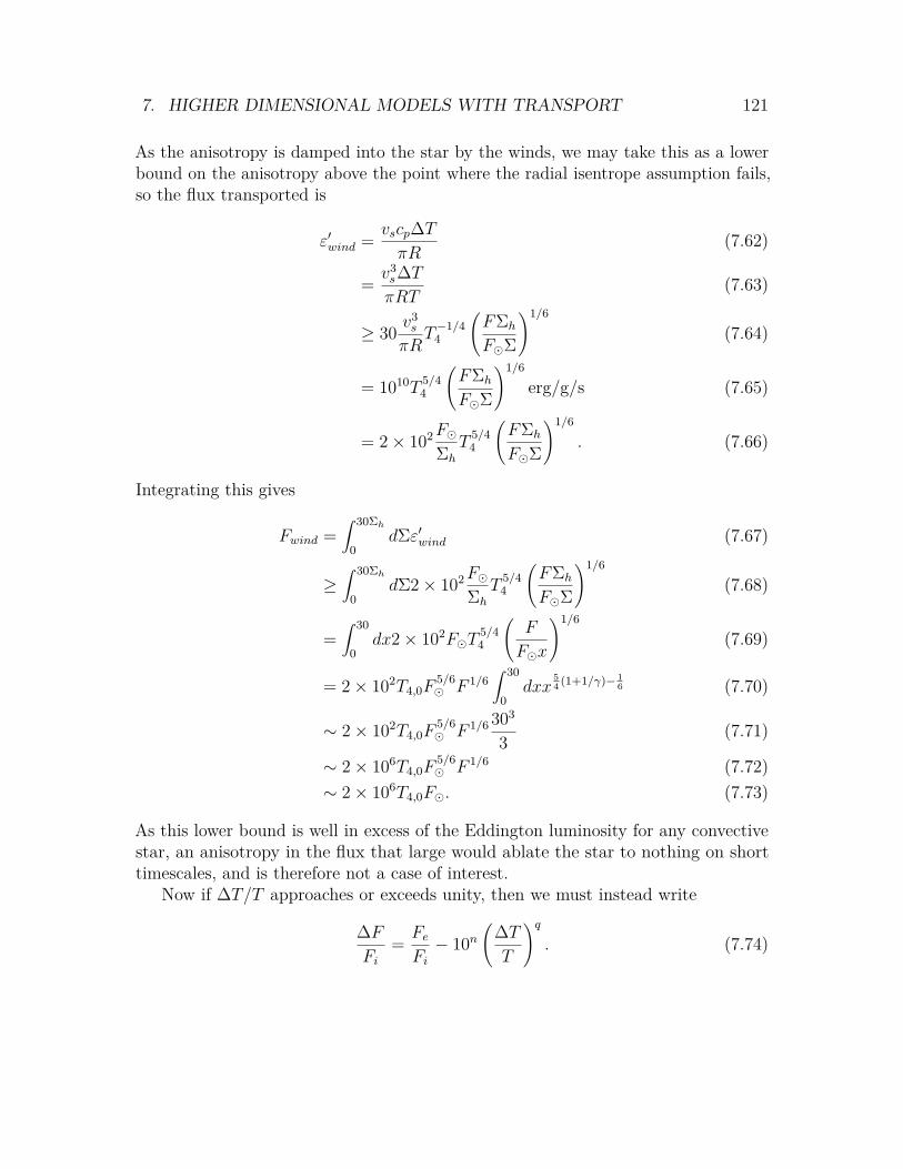
7. HIGHER DIMENSIONAL MODELS WITH TRANSPORT 121
As the anisotropy is damped into the star by the winds, we may take this as a lowerbound on the anisotropy above the point where the radial isentrope assumption fails,so the flux transported is
ε′wind = vscp∆TπR
(7.62)
= v3s∆TπRT
(7.63)
≥ 30 v3s
πRT−1/44
(FΣh
FΣ
)1/6
(7.64)
= 1010T5/44
(FΣh
FΣ
)1/6
erg/g/s (7.65)
= 2× 10²FΣh
T5/44
(FΣh
FΣ
)1/6
. (7.66)
Integrating this gives
Fwind =∫ 30Σh
0dΣε′wind (7.67)
≥∫ 30Σh
0dΣ2× 10²F
Σh
T5/44
(FΣh
FΣ
)1/6
(7.68)
=∫ 30
0dx2× 102FT
5/44
(F
Fx
)1/6
(7.69)
= 2× 10²T4,0F5/6 F 1/6
∫ 30
0dxx
54 (1+1/γ)− 1
6 (7.70)
∼ 2× 10²T4,0F5/6 F 1/6 303
3 (7.71)
∼ 2× 10⁶T4,0F5/6 F 1/6 (7.72)
∼ 2× 10⁶T4,0F. (7.73)
As this lower bound is well in excess of the Eddington luminosity for any convectivestar, an anisotropy in the flux that large would ablate the star to nothing on shorttimescales, and is therefore not a case of interest.
Now if ∆T/T approaches or exceeds unity, then we must instead write
∆FFi
= FeFi− 10n
(∆TT
)q. (7.74)

7. HIGHER DIMENSIONAL MODELS WITH TRANSPORT 122
Recalling that ∆F ∼ σ(∆T )4 in this case,
∆FFi
= FeFi− 10n
(∆FFi
)q/4 (TiT
)q. (7.75)
As the flux has raised the mean temperature by approximately (Fe/Fi + 1)1/4,
∆FFi
= FeFi− 10n
(∆FFi
)q/4 (FeFi
+ 1)q/4
. (7.76)
As Fe must be large relative to Fi to bring about a change of this magnitude, thefactor of unity at the end may be removed, giving
∆FFi
= FeFi− 10n
(∆FFi
)q/4 (FeFi
)q/4. (7.77)
The nature of the solutions is the same as the nature of the solutions in the previoussection, just with
q → q
4 (7.78)
n→ n+ q
4 log FeFi
(7.79)
∆TT→ ∆F
Fi. (7.80)
As in the previous section, it is now more appropriate to speak of the flux anisotropyas ∆F/Fe, so
∆FFe
= 1− 10n(
∆FFe
)q/4 (FeFi
)q/2−1. (7.81)
For external luminosities, we require
∆FFe
= 10−4nq
(4− 2qq
), (7.82)
while for large external luminosities we have
∆FFi
= FeFi− 10n
(FeFi
)q/4. (7.83)
Here large and small are of course referenced to 104n/qFi.

7. HIGHER DIMENSIONAL MODELS WITH TRANSPORT 123
Finally, if the thermal and flux anisotropies are large, the wind is sonic and weexpect y′ = 10, q = 1, a = 0, and b = 0. This greatly increases the efficiency ofcircumferential transport, and results in n increasing by an additive factor somewherebetween 1 and 4. This pushes us further into the regime where our assumption thata > 0 holds, and the remainder of the above analysis is unchanged.
It is worth noting that in all of the cases above, we saw no transition fromconvective to radiative behavior. This is because increasing the requisite flux does notforce this transition. Rather, it is increasing the flux while at the same time insistingthat the ratio of the temperature at the base of the convection zone to that at thetop of the convection zone remain invariant. Of course if Σc is small, then increasingthe luminosity results in shrinking the convection zone appreciably in relative terms.This can, as in the case of our one-dimensional model of the sun, cause the convectionzone to disappear.
7. HIGHER DIMENSIONAL MODELS WITH TRANSPORT 124
ReferencesBrickhill, A. J. “The pulsations of ZZ Ceti stars. III - The driving mechanism”. In:
Monthly Notices of the Royal Astronomical Society 251 (Aug. 1991), pp. 673–680(cit. on p. 111).
Mei, C. C. and T. Y.-t. Wu. “Gravity Waves due to a Point Disturbance in a PlaneFree Surface Flow of Stratified Fluids”. In: Physics of Fluids 7 (Aug. 1964),pp. 1117–1133. doi: 10.1063/1.1711351 (cit. on p. 111).
Shiode, J. H. et al. “The observational signatures of convectively excited gravitymodes in main-sequence stars”. In: Monthly Notices of the Royal AstronomicalSociety 430 (Apr. 2013), pp. 1736–1745. doi: 10.1093/mnras/sts719. arXiv:1210.5525 [astro-ph.SR] (cit. on p. 111).
Wu, Y. and P. Goldreich. “Gravity Modes in ZZ Ceti Stars. IV. Amplitude Saturationby Parametric Instability”. In: The Astrophysical Journal 546 (Jan. 2001), pp. 469–483. doi: 10.1086/318234. eprint: astro-ph/0003163 (cit. on p. 111).

8
Time Dependence
It is all a matter of time scale. An event that would be unthinkable in ahundred years may be inevitable in a hundred million.
– Carl Sagan
The results of our one-dimensional model indicate that there are two modes ofbehavior for stars in the presence of external illumination, and that stars pick oneor the other on the basis of being predominantly radiative or convective. In thischapter we will analyze these behaviors in the transient case through a combinationof numerics and analytics. We begin by describing the numerical methods used, andthen proceed to introduce the cases of fully radiative, fully convective, and mixedradiation-convection stars.
8.1 Assumptions and Computational MethodsThe time-dependent portion of Acorn represents a compromise between the simplicityof time-independent codes like Gob and the complexity of modern time-dependentcodes like MESA. The equation of state used is the same one present in Gob andin the time-independent portion of Acorn, incorporating at leading order variousionization effects as well as radiation pressure. The opacity is the same as that usedin Acorn, a mix of the OPAL1 and Ferguson2 tables. The thin shell approximation isused everywhere, and only envelope evolution is considered. Hydrostatic equilibrium
1C. A. Iglesias and F. J. Rogers. “Updated Opal Opacities”. In: The Astrophysical Journal 464(June 1996), p. 943. doi: 10.1086/177381.
2Jason W. Ferguson et al. “Low-Temperature Opacities”. In: The Astrophysical Journal 623.1(2005), p. 585. url: http://stacks.iop.org/0004-637X/623/i=1/a=585.
125
8. TIME DEPENDENCE 126
is assumed at all times. Finally, it is assumed that convection adjusts to the changingflux being carried faster than the thermal adjustment timescale of the envelope, andhence that it may be assumed that the convective gradient is the gradient requiredto carry the appropriate flux in steady-state. This last assumption will be justifiedlater on.
Assuming hydrostatic equilibrium only, the time-dependent equations of stellarstructure are3
∂r
∂m= − 1
4πr2ρ, (8.1)
∂P
∂m= Gm
4πr2 , (8.2)∂L
∂m= −ε+ cp
∂T
∂t− δ
ρ
∂P
∂t, (8.3)
∂T
∂m= GmT
4πr4P∇, (8.4)
where ε is the power per unit mass being deposited by external illumination, and thesigns have been chosen such that the mass coordinate is the mass above the point inquestion. Note that we include the equation governing r for purposes of tracking howr changes as the other quantities vary, but we do not allow it to produce feedbackwith the other equations. Note also that the time derivatives are to be taken at fixedmass, not at fixed spatial coordinate. Now the condition of hydrostatic equilibriummeans that ∂P
∂t= 0, so we may drop this term.
We now make the substitution
P = mg
4πr2 , (8.5)
in accordance with the thin-shell approximation. This, combined with the previousarguments regarding time derivatives, allows us to eliminate P and write
P = mg
4πr2 , (8.6)∂r
∂m= − 1
4πr2ρ, (8.7)
∂L
∂m= −ε+ cp
∂T
∂t, (8.8)
∂T
∂m= T
m∇. (8.9)
3Rudolf Kippenhahn, Alfred Weigert, and Achim Weiss. Stellar Structure and Evolution. Springer,2012. isbn: 978-3-642-30304-3.

8. TIME DEPENDENCE 127
In order to fully specify the system, we must of course specify boundary conditions.For the t = 0 boundary, we specify that ε = 0 and that ∂tT = 0. When the masscoordinate equals the envelope mass, i.e. m = Me, we choose to hold T constant.Physically this choice simply means that we must only consider timescales shorterthan the thermal timescale of the envelope, given by
te = cpT (Me)Me
Lin≈ 7× 10¹²sT5
MeLML
. (8.10)
The envelope mass was generally chosen to optimize convergence of the time-steppingcode and to stay carefully within the realm of validity of the opacity and equation ofstate microphysics. As a result, typical values were 3×10⁻³M . Typical envelope-basetemperatures are T ≈ 105K, and generally ML
ML≈ 1, so the timescales the code may
investigate with this boundary condition are those shorter than 2×10⁹s, which shouldbe long enough to see the transient effects of interest. Note that in considering ∇to respond immediately, we are also imposing a minimum timescale over which theresults may be taken seriously. This timescale is given roughly by the convectiveturnover time, l/vc, or around 106s at the base of the envelope and 103s whereconvection begins. As a result, time steps will usually be chosen at 106s.
The remaining boundary condition we use to set
4πr2σT 4 = wL, (8.11)
where all quantities are evaluated at the mass corresponding to τ = 2/3 and w is afudge factor obtained from the steady state evolution which makes this relation trueat t = 0. Note that this means that we only track the mass in the star at τ > 2/3.This helps with numerical stability, as it reduces the range of densities to consider,which drastically improves the condition number of the linear algebra problems solvedin the time-stepping process.
In typical simulations, w was found to be roughly 0.5. This is not a matter of amisplaced factor of two in the surface temperature determination. Rather, it is dueto well-documented approximations made in Gob’s, and hence Acorn’s, method forcomputing the effects of radiation dilution in the photosphere4. It is clear that theseboundary conditions are sufficient, for L and T are the only variables involved, allothers being determined by either the approximations made or the equation of state,and we now have two first order differential equations with one boundary conditioneach in one dimension.
4B. Paczyński. “Envelopes of Red Supergiants”. In: Acta Astronomica 19 (1969), p. 1.

8. TIME DEPENDENCE 128
For the starting state, we use the steady state solution. This additionally definesthe mass grid used to discretize the problem. Note that this produces N + 1 pointsfor L and N points for T , such that the temperature is defined only between pairsof points at which the luminosity is defined. For the sake of writing down thediscretization, let there be 2N + 1 points in the mass grid numbered 0 through 2N .Define L on all even-numbered points and all other quantities on the odd-numberedpoints. The equations of interest are then:
∂tρ2i+1 = ∂ρ2i+1
∂T|P∂tT2i+1 (8.12)
(i 6= N)∂tT2i+1 = 1cp(2i+1)
[ε2i+1 −
L2i+2 − L2i
m2i+2 −m2i− cp(2i+1)
vφ(2i+1)
R∂φT(2i+1)
](8.13)
(i 6= 0) T2i+1 − T2i−1
m2i+1 −m2i−1= ∇2i+1
T2i+1
m2i+1(8.14)
∂tT2N−1 = 0 (8.15)∂tL0 = 16wπR2σT 3
1 ∂tT1 (8.16)
Note that the boundary conditions are enforced in differential form. In addition, notethat our use of asymmetric differences in places should not matter in the limit oflarge N .
The equations complete and discretized, we turn to the method of solution.For numerical stability the backwards Euler method was used, such that all timederivatives were written in the form
∂tA(t) = A(t+ dt)− A(t)dt
. (8.17)
Thus the equations solved were of the form
f(t+ dt) = f(t) + dtdf
dt|t=t+dt. (8.18)
This method is particularly appropriate given the stiff nature of ∇ in convectionzones, a fact that will be discussed at length later on. As the backwards Euler methodis an implicit integrator, it requires knowledge of all relevant derivatives evaluated inthe future. To solve for these self-consistently, a damped version of Newton’s methodwas implemented. The Jacobian was constructed analytically, with the exceptionof parts involving ∇, which were computed numerically. This then allowed for aniterative solution of the form
f i+1(t+ dt) = f i(t+ dt) + λδ, (8.19)

8. TIME DEPENDENCE 129
where λ is an adaptively chosen damping parameter beginning at 0.3 for i = 0 andthen reduced geometrically whenever slow convergence was indicated. Here δ is thesolution to the equation
Jδ = −b, (8.20)where b is a vector formed by subtracting the right side of each of the discretizedequations from the left and J is the operator formed from the derivatives of b’scomponents with respect to the entries in f . The latter is fortunately sparse, andso the equation does not require an explicit matrix inversion and hence is fast tosolve. The above procedure is iterated in the code until the error, as measured by b,falls below a critical threshold, usually defined as 10−4 relative to f . Given a desiredtime-step, this procedure was attempted first for the full step. If the solution provesnumerically unstable, the step is divided in two and attempted again. This is donerecursively until the full requested step has completed or until a certain number offailures are reached, at which point an error is generated and the program exits.
It is finally worth noting that an initial settling period is allowed, generally twentytime-steps, over which any deviations due to numerical imprecision in the steadystate solution are worked out and allowed to come to equilibrium. This generallyresults in the luminosity of the star shifting by as much as several percent.
8.2 Fully Radiative StarsThe first model of interest is that of a completely radiative star, such that wemay verify our claim that such stars are only heated significantly at depths abovethe heating one. Figure 8.1 shows the time evolution of just such a star, withM = M, R = R, L = 100L. From the figure it is clear that the change intemperature does indeed drop off exponentially for Σ = Σh, as predicted. Additionally,the value of ∆T/T at the surface, roughly 0.19, matches our expectation of
∆TT0
=L
1/4f − L
1/4i
L1/4i
=(LfLi
)1/4− 1 = 21/4 − 1 = 0.19. (8.21)
To verify that the star was indeed in equilibrium at the end of this simulation, thesame scenario was run again with twice the total time interval, such that the final108s had constant luminosity. The results of this are shown in figure 8.2. The goodagreement between the two simulations indicates that the star is indeed in equilibriumat the end of the first one.
Now in many cases we are actually interested in the case where the star is initiallyilluminated from without and that illumination is turned off. The results of simulating

8. TIME DEPENDENCE 130
−1 0 1 2 3 4 5 6 7 8−0.05
0.00
0.05
0.10
0.15
0.20
∆T/T
Lin=100Lsun,∆t=1e8s
−1 0 1 2 3 4 5 6 7 8Log Σ
100
120
140
160
180
200
220
L/L
sun
t=0e7st=1e7st=2e7st=3e7st=4e7st=5e7st=6e7st=7e7st=8e7st=9e7st=10e7s
Figure 8.1: ∆T/T0 (top) and L/L (bottom) versus log Σ (in g/cm2) for a starof mass M, radius R, and luminosity 100L. The external heat was put in atΣ = 103g/cm2 and linearly increased from zero to 100L over the course of 108s,which is where the simulation ends. Color represents time, with the simulationbeginning at violet and ending with red.

8. TIME DEPENDENCE 131
−1 0 1 2 3 4 5 6 7 8−0.05
0.00
0.05
0.10
0.15
0.20
∆T/T
Lin=100Lsun,∆t=2e8s
−1 0 1 2 3 4 5 6 7 8Log Σ
100
120
140
160
180
200
220
L/L
sun
t=0e7st=2e7st=4e7st=6e7st=8e7st=10e7st=12e7st=14e7st=16e7st=18e7st=20e7s
Figure 8.2: ∆T/T0 (top) and L/L (bottom) versus log Σ (in g/cm2) for a starof mass M, radius R, and luminosity 100L. The external heat was put in atΣ = 103g/cm2 and linearly increased from zero to 100L over the course of 108s, afterwhich the simulation continued for another 108s to allow for equilibration. Colorrepresents time, with the simulation beginning at violet and ending with red.

8. TIME DEPENDENCE 132
this scenario on the same radiative star as before are shown in figure 8.3. The trend isjust the same as before, with the temperature falling by the same amount it initiallyrose, and the luminosity falling everywhere back down to the internally generatedvalue.
These results confirm that radiative stars exponentially damp temperature differ-ences as a function of depth. Additionally, the quick response of radiative stars tochanges in external illumination mean that they track the present-day properties ofthe pulsar wind. This, combined with possible anisotropies in their thermal profiles,means that they may still be useful for exploring the environments pulsars produce.
8.3 Fully Convective StarsWe now turn to fully convective stars. Figure 8.4 shows a fully convective star withM = 0.3M, Lin = 0.1L, R = 2.65R. The star was initially subjected to externalillumination equal to its intrinsic illumination, and this was then turned off over thecourse of 108s. To verify that the final state is indeed an equilibrium solution, thisscenario was then run for an additional 108s, with the results shown in figure 8.5.The good agreement between these two figures indicates that 108s suffices to computean equilibrium, though the question of what is meant by equilibrium is actually quitesubtle in this case. As specified in the differential equations being solved, the solutionis in equilibrium. That is, all time derivatives are zero within the envelope. This doesnot, however, mean that the solution describes an equilibrium scenario for the starin question. This is because the luminosity at the lower boundary has adjusted upto match the initial outer boundary luminosity. As a result heat is exiting the starbelow this envelope faster than it is being produced by nuclear burning. This effectis also seen in cases with much higher external luminosities, as shown in figure 8.6,where Le = L. To understand this, we must examine in more detail the structure of∇ as a function of L.
In radiative zones, ∇ ∝ L, and so both lnT and L adjust to similar degreesto changing circumstances. In convective regions, on the other hand, ∇ is nearlyindependent of L, and so the equations become stiff in lnT relative to L. In the caseof a fully convective envelope, then, to a good approximation, T may be treated asfixed, while L is allowed to vary. The surface temperature sets the outer boundarycondition on L, and so this leads to L rising in the interior to meet the outgoing fluxat the surface, rather than the surface flux falling to match that of the interior.
The process outlined above cannot happen instantaneously. Rather, the timescale

8. TIME DEPENDENCE 133
−1 0 1 2 3 4 5 6 7 8−0.16
−0.14
−0.12
−0.10
−0.08
−0.06
−0.04
−0.02
0.00
0.02
∆T/T
Lin=100Lsun,∆t=1e8s
−1 0 1 2 3 4 5 6 7 8Log Σ
100
120
140
160
180
200
220
L/L
sun
t=0e7st=1e7st=2e7st=3e7st=4e7st=5e7st=6e7st=7e7st=8e7st=9e7st=10e7s
Figure 8.3: ∆T/T0 (top) and L/L (bottom) versus log Σ (in g/cm2) for a starof mass M, radius R, and luminosity 100L. The external heat was put in atΣ = 103g/cm2 and linearly decreased from 100L to zero over the course of 108s.Color represents time, with the simulation beginning at violet and ending with red.

8. TIME DEPENDENCE 134
1 2 3 4 5 6 7−0.012
−0.010
−0.008
−0.006
−0.004
−0.002
0.000
∆T/T
Lin=0.1Lsun,∆t=1e8s
1 2 3 4 5 6 7Log Σ
0.10
0.12
0.14
0.16
0.18
0.20
L/L
sun
t=0e7st=1e7st=2e7st=3e7st=4e7st=5e7st=6e7st=7e7st=8e7st=9e7st=10e7s
Figure 8.4: ∆T/T0 (top) and L/L (bottom) versus log Σ (in g/cm2) for a star ofmass 0.3M, radius 2.65R, and luminosity 0.1L. The external heat was put inat Σ = 103g/cm2 and linearly decreased from 0.1L to zero over the course of 108s.Color represents time, with the simulation beginning at violet and ending with red.

8. TIME DEPENDENCE 135
1 2 3 4 5 6 7−0.012
−0.010
−0.008
−0.006
−0.004
−0.002
0.000
∆T/T
Lin=0.1Lsun,∆t=2e8s
1 2 3 4 5 6 7Log Σ
0.10
0.12
0.14
0.16
0.18
0.20
L/L
sun
t=0e7st=2e7st=4e7st=6e7st=8e7st=10e7st=12e7st=14e7st=16e7st=18e7st=20e7s
Figure 8.5: ∆T/T0 (top) and L/L (bottom) versus log Σ (in g/cm2) for a star ofmass 0.3M, radius 2.65R, and luminosity 0.1L. The external heat was put inat Σ = 103g/cm2 and linearly decreased from 0.1L to zero over the course of 108s.The simulation was then run for an additional 108s with no external heating. Colorrepresents time, with the simulation beginning at violet and ending with red.

8. TIME DEPENDENCE 136
1 2 3 4 5 6 7−0.05
−0.04
−0.03
−0.02
−0.01
0.00
0.01
∆T/T
Lin=0.1Lsun,∆t=1e8s
1 2 3 4 5 6 7Log Σ
0.0
0.2
0.4
0.6
0.8
1.0
1.2
L/L
sun
t=0e7st=1e7st=2e7st=3e7st=4e7st=5e7st=6e7st=7e7st=8e7st=9e7st=10e7s
Figure 8.6: ∆T/T0 (top) and L/L (bottom) versus log Σ (in g/cm2) for a star ofmass 0.3M, radius 2.65R, and luminosity 0.1L. The external heat was put inat Σ = 103g/cm2 and linearly decreased from L to zero over the course of 108s.The simulation was then run for an additional 108s with no external heating. Colorrepresents time, with the simulation beginning at violet and ending with red.

8. TIME DEPENDENCE 137
of adjustment for L in a convection cell is set by the convective turnover time l/vc5,and so what occurs is that the temperature adjusts due to the nonzero slope of Lin m for a time l/vc, after which the flux has uniformly risen to match the outerboundary condition. At this point and in this region, the flux ceases to vary, andhence ∂tT falls to zero. The expected change in T is then expected to be roughly
δT ≈ ∂tTδt ≈∆Lcpδm
δz
vc= ∆L
4πr2ρcpvc, (8.22)
where δm and δz refer to the mass and thickness of a spherical shell of material, and∆L is the change in luminosity, which should be equal to the external luminosity.Now the convective flux may be written as
Fc ≈ ρv3c ≈
Lin4πr2 , (8.23)
so
δT ≈ Le4πr2ρcp
(Lin
4πr2ρ
)−1/3
= 1cp
(Le
4πr2ρ
)2/3 (LeLin
)1/3. (8.24)
This may also be written as
δ lnT ≈ δT
T≈ v2
c
v2s
(LeLin
). (8.25)
Near the surface of a fully convective star, we usually have vc ≈ vs/10, so for Le = Linwe expect δT/T ≈ 10−2. Furthermore, at higher pressures the sound speed risesrelative to the convection speed, and so the difference drops off. This may beunderstood as following from the above result that δT ∝ ρ−2/3. The endpoint of thisprocess occurs when the moving "wavefront" of the flux change reaches the nuclearburning regime. At this stage the temperature will drop significantly more, for thereis nowhere else for the wavefront to go.
To understand what happens next, we first remark that the convection zone willadjust to maintain an adiabatic gradient on a timescale set by the convective turnoverrate. As a result, the timescale for the entire star to adjust to maintain this gradientis
τadj =∫ dr
vc=∫ 1ρvc
dΣ ≈∫ρ−1
(F
ρ
)−1/3
dΣ = F−1/3∫ρ−2/3dΣ, (8.26)
5Recall that this is why Acorn only takes time-steps which are at least max(l/vc) in size.

8. TIME DEPENDENCE 138
where the integral is taken over the entire star. In a convective atmosphere, P ∝ ργ,so ρ ∝ P 1/γ. If we make the thin atmosphere approximation throughout the star,just to gain an order-of-magnitude estimate, then P = gΣ, and so
τadj ≈ g−1F−1/3∫ρ−2/3dP = g−1F−1/3ρ
−2/30
∫ (P
P0
)−2/3γdP (8.27)
= 11− 2
3γg−1F−1/3ρ
−2/30 P
2/3γ0
(P
1−2/3γf − P 1−2/3γ
0
). (8.28)
Now γ is typically 5/3 outside of the ionization zone, so 2/3γ=2/5, and hence
τadj ≈5P 2/5
0
3gF 1/3ρ2/30
(P
3/5f − P 3/5
0
)≈
5P 2/50 P
3/5f
3gF 1/3ρ2/30
=5v2
s,0
3γgvc,0
(PfP0
)3/5=
v2s,0
gvc,0
(PfP0
)3/5,
(8.29)where we have made the approximation that the core pressure vastly exceeds thepressure at the top of the convection zone. Now vc,0 is typically around vs,0/10, andvs,0 is typically around 106cm/s ≈ 100sg, so the prefactor is around 103s. TypicallyP0 ∼ 105erg/cm3, and Pf ∼ gM/(4πR2) ∼ 1015erg/cm3 for the sun, so the overalltimescale is around 103+6 = 109s, scaling roughly as M6/5R−12/5. For the fullyconvective star considered in simulation, M = 0.3M and R = 2.65R, so thistimescale is smaller by a factor of 25, giving around 4× 10⁷s, or roughly a year.
On the other hand, the core adjusts its temperature in time
τcore = mcorecpTcoreLe
= fMLinLe
τK = fMGM2
2RLe, (8.30)
where fM ≈ 1/10 is the fraction of the star’s mass in the core and τK is the Kelvintimescale for the star. This is typically of order ten million years, and so if Le = Linthe core’s adjustment timescale is of order a million years. As this is much shorterthan the timescale required to maintain adiabaticity, the star may be approximatedas being adiabatic at all times after the cooling wavefront reaches the core.
8.4 Mixed StarsFor stars with a convection zone above a radiative region, there are two considerationswhich our steady-state analysis leads us to expect to differ from the fully convectivecase. First, any bloating effects are limited to the convection zone, and so the extentof bloating is decreased proportional to the size of the zone. Additionally, the nuclearburning of the core is unchanged by the addition or removal of external illumination

8. TIME DEPENDENCE 139
in these stars, meaning that the bloating effect is further decreased by the amountgiven in figure 2.7.
To investigate these effects in the transient case, we first simulated a sun-typestar initially illuminated by Le = L and watched as the illumination was turnedoff. The results of this are shown in figure 8.7. The key feature we see here isthat the luminosity sits fixed near the initial steady-state value at the surface, andthat the main effect of time evolution is to push the transition between this valueand the nuclear-burning value deeper into the star. The depth at which this occursis between Σ = 104g/cm2 and Σ = 105g/cm2, just slightly deeper than the pointin our steady-state calculations where the radiative-convective transition arises inilluminated equilibrium in this sort of star. This feature is not unique to stars ofM = M. Figure 8.8 shows a star of the form examined in the preceding section,but with Le = 10L. This star exhibits a similar transition between radiative andconvective heat transport in the steady state and hence exhibits a similar transientadjustment process. The story behind the evolution of stars such as these is thenthat the external illumination shuts off convection beyond a certain depth. Whenthe illumination is removed, that radiative region dampens the resulting change intemperature exponentially into the star, while the convective region maintains aluminosity close to the initial steady-state value. This is precisely what we see, but wecan further test this notion by examining the star on longer timescales. If this storyis correct, the star will slowly turn the radiative zone back into a convection zone,and in the process the luminosity profile will settle down to have L = L everywhere.
To determine if this is the case, the simulation was run for another 108s and foundindeed to be out of equilibrium, a feature not seen in any of the previous scenariosconsidered. The results of the longer simulation are shown in figure 8.9. Note that asthe luminosity transition region pushes deeper into the star, the magnitude of thetransition falls. Over even longer timescales, the equilibration continues but slowsdown somewhat, as shown in figure 8.10. The adjustment time for this process is onthe order of the thermal timescale for the entire region in which the mode of heattransport shifted from being convective to being radiative, perhaps decreased by afactor of 10 to account for the relatively small temperature changes required to dothis at high Σ. As a result, the full adjustment process requires timescales beyond therealm of validity of our lower boundary condition on T . Fortunately all that mattersfor our purposes are the trend and timescale involved, which are clearly seen in thesimulations which are accessible.

8. TIME DEPENDENCE 140
0 1 2 3 4 5 6 7 8−0.35
−0.30
−0.25
−0.20
−0.15
−0.10
−0.05
0.00
0.05
∆T/T
Lin=Lsun,∆t=1e8s
0 1 2 3 4 5 6 7 8Log Σ
1.0
1.2
1.4
1.6
1.8
2.0
2.2
L/L
sun
t=0e7st=1e7st=2e7st=3e7st=4e7st=5e7st=6e7st=7e7st=8e7st=9e7st=10e7s
Figure 8.7: ∆T/T0 (top) and L/L (bottom) versus log Σ (in g/cm2) for a star of massM, radius R, and luminosity L. The external heat was put in at Σ = 103g/cm2
and linearly decreased from L to zero over the course of 108s. Color represents time,with the simulation beginning at violet and ending with red.

8. TIME DEPENDENCE 141
0 1 2 3 4 5 6 7−0.7
−0.6
−0.5
−0.4
−0.3
−0.2
−0.1
0.0
0.1
∆T/T
Lin=0.1Lsun,∆t=1e8s
0 1 2 3 4 5 6 7Log Σ
0
2
4
6
8
10
12
L/L
sun
t=0e7st=1e7st=2e7st=3e7st=4e7st=5e7st=6e7st=7e7st=8e7st=9e7st=10e7s
Figure 8.8: ∆T/T0 (top) and L/L (bottom) versus log Σ (in g/cm2) for a star ofmass 0.3M, radius 2.65R, and luminosity 0.1L. The external heat was put inat Σ = 103g/cm2 and linearly decreased from 10L to zero over the course of 108s.The simulation was then run for an additional 108s with no external heating. Colorrepresents time, with the simulation beginning at violet and ending with red.

8. TIME DEPENDENCE 142
0 1 2 3 4 5 6 7 8−0.5
−0.4
−0.3
−0.2
−0.1
0.0
0.1
∆T/T
Lin=Lsun,∆t=2e8s
0 1 2 3 4 5 6 7 8Log Σ
1.0
1.2
1.4
1.6
1.8
2.0
2.2
L/L
sun
t=0e7st=2e7st=4e7st=6e7st=8e7st=10e7st=12e7st=14e7st=16e7st=18e7st=20e7s
Figure 8.9: ∆T/T0 (top) and L/L (bottom) versus log Σ (in g/cm2) for a star of massM, radius R, and luminosity L. The external heat was put in at Σ = 103g/cm2
and linearly decreased from L to zero over the course of 108s. It was then run foranother 108s at that value. Color represents time, with the simulation beginning atviolet and ending with red.

8. TIME DEPENDENCE 143
0 1 2 3 4 5 6 7 8−0.6
−0.5
−0.4
−0.3
−0.2
−0.1
0.0
0.1
∆T/T
Lin=Lsun,∆t=1e9s
0 1 2 3 4 5 6 7 8Log Σ
1.0
1.2
1.4
1.6
1.8
2.0
2.2
L/L
sun
t=0e8st=1e8st=2e8st=3e8st=4e8st=5e8st=6e8st=7e8st=8e8st=9e8st=10e8s
Figure 8.10: ∆T/T0 (top) and L/L (bottom) versus log Σ (in g/cm2) for a starof mass M, radius R, and luminosity L. The external heat was put in atΣ = 103g/cm2 and immediately decreased from L to zero over the course of 108sbefore being run for another 109s. Color represents time, with the simulation beginningat violet and ending with red.

Part II
Applications in Astronomy
144

9
X-Ray Binaries
You know, you blow up one sun and suddenly everyone expects you towalk on water.
– Lt Col. Samantha Carter, Stargate SG-1 Season 8 Episode 17
The results presented thus far have been general, in the sense that while therewere motivating examples of phenomena of interest, many avenues were pursuedto provide a picture of the phenomenology of pulsar-companion systems. We arenow interested in examining the specific case in which the pulsar interacts with itscompanion to produce transient X-ray emissions. This case has long been studied1,though conclusions have proven scarce. In addition, while in previous chapters thecompanion was a passive agent, here we will consider the role it plays in influencingits own fate. The first section deals with the isotropic illumination case, while thesecond discusses the effects of anisotropy.
9.1 Accretion rateThe initial heating of the star causes it to expand at some rate R. This rate iseverywhere the same in the atmosphere due to the expansion being driven by deepheating, as discussed earlier. As the atmosphere of the star falls off exponentially
1J. C. Brown and C. B. Boyle. “An exploratory eccentric orbit ’Roche lobe’ overflow modelfor recurrent X-ray transients”. In: Astronomy and Astrophysics 141 (Dec. 1984), pp. 369–375;H. Ritter, Z.-Y. Zhang, and U. Kolb. “Irradiation and mass transfer in low-mass compact binaries”.In: Astronomy and Astrophysics 360 (Aug. 2000), p. 969. eprint: astro-ph/0005480; A. R. Kinget al. “Mass Transfer Cycles in Close Binaries with Evolved Companions”. In: The AstrophysicalJournal 482 (June 1997), pp. 919–928. eprint: astro-ph/9701206.
145

9. X-RAY BINARIES 146
in the radial coordinate above the photosphere, no significant accretion is expecteduntil this region approaches the Roche lobe radius Rb. The accretion rate is expectedto be2
M =√
2πRhsvsρ(Rb). (9.1)Here hs ≈ Rv2
s/v20, where v0 is the orbital velocity of the star. This is due to the fact
that in the vicinity of the Roche lobe, the pressure profile is set by orbital parametersrather than the thermal structure of the star. As a result, we may write
M ≈√
2πR2v−20 v3
sρ(Rb). (9.2)
If the accretion rate is low3, it typically means that ρ is low at Rb, the Rocheradius, and hence that we are in the upper portion of the atmosphere. This allows usto make use of ρ ∝ exp(−r/hs) and write
M ≈√
2πR2v−20 v3
sρ0 exp(rv2
0Rv2
s
)=√
2πΩ−2v3sρ0 exp
(rR2
0Ω2
Rv2s
), (9.3)
where ρ0 is chosen to make this relation true and r is a Lagrangian quantity. Forthe accretion to be significant we must have R ≈ Rb, for R,Rb hs becausev0 ≈ 107cm/s 105cm/s ≈ vs. Thus
M ≈√
2πΩ−2v3sρ0 exp
(rR2
0Ω2
Rbv2s
). (9.4)
In Part 1, we found that only stars with deep convection can swell to the point whereR ∼ Rb, so we restrict ourselves to stars of this form. As a result, M < 1.2M. UsingMp ≈ 2M, we may approximate4
Rb ≈ 0.46R0
(M
M +Mp
)1/3
, (9.5)
yielding
M ≈√
2πΩ−2v3sρ0 exp
(2rR0Ω2(M +Mp)2/3
M2/3v2s
), (9.6)
2Brown and Boyle, op. cit.3Using Eq. (9.2), we find that M ∼ 1024ρcm3/s. Based on the data in Appendix E, the exponential
atmosphere assumption holds at least up to ρ ∼ 10−8g/cm3, so we are safe making this assumptionif M < 1016g/s. As will become clear subsequently, this is much larger than the typical values wewill encounter.
4B. Paczyński. “Evolutionary Processes in Close Binary Systems”. In: Annual Review ofAstronomy and Astrophysics 9 (1971), p. 183. doi: 10.1146/annurev.aa.09.090171.001151.

9. X-RAY BINARIES 147
where
R0 =(G(M +Mp)
Ω2
)1/3
. (9.7)
Typical atmospheric temperatures are such that µ = mp, so γ = 5/3 and
v2s = 5kBT
3mp
. (9.8)
Thus we can compute all of the quantities in the exponential.Now we haven’t yet fixed r or ρ0, and so we actually have the freedom to absorb
any constants we wish. Furthermore, relative to the exponential the dependence onT is negligible, so we may let T → T0 for some reference photospheric temperatureT0 and absorb it as well. Thus we will write instead
M ≈ exp(
2rR0Ω2(M +Mp)2/3
M2/3v2s
). (9.9)
We now no longer have the freedom to pick the zero-point of r. Rather, it is uniquelydetermined given M at some time. Without solving for it, though, we may write
M = 2R0Ω2(M +Mp)2/3
M2/3v2s
rM . (9.10)
Using r = R and dividing through by M yields
∂t ln M = 2rR0Ω2(M +Mp)2/3
M2/3v2s
R. (9.11)
This equation is independent of the zero-point of r, for r no longer appears anywherein it. Given ln M at some point in time, we may use this relation to determine it atany subsequent point so long as we know R.
9.2 Pre-Roche ExpansionRecall that the radius of the star obeys
dr
dm= 1
4πr2ρ. (9.12)
This may also be written asdr3
dm= 3
4πρ. (9.13)

9. X-RAY BINARIES 148
Differentiating with respect to time gives
d
dm
(dr3
dt
)= −3
4πρ
(d ln ρdt
)= −dr
3
dm
(d ln ρdt
). (9.14)
At fixed pressure, d ln ρ = −d lnT , neglecting the small space occupied by theionization zone, so
d ln ρdt
= −d lnTdt
. (9.15)
As a result,d
dm
(dr3
dt
)= dr3
dm
d lnTdt
, (9.16)
and hencedR3
dt= R3d lnT
dt. (9.17)
Note that we have assumed here that the majority of the star, as measured bythe radial coordinate cubed, is convective. This is equivalent to assuming that themajority of the volume of the star is convective. This must be true in order for us toget the expansion of interest, and so may be thought of as a condition on the star,rather than an assumption to be tested later on. Though in equilibrium many starsbecome fully radiative, as we found in Chapter 2, during the initial expansion thestar remains convective for quite a while. For many systems the equilibrium state isnever reached, as the Roche lobe overflows well before this occurs, and so we maysafely assume that a substantial convection zone remains.
Now the convective turnover timescale of the star is given by Eq. (8.29) as
τadj =v2s,0
gvc,0
(PfP0
)3/5, (9.18)
where vc,0 is the convection speed near the top of the efficient convection region (i.e.where Γ ∼ 10), vs,0 is the sound speed at the same location, P0 is the pressure atthe same location, and Pf is the pressure at the base of the convection zone. The

9. X-RAY BINARIES 149
thermal adjustment time, on the other hand, is
τ ′adj =∫conv cpTdm
(Li + Le − Lsurface)(9.19)
=∫conv cpT4πr2dp
g (Li + Le − Lsurface)(9.20)
≈ 4πR2cpT0P0 (Pf/P0)∇ad+1
g(∇ad + 1) (Li + Le − Lsurface)(9.21)
=4πR2v2
s,0P0 (Pf/P0)∇ad+1
gγ(∇ad + 1) (Li + Le − Lsurface)(9.22)
= 4πR2τadjvc,0P0 (Pf/P0)∇ad+2/5
γ(∇ad + 1) (Li + Le − Lsurface)(9.23)
= 4πR2τadjvc,0P0 (Pf/P0)∇ad+2/5
γ(∇ad + 1) (Li + Le − Lsurface)(9.24)
∴τ ′adjτadj≈ 4πR2P0vc,0 (Pf/P0)∇ad+2/5
γ(∇ad + 1) (Li + Le − Lsurface). (9.25)
Note that we have made use of the fact that the heat being bottled up is Li + Le −Lsurface, where Li is a time-dependent quantity in the case that the core is heated. Thisis the isotropic expression, as we are assuming deep convection. Now R ∼ 1011cm,vc,0 is generally between 104cm/s and 105cm/s, P0 ∼ 105erg/cm3, Li < 1035erg/s, sothis ratio is at least
τ ′adjτadj
= 10−7 (Pf/P0)∇ad+2/5 ∼ 10−7 (Pf/P0)4/5 . (9.26)
As long as Pf > 108P0 the thermal adjustment time is greater than the convectiveadjustment time, and we may take the convective gradient to hold everywhere. Thiswill always be the case in the stars of interest: if it does not hold, a substantialfraction of the convection zone will disappear when the heating is introduced, asdiscussed in Chapter 2.
Our result involving R3 may now be cast as a result involving R, giving
R = R
3d lnTdt
. (9.27)
Now the characteristic timescale defined by d lnT/dt is just τ ′adj, so
R = R
3d lnTdt
= R
3τ ′adj= gγ(∇ad + 1) (Li + Le − Lsurface)
12πRv2s,0P0 (Pf/P0)∇ad+1 . (9.28)

9. X-RAY BINARIES 150
Note that we have neglected the gravitational potential energy associated with thechange in radius. By the virial theorem, we expect that the fraction of the inputenergy which goes into changing the gravitational potential is half that which goesinto changing the temperature. As this is an order unity correction we are justifiedin neglecting it.
Now there are three possible cases. First, the Roche radius may exceed themaximum possible radius the star can expand to. In this case no accretion is observed.Second, the Roche radius may be smaller than the main sequence radius of the star.In this case we expect the star to cataclysmically accrete onto the companion. Thispossibility has been extensively studied elsewhere and is not the focus of this text.Finally, the Roche radius may lie between the main sequence radius of the companionand the maximum possible radius the companion can expand to. It is this final casewhich is of interest in this chapter.
To examine the case of interest, we need to compute the maximum possiblepost-expansion companion radius. Formally, the problem of interest is to determinethe maximum R consistent with the constraint that R = Rb and with the incidentexternal illumination Le. To do this, we must first determine the depth of the baseof the convection zone. In the region deeper than the ionization zone, the Krameropacities are valid and we may write
κ = βPT−4.5, (9.29)where β is a constant independent of pressure or temperature. As we are interestedin the expansion of the entire star, we may focus on this region and neglect effectsnear the surface. The base of the convection zone is the location where
∇ad = ∇rad. (9.30)Solving this with the known form of ∇rad gives
T 9.5 = 3βP 2L
16πacGM∇ad
. (9.31)
As we are working deep in the star, ∇ad is a constant, and so we know that there isonly one solution. Now at any given pressure in the convection zone,
T = T0
(P
P0
)∇ad, (9.32)
where T0 and P0 are just the temperature and pressure at some reference position inthe convection zone. Using this we may solve for the base of the convection zone as
Pf = P0
(∇rad(P = P0)
∇ad
) 19.5∇ad−2
. (9.33)

9. X-RAY BINARIES 151
Using ∇ad = 0.4, the exponent may be evaluated as 0.56. Thus
Pf = P0
(∇rad(P = P0)
∇ad
)0.56
. (9.34)
What this means is that we may compute a stellar envelope down to some positiondeeper than the ionization zone and determine the position of the base of the convectionzone from local thermodynamic quantities in the envelope. This means that if thecomputed Pf is smaller than P0, we know that the envelope is radiative through thereference pressure. We will pick P0 as shallow as possible while remaining deeperthan the ionization zone, such that this allows us to classify the entire envelope minusthe portion very close to the surface. In practice this amounts to picking a test P0above the ionization zone, and then increasing it geometrically until a well-convergedenvelope matching the self-consistency conditions is achieved.
Using our knowledge of Pf , along with our equations giving R in terms of it, wemay compute the radius of a star as a function of its main sequence and current Pfvalues. This is just given by
R(P ′f ) = R(Pf ) max(
1, PfP ′f
) 23∗9.5
, (9.35)
where we have once more made use of Kramer’s opacities in the deep stellar inte-rior. We see that this provides a self-consistency relation which must be evaluatednumerically. To solve this, an add-on to the core Acorn code was developed. Thefull code is shown in Appendix B.2. It begins by computing for a given star and agiven pulsar luminosity the maximum radius the star may achieve through thermalexpansion. This accounts for the fact that the orbital position is not independent ofthe Roche radius, as well as the fact that the incident flux is not independent of theorbital position. A shooting method is used in these computations, where a guessof P ′f is used to compute a new value of it. The resulting radius is averaged withthat of the previous guess, and used as input for the next iteration. Convergence isachieved when the radius changes by less than 10−3R per iteration. To determinethe surface luminosity of stars with radii between the main sequence radius and themaximum radius, binary search is used. The algorithm tracks a lower and upperbound on the luminosity, initially between Le and Le + Li. Given such an interval,the radius resulting from the midpoint luminosity is computed. If this is larger thanthe desired radius, the upper bound on the interval is set to the midpoint. Likewiseif it is smaller than the desired radius, the lower bound is set to the midpoint. Thealgorithm converges when the computed radius minus the main sequence radius iswithin one part in one thousand of the desired difference.

9. X-RAY BINARIES 152
Putting all of this together, we can compute the characteristic timescale τexp =hs/R over which M increases by a factor of e. A plot of this is shown in figure 9.1.Note that low mass stars have a much easier time expanding, both because they havelower thermal content and because they both can be and have to be much closer tothe pulsar to satisfy the expansion criteria.
9.3 Post-Roche AccretionFrom the previous section, we know that the characteristic increase timescale τexpfor M is of order of a century for most stars. This exponential increase in M clearlycannot continue indefinitely. There are three processes which may interrupt it. First,the star could continue expanding until it all overflows the Roche lobe. This is unlikelygiven that long before that happens the pulsar’s radiation will be blocked by theaccreting material. This is the second possibility: the accreting material can preventthe heating from continuing, putting an upper limit on M . Finally, the star can reacha balance where the amount of heat being removed by the accreting material equalsthe input heat.
Ignoring the first possibility, we turn to the second. Let r be distance from thepulsar. The pressure exerted by the pulsar wind is
Pw = Lp4πr2c
. (9.36)
The pressure exerted by the accreting material is given roughly by ρv2r , where vr
is the radial velocity. If we assume that the accreting material spreads out in alldirections by the time it reaches the pulsar, then
M = 4πr2ρv. (9.37)
Now v should be roughly the free-fall velocity onto the pulsar, given by
v ∼ GMp
r, (9.38)
so assuming spherical accretion yields
Pacc =M√GMp
4πr5/2 . (9.39)
Equating this with the pulsar wind pressure, we find
req = GMpc2
L2p
M2. (9.40)

9. X-RAY BINARIES 153
0.2 0.4 0.6 0.8 1.0 1.2M
3.6
3.8
4.0
4.2
4.4
4.6
4.8
Log P
Lp =1.0L¯
0.2 0.4 0.6 0.8 1.0 1.2M
3.6
3.8
4.0
4.2
4.4
4.6
4.8
Log P
Lp =10.0L¯
0.2 0.4 0.6 0.8 1.0 1.2M
3.6
3.8
4.0
4.2
4.4
4.6
4.8
Log P
Lp =25.0L¯
0.2 0.4 0.6 0.8 1.0 1.2M
3.6
3.8
4.0
4.2
4.4
4.6
4.8
Log P
Lp =50.0L¯
6.4
7.2
8.0
8.8
9.6
10.4
11.2
12.0
12.8
Log hs/R
Figure 9.1: The vertical axis is logP in seconds, the horizontal axis is the com-panion mass M in solar masses, and the color represents the log of the expansiontimescale hs/R in seconds. The four different plots correspond to four different pulsarluminosities.

9. X-RAY BINARIES 154
If this radius falls within the Pulsar’s light cylinder it will bury the magnetic field5.This occurs when
Mc = Lp√ωGMpc
= 5× 10¹³P1/2p,−3
LpL
g/s, (9.41)
where Pp,−3 is the pulsar period measured in milliseconds. We may compute thethermal energy lost when this mass leaves the star at ∼ 104K. The result is roughly3 × 10−8Lp. As the input heat is expected to be only a few orders of magnitudebelow Lp, this effect is negligible. Thus we expect the limiting factor in the accretionprocess to be that the heat coming from the pulsar is blocked above a certain M .
Now at the accretion rate Mc we may estimate the structure of the accretion diskwhich forms. The accretion luminosity is
Lacc = GMpM
R0/2. (9.42)
We may equate this with the heat flux of the disk as a black body, giving
T =(GMpM
πR30σ
)1/4
. (9.43)
If the disk is optically thin, then the temperature gradient in the vertical direction isnegligible. We will assume that this is the case, and later demonstrate its consistencyin the regimes of interest. The remaining structural equations which must be solved
5There is some evidence that the actual radius to compare to is smaller than the light cylinderradius by a factor of 20 or so (Unal Ertan. “Inner disk radius, accretion and the propeller effect inthe spin-down phase of neutron stars”. In: []. eprint: http://arxiv.org/pdf/1504.03996v1.pdf).As this work is only suggestive, we proceed with the currently accepted model. If it turns out that asmaller radius is necessary, the critical accretion rates and associated luminosities will be reduced,which would mean a higher disk timescale and hence more type 1 cycles, as will be explained insubsequent sections. If the increase in timescale is sufficient, it could even allow asteroids and othersimilar objects to form in the disk, providing an explanation for some of the timing noise in pulsarswith known companions.

9. X-RAY BINARIES 155
are6
hs = vsR3/20√
GMp
(9.44)
v2s = P
ρ(9.45)
αvshsΣ = M
3πf, (9.46)
where α is a dimensionless parameter less than unity relating the viscosity of thedisk to the product of hs and vs, and f is a dimensionless parameter equal to(1−
√Rinner/R0)1/4 ≈ 1. Solving for Σ yields
Σ ≈ 2Mmp
3αkBTP
√M
2 +M, (9.47)
where M is measured in solar masses. Plugging in M = 1013g/s, P ∼ 104s, andα > 10−2 yields Σ < 2g/cm2. Low-temperature opacities tend towards ∼ 1cm2/g, sofor this M the optically-thin assumption is valid. The worst case scenario for thisassumption while still keeping M sub-critical occurs when T ∼ 103K. For hotter disks,the opacity drops off by several orders of magnitude7. When T is 103K, Σ is between0.2g/cm2 and 20g/cm2, depending on the chosen value of α. Here τ can be as greatas 10, so taking the system to be optically thin is perhaps not a good assumption. Onthe other hand, the ratio of the disk interior temperature to the surface temperaturegoes as the optical depth to the one-fourth power, and this ratio is the resulting errorin the scale height and squared sound speed, so even an optical depth of 10 does notincur error in Σ greater than the existing error due to the uncertainty in α. Thus wewill proceed with the optically-thin assumption.
Now the radial velocity of the accreting material is determined by the timescaleover which viscosity dissipates angular momentum. This is given by8
τdisk = R20ν
= R20
αhsv0= R0
α
√mp
kBT∼ 3× 10⁵sR5/8
0 M−1/813.7 , (9.48)
6T. Padmanabhan. Theoretical Astrophysics. Vol. 2. ISBN: 978-0521566315. CambridgeUniversity Press, 2001. Chap. 6.
7Jason W. Ferguson et al. “Low-Temperature Opacities”. In: The Astrophysical Journal 623.1(2005), p. 585. url: http://stacks.iop.org/0004-637X/623/i=1/a=585.
8D. Lynden-Bell and J. E. Pringle. “The evolution of viscous discs and the origin of the nebularvariables.” In: Monthly Notices of the Royal Astronomical Society 168 (Sept. 1974), pp. 603–637.

9. X-RAY BINARIES 156
where R0 is measured in solar radii. At the critical accretion rate, this is
τdisk,c = 3× 10⁵sL−1/8p P−1/16
p,−3 R5/80 , (9.49)
where Lp is measured in solar luminosities, R0 is in solar radii, and P is measured inseconds. This timescale may be viewed as the time over which material falling ontothe outer edge of the disk travels to the inner edge when the accretion rate is nearthe critical value. We see that in most cases this is quite short, only of order onehundred orbits.
It is extremely important to note in this analysis that the pulsar field only turnsoff when the mass loss rate on the inner edge of the disk reaches the critical value.In the event that the disk forms quickly relative to τexp, this M is the same as the Mwhich fell onto the disk a time τdisk earlier, so there is a time delay associated withwaiting for the material to reach the pulsar. This has two key impacts on our system.First, it introduces the possibility of limit-cycles by building in a characteristic delaytimescale, and second it allows the mass loss rate to continue to grow after Mc hasbeen reached at the companion. When the disk timescale is not too much longer thanthe expansion timescale, the typical overshoot in mass loss associated with this delayis
∆ ln M = τdisk
τexp. (9.50)
We can plot this using our numerical results for τexp. In figure 9.2 we have done thisfor a variety of Lp values with Pp = 10−3s. Examining the figure, we see in all casesthat the growth is negligible, so the limit-cycle possibility is the key impact of thedisk clearing time.
Of course, in the event that the disk forms slowly, the disk forming time maybecome the relevant parameter. In this case, we expect
∆ ln M = τspread
τexp, (9.51)
where τspread is the time the disk takes to form and spread once the companion staroverflows the Roche radius. We will consider this timescale in more detail in latersections.

9. X-RAY BINARIES 157
0.2 0.4 0.6 0.8 1.0 1.2M
3.6
3.8
4.0
4.2
4.4
4.6
4.8
Log P
Lp =1.0L¯
0.2 0.4 0.6 0.8 1.0 1.2M
3.6
3.8
4.0
4.2
4.4
4.6
4.8
Log P
Lp =10.0L¯
0.2 0.4 0.6 0.8 1.0 1.2M
3.6
3.8
4.0
4.2
4.4
4.6
4.8
Log P
Lp =25.0L¯
0.2 0.4 0.6 0.8 1.0 1.2M
3.6
3.8
4.0
4.2
4.4
4.6
4.8
Log P
Lp =50.0L¯
7.2
6.4
5.6
4.8
4.0
3.2
2.4
1.6
Log τ
dis
k/τ e
xp
Figure 9.2: The vertical axis is logP in seconds, the horizontal axis is the companionmass M in solar masses, and the color represents the log of τdisk/τexp. The four plotscorrespond to different pulsar luminosities.

9. X-RAY BINARIES 158
9.4 Critical Accretion DynamicsOnce the accretion rate reaches the critical rate, the heating stops on a very shorttimescale9. At this point, the short time dynamics of the star are important. Theenvelope has some momentum, as R was 2× 10⁻³cm/s prior to the heating ceasing.This will continue at a minimum until a wave traveling at the sound speed traversesthe star, which takes time R/vs ∼ 105s. More importantly, the deep convective andshallow regions have characteristic adjustment timescales which exceed this.
As discussed in Chapters 2 and 8, the convection zone cannot adjust on timescalesshorter than the eddy turnover time. This was determined in Chapter 2 to be
τeddy ∼v2s,0
gvc,0
(PfP0
)3/5(9.52)
=v2s,0
gvc,0
(PfPc
)3/5 (PcP0
)3/5(9.53)
= 5× 10⁸ M1/5T0,4
R2/5P3/50,5 vc,0,5
min(
1, 12M
−4/5), (9.54)
where P9 is the pressure at the top of the convection zone, T0 is the correspondingtemperature, vc,0 is the convection speed at the top of the efficient portion of theconvection zone, and M and R are measured in solar units. This sets a lower boundon the adjustment timescale for the convection zone. In the event that this is longerthan the thermal adjustment timescale, then eddy turnover is the limiting factorand we expect this to be the relevant timescale. If, on the other hand, adjusting thethermal profile to match the new flux profile takes longer, then the time that takes isthe relevant timescale.
To quantify the thermal adjustment timescale, we first compute ∂L∇. Note thatthe thermal gradient needs very little correction, as ∇ is very nearly independent ofL. Making use of the mixing length theory from Gob10, we may write
∇ = ∇ad + (∇rad −∇ad) y(y + V ), (9.55)
2AVy3 + y2 + V y − 1 = 0, (9.56)
9Naively one might expect this to be R0/c, typically of order one second. There are, however,geometric factors involved which adjust on the star’s orbital period, so a few hours is probably abetter estimate.
10B. Paczyński. “Envelopes of Red Supergiants”. In: Acta Astronomica 19 (1969), p. 1.

9. X-RAY BINARIES 159
andV = 1
γ0
√C (∇rad −∇ad)
, (9.57)
where A,C, γ0, and ∇ad are parameters independent of L and where V is typicallywithin an order of magnitude of unity. Implicit differentiation of the second equationyields
6AVy2∂Ly −
2AV 2 y
3∂LV + 2y∂Ly + y∂LV + V ∂Ly = 0, (9.58)
and hence
∂Ly =2AV 2y
3∂LV + y∂LV
V + 2y + 6AVy2 = −
(V
2(∇rad −∇ad)
) 2AV 2y
3 + y
V + 2y + 6AVy2∂L∇rad. (9.59)
This may be used to compute ∂L∇ as
∂L∇ = y(y + V )∂L∇rad + (∇rad −∇ad)2y∂Ly + (∇rad −∇ad) (V ∂Ly + y∂LV )
(9.60)
=(y(y + V )−
2AV 2y
3 + y
V + 2y + 6AVy2
[V y + V 2
2
]− yV
2
)∂L∇rad (9.61)
=(y2(V + 2y)(V + 2Ay)V 2 + 2V y + 6Ay2
)∂L∇rad. (9.62)
Now (∇rad −∇ad)y(y + V ) is a measure of the superadiabaticity of the convection.Denote this by P. Then in efficient convection we expect P 1, and hence y(y+V )1, as ∇rad −∇ad is typically at least of order 0.1 in convection zones. Thus y 1, so
∂lnL ln∇ ∼ y2∂lnL ln∇rad. (9.63)
We can relate y to vc as11
vc = yvs
√∇rad −∇ad
8 ∼ 13yvs∇
1/2rad. (9.64)
The ratio of the time dt over which the thermal structure in a layer adjusts to thethickness dr of the layer is
vadj = FeρcpT∆ (∇ad)
= FiρcpTy2∇rad
= v3c
v2sy
2∇rad
= 130yvs∇
1/2rad = vc
10 . (9.65)
11Ibid.

9. X-RAY BINARIES 160
whereas the corresponding rate for eddy adjustment is just vc. Thus the true timescaleover which the convection zone "notices" that the heating has been turned off is tentimes the eddy timescale. The change in temperature is just
∆T = ∆L4πR2ρvadjcp
. (9.66)
The resulting rate at which R changes is
R = vadj∆TT
= ∆L4πR2ρcpT
= ∆L10πR2P
, (9.67)
where here ρ is evaluated at the location of the advancing flux adjustment wave and∆L is Le + Li − Lsurface. Using P ∼ exp(vadjt/l), we may write
R = vadj∆TT
= ∆Le−vct/10
4πR2P0, (9.68)
where P0 is the pressure at the shallowest point in the convection zone above theionization zone. When the adjustment wave reaches the base of the convection zone,R approaches the negative of the expansion rate.
We now turn to the shallow case. When the external illumination is turned off theupper envelope temperature drops due to ∂mL− ε being nonzero in the heating zone.Simultaneously, the convection zone adjusts to provide the flux needed to match thesurface temperature. The boundary condition which reconciles these two is that theconvection zone maintains an adiabatic gradient, and so deeper than the ionizationzone its temperature must be effectively unchanged. The code we have used tocompute the various expansion plots shown previously has a module which computesthis process, once more using binary search. Here the objective is to minimize thedeviation in the convection zone temperature in the parts deeper than the ionizationzone from the heated value, and the free parameter is the surface temperature. Theresulting stellar structure allows us to compute the extent of the fast contraction,occurring on a thermal timescale for the heating zone, for each heated stellar model.The results of this calculation are shown in figure 9.3. Note that this contraction doesnot just occur on the day side of the star. In cases where substantial bloating hasoccurred, the flux profile has been altered by winds, so turning off the illuminationdoes precisely what would be expected from these calculations. The characteristictimescale for adjustment of the day-side surface region is just
τrad ∼4πR2ΣhcpT
∆L = Li∆L
(ΣhcpT 3σ
)= 104 Li
(T/T)3∆Ls. (9.69)

9. X-RAY BINARIES 161
0.2 0.4 0.6 0.8 1.0 1.2M
3.6
3.8
4.0
4.2
4.4
4.6
4.8
Log P
Lp =1.0L¯
0.2 0.4 0.6 0.8 1.0 1.2M
3.6
3.8
4.0
4.2
4.4
4.6
4.8
Log P
Lp =10.0L¯
0.2 0.4 0.6 0.8 1.0 1.2M
3.6
3.8
4.0
4.2
4.4
4.6
4.8
Log P
Lp =25.0L¯
0.2 0.4 0.6 0.8 1.0 1.2M
3.6
3.8
4.0
4.2
4.4
4.6
4.8
Log P
Lp =50.0L¯
4
3
2
1
0
1
2
3
Log ∆R/hs
Figure 9.3: The vertical axis is logP in seconds, the horizontal axis is the companionmass M in solar masses, and the color represents the log of the ratio of the quickcontraction length to the scale height. The four plots correspond to different pulsarluminosities.

9. X-RAY BINARIES 162
0.2 0.4 0.6 0.8 1.0 1.2M
3.6
3.8
4.0
4.2
4.4
4.6
4.8Lo
g P
Lp =1.0L¯
0.2 0.4 0.6 0.8 1.0 1.2M
3.6
3.8
4.0
4.2
4.4
4.6
4.8
Log P
Lp =10.0L¯
0.2 0.4 0.6 0.8 1.0 1.2M
3.6
3.8
4.0
4.2
4.4
4.6
4.8
Log P
Lp =25.0L¯
0.2 0.4 0.6 0.8 1.0 1.2M
3.6
3.8
4.0
4.2
4.4
4.6
4.8Lo
g P
Lp =50.0L¯
4.0
4.4
4.8
5.2
5.6
6.0
6.4
6.8
7.2
Log τ
contr
act
ion
Figure 9.4: The vertical axis is logP in seconds, the horizontal axis is the companionmass M in solar masses, and the color represents the log of the contraction timescale.The four plots correspond to different pulsar luminosities.
Now only the irradiated side can adjust this quickly: the other side, if radiative,will adjust on the wind timescale, typically an order of magnitude longer than thesound speed timescale. Thus 106s is an upper bound on the timescale associatedwith radiative envelope adjustments. This is much faster than the eddy or convectivethermal timescale, both at least four orders of magnitude larger, and so this will bethe dominant timescale where applicable.
Putting it all together, we may compute the expected timescale over which theaccretion rate drops by a factor of ten when the heating turns off. This is shownin figure 9.4. We see that for most stars, the time is quite short. For those whichhave the least sudden contraction, the timescale is longest, as expected. The divideis primarily one of mass, indicating that companion mass is the primary determining

9. X-RAY BINARIES 163
factor in the accretion response of the companion.One thing worth noting is that the computed contraction timescales are, to leading
order, the same as the expected expansion timescales if the pulsar is turned off andthen back on. The ratio of the disk time to the contraction time can then provide ameasure of M overshoot, and is shown in figure 9.5.
9.5 Limit CyclesHaving now characterized the initial heating, post-Roche processes, and accretiondisk dynamics, we now turn to the possibility of a limit cycle. The general picture isthis:
1. The initial heat goes on until the star overflows its Roche-lobe.
2. The resulting accretion builds up a disk.
3. When M = Mc at the inside of the disk, a time τdisk after M on the star reachesthis value, the pulsar shuts off.
4. The accretion turns off as the companion cools.
5. The accretion disk clears after time τdisk, after which the pulsar turns back on.
6. Accretion begins rapidly, as the radiative zone expands once more and beginsto build a disk.
7. Time τdisk later, the material reaches the pulsar and it turns off. The processthen repeats.
There are four timescales which are potentially of interest for these cycles:
1. τdisk - The time over which the equilibrium disk adjusts to perturbations.
2. τspread - The time over which a disk forms and spreads to the pulsar.
3. τM - The timescale over which M changes by a factor of e prior to the limitcycle. Note that this is the same as τexp.
4. τM,L - The timescale over which M changes by a factor of e inside the limitcycle. Note that this is what we have previously been calling τcontraction, as the
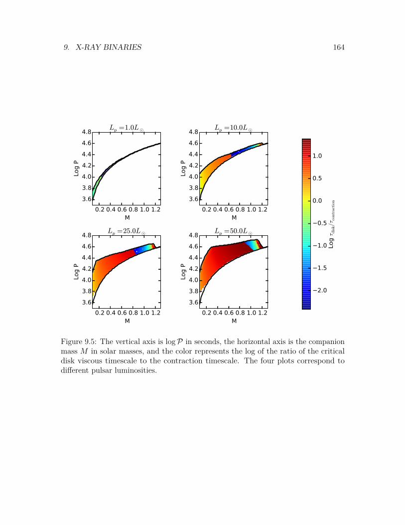
9. X-RAY BINARIES 164
0.2 0.4 0.6 0.8 1.0 1.2M
3.6
3.8
4.0
4.2
4.4
4.6
4.8
Log P
Lp =1.0L¯
0.2 0.4 0.6 0.8 1.0 1.2M
3.6
3.8
4.0
4.2
4.4
4.6
4.8
Log P
Lp =10.0L¯
0.2 0.4 0.6 0.8 1.0 1.2M
3.6
3.8
4.0
4.2
4.4
4.6
4.8
Log P
Lp =25.0L¯
0.2 0.4 0.6 0.8 1.0 1.2M
3.6
3.8
4.0
4.2
4.4
4.6
4.8
Log P
Lp =50.0L¯
2.0
1.5
1.0
0.5
0.0
0.5
1.0
Log τ
dis
k/τ
contr
action
Figure 9.5: The vertical axis is logP in seconds, the horizontal axis is the companionmass M in solar masses, and the color represents the log of the ratio of the criticaldisk viscous timescale to the contraction timescale. The four plots correspond todifferent pulsar luminosities.

9. X-RAY BINARIES 165
corresponding timescale for expansion when the pulsar turns on is the same toleading order12.
To investigate the properties of these limit cycles, we begin by computing τspread,as it is the only timescale of interest which we have not determined. To that end,suppose that we have a disk with inner radius Ri and outer radius equal to thecompanion orbital radius R0. The area of the disk is then
A = π(R2
0 −R2i
), (9.70)
and the accretion luminosity is
La = GMpM
Ra
, (9.71)
whereRa ≡
R0 +Ri
2 (9.72)
is the mean radius. If the disk thermally equilibrates on timescales short relative toτspread, as we will verify is the case, then
T =(La
2Aσ
)1/4. (9.73)
We will later verify that Σ monotonically approaches its equilibrium value, suchthat our prior calculations showing that the surface and interior temperatures ofequilibrium disks applies here as well. Assuming this for the moment, we find thatthe viscous timescale for the disk is
τvisc = R20ν
= 3πR20vsΣ
Mfv0, (9.74)
where v0 is mean orbital speed, vs is the mean sound speed, Σ is the mean columndensity, and f is given by
f ≡(
1−√Ri
R0
)1/4
. (9.75)
In the limit where R0 −Ri R0, we may write
R0 −Ri = εR0. (9.76)12There is a small discrepancy due to the changed thermal properties of the star, but this is
irrelevant at the level of estimation being used here.

9. X-RAY BINARIES 166
In this regime,
f =(ε
2
)1/4(9.77)
A = 2πR20ε (9.78)
vsvs,0
=(A
A0
)−1/8= (2ε)−1/8, (9.79)
where vs,0 is the equilibrium mean sound speed and vs is the instantaneous meansound speed. Using these approximations, as well as our expression in Eq. (9.48) forτdisk, we may expand τvisc as
τvisc = 123+1/8 τdiskε
−11/8, (9.80)
where τdisk is the timescale for the equilibrium disk at this M . Note that in performingthis expansion, we made use of the fact that the mean orbital radius and mean soundspeed both depend on ε. The differential equation for the evolution of ε is therefore
∂tε = 23+1/8τ−1diskε
11/8, (9.81)
and henceε =
(ε−3/80 − 3× 21/8 t
τdisk
)−8/3. (9.82)
Setting this equal to unity, we see that
τspread
τdisk= ε
−3/80 − 13× 21/8 . (9.83)
This method of solution is justified by the fact that τvisc diverges at small ε, and hencewe may focus on the time spent in that regime. Now typically we expect ε0, whichmeasures the initial disk width in units of R0, to be comparable to the atmosphericscale height of the companion. This is given by Rbv
2s/v
20, so
ε0 = Rb
R0
(vsv0
)2= 0.46
(M
M +Mp
)1/3 (vsv0
)2. (9.84)
For an order of magnitude estimate, we note that M ∼ M, Mp ≈ 2M, andvs ∼ v0/10, giving ε0 ∼ 1/300. As a result, we may write simply
τspread
τdisk≈ 2
5
( M
M +Mp
)1/3 (vsv0
)2−3/8
. (9.85)

9. X-RAY BINARIES 167
This tells us that the spreading time always exceeds the equilibrium disk viscous time.The factor by which this occurs is typically of order a few, and so does not changethe conclusion that the accretion rate does not change substantially from the criticalvalue before the heating turns off.
To tie up loose ends, we now must verify some assumptions. First, consider thequestion of the monotonicity of Σ. We may write
Σ = ∂
∂t
(Ma
A
)= M
A− MaA
A2 = Σ (∂t lnMa − ∂t lnA) , (9.86)
where Ma is the disk mass. Now initially ∂t lnA is roughly τ−1spread and ∂t lnMa
is infinite. Thus Σ begins positive. Now Ma increases monotonically, so ∂t lnMa
decreases monotonically if M is fixed. This decrease ends with a sharp drop tozero, coinciding with the time when the increase in A ends, as then the steady-state is achieved. Right before that time, Ma = Mτspread, so at all times beforethis ∂t lnMa ≥ τ−1
spread. As a result, Σ is monotonically increasing in time prior toequilibrium being established.
Next consider the question of thermal equilibration. The relevant dimensionlessquantity of interest is Macp∂tT/La, where the time derivative is computed assumingthermal equilibrium. If the magnitude of this is less than unity then it is valid toassume thermal equilibrium. The rate at which T changes is given by
∂tT = −14T∂t lnA = − T
4τspread. (9.87)
As a result, our dimensionless quantity is roughly Mav2s/4La. The numerator is
maximized in equilibrium, where Ma = Mτspread, for v2s ∝ T ∝ A−1/4, whereas
Ma = ΣA scales at least as A, as Σ increases monotonically in A. The denominator ismaximized initially, as La ∝ R−1
a , so we may upper bound the quantity of interest by
τspreadv2sR0
4GMp
. (9.88)
For an order of magnitude estimate, R0 ∼ 1011cm, v2s ≤ 3×1010cm2/s2,Mp ∼ 4×1034g,
4G ∼ 3× 10⁻⁷cm3/g/s2, so this quantity is at most 3× 10⁻⁷τspreads−1. From the lastsection, we know that τdisk ∼ 3× 10⁵s, so really we are interested in the quantity
250
( M
M +Mp
)1/3 (vsv0
)2−3/8
. (9.89)

9. X-RAY BINARIES 168
We may determine the maximum value of v0/vs by setting this equal to unity, givinga ratio of 2000. Typically v0/vs is at most 100, so we are safe in assuming thermalequilibrium.
Having determined that the spreading time exceeds the equilibrium viscous time,and having satisfied our various assumptions, we note that there are three possiblelimit cycle cases to consider:
1. τspread > τdisk > τM,L
2. τspread > τM,L > τdisk
3. τM,L > τspread > τdisk
We have not included τM in these orderings because it is only relevant in determininghow long the cycle takes to begin, and because it is typically much larger than theother three timescales.
Examining the timescales involved, we may classify regions of phase space intothe different kinds of limit cycle. This is done in figure 9.6. The first thing to noteabout this plot is that as the pulsar luminosity increases, the low mass companionslose the possibility of a type 2 cycle. This results from the adjustment of the upperradiative zone increasing with Lp, thereby reducing τM,L. That the type 2 cycles alsodisappear as we go to higher M at fixed Lp results from the deepening of the upperradiative layer as we approach the main sequence line.
The transition from type 1 to type 3 around 0.6M is due to the shrinkageand eventual disappearance of the heating-induced radiative zone. The radiative-convective transition is set by the condition that ∇ad = ∇rad. In the upper layers ofthe star, this requires that the escaping luminosity be Lesc Lin, which makes thetransition quite sharp. Additionally, the transition depends on the microphysics ofopacity and ionization. These phenomena are often exponentially dependent on thethermal structure of the outer layers of the star, which further sharpens the change.
The transition from type 3 to type 2, and eventually to type 1 as M increases isjust due to the convection zone shrinking, which reduces τM,L by reducing the relevantthermal mass. The thermal mass goes roughly as the convective base pressure Pf tothe three-fifths power13. If we hold the period fixed, then to a good approximationR is fixed. As a result, the thermal mass just scales as M6/5. We expect that τM,Lwill be proportional to this. At the same time, the scale height is increasing, whichcounteracts this effect. We may compute the scaling as
hs = R0v2s
v0
2
∼ v2s ∝ T ∝ L1/4
R1/2 ∝M2.3/4
M0.9/2 ∝M0.13. (9.90)
13This is set by the adiabatic constant γ.

9. X-RAY BINARIES 169
0.2 0.4 0.6 0.8 1.0 1.2M
3.6
3.8
4.0
4.2
4.4
4.6
4.8
Log P
Lp =1.0L¯
0.2 0.4 0.6 0.8 1.0 1.2M
3.6
3.8
4.0
4.2
4.4
4.6
4.8
Log P
Lp =10.0L¯
0.2 0.4 0.6 0.8 1.0 1.2M
3.6
3.8
4.0
4.2
4.4
4.6
4.8
Log P
Lp =25.0L¯
0.2 0.4 0.6 0.8 1.0 1.2M
3.6
3.8
4.0
4.2
4.4
4.6
4.8
Log P
Lp =50.0L¯
Figure 9.6: The vertical axis is logP in seconds, the horizontal axis is the companionmass M in solar masses, and the color represents the type of limit cycle. Blue is type1, Green is type 2, Maroon is type 3. The four plots correspond to different pulsarluminosities.

9. X-RAY BINARIES 170
As this is a much lower power of M , we expect that τM,L ∝ hs/M6/5 will decrease as
we move to higher mass.Having established which kind of cycle occurs in which regime, it is worth con-
trasting the various kinds of cycles. The first case corresponds to the fast expansioncase. Based on figure 9.2, this case matters in a fairly wide regime. Here the limitcycle time is set by 2τspread + 2τM,L. This may be seen by noting that when accretionbegins, it takes time τspread for material to reach the pulsar. It then takes time τM,Lfor the accretion rate at the pulsar to reach the critical value, assuming that in theprevious cycle it reached the critical value. It then takes time τM,L for the accretion tohalt. Finally, it takes time τspread for the disk to clear, allowing the process to beginagain. The reason τspread is relevant here is that the disk is never near equilibriumat any stage of the process. Given the orderings of timescales, we make at most afactor of two error by writing the full timescale as 2τspread. Naively, one might expectthe corresponding overshoot in M to be exp (τspread/τM,L). In practice this is not thecase. To see why, note that τspread and τdisk both decrease with T , the latter as T−1/2
and the former as T−7/8. As a result, as T increases, the disk spreads faster, and sowhen τspread is considerably larger than τM,L, the increase in M will be that requiredto set the relevant timescale connecting the outer and inner portions of the disk toτM,L. As that timescale is τspread in this case, and as T ∝ M1/4 and τspread ∝ M−1,we see that M will increase by a factor of (τspread/τM,L)15/8 over the critical value.This typically involves just a few extra scale heights of motion, and so we do notexpect the timescale τM,L to be off by too much from the actual timescale over whichthe mass loss rate adjusts, and at any rate the limit cycle timescale is dominated byτspread, so any corrections to the adjustment timescale effect are not relevant.
Now consider the second case. Here the limit cycle time is set by τspread + τdisk +2τM,L. This may be seen by noting that when accretion begins, it takes time τspreadfor material to reach the pulsar. It then takes time τM,L for the accretion rate at thepulsar to reach the critical value, assuming that in the previous cycle it reached thecritical value. It then takes time τM,L for the accretion to halt. Finally, it takes timeτdisk for the disk to clear, allowing the process to begin again. To good approximation,given this ordering, we may simply say that the limit cycle takes time τspread, andthereby incur error of at most a factor of two given the large disparity between τspreadand τdisk. The overshoot is given by the same expression as in the first case, for oncemore the disk is out of equilibrium the entire time.
In the third case, the expansion is slow, and so the spreading time is irrelevant tothe overshoot. The limit cycle time is once more set by τspread + τdisk + 2τM,L. Giventhe ordering of timescales, we may approximate this as 2τM,L, and thereby at mosta 50% error. The overshoot in M is exp (τdisk/τM,L), for now τdisk is the timescale

9. X-RAY BINARIES 171
mediating the delay between the companion and the accretion onto the pulsar.In summary, then, we expect that there are three kinds of accretion disk limit
cycles which are unique to these illuminated companion systems. These cycles arecharacterized by the relative orderings of the companion atmospheric timescale, thecritical accretion disk formation timescale, and the equilibrium critical accretion diskviscous timescale. The cycles range in timescale from days to years, with on-off timestypically measured in days. The key difference between the cycles is generally theprocess modulating them, either atmospheric effects or disk dynamics, as well asthe scales of these effects. The luminosity of the accretion disk in each case is givenapproximately by the accretion luminosity of the mid-disk ring, and corresponds toa mass loss rate on the order of 1014±1g/s. This puts the accretion disk radiationsomewhere between the IR and soft X-Ray bands, depending on the precise systemparameters. The luminosity of the accreting material at the pulsar is therefore oforder 1035±1erg/s. This radiation is expected to be mostly X-Rays, as is typical ofaccreting magnetic neutron stars.

9. X-RAY BINARIES 172
ReferencesBrown, J. C. and C. B. Boyle. “An exploratory eccentric orbit ’Roche lobe’ overflow
model for recurrent X-ray transients”. In: Astronomy and Astrophysics 141 (Dec.1984), pp. 369–375 (cit. on pp. 145, 146).
Ferguson, Jason W. et al. “Low-Temperature Opacities”. In: The Astrophysical Journal623.1 (2005), p. 585. url: http://stacks.iop.org/0004-637X/623/i=1/a=585(cit. on p. 155).
King, A. R. et al. “Mass Transfer Cycles in Close Binaries with Evolved Companions”.In: The Astrophysical Journal 482 (June 1997), pp. 919–928. eprint: astro -ph/9701206 (cit. on p. 145).
Lynden-Bell, D. and J. E. Pringle. “The evolution of viscous discs and the origin ofthe nebular variables.” In: Monthly Notices of the Royal Astronomical Society 168(Sept. 1974), pp. 603–637 (cit. on p. 155).
Paczyński, B. “Envelopes of Red Supergiants”. In: Acta Astronomica 19 (1969), p. 1(cit. on pp. 158, 159).
— “Evolutionary Processes in Close Binary Systems”. In: Annual Review of Astron-omy and Astrophysics 9 (1971), p. 183. doi: 10.1146/annurev.aa.09.090171.001151 (cit. on p. 146).
Padmanabhan, T. Theoretical Astrophysics. Vol. 2. ISBN: 978-0521566315. CambridgeUniversity Press, 2001. Chap. 6 (cit. on p. 155).
Ritter, H., Z.-Y. Zhang, and U. Kolb. “Irradiation and mass transfer in low-masscompact binaries”. In: Astronomy and Astrophysics 360 (Aug. 2000), p. 969. eprint:astro-ph/0005480 (cit. on p. 145).
Unal Ertan. “Inner disk radius, accretion and the propeller effect in the spin-downphase of neutron stars”. In: (). eprint: http://arxiv.org/pdf/1504.03996v1.pdf (cit. on p. 154).

10
Accretion Induced Collapse
... being nine years old, I’m enthusiastic about a lot of things.– Thomas A. Tombrello1
Recently, a number of millisecond pulsars with white dwarf companions and higheccentricities have been discovered2. The observed eccentricities exceed the period-eccentricity relations for accreting red giants by several orders of magnitude3. It hasbeen proposed that these systems are a result of rotationally delayed accretion inducedcollapse4, though this model has difficulty explaining the relatively small magneticfields these pulsars are observed to have. It has also been proposed that these systemsare formed by the spin-up of an accreting neutron star with a circumbinary disk,but the lack of longer period systems of this sort, which support a higher M , runscounter to this model. Kozai encounters in triple star systems may also explain thesesystems, but the expected mass distribution of companions after one star is ejected issubstantially different than what is observed.
Here we propose a different model for the formation of high eccentricity millisecondpulsar-white dwarf systems. In this model, accretion from a red giant onto a white
1Thomas A. Tombrello. Caltech Oral History. Dec. 2012. url: http://resolver.caltech.edu/CaltechOH:OH_Tombrello_T.
2B. Knispel et al. “Einstein@Home Discovery of a PALFA Millisecond Pulsar in an EccentricBinary Orbit”. In: ArXiv e-prints (Apr. 2015). arXiv: 1504.03684 [astro-ph.HE].
3E. S. Phinney. “Pulsars as Probes of Newtonian Dynamical Systems”. In: Royal Society ofLondon Philosophical Transactions Series A 341 (Oct. 1992), pp. 39–75. doi: 10.1098/rsta.1992.0084.
4P. C. C. Freire and T. M. Tauris. “Direct formation of millisecond pulsars from rotationallydelayed accretion-induced collapse of massive white dwarfs”. In: Monthly Notices of the RoyalAstronomical Society 438 (Feb. 2014), pp. L86–L90. doi: 10 . 1093 / mnrasl/ slt164. arXiv:1311.3478 [astro-ph.SR].
173

10. ACCRETION INDUCED COLLAPSE 174
dwarf induces the dwarf’s collapse into a pulsar. The pulsar wind then irradiates thered giant, forcing it to bloat and lose its upper atmosphere on timescales shorter thanthe tidal circularization time.
In order for this to occur, the timescale over which the envelope is lost must beshort relative to the orbital circularization time, given as5
τc ∼(R0
R
)8 (Mc
Mp
)2 (Mp
Mc +Mp
)Mc
Menv
(R2Menv
Li
)1/3
. (10.1)
Letting Mp ∼ 2 and working in solar units, we find that
τc = 7× 10¹⁷s(M + 2)1/3P2/3
6R
8 (Mc
2
)2 ( 2Mc + 2
)Mc
Menv
(R2Menv
Li
)1/3
. (10.2)
At the end of the day, we want a white dwarf core left over with mass ∼ 0.25M, sowe set Mc = 0.25. This yields
τc = 2× 10¹⁶sP32/36 M−2/3
env R−22/3L−1/3i . (10.3)
In order for the red giant to have evolved in at most the age of the universe, we musthave Mc + Menv > 1, and in order to have red giants with a helium flash at all wemust have Mc +Menv < 2.56. Thus Menv is within a factor of two of M. As a result,we will write
τc = 2× 10¹⁶sP32/36 R−22/3L
−1/3i . (10.4)
If the envelope will be bloated away, the characteristic timescale for this process tooccur is
τe = MenvcpT
Le= 5× 10¹²sMR−2Li
Le, (10.5)
where Le is the luminosity arriving from the pulsar at the companion. Note that weare assuming that Li > Le in this analysis, such that all of the heat arriving at thecompanion is bottled up by its convective envelope. Further note that this timescalerelies on the fact that the scale height is approximately R, and hence we only needto achieve a bloating of a single scale height. Thus
τeτc
= 2.5× 10⁻⁴P−32/36 R16/3ML
4/3i L−1
e . (10.6)
5Phinney, op. cit.6Rudolf Kippenhahn, Alfred Weigert, and Achim Weiss. Stellar Structure and Evolution. Springer,
2012. isbn: 978-3-642-30304-3.

10. ACCRETION INDUCED COLLAPSE 175
Making use of Le = LpR2/R2
0 = LpR2(M + 2)−2/3P−4/3
4 , we see that
τeτc
= 10−1P−28/36 R10/3M(M + 2)2/3L
4/3i L−1
p . (10.7)
Now we may find Li by7
Li = 105.3(Mc/M)6
1 + 100.4(Mc/M)4 + 100.5(Mc/M)5 ∼ 50M−6. (10.8)
Likewise8,R = 3.7× 10³(Mc/M)4
1 + (Mc/M)3 + 1.75(Mc/M)4 ∼ 14M−4. (10.9)
Thusτeτc
= 10−4(P6
2
)−28/3 (M2
)−20.3(M + 2)2/3L−1
p . (10.10)
As a result, for the observed periods of ∼ 20days and total masses near M = 2M,the time for the envelope to be swept away, if it is swept away, is well below the orbitcircularization time.
Of course in order for this process to occur, the envelope must be lost in muchless than the timescale over which the core grows by fusion. Otherwise the envelopewill be replenished faster than it is lost. This timescale is given by9
dMc
dt∼ Li
0.007c2 → τf ∼0.007Mcc
2
Li∼ 2.5× 10¹⁴s
(M
2
)−6. (10.11)
By comparison, the timescale τe is
τe ∼ 5× 10¹⁵s(M
2
)11L−1p (M + 2)2/3P4/3
6 . (10.12)
The timescale ratio is therefore
τeτf
= 50(M
2
)17L−1p (M + 2)2/3
(P6
2
)4/3. (10.13)
7P. C. Joss, S. Rappaport, and W. Lewis. “The core mass-radius relation for giants - A newtest of stellar evolution theory”. In: The Astrophysical Journal 319 (Aug. 1987), pp. 180–187. doi:10.1086/165443.
8Ibid.9S. Refsdal and A. Weigert. “Shell Source Burning Stars with Highly Condensed Cores”. In:
Astronomy and Astrophysics 6 (July 1970), p. 426.
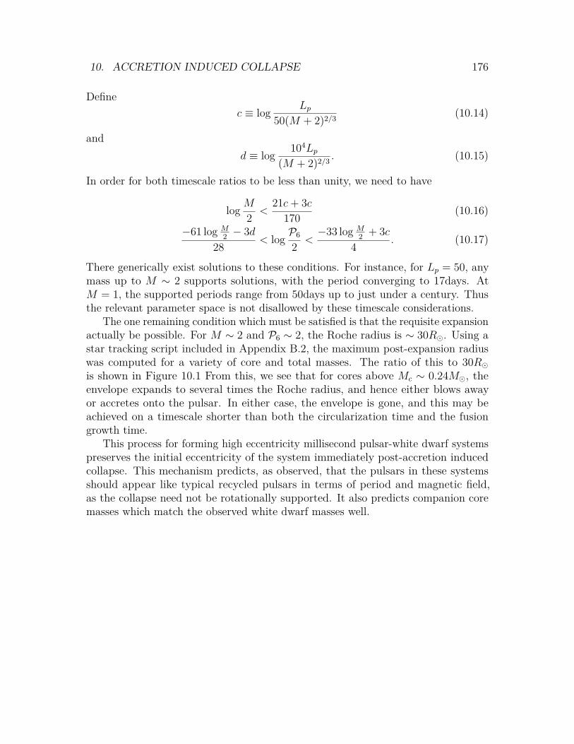
10. ACCRETION INDUCED COLLAPSE 176
Definec ≡ log Lp
50(M + 2)2/3 (10.14)
andd ≡ log 104Lp
(M + 2)2/3 . (10.15)
In order for both timescale ratios to be less than unity, we need to have
log M2 <21c+ 3c
170 (10.16)
−61 log M2 − 3d
28 < log P6
2 <−33 log M
2 + 3c4 . (10.17)
There generically exist solutions to these conditions. For instance, for Lp = 50, anymass up to M ∼ 2 supports solutions, with the period converging to 17days. AtM = 1, the supported periods range from 50days up to just under a century. Thusthe relevant parameter space is not disallowed by these timescale considerations.
The one remaining condition which must be satisfied is that the requisite expansionactually be possible. For M ∼ 2 and P6 ∼ 2, the Roche radius is ∼ 30R. Using astar tracking script included in Appendix B.2, the maximum post-expansion radiuswas computed for a variety of core and total masses. The ratio of this to 30Ris shown in Figure 10.1 From this, we see that for cores above Mc ∼ 0.24M, theenvelope expands to several times the Roche radius, and hence either blows awayor accretes onto the pulsar. In either case, the envelope is gone, and this may beachieved on a timescale shorter than both the circularization time and the fusiongrowth time.
This process for forming high eccentricity millisecond pulsar-white dwarf systemspreserves the initial eccentricity of the system immediately post-accretion inducedcollapse. This mechanism predicts, as observed, that the pulsars in these systemsshould appear like typical recycled pulsars in terms of period and magnetic field,as the collapse need not be rotationally supported. It also predicts companion coremasses which match the observed white dwarf masses well.

10. ACCRETION INDUCED COLLAPSE 177
0.20 0.22 0.24 0.26 0.28 0.30Mc (M¯)
1.0
1.2
1.4
1.6
1.8
2.0
2.2
2.4
M(M
¯)
0.4
0.6
0.8
1.0
1.2
1.4
1.6
1.8
2.0
Figure 10.1: The vertical axis is M/M, the horizontal axis is Mc/M, with bothaxes log-scaled. The color represents the ratio Rmax/30R, the denominator beingthe approximate Roche radius for the period and mass range of interest, and thenumerator being the post-expansion radius of the red giant of interest.
10. ACCRETION INDUCED COLLAPSE 178
ReferencesFreire, P. C. C. and T. M. Tauris. “Direct formation of millisecond pulsars from
rotationally delayed accretion-induced collapse of massive white dwarfs”. In:Monthly Notices of the Royal Astronomical Society 438 (Feb. 2014), pp. L86–L90.doi: 10.1093/mnrasl/slt164. arXiv: 1311.3478 [astro-ph.SR] (cit. on p. 173).
Joss, P. C., S. Rappaport, and W. Lewis. “The core mass-radius relation for giants -A new test of stellar evolution theory”. In: The Astrophysical Journal 319 (Aug.1987), pp. 180–187. doi: 10.1086/165443 (cit. on p. 175).
Kippenhahn, Rudolf, Alfred Weigert, and Achim Weiss. Stellar Structure and Evolu-tion. Springer, 2012. isbn: 978-3-642-30304-3 (cit. on p. 174).
Knispel, B. et al. “Einstein@Home Discovery of a PALFA Millisecond Pulsar inan Eccentric Binary Orbit”. In: ArXiv e-prints (Apr. 2015). arXiv: 1504.03684[astro-ph.HE] (cit. on p. 173).
Phinney, E. S. “Pulsars as Probes of Newtonian Dynamical Systems”. In: RoyalSociety of London Philosophical Transactions Series A 341 (Oct. 1992), pp. 39–75.doi: 10.1098/rsta.1992.0084 (cit. on pp. 173, 174).
Refsdal, S. and A. Weigert. “Shell Source Burning Stars with Highly CondensedCores”. In: Astronomy and Astrophysics 6 (July 1970), p. 426 (cit. on p. 175).
Tombrello, Thomas A. Caltech Oral History. Dec. 2012. url: http://resolver.caltech.edu/CaltechOH:OH_Tombrello_T (cit. on p. 173).

11
Spotted Black Widows
The universe is asymmetric and I am persuaded that life, as it is knownto us, is a direct result of the asymmetry of the universe or if its indirectconsequences.
– Louis Pasteur, Comptes Rendus de l’Acadmie des Sciences
In this chapter we will examine the question of observable thermal anisotropy inpulsar companions. The methods developes here are also of potential interest forexoplanets1 The objects under consideration will be either radiative or convective forΣ < Σh. We need not consider the in-between cases, as the transition in this regionbetween the two modes is sharp, and as whichever mode holds near the base of thisregion will dominate the heat transfer. Except for at low mass, all stars consideredwill be on the main sequence. For the deep convective stars, we will consider bothmain sequence objects and brown dwarfs with negligible intrinsic luminosity.
Throughout this chapter all masses, luminosities, fluxes, and distances will be1A. Roy, J. T. Wright, and S. Sigurðsson. “Earthshine on a Young Moon: Explaining the
Lunar Farside Highlands”. In: The Astrophysical Journal 788, L42 (June 2014), p. L42. doi:10.1088/2041- 8205/788/2/L42. arXiv: 1406.2020 [astro-ph.EP]; V. Parmentier, A. P.Showman, and Y. Lian. “3D mixing in hot Jupiters atmospheres. I. Application to the day/nightcold trap in HD 209458b”. In: Astronomy and Astrophysics 558, A91 (Oct. 2013), A91. doi:10.1051/0004-6361/201321132. arXiv: 1301.4522 [astro-ph.EP]; B. Hansen et al. Day andNight on Hot Jupiters. Spitzer Proposal. June 2005; A. P. Showman, K. Menou, and J. Y.-K. Cho.“Atmospheric Circulation of Hot Jupiters: A Review of Current Understanding”. In: Extreme SolarSystems. Ed. by D. Fischer et al. Vol. 398. Astronomical Society of the Pacific Conference Series.2008, p. 419. arXiv: 0710.2930; T. Kataria et al. “The Atmospheric Circulation of the Hot JupiterWASP-43b: Comparing Three-Dimensional Models to Spectrophotometric Data”. In: AAS/Divisionfor Planetary Sciences Meeting Abstracts. Vol. 46. AAS/Division for Planetary Sciences MeetingAbstracts. Nov. 2014, 104.03.
179

11. SPOTTED BLACK WIDOWS 180
given in solar units. Speeds will be given in cm/s, temperatures in K, and times inseconds. Subscript notation will be used, as usual, to denote an exponent to divideout.
11.1 SetupRecall from Chapter 7 that
∆FFi
= FeFi− 5y′T 3/2
4 R−1(
∆TT
)q ( 104l
2πR
)aRobsF−1
i , (11.1)
where the rightmost term is twice the flux transported by the wind. Once more Rosis the sonic Rossby number, l is the convective mixing length, Fe is the flux whichimpinges on the star averaged over the pulsar-facing (day) side, ∆F is the differencein the flux emerging from the day and night sides, Fi is the intrinsic flux, R is thecompanion radius, T4 is the mean surface temperature measured in units of 104K, anda, b, q, and y′ are dimensionless constants characteristic of the wind pattern of interest,to be determined self-consistently. Actually, as we learned in Chapter 8, this is notquite right on timescales shorter than the star’s thermal timescale, as convectionzones may absorb some of the external flux. Thus the relation really should be
∆FFi
= Fe − Fbottle
Fi− 5y′T 3/2
4 R−1(
∆TT
)q ( 104l
2πR
)aRobsF−1
i , (11.2)
where Fbottle is the bottled flux of the convection zone. We may solve this equation ifwe note that
T4 = 0.3(F
1/4day + F
1/4night
)(11.3)
and∆TT
= 2F
1/4day − F
1/4night
F1/4day + F
1/4day
. (11.4)
Note that we do not simplify this last expression yet, as we may need to deal with fluxanisotropies which push this relation outside of the linear regime. Further note thatbecause we have been more careful than before in letting T be the average surfacetemperature, we do not need to deal with the case of supersonic winds: the formalismautomatically precludes them. The day and night fluxes are related by
Fday − Fnight = ∆F, (11.5)Fday + Fnight = Fe + 2Fi − Fbottle, (11.6)

11. SPOTTED BLACK WIDOWS 181
As this quantity is uniquely determined by the flux carried by the wind, our equationis closed and may in principle be solved.
The first step to a solution is eliminating as many variables as possible. To thatend, note that
Ros = vs2πRΩ ≈ 0.012T 1/2
4 P4R−1, (11.7)
104l
2πR = 104v2s
2πRg ≈ 2T4RM−1, (11.8)
Fday = Fi + 12 (Fe − Fbottle + ∆F ) , (11.9)
Fnight = Fi + 12 (Fe − Fbottle −∆F ) , (11.10)
Fe = Lp2R2
0, (11.11)
R30P2
4= M + 2, (11.12)
where R0 is the orbital radius and is as usual measured in solar units. Note thatthe final relation here is only a good approximation at low orbital eccentricity. Athigh eccentricity, it gives the approximate mean distance, the inverse square of whichmay deviate somewhat from the relevant mean inverse square distance. To orderof magnitude, however, this should not matter significantly. Additionally, pulsar-companion systems are not generally expected or observed to have high eccentricities,so we will proceed with this approximation. Making use of these substitutions leavesas variables only Fbottle, ∆F , and the various dimensionless constants characteristicof the wind.
We now wish to compute the bottled flux in convective stars. For these objectsthere are two possibilities: either the flux reaching the convection zone exceeds theintrinsic flux, or it does not. If it does not exceed the intrinsic flux, then the factthat the non-irradiated ∇rad ∇ad implies that the star remains convective, andthe resulting stiffness of ∇ in L implies that the star’s surface temperature goesunchanged except over thermal timescales. As a result, when Fe < Fi, the full flux isbottled, giving Fbottle = Fe.
In the opposing case, where Fe > Fi, the irradiated side of the star should becomeradiative, as ∇rad becomes negative and hence trivially falls below the always-positive∇ad. This will once more bottle up heat and lead to swelling, but now some of theexcess Fe−Fi may escape, raising the surface temperature on the day side. This maythen drive a wind, heating the night side. As discussed in Chapter 7, this wind leads

11. SPOTTED BLACK WIDOWS 182
to an increase in the area over which the star bottles heat, such that the bottled heatis
Fbottle = A
4πR2Fi. (11.13)
The area fraction is given byA
4πR2 = min(
1, 12
(1 + W
Fi
)), (11.14)
where W is the flux transported by the winds. This relation, which effectively statesthat the winds organize to maximize bottling, fundamentally results from the windmoving more easily through radiative zones than through convection zones. Puttingall of this together, we see that
Fbottle = min(Fe, Fi min
(1, 1
2
(1 + W
Fi
))). (11.15)
Now we have all relevant quantities except for the wind constants. These may befound in Table 6.1. As the convection zone always has a significantly higher viscositythan the radiation zone, the winds will always move around any residual convectionzone. Thus we may focus on the radiative wind cases. There are mercifully only threeof these: ballistic, hurricanes, and Rhines. The decision between the first two is madebased on the Rossby number. This is a function of the flux anisotropy, of course, andso a solution must be found self-consistently. In cases where the criteria for Rhinesscaling are satisfied and where the full area of the star is radiative, this model is used.We require that the full star be radiative for this because Rhines transport works byforming continuous bands around the star.
The driving turbulence in the Rhines case is the primarily horizontal turbulencethat the wind itself produces. The condition we derived for this to occur is given byEq. (6.106) as
T4 > 100F(
∆TT
)2
Σ−1Ω−1−4, (11.16)
where F is the mean flux over the surface of the star and column density is measuredin units of Σh. This relation may also be written as
T4 > 16F(
∆TT
)2
Σ−1P4. (11.17)
Recalling that T4 here refers to the typical temperature for Σ < Σh, we may writeT4 ∼ 0.6F 1/4. This yields
1 > 25F 3/4(
∆TT
)2
Σ−1P4. (11.18)
11. SPOTTED BLACK WIDOWS 183
The best case scenario for this inequality is when Σ = Σh, which gives
1 > 25F 3/4(
∆TT
)2
P4. (11.19)
Fortunately we don’t need to consider the edge case where the inequality holds forsome Σ < Σh but not for all. This is because to leading order the majority of theheat is carried at larger Σ due to vs and ρ being so much greater. Thus we will ignorethe edge case, as the strong depth dependence of heat transport makes the transitionbetween Rhines and non-Rhines transport sharp. Note that κ, the opacity, is requiredto compute y′ for Rhines scaling. In the majority of the heating zone these stars arehot enough to fully ionize, so we may use the Kramer opacity2
κ1 ∼ 4× 10¹⁰(1 +X)(Z + 10−3) ρ0
T 3.54, (11.20)
where κ1 is the opacity measured in units of 10cm2/g and where we will generallyuse X ∼ 1 and Z ∼ 10−2. The full expression may be evaluated by making use of therelation
ρ = P/v2s = Σg/v2
s . (11.21)
11.2 Main Sequence SolutionsThe equations described in the previous section are nonlinear and involve many cases.As a result, a numerical approach was used rather than an analytic one. The completecode used may be found in Appendix D. The space of possible systems was discretizedin Lp, P, and M . The discretization in Lp was done with the usual four values of1, 10, 25, 50L, with dense grids in the other quantities. This grid was then expandedto include as a dimension ∆F/Fi. This dimension scales from 0 to Fe/Fi, with 0prepended to an exponentially spaced grid.
The main sequence scaling laws were used to fill in R and Li. The specific relationsused were3
Li =
24−3.6M3.6 if 2 < M < 20M4 if 0.43 < M < 20.434−2.3M2.3 if 0.08 < M < 0.43
(11.22)
2Bradley W. Carroll. An Introduction to Modern Astrophysics. Vol. 1. Addison-Wesley, 1996,p. 274.
3Maurizio Salaris and Cassisi Santi. Evolution of stars and stellar populations. Vol. 1. ISBN:0-470-09220-3. John Wiley Sons, 2005, pp. 138–140; O. Demircan and G. Kahraman. “Stellarmass-luminosity and mass-radius relations”. In: Astrophysics and Space Science 181 (July 1991),pp. 313–322. doi: 10.1007/BF00639097.

11. SPOTTED BLACK WIDOWS 184
and
R =
20.72−0.57M0.57 if 2 < M < 20M0.57 if 0.08 < M < 2
(11.23)
Masses from 0.08M to 20M were considered, with the lower end chosen due toits role in separating the main sequence from brown dwarfs4. Periods ranging from3 × 103s up to 107s were considered. This range was chosen to capture all of therelevant physics after examining several different ranges.
At each point in the grid, the dominant kind of wind transport was computed,and from this the squared violation of the anisotropy relation. As the area fractiondepends on W , and W depends on the area fraction through T , an iterative approachwas used, treating the area fraction first as 0, computing W , then updating A, thenupdating W , and so on. This method converges in only a few iterations due to thesmall allowed range for A.
The wind calculations were handled carefully in these numerics. The number ofcases was reduced by smoothly interpolating between ballistic and hurricane winds.This was done because these cases do not precisely match at their boundary asparametrized. The interpolation was done by letting each of a, b, q, and y′ vary astanh(Ro)2. The tanh function was chosen because an exponential variation is expected.This was squared because Ro depends on v = |v|, and the physical constructionsdepending on a single vector are generally even rather than odd. Note that theRossby number was computed as
Ro = v
2πRΩ . (11.24)
Rhines scaling was examined at each grid point, but never produced self-consistentsolutions. This is due to Rhines scaling being more prevalent at low P, but beingunable to carry the increased flux associated with the companion being closer to thepulsar.
Note that we must filter for companions with Roche radii exceeding their mainsequence radii. This is done by noting that the Roche radius for such stars is5
Rb =(
0.38 + 0.2 log M2
)R0 =
(0.38 + 0.2 log M2
)(M + 2)1/3P2/3
4 . (11.25)
4D. J. Stevenson. “The search for brown dwarfs”. In: Annual Review of Astronomy andAstrophysics 29 (1991), pp. 163–193. doi: 10.1146/annurev.aa.29.090191.001115.
5B. Paczyński. “Evolutionary Processes in Close Binary Systems”. In: Annual Review ofAstronomy and Astrophysics 9 (1971), p. 183. doi: 10.1146/annurev.aa.09.090171.001151;P. P. Eggleton. “Approximations to the radii of Roche lobes”. In: The Astrophysical Journal 268(May 1983), p. 368. doi: 10.1086/160960.

11. SPOTTED BLACK WIDOWS 185
Below the Roche cutoff we get into murky territory. Radiative stars, as well assome convective ones, are often catastrophically unstable in this regime. Should acase below the Roche cutoff be of interest, nothing precludes applying the methodsdescribed here below the cutoff.
Using all of these results, we may finally compute the anisotropy. Figure 11.1shows the ratio Fday/Fnight over the mass and radius range of interest. This decreasesas P increases, for this corresponds to the companion being placed further from thepulsar. It also increases as the pulsar luminosity increases, again in accordance withexpectations. Similarly, as the companion mass increases, this ratio decreases. This isbecause the scaling relations indicate that Fi increases with M , for Li increases fasterthan R2. The maximum anisotropy is quite large, of order several hundred. This isbecause at low M , Fe may be thousands of times Fi, a difference which significantlyexceeds the heat transport capacity of even a sonic wind.
At first glance, it appears that only low-period low-mass convective companionsexhibit interesting anisotropy physics, with a small blip near M = 2. To dispel thisnotion, we turn to the quantity ∆F/F , shown in Figure 11.2. In this plot, whiteregions above the Roche cutoff are those where ∆F = 0 due to complete heat bottling.It is apparent that there are three distinct regions here. First, there is the convectiveregime on the left where not all of Fe is bottled. This corresponds to the significantanisotropy we saw in Figure 11.1. The size of this region depends on Lp as expected,as it is easier to have unbottled heat with higher values of Fe.
On the right there is the radiative regime where no heat is bottled. The anisotropyis small in this regime cases, peaking at a few percent, just at the edge of what canbe observed. Note that the transition between the white region and the radiativeone is shown as being infinitely sharp here. This is not quite accurate; there is anexponential transition as the convection zone disappears. This transition is coupledto the timescale of interest; as the convection zone disappears, the timescale overwhich heat bottling occurs drops, until in the radiative case it reaches the thermaltimescale for the heating layer. As a result the precise smearing is not well defined,and the relevant physics is well represented by a sharp boundary.
The data presented thus far say little directly about the effect of winds. Therelevant quantities here are the difference between the anisotropy with and withoutwinds. To that end, Figure 11.3 shows the ratio Fday/(Fi + Fe). This is what weexpect observation to see. The ratio deviates most from unity near the bottlingboundary. This is just a result of the bottled heat being a maximum possible fractionof Fe + Fi at this boundary.
To examine the effect of the wind on the day side separately, we now considerthe quantity W/(Fi + Fe). This is shown for the day side in Figure 11.4. Here we

11. SPOTTED BLACK WIDOWS 186
10-1 100 101
104
105
106
107
P (
s)
Lp =1
10-1 100 101
104
105
106
107 Lp =10
10-1 100 101
M (M¯)
104
105
106
107
P (
s)
Lp =25
10-1 100 101
M (M¯)
104
105
106
107 Lp =50
0.00
0.15
0.30
0.45
0.60
0.75
0.90
1.05
logF
day/Fnight
Figure 11.1: The vertical axis is P in seconds, the horizontal axis is the companionmass in solar masses, with both axes log-scaled. The color represents the log ofthe day/night flux ratio logFday/Fnight. The four different plots correspond to fourdifferent pulsar luminosities. The black line corresponds to the Roche cutoff.

11. SPOTTED BLACK WIDOWS 187
10-1 100 101
104
105
106
107
P (
s)
Lp =1
10-1 100 101
104
105
106
107 Lp =10
10-1 100 101
M (M¯)
104
105
106
107
P (
s)
Lp =25
10-1 100 101
M (M¯)
104
105
106
107 Lp =50
8
7
6
5
4
3
2
1
0
log∆F/F
Figure 11.2: The vertical axis is P in seconds, the horizontal axis is the companionmass in solar masses, with both axes log-scaled. The color represents the log of theday/night flux ratio log ∆F/F . The four different plots correspond to four differentpulsar luminosities. The black line corresponds to the Roche cutoff. The white regionsabove the Roche cutoff have ∆F = 0 due to heat bottling.

11. SPOTTED BLACK WIDOWS 188
10-1 100 101
104
105
106
107
P (
s)
Lp =1
10-1 100 101
104
105
106
107 Lp =10
10-1 100 101
M (M¯)
104
105
106
107
P (
s)
Lp =25
10-1 100 101
M (M¯)
104
105
106
107 Lp =50
0.42
0.36
0.30
0.24
0.18
0.12
0.06
0.00
logF
day/
(Fe+Fi)
Figure 11.3: The vertical axis is P in seconds, the horizontal axis is the companionmass in solar masses, with both axes log-scaled. The color represents the log of theday/night flux ratio logFday/(Fi + Fe). The four different plots correspond to fourdifferent pulsar luminosities. The black line corresponds to the Roche cutoff.

11. SPOTTED BLACK WIDOWS 189
10-1 100 101
104
105
106
107
P (
s)
Lp =1
10-1 100 101
104
105
106
107 Lp =10
10-1 100 101
M (M¯)
104
105
106
107
P (
s)
Lp =25
10-1 100 101
M (M¯)
104
105
106
107 Lp =50
45
40
35
30
25
20
15
10
5
0
logW
/(Fi+Fe)
Figure 11.4: The vertical axis is P in seconds, the horizontal axis is the companionmass in solar masses, with both axes log-scaled. The color represents the log of theday/night flux ratio logW/(Fi + Fe). The four different plots correspond to fourdifferent pulsar luminosities. The black line corresponds to the Roche cutoff. Notethat the white region above the Roche cutoff corresponds to the case W = 0

11. SPOTTED BLACK WIDOWS 190
see that the winds transport up to ∼ 10% of the flux. Except for the dimmest Lpconsidered, the transported fraction is not maximized when P is minimized as onemight expect. This is because at low P the winds are solidly in the hurricane regime,where the transported flux goes as P3. Thus a balance between maximizing ∆F/Fand maximizing P is struck. In the case of very low Lp, the optimum does actuallyoccur at the minimum P , but this is because the Fe curve is pushed down in P untilit runs up against the Roche cutoff.
On the night side, the relevant ratio is Fnight/Fi, as we need not worry abouthandling bottled flux in the denominator, and this is the directly observable quantity.This ratio is shown in Figure 11.5. Here we see that the winds make a tremendousdifference, up to a factor of 30. Here we see the maximum impact made at thelowest P values. The difference between the day side and the night side in thisregard is entirely that the night side’s windless flux does not become greater as Feincreases, and so the function being maximized looks like FeP3(∆F/F )q rather thanFeP3(∆F/F )q.
If this analysis were done on the swollen stars discussed in the X-ray binarycontext, the key difference would be that R would not match the main sequence.This has the effect of pushing the radiative-convective boundary towards lower M ,with the fully-swollen stars being radiative at all M . In that limit, the bottled fluxvanishes and the swelling ceases. An interesting extension of this work would be tocouple the code which computes swelling to the code which computes anisotropy todetermine the difference that wind transport makes to the swelling timescale. Thiseffect is unlikely to change the estimated order of magnitude of the swelling time, sowe neglect it here.
11.3 Brown DwarfsBrown dwarfs typically have 10−2 < M < 0.08 and so are not nuclear burning.This means that there is no mass-radius or mass-luminosity relation for browndwarfs, as these properties are history-dependent. Importantly, if heating changes theupper atmospheric boundary condition, the core luminosity adjusts on the convectivetimescale of a few decades. This, combined with Fi generally being of order 10−3,means that the core luminosity is not a relevant variable. Rather, we ought to view

11. SPOTTED BLACK WIDOWS 191
10-1 100 101
104
105
106
107
P (
s)
Lp =1
10-1 100 101
104
105
106
107 Lp =10
10-1 100 101
M (M¯)
104
105
106
107
P (
s)
Lp =25
10-1 100 101
M (M¯)
104
105
106
107 Lp =50
0.0
0.2
0.4
0.6
0.8
1.0
1.2
1.4
1.6
logF
night/Fi
Figure 11.5: The vertical axis is P in seconds, the horizontal axis is the companionmass in solar masses, with both axes log-scaled. The color represents the log of theday/night flux ratio logFnight/Fi. The four different plots correspond to four differentpulsar luminosities. The black line corresponds to the Roche cutoff.
11. SPOTTED BLACK WIDOWS 192
the outer boundary conditions as being set by the illumination. To be quantitative,
Fday = Fi + 12 (Fe − Fbottle + ∆F ) = 1
2(Fe + ∆F ), (11.26)
Fnight = Fi + 12 (Fe − Fbottle −∆F ) = 1
2(Fe −∆F ). (11.27)
Note that we have dropped Fbottle, as it is bounded above by Fi. The wind equationmay now be written as
∆F = Fe − 5y′T 3/24 R−1
(∆TT
)q ( 104l
2πR
)aRobs. (11.28)
Noting that
Ros = vs2πRΩ ≈ 0.012T 1/2
4 P4R−1, (11.29)
104l
2πR = 104v2s
2πRg ≈ 2T4RM−1, (11.30)
(11.31)
we find that
∆F = Fe − 5y′T 3/24 R−1
(∆TT
)q (2T4RM
−1)a (
0.012T 1/24 P4R
−1)b. (11.32)
This may also be written as
Fday = 0.4y′(F
1/4day + F
1/4night
)R−1
2F
1/4day − F
1/4night
F1/4day + F
1/4day
q (2T4RM−1)a (
0.012T 1/24 P4R
−1)b.
(11.33)If we assume that hurricanes are the dominant transport mechanism, then
∆F = Fe −5T 3
4P34
106R4
(∆TT
)5
. (11.34)
Now note thatT4 ∼ 0.6
(Fe2
)1/4. (11.35)
This is true to within 40% in the Fi → 0 limit regardless of ∆F . Thus
∆F = Fe −2.5F 3/4
e P34
106R4
(∆TT
)5
= Fe
1− 4P10/34
106L1/4p R4
(∆TT
)5 . (11.36)

11. SPOTTED BLACK WIDOWS 193
This may also be written as
∆FFe
= 1− χ(
∆TT
)5
, (11.37)
where
χ = 4P10/34
106L1/4p R4
= P10/34
25L1/4p R4
−1. (11.38)
There is now only one relevant parameter, χ. The solutions for ∆F/Fe and Fday/Fnightas functions of χ are shown in Figure 11.6. Low values of χ, corresponding to shortorbital periods and bright pulsars, exhibit unbounded anisotropies. As χ increasespast unity, the anisotropy drops rapidly. Noting that R−1 is close to the smallestradius a brown dwarf can achieve6, we see that for the pulsar luminosities of interestthe small-χ regime is characterized by P < 3× 10⁴s.
It is worth noting that in all cases, the wind speed is comparable to the soundspeed, for ∆T/T is of order unity for these objects so long as Fe Fi. As a result,the Rossby number is just the sonic Rossby number to good approximation. Thismay be written as
Ros ∼Lp
40R−1P1/34
. (11.39)
Thus the hurricane model holds down to periods of
P ∼ 150(Lp10
)3s. (11.40)
Given that these objects cannot have periods much less than 3× 10³s, we expect anyregions where the Rossby number exceeds unity to be small enough that extrapolationfrom the hurricane regime is appropriate. Note that the condition for Rhines scalingreduces in this case to
4 > 25L3/4p
(∆TT
)2
. (11.41)
This is unlikely to be satisfied, given that ∆T ∼ T .In summary, we have computed the anisotropy of flux between the pulsar-facing
(day) and night side of both main sequence and brown dwarf stars. These results6Adam Burrows et al. “The theory of brown dwarfs and extrasolar giant planets”. In: Rev. Mod.
Phys. 73 (3 Sept. 2001), pp. 719–765. doi: 10.1103/RevModPhys.73.719. eprint: http://arxiv.org/pdf/astro-ph/0607583. url: http://link.aps.org/doi/10.1103/RevModPhys.73.719;Stevenson, op. cit.

11. SPOTTED BLACK WIDOWS 194
-2 2 4 6 8Log[χ ]
0.2
0.4
0.6
0.8
1.0
ΔF/Fe
-2 2 4 6 8Log[χ ]
0.5
1.0
1.5
2.0
2.5
Log[Fday /Fnight ]
Figure 11.6: Top: ∆F/Fe is shown as a function of logχ. Bottom: logFday/Fnight isshown as a function of logχ.

11. SPOTTED BLACK WIDOWS 195
deviate substantially in many cases from the usual predicted black body values. Thisis a result of our use of a realistic wind transport model. It is worth noting thatthese results depend on the flux of high energy particles Lp, as well as on their energy,which determines the absorption column density. The former we have carried aroundas an explicit functional dependence, while the latter we have set to a specific value.These calculations may be redone at any Σ, however. To leading order, the wind fluxgoes as Σ1+3∇/2, with the dependence on ∇ arising from averaging T 3/2 ∼ v3
s over theheating depth. As the dependence on Lp is distinct from the dependence on Σ, a seriesof observations of different systems may reveal Σ, so long as any interdependencebetween the total power output of the pulsar and the individual particle energiesis known. This model, therefore, allows us to place an additional constraint on thepulsar wind, but does not on its own tell us everything that there is to know.

11. SPOTTED BLACK WIDOWS 196
ReferencesBurrows, Adam et al. “The theory of brown dwarfs and extrasolar giant planets”.
In: Rev. Mod. Phys. 73 (3 Sept. 2001), pp. 719–765. doi: 10.1103/RevModPhys.73 . 719. eprint: http : / / arxiv . org / pdf / astro - ph / 0607583. url: http ://link.aps.org/doi/10.1103/RevModPhys.73.719 (cit. on p. 193).
Carroll, Bradley W. An Introduction to Modern Astrophysics. Vol. 1. Addison-Wesley,1996, p. 274 (cit. on p. 183).
Demircan, O. and G. Kahraman. “Stellar mass-luminosity and mass-radius relations”.In: Astrophysics and Space Science 181 (July 1991), pp. 313–322. doi: 10.1007/BF00639097 (cit. on p. 183).
Eggleton, P. P. “Approximations to the radii of Roche lobes”. In: The AstrophysicalJournal 268 (May 1983), p. 368. doi: 10.1086/160960 (cit. on p. 184).
Hansen, B. et al. Day and Night on Hot Jupiters. Spitzer Proposal. June 2005 (cit. onp. 179).
Kataria, T. et al. “The Atmospheric Circulation of the Hot Jupiter WASP-43b: Com-paring Three-Dimensional Models to Spectrophotometric Data”. In: AAS/Divisionfor Planetary Sciences Meeting Abstracts. Vol. 46. AAS/Division for PlanetarySciences Meeting Abstracts. Nov. 2014, 104.03 (cit. on p. 179).
Paczyński, B. “Evolutionary Processes in Close Binary Systems”. In: Annual Reviewof Astronomy and Astrophysics 9 (1971), p. 183. doi: 10.1146/annurev.aa.09.090171.001151 (cit. on p. 184).
Parmentier, V., A. P. Showman, and Y. Lian. “3D mixing in hot Jupiters atmospheres.I. Application to the day/night cold trap in HD 209458b”. In: Astronomy andAstrophysics 558, A91 (Oct. 2013), A91. doi: 10.1051/0004-6361/201321132.arXiv: 1301.4522 [astro-ph.EP] (cit. on p. 179).
Roy, A., J. T. Wright, and S. Sigurðsson. “Earthshine on a Young Moon: Explainingthe Lunar Farside Highlands”. In: The Astrophysical Journal 788, L42 (June 2014),p. L42. doi: 10.1088/2041-8205/788/2/L42. arXiv: 1406.2020 [astro-ph.EP](cit. on p. 179).
Salaris, Maurizio and Cassisi Santi. Evolution of stars and stellar populations. Vol. 1.ISBN: 0-470-09220-3. John Wiley Sons, 2005, pp. 138–140 (cit. on p. 183).
Showman, A. P., K. Menou, and J. Y.-K. Cho. “Atmospheric Circulation of HotJupiters: A Review of Current Understanding”. In: Extreme Solar Systems. Ed. byD. Fischer et al. Vol. 398. Astronomical Society of the Pacific Conference Series.2008, p. 419. arXiv: 0710.2930 (cit. on p. 179).

11. SPOTTED BLACK WIDOWS 197
Stevenson, D. J. “The search for brown dwarfs”. In: Annual Review of Astronomyand Astrophysics 29 (1991), pp. 163–193. doi: 10.1146/annurev.aa.29.090191.001115 (cit. on pp. 184, 193).

12
Banded Stars
The goal of this chapter is to examine the case where spontaneous atmospheric bandingoccurs in an axisymmetric star. This effect has been seen in limited circumstances insimulations1, though analytic understanding has proven elusive. Though this does notrelate to the question of pulsar-companion interactions, the possibility is suggestedby our analysis in Chapter 6.
To begin, we are interested in lone stars which are axisymmetric and do notexperience external heating. Recall that
kfr =
√√√√ ΩRvφ
=√
1Rl, (12.1)
kβ =(
Ω3
R3ε
)1/5
=(
Ω3
R3v2φN
)1/5
=(
ΩR3lvcr
)1/5
. (12.2)
The criterion for the Rhines cascade to be in effect is that kβ > kfr, so
1R5l5
<Ω2
R6l2v2cr
(12.3)
∴v2cr
l3<
Ω2
R. (12.4)
1U. R. Christensen. “Zonal flow driven by strongly supercritical convection in rotating spher-ical shells”. In: Journal of Fluid Mechanics 470 (Nov. 2002), pp. 115–133. doi: 10 . 1017 /S0022112002002008.
198

12. BANDED STARS 199
The critical Ω at which the star cannot hold itself together is Ωcrit ≈√g/R. Thus
v2cr
l3<
(Ω
Ωcrit
)2g
R2 (12.5)
∴F 2/3
ρ2/3l3<
(Ω
Ωcrit
)2g
R2 . (12.6)
(12.7)
The rotation rate is often close to criticality for stars of mass outside the range[0.5, 2.0]M. This is because stars below this range do not have substantial windswith which to spin down, while those above it lack the convectively-driven magneticfield needed to exert a substantial torque2. Letting Ω = Ωcrit then yields
F 2ρ−2l−9R6g−3 < 1. (12.8)
This may also be written assF 2(GM)6
R6P 4C< 1, (12.9)
where Ts is the surface temperature and C ≡ P 5ρ−7 is the constant determining thepolytrope of interest. We may estimate this using the central density and pressure.The central density is roughly twice the average, and the central pressure is roughly3
Pc ∼ 2ρavggavgR = 2 3M4πR3
(GM
R2
)R = 3GM2
2πR4 . (12.10)
Thus
C = P 5ρ−7 =(
2πR3
3M
)7 (3GM2
2πR4
)5
= 4π2
9 G5M3R. (12.11)
Using this, our condition becomes
9F 2GM3
4π2P 4R7 < 1, (12.12)
orP > 2× 10⁹F 1/2M3/4R−7/4, (12.13)
2J. B. Stauffer and L. W. Hartmann. “The rotational velocities of low-mass stars”. In:Astronomical Society of the Pacific, Publications 98 (Dec. 1986), pp. 1233–1251. doi: 10.1086/131926.
3E. Böhm-Vitense. Introduction to Stellar Astrophysics. Vol. 3. ISBN 0521344042. CambridgeUniversity Press, 1992.

12. BANDED STARS 200
where P is measured in erg/cm3 and the remaining quantities are all in solar units.Given the scaling of the quantities on the right, we expect most objects exhibitingspontaneous banding near the surface to be low-mass stars. Using the scaling relationsfor mass and luminosity for this sort of object as well as the fact that M ∝ R forM < M we find4
P > 3× 10⁸M−0.85. (12.14)This may be phrased in terms of Σ in the thin-envelope limit as
Σ > 104M0.15. (12.15)
Note that in this derivation we have assumed that the object remains nuclear burning.From this it is clear that convection alone can drive a banded structure. The numberof bands is expected to be
n = Rkβ =(
ΩR2
lvc
)1/5
. (12.16)
In the low mass stars which exhibit these properties, Ω ∼ 10−4s−1, vc ∼ 104cm/s,l ∼ 108cm, and R ∼ 1010cm, so n ∼ 10.
As a result of all of this, our first prediction regarding these stars is that theywill be banded, and that the depth of the bands will be roughly 3× 10³g/cm2. Thenumber of bands ought to be on the order of 10. In many cases this is close enoughto the photosphere that the structure may reasonably be expected to be observable.While it will be difficult to observe this structure using doppler spread measurements,the case is somewhat better if there is a transiting planet. As the planet blocks adifferent portion of the star at different times, and may be tracked across the star, thechange in the doppler spread over the course of the transit may be used to determinethe presence of bands.
In addition, for Jupiter-type planets the bands will be much more easily visible.With F ∼ 10−6F, M ∼ 10−3M, and R ∼ 10−1R, the lower bound on Σ is just250g/cm2. At and near optical frequencies this is well above the photosphere, and soshould be observable. The expected number of bands for a cold Jupiter is similar towhat we expect for stars5. The precise number may be computed via Eq. (12.16). Forhot Jupiters, the temperature anisotropy dominates over the spontaneous banding
4Maurizio Salaris and Cassisi Santi. Evolution of stars and stellar populations. Vol. 1. ISBN:0-470-09220-3. John Wiley Sons, 2005, pp. 138–140.
5Roughly half of the driving force for Jupiter’s bands comes from its temperature asymmetry.The remainder comes from convective anisotropy. Thus these objects should have a similar numberof bands to Jupiter, with somewhat faster rotation but no temperature anisotropy

12. BANDED STARS 201
effect. Once more transiting objects such as moons provide an easier test than justmeasuring the doppler spread.

12. BANDED STARS 202
ReferencesBöhm-Vitense, E. Introduction to Stellar Astrophysics. Vol. 3. ISBN 0521344042.
Cambridge University Press, 1992 (cit. on p. 199).Christensen, U. R. “Zonal flow driven by strongly supercritical convection in rotating
spherical shells”. In: Journal of Fluid Mechanics 470 (Nov. 2002), pp. 115–133.doi: 10.1017/S0022112002002008 (cit. on p. 198).
Salaris, Maurizio and Cassisi Santi. Evolution of stars and stellar populations. Vol. 1.ISBN: 0-470-09220-3. John Wiley Sons, 2005, pp. 138–140 (cit. on p. 200).
Stauffer, J. B. and L. W. Hartmann. “The rotational velocities of low-mass stars”. In:Astronomical Society of the Pacific, Publications 98 (Dec. 1986), pp. 1233–1251.doi: 10.1086/131926 (cit. on p. 199).

Appendices
203

Appendix A
Viscosity Code
The code used to interpolate the viscosity of a star is shown below. It makes use of tabulated data1 aswell as analytic results2, choosing between them based on the range of validity of each. Within the rangeof the tabular data, multilinear interpolation in temperature and log-pressure space is used. Above themaximum temperature covered by this table, which roughly aligns with the bottom edge of validity ofthe analytic results, the analytic results are used. There are regions at low temperature and very highpressure where neither result is valid, and in these the code returns the IEEE NaN value. Note that thiscode requires Python, NumPy, and SciPy, and was tested with versions 2.7, 1.9.0, and 0.14.0 respectively.
Viscosity Interpolation Code: viscosity.py
1 import numpy as np2 import cons tant s3 from sc ipy . i n t e r p o l a t e import Regu la rGr id Inte rpo la to r45 naan = f l o a t ( ’ nan ’ )67 va lue s = np . array ( [8 34 . 1 , 34 . 1 , 34 . 1 , 34 . 1 , 34 . 1 , 34 . 1 , 34 . 1 , 34 . 1 , naan , naan , naan , naan ,9 38 . 1 , 38 . 1 , 38 . 1 , 38 . 1 , 38 . 1 , 38 . 1 , 38 . 1 , 38 . 1 , naan , naan , naan , naan ,
10 43 . 5 , 43 . 5 , 43 . 5 , 43 . 5 , 43 . 5 , 43 . 5 , 43 . 5 , 43 . 5 , 43 . 5 , naan , naan , naan ,11 51 . 5 , 51 . 5 , 51 . 5 , 51 . 5 , 51 . 5 , 51 . 5 , 51 . 5 , 51 . 5 , 51 . 5 , naan , naan , naan ,12 52 . 7 , 62 . 6 , 62 . 0 , 63 . 2 , 63 . 2 , 63 . 2 , 63 . 2 , 63 . 2 , 63 . 2 , naan , naan , naan ,13 12 . 5 , 16 . 2 , 22 . 4 , 31 . 3 , 44 . 5 , 56 . 4 , 66 . 3 , 82 . 2 , 82 . 5 , naan , naan , naan ,14 3 . 98 , 7 . 61 , 12 . 2 , 15 . 9 , 18 . 6 , 23 . 6 , 32 . 1 , 61 . 2 , 85 . 8 , naan , naan , naan ,15 2 . 84 , 3 . 05 , 3 . 26 , 3 . 56 , 4 . 83 , 9 . 67 , 21 . 5 , 27 . 8 , 61 . 3 , 97 . 1 , 117 , naan ,16 4 . 74 , 6 . 31 , 6 . 80 , 7 . 29 , 7 . 87 , 8 . 46 , 9 . 24 , 13 . 3 , 29 . 1 , 79 . 6 , 109 , 159 ,17 9 . 76 , 10 . 3 , 10 . 9 , 11 . 6 , 12 . 5 , 14 . 1 , 17 . 3 , 26 . 7 , 33 . 0 , 46 . 1 , 100 , 163 ,18 22 . 0 , 23 . 2 , 24 . 4 , 25 . 8 , 27 . 4 , 28 . 6 , 30 . 7 , 37 . 5 , 52 . 6 , 86 . 6 , 119 , 185 ,19 47 . 9 , 50 . 8 , 53 . 3 , 56 . 1 , 59 . 7 , 63 . 3 , 67 . 3 , 77 . 4 , 91 . 2 , 112 , 198 , 28420 ] ) # dynamic v i s c o s i t y2122 theta = np . array (23 [ 1 . 4 , 1 . 2 , 1 . 0 , 0 . 8 , 0 . 6 , 0 . 4 , 0 . 3 , 0 . 2 , 0 . 15 , 0 . 1 , 0 . 07 , 0 . 0 5 ] )24 t s = 5040 . / theta25 tmax = max( t s )26 logp = np . array ( [ 3 , 3 . 5 , 4 , 4 . 5 , 5 , 5 . 5 , 6 , 7 , 8 , 9 , 10 , 1 1 ] )
1F. N. Edmonds Jr. “The Coefficients of Viscosity and Thermal Conductivity in the Hydrogen Convection Zone.” In:The Astrophysical Journal 125 (Mar. 1957), p. 535. doi: 10.1086/146327.
2Daniel Kagan and J. Craig Wheeler. “The Role of the Magnetorotational Instability in the Sun”. In: The AstrophysicalJournal 787.1 (2014), p. 21. url: http://stacks.iop.org/0004-637X/787/i=1/a=21.
204

APPENDIX A. VISCOSITY CODE 205
27 in t e rp = Regu la rGr id Inte rpo la to r ( ( ts , logp ) ,np . reshape ( values , ( 1 2 , 1 2 ) ) , bounds_error=False ,f i l l _ v a l u e=np . nan )
2829 de f i n t e r p o l a t e ( t , p , rho ) :30 re turn 1e−5∗ i n t e rp (np . t ranspose ( [ t , np . log10 (p) ] ) ) / rho3132 de f loglam ( t , rho ) :33 d0 = −17.4 + 1 .5 ∗ np . l og ( t ) − 0 .5 ∗ np . l og ( rho )34 d1 = −12.7 + np . l og ( t ) − 0 .5 ∗ np . l og ( rho )35 boo l a r r = 1 .0 ∗ ( t < 1 .1 e5 ∗ np . ones ( t . shape ) )36 re turn d0 ∗ boo l a r r + d1 ∗ (1 − boo l a r r )373839 de f s p i t z e r ( t , rho ) :40 re turn 5 .2 e−15 ∗ np . power ( t , 5 . / 2) / ( rho ∗ loglam ( t , rho ) )4142 de f o v e r a l l ( t , p , rho , kappa , an i s=1) :43 t = np . array ( t )44 p = np . array (p)45 rho = np . array ( rho )46 # Fir s t , produce nu from actua l data47 d0 = i n t e r p o l a t e ( t , p , rho )48 # Next , compute Sp i t z e r va lue s49 d1 = s p i t z e r ( t , rho )50 # Replace Sp i t z e r va lue s with NaN i f they aren ’ t above the i o n i z a t i o n zone51 d1 [ t <10∗∗4.1] = np . nan52 # Replace data va lue s with Sp i t z e r va lue s i f they are NaN53 d0 [ np . i snan ( d0 ) ] = d1 [ np . i snan ( d0 ) ]54 d0∗=an i s55 re turn d05657 q = 4.80320451 e−1058 c = 29979245800.59 de f i s o t r op i cB ( t , p , rho ,mu) :60 nu = ov e r a l l ( t , p , rho )61 re turn 3∗p∗mu∗c /( rho∗q∗nu)

APPENDIX A. VISCOSITY CODE 206
ReferencesEdmonds Jr., F. N. “The Coefficients of Viscosity and Thermal Conductivity in the Hydrogen Convection
Zone.” In: The Astrophysical Journal 125 (Mar. 1957), p. 535. doi: 10.1086/146327 (cit. on p. 204).Kagan, Daniel and J. Craig Wheeler. “The Role of the Magnetorotational Instability in the Sun”. In: The
Astrophysical Journal 787.1 (2014), p. 21. url: http://stacks.iop.org/0004-637X/787/i=1/a=21(cit. on p. 204).

Appendix B
Acorn Stellar Integration Code
B.1 Opal and Ferguson Opacity Table ParserTo support the Acorn stellar integration code, modern tables of the Rosseland mean opacity were neededover a wide range of temperatures and densities. In particular, at low temperatures molecular effectsbecome significant, something opacity tables have historically lacked. For this purpose, an interpolationroutine was written which uses the OPAL1 and Ferguson2 opacity tables. The former is good at hightemperature, the latter at low temperature. The OPAL Type 1 and Ferguson 05 tables were used withthe GS98 solar composition for this purpose, though other choices are also valid. The code used in thisroutine is shown below, along with an example of its usage. Note that interpolation proceeds first overstellar composition (X and Y ) and then over log T and the factor logR, defined as log ρ− 3 log T6, whereρ is in cgs units and T6 is defined as the temperature measured in units of 106K. When R exceeds themaximum tabulated R, the maximum tabulated R is used instead. This was found to not matter inmost cases, as it only occurred well within highly efficient convection regions where the opacity is largelyirrelevant. Multilinear interpolation is used at each step, and the output is the logarithm of the opacity.Note that this code requires Python, NumPy, and SciPy, and was tested with versions 2.7, 1.9.0, and0.14.0 respectively.
Opacity Interface (opacity.py)
1 import s c ipy . i n t e r p o l a t e as s i n2 import numpy as np3 import os45 de f i n t e rp ( data , x0 , y0 ) :6 # Now we ’ re going to assume that rRange and tRange are the same ac ro s s a l l t a b l e s .7 # Fi r s t , i n t e r p o l a t e the 2D R vs . T gr id a c ro s s the X,Y va lues o f i n t e r e s t .8 x = [ i [ 0 ] f o r i in data ]9 y = [ i [ 1 ] f o r i in data ]
10 z = [ i [ 4 ] f o r i in data ]11 tab l e = s i n . g r iddata ( ( x , y ) , z , ( x0 , y0 ) )12 re turn tab l e1314 de f b i l i n e a r_ i n t e r p o l a t o r ( data , xPts , yPts ) :
1C. A. Iglesias and F. J. Rogers. “Updated Opal Opacities”. In: The Astrophysical Journal 464 (June 1996), p. 943.doi: 10.1086/177381.
2Jason W. Ferguson et al. “Low-Temperature Opacities”. In: The Astrophysical Journal 623.1 (2005), p. 585. url:http://stacks.iop.org/0004-637X/623/i=1/a=585.
207

APPENDIX B. ACORN STELLAR INTEGRATION CODE 208
15 return s i n . Regu la rGr id Inte rpo la to r ( ( xPts , yPts ) , data , bounds_error=False , f i l l _ v a l u e=np .nan )
1617 c l a s s opac :1819 de f __init__( s e l f , opalName , fergName , x , y ) :20 s e l f . a = opacInt ( opalName , x , y , " opal " )21 s e l f . b = opacInt ( fergName , x , y , " f e r g " )2223 de f opac i ty ( s e l f , t , rho ) :24 i f not i s i n s t a n c e ( t , np . ndarray ) :25 op = s e l f . b . opac i ty ( t , rho ) [ 0 , 0 ]26 i f np . i snan ( op ) :27 op = s e l f . a . opac i ty ( t , rho ) [ 0 , 0 ]28 e l s e :29 op = s e l f . b . opac i ty ( t , rho )30 whereNan = np . where (np . i snan ( op ) )31 op [ whereNan ] = s e l f . a . opac i ty ( t [ whereNan [ 0 ] ] , rho [ whereNan [ 1 ] ] )32 re turn op3334 de f dkdT( s e l f , t , rho , eps=1e−3) :35 k0 = 10∗∗ s e l f . opac i ty ( t∗(1− eps ) , rho )36 k1 = 10∗∗ s e l f . opac i ty ( t ∗(1+eps ) , rho )37 re turn ( k1−k0 ) /(2∗ t ∗ eps )3839 de f dkdRho( s e l f , t , rho , eps=1e−3) :40 k0 = 10∗∗ s e l f . opac i ty ( t , rho∗(1− eps ) )41 k1 = 10∗∗ s e l f . opac i ty ( t , rho∗(1+eps ) )42 re turn ( k1−k0 ) /(2∗ rho∗ eps )434445 c l a s s opacInt :4647 de f __init__( s e l f , fname , x , y , opalFerg ) :48 s e l f . c u t o f f = 049 s e l f . data = None50 i f opalFerg==" opal " :51 s e l f . c u t o f f = 1052 s e l f . data = readOpalTables ( fname )53 e l i f opalFerg==" f e r g " :54 s e l f . c u t o f f = 1255 s e l f . data = readFergTables ( fname )56 e l s e :57 r a i s e Exception ( "No tab l e type s p e c i f i e d . " )58 s e l f . interpData = in t e rp ( s e l f . data , x , y )59 s e l f . i n t e r p o l a t o r = b i l i n e a r_ i n t e r p o l a t o r ( s e l f . interpData , s e l f . data [ 0 ] [ 3 ] , s e l f .
data [ 0 ] [ 2 ] )6061 de f opacityTR ( s e l f , t , r ) :62 t t = np . copy ( t )63 t t [ tt <600] = 600 .64 t t = np . log10 ( t t )65 r = np . log10 ( r )66 r = np . array ( r )67 r [ r >1] = 0 .9968 k = s e l f . i n t e r p o l a t o r (np . dstack ( ( tt , r ) ) )69 k [ np . i snan (k ) ] = 2∗ s e l f . c u t o f f

APPENDIX B. ACORN STELLAR INTEGRATION CODE 209
70 k [ k>s e l f . c u t o f f ] = np . nan # Each tab l e has a maximum value , so t h i s cuts o f fi n t e r p o l a t i o n there
71 re turn k7273 de f opac i ty ( s e l f , t , rho ) :74 r = rho / ( t ∗ 1e−6) ∗∗ 375 return s e l f . opacityTR ( t , r )7677 # Method f o r read ing in non−enr i ched OPAL tab l e s ( i . e . j u s t X,Y,Z are78 # nonzero , no dXc or dXo) . Tested on l a t e s t ( as o f August 2014)79 # GS98 compos it ion t ab l e s .808182 de f readOpalTables ( fname ) :83 f = open ( fname )84 # checks i f we ’ re in the zone where the t ab l e s are ( as opposed to the85 # header )86 t ab l e s = False87 x = 088 y = 0 # note that z = 1−x−y by d e f i n i t i o n89 data = [ ]90 f o r l i n e in f :91 l i n e = l i n e . r s t r i p ( ’ \n ’ ) # remove newl ines92 i f t ab l e s and l en ( l i n e ) > 2 : # e l im ina t e s empty l i n e s93 i f ’TABLE’ in l i n e : # reads in x , y , z f o r the t ab l e94 s = l i n e . r ep l a c e ( ’=’ , ’ ’ ) . s p l i t ( ’ ’ )95 f o r i , a in enumerate ( s ) :96 i f a == ’X ’ :97 x = f l o a t ( s [ i + 1 ] )98 e l i f a == ’Y ’ :99 y = f l o a t ( s [ i + 1 ] )100 data . append ( [ x , y , [ ] , [ ] , [ ] ] )101 e l i f ’ logT ’ in l i n e : # reads in the logR va lue s f o r the t ab l e102 s = l i n e . s p l i t ( ’ ’ )103 rRange = [ f l o a t ( a ) f o r a in s [ 1 : ] i f l en ( a ) > 0 ]104 data [ −1 ] [ 2 ] = rRange105 e l i f ’R ’ not in l i n e : # reads in the tab l e106 s = l i n e . s p l i t ( ’ ’ )107 s = [ i f o r i in s i f l en ( i ) > 0 ]108 t = f l o a t ( s [ 0 ] )109 s = s [ 1 : ]110 data [ − 1 ] [ 3 ] . append ( t )111 data [ − 1 ] [ 4 ] . append ( [ ] )112 f o r i , a in enumerate ( s ) :113 data [ −1 ] [ 4 ] [ −1 ] . append ( f l o a t ( a ) )114 i f l en ( s ) < len ( data [ − 1 ] [ 2 ] ) :115 f o r i in range ( l en ( data [ − 1 ] [ 2 ] ) − l en ( s ) ) :116 data [ −1 ] [ 4 ] [ −1 ] . append (1 e10 ) # absurd value117 i f ’ ∗∗∗∗∗∗∗∗∗∗∗∗∗∗∗∗∗∗∗∗∗∗∗∗∗∗ ’ in l i n e :118 t ab l e s = True119 f o r i in range ( l en ( data ) ) :120 data [ i ] [ 4 ] = np . array ( data [ i ] [ 4 ] )121 re turn data122 # Note that the re i s some redundancy , as rRange and tRange are expected to123 # be the same f o r each tab l e . We l eave the par s e r more genera l , however , as the124 # wasted space i s minimal .125

APPENDIX B. ACORN STELLAR INTEGRATION CODE 210
126 # Method f o r read ing in Ferguson t ab l e s . Tested on l a t e s t ( as o f August 2014)127 # GS98 compos it ion t ab l e s .128129130 de f readFergTable ( fname , x , y ) :131 # These t ab l e s are pre−s p l i t by (X,Z) value , so we can j u s t f o cus on the132 # read ing part .133 f = open ( fname )134 # We’ re i n t e n t i o n a l l y keeping the format the same as the opa lParser format .135 data = [ x , y , [ ] , [ ] , [ ] ]136 f o r l i n e in f :137 l i n e = l i n e . r s t r i p ( ’ \n ’ ) # remove newl ines138 i f ’ l og T ’ in l i n e : # reads in the logR va lue s f o r the t ab l e139 s = l i n e . s p l i t ( ’ ’ )140 rRange = [ f l o a t ( a ) f o r a in s [ 2 : ] i f l en ( a ) > 0 ]141 data [ 2 ] = rRange142 # reads in the tab l e143 e l i f ’R ’ not in l i n e and l en ( l i n e ) > 1 and ’Grev ’ not in l i n e :144 s = l i n e145 t = f l o a t ( s [ : 5 ] )146 s s = [ ]147 counter = 6148 whi l e counter < len ( s ) :149 s s . append ( s [ counter : counter + 7 ] )150 counter += 7151 data [ 3 ] . append ( t )152 data [ 4 ] . append ( [ ] )153 # Now we need to f i l t e r f o r columns which merged due to Fortran154 # formatt ing155 s = s s156 f o r i , a in enumerate ( s ) :157 data [ 4 ] [ − 1 ] . append ( f l o a t ( a ) )158 i f l en ( s ) < len ( data [ 2 ] ) :159 f o r i in range ( l en ( data [ 2 ] ) − l en ( s ) ) :160 data [ 4 ] [ − 1 ] . append (1 e10 ) # absurd value161 data [ 4 ] = np . array ( data [ 4 ] )162 data [ 4 ] = data [ 4 ] [ : : − 1 ]163 data [ 3 ] = np . array ( data [ 3 ] )164 data [ 3 ] = data [ 3 ] [ : : − 1 ]165 re turn data166167168 de f readFergTables ( dirName ) :169 data = [ ]170 f o r f i l ename in os . l i s t d i r ( dirName ) :171 s = f i l ename [ 4 : ] # remove the ’ g ’ from the beg inning172 s = s . s p l i t ( ’ . ’ )173 x = f l o a t ( s [ 0 ] ) / 10 ∗∗ l en ( s [ 0 ] )174 z = f l o a t ( s [ 1 ] ) / 10 ∗∗ l en ( s [ 1 ] )175 y = 1 − x − z176 data . append ( readFergTable ( ( dirName + f i l ename ) , x , y ) )177 re turn data
Usage Example (opacityTest.py)
1 import numpy as np2 import matp lo t l i b . pyplot as p l t
APPENDIX B. ACORN STELLAR INTEGRATION CODE 211
3 from opac i ty import ∗4 a = opac ( ’ . . / OpacityTables /Opal/GS98 . txt ’ , ’ . . / OpacityTables /Ferguson/ f05 . gs98 / ’ , 0 . 7 ,
0 . 2 8 )5 tRan = [10 ∗∗ ( i / 2 0 . ) f o r i in range (60 , 180) ]6 rRan = [10 ∗∗ ( i / 2 0 . ) f o r i in range (−200 , 120) ]7 t , r = np . meshgrid ( tRan , rRan )8 z = a . opac i ty ( t , r )9 bigR = r /( ( t /1 e6 ) ∗∗3)
10 z [ bigR>10] = np . nan11 p r i n t t . shape12 p r i n t r . shape13 p r i n t z14 p r i n t z . shape15 p l t . imshow ( z , extent =[3 , 9 , −10, 6 ] , o r i g i n=’ lower ’ , a spect =0.3)16 cb = p l t . c o l o rba r ( )17 cb . s e t_ labe l ( ’ l og $\kappa$ ’ )18 p l t . y l ab e l ( ’ l og $\\ rho$ ’ )19 p l t . x l ab e l ( ’ l og T ’ )20 p l t . show ( )21 cs = p l t . contour f (np . log10 ( tRan ) , np . log10 ( rRan ) , z )2223 cb . s e t_ labe l ( ’ l og $\kappa$ ’ )24 p l t . y l ab e l ( ’ l og $\\ rho$ ’ )25 p l t . x l ab e l ( ’ l og T ’ )26 p l t . show ( )
B.2 Stellar Integration CodeThe thermodynamics functions from the Gob stellar integration code3 were translated into Python, andsubsequently into Cython. This is the first file shown below. The next file contains caching routines whichprecompute the equation of state and perform high-speed vectorized interpolation. These routines havebeen verified to an accuracy of one part in 104, though higher accuracy may be achieved by adjustingthe various resolution parameters they accept. The third file simply contains various physical constants.The fourth file contains both a steady-state stellar integrator and a time-dependent stellar code. Theseprovide an interface which accepts as input the macroscopic stellar quantities such as luminosity, externalillumination, mass, and radius, and computes the steady-state structure. From there, the time-dependentcode may be used to evolve the star, accepting a new external illumination at each time step. The nextfile provides an example of the usage of the whole package. The next three files provide the addon usedto compute self-consistent companion radii as well as the scripts which call it and analyze the resultingoutput. The final two files provide a caller script and analyzer script for examining accretion inducedcollapse in red giant systems. Note that this code requires Python, Cython, gcc, NumPy, and SciPy, andwas tested with versions 2.7, 0.21, 4.9.0-20130929, 1.9.0, and 0.14.0 respectively.
Thermodynamic Methods (gob.pyx)
1 #cython : c d i v i s i o n=True2 #cython : in f e r_types=True3 import numpy as np4 from numpy import exp5 from numpy import sq r t
3B. Paczyński. “Envelopes of Red Supergiants”. In: Acta Astronomica 19 (1969), p. 1.

APPENDIX B. ACORN STELLAR INTEGRATION CODE 212
6 from sc ipy . i n t e r p o l a t e import gr iddata78 # Use fu l cons tant s9 # −−−−−−− s e t the va lue s o f c r i t i c a l d e n s i t i e s f o r p r e s su r e i o n i z a t i o n :
10 # " rhc1 " , " rhc2 " , " rhc3 "11 # −−−−−−− the value o f c r i t i c a l second helium i o n i z a t i o n : " hel im2 "12 # −−−−−−− and the average charge o f " metals " : " zav " .13 cde f double rhc l 1 = −1.014 cde f double rhc l 2 = −0.515 cde f double rhc l 3 = 0 .016 cde f double he2l im = 0.9917 cde f double zav = 10 .018 cde f double rhc1 = 10 .0 ∗∗ rh c l 119 cde f double rhc2 = 10 .0 ∗∗ rh c l 220 cde f double rhc3 = 10 .0 ∗∗ rh c l 32122 # p = pre s su r e ( cgs )23 # ro = dens i ty ( cgs )24 # u = energy dens i ty per un i t mass ( cgs )25 # x = hydrogen mass f r a c t i o n26 # y = helium mass f r a c t i o n27 # Returns p , u , as we l l as28 # xh1 hydrogen i o n i z a t i o n f r a c t i o n29 # xhe1 helium f i r s t i o n i z a t i o n f r a c t i o n30 # xhe2 helium second i o n i z a t i o n f r a c t i o n313233 cde f energ ( double ro , double t , double x , double y ) :34 # rhc1 , rhc2 , rhc3 are c r i t i c a l d e n s i t i e s f o r " p r e s su r e i o n i z a t i o n "35 cde f double t e ta = 5040 . / t36 cde f double dm = 2.30258537 cde f double tm = 1 / te ta / dm38 cde f double l o g t = np . log10 ( t )39 cde f double mue = ( 1 . + x ) / 2 .40 cde f double h = 1.6734 e−2441 cde f double nh = x ∗ ro / h42 cde f double nhe = 0.25 ∗ y ∗ ro / h43 cde f double nmet = 1 . / zav / 2 . ∗ ( 1 . 0 − x − y ) ∗ ro / h44 # Assume metals f u l l y i on i z ed45 cde f double nmetel = nmet ∗ zav46 cde f double ne = 0 .047 cde f double nhi = nh48 cde f double nh i i = 0 .049 cde f double nhei = nhe50 cde f double nh e i i = 0 .51 cde f double n h e i i i = 0 .52 cde f double xh1 = 0 .053 cde f double xhe1 = 0 .054 cde f double xhe2 = 0 .055 cde f double f ac1 = 0 .056 cde f double f ac2 = 0 .057 cde f double f ac3 = 0 .058 # Hydrogen i o n i z a t i o n59 cde f double h i1 = 13.59560 cde f double h i = hi1 ∗ (1 − ro / rhc1 ∗ (1 + tm / hi1 ) )61 cde f double f h l = np . log10 (nh)62 cde f double b10 = 15.3828 + 1 .5 ∗ l o g t − hi ∗ t e t a − f h l

APPENDIX B. ACORN STELLAR INTEGRATION CODE 213
63 i f b10 > 10 . 0 :64 b10 = 10 .065 i f b10 > −10:66 b = 10 .0 ∗∗ b1067 c = b68 fac1 = c ∗ nh69 bc = 0 .5 ∗ b / c70 xx = 1 .0 / ( sq r t ( bc ∗ bc + 1 .0 / c ) + bc )71 # xx i s the p o s i t i v e root o f equat ion : xx∗∗2 + b∗xx − c = 072 xx1 = 1 .0 − xx73 i f xx1 < 1 .0 e−10:74 xx1 = 1 .0 e−1075 nh i i = nh ∗ xx76 ne = nh i i77 nhi = nh ∗ xx178 xh1 = xx79 # Helium i o n i z a t i o n80 hi2 = 24.58081 h i = hi2 ∗ (1 − ro / rhc2 ∗ (1 + tm / hi2 ) )82 f h e l = np . log10 ( nhe )83 b10 = 15.9849 + 1 .5 ∗ l o g t − hi ∗ t e t a − f h e l84 i f b10 > 10 . 0 :85 b10 = 10 .086 i f b10 > −10:87 c = 10 .0 ∗∗ b1088 b = c + ne / nhe89 fac2 = c ∗ nhe90 bc = 0 .5 ∗ b / c91 xx = 1 .0 / ( sq r t ( bc ∗ bc + 1 .0 / c ) + bc )92 xx1 = 1 .0 − xx93 i f xx1 < 1e−10:94 xx1 = 1e−1095 nh e i i = nhe ∗ xx96 ne = ne + nhe i i97 nhei = nhe ∗ xx198 xhe1 = xx99 # Second Helium i o n i z a t i o n100 hi3 = 54.403101 h i = hi3 ∗ (1 − ro / rhc2 ∗ (1 + tm / hi3 ) )102 f h e l = np . log10 ( nh e i i )103 b10 = 15.3828 + 1 .5 ∗ l o g t − hi ∗ t e t a − f h e l104 i f b10 > 10 :105 b10 = 10106 i f b10 > −10:107 c = 10 .0 ∗∗ b10108 b = c + ne / nhe i i109 fac3 = c ∗ nhe i i110 bc = 0 .5 ∗ b / c111 xx = 1 .0 / ( sq r t ( bc ∗ bc + 1 .0 / c ) + bc )112 xx1 = 1 .0 − xx113 i f xx1 < 1e−10:114 xx1 = 1e−10115 n h e i i i = nhe i i ∗ xx116 ne = ne + nh e i i i117 nh e i i = nhe i i ∗ xx1118 xhe2 = xx119 f1 = fac1 / ne

APPENDIX B. ACORN STELLAR INTEGRATION CODE 214
120 f2 = fac2 / ne121 f3 = fac3 / ne122 f4 = nh / ne123 f5 = y / 4 / x124 zz = 1 .0125 zz = f z z ( zz , f1 , f2 , f3 , f4 , f 5 )126 ne = ne ∗ zz127 xh1 = f1 / (1 + f1 )128 xhe1 = f2 / (1 + f2 ∗ (1 + f3 ) )129 xhe2 = xhe1 ∗ f 3130 nhi = nh ∗ (1 − xh1 )131 nh i i = nh ∗ xh1132 nhei = nhe ∗ (1 − xhe1 − xhe2 )133 nh e i i = nhe ∗ xhe1134 n h e i i i = nhe ∗ xhe2135 nh2 = 0 .0136 i f nhi > 0.001 ∗ nh and t < 20000:137 f a c = 28.0925 − t e t a ∗ (4 .92516 − t e t a ∗ (0 .056191 + te ta ∗ 0 .0032688) ) − l o g t138 i f t < 12000 :139 f a c = fac + ( t − 12000) / 1000 .140 f a c = exp (dm ∗ f a c )141 i f f a c > 1e−20 ∗ nhi :142 b = fac / nhi143 bc = 0 .5144 xx = 1 .0 / ( sq r t ( bc ∗ bc + 1 .0 / b) + bc )145 nh2 = 0 .5 ∗ nhi ∗ (1 − xx )146 nhi = nhi ∗ xx147 e l s e :148 nh2 = 0 .5 ∗ nhi149 nhi = 0 .0150 # Correc t ion f o r s l i g h t e l e c t r on degeneracy151 nedgen = ( nmetel + ne ) ∗ ( 1 . + 2 .19 e−2 ∗ ( ro / mue) ∗ ( t / 1 . e6 ) ∗∗ (−1.5) )152 nt = nh − nh2 + nhe + nedgen + nmet153 pg = 1.3805 e−16 ∗ nt ∗ t154 pr = 2.521922460548802 e−15∗ t ∗∗4155 p = pg + pr156 uh2 = t ∗ ( 2 . 1 + t ∗ 2 .5 e−4)157 i f t > 3000 :158 uh2 = −1890. + t ∗ ( 3 . 36 + t ∗ 0 .4 e−4)159 u = (1 . 5 ∗ pg + 3 . ∗ pr + 1.3805 e−16 ∗ nh2 ∗ uh2 + 3.585 e−12 ∗ nhi + 25 .36 e−12 ∗ nh i i
+160 39 .37 e−12 ∗ nhe i i + 126 .52 e−12 ∗ n h e i i i ) / ro161 re turn p , u , xh1 , xhe1 , xhe2162163 # input :164 # zz = a guess o f c o r r e c t i n g f a c t o r to the e l e c t r on dens i ty (=1.0)165 # f1 , f2 , f 3 = i o n i z a t i o n f a c t o r s d iv ided by e l e c t r on dens i ty166 # f4 = number dens i ty o f hydrogen ions and atoms / e l e c t r on number dens i ty167 # f5 = r a t i o o f helium to hydrogen nu c l e i168 # output :169 # zz = the i t e r a t e d value o f the c o r r e c t i n g f a c t o r170 # f1 , f2 , f 3 = i o n i z a t i o n f a c t o r s d iv ided by the co r r e c t ed e l e c t r on dens i ty171 # Helper method f o r c o r r e c t i n g e l e c t r o n dens i ty172173174 cde f double f z z ( double zz , double f1 , double f2 , double f3 , double f4 , double f5 , double de l t a
=0.001 , double acc =0.00001 , i n t itmax = 30) :
APPENDIX B. ACORN STELLAR INTEGRATION CODE 215
175 cde f i n t i t e r a t i o n s = 1176 f z = funzz ( zz , f1 , f2 , f3 , f4 , f 5 )177 whi l e abs ( f z ) > acc and i t e r a t i o n s <= itmax :178 zz1 = zz + de l t a179 f z1 = funzz ( zz1 , f1 , f2 , f3 , f4 , f 5 )180 dz = de l t a ∗ f z / ( f z − f z 1 )181 zz = zz + dz182 i t e r a t i o n s += 1183 f z = funzz ( zz , f1 , f2 , f3 , f4 , f 5 )184 i f i t e r a t i o n s == itmax :185 p r i n t ’Warning : f z z i t e r a t i o n s donot converge . ’186 re turn zz187188189 cde f double funzz ( double zz , double f1 , double f2 , double f3 , double f4 , double f 5 ) : # Helper
method190 return f1 / ( f 1 + zz ) + f5 ∗ f 2 ∗ ( zz + 2 ∗ f 3 ) / ( zz ∗ zz + f2 ∗ ( zz + f3 ) ) − zz /
f4191192 # input :193 # ro dens i ty ( c . g . s . )194 # t temp(k )195 # x hydrogen mass f r a c t i o n196 # y helium mass f r a c t i o n197 # typ con t r o l v a r i ab l e :198 # > 0 inc lude r ad i a t i on in i o n i z a t i o n r eg i on199 # <=0 neg l e c t r ad i a t i on in i o n i z a t i o n r eg i on200 # output :201 # q −(d ln rho /d ln t )p |202 # cp (du/dt )p s p e c i f i c heat cap . at const p |203 # gradad (d ln t /d ln p) s ad i aba t i c g rad i ent |204 # p pre s su r e ( c . g . s . ) |205 # dpro (dp/drho ) t |−−> c . g . s . k .206 # dpt (dp/dt ) rho |207 # u s p e c i f i c i n t e r n a l energy |208 # dut (du/dt ) rho s p e c i f i c heat cap . at const vo l . |209 # vad ad i aba t i c sound speed |210 # e r r o r l og ( e r r o r )211 # xh1 hydrogen i o n i z a t i o n f r a c t i o n212 # xhe1 helium f i r s t i o n i z a t i o n f r a c t i o n213 # xhe2 helium second i o n i z a t i o n f r a c t i o n214 # an adjustment i s made to take in to account weak e l e c t r o n degen . ,215 # here f o r f u l l i on i z a t i on , in energ f o r p a r t i a l i o n i z a t i o n216217218 cpdef termo ( double ro , double t , double x , double y ) :219 p , u , xh1 , xhe1 , xhe2 = energ ( ro , t , x , y )220 z = 1 . − x − y221 i f xhe2 >= he2lim :222 xh1 = 1 .0223 xhe1 = 0 .0224 xhe2 = 1 .0225 # f u l l i o n i z a t i o n226 n e l e c t = (x + y / 2 . + z / 2 . )227 nnucl = (x + y / 4 . + z / zav / 2 . )228 mue = ( 1 . + x) / 2 .229 ndgen = ne l e c t ∗ ( 1 . + 2 .19 e−2 ∗ ( ro / mue) ∗ ( t / 1 . e6 ) ∗∗ (−1.5) )

APPENDIX B. ACORN STELLAR INTEGRATION CODE 216
230 # p1 i s f o r p a r t i c l e s , p2 i s f o r photons231 p1 = 0.825075 e8 ∗ ( ndgen + nnucl )232 p2 = 2.523 e−15 ∗ t ∗∗ 3 / ro233 p = (p1 + p2 ) ∗ ro ∗ t234 u = (1 . 5 ∗ p1 + 3 . ∗ p2 ) ∗ t + 1.516 e13 ∗ x + 1.890 e13 ∗ y235 dpro = p1 ∗ t236 dpt = (p1 + 4 . ∗ p2 ) ∗ ro237 duro = −3. ∗ p2 ∗ t / ro238 dut = 1 .5 ∗ p1 + 12 . ∗ p2239 e l s e :240 # pa r t i a l i o n i z a t i o n o f hydrogen and helium241 p1 , u1 , xh1 , xhe1 , xhe2 = energ ( ro , 0 .999 ∗ t , x , y )242 p2 , u2 , xh1 , xhe1 , xhe2 = energ ( ro , 1 .001 ∗ t , x , y )243 p3 , u3 , xh1 , xhe1 , xhe2 = energ (0 . 999 ∗ ro , t , x , y )244 p4 , u4 , xh1 , xhe1 , xhe2 = energ (1 . 001 ∗ ro , t , x , y )245 p = (p1 + p2 + p3 + p4 ) / 4246 u = (u1 + u2 + u3 + u4 ) / 4247 dpro = (p4 − p3 ) ∗ 500 / ro248 dpt = (p2 − p1 ) ∗ 500 / t249 duro = (u4 − u3 ) ∗ 500 / ro250 dut = (u2 − u1 ) ∗ 500 / t251 # eva lua t i on o f more complex thermodynamic f unc t i on s and the e r r o r252 q = t / ro ∗ dpt / dpro253 cp = dut + q / ro ∗ dpt254 gradad = p ∗ q / ( cp ∗ ro ∗ t )255 vad = sq r t ( dpro ∗ cp / dut )256 er1 = np . abs (1 − t / p ∗ dpt − duro ∗ ro ∗∗ 2 / p) + 1 .0 e−10257 e r r o r = np . log10 ( er1 )258 re turn q , cp , gradad , p , dpro , dpt , u , dut , vad , e r ror , xh1 , xhe1 , xhe2
Thermodynamic Caches (thermoCache.py)
1 import numpy as np2 import pyximport3 pyximport . i n s t a l l ( )4 import gob5 from sc ipy . i n t e r p o l a t e import Regu la rGr id Inte rpo la to r6 from sc ipy . opt imize import newton7 from constant s import ∗89 c l a s s thermCache : # Cache ob j e c t a l l ow ing f o r precomputation o f thermodynamic quan t i t i e s
10 de f __init__( s e l f , x , y , minLogRho=−13,maxLogRho=8,minLogT=2.5 ,maxLogT=8, resRho=500 , resT=500) :
11 rran = 10∗∗np . l i n s p a c e (minLogRho ,maxLogRho ,num=resRho )12 tran = 10∗∗np . l i n s p a c e (minLogT ,maxLogT ,num=resT )13 data = np . z e r o s ( ( l en ( rran ) , l en ( tran ) ,13) )14 f o r i in range ( l en ( rran ) ) :15 f o r j in range ( l en ( tran ) ) :16 data [ i , j ] = gob . termo ( rran [ i ] , t ran [ j ] , x , y )17 s e l f . r ran = rran18 s e l f . t ran = tran19 s e l f . data = data20 s e l f . i n t e rp = [ ]21 s e l f . needsLog = [ 3 , 4 , 6 , 8 ]22 data [ : , : , s e l f . needsLog ] = np . log10 ( data [ : , : , s e l f . needsLog ] )23 s e l f . i n t e rp = Regu la rGr id Inte rpo la to r ( ( rran , tran ) , data , bounds_error=False
, f i l l _ v a l u e=np . nan )

APPENDIX B. ACORN STELLAR INTEGRATION CODE 217
24 s e l f . indDict = ’ q ’ : 0 , ’ cp ’ : 1 , ’ gradad ’ : 2 , ’p ’ : 3 , ’ dpro ’ : 4 , ’ dpt ’ : 5 , ’u ’ : 6 , ’ dut’ : 7 , ’ vad ’ : 8 , ’ e r r ’ : 9 , \
25 ’ xh1 ’ : 1 0 , ’ xhe1 ’ : 1 1 , ’ xhe2 ’ :122627 de f termo ( s e l f , rho , t , name=None ) :28 # Pass ing name causes t h i s to j u s t re turn the s p e c i f i e d quantity ,29 # otherwi se a l l computed quan t i t i e s are returned .30 r e t = np . t ranspose ( s e l f . i n t e rp (np . t ranspose ( [ rho , t ] ) ) )31 r e t [ s e l f . needsLog ] = 10∗∗ r e t [ s e l f . needsLog ]32 i f name==None :33 re turn r e t34 re turn r e t [ s e l f . indDict [ name ] ]3536 de f rhoFromP( s e l f , p , t ) :37 pg = p−(a∗ t ∗∗4) /338 i f pg<0: # In c on s i s t e n t with Eddington l im i t39 re turn np . nan40 rho0 = mP∗pg/(kB∗ t )41 f = lambda rho : 1− s e l f . termo ( abs ( rho ) , t , name=’p ’ ) [ 0 ] / p42 fp = lambda rho : −(1/p) ∗ s e l f . termo ( abs ( rho ) , t , name=’ dpro ’ ) [ 0 ]43 r e t = np . nan44 try :45 r e t = np . abs ( newton ( f , rho0 , fpr ime=fp , maxiter=50) )46 except :47 p r i n t ’WARNING: Convergence Fa i l u r e in Rho−s o l v i n g ! Inputs are
log (p) , ’ , np . log10 (p) , ’ l og ( t ) , ’ , np . log10 ( t )48 re turn r e t495051 c l a s s rhoCache : # Cache ob j e c t a l l ow ing f o r i n v e r s i o n o f the equat ion o f s t a t e52 de f __init__( s e l f , thermcache , minLogP=−6,maxLogP=16,minLogT=2.5 ,maxLogT=8, resP
=150 , resT=150) :53 pran = 10∗∗np . l i n s p a c e (minLogP ,maxLogP ,num=resP )54 tran = 10∗∗np . l i n s p a c e (minLogT ,maxLogT ,num=resT )55 data = np . z e r o s ( ( l en ( pran ) , l en ( tran ) ) )56 f o r i in range ( l en ( pran ) ) :57 f o r j in range ( l en ( tran ) ) :58 data [ i , j ] = np . log10 ( thermcache . rhoFromP( pran [ i ] , t ran [ j ] )
)59 s e l f . pran = pran60 s e l f . t ran = tran61 s e l f . data = data62 s e l f . i n t e rp = Regu la rGr id Inte rpo la to r ( ( pran , tran ) , data , bounds_error=False
, f i l l _ v a l u e=np . nan )6364 de f rho ( s e l f , p , t ) :65 pg = p−(a∗ t ∗∗4) /366 i f not i s i n s t a n c e ( t , np . ndarray ) :67 i f pg<0: # In c on s i s t e n t with Eddington l im i t68 re turn np . nan69 e l s e :70 r e t = np . z e ro s ( l en (p) )71 r e t [ pg<0] = np . nan # In c on s i s t e n t with Eddington l im i t72 # The above code i s nece s sa ry because the photosphere sometimes
i n t e r p o l a t e s to NaN va lue s73 # due to proximity to Eddington−v i o l a t i n g parameters .74 r e t [ r e t==0] = (10∗∗ s e l f . i n t e rp (np . t ranspose ( [ p , t ] ) ) ) [ r e t==0]

APPENDIX B. ACORN STELLAR INTEGRATION CODE 218
75 return r e t7677 de f drhodT( s e l f , p , t , eps=1e−3) : # Scipy ’ s Rec tB iva r i a t eSp l i n e d i f f e r e n t i a t o r i s
broken so I wrote my own78 return ( s e l f . rho (p , t ∗(1+eps ) )− s e l f . rho (p , t∗(1− eps ) ) ) /(2∗ eps ∗ t )7980 c l a s s convGradCache : # Cache ob j e c t f o r the root−f i n d i n g problem o f the convec t ive
g rad i ent81 de f __init__( s e l f , minLogV=−20,maxLogV=20,minLogA=−20,maxLogA=20, resV=100 , resA
=100) :82 vran = 10∗∗np . l i n s p a c e (minLogV ,maxLogV ,num=resV )83 aran = 10∗∗np . l i n s p a c e (minLogA ,maxLogA ,num=resA )84 data = np . z e r o s ( ( l en ( vran ) , l en ( aran ) ) )85 f o r i in range ( l en ( vran ) ) :86 f o r j in range ( l en ( aran ) ) :87 roo t s = np . r oo t s ( [ 2∗ aran [ j ] , vran [ i ] , vran [ i ]∗∗2 ,− vran [ i ] ] )88 data [ i , j ] = np .max(np . r e a l ( r oo t s [ np . where (np . i s r e a l ( r oo t s
) ) ] ) )89 s e l f . vran = vran90 s e l f . aran = aran91 s e l f . data = data92 s e l f . i n t e rp = Regu la rGr id Inte rpo la to r ( ( vran , aran ) , data , bounds_error=False
, f i l l _ v a l u e=np . nan )9394 de f convGrad ( s e l f , v , a ) :95 re turn s e l f . i n t e rp (np . t ranspose ( [ v , a ] ) )
Fundamental Constants (constants.py)
1 c = 2.99792458 e10 # cm/ s Speed o f l i g h t2 sigma = 5.670400 e−5 # erg /cm^2/ s /K^4 Stephan−Boltzmann3 a = 4∗ sigma/c # erg /cm^3/K^4 Photon gas i n t e r n a l energy constant4 kB = 1.3806488 e−16 # erg /K Boltzmann5 mP = 1.672622 e−24 # g Proton mass6 newtonG = 6.67 e−8 # erg cm/g^2 G7 mSun = 1.9988435 e33 # g So la r Mass8 rSun = 6.96 e10 # cm So la r Radius9 lSun = 3.846 e33 # erg / s So la r Luminosity
10 kappaG = 1000 . # g/cm^2 Gamma ray opac i ty
Steady-state and Time-dependent Integrators (star.py)
1 import opac i ty2 import numpy as np3 from thermoCache import ∗4 from sc ipy . spa r s e import csr_matrix5 from sc ipy . spa r s e . l i n a l g import sp so l v e6 from numpy import p i7 from constant s import ∗8 import p l o tU t i l s as pu9
10 de f f ( tau ) :11 d = np . array (1−1.5∗ tau )12 d [ d<0] = 013 return d

APPENDIX B. ACORN STELLAR INTEGRATION CODE 219
1415 de f s ( t , rho , l , r ,m) :16 re turn ( 2 . / 3 ) ∗a∗ t ∗∗3∗ r ∗∗0 .5∗ ( np . abs ( l ) /(8∗ pi ∗ sigma ) ) ∗∗0 .25/( newtonG∗m∗ rho )1718 de f gradR ( kappa , l ,m, f f , ss , p , t ) :19 re turn 3∗p∗( kappa∗ l+f f ∗ s s ∗4∗ pi ∗newtonG∗m∗c ) /(16∗ pi ∗newtonG∗m∗c∗a∗ t ∗∗4∗(1+ f f ∗ s s ) )2021 de f gradRho (p , dpdt , t , gradd , dpdrho , rho ) :22 re turn (p−dpdt∗ t ∗gradd ) /( dpdrho∗ rho )2324 de f gradConv ( gradRr , gradAd , kappa , rho , hs , alpha ,m, r , q , cp , t , convcache ) :25 l t = hs∗ alpha26 w = kappa∗ rho∗ l t27 g0 = cp∗ rho ∗(1+(w∗∗2) /3) /(8∗ sigma∗ t ∗∗3∗w)28 d = newtonG∗m∗ l t ∗∗2∗q/(8∗ hs∗ r ∗∗2)29 aa = 9∗w∗∗2/(8∗(3+w∗∗2) )30 v = 1/( g0∗d ∗∗0 .5∗ ( gradRr−gradAd ) ∗∗0 . 5 )31 y0 = convcache . convGrad (v , aa )32 re turn gradAd+(gradRr−gradAd ) ∗y0 ∗( y0+v) , y0/v , y0 /(v∗g0 )3334 de f gradFul l (m, r , tau , l , t , rho , opac , x , y , alpha , thermcache , convcache ) :35 f f = f ( tau )36 s s = s ( t , rho , l , r ,m)37 q , cp , gradad , p , dpro , dpt , u , dut , vad , e r ror , xh1 , xhe1 , xhe2 = thermcache . termo ( rho , t )38 dlnp = −newtonG∗m∗(1+ f f ∗ s s ) /(4∗ pi ∗p∗ r ∗∗4)39 kappa = 10∗∗ opac . opac i ty ( t , rho )40 gradRr = gradR ( kappa , l ,m, f f , ss , p , t )41 hs = p∗ r ∗∗2/( rho∗newtonG∗m)42 gradd = gradR ( kappa , l ,m, f f , ss , p , t )43 i f not i s i n s t a n c e ( gradd , np . ndarray ) :44 i f gradRr>gradad :45 gradd = gradConv ( gradRr , gradad , kappa , rho , hs , alpha ,m, r , q , cp , t ,
convcache ) [ 0 ] [ 0 ]46 e l s e :47 gradd [ gradRr>gradad ] = gradConv ( gradRr , gradad , kappa , rho , hs , alpha ,m, r , q , cp
, t , convcache ) [ 0 ] [ gradRr>gradad ]48 i f l en (np . where (np . i snan ( gradd ) ) [ 0 ] ) >0:49 p r i n t ’ Error : I nva l i d numerics detec ted in grad i ent c a l c u l a t i o n . ’50 p r i n t ’ Inputs are : ’51 p r i n t ’ t ’ , t52 p r i n t ’ rho ’ , rho53 p r i n t ’p ’ ,p54 p r i n t ’ kappa ’ , kappa55 pr i n t ’ l ’ , l56 p r i n t ’ Inte rmed iate va lue s are : ’57 p r i n t ’ Radiat ive Gradient ’ , gradRr58 pr i n t ’ Adiabat ic Gradient ’ , gradad59 e x i t ( )60 re turn gradd6162 de f dgraddT (m, r , p , tau , l , t , opac , x , y , alpha , thermcache , convcache , rhocache , eps=1e−3) :63 rho0 = rhocache . rho (p , t∗(1− eps ) )64 rho1 = rhocache . rho (p , t ∗(1+eps ) )65 g0 = gradFul l (m, r , tau , l , t∗(1− eps ) , rho0 , opac , x , y , alpha , thermcache , convcache )66 g1 = gradFul l (m, r , tau , l , t ∗(1+eps ) , rho1 , opac , x , y , alpha , thermcache , convcache )67 re turn ( g1−g0 ) /(2∗ t ∗ eps )68

APPENDIX B. ACORN STELLAR INTEGRATION CODE 220
69 de f dgraddL (m, r , p , tau , l , t , opac , x , y , alpha , thermcache , convcache , rhocache , l0 , eps=1e−3) :70 rho = rhocache . rho (p , t )71 dlp = eps ∗ l 072 g0 = gradFul l (m, r , tau , l−dlp , t , rho , opac , x , y , alpha , thermcache , convcache )73 g1 = gradFul l (m, r , tau , l+dlp , t , rho , opac , x , y , alpha , thermcache , convcache )74 re turn ( g1−g0 ) /(2∗ dlp )7576 c l a s s s t a r :77 de f __init__( s e l f , x , y ,m0, r0 , l0 , alpha , thermcache , rhocache , convcache , fnameOpal=’ . . /
OpacityTables /Opal/GS98 . txt ’ , fnameFerg=’ . . / OpacityTables /Ferguson/ f05 . gs98 /’ , delM=3e−3, l e x t =0,minRes=500 , caut ion=500 , qu i e t=False ) :
78 # Store inputs79 s e l f . x = x80 s e l f . y = y81 s e l f .m0 = m082 s e l f . r0 = r083 s e l f . t0 = ( ( l 0 + l e x t ) /(8∗ pi ∗ sigma∗ s e l f . r0 ∗∗2) ) ∗∗0 .25 # T0 i s the su r f a c e
temp , not the photosphere temp : r e l a t e d by 2^(1/4)84 s e l f . l 0 = l 085 s e l f . l = None86 s e l f . l e x t = l e x t87 s e l f . alpha = alpha88 s e l f . delM = delM89 s e l f . qu i e t = qu i e t9091 # Prepare opac i ty i n t e r p o l a t o r92 s e l f . opalName = fnameOpal93 s e l f . fergName = fnameFerg94 s e l f . opac = opac i ty . opac ( fnameOpal , fnameFerg , x , y )9596 # Caches97 s e l f . thermcache = thermcache98 s e l f . rhocache = rhocache99 s e l f . convcache = convcache100101 # Helper f o r read ing out data102 s e l f . indDict = ’ t ’ : 0 , ’ rho ’ : 1 , ’ r ’ : 2 , ’ tau ’ : 3 , ’p ’ : 4 , ’ cp ’ : 5 , ’ gradad ’ : 6 , ’ dpro
’ : 7 , ’ dpt ’ : 8 , ’ u ’ : 9 , ’ dut ’ : 10 , \103 ’ vad ’ : 1 1 , ’ grad ’ : 1 2 , ’ gradRho ’ : 1 3 , ’ gradR ’
: 1 4 , ’ q ’ : 1 5 , ’mUp’ : 1 6 , ’dm ’ : 17 , ’mDown ’: 18 , \
104 ’ kappa ’ : 1 9 , ’ hs ’ : 2 0 , ’gamma ’ : 2 1 , ’ vc ’ : 2 2 , ’mu’ : 2 3 , ’ sigma ’ :24
105106 # Prepare i n i t i a l s t a r s t a t e107 s e l f . s teady = s e l f . s t e ady In t eg ra t e (minRes=minRes , caut ion=caut ion )108 sg = np . t ranspose ( [ s e l f . s teady [ : , 1 6 ] / ( 4 ∗ pi ∗ s e l f . r0 ∗∗2) ] )109 s e l f . s teady = np . concatenate ( ( s e l f . steady , sg ) , ax i s=1)110 s e l = np . where ( s e l f . s teady [: ,−1] >1e−2)111 s e l f . s teady = s e l f . s teady [ s e l ] # For p l o t t i n g convenience112 s e l f . l = s e l f . l [ s e l ]113114 # Prepare f o r time i n t e g r a t i o n115 s e l f . s t a t e = np . copy ( s e l f . s teady )116 s e l = np . where ( s e l f . s t a t e [ : , 3 ] >2 . / 3 )117 s e l f . s t a t e = s e l f . s t a t e [ s e l ] # Chop o f f top o f photosphere f o r time
i n t e g r a t i o n

APPENDIX B. ACORN STELLAR INTEGRATION CODE 221
118 s e l f . l = s e l f . l [ s e l ]119 s e l f . l = np . concatenate ( ( s e l f . l , [ s e l f . l 0 ] ) )120 s e l f . tb = s e l f . s teady [−1 ,0 ]121 # Prepare he lpe r v a r i a b l e s f o r time i n t e g r a t i o n122 s e l f .m = s e l f . s t a t e [ : , 1 8 ]123 s e l f .dm = s e l f . s t a t e [ : −1 ,17 ]124 s e l f .mUp = s e l f . s t a t e [ : , 1 6 ]125 s e l f .mL = np . concatenate ( ( [ s e l f .m[ 0 ] ] , ( s e l f .m[ 1 : ]+ s e l f .m[ : −1 ] ) /2 , [ s e l f .m
[ −1 ] ] ) )126 s e l f .mLup = np . concatenate ( ( [ s e l f .mUp[ 0 ] ] , ( s e l f .mUp[ 1 : ]+ s e l f .mUp[ : −1 ] )
/2 , [ s e l f .mUp[ −1 ] ] ) )127 s e l f .dmL = np . concatenate ( ( [ s e l f .dm[ 0 ] / 2 ] , ( s e l f .dm[ 1 : ]+ s e l f .dm[ : −1 ] ) /2 , [
s e l f .dm[ −1 ]/2 ] ) )128 s e l f . f a c t = s e l f . l [ 0 ] / ( 4 ∗ pi ∗ s e l f . r0 ∗∗2∗ sigma∗ s e l f . s t a t e [ 0 , 0 ] ∗ ∗ 4 ) # Temp
BC co r r e c t i o n129 i f not s e l f . qu i e t :130 p r i n t s e l f . f ac t , s e l f . l [ 0 ] / ( 4 ∗ pi ∗ s e l f . r0 ∗∗2∗ sigma∗ s e l f . s t a t e
[ 0 , 0 ] ∗ ∗ 4 )131132 # Prepare d e r i v a t i v e s matrix133 # L oupie s 0 through N, T oup ie s N+1 through 2N134 n = s e l f . s t a t e . shape [ 0 ]135 i f not s e l f . qu i e t :136 p r i n t n137 i j = np . z e r o s ( (4∗n−2 ,2) )138 vs = np . z e ro s (4∗n−2)139140 # Luminosity d e r i v a t i v e s141 i j [ : n ] = [ [ i +1, i ] f o r i in range (n) ]142 vs [ : n ] = −1/ s e l f .dmL143 i j [ n : 2∗n ] = [ [ i +1, i +1] f o r i in range (n) ]144 vs [ n : 2∗n ] = 1/ s e l f .dmL145146 # Temperature d e r i v a t i v e s147 i j [ 2∗n :3∗n−1] = [ [ i+n+2, i+n+1] f o r i in range (n−1) ]148 vs [ 2∗n :3∗n−1] = − s e l f .mUp[ : −1 ]/ s e l f .dm149 i j [ 3∗n−1:4∗n−2] = [ [ i+n+2, i+n+2] f o r i in range (n−1) ]150 vs [ 3∗n−1:4∗n−2] = s e l f .mUp[ : −1 ]/ s e l f .dm151152 # Put i t a l l t oge the r153 i j = np . t ranspose ( i j )154 s e l f . d i f fMat = csr_matrix ( ( vs , i j ) , shape=(2∗n+1,2∗n+1) )155 s e l f . eps0 = −( s e l f . d i f fMat ∗np . concatenate ( ( s e l f . l , s e l f . s t a t e [ : , 0 ] ) ) ) [1 :1+
len ( s e l f . s t a t e ) ]156157 de f p l o t ( s e l f , kind , xVar , yVar , logX , logY , xlab , ylab , ax i s , endMarker=None ,
endMarkerSize=None ) :158 x = s e l f . r e t r i e v e ( xVar , kind )159 y = s e l f . r e t r i e v e ( yVar , kind )160 r = s e l f . r e t r i e v e ( ’ r ’ , kind )161162 # Compute marker on the heat ing depth163 s i g = s e l f . r e t r i e v e ( ’ sigma ’ , kind )164 heatLoc = np . argmin (np . abs ( s ig−1e3 ) )165 xH = x [ heatLoc ]166 yH = y [ heatLoc ]167

APPENDIX B. ACORN STELLAR INTEGRATION CODE 222
168 # Compute marker on the photosphere169 tau = s e l f . r e t r i e v e ( ’ tau ’ , kind )170 pLoc = np . argmin (np . abs ( tau −2./3) )171 xP = x [ pLoc ]172 yP = y [ pLoc ]173174 # Continue with p l o t t i n g175 isConv = ( s e l f . r e t r i e v e ( ’ gradad ’ , kind )>=s e l f . r e t r i e v e ( ’ gradR ’ , kind ) )176 i f l en (x ) >500:177 red = len (x ) /500178 x = np . copy (x [ : : red ] )179 y = np . copy (y [ : : red ] )180 r = np . copy ( r [ : : red ] )181 isConv = isConv [ : : red ]182 i f logX :183 x = np . log10 (x )184 xH = np . log10 (xH)185 xP = np . log10 (xP)186 i f logY :187 y = np . log10 (y )188 yH = np . log10 (yH)189 yP = np . log10 (yP)190 i f yVar!= ’ r ’ :191 th inApproxFi l t e r = np . abs ( r−s e l f . r0 ) <0.5∗ s e l f . r0192 x = x [ th inApproxFi l t e r ]193 y = y [ th inApproxFi l t e r ]194 pu . c o l o r l i n e ( ax is , x , y , z=0.15+0.7∗ isConv )195 ranX = np . nanmax(x )−np . nanmin (x )196 ranY = np . nanmax(y )−np . nanmin (y )197 ax i s . set_xlim ( [ np . nanmin (x )−ranX/10 ,np . nanmax(x )+ranX /10 ] )198 ax i s . set_ylim ( [ np . nanmin (y )−ranY/10 ,np . nanmax(y )+ranY /10 ] )199 ax i s . s e t_x labe l ( xlab )200 ax i s . s e t_y labe l ( ylab )201 heatLoc = np . argmin (np . abs (x−1e3 ) )202203 # Place markers204 i f xVar==’ sigma ’ :205 ax i s . axvspan (xP , xH, alpha =0.3 , c o l o r=’ grey ’ )206 i f not endMarker i s None :207 ax i s . s c a t t e r ( x [−1] , y [−1] , marker=endMarker , s=endMarkerSize , c=’k ’ ,
zorder=100)208209210 de f r e t r i e v e ( s e l f , name , kind ) :211 i f kind==’ steady ’ :212 i f name==’ l ’ :213 re turn s e l f . l 0214 re turn s e l f . s teady [ : , s e l f . indDict [ name ] ]215 e l i f kind==’ timedep ’ :216 i f name==’ l ’ :217 re turn s e l f . l218 re turn s e l f . s t a t e [ : , s e l f . indDict [ name ] ]219 e l s e :220 p r i n t ’ Error : I nva l i d kind . Please s p e c i f y e i t h e r steady or
timedep . ’221222 de f sigma ( s e l f , kind ) :

APPENDIX B. ACORN STELLAR INTEGRATION CODE 223
223 return s e l f . r e t r i e v e ( ’p ’ , kind ) ∗ s e l f . r0 ∗∗2/(newtonG∗ s e l f .m0)224225 de f mu( s e l f , kind ) :226 re turn s e l f . r e t r i e v e ( ’ rho ’ , kind ) ∗kB∗ s e l f . r e t r i e v e ( ’ t ’ , kind ) / s e l f . r e t r i e v e
( ’p ’ , kind )227228 de f s t e ady In t eg ra t e ( s e l f , minRes=500 , caut ion=500) :229 z = np . array ( [ np . l og ( s e l f . t0 ) , np . l og (1 e−12) , s e l f . r0 , 0 ] ) # rho0 = 1e−12230 i = 0231 data = [ ]232 mUp = 1e−30233 whi l e mUp<s e l f . delM∗ s e l f .m0:234 # Prepare luminos i ty235 l e = s e l f . l e x t ∗np . exp(−mUp/(kappaG∗4∗ pi ∗ s e l f . r0 ∗∗2) )236 l = s e l f . l 0 + l e237 # Prepare thermodynamics238 t = np . exp ( z [ 0 ] )239 rho = np . exp ( z [ 1 ] )240 tau = z [ 3 ]241 r = s e l f . r0242 f f = f ( tau )243 s s = s ( t , rho , l , r , s e l f .m0)244 kappa = 10∗∗ s e l f . opac . opac i ty ( t , rho )245 q , cp , gradad , p , dpro , dpt , u , dut , vad , e r ror , xh1 , xhe1 , xhe2 = s e l f .
thermcache . termo ( rho , t ) [ : , 0 ]246 gradRr = gradR ( kappa , l , s e l f .m0, f f , ss , p , t )247248 # Compute d e r i v a t i v e s249 dlnp = −newtonG∗ s e l f .m0∗(1+ f f ∗ s s ) /(4∗ pi ∗p∗ r ∗∗4)250 dr = 1 ./ (4∗ pi ∗ r ∗∗2∗ rho )251 dtau = −kappa /(4∗ pi ∗ r ∗∗2)252 dp = p∗dlnp253254 # Compute other qu an t i t i e s o f i n t e r e s t255 hs = p∗ r ∗∗2/( rho∗newtonG∗ s e l f .m0)256 gradC , gam , vc = gradConv ( gradRr , gradad , kappa , rho , hs , s e l f . alpha ,
s e l f .m0, r , q , cp , t , s e l f . convcache )257 gam = gam [ 0 ]258 vc = vc [ 0 ]259 mu = kB∗ t ∗ rho /(p−a ∗( t ∗∗4) /3)260261 # More d e r i v a t i v e s262 gradd = gradRr263 i f gradRr>gradad :264 gradd = gradC [ 0 ]265 gradRhoo = gradRho (p , dpt , t , gradd , dpro , rho )266 dlnrho = gradRhoo∗dlnp267 d lnt = gradd∗dlnp268269 # Wrap d e r i v a t i v e s270 de r i v s = np . array ( [ dlnt , dlnrho , dr , dtau ] )271272 # Set s tep s i z e273 h = min ( s e l f .m0∗ s e l f . delM/minRes , ( 1 . / caut ion ) ∗(np . min ( [ 1 , 1 , z [ 2 ] ] /
np . abs ( d e r i v s [ : −1 ] ) ) ) )274275 # Compute cur rent s t a t e

APPENDIX B. ACORN STELLAR INTEGRATION CODE 224
276 nums = np . array ( [ t , rho , r , tau , p , cp , gradad , dpro , dpt , u , dut , vad , gradd, gradRhoo , gradRr , q , 0 , 0 , s e l f .m0, kappa , hs , gam , vc ,mu] )
277 nums [ s e l f . indDict [ ’ r ’ ] ] = z [ 2 ]278 nums [ s e l f . indDict [ ’mDown ’ ] ] = s e l f .m0−mUp279 nums [ s e l f . indDict [ ’dm ’ ] ] = h280 nums [ s e l f . indDict [ ’mUp’ ] ] = mUp281282 # Step forward283 data . append (nums)284 z −= h∗ de r i v s285 mUp += h286 i+=1287 # Check f o r e r r o r s288 i f not s e l f . qu i e t :289 i f i %1000==0:290 p r in t ’MassStep : ’ , h291 p r in t ’NetMass : ’ ,mUp/ s e l f .m0292 i f i >1000000:293 p r i n t ’Warning : Mass s tep too low ! ’294 r a i s e ValueError ( ’Mass s tep too low ! ’ )295 s e l f . l = np . ones ( l en ( data ) ) ∗ s e l f . l 0296 re turn np . array ( data )297298 de f j a c ( s e l f , vec , t s t ep ) :299 # Read in s t a t e300 r = s e l f . s t a t e [ : , 2 ]301 tau = s e l f . s t a t e [ : , 3 ]302 p = s e l f . s t a t e [ : , 4 ]303 cp = s e l f . s t a t e [ : , 5 ]304 n = s e l f . s t a t e . shape [ 0 ]305306 # Produce updated quan t i t i e s307 t = s e l f . s t a t e [ : , 0 ] + vec [ n+1:2∗n+1]308 l = s e l f . l + vec [ : n+1]∗ s e l f . l 0309 rho = s e l f . rhocache . rho (p , t )310311 # Compute he lpe r term312 g = newtonG∗ s e l f .m0/ s e l f . r0 ∗∗2313314 # Compute grad315 grad = gradFul l ( s e l f .m0, s e l f . r0 , tau , l [ : −1 ] , t , rho , s e l f . opac , s e l f . x , s e l f . y
, s e l f . alpha , s e l f . thermcache , s e l f . convcache )316317 # Compute grad d e r i v a t i v e s318 dgdt = dgraddT ( s e l f .m0, s e l f . r0 , p , tau , l [ : −1 ] , t , s e l f . opac , s e l f . x , s e l f . y ,
s e l f . alpha , s e l f . thermcache , s e l f . convcache , s e l f . rhocache )319 dgdl = dgraddL ( s e l f .m0, s e l f . r0 , p , tau , l [ : −1 ] , t , s e l f . opac , s e l f . x , s e l f . y ,
s e l f . alpha , s e l f . thermcache , s e l f . convcache , s e l f . rhocache , s e l f . l 0 )320321 # Prepare spar s e matrix322 # L occup i e s 0 through N, T occup i e s N+1 through 2N, tau goes 2N+1 to 3N323324 i j = np . z e ro s ((2+3∗n , 2 ) )325 vs = np . z e ro s (2+3∗n)326327 # Boundary cond i t i on on T at base328 i j [ 0 ] = [ n+1 ,2∗n ]

APPENDIX B. ACORN STELLAR INTEGRATION CODE 225
329 vs [ 0 ] = 1 .330331 # Boundary cond i t i on on L at top332 i j [ 1 ] = [ 0 , 0 ]333 vs [ 1 ] = 1 .334 i j [ 2 ] = [ 0 , n+1]335 vs [ 2 ] = − s e l f . f a c t ∗16∗ pi ∗ s e l f . r0 ∗∗2∗ sigma∗ t [ 0 ]∗∗3/ s e l f . l 0336337 # Der i va t i v e s338339 # Output L340 i j [4 :4+n ] = [ [ i +1, i+n+1] f o r i in range (n) ]341 vs [4 :4+n ] = −cp/ t s t ep / s e l f . l 0342343 # Output T344 i j [4+n:3+2∗n ] = [ [ i+n+2, i ] f o r i in range (n−1) ]345 vs [4+n:3+2∗n ] = −t [ : −1 ]∗ dgdl [ : −1 ]∗ s e l f . l 0346 i j [3+2∗n:2+3∗n ] = [ [ i+n+2, i+n+1] f o r i in range (n−1) ]347 vs [3+2∗n:2+3∗n ] = −(( t ∗dgdt+grad ) [ : −1 ] )348349 # Put i t a l l t oge the r and so l v e350 i j = np . t ranspose ( i j )351 mat = csr_matrix ( ( vs , i j ) , shape=(2∗n+1,2∗n+1) )352 amat = mat + s e l f . d i f fMat353 re turn amat354355 de f func ( s e l f , vec , t s tep , eps ) :356 # Read in unchanged th ing s357 r = s e l f . s t a t e [ : , 2 ]358 tau = s e l f . s t a t e [ : , 3 ]359 p = s e l f . s t a t e [ : , 4 ]360 cp = s e l f . s t a t e [ : , 5 ]361 n = s e l f . s t a t e . shape [ 0 ]362363 # Produce updated quan t i t i e s364 t1 = s e l f . s t a t e [ : , 0 ] + vec [ n+1:2∗n+1]365 l 1 = s e l f . l + vec [ : n+1]∗ s e l f . l 0366 rho1 = s e l f . rhocache . rho (p , t1 )367 grad1 = gradFul l ( s e l f .m0, s e l f . r0 , tau , l 1 [ : −1 ] , t1 , rho1 , s e l f . opac , s e l f . x ,
s e l f . y , s e l f . alpha , s e l f . thermcache , s e l f . convcache )368 k = s e l f . opac . opac i ty ( t1 , rho1 )369 # Evaluate d e r i v a t i v e cond i t i on s370 ders = s e l f . d i f fMat ∗np . concatenate ( ( l1 , t1 ) )371372 # Evaluate l e f t s i d e BC’ s373 l b c s = np . z e r o s ( l en ( ders ) )374 l b c s [ 0 ] = l 1 [ 0 ]375 l b c s [ n+1] = t1 [ n−1]376377 # Put i t toge the r378 l e f t = ders + lb c s379380 # Evaluate r i g h t s i d e381 rght = np . concatenate ( ( [ s e l f . f a c t ∗4∗ pi ∗ s e l f . r0 ∗∗2∗ sigma∗ t1 [ 0 ] ∗ ∗ 4 ] \382 , ( cp ∗( vec [ n+1:2∗n+1]/
t s t ep ) )−eps \

APPENDIX B. ACORN STELLAR INTEGRATION CODE 226
383 , [ s e l f . tb ] , ( grad1∗ t1 )[ : −1 ] ) )
384 bNew = l e f t −rght385 bNew [ : n+2]/= s e l f . l 0386 re turn bNew387388 de f s t epCon t r o l l e r ( s e l f , t s tep , eps ) :389 dt = t s t ep390 de l t a = 0391 whi l e de l ta<t s t ep :392 backup = np . copy ( s e l f . s t a t e )393 backupL = np . copy ( s e l f . l )394 done = False395 whi l e not done :396 i f not s e l f . qu i e t :397 p r in t ’ dt=’ , dt398 r e t = s e l f . newStep ( dt , eps )399 i f r e t==−1 or np . sum(1 . 0∗ ( s e l f . s t a t e [ : , 0 ] <0 ) )>0 or np . sum
(1 . 0∗ ( s e l f . s t a t e [ : , 0 ] >1 e11 ) ) >0:400 s e l f . s t a t e = np . copy ( backup )401 s e l f . l = np . copy ( backupL )402 dt /= 2403 e l s e :404 done = True405 de l t a += dt406407 de f newStep ( s e l f , t s tep , eps , r t o l=1e−3, s t epS i z e =0.3) :408 n = s e l f . s t a t e . shape [ 0 ]409 vec = np . z e r o s (2∗ s e l f . s t a t e . shape [0 ]+1)410 e r r = 1 .0411 i=0412 whi l e err>r t o l :413 j = s e l f . j a c ( vec , t s t ep )414 b = s e l f . func ( vec , t s tep , eps )415 dVec = spso l v e ( j ,−b)416 vec += dVec∗ s t epS i z e417 i f np . sum(1 . 0∗ np . i snan ( vec ) ) >0:418 re turn −1419 b [ n+2:2∗n+1]/= s e l f . s t a t e [ : −1 ,0 ]420 b [ 1 : n+2]∗= s e l f . delM∗ s e l f .m0421 e r r = np . sum(b∗∗2) ∗∗0 .5/ l en (b)422 i f not s e l f . qu i e t :423 p r i n t err , s t epS i ze , n , np . argmax (np . abs (b) ) , np .max(np . abs (
vec /np . concatenate ( ( s e l f . l / s e l f . l0 , s e l f . s t a t e [ : , 0 ] ) ) ))
424 i f i >100 and i%200==0:425 s t epS i z e /=2426 i f i >1000:427 re turn −1428 i+=1429 i f not s e l f . qu i e t :430 p r i n t ’ Stepdone . Error : ’ , e r r431 p r i n t vec [ : n+1:100]432 p r i n t vec [ n+1 : : 100 ]433 s e l f . l += s e l f . l 0 ∗vec [ : n+1]434 s e l f . s t a t e [ : , 0 ] += vec [ n+1:2∗n+1]435 s e l f . s t a t e [ : , 1 ] = s e l f . rhocache . rho ( s e l f . s t a t e [ : , 4 ] , s e l f . s t a t e [ : , 0 ] )

APPENDIX B. ACORN STELLAR INTEGRATION CODE 227
436 kappa = 10∗∗ s e l f . opac . opac i ty ( s e l f . s t a t e [ : , 0 ] , s e l f . s t a t e [ : , 1 ] )437 q , cp , gradad , p , dpro , dpt , u , dut , vad , e r ror , xh1 , xhe1 , xhe2 = s e l f . thermcache .
termo ( s e l f . s t a t e [ : , 1 ] , s e l f . s t a t e [ : , 0 ] ) [ : , 0 ]438 f f = f ( s e l f . s t a t e [ : , 3 ] )439 s s = s ( s e l f . s t a t e [ : , 0 ] , s e l f . s t a t e [ : , 1 ] , s e l f . l [ : −1 ] , s e l f . r0 , s e l f .m0)440 s e l f . s t a t e [ : , 5 ] = cp441 s e l f . s t a t e [ : , 6 ] = gradad442 s e l f . s t a t e [ : , 7 ] = dpro443 s e l f . s t a t e [ : , 8 ] = dpt444 s e l f . s t a t e [ : , 9 ] = u445 s e l f . s t a t e [ : , 1 0 ] = dut446 s e l f . s t a t e [ : , 1 1 ] = vad447 s e l f . s t a t e [ : , 1 2 ] = gradFul l ( s e l f .m0, s e l f . r0 , s e l f . s t a t e [ : , 3 ] , s e l f . l [ : −1 ] ,
s e l f . s t a t e [ : , 0 ] , s e l f . s t a t e [ : , 1 ] \448 , s e l f . opac , s e l f . x , s e l f . y , s e l f .
alpha , s e l f . thermcache , s e l f .convcache )
449 s e l f . s t a t e [ : , 1 3 ] = gradRho ( s e l f . s t a t e [ : , 4 ] , s e l f . s t a t e [ : , 8 ] , s e l f . s t a t e[ : , 0 ] , s e l f . s t a t e [ : , 1 2 ] , \
450 s e l f . s t a t e [ : , 7 ] , s e l f . s t a t e [ : , 1 ] )451 s e l f . s t a t e [ : , 1 4 ] = gradR ( kappa , s e l f . l [ : −1 ] , s e l f .m0, f f , ss , s e l f . s t a t e [ : , 4 ] ,
s e l f . s t a t e [ : , 0 ] )452 s e l f . s t a t e [ : , 1 5 ] = q453 s e l f . s t a t e [ : , 1 9 ] = kappa454 # TODO: Update r
Example Usage (starExample.py)
1 import s t a r2 import numpy as np3 from numpy import p i4 import matp lo t l i b . pyplot as p l t5 from constant s import ∗6 from thermoCache import ∗78 x = 0 .79 y = 0.27
10 thermcache = thermCache (x , y )11 rhocache = rhoCache ( thermcache )12 convcache = convGradCache ( )1314 c o l o r=p l t . cm . rainbow (np . l i n s p a c e (0 ,1 , 200 ) )15 s t = s t a r . s t a r (x , y ,mSun , rSun ,100∗ lSun , 1 . 5 , thermcache , rhocache , convcache , l e x t =0)16 eps = 0.5∗np . exp((− s t . s t a t e [ : , 1 6 ] ) /(4∗ pi ∗ rSun ∗∗2∗1000) ) ∗ s t . l 0 /(4∗ pi ∗ rSun ∗∗2∗1000)17 t0 = s t . s t a t e [ : , 0 ]18 t = 019 tnext = 1e620 f o r i in range (20) :21 tnext = s t . s t epCon t r o l l e r ( tnext , 0 )22 t0 = np . copy ( s t . s t a t e [ : , 0 ] )23 f o r i in range (200) : # 501 , 1001 , 500124 p l t . subp lot (211)25 p l t . t i t l e ( ’$L_ in =100L_sun , \Delta t=2e8s$ ’ )26 p l t . p l o t (np . log10 ( s t . s t a t e [ : , 2 4 ] ) , ( s t . s t a t e [ : , 0 ] − t0 ) / t0 , c o l o r = co l o r [ i ] )27 p l t . y l ab e l ( ’ $\Delta T/T$ ’ )28 p l t . subp lot (212)29 p l t . p l o t (np . log10 ( s t . s t a t e [ : , 2 4 ] ) , s t . l [ : −1 ]/ lSun , c o l o r = co l o r [ i ] )

APPENDIX B. ACORN STELLAR INTEGRATION CODE 228
30 p l t . y l ab e l ( ’ $L/L_sun$ ’ )31 p l t . x l ab e l ( ’ Log$\Sigma$ ’ )32 i f i %200==199:33 p l t . show ( )34 t += tnext35 tnext = s t . s t epCon t r o l l e r ( tnext , i ∗ eps /100)36 i f i >100:37 tnext = s t . s t epCon t r o l l e r ( tnext , eps )
Radius Addon (starTracker.py)
1 import s t a r2 import numpy as np3 from numpy import p i4 from constant s import ∗5 from thermoCache import ∗6 from sc ipy . i n t e r p o l a t e import inte rp1d7 import os . path8 import p i c k l e9
10 q = 4 .5 # Kramer ’ s P,T opac i ty law11 gA = 0.4 # Adiabat ic g rad i ent in i on i z ed matter12 x = 0 .713 y = 0.271415 i f not os . path . e x i s t s ( ’ cachesLowRes ’ ) :16 thermcache = thermCache (x , y , resRho=100 , resT=100)17 rhocache = rhoCache ( thermcache )18 convcache = convGradCache ( )19 p i c k l e . dump ( [ thermcache , rhocache , convcache ] , open ( ’ cachesLowRes ’ , ’w+’ ) )20 e l s e :21 thermcache , rhocache , convcache = p i c k l e . load ( open ( ’ cachesLowRes ’ , ’ rb ’ ) )2223 de f lum(m,mc=None ) :24 i f m<0.43 and mc i s None :25 re turn 0 .23∗m∗∗2 .326 e l i f mc i s None :27 re turn m∗∗428 e l s e :29 re turn (10∗∗5 . 3 ) ∗(mc∗∗6) /(1+10∗∗0.4∗mc∗∗4+10∗∗0.5∗mc∗∗5)3031 de f r (m,mc=None ) :32 i f mc i s None :33 re turn m∗∗0 .934 e l s e :35 re turn 3.7∗10∗∗3∗mc∗∗4/(1+mc∗∗3+1.75∗mc∗∗4)3637 c l a s s starT :38 de f __init__( s e l f ,m,mc=None , sc=1e6 ) :39 # Compute unperturbed equ i l i b r ium p r op e r t i e s40 s e l f .m = m41 s e l f .mc = mc42 s e l f . s c = sc43 s e l f . l = lum(m,mc=mc)44 s e l f . r0 = r (m,mc=mc)45 s e l f . delMmult = 32702 .6∗ (1 e6/ sc )46 s e l f . eq = s t a r . s t a r (x , y ,mSun∗m, rSun∗ s e l f . r0 , lSun∗ s e l f . l , 1 . 5 , \

APPENDIX B. ACORN STELLAR INTEGRATION CODE 229
47 thermcache , rhocache , convcache , \48 delM=s e l f . r0 ∗∗2/m/ s e l f . delMmult , l e x t =0,\49 minRes=350 , caut ion=50, qu i e t=True )5051 # Compute expansion po t e n t i a l52 sg = s e l f . eq . r e t r i e v e ( ’ sigma ’ , ’ s teady ’ )53 gR = s e l f . eq . r e t r i e v e ( ’ gradR ’ , ’ s teady ’ )54 p = s e l f . eq . r e t r i e v e ( ’p ’ , ’ s teady ’ )55 t = s e l f . eq . r e t r i e v e ( ’ t ’ , ’ s teady ’ )56 bS = np . argmin (np . abs ( sg−s e l f . s c ) )57 s e l f . pbs = p [ bS ]58 s e l f . pb0 = p [ bS ] ∗ ( gR [ bS ] /gA) ∗∗ ( 1 . / (gA∗(4+q)−2) )59 s e l f . t s = t [ bS ]60 s e l f . rMax = s e l f . r0 ∗max(1 , ( s e l f . pb0/ s e l f . pbs ) ∗∗(2 ./(3∗(4+q) ) ) )6162 de f rmax( s e l f , f l u x ) :63 p r i n t ’Computing s e l f −c on s i s t e n t maximum rad iu s . . . ’64 r = s e l f . r065 dev = 166 whi l e abs ( dev )>1e−3:67 s t = s t a r . s t a r (x , y ,mSun∗ s e l f .m, rSun∗ r , lSun∗ s e l f . l , 1 . 5 , \68 thermcache , rhocache , convcache , \69 delM=r ∗∗2/ s e l f .m/ s e l f . delMmult , l e x t=f l ux ∗ lSun∗ pi ∗
r ∗∗2 ,\70 minRes=350 , caut ion=50, qu i e t=True )71 sg = s t . r e t r i e v e ( ’ sigma ’ , ’ s teady ’ )72 gR = st . r e t r i e v e ( ’ gradR ’ , ’ s teady ’ )73 p = s t . r e t r i e v e ( ’p ’ , ’ s teady ’ )74 bS = np . argmin (np . abs ( sg−s e l f . s c ) )75 pb = ( r ∗∗2/ s e l f . r0 ∗∗2) ∗p [ bS ] ∗ ( gR [ bS ] /gA) ∗∗ ( 1 . / (gA∗(4+q)−2) )76 rNew = s e l f . r0 ∗max(1 , ( s e l f . pb0/max(pb , s e l f . pbs ) ) ∗∗(2 ./(3∗(4+q) ) ) )77 r = (rNew + r ) /278 dev = rNew − r79 p r i n t ’Done ! ’ , r80 re turn r8182 de f rmaxFromL( s e l f , lum) :83 p r i n t ’Computing s e l f −c on s i s t e n t maximum per iod . . . ’84 r = s e l f . r085 dev = 186 whi l e abs ( dev )>1e−3:87 rOrbit = ( r /0 . 46 ) ∗((2+ s e l f .m) / s e l f .m) ∗∗ ( 1 . /3 )88 f l u x = lum/(4∗ pi ∗ rOrbit ∗∗2)89 s t = s t a r . s t a r (x , y ,mSun∗ s e l f .m, rSun∗ r , lSun∗ s e l f . l , 1 . 5 , \90 thermcache , rhocache , convcache , \91 delM=r ∗∗2/ s e l f .m/ s e l f . delMmult , l e x t=f l ux ∗ lSun∗ pi ∗
r ∗∗2 ,\92 minRes=350 , caut ion=50, qu i e t=True )93 sg = s t . r e t r i e v e ( ’ sigma ’ , ’ s teady ’ )94 gR = st . r e t r i e v e ( ’ gradR ’ , ’ s teady ’ )95 p = s t . r e t r i e v e ( ’p ’ , ’ s teady ’ )96 bS = np . argmin (np . abs ( sg−s e l f . s c ) )97 pb = ( r ∗∗2/ s e l f . r0 ∗∗2) ∗p [ bS ] ∗ ( gR [ bS ] /gA) ∗∗ ( 1 . / (gA∗(4+q)−2) )98 rNew = s e l f . r0 ∗max(1 , ( s e l f . pb0/max(pb , s e l f . pbs ) ) ∗∗(2 ./(3∗(4+q) ) ) )99 r = (rNew + r ) /2100 dev = rNew − r101 p r i n t r , dev

APPENDIX B. ACORN STELLAR INTEGRATION CODE 230
102 p r i n t ’Done ! ’ , r103 re turn r104105 de f l I n ( s e l f , r , f lux , rm=None ) :106 p r i n t ’Computing f l ux . . . ’107 i f rm i s None :108 rm = s e l f . rmax( f l u x )109 p r i n t rm110 i f r>rm :111 p r i n t ’ Error : Requested rad iu s g r e a t e r than po s s i b l e . ’112 re turn None , None , None , None , None113 e l i f r<s e l f . r0 :114 p r i n t ’ Error : Requested rad iu s l e s s than po s s i b l e . ’115 re turn None , None , None , None , None116 pbExp = ( s e l f . r0 / r ) ∗∗2∗ s e l f . pb0 ∗( s e l f . r0 / r ) ∗∗(3.∗(4+q) /2)117 l = s e l f . l /2118 lower = 0119 upper = s e l f . l120 dev = 1121 counter = 0122 s t = None123 whi l e abs ( dev )>3e−3:124 counter += 1125 s t = s t a r . s t a r (x , y ,mSun∗ s e l f .m, rSun∗ r , lSun∗ l , 1 . 5 , \126 thermcache , rhocache , convcache , \127 delM=r ∗∗2/ s e l f .m/ s e l f . delMmult , l e x t=f l ux ∗ lSun∗ pi ∗
r ∗∗2 ,\128 minRes=350 , caut ion=50, qu i e t=True )129 sg = s t . r e t r i e v e ( ’ sigma ’ , ’ s teady ’ )130 gR = st . r e t r i e v e ( ’ gradR ’ , ’ s teady ’ )131 p = s t . r e t r i e v e ( ’p ’ , ’ s teady ’ )132 bS = np . argmin (np . abs ( sg−s e l f . s c ) )133 pb = ( r / s e l f . r0 ) ∗∗2∗p [ bS ] ∗ ( ( s e l f . l / l ) ∗gR [ bS ] /gA) ∗∗ ( 1 . / (gA∗(4+q)
−2) )134 dev = ( r−s e l f . r0 ∗max(1 , ( s e l f . pb0/max(pb , s e l f . pbs ) ) ∗∗(2 ./(3∗(4+q) )
) ) ) /( r−s e l f . r0 )135 i f dev<0:136 upper = l137 e l i f dev>0:138 lower = l139 l = ( upper + lower ) /2140 # pr in t l , dev , s e l f . l , r , s e l f . r0 , f l u x141 i f l <1e−4∗ s e l f . l :142 p r i n t ’Needmoremass ! ’ , s e l f . s c143 s = starT ( s e l f .m, sc=s e l f . s c ∗2)144 re turn s . l I n ( r , f lux , rm=None)145 i f counter > 100 :146 p r i n t ’ Error : No s o l u t i o n found ! ’147 re turn None , None , None , None , None148 p r i n t ’Done ! ’ , s e l f .m, r , f l u x149150 # Process outputs151 dm = st . r e t r i e v e ( ’dm ’ , ’ steady ’ )152 gR = st . r e t r i e v e ( ’ gradR ’ , ’ s teady ’ )153 sg = s t . r e t r i e v e ( ’ sigma ’ , ’ s teady ’ )154 t = s t . r e t r i e v e ( ’ t ’ , ’ s teady ’ )155 dr = dm/(4∗ pi ∗ r ∗∗2∗ rSun∗∗2∗ s t . r e t r i e v e ( ’ rho ’ , ’ s teady ’ ) )

APPENDIX B. ACORN STELLAR INTEGRATION CODE 231
156 bs = np . argmin (np . abs ( sg−s e l f . s c ) )157 t s = t [ bs ]158 pbs = p [ bs ]159 pb0 = ( r / s e l f . r0 ) ∗∗2∗p [ bS ] ∗ ( ( s e l f . l / l ) ∗gR [ bS ] /gA) ∗∗ ( 1 . / (gA∗(4+q)−2) )160 tau = s t . r e t r i e v e ( ’ tau ’ , ’ s teady ’ )161 bt = np . argmin (np . abs ( tau −2./3) )162 dRpre = np . sum( dr [ bt : bs ] )163164 # Compute sudden c o l l a p s e s t a r165 p r i n t ’Computingsudden c o l l a p s e . . . ’166 s tp r e = s t167 dev = 1168 s t = None169 lower = 0170 upper = l + f l ux ∗ pi ∗ r ∗∗2171 l Su r f = ( lower+upper ) /2172 counter = 0173 whi l e abs ( dev )>3e−3:174 counter += 1175 s t = s t a r . s t a r (x , y ,mSun∗ s e l f .m, rSun∗ r , l S u r f ∗ lSun , 1 . 5 , \176 thermcache , rhocache , convcache , \177 delM=r ∗∗2/ s e l f .m/ s e l f . delMmult , l e x t =0,\178 minRes=350 , caut ion=50, qu i e t=True )179 sg = s t . r e t r i e v e ( ’ sigma ’ , ’ s teady ’ )180 t = s t . r e t r i e v e ( ’ t ’ , ’ s teady ’ )181 bS = np . argmin (np . abs ( sg−s e l f . s c ) )182 dev = ( t [ bS ] − t s ) / t s183 i f dev>0:184 upper = l Su r f185 e l i f dev<0:186 lower = l Su r f187 l Su r f = ( upper+lower ) /2188 # pr in t lSur f , dev , s e l f . l , r , s e l f . r0 , f l u x189 i f counter > 100 :190 p r i n t ’ Error : No s o l u t i o n found ! ’191 re turn None , None , None , None , None192 # Determine change in rad iu s193 sg = s t . r e t r i e v e ( ’ sigma ’ , ’ s teady ’ )194 dm = st . r e t r i e v e ( ’dm ’ , ’ steady ’ )195 dr = dm/(4∗ pi ∗ r ∗∗2∗ rSun∗∗2∗ s t . r e t r i e v e ( ’ rho ’ , ’ s teady ’ ) )196 bs = np . argmin (np . abs ( sg−s e l f . s c ) )197 tau = s t . r e t r i e v e ( ’ tau ’ , ’ s teady ’ )198 bt = np . argmin (np . abs ( tau −2./3) )199 dR = np . sum( dr [ bt : bs ] )200 p r i n t ’Done ! ! ’ , s e l f .m, r , f l u x201 return l , ts , pb0 , pbs , dRpre−dR
Radius Caller (stNew.py)
1 from starTracker import ∗2 import numpy as np3 import p i c k l e4 from numpy import p i5 from mul t i p ro c e s s i ng import Pool67 nM = 808 nR = 80

APPENDIX B. ACORN STELLAR INTEGRATION CODE 232
910 lRan = [ 1 . , 1 0 . , 2 5 . , 5 0 . ]11 nL = len ( lRan )12 mRan = np . l i n s p a c e ( 0 . 0 8 , 1 . 3 ,num=nM, endpoint=True )13 minR = np . z e ro s (nM) ∗ f l o a t ( ’NaN ’ )14 maxR = np . z e ro s (nM) ∗ f l o a t ( ’NaN ’ )15 maxRL = np . z e ro s ( (nM, nL) ) ∗ f l o a t ( ’NaN ’ )1617 l i = np . z e r o s ( (nM, nL ,nR) )18 dR = np . z e ro s ( (nM, nL ,nR) )19 pbs = np . z e r o s ( (nM, nL ,nR) )20 pb0 = np . z e ro s ( (nM, nL ,nR) )21 t s = np . z e r o s ( (nM, nL ,nR) )2223 f o r i in range (nM) :24 s = starT (mRan[ i ] , s c=1e6 )25 minR [ i ] = s . r026 maxR[ i ] = s . rMax2728 f o r j in range ( l en ( lRan ) ) :29 maxRL[ i , j ] = s . rmaxFromL( lRan [ j ] )30 rRan = np . l i n s p a c e (minR [ i ]+1e−2,maxRL[ i , j ] ,num=nR, endpoint=True )3132 de f f ( k ) :33 rOrbit = ( rRan [ k ] / 0 . 4 6 ) ∗((2+mRan[ i ] ) /mRan[ i ] ) ∗∗ ( 1 . /3 )34 f l u x = lRan [ j ] / ( 4∗ pi ∗ rOrbit ∗∗2)35 r e t = None36 try :37 r e t = s . l I n ( rRan [ k ] , f lux , rm=maxRL[ i , j ] )38 except ValueError as e :39 r e t = (None , None , None , None , None )40 re turn r e t41 p = Pool (16)42 r e t = p .map( f , range (nR) )43 f o r k in range (nR) :44 l i [ i , j , k ] , t s [ i , j , k ] , pb0 [ i , j , k ] , pbs [ i , j , k ] , dR [ i , j , k ] = r e t [ k ]45 p . c l o s e ( )46 p r i n t "You are at " , i , j , " . Percent done : " , 1 00 .∗ ( i ∗nL+j+1)/(nM∗nL)4748 p i c k l e . dump ( [minR ,maxR, pbs , pb0 , ts ,maxRL, l i , dR,mRan,nR, lRan ] , open ( ’dataDump2 ’ , ’w+’ ) )
Radius Analyzer (stAnalysisNew.py)
1 import p i c k l e2 import numpy as np3 from numpy import p i4 import matp lo t l i b . pyplot as p l t5 from sc ipy . i n t e r p o l a t e import interp1d , gr iddata6 from constant s import ∗7 import f u l l t im e89 de f pFromR( r ,m) :
10 re turn ( r /(0 .46∗0 .0021538∗m∗∗ ( 1 . /3 ) ) ) ∗∗ ( 3 . /2 )1112 de f lumm(m) :13 re turn 0 .23∗m∗∗2 .3∗ (m<0.43)+(m>=0.43)∗m∗∗414

APPENDIX B. ACORN STELLAR INTEGRATION CODE 233
15 # Read in parameter sweep16 minR ,maxR, pbs , pb0 , ts ,maxRL, l i , dR,mRan,nR, lRan = p i c k l e . load ( open ( ’dataDump2 ’ ) )1718 # Set sweep parameters19 nM = len (mRan)20 nL = len ( lRan )2122 numFigs = 623 f i g s = [ ]24 imm = [ ]25 f o r i in range ( numFigs ) :26 f i g s . append ( p l t . f i g u r e ( ) )27 imm. append ( [ ] )2829 # Loop over l um i n o s i t i e s30 f o r l Index in range (nL) :3132 # Set o r b i t a l parameters33 nP = 15034 pRan = 10∗∗np . l i n s p a c e ( 3 . 5 , 4 . 8 ,num=nP , endpoint=True )35 rRoche = 0 .46∗0 .0021538∗ ( np . outer (mRan, pRan∗∗2) ) ∗∗ ( 1 . /3 ) # 0.0021538 i s (GM_sun/
R_sun^3∗ s ^2/(4 p i ^2) ) ^(1/3)36 rOrbit = ( rRoche /0 .46 ) ∗ ( (mRan [ : , np . newaxis ]+2)/mRan [ : , np . newaxis ] ) ∗∗ ( 1 . /3 )37 f l u x = np . array ( [ lRan [ i ] / ( 4∗ pi ∗ rOrbit ∗∗2) f o r i in range (nL) ] )3839 # Find max/min per iod as a func t i on o f mass40 pMax = np . z e ro s ( (nM, nL) )41 pMin = np . z e r o s ( (nM, nL) )42 f o r i in range (nM) :43 f o r j in range (nL) :44 pMax [ i , j ] = pFromR(maxRL[ i , j ] ,mRan[ i ] )45 pMin [ i , j ] = pFromR(minR [ i ] ,mRan[ i ] )4647 # F i l t e r pb048 f o r i in range (nM) :49 rRan = np . l i n s p a c e (minR [ i ]+1e−2,maxRL[ i , l Index ] ,num=nR, endpoint=True )50 f o r j in range (nR) :51 i f pb0 [ i , l Index , j ] > newtonG∗mSun∗∗2∗mRan[ i ]∗∗2/(4∗ pi ∗rRan [ j ]∗∗4∗
rSun ∗∗4) :52 pb0 [ i , l Index , j ] = newtonG∗mSun∗∗2∗mRan[ i ]∗∗2/(4∗ pi ∗rRan [ j
]∗∗4∗ rSun ∗∗4)5354 # In t e r p o l a t e var i ous p r op e r t i e s55 lum = np . z e r o s ( (nP ,nM) )56 t s s = np . z e ro s ( (nP ,nM) )57 radP = np . z e ro s ( (nP ,nM) )58 netP = np . z e r o s ( (nP ,nM) )59 pb00 = np . z e ro s ( (nP ,nM) )60 pbss = np . z e ro s ( (nP ,nM) )61 dRR = np . z e ro s ( (nP ,nM) )62 f o r i in range (nM) :63 rRan = np . l i n s p a c e (minR [ i ]+1e−2,maxR[ i ] ,num=nR, endpoint=True )64 i n t e rp = interp1d ( rRan , l i [ i , l Index , : ] , bounds_error=False )65 lum [ : , i ] = in t e rp ( rRoche [ i ] )66 i n t e rp = interp1d ( rRan , t s [ i , l Index , : ] , bounds_error=False )67 t s s [ : , i ] = in t e rp ( rRoche [ i ] )68 i n t e rp = interp1d ( rRan , pb0 [ i , l Index , : ] , bounds_error=False )

APPENDIX B. ACORN STELLAR INTEGRATION CODE 234
69 pb00 [ : , i ] = in t e rp ( rRoche [ i ] )70 i n t e rp = interp1d ( rRan , pbs [ i , l Index , : ] , bounds_error=False )71 pbss [ : , i ] = in t e rp ( rRoche [ i ] )72 i n t e rp = interp1d ( rRan ,dR[ i , l Index , : ] , bounds_error=False )73 dRR[ : , i ] = in t e rp ( rRoche [ i ] )7475 # Compute Roche s c a l e he ight76 v0 = rSun∗ rOrbit ∗2∗ pi /pRan [ np . newaxis , : ]77 hs = rSun∗np . t ranspose ( rRoche ) ∗(5∗kB/(3∗mP) ) ∗ ( ( ( lumm(mRan) [ np . newaxis , : ]+ lum) ∗
lSun /(4∗ pi ∗ rSun∗∗2∗np . t ranspose ( rRoche ) ∗∗2∗ sigma ) ) ∗∗ ( 1 . /4 ) ) /np . t ranspose ( v0 )∗∗2
78 vs = (5∗kB∗ ( ( ( lumm(mRan) [ np . newaxis , : ]+ lum) ∗ lSun /(4∗ pi ∗ rSun∗∗2∗np . t ranspose (rRoche ) ∗∗2∗ sigma ) ) ∗∗ ( 1 . /4 ) ) /(3∗mP) ) ∗∗0 .5
79 f o r i in range (nM) :80 hs [ pRan>pMax [ i , l Index ] , i ] = np . nan8182 # Compute g83 g = newtonG∗mRan [ : , np . newaxis ]∗mSun/( rSun∗∗2∗ rRoche ∗∗2)8485 # Compute \dotR f o r expansion86 rdot = 1 . 4∗ (mP/2) ∗ lSun ∗(lumm(mRan) [ np . newaxis , : ] − lum) ∗np . t ranspose ( g ) /(12∗ pi ∗np .
t ranspose ( rRoche ) ∗ rSun∗kB∗ t s s ∗pbss ∗( pb00/pbss ) ∗∗1 . 4 )8788 # Compute con t ra c t i on t ime s ca l e89 time = np . z e r o s ( (nP ,nM) )90 f o r i in range (nP) :91 f o r j in range (nM) :92 rho0 = pbss [ i , j ]∗mP/(2∗ t s s [ i , j ]∗kB)93 time [ i , j ] = f u l l t im e . f ( hs [ i , j ]∗ np . l og (10) ,dRR[ i , j ] , rRoche [ j , i ] ,
mRan[ j ] , lumm(mRan[ j ] )−lum [ i , j ] , lumm(mRan[ j ] ) , rho0 , pb00 [ i , j ] ,pbss [ i , j ] )
94 l Su r f = lum [ i , j ] + pi ∗ rRoche [ j , i ]∗∗2∗ f l u x [ l Index ] [ j , i ]95 time [ i , j ] += 1e4 ∗(lumm(mRan[ j ] ) /(lumm(mRan[ j ] )−lum [ i , j ] ) ) /( l S u r f )
∗∗ ( 3 . /4 )96 f o r i in range (nM) :97 time [ pRan>pMax [ i , l Index ] , i ] = np . nan98 time [ pRan<pMin [ i , l Index ] , i ] = np . nan99100 ax = f i g s [ 0 ] . add_subplot (2 , 2 , l Index+1)101 # Plot maximum radius , minimum rad iu s102 ax . p l o t (mRan, np . log10 (pMax [ : , l Index ] ) , c=’ k ’ , l i n ew id th=2)103 ax . p l o t (mRan, np . log10 (pMin [ : , l Index ] ) , c=’k ’ , l i n ew id th=2)104 # Color by expansion t ime s ca l e105 im = ax . imshow (np . log10 (np . abs ( hs/ rdot ) ) , o r i g i n=’ lower ’ , extent =
[ 0 . 0 8 , 1 . 3 , 3 . 5 , 4 . 8 ] )106 imm [ 0 ] . append ( im)107 ax . s e t_x labe l ( ’M’ )108 ax . s e t_y labe l ( ’ LogP ’ )109 ax . s e t_ t i t l e ( ’$L_p=’+s t r ( lRan [ l Index ] )+’L_\odot$ ’ )110111 ax = f i g s [ 1 ] . add_subplot (2 , 2 , l Index+1)112 # Plot maximum radius , minimum rad iu s113 ax . p l o t (mRan, np . log10 (pMax [ : , l Index ] ) , c=’ k ’ , l i n ew id th=2)114 ax . p l o t (mRan, np . log10 (pMin [ : , l Index ] ) , c=’k ’ , l i n ew id th=2)115 # Color by rap id con t ra c t i on116 im = ax . imshow (np . log10 (np . abs (dRR/hs ) ) , o r i g i n=’ lower ’ , extent =
[ 0 . 0 8 , 1 . 3 , 3 . 5 , 4 . 8 ] )
APPENDIX B. ACORN STELLAR INTEGRATION CODE 235
117 imm [ 1 ] . append ( im)118 ax . s e t_x labe l ( ’M’ )119 ax . s e t_y labe l ( ’ LogP ’ )120 ax . s e t_ t i t l e ( ’$L_p=’+s t r ( lRan [ l Index ] )+’L_\odot$ ’ )121122 ax = f i g s [ 2 ] . add_subplot (2 , 2 , l Index+1)123 # Plot maximum radius , minimum rad iu s124 ax . p l o t (mRan, np . log10 (pMax [ : , l Index ] ) , c=’ k ’ , l i n ew id th=2)125 ax . p l o t (mRan, np . log10 (pMin [ : , l Index ] ) , c=’k ’ , l i n ew id th=2)126 # Color by d i sk : expansion t ime s ca l e r a t i o .127 logTimescaleRat = np . log10 (np . abs ( (3 e5∗ lRan [ l Index ]∗∗(−1./8) ∗np . t ranspose ( rRoche
∗∗ ( 5 . /8 ) ) ) /( hs/ rdot ) ) )128 im = ax . imshow ( logTimescaleRat , o r i g i n=’ lower ’ , extent = [ 0 . 0 8 , 1 . 3 , 3 . 5 , 4 . 8 ] )129 imm [ 2 ] . append ( im)130 ax . s e t_x labe l ( ’M’ )131 ax . s e t_y labe l ( ’ LogP ’ )132 ax . s e t_ t i t l e ( ’$L_p=’+s t r ( lRan [ l Index ] )+’L_\odot$ ’ )133134 ax = f i g s [ 3 ] . add_subplot (2 , 2 , l Index+1)135 # Plot maximum radius , minimum rad iu s136 ax . p l o t (mRan, np . log10 (pMax [ : , l Index ] ) , c=’ k ’ , l i n ew id th=2)137 ax . p l o t (mRan, np . log10 (pMin [ : , l Index ] ) , c=’k ’ , l i n ew id th=2)138 # Color by con t ra c t i on t ime s ca l e .139 im = ax . imshow (np . log10 ( time ) , o r i g i n=’ lower ’ , extent = [ 0 . 0 8 , 1 . 3 , 3 . 5 , 4 . 8 ] )140 imm [ 3 ] . append ( im)141 ax . s e t_x labe l ( ’M’ )142 ax . s e t_y labe l ( ’ LogP ’ )143 ax . s e t_ t i t l e ( ’$L_p=’+s t r ( lRan [ l Index ] )+’L_\odot$ ’ )144145 ax = f i g s [ 4 ] . add_subplot (2 , 2 , l Index+1)146 # Plot maximum radius , minimum rad iu s147 ax . p l o t (mRan, np . log10 (pMax [ : , l Index ] ) , c=’ k ’ , l i n ew id th=2)148 ax . p l o t (mRan, np . log10 (pMin [ : , l Index ] ) , c=’k ’ , l i n ew id th=2)149 # Color by con t ra c t i on t ime s ca l e .150 im = ax . imshow (np . log10 ( (3 e5∗ lRan [ l Index ]∗∗(−1./8) ∗np . t ranspose ( rRoche ∗∗ ( 5 . /8 ) ) ) /
time ) , o r i g i n=’ lower ’ , extent = [ 0 . 0 8 , 1 . 3 , 3 . 5 , 4 . 8 ] )151 imm [ 4 ] . append ( im)152 ax . s e t_x labe l ( ’M’ )153 ax . s e t_y labe l ( ’ LogP ’ )154 ax . s e t_ t i t l e ( ’$L_p=’+s t r ( lRan [ l Index ] )+’L_\odot$ ’ )155156 ax = f i g s [ 5 ] . add_subplot (2 , 2 , l Index+1)157 # Plot maximum radius , minimum rad iu s158 ax . p l o t (mRan, np . log10 (pMax [ : , l Index ] ) , c=’ k ’ , l i n ew id th=2)159 ax . p l o t (mRan, np . log10 (pMin [ : , l Index ] ) , c=’k ’ , l i n ew id th=2)160 # Color by con t ra c t i on t ime s ca l e .161 tML = time162 tDisk = 3e5∗ lRan [ l Index ]∗∗(−1./8) ∗np . t ranspose ( rRoche ∗∗ ( 5 . /8 ) )163 tSpread = (2 . / 5 ) ∗ ( (mRan/(mRan+2) ) ∗( vs /np . t ranspose ( v0 ) ) ∗∗2) ∗∗(−3./8)∗ tDisk164 pdata = 1 . 0∗ (tML>tDisk ) +1.0∗(tML>tSpread )165 # pdata = np . log10 (np . abs ( hs/ rdot ) )166 pdata [ np . i snan (np . log10 (np . abs ( hs/ rdot ) ) ) ] = np . nan167 im = ax . imshow ( pdata , o r i g i n=’ lower ’ , extent = [ 0 . 0 8 , 1 . 3 , 3 . 5 , 4 . 8 ] )168 imm [ 5 ] . append ( im)169 ax . s e t_x labe l ( ’M’ )170 ax . s e t_y labe l ( ’ LogP ’ )171 ax . s e t_ t i t l e ( ’$L_p=’+s t r ( lRan [ l Index ] )+’L_\odot$ ’ )

APPENDIX B. ACORN STELLAR INTEGRATION CODE 236
172173174175 mins = [1 e10 f o r i in range ( numFigs ) ]176 maxs = [−1e10 f o r i in range ( numFigs ) ]177 f o r i in range ( numFigs ) :178 f o r j in range (nL) :179 ran = imm[ i ] [ j ] . get_clim ( )180 i f ran [0] <mins [ i ] :181 mins [ i ] = ran [ 0 ]182 i f ran [1] >maxs [ i ] :183 maxs [ i ] = ran [ 1 ]184 f o r i in range ( numFigs ) :185 f o r j in range (nL) :186 imm[ i ] [ j ] . set_cl im (mins [ i ] , maxs [ i ] )187188 cax = f i g s [ 0 ] . add_axes ( [ 0 . 8 5 , 0 . 1 , 0 . 0 3 , 0 . 8 ] )189 cbar = f i g s [ 0 ] . c o l o rba r (imm [ 0 ] [ 0 ] , cax=cax )190 cbar . set_cl im (mins [ 0 ] , maxs [ 0 ] )191 cbar . s e t_ labe l ( ’ Log$h_s/\dotR$ ’ )192 cax = f i g s [ 1 ] . add_axes ( [ 0 . 8 5 , 0 . 1 , 0 . 0 3 , 0 . 8 ] )193 cbar = f i g s [ 1 ] . c o l o rba r (imm [ 1 ] [ 0 ] , cax=cax )194 cbar . set_cl im (mins [ 1 ] , maxs [ 1 ] )195 cbar . s e t_ labe l ( ’ Log$\Delta R/h_s$ ’ )196 cax = f i g s [ 2 ] . add_axes ( [ 0 . 8 5 , 0 . 1 , 0 . 0 3 , 0 . 8 ] )197 cbar = f i g s [ 2 ] . c o l o rba r (imm [ 2 ] [ 0 ] , cax=cax )198 cbar . set_cl im (mins [ 2 ] , maxs [ 2 ] )199 cbar . s e t_ labe l ( ’ Log$\\tau_\mathrm d i sk /\\tau_\mathrmexp$ ’ )200 cax = f i g s [ 3 ] . add_axes ( [ 0 . 8 5 , 0 . 1 , 0 . 0 3 , 0 . 8 ] )201 cbar = f i g s [ 3 ] . c o l o rba r (imm [ 3 ] [ 0 ] , cax=cax )202 cbar . set_cl im (mins [ 3 ] , maxs [ 3 ] )203 cbar . s e t_ labe l ( ’ Log$\\tau_\mathrm con t ra c t i on $ ’ )204 cax = f i g s [ 4 ] . add_axes ( [ 0 . 8 5 , 0 . 1 , 0 . 0 3 , 0 . 8 ] )205 cbar = f i g s [ 4 ] . c o l o rba r (imm [ 4 ] [ 0 ] , cax=cax )206 cbar . set_cl im (mins [ 4 ] , maxs [ 4 ] )207 cbar . s e t_ labe l ( ’ Log$\\tau_\mathrm d i sk /\\tau_\mathrm con t ra c t i on $ ’ )208 #cax = f i g s [ 5 ] . add_axes ( [ 0 . 8 5 , 0 . 1 , 0 . 0 3 , 0 . 8 ] )209 #cbar = f i g s [ 5 ] . c o l o rba r (imm [ 5 ] [ 0 ] , cax=cax )210 #cbar . set_cl im (mins [ 5 ] , maxs [ 5 ] )211 #cbar . s e t_ labe l ( ’ Cycle Type ’ )212213 f o r i in range ( l en ( f i g s ) ) :214 f i g s [ i ] . t i ght_layout ( )215 i f i !=5:216 f i g s [ i ] . subplots_adjust ( r i g h t =0.8)217218 f i g s [ 0 ] . s a v e f i g ( ’ P lo t s / ’+’ L_expansionTime . pdf ’ , dpi=200)219 f i g s [ 1 ] . s a v e f i g ( ’ P lo t s / ’+’ L_contract ion . pdf ’ , dpi=200)220 f i g s [ 2 ] . s a v e f i g ( ’ P lo t s / ’+’L_TimeRatio . pdf ’ , dpi=200)221 f i g s [ 3 ] . s a v e f i g ( ’ P lo t s / ’+’ L_contractionTime . pdf ’ , dpi=200)222 f i g s [ 4 ] . s a v e f i g ( ’ P lo t s / ’+’ L_contractionTimeRatio . pdf ’ , dpi=200)223 f i g s [ 5 ] . s a v e f i g ( ’ P lo t s / ’+’ L_cycleType . pdf ’ , dpi=200)
Red Giant Caller (redGiant.py)
1 from starTracker import ∗2 import numpy as np

APPENDIX B. ACORN STELLAR INTEGRATION CODE 237
3 import p i c k l e4 from numpy import p i5 from mul t i p ro c e s s i ng import Pool67 nM = 108 nC = 109 p = 22 # days
1011 lRan = np . array ( [ 1 . , 1 0 . , 2 5 . , 5 0 . ] )12 nL = len ( lRan )13 mRan = np . l i n s p a c e ( 1 . , 2 . 5 ,num=nM, endpoint=True )14 cRan = np . l i n s p a c e ( 0 . 2 , 0 . 3 ,num=nC, endpoint=True )1516 minR = np . z e ro s ( (nM,nC) )17 maxR = np . z e ro s ( (nM,nC) )18 tKel = np . z e ro s ( (nM,nC) )19 tExp = np . z e ro s ( (nM,nC, nL) )20 l i = np . z e r o s ( (nM,nC) )2122 f o r i in range (nM) :23 f o r j in range (nC) :24 s = starT (mRan[ i ] , s c=1e6 ,mc=cRan [ j ] )25 minR [ i , j ] = s . r026 maxR[ i , j ] = s . rMax27 tKel [ i , j ] = 6∗10∗∗14∗mRan[ i ]∗∗2/ s . r0 / s . l28 l i [ i , j ] = s . l29 r = (216 . /25 ) ∗p ∗∗ ( 2 . /3 )30 p r i n t i , j31 f o r k in range (nL) :32 l e = ( 1 . / 4 ) ∗ lRan [ k ] ∗ ( s . r0 ∗∗2/ r ∗∗2)33 tExp [ i , j , k ] = tKel [ i , j ]∗ s . l /min ( le , s . l )3435 p i c k l e . dump ( [nM,nC, nL , p ,mRan, cRan , lRan ,minR ,maxR, l i , tKel , tExp ] , open ( ’dataDumpRed ’ , ’w+’ ) )
Red Giant Analysis (redAnalysis.py)
1 import p i c k l e2 import numpy as np3 from numpy import p i4 import matp lo t l i b . pyplot as p l t5 from constant s import ∗67 nM,nC, nL , p ,mRan, cRan , lRan ,minR ,maxR, l i , tKel , tExp = p i c k l e . load ( open ( ’dataDumpRed ’ ) )89 p l t . imshow (maxR/30 , o r i g i n=’ lower ’ , extent = [ 0 . 2 , 0 . 3 , 1 , 2 . 5 ] , a spect =0.07)
10 p l t . x l ab e l ( ’$M_c (M_\odot ) $ ’ )11 p l t . y l ab e l ( ’$M (M_\odot ) $ ’ )12 p l t . c o l o rba r ( )13 p l t . s a v e f i g ( ’ P lo t s / r edg i an t s . pdf ’ , dpi=200)

APPENDIX B. ACORN STELLAR INTEGRATION CODE 238
ReferencesFerguson, Jason W. et al. “Low-Temperature Opacities”. In: The Astrophysical Journal 623.1 (2005),
p. 585. url: http://stacks.iop.org/0004-637X/623/i=1/a=585 (cit. on p. 207).Iglesias, C. A. and F. J. Rogers. “Updated Opal Opacities”. In: The Astrophysical Journal 464 (June
1996), p. 943. doi: 10.1086/177381 (cit. on p. 207).Paczyński, B. “Envelopes of Red Supergiants”. In: Acta Astronomica 19 (1969), p. 1 (cit. on p. 211).

Appendix C
Gob Stellar Integration Code
The unmodified Gob code1 is shown below. It may be compiled with gfortran version 4.9.0 20140201 viathe command
1 g f o r t r an −std=legacy gob84 . f
Following the original code is the output of the Unix ’diff’ command run with the original code and ourmodified version as its arguments in that order. This may be used in conjunction with the original codeto produce the new code2. The new version incorporates our modifications to accommodate an input heatat a column density of 1000 g
cm2 . In addition, it uses more numerical precision than the previous version,and has a much more extensive output, giving many more atmospheric quantities of interest. It also usescommand line arguments rather than interactive input. The code may be compiled with the same versionof gfortran using the command
1 g f o r t r an −std=legacy −f d e f au l t−r ea l −8 gobV5 . f ,
where gobV5.f is the filename of the new version. The opacity table used by Gob is shown next. Finally,the first author also wrote a Python script for interfacing with Gob. This is shown at the end of thisAppendix. Note that this script is Cython-compatible, and calling it in a Cython context significantlyimproves performance. Further note that this script requires the new version of Gob, and requires that itbe compiled into an executable named ’gob’ in the same directory. This script was used to test Acorn,which was ultimately used to generate the figures and data tables in this document.
Gob - Original
1 ∗∗∗∗∗∗∗∗∗∗∗∗∗∗∗∗∗∗∗∗∗∗∗∗∗∗∗∗∗∗∗∗∗∗∗∗∗∗∗∗∗∗∗∗∗∗∗∗∗∗∗∗∗∗∗∗∗∗∗∗∗∗∗∗∗∗∗∗∗∗∗∗∗∗∗∗23 ∗∗∗∗∗∗∗∗∗∗∗∗∗∗∗∗∗∗∗∗∗∗∗∗∗∗∗∗∗∗∗∗∗∗∗∗∗∗∗∗∗∗∗∗∗∗∗∗∗∗∗∗∗∗∗∗∗∗∗∗∗∗∗∗∗∗∗∗∗∗∗∗∗∗∗∗4 program gob845 c − " gob84 . f o r " has been t e s t ed at Pr inceton on IBM PC/XT on Sept . , 24 , 19846 c −−−−−−−−−−−−−−−−−−−−−−−−−−−−−−−−−−−−−−−−−−−−−−−−−−−−−−−−−−−−−−−−−−−−−−−−−−7 c8 c input :9 c
10 c un i t=1, f i l e =’ opac i ty . dat ’ opac i ty data made by caokap . f11 c un i t=∗ , terminal , c on t r o l v a r i a b l e s12 c −−−−−−−−−−−−−−−−−−−−−−−−−−−−−−−−−−−−−−−−−−−−−−−−−−−−−−−−−−−−−−−−−−−−−−−−−−−13 c14 c output :
1B. Paczyński. “Envelopes of Red Supergiants”. In: Acta Astronomica 19 (1969), p. 1.2The Unix ’patch’ command may be used to do this.
239

APPENDIX C. GOB STELLAR INTEGRATION CODE 240
15 c16 c un i t=2, f i l e =’obc . dat ’ outer boundary cond i t i on s to be used by17 c sch . f and hen . f18 c un i t=3, f i l e =’ p r i n t . gob ’ r e s u l t s to be pr in ted19 c un i t=∗ , terminal , condensed output .20 c −−−−−−−−−−−−−−−−−−−−−−−−−−−−−−−−−−−−−−−−−−−−−−−−−−−−−−−−−−−−−−−−−−−−−−−−−−−−21 r e a l m, l , rp , rop , tauf , a l f a , x , y , tp , ya , h , dt , vt , vad , fac , tauc ,22 ∗ grad , gradad , gradra , tmax , kap , xx , xp , yy ,w, acc , mbol23 i n t e g e r i , j24 common/ fpso /vad , grad , gradad , gradra , rp , tauf , tp , ya ,m25 common/kapa/kap (51 ,31)26 common/dens/ rhc1 , rhc2 , rhc3 , xh1 , xhe1 , xhe2 , e r r o r27 common/dathe2/he2lim , zav28 dimension xx (6 ) , xp (6 ) , yy (6 ) ,w(6 ) , acc (5 )2930 wr i t e (∗ ,∗ ) ’ program " gob84 . f " i s running ’31 open (1 , f i l e=’ opac i ty . dat ’ )32 rewind (1)33 open (2 , f i l e=’ obc . dat ’ )34 rewind (2)35 open (3 , f i l e=’ p r i n t . gob ’ )36 rewind (3)3738 c −−−−−−−−−−−−−−−−−−−−−−−− read the o p a c i t i e s −−−−−−−−−−−−−−−−−−−−−−−−−−−39 100 format (2 f8 . 5 )40 read (1 ,100) x , z41 i=042 k2=043 300 cont inue44 i=i+145 i f ( i . gt . 5 1 ) go to 30446 301 format (1x , i5 , 14 f5 . 2 )47 k2=k2+148 read (1 ,301) k1 , ( kap ( i , j ) , j =1 ,14)49 i f ( k1 . ne . k2 ) go to 30250 k2=k2+151 read (1 ,301) k1 , ( kap ( i , j ) , j =15 ,28)52 i f ( k1 . ne . k2 ) go to 30253 k2=k2+154 read (1 ,301) k1 , ( kap ( i , j ) , j =29 ,31)55 i f ( k1 . ne . k2 ) go to 30256 go to 30057 302 cont inue58 303 format (1x ,21 hwrong opac i ty card , k=, i 3 )59 wr i t e (∗ , 303) k260 c a l l e x i t61 304 cont inue62 305 format (7 f6 . 4 , 3 e8 . 1 , i 4 )6364 c −−−−−−−−−−−−−−−−−−−−−−−−−−−−− s e t t i n g some con t r o l cons tant s −−−−−−−−−−65 tau f =2.0/3.066 a l f a =1.067 rop=1.1e−1268 tmax=1.5 e869 rmin=0.0170 acc (1 ) =0.271 acc (2 ) =0.05

APPENDIX C. GOB STELLAR INTEGRATION CODE 241
72 acc (3 ) =0.1573 acc (4 ) =0.0574 acc (5 ) =0.175 c −−−−−−−−−−−−−−−−−−−−−−−−−−− end o f cons tant s −−−−−−−−−−−−−−−−−−−−−−−−767778 c −−−−−−−−−−−−−−−−−−−−−−−−−−− begin a s e t o f enve lopes −−−−−−−−−−−−−−−−−79 400 cont inue80 wr i t e (∗ , 106) x , z81 106 format (1x , 4 h x =, f9 . 6 , 8 h z =, f9 . 6 , / ,82 ∗ 59h m, fm , f lp1 , tp1 , d f lp , dtp , n f lp , ntp , i p r i n t , alpha = ?)8384 c −−−−−−−−−−−−−−−−− input the con t r o l parameters from the te rmina l −−−−−8586 read (∗ ,∗ )m, fm , f lp1 , tp1 , d f lp , dtp , n f lp , ntp , i p r i n t , a l f a87 i f (m. l e . 0 . ) c a l l e x i t8889 c −−−−−−− s e t the va lue s o f c r i t i c a l d e n s i t i e s f o r p r e s su r e i o n i z a t i o n :90 c " rhc1 " , " rhc2 " , " rhc3 "91 c −−−−−−− the value o f c r i t i c a l second helium i o n i z a t i o n : " hel im2 "92 c −−−−−−− and the average charge o f " metals " : " zav " .93 rhc l 1=−1.094 rhc l 2=−0.595 rhc l 3 =0.096 he2l im=0.9997 zav=10.098 rhc1=10.0∗∗ rh c l 199 rhc2=10.0∗∗ rh c l 2100 rhc3=10.0∗∗ rh c l 3101102 y=1.0−x−z103 310 format (1x , 2 f7 . 4 , 2 f 9 . 6 , 5 f 6 . 3 , 2 i 4 )104 i f ( i p r i n t . l e . 0 )105 ∗wr i t e (∗ , 310) m, fm , x , z , a l f a , f lp1 , tp1 , d f lp , dtp , n f lp , ntp106 wr i t e (2 ,310) m, fm , x , z , a l f a , f lp1 , tp1 , d f lp , dtp , n f lp , ntp107 wr i t e (3 ,199) rhc l1 , rhc l2 , rhc l3 , xxx108 199 format (1x , ’ l og rhc1 , l og rhc2 , l og rhc3 , xxx= ’ ,4 f 8 . 4 )109 wr i t e (3 ,101)110 101 format (// ,30x , ’ pr in ted r e s u l t s fromprogramgob84 . f ’ ,/ ,1 x ,111 ∗42h m/msun fm/msun x z alpha log Lo ,112 ∗33h log To d logL d logT nL nT ip r )113 102 format (1x , 9 f7 . 4 , 3 i 4 )114 wr i t e (3 ,102) m, fm , x , z , a l f a , f lp1 , tp1 , d f lp , dtp , n f lp , ntp , i p r i n t115 wr i t e (3 ,199) rhc l1 , rhc l2 , rh c l 3116 i p r=i p r i n t117118119 c −−−−−−−−−−−−−−−−−−−−−−−−−−−−−−−−−−−− enve lope i n t e g r a t i o n s begin −−−−−−−−−−120 do 311 n f l =1, n f l p121 do 311 nt=1,ntp122 xh1=0.0123 xhe1=0.0124 xhe2=0.0125 ermax=−10.0126 i p r i n t=ip r127 f l=f l p 1+(n f l −1)∗ d f l p128 f t=tp1+(nt−1)∗dtp

APPENDIX C. GOB STELLAR INTEGRATION CODE 242
129 l =10.0∗∗ f l130 tp=10.0∗∗ f t131 rp=sq r t ( 5 . 6 e14∗ l ) / tp/ tp132 ya=1.0133 dt=0.0134 mbol=4.74−1.0857∗ a log ( l )135 rp log=alog10 ( rp )136 rop log=alog10 ( rop )137 105 format (1x ,13h log l / l sun =, f6 . 3 , 11 h m bol =, f 6 . 3 ,138 ∗ 16h log r / rsun =, f6 . 3 , 12 h log t0 =, f6 . 3 )139 104 format (1x ,35h l dm l t l rho l r l tau ,140 ∗ 41h l gr l ga l ra xh1 xhe1 xhe2 e r r )141 103 format (1x , 8 f7 . 2 , 3 f 5 . 2 , f 6 . 2 )142 i f ( i p r i n t . l e . 0 ) go to 2143 wr i t e (∗ , 105) f l , mbol , rplog , f t144 wr i t e (∗ , 104)145 wr i t e (3 ,105) f l , mbol , rp log , f t146 wr i t e (3 ,103)147 wr i t e (3 ,104)148 wr i t e (3 ,103)149 2 cont inue150 xx (1 ) =1.0e−30151 xx (2 )=tp152 xx (3 )=rop153 xx (4 )=rp154 xx (5 ) =1.0e−30155 xx (6 ) =0.0156 k=0157158 109 cont inue159 k=k+1160 i f ( k . gt . 3 00 ) go to 115161 do 110 i =1,6162 w( i )=xx ( i )163 110 cont inue164 c a l l pso (xx , x , y , l , a l f a , yy , vt , dturb )165 i f ( e r r o r . gt . ermax ) ermax=e r r o r166 i p r i n t=i p r i n t+1167 i f ( i p r i n t . l t . 0 . or . i p r . l t . 0 ) go to 1002168 i p r i n t=−i p r169 dmlog=alog10 ( xx (1 ) )170 t l o g=alog10 ( xx (2 ) )171 rh log=alog10 ( xx (3 ) )172 r l o g=alog10 ( xx (4 ) )173 tau log=alog10 ( xx (5 ) )174 g r l=alog10 ( grad )175 ga l=alog10 ( gradad )176 g r a l=alog10 ( gradra )177 wr i t e (∗ , 103) dmlog , t log , rhlog , r log , taulog , g r l , gal , g r a l178 ∗ , xh1 , xhe1 , xhe2 , e r r o r179 wr i t e (3 ,103) dmlog , t log , rhlog , r log , taulog , g r l , gal , g r a l180 ∗ , xh1 , xhe1 , xhe2 , e r r o r181 1002 cont inue182183 c −−−−−−−−−−−−−−−−−−−−−−−−−−−− choose an i n t e g r a t i o n step = h −−−−−−−−−−−−−−184 h=0.0185 i f ( xx (5 ) . l t . t au f )h=abs ( yy (5 ) / acc (5 ) )

APPENDIX C. GOB STELLAR INTEGRATION CODE 243
186 i f (h . l t . 1 . / acc (1 ) /(m−xx (1 ) ) )h=1./ acc (1 ) /(m−xx (1 ) )187 do 120 i =2,4188 i f (h . l t . abs ( yy ( i ) / acc ( i ) /xx ( i ) ) )h=abs ( yy ( i ) / acc ( i ) /xx ( i ) )189 120 cont inue190 h=−1./h191 c −−−−−−−−−−−−−−−−−−−−−−−−−− i n t e g r a t i o n step = h has been chosen −−−−−−−−−−192193 iend=−1194 i f ( ( xx (1 )−h) . l t . fm) go to 307195 h=xx (1)−fm196 iend=1197 307 cont inue198 do 111 i =1,6199 xp ( i )=xx ( i ) +0.5∗h∗yy ( i )200 111 cont inue201 c a l l pso (xp , x , y , l , a l f a , yy , vt , dturb )202 do 112 i =1,6203 xx ( i )=xx ( i )+h∗yy ( i )204 112 cont inue205 c −−−−−−−−−−−−−−−−−−−−−−−−−−−− an i n t e g r a t i o n step has been completed −−−−−−−−206 dt=−6.96e10∗h∗yy (4 ) /vad207 i f ( iend . l t . 0 ) go to 313208 i f ( i p r . l t . 0 ) go to 1003209 dmlog=alog10 ( xx (1 ) )210 t l o g=alog10 ( xx (2 ) )211 rh log=alog10 ( xx (3 ) )212 r l o g=alog10 ( xx (4 ) )213 tau log=alog10 ( xx (5 ) )214 g r l=alog10 ( grad )215 ga l=alog10 ( gradad )216 g r a l=alog10 ( gradra )217 wr i t e (∗ , 103) dmlog , t log , rhlog , r log , taulog , g r l , gal , g r a l218 ∗ , xh1 , xhe1 , xhe2 , e r r o r219 wr i t e (3 ,103) dmlog , t log , rhlog , r log , taulog , g r l , gal , g r a l220 ∗ , xh1 , xhe1 , xhe2 , e r r o r221 1003 cont inue222 go to 115223 313 cont inue224 tauc=−1.0225 i f ( xx (5 ) . gt . 0 . 0 5 . and .w(5) . l t . 0 . 0 5 ) tauc=0.05226 i f ( xx (5 ) . gt . t au f . and .w(5) . l t . t au f ) tauc=tau f227 i f ( tauc . l t . 0 . ) go to 113228 f a c=(xx (5 )−tauc ) /( xx (5 )−w(5) )229 do 114 i =1,6230 w( i )=fa c ∗w( i )+(1.− f a c ) ∗xx ( i )231 114 cont inue232 i f ( i p r . l t . 0 ) go to 1004233 c −−−−−−−−−−−−−−−−−−−−− p r i n t i n g at o p t i c a l depth = 0 .05 , 0 .66667 −−−−−−−−−−−234 dmlog=alog10 (w(1) )235 t l o g=alog10 (w(2) )236 rh log=alog10 (w(3) )237 r l o g=alog10 (w(4) )238 tau log=alog10 (w(5) )239 wr i t e (∗ , 103) dmlog , t log , rhlog , r log , tau log240 wr i t e (3 ,103) dmlog , t log , rhlog , r log , tau log241 1004 cont inue242 i f ( abs (1.0− tauc / tau f ) . l t . 0 . 0 1 ) t e f=alog10 (w(2) )

APPENDIX C. GOB STELLAR INTEGRATION CODE 244
243 113 cont inue244 i f ( xx (2 ) . gt . tmax) go to 115245 i f ( xx (1 ) . gt . 0 . 9 ∗m) go to 115246 i f ( xx (3 ) . gt . 1 0 0 0 . ) go to 115247 i f ( xx (3 ) . l t . 1 . e−12.and . xx (5 ) . gt . t au f ) go to 115248 go to 109249 c −−−−−−−−−−−−−−−−−−−−−−−−−−−−−−−−−−−−−−−−−−−−− end o f i n t e g r a t i o n −−−−−−−−−−250251 c −−−−−−−−−−−−−−−−−−−−−−−−−−−−− prepara t i on s o f output at the base o f enve lope252 115 cont inue253 i f ( xx (2 ) . l t . tmax) go to 116254 f a c=(xx (2 )−tmax) /( xx (2 )−w(2) )255 do 117 i =1,6256 w( i )=fa c ∗w( i )+(1.− f a c ) ∗xx ( i )257 117 cont inue258 f a c=w(6) /w(1)259 116 cont inue260 f a c =617.∗ s q r t ( abs ( f a c ) ) ∗ s i gn ( 1 . , f a c )261 r e f =7.5246+0.5∗ f l −2.0∗ t e f262 t i=alog10 ( xx (2 ) )263 rho i=alog10 ( xx (3 ) )264 r i=alog10 ( xx (4 ) )265 308 format (1x , 9 f8 . 4 , f 6 . 2 )266 wr i t e (∗ , 308) m, fm , f l , f t , t e f , r e f , t i , rho i , r i , ermax267 wr i t e (3 ,308) m, fm , f l , f t , t e f , r e f , t i , rhoi , r i , ermax268 wr i t e (2 ,308) m, fm , f l , f t , t e f , r e f , t i , rhoi , r i269 311 cont inue270 c −−−−−−−−−−−−−−−−−−−−−−−−−−−−−−−−−−−− enve lope i n t e g r a t i o n s end −−−−−−−−−−−|271272273 go to 400274 end275 ∗∗∗∗∗∗∗∗∗∗∗∗∗∗∗∗∗∗∗∗∗∗∗∗∗∗∗∗∗∗∗∗∗∗∗∗∗∗∗∗∗∗∗∗∗∗∗∗∗∗∗∗∗∗∗∗∗∗∗∗∗∗∗∗∗∗∗∗∗∗∗∗∗∗∗∗∗276277 ∗∗∗∗∗∗∗∗∗∗∗∗∗∗∗∗∗∗∗∗∗∗∗∗∗∗∗∗∗∗∗∗∗∗∗∗∗∗∗∗∗∗∗∗∗∗∗∗∗∗∗∗∗∗∗∗∗∗∗∗∗∗∗∗∗∗∗∗∗∗∗∗∗∗∗∗∗278 subrout ine pso (xx , x , y , l r , a l f a , yy , vt , d e l t )279 r e a l xx , x , y , l r , a l f a , yy ,mr , t , ro , r , q , cp , p , dpro , dpt , kp ,dpm, g , hp ,280 ∗ l t , u , omega , a , gamma, sqc , sqg , v , grop , vad , grad , gradad , gradra , rp , tauf ,281 ∗ tp , ya ,m, vt , kappa282 dimension xx (6 ) , yy (6 )283 common/ fpso /vad , grad , gradad , gradra , rp , tauf , tp , ya ,m284 mr=m−xx (1 )285 t=xx (2)286 ro=xx (3)287 r=xx (4 )288 c a l l termo ( ro , t , x , y , 1 . , q , cp , gradad , p , dpro , dpt , u , cv , vad )289 kp=kappa ( ro , t )290 dpm=−8.97e14∗mr/ r ∗∗4291 yy (4 ) =0.470/ r ∗∗2/ ro292 yy (5 )=−3.27e10/ r ∗∗2∗kp293 yy (6)=mr/r−5.24e−16∗u294 yy (1)=−1.0295 gradra=7.65 e9∗kp∗p/ t ∗∗4∗ l r /mr296 i f ( xx (5 ) . gt . t au f ) go to 40297 a=1.285e−26∗( l r ∗ r ∗∗2) ∗∗0.25∗(1−xx (5 ) / tau f ) / ro /mr∗ t ∗∗3298 dpm=dpm∗(1.+a )299 gradra=gradra ∗(1+1.296 e4∗mr/ l r /kp∗a ) /(1+a )

APPENDIX C. GOB STELLAR INTEGRATION CODE 245
300 40 cont inue301 i f ( gradra . gt . gradad ) go to 41302 grad=gradra303 vt=0.0304 d e l t =0.0305 go to 42306 41 cont inue307 g=2.74 e4∗mr/ r ∗∗2308 hp=p/ ro /g309 l t=a l f a ∗hp310 omega=kp∗ ro ∗ l t311 a=1.125∗omega∗∗2/(3.+omega∗∗2)312 gamma=826.7∗ cp∗ ro / t ∗∗3∗omega/a313 sqc=l t ∗ s q r t ( g∗q /8 ./ hp)314 sqg=sq r t ( gradra−gradad )315 v=1./gamma/ sqc / sqg316 a=2∗a/v317 43 cont inue318 vt=(1.−ya ∗( v+ya∗(1.+ya∗a ) ) ) /(v+ya∗(2.+ya ∗3 .∗ a ) )319 ya=ya+vt320 i f ( abs ( vt /ya ) . gt . 0 . 0 0 1 ) go to 43321 vt=sqc ∗ sqg∗ya322 grad=gradad+(gradra−gradad ) ∗ya ∗( ya+v)323 d e l t=t ∗4 .0∗ vt∗vt /g/ l t /q324 42 cont inue325 grop=(p−grad∗ t ∗dpt ) / ro /dpro326 yy (2 )=grad∗ t /p∗dpm327 yy (3)=grop∗ ro /p∗dpm328 return329 end330 ∗∗∗∗∗∗∗∗∗∗∗∗∗∗∗∗∗∗∗∗∗∗∗∗∗∗∗∗∗∗∗∗∗∗∗∗∗∗∗∗∗∗∗∗∗∗∗∗∗∗∗∗∗∗∗∗∗∗∗∗∗∗∗∗∗∗∗∗∗∗∗∗∗∗∗∗∗331332 ∗∗∗∗∗∗∗∗∗∗∗∗∗∗∗∗∗∗∗∗∗∗∗∗∗∗∗∗∗∗∗∗∗∗∗∗∗∗∗∗∗∗∗∗∗∗∗∗∗∗∗∗∗∗∗∗∗∗∗∗∗∗∗∗∗∗∗∗∗∗∗∗∗∗∗∗∗333 r e a l f unc t i on kappa ( ro , te )334 common/kapa/kap (51 ,31)335 r e a l ro , te , d , t , kapp , kap336 i n t e g e r di , t i337 d=2.0∗ a log10 ( ro )+25.0338 d i=in t (d)339 d=d−di340 t=20.∗ a log10 ( te )−65.341 i f ( t . gt . 3 5 . ) t=35.+(t −35.) /4 .342 t i=in t ( t )343 t=t−t i344 i f ( d i . ge . 1 ) go to 30345 d i=1346 d=0.347 30 cont inue348 i f ( d i . l e . 3 0 ) go to 31349 d i=30350 d=1.351 31 cont inue352 i f ( t i . ge . 1 ) go to 32353 t i=1354 t=0.355 32 cont inue356 i f ( t i . l e . 5 0 ) go to 33

APPENDIX C. GOB STELLAR INTEGRATION CODE 246
357 t i =50358 t=1.359 33 cont inue360 kapp=(1.− t ) ∗((1.−d) ∗kap ( t i , d i )+d∗kap ( t i , d i+1) )+361 ∗ t ∗((1.−d) ∗kap ( t i +1, d i )+d∗kap ( t i +1, d i+1) )362 kappa=exp (2 .3026∗ kapp )363 re turn364 end365 ∗∗∗∗∗∗∗∗∗∗∗∗∗∗∗∗∗∗∗∗∗∗∗∗∗∗∗∗∗∗∗∗∗∗∗∗∗∗∗∗∗∗∗∗∗∗∗∗∗∗∗∗∗∗∗∗∗∗∗∗∗∗∗∗∗∗∗∗∗∗∗∗∗∗∗∗∗366367 ∗∗∗∗∗∗∗∗∗∗∗∗∗∗∗∗∗∗∗∗∗∗∗∗∗∗∗∗∗∗∗∗∗∗∗∗∗∗∗∗∗∗∗∗∗∗∗∗∗∗∗∗∗∗∗∗∗∗∗∗∗∗∗∗∗∗∗∗∗∗∗∗∗∗∗∗∗368 subrout ine termo ( ro , t , x , y , typ , q , cp , gradad , p , dpro , dpt , u , dut , vad )369 c −−−−−−−−−−−−−−−−−−−−−−−−−−−−−−−−−370 c input :371 c ro dens i ty ( c . g . s . )372 c t temp(k )373 c x hydrogen mass f r a c t i o n374 c y helium mass f r a c t i o n375 c typ con t r o l v a r i ab l e :376 c > 0 inc lude r ad i a t i on in i o n i z a t i o n r eg i on377 c <=0 neg l e c t r ad i a t i on in i o n i z a t i o n r eg i on378 c output :379 c q −(d ln rho /d ln t )p |380 c cp (du/dt )p s p e c i f i c heat cap . at const p |381 c gradad (d ln t /d ln p) s ad i aba t i c g rad i en t |382 c p pr e s su r e ( c . g . s . ) |383 c dpro (dp/drho ) t |−−> c . g . s . k .384 c dpt (dp/dt ) rho |385 c u s p e c i f i c i n t e r n a l energy |386 c dut (du/dt ) rho s p e c i f i c heat cap . at const vo l . |387 c vad ad i aba t i c sound speed |388 c389 c an adjustment i s made to take in to account weak e l e c t r on degen . ,390 c here f o r f u l l i o n i z a t i on , in energ f o r p a r t i a l i o n i z a t i o n391 c −−−−−−−−−−−−−−−−−−−−−−−−−−−−−−−−−−−−−−−−−−−−−−−−−−−−−−−−−−−−−−−−−−−−−−−−−−∗392 c393 r e a l ro , t , x , y , typ , q , cp , gradad , p , dpro , dpt , u , vad , p1 , p2 , p3 , p4 , u1 , u2 ,394 ∗ u3 , u4 , duro , dut , z , ne l e c t , nnucl ,mue , ndgen395 common/dens/ rhc1 , rhc2 , rhc3 , xh1 , xhe1 , xhe2 , e r r o r396 common/dathe2/he2lim , zav397 c398 z = 1.−x−y399 c400 i f ( xhe2 . l t . he2l im ) go to 2401 c402 c −−−−−−− f u l l i o n i z a t i o n −−−−−−−−−−−−−−−−−−−−−−−−−−−−−−−−−−−−−−−−−−−−−−−−−403 c404 xh1=1.0405 xhe1=0.0406 xhe2=1.0407 c408 c p1 i s f o r p a r t i c l e s , p2 i s f o r photons409 c410 n e l e c t = (x+y/2.+z /2 . )411 nnucl = (x+y/4.+z/zav /2 . )412 mue = (1.+x) /2 .413 ndgen = ne l e c t ∗ ( 1 . + 2 .19 e−2∗( ro /mue) ∗( t /1 . e6 ) ∗∗(−1.5) )

APPENDIX C. GOB STELLAR INTEGRATION CODE 247
414 c p1=0.825075 e8 ∗(0 .5+1.5∗x+0.25∗y ) o ld l e s s accurate way415 p1=0.825075 e8 ∗( ndgen + nnucl )416 p2=2.523e−15∗ t ∗∗3/ ro417 p=(p1+p2 ) ∗ ro ∗ t418 u=(1.5∗p1+3.∗p2 ) ∗ t +1.516 e13∗x+1.890 e13∗y419 c420 dpro=p1∗ t421 dpt=(p1+4.∗p2 ) ∗ ro422 duro=−3.∗p2∗ t / ro423 dut=1.5∗p1+12.∗p2424 go to 3425 c426 2 cont inue427 c428 c −−−−−−−−−−−−−− p a r t i a l i o n i z a t i o n o f hydrogen and helium −−−−−−−−−−−−−−−−−429 c430 c a l l energ ( ro , 0 . 9 99∗ t , x , y , p1 , u1 , typ )431 c a l l energ ( ro , 1 . 0 01∗ t , x , y , p2 , u2 , typ )432 c a l l energ (0 .999∗ ro , t , x , y , p3 , u3 , typ )433 c a l l energ (1 .001∗ ro , t , x , y , p4 , u4 , typ )434 c435 p=(p1+p2+p3+p4 ) ∗0 .25436 u=(u1+u2+u3+u4 ) ∗0 .25437 c438 dpro=(p4−p3 ) / ro ∗500 .439 dpt=(p2−p1 ) / t ∗500 .440 duro=(u4−u3 ) / ro ∗500 .441 dut=(u2−u1 ) / t ∗500 .442 c443 3 cont inue444 c445 c −−−−− eva lua t i on o f more complex thermodynamic f unc t i on s and the e r r o r446 c447 q=t / ro ∗dpt/dpro448 cp=dut+q/ ro ∗dpt449 gradad=p∗q/cp/ ro / t450 vad=sq r t ( dpro∗cp/dut )451 c452 er1=abs(1− t /p∗dpt−duro∗ ro ∗∗2/p)+1.0e−10453 e r r o r=alog10 ( er1 )454 c455 re turn456 end457 ∗∗∗∗∗∗∗∗∗∗∗∗∗∗∗∗∗∗∗∗∗∗∗∗∗∗∗∗∗∗∗∗∗∗∗∗∗∗∗∗∗∗∗∗∗∗∗∗∗∗∗∗∗∗∗∗∗∗∗∗∗∗∗∗∗∗∗∗∗∗∗∗∗∗∗∗∗458459 ∗∗∗∗∗∗∗∗∗∗∗∗∗∗∗∗∗∗∗∗∗∗∗∗∗∗∗∗∗∗∗∗∗∗∗∗∗∗∗∗∗∗∗∗∗∗∗∗∗∗∗∗∗∗∗∗∗∗∗∗∗∗∗∗∗∗∗∗∗∗∗∗∗∗∗∗∗460 subrout ine energ ( ro , t , x , y , p , u , typ )461 c −−−−−−−−−−−−−−−−−−−−−−−−−−−−−−−−−−−−−−−462 c input :463 c ro dens i ty ( c . g . s . )464 c t temp(k )465 c x hydrogen mass f r a c t i o n466 c y helium mass f r a c t i o n467 c typ con t r o l v a r i ab l e :468 c > 0 to inc lude r ad i a t i on469 c <=0 to neg l e c t r ad i a t i on470 c output :

APPENDIX C. GOB STELLAR INTEGRATION CODE 248
471 c p pre s su r e ( c . g . s . )472 c u s p e c i f i c i n t e r n a l energy473 c474 c the gas i s assumed non−r e l a t i v i s t i c . a f i r s t −order475 c e l e c t r on−degeneracy c o r r e c t i o n i s made .476 c the metals are assumed to be f u l l y i on i z ed ( poor assumption )477 c−−−−−−−−−−−−−−−−−−−−−−−−−−−−−−−−−−−−−−−−−−−−−−−−−−−−−−−−−−−−−−−−−−−−−−−−−−−∗478 r e a l ro , t , x , y , p , u , typ , nt , nh2 , nhi , nh i i , nhei , nhe i i , n h e i i i , ne , pg , pr ,479 ∗ uh2 , teta , logt , h ,dm, fac , nh , nhe , nmet ,mue , nmetel , nedgen480 c481 common/dens/ rhc1 , rhc2 , rhc3 , xh1 , xhe1 , xhe2 , e r r o r482 common/dathe2/he2lim , zav483 c484 c −−−−−− rhc1 , rhc2 , rhc3 are c r i t i c a l d e n s i t i e s f o r " p r e s su r e i o n i z a t i o n "485 c486 t e ta =5040./ t487 dm=2.302585488 tm=1/te ta /dm489 l o g t=alog10 ( t )490 mue = (1.+x) /2 .491 c492 h=1.6734e−24493 nh=x∗ ro /h494 nhe=0.25∗y∗ ro /h495 nmet=1./ zav /2.∗(1.0−x−y ) ∗ ro /h496 c −−−−assume metals f u l l y i on i z ed497 nmetel=nmet∗zav498 ne=0.0499 nhi=nh500 nh i i =0.0501 nhei=nhe502 nh e i i =0.503 n h e i i i =0.504 c505 xh1=0.0506 xhe1=0.0507 xhe2=0.0508 c509 fac1 =0.0510 fac2 =0.0511 fac3 =0.0512 c513 c −−−−−−−−−−−−−−−−− hydrogen i o n i z a t i o n514 hi1 =13.595515 h i=hi1 ∗(1− ro / rhc1∗(1+tm/hi1 ) )516 f h l=alog10 (nh)517 b10=15.3828+1.5∗ l ogt−hi ∗ teta−f h l518 i f ( b10 . gt . 1 0 . 0 ) b10=10.0519 i f ( b10 . l t . ( −10 .0) ) go to 21520 b=10.0∗∗b10521 c=b522 fac1=c∗nh523 bc=0.5∗b/c524 xx=1.0/( sq r t ( bc∗bc+1.0/ c )+bc )525 c526 c −−−−−− " xx " i s the p o s i t i v e root o f equat ion : " xx∗∗2 + b∗xx − c = 0 "527 xx1=1.0−xx

APPENDIX C. GOB STELLAR INTEGRATION CODE 249
528 i f ( xx1 . l t . 1 . 0 e−10)xx1=1.0e−10529 nh i i=nh∗xx530 ne=nh i i531 nhi=nh∗xx1532 xh1=xx533 c534 c −−−−−−−−−−−−−−−−− f i r s t helium i o n i z a t i o n535 hi2 =24.580536 h i=hi2 ∗(1− ro / rhc2∗(1+tm/hi2 ) )537 f h e l=alog10 ( nhe )538 b10=15.9849+1.5∗ l ogt−hi ∗ teta−f h e l539 i f ( b10 . gt . 1 0 . 0 ) b10=10.0540 i f ( b10 . l t . ( −10 .0) ) go to 21541 c=10.0∗∗b10542 b=c+ne/nhe543 fac2=c∗nhe544 bc=0.5∗b/c545 xx=1.0/( sq r t ( bc∗bc+1.0/ c )+bc )546 xx1=1.0−xx547 c548 i f ( xx1 . l t . 1 . 0 e−10)xx1=1.0e−10549 nh e i i=nhe∗xx550 ne=ne+nhe i i551 nhei=nhe∗xx1552 xhe1=xx553 c554 c −−−−−−−−−−−−−−−−−− second helium i o n i z a t i o n555 hi3 =54.403556 h i=hi3 ∗(1− ro / rhc2∗(1+tm/hi3 ) )557 f h e l=alog10 ( nh e i i )558 b10=15.3828+1.5∗ l ogt−hi ∗ teta−f h e l559 i f ( b10 . gt . 1 0 . 0 ) b10=10.0560 i f ( b10 . l t . ( −10 .0) ) go to 20561 c=10.0∗∗b10562 b=c+ne/ nhe i i563 fac3=c∗ nhe i i564 bc=0.5∗b/c565 xx=1.0/( sq r t ( bc∗bc+1.0/ c )+bc )566 xx1=1.0−xx567 c568 i f ( xx1 . l t . 1 . 0 e−10)xx1=1.0e−10569 n h e i i i=nhe i i ∗xx570 ne=ne+nh e i i i571 nh e i i=nhe i i ∗xx1572 xhe2=xx573 20 cont inue574 c575 c −−−−−−−−−−−−−−−− c o r r e c t the i o n i z a t i o n o f hydrogen and helium −−576 f1=fac1 /ne577 f2=fac2 /ne578 f3=fac3 /ne579 f4=nh/ne580 f5=y/4/x581 zz=1.0582 c583 c a l l f z z ( zz , f1 , f2 , f3 , f4 , f 5 )584 c

APPENDIX C. GOB STELLAR INTEGRATION CODE 250
585 ne=ne∗ zz586 xh1=f1 /(1+ f1 )587 xhe1=f2 /(1+ f2 ∗(1+ f3 ) )588 xhe2=xhe1∗ f 3589 c590 nhi=nh∗(1−xh1 )591 nh i i=nh∗xh1592 nhei=nhe∗(1−xhe1−xhe2 )593 nh e i i=nhe∗xhe1594 n h e i i i=nhe∗xhe2595 c596 c −−−−−−−−−−−−−−−−−−− molecu lar hydrogen −−−−−−−−−−−−−−−−−−−−−−−−−−597 21 cont inue598 nh2=0.599 i f ( nhi . l t . 0 . 0 01∗ nh . or . t . gt . 2 0 0 0 0 . ) go to 22600 f a c =28.0925− t e t a ∗(4.92516− t e t a ∗(0.056191+ te ta ∗0 .0032688) )− l o g t601 i f ( t . gt . 1 2 0 0 0 . ) f a c=fac+(t −12000.) /1000 .602 f a c=exp (dm∗ f a c )603 i f ( f a c . l t . ( 1 . 0 e−20∗nhi ) ) go to 23604 b=fac /nhi605 c=b606 bc=0.5∗b/c607 xx=1.0/( sq r t ( bc∗bc+1.0/ c )+bc )608 nh2=0.5∗ nhi∗(1−xx )609 nhi=nhi ∗xx610 c611 c −−−−−−−−−−−−−−−−− c a l c u l a t i o n o f energy and pre s su r e612 c613 22 cont inue614 c −−−−−co r r . f o r s l i g h t e l e c t r on degeneracy615 nedgen = ( nmetel+ne ) ∗ ( 1 . + 2 .19 e−2∗( ro /mue) ∗( t /1 . e6 ) ∗∗(−1.5) )616 nt=nh−nh2+nhe+nedgen+nmet617 pg=1.3805e−16∗nt∗ t618 pr=0.619 i f ( typ . gt . 0 . ) pr=2.523e−15∗ t ∗∗4620 p=pg+pr621 uh2=t ∗(2.1+ t ∗2 .5 e−4)622 i f ( t . gt . 3 0 0 0 . ) uh2=−1890.+t ∗(3.36+ t ∗0 .4 e−4)623 u=(1.5∗pg+3.∗pr+1.3805e−16∗nh2∗uh2+3.585e−12∗nhi +25.36e−12∗ nh i i+624 & 39.37 e−12∗ nhe i i +126.52e−12∗ n h e i i i ) / ro625 re turn626 c627 23 cont inue628 nh2=0.5∗ nhi629 nhi=0.0630 go to 22631 c632 end633 ∗∗∗∗∗∗∗∗∗∗∗∗∗∗∗∗∗∗∗∗∗∗∗∗∗∗∗∗∗∗∗∗∗∗∗∗∗∗∗∗∗∗∗∗∗∗∗∗∗∗∗∗∗∗∗∗∗∗∗∗∗∗∗∗∗∗∗∗∗∗∗∗∗∗∗∗∗634635 ∗∗∗∗∗∗∗∗∗∗∗∗∗∗∗∗∗∗∗∗∗∗∗∗∗∗∗∗∗∗∗∗∗∗∗∗∗∗∗∗∗∗∗∗∗∗∗∗∗∗∗∗∗∗∗∗∗∗∗∗∗∗∗∗∗∗∗∗∗∗∗∗∗∗∗∗∗636 subrout ine f z z ( zz , f1 , f2 , f3 , f4 , f 5 )637 c−−−−−−−−−−−−−−−−−−−−−−−−−−−−−−−−−−−−−−−−−−−−−−−−−−−−−−−−−−−−−−−−−−−−−−−−−−−−638 c input :639 c zz = a guess o f c o r r e c t i n g f a c t o r to the e l e c t r on dens i ty (=1.0)640 c f1 , f2 , f 3 = i o n i z a t i o n f a c t o r s d iv ided by e l e c t r o n dens i ty641 c f4 = number dens i ty o f hydrogen i on s and atoms / e l e c t r o n number dens i ty

APPENDIX C. GOB STELLAR INTEGRATION CODE 251
642 c f5 = r a t i o o f helium to hydrogen nu c l e i643 c output :644 c zz = the i t e r a t e d value o f the c o r r e c t i n g f a c t o r645 c f1 , f2 , f 3 = i o n i z a t i o n f a c t o r s d iv ided by the co r r e c t ed e l e c t r on dens i ty646 c−−−−−−−−−−−−−−−−−−−−−−−−−−−−−−−−−−−−−−−−−−−−−−−−−−−−−−−−−−−−−−−−−−−−−−−−−−−−647 de l =0.001648 acc =0.00001649 itmax=30650 i t e r=0651 1 cont inue652 i t e r=i t e r+1653 i f ( i t e r . gt . itmax ) go to 2654 c a l l funzz ( zz , f1 , f2 , f3 , f4 , f5 , f z )655 i f ( abs ( f z ) . l t . acc ) go to 3656 zz1=zz+de l657 c a l l funzz ( zz1 , f1 , f2 , f3 , f4 , f5 , f z 1 )658 dz=de l ∗ f z /( fz−f z 1 )659 zz=zz+dz660 go to 1661 2 cont inue662 wr i t e (0 ,∗ ) ’ f z z i t e r a t i o n s donot converge ’663 stop664 3 cont inue665 c −−−−−−−−−−−−−−− i t e r a t i o n s converged −−−−−−−−−−−−−−−−−−−−−−−−−−−−−−−−666 f1=f1 / zz667 f2=f2 / zz668 f3=f3 / zz669 re turn670 end671 ∗∗∗∗∗∗∗∗∗∗∗∗∗∗∗∗∗∗∗∗∗∗∗∗∗∗∗∗∗∗∗∗∗∗∗∗∗∗∗∗∗∗∗∗∗∗∗∗∗∗∗∗∗∗∗∗∗∗∗∗∗∗∗∗∗∗∗∗∗∗∗∗∗∗∗∗∗672673 ∗∗∗∗∗∗∗∗∗∗∗∗∗∗∗∗∗∗∗∗∗∗∗∗∗∗∗∗∗∗∗∗∗∗∗∗∗∗∗∗∗∗∗∗∗∗∗∗∗∗∗∗∗∗∗∗∗∗∗∗∗∗∗∗∗∗∗∗∗∗∗∗∗∗∗∗∗674 subrout ine funzz ( zz , f1 , f2 , f3 , f4 , f5 , f z )675 c−−−−−−−−−−−−−−−−−−−−−−−−−−−−−−−−−−−−−−−−−−−−−−−−−−−−−−−−−−−−−−−−−−−−−−−−−−−−676 f z=f1 /( f 1+zz )+f5 ∗ f 2 ∗( zz+2∗ f 3 ) /( zz ∗ zz+f2 ∗( zz+f3 ) )−zz / f4677 re turn678 end679 ∗∗∗∗∗∗∗∗∗∗∗∗∗∗∗∗∗∗∗∗∗∗∗∗∗∗∗∗∗∗∗∗∗∗∗∗∗∗∗∗∗∗∗∗∗∗∗∗∗∗∗∗∗∗∗∗∗∗∗∗∗∗∗∗∗∗∗∗∗∗∗∗∗∗∗∗∗680681 ∗∗∗∗∗∗∗∗∗∗∗∗∗∗∗∗∗∗∗∗∗∗∗∗∗∗∗∗∗∗∗∗∗∗∗∗∗∗∗∗∗∗∗∗∗∗∗∗∗∗∗∗∗∗∗∗∗∗∗∗∗∗∗∗∗∗∗∗∗∗∗∗∗∗∗∗∗
Gob - Modified, Diff
1 4c42 < program gob843 −−−4 > program gobV55 5a6 , 76 > c −7 > c − modi f i ed ( to gobV5) by a s j to in c lude ex t e rna l heat ing Apr i l 20148 21 ,22 c23 ,259 < r e a l m, l , rp , rop , tauf , a l f a , x , y , tp , ya , h , dt , vt , vad , fac , tauc ,
10 < ∗ grad , gradad , gradra , tmax , kap , xx , xp , yy ,w, acc , mbol11 −−−12 > r e a l (8 ) m, l , rp , rop , tauf , a l f a , x , y , tp , ya , h , dt , vt , vad , fac , tauc ,13 > ∗ grad , gradad , gradra , tmax , kap , xx , xp , yy ,w, acc , mbol , dlm , le ,14 > ∗ kappaGamma , l0 , u , lu , gamma, cp , cv

APPENDIX C. GOB STELLAR INTEGRATION CODE 252
15 23a2716 > CHARACTER(LEN=100) : : arg17 85 ,86 c89 ,11618 <19 < read (∗ ,∗ )m, fm , f lp1 , tp1 , d f lp , dtp , n f lp , ntp , i p r i n t , a l f a20 −−−21 > c Note that kappaGamma i s in un i t s o f M0/R0^2 , so 2 .43 e−15 i s equ iva l en t22 > c to 1e−3g/cm^223 > c l e i s the ex t e rna l luminos i ty being depos i t ed .24 > c −−−−−−−−−−−−−−−−−−−−−−−−−−−−−−−−−−−−−−−−−−−−−−−−−−−−−−−−−−−−−−−−−−−−−−−25 > CALL getarg (1 , arg )26 > read ( arg , ∗ ) m27 > CALL getarg (2 , arg )28 > read ( arg , ∗ ) fm29 > CALL getarg (3 , arg )30 > read ( arg , ∗ ) f l p 131 > CALL getarg (4 , arg )32 > read ( arg , ∗ ) tp133 > CALL getarg (5 , arg )34 > read ( arg , ∗ ) d f l p35 > CALL getarg (6 , arg )36 > read ( arg , ∗ ) dtp37 > CALL getarg (7 , arg )38 > read ( arg , ∗ ) n f l p39 > CALL getarg (8 , arg )40 > read ( arg , ∗ ) ntp41 > CALL getarg (9 , arg )42 > read ( arg , ∗ ) i p r i n t43 > CALL getarg (10 , arg )44 > read ( arg , ∗ ) alpha45 > CALL getarg (11 , arg )46 > read ( arg , ∗ ) kappaGamma47 > CALL getarg (12 , arg )48 > read ( arg , ∗ ) f l e49 121 a15250 > dlm=0.051 129a161 ,16352 > l0=l53 > l e =10.0∗∗ f l e54 > l=l e+l55 130a165 ,16656 > c 5 .6 e14=(4p i ∗R_sun^2∗K^4∗ sigma ∗2/L_sun) ^(−1)57 > c The f a c t o r o f 2 comes from co r r e c t i n g to e f f e c t i v e temperature58 134 ,136 c170 ,17259 < mbol=4.74−1.0857∗ a log ( l )60 < rp log=alog10 ( rp )61 < rop log=alog10 ( rop )62 −−−63 > mbol=4.74−1.0857∗ l og ( l )64 > rp log=log10 ( rp )65 > rop log=log10 ( rop )66 139 ,141 c175 ,17867 < 104 format (1x ,35h l dm l t l rho l r l tau ,68 < ∗ 41h l gr l ga l ra xh1 xhe1 xhe2 e r r )69 < 103 format (1x , 8 f7 . 2 , 3 f 5 . 2 , f 6 . 2 )70 −−−71 > 104 format (1x ,43h l dm l t l rho l r l tau l gr ,

APPENDIX C. GOB STELLAR INTEGRATION CODE 253
72 > ∗ 60h l ga l ra xh1 xhe1 xhe2 e r r l p r e s s u r e l lu g r r grb ,73 > ∗ 30h gr lu vad vt gamma cp cv )74 > 103 format (1x ,23 f20 . 8 )75 157d19376 <77 164 c200 ,20178 < c a l l pso (xx , x , y , l , a l f a , yy , vt , dturb )79 −−−80 > c −−−−−−−−−−−−−−−−−−−−−−−−−−−−−−−−−−−−−−−−−−−−−−−−−−−−−−−−−−−−−−−−−−−−−−−−−−−−81 > c a l l pso (xx , x , y , l , a l f a , yy , vt , dturb , p , u , gamma, cp , cv )82 169 ,176 c206 ,24283 < dmlog=alog10 ( xx (1 ) )84 < t l o g=alog10 ( xx (2 ) )85 < rh log=alog10 ( xx (3 ) )86 < r l o g=alog10 ( xx (4 ) )87 < tau log=alog10 ( xx (5 ) )88 < g r l=alog10 ( grad )89 < ga l=alog10 ( gradad )90 < g ra l=alog10 ( gradra )91 −−−92 > dmlog=log10 ( xx (1 ) )93 > t l o g=log10 ( xx (2 ) )94 > rh log=log10 ( xx (3 ) )95 > r l o g=log10 ( xx (4 ) )96 > tau log=log10 ( xx (5 ) )97 > g r l=log10 ( grad )98 > ga l=log10 ( gradad )99 > g ra l=log10 ( gradra )100 > lu = log10 (u)101 > c −−−−−−−−−−−−−−−−−−−−−−−−−−−−−−−−−−−−−−−−−−−−−−−−−−−−−−−−−−−−−−−−−−−−−−−−−−−−102 > c dmlog = Log (mass ) in s o l a r un i t s103 > c t l o g = Log ( T_surface ) in K. Note that T_eff i s the su r f a c e temperature ( i . e .104 > c photosphere ) , o f f s e t from the e f f e c t i v e temperature by105 > c T_eff=2^(1/4) T_surf .106 > c rh log = Log ( dens i ty ) in c . g . s .107 > c r l o g = Log ( rad iu s ) in s o l a r un i t s108 > c tau log = Log ( o p t i c a l depth )109 > c g r l = log ( t rue g rad i ent )110 > c ga l = log ( ad i aba t i c g rad i en t )111 > c g r a l = log ( r a d i a t i v e g rad i en t )112 > c xh1 = ?113 > c xhe1 = ?114 > c xhe2 = ?115 > c e r r o r = e r r o r116 > c p = pre s su r e in c . g . s .117 > c l = luminos i ty in s o l a r un i t s118 > c gradra = r ad i a t i v e g rad i en t119 > c gradad = ad i aba t i c g rad i en t120 > c grad = true g rad i en t121 > c lu = log ( s p e c i f i c energy dens i ty ) in c . g . s .122 > c vad = ad i aba t i c sound speed123 > c vt = Convective speed124 > c gamma = convect ion e f f i c i e n c y ( in un i t s o f 1/ vt )125 > c cp = heat capac i ty at constant p r e s su r e ( per un i t mass ) in c . g . s .126 > c dut = heat capac i ty at constant volume ( per un i t mass ) in c . g . s .127 > c a s j 7/10/2014128 > c −−−−−−−−−−−−−−−−−−−−−−−−−−−−−−−−−−−−−−−−−−−−−−−−−−−−−−−−−−−−−−−−−−−−−−−−−−−−

APPENDIX C. GOB STELLAR INTEGRATION CODE 254
129 178 c244 ,245130 < ∗ , xh1 , xhe1 , xhe2 , e r r o r131 −−−132 > ∗ , xh1 , xhe1 , xhe2 , e r ror , log10 (p) , log10 ( l ) , gradra , gradad , grad , lu133 > ∗ , vad , vt , gamma, cp , cv134 180 c247 ,248135 < ∗ , xh1 , xhe1 , xhe2 , e r r o r136 −−−137 > ∗ , xh1 , xhe1 , xhe2 , e r ror , log10 (p) , log10 ( l ) , gradra , gradad , grad , lu138 > ∗ , vad , vt , gamma, cp , cv139 201 c269 ,273140 < c a l l pso (xp , x , y , l , a l f a , yy , vt , dturb )141 −−−142 > c a l l pso (xp , x , y , l , a l f a , yy , vt , dturb , p , u , gamma, cp , cv )143 > l=l0+l e ∗exp(−xx (1 ) ∗3 .271 e10∗kappaGamma/( rp∗ rp ) )144 > c l=l 0+l e ∗exp(−xx (1 ) ∗ rp∗ rp∗kappaGamma∗3 .271 e10 )145 > c wr i t e (∗ , 103) xx (1 ) ∗3 .271 e10 , l , l e , p/(27400) ,h146 > c wr i t e (∗ , 103) xx (1 ) ∗2 .603 e9 , rp , p/(27400) , l147 203 a276148 > wr i t e (∗ , 103) log10(−h) , yy (1 ) , yy (2 ) , yy (3 ) , yy (4 ) , xx (1 ) , xx (2 ) , xx (3 ) , xx (4 )149 209 ,216 c282 ,318150 < dmlog=alog10 ( xx (1 ) )151 < t l o g=alog10 ( xx (2 ) )152 < rh log=alog10 ( xx (3 ) )153 < r l o g=alog10 ( xx (4 ) )154 < tau log=alog10 ( xx (5 ) )155 < g r l=alog10 ( grad )156 < ga l=alog10 ( gradad )157 < g ra l=alog10 ( gradra )158 −−−159 > dmlog=log10 ( xx (1 ) )160 > t l o g=log10 ( xx (2 ) )161 > rh log=log10 ( xx (3 ) )162 > r l o g=log10 ( xx (4 ) )163 > tau log=log10 ( xx (5 ) )164 > g r l=log10 ( grad )165 > ga l=log10 ( gradad )166 > g ra l=log10 ( gradra )167 > lu=log10 (u)168 > c −−−−−−−−−−−−−−−−−−−−−−−−−−−−−−−−−−−−−−−−−−−−−−−−−−−−−−−−−−−−−−−−−−−−−−−−−−−−169 > c dmlog = Log (mass ) in s o l a r un i t s170 > c t l o g = Log ( T_surface ) in K. Note that T_eff i s the su r f a c e temperature ( i . e .171 > c photosphere ) , o f f s e t from the e f f e c t i v e temperature by172 > c T_eff=2^(1/4) T_surf .173 > c rh log = Log ( dens i ty ) in c . g . s .174 > c r l o g = Log ( rad iu s ) in s o l a r un i t s175 > c tau log = Log ( o p t i c a l depth )176 > c g r l = log ( t rue g rad i ent )177 > c ga l = log ( ad i aba t i c g rad i en t )178 > c g r a l = log ( r a d i a t i v e g rad i en t )179 > c xh1 = ?180 > c xhe1 = ?181 > c xhe2 = ?182 > c e r r o r = e r r o r183 > c p = pre s su r e in c . g . s .184 > c l = luminos i ty in s o l a r un i t s185 > c gradra = r ad i a t i v e g rad i en t

APPENDIX C. GOB STELLAR INTEGRATION CODE 255
186 > c gradad = ad i aba t i c g rad i en t187 > c grad = true g rad i en t188 > c lu = log ( s p e c i f i c energy dens i ty ) in c . g . s .189 > c vad = ad i aba t i c sound speed190 > c vt = Convective speed191 > c gamma = convect ion e f f i c i e n c y ( in un i t s o f 1/ vt )192 > c cp = heat capac i ty at constant p r e s su r e ( per un i t mass ) in c . g . s .193 > c dut = heat capac i ty at constant volume ( per un i t mass ) in c . g . s .194 > c a s j 7/10/2014195 > c −−−−−−−−−−−−−−−−−−−−−−−−−−−−−−−−−−−−−−−−−−−−−−−−−−−−−−−−−−−−−−−−−−−−−−−−−−−−196 218 c320 ,321197 < ∗ , xh1 , xhe1 , xhe2 , e r r o r198 −−−199 > ∗ , xh1 , xhe1 , xhe2 , e r ror , log10 (p) , log10 ( l ) , gradra , gradad , grad , lu200 > ∗ , vad , vt , gamma, cp , cv201 220 c323 ,324202 < ∗ , xh1 , xhe1 , xhe2 , e r r o r203 −−−204 > ∗ , xh1 , xhe1 , xhe2 , e r ror , log10 (p) , log10 ( l ) , gradra , gradad , grad , lu205 > ∗ , vad , vt , gamma, cp , cv206 234 ,240 c338 ,344207 < dmlog=alog10 (w(1) )208 < t l o g=alog10 (w(2) )209 < rh log=alog10 (w(3) )210 < r l o g=alog10 (w(4) )211 < tau log=alog10 (w(5) )212 < wr i t e (∗ , 103) dmlog , t log , rhlog , r log , tau log213 < wr i t e (3 ,103) dmlog , t log , rhlog , r log , tau log214 −−−215 > dmlog=log10 (w(1) )216 > t l o g=log10 (w(2) )217 > rh log=log10 (w(3) )218 > r l o g=log10 (w(4) )219 > tau log=log10 (w(5) )220 > wr i t e (∗ , 103) dmlog , t log , rhlog , r log , taulog , l e , l221 > wr i t e (3 ,103) dmlog , t log , rhlog , r log , taulog , l e , l222 242 c346223 < i f ( abs (1.0− tauc / tau f ) . l t . 0 . 0 1 ) t e f=alog10 (w(2) )224 −−−225 > i f ( abs (1.0− tauc / tau f ) . l t . 0 . 0 1 ) t e f=log10 (w(2) )226 262 ,264 c366 ,368227 < t i=alog10 ( xx (2 ) )228 < rho i=alog10 ( xx (3 ) )229 < r i=alog10 ( xx (4 ) )230 −−−231 > t i=log10 ( xx (2 ) )232 > rho i=log10 ( xx (3 ) )233 > r i=log10 ( xx (4 ) )234 273d376235 < go to 400236 278 ,279 c381 ,382237 < subrout ine pso (xx , x , y , l r , a l f a , yy , vt , d e l t )238 < r e a l xx , x , y , l r , a l f a , yy ,mr , t , ro , r , q , cp , p , dpro , dpt , kp ,dpm, g , hp ,239 −−−240 > subrout ine pso (xx , x , y , l r , a l f a , yy , vt , de l t , p , u , gamma, cp , cv )241 > r e a l (8 ) xx , x , y , l r , a l f a , yy ,mr , t , ro , r , q , p , dpro , dpt , kp ,dpm, g , hp ,242 299 a403

APPENDIX C. GOB STELLAR INTEGRATION CODE 256
243 > c pr in t ∗ , t , p , xx (5 ) , gradra244 333 c437245 < r e a l func t i on kappa ( ro , te )246 −−−247 > r e a l (8 ) func t i on kappa ( ro , te )248 335 c439249 < r e a l ro , te , d , t , kapp , kap250 −−−251 > r e a l (8 ) ro , te , d , t , kapp , kap252 337 c441253 < d=2.0∗ a log10 ( ro )+25.0254 −−−255 > d=2.0∗ l og10 ( ro )+25.0256 340 c444257 < t=20.∗ a log10 ( te )−65.258 −−−259 > t=20.∗ l og10 ( te )−65.260 393 c497261 < r e a l ro , t , x , y , typ , q , cp , gradad , p , dpro , dpt , u , vad , p1 , p2 , p3 , p4 , u1 , u2 ,262 −−−263 > r e a l (8 ) ro , t , x , y , typ , q , cp , gradad , p , dpro , dpt , u , vad , p1 , p2 , p3 , p4 , u1 , u2 ,264 453 c557265 < e r r o r=alog10 ( er1 )266 −−−267 > e r r o r=log10 ( er1 )268 478 c582269 < r e a l ro , t , x , y , p , u , typ , nt , nh2 , nhi , nh i i , nhei , nhe i i , n h e i i i , ne , pg , pr ,270 −−−271 > r e a l (8 ) ro , t , x , y , p , u , typ , nt , nh2 , nhi , nh i i , nhei , nhe i i , n h e i i i , ne , pg , pr ,272 489 c593273 < l og t=alog10 ( t )274 −−−275 > l og t=log10 ( t )276 516 c620277 < f h l=alog10 (nh)278 −−−279 > f h l=log10 (nh)280 537 c641281 < f h e l=alog10 ( nhe )282 −−−283 > f h e l=log10 ( nhe )284 557 c661285 < f h e l=alog10 ( nh e i i )286 −−−287 > f h e l=log10 ( nh e i i )
Gob Opacity Table
1 0.70000 0.030002 1−4.48−3.80−3.20−2.86−2.72−2.67−2.64−2.63−2.63−2.62−2.62−2.62−2.61−2.603 2−2.60−2.59−2.58−2.56−2.54−2.52−2.49−2.46−2.42−5.65−4.66−4.66−4.66−4.664 3−4.66−4.66−4.665 4−4.73−4.71−4.59−4.14−3.52−3.04−2.80−2.69−2.65−2.63−2.61−2.60−2.59−2.576 5−2.55−2.52−2.49−2.44−2.39−2.33−2.26−2.18−2.09−5.43−4.48−4.48−4.48−4.487 6−4.48−4.48−4.488 7−4.53−4.51−4.48−4.41−4.29−4.05−3.60−3.12−2.83−2.69−2.62−2.57−2.53−2.489 8−2.43−2.36−2.29−2.20−2.09−1.98−1.85−1.72−1.59−5.20−4.30−4.30−4.30−4.30

APPENDIX C. GOB STELLAR INTEGRATION CODE 257
10 9−4.30−4.30−4.3011 10−4.44−4.41−4.38−4.31−4.21−4.08−3.90−3.64−3.28−2.90−2.60−2.41−2.25−2.1312 11−2.01−1.88−1.73−1.59−1.43−1.28−1.12−0.96−0.81−4.98−4.12−4.12−4.12−4.1213 12−4.12−4.12−4.1214 13−4.31−4.29−4.32−4.24−4.10−3.92−3.68−3.39−3.06−2.72−2.38−2.07−1.82−1.6215 14−1.45−1.27−1.08−0.90−0.71−0.52−0.33−0.15−0.05−4.76−3.94−3.94−3.94−3.9416 15−3.94−3.94−3.9417 16−4.13−4.14−4.23−4.12−3.94−3.68−3.37−3.04−2.69−2.35−2.03−1.72−1.44−1.2018 17−0.98−0.76−0.53−0.30−0.08 0 .15 0 .38 0 .60 0.50−4.54−3.76−3.76−3.76−3.7619 18−3.76−3.76−3.7620 19−3.96−3.99−4.03−3.92−3.71−3.39−3.03−2.69−2.35−2.04−1.73−1.43−1.13−0.8621 20−0.60−0.33−0.06 0 .21 0 .47 0 .74 1 .01 1 .24 0.79−4.32−3.57−3.57−3.57−3.5722 21−3.57−3.57−3.5723 22−3.31−3.40−3.56−3.52−3.37−3.12−2.82−2.51−2.17−1.82−1.47−1.13−0.80−0.5124 23−0.24 0 .05 0 .33 0 .61 0 .89 1 .17 1 .46 1 .67 0.95−4.09−3.39−3.39−3.39−3.3925 24−3.39−3.39−3.3926 25−2.63−2.79−2.95−2.98−2.93−2.78−2.55−2.28−1.96−1.59−1.21−0.84−0.50−0.2027 26 0 .08 0 .37 0 .66 0 .96 1 .25 1 .54 1 .83 2 .00 1.07−3.87−3.21−3.21−3.21−3.2128 27−3.21−3.21−3.2129 28−1.90−2.06−2.24−2.37−2.39−2.27−2.06−1.81−1.53−1.23−0.91−0.58−0.26 0 .0530 29 0 .36 0 .67 0 .98 1 .29 1 .60 1 .91 2 .22 2 .31 1.19−3.65−3.03−3.03−3.03−3.0331 30−3.03−3.03−3.0332 31−1.27−1.39−1.49−1.61−1.66−1.56−1.39−1.18−0.96−0.72−0.47−0.20 0 .09 0 .3833 32 0 .68 0 .97 1 .28 1 .58 1 .88 2 .18 2 .47 2 .48 1.30−3.43−2.85−2.85−2.85−2.8534 33−2.85−2.85−2.8535 34−0.79−0.79−0.77−0.79−0.80−0.73−0.62−0.47−0.30−0.10 0 .11 0 .33 0 .56 0 .8136 35 1 .06 1 .32 1 .59 1 .85 2 .12 2 .38 2 .64 2 .59 1.41−3.21−2.67−2.67−2.67−2.6737 36−2.67−2.67−2.6738 37−0.40−0.32−0.23−0.16−0.08−0.01 0 .07 0 .19 0 .33 0 .49 0 .67 0 .86 1 .06 1 .2939 38 1 .52 1 .76 2 .01 2 .25 2 .49 2 .73 2 .96 2 .77 1.52−2.99−2.49−2.49−2.49−2.4940 39−2.49−2.49−2.4941 40−0.44−0.26−0.07 0 .18 0 .42 0 .59 0 .74 0 .86 0 .97 1 .10 1 .24 1 .39 1 .56 1 .7642 41 1 .97 2 .18 2 .40 2 .62 2 .83 3 .05 3 .25 2 .91 1.63−2.76−2.31−2.31−2.31−2.3143 42−2.31−2.31−2.3144 43−0.47−0.28−0.08 0 .22 0 .55 0 .89 1 .19 1 .39 1 .54 1 .66 1 .77 1 .90 2 .05 2 .2145 44 2 .38 2 .58 2 .78 2 .97 3 .17 3 .36 3 .52 3 .04 1.74−2.54−2.13−2.13−2.13−2.1346 45−2.13−2.13−2.1347 46−0.47−0.40−0.31 0 .01 0 .43 0 .86 1 .28 1 .62 1 .90 2 .09 2 .24 2 .37 2 .50 2 .6348 47 2 .78 2 .95 3 .12 3 .31 3 .49 3 .67 3 .80 3 .16 1.85−2.32−1.95−1.95−1.95−1.9549 48−1.95−1.95−1.9550 49−0.47−0.47−0.48−0.18 0 .24 0 .68 1 .14 1 .59 2 .00 2 .31 2 .56 2 .74 2 .88 3 .0151 50 3 .14 3 .28 3 .44 3 .60 3 .78 3 .97 4 .07 3 .27 1.96−2.10−1.77−1.77−1.77−1.7752 51−1.77−1.77−1.7753 52−0.47−0.47−0.49−0.26 0 .09 0 .49 0 .93 1 .42 1 .90 2 .33 2 .69 2 .96 3 .16 3 .3254 53 3 .45 3 .58 3 .72 3 .87 4 .04 4 .24 4 .30 3 .37 2.07−1.88−1.59−1.59−1.59−1.5955 54−1.59−1.59−1.5956 55−0.47−0.47−0.47−0.30−0.04 0 .29 0 .70 1 .19 1 .71 2 .22 2 .68 3 .04 3 .32 3 .5457 56 3 .71 3 .85 3 .98 4 .12 4 .28 4 .44 4 .43 3 .45 2.18−1.66−1.41−1.41−1.41−1.4158 57−1.41−1.41−1.4159 58−0.47−0.47−0.47−0.35−0.15 0 .15 0 .53 1 .01 1 .53 2 .07 2 .58 3 .01 3 .37 3 .6660 59 3 .89 4 .07 4 .21 4 .36 4 .50 4 .58 4 .48 3 .53 2.28−1.43−1.23−1.23−1.23−1.2361 60−1.23−1.23−1.2362 61−0.47−0.47−0.47−0.39−0.23 0 .03 0 .38 0 .83 1 .34 1 .89 2 .43 2 .91 3 .33 3 .7163 62 4 .02 4 .24 4 .41 4 .58 4 .70 4 .71 4 .53 3 .61 2.39−1.21−1.05−1.05−1.05−1.0564 63−1.05−1.05−1.0565 64−0.47−0.47−0.47−0.40−0.26−0.04 0 .27 0 .69 1 .18 1 .73 2 .28 2 .79 3 .26 3 .6966 65 4 .06 4 .34 4 .57 4 .78 4 .93 4 .95 4 .71 3 .71 2.50−0.99−0.86−0.86−0.86−0.86

APPENDIX C. GOB STELLAR INTEGRATION CODE 258
67 66−0.86−0.86−0.8668 67−0.47−0.47−0.47−0.40−0.28−0.10 0 .17 0 .56 1 .04 1 .57 2 .13 2 .66 3 .17 3 .6469 68 4 .06 4 .41 4 .69 4 .94 5 .12 5 .17 4 .87 3 .81 2.61−0.77−0.68−0.68−0.68−0.6870 69−0.68−0.68−0.6871 70−0.47−0.47−0.47−0.41−0.29−0.14 0 .09 0 .46 0 .91 1 .43 1 .99 2 .53 3 .05 3 .5672 71 4 .02 4 .43 4 .77 5 .06 5 .27 5 .35 5 .00 3 .90 2.72−0.55−0.50−0.50−0.50−0.5073 72−0.50−0.50−0.5074 73−0.47−0.47−0.47−0.42−0.32−0.18 0 .03 0 .38 0 .82 1 .33 1 .88 2 .42 2 .95 3 .4675 74 3 .95 4 .40 4 .79 5 .11 5 .35 5 .44 5 .07 3 .98 2.83−0.32−0.32−0.32−0.32−0.3276 75−0.32−0.32−0.3277 76−0.47−0.47−0.47−0.44−0.36−0.23−0.02 0 .32 0 .75 1 .26 1 .80 2 .33 2 .86 3 .3878 77 3 .88 4 .34 4 .76 5 .10 5 .35 5 .42 5 .09 4 .07 2.93−0.10−0.14−0.14−0.14−0.1479 78−0.14−0.14−0.1480 79−0.47−0.47−0.47−0.46−0.40−0.28−0.07 0 .26 0 .68 1 .18 1 .72 2 .24 2 .76 3 .2881 80 3 .78 4 .26 4 .68 5 .05 5 .30 5 .35 5 .07 4 .14 3 .04 0 .12 0 .04 0 .04 0 .04 0 .0482 81 0 .04 0 .04 0 .0483 82−0.47−0.47−0.47−0.47−0.44−0.32−0.12 0 .20 0 .60 1 .10 1 .63 2 .14 2 .65 3 .1684 83 3 .67 4 .15 4 .58 4 .95 5 .21 5 .23 5 .00 4 .21 3 .15 0 .34 0 .22 0 .22 0 .22 0 .2285 84 0 .22 0 .22 0 .2286 85−0.47−0.47−0.47−0.49−0.47−0.36−0.16 0 .14 0 .52 1 .00 1 .52 2 .02 2 .52 3 .0487 86 3 .54 4 .01 4 .44 4 .82 5 .07 5 .07 4 .88 4 .25 3 .25 0 .56 0 .40 0 .40 0 .40 0 .4088 87 0 .40 0 .40 0 .4089 88−0.47−0.47−0.47−0.49−0.48−0.39−0.23 0 .01 0 .35 0 .80 1 .31 1 .82 2 .34 2 .8790 89 3 .39 3 .87 4 .30 4 .67 4 .92 4 .94 4 .81 4 .30 3 .36 0 .78 0 .58 0 .58 0 .58 0 .5891 90 0 .58 0 .58 0 .5892 91−0.47−0.47−0.47−0.49−0.48−0.42−0.30−0.11 0 .17 0 .60 1 .10 1 .61 2 .15 2 .7093 92 3 .22 3 .71 4 .14 4 .50 4 .76 4 .81 4 .73 4 .34 3 .46 1 .01 0 .76 0 .76 0 .76 0 .7694 93 0 .76 0 .76 0 .7695 94−0.47−0.47−0.47−0.48−0.47−0.44−0.36−0.22 0 .01 0 .39 0 .87 1 .39 1 .94 2 .5096 95 3 .04 3 .54 3 .97 4 .34 4 .59 4 .68 4 .66 4 .37 3 .56 1 .23 0 .94 0 .94 0 .94 0 .9497 96 0 .94 0 .94 0 .9498 97−0.47−0.47−0.47−0.48−0.47−0.46−0.41−0.30−0.09 0 .25 0 .68 1 .18 1 .72 2 .2999 98 2 .85 3 .36 3 .81 4 .19 4 .47 4 .59 4 .59 4 .37 3 .65 1 .45 1 .12 1 .12 1 .12 1 .12100 99 1 .12 1 .12 1 .12101 100−0.47−0.47−0.47−0.47−0.47−0.47−0.44−0.35−0.17 0 .12 0 .51 0 .98 1 .50 2 .07102 101 2 .64 3 .17 3 .65 4 .05 4 .35 4 .49 4 .52 4 .33 3 .72 1 .67 1 .30 1 .30 1 .30 1 .30103 102 1 .30 1 .30 1 .30104 103−0.47−0.47−0.47−0.47−0.47−0.49−0.47−0.39−0.23 0 .01 0 .34 0 .78 1 .29 1 .85105 104 2 .43 2 .98 3 .48 3 .91 4 .23 4 .40 4 .43 4 .27 3 .76 1 .89 1 .48 1 .13 0.57−0.42106 105−1.40−2.40−3.43107 106−0.47−0.47−0.47−0.47−0.47−0.48−0.49−0.46−0.40−0.30−0.13 0 .16 0 .56 1 .07108 107 1 .63 2 .22 2 .76 3 .21 3 .54 3 .75 3 .82 3 .79 3 .63 2 .73 2 .19 1 .68 1 .07 0 .09109 108−0.88−1.87−2.89110 109−0.47−0.47−0.47−0.47−0.47−0.47−0.47−0.47−0.47−0.44−0.37−0.22 0 .02 0 .38111 110 0 .83 1 .36 1 .91 2 .39 2 .77 3 .01 3 .15 3 .18 3 .18 3 .10 2 .77 2 .21 1 .56 0 .61112 111−0.36−1.34−2.35113 112−0.47−0.47−0.47−0.47−0.47−0.47−0.47−0.48−0.48−0.48−0.46−0.42−0.31−0.14114 113 0 .13 0 .54 1 .02 1 .53 1 .99 2 .31 2 .54 2 .64 2 .71 2 .83 2 .90 2 .63 2 .03 1 .12115 114 0.16−0.82−1.81116 115−0.47−0.47−0.47−0.47−0.47−0.47−0.47−0.47−0.47−0.47−0.47−0.47−0.45−0.41117 116−0.29−0.06 0 .27 0 .70 1 .17 1 .60 1 .96 2 .19 2 .36 2 .52 2 .70 2 .78 2 .45 1 .62118 117 0.68−0.30−1.29119 118−0.47−0.47−0.47−0.47−0.47−0.47−0.47−0.47−0.47−0.47−0.47−0.47−0.46−0.46120 119−0.42−0.36−0.22 0 .06 0 .43 0 .92 1 .40 1 .77 2 .06 2 .23 2 .36 2 .52 2 .54 2 .05121 120 1 .19 0.22−0.77122 121−0.47−0.47−0.47−0.47−0.47−0.47−0.47−0.47−0.47−0.47−0.47−0.47−0.47−0.47123 122−0.47−0.45−0.39−0.26−0.03 0 .34 0 .77 1 .23 1 .64 1 .89 2 .05 2 .16 2 .24 2 .21

APPENDIX C. GOB STELLAR INTEGRATION CODE 259
124 123 1 .65 0.73−0.26125 124−0.47−0.47−0.47−0.47−0.47−0.47−0.47−0.47−0.47−0.47−0.47−0.47−0.47−0.47126 125−0.47−0.47−0.44−0.40−0.30−0.10 0 .19 0 .59 1 .01 1 .31 1 .53 1 .65 1 .74 1 .89127 126 1 .83 1 .18 0 .23128 127−0.47−0.47−0.47−0.47−0.47−0.47−0.47−0.47−0.47−0.47−0.47−0.47−0.47−0.47129 128−0.48−0.48−0.47−0.47−0.43−0.37−0.23 0 .01 0 .30 0 .59 0 .85 1 .01 1 .15 1 .33130 129 1 .50 1 .42 0 .70131 130−0.48−0.48−0.48−0.48−0.48−0.48−0.48−0.48−0.48−0.48−0.48−0.48−0.48−0.48132 131−0.48−0.48−0.48−0.48−0.48−0.47−0.44−0.35−0.21−0.02 0 .20 0 .39 0 .57 0 .74133 132 0 .93 1 .16 1 .01134 133−0.48−0.48−0.48−0.48−0.48−0.48−0.48−0.48−0.48−0.48−0.48−0.48−0.48−0.48135 134−0.48−0.48−0.48−0.48−0.48−0.48−0.47−0.46−0.43−0.35−0.24−0.09 0 .07 0 .22136 135 0 .41 0 .66 0 .87137 136−0.49−0.49−0.49−0.49−0.49−0.49−0.49−0.49−0.49−0.49−0.49−0.49−0.49−0.49138 137−0.49−0.49−0.49−0.49−0.49−0.49−0.49−0.49−0.49−0.47−0.43−0.35−0.26−0.15139 138−0.01 0 .20 0 .43140 139−0.50−0.50−0.50−0.50−0.50−0.50−0.50−0.50−0.50−0.50−0.50−0.50−0.50−0.50141 140−0.50−0.50−0.50−0.50−0.50−0.50−0.50−0.50−0.50−0.50−0.49−0.47−0.43−0.37142 141−0.28−0.14 0 .03143 142−0.51−0.51−0.51−0.51−0.51−0.51−0.51−0.51−0.51−0.51−0.51−0.51−0.51−0.51144 143−0.51−0.51−0.51−0.51−0.51−0.51−0.51−0.51−0.51−0.52−0.52−0.52−0.50−0.48145 144−0.44−0.36−0.26146 145−0.53−0.53−0.53−0.53−0.53−0.53−0.53−0.53−0.53−0.53−0.53−0.53−0.53−0.53147 146−0.53−0.53−0.53−0.53−0.53−0.53−0.53−0.53−0.53−0.53−0.53−0.53−0.53−0.53148 147−0.51−0.49−0.43149 148−0.56−0.56−0.56−0.56−0.56−0.56−0.56−0.56−0.56−0.56−0.56−0.56−0.56−0.56150 149−0.56−0.56−0.56−0.56−0.56−0.56−0.56−0.56−0.56−0.56−0.56−0.56−0.56−0.56151 150−0.56−0.55−0.53152 151−0.61−0.61−0.61−0.61−0.61−0.61−0.61−0.61−0.61−0.61−0.61−0.61−0.61−0.61153 152−0.61−0.61−0.61−0.61−0.61−0.61−0.61−0.61−0.61−0.61−0.61−0.61−0.61−0.61154 153−0.61−0.60−0.60
Modified Gob Python Interface: gobPy.pyx
1 import subproces s2 import numpy as np3 from numpy import p i4 import random5 import s c ipy . opt imize as opt6 import v i s c o s i t y as v i s c78 # m − Mass ( in s o l a r masses )9 # fm − Fract ion o f the mass in the enve lope ( in s o l a r masses )
10 # f l p − Log o f luminos i ty / s o l a r luminos i ty11 # tp1 − Log o f s u r f a c e temperature in K ( o f f s e t by 2^(−1/4) from T__eff )12 # alpha − Dimens ion les s mixing l ength parameter13 # kappaGamma − Opacity in cm^2/g14 # l e − Log o f ex t e rna l luminos i ty / s o l a r luminos i ty1516 de f run (m, fm , f lp , tp1 , alpha , kappaGamma , le , i p r i n t =1) :17 # i p r i n t = Number o f i n t e g r a t i o n s t ep s per pr in ted l i n e18 d f l p = 0.15 # Step ( in l og space ) f o r sampling luminos i ty19 dtp = 0.15 # Step ( in log space ) f o r sampling temperature20 n f l p = 1 # Number o f l um i n o s i t i e s to con s id e r ( l og sampled )21 ntp = 1 # Number o f temperatures to con s id e r ( l og sampled )22 p = subproces s . check_output ( [ ’ . . / gob/gob ’ , s t r (m) , s t r ( fm∗m) , s t r ( f l p ) , s t r ( tp1 ) ,\

APPENDIX C. GOB STELLAR INTEGRATION CODE 260
23 s t r ( d f l p ) , s t r ( dtp ) , s t r ( n f l p ) , s t r ( ntp ) , s t r ( i p r i n t )\
24 , s t r ( alpha ) , s t r (kappaGamma) , s t r ( l e ) ] )25 p=p . s p l i t ( ’ \n ’ )26 data =[ ]27 counter=−128 f o r l i n e in p :29 i f ’ l og ’ in l i n e :30 data . append ( [ ] )31 counter+=132 e l i f counter !=−1 and not ’dm ’ in l i n e :33 temp=[ ]34 excepted=False35 f o r i in l i n e . s p l i t ( ) :36 t ry :37 temp . append ( f l o a t ( i ) )38 except :39 excepted=True40 i f not excepted and l en ( temp) >14:41 data [ counter ] . append ( temp)42 f o r i in range ( l en ( data ) ) :43 data [ i ]=np . array ( data [ i ] )44 d=[ ]45 f o r i in range ( n f l p ) :46 d . append ( [ ] )47 f o r j in range ( ntp ) :48 d [ i ] . append ( data [ ntp∗ i+j ] )49 re turn d [ 0 ] [ 0 ] [ 1 : ]50 # We chop o f f the f i r s t datapoint , as i t i s the boundary cond i t i on5152 # d now holds the data indexed in the same order that Gob output i t .53 # These are g iven in that order by :54 # dmlog = Log (mass ) in s o l a r un i t s55 # t l o g = Log ( T_surface ) in K. Note that T_eff i s the su r f a c e temperature ( i . e .56 # photosphere ) , o f f s e t from the e f f e c t i v e temperature by57 # T_eff=2^(1/4) T_surf .58 # rh log = Log ( dens i ty ) in c . g . s .59 # r l o g = Log ( rad iu s ) in s o l a r un i t s60 # tau log = Log ( o p t i c a l depth )61 # g r l = log ( t rue g rad i ent )62 # ga l = log ( ad i aba t i c g rad i en t )63 # g ra l = log ( r a d i a t i v e g rad i en t )64 # xh1 = ?65 # xhe1 = ?66 # xhe2 = ?67 # e r r o r = e r r o r68 # p = log ( p r e s su r e ) in c . g . s .69 # l = log ( luminos i ty ) in s o l a r un i t s70 # gradra = r ad i a t i v e g rad i en t71 # gradad = ad i aba t i c g rad i en t72 # grad = true g rad i en t73 # lu = log ( s p e c i f i c energy dens i ty ) in c . g . s .74 # vad = ad i aba t i c sound speed75 # vc = convec t ive v e l o c i t y76 # gamma = e f f i c i e n c y /vc77 # cp = s p e c i f i c heat capac i ty in c . g . s .78 # cv = s p e c i f i c heat capac i ty in c . g . s .

APPENDIX C. GOB STELLAR INTEGRATION CODE 261
7980 # Various he lpe r methods and quan t i t i e s , a l l outputs in cgs81 # Al l q u an t i t i e s i nvo l v i ng v e r t i c a l shear assume a s c a l e he ight f o r the shear82 # r , m when used as inputs are in s o l a r un i t s8384 mSun = 1.9891 e33 # g85 rSun = 6.955 e10 # cm86 c=2.99792458 e10 # cm/ s87 kB = 1.38 e−16 # erg /K88 newtonG = 6.67259 e−8 # cm^3/g/ s^289 lSun = 3.846 e33 # erg / s90 fSun = lSun /(4∗np . p i ∗ rSun ∗∗2)9192 de f r (d) :93 re turn rSun ∗(10∗∗d [ : , 3 ] )9495 de f sigma (d) :96 re turn mSun∗10∗∗d [ : , 0 ] / ( 4 ∗ np . p i ∗( r (d) ) ∗∗2)9798 de f p(d) :99 re turn 10∗∗d [ : , 1 2 ]100101 de f radGrad (d) :102 re turn d [ : , 1 4 ]103104 de f adGrad (d) :105 re turn d [ : , 1 5 ]106107 de f cp (d) :108 re turn d [ : , 2 1 ]109110 de f cv (d) :111 re turn d [ : , 2 2 ]112113 de f adiabat icExp (d) :114 re turn cp (d) /cv (d)115116 de f mAbove(d) :117 re turn mSun∗(10∗∗d [ : , 0 ] )118119 de f mBelow(d ,m) : # m i s in s o l a r un i t s120 re turn mSun∗(m−10∗∗d [ : , 0 ] )121122 de f g (d ,m) : # m i s in s o l a r un i t s123 re turn newtonG∗mBelow(d ,m) / r (d) ∗∗2124125 de f vs (d) :126 re turn d [ : , 1 8 ]127128 de f vc (d) :129 re turn d [ : , 1 9 ]130131 de f rho (d) :132 re turn 10∗∗d [ : , 2 ]133134 de f t (d) :135 re turn 10∗∗d [ : , 1 ]

APPENDIX C. GOB STELLAR INTEGRATION CODE 262
136137 de f hs (d ,m) : # m i s in s o l a r un i t s138 re turn p(d) /( g (d ,m) ∗ rho (d) )139140 de f mu(d) :141 re turn rho (d) ∗kB∗ t (d) /p(d)142143 de f muGrad(d) :144 re turn np . g rad i ent (np . log10 (mu(d) ) ) /np . g rad i en t (d [ : , 1 ] )145146 de f i sConvec t ive (d) :147 re turn 1 . 0∗ ( d [ : ,14] >=d [ : , 1 5 ] )148149 de f gamma(d) :150 re turn d [ : , 2 0 ] ∗ d [ : , 1 9 ]151152 de f lum(d) :153 re turn lSun ∗10∗∗(d [ : , 1 3 ] )154155 de f f l u x (d) :156 re turn lum(d) /(4∗np . p i ∗ r (d) ∗∗2)157158 de f thermalK (d ,m) :159 re turn lum(d) ∗np . g rad i en t (p(d) ) /( rho (d) ∗g (d ,m) ∗4∗np . p i ∗ r (d) ∗∗2∗np . g rad i en t ( t (d) ) )160161 de f m ic roV i s co s i ty (d) :162 re turn v i s c . o v e r a l l ( t (d) ,p (d) , rho (d) )163164 de f r adV i s co s i t y (d ,m) :165 re turn 3∗ f l u x (d) /(4∗ g (d ,m) ∗( c ∗∗2) ∗radGrad (d) )166167 de f r i chardsonVi s c (d ,m, alpha ,muG, v i s c , viscR , v ) : # Returns the v e r t i c a l v i s c o s i t y
from the Richardson c i r t e r i o n168 # Note : t h i s i s only va l i d in
r a d i a t i v e zones .169 richardDenom = g (d ,m) ∗hs (d ,m) ∗ ( ( radGrad (d)−adGrad (d) ) /( alpha+v i s c )+(1/ v i s c ) ∗muG)170 i f v∗∗2/ richardDenom<viscR :171 re turn viscR172 return v∗∗2/ richardDenom173174 de f zonalWind (d , omega ,m, eps ) :175 a = ( vc (d) /hs (d ,m) ) ∗( r (d) /( omega∗( vc (d) ∗∗3/(2∗ hs (d ,m) )+eps ) ) ) ∗∗ ( 1 . /3 )176 b = a∗hs (d ,m) ∗( omega/ r (d) ) ∗∗ ( 0 . 5 )177 ar r = np . array ( [ a , np . z e r o s ( a . shape ) ,−np . ones ( a . shape ) ,b ] )178 q = map(np . roots , np . t ranspose ( a r r ) )179 r e t = [ ]180 f o r k in q :181 i f max(np . imag (k ) )<1e−10:182 r e t . append (np .max(k ) )183 e l s e :184 counter=0185 f o r kk in k :186 i f np . imag ( kk )<1e−10 and counter==0:187 r e t . append ( kk )188 counter+=1189 return np . array ( r e t )190

APPENDIX C. GOB STELLAR INTEGRATION CODE 263
191 de f c o r i o l i sRad i u s (d ,m, omega , theta , v ) :192 c = omega∗∗2∗np . abs (np . s i n ( theta ) ) ∗ r (d)193 gg = g (d ,m)194 return v∗np . abs (np . s i n ( theta ) ) ∗np . sq r t ( gg∗∗2+2∗gg∗c+2∗c∗gg∗np . s i n ( theta ) ) /(2∗ gg∗
omega∗np . abs (np . cos ( theta ) ) )195196 de f windDi f fus ionFlux (d ,m, tK , omega , theta , tg , v ) :197 r = c o r i o l i sRad i u s (d ,m, omega , theta , v )198 re turn hs (d ,m) ∗ t (d) ∗ tg ∗np .minimum(2∗ cp (d) ∗v∗ r , tK) /(3∗ r )199200 de f rad ia t iveWindDi f fu s i on (dd ,m, omega , theta , tg , r e c=1e3 ) :201 # Returns the thermal f l u x along i s oba r s202 # due to wind . theta i s the ang le from the po le . tg i s203 # the t yp i c a l va lue o f | \ nabla_p ln T | .204 v i s c = mic roV i s co s i ty (dd) + radV i s co s i t y (dd ,m) # assume non−turbu l ent205 tK = thermalK (dd ,m)206 alpha = tK/( rho (dd) ∗cp (dd) )207 muG = muGrad(dd)208 # so l v e f o r v at each po int209 vv = np . z e r o s ( l en (dd) )210 f o r i , de in enumerate (dd) :211 d = np . array ( [ de ] )212 # Fir s t , assume turbu l ent and k>2cp∗v∗ r / rho213 h = lambda v : rho (d) ∗ r i chardsonVi s c (d ,m, alpha [ i ] ,muG[ i ] , abs ( v ) \214 ∗ c o r i o l i sRad i u s (d ,m, omega , theta , abs ( v ) ) , v i s c [ i ] , abs ( v ) ) ∗abs (v )
∗(1/ hs (d ,m) ) ∗∗2\215 −hs (d ,m) ∗ t (d) ∗ tg ∗∗2∗2∗ cp (d) /(3∗ rho (d) )216 try :217 vv [ i ] = opt . brentq (h , 1 e−5,1e30 , maxiter=300)218 except :219 vv [ i ] = f l o a t ( ’NaN ’ )220 i f tK [ i ]<2∗cp (d) ∗vv [ i ]∗ c o r i o l i sRad i u s (d ,m, omega , theta , vv [ i ] ) / rho (d) :221 h = lambda v : rho (d) ∗ r i chardsonVi s c (d ,m, alpha [ i ] ,muG[ i ] , abs ( v ) \222 ∗ c o r i o l i sRad i u s (d ,m, omega , theta , abs (v ) ) , v i s c [ i ] , v ) ∗( v/hs (
d ,m) ) ∗∗2\223 −tK [ i ]∗ hs (d ,m) ∗ t (d) ∗ tg ∗∗2/(3∗ c o r i o l i sRad i u s (d ,m, omega ,
theta , abs (v ) ) )224 try :225 vv [ i ] = opt . brentq (h , 1 e−5,1e30 , maxiter=300)226 except :227 vv [ i ] = f l o a t ( ’NaN ’ )228 i f vv [ i ]∗ c o r i o l i sRad i u s (d ,m, omega , theta , vv [ i ] ) / v i s c [ i ] < rec :229 h = lambda v : rho (d) ∗ r i chardsonVi s c (d ,m, alpha [ i ] ,muG[ i ] , v i s c [ i ] ,
v i s c [ i ] , v ) ∗v∗(1/ hs (d ,m) ) ∗∗2\230 −hs (d ,m) ∗ t (d) ∗ tg ∗∗2∗2∗ cp (d) /(3∗ rho (d) )231 try :232 vv [ i ] = opt . brentq (h , 1 e−5,1e30 , maxiter=300)233 except :234 vv [ i ] = f l o a t ( ’NaN ’ )235 i f tK [ i ]<2∗cp (d) ∗vv [ i ]∗ c o r i o l i sRad i u s (d ,m, omega , theta , vv [ i ] ) / rho (
d) :236 h = lambda v : rho (d) ∗ r i chardsonVi s c (d ,m, alpha [ i ] ,muG[ i ] ,
v i s c [ i ] , v i s c [ i ] , v ) ∗( v/hs (d ,m) ) ∗∗2\237 −tK [ i ]∗ hs (d ,m) ∗ t (d) ∗ tg ∗∗2/(3∗ c o r i o l i sRad i u s (d ,m,
omega , theta , abs (v ) ) )238 try :239 vv [ i ] = opt . brentq (h , 1 e−5,1e30 , maxiter=300)

APPENDIX C. GOB STELLAR INTEGRATION CODE 264
240 except :241 vv [ i ] = f l o a t ( ’NaN ’ )242 vv = np . abs ( vv )243 re turn windDi f fus ionFlux (dd ,m, tK , omega , theta , tg , vv )244245 # Assumes edd i e s are c l o s e enough to i s o t r o p i c246 de f c onve c t i v eV i s c o s i t y (d ,m, aleph =1.5) :247 re turn aleph ∗vc (d) ∗hs (d ,m)248249 de f o v e r a l lV i s c o s i t y (d ,m, aleph =1.5) :250 re turn np .maximum( mic roV i s co s i ty (d) , c onv e c t i v eV i s c o s i t y (d ,m, aleph=aleph ) ) \251 +radV i s co s i t y (d ,m)252253 de f microReynolds (d ,m, v , a leph =1.5 ,x=0, v e r t i c a l=True ) : # m i s in s o l a r un i t s254 i f v e r t i c a l :255 re turn v∗ aleph ∗hs (d ,m) /mic roV i s co s i ty (d)256 e l s e :257 re turn v∗x/mic roV i s co s i ty (d)258259 de f convect iveReynolds (d ,m, v , a leph =1.5 ,x=0, v e r t i c a l=True ) : # m i s in s o l a r un i t s260 i f v e r t i c a l :261 re turn v∗ aleph ∗hs (d ,m) / conve c t i v eV i s c o s i t y (d ,m, aleph=aleph )262 e l s e :263 re turn (v∗x ) /( vc (d) ∗ aleph ∗hs (d ,m) )264265 de f ove ra l lReyno lds (d ,m, v , a leph =1.5 ,x=0, v e r t i c a l=True ) : # m i s in s o l a r un i t s266 i f v e r t i c a l :267 re turn aleph ∗hs (d ,m) ∗v/ o v e r a l lV i s c o s i t y (d ,m, aleph=aleph )268 e l s e :269 re turn x∗v/ o v e r a l lV i s c o s i t y (d ,m)270271 de f bruntva i sa l a squared (d ,m) :272 re turn ( g (d ,m) ∗∗2) ∗np . g rad i en t ( rho (d) ) /np . g rad i en t (p(d) )273274 de f bandSpeed (d , theta , tg , omega ) :275 re turn (kB/mu(d) ) ∗ tg /(2∗omega∗ r (d) ∗np . cos ( theta ) )276277 de f r i chardson (d ,m, v ) :278 re turn bruntva i sa l a squared (d ,m) ∗( hs (d ,m) ∗∗2) /(v∗∗2)279280 de f alpha (d ,m) :281 re turn thermalK (d ,m) ∗mu(d) /( adiabat icExp (d) ∗kB∗ rho (d) )282283 de f p e c l e t (d ,m, v , z=0, v e r t i c a l=True ) :284 i f v e r t i c a l :285 re turn v∗hs (d ,m) / alpha (d ,m)286 e l s e :287 re turn v∗z/ alpha (d ,m)288289 de f r i cha rd sonCr i t (d ,m, v ) :290 re turn np .maximum(1 ,1/ p e c l e t (d ,m, v , v e r t i c a l=True ) )

APPENDIX C. GOB STELLAR INTEGRATION CODE 265
ReferencesPaczyński, B. “Envelopes of Red Supergiants”. In: Acta Astronomica 19 (1969), p. 1 (cit. on p. 239).

Appendix D
Anisotropy Code
The code used to compute and plot various quantities relating to the anisotropy in surface flux of pulsarcompanions may be found below. The equations this code solves are described in Chapter 11. Notethat this code requires Python, NumPy, and SciPy, and was tested with versions 2.7, 1.9.0, and 0.14.0respectively.
Anisotropy Calculator
1 import numpy as np2 import matp lo t l i b . pyplot as p l t34 de f l r (m, eps=1e−4) : # Implements L ,R main sequence r e l a t i o n s5 s = m. shape6 m = np . reshape (m,(−1 ,) )7 l = np . z e ro s (m. shape )8 l [ (m>=2) & (m<20+eps ) ] = 2∗∗(4−3.6)∗m[ (m>=2) & (m<20+eps ) ]∗∗3 . 69 l [ (m>=0.43) & (m<2) ] = m[ (m>=0.43) & (m<2) ]∗∗4
10 l [ (m>=0.08−eps ) & (m<0.43) ] = ( 0 . 4 3 ) ∗∗(4−2.3)∗m[ (m>=0.08−eps ) & (m<0.43) ]∗∗2 . 311 r = np . z e r o s (m. shape )12 r [ (m>=2) & (m<20+eps ) ] = 2∗∗(0 .72−0.57) ∗m[ (m>=2) & (m<20+eps ) ]∗∗0 . 5 713 r [ (m>=0.43) & (m<2) ] = m[ (m>=0.43) & (m<2) ]∗∗0 . 7 214 r [ (m>=0.08−eps ) & (m<0.43) ] = m[ (m>=0.08−eps ) & (m<0.43) ]∗∗0 . 7 215 l = np . reshape ( l , s )16 r = np . reshape ( r , s )17 m = np . reshape (m, s )18 re turn l , r1920 de f ut (m, p , lp , df , fe , f i ) : # Compute T and dT/T21 fn = ( f e+f i ∗(2−df ) ) /222 fd = ( f e+f i ∗(2+df ) ) /223 t = 0 . 6∗ ( fd ∗∗ ( 1 . /4 )+fn ∗∗ ( 1 . /4 ) ) /224 u = 2∗( fd ∗∗ ( 1 . /4 )−fn ∗∗ ( 1 . /4 ) ) /( fd ∗∗ ( 1 . /4 )+fn ∗∗ ( 1 . /4 ) )25 re turn u , t2627 de f wind (m, p , lp , df ) : # Se l f−c o n s i s t e n t l y compute wind f l u x / f i28 l i , r r = l r (m)29 f i = l i / r r ∗∗230 f e = lp /(((2+m) ∗p∗∗2) ∗∗ ( 2 . /3 ) ) /231 f o r i in range (5 ) : # Se l f−con s i s t ency loop32 u , t = ut (m, p , lp , df , fe , f i )33 ro = 0.012∗ t ∗∗0 .5∗p/ r r34 rov = ro ∗u∗∗2/(16∗np . p i )
266

APPENDIX D. ANISOTROPY CODE 267
3536 a = 037 b = 3∗np . tanh ( rov ) ∗∗238 q = 5−3∗np . tanh ( rov ) ∗∗239 y = 1+9∗np . tanh ( rov ) ∗∗24041 w = 5∗y∗ t ∗∗ ( 3 . /2 ) ∗u∗∗q∗ ro ∗∗b∗(2∗ t ∗ r r /m) ∗∗a /( f i ∗ r r )4243 rho = 2∗10∗∗4∗m∗10∗∗3/ r r ∗∗2/(10∗∗13∗ t )44 y = ((4∗10∗∗10∗10∗∗(−2)∗ rho/ t ∗∗ (7) ) ∗(m/ r r ∗∗2) ) ∗∗ ( 1 . /3 )45 s = m. shape46 m = np . reshape (m,(−1 ,) )47 p = np . reshape (p ,(−1 ,) )48 t = np . reshape ( t ,(−1 ,) )49 y = np . reshape (y ,(−1 ,) )50 u = np . reshape (y ,(−1 ,) )51 f e = np . reshape ( fe , (−1 ,) )52 f i = np . reshape ( f i , (−1 ,) )53 r r = np . reshape ( rr , (−1 ,) )54 ro = np . reshape ( ro ,(−1 ,) )55 w = np . reshape (w,(−1 ,) )56 a = 1./357 q = 358 b = 059 w[1 >25∗(( f e+f i ) /2) ∗∗ ( 3 . /4 ) ∗u∗∗2∗p ] = (5∗y∗ t ∗∗ ( 3 . /2 ) ∗u∗∗q∗ ro ∗∗b∗(2∗ t ∗ r r /m)
∗∗a /( f i ∗ r r ) ) [1 >25∗(( f e+f i ) /2) ∗∗ ( 3 . /4 ) ∗u∗∗2∗p ]60 t = np . reshape (m, s )61 p = np . reshape (p , s )62 y = np . reshape (y , s )63 u = np . reshape (u , s )64 f e = np . reshape ( fe , s )65 f i = np . reshape ( f i , s )66 r r = np . reshape ( rr , s )67 ro = np . reshape ( ro , s )68 w = np . reshape (w, s )69 m = np . reshape (m, s )7071 # Calcu la te bo t t l ed area f r a c t i o n72 ar = (1 . / 2 ) ∗(1+w/2)73 ar [ ar >1]=174 ar [ np . i snan ( ar ) ]=1./2 # In case a prev ious i t e r a t i o n messed up7576 # Calcu la te r e v i s e d f e77 l r a t = lp /(((2+m) ∗p∗∗2) ∗∗ ( 2 . /3 ) ) /2/ f i78 m = np . reshape (m,(−1 ,) )79 ar = np . reshape ( ar ,(−1 ,) )80 l r a t = np . reshape ( l r a t ,(−1 ,) )81 w = np . reshape (w,(−1 ,) )82 l r a t [ (m<2) & ( l r a t <2) ] = 083 l r a t [ (m<2) & ( l r a t >2) ] −= 4∗( ar [ ( l r a t >2) & (m<2) ] )84 m = np . reshape (m, s )85 w = np . reshape (w, s )86 ar = np . reshape ( ar , s )87 l r a t = np . reshape ( l r a t , s )88 df ∗= l r a t ∗ f i / f e89 f e = l r a t ∗ f i90 re turn w, ar , l r a t , df , rov

APPENDIX D. ANISOTROPY CODE 268
9192 l p r = [ 1 , 1 0 , 2 5 , 5 0 ]93 f i g s = [ ]94 imm = [ ]95 s t r s = [ ’ $\ log F_day/F_ night $ ’ , ’ $\ l og F_day /(F_e+F_i ) $ ’ , ’ $\ l og F_night /F_i$ ’ , ’ $\
l og \Delta F/F$ ’ , ’ $\ l og W/(F_i+F_e) $ ’ ]96 numFigs = 597 f o r i in range ( numFigs ) :98 f i g s . append ( p l t . f i g u r e ( ) )99 imm. append ( [ ] )100 f o r q in range (4 ) :101 lp = lp r [ q ]102 mr = 10∗∗np . l i n s p a c e (np . log10 ( 0 . 0 8 ) , np . log10 (20) ,num=200 , endpoint=True )103 pr = 10∗∗np . l i n s p a c e (−0.5 ,3 ,num=200 , endpoint=True )104 d f r = np . concatenate ( [ [ 0 ] , 1 0 ∗ ∗ np . l i n s p a c e (−10 ,−2 ,num=150 , endpoint=True ) \105 ,10∗∗np . l i n s p a c e (−2 ,0 ,num=400 , endpoint=
True ) ] )106 m, pp , df = np . meshgrid (mr , pr , dfr , index ing=’ i j ’ )107 l i , r r = l r (m)108 f i = l i / r r ∗∗2109 f e = lp /(((2+m) ∗pp∗∗2) ∗∗ ( 2 . /3 ) ) /2110 df ∗= f e / f i111112 w, ar , l ra , df , rov = wind (m, pp , lp , df )113 # These l o c a t i o n s get NaN ’d because we zero−out f e in the114 # convec t ive f u l l −bo t t l i n g zone , and then update df a c co rd ing ly .115 # Everywhere that t h i s occurs , df should proper ly be zero .116 df [ np . i snan ( df ) ] = 0117 r e s = ( df − l r a + w)118 fN = np . z e r o s ( ( l en (mr) , l en ( pr ) ) )119 fD = np . z e r o s ( ( l en (mr) , l en ( pr ) ) )120 l r a a = np . z e r o s ( ( l en (mr) , l en ( pr ) ) )121 l r r = l r (mr)122 f o r i in range ( l en (mr) ) :123 f o r j in range ( l en ( pr ) ) :124 l r a a [ i , j ] = l r a [ i , j , np . argmin ( r e s [ i , j ]∗∗2 ) ]125 fN [ i , j ] = f i [ i , j , 0 ] ∗ ( l r a a [ i , j ]+2−df [ i , j , np . argmin ( r e s [ i , j ]∗∗2 ) ] )
/2126 fD [ i , j ] = f i [ i , j , 0 ] ∗ ( l r a a [ i , j ]+2+df [ i , j , np . argmin ( r e s [ i , j ]∗∗2 ) ] )
/2127 w[ i , j , 0 ] = w[ i , j , np . argmin ( r e s [ i , j ]∗∗2 ) ]128 i f l r r [ 1 ] [ i ] >0.49∗ ( (mr [ i ]+2) ∗∗0 .5∗ pr [ j ] ∗ (mr [ i ] / 2 ) ) ∗∗ ( 2 . /3 ) / ( 0 . 6∗ (
mr [ i ] / 2 ) ∗∗ ( 2 . /3 )+np . l og (1+(mr [ i ] / 2 ) ∗∗ ( 1 . /3 ) ) ) :129 fN [ i , j ] = 0130 fD [ i , j ] = 0131 w[ i , j , 0 ] = 0132 w = w[ : , : , 0 ]133 fN = np . t ranspose ( fN )134 fD = np . t ranspose ( fD )135 ax = f i g s [ 4 ] . add_subplot (2 , 2 , q+1)136 ax . p l o t (mr , 1 0∗∗4∗ ( 0 . 4 9∗ ( (mr+2) ∗∗0 .5∗ (mr/2) ) ∗∗ ( 2 . /3 ) / ( 0 . 6∗ (mr/2) ∗∗ ( 2 . /3 )+np . l og
(1+(mr/2) ∗∗ ( 1 . /3 ) ) ) / l r r [ 1 ] ) ∗∗(−3./2) , c=’k ’ , l i n ew id th=2)137 im = ax . imshow (np . log10 (np . t ranspose ( (w∗ f i [ : , : , 0 ] ) /( f i [ : , : , 0 ] + ( lp /(((2+m) ∗pp∗∗2)
∗∗ ( 2 . /3 ) ) /2) [ : , : , 0 ] ) ) ) , o r i g i n=’ lower ’ , extent =[0 .08 ,20 ,3∗10∗∗3 ,10∗∗7 ] , a spect=0.65)
138 ax . set_xlim ( [ 0 . 0 8 , 2 0 ] )139 ax . set_ylim ( [ 3∗10∗∗3 , 10∗∗7 ] )

APPENDIX D. ANISOTROPY CODE 269
140 imm [ 4 ] . append ( im)141 ax . s e t_ t i t l e ( ’$L_p=’+s t r ( l p r [ q ] )+’ $ ’ )142 ax . s e t_xsca l e ( ’ l og ’ )143 ax . s e t_ysca l e ( ’ l og ’ )144 i f q==2 or q==3:145 ax . s e t_x labe l ( ’M ($M_\odot$ ) ’ )146 i f q==0 or q==2:147 ax . s e t_y labe l ( ’P ( s ) ’ )148 ax = f i g s [ 3 ] . add_subplot (2 , 2 , q+1)149 ax . p l o t (mr , 1 0∗∗4∗ ( 0 . 4 9∗ ( (mr+2) ∗∗0 .5∗ (mr/2) ) ∗∗ ( 2 . /3 ) / ( 0 . 6∗ (mr/2) ∗∗ ( 2 . /3 )+np . l og
(1+(mr/2) ∗∗ ( 1 . /3 ) ) ) / l r r [ 1 ] ) ∗∗(−3./2) , c=’k ’ , l i n ew id th=2)150 im = ax . imshow (np . log10 (2∗ ( fD−fN ) /( fD+fN ) ) , o r i g i n=’ lower ’ , extent
=[0 .08 ,20 ,3∗10∗∗3 ,10∗∗7 ] , a spect =0.65)151 ax . set_xlim ( [ 0 . 0 8 , 2 0 ] )152 ax . set_ylim ( [ 3∗10∗∗3 , 10∗∗7 ] )153 imm [ 3 ] . append ( im)154 ax . s e t_ t i t l e ( ’$L_p=’+s t r ( l p r [ q ] )+’ $ ’ )155 ax . s e t_xsca l e ( ’ l og ’ )156 ax . s e t_ysca l e ( ’ l og ’ )157 i f q==2 or q==3:158 ax . s e t_x labe l ( ’M ($M_\odot$ ) ’ )159 i f q==0 or q==2:160 ax . s e t_y labe l ( ’P ( s ) ’ )161 ax = f i g s [ 2 ] . add_subplot (2 , 2 , q+1)162 ax . p l o t (mr , 1 0∗∗4∗ ( 0 . 4 9∗ ( (mr+2) ∗∗0 .5∗ (mr/2) ) ∗∗ ( 2 . /3 ) / ( 0 . 6∗ (mr/2) ∗∗ ( 2 . /3 )+np . l og
(1+(mr/2) ∗∗ ( 1 . /3 ) ) ) / l r r [ 1 ] ) ∗∗(−3./2) , c=’k ’ , l i n ew id th=2)163 im = ax . imshow (np . log10 ( fN/np . t ranspose ( f i [ : , : , 0 ] ) ) , o r i g i n=’ lower ’ , extent
=[0 .08 ,20 ,3∗10∗∗3 ,10∗∗7 ] , a spect =0.65)164 ax . set_xlim ( [ 0 . 0 8 , 2 0 ] )165 ax . set_ylim ( [ 3∗10∗∗3 , 10∗∗7 ] )166 imm [ 2 ] . append ( im)167 ax . s e t_ t i t l e ( ’$L_p=’+s t r ( l p r [ q ] )+’ $ ’ )168 ax . s e t_xsca l e ( ’ l og ’ )169 ax . s e t_ysca l e ( ’ l og ’ )170 i f q==2 or q==3:171 ax . s e t_x labe l ( ’M ($M_\odot$ ) ’ )172 i f q==0 or q==2:173 ax . s e t_y labe l ( ’P ( s ) ’ )174 ax = f i g s [ 1 ] . add_subplot (2 , 2 , q+1)175 ax . p l o t (mr , 1 0∗∗4∗ ( 0 . 4 9∗ ( (mr+2) ∗∗0 .5∗ (mr/2) ) ∗∗ ( 2 . /3 ) / ( 0 . 6∗ (mr/2) ∗∗ ( 2 . /3 )+np . l og
(1+(mr/2) ∗∗ ( 1 . /3 ) ) ) / l r r [ 1 ] ) ∗∗(−3./2) , c=’k ’ , l i n ew id th=2)176 im = ax . imshow (np . log10 ( fD/np . t ranspose ( f i [ : , : , 0 ] + ( lp /(((2+m) ∗pp∗∗2) ∗∗ ( 2 . /3 ) ) /2)
[ : , : , 0 ] ) ) , o r i g i n=’ lower ’ , extent =[0 .08 ,20 ,3∗10∗∗3 ,10∗∗7 ] , a spect =0.65)177 ax . set_xlim ( [ 0 . 0 8 , 2 0 ] )178 ax . set_ylim ( [ 3∗10∗∗3 , 10∗∗7 ] )179 imm [ 1 ] . append ( im)180 ax . s e t_ t i t l e ( ’$L_p=’+s t r ( l p r [ q ] )+’ $ ’ )181 ax . s e t_xsca l e ( ’ l og ’ )182 ax . s e t_ysca l e ( ’ l og ’ )183 i f q==2 or q==3:184 ax . s e t_x labe l ( ’M ($M_\odot$ ) ’ )185 i f q==0 or q==2:186 ax . s e t_y labe l ( ’P ( s ) ’ )187 ax = f i g s [ 0 ] . add_subplot (2 , 2 , q+1)188 ax . p l o t (mr , 1 0∗∗4∗ ( 0 . 4 9∗ ( (mr+2) ∗∗0 .5∗ (mr/2) ) ∗∗ ( 2 . /3 ) / ( 0 . 6∗ (mr/2) ∗∗ ( 2 . /3 )+np . l og
(1+(mr/2) ∗∗ ( 1 . /3 ) ) ) / l r r [ 1 ] ) ∗∗(−3./2) , c=’k ’ , l i n ew id th=2)

APPENDIX D. ANISOTROPY CODE 270
189 im = ax . imshow (np . log10 ( fD/fN ) , o r i g i n=’ lower ’ , extent =[0 .08 ,20 ,3∗10∗∗3 ,10∗∗7 ] ,a spect =0.65)
190 ax . set_xlim ( [ 0 . 0 8 , 2 0 ] )191 ax . set_ylim ( [ 3∗10∗∗3 , 10∗∗7 ] )192 imm [ 0 ] . append ( im)193 ax . s e t_ t i t l e ( ’$L_p=’+s t r ( l p r [ q ] )+’ $ ’ )194 ax . s e t_xsca l e ( ’ l og ’ )195 ax . s e t_ysca l e ( ’ l og ’ )196 i f q==2 or q==3:197 ax . s e t_x labe l ( ’M ($M_\odot$ ) ’ )198 i f q==0 or q==2:199 ax . s e t_y labe l ( ’P ( s ) ’ )200201 f o r j in range ( numFigs ) :202 minn = 1e10203 maxx = −1e10204 f o r i in range (4 ) :205 ran = imm[ j ] [ i ] . get_clim ( )206 i f ran [0] <minn :207 minn=ran [ 0 ]208 i f ran [1] >maxx :209 maxx=ran [ 1 ]210 f o r i in range (4 ) :211 i f j !=4:212 imm[ j ] [ i ] . set_cl im (minn ,maxx)213 e l s e :214 imm[ j ] [ i ] . set_cl im (minn , 0 )215216 cax = f i g s [ j ] . add_axes ( [ 0 . 8 5 , 0 . 1 , 0 . 0 3 , 0 . 8 ] )217 cbar = f i g s [ j ] . c o l o rba r (imm[ j ] [ 0 ] , cax=cax )218 cbar . s e t_ labe l ( s t r s [ j ] )219 f i g s [ j ] . subplots_adjust ( r i g h t =0.8)220 f i g s [ j ] . s a v e f i g ( ’ . . / Thes i s / an i so t ropy ’+s t r ( j +1)+’ . pdf ’ , dpi=200)

Appendix E
Reference Stellar Models
All quantities other than R and M are given in c.g.s.k., with the former two given in solar units. M+represents the mass above the current integration point, while M− is the mass below. The quantities vs,GradR, GradA, and Grad are vs, ∇rad, ∇ad, and ∇ respectively. The quantity M represents the totalmass above the current integration point. If R is similar to the stellar radius this is related to the columndensity by Σ = M
4πR2 . The code used to produce these tables is in Appendix B.2.
The Sun: M = M,Lin = L,Tsurface = 103.76K,Le = 0
Log(Sigma) Log(M+) Log(M-) Log(Rho) Log(p) Log(T) Log(hs) Log(vs) Log(vc)-1.999 20.785 33.301 -8.817 2.443 3.687 6.820 5.675 nan-1.828 20.956 33.301 -8.643 2.613 3.687 6.816 5.672 nan-1.657 21.127 33.301 -8.469 2.784 3.687 6.813 5.671 nan-1.485 21.299 33.301 -8.295 2.955 3.687 6.811 5.669 nan-1.313 21.471 33.301 -8.122 3.127 3.687 6.809 5.668 nan-1.141 21.644 33.301 -7.948 3.300 3.687 6.808 5.667 nan-0.968 21.816 33.301 -7.774 3.472 3.687 6.807 5.667 nan-0.795 21.990 33.301 -7.601 3.645 3.688 6.806 5.666 nan-0.621 22.164 33.301 -7.427 3.819 3.689 6.806 5.666 nan-0.446 22.339 33.301 -7.253 3.994 3.690 6.808 5.667 nan-0.268 22.516 33.301 -7.079 4.172 3.695 6.811 5.669 nan-0.086 22.699 33.301 -6.906 4.354 3.703 6.820 5.673 nan0.107 22.892 33.301 -6.732 4.547 3.722 6.840 5.683 nan0.329 23.113 33.301 -6.558 4.769 3.764 6.887 5.709 3.9230.782 23.567 33.301 -6.457 5.223 3.919 7.240 5.950 5.3361.149 23.933 33.301 -6.286 5.589 4.036 7.435 5.979 5.2701.396 24.180 33.301 -6.113 5.836 4.086 7.509 6.013 5.1981.627 24.411 33.301 -5.939 6.067 4.122 7.566 6.042 5.1361.850 24.635 33.301 -5.765 6.291 4.155 7.616 6.068 5.0822.071 24.855 33.301 -5.591 6.511 4.185 7.663 6.093 5.0362.290 25.074 33.301 -5.418 6.730 4.215 7.708 6.118 4.9752.509 25.293 33.301 -5.244 6.949 4.245 7.753 6.143 4.9282.729 25.513 33.301 -5.070 7.168 4.276 7.799 6.168 4.8742.950 25.734 33.301 -4.896 7.390 4.309 7.846 6.195 4.8333.174 25.958 33.301 -4.723 7.613 4.344 7.896 6.223 4.7773.400 26.184 33.301 -4.549 7.840 4.383 7.949 6.253 4.733
271

APPENDIX E. REFERENCE STELLAR MODELS 272
Log(Sigma) Log(M+) Log(M-) Log(Rho) Log(p) Log(T) Log(hs) Log(vs) Log(vc)3.630 26.414 33.301 -4.375 8.070 4.424 8.006 6.285 4.6913.864 26.648 33.301 -4.202 8.304 4.470 8.066 6.319 4.6394.102 26.886 33.301 -4.028 8.542 4.521 8.130 6.355 4.5914.345 27.129 33.301 -3.854 8.784 4.576 8.199 6.395 4.5474.594 27.379 33.301 -3.680 9.034 4.640 8.275 6.440 4.5084.854 27.638 33.301 -3.507 9.294 4.715 8.361 6.492 4.4675.124 27.909 33.301 -3.333 9.564 4.804 8.458 6.548 4.4315.401 28.185 33.301 -3.159 9.841 4.900 8.560 6.600 4.3705.674 28.458 33.301 -2.986 10.114 4.994 8.660 6.646 4.3075.945 28.729 33.301 -2.812 10.385 5.086 8.757 6.696 4.2506.221 29.005 33.301 -2.638 10.661 5.183 8.859 6.753 4.2026.503 29.288 33.301 -2.464 10.943 5.288 8.968 6.811 4.1516.790 29.574 33.301 -2.291 11.230 5.399 9.081 6.870 4.0967.079 29.863 33.301 -2.117 11.518 5.513 9.196 6.928 4.0407.368 30.152 33.300 -1.943 11.808 5.628 9.312 6.987 3.9887.658 30.442 33.300 -1.770 12.098 5.744 9.428 7.045 3.9237.947 30.732 33.300 -1.596 12.388 5.859 9.544 7.103 3.8668.237 31.021 33.298 -1.422 12.677 5.975 9.660 7.161 3.7998.527 31.311 33.296 -1.248 12.967 6.090 9.775 7.219 3.7258.817 31.601 33.292 -1.075 13.257 6.206 9.892 7.277 3.6219.106 31.891 33.284 -0.901 13.546 6.321 10.008 7.335 nan9.356 32.140 33.270 -0.727 13.796 6.397 10.084 7.373 nan
Log(Sigma) Log(Gamma) Log(mu) Log(Grad) Log(GradA) Log(GradR) Log(Tau) Log(R)-1.999 nan -23.431 -4.145 -0.842 -4.145 -4.417 10.842-1.828 nan -23.428 -4.021 -0.831 -4.021 -4.127 10.842-1.657 nan -23.425 -3.843 -0.820 -3.843 -3.830 10.842-1.485 nan -23.423 -3.611 -0.810 -3.611 -3.527 10.842-1.313 nan -23.422 -3.341 -0.801 -3.341 -3.218 10.842-1.141 nan -23.420 -3.049 -0.792 -3.049 -2.905 10.842-0.968 nan -23.419 -2.744 -0.785 -2.744 -2.590 10.842-0.795 nan -23.418 -2.432 -0.779 -2.432 -2.272 10.842-0.621 nan -23.417 -2.118 -0.774 -2.118 -1.952 10.842-0.446 nan -23.417 -1.806 -0.769 -1.806 -1.630 10.842-0.268 nan -23.416 -1.493 -0.767 -1.493 -1.303 10.842-0.086 nan -23.417 -1.179 -0.767 -1.179 -0.962 10.8420.107 nan -23.418 -0.885 -0.771 -0.885 -0.598 10.8420.329 -2.061 -23.423 -0.565 -0.790 -0.571 -0.167 10.8420.782 1.203 -23.621 -0.574 -0.821 0.593 1.377 10.8421.149 2.288 -23.699 -0.621 -0.878 1.639 2.882 10.8421.396 3.061 -23.722 -0.764 -0.927 2.108 3.684 10.8421.627 3.638 -23.743 -0.829 -0.934 2.466 4.270 10.8421.850 4.147 -23.761 -0.857 -0.928 2.786 4.762 10.8422.071 4.611 -23.777 -0.865 -0.915 3.074 5.204 10.8412.290 5.036 -23.793 -0.865 -0.898 3.353 5.621 10.8412.509 5.460 -23.808 -0.854 -0.877 3.626 6.024 10.841

APPENDIX E. REFERENCE STELLAR MODELS 273
Log(Sigma) Log(Gamma) Log(mu) Log(Grad) Log(GradA) Log(GradR) Log(Tau) Log(R)2.729 5.849 -23.822 -0.838 -0.853 3.881 6.418 10.8412.950 6.243 -23.837 -0.815 -0.826 4.133 6.807 10.8413.174 6.606 -23.852 -0.789 -0.796 4.377 7.195 10.8403.400 6.971 -23.866 -0.758 -0.764 4.614 7.587 10.8403.630 7.327 -23.881 -0.725 -0.729 4.844 7.984 10.8403.864 7.644 -23.895 -0.692 -0.694 5.043 8.384 10.8394.102 7.947 -23.909 -0.658 -0.659 5.220 8.772 10.8394.345 8.190 -23.922 -0.619 -0.620 5.335 9.151 10.8384.594 8.321 -23.935 -0.569 -0.570 5.345 9.493 10.8384.854 8.282 -23.945 -0.510 -0.511 5.189 9.771 10.8375.124 8.136 -23.954 -0.464 -0.464 4.891 9.978 10.8365.401 8.019 -23.960 -0.456 -0.456 4.583 10.137 10.8355.674 8.007 -23.965 -0.471 -0.471 4.344 10.281 10.8335.945 7.954 -23.971 -0.466 -0.466 4.080 10.420 10.8316.221 7.765 -23.976 -0.441 -0.441 3.701 10.539 10.8286.503 7.479 -23.979 -0.419 -0.419 3.220 10.629 10.8256.790 7.188 -23.981 -0.407 -0.407 2.718 10.695 10.8207.079 6.933 -23.982 -0.402 -0.402 2.239 10.747 10.8147.368 6.737 -23.983 -0.400 -0.400 1.812 10.794 10.8067.658 6.584 -23.983 -0.400 -0.400 1.436 10.843 10.7967.947 6.445 -23.984 -0.399 -0.399 1.066 10.897 10.7818.237 6.299 -23.984 -0.399 -0.399 0.698 10.955 10.7618.527 6.160 -23.984 -0.399 -0.399 0.343 11.019 10.7348.817 5.966 -23.985 -0.399 -0.399 -0.035 11.088 10.6969.106 nan -23.985 -0.420 -0.400 -0.420 11.158 10.6419.356 nan -23.985 -0.585 -0.400 -0.585 11.223 10.572
The Sun: M = M,Lin = L,Tsurface = 103.76K,Le = Lin
Log(Sigma) Log(M+) Log(M-) Log(Rho) Log(p) Log(T) Log(hs) Log(vs) Log(vc)-2.000 20.785 33.301 -8.980 2.445 3.762 6.985 5.784 nan-1.840 20.944 33.301 -8.806 2.603 3.762 6.970 5.774 nan-1.679 21.105 33.301 -8.632 2.763 3.762 6.956 5.765 nan-1.517 21.268 33.301 -8.459 2.925 3.762 6.944 5.756 nan-1.353 21.432 33.301 -8.285 3.088 3.762 6.934 5.748 nan-1.188 21.597 33.301 -8.111 3.253 3.762 6.925 5.741 nan-1.021 21.764 33.301 -7.938 3.419 3.763 6.917 5.735 nan-0.853 21.932 33.301 -7.764 3.587 3.763 6.912 5.730 nan-0.682 22.102 33.301 -7.590 3.757 3.765 6.908 5.727 nan-0.510 22.275 33.301 -7.416 3.930 3.767 6.907 5.725 nan-0.333 22.452 33.301 -7.243 4.107 3.772 6.910 5.727 nan-0.146 22.638 33.301 -7.069 4.294 3.783 6.923 5.735 nan0.091 22.875 33.301 -6.895 4.531 3.821 6.986 5.781 4.2760.341 23.125 33.301 -7.017 4.780 3.970 7.358 5.942 5.5750.720 23.504 33.301 -6.914 5.160 4.115 7.635 6.073 5.5381.038 23.822 33.301 -6.741 5.478 4.187 7.779 6.153 5.5201.334 24.118 33.301 -6.567 5.774 4.268 7.901 6.229 5.518

APPENDIX E. REFERENCE STELLAR MODELS 274
Log(Sigma) Log(M+) Log(M-) Log(Rho) Log(p) Log(T) Log(hs) Log(vs) Log(vc)1.620 24.404 33.301 -6.393 6.060 4.361 8.014 6.290 5.4761.903 24.687 33.301 -6.220 6.343 4.458 8.123 6.372 5.4722.217 25.002 33.301 -6.046 6.657 4.596 8.263 6.458 5.4392.503 25.287 33.301 -5.872 6.943 4.705 8.375 6.488 5.3212.755 25.539 33.301 -5.698 7.195 4.777 8.454 6.521 5.2403.012 25.796 33.301 -5.525 7.451 4.853 8.536 6.579 5.1763.290 26.074 33.301 -5.351 7.729 4.955 8.641 6.647 5.0813.577 26.362 33.301 -5.177 8.018 5.068 8.755 6.708 4.8753.853 26.638 33.301 -5.004 8.294 5.169 8.858 6.758 nan4.101 26.885 33.301 -4.830 8.541 5.243 8.931 6.795 nan4.339 27.123 33.301 -4.656 8.779 5.307 8.995 6.827 nan4.570 27.355 33.301 -4.482 9.010 5.364 9.053 6.856 nan4.796 27.581 33.301 -4.309 9.236 5.417 9.105 6.882 nan5.019 27.804 33.301 -4.135 9.459 5.466 9.155 6.907 nan5.241 28.026 33.301 -3.961 9.681 5.515 9.203 6.931 nan5.463 28.247 33.301 -3.788 9.903 5.562 9.251 6.955 nan5.684 28.469 33.301 -3.614 10.124 5.610 9.299 6.979 nan5.906 28.690 33.301 -3.440 10.346 5.659 9.346 7.003 nan6.128 28.912 33.301 -3.266 10.568 5.707 9.394 7.027 nan6.349 29.134 33.301 -3.093 10.789 5.755 9.442 7.051 nan6.570 29.354 33.301 -2.919 11.009 5.801 9.489 7.074 nan6.789 29.573 33.301 -2.745 11.229 5.847 9.534 7.097 nan7.008 29.792 33.301 -2.572 11.448 5.892 9.580 7.120 nan7.227 30.011 33.301 -2.398 11.667 5.938 9.625 7.143 nan7.447 30.231 33.300 -2.224 11.887 5.984 9.671 7.166 nan7.668 30.452 33.300 -2.050 12.108 6.032 9.719 7.190 nan7.890 30.674 33.300 -1.877 12.330 6.080 9.767 7.214 nan8.112 30.897 33.299 -1.703 12.552 6.129 9.815 7.238 nan8.336 31.120 33.298 -1.529 12.776 6.179 9.865 7.263 nan8.560 31.344 33.296 -1.356 13.000 6.229 9.916 7.288 nan8.785 31.569 33.293 -1.182 13.225 6.280 9.967 7.314 nan9.009 31.794 33.287 -1.008 13.450 6.331 10.018 7.339 nan9.233 32.017 33.278 -0.834 13.673 6.381 10.068 7.364 nan9.436 32.221 33.263 -0.675 13.876 6.425 10.112 7.386 nan
Log(Sigma) Log(Gamma) Log(mu) Log(Grad) Log(GradA) Log(GradR) Log(Tau) Log(R)-2.000 nan -23.518 -3.801 -0.921 -3.801 -3.769 10.842-1.840 nan -23.504 -3.660 -0.914 -3.660 -3.546 10.842-1.679 nan -23.491 -3.484 -0.906 -3.484 -3.316 10.842-1.517 nan -23.480 -3.276 -0.896 -3.276 -3.077 10.842-1.353 nan -23.470 -3.050 -0.886 -3.050 -2.832 10.842-1.188 nan -23.461 -2.806 -0.875 -2.806 -2.582 10.842-1.021 nan -23.454 -2.548 -0.864 -2.548 -2.323 10.842-0.853 nan -23.447 -2.284 -0.854 -2.284 -2.057 10.842-0.682 nan -23.442 -2.003 -0.844 -2.003 -1.783 10.842-0.510 nan -23.439 -1.711 -0.836 -1.711 -1.495 10.842
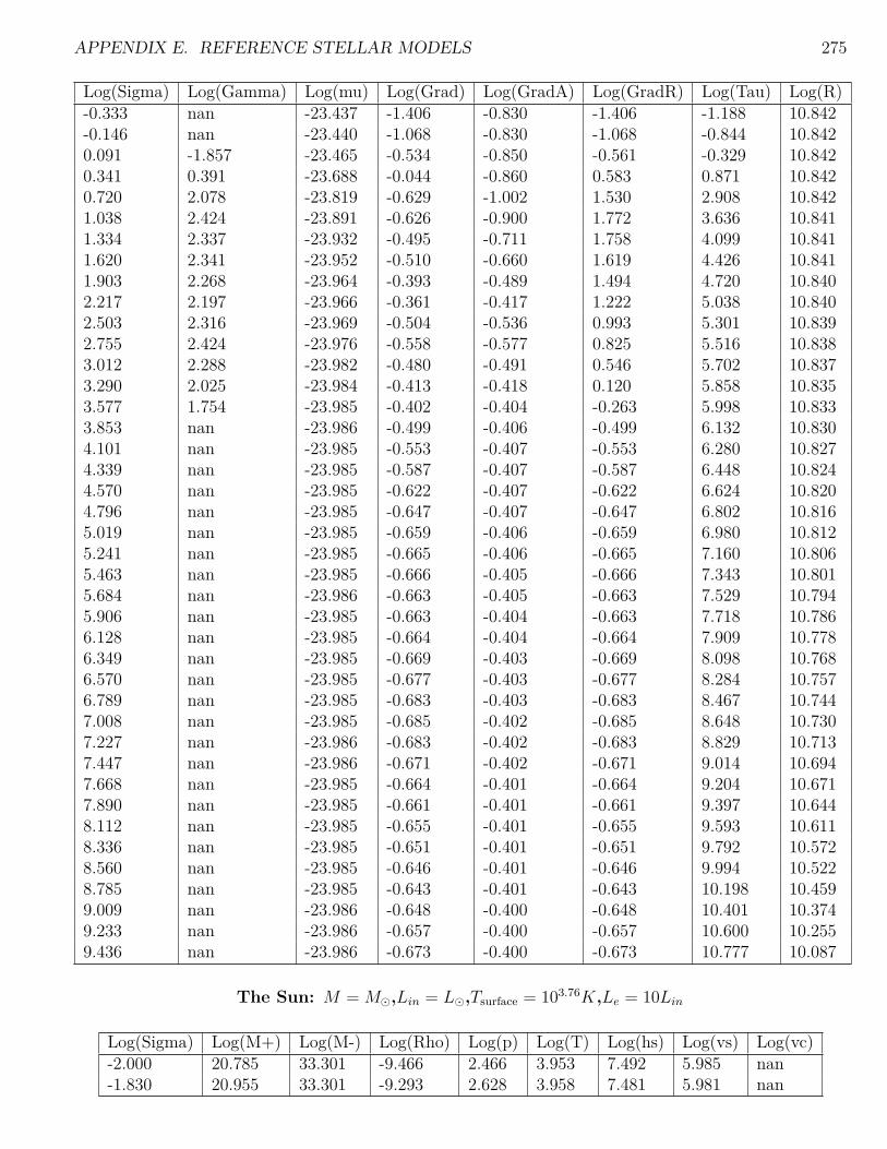
APPENDIX E. REFERENCE STELLAR MODELS 275
Log(Sigma) Log(Gamma) Log(mu) Log(Grad) Log(GradA) Log(GradR) Log(Tau) Log(R)-0.333 nan -23.437 -1.406 -0.830 -1.406 -1.188 10.842-0.146 nan -23.440 -1.068 -0.830 -1.068 -0.844 10.8420.091 -1.857 -23.465 -0.534 -0.850 -0.561 -0.329 10.8420.341 0.391 -23.688 -0.044 -0.860 0.583 0.871 10.8420.720 2.078 -23.819 -0.629 -1.002 1.530 2.908 10.8421.038 2.424 -23.891 -0.626 -0.900 1.772 3.636 10.8411.334 2.337 -23.932 -0.495 -0.711 1.758 4.099 10.8411.620 2.341 -23.952 -0.510 -0.660 1.619 4.426 10.8411.903 2.268 -23.964 -0.393 -0.489 1.494 4.720 10.8402.217 2.197 -23.966 -0.361 -0.417 1.222 5.038 10.8402.503 2.316 -23.969 -0.504 -0.536 0.993 5.301 10.8392.755 2.424 -23.976 -0.558 -0.577 0.825 5.516 10.8383.012 2.288 -23.982 -0.480 -0.491 0.546 5.702 10.8373.290 2.025 -23.984 -0.413 -0.418 0.120 5.858 10.8353.577 1.754 -23.985 -0.402 -0.404 -0.263 5.998 10.8333.853 nan -23.986 -0.499 -0.406 -0.499 6.132 10.8304.101 nan -23.985 -0.553 -0.407 -0.553 6.280 10.8274.339 nan -23.985 -0.587 -0.407 -0.587 6.448 10.8244.570 nan -23.985 -0.622 -0.407 -0.622 6.624 10.8204.796 nan -23.985 -0.647 -0.407 -0.647 6.802 10.8165.019 nan -23.985 -0.659 -0.406 -0.659 6.980 10.8125.241 nan -23.985 -0.665 -0.406 -0.665 7.160 10.8065.463 nan -23.985 -0.666 -0.405 -0.666 7.343 10.8015.684 nan -23.986 -0.663 -0.405 -0.663 7.529 10.7945.906 nan -23.985 -0.663 -0.404 -0.663 7.718 10.7866.128 nan -23.985 -0.664 -0.404 -0.664 7.909 10.7786.349 nan -23.985 -0.669 -0.403 -0.669 8.098 10.7686.570 nan -23.985 -0.677 -0.403 -0.677 8.284 10.7576.789 nan -23.985 -0.683 -0.403 -0.683 8.467 10.7447.008 nan -23.985 -0.685 -0.402 -0.685 8.648 10.7307.227 nan -23.986 -0.683 -0.402 -0.683 8.829 10.7137.447 nan -23.986 -0.671 -0.402 -0.671 9.014 10.6947.668 nan -23.985 -0.664 -0.401 -0.664 9.204 10.6717.890 nan -23.985 -0.661 -0.401 -0.661 9.397 10.6448.112 nan -23.985 -0.655 -0.401 -0.655 9.593 10.6118.336 nan -23.985 -0.651 -0.401 -0.651 9.792 10.5728.560 nan -23.985 -0.646 -0.401 -0.646 9.994 10.5228.785 nan -23.985 -0.643 -0.401 -0.643 10.198 10.4599.009 nan -23.986 -0.648 -0.400 -0.648 10.401 10.3749.233 nan -23.986 -0.657 -0.400 -0.657 10.600 10.2559.436 nan -23.986 -0.673 -0.400 -0.673 10.777 10.087
The Sun: M = M,Lin = L,Tsurface = 103.76K,Le = 10Lin
Log(Sigma) Log(M+) Log(M-) Log(Rho) Log(p) Log(T) Log(hs) Log(vs) Log(vc)-2.000 20.785 33.301 -9.466 2.466 3.953 7.492 5.985 nan-1.830 20.955 33.301 -9.293 2.628 3.958 7.481 5.981 nan

APPENDIX E. REFERENCE STELLAR MODELS 276
Log(Sigma) Log(M+) Log(M-) Log(Rho) Log(p) Log(T) Log(hs) Log(vs) Log(vc)-1.648 21.136 33.301 -9.119 2.803 3.966 7.483 5.984 nan-1.421 21.363 33.301 -8.945 3.025 3.991 7.531 6.011 3.098-1.032 21.752 33.301 -8.771 3.411 4.096 7.742 6.140 2.313-0.790 21.995 33.301 -8.598 3.652 4.154 7.810 6.194 nan-0.561 22.223 33.301 -8.424 3.880 4.204 7.864 6.209 1.391-0.330 22.455 33.301 -8.250 4.111 4.255 7.922 6.235 2.218-0.099 22.685 33.301 -8.077 4.342 4.306 7.978 6.282 nan0.131 22.915 33.301 -7.903 4.571 4.360 8.034 6.332 nan0.364 23.148 33.301 -7.729 4.804 4.418 8.093 6.371 nan0.600 23.384 33.301 -7.555 5.040 4.480 8.156 6.404 nan0.848 23.632 33.301 -7.382 5.288 4.553 8.230 6.431 nan1.115 23.899 33.301 -7.208 5.555 4.640 8.323 6.446 4.8081.378 24.162 33.301 -7.034 5.818 4.718 8.412 6.502 nan1.610 24.394 33.301 -6.861 6.050 4.774 8.471 6.548 nan1.832 24.617 33.301 -6.687 6.272 4.823 8.520 6.581 nan2.052 24.836 33.301 -6.513 6.492 4.869 8.565 6.607 nan2.271 25.055 33.301 -6.339 6.711 4.915 8.611 6.632 nan2.490 25.275 33.301 -6.166 6.930 4.962 8.656 6.655 nan2.709 25.494 33.301 -5.992 7.149 5.008 8.701 6.678 nan2.926 25.711 33.301 -5.818 7.366 5.051 8.745 6.700 nan3.138 25.922 33.301 -5.645 7.578 5.090 8.783 6.719 nan3.343 26.127 33.301 -5.471 7.783 5.123 8.814 6.735 nan3.544 26.329 33.301 -5.297 7.984 5.151 8.842 6.749 nan3.748 26.532 33.301 -5.123 8.188 5.182 8.871 6.765 nan3.962 26.747 33.301 -4.950 8.402 5.223 8.912 6.785 nan4.187 26.971 33.301 -4.776 8.627 5.274 8.963 6.811 nan4.416 27.200 33.301 -4.602 8.855 5.329 9.018 6.838 nan4.642 27.427 33.301 -4.429 9.082 5.382 9.071 6.865 nan4.866 27.651 33.301 -4.255 9.306 5.433 9.121 6.890 nan5.089 27.873 33.301 -4.081 9.529 5.482 9.170 6.915 nan5.310 28.095 33.301 -3.907 9.750 5.530 9.218 6.939 nan5.532 28.316 33.301 -3.734 9.971 5.577 9.265 6.962 nan5.753 28.538 33.301 -3.560 10.193 5.625 9.313 6.986 nan5.975 28.759 33.301 -3.386 10.415 5.674 9.361 7.011 nan6.197 28.981 33.301 -3.212 10.636 5.722 9.409 7.035 nan6.418 29.202 33.301 -3.039 10.858 5.769 9.457 7.058 nan6.638 29.422 33.301 -2.865 11.078 5.816 9.503 7.082 nan6.857 29.641 33.301 -2.691 11.297 5.861 9.549 7.104 nan7.076 29.860 33.301 -2.518 11.516 5.906 9.594 7.127 nan7.295 30.079 33.301 -2.344 11.735 5.952 9.639 7.150 nan7.515 30.300 33.300 -2.170 11.955 5.999 9.685 7.173 nan7.737 30.521 33.300 -1.996 12.176 6.047 9.733 7.197 nan7.959 30.743 33.300 -1.823 12.399 6.095 9.782 7.221 nan8.182 30.966 33.299 -1.649 12.622 6.144 9.831 7.246 nan8.405 31.190 33.297 -1.475 12.845 6.194 9.881 7.271 nan8.630 31.414 33.295 -1.302 13.070 6.245 9.932 7.296 nan8.854 31.639 33.291 -1.128 13.295 6.296 9.983 7.322 nan

APPENDIX E. REFERENCE STELLAR MODELS 277
Log(Sigma) Log(M+) Log(M-) Log(Rho) Log(p) Log(T) Log(hs) Log(vs) Log(vc)9.079 31.863 33.285 -0.954 13.519 6.347 10.033 7.347 nan9.300 32.085 33.274 -0.782 13.740 6.396 10.082 7.372 nan9.463 32.247 33.261 -0.654 13.903 6.431 10.117 7.389 nan
Log(Sigma) Log(Gamma) Log(mu) Log(Grad) Log(GradA) Log(GradR) Log(Tau) Log(R)-2.000 nan -23.814 -1.682 -1.128 -1.682 -1.423 10.841-1.830 nan -23.804 -1.453 -1.131 -1.453 -1.174 10.841-1.648 nan -23.803 -1.184 -1.130 -1.184 -0.896 10.841-1.421 -4.740 -23.830 -0.747 -1.114 -0.793 -0.499 10.841-1.032 -6.165 -23.935 -0.574 -0.770 -0.588 0.259 10.841-0.790 nan -23.945 -0.650 -0.606 -0.650 0.563 10.841-0.561 -6.917 -23.950 -0.666 -0.680 -0.667 0.799 10.840-0.330 -5.831 -23.958 -0.662 -0.708 -0.669 1.019 10.840-0.099 nan -23.964 -0.641 -0.578 -0.641 1.237 10.8400.131 nan -23.966 -0.615 -0.468 -0.615 1.462 10.8400.364 nan -23.966 -0.590 -0.432 -0.590 1.701 10.8390.600 nan -23.967 -0.570 -0.426 -0.570 1.953 10.8390.848 nan -23.967 -0.510 -0.462 -0.510 2.247 10.8381.115 -1.712 -23.972 -0.470 -0.635 -0.493 2.592 10.8371.378 nan -23.981 -0.589 -0.566 -0.589 2.905 10.8371.610 nan -23.984 -0.646 -0.482 -0.646 3.135 10.8361.832 nan -23.985 -0.670 -0.449 -0.670 3.336 10.8352.052 nan -23.985 -0.677 -0.435 -0.677 3.531 10.8332.271 nan -23.985 -0.675 -0.424 -0.675 3.729 10.8322.490 nan -23.985 -0.674 -0.423 -0.674 3.938 10.8312.709 nan -23.985 -0.685 -0.421 -0.685 4.160 10.8292.926 nan -23.985 -0.710 -0.419 -0.710 4.397 10.8283.138 nan -23.985 -0.769 -0.417 -0.769 4.644 10.8263.343 nan -23.985 -0.831 -0.414 -0.831 4.900 10.8243.544 nan -23.986 -0.855 -0.411 -0.855 5.172 10.8223.748 nan -23.985 -0.774 -0.409 -0.774 5.461 10.8203.962 nan -23.985 -0.672 -0.408 -0.672 5.764 10.8174.187 nan -23.985 -0.625 -0.407 -0.625 6.058 10.8144.416 nan -23.985 -0.623 -0.407 -0.623 6.327 10.8114.642 nan -23.985 -0.641 -0.407 -0.641 6.567 10.8074.866 nan -23.985 -0.655 -0.406 -0.655 6.784 10.8025.089 nan -23.985 -0.662 -0.406 -0.662 6.988 10.7975.310 nan -23.986 -0.666 -0.405 -0.666 7.186 10.7925.532 nan -23.985 -0.665 -0.405 -0.665 7.380 10.7855.753 nan -23.985 -0.664 -0.404 -0.664 7.575 10.7785.975 nan -23.985 -0.663 -0.404 -0.663 7.769 10.7706.197 nan -23.985 -0.666 -0.404 -0.666 7.963 10.7616.418 nan -23.985 -0.673 -0.403 -0.673 8.153 10.7506.638 nan -23.985 -0.680 -0.403 -0.680 8.339 10.7386.857 nan -23.986 -0.684 -0.402 -0.684 8.522 10.7257.076 nan -23.986 -0.684 -0.402 -0.684 8.703 10.709

APPENDIX E. REFERENCE STELLAR MODELS 278
Log(Sigma) Log(Gamma) Log(mu) Log(Grad) Log(GradA) Log(GradR) Log(Tau) Log(R)7.295 nan -23.985 -0.681 -0.402 -0.681 8.885 10.6917.515 nan -23.985 -0.669 -0.401 -0.669 9.072 10.6707.737 nan -23.985 -0.663 -0.401 -0.663 9.264 10.6457.959 nan -23.985 -0.660 -0.401 -0.660 9.458 10.6158.182 nan -23.985 -0.653 -0.401 -0.653 9.654 10.5798.405 nan -23.985 -0.650 -0.401 -0.650 9.854 10.5348.630 nan -23.986 -0.644 -0.401 -0.644 10.057 10.4788.854 nan -23.986 -0.643 -0.400 -0.643 10.261 10.4049.079 nan -23.985 -0.652 -0.400 -0.652 10.464 10.3039.300 nan -23.985 -0.659 -0.400 -0.659 10.660 10.1559.463 nan -23.985 -0.676 -0.400 -0.676 10.800 9.981
Low-mass nuclear-burning: M = 0.3M,Lin = 0.1L,Tsurface = 103.3K,Le = 0
Log(Sigma) Log(M+) Log(M-) Log(Rho) Log(p) Log(T) Log(hs) Log(vs) Log(vc)-1.999 20.052 32.778 -8.273 2.651 3.370 6.274 5.509 nan-1.826 20.226 32.778 -8.099 2.824 3.370 6.274 5.509 nan-1.652 20.399 32.778 -7.925 2.998 3.370 6.274 5.509 nan-1.478 20.573 32.778 -7.752 3.172 3.370 6.274 5.509 nan-1.304 20.747 32.778 -7.578 3.346 3.370 6.274 5.509 nan-1.130 20.921 32.778 -7.404 3.520 3.370 6.274 5.509 nan-0.957 21.095 32.778 -7.231 3.694 3.370 6.274 5.509 nan-0.783 21.269 32.778 -7.057 3.867 3.371 6.274 5.509 nan-0.608 21.443 32.778 -6.883 4.041 3.371 6.275 5.509 nan-0.434 21.617 32.778 -6.709 4.216 3.372 6.275 5.510 nan-0.260 21.792 32.778 -6.536 4.390 3.372 6.276 5.510 nan-0.085 21.967 32.778 -6.362 4.565 3.374 6.277 5.511 nan0.091 22.142 32.778 -6.188 4.741 3.376 6.280 5.512 nan0.268 22.319 32.778 -6.015 4.918 3.379 6.283 5.513 nan0.446 22.497 32.778 -5.841 5.096 3.383 6.287 5.515 nan0.626 22.678 32.778 -5.667 5.276 3.390 6.294 5.518 nan0.811 22.862 32.778 -5.493 5.460 3.400 6.304 5.523 nan1.001 23.052 32.778 -5.320 5.651 3.417 6.321 5.531 nan1.204 23.255 32.778 -5.146 5.853 3.446 6.349 5.545 nan1.420 23.471 32.778 -4.972 6.070 3.488 6.392 5.565 4.2821.636 23.688 32.778 -4.799 6.286 3.531 6.435 5.587 4.2871.852 23.903 32.778 -4.625 6.502 3.573 6.477 5.608 4.2812.067 24.119 32.778 -4.451 6.717 3.615 6.519 5.628 4.2602.282 24.333 32.778 -4.277 6.932 3.655 6.559 5.648 4.2202.495 24.546 32.778 -4.104 7.145 3.695 6.599 5.668 4.1652.708 24.759 32.778 -3.930 7.358 3.734 6.638 5.687 4.1052.921 24.972 32.778 -3.756 7.571 3.773 6.677 5.707 4.0573.133 25.184 32.778 -3.583 7.783 3.810 6.715 5.726 3.9903.345 25.397 32.778 -3.409 7.995 3.848 6.754 5.746 3.9303.559 25.610 32.778 -3.235 8.209 3.885 6.794 5.769 3.8763.777 25.829 32.778 -3.061 8.427 3.923 6.839 5.798 3.8144.009 26.061 32.778 -2.888 8.659 3.963 6.897 5.850 3.762

APPENDIX E. REFERENCE STELLAR MODELS 279
Log(Sigma) Log(M+) Log(M-) Log(Rho) Log(p) Log(T) Log(hs) Log(vs) Log(vc)4.291 26.342 32.778 -2.714 8.941 4.011 7.005 5.969 3.6924.678 26.729 32.778 -2.540 9.327 4.079 7.217 6.081 3.6834.948 27.000 32.778 -2.366 9.597 4.165 7.313 6.072 3.6695.207 27.258 32.778 -2.193 9.856 4.244 7.399 6.109 3.6045.463 27.514 32.778 -2.019 10.126 4.316 7.495 6.155 3.5335.723 27.774 32.778 -1.845 10.381 4.383 7.576 6.197 3.4685.985 28.036 32.778 -1.672 10.639 4.447 7.661 6.245 3.4056.255 28.306 32.778 -1.498 10.907 4.511 7.755 6.303 3.3366.541 28.593 32.778 -1.324 11.193 4.578 7.867 6.375 3.2756.851 28.902 32.778 -1.150 11.502 4.649 8.002 6.460 3.2237.180 29.231 32.778 -0.977 11.830 4.733 8.157 6.543 3.1877.502 29.553 32.778 -0.803 12.153 4.832 8.306 6.605 3.1617.806 29.857 32.777 -0.629 12.456 4.936 8.436 6.660 3.1108.106 30.158 32.777 -0.456 12.757 5.040 8.562 6.726 3.0568.402 30.453 32.776 -0.282 13.052 5.156 8.684 6.779 3.0148.692 30.743 32.774 -0.108 13.342 5.272 8.800 6.836 2.9498.982 31.033 32.770 0.066 13.632 5.388 8.916 6.894 2.8919.267 31.318 32.763 0.236 13.917 5.502 9.030 6.951 2.836
Log(Sigma) Log(Gamma) Log(mu) Log(Grad) Log(GradA) Log(GradR) Log(Tau) Log(R)-1.999 nan -23.413 -3.903 -0.711 -3.903 -3.685 10.476-1.826 nan -23.413 -3.755 -0.711 -3.755 -3.480 10.476-1.652 nan -23.413 -3.596 -0.711 -3.596 -3.280 10.476-1.478 nan -23.413 -3.432 -0.711 -3.432 -3.086 10.476-1.304 nan -23.414 -3.263 -0.711 -3.263 -2.896 10.476-1.130 nan -23.414 -3.090 -0.711 -3.090 -2.709 10.476-0.957 nan -23.414 -2.916 -0.711 -2.916 -2.524 10.476-0.783 nan -23.413 -2.740 -0.711 -2.740 -2.340 10.476-0.608 nan -23.413 -2.563 -0.711 -2.563 -2.157 10.476-0.434 nan -23.413 -2.391 -0.711 -2.391 -1.976 10.476-0.260 nan -23.413 -2.218 -0.711 -2.218 -1.796 10.476-0.085 nan -23.413 -2.044 -0.712 -2.044 -1.616 10.4760.091 nan -23.414 -1.870 -0.712 -1.870 -1.435 10.4760.268 nan -23.414 -1.695 -0.712 -1.695 -1.252 10.4760.446 nan -23.414 -1.519 -0.713 -1.519 -1.065 10.4760.626 nan -23.413 -1.340 -0.715 -1.340 -0.871 10.4760.811 nan -23.413 -1.155 -0.717 -1.155 -0.666 10.4761.001 nan -23.413 -0.960 -0.720 -0.960 -0.439 10.4761.204 nan -23.413 -0.744 -0.726 -0.744 -0.170 10.4761.420 0.628 -23.413 -0.700 -0.733 -0.547 0.159 10.4761.636 0.878 -23.414 -0.706 -0.735 -0.452 0.479 10.4761.852 1.269 -23.414 -0.713 -0.737 -0.247 0.785 10.4762.067 1.807 -23.414 -0.720 -0.739 0.101 1.178 10.4762.282 2.406 -23.414 -0.727 -0.741 0.523 1.688 10.4762.495 2.933 -23.414 -0.733 -0.744 0.888 2.221 10.4762.708 3.373 -23.414 -0.739 -0.747 1.172 2.716 10.475

APPENDIX E. REFERENCE STELLAR MODELS 280
Log(Sigma) Log(Gamma) Log(mu) Log(Grad) Log(GradA) Log(GradR) Log(Tau) Log(R)2.921 3.810 -23.414 -0.745 -0.750 1.439 3.164 10.4753.133 4.256 -23.415 -0.751 -0.754 1.729 3.595 10.4753.345 4.789 -23.416 -0.757 -0.759 2.090 4.066 10.4753.559 5.391 -23.419 -0.761 -0.762 2.497 4.583 10.4753.777 6.030 -23.426 -0.761 -0.762 2.911 5.139 10.4754.009 6.790 -23.444 -0.760 -0.760 3.345 5.737 10.4754.291 7.790 -23.503 -0.786 -0.786 3.846 6.447 10.4754.678 8.473 -23.648 -0.605 -0.605 4.490 7.368 10.4754.948 8.835 -23.658 -0.501 -0.501 5.004 8.134 10.4755.207 9.489 -23.665 -0.535 -0.535 5.419 8.893 10.4755.463 10.056 -23.689 -0.565 -0.565 5.778 9.573 10.4745.723 10.576 -23.703 -0.593 -0.593 6.060 10.191 10.4745.985 11.048 -23.723 -0.614 -0.614 6.304 10.734 10.4746.255 11.440 -23.754 -0.630 -0.630 6.489 11.223 10.4736.541 11.765 -23.799 -0.638 -0.638 6.622 11.699 10.4736.851 11.957 -23.863 -0.623 -0.623 6.654 12.118 10.4727.180 11.962 -23.934 -0.556 -0.556 6.524 12.457 10.4707.502 11.908 -23.984 -0.479 -0.479 6.272 12.707 10.4697.806 11.892 -24.010 -0.466 -0.466 6.004 12.903 10.4668.106 11.797 -24.032 -0.430 -0.430 5.718 13.081 10.4638.402 11.596 -24.038 -0.399 -0.399 5.276 13.225 10.4588.692 11.455 -24.038 -0.398 -0.398 4.777 13.328 10.4538.982 11.205 -24.038 -0.398 -0.398 4.295 13.407 10.4459.267 10.998 -24.038 -0.398 -0.398 3.857 13.472 10.436
Low-mass nuclear-burning: M = 0.3M,Lin = 0.1L,Tsurface = 103.3K,Le = Lin
Log(Sigma) Log(M+) Log(M-) Log(Rho) Log(p) Log(T) Log(hs) Log(vs) Log(vc)-2.000 20.051 32.778 -8.612 2.652 3.692 6.613 5.677 nan-1.829 20.222 32.778 -8.438 2.822 3.693 6.610 5.675 nan-1.657 20.394 32.778 -8.264 2.993 3.693 6.608 5.673 nan-1.485 20.566 32.778 -8.090 3.165 3.693 6.606 5.672 nan-1.313 20.738 32.778 -7.917 3.337 3.693 6.604 5.671 nan-1.141 20.911 32.778 -7.743 3.510 3.693 6.603 5.670 nan-0.968 21.084 32.778 -7.569 3.683 3.693 6.602 5.670 nan-0.794 21.257 32.778 -7.396 3.856 3.694 6.602 5.669 nan-0.619 21.432 32.778 -7.222 4.030 3.695 6.603 5.670 nan-0.443 21.608 32.778 -7.048 4.207 3.698 6.605 5.671 nan-0.263 21.788 32.778 -6.874 4.387 3.705 6.611 5.674 nan-0.076 21.975 32.778 -6.701 4.574 3.718 6.625 5.681 nan0.128 22.180 32.778 -6.527 4.779 3.746 6.656 5.697 3.2700.438 22.489 32.778 -6.381 5.088 3.852 6.819 5.813 5.2460.948 22.999 32.778 -6.225 5.598 4.000 7.174 5.963 5.2891.209 23.260 32.778 -6.052 5.859 4.065 7.261 5.996 5.2011.442 23.494 32.778 -5.878 6.093 4.106 7.321 6.026 5.1261.667 23.719 32.778 -5.704 6.317 4.139 7.372 6.052 5.0651.888 23.939 32.778 -5.531 6.538 4.170 7.418 6.076 5.007

APPENDIX E. REFERENCE STELLAR MODELS 281
Log(Sigma) Log(M+) Log(M-) Log(Rho) Log(p) Log(T) Log(hs) Log(vs) Log(vc)2.106 24.158 32.778 -5.357 6.756 4.200 7.463 6.100 4.9532.324 24.376 32.778 -5.183 6.974 4.230 7.508 6.124 4.8812.543 24.594 32.778 -5.009 7.193 4.261 7.553 6.149 4.8202.762 24.814 32.778 -4.836 7.413 4.293 7.599 6.174 4.7312.984 25.035 32.778 -4.662 7.634 4.327 7.646 6.201 4.6323.208 25.259 32.778 -4.488 7.858 4.363 7.696 6.229 4.5073.435 25.486 32.778 -4.315 8.085 4.401 7.749 6.259 4.3513.665 25.717 32.778 -4.141 8.315 4.444 7.806 6.291 4.2123.900 25.951 32.778 -3.967 8.550 4.490 7.867 6.325 4.1434.138 26.190 32.778 -3.793 8.788 4.541 7.932 6.362 4.0994.382 26.433 32.778 -3.620 9.032 4.597 8.002 6.402 4.0494.632 26.684 32.778 -3.446 9.283 4.660 8.079 6.447 4.0094.891 26.943 32.778 -3.272 9.542 4.734 8.164 6.498 3.9735.161 27.212 32.778 -3.099 9.811 4.820 8.259 6.553 3.9205.436 27.487 32.778 -2.925 10.086 4.915 8.361 6.606 3.8755.711 27.762 32.778 -2.751 10.361 5.010 8.462 6.654 3.8155.984 28.035 32.778 -2.577 10.634 5.104 8.561 6.705 3.7516.260 28.312 32.778 -2.404 10.910 5.201 8.664 6.760 3.7066.542 28.594 32.778 -2.230 11.193 5.305 8.773 6.819 3.6516.829 28.880 32.778 -2.056 11.479 5.416 8.886 6.877 3.5957.117 29.169 32.778 -1.883 11.768 5.529 9.000 6.936 3.5367.407 29.458 32.778 -1.709 12.057 5.644 9.116 6.994 3.4757.696 29.748 32.777 -1.535 12.347 5.759 9.232 7.052 3.3827.986 30.038 32.777 -1.361 12.636 5.874 9.348 7.110 3.2448.271 30.322 32.776 -1.188 12.921 5.984 9.458 7.166 nan8.515 30.566 32.775 -1.014 13.165 6.054 9.529 7.201 nan8.746 30.797 32.773 -0.840 13.396 6.112 9.587 7.230 nan8.973 31.025 32.770 -0.666 13.624 6.164 9.640 7.256 nan9.198 31.250 32.765 -0.493 13.848 6.215 9.691 7.282 nan9.410 31.462 32.756 -0.327 14.061 6.261 9.738 7.305 nan
Log(Sigma) Log(Gamma) Log(mu) Log(Grad) Log(GradA) Log(GradR) Log(Tau) Log(R)-2.000 nan -23.429 -3.985 -0.835 -3.985 -4.262 10.476-1.829 nan -23.426 -3.861 -0.824 -3.861 -3.969 10.476-1.657 nan -23.424 -3.676 -0.814 -3.676 -3.668 10.475-1.485 nan -23.422 -3.441 -0.804 -3.441 -3.360 10.475-1.313 nan -23.421 -3.170 -0.796 -3.170 -3.048 10.475-1.141 nan -23.420 -2.873 -0.788 -2.873 -2.732 10.475-0.968 nan -23.419 -2.565 -0.781 -2.565 -2.413 10.475-0.794 nan -23.418 -2.251 -0.776 -2.251 -2.092 10.475-0.619 nan -23.417 -1.939 -0.771 -1.939 -1.769 10.475-0.443 nan -23.416 -1.624 -0.768 -1.624 -1.443 10.475-0.263 nan -23.416 -1.312 -0.767 -1.312 -1.108 10.475-0.076 nan -23.417 -1.013 -0.769 -1.013 -0.758 10.4750.128 -2.668 -23.419 -0.718 -0.778 -0.725 -0.370 10.4750.438 0.241 -23.477 -0.430 -0.845 -0.057 0.429 10.475

APPENDIX E. REFERENCE STELLAR MODELS 282
Log(Sigma) Log(Gamma) Log(mu) Log(Grad) Log(GradA) Log(GradR) Log(Tau) Log(R)0.948 1.812 -23.684 -0.499 -0.778 1.311 2.345 10.4751.209 2.751 -23.706 -0.705 -0.888 1.886 3.309 10.4751.442 3.394 -23.725 -0.799 -0.913 2.282 3.966 10.4751.667 3.927 -23.742 -0.842 -0.916 2.606 4.494 10.4751.888 4.409 -23.758 -0.860 -0.909 2.897 4.961 10.4742.106 4.868 -23.773 -0.863 -0.897 3.171 5.394 10.4742.324 5.274 -23.787 -0.859 -0.880 3.408 5.805 10.4742.543 5.682 -23.801 -0.846 -0.860 3.622 6.207 10.4742.762 6.048 -23.815 -0.830 -0.837 3.793 6.601 10.4732.984 6.389 -23.829 -0.808 -0.812 3.897 6.996 10.4733.208 6.699 -23.844 -0.782 -0.784 3.914 7.392 10.4733.435 6.970 -23.858 -0.752 -0.753 3.840 7.795 10.4723.665 7.238 -23.872 -0.721 -0.721 3.797 8.202 10.4723.900 7.512 -23.887 -0.688 -0.689 3.894 8.595 10.4714.138 7.825 -23.901 -0.655 -0.656 4.070 8.980 10.4714.382 8.046 -23.915 -0.618 -0.618 4.164 9.346 10.4704.632 8.149 -23.928 -0.573 -0.573 4.139 9.668 10.4694.891 8.111 -23.939 -0.520 -0.520 3.973 9.926 10.4685.161 7.967 -23.949 -0.474 -0.474 3.695 10.123 10.4665.436 7.866 -23.955 -0.458 -0.458 3.400 10.281 10.4645.711 7.826 -23.961 -0.465 -0.465 3.141 10.424 10.4625.984 7.745 -23.967 -0.463 -0.463 2.853 10.557 10.4596.260 7.548 -23.973 -0.443 -0.443 2.456 10.668 10.4556.542 7.246 -23.977 -0.422 -0.422 1.961 10.749 10.4506.829 6.954 -23.980 -0.410 -0.410 1.462 10.809 10.4437.117 6.702 -23.981 -0.404 -0.404 0.992 10.858 10.4347.407 6.500 -23.982 -0.401 -0.401 0.568 10.902 10.4217.696 6.323 -23.983 -0.400 -0.400 0.197 10.949 10.4047.986 6.117 -23.983 -0.400 -0.400 -0.157 11.002 10.3818.271 nan -23.984 -0.483 -0.399 -0.483 11.060 10.3508.515 nan -23.984 -0.586 -0.399 -0.586 11.121 10.3158.746 nan -23.985 -0.623 -0.399 -0.623 11.197 10.2728.973 nan -23.985 -0.641 -0.399 -0.641 11.292 10.2199.198 nan -23.986 -0.654 -0.399 -0.654 11.408 10.1519.410 nan -23.987 -0.668 -0.398 -0.668 11.533 10.065
Low-mass nuclear-burning: M = 0.3M,Lin = 0.1L,Tsurface = 103.3K,Le = 10Lin
Log(Sigma) Log(M+) Log(M-) Log(Rho) Log(p) Log(T) Log(hs) Log(vs) Log(vc)-1.999 20.052 32.778 -9.204 2.665 3.944 7.219 5.957 nan-1.829 20.223 32.778 -9.030 2.831 3.948 7.212 5.954 nan-1.648 20.404 32.778 -8.857 3.009 3.956 7.215 5.958 nan-1.434 20.617 32.778 -8.683 3.220 3.977 7.253 5.977 3.099-1.027 21.024 32.778 -8.565 3.624 4.108 7.540 6.144 2.770-0.777 21.274 32.778 -8.391 3.874 4.173 7.615 6.200 nan-0.546 21.505 32.778 -8.218 4.104 4.224 7.672 6.217 2.167-0.313 21.739 32.778 -8.044 4.338 4.276 7.732 6.249 2.358

APPENDIX E. REFERENCE STELLAR MODELS 283
Log(Sigma) Log(M+) Log(M-) Log(Rho) Log(p) Log(T) Log(hs) Log(vs) Log(vc)-0.081 21.971 32.778 -7.870 4.570 4.329 7.790 6.300 nan0.151 22.203 32.778 -7.696 4.802 4.386 7.848 6.348 nan0.386 22.437 32.778 -7.523 5.036 4.446 7.909 6.385 nan0.626 22.678 32.778 -7.349 5.276 4.512 7.975 6.418 nan0.880 22.932 32.778 -7.175 5.530 4.590 8.056 6.439 3.1761.151 23.202 32.778 -7.001 5.801 4.678 8.152 6.465 4.9071.398 23.450 32.778 -6.828 6.048 4.745 8.226 6.520 nan1.626 23.677 32.778 -6.654 6.276 4.797 8.280 6.561 nan1.847 23.898 32.778 -6.480 6.497 4.844 8.327 6.591 nan2.066 24.117 32.778 -6.307 6.716 4.890 8.373 6.617 nan2.286 24.337 32.778 -6.133 6.936 4.936 8.419 6.642 nan2.506 24.557 32.778 -5.959 7.156 4.984 8.466 6.666 nan2.725 24.777 32.778 -5.785 7.375 5.030 8.511 6.689 nan2.941 24.992 32.778 -5.612 7.591 5.072 8.553 6.710 nan3.149 25.200 32.778 -5.438 7.799 5.107 8.587 6.727 nan3.348 25.399 32.778 -5.264 7.998 5.133 8.612 6.740 nan3.537 25.588 32.778 -5.091 8.187 5.149 8.628 6.748 nan3.718 25.769 32.778 -4.917 8.368 5.158 8.635 6.753 nan3.897 25.949 32.778 -4.743 8.547 5.164 8.641 6.756 nan4.080 26.132 32.778 -4.569 8.730 5.173 8.650 6.760 nan4.271 26.323 32.778 -4.396 8.921 5.191 8.667 6.769 nan4.475 26.526 32.778 -4.222 9.125 5.221 8.697 6.784 nan4.689 26.741 32.778 -4.048 9.339 5.262 8.738 6.805 nan4.910 26.961 32.778 -3.875 9.560 5.309 8.785 6.828 nan5.131 27.183 32.778 -3.701 9.781 5.356 8.832 6.852 nan5.351 27.403 32.778 -3.527 10.002 5.403 8.879 6.875 nan5.571 27.622 32.778 -3.353 10.221 5.448 8.924 6.898 nan5.789 27.840 32.778 -3.180 10.439 5.493 8.969 6.920 nan6.007 28.059 32.778 -3.006 10.657 5.538 9.013 6.943 nan6.226 28.277 32.778 -2.832 10.876 5.583 9.058 6.965 nan6.445 28.496 32.778 -2.659 11.095 5.628 9.104 6.988 nan6.664 28.716 32.778 -2.485 11.314 5.673 9.149 7.011 nan6.884 28.935 32.778 -2.311 11.534 5.720 9.196 7.034 nan7.104 29.155 32.778 -2.137 11.754 5.766 9.242 7.057 nan7.323 29.375 32.778 -1.964 11.973 5.812 9.287 7.079 nan7.542 29.594 32.778 -1.790 12.192 5.857 9.332 7.102 nan7.761 29.813 32.777 -1.616 12.411 5.903 9.377 7.125 nan7.981 30.033 32.777 -1.443 12.631 5.949 9.424 7.148 nan8.202 30.253 32.777 -1.269 12.852 5.997 9.471 7.172 nan8.424 30.476 32.776 -1.095 13.074 6.045 9.520 7.196 nan8.647 30.699 32.774 -0.921 13.298 6.094 9.569 7.221 nan8.871 30.923 32.772 -0.748 13.521 6.144 9.619 7.246 nan9.095 31.146 32.768 -0.574 13.745 6.193 9.669 7.271 nan9.302 31.353 32.761 -0.413 13.953 6.239 9.715 7.294 nan

APPENDIX E. REFERENCE STELLAR MODELS 284
Log(Sigma) Log(Gamma) Log(mu) Log(Grad) Log(GradA) Log(GradR) Log(Tau) Log(R)-1.999 nan -23.771 -1.718 -1.132 -1.718 -1.439 10.474-1.829 nan -23.763 -1.477 -1.127 -1.477 -1.192 10.474-1.648 nan -23.762 -1.209 -1.121 -1.209 -0.915 10.474-1.434 -4.492 -23.780 -0.825 -1.118 -0.834 -0.546 10.474-1.027 -5.430 -23.934 -0.507 -0.778 -0.534 0.365 10.474-0.777 nan -23.945 -0.638 -0.614 -0.638 0.688 10.473-0.546 -5.861 -23.951 -0.654 -0.698 -0.660 0.925 10.473-0.313 -5.452 -23.959 -0.647 -0.682 -0.652 1.147 10.473-0.081 nan -23.964 -0.626 -0.538 -0.626 1.373 10.4720.151 nan -23.966 -0.601 -0.449 -0.601 1.606 10.4720.386 nan -23.967 -0.579 -0.424 -0.579 1.853 10.4710.626 nan -23.967 -0.521 -0.425 -0.521 2.120 10.4700.880 -3.518 -23.968 -0.498 -0.505 -0.499 2.437 10.4691.151 -1.362 -23.975 -0.523 -0.638 -0.531 2.782 10.4681.398 nan -23.982 -0.614 -0.534 -0.614 3.053 10.4671.626 nan -23.984 -0.661 -0.467 -0.661 3.267 10.4661.847 nan -23.985 -0.677 -0.439 -0.677 3.463 10.4642.066 nan -23.985 -0.678 -0.428 -0.678 3.657 10.4622.286 nan -23.985 -0.671 -0.418 -0.671 3.859 10.4602.506 nan -23.985 -0.672 -0.416 -0.672 4.074 10.4582.725 nan -23.985 -0.686 -0.415 -0.686 4.303 10.4562.941 nan -23.985 -0.734 -0.413 -0.734 4.545 10.4533.149 nan -23.985 -0.823 -0.411 -0.823 4.793 10.4513.348 nan -23.985 -0.968 -0.409 -0.968 5.053 10.4483.537 nan -23.986 -1.201 -0.406 -1.201 5.324 10.4453.718 nan -23.986 -1.449 -0.404 -1.449 5.610 10.4423.897 nan -23.985 -1.416 -0.402 -1.416 5.915 10.4394.080 nan -23.985 -1.160 -0.401 -1.160 6.236 10.4364.271 nan -23.985 -0.925 -0.400 -0.925 6.564 10.4334.475 nan -23.985 -0.767 -0.400 -0.767 6.887 10.4304.689 nan -23.985 -0.688 -0.400 -0.688 7.189 10.4254.910 nan -23.985 -0.665 -0.399 -0.665 7.458 10.4215.131 nan -23.986 -0.670 -0.399 -0.670 7.696 10.4155.351 nan -23.985 -0.679 -0.399 -0.679 7.909 10.4095.571 nan -23.985 -0.687 -0.399 -0.687 8.107 10.4025.789 nan -23.985 -0.690 -0.399 -0.690 8.297 10.3946.007 nan -23.985 -0.690 -0.399 -0.690 8.482 10.3866.226 nan -23.985 -0.687 -0.399 -0.687 8.666 10.3766.445 nan -23.985 -0.683 -0.399 -0.683 8.850 10.3656.664 nan -23.985 -0.679 -0.399 -0.679 9.035 10.3526.884 nan -23.986 -0.678 -0.399 -0.678 9.220 10.3377.104 nan -23.985 -0.679 -0.399 -0.679 9.406 10.3207.323 nan -23.985 -0.680 -0.399 -0.680 9.590 10.3007.542 nan -23.984 -0.681 -0.399 -0.681 9.773 10.2777.761 nan -23.984 -0.680 -0.399 -0.680 9.957 10.2507.981 nan -23.984 -0.676 -0.399 -0.676 10.142 10.218

APPENDIX E. REFERENCE STELLAR MODELS 285
Log(Sigma) Log(Gamma) Log(mu) Log(Grad) Log(GradA) Log(GradR) Log(Tau) Log(R)8.202 nan -23.984 -0.667 -0.399 -0.667 10.331 10.1788.424 nan -23.984 -0.659 -0.399 -0.659 10.524 10.1308.647 nan -23.985 -0.654 -0.399 -0.654 10.721 10.0678.871 nan -23.985 -0.655 -0.399 -0.655 10.920 9.9849.095 nan -23.985 -0.655 -0.399 -0.655 11.118 9.8689.302 nan -23.986 -0.666 -0.398 -0.666 11.299 9.701
Brown Dwarf: M = 0.02M,Lin = 0.01L,Tsurface = 103K,Le = 0
Log(Sigma) Log(M+) Log(M-) Log(Rho) Log(p) Log(T) Log(hs) Log(vs) Log(vc)-1.999 19.078 31.602 -8.220 2.449 3.116 6.221 5.387 nan-1.824 19.253 31.602 -8.046 2.624 3.117 6.222 5.387 nan-1.648 19.428 31.602 -7.872 2.800 3.119 6.224 5.388 nan-1.472 19.605 31.602 -7.699 2.977 3.122 6.228 5.390 nan-1.293 19.783 31.602 -7.525 3.156 3.127 6.232 5.392 nan-1.113 19.964 31.602 -7.351 3.336 3.133 6.238 5.395 nan-0.931 20.146 31.602 -7.178 3.518 3.142 6.247 5.399 nan-0.747 20.330 31.602 -7.004 3.702 3.152 6.257 5.404 nan-0.562 20.514 31.602 -6.830 3.886 3.163 6.268 5.409 nan-0.379 20.697 31.602 -6.656 4.069 3.172 6.277 5.414 nan-0.200 20.876 31.602 -6.483 4.248 3.177 6.283 5.416 nan-0.023 21.054 31.602 -6.309 4.426 3.181 6.286 5.418 nan0.155 21.232 31.602 -6.135 4.604 3.185 6.291 5.420 nan0.335 21.412 31.602 -5.962 4.784 3.192 6.297 5.423 nan0.519 21.596 31.602 -5.788 4.968 3.202 6.307 5.428 nan0.709 21.785 31.602 -5.614 5.157 3.218 6.323 5.436 nan0.906 21.982 31.602 -5.440 5.354 3.241 6.346 5.447 nan1.101 22.178 31.602 -5.267 5.550 3.263 6.368 5.458 nan1.282 22.358 31.602 -5.093 5.730 3.270 6.375 5.461 nan1.461 22.537 31.602 -4.919 5.910 3.275 6.380 5.463 nan1.643 22.719 31.602 -4.746 6.091 3.283 6.388 5.467 nan1.829 22.905 31.602 -4.572 6.277 3.295 6.401 5.473 nan2.022 23.098 31.602 -4.398 6.470 3.315 6.420 5.483 nan2.226 23.303 31.602 -4.224 6.674 3.345 6.450 5.497 nan2.442 23.518 31.602 -4.051 6.890 3.387 6.492 5.517 3.6492.657 23.734 31.602 -3.877 7.105 3.429 6.534 5.537 3.6892.871 23.948 31.602 -3.703 7.320 3.469 6.575 5.556 3.6563.085 24.161 31.602 -3.530 7.533 3.508 6.614 5.576 3.6133.298 24.374 31.602 -3.356 7.747 3.548 6.654 5.596 3.5583.511 24.588 31.602 -3.182 7.959 3.587 6.693 5.615 3.5083.724 24.801 31.602 -3.008 8.172 3.626 6.732 5.635 3.4563.937 25.013 31.602 -2.835 8.385 3.665 6.771 5.654 3.4004.149 25.226 31.602 -2.661 8.598 3.703 6.810 5.673 3.3434.362 25.439 31.602 -2.487 8.811 3.741 6.849 5.693 3.2904.575 25.651 31.602 -2.313 9.023 3.779 6.888 5.712 3.2244.787 25.864 31.602 -2.140 9.236 3.817 6.927 5.732 3.1695.000 26.077 31.602 -1.966 9.449 3.854 6.966 5.752 3.111

APPENDIX E. REFERENCE STELLAR MODELS 286
Log(Sigma) Log(M+) Log(M-) Log(Rho) Log(p) Log(T) Log(hs) Log(vs) Log(vc)5.213 26.290 31.602 -1.792 9.662 3.890 7.006 5.772 3.0485.428 26.505 31.602 -1.619 9.877 3.927 7.047 5.795 2.9865.648 26.724 31.602 -1.445 10.096 3.963 7.093 5.827 2.9245.889 26.966 31.602 -1.271 10.338 4.001 7.161 5.902 2.8476.264 27.341 31.602 -1.100 10.715 4.041 7.366 6.166 2.7006.570 27.647 31.602 -1.024 11.022 4.061 7.598 6.359 2.659
Log(Sigma) Log(Gamma) Log(mu) Log(Grad) Log(GradA) Log(GradR) Log(Tau) Log(R)-1.999 nan -23.413 -2.220 -0.674 -2.220 -1.889 9.988-1.824 nan -23.413 -2.031 -0.674 -2.031 -1.674 9.988-1.648 nan -23.414 -1.851 -0.674 -1.851 -1.467 9.988-1.472 nan -23.414 -1.674 -0.675 -1.674 -1.266 9.988-1.293 nan -23.414 -1.516 -0.675 -1.516 -1.069 9.988-1.113 nan -23.413 -1.383 -0.676 -1.383 -0.881 9.988-0.931 nan -23.413 -1.280 -0.677 -1.280 -0.705 9.988-0.747 nan -23.413 -1.233 -0.678 -1.233 -0.546 9.988-0.562 nan -23.413 -1.254 -0.679 -1.254 -0.417 9.988-0.379 nan -23.413 -1.420 -0.681 -1.420 -0.322 9.988-0.200 nan -23.414 -1.651 -0.681 -1.651 -0.275 9.988-0.023 nan -23.414 -1.691 -0.682 -1.691 -0.243 9.9880.155 nan -23.414 -1.519 -0.682 -1.519 -0.205 9.9880.335 nan -23.413 -1.346 -0.683 -1.346 -0.152 9.9880.519 nan -23.413 -1.170 -0.684 -1.170 -0.075 9.9880.709 nan -23.413 -0.996 -0.687 -0.996 0.031 9.9880.906 nan -23.413 -0.888 -0.690 -0.888 0.173 9.9881.101 nan -23.413 -1.211 -0.693 -1.211 0.294 9.9871.282 nan -23.414 -1.582 -0.694 -1.582 0.330 9.9871.461 nan -23.414 -1.441 -0.695 -1.441 0.358 9.9871.643 nan -23.414 -1.266 -0.696 -1.266 0.400 9.9871.829 nan -23.414 -1.092 -0.698 -1.092 0.462 9.9872.022 nan -23.414 -0.917 -0.701 -0.917 0.555 9.9872.226 nan -23.414 -0.741 -0.707 -0.741 0.696 9.9872.442 1.725 -23.414 -0.712 -0.714 -0.549 0.909 9.9872.657 2.207 -23.414 -0.720 -0.723 -0.324 1.193 9.9872.871 2.620 -23.414 -0.730 -0.731 -0.101 1.531 9.9873.085 2.935 -23.414 -0.733 -0.734 0.042 1.872 9.9873.298 3.186 -23.414 -0.735 -0.736 0.132 2.171 9.9873.511 3.632 -23.414 -0.737 -0.738 0.414 2.497 9.9873.724 4.172 -23.415 -0.740 -0.740 0.792 2.914 9.9873.937 4.726 -23.415 -0.742 -0.743 1.189 3.428 9.9864.149 5.236 -23.416 -0.745 -0.745 1.540 3.946 9.9864.362 5.668 -23.417 -0.748 -0.748 1.811 4.420 9.9864.575 6.081 -23.418 -0.752 -0.752 2.076 4.859 9.9864.787 6.547 -23.419 -0.756 -0.756 2.382 5.290 9.9865.000 7.071 -23.421 -0.761 -0.761 2.747 5.766 9.9865.213 7.637 -23.424 -0.767 -0.767 3.153 6.286 9.985
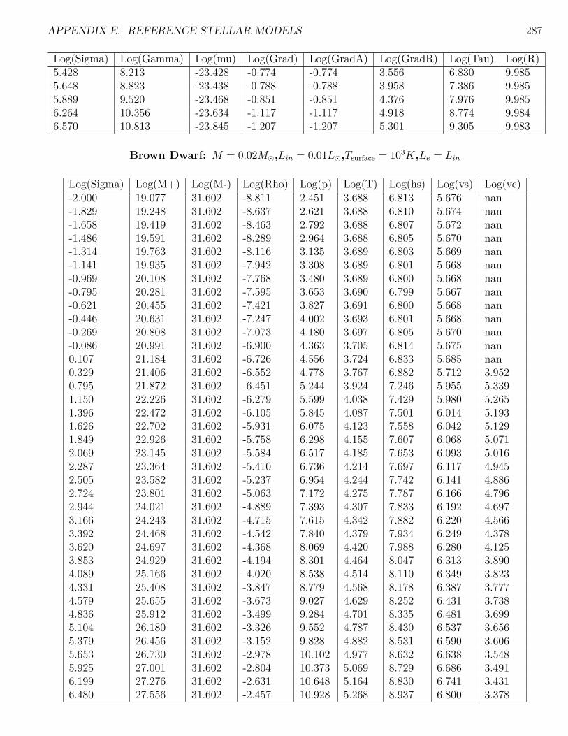
APPENDIX E. REFERENCE STELLAR MODELS 287
Log(Sigma) Log(Gamma) Log(mu) Log(Grad) Log(GradA) Log(GradR) Log(Tau) Log(R)5.428 8.213 -23.428 -0.774 -0.774 3.556 6.830 9.9855.648 8.823 -23.438 -0.788 -0.788 3.958 7.386 9.9855.889 9.520 -23.468 -0.851 -0.851 4.376 7.976 9.9856.264 10.356 -23.634 -1.117 -1.117 4.918 8.774 9.9846.570 10.813 -23.845 -1.207 -1.207 5.301 9.305 9.983
Brown Dwarf: M = 0.02M,Lin = 0.01L,Tsurface = 103K,Le = Lin
Log(Sigma) Log(M+) Log(M-) Log(Rho) Log(p) Log(T) Log(hs) Log(vs) Log(vc)-2.000 19.077 31.602 -8.811 2.451 3.688 6.813 5.676 nan-1.829 19.248 31.602 -8.637 2.621 3.688 6.810 5.674 nan-1.658 19.419 31.602 -8.463 2.792 3.688 6.807 5.672 nan-1.486 19.591 31.602 -8.289 2.964 3.688 6.805 5.670 nan-1.314 19.763 31.602 -8.116 3.135 3.689 6.803 5.669 nan-1.141 19.935 31.602 -7.942 3.308 3.689 6.801 5.668 nan-0.969 20.108 31.602 -7.768 3.480 3.689 6.800 5.668 nan-0.795 20.281 31.602 -7.595 3.653 3.690 6.799 5.667 nan-0.621 20.455 31.602 -7.421 3.827 3.691 6.800 5.668 nan-0.446 20.631 31.602 -7.247 4.002 3.693 6.801 5.668 nan-0.269 20.808 31.602 -7.073 4.180 3.697 6.805 5.670 nan-0.086 20.991 31.602 -6.900 4.363 3.705 6.814 5.675 nan0.107 21.184 31.602 -6.726 4.556 3.724 6.833 5.685 nan0.329 21.406 31.602 -6.552 4.778 3.767 6.882 5.712 3.9520.795 21.872 31.602 -6.451 5.244 3.924 7.246 5.955 5.3391.150 22.226 31.602 -6.279 5.599 4.038 7.429 5.980 5.2651.396 22.472 31.602 -6.105 5.845 4.087 7.501 6.014 5.1931.626 22.702 31.602 -5.931 6.075 4.123 7.558 6.042 5.1291.849 22.926 31.602 -5.758 6.298 4.155 7.607 6.068 5.0712.069 23.145 31.602 -5.584 6.517 4.185 7.653 6.093 5.0162.287 23.364 31.602 -5.410 6.736 4.214 7.697 6.117 4.9452.505 23.582 31.602 -5.237 6.954 4.244 7.742 6.141 4.8862.724 23.801 31.602 -5.063 7.172 4.275 7.787 6.166 4.7962.944 24.021 31.602 -4.889 7.393 4.307 7.833 6.192 4.6973.166 24.243 31.602 -4.715 7.615 4.342 7.882 6.220 4.5663.392 24.468 31.602 -4.542 7.840 4.379 7.934 6.249 4.3783.620 24.697 31.602 -4.368 8.069 4.420 7.988 6.280 4.1253.853 24.929 31.602 -4.194 8.301 4.464 8.047 6.313 3.8904.089 25.166 31.602 -4.020 8.538 4.514 8.110 6.349 3.8234.331 25.408 31.602 -3.847 8.779 4.568 8.178 6.387 3.7774.579 25.655 31.602 -3.673 9.027 4.629 8.252 6.431 3.7384.836 25.912 31.602 -3.499 9.284 4.701 8.335 6.481 3.6995.104 26.180 31.602 -3.326 9.552 4.787 8.430 6.537 3.6565.379 26.456 31.602 -3.152 9.828 4.882 8.531 6.590 3.6065.653 26.730 31.602 -2.978 10.102 4.977 8.632 6.638 3.5485.925 27.001 31.602 -2.804 10.373 5.069 8.729 6.686 3.4916.199 27.276 31.602 -2.631 10.648 5.164 8.830 6.741 3.4316.480 27.556 31.602 -2.457 10.928 5.268 8.937 6.800 3.378

APPENDIX E. REFERENCE STELLAR MODELS 288
Log(Sigma) Log(Gamma) Log(mu) Log(Grad) Log(GradA) Log(GradR) Log(Tau) Log(R)-2.000 nan -23.431 -3.447 -0.843 -3.447 -4.409 9.986-1.829 nan -23.428 -3.422 -0.832 -3.422 -4.119 9.986-1.658 nan -23.426 -3.372 -0.821 -3.372 -3.823 9.986-1.486 nan -23.424 -3.280 -0.811 -3.280 -3.521 9.986-1.314 nan -23.422 -3.134 -0.802 -3.134 -3.212 9.986-1.141 nan -23.420 -2.932 -0.794 -2.932 -2.900 9.986-0.969 nan -23.419 -2.681 -0.786 -2.681 -2.584 9.986-0.795 nan -23.418 -2.400 -0.780 -2.400 -2.266 9.986-0.621 nan -23.417 -2.101 -0.774 -2.101 -1.945 9.985-0.446 nan -23.417 -1.796 -0.770 -1.796 -1.622 9.985-0.269 nan -23.417 -1.486 -0.768 -1.486 -1.294 9.985-0.086 nan -23.417 -1.176 -0.768 -1.176 -0.953 9.9850.107 nan -23.418 -0.883 -0.772 -0.883 -0.589 9.9850.329 -2.023 -23.423 -0.562 -0.792 -0.562 -0.153 9.9850.795 1.229 -23.631 -0.558 -0.807 0.639 1.444 9.9841.150 2.309 -23.699 -0.628 -0.880 1.646 2.904 9.9831.396 3.068 -23.723 -0.768 -0.927 2.104 3.694 9.9831.626 3.640 -23.743 -0.832 -0.934 2.452 4.276 9.9821.849 4.142 -23.761 -0.860 -0.928 2.758 4.765 9.9812.069 4.596 -23.777 -0.869 -0.915 3.025 5.204 9.9802.287 5.011 -23.792 -0.869 -0.897 3.272 5.620 9.9792.505 5.421 -23.806 -0.858 -0.877 3.490 6.021 9.9782.724 5.777 -23.820 -0.843 -0.854 3.655 6.413 9.9762.944 6.114 -23.834 -0.822 -0.828 3.759 6.801 9.9753.166 6.405 -23.849 -0.796 -0.799 3.752 7.187 9.9733.392 6.630 -23.863 -0.766 -0.767 3.576 7.577 9.9713.620 6.782 -23.877 -0.734 -0.734 3.167 7.974 9.9693.853 6.925 -23.891 -0.700 -0.700 2.833 8.374 9.9664.089 7.212 -23.905 -0.666 -0.666 2.950 8.762 9.9634.331 7.468 -23.918 -0.629 -0.629 3.078 9.144 9.9604.579 7.623 -23.931 -0.582 -0.582 3.108 9.492 9.9554.836 7.625 -23.942 -0.525 -0.525 2.991 9.782 9.9495.104 7.484 -23.951 -0.474 -0.474 2.715 10.000 9.9425.379 7.356 -23.958 -0.455 -0.455 2.403 10.166 9.9325.653 7.327 -23.963 -0.467 -0.467 2.146 10.310 9.9205.925 7.300 -23.969 -0.469 -0.469 1.900 10.451 9.9046.199 7.125 -23.974 -0.448 -0.448 1.542 10.575 9.8836.480 6.846 -23.978 -0.424 -0.424 1.074 10.669 9.854
Brown Dwarf: M = 0.02M,Lin = 0.01L,Tsurface = 103K,Le = 10Lin
Log(Sigma) Log(M+) Log(M-) Log(Rho) Log(p) Log(T) Log(hs) Log(vs) Log(vc)-2.000 19.077 31.602 -9.432 2.472 3.946 7.456 5.971 nan-1.830 19.246 31.602 -9.258 2.634 3.950 7.444 5.968 nan-1.652 19.425 31.602 -9.084 2.808 3.957 7.443 5.969 nan-1.448 19.629 31.602 -8.910 3.008 3.974 7.470 5.984 2.900-1.042 20.035 31.602 -8.748 3.410 4.081 7.709 6.120 2.864

APPENDIX E. REFERENCE STELLAR MODELS 289
Log(Sigma) Log(M+) Log(M-) Log(Rho) Log(p) Log(T) Log(hs) Log(vs) Log(vc)-0.780 20.297 31.602 -8.575 3.671 4.151 7.797 6.191 nan-0.549 20.527 31.602 -8.401 3.900 4.202 7.852 6.209 1.233-0.318 20.759 31.602 -8.227 4.131 4.253 7.910 6.233 2.336-0.086 20.990 31.602 -8.053 4.362 4.305 7.967 6.280 nan0.144 21.221 31.602 -7.880 4.593 4.359 8.024 6.331 nan0.377 21.453 31.602 -7.706 4.826 4.417 8.083 6.370 nan0.613 21.690 31.602 -7.532 5.062 4.479 8.146 6.403 nan0.860 21.937 31.602 -7.358 5.309 4.552 8.219 6.431 nan1.126 22.203 31.602 -7.185 5.575 4.638 8.311 6.445 4.8361.390 22.467 31.602 -7.011 5.839 4.717 8.401 6.500 nan1.622 22.699 31.602 -6.837 6.071 4.773 8.460 6.547 nan1.845 22.922 31.602 -6.664 6.293 4.822 8.509 6.579 nan2.064 23.141 31.602 -6.490 6.513 4.868 8.554 6.606 nan2.283 23.359 31.602 -6.316 6.732 4.913 8.599 6.631 nan2.501 23.578 31.602 -6.142 6.951 4.959 8.645 6.654 nan2.719 23.796 31.602 -5.969 7.168 5.003 8.688 6.676 nan2.934 24.010 31.602 -5.795 7.382 5.045 8.729 6.697 nan3.141 24.218 31.602 -5.621 7.590 5.080 8.763 6.714 nan3.339 24.416 31.602 -5.448 7.788 5.106 8.787 6.727 nan3.527 24.604 31.602 -5.274 7.976 5.121 8.801 6.734 nan3.707 24.784 31.602 -5.100 8.156 5.128 8.807 6.738 nan3.882 24.959 31.602 -4.926 8.331 5.130 8.809 6.739 nan4.057 25.133 31.602 -4.753 8.506 5.131 8.810 6.740 nan4.232 25.309 31.602 -4.579 8.681 5.134 8.811 6.740 nan4.410 25.486 31.602 -4.405 8.858 5.138 8.815 6.742 nan4.592 25.669 31.602 -4.232 9.040 5.147 8.824 6.746 nan4.783 25.859 31.602 -4.058 9.231 5.164 8.840 6.754 nan4.985 26.062 31.602 -3.884 9.433 5.193 8.869 6.769 nan5.197 26.274 31.602 -3.710 9.646 5.231 8.908 6.788 nan5.415 26.492 31.602 -3.537 9.864 5.276 8.952 6.811 nan5.634 26.711 31.602 -3.363 10.083 5.321 8.998 6.833 nan5.852 26.929 31.602 -3.189 10.301 5.365 9.041 6.856 nan6.068 27.145 31.602 -3.016 10.517 5.408 9.084 6.877 nan6.279 27.356 31.602 -2.846 10.728 5.449 9.125 6.898 nan6.427 27.503 31.602 -2.727 10.875 5.478 9.154 6.912 nan6.520 27.597 31.602 -2.651 10.969 5.496 9.172 6.921 nan6.581 27.658 31.602 -2.602 11.030 5.507 9.183 6.927 nan6.621 27.697 31.602 -2.570 11.069 5.515 9.191 6.931 nan6.647 27.724 31.602 -2.549 11.095 5.520 9.196 6.933 nan6.664 27.741 31.602 -2.535 11.113 5.523 9.199 6.935 nan
Log(Sigma) Log(Gamma) Log(mu) Log(Grad) Log(GradA) Log(GradR) Log(Tau) Log(R)-2.000 nan -23.795 -1.731 -1.132 -1.731 -1.486 9.980-1.830 nan -23.786 -1.503 -1.133 -1.503 -1.237 9.980-1.652 nan -23.783 -1.256 -1.131 -1.256 -0.963 9.979-1.448 -4.780 -23.796 -0.897 -1.125 -0.931 -0.624 9.979

APPENDIX E. REFERENCE STELLAR MODELS 290
Log(Sigma) Log(Gamma) Log(mu) Log(Grad) Log(GradA) Log(GradR) Log(Tau) Log(R)-1.042 -5.368 -23.928 -0.499 -0.863 -0.524 0.233 9.977-0.780 nan -23.944 -0.634 -0.612 -0.634 0.595 9.976-0.549 -7.026 -23.949 -0.663 -0.672 -0.664 0.835 9.974-0.318 -5.649 -23.957 -0.660 -0.713 -0.669 1.055 9.972-0.086 nan -23.963 -0.641 -0.586 -0.641 1.274 9.9700.144 nan -23.966 -0.615 -0.471 -0.615 1.500 9.9670.377 nan -23.966 -0.590 -0.432 -0.590 1.739 9.9650.613 nan -23.967 -0.570 -0.425 -0.570 1.991 9.9610.860 nan -23.967 -0.511 -0.457 -0.511 2.284 9.9571.126 -1.633 -23.972 -0.470 -0.628 -0.493 2.626 9.9521.390 nan -23.981 -0.587 -0.572 -0.587 2.942 9.9451.622 nan -23.984 -0.646 -0.484 -0.646 3.173 9.9381.845 nan -23.984 -0.672 -0.449 -0.672 3.375 9.9302.064 nan -23.985 -0.680 -0.434 -0.680 3.570 9.9212.283 nan -23.985 -0.681 -0.423 -0.681 3.768 9.9112.501 nan -23.986 -0.682 -0.421 -0.682 3.977 9.8992.719 nan -23.986 -0.698 -0.419 -0.698 4.199 9.8872.934 nan -23.985 -0.735 -0.417 -0.735 4.436 9.8723.141 nan -23.985 -0.824 -0.415 -0.824 4.684 9.8563.339 nan -23.985 -0.977 -0.411 -0.977 4.940 9.8393.527 nan -23.985 -1.233 -0.408 -1.233 5.209 9.8223.707 nan -23.985 -1.656 -0.405 -1.656 5.494 9.8043.882 nan -23.985 -2.151 -0.403 -2.151 5.797 9.7864.057 nan -23.986 -2.099 -0.401 -2.099 6.117 9.7684.232 nan -23.985 -1.779 -0.403 -1.779 6.448 9.7484.410 nan -23.985 -1.463 -0.403 -1.463 6.785 9.7274.592 nan -23.985 -1.175 -0.404 -1.175 7.124 9.7034.783 nan -23.984 -0.939 -0.404 -0.939 7.460 9.6774.985 nan -23.984 -0.782 -0.403 -0.782 7.784 9.6455.197 nan -23.985 -0.708 -0.403 -0.708 8.080 9.6075.415 nan -23.985 -0.686 -0.402 -0.686 8.342 9.5585.634 nan -23.985 -0.689 -0.401 -0.689 8.571 9.4975.852 nan -23.985 -0.698 -0.401 -0.698 8.777 9.4176.068 nan -23.984 -0.707 -0.400 -0.707 8.967 9.3096.279 nan -23.984 -0.713 -0.400 -0.713 9.142 9.1526.427 nan -23.984 -0.714 -0.400 -0.714 9.262 8.9786.520 nan -23.984 -0.715 -0.400 -0.715 9.337 8.8046.581 nan -23.984 -0.714 -0.400 -0.714 9.386 8.6306.621 nan -23.984 -0.714 -0.400 -0.714 9.417 8.4566.647 nan -23.984 -0.714 -0.400 -0.714 9.438 8.2836.664 nan -23.984 -0.714 -0.400 -0.714 9.452 8.109

Bibliography
A. Maeder. “Stellar rotation: Evidence for a large horizontal turbulence and itseffects on evolution”. In: Astronomy and Astrophysics 399.1 (2003), pp. 263–269.doi: 10.1051/0004-6361:20021731. eprint: http://arxiv.org/abs/astro-ph/0301258. url: http://dx.doi.org/10.1051/0004-6361:20021731.
Adzhemyan, L. Ts. et al. “Renormalization-group approach to the stochasticNavier Stokes equation: Two-loop approximation”. In: International Jour-nal of Modern Physics B 17.10 (2003), pp. 2137–2170. doi: 10 . 1142 /S0217979203018193. eprint: http://www.worldscientific.com/doi/pdf/10.1142/S0217979203018193. url: http://www.worldscientific.com/doi/abs/10.1142/S0217979203018193.
Anderhub, H. et al. “Search for Very High Energy Gamma-ray Emission from Pulsar-Pulsar Wind Nebula Systems with the MAGIC Telescope”. In: The AstrophysicalJournal 710.1 (2010), p. 828. url: http://stacks.iop.org/0004-637X/710/i=1/a=828.
Atkinson, D. H., J. B. Pollack, and A. Seiff. “The Galileo probe Doppler wind experi-ment: Measurement of the deep zonal winds on Jupiter”. In: Journal of GeophysicalResearch 103 (Sept. 1998), pp. 22911–22928. doi: 10.1029/98JE00060.
Balbus, S. A. “A simple model for solar isorotational contours”. In: Monthly Noticesof the Royal Astronomical Society 395 (June 2009), pp. 2056–2064. doi: 10.1111/j.1365-2966.2009.14469.x. arXiv: 0809.2883.
Balbus, S. A. and H. N. Latter. “The tachocline and differential rotation in theSun”. In: Monthly Notices of the Royal Astronomical Society 407 (Oct. 2010),pp. 2565–2574. doi: 10.1111/j.1365-2966.2010.17086.x. arXiv: 1005.5100[astro-ph.SR].
Balbus, S. A., H. Latter, and N. Weiss. “Global model of differential rotation in theSun”. In: Monthly Notices of the Royal Astronomical Society 420 (Mar. 2012),pp. 2457–2466. doi: 10.1111/j.1365-2966.2011.20217.x. arXiv: 1111.3809[astro-ph.SR].
291

BIBLIOGRAPHY 292
Balbus, S. A. and E. Schaan. “The stability of stratified, rotating systems and thegeneration of vorticity in the Sun”. In: Monthly Notices of the Royal AstronomicalSociety 426 (Oct. 2012), pp. 1546–1557. doi: 10.1111/j.1365-2966.2012.21729.x. arXiv: 1207.3810 [astro-ph.SR].
Balbus, S. A. and N. O. Weiss. “Differential rotation in fully convective stars”. In:Monthly Notices of the Royal Astronomical Society 404 (May 2010), pp. 1263–1271.doi: 10.1111/j.1365-2966.2010.16380.x. arXiv: 1001.3542 [astro-ph.SR].
Balbus, S. A. et al. “Differential rotation and convection in the Sun”. In: MonthlyNotices of the Royal Astronomical Society 400 (Nov. 2009), pp. 176–182. doi:10.1111/j.1365-2966.2009.15464.x. arXiv: 0907.5075 [astro-ph.SR].
Barbi, Dirk and Gernot Munster. Renormalization Group Analysis of TurbulentHydrodynamics. May 2013. url: http://arxiv.org/abs/1012.0461.
Beringer, J. et al. “Particle Data Group”. In: Phys. Rev. D 86 (2012), p. 010001.Beuermann, K. et al. “The eclipsing post-common envelope binary CSS21055: a white
dwarf with a probable brown-dwarf companion”. In: Astronomy and Astrophysics558, A96 (Oct. 2013), A96. doi: 10.1051/0004-6361/201322241. arXiv: 1312.5088 [astro-ph.SR].
Bhattacharya, Dipankar. “The Evolution of the Magnetic Fields of Neutron Stars”.In: J. Astrophys. Astr. 16 (Mar. 1994), pp. 217–232. url: http://www.ias.ac.in/jarch/jaa/16/217-232.pdf.
Bhattacharyya, B. et al. “GMRT Discovery of PSR J1544+4937: An Eclipsing Black-widow Pulsar Identified with a Fermi-LAT Source”. In: The Astrophysical JournalLetters 773.1 (2013), p. L12. eprint: http://arxiv.org/abs/1304.7101. url:http://stacks.iop.org/2041-8205/773/i=1/a=L12.
Boffetta, G et al. Kolmogorov and Bolgiano scaling in thermal convection: the caseof Rayleigh-Taylor turbulence. Tech. rep. arXiv:1101.5917. Comments: 4 pages, 5figures. Feb. 2011. url: http://arxiv.org/pdf/1101.5917.pdf.
Böhm-Vitense, E. Introduction to Stellar Astrophysics. Vol. 3. ISBN 0521344042.Cambridge University Press, 1992.
Breton, R. P. et al. “Discovery of the Optical Counterparts to Four Energetic FermiMillisecond Pulsars”. In: The Astrophysical Journal 769 (2013), p. 108. url:http://arxiv.org/abs/1302.1790.
Brickhill, A. J. “The pulsations of ZZ Ceti stars. III - The driving mechanism”. In:Monthly Notices of the Royal Astronomical Society 251 (Aug. 1991), pp. 673–680.
Brown, J. C. and C. B. Boyle. “An exploratory eccentric orbit ’Roche lobe’ overflowmodel for recurrent X-ray transients”. In: Astronomy and Astrophysics 141 (Dec.1984), pp. 369–375.

BIBLIOGRAPHY 293
Brown, R. A. “Longitudinal instabilities and secondary flows in the planetary boundarylayer: A review”. In: Reviews of Geophysics 18.3 (1980), pp. 683–697. issn: 1944-9208. doi: 10.1029/RG018i003p00683. url: http://dx.doi.org/10.1029/RG018i003p00683.
Burrows, Adam et al. “The theory of brown dwarfs and extrasolar giant planets”.In: Rev. Mod. Phys. 73 (3 Sept. 2001), pp. 719–765. doi: 10.1103/RevModPhys.73 . 719. eprint: http : / / arxiv . org / pdf / astro - ph / 0607583. url: http ://link.aps.org/doi/10.1103/RevModPhys.73.719.
Canuto, V. M. “Turbulence in Stars. II. Shear, Stable Stratification, and RadiativeLosses”. In: The Astrophysical Journal 508.2 (1998), p. 767. url: http://stacks.iop.org/0004-637X/508/i=2/a=767.
Carroll, Bradley W. An Introduction to Modern Astrophysics. Vol. 1. Addison-Wesley,1996, p. 274.
Chen, Hai-Liang et al. “Formation of Black Widows and Redbacks—Two DistinctPopulations of Eclipsing Binary Millisecond Pulsars”. In: The Astrophysical Journal775.1 (2013), p. 27. eprint: http://arxiv.org/abs/1308.4107. url: http://stacks.iop.org/0004-637X/775/i=1/a=27.
Ching, Emily S. C. et al. “Scaling behavior in turbulent Rayleigh-Bénard convectionrevealed by conditional structure functions”. In: Phys. Rev. E 87 (1 Jan. 2013),p. 013005. doi: 10.1103/PhysRevE.87.013005. url: http://link.aps.org/doi/10.1103/PhysRevE.87.013005.
Christensen, U. R. “Zonal flow driven by strongly supercritical convection in rotatingspherical shells”. In: Journal of Fluid Mechanics 470 (Nov. 2002), pp. 115–133.doi: 10.1017/S0022112002002008.
Clayton, Donald D. Principles of Stellar Evolution and Nucleosynthesis. Vol. 1. ISBN:978-0521566315. University of Chicago Press, 1968.
Danilov, S. and D. Gurarie. “Scaling, spectra and zonal jets in beta-plane turbulence”.In: Physics of Fluids 16 (July 2004), pp. 2592–2603. doi: 10.1063/1.1752928.
Danilov, Sergey and David Gurarie. “Rhines scale and spectra of the β-plane tur-bulence with bottom drag”. In: Phys. Rev. E 65 (6 June 2002), p. 067301. doi:10.1103/PhysRevE.65.067301. url: http://link.aps.org/doi/10.1103/PhysRevE.65.067301.
Demircan, O. and G. Kahraman. “Stellar mass-luminosity and mass-radius relations”.In: Astrophysics and Space Science 181 (July 1991), pp. 313–322. doi: 10.1007/BF00639097.
Edmonds Jr., F. N. “The Coefficients of Viscosity and Thermal Conductivity inthe Hydrogen Convection Zone.” In: The Astrophysical Journal 125 (Mar. 1957),p. 535. doi: 10.1086/146327.

BIBLIOGRAPHY 294
Eggleton, P. P. “Approximations to the radii of Roche lobes”. In: The AstrophysicalJournal 268 (May 1983), p. 368. doi: 10.1086/160960.
Ferguson, Jason W. et al. “Low-Temperature Opacities”. In: The Astrophysical Journal623.1 (2005), p. 585. url: http://stacks.iop.org/0004-637X/623/i=1/a=585.
Feynman, Richard P. Los Alamos From Below. https://www.youtube.com/watch?v=0ogSC6JKkrY. Feb. 6, 1975. url: http://calteches.library.caltech.edu/34/3/FeynmanLosAlamos.htm.
Freire, P. C. C. and T. M. Tauris. “Direct formation of millisecond pulsars fromrotationally delayed accretion-induced collapse of massive white dwarfs”. In:Monthly Notices of the Royal Astronomical Society 438 (Feb. 2014), pp. L86–L90.doi: 10.1093/mnrasl/slt164. arXiv: 1311.3478 [astro-ph.SR].
Galperin, Boris, Semion Sukoriansky, and Huei-Ping Huang. “Universal n-5 spectrumof zonal flows on giant planets”. In: Physics of Fluids (1994-present) 13.6 (2001),pp. 1545–1548. doi: http://dx.doi.org/10.1063/1.1373684. url: http://scitation.aip.org/content/aip/journal/pof2/13/6/10.1063/1.1373684.
Garaud, P. et al. “A model of the entropy flux and Reynolds stress in turbulentconvection”. In:Monthly Notices of the Royal Astronomical Society 407 (Oct. 2010),pp. 2451–2467. doi: 10.1111/j.1365-2966.2010.17066.x. arXiv: 1004.3239[astro-ph.SR].
Hansen, B. et al. Day and Night on Hot Jupiters. Spitzer Proposal. June 2005.Hathaway, D. H., L. Upton, and O. Colegrove. “Giant Convection Cells Found on
the Sun”. In: ArXiv e-prints (Jan. 2014). arXiv: 1401.0551 [astro-ph.SR].Hessels, J. “M28I and J1023+0038: The Missing Links Go Missing, but Provide
a New Link”. In: NS Workshop. Dec. 2013. url: http://www.astro.uni-bonn.de/NS2013-2/Hessel_M28i.pdf.
Icdem, B. and Baykal, A. “Viscous timescale in high mass X-ray binaries”. In: As-tronomy and Astrophysics 529 (2011), A7. doi: 10.1051/0004-6361/201015810.eprint: http://arxiv.org/abs/1102.4203. url: http://dx.doi.org/10.1051/0004-6361/201015810.
Iglesias, C. A. and F. J. Rogers. “Updated Opal Opacities”. In: The AstrophysicalJournal 464 (June 1996), p. 943. doi: 10.1086/177381.
Itsweire, E. C., K. N. Helland, and C. W. Van Atta. “The evolution of grid-generatedturbulence in a stably stratified fluid”. In: Journal of Fluid Mechanics 162 (Jan.1986), pp. 299–338. issn: 1469-7645. doi: 10.1017/S0022112086002069. url:http://journals.cambridge.org/article_S0022112086002069.
Joss, P. C., S. Rappaport, and W. Lewis. “The core mass-radius relation for giants -A new test of stellar evolution theory”. In: The Astrophysical Journal 319 (Aug.1987), pp. 180–187. doi: 10.1086/165443.

BIBLIOGRAPHY 295
Kagan, Daniel and J. Craig Wheeler. “The Role of the Magnetorotational Instabilityin the Sun”. In: The Astrophysical Journal 787.1 (2014), p. 21. url: http ://stacks.iop.org/0004-637X/787/i=1/a=21.
Kaltenegger, L. and W. A. Traub. “Transits of Earth-like Planets”. In: The Astrophys-ical Journal 698 (June 2009), pp. 519–527. doi: 10.1088/0004-637X/698/1/519.arXiv: 0903.3371 [astro-ph.IM].
Kataria, T. et al. “The Atmospheric Circulation of the Hot Jupiter WASP-43b: Com-paring Three-Dimensional Models to Spectrophotometric Data”. In: AAS/Divisionfor Planetary Sciences Meeting Abstracts. Vol. 46. AAS/Division for PlanetarySciences Meeting Abstracts. Nov. 2014, 104.03.
Kerkwijk, M. H. van, R. P. Breton, and S. R. Kulkarni. “Evidence for a MassiveNeutron Star from a Radial-velocity Study of the Companion to the Black-widowPulsar PSR B1957+20”. In: The Astrophysical Journal 728.2 (2011), p. 95. eprint:http://arxiv.org/abs/1009.5427. url: http://stacks.iop.org/0004-637X/728/i=2/a=95.
King, A. R. et al. “Mass Transfer Cycles in Close Binaries with Evolved Companions”.In: The Astrophysical Journal 482 (June 1997), pp. 919–928. eprint: astro -ph/9701206.
Kippenhahn, Rudolf, Alfred Weigert, and Achim Weiss. Stellar Structure and Evolu-tion. Springer, 2012. isbn: 978-3-642-30304-3.
Knispel, B. et al. “Einstein@Home Discovery of a PALFA Millisecond Pulsar inan Eccentric Binary Orbit”. In: ArXiv e-prints (Apr. 2015). arXiv: 1504.03684[astro-ph.HE].
Köhler, H. “Differential Rotation Caused by Anisotropic Turbulent Viscosity”. In:Solar Physics 13 (July 1970), pp. 3–18. doi: 10.1007/BF00963937.
Lattimer, J. M. and M. Prakash. “Neutron Star Structure and the Equation ofState”. In: The Astrophysical Journal 550.1 (2001), p. 426. eprint: http://arxiv.org/abs/astro-ph/0002232. url: http://stacks.iop.org/0004-637X/550/i=1/a=426.
Lesaffre, Pierre et al. “A two-dimensional mixing length theory of convective trans-port”. In: Monthly Notices of the Royal Astronomical Society (2013). doi: 10.1093/mnras/stt317. eprint: http://mnras.oxfordjournals.org/content/early/2013/03/20/mnras.stt317.full.pdf+html. url: http://mnras.oxfordjournals.org/content/early/2013/03/20/mnras.stt317.abstract.
Linares, M. “X-Ray States of Redback Millisecond Pulsars”. In: The AstrophysicalJournal 795, 72 (Nov. 2014), p. 72. doi: 10.1088/0004-637X/795/1/72. arXiv:1406.2384 [astro-ph.HE].

BIBLIOGRAPHY 296
Littlefair, S. P. et al. The substellar companion in the eclipsing white dwarf binarySDSS J141126.20+200911.1. 2014. eprint: arXiv:1409.3125.
Lohse, Detlef and Ke-Qing Xia. “Small-Scale Properties of Turbulent Rayleigh-BenardConvection”. English. In: Annual Review Of Fluid Mechanics. Annual Review ofFluid Mechanics 42 (2010), pp. 335–364. issn: 0066-4189. doi: 10.1146/annurev.fluid.010908.165152.
Lommen, Andrea N and Paul Demorest. “Pulsar timing techniques”. In: Classicaland Quantum Gravity 30.22 (2013), p. 224001. eprint: http://arxiv.org/abs/1309.1767. url: http://stacks.iop.org/0264-9381/30/i=22/a=224001.
Lyman Spitzer, Jr. Physics of Fully Ionized Gases. Vol. 1. ISBN 978-0-486-44982-1.Dover, 2006.
Lynden-Bell, D. and J. E. Pringle. “The evolution of viscous discs and the origin ofthe nebular variables.” In: Monthly Notices of the Royal Astronomical Society 168(Sept. 1974), pp. 603–637.
Lyons, Richard, A. H. Panopsky, and Sarah Wollaston. “The Critical RichardsonNumber and Its Implications for Forecast Problems”. In: Journal of AppliedMeteorology 3 (Jan. 1964), pp. 136–142. url: http://journals.ametsoc.org/doi/pdf/10.1175/1520-0450(1964)003%3C0136:TCRNAI%3E2.0.CO;2.
Mei, C. C. and T. Y.-t. Wu. “Gravity Waves due to a Point Disturbance in a PlaneFree Surface Flow of Stratified Fluids”. In: Physics of Fluids 7 (Aug. 1964),pp. 1117–1133. doi: 10.1063/1.1711351.
Mergui, S., X. Nicolas, and S. Hirata. “Sidewall and thermal boundary condition effectson the evolution of longitudinal rolls in Rayleigh-Bénard-Poiseuille convection”.In: Physics of Fluids (1994-present) 23.8, 084101 (2011), pages. doi: http://dx.doi.org/10.1063/1.3605698. url: http://scitation.aip.org/content/aip/journal/pof2/23/8/10.1063/1.3605698.
Mestel, L. and D. L. Moss. “On mixing the Eddington-Sweet circulation”. In: MonthlyNotices of the Royal Astronomical Society 221 (July 1986), pp. 25–51.
Nguyen Duc, J.M., Ph. Caperan, and J. Sommeria. “An Experimental Study of theInverse Cascade of Energy in Two-Dimensional Turbulence”. English. In: Advancesin Turbulence. Ed. by Geneviève Comte-Bellot and Jean Mathieu. Springer BerlinHeidelberg, 1987, pp. 265–268. isbn: 978-3-642-83047-1. doi: 10.1007/978-3-642-83045-7_30. url: http://dx.doi.org/10.1007/978-3-642-83045-7_30.
Paczyński, B. “Envelopes of Red Supergiants”. In: Acta Astronomica 19 (1969), p. 1.— “Evolutionary Processes in Close Binary Systems”. In: Annual Review of Astron-
omy and Astrophysics 9 (1971), p. 183. doi: 10.1146/annurev.aa.09.090171.001151.

BIBLIOGRAPHY 297
Padmanabhan, T. Theoretical Astrophysics. Vol. 2. ISBN: 978-0521566315. CambridgeUniversity Press, 2001. Chap. 6.
Parmentier, V., A. P. Showman, and Y. Lian. “3D mixing in hot Jupiters atmospheres.I. Application to the day/night cold trap in HD 209458b”. In: Astronomy andAstrophysics 558, A91 (Oct. 2013), A91. doi: 10.1051/0004-6361/201321132.arXiv: 1301.4522 [astro-ph.EP].
Paxton, Bill et al. “Modules for Experiments in Stellar Astrophysics (MESA): Plan-ets, Oscillations, Rotation, and Massive Stars”. In: The Astrophysical JournalSupplement Series 208.1 (2013), p. 4. url: http://stacks.iop.org/0067-0049/208/i=1/a=4.
Phinney, E. S. “Pulsars as Probes of Newtonian Dynamical Systems”. In: RoyalSociety of London Philosophical Transactions Series A 341 (Oct. 1992), pp. 39–75.doi: 10.1098/rsta.1992.0084.
Podsiadlowski, P. “Irradiation-driven mass transfer low-mass X-ray binaries”. In:Nature 350 (Mar. 1991), pp. 136–138. doi: 10.1038/350136a0.
Podsiadlowski, P., S. Rappaport, and E. D. Pfahl. “Evolutionary Sequences for Low-and Intermediate-Mass X-Ray Binaries”. In: The Astrophysical Journal 565 (Feb.2002), pp. 1107–1133. doi: 10.1086/324686. eprint: astro-ph/0107261.
Pons, José A. et al. “Evidence for Heating of Neutron Stars by Magnetic-Field Decay”.In: Phys. Rev. Lett. 98 (7 Feb. 2007), p. 071101. doi: 10.1103/PhysRevLett.98.071101. eprint: http://arxiv.org/pdf/astro-ph/0607583.pdf?origin=publication_detail. url: http://link.aps.org/doi/10.1103/PhysRevLett.98.071101.
Prat, V. and Lignières, F. “Turbulent transport in radiative zones of stars”. In:Astronomy and Astrophysics 551 (2013), p. L3. doi: 10 . 1051 / 0004 - 6361 /201220577. eprint: http://arxiv.org/abs/1301.4151. url: http://dx.doi.org/10.1051/0004-6361/201220577.
Refsdal, S. and A. Weigert. “Shell Source Burning Stars with Highly CondensedCores”. In: Astronomy and Astrophysics 6 (July 1970), p. 426.
Reynolds, M. T. et al. “The light curve of the companion to PSR B1957+20”. In:Monthly Notices of the Royal Astronomical Society 379.3 (2007), pp. 1117–1122.doi: 10.1111/j.1365-2966.2007.11991.x. eprint: http://arxiv.org/abs/0705.2514. url: http://mnras.oxfordjournals.org/content/379/3/1117.abstract.
Rhines, Peter B. “Waves and turbulence on a beta-plane”. In: Journal of FluidMechanics 69 (03 June 1975), pp. 417–443. issn: 1469-7645. doi: 10.1017/S0022112075001504. url: http : / / journals . cambridge . org / article _S0022112075001504.

BIBLIOGRAPHY 298
Rincon, F. Theories of convection and the spectrum of turbulence in the solar photo-sphere. Tech. rep. astro-ph/0611842. Contribution to the proceedings : 239 Convec-tion in Astrophysics, International Astronomical Union., held 21-25 August, 2006in Prague, Czech Republic. Nov. 2006. eprint: http://arxiv.org/pdf/astro-ph/0611842.pdf. url: http://cds.cern.ch/record/1001690/files/0611842.pdf.
Ritter, H., Z.-Y. Zhang, and U. Kolb. “Irradiation and mass transfer in low-masscompact binaries”. In: Astronomy and Astrophysics 360 (Aug. 2000), p. 969. eprint:astro-ph/0005480.
Roberts, Mallory S. E. Surrounded by Spiders! New Black Widows and Redbacks inthe Galactic Field. 2012. eprint: arXiv:1210.6903. url: http://arxiv.org/abs/1210.6903.
Romani, Roger W. et al. “PSR J1311–3430: A Heavyweight Neutron Star with aFlyweight Helium Companion”. In: The Astrophysical Journal Letters 760.2 (2012),p. L36. eprint: http://arxiv.org/abs/1210.6884. url: http://stacks.iop.org/2041-8205/760/i=2/a=L36.
Roy, A., J. T. Wright, and S. Sigurðsson. “Earthshine on a Young Moon: Explainingthe Lunar Farside Highlands”. In: The Astrophysical Journal 788, L42 (June 2014),p. L42. doi: 10.1088/2041-8205/788/2/L42. arXiv: 1406.2020 [astro-ph.EP].
S. Mathis, A. Palacios, and J.-P. Zahn. “On shear-induced turbulence in rotating stars”.In: Astronomy and Astrophysics 425.1 (2004), pp. 243–247. doi: 10.1051/0004-6361:20040279. eprint: http://arxiv.org/abs/astro- ph/0403580. url:http://dx.doi.org/10.1051/0004-6361:20040279.
Salaris, Maurizio and Cassisi Santi. Evolution of stars and stellar populations. Vol. 1.ISBN: 0-470-09220-3. John Wiley Sons, 2005, pp. 138–140.
Schatzman, E., J.P. Zahn, and P. Morel. “Shear turbulence beneath the solartachocline”. In: Astronomy and Astrophysics (Oct. 2000). eprint: http://arxiv.org/pdf/astro-ph/0010543v1.pdf.
Shiode, J. H. et al. “The observational signatures of convectively excited gravitymodes in main-sequence stars”. In: Monthly Notices of the Royal AstronomicalSociety 430 (Apr. 2013), pp. 1736–1745. doi: 10.1093/mnras/sts719. arXiv:1210.5525 [astro-ph.SR].
Showman, A. P., K. Menou, and J. Y.-K. Cho. “Atmospheric Circulation of HotJupiters: A Review of Current Understanding”. In: Extreme Solar Systems. Ed. byD. Fischer et al. Vol. 398. Astronomical Society of the Pacific Conference Series.2008, p. 419. arXiv: 0710.2930.
Škandera, Dan, Angela Busse, and Wolf-Christian Müller. Scaling Properties ofConvective Turbulence. English. Ed. by Siegfried Wagner et al. Springer Berlin

BIBLIOGRAPHY 299
Heidelberg, 2009, pp. 387–396. isbn: 978-3-540-69181-5. doi: 10.1007/978-3-540-69182-2_31. url: http://dx.doi.org/10.1007/978-3-540-69182-2_31.
Smith David, A. “Gamma Ray Pulsars with the Fermi LAT”. In: 3rd Fermi Symposium.May 2011. url: http://fermi.gsfc.nasa.gov/science/mtgs/symposia/2011/program/session14/Smith_FermiPSRs.pdf.
Stauffer, J. B. and L. W. Hartmann. “The rotational velocities of low-mass stars”. In:Astronomical Society of the Pacific, Publications 98 (Dec. 1986), pp. 1233–1251.doi: 10.1086/131926.
Stevens, Richard J.A.M., Herman J.H. Clercx, and Detlef Lohse. “Heat transportand flow structure in rotating RayleighâBÃ c©nard convection”. In: EuropeanJournal of Mechanics - B/Fluids 40 (2013). Fascinating Fluid Mechanics: 100-Year Anniversary of the Institute of Aerodynamics, RWTH Aachen University,pp. 41–49. issn: 0997-7546. doi: http://dx.doi.org/10.1016/j.euromechflu.2013.01.004. url: http://www.sciencedirect.com/science/article/pii/S0997754613000058.
Stevenson, D. J. “The search for brown dwarfs”. In: Annual Review of Astronomyand Astrophysics 29 (1991), pp. 163–193. doi: 10.1146/annurev.aa.29.090191.001115.
Sukoriansky, Seimion, Nadejda Dikovskaya, and Boris Galperin. “On the Arrest ofInverse Energy Cascade and the Rhines Scale”. In: Journal of the AtmosphericSciences 64 (2006). url: http://journals.ametsoc.org/doi/abs/10.1175/JAS4013.1.
Sukoriansky, Semion, Boris Galperin, and Nadejda Dikovskaya. “Universal Spectrumof Two-Dimensional Turbulence on a Rotating Sphere and Some Basic Featuresof Atmospheric Circulation on Giant Planets”. In: Phys. Rev. Lett. 89 (12 Aug.2002), p. 124501. doi: 10.1103/PhysRevLett.89.124501. url: http://link.aps.org/doi/10.1103/PhysRevLett.89.124501.
Tombrello, Thomas A. Caltech Oral History. Dec. 2012. url: http://resolver.caltech.edu/CaltechOH:OH_Tombrello_T.
Unal Ertan. “Inner disk radius, accretion and the propeller effect in the spin-downphase of neutron stars”. In: (). eprint: http://arxiv.org/pdf/1504.03996v1.pdf.
Verhoeven, J. and S. Stellmach. “The compressional beta effect: A source of zonalwinds in planets?” In: Icarus 237 (July 2014), pp. 143–158. doi: 10.1016/j.icarus.2014.04.019. arXiv: 1404.6940 [astro-ph.EP].
Wu, Y. and P. Goldreich. “Gravity Modes in ZZ Ceti Stars. IV. Amplitude Saturationby Parametric Instability”. In: The Astrophysical Journal 546 (Jan. 2001), pp. 469–483. doi: 10.1086/318234. eprint: astro-ph/0003163.

BIBLIOGRAPHY 300
Yakhot, Victor and StevenA. Orszag. “Renormalization group analysis of turbulence.I. Basic theory”. English. In: Journal of Scientific Computing 1.1 (1986), pp. 3–51.issn: 0885-7474. doi: 10.1007/BF01061452. url: http://dx.doi.org/10.1007/BF01061452.
Zhou, Ye, David W. McComb, and George Vahala. “Renormalization Group (RG) inTurbulence: Historical and Comparative Perspective”. In: (Aug. 1997). url: http://ntrs.nasa.gov/archive/nasa/casi.ntrs.nasa.gov/19970028852.pdf.