Implicit Adaptive Mesh Refinement for 2D

Reduced Resistive Magnetohydrodynamics

Bobby Philip, Luis Chacon

Theoretical Division, Los Alamos National Laboratory, Los Alamos, NM 87545

Michael Pernice

Center for Advanced Modeling and Simulation, Idaho National Laboratory, IdahoFalls, ID 83415-2211

Abstract

An implicit structured-adaptive-mesh-refinement (SAMR) solver for 2D reducedmagnetohydrodynamics (MHD) is described. The time-implicit discretization isable to step over fast normal modes, while the spatial adaptivity resolves thin,dynamically evolving features. A Jacobian-free Newton-Krylov method is used forthe nonlinear solver engine. For preconditioning, we have extended the optimal“physics-based” approach developed in [11] (which employed multigrid solver tech-nology in the preconditioner for scalability) to SAMR grids using the well-knownFast Adaptive Composite grid (FAC) method [35]. A grid convergence study demon-strates that the solver performance is independent of the number of grid levels andonly depends of the finest resolution considered, and that it scales well with gridrefinement. The study of error generation and propagation in our SAMR imple-mentation demonstrates that high-order (cubic) interpolation during regridding,combined with a robustly damping second-order temporal scheme such as BDF2,is required to minimize impact of grid errors at coarse fine interfaces on the overallerror of the computation for this MHD application. We also demonstrate that ourimplementation features the desired property that the overall numerical error levelis dependent only on the finest resolution level considered, and not on the base-gridresolution or on the number of refinement levels present during the simulation. Wedemonstrate the effectiveness of the tool on several challenging problems.

Key words: Adaptive mesh refinement, Newton-Krylov, implicit methods,magnetohydrodynamics, multilevel solversPACS:

Email addresses: bphilip@lanl.gov,chacon@lanl.gov (Bobby Philip, LuisChacon), michael.pernice@inl.gov (Michael Pernice).

Preprint submitted to Elsevier 18 December 2007

1 Introduction

The magnetohydrodynamics (MHD) model is useful for studying the macro-scopic behavior of fully ionized gases (plasmas). Plasmas exhibit a wide rangeof complex behavior, and are intrinsically multiscale both temporally and spa-tially. While MHD provides a tractable model for the macroscopic descriptionof plasmas, it still presents formidable challenges for the numerical modeler.In particular, MHD (even in its simplest form) supports multiple time scales(which manifest in the form of waves) and multiple length scales (which man-ifest in the form of microscopic layer formation, often with macroscopic rele-vance).

Algorithmically, the multiscale nature of MHD needs to be addressed sep-arately in time and space. Spatially, the dynamic formation of thin layersrequires grid adaptation that can respond dynamically. While there are manyoptions available for dynamic grid adaptation depending on the spatial repre-sentation of choice (e.g., r-refinement, h-refinement, p-refinement), our focushere is on h-refinement in the finite-volume context via structured adaptivemesh refinement (SAMR). A SAMR grid is organized as a hierarchy of nestedrefinement levels, with each level comprised of a union of rectangular patches.As the locally refined grid evolves to follow important features in the solu-tion, these levels are created and destroyed as needed, and the solution istransferred from the old grid to the new grid to continue the simulation. Weuse SAMRAI [26] to handle this complexity of grid and data management.SAMR benefits from a structured block-based approach, which allows one tostraightforwardly retrofit structured-mesh codes into a SAMR framework.

Temporally, our interest is on applications where fast time scales are para-sitic to a slower dynamical time scale of interest (such applications arise, forinstance, in fusion [48,46] and space [23,42] plasmas). Accordingly, it is ofinterest to step over such fast time scales in order to resolve those of dynami-cal interest, while preserving the temporal accuracy of the approach. Explicittime integration methods are subject to stability constraints that arise fromthe fastest time scales, and are inappropriate for this purpose because theyforce the modeler to follow the fastest time scale supported. Fully-implicittime integration methods allow stepping over fast time scales, since time stepsare generally constrained only by accuracy, not stability. However, they re-quire the solution of large-scale systems of nonlinear equations at each timestep, and fast, robust solution methods are necessary for implicit methods tobe practical. Fortunately, Newton-Krylov methods [8] have provided such ro-bust solvers for a variety of contexts [31], including MHD [11,10,9], providedeffective preconditioning is used. In Refs. [11,10,9], the key for algorithmicperformance was the use of multigrid methods in the preconditioner stage.

2

Patch-based refinement in the context of MHD has been explored by manyprevious studies in the literature, both in the context of finite volumes (see e.g.[4,29,48,47,54,22]) and finite (and spectral) elements (e.g., [51,33,44]). In thefinite-volume context, these studies have focused on various aspects of boththe temporal and spatial discretization of the MHD equations on AMR grids.Spatially, authors have explored both staggered [4] and cell-centered [29,48,47]representations, with special emphasis on the preservation of conserved quan-tities and the solenoidal property of the magnetic field. An interesting studycomparing the accuracy of finite volumes/differences vs. spectral elements inan MHD-AMR context can be found in Ref. [38]. Temporally, most AMRimplementations have relied on explicit methods, albeit with some flavor oftime-step subcycling for better performance (see e.g. [4,29]). However, a num-ber of authors have explored more advanced time-stepping algorithms, such aspartially implicit [47] (where hyperbolic terms are treated explicitly, and dif-fusive terms implicitly), implicit/explicit [54] (where some blocks are treatedexplicitly, while others are treated linearly implicitly), and fully implicit [22](although using inefficient direct solvers).

The focus of this study is to merge the SAMR dynamic adaptive grid ap-proach with efficient, scalable fully implicit time integration, in the contextof MHD. For simplicity, we focus our attention on the 2D reduced resistiveMHD model [52,15,25], which is rigorously valid in the presence of a largeguide magnetic field. The reduced resistive MHD model has the advantageof simplicity while maintaining a truly multiscale character, both temporallyand spatially. Furthermore, mature fully-implicit technology is available [11],which will be reused for this study.

The advantages of fully implicit SAMR are obvious, as it enables dynamic re-finement while decoupling the time integrator from the small explicit Courant-Friedrichs-Lewy (CFL) stability limits ∆tCFL (which scales with the mesh size)that would arise in the patches of finest resolution. Key to the effectiveness andscalability of the proposed approach is to generalize the multigrid treatmentproposed in Refs. [11,10] to SAMR grids. This can be achieved with fast multi-level methods that exploit the structure of the mesh, such as the Fast AdaptiveComposite grid (FAC) method [35], as has been already demonstrated in thecontext of 2D radiation-diffusion [40].

Preliminary results on combining implicit time integration with SAMR for re-sistive MHD were first reported in [41]. Here we expand the study to includeconsiderations of accuracy and provide details of our treatment of discretiza-tion at coarse-fine interfaces. Section 2 describes the mathematical model andits numerical discretization. Section 3 introduces the nonlinear solver of choice,Jacobian-free Newton-Krylov methods, and the preconditioning approach tomake it efficient. The specifics of the coarse-fine interface treatment for thisapplication are provided in Sec. 4. Finally, numerical results focusing on per-

3

formance and accuracy aspects of the solver are presented in Sec. 5, and weconclude in Sec. 6.

2 Numerical model: Current-Vorticity Formulation of Reduced MHD

In the 2D reduced MHD (RMHD) formalism, the magnetic field component inthe ignorable direction Bz is much larger than the magnitude of the poloidalmagnetic field ~Bp. As a result, Bz ≈ constant and the poloidal velocity ~vis incompressible (∇ · ~v = 0), and the general MHD formalism reduces to[52,15,25]:

∇2Φ =ω, (1)

(∂t + ~v · ∇ − η

µ0

∇2)Ψ + E0 = 0, (2)

ρ(∂t + ~v · ∇ − ν∇2)ω=1

µ0

~B · ∇J, (3)

where Φ is the poloidal velocity stream function (~v = ~z×∇Φ), ω is the vorticityin the poloidal plane (ω = ~z · ∇ × ~v), Ψ is the poloidal flux function (which

gives ~Bp = ~z × ∇Ψ), ~B = ~Bp + Bz~z is the total magnetic field, J = ∇2Ψ is

the current, and ρ is the density (which is taken as constant). Note that ~Balways satisfies the solenoidal property. The source E0 (the applied electricfield in the z-direction) has been included to balance the resistive decay ofthe equilibrium. The transport parameters (the kinematic viscosity ν and the

resistivity η) are assumed constant. We note that ~B ·∇ = ~Bp ·∇ since ∂z = 0,

but we keep ~B for the sake of generality.

Equations 1-3 are normalized as follows: ~B is normalized to the characteristicpoloidal magnetic field B0, ρ to the constant density ρ0, lengths to the domainlength in the y-direction Ly, and the time to the poloidal Alfven time τA =Ly/vA, where vA = B0/

√ρ0µ0 is the Alfven speed. The normalized set of

RMHD equations reads:

∂tω + ~v · ∇ω − ν∇2ω = ~B · ∇J∂tΨ + ~v · ∇Ψ− η∇2Ψ = −E0

∇2Φ = ω

(4)

where η is the normalized resistivity (the inverse of the Lundquist number)and ν is the normalized viscosity (the inverse of the Reynolds number).

While the form in (4) was successfully treated in [11], we have found that thisformulation is not well-suited for SAMR, due to difficulties discretizing the

4

high-order term ~B · ∇J = ~B · ∇∇2Ψ at coarse-fine interfaces. This is similarto difficulties reported in [51] for an ideal reduced MHD formulation. Instead,following Refs. [51,33], we use the current-vorticity formulation obtained byapplying a ∇2 to the poloidal flux equation above, to obtain:

∂tω + ~v · ∇ω − ν∇2ω = ~B · ∇J∂tJ + ~v · ∇J − ~B · ∇ω − φ, ψ − η∇2J = 0

∇2φ = ω

∇2ψ = J

(5)

where φ, ψ = 2[φxy(ψxx − ψyy) − ψxy(φxx − φyy)]. This formulation is ad-vantageous because it avoids derivatives that are higher than second order,and all dependent variables are determined from integration rather than dif-ferentiation. However, it features two elliptic constraints instead of one in (4).Furthermore, its implementation requires modifications to the semi-implicitpreconditioner developed in [11] for (4), which will be discussed later in thispaper (Sec. 3.2).

For the temporal discretization of (5), we will explore two approaches: a θ-scheme (θ = 0.5 is second-order accurate, and corresponds to the Crank-Nicolson scheme [12] ) and second-order backward differentiation formula(BDF2) [13,21]. The θ-scheme reads:

(Jn+1−Jn)∆t

+ [~v · ∇J ]n+θ − η∆Jn+θ = [ ~B · ∇ω]n+θ + Φ,Ψn+θ

(ωn+1−ωn)∆t

+ [~v · ∇ω]n+θ − ν∆ωn+θ = [ ~B · ∇J ]n+θ

∆Φn+θ = ωn+θ

∆Ψn+θ = Jn+θ

(6)

where n+ θ quantities are calculated as ξn+θ = (1− θ)ξn + θξn+1. The BDF2scheme discretizes the temporal derivative terms by fitting a quadratic poly-nomial using the n+1, n, and n−1 time levels, and then differencing it at thenew time level n+ 1. Unlike Crank-Nicolson, BDF2 features robust dampingof dissipative terms [21]. The purpose of considering these two approaches isto compare their error propagation properties in the presence of coarse-fineinterfaces (Sec. 5).

Within AMR patches, spatial operators in (6) are discretized using second-order centered finite differences. Following [11], advective terms are discretizedin non-conservative form, using centered differences. Boundary conditions (ei-ther at physical boundaries or at coarse-fine interfaces) are imposed usingghost cells. The spatial treatment of coarse-fine interfaces employed in thisapplication is described in detail later in this paper (Sec. 4).

5

3 Nonlinear solution algorithm

Our general approach to the solution of (6) is via preconditioned Jacobian-freeNewton-Krylov methods (JFNK). These methods have demonstrated their ef-fectiveness in many similar applications [31], including 2D reduced resistiveMHD [11] and Hall MHD [10], and 3D resistive MHD [9]. Our approach gen-eralizes that of [11] in two fundamental ways: firstly, we have adapted thepreconditioning strategy to deal with the J − ω formulation instead of theΨ − ω formulation; and secondly, we have generalized the single-mesh multi-grid treatment advocated in that reference to AMR meshes using the FastAdaptive Composite grid (FAC) method [35]. In what follows, we summarizethe JFNK philosophy and our approach to preconditioning. The next sectionwill deal with the AMR aspects of this application.

3.1 Jacobian-free Newton-Krylov Methods

Let F : Rn → Rn be a nonlinear function and consider calculating the solutionx? ∈ Rn of the system of nonlinear equations

F (x?) = 0. (7)

Classical Newton’s method for solving (7) generates a sequence of approxima-tions xk to x?, where xk+1 = xk + sk and the Newton step sk is the solutionto the system of linear equations

F ′(xk)sk = −F (xk), (8)

where F ′ is the Jacobian of F evaluated at xk. Newton’s method is attractivebecause of its fast local convergence properties, but for large-scale problems,it is impractical to solve (8) with a direct method. Furthermore, it is oftenuseless to solve (8) using a tight convergence tolerance when xk is far fromx?, since the linearization that leads to (8) may be a poor approximation toF (x). Generally, it is much more efficient to employ so-called inexact Newtonmethods [14], in which the linear tolerance for (8) is selected adaptively byrequiring that sk only satisfy:

‖F (xk) + F ′(xk)sk‖ ≤ ηk‖F (xk)‖ (9)

for some ηk ∈ (0, 1) [14]. When the forcing term ηk is chosen appropriately,superlinear and even quadratic convergence of the iteration can be achieved[16].

6

While any iterative method can be used to find an sk that satisfies (9), Krylovsubspace methods are distinguished by the fact that they require only matrix-vector products to proceed. These matrix-vector products can be approxi-mated by a finite-difference version of the directional (Gateaux) derivativeas:

F ′(xk)v ≈F (xk + εv)− F (xk)

ε, (10)

which is especially advantageous when F ′ is difficult to compute or expensiveto store (as is the case in this application due to the presence of multiple gridpatches). While the selection of a suitable differencing parameter ε may benon-trivial for some applications, it is generally well-understood [28]. For thisapplication,

ε =√εmach

√1 + ‖xk‖‖v‖

,

where εmach is machine precision.

Among the various Krylov methods available, GMRES is selected because itguarantees convergence with nonsymmetric, nonpositive definite systems [45](the case here because of flow and wave propagation), and because it providesnormalized Krylov vectors ‖v‖ = 1, thus bounding the error introduced inthe difference approximation of (10) (whose leading error term is proportionalto ε‖v‖2) [37]. However, GMRES can be memory intensive (storage increaseslinearly with the number of GMRES iterations per Jacobian solve) and ex-pensive (computational complexity of GMRES increases with the square ofthe number of GMRES iterations per Jacobian solve). Restarted GMRES canin principle deal with these limitations; however, it lacks a theory of con-vergence, and stalling is frequently observed in real applications [32]. Here,we focus on minimizing the number of GMRES iterations per Jacobian solvefor efficiency and robustness by: 1) using inexact Newton techniques (as de-scribed above), and 2) improving the condition number of the Jacobian matrixby preconditioning the problem. The next section describes our approach topreconditioning.

3.2 Preconditioning

Implicit time differencing eliminates CFL-based stability constraints, allow-ing us to select time steps independent of the level of mesh refinement, byintroducing dispersion in waves and by treating elliptic operators (such asdiffusion) nonlocally. However, some of the mechanisms that are sources of

7

numerical instabilities in explicit methods continue to manifest themselves inimplicit schemes in the form of ill-conditioned algebraic systems, which itera-tive techniques have difficulty in handling.

As is explained in [11], there are two sources of ill-conditioning in the systemof MHD equations: elliptic operators and hyperbolic couplings. The formercan be dealt with effectively with multilevel techniques. The latter, however,cannot be unless the hyperbolic couplings are reformulated in a multilevel-friendly fashion. References [11,10] provide a systematic way of doing this,which we follow here.

3.2.1 Approximate formulation of the reduced MHD system

Krylov techniques are employed here to approximately solve (8) to the dynam-ically selected tolerance (9) in each Newton step. Hence, the construction ofthe physics-based preconditioner necessarily starts from the linearized systemof equations. For the system in (5), the linearized equations read (in blockform):

Lη −θB0 · ∇ UJ,ψ UJ,φ

−θB0 · ∇ Lν Uω,ψ Uω,φ

I 0 −∆ 0

0 I 0 −∆

δJ

δω

δΨ

δΦ

=

rJ

rω

rψ

rφ

(11)

where the diagonal blocks Lη and Lν read

Lη =I

∆t+ θ(u0 · ∇ − η∆) , Lν =

I∆t

+ θ(u0 · ∇ − ν∆).

and the off-diagonal entries UJ,ψ, UJ,φ, Uω,ψ and Uω,φ are given by:

UJ,ψ = −θ(∇ω0 · ~z ×∇+ φ0, ·), UJ,φ = θ(∇J0 · ~z ×∇− ·, ψ0),

and

Uω,ψ = −θ∇J0 · ~z ×∇, Uω,φ = θ∇ω0 · ~z ×∇.

In order to formulate an approximate, multilevel-friendly form of the linearizedset, we follow [11] to reduce the order of the δJ , δω equations by factoring out aLaplacian operator (thus rendering equations for δΨ, δΦ, respectively). This isdone by first eliminating δJ and δω from the corresponding equations in favor

8

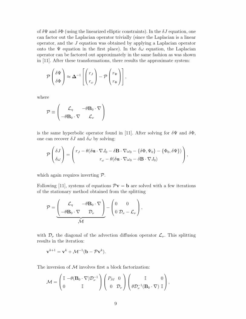
of δΨ and δΦ (using the linearized elliptic constraints). In the δJ equation, onecan factor out the Laplacian operator trivially (since the Laplacian is a linearoperator, and the J equation was obtained by applying a Laplacian operatoronto the Ψ equation in the first place). In the δω equation, the Laplacianoperator can be factored out approximately in the same fashion as was shownin [11]. After these transformations, there results the approximate system:

P

δΨ

δΦ

≈ ∆−1

rJ

rω

− P

rΨ

rΦ

,

where

P ≡

Lη −θB0 · ∇−θB0 · ∇ Lν

is the same hyperbolic operator found in [11]. After solving for δΨ and δΦ,one can recover δJ and δω by solving:

P

δJ

δω

=

rJ − θ(δu · ∇J0 − δB · ∇ω0 − δΦ,Ψ0 − Φ0, δΨ)rω − θ(δu · ∇ω0 − δB · ∇J0)

,

which again requires inverting P .

Following [11], systems of equations Pv = b are solved with a few iterationsof the stationary method obtained from the splitting

P =

Lη −θB0 · ∇−θB0 · ∇ Dν

︸ ︷︷ ︸

M

−

0 0

0 Dν − Lν

,

with Dν the diagonal of the advection diffusion operator Lν . This splittingresults in the iteration:

vk+1 = vk +M−1(b− Pvk).

The inversion of M involves first a block factorization:

M =

I −θ(B0 · ∇)D−1ν

0 I

PSI 0

0 Dν

I 0

θD−1ν (B0 · ∇) I

,

9

with PSI = Lη − θ2∇ · (B0D−1ν BT

0∇), and then the inversion of the resultingmatrices, yielding:

M−1 =

I 0

−θD−1ν (B0 · ∇) I

P−1

SI 0

0 D−1ν

I θ(B0 · ∇)D−1

ν

0 I

.

The implementation of M−1 only requires the (trivial) inversion of Dν (whichis a diagonal matrix), and the inversion of the semi-implicit operator PSI . Thelatter is a parabolic operator, amenable to multilevel techniques, as describedin [11].

4 Adaptive Mesh Refinement

The previous discussion has considered the generalization of the physics-basedpreconditioner proposed in Ref. [11] to the application at hand, without regardto the specifics of the spatial discretization employed. In what follows, wedescribe the AMR-specific details of our treatment of the MHD equations, withparticular emphasis on 1) the spatial discretization at coarse-fine interfaces,2) the generalization of multilevel solvers for SAMR grids, and 3) regriddingand its impact on time integration.

4.1 Structured AMR Grids

Let Ω = [xlo , ylo ]× [xhi , yhi ] be a rectangular computational domain. We createa discrete computational domain by subdividing [xlo , xhi ] into nx subintervalswith centers xi = x0 +(i+ 1

2)hx with hx = (xhi −xlo)/nx for i = 0, . . . , nx− 1.

Each subinterval has faces located at xi− 12

= xi − hx/2 and xi+ 12

= xi + hx/2.

Likewise [ylo , yhi ] is partitioned into ny subintervals with centers yj = y0 +(j+12)hy with hy = (yhi − ylo)/ny for j = 0, . . . , ny − 1 and faces yj− 1

2= yj − hy/2

and yj+ 12

= yj + hy/2. The tensor product of these subintervals partitions Ω

into a collection of computational cells Ωh = Ωi,j each with size hx × hycentered at coordinates (xi, yj). These ideas are readily extended to the casewhere Ω is a union of non-overlapping rectangular regions, and we continueto use the same notation Ωh to denote such a collection of computationalcells. Such regular grids are in widespread use in computational science andengineering, and a great deal of high quality software that is tuned to regulargrids, such as geometric multigrid methods, is available.

Let K ≥ 1 and Ω1 ≡ Ω ⊃ Ω2 ⊃ · · ·ΩK be a nested set of subdomains of thecomputational domain Ω. For simplicity, assume that each Ω`, 2 ≤ ` ≤ K is

10

Fig. 1. Example of a multilevel SAMR grid with three levels.

a union of non-overlapping rectangular regions; these are the subregions of Ωwhere additional resolution is desired. A composite structured AMR (SAMR)grid Ωc on Ω is a nested hierarchy of grids Ωh1

1 ⊃ Ωh22 ⊃ · · · ⊃ ΩhK

K consistingof K levels, with mesh spacing h1 > h2 > · · · > hK , with the coarsest grid Ωh1

1

covering Ω. Each level Ωh`` consists of a union of non-overlapping rectangular

regions, or patches, at the same resolution h`. When there is no risk of con-fusion we will drop the ` subscript and simply refer to Ωh` . This hierarchicalrepresentation allows operations on Ωc to be implemented as operations onindividual levels Ωh` , which in turn are decomposed into operations on indi-vidual patches, each of which covers a rectangular region [xlo , ylo ]× [xhi , yhi ].This property facilitates reuse of software written for regular grids. Figure 1shows a SAMR grid with K = 3 and two patches on each of the two refine-ment levels. Note that while each level is nested in the next coarser level,there is no requirement that a patch at one refinement level is nested fullyin a patch at another refinement level, i.e., a fine patch at refinement level lmay lie over one or more coarser patches at refinement level (l − 1). Figure 2shows the decomposition of a fairly complex SAMR grid with six refinementlevels into its constituent refinement levels and patches, as is encountered inour simulations.

4.2 Function evaluation on SAMR grids

For a viable JFNK solver, a given application only needs to provide methodsto evaluate F , set up a preconditioner, and apply the preconditioner. By gener-alizing these steps to a SAMR grid hierarchy, JFNK can be readily adapted toSAMR applications. In this work, we use the PETSc parallel implementationof JFNK [3], which is made SAMR-aware via the PETSc-SAMRAI interfacesdescribed in [39]. Considerations for evaluating F are described next.

11

Fig. 2. The decomposition of a SAMR grid into its constituent refinement levels

4.2.1 Single grid discretization

In order to discretize F [given by (6)] in space, a cell-centered collocated finite-

volume scheme is used for ω, J,Φ, and Ψ. The magnetic field, ~B = (B1, B2)T,and the velocity, ~v = (u1, u2)T, are also stored at cell centers, and are computedusing centered differences from Ψ and Φ, respectively, using the discrete curloperations:

B1i,j = −Ψi,j+1 −Ψi,j−1

2hy,

B2i,j =

Ψi+1,j −Ψi−1,j

2hx,

(12)

and

u1i,j = −Φi,j+1 − Φi,j−1

2hy,

u2i,j =

Φi+1,j − Φi−1,j

2hx.

(13)

We note that this discretization ensures that the divergence-free conditions on~B and ~v are satisfied locally to numerical round-off.

Diffusive operators are discretized in each cell (i, j) by first computing approx-imate face-centered diffusive fluxes and then summing over the faces of each

12

cell resulting in the standard five-point finite-volume discretization:

1

hxhy

∫Ωi,j

∇ · ∇Ψ dA≈ Ψi+1,j −Ψi,j

h2x

− Ψi,j −Ψi−1,j

h2x

+ (14)

Ψi,j+1 −Ψi,j

h2y

− Ψi,j −Ψi,j−1

h2y

.

Advective quantities are discretized using standard centered differences. Thestandard cell-centered difference discretization for the gradient operator canbe derived by using a variant of the Gauss theorem for gradients on each cell:

∫Ωi,j

∇ω dA=∫

∂Ωi,j

ωn ds

where n is the unit outward-facing normal on ∂Ωi,j, and approximating theface centered values by averaging from cell centers. This results in

1

hxhy

∫Ωi,j

∇ω dA =ωi+1,j − ωi−1,j

2hx~i+

ωi,j+1 − ωi,j−1

2hy~j (15)

When applied to discretize quantities such as ~B · ∇ω using a finite-volumeformulation, we note that there is an implicit assumption that ~B is constantover each cell.

4.2.2 Extension to SAMR grids

The discretizations described in the previous subsection are valid in the inte-riors of individual patches as well as the boundaries between two patches onthe same refinement level. However, in order to maintain accuracy, changesare required at the boundaries between coarse and fine patches. Figure 3 (left)shows the interface between a coarse and fine patch. We use ghost cells (bothcoarse and fine) for communication at coarse-fine interfaces, as well as be-tween patches in the same refinement level. A fine ghost-cell (Figure 3, cen-ter) overlaps one coarse cell. A coarse ghost-cell (Figure 3, right), however,lies underneath four fine cells when a refinement ratio of 2 is used.

For computations of fine-ghost-cell values at coarse-fine interfaces, data isquadratically interpolated from a combination of coarse and fine-grid cell data.Figure 4(left) shows the coarse grid cells that would be involved in performingquadratic tangential interpolation of coarse-grid data to align it with fine-grid data. Figure 4(right) shows the piecewise quadratic normal interpolation

13

Fig. 3. (left) A coarse-fine interface. (center) Fine ghost cell. (right) Coarse ghostcell.involving fine cells to calculate the fine-ghost-cell value. Once data has beeninterpolated to fine ghost-cells, fine cells at coarse-fine interfaces can be treatedidentically to cells that lie in the interior of the fine patch. Figure 4 onlyshows the simplest case where a sufficient number of coarse cells (in this case,three), are available to do standard quadratic interpolation tangential to theinterface. In general, for block-structured AMR, many special cases need to beaccounted for, where two or more fine patches may be adjacent to each other,resulting in very irregular coarse-fine interfaces (see for example Figure 2). Wedo not detail the adjustments needed in each of these cases to interpolate dataquadratically, due to space limitations. However, [2] provides a glimpse of thetypes of adjustments required.

Fig. 4. Schematic of interpolation. (Left) Crosses show coarse grid data alignedwith fine grid data by interpolation. (Right) Open circles denote fine ghost-celldata obtained by interpolation from aligned coarse data and fine grid data.

Regarding coarse ghost-cells at coarse-fine interfaces, their treatment is doneas follows:

Magnetic and velocity fields: ~B and ~v are computed from Ψ and Φ us-ing centered differences. While this maintains the vector fields divergence-freeeverywhere, it requires values of Ψ and Φ to be available at the coarse ghost-cells. A simple averaging of fine Ψ and Φ data to coarse ghost-cells produces

14

second-order accurate coarse values, and therefore the resulting ~B and ~v areonly first-order accurate. Local first-order accuracy at coarse-fine interfacesis unlikely to affect the global second-order accuracy of the calculation whenthe number of coarse fine cells is small relative to the total number of cells.However, Ref. [1] gives examples of cases not unlike the situations present inour simulations where the number of coarse-fine interface cells can be up to30% of the total number of cells. In such cases, global accuracy will be af-fected by the local first-order accuracy at coarse-fine interfaces. To avoid thissituation, we use piecewise cubic interpolation of fine-grid data for Ψ, Φ tocoarse ghost-cells. This, in turn, results in second-order discretizations for thevectors at coarse cells adjacent to the coarse-fine interface.

Diffusion operators: To compute the numerical diffusive fluxes at coarsecells adjacent to the coarse-fine interface, it is possible to use coarse ghost-cellvalues underlying the fine grid. However, for flux conservation, we computethe diffusive fluxes at fine cell faces (as described in Sec. 4.2.1) and averagethem down to provide the coarse flux at the coarse face.

Advection operators: Centered differences in each coarse cell are computedby first computing face-averaged values of the advected quantity as describedin section 4.2.1. At coarse-fine interfaces, we follow Ref. [24] and find a coarseface-averaged value by averaging fine face-averaged data. (The alternative isto compute a coarse ghost-cell value directly from coarse data, but this doesnot work as well.)

4.3 Regridding

For fully dynamic AMR simulations, the grid hierarchy will change during thesimulation as the solution evolves in time and space. This involves the addi-tion of fine patches in regions where additional resolution is required and theremoval of patches in regions where coarser resolution is sufficient. The regrid-ding process involves using some refinement indicator to determine requiredgrid resolution, and then constructing a new grid hierarchy based on this in-formation. The ideal refinement indicator is a sharp estimate of the spatialerror that is inexpensive to compute. When such an estimate is not available,refinement indicators that detect features in the solution, such as regions oflarge gradients or curvature, are used. We detail the refinement indicators weemploy in this study in Sec. 5.

Once regridding is done, data needs to be transferred from the old grid hierar-chy to the new one. Typically, the solution obtained on the old grid hierarchyis no longer a solution on the new grid hierarchy. This has been observed inour simulations as well as reported by others [6]. Two approaches are com-

15

mon in the literature. One approach, referred to as the ”warm restart” [5],continues the time integration on the new grid hierarchy (with a time stepcomparable to that before regridding) using the interpolated data on the newgrid hierarchy. The second approach, called a ”cold restart” [5], alters the timestep and possibly the time integration scheme to account for regridding andintroduction of spatial errors.

In this study, we use a third approach. After interpolation of the requiredvectors (including current and previous time-step solutions required for thetime integration scheme), we solve for the current time step solution on thenew grid hierarchy using the solution interpolated from the old grid hierarchyas an initial guess. This synchronizes the current time step solution with thenew grid hierarchy before advancing in time. Numerically, this procedure isrobust, and avoids propagation of interpolation errors during regridding steps.A detailed evaluation of all three approaches is reserved for future work.

4.4 Preconditioning and the Fast Adaptive Composite Grid Method

Physics-based preconditioning, as described in section 3.2, requires the inver-sion of the parabolic operator PSI = Lη − θ2∇ · (B0D−1

ν BT0∇). The operator

∇ · (B0D−1ν BT

0∇) is negative definite and self-adjoint. The discretization ofthis operator follows [50] so that it is compact (i.e., on a nine-point sten-cil), and the resulting matrix is symmetric negative definite. We note that,at coarse-fine interfaces, symmetry is lost. The convective operator in PSI isdiscretized using a first-order upwind scheme for robustness (instead of thecentered differences employed to evaluate the nonlinear residual). This leadsto an algebraically better conditioned operator that increases the robustnessof the preconditioner but does not affect the accuracy of the solution, whichis determined by (7).

On a SAMR grid, the inversion of PSI is performed efficiently by using the FastAdaptive Composite grid (FAC) method [35,36]. FAC extends techniques frommultigrid on uniform grids to AMR grids. FAC solves problems on AMR gridsby combining smoothing on refinement levels with a coarse-grid solve using anapproximate solver, such as a V-cycle of multigrid. First we introduce somenotation to describe the FAC algorithm:

• I`c : Ωc → Ωh` and Ic` : Ωh

` → Ωc respectively denote restriction and interpo-lation operators between the composite SAMR grid, Ωc and an individualrefinement level. Here we use bilinear interpolation for Ic` and simple aver-aging for I`c .

• I``+1 : Ωh` → Ωh

`+1 and I`+1` : Ωh

`+1 → Ωh` respectively denote restriction and

interpolation operators between consecutive refinement levels.

16

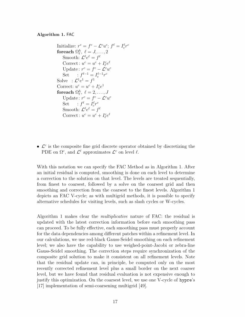
Algorithm 1. FAC

Initialize: rc = f c − Lcuc; f ` = I`crc

foreach Ωh` , ` = J, . . . , 2

Smooth: L`e` = f `

Correct : uc = uc + Ic` e`

Update : rc = f c − LcucSet : f `−1 = I`−1

c rc

Solve : L1e1 = f 1

Correct: uc = uc + Ic1e1

foreach Ωh` , ` = 2, . . . , J

Update : rc = f c − LcucSet : f ` = I`cr

c

Smooth: L`e` = f `

Correct : uc = uc + Ic` e`

• Lc is the composite fine grid discrete operator obtained by discretizing thePDE on Ωc, and L` approximates Lc on level `.

With this notation we can specify the FAC Method as in Algorithm 1. Afteran initial residual is computed, smoothing is done on each level to determinea correction to the solution on that level. The levels are treated sequentially,from finest to coarsest, followed by a solve on the coarsest grid and thensmoothing and correction from the coarsest to the finest levels. Algorithm 1depicts an FAC V-cycle; as with multigrid methods, it is possible to specifyalternative schedules for visiting levels, such as slash cycles or W-cycles.

Algorithm 1 makes clear the multiplicative nature of FAC: the residual isupdated with the latest correction information before each smoothing passcan proceed. To be fully effective, each smoothing pass must properly accountfor the data dependencies among different patches within a refinement level. Inour calculations, we use red-black Gauss-Seidel smoothing on each refinementlevel; we also have the capability to use weighed-point-Jacobi or zebra-lineGauss-Seidel smoothing. The correction steps require synchronization of thecomposite grid solution to make it consistent on all refinement levels. Notethat the residual update can, in principle, be computed only on the mostrecently corrected refinement level plus a small border on the next coarserlevel, but we have found that residual evaluation is not expensive enough tojustify this optimization. On the coarsest level, we use one V-cycle of hypre’s[17] implementation of semi-coarsening multigrid [49].

17

5 Numerical results

This section introduces several challenging test cases with the goal of demon-strating two main aspects of our implicit AMR implementation: algorith-mic performance, and its accuracy properties. In regards to performance, wedemonstrate that the convergence properties of the iterative approach are es-sentially independent of the number of grid levels present in the simulation(for equivalent fine-level resolution), and that it has good scaling propertieswith respect to the total number of unknowns. Both these aspects are centralin a scalable implicit AMR algorithm.

Accuracy and error propagation in the SAMR context is also a major subjectof this section. Clearly, the main motivation for using an AMR-based strategyis to minimize the number of unknowns required to achieve a given error level,by using fine resolution only where it is needed. However, time integration onSAMR grids can pose additional difficulties and introduce sources of error notencountered in uniform-grid calculations, especially at the interface betweencoarse and fine refinement levels. For nonlinear problems, these errors can ex-hibit themselves in unexpected ways that are often hard to identify and offset.In fact, the potential exists that errors generated at coarse-fine interfaces, com-bined with the wrong temporal integrator, may overwhelm the simulation andresult in errors that scale with the coarsest (instead of the finest) resolutionin the computational mesh.

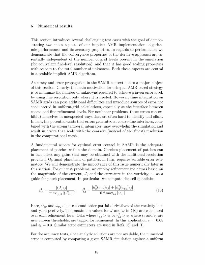
A fundamental aspect for optimal error control in SAMR is the adequateplacement of patches within the domain. Careless placement of patches canin fact offset any gains that may be obtained with the additional resolutionprovided. Optimal placement of patches, in turn, requires suitable error esti-mators. We will demonstrate the importance of this issue numerically later inthis section. For our test problems, we employ refinement indicators based onthe magnitude of the current, J , and the curvature in the vorticity, ω, as aguide for patch placement. In particular, we compute the cell quantities

τ 1i,j =

|(J)i,j|max(i,j) |(J)i,j|

, τ 2i,j =

|h2x(ωxx)i,j|+ |h2

y(ωyy)i,j|0.2 maxi,j |ωi,j|

. (16)

Here, ωxx and ωyy denote second-order partial derivatives of the vorticity in xand y, respectively. The maximum values for J and ω in (16) are calculatedover each refinement level. Cells where τ 1

i,j > ε1 or τ 2i,j > ε2 where ε1 and ε2 are

user chosen thresholds, are tagged for refinement. In this application ε1 = 0.65and ε2 = 0.3. Similar error estimators are used in Refs. [6] and [1].

For the accuracy tests, since analytic solutions are not available, the numericalerror is computed by comparing a given SAMR simulation against a uniform

18

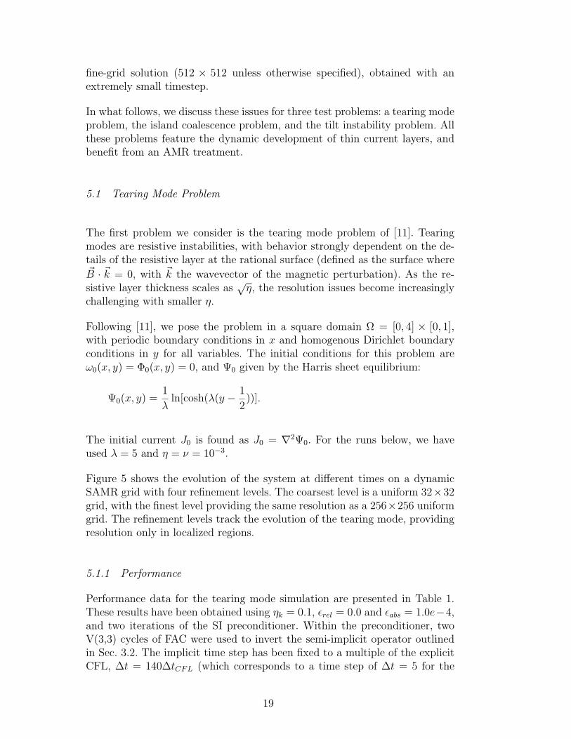
fine-grid solution (512 × 512 unless otherwise specified), obtained with anextremely small timestep.

In what follows, we discuss these issues for three test problems: a tearing modeproblem, the island coalescence problem, and the tilt instability problem. Allthese problems feature the dynamic development of thin current layers, andbenefit from an AMR treatment.

5.1 Tearing Mode Problem

The first problem we consider is the tearing mode problem of [11]. Tearingmodes are resistive instabilities, with behavior strongly dependent on the de-tails of the resistive layer at the rational surface (defined as the surface where~B · ~k = 0, with ~k the wavevector of the magnetic perturbation). As the re-sistive layer thickness scales as

√η, the resolution issues become increasingly

challenging with smaller η.

Following [11], we pose the problem in a square domain Ω = [0, 4] × [0, 1],with periodic boundary conditions in x and homogenous Dirichlet boundaryconditions in y for all variables. The initial conditions for this problem areω0(x, y) = Φ0(x, y) = 0, and Ψ0 given by the Harris sheet equilibrium:

Ψ0(x, y) =1

λln[cosh(λ(y − 1

2))].

The initial current J0 is found as J0 = ∇2Ψ0. For the runs below, we haveused λ = 5 and η = ν = 10−3.

Figure 5 shows the evolution of the system at different times on a dynamicSAMR grid with four refinement levels. The coarsest level is a uniform 32×32grid, with the finest level providing the same resolution as a 256×256 uniformgrid. The refinement levels track the evolution of the tearing mode, providingresolution only in localized regions.

5.1.1 Performance

Performance data for the tearing mode simulation are presented in Table 1.These results have been obtained using ηk = 0.1, εrel = 0.0 and εabs = 1.0e−4,and two iterations of the SI preconditioner. Within the preconditioner, twoV(3,3) cycles of FAC were used to invert the semi-implicit operator outlinedin Sec. 3.2. The implicit time step has been fixed to a multiple of the explicitCFL, ∆t = 140∆tCFL (which corresponds to a time step of ∆t = 5 for the

19

t = 50 t = 120 t = 200

Fig. 5. Time snapshots of current (top) and vorticity (bottom) for the tearing modeproblem.

coarsest 64× 32 grid), and we have averaged the performance results over thecourse of the simulation up to Tmax = 250.

Table 1Summary of performance for tearing mode. NNI: average number of nonlinear iter-ations; NLI: average number of linear iterations.

NNI NLI

Levels 1 2 3 4 5 1 2 3 4 5

64× 32 2.4 2.7 2.8 2.8 2.7 8.2 10.3 14.1 15.8 16.4

128× 64 2.3 2.6 2.7 2.6 – 8.0 12.9 15.1 16.1 –

256× 128 2.0 2.1 2.4 – – 9.4 13.9 12.8 – –

512× 256 2.0 2.1 – – – 12.4 13.3 – – –

The first column of the Table specifies the resolution of the coarse grid, whilelevels refers to the number of refinement levels active on the SAMR grid. Mov-ing diagonally from left to right, for example from the cell corresponding tothe 512×256 grid with one refinement level to the cell with a 64×32 base gridand five levels of refinement, we see that the number of nonlinear iterations,NNI, remains more or less constant. The number of linear iterations, NLI,grows slightly with resolution, both in single-grid and AMR computations.Nevertheless, it is apparent that we are obtaining very similar solver perfor-mance on a SAMR grid to what we would expect to see on a uniform gridwith comparable fine resolution.

20

This substantially equivalent solver performance is obtained for significantlyless computational effort and memory storage. For example, the 512 × 256run requires a total wall-clock time of 29919 seconds while the equivalent64× 32 run with 4 levels of refinement takes 4998 seconds of wall-clock time.Furthermore, on average, the 64× 32 run with 4 levels of refinement requiresonly 14% of the number of degrees of freedom that a uniform 512 × 256 runwould require. The timing runs were obtained on a MacBook Pro with a 2.33GHz Intel Core 2 Duo processor, 2 GB of RAM, running Mac OS X 10.4.10.

Similar results both in solver performance as well as time and memory savingswere obtained in all our simulations.

5.1.2 Time-integration errors

We seek to characterize the importance of adequate interpolation order dur-ing regridding to avoid discretization errors, and of robust damping in theimplicit temporal integration scheme to avoid error propagation throughoutthe domain.

Fig. 6. Grid hierarchy and error in J after one regrid operation at t = 2.5 andseveral time steps up to t = 7.5.

A common approach for time integration on AMR grids is to use linear inter-polation to transfer data from an old grid hierarchy to a new grid hierarchyduring regridding. For problems with discontinuous coefficients and steep solu-tion gradients [40], this works better than higher-order interpolation schemes.However, linear interpolation is not suitable for all problems. Figure 6 depictsthe error in J on a SAMR grid after one regrid operation at t = 2.5 and subse-quent time-stepping using Crank-Nicolson (CN) and quadratic interpolationat coarse-fine interfaces up to t = 7.5. Linear interpolation was used to transferdata from the old to the new grid hierarchy during regrid. The concentrationof discretization errors at coarse-fine interfaces introduced during regriddingis evident, despite the fact that quadratic interpolation was used at coarse-fine

21

interfaces during the time evolution. Furthermore, the poor damping proper-ties of CN preserves the memory of generated errors, even if the location of thecoarse-fine interfaces changes. To show this, we transfer the previous solutionat t = 7.5 to a uniform mesh with resolution equivalent to the finest SAMRpatch, and run the simulation further in time to t = 42.5. The result is de-picted in Figure 7, and shows that the error in J generated during regriddingat coarse-fine interfaces remains throughout the calculation. We note that themagnitude of the error does not appear to be changing significantly.

Fig. 7. Grid hierarchy and error in J after a second regrid operation to a uniformmesh at t = 7.5 and subsequent time-stepping until t = 42.5.

A related test with a different initial grid configuration is shown in Figure 8.In this case, the error in J is largest on the left and right coarse-fine interfacesat time t = 7.5. After several dynamical regridding operations, the solutionhas memory of errors generated at all coarse-fine interfaces during regridding,and at time t = 42.5 the error (Figure 9) traces all coarse-fine interfaces thathave been present during the simulation. In this example, it is clear that, atsome locations, the error is actually being amplified further, as for example atthe left and right coarse-fine interfaces present in the initial grid hierarchy att = 7.5.

The previous examples illustrate potential sources of error that can accumu-late due to a combination of a poor temporal integrator (CN) and low-orderinterpolation during regridding, even if higher-order interpolation is used atcoarse-fine interfaces. Low-order interpolation generates spatial errors thatare not damped in time by the temporal scheme. Coarse-fine errors mostlydisappear when sufficiently high-order interpolation is used (both at regridoperations and subsequently during time evolution) in combination with a ro-bustly damping temporal scheme. Figure 10 shows plots of the error in J attimes t = 10 and t = 50, using cubic interpolation at regrid, quadratic interpo-lation in between regrid operations, and BDF2 as the time integrator. In thiscase, we see that there is no accumulation of error at coarse-fine interfaces,even after several regrid operations have taken place.

22

Fig. 8. Grid hierarchy and error in J at t = 7.5 after one regrid operation at t = 2.5.

Fig. 9. Grid hierarchy and error in J at t = 42.5 after several regridding operations.

5.2 Island Coalescence

In the island coalescence problem, two magnetic islands (current channels)attract and reconnect. In resistive MHD, and during the reconnection process,a thin, elongated current sheet forms at the reconnection site, which governsthe reconnection rate, and therefore the global dynamics [30]. As in the tearingmode problem, the current thickness scales as

√η, and therefore the problem

becomes computationally more challenging for smaller resistivities.

The island coalescence problem equilibrium is given by ω0(x, y) = Φ0(x, y) =0, and Ψ0 defined as [20]:

Ψ0(x, y) = −λΨ ln[cosh

(y

λΨ

)+ ε cos

(x

λΨ

)], (17)

where λΨ = 12π

is the current sheet equilibrium scale length, and ε = 0.2 is the

23

Fig. 10. Plots of error in J for t = 10 and t = 50 using BDF2 for time integrationand cubic interpolation for regridding operations.

Fig. 11. Snapshots of the current at early stages of the coalescence process (t = 4,left) and at the peak of the reconnection (t = 8, right) during the coalescenceprocess.

island width. The computational domain is Ω ∈ [−1, 1] × [−1, 1]. Boundaryconditions are Dirichlet in y, and periodic in x. Both η and ν are set to10−4. The calculation is started with a perturbation in Ψ. Full dynamicalSAMR regridding is employed to adapt to developing features. The islandconfiguration at the early stages of the coalescence process is shown in Figure11. The configuration at the peak of the reconnection rate, well in the nonlinearstage, is shown in Figure 11, and shows the formation of the current sheet inthe symmetry plane between the islands. The multiscale nature of this problemis evident.

24

5.2.1 Numerical error generation and propagation

As mentioned earlier, the purpose of grid adaptation is to minimize the numberof degrees of freedom required for a given simulation, while being compatiblewith a given numerical error level. In practice, the expectation is that the over-all numerical error of the simulation does not increase due to the presence ofpatches, and the related coarse-fine boundary treatment. Otherwise, it woulddefeat the purpose of using a patch-based adaptive scheme in the first place.

We use the island coalescence problem to characterize the generation andtemporal propagation of errors in our SAMR implementation. We focus ontwo main aspects of error generation in SAMR: 1) the treatment of coarse-fineinterfaces at patches’ boundaries, and 2) the placement of patches themselves.The former is fundamentally a spatial discretization issue, whereas the latteris more related to error estimation.

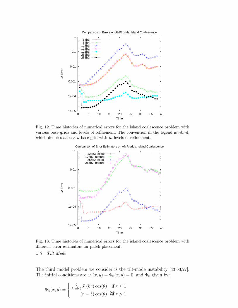
Figure 12 depicts several time histories of SAMR simulations featuring differ-ent base grids and levels of refinement. The error is obtained with an “exact”error detector, which compares the SAMR solution with the 512×512 referencesolution. The point of this plot is to establish that the error is fundamentally afunction of the finest resolution employed, and not a function of the base gridsize or the number of levels of refinement. For instance, the 64b3l, 128b2l, and256b1l simulations feature the same error (time histories are actually superim-posed), while using different base grid refinements and number of grid levels.The same is true for 64b4l, 128b3l, and 256b2l (although error differences aremore noticeable due to the log scale of the plot). Another side point from thisfigure is the impact that adding a level of refinement has on the overall error ofthe computation: the error decreases about 2 orders of magnitude on average.

The effect of choice of refinement indicator is depicted in Figure 13, where timehistories of the numerical error resulting from two different error estimators areprovided. The exact error estimator is compared against an ad-hoc indicator(16). The error plot labeled 128b3l-exact plots the magnitude of the L2 erroron an AMR grid with 3 levels, when the placement of patches is determinedby the “exact” error detector. Similarly, the error plot labeled 128b3l-featureplots the error on an AMR grid determined using (16). Clearly, the overallnumerical error resulting from the ad-hoc approach is about two orders ofmagnitude larger, almost offsetting the accuracy gains obtained by addingrefinement levels. This result underscores the importance of further researchon reliable error estimators for adaptive-grid applications. This is left for futurework.

25

1e-05

1e-04

0.001

0.01

0.1

1

0 5 10 15 20 25 30 35 40

L2 E

rror

Time

Comparison of Errors on AMR grids: Island Coalescence

64b3l64b4l

128b1l128b2l128b3l256b1l256b2l

Fig. 12. Time histories of numerical errors for the island coalescence problem withvarious base grids and levels of refinement. The convention in the legend is nbml,which denotes an n× n base grid with m levels of refinement.

1e-05

1e-04

0.001

0.01

0.1

0 5 10 15 20 25 30 35 40

L2 E

rror

Time

Comparison of Error Estimators on AMR grids: Island Coalescence

128b3l-exact128b3l-feature

256b2l-exact256b2l-feature

Fig. 13. Time histories of numerical errors for the island coalescence problem withdifferent error estimators for patch placement.

5.3 Tilt Mode

The third model problem we consider is the tilt-mode instability [43,53,27].The initial conditions are ω0(x, y) = Φ0(x, y) = 0, and Ψ0 given by:

Ψ0(x, y) =

2

kJ0(k)J1(kr) cos(θ) if r ≤ 1

(r − 1r) cos(θ) if r > 126

with J0 = ∇2Ψ0. The boundary conditions are periodic in x and Dirichlet iny for all variables. The system is perturbed from its initial equilibrium witha rotational perturbation in Φ of the form: δΦ = 10−3e−r

2. The domain for

this problem is Ω = [−2π, 2π] × [−5, 5]. The parameter k is the zero of theBessel function of the first kind, i.e., J1(k) = 0, and both η and ν are set to10−3. The refinement criteria for this problem is also given by (16). Figure5.3 shows snapshots of the current and vorticity during the evolution of thetilt instability at times t = 4.0 (early in the linear phase) and t = 7.0 (wellin the nonlinear regime). This calculation required seven levels of refinementstarting from a coarse initial 64× 64 mesh.

As evolving features in this problem are extremely small compared to the do-main size, this AMR calculation on average only required 0.36% of the degreesof freedom of a uniform grid calculation (a uniform grid calculation would haverequired 67108864 degrees of freedom, which corresponds to a 4096×4096 uni-form grid with 4 unknowns per grid cell). This example serves to illustrate thesignificant savings that AMR can provide over uniform grid calculations. Wenote that the relatively small number of degrees of freedom enabled us to per-form this calculation on a workstation, while a parallel machine would havebeen required to perform the uniform-grid calculation.

6 Conclusions

We have described the implementation of a scalable, fully implicit, SAMRsimulation tool for 2D reduced resistive MHD. The tool employs Jacobian-free Newton-Krylov methods as the solver engine. We use the reduced MHDsolver developed in [11] as a starting point, albeit with several modifications.Following [51], we have reformulated the original problem (in terms of poloidalflux, vorticity, and streamfunction) using the current as a dynamic variableinstead of the poloidal flux. This avoids issues with SAMR and the high-orderdifferentiation of the latter in terms like ~B · ∇J .

We have also extended the optimal “physics-based” approach developed in[11] (which employed multigrid solver technology in the preconditioner forscalability) for this application in two ways. Firstly, we have adapted thepreconditioner formulation to deal with J instead of Ψ, as required. Secondly,we have extended the multilevel treatment in [11] to SAMR grids using thewell-known Fast Adaptive Composite grid (FAC) method [35]. As a result, ourapproach inherits the algorithmic benefits of a multilevel treatment and theaccuracy benefits of dynamic grid adaptation.

We have demonstrated such benefits with several challenging tests. A gridconvergence study has shown that the solver performance is independent of

27

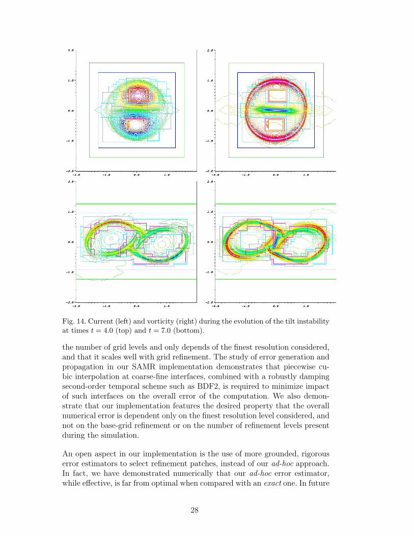
Fig. 14. Current (left) and vorticity (right) during the evolution of the tilt instabilityat times t = 4.0 (top) and t = 7.0 (bottom).

the number of grid levels and only depends of the finest resolution considered,and that it scales well with grid refinement. The study of error generation andpropagation in our SAMR implementation demonstrates that piecewise cu-bic interpolation at coarse-fine interfaces, combined with a robustly dampingsecond-order temporal scheme such as BDF2, is required to minimize impactof such interfaces on the overall error of the computation. We also demon-strate that our implementation features the desired property that the overallnumerical error is dependent only on the finest resolution level considered, andnot on the base-grid refinement or on the number of refinement levels presentduring the simulation.

An open aspect in our implementation is the use of more grounded, rigorouserror estimators to select refinement patches, instead of our ad-hoc approach.In fact, we have demonstrated numerically that our ad-hoc error estimator,while effective, is far from optimal when compared with an exact one. In future

28

work, we will explore more rigorous error estimators, such as the τ (or two-grid) error estimator, which employs differences between two grid resolutionsto estimate the truncation error. The approach, which is rigourous in thecontext of linear, conservative operators, can be used effectively for non-linearones (see e.g. Refs. [7,19,34,18] for theory and practical implementation detailsand effectiveness of this error estimator in various contexts; in particular, Ref.[18] employs it for an anisotropic AMR implementation).

Acknowledgments

The authors acknowledge useful discussions with D. A. Knoll. The work wasfunded by the Los Alamos Directed Research and Development program atLos Alamos National Laboratory, operated for DOE under contract No. DE-AC52-06NA25396, and by the DOE Office of ASCR program in Applied Math-ematical Sciences.

References

[1] M. J. Aftosmis and M.J. Berger, Multilevel error estimation and adaptiveh-refinement for cartesian meshes with embedded boundaries, in 40th AIAAAerospace Sciences Meeting and Exhibit, no. 2002-0863 in AIAA Paper,January 2002.

[2] A. S. Almgren, J. B. Bell, P. Colella, L. H. Howell, and M. L.Welcome, A conservative adaptive projection method for the variable densityincompressible Navier-Stokes equations, J. Comput. Phys., 142 (1998), pp. 1–46.

[3] S. Balay, W. D. Gropp, L. Curfman-McInnes, and B. F. Smith, PETScUsers Manual, Tech. Report ANL-95/11 - Revision 2.1.6, Argonne NationalLaboratory, 2004.

[4] Dinshaw S. Balsara, Divergence-free adaptive mesh refinement formagnetohydrodynamics, J. Comput. Phys., 174 (2001), pp. 614–648.

[5] Martin Berzins, Philip J. Capon, and Peter K. Jimack, On spatialadaptivity and interpolation when using the method of lines, Applied NumericalMathematics: Transactions of IMACS, 26 (1997), pp. 117–133.

[6] J. G. Blom and J. G. Verwer, Algorithm 759: Vlugr3: a vectorizableadaptive-grid solver for PDEs in 3d;part ii. code description, ACM Trans. Math.Softw., 22 (1996), pp. 329–347.

[7] A. Brandt, Multigrid techniques: 1984 guide, with applications to fluiddynamics, gmd studien nr. 85, GMD, GMD-AIW, Postfach 1240, D-5205, St.Augustin 1, Germany, 1984. 191 pages.

29

[8] P. N. Brown and Y. Saad, Hybrid Krylov methods for nonlinear systems ofequations, SIAM J. Sci. Statist. Comput., 11 (1990), pp. 450–481.

[9] L. Chacon, An optimal, parallel, fully implicit newton-krylov solver forthree-dimensional visco-resistive magnetohydrodynamics, submitted to Phys.Plasmas, (2007).

[10] L. Chacon and D. A. Knoll, A 2D high-β Hall MHD implicit nonlinearsolver, J. Comput. Phys., 188 (2003), pp. 573–592.

[11] L. Chacon, D. A. Knoll, and J. M. Finn, An implicit, nonlinear reducedresistive MHD solver, J. Comput. Phys., 178 (2002), pp. 15–36.

[12] J. Crank and P. Nicolson, A practical method for numerical evaluationof solutions of partial differential equations of the heat conduction type, Proc.Camb. Phil. Soc., 43 (1947), pp. 50–67.

[13] C. F. Curtiss and J. O. Hirschfelder, Integration of stiff equations, Proc.Nat. Acad. Sci., 38 (1952), pp. 235–243.

[14] R. S. Dembo, S. C. Eisenstat, and T. Steihaug, Inexact Newton methods,SIAM J. Numer. Anal., 19 (1982), pp. 400–408.

[15] J. F. Drake and T. M. Antonsen, Nonlinear reduced fluid equations fortoroidal plasmas, Phys. Fluids, 27 (1984), pp. 898–908.

[16] S. C. Eisenstat and H. F. Walker, Globally convergent inexact Newtonmethods, SIAM J. Optimization, 4 (1994), pp. 393–422.

[17] R. D. Falgout and U. Meier Yang, hypre: a library of high performancepreconditioners, in Computational Science - CARS 2002 Part III, P. M. A. Sloot,C. J. K. Tan, J. J. Dongarra, and A. G. Hoekstra, eds., vol. 2331 of LectureNotes in Computer Science, New York, 2002, Springer-Verlag, pp. 632–641.

[18] L. Ferm and P. Lotstedt, Anisotropic grid adaptation for Navier-Stokesequations., J. Comput. Phys., 190 (2003), pp. 22 – 41.

[19] L. Ferm and P. L. Lotstedt, Adaptive error control for steady state solutionsof inviscid flow, SIAM Journal on Scientific Computing, 23 (2002), pp. 1777 –98.

[20] J. M. Finn and P.K. Kaw, Coalescence instability of magnetic islands, Phys.Fluids, 20 (1977), pp. 72–78.

[21] C. W. Gear, Numercial initial value problems in ordinary differentialequations, Prentice-Hall, 1971.

[22] K. Germaschewski, A. Bhattacharjee, and C.-S. Ng, The MagneticReconnection code: an AMR-based fully implicit simulation suite, in NumericalModeling of Space Plasma Flows, N. B. Pogorelov and G. P. Zank, eds., vol. 359of ASP Conference Series, 2006.

30

[23] T. I. Gombosi, Solution-adaptive magnetohydrodynamics for space plasmas:Sun-to-earth simulations., Computing in science & engineering, 6 (2004), pp. 14– 35.

[24] D. M. Greaves, Simulation of viscous water column collapse using adaptinghierarchical grids, International Journal for Numerical Methods in Fluids, 50(2006), pp. 693–711.

[25] R. D. Hazeltine, M. Kotschenreuther, and P. J. Morrison, A four-field model for tokamak plasma dynamics, Phys. Fluids, 28 (1985), pp. 2466–2477.

[26] R. D. Hornung and S. Kohn, Managing application complexity in theSAMRAI object-oriented framework, Concurrency Comput.: Pract. Exp., 14(2002), pp. 347–368.

[27] S. C. Jardin and J. A. Breslau, Implicit solution of the four-field extended-magnetohydrodynamic equations using high-order high-continuityfinite elements, Physics of Plasmas, 12 (2005), p. 056101.

[28] C. T. Kelley, Iterative methods for linear and nonlinear equations, SIAM,Philadelphia, 1995.

[29] R. Keppens, Adaptive mesh refinement for conservative systems: Multi-dimensional efficiency evaluation., Computer Physics Communications, 153(2003), pp. 317 – 339.

[30] D. A. Knoll and L. Chacon, Coalescence of magnetic islands, sloshing, andthe pressure problem., Phys. Plasmas, 13 (2006), pp. 32307 – 1.

[31] D. A. Knoll and D. E. Keyes, Jacobian-free Newton-Krylov methods: asurvey of approaches and applications, J. Comput. Phys., 193 (2004), pp. 357–397.

[32] D. A. Knoll and P. R. McHugh, Enhanced nonlinear iterative techniquesapplied to a nonequilibrium plasma flow, SIAM J. Sci. Comput., 19 (1998),pp. 291–301.

[33] S. Lankalapalli, J. E. Flaherty, M. S. Shephard, and H. Strauss,An adaptive finite element method for magnetohydrodynamics, Journal ofComputational Physics, 225 (2007), pp. 363 – 381.

[34] P. Lotstedt, S. Soderberg, A. Ramage, and L. Hemmingsson-Franden, Implicit solution of hyperbolic equations with space-time adaptivity,BIT, 42 (2002), pp. 134 – 58.

[35] S. McCormick, Multilevel Adaptive Methods for Partial DifferentialEquations, SIAM, Philadelphia, PA, 1989.

[36] S. F. McCormick and J. W. Thomas, The fast adaptive composite grid(FAC) method for elliptic equations, Math. Comp., 46 (1986), pp. 439–456.

31

[37] P. R. McHugh and D. A. Knoll, Inexact Newton’s method solution to theincompressible Navier-Stokes and energy equations using standard and matrix-free implementations, AIAA J., 32 (1994), pp. 2394–2400.

[38] C. S. Ng, D. Rosenberg, K. Germaschewski, A. Pouquet, andA. Bhatthacharjee, A comparison of spectral element and finite differencesimulations with adaptive mesh refinement for the MHD island coalescenceinstability problem, New journal of physics. in preparation.

[39] M. Pernice and R. D. Hornung, Newton-Krylov-FAC methods for problemsdiscretized on locally refined grids, Comput. Vis. Sci., 8 (2005), pp. 107–118.

[40] Michael Pernice and Bobby Philip, Solution of equilibrium radiationdiffusion problems using implicit adaptive mesh refinement, SIAM J. Sci.Comput., 27 (2006), pp. 1709–1726.

[41] B. Philip, M. Pernice, and L. Chacon, Solution of reduced resistivemagnetohydrodynamics using implicit adaptive mesh refinement, in DomainDecomposition Methods in Science and Engineering XVI, Olof B. Widlund andDavid E. Keyes, eds., vol. 55 of Lecture Notes in Computational Science andEngineering, Springer-Verlag, 2007, pp. 725–731.

[42] K. G. Powell, Parallel, AMR MHD for global space weather simulations,Lecture notes in computational science and engineering, 41 (2005), pp. 473 –490.

[43] R. L. Richard, R. D. Sydora, and M. Ashour-Abdalla, Magneticreconnection driven by current repulsion, Physics of Fluids B: Plasma Physics,2 (1990), pp. 488–494.

[44] D. Rosenberg, A. Pouquet, and P. D. Mininni, Adaptive mesh refinementwith spectral accuracy for magnetohydrodynamics in two space dimensions, Newjournal of physics, 9 (2007), pp. 304 –.

[45] Y. Saad and M.H. Schultz, GMRES: A generalized minimal residualalgorithm for solving non-symetric linear systems, SIAM J. Sci. Stat. Comput.,7 (1986), pp. 856–869.

[46] R. Samtaney, Adaptive mesh refinement for MHD fusion applications, Lecturenotes in computational science and engineering, 41 (2005), pp. 491 – 503.

[47] R. Samtaney, P. Colella, T. J. Ligocki, D. F. Martin, and S. C.Jardin, An adaptive mesh semi-implicit conservative unsplit method forresistive MHD, in SciDAC 2005. San Francisco, June 26-30. Journal of physics:Conference series., A. Mezzacappa et. al., ed., 2005.

[48] R. Samtaney, S. C. Jardin, P. Colella, and D. F. Martin, 3D adaptivemesh refinement simulations of pellet injection in tokamaks, Computer PhysicsComm., 164 (2004), pp. 220–228.

[49] S. Schaffer, A semicoarsening multigrid method for elliptic partial differentialequations with highly discontinuous and anisotropic coefficients, SIAM J. Sci..Comput., 20 (1999), pp. 228–242.

32

[50] Mikhail Shashkov and Stanly Steinberg, Support-operator finite-difference algorithms for general elliptic problems, J. Comput. Phys., 118 (1995),pp. 131–151.

[51] H. Strauss and D. Longcope, An adaptive finite element method formagnetohydrodynamics, J. Comput. Phys., 147 (1998), pp. 318–336.

[52] H. R. Strauss, Nonlinear, 3-dimensional magnetohydrodynamics ofnoncircular tokamaks, Phys. Fluids, 19 (1976), pp. 134–140.

[53] H. R. Strauss and D. W. Longcope, An adaptive finite element method formagnetohydrodynamics, J. Comput. Phys., 147 (1998), pp. 318–336.

[54] G. Toth, D. L. De Zeeuw, T. I. Gombosi, and K. G. Powell, A parallelexplicit/implicit time stepping scheme on block-adaptive grids, J. of Comput.Phys., 217 (2006), pp. 722 – 58.

33