Amplitude death in systems of coupled oscillators with

distributed-delay coupling

Y.N. Kyrychko∗, K.B. Blyuss

Department of Mathematics, University of Sussex,Brighton, BN1 9QH, United Kingdom

E. Scholl

Institut fur Theoretische Physik, Technische Universitat Berlin,10623 Berlin, Germany

February 2, 2012

Abstract

This paper studies the effects of coupling with distributed delay on the suppression of os-cillations in a system of coupled Stuart-Landau oscillators. Conditions for amplitude death areobtained in terms of strength and phase of the coupling, as well as the mean time delay andthe width of the delay distribution for uniform and gamma distributions. Analytical resultsare confirmed by numerical computation of the eigenvalues of the corresponding characteristicequations. These results indicate that larger widths of delay distribution increase the regionsof amplitude death in the parameter space. In the case of a uniformly distributed delay kernel,for sufficiently large width of the delay distribution it is possible to achieve amplitude death foran arbitrary value of the average time delay, provided that the coupling strength has a valuein the appropriate range. For a gamma distribution of delay, amplitude death is also possiblefor an arbitrary value of the average time delay, provided that it exceeds a certain value asdetermined by the coupling phase and the power law of the distribution. The coupling phasehas a destabilizing effect and reduces the regions of amplitude death.

1 Introduction

Coupled oscillator systems are used to model a wide range of physical and biological phenomena,where the dynamics of the underlying complex system is dominated by the interactions of itselements over multiple temporal and spatial scales. The main advantage of using such a modellingapproach stems from the fact that it allows one to obtain vital information about the behaviourof the complex systems by studying the laws and rules that govern different dynamical regimes,including (de)synchronization, cooperation, stability etc. For instance, some brain pathologiesand cognitive deficiencies, such as Parkinson’s disease, Alzheimer’s disease, epilepsy, autism areknown to be associated with the synchronisation of oscillating neural populations [1, 2, 3]. Phasesynchronisation arises when two or more coupled elements start to oscillate with the same frequency,

∗Corresponding author. Email: y.kyrychko@sussex.ac.uk

1

arX

iv:1

202.

0226

v1 [

nlin

.CD

] 1

Feb

201

2

and if the coupling strength is quite weak, the amplitudes stay unchanged. However, when thecoupling strength becomes stronger, the amplitudes start to interact, which may lead to completesynchronization or amplitude death [4, 5]. The coupling between elements is often not instantaneousaccounting, for example, for propagation delays or processing times and these time delays havebeen shown to play a crucial role in sychronisation as well as in (de)stabilisation of general coupledoscillator systems [6, 7, 8, 9, 10, 11], coupled semiconductor lasers [12, 13, 14], neural [15, 16] andengineering systems [17, 18].

In coupled oscillator systems with delayed couplings one of the intriguing effects of time delaysis amplitude death [19, 20], or death by delay [21], when oscillations are suppressed, and thesystem is driven to a stable equilibrium. The amplitude death phenomenon has been studied boththeoretically and experimentally [22, 23], and it has been shown that in the presence of time delays,amplitude death can occur even if the frequencies of the individual oscillators are the same. Onthe contrary, in the non-delayed case, the amplitude death in coupled oscillator systems can onlybe observed if the frequencies of the individual oscillators are sufficiently different [26, 27].

The majority of research on the effects of time delays upon the stability of coupled oscillators hasbeen focussed on systems with one or several constant time delays. This is a valid, though somewhatlimiting, assumption for some systems where the time delay is fixed and does not change with time.However, many real-life applications involve time delays which are non-constant [28, 29], or morecrucially, where the exact value of the time delay is not explicitly known. This assumption can beovercome by considering distributed-delay systems, where the time delay is given by an integral witha memory kernel in the form of a prescribed delay distribution function. In population dynamicsmodels, distributed time delays have been used to represent maturation time, which varies betweenindividuals [30, 31]; in some engineering systems, the use of distributed time delays is better suiteddue to the fact that only an approximate value of time delay is known [32, 33]; in neural systems, thetime delay is different for different paths of the feedback signals and inclusion of a distribution overtime delays has been shown to increase the stability region of the system as opposed to the samesystems with constant time delays [34]; a similar effect has been shown to occur in predator-preyand ecological food webs [35], in epidemiological models distributed time delays have been usedto model the effects of waning immunity times after disease or vaccination, which differs betweenindividuals [36]. The influence of distributed delays on the overall stability of the system underconsideration has been discussed by a number of authors; for example, in [37], the effects of thetime delays are studied in relation to the coupled oscillators, and in traffic dynamics [38], and in[39] the authors have shown how to approximate the stability boundary around a steady state fora general distribution function.

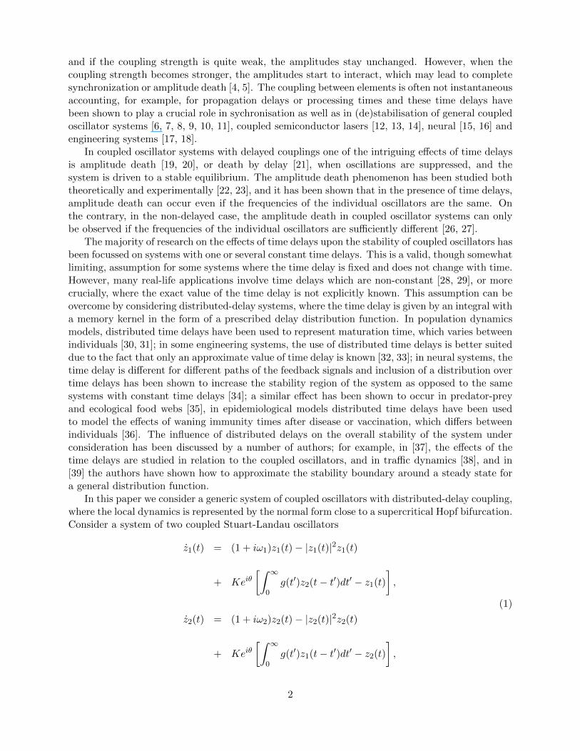
In this paper we consider a generic system of coupled oscillators with distributed-delay coupling,where the local dynamics is represented by the normal form close to a supercritical Hopf bifurcation.Consider a system of two coupled Stuart-Landau oscillators

z1(t) = (1 + iω1)z1(t)− |z1(t)|2z1(t)

+ Keiθ[∫ ∞

0g(t′)z2(t− t′)dt′ − z1(t)

],

(1)

z2(t) = (1 + iω2)z2(t)− |z2(t)|2z2(t)

+ Keiθ[∫ ∞

0g(t′)z1(t− t′)dt′ − z2(t)

],

2

where z1,2 ∈ C, ω1,2 are the oscillator frequencies, K ∈ R+ and θ ∈ R are the strength and thephase of coupling, respectively, and g(·) is a distributed-delay kernel, satisfying

g(u) ≥ 0,

∫ ∞0

g(u)du = 1.

When g(u) = δ(u), one recovers an instantaneous coupling (z2 − z1); when g(u) = δ(u − τ), thecoupling takes the form of a discrete time delay [z2(t − τ) − z1(t)]. We will concentrate on thecase of identical oscillators having the same frequency ω1 = ω2 = ω0. Without coupling, the localdynamics exhibits an unstable steady state z = 0 and a stable limit cycle with |z(t)| = 1. It isknown that time delay in the coupling can introduce amplitude death, which means destruction ofa periodic orbit and stabilization of the unstable steady state.

The system (1) has been analysed by Atay in the case of zero coupling phase for a uniformlydistributed delay kernel [37]. He has shown that distributed delays increase stability of the steadystate and lead to merging of death islands in the parameter space. In this paper, we extend thiswork in three directions. First of all, we also take into consideration a coupling phase, whichis important not only theoretically, but also in experimental realizations of the coupling, as hasalready been demonstrated in laser experiments [40, 41]. Second, to get a better understanding ofthe system behavior inside the stability regions, we will numerically compute eigenvalues. Finally,we will also consider the case of a practically important gamma distributed delay kernel to illustratethat it is not only the mean delay and the width of the distribution, but also the actual shape ofthe distribution that affects amplitude death in systems with distributed-delay coupling.

The outline of this paper is as follows. In Sec. 2 we study amplitude death in the system (1)with a uniformly distributed delay kernel. This includes finding analytically boundaries of stabilityof the trivial steady state, as well as numerical computation of the eigenvalues of the correspondingcharacteristic equations. Section 3 is devoted to the analysis of amplitude death for the case ofa gamma distributed delay kernel. We illustrate how regions of amplitude death are affected bythe coupling parameters and characteristics of the delay distribution. The paper concludes with asummary of our findings, together with an outlook on their implications.

2 Uniformly distributed delay

To study the possibility of amplitude death in the system (1), we linearize this system near thetrivial steady state z1,2 = 0. The corresponding characteristic equation is given by(

1 + iω0 −Keiθ − λ)2−K2e2iθ [{Lg}(λ)]2 = 0, (2)

where λ is an eigenvalue of the Jacobian, and

{Lg}(s) =

∫ ∞0

e−sug(u)du, (3)

is the Laplace transform of the function g(u). To make further analytical progress, it is instructiveto specify a particular choice of the delay kernel. As a first example, we consider a uniformlydistributed kernel

g(u) =

1

2ρfor τ − ρ ≤ u ≤ τ + ρ,

0 elsewhere.

(4)

3

This distribution has the mean time delay

τm ≡< τ >=

∫ ∞0

ug(u)du = τ,

and the variance

σ2 =

∫ ∞0

(u− τm)2g(u)du =ρ2

3. (5)

In the case of a uniformly distributed kernel Eq. (4), it is quite easy to compute the Laplacetransform of the distribution g(u) as:

{Lg}(λ) =1

2ρλe−λτ

(eλρ − e−λρ

)= e−λτ

sinh(λρ)

λρ,

and this also transforms the characteristic equation (2) as

1 + iω0 −Keiθ − λ = ±Keiθe−λτ sinh(λρ)

λρ. (6)

Since the roots of the characteristic equation (6) are complex-valued, stability of the trivial steadystate can only change if some of these eigenvalues cross the imaginary axis. To this end, we canlook for characteristic roots in the form λ = iω. Substituting this into the characteristic equation(6) and separating real and imaginary parts gives the following system of equations for (K, τ):

K2 [1− δ(ρ, ω)]− 2K[cos θ + (ω0 − ω) sin θ]

+(ω0 − ω)2 + 1 = 0,

tan(θ − ωτ) =ω0 − ω −K sin θ

1−K cos θ,

(7)

where

δ(ρ, ω) =

[sin(ωρ)

ωρ

]2,

We begin the analysis of the effect of the coupling phase θ on stability by first considering the caseθ = 0. In this case, the system (7) simplifies to

K2 [1− δ(ρ, ω)]− 2K + (ω0 − ω)2 + 1 = 0,

tan(ωτ) =ω − ω0

1−K.

(8)

To illustrate the effects of varying the coupling stren gth K and the time delay τ on the(in)stability of the trivial steady state, we now compute the stability boundaries (8) as parametrizedby the Hopf frequency ω. Besides the stability boundaries themselves, which enclose the amplitudedeath regions, we also compute the maximum real part of the eigenvalues using the traceDDEpackage in Matlab. In order to compute these eigenvalues, we introduce real variables z1r,i andz2r,i, where z1 = z1r + iz1i and z2 = z2r + iz2i, and rewrite the linearized system (SL) with thedistributed kernel (4) as

z(t) = L0z(t) +K

2ρ

∫ −(τ−ρ)−(τ+ρ)

Mz(t+ s)ds, (9)

4

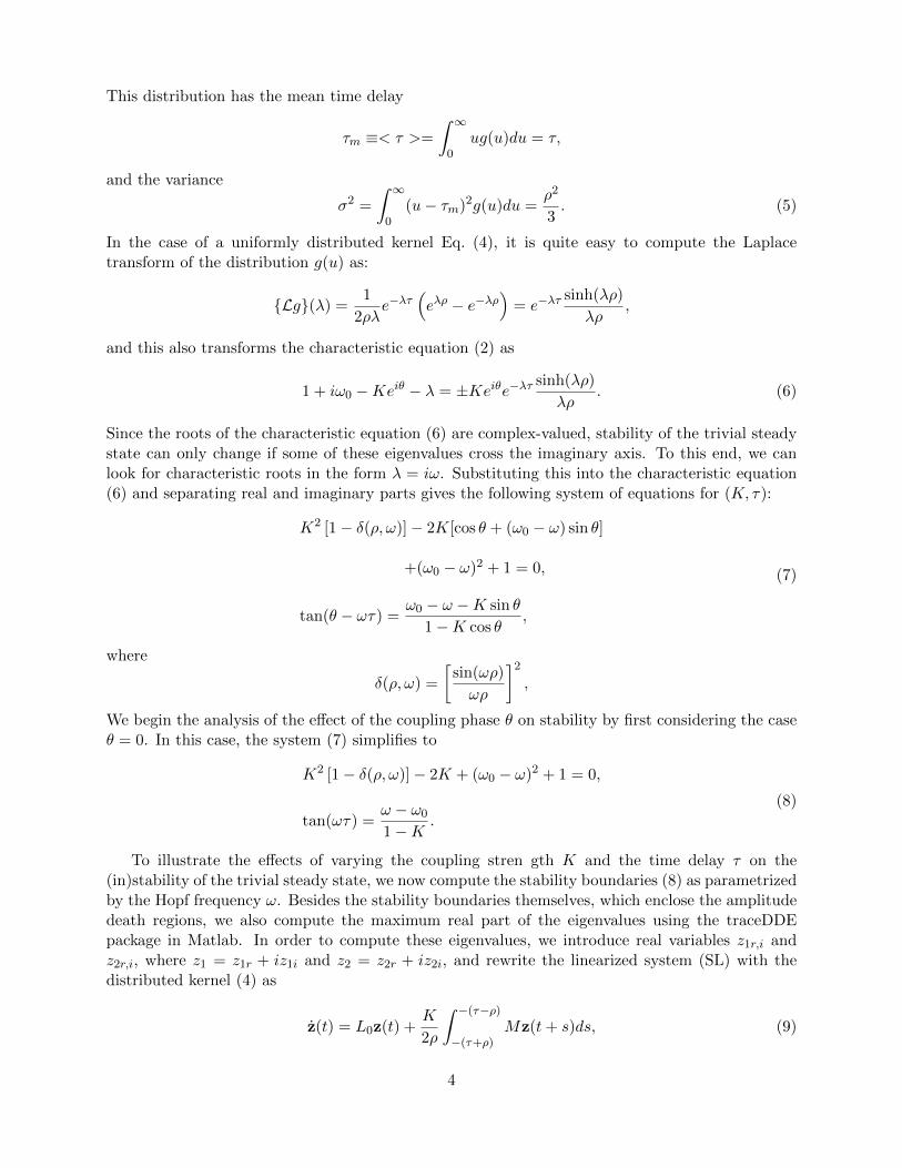
Figure 1: Areas of amplitude death in the plane of the coupling strength K and the mean timedelay τ for θ = 0, ω0 = 20. Colour code denotes [−max{Re(λ)}] for max{Re(λ)} ≤ 0. (a) ρ = 0.(b) ρ = 0.005. (c) ρ = 0.015. (d) ρ = 0.018.

where

z = (z1r, z1i, z2r, z2i)T , L0 =

(N 0202 N

),

M =

(02 RR 02

), R =

(cos θ sin θ− sin θ cos θ

),

N =

(1−K cos θ K sin θ − ω0

ω0 −K sin θ 1−K cos θ

),

and 02 denotes a 2 × 2 zero matrix. When ρ = 0, the last term in the system (9) turns intoKMz(t− τ), which describes the system with a single discrete time delay τ . System (9) is in theform in which it is amenable to the algorithms described in Breda et al. [42] and implemented intraceDDE.

Figure 1 shows the boundaries of the amplitude death together with the magnitude of thereal part of the leading eigenvalue for different widths of the delay distribution ρ. When ρ = 0(single discrete time delay τ), there are two distinct islands in the (K, τ) parameter space, in

5

Figure 2: Areas of amplitude death depending on the coupling strength K and the phase θ forτ = 0.08 and ω0 = 20. Colour code denotes [−max{Re(λ)}]. (a) ρ = 0. (b) ρ = 0.002. (c)ρ = 0.004. (d) ρ = 0.026.

which the trivial steady state is stable. It is noteworthy that the number of such stability islandsincreases with increasing fundamental frequency ω0 (e.g., there are three islands for ω0 = 30). Thisbehaviour agrees with that of an equivalent single system with time-delayed feedback and delay 2τ[45], where similar islands of stability of the trivial steady state form in the (K, τ) plane around2τ = 2n+1

2 T0 ≡ 2n+12 2π/ω0 (n = 0, 1, 2, ...), and the number and size of those islands increases with

increasing ratio ω0/λ0 [43]. As the width of the delay distribution ρ increases, the stability islandsgrow (see Fig. 1 (b) and (c)) until they merge into a single continuous region in the parameterspace, as shown in Fig. 1 (d).

Next, we consider the effects of the coupling phase on stability of the trivial steady state in thesystem (1) with a uniformly distributed delay kernel (4). The boundaries of amplitude death inthis case as parametrized by the Hopf frequency ω are given in Eq. (7). Figure 2 shows how theareas of amplitude death depend on the coupling strength and coupling phase for various delaydistribution widths ρ. In the case of a single delay (ρ = 0), the only area of amplitude death issymmetric around θ = 0 and also has the largest range of K values at θ = 0, for which amplitudedeath is achieved, as illustrated in Fig. 2(a). Provided that the coupling phase is large enoughby the absolute value, oscillations in the system (1) are maintained, and amplitude death cannot

6

Figure 3: (a) Amplitude of oscillations depending on the coupling phase θ and the width of dis-tribution ρ. (b) Sections for various values of θ. Parameter values are K = 120, τ = 0.08 andω0 = 20.

be achieved for any values of the coupling strength K. As the width of the delay distribution ρincreases, this leads to an increase in the size of the amplitude death region in (K, θ) space, as wellas to an asymmetry with regard to the coupling phase: for sufficiently large ρ, amplitude death canoccur for an arbitrarily large K if θ is negative, but only for a very limited range of K values if θis positive. At the same time, if the coupling phase exceeds π/2 by the absolute value, amplitudedeath does not occur, irrespectively of the values of K.

Whilst distributed-delay coupling may fail to suppress oscillations in a certain part of theparameter space, it will still have an effect on the amplitude of oscillations. In Fig. 3 we illustratehow the amplitude of oscillations varies depending on the coupling phase θ and the delay distributionwidth ρ for a fixed value of the coupling strength K. As the magnitude of the coupling phaseincreases, the range of possible delay distribution widths, for which oscillations are observed, isgrowing, and the amplitude reaches its maximum at ρ = 0 corresponding to the case of discretetime delay.

3 Gamma distributed delay

In many realistic situations, the distribution of time delays is better represented by a gammadistribution, which can be written as

g(u) =up−1αpe−αu

Γ(p), (10)

with α, p ≥ 0, and Γ(p) being an Euler gamma function defined by Γ(0) = 1 and Γ(p+ 1) = pΓ(p).For integer powers p, this can be equivalently written as

g(u) =up−1αpe−αu

(p− 1)!. (11)

7

For p = 1 this is simply an exponential distribution (also called a weak delay kernel) with themaximum contribution to the coupling coming from the present values of variables z1 and z2. Forp > 1 (known as strong delay kernel in the case p = 2), the biggest influence on the coupling at anymoment of time t is from the values of z1,2 at t− (p− 1)/α.

The delay distribution (11) has the mean time delay

τm =

∫ ∞0

ug(u)du =p

α, (12)

and the variance

σ2 =

∫ ∞0

(u− τm)2g(u)du =p

α2.

When studying stability of the trivial steady state of the system (1) with the delay distributionkernel (11), one could use the same strategy as the one described in the previous section. Theonly complication with such an analysis would stem once again from the Laplace transform of thedistribution kernel, which in this case has the form

{Lg}(λ) =αp

(λ+ α)p.

A convenient way to circumvent this is to use the linear chain trick [44], which allows one to replacean equation with a gamma distributed delay kernel by an equivalent system of (p + 1) ordinarydifferential equations. To illustrate this, we consider a particular case of system (1) with a weakdelay kernel given by (11) with p = 1, which is equivalent to a low-pass filter [45]:

gw(u) = αe−αu. (13)

Introducing new variables

Y1(t) =

∫ ∞0

αe−αsz1(t− s)ds,

Y2(t) =

∫ ∞0

αe−αsz2(t− s)ds,

allows us to rewrite the system (1) as follows

z1(t) = (1 + iω1)z1(t)− |z1(t)2|z1(t)

+ Keiθ [Y2(t)− z1(t)] ,

z2(t) = (1 + iω2)z2(t)− |z2(t)2|z2(t)

+ Keiθ [Y1(t)− z2(t)] ,(14)

Y1(t) = αz1(t)− αY1(t),

Y2(t) = αz2(t)− αY2(t),

where the distribution parameter α is related to the mean time delay as α = 1/τm. The trivialequilibrium z1 = z2 = 0 of the original system (1) corresponds to a steady state z1 = z2 = Y1 =

8

Figure 4: (a) Stability boundary for the system (1) with a weak delay distribution kernel (13) forθ = 0 (p = 1).The trivial steady state is unstable outside the boundary surface and stable insidethe boundary surface. (b) Stability boundary for ω0 = 10. Colour code denotes [−max{Re(λ)}].

Y2 = 0 of the modified system (14). The characteristic equation for the linearization of system (14)near this trivial steady state reduces to

[λ2 + λ(Keiθ − 1 + α− iω0

)− α(1 + iω0)]×

[λ2 + λ(Keiθ − 1 + α− iω0

)(15)

−α(1 + iω0 − 2Keiθ)] = 0.

Let us consider the first factor in Eq. (15)

λ2 + λ(Keiθ − 1 + α− iω0

)− α(1 + iω0) = 0. (16)

Since λ = 0 is not a solution of this equation, the only way how stability of the trivial steady statecan change is when λ crosses the imaginary axis. To find the values of system parameters whenthis can happen, we look for solutions of equation (16) in the form λ = iω. Substituting this intothe above equation and separating real and imaginary parts gives

ωK sin θ = ωω0 − α− ω2,

ωK cos θ = αω0 + ω(1− α).

Solving this system gives the coupling strength K and the inverse mean time delay α as functionsof the coupling phase θ and the Hopf frequency ω:

K =1 + (ω − ω0)

2

cos θ + sin θ(ω0 − ω),

α = −ω[sin θ + cos θ(ω − ω0)

cos θ + sin θ(ω0 − ω).

(17)

9

Figure 5: (a) Stability boundary for the system (1) with a weak delay distribution kernel (13) withω0 = 10 (p = 1). The trivial steady state is unstable outside the boundary and stable inside theboundary. (b) Sections for various values of θ.

When the coupling phase θ is equal to zero, these expressions simplify to

K = 1 + (ω − ω0)2, α = ω(ω0 − ω). (18)

This implies that the permissible range of Hopf frequencies is 0 ≤ ω ≤ ω0, the minimal value ofthe mean time delay for which the amplitude death can occur is τmin = 1/αmax = 4/ω2

0, and theminimal coupling strength required for amplitude death is K = 1. Figure 4 illustrates how thestability boundary (18) depends on the intrinsic frequency ω0, and it also shows how the leadingeigenvalues vary inside the stable parameter region. As the intrinsic frequency ω0 increases, theregion in the (K,α) space for which amplitude death occurs grows, thus indicating that it is possibleto stabilise a trivial steady state for even smaller values of the mean time delay.

For θ different from zero, the requirement K ≥ 0, α ≥ 0 in (17) translates into a restrictionon admissible coupling phases 0 ≤ θ ≤ arctan(ω0). Figure 5 shows how for a fixed value of ω0 thestability area reduces as θ grows, eventually collapsing at θ = arctan(ω0). The range of admissibleHopf frequencies also reduces and is given for each θ by 0 ≤ ω ≤ ω0 − tan θ. The second factorin (15) provides another stability boundary in the parameter space, but the values of K and αsatisfying this equation with λ = iω lie outside the feasible range of K ≥ 0, α ≥ 0. Hence, itsuffices to consider the stability boundary given by (17).

Next, we consider the case of the strong delay kernel (p = 2)

gw(u) = α2ue−αu. (19)

10

Figure 6: (a) Stability boundary for the system (1) with a strong delay distribution kernel (19) forθ = 0 (p = 2). The trivial steady state is unstable outside the boundary surface and stable insidethe boundary surface. (b) Stability boundary for ω0 = 10. Colour code denotes [−max{Re(λ)}].

Following the same strategy as in the case of the weak delay kernel (14), we introduce new variables

Y11(t) =∫∞0 αe−αsz1(t− s)ds,

Y12(t) =∫∞0 α2se−αsz1(t− s)ds,

Y21(t) =∫∞0 αe−αsz2(t− s)ds,

Y22(t) =∫∞0 α2se−αsz2(t− s)ds,

and then rewrite the system (1) in the form

z1(t) = (1 + iω1)z1(t)− |z1(t)2|z1(t)

+ Keiθ [Y12(t)− z1(t)] ,

z2(t) = (1 + iω2)z2(t)− |z2(t)2|z2(t)

+ Keiθ [Y22(t)− z2(t)] ,(20)

Y11(t) = αz1(t)− αY11(t),

Y12(t) = α2z1(t) + αY11(t)− αY12(t),

Y21(t) = αz2(t)− αY21(t),

11

Figure 7: (a) Stability boundary for the system (1) with a strong delay distribution kernel (19)with ω0 = 10 (p = 2). The trivial steady state is unstable outside the boundary and stable insidethe boundary. (b) Sections for various values of θ.

Y22(t) = α2z2(t) + αY21(t)− αY22(t),

where the mean time delay is given by τm = 2/α. Linearizing system (20) near the steady statez1 = z2 = Y11 = Y12 = Y21 = Y22 = 0 yields a characteristic equation, which is more involved thanin the case of the weak delay kernel. Solving this characteristic equation provides the boundary ofamplitude death depending on system parameters. Figure 6 illustrates how this boundary changeswith the coupling strength K, fundamental frequency ω0, and the inverse time delay α/2 in thecase θ = 0. Similar to the case of the weak delay kernel, as the inverse time delay ∼ α approacheszero, the larger value of the critical coupling strength of K tends to some finite value. At the sametime, the lower value of the critical coupling strength K does vary depending on the coupling phaseunlike the case of the weak kernel. Also, in the case of a strong delay kernel, the amplitude deathis achieved for a much smaller range of coupling strengths K and only for much larger mean timedelays τm = 2/α. However, the effect of the coupling phase on the region of amplitude death issimilar to that for a weak delay kernel, i.e., as the coupling phase increases, this reduces the areain the (K,α) parameter plane where amplitude death is observed, as shown in Fig. 7.

4 Discussion

In this paper, we have studied the effects of distribu- ted-delay coupling on the stability of the trivialsteady state in a system of coupled oscillators. Using generic Stuart-Landau oscillators, we haveidentified parameter regimes of amplitude death, i.e., stabilised steady states, in terms of intrinsicoscillator frequency and characteristics of the coupling. In order to better understand the dynamicsinside stable regimes, we have numerically computed eigenvalues of the corresponding characteristicequation. We have considered two particular types of delay distribution: a uniform distributionaround some mean time delay and a class of exponential or more general gamma distributions.For both of these distributions it has been possible to find stability in terms of coupling strength,coupling phase, and the mean time delay. These results suggest that the coupling phase plays an

12

important role in determining the ranges of admissible Hopf frequencies and values of the couplingstrength, for which stabilisation of the trivial steady state is possible.

For the uniformly distributed delay kernel, as the width of the distribution increases, the regionof amplitude death in the parameter space of the coupling strength and the average time delayincreases. As the coupling phase θ moves away from zero, the range of coupling strength providingamplitude death gets smaller until some critical value of the width of distribution, beyond which anasymmetry in θ is introduced and this range is significantly larger for negative values of θ than itis for θ ≥ 0. Furthermore, as the magnitude of the coupling phase grows, the maximum amplitudeof oscillations in the coupled system also grows, and such oscillations can be observed for a largerrange of delay distribution widths.

In the case of gamma distributed delay, the region of amplitude death does not consist of isolatedstability islands but is always a continuous region in the (K, τm) plane. Similar to the uniform delaydistribution, as the coupling phase increases from zero, the range of coupling strengths for whichstabilisation of the steady state can be achieved reduces, while the minimum average time delayrequired for the stabilization increases. However, unlike the uniform distribution, within the stableregion the amplitude death can occur for an arbitrarily large value of the average time delay,provided it is above some minimum value and the coupling strength is within the appropriaterange.

So far, we have considered the effects of distribu- ted-delay coupling on the dynamics of identicalcoupled oscillators only. The next step would be to extend this analysis to the case when theoscillators have differing intrinsic frequencies in order to understand the dynamics of the phasedifference, as well as to analyse the stability of in-phase and anti-phase oscillations.

Acknowledgements

This work was partially supported by DFG in the framework of SFB 910: Control of self-organizingnonlinear systems: Theoretical methods and concepts of application.

References

[1] P. J. Uhlhaas and W. Singer, Neuron 52, 155 (2006).

[2] O. V. Popovych, C. Hauptmann, and P. A. Tass, Phys. Rev. Lett. 94, 164102 (2005).

[3] A. Schnitzler and J. Gross, Nat. Rev. Neuroscience 6, 285 (2005).

[4] C. U. Choe, V. Flunkert, P. Hovel, H. Benner, and E. Scholl, Phys. Rev. E 75, 0426206 (2007).

[5] B. Fiedler, V. Flunkert, P. Hovel, and E. Scholl, Phil. Trans. R. Soc. A 368, 319 (2010).

[6] A. Pikovsky, M. Rosenblum, and J. Kurths, Synchronization: a universal concept in nonlinearsciences. (CUP, Cambridge, 2001).

[7] W. Just, A. Pelster, M. Schanz, and E. Scholl (eds.), Phil. Trans. R. Soc. A 368, 303 (2010).

[8] O. D’Huys, R. Vicente, J. Danckaert, and I. Fischer, Chaos 20, 043127 (2010).

[9] C. U. Choe, T. Dahms, P. Hovel, and E. Scholl, Phys. Rev. E 81, 025205(R) (2010).

[10] V. Flunkert, S. Yanchuk, T. Dahms, and E. Scholl, Phys. Rev. Lett. 105, 254101 (2010).

13

[11] E. Scholl, P. Hovel, V. Flunkert, and M. A. Dahlem, in Complex Time-Delay Systems, editedby F. M. Atay (Springer, Berlin, 2010), p. 85.

[12] T. Heil, I. Fischer, W. Elsasser, J. Mulet, and C. R. Mirasso, Phys. Rev. Lett 86, 795 (2001).

[13] V. Flunkert, O. D’Huys, J. Danckaert, I. Fischer, and E. Scholl, Phys. Rev. E 79, 065201 (R)(2009).

[14] K. Hicke, O. D’Huys, V. Flunkert, E. Scholl, J. Danckaert, and I. Fischer, Phys. Rev. E 83,056211 (2011).

[15] M. A. Dahlem, G. Hiller, A. Panchuk, and E. Scholl, Int. J. Bifur. Chaos 19, 745 (2009).

[16] E. Scholl, G. Hiller, P. Hovel, and M. A. Dahlem, Phil. Trans. R. Soc. A 367, 1079 (2009).

[17] Y. N. Kyrychko, K. B. Blyuss, A. Gonzalez-Buelga, S. J. Hogan & D. J. Wagg, Proc. R. Soc.A 462, 1271 (2006).

[18] Y. N. Kyrychko and S. J. Hogan, J. Vibr. Control 16, 943 (2010).

[19] D. V. Ramana Reddy, A. Sen, and G. L. Johnston, Phys. Rev. Lett. 80, 5109 (1998).

[20] D. V. Ramana Reddy, A. Sen, and G. L. Johnston, Physica D 129, 15 (1999).

[21] S. H. Strogatz, Nature 394, 316 (1998).

[22] R. Herrero, M. Figueras, J. Rius, F. Pi, and G. Orriols, Phys. Rev. Lett. 84, 5312 (2000).

[23] A. Takamatsu, T. Fujii, and I. Endo, Phys. Rev. Lett. 85, 2026 (2000).

[24] A. Ahlborn, U. Parlitz, Phys. Rev. Lett. 93, 264101 (2004).

[25] A. Ahlborn, U. Parlitz, Phys. Rev. E 72, 016206 (2005).

[26] D. G. Aronson, G. B. Ermentrout, and N. Kopell, Physica D 41, 403 (1990).

[27] R. E. Mirollo and S. H. Strogatz, J. Stat. Phys. 60, 245 (1990).

[28] A. Gjurchinovski and V. Urumov, Europhys. Lett. 84, 40013 (2008).

[29] A. Gjurchinovski and V. Urumov, Phys. Rev. E 81, 016209 (2010).

[30] S. A. Gourley & J. W.-H. So, Proc. R. Soc. Edinburgh 133, 527 (2003).

[31] T. Faria and S. Trofimchuk, Nonlinearity 23, 2457 (2010).

[32] G. Kiss and B. Krauskopf, Dyn. Syst. 26, 85 (2011).

[33] W. Michiels, V. Van Assche, and S.-I. Niculescu, IEEE Trans. Automat. Contr. 50, 493 (2005).

[34] A. Thiel, H. Schwegler, and C. W. Eurich, Complexity 8, 102 (2003).

[35] C. W. Eurich, A. Thiel, and L. Fahse, Phys. Rev. Lett. 94, 158104 (2005).

[36] K. B. Blyuss and Y. N. Kyrychko, Bull. Math. Biol. 72, 490 (2010).

[37] F. Atay, Phys. Rev. Lett. 91, 094101 (2003).

14

[38] R. Sipahi, F. M. Atay, and S.-I. Niculescu, SIAM J. Appl. Math. 68, 738 (2008).

[39] S. A. Campbell and R. Jessop, Math. Model. Nat. Phenom. 4, 1 (2009).

[40] S. Schikora, P. Hovel, H.-J. Wunsche, E. Scholl, and F. Henneberger, Phys. Rev. Lett. 97,213902 (2006).

[41] A. P. A. Fischer, O. K. Andersen, M. Yousefi, S. Stolte, and D. Lenstra, IEEE J. QuantumElectron. 36, 375 (2000).

[42] D. Breda, S. Maset, and R. Vermiglioa, Appl. Numer. Math. 56, 318 (2006).

[43] Note that we have set the bifurcation parameter λ0 = 1 in Eq. (1) and throughout the presentpaper.

[44] N. MacDonald, Time lags in biological systems. (Springer, New York, 1978).

[45] P. Hovel and E. Scholl, Phys. Rev. E 72, 046203 (2005).

15