Non-Voluntary Return? The Politics of Return to Afghanistan: The Politics of Return to Afghansitan
Chapter 1
The Constant Expected Return
Model
Date: September 6, 2013
The first model of asset returns we consider is the very simple constant
expected return (CER) model. This model assumes that an asset’s return
over time is independent and identically normally distributed with a con-
stant (time invariant) mean and variance. The model allows for the returns
on different assets to be contemporaneously correlated but that the corre-
lations are constant over time. The CER model is widely used in finance.
For example, it is used in mean-variance portfolio analysis, the Capital As-
set Pricing model, and the Black-Scholes option pricing model. Although
this model is very simple, it provides important intuition about the statisti-
cal behavior of asset returns and prices and serves as a benchmark against
which more complicated models can be compared and evaluated. It allows us
to discuss and develop several important econometric topics such as Monte
Carlo simulation, estimation, bootstrapping, hypothesis testing, forecasting
and model evaluation.
1.1 CER Model Assumptions
Let = ln(−1) denote the continuously compounded return on asset at time We make the following assumptions regarding the probability
distribution of for = 1 assets over the time horizon = 1
Assumption 1
1

2CHAPTER 1 THECONSTANT EXPECTEDRETURNMODEL
(i) Covariance stationarity and ergodicity: {1 } = {}=1 is acovariance stationary and ergodic stochastic process with [] =
var() = 2 , cov( ) = and cor( ) =
(ii) Normality: ∼ ( 2 ) for all and
(iii) No serial correlation: cov( ) = cor( ) = 0 for 6= and
= 1
Assumption 1 states that in every time period asset returns are jointly
(multivariate) normally distributed, that the means and the variances of
all asset returns, and all of the pairwise contemporaneous covariances and
correlations between assets are constant over time. In addition, all of the
asset returns are serially uncorrelated
cor( ) = cov( ) = 0 for all and 6=
and the returns on all possible pairs of assets and are serially uncorrelated
cor( ) = cov( ) = 0 for all 6= and 6=
Clearly, these are very strong assumptions. However, they allow us to develop
a straightforward probabilistic model for asset returns as well as statistical
tools for estimating the parameters of the model, testing hypotheses about
the parameter values and assumptions.
1.1.1 Regression Model Representation
A convenient mathematical representation or model of asset returns can be
given based on Assumption 1. This is the CER regression model. For assets
= 1 and time periods = 1 the CER regression model is
= + (1.1)
{}=1 ∼ GWN(0 2 )
cov( ) =
⎧⎨⎩
0
=
6=
The notation ∼ GWN(0 2 ) stipulates that the stochastic process {}=1is a Gaussian white noise process with [] = 0 and var() = 2 In
1.1 CER MODEL ASSUMPTIONS 3
addition, the random error term is independent of for all assets 6=
and all time periods 6= .
Using the basic properties of expectation, variance and covariance, we
can derive the following properties of returns in the CER model:
[] = [ + ] = + [] =
var() = var( + ) = var() = 2
cov( ) = cov( + + ) = cov( ) =
cov( ) = cov( + + ) = cov( ) = 0 6=
Given that covariances and variances of returns are constant over time im-
plies that the correlations between returns over time are also constant:
cor( ) =cov( )pvar()var()
=
=
cor( ) =cov( )pvar()var()
=0
= 0 6= 6=
Finally, since {}=1 ∼ GWN(0 2 ) it follows that {}=1 ∼ ( 2 )
Hence, the CER regression model (1.1) for is equivalent to the model
implied by Assumption 1.
1.1.2 Interpretation of the CER Regression Model
The CER model has a very simple form and is identical to the measurement
error model in the statistics literature.1 In words, the model states that each
asset return is equal to a constant (the expected return) plus a normally
distributed random variable with mean zero and constant variance. The
random variable can be interpreted as representing the unexpected news
concerning the value of the asset that arrives between time − 1 and time To see this, (1.1) implies that
= − = −[]
1In the measurement error model, represents the measurement of some phys-
ical quantity and represents the random measurement error associated with the
measurement device. The value represents the typical size of a measurement error.

4CHAPTER 1 THECONSTANT EXPECTEDRETURNMODEL
so that is defined as the deviation of the random return from its expected
value. If the news between times − 1 and is good, then the realized
value of is positive and the observed return is above its expected value
If the news is bad, then is negative and the observed return is less than
expected. The assumption[] = 0means that news, on average, is neutral;
neither good nor bad. The assumption that var() = 2 can be interpreted
as saying that volatility, or typical magnitude, of news arrival is constant
over time. The random news variable affecting asset , is allowed to be
contemporaneously correlated with the random news variable affecting asset
to capture the idea that news about one asset may spill over and affect
another asset. For example, if asset is Microsoft stock and asset is Apple
Computer stock, then one interpretation of news in this context is general
news about the computer industry and technology. Good news should lead
to positive values of both and Hence these variables will be positively
correlated due to a positive reaction to a common news component. Finally,
the news on asset at time is unrelated to the news on asset at time for
all times 6= For example, this means that the news for Apple in January
is not related to the news for Microsoft in February.
Sometimes it is convenient to re-express the CER model (1.1) as
= + = + · (1.2)
{}=1 ∼ GWN(0 1)
In this form, the random news shock is the standard normal random vari-
able scaled by the “news” volatility This form is particularly convenient
for value-at-risk calculations.
1.1.3 Time Aggregation and the CER Model
The CER model for continuously compounded returns has the following nice
aggregation property with respect to the interpretation of as news. Sup-
pose that represents months so that is the continuously compounded
monthly return on asset . Now, instead of the monthly return, suppose we
are interested in the annual continuously compounded return = (12).
Since multi-period continuously compounded returns are additive, (12) is
the sum of 12 monthly continuously compounded returns:
= (12) =
11X=0
− = + −1 + · · ·+ −11
1.1 CER MODEL ASSUMPTIONS 5
Using the CER regression model (1.1) for the monthly return we may
express the annual return (12) as
(12) =
11X=0
( + ) = 12 · +11X=0
= + (12)
where = 12 · is the annual expected return on asset and (12) =P11
=0 − is the annual random news component. The annual expected
return, is simply 12 times the monthly expected return, . The annual
random news component, (12) , is the accumulation of news over the year.
As a result, the variance of the annual news component,¡¢2 is 12 time
the variance of the monthly news component:
var((12)) = var
Ã11X=0
−
!
=
11X=0
var(−) since is uncorrelated over time
=
11X=0
2 since var() is constant over time
= 12 · 2 =¡¢2
It follows that the standard deviation of the annual news is equal to√12
times the standard deviation of monthly news:
SD((12)) =√12SD() =
√12
This result is known as the square root of time rule. Similarly, due to the
additivity of covariances, the covariance between (12) and (12) is 12

6CHAPTER 1 THECONSTANT EXPECTEDRETURNMODEL
times the monthly covariance:
cov((12) (12)) = cov
Ã11X=0
−11X=0
−
!
=
11X=0
cov(− −) since and are uncorrelated over time
=
11X=0
since cov( ) is constant over time
= 12 · =
The above results imply that the correlation between the annual errors (12)
and (12) is the same as the correlation between the monthly errors and
:
cor((12) (12)) =cov((12) (12))pvar((12)) · var((12))
=12 · q122 · 122
=
= = cor( )
1.1.4 The Random Walk Model of Asset Prices
The CER model of asset returns (1.1) gives rise to the so-called random
walk (RW) model for the logarithm of asset prices. To see this, recall that
the continuously compounded return, is defined from asset prices via
= ln³
−1
´= ln() − ln(−1) Letting = ln() and using the
representation of in the CER model (1.1), we can express the log-price as:
= −1 + + (1.3)
The representation in (1.3) is known as the RW model for log-prices.2 It is
a representation of the CER model in terms of log-prices.
2The model (1.3) is technically a random walk with drift A pure random walk has
zero drift ( = 0).
1.1 CER MODEL ASSUMPTIONS 7
In the RW model (1.3), represents the expected change in the log-
price (continuously compounded return) between months − 1 and and represents the unexpected change in the log-price That is,
[∆] = [] =
= ∆ −[∆]
where ∆ = − −1 Further, in the RW model, the unexpected changes
in log-price, are uncorrelated over time (cov( ) = 0 for 6= ) so
that future changes in log-price cannot be predicted from past changes in
the log-price.3
The RW model gives the following interpretation for the evolution of log
prices. Let 0 denote the initial log price of asset . The RW model says
that the log-price at time = 1 is
1 = 0 + + 1
where 1 is the value of random news that arrives between times 0 and 1
At time = 0 the expected log-price at time = 1 is
[1] = 0 + +[1] = 0 +
which is the initial price plus the expected return between times 0 and 1.
Similarly, by recursive substitution the log-price at time = 2 is
2 = 1 + + 2
= 0 + + + 1 + 2
= 0 + 2 · +2X
=1
which is equal to the initial log-price, 0 plus the two period expected return,
2 · , plus the accumulated random news over the two periods,P2
=1 By
repeated recursive substitution, the log price at time = is
= 0 + · +X=1
3The notion that future changes in asset prices cannot be predicted from past changes
in asset prices is often referred to as the weak form of the efficient markets hypothesis.
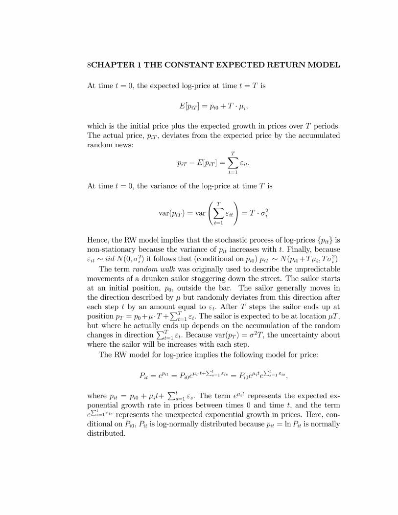
8CHAPTER 1 THECONSTANT EXPECTEDRETURNMODEL
At time = 0 the expected log-price at time = is
[ ] = 0 + ·
which is the initial price plus the expected growth in prices over periods.
The actual price, deviates from the expected price by the accumulated
random news:
−[ ] =
X=1
At time = 0 the variance of the log-price at time is
var( ) = var
ÃX=1
!= · 2
Hence, the RWmodel implies that the stochastic process of log-prices {} isnon-stationary because the variance of increases with Finally, because
∼ (0 2 ) it follows that (conditional on 0) ∼ (0+ 2 )
The term random walk was originally used to describe the unpredictable
movements of a drunken sailor staggering down the street. The sailor starts
at an initial position, 0 outside the bar. The sailor generally moves in
the direction described by but randomly deviates from this direction after
each step by an amount equal to After steps the sailor ends up at
position = 0+ ·+P
=1 The sailor is expected to be at location
but where he actually ends up depends on the accumulation of the random
changes in directionP
=1 Because var( ) = 2 the uncertainty about
where the sailor will be increases with each step.
The RW model for log-price implies the following model for price:
= = 0·+
=1 = 0
=1
where = 0 + +P
=1 The term represents the expected ex-
ponential growth rate in prices between times 0 and time and the term
=1 represents the unexpected exponential growth in prices. Here, con-
ditional on 0 is log-normally distributed because = ln is normally
distributed.

1.2 MONTE CARLO SIMULATION OF THE CER MODEL 9
1.1.5 The CER Model in Matrix Notation
Define the × 1 vectors = (1 )0, μ = (1 )
0 ε =(1 )
0 and the × symmetric covariance matrix
var(ε) = Σ =
⎛⎜⎜⎜⎜⎜⎜⎝21 12 · · · 1
12 22 · · · 2...
.... . .
...
1 2 · · · 2
⎞⎟⎟⎟⎟⎟⎟⎠
Then the CER model matrix notation is
r = μ+ ε (1.4)
ε ∼ (0Σ)
which implies that ∼ (μΣ)
1.2 Monte Carlo Simulation of the CERModel
A simple technique that can be used to understand the probabilistic behavior
of a model involves using computer simulation methods to create pseudo data
from the model. The process of creating such pseudo data is called Monte
Carlo simulation.4 To illustrate the use of Monte Carlo simulation, consider
creating pseudo return data from the CER model (1.1) for a single asset.
The steps to create a Monte Carlo simulation from the CER model are:
1. Fix values for the CER model parameters and .
2. Determine the number of simulated values, to create.
3. Use a computer random number generator to simulate values
of from a (0 2) distribution. Denote these simulated values as
1
4. Create the simulated return data = + for = 1
4Monte Carlo refers to the famous city in Monaco where gambling is legal.
10CHAPTER 1 THECONSTANTEXPECTEDRETURNMODEL
1 9 9 3 1 9 9 6 1 9 9 9
-0.4
-0.3
-0.2
-0.1
0.0
0.1
0.2
0.3
Ind e x
retu
rns
re turns
Fre
qu
en
cy-0 .4 -0 .2 0 .0 0 .2
01
02
03
04
0
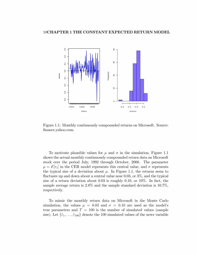
Figure 1.1: Monthly continuously compounded returns on Microsoft. Source:
finance.yahoo.com.
To motivate plausible values for and in the simulation, Figure 1.1
shows the actual monthly continuously compounded return data on Microsoft
stock over the period July, 1992 through October, 2000. The parameter
= [] in the CER model represents this central value, and represents
the typical size of a deviation about . In Figure 1.1, the returns seem to
fluctuate up and down about a central value near 0.03, or 3%, and the typical
size of a return deviation about 0.03 is roughly 0.10, or 10%. In fact, the
sample average return is 2.8% and the sample standard deviation is 10.7%,
respectively.
To mimic the monthly return data on Microsoft in the Monte Carlo
simulation, the values = 003 and = 010 are used as the model’s
true parameters and = 100 is the number of simulated values (sample
size) Let {1 100} denote the 100 simulated values of the news variable

1.2 MONTE CARLO SIMULATION OF THE CER MODEL 11
∼ GWN(0 (010)2)The simulated returns are then computed using5
= 003 + = 1 100 (1.5)
Example 1 Simulating observations from the CER model using R
To create and plot the simulated returns from (1.5) use
> mu = 0.03
> sd.e = 0.10
> nobs = 100
> set.seed(111)
> sim.e = rnorm(nobs, mean=0, sd=sd.e)
> sim.ret = mu + sim.e
> par(mfrow=c(1,2))
> ts.plot(sim.ret, main="",
+ xlab="months",ylab="return", lwd=2, col="blue")
> abline(h=mu)
> hist(sim.ret, main="", xlab="returns", col="slateblue1")
> par(mfrow=c(1,1))
The simulated returns {}100=1 are shown in Figure 1.2. The simulated return
data fluctuate randomly about = 003 and the typical size of the fluctu-
ation is approximately equal to = 010 The simulated return data look
somewhat like the actual monthly return data for Microsoft. The main dif-
ference is that the return volatility for Microsoft appears to have increased
in the latter part of the sample whereas the simulated data has constant
volatility over the entire sample. ¥Monte Carlo simulation of a model can be used as a first pass “reality
check” of the model. If simulated data from the model do not look like the
data that the model is supposed to describe, then serious doubt is cast on the
model. However, if simulated data look reasonably close to the actual data
then the first step reality check is passed. Ideally, one should consider many
simulated samples from the model because it is possible for a given simulated
sample to look strange simply because of an unusual set of random numbers.
Example 2 Simulating log-prices from the RW model
5Alternatively, the returns can be simulated directly by simulating observations from
a normal distribution with mean 005 and standard deviation 010
12CHAPTER 1 THECONSTANTEXPECTEDRETURNMODEL
m o nths
retu
rn
0 20 4 0 60 8 0 1 0 0
-0.3
-0.2
-0.1
0.0
0.1
0.2
0.3
re turns
Fre
qu
ency
-0 .3 -0 .1 0 .1 0 .3
01
02
030
40
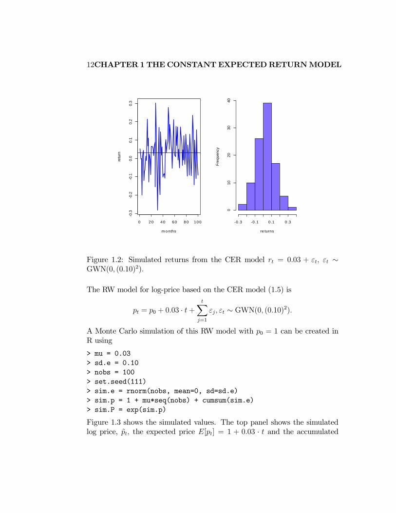
Figure 1.2: Simulated returns from the CER model = 003 + ∼GWN(0 (010)2)
The RW model for log-price based on the CER model (1.5) is
= 0 + 003 · +X
=1
∼ GWN(0 (010)2)
A Monte Carlo simulation of this RW model with 0 = 1 can be created in
R using
> mu = 0.03
> sd.e = 0.10
> nobs = 100
> set.seed(111)
> sim.e = rnorm(nobs, mean=0, sd=sd.e)
> sim.p = 1 + mu*seq(nobs) + cumsum(sim.e)
> sim.P = exp(sim.p)
Figure 1.3 shows the simulated values. The top panel shows the simulated
log price, the expected price [] = 1 + 003 · and the accumulated

1.2 MONTE CARLO SIMULATION OF THE CER MODEL 13
Time
log
pric
e
0 20 40 60 80 100
-20
12
34
p(t)E[p(t)]p(t)-E[p(t)]
Time
pri
ce
0 20 40 60 80 100
020
40
Figure 1.3: Simulated values from the RW model = 0+003 · +P
=1
∼ GWN(0 (010)2)
random news −[] =P
=1 . The bottom panel shows the simulated
price levels = Figure 1.4 shows the actual log prices and price levels for
Microsoft stock. Notice the similarity between the simulated random walk
data and the actual data. ¥
1.2.1 Simulating Returns on More than One Asset
Creating a Monte Carlo simulation of more than one return from the CER
model requires simulating observations from a multivariate normal distribu-
tion. This follows from the matrix representation of the CER model given
in (1.4). The steps required to create a multivariate Monte Carlo simulation
are:
1. Fix values for × 1 mean vector μ and the × covariance matrix
Σ.

14CHAPTER 1 THECONSTANTEXPECTEDRETURNMODEL
Log monthly prices on MSFT
1993 1994 1995 1996 1997 1998 1999 2000 2001
610
2040
80
Monthly Prices on MSFT
1993 1994 1995 1996 1997 1998 1999 2000 2001
2040
6080
100
Figure 1.4: Monthly prices and log-prices on Microsoft stock. Source: fi-
nance.yahoo.com.
2. Determine the number of simulated values, to create.
3. Use a computer random number generator to simulate values of
the × 1 random vector ε from the multivariate normal distribution(0Σ). Denote these simulated vectors as ε1 ε
4. Create the × 1 simulated return vector = μ+ ε for = 1
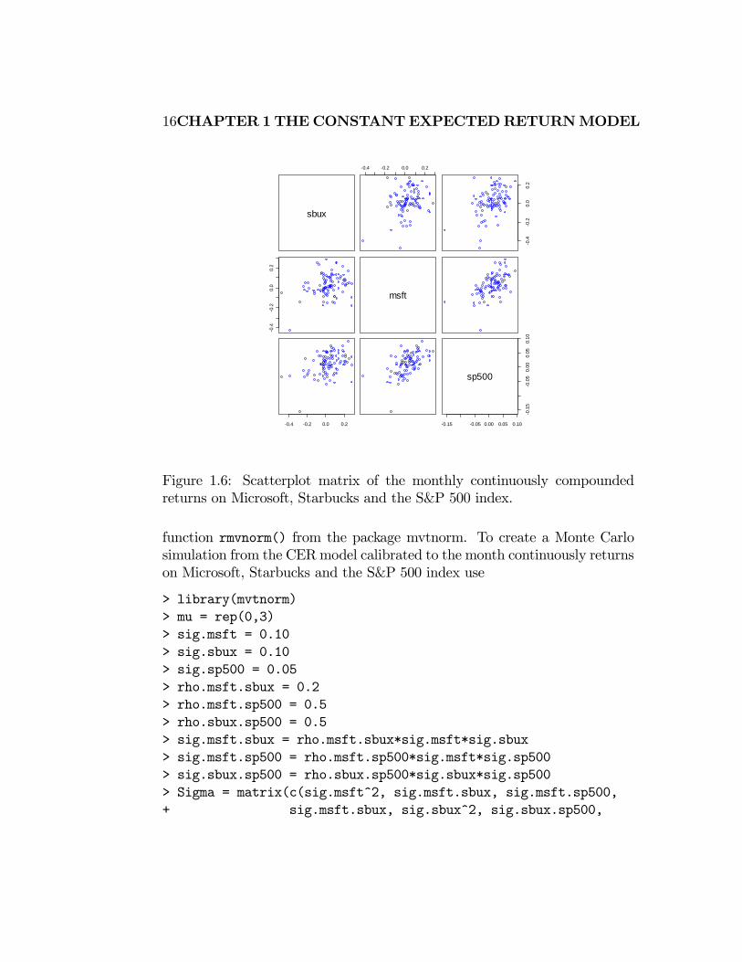
To motivate the parameters for a multivariate simulation of the CER
model, consider the monthly continuously compounded returns for Microsoft,
Starbucks and the S & P 500 index over the ten-year period July, 1992
through October, 2000 illustrated in Figures 1.5 and 1.6. All returns seem
to fluctuate around a mean value near zero. The volatilities of Microsoft
and Starbucks are similar with typical magnitudes around 0.10, or 10%. The
volatility of the S&P 500 index is considerably smaller at about 0.05, or
5%. The pairwise scatterplots show that all returns appear to be positively
related. The pairs (MSFT, SP500) and (SBUX, SP500) appear to be the most
correlated, and the shape of the scatter indicates correlation values around
0.5. The pair (MSFT, SBUX) shows a weak positive correlation around 0.2.

1.2 MONTE CARLO SIMULATION OF THE CER MODEL 15
-0.4
-0.2
0.0
0.2
sbux
-0.4
-0.2
0.0
0.2
msf
t
1993 1994 1995 1996 1997 1998 1999 2000
-0.1
5-0
.05
0.00
0.05
0.10
sp50
0
Index
Figure 1.5: Monthly continuously compounded returns on Microsoft, Star-
bucks and the S&P 500 index. Source: finance.yahoo.com.
Let = ( 500)0. Then, a plausible value for μ is μ = (0 0 0)0
and a plausible value for Σ is
Σ =
⎛⎜⎜⎜⎝(010)2 (010)(010)(02) (010)(005)(05)
(010)(010)(02) (010)2 (010)(005)(05)
(010)(005)(05) (010)(005)(05) (005)2
⎞⎟⎟⎟⎠
=
⎛⎜⎜⎜⎝00100 00020 00025
00020 00100 00025
00025 00025 00025
⎞⎟⎟⎟⎠
Example 3 Monte Carlo simulation of CER model for three assets
Simulating values from the multivariate CER model (1.4) requires simulating
multivariate normal random variables. In R, this can be done using the
16CHAPTER 1 THECONSTANTEXPECTEDRETURNMODEL
sbux
-0.4 -0.2 0.0 0.2
-0.4
-0.2
0.0
0.2
-0.4
-0.2
0.0
0.2
msft
-0.4 -0.2 0.0 0.2 -0.15 -0.05 0.00 0.05 0.10
-0.1
5-0
.05
0.00
0.05
0.10
sp500
Figure 1.6: Scatterplot matrix of the monthly continuously compounded
returns on Microsoft, Starbucks and the S&P 500 index.
function rmvnorm() from the package mvtnorm. To create a Monte Carlo
simulation from the CERmodel calibrated to the month continuously returns
on Microsoft, Starbucks and the S&P 500 index use
> library(mvtnorm)
> mu = rep(0,3)
> sig.msft = 0.10
> sig.sbux = 0.10
> sig.sp500 = 0.05
> rho.msft.sbux = 0.2
> rho.msft.sp500 = 0.5
> rho.sbux.sp500 = 0.5
> sig.msft.sbux = rho.msft.sbux*sig.msft*sig.sbux
> sig.msft.sp500 = rho.msft.sp500*sig.msft*sig.sp500
> sig.sbux.sp500 = rho.sbux.sp500*sig.sbux*sig.sp500
> Sigma = matrix(c(sig.msft^2, sig.msft.sbux, sig.msft.sp500,
+ sig.msft.sbux, sig.sbux^2, sig.sbux.sp500,
1.3 ESTIMATINGTHEPARAMETERSOF THECERMODEL17
-0.2
-0.1
0.0
0.1
0.2
msf
t
-0.2
-0.1
0.0
0.1
0.2
0.3
sbux
0 20 40 60 80 100
-0.0
50.
000.
050.
10
sp50
0
Index
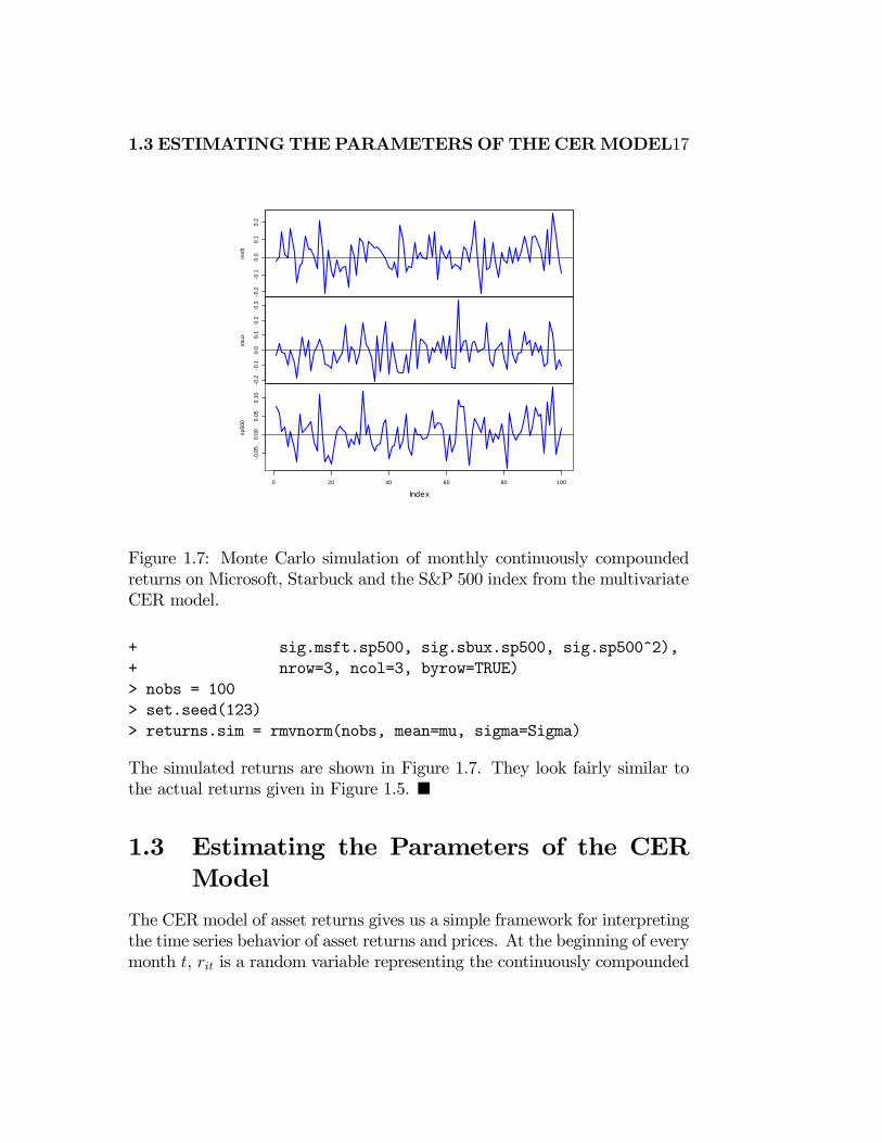
Figure 1.7: Monte Carlo simulation of monthly continuously compounded
returns on Microsoft, Starbuck and the S&P 500 index from the multivariate
CER model.
+ sig.msft.sp500, sig.sbux.sp500, sig.sp500^2),
+ nrow=3, ncol=3, byrow=TRUE)
> nobs = 100
> set.seed(123)
> returns.sim = rmvnorm(nobs, mean=mu, sigma=Sigma)
The simulated returns are shown in Figure 1.7. They look fairly similar to
the actual returns given in Figure 1.5. ¥
1.3 Estimating the Parameters of the CER
Model
The CER model of asset returns gives us a simple framework for interpreting
the time series behavior of asset returns and prices. At the beginning of every
month , is a random variable representing the continuously compounded

18CHAPTER 1 THECONSTANTEXPECTEDRETURNMODEL
msft
-0.2 -0.1 0.0 0.1 0.2 0.3
-0.2
-0.1
0.0
0.1
0.2
-0.2
-0.1
0.0
0.1
0.2
0.3
sbux
-0.2 -0.1 0.0 0.1 0.2 -0.05 0.00 0.05 0.10
-0.0
50.
000.
050.
10
sp500
Figure 1.8: Scatterplot matrix of the simulated returns on Microsoft, Star-
bucks and the S&P 500 index.
return to be realized at the end of the month. The CER model states that
∼ ( 2 ). Our best guess for the return at the end of the month
is [] = , our measure of uncertainty about our best guess is captured
by SD() = and our measures of the direction and strength of linear
association between and are = cov( ) and = cor( )
respectively. The CER model assumes that the economic environment is
constant over time so that the normal distribution characterizing monthly
returns is the same every month.
Our life would be very easy if we knew the exact values of 2 and
the parameters of the CER model. In actuality, however, we do not know
these values with certainty. Therefore, a key task in financial econometrics
is estimating these values from a history of observed return data.
Suppose we observe monthly continuously compounded returns on dif-
ferent assets over the horizon = 1 It is assumed that the observed
returns are realizations of the stochastic process {1}=1 , where is de-
1.3 ESTIMATINGTHEPARAMETERSOF THECERMODEL19
scribed by the CER model (1.1). Under these assumptions, we can use the
observed returns to estimate the unknown parameters of the CER model.
However, before we describe the estimation of the CER model, it is necessary
to review some fundamental concepts in the statistical theory of estimation.
1.3.1 Estimators and Estimates
Let denote some characteristic of the CER model (1.1) we are interested
in estimating. For example, if we are interested in the expected return, then
= ; if we are interested in the variance of returns, then = 2 ; if we are
interested in the correlation between two returns then = The goal is to
estimate based on a sample of size of the observed data.
Definition 4 Let {1 } denote a collection of random returns fromthe CER model (1.1), and let denote some characteristic of the model. An
estimator of denoted is a rule or algorithm for estimating as a function
of the random returns {1 } Here, is a random variable.
Definition 5 Let {1 } denote an observed sample of size from theCER model (1.1), and let denote some characteristic of the model. An
estimate of denoted is simply the value of the estimator for based on
the observed sample. Here, is a number.
Example 6 The sample average as an estimator and an estimate
Let {1 } be described by the CER model (1.1), and suppose we areinterested in estimating = = []. The sample average =
1
P
=1 is an algorithm for computing an estimate of the expected return Before
the sample is observed, is a simple linear function of the random variables
{1 } and so is itself a random variable. After the sample is observed,the sample average can be evaluated using the observed data which produces
the estimate. For example, suppose = 5 and the realized values of the
returns are 1 = 01 2 = 005 3 = 0025 4 = −01 5 = −005 Then theestimate of using the sample average is
=1
5(01 + 005 + 0025 +−01 +−005) = 0005
¥
20CHAPTER 1 THECONSTANTEXPECTEDRETURNMODEL
The example above illustrates the distinction between an estimator and
an estimate of a parameter . However, typically in the statistics literature
we use the same symbol, , to denote both an estimator and an estimate.
When is treated as a function of the random returns it denotes an estimator
and is a random variable. When is evaluated using the observed data it
denotes an estimate and is simply a number The context in which we discuss
will determine how to interpret it
1.3.2 Properties of Estimators
Consider as a random variable. In general, the pdf of () depends
on the pdf’s of the random variables {1 } The exact form of ()
may be very complicated. Sometimes we can use analytical calculations to
determine the exact form of () In general, the exact form of () is often
too difficult to derive exactly. When () is too difficult to compute we
can often approximate () using either Monte Carlo simulation techniques
or the Central Limit Theorem (CLT). In Monte Carlo simulation, we use
the computer the simulate many different realizations of the random returns
{1 } and on each simulated sample we evaluate the estimator The Monte Carlo approximation of () is the empirical distribution over
the different simulated samples. For a given sample size Monte Carlo
simulation gives a very accurate approximation to () if the number of
simulated samples is very large. The CLT approximation of () is a normal
distribution approximation that becomes more accurate as the sample size
gets very large. An advantage of the CLT approximation is that it is often
easy to compute. The disadvantage is that the accuracy of the approximation
depends on the estimate and sample size
For analysis purposes, we often focus on certain characteristics of ()
like its expected value (center), variance and standard deviation (spread
about expected value) The expected value of an estimator is related to the
concept of estimator bias, and the variance/standard deviation of an estima-
tor is related to the concept of estimator precision. Different realizations of
the random variables {1 } will produce different values of Somevalues of will be bigger than and some will be smaller. Intuitively, a good
estimator of is one that is on average correct (unbiased) and never gets too
far away from (small variance). That is, a good estimator will have small
bias and high precision.

1.3 ESTIMATINGTHEPARAMETERSOF THECERMODEL21
Bias
Bias concerns the location or center of () in relation to If () is centered
away from then we say is a biased estimator of . If () is centered at
then we say that is an unbiased estimator of . Formally, we have the
following definitions:
Definition 7 The estimation error is the difference between the estimator
and the parameter being estimated:
error( ) = −
Definition 8 The bias of an estimator of is the expected estimation
error:
bias( ) = [error( )] = []−
Definition 9 An estimator of is unbiased if bias( ) = 0; i.e., if [] =
or [error( )] = 0
Unbiasedness is a desirable property of an estimator. It means that the es-
timator produces the correct answer “on average”, where “on average” means
over many hypothetical realizations of the random variables {1 }. Itis important to keep in mind that an unbiased estimator for may not be
very close to for a particular sample, and that a biased estimator may be
actually be quite close to . For example, consider two estimators of 1and 2 The pdfs of 1 and 2 are illustrated in Figure 1.9. 1 is an unbiased
estimator of with a large variance, and 2 is a biased estimator of with a
small variance. Consider first, the pdf of 1. The center of the distribution is
at the true value = 0 [1] = 0 but the distribution is very widely spread
out about = 0 That is, var(1) is large. On average (over many hypothet-
ical samples) the value of 1 will be close to but in any given sample the
value of 1 can be quite a bit above or below Hence, unbiasedness by itself
does not guarantee a good estimator of Now consider the pdf for 2 The
center of the pdf is slightly higher than = 0 i.e., bias(2 ) 0 but the
spread of the distribution is small. Although the value of 2 is not equal to
0 on average we might prefer the estimator 2 over 1 because it is generally
closer to = 0 on average than 1

22CHAPTER 1 THECONSTANTEXPECTEDRETURNMODEL
-3 -2 -1 0 1 2 3
0.0
0.5
1.0
1.5
estimate value
theta.hat 1theta.hat 2
Figure 1.9: Distributions of competiting estimators for = 0 1 is unbiased
but has high variance, and 2 is biased but has low variance.
Precision
An estimate is, hopefully, our best guess of the true (but unknown) value of
. Our guess most certainly will be wrong, but we hope it will not be too
far off. A precise estimate is one in which the variability of the estimation
error is small. The variability of the estimation error is captured by themean
squared error.
Definition 10 The mean squared error of an estimator of is given by
mse( ) = [( − )2] = [error( )2]
The mean squared error measures the expected squared deviation of from
If this expected deviation is small, then we know that will almost always
be close to Alternatively, if the mean squared is large then it is possible
to see samples for which is quite far from A useful decomposition of
mse( ) is
mse( ) = [( −[])2] +³[]−
´2= var() + bias( )2
1.3 ESTIMATINGTHEPARAMETERSOF THECERMODEL23
The derivation of this result is straightforward and is given in the appendix.
The result states that for any estimator of mse( ) can be split into
a variance component, var() and a bias component, bias( )2 Clearly,
mse( ) will be small only if both components are small. If an estimator is
unbiased then mse( ) = var() = [( − )2] is just the squared deviation
of about Hence, an unbiased estimator of is good, if it has a small
variance.
The mse( ) and var() are based on squared deviations and so are not
in the same units of measurement as Measures of precision that are in the
same units as are the root mean square error
rmse( ) =
qmse( )
and the standard error
se() =
qvar()
1.3.3 Asymptotic Properties of Estimators
Estimator bias and precision are finite sample properties. That is, they
are properties that hold for a fixed sample size Very often we are also
interested in properties of estimators when the sample size gets very large.
For example, analytic calculations may show that the bias and mse of an
estimator depend on in a decreasing way. That is, as gets very large
the bias and mse approach zero. So for a very large sample, is effectively
unbiased with high precision. In this case we say that is a consistent
estimator of In addition, for large samples the CLT says that () can
often be well approximated by a normal distribution. In this case, we say
that is asymptotically normally distributed. The word “asymptotic” means
“in an infinitely large sample” or “as the sample size goes to infinity”. Of
course, in the real world we don’t have an infinitely large sample and so the
asymptic results are only approximations. How good these approximation are
for a given sample size depends on the context. Monte Carlo simulations
can often be used to evaluate asymptotic approximations in a given context.
Consistency
Let be an estimator of based on the random returns {1 }
24CHAPTER 1 THECONSTANTEXPECTEDRETURNMODEL
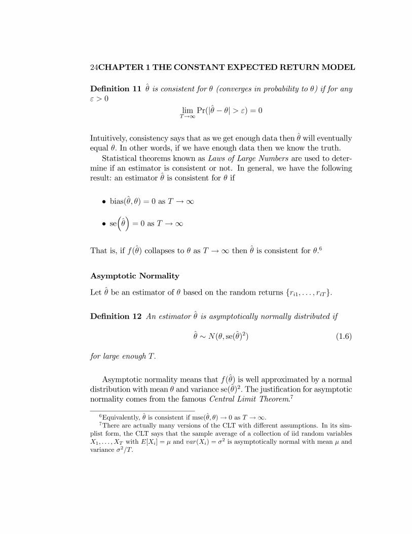
Definition 11 is consistent for (converges in probability to ) if for any
0
lim→∞
Pr(| − | ) = 0
Intuitively, consistency says that as we get enough data then will eventually
equal In other words, if we have enough data then we know the truth.
Statistical theorems known as Laws of Large Numbers are used to deter-
mine if an estimator is consistent or not. In general, we have the following
result: an estimator is consistent for if
• bias( ) = 0 as →∞
• se³´= 0 as →∞
That is, if () collapses to as →∞ then is consistent for 6
Asymptotic Normality
Let be an estimator of based on the random returns {1 }
Definition 12 An estimator is asymptotically normally distributed if
∼ ( se()2) (1.6)
for large enough
Asymptotic normality means that () is well approximated by a normal
distribution with mean and variance se()2 The justification for asymptotic
normality comes from the famous Central Limit Theorem.7
6Equivalently, is consistent if mse( )→ 0 as →∞7There are actually many versions of the CLT with different assumptions. In its sim-
plist form, the CLT says that the sample average of a collection of iid random variables
1 with [] = and () = 2 is asymptotically normal with mean and
variance 2

1.3 ESTIMATINGTHEPARAMETERSOF THECERMODEL25
1.3.4 Estimators for the Parameters of the CERModel
To estimate the CER model parameters 2 and we can use the
plug-in principle from statistics:
Plug-in-Principle: Estimate model parameters using corresponding sample
statistics.
For the CER model, the plug-in principle estimates for the CER model
parameters 2 and are the following sample descriptive statistics:
=1
X=1
= (1.7)
2 =1
− 1X=1
( − )2 (1.8)
=
q2 (1.9)
=1
− 1X=1
( − )( − ) (1.10)
=
(1.11)
The plug-in principle is appropriate because the the CER model parameters
2 and are characteristics of the underlying distribution of returns
that are naturally estimated using sample statistics.
Example 13 Estimating the CER model parameters for Microsoft, Star-
bucks and the S&P 500 index.
To illustrate typical estimates of the CER model parameters, we use data on
= 100 monthly continuously compounded returns for Microsoft, Starbucks
and the S & P 500 index over the period July 1992 through October 2000 in
the matrix object returns.mat. These data are illustrated in Figures 1.5 and
1.6. The estimates of using (1.7) can be computed using the R functions
apply() and mean()
> muhat.vals = apply(returns.mat,2,mean)
> muhat.vals
sbux msft sp500
0.02777 0.02756 0.01253
26CHAPTER 1 THECONSTANTEXPECTEDRETURNMODEL
giving = 002777 = 002756 and 500 = 001253 The expected
return estimates for Microsoft and Starbucks are very similar at about 2.8%
per month, whereas the S&P 500 expected return estimate is smaller at only
1.25% per month. The estimates of the parameters 2 using (1.8) and
(1.9) can be computed using apply(), var() and sd()
> sigma2hat.vals = apply(returns.mat,2,var)
> sigma2hat.vals
sbux msft sp500
0.018459 0.011411 0.001432
> sigmahat.vals = apply(returns.mat,2,sd)
> sigmahat.vals
sbux msft sp500
0.13586 0.10682 0.03785
giving
2 = 00185 = 01359
2 = 00114 = 01068
2500 = 00014 500 = 00379
Starbucks has the most variable monthly returns, and the S&P 500 index
has the smallest. The scatterplots of the returns are illustrated in Figure 1.6.
All returns appear to be positively related. The pairs (MSFT, SP500) and
(SBUX, SP500) appear to be the most correlated. The estimates of and
using (1.10) and (1.11) can be computed using the functions var() and
cor()
> cov.mat
sbux msft sp500
sbux 0.018459 0.004031 0.002158
msft 0.004031 0.011411 0.002244
sp500 0.002158 0.002244 0.001432
> cor.mat = cor(returns.z)
> cor.mat
sbux msft sp500
sbux 1.0000 0.2777 0.4198
msft 0.2777 1.0000 0.5551
sp500 0.4198 0.5551 1.0000

1.4 STATISTICALPROPERTIESOFTHECERMODELESTIMATES27
Notice when var() and cor() are given a matrix of returns they return the
estimated variance matrix and the estimated correlation matrix, respectively.
To extract the unique pairwise values use
> covhat.vals = cov.mat[lower.tri(cov.mat)]
> rhohat.vals = cor.mat[lower.tri(cor.mat)]
> names(covhat.vals) <- names(rhohat.vals) <-
+ c("sbux,msft","sbux,sp500","msft,sp500")
> covhat.vals
sbux,msft sbux,sp500 msft,sp500
0.004031 0.002158 0.002244
> rhohat.vals
sbux,msft sbux,sp500 msft,sp500
0.2777 0.4198 0.5551
The pairwise covariances and correlations are
= 00040 500 = 00022 500 = 00022
= 02777 500 = 05551 500 = 04198
These estimates confirm the visual results from the scatterplot matrix in
Figure 1.6.
1.4 Statistical Properties of the CER Model
Estimates
To determine the statistical properties of plug-in principle estimators 2
and in the CERmodel, we treat them as functions of the stochastic process
{1}=1 where is assumed to be generated by the CER model (1.1) for = 1 . We first consider the statistical properties of because the
derivations are the most straightforward. We then summarize the properties
of the remaining estimators.
1.4.1 Statistical Properties of
Consider the estimator given by (1.7) The following sub-sections give
derivations of the statistical properties of .

28CHAPTER 1 THECONSTANTEXPECTEDRETURNMODEL
Bias
To determine bias( ) we must first compute [] = [−1P
=1 ] Us-
ing results about the expectation of a linear combination of random variables,
it follows that
[] =
"1
X=1
#
=
"1
X=1
( + )
#(since = + )
=1
X=1
+1
X=1
[] (by the linearity of [·])
=1
X=1
(since [] = 0 = 1 )
=1
· =
Hence, the mean of () is equal to We have just proved that an
unbiased estimator for in the CER model.
Precision
Because bias( ) = 0 the precision of is determined by var() =
var(−1P
=1 ) Using the results about the variance of a linear combi-

1.4 STATISTICALPROPERTIESOFTHECERMODELESTIMATES29
nation of uncorrelated random variables, we have
var() = var
Ã1
X=1
!
= var
Ã1
X=1
( + )
!(since = + )
= var
Ã1
X=1
!(since is a constant)
=1
2
X=1
var() (since is independent over time)
=1
2
X=1
2 (since var() = 2 = 1 )
=1
22 =
2
Hence,
var() =2 (1.12)
Notice var() = var() and so is much smaller than var() Also, as
the sample size gets larger and larger, var() gets smaller and smaller.
Using (1.12), the standard deviation of is
SD() =pvar() =
√ (1.13)
The standard deviation of is often called the standard error of and is
denoted se() :
se() = SD() =√ (1.14)
The value of se() is in the same units as and measures the precision of as an estimate. If se() is small relative to then is a relatively precise
of because () will be tightly concentrated around ; if se() is large
relative to then is a relatively imprecise estimate of because ()
will be spread out about Figure 1.10 illustrates these relationships.
30CHAPTER 1 THECONSTANTEXPECTEDRETURNMODEL
estimate value
pd
f
-3 -2 -1 0 1 2 3
0.0
0.2
0.4
0.6
0.8
pdf 1pdf 2
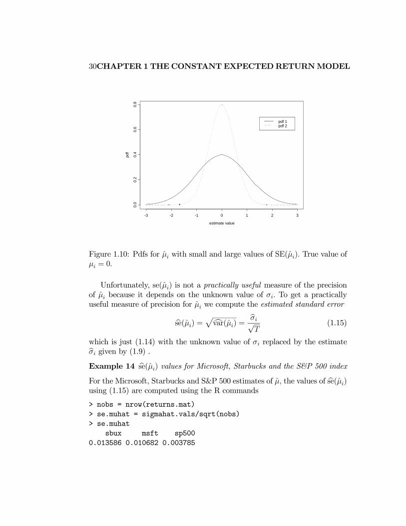
Figure 1.10: Pdfs for with small and large values of SE() True value of
= 0
Unfortunately, se() is not a practically useful measure of the precision
of because it depends on the unknown value of To get a practically
useful measure of precision for we compute the estimated standard error
bse() =pcvar() = b√
(1.15)
which is just (1.14) with the unknown value of replaced by the estimateb given by (1.9) .Example 14 bse() values for Microsoft, Starbucks and the S&P 500 indexFor the Microsoft, Starbucks and S&P 500 estimates of the values of bse()using (1.15) are computed using the R commands
> nobs = nrow(returns.mat)
> se.muhat = sigmahat.vals/sqrt(nobs)
> se.muhat
sbux msft sp500
0.013586 0.010682 0.003785
1.4 STATISTICALPROPERTIESOFTHECERMODELESTIMATES31
giving
bse() = 01359√100
= 001359
bse() =01068√100
= 001068
bse(500) = 00379√100
= 000379
Clearly, the mean return is estimated more precisely for the S&P 500 index
than it is for Microsoft and Starbucks. This occurs because 500 is much
smaller than and It is useful to compare the magnitude of bse()to the value of to evaluate if is a precise estimate:
bse()=002756
001068= 2580
bse() = 002777
001359= 2043
500bse(500) = 001253
000378= 3315
Here we see that and are over two times their estimated standard
error values, and 500 is more than three times its estimated standard error
value. ¥
The Sampling Distribution and Consistency
In the CER model, ∼ ( 2 ) and since is an average of these
normal random variables, it is also normally distributed. The mean of is
and its variance is2 Therefore, we can express the probability distribution
of as
∼
µ
2
¶ (1.16)
The distribution for is centered at the true value and the spread about
the average depends on the magnitude of 2 the variability of and the
sample size, . For a fixed sample size, , the uncertainty in is larger
for larger values of 2 Notice that the variance of is inversely related to
the sample size Given 2 var() is smaller for larger sample sizes than
32CHAPTER 1 THECONSTANTEXPECTEDRETURNMODEL
-3 -2 -1 0 1 2 3
0.0
0.5
1.0
1.5
2.0
2.5
x.vals
1
pdf: T=1pdf: T=10pdf: T=50
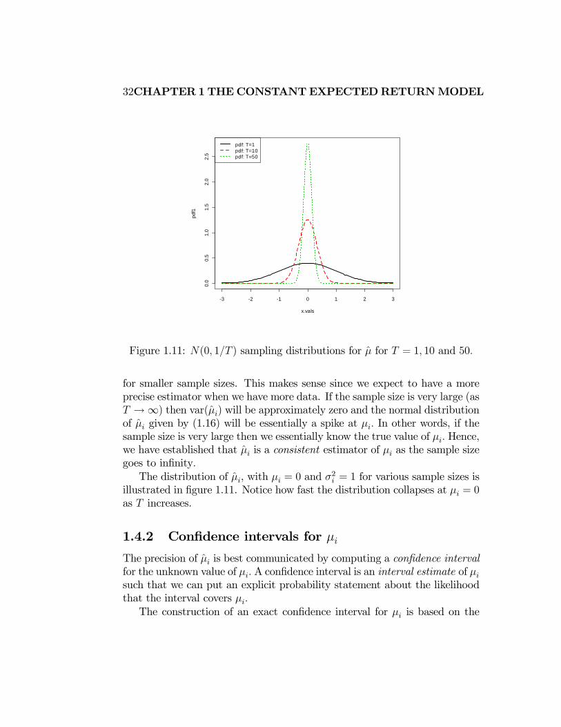
Figure 1.11: (0 1 ) sampling distributions for for = 1 10 and 50
for smaller sample sizes. This makes sense since we expect to have a more
precise estimator when we have more data. If the sample size is very large (as
→∞) then var() will be approximately zero and the normal distributionof given by (1.16) will be essentially a spike at In other words, if the
sample size is very large then we essentially know the true value of Hence,
we have established that is a consistent estimator of as the sample size
goes to infinity
The distribution of , with = 0 and 2 = 1 for various sample sizes is
illustrated in figure 1.11. Notice how fast the distribution collapses at = 0
as increases.
1.4.2 Confidence intervals for
The precision of is best communicated by computing a confidence interval
for the unknown value of A confidence interval is an interval estimate of such that we can put an explicit probability statement about the likelihood
that the interval covers
The construction of an exact confidence interval for is based on the
1.4 STATISTICALPROPERTIESOFTHECERMODELESTIMATES33
following statistical result (see the appendix for details).
Result: Let {}=1 denote a stochastic process generated from the CERmodel (1.1). Define the -ratio as
= − bse() (1.17)
Then ∼ −1 where −1 denotes a Student’s random variable with − 1degrees of freedom.
The Student’s distribution with 0 degrees of freedom is a symmetric
distribution centered at zero, like the standard normal. The tail-thickness
(kurtosis) of the distribution is determined by the degrees of freedom para-
meter For values of close to zero, the tails of the Student’s distribution
are much fatter than the tails of the standard normal distribution. As gets
large, the Student’s distribution approaches the standard normal distribu-
tion.
For ∈ (0 1) we compute a (1 − ) · 100% confidence interval for using (1.17) and the 1− 2 quantile (critical value) −1(1− 2) to give
Pr
µ−−1(1− 2) ≤ − bse() ≤ −1(1− 2)
¶= 1−
which can be rearranged as
Pr ( − −1(1− 2) · bse() ≤ ≤ + −1(1− 2) · bse()) = 1−
Hence, the interval
[ − −1(1− 2) · bse() + −1(1− 2) · bse()] (1.18)
= ± −1(1− 2) · bse()covers the true unknown value of with probability 1−
For example, suppose we want to compute a 95% confidence interval for
In this case = 005 and 1− = 095 Suppose further that − 1 = 60(five years of monthly return data) so that −1(1 − 2) = 60(0975) = 2
Then the 95% confidence for is given by
± 2 · bse() (1.19)

34CHAPTER 1 THECONSTANTEXPECTEDRETURNMODEL
The above formula for a 95% confidence interval is often used as a rule of
thumb for computing an approximate 95% confidence interval for moderate
sample sizes. It is easy to remember and does not require the computation
of the quantile −1(1 − 2) from the Student’s distribution. It is also
an approximate 95% confidence interval that is based the asymptotic nor-
mality of Recall, for a normal distribution with mean and variance 2
approximately 95% of the probability lies between ± 2The coverage probability associated with the confidence interval for is
based on the fact that the estimator is a random variable. Since confidence
interval is constructed as ±−1(1−2)· bse() it is also a random variable.An intuitive way to think about the coverage probability associated with the
confidence is to think about the game of horse shoes. The horse shoe is the
confidence interval and the parameter is the post at which the horse shoe
is tossed. Think of playing game 100 times (i.e, simulate 100 samples of the
CER model). If the thrower is 95% accurate (if the coverage probability is
0.95) then 95 of the 100 tosses should ring the post (95 of the constructed
confidence intervals should contain the true value ).
Example 15 95% confidence intervals for for Microsoft, Starbucks and
the S & P 500 index.
Consider computing 95% confidence intervals for using (1.18) based on
the estimated results for the Microsoft, Starbucks and S&P 500 data. The
degrees of freedom for the Student’s distribution is − 1 = 99 The 97.5%quantile, 99(0975) can be computed using the R function qt()
> qt(0.975, df=99)
[1] 1.984
Notice that this quantile is very close to 2 Then the exact 95% confidence
intervals are given by
: 002756± 1984 · 001068 = [00064 00488] : 002777± 1984 · 001359 = [00008 00547]500 : 001253± 1984 · 000379 = [00050 00200]
With probability 0.95, the above intervals will contain the true mean values
assuming the CER model is valid. The 95% confidence intervals for MSFT
and SBUX are fairly wide. The widths are almost 5%, with lower limits
1.4 STATISTICALPROPERTIESOFTHECERMODELESTIMATES35
near 0% and upper limits near 5%. This means that with probability 0.95,
the true monthly expected return is somewhere between 0% and 5%. The
economic implications of a 0% expected return and a 5% expected return are
vastly different. In contrast, the 95% confidence interval for SP500 is about
half the width of the MSFT or SBUX confidence interval. The lower limit is
near 0.5% and the upper limit is near 2%. This clearly shows that the mean
return for SP500 is estimated much more precisely than the mean return for
MSFT or SBUX.
1.4.3 Interpreting [] se() and Confidence Intervals
Using Monte Carlo Simulation
The exact meaning of unbiasedness, [] = the interpretation of se()
as a measure of precision, and the interpretation of the coverage probability
of a confidence interval can be a bit hard to grasp at first. Strictly speaking,
[] = means that over an infinite number of repeated samples of {}=1the average of the values computed over the infinite samples is equal to
the true value The value of se() represents the standard deviation of
these values. And the 95% confidence intervals for will actually contain
in 95% of the samples We can think of these hypothetical samples as
different Monte Carlo simulations of the CER model. In this way we can
approximate the computations involved in evaluating [] se() and the
coverage probability of a confidence interval using a large, but finite, number
of Monte Carlo simulations.
To illustrate, consider the CER model
= 005 + = 1 100 (1.20)
∼ (0 (010)2)
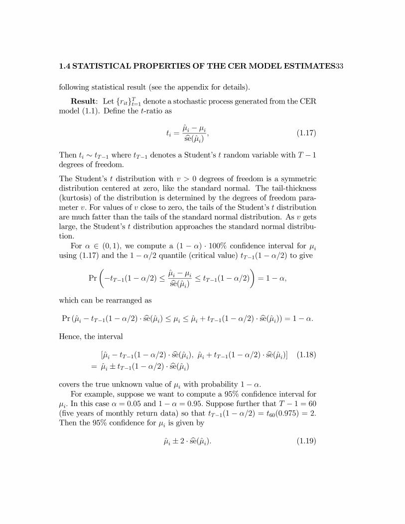
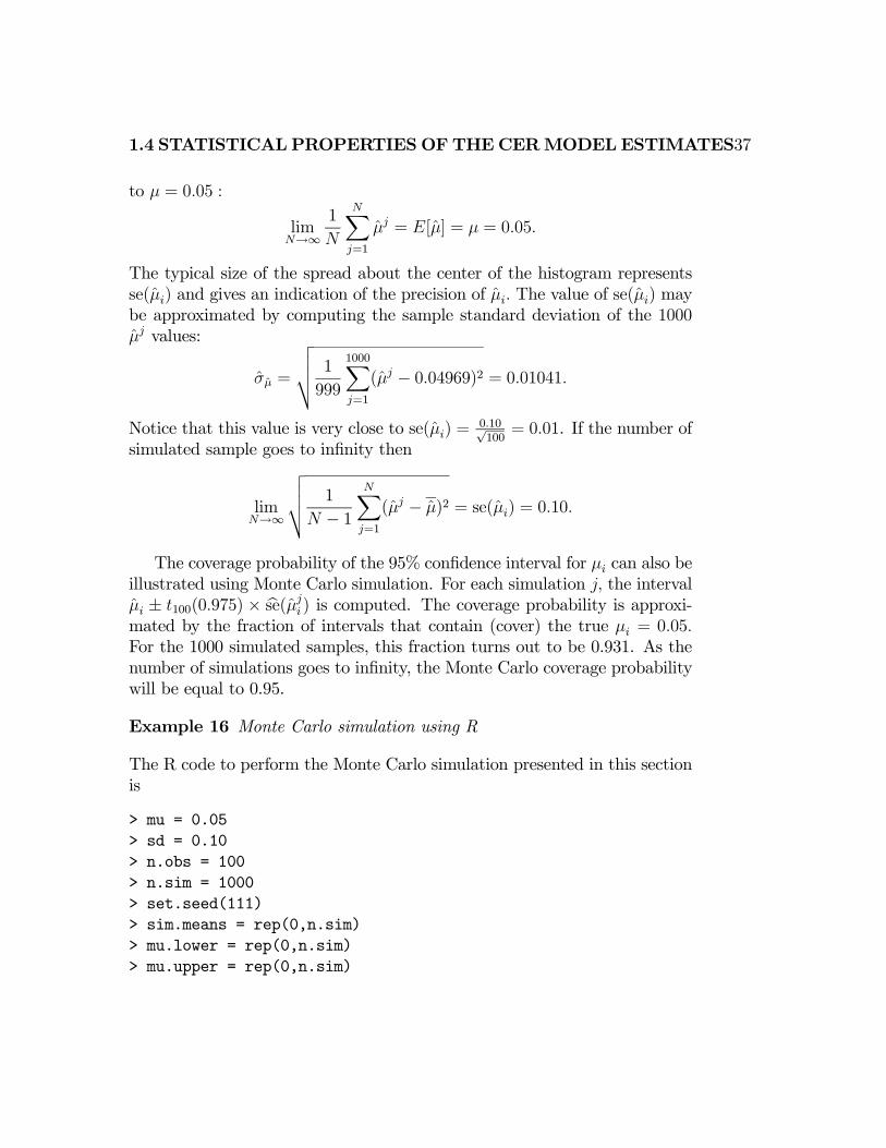
Using Monte Carlo simulation, we can simulate = 1000 samples of
size = 100 from (1.20) giving the sample realizations {}100=1 for =
1 1000 The first 10 of these simulated samples are illustrated in Figure
1.12. Notice that there is considerable variation in the simulated samples,
but that all of the simulated samples fluctuate about the true mean value
of = 005 and have a typical deviation from the mean of about 010 For
each of the 1000 simulated samples the estimate is formed giving 1000
mean estimates {1 1000} A histogram of these 1000 mean values is
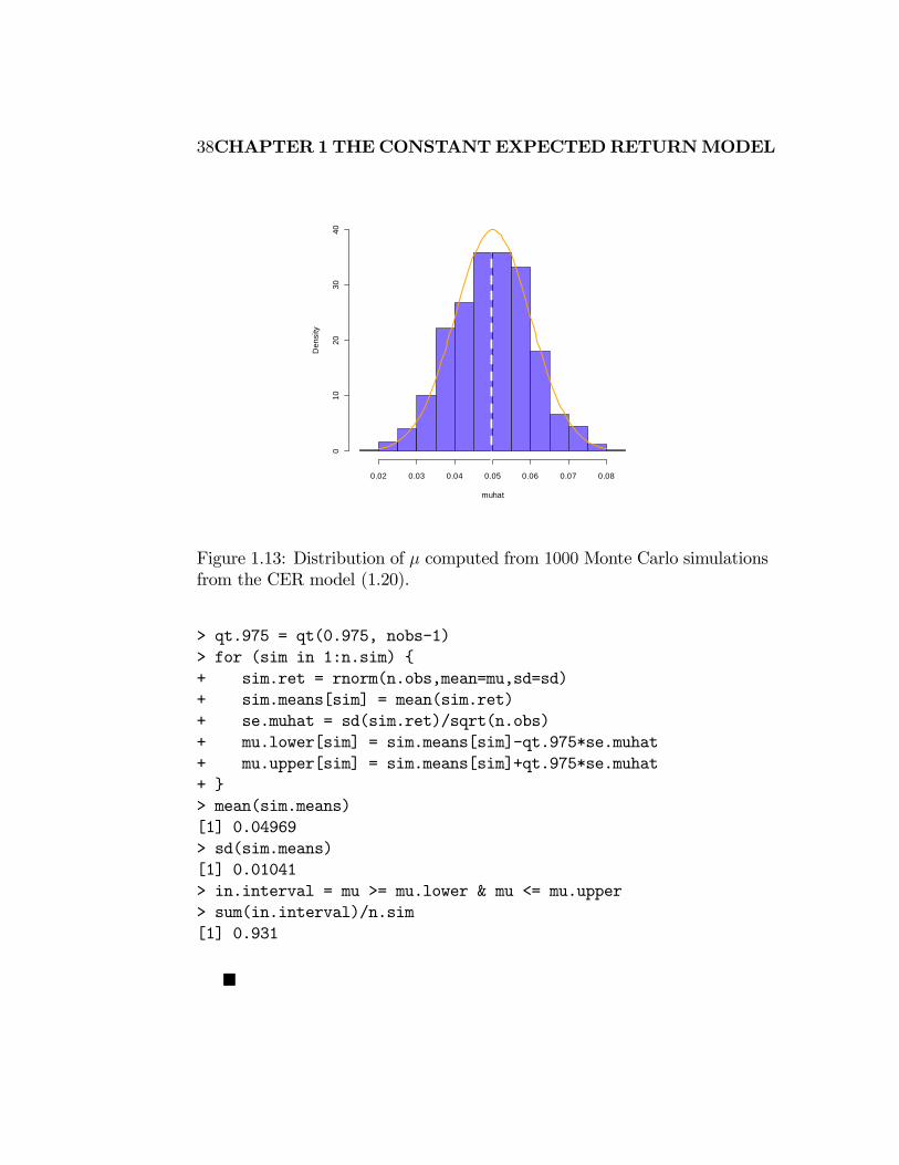
illustrated in Figure 1.13. The histogram of the estimated means, can
36CHAPTER 1 THECONSTANTEXPECTEDRETURNMODEL
Ser
ies
1
-0.2
0.0
0.2
Ser
ies
2
-0.3
-0.1
0.1
0.3
Ser
ies
3
-0.1
0.1
0.3
Ser
ies
4
-0.2
0.0
0.2
0 20 40 60 80 100
-0.2
0.0
0.2
Ser
ies
5
IndexS
erie
s 6
-0.1
0.1
0.3
Ser
ies
7
-0.1
0.1
Ser
ies
8
-0.1
0.0
0.1
0.2
Ser
ies
9
-0.1
0.1
0.3
0 20 40 60 80 100
-0.1
0.1
0.3
Ser
ies
10
Index
Figure 1.12: Ten simulated samples of size = 100 from the CER model
= 005 + ∼ (0 (010)2)
be thought of as an estimate of the underlying pdf, () of the estimator
which we know from (1.16) is a normal pdf centered at [] = = 005 with
se() =010√100= 001. This normal curve is superimposed on the histogram
in Figure 1.13. Notice that the center of the histogram is very close to the
true mean value = 005 That is, on average over the 1000 Monte Carlo
samples the value of is about 0.05. In some samples, the estimate is too big
and in some samples the estimate is too small but on average the estimate is
correct. In fact, the average value of {1 1000} from the 1000 simulatedsamples is
=1
1000
1000X=1
= 004969
which is very close to the true value 005. If the number of simulated samples
is allowed to go to infinity then the sample average will be exactly equal
1.4 STATISTICALPROPERTIESOFTHECERMODELESTIMATES37
to = 005 :
lim→∞
1
X=1
= [] = = 005
The typical size of the spread about the center of the histogram represents
se() and gives an indication of the precision of The value of se() may
be approximated by computing the sample standard deviation of the 1000
values:
=
vuut 1
999
1000X=1
( − 004969)2 = 001041
Notice that this value is very close to se() =010√100= 001. If the number of
simulated sample goes to infinity then
lim→∞
vuut 1
− 1X=1
( − )2 = se() = 010
The coverage probability of the 95% confidence interval for can also be
illustrated using Monte Carlo simulation. For each simulation the interval
± 100(0975) × bse( ) is computed. The coverage probability is approxi-mated by the fraction of intervals that contain (cover) the true = 005
For the 1000 simulated samples, this fraction turns out to be 0.931. As the
number of simulations goes to infinity, the Monte Carlo coverage probability
will be equal to 0.95.
Example 16 Monte Carlo simulation using R
The R code to perform the Monte Carlo simulation presented in this section
is
> mu = 0.05
> sd = 0.10
> n.obs = 100
> n.sim = 1000
> set.seed(111)
> sim.means = rep(0,n.sim)
> mu.lower = rep(0,n.sim)
> mu.upper = rep(0,n.sim)
38CHAPTER 1 THECONSTANTEXPECTEDRETURNMODEL
muhat
De
nsi
ty
0.02 0.03 0.04 0.05 0.06 0.07 0.08
010
20
30
40
Figure 1.13: Distribution of computed from 1000 Monte Carlo simulations
from the CER model (1.20).
> qt.975 = qt(0.975, nobs-1)
> for (sim in 1:n.sim) {
+ sim.ret = rnorm(n.obs,mean=mu,sd=sd)
+ sim.means[sim] = mean(sim.ret)
+ se.muhat = sd(sim.ret)/sqrt(n.obs)
+ mu.lower[sim] = sim.means[sim]-qt.975*se.muhat
+ mu.upper[sim] = sim.means[sim]+qt.975*se.muhat
+ }
> mean(sim.means)
[1] 0.04969
> sd(sim.means)
[1] 0.01041
> in.interval = mu >= mu.lower & mu <= mu.upper
> sum(in.interval)/n.sim
[1] 0.931
¥

1.4 STATISTICALPROPERTIESOFTHECERMODELESTIMATES39
1.4.4 Evaluating Consistency of using Monte Carlo
Simulation
Monte Carlo simulations can also be used to illustrate the asymptotic prop-
erty that is a consistent estimator of
To be completed.
1.4.5 Statistical properties of the estimators of 2 and
To determine the statistical properties of 2 and we need to treat
them as a functions of the random variables {}=1 We could straightfor-wardly derive the statistical properties of Unfortunately, the correspond-
ing derivations for 2 and are much messier and in many cases we
do not have simple exact results. Hence, we only state the results and give
references for the exact derivations.
Bias
Assuming that returns are generated by the CER model (1.1), the sample
variances and covariances are unbiased estimators,
[2 ] = 2
[] =
but the sample standard deviations and correlations are biased estimators,
[] 6=
[] 6=
The biases in and are very small and decreasing in such that
bias( ) = bias( ) = 0 as → ∞. The proofs of these results
are beyond the scope of this book and may be found, for example, in Gold-
berger (19xx). However, the results can be easily verified using Monte Carlo
methods.
Precision
The derivations of the variances of 2 and are complicated, and
the exact results are extremely messy and hard to work with. However, there

40CHAPTER 1 THECONSTANTEXPECTEDRETURNMODEL
are simple approximate formulas for the variances of 2 and based on
the CLT that are valid if the sample size, is reasonably large.8 These large
sample approximate formulas are given by
se(2 ) ≈√22√=
2p2
(1.21)
se() ≈ √2
(1.22)
se() ≈(1− 2)√
(1.23)
where “≈” denotes approximately equal. The approximations are such thatthe approximation error goes to zero as the sample size gets very large.
As with the formula for the standard error of the sample mean, the formulas
for se(2 ) and se() depend on 2 Larger values of 2 imply less precise
estimates of 2 and The formula for se() however, does not depend on
2 but rather depends on 2 and is smaller the closer 2 is to unity. Intu-
itively, this makes sense because as 2 approaches one the linear dependence
between and becomes almost perfect and this will be easily recogniz-
able in the data (scatterplot will almost follow a straight line). Additionally,
the formulas for the standard errors above are inversely related to the square
root of the sample size. Interestingly, se() goes to zero the fastest and
se(2 ) goes to zero the slowest. Hence, for a fixed sample size, these formulas
suggest that is generally estimated more precisely than 2 and and
is estimated generally more precisely than 2
The above formulas (1.21) - (1.23) are not practically useful, however,
because they depend on the unknown quantities 2 and Practically
useful formulas replace 2 and by the estimates 2 and and give
8The large sample approximate formula for the variance of is too messy to work
with so we omit it here. In practice, we can use the bootstrap to provide an estimated
standard error for
1.4 STATISTICALPROPERTIESOFTHECERMODELESTIMATES41
rise to the estimated standard errors:
bse(2 ) ≈ 2p2
(1.24)
bse() ≈ √2
(1.25)
bse() ≈ (1− 2)√
(1.26)
Example 17 Computing bse(2 ) bse() and bse() for Microsoft, Starbucksand the S & P 500.
For the Microsoft, Starbucks and S&P 500 return data, the values of bse(2 )bse() are computed using> se.sigma2hat = sigma2hat.vals/sqrt(nobs/2)
> se.sigmahat = sigmahat.vals/sqrt(2*nobs)
> se.sigma2hat
sbux msft sp500
0.0026105 0.0016138 0.0002026
> se.sigmahat
sbux msft sp500
0.009607 0.007554 0.002676
which gives
bse(2) = (01359)2p
1002= 000261 bse() = 01359√
2 · 100 = 000961
bse(2) =(01068)
2p1002
= 000161 bse() =01068√2 · 100 = 000755
bse(2500) = (00379)2p
1002= 000020 bse(500) = 00379√
2 · 100 = 000268
Notice that 500 is estimated much more precisely than and
Also notice that is estimated more precisely than The values of bse()relative to are much smaller than the values of bse() to The values of bse() are computed using

42CHAPTER 1 THECONSTANTEXPECTEDRETURNMODEL
> se.rhohat
sbux,msft sbux,sp500 msft,sp500
0.09229 0.08238 0.06919
which gives
bse() =1− (02777)2√
100= 009229
bse(500) = 1− (04198)2√100
= 008238
bse(500) =1− (05551)2√
100= 006919
These standard errors are moderate in size (relative to ) Notice that
500 has the smallest estimated standard error because 2500 is
closest to one.
Sampling distributions
The exact distributions of 2 and are difficult to derive.9 However,
approximate normal distributions of the form (1.6) based on the CLT are
readily available:
2 ∼
µ2
44
∼
µ
22
∼
Ã
(1− 2)2
!
These appoximate normal distributions can be used to compute approximate
confidence intervals for 2 and
9For example, the exact sampling distribution of ( − 1)2 2 is chi-square with − 1degrees of freedom.
1.4 STATISTICALPROPERTIESOFTHECERMODELESTIMATES43
Approximate Confidence Intervals for 2 and
Approximate 95% confidence intervals for 2 and are given by
2 ± 2 · bse(2 ) = 2 ± 2 ·2p2
± 2 · bse() = ± 2 · √2
± 2 · bse() = ± 2 ·(1− 2)√
Example 18 95% confidence intervals for 2 and for Microsoft, Star-
bucks and the S&P 500.
For the Microsoft, Starbucks and S&P 500 return data the approximate 95%
confidence intervals for 2 are
: 001141± 2 · (000161) = [000818 001464] : 001846± 2 · (000261) = [001324 002368]500 : 000143± 2 · (000020) = [000103 000184]
The approximate 95% confidence intervals for are
: 01068± 2 · (0007554) = [009172 01219] : 01359± 2 · (0009607) = [011665 01551]500 : 00379± 2 · (0002676) = [003249 00432]
The approximate 95% confidence intervals for are
: 02777± 2 · (009229) = [009314 04623] 500 : 05551± 2 · (006919) = [041674 06935]500 : 04198± 2 · (008238) = [025499 05845]
Evaluating the Statistical Properties of 2 and by Monte Carlo
simulation
We can evaluate the statistical properties of 2 and by Monte Carlo sim-
ulation in the same way that we evaluated the statistical properties of .

44CHAPTER 1 THECONSTANTEXPECTEDRETURNMODEL
0.004 0.006 0.008 0.010 0.012 0.014 0.016
050
100
150
200
Estimate of variance
0.08 0.10 0.12
050
100
150
200
Estimate of std. deviation
Figure 1.14: Histograms of 2 and computed from = 1000 Monte Carlo
samples from CER model.
Consider first the variability estimates 2 and We use the simulation
model (1.20) and = 1000 simulated samples of size = 50 to compute the
estimates {¡2¢1 ¡2¢1000} and {1 1000} The histograms of thesevalues are displayed in figure 1.14. The histogram for the 2 values is bell-
shaped and slightly right skewed but is centered very close to 0010 = 2 The
histogram for the values is more symmetric and is centered near 010 =
The average values of 2 and from the 1000 simulations are
1
1000
1000X=1
2 = 0009952
1
1000
1000X=1
= 009928
The sample standard deviation values of the Monte Carlo estimates of 2
and give approximations to SD(2) and SD()
1.5 FURTHER READING 45
1.4.6 Evaluating the Statistical Properties of and
by Monte Carlo simulation
To be completed
1.4.7 Estimating Value-at-Risk in the CER Model
To be completed
1.5 Further Reading
To be completed
1.6 Appendix
1.6.1 Proofs of Some Technical Results
Result: mse( ) = [( −[])2] +³[]−
´2= var() + bias( )2
Proof. Recall, mse( ) = [( − )2] Write
− = −[] + []−
Then
( − )2 =³ −[]
´2+ 2
³ −[]
´³[]−
´+³[]−
´2
Taking expectations of both sides gives
mse( ) = h³
−[]´i2
+
∙³[]−
´2¸= var() + bias( )2

46CHAPTER 1 THECONSTANTEXPECTEDRETURNMODEL
1.6.2 The Chi-Square distribution with degrees of
freedom
Let 1 2 be independent standard normal random variables. That
is,
∼ (0 1) = 1
Define a new random variable such that
= 21 + 22 + · · ·2 =X=1
2
Then is a chi-square random variable with degrees of freedom. Such a
random variable is often denoted 2 and we use the notation ∼ 2 The
pdf of is illustrated in Figure xxx for various values of Notice that
is only allowed to take non-negative values. The pdf is highly right skewed
for small values of and becomes symmetric as gets large. The mean of
the distribution is
[] = [21 ] +[22 ] + · · ·[2 ] =
since [2 ] = var() = 1
1.6.3 Student’s t distribution with degrees of free-
dom
Let be a standard normal random variable, ∼ (0 1) and let be
a chi-square random variable with degrees of freedom, ∼ 2 Assume
that and are independent. Define a new random variable such that
=p
Then is a Student’s t random variable with degrees of freedom and we
use the notation ∼ to indicate that is distributed Student’s-t. Figure
xxx shows the pdf of for various values of the degrees of freedom Notice
that the pdf is symmetric about zero and has a bell shape like the normal.
The tail thickness of the pdf is determined by the degrees of freedom. For
small values of , the tails are quite spread out and are thicker than the
tails of the normal. As gets large the tails shrink and become close to the

1.6 APPENDIX 47
normal. In fact, as → ∞ the pdf of the Student’s t converges to the pdf
of the normal.
The Student’s-t distribution is used heavily in statistical inference and
critical values from the distribution are often needed. Let () denote the
critical value such that
Pr( ()) =
For example, if = 10 and = 0025 then 10(0025) = 2228; if = 100
then 60(0025) = 200 Since the Student’s-t distribution is symmetric about
zero, we have that
Pr(− () ≤ ≤ ()) = 1− 2
For example, if = 60 and = 2 then 60(0025) = 2 and
Pr(−60(0025) ≤ ≤ 60(0025)) = Pr(−2 ≤ ≤ 2) = 1− 2(0025) = 095


Bibliography
[1] Campbell, Lo and MacKinley (1998). The Econometrics of Financial
Markets, Princeton University Press, Princeton, NJ.
49
Copyright © 2022 FDOKUMEN