65constant , where is the radius, fills the space between the conductors. Determine the capacitance of the capacitor.

7. Determine whether the functions given below satisfy Laplace 's equation

i)

ii)

Unit III Magnetostatics

In previous chapters we have seen that an electrostatic field is produced by static or stationary charges. The relationship of the steady magnetic field to its sources is much more

complicated.

The source of steady magnetic field may be a permanent magnet, a direct current or an electric field changing with time. In this chapter we shall mainly consider the magnetic field produced by a direct current. The magnetic field produced due to time varying electric field will be discussed later. Historically, the link between the electric and magnetic field was established Oersted in 1820. Ampere and others extended the investigation of magnetic effect of electricity . There are two major laws governing the magnetostatic fields are:

Biot-Savart Law

Ampere's Law

Usually, the magnetic field intensity is represented by the vector . It is customary to represent the direction of the magnetic field intensity (or current) by a small circle with a dot or cross sign depending on whether the field (or current) is out of or into the page as shown in Fig. 4.1.

66

(or l ) out of the page (or l ) into the page

Fig. 4.1: Representation of magnetic field (or current)

Biot- Savart Law

This law relates the magnetic field intensity dH produced at a point due to a differential

current element as shown in Fig. 4.2.

Fig. 4.2: Magnetic field intensity due to a current element

The magnetic field intensity at P can be written as,

............................(4.1a)

..............................................(4.1b)

where is the distance of the current element from the point P.

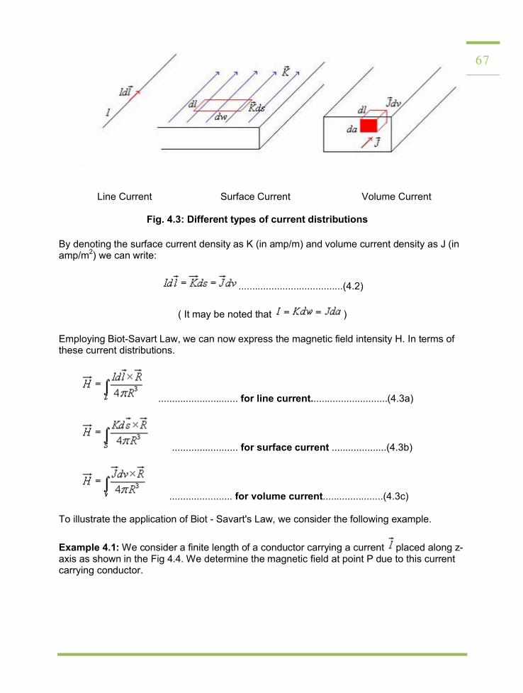
Similar to different charge distributions, we can have different current distribution such as line current, surface current and volume current. These different types of current densities are shown in Fig. 4.3.

67

Line Current Surface Current Volume Current

Fig. 4.3: Different types of current distributions

By denoting the surface current density as K (in amp/m) and volume current density as J (in amp/m

2) we can write:

......................................(4.2)

( It may be noted that )

Employing Biot-Savart Law, we can now express the magnetic field intensity H. In terms of these current distributions.

............................. for line current............................(4.3a)

........................ for surface current ....................(4.3b)

....................... for volume current......................(4.3c)

To illustrate the application of Biot - Savart's Law, we consider the following example.

Example 4.1: We consider a finite length of a conductor carrying a current placed along z-axis as shown in the Fig 4.4. We determine the magnetic field at point P due to this current carrying conductor.

68

Fig. 4.4: Field at a point P due to a finite length current carrying conductor

With reference to Fig. 4.4, we find that

.......................................................(4.4)

Applying Biot - Savart's law for the current element

we can write,

........................................................(4.5)

Substituting we can write,

.........................(4.6)

We find that, for an infinitely long conductor carrying a current I , and

Therefore, .........................................................................................(4.7)

Ampere's Circuital Law:

Ampere's circuital law states that the line integral of the magnetic field (circulation of H ) around a closed path is the net current enclosed by this path. Mathematically,

69 ......................................(4.8)

The total current I enc can be written as,

......................................(4.9) By applying Stoke's theorem, we can write

......................................(4.10) which is the Ampere's law in the point form.

Applications of Ampere's law:

We illustrate the application of Ampere's Law with some examples.

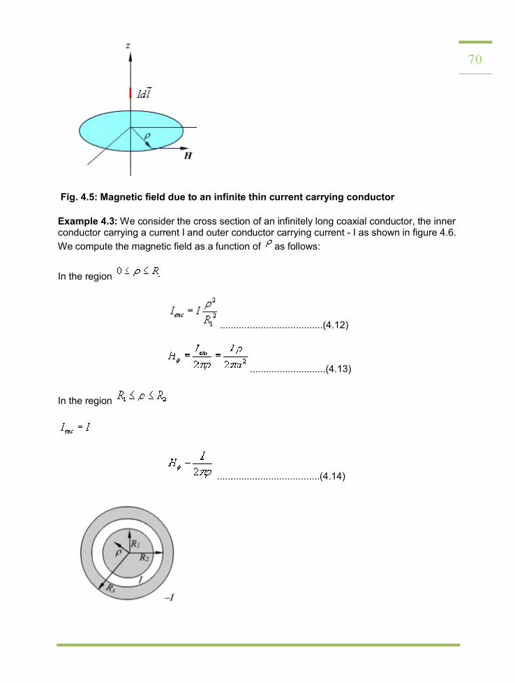
Example 4.2: We compute magnetic field due to an infinitely long thin current carrying conductor as shown in Fig. 4.5. Using Ampere's Law, we consider the close path to be a

circle of radius as shown in the Fig. 4.5.

If we consider a small current element , is perpendicular to the plane

containing both and . Therefore only component of that will be present is

,i.e., .

By applying Ampere's law we can write,

......................................(4.11)

Therefore, which is same as equation (4.7)

70

Fig. 4.5: Magnetic field due to an infinite thin current carrying conductor

Example 4.3: We consider the cross section of an infinitely long coaxial conductor, the innerconductor carrying a current I and outer conductor carrying current - I as shown in figure 4.6.

We compute the magnetic field as a function of as follows:

In the region

......................................(4.12)

............................(4.13)

In the region

......................................(4.14)

71 Fig. 4.6: Coaxial conductor carrying equal and opposite

currents

In the region

......................................(4.15)

........................................(4.16)

In the region

......................................(4.17) Magnetic Flux Density:

In simple matter, the magnetic flux density related to the magnetic field intensity as

where called the permeability. In particular when we consider the free space

where H/m is the permeability of the free space. Magnetic flux density is measured in terms of Wb/m

2.

The magnetic flux density through a surface is given by:

Wb ......................................(4.18)

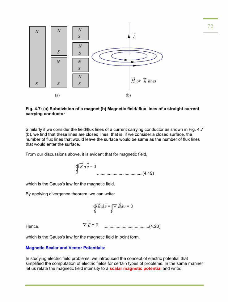
In the case of electrostatic field, we have seen that if the surface is a closed surface, the net flux passing through the surface is equal to the charge enclosed by the surface. In case of magnetic field isolated magnetic charge (i. e. pole) does not exist. Magnetic poles always occur in pair (as N-S). For example, if we desire to have an isolated magnetic pole by dividing the magnetic bar successively into two, we end up with pieces each having north (N) and south (S) pole as shown in Fig. 4.7 (a). This process could be continued until the magnets are of atomic dimensions; still we will have N-S pair occurring together. This means that the magnetic poles cannot be isolated.

72

Fig. 4.7: (a) Subdivision of a magnet (b) Magnetic field/ flux lines of a straight current carrying conductor

Similarly if we consider the field/flux lines of a current carrying conductor as shown in Fig. 4.7 (b), we find that these lines are closed lines, that is, if we consider a closed surface, the number of flux lines that would leave the surface would be same as the number of flux lines that would enter the surface.

From our discussions above, it is evident that for magnetic field,

......................................(4.19)

which is the Gauss's law for the magnetic field.

By applying divergence theorem, we can write:

Hence, ......................................(4.20)

which is the Gauss's law for the magnetic field in point form.

Magnetic Scalar and Vector Potentials:

In studying electric field problems, we introduced the concept of electric potential that simplified the computation of electric fields for certain types of problems. In the same manner let us relate the magnetic field intensity to a scalar magnetic potential and write:

73...................................(4.21)

From Ampere's law , we know that

......................................(4.22)

Therefore, ............................(4.23)

But using vector identity, we find that is valid only where .

Thus the scalar magnetic potential is defined only in the region where . Moreover, Vm

in general is not a single valued function of position.

This point can be illustrated as follows. Let us consider the cross section of a coaxial line as shown in fig 4.8.

In the region , and

Fig. 4.8: Cross Section of a Coaxial Line

If Vm is the magnetic potential then,

74

If we set Vm = 0 at then c=0 and

We observe that as we make a complete lap around the current carrying conductor , we

reach again but Vm this time becomes

We observe that value of Vm keeps changing as we complete additional laps to pass through the same point. We introduced Vm analogous to electostatic potential V. But for static electric

fields, and , whereas for steady magnetic field wherever

but even if along the path of integration.

We now introduce the vector magnetic potential which can be used in regions where current density may be zero or nonzero and the same can be easily extended to time varying cases. The use of vector magnetic potential provides elegant ways of solving EM field problems.

Since and we have the vector identity that for any vector , , we can

write .

Here, the vector field is called the vector magnetic potential. Its SI unit is Wb/m. Thus if

can find of a given current distribution, can be found from through a curl operation.

We have introduced the vector function and related its curl to . A vector function is

defined fully in terms of its curl as well as divergence. The choice of is made as follows.

...........................................(4.24)

By using vector identity, .................................................(4.25)

.........................................(4.26)

75Great deal of simplification can be achieved if we choose .

Putting , we get which is vector poisson equation. In Cartesian coordinates, the above equation can be written in terms of the components as

......................................(4.27a)

......................................(4.27b)

......................................(4.27c)

The form of all the above equation is same as that of

..........................................(4.28)

for which the solution is

..................(4.29)

In case of time varying fields we shall see that , which is known as Lorentz condition, V being the electric potential. Here we are dealing with static magnetic field, so

.

By comparison, we can write the solution for Ax as

...................................(4.30)

Computing similar solutions for other two components of the vector potential, the vector potential can be written as

.......................................(4.31)

This equation enables us to find the vector potential at a given point because of a volume

current density . Similarly for line or surface current density we can write

76...................................................(4.32)

respectively. ..............................(4.33)

The magnetic flux through a given area S is given by

.............................................(4.34)

Substituting

.........................................(4.35)

Vector potential thus have the physical significance that its integral around any closed path is equal to the magnetic flux passing through that path.

Boundary Condition for Magnetic Fields:

Similar to the boundary conditions in the electro static fields, here we will consider the

behavior of and at the interface of two different media. In particular, we determine how the tangential and normal components of magnetic fields behave at the boundary of two regions having different permeabilities.

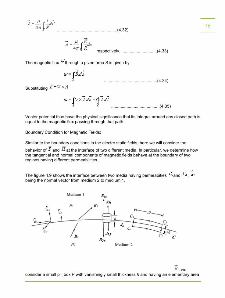
The figure 4.9 shows the interface between two media having permeabities and , being the normal vector from medium 2 to medium 1.

Figure 4.9: Interface between two magnetic media

To determine the condition for the normal component of the flux density vector , we consider a small pill box P with vanishingly small thickness h and having an elementary area

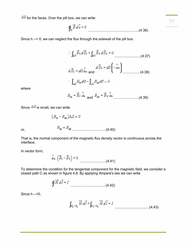
77for the faces. Over the pill box, we can write

....................................................(4.36)

Since h --> 0, we can neglect the flux through the sidewall of the pill box.

...........................(4.37)

and ..................(4.38)

where

and ..........................(4.39)

Since is small, we can write

or, ...................................(4.40)

That is, the normal component of the magnetic flux density vector is continuous across the interface.

In vector form,

...........................(4.41)

To determine the condition for the tangential component for the magnetic field, we consider a closed path C as shown in figure 4.8. By applying Ampere's law we can write

....................................(4.42)

Since h -->0,

...................................(4.43)

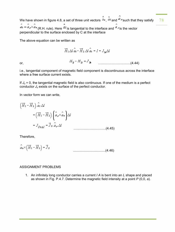
78We have shown in figure 4.8, a set of three unit vectors , and such that they satisfy

(R.H. rule). Here is tangential to the interface and is the vector perpendicular to the surface enclosed by C at the interface

The above equation can be written as

or, ...................................(4.44) i.e., tangential component of magnetic field component is discontinuous across the interface where a free surface current exists.

If Js = 0, the tangential magnetic field is also continuous. If one of the medium is a perfect conductor Js exists on the surface of the perfect conductor.

In vector form we can write,

...................................(4.45)

Therefore,

...................................(4.46)

ASSIGNMENT PROBLEMS

1. An infinitely long conductor carries a current I A is bent into an L shape and placed as shown in Fig. P.4.7. Determine the magnetic field intensity at a point P (0,0, a).

79

Figure P.4.7

2. Consider a long filamentary carrying a current IA in the + Z direction. Calculate the magnetic field intensity at point O (- a , a ,0). Also determine the flux through this

region described by and .3. A very long air cored solenoid is to produce an inductance 0.1H/m. If the member of

turns per unit length is 1000/m. Determine the diameter of this turns of the solenoid. 4. Determine the force per unit length between two infinitely long conductor each

carrying current IA and the conductor are separated by a distance ? d '.

Unit IV Electrodynamic fields

Introduction:

In our study of static fields so far, we have observed that static electric fields are produced by electric charges, static magnetic fields are produced by charges in motion or by steady current. Further, static electric field is a conservative field and has no curl, the static magnetic field is continuous and its divergence is zero. The fundamental relationships for static electric fields among the field quantities can be summarized as:

(5.1a)

(5.1b)

For a linear and isotropic medium,

(5.1c)

Similarly for the magnetostatic case

80 (5.2a)

(5.2b)

(5.2c)

It can be seen that for static case, the electric field vectors and and magnetic field

vectors and form separate pairs.

In this chapter we will consider the time varying scenario. In the time varying case we will observe that a changing magnetic field will produce a changing electric field and vice versa.

We begin our discussion with Faraday's Law of electromagnetic induction and then present the Maxwell's equations which form the foundation for the electromagnetic theory.

Faraday's Law of electromagnetic Induction

Michael Faraday, in 1831 discovered experimentally that a current was induced in a conducting loop when the magnetic flux linking the loop changed. In terms of fields, we can say that a time varying magnetic field produces an electromotive force (emf) which causes a current in a closed circuit. The quantitative relation between the induced emf (the voltage that arises from conductors moving in a magnetic field or from changing magnetic fields) and the rate of change of flux linkage developed based on experimental observation is known as Faraday's law. Mathematically, the induced emf can be written as

Emf = Volts (5.3)

where is the flux linkage over the closed path.

A non zero may result due to any of the following:

(a) time changing flux linkage a stationary closed path.

(b) relative motion between a steady flux a closed path.

(c) a combination of the above two cases.

The negative sign in equation (5.3) was introduced by Lenz in order to comply with the polarity of the induced emf. The negative sign implies that the induced emf will cause a current flow in the closed loop in such a direction so as to oppose the change in the linking magnetic flux which produces it. (It may be noted that as far as the induced emf is concerned, the closed path forming a loop does not necessarily have to be conductive).

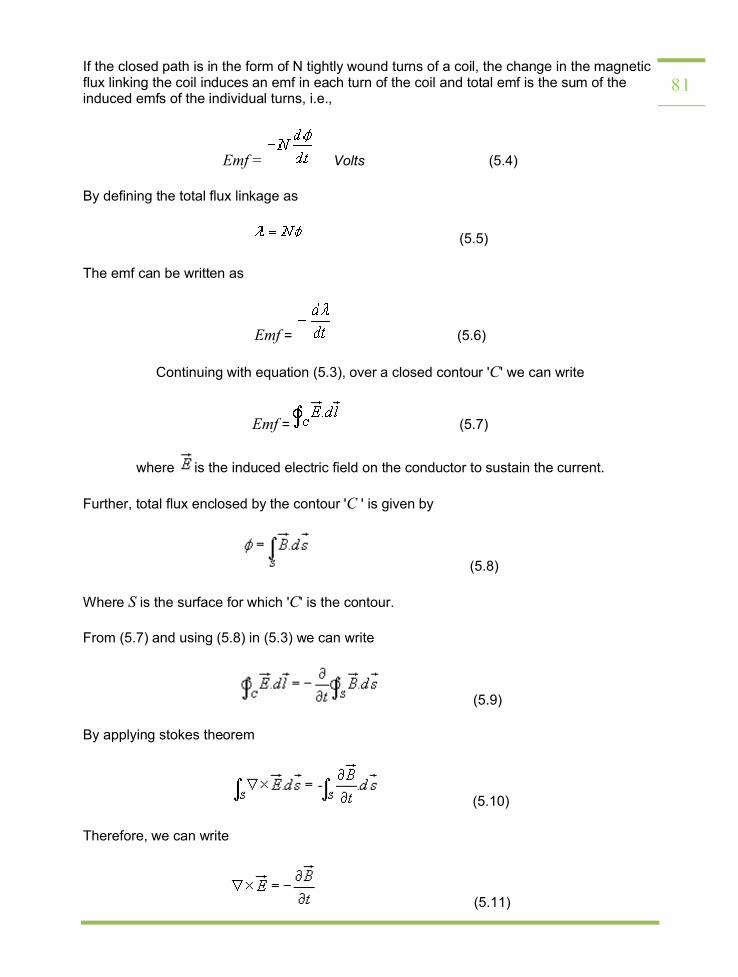
81If the closed path is in the form of N tightly wound turns of a coil, the change in the magnetic flux linking the coil induces an emf in each turn of the coil and total emf is the sum of the induced emfs of the individual turns, i.e.,

Emf = Volts (5.4)

By defining the total flux linkage as

(5.5)

The emf can be written as

Emf = (5.6)

Continuing with equation (5.3), over a closed contour 'C' we can write

Emf = (5.7)

where is the induced electric field on the conductor to sustain the current.

Further, total flux enclosed by the contour 'C ' is given by

(5.8)

Where S is the surface for which 'C' is the contour.

From (5.7) and using (5.8) in (5.3) we can write

(5.9)

By applying stokes theorem

(5.10)

Therefore, we can write

(5.11)

82which is the Faraday's law in the point form

We have said that non zero can be produced in a several ways. One particular case is when a time varying flux linking a stationary closed path induces an emf. The emf induced in a stationary closed path by a time varying magnetic field is called a transformer emf .

Example: Ideal transformer

As shown in figure 5.1, a transformer consists of two or more numbers of coils coupled magnetically through a common core. Let us consider an ideal transformer whose winding has zero resistance, the core having infinite permittivity and magnetic losses are zero.

Fig 5.1: Transformer with secondary open

These assumptions ensure that the magnetization current under no load condition is vanishingly small and can be ignored. Further, all time varying flux produced by the primary winding will follow the magnetic path inside the core and link to the secondary coil without any leakage. If N1 and N2 are the number of turns in the primary and the secondary windings respectively, the induced emfs are

(5.12a)

(5.12b)

(The polarities are marked, hence negative sign is omitted. The induced emf is +ve at the dotted end of the winding.)

(5.13)

83i.e., the ratio of the induced emfs in primary and secondary is equal to the ratio of their turns. Under ideal condition, the induced emf in either winding is equal to their voltage rating.

(5.14)

where 'a' is the transformation ratio. When the secondary winding is connected to a load, the

current flows in the secondary, which produces a flux opposing the original flux. The net flux in the core decreases and induced emf will tend to decrease from the no load value. This causes the primary current to increase to nullify the decrease in the flux and induced emf. The current continues to increase till the flux in the core and the induced emfs are restored to the no load values. Thus the source supplies power to the primary winding and the secondary winding delivers the power to the load. Equating the powers

(5.15)

(5.16)

Further,

(5.17)

i.e., the net magnetomotive force (mmf) needed to excite the transformer is zero under ideal condition.

Motional EMF:

Let us consider a conductor moving in a steady magnetic field as shown in the fig 5.2.

Fig 5.2

If a charge Q moves in a magnetic field , it experiences a force

(5.18)

84This force will cause the electrons in the conductor to drift towards one end and leave the other end positively charged, thus creating a field and charge separation continuous until electric and magnetic forces balance and an equilibrium is reached very quickly, the net force on the moving conductor is zero.

can be interpreted as an induced electric field which is called the motional electric field

(5.19)

If the moving conductor is a part of the closed circuit C, the generated emf around the circuit

is . This emf is called the motional emf.

A classic example of motional emf is given in Additonal Solved Example No.1 .

Maxwell's Equation

Equation (5.1) and (5.2) gives the relationship among the field quantities in the static field. For time varying case, the relationship among the field vectors written as

(5.20a)

(5.20b)

(5.20c)

(5.20d)

In addition, from the principle of conservation of charges we get the equation of continuity

(5.21) The equation 5.20 (a) - (d) must be consistent with equation (5.21).

We observe that

(5.22)

Since is zero for any vector .

Thus applies only for the static case i.e., for the scenario when .