Palestine Polytechnic University

College of Engineering

Mechanical Engineering Department

Graduation Project

Reverse Engineering in Manufacturing

Students:

Abdalrhman Sharabati Oday Al haimoni

Supervisor:

Mr. Majdi Zalloum

Submitted to the College of Engineering

in partial fulfillment of the requirements for the

Bachelor degree in Mechanical Engineering

Hebron – Palestine

2016

II

Dedication (Arabic)

بالنصح ، و فكري يضيء نبراسا في الصغر ، وكانا لي بالتربية إلى من تعهداني

وأبي أمي ، في الكبر التوجيه

حفظهما هللا

، إخوتي ، وأخواتي ، وحفزوني للتقدم إلى من شملوني بالعطف ، وأمدوني بالعون

رعاهم هللا

العلم ، والمعرفة يل تحصيل في سب بيدي إلى كل من علمني حرفا ، وأخذ

المتواضع بحثي جهدي ، ونتاج ثمرة أهدي إليهم جميعا

III

Abstract

Reverse Engineering in terms of mechanical engineering is interested in design, its

processing includes a 3D scanning of the primitive object, then it transfers it into computer aid

design (CAD) model (solid, surfaces…etc.), which involve the measurements and data sensing

with high quality of 3D analysis. These models exploit in analyzing, manufacturing,

modification and optimization, this branch is being applied into a wide field in factory products,

such as automotive industries. By using reverse engineering, we obtain an accurate benefit as

improving product quality, creating a complete overview of competing products, as well as

reducing the time and the cost.

Most of the engineering majors focus on traditional engineering, which is based in the

development and improvement of their products using geometric and abstract concepts by

applying the scientific and mathematical principles to practical ends, such as the design

manufacture, operation of efficient and economical structures, machines, processes, and

systems. On the other hand, reverse engineering aims to create a CAD model by making 3D

scanning of the object, and its partial component to analyze the internal relations of these partial

components.

In order to observe a high accuracy models, the mechanical five dimensional (5D)

machined parts are used for this situation. That helps to know and analyze all details and

constrains of object. By understanding common design practices and manufacturing

knowledge of 5D machining, it can be used to guide the reverse engineering process in order

to achieve the best accuracy models.

Getting a CAD model requires professional packages, which deal with 3D scan data

and create parametric CAD solids with high accuracy, and to minimize the time required.

IV

Geomagic studio is a useful software used in reverse engineering, it provides amount

of features, that associate redesign, Analyze, Seamless Data Transfer and other features

together.

V

المستخلص

بحيث اصبح هذا المجال في مجال الهندسة الميكانيكية ، العكسية في يهدف البحث الى تناول موضوع الهندسة

.هذه االيام ذو نطاق واسع في المصانع والشركات العمالقة بهدف تحسين جودة المنتج ،ودراسة وتحليل منتجات المنافسين

يعتبر مفهوم الهندسة العكسية في الهندسة الميكانيكية وفي مجال التصنيع عبارة عن عملية اعادة انتاج قطع او

بعض التعديالت ، حسب بناء على اجسام ، " ال يشترط ان تكون ميكانيكية "، من نماذج اصلية، حسب شكلها االصلي او

عة من العمليات، الهندسة العكسية في مجال الهندسة من خالل مجمو وتتم عمليةالحالة او الوضع المراد استخدامها فيه،

من ( 3D scannerبحيث تبدأ اول مراحل الهندسة العكسية بعملية المسح للقطعة االصلية باستخدام الماسح ثالثي االبعاد )

مل معها من اجل معالجتها ( التعاcomputer aid designخاللها يتم تحويل القطعة االصلية الى معلومات تسطيع برامج )

" ومن ثم تحويل المعلومات الناتجة الى الماكنات واجراء التعديالت عليها واخراجها بشكلها النهائي "عملية انتاج القالب

.(CNC)االلية المحوسبة

يقوم العمل من خالل هذا المشروع على العمل على مجموعة من برامج التصميم الحاسوبية ، ومن اهم هذه

بحيث انها تقوم بمجموعة من العمليات التي تحسن من ”Geomagic Studio“و ”Geomagic Design X“البرامج

والذي من خالله تتم عملية رسم القالب ”Catia V5“المعلومات القادة من المسح ، باالضافة الى االستعانة في برنامج

الخاص في القطعة .

VI

Table of Content

Abstract .................................................................................................................................... III

V ..................................................................................................................................... المستخلص

Table of Content ...................................................................................................................... VI

List of Figures ........................................................................................................................ VII

List of Tables ........................................................................................................................... IX

Time Table of First Semester .................................................................................................... X

Time Table of Second Semester: .............................................................................................. X

List of equations symbols ........................................................................................................ XI

Chapter One ............................................................................................................................... 1

Introduction ................................................................................................................................ 1

1.1 Goals, Validation Techniques and constrains levels ........................................................ 2

1.2 Reverse Engineering Process ........................................................................................... 3

1.3 Optimization of Geometry ............................................................................................... 3

1.4 Reverse Engineering Software’s ...................................................................................... 5

Chapter Two............................................................................................................................... 7

Background ................................................................................................................................ 7

2.1 Reverse Engineering in factories ..................................................................................... 8

2.2 Geometric Modeling ........................................................................................................ 9

2.3 Data Segmentation and Fitting....................................................................................... 12

2.4 Geometric Constraints ................................................................................................... 13

Chapter Three........................................................................................................................... 16

Reverse Engineering Processes................................................................................................ 16

3.1 Scanning by using 3D scanner ....................................................................................... 17

3.1.1 Types of scanning technologies .................................................................................. 17

3.1.2 Power of 3D scanning data ......................................................................................... 19

3.1.3 Measurement and Inspection ...................................................................................... 21

3.2 Geomagic Studio 2012 ................................................................................................... 23

3.3 Geomagic Design X ....................................................................................................... 33

3.3.1 Introduction ................................................................................................................. 33

3.3.2 Mesh ............................................................................................................................ 34

3.3.3 Region Group .............................................................................................................. 37

3.3.4 Sketching..................................................................................................................... 38

3.3.5 Auto Surfacing ............................................................................................................ 40

VII

Chapter Four ............................................................................................................................ 43

Action Sequence ...................................................................................................................... 43

4.1 Processes of Geomagic Design X for an object: ............................................................ 44

4.1.1 Mesh Buildup Wizard ................................................................................................ 45

4.1.2 Optimize the Meshing data by Mesh mode ................................................................ 46

4.1.3 Appling Region Group:............................................................................................... 50

4.1.4 Auto Surfacing: .......................................................................................................... 51

4.1.5 Export the development object to Catia: ................................................................... 52

4.2 Creating Core Cavity For the object in Catia ............................................................... 53

Chapter Five ............................................................................................................................. 58

Geomagic Algorithms .............................................................................................................. 58

5.1 Bezier curves and surfaces ............................................................................................. 58

5.1.1 Bezier curves ............................................................................................................... 58

5.1.2 Bezier surfaces: ........................................................................................................... 62

5.2 Basic Spline Curves ....................................................................................................... 63

5.3 NURBS .......................................................................................................................... 65

Chapter Six............................................................................................................................... 67

Applications ............................................................................................................................. 67

6.1 Work Samples .............................................................................................................. 68

6.2 Practical Case ................................................................................................................. 74

6.3 Recommendations: ......................................................................................................... 78

References ................................................................................................................................ 79

List of Figures

Figure 1.1: Reverse engineering process ....................................................................... 4

Figure 2.1: Point Cloud from real shape ...................................................................... 10

Figure 2.2: Mesh for Complex Shape .......................................................................... 11

Figure 3.1: single point laser ........................................................................................ 18

Figure 3.2: laser Profile................................................................................................ 18

Figure 3.3: Snapshot devices ....................................................................................... 19

Figure 3.4: 3D scan data by resolution ........................................................................ 19

Figure 3.5: 3D scan data .............................................................................................. 21

VIII

Figure 3.6: Multi Stripe Laser Triangulation (MLT) ................................................... 22

Figure 3.7: Home page of Geomagic Studio 2012 ...................................................... 25

Figure 3.8: Point Cloud object ..................................................................................... 25

Figure 3.9: Polygon Phase object................................................................................. 26

Figure 3.10: CAD Phase object ................................................................................... 26

Figure 3.11: stages in Geomagic Studio ...................................................................... 27

Figure 3.12: Point Phase data sample .......................................................................... 28

Figure 3.13: Points to Polygonal Phase ....................................................................... 29

Figure 3.14: Manual Registration ................................................................................ 29

Figure 3.15: Before register two Bobs ......................................................................... 30

Figure 3.16: Registered of two Bobs as a single .......................................................... 30

Figure 3.17: Edition for contours by use Draw operation ........................................... 32

Figure 3.18: Parametric Exchange icon ....................................................................... 32

Figure 3.19:point to mesh sample ................................................................................ 34

Figure 3.20: healing wizard detection .......................................................................... 35

Figure 3.21: Edit boundaries ........................................................................................ 36

Figure 3.22: Fill Hole ................................................................................................... 36

Figure 3.23: Merge in Geomagic Design X ................................................................. 37

Figure 3.24: Split in Geomagic Design X .................................................................... 38

Figure 3.25 Mesh sketch .............................................................................................. 38

Figure 3.26: 3D Mesh Sketch ...................................................................................... 39

Figure 3.27: Auto Surfacing ........................................................................................ 40

Figure 3.28 Creates lofted bodies with a set of sketches ............................................. 41

Figure 3.29 : Lofts bodies using a set of sketches ....................................................... 42

Figure 4.1: import. xrl/stp file ...................................................................................... 44

Figure 4.2: men’s shoe sole ......................................................................................... 46

Figure 4.3: sole of elegant shoe ................................................................................... 47

Figure 4.4: before and after Applying Smooth Command .......................................... 48

Figure 4.5: After applying Global mesh ...................................................................... 49

Figure 4.6: Final Shape of optimizing Mesh phase ..................................................... 50

Figure 4.7: Region Group ............................................................................................ 51

Figure 4.8: Auto Surfacing in Evenly Following Network.......................................... 51

Figure 4.9: steps in Geomagic to Export an object ...................................................... 52

Figure 4.10 Core and Cavity tool icon ......................................................................... 53

Figure 4.11: prepare a pair of sole ............................................................................... 54

Figure 4.12: Pulling Direction ..................................................................................... 54

Figure 4.13: Core-Cavity and Pulling Direction box view. ......................................... 55

IX

Figure 4.14: Processes in Geomagic Design X ............................................................ 56

Figure 5.1: Quadratic Bezier Curve ............................................................................. 59

Figure 5.2: 2D Bezier curve ......................................................................................... 60

Figure 5.3: 3D Bezier curve ......................................................................................... 60

Figure5.4: Control point............................................................................................... 61

Figure 5.5: original cubic curve ................................................................................... 62

Figure 5.6: Bezier surface sample ................................................................................ 63

Figure 6.1 mold of shoe after scanning ........................................................................ 69

Figure 6.2: The mold of shoe in Mesh phase ............................................................... 69

Figure 6.3: The mold of shoe in Auto Surface phase .................................................. 70

Figure 6.4: mold of shoe after scanning....................................................................... 70

Figure 6.5: mold after optimizing mesh ....................................................................... 71

Figure 5.6: Auto Surface .............................................................................................. 71

Figure 5.7: Extract the mold ........................................................................................ 72

Figure 6.8: two sport sole shoe after scanning ............................................................. 72

Figure 6.9: two sport sole shoe final shape in mesh mode. ......................................... 73

Figure 6.10: Auto Surface phase for two models sport sole shoe. ............................... 73

Figure 6.11: original mesh phase ................................................................................. 74

Figure 6.12: solid part from mesh sketch ..................................................................... 74

Figure 6.14: Plastic Chair on Geomagic ...................................................................... 75

Figure 6.15: Problems detection in chair by healing wizard ....................................... 76

Figure 6.16: bolts at the backrest of chair .................................................................... 77

Figure 6.17: bolts removed and built new surfaces ..................................................... 78

List of Tables

Table 3.1: Main tools in Edit Contours ........................................................................ 31

Table 4.1: tools in mesh phase ..................................................................................... 46

X

Time Table of First Semester

Time Table of Second Semester:

February March April

Action

Week 1 2 3 4 1 2 3 4 1 2 3 4

Searching about Reverse Engineering

Collecting information from some references

Writing Chapter one and two

learning on Geomagic Design X and Studio Applying Scanning Samples on Geomagic Design X

and Studio

Complete Other Chapters

September October November December

Action Week

1 2 3 4 1 2 3 4 1 2 3 4 1 2

Making a scanning for some parts

Preparing the Scanning data by Geomagic & Catia in a required shape

Studying the Problem Cases in local factories

Editing and Finishing all Chapters

XI

List of equations symbols

Symbol Meaning

C(t) NURBS equation

Wi the weights

E Error function.

wr is a vector of weights

r number of data elements

p data vector

Z the model

𝐵𝑖𝑛(𝑢) and 𝐵𝑗

𝑚(𝑣) represent the Bernstein polynomials of degrees m and n

u and v the variables of equation

𝑄𝑖 new control points

Pi Control Points

t Knot vector

Ni, k(t) B-spline basis functions

1 Chapter One

Introduction

2

Reverse Engineering can be defined as the process of analyzing a physical object

to identify and find the relationship between the particles and components of it, and create

representations of the object in another form or at a higher quality. Also, they can say that

it is the process of duplicating an existing component by capturing the physical dimensions’

components.

1.1 Goals, Validation Techniques and constrains levels

The primary goal of reverse engineering is to create high precision models from the

object that reflect to geometry, and the intended design behind the geometry. The

knowledge of geometric and parametric constraints is not sufficient to optimize the

algorithms. Reverse engineering expresses the issue of constrained optimization that

produces more accurate models than the knowledge of geometric and parametric

constraints.

The original models are available for comparison with the reverse engineered models

through successful and powerful developed techniques that will be discussed. They will

overcome the error measurements of the original design that is given for a variety of parts.

The accuracy in Modeling depends on the properties of sensor that scans the geometry

and relative error of this sensor. There are three levels of constraints that are useful in

creating the model, they are:

1) Specific primitives narrow the possible shape of the reconstructed model from

arbitrary geometry down to a well-defined set of design and manufacturing

3

2) Specific domain pragmatics attempt to capture specific geometric conditions and

conformities that are likely to be found based on how a part is designed and

manufactured.

3) Functional constraints describe interaction among the features of the object.

1.2 Reverse Engineering Process

The following figure 1.1, shows the data that are getting by 3D scanner, used fast

blue light 3D scanning technology in order to capture information that describes all

geometric features of the object such as line, holes, pockets…, producing clouds of points.

These points describe the common geometry of part, and define the surface geometry, then

they set the original of geometric primitives. By this original mode, the ability for analyzing

to produce amount of constraints on the geometry assist in designing base and optimization.

1.3 Optimization of Geometry

Optimization method can be interpreted as a process to minimize some undesirable

criteria, it is divided into two cases, constraint and unconstraint optimization.

In the unconstraint case, the optimization occurs just on geometric dimensions

between algorithms and sense data points, while in the constrained case, the hypothesized

model is created using a limited set of appropriate geometric forms that are then optimized

based on the data. It’s very important to know geometric constraint because it helps us to

prevent the sense data, which leads us to the primitive object.

4

To achieve good optimization, the constraint and the model should be displayed

mathematically. By using the degree of freedom (DOF) which purpose is to reduce the

dimensions of the model to be redefined using fewer variables, it is possible to define error

metrics for the sensed data, and for the violation of constraints

Figure 1.1: Reverse engineering process

5

1.4 Reverse Engineering Software’s

During the past decades, there was a significant change in the processes of design

by dropping the traditional design a sculpt on clay in automotive factories and tend to

computer-aided design packages because it’s flexible and easy, provides the designer

variant features and tool, which allow the possibility of creating a 3D virtual model from

the primitive model with high resolution. Also, it makes the cost less expensive for models

that are used for immediate replacement and additional spares to for a longer period.

The reverse engineering process requires software that reconstructs the object as a

3D model. At the beginning, the physical object can be measured using 3D scanning

technologies, like a coordinate measuring machine, laser scanner, structured light digitizer

or computed tomography, then a high-performance program requires to deal with 3D

scanning, and that will be by using a unique software’s as Geomagic packages.

Geomagic package “first series were released in nineteen ninety-seven” is a

professional computer-aid, which substitutes the requirements of processing and geometric

modeling. Selection of geomagic product depends on the features of this application

according to the intended work. The main programs that will use reengineering process

are:

1. Geomagic Capture is a product of 3D scanning is using it for transforming the 3D

physical object by using scanner for an accurate CAD model, this scanner delivers

accurate and fast blue light 3D scanning technology.

2. Geomagic Design X is one of Scanning Software, which has a feature that doesn’t

exist in others, it owns a combination of an automatic and a guided 3D model

6

extraction, it converts 3D scan data into high-quality feature-based and more

accurate CAD models, also it creates a custom component that integrates perfectly

with existing products and requires a perfect fit.

3. Geomagic Studio it’s also an integrated program that transforms the 3D scanned

data into highly accurate surface and 3D CAD model, in general it has a

professional characteristic that can edit point cloud, making mesh analysis, also it

has tools that can interstate the internal structure of any object, which help to create

a high quality of 3D models, and Optimize for fast data processing.

Through this project, the practice will be on Geomagic Design X and Studio due to

the fact that both programs own, in addition to other software as Solidworks and Catia,

which assist those programs in order to make a modification and finishers to final output.

7

2 Chapter Two

Background

8

2.1 Reverse Engineering in factories

The main purpose of reverse engineering in manufacturing is repeating the original

object, which exploit whether in the modifying after the initial design stage or in

maintenance process (as a spare parts), this process has found use in computer aid designs

and animation.

Raband et al. [2] identifies the results of a reverse engineering operation as

producing a type three drawing set and a set of intelligent CAD models of the components.

Further, they define the reverse engineering preprocess as:

1. Collecting all available information and documentations, including nonproprietary

drawings, functional requirements, tooling requirements, processing and material

requirements, etc.

2. Identifying new data elements required for a complete technical data package.

3. Performing a cost/benefit analysis.

4. Contacting the cognizant engineer.

5. Establishing a reverse engineering management plan.

6. Establishing acceptance criteria.

When these considerations have been applied, the processes of reverse engineering

must be precisely and clear. The stage of collecting information and documentation

indicates to scan the object, that is often simply includes a set of 3D geometric points

9

associated with the surface of the object. Broacha and Young [3]. They discuss the

important points that should be provided in any reverse engineering system.

1. These include an ability to collect data.

2. A geometrical foundation of surface modeling which depends on the data.

3. Comprehensive functionality for displaying and manipulating point data.

4. The actual process for reverse engineering or surfacing.

These established reverse engineering systems should be flexible and easy to those

who are interested in this matter.

2.2 Geometric Modeling

The term modeling refers to the aspects and dimensions of an object, it’s also called

a geometric model, in the manufacturing fields it is called a blueprint or engineering

drawing, the model should specify geometric information as well as assembly material and

tolerance, it is sufficient for manufacturing engineer to translate the model (drawing) into

a manufacturing plan.

In order to make this models more accurate, it should follow these characteristics

as gathering of expert’s judgment:

Parameter Estimation: When modeling has a known curve, it is often necessary to

Instantiate the parameters of that curve.

10

Functional Representation: Functions give us values over the entire range of the data, as

well as provide derivative information.

Data Smoothing: taking the sense data of the object may include some errors, so it’s not

sufficient to describe the object exactly, and that leads to make approximation for sense

data.

Data Reduction: a set of parameters for the data will make it smaller than the Original

data set, and that will reduce the volume of storage, and manipulation, with the broad

development of the technology, it’s easy to design an accurate model by exploiting a

computer design programs. This stage depends on the ability of these programs to

manipulate the data of model, in order to create a high quality of those models, which the

construction process is similar to the original drafting process. This will lead to define a

CAD system, which seems exactly as the engineer designs part.

Point clouds: are collections of 3D geometric points that are associated with the

surface of an object. They describe the physical appearance of the shape, also they

are using as the input to various data fitting algorithms, it’s just available for coarse

shape of a part, but they are onerous and lack precise geometric information to

describe all accurately.

Figure 2.1: Point Cloud from real shape

11

Polygonal meshes: they are one form of model that can easily be constructed from

actual data. This meshes are a surface that is constructed out of a set of polygons

that are joined together by common edge.

All these features aim to represent CAD model, in order to transfer this

model form design to manufacturing by a specified of operations, based on common

mechanical features, to describe the object.

Figure 2.2: Mesh for Complex Shape

Polygon mesh use some methods for construction the object, one of these

methods called box modeling, which has two simple tools, they are the subdivide

tool splits faces and edges into smaller pieces by adding new vertices.

The extrude tool is applied to a face or a group of faces. It creates a new

face of the same size and shape which is connected to each of the existing edges by

a face. Thus, performing the extrude operation on a square face would create a cube

connected to the surface at the location of the face.

12

Other method of polygonal mesh is called extrusion modeling, this method

is use for faces and heads, during which a 2D shape traces the boundary of the

drawing drawing and then use a different angle and extrudes the 2D into 3D.

2.3 Data Segmentation and Fitting

The goal of data segmentation is to associate data points with the hypothesized

feature they represent. Proper classification of data points into their associated features is

necessary before fitting can begin. This process starts from the vision community during it

the vision image is partitioning on the main benefit. There are two primary methods exist

for segmentation of a range image, first is the edge based. It’s a method use discontinuities

to encircle a region that is then considered classified. The second is the region based

segmentation, it’s a method try to classify points based on local properties, such as intensity

value, orientation, or curvature. [4]

3D point cloud segmentation is the process of classifying point clouds into multiple

homogeneous regions, the points in the same region will have the same properties. [5]

3D segmentation of clouds depends on the two approaches, which are the bottom-

up segmentation, and top-down segmentation. Recently the work suggests to work top-

down segmentation because the bottom-up segmentation lines, planes, and arcs, are

identified and then combined into shapes such as pockets or outlines. This technique can

fail when the data is extremely noisy, or when the surface does not conform to standard

assumptions of smoothness and local uniformity.

Data fitting techniques in general include approximation and interpolation. In the

simplest case, interpolation techniques fit functions directly through the measured data

points. Approximation techniques fit functions in the neighborhood of the data points,

13

attempting to minimize some error function. Interpolation is often used in the design

process where the designer represents a shape, such as the profile of the part, by several

points and asks the computer to connect them via primitives such as arcs, lines, or splines

[1].

Lots of CAD programs provided with spline based model [4], that is because splines

supply a mathematically, a good representation for 3D curves and surfaces that which has

a superb feature such as smoothness constraints and data reduction. Splines can also be

broken up into local sections to model more complex geometry. These local sections can

be modified without affecting any other part of the surface. Unfortunately, splines are a

generic approximation of a surface they can undulate through the noise reducing the error

to the data, so splines can actually over fit the data. This can produce a curved surface

where a lower DOF surface, such as a line or arc, is more appropriate.

2.4 Geometric Constraints

Geometric constraints describe the physical representation of the geometry, in order

to create a mathematical model, describe the features of the object.

Many strategies have been tried, beginning as early as the 1960s with Sutherland's

Sketchpad program. Hsu's dissertation [6] attempts to address the idea of geometric

constraint solving in the design process. He lists several criteria for an ideal constraint. He

lists several criteria for an ideal constraint solver:

1. Reliability - Derive all possible solutions (if required).

2. Predictability - Do not jump erratically through the solution space and should provide

a way for a human to control the results.

14

3. Efficiency - Allow interactive response times.

4. Robustness - Handle over and under-constrained problems.

5. Generality - Handle a wide variety of constraint types and not be restricted to any

Specific dimensions.

Couching these requirements in terms of a computer aided reverse engineering

system gives:

1. Reliability - The algorithm should derive a model that is consistent with the data given

it and its knowledge of the design and manufacturing processes.

2. Predictability - The algorithm should come up with the simplest accurate solution. An

interactive user should be able to guide the process.

3. Efficiency - The algorithm should run at interactive speeds.

4. Robustness - The algorithm should be able to handle over and under-constrained

hypothesized features.

5. Generality - The algorithm should be able to handle a wide variety of parts and inter-

related constraints and not be restricted to any specific dimensions.

Through these assumption, Hsu defines four methods developed to address the

constraint-solving problem. These include propagation methods that is the process of

representing the geometrical constraints in the form of an acyclic graph. Numerical

methods, that described previously in relation to data fitting, and geometry is represented

as algebraic formulas and constraints are created by relating variables across equations.

Constructive methods unfortunately, these techniques are sometimes unpredictable and can

have difficulties converging, so there are some newer methods of constraint solving which

15

applies to problems solvable by ruler-and-compass construction is known as the

constructive approach.

In the rule-based approach, geometric constraints are represented symbolically.

Rewrite rules are utilized to simplify geometry and reduce DOFs. Unfortunately, rule-

based systems tend to be slow. [1] Graph-based approaches consist of two steps. One, a

top-down phase is entered where the graph is analyzed and a sequence of constructive steps

is derived. Two, a bottom-up phase occurs where the construction steps are carried out and

the model is constructed.

The final method that Hsu addressed is algebraic methods, which the geometric

constraints are written as algebraic formulas, which are then combined and reduced using

elimination methods. This method tends to be extremely slow and often have exponential

complexity.

16

3 Chapter Three

Reverse Engineering Processes

17

3.1 Scanning by using 3D scanner

3D scanning is getting popular in various fields, and its usage for different purpose,

this means that there are a different kinds objects, simple or complex can collect the data

of them, and many details to understand.

Collecting data about object in two-way hand held and modern scanning.

Traditional scanning or manually driven sensors such as calipers and micrometers. These

devices fall within the paradigm of touch sensing, requiring some sort of probe to

physically contact the surface of the part, within using a modern sensing tools, other is

modern scanning within use 3D laser scanners.

3D laser scanners are a technology that digitally captures the shape of physical

objects using a line of laser light. 3D laser scanners create “point clouds” of data from the

surface of an object. In other words, 3D laser scanning is a way to capture a physical

object’s exact size and shape into the computer world as a digital 3D representation, with

high resolution and minimum error data.

3.1.1 Types of scanning technologies

In these days, there are many types of 3D scanning technologies on the market today.

The most commonly used technologies fall into three categories: Displacement. Profile,

and Snapshot (aka, Scanner).

Displacement devices use a single point laser beam projection as in figure 3.1 to

measure the height, thickness, or position of a project.

18

Figure 3.1: single point laser

Line Profile devices typically use a projected laser line to create a cross action

profile for measuring aspects of an object’s contour. Moving an object under the

laser line creates many profiles that can be combined into a complete 3D shape.

Figure 3.2 describe the process of type.

Figure 3.2: laser Profile

Snapshot devices as in figure 3.3, use structured light (non-laser) and stereo-vision

to generate full 3D volume data. Because Snapshot technology captures so much

3D data at one time, objects need to remain stationary during the scanning process.

19

Figure 3.3: Snapshot devices

3.1.2 Power of 3D scanning data

A 3D scanner is a device that captures a real object or environment as 3D shape data.

The collected 3D information is converted into digital data commonly called 3D scan data

or scan data. 3D scan data is a set of points. A point represents a location on a real object

and contains the X, Y, and Z coordinates. Numerous points can be used to describe a real

object. For example, a digital photo with a high-resolution pixel count can represent the

detailed shape of a real object.

Figure 3.4: 3D scan data by resolution

20

A point set, also known as a point cloud, can be converted into an informative

digital model with software operations and used in various industrial fields. 3D scan

data has the following strengths [11]:

Quickly create digital versions of real objects

Accuracy

Capture complex freeform surfaces

Capture small to large scale objects (depending on 3D scanner)

Obtain color information (depending on 3D scanner)

Simulate environments and situations

Change to different scales and measurements easily

Easily extract length, height, width, volume and position data

Extract sectional information

Compatibility in a general PC environment

21

Figure 3.5: 3D scan data

Since 3D scan data can represent a real object with high accuracy, it is used for

various purposes. The use of scan data is also increasingly expanding to custom markets

as scan technology becomes easier to use and more intuitive. Currently, 3D scan data is

used primarily for the various purposes, the following is discoursing two types of them:

3.1.3 Measurement and Inspection

3D scan data is increasingly used for metrology or inspection. The more accurate

points that are used to measure a feature will increase the credibility of an inspection. The

scan data of a manufactured part can be aligned with its CAD model (nominal data), and

subsequently compared to check for differences and whether or not they pass/fail within

set tolerances.

22

3.1.4 Ultra HD 3D scanner

This is one of scanners, which has a superb feature such as:

The dimensional accuracy of this it is about ±100 micron in micro mode and ±300

micron in wide mode.

The process speed about 50 thousand points per second.

Twin 5 megapixel CMOS image sensor.

Scans can be output as STL, OBJ, VRML, XYZ, and PLY files, which is available

with geomagic back ages.

This type use Multi Stripe Laser Triangulation (MLT) Technology, this technology is

relatively cheaper than others, so it can be available for schools, universities and some

people interested with reverse engineering, in figure 3.6 shows the components of this

scanners

Figure 3.6: Multi Stripe Laser Triangulation (MLT)

23

3.2 Geomagic Studio 2012

Geomagic Studio is an intelligent program for engineering design, that can create

or transforming 3d scan of physical part into highly accurate polygon and native CAD

models for reverse engineering, product design, rapid prototyping and analysis. It’s the first

reverse engineering software that directly integrates with all leading mechanical CAD

packages.

3.2.1 Benefits of Geomagic Studio

Immediately and rapidly create high quality 3d data from almost any source.

Increase productivity in design, manufacturing and repair workflows by quickly

and accurately testing and redesigning existing parts and objects in 3D.

It can Access the fastest path to cad from point and polygon data.

Optimize work time by using the fastest path to CAD from point and polygon data.

Access the industry best tools for reverse engineering.

Deliver and Design Revolutionary New Products and Treatments

Deliver results immediately.

Leverage the physical objects you already have into digital assets. [16]

24

As any engineering software, Geomagic Studio has a unique feature that make it

distinct from others. It’s Available in 9 languages. It’s automated and flexible, it can deliver

the best experience and the highest quality 3D data from scan data Integrates accurate, its

deal CATIA, Autodesk Inventor, SolidWorks and Cero Elements/Pro parametric CAD

systems, by export a suitable file with these programs for mediate use in design and editing.

It can export 3D data in all major neutral polygonal and NURBS in high quality formats

for immediate downstream use Comprehensive support, technical help, training, and free

trials of the Geomagic products.

In the newest available version of Geomagic Studio 2012, it has Top New Features such

as [16]:

Self-evident for new Sketch function allows direct creation and editing of cross-

section curves from both point clouds and polygon models.

Powerful scripting environment extends, customizes and automates functions with

deep access into selected commands in the software.

Improved editing, navigation and visualization of point clouds from mid- and long-

range scanners for scene level 3D models.

Remeshing tool enables fast, accurate triangulation of polygon models for cleaner,

more usable 3Dmodels for Digital Content Creation (DCC) and 3D printing.

New ‘Patch’ command delivers superior power for quickly and accurately repairing

polygon models

3.2.2 Basics on Geomagic Studio

In this image, there is the background of the program when it starts, through this

window we can import the scanning data to start on start on editing and optimizing, that’s

by click on Geomagic icon on the top left of the screen and click on import.

25

When the Geomagic Studio import 3D scanning data, it’s always exists in one of

several, and this phases are:

• Point Phase: the state of an object when it is a collection of scanned points, which

discarding the scanner detected blunder, and its more millions of points.

Figure 3.8: Point Cloud object

Figure 3.7: Home page of Geomagic Studio 2012

26

• Polygon Phase: the state of an object when its appearance is approximated by

drawing a triangular surface between every three data points, this phase will be by make

surface mesh generation.

Figure 3.9: Polygon Phase object

• Surface Phase (either Exact Surfaces Phase or Parametric Surfaces Phase): the state

of an object when a reproducible surface is being applied over its underlying polygon

mesh.

• CAD Phase: the state of an object when it is ready to be exported to a CAD package.

The figure 3.11 , shows the processes stages of the object in program, and the sub

tools for each process, and its output.

Figure 3.10: CAD Phase object

27

Figure 3.11: stages in Geomagic Studio

28

3.2.3 Restoration of intended design

It means that all surfaces are arrangement and replace with a perfect geometric

CAD face. For example, cone-like surfaces are replaced with perfectly conical CAD

faces.

This procedure begin by take the 3D scanning data, which is in Point Phase, making

cleaning of additional points and then transfer the Point Phase to the polygon phase this

process called warped to form of polygon object, in the sample data follow, this shape

in Point Phase which contain 132460 points, also in this sample, there is a red points,

these points are additional data due to noise that the sensor phased, this data should

clean them, highlight them by using the lasso Selection Tool ,also these points can be

clean in Polygonal Phase.

To convert the Points to Polygonal Phase, by using Warp icon in Points bar, as

shown in follow, the color indicates that the object converted from Point Phase to

Polygonal Phase

Figure 3.12: Point Phase data sample

29

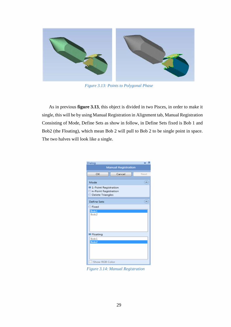
Figure 3.13: Points to Polygonal Phase

As in previous figure 3.13, this object is divided in two Pisces, in order to make it

single, this will be by using Manual Registration in Alignment tab, Manual Registration

Consisting of Mode, Define Sets as show in follow, in Define Sets fixed is Bob 1 and

Bob2 (the Floating), which mean Bob 2 will pull to Bob 2 to be single point in space.

The two halves will look like a single.

Figure 3.14: Manual Registration

30

To complete the register of the object, first these objects should be in similar

orientations. As click a point on the fixed object, click a point on the Floating object

that lies at the same position as the one clicked on the fixed object. If there are more

points in two objects, that will be more accurate.

Figure 3.15: Before register two Bobs

Then press on OK, it will be as a single object as in figure 3.16

Figure 3.16: Registered of two Bobs as a single

3.2.4 Exact Surfaces Phase

In this stage, the process will be in two choices, the first choice by using Exact

Emphasis on Curved Regions, this will be by detect contours and edit them, then fill

empty panels by use the shuffle Panels tools, then using Construct Grids in order to

31

adapt the resolution of grids and final apply the Construct Grids on object to export it

a convert it as a CAD Phase.

Second process is called Exact Surfaces Phase with Legacy Workflow, it’s better

than the Exact Emphasis on Curved Regions, it has the same procedure, but different

is using Shuffle Curvature Lines rather than editing contours, which achieve an optimal

set of lines are to outline the curve.

Edit Contours

Edit contours is one of an intelligent command in geomagic studio, during which

can edit the boundary in order to optimize the geometry of the object, also it help to

detect and segment the surfaces of the object. Contour Edit command has

subcommands that can use for various processes. Table 3-1 show these tools and its

function [17].

Table 3.1: Main tools in Edit Contours.

Icon Discerption

Draw operation tool use to drag the subdivision points (if

needed) to the center of the rounded areas.

To change the contour lines to extendable (yellow) contours, to

estimate curved regions, locations of curved regions need to be

converted into actual locations of curved regions.

32

Figure 3.17: Edition for contours by use Draw operation

3.2.5 Parametric Exchange

Parametric Exchange one of important tools of Geomagic Studio during which

offers an intelligent connection between Geomagic Studio and a compatible CAD

package such as Solid works and Catia, it can transfer the Parametric surfaces to a CAD

system, and to transfer the reverse-engineered CAD object back to Geomagic Studio in

order to proving the reverse-engineered part to the o reginal polygon object. Figure

3.18 show the icon of Parametric Exchange in program [17].

Figure 3.18: Parametric Exchange icon

33

3.3 Geomagic Design X

3.3.1 Introduction

Geomagic Design X, the industry's most comprehensive reverse engineering software,

combines history-based CAD with 3D scan data processing so the creating feature-based,

editable solid models compatible with your existing CAD software, through the experiment

of Geomagic design X, there are unique features that this program owned, such as [11].

Powerful and Flexible

Geomagic Design X is purpose-built for converting 3D scan data into high-quality

feature-based CAD models. It does what no other software can with its combination of

automatic and guided solid model extraction, incredibly accurate exact surface fitting to

organic 3D scans, mesh editing and point cloud processing. Now, you can scan virtually

anything and create manufacturing-ready designs [11].

Do the Impossible

Create products that cannot be designed without reverse engineering, customized parts

that require a perfect fit with the human body. Create components that integrate perfectly

with existing products. Recreate complex geometry that cannot be measured any other way

[11].

34

Geomagic Design X workflows

Geomagic Design X, the ultimate in 3D scan to CAD reverse engineering software,

delivers multiple options for 3D model creation including Live Transfer to all major

MCAD platforms, CAD and NURBS surface model creation and tessellated models [11].

3.3.2 Mesh

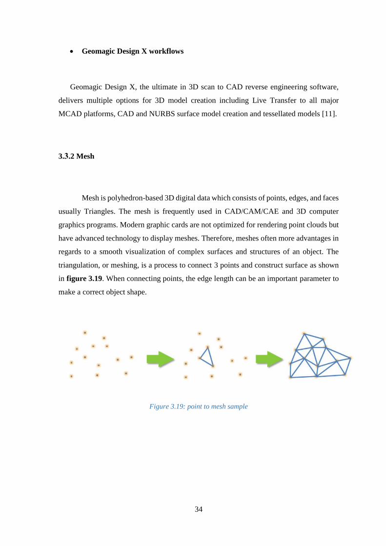
Mesh is polyhedron-based 3D digital data which consists of points, edges, and faces

usually Triangles. The mesh is frequently used in CAD/CAM/CAE and 3D computer

graphics programs. Modern graphic cards are not optimized for rendering point clouds but

have advanced technology to display meshes. Therefore, meshes often more advantages in

regards to a smooth visualization of complex surfaces and structures of an object. The

triangulation, or meshing, is a process to connect 3 points and construct surface as shown

in figure 3.19. When connecting points, the edge length can be an important parameter to

make a correct object shape.

Figure 3.19: point to mesh sample

35

The healing wizard

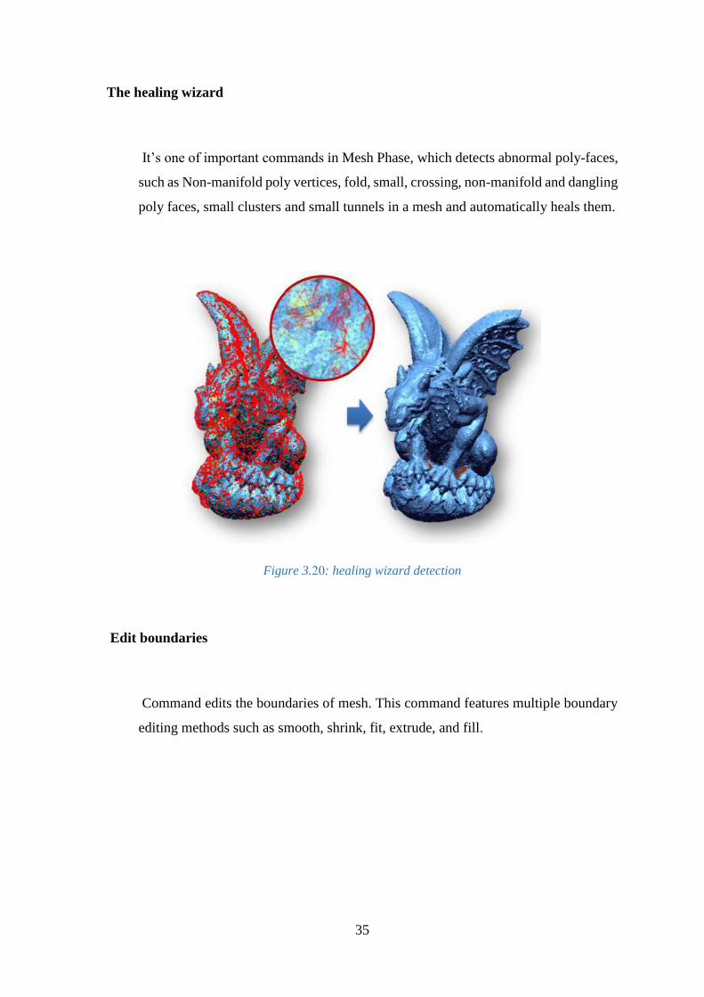
It’s one of important commands in Mesh Phase, which detects abnormal poly-faces,

such as Non-manifold poly vertices, fold, small, crossing, non-manifold and dangling

poly faces, small clusters and small tunnels in a mesh and automatically heals them.

Figure 3.20: healing wizard detection

Edit boundaries

Command edits the boundaries of mesh. This command features multiple boundary

editing methods such as smooth, shrink, fit, extrude, and fill.

36

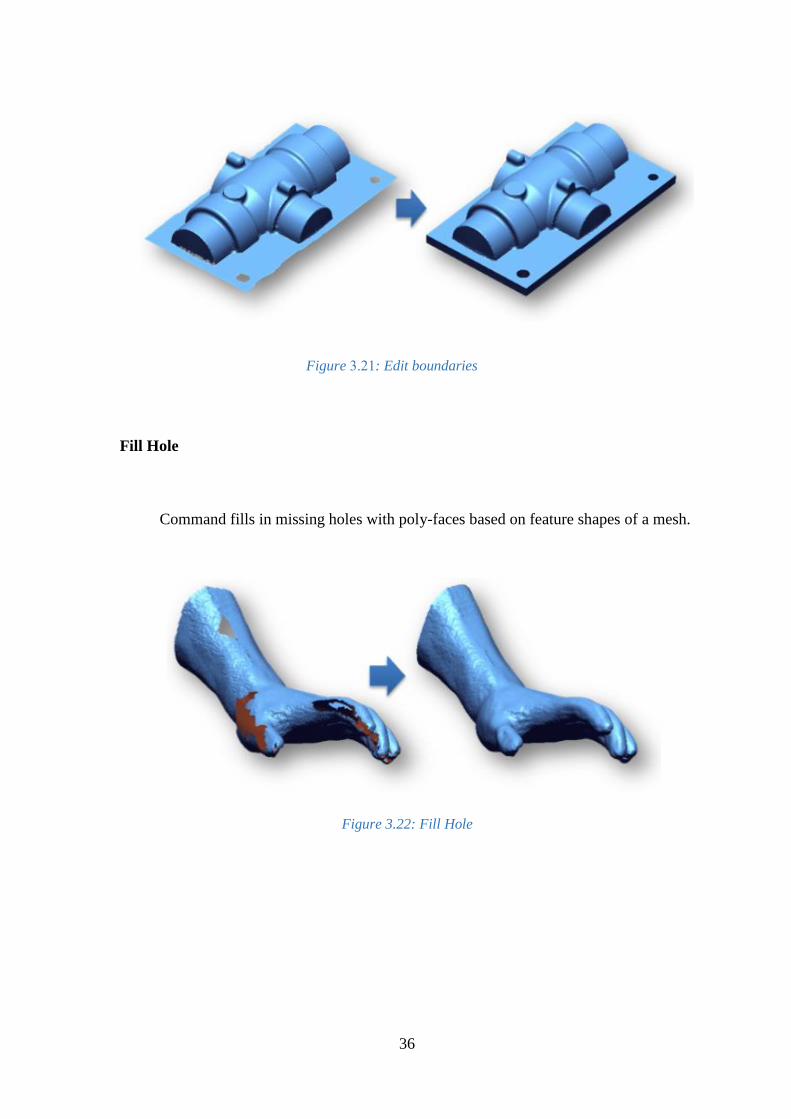
Fill Hole

Command fills in missing holes with poly-faces based on feature shapes of a mesh.

Figure 3.22: Fill Hole

Figure 3.21: Edit boundaries

37

3.3.3 Region Group

Region Group classifies areas of mesh based on geometry features. The Region Group

mode automatically or manually classify.

Auto Segment

The Auto Segment command automatically classifies feature regions by recognizing

3D features.

Merge

The Merge command merges multiple feature regions into a single feature region.

Split

Figure 3.23: Merge in Geomagic Design X

38

The Split command divides a feature region into multiple parts. Figure 3.24

describe this stage, notice that the color indicated to split command.

After aligning using one of this to convert the 3D point part to 2D sketch

3.3.4 Sketching

Mesh sketch

This mode extracts sectional polylines or silhouette polylines based on a mesh or a

Point cloud as well as the creation of 2D geometries such as lines, circles, arcs, rectangles

Figure 3.24: Split in Geomagic Design X

Figure 3.25 Mesh sketch

39

based on Extracted polylines. Constraints on sketch entities can be applied to generate a

fully parametric model. The Mesh

Sketch mode extracts correct and accurate design intent from scan data.

Sketch

The Sketch mode creates 2D geometries such as lines, arcs, and splines, and can

edit created 2D geometries.

3D Mesh Sketch

3D Mesh Sketch creates splines on a mesh using various commands. This splines

can be edit by using tools such as the Trim, Offset, and Project commands.

3D Sketch

Figure 3.26: 3D Mesh Sketch

40

3D Sketch mode creates 3D geometries such as splines, sections and boundaries on a mesh.

That help to make curves can be edited by using the Trim, Offset, and Project commands.

3.3.5 Auto Surfacing

Auto Surfacing is used in the Modeling phase and is an innovative and automatic tool for

fitting surface patches onto a mesh and creating a surface body.

Solid

The Insert Solid menu features various commands used to generate and edit solid

bodies and surfaces.

Figure 3.27: Auto Surfacing

41

Generating Solid Bodies from Sketches

• Extrude

Creates extruded bodies with a sketch, direction and length

• Revolve

Creates revolved bodies with a sketch, axis and revolution angle

• Sweep

Creates swept bodies with a sketch and path

• Loft

Surface

The Insert Surface menu features various commands used to generate and edit

surfaces.

Generating Surface Bodies from Sketches

• Extrude

Extrudes bodies using a sketch, direction and length

• Revolve

Figure 3.28 Creates lofted bodies with a set of sketches

42

Revolves bodies using a sketch, axis and revolution angle

• Sweep

Sweeps bodies using a sketch and path

• Loft

The object sections are expressed by a single profile or multiple profiles on a 2D

or 3D sketch and can be drawn by circles, splines, lines and arc sketch entities.

.

Figure 3.29: Lofts bodies using a set of sketches

43

4 Chapter Four

Action Sequence

44

4.1 Processes of Geomagic Design X for an object:

The processes in Geomagic Design X depends in general on the

structure of the object, some objects can easy make an auto surface for it,

others need mesh sketch or 3D mesh sketch, in figure 4.14 shows in general

the processes of the program, but in this chapter, will discuss the Auto Surface

because more useful than others.

For Auto surface for example, this process is starting after obtaining a scanning

data of sample, first step starts by import the scanning file data as in figure 4.1, usually the

type of this files is “. xrl or stp “, also these files are in mesh data, figure 4.2 shows the

basic sample data that this project works on it.

Figure 4.1: import. xrl/stp file

At the beginning the import file has some disturbances that in the sample and around

it, that is because some noises that effect on the original object through the scanning process

and it acts on the sensors of scanner, so first step is removing this disturbance.

45

4.1.1 Mesh Buildup Wizard

After import the scanning data, this is the first step for optimizing this phase,

through this command can wizard style interface for creating defect-free, also it help

when the 3D scan data files that have not been aligned This tool consists of 5 stages.

Each stage can be executed in just few clicks, enabling the speedy creation of optimal

mesh for use in the final reverse design stages. The 5 stages are [11]:

• Data Preparation stage: Analyzes the state of scan data and defining the next process

according to the type of target scan data.

• Data Editing stage: Remove noisy clusters and unnecessary point clouds or meshes

• Data Pre-Aligning stage: Aligns multiple scan data files quickly.

• Best-Fit Aligning stage: Aligns multiple scan data files by using geometry shape

information.

• Data Merging stage: Merges scan data and creates an optimized mesh.

This command can be done by selecting it form tools and then scan tools, figure

4.2 shows the sole of men’s shoe after using this tool, there is no different between the

primitive 3D scanning and after buildup wizard, but it’s better for using it, because its

aligning large amounts of 3D scan data and generating high quality mesh from it and

Reducing the time consuming on processing tasks on 3D scan data.

46

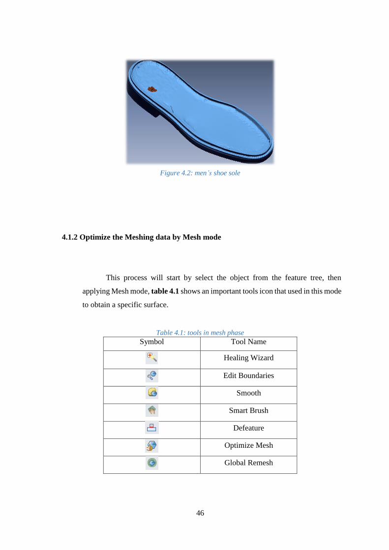
Figure 4.2: men’s shoe sole

4.1.2 Optimize the Meshing data by Mesh mode

This process will start by select the object from the feature tree, then

applying Mesh mode, table 4.1 shows an important tools icon that used in this mode

to obtain a specific surface.

Table 4.1: tools in mesh phase

Symbol Tool Name

Healing Wizard

Edit Boundaries

Smooth

Smart Brush

Defeature

Optimize Mesh

Global Remesh

47

By using healing wizard, the object automatically detects various defects

in the mesh such as Non-manifold poly vertices, fold, small, crossing, non-manifold

and dangling poly faces, small clusters and small tunnels. So, can be obtained mesh

model without any abnormal poly-faces, figure 4.3 shows a sole of elegant shoe

before and after healing wizard

Figure 4.3: sole of elegant shoe

As shown in figure 4.3, there is a gap in sole, Edit Boundary tool can help

to fill this gap, also it can Reduce the effect of noise and roughness, this command

features multiple boundary editing methods such as Smooth, Shrink, Fit, Extend,

Extrude, and Fill.in this case the mesh needs fill command, that fills poly-faces in

a boundary.

After this processes, there is a lot of optimizing on 3D scanning data but the

mesh still has some defects, as in figure 4.4 left side, mesh seems so rough and

contains some of noises, in this shape there is not clear, but when making a scan for

very shiny object, the reflection generates noise, and generate a rough surface on

the mesh. Smooth tool removes spiky points by averaging with surrounding points

and Improving the quality of a mesh.

48

Figure 4.4: before and after Applying Smooth Command

After applying these tools on 3D scanning data, it gives an acceptable shape

but in needs more enhancement for a good feature, Global Remesh can regenerates

poly-faces with uniform poly-edge lengths on a mesh and improves the quality of

the mesh, optimize combined mesh that is complex and overlapped, and that can be

noticed at regions do not have boundaries.

Global Remesh command is useful for [11]:

• Optimizing mesh so that it has poly-faces globally with uniform poly-edge

lengths.

• Optimizing mesh to be used for creating a high-quality surface body.

• Reducing the effects of defects and roughness on a mesh.

• Creating a high-quality mesh from combined mesh that is complex and

overlapped.

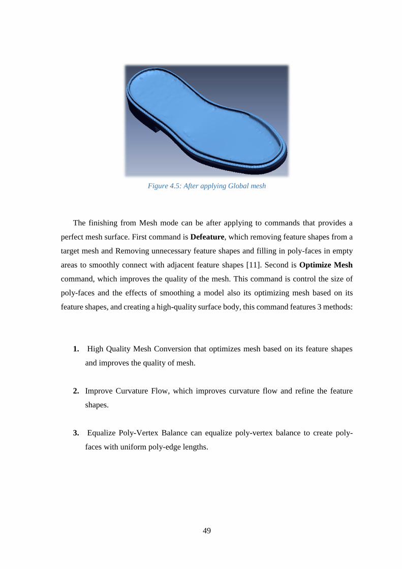
49

Figure 4.5: After applying Global mesh

The finishing from Mesh mode can be after applying to commands that provides a

perfect mesh surface. First command is Defeature, which removing feature shapes from a

target mesh and Removing unnecessary feature shapes and filling in poly-faces in empty

areas to smoothly connect with adjacent feature shapes [11]. Second is Optimize Mesh

command, which improves the quality of the mesh. This command is control the size of

poly-faces and the effects of smoothing a model also its optimizing mesh based on its

feature shapes, and creating a high-quality surface body, this command features 3 methods:

1. High Quality Mesh Conversion that optimizes mesh based on its feature shapes

and improves the quality of mesh.

2. Improve Curvature Flow, which improves curvature flow and refine the feature

shapes.

3. Equalize Poly-Vertex Balance can equalize poly-vertex balance to create poly-

faces with uniform poly-edge lengths.

50

This command is can be applied three times to achieve best quality of surface mesh,

figure 4.6 describes the final shape in Mesh Mode that can be obtained, the surface is

smooth and prefect also all holes are filled.

Figure 4.6: Final Shape of optimizing Mesh phase

4.1.3 Appling Region Group:

Region Group features contains various commands used to generate and edit feature

regions on a mesh. It can automatically classify feature regions by recognizing 3D scanning

features and detect it quickly, by using geometric feature information for easily and quickly

creating features, for example it can detect, define and classify the regions that are a

cylinder or plane, figure 4.7 shows that each color in sole express about specific region

and that depend on the geometry, on other hand, some of tools cannot use if region group

does not apply such as alignment wizard, after making Region Group its recommended to

make a Merge for all regions, in order to make it a single Region group and meagre a

separate regions as single region.

51

Figure 4.7: Region Group

4.1.4 Auto Surfacing:

Auto surfacing technology that automatically converts point clouds into

NURBS surface models has been developed by previous tools, during this

command, region group phase will convert to surface body smooth and quickly,

this tool uses when the shape is complex freeform part, it can create a surface body

that can envelope an entire geometric shape of a specific mesh, figure 4.8 shows

the form of sole after applying auto surface.

Figure 4.8: Auto Surfacing in Evenly Following Network

52

4.1.5 Export the development object to Catia:

Through this step can export the object to the Catia or Solidworks into Many

multi-platform formats are offered, in order to enhancing if required or to create the

core and cavity for the object, this command can be done by selecting the command

Export from File tape, select the object, press OK, and save it in a specific folder

as shown in figure 4.9 and select an acceptable type format, that can other software

deal with it, for Catia V5 R17 for example, the suitable format is STEP file “ .stp

“.

Figure 4.9: steps in Geomagic to Export an object

53

4.2 Creating Core Cavity For the object in Catia

Core and cavity tool can help for analyzing the part that require mold, by defining

two sides of part.

This operation starts after importing the sole stp file, which import from Geomagic

Design X, then select core and cavity operation from Start, Part design and select core and

cavity.

first step should be by making a join for the sole, because the Geomagic export it as a

surface and it should be as a one part in order to apply all required operations, after that the

sole should has

Figure 4.10 Core and Cavity tool icon

other pair to make the mold of pair sole, by using symmetry tool that can be solve this

action, as shown in figure 4.11, there is a pair sole, other pair making by symmetry about

axis, also it uses other rotation in small angle about a normal axis on it, in order to enhance

the location of it and optimize the volume of the mold and its lines in forward processes.

54

Figure 4.11: prepare a pair of sole

The process of core and cavity starts by using Pulling Direction tool, this

tools helps to define the core and cavity surfaces and define the core-cavity

separation , the compass is snapped automatically onto the current axis system, by

clicking on its icon it displays the box view after selecting the body, that through it

can adapt the pulling axis direction that, figure 4.12 shows how the two soles

divided in two regions, the red region means that is the core surface and green

region means that is the cavity surface, sometimes this tool cannot exactly divide

the two region as it as should to be, so it should select the small regions surfaces,

which is should be in core surface and select others that it should be cavity.

Figure 4.12: Pulling Direction

55

Figure 4.13: Core-Cavity and Pulling Direction box view.

56

Figure 4.14: Processes in Geomagic Design X

57

5

58

Chapter Five

Geomagic Algorithms

5.1 Bezier curves and surfaces

5.1.1 Bezier curves

Bézier curve is defined by a single particular polynomial (a Bernstein polynomial) also its

mathematically defined curve used in two-dimensional graphic applications. Bezier curves

are smooth curves, that are continuous, and its continuously turning tangent the derivative

59

its defined by using control points and its degree is defined by n + 1 control points Pi, as

in equation:

𝐶 (𝑡) = ∑ 𝑃𝑖𝐵𝑖𝑛(𝑡)

𝑛

𝑖=0 (5.1)

Where represent the Bernstein polynomials, which are given by:

𝐵𝑖𝑛 = (𝑛

𝑖)(1 − 𝑡)𝑛−𝑖𝑡𝑖 (5.2)

𝐵𝑖𝑛 Attains exactly one maximum on the interval [0, 1], that (𝑛

𝑖) is called a binomial

coefficient, where n is the degree, i is the index and t is the variable of equation, it

sometimes spoken as “n - choose - i”, which equal 𝑛!

𝑖!(𝑛−1)! . For example, for Quadratic n

= 2 , 𝑚0 = 𝐵02 = (1 − 𝑡)2, 𝑚1 = 𝐵1

2 = 2𝑡(1 − 𝑡) ,and 𝑚2 = 𝐵22 = 𝑡2 so 𝐵(𝑡) =

(1 − 𝑡)2 𝑃0 + 2𝑡(𝑡 − 1)𝑃1 + 𝑡2𝑃2.

Figure 5.1: Quadratic Bezier Curve

In figure 5.2 shows as an example, this is a Bezier curve which has six control points (the

blue points), and the degree of the curve n = 5, notice that the derivative at sharp edges is

not exist, for example at (2,4) is not exist on other hand the figure shows that The Bezier

60

curve generally follows the shape of the control polygon, which consists of the segments

joining the control points, whether 2D or 3D as in figure 5.3.

Figure 5.2: 2D Bezier curve

Figure 5.3: 3D Bezier curve

Main properties of the Bezier curves

Bezier curves consist of two type of curves on is called local control and other is global

control, Bezier curves exhibit global control, moving a control point alters the shape of

the whole curve as in figure 5.4 at the left. In local, only a part of the curve is modified

when changing a control point and in the right of figure, this curves can be straight line

if the control points is collinear, on other hand all control points can moved and modify

61

the curve except the end points, also if the starting point and end point reflected so the

direction of will reflect.

Control point translation Control point translation

Figure5.4: Control point

The meaning of splitting curve is to cut a given Bézier curve at C(u) for some u into two

curve segments, each of which is still a Bézier curve. Because the resulting Bézier curves

must have their own new control points, the original set of control points is discarded. and

since the original Bezier curve of degree n is cut into two pieces, each of which is a subset

of the original degree n Bezier curve, the resulting Bezier curves must be of degree n.

A Bezier curve always interpolates the end control points, these endpoints tangent vectors

are parallel to the control points [𝑃0, 𝑃1, . . . , 𝑃𝑛 ].This curve is also contained convex hull,

which are defining control points.

Any Bezier curve of degree n (with control points 𝑃𝑖 can be expressed in terms of a new

basis of degree n+1. The new control points 𝑄𝑖 are given by

𝑄𝑖 =𝑖

𝑛+1𝑃𝑖−1 + (1 −

𝑖

𝑛+1 )𝑃𝑖 𝑃𝑖−1 = 𝑃𝑛+1 = 0

i = 0, . . . , 𝑛 + 1

(5.3)

62

As show in figure5.5, at left graph show an original cubic curve, which has four control

points, on right graph, there is addition on control points to be five control points and the

curve being quartic.

Figure 5.5: original cubic curve

5.1.2 Bezier surfaces:

A Bézier surface patch is defined by its 4 x 4 Bézier geometry matrix, which

specifies the control points of the surface. As in the case of Bézier curves, the corner points

of matrix specify actual points on the edge of the interpolated surface, P= {{

𝑃00, 𝑃01, . . . , 𝑃0𝑛 }, { 𝑃10, 𝑃11, . . . , 𝑃1𝑛 }……. { 𝑃𝑚0, 𝑃𝑚1, . . . , 𝑃𝑚𝑛}}.

be a set of point’s 𝑃𝑖𝑗 ∈ 𝑅2 (i = 0, 1... m; j=0, 1...n)

The Bezier surface associated with the set P is defined by:

𝑆 (𝑢, 𝑣) = ∑ ∑ 𝑃𝑖𝑗𝐵𝑖𝑛(𝑢)𝐵𝑗

𝑚(𝑣)

𝑛

𝑖=0

𝑚

𝑗=0

Q1

(5.4)

63

Where𝐵𝑖𝑛(𝑢) and 𝐵𝑗

𝑚(𝑣) represent the Bernstein polynomials of degrees m and n and in

the variables u and v, respectively, which are non-negative, and m, n range between 0 and

1.

Figure 5.6: Bezier surface sample

Disadvantages of Bezier:

Single piece, no local control (move a control point, whole curve changes).

Complex shapes: can be very high degree, difficult to deal with

In practice: combine many Bezier curve segments.

5.2 Basic Spline Curves

B-spline is a piecewise polynomial real function is: [a,b] ∈ R on an interval [a,b],

is composed of k subintervals, [𝑡𝑖−1𝑖, 𝑡𝑖, ] with a= Pi

The restriction s to an interval i is a polynomial Pi = [𝑡𝑖−1𝑖, 𝑡𝑖 , ],so that s(t) = Pi(t),

Let[𝑃0, 𝑃1, . . . , 𝑃𝑛 ] be the control points. The nonnational form of a B-spline is

given by s an interiod

64

𝑃 (𝑢) = ∑ 𝑃𝑖𝑁𝑖,𝐷𝑛 (𝑢)

𝑛

𝑖=0 (5.5)

Where Pi refers to Control Points, Ni, k (t) is the B-spline basis functions and t is Knot

vector, which the number of knots in the knot vector is always equal to the number of

control points plus the order of the curve. E.g., a cubic (order=4) with four control points

has eight items in the knot vector. Pi are control points, and are B-spline basis functions

defined on A non-decreasing knot vector T= {t0, t1…tm+k+1}. For a B-spline curve a number

D determines its degree which is D − 1.

For each b-spline has a knots vector, which define a sequence of parameter values at which

the blending functions will be switched on and off

B-spline curves have two main advantages:

1. The degree of a B-spline polynomial can be set independently of the number of

control points.

2. B-splines allow local control over the shape of a spline curve (or surface)

Different Between Bezier and B-Spline curves: [20]

Both Bezier and B-Spline curves are used for drawing and evaluating smooth

curves, especially in computer graphics and animations.

B-Spline are considered a special case of Bezier curves

B-Spline offer more control and flexibility than Bezier curves

65

5.3 NURBS

(Non-Uniform Rational B-Splines), are mathematical representations of 3D geometry

that can accurately describe any shape from a simple 2D line, circle, arc, or curve to

the most complex 3D organic free-form surface or solid, it’s using in any process from

illustration and animation to manufacturing.

NURBS can be defined by created curves which are defined by control points and take

the average of the surrounding points to create a curved surface.

NURBS has wonderful properties for computer geometry representation in

modeling as:

1- It can accurately represent both standard geometric objects like lines, circles,

ellipses, spheres, and tori, and free-form geometry like car bodies and human

bodies.

2- NURBS needs a few amount of information to represent a piece of geometry,

this will make it better than common faceted approximations.

3- It’s very use full for representing a smooth object and it’s describe an exact

surface.

A NURBS curve 𝐶(𝑢) is a vector-valued, piecewise rational polynomial

function, is defined as

(5.6)

66

Also, 𝑅𝑖,𝑝(𝑢) is defined as:

Where Pi are the control points, 𝑊𝑖 are the weights and 𝑁𝑖,𝑝 are the B-spline basis

functions defined on the non-periodic and non-uniform knot vector, which is a list of

(degree + number of control points-1), also there is important properties of NURBS

function ,such as 𝑅𝑖,𝑝(𝑢) is a degree p rational function in 𝑢 ,it’s is always positive, on

other hand any knot span [𝑢𝑖 , 𝑢𝑖 + 1) at most 𝑝 + 1degree p basis functions are non-zero

namely 𝑅𝑖,𝑝 𝑝(𝑢), 𝑅𝑖,𝑝+1 𝑝(𝑢), 𝑅𝑖,𝑝+2 𝑝(𝑢), ..., and 𝑅𝑖,𝑝(𝑢). If all weights are equal to 1, a

NURBS curve reduces to a B-spline curve.

All these representations attempt to assist the manufacturing field by transferring the CAD

model to design model. They restrict the designer to a set of well-defined operations, based

on common mechanical features, which are used to describe a part.

(5.7)

67

6 Chapter Six

Applications

68

6.1 Work Samples

This Section includes some of parts that are working and optimizing it at

Geomagic Design X, all these objects are using the same procedure as used in soles,

but some of it required more time to achieve the best surface. Notice that all surfaces

in these objects made by Auto Surface, because these objects don’t have a regular

surface, which can through it make a mesh sketch.

Parts One: Two models of mold of shoes

Figure 6.1 shows the first model of the mold of shoe, which the shoemaker uses

when he wants to assemble all component of shoe, this figure show it after scanning

process, notice that it has lots of gabs and noises on it.

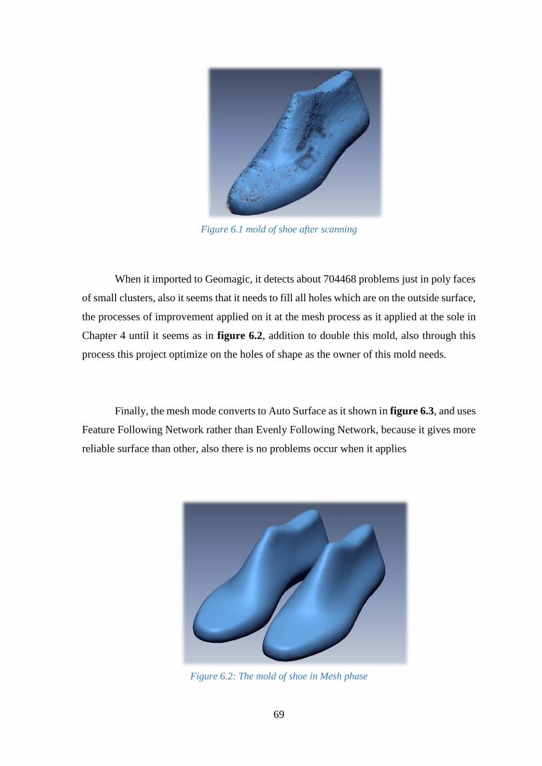
69

Figure 6.1 mold of shoe after scanning

When it imported to Geomagic, it detects about 704468 problems just in poly faces

of small clusters, also it seems that it needs to fill all holes which are on the outside surface,

the processes of improvement applied on it at the mesh process as it applied at the sole in

Chapter 4 until it seems as in figure 6.2, addition to double this mold, also through this

process this project optimize on the holes of shape as the owner of this mold needs.

Finally, the mesh mode converts to Auto Surface as it shown in figure 6.3, and uses

Feature Following Network rather than Evenly Following Network, because it gives more

reliable surface than other, also there is no problems occur when it applies

Figure 6.2: The mold of shoe in Mesh phase

70

Figure 6.3: The mold of shoe in Auto Surface phase

Figure 6.4: mold of shoe after scanning

71

Figure 6.5: mold after optimizing mesh

Figure 5.6: Auto Surface

72

Figure 5.7: Extract the mold

Part Two: Two models of sport sole shoe

This object also one of others that needs to make a mold for it, it’s somewhat

requires an intelligent skill to make core and cavity, figure 6.8 displays the

scanning shape of this sole, notice that the upper region needs a neat core

process in Catia, figure 6.9 shows the final shape of sole after all process in

mesh mode, and 6.10after making auto surface.

Figure 6.8: two sport sole shoe after scanning

73

Figure 6.9: two sport sole shoe final shape in mesh mode.

Figure 6.10: Auto Surface phase for two models sport sole shoe.

Part three: mesh sketch for mechanical part from machine

In figure 6.11 is a part that used in machine for lubrication ,and needs to re-

produce ,so after making scanning as shown and converting it to mesh phase, this

type of shapes can making a sketches from the origin 3D scanning, so by using

mesh sketch after making an optimizing for the origin mesh, will be easy to take a

sketches as and create a solid part which can also making a live transfer to

Solidworks 2012 or 2013 “this is the suitable versions of Solidworks can deal with

Geomagic, others will phase a problems”.

74

After making a mesh sketch as shown in figure 6.12, it can export to Catia, in

order to make a G-Code for it.

Figure 6.11: original mesh phase

Figure 6.12: solid part from mesh sketch

6.2 Practical Case

One of application by using Reverse Engineering, it helps to detect problems in the

structure of any object, by the Geomagic packages and especially Design X, it can help to

detect the problems that are in the objects, not just at the external shape, also this program

helps to detect problems internal the body.

Through figure 6.14, is a plastic chair that manufactured by Royal Company in Hebron,

this chair suffered from the broken exactly at the backrest and seat, also from other sides

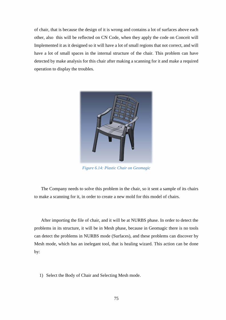
75

of chair, that is because the design of it is wrong and contains a lot of surfaces above each

other, also this will be reflected on CN Code, when they apply the code on Conceit will

Implemented it as it designed so it will have a lot of small regions that not correct, and will

have a lot of small spaces in the internal structure of the chair. This problem can have

detected by make analysis for this chair after making a scanning for it and make a required

operation to display the troubles.

Figure 6.14: Plastic Chair on Geomagic

The Company needs to solve this problem in the chair, so it sent a sample of its chairs

to make a scanning for it, in order to create a new mold for this model of chairs.

After importing the file of chair, and it will be at NURBS phase. In order to detect the

problems in its structure, it will be in Mesh phase, because in Geomagic there is no tools

can detect the problems in NURBS mode (Surfaces), and these problems can discover by

Mesh mode, which has an inelegant tool, that is healing wizard. This action can be done

by:

1) Select the Body of Chair and Selecting Mesh mode.

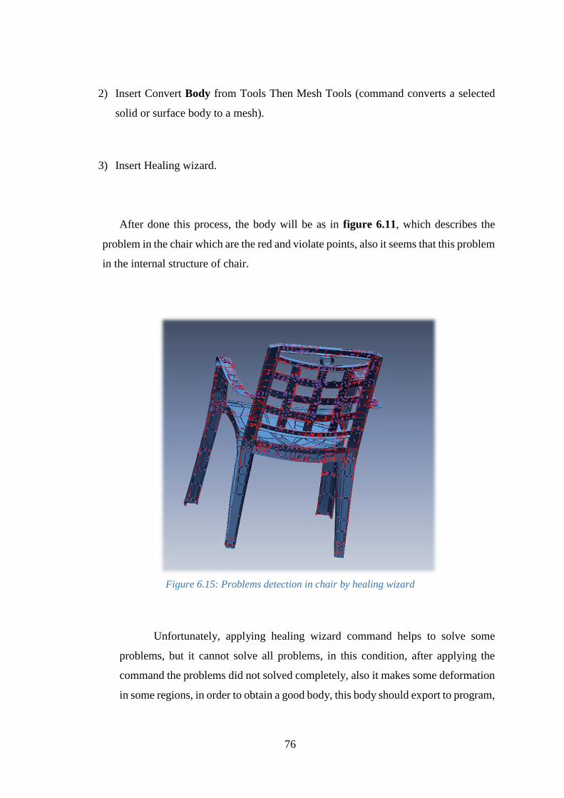
76

2) Insert Convert Body from Tools Then Mesh Tools (command converts a selected

solid or surface body to a mesh).

3) Insert Healing wizard.

After done this process, the body will be as in figure 6.11, which describes the

problem in the chair which are the red and violate points, also it seems that this problem

in the internal structure of chair.

Figure 6.15: Problems detection in chair by healing wizard

Unfortunately, applying healing wizard command helps to solve some

problems, but it cannot solve all problems, in this condition, after applying the

command the problems did not solved completely, also it makes some deformation

in some regions, in order to obtain a good body, this body should export to program,

77

which is more flexible and has possibilities more than Geomagic, Catia can

performs the purpose.

After importing the chair file to Catia, the correcting of the problems starts

form the bolts of chair as shown in figure 6.16, there is a lot of surfaces and splines,

which are above each other, also there is same thing at the hands and seat of it,

because the factor doesn’t need this bolt in the chair, they want to remove these

bolts form chair, so these bolts removed and built a new surface as shown in figure

6.13.

Figure 6.16: bolts at the backrest of chair

78

Figure 6.17: bolts removed and built new surfaces

Hint: All these objects files and other objects are in CD of graduation.

6.3 Recommendations:

There is some recommendations and inference that should be recall, during

the problems that faced in this project:

1) The output quality of objects, which export from the Geomagic Design X

depends on the scanning quality, some of parts cannot healing it also cannot

making an auto surface or mesh sketch, because the boundaries of object cannot

help when applying healing wizard or any process come after this process, also

when applying healing wizard or other commands, which use for repairing the

sketch and it cannot repair it, the problems will be twice or tribble in region

group and other processes.

2) The work in this project focuses just on the Geomagic Design X and Catia, it

has been dispensed about Geomagic Studio, because Geomagic Design X has

more power, more feature tools and it can export to various formulas, Geomagic

Studio works just for simple parts, but in Design X have more powerful and can

deal with all objects.

3) Through the various works in this project on various parts, it takes a long time

for the processes in programs, for example in the sole figure 4.1 takes at healing

wizard about fifteen minute to finish it, so this work requires a high-

performance computers processors and graphics, in order to achieve a good

work in short time.

79

References

[1] H.J. de St. Germaine, S.R. Stark, W.B. Thompson, and T.C. Henderson,

“Constraint Optimization and Feature-Based Model Construction for Reverse

Engineering,” Proceedings of the ARPA Image Understanding Workshop, Feb. 1996.

[2] M.T. Triband, F.W. Tillostson, and J.D. Martin, “Reverse and Re-Engineering in

the DOD Organic Maintenance Community: Current Status and Future Direction,”

Technical Report 96-060, Applied Research Laboratory, the Pennsylvania State

University, Feb. 1996.

[3] R. Broacha and M. Young, “Getting from Points to Products,” Computer-Aided

Engineering, Jul. 1995.

[4] J.C. Owen, Feature-Based Reverse Engineering, master’s thesis, Dept. of Computer

Science, University of Utah, 1994.

[5] 3D Point Cloud Segmentation: A survey, 2013 6th International Conference on

Robotics, Automation and Mechatronics (RAM).

[6] C. Hsu, Graph-Based Approach for Solving Geometric Constraint Problems,

doctoral dissertation, Dept. of Computer Science, University of Utah, 1996.

[7] P.J. Best and R.C. Jain, “Three-Dimensional Object Recognition,” ACM

Computing Surveys, vol. 17, no. 1, pp. 75-145, 1985.

80

[8] Application of reverse engineering techniques in mechanic’s system Services by

Michal Dubrovnik and Stefan Kinder.

[9] Reverse Engineering an Industrial Perspective by Prof. Vines Raja and Dr. Kiran

Jude Fernandes

[10] REVERSE ENGINEERING IN PRODUCT MANUFACTURING: AN

OVERVIEW KUMAR A.; JAIN, P. K. & PATHAK, P. M. Its international scientific

book 2013 pp. 665-678 chapter 39.

[11] GeomagicDesignX2014 User Guide. It has an information and details about its

components and tools about Geomagic Design X software.

[12] Ngozi Sherry Ali (May 2005) “Reverse Engineering of Automotive Parts

Applying Laser Scanning and Structured Light Techniques”, the University of

Tennessee, Knoxville.

[13] James Casey, Exploring Curvature, Friedr. Vieweg & Sohn,

Braunschweig/Wiesbaden, 1996.

[14] Gerald Farin, Curves and Surfaces for CAGD: A Practical Guide, fourth edition,

Academic Press, 1997.

[15] Introduction to Computing with Geometry Notes Dr. C.-K. Shene.

81

[16] 3D SOFTWARE - STUDIO 2012: Applied precision 3D digitizing system and

services INC. 208 Britannia Rd. E., Unit 3, Canada L4Z126, pp. 1-2

[17] 2013 INTERACTIVE USER GUIDE. Exact Surfacing for the Precise Reproduction

of Surfaces

[18] Brian A. Barsky and Tony D. DE Rose, Geometric Continuity of Parametric

Curves: Constructions of Geometrically Continuous Splines, IEEE Computer Graphics &

Applications, Vol. 10 (1910), No. 1 (January), pp. 60-68.

[19]http://homepages.inf.ed.ac.uk/rbf/CVonline/LOCAL_COPIES/AV0405/DONAV

ANIK/bezier.html ,visited in 10/1/2017 at 7:49pm.

[20]http://www.differencebetween.com/difference-between-bezier-curve-and-vs-b-

spline-curve/,visited in 10/1/2017 at 10:03pm