Envelope broadening of spherically outgoing waves in three-dimensional random media having power law...

Envelope broadening of spherically outgoing waves in

three-dimensional random media having power law spectra

Tatsuhiko Saito, Haruo Sato, and Masakazu OhtakeDepartment of Geophysics, Graduate School of Science, Tohoku University, Sendai, Japan

Received 5 September 2000; revised 30 May 2001; accepted 13 September 2001; published 9 May 2002.

[1] High-frequency S wave seismogram envelopes are broadened with increasing travel distancedue to diffraction and scattering. The basic mechanism of the broadening has been studied onthe basis of the scattering theory with the parabolic approximation for the scalar wave equation inrandom media. However, conventional models are not realistic enough since the plane wavemodeling is too simple and the Gaussian autocorrelation function (ACF) is far from the realityto represent the inhomogeneity in the Earth. Focusing on the early part of envelopes, we formulatedthe envelope broadening of spherically outgoing scalar waves in three-dimensional von Karman-type random media, of which the spectra decay according to a power law at large wave numbers.Random media are characterized by three parameters: RMS fractional velocity fluctuation e,correlation distance a, and order k that controls the gradient of the power law spectra. This modelpredicts that the envelope duration increases with both travel distance and frequency whenshort-wavelength components are rich in random media, while the duration is independent offrequency when short-wavelength components are poor. Introducing phenomenological attenuationQ, we developed a method for estimating the parameters of inhomogeneity and attenuation from theenvelope duration. Applying this method to S wave seismogram envelopes for the frequencyrange from 2 to 32 Hz in northeastern Honshu Japan, we estimated the random inhomogeneityparameters as k = 0.6, e2.2a�1 � 10�3.6 [km�1] and f /Q = 0.0095 [s�1], where f is frequency. Thepower law portion of the estimated power spectral density function is P(m) � 0.01 m�4.2 [km3],where m is wave number. INDEX TERMS: 7203 Seismology: Body wave propagation; 7218Seismology: Lithosphere and upper mantle; 7260 Seismology: Theory and modeling; KEYWORDS:envelope, inhomogeneity, scattering, parabolic approximation, lithosphere

1. Introduction

[2] For the study of seismic wave propagation for frequencieshigher than 1 Hz the velocity structure of the lithosphere cannotbe simply modeled by horizontal layers. Aki and Chouet [1975]first showed that coda waves of local earthquakes are composedof scattered body waves by distributed scatterers in the litho-sphere and that random inhomogeneity in elastic properties is themost probable origin of scattering. Sato [1989] proposed that theenvelope broadening of S wave seismograms with increasingtravel distance could be a powerful tool for the quantitativestudy of random velocity inhomogeneity in the lithosphere. Forthe incidence of scalar plane wave to random media extending ina half-space, Lee and Jokipii [1975] and Sreenivasiah et al.[1976] proposed a method to synthesize mean square (MS)envelope based on the Markov approximation for the parabolicwave equation when the random media is characterized by aGaussian autocorrelation function (ACF) and the characteristicscale of inhomogeneity is much larger than the wavelength ofincident waves. Their model predicts that diffraction and multi-ple forward scattering cause the envelope broadening. ThisMarkov approximation method is an extension of the phasescreen method for synthesizing waveforms to the stochasticsynthesis of MS envelopes. Comparing the envelope simulationwith the numerical waveform simulation based on the finitedifference method, Fehler et al. [2000] recently confirmed thevalidity of both the Markov approximation method and thephase screen method for the synthesis of waveforms except

latter coda in two-dimensional random media characterized by aGaussian ACF. Introducing an attenuation factor in the Markovapproximation method, Sato [1989] and Scherbaum and Sato[1991] quantitatively estimated the ACF of random velocityinhomogeneity in the lithosphere beneath the Kanto region,Japan, from the envelope analysis of small-earthquake records.Their simulations can basically explain the envelope-broadeningphenomenon. However, if we apply the above scattering modelto observed seismogram envelopes, it is better to use not planewaves but spherical waves. Therefore we need to developmathematics for modeling envelope of spherically outgoingwaves radiated from a point source.[3] Analyzing seismic coda waves, Wu and Aki [1985] found

that the spectral characteristics of velocity fluctuation obey a powerlaw. In order to explain the frequency dependence of S waveattenuation and coda excitation, Sato [1990] proposed a scattering-loss model to use the von Karman-type ACF for describing therandom inhomogeneity which has power law spectra at large wavenumbers. The spectral structure of random inhomogeneity was alsostudied by the correlation analysis of teleseismic waves based onthe parabolic approximation for scalar wave equation [Aki, 1973;Capon, 1974]. Flatte and Wu [1988] developed this method andanalyzed seismic array data at NORSAR. They proposed a two-overlapping-layer model that has power law spectra. Gusev andAbubakirov [1996] simulated not only coda part but also fullenvelopes in random media by using the Monte Carlo simulationmethod based on the radiative transfer theory with a scatteringcoefficient derived from the Born approximation. They concludedthat simulated envelopes qualitatively well explain observed seis-mogram envelopes when the PSDF has power law spectra with itspower being �3.5 to �4 for large wave numbers. Shiomi et al.

JOURNAL OF GEOPHYSICAL RESEARCH, VOL. 107, NO. B5, 10.1029/2001JB000264, 2002

Copyright 2002 by the American Geophysical Union.0148-0227/02/2001JB000264$09.00

ESE 3 - 1

[1997] reported that the small-scale inhomogeneity in the shallowcrust is random by examining elastic wave velocities and densityfrom well log data at various sites. They concluded that its powerspectral density function (PSDF) has power law spectra. Fromthese studies we get to know that the velocity inhomogeneity of thereal earth medium is random in space and its statistical character iswell represented by PSDF having power law spectra. For thesimulation of envelopes, Obara and Sato [1995] introduced anexponential-like function for the longitudinal integral of ACF andattempted to explain the frequency dependence of envelope broad-ening characteristics observed in Kanto-Tokai area in Japan, butthe corresponding ACF was not mathematically defined yet.Therefore we need to develop mathematics to synthesize envelopesin random media of which the PSDF has power law spectra. Thevon Karman-type ACF is one of the simplest functions that havepower law spectra at large wave numbers.[4] In this paper, we develop mathematics to simulate the

envelope of spherically outgoing scalar waves radiated from apoint source in three-dimensional (3-D) random media that arecharacterized by the von Karman-type ACF. Shishov [1974]solved a similar problem, but his result is limited to the caseof Gaussian ACF only. On the basis of this new model wepropose a method to estimate the PSDF characterizing therandom inhomogeneity and the attenuation factor from the traveldistance dependence and the frequency dependence of envelopebroadening. As an application of this method, we quantitativelyestimate the PSDF of random velocity inhomogeneity of thelithosphere beneath northeastern Honshu, Japan, from the analysisof S wave seismogram envelopes of small earthquakes recordedat a single station.

2. Envelope Synthesis in Random Media

[5] We imagine that waves radiated from a point source spheri-cally propagate through a 3-D inhomogeneous medium as sche-matically illustrated in Figure 1. Velocity inhomogeneities causescattering and diffraction effects on the waves. As a result, waves,which are impulsive at the source, are distorted, and the durationgets longer as the propagation distance increases. Here we focus onthe envelope broadening phenomenon and study mathematicallythe physical mechanism. The wave velocity inhomogeneity iswritten as V(x) = V0{1 + x(x)}, where V0 is the background

velocity and fractional fluctuation x(x) is a spatially randomfunction. We introduce an ensemble of random function {x(x)},where hx(x)i = 0. The angle brackets indicate the ensembleaverage. We assume that the randomness is statistically homoge-neous and isotropic. The random media can be characterized by theACF of fractional velocity fluctuation R(x) � hx(x + x0) x(x0)i. Themagnitude of inhomogeneity is given by the MS fractional fluctu-ation e2 � R(0) = hx(0)2i, and the characteristic scale is given bythe correlation distance a.

2.1. Markov Approximation for the Parabolic WaveEquation

[6] We assume that the wavelength l(= 2p/k) is shorter than thecorrelation distance a of the random inhomogeneity (ak � 1),where k is the wave number. Neglecting conversion scatteringbetween P and S waves in such a case, it is justified to describe theprincipal characteristics of elastic wave propagation by using thewave equation for scalar wave field u(x, t):

�� 1

V xð Þ2@2

@t2

!u x; tð Þ ¼ 0; ð1Þ

where � is Laplacian. When the fractional velocity fluctuation issmall, |x(x)| � 1, the wave equation (1) is written as

�� 1

V 20

@2

@t2

� �u x; tð Þ þ 2

V 20

x xð Þ @2

@t2u x; tð Þ ¼ 0: ð2Þ

We study the propagation of spherically outgoing waves radiatedfrom a point source located at the origin. Therefore we introducepolar coordinates (r, q, f), where angle q is measured from thedirection of a receiver. We may write the scalar wave field as asuperposition of harmonic spherical waves of angular frequency was

u x; tð Þ ¼ 1

2p

Z1�1

U r; q;f;wð Þr

ei kr�wtð Þdw; ð3Þ

where k = w/V0 and r = |x|. The Laplacian in (2) is written as

� ¼ 1

r2@

@rr2

@

@r

� �þ 1

r2�?; ð4Þ

where the angular part of Laplacian �? is given by

�?¼1

sin q@

@ qsin q

@

@ q

� �þ 1

sin q2@ 2

@ f2: ð5Þ

When ak � 1, substituting equations (3) and (4) into (2) andneglecting the second derivative with respect to r, we obtain theparabolic wave equation:

2ik@

@rU r; q;f;wð Þ þ 1

r2�?U r; q;f;wð Þ

�2k2x r; q;fð ÞU r; q;f;wð Þ ¼ 0: ð6Þ

The parabolic approximation neglecting large-angle scattering isconsidered to be applicable only when the medium has poorshort-wavelength components. However, the parabolic waveequation would be able to predict at least early part of waveformsquantitatively even when random media have rich short-wavelength components because the early part is mainly

Figure 1. Schematic illustration of spherically outgoing wavesradiated from a point source and their envelopes in a randomlyinhomogeneous medium. Waves, which are impulsive at the sourceradiation, are distorted, and the duration gets longer with increasingpropagation distance.

ESE 3 - 2 SAITO ET AL.: ENVELOPE BROADENING IN RANDOM MEDIA

composed of waves scattered within narrow angles around thereceiver direction. By comparing waveforms numerically calcu-lated from the wave equation and those from the parabolic waveequation, Liu and Wu [1994] confirmed the validity of theparabolic approximation in von Karman-type random media withthe order of 0.5 and in flicker-noise random media when thefractional velocity fluctuation is <10%.[7] For the case of ak � 1, small-angle scattering dominates.

Therefore we use the local Cartesian coordinate system in a smallvolume at a large distance r from the source (r � a), where oneaxis is chosen to be in the receiver direction and the other two axesare in the transverse plane which is tangent to the sphere of radius r

(see Figure 2). According to Ishimaru [1978] we define the two-frequency mutual coherence function (TMCF) on the transverseplane at distance r, which means the correlation between differentlocations r?1 and r?2 on the transverse plane and different angularfrequencies w1 and w2,

�2 r? 1; r? 2; r;w1;w2ð Þ � U r; r? 1;w1ð ÞU* r; r? 2;w2ð Þh i; ð7Þ

where the asterisk indicates complex conjugate. Since the randommedia are statistically homogeneous, �2 depends only on thedifference between r?1 and r?2. For quasi-monochromatic waves,that is, w1 � w2, we can get the master equation for �2 from (6)as

@

@r�2 þ i

kd

2k2c

1

r2@2

@ q2dþ 1

qd

@

@ qd

!�2

þ k2c A 0ð Þ � A r qdð Þ½ ��2 þk2d2A 0ð Þ�2 ¼ 0; ð8Þ

where the difference transverse coordinate is defined as r?d �r?1 � r?2 and the difference angle is defined as qd � |r?d|/r. Thederivation is given in Appendix A. Note that we assume nobackscattering. This derivation is called the Markov approxima-tion [Tatarskii, 1971]. This approximation puts a focus on strongforward scattering and diffraction effect. We introduce the centerof mass and difference coordinates in the wave number space askc = (k1 + k2)/2 and kd = k1 � k2 (kd � kc), respectively.Corresponding coordinates for angular frequency will also beused. The effect of inhomogeneity is included in the longitudinalintegral of ACF:

A r?dð Þ ¼ A r?dð Þ �Z1�1

dzR r?d; zð Þ; ð9Þ

where z is the radial coordinate in ACF and r?d = |r?d|. The lastterm in (8) does not affect the broadening of individual wavepackets but shows the wandering effect, which is the travel timefluctuation over different rays for each element of ensemble [Lee

Figure 2. At a large distance r from the source (r � a) we takethe local Cartesian coordinates in a small volume, where the oneaxis is in the direction of a receiver and the other two axes are inthe transverse plane which is tangent to the sphere of radius r.Angle q is measured from the receiver direction.

Figure 3. Plots of (a) von Karman-type autocorrelation function and (b) the corresponding power spectral densityfunction for different values of order k. The power spectral density function decays according to a power law m�2k�3

for large wave number.

SAITO ET AL.: ENVELOPE BROADENING IN RANDOM MEDIA ESE 3 - 3

and Jokipii, 1975]. Therefore, removing the last term, we get themaster equation as

@

@r0�2 þ i

kd

2k2c

1

r2@2

@ q2dþ 1

qd

@

@ qd

!0�2

þ k2c A 0ð Þ � A r qdð Þ½ �0�2 ¼ 0; ð10Þ

where we use the symbol 0�2 instead of �2 in the following.Equation (10) corresponds to equation (8) of Shishov [1974]. Theabove derivation is analogous to that for plane waves [Ishimaru,1978; Sato, 1989; Sato and Fehler, 1998].[8] We define the intensity of waves at radial distance r and

lapse time t as an ensemble average of wave’s power:

I0 r; tð Þ � u r; r?; tð Þu* r; r?; tð Þh i

¼ 1

2pð Þ21

r2

Z1�

Z1

dwddwc

� 0�2 q ¼ d0; r;wd ;wcð Þe�iwd t�r=V0ð Þ

¼ 1

2p

Z1�1

dwcI0 r; t;wcð Þ: ð11Þ

The intensity spectral density (ISD) I0 is written as the inverseFourier transform of the TMCF with respect to difference angularfrequency:

I0 r; t;wcð Þ ¼ 1

2p r2

Z1�1

0�2 qd ¼ 0; r;wd ;wcð Þe�iwd t�r=V0ð Þdwd: ð12Þ

It corresponds to the mean square of a band-pass-filtered tracehaving center angular-frequency wc, that is, the MS envelope. Itssquare root gives the RMS envelope. When we take 0�2 to benondimensional for a unit source radiation,

0�2 qd ; r ¼ 0;wd;wcð Þ ¼ 1=4p; ð13Þ

as the initial condition for coherent isotropic radiation from thepoint source, the ISD has a dimension of flux density and satisfies

I0 r ! 0; t;wcð Þ ¼ 1

4p r2d t � r

V0

� �: ð14Þ

2.2. MS Envelopes in von Karman-Type Random Media

2.2.1. The von Karman-type random media. [9] A vonKarman-type ACF (Figure 3a) is given by

R yð Þ ¼ R yð Þ ¼ e221�k

� kð Þy

a

� �kKk

y

a

� �; ð15Þ

where y = |y|, � is the gamma function and Kk is the modifiedBessel function of the second kind of order k. The correspondingPSDF (Figure 3b) is

P mð Þ ¼ P mð Þ ¼8p

32e2a3� kþ 3

2

� � kð Þ 1þ a2m2ð Þkþ

32

�8p

32� kþ 3

2

� e1=ka

� �2k� kð Þ m�2k�3 am � 1: ð16Þ

Figure 4. Comparison between the function B(x) given by equation (19) (solid curve) and its approximation formgiven by equation (20) (dashed line) for various k values for 10�4 < x < 10�1. Coefficients used in the approximationform are listed in Table 1.

Table 1. C(k) and p(k) in Equation (20) Estimated for 10�4 <

x < 10�1

k C(k) p(k)

0.1 0.56 1.190.2 1.06 1.380.3 1.56 1.560.4 2.00 1.710.5 2.28 1.830.6 2.31 1.910.7 2.14 1.950.8 1.90 1.980.9 1.68 1.991.0 1.50 1.99


The PSDF obeys the power law for large wave numbers, andthe power is given by �2k � 3. It means that short-wavelengthcomponents of random media increase with decreasing theorder k. In this study, we restrict the range of k to be between0 and 1.

2.2.2. ISD for the von Karman-type random media.[10] For the von Karman-type random media we can calculatethe longitudinal integral of ACF A (see equation (9)) from thePSDF as

A r?dð Þ ¼Z1�1

dz1

2pð Þ3Z Z1

�1

ZP mð Þeim r?dþzezð Þdm

¼ 2�kþ3=2 ffiffiffip

pe2a

� kð Þr?d

a

� �kþ1=2Kkþ1=2

r?d

a

� �; ð17Þ

by using integral formulas [Abramowitz and Stegun, 1970]. Thenwe need to get the representation of difference A(0) � A(r qd)appearing in equation (10). We may write that as

A 0ð Þ � A r qdð Þ ¼ e2a Br qda

; k� �

; ð18Þ

where

B x; kð Þ � 2�kþ32

ffiffiffip

p

� kð Þ limx!0

xkþ12Kkþ1

2xð Þ

� �� xkþ

12Kkþ1

2xð Þ

� �: ð19Þ

At a long travel distance from the source the correlation of wavefield at two points spatially separated on a transverse plane rapidlydecreases to zero with increasing lag distance [Sato and Fehler,1998], and as a result, 0�2 gets close to zero with increasing lagdistance. Therefore the contribution from a small transversedistance r?d � a is dominant. That is, the contribution of B(x;k) for x � 1 is important. We may approximate as

B x; kð Þ � C kð Þx p kð Þ x � 1: ð20Þ

Using an expansion formula for B(x;k) given by equation (19)[Abramowitz and Stegun, 1970], except for k = 1/2, we get theapproximation form as

B x; kð Þ � 2�kþ12p

32

� kð Þcos kp � 2k�32

� 32� k

� x2 þ 2�k�12

� 32þ k

� x2kþ1

( )x � 1:

ð21Þ

For the case of k � 1/2 and the case of k � 1/2, the leading termin equation (21) is dominant:

Br?d

a; k

� �� 2�kþ1

2p32

� kð Þcos kp�2�k�1

2

� 3=2þ kð Þr?d

a

� �2kþ1

( )ð22aÞ

Figure 5. Plots of power index p(k) against k for 10�4 <x < 10�1. Dashed line shows the asymptote 2k +1 for k� 0.5. Theasymptotic value for k � 0.5 is 2.

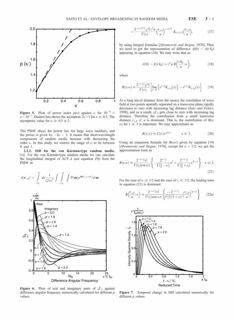
Figure 6. Plots of real and imaginary parts of 0�2 againstdifference angular frequency numerically calculated for different pvalues.

Figure 7. Temporal change in ISD calculated numerically fordifferent p values.


for k � 1/2, and

Br?d

a; k

� �� 2�kþ1

2p32

� kð Þcos kp2k�

32

� 3=2� kð Þr?d

a

� �2( )ð22bÞ

for k � 1/2. Thus we get to know the asymptotical behavior of Bfor x � 1 in the cases of small and large k values.[11] These asymptotic solutions, however, are not available

when k is close to 1/2, so that we take advantage of numericalevaluation. Varying k from 0.1 to 1.0 by 0.1 step in equation (19),we numerically estimate p(k) and C(k) in equation (20). In Figure 4the approximation form (equation (20)) is plotted by a dashed linetogether with its original form (equation (19)) by a solid line for thex range from 10�4 to 10�1 in logarithmic scale for different kvalues. For the corresponding x range, we can approximate thefunction B(x; k) within 15% error. The estimated p(k) and C(k) arelisted in Table 1. Plot of p(k) against k is given in Figure 5. Valuep(k) increases and the gradient decreases as k increases. At k = 0.1and 1.0, p(k) is nearly 1.2 and 2.0, respectively, as predicted byanalytical asymptotic solutions.[12] Substituting equations (18) and (20) into (10), we get

@

@r0�2 þ i

kd

2k2c

1

r2@2

@ q2dþ 1

qd

@

@qd

!0�2

þ k2c e2aC kð Þ r qd

a

� �p

0�2 ¼ 0: ð23Þ

We define the characteristic time as

tM ¼ C kð Þ2pe

4pa

2V0

awV0

� ��2pþ4p r 0

a

� �pþ2p

¼ C kð Þ2pV

p�4p

0

2e

1p�1a�1

� �2p�2p

w�2pþ4

p rpþ2p

0 ; ð24Þ

and the nondimensional propagation distance t and the transversedistance c as

t ¼ r=r 0; c ¼ffiffiffiffiffiffiffiffiffiffiffiffiffiffiffiffiffiffiffiffiffi2r0V0k2c tM

qqd : ð25Þ

Using equations (24) and (25), we may write (23) in nondimen-sional form as

@

@t 0�2 þ itMwd

1

t2@2

@c2þ 1

c@

@c

� �0�2 þ tpcp

0�2 ¼ 0: ð26Þ

Additionally, introducing new parameters m and v as

m ¼ tMwdð Þp= pþ2ð Þt v ¼ tMwdð Þ� pþ1ð Þ= pþ2ð Þc; ð27Þ

we rewrite equation (26) as

@

@m 0�2 þ i1

m2@2

@v2þ 1

v

@

@v

� �0�2 þ mpv p

0�2 ¼ 0: ð28Þ

For the case p = 2, we can get an analytical solution of equation(26). Substituting the solution into equation (12), we get analyticalsolution for ISD at a distance r0 as

I0 r 0; tð Þ ¼ 1

4p r20H t � r 0

V0

� �p2

2tM

�X1n¼1

�1ð Þnþ1n2exp � n2p2 t � r0=V0ð Þ

4tM

� �ð29Þ

for p = 2, where H(t) is a step function. Representation (29) is thesame as the solution for random media characterized by aGaussian ACF, except for the definition of characteristic time,

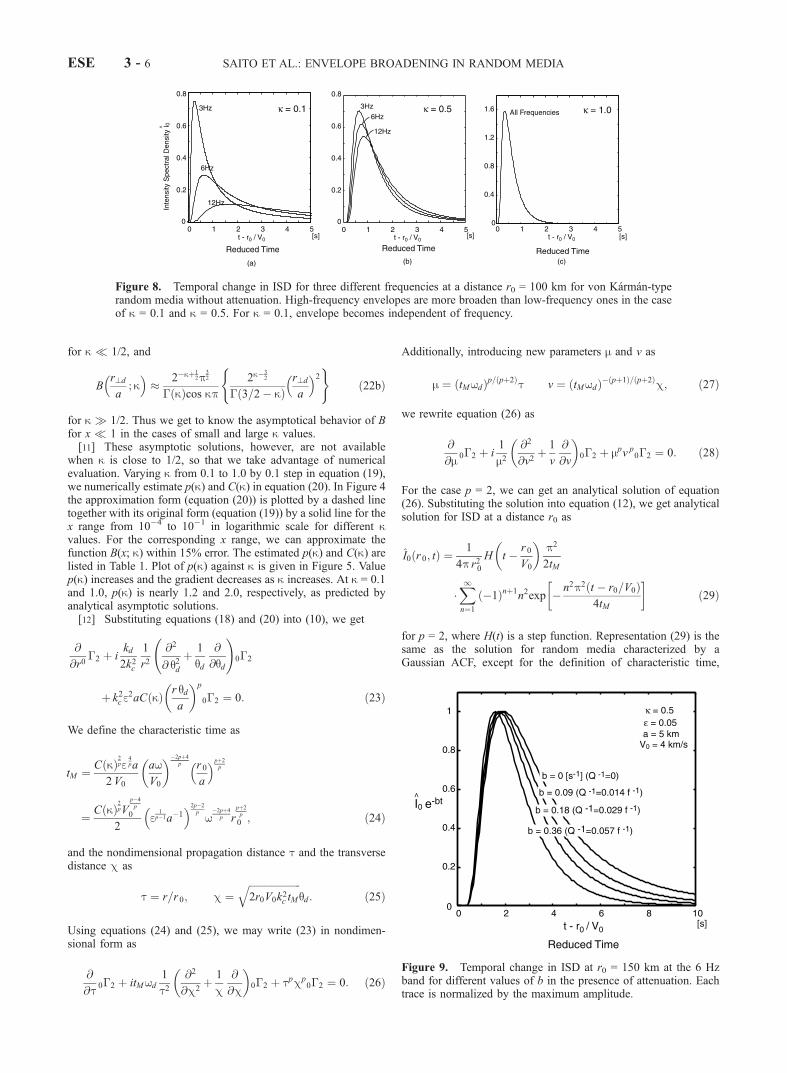
Figure 8. Temporal change in ISD for three different frequencies at a distance r0 = 100 km for von Karman-typerandom media without attenuation. High-frequency envelopes are more broaden than low-frequency ones in the caseof k = 0.1 and k = 0.5. For k = 0.1, envelope becomes independent of frequency.

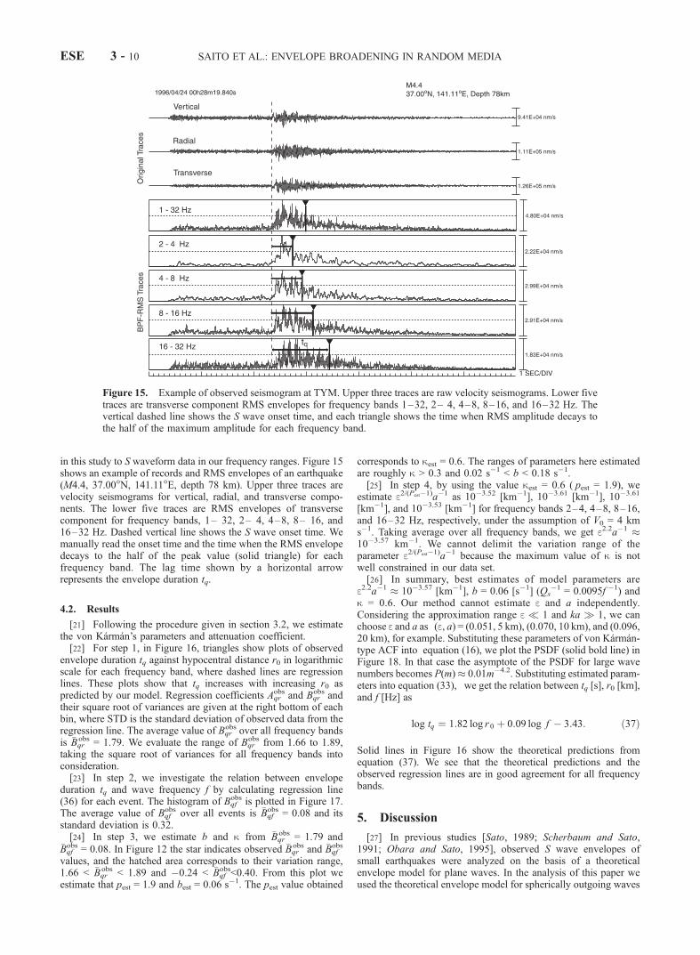
Figure 9. Temporal change in ISD at r0 = 150 km at the 6 Hzband for different values of b in the presence of attenuation. Eachtrace is normalized by the maximum amplitude.


which was originally solved by Shishov [1974] (see Appendix B).For the case p 6¼ 2 it is difficult to solve equation (28) analytically.We can numerically solve equation (28) under the initial condition

0�2(v, m = 0) = 1/4p. We use the Crank-Nicholson method [Presset al., 1987], where m is developed by 0.01 step and the interval inthe v space (0, 10) is divided into 600 segments. Then wetransform 0�2(v, m) into 0�2(c,t; tMwd). Figure 6 shows resultant

0�2(c = 0, t = 1; tMwd) for various p values. We numericallysimulate the ISD for different p values using the Fourier transform of

0�2 with respect to tMwd. Synthesized ISDs for various p values areillustrated in Figure 7 after the correction of geometrical spreading.Reduced time t � r0/V0 is scaled by characteristic time tM. We seethat envelope ‘‘shape’’ for larger p has apparently longer duration inthe scaled time in Figure 7 but note that we need to take not onlyenvelope shape but also characteristic time tM (equation (24)) intoaccount when we evaluate envelope duration in time.

2.2.3. Travel distance dependence and wave frequencydependence of ISD. [13] In the definition of characteristic time(see equation (24)) the power of travel distance is 1 + 2/p, and pincreases with k (see Figure 5). It means that the travel distancedependence of the ISD is strong when the inhomogeneity spectrahave rich short-wavelength components (small k), while thedependence is weak when the spectra have poor short-wavelengthcomponents (large k). The power of angular frequency is �2 + 4/p.This means that there is no frequency dependence of ISD for the casep = 2, that is, poor in short-wavelength component (k� 1.0). On theother hand, the frequency dependence increases as short-wavelengthcomponents of random media increase (k or p value decreases). Asan example, Figure 8 shows the frequency dependence of the ISD atr0 = 100 km for various k values, where e = 0.05, a = 5 km, V0 = 4km/s. For randommedia with k = 0.1 the envelope strongly dependson frequency. High-frequency envelopes are more broaden thanlow-frequency ones. For random media with k = 0.5, which haveless short-wavelength components, the frequency dependencebecomes weak, and for k = 1.0 the envelope is independent offrequency. Previous studies [Sato, 1989; Scherbaum and Sato,1991; Obara and Sato, 1995] mentioned that the frequencyindependence of envelope broadening is the result of a GaussianACF. However, our result indicates that the frequencyindependence is not proper to the Gaussian ACF random media,and the envelope broadening becomes independent of frequencyeven for von Karman-type random media when short-wavelengthcomponents are poor as k � 1.0.

2.2.4. Contribution of intrinsic absorption and large-anglescattering. [14] In the model we developed above, we have

neglected attenuation due to intrinsic absorption and large-anglescattering due to small-scale inhomogeneity. Large-angle scatteringworks mainly as attenuation in early part of envelopes. To includethe attenuation due to large-angle scattering and also intrinsicabsorption, we phenomenologically multiply exp (�bt) to theISD I0 as

I0 r; t;wcð Þe�bt; ð30Þ

where the relation between attenuation coefficient b and qualityfactor Q is

b ¼ 2p f Q�1: ð31Þ

For frequencies higher than 1 Hz we assume that b takes a constantvalue, since Q for S waves is nearly proportional to wavefrequency f in the lithosphere [Sato, 1984]. Figure 9 shows the ISDat r0 = 150 km in the 6-Hz band for different values of b. Eachenvelope, normalized by the maximum amplitude, is calculated fork = 0.5, e = 0.05, a = 5 km, V0 = 4 km/s. Figure 9 shows that theenvelope duration decreases with increasing attenuation (large b)because amplitudes attenuate more rapidly with increasing lapsetime.

3. Estimation of the Power Spectra ofRandom Inhomogeneity

[15] For random media having rich short-wavelength compo-nents our model would fail to predict the later part of envelope, or

Table 2. List of Coefficients Aq and Bq in Equation (32) for 0.5

s < tq < 30 s

b Aq Bq

p = 1.20 �0.222 1

0.045 �0.180 0.8580.09 �0.144 0.7520.18 �0.101 0.6200.36 �0.153 0.581

p = 1.40 �0.132 1

0.045 �0.103 0.8720.09 �0.088 0.7900.18 �0.057 0.6620.36 �0.104 0.624

p = 1.60 �0.070 1

0.045 �0.058 0.9010.09 �0.052 0.8290.18 �0.016 0.7050.36 �0.049 0.650

p = 1.80 �0.022 1

0.045 �0.011 0.9070.09 �0.013 0.8550.18 �0.005 0.7540.36 �0.026 0.684

p = 2.00 0. 016 1

0.045 0.022 0.9250.09 0.025 0.8620.18 0.026 0.7810.36 0.007 0.711

Figure 10. Duration tq is defined as the time lag between theonset and the time when the root-mean-square (RMS) envelopedecays to the half of the maximum value.


coda, because the parabolic approximation neglect large-anglescattering. Therefore we will focus on the early part of envelopecharacterized by its duration as follows. The duration tq is definedas the time lag between the onset time and the time when RMSenvelope decays to the half of the maximum amplitude (Figure 10).That is, the ISD decays to the quarter of the maximum peak value.The duration can be used as a measure of inhomogeneity fromrecorded wave traces. First, we show a theoretical relation betweentq value and the inhomogeneity parameters, and then we develop amethod for estimating the inhomogeneity from measured tq valuesof S wave seismogram envelopes of small earthquakes.

3.1. Relation Between Envelope Duration and ParametersCharacterizing Random Media

[16] We plot tq against tM from the ISD numerically simulatedfor a given set of b and p values. Assuming

log tq ¼ Aq p; bð Þ þ Bq p; bð Þlog tM ; ð32Þ

we estimate Aq and Bq values by using the least squares method fordifferent sets of b and p values in the tq range from 0.5 to 30 s (seeTable 2). For examples, plots for the cases of p = 2 for various bvalues are shown in Figure 11. For small b values, the relationbetween tq and tM is well represented by equation (32) for a widerange of tq. Equation (32) will provide a simple relation between tqand random media parameters as follows.[17] Substituting tM of equation (24) into (32), we get a relation

between tq and parameters characterizing random media:

log tq ¼ Bqr p; bð Þlog r 0 þ Bq f p; bð Þlogf

þBq p; bð ÞD p; e; að Þ þ Aq p; bð Þ; ð33Þ

where coefficients are

Bqr p; bð Þ ¼ Bq p; bð Þ pþ 2

p; Bqf p; bð Þ ¼ Bq p; bð Þ�2pþ 4

p;

D p; e; að Þ ¼ logC k pð Þ½ �

2p

22pð Þ

�2pþ4p V

p�4p

0 e2

p�1a�1� �2p�2

p

" #: ð34Þ

In the following, we use the dimension of each parameter asfollows: r0 in km, f in Hz, V0 in km s�1, a in km, and b in s�1. Fromequation (34) we can get a relation between Bqr and Bqf for various band p(k) values as plotted by fine dashed lines in Figure 12. It showsthat Bqr values, which represent the dependence of tq on r0, decreasewith increasing b values, and Bqf values, which represent thedependence of tq on f, decrease with increasing p(k) values. InFigure 13 we plot tq against r0 for several sets of b and f values asexamples for the case of V0 = 4 km s�1, a = 5 km, e = 0.05, andk = 0.3. The gradient Bqr becomes smaller with increasing

Figure 11. Plots of envelope duration tq (dots) against characteristic time tM in the case p = 2 for various attenuationcoefficients b. The solid line is the regression line given by equation (32).

Figure 12. Dashed lines show the relation between Bqr and Bqf

for various b and p(k) values numerically calculated. Starindicates the average observed values in northeastern Honshu,Japan, �Bqr

obs = 1.79 and �Bq fobs = 0.08. The hatched area

corresponds to the range evaluated from the square root ofvariances, 1.66 < Bqr < 1.89 and �0.24 < Bqf < 0.40.


attenuation coefficient b for the same frequency band. Theduration tq becomes larger with increasing frequency for the sameb value.

3.2. Estimation of Random Inhomogeneity Parameters Fromthe Measurements of tq Values

[18] Considering the travel distance dependence and the fre-quency dependence of envelope durations, we estimate the param-eters of the random media as follows. At step 1 we investigate howtq depends on r0. Plotting tq values against hypocentral distance r0for many events in each wave frequency band, we get the best fitregression line:

log tq ¼ Aobsqf þ Bobs

qf log r 0: ð35Þ

We calculate �Bqfobs by averaging Bqf

obs over all frequency bands. Atstep 2 we investigate how tq values depend on frequency f. Plottingtq values against f for each event, we get the best fit regression line:

log tq ¼ Aobsqf þ Bobs

qf log f : ð36Þ

We calculate �Bqfobs by averaging Bqr

obs over all events. At step 3 weestimate parameters b and p from �Bqr

obs and �Bqfobs using the

theoretical relation between Bqr and Bqf in Figure 12. Then theorder k is estimated from p value using the relation in Figure 5. Atstep 4 we estimate e2/(Pest�1)a�1, so that the theoretical relation(33) agrees with the observed regression line (35) where pest isthe estimated p value in step 3.

4. Analysis of Observed S Wave SeismogramEnvelopes

4.1. Data

[19] Applying the method developed above to S wave seismo-grams of small earthquakes, we estimate the PSDF of randominhomogeneity of lithosphere beneath northeastern Honshu, Japan.The data we use are velocity seismograms recorded at the Tsuyamastation (TYM) located at northeastern Honshu, Japan (38.66 N,141.37 E, altitude 100 m) (see Figure 14), where a broadbandseismometer STS-2 is installed on hard rock. Seismograms aredigitized with the sampling frequency of 80 Hz. We selected eventsfor the analysis by the following criteria: the focal depth is deeperthan 35 km to avoid crustal reflections, and the magnitude is from3 to 5 to satisfy the condition that the source duration time is shortenough. Figure 14 shows the hypocenter distribution of 328earthquakes that we used. Station TYM is shown by a triangle.Hypocenter locations were automatically determined by theResearch Center for Prediction of Earthquakes and VolcanicEruptions, Tohoku University. Hypocentral distances analyzed inthis study range from 60 to 400 km.

[20] Velocity seismograms in transverse component are calcu-lated from two horizontal component seismograms. Then we makeband-pass-filtered traces for four octave width frequency bands 2–4, 4– 8, 8–16, and 16– 32 Hz. Squared band-pass-filtered tracesare smoothed by applying a moving time window of which thewidth is one half of the center period of each frequency band. Werefer to the square root of these traces as RMS envelopes. Exceptfor studies on backscattered coda waves and well log data in theshallow crust, many researches reported that the correlation dis-tance ranges larger than a 10-km as shown in Figure 1 of Wu andAki [1988]. Therefore we may apply the envelope model developed

Figure 13. Plots of tq against r0 for different values of b for V0 = 4 km s�1, a = 5 km, e = 0.05, k = 0.3: (a) f = 3 Hz,(b) f = 6 Hz, (c) f = 12 Hz, and (d) f = 24 Hz.

Figure 14. Distribution of 328 small earthquakes that wereobserved at station TYM (triangle) in northeastern Honshu, Japan.Hypocenter locations were automatically determined by theResearch Center for Prediction of Earthquakes and VolcanicEruptions, Tohoku University.


in this study to S waveform data in our frequency ranges. Figure 15shows an example of records and RMS envelopes of an earthquake(M4.4, 37.00 N, 141.11 E, depth 78 km). Upper three traces arevelocity seismograms for vertical, radial, and transverse compo-nents. The lower five traces are RMS envelopes of transversecomponent for frequency bands, 1– 32, 2– 4, 4–8, 8– 16, and16–32 Hz. Dashed vertical line shows the S wave onset time. Wemanually read the onset time and the time when the RMS envelopedecays to the half of the peak value (solid triangle) for eachfrequency band. The lag time shown by a horizontal arrowrepresents the envelope duration tq.

4.2. Results

[21] Following the procedure given in section 3.2, we estimatethe von Karman’s parameters and attenuation coefficient.[22] For step 1, in Figure 16, triangles show plots of observed

envelope duration tq against hypocentral distance r0 in logarithmicscale for each frequency band, where dashed lines are regressionlines. These plots show that tq increases with increasing r0 aspredicted by our model. Regression coefficients Aqr

obs and Bqrobs and

their square root of variances are given at the right bottom of eachbin, where STD is the standard deviation of observed data from theregression line. The average value of Bqr

obs over all frequency bandsis �Bqr

obs = 1.79. We evaluate the range of Bqrobs from 1.66 to 1.89,

taking the square root of variances for all frequency bands intoconsideration.[23] In step 2, we investigate the relation between envelope

duration tq and wave frequency f by calculating regression line(36) for each event. The histogram of Bqf

obs is plotted in Figure 17.The average value of Bqf

obs over all events is �Bqfobs = 0.08 and its

standard deviation is 0.32.[24] In step 3, we estimate b and k from �Bqr

obs = 1.79 and�Bqfobs = 0.08. In Figure 12 the star indicates observed �Bqr

obs and �Bqfobs

values, and the hatched area corresponds to their variation range,1.66 < �Bqr

obs < 1.89 and �0.24 < �Bqfobs<0.40. From this plot we

estimate that pest = 1.9 and best = 0.06 s�1. The pest value obtained

corresponds to kest = 0.6. The ranges of parameters here estimatedare roughly k > 0.3 and 0.02 s�1 < b < 0.18 s�1.[25] In step 4, by using the value kest = 0.6 ( pest = 1.9), we

estimate e2/(Pest�1)a�1 as 10�3.52 [km�1], 10�3.61 [km�1], 10�3.61

[km�1], and 10�3.53 [km�1] for frequency bands 2–4, 4–8, 8–16,and 16–32 Hz, respectively, under the assumption of V0 = 4 kms�1. Taking average over all frequency bands, we get e2.2a�1 �10�3.57 km�1. We cannot delimit the variation range of theparameter e2/(Pest�1)a�1 because the maximum value of k is notwell constrained in our data set.[26] In summary, best estimates of model parameters are

e2.2a�1 � 10�3.57 [km�1], b = 0.06 [s�1] (Qs�1 = 0.0095f �1) and

k = 0.6. Our method cannot estimate e and a independently.Considering the approximation range e � 1 and ka � 1, we canchoose e and a as (e, a) = (0.051, 5 km), (0.070, 10 km), and (0.096,20 km), for example. Substituting these parameters of von Karman-type ACF into equation (16), we plot the PSDF (solid bold line) inFigure 18. In that case the asymptote of the PSDF for large wavenumbers becomes P(m)� 0.01m�4.2. Substituting estimated param-eters into equation (33), we get the relation between tq [s], r0 [km],and f [Hz] as

log tq ¼ 1:82 log r 0 þ 0:09 log f � 3:43: ð37Þ

Solid lines in Figure 16 show the theoretical predictions fromequation (37). We see that the theoretical predictions and theobserved regression lines are in good agreement for all frequencybands.

5. Discussion

[27] In previous studies [Sato, 1989; Scherbaum and Sato,1991; Obara and Sato, 1995], observed S wave envelopes ofsmall earthquakes were analyzed on the basis of a theoreticalenvelope model for plane waves. In the analysis of this paper weused the theoretical envelope model for spherically outgoing waves

Figure 15. Example of observed seismogram at TYM. Upper three traces are raw velocity seismograms. Lower fivetraces are transverse component RMS envelopes for frequency bands 1–32, 2– 4, 4–8, 8–16, and 16–32 Hz. Thevertical dashed line shows the S wave onset time, and each triangle shows the time when RMS amplitude decays tothe half of the maximum amplitude for each frequency band.


radiated from a point source, which accurately represents a geo-metrical spreading effect in 3-D media. We examine the differencebetween the envelopes derived from above two models. The solidcurve in Figure 19 shows ISD, which correspond to the MSenvelope, of spherically outgoing waves in random media charac-terized by a Gaussian ACF without attenuation, where the charac-teristic time tM =

ffiffiffip

pe2r0

2 /(2V0a). The exact derivation is given inAppendix B. The envelope duration tq � 1.05tM for ISD ofspherically outgoing waves, while tq � 3.11tM for ISD of planewaves as drawn by a dashed curve [after Sato, 1989]. We may saythat the envelope duration of spherically outgoing waves is about1/3 as long as that of plane waves for a given randomness. It meansthat the ratio e2/a estimated from observed envelope durations

based on the plane wave model is systematically underestimated.Such a difference in envelope durations occurs for von Karman-type random media as well.[28] Our observational results show that the frequency depend-

ence of envelopes is weak but clear, as shown in Figure 17. In thecase of random media having Gaussian ACF, envelopes areindependent of wave frequency. Envelopes for von Karman-typerandom media change with wave frequency. Observed envelopes,in general, change with wave frequency as was reported by Obaraand Sato [1995]. They introduce parameter p [Obara and Sato,1995, equation (3)] to generalize an exponential function for thelongitudinal integral of ACF to represent the frequency dependenceof envelopes; however, they could not derive the corresponding

Figure 16. Plots of envelope duration tq observed (triangle) against hypocentral distance r0 in logarithmic scale.Dashed lines are regression lines given by equation (35). Regression coefficients Aqr

obs and Bqrobs and standard

deviation of observed data from each regression line are shown at the right bottom. Solid lines are theoreticallypredicted by our model equation (37).


ACF. Our formulation succeeded in relating p value with the orderk of von Karman-type ACF by using both analytical and numericalsimulations (see Figure 5). We note that p(k) and C(k) valuesestimated in equation (20) slightly vary when we choose a differentx range. The variation of these values estimated from different xranges is the largest around k = 0.5. For example, when k = 0.5, thep value is 1.80 for the range 10�5 � 10�1, while the p value is 1.85for the range 10�3 � 10�1. As examples, we plot RMS envelopesat 8 Hz at distance 150 km for different choices of x range inFigure 20, where we take V0 = 4 km s�1, e = 0.05, and a = 5 km.The scatter of these traces is within 3% of the maximum peak, and

the scatter of measured envelope duration tq is within 10% error.The variation of p(k) and C(k) depending on the x range means thatboth frequency and travel distance dependencies of envelopebroadening slightly vary with travel distance. However, the differ-ence is very small in synthesized envelopes.[29] We cannot estimate independently parameters e, a, and k

characterizing PSDF of random media, so that we cannotmeasure the corner of PSDF curve that corresponds to thereciprocal of the correlation distance. However, the PSDFs inhigh wave numbers (beyond the corner wave number) takealmost the same value for possible combinations of e and a asshown in Figure 18. That is, we cannot discuss the corner, but

Figure 17. Histogram of Bqfobs for all events. The average of Bqf

obs

is 0.08, and its standard deviation is 0.32.

Figure 18. Plots of two von Karman-type PSDFs estimated innortheastern Honshu, Japan (solid curves): (e, a, k) = (0.051, 5 km,0.6), (0.070, 10 km, 0.6) and (0.096, 20 km, 0.6). Dashed curveshows the PSDF estimated from the frequency dependence of Swave attenuation and coda excitation by Sato [1990] (e = 0.08, a =2.1 km, k = 0.35) as a reference. The vertical dashed line showstwice the maximum wave frequency used in this study.

Figure 19. Comparison of the ISD for spherically outgoingwaves (solid curve) and that for plane waves (dashed curve) in 3-Drandom media characterized by a Gaussian ACF withoutattenuation. Each trace is normalized by the peak value.

Figure 20. RMS envelopes for different approximation forms ofB(x) for k = 0.5.


we can discuss the power index and the level of PSDF for highwave numbers. In the Born approximation [see Sato and Fehler,1998] the maximum wave number contributing to scatteringamplitudes is twice the incident wave number. The correspondingfrequency, which is twice the maximum wave frequency 32 Hz,is shown by the vertical dotted line in Figure 18. Our estimationof the power index is �4.2 (k = 0.6) and its variation range isless than �3.6 (k > 0.3). Gusev and Abubakirov [1996] concludedthat the power index of PSDF to be �3.5 � �4 for explainingqualitative character of observed envelopes. Our result is consistentwith their results. There have been a few studies on the estimation ofvon Karman’s parameters in Japan. From the analysis of frequencydependence of attenuation as scattering loss and coda excitation inthe lithosphere, Sato [1990] estimated as e = 0.08, a = 2.1 [km], andk = 0.35. The estimated PSDFs from these values are also shown bythe dashed curve in Figure 18 with our results. Our PSDF containsless short-wavelength components than that of Sato [1990]. Onereason for the difference might come from the difference of theenvelope models: this study assumed multiple forward scatteringdiscarding backscattering and analyzed early part of envelopes,while Sato [1990]assumed single scattering of elastic waves andexamined frequency dependencies of both attenuation and codaexcitation.[30] In this study, we included the contribution of large-angle

scattering only as an attenuation factor in equation (30). Large-angle scattering, however, would cause not only attenuation of theearly part of envelope but also later coda excitation. It also hassmall influence on envelope broadening. We will have to includesuch a contribution of large-angle scattering because of short-wavelength inhomogeneities in the envelope synthesis in future.We will measure how large-angle scattering contributes to seismo-gram envelopes in von Karman-type random media by comparingenvelopes of finite difference simulations and those of the Markovapproximation method. For more precise modeling of seismogramenvelopes from onset to later coda, we need to take not onlyforward scattering but also large-angle scattering into account. Wewill be able to establish this task by combining the Markovapproximation method and the radiative transfer theory.

6. Conclusion

[31] Using the Markov approximation for the parabolic waveequation, we theoretically derived the MS envelope of sphericallyoutgoing scalar waves radiated from a point source in 3-D randommedia characterized by a von Karman-type ACF. This modelpredicts that the envelope duration is proportional to the secondto third power of travel distance and is proportional to the zeroth tosecond power of wave frequency. When the short-wavelengthcomponents are rich in random media, the envelope durationincreases with both distance and frequency, while the duration isindependent of frequency and is proportional to the square of traveldistance when the random inhomogeneity is poor in short-wave-length components. We note that the frequency independence ofenvelope duration is not a unique consequence of Gaussian ACF,as was suggested in previous studies. For modeling the early partof envelope more realistically, the attenuation coefficient b wasphenomenologically introduced as a sum of large-angle scatteringloss and intrinsic absorption. On the basis of the theoretical modelwe established a method for estimating parameters characterizingrandom media by analyzing the travel distance dependence andwave frequency dependence of envelope durations. Applying thismethod to S wave envelopes of 328 small earthquakes recorded at asingle station in northeastern Honshu, Japan, we estimated thePSDF of the random inhomogeneity of the lithosphere for thefrequency range from 2 to 32 Hz. A positive correlation betweenthe envelope duration and travel distance was confirmed aspredicted, and the parameters are estimated as k = 0.6, e2.2a�1 �10�3.57 [km�1], and b = 0.06 [s�1] (Qs

�1 = 0.0095f �1). In that

case, the power law portion of the estimated PSDF becomes P(m)� 0.01m�4.2 [km3].

Appendix A: Derivation of the DifferentialEquation for Two-Frequency Mutual CoherenceFunction

[32] For spherically outgoing scalar waves in 3-D randommedia the differential equation for two-frequency mutual coher-ence function (TMCF) was given by Shishov [1974]. Here wereproduce the derivation of the differential equation.[33] Taking an ensemble average of a product of wave fields

governed by equation (6), we obtain

2i@

@r�2 þ

1

r2�?1

k1��?2

k2

� ��2 � 2 k1x1 � k2x2ð ÞU1U2

*D E

¼ 0:

ðA1Þ

Here subscript i means that arguments are (r, qi, fi, wi), �?i is theangular part of Laplacian for qi and fi, and ki = wi/V0 for i = 1 and 2.The last term can be rewritten by using the longitudinal integral ofACF along the global ray from the source to the receiver A(r?d)and TMCF:

k1x1 � k2x2ð ÞU1U2*

D E¼ � i

2k21 þ k22�

A 0ð Þ � 2k1k2A r?dð Þ� �

�2:

ðA2Þ

The procedure to derive equation (A2) is the same as in the case ofplane waves [see Sato and Fehler, 1998, equation (8.54)]. Then,equation (A1) is written as

2i@

@r�2 þ

1

r2�?1

k1��?2

k2

� ��2

þ i k21 þ k22�

A 0ð Þ � 2k1k2A r?dð Þ� �

�2 ¼ 0: ðA3Þ

For scattering within a small angle around the receiver direction,Laplacian for qi and fi can be written as

�?i �1

qi

@

@ qiqi

@

@ qi

� �þ 1

q2i

@

@f2i

qi � 1: ðA4Þ

Interpreting qi and fi as polar coordinates on the transverse planeand introducing nondimensional Cartesian coordinates:

hxi ¼ qi cosfi; hyi ¼ qi sinfi; ðA5Þ

we rewrite equation (A4) as

�?i ¼@2

@ h2xiþ @2

@ h2yiqi � 1: ðA6Þ

Introducing center-of-mass and difference coordinates for twopoints at Hi = (h xi, h yi) on the transverse plane

Hc ¼ H1 þ H2ð Þ=2; Hd ¼ H1 � H2; ðA7Þ

we can write equation (A4) as

�?1 ¼1

4r?c þr?cr?d þ�?d ;

�?2 ¼1

4r?c �r?cr?d þ�?d ;

ðA8Þ


where r?c and �?c are for Hc, and r?d and �?d are for Hd.Laplacian for Hd is written by using polar coordinates (qd, fd)as

�?d ¼1

qd

@

@ qdqd

@

@ qd

� �þ 1

q2d

@2

@f2d

: ðA9Þ

The dimensional difference of two points on the transverseplane r?d = r?d is written as

r?d ¼ r qd � ðA10Þ

We note that �2 is independent of center-of-mass coordinate hcand angle fd because random media is statistically homo-geneous and isotropic: �c�2 = 0 and @�2/@fd = 0. For the caseof quasi-monochromatic waves (k1 � k2), we may writeequation (A3) as

@

@r�2 þ i

kd

2k2c

1

r2@2

@ q2dþ 1

qd

@

@ qd

!�2

þ k2c A 0ð Þ � A r qdð Þ½ ��2 þk2d2A 0ð Þ�2 ¼ 0; ðA11Þ

where kc = (k1 + k2)/2 and kd = k1 � k2. This is the masterequation for TMCF.

Appendix B: MS Envelopes in Random MediaHaving Gaussian ACF

[34] For spherically outgoing waves in 3-D random mediahaving Gaussian ACF, analytical representation of intensity spec-tral density (ISD) was first obtained by Shishov [1974]. Here wereproduce the derivation in the following. The Gaussian ACF isgiven by

R xð Þ ¼ e2exp �r2�a2

� : ðB1Þ

Its longitudinal integral A (see equation (9)) becomes

A r?dð Þ ¼ffiffiffip

pe2ae�r2?d=a

2 �ffiffiffip

pe2a 1� r?d=að Þ2n o

r?d � a:

ðB2Þ

Substituting equation (B2) in (10), we get the differential equationfor 0�2 as

@

@r0�2 þ i

kd

2k2c

1

r2@2

@ q2dþ 1

qd

@

@ qd

!0�2 þ

ffiffiffip

pk2c e

2ar qda

� �2

0�2 ¼ 0

ðB3Þ

for qd � 1. Introducing the characteristic time as

tM ¼ffiffiffip

pe2a

2V0

r 0

a

� �2; ðB4Þ

nondimensional propagation distance t and the transverse distancec as given by equation (25), we get a nondimensional form ofequation (B3) as

@

@t 0�2 þ itMwd

1

t2@

@c2þ 1

c@

@c

� �0�2 þ t2c2

0�2 ¼ 0: ðB5Þ

Writing the solution a priori in the form as

0�2 c; tð Þ ¼ ev tð Þt2c2

w tð Þ ðB6Þ

and substituting it into equation (B5), we get two differentequations:

v0 þ 2v

tþ s20v

2 þ 1 ¼ 0; ðB7Þ

s20v�w0

w¼ 0; ðB8Þ

where s0 = 2eip/4ffiffiffiffiffiffiffiffiffiffitMwd

p. Equation (B7) is a Riccati equation.

Solutions of these equations are

v ¼ 1

s0cot s0tþ c1ð Þ � 1

s20t; ðB9Þ

w ¼ c2 sin s0tþ c1ð Þs0t

: ðB10Þ

Under the initial condition (13), we obtain the analytical solution

0�2 ¼1

4ps0t

sin s0texp

t2

s0cot s0t�

ts20

� �c2

� �: ðB11Þ

Substituting equation (B11) into (12), we obtain the ISD at adistance r0 as

I0 r0; t;wcð Þ¼ 1

2pr20

Z1�1

0�2 t ¼ 1;c ¼ 0; tMwdð Þe�iwd t�r0=V0ð Þdwd

¼ 1

2pr20

Z1�1

1

4p2eip=4

ffiffiffiffiffiffiffiffiffiffitMwd

p

sin 2eip=4ffiffiffiffiffiffiffiffiffiffitMwd

pf g

e�iwd t�r0=V0ð Þ

dwd

Figure B1. Temporal change in ISD for spherically outgoingwaves in random media characterized by a Gaussian ACF withoutattenuation, where the characteristic time is tM = (

ffiffiffip

pe2r20)/2V0a.


¼ 1

4pr20H t � r0

V0

� �p2

2tM

X1n¼1

�1ð Þnþ1n2e

�n2 r2 t�r0=V0ð Þ4tM

ðB12Þ

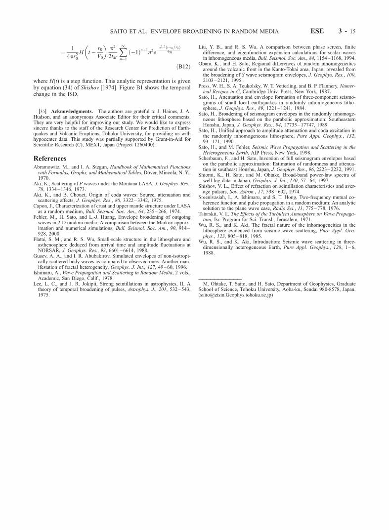
where H(t) is a step function. This analytic representation is givenby equation (34) of Shishov [1974]. Figure B1 shows the temporalchange in the ISD.

[35] Acknowledgments. The authors are grateful to J. Haines, J. A.Hudson, and an anonymous Associate Editor for their critical comments.They are very helpful for improving our study. We would like to expresssincere thanks to the staff of the Research Center for Prediction of Earth-quakes and Volcanic Eruptions, Tohoku University, for providing us withhypocenter data. This study was partially supported by Grant-in-Aid forScientific Research (C), MEXT, Japan (Project 1260400).

ReferencesAbramowitz, M., and I. A. Stegun, Handbook of Mathematical Functionswith Formulas, Graphs, and Mathematical Tables, Dover, Mineola, N. Y.,1970.

Aki, K., Scattering of P waves under the Montana LASA, J. Geophys. Res.,78, 1334–1346, 1973.

Aki, K., and B. Chouet, Origin of coda waves: Source, attenuation andscattering effects, J. Geophys. Res., 80, 3322–3342, 1975.

Capon, J., Characterization of crust and upper mantle structure under LASAas a random medium, Bull. Seismol. Soc. Am., 64, 235–266, 1974.

Fehler, M., H. Sato, and L.-J. Huang, Envelope broadening of outgoingwaves in 2-D random media: A comparison between the Markov approx-imation and numerical simulations, Bull. Seismol. Soc. Am., 90, 914–928, 2000.

Flatte, S. M., and R. S. Wu, Small-scale structure in the lithosphere andasthenosphere deduced from arrival time and amplitude fluctuations atNORSAR, J. Geophys. Res., 93, 6601–6614, 1988.

Gusev, A. A., and I. R. Abubakirov, Simulated envelopes of non-isotropi-cally scattered body waves as compared to observed ones: Another man-ifestation of fractal heterogeneity, Geophys. J. Int., 127, 49–60, 1996.

Ishimaru, A., Wave Propagation and Scattering in Random Media, 2 vols.,Academic, San Diego, Calif., 1978.

Lee, L. C., and J. R. Jokipii, Strong scintillations in astrophysics, II, Atheory of temporal broadening of pulses, Astrophys. J., 201, 532–543,1975.

Liu, Y. B., and R. S. Wu, A comparison between phase screen, finitedifference, and eigenfunction expansion calculations for scalar wavesin inhomogeneous media, Bull. Seismol. Soc. Am., 84, 1154–1168, 1994.

Obara, K., and H. Sato, Regional differences of random inhomogeneitiesaround the volcanic front in the Kanto-Tokai area, Japan, revealed fromthe broadening of S wave seismogram envelopes, J. Geophys. Res., 100,2103–2121, 1995.

Press, W. H., S. A. Teukolsky, W. T. Vetterling, and B. P. Flannery, Numer-ical Recipes in C, Cambridge Univ. Press, New York, 1987.

Sato, H., Attenuation and envelope formation of three-component seismo-grams of small local earthquakes in randomly inhomogeneous litho-sphere, J. Geophys. Res., 89, 1221–1241, 1984.

Sato, H., Broadening of seismogram envelopes in the randomly inhomoge-neous lithosphere based on the parabolic approximation: SoutheasternHonshu, Japan, J. Geophys. Res., 94, 17735–17747, 1989.

Sato, H., Unified approach to amplitude attenuation and coda excitation inthe randomly inhomogeneous lithosphere, Pure Appl. Geophys., 132,93–121, 1990.

Sato, H., and M. Fehler, Seismic Wave Propagation and Scattering in theHeterogeneous Earth, AIP Press, New York, 1998.

Scherbaum, F., and H. Sato, Inversion of full seismogram envelopes basedon the parabolic approximation: Estimation of randomness and attenua-tion in southeast Honshu, Japan, J. Geophys. Res., 96, 2223–2232, 1991.

Shiomi, K., H. Sato, and M. Ohtake, Broad-band power-law spectra ofwell-log data in Japan, Geophys. J. Int., 130, 57–64, 1997.

Shishov, V. L., Effect of refraction on scintillation characteristics and aver-age pulsars, Sov. Astron., 17, 598–602, 1974.

Sreenivasiah, I., A. Ishimaru, and S. T. Hong, Two-frequency mutual co-herence function and pulse propagation in a random medium: An analyticsolution to the plane wave case, Radio Sci., 11, 775–778, 1976.

Tatarskii, V. I., The Effects of the Turbulent Atmosphere on Wave Propaga-tion, Isr. Program for Sci. Transl., Jerusalem, 1971.

Wu, R. S., and K. Aki, The fractal nature of the inhomogeneities in thelithosphere evidenced from seismic wave scattering, Pure Appl. Geo-phys., 123, 805–818, 1985.

Wu, R. S., and K. Aki, Introduction: Seismic wave scattering in three-dimensionally heterogeneous Earth, Pure Appl. Geophys., 128, 1 –6,1988.

��M. Ohtake, T. Saito, and H. Sato, Department of Geophysics, Graduate

School of Science, Tohoku University, Aoba-ku, Sendai 980-8578, Japan.([email protected])


Envelope broadening of spherically outgoing waves in three-dimensional random media having power law...

Documents

Transcript of Envelope broadening of spherically outgoing waves in three-dimensional random media having power law...