Citation: Abouelregal, A.E.; Marin,

M.; Alsharari, F. Thermoelastic Plane

Waves in Materials with a

Microstructure Based on Micropolar

Thermoelasticity with Two

Temperature and Higher Order Time

Derivatives. Mathematics 2022, 10,

1552. https://doi.org/10.3390/

math10091552

Academic Editor: Paul W Eloe

Received: 30 March 2022

Accepted: 26 April 2022

Published: 5 May 2022

Publisher’s Note: MDPI stays neutral

with regard to jurisdictional claims in

published maps and institutional affil-

iations.

Copyright: © 2022 by the authors.

Licensee MDPI, Basel, Switzerland.

This article is an open access article

distributed under the terms and

conditions of the Creative Commons

Attribution (CC BY) license (https://

creativecommons.org/licenses/by/

4.0/).

mathematics

Article

Thermoelastic Plane Waves in Materials with a MicrostructureBased on Micropolar Thermoelasticity with Two Temperatureand Higher Order Time DerivativesAhmed E. Abouelregal 1,2 , Marin Marin 3,* and Fahad Alsharari 1

1 Department of Mathematics, College of Science and Arts, Jouf University, Al-Qurayyat 77455, Saudi Arabia;ahabogal@gmail.com (A.E.A.); f.alsharari@ju.edu.sa (F.A.)

2 Department of Mathematics, Faculty of Science, Mansoura University, Mansoura 35516, Egypt3 Department of Mathematics and Computer Science, Transilvania University of Brasov,

500036 Bras, ov, Romania* Correspondence: m.marin@unitbv.ro

Abstract: The study of the effect of the microstructure is important and is most evident in elas-tic vibrations of high frequency and short-wave duration. In addition to deformation caused bytemperature and acting forces, the theory of micropolar thermoelasticity is applied to investigatethe microstructure of materials when the vibration of their atoms or molecules is increased. Thispaper addresses a two-dimensional problem involving a thermoelastic micro-polar half-space with atraction-free surface and a known conductive temperature at the medium surface. The problem istreated in the framework of the concept of two-temperature thermoelasticity with a higher-order timederivative and phase delays, which takes into consideration the impact of microscopic structuresin non-simple materials. The normal mode technique was applied to find the analytical formulasfor thermal stresses, displacements, micro-rotation, temperature changes, and coupled stress. Thenumerical results are graphed, and the effect of the discrepancy indicator and higher-order temporalderivatives is examined. There are also some exceptional cases that are covered.

Keywords: two-temperature thermoelasticity; micropolar; phase-lags; higher-order; half-space

MSC: 74A15; 74J15; 80M05; 80M50

1. Introduction

In 1837, Duhamel established the coupled thermoelasticity theory that takes into ac-count the constitutive relationship between the fields of heat and strain. Biot [1] introducedthe model of coupled temperature elasticity, in which the basic equations were built usingFourier’s law, where the many theories of thermoelasticity were defined using the ther-modynamics of irreversible processes. Based on this idea, the system governing the heatequation is of the parabolic type, which states that any thermal oscillation in a substancewill affect all locations of the body instantly.

Several different models have been proposed by different researchers in the field ofthermoelasticity to obtain hyperbolic heat conduction equations that allow finite velocitiesof heat waves. The first generalization in this context, known as “generalized LS theory”,was suggested by Lord and Shulman [2]. Green and Lindsey [3] proposed the GL model,which generalized the constitutive connections of stress and entropy by taking into accounttwo alternative relaxation factors. Green and Naghdi [4–6] provided an additional extensionof the theory of thermoelasticity as they proposed three new thermoelastic theories forhomogeneous materials, termed GN models I, II and III. The dual-phase-delay theory(DPL), which was refined by Tzou [7–9], is the next extension of the thermoelastic theory.By incorporating dual-phase-lag into the heat flow and the temperature gradient, Tzou [7–9]

Mathematics 2022, 10, 1552. https://doi.org/10.3390/math10091552 https://www.mdpi.com/journal/mathematics

Mathematics 2022, 10, 1552 2 of 21

constructed a foundational equation to describe the delayed performance of heat and masstransfer in different materials and microstructural factors such as phonon-electron interplayand phonon scattering.

Abouelregal [10–14] recently developed a set of new mathematical models that de-scribe the heat transfer process in elastic bodies, involving higher-order time derivativesand phase delays (HOPL). These models are an extension of the mechanical frameworksfor the heat transfer theories of Green-Naghdi [5,6] and Choudhuri [15] and heat transfermodels with three-phase-delay (TPL) as well as Tzou [7–9] models. HOPL models providea broad theoretical model of heat transfer with diverse microstructural interests, allowingresearchers working in the field of heat transfer to reliably predict the thermal response ofstructures using a multiscale model.

The thermoelasticity model with two-temperature (2TT) was developed by Chen andGurtin [16] and Chen et al. [17,18]. The Clausius–Duhem inequality was modified in thistheory by a model based on two different temperatures: conductive and thermodynamictemperatures. The first was caused by a heat process, and the second was caused by amechanical system that involves placing between the particles and the slabs of elasticmaterial. They argued that the distinction between these three temperatures is proportionalto the amount of heat supplied and that, in the absence of heat supply, the two temper-atures are equal in a time-independent scenario. There are no differences between thetwo temperatures in simple substances and vice versa in the second category. The maindifference between this theory and the classical one is the thermal dependence. One ofthe advantages of this model is that it describes the thermodynamic behavior better inthermoelastic problems that involve time-dependent heat sources, as the two temperaturesare proportional to the heat source. In the case where the heat source is absent, the twotemperatures are equal.

Quintanilla [19] discovered two-temperature thermoelasticity and described its exis-tence, structural stability, convergence, and spatial behavior. Youssef [20] continued thisconcept based on the thermoelastic theory of heat transfer with a relaxation factor. In thisregard, Abouelregal [10] also created a two-temperature modified thermoelastic versionwith higher-order time derivatives (HOPL) and three distinct phase delays. Ezzat andEl-Karamany [21] developed a state space technique to provide a model of one-dimensionalequations of two temperatures, extending magnetothermoelastic theory in a perfect elec-tric conducting medium with two relaxation periods. Mukhopadhyay et al. expandedthermoelastic theory with two temperatures and dual-phase-lag in their paper [22]. Inrecent decades, researchers have devoted close attention to the concept of two-temperaturethermoelasticity [23–26].

The micropolar elasticity theory, also known as the Cosserat elasticity theory or microp-olar continuity mechanics, involves local point rotation in addition to the transformationassumed in the conventional model of elasticity, plus couple stress and force per unitarea. In the conventional theory of elasticity, where there is no other type of stress, forcestress is simply referred to as “stress”. The concept of couple stress can be traced back toVoigt’s early work on elasticity theory. Couple stress theories have recently been developed,utilizing the full range of current continuity mechanics possibilities. Because a drop in thestress concentration factor near holes and fractures is expected, generalized continuumconcepts such as Cosserat elasticity are relevant to material performance. This can lead toincreased hardness [27].

In recent years, Eringen’s theory of micropolar elasticity has attracted a lot of attentionbecause of its potential value in examining the deformation characteristics of solids forwhich the conventional model is insufficient [28]. The micropolar concept is thought tobe especially effective in studying materials made up of bar-like molecules with micro-rotational influences and the ability to sustain body and surface couples. A micropolarcontinuum is a compendium of linked particles that take the shape of tiny stiff bodiesand move in both directions. The stress vector at a place on a body’s surface elemententirely defines the force there [29]. Micropolarity has a substantial impact on all of the

Mathematics 2022, 10, 1552 3 of 21

domains covered. Micropolarity has a diminishing influence on the magnitudes of allthermo-physical fields investigated.

The linear description of micropolar thermoelasticity was created by including the tem-perature influence into the concept of micropolar continua. The micropolar thermoelastictheory was established by Nowacki [30] and Eringen [31], who integrated thermal proper-ties into the micropolar concept. Tauchert et al. [32] have developed the basic equations ofthe mathematical model of micropolar thermoelasticity. By studying the Green–Lindsaymodel, Dost and Tabarrok [33] were able to derive the equations for micropolar generalizedthermoelasticity. Chandrasekharaiah [34] established an energy balance equation and auniqueness theorem for anisotropic materials using a micropolar thermo elasticity modelin which constitutive variables are dependent on heat flow. The constitutive foundations ofthe three-phase-lag theory of micropolar thermoelasticity were developed by El-Karamanyand Ezzat [35]. They constructed a variational principle for a linear micropolar anisotropicand heterogeneous thermoelastic solid by proving the reciprocity and uniqueness theorems.Under the influence of mechanical plate stress, Alharbi et al. [36] proposed a mathematicalmodel of a thermoelastic magnetic micropolar half-space with temperature-dependentmaterial variables. Several comprehensive works have been presented that include thetheory of micropolar thermoelasticity [37–45].

The main object of this investigation is to present a modified model of micropolarthermoelasticity with higher-order derivatives and dual-phase delay time. In addition tothe proposed model incorporating microstructural influences in the heat transfer process,the macroscopic construction was also taken into account, with the assumption that thephonon–electron responses lead to a delay in the lattice temperature growth on the macro-scopic scales. The proposed model was derived by applying the Taylor series expansionsof Fourier’s law and the relationship between the two temperatures while maintainingconditions in phase lags and up to suitable higher orders.

The proposed model with phase lags is considered to be an extension of the two-temperature thermoelastic theory with one relaxation time [20] and a two-temperaturemodel with two phase lags [22]. Through several previous studies, it has been realized thatthe concepts of dual-temperature thermoelasticity may be more applicable in real-worldsettings. As a result, it is expected that as the practical and theoretical study progresses,these generalized ideas of thermal elasticity with higher time derivatives will be revealedto be highly relevant to many technological applications and challenges.

The topic of wave propagation on the surface of an isotropic micropolar semi-spacewhose boundary is traction-free was investigated using the proposed model. The expres-sions for thermodynamic temperature, conductive temperature, microrotation, displace-ments, and thermal stresses are derived. For the purpose of comparison and investigationin the presented model, the distributions of the examined variables were estimated in tablesand figures.

2. Mathematical Model and Basic Equations

In this section, field equations and constitutive relationships will be presented in amicropolar solid in the case of a thermal conductivity model with two temperature biphasicdelays and higher-order time derivatives. The basic equations as presented by Eringen [31]in the absence of body forces, body couples, heat supply, and the balanced external force ofthe body take the following forms [46–48]:

The constitutive equations:

σij = λεkkδij + (µ + α)εij + µε ji − 2αεijkωk − γθδij, (1)

mij = εωk,kδij + (υ + β)ωj,i + (υ− β)ωi,j. (2)

εij =12(uj,i + ui,j

). (3)

Mathematics 2022, 10, 1552 4 of 21

Here, σij is the stress tensor components, ui represents the displacement components,ωk alludes to the components of the microrotation vector, mij gives the components of thecouple stress tensor, λ, µ, α υ, β and ε are material constants, δij is known as the Kroneckerdelta function, εij describes the components of the electrode small stress tensor, ωi showsthe components of rotation, θ = T − T0 denotes the change in temperature above thereference temperature T0 and γ is the material constant given by γ = (3λ + 2µ + α)αt.

The equations of motion are given by:

i 6= j

σij,j = ρ..ui, (4)

εijkσjk + mji,j = ρj..ω,i i, j, k = 1, 2, 3, (5)

where εijk is the permutation symbol, ρ is the mass density and j is micro-inertia.Now, using the constitutive Equations (1) and (2), we can remove the stresses σij and

mij from the equations of motion (4) and (5) to obtain:

(µ + α)∇2→u + (λ + µ− α)∇(∇.→u) + 2α∇×→ω− γ∇θ = ρ

∂2→u∂t2 , (6)

(υ + β)∇2→ω+ (ε + υ− β)∇(∇.→ω) + 2α∇×→u − 4α

→ω = ρj

∂2→ω

∂t2 . (7)

The energy equation can be written as:

ρCE∂θ

∂t+ γT0

∂

∂t(div

→u) = −∇.

→q + ρQ, (8)

where CE is specific heat and→q is the heat flux vector. The conventional Fourier law can be

written as:→q (→x , t) = −K∇θ(

→x , t), (9)

where→x is the position vector and K is the thermal conductivity.

A non-simple substance, according to Gurtin and Williams [17], is one in whichthe stress, energy, entropy, heat flow, and thermodynamic temperature at a given timeall depend on the pasts of the deformation gradient, conduction temperature, and thattemperature gradient up to that point.

Quintanilla [49,50] replaced the traditional Fourier law (9) as a consequence of thetwo-temperature concept to be in the form:

→q (→x , t) = −K∇ϕ(

→x , t), (10)

where K denotes the thermal conductivity and ϕ represents the conductive temperaturemeasured fulfils the relationship [16–18]:

ϕ− θ = a∇2 ϕ, (11)

where a > 0 is the two-temperature factor.Quintanilla [20] and Mukhopadhyay et al. [22] developed the heat conduction with

dual-phase-lag, which included a two-temperature model that took into account microstruc-tural influences in the heat transmission process,

→q (→x , t + τq) = −K∇ϕ(

→x , t + τϕ), (12)

where τq and τϕ the phase delays of the heat flux and the conductive temperature gradient.

Mathematics 2022, 10, 1552 5 of 21

The expansion of the Taylor series for both sides of Equation (12) will be appliedseparately in the phase delays τq, and τϕ until a sufficiently higher order of the m and nterms respectively [10,11]:(

1 +m

∑r=1

τrq

r!∂r

∂tr

)→q = −K

(1 +

n

∑r=1

τrϕ

r!∂r

∂tr

)∇ϕ. (13)

If Equation (13) is combined with the energy Equation (8), we get the modified equationfor higher order thermal conductivity with two temperatures as follows:

K

(1 +

n

∑r=1

τrϕ

r!∂r

∂tr

)∇2 ϕ =

(1 +

m

∑r=1

τrq

r!∂r

∂tr

)(ρCE

∂θ

∂t+ γT0

∂

∂t

(div→u)− ρQ

). (14)

The constraints on the thermomechanical parameters of an isotropic object satisfy thefollowing inequalities:

3λ + 2µ > 0, µ > 0, µ + α > 0, γ + ε > 0, α, γ, ε > 0. (15)

Chirita et al. [51–53] show that there are certain limitations to the use of higher ordersm and n, such as when m ≥ 5 produces an unstable system incapable of describing anactual physical aspect. However, when the approximation orders are less than or equal tofour, the compliance with the Second Law of Thermodynamics must be investigated.

3. Particular Cases

From the modified higher order heat equation with two temperatures (14), it is possibleto derive many models of thermoelasticity with two temperatures, both in the existence ofthe micropolar effect and in the absence of it. One-temperature thermoelastic models canalso be derived.

Case 1:In the absence of the micropolar influence, one/two-temperature thermoelastic theo-

ries can be obtained as follows:

• The conventional thermoelastic theory (CTE) [1] when τq = τϕ = 0, a = 0, θ = ϕ;• The Lord-Shulman generalized thermoelastic model (LS) [2] by setting τq = τ0 > 0,

a = 0, θ = ϕ, τθ , τϕ → 0 and taken m = 1;• The dual-phase-lag thermoelastic theory (DPL) [8,9] when a = 0, τq, τϕ > 0, n = 1,

and m = 2;• The dual-phase-lag two-temperature thermoelastic model (2DPL) [22] if a > 0, τθ = τϕ,

m = n = 1;• The generalized two-temperature model with one relaxation time (2LS) [20] if a > 0,

τϕ = 0, τq = τ0 > 0, m = n = 1;• The generalized dual-phase-lag two-temperature thermoelastic model with high-order

(2HDPL) [10] is obtained when a > 0, τq, τϕ > 0, n, m ≥ 1;• The generalized dual-phase-lag one-temperature thermoelastic model with high-order

(1HDPL) [11] is obtained when a = 0, τq, τϕ > 0, n, m ≥ 1.

Case 2:In the case of a micropolar effect, one or two-temperature thermoelastic theories can

also be obtained. It will be the same as in the previous cases, but the new models willbe referred to with the same abbreviations with the addition of the letter “M” to them tobecome, respectively, 2MLS, 2MDPL, 2MHDPL, MTTLS, and MHTTE.

4. Problem Formulation

In this section, a half-space area of a micropolar homogeneous thermal material willbe considered (see Figure 1). Initially, the medium is not deformed, uncompressed, and ata constant temperature of T0. It was also hypothesized that the boundary of the medium

Mathematics 2022, 10, 1552 6 of 21

y = 0 is traction-free and exposed to a heat source, which would decrease over time andaffect a small 2L bandwidth surrounding the x-axis. To study the problem, we will takethe Cartesian coordinate system (x, y, z), provided that the origin of the coordinates is onthe upper surface of the plane y = 0, and the y-axis usually indicates the depth of thehalf-space. When considering plane waves in a plane, all particles on a line parallel to the zaxis are shifted equally. As a result, all considered fields are only functions of the x, y, and tvariables and do not depend on the z-coordinate. On the basis of these assumptions, thecomponents of the displacement and microrotation vector will be in the following forms:

ux = (x, y, t), uy = v(x, y, t), uz = 0,→ω = (0, ω, 0). (16)

Mathematics 2022, 10, x FOR PEER REVIEW 6 of 21

dium 𝑦 = 0 is traction-free and exposed to a heat source, which would decrease over

time and affect a small 2𝐿 bandwidth surrounding the 𝑥-axis. To study the problem, we

will take the Cartesian coordinate system (𝑥, 𝑦, 𝑧), provided that the origin of the coor-

dinates is on the upper surface of the plane 𝑦 = 0, and the 𝑦-axis usually indicates the

depth of the half-space. When considering plane waves in a plane, all particles on a line

parallel to the 𝑧 axis are shifted equally. As a result, all considered fields are only func-

tions of the 𝑥, 𝑦, and 𝑡 variables and do not depend on the 𝑧-coordinate. On the basis of

these assumptions, the components of the displacement and microrotation vector will be

in the following forms:

𝑢𝑥 = (𝑥, 𝑦, 𝑡), 𝑢𝑦 = 𝑣(𝑥, 𝑦, 𝑡), 𝑢𝑧 = 0, ω = (0, 𝜔, 0). (16)

Then in 𝑥-𝑦 plane, cubical dilatation 𝑒 can be written as:

𝑒 = 휀𝑘𝑘 = div u =𝜕𝑢

𝜕𝑥+

𝜕𝑣

𝜕𝑦. (17)

For two-dimensional problems, two equations for motion are obtained from Equa-

tion (6) and one for momentum balance from Equation (7) and can be expressed as fol-

lows:

(𝜆 + 𝜇 − 𝛼)𝜕𝑒

𝜕𝑥+ (𝜇 + 𝛼)∇2𝑢 − 𝛾

𝜕휃

𝜕𝑥+ 2𝛼

𝜕𝜔

𝜕𝑦= 𝜌

𝜕2𝑢

𝜕𝑡2, (18)

(𝜆 + 𝜇 − 𝛼)𝜕𝑒

𝜕𝑦+ (𝜇 + 𝛼)∇2𝑣 − 𝛾

𝜕휃

𝜕𝑦− 2𝛼

𝜕𝜔

𝜕𝑥= 𝜌

𝜕2𝑣

𝜕𝑡2, (19)

(𝜐 + 𝛽)∇2𝜔 + 2𝛼 (𝜕𝑣

𝜕𝑥−

𝜕𝑢

𝜕𝑦) − 4𝛼𝜔 = 𝜌𝑗

𝜕2𝜔

𝜕𝑡2. (20)

Figure 1. Schematic of the half-space under the influence of external heat source.

The higher order heat conduction Equation (14) with two temperatures can be ex-

pressed as:

𝐾 (1 + ∑𝜏𝜑

𝑟

𝑟!

𝜕𝑟

𝜕𝑡𝑟

𝑛

𝑟=1

)∇2𝜑 = (1 + ∑𝜏𝑞

𝑟

𝑟!

𝜕𝑟

𝜕𝑡𝑟

𝑚

𝑟=1

)(𝜌𝐶𝐸

𝜕휃

𝜕𝑡+ 𝛾𝑇0

𝜕휀𝑘𝑘

𝜕𝑡). (21)

In the 𝑥-𝑦 plane, the constitutive relations (1) and (2) are:

𝜎𝑥𝑥 = (𝜆 + 2𝜇)𝜕𝑢

𝜕𝑥+ 𝜆

𝜕𝑣

𝜕𝑦− 𝛾휃, (22)

𝜎𝑦𝑦 = (𝜆 + 2𝜇)𝜕𝑣

𝜕𝑦+ 𝜆

𝜕𝑢

𝜕𝑥− 𝛾휃, (23)

Figure 1. Schematic of the half-space under the influence of external heat source.

Then in x-y plane, cubical dilatation e can be written as:

e = εkk = div→u =

∂u∂x

+∂v∂y

. (17)

For two-dimensional problems, two equations for motion are obtained from Equation (6)and one for momentum balance from Equation (7) and can be expressed as follows:

(λ + µ− α)∂e∂x

+ (µ + α)∇2u− γ∂θ

∂x+ 2α

∂ω

∂y= ρ

∂2u∂t2 , (18)

(λ + µ− α)∂e∂y

+ (µ + α)∇2v− γ∂θ

∂y− 2α

∂ω

∂x= ρ

∂2v∂t2 , (19)

(υ + β)∇2ω + 2α

(∂v∂x− ∂u

∂y

)− 4αω = ρj

∂2ω

∂t2 . (20)

The higher order heat conduction Equation (14) with two temperatures can be ex-pressed as:

K

(1 +

n

∑r=1

τrϕ

r!∂r

∂tr

)∇2 ϕ =

(1 +

m

∑r=1

τrq

r!∂r

∂tr

)(ρCE

∂θ

∂t+ γT0

∂εkk∂t

). (21)

In the x-y plane, the constitutive relations (1) and (2) are:

σxx = (λ + 2µ)∂u∂x

+ λ∂v∂y− γθ, (22)

σyy = (λ + 2µ)∂v∂y

+ λ∂u∂x− γθ, (23)

Mathematics 2022, 10, 1552 7 of 21

σzz = λ

(∂u∂x

+∂v∂y

)− γθ, (24)

σxy = (µ + α)∂v∂x

+ (µ− α)∂u∂y− 2αω, (25)

σyx = (µ− α)∂v∂x

+ (µ + α)∂u∂y

+ 2αω, (26)

mzx = (υ− β)∂ω

∂x= (υ− β)mxz, (27)

mzy = (υ− β)∂ω

∂y= (υ− β)myz, (28)

ϕ− θ = a∇2 ϕ, ∇2 =∂2

∂x2 +∂2

∂y2 . (29)

The above basic equations can be applied to any boundary condition problem. The mi-cropolar thermoelastic semi-area with a traction-free surface exposed to a time-dependentdecreasing heat source will be considered that affects a small 2L-wide band inclosing thex-axis. Accordingly, the following boundary conditions will be taken into consideration:

• The mechanical boundary conditions:

σyy = σxy = 0 at y = 0, (30)

myz = 0 at y = 0. (31)

• Thermal boundary condition:

ϕ(x, y, t) = ϕ0H(L− |x|) exp(−bt) at y = 0, (32)

where ϕ0 is a constant and H(.) is the known Heaviside unit step function. Thisrelationship also indicates that the width of the applied thermal mechanical shock is2L on the surface of the x-axis half space and its value is zero elsewhere.

5. Solution Methodology

For convenience, the following dimensionless quantities can be defined:

x′, y′, u′, v′ = c1η x, y, u, v, θ′, ϕ′ = γ

ρc21θ, ϕ,

t′, τ′q, τ′θ

=

c21

η

t, τq, τθ

σ′ij =

σijα+µ , m′ij =

α η mijc1(α+µ)(υ+β)

, ω′ = αωα+µ , c2

1 = (λ+2µ)ρ , η = k

ρCE.

(33)

After eliminating primes for convenience in the nomenclature and using dimensionlessforms (33), the motion and balance of momentum Equations (18)–(21) and the modifiedEquation (21) can be expressed as:

β21

∂2u∂x2 + β2

2∂2v

∂x∂y+

∂2u∂y2 − β2

1∂θ

∂x+ 2

∂ω

∂y= β2

1∂2u∂t2 , (34)

β21

∂2v∂y2 + β2

2∂2u

∂x∂y+

∂2v∂x2 − β2

1∂θ

∂y− 2

∂ω

∂x= β2

1∂2v∂t2 , (35)

∇2ω + g1

(∂v∂x− ∂u

∂y

)− g2ω = g3

∂2ω

∂t2 , (36)(1 +

n

∑r=1

τrϕ

r!∂r

∂tr

)∇2 ϕ =

(1 +

m

∑r=1

τrq

r!∂r

∂tr

)(∂θ

∂t+ g

∂εkk∂t

), (37)

Mathematics 2022, 10, 1552 8 of 21

whereβ2

1 = λ+2µα+µ , β2

2 =(

β21 − 1

), g1 = 2α2η2

c21(α+µ)(υ+β)

g2 = 4αη2

c21(υ+β)

, g3 =ρjc2

1υ+β , g = ηγ2T0

ρc21K

. (38)

In the same way, using the non-dimensional constitutive Equations (22)–(29), they become:

σxx = β21

∂u∂x

+ δ2∂v∂y− β2

1θ, (39)

σyy = β21

∂v∂y

+ δ2∂u∂x− β2

1θ, (40)

σzz = δ2

(∂u∂x

+∂v∂y

)− β2

1θ, (41)

σxy =∂v∂x

+ δ3∂u∂y− 2ω, (42)

σyx =∂u∂x

+ δ3∂v∂y

+ 2ω, (43)

mzx = δ4∂ω

∂x= δ4mxz, (44)

mzy = δ4∂ω

∂y= δ4myz, (45)

ϕ− θ = a1∇2 ϕ, (46)

where

δ2 =λ

α + µ, δ3 =

µ− α

α + µ, δ4 =

υ− β

υ + β, a1 =

c21

η2 a. (47)

Due to the large number of differential equations as well as field variables, the potential

functions Φ(x, y, t) and→Ψ(x, y, t) can be introduced, which are defined by the relations:

→u = ∇Φ +∇×

→Ψ,

→Ψ = (0, 0, Ψ). (48)

Using the above relationship, the components of the displacement u(x, y, t) andv(x, y, t) can be expressed as:

u =∂Φ∂x

+∂Ψ∂y

, (49)

v =∂Φ∂y− ∂Ψ

∂x. (50)

Entering (49) and (50) into (34)–(37) yields the following results:

∇2(

β21

∂Φ∂x

+∂Ψ∂y

)− β2

1∂θ

∂x+ 2

∂ω

∂y= β2

1∂2

∂t2

(∂Φ∂x

+∂Ψ∂y

), (51)

∇2(

β21

∂Φ∂y− ∂Ψ

∂x

)− β2

1∂θ

∂y− 2

∂ω

∂x= β2

1∂2

∂t2

(∂Φ∂y− ∂Ψ

∂x

), (52)(

∇2 − g3∂2

∂t2 − g2

)ω = g1∇2Ψ, (53)(

1 +n

∑r=1

τrϕ

r!∂r

∂tr

)∇2 ϕ =

(1 +

m

∑r=1

τrq

r!∂r

∂tr

)(∂θ

∂t+ g

∂2

∂t2∇2Φ)

. (54)

Mathematics 2022, 10, 1552 9 of 21

Equations (51) and (52) can be simplified to the following equations.(∇2 − ∂2

∂t2

)Φ = θ, (55)

(∇2 − β2

1∂2

∂t2

)Ψ = −2ω. (56)

6. Normal Mode Solution

To solve equations from (51) to (56), the solutions will be imposed as follows:(θ, ϕ, u, v, σij, Φ, mij, Ψ, ω

)=(θ, ϕ, u, v, σij, Φ, mij, Ψ, ω

)(y) exp(iζx + Ωt), (57)

where Ω denotes the complex constant angular frequency and ζ denotes the wave numberalong the x-axis. The variables θ, ϕ, u, v, σij, Φ, Ψ and ω are indefinite amplitude functionsin the variable y only and are completely separate from the time t and coordinate x.

Substituting Equation (57) in Equations (51)–(56), the following equations can be obtained:(D2 − ε1

)Φ = θ (58)(

D2 − ζ2)

ϕ = ε4

(θ + g

(D2 − ζ2

)Φ)

(59)

ϕ− θ = a1

(D2 − ζ2

)ϕ (60)(

D2 − ε2

)Ψ = −2ω (61)(

D2 − ε3

)ω = g1

(D2 − ζ2

)Ψ, (62)

where

D = ddy , ε1 = ζ2 + Ω2, ε2 = ζ2 + β2

1Ω2, ε3 = ζ2 + g2 + g3Ω2,

ε4 =ΩLqLϕ

, Lq = 1 +m∑

r=1

Ωrτrq

r! , Lϕ = 1 +n∑

r=1

Ωrτrϕ

r! .(63)

By removing θ, ϕ, Φ from Equations (58)–(60) and ω, Ψ from Equations (61) and (62),we obtain: (

D4 − η1D2 + γ1

)θ, ϕ, Φ

(y) = 0, (64)(

D4 − η2D2 + γ2

)ω, Ψ

(y) = 0, (65)

whereη1 =

(ζ2+ε1+ε4[a1(ε1+gζ2)+(a1ζ2+1)(g+1))])(a1ε4(g+1)+1) , η2 = ε2 + ε3 − g1,

γ1 =(ζ2ε1+ε4(a1ζ2+1)(ε1+gζ2))

(a1ε4(g+1)+1) , γ2 = ε2ε3 − 2g1ζ2.(66)

The solutions of Equations (64) and (65) fulfill the consistency criteria such that thefunctions θ, ϕ, u, v, σij, Φ, Ψ and ω trend to zero as y goes to infinity may be expressed as:

Φ(y) =2

∑j=1

Aj e−λjy, (67)

Ψ(y) =2

∑j=1

Bj e−µjy, (68)

Mathematics 2022, 10, 1552 10 of 21

θ(y) =2

∑j=1

A′j e−λjy, (69)

ϕ(y) =2

∑j=1

A′′j e−λjy, (70)

ω(y) = ∑2j=1 B′j e−µjy, (71)

where the parameters Aj, A′j, A′′j , Bj and B′j,(i = 1, 2, 3) are some parameters depending onζ and Ω. The parameters λi, µj, (i = 1, 2) are the positive roots of the equations:

λ4 − η1λ2 + γ1 = 0, (72)

µ4 − η2µ2 + γ2 = 0. (73)

Substituting Equations (67)–(71) into Equations (58)–(62), the following relations canbe obtained:

A′j =(

λ2j − ε1

)Aj, A′′j =

(λ2

j − ε1

)1− a1

(λ2

j − ζ2)Aj, B′j = −

12

(µ2

j − ε2

)Bj, j = 1, 2. (74)

Introducing relations (74) into Equations (67)–(71), then we have:

θ =2

∑j=1

(λ2

j − ε1

)Aj e−λjy, (75)

ϕ =2

∑j=1

λ2j − ε1

1− a1

(λ2

j − ζ2)Aj e−λjy, (76)

ω = −12

2

∑j=1

(µ2

j − ε2

)Bj e−µjy. (77)

To derive the displacement components u and v, we first substitute Equation (57) intoEquations (49) and (50) and then use Equations (67) and (68):

u = iζ2

∑j=1

λj Aj e−λjy −2

∑j=1

λjBj e−µjy, (78)

v = −2

∑j=1

λj Aj e−λjy − iζ2

∑j=1

λjBj e−µjy. (79)

After applying the normal mode solution method, the thermal and couple stressescomponents σij and mij can be written in the forms:

σxx =2

∑j=1

α1j Aj e−λjy +2

∑j=1

β1jBj e−µjy, (80)

σyy =2

∑j=1

α2j Aj e−λjy +2

∑j=1

β2jBj e−µjy, (81)

σzz =2

∑j=1

α3j Aj e−λjy +2

∑j=1

β3jBj e−µjy, (82)

Mathematics 2022, 10, 1552 11 of 21

σxy =2

∑j=1

α4j Aj e−λjy +2

∑j=1

β4jBj e−µjy, (83)

σyx =2

∑j=1

α5j Aj e−λjy +2

∑j=1

β5jBj e−µjy, (84)

mxz = −iζ2

2

∑j=1

(µ2

j − ε2

)Bj e−µjy, (85)

myz =12

2

∑j=1

µj

(µ2

j − ε2

)Bj e−µjy, (86)

where

α1j =(δ2 − β2

1)λ2

j + β21ε1 − ζ2β2

1, β1j = iζµj(δ2 − δ1), α2j = β21ε1 − ζ2δ2,

β2j = iζµj(

β21 − δ2

), α3j = −β2

1

(λ2

j − ε1

)− ζ2δ2, β3j = −iζµjδ2, α4j = −2iζλj,

β4j = ζ2 − ε2 + µ2j (1 + δ3), α5j = −iζλj(1 + δ3), β5j = δ3ζ2 + ε2.

(87)

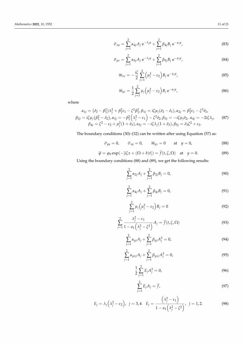
The boundary conditions (30)–(32) can be written after using Equation (57) as:

σyy = 0, σxy = 0, myz = 0 at y = 0, (88)

ϕ = ϕ0 exp(−[iζx + (Ω + b)t]) = f (t, ζ, Ω) at y = 0. (89)

Using the boundary conditions (88) and (89), we get the following results:

2

∑j=1

α2j Aj +2

∑j=1

β2jBj = 0, (90)

2

∑j=1

α4j Aj +2

∑j=1

β4jBj = 0, (91)

2

∑j=1

µj

(µ2

j − ε2

)Bj = 0 (92)

2

∑j=1

λ2j − ε1

1− a1

(λ2

j − ζ2)Aj = f (t, ζ, Ω) (93)

2

∑j=1

αyj Aj +2

∑j=1

βyj A3j = 0, (94)

2

∑j=1

αyxj Aj +2

∑j=1

βyxj A3j = 0, (95)

12

2

∑j=1

Ej A3j = 0, (96)

2

∑j=1

Ej Aj = f , (97)

Ej = λj

(λ2

j − ε2

), j = 3, 4 Ej =

(λ2

j − ε1

)1− a1

(λ2

j − ζ2) , j = 1, 2. (98)

Mathematics 2022, 10, 1552 12 of 21

After solving the system of equations above, the constants Aj, Bj,(j = 1, 2) can be set.Thus, the full expressions for the different studied physical fields have been obtained.

7. Discussion of the Numerical Results

We now present some discussion of the numerical results of the physical field variablesto highlight the theoretical results and the derived mathematical model in the previoussections. For the purpose of comparisons, an investigation will be conducted on a mag-nesium crystal material. At standard temperature T0 = 298 K, the values of the physicalparameters are [48]:

λ = 9.4× 1010(N/m2), µ = 4.5× 1010(N/m2),α = 0.5× 1010(N/m2), υ + β = 0.779× 10−5(N/m2),

K = 1.7× 102(J/msK), CE = 1.04× 103(J/kgK),ρ = 1.74× 103kg/m3, j = 0.2× 10−19m2, γ = 0.779× 10−9N.

We may take Ω as real (Ω = 2) for small values of time. The other physical values areassumed to be [48]: ζ = 2, L = 2, a1 = 0.2, ϕ0 = 1, and b = 1.

The calculations are performed at non-dimensional time t = 0.2, in the surface x = 0.1during the interval 0 ≤ y ≤ 3, taking into account the real component of the amplitude ofthe physical field variables shown on the vertical axis. At different vertical positions ofthe y-axis, the distributions of conductive and dynamic temperatures (ϕ and θ), thermalstresses (σxx, σyy, and σyx), the components of the displacement vector (u and v), micro-rotation ω and the components of the couple stress myz will be graphically illustrated asa result of changing some effective parameters such as the discrepancy coefficient a1 aswell as the higher orders of time derivatives m and n. Some comparisons were also madebetween the different models in the presence or absence of the micropolar.

The graphs show that the discrepancy coefficient a1 and the higher orders of timederivatives m and n have a substantial effect on all the physical fields. It is also shownthat, depending on the value of the higher order of the time derivatives as well as thediscrepancy coefficient a1, thermal and mechanical waves achieve a stable state. As aresult of this analysis, it is necessary to consider the effect of these parameters and also todistinguish between dynamic and conductivity temperatures.

We remember that Chirita et al. [51,52] gave interesting results with respect to somelimitations when considering more information about the possibilities available for Taylorseries expansion orders m and n. They demonstrated that m > 5 or n > 5 equivalentmodels always lead to mechanically unstable systems (see also [53]). When expansionorders are less than or equal to four, the necessary models can be thermodynamicallyconsistent if appropriate assumptions are made throughout the delay [54,55].

In this section, the differences in the distribution of the studied fields with distance ywill be studied in the case of the thermoelastic micropolar model and two temperatures withone relaxation time (2MLS), in the case of the two-temperature micropolar thermoelasticmodel with dual-phase lag (2MDPL), and in the case of the one/two-temperature thermoe-lastic dual-phase lag model and higher orders of time derivatives in the presence and ab-sence of the micropolar (2MHDPL, 2HDPL and 1HDPL), respectively. In fact, Figures 2–10represent the amount of thermodynamic processes that occurred within the material underinvestigation. We note that the theories of thermoelasticity with two temperatures can beobtained if we ignore the effect of micropolarity, that is, when α = β = α = υ = ε = j = 0.One-temperature thermoelastic theories can also be obtained in the case of a1 = 0. Fromthe tables and the results obtained in references [10,12,14], it was found that it is sufficientto put m = 3 and n = 2 to get close to each other’s results.

Mathematics 2022, 10, 1552 13 of 21Mathematics 2022, 10, x FOR PEER REVIEW 13 of 21

Figure 2. Dynamic temperature fluctuations 휃 for various models of thermoelasticity in the pres-

ence and absence of micropolarity.

Figure 3. Conductive temperature fluctuations 𝜑 for various models of thermoelasticity in the

presence and absence of micropolarity.

Figure 2. Dynamic temperature fluctuations θ for various models of thermoelasticity in the presenceand absence of micropolarity.

Mathematics 2022, 10, x FOR PEER REVIEW 13 of 21

Figure 2. Dynamic temperature fluctuations 휃 for various models of thermoelasticity in the pres-

ence and absence of micropolarity.

Figure 3. Conductive temperature fluctuations 𝜑 for various models of thermoelasticity in the

presence and absence of micropolarity. Figure 3. Conductive temperature fluctuations ϕ for various models of thermoelasticity in thepresence and absence of micropolarity.

Mathematics 2022, 10, 1552 14 of 21Mathematics 2022, 10, x FOR PEER REVIEW 14 of 21

Figure 4. Normal displacement fluctuations 𝑢 for various models of thermoelasticity in the pres-

ence and absence of micropolarity.

Figure 5. Tangential displacement fluctuations 𝑣 for various models of thermoelasticity in the

presence and absence of micropolarity.

Figure 4. Normal displacement fluctuations u for various models of thermoelasticity in the presenceand absence of micropolarity.

Mathematics 2022, 10, x FOR PEER REVIEW 14 of 21

Figure 4. Normal displacement fluctuations 𝑢 for various models of thermoelasticity in the pres-

ence and absence of micropolarity.

Figure 5. Tangential displacement fluctuations 𝑣 for various models of thermoelasticity in the

presence and absence of micropolarity. Figure 5. Tangential displacement fluctuations v for various models of thermoelasticity in thepresence and absence of micropolarity.

Mathematics 2022, 10, 1552 15 of 21Mathematics 2022, 10, x FOR PEER REVIEW 15 of 21

Figure 6. The normal stress variation 𝜎𝑥𝑥 for various models of thermoelasticity in the presence

and absence of micropolarity.

Figure 7. The normal stress variation 𝜎𝑦𝑦 for various models of thermoelasticity in the presence

and absence of micropolarity.

Figure 6. The normal stress variation σxx for various models of thermoelasticity in the presence andabsence of micropolarity.

Mathematics 2022, 10, x FOR PEER REVIEW 15 of 21

Figure 6. The normal stress variation 𝜎𝑥𝑥 for various models of thermoelasticity in the presence

and absence of micropolarity.

Figure 7. The normal stress variation 𝜎𝑦𝑦 for various models of thermoelasticity in the presence

and absence of micropolarity. Figure 7. The normal stress variation σyy for various models of thermoelasticity in the presence andabsence of micropolarity.

Mathematics 2022, 10, 1552 16 of 21Mathematics 2022, 10, x FOR PEER REVIEW 16 of 21

Figure 8. The shear stress variation 𝜎𝑦𝑥 for various models of thermoelasticity in the presence and

absence of micropolarity.

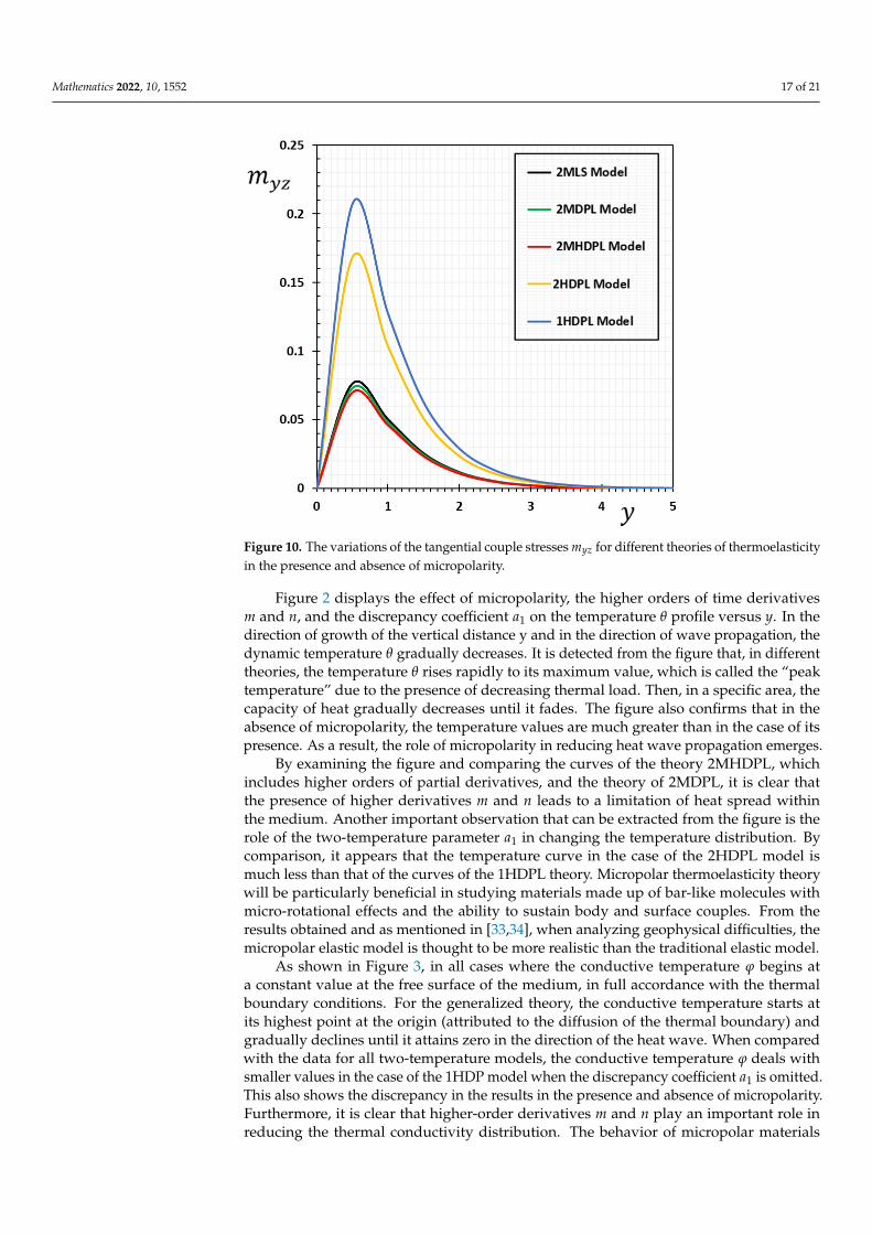
Figure 9. The variations of the micro-rotation 𝜔 for various models of thermoelasticity in the

presence and absence of micropolarity.

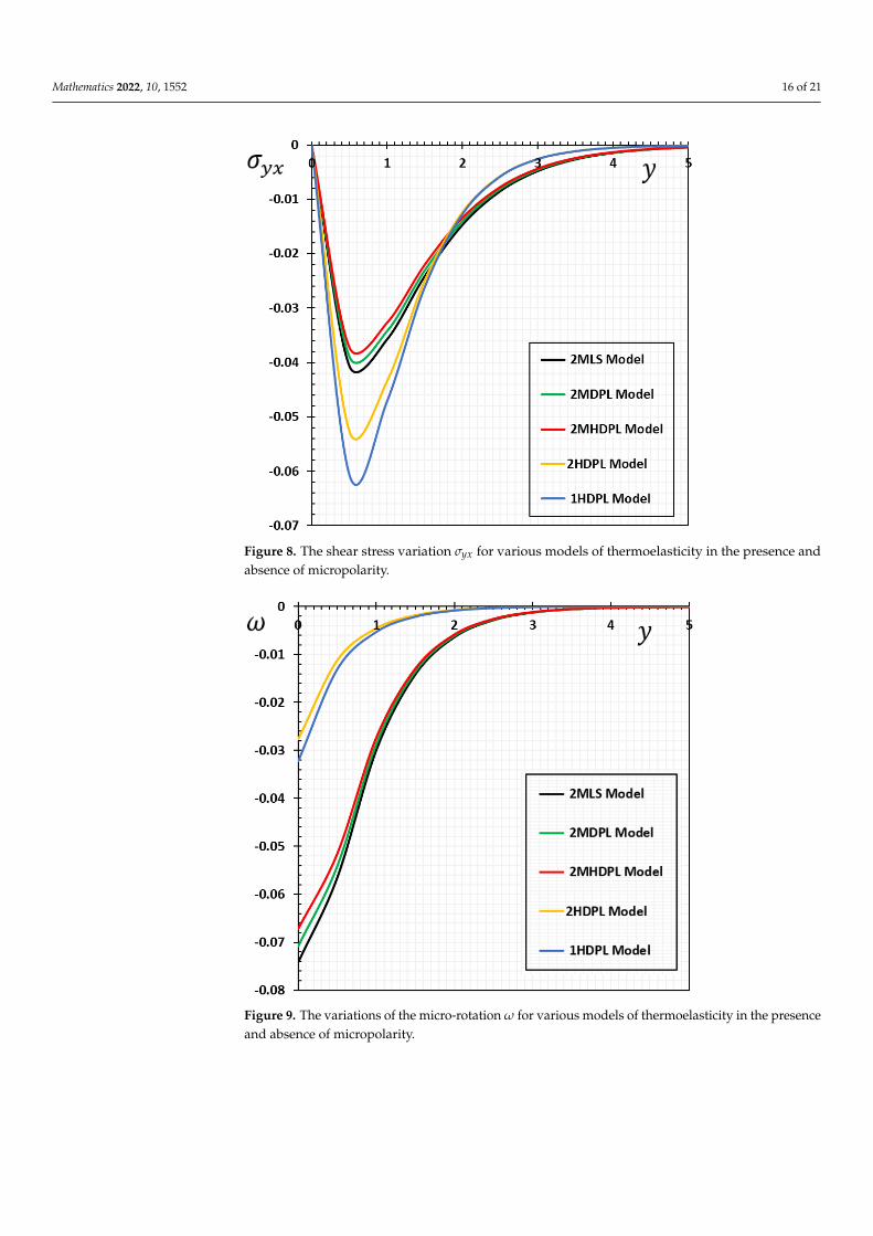
Figure 8. The shear stress variation σyx for various models of thermoelasticity in the presence andabsence of micropolarity.

Mathematics 2022, 10, x FOR PEER REVIEW 16 of 21

Figure 8. The shear stress variation 𝜎𝑦𝑥 for various models of thermoelasticity in the presence and

absence of micropolarity.

Figure 9. The variations of the micro-rotation 𝜔 for various models of thermoelasticity in the

presence and absence of micropolarity.

Figure 9. The variations of the micro-rotation ω for various models of thermoelasticity in the presenceand absence of micropolarity.

Mathematics 2022, 10, 1552 17 of 21

Mathematics 2022, 10, x FOR PEER REVIEW 17 of 21

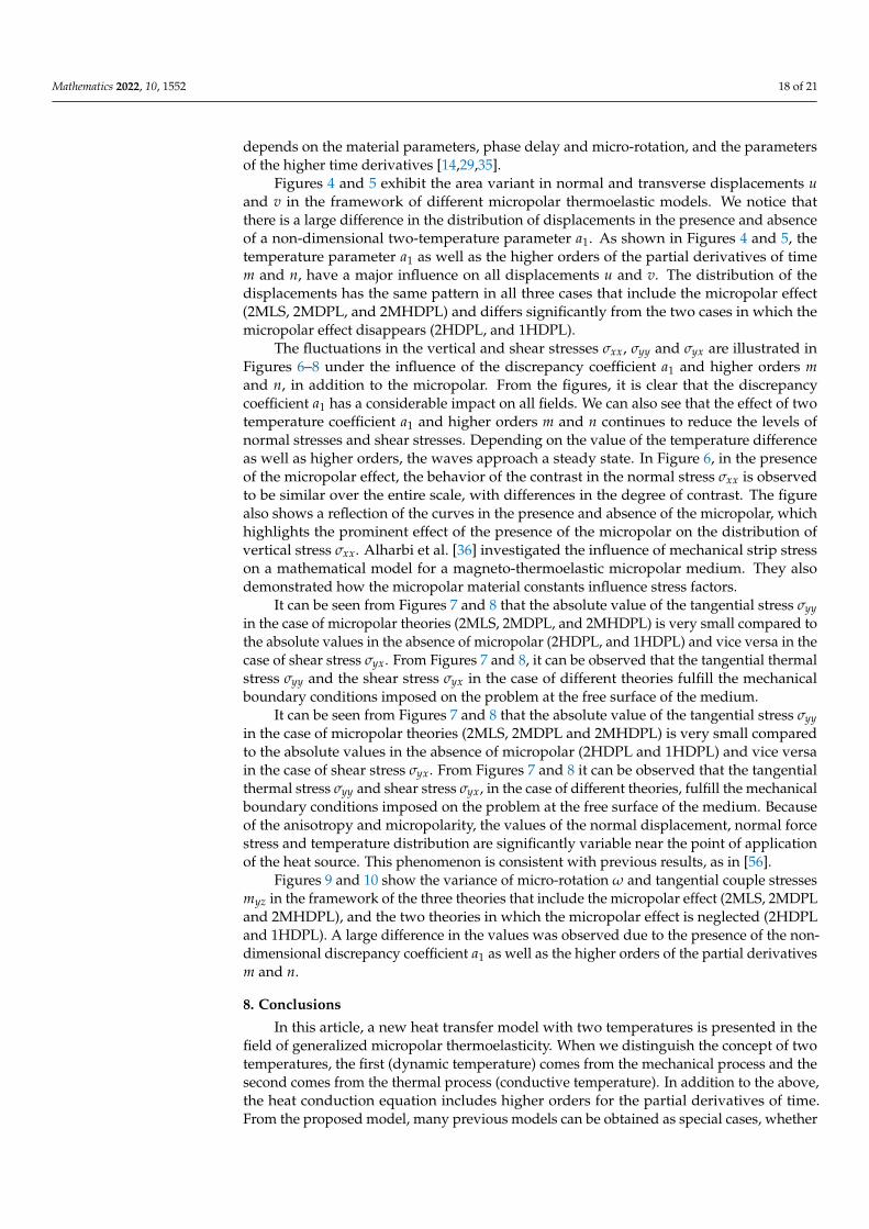
Figure 10. The variations of the tangential couple stresses 𝑚𝑦𝑧 for different theories of thermoe-

lasticity in the presence and absence of micropolarity.

Figure 2 displays the effect of micropolarity, the higher orders of time derivatives 𝑚

and 𝑛, and the discrepancy coefficient 𝑎1 on the temperature 휃 profile versus 𝑦. In the

direction of growth of the vertical distance y and in the direction of wave propagation,

the dynamic temperature 휃 gradually decreases. It is detected from the figure that, in

different theories, the temperature 휃 rises rapidly to its maximum value, which is called

the “peak temperature” due to the presence of decreasing thermal load. Then, in a specific

area, the capacity of heat gradually decreases until it fades. The figure also confirms that in

the absence of micropolarity, the temperature values are much greater than in the case of

its presence. As a result, the role of micropolarity in reducing heat wave propagation

emerges.

By examining the figure and comparing the curves of the theory 2MHDPL, which

includes higher orders of partial derivatives, and the theory of 2MDPL, it is clear that the

presence of higher derivatives 𝑚 and 𝑛 leads to a limitation of heat spread within the

medium. Another important observation that can be extracted from the figure is the role

of the two-temperature parameter 𝑎1 in changing the temperature distribution. By

comparison, it appears that the temperature curve in the case of the 2HDPL model is

much less than that of the curves of the 1HDPL theory. Micropolar thermoelasticity the-

ory will be particularly beneficial in studying materials made up of bar-like molecules

with micro-rotational effects and the ability to sustain body and surface couples. From

the results obtained and as mentioned in [33,34], when analyzing geophysical difficulties,

the micropolar elastic model is thought to be more realistic than the traditional elastic

model.

As shown in Figure 3, in all cases where the conductive temperature 𝜑 begins at a

constant value at the free surface of the medium, in full accordance with the thermal

boundary conditions. For the generalized theory, the conductive temperature starts at its

highest point at the origin (attributed to the diffusion of the thermal boundary) and

gradually declines until it attains zero in the direction of the heat wave. When compared

with the data for all two-temperature models, the conductive temperature 𝜑 deals with

smaller values in the case of the 1HDP model when the discrepancy coefficient 𝑎1 is

omitted. This also shows the discrepancy in the results in the presence and absence of

micropolarity. Furthermore, it is clear that higher-order derivatives 𝑚 and 𝑛 play an

important role in reducing the thermal conductivity distribution. The behavior of mi-

cropolar materials depends on the material parameters, phase delay and micro-rotation,

and the parameters of the higher time derivatives [14,29,35].

Figure 10. The variations of the tangential couple stresses myz for different theories of thermoelasticityin the presence and absence of micropolarity.

Figure 2 displays the effect of micropolarity, the higher orders of time derivativesm and n, and the discrepancy coefficient a1 on the temperature θ profile versus y. In thedirection of growth of the vertical distance y and in the direction of wave propagation, thedynamic temperature θ gradually decreases. It is detected from the figure that, in differenttheories, the temperature θ rises rapidly to its maximum value, which is called the “peaktemperature” due to the presence of decreasing thermal load. Then, in a specific area, thecapacity of heat gradually decreases until it fades. The figure also confirms that in theabsence of micropolarity, the temperature values are much greater than in the case of itspresence. As a result, the role of micropolarity in reducing heat wave propagation emerges.

By examining the figure and comparing the curves of the theory 2MHDPL, whichincludes higher orders of partial derivatives, and the theory of 2MDPL, it is clear thatthe presence of higher derivatives m and n leads to a limitation of heat spread withinthe medium. Another important observation that can be extracted from the figure is therole of the two-temperature parameter a1 in changing the temperature distribution. Bycomparison, it appears that the temperature curve in the case of the 2HDPL model ismuch less than that of the curves of the 1HDPL theory. Micropolar thermoelasticity theorywill be particularly beneficial in studying materials made up of bar-like molecules withmicro-rotational effects and the ability to sustain body and surface couples. From theresults obtained and as mentioned in [33,34], when analyzing geophysical difficulties, themicropolar elastic model is thought to be more realistic than the traditional elastic model.

As shown in Figure 3, in all cases where the conductive temperature ϕ begins ata constant value at the free surface of the medium, in full accordance with the thermalboundary conditions. For the generalized theory, the conductive temperature starts atits highest point at the origin (attributed to the diffusion of the thermal boundary) andgradually declines until it attains zero in the direction of the heat wave. When comparedwith the data for all two-temperature models, the conductive temperature ϕ deals withsmaller values in the case of the 1HDP model when the discrepancy coefficient a1 is omitted.This also shows the discrepancy in the results in the presence and absence of micropolarity.Furthermore, it is clear that higher-order derivatives m and n play an important role inreducing the thermal conductivity distribution. The behavior of micropolar materials

Mathematics 2022, 10, 1552 18 of 21

depends on the material parameters, phase delay and micro-rotation, and the parametersof the higher time derivatives [14,29,35].

Figures 4 and 5 exhibit the area variant in normal and transverse displacements uand v in the framework of different micropolar thermoelastic models. We notice thatthere is a large difference in the distribution of displacements in the presence and absenceof a non-dimensional two-temperature parameter a1. As shown in Figures 4 and 5, thetemperature parameter a1 as well as the higher orders of the partial derivatives of timem and n, have a major influence on all displacements u and v. The distribution of thedisplacements has the same pattern in all three cases that include the micropolar effect(2MLS, 2MDPL, and 2MHDPL) and differs significantly from the two cases in which themicropolar effect disappears (2HDPL, and 1HDPL).

The fluctuations in the vertical and shear stresses σxx, σyy and σyx are illustrated inFigures 6–8 under the influence of the discrepancy coefficient a1 and higher orders mand n, in addition to the micropolar. From the figures, it is clear that the discrepancycoefficient a1 has a considerable impact on all fields. We can also see that the effect of twotemperature coefficient a1 and higher orders m and n continues to reduce the levels ofnormal stresses and shear stresses. Depending on the value of the temperature differenceas well as higher orders, the waves approach a steady state. In Figure 6, in the presenceof the micropolar effect, the behavior of the contrast in the normal stress σxx is observedto be similar over the entire scale, with differences in the degree of contrast. The figurealso shows a reflection of the curves in the presence and absence of the micropolar, whichhighlights the prominent effect of the presence of the micropolar on the distribution ofvertical stress σxx. Alharbi et al. [36] investigated the influence of mechanical strip stresson a mathematical model for a magneto-thermoelastic micropolar medium. They alsodemonstrated how the micropolar material constants influence stress factors.

It can be seen from Figures 7 and 8 that the absolute value of the tangential stress σyyin the case of micropolar theories (2MLS, 2MDPL, and 2MHDPL) is very small compared tothe absolute values in the absence of micropolar (2HDPL, and 1HDPL) and vice versa in thecase of shear stress σyx. From Figures 7 and 8, it can be observed that the tangential thermalstress σyy and the shear stress σyx in the case of different theories fulfill the mechanicalboundary conditions imposed on the problem at the free surface of the medium.

It can be seen from Figures 7 and 8 that the absolute value of the tangential stress σyyin the case of micropolar theories (2MLS, 2MDPL and 2MHDPL) is very small comparedto the absolute values in the absence of micropolar (2HDPL and 1HDPL) and vice versain the case of shear stress σyx. From Figures 7 and 8 it can be observed that the tangentialthermal stress σyy and shear stress σyx, in the case of different theories, fulfill the mechanicalboundary conditions imposed on the problem at the free surface of the medium. Becauseof the anisotropy and micropolarity, the values of the normal displacement, normal forcestress and temperature distribution are significantly variable near the point of applicationof the heat source. This phenomenon is consistent with previous results, as in [56].

Figures 9 and 10 show the variance of micro-rotation ω and tangential couple stressesmyz in the framework of the three theories that include the micropolar effect (2MLS, 2MDPLand 2MHDPL), and the two theories in which the micropolar effect is neglected (2HDPLand 1HDPL). A large difference in the values was observed due to the presence of the non-dimensional discrepancy coefficient a1 as well as the higher orders of the partial derivativesm and n.

8. Conclusions

In this article, a new heat transfer model with two temperatures is presented in thefield of generalized micropolar thermoelasticity. When we distinguish the concept of twotemperatures, the first (dynamic temperature) comes from the mechanical process and thesecond comes from the thermal process (conductive temperature). In addition to the above,the heat conduction equation includes higher orders for the partial derivatives of time.From the proposed model, many previous models can be obtained as special cases, whether

Mathematics 2022, 10, 1552 19 of 21

in the presence or absence of the micropolar effects, as long as the discrepancy coefficient isneglected. The suggested thermoelastic model was used to examine the behavior of thermalstresses, temperatures, displacements, and micro-rotation in an isotropic, homogeneous,micropolar, thermoelastic half-space by means of normal mode analysis. Calculations anddiscussions showed the following conclusions:

• The results indicate that the discrepancy coefficient has a substantial influence on thethermoelastic distributions within the medium, but the effect on the displacementsand thermal stress disturbances is very clear;

• There is a large discrepancy in the results between the cases of theories that includetwo-temperature and those that include one-temperature. The coefficient of two-temperature works to reduce thermal and mechanical waves. Thus, the study of elasticbodies in the case of two-temperature theories is more realistic than the generalizedthermoelastic theory at one temperature. Thus, the so-called conductive heat wavemust be separated from the so-called thermodynamic heat wave;

• Higher orders for partial derivatives play a critical role in all distributions of theinvestigated domain variables. Thermal and mechanical waves are reduced by usinghigher orders for partial derivatives. Thus, the extended theory with phase lag timesand higher order derivatives may be a better option for describing thermoelasticitythan the previous generalized theories as well as the traditional ones;

• Micropolarity has a substantial impact on all of the domains covered. Except fortangential stress and thermodynamical temperature, micropolarity has a diminishinginfluence on the magnitudes of all thermo-physical fields investigated.

Finally, when examining the real behavior of some properties of materials in conjunc-tion with the appropriate geometry of the presented model, the proposed problem takeson a whole new meaning. For example, within the earth, precious materials such as oiland liquid-like elements are found in unrefined form, while the rocks and minerals presentmay be granular in nature. The fields of geomechanics, seismic engineering, soil dynamics,and other fields are also considered to have practical applications for the specialization ofthermal elasticity and waves.

Author Contributions: Conceptualization: A.E.A., M.M. and F.A.; methodology: A.E.A. and F.A.;validation: A.E.A., F.A. and M.M.; formal analysis: A.E.A., F.A. and M.M.; investigation: A.E.A., M.M.and F.A.; resources: F.A.; data curation: A.E.A., F.A. and M.M.; writing—original draft preparation:A.E.A., F.A. and M.M.; writing—review and editing: A.E.A.; visualization: F.A. and M.M.; supervision:A.E.A., F.A. and M.M.; project administration: A.E.A. All authors have read and agreed to thepublished version of the manuscript.

Funding: The Deanship of Scientific Research at Jouf University, Saudi Arabia funded this projectunder grant No. (DSR-2021-03-0376).

Institutional Review Board Statement: Not Applicable.

Informed Consent Statement: Not Applicable.

Data Availability Statement: The authors confirm that the data supporting the findings of this studyare available within the article.

Acknowledgments: The authors extend their appreciation to the core member of Scientific Researchat Jouf University for funding this work through research. We would also like to extend our sincerethanks to the College of Science and Arts in Al-Qurayyat for its technical support.

Conflicts of Interest: The authors declare no conflict of interest.

References1. Biot, M. Thermoelasticity and irreversible thermodynamics. J. Appl. Phys. 1956, 27, 240–253. [CrossRef]2. Lord, H.W.; Shulman, Y.H. A generalized dynamical theory of thermoelasticity. J. Mech. Phys. Solids 1967, 15, 299–309. [CrossRef]3. Green, A.E.; Naghdi, P.M. A re-examination of the basic results of thermomechanics. Proc. Math. Phys. Sci. 1991, 432, 171–194.4. Green, A.E.; Lindsay, K.A. Thermoelasticity. J. Elast. 1972, 2, 1–7. [CrossRef]5. Green, A.E.; Naghdi, P.M. On undamped heat waves in an elastic solid. J. Therm. Stress. 1992, 15, 252–264. [CrossRef]

Mathematics 2022, 10, 1552 20 of 21

6. Green, A.E.; Naghdi, P.M. Thermoelasticity without energy dissipation. J. Elast. 1993, 31, 189–208. [CrossRef]7. Tzou, D.Y. A unified filed approach for heat conduction from macro to macroscales. ASME J. Heat Transf. 1995, 117, 8–16.

[CrossRef]8. Tzou, D.Y. The generalized lagging response in small-scale and high-rate heating. Int. J. Heat Mass Transf. 1995, 38, 3231–3234.

[CrossRef]9. Tzou, D.Y. Experimental support for the lagging behavior in heat propagation. J. Thermophys. Heat Transf. 1995, 9, 686–693.

[CrossRef]10. Abouelregal, A.E. Two-temperature thermoelastic model without energy dissipation including higher order time-derivatives and

two phase-lags. Mater. Res. Express 2019, 6, 116535. [CrossRef]11. Abouelregal, A.E. On Green and Naghdi thermoelasticity model without energy dissipation with higher order time differential

and phase-lags. J. Appl. Comput. Mech. 2020, 6, 445–456.12. Abouelregal, A.E. A novel generalized thermoelasticity with higher-order time-derivatives and three-phase lags. Multidiscip.

Model. Mater. Struct. 2019, 16, 689–711. [CrossRef]13. Abouelregal, A.E. A novel model of nonlocal thermoelasticity with time derivatives of higher order. Math. Methods Appl. Sci.

2020, 43, 6746–6760. [CrossRef]14. Abouelregal, A.E. Three-phase-lag thermoelastic heat conduction model with higher-order time-fractional derivatives. Indian J.

Phys. 2020, 94, 1949–1963. [CrossRef]15. Choudhuri, S.R. On a thermoelastic three-phase-lag model. J. Therm. Stress. 2007, 30, 231–238. [CrossRef]16. Chen, P.J.; Gurtin, M.E. On a theory of heat conduction involving two temperatures. Z. Angew. Math. Phys. 1968, 19, 614–627.

[CrossRef]17. Chen, P.J.; Williams, W.O. A note on non-simple heat conduction. Z. Angew. Math. Phys. 1968, 19, 969–970. [CrossRef]18. Chen, P.J.; Gurtin, M.E.; Williams, W.O. On the thermodynamics of non-simple elastic materials with two temperatures. Z. Angew.

Math. Phys. 1969, 20, 107–112. [CrossRef]19. Quintanilla, R. On existence, structural stability, convergence and spatial behavior in thermoelasticity with two temperatures.

Acta Mech. 2004, 168, 61–73. [CrossRef]20. Youssef, H. Theory of two-temperature-generalized thermoelasticity. IMA J. Appl. Math. 2006, 71, 383–390. [CrossRef]21. Ezzat, M.A.; El-Karamany, A.S. Two temperature theory in generalized magneto thermoelasticity with two relaxation times.

Meccanica 2011, 46, 785–794. [CrossRef]22. Mukhopadhyay, S.; Prasad, R.; Kumar, R. On the theory of two-temperature thermoelasticity with two phase-lags. J. Therm. Stress.

2011, 34, 352–365. [CrossRef]23. Mukhopadhyay, S.; Kumar, R. Thermoelastic Interactions on Two-Temperature Generalized Thermoelasticity in an Infinite

Medium with a Cylindrical Cavity. J. Therm. Stress. 2009, 32, 341–360. [CrossRef]24. Fernández, J.R.; Quintanilla, R. Uniqueness and exponential instability in a new two-temperature thermoelastic theory. AIMS

Math. 2021, 6, 5440–5451. [CrossRef]25. Sarkar, N.; Mondal, S. Two-dimensional problem of two-temperature generalized thermoelasticity using memory-dependent heat

transfer: An integral transform approach. Indian J. Phys. 2020, 94, 1965–1974. [CrossRef]26. Hobiny, A.; Alzahrani, F.; Abbas, I.; Marin, M. The effect of fractional time derivative of bioheat model in skin tissue induced to

laser irradiation. Symmetry 2020, 12, 602. [CrossRef]27. Hassanpour, S.; Heppler, G.R. Micropolar elasticity theory: A survey of linear isotropic equations, representative notations, and

experimental investigations. Math. Mech. Solids 2017, 22, 224–242. [CrossRef]28. Eringen, A.C. Linear theory of micropolar elasticity. J. Appl. Math. Mech. 1966, 15, 909–923.29. Abouelregal, A.E.; Marin, M. The size-dependent thermoelastic vibrations of nanobeams subjected to harmonic excitation and

rectified sine wave heating. Mathematics 2020, 8, 1128. [CrossRef]30. Nowacki, W. Theory of Asymmetric Elasticity; Pergamon Press: Oxford, NY, USA, 1986.31. Eringen, A.C. Foundations of Micropolar Thermoelasticity; International Centre for Mechanical Science, Udine Course and Lectures

23; Springer: Berlin, Germany, 1970.32. Tauchert, T.R.; Claus, W.D.; Ariman, T. The linear theory of micropolar thermoelasticity. Int. J. Eng. Sci. 1968, 6, 37–47. [CrossRef]33. Dost, S.; Tabarrok, B. Generalized micropolar thermoelasticity. Int. J. Eng. Sci. 1978, 16, 173. [CrossRef]34. Chandrasekhariah, D.S. Heat flux dependent micropolar elasticity. Int. J. Eng. Sci. 1986, 24, 1389–1395. [CrossRef]35. El-Karamany, A.S.; Ezzat, M.A. On the three-phase-lag linear micropolar thermoelasticity theory. Eur. J. Mech.-A Solids 2013,

40, 198–208. [CrossRef]36. Alharbi, A.M.; Said, S.M.; Abd-Elaziz, E.M.; Othman, M.I.A. Mathematical model for a magneto-thermoelastic micropolar

medium with temperature-dependent material moduli under the effect of mechanical strip load. Acta Mech. 2021, 232, 2331–2346.[CrossRef]

37. Marin, M.; Othman, M.I.A.; Abbas, I.A. An extension of the domain of influence theorem for generalized thermoelasticity ofanisotropic material with voids. J. Comput. Theor. Nanosci. 2015, 12, 1594–1598. [CrossRef]

38. Sharma, H.; Kumari, S.; Kumar, A. Study of micropolar thermo-elasticity. Adv. Math. Sci. Appl. 2020, 19, 929–941.39. Hilal, M.I.M.; Abd-Elaziz, E.M.; Hanoura, S.A. Reflection of plane waves in magneto-micropolar thermoelastic medium with

voids and one relaxation time due to gravity and two-temperature theory. Indian J. Phys. 2021, 95, 915–924. [CrossRef]

Mathematics 2022, 10, 1552 21 of 21

40. Kumar, R.; Prasad, R.; Kumar, R. Thermoelastic interactions on hyperbolic two-temperature generalized thermoelasticity in aninfinite medium with a cylindrical cavity. Eur. J. Mech.-A Solids 2020, 8, 104007. [CrossRef]

41. Lianngenga, R.; Singh, S.S. Reflection of coupled dilatational and shear waves in the generalized micropolar thermoelasticmaterials. J. Vib. Control 2020, 26, 1948–1955. [CrossRef]

42. Othman, M.I.A.; Said, S.; Marin, M. A novel model of plane waves of two-temperature fiber-reinforced thermoelastic mediumunder the effect of gravity with three-phase-lag model. Int. J. Numer. Methods Heat Fluid Flow 2019, 29, 4788–4806. [CrossRef]

43. Abouelregal, A.E.; Zenkour, A.M. Two-temperature thermoelastic surface waves in micropolar thermoelastic media via dual-phase-lag model. Adv. Aircr. Spacecr. Sci. 2017, 4, 711–727.

44. Guesmia, A.; Muñoz Rivera, J.E.; Sepúlveda Cortés, M.A.; Vera Villagrán, O. Well-posedness and stability of a generalizedmicropolar thermoelastic body with infinite memory. Q. J. Math. 2021, 72, 1495–1515. [CrossRef]

45. Marin, M. Harmonic vibrations in thermoelasticity of microstretch materials. J. Vib. Acoust. Trans. ASME 2010, 132, 044501.[CrossRef]

46. Kumar, R.; Abbas, I.A. Deformation due to thermal source in micropolar thermoelastic media with thermal and conductivetemperatures. J. Comput. Theor. Nanosci. 2013, 10, 2241–2247. [CrossRef]

47. Shaw, S.; Mukhopadhyay, B. Moving heat source response in micropolar half-space with two-temperature theory. Contin. Mech.Thermodyn. 2013, 25, 523–535. [CrossRef]

48. Ezzat, M.A.; Awad, E.S. Constitutive relations, uniqueness of solution and thermal shock application in the linear theory ofmicropolar generalized thermoelasticity involving two temperatures. J. Therm. Stress. 2010, 33, 226–250. [CrossRef]

49. Quintanilla, R. Exponential stability and uniqueness in thermoelasticity with two temperatures, Dynamics Continous. Discret.Impulsive Sys. Ser. A Math. Anal. 2004, 11, 57–68.

50. Quintanilla, R. A well posed problem for the Dual-Phase-Lag heat conduction. J. Therm. Stress. 2008, 31, 260–269. [CrossRef]51. Chirită, S. On the time differential dual-phase-lag thermoelastic model. Meccanica 2017, 52, 349–361. [CrossRef]52. Chirită, S.; Ciarletta, M.; Tibullo, V. On the thermomechanic consistency of the time differential dual-phase-lag models of heat

conduction. Int. J. Heat Mass Transf. 2017, 114, 277–285. [CrossRef]53. Chirită, S.; Ciarletta, M.; Tibullo, V. The wave propagation in the time differential dual-phase-lag thermoelastic model. Proc. R.

Soc. A 2015, 471, 20150400. [CrossRef]54. Chirită, S. High-order approximations of three-phase-lag heat conduction model: Some qualitative results. J. Therm. Stress. 2018,

41, 608–626. [CrossRef]55. Chirită, S.; D’Apice, C.; Zampoli, V. The time differential three-phase-lag heat conduction model: Thermodynamic compatibility

and continuous dependence. Int. J. Heat Mass Transf. 2016, 102, 226–232. [CrossRef]56. Praveen, A.; Kumar, S.S.; Devinder, P. A two dimensional fibre reinforced micropolar thermoelastic problem for a half-space

subjected to mechanical force. Theoret. Appl. Mech. 2015, 42, 11–25.