
Plane Answers to Complex Questions - Index of
517
-
Upload
khangminh22 -
Category
Documents
-
view
1 -
download
0
Transcript of Plane Answers to Complex Questions - Index of


For other titles published in this series, go towww.springer.com/series/417
G. Casella S. Fienberg I. Olkin
Series Editors
Springer Texts in Statistics


Ronald Christensen
The Theory of Linear Models
Fourth edition
Plane Answers to ComplexQuestions

ISSN 1431-875X ISBN 978-1-4419-9815-6 e-ISBN 978-1-4419-9816-3
Springer New York Dordrecht Heidelberg London
All rights reserved. This work may not be translated or copied in whole or in part without the written permission of the publisher (Springer Science+Business Media, LLC, 233 Spring Street, New York, NY 10013, USA), except for brief excerpts in connection with reviews or scholarly analysis. Use in connection with any form of information storage and retrieval, electronic adaptation, computer software, or by similar or dissimilar methodology now known or hereafter developed is forbidden. The use in this publication of trade names, trademarks, service marks, and similar terms, even if they are not identified as such, is not to be taken as an expression of opinion as to whether or not they are subject to proprietary rights.
Printed on acid-free paper
Ronald Christensen Department of Mathematics and Statistics
USA
DOI 10.1007/978-1-4419-9816-3
Library of Congress Control Number: 2011928555
© Springer Science+Business Media, LLC 2011
Albuquerque, New Mexico, 87131-0001
MSC01 11151 University of New Mexico
Department of Statistics
USA
Department of Statistics
Gainesville, Pittsburgh, PA 15213-3890
Department of Statistics
USA
Stanford University Stanford, CA 94305FL 32611-8545
USA
Ingram OlkinGeorge CasellaSeries Editors:
Carnegie Mellon University University of Florida
Stephen Fienberg
Springer is part of Springer Science+Business Media (www.springer.com)

To Dad, Mom, Sharon, Fletch, and Don


Preface
Preface to the Fourth Edition
“Critical assessment of data is the the essential task of the educated mind.”Professor Garrett G. Fagan, Pennsylvania State University.
The last words in his audio course The Emperors of Rome, The Teaching Company.
As with the prefaces to the second and third editions, this focuses on changes tothe previous edition. The preface to the first edition discusses the core of the book.
Two substantial changes have occurred in Chapter 3. Subsection 3.3.2 uses a sim-plified method of finding the reduced model and includes some additional discus-sion of applications. In testing the generalized least squares models of Section 3.8,even though the data may not be independent or homoscedastic, there are conditionsunder which the standard F statistic (based on those assumptions) still has the stan-dard F distribution under the reduced model. Section 3.8 contains a new subsectionexamining such conditions.
The major change in the fourth edition has been a more extensive discussion ofbest prediction and associated ideas of R2 in Sections 6.3 and 6.4. It also includes anice result that justifies traditional uses of residual plots. One portion of the new ma-terial is viewing best predictors (best linear predictors) as perpendicular projectionsof the dependent random variable y into the space of random variables that are (lin-ear) functions of the predictor variables x. A new subsection on inner products andperpendicular projections for more general spaces facilitates the discussion. Whilethese ideas were not new to me, their inclusion here was inspired by deLaubenfels(2006).
Section 9.1 has an improved discussion of least squares estimation in ACOVAmodels. A new Section 9.5 examines Milliken and Graybill’s generalization ofTukey’s one degree of freedom for nonadditivity test.
A new Section 10.5 considers estimable parameters that can be known with cer-tainty when C(X) �⊂ C(V ) in a general Gauss–Markov model. It also contains a
vii

viii Preface
relatively simple way to estimate estimable parameters that are not known with cer-tainty. The nastier parts in Sections 10.1–10.4 are those that provide sufficient gen-erality to allow C(X) �⊂C(V ). The approach of Section 10.5 seems more appealing.
In Sections 12.4 and 12.6 the point is now made that ML and REML methodscan also be viewed as method of moments or estimating equations procedures.
The biggest change in Chapter 13 is a new title. The plots have been improvedand extended. At the end of Section 13.6 some additional references are given oncase deletions for correlated data as well as an efficient way of computing casedeletion diagnostics for correlated data.
The old Chapter 14 has been divided into two chapters, the first on variable se-lection and the second on collinearity and alternatives to least squares estimation.Chapter 15 includes a new section on penalized estimation that discusses both ridgeand lasso estimation and their relation to Bayesian inference. There is also a newsection on orthogonal distance regression that finds a regression line by minimizingorthogonal distances, as opposed to least squares, which minimizes vertical dis-tances.
Appendix D now contains a short proof of the claim: If the random vectors x andy are independent, then any vector-valued functions of them, say g(x) and h(y), arealso independent.
Another significant change is that I wanted to focus on Fisherian inference, ratherthan the previous blend of Fisherian and Neyman–Pearson inference. In the interestsof continuity and conformity, the differences are soft-pedaled in most of the book.They arise notably in new comments made after presenting the traditional (one-sided) F test in Section 3.2 and in a new Subsection 5.6.1 on multiple comparisons.The Fisherian viewpoint is expanded in Appendix F, which is where it primarilyoccurred in the previous edition. But the change is most obvious in Appendix E. Inall previous editions, Appendix E existed just in case readers did not already knowthe material. While I still expect most readers to know the “how to” of Appendix E,I no longer expect most to be familiar with the “why” presented there.
Other minor changes are too numerous to mention and, of course, I have cor-rected all of the typographic errors that have come to my attention. Comments byJarrett Barber led me to clean up Definition 2.1.1 on identifiability.
My thanks to Fletcher Christensen for general advice and for constructing Fig-ures 10.1 and 10.2. (Little enough to do for putting a roof over his head all thoseyears. :-)
Ronald ChristensenAlbuquerque, New Mexico, 2010

Preface ix
Preface to the Third Edition
The third edition of Plane Answers includes fundamental changes in how some as-pects of the theory are handled. Chapter 1 includes a new section that introducesgeneralized linear models. Primarily, this provides a definition so as to allow com-ments on how aspects of linear model theory extend to generalized linear models.
For years I have been unhappy with the concept of estimability. Just becauseyou cannot get a linear unbiased estimate of something does not mean you cannotestimate it. For example, it is obvious how to estimate the ratio of two contrasts inan ANOVA, just estimate each one and take their ratio. The real issue is that if themodel matrix X is not of full rank, the parameters are not identifiable. Section 2.1now introduces the concept of identifiability and treats estimability as a special caseof identifiability. This change also resulted in some minor changes in Section 2.2.
In the second edition, Appendix F presented an alternative approach to dealingwith linear parametric constraints. In this edition I have used the new approach inSection 3.3. I think that both the new approach and the old approach have virtues,so I have left a fair amount of the old approach intact.
Chapter 8 contains a new section with a theoretical discussion of models forfactorial treatment structures and the introduction of special models for homologousfactors. This is closely related to the changes in Section 3.3.
In Chapter 9, reliance on the normal equations has been eliminated from thediscussion of estimation in ACOVA models — something I should have done yearsago! In the previous editions, Exercise 9.3 has indicated that Section 9.1 shouldbe done with projection operators, not normal equations. I have finally changed it.(Now Exercise 9.3 is to redo Section 9.1 with normal equations.)
Appendix F now discusses the meaning of small F statistics. These can occurbecause of model lack of fit that exists in an unsuspected location. They can alsooccur when the mean structure of the model is fine but the covariance structure hasbeen misspecified.
In addition there are various smaller changes including the correction of typo-graphical errors. Among these are very brief introductions to nonparametric re-gression and generalized additive models; as well as Bayesian justifications for themixed model equations and classical ridge regression. I will let you discover theother changes for yourself.
Ronald ChristensenAlbuquerque, New Mexico, 2001


Preface xi
Preface to the Second Edition
The second edition of Plane Answers has many additions and a couple of dele-tions. New material includes additional illustrative examples in Appendices A andB and Chapters 2 and 3, as well as discussions of Bayesian estimation, near replicatelack of fit tests, testing the independence assumption, testing variance components,the interblock analysis for balanced incomplete block designs, nonestimable con-straints, analysis of unreplicated experiments using normal plots, tensors, and prop-erties of Kronecker products and Vec operators. The book contains an improveddiscussion of the relation between ANOVA and regression, and an improved pre-sentation of general Gauss–Markov models. The primary material that has beendeleted are the discussions of weighted means and of log-linear models. The mate-rial on log-linear models was included in Christensen (1997), so it became redun-dant here. Generally, I have tried to clean up the presentation of ideas wherever itseemed obscure to me.
Much of the work on the second edition was done while on sabbatical at theUniversity of Canterbury in Christchurch, New Zealand. I would particularly like tothank John Deely for arranging my sabbatical. Through their comments and criti-cisms, four people were particularly helpful in constructing this new edition. I wouldlike to thank Wes Johnson, Snehalata Huzurbazar, Ron Butler, and Vance Berger.
Ronald ChristensenAlbuquerque, New Mexico, 1996


Preface xiii
Preface to the First Edition
This book was written to rigorously illustrate the practical application of the pro-jective approach to linear models. To some, this may seem contradictory. I contendthat it is possible to be both rigorous and illustrative, and that it is possible to use theprojective approach in practical applications. Therefore, unlike many other bookson linear models, the use of projections and subspaces does not stop after the gen-eral theory. They are used wherever I could figure out how to do it. Solving normalequations and using calculus (outside of maximum likelihood theory) are anathemato me. This is because I do not believe that they contribute to the understanding oflinear models. I have similar feelings about the use of side conditions. Such topicsare mentioned when appropriate and thenceforward avoided like the plague.
On the other side of the coin, I just as strenuously reject teaching linear modelswith a coordinate free approach. Although Joe Eaton assures me that the issues incomplicated problems frequently become clearer when considered free of coordi-nate systems, my experience is that too many people never make the jump fromcoordinate free theory back to practical applications. I think that coordinate freetheory is better tackled after mastering linear models from some other approach. Inparticular, I think it would be very easy to pick up the coordinate free approach afterlearning the material in this book. See Eaton (1983) for an excellent exposition ofthe coordinate free approach.
By now it should be obvious to the reader that I am not very opinionated onthe subject of linear models. In spite of that fact, I have made an effort to identifysections of the book where I express my personal opinions.
Although in recent revisions I have made an effort to cite more of the literature,the book contains comparatively few references. The references are adequate to theneeds of the book, but no attempt has been made to survey the literature. This wasdone for two reasons. First, the book was begun about 10 years ago, right after Ifinished my Masters degree at the University of Minnesota. At that time I was notaware of much of the literature. The second reason is that this book emphasizesa particular point of view. A survey of the literature would best be done on theliterature’s own terms. In writing this, I ended up reinventing a lot of wheels. Myapologies to anyone whose work I have overlooked.
Using the Book
This book has been extensively revised, and the last five chapters were written atMontana State University. At Montana State we require a year of Linear Modelsfor all of our statistics graduate students. In our three-quarter course, I usually endthe first quarter with Chapter 4 or in the middle of Chapter 5. At the end of winterquarter, I have finished Chapter 9. I consider the first nine chapters to be the corematerial of the book. I go quite slowly because all of our Masters students are re-quired to take the course. For Ph.D. students, I think a one-semester course might be

xiv Preface
the first nine chapters, and a two-quarter course might have time to add some topicsfrom the remainder of the book.
I view the chapters after 9 as a series of important special topics from whichinstructors can choose material but which students should have access to even if theircourse omits them. In our third quarter, I typically cover (at some level) Chapters 11to 14. The idea behind the special topics is not to provide an exhaustive discussionbut rather to give a basic introduction that will also enable readers to move on tomore detailed works such as Cook and Weisberg (1982) and Haberman (1974).
Appendices A–E provide required background material. My experience is thatthe student’s greatest stumbling block is linear algebra. I would not dream of teach-ing out of this book without a thorough review of Appendices A and B.
The main prerequisite for reading this book is a good background in linear al-gebra. The book also assumes knowledge of mathematical statistics at the level of,say, Lindgren or Hogg and Craig. Although I think a mathematically sophisticatedreader could handle this book without having had a course in statistical methods, Ithink that readers who have had a methods course will get much more out of it.
The exercises in this book are presented in two ways. In the original manuscript,the exercises were incorporated into the text. The original exercises have not beenrelocated. It has been my practice to assign virtually all of these exercises. At a laterdate, the editors from Springer-Verlag and I agreed that other instructors might likemore options in choosing problems. As a result, a section of additional exerciseswas added to the end of the first nine chapters and some additional exercises wereadded to other chapters and appendices. I continue to recommend requiring nearlyall of the exercises incorporated in the text. In addition, I think there is much to belearned about linear models by doing, or at least reading, the additional exercises.
Many of the exercises are provided with hints. These are primarily designed sothat I can quickly remember how to do them. If they help anyone other than me, somuch the better.
Acknowledgments
I am a great believer in books. The vast majority of my knowledge about statisticshas been obtained by starting at the beginning of a book and reading until I coveredwhat I had set out to learn. I feel both obligated and privileged to thank the authors ofthe books from which I first learned about linear models: Daniel and Wood, Draperand Smith, Scheffe, and Searle.
In addition, there are a number of people who have substantially influenced par-ticular parts of this book. Their contributions are too diverse to specify, but I shouldmention that, in several cases, their influence has been entirely by means of theirwritten work. (Moreover, I suspect that in at least one case, the person in questionwill be loathe to find that his writings have come to such an end as this.) I wouldlike to acknowledge Kit Bingham, Carol Bittinger, Larry Blackwood, Dennis Cook,Somesh Das Gupta, Seymour Geisser, Susan Groshen, Shelby Haberman, David

Preface xv
Harville, Cindy Hertzler, Steve Kachman, Kinley Larntz, Dick Lund, Ingram Olkin,S. R. Searle, Anne Torbeyns, Sandy Weisberg, George Zyskind, and all of my stu-dents. Three people deserve special recognition for their pains in advising me on themanuscript: Robert Boik, Steve Fienberg, and Wes Johnson.
The typing of the first draft of the manuscript was done by Laura Cranmer andDonna Stickney.
I would like to thank my family: Sharon, Fletch, George, Doris, Gene, and Jim,for their love and support. I would also like to thank my friends from graduate schoolwho helped make those some of the best years of my life.
Finally, there are two people without whom this book would not exist: FrankMartin and Don Berry. Frank because I learned how to think about linear models ina course he taught. This entire book is just an extension of the point of view that Ideveloped in Frank’s class. And Don because he was always there ready to help —from teaching my first statistics course to being my thesis adviser and everywherein between.
Since I have never even met some of these people, it would be most unfair toblame anyone but me for what is contained in the book. (Of course, I will be morethan happy to accept any and all praise.) Now that I think about it, there may beone exception to the caveat on blame. If you don’t like the diatribe on prediction inChapter 6, you might save just a smidgen of blame for Seymour (even though he didnot see it before publication).
Ronald ChristensenBozeman, Montana, 1987


Contents
1 Introduction . . . . . . . . . . . . . . . . . . . . . . . . . . . . . . . . . . . . . . . . . . . . . . . . . . . 11.1 Random Vectors and Matrices . . . . . . . . . . . . . . . . . . . . . . . . . . . . . . . . 31.2 Multivariate Normal Distributions . . . . . . . . . . . . . . . . . . . . . . . . . . . . . 51.3 Distributions of Quadratic Forms . . . . . . . . . . . . . . . . . . . . . . . . . . . . . 81.4 Generalized Linear Models . . . . . . . . . . . . . . . . . . . . . . . . . . . . . . . . . . 121.5 Additional Exercises . . . . . . . . . . . . . . . . . . . . . . . . . . . . . . . . . . . . . . . . 14
2 Estimation . . . . . . . . . . . . . . . . . . . . . . . . . . . . . . . . . . . . . . . . . . . . . . . . . . . . 172.1 Identifiability and Estimability . . . . . . . . . . . . . . . . . . . . . . . . . . . . . . . 182.2 Estimation: Least Squares . . . . . . . . . . . . . . . . . . . . . . . . . . . . . . . . . . . 232.3 Estimation: Best Linear Unbiased . . . . . . . . . . . . . . . . . . . . . . . . . . . . . 282.4 Estimation: Maximum Likelihood . . . . . . . . . . . . . . . . . . . . . . . . . . . . . 292.5 Estimation: Minimum Variance Unbiased . . . . . . . . . . . . . . . . . . . . . . 302.6 Sampling Distributions of Estimates . . . . . . . . . . . . . . . . . . . . . . . . . . . 312.7 Generalized Least Squares . . . . . . . . . . . . . . . . . . . . . . . . . . . . . . . . . . . 332.8 Normal Equations . . . . . . . . . . . . . . . . . . . . . . . . . . . . . . . . . . . . . . . . . . 372.9 Bayesian Estimation . . . . . . . . . . . . . . . . . . . . . . . . . . . . . . . . . . . . . . . . 38
2.9.1 Distribution Theory . . . . . . . . . . . . . . . . . . . . . . . . . . . . . . . . . . 422.10 Additional Exercises . . . . . . . . . . . . . . . . . . . . . . . . . . . . . . . . . . . . . . . . 46
3 Testing . . . . . . . . . . . . . . . . . . . . . . . . . . . . . . . . . . . . . . . . . . . . . . . . . . . . . . . . 493.1 More About Models . . . . . . . . . . . . . . . . . . . . . . . . . . . . . . . . . . . . . . . . 493.2 Testing Models . . . . . . . . . . . . . . . . . . . . . . . . . . . . . . . . . . . . . . . . . . . . 52
3.2.1 A Generalized Test Procedure . . . . . . . . . . . . . . . . . . . . . . . . . . 593.3 Testing Linear Parametric Functions . . . . . . . . . . . . . . . . . . . . . . . . . . . 61
3.3.1 A Generalized Test Procedure . . . . . . . . . . . . . . . . . . . . . . . . . . 703.3.2 Testing an Unusual Class of Hypotheses . . . . . . . . . . . . . . . . . 72
3.4 Discussion . . . . . . . . . . . . . . . . . . . . . . . . . . . . . . . . . . . . . . . . . . . . . . . . 743.5 Testing Single Degrees of Freedom in a Given Subspace . . . . . . . . . . 763.6 Breaking a Sum of Squares into Independent Components . . . . . . . . 77
3.6.1 General Theory . . . . . . . . . . . . . . . . . . . . . . . . . . . . . . . . . . . . . . 77
xvii

xviii Contents
3.6.2 Two-Way ANOVA . . . . . . . . . . . . . . . . . . . . . . . . . . . . . . . . . . . 813.7 Confidence Regions . . . . . . . . . . . . . . . . . . . . . . . . . . . . . . . . . . . . . . . . 833.8 Tests for Generalized Least Squares Models . . . . . . . . . . . . . . . . . . . . 84
3.8.1 Conditions for Simpler Procedures . . . . . . . . . . . . . . . . . . . . . . 863.9 Additional Exercises . . . . . . . . . . . . . . . . . . . . . . . . . . . . . . . . . . . . . . . . 89
4 One-Way ANOVA . . . . . . . . . . . . . . . . . . . . . . . . . . . . . . . . . . . . . . . . . . . . . . 914.1 Analysis of Variance . . . . . . . . . . . . . . . . . . . . . . . . . . . . . . . . . . . . . . . . 924.2 Estimating and Testing Contrasts . . . . . . . . . . . . . . . . . . . . . . . . . . . . . 994.3 Additional Exercises . . . . . . . . . . . . . . . . . . . . . . . . . . . . . . . . . . . . . . . . 102
5 Multiple Comparison Techniques . . . . . . . . . . . . . . . . . . . . . . . . . . . . . . . . 1055.1 Scheffe’s Method . . . . . . . . . . . . . . . . . . . . . . . . . . . . . . . . . . . . . . . . . . . 1065.2 Least Significant Difference Method . . . . . . . . . . . . . . . . . . . . . . . . . . . 1105.3 Bonferroni Method . . . . . . . . . . . . . . . . . . . . . . . . . . . . . . . . . . . . . . . . . 1115.4 Tukey’s Method . . . . . . . . . . . . . . . . . . . . . . . . . . . . . . . . . . . . . . . . . . . . 1125.5 Multiple Range Tests: Newman–Keuls and Duncan . . . . . . . . . . . . . . 1145.6 Summary . . . . . . . . . . . . . . . . . . . . . . . . . . . . . . . . . . . . . . . . . . . . . . . . . 115
5.6.1 Fisher Versus Neyman–Pearson . . . . . . . . . . . . . . . . . . . . . . . . 1185.7 Additional Exercises . . . . . . . . . . . . . . . . . . . . . . . . . . . . . . . . . . . . . . . . 119
6 Regression Analysis . . . . . . . . . . . . . . . . . . . . . . . . . . . . . . . . . . . . . . . . . . . . 1216.1 Simple Linear Regression . . . . . . . . . . . . . . . . . . . . . . . . . . . . . . . . . . . . 1226.2 Multiple Regression . . . . . . . . . . . . . . . . . . . . . . . . . . . . . . . . . . . . . . . . 123
6.2.16.3 General Prediction Theory . . . . . . . . . . . . . . . . . . . . . . . . . . . . . . . . . . . 130
6.3.1 Discussion . . . . . . . . . . . . . . . . . . . . . . . . . . . . . . . . . . . . . . . . . . 1306.3.2 General Prediction . . . . . . . . . . . . . . . . . . . . . . . . . . . . . . . . . . . 1316.3.3 Best Prediction . . . . . . . . . . . . . . . . . . . . . . . . . . . . . . . . . . . . . . 1326.3.4 Best Linear Prediction . . . . . . . . . . . . . . . . . . . . . . . . . . . . . . . . 1346.3.5
6.4 Multiple Correlation . . . . . . . . . . . . . . . . . . . . . . . . . . . . . . . . . . . . . . . . 1396.4.1 Squared Predictive Correlation . . . . . . . . . . . . . . . . . . . . . . . . . 142
6.5 Partial Correlation Coefficients . . . . . . . . . . . . . . . . . . . . . . . . . . . . . . . 1436.6 Testing Lack of Fit . . . . . . . . . . . . . . . . . . . . . . . . . . . . . . . . . . . . . . . . . 146
6.6.1 The Traditional Test . . . . . . . . . . . . . . . . . . . . . . . . . . . . . . . . . . 1476.6.2 Near Replicate Lack of Fit Tests . . . . . . . . . . . . . . . . . . . . . . . . 1496.6.3 Partitioning Methods . . . . . . . . . . . . . . . . . . . . . . . . . . . . . . . . . 1516.6.4 Nonparametric Methods . . . . . . . . . . . . . . . . . . . . . . . . . . . . . . 154
6.7 Polynomial Regression and One-Way ANOVA . . . . . . . . . . . . . . . . . . 1556.8 Additional Exercises . . . . . . . . . . . . . . . . . . . . . . . . . . . . . . . . . . . . . . . . 159
Nonparametric Regression and Generalized Additive Models . 128
Inner Products and Orthogonal Projections in General Spaces . 138

Contents xix
7 Multifactor Analysis of Variance . . . . . . . . . . . . . . . . . . . . . . . . . . . . . . . . . 1637.1 Balanced Two-Way ANOVA Without Interaction . . . . . . . . . . . . . . . . 163
7.1.1 Contrasts . . . . . . . . . . . . . . . . . . . . . . . . . . . . . . . . . . . . . . . . . . . 1677.2 Balanced Two-Way ANOVA with Interaction . . . . . . . . . . . . . . . . . . . 169
7.2.1 Interaction Contrasts . . . . . . . . . . . . . . . . . . . . . . . . . . . . . . . . . 1737.3 Polynomial Regression and the Balanced Two-Way ANOVA . . . . . . 1797.4 Two-Way ANOVA with Proportional Numbers . . . . . . . . . . . . . . . . . . 1827.5 Two-Way ANOVA with Unequal Numbers: General Case . . . . . . . . . 1847.6 Three or More Way Analyses . . . . . . . . . . . . . . . . . . . . . . . . . . . . . . . . . 1917.7 Additional Exercises . . . . . . . . . . . . . . . . . . . . . . . . . . . . . . . . . . . . . . . . 199
8 Experimental Design Models . . . . . . . . . . . . . . . . . . . . . . . . . . . . . . . . . . . . 2038.1 Completely Randomized Designs . . . . . . . . . . . . . . . . . . . . . . . . . . . . . 2048.2 Randomized Complete Block Designs: Usual Theory . . . . . . . . . . . . 2048.3 Latin Square Designs . . . . . . . . . . . . . . . . . . . . . . . . . . . . . . . . . . . . . . . 2058.4 Factorial Treatment Structures . . . . . . . . . . . . . . . . . . . . . . . . . . . . . . . . 2088.5 More on Factorial Treatment Structures . . . . . . . . . . . . . . . . . . . . . . . . 2118.6 Additional Exercises . . . . . . . . . . . . . . . . . . . . . . . . . . . . . . . . . . . . . . . . 214
9 Analysis of Covariance . . . . . . . . . . . . . . . . . . . . . . . . . . . . . . . . . . . . . . . . . 2159.1 Estimation of Fixed Effects . . . . . . . . . . . . . . . . . . . . . . . . . . . . . . . . . . 2169.2 Estimation of Error and Tests of Hypotheses . . . . . . . . . . . . . . . . . . . . 2209.3 Application: Missing Data . . . . . . . . . . . . . . . . . . . . . . . . . . . . . . . . . . . 2239.4 Application: Balanced Incomplete Block Designs . . . . . . . . . . . . . . . . 2259.5 Application: Testing a Nonlinear Full Model . . . . . . . . . . . . . . . . . . . . 2339.6 Additional Exercises . . . . . . . . . . . . . . . . . . . . . . . . . . . . . . . . . . . . . . . . 235
10 General Gauss–Markov Models . . . . . . . . . . . . . . . . . . . . . . . . . . . . . . . . . 23710.1 BLUEs with an Arbitrary Covariance Matrix . . . . . . . . . . . . . . . . . . . . 23810.2 Geometric Aspects of Estimation . . . . . . . . . . . . . . . . . . . . . . . . . . . . . 24310.3 Hypothesis Testing . . . . . . . . . . . . . . . . . . . . . . . . . . . . . . . . . . . . . . . . . 24710.4 Least Squares Consistent Estimation . . . . . . . . . . . . . . . . . . . . . . . . . . 25210.5 Perfect Estimation and More . . . . . . . . . . . . . . . . . . . . . . . . . . . . . . . . . 259
11 Split Plot Models . . . . . . . . . . . . . . . . . . . . . . . . . . . . . . . . . . . . . . . . . . . . . . . 26711.1 A Cluster Sampling Model . . . . . . . . . . . . . . . . . . . . . . . . . . . . . . . . . . . 26811.2 Generalized Split Plot Models . . . . . . . . . . . . . . . . . . . . . . . . . . . . . . . . 27211.3 The Split Plot Design . . . . . . . . . . . . . . . . . . . . . . . . . . . . . . . . . . . . . . . 28111.4 Identifying the Appropriate Error . . . . . . . . . . . . . . . . . . . . . . . . . . . . . 28411.5 Exercise: An Unusual Split Plot Analysis . . . . . . . . . . . . . . . . . . . . . . . 288
12 Mixed Models and Variance Components . . . . . . . . . . . . . . . . . . . . . . . . . 29112.1 Mixed Models . . . . . . . . . . . . . . . . . . . . . . . . . . . . . . . . . . . . . . . . . . . . . 29112.2 Best Linear Unbiased Prediction . . . . . . . . . . . . . . . . . . . . . . . . . . . . . . 29312.3 Mixed Model Equations . . . . . . . . . . . . . . . . . . . . . . . . . . . . . . . . . . . . . 29712.4 Variance Component Estimation: Maximum Likelihood . . . . . . . . . . 299

xx Contents
12.6 Variance Component Estimation: REML . . . . . . . . . . . . . . . . . . . . . . . 30412.7 Variance Component Estimation: MINQUE . . . . . . . . . . . . . . . . . . . . 30712.8 Variance Component Estimation: MIVQUE . . . . . . . . . . . . . . . . . . . . 31012.9 Variance Component Estimation: Henderson’s Method 3 . . . . . . . . . . 31112.10 Exact F Tests for Variance Components . . . . . . . . . . . . . . . . . . . . . . . 314
12.10.1 Wald’s Test . . . . . . . . . . . . . . . . . . . . . . . . . . . . . . . . . . . . . . . . 31412.10.2 Ofversten’s Second Method . . . . . . . . . . . . . . . . . . . . . . . . . . 31612.10.3 Comparison of Tests . . . . . . . . . . . . . . . . . . . . . . . . . . . . . . . . . 318
12.11 Recovery of Interblock Information in BIB Designs . . . . . . . . . . . . . 32012.11.1 Estimation . . . . . . . . . . . . . . . . . . . . . . . . . . . . . . . . . . . . . . . . . 32212.11.2 Model Testing . . . . . . . . . . . . . . . . . . . . . . . . . . . . . . . . . . . . . . 32512.11.3 Contrasts . . . . . . . . . . . . . . . . . . . . . . . . . . . . . . . . . . . . . . . . . . 32712.11.4 Alternative Inferential Procedures . . . . . . . . . . . . . . . . . . . . . 32812.11.5 Estimation of Variance Components . . . . . . . . . . . . . . . . . . . 329
13 Model Diagnostics . . . . . . . . . . . . . . . . . . . . . . . . . . . . . . . . . . . . . . . . . . . . . . 33313.1 Leverage . . . . . . . . . . . . . . . . . . . . . . . . . . . . . . . . . . . . . . . . . . . . . . . . . . 335
13.1.1 Mahalanobis Distances . . . . . . . . . . . . . . . . . . . . . . . . . . . . . . . 33713.1.2 Diagonal Elements of the Projection Operator . . . . . . . . . . . . 33913.1.3 Examples . . . . . . . . . . . . . . . . . . . . . . . . . . . . . . . . . . . . . . . . . . . 340
13.2 Checking Normality . . . . . . . . . . . . . . . . . . . . . . . . . . . . . . . . . . . . . . . . 34613.2.1 Other Applications for Normal Plots . . . . . . . . . . . . . . . . . . . . 352
13.3 Checking Independence . . . . . . . . . . . . . . . . . . . . . . . . . . . . . . . . . . . . . 35413.3.1 Serial Correlation . . . . . . . . . . . . . . . . . . . . . . . . . . . . . . . . . . . . 355
13.4 Heteroscedasticity and Lack of Fit . . . . . . . . . . . . . . . . . . . . . . . . . . . . 36113.4.1 Heteroscedasticity . . . . . . . . . . . . . . . . . . . . . . . . . . . . . . . . . . . 36113.4.2 Lack of Fit . . . . . . . . . . . . . . . . . . . . . . . . . . . . . . . . . . . . . . . . . . 365
13.5 Updating Formulae and Predicted Residuals . . . . . . . . . . . . . . . . . . . . 37013.6 Outliers and Influential Observations . . . . . . . . . . . . . . . . . . . . . . . . . . 37313.7 Transformations . . . . . . . . . . . . . . . . . . . . . . . . . . . . . . . . . . . . . . . . . . . . 377
14 Variable Selection . . . . . . . . . . . . . . . . . . . . . . . . . . . . . . . . . . . . . . . . . . . . . . 38114.1 All Possible Regressions and Best Subset Regression . . . . . . . . . . . . . 382
14.1.1 R2 . . . . . . . . . . . . . . . . . . . . . . . . . . . . . . . . . . . . . . . . . . . . . . . . . 38214.1.2 Adjusted R2 . . . . . . . . . . . . . . . . . . . . . . . . . . . . . . . . . . . . . . . . . 38314.1.3 Mallows’s Cp . . . . . . . . . . . . . . . . . . . . . . . . . . . . . . . . . . . . . . . 384
14.2 Stepwise Regression . . . . . . . . . . . . . . . . . . . . . . . . . . . . . . . . . . . . . . . . 38514.2.1 Forward Selection . . . . . . . . . . . . . . . . . . . . . . . . . . . . . . . . . . . . 38514.2.2 Tolerance . . . . . . . . . . . . . . . . . . . . . . . . . . . . . . . . . . . . . . . . . . . 38614.2.3 Backward Elimination . . . . . . . . . . . . . . . . . . . . . . . . . . . . . . . . 38614.2.4 Other Methods . . . . . . . . . . . . . . . . . . . . . . . . . . . . . . . . . . . . . . 387
14.3 Discussion of Variable Selection Techniques . . . . . . . . . . . . . . . . . . . . 387
. 30312.5 Maximum Likelihood Estimation for Singular Normal Distributions

Contents xxi
15 Collinearity and Alternative Estimates . . . . . . . . . . . . . . . . . . . . . . . . . . . 39115.1 Defining Collinearity . . . . . . . . . . . . . . . . . . . . . . . . . . . . . . . . . . . . . . . 39115.2 Regression in Canonical Form and on Principal Components . . . . . . 396
15.2.1 Principal Component Regression . . . . . . . . . . . . . . . . . . . . . . . 39815.2.2 Generalized Inverse Regression . . . . . . . . . . . . . . . . . . . . . . . . 399
15.3 Classical Ridge Regression . . . . . . . . . . . . . . . . . . . . . . . . . . . . . . . . . . 39915.4 More on Mean Squared Error . . . . . . . . . . . . . . . . . . . . . . . . . . . . . . . . 40215.5 Penalized Estimation . . . . . . . . . . . . . . . . . . . . . . . . . . . . . . . . . . . . . . . . 402
15.5.1 Bayesian Connections . . . . . . . . . . . . . . . . . . . . . . . . . . . . . . . . 40515.6 Orthogonal Regression . . . . . . . . . . . . . . . . . . . . . . . . . . . . . . . . . . . . . . 406
A Vector Spaces . . . . . . . . . . . . . . . . . . . . . . . . . . . . . . . . . . . . . . . . . . . . . . . . . . 411
B Matrix Results . . . . . . . . . . . . . . . . . . . . . . . . . . . . . . . . . . . . . . . . . . . . . . . . . 419B.1 Basic Ideas . . . . . . . . . . . . . . . . . . . . . . . . . . . . . . . . . . . . . . . . . . . . . . . . 419B.2 Eigenvalues and Related Results . . . . . . . . . . . . . . . . . . . . . . . . . . . . . . 421B.3 Projections . . . . . . . . . . . . . . . . . . . . . . . . . . . . . . . . . . . . . . . . . . . . . . . . 425B.4 Miscellaneous Results . . . . . . . . . . . . . . . . . . . . . . . . . . . . . . . . . . . . . . . 434B.5 Properties of Kronecker Products and Vec Operators . . . . . . . . . . . . . 435B.6 Tensors . . . . . . . . . . . . . . . . . . . . . . . . . . . . . . . . . . . . . . . . . . . . . . . . . . . 437B.7 Exercises . . . . . . . . . . . . . . . . . . . . . . . . . . . . . . . . . . . . . . . . . . . . . . . . . 438
C Some Univariate Distributions . . . . . . . . . . . . . . . . . . . . . . . . . . . . . . . . . . . 443
D Multivariate Distributions . . . . . . . . . . . . . . . . . . . . . . . . . . . . . . . . . . . . . . . 447
E Inference for One Parameter . . . . . . . . . . . . . . . . . . . . . . . . . . . . . . . . . . . . 451E.1 Testing . . . . . . . . . . . . . . . . . . . . . . . . . . . . . . . . . . . . . . . . . . . . . . . . . . . 452E.2 P values . . . . . . . . . . . . . . . . . . . . . . . . . . . . . . . . . . . . . . . . . . . . . . . . . . 455E.3 Confidence Intervals . . . . . . . . . . . . . . . . . . . . . . . . . . . . . . . . . . . . . . . . 456E.4 Final Comments on Significance Testing . . . . . . . . . . . . . . . . . . . . . . . 457
F Significantly Insignificant Tests . . . . . . . . . . . . . . . . . . . . . . . . . . . . . . . . . . 459F.1 Lack of Fit and Small F Statistics . . . . . . . . . . . . . . . . . . . . . . . . . . . . . 460F.2 The Effect of Correlation and Heteroscedasticity on F Statistics . . . . 463
G Randomization Theory Models . . . . . . . . . . . . . . . . . . . . . . . . . . . . . . . . . . 469G.1 Simple Random Sampling . . . . . . . . . . . . . . . . . . . . . . . . . . . . . . . . . . . 469G.2 Completely Randomized Designs . . . . . . . . . . . . . . . . . . . . . . . . . . . . . 471G.3 Randomized Complete Block Designs . . . . . . . . . . . . . . . . . . . . . . . . . 473
References. . . . . . . . . . . . . . . . . . . . . . . . . . . . . . . . . . . . . . . . . . . . . . . . . . . . . . . . . . . . . . 477
Author Index. . . . . . . . . . . . . . . . . . . . . . . . . . . . . . . . . . . . . . . . . . . . . . . . . . . . . . . . . . . . . . 483
Index . . . . . . . . . . . . . . . . . . . . . . . . . . . . . . . . . . . . . . . . . . . . . . . . . . . . . . . . . . . . . 487


Chapter 1
Introduction
This book is about linear models. Linear models are models that are linear in theirparameters. A typical model considered is
Y = Xβ + e,
where Y is an n× 1 vector of random observations, X is an n× p matrix of knownconstants called the model (or design) matrix, β is a p× 1 vector of unobservablefixed parameters, and e is an n× 1 vector of unobservable random errors. Both Yand e are random vectors. We assume that the errors have mean zero, a commonvariance, and are uncorrelated. In particular, E(e) = 0 and Cov(e) = σ 2I, whereσ 2 is some unknown parameter. (The operations E(·) and Cov(·) will be definedformally a bit later.) Our object is to explore models that can be used to predictfuture observable events. Much of our effort will be devoted to drawing inferences,in the form of point estimates, tests, and confidence regions, about the parametersβ and σ 2. In order to get tests and confidence regions, we will assume that e hasan n-dimensional normal distribution with mean vector (0,0, . . . ,0)′ and covariancematrix σ 2I, i.e., e ∼ N(0,σ 2I).
Applications often fall into two special cases: Regression Analysis and Analy-sis of Variance. Regression Analysis refers to models in which the matrix X ′X isnonsingular. Analysis of Variance (ANOVA) models are models in which the modelmatrix consists entirely of zeros and ones. ANOVA models are sometimes calledclassification models.
EXAMPLE 1.0.1. Simple Linear Regression.Consider the model
yi = β0 +β1xi + ei,
i = 1, . . . ,6, (x1,x2,x3,x4,x5,x6) = (1,2,3,4,5,6), where the eis are independentN(0,σ 2). In matrix notation we can write this as
1
© Springer Science+Business Media, LLC 2011 Springer Texts in Statistics, DOI 10.1007/978-1-4419-9816-3_1, R. Christensen, Plane Answers to Complex Questions: The Theory of Linear Models,

2 1 Introduction⎡⎢⎢⎢⎢⎢⎣y1y2y3y4y5y6
⎤⎥⎥⎥⎥⎥⎦ =
⎡⎢⎢⎢⎢⎢⎣1 11 21 31 41 51 6
⎤⎥⎥⎥⎥⎥⎦[
β0β1
]+
⎡⎢⎢⎢⎢⎢⎣e1e2e3e4e5e6
⎤⎥⎥⎥⎥⎥⎦Y = X β + e.
EXAMPLE 1.0.2 One-Way Analysis of Variance.The model
yi j = μ +αi + ei j,
i = 1, . . . ,3, j = 1, . . . ,Ni, (N1,N2,N3) = (3,1,2), where the ei js are independentN(0,σ 2), can be written as⎡⎢⎢⎢⎢⎢⎣
y11y12y13y21y31y32
⎤⎥⎥⎥⎥⎥⎦ =
⎡⎢⎢⎢⎢⎢⎣1 1 0 01 1 0 01 1 0 01 0 1 01 0 0 11 0 0 1
⎤⎥⎥⎥⎥⎥⎦⎡⎢⎣
μα1α2α3
⎤⎥⎦ +
⎡⎢⎢⎢⎢⎢⎣e11e12e13e21e31e32
⎤⎥⎥⎥⎥⎥⎦Y = X β + e.
Examples 1.0.1 and 1.0.2 will be used to illustrate concepts in Chapters 2 and 3.With any good statistical procedure, it is necessary to investigate whether the
assumptions that have been made are reasonable. Methods for evaluating the validityof the assumptions will be considered. These consist of both formal statistical testsand the informal examination of residuals. We will also consider the issue of how toselect a model when several alternative models seem plausible.
The approach taken here emphasizes the use of vector spaces, subspaces, orthog-onality, and projections. These and other topics in linear algebra are reviewed inAppendices A and B. It is absolutely vital that the reader be familiar with the ma-terial presented in the first two appendices. Appendix C contains the definitions ofsome commonly used distributions. Much of the notation used in the book is set inAppendices A, B, and C. To develop the distribution theory necessary for tests andconfidence regions, it is necessary to study properties of the multivariate normal dis-tribution and properties of quadratic forms. We begin with a discussion of randomvectors and matrices.
Exercise 1.1 Write the following models in matrix notation:(a) Multiple regression
yi = β0 +β1xi1 +β2xi2 +β3xi3 + ei,

1.1 Random Vectors and Matrices 3
i = 1, . . . ,6.(b) Two-way ANOVA with interaction
yi jk = μ +αi +β j + γi j + ei jk,
i = 1,2,3, j = 1,2, k = 1,2.(c) Two-way analysis of covariance (ACOVA) with no interaction
yi jk = μ +αi +β j + γxi jk + ei jk,
i = 1,2,3, j = 1,2, k = 1,2.(d) Multiple polynomial regression
yi = β00 +β10xi1 +β01xi2 +β20x2i1 +β02x2
i2 +β11xi1xi2 + ei,
i = 1, . . . ,6.
1.1 Random Vectors and Matrices
Let y1, . . . ,yn be random variables with E(yi) = μi, Var(yi) = σii, and Cov(yi,y j) =σi j ≡ σ ji.
Writing the random variables as an n-dimensional vector Y , we can define theexpected value of Y elementwise as
E(Y ) = E
⎡⎢⎢⎣y1y2...
yn
⎤⎥⎥⎦=
⎡⎢⎢⎣Ey1Ey2
...Eyn
⎤⎥⎥⎦=
⎡⎢⎢⎣μ1μ2...
μn
⎤⎥⎥⎦= μ .
In general, we can define a random matrix W = [wi j], where each wi j, i = 1, . . . ,r,j = 1, . . . ,s, is a random variable. The expected value of W is taken elementwise,i.e., E(W ) = [E(wi j)]. This leads to the definition of the covariance matrix of Y as
Cov(Y ) = E[(Y −μ)(Y −μ)′
]=
⎡⎢⎢⎣σ11 σ12 · · · σ1nσ21 σ22 · · · σ2n
......
. . ....
σn1 σn2 · · · σnn
⎤⎥⎥⎦ .
A random vector is referred to as singular or nonsingular depending on whether itscovariance matrix is singular or nonsingular. Sometimes the covariance matrix iscalled the variance-covariance matrix or the dispersion matrix.
It is easy to see that if Y is an n-dimensional random vector, A is a fixed r× nmatrix, and b is a fixed vector in Rr, then

4 1 Introduction
E(AY +b) = AE(Y )+b
andCov(AY +b) = ACov(Y )A′.
This last equality can be used to show that for any random vector Y , Cov(Y ) isnonnegative definite. It follows that Y is nonsingular if and only if Cov(Y ) is positivedefinite.
Exercise 1.2 Let W be an r × s random matrix, and let A and C be n× r andn× s matrices of constants, respectively. Show that E(AW +C) = AE(W )+C. If Bis an s× t matrix of constants, show that E(AWB) = AE(W )B. If s = 1, show thatCov(AW +C) = ACov(W )A′.
Exercise 1.3 Show that Cov(Y ) is nonnegative definite for any random vectorY .
The covariance of two random vectors with possibly different dimensions can bedefined. If Wr×1 and Ys×1 are random vectors with EW = γ and EY = μ , then thecovariance of W and Y is the r× s matrix
Cov(W,Y ) = E[(W − γ)(Y −μ)′].
In particular, Cov(Y,Y ) = Cov(Y ). If A and B are fixed matrices, the results of Ex-ercise 1.2 quickly yield
Cov(AW,BY ) = ACov(W,Y )B′.
Another simple consequence of the definition is:
Theorem 1.1.1. If A and B are fixed matrices and W and Y are random vectors,and if AW and BY are both vectors in Rn, then, assuming that the expectations exist,
Cov(AW +BY ) = ACov(W )A′ +BCov(Y )B′ +ACov(W,Y )B′ +BCov(Y,W )A′.
PROOF. Without loss of generality we can assume that E(W ) = 0 and E(Y ) = 0:
Cov(AW +BY ) = E[(AW +BY )(AW +BY )′]= AE[WW ′]A′ +BE[YY ′]B′ +AE[WY ′]B′ +BE[YW ′]A′
= ACov(W )A′ +BCov(Y )B′ +ACov(W,Y )B′ +BCov(Y,W )A′.
�

1.2 Multivariate Normal Distributions 5
1.2 Multivariate Normal Distributions
It is assumed that the reader is familiar with the basic ideas of multivariate distribu-tions. A summary of these ideas is contained in Appendix D.
Let Z = [z1, . . . ,zn]′ be a random vector with z1, . . . ,zn independent identicallydistributed (i.i.d.) N(0,1) random variables. Note that E(Z) = 0 and Cov(Z) = I.
Definition 1.2.1. Y has an r-dimensional multivariate normal distribution if Yhas the same distribution as AZ +b, i.e., Y ∼ AZ +b, for some n, some fixed r×nmatrix A, and some fixed r vector b. We indicate the multivariate normal distributionof Y by writing Y ∼ N(b,AA′).
Since A and b are fixed, and since E(Z) = 0, Cov(Z) = I, we have E(Y ) = b andCov(Y ) = AA′.
It is not clear that the notation Y ∼ N(b,AA′) is well defined, i.e., that a multi-variate normal distribution depends only on its mean vector and covariance matrix.Clearly, if we have Y ∼ AZ +b, then the notation Y ∼ N(b,AA′) makes sense. How-ever, if we write, say, Y ∼ N(μ ,V ), we may be able to write both V = AA′ andV = BB′, where A �= B. In that case, we do not know whether to take Y ∼ AZ + μ orY ∼ BZ + μ . In fact, the number of columns in A and B need not even be the same,so the length of the vector Z could change between Y ∼ AZ + μ and Y ∼ BZ + μ .We need to show that it does not matter which characterization is used. We nowgive such an argument based on characteristic functions. The argument is based onthe fact that any two random vectors with the same characteristic function have thesame distribution. Appendix D contains the definition of the characteristic functionof a random vector.
Theorem 1.2.2. If Y ∼ N(μ ,V ) and W ∼ N(μ ,V ), then Y and W have the samedistribution.
PROOF. Observe that
ϕZ(t) = E[exp(it ′Z)] =n
∏j=1
E[exp(it jz j)] =n
∏j=1
exp(−t2j /2) = exp(−t ′t/2).
Define Y ∼ AZ + μ , where AA′ = V . The characteristic function of Y is
ϕY (t) = E[exp(it ′Y )] = E[exp(it ′[AZ + μ ])]= exp(it′μ)ϕZ(A′t)= exp(it ′μ)exp(−t ′AA′t/2)= exp(it ′μ − t ′Vt/2).
Similarly,ϕW (t) = exp(it ′μ − t ′Vt/2).

6 1 Introduction
Since the characteristic functions are the same, Y ∼W . �
Suppose that Y is nonsingular and that Y ∼ N(μ ,V ); then Y has a density. Bydefinition, Y nonsingular means precisely that V is positive definite. By CorollaryB.23, we can write V = AA′, with A nonsingular. Since Y ∼ AZ + μ involves anonsingular transformation of the random vector Z, which has a known density, it isquite easy to find the density of Y . The density is
f (y) = (2π)−n/2[det(V )]−1/2 exp[−(y−μ)′V−1(y−μ)/2],
where det(V ) is the determinant of V .
Exercise 1.4 Show that the function f (y) given above is the density of Y whenY ∼ N(μ ,V ) and V is nonsingular.
Hint: If Z has density fZ(z) and Y = G(Z), the density of Y is
fY (y) = fZ(G−1(y))|det(dG−1)|,
where dG−1 is the derivative (matrix of partial derivatives) of G−1 evaluated at y.
An important and useful result is that for random vectors having a joint multi-variate normal distribution, the condition of having zero covariance is equivalent tothe condition of independence.
Theorem 1.2.3. If Y ∼ N(μ,V ) and Y =[
Y1Y2
], then Cov(Y1,Y2) = 0 if and only
if Y1 and Y2 are independent.
PROOF. Partition V and μ to conform with Y , giving V =[
V11 V12V21 V22
]and μ =[
μ1μ2
]. Note that V12 = V ′
21 = Cov(Y1,Y2).
⇐ If Y1 and Y2 are independent,
V12 = E[(Y1 −μ1)(Y2 −μ2)′] = E(Y1 −μ1)E(Y2 −μ2)′ = 0.
⇒ Suppose Cov(Y1,Y2) = 0, so that V12 = V ′21 = 0. Using the definition of mul-
tivariate normality, we will generate a version of Y in which it is clear that Y1 andY2 are independent. Given the uniqueness established in Theorem 1.2.2, this is suf-ficient to establish independence of Y1 and Y2.
Since Y is multivariate normal, by definition we can write Y ∼ AZ + μ , where A
is an r×n matrix. Partition A in conformance with[
Y1Y2
]as A =
[A1A2
]so that
V =[
V11 V12V21 V22
]=[
A1A′1 A1A′
2A2A′
1 A2A′2
].
1.2 Multivariate Normal Distributions 7
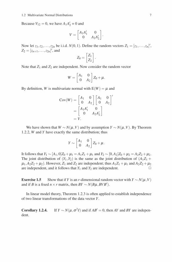
Because V12 = 0, we have A1A′2 = 0 and
V =[
A1A′1 0
0 A2A′2
].
Now let z1,z2, . . . ,z2n be i.i.d. N(0,1). Define the random vectors Z1 = [z1, . . . ,zn]′,Z2 = [zn+1, . . . ,z2n]′, and
Z0 =[
Z1Z2
].
Note that Z1 and Z2 are independent. Now consider the random vector
W =[
A1 00 A2
]Z0 + μ.
By definition, W is multivariate normal with E(W ) = μ and
Cov(W ) =[
A1 00 A2
][A1 00 A2
]′=[
A1A′1 0
0 A2A′2
]= V.
We have shown that W ∼ N(μ,V ) and by assumption Y ∼ N(μ ,V ). By Theorem1.2.2, W and Y have exactly the same distribution; thus
Y ∼[
A1 00 A2
]Z0 + μ .
It follows that Y1 ∼ [A1,0]Z0 +μ1 = A1Z1 +μ1 and Y2 ∼ [0,A2]Z0 +μ2 = A2Z2 +μ2.The joint distribution of (Y1,Y2) is the same as the joint distribution of (A1Z1 +μ1,A2Z2 + μ2). However, Z1 and Z2 are independent; thus A1Z1 +μ1 and A2Z2 +μ2are independent, and it follows that Y1 and Y2 are independent. �
Exercise 1.5 Show that if Y is an r-dimensional random vector with Y ∼N(μ ,V )and if B is a fixed n× r matrix, then BY ∼ N(Bμ ,BV B′).
In linear model theory, Theorem 1.2.3 is often applied to establish independenceof two linear transformations of the data vector Y .
Corollary 1.2.4. If Y ∼ N(μ ,σ 2I) and if AB′ = 0, then AY and BY are indepen-dent.

8 1 Introduction
PROOF. Consider the distribution of[
AB
]Y . By Exercise 1.5, the joint distribution
of AY and BY is multivariate normal. Since Cov(AY,BY ) = σ 2AIB′ = σ 2AB′ = 0,Theorem 1.2.3 implies that AY and BY are independent. �
1.3 Distributions of Quadratic Forms
In this section, quadratic forms are defined, the expectation of a quadratic form isfound, and a series of results on independence and chi-squared distributions aregiven.
Definition 1.3.1. Let Y be an n-dimensional random vector and let A be an n×nmatrix. A quadratic form is a random variable defined by Y ′AY for some Y and A.
Note that since Y ′AY is a scalar, Y ′AY =Y ′A′Y =Y ′(A+A′)Y/2. Since (A+A′)/2is always a symmetric matrix, we can, without loss of generality, restrict ourselvesto quadratic forms where A is symmetric.
Theorem 1.3.2. If E(Y ) = μ and Cov(Y ) = V , then E(Y ′AY ) = tr(AV )+ μ ′Aμ .
PROOF.
(Y −μ)′A(Y −μ) = Y ′AY −μ ′AY −Y ′Aμ + μ ′Aμ ,
E[(Y −μ)′A(Y −μ)] = E[Y ′AY ]−μ ′Aμ −μ ′Aμ + μ ′Aμ ,
so E[Y ′AY ] = E[(Y −μ)′A(Y −μ)]+ μ ′Aμ .It is easily seen that for any random square matrix W , E(tr(W )) = tr(E(W )). Thus
E[(Y −μ)′A(Y −μ)] = E(tr[(Y −μ)′A(Y −μ)])= E(tr[A(Y −μ)(Y −μ)′])= tr(E[A(Y −μ)(Y −μ)′])= tr(AE[(Y −μ)(Y −μ)′])= tr(AV ).
Substitution givesE(Y ′AY ) = tr(AV )+ μ ′Aμ. �
We now proceed to give results on chi-squared distributions and independenceof quadratic forms. Note that by Definition C.1 and Theorem 1.2.3, if Z is an n-dimensional random vector and Z ∼ N(μ , I), then Z′Z ∼ χ2(n,μ ′μ/2).

1.3 Distributions of Quadratic Forms 9
Theorem 1.3.3. If Y is a random vector with Y ∼ N(μ , I) and if M is any per-pendicular projection matrix, then Y ′MY ∼ χ2(r(M),μ ′Mμ/2).
PROOF. Let r(M) = r and let o1, . . . ,or be an orthonormal basis for C(M). LetO = [o1, . . . ,or] so that M = OO′. We now have Y ′MY = Y ′OO′Y = (O′Y )′(O′Y ),where O′Y ∼ N(O′μ ,O′IO). The columns of O are orthonormal, so O′O is an r× ridentity matrix, and by definition (O′Y )′(O′Y )∼ χ2(r,μ ′OO′μ/2) where μ ′OO′μ =μ ′Mμ . �
Observe that if Y ∼ N(μ,σ 2I
), then [1/σ ]Y ∼ N ([1/σ ]μ, I) and Y ′MY/σ 2 ∼
χ2(r(M),μ ′Mμ/2σ 2
).
Theorem 1.3.6 provides a generalization of Theorem 1.3.3 that is valid for anarbitrary covariance matrix. The next two lemmas are used in the proof of Theorem1.3.6.
Lemma 1.3.4. If Y ∼ N(μ ,M), where μ ∈ C(M) and if M is a perpendicularprojection matrix, then Y ′Y ∼ χ2(r(M),μ ′μ/2).
PROOF. Let O have r orthonormal columns with M = OO′. Since μ ∈ C(M),μ = Ob. Let W ∼ N(b, I), then Y ∼ OW . Since O′O = Ir is also a perpendicularprojection matrix, the previous theorem gives Y ′Y ∼ W ′O′OW ∼ χ2(r,b′O′Ob/2).The proof is completed by observing that r = r(M) and b′O′Ob = μ ′μ . �
The following lemma establishes that, if Y is a singular random variable, thenthere exists a proper subset of Rn that contains Y with probability 1.
Lemma 1.3.5. If E(Y ) = μ and Cov(Y ) = V , then Pr[(Y −μ) ∈C(V )] = 1.
PROOF. Without loss of generality, assume μ = 0. Let MV be the perpendicularprojection operator onto C(V ); then Y = MVY +(I−MV )Y . Clearly, E[(I−MV )Y ] =0 and Cov[(I−MV )Y ] = (I−MV )V (I−MV ) = 0. Thus, Pr[(I−MV )Y = 0] = 1 andPr[Y = MVY ] = 1. Since MVY ∈C(V ), we are done. �
Exercise 1.6 Show that if Y is a random vector and if E(Y ) = 0 and Cov(Y ) = 0,then Pr[Y = 0] = 1.
Hint: For a random variable w with Pr[w ≥ 0] = 1 and k > 0, show that Pr[w ≥k] ≤ E(w)/k. Apply this result to Y ′Y .
Theorem 1.3.6. If Y ∼ N(μ,V ), then Y ′AY ∼ χ2(tr(AV ),μ ′Aμ/2) provided that(1) VAVAV = VAV , (2) μ ′AVAμ = μ ′Aμ , and (3) VAVAμ = VAμ .
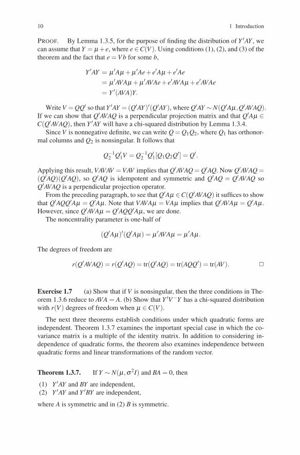
10 1 Introduction
PROOF. By Lemma 1.3.5, for the purpose of finding the distribution of Y ′AY , wecan assume that Y = μ +e, where e ∈C(V ). Using conditions (1), (2), and (3) of thetheorem and the fact that e = V b for some b,
Y ′AY = μ ′Aμ + μ ′Ae+ e′Aμ + e′Ae
= μ ′AVAμ + μ ′AVAe+ e′AVAμ + e′AVAe
= Y ′(AVA)Y.
Write V = QQ′ so that Y ′AY =(Q′AY )′(Q′AY ), where Q′AY ∼N(Q′Aμ ,Q′AVAQ).If we can show that Q′AVAQ is a perpendicular projection matrix and that Q′Aμ ∈C(Q′AVAQ), then Y ′AY will have a chi-squared distribution by Lemma 1.3.4.
Since V is nonnegative definite, we can write Q = Q1Q2, where Q1 has orthonor-mal columns and Q2 is nonsingular. It follows that
Q−12 Q′
1V = Q−12 Q′
1[Q1Q2Q′] = Q′.
Applying this result, VAVAV = VAV implies that Q′AVAQ = Q′AQ. Now Q′AVAQ =(Q′AQ)(Q′AQ), so Q′AQ is idempotent and symmetric and Q′AQ = Q′AVAQ soQ′AVAQ is a perpendicular projection operator.
From the preceding paragraph, to see that Q′Aμ ∈C(Q′AVAQ) it suffices to showthat Q′AQQ′Aμ = Q′Aμ . Note that VAVAμ = VAμ implies that Q′AVAμ = Q′Aμ .However, since Q′AVAμ = Q′AQQ′Aμ , we are done.
The noncentrality parameter is one-half of
(Q′Aμ)′(Q′Aμ) = μ ′AVAμ = μ ′Aμ.
The degrees of freedom are
r(Q′AVAQ) = r(Q′AQ) = tr(Q′AQ) = tr(AQQ′) = tr(AV ). �
Exercise 1.7 (a) Show that if V is nonsingular, then the three conditions in The-orem 1.3.6 reduce to AVA = A. (b) Show that Y ′V−Y has a chi-squared distributionwith r(V ) degrees of freedom when μ ∈C(V ).
The next three theorems establish conditions under which quadratic forms areindependent. Theorem 1.3.7 examines the important special case in which the co-variance matrix is a multiple of the identity matrix. In addition to considering in-dependence of quadratic forms, the theorem also examines independence betweenquadratic forms and linear transformations of the random vector.
Theorem 1.3.7. If Y ∼ N(μ,σ 2I) and BA = 0, then
(1) Y ′AY and BY are independent,(2) Y ′AY and Y ′BY are independent,
where A is symmetric and in (2) B is symmetric.

1.3 Distributions of Quadratic Forms 11
PROOF. By Corollary 1.2.4, if BA = 0, BY and AY are independent. In addition,as discussed near the end of Appendix D, any function of AY is independent of anyfunction of BY . Since Y ′AY = Y ′AA−AY and Y ′BY = Y ′BB−BY are functions of AYand BY , the theorem holds. �
The final two theorems provide conditions for independence of quadratic formsunder general covariance matrices.
Theorem 1.3.8. If Y ∼N(μ ,V ), A and B are nonnegative definite, and VAV BV =0, then Y ′AY and Y ′BY are independent.
PROOF. Since A and B are nonnegative definite, we can write A = RR′ and B = SS′.We can also write V = QQ′.
Y ′AY = (R′Y )′(R′Y ) and Y ′BY = (S′Y )′(S′Y ) are independent
if R′Y and S′Y are independentiff Cov(R′Y,S′Y ) = 0iff R′V S = 0iff R′QQ′S = 0iff C(Q′S) ⊥C(Q′R).
Since C(AA′) = C(A) for any A, we have
C(Q′S) ⊥C(Q′R) iff C(Q′SS′Q) ⊥C(Q′RR′Q)iff [Q′SS′Q][Q′RR′Q] = 0iff Q′BVAQ = 0iff C(Q) ⊥C(BVAQ)iff C(QQ′) ⊥C(BVAQ)iff QQ′BVAQ = 0iff V BVAQ = 0.
Repeating similar arguments for the right side gives V BVAQ = 0 iff V BVAV = 0. �
Theorem 1.3.9. If Y ∼ N(μ ,V ) and (1) VAV BV = 0, (2) VAV Bμ = 0, (3)V BVAμ = 0, (4) μ ′AV Bμ = 0, and conditions (1), (2), and (3) from Theorem 1.3.6hold for both Y ′AY and Y ′BY , then Y ′AY and Y ′BY are independent.
Exercise 1.8 Prove Theorem 1.3.9.Hints: Let V = QQ′ and write Y = μ + QZ, where Z ∼ N(0, I). Using |= to
indicate independence, show that[Q′AQZμ ′AQZ
]
|=
[Q′BQZμ ′BQZ
]

12 1 Introduction
and that, say, Y ′AY is a function Q′AQZ and μ ′AQZ.
Note that Theorem 1.3.8 applies immediately if AY and BY are independent,i.e., if AV B = 0. In something of a converse, if V is nonsingular, the conditionVAV BV = 0 is equivalent to AV B = 0; so the theorem applies only when AY andBY are independent. However, if V is singular, the conditions of Theorems 1.3.8and 1.3.9 can be satisfied even when AY and BY are not independent.
Exercise 1.9 Let M be the perpendicular projection operator onto C(X). Showthat (I −M) is the perpendicular projection operator onto C(X)⊥. Find tr(I −M) interms of r(X).
Exercise 1.10 For a linear model Y = Xβ + e, E(e) = 0, Cov(e) = σ 2I, showthat E(Y ) = Xβ and Cov(Y ) = σ 2I.
Exercise 1.11 For a linear model Y = Xβ + e, E(e) = 0, Cov(e) = σ 2I, theresiduals are
e = Y −X β = (I −M)Y,
where M is the perpendicular projection operator onto C(X). Find(a) E(e).(b) Cov(e).(c) Cov(e,MY ).(d) E(e′e).(e) Show that e′e = Y ′Y − (Y ′M)Y .
[Note: In Chapter 2 we will show that for a least squares estimate of β , say β , wehave MY = X β .]
(f) Rewrite (c) and (e) in terms of β .
1.4 Generalized Linear Models
We now give a brief introduction to generalized linear models. On occasion throughthe rest of the book, reference will be made to various properties of linear modelsthat extend easily to generalized linear models. See McCullagh and Nelder (1989)or Christensen (1997) for more extensive discussions of generalized linear modelsand their applications. First it must be noted that a general linear model is a linearmodel but a generalized linear model is a generalization of the concept of a linearmodel. Generalized linear models include linear models as a special case but alsoinclude logistic regression, exponential regression, and gamma regression as specialcases. Additionally, log-linear models for multinomial data are closely related togeneralized linear models.

1.4 Generalized Linear Models 13
Consider a random vector Y with E(Y ) = μ . Let h be an arbitrary function on thereal numbers and, for a vector v = (v1, . . . ,vn)′, define the vector function
h(v) ≡
⎡⎢⎣h(v1)...
h(vn)
⎤⎥⎦ .
The primary idea of a generalized linear model is specifying that
μ = h(Xβ ),
where h is a known invertible function and X and β are defined as for linearmodels. The inverse of h is called the link function. In particular, linear modelsuse the identity function h(v) = v, logistic regression uses the logistic transformh(v) = ev/(1 + ev), and both exponential regression and log-linear models use theexponential transform h(v) = ev. Their link functions are, respectively, the identity,logit, and log transforms. Because the linear structure Xβ is used in generalizedlinear models, many of the analysis techniques used for linear models can be easilyextended to generalized linear models.
Typically, in a generalized linear model it is assumed that the yis are independentand each follows a distribution having density or mass function of the form
f (yi|θi,φ ;wi) = exp{
wi
φ[θiyi − r(θi)]
}g(yi,φ ,wi), (1)
where r(·) and g(·, ·, ·) are known functions and θi, φ , and wi are scalars. By as-sumption, wi is a fixed known number. Typically, it is a known weight that indicatesknowledge about a pattern in the variabilities of the yis. φ is either known or is anunknown parameter, but for some purposes is always treated like it is known. It isrelated to the variance of yi. The parameter θi is related to the mean of yi. For linearmodels, the standard assumption is that the yis are independent N(θi,φ/wi), withφ ≡ σ2 and wi ≡ 1. The standard assumption of logistic regression is that the Niyisare distributed as independent binomials with Ni trials, success probability
E(yi) ≡ μi ≡ pi = eθi/[1+ eθi ],
wi = Ni, and φ = 1. Log-linear models fit into this framework when one assumesthat the yis are independent Poisson with mean μi = eθi , wi = 1, and φ = 1. Notethat in these cases the mean is some function of θi and that φ is merely related to thevariance. Note also that in the three examples, the h function has already appeared,even though these distributions have not yet incorporated the linear structure of thegeneralized linear model.
To investigate the relationship between the θi parameters and the linear structurex′iβ , where x′i is the ith row of X , let r(θi) be the derivative dr(θi)/dθi. It can beshown that
E(yi) ≡ μi = r(θi).

14 1 Introduction
Thus, another way to think about the modeling process is that
μi = h(x′iβ ) = r(θi),
where both h and r are invertible. In matrix form, write θ = (θ1, . . . ,θn)′ so that
Xβ = h−1(μ) = h−1 [r(θ)] and r−1 [h(Xβ )] = r−1 (μ) = θ .
The special case of h(·) = r(·) gives Xβ = θ . This is known as a canonical gener-alized linear model, or as using a canonical link function. The three examples givenearlier are all examples of canonical generalized linear models. Linear models withnormally distributed data are canonical generalized linear models. Logistic regres-sion is the canonical model having Niyi distributed Binomial(Ni,μi) for known Niwith h−1(μi) ≡ log(μi/[1−μi]). Another canonical generalized linear model has yidistributed Poisson(μi) with h−1(μi) ≡ log(μi).
1.5 Additional Exercises
Exercise 1.5.1 Let Y = (y1,y2,y3)′ be a random vector. Suppose that E(Y )∈M ,where M is defined by
M = {(a,a−b,2b)′|a,b ∈ R}.
(a) Show that M is a vector space.(b) Find a basis for M .(c) Write a linear model for this problem (i.e., find X such that Y = Xβ + e,
E(e) = 0).(d) If β = (β1,β2)′ in part (c), find two vectors r = (r1,r2,r3)′ and s =
(s1,s2,s3)′ such that E(r′Y ) = r′Xβ = β1 and E(s′Y ) = β2. Find another vectort = (t1,t2,t3)′ with r �= t but E(t ′Y ) = β1.
Exercise 1.5.2 Let Y = (y1,y2,y3)′ with Y ∼ N(μ ,V ), where
μ = (5,6,7)′
and
V =
⎡⎣2 0 10 3 21 2 4
⎤⎦ .
Find(a) the marginal distribution of y1,(b) the joint distribution of y1 and y2,

1.5 Additional Exercises 15
(c) the conditional distribution of y3 given y1 = u1 and y2 = u2,(d) the conditional distribution of y3 given y1 = u1,(e) the conditional distribution of y1 and y2 given y3 = u3,(f) the correlations ρ12, ρ13, ρ23,(g) the distribution of
Z =[
2 1 01 1 1
]Y +[−15−18
],
(h) the characteristic functions of Y and Z.
Exercise 1.5.3 The density of Y = (y1,y2,y3)′ is
(2π)−3/2|V |−1/2e−Q/2,
whereQ = 2y2
1 + y22 + y2
3 +2y1y2 −8y1 −4y2 +8.
Find V−1 and μ .
Exercise 1.5.4 Let Y ∼ N(Jμ,σ 2I) and let O =[n−1/2J,O1
]be an orthogonal
matrix.(a) Find the distribution of O′Y .(b) Show that y· = (1/n)J′Y and that s2 = Y ′O1O′
1Y/(n−1).(c) Show that y· and s2 are independent.Hint: Show that Y ′Y = Y ′OO′Y = Y ′(1/n)JJ′Y +Y ′O1O′
1Y .
Exercise 1.5.5 Let Y = (y1,y2)′ have a N(0, I) distribution. Show that if
A =[
1 aa 1
]B =[
1 bb 1
],
then the conditions of Theorem 1.3.7 implying independence of Y ′AY and Y ′BY aresatisfied only if |a| = 1/|b| and a = −b. What are the possible choices for a and b?
Exercise 1.5.6 Let Y = (y1,y2,y3)′ have a N(μ,σ 2I) distribution. Consider thequadratic forms defined by the matrices M1, M2, and M3 given below.
(a) Find the distribution of each Y ′MiY .(b) Show that the quadratic forms are pairwise independent.(c) Show that the quadratic forms are mutually independent.
M1 =13
J33 , M2 =
114
⎡⎣ 9 −3 −6−3 1 2−6 2 4
⎤⎦ ,

16 1 Introduction
M3 =1
42
⎡⎣ 1 −5 4−5 25 −20
4 −20 16
⎤⎦ .
Exercise 1.5.7 Let A be symmetric, Y ∼ N(0,V ), and w1, . . . ,ws be indepen-dent χ2(1) random variables. Show that for some value of s and some numbers λi,Y ′AY ∼ ∑s
i=1 λiwi.Hint: Y ∼ QZ so Y ′AY ∼ Z′Q′AQZ. Write Q′AQ = PD(λi)P′.
Exercise 1.5.8. Show that(a) for Example 1.0.1 the perpendicular projection operator onto C(X) is
M =16
J66 +
170
⎡⎢⎢⎢⎢⎢⎣25 15 5 −5 −15 −2515 9 3 −3 −9 −155 3 1 −1 −3 −5
−5 −3 −1 1 3 5−15 −9 −3 3 9 15−25 −15 −5 5 15 25
⎤⎥⎥⎥⎥⎥⎦ ;
(b) for Example 1.0.2 the perpendicular projection operator onto C(X) is
M =
⎡⎢⎢⎢⎢⎢⎣1/3 1/3 1/3 0 0 01/3 1/3 1/3 0 0 01/3 1/3 1/3 0 0 0
0 0 0 1 00 0 0 0 1/2 1/20 0 0 0 1/2 1/2
⎤⎥⎥⎥⎥⎥⎦ .

Chapter 2
Estimation
In this chapter, properties of least squares estimates are examined for the model
Y = Xβ + e, E(e) = 0, Cov(e) = σ 2I.
The chapter begins with a discussion of the concepts of identifiability and estima-bility in linear models. Section 2 characterizes least squares estimates. Sections 3,4, and 5 establish that least squares estimates are best linear unbiased estimates,maximum likelihood estimates, and minimum variance unbiased estimates. The lasttwo of these properties require the additional assumption e ∼ N(0,σ 2I). Section 6also assumes that the errors are normally distributed and presents the distributionsof various estimates. From these distributions various tests and confidence intervalsare easily obtained. Section 7 examines the model
Y = Xβ + e, E(e) = 0, Cov(e) = σ 2V,
where V is a known positive definite matrix. Section 7 introduces generalized leastsquares estimates and presents properties of those estimates. Section 8 presents thenormal equations and establishes their relationship to least squares and generalizedleast squares estimation. Section 9 discusses Bayesian estimation.
The history of least squares estimation goes back at least to 1805, when Legendrefirst published the idea. Gauss made important early contributions (and claimed tohave invented the method prior to 1805).
There is a huge body of literature available on estimation and testing in linearmodels. A few books dealing with the subject are Arnold (1981), Eaton (1983),Graybill (1976), Rao (1973), Ravishanker and Dey (2002), Rencher (2008), Scheffe(1959), Searle (1971), Seber (1966, 1977), and Wichura (2006).
© Springer Science+Business Media, LLC 2011
17Springer Texts in Statistics, DOI 10.1007/978-1-4419-9816-3_2, R. Christensen, Plane Answers to Complex Questions: The Theory of Linear Models,

18 2 Estimation
2.1 Identifiability and Estimability
A key issue in linear model theory is figuring out which parameters can be estimatedand which cannot. We will see that what can be estimated are functions of the pa-rameters that are identifiable. Linear functions of the parameters that are identifiableare called estimable and have linear unbiased estimators. These concepts also havenatural applications to generalized linear models. The definitions used here are tai-lored to (generalized) linear models but the definition of an identifiable parameteri-zation coincides with more common definitions of identifiability; cf. Christensen etal. (2010, Section 4.14). For other definitions, the key idea is that the distribution ofY should be either completely determined by E(Y ) alone or completely determinedby E(Y ) along with some parameters (like σ 2) that are functionally unrelated to theparameters in E(Y ).
Consider the general linear model
Y = Xβ + e, E(e) = 0,
where again Y is an n× 1 vector of observations, X is an n× p matrix of knownconstants, β is a p×1 vector of unobservable parameters, and e is an n×1 vector ofunobservable random errors whose distribution does not depend on β . We can onlylearn about β through Xβ . If x′i is the ith row of X , x′iβ is the ith row of Xβ and wecan only learn about β through the x′iβ s. Xβ can be thought of as a vector of innerproducts between β and a spanning set for C(X ′). Thus, we can learn about innerproducts between β and C(X ′). In particular, when λ is a p× 1 vector of knownconstants, we can learn about functions λ ′β where λ ∈C(X ′), i.e., where λ = X ′ρfor some vector ρ . These are precisely the estimable functions of β . We now givemore formal arguments leading us to focus on functions λ ′β where λ ′ = ρ ′X or,more generally, vectors Λ ′β where Λ ′ = P′X .
In general, a parameterization for the n×1 mean vector E(Y ) consists of writingE(Y ) as a function of some parameters β , say,
E(Y ) = f (β ).
A general linear model is a parameterization
E(Y ) = Xβ
because E(Y ) = E(Xβ + e) = Xβ +E(e) = Xβ . A parameterization is identifiableif knowing E(Y ) tells you the parameter vector β .
Definition 2.1.1 The parameter β is identifiable if for any β1 and β2, f (β1) =f (β2) implies β1 = β2. If β is identifiable, we say that the parameterization f (β ) isidentifiable. Moreover, a vector-valued function g(β ) is identifiable if f (β1) = f (β2)implies g(β1) = g(β2). If the parameterization is not identifiable but nontrivial iden-tifiable functions exist, then the parameterization is said to be partially identifiable.
2.1 Identifiability and Estimability 19
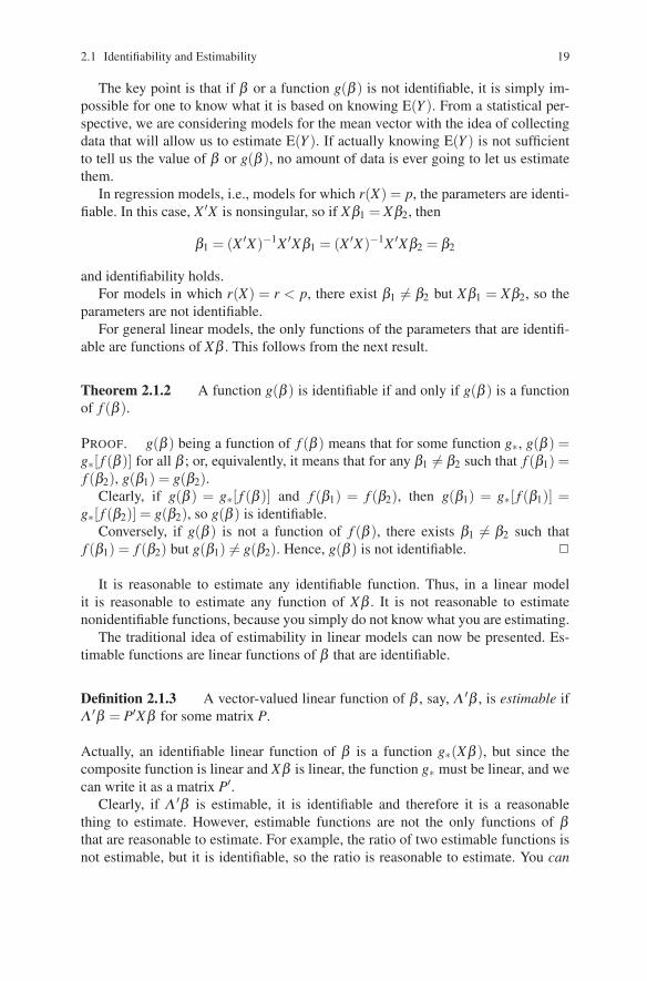
The key point is that if β or a function g(β ) is not identifiable, it is simply im-possible for one to know what it is based on knowing E(Y ). From a statistical per-spective, we are considering models for the mean vector with the idea of collectingdata that will allow us to estimate E(Y ). If actually knowing E(Y ) is not sufficientto tell us the value of β or g(β ), no amount of data is ever going to let us estimatethem.
In regression models, i.e., models for which r(X) = p, the parameters are identi-fiable. In this case, X ′X is nonsingular, so if Xβ1 = Xβ2, then
β1 = (X ′X)−1X ′Xβ1 = (X ′X)−1X ′Xβ2 = β2
and identifiability holds.For models in which r(X) = r < p, there exist β1 �= β2 but Xβ1 = Xβ2, so the
parameters are not identifiable.For general linear models, the only functions of the parameters that are identifi-
able are functions of Xβ . This follows from the next result.
Theorem 2.1.2 A function g(β ) is identifiable if and only if g(β ) is a functionof f (β ).
PROOF. g(β ) being a function of f (β ) means that for some function g∗, g(β ) =g∗[ f (β )] for all β ; or, equivalently, it means that for any β1 �= β2 such that f (β1) =f (β2), g(β1) = g(β2).
Clearly, if g(β ) = g∗[ f (β )] and f (β1) = f (β2), then g(β1) = g∗[ f (β1)] =g∗[ f (β2)] = g(β2), so g(β ) is identifiable.
Conversely, if g(β ) is not a function of f (β ), there exists β1 �= β2 such thatf (β1) = f (β2) but g(β1) �= g(β2). Hence, g(β ) is not identifiable. �
It is reasonable to estimate any identifiable function. Thus, in a linear modelit is reasonable to estimate any function of Xβ . It is not reasonable to estimatenonidentifiable functions, because you simply do not know what you are estimating.
The traditional idea of estimability in linear models can now be presented. Es-timable functions are linear functions of β that are identifiable.
Definition 2.1.3 A vector-valued linear function of β , say, Λ ′β , is estimable ifΛ ′β = P′Xβ for some matrix P.
Actually, an identifiable linear function of β is a function g∗(Xβ ), but since thecomposite function is linear and Xβ is linear, the function g∗ must be linear, and wecan write it as a matrix P′.
Clearly, if Λ ′β is estimable, it is identifiable and therefore it is a reasonablething to estimate. However, estimable functions are not the only functions of βthat are reasonable to estimate. For example, the ratio of two estimable functions isnot estimable, but it is identifiable, so the ratio is reasonable to estimate. You can

20 2 Estimation
estimate many functions that are not “estimable.” What you cannot do is estimatenonidentifiable functions.
Unfortunately, the term “nonestimable” is often used to mean something otherthan “not being estimable.” You can be “not estimable” by being either not linearor not identifiable. In particular, a linear function that is “not estimable” is auto-matically nonidentifiable. However, nonestimable is often taken to mean a linearfunction that is not identifiable. In other words, some authors (perhaps, on occasion,even this one) presume that nonestimable functions are linear, so that nonestimabil-ity and nonidentifiability become equivalent.
It should be noted that the concepts of identifiability and estimability are basedentirely on the assumption that E(Y ) = Xβ . Identifiability and estimability do notdepend on Cov(Y ) = Cov(e) (as long as the covariance matrix is not also a functionof β ).
An important property of estimable functions Λ ′β = P′Xβ is that although Pneed not be unique, its perpendicular projection (columnwise) onto C(X) is unique.Let P1 and P2 be matrices with Λ ′ = P′
1X = P′2X , then MP1 = X(X ′X)−X ′P1 =
X(X ′X)−Λ = X(X ′X)−X ′P2 = MP2.
EXAMPLE 2.1.4. In the simple linear regression model of Example 1.0.1, β1 isestimable because
135
(−5,−3,−1,1,3,5)
⎡⎢⎢⎢⎢⎢⎣1 11 21 31 41 51 6
⎤⎥⎥⎥⎥⎥⎦[
β0β1
]= (0,1)
[β0β1
]= β1.
β0 is also estimable. Note that
16(1,1,1,1,1,1)
⎡⎢⎢⎢⎢⎢⎣1 11 21 31 41 51 6
⎤⎥⎥⎥⎥⎥⎦[
β0β1
]= β0 +
72
β1,
so
β0 =(
β0 +72
β1
)− 7
2β1
=
⎡⎢⎢⎢⎢⎢⎣16
⎛⎜⎜⎜⎜⎜⎝111111
⎞⎟⎟⎟⎟⎟⎠− 72
(1
35
)⎛⎜⎜⎜⎜⎜⎝−5−3−1
135
⎞⎟⎟⎟⎟⎟⎠
⎤⎥⎥⎥⎥⎥⎦
′⎡⎢⎢⎢⎢⎢⎣1 11 21 31 41 51 6
⎤⎥⎥⎥⎥⎥⎦[
β0β1
]

2.1 Identifiability and Estimability 21
=1
30(20,14,8,2,−4,−10)
⎡⎢⎢⎢⎢⎢⎣1 11 21 31 41 51 6
⎤⎥⎥⎥⎥⎥⎦[
β0β1
].
For any fixed number x, β0 +β1x is estimable because it is a linear combination ofestimable functions.
EXAMPLE 2.1.5. In the one-way ANOVA model of Example 1.0.2, we can esti-mate parameters like μ +α1, α1 −α3, and α1 +α2 −2α3. Observe that
(1,0,0,0,0,0)
⎡⎢⎢⎢⎢⎢⎣1 1 0 01 1 0 01 1 0 01 0 1 01 0 0 11 0 0 1
⎤⎥⎥⎥⎥⎥⎦⎡⎢⎣
μα1α2α3
⎤⎥⎦= μ +α1,
(1,0,0,0,−1,0)
⎡⎢⎢⎢⎢⎢⎣1 1 0 01 1 0 01 1 0 01 0 1 01 0 0 11 0 0 1
⎤⎥⎥⎥⎥⎥⎦⎡⎢⎣
μα1α2α3
⎤⎥⎦= α1 −α3,
but also
(13,
13,
13,0,
−12
,−12
)⎡⎢⎢⎢⎢⎢⎣
1 1 0 01 1 0 01 1 0 01 0 1 01 0 0 11 0 0 1
⎤⎥⎥⎥⎥⎥⎦⎡⎢⎣
μα1α2α3
⎤⎥⎦= α1 −α3,
and
(1,0,0,1,−2,0)
⎡⎢⎢⎢⎢⎢⎣1 1 0 01 1 0 01 1 0 01 0 1 01 0 0 11 0 0 1
⎤⎥⎥⎥⎥⎥⎦⎡⎢⎣
μα1α2α3
⎤⎥⎦= α1 +α2 −2α3.
We have given two vectors ρ1 and ρ2 with ρ ′i Xβ = α1 −α3. Using M given in
Exercise 1.5.8b, the reader can verify that Mρ1 = Mρ2.
In the one-way analysis of covariance model,

22 2 Estimation
yi j = μ +αi + γxi j + ei j, E(ei j) = 0,
i = 1, . . . ,a, j = 1, . . . ,Ni, xi j is a known predictor variable and γ is its unknowncoefficient. γ is generally identifiable but μ and the αis are not. The following resultallows one to tell whether or not an individual parameter is identifiable.
Proposition 2.1.6 For a linear model, write Xβ = ∑pk=1 Xkβk where the Xks are
the columns of X . An individual parameter βi is not identifiable if and only if thereexist scalars αk such that Xi = ∑k �=i Xkαk.
PROOF. To show that the condition on X implies nonidentifiability, it is enoughto show that there exist β and β∗ with Xβ = Xβ∗ but βi �= β∗i. The condition Xi =∑k �=i Xkαk is equivalent to there existing a vector α with αi �= 0 and Xα = 0. Letβ∗ = β +α and the proof is complete.
Rather than showing that when βi is not identifiable, the condition on X holds,we show the contrapositive, i.e., that when the condition on X does not hold, βi isidentifiable. If there do not exist such αks, then whenever Xα = 0, we must haveαi = 0. In particular, if Xβ = Xβ∗, then X(β −β∗) = 0, so (βi −β∗i) = 0 and βi isidentifiable. �
The concepts of identifiability and estimability apply with little change to gen-eralized linear models. In generalized linear models, the distribution of Y is eithercompletely determined by E(Y ) or it is determined by E(Y ) along with another pa-rameter φ that is unrelated to the parameterization of E(Y ). A generalized linearmodel has E(Y ) = h(Xβ ). By Theorem 2.1.2, a function g(β ) is identifiable if andonly if it is a function of h(Xβ ). However, the function h(·) is assumed to be in-vertible, so g(β ) is identifiable if and only if it is a function of Xβ . A vector-valuedlinear function of β , say, Λ ′β is identifiable if Λ ′β = P′Xβ for some matrix P,hence Definition 2.1.3 applies as well to define estimability for generalized linearmodels as it does for linear models. Proposition 2.1.6 also applies without change.
Finally, the concept of estimability in linear models can be related to the existenceof linear unbiased estimators. A linear function of the parameter vector β , say λ ′β ,is estimable if and only if it admits a linear unbiased estimate.
Definition 2.1.7. An estimate f (Y ) of g(β ) is unbiased if E[ f (Y )] = g(β ) forany β .
Definition 2.1.8. f (Y ) is a linear estimate of λ ′β if f (Y ) = a0 + a′Y for somescalar a0 and vector a.
Proposition 2.1.9. A linear estimate a0 +a′Y is unbiased for λ ′β if and only ifa0 = 0 and a′X = λ ′.
PROOF. ⇐ If a0 = 0 and a′X = λ ′, then E(a0 +a′Y ) = 0+a′Xβ = λ ′β .

2.2 Estimation: Least Squares 23
⇒ If a0 +a′Y is unbiased, λ ′β = E(a0 +a′Y ) = a0 +a′Xβ , for any β . Subtractinga′Xβ from both sides gives
(λ ′ −a′X)β = a0
for any β . If β = 0, then a0 = 0. Thus the vector λ −X ′a is orthogonal to any vectorβ . This can only occur if λ −X ′a = 0; so λ ′ = a′X . �
Corollary 2.1.10. λ ′β is estimable if and only if there exists ρ such thatE(ρ ′Y ) = λ ′β for any β .
2.2 Estimation: Least Squares
Consider the model
Y = Xβ + e, E(e) = 0, Cov(e) = σ 2I.
Suppose we want to estimate E(Y ). We know that E(Y ) = Xβ , but β is unknown; soall we really know is that E(Y ) ∈C(X). To estimate E(Y ), we might take the vectorin C(X) that is closest to Y . By definition then, an estimate β is a least squaresestimate if X β is the vector in C(X) that is closest to Y . In other words, β is a leastsquares estimate (LSE) of β if
(Y −X β )′(Y −X β ) = minβ
(Y −Xβ )′(Y −Xβ ).
For a vector Λ ′β , a least squares estimate is defined as Λ ′β for any least squaresestimate β .
In this section, least squares estimates are characterized and uniqueness and un-biasedness properties of least squares estimates are given. An unbiased estimate ofσ 2 is then presented. Finally, at the end of the section, the geometry associated withleast squares estimation and unbiased estimation of σ 2 is discussed. The geometryprovides good intuition for n-dimensional problems but the geometry can only bevisualized in three dimensions. In other words, although it is a fine pedagogical tool,the geometry can only be spelled out for three or fewer data points. The fundamentalgoal of this book is to build the theory of linear models on vector space generaliza-tions of these fundamentally geometric concepts. We now establish the fundamentaltheorem of least squares estimation, that the vector in C(X) that is closest to Y is theperpendicular projection of Y onto C(X).
Theorem 2.2.1. β is a least squares estimate of β if and only if X β = MY , whereM is the perpendicular projection operator onto C(X).
PROOF. We will show that

24 2 Estimation
(Y −Xβ )′(Y −Xβ) = (Y −MY )′(Y −MY )+(MY −Xβ )′(MY −Xβ ).
Both terms on the righthand side are nonnegative, and the first term does not dependon β . (Y − Xβ )′(Y − Xβ ) is minimized by minimizing (MY −Xβ )′(MY − Xβ ).This is the squared distance between MY and Xβ . The distance is zero if and onlyif MY = Xβ , which proves the theorem. We now establish the equation.
(Y −Xβ )′(Y −Xβ ) = (Y −MY +MY −Xβ )′(Y −MY +MY −Xβ )= (Y −MY )′(Y −MY )+(Y −MY )′(MY −Xβ )
+(MY −Xβ )′(Y −MY )+(MY −Xβ)′(MY −Xβ ).
However, (Y −MY )′(MY −Xβ ) = Y ′(I −M)MY −Y ′(I −M)Xβ = 0 because (I −M)M = 0 and (I −M)X = 0. Similarly, (MY −Xβ )′(Y −MY ) = 0. �
Corollary 2.2.2. (X ′X)−X ′Y is a least squares estimate of β .
In Example 1.0.2, with M given in Exercise 1.5.8b, it is not difficult to see that
MY =
⎡⎢⎢⎢⎢⎢⎣y1·y1·y1·y21y3·y3·
⎤⎥⎥⎥⎥⎥⎦=
⎡⎢⎢⎢⎢⎢⎣1 1 0 01 1 0 01 1 0 01 0 1 01 0 0 11 0 0 1
⎤⎥⎥⎥⎥⎥⎦⎡⎢⎣
0y1·y21y3·
⎤⎥⎦=
⎡⎢⎢⎢⎢⎢⎣1 1 0 01 1 0 01 1 0 01 0 1 01 0 0 11 0 0 1
⎤⎥⎥⎥⎥⎥⎦⎡⎢⎣
y1·0
y21 − y1·y3· − y1·
⎤⎥⎦ .
Thus, both β1 = (0, y1·,y21, y3·)′ and β2 = (y1·,0,y21− y1·, y3·− y1·)′ are least squaresestimates of β . From Example 2.1.5,
α1 −α3 = (1,0,0,0,−1,0)Xβ = (1/3,1/3,1/3,0,−1/2,−1/2)Xβ .
The least squares estimates are
(1,0,0,0,−1,0)X β = (1,0,0,0,−1,0)MY = y1· − y3·,
but also
(1/3,1/3,1/3,0,−1/2,−1/2)X β = (1/3,1/3,1/3,0,−1/2,−1/2)MY
= y1· − y3·.
Moreover, these estimates do not depend on the choice of least squares estimates.Either β1 or β2 gives this result.
In Example 1.0.1, X ′X has a true inverse, so the unique least squares estimate ofβ is
β =(X ′X)−1 X ′Y =
[6 2121 91
]−1 [1 1 1 1 1 11 2 3 4 5 6
]Y.

2.2 Estimation: Least Squares 25
An immediate result of Theorem 2.2.1, the uniqueness of perpendicular projec-tion operators (Proposition B.34), and Theorem 2.1.2 as applied to linear mod-els, is that the least squares estimate of any identifiable function is unique. Anyleast squares estimates β1 and β2 have X β1 = X β2, so if g(β ) is identifiable,g(β1) = g(β2). In particular, least squares estimates of estimable functions areunique.
Corollary 2.2.3. The unique least squares estimate of ρ ′Xβ is ρ ′MY .
Recall that a vector-valued linear function of the parameters, say Λ ′β , is estimableif and only if Λ ′ = P′X for some matrix P. The unique least squares estimate of Λ ′βis then P′MY = Λ ′β .
We now show that the least squares estimate of λ ′β is unique only if λ ′β isestimable.
Theorem 2.2.4. λ ′ = ρ ′X if λ ′β1 = λ ′β2 for any β1, β2 that satisfy X β1 = X β2 =MY .
PROOF. Decompose λ into vectors in C(X ′) and its orthogonal complement.Let N be the perpendicular projection operator onto C(X ′); then we can writeλ = X ′ρ1 + (I −N)ρ2. We want to show that (I −N)ρ2 = 0. This will be doneby showing that (I −N)ρ2 is orthogonal to every vector in Rp.
By assumption, λ ′(β1 − β2) = 0, and we know that ρ ′1X(β1 − β2) = 0; so we
must have ρ ′2(I−N)(β1− β2) = 0, and this holds for any least squares estimates β1,
β2.Let β1 be any least squares estimate and take v such that v ⊥ C(X ′), then β2 =
β1 − v is a least squares estimate. This follows because X β2 = X β1 −Xv = X β1 =MY . Substituting above gives 0 = ρ ′
2(I −N)(β1 − β2) = ρ ′2(I −N)v for any v ⊥
C(X ′). Moreover, by definition of N for any v ∈C(X ′), (I−N)v = 0. It follows thatρ ′
2(I −N)v = 0 for any v ∈ Rp and thus (I −N)ρ2 = 0. �
When β is not identifiable, sometimes side conditions are arbitrarily imposed onthe parameters to allow “estimation” of nonidentifiable parameters. Imposing sideconditions amounts to choosing one particular least squares estimate of β . In ourearlier discussion of estimation for Example 1.0.2, we presented two sets of param-eter estimates. The first estimate, β1, arbitrarily imposed μ = 0 and β2 arbitrarilyimposed α1 = 0. Side conditions determine a particular least squares estimate byintroducing a nonidentifiable, typically a linear nonestimable, constraint on the pa-rameters. With r ≡ r(X) < p, one needs p− r individual side conditions to identifythe parameters and thus allow “estimation” of the otherwise nonidentifiable param-eters. Initially, the model was overparameterized. A linear nonestimable constraintis chosen to remove the ambiguity. Fundamentally, one choice of side conditions isas good as any other. See the discussion near Corollary 3.3.8 for further explication

26 2 Estimation
of linear nonestimable constraints. The use of a side condition in one-way ANOVAis also considered in Chapter 4.
Personally, I find it silly to pretend that nonidentifiable functions of the parame-ters can be estimated. The one good thing about imposing arbitrary side conditionsis that they allow computer programs to print out parameter estimates. But differ-ent programs use different (equally valid) side conditions, so the printed estimatesmay differ from program to program. Fortunately, the estimates should agree on allestimable (and, more generally, identifiable) functions of the parameters.
Least squares estimation is not a statistical procedure! Its justification as an op-timal estimate is geometric, not statistical. Next we consider two statistical resultson unbiased estimation related to least squares estimates. First, we note that leastsquares estimates of estimable functions are unbiased.
Proposition 2.2.5. If λ ′ = ρ ′X , then E(ρ ′MY ) = λ ′β .
PROOF. E(ρ ′MY ) = ρ ′ME(Y ) = ρ ′MXβ = ρ ′Xβ = λ ′β . �
None of our results on least squares estimation involve the assumption thatCov(e) = σ 2I. Least squares provides unique estimates of identifiable functions andunbiased estimates of estimable functions, regardless of the covariance structure.The next three sections establish that least squares estimates have good statisticalproperties when Cov(e) = σ 2I.
We now consider unbiased estimation of the variance parameter σ 2. First writethe fitted values (also called the predicted values)
Y ≡ X β = MY
and the residualse ≡Y −X β = (I −M)Y.
The data vector Y can be decomposed as
Y = Y + e = MY +(I −M)Y.
The perpendicular projection of Y onto C(X) (i.e., MY ) provides an estimate ofXβ . Note that MY = MXβ + Me = Xβ + Me so that MY equals Xβ plus someerror where E(Me) = ME(e) = 0. Similarly, (I −M)Y = (I −M)Xβ +(I −M)e =(I −M)e, so (I −M)Y depends only on the error vector e. Since σ2 is a property ofthe error vector, it is reasonable to use (I −M)Y to estimate σ 2.
Theorem 2.2.6. Let r(X) = r and Cov(e) = σ 2I, then Y ′(I −M)Y/(n− r) is anunbiased estimate of σ 2.
PROOF. From Theorem 1.3.2 and the facts that E(Y ) = Xβ and Cov(Y ) = σ 2I,we have
E[Y ′(I −M)Y
]= tr[σ 2(I −M)
]+β ′X ′(I −M)Xβ .

2.2 Estimation: Least Squares 27
However, tr(σ 2(I −M)
)= σ 2 tr(I −M) = σ 2 r(I −M) = σ 2 (n− r) and (I −
M)X = 0, so β ′X ′(I −M)Xβ = 0; therefore,
E[Y ′(I −M)Y
]= σ 2 (n− r)
andE[Y ′(I −M)Y/(n− r)
]= σ 2. �
Y ′(I −M)Y is called the sum of squares for error (SSE). It is the squared lengthof the residual vector (I −M)Y . Y ′(I − M)Y/(n− r) is called the mean squarederror (MSE). It is the squared length of (I−M)Y divided by the rank of (I−M). Ina sense, the MSE is the average squared length of (I −M)Y , where the average isover the number of dimensions in C(I−M). The rank of I−M is called the degreesof freedom for error, denoted dfE.
For Example 1.0.1,
SSE = (y1 − β0 − β11)2 +(y2 − β0 − β12)2 + · · ·+(y6 − β0 − β16)2
and MSE = SSE/(6−2). For Example 1.0.2,
SSE = (y11 − y1·)2 +(y12 − y1·)2 +(y13 − y1·)2
+(y21 − y21)2 +(y31 − y3·)2 +(y32 − y3·)2
and MSE = SSE/(6−3).Finally, one can think about the geometry of least squares estimation in three
dimensions. Consider a rectangular table. (Yes, that furniture you have in yourkitchen!) Take one corner of the table to be the origin. Take C(X) as the two-dimensional subspace determined by the surface of the table. Y can be any vectororiginating at the origin, i.e., any point in three-dimensional space. The linear modelsays that E(Y ) = Xβ , which just says that E(Y ) is somewhere on the surface of thetable. The least squares estimate MY = X β is the perpendicular projection of Y ontothe table surface. The residual vector (I −M)Y is the vector starting at the origin,perpendicular to the surface of the table, that reaches the same height as Y . Anotherway to think of the residual vector is to connect the ends of MY and Y with a linesegment (that is perpendicular to the surface of the table) but then shift the line seg-ment along the surface (keeping it perpendicular) until the line segment has one endat the origin. The residual vector is the perpendicular projection of Y onto C(I−M),that is, the projection onto the orthogonal complement of the table surface. The or-thogonal complement is the one-dimension space in the vertical direction that goesthrough the origin. Because the orthogonal complement has only one dimension,MSE is just the squared length of the residual vector.
Alternatively, one could take C(X) to be a one-dimensional subspace determinedby an edge of the table that includes the origin. The linear model now says that E(Y )is somewhere on this edge of the table. MY = X β is found by dropping a perpen-dicular from Y to the edge of the table. If you connect MY and Y , you essentially

28 2 Estimation
get the residual vector (I−M)Y , except that the line segment has to be shifted downthe edge so that it has one end at the origin. The residual vector is perpendicular tothe C(X) edge of the table, but typically would not be perpendicular to the surfaceof the table. C(I−M) is now the plane that contains everything (through the origin)that is perpendicular to the C(X) edge of the table. In other words, C(I −M) is thetwo-dimensional space determined by the vertical direction and the other edge ofthe table that goes through the origin. MSE is the squared length of the residualvector divided by 2, because C(I −M) is a two-dimensional space.
2.3 Estimation: Best Linear Unbiased
Another criterion for estimation of λ ′β is to choose the best linear unbiased estimate(BLUE) of λ ′β . We prove the Gauss–Markov theorem that least squares estimatesare best linear unbiased estimates.
Definition 2.3.1. a′Y is a best linear unbiased estimate of λ ′β if a′Y is unbiasedand if for any other linear unbiased estimate b′Y , Var(a′Y ) ≤ Var(b′Y ).
Gauss–Markov Theorem 2.3.2. Consider the linear model
Y = Xβ + e, E(e) = 0, Cov(e) = σ 2I.
If λ ′β is estimable, then the least squares estimate of λ ′β is a BLUE of λ ′β .
PROOF. Let M be the perpendicular projection operator onto C(X). Since λ ′β isan estimable function, let λ ′ = ρ ′X for some ρ . We need to show that if a′Y is anunbiased estimate of λ ′β , then Var(a′Y ) ≥ Var(ρ ′MY ). Since a′Y is unbiased forλ ′β , λ ′β = E(a′Y ) = a′Xβ for any value of β . Therefore ρ ′X = λ ′ = a′X . Write
Var(a′Y ) = Var(a′Y −ρ ′MY +ρ ′MY )= Var(a′Y −ρ ′MY )+Var(ρ ′MY )+2Cov
[(a′Y −ρ ′MY ),ρ ′MY
].
Since Var(a′Y − ρ ′MY ) ≥ 0, if we show that Cov[(a′Y −ρ ′MY ),ρ ′MY ] = 0, thenVar(a′Y ) ≥ Var(ρ ′MY ) and the theorem holds.
We now show that Cov[(a′Y −ρ ′MY ),ρ ′MY ] = 0.
Cov[(a′Y −ρ ′MY ),ρ ′MY
]= Cov
[(a′ −ρ ′M)Y,ρ ′MY
]= (a′ −ρ ′M)Cov(Y )Mρ= σ2(a′ −ρ ′M)Mρ= σ2(a′M−ρ ′M)ρ.

2.4 Estimation: Maximum Likelihood 29
As shown above, a′X = ρ ′X , and since we can write M = X(X ′X)−X ′, we havea′M = ρ ′M. It follows that σ 2(a′M−ρ ′M)ρ = 0 as required. �
Corollary 2.3.3. If σ2 > 0, there exists a unique BLUE for any estimable func-tion λ ′β .
PROOF. Let λ ′ = ρ ′X , and recall from Section 1 that the vector ρ ′M is uniquelydetermined by λ ′. In the proof of Theorem 2.3.2, it was shown that for an arbitrarylinear unbiased estimate a′Y ,
Var(a′Y ) = Var(ρ ′MY )+Var(a′Y −ρ ′MY ).
If a′Y is a BLUE of λ ′β , it must be true that Var(a′Y −ρ ′MY ) = 0. It is easily seenthat
0 = Var(a′Y −ρ ′MY ) = Var[(a′ −ρ ′M)Y
]= σ 2(a−Mρ)′(a−Mρ).
For σ 2 > 0, this occurs if and only if a−Mρ = 0, which is equivalent to the condi-tion a = Mρ . �
2.4 Estimation: Maximum Likelihood
Another criterion for choosing estimates of β and σ 2 is maximum likelihood. Thelikelihood function is derived from the joint density of the observations by consider-ing the parameters as variables and the observations as fixed at their observed values.If we assume Y ∼ N
(Xβ ,σ 2I
), then the maximum likelihood estimates (MLEs) of
β and σ 2 are obtained by maximizing
(2π)−n/2[det(σ 2I)]−1/2 exp[−(Y −Xβ)′(Y −Xβ )/2σ 2] . (1)
Equivalently, the log of the likelihood can be maximized. The log of (1) is
−n2
log(2π)− 12
log[(σ 2)n]− (Y −Xβ )′(Y −Xβ )/2σ 2.
For every value of σ2, the log-likelihood is maximized by taking β to minimize(Y −Xβ )′(Y −Xβ ), i.e., least squares estimates are MLEs. To estimate σ 2 we cansubstitute Y ′(I−M)Y =(Y −X β )′(Y −X β) for (Y −Xβ )′(Y −Xβ ) and differentiatewith respect to σ2 to get Y ′(I −M)Y/n as the MLE of σ2.
The MLE of σ 2 is rarely used in practice. The MSE is the standard estimate ofσ 2. For almost any purpose except point estimation of σ2, it is immaterial whetherthe MSE or the MLE is used. They lead to identical confidence intervals and tests forσ 2. They also lead to identical confidence regions and tests for estimable functions

30 2 Estimation
of β . It should be emphasized that it is not appropriate to substitute the MLE for theMSE and then form confidence intervals and tests as if the MSE were being used.
2.5 Estimation: Minimum Variance Unbiased
In Section 3, it was shown that least squares estimates give best estimates among theclass of linear unbiased estimates. If the error vector is normally distributed, leastsquares estimates are best estimates among all unbiased estimates. In particular, withnormal errors, the best estimates happen to be linear estimates. As in Section 3, abest unbiased estimate is taken to be an unbiased estimate with minimum variance.
It is not the purpose of this monograph to develop the theory of minimum vari-ance unbiased estimation. However, we will outline the application of this theory tolinear models. See Lehmann (1983, Sections 1.4, 1.5) and Lehmann (1986, Sections2.6, 2.7, 4.3) for a detailed discussion of the definitions and theorems used here. Ourmodel is
Y = Xβ + e, e ∼ N(0,σ 2I
).
Definition 2.5.1. A vector-valued sufficient statistic T (Y ) is said to be completeif E[h(T (Y ))] = 0 for all β and σ 2 implies that Pr[h(T (Y )) = 0] = 1 for all β andσ 2.
Theorem 2.5.2. If T (Y ) is a complete sufficient statistic, then f (T (Y )) is aminimum variance unbiased estimate (MVUE) of E[ f (T (Y ))].
PROOF. Suppose g(Y ) is an unbiased estimate of E[ f (T (Y ))]. By the Rao–Blackwell theorem (see Cox and Hinkley, 1974),
Var(E[g(Y )|T (Y )]) ≤ Var(g(Y )) .
Since E[g(Y )|T (Y )] is unbiased, E{ f (T (Y ))−E[g(Y )|T (Y )]} = 0. By complete-ness of T (Y ), Pr{ f (T (Y )) = E[g(Y )|T (Y )]} = 1. It follows that Var( f (T (Y ))) ≤Var(g(Y )). �
We wish to use the following result from Lehmann (1983, pp. 28, 46):
Theorem 2.5.3. Let θ = (θ1, . . . ,θs)′ and let Y be a random vector with proba-bility density function
f (Y ) = c(θ)exp
[s
∑i=1
θiTi(Y )
]h(Y );

2.6 Sampling Distributions of Estimates 31
then T (Y ) = (T1(Y ),T2(Y ), . . . ,Ts(Y ))′ is a complete sufficient statistic provided thatneither θ nor T (Y ) satisfy any linear constraints.
Suppose r(X) = r < p, then the theorem cannot apply to X ′Y because, for b ⊥C(X ′), Xb = 0; so b′X ′Y is subject to a linear constraint. We need to consider thefollowing reparameterization. Let Z be an n× r matrix whose columns form a basisfor C(X). For some matrix U , we have X = ZU . Let λ ′β be an estimable function.Then for some ρ , λ ′β = ρ ′Xβ = ρ ′ZUβ . Define γ = Uβ and consider the linearmodel
Y = Zγ + e, e ∼ N(0,σ 2I
).
The usual estimate of λ ′β = ρ ′Zγ is ρ ′MY regardless of the parameterization used.We will show that ρ ′MY is a minimum variance unbiased estimate of λ ′β . Thedensity of Y can be written
f (Y ) = (2π)−n/2 (σ 2)−n/2exp[−(Y −Zγ)′(Y −Zγ)/2σ 2]
= C1(σ 2)exp[−(Y ′Y −2γ ′Z′Y + γ ′Z′Zγ
)/2σ2]
= C2(γ,σ2)exp[(−1/2σ 2)Y ′Y +(σ−2γ ′)(Z′Y )
].
This is the form of Theorem 2.5.3. There are no linear constraints on the parameters(−1/2σ2,γ1/σ2, . . . ,γr/σ 2) nor on (Y ′Y,Y ′Z)′, so (Y ′Y,Y ′Z)′ is a complete suffi-cient statistic. An unbiased estimate of λ ′β = ρ ′Xβ is ρ ′MY = ρ ′Z(Z′Z)−1Z′Y .ρ ′MY is a function of Z′Y , so it is a minimum variance unbiased estimate. More-over, Y ′(I −M)Y/(n− r) is an unbiased estimate of σ 2 and Y ′(I −M)Y = Y ′Y −(Y ′Z)(Z′Z)−1(Z′Y ) is a function of the complete sufficient statistic (Y ′Y,Y ′Z)′, soMSE is a minimum variance unbiased estimate. We have established the followingresult:
Theorem 2.5.4. MSE is a minimum variance unbiased estimate of σ 2 and ρ ′MYis a minimum variance unbiased estimate of ρ ′Xβ whenever e ∼ N
(0,σ 2I
).
2.6 Sampling Distributions of Estimates
If we continue to assume that Y ∼ N(Xβ ,σ 2I
), the distributions of estimates are
straightforward. The least squares estimate of Λ ′β where Λ ′ = P′X is Λ ′β = P′MY .The distribution of P′MY is N
(P′Xβ ,σ 2P′MIMP
)or, equivalently,
P′MY ∼ N(Λ ′β ,σ 2P′MP
).
Since M = X(X ′X)−X ′, we can also write
Λ ′β ∼ N(Λ ′β ,σ 2Λ ′(X ′X)−Λ
).

32 2 Estimation
Two special cases are of interest. First, the estimate of Xβ is
Y ≡ MY ∼ N(Xβ ,σ2M
).
Second, if (X ′X) is nonsingular, β is estimable and
β ∼ N(β ,σ 2(X ′X)−1) .
In Section 2 it was shown that the mean square error Y ′(I −M)Y/(n− r) is anunbiased estimate of σ2. We now show that Y ′(I −M)Y/σ 2 ∼ χ2(n− r). ClearlyY/σ ∼ N(Xβ/σ , I), so by Theorem 1.3.3
Y ′(I −M)Y/σ 2 ∼ χ2(r(I −M),β ′X ′(I −M)Xβ/2σ 2) .We have already shown that r(I −M) = n− r and β ′X ′(I −M)Xβ/2σ 2 = 0. More-over, by Theorem 1.3.7, MY and Y ′(I −M)Y are independent.
Exercise 2.1 Show that for λ ′β estimable,
λ ′β −λ ′β√MSE λ ′(X ′X)−λ
∼ t(dfE).
Find the form of an α level test of H0 : λ ′β = 0 and the form for a (1−α)100%confidence interval for λ ′β .
Hint: The test and confidence interval can be found using the methods of Ap-pendix E.
Exercise 2.2 Let y11,y12, . . . ,y1r be N(μ1,σ 2) and y21,y22, . . . ,y2s be N(μ2,σ 2)with all yi js independent. Write this as a linear model. For the rest of the problemuse the results of Chapter 2. Find estimates of μ1, μ2, μ1 − μ2, and σ 2. Using Ap-pendix E and Exercise 2.1, form an α = .01 test for H0 : μ1 = μ2. Similarly, form95% confidence intervals for μ1 −μ2 and μ1. What is the test for H0 : μ1 = μ2 +Δ ,where Δ is some known fixed quantity? How do these results compare with the usualanalysis for two independent samples?
Exercise 2.3 Let y1,y2, . . . ,yn be independent N(μ ,σ 2). Write a linear model forthese data. For the rest of the problem use the results of Chapter 2, Appendix E, andExercise 2.1. Form an α = .01 test for H0 : μ = μ0, where μ0 is some known fixednumber and form a 95% confidence interval for μ . How do these results comparewith the usual analysis for one sample?

2.7 Generalized Least Squares 33
2.7 Generalized Least Squares
A slightly more general linear model than the one considered so far is
Y = Xβ + e, E(e) = 0, Cov(e) = σ 2V, (1)
where V is some known positive definite matrix. By Corollary B.23, we can writeV = QQ′ for some nonsingular matrix Q. It follows that Q−1V Q′−1 = I.
Instead of analyzing model (1), we analyze the equivalent model,
Q−1Y = Q−1Xβ +Q−1e. (2)
For model (2), E(Q−1e) = 0 and Cov(Q−1e) = σ 2Q−1V Q−1′ = σ 2I. The trans-formed model satisfies the assumptions made in the previously developed theory.For the transformed model, the least squares estimates minimize(
Q−1Y −Q−1Xβ)′ (
Q−1Y −Q−1Xβ)
= (Y −Xβ )′ Q−1′Q−1 (Y −Xβ )
= (Y −Xβ )′V−1 (Y −Xβ) .
The estimates of β that minimize this function are called generalized least squaresestimates because instead of minimizing the squared distance between Y and Xβ ,a generalized squared distance determined by V−1 is minimized. Generalized leastsquares is a concept in linear model theory and should not be confused with general-ized linear models. To differentiate from generalized least squares, the least squaresestimation of Section 2 is sometimes called ordinary least squares (OLS).
Theorem 2.7.1.
(a) λ ′β is estimable in model (1) if and only if λ ′β is estimable in model (2).(b) β is a generalized least squares estimate of β if and only if
X(X ′V−1X
)−X ′V−1Y = X β .
For any estimable function there exists a unique generalized least squares esti-mate.
(c) For an estimable function λ ′β , the generalized least squares estimate is theBLUE of λ ′β .
(d) If e ∼ N(0,σ 2V ), then for any estimable function λ ′β , the generalized leastsquares estimate is the minimum variance unbiased estimate.
(e) If e ∼ N(0,σ 2V ), then any generalized least squares estimate of β is a maxi-mum likelihood estimate of β .
PROOF.
(a) If λ ′β is estimable in model (1), we can write

34 2 Estimation
λ ′ = ρ ′X = (ρ ′Q)Q−1X ;
so λ ′β is estimable in model (2). If λ ′β is estimable in model (2), then λ ′ =ρ ′Q−1X = (ρ ′Q−1)X ; so λ ′β is estimable in model (1).
(b) By Theorem 2.2.1, the generalized least squares estimates (i.e., the leastsquares estimates for model (2)) satisfy the equation
Q−1X(X ′Q−1′Q−1X
)−X ′Q−1′Q−1Y = Q−1X β .
Simplifying and multiplying through on the left by Q gives the equivalent condition
X(X ′V−1X
)−X ′V−1Y = X β .
From Theorem 2.2.3, generalized least squares estimates of estimable functions areunique.
(c) From Theorem 2.3.2 as applied to model (2), the generalized least squaresestimate of λ ′β is the BLUE of λ ′β among all unbiased linear combinations of thevector Q−1Y . However, any linear combination, in fact any function, of Y can beobtained from Q−1Y because Q−1 is invertible. Thus, the generalized least squaresestimate is the BLUE.
(d) Applying Theorem 2.5.4 to model (2) establishes that the generalized leastsquares estimate is the MVUE from among unbiased estimates that are functionsof Q−1Y . Since Q is nonsingular, any function of Y can be written as a function ofQ−1Y ; so the generalized least squares estimate is the minimum variance unbiasedestimate.
(e) The likelihood functions from models (1) and (2) are identical. From model(2), a generalized least squares estimate β maximizes the likelihood among all func-tions of Q−1Y , but since Q is nonsingular, β maximizes the likelihood among allfunctions of Y . �
Theorem 2.7.1(b) is the generalized least squares equivalent of Theorem 2.2.1.Theorem 2.2.1 relates X β to the perpendicular projection of Y onto C(X). Theorem2.7.1(b) also relates X β to a projection of Y onto C(X), but in Theorem 2.7.1(b) theprojection is not the perpendicular projection. If we write
A = X(X ′V−1X
)−X ′V−1, (3)
then the condition in Theorem 2.7.1(b) is
AY = X β .
We wish to show that A is a projection operator onto C(X). The perpendicularprojection operator onto C(Q−1X) is
Q−1X[(Q−1X)′(Q−1X)
]−(Q−1X)′.
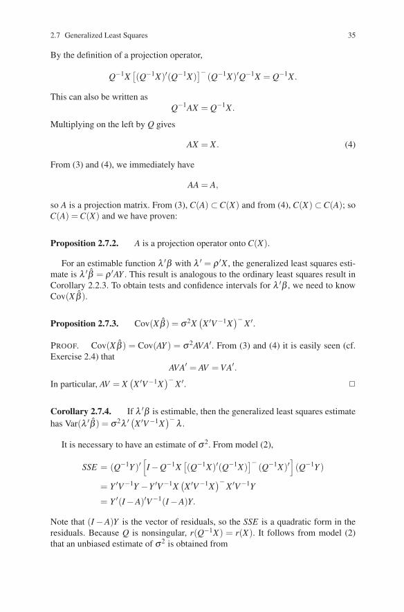
2.7 Generalized Least Squares 35
By the definition of a projection operator,
Q−1X[(Q−1X)′(Q−1X)
]−(Q−1X)′Q−1X = Q−1X .
This can also be written asQ−1AX = Q−1X .
Multiplying on the left by Q gives
AX = X . (4)
From (3) and (4), we immediately have
AA = A,
so A is a projection matrix. From (3), C(A) ⊂C(X) and from (4), C(X) ⊂C(A); soC(A) = C(X) and we have proven:
Proposition 2.7.2. A is a projection operator onto C(X).
For an estimable function λ ′β with λ ′ = ρ ′X , the generalized least squares esti-mate is λ ′β = ρ ′AY . This result is analogous to the ordinary least squares result inCorollary 2.2.3. To obtain tests and confidence intervals for λ ′β , we need to knowCov(X β ).
Proposition 2.7.3. Cov(X β ) = σ 2X(X ′V−1X
)− X ′.
PROOF. Cov(X β ) = Cov(AY ) = σ 2AVA′. From (3) and (4) it is easily seen (cf.Exercise 2.4) that
AVA′ = AV = VA′.
In particular, AV = X(X ′V−1X
)− X ′. �
Corollary 2.7.4. If λ ′β is estimable, then the generalized least squares estimatehas Var(λ ′β ) = σ 2λ ′ (X ′V−1X
)− λ .
It is necessary to have an estimate of σ 2. From model (2),
SSE = (Q−1Y )′[I −Q−1X
[(Q−1X)′(Q−1X)
]−(Q−1X)′
](Q−1Y )
= Y ′V−1Y −Y ′V−1X(X ′V−1X
)−X ′V−1Y
= Y ′(I −A)′V−1(I −A)Y.
Note that (I −A)Y is the vector of residuals, so the SSE is a quadratic form in theresiduals. Because Q is nonsingular, r(Q−1X) = r(X). It follows from model (2)that an unbiased estimate of σ 2 is obtained from

36 2 Estimation
MSE = Y ′(I −A)′V−1(I −A)Y/
[n− r(X)] .
With normal errors, this is also the minimum variance unbiased estimate of σ 2.Suppose that e is normally distributed. From Theorem 1.3.7 applied to model (2),
the MSE is independent of Q−1X β . Since X β is a function of Q−1X β , the MSE isindependent of X β . Moreover, X β is normally distributed and SSE/σ 2 has a chi-squared distribution.
A particular application of these results is that, for an estimable function λ ′β ,
λ ′β −λ ′β√MSE λ ′ (X ′V−1X)− λ
∼ t(n− r(X)).
Given this distribution, tests and confidence intervals involving λ ′β can be obtainedas in Appendix E.
We now give a result that determines when generalized least squares estimates are(ordinary) least squares estimates. The result will be generalized in Theorem 10.4.5.The generalization changes it to an if and only if statement for arbitrary covariancematrices.
Proposition 2.7.5. If V is nonsingular and C(V X) ⊂ C(X), then least squaresestimates are BLUEs.
PROOF. The proof proceeds by showing that A ≡ X(X ′V−1X)−X ′V−1 is the per-pendicular projection operator onto C(X). We already know that A is a projectionoperator onto C(X), so all we need to establish is that if w ⊥C(X), then Aw = 0.
V being nonsingular implies that the null spaces of V X and X are identical, sor(V X) = r(X). With C(V X)⊂C(X), we must have C(V X) = C(X). C(V X) = C(X)implies that for some matrices B1 and B2, V XB1 = X and V X = XB2. Multiplyingthrough by V−1 in both equations gives XB1 = V−1X and X = V−1XB2, so C(X) =C(V−1X). It follows immediately that C(X)⊥ = C(V−1X)⊥. Now, w ⊥C(X) if andonly if w ⊥C(V−1X), so
Aw =[X(X ′V−1X)−X ′V−1]w = X(X ′V−1X)−
[X ′V−1w
]= 0. �
Frequently in regression analysis, V is a diagonal matrix, in which case gener-alized least squares is referred to as weighted least squares (WLS). Considerablesimplification results.
Exercise 2.4
(a) Show that AVA′ = AV = VA′.(b) Show that A′V−1A = A′V−1 = V−1A.(c) Show that A is the same for any choice of
(X ′V−1X
)−.

2.8 Normal Equations 37
The following result will be useful in Section 9. It is essentially the Pythagoreantheorem and can be used directly to show Theorem 2.7.1(b), that X β is a generalizedleast squares estimate if and only if X β = AY .
Lemma 2.7.6 Let A = X(X ′V−1X)−X ′V−1, then
(Y −Xβ )V−1(Y −Xβ) = (Y −AY )′V−1(Y −AY )+(AY −Xβ )V−1(AY −Xβ )
= (Y −AY )′V−1(Y −AY )+(β −β )′(X ′V−1X)(β −β )
where β = (X ′V−1X)−X ′V−1Y .
PROOF. Following the proof of Theorem 2.2.2, write (Y −Xβ ) = (Y −AY )+(AY −Xβ ) and eliminate cross product terms using Exercise 2.4 and
(I −A)′V−1(AY −Xβ ) = V−1(I −A)(AY −Xβ ) = 0. �
Exercise 2.5 Show that A is the perpendicular projection operator onto C(X)when the inner product between two vectors x and y is defined as x′V−1y.
Hint: Recall the discussion after Definition B.50.
2.8 Normal Equations
An alternative method for finding least squares estimates of the parameter β in themodel
Y = Xβ + e, E(e) = 0, Cov(e) = σ 2I
is to find solutions of what are called the normal equations. The normal equationsare defined as
X ′Xβ = X ′Y.
They are usually arrived at by setting equal to zero the partial derivatives of (Y −Xβ )′(Y −Xβ ) with respect to β .
Corollary 2.8.2 shows that solutions of the normal equations are least squaresestimates of β . Recall that, by Theorem 2.2.1, least squares estimates are solutionsof Xβ = MY .
Theorem 2.8.1. β is a least squares estimate of β if and only if (Y −X β )⊥C(X).
PROOF. Since M is the perpendicular projection operator onto C(X), (Y −X β )⊥C(X) if and only if M(Y −X β ) = 0, i.e, if and only if MY = X β . �
Corollary 2.8.2. β is a least squares estimate of β if and only if X ′X β = X ′Y .

38 2 Estimation
PROOF. X ′X β = X ′Y if and only if X ′(Y −X β ) = 0, which occurs if and only if(Y −X β ) ⊥C(X). �
For generalized least squares problems, the normal equations are found frommodel (2.7.2). The normal equations simplify to
X ′V−1Xβ = X ′V−1Y.
2.9 Bayesian Estimation
Bayesian estimation incorporates the analyst’s subjective information about a prob-lem into the analysis. It appears to be the only logically consistent method of anal-ysis, but not the only useful one. Some people object to the loss of objectivity thatresults from using the analyst’s subjective information, but either the data are strongenough for reasonable people to agree on their interpretation or, if not, analystsshould be using their subjective (prior) information for making appropriate deci-sions related to the data.
There is a vast literature on Bayesian statistics. Three fundamental works are deFinetti (1974, 1975), Jeffreys (1961), and Savage (1954). Good elementary introduc-tions to the subject are Lindley (1971) and Berry (1996). A few of the well-knownbooks on the subject are Berger (1993), Box and Tiao (1973), DeGroot (1970),Geisser (1993), Raiffa and Schlaifer (1961), and Zellner (1971). My favorite is nowChristensen, Johnson, Branscum, and Hanson (2010), which also includes manymore references to many more excellent books. Christensen et al. contains a farmore extensive discussion of Bayesian linear models than this relatively short sec-tion.
Consider the linear model
Y = Xβ + e, e ∼ N(0,σ 2I),
where r(X) = r. It will be convenient to consider a full rank reparameterization ofthis model,
Y = Zγ + e, e ∼ N(0,σ 2I),
where C(X) = C(Z). As in Sections 1.2 and 2.4, this determines a density for Ygiven γ and σ 2, say, f (Y |γ,σ 2). For a Bayesian analysis, we must have a joint den-sity for γ and σ 2, say p(γ,σ 2). This distribution reflects the analyst’s beliefs, priorto collecting data, about the process of generating the data. We will actually specifythis distribution conditionally as p(γ,σ 2) = p(γ|σ 2)p(σ 2). In practice, it is difficultto specify these distributions for γ given σ 2 and σ 2. Convenient choices that haveminimal impact on (most aspects of) the analysis are the (improper) reference priorsp(γ|σ 2) = 1 and p(σ 2) = 1/σ 2. These are improper in that neither prior density in-tegrates to 1. Although these priors are convenient, a true Bayesian analysis requiresthe specification of proper prior distributions.

2.9 Bayesian Estimation 39
Specifying prior information is difficult, particularly about such abstract quan-tities as regression coefficients. A useful tool in specifying prior information is tothink in terms of the mean of potential observations. For example, we could specifya vector of predictor variables, say zi, and specify the distribution for the mean ofobservations having those predictor variables. With covariates zi, the mean of poten-tial observables is z′iγ . Typically, we assume that z′iγ has a N(yi,σ2wi) distribution.One way to think about yi and wi is that yi is a prior guess for what one would seewith covariates zi, and 1/wi is the number of observations this guess is worth. Tospecify a proper prior distribution for γ given σ 2, we specify independent priors atvectors zi, i = 1, . . . ,r, where r is the dimension of γ . As will be seen later, under amild condition this prior specification leads easily to a proper prior distribution onγ . Although choosing the zis and specifying the priors may be difficult to do, it ismuch easier to do than trying to specify an intelligent joint prior directly on γ . If onewishes to specify only partial prior information, one can simply choose fewer thanr vectors zi and the analysis follows as outlined below. In fact, using the referenceprior for γ amounts to not choosing any zis. Again, the analysis follows as outlinedbelow. Bedrick, Christensen, and Johnson (1996) and Christensen et al. (2010) dis-cuss these techniques in more detail.
I believe that the most reasonable way to specify a proper prior on σ 2 is to thinkin terms of the variability of potential observables around some fixed mean. Unfor-tunately, the implications of this idea are not currently as well understood as theyare for the related technique of specifying the prior for γ indirectly through priorson means of potential observables. For now, we will simply consider priors for σ 2
that are inverse gamma distributions, i.e., distributions in which 1/σ 2 has a gammadistribution. An inverse gamma distribution has two parameters, a and b. One canthink of the prior as being the equivalent of 2a (prior) observations with a priorguess for σ2 of b/a.
It is convenient to write Y = (y1, . . . , yr)′ and Z as the r× r matrix with ith rowz′i. In summary, our distributional assumptions are
Y |γ,σ 2 ∼ N(Zγ,σ 2I),Zγ|σ 2 ∼ N(Y ,σ 2D(w)),
σ 2 ∼ InvGa(a,b).
We assume that Z is nonsingular, so that the second of these induces the distribution
γ|σ 2 ∼ N(Z−1Y ,σ 2Z−1D(w)Z−1′).
Actually, any multivariate normal distribution for γ given σ 2 will lead to essentiallythe same analysis as given here.
A Bayesian analysis is based on finding the distribution of the parameters giventhe data, i.e., p(γ,σ 2|Y ). This is accomplished by using Bayes’s theorem, whichstates that
p(γ ,σ 2|Y ) =f (Y |γ ,σ 2)p(γ,σ2)
f (Y ).

40 2 Estimation
If we know the numerator of the fraction, we can obtain the denominator by
f (Y ) =∫
f (Y |γ,σ 2)p(γ,σ2)dγ dσ 2.
In fact, because of this relationship, we only need to know the numerator up to aconstant multiple, because any multiple will cancel in the fraction.
Later in this section we will show that
p(γ ,σ 2|Y ) ∝(σ2)−(n+r)/2
p(σ2)
× exp{ −1
2σ 2
[(γ − γ)′(Z′Z + Z′D−1(w)Z)(γ − γ)
]}(1)
× exp{ −1
2σ 2
[(Y −Zγ)′(Y −Zγ)+(Y − Zγ)′D−1(w)(Y − Zγ)
]},
whereγ =(Z′Z + Z′D−1(w)Z
)−1 [Z′Y + Z′D−1(w)Y
]. (2)
The joint posterior (post data) density is the righthand side of (1) divided by itsintegral with respect to γ and σ 2.
The form (1) for the joint distribution given the data is not particularly useful.What we really need are the marginal distributions of σ 2 and functions ρ ′Zγ ≡ρ ′Xβ , and predictive distributions for new observations.
As will be shown, the Bayesian analysis turns out to be quite consistent with thefrequentist analysis. For the time being, we use the reference prior p(σ 2) = 1/σ 2.In our model, we have Zγ random, but it is convenient to think of Y as being rindependent prior observations with mean Zγ and weights w. Now consider thegeneralized least squares model[
YY
]=[
ZZ
]γ +[
ee
],
[ee
]∼ N([
0n×10r×1
],σ 2[
In 00 D(w)
]). (3)
This generalized least squares model can also be written as, say,
Y∗ = Z∗γ + e∗, e∗ ∼ N(0,σ2V∗).
The generalized least squares estimate from this model is γ as given in (2). In theBayesian analysis, γ is the expected value of γ given Y . Let BMSE denote the meansquared error from the (Bayesian) generalized least squares model with BdfE de-grees of freedom for error.
In the frequentist generalized least squares analysis, for fixed γ with random γand BMSE ,
λ ′γ −λ ′γ√BMSE λ ′ (Z′Z + Z′D−1(w)Z
)−1 λ∼ t(BdfE).
In the Bayesian analysis the same distribution holds, but for fixed γ and BMSEwith random γ . Frequentist confidence intervals for λ ′γ are identical to Bayesian

2.9 Bayesian Estimation 41
posterior probability intervals for λ ′γ . Note that for estimating a function ρ ′Xβ ,simply write it as ρ ′Xβ = ρ ′Zγ and take λ ′ = ρ ′Z.
In the frequentist generalized least squares analysis, for fixed σ 2 and randomBMSE ,
(BdfE)BMSEσ2 ∼ χ2(BdfE).
In the Bayesian analysis, the same distribution holds, but for fixed BMSE and ran-dom σ 2. Confidence intervals for σ2 are identical to Bayesian posterior probabilityintervals for σ 2.
In the frequentist generalized least squares analysis, a prediction interval for afuture independent observation y0 with predictor vector z0 and weight 1 is based onthe distribution
y0 − z′0γ√BMSE
[1+ z′0
(Z′Z + Z′D−1(w)Z
)−1 z0
] ∼ t(BdfE), (4)
where γ and BMSE are random and y0 is independent of Y for given γ and σ 2,see Exercise 2.10.1. In the Bayesian analysis, the same distribution holds, but forfixed γ and BMSE . Standard prediction intervals for y0 are identical to Bayesianprediction intervals.
If we specify an improper prior on γ using fewer than r vectors zi, these relation-ships between generalized least squares and the Bayesian analysis remain valid. Infact, for the reference prior on γ , i.e., choosing no zis, the generalized least squaresmodel reduces to the usual model Y = Xβ + e, e ∼ N(0,σ 2I), and the Bayesiananalysis becomes analogous to the usual ordinary least squares analysis.
In the generalized least squares model (3), BdfE = n. If we take σ 2 ∼ InvGa(a,b),the only changes in the Bayesian analysis are that BMSE changes to [(BdfE)BMSE +2b]/(BdfE + 2a) and the degrees of freedom for the t and χ2 distributions changefrom BdfE to BdfE +2a. With reference priors for both γ and σ 2, BdfE = n− r, asin ordinary least squares.
EXAMPLE 2.9.1. Schafer (1987) presented data on 93 individuals at the Har-ris Bank of Chicago in 1977. The response is beginning salary in hundreds ofdollars. There are four covariates: sex, years of education, denoted EDUC, yearsof experience, denoted EXP, and time at hiring as measured in months after 1-1-69, denoted TIME. This is a regression, so we can take Z ≡ X , γ ≡ β , and writeX ≡ Z. With an intercept in the model, Johnson, Bedrick, and I began by speci-fying five covariate vectors x′i = (1,SEXi,EDUCi,EXPi,T IMEi), say, (1,0,8,0,0),(1,1,8,0,0), (1,1,16,0,0), (1,1,16,30,0), and (1,1,8,0,36), where a SEX valueof 1 indicates a male. For example, the vector (1,0,8,0,0) corresponds to a male with8 years of education, no previous experience, and starting work on 1-1-69. Thinkingabout the mean salary for each set of covariates, we chose y′ = (40,40,60,70,50),which reflects a prior belief that starting salaries are the same for equally quali-fied men and women and a belief that salary is increasing as a function of EDUC,

42 2 Estimation
EXP, and TIME. The weights wi are all chosen to be 0.4, so that in total theprior carries the same weight as two sampled observations. The induced prior onβ given σ 2 has mean vector (20,0,2.50,0.33,0.28)′ and standard deviation vectorσ ≡ (2.74,2.24,0.28,0.07,0.06)′.
To illustrate partial prior information, we consider the same example, only withthe fifth “prior observation” deleted. In this instance, the prior does not reflect anyinformation about the response at TIMEs other than 0. The prior is informative aboutthe mean responses at the first four covariate vectors but is noninformative (the prioris constant) for the mean response at the fifth covariate vector. Moreover, the prioris constant for the mean response with any other choice of fifth vector, providedthis vector is linearly independent of the other four. (All such vectors must havea nonzero value for the time component.) In this example, the induced improperdistribution on β has the same means and standard deviations for β1, β2, β3, and β4,but is flat for β5.
We specify a prior on σ2 worth 2a = 2 observations with a prior guess for σ 2
of b/a = 25. The prior guess reflects our belief that a typical salary has a standarddeviation of 5.
Using our informative prior, the posterior mean of β is
β = (33.68,6.96,1.02,0.18,0.23)′
with BdfE = 95 and BMSE = 2404/95 = 25.3053. The standard deviations for βare√
95/93(310,114,23.43,6.76,5.01)′/100. In the partially informative case dis-cussed above, the posterior mean is
β = (34.04,7.11,0.99,0.17,0.23),
BdfE = 94, BMSE = 2383/94 = 25.3511, and the standard deviations for β are√94/92(313,116,23.78,6.80,5.06)′/100. Using the standard reference prior, i.e.,
using ordinary least squares without prior data, β = (35.26,7.22,0.90,0.15,0.23)′,BdfE = 88, BMSE = 2266/88 = 25.75, and the standard deviations for β are√
88/86(328,118,24.70,7.05,5.20)′/100. The 95% prediction interval for x0 =(1,0,10,3.67,7)′ with a weight of 1 is (35.97,56.34) for the informative prior,(35.99,56.38) with partial prior information, and (36.27,56.76) for the referenceprior.
2.9.1 Distribution Theory
For the time being, we will assume relation (1) for the joint posterior and use it toarrive at marginal distributions. Afterwards, we will establish relation (1).
The distribution theory for the Bayesian analysis involves computations unlikeanything else done in this book. It requires knowledge of some basic facts.
The density of a gamma distribution with parameters a > 0 and b > 0 is

2.9 Bayesian Estimation 43
g(τ) =ba
Γ (a)τa−1 exp[−bτ]
for τ > 0. A Gamma(n/2,1/2) distribution is the same as a χ2(n) distribution. Wewill not need the density of an inverse gamma, only the fact that y has a Gamma(a,b)distribution if and only if 1/y has an InvGa(a,b) distribution. The improper refer-ence distribution corresponds to a = 0,b = 0.
The t distribution is defined in Appendix C. The density of a t(n) distribution is
g(w) =[
1+w2
n
]−(n+1)/2
Γ(
n+12
)/[Γ(n
2
)√nπ].
Eliminating the constants required to make the density integrate to 1 gives
g(w) ∝[
1+w2
n
]−(n+1)/2
.
Bayesian linear models involve multivariate t distributions, cf. DeGroot (1970,Section 5.6). Let W ∼ N(μ,V ), Q ∼ χ2(n), with W and Q independent. Then if
Y ∼ (W −μ)1√Q/n
+ μ ,
by definitionY ∼ t(n,μ,V ) .
For an r vector Y , a multivariate t(n) distribution with center μ and dispersion matrixV has density
g(y) =[
1+1n(y−μ)′V−1(y−μ)
]−(n+r)/2
×Γ(
n+ r2
)/{Γ(n
2
)(nπ)r/2[det(V )]1/2
}.
This distribution has mean μ for n > 1 and covariance matrix [n/(n−2)]V for n > 2.To get noninteger degrees of freedom a, just replace Q/n in the definition with bT/a,where T ∼ Gamma(a/2,b/2) independent of W .
Note that from the definition of a multivariate t,
λ ′Y −λ ′μ√λ ′V λ
∼ (λ ′W −λ ′μ)/√
λ ′Vλ√Q/n
∼ t(n). (5)
Proceeding with the Bayesian analysis, to find the marginal posterior of γ let
Q =[(Y −Zγ)′(Y −Zγ)+(Y − Zγ)′D−1(w)(Y − Zγ)
]+[(γ − γ)′(Z′Z + Z′D−1(w)Z)(γ − γ)
].

44 2 Estimation
From (1),
p(γ|Y ) ∝∫ (
σ 2)−(n+r)/2p(σ 2)exp
{ −12σ 2 Q
}dσ2.
Transforming σ 2 into τ = 1/σ 2 gives σ 2 = 1/τ and dσ 2 = |− τ−2|dτ . Thus
p(γ|Y ) ∝∫
(τ)(n+r)/2 p(1/τ)exp{−τQ/2}τ−2dτ.
Note that if σ 2 has an inverse gamma distribution with parameters a and b, then τhas a gamma distribution with parameters a and b; so p(1/τ)τ−2 is a gamma densityand
p(γ |Y ) ∝∫
(τ)(n+r+2a−2)/2 exp{−τ(Q+2b)/2}dτ.
The integral is a gamma integral, e.g., the gamma density given earlier integrates to1, so
p(γ|Y ) ∝ Γ [(n+ r +2a)/2]/
[(Q+2b)/2](n+r+2a)/2
orp(γ|Y ) ∝ [Q+2b]−(n+r+2a)/2 .
We can rewrite this as
p(γ|Y ) ∝[(BdfE)(BMSE)+2b+(γ − γ)′
(Z′Z + Z′D−1(w)Z
)(γ − γ)
]−(n+r+2a)/2
∝
[1+
1n+2a
(γ − γ)′(Z′Z + Z′D−1(w)Z
)(γ − γ)
[(BdfE)(BMSE)+2b]/(n+2a)
]−(n+2a+r)/2
,
so
γ|Y ∼ t(
n+2a, γ ,(BdfE)(BMSE)+2b
n+2a
(Z′Z + Z′D−1(w)Z
)−1)
.
Together with (5), this provides the posterior distribution of λ ′γ .Now consider the marginal (posterior) distribution of σ 2.
p(σ 2|Y ) ∝(σ 2)−n/2
p(σ 2)
× exp{ −1
2σ 2
[(Y −Zγ)′(Y −Zγ)+(Y − Zγ)′D−1(w)(Y − Zγ)
]}×∫ (
σ 2)−r/2exp{ −1
2σ 2
[(γ − γ)′(Z′Z + Z′D−1(w)Z)(γ − γ)
]}dγ.
The term being integrated is proportional to a normal density, so the integral is aconstant that does not depend on σ 2. Hence,
p(σ 2|Y ) ∝(σ2)−n/2
p(σ 2)
× exp{ −1
2σ 2
[(Y −Zγ)′(Y −Zγ)+(Y − Zγ)′D−1(w)(Y − Zγ)
]}

2.9 Bayesian Estimation 45
or, using the generalized least squares notation,
p(σ 2|Y ) ∝(σ 2)−n/2
p(σ 2)exp[ −1
2σ 2 (BdfE)(BMSE)].
We transform to the precision, τ ≡ 1/σ 2. The InvGa(a,b) distribution for σ 2 yields
p(τ|Y ) ∝ (τ)n/2 (τ)a−1 exp[−bτ]exp[−τ
2(BdfE)(BMSE)
]= (τ)[(n+2a)/2]−1 exp
[−2b+(BdfE)(BMSE)
2τ]
;
so
τ|Y ∼ Gamma(
n+2a2
,2b+(BdfE)(BMSE)
2
).
It is not difficult to show that
[2b+(BdfE)(BMSE)]τ|Y ∼ Gamma(
n+2a2
,12
),
i.e.,2b+(BdfE)(BMSE)
σ 2
∣∣∣Y ∼ Gamma(
n+2a2
,12
).
As mentioned earlier, for the reference distribution with a = 0,b = 0,
(BdfE)(BMSE)σ2
∣∣∣Y ∼ Gamma(
n2,
12
)= χ2(n).
Finally, we establish relation (1).
p(γ,σ 2|Y ) ∝ f (Y |γ,σ2)p(γ|σ 2)p(σ 2)
∝{(
σ 2)−n/2exp[−(Y −Zγ)′(Y −Zγ)/2σ 2]}
×{(
σ 2)−r/2exp[−(γ − Z−1Y
)′(Z′D−1(w)Z
)(γ − Z−1Y
)/2σ 2]}
× p(σ 2)
Most of the work involves simplifying the terms in the exponents. We isolate thoseterms, deleting the multiple −1/2σ 2.
(Y −Zγ)′(Y −Zγ)+(γ − Z−1Y
)′ (Z′D−1(w)Z
)(γ − Z−1Y
)= (Y −Zγ)′(Y −Zγ)+(Y − Zγ)′D(w)−1(Y − Zγ)
=([
YY
]−[
ZZ
]γ)′ [ I 0
0 D(w)−1
]([YY
]−[
ZZ
]γ)
.
Write

46 2 Estimation
Y∗ =[
YY
], Z∗ =
[ZZ
], V∗ =
[I 00 D(w)
]and apply Lemma 2.7.6 to get
(Y −Zγ)′(Y −Zγ)+(γ − Z−1Y
)′ (Z′D−1(w)Z
)(γ − Z−1Y
)= (Y∗ −Z∗γ)′V−1
∗ (Y∗ −Z∗γ)= (Y∗ −A∗Y∗)′V−1
∗ (Y∗ −A∗Y∗)+(γ − γ)′(Z′∗V
−1∗ Z∗)(γ − γ),
where A∗ = Z∗(Z′∗V−1∗ Z∗)−1Z′∗V−1∗ and
γ = (Z′∗V
−1∗ Z∗)−1Z′
∗V−1∗ Y∗
=(Z′Z + Z′D−1(w)Z
)−1 [Z′Y + Z′D−1(w)Y
].
Finally, observe that
(Y∗ −A∗Y∗)′V−1∗ (Y∗ −A∗Y∗)+(γ − γ)′(Z′
∗V−1∗ Z∗)(γ − γ)
=[(Y −Zγ)′(Y −Zγ)+(Y − Zγ)′D−1(w)(Y − Zγ)
]+[(γ − γ)′(Z′Z + Z′D−1(w)Z)(γ − γ)
].
Substitution gives (1).
Exercise 2.6 Prove relation (4).
2.10 Additional Exercises
Exercise 2.10.1 Consider a regression model Y = Xβ + e, e ∼ N(0,σ 2I) andsuppose that we want to predict the value of a future observation, say y0, that willbe independent of Y and be distributed N(x′0β ,σ2).
(a) Find the distribution of
y0 − x′0β√MSE
[1+ x′0(X ′X)−1x0
] .(b) Find a 95% prediction interval for y0.Hint: A prediction interval is similar to a confidence interval except that, rather
than finding parameter values that are consistent with the data and the model, onefinds new observations y0 that are consistent with the data and the model as deter-mined by an α level test.
(c) Let η ∈ (0,0.5]. The 100η th percentile of the distribution of y0 is, say,γ(η) = x′0β + z(η)σ . (Note that z(η) is a negative number.) Find a (1−α)100%

2.10 Additional Exercises 47
lower confidence bound for γ(η). In reference to the distribution of y0, this lowerconfidence bound is referred to as a lower η tolerance point with confidence coef-ficient (1−α)100%. For example, if η = 0.1, α = 0.05, and y0 is the octane valueof a batch of gasoline manufactured under conditions x0, then we are 95% confidentthat no more than 10% of all batches produced under x0 will have an octane valuebelow the tolerance point.
Hint: Use a noncentral t distribution based on x′0β − γ(η).Comment: For more detailed discussions of prediction and tolerance (and we allknow that tolerance is a great virtue), see Geisser (1993), Aitchison and Dunsmore(1975), and Guttman (1970).
Exercise 2.10.2 Consider the model
Y = Xβ +b+ e, E(e) = 0, Cov(e) = σ2I,
where b is a known vector. Show that Proposition 2.1.3 is not valid for this modelby producing a linear unbiased estimate of ρ ′Xβ , say a0 +a′Y , for which a0 �= 0.
Hint: Modify ρ ′MY .
Exercise 2.10.3 Consider the model yi = β1xi1 + β2xi2 + ei, eis i.i.d. N(0,σ 2).Use the data given below to answer (a) through (d). Show your work, i.e., do not usea regression or general linear models computer program.
(a) Estimate β1, β2, and σ 2.(b) Give 95% confidence intervals for β1 and β1 +β2.(c) Perform an α = 0.01 test for H0 : β2 = 3.(d) Find an appropriate P value for the test of H0 : β1 −β2 = 0.
obs. 1 2 3 4 5 6 7 8y 82 79 74 83 80 81 84 81
x1 10 9 9 11 11 10 10 12x2 15 14 13 15 14 14 16 13
Exercise 2.10.4 Consider the model yi = β1xi1 + β2xi2 + ei, eis i.i.d. N(0,σ 2).There are 15 observations and the sum of the squared observations is Y ′Y = 3.03.Use the normal equations given below to answer parts (a) through (c).
(a) Estimate β1, β2, and σ 2.(b) Give 98% confidence intervals for β2 and β2 −β1.(c) Perform an α = 0.05 test for H0 : β1 = 0.5.
The normal equations are[15.00 374.50
374.50 9482.75
][β1β2
]=[
6.03158.25
].

48 2 Estimation
Exercise 2.10.5 Consider the model
yi = β0 +β1xi1 +β2xi2 +β11x2i1 +β22x2
i2 +β12xi1xi2 + ei,
where the predictor variables take on the following values.
i 1 2 3 4 5 6 7xi1 1 1 −1 −1 0 0 0xi2 1 −1 1 −1 0 0 0
Show that β0, β1, β2, β11 + β22, β12 are estimable and find (nonmatrix) algebraicforms for the estimates of these parameters. Find the MSE and the standard errorsof the estimates.

Chapter 3
Testing
We will consider two approaches to testing linear models. The approaches are iden-tical in that a test under either approach is a well-defined test under the other. Thetwo methods differ only conceptually. One approach is that of testing models; theother approach involves testing linear parametric functions.
Section 1 discusses the notion that a linear model depends fundamentally onC(X) and that the vector of parameters β is of secondary importance. Section 2 dis-cusses testing different models against each other. Section 3 discusses testing linearfunctions of the β vector. Section 4 presents a brief discussion of the relative meritsof testing models versus testing linear parametric functions. Section 5 examines theproblem of testing parametric functions that put a constraint on a given subspace ofC(X). In particular, Section 5 establishes that estimates and tests can be obtainedby using the projection operator onto the subspace. This result is valuable whenusing one-way ANOVA methods to analyze balanced multifactor ANOVA mod-els. Section 6 considers the problem of breaking sums of squares into independentcomponents. This is a general discussion that relates to breaking ANOVA treatmentsums of squares into sums of squares for orthogonal contrasts and also relates to theissue of writing multifactor ANOVA tables with independent sums of squares. Sec-tion 7 discusses the construction of confidence regions for estimable linear paramet-ric functions. Section 8 presents testing procedures for the generalized least squaresmodel of Section 2.7.
3.1 More About Models
For estimation in the model
Y = Xβ + e, E(e) = 0, Cov(e) = σ 2I,
we have found that the crucial item needed is M, the perpendicular projection op-erator onto C(X). For convenience, we will call C(X) the estimation space and
© Springer Science+Business Media, LLC 2011
49Springer Texts in Statistics, DOI 10.1007/978-1-4419-9816-3_3, R. Christensen, Plane Answers to Complex Questions: The Theory of Linear Models,

50 3 Testing
C(X)⊥ the error space. I − M is the perpendicular projection operator onto theerror space. In a profound sense, any two linear models with the same estima-tion space are the same model. For example, any two such models will give thesame predicted values for the observations and the same estimate of σ 2. Supposewe have two linear models for a vector of observations, say Y = X1β1 + e1 andY = X2β2 + e2 with C(X1) = C(X2). For these alternative parameterizations, i.e.,reparameterizations, M does not depend on which of X1 or X2 is used; it dependsonly on C(X1)[= C(X2)]. Thus, the MSE does not change, and the least squares esti-mate of E(Y ) is Y = MY = X1β1 = X2β2. In fact, we could simply write the originalmodel as
E(Y ) ∈C(X), Cov(Y ) = σ 2I.
The expected values of the observations are fundamental to estimation in lin-ear models. Identifiable parameteric functions are functions of the expected val-ues. Attention is often restricted to estimable functions, i.e., functions ρ ′Xβ whereXβ = E(Y ). The key idea in estimability is restricting estimation to linear combi-nations of the rows of E(Y ). E(Y ) depends only on the choice of C(X), whereasthe vector β depends on the particular choice of X . Consider again the two mod-els discussed above. If λ ′
1β1 is estimable, then λ ′1β1 = ρ ′X1β1 = ρ ′E(Y ) for some
ρ . This estimable function is the same linear combination of the rows of E(Y ) asρ ′E(Y ) = ρ ′X2β2 = λ ′
2β2. These are really the same estimable function, but theyare written with different parameters. This estimable function has a unique leastsquares estimate, ρ ′MY .
EXAMPLE 3.1.1. One-Way ANOVA.Two parameterizations for a one-way ANOVA are commonly used. They are
yi j = μ +αi + ei j
andyi j = μi + ei j.
It is easily seen that these models determine the same estimation space. The esti-mates of σ 2 and E(yi j) are identical in the two models. One convenient aspect ofthese models is that the relationships between the two sets of parameters are easilyidentified. In particular,
μi = E(yi j) = μ +αi.
It follows that the mean of the μis equals μ plus the mean of the αis, i.e., μ· = μ + α·.It also follows that μ1 − μ2 = α1 −α2, etc. The parameters in the two models aredifferent, but they are related. Any estimable function in one model determines acorresponding estimable function in the other model. These functions have the sameestimate. Chapter 4 contains a detailed examination of these models.
EXAMPLE 3.1.2. Simple Linear Regression.The models
yi = β0 +β1xi + ei

3.1 More About Models 51
andyi = γ0 + γ1(xi − x·)+ ei
have the same estimation space (x· is the mean of the xis). Since
β0 +β1xi = E(yi) = γ0 + γ1(xi − x·) (1)
for all i, it is easily seen from averaging over i that
β0 +β1x· = γ0.
Substituting β0 = γ0 −β1x· into (1) leads to
β1(xi − x·) = γ1(xi − x·)
and, if the xis are not all identical,
β1 = γ1.
These models are examined in detail in Section 6.1.
When the estimation spaces C(X1) and C(X2) are the same, write X1 = X2T toget
X1β1 = X2T β1 = X2β2. (2)
Estimable functions are equivalent in the two models: Λ ′1β1 = P′X1β1 = P′X2β2 =
Λ ′2β2. It also follows from equation (2) that the parameterizations must satisfy the
relationβ2 = T β1 + v (3)
for some v ∈ C(X ′2)
⊥. In general, neither of the parameter vectors β1 or β2 isuniquely defined but, to the extent that either parameter vector is defined, equation(3) establishes the relationship between them. A unique parameterization for, say,the X2 model occurs if and only if X ′
2X2 is nonsingular. In such a case, the columnsof X2 form a basis for C(X2), so the matrix T is uniquely defined. In this case, thevector v must be zero because C(X ′
2)⊥ = {0}. An alternative and detailed presenta-
tion of equivalent linear models, both the reparameterizations considered here andthe equivalences between constrained and unconstrained models considered in sub-sequent sections, is given by Peixoto (1993).
Basically, the β parameters in
Y = Xβ + e, E(e) = 0, Cov(e) = σ 2I
are either a convenience or a nuisance, depending on what we are trying to do.Having E(e) = 0 gives E(Y ) = Xβ , but since β is unknown, this is merely sayingthat E(Y ) is some linear combination of the columns of X . The essence of the modelis that
E(Y ) ∈C(X), Cov(Y ) = σ 2I.

52 3 Testing
As long as we do not change C(X), we can change X itself to suit our convenience.
3.2 Testing Models
In this section, the basic theory for testing a linear model against a reduced modelis presented. A generalization of the basic procedure is also presented.
Testing in linear models typically reduces to putting a constraint on the estima-tion space. We start with a (full) model that we know (assume) to be valid,
Y = Xβ + e, e ∼ N(0,σ 2I). (1)
Our wish is to reduce this model, i.e., we wish to know if some simpler model givesan acceptable fit to the data. Consider whether the model
Y = X0γ + e, e ∼ N(0,σ2I), C(X0) ⊂C(X) (2)
is acceptable. Clearly, if model (2) is correct, then model (1) is also correct. Thequestion is whether (2) is correct.
The procedure of testing full and reduced models is a commonly used method instatistics.
EXAMPLE 3.2.0.
(a) One-Way ANOVA.The full model is
yi j = μ +αi + ei j.
To test for no treatment effects, i.e., to test that the αis are extraneous, the reducedmodel simply eliminates the treatment effects. The reduced model is
yi j = γ + ei j.
Additionally, consider testing H0 : α1 −α3 = 0 in Example 1.0.2. The full modelis ⎡⎢⎢⎢⎢⎢⎣
y11y12y13y21y31y32
⎤⎥⎥⎥⎥⎥⎦=
⎡⎢⎢⎢⎢⎢⎣1 1 0 01 1 0 01 1 0 01 0 1 01 0 0 11 0 0 1
⎤⎥⎥⎥⎥⎥⎦⎡⎢⎣
μα1α2α3
⎤⎥⎦+
⎡⎢⎢⎢⎢⎢⎣e11e12e13e21e31e32
⎤⎥⎥⎥⎥⎥⎦ .
We can rewrite this as

3.2 Testing Models 53
Y = μ
⎡⎢⎢⎢⎢⎢⎣111111
⎤⎥⎥⎥⎥⎥⎦+α1
⎡⎢⎢⎢⎢⎢⎣111000
⎤⎥⎥⎥⎥⎥⎦+α2
⎡⎢⎢⎢⎢⎢⎣000100
⎤⎥⎥⎥⎥⎥⎦+α3
⎡⎢⎢⎢⎢⎢⎣000011
⎤⎥⎥⎥⎥⎥⎦+ e.
If we impose the constraint H0 : α1 −α3 = 0, i.e., α1 = α3, we get
Y = μJ +α1
⎡⎢⎢⎢⎢⎢⎣111000
⎤⎥⎥⎥⎥⎥⎦+α2
⎡⎢⎢⎢⎢⎢⎣000100
⎤⎥⎥⎥⎥⎥⎦+α1
⎡⎢⎢⎢⎢⎢⎣000011
⎤⎥⎥⎥⎥⎥⎦+ e,
or
Y = μJ +α1
⎛⎜⎜⎜⎜⎜⎝
⎡⎢⎢⎢⎢⎢⎣111000
⎤⎥⎥⎥⎥⎥⎦+
⎡⎢⎢⎢⎢⎢⎣000011
⎤⎥⎥⎥⎥⎥⎦
⎞⎟⎟⎟⎟⎟⎠+α2
⎡⎢⎢⎢⎢⎢⎣000100
⎤⎥⎥⎥⎥⎥⎦+ e,
or ⎡⎢⎢⎢⎢⎢⎣y11y12y13y21y31y32
⎤⎥⎥⎥⎥⎥⎦=
⎡⎢⎢⎢⎢⎢⎣1 1 01 1 01 1 01 0 11 1 01 1 0
⎤⎥⎥⎥⎥⎥⎦⎡⎣ μ
α1α2
⎤⎦+
⎡⎢⎢⎢⎢⎢⎣e11e12e13e21e31e32
⎤⎥⎥⎥⎥⎥⎦ .
This is the reduced model determined by H0 : α1−α3 = 0. However, the parametersμ , α1, and α2 no longer mean what they did in the full model.
(b) Multiple Regression.Consider the full model
yi = β0 +β1xi1 +β2xi2 +β3xi3 + ei.
For a simultaneous test of whether the variables x1 and x3 are adding significantlyto the explanatory capability of the regression model, simply eliminate the variablesx1 and x3 from the model. The reduced model is
yi = γ0 + γ2xi2 + ei.
Now write the original model matrix as X = [J,X1,X2,X3], so

54 3 Testing
Y = [J,X1,X2,X3]
⎡⎢⎣β0β1β2β3
⎤⎥⎦+ e = β0J +β1X1 +β2X2 +β3X3 + e.
Consider the hypothesis H0 : β2 −β3 = 0 or H0 : β2 = β3. The reduced model is
Y = β0J +β1X1 +β2X2 +β2X3 + e
= β0J +β1X1 +β2(X2 +X3)+ e
= [J,X1,X2 +X3]
⎡⎣β0β1β2
⎤⎦+ e.
However, these β parameters no longer mean what they did in the original model,so it is better to write the model as
Y = [J,X1,X2 +X3]
⎡⎣γ0γ1γ2
⎤⎦+ e.
The distribution theory for testing models is given in Theorem 3.2.1. Before stat-ing those results, we discuss the intuitive background of the test based only on theassumptions about the first two moments. Let M and M0 be the perpendicular pro-jection operators onto C(X) and C(X0), respectively. Note that with C(X0) ⊂C(X),M −M0 is the perpendicular projection operator onto the orthogonal complementof C(X0) with respect to C(X), that is, onto C(M −M0) = C(X0)⊥C(X), see Theo-rems B.47 and B.48.
Under model (1), the estimate of E(Y ) is MY . Under model (2), the estimate isM0Y . Recall that the validity of model (2) implies the validity of model (1); so ifmodel (2) is true, MY and M0Y are estimates of the same quantity. This suggeststhat the difference between the two estimates, MY −M0Y = (M −M0)Y , shouldbe reasonably small. Under model (2), the difference is just error because E[(M −M0)Y ] = 0.
On the other hand, a large difference between the estimates suggests that MYand M0Y are estimating different things. By assumption, MY is always an estimateof E(Y ); so M0Y must be estimating something different, namely, M0E(Y ) �= E(Y ).If M0Y is not estimating E(Y ), model (2) cannot be true because model (2) impliesthat M0Y is an estimate of E(Y ).
The decision about whether model (2) is appropriate hinges on deciding whetherthe vector (M−M0)Y is large. An obvious measure of the size of (M−M0)Y is itssquared length, [(M −M0)Y ]′[(M−M0)Y ] = Y ′(M −M0)Y . However, the length of(M−M0)Y is also related to the relative sizes of C(M) and C(M0). It is convenient(not crucial) to adjust for this factor. As a measure of the size of (M−M0)Y , we usethe value
Y ′(M−M0)Y/
r(M−M0).

3.2 Testing Models 55
Even though we have an appropriate measure of the size of (M −M0)Y , we stillneed some idea of how large the measure will be both when model (2) is true andwhen model (2) is not true. Using only the assumption that model (1) is true, Theo-rem 1.3.2 implies that
E[Y ′(M−M0)Y/
r(M−M0)] = σ 2 +β ′X ′(M−M0)Xβ/
r(M−M0).
If model (2) is also true, Xβ = X0γ and (M −M0)X0 = 0; so the expected value ofY ′(M −M0)Y
/r(M −M0) is σ 2. If σ 2 were known, our intuitive argument would
be complete. If Y ′(M−M0)Y/
r(M−M0) is not much larger than σ2, then we haveobserved something that is consistent with the validity of model (2). Values thatare much larger than σ 2 indicate that model (2) is false because they suggest thatβ ′X ′(M−M0)Xβ
/r(M−M0) > 0.
Typically, we do not know σ 2, so the obvious thing to do is to estimate it.Since model (1) is assumed to be true, the obvious estimate is the MSE = Y ′(I −M)Y/r(I −M). Now, values of Y ′(M−M0)Y
/r(M−M0) that are much larger than
MSE cause us to doubt the validity of model (2). Equivalently, values of the teststatistic
Y ′(M−M0)Y/
r(M−M0)MSE
that are considerably larger than 1 cause precisely the same doubts.We now examine the behavior of this test statistic when model (2) is not correct
but model (1) is. Y ′(M −M0)Y/r(M −M0) and MSE are each estimates of theirexpected values, so the test statistic obviously provides an estimate of the ratio oftheir expected values. Recalling E[Y ′(M −M0)Y/r(M −M0)] from above and thatE(MSE) = σ2, the test statistic gives an estimate of 1 + β ′X ′(M −M0)Xβ
/r(M −
M0)σ 2. The term β ′X ′(M −M0)Xβ is crucial to evaluating the behavior of the teststatistic when model (1) is valid but model (2) is not, cf. the noncentrality parameterin Theorem 3.2.1, part i. Note that β ′X ′(M−M0)Xβ = [Xβ −M0Xβ ]′[Xβ −M0Xβ ]is the squared length of the difference between Xβ (i.e., E(Y)) and M0Xβ (the pro-jection of Xβ onto C(X0)). If Xβ −M0Xβ is large (relative to σ 2), then model (2)is very far from being correct, and the test statistic will tend to be large. On theother hand, if Xβ −M0Xβ is small (relative to σ2), then model (2), although notcorrect, is a good approximation to the correct model. In this case the test statisticwill tend to be a little larger than it would be if model (2) were correct, but the effectwill be very slight. In other words, if β ′X ′(M−M0)Xβ
/r(M−M0)σ 2 is small, it is
unreasonable to expect any test to work very well.One can think about the geometry of all this in three dimensions. As in Section
2.2, consider a rectangular table. Take one corner of the table to be the origin. TakeC(X) as the two-dimensional subspace determined by the surface of the table andtake C(X0) to be a one-dimensional subspace determined by an edge of the table thatincludes the origin. Y can be any vector originating at the origin, i.e., any point inthree-dimensional space. The full model (1) says that E(Y ) = Xβ , which just saysthat E(Y ) is somewhere on the surface of the table. The reduced model (2) says thatE(Y ) is somewhere on the C(X0) edge of the table. MY = X β is the perpendicular

56 3 Testing
projection of Y onto the table surface. M0Y = X0γ is the perpendicular projection ofY onto the C(X0) edge of the table. The residual vector (I−M)Y is the perpendicularprojection of Y onto the vertical line through the origin.
If MY is close to the C(X0) edge of the table, it must be close to M0Y . This isthe behavior we would expect if the reduced model is true, i.e., if Xβ = X0γ . Thedifference between the two estimates, MY −M0Y , is a vector that is on the table,but perpendicular to the C(X0) edge. In fact, the table edge through the origin thatis perpendicular to the C(X0) edge is the orthogonal complement of C(X0) withrespect to C(X), that is, it is C(X0)⊥C(X) = C(M −M0). The difference between thetwo estimates is MY −M0Y = (M −M0)Y , which is the perpendicular projectionof Y onto C(M −M0). If (M −M0)Y is large, it suggests that the reduced modelis not true. To decide if (M −M0)Y is large, we find its average (mean) squaredlength, where the average is computed relative to the dimension of C(M−M0), andcompare that to the averaged squared length of the residual vector (I−M)Y (i.e., theMSE). In our three-dimensional example, the dimensions of both C(M −M0) andC(I −M) are 1. If (M −M0)Y is, on average, much larger than (I −M)Y , we rejectthe reduced model.
If the true (but unknown) Xβ happens to be far from the C(X0) edge of the table,it will be very easy to see that the reduced model is not true. This occurs because MYwill be near Xβ , which is far from anything in C(X0) so, in particular, it will be farfrom M0Y . Remember that the meaning of “far” depends on σ2 which is estimatedby the MSE . On the other hand, if Xβ happens to be near, but not on, the C(X0) edgeof the table, it will be very hard to tell that the reduced model is not true becauseMY and M0Y will tend to be close together. On the other hand, if Xβ is near, but noton, the C(X0) edge of the table, using the incorrect reduced model may not creategreat problems.
To this point, the discussion has been based entirely on the assumptions Y =Xβ + e, E(e) = 0, Cov(e) = σ2I. We now quantify the precise behavior of the teststatistic for normal errors.
Theorem 3.2.1. Consider a full model
Y = Xβ + e, e ∼ N(0,σ2I)
that holds for some values of β and σ 2 and a reduced model
Y = X0γ + e, e ∼ N(0,σ 2I), C(X0) ⊂C(X).
(i) If the full model is true,
Y ′(M−M0)Y/r(M−M0)Y ′(I −M)Y/r(I −M)
∼ F(r(M−M0),r(I −M),β ′X ′(M−M0)Xβ/2σ 2) .
(ii) If the reduced model is true,

3.2 Testing Models 57
Y ′(M−M0)Y/r(M−M0)Y ′(I −M)Y/r(I −M)
∼ F(r(M−M0),r(I −M),0) .
When the full model is true, this distribution holds only if the reduced model istrue.
PROOF.(i) Since M and M0 are the perpendicular projection matrices onto C(X) and
C(X0), M −M0 is the perpendicular projection matrix onto C(M −M0), cf. Theo-rem B.47. As in Section 2.6,
Y ′(I −M)Yσ2 ∼ χ2(r(I −M))
and from Theorem 1.3.3 on the distribution of quadratic forms,
Y ′(M−M0)Yσ2 ∼ χ2(r(M−M0),β ′X ′(M−M0)Xβ/2σ2) .
Theorem 1.3.7 establishes that Y ′(M −M0)Y and Y ′(I −M)Y are independent be-cause
(M−M0)(I −M) = M−M0 −M +M0M
= M−M0 −M +M0 = 0.
Finally, part (i) of the theorem holds by Definition C.3.
(ii) It suffices to show that β ′X ′(M−M0)Xβ = 0 if and only if E(Y ) = X0γ forsome γ .
⇐ If E(Y ) = X0γ , we have E(Y ) = Xβ for some β because C(X0) ⊂ C(X). Inparticular, β ′X ′(M −M0)Xβ = γ ′X ′
0(M −M0)X0γ , but since (M −M0)X0 = X0 −X0 = 0, we have β ′X ′(M−M0)Xβ = 0.
⇒ If β ′X ′(M −M0)Xβ = 0, then [(M −M0)Xβ ]′[(M −M0)Xβ ] = 0. Since forany x, x′x = 0 if and only if x = 0, we have (M −M0)Xβ = 0 or Xβ = M0Xβ =X0(X ′
0X0)−X ′0Xβ . Taking γ = (X ′
0X0)−X ′0Xβ , we have E(Y ) = X0γ . �
People typically reject the hypothesis
H0 : E(Y ) = X0γ for some γ,
for large observed values of the test statistic. The informal second moment argu-ments given prior to Theorem 3.2.1 suggest rejecting large values and the existencea positive noncentrality parameter in Theorem 3.2.1(i) would shift the (central) Fdistribution to the right which also suggests rejecting large values. Both of thesearguments depend on the full model being true. Theorem 3.2.1(ii) provides a distri-bution for the test statistic under the reduced (null) model, so under the conditionsof the theorem this test of
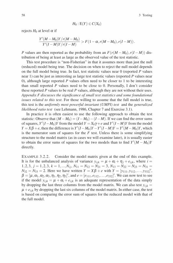
58 3 Testing
H0 : E(Y ) ∈C(X0)
rejects H0 at level α if
Y ′(M−M0)Y/r(M−M0)Y ′(I −M)Y/r(I −M)
> F(1−α,r(M−M0),r(I −M)) .
P values are then reported as the probability from an F(r(M−M0),r(I −M)) dis-tribution of being at least as large as the observed value of the test statistic.
This test procedure is “non-Fisherian” in that it assumes more than just the null(reduced) model being true. The decision on when to reject the null model dependson the full model being true. In fact, test statistic values near 0 (reported P valuesnear 1) can be just as interesting as large test statistic values (reported P values near0), although large reported P values often need to be closer to 1 to be interestingthan small reported P values need to be close to 0. Personally, I don’t considerthese reported P values to be real P values, although they are not without their uses.Appendix F discusses the significance of small test statistics and some foundationalissues related to this test. For those willing to assume that the full model is true,this test is the uniformly most powerful invariant (UMPI) test and the generalizedlikelihood ratio test (see Lehmann, 1986, Chapter 7 and Exercise 3.1).
In practice it is often easiest to use the following approach to obtain the teststatistic: Observe that (M−M0) = (I−M0)− (I−M). If we can find the error sumsof squares, Y ′(I−M0)Y from the model Y = X0γ +e and Y ′(I−M)Y from the modelY = Xβ +e, then the difference is Y ′(I−M0)Y −Y ′(I−M)Y =Y ′(M−M0)Y , whichis the numerator sum of squares for the F test. Unless there is some simplifyingstructure to the model matrix (as in cases we will examine later), it is usually easierto obtain the error sums of squares for the two models than to find Y ′(M −M0)Ydirectly.
EXAMPLE 3.2.2. Consider the model matrix given at the end of this example.It is for the unbalanced analysis of variance yi jk = μ + αi + η j + ei jk, where i =1,2,3, j = 1,2,3, k = 1, ...,Ni j, N11 = N12 = N21 = 3, N13 = N22 = N23 = N31 =N32 = N33 = 2. Here we have written Y = Xβ + e with Y = [y111,y112, . . . ,y332]′,β = [μ ,α1,α2,α3,η1,η2,η3]′, and e = [e111,e112, . . . ,e332]′. We can now test to seeif the model yi jk = μ + αi + ei jk is an adequate representation of the data simplyby dropping the last three columns from the model matrix. We can also test yi jk =μ +ei jk by dropping the last six columns of the model matrix. In either case, the testis based on comparing the error sum of squares for the reduced model with that ofthe full model.

3.2 Testing Models 59
X =
⎡⎢⎢⎢⎢⎢⎢⎢⎢⎢⎢⎢⎢⎢⎢⎢⎢⎢⎢⎢⎢⎢⎢⎢⎢⎢⎢⎢⎢⎢⎢⎢⎢⎢⎢⎢⎣
1 1 0 0 1 0 01 1 0 0 1 0 01 1 0 0 1 0 01 1 0 0 0 1 01 1 0 0 0 1 01 1 0 0 0 1 01 1 0 0 0 0 11 1 0 0 0 0 11 0 1 0 1 0 01 0 1 0 1 0 01 0 1 0 1 0 01 0 1 0 0 1 01 0 1 0 0 1 01 0 1 0 0 0 11 0 1 0 0 0 11 0 0 1 1 0 01 0 0 1 1 0 01 0 0 1 0 1 01 0 0 1 0 1 01 0 0 1 0 0 11 0 0 1 0 0 1
⎤⎥⎥⎥⎥⎥⎥⎥⎥⎥⎥⎥⎥⎥⎥⎥⎥⎥⎥⎥⎥⎥⎥⎥⎥⎥⎥⎥⎥⎥⎥⎥⎥⎥⎥⎥⎦
.
3.2.1 A Generalized Test Procedure
Before considering tests of parametric functions, we consider a generalization of thetest procedure outlined earlier. Assume that the model Y = Xβ + e is correct. Wewant to test the adequacy of a model Y = X0γ +Xb + e, where C(X0) ⊂ C(X) andXb is some known vector. In generalized linear model terminology, Xb is called anoffset.
EXAMPLE 3.2.3. Multiple Regression. Consider the model
Y = [J,X1,X2,X3]
⎡⎢⎣β0β1β2β3
⎤⎥⎦+ e = β0J +β1X1 +β2X2 +β3X3 + e.
To test H0 : β2 = β3 +5,β1 = 0, write the reduced model as
Y = β0J +(β3 +5)X2 +β3X3 + e
= β0J +β3(X2 +X3)+5X2 + e (3)
= [J,X2 +X3][
β0β3
]+5X2 + e.

60 3 Testing
Alternatively, we could write the reduced model as
Y = β0J +β2X2 +(β2 −5)X3 + e
= β0J +β2(X2 +X3)−5X3 + e (4)
= [J,X2 +X3][
β0β2
]−5X3 + e.
We will see that both reduced models lead to the same test.
The model Y = Xβ + e can be rewritten as Y −Xb = Xβ −Xb + e. Since Xb ∈C(X), this amounts to a reparameterization, Y −Xb = Xβ ∗ + e, where β ∗ = β −b.Since Xb is known, Y −Xb is still an observable random variable.
The reduced model Y = X0γ + Xb + e can be rewritten as Y − Xb = X0γ + e.The question of testing the adequacy of the reduced model is now a straightforwardapplication of our previous theory. The distribution of the test statistic is
(Y −Xb)′(M−M0)(Y −Xb)/r(M−M0)(Y −Xb)′(I −M)(Y −Xb)/r(I −M)
∼ F(r(M−M0),r(I −M),β ∗′X ′(M−M0)Xβ ∗/2σ 2) .
The noncentrality parameter is zero if and only if 0 = β ∗′X ′(M−M0)Xβ ∗ = [(M−M0)(Xβ −Xb)]′[(M−M0)(Xβ −Xb)], which occurs if and only if (M−M0)(Xβ −Xb) = 0 or Xβ = M0(Xβ −Xb)+Xb. The last condition is nothing more or less thanthat the reduced model is valid with γ = (X ′
0X0)−X0(Xβ −Xb), a fixed unknownparameter.
Note also that, since (I −M)X = 0, in the denominator of the test statistic (Y −Xb)′(I−M)(Y −Xb) = Y ′(I−M)Y , which is the SSE from the original full model.Moreover, the numerator sum of squares is
(Y −Xb)′(M−M0)(Y −Xb) = (Y −Xb)′(I −M0)(Y −Xb)−Y ′(I −M)Y,
which can be obtained by subtracting the SSE of the original full model from theSSE of the reduced model. To see this, write I −M0 = (I −M)+(M−M0).
EXAMPLE 3.2.3 CONTINUED. The numerator sum of squares for testing model(4) is (Y +5X3)′(M−M0)(Y +5X3). But (M−M0)[X2 +X3] = 0, so, upon observingthat 5X3 = −5X2 +5[X2 +X3],
(Y +5X3)′(M−M0)(Y +5X3)= (Y −5X2 +5[X2 +X3])′(M−M0)(Y −5X2 +5[X2 +X3])= (Y −5X2)′(M−M0)(Y −5X2),
which is the numerator sum of squares for testing model (3). In fact, models (3) and(4) are equivalent because the only thing different about them is that one uses 5X2and the other uses −5X3; but the only difference between these terms is 5[X2 +X3]∈C(X0).
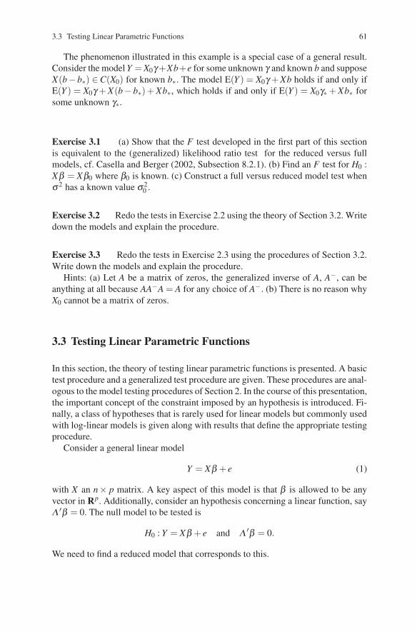
3.3 Testing Linear Parametric Functions 61
The phenomenon illustrated in this example is a special case of a general result.Consider the model Y = X0γ +Xb+e for some unknown γ and known b and supposeX(b−b∗) ∈C(X0) for known b∗. The model E(Y ) = X0γ + Xb holds if and only ifE(Y ) = X0γ + X(b− b∗)+ Xb∗, which holds if and only if E(Y ) = X0γ∗ + Xb∗ forsome unknown γ∗.
Exercise 3.1 (a) Show that the F test developed in the first part of this sectionis equivalent to the (generalized) likelihood ratio test for the reduced versus fullmodels, cf. Casella and Berger (2002, Subsection 8.2.1). (b) Find an F test for H0 :Xβ = Xβ0 where β0 is known. (c) Construct a full versus reduced model test whenσ 2 has a known value σ 2
0 .
Exercise 3.2 Redo the tests in Exercise 2.2 using the theory of Section 3.2. Writedown the models and explain the procedure.
Exercise 3.3 Redo the tests in Exercise 2.3 using the procedures of Section 3.2.Write down the models and explain the procedure.
Hints: (a) Let A be a matrix of zeros, the generalized inverse of A, A−, can beanything at all because AA−A = A for any choice of A−. (b) There is no reason whyX0 cannot be a matrix of zeros.
3.3 Testing Linear Parametric Functions
In this section, the theory of testing linear parametric functions is presented. A basictest procedure and a generalized test procedure are given. These procedures are anal-ogous to the model testing procedures of Section 2. In the course of this presentation,the important concept of the constraint imposed by an hypothesis is introduced. Fi-nally, a class of hypotheses that is rarely used for linear models but commonly usedwith log-linear models is given along with results that define the appropriate testingprocedure.
Consider a general linear model
Y = Xβ + e (1)
with X an n× p matrix. A key aspect of this model is that β is allowed to be anyvector in Rp. Additionally, consider an hypothesis concerning a linear function, sayΛ ′β = 0. The null model to be tested is
H0 : Y = Xβ + e and Λ ′β = 0.
We need to find a reduced model that corresponds to this.

62 3 Testing
The constraint Λ ′β = 0 can be stated in an infinite number of ways. Observe thatΛ ′β = 0 holds if and only if β ⊥C(Λ ); so if Γ is another matrix with C(Γ ) =C(Λ ),the constraint can also be written as β ⊥C(Γ ) or Γ ′β = 0.
To identify the reduced model, pick a matrix U such that
C(U) = C(Λ)⊥,
then Λ ′β = 0 if and only if β ⊥C(Λ ) if and only if β ∈C(U), which occurs if andonly if for some vector γ ,
β = Uγ . (2)
Substituting (2) into the linear model gives the reduced model
Y = XUγ + e
or, letting X0 ≡ XU ,Y = X0γ + e. (3)
Note that C(X0) ⊂ C(X). If e ∼ N(0,σ 2I), the reduced model (3) allows us totest Λ ′β = 0 by applying the results of Section 2. If C(X0) = C(X), the constraintinvolves only a reparameterization and there is nothing to test. In other words, ifC(X0) = C(X), then Λ ′β = 0 involves only arbitrary side conditions that do notaffect the model. Moreover, the reduced model does not depend on Cov(Y ) or theexact distribution of e, it only depends on E(Y ) = Xβ and the constraint Λ ′β = 0.
EXAMPLE 3.3.1. Consider the one-way analysis of variance model⎡⎢⎢⎢⎢⎢⎣y11y12y13y21y31y32
⎤⎥⎥⎥⎥⎥⎦=
⎡⎢⎢⎢⎢⎢⎣1 1 0 01 1 0 01 1 0 01 0 1 01 0 0 11 0 0 1
⎤⎥⎥⎥⎥⎥⎦β + e,
where β = (μ , α1, α2, α3 )′. The parameters in this model are not uniquelydefined because the rank of X is less than the number of columns.
Let λ ′1 = (0,1,0,−1). The contrast λ ′
1β is estimable, so the hypothesis α1−α3 =λ ′
1β = 0 determines an estimable constraint. To obtain C(λ1)⊥ =C(U), one can pick
U =
⎡⎢⎣1 0 00 1 00 0 10 1 0
⎤⎥⎦ ,
which yields

3.3 Testing Linear Parametric Functions 63
XU =
⎡⎢⎢⎢⎢⎢⎣1 1 01 1 01 1 01 0 11 1 01 1 0
⎤⎥⎥⎥⎥⎥⎦ . (4)
This is a real restriction on C(X), i.e., C(XU) �= C(X).Let λ ′
2 = (0,1,1,1). A nonestimable linear constraint for a one-way analysis ofvariance is that
α1 +α2 +α3 = λ ′2β = 0.
Consider two choices for U with C(λ2)⊥ = C(U), i.e.,
U1 =
⎡⎢⎣1 0 00 1 10 −1 10 0 −2
⎤⎥⎦ and U2 =
⎡⎢⎣1 0 00 1 10 0 −20 −1 1
⎤⎥⎦ .
These yield
XU1 =
⎡⎢⎢⎢⎢⎢⎣1 1 11 1 11 1 11 −1 11 0 −21 0 −2
⎤⎥⎥⎥⎥⎥⎦ and XU2 =
⎡⎢⎢⎢⎢⎢⎣1 1 11 1 11 1 11 0 −21 −1 11 −1 1
⎤⎥⎥⎥⎥⎥⎦ .
Note that C(X) = C(XU1) = C(XU2). The models determined by XU1 and XU2 areequivalent linear models but have different parameterizations, say Y = XU1ξ1 + eand Y = XU2ξ2 + e, with ξi = (ξi1,ξi2,ξi3)′. Transforming to the original β param-eterization using (2), for example,⎡⎢⎣
μα1α2α3
⎤⎥⎦= β = U1ξ1 =
⎡⎢⎣ξ11
ξ12 +ξ13−ξ12 +ξ13−2ξ13
⎤⎥⎦ .
Both ξi parameterizations lead to α1 +α2 +α3 = 0. Thus both determine the samespecific choice for the parameterization of the original one-way analysis of variancemodel.
Similar results hold for alternative nonidentifiable constraints such as α1 = 0. Aswill be established later, any nonidentifiable constraint leaves the estimation spaceunchanged and therefore yields the same estimates of estimable functions.
Now consider the joint constraint Λ ′1β = 0, where
Λ ′1 =[
λ ′1
λ ′2
].

64 3 Testing
λ ′1β is a contrast, so it is estimable; therefore Λ ′
1β has estimable aspects. One choiceof U with C(Λ1)⊥ = C(U) is
U3 =
⎡⎢⎣1 00 10 −20 1
⎤⎥⎦ .
This gives
XU3 =
⎡⎢⎢⎢⎢⎢⎣1 11 11 11 −21 11 1
⎤⎥⎥⎥⎥⎥⎦ ,
and the estimation space is the same as in (4), where only the contrast λ ′1β was
assumed equal to zero.A constraint equivalent to Λ ′
1β = 0 is Λ ′2β = 0, where
Λ ′2 =[
λ ′3
λ ′2
]=[
0 2 1 00 1 1 1
].
The constraints are equivalent because C(Λ1) = C(Λ2). (Note that λ3 − λ2 = λ1.)Neither λ ′
3β nor λ ′2β is estimable, so separately they would affect only the param-
eterization of the model. However, Λ ′1β = 0 involves an estimable constraint, so
Λ ′2β = 0 also has an estimable part to the constraint. The concept of the estimable
part of a constraint will be examined in detail later.
Estimable Constraints
We have established a perfectly general method for identifying the reduced modeldetermined by an arbitrary linear constraint Λ ′β = 0, and thus we have a generalmethod for testing Λ ′β = 0 by applying the results of Section 2. Next, we willexamine the form of the test statistic when Λ ′β is estimable. Afterwards, we presentresults showing that there is little reason to consider nonestimable linear constraints.
When Λ ′β is estimable, so that Λ ′ = P′X for some P, rather than finding Uwe can find the numerator projection operator for testing Λ ′β = 0 in terms of Pand M. Better yet, we can find the numerator sum of squares in terms of Λ andany least squares estimate β . Recall from Section 2 that the numerator sum ofsquares is Y ′(M −M0)Y , where M −M0 is the perpendicular projection operatoronto the orthogonal complement of C(X0) with respect to C(X). In other words,M −M0 is a perpendicular projection operator with C(M −M0) = C(X0)⊥C(X). Fortesting an estimable parametric hypothesis with Λ ′ = P′X , we now show that the

3.3 Testing Linear Parametric Functions 65
perpendicular projection operator onto C(MP) is also the perpendicular projectionoperator onto the orthogonal complement of C(X0) with respect to C(X), i.e., thatC(MP) = C(X0)⊥C(X). It follows immediately that the numerator sum of squares inthe test is Y ′MMPY , where MMP ≡ MP(P′MP)−P′M is the perpendicular projectionoperator onto C(MP). In particular, from Section 2
Y ′MMPY/r(MMP)Y ′(I −M)Y/r(I −M)
∼ F(r(MMP),r(I −M),β ′X ′MMPXβ/2σ 2) . (5)
Proposition 3.3.2 provides a formal proof of the necessary result. However, afterthe proof, we give an alternative justification based on finding the reduced modelassociated with the constraint. This reduced model argument differs from the onegiven at the beginning of the section in that it only applies to estimable constraints.
Proposition 3.3.2. With U and P defined for Λ ′β = 0,
C(M−M0) = C(X0)⊥C(X) ≡C(XU)⊥C(X) = C(MP).
PROOF. From Section 2, we already know that C(M −M0) = C(X0)⊥C(X). Since
X0 ≡ XU , we need only establish that C(XU)⊥C(X) = C(MP).If x ∈C(XU)⊥C(X), then 0 = x′XU , so X ′x ⊥C(U) and X ′x ∈C(Λ ) = C(X ′P). It
follows that
x = Mx = [X(X ′X)−]X ′x ∈C([X(X ′X)−]X ′P) = C(MP).
Conversely, if x ∈C(MP), then x = MPb for some b and
x′XU = b′P′MXU = b′P′XU = b′Λ ′U = 0,
so x ∈C(XU)⊥C(X) . �
Exercise 3.4 Show that β ′X ′MMPXβ = 0 if and only if Λ ′β = 0.
Earlier, we found the reduced model matrix X0 = XU directly and then, forΛ ′ = P′X , we showed that C(MP) = C(X0)⊥C(X), which led to the numerator sum
of squares. An alternative derivation of the test arrives at C(M−M0) = C(X0)⊥C(X) =C(MP) more directly for estimable constraints. The reduced model is
Y = Xβ + e and P′Xβ = 0,
orY = Xβ + e and P′MXβ = 0,

66 3 Testing
orE(Y ) ∈C(X) and E(Y ) ⊥C(MP),
orE(Y ) ∈C(X)∩ C(MP)⊥.
The reduced model matrix X0 must satisfy C(X0) = C(X)∩C(MP)⊥ ≡C(MP)⊥C(X).
It follows immediately that C(X0)⊥C(X) = C(MP). Moreover, it is easily seen that X0
can be taken as X0 = (I −MMP)X .
Theorem 3.3.3. C[(I −MMP)X ] = C(X)∩ C(MP)⊥.
PROOF. First, assume x ∈ C(X) and x ⊥ C(MP). Write x = Xb for some b andnote that MMPx = 0. It follows that x = (I −MMP)x = (I −MMP)Xb, so x ∈C[(I −MMP)X ].
Conversely, if x = (I −MMP)Xb for some b, then clearly x ∈ C(X) and x′MP =b′X ′(I −MMP)MP = 0 because (I −MMP)MP = 0 �
Note also that C(X)∩ C(MP)⊥ = C(X)∩ C(P)⊥.
EXAMPLE 3.3.4. To illustrate these ideas, consider testing H0 : α1 −α3 = 0 inExample 3.3.1. The constraint can be written
0 = α1 −α3 =(
13,
13,
13,0,
−12
,−12
)⎡⎢⎢⎢⎢⎢⎣
1 1 0 01 1 0 01 1 0 01 0 1 01 0 0 11 0 0 1
⎤⎥⎥⎥⎥⎥⎦⎡⎢⎣
μα1α2α3
⎤⎥⎦ ,
so P′ = (1/3,1/3,1/3,0,−1/2,−1/2). We need C(X)∩ C(MP)⊥. Note that vec-tors in C(X) have the form (a,a,a,b,c,c)′ for any a,b,c, so P = MP. Vectors inC(MP)⊥ are v = (v11,v12,v13,v21,v31,v32)′ with P′v = v1· − v3· = 0. Vectors inC(X)∩ C(MP)⊥ have the first three elements identical, the last two elements iden-tical, and the average of the first three equal to the average of the last two, i.e., theyhave the form (a,a,a,b,a,a)′. A spanning set for this space is given by the columnsof
X0 =
⎡⎢⎢⎢⎢⎢⎣1 1 01 1 01 1 01 0 11 1 01 1 0
⎤⎥⎥⎥⎥⎥⎦ .
As seen earlier, another choice for P is (1,0,0,0,−1,0)′. Using M from Exer-cise 1.5.8b, this choice for P also leads to MP = (1/3,1/3,1/3,0,−1/2,−1/2)′. Tocompute (I −MMP)X , observe that

3.3 Testing Linear Parametric Functions 67
MMP =1
(1/3)+(1/2)
⎡⎢⎢⎢⎢⎢⎣1/9 1/9 1/9 0 −1/6 −1/61/9 1/9 1/9 0 −1/6 −1/61/9 1/9 1/9 0 −1/6 −1/6
0 0 0 0 0 0−1/6 −1/6 −1/6 0 1/4 1/4−1/6 −1/6 −1/6 0 1/4 1/4
⎤⎥⎥⎥⎥⎥⎦
=15
⎡⎢⎢⎢⎢⎢⎣2/3 2/3 2/3 0 −1 −12/3 2/3 2/3 0 −1 −12/3 2/3 2/3 0 −1 −1
0 0 0 0 0 0−1 −1 −1 0 3/2 3/2−1 −1 −1 0 3/2 3/2
⎤⎥⎥⎥⎥⎥⎦ .
Then
(I −MMP)X = X −MMPX
= X − 15
⎡⎢⎢⎢⎢⎢⎣0 2 0 −20 2 0 −20 2 0 −20 0 0 00 −3 0 30 −3 0 3
⎤⎥⎥⎥⎥⎥⎦=
⎡⎢⎢⎢⎢⎢⎣1 3/5 0 2/51 3/5 0 2/51 3/5 0 2/51 0 1 01 3/5 0 2/51 3/5 0 2/5
⎤⎥⎥⎥⎥⎥⎦ ,
which has the same column space as X0 given earlier.We have reduced the problem of finding X0 to that of finding C(X)∩ C(MP)⊥,
which is just the orthogonal complement of C(MP) with respect to C(X). By Theo-rem B.48, C(X)∩C(MP)⊥ = C(M−MMP), so M−MMP is another valid choice forX0. For Example 3.3.1 with H0 : α1 −α3 = 0, M was given in Exercise 1.5.8b andMMP was given earlier, so
M−MMP =
⎡⎢⎢⎢⎢⎢⎣1/5 1/5 1/5 0 1/5 1/51/5 1/5 1/5 0 1/5 1/51/5 1/5 1/5 0 1/5 1/5
0 0 0 1 0 01/5 1/5 1/5 0 1/5 1/51/5 1/5 1/5 0 1/5 1/5
⎤⎥⎥⎥⎥⎥⎦ .
This matrix has the same column space as the other choices of X0 that have beengiven.
For Λ ′β estimable, we now rewrite the test statistic in (5) in terms of Λ and β .First, we wish to show that r(Λ) = r(MMP). It suffices to show that r(Λ) = r(MP).Writing Λ = X ′P, we see that for any vector b, X ′Pb = 0 if and only if Pb ⊥C(X),which occurs if and only if MPb = 0. It follows that C(P′X)⊥ = C(P′M)⊥ so thatC(P′X) = C(P′M), r(P′X) = r(P′M), and r(Λ) = r(X ′P) = r(MP).

68 3 Testing
Now rewrite the quadratic form Y ′MMPY . Recall that since X β = MY , we haveΛ ′β = P′X β = P′MY . Substitution gives
Y ′MMPY = Y ′MP(P′MP)−P′MY
= β ′Λ(P′X(X ′X)−X ′P)−Λ ′β= β ′Λ [Λ ′(X ′X)−Λ ]−Λ ′β .
The test statistic in (5) becomes
β ′Λ [Λ ′(X ′X)−Λ ]−Λ ′β/r(Λ)MSE
.
A similar argument shows that the noncentrality parameter in (5) can be writ-ten as β ′Λ [Λ ′(X ′X)−Λ ]−Λ ′β/2σ 2. The test statistic consists of three main parts:MSE , Λ ′β , and the generalized inverse of Λ ′(X ′X)−Λ . Note that σ 2Λ ′(X ′X)−Λ =Cov(Λ ′β ). These facts give an alternative method of deriving tests. One can simplyfind the estimate Λ ′β , the covariance matrix of the estimate, and the MSE.
For a single degree of freedom hypothesis H0 : λ ′β = 0, the numerator takes theespecially nice form
β ′λ [λ ′(X ′X)−λ ]−1λ ′β = (λ ′β )2/[λ ′(X ′X)−λ ];
so the F test becomes: reject H0 : λ ′β = 0 if
(λ ′β)2
MSE[λ ′(X ′X)−λ ]> F(1−α,1,d fE) ,
which is just the square of the t test that could be derived from the sampling distri-butions of the least squares estimate and the MSE , cf. Exercise 2.1.
Definition 3.3.5. The condition E(Y ) ⊥ C(MP) is called the constraint on themodel caused (imposed) by Λ ′β = 0, where Λ ′ = P′X . As a shorthand, we will callC(MP) the constraint caused by Λ ′β = 0. If M ⊂C(X) and C(MP) ⊂ M , we saythat C(MP) is the constraint on M caused by Λ ′β = 0. If Λ ′β = 0 puts a constrainton M , we say that Λ ′β = 0 is an hypothesis in M .
Exercise 3.5 Show that a necessary and sufficient condition for ρ ′1Xβ = 0 and
ρ ′2Xβ = 0 to determine orthogonal constraints on the model is that ρ ′
1Mρ2 = 0.

3.3 Testing Linear Parametric Functions 69
Theoretical Complements
If, rather than testing the constraint Λ ′β = 0, our desire is to estimate β subject tothe constraint, simply estimate γ in model (3) and use β = U γ . In this constrainedestimation, the estimates automatically satisfy Λ ′β = 0. Moreover, estimable func-tions Γ ′β = Q′Xβ are equivalent to Γ ′Uγ = Q′XUγ , and optimal estimates of γ aretransformed into optimal estimates of β .
We now examine the implications of testing Λ ′β = 0 when Λ ′β is not estimable.Recall that we began this section by finding the reduced model associated with sucha constraint, so we already have a general method for performing such tests.
The first key result is that in defining a linear constraint there is no reason to useanything but estimable functions, because only estimable functions induce a realconstraint on C(X). Theorem 3.3.6 identifies the estimable part of Λ ′β , say Λ ′
0β ,and implies that Λ ′
0β = 0 gives the same reduced model as Λ ′β = 0. Λ0 is a matrixchosen so that C(Λ )∩ C(X ′) = C(Λ0). With such a choice, Λ ′β = 0 implies thatΛ ′
0β = 0 but Λ ′0β is estimable because C(Λ0) ⊂C(X ′), so Λ ′
0 = P′0X for some P0.
Theorem 3.3.6. If C(Λ)∩C(X ′) = C(Λ0) and C(U0) = C(Λ0)⊥, then C(XU) =C(XU0). Thus Λ ′β = 0 and Λ ′
0β = 0 induce the same reduced model.
PROOF. C(Λ0) ⊂ C(Λ ), so C(U) = C(Λ )⊥ ⊂ C(Λ0)⊥ = C(U0) and C(XU) ⊂C(XU0).
To complete the proof, we show that there cannot be any vectors in C(XU0)that are not in C(XU). In particular, we show that there are no nontrivial vectorsin C(XU0) that are orthogonal to C(XU), i.e., if v ∈ C(XU)⊥C(XU0) then v = 0. If
v ∈ C(XU)⊥C(XU0), then v′XU = 0, so X ′v ⊥ C(U) and X ′v ∈ C(Λ). But also notethat X ′v ∈C(X ′), so X ′v∈C(Λ)∩C(X ′) =C(Λ0). This implies that X ′v⊥C(U0), sov ⊥C(XU0). We have shown that the vector v which, by assumption, is in C(XU0),is also orthogonal to C(XU0). The only such vector is the 0 vector. �
Nontrivial estimable constraints always induce a real constraint on the columnspace.
Proposition 3.3.7. If Λ ′β is estimable and Λ �= 0, then Λ ′β = 0 implies thatC(XU) �= C(X).
PROOF. With Λ ′ = P′X , the definition of U gives 0 = Λ ′U = P′XU = P′MXU , soC(XU) ⊥C(MP). Both are subspaces of C(X); therefore if C(MP) �= {0}, we haveC(X) �=C(XU). However, P′MX = Λ ′ �= 0, so C(MP) is not orthogonal to C(X) andC(MP) �= {0}. �
Note that Proposition 3.3.7 also implies that whenever the estimable part Λ0 is dif-ferent from 0, there is always a real constraint on the column space.

70 3 Testing
Corollary 3.3.8 establishes that Λ ′β has no estimable part if and only if the con-straint does not affect the model. If the constraint does not affect the model, it merelydefines a reparameterization, in other words, it merely specifies arbitrary side con-ditions. The corollary follows from the observation made about Λ0 after Proposi-tion 3.3.7 and taking Λ0 = 0 in Theorem 3.3.6.
Corollary 3.3.8. C(Λ)∩ C(X ′) = {0} if and only if C(XU) = C(X).
In particular, if Λ ′β is not estimable, we can obtain the numerator sum of squaresfor testing Λ ′β = 0 either by finding X0 = XU directly and using it to get M−M0,or by finding Λ0, writing Λ ′
0 = P′0X , and using MMP0 . But as noted earlier, there is
no reason to have Λ ′β not estimable.
3.3.1 A Generalized Test Procedure
We now consider hypotheses of the form Λ ′β = d where d ∈ C(Λ ′) so that theequation Λ ′β = d is solvable. Let b be such a solution. Note that
Λ ′β = Λ ′b = d
if and only ifΛ ′(β −b) = 0
if and only if(β −b) ⊥C(Λ ).
Again picking a matrix U such that
C(U) = C(Λ)⊥,
Λ ′(β −b) = 0 if and only if(β −b) ∈C(U),
which occurs if and only if for some vector γ
(β −b) = Uγ.
Multiplying both sides by X gives
Xβ −Xb = XUγ
orXβ = XUγ +Xb.
We can now substitute this into the linear model to get the reduced model

3.3 Testing Linear Parametric Functions 71
Y = XUγ +Xb+ e,
or, letting X0 ≡ XU ,Y = X0γ +Xb+ e. (6)
Recall that b is a vector we can find, so Xb is a known (offset) vector.The analysis for reduced models such as (6) was developed in Section 2. For non-
estimable linear hypotheses, use that theory directly. If Λ ′ = P′X , then C(X0)⊥C(X) =C(MP) and the test statistic is easily seen to be
(Y −Xb)′MMP(Y −Xb)/r(MMP)(Y −Xb)′(I −M)(Y −Xb)/r(I −M)
.
Note that Λ ′β = d imposes the constraint E(Y −Xb) ⊥ C(MP), so once again wecould refer to C(MP) as the constraint imposed by the hypothesis.
We did not specify the solution b to Λ ′β = d that should be used. Fortunately,for Λ ′β estimable, the test does not depend on the choice of b. As mentioned inthe previous section, (Y −Xb)′(I −M)(Y −Xb) = Y ′(I −M)Y , so the denominatorof the test is just the MSE and does not depend on b. The numerator term (Y −Xb)′MMP(Y −Xb) equals (Λ ′β −d)′[Λ ′(X ′X)−Λ ]−(Λ ′β −d). The test statistic canbe written as
(Λ ′β −d)′[Λ ′(X ′X)−Λ ]−(Λ ′β −d)/r(Λ)MSE
.
For Λ ′β estimable, the linear model Y = X0γ + Xb + e implies that Λ ′β = d,but for nonestimable linear constraints, there are infinitely many constraints thatresult in the same reduced model. (If you think of nonestimable linear constraints asincluding arbitrary side conditions, that is not surprising.) In particular, if Λ ′β = d,the same reduced model results if we take Λ ′β = d0 where d0 = d +Λ ′v and v ⊥C(X ′). Note that, in this construction, if Λ ′β is estimable, d0 = d for any v.
We now present an application of this testing procedure. The results are givenwithout justification, but they should seem similar to results from a statistical meth-ods course.
EXAMPLE 3.3.9. Consider the balanced two-way ANOVA without interactionmodel
yi jk = μ +αi +η j + ei jk,
i = 1, . . . ,a, j = 1, . . . ,b, k = 1, . . . ,N. (The analysis for this model is presented inSection 7.1.) We examine the test of the null hypothesis
H0 :a
∑i=1
λiαi = 4 andb
∑j=1
γ jη j = 7,
where ∑ai=1 λi = 0 = ∑b
j=1 γ j . The hypothesis is simultaneously specifying the valuesof a contrast in the αis and a contrast in the η js.
In terms of the model Y = Xβ + e, we have

72 3 Testing
β = [μ ,α1, . . . ,αa,η1, . . . ,ηb]′
Λ ′ =[
0 λ1 · · · λa 0 · · · 00 0 · · · 0 γ1 · · · γb
]d =[
47
]Λ ′β =
[∑a
i=1 λiyi··∑b
j=1 γ j y· j·
]Cov(Λ ′β )/σ2 = Λ ′(X ′X)−Λ =
[∑a
i=1 λ 2i /bN 0
0 ∑bj=1 γ2
j /aN
].
The diagonal elements of the covariance matrix are just the variances of the es-timated contrasts. The off-diagonal elements are zero because this is a balancedtwo-way ANOVA, hence the estimates of the α contrast and the η contrast are inde-pendent. We will see in Chapter 7 that these contrasts define orthogonal constraintsin the sense of Definition 3.3.5, so they are often referred to as being orthogonalparameters.
There are two linearly independent contrasts being tested, so r(Λ ) = 2. The teststatistic is
12MSE
[∑ai=1 λiyi·· −4 ∑b
j=1 γ j y· j· −7 ]
×⎡⎣ bN
∑ai=1 λ 2
i0
0 aN∑b
j=1 γ2j
⎤⎦[ ∑ai=1 λiyi·· −4
∑bj=1 γ j y· j· −7
]or
12MSE
[(∑a
i=1 λiyi·· −4)2
∑ai=1 λ 2
i /bN+
(∑b
j=1 γ j y· j· −7)2
∑bj=1 γ2
j /aN
].
Note that the term (∑ai=1 λiyi·· −4)2/(∑a
i=1 λ 2i /bN
)is, except for subtracting the 4,
the sum of squares for testing ∑ai=1 λiαi = 0 We are subtracting the 4 because we
are testing ∑ai=1 λiαi = 4. Similarly, we have a term that is very similar to the sum
of squares for testing ∑bj=1 γ jη j = 0. The test statistic takes the average of these
sums of squares and divides by the MSE. The test is then defined by reference to anF(2,d fE,0) distribution.
3.3.2 Testing an Unusual Class of Hypotheses
Occasionally, a valid linear hypothesis Λ ′β = d is considered where d is not com-pletely known but involves other parameters. (This is the linear structure involved increating a logistic regression model from a log-linear model.) For Λ ′β = d to give

3.3 Testing Linear Parametric Functions 73
a valid linear hypothesis, Λ ′β = d must put a restriction on C(X), so that when thehypothesis is true, E(Y ) lies in some subspace of C(X).
Let X1 be such that C(X1) ⊂C(X) and consider an hypothesis
P′Xβ = P′X1δ
for some parameter vector δ . We seek an appropriate reduced model for such anhypothesis.
Note that the hypothesis occurs if and only if
P′M(Xβ −X1δ ) = 0,
which occurs if and only if
(Xβ −X1δ ) ⊥C(MP),
which occurs if and only if
(Xβ −X1δ ) ∈C(MP)⊥C(X).
As discussed earlier in this section, we choose X0 so that C(MP)⊥C(X) = C(X0). Thechoice of X0 does not depend on X1. Using X0, the hypothesis occurs if and only iffor some γ
(Xβ −X1δ ) = X0γ.
Rewriting these terms, we see that
Xβ = X0γ +X1δ
which is the mean structure for the reduced model. In other words, assuming thenull hypothesis is equivalent to assuming a reduced model
Y = X0γ +X1δ + e.
To illustrate, consider a linear model for pairs of observations (y1 j,y2 j), j =1, . . . ,N. Write Y = (y11, . . . ,y1N ,y21, . . . ,y2N)′. Initially, we will impose no structureon the means so that E(yi j) = μi j. We are going to consider an hypothesis for thedifferences between the pairs,
μ1 j −μ2 j = z′jδ
for some known predictor vector z j. Of course we could just fit a linear model to thedifferences y1 j −y2 j, but we want to think about comparing such a model to modelsthat are not based on the differences.
The conditions just specified correspond to a linear model Y = Xβ + e in whichX = I2N and β = (μ11, . . . ,μ2N)′. Write

74 3 Testing
P =[
IN−IN
]and X1 =
[Z0
]where Z′ = [z1, . . . ,zN ]. Then the hypothesis for the differences can be specified as
P′Xβ = P′X1δ = Zδ .
Finally, it is not difficult to see that a valid choice of X0 is
X0 =[
ININ
].
It follows that, under the reduced model
Xβ ≡ Iβ =[
I ZI 0
][γδ
]or that the reduced model is
Y =[
I ZI 0
][γδ
]+ e.
This relationship is of particular importance in the analysis of frequency data.The model yi j = μi j +ei j is analogous to a saturated log-linear model. An hypothesisμ1 j −μ2 j = α0 +α1t j ≡ z′jδ is analogous to the hypothesis that a simple linear logitmodel holds. We have found the vector space such that restricting the log-linearmodel to that space gives the logit model, see also Christensen (1997).
Exercise 3.6 In testing a reduced model Y = X0γ + e against a full model Y =Xβ + e, what linear parametric function of the parameters is being tested?
3.4 Discussion
The reason that we considered testing models first and then discussed testing para-metric functions by showing them to be changes in models is because, in general,only model testing is ever performed. This is not to say that parametric functions arenot tested as such, but that parametric functions are only tested in special cases. Inparticular, parametric functions can easily be tested in balanced ANOVA problemsand one-way ANOVAs. Multifactor ANOVA designs with unequal numbers of ob-servations in the treatment cells, as illustrated in Example 3.2.2, are best analyzedby considering alternative models. Even in regression models, where all the parame-ters are estimable, it is often more enlightening to think in terms of model selection.Of course, in regression there is a special relationship between the parameters andthe model matrix. For the model yi = β0 + β1xi1 + β2xi2 + · · ·+βp−1xi p−1 + e, the

3.4 Discussion 75
model matrix can be written as X = [J,X1, . . . ,Xp−1], where Xj = [x1 j,x2 j, . . . ,xn j]′.The test of H0 : β j = 0 is obtained by just leaving Xj out of the model matrix.
Another advantage of the method of testing models is that it is often easy insimple but nontrivial cases to see immediately what new model is generated by anull hypothesis. This was illustrated in Examples 3.2.0 and 3.2.3.
EXAMPLE 3.4.1. One-Way ANOVA.Consider the model yi j = μ +αi +ei j, i = 1,2,3, j = 1, . . . ,Ni, N1 = N3 = 3, N2 = 2.In matrix terms this is
Y =
⎡⎢⎢⎢⎢⎢⎢⎢⎢⎢⎣
1 1 0 01 1 0 01 1 0 01 0 1 01 0 1 01 0 0 11 0 0 11 0 0 1
⎤⎥⎥⎥⎥⎥⎥⎥⎥⎥⎦
⎡⎢⎣μα1α2α3
⎤⎥⎦+ e.
Let the null hypothesis be α1 = μ +2α2. Writing X = [J,X1,X2,X3] and
E(Y ) = Xβ = μJ +α1X1 +α2X2 +α3X3,
the reduced model is easily found by substituting μ +2α2 for α1 which leads to
E(Y ) = μ(J +X1)+α2(2X1 +X2)+α3X3.
This gives the reduced model
Y =
⎡⎢⎢⎢⎢⎢⎢⎢⎢⎢⎣
2 2 02 2 02 2 01 1 01 1 01 0 11 0 11 0 1
⎤⎥⎥⎥⎥⎥⎥⎥⎥⎥⎦⎡⎣γ0
γ1γ2
⎤⎦+ e.
For Examples 3.2.0, 3.2.3, and 3.5.1, it would be considerable work to go throughthe procedure developed in Section 3 to test the hypotheses. In fairness, it should beadded that for these special cases, there is no need to go through the general pro-cedures of Section 3 to get the tests (assuming that you get the necessary computeroutput for the regression problem).
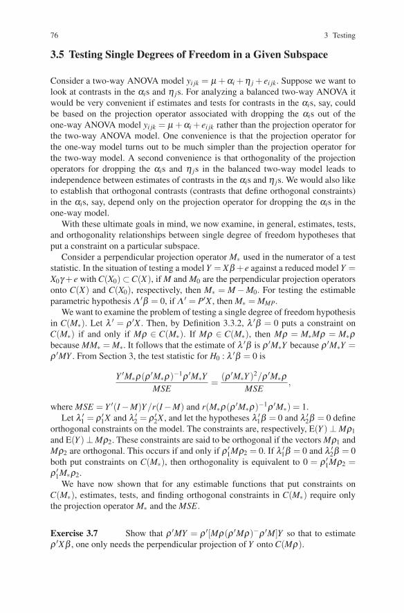
76 3 Testing
3.5 Testing Single Degrees of Freedom in a Given Subspace
Consider a two-way ANOVA model yi jk = μ +αi +η j + ei jk. Suppose we want tolook at contrasts in the αis and η js. For analyzing a balanced two-way ANOVA itwould be very convenient if estimates and tests for contrasts in the αis, say, couldbe based on the projection operator associated with dropping the αis out of theone-way ANOVA model yi jk = μ +αi + ei jk rather than the projection operator forthe two-way ANOVA model. One convenience is that the projection operator forthe one-way model turns out to be much simpler than the projection operator forthe two-way model. A second convenience is that orthogonality of the projectionoperators for dropping the αis and η js in the balanced two-way model leads toindependence between estimates of contrasts in the αis and η js. We would also liketo establish that orthogonal contrasts (contrasts that define orthogonal constraints)in the αis, say, depend only on the projection operator for dropping the αis in theone-way model.
With these ultimate goals in mind, we now examine, in general, estimates, tests,and orthogonality relationships between single degree of freedom hypotheses thatput a constraint on a particular subspace.
Consider a perpendicular projection operator M∗ used in the numerator of a teststatistic. In the situation of testing a model Y = Xβ +e against a reduced model Y =X0γ +e with C(X0) ⊂C(X), if M and M0 are the perpendicular projection operatorsonto C(X) and C(X0), respectively, then M∗ = M −M0. For testing the estimableparametric hypothesis Λ ′β = 0, if Λ ′ = P′X , then M∗ = MMP.
We want to examine the problem of testing a single degree of freedom hypothesisin C(M∗). Let λ ′ = ρ ′X . Then, by Definition 3.3.2, λ ′β = 0 puts a constraint onC(M∗) if and only if Mρ ∈ C(M∗). If Mρ ∈ C(M∗), then Mρ = M∗Mρ = M∗ρbecause MM∗ = M∗. It follows that the estimate of λ ′β is ρ ′M∗Y because ρ ′M∗Y =ρ ′MY . From Section 3, the test statistic for H0 : λ ′β = 0 is
Y ′M∗ρ(ρ ′M∗ρ)−1ρ ′M∗YMSE
=(ρ ′M∗Y )2/ρ ′M∗ρ
MSE,
where MSE = Y ′(I −M)Y/r(I −M) and r(M∗ρ(ρ ′M∗ρ)−1ρ ′M∗) = 1.Let λ ′
1 = ρ ′1X and λ ′
2 = ρ ′2X , and let the hypotheses λ ′
1β = 0 and λ ′2β = 0 define
orthogonal constraints on the model. The constraints are, respectively, E(Y ) ⊥ Mρ1and E(Y )⊥ Mρ2. These constraints are said to be orthogonal if the vectors Mρ1 andMρ2 are orthogonal. This occurs if and only if ρ ′
1Mρ2 = 0. If λ ′1β = 0 and λ ′
2β = 0both put constraints on C(M∗), then orthogonality is equivalent to 0 = ρ ′
1Mρ2 =ρ ′
1M∗ρ2.We have now shown that for any estimable functions that put constraints on
C(M∗), estimates, tests, and finding orthogonal constraints in C(M∗) require onlythe projection operator M∗ and the MSE .
Exercise 3.7 Show that ρ ′MY = ρ ′[Mρ(ρ ′Mρ)−ρ ′M]Y so that to estimateρ ′Xβ , one only needs the perpendicular projection of Y onto C(Mρ).

3.6 Breaking a Sum of Squares into Independent Components 77
3.6 Breaking a Sum of Squares into Independent Components
We now present a general theory that includes, as special cases, the breaking downof the treatment sum of squares in a one-way ANOVA into sums of squares fororthogonal contrasts and the breaking of the sum of squares for the model into in-dependent sums of squares as in an ANOVA table. This is an important device instatistical analyses.
Frequently, a reduced model matrix X0 is a submatrix of X . This is true forthe initial hypotheses considered in both cases of Example 3.2.0 and for Exam-ple 3.2.2. If we can write X = [X0,X1], it is convenient to write SSR(X1|X0) ≡Y ′(M−M0)Y . SSR(X1|X0) is called the sum of squares for regressing X1 after X0. Wewill also write SSR(X) ≡ Y ′MY , the sum of squares for regressing on X . Similarly,SSR(X0) ≡ Y ′M0Y . The SSR(·) notation is one way of identifying sums of squaresfor tests. Other notations exist, and one alternative will soon be introduced. Notethat SSR(X) = SSR(X0) + SSR(X1|X0), which constitutes a breakdown of SSR(X)into two parts. If e ∼ N(0,σ 2I), these two parts are independent.
We begin with a general theory and conclude with a discussion of breaking downthe sums of squares in a two-way ANOVA model yi jk = μ + αi + η j + ei jk. Theprojection operators used in the numerator sums of squares for dropping the αis andη js are orthogonal if and only if the numerator sum of squares for dropping the η jsout of the two-way model is the same as the numerator sum of squares for droppingthe η js out of the one-way ANOVA model yi jk = μ +η j + ei jk.
3.6.1 General Theory
We now present a general theory that is based on finding an orthonormal basis fora subspace of the estimation space. (This subspace could be the entire estimationspace.) We discuss two methods of doing this. The first is a direct method involvingidentifying the subspace and choosing an orthonormal basis. The second methoddetermines an orthonormal basis indirectly by examining single degree of freedomhypotheses and the constraints imposed by those hypotheses.
Our general model is Y = Xβ + e with M the perpendicular projection operatoronto C(X). Let M∗ be any perpendicular projection operator with C(M∗) ⊂ C(X).Then M∗ defines a test statistic
Y ′M∗Y/r(M∗)Y ′(I −M)Y/r(I −M)
for testing the reduced model, say, Y = (M −M∗)γ + e. If r(M∗) = r, then we willshow that we can break the sum of squares based on M∗ (i.e., Y ′M∗Y ) into as manyas r independent sums of squares whose sum will equal Y ′M∗Y . By using M∗ in thenumerator of the test, we are testing whether the subspace C(M∗) is adding anythingto the predictive (estimative) ability of the model. What we have done is break C(X)

78 3 Testing
into two orthogonal parts, C(M∗) and C(M −M∗). In this case, C(M −M∗) is theestimation space under H0 and we can call C(M∗) the test space. C(M∗) is a spacethat will contain only error if H0 is true but which is part of the estimation spaceunder the full model. Note that the error space under H0 is C(I − (M −M∗)), butI − (M−M∗) = (I −M)+M∗ so that C(I −M) is part of the error space under bothmodels.
We now break C(M∗) into r orthogonal subspaces. Take an orthonormal basis forC(M∗), say R1,R2, . . . ,Rr. Note that, using Gram–Schmidt, R1 can be any normal-ized vector in C(M∗). It is the statistician’s choice. R2 can then be any normalizedvector in C(M∗) orthogonal to R1, etc. Let R = [R1,R2, . . . ,Rr], then as in Theo-rem B.35,
M∗ = RR′ = [R1, . . . ,Rr]
⎡⎢⎣R′1...
R′r
⎤⎥⎦=r
∑i=1
RiR′i.
Let Mi = RiR′i, then Mi is a perpendicular projection operator in its own right and
MiMj = 0 for i �= j because of the orthogonality of the Ris.The goal of this section is to break up the sum of squares into independent com-
ponents. By Theorem 1.3.7, the sums of squares Y ′MiY and Y ′MjY are indepen-dent for any i �= j because MiMj = 0. Also, Y ′M∗Y = ∑r
i=1Y ′MiY simply becauseM∗ = ∑r
i=1 Mi. Moreover, since r(Mi) = 1,
Y ′MiYY ′(I −M)Y/r(I −M)
∼ F(1,r(I −M),β ′X ′MiXβ/2σ2).
In a one-way ANOVA, Y ′M∗Y corresponds to the treatment sum of squares whilethe Y ′MiY s correspond to the sums of squares for a set of orthogonal contrasts, cf.Example 3.6.2.
We now consider the correspondence between the hypothesis tested using Y ′M∗Yand those tested using the Y ′MiY s. Because M∗ and the Mis are nonnegative definite,
0 = β ′X ′M∗Xβ =r
∑i=1
β ′X ′MiXβ
if and only if β ′X ′MiXβ = 0 for all i if and only if R′iXβ = 0 for all i. Thus, the null
hypothesis that corresponds to the test based on M∗ is true if and only if the nullhypotheses R′
iXβ = 0 corresponding to all the Mis are true. Equivalently, if the nullhypothesis corresponding to M∗ is not true, we have
0 < β ′X ′M∗Xβ =r
∑i=1
β ′X ′MiXβ .
Again, since M∗ and the Mis are nonnegative definite, this occurs if and only if atleast one of the terms β ′X ′MiXβ is greater than zero. Thus the null hypothesis corre-sponding to M∗ is not true if and only if at least one of the hypotheses correspondingto the Mis is not true. Thinking in terms of a one-way ANOVA, these results cor-

3.6 Breaking a Sum of Squares into Independent Components 79
respond to stating that 1) the hypothesis of no treatment effects is true if and onlyif all the contrasts in a set of orthogonal contrasts are zero or, equivalently, 2) thehypothesis of no treatment effects is not true if and only if at least one contrast in aset of orthogonal contrasts is not zero.
We have broken Y ′M∗Y into r independent parts. It is easy to see how tobreak it into less than r parts. Suppose r = 7. We can break Y ′M∗Y into threeparts by looking at projections onto only three subspaces. For example, Y ′M∗Y =Y ′(M1 + M3 + M6)Y +Y ′(M2 + M7)Y +Y ′(M4 + M5)Y , where we have used threeprojection operators M1 + M3 + M6, M2 + M7, and M4 + M5. Note that these threeprojection operators are orthogonal, so the sums of squares are independent. Byproperly choosing R, an ANOVA table can be developed using this idea.
EXAMPLE 3.6.1. One-Way ANOVA.In this example we examine breaking up the treatment sum of squares in a one-wayANOVA. Consider the model yi j = μ + αi + ei j, i = 1,2,3, j = 1,2,3. In matrixterms this is
Y =
⎡⎢⎢⎢⎢⎢⎢⎢⎢⎢⎢⎢⎣
1 1 0 01 1 0 01 1 0 01 0 1 01 0 1 01 0 1 01 0 0 11 0 0 11 0 0 1
⎤⎥⎥⎥⎥⎥⎥⎥⎥⎥⎥⎥⎦
⎡⎢⎣μα1α2α3
⎤⎥⎦+ e. (1)
Denote the model matrix X = [J,X1,X2,X3]. To test H0 : α1 = α2 = α3, the reducedmodel is clearly
Y = Jμ + e.
The projection operator for the test is M∗ = M− [1/n]JJ′. The test space is C(M∗) =C(M− [1/n]JJ′), i.e., the test space is the set of all vectors in C(X) that are orthog-onal to a column of ones. The test space can be obtained by using Gram–Schmidtto remove the effect of J from the last three columns of the model matrix, that is,C(M∗) is spanned by the columns of⎡⎢⎢⎢⎢⎢⎢⎢⎢⎢⎢⎢⎣
2 −1 −12 −1 −12 −1 −1
−1 2 −1−1 2 −1−1 2 −1−1 −1 2−1 −1 2−1 −1 2
⎤⎥⎥⎥⎥⎥⎥⎥⎥⎥⎥⎥⎦,

80 3 Testing
which is a rank 2 matrix. The statistician is free to choose R1 within C(M∗). R1could be a normalized version of⎡⎢⎢⎢⎢⎢⎢⎢⎢⎢⎢⎢⎣
222
−1−1−1−1−1−1
⎤⎥⎥⎥⎥⎥⎥⎥⎥⎥⎥⎥⎦+
⎡⎢⎢⎢⎢⎢⎢⎢⎢⎢⎢⎢⎣
−1−1−1
222
−1−1−1
⎤⎥⎥⎥⎥⎥⎥⎥⎥⎥⎥⎥⎦=
⎡⎢⎢⎢⎢⎢⎢⎢⎢⎢⎢⎢⎣
111111
−2−2−2
⎤⎥⎥⎥⎥⎥⎥⎥⎥⎥⎥⎥⎦,
which was chosen as X1 + X2 with the effect of J removed. R2 must be the onlynormalized vector left in C(M∗) that is orthogonal to R1. R2 is a normalized versionof [1,1,1,−1,−1,−1,0,0,0]′. The sum of squares for testing H0 : α1 = α2 = α3 isY ′R1R′
1Y +Y ′R2R′2Y .
Using the specified form of R1, Y ′M1Y is the numerator sum of squares for testing
0 = R′1Xβ ∝ (0,3,3,−6)
⎡⎢⎣μα1α2α3
⎤⎥⎦= 6(
α1 +α2
2−α3
).
Similarly,R′
2Xβ ∝ α1 −α2.
R1 was chosen so that Y ′R2R′2Y would be the sum of squares for testing H0 : α1 = α2.
The discussion thus far has concerned itself with directly choosing an orthonor-mal basis for C(M∗). An equivalent approach to the problem of finding an orthogo-nal breakdown is in terms of single degree of freedom hypotheses λ ′β = 0.
If we choose any r single degree of freedom hypotheses λ ′1β = · · · = λ ′
rβ = 0with ρ ′
kX = λ ′k, Mρk ∈ C(M∗), and ρ ′
kMρh = 0 for all k �= h, then the vectorsMρk/
√ρ ′
kMρk form an orthonormal basis for C(M∗). The projection operators areMk = Mρk(ρ ′
kMρk)−1ρ ′kM. The sums of squares for these hypotheses, Y ′MkY =
Y ′Mρk(ρ ′kMρk)−1ρ ′
kMY = (ρ ′kMY )2/ρ ′
kMρk = (ρkM∗Y )2/ρ ′kM∗ρk, form an orthog-
onal breakdown of Y ′M∗Y .As shown in Section 3, the sum of squares for testing λ ′
kβ = 0 can be foundfrom λk, β , and (X ′X)−. In many ANOVA problems, the condition ρ ′
kMρh = 0 canbe checked by considering an appropriate function of λk and λh. It follows that, inmany problems, an orthogonal breakdown can be obtained without actually findingthe vectors ρ1, . . . ,ρr.
EXAMPLE 3.6.2. One-Way ANOVA.Consider the model yi j = μ + αi + ei j, i = 1, . . . , t, j = 1, . . . ,Ni. Let Y ′M∗Y cor-respond to the sum of squares for treatments (i.e., the sum of squares for testing

3.6 Breaking a Sum of Squares into Independent Components 81
α1 = · · ·= αt ). The hypotheses λ ′kβ = 0 correspond to contrasts ck1α1 + · · ·+cktαt =
0, where ck1 + · · ·+ ckt = 0. In Chapter 4, it will be shown that contrasts are es-timable functions and that any contrast imposes a constraint on the space for testingequality of treatments. In other words, Chapter 4 shows that the λ ′
kβ s can be con-trasts and that if they are contrasts, then Mρk ∈ C(M∗). In Chapter 4 it will alsobe shown that the condition for orthogonality, ρ ′
kMρh = 0, reduces to the conditionck1ch1/N1 + · · ·+ cktcht/Nt = 0. If the contrasts are orthogonal, then the sums ofsquares for the contrasts add up to the sums of squares for treatments, and the sumsof squares for the contrasts are independent.
3.6.2 Two-Way ANOVA
We discuss the technique of breaking up sums of squares as it applies to the two-way ANOVA model of Example 3.2.2. The results really apply to any two-wayANOVA with unequal numbers. The sum of squares for the full model is Y ′MY(by definition). We can break this up into three parts, one for fitting the η js afterhaving fit the αis and μ , one for fitting the αis after fitting μ , and one for fitting μ .In Example 3.2.2, the model is yi jk = μ +αi +η j + ei jk, i = 1,2,3, j = 1,2,3. Theseven columns of X correspond to the elements of β = [μ ,α1,α2,α3,η1,η2,η3]′.Let J = (1, . . . ,1)′ be the first column of X . Let X0 be a matrix consisting of thefirst four columns of X , those corresponding to μ , α1, α2, and α3. Take M and M0corresponding to X and X0. It is easy to see that (1/21)JJ′ is the perpendicularprojection operator onto C(J).
Since J ∈C(X0) ⊂C(X), we can write, with n = 21,
Y ′MY = Y ′ 1n
JJ′Y +Y ′(
M0 − 1n
JJ′)
Y +Y ′ (M−M0)Y,
where (1/n)JJ′, M0 − (1/n)JJ′, and M−M0 are all perpendicular projection matri-ces. Since X0 is obtained from X by dropping the columns corresponding to the η js,Y ′(M −M0)Y is the sum of squares used to test the full model against the reducedmodel with the η js left out. Recalling our technique of looking at the differencesin error sums of squares, we write Y ′(M −M0)Y ≡ R(η |α ,μ). R(η |α,μ) is the re-duction in (error) sum of squares due to fitting the η js after fitting μ and the αis,or, more simply, the sum of squares due to fitting the η js after the αis and μ . Simi-larly, if we wanted to test the model yi jk = μ + ei jk against yi jk = μ +αi + ei jk, wewould use Y ′(M0 − [1/n]JJ′)Y ≡ R(α|μ), the sum of squares for fitting the αis afterμ . Finally, to test yi jk = μ + ei jk against yi jk = μ + αi + η j + ei jk, we would useY ′(M− [1/n]JJ′)Y ≡ R(α,η|μ). Note that R(α,η|μ) = R(η|α,μ)+R(α|μ).
The notations SSR(·) and R(·) are different notations for essentially the samething. The SSR(·) notation emphasizes variables and is often used in regressionproblems. The R(·) notation emphasizes parameters and is frequently used in anal-ysis of variance problems.

82 3 Testing
Alternatively, we could have chosen to develop the results in this discussion bycomparing the model yi jk = μ + αi + η j + ei jk to the model yi jk = μ + η j + ei jk.Then we would have taken X0 as columns 1, 5, 6, and 7 of the X matrix in-stead of columns 1, 2, 3, and 4. This would have led to terms such as R(η|μ),R(α|η ,μ), and R(α ,η |μ). In general, these two analyses will not be the same. Typ-ically, R(η |α,μ) �= R(η|μ) and R(α|μ) �= R(α|η ,μ). There do exist cases (e.g.,balanced two-way ANOVA models) where the order of the analysis has no effect.Specifically, if the columns of the X matrix associated with α and those associ-ated with η are orthogonal after somehow fitting μ , then R(η |α ,μ) = R(η |μ) andR(α|μ) = R(α |η ,μ).
As mentioned, the preceding discussion applies to all two-way ANOVA mod-els. We now state precisely the sense in which the columns for α and η need tobe orthogonal. Let X0 be the columns of X associated with μ and the αis, andlet X1 be the columns of X associated with μ and the η js. Let M0 and M1 bethe projection operators onto C(X0) and C(X1), respectively. We will show thatR(η|α,μ) = R(η|μ) for all Y if and only if C(M1 − [1/n]JJ′) ⊥C(M0 − [1/n]JJ′),i.e., (M1 − [1/n]JJ′)(M0 − [1/n]JJ′) = 0.
Since R(η |μ) = Y ′(M1 − [1/n]JJ′)Y and R(η|α,μ) = Y ′(M −M0)Y , it sufficesto show the next proposition.
Proposition 3.6.3. In two-way ANOVA, (M1− [1/n]JJ′) = (M−M0) if and onlyif (M1 − [1/n]JJ′)(M0 − [1/n]JJ′) = 0.
PROOF. ⇒ If (M1 − [1/n]JJ′) = (M−M0), then
(M1 − [1/n]JJ′)(M0 − [1/n]JJ′) = (M−M0)(M0 − [1/n]JJ′) = 0
because J ∈C(M0) ⊂C(M).⇐ To simplify notation, let
Mα ≡ (M0 − [1/n]JJ′) and Mη ≡ (M1 − [1/n]JJ′).
We know that M = [1/n]JJ′+Mα +(M−M0). If we could show that M = [1/n]JJ′+Mα +Mη , we would be done.
[1/n]JJ′ +Mα +Mη is symmetric and is easily seen to be idempotent since 0 =MηMα = Mα Mη . It suffices to show that C[(1/n)JJ′ +Mα +Mη ] = C(X). Clearly,C[(1/n)JJ′ +Mα +Mη ] ⊂C(X).
Suppose now that v ∈C(X). Since C(M0) = C(X0) and C(M1) = C(X1), if we letZ = [M0,M1], then C(Z) = C(X) and v = Zb = M0b0 +M1b1. Since J ∈C(X0) andJ ∈C(X1), it is easily seen that Mα M1 = MαMη = 0 and Mη M0 = 0. Observe that[
1n
JJ′ +Mα +Mη
]v = [M0 +Mη ]M0b0 +[M1 +Mα ]M1b1
= M0b0 +M1b1 = v,
so C(X) ⊂C[(1/n)JJ′ +Mα +Mη ]. �

3.7 Confidence Regions 83
The condition (M1 − [1/n]JJ′)(M0 − [1/n]JJ′) = 0 is equivalent to what follows.Using the Gram–Schmidt orthogonalization algorithm, make all the columns cor-responding to the αs and ηs orthogonal to J. Now, if the transformed α columnsare orthogonal to the transformed η columns, then R(η|α,μ) = R(η|μ). In otherwords, check the condition X ′
0(I − [1/n]JJ′)X1 = 0. In particular, this occurs in abalanced two-way ANOVA model, see Section 7.1.
From the symmetry of the problem, it follows that R(α|η,μ) = R(α|μ) when-ever R(η |α,μ) = R(η |μ).
3.7 Confidence Regions
Consider the problem of finding a confidence region for the estimable parametricvector Λ ′β . A (1−α)100% confidence region for Λ ′β consists of all the vectorsd that would not be rejected by an α level test of Λ ′β = d. That is to say, a (1−α)100% confidence region for Λ ′β consists of all the vectors d that are consistentwith the data and the full model as determined by an α level test of Λ ′β = d. Basedon the distribution theory of Section 2 and the algebraic simplifications of Section3, the (1−α)100% confidence region consists of all the vectors d that satisfy theinequality
[Λ ′β −d]′[Λ ′(X ′X)−Λ ]−[Λ ′β −d]/r(Λ)MSE
≤ F(1−α,r(Λ ),r(I −M)). (1)
These vectors form an ellipsoid in r(Λ )-dimensional space.Alternative forms for the confidence region are
[Λ ′β −d]′[Λ ′(X ′X)−Λ ]−[Λ ′β −d] ≤ r(Λ ) MSE F(1−α,r(Λ ),r(I −M))
and
[P′MY −d]′(P′MP)−[P′MY −d] ≤ r(MP) MSE F(1−α,r(MP),r(I −M)).
For regression problems we can get a considerable simplification. If we takeP′ = (X ′X)−1X ′, then we have Λ ′ = P′X = Ip and Λ ′β = β = d. Using these in (1)and renaming the placeholder variable d as β gives
[Λ ′β −d]′[Λ ′(X ′X)−Λ ]−[Λ ′β −d] = (β −β )′[(X ′X)−1]−1(β −β )
= (β −β )′(X ′X)(β −β )
with r(Λ ) = r(Ip) = r(X). The confidence region is thus the set of all β s satisfying
(β −β )′(X ′X)(β −β ) ≤ p MSE F(1−α, p,n− p).

84 3 Testing
3.8 Tests for Generalized Least Squares Models
We now consider the problem of deriving tests for the model of Section 2.7. Fortesting, we take the generalized least squares model as
Y = Xβ + e, e ∼ N(0,σ 2V
), (1)
where V is a known positive definite matrix. As in Section 2.7, we can write V = QQ′for Q nonsingular. The model
Q−1Y = Q−1Xβ +Q−1e, Q−1e ∼ N(0,σ 2I
)(2)
is analyzed instead of model (1).First consider the problem of testing model (1) against a reduced model, say
Y = X0β0 + e, e ∼ N(0,σ 2V
), C(X0) ⊂C(X). (3)
The reduced model can be transformed to
Q−1Y = Q−1X0β0 +Q−1e, Q−1e ∼ N(0,σ 2I
). (4)
The test of model (3) against model (1) is performed by testing model (4) againstmodel (2). To test model (4) against model (2), we need to know that model (4)is a reduced model relative to model (2). In other words, we need to show thatC(Q−1X0) ⊂ C(Q−1X). From model (3), C(X0) ⊂ C(X), so there exists a ma-trix U such that X0 = XU . It follows immediately that Q−1X0 = Q−1XU ; henceC(Q−1X0) ⊂C(Q−1X).
Recall from Section 2.7 that A = X(X ′V−1X)−X ′V−1 and that for model (1)
MSE = Y ′(I −A)′V−1(I −A)Y/
[n− r(X)].
Define A0 = X0(X ′0V−1X0)−X ′
0V−1. The test comes from the following distributionalresult.
Theorem 3.8.1.
(i)Y ′(A−A0)′V−1(A−A0)Y/[r(X)− r(X0)]
MSE∼ F(r(X)− r(X0),n− r(X),π) ,
where π = β ′X ′(A−A0)′V−1(A−A0)Xβ/2σ 2.
(ii) β ′X ′(A−A0)′V−1(A−A0)Xβ = 0 if and only if E(Y ) ∈C(X0).
PROOF.(i) Theorem 3.2.1 applied to models (2) and (4) gives the appropriate test statis-
tic. It remains to show that part (i) involves the same test statistic. Exercise 3.8 is

3.8 Tests for Generalized Least Squares Models 85
to show that Y ′(A−A0)′V−1(A−A0)Y/[r(X)− r(X0)] is the appropriate numeratormean square.
(ii) From part (i) and Theorem 3.2.1 applied to models (2) and (4),
β ′X ′(A−A0)′V−1(A−A0)Xβ = 0
if and only if E(Q−1Y ) ∈ C(Q−1X0). E(Q−1Y ) ∈ C(Q−1X0) if and only if E(Y ) ∈C(X0). �
Exercise 3.8 Show that Y ′(A−A0)′V−1(A−A0)Y/[r(X)− r(X0)] is the appro-priate numerator mean square for testing model (4) against model (2).
The intuition behind the test based on Theorem 3.8.1 is essentially the same asthat behind the usual test (which was discussed in Section 2). The usual test is basedon the difference MY −M0Y = (M −M0)Y . MY is the estimate of E(Y ) from thefull model, and M0Y is the estimate of E(Y ) from the reduced model. The differencebetween these estimates indicates how well the reduced model fits. If the differenceis large, the reduced model fits poorly; if the difference is small, the reduced modelfits relatively well. To determine whether the difference vector is large or small, thesquared length of the vector, as measured in Euclidean distance, is used. The squaredlength of (M−M0)Y reduces to the usual form Y ′(M−M0)Y . The basis of the test isto quantify how large the difference vector must be before there is some assurancethat the difference between the vectors is due to more than just the variability of thedata.
For generalized least squares models, the estimate of E(Y ) from the full modelis AY and the estimate of E(Y ) from the reduced model is A0Y . The difference be-tween these vectors, AY −A0Y = (A−A0)Y , indicates how well the reduced modelfits. The test is based on the squared length of the vector (A−A0)Y , but the lengthof the vector is no longer measured in terms of Euclidean distance. The inverse ofthe covariance matrix is used to define a distance measure appropriate to general-ized least squares models. Specifically, the squared distance between two vectors uand v is defined to be (u− v)′V−1(u− v). Note that with this distance measure, thegeneralized least squares estimate AY is the vector in C(X) that is closest to Y , i.e.,AY is the perpendicular projection onto C(X) (cf. Section 2.7).
It should be noted that if V = I, then A = M, A0 = M0, and the test is exactly asin Section 2. Also as in Section 2, the key term in the numerator of the test statistic,Y ′(A−A0)′V−1(A−A0)Y , can be obtained as the difference between the SSE forthe reduced model and the SSE for the full model.
We now consider testing parametric functions. If Λ ′β is an estimable parametricvector, then the test of the hypothesis Λ ′β = 0 can be obtained from the followingresult:
Theorem 3.8.2.
(i)β ′Λ[Λ ′(X ′V−1X)−Λ
]−Λ ′β/r(Λ)MSE
∼ F(r(Λ),n− r(X),π) ,

86 3 Testing
where π = β ′Λ[Λ ′(X ′V−1X)−Λ
]−Λ ′β/2σ 2.
(ii) β ′Λ[Λ ′(X ′V−1X)−Λ
]−Λ ′β = 0 if and only if Λ ′β = 0.
PROOF. Λ ′β is estimable in model (1) if and only if Λ ′β is estimable in model(2). Λ ′β is the least squares estimate of Λ ′β from model (2), and σ 2Λ ′(X ′V−1X)−Λis the covariance matrix of Λ ′β . The result follows immediately from Section 3applied to model (2). �
Note that Λ ′β = 0 defines the same reduced model as in Section 3 but the testof the reduced model changes. Just as in Section 3 for ordinary least squares mod-els, Theorem 3.8.2 provides a method of finding tests for generalized least squaresmodels. To test Λ ′β = 0, one need only find Λ ′β , Cov(Λ ′β ), and MSE. If these canbe found, the test follows immediately.
We have assumed that V is a known matrix. Since the results depend on V , theywould seem to be of little use if V were not known. Nevertheless, the validity ofthe results does not depend on V being known. In Chapter 11, we will considercases where V is not known, but where V and X are related in such a way that theresults of this section can be used. In Chapter 11, we will need the distribution ofthe numerators of the test statistics.
Theorem 3.8.3.
(i) Y ′(A−A0)′V−1(A−A0)Y/σ 2 ∼ χ2(r(X)− r(X0),π) ,
where π = β ′X ′(A−A0)′V−1(A−A0)Xβ/2σ 2, and β ′X ′(A−A0)′V−1(A−A0)Xβ =0 if and only if E(Y ) ∈C(X0).
(ii) β ′Λ[Λ ′(X ′V−1X)−Λ
]−Λ ′β/σ 2 ∼ χ2(r(Λ),π) ,
where π = β ′Λ[Λ ′(X ′V−1X)−Λ
]−Λ ′β/2σ 2, and Λ ′β = 0 if and only if π = 0.
PROOF. The results follow from Sections 3.2 and 3.3 applied to model (2). �
Exercise 3.9 Show that Y ′(A−A0)′V−1(A−A0)Y equals the difference in theSSEs for models (3) and (1).
3.8.1 Conditions for Simpler Procedures
Just as Proposition 2.7.5 establishes that least squares estimates can be BLUEs evenwhen Cov(Y ) ≡ σ 2V �= σ 2I, there exist conditions where Cov(Y ) ≡ σ 2V �= σ 2Ibut under which the F statistic of Section 3.2 still has an F(r(M −M0),r(I −M))distribution under the null hypothesis with multivariate normal errors. In particular,when testing Y = Xβ + e versus the reduced model Y = X0γ + e where Cov(Y ) ≡

3.8 Tests for Generalized Least Squares Models 87
V = σ2[I +X0B′ +BX ′0], the standard central F distribution continues to hold under
the null hypothesis. In fact, the matrix B can even contain unknown parameterswithout affecting the validity of this result.
To see the result on F tests, one need only check that the usual numerator anddenominator have the same independent χ2 distributions under the null hypothesisas established in the proof of Theorem 3.2.1. This can be demonstrated by apply-ing Theorems 1.3.6 and 1.3.8. In particular, Y ′(M −M0)Y/σ 2 ∼ χ2(r(M −M0))because, with this V ,[
1σ 2 (M−M0)
]V[
1σ 2 (M−M0)
]=
1σ 2 (M−M0).
Similarly, Y ′(I −M)Y/σ 2 ∼ χ2(r(I −M)) because[1
σ2 (I −M)]
V[
1σ 2 (I −M)
]=
1σ 2 (I −M).
Finally, independence follows from the fact that[1
σ 2 (M−M0)]
V[
1σ 2 (I −M)
]= 0.
Moreover, the arguments given in Huynh and Feldt (1970) should generalize toestablish that the F distribution holds only if V has the form indicated.
Of course, it is not clear whether σ2[I + X0B′ + BX ′0] is positive definite, as
good covariance matrices should be. However, X0B′ + BX ′0 is symmetric, so it
has real eigenvalues, and if the negative of its smallest eigenvalue is less than 1,I + X0B′ + BX ′
0 will be positive definite. A special case of this covariance structurehas X0B′ +BX ′
0 = X0B0X ′0 for some B0. In this special case, it is enough to have B0
nonnegative definite. Also in this special case, not only do standard F tests apply,but least squares estimates are BLUEs because C(V X)⊂C(X), so Proposition 2.7.5applies. But in general with V = I +X0B′ +BX ′
0, it is possible to use the standard Ftests even though least squares does not give BLUEs.
To illustrate the ideas, consider a balanced two-way ANOVA without interactionor replication, yi j = μ + αi + η j + ei j, i = 1, . . . ,a, j = 1, . . . ,b. In this context, wethink about the αis as block effects, so there are a blocks and b treatments. Weexplore situations in which observations within each block are correlated, but theusual F test for treatment effects continues to apply. Write the linear model in matrixform as
Y = Xβ + e = [Jab,Xα ,Xη ]
⎡⎣μαη
⎤⎦+ e.
Here α = (α1, . . . ,αa)′ and η = (η1, . . . ,ηb)′ The test of no treatment effects usesthe reduced model
Y = X0γ + e = [Jab,Xα ][
μα
]+ e.

88 3 Testing
In the first illustration given below, V = I +Xα B0∗X ′α for some B0∗. In the second
illustration, V = I+XαB′∗+B∗X ′α . In both cases it suffices to write V using Xα rather
than X0. This follows because C(X0) =C(Xα), so we can always write X0B′ = Xα B′∗.One covariance structure that is commonly used involves compound symmetry,
that is, independence between blocks, homoscedasticity, and constant correlationwithin blocks. In other words,
Cov(yi j,yi′ j′) =
⎧⎨⎩σ 2∗ if i = i′, j = j′σ 2∗ρ if i = i′, j �= j′0 if i �= i′ .
One way to write this covariance matrix is as
σ 2V = σ2∗ (1−ρ)I +σ 2
∗ ρXα X ′α .
In the context, σ 2 from the general theory is σ2∗ (1−ρ) from the example and B0∗ ≡[ρ/(1−ρ)]Ia.
A more general covariance structure is
Cov(yi j,yi′ j′) =
⎧⎨⎩σ 2(1+2δ j) if i = i′, j = j′σ 2(δ j +δ j′) if i = i′, j �= j′0 if i �= i′ .
We want to find B so that this covariance structure can be written as σ 2[I +X0B′ +BX ′
0]. It suffices to show that for some B∗ we can write V = I + XαB′∗ + B∗X ′α .
In the balanced two-way ANOVA without interaction or replication, when Y =[y11,y12, . . . ,yab]′, Xα can be written using Kronecker products as
Xα = [Ia ⊗ Jb] =
⎡⎢⎢⎢⎣Jb 0 · · · 0
0 Jb...
.... . .
0 · · · Jb
⎤⎥⎥⎥⎦ .
Now define δ = (δ1, . . . ,δb)′ and take
B∗ = [Ia ⊗δ ] =
⎡⎢⎢⎢⎣δ 0 · · · 0
0 δ...
.... . .
0 · · · δ
⎤⎥⎥⎥⎦ .
With these choices, it is not difficult to see that the covariance structure specifiedearlier has
V = Iab +[Ia ⊗ Jb][Ia ⊗δ ]′ +[Ia ⊗δ ][Ia ⊗ Jb]′.
This second illustration is similar to a discussion in Huynh and Feldt (1970). Thesplit plot models of Chapter 11 involve covariance matrices with compound sym-

3.9 Additional Exercises 89
metry, so they are similar in form to the first illustration that involved σ 2I +X0B0X ′0.
The results here establish that the F tests in the subplot analyses of Chapter 11 couldstill be obtained when using the more general covariance structures considered here.
3.9 Additional Exercises
Exercise 3.9.1 Consider the model yi = β0 +β1xi1 +β2xi2 +ei, eis i.i.d. N(0,σ 2).Use the data given below to answer (a) and (b).
Obs. 1 2 3 4 5 6y −2 7 2 5 8 −1x1 4 −1 2 0 −2 3x2 2 −3 0 −2 −4 1
(a) Find SSR(X1,X2|J) = R(β1,β2|β0).(b) Are β0, β1, and β2 estimable?
Exercise 3.9.2 For a standard linear model, find the form of the generalizedlikelihood ratio test of H0 : σ2 = σ 2
0 versus HA : σ 2 �= σ 20 in terms of rejecting H0
when some function of SSE/σ20 is small. Show that the test makes sense in that it
rejects for both large and small values of SSE/σ 20 .
Exercise 3.9.3 Consider a set of seemingly unrelated regression equations
Yi = Xiβi + ei, ei ∼ N(0,σ 2I
),
i = 1, . . . ,r, where Xi is an ni × p matrix and the eis are independent. Find the testfor H0 : β1 = · · · = βr.
Exercise 3.9.4 What happens to the test of Λ ′β = d if Λ ′β has no estimablepart?
Exercise 3.9.5 Consider the model
Y = Xβ + e, E(e) = 0, Cov(e) = σ 2I, (1)
with the additional restrictionΛ ′β = d,
where d = Λ ′b for some (known) vector b and Λ ′ = P′X . Model (1) with the addi-tional restriction is equivalent to the model

90 3 Testing
(Y −Xb) = (M−MMP)γ + e. (2)
If the parameterization of model (1) is particularly appropriate, then we might beinterested in estimating Xβ subject to the restriction Λ ′β = d. To do this, write
Xβ = E(Y ) = (M−MMP)γ +Xb,
and define the BLUE of λ ′β = ρ ′Xβ in the restricted version of (1) to be ρ ′(M −MMP)γ +ρ ′Xb, where ρ ′(M−MMP)γ is the BLUE of ρ ′(M−MMP)γ in model (2).Let β1 be the least squares estimate of β in the unrestricted version of model (1).Show that the BLUE of λ ′β in the restricted version of model (1) is
λ ′β1 −[Cov(λ ′β1,Λ ′β1)
][Cov(Λ ′β1)
]−(Λ ′β1 −d), (3)
where the covariance matrices are computed as in the unrestricted version of model(1).
Hint: This exercise is actually nothing more than simplifying the terms in (3) toshow that it equals ρ ′(M−MMP)γ +ρ ′Xb.
Note: The result in (3) is closely related to best linear prediction, cf. Sections 6.3and 12.2.
Exercise 3.9.6 Discuss how the testing procedures from this chapter wouldchange if you actually knew the variance σ 2.
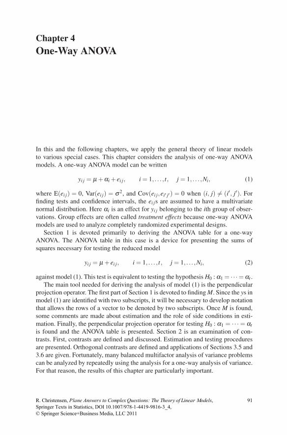
Chapter 4
One-Way ANOVA
In this and the following chapters, we apply the general theory of linear modelsto various special cases. This chapter considers the analysis of one-way ANOVAmodels. A one-way ANOVA model can be written
yi j = μ +αi + ei j, i = 1, . . . , t, j = 1, . . . ,Ni, (1)
where E(ei j) = 0, Var(ei j) = σ 2, and Cov(ei j,ei′ j′) = 0 when (i, j) �= (i′, j′). Forfinding tests and confidence intervals, the ei js are assumed to have a multivariatenormal distribution. Here αi is an effect for yi j belonging to the ith group of obser-vations. Group effects are often called treatment effects because one-way ANOVAmodels are used to analyze completely randomized experimental designs.
Section 1 is devoted primarily to deriving the ANOVA table for a one-wayANOVA. The ANOVA table in this case is a device for presenting the sums ofsquares necessary for testing the reduced model
yi j = μ + ei j, i = 1, . . . , t, j = 1, . . . ,Ni, (2)
against model (1). This test is equivalent to testing the hypothesis H0 : α1 = · · ·= αt .The main tool needed for deriving the analysis of model (1) is the perpendicular
projection operator. The first part of Section 1 is devoted to finding M. Since the ys inmodel (1) are identified with two subscripts, it will be necessary to develop notationthat allows the rows of a vector to be denoted by two subscripts. Once M is found,some comments are made about estimation and the role of side conditions in esti-mation. Finally, the perpendicular projection operator for testing H0 : α1 = · · · = αtis found and the ANOVA table is presented. Section 2 is an examination of con-trasts. First, contrasts are defined and discussed. Estimation and testing proceduresare presented. Orthogonal contrasts are defined and applications of Sections 3.5 and3.6 are given. Fortunately, many balanced multifactor analysis of variance problemscan be analyzed by repeatedly using the analysis for a one-way analysis of variance.For that reason, the results of this chapter are particularly important.
© Springer Science+Business Media, LLC 2011
91Springer Texts in Statistics, DOI 10.1007/978-1-4419-9816-3_4, R. Christensen, Plane Answers to Complex Questions: The Theory of Linear Models,

92 4 One-Way ANOVA
4.1 Analysis of Variance
In linear model theory, the main tools we need are perpendicular projection matrices.Our first project in this section is finding the perpendicular projection matrix for aone-way ANOVA model. We will then discuss estimation, side conditions, and theANOVA table.
Usually, the one-way ANOVA model is written
yi j = μ +αi + ei j, i = 1, . . . , t, j = 1, . . . ,Ni.
Let n = ∑ti=1 Ni. Although the notation Ni is standard, we will sometimes use N(i)
instead. Thus, N(i) ≡ Ni. We proceed to find the perpendicular projection matrixM = X(X ′X)−X ′.
EXAMPLE 4.1.1. In any particular example, the matrix manipulations necessaryfor finding M are simple. Suppose t = 3, N1 = 5, N2 = 3, N3 = 3. In matrix notationthe model can be written⎡⎢⎢⎢⎢⎢⎢⎢⎢⎢⎢⎢⎢⎢⎢⎢⎣
y11y12y13y14y15y21y22y23y31y32y33
⎤⎥⎥⎥⎥⎥⎥⎥⎥⎥⎥⎥⎥⎥⎥⎥⎦=
⎡⎢⎢⎢⎢⎢⎢⎢⎢⎢⎢⎢⎢⎢⎢⎢⎣
1 1 0 01 1 0 01 1 0 01 1 0 01 1 0 01 0 1 01 0 1 01 0 1 01 0 0 11 0 0 11 0 0 1
⎤⎥⎥⎥⎥⎥⎥⎥⎥⎥⎥⎥⎥⎥⎥⎥⎦
⎡⎢⎣μα1α2α3
⎤⎥⎦+ e.
To find the perpendicular projection matrix M, first find
X ′X =
⎡⎢⎣11 5 3 35 5 0 03 0 3 03 0 0 3
⎤⎥⎦ .
By checking that (X ′X)(X ′X)−(X ′X) = X ′X , it is easy to verify that
(X ′X)− =
⎡⎢⎣0 0 0 00 1/5 0 00 0 1/3 00 0 0 1/3
⎤⎥⎦ .

4.1 Analysis of Variance 93
Then
M
= X(X ′X)−X ′
= X
⎡⎢⎣0 0 0 0 0 0 0 0 0 0 0
1/5 1/5 1/5 1/5 1/5 0 0 0 0 0 00 0 0 0 0 1/3 1/3 1/3 0 0 00 0 0 0 0 0 0 0 1/3 1/3 1/3
⎤⎥⎦
=
⎡⎢⎢⎢⎢⎢⎢⎢⎢⎢⎢⎢⎢⎢⎢⎢⎣
1/5 1/5 1/5 1/5 1/5 0 0 0 0 0 01/5 1/5 1/5 1/5 1/5 0 0 0 0 0 01/5 1/5 1/5 1/5 1/5 0 0 0 0 0 01/5 1/5 1/5 1/5 1/5 0 0 0 0 0 01/5 1/5 1/5 1/5 1/5 0 0 0 0 0 00 0 0 0 0 1/3 1/3 1/3 0 0 00 0 0 0 0 1/3 1/3 1/3 0 0 00 0 0 0 0 1/3 1/3 1/3 0 0 00 0 0 0 0 0 0 0 1/3 1/3 1/30 0 0 0 0 0 0 0 1/3 1/3 1/30 0 0 0 0 0 0 0 1/3 1/3 1/3
⎤⎥⎥⎥⎥⎥⎥⎥⎥⎥⎥⎥⎥⎥⎥⎥⎦.
Thus, in this example, M is Blk diag[N−1i JN(i)
N(i) ], where Jcr is a matrix of 1s with r
rows and c columns. In fact, we will see below that this is the general form for M ina one-way ANOVA when the observation vector Y has subscripts changing fasteston the right.
A somewhat easier way of finding M is as follows. Let Z be the model matrix forthe alternative one-way analysis of variance model
yi j = μi + ei j,
i = 1, . . . , t, j = 1, . . . ,Ni. (See Example 3.1.1.) Z is then just a matrix consist-ing of the last t columns of X , i.e., X = [J,Z]. Clearly C(X) = C(Z), Z′Z =Diag(N1,N2, . . . ,Nt), and (Z′Z)−1 = Diag(N−1
1 ,N−12 , . . . ,N−1
t ). It is easy to see thatZ(Z′Z)−Z′ = Blk diag[N−1
i JN(i)N(i) ].
We now present a rigorous derivation of these results. The ideas involved in Ex-ample 4.1.1 are perfectly general. A similar computation can be performed for anyvalues of t and the Nis. The difficulty in a rigorous general presentation lies entirelyin being able to write down the model in matrix form. The elements of Y are the yi js.The yi js have two subscripts, so a pair of subscripts must be used to specify eachrow of the vector Y . The elements of the model matrices X and Z are determinedentirely by knowing the order in which the yi js have been listed in the Y vector. Forexample, the row of Z corresponding to yi j would have a 1 in the ith column and0s everywhere else. Clearly, it will also be convenient to use a pair of subscripts tospecify the rows of the model matrices. Specifically, let

94 4 One-Way ANOVA
Y ′ = (y11,y12, . . . ,y1N(1),y21, . . . ,ytN(t)),
where y21 is the N1 + 1 row of Y . In general, write a vector S as S = [si j], wherefor j = 1, . . . ,Ni, si j denotes the (N1 + · · ·+Ni−1 + j)th row of S. The discussion oftensors in Appendix B may help the reader feel more comfortable with our use ofsubscripts.
To specify the model matrices X and Z we must identify the columns of X andZ. Write X = [J,X1,X2, . . . ,Xt ] and Z = [X1,X2, . . . ,Xt ]. Note that the kth column ofZ can be written
Xk = [ti j], where ti j = δik (1)
with δik equal to 0 if i �= k and 1 if i = k. This means that if the observation in the i jrow belongs to the kth group, the i j row of Xk is 1. If not, the i j row of Xk is zero.
Our goal is to find M = Z(Z′Z)−1Z′. To do this we need to find (Z′Z) and(Z′Z)−1. Noting that (Xk)′(Xq) is a real number, we can write the elements of Z′Zas
(Z′Z) =[(Xk)′(Xq)
]t×t .
Now, from (1)
(Xk)′(Xk) = ∑i j
δikδik =t
∑i=1
Ni
∑j=1
δik =t
∑i=1
Niδik = Nk
and for k �= q
(Xk)′(Xq) =t
∑i=1
Ni
∑j=1
δikδiq =t
∑i=1
Niδikδiq = 0.
It follows that(Z′Z) = Diag(Ni)
and clearly(Z′Z)−1 = Diag(N−1
i ).
We can now find Z(Z′Z)−1.
Z(Z′Z)−1 = [X1,X2, . . . ,Xt ]Diag(N−1i )
=[N−1
1 X1,N−12 X2, . . . ,N−1
t Xt].
Finally, we are in a position to find M = Z(Z′Z)−1Z′. We denote the columns ofan n× n matrix using the convention introduced above for denoting rows, i.e., byusing two subscripts. Then the matrix M can be written
M = [mi j,i′ j′ ].
We now find the entries of this matrix. Note that mi j,i′ j′ is the i j row of Z(Z′Z)−1
times the i′ j′ column of Z′ (i.e., the i′ j′ row of Z). The i j row of Z(Z′Z)−1 is(N−1
1 δi1, . . . ,N−1t δit). The i′ j′ row of Z is (δi′1, . . . ,δi′t). The product is

4.1 Analysis of Variance 95
mi j,i′ j′ =t
∑k=1
N−1k δikδi′k
= N−1i δii′ .
These values of mi j,i′ j′ determine a block diagonal matrix
M = Blk diag(N−1i JN(i)
N(i) ),
just as in Example 4.1.1.The notation and methods developed above are somewhat unusual, but they are
necessary for giving a rigorous treatment of ANOVA models. The device of indi-cating the rows of vectors with multiple subscripts will be used extensively in laterdiscussions of multifactor ANOVA. It should be noted that the arguments givenabove really apply to any order of specifying the entries in a vector S = [si j]; they donot really depend on having S = (s11,s12, . . . ,stN(t))′. If we specified some other or-dering, we would still get the perpendicular projection matrix M; however, M mightno longer be block diagonal.
Exercise 4.1 To develop some facility with this notation, let
Tr = [ti j], where ti j = δir − Nr
n
for r = 1, . . . , t. Find T ′r Tr, T ′
r Ts for s �= r, and J′Tr.
A very important application of this notation is in characterizing the vector MY .As discussed in Section 3.1, the vector MY is the base from which all estimates ofparametric functions are found. A second important application involves the projec-tion operator
Mα = M− 1n
Jnn .
Mα is useful in testing hypotheses and is especially important in the analysis ofmultifactor ANOVAs. It is therefore necessary to have a characterization of Mα .
Exercise 4.2 Show that
MY = [ti j], where ti j = yi·
andMαY = [ui j], where ui j = yi· − y·· .
Hint: Write MαY = MY − ( 1n Jn
n )Y .
Knowing these characterizations MY and MαY tell us how to find Mv and Mαvfor any vector v. In fact, they completely characterize the perpendicular projectionoperators M and Mα .

96 4 One-Way ANOVA
EXAMPLE 4.1.1 CONTINUED. In this example,
MY = (y1·, y1·, y1·, y1·, y1·, y2·, y2·, y2·, y3·, y3·, y3·)′
and
MαY = (y1· − y··, y1· − y··, y1· − y··, y1· − y··, y1· − y··,y2· − y··, y2· − y··, y2· − y··, y3· − y··, y3· − y··, y3· − y··)′.
We can now obtain a variety of estimates. Recall that estimable functions are linearcombinations of the rows of Xβ , e.g., ρ ′Xβ . Since
Xβ =(μ +α1,μ +α1,μ +α1,μ +α1,μ +α1,
μ +α2,μ +α2,μ +α2,μ +α3,μ +α3,μ +α3)′
,
if ρ ′ is taken to be ρ ′ = (1,0,0,0,0,0,0,0,0,0,0)′, then it is easily seen thatμ +α1 = ρ ′Xβ is estimable. The estimate of μ + α1 is ρ ′MY = y1·. Similarly, theestimates of μ + α2 and μ + α3 are y2· and y3·, respectively. The contrast α1 −α2can be obtained as ρ ′Xβ using ρ ′ = (1,0,0,0,0,−1,0,0,0,0,0)′. The estimate ofα1 −α2 is ρ ′MY = y1· − y2·. Note that for this contrast ρ ′MY = ρ ′MαY .
Estimation is as easy in a general one-way ANOVA as it is in Example 4.1.1. Wehave found M and MY , and it is an easy matter to see that, for instance, μ + αi isestimable and the estimate of μ +αi is
{μ + αi} = yi· .
The notation {μ + αi} will be used throughout this chapter to denote the estimateof μ +αi.
For computational purposes, it is often convenient to present one particular set ofleast squares estimates. In one-way ANOVA, the traditional side condition on theparameters is ∑t
i=1 Niαi = 0. With this condition, one obtains
μ =1n
t
∑i=1
Ni(μ +αi)
and an estimate
μ =1n
t
∑i=1
Ni{μ + αi} =1n
t
∑i=1
Ni
Ni
Ni
∑j=1
yi j = y··,
which is the mean of all the observations. Similarly,
αi = {μ + αi}− μ = yi· − y·· .

4.1 Analysis of Variance 97
Exercise 4.9 involves finding parameter estimates that satisfy a different commonlyused side condition. Fortunately, all side conditions lead to the same estimates ofidentifiable functions, so one choice of a side condition is as good as any other. Thebest choice of a side condition is the most convenient choice. However, different sideconditions do lead to different “estimates” of nonidentifiable parameters. Do notbe lulled into believing that an arbitrary side condition allows you to say anythingmeaningful about nonidentifiable parameters. That is just silly!
We now derive the analysis of variance table for the one-way ANOVA. The anal-ysis of variance table is a device for displaying an orthogonal breakdown of the totalsum of squares of the data (SSTot), i.e., Y ′Y . Sometimes, the total sum of squarescorrected for fitting the grand mean is broken down. The sum of squares for fittingthe grand mean (SSGM), also known as the correction factor (C), is just the sum ofsquares accounted for by the model
Y = Jμ + e.
The total sum of squares corrected for the grand mean (SSTot −C) is the error sumof squares for this model, i.e., Y ′ (I − [1/n]Jn
n )Y . Included in an ANOVA table isinformation to identify the sums of squares (Source), the degrees of freedom forthe sums of squares (df ), the sums of squares (SS), and the mean squares (MS).The mean squares are just the sums of squares divided by their degrees of freedom.Sometimes the expected values of the mean squares are included. From the expectedmean squares, the hypotheses tested by the various sums of squares can be identi-fied. Recall that, when divided by σ 2, the sums of squares have χ2 distributionsand that there is a very close relationship between the expected mean square, theexpected sum of squares, the noncentrality parameter of the χ2 distribution, and thenoncentrality parameter of an F distribution with the mean square in the numerator.In particular, if the expected mean square is σ 2 + π/df , then the noncentrality pa-rameter is π/2σ 2. Assuming the full model is true, the null hypothesis being testedis that the noncentrality parameter of the F distribution is zero.
The usual orthogonal breakdown for a one-way ANOVA is to isolate the effect ofthe grand mean (μ), and then the effect of fitting the treatments (αis) after fitting themean. The sum of squares for treatments (SSTrts) is just what is left after removingthe sum of squares for μ from the sum of squares for the model. In other words, thesum of squares for treatments is the sum of squares for testing the reduced model(4.0.2) against model (4.0.1). As we have seen earlier, the projection operator forfitting the grand mean is based on the first column of X , i.e., J. The projectionoperator is (1/n)Jn
n = (1/n)JJ′. The projection operator for the treatment sum ofsquares is then
Mα = M− 1n
Jnn .
The sum of squares for fitting treatments after μ , Y ′MαY , is the difference betweenthe sum of squares for fitting the full model, Y ′MY , and the sum of squares for fittingthe model with just the mean, Y ′ ([1/n]Jn
n )Y .
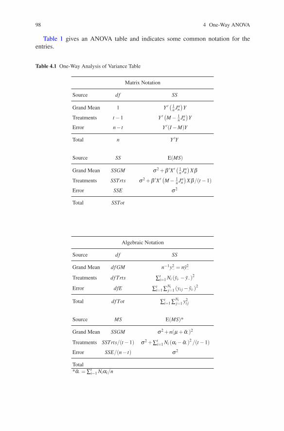
98 4 One-Way ANOVA
Table 1 gives an ANOVA table and indicates some common notation for theentries.
Table 4.1 One-Way Analysis of Variance Table
Matrix Notation
Source df SS
Grand Mean 1 Y ′ ( 1n Jn
n)
Y
Treatments t −1 Y ′ (M− 1n Jn
n)
Y
Error n− t Y ′(I −M)Y
Total n Y ′Y
Source SS E(MS)
Grand Mean SSGM σ2 +β ′X ′ ( 1n Jn
n)
Xβ
Treatments SSTrts σ2 +β ′X ′ (M− 1n Jn
n)
Xβ/(t −1)
Error SSE σ 2
Total SSTot
Algebraic Notation
Source df SS
Grand Mean df GM n−1y2·· = ny2··
Treatments df Trts ∑ti=1 Ni (yi· − y··)2
Error dfE ∑ti=1 ∑Ni
j=1 (yi j − yi·)2
Total df Tot ∑ti=1 ∑Ni
j=1 y2i j
Source MS E(MS)*
Grand Mean SSGM σ2 +n(μ + α·)2
Treatments SSTrts/(t −1) σ2 +∑ti=1 Ni (αi − α·)2 /(t −1)
Error SSE/(n− t) σ2
Total*α· = ∑t
i=1 Niαi/n

4.2 Estimating and Testing Contrasts 99
Exercise 4.3 Verify that the estimate of μ + αi is yi· and that the algebraicformulas for the sums of squares in the ANOVA table are correct.
Hint: To find, for example, Y (M− [1/n]Jnn )Y = Y ′MαY , use Exercise 4.2 to get
MαY and recall that Y ′MαY = [MαY ]′ [MαY ].
Exercise 4.4 Verify that the formulas for expected mean squares in the ANOVAtable are correct.
Hint: Use Theorem 1.3.2 and Exercise 4.3.
The techniques suggested for Exercises 4.3 and 4.4 are very useful. The readershould make a point of remembering them.
4.2 Estimating and Testing Contrasts
In this section, contrasts are defined and characterizations of contrasts are given.Estimates of contrasts are found. The numerator sum of squares necessary for doingan F test of a contrast and the form of the F test are given. The form of a confidenceinterval for a contrast is presented and the idea of orthogonal contrasts is discussed.Finally, the results of Section 3.5 are reviewed by deriving them anew for the one-way ANOVA model.
A contrast in the one-way ANOVA (4.0.1) is a function ∑ti=1 λiαi, with ∑t
i=1 λi =0. In other words, the vector λ ′ in λ ′β is (0,λ1,λ2, . . . ,λt) and λ ′Jt+1 = 0. To es-tablish that λ ′β is estimable, we need to find ρ such that ρ ′X = λ ′. Write
ρ ′ = (λ1/N1, . . . ,λ1/N1,λ2/N2, . . . ,λ2/N2,λ3/N3, . . . ,λt/Nt),
where ρ ′ is a 1×n vector and the string of λi/Nis is Ni long. In the alternate notationthat uses two subscripts to denote a row of a vector, we have
ρ = [ti j], where ti j = λi/Ni. (1)
Recall from Section 2.1 that, while other choices of ρ may exist with ρ ′X = λ ′,the vector Mρ is unique. As shown in Exercise 4.10, for ρ as in (1), ρ ∈ C(X); soρ = Mρ . Thus, for any contrast λ ′β , the vector Mρ has the structure
Mρ = [ti j], where ti j = λi/Ni. (2)
We now show that the contrasts are precisely the estimable functions that do notinvolve μ . Note that since J is the column of X associated with μ , ρ ′Xβ does notinvolve μ if and only if ρ ′J = 0.
Proposition 4.2.1. ρ ′Xβ is a contrast if and only if ρ ′J = 0.

100 4 One-Way ANOVA
PROOF. Clearly, a contrast does not involve μ , so ρ ′J = 0. Conversely, if ρ ′J = 0,then ρ ′Xβ = ρ ′[J,Z]β does not involve μ; so we need only show that 0 = ρ ′XJt+1.This follows because XJt+1 = 2Jn, and we know that ρ ′Jn = 0. �
We now show that the contrasts are the estimable functions that impose con-straints on C(Mα). Recall that the constraint imposed on C(X) by ρ ′Xβ = 0 is thatE(Y ) ∈C(X) and E(Y ) ⊥ Mρ , i.e., E(Y ) is constrained to be orthogonal to Mρ . Bydefinition, ρ ′Xβ puts a constraint on C(Mα) if Mρ ∈C(Mα).
Proposition 4.2.2. ρ ′Xβ is a contrast if and only if Mρ ∈C(Mα).
PROOF. Using Proposition 4.2.1 and J ∈C(X), we see that ρ ′Xβ is a contrast ifand only if 0 = ρ ′J = ρ ′MJ, i.e., J ⊥ Mρ . However, C(Mα) is everything in C(X)that is orthogonal to J; thus J ⊥ Mρ if and only if Mρ ∈C(Mα). �
Finally, we can characterize C(Mα).
Proposition 4.2.3. C(Mα) ={
ρ∣∣∣ρ = [ti j], ti j = λi/Ni, ∑t
i=1 λi = 0}
.
PROOF. Any vector ρ with the structure of (1) and ∑i λi = 0 has ρ ′J = 0 and byProposition 4.2.1 determines a contrast ρ ′Xβ . By Proposition 4.2.2, Mρ ∈C(Mα).However, vectors that satisfy (1) also satisfy Mρ = ρ, so ρ ∈C(Mα). Conversely, ifρ ∈C(Mα), then ρ ′J = 0; so ρ ′Xβ determines a contrast. It follows that Mρ mustbe of the form (2), where λ1 + · · ·+λt = 0. However, since ρ ∈C(Mα), Mρ = ρ; soρ must be of the form (1) with λ1 + · · ·+λt = 0.
Exercise 4.5 Show that α1 = α2 = · · · = αt if and only if all contrasts are zero.
We now consider estimation and testing for contrasts. The least squares estimateof a contrast ∑t
i=1 λiαi is easily obtained. Let μ , α1, . . . , αt be any choice of leastsquares estimates for the nonidentifiable parameters μ ,α1, . . . ,αt . Since ∑t
i=1 λi = 0,we can write
t
∑i=1
λiαi =t
∑i=1
λi{μ + αi} =t
∑i=1
λiyi·,
because μ + αi is estimable and its unique least squares estimate is yi·. This resultcan also be seen by examining ρ ′Y = ρ ′MY for the ρ given earlier in (1). To test thehypothesis that λ ′β = 0, we have seen that the numerator of the F test statistic is(ρ ′MY )2/ρ ′Mρ . However, ρ ′MY = ρ ′X β = λ ′β = ∑t
i=1 λiyi·. We also need to findρ ′Mρ . The easiest way is to observe that, since Mρ has the structure of (2),
ρ ′Mρ = [Mρ]′[Mρ]
=t
∑i=1
Ni
∑j=1
λ 2i /N2
i

4.2 Estimating and Testing Contrasts 101
=t
∑i=1
λ 2i /Ni.
The numerator sum of squares for testing the contrast is
SS(λ ′β ) ≡(
t
∑i=1
λiyi·
)2/( t
∑i=1
λ 2i /Ni
).
The α level test for H0 : ∑ti=1 λiαi = 0 is to reject H0 if
(∑ti=1 λiyi·)
2/(
∑ti=1 λ 2
i /Ni)
MSE> F(1−α,1,dfE).
Equivalently, ∑ti=1 λiyi· has a normal distribution, E(∑t
i=1 λiyi·) = ∑ti=1 λi(μ +
αi) = ∑ti=1 λiαi, and Var(∑t
i=1 λiyi·) = ∑ti=1 λ 2
i Var(yi·) = σ 2 ∑ti=1 λ 2
i /Ni, so we havea t test available. The α level test is to reject H0 if
|∑ti=1 λiyi·|√
MSE ∑ti=1 λ 2
i /Ni
> t(
1− α2
,dfE)
.
Note that since ∑ti=1 λiyi· = ρ ′MY is a function of MY and MSE is a function of
Y ′(I −M)Y , we have the necessary independence for the t test. In fact, all tests andconfidence intervals follow as in Exercise 2.1.
In order to break up the sums of squares for treatments into t−1 orthogonal singledegree of freedom sums of squares, we need to find t − 1 contrasts λ ′
1β , . . . ,λ ′t−1β
with the property that ρ ′rMρs = 0 for r �= s, where ρ ′
rX = λ ′r (see Section 3.6). Let
λ ′r = (0,λr1, . . . ,λrt) and recall that Mρr has the structure of (2). The condition
required is
0 = ρ ′rMρs
= [Mρr]′[Mρs]
=t
∑i=1
Ni
∑j=1
(λri/Ni)(λsi/Ni)
=t
∑i=1
λriλsi/Ni.
With any set of contrasts ∑ti=1 λriαi, r = 1, . . . , t−1, for which 0 = ∑t
i=1 λriλsi/Nifor all r �= s, we have a set of t − 1 orthogonal constraints on the test space so thatthe sums of squares for the contrasts add up to the SSTrts. Contrasts that determineorthogonal constraints are referred to as orthogonal contrasts.
In later analyses, we will need to use the fact that the analysis developed heredepends only on the projection matrix onto the space for testing α1 = α2 = · · ·= αt .That projection matrix is Mα = M − (1/n)Jn
n . Note that M = (1/n)Jnn + Mα . For

102 4 One-Way ANOVA
any contrast λ ′β with ρ ′X = λ ′, we know that ρ ′Jn = 0. It follows that ρ ′M =ρ ′(1/n)Jn
n +ρ ′Mα = ρ ′Mα . There are two main uses for this fact. First,
t
∑i=1
λiαi =t
∑i=1
λiyi· = ρ ′MY = ρ ′MαY,
t
∑i=1
λ 2i /Ni = λ ′(X ′X)−λ = ρ ′Mρ = ρ ′Mα ρ,
so estimation, and therefore tests, depend only on the projection Mα . Second, thecondition for contrasts to give an orthogonal breakdown of SSTrts is
0 =t
∑i=1
λriλsi/Ni = ρ ′rMρs = ρ ′
rMα ρs,
which depends only on Mα . This is just a specific example of the theory of Sec-tion 3.5.
Exercise 4.6 Using the theories of Sections 3.3 and 2.6, respectively, find the Ftest and the t test for the hypothesis H0 : ∑t
i=1 λiαi = d in terms of the MSE , the yi·s,and the λis.
Exercise 4.7 Suppose N1 = N2 = · · · = Nt ≡ N. Rewrite the ANOVA table in-corporating any simplifications due to this assumption.
Exercise 4.8 If N1 = N2 = · · · = Nt ≡ N, show that two contrasts λ ′1β and λ ′
2βare orthogonal if and only if λ ′
1λ2 = 0.
Exercise 4.9 Find the least squares estimates of μ , α1, and αt using the sidecondition α1 = 0.
Exercise 4.10 Using ρ as defined by (1) and X as defined in Section 1, especially(4.1.1), show that
(a) ρ ′X = λ ′, where λ ′ = (0,λ1, . . . ,λt).(b) ρ ∈C(X).
4.3 Additional Exercises
Exercise 4.3.1 An experiment was conducted to see which of four brands of bluejeans were most resistant to wearing out as a result of students kneeling before their

4.3 Additional Exercises 103
linear models instructor begging for additional test points. In a class of 32 students,8 students were randomly assigned to each brand of jeans. Before being informed oftheir test score, each student was required to fall to his/her knees and crawl 3 metersto the instructor’s desk. This was done after each of 5 mid-quarter and 3 final exams.(The jeans were distributed along with each of the 8 test forms and were collectedagain 36 hours after grades were posted.) A fabric wear score was determined foreach pair of jeans. The scores are listed below.
Brand 1: 3.41 1.83 2.69 2.04 2.83 2.46 1.84 2.34Brand 2: 3.58 3.83 2.64 3.00 3.19 3.57 3.04 3.09Brand 3: 3.32 2.62 3.92 3.88 2.50 3.30 2.28 3.57Brand 4: 3.22 2.61 2.07 2.58 2.80 2.98 2.30 1.66
(a) Give an ANOVA table for these data, and perform and interpret the F testfor the differences between brands.
(b) Brands 2 and 3 were relatively inexpensive, while Brands 1 and 4 were verycostly. Based on these facts, determine an appropriate set of orthogonal contrasts toconsider in this problem. Find the sums of squares for the contrasts.
(c) What conclusions can be drawn from these data? Perform any additionalcomputations that may be necessary
Exercise 4.3.2 After the final exam of spring quarter, 30 of the subjects of theprevious experiment decided to test the sturdiness of 3 brands of sport coats and 2brands of shirts. In this study, sturdiness was measured as the length of time beforetearing when the instructor was hung by his collar out of his second-story officewindow. Each brand was randomly assigned to 6 students, but the instructor wasoccasionally dropped before his collar tore, resulting in some missing data. Thedata are listed below.
Coat 1: 2.34 2.46 2.83 2.04 2.69Coat 2: 2.64 3.00 3.19 3.83Coat 3: 2.61 2.07 2.80 2.58 2.98 2.30Shirt 1: 1.32 1.62 1.92 0.88 1.50 1.30Shirt 2: 0.41 0.83 0.53 0.32 1.62
(a) Give an ANOVA table for these data, and perform and interpret the F testfor the differences between brands.
(b) Test whether, on average, these brands of coats are sturdier than thesebrands of shirts.
(c) Give three contrasts that are mutually orthogonal and orthogonal to thecontrast used in (b). Compute the sums of squares for all four contrasts.
(d) Give a 95% confidence interval for the difference in sturdiness betweenshirt Brands 1 and 2. Is one brand significantly sturdier than the other?


Chapter 5
Multiple Comparison Techniques
In analyzing a linear model we can examine as many single degree of freedomhypotheses as we want. If we test all of these hypotheses at, say, the 0.05 level, thenthe (weak) experimentwise error rate (the probability of rejecting at least one ofthese hypotheses when all are true) will be greater than 0.05. Multiple comparisontechniques are methods of performing the tests so that if all the hypotheses aretrue, then the probability of rejecting any of the hypotheses is no greater than somespecified value, i.e., the experimentwise error rate is controlled.
A multiple comparison method can be said to be more powerful than a competingmethod if both methods control the experimentwise error rate at the same level, butthe method in question rejects hypotheses more often than its competitor. Beingmore powerful, in this sense, is a mixed blessing. If one admits the idea that a nullhypothesis really can be true (an idea that I am often loath to admit), then the purposeof a multiple comparison procedure is to identify which hypotheses are true andwhich are false. The more powerful of two multiple comparison procedures will bemore likely to correctly identify hypotheses that are false as being false. It will alsobe more likely to incorrectly identify hypotheses that are true as being false.
A related issue is that of examining the data before deciding on the hypotheses. Ifthe data have been examined, an hypothesis may be chosen to test because it looksas if it is likely to be significant. The nominal significance level of such a test isinvalid. In fact, when doing multiple tests by any standard method, nearly all thenominal significance levels are invalid. For some methods, however, selecting thehypotheses after examining the data make the error levels intolerably bad.
The sections of this chapter contain discussions of individual multiple compar-ison methods. The methods discussed are Scheffe’s method, the Least SignificantDifference (LSD) method, the Bonferroni method, Tukey’s Honest Significant Dif-ference (HSD) method, and multiple range tests. The section on multiple range testsexamines both the Newman–Keuls method and Duncan’s method. The final sectionof the chapter compares the various methods. For a more complete discussion ofmultiple comparison methods, see Miller (1981) or, more recently, Hochberg andTamhane (1987) or Hsu (1996). Miller’s book includes several methods that are notdiscussed here. Christensen (1996a) discusses the methods of this chapter at a more
© Springer Science+Business Media, LLC 2011
105Springer Texts in Statistics, DOI 10.1007/978-1-4419-9816-3_5, R. Christensen, Plane Answers to Complex Questions: The Theory of Linear Models,

106 5 Multiple Comparison Techniques
applied level, discusses Dunnett’s method for comparing treatments with a control,and discusses Ott’s analysis of means method.
5.1 Scheffe’s Method
Scheffe’s method of multiple comparisons is an omnibus technique that allows oneto test any and all single degree of freedom hypotheses that put constraints on agiven subspace. It provides the assurance that the experimentwise error rate will notexceed a given level α . Typically, this subspace will be for fitting a set of parametersafter fitting the mean, and in ANOVA problems is some sort of treatment space.
It is, of course, easy to find silly methods of doing multiple comparisons. Onecould, for example, always accept the null hypothesis. However, if the subspace isof value in fitting the model, Scheffe’s method assures us that there is at least onehypothesis in the subspace that will be rejected. That is, if the F test is significantfor testing that the subspace adds to the model, then there exists a linear hypothesis,putting a constraint on the subspace, that will be deemed significant by Scheffe’smethod.
Scheffe’s method is that an hypothesis H0 : λ ′β = 0 is rejected if
SS(λ ′β )/sMSE
> F(1−α,s,dfE),
where SS(λ ′β ) is the sum of squares for the usual test of the hypothesis, s is thedimension of the subspace, and λ ′β = 0 is assumed to put a constraint on the sub-space.
In terms of a one-way analysis of variance where the subspace is the space fortesting equality of the treatment means, Scheffe’s method applies to testing whetherall contrasts equal zero. With t treatments, a contrast is deemed significantly differ-ent from zero at the α level if the sum of squares for the contrast divided by t − 1and the MSE is greater than F(1−α, t −1,dfE).
Theorem 5.1.1 given below leads immediately to the key properties of Scheffe’smethod. Recall that if ρ ′Xβ = 0 puts a constraint on a subspace, then Mρ is anelement of that subspace. Theorem 5.1.1 shows that the F test for the subspace re-jects if and only if the Scheffe test rejects the single degree of freedom hypothesisρ ′Xβ = 0 for some ρ with Mρ in the subspace. The proof is accomplished by find-ing a vector in the subspace having the property that the sum of squares for testingthe corresponding one degree of freedom hypothesis equals the sum of squares forthe entire space. Of course, the particular vector that has this property depends onY . To emphasize this dependence on Y , the vector is denoted mY . In the proof of thetheorem, mY is seen to be just the projection of Y onto the subspace (hence the useof the letter m in the notation).
It follows that for a one-way ANOVA there is always a contrast for which thecontrast sum of squares equals the sum of squares for treatments. The exact natureof this contrast depends on Y and often the contrast is completely uninterpretable.

5.1 Scheffe’s Method 107
Nevertheless, the existence of such a contrast establishes that Scheffe’s method re-jects for some contrast if and only if the test for equality of treatments is rejected.
Theorem 5.1.1. Consider the linear model Y = Xβ + e and let M∗ be the per-pendicular projection operator onto some subspace of C(X). Let r(M∗) = s. Then
Y ′M∗Y/sMSE
> F(1−α,s,dfE)
if and only if there exists a vector mY such that MmY ∈C(M∗) and
SS(m′Y Xβ )/s
MSE> F(1−α,s,dfE).
PROOF. ⇒ We want to find a vector mY so that if the F test for the subspaceis rejected, then MmY is in C(M∗), and the hypothesis m′
Y Xβ = 0 is rejected byScheffe’s method. If we find mY within C(M∗) and SS(m′
Y Xβ ) = Y ′M∗Y , we aredone. Let mY = M∗Y .
As in Section 3.5, SS(m′Y Xβ ) = Y ′M∗mY [m′
Y M∗mY ]−1m′Y M∗Y . Since
M∗mY = M∗M∗Y = M∗Y = mY , we have SS(m′Y Xβ ) = Y ′mY [m′
Y mY ]−1m′YY =
(Y ′M∗Y )2/Y ′M∗Y = Y ′M∗Y , and we are finished.⇐ We prove the contrapositive, i.e., if Y ′M∗Y/s MSE ≤ F(1−α,s,dfE), then
for any ρ such that Mρ ∈C(M∗), we have SS(ρ ′Xβ)/s MSE ≤ F(1−α,s,dfE). Tosee this, observe that
SS(ρ ′Xβ ) = Y ′[Mρ(ρ ′Mρ)−1ρ ′M]Y.
Since [Mρ(ρ ′Mρ)−1ρ ′M] is the perpendicular projection matrix onto a subspace ofC(M∗),
Y ′[Mρ(ρ ′Mρ)−1ρ ′M]Y ≤ Y ′M∗Y
and we are done. �
Y ′M∗Y is the sum of squares for testing the reduced model Y = (M −M∗)γ + e.If this null model is true,
Pr[
Y ′M∗Ys MSE
> F(1−α,s,dfE)]
= α.
The theorem therefore implies that the experimentwise error rate for testing all hy-potheses ρ ′Xβ = 0 with Mρ ∈ C(M∗) is exactly α . More technically, we wish totest the hypotheses
H0 : λ ′β = 0 for λ ∈ {λ |λ ′ = ρ ′X with Mρ ∈C(M∗)}.
The theorem implies that

108 5 Multiple Comparison Techniques
Pr[SS(λ ′β )/s
MSE> F(1−α,s,dfE) for some λ ,λ ′ = ρ ′X ,Mρ ∈C(M∗)
]= α ,
so the experimentwise error rate is α . The theorem also implies that if the omnibusF test rejects, there exists some single degree of freedom test that will be rejected.Note that which single degree of freedom tests are rejected depends on what the dataare, as should be expected.
Scheffe’s method can also be used for testing a subset of the set of all hypothesesputting a constraint on C(M∗). For testing a subset, the experimentwise error ratewill be no greater than α and typically much below α . The primary problem withusing Scheffe’s method is that, for testing a finite number of hypotheses, the exper-imentwise error rate is so much below the nominal rate of α that the procedure hasvery little power. (On the other hand, you can be extra confident, when rejectingwith Scheffe’s method, that you are not making a type I error.)
Suppose that we want to test
H0 : λ ′kβ = 0, k = 1, . . . ,r.
The constraints imposed by these hypotheses are Mρk, k = 1, . . . ,r, where λ ′k =
ρ ′kX . If C(M∗) is chosen so that C(Mρ1, . . . ,Mρr) ⊂ C(M∗), then by the previous
paragraph, if H0 is true,
Pr[SS(λ ′
kβ )/sMSE
> F(1−α,s,dfE) for some k, k = 1, . . . ,r]≤ α.
For testing a finite number of hypotheses, it is possible to reject the overall F testbut not reject for any of the specific hypotheses.
We now show that the most efficient procedure is to choose C(Mρ1, . . . ,Mρr) =C(M∗). In particular, given that a subspace contains the necessary constraints, thesmaller the rank of the subspace, the more powerful is Scheffe’s procedure. Considertwo subspaces, one of rank s and another of rank t, where s > t. Both proceduresguarantee that the experimentwise error rate is no greater than α . The more powerfulprocedure is the one that rejects more often. Based on the rank s subspace, Scheffe’smethod rejects if
SS(λ ′β )/MSE > sF(1−α,s,dfE).
For the rank t subspace, the method rejects if
SS(λ ′β )/MSE > tF(1−α,t,dfE).
With s > t, by Theorem C.4,
sF(1−α,s,dfE) ≥ tF(1−α,t,dfE).
One gets more rejections with the rank t space, hence it gives a more powerfulprocedure.

5.1 Scheffe’s Method 109
EXAMPLE 5.1.2. One-Way ANOVA.Consider the model
yi j = μ +αi + ei j, ei js i.i.d. N(0,σ 2),
i = 1,2,3,4, j = 1, . . . ,N. To test the three contrast hypotheses
λ ′1β = α1 +α2 −α3 −α4 = 0,
λ ′2β = α1 −α2 +α3 −α4 = 0,
λ ′3β = α1 +0+0−α4 = 0,
we can observe that the contrasts put constraints on the space for testing H0 : α1 =α2 = α3 = α4 and the space has rank 3. We can apply Scheffe’s method: rejectH0 : λ ′
kβ = 0 ifSS(λ ′
kβ )/3MSE
> F(1−α ,3,4(N −1)).
A more efficient method is to notice that λ ′1β +λ ′
2β = 2λ ′3β . This is true for any
β , so λ ′1 + λ ′
2 = 2λ ′3 and, using (4.2.2), Mρ1 + Mρ2 = 2Mρ3. Since λ1 and λ2 are
linearly independent, Mρ1 and Mρ2 are also; thus C(Mρ1,Mρ2,Mρ3) is a rank 2space and Scheffe’s method can be applied as: reject H0 : λ ′
kβ = 0 if
SS(λ ′kβ )/2
MSE> F(1−α ,2,4(N −1)).
One virtue of Scheffe’s method is that since it is really a test of all the hypothesesin a subspace, you can look at the data to help you pick an hypothesis and the testremains valid.
Scheffe’s method can also be used to find simultaneous confidence intervals. Toshow this we need some additional structure for the problem. Let X = [X0,X1] andlet β ′ = [β ′
0,β ′1], so that
Y = X0β0 +X1β1 + e.
Let M and M0 be the perpendicular projection operators onto C(X) and C(X0), re-spectively, and let M∗ = M −M0. We seek to find simultaneous confidence inter-vals for all estimable functions ρ ′X1β1. Note that ρ ′X1β1 is estimable if and only ifρ ′X0 = 0, which occurs if and only if 0 = M0ρ = Mρ −M∗ρ , i.e., Mρ = M∗ρ . It fol-lows that if ρ ′X1β1 is an estimable function, then ρ ′X1β1 = ρ ′MX1β1 = ρ ′M∗X1β1.Conversely, for any vector ρ , ρ ′M∗(X0β0 +X1β1) = ρ ′M∗X1β1 is an estimable func-tion. Proceeding as in Section 3.7, and observing that M∗Xβ = M∗X0β0 +M∗X1β1 =M∗X1β1, we have
(Y −X1β1)′M∗(Y −X1β1)/r(M∗)MSE
∼ F(r(M∗),dfE,0),
so that

110 5 Multiple Comparison Techniques
Pr[ (Y −X1β1)′M∗(Y −X1β1)/r(M∗)
MSE≤ F(1−α ,r(M∗),dfE)
]= 1−α
or, equivalently,
1−α = Pr[(Y −X1β1)′M∗ρ(ρ ′M∗ρ)−1ρ ′M∗(Y −X1β1)/r(M∗)
MSE
≤ F(1−α,r(M∗),dfE) for all ρ]
= Pr[ |ρ ′M∗Y −ρ ′M∗X1β1|
≤√
(ρ ′M∗ρ)(MSE)r(M∗)F(1−α,r(M∗),dfE) for all ρ].
This leads to obvious confidence intervals for all functions ρ ′M∗X1β1 and thus toconfidence intervals for arbitrary estimable functions ρ ′X1β1.
EXAMPLE 5.1.3. One-Way ANOVA.Consider the model yi j = μ + αi + ei j, ei js independent N(0,σ 2), i = 1, . . . , t, j =1, . . . ,Ni, and the space for testing α1 = α2 = · · · = αt . The linear functions thatput constraints on that space are the contrasts. Scheffe’s method indicates that H0 :∑t
i=1 λiαi = 0 should be rejected if
(∑λiyi·)2/(∑λ 2i /Ni)
(t −1)MSE> F(1−α,t −1,dfE).
To find confidence intervals for contrasts, write X = [J,X1] and β ′ = [μ ,β ′1],
where β ′1 = [α1, . . . ,αt ]. We can get simultaneous confidence intervals for estimable
functions ρ ′X1β1. As discussed in Chapter 4, the estimable functions ρ ′X1β1 areprecisely the contrasts. The simultaneous (1−α)100% confidence intervals havelimits
∑λiyi· ±√
(t −1)F(1−α,t −1,dfE)MSE(∑λ 2
i /Ni).
5.2 Least Significant Difference Method
The Least Significant Difference (LSD) method is a general technique for testinga fixed number of hypotheses λ ′
kβ = 0, k = 1, . . . ,r, chosen without looking at thedata. The constraints imposed by these hypotheses generate some subspace. (Com-monly, one identifies the subspace first and picks hypotheses that will generateit.) The technique is a simple two-stage procedure. First, do an α level F test forwhether the subspace adds to the model. If this omnibus F test is not significant, wecan conclude that the data are consistent with λ ′
kβ = 0, k = 1, . . . ,r. If the F test issignificant, we want to identify which hypotheses are not true. To do this, test eachhypothesis λ ′
kβ = 0 with a t test (or an equivalent F test) at the α level.

5.3 Bonferroni Method 111
The experimentwise error rate is controlled by using the F test for the subspace.When all of the hypotheses are true, the probability of identifying any of them asfalse is no more than α , because α is the probability of rejecting the omnibus Ftest. Although the omnibus F test is precisely a test of λ ′
kβ = 0, k = 1, . . . ,r, even ifthe F test is rejected, the LSD method may not reject any of the specific hypothesesbeing considered. For this reason, the experimentwise error rate is less than α .
The LSD method is more powerful than Scheffe’s method. If the hypothesesgenerate a space of rank s, then Scheffe’s method rejects if SS(λ ′
kβ )/MSE > sF(1−α,s,dfE). The LSD rejects if SS(λ ′
kβ )/MSE > F(1−α,1,dfE). By Theorem C.4,sF(1−α,s,dfE) > F(1−α,1,dfE), so the LSD method will reject more often thanScheffe’s method. Generally, the LSD method is more powerful than other methodsfor detecting when λ ′
kβ �= 0; but if λ ′kβ = 0, it is more likely than other methods to
incorrectly identify the hypothesis as being different from zero.Note that it is not appropriate to use an F test for a space that is larger than the
space generated by the r hypotheses. Such an F test can be significant for reasonscompletely unrelated to the hypotheses, thus invalidating the experimentwise errorrate.
Exercise 5.1 Consider the ANOVA model
yi j = μ +αi + ei j,
i = 1, . . . , t, j = 1, . . . ,N, with the ei js independent N(0,σ 2). Suppose it is desiredto test the hypotheses αi = αi′ for all i �= i′. Show that there is one number, calledthe LSD, so that the least significant difference rejects αi = αi′ precisely when
|yi· − yi′ ·| > LSD.
Exercise 5.2 In the model of Exercise 5.1, let t = 4. Suppose we want to use theLSD method to test contrasts defined by
Name λ1 λ2 λ3 λ4A 1 1 −1 −1B 0 0 1 −1C 1/3 1/3 1/3 −1
Describe the procedure. Give test statistics for each test that is to be performed.
5.3 Bonferroni Method
Suppose we have chosen, before looking at the data, a set of r hypotheses to test,say, λ ′
kβ = 0, k = 1, . . . ,r. The Bonferroni method consists of rejecting H0 : λ ′kβ = 0
if

112 5 Multiple Comparison Techniques
SS(λ ′kβ)
MSE> F(
1− αr
,1,dfE)
.
The Bonferroni method simply reduces the significance level of each individualtest so that the sum of the significance levels is no greater than α . (In fact, thereduced significance levels do not have to be α/r as long as the sum of the individualsignificance levels is α .)
This method rests on a Bonferroni inequality. For sets A1, . . . ,Ar, Pr(⋃r
k=1 Ak) ≤∑r
k=1 Pr(Ak). (This inequality is nothing more than the statement that a probabilitymeasure is finitely subadditive.) If all the hypotheses λ ′
kβ = 0, k = 1, . . . ,r are true,then the experimentwise error rate is
Pr(
SS(λ ′kβ ) > MSE F
(1− α
r,1,dfE
)for some k
)= Pr
(r⋃
k=1
[SS(λ ′
kβ ) > MSE F(
1− αr
,1,dfE)])
≤r
∑k=1
Pr(
SS(λ ′kβ) > MSE F
(1− α
r,1,dfE
))=
r
∑k=1
αr
= α.
If the hypotheses to be tested are chosen after looking at the data, the individualsignificance levels of α/r are invalid, so the experimentwise error rate has not beencontrolled.
Given that the subspace F test is rejected, the LSD method is more powerful thanthe Bonferroni method because F
(1− α
r ,1,dfE)
> F(1−α,1,dfE). The Bonfer-roni method is designed to handle a finite number of hypotheses, so it is not surpris-ing that it is usually a more powerful method than Scheffe’s method for testing ther hypotheses if r is not too large.
5.4 Tukey’s Method
Tukey’s method, also known as the Honest Significant Difference (HSD) method, isdesigned to compare all pairs of means for a set of independent normally distributedrandom variables with a common variance. Let yi ∼ N(μi,σ2), i = 1, . . . , t, let theyis be independent, and let S2 be an estimate of σ 2 with S2 independent of the yisand
vS2
σ 2 ∼ χ2(v).
Tukey’s method depends on knowing the distribution of the Studentized range whenμ1 = μ2 = · · · = μt , i.e., we need to know that

5.4 Tukey’s Method 113
Q ≡ maxi yi −mini yi
S∼ Q(t,v)
and we need to be able to find percentage points of the Q(t,v) distribution. Theseare tabled in many books on statistical methods, e.g., Christensen (1996a), Snedecorand Cochran (1980), and Kutner, Nachtsheim, Neter, and Li (2005).
If the observed value of Q is too large, the null hypothesis H0 : μ1 = · · · = μtshould be rejected. That is because any differences in the μis will tend to make therange large relative to the distribution of the range when all the μis are equal. Sincethe hypothesis H0 : μ1 = · · · = μt is equivalent to the hypothesis H0 : μi = μ j for alli and j, we can use the Studentized range test to test all pairs of means. Reject thehypothesis that H0 : μi = μ j if
|yi − y j|S
> Q(1−α,t,v),
where Q(1−α,t,v) is the (1−α)100 percentage point of the Q(t,v) distribution.If H0 : μi = μ j for all i and j is true, then at least one of these tests will reject H0 ifand only if
maxi yi −mini yi
S> Q(1−α,t,v),
which happens with probability α . Thus the experimentwise error rate is exactly α .
EXAMPLE 5.4.1. Two-Way ANOVA.Consider the model
yi jk = μ +αi +β j + ei jk, ei jks i.i.d. N(0,σ 2),
i = 1, . . . ,a, j = 1, . . . ,b, k = 1, . . . ,N. Suppose we want to test the hypotheses H0 :β j = β j′ for all j �= j′. Consider the y· j· values. Here
y· j· ∼ N(μ + α· +β j,σ 2/aN
)and the y· j·s are independent because y· j· depends only on e· j· for its randomness;and since e· j· and e· j′· are based on disjoint sets of the ei jks, they must be inde-pendent. We will see in Section 7.1 that the y· j·s are least squares estimates of theμ + α· +β js, so the y· j·s must be independent of the MSE . It follows quickly that ifH0 : β1 = · · · = βb is true, then
max j y· j· −min j y· j·√MSE/aN
∼ Q(b,dfE);
and we reject H0 : β j = β j′ if
|y· j· − y· j′·| > Q(1−α,b,dfE)√
MSE/aN.

114 5 Multiple Comparison Techniques
Note that Tukey’s method provides a competitor to the usual analysis of varianceF test for the hypothesis H0 : β1 = · · ·= βb. Also, Tukey’s method is only applicablewhen all the means being used are based on the same number of observations.
5.5 Multiple Range Tests: Newman–Keuls and Duncan
The Newman–Keuls multiple range method is a competitor to the Tukey method.It looks at all pairs of means. In fact, it amounts to a sequential version of Tukey’smethod. Using the notation of the previous section, order the yis from smallest tolargest, say
y(1) ≤ y(2) ≤ ·· · ≤ y(t),
and define μ(i) = μ j when y(i) = y j. Note that the μ(i)s need not be ordered in anyparticular way. However, the Newman–Keuls method acts as if the μ(i)s are alsoordered. With this notation, we can write the Studentized range as
Q =y(t)− y(1)
S.
The Newman–Keuls method rejects H0 : μ(t) = μ(1) if y(t)−y(1) > SQ(1−α ,t,v).If this hypothesis is not rejected, stop. All means are considered equal. If this hy-pothesis is rejected, we continue.
The next step tests two hypotheses. H0 : μ(t−1) = μ(1) is rejected if y(t−1)−y(1) >SQ(1−α ,t − 1,v). H0 : μ(t) = μ(2) is rejected if y(t) − y(2) > SQ(1−α,t − 1,v).If μ(t−1) = μ(1) is not rejected, then μ(1),μ(2), . . . ,μ(t−1) are assumed to be equal,and no more tests concerning only those means are performed. Similar conclusionshold if μ(t) = μ(2) is not rejected. If either hypothesis is rejected, the next round ofhypotheses is considered.
The next round of hypotheses includes three hypotheses: H0 : μ(t) = μ(3), H0 :μ(t−1) = μ(2), and H0 : μ(t−2) = μ(1). The hypothesis H0 : μ(t−3+i) = μ(i) is rejectedif y(t−3+i) − y(i) > SQ(1−α,t −2,v) for i = 1,2,3.
The procedure continues until, at the last round, the hypotheses H0 : μ(i) = μ(i−1),i = 2, . . . , t, are considered. An hypothesis is rejected if y(i) = y(i−1) > SQ(1 −α,2,v).
Remember that if, say, H0 : μ(t−1) = μ(1) is not rejected, we will never test H0 :μ(t−1) = μ(2) or H0 : μ(t−2) = μ(1) in the next round or any other hypothesis in anyother round that involves only μ(1),μ(2), . . . ,μ(t−1).
The experimentwise error rate is exactly α because if H0 : μ1 = · · · = μt is true,the Newman–Keuls procedure will conclude that there is a difference in the meansif and only if the Tukey method concludes that there is a difference. Because Q(1−α,2,v) < Q(1−α ,3,v) < · · · < Q(1−α,t − 1,v) < Q(1−α,t,v), the Newman–Keuls method will reject the hypothesis that a pair of means is equal more oftenthan Tukey’s method. The Newman–Keuls method is thus more powerful. On the

5.6 Summary 115
other hand, for pairs of μs that are equal, the Newman–Keuls method will makemore mistakes than the Tukey method.
EXAMPLE 5.5.1. Let α = .01, v = 10, S = 1, t = 5, and y1 = 6.5, y2 = 1.2, y3 =6.9, y4 = 9.8, y5 = 3.4. We need the numbers Q(0.99,5,10) = 6.14, Q(0.99,4,10) =5.77, Q(0.99,3,10) = 5.27, Q(0.99,2,10) = 4.48. Ordering the yis gives
i 2 5 1 3 4yi 1.2 3.4 6.5 6.9 9.8
To test H0 : μ4 = μ2, consider 9.8−1.2 = 8.6, which is larger than SQ(0.99,5,10) =6.14. There is a difference. Next test H0 : μ2 = μ3. Since 6.9−1.2 = 5.7 is less than5.77, we conclude that μ2 = μ5 = μ1 = μ3. We do no more tests concerning onlythose means. Now test H0 : μ5 = μ4. Since 9.8− 3.4 = 6.4 > 5.77, we reject thehypothesis.
We have concluded that μ2 = μ5 = μ1 = μ3, so the next allowable test is H0 :μ1 = μ4. Since 9.8−6.5 = 3.4 < 5.27, we conclude that μ1 = μ3 = μ4.
Drawing lines under the values that give no evidence of a difference in means,we can summarize our results as follows:
i 2 5 1 3 4yi 1.2 3.4 6.5 6.9 9.8
Note that if we had concluded that μ2 �= μ3, we could test H0 : μ2 = μ1. Thetest would be 6.5− 1.2 = 5.3 > 5.27, so we would have rejected the hypothesis.However, since we concluded that μ2 = μ5 = μ1 = μ3, we never get to do the testof μ2 = μ1.
Duncan has a multiple range test that is similar to Newman–Keuls but where theα levels for the various rounds of tests keep decreasing. In fact, Duncan’s methodis exactly the same as Newman–Keuls except that the α levels used when takingvalues from the table of the Studentized range are different. Duncan suggests usinga 1− (1−α)p−1 level test when comparing a set of p means. If there is a total oft means to be compared, Duncan’s method only controls the experimentwise errorrate at 1−(1−α)t−1. For α = 0.05 and t = 6, Duncan’s method can only be said tohave an experimentwise error rate of 0.23. As Duncan suggests, his method shouldonly be performed when a corresponding omnibus F test has been found significant.This two stage procedure may be a reasonable compromise between the powers ofthe LSD and Newman–Keuls methods.
5.6 Summary
The emphasis in this chapter has been on controlling the experimentwise error rate.We have made some mention of power and the fact that increased power can be

116 5 Multiple Comparison Techniques
a mixed blessing. The really difficult problem for multiple comparison proceduresis not in controlling the experimentwise error rate, but in carefully addressing theissues of power and the sizes of individual tests.
The discussion of Duncan’s multiple range test highlights an interesting factabout multiple comparison methods. Any method of rejecting hypotheses, if pre-ceded by an appropriate omnibus F test, is a valid multiple comparison procedure,valid in the sense that the experimentwise error rate is controlled. For example, ifyou do an F test first and stop if the F test does not reject, you can then 1) rejectall individual hypotheses if the analysis is being performed on your mother’s birthdate, 2) reject no individual hypotheses on other dates. As stupid as this is, the ex-perimentwise error rate is controlled. Intelligent choice of a multiple comparisonmethod also involves consideration of the error rates (probabilities of type I errors)for the individual hypotheses. The main question is: If not all of the hypotheses aretrue, how many of the various kinds of mistakes do the different methods make?
A reasonable goal might be to have the experimentwise error rate and the errorrates for the individual hypotheses all no greater than α . The Scheffe, LSD, Bonfer-roni, Tukey, and Newman–Keuls methods all seem to aim at this goal. The Duncanmethod does not seem to accept this goal.
Suppose we want α level tests of the hypotheses
H0 : λ ′kβ = 0, k ∈ Ω .
A reasonable procedure is to reject an hypothesis if
SS(λ ′kβ )/MSE > C
for some value C. For example, the LSD method takes C = F(1−α,1,dfE). IfΩ consists of all the hypotheses in a t-dimensional space, Scheffe’s method takesC = tF(1−α,t,dfE). If Ω is a finite set, say Ω = {1, . . . ,r}, then the Bonferronimethod takes C = F(1−α/r,1,dfE).
To control the level of the individual test H0 : λ ′kβ = 0, one needs to pick C as the
appropriate percentile of the distribution of SS(λ ′kβ )/MSE . At one extreme, if one
ignores everything else that is going on and if λ ′kβ was chosen without reference to
the data, the appropriate distribution for SS(λ ′kβ )/MSE is F(1,dfE). At the other
extreme, if one picks λ ′kβ so that SS(λ ′
kβ ) is maximized in a t-dimensional space,then the appropriate distribution for SS(λ ′
kβ )/MSE is t times an F(t,dfE); it is clearthat the probability of rejecting any hypothesis other than that associated with max-imizing SS(λ ′
kβ ) must be less than α . Thus, in the extremes, we are led to the LSDand Scheffe methods. What one really needs is the distribution of SS(λ ′
kβ )/MSEgiven λ ′
kβ = 0, and all the information contained in knowing λ ′jβ for j ∈ Ω −{k}
and that SS(λ ′jβ ) for j ∈ Ω −{k} will also be observed. Since the desired distri-
bution will depend on the λ ′jβ s, and they will never be known, there is no hope of
achieving this goal.The quality of the LSD method depends on how many hypotheses are to be tested.
If only one hypothesis is to be tested, LSD is the method of choice. If all of the hy-potheses in a subspace are to be tested, LSD is clearly a bad choice for testing

5.6 Summary 117
the hypothesis that maximizes SS(λ ′kβ ) and also a bad choice for testing other hy-
potheses that look likely to be significant. For testing a reasonably small number ofhypotheses that were chosen without looking at the data, the LSD method seems tokeep the levels of the individual tests near the nominal level of α . (The fact that theindividual hypotheses are tested only if the omnibus F test is rejected helps keep theerror rates near their nominal levels.) However, as the number of hypotheses to betested increases, the error rate of the individual tests can increase greatly. The LSDmethod is not very responsive to the problem of controlling the error level of eachindividual test, but it is very powerful in detecting hypotheses that are not zero.
Scheffe’s method puts an upper bound of α on the probability of type I error foreach test, but for an individual hypothesis chosen without examining the data, thetrue probability of type I error is typically far below α . Scheffe’s method controlsthe type I error but at a great cost in the power of each test.
The Bonferroni method uses the same distributions for SS(λ ′kβ )/MSE, k ∈ Ω ,
as the LSD method uses. The difference is in the different ways of controlling theexperimentwise error rate. Bonferroni reduces the size of each individual test, whileLSD uses an overall F test. The Bonferroni method, since it reduces the size of eachtest, does a better job of controlling the error rate for each individual hypothesisthan does the LSD method. This is done at the cost of reducing the power relativeto LSD. For a reasonable number of hypotheses, the Bonferroni method tends tobe more powerful than Scheffe’s method and tends to have error levels nearer thenominal than Scheffe’s method.
A similar evaluation can be made of the methods for distinguishing betweenpairs of means. The methods that are most powerful have the highest error rates forindividual hypotheses. From greatest to least power, the methods seem to rank asLSD, Duncan, Newman–Keuls, Tukey. Scheffe’s method should rank after Tukey’s.The relative position of Bonferroni’s method is unclear.
When deciding on a multiple comparison method, one needs to decide on theimportance of correctly identifying nonzero hypotheses (high power) relative to theimportance of incorrectly identifying zero hypotheses as being nonzero (controllingthe type I error). With high power, one will misidentify some zero hypotheses asbeing nonzero. When controlling the type I error, one is more likely not to identifysome nonzero hypotheses as being nonzero.
Table 5.1 contains a summary of the methods considered in this chapter. It liststhe hypotheses for which each method is appropriate, the method by which theexperimentwise error rate is controlled, and comments on the relative powers andprobabilities of type I error (error rates) for testing individual hypotheses.
Exercise 5.3 Show that for testing all hypotheses in a six-dimensional space with30 degrees of freedom for error, if the subspace F test is omitted and the nominalLSD level is α = 0.005, then the true error rate must be less than 0.25.
Hint: Try to find a Scheffe rejection region that is comparable to the LSD rejec-tion region.

118 5 Multiple Comparison Techniques
Table 5.1 Summary of Multiple Comparison Methods
Method Hypotheses Control CommentsScheffe Any and all F test for Lowest error rate and power
hypotheses subspace of any method. Good forconstraining data snooping. HSD bettera particular for pairs of means.subspace
LSD Any and all F test for Highest error rate and powerhypotheses subspace of any method. Best suitedconstraining for a finite number ofa particular hypotheses.subspace
Bonferroni Any finite set of Bonferroni Most flexible method. Oftenhypotheses inequality similar to HSD for pairs of
means.Tukey’s All differences Studentized Lowest error rate and powerHSD between pairs range test for pairs of means.
of meansNewman– All differences Studentized Error rate and power inter-Keuls between pairs range test mediate between HSD and
of means Duncan.Duncan All differences Studentized Error rate and power inter-
between pairs range test mediate between Newman–of means or F test Keuls and LSD.
5.6.1 Fisher Versus Neyman–Pearson
I have tried to maintain a Fisherian view towards statistical inference in this editionof the book. However, I think multiple comparison procedures are fundamentally atool of Neyman–Pearson testing. Fisherian testing is about measuring the evidenceagainst the null model, while Neyman–Pearson testing is about controlling errorrates. Controlling the experimentwise error rate seems anti-Fisherian to me.
Fisher is often credited with (blamed for) the LSD method. However, Fisher(1935, Chapter 24) did not worry about the experimentwise error rate when mak-ing multiple comparisons using his least significant difference method in analysis ofvariance. He did, however, worry about drawing inappropriate conclusions by usingan invalid null distribution for tests determined by examining the data. In particular,Fisher proposed a Bonferroni correction when comparing the largest and smallestsample means.
If you are going to look at all pairs of means, then the appropriate distribution forcomparing the largest and smallest sample means is the Studentized range. It givesthe approriate P value. An appropriate P value for other comparisons is difficult, butP values based on the Studentized range should be conservative (larger than the trueP value). Similar arguments can be made for other procedures.

5.7 Additional Exercises 119
5.7 Additional Exercises
Exercise 5.7.1 Compare all pairs of means for the blue jeans exercise of Chap-ter 4. Use the following methods:
(a) Scheffe’s method, α = 0.01,(b) LSD method, α = 0.01,(c) Bonferroni method, α = 0.012,(d) Tukey’s HSD method, α = 0.01,(e) Newman–Keuls method, α = 0.01.
Exercise 5.7.2 Test whether the four orthogonal contrasts you chose for theblue jeans exercise of Chapter 4 equal zero. Use all of the appropriate multiplecomparison methods discussed in this chapter to control the experimentwise errorrate at α = 0.05 (or thereabouts).
Exercise 5.7.3 Compare all pairs of means in the coat–shirt exercise of Chap-ter 4. Use all of the appropriate multiple comparison methods discussed in this chap-ter to control the experimentwise error rate at α = 0.05 (or thereabouts).
Exercise 5.7.4 Suppose that in a balanced one-way ANOVA the treatment meansy1·, . . . , yt· are not independent but have some nondiagonal covariance matrix V .How can Tukey’s HSD method be modified to accommodate this situation?
Exercise 5.7.5 For an unbalanced one-way ANOVA, give the contrast coeffi-cients for the contrast whose sum of squares equals the sum of squares for treat-ments. Show the equality of the sums of squares.


Chapter 6
Regression Analysis
A regression model is any general linear model Y = Xβ +e in which X ′X is nonsin-gular. X ′X is nonsingular if and only if the n× p matrix X has rank p. In regressionmodels, the parameter vector β is estimable. Let P′ = (X ′X)−1X ′, then β = P′Xβ .
The simple linear regression model considered in Section 1 is similar to the one-way ANOVA model considered in Chapter 4 in that the theory of estimation andtesting simplifies to the point that results can be presented in simple algebraic for-mulae. For the general regression model of Section 2 there is little simplification.Section 2 also contains brief introductions to nonparametric regression and general-ized additive models as well as an analysis of a partitioned model. The partitionedmodel is important for two reasons. First, the partitioned model appears in manydiscussions of regression. Second, the results for the partitioned model are used toestablish the correspondence between the standard regression theory presented inSection 2 and an alternative approach to regression, based on best prediction andbest linear prediction, presented in Section 3. The approach given in Section 3 as-sumes that the rows of the model matrix are a random sample from a populationof possible row vectors. Thus, in Section 3, X is a random matrix, whereas in Sec-tion 2, X is fixed. Section 3 presents the alternative approach which establishes thatbest linear prediction also yields the least squares estimates. Sections 4 and 5 dis-cuss some special correlation coefficients related to best predictors and best linearpredictors. It is established that the natural estimates of these correlation coefficientscan be obtained from standard regression results. Section 6 examines testing for lackof fit. Finally, Section 7 establishes the basis of the relationship between polynomialregression and polynomial contrasts in one-way ANOVA.
There is additional material, spread throughout the book, that relates to the ma-terial in this chapter. Section 2 examines a partitioned model. Partitioned modelsare treated in general in Sections 9.1 and 9.2. Chapter 9 also contains an exercisethat establishes the basis of the sweep operator used in regression computations.The results of Section 7 are extended in Section 7.3 to relate polynomial regres-sion with polynomial contrasts in a two-way ANOVA. Section 12.2 is an extensionof Section 3. Finally, Chapters 13, 14, and 15 are concerned with topics that aretraditionally considered part of regression analysis.
© Springer Science+Business Media, LLC 2011
121Springer Texts in Statistics, DOI 10.1007/978-1-4419-9816-3_6, R. Christensen, Plane Answers to Complex Questions: The Theory of Linear Models,

122 6 Regression Analysis
There are a number of fine books available on regression analysis. Those that Irefer to most often are Cook and Weisberg (1999), Daniel and Wood (1980), Draperand Smith (1998), and Weisberg (1985).
6.1 Simple Linear Regression
The model for simple linear regression is yi = β0 +β1xi + ei or Y = Xβ + e, whereβ ′ = [β0,β1] and
X ′ =[
1 1 · · · 1x1 x2 · · · xn
].
Often it is easier to work with the alternative model yi = γ0 + γ1(xi − x·) + ei orY = X∗γ + e, where γ ′ = [γ0,γ1] and
X ′∗ =[
1 1 · · · 1x1 − x· x2 − x· · · · xn − x·
].
Note that C(X) = C(X∗). In fact, letting
U =[
1 −x·0 1
],
we have X∗ = XU and X∗U−1 = X . Moreover, E(Y ) = Xβ = X∗γ = XUγ . LettingP′ = (X ′X)−1X ′ leads to
β = P′Xβ = P′XUγ = Uγ.
In particular, [β0β1
]=[
γ0 − γ1x·γ1
].
(See also Example 3.1.2.)To find the least squares estimates and the projection matrix, observe that
X ′∗X∗ =
[n 00 ∑n
i=1(xi − x·)2
],
(X ′∗X∗)−1 =
[1/n 00 1
/∑n
i=1(xi − x·)2
],
and, since the inverse of X ′∗X∗ exists, the estimate of γ is
γ = (X ′∗X∗)−1X ′
∗Y =[
y·∑n
i=1(xi − x·)yi/
∑ni=1(xi − x·)2
].
Moreover,

6.2 Multiple Regression 123
β = U γ ,
so the least squares estimate of β is
β =[
y· − γ1x·γ1
].
The projection matrix M = X∗(X ′∗X∗)−1X ′∗ is⎡⎢⎢⎣1n + (x1−x·)2
∑ni=1(xi−x·)2 · · · 1
n + (x1−x·)(xn−x·)∑n
i=1(xi−x·)2
......
1n + (x1−x·)(xn−x·)
∑ni=1(xi−x·)2 · · · 1
n + (xn−x·)2
∑ni=1(xi−x·)2
⎤⎥⎥⎦ .
The covariance matrix of γ is σ 2(X ′∗X∗)−1; for β it is σ 2(X ′X)−1. The usual testsand confidence intervals follow immediately upon assuming that e ∼ N(0,σ 2I).
A natural generalization of the simple linear regression model yi = β0 +β1xi +eiis to expand it into a polynomial, say
yi = β0 +β1xi +β2x2i + · · ·+βp−1xp−1
i + ei.
Although polynomial regression has some special features that will be discussedlater, at a fundamental level it is simply a linear model that involves an intercept andp−1 predictor variables. It is thus a special case of multiple regression, the modeltreated in the next section.
Exercise 6.1 For simple linear regression, find the MSE , Var(β0), Var(β1), andCov(β0, β1).
Exercise 6.2 Use Scheffe’s method of multiple comparisons to derive theWorking–Hotelling simultaneous confidence band for a simple linear regression lineE(y) = β0 +β1x.
6.2 Multiple Regression
Multiple regression is any regression problem with p ≥ 2 that is not simple linearregression. If we take as our model Y = Xβ + e, we have
β = (X ′X)−1X ′Y,
Cov(
β)
= σ 2(X ′X)−1X ′IX(X ′X)−1 = σ 2(X ′X)−1,
SSR(X) = Y ′MY = β ′(X ′X)β ,

124 6 Regression Analysis
SSE = Y ′(I −M)Y,
dfE = r(I −M) = n− p.
Since β is estimable, Any linear function λ ′β is estimable. If Y ∼ N(Xβ ,σ 2I),tests and confidence intervals based on
λ ′β −λ ′β√MSE λ ′(X ′X)−1λ
∼ t(dfE)
are available.Suppose we write the regression model as
Y = [X1, . . . ,Xp]
⎡⎢⎣β1...
βp
⎤⎥⎦+ e.
If we let λ ′j = (0, . . . ,0,1,0, . . . ,0), with the 1 in the jth place, we have
β j −β j√MSE λ ′
j(X ′X)−1λ j
∼ t(dfE),
where λ ′j(X
′X)−1λ j is the jth diagonal element of (X ′X)−1. This yields a test of thehypothesis H0 : β j = 0. It is important to remember that this t test is equivalent tothe F test for testing the reduced model
Y = [X1, . . . ,Xj−1,Xj+1, . . . ,Xp]
⎡⎢⎢⎢⎢⎢⎢⎢⎢⎣
β1...
β j−1β j+1
...βp
⎤⎥⎥⎥⎥⎥⎥⎥⎥⎦+ e
against the full regression model. The t and F tests for β j = 0 depend on all ofthe other variables in the regression model. Add or delete any other variable in themodel and the tests change.
SSR(X) can be broken down into single degree of freedom components:
SSR(X) = SSR(X1)+SSR(X2|X1)+SSR(X3|X1,X2)+ · · ·+SSR(Xp|X1, . . . ,Xp−1)= R(β1)+R(β2|β1)+R(β3|β1,β2)+ · · ·+R(βp|β1, . . . ,βp−1).
Of course, any permutation of the subscripts 1, . . . , p gives another breakdown. Theinterpretation of these terms is somewhat unusual. For instance, SSR(X3|X1,X2) isnot the sum of squares for testing any very interesting hypothesis about the fullregression model. SSR(X3|X1,X2) is the sum of squares needed for testing the model

6.2 Multiple Regression 125
Y = [X1,X2][
β1β2
]+ e
against the larger model
Y = [X1,X2,X3]
⎡⎣β1β2β3
⎤⎦+ e.
This breakdown is useful in that, for instance,
SSR(Xp−1,Xp|X1, . . . ,Xp−2) = SSR(Xp|X1, . . . ,Xp−1)+SSR(Xp−1|X1, . . . ,Xp−2).
SSR(Xp−1,Xp|X1, . . . ,Xp−2) is the sum of squares needed to test H0 : βp = βp−1 = 0.Often, multiple regression models are assumed to have a column of 1s in the
model matrix. In that case, the model can be written
yi = β0 +β1xi1 +β2xi2 + · · ·+βp−1xip−1 + ei.
An analysis of variance table is often written for testing this model against the model
yi = β0 + ei,
for which the model matrix consists only of a column of 1s. The table is given below.
ANOVASource df SS
β0 1 Y ′ ( 1n Jn
n)
Y
Regression p−1 Y ′ (M− 1n Jn
n)
Y
Error n− p Y ′ (I −M)Y
Total n Y ′Y
The SSReg from the table can be rewritten as β ′(X ′X)β −C, where C is thecorrection factor, i.e., C = Y ′([1/n]Jn
n )Y = n(y·)2.
EXAMPLE 6.2.1. Consider the data given in Table 6.1 on the heating require-ments for a factory. There are 25 observations on a dependent variable y (the num-ber of pounds of steam used per month) and 2 independent variables, x1 (the averageatmospheric temperature for the month in ◦F) and x2 (the number of operating daysin the month). The predictor variables are from Draper and Smith (1998).
The parameter estimates, standard errors, and t statistics for testing whether eachparameter equals zero are

126 6 Regression Analysis
Table 6.1 Steam Data
Obs. Obs.no. x1 x2 y no. x1 x2 y1 35.3 20 17.8270 14 39.1 19 19.01982 29.7 20 17.0443 15 46.8 23 20.61283 30.8 23 15.6764 16 48.5 20 20.79724 58.8 20 26.0350 17 59.3 22 28.14595 61.4 21 28.3908 18 70.0 22 33.25106 71.3 22 31.1388 19 70.0 11 30.47117 74.4 11 32.9019 20 74.5 23 36.11308 76.7 23 37.7660 21 72.1 20 35.36719 70.7 21 31.9286 22 58.1 21 25.7301
10 57.5 20 24.8575 23 44.6 20 19.972911 46.4 20 21.0482 24 33.4 20 16.650412 28.9 21 15.3141 25 28.6 22 16.559713 28.1 21 15.2673
Parameter Estimate SE tβ0 −1.263 2.423 −0.052β1 0.42499 0.01758 24.18β2 0.1790 0.1006 1.78
As will be seen from the ANOVA table below, the t statistics have 22 degrees offreedom. There is a substantial effect for variable x1. The P value for β2 is ap-proximately 0.10. The estimated covariance matrix for the parameter estimates isMSE (X ′X)−1. MSE is given in the ANOVA table below. The matrix (X ′X)−1 is
β0 β1 β2β0 2.77875 −0.01124 −0.10610β1 −0.01124 0.00015 0.00018β2 −0.10610 0.00018 0.00479
The analysis of variance table is
ANOVASource df SS MS Fβ0 1 15270.78 15270.78Regression 2 1259.32 629.66 298Error 22 46.50 2.11Total 25 16576.60
The F statistic is huge. There is a very significant effect due to fitting the regressionvariables (after fitting a mean value to the data). One breakdown of the sum ofsquares for regression is
SSR(X1|J) = 1252.62SSR(X2|X1,J) = 6.70.
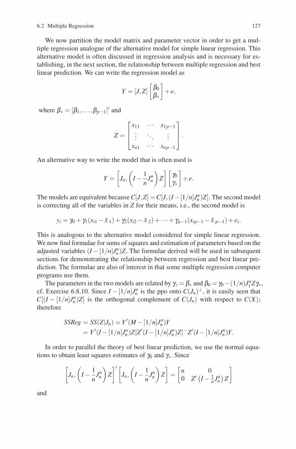
6.2 Multiple Regression 127
We now partition the model matrix and parameter vector in order to get a mul-tiple regression analogue of the alternative model for simple linear regression. Thisalternative model is often discussed in regression analysis and is necessary for es-tablishing, in the next section, the relationship between multiple regression and bestlinear prediction. We can write the regression model as
Y = [J,Z][
β0β∗
]+ e,
where β∗ = [β1, . . . ,βp−1]′ and
Z =
⎡⎢⎣x11 · · · x1p−1...
. . ....
xn1 · · · xnp−1
⎤⎥⎦ .
An alternative way to write the model that is often used is
Y =[
Jn,
(I − 1
nJn
n
)Z][
γ0γ∗
]+ e.
The models are equivalent because C[J,Z] =C[J,(I− [1/n]Jnn )Z]. The second model
is correcting all of the variables in Z for their means, i.e., the second model is
yi = γ0 + γ1(xi1 − x·1)+ γ2(xi2 − x·2)+ · · ·+ γp−1(xip−1 − x·p−1)+ ei.
This is analogous to the alternative model considered for simple linear regression.We now find formulae for sums of squares and estimation of parameters based on theadjusted variables (I − [1/n]Jn
n )Z. The formulae derived will be used in subsequentsections for demonstrating the relationship between regression and best linear pre-diction. The formulae are also of interest in that some multiple regression computerprograms use them.
The parameters in the two models are related by γ∗ = β∗ and β0 = γ0−(1/n)Jn1 Zγ∗,
cf. Exercise 6.8.10. Since I − [1/n]Jnn is the ppo onto C(Jn)⊥, it is easily seen that
C[(I − [1/n]Jnn )Z] is the orthogonal complement of C(Jn) with respect to C(X);
therefore
SSReg = SS(Z|Jn) = Y ′(M− [1/n]Jnn )Y
= Y ′(I − [1/n]Jnn )Z[Z′(I − [1/n]Jn
n )Z]−Z′(I − [1/n]Jnn )Y.
In order to parallel the theory of best linear prediction, we use the normal equa-tions to obtain least squares estimates of γ0 and γ∗. Since[
Jn,
(I − 1
nJn
n
)Z]′[
Jn,
(I − 1
nJn
n
)Z]
=[
n 00 Z′ (I − 1
n Jnn)
Z
]and

128 6 Regression Analysis[Jn,
(I − 1
nJn
n
)Z]′
Y =[
∑ni=1 yi
Z′ (I − 1n Jn
n)
Y
],
the least squares estimates of γ0 and γ∗ are solutions to[n 00 Z′ (I − 1
n Jnn)
Z
][γ0γ∗
]=[
∑ni=1 yi
Z′ (I − 1n Jn
n)
Y
].
Equivalently γ0 = y· and γ∗ is a solution to
Z′(
I − 1n
Jnn
)Zγ∗ = Z′
(I − 1
nJn
n
)Y.
Since γ∗ = β∗, we have that γ∗ = β∗. Since β0 = γ0 − (1/n)Jn1 Zγ∗ = γ0 − β1x·1 −
·· ·−βp−1x·p−1, we have β0 = γ0 − β1x·1 −·· ·− βp−1x·p−1.Finally, from the formula for SSReg developed earlier, the normal equations, and
the fact that γ∗ = β∗, we get
SSReg = Y ′(
I − 1n
Jnn
)Z[
Z′(
I − 1n
Jnn
)Z]−
Z′(
I − 1n
Jnn
)Y
= β ′∗Z′(
I − 1n
Jnn
)Z[
Z′(
I − 1n
Jnn
)Z]−
Z′(
I − 1n
Jnn
)Zβ∗
= β ′∗Z′(
I − 1n
Jnn
)Zβ∗,
where the last equality follows from the definition of a generalized inverse.
6.2.1 Nonparametric Regression and Generalized Additive Models
In general, regression models assume yi = m(xi) + ei, E(ei) = 0, where xi is a pvector of known predictor variables and m(·) is some function. If m(xi) = x′iβ , themodel is linear. If m(xi) = h(x′iβ ) for a known function h, the model is generalizedlinear as discussed in Section 1.4. If m(xi) = h(xi;β ), for a known h depending onthe predictor variables xi and some parameters β , the model is nonlinear regression,see Christensen (1996a, Chapter 18).
In nonparametric regression, m is not assumed to fall into any such parametricfamily. However, by making weak assumptions about m(x), one can often write itas m(x) = ∑∞
j=1 β jφ j(x) for some class of known functions {φ j}. When x is a scalar,examples of such classes include polynomials, cosines, and wavelets. In practice,one fits a linear model
yi =p
∑j=1
β jφ j(xi)+ ei, (1)

6.2 Multiple Regression 129
where p is large enough to capture the interesting behavior of m(·), see Christensen(2001, Chapter 7). Note that in the linear model, each of the terms φ j(xi) is a pre-dictor variable, i.e., the jth column of the model matrix is [φ j(x1), · · · ,φ j(xn)]′.
This “basis function” approach to nonparametric regression involves fitting onelarge, complicated linear model. Other approaches involve fitting many simple linearmodels. For example, the lowess fit (locally weighted scatterplot smoother) beginsestimation of m(x) by fitting a weighted linear regression to some fraction of thexis that are nearest x with weights proportional to the distance from x. The linearmodel is used only to estimate one point, m(x). One performs a separate fit for alarge number of points xg, and to estimate all of m(x) just connect the dots in thegraph of [xg, m(xg)]. Kernel estimation is similar but the weights are determined bya kernel function and the estimate is just a weighted average, not the result of fittinga weighted line or plane.
Unfortunately, these methods quickly run into a “curse of dimensionality.” Withthe basis function approach and only one predictor variable, it might take, for exam-ple, p = 8 functions to get an adequate approximation to m(·). No problem! With2 predictor variables, we could expect to need approximately p = 82 = 64 predic-tor variables in the linear model. Given a few hundred observations, this is doable.However, with 5 predictor variables, we could expect to need about p = 85 = 32,768functions.
One way to get around this curse of dimensionality is to fit generalized additivemodels. For example, with 3 predictor variables, x = (x1,x2,x3)′, we might expectto need p = 83 = 512 terms to approximate m(·). To simplify the problem, we mightassume that m(·) follows a generalized additive model such as
m(x) = f1(x1)+ f23(x2,x3) (2)
orm(x) = f12(x1,x2)+ f23(x2,x3). (3)
If we need 8 terms to approximate f1(·) and 64 terms to approximate each of thef jk(·, ·)s, the corresponding linear model for (2) involves fitting only 72 predictorvariables, and for model (3) only 128− 8 = 120 rather than 83 = 512. Fitting f12and f23 typically duplicates fitting of an f2 term. With the same 8 term approxima-tions and 5 predictor variables, a generalized additive model that includes all of thepossible f jk(·, ·)s involves only 526 terms, rather than the 32,768 required by a fullimplementation of a nonparametric regression.
I should repeat that my use of 8 terms per dimension is merely an illustration.One might need 5 terms, or 10 terms, or 15 terms. And in two dimensions, one mightneed more or less than 82 terms. But these computations illustrate the magnitude ofthe problem. It should also be noted that with alternative (nonlinear) methods offitting generalized additive models it may be necessary to fit lower order terms, i.e.,instead of model (3), fit
m(x) = f1(x1)+ f2(x2)+ f3(x3)+ f12(x1,x2)+ f23(x2,x3).

130 6 Regression Analysis
Another problem with the basis function approach is that it can lead to verystrange results if the number of functions p being fitted is too large. It is well known,see for example Christensen (1996a, Section 7.11), that fitting high order polyno-mials can be a bad thing to do. For x a scalar predictor, by a high order polynomialwe mean a polynomial in which the number of polynomial terms p is close to thenumber of distinct xi values in the data. If the xi values are all distinct, a high or-der polynomial will fit every observed data point almost perfectly. The price of thisalmost perfect fit to the data is that between the xi values the polynomial can dovery weird and inappropriate things. Thus, we have a model that will work poorlyfor future predictions. This behavior is not unique to polynomials. It occurs with allthe standard classes of functions (with the possible exception of wavelets). Similarproblems occur when the xi values are not all distinct.
6.3 General Prediction Theory
General prediction theory provides another approach to regression analysis. It ties inclosely with linear model theory but also with generalized linear models, nonlinearregression, and nonparametric regression.
One of the great things about writing a technical book is that if you do enoughgood mathematics, people will put up with you spouting off once in a while. Inthis section, we take up the subject of prediction and its application to linear modeltheory. To me, prediction is what science is all about, and I cannot resist the urgeto spout off. If you just want to get to work, skip down to the subsection headed“General Prediction.”
6.3.1 Discussion
There is a fundamental philosophical conflict in statistics between Bayesians (whoincorporate subjective beliefs into their analyses) and non-Bayesians. On the philo-sophical issues, the Bayesians seem to me to have much the better of the argument.(Yes, hard as it may be to believe, the author of this book is a Bayesian.) However, inthe practice of statistics, the non-Bayesians have carried the day. (Although I believethat the trend is shifting.) Perhaps the most difficult aspect of Bayesian statistics fornon-Bayesians to accept is the incorporation of subjective beliefs. Many scientistsbelieve that objectivity is of paramount importance, and classical statistics main-tains the semblance of objectivity. (In fact, classical statistics is rife with subjectiveinputs. Choosing an experimental design, choosing independent variables to con-sider in regression, and any form of data snooping such as choosing contrasts afterlooking at the data are examples.)
As Smith (1986) has pointed out, this concept of objectivity is very elusive. Ob-jectivity is almost indistinguishable from the idea of consensus. If all the “clear

6.3 General Prediction Theory 131
thinking” people agree on something, then the consensus is (for the time being)“objective” reality.
Fortunately, the essence of science is not objectivity; it is repeatability. The objectof scientific statistical inference is not the examination of parameters (too often cre-ated by and for statisticians so that they have something to draw inferences about).The object of scientific statistical inference is the (correct) prediction of future ob-servable events. (I bet you were wondering what all this had to do with prediction.)Parameters are at best a convenience, and parameters are at their best when they areclosely related to prediction (e.g., probabilities of survival). Geisser (1971, 1993)gives excellent discussions of the predictive approach.
In this book the emphasis has been placed on models rather than on parameters.Now you know why. Models can be used for prediction. They are an endproduct.Parameters are an integral part of most models, but they are a tool and not an end inthemselves. Christensen (1995) gives a short discussion on the relation among mod-els, prediction, and testing. Having now convinced a large portion of the statisticalcommunity of the unreliability of my ideas, I shall return to the issue at hand.
6.3.2 General Prediction
Suppose we have random variables y,x1,x2, . . . ,xp−1. Regression can be viewed asthe problem of predicting y from the values of x1, . . . ,xp−1. We will examine thisproblem and consider its relationship to the linear model theory approach to regres-sion. Let x be the vector x = (x1, . . . ,xp−1)′. A reasonable criterion for choosing apredictor of y is to pick a predictor f (x) that minimizes the mean squared error,E[y− f (x)]2. (The MSE defined in linear model theory is a function of the obser-vations that estimates the theoretical mean squared error defined here.) Note that,unlike standard linear model theory, the expected value is taken over the joint dis-tribution of y and x.
The use of an expected squared error criterion presupposes the existence of firstand second moments for y and f (x). Let E(y) = μy, Var(y) = σ 2
y ≡ σyy and letE[ f (x)] = μ f , Var[ f (x)] = σ f f , and Cov[y, f (x)] = σy f , with similar notations forother functions of x, e.g., m(x) has σym = Cov[y,m(x)].
The remainder of this section consists of three subsections. The next examinesbest predictors, i.e., those functions f (x) that do the best job of predicting y. Withoutknowing (or being able to estimate) the joint distribution of x and y, we cannot findthe best predictor, so in Subsection 4 we examine the best predictors among func-tions f (x) that are restricted to be linear functions of x. These best linear predictorsdepend only on the means and covariances of the random variables and are thus rel-atively easy to estimate. Subsection 4 also examines the relationship between bestlinear predictors and least squares estimation. Both the best predictor and the bestlinear predictor can be viewed as orthogonal projections in an appropriate vectorspace, a subject that is commented on earlier but is amplified in Subsection 5.

132 6 Regression Analysis
6.3.3 Best Prediction
We now establish that the best predictor is the conditional expectation of y given x.See Appendix D for definitions and results about conditional expectations.
Theorem 6.3.1. Let m(x) ≡ E(y|x). Then for any other predictor f (x), E[y−m(x)]2 ≤ E[y− f (x)]2; thus m(x) is the best predictor of y.
PROOF.
E[y− f (x)]2 = E[y−m(x)+m(x)− f (x)]2
= E[y−m(x)]2 +E[m(x)− f (x)]2 +2E{[y−m(x)][m(x)− f (x)]}.
Since both E[y−m(x)]2 and E[m(x)− f (x)]2 are nonnegative, it is enough to showthat E{[y−m(x)][m(x)− f (x)]} = 0. Consider this expectation conditional on x.
E{[y−m(x)][m(x)− f (x)]} = E(E{[y−m(x)][m(x)− f (x)]|x})= E([m(x)− f (x)]E{[y−m(x)]|x})= E([m(x)− f (x)]0) = 0
where E{[y−m(x)]|x} = 0 because E(y|x) = m(x). �
The goal of most predictive procedures is to find, or rather estimate, the func-tion E(y|x) = m(x). Suppose we have a random sample (x′i,yi), i = 1, . . . ,n. In linearregression, m(xi) = α + x′iβ with α and β unknown. A generalized linear modelassumes a distribution for y given x and that E(yi|xi) = m(xi) = h(α + x′iβ ) forknown h and unknown α and β . Here h is just the inverse of the link function.The standard nonlinear regression model is a more general version of these. It usesm(xi) = h(xi;α,β ), where h is some known function but α and β are unknown.The conditional mean structure of all three parametric models is that of the non-linear regression model: m(x) = h(x;α,β ), h known. We then become interested inestimating α and β . Evaluating whether we have the correct “known” form for his a question of whether lack of fit exists, see Section 6. Nonparametric regressionis unwilling to assume a functional form h(x;α,β ). The standard nonparametricregression model is yi = m(xi)+ ei where, conditional on the xis, the eis are inde-pendent with mean 0 and variance σ 2. In nonparametric regression, m is completelyunknown.
All of these versions of regression involve estimating whatever parts of m(x) arenot assumed to be known. On the other hand, best prediction theory treats m(x) as aknown function, so for models involving α and β it treats them as known.
In Theorem 6.3.3, we present a result that does two things. First, it provides a jus-tification for the residual plots used in Chapter 13 to identify lack of fit. Second, asdiscussed in Subsection 5, it establishes that E(y|x) can be viewed as the perpendic-ular projection of y into the space of random variables, say f (x), that are functions

6.3 General Prediction Theory 133
of x alone, have mean E[ f (x)] = E[y], and a finite variance, see also deLaubenfels(2006). Before doing this, we need to establish some covariance and correlationproperties.
Proposition 6.3.2. Cov[y, f (x)] = Cov[m(x), f (x)]. In particular, Cov[y,m(x)] =Var[m(x)] = σmm and Corr2[y,m(x)] = σmm/σyy.
PROOF. Recall that, from the definition of conditional expectation, E[m(x)] = μy.
Cov[y, f (x)] = Eyx[(y−μy) f (x)]= ExEy|x[(y−m(x)+m(x)−μy) f (x)]= Ex[(m(x)−μy) f (x)]= Cov[m(x), f (x)].
�
Now consider an arbitrary predictor y(x).
Theorem 6.3.3. Let y(x) be any predictor with E[y(x)] = μy, then Cov[ f (x),y−y(x)] = 0 for any function f if and only if E(y|x) = y(x) almost surely.
PROOF. ⇐ If E(y|x) ≡ m(x) = y(x), the fact that Cov[ f (x),y−m(x)] = 0 for anyfunction f is an immediate consequence of Proposition 2.
⇒ Now suppose that E[y(x)] = μy and Cov[ f (x),y− y(x)] = 0 for any function f .To show that y(x) = m(x) a.s., it is enough to note that E[y(x)−m(x)] = μy −μy =0 and to show that Var[y(x)−m(x)] = 0. Thinking of f (x) = y(x)−m(x) in thecovariance conditions, observe that
Var[y(x)−m(x)] = Cov[y(x)−m(x), y(x)−m(x)]= Cov{[y−m(x)]− [y− y(x)], [y(x)−m(x)]}= Cov{[y−m(x)], [y(x)−m(x)]}−Cov{[y− y(x)], [y(x)−m(x)]}= 0−0.
�
In fitting linear models, or any other regression procedure, we typically obtainfitted values yi corresponding to the observed data yi, from which we can obtainresiduals yi− yi. According to Theorem 6.3.3, if the fitted values are coming from thebest predictor, plotting the residuals against any function of the predictor vector xishould display zero correlation. Thus, if we plot the residuals against some functionf (xi) of the predictors and observe a correlation, we obviously do not have thebest predictor, so we should try fitting some other model. In particular, regardlessof how nonlinear the original regression model might have been, adding a linearterm to the model using f (xi) as the predictor should improve the fit of the model.Unfortunately, there is no reason to think that adding such a linear term will getyou to the best predictor. Finally, it should be noted that a common form of lack

134 6 Regression Analysis
of fit detected in residual plots is a parabolic shape, which does not necessarilysuggest a nonzero correlation with the predictor used in the plot. However, whenthe residual plot is a parabola, a plot of the residuals versus the (suitably centered)squared predictor will display a nonzero correlation.
Finally, if we plot the residuals against some predictor variable z that is not partof x, the fact that we would make such a plot suggests that we really want the bestpredictor m(x,z) rather than m(x), although if we originally left z out, we probablysuspect that m(x) = m(x,z). A linear relationship between the residuals and z indi-cates that the estimated regression function m(x) is not an adequate estimate of thebest predictor m(x,z).
6.3.4 Best Linear Prediction
The ideas of best linear prediction and best linear unbiased prediction (see Sec-tion 12.2) are very important. As will be seen here and in Chapter 12, best linearprediction theory has important applications in standard linear models, mixed mod-els, and the analysis of spatial data. The theory has traditionally been taught as partof multivariate analysis (cf. Anderson, 1984). It is important for general stochasticprocesses (cf. Doob, 1953), time series (cf. Shumway and Stoffer, 2000; Brock-well and Davis, 1991; or Christensen, 2001, Chapters 4 and 5), principal componentanalysis (cf. Christensen, 2001, Chapter 3), and it is the basis for linear Bayesianmethods (cf. Hartigan, 1969). For applications to spatial data, see also Christensen(2001, Chapter 6), Cressie (1993), and Ripley (1981).
In order to use the results on best prediction, one needs to know E(y|x), whichgenerally requires knowledge of the joint distribution of (y,x1,x2, . . . ,xp−1)′. If thejoint distribution is not available but the means, variances, and covariances areknown, we can find the best linear predictor of y. We seek a linear predictor α +x′βthat minimizes E[y−α − x′β ]2 for all scalars α and (p−1)×1 vectors β .
In addition to our earlier assumptions that first and second moments for y exist,we now also assume the existence of E(x) = μx, Cov(x) = Vxx, and Cov(x,y) =Vxy = V ′
yx = Cov(y,x)′.Let β∗ be a solution to Vxxβ = Vxy, then we will show that the function
E(y|x) ≡ μy +(x−μx)′β∗
is a best linear predictor of y based on x. E(y|x) is also called the linear expectationof y given x. (Actually, it is the linear expectation of y given x and a random variablethat is constant with probability 1.) Note that when Vxx is singular, there are aninfinite number of vectors β∗ that solve to Vxxβ = Vxy, but by using Lemma 1.3.5 wecan show that all such solutions give the same best linear predictor with probability1. The idea is that since (x− μx) ∈ C(Vxx) with probability 1, for some random b,(x−μx) = Vxxb with probability 1, so
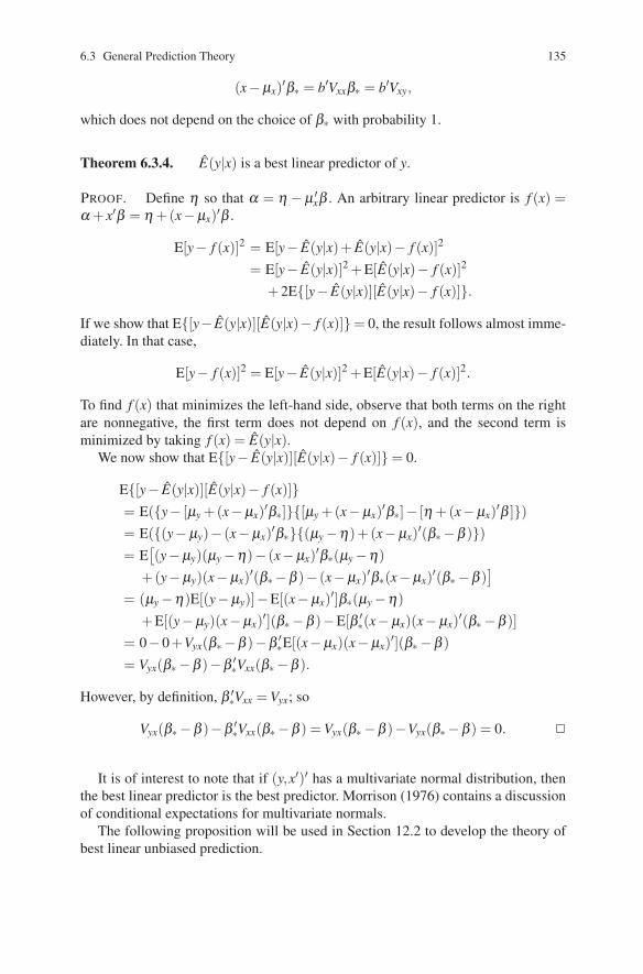
6.3 General Prediction Theory 135
(x−μx)′β∗ = b′Vxxβ∗ = b′Vxy,
which does not depend on the choice of β∗ with probability 1.
Theorem 6.3.4. E(y|x) is a best linear predictor of y.
PROOF. Define η so that α = η − μ ′xβ . An arbitrary linear predictor is f (x) =
α + x′β = η +(x−μx)′β .
E[y− f (x)]2 = E[y− E(y|x)+ E(y|x)− f (x)]2
= E[y− E(y|x)]2 +E[E(y|x)− f (x)]2
+2E{[y− E(y|x)][E(y|x)− f (x)]}.
If we show that E{[y− E(y|x)][E(y|x)− f (x)]}= 0, the result follows almost imme-diately. In that case,
E[y− f (x)]2 = E[y− E(y|x)]2 +E[E(y|x)− f (x)]2.
To find f (x) that minimizes the left-hand side, observe that both terms on the rightare nonnegative, the first term does not depend on f (x), and the second term isminimized by taking f (x) = E(y|x).
We now show that E{[y− E(y|x)][E(y|x)− f (x)]} = 0.
E{[y− E(y|x)][E(y|x)− f (x)]}= E({y− [μy +(x−μx)′β∗]}{[μy +(x−μx)′β∗]− [η +(x−μx)′β ]})= E({(y−μy)− (x−μx)′β∗}{(μy −η)+(x−μx)′(β∗ −β )})= E[(y−μy)(μy −η)− (x−μx)′β∗(μy −η)
+(y−μy)(x−μx)′(β∗ −β )− (x−μx)′β∗(x−μx)′(β∗ −β )]
= (μy −η)E[(y−μy)]−E[(x−μx)′]β∗(μy −η)+E[(y−μy)(x−μx)′](β∗ −β)−E[β ′
∗(x−μx)(x−μx)′(β∗ −β )]= 0−0+Vyx(β∗ −β )−β ′
∗E[(x−μx)(x−μx)′](β∗ −β )= Vyx(β∗ −β )−β ′
∗Vxx(β∗ −β ).
However, by definition, β ′∗Vxx = Vyx; so
Vyx(β∗ −β )−β ′∗Vxx(β∗ −β ) = Vyx(β∗ −β )−Vyx(β∗ −β) = 0. �
It is of interest to note that if (y,x′)′ has a multivariate normal distribution, thenthe best linear predictor is the best predictor. Morrison (1976) contains a discussionof conditional expectations for multivariate normals.
The following proposition will be used in Section 12.2 to develop the theory ofbest linear unbiased prediction.

136 6 Regression Analysis
Proposition 6.3.5. E[y−α − x′β ]2 = E[y− E(y|x)]2 +E[E(y|x)−α − x′β ]2.
PROOF. The result is part of the proof of Theorem 6.3.4. �
We show that best linear predictors are essentially unique. In other words, weshow that to minimize E[E(y|x)−η −(x−μx)′β ]2, you need μy = η and β must bea solution to Vxxβ = Vxy. It is not difficult to show that
E[E(y|x)−η − (x−μx)′β ]2 = (μy −η)2 +E[(x−μx)′β∗ − (x−μx)′β ]2.
Clearly, minimization requires μy = η and E[(x− μx)′β∗ − (x− μx)′β ]2 = 0. Thebest linear predictors will be essentially unique if we can show that E[(x−μx)′β∗ −(x−μx)′β ]2 = 0 implies that β must be a solution to Vxxβ = Vxy. Observe that
E[(x−μx)′β∗ − (x−μx)′β ]2 = E[(x−μx)′(β∗ −β )]2
= Cov[(x−μx)′(β∗ −β )]= (β∗ −β )′Vxx(β∗ −β ).
Write Vxx = QQ′ with C(Vxx) = C(Q). Then (β∗ −β )′Vxx(β∗ −β ) = 0 if and only if(β∗ −β )′QQ′(β∗ −β ) = 0 if and only if Q′(β∗ −β ) = 0 if and only if (β∗ −β ) ⊥C(Q) = C(Vxx) if and only if Vxx(β∗ −β ) = 0 if and only if Vxxβ = Vxxβ∗ = Vxy. Soβ must be a solution.
The variance of the prediction error y− E(y|x) is given in Section 5. (Actually,the covariance matrix for a bivariate prediction is given.)
Next, we examine the correspondence between this theory and linear modelregression theory. Suppose we have n observations on the vector (y,x′)′ =(y,x1,x2, . . . ,xp−1)′. We can write these as (yi,x′i)
′ = (yi,xi1,xi2, . . . ,xi,p−1)′, i =1, . . . ,n. In matrix notation write Y = (y1,y2, . . . ,yn)′ and Z = [xi j], i = 1, . . . ,n,j = 1, . . . , p− 1. (Z plays the same role as Z did in Section 2 on multiple regres-sion.) The usual estimates for Vxx and Vxy can be written as
Sxx =1
n−1Z′(
I − 1n
Jnn
)Z =
1n−1
n
∑i=1
(xi − x·)(xi − x·)′
Sxy =1
n−1Z′(
I − 1n
Jnn
)Y =
1n−1
n
∑i=1
(xi − x·)(yi − y·).
The usual estimates of μy and μx are
y· =1n
Jn1Y =
1n
n
∑i=1
yi

6.3 General Prediction Theory 137
x′· =1n
Jn1 Z =
(1n
n
∑i=1
xi1, . . . ,1n
n
∑i=1
xip−1
)′.
The natural predictor of y is
y = y+(x− x)′β∗,
where β∗ is a solution to Sxxβ∗ = Sxy, i.e., it solves Z′ (I − 1n Jn
n)
Zβ∗ = Z′ (I − 1n Jn
n)
Y .From the results of Section 2, y = γ0 and any solution of Z′ (I − 1
n Jnn)
Zβ∗ =Z′ (I − 1
n Jnn)
Y is a least squares estimate of β∗ = γ∗. Thus, the natural estimatesof the parameters in the best linear predictor are the least squares estimates from themean corrected regression model considered in the previous section.
Finally, we include a result for best linear predictors that is analogous to Theo-rem 6.3.3 for best predictors. First, if we have residuals from the best linear predic-tor, they will be uncorrelated with any linear combination of the predictor variables.Second, E(y|x) can be viewed as the perpendicular projection of y into the spaceof random variables f (x) that are linear functions of x and have E[ f (x)] = E[y], cf.Subsection 5.
Theorem 6.3.6. Suppose y(x) is any linear predictor with E[y(x)] = μy, thenCov[ f (x),y− y(x)] = 0 for any linear function f if and only if E(y|x) = y(x) almostsurely.
PROOF. Let f (x) = η +(x−μx)′β and let y = μy +(x−μx)′δ .⇐ For E(y|x) = y(x),
Cov[η +(x−μx)′β ,(y−μy)− (x−μx)′β∗] = β ′Vxy −β ′Vxxβ∗= β ′Vxy −β ′Vxy = 0.
⇒ If
0 = Cov[η +(x−μx)′β ,(y−μy)− (x−μx)′δ ]= β ′Vxy −β ′Vxxδ
for any β , then Vxy = Vxxδ , so y(x) = E(y|x) with probability 1. �
As mentioned earlier, the theory of best linear predictors also comes up in devel-oping the theory of best linear unbiased predictors (BLUPs), which is an importantsubject in models that have random effects. In random effects models, part of the βvector in Y = Xβ + e is assumed to be random and unobservable. Random effectsmodels and BLUPs are discussed in Chapter 12.
The result of the next exercise will be used in Section 5 on partial correlations.
Exercise 6.3 For predicting y = (y1, . . . ,yq)′ from x = (x1, . . . ,xp−1)′ we say that

138 6 Regression Analysis
a predictor f (x) is best if the scalar E{[y− f (x)]′[y− f (x)]} is minimized. Show thatwith simple modifications, Theorems 6.3.1 and 6.3.4 hold for the extended problem,as does Proposition 6.3.5.
6.3.5 Inner Products and Orthogonal Projections in GeneralSpaces
In most of this book, we define orthogonality and length using the Euclidean innerproduct in Rn. For two vectors x and y, the Euclidean inner product is x′y, so x ⊥ y ifx′y = 0 and the length of x is ‖x‖=
√x′x. In Section B.3 we discussed, in detail, per-
pendicular projection operators relative to this inner product. We established that theprojection of a vector Y into C(X) is Y ≡ MY . It also follows from Theorems 2.2.1and 2.8.1 that Y is the unique vector in C(X) that satisfies (Y − Y ) ⊥ C(X). Thislast property is sometimes used to define what it means for Y to be the perpendic-ular projection of Y into C(X). We use this concept to extend the application ofperpendicular projections to more general vector spaces
More generally in Rn, we can use any positive definite matrix B to define an in-ner product between x and y as x′By. As before, x and y are orthogonal if their innerproduct x′By is zero and the length of x is the square root of its inner product with it-self, now ‖x‖B ≡√
x′Bx. As argued in Section B.3, any idempotent matrix is alwaysa projection operator, but which one is the perpendicular projection operator de-pends on the inner product. As can be seen from Proposition 2.7.2 and Exercise 2.5,the matrix A ≡ X(X ′BX)−X ′B is an oblique projection operator onto C(X) for theEuclidean inner product, but it is the perpendicular projection operator onto C(X)with the inner product defined using the matrix B. It is not too difficult to see that AYis the unique vector in C(X) that satisfies (Y −AY ) ⊥B C(X), i.e., (Y −AY )′BX = 0.
These ideas can be applied in very general spaces. In particular, they can beapplied to the concepts of prediction introduced in this section. For example, wecan define the inner product between two random variables y and x with mean 0and finite variance as the Cov(x,y). In this case, Var(x) plays the role of the squaredlength of the random variable and the standard deviation is the length. Two randomvariables are orthogonal if they are uncorrelated.
Now consider a vector of random variables x = (x1, . . . ,xp−1)′ and the space of allfunctions f (x) into R1 that have mean 0 and variances. We showed in Theorem 6.3.3that m(x) ≡ E(y|x) is the unique function of x having mean μy for which Cov[y−m(x), f (x)] = 0 for any f (x). Thus, as alluded to above, m(x)−μy satisfies a propertyoften used to define the perpendicular projection of y−μy into the space of functionsof x that have mean 0 and variances. Alternatively, we can think of m(x) as theperpendicular projection of y into the space of functions of x that have mean μy andvariances.
We can also consider a reduced space of random variables, the linear functions ofx, i.e., f (x) = α +x′β . In Theorem 6.3.6 we show that Cov[y− E(y|x),α +x′β ] = 0

6.4 Multiple Correlation 139
for any linear function of x, so once again, the best linear predictor is the perpendic-ular projection of y into the linear functions of x with mean μy.
We now generalize the definitions of an inner product space, orthogonality, andorthogonal projection.
Definition A.11 (Alternate). A vector space X is an inner product space if forany x,y ∈ X , there exists a symmetric bilinear function [x,y] into R with [x,x] >0 for any x �= 0. A bilinear function has the properties that for any scalars a1,a2and any vectors x1,x2,y, [a1x1 +a2x2,y] = a1[x1,y]+a2[x2,y] and [y,a1x1 +a2x2] =a1[y,x1]+a2[y,x2]. A symmetric function has [x1,x2] = [x2,x1]. The vectors x and yare orthogonal if [x,y] = 0 and the squared length of x is [x,x]. The perpendicularprojection of y into a subspace X0 of X is defined as the unique vector y0 ∈ X0with the property that [y− y0,x] = 0 for any x ∈ X0.
Note that the set of mean zero, finite variance, real-valued functions of x andy form a vector space under Definition A.1 and an inner product space using thecovariance of any two such functions as the inner product. Both the set of mean0, finite variance functions of x and the set of mean 0 linear functions of x aresubspaces, so y can be projected into either subspace.
We now relate Definition A.11 (Alternate) to the concept of a perpendicular pro-jection operator.
Exercise 6.4 Consider an inner product space X and a subspace X0. Supposethat any vector y ∈X can be written uniquely as y = y0 +y1 with y0 ∈X0 and y1 ⊥X0. Let M(x) be a linear operator on X in the sense that for any x ∈ X , M(x) ∈X and for any scalars a1,a2 and any vectors x1,x2, M(a1x1 + a2x2) = a1M(x1)+a2M(x2). M(x) is defined to be a perpendicular projection operator onto X0 if forany x0 ∈ X0, M(x0) = x0, and for any x1 ⊥ X0, M(x1) = 0. Using Definition A.11(Alternate), show that for any vector y, M(y) is the perpendicular projection of yinto X0.
6.4 Multiple Correlation
The coefficient of determination, denoted R2, is a commonly used measure of thepredictive ability of a model. Computationally, it is most often defined as
R2 =SSReg
SSTot −C,
so it is the proportion of the total variability explained by the independent variables.The greater the proportion of the total variability in the data that is explained bythe model, the better the ability to predict with that model. The use and possibleabuse of R2 as a tool for comparing models is discussed in Chapter 14, however it

140 6 Regression Analysis
should be noted here that since R2 is a measure of the predictive ability of a model,R2 does not give direct information about whether a model fits the data properly.Demonstrably bad models can have very high R2s and perfect models can have lowR2s.
We now define the multiple correlation, characterize it in terms of the best linearpredictor, and show that R2 is the natural estimate of it. Subsection 6.4.1 generalizesthe idea of R2 from best linear prediction to best prediction.
Recall that the correlation between two random variables, say x1 and x2, is
Corr(x1,x2) = Cov(x1,x2)/√
Var(x1)Var(x2).
1 2 p−1′
x′β ) over all α and β . Note that
Cov(y,α + x′β ) = Vyxβ = β ′∗Vxxβ ,
where β∗ is defined as in Subsection 6.3.4 and
Var(α + x′β ) = β ′Vxxβ .
In particular, Cov(y,α + x′β∗) = β ′∗Vxxβ∗ = Var(α + x′β∗). The Cauchy–Schwarzinequality says that (
t
∑i=1
risi
)2
≤t
∑i=1
r2i
t
∑i=1
s2i .
Since Vxx = RR′ for some matrix R, the Cauchy–Schwarz inequality gives(β ′∗Vxxβ
)2 ≤ (β ′Vxxβ)(
β ′∗Vxxβ∗
).
Considering the squared correlation gives
Corr2(y,α + x′β) =(β ′∗Vxxβ
)2/(β ′Vxxβ)
σ2y
≤ β ′∗Vxxβ∗
/σ 2
y
=(β ′∗Vxxβ∗
)2/(β ′∗Vxxβ∗
)σ 2
y
= Corr2(y,α + x′β∗)
and the squared multiple correlation between y and x equals
Corr2(y,α + x′β∗) = β ′∗Vxxβ∗
/σ 2
y .
If we have observations (yi,xi1,xi2, . . . ,xi,p−1)′, i = 1, . . . ,n, the usual estimate ofσ 2
y can be written as
s2y =
1n−1
Y ′(
I − 1n
Jnn
)Y =
1n−1
n
∑i=1
(yi − y)2.
The multiple correlation of y and (x ,x ,..., x ) = x is the maximum of Corr(y,α +

6.4 Multiple Correlation 141
Using equivalences derived earlier, the natural estimate of the squared multiple cor-relation coefficient between y and x is
β ′∗Sxxβ∗s2
y=
β ′∗Z′ (I − 1n Jn
n)
Zβ∗Y ′ (I − 1
n Jnn)
Y=
SSRegSSTot −C
.
It is worth noticing that SSTot −C = SSReg+SSE and that
SSReg/
SSE = SSReg/[(SSE +SSReg)−SSReg]
= SSReg/[SSTot −C−SSReg]
=SSReg
[SSTot −C][1−R2]
= R2/[1−R2].
For normally distributed data, the α level F test for H0 : β1 = β2 = · · · = βp−1 = 0is to reject H0 if
n− pp−1
R2
1−R2 > F(1−α, p−1,n− p).
EXAMPLE 6.4.1. From the information given in Example 6.2.1, the coefficientof determination can be found. From the ANOVA table in Example 6.2.1, we get
SSReg = 1259.32
SSTot −C = SSTotal −SS(β0) = 16576.60−15270.78 = 1305.82
andR2 = 1259.32/1305.82 = 0.964.
This is a very high value for R2 and indicates that the model has very substantialpredictive ability. However, before you conclude that the model actually fits thedata well, see Example 6.6.3.
Exercise 6.5 Show that for a linear model with an intercept, R2 is simply thesquare of the correlation between the data yi and the predicted values yi.
This discussion has focused on R2, which estimates the squared multiple corre-lation coefficient, a measure of the predictive ability of the best linear predictor. Wenow consider an analogous measure for the best predictor.

142 6 Regression Analysis
6.4.1 Squared Predictive Correlation
As in Subsection 6.3.2, consider an arbitrary predictor y(x). This is a function of xalone and not a function of y.
The squared predictive correlation of y(x) is Corr2[y, y(x)]. The highest squaredpredictive correlation is obtained by using the best predictor. Note that in the spe-cial case where the best predictor m(x) is also the best linear predictor, the highestsquared predictive correlation equals the squared multiple correlation coefficient.
Theorem 6.4.1. Corr2[y, y(x)] ≤ Corr2[y,m(x)].
PROOF. By Cauchy-Schwarz, (σmy)2 ≤ σmmσyy, so (σmy)2/σyy ≤ σmm. UsingProposition 6.3.2,
Corr2[y, y(x)] =(σyy)2
σyyσyy=
(σmy)2
σyyσyy≤ σmm
σyy= Corr2[y,m(x)].
The result follows from the last part of Proposition 6.3.2. �
Theorem 6.4.1 is also established in Rao (1973, Section 4g.1). From Theo-rem 6.4.1, the best regression function m(x) has the highest squared predictive cor-relation. When we have perfect prediction, the highest squared predictive correlationis 1. In other words, if the conditional variance of y given x is 0, then y = m(x) a.s.,and the highest squared predictive correlation is the correlation of m(x) with itself,which is 1. On the other hand, if there is no regression relationship, i.e., if m(x) = μya.s., then σmm = 0, and the highest squared predictive correlation is 0.
We would now like to show that as the squared predictive correlation increases,we get increasingly better prediction. First we need to deal with the fact that highsquared predictive correlations can be achieved by bad predictors. Just because y(x)is highly correlated with y does not mean that y(x) is actually close to y. Recall thaty(x) is simply a random variable that is being used to predict y. As such, y(x) is alinear predictor of y, that is, y(x) = 0 + 1y(x). We can apply Theorem 6.3.4 to thisrandom variable to obtain a linear predictor that is at least as good as y(x), namely
y(x) = μy +σyy
σyy[y(x)−μy].
We refer to such predictors as linearized predictors. Note that E[y(x)] ≡ μy = μy,
σyy ≡ Var[y(x)] =(
σyy
σyy
)2
σyy =(σyy)2
σyy,
and
σyy ≡ Cov[y, y(x)] =σyy
σyyσyy =
(σyy)2
σyy.

6.5 Partial Correlation Coefficients 143
In particular, σyy = σyy, so the squared predictive correlation of y(x) is
Corr2[y, y(x)] =σyy
σyy.
In addition, the direct measure of the goodness of prediction for y(x) is
E[y− y(x)]2 = σyy −2σyy +σyy = σyy −σyy.
This leads directly to the next result.
Theorem 6.4.2. For two linearized predictors y1(x) and y2(x), the squared pre-dictive correlation of y2(x) is higher if and only if y2(x) is a better predictor.
PROOF. σy1 y1/σyy < σy2 y2/σyy if and only if σy1 y1 < σy2 y2 if and only if σyy −σy2 y2 < σyy −σy1 y1 . �
It should be noted that linearizing m(x) simply returns m(x).For any predictor y(x), no matter how one arrives at it, to estimate the squared
predictive correlation from data yi, simply compute the squared sample correlationbetween yi and its predictor of y(xi).
6.5 Partial Correlation Coefficients
Many regression programs have options available to the user that depend on thevalues of the sample partial correlation coefficients. The partial correlation is definedin terms of two random variables of interest, say y1 and y2, and several auxiliaryvariables, say x1, . . . ,xp−1. The partial correlation coefficient of y1 and y2 givenx1, . . . ,xp−1, written ρy·x, is a measure of the linear relationship between y1 and y2after taking the effects of x1, . . . ,xp−1 out of both variables.
Writing y = (y1,y2)′ and x = (x1, . . . ,xp−1)′, Exercise 6.3 indicates that the bestlinear predictor of y given x is
E(y|x) = μy +β ′∗(x−μx),
where β∗ is a solution of Vxxβ∗ = Vxy and Vxy is now a (p−1)×2 matrix. We takethe effects of x out of y by looking at the prediction error
y− E(y|x) = (y−μy)−β ′∗(x−μx),
which is a 2×1 random vector. The partial correlation is simply the correlation be-tween the two components of this vector and is readily obtained from the covariancematrix. We now find the prediction error covariance matrix. Let Cov(y) ≡Vyy.

144 6 Regression Analysis
Cov[(y−μy)−β ′∗(x−μx)] = Cov(y−μy)+β ′
∗Cov(x−μx)β∗−Cov(y−μy,x−μx)β∗−β ′
∗Cov(x−μx,y−μy)= Vyy +β ′
∗Vxxβ∗ −Vyxβ∗ −β ′∗Vxy
= Vyy +β ′∗Vxxβ∗ −β ′
∗Vxxβ∗ −β ′∗Vxxβ∗
= Vyy −β ′∗Vxxβ∗.
Since Vxxβ∗ = Vxy and, for any generalized inverse, VxxV−xxVxx = Vxx,
Cov[(y−μy)−β ′∗(x−μx)] = Vyy −β ′
∗VxxV−xxVxxβ∗
= Vyy −VyxV−xxVxy.
If we have a sample of the ys and xs, say yi1,yi2,xi1,xi2, . . . ,xi,p−1, i = 1, . . . ,n,we can estimate the covariance matrix in the usual way. The relationship with thelinear regression model of Section 2 is as follows: Let
Y =
⎡⎢⎣y11 y12...
...yn1 yn2
⎤⎥⎦= [Y1,Y2]
and
Z =
⎡⎢⎣x11 · · · x1p−1...
. . ....
xn1 · · · xnp−1
⎤⎥⎦ .
The usual estimate of Vyy −VyxV−xxVxy is (n−1)−1 times
Y ′(
I − 1n
Jnn
)Y −Y ′
(I − 1
nJn
n
)Z[
Z′(
I − 1n
Jnn
)Z]−
Z′(
I − 1n
Jnn
)Y.
From Section 2, we know that this is the same as
Y ′(
I − 1n
Jnn
)Y −Y ′
(M− 1
nJn
n
)Y = Y ′ (I −M)Y,
where M is the perpendicular projection operator onto C([J,Z]). Remembering thatY ′(I−M)Y = [(I−M)Y ]′[(I−M)Y ], we can see that the estimate of ρy·x, written ry·xand called the sample partial correlation coefficient, is just the sample correlationcoefficient between the residuals of fitting Y1 = [J,Z]β +e and the residuals of fittingY2 = [J,Z]β + e, i.e.,
ry·x =Y ′
1(I −M)Y2√Y ′
1(I −M)Y1Y ′2(I −M)Y2
.

6.5 Partial Correlation Coefficients 145
The square of the sample partial correlation coefficient, often called the coeffi-cient of partial determination, has a nice relationship to another linear model. Con-sider fitting Y1 = [J,Z,Y2]γ +e. Because C[(I−M)Y2] is the orthogonal complementof C([J,Z]) with respect to C([J,Z,Y2]), the sum of squares for testing whether Y2adds to the model is
SSR(Y2|J,Z) = Y ′1(I −M)Y2[Y ′
2(I −M)Y2]−1Y ′2(I −M)Y1.
Since Y ′2(I −M)Y2 is a scalar, it is easily seen that
r2y·x =
SSR(Y2|J,Z)SSE(J,Z)
,
where SSE(J,Z) = Y ′1(I−M)Y1, the sum of squares for error when fitting the model
Y1 = [J,Z]β + e.Finally, for normally distributed data we can do a t test of the null hypothesis
H0 : ρy·x = 0. If H0 is true, then√n− p−1 ry·x
/√1− r2
y·x ∼ t(n− p−1).
See Exercise 6.6 for a proof of this result.
EXAMPLE 6.5.1. Using the data of Example 6.2.1, the coefficient of partial de-termination (squared sample partial correlation coefficient) between y and x2 givenx1 can be found:
SSR(X2|J,X1) = 6.70,
SSE(J,X1) = SSE(J,X1,X2)+SSR(X2|J,X1) = 46.50+6.70 = 53.20,
r2y·x = 6.70/53.20 = 0.1259.
The absolute value of the t statistic for testing whether ρy2·1 = 0 can also be found.In this application we are correcting Y and X2 for only one variable X1, so p−1 = 1and p = 2. The formula for the absolute t statistic becomes
√25−2−1
√0.1259
/√1−0.1259 = 1.78.
Note that this is precisely the t statistic reported for β2 in Example 6.2.1.
Exercise 6.5 Assume that Vxx is nonsingular. Show that ρy·x = 0 if and only ifthe best linear predictor of y1 based on x and y2 equals the best linear predictor ofy1 based on x alone.
Exercise 6.6 If (yi1,yi2,xi1,xi2, . . . ,xi,p−1)′, i = 1, . . . ,n are independent N(μ ,V ),
find the distribution of√
n− p−1 ry·x/√
1− r2y·x when ρy·x = 0.

146 6 Regression Analysis
Hint: Use the linear model E(Y1|X ,Y2) ∈ C(J,X ,Y2), i.e., Y1 = [J,X ,Y2]γ + e, tofind a distribution conditional on X ,Y2. Note that the distribution does not dependon the values of X and Y2, so it must also be the unconditional distribution. Note alsothat from Exercise 6.5 and the equality between the conditional expectation and thebest linear predictor for multivariate normals that we have ρy·x = 0 if and only if theregression coefficient of Y2 is zero.
Finally, the usual concept of partial correlation, which looks at the correlationbetween the components of y− E(y|x), i.e., the residuals based on best linear predic-tion, can be generalized to a concept based on examining the correlations betweenthe components of y−E(y|x), the residuals from the best predictor.
6.6 Testing Lack of Fit
Suppose we have a linear model Y = Xβ + e and we suspect that the model is aninadequate explanation of the data. The obvious thing to do to correct the problem isto add more variables to the model, i.e, fit a model Y = Zγ +e, where C(X) ⊂C(Z).Two questions present themselves: 1) how does one choose Z, and 2) is there reallya lack of fit? Given a choice for Z, the second of these questions can be addressedby testing Y = Xβ + e against Y = Zγ + e. This is referred to as a test for lack offit. Since Z is chosen so that Y = Zγ + e will actually fit the data (or at least fit thedata better than Y = Xβ + e), the error sum of squares for the model Y = Zγ + e,say SSE(Z), can be called the sum of squares for pure error, SSPE. The differenceSSE(X)− SSE(Z) is used for testing lack of fit, so SSE(X)− SSE(Z) is called thesum of squares for lack of fit, SSLF .
In general, there are few theoretical guidelines for choosing Z. The most com-mon situation is where there are a variety of other variables that are known and it isnecessary to select variables to include in the model. Variable selection techniquesare discussed in Chapter 14. In this section, we discuss the problem of testing lackof fit when there are no other variables available for inclusion in the model. With noother variables available, the model matrix X must be used as the basis for choosingZ. We will present four approaches. The first is the traditional method based on hav-ing a model matrix X in which some of the rows are identical. A second approach isbased on identifying clusters of rows in X that are nearly identical. A third approachexamines different subsets of the data. Finally, we briefly mention a nonparametricregression approach to testing lack of fit.
One final note. This section is in the chapter on regression because testing lackof fit has traditionally been considered as a topic in regression analysis. Nowhere inthis section do we assume that X ′X is nonsingular. The entire discussion holds forgeneral linear models.

6.6 Testing Lack of Fit 147
6.6.1 The Traditional Test
To discuss the traditional approach that originated with Fisher (1922), we requirenotation for identifying which rows of the model matrix are identical. A model withreplications can be written
yi j = x′iβ + ei j,
where β is the vector of parameters, x′i = (xi1, . . . ,xip), i = 1, · · · ,c, and j = 1, · · · ,Ni.We will assume that x′i �= x′k for i �= k. Using the notation of Chapter 4 in which apair of subscripts is used to denote a row of a vector or a row of the model matrix,we have Y = [yi j] and
X = [w′i j], where w′
i j = x′i.
The idea of pure error, when there are rows of X that are replicated, is that ifseveral observations have the same mean value, the variability about that mean valueis in some sense pure error. The problem is to estimate the mean value. If we estimatethe mean value in the ith group with x′iβ , then estimate the variance for the groupby looking at the deviations about the estimated mean value, and finally pool theestimates from the different groups, we get MSE(X). Now consider a more generalmodel, Y = Zγ + e, where C(X) ⊂C(Z) and Z is chosen so that
Z = [z′i j], where z′i j = v′i
for some vectors v′i, i = 1, . . . ,c. Two rows of Z are the same if and only if thecorresponding rows of X are the same. Thus, the groups of observations that hadthe same mean value in the original model still have the same mean value in thegeneralized model. If there exists a lack of fit, we hope that the more general modelgives a more accurate estimate of the mean value.
It turns out that there exists a most general model Y = Zγ + e that satisfies thecondition that two rows of Z are the same if and only if the corresponding rows of Xare the same. We will refer to the property that rows of Z are identical if and only ifthe corresponding rows of X are identical as X and Z having the same row structure.X was defined to have c distinct rows, therefore r(X) ≤ c. Since Z has the samerow structure as X , we also have r(Z) ≤ c. The most general matrix Z, the one withthe largest column space, will have r(Z) = c. We need to find Z with C(X) ⊂C(Z),r(Z) = c, and the same row structure as X . We also want to show that the columnspace is the same for any such Z.
Let Z be the model matrix for the model yi j = μi +ei j, i = 1, . . . ,c, j = 1, . . . ,Ni.If we let zi j,k denote the element in the i jth row and kth column of Z, then fromChapter 4
Z = [zi j,k], where zi j,k = δik.
Z is a matrix where the kth column is 0 everywhere except that it has 1s in rows thatcorrespond to the yk js. Since the values of zi j,k do not depend on j, it is clear that Zhas the same row structure as X . Since the c columns of Z are linearly independent,
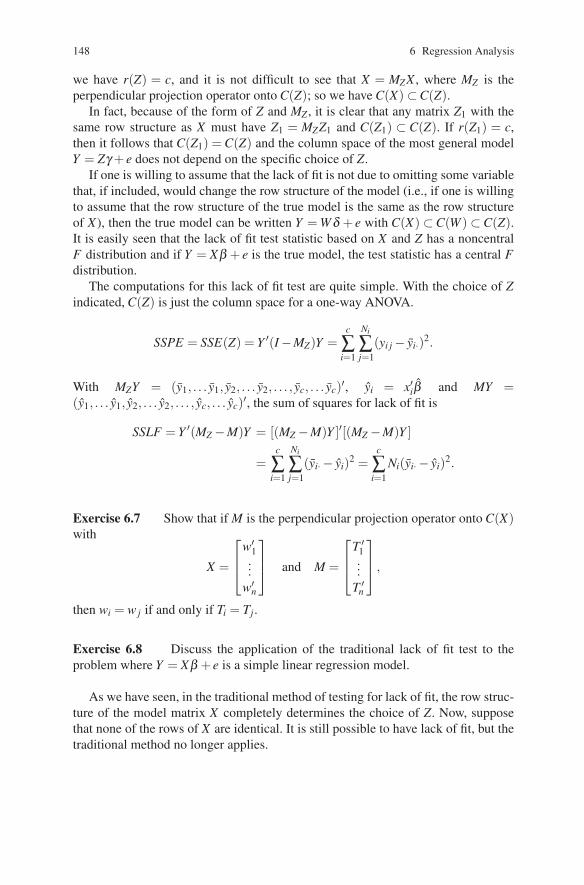
148 6 Regression Analysis
we have r(Z) = c, and it is not difficult to see that X = MZX , where MZ is theperpendicular projection operator onto C(Z); so we have C(X) ⊂C(Z).
In fact, because of the form of Z and MZ , it is clear that any matrix Z1 with thesame row structure as X must have Z1 = MZZ1 and C(Z1) ⊂ C(Z). If r(Z1) = c,then it follows that C(Z1) = C(Z) and the column space of the most general modelY = Zγ + e does not depend on the specific choice of Z.
If one is willing to assume that the lack of fit is not due to omitting some variablethat, if included, would change the row structure of the model (i.e., if one is willingto assume that the row structure of the true model is the same as the row structureof X), then the true model can be written Y = Wδ + e with C(X) ⊂C(W ) ⊂ C(Z).It is easily seen that the lack of fit test statistic based on X and Z has a noncentralF distribution and if Y = Xβ + e is the true model, the test statistic has a central Fdistribution.
The computations for this lack of fit test are quite simple. With the choice of Zindicated, C(Z) is just the column space for a one-way ANOVA.
SSPE = SSE(Z) = Y ′(I −MZ)Y =c
∑i=1
Ni
∑j=1
(yi j − yi·)2.
With MZY = (y1, . . . y1, y2, . . . y2, . . . , yc, . . . yc)′, yi = x′iβ and MY =(y1, . . . y1, y2, . . . y2, . . . , yc, . . . yc)′, the sum of squares for lack of fit is
SSLF = Y ′(MZ −M)Y = [(MZ −M)Y ]′[(MZ −M)Y ]
=c
∑i=1
Ni
∑j=1
(yi· − yi)2 =c
∑i=1
Ni(yi· − yi)2.
Exercise 6.7 Show that if M is the perpendicular projection operator onto C(X)with
X =
⎡⎢⎣w′1
...w′
n
⎤⎥⎦ and M =
⎡⎢⎣T ′1...
T ′n
⎤⎥⎦ ,
then wi = w j if and only if Ti = Tj .
Exercise 6.8 Discuss the application of the traditional lack of fit test to theproblem where Y = Xβ + e is a simple linear regression model.
As we have seen, in the traditional method of testing for lack of fit, the row struc-ture of the model matrix X completely determines the choice of Z. Now, supposethat none of the rows of X are identical. It is still possible to have lack of fit, but thetraditional method no longer applies.

6.6 Testing Lack of Fit 149
6.6.2 Near Replicate Lack of Fit Tests
Another set of methods for testing lack of fit is based on mimicking the traditionallack of fit test. With these methods, rows of the model matrix that are nearly repli-cates are identified. One way of identifying near replicates is to use a hierarchicalclustering algorithm (see Gnanadesikan, 1977) to identify rows of the model matrixthat are near one another. Tests for lack of fit using near replicates are reviewedby Neill and Johnson (1984). The theory behind such tests is beautifully explainedin Christensen (1989, 1991). (OK, so I’m biased in favor of this particular author.)Miller, Neill, and Sherfey (1998, 1999) provide a theoretical basis for choosing nearreplicate clusters.
Christensen (1991) suggests that a very good all-purpose near replicate lack offit test was introduced by Shillington (1979). Write the regression model in terms ofc clusters of near replicates with the ith cluster containing Ni cases, say
yi j = x′i jβ + ei j, (1)
i = 1, . . . ,c, j = 1, . . . ,Ni. Note that at this point we have done nothing to the modelexcept play with the subscripts; model (1) is just the original model. Shillington’stest involves finding means of the predictor variables in each cluster and fitting themodel
yi j = x′i·β + ei j. (2)
The numerator for Shillington’s test is then the numerator mean square used in com-paring this model to the one-way ANOVA model
yi j = μi + ei j. (3)
However, the denominator mean square for Shillington’s test is the mean squarederror from fitting the model
yi j = x′i jβ + μi + ei j. (4)
It is not difficult to see that if model (1) holds, then Shillington’s test statistic has acentral F distribution with the appropriate degrees of freedom. Christensen (1989,1991) gives details and explains why this should be a good all-purpose test — eventhough it is not the optimal test for either of the alternatives developed by Chris-tensen. The near replicate lack of fit test proposed in Christensen (1989) is the testof model (1) against model (4). The test proposed in Christensen (1991) uses thesame numerator as Shillington’s test, but a denominator sum of squares that is theSSE from model (1) minus the numerator sum of squares from Shillington’s test.Both of Christensen’s tests are optimal for certain types of lack of fit. If the clustersconsist of exact replicates, then all of these tests reduce to the traditional test.

150 6 Regression Analysis
EXAMPLE 6.6.1. Using the data of Example 6.2.1 we illustrate the near replicatelack of fit tests. Near replicates were chosen visually by plotting x1 versus x2. Thenear replicates are presented below.
Near Replicate Clusters for Steam DataObs. Near Obs. Nearno. x1 x2 rep. no. x1 x2 rep.
1 35.3 20 2 14 39.1 19 112 29.7 20 2 15 46.8 23 123 30.8 23 9 16 48.5 20 34 58.8 20 4 17 59.3 22 135 61.4 21 5 18 70.0 22 76 71.3 22 7 19 70.0 11 17 74.4 11 1 20 74.5 23 88 76.7 23 8 21 72.1 20 149 70.7 21 10 22 58.1 21 5
10 57.5 20 4 23 44.6 20 311 46.4 20 3 24 33.4 20 212 28.9 21 6 25 28.6 22 1513 28.1 21 6
Fitting models (1) through (4) gives the following results:
Model (1) (2) (3) (4)dfE 22 22 10 9SSE 46.50 50.75 12.136 7.5
Shillington’s test is
FS =[50.75−12.136]/[22−10]
7.5/9= 3.8614 > 3.073 = F(0.95,12,9).
Christensen’s (1989) test is
F89 =[46.50−7.5]/[22−9]
7.5/9= 3.6000 > 3.048 = F(0.95,13,9).
Christensen’s (1991) test is
F91 =[50.75−12.136]/[22−10]
[46.5− (50.75−12.136)]/[22− (22−10)]= 4.0804
> 2.913 = F(0.95,12,10).
All three tests indicate a lack of fit.
In this example, all of the tests behaved similarly. Christensen (1991) shows thatthe tests can be quite different and that for the single most interesting type of lack
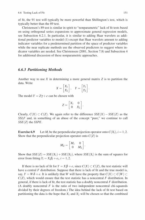
6.6 Testing Lack of Fit 151
of fit, the 91 test will typically be more powerful than Shillington’s test, which istypically better than the 89 test.
Christensen’s 89 test is similar in spirit to “nonparametric” lack of fit tests basedon using orthogonal series expansions to approximate general regression models,see Subsection 6.2.1. In particular, it is similar to adding Haar wavelets as addi-tional predictor variables to model (1) except that Haar wavelets amount to addingindicator variables for a predetermined partition of the space of predictor variableswhile the near replicate methods use the observed predictors to suggest where in-dicator variables are needed. See Christensen (2001, Section 7.8) and Subsection 4for additional discussion of these nonparametric approaches.
6.6.3 Partitioning Methods
Another way to use X in determining a more general matrix Z is to partition thedata. Write
X =[
X1X2
], Y =
[Y1Y2
].
The model Y = Zγ + e can be chosen with
Z =[
X1 00 X2
].
Clearly, C(X) ⊂ C(Z). We again refer to the difference SSE(X)− SSE(Z) as theSSLF and, in something of an abuse of the concept “pure,” we continue to callSSE(Z) the SSPE.
Exercise 6.9 Let Mi be the perpendicular projection operator onto C(Xi), i = 1,2.Show that the perpendicular projection operator onto C(Z) is
MZ =[
M1 00 M2
].
Show that SSE(Z) = SSE(X1)+SSE(X2), where SSE(Xi) is the sum of squares forerror from fitting Yi = Xiβi + ei, i = 1,2.
If there is no lack of fit for Y = Xβ + e, since C(X) ⊂C(Z), the test statistic willhave a central F distribution. Suppose that there is lack of fit and the true model is,say, Y = Wδ + e. It is unlikely that W will have the property that C(X) ⊂C(W ) ⊂C(Z), which would ensure that the test statistic has a noncentral F distribution. Ingeneral, if there is lack of fit, the test statistic has a doubly noncentral F distribution.(A doubly noncentral F is the ratio of two independent noncentral chi-squaredsdivided by their degrees of freedom.) The idea behind the lack of fit test based onpartitioning the data is the hope that X1 and X2 will be chosen so that the combined
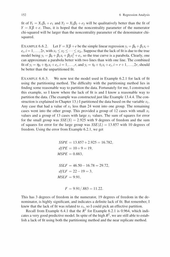
152 6 Regression Analysis
fit of Y1 = X1β1 + e1 and Y2 = X2β2 + e2 will be qualitatively better than the fit ofY = Xβ + e. Thus, it is hoped that the noncentrality parameter of the numeratorchi-squared will be larger than the noncentrality parameter of the denominator chi-squared.
EXAMPLE 6.6.2. Let Y = Xβ +e be the simple linear regression yi = β0 +β1xi +ei, i = 1, . . . ,2r, with x1 ≤ x2 ≤ ·· · ≤ x2r. Suppose that the lack of fit is due to the truemodel being yi = β0 +β1xi +β2x2
i + ei, so the true curve is a parabola. Clearly, onecan approximate a parabola better with two lines than with one line. The combinedfit of yi = η0 +η1xi +ei, i = 1, . . . ,r, and yi = τ0 +τ1xi +ei, i = r+1, . . . ,2r, shouldbe better than the unpartitioned fit.
EXAMPLE 6.6.3. We now test the model used in Example 6.2.1 for lack of fitusing the partitioning method. The difficulty with the partitioning method lies infinding some reasonable way to partition the data. Fortunately for me, I constructedthis example, so I know where the lack of fit is and I know a reasonable way topartition the data. (The example was constructed just like Example 13.4.4. The con-struction is explained in Chapter 13.) I partitioned the data based on the variable x1.Any case that had a value of x1 less than 24 went into one group. The remainingcases went into the other group. This provided a group of 12 cases with small x1values and a group of 13 cases with large x1 values. The sum of squares for errorfor the small group was SSE(S) = 2.925 with 9 degrees of freedom and the sumof squares for error for the large group was SSE(L) = 13.857 with 10 degrees offreedom. Using the error from Example 6.2.1, we get
SSPE = 13.857+2.925 = 16.782,
df PE = 10+9 = 19,
MSPE = 0.883,
SSLF = 46.50−16.78 = 29.72,
df LF = 22−19 = 3,
MSLF = 9.91,
F = 9.91/.883 = 11.22.
This has 3 degrees of freedom in the numerator, 19 degrees of freedom in the de-nominator, is highly significant, and indicates a definite lack of fit. But remember, Iknew that the lack of fit was related to x1, so I could pick an effective partition.
Recall from Example 6.4.1 that the R2 for Example 6.2.1 is 0.964, which indi-cates a very good predictive model. In spite of the high R2, we are still able to estab-lish a lack of fit using both the partitioning method and the near replicate method.

6.6 Testing Lack of Fit 153
The partitioning method can easily be extended, cf. Atwood and Ryan (1977).For example, one could select three partitions of the data and write
X =
⎡⎣X1X2X3
⎤⎦ , Y =
⎡⎣Y1Y2Y3
⎤⎦ , Z =
⎡⎣X1 0 00 X2 00 0 X3
⎤⎦ .
The lack of fit test would proceed as before. Note that the partitioning method isactually a generalization of the traditional method. If the partition of the data con-sists of the different sets of identical rows of the model matrix, then the partitioningmethod gives the traditional lack of fit test. The partitioning method can also beused to give a near replicate lack of fit test with the partitions corresponding to theclusters of near replicates. As mentioned earlier, it is not clear in general how tochoose an appropriate partition.
Utts (1982) presented a particular partition to be used in what she called theRainbow Test (for lack of fit). She suggests selecting a set of rows from X that arecentrally located to serve as X1, and placing each row of X not in X1 into a separateset that consists only of that row. With this partitioning, each of the separate setsdetermined by a single row corresponds to p columns of Z that are zero except forthe entries in that row. These p columns are redundant. Eliminating unnecessarycolumns allows the Z matrix to be rewritten as
Z =[
X1 00 I
].
From Exercise 6.9, it is immediately seen that SSE(Z) = SSE(X1); thus, the Rain-bow Test amounts to testing Y = Xβ +e against Y1 = X1β +e1. To select the matrixX1, Utts suggests looking at the diagonal elements of M = [mi j]. The smallest valuesof the miis are the most centrally located data points, cf. Section 13.1. The author’sexperience indicates that the Rainbow Test works best when one is quite selectiveabout the points included in the central partition.
EXAMPLE 6.6.3 CONTINUED. First consider the Rainbow Test using half of thedata set. The variables x1, x2, and an intercept were fitted to the 12 cases that hadthe smallest mii values. This gave a SSE = 16.65 with 9 degrees of freedom. TheRainbow Test mean square for lack of fit, mean square for pure error, and F statisticare
MSLF = (46.50−16.65)/(22−9) = 2.296,
MSPE = 16.65/9 = 1.850,
F = 2.296/1.850 = 1.24.
The F statistic is nowhere near being significant. Now consider taking the quarterof the data with the smallest mii values. These 6 data points provide a SSE = 0.862with 3 degrees of freedom.
MSLF = (46.50−0.862)/(22−3) = 2.402,

154 6 Regression Analysis
MSPE = .862/3 = 0.288,
F = 2.402/0.288 = 8.35.
In spite of the fact that this has only 3 degrees of freedom in the denominator,the F statistic is reasonably significant. F(0.95,19,3) is approximately 8.67 andF(0.90,19,3) is about 5.19.
6.6.4 Nonparametric Methods
As discussed in Subsection 6.2.1, one approach to nonparametric regression is tofit very complicated linear models. One particular application of this approach tononparametric regression is the fitting of moderate (as opposed to low or high)order polynomials. Christensen (2001, Chapter 7) provides more details of thisgeneral approach to nonparametric regression and in particular his Section 7.8 dis-cusses testing lack of fit. Fundamentally, the idea is to test the original linear modelyi = x′iβ + ei against a larger model that incorporates the nonparametric regressioncomponents, i.e., yi = x′iβ +∑q
j=1 γ jφ j(xi)+ ei. For high dimensional problems, thelarger model may need to involve generalized additive functions.
Exercise 6.10 Test the model yi j = β0 +β1xi +β2x2i +ei j for lack of fit using the
data:
xi 1.00 2.00 0.00 −3.00 2.50yi j 3.41 22.26 −1.74 79.47 37.96
2.12 14.91 1.32 80.04 44.236.26 23.41 −2.55 81.63
18.39
Exercise 6.11 Using the following data, test the model yi j = β0 +β1xi1 +β2xi2 +ei j for lack of fit. Explain and justify your method.
X1 X2 Y X1 X2 Y31 9.0 122.41 61 2.2 70.0843 8.0 115.12 36 4.7 66.4250 2.8 64.90 52 9.4 150.1538 5.0 64.91 38 1.5 38.1538 5.1 74.52 41 1.0 45.6751 4.6 75.02 41 5.0 68.6641 7.2 101.36 52 4.5 76.1557 4.0 74.45 29 2.7 36.2046 2.5 56.22
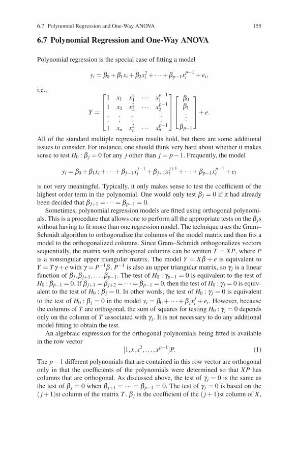
6.7 Polynomial Regression and One-Way ANOVA 155
6.7 Polynomial Regression and One-Way ANOVA
Polynomial regression is the special case of fitting a model
yi = β0 +β1xi +β2x2i + · · ·+βp−1xp−1
i + ei,
i.e.,
Y =
⎡⎢⎢⎢⎣1 x1 x2
1 · · · xp−11
1 x2 x22 · · · xp−1
2...
......
...1 xn x2
n · · · xp−1n
⎤⎥⎥⎥⎦⎡⎢⎢⎣
β0β1...
βp−1
⎤⎥⎥⎦+ e.
All of the standard multiple regression results hold, but there are some additionalissues to consider. For instance, one should think very hard about whether it makessense to test H0 : β j = 0 for any j other than j = p−1. Frequently, the model
yi = β0 +β1xi + · · ·+β j−1x j−1i +β j+1x j+1
i + · · ·+βp−1xp−1i + ei
is not very meaningful. Typically, it only makes sense to test the coefficient of thehighest order term in the polynomial. One would only test β j = 0 if it had alreadybeen decided that β j+1 = · · · = βp−1 = 0.
Sometimes, polynomial regression models are fitted using orthogonal polynomi-als. This is a procedure that allows one to perform all the appropriate tests on the β jswithout having to fit more than one regression model. The technique uses the Gram–Schmidt algorithm to orthogonalize the columns of the model matrix and then fits amodel to the orthogonalized columns. Since Gram–Schmidt orthogonalizes vectorssequentially, the matrix with orthogonal columns can be written T = XP, where Pis a nonsingular upper triangular matrix. The model Y = Xβ + e is equivalent toY = T γ + e with γ = P−1β . P−1 is also an upper triangular matrix, so γ j is a linearfunction of β j,β j+1, . . . ,βp−1. The test of H0 : γp−1 = 0 is equivalent to the test ofH0 : βp−1 = 0. If β j+1 = β j+2 = · · ·= βp−1 = 0, then the test of H0 : γ j = 0 is equiv-alent to the test of H0 : β j = 0. In other words, the test of H0 : γ j = 0 is equivalentto the test of H0 : β j = 0 in the model yi = β0 + · · ·+ β jx
ji + ei. However, because
the columns of T are orthogonal, the sum of squares for testing H0 : γ j = 0 dependsonly on the column of T associated with γ j. It is not necessary to do any additionalmodel fitting to obtain the test.
An algebraic expression for the orthogonal polynomials being fitted is availablein the row vector
[1,x,x2, . . . ,xp−1]P. (1)
The p−1 different polynomials that are contained in this row vector are orthogonalonly in that the coefficients of the polynomials were determined so that XP hascolumns that are orthogonal. As discussed above, the test of γ j = 0 is the same asthe test of β j = 0 when β j+1 = · · · = βp−1 = 0. The test of γ j = 0 is based on the( j +1)st column of the matrix T . β j is the coefficient of the ( j +1)st column of X ,

156 6 Regression Analysis
i.e., the jth degree term in the polynomial. By analogy, the ( j +1)st column of T iscalled the jth degree orthogonal polynomial.
Polynomial regression has some particularly interesting relationships with theproblem of estimating pure error and with one-way ANOVA problems. It is clearthat for all values of p, the row structure of the model matrices for the polynomialregression models is the same, i.e., if xi = xi′ , then xk
i = xki′ ; so the i and i′ rows of X
are the same regardless of the order of the polynomial. Suppose there are q distinctvalues of xi in the model matrix. The most general polynomial that can be fittedmust give a rank q model matrix; thus the most general model must be
yi = β0 +β1xi + · · ·+βq−1xq−1i + ei.
It also follows from the previous section that the column space of this model is ex-actly the same as the column space for fitting a one-way ANOVA with q treatments.
Using double subscript notation with i = 1, . . . ,q, j = 1, . . . ,Ni, the models
yi j = β0 +β1xi + · · ·+βq−1xq−1i + ei j (2)
andyi j = μ +αi + ei j
are equivalent. Since both β0 and μ are parameters corresponding to a column of1s, the tests of H0 : β1 = · · · = βq−1 = 0 and H0 : α1 = · · · = αq are identical. Bothtests look at the orthogonal complement of Jn with respect to C(X), where C(X) isthe column space for either of the models. Using the ideas of Section 3.6, one wayto break this space up into q−1 orthogonal one-degree-of-freedom hypotheses is tolook at the orthogonal polynomials for i = 1, . . . ,q−1. As seen in Section 4.2, anyvector in C(X) that is orthogonal to J determines a contrast in the αis. In particular,each orthogonal polynomial corresponds to a contrast in the αis.
Finding a set of q−1 orthogonal contrasts amounts to finding an orthogonal basisfor C(Mα). If we write T = [T0, . . . ,Tq−1], then T1, . . . ,Tq−1 is an orthogonal basisfor C(Mα). Given these vectors in C(Mα), we can use Proposition 4.2.3 to read offthe corresponding contrasts. Moreover, the test for dropping, say, Tj from the modelis the test of H0 : γ j = 0, which is just the test that the corresponding contrast iszero. Note that testing this contrast is not of interest unless β j+1 = · · · = βq−1 = 0or, equivalently, if γ j+1 = · · · = γq−1 = 0 or, equivalently, if all the higher orderpolynomial contrasts are zero.
Definition 6.7.1. The orthogonal contrasts determined by the orthogonal poly-nomials are called the polynomial contrasts. The contrast corresponding to the firstdegree orthogonal polynomial is called the linear contrast. The contrasts for higherdegree orthogonal polynomials are called the quadratic, cubic, quartic, etc., con-trasts.
Using Proposition 4.2.3, if we identify an orthogonal polynomial as a vectorρ ∈C(Mα), then the corresponding contrast can be read off. For example, the second
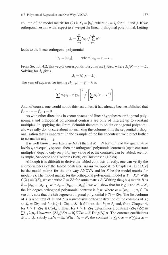
6.7 Polynomial Regression and One-Way ANOVA 157
column of the model matrix for (2) is X1 = [ti j], where ti j = xi for all i and j. If weorthogonalize this with respect to J, we get the linear orthogonal polynomial. Letting
x· =q
∑i=1
Nixi
/ q
∑i=1
Ni
leads to the linear orthogonal polynomial
T1 = [wi j], where wi j = xi − x· .
From Section 4.2, this vector corresponds to a contrast ∑λiαi, where λi/Ni = xi− x·.Solving for λi gives
λi = Ni(xi − x·).
The sum of squares for testing H0 : β1 = γ1 = 0 is[∑
iNi(xi − x·)yi·
]2/[∑
iNi(xi − x·)2
].
And, of course, one would not do this test unless it had already been established thatβ2 = · · · = βq−1 = 0.
As with other directions in vector spaces and linear hypotheses, orthogonal poly-nomials and orthogonal polynomial contrasts are only of interest up to constantmultiples. In applying the Gram–Schmidt theorem to obtain orthogonal polynomi-als, we really do not care about normalizing the columns. It is the sequential orthog-onalization that is important. In the example of the linear contrast, we did not botherto normalize anything.
It is well known (see Exercise 6.12) that, if Ni = N for all i and the quantitativelevels xi are equally spaced, then the orthogonal polynomial contrasts (up to constantmultiples) depend only on q. For any value of q, the contrasts can be tabled; see, forexample, Snedecor and Cochran (1980) or Christensen (1996a).
Although it is difficult to derive the tabled contrasts directly, one can verify theappropriateness of the tabled contrasts. Again we appeal to Chapter 4. Let [J,Z]be the model matrix for the one-way ANOVA and let X be the model matrix formodel (2). The model matrix for the orthogonal polynomial model is T = XP. WithC(X) =C(Z), we can write T = ZB for some matrix B. Writing the q×q matrix B asB =[b0, . . . ,bq−1
]with bk =
(b1k, . . . ,bqk
)′, we will show that for k ≥ 1 and Ni = N,the kth degree orthogonal polynomial contrast is b′kα , where α = (α1, . . . ,αq)
′. Tosee this, note that the kth degree orthogonal polynomial is Tk = Zbk. The first columnof X is a column of 1s and T is a successive orthogonalization of the columns of X ;so Jn = Zb0 and for k ≥ 1, Zbk ⊥ Jn. It follows that b0 = Jq and, from Chapter 4,for k ≥ 1, Zbk ∈ C(Mα). Thus, for k ≥ 1, Zbk determines a contrast (Zbk)′Zα ≡∑q
i=1 λiαi. However, (Zbk)′Zα = b′kZ′Zα = b′kDiag(Ni)α . The contrast coefficientsλ1, . . . ,λq satisfy bikNi = λi. When Ni = N, the contrast is ∑i λiαi = N ∑i bikαi =

158 6 Regression Analysis
Nb′kα . Orthogonal polynomial contrasts are defined only up to constant multiples,so the kth degree orthogonal polynomial contrast is also b′kα .
Given a set of contrast vectors b1, . . . ,bq−1, we can check whether these are theorthogonal polynomial contrasts. Simply compute the corresponding matrix T = ZBand check whether this constitutes a successive orthogonalization of the columns ofX .
Ideas similar to these will be used in Section 9.4 to justify the use of tabled con-trasts in the analysis of balanced incomplete block designs. These ideas also relate toSection 7.3 on Polynomial Regression and the Balanced Two-Way ANOVA. Finally,these ideas relate to nonparametric regression as discussed in Subsection 6.2.1.There, polynomials were used as an example of a class of functions that can be usedto approximate arbitrary continuous functions. Other examples mentioned werecosines and wavelets. The development given in this section for polynomials canbe mimicked for any approximating class of functions.
For completeness, an alternative idea of orthogonal polynomials should be men-tioned. In equation (1), rather than using the matrix P that transforms the columnsof X into T with orthonormal columns, one could instead choose a P0 so that thetransformed functions are orthogonal in an appropriate function space. The Legen-dre polynomials are such a collection. The fact that such orthogonal polynomials donot depend on the specific xis in the data is both an advantage and a disadvantage. Itis an advantage in that they are well known and do not have to be derived for eachunique set of xis. It is a disadvantage in that, although they display better numeri-cal properties than the unadjusted polynomials, since T0 = XP0 typically does nothave (exactly) orthonormal columns, these polynomials will not display the precisefeatures exploited earlier in this section.
Exercise 6.12
(a) Find the model matrix for the orthogonal polynomial model Y = T γ + ecorresponding to the model
yi j = β0 +β1xi +β2x2i +β3x3
i + ei j,
i = 1,2,3,4, j = 1, . . . ,N, where xi = a+(i−1)t.Hint: First consider the case N = 1.
(b) For the model yi j = μ + αi + ei j, i = 1,2,3,4, j = 1, . . . ,N, and for k =1,2,3, find the contrast ∑λikαi such that the test of H0 : ∑λikαi = 0 is the same asthe test of H0 : γk = 0, i.e., find the polynomial contrasts.
Exercise 6.13 Repeat Exercise 6.11 with N = 2 and x1 = 2, x2 = 3, x3 = 5,x4 = 8.

6.8 Additional Exercises 159
6.8 Additional Exercises
The first three exercises involve deriving Fieller’s method of finding confidenceintervals.
Exercise 6.8.1 Calibration.Consider the regression model Y = Xβ + e, e ∼ N(0,σ2I) and suppose that we areinterested in a future observation, say y0, that will be independent of Y and havemean x′0β . In previous work with this situation, y0 was not yet observed but the cor-responding vector x0 was known. The calibration problem reverses these assump-tions. Suppose that we have observed y0 and wish to infer what the correspondingvector x0 might be.
A typical calibration problem might involve two methods of measuring somequantity: y, a cheap and easy method, and x, an expensive but very accurate method.Data are obtained to establish the relationship between y and x. Having done this,future measurements are made with y and the calibration relationship is used toidentify what the value of y really means. For example, in sterilizing canned food,x would be a direct measure of the heat absorbed into the can, while y might be thenumber of bacterial spores of a certain strain that are killed by the heat treatment.(Obviously, one needs to be able to measure the number of spores in the can bothbefore and after heating.)
Consider now the simplest calibration model, yi = β0 + β1xi + ei, eis i.i.d.N(0,σ 2), i = 1,2,3, . . . ,n. Suppose that y0 is observed and that we wish to estimatethe corresponding value x0 (x0 is viewed as a parameter here).
(a) Find the MLEs of β0, β1, x0, and σ 2.Hint: This is a matter of showing that the obvious estimates are MLEs.(b) Suppose now that a series of observations y01, . . . ,y0r were taken, all of
which correspond to the same x0. Find the MLEs of β0, β1, x0, and σ 2.Hint: Only the estimate of σ 2 changes form.(c) Based on one observation y0, find a (1−α)100% confidence interval for
x0. When does such an interval exist?Hint: Use an F(1,n−2) distribution based on (y0 − β0 − β1x0)2.Comment: Aitchison and Dunsmore (1975) discuss calibration in considerable
detail, including a comparison of different methods.
Exercise 6.8.2 Maximizing a Quadratic Response.Consider the model, yi = β0 + β1xi +β2x2
i + ei, eis i.i.d. N(0,σ2), i = 1,2,3, . . . ,n.Let x0 be the value at which the function E(y) = β0 +β1x +β2x2 is maximized (orminimized).
(a) Find the maximum likelihood estimate of x0.(b) Find a (1−α)100% confidence interval for x0. Does such an interval al-
ways exist?Hint: Use an F(1,n−3) distribution based on (β1 +2β2x0)2.

160 6 Regression Analysis
Comment: The problem of finding values of the independent variables that max-imize (or minimize) the expected y value is a basic problem in the field of responsesurface methods. See Box, Hunter, and Hunter (1978) or Christensen (2001, Chap-ter 8) for an introduction to the subject, or Box and Draper (1987) for a detailedtreatment.
Exercise 6.8.3 Two-Phase Linear Regression.Consider the problem of sterilizing canned pudding. As the pudding is sterilized bya heat treatment, it is simultaneously cooked. If you have ever cooked pudding, youknow that it starts out soupy and eventually thickens. That, dear reader, is the pointof this little tale. Sterilization depends on the transfer of heat to the pudding andthe rate of transfer depends on whether the pudding is soupy or gelatinous. On anappropriate scale, the heating curve is linear in each phase. The question is, “Wheredoes the line change phases?”
Suppose that we have collected data (yi,xi), i = 1, . . . ,n + m, and that we knowthat the line changes phases between xn and xn+1. The model yi = β10 +β11xi + ei,eis i.i.d. N(0,σ2), i = 1, . . . ,n, applies to the first phase and the model yi = β20 +β21xi + ei, eis i.i.d. N(0,σ2), i = n+1, . . . ,n+m, applies to the second phase. Let γbe the value of x at which the lines intersect.
(a) Find estimates of β10, β11, β20, β21, σ 2, and γ .Hint: γ is a function of the other parameters.(b) Find a (1−α)100% confidence interval for γ . Does such an interval always
exist?Hint: Use an F(1,n+m−4) distribution based on[
(β10 + β11γ)− (β20 + β21γ)]2
.
Comment: Hinkley (1969) has treated the more realistic problem in which it isnot known between which xi values the intersection occurs.
Exercise 6.8.4 Consider the model yi = β0 + β1xi + ei, eis i.i.d. N(0,σ 2di),i = 1,2,3, . . . ,n, where the dis are known numbers. Derive algebraic formulas forβ0, β1, Var(β0), and Var(β1).
Exercise 6.8.5 Consider the model yi = β0 + β1xi + ei, eis i.i.d. N(0,σ 2), i =1,2,3, . . . ,n. If the xis are restricted to be in the closed interval [−10,15], determinehow to choose the xis to minimize
(a) Var(β0).(b) Var(β1).(c) How would the choice of the xis change if they were restricted to the closed
interval [−10,10]?

6.8 Additional Exercises 161
Exercise 6.8.6 Find E[y− E(y|x)]2 in terms of the variances and covariances ofx and y. Give a “natural” estimate of E
[y− E(y|x)]2.
Exercise 6.8.7 Test whether the data of Example 6.2.1 indicate that the multiplecorrelation coefficient is different from zero.
Exercise 6.8.8 Test whether the data of Example 6.2.1 indicate that the partialcorrelation coefficient ρy1·2 is different from zero.
Exercise 6.8.9 Show that
(a) ρ12·3 =ρ12 −ρ13ρ23√
1−ρ213
√1−ρ2
23
(b) ρ12·34 =ρ12·4 −ρ13·4ρ23·4√1−ρ2
13·4√
1−ρ223·4
.
Exercise 6.8.10 Show that in Section 2, γ∗ = β∗ and β0 = γ0 − (1/n)Jn1 Zγ∗.
Hint: Examine the corresponding argument given in Section 1 for simple linearregression.


Chapter 7
Multifactor Analysis of Variance
Chapter 7 presents the analysis of multifactor ANOVA models. The first threesections deal with the balanced two-way ANOVA model. Section 1 examines theno interaction model. Section 2 examines the model with interaction. Section 3 dis-cusses the relationship between polynomial regression and the balanced two-wayANOVA model. Sections 4 and 5 discuss unbalanced two-way ANOVA models.Section 4 treats the special case of proportional numbers. Section 5 examines thegeneral case. Finally, Section 6 extends the earlier results of the chapter to modelswith more than two factors. A review of the tensor concepts in Appendix B may aidthe reader of this chapter.
7.1 Balanced Two-Way ANOVA Without Interaction
The balanced two-way ANOVA without interaction model is generally written
yi jk = μ +αi +η j + ei jk, (1)
i = 1, . . . ,a, j = 1, . . . ,b, k = 1, . . . ,N.
© Springer Science+Business Media, LLC 2011
163Springer Texts in Statistics, DOI 10.1007/978-1-4419-9816-3_7, R. Christensen, Plane Answers to Complex Questions: The Theory of Linear Models,

164 7 Multifactor Analysis of Variance
EXAMPLE 7.1.1. Suppose a = 3, b = 2, N = 4. In matrix terms write⎡⎢⎢⎢⎢⎢⎢⎢⎢⎢⎢⎢⎢⎢⎢⎢⎢⎢⎢⎢⎢⎢⎢⎢⎢⎢⎢⎢⎢⎢⎢⎢⎢⎢⎢⎢⎢⎢⎢⎢⎢⎢⎣
y111y112y113y114y121y122y123y124y211y212y213y214y221y222y223y224y311y312y313y314y321y322y323y324
⎤⎥⎥⎥⎥⎥⎥⎥⎥⎥⎥⎥⎥⎥⎥⎥⎥⎥⎥⎥⎥⎥⎥⎥⎥⎥⎥⎥⎥⎥⎥⎥⎥⎥⎥⎥⎥⎥⎥⎥⎥⎥⎦
=
⎡⎢⎢⎢⎢⎢⎢⎢⎢⎢⎢⎢⎢⎢⎢⎢⎢⎢⎢⎢⎢⎢⎢⎢⎢⎢⎢⎢⎢⎢⎢⎢⎢⎢⎢⎢⎢⎢⎢⎢⎢⎢⎣
1 1 0 0 1 01 1 0 0 1 01 1 0 0 1 01 1 0 0 1 01 1 0 0 0 11 1 0 0 0 11 1 0 0 0 11 1 0 0 0 11 0 1 0 1 01 0 1 0 1 01 0 1 0 1 01 0 1 0 1 01 0 1 0 0 11 0 1 0 0 11 0 1 0 0 11 0 1 0 0 11 0 0 1 1 01 0 0 1 1 01 0 0 1 1 01 0 0 1 1 01 0 0 1 0 11 0 0 1 0 11 0 0 1 0 11 0 0 1 0 1
⎤⎥⎥⎥⎥⎥⎥⎥⎥⎥⎥⎥⎥⎥⎥⎥⎥⎥⎥⎥⎥⎥⎥⎥⎥⎥⎥⎥⎥⎥⎥⎥⎥⎥⎥⎥⎥⎥⎥⎥⎥⎥⎦
⎡⎢⎢⎢⎢⎢⎣μα1α2α3η1η2
⎤⎥⎥⎥⎥⎥⎦+ e.
In general, we can write the model as
Y = [X0,X1, . . . ,Xa,Xa+1, . . . ,Xa+b]
⎡⎢⎢⎢⎢⎢⎢⎢⎢⎢⎣
μα1...
αaη1...
ηb
⎤⎥⎥⎥⎥⎥⎥⎥⎥⎥⎦+ e.
Write n = abN and the observation vector as Y = [yi jk], where the three subscriptsi, j, and k denote a row of the vector. (Multiple subscripts denoting the rows andcolumns of matrices were introduced in Chapter 4.) The model matrix of the bal-anced two-way ANOVA model has
X0 = J,Xr = [ti jk], ti jk = δir, r = 1, . . . ,a,
Xa+s = [ti jk], ti jk = δ js, s = 1, . . . ,b,
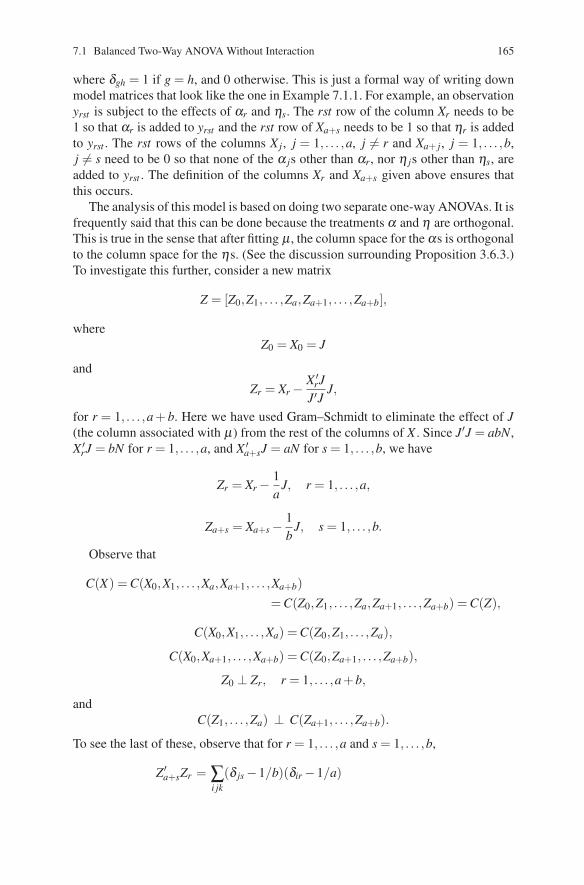
7.1 Balanced Two-Way ANOVA Without Interaction 165
where δgh = 1 if g = h, and 0 otherwise. This is just a formal way of writing downmodel matrices that look like the one in Example 7.1.1. For example, an observationyrst is subject to the effects of αr and ηs. The rst row of the column Xr needs to be1 so that αr is added to yrst and the rst row of Xa+s needs to be 1 so that ηr is addedto yrst . The rst rows of the columns Xj , j = 1, . . . ,a, j �= r and Xa+ j, j = 1, . . . ,b,j �= s need to be 0 so that none of the α js other than αr, nor η js other than ηs, areadded to yrst . The definition of the columns Xr and Xa+s given above ensures thatthis occurs.
The analysis of this model is based on doing two separate one-way ANOVAs. It isfrequently said that this can be done because the treatments α and η are orthogonal.This is true in the sense that after fitting μ , the column space for the αs is orthogonalto the column space for the ηs. (See the discussion surrounding Proposition 3.6.3.)To investigate this further, consider a new matrix
Z = [Z0,Z1, . . . ,Za,Za+1, . . . ,Za+b],
whereZ0 = X0 = J
and
Zr = Xr − X ′rJ
J′JJ,
for r = 1, . . . ,a + b. Here we have used Gram–Schmidt to eliminate the effect of J(the column associated with μ) from the rest of the columns of X . Since J′J = abN,X ′
rJ = bN for r = 1, . . . ,a, and X ′a+sJ = aN for s = 1, . . . ,b, we have
Zr = Xr − 1a
J, r = 1, . . . ,a,
Za+s = Xa+s − 1b
J, s = 1, . . . ,b.
Observe that
C(X) = C(X0,X1, . . . ,Xa,Xa+1, . . . ,Xa+b)= C(Z0,Z1, . . . ,Za,Za+1, . . . ,Za+b) = C(Z),
C(X0,X1, . . . ,Xa) = C(Z0,Z1, . . . ,Za),
C(X0,Xa+1, . . . ,Xa+b) = C(Z0,Za+1, . . . ,Za+b),
Z0 ⊥ Zr, r = 1, . . . ,a+b,
andC(Z1, . . . ,Za) ⊥ C(Za+1, . . . ,Za+b).
To see the last of these, observe that for r = 1, . . . ,a and s = 1, . . . ,b,
Z′a+sZr = ∑
i jk(δ js −1/b)(δir −1/a)

166 7 Multifactor Analysis of Variance
= ∑i jk
δ jsδir −∑i jk
δ js1a−∑
i jkδir
1b
+∑i jk
1ab
= ∑i j
Nδ jsδir −∑j
δ jsaNa
−∑i
δirbNb
+abNab
= N −aN/a−bN/b+N = 0.
We have decomposed C(X) into three orthogonal parts, C(Z0), C(Z1, . . . ,Za), andC(Za+1, . . . ,Za+b). M, the perpendicular projection operator onto C(X), can be writ-ten as the matrix sum of the perpendicular projection matrices onto these threespaces. By appealing to the one-way ANOVA, we can actually identify these pro-jection matrices.
C([X0,X1, . . . ,Xa]) is the column space for the one-way ANOVA model
yi jk = μ +αi + ei jk, (2)
where the subscripts j and k are both used to indicate replications. Similarly,C([X0,Xa+1, . . . ,Xa+b]) is the column space for the one-way ANOVA model
yi jk = μ +η j + ei jk, (3)
where the subscripts i and k are both used to indicate replications. If one actuallywrites down the matrix [X0,Xa+1, . . . ,Xa+b], it looks a bit different from the usualform of a one-way ANOVA model matrix because the rows have been permuted outof the convenient order generally used.
Let Mα be the projection matrix used to test for no treatment effects in model(2). Mα is the perpendicular projection matrix onto C(Z1, . . . ,Za). Similarly, if Mηis the projection matrix for testing no treatment effects in model (3), then Mη is theperpendicular projection matrix onto C(Za+1, . . . ,Za+b). It follows that
M =1n
Jnn +Mα +Mη .
By comparing models, we see, for instance, that the test for H0 : α1 = · · · = αa isbased on
Y ′MαY/r(Mα)Y ′(I −M)Y/r(I −M)
.
It is easy to see that r(Mα) = a−1 and r(I −M) = n−a−b+1. Y ′MαY can befound as in Chapter 4 by appealing to the analysis of the one-way ANOVA model(2). In particular, since pairs jk identify replications,
MαY = [ti jk], where ti jk = yi·· − y··· (4)
and
SS(α) = Y ′MαY = [MαY ]′[MαY ] = bNa
∑i=1
(yi·· − y···)2.

7.1 Balanced Two-Way ANOVA Without Interaction 167
Expected mean squares can also be found by appealing to the one-way ANOVA
E(Y ′MαY ) = σ 2(a−1)+β ′X ′Mα Xβ .
Substituting μ +αi +η j for yi jk in (4) gives
Mα Xβ = [ti jk], where ti jk = αi − α·
and thus
E[Y ′MαY/(a−1)
]= σ 2 +
bNa−1
a
∑i=1
(αi − α·)2.
Similar results hold for testing H0 : η1 = · · · = ηb.The SSE can be found using (4) and the facts that
MηY = [ti jk], where ti jk = y· j· − y···
and1n
JnnY = [ti jk], where ti jk = y··· .
Because (I −M)Y = Y − (1/n)JnnY −MαY −MηY ,
(I −M)Y = [ti jk]
where
ti jk = yi jk − y··· − (yi·· − y···)− (y· j· − y···)= yi jk − yi·· − y· j· + y···.
Finally,
SSE = Y ′(I −M)Y = [(I −M)Y ]′[(I −M)Y ]
=a
∑i=1
b
∑j=1
N
∑k=1
(yi jk − yi·· − y· j· + y···)2.
The analysis of variance table is given in Table 7.1.
7.1.1 Contrasts
We wish to show that estimation and testing of contrasts in a balanced two-wayANOVA is done exactly as in the one-way ANOVA: by ignoring the fact that asecond type of treatment exists. This follows from showing that, say, a contrastin the αis involves a constraint on C(Mα), and C(Mα) is defined by the one-wayANOVA without the η js.

168 7 Multifactor Analysis of Variance
Table 7.1 Balanced Two-Way Analysis of Variance Table with No Interaction.
Matrix Notation
Source df SS
Grand Mean 1 Y ′ ( 1n Jn
n)
Y
Treatments(α) a−1 Y ′MαY
Treatments(η) b−1 Y ′MηY
Error n−a−b+1 Y ′(I−M)Y
Total n = abN Y ′Y
Source SS E(MS)
Grand Mean SSGM σ2 +β ′X ′ ( 1n Jn
n)
Xβ
Treatments(α) SS(α) σ2 +β ′X ′Mα Xβ/(a−1)
Treatments(η) SS(η) σ2 +β ′X ′Mη Xβ/(b−1)
Error SSE σ2
Total SSTot
Algebraic Notation
Source df SS
Grand Mean df GM n−1y2··· = ny2···
Treatments(α) df (α) bN ∑ai=1 (yi·· − y···)2
Treatments(η) df (η) aN ∑bj=1 (y· j· − y···)2
Error dfE ∑i jk(yi jk − yi·· − y· j· + y···
)2Total df Tot ∑i jk y2
i jk
Source MS E(MS)
Grand Mean SSGM σ2 +abN(μ + α· + η·)2
Treatments(α) SS(α)/(a−1) σ2 +bN ∑ai=1 (αi − α·)2 /(a−1)
Treatments(η) SS(η)/(b−1) σ2 +aN ∑bj=1 (η j − η·)2 /(b−1)
Error SSE/(n−a−b+1) σ 2

7.2 Balanced Two-Way ANOVA with Interaction 169
Theorem 7.1.2. Let λ ′β be estimable and ρ ′X = λ ′. Then λ ′β is a contrast inthe αis if and only if ρ ′M = ρ ′Mα . In this case, λ ′β = ρ ′MY = ρ ′MαY , which isthe estimate from the one-way ANOVA ignoring the η js.
PROOF. Let λ ′β = ∑ai=1 ciαi with ∑a
i=1 ci = 0. Thus, λ ′ = (0,c1, . . . ,ca,0, . . . ,0)and λ ′Ja+b+1 = 0. To have such a λ is to have ρ with
ρ ′Xi = 0, i = 0,a+1,a+2, . . . ,a+b,
which happens if and only if ρ is orthogonal to C(Z0,Za+1, . . . ,Za+b) =C(M−Mα).In other words, ρ ′(M−Mα) = 0 and ρ ′M = ρ ′Mα . �
One interpretation of this result is that having a contrast in the αis equal to zeroputs a constraint on C(X) that requires E(Y ) ∈C(X) and E(Y ) ⊥ Mα ρ . Clearly thisconstitutes a constraint on C(Mα), the space for the α treatments. Another interpre-tation is that estimation or testing of a contrast in the αis is done using Mα , whichis exactly the way it is done in a one-way ANOVA ignoring the η js.
Specifically, if we have a contrast ∑ai=1 ciαi, then the corresponding vector Mα ρ
isMα ρ = [ti jk], where ti jk = ci/bN.
The estimated contrast is ρ ′MαY = ∑ai=1 ciyi·· having a variance of σ 2ρ ′Mα ρ =
σ 2 ∑ai=1 c2
i /bN and a sum of squares for testing H0 : ∑ai=1 ciαi = 0 of(
a
∑i=1
ciyi··
)2/( a
∑i=1
c2i /bN
).
To get two orthogonal constraints on C(Mα), as in the one-way ANOVA, takeρ1 and ρ2 such that ρ ′
1Xβ and ρ ′2Xβ are contrasts in the αis and ρ ′
1Mαρ2 = 0. Ifρ ′
jXβ = ∑ai=1 c jiαi, then, as shown for the one-way ANOVA, ρ ′
1Mα ρ2 = 0 if andonly if ∑a
i=1 c1ic2i = 0.In the balanced two-way ANOVA without interaction, if N is greater than 1, we
have a row structure to the model matrix with ab distinct rows. This allows estima-tion of pure error and lack of fit. The balanced two-way ANOVA with interactionretains the row structure and is equivalent to a large one-way ANOVA with ab treat-ments. Thus, the interaction model provides one parameterization of the model de-veloped in Subsection 6.6.1 for testing lack of fit. The sum of squares for interactionis just the sum of squares for lack of fit of the no interaction model.
7.2 Balanced Two-Way ANOVA with Interaction
The balanced two-way ANOVA with interaction model is written

170 7 Multifactor Analysis of Variance
yi jk = μ +αi +η j + γi j + ei jk,
i = 1, . . . ,a, j = 1, . . . ,b, k = 1, . . . ,N.
EXAMPLE 7.2.1. Suppose a = 3, b = 2, N = 4. In matrix terms we write⎡⎢⎢⎢⎢⎢⎢⎢⎢⎢⎢⎢⎢⎢⎢⎢⎢⎢⎢⎢⎢⎢⎢⎢⎢⎢⎢⎢⎢⎢⎢⎢⎢⎢⎢⎢⎢⎢⎢⎢⎢⎢⎣
y111y112y113y114y121y122y123y124y211y212y213y214y221y222y223y224y311y312y313y314y321y322y323y324
⎤⎥⎥⎥⎥⎥⎥⎥⎥⎥⎥⎥⎥⎥⎥⎥⎥⎥⎥⎥⎥⎥⎥⎥⎥⎥⎥⎥⎥⎥⎥⎥⎥⎥⎥⎥⎥⎥⎥⎥⎥⎥⎦
=
⎡⎢⎢⎢⎢⎢⎢⎢⎢⎢⎢⎢⎢⎢⎢⎢⎢⎢⎢⎢⎢⎢⎢⎢⎢⎢⎢⎢⎢⎢⎢⎢⎢⎢⎢⎢⎢⎢⎢⎢⎢⎢⎣
1 1 0 0 1 0 1 0 0 0 0 01 1 0 0 1 0 1 0 0 0 0 01 1 0 0 1 0 1 0 0 0 0 01 1 0 0 1 0 1 0 0 0 0 01 1 0 0 0 1 0 1 0 0 0 01 1 0 0 0 1 0 1 0 0 0 01 1 0 0 0 1 0 1 0 0 0 01 1 0 0 0 1 0 1 0 0 0 01 0 1 0 1 0 0 0 1 0 0 01 0 1 0 1 0 0 0 1 0 0 01 0 1 0 1 0 0 0 1 0 0 01 0 1 0 1 0 0 0 1 0 0 01 0 1 0 0 1 0 0 0 1 0 01 0 1 0 0 1 0 0 0 1 0 01 0 1 0 0 1 0 0 0 1 0 01 0 1 0 0 1 0 0 0 1 0 01 0 0 1 1 0 0 0 0 0 1 01 0 0 1 1 0 0 0 0 0 1 01 0 0 1 1 0 0 0 0 0 1 01 0 0 1 1 0 0 0 0 0 1 01 0 0 1 0 1 0 0 0 0 0 11 0 0 1 0 1 0 0 0 0 0 11 0 0 1 0 1 0 0 0 0 0 11 0 0 1 0 1 0 0 0 0 0 1
⎤⎥⎥⎥⎥⎥⎥⎥⎥⎥⎥⎥⎥⎥⎥⎥⎥⎥⎥⎥⎥⎥⎥⎥⎥⎥⎥⎥⎥⎥⎥⎥⎥⎥⎥⎥⎥⎥⎥⎥⎥⎥⎦
⎡⎢⎢⎢⎢⎢⎢⎢⎢⎢⎢⎢⎢⎢⎢⎢⎢⎢⎣
μα1α2α3η1η2γ11γ12γ21γ22γ31γ32
⎤⎥⎥⎥⎥⎥⎥⎥⎥⎥⎥⎥⎥⎥⎥⎥⎥⎥⎦
+ e.
In general, the model matrix can be written
X = [X0,X1, . . . ,Xa,Xa+1, . . . ,Xa+b,Xa+b+1, . . . ,Xa+b+ab].
The columns X0, . . . ,Xa+b are exactly the same as for (7.1.1), the model withoutinteraction. The key fact to notice is that
C(X) = C(Xa+b+1, . . . ,Xa+b+ab);
this will be shown rigorously later. We can write an equivalent model using justXa+b+1, . . . ,Xa+b+ab, say
yi jk = μi j + ei jk.
This is just a one-way ANOVA model with ab treatments and is sometimes calledthe cell means model.
We can decompose C(X) into four orthogonal parts based on the identity
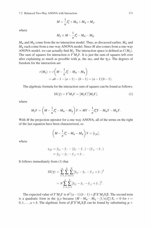
7.2 Balanced Two-Way ANOVA with Interaction 171
M =1n
Jnn +Mα +Mη +Mγ ,
whereMγ ≡ M− 1
nJn
n −Mα −Mη .
Mα and Mη come from the no interaction model. Thus, as discussed earlier, Mα andMη each come from a one-way ANOVA model. Since M also comes from a one-wayANOVA model, we can actually find Mγ . The interaction space is defined as C(Mγ).The sum of squares for interaction is Y ′MγY . It is just the sum of squares left overafter explaining as much as possible with μ , the αis, and the η js. The degrees offreedom for the interaction are
r(Mγ) = r(
M− 1n
Jnn −Mα −Mη
)= ab−1− (a−1)− (b−1) = (a−1)(b−1).
The algebraic formula for the interaction sum of squares can be found as follows:
SS(γ) = Y ′MγY = [MγY ]′[MγY ], (1)
where
MγY =(
M− 1n
Jnn −Mα −Mη
)Y = MY − 1
nJn
nY −MαY −MηY.
With M the projection operator for a one-way ANOVA, all of the terms on the rightof the last equation have been characterized, so(
M− 1n
Jnn −Mα −Mη
)Y = [ti jk],
where
ti jk = yi j· − y··· − (yi·· − y···)− (y· j· − y···)= yi j· − yi·· − y· j· + y···.
It follows immediately from (1) that
SS(γ) =a
∑i=1
b
∑j=1
N
∑k=1
[yi j· − yi·· − y· j· + y···]2
= Na
∑i=1
b
∑j=1
[yi j· − yi·· − y· j· + y···]2.
The expected value of Y ′MγY is σ 2(a−1)(b−1)+β ′X ′Mγ Xβ . The second termis a quadratic form in the γi js because (M−Mα −Mη − [1/n]Jn
n )Xr = 0 for r =0,1, . . . ,a + b. The algebraic form of β ′X ′Mγ Xβ can be found by substituting μ +

172 7 Multifactor Analysis of Variance
αi +η j + γi j for yi jk in SS(γ). Simplification gives
β ′X ′MγXβ = N ∑i j
[γi j − γi· − γ· j − γ··]2.
The expected values of Y ′MαY , Y ′MηY , and Y ′(1/n)JnnY are now different from
those found for the no interaction model. As above, algebraic forms for the expectedvalues can be computed by substituting for the yi jks in the algebraic forms for thesums of squares. For instance,
E(Y ′MαY ) = σ 2(a−1)+β ′X ′MαXβ = σ 2(a−1)+bNa
∑i=1
(αi + γi· − α· − γ··)2,
which depends on the γi js and not just the αis. This implies that the standard testis not a test that the αis are all equal; it is a test that the (αi + γi·)s are all equal.In fact, since the column space associated with the γi js spans the entire space, i.e.,C(Xa+b+1, . . . ,Xa+b+ab) = C(X), all estimable functions of the parameters are func-tions of the γi js. To see this, note that if λ ′β is not a function of the γi js, but isestimable, then ρ ′Xi = 0, i = a+b+1, . . . ,a +b +ab, and hence λ ′ = ρ ′X = 0; soλ ′β is identically zero.
If we impose the “usual” side conditions, α· = η· = γi· = γ· j = 0, we obtain, forexample,
E(Y ′MαY ) = σ 2(a−1)+bNa
∑i=1
α2i ,
which looks nice but serves no purpose other than to hide the fact that these new αiterms are averages over any interactions that exist.
As we did for a two-way ANOVA without interaction, we can put a single degreeof freedom constraint on, say, C(Mα) by choosing a function λ ′β such that λ ′ = ρ ′Xand ρ ′M = ρ ′Mα . However, such a constraint no longer yields a contrast in theαis. To examine ρ ′MαXβ , we examine the nature of Mα Xβ . Since MαY is a vectorwhose rows are made up of terms like (yi·· − y···), algebraic substitution gives Mα Xβas a vector whose rows are terms like (αi + γi· − α· − γ··). λ ′β = ρ ′MαXβ will be acontrast in these terms or, equivalently, in the (αi + γi·)s. Such contrasts are generallyhard to interpret. A contrast in the terms (αi + γi·) will be called a contrast in the αspace. Similarly, a contrast in the terms (η j + γ· j) will be called a contrast in the ηspace.
There are two fundamental approaches to analyzing a two-way ANOVA withinteraction. In both methods, the test for whether interaction adds to the two-waywithout interaction model is performed. If this is not significant, the interactions aretentatively assumed to be zero. If the effect of the interaction terms is significant,the easiest approach is to do the entire analysis as a one-way ANOVA. The alterna-tive approach consists of trying to interpret the contrasts in C(Mα) and C(Mη) andexamining constraints in the interaction space.

7.2 Balanced Two-Way ANOVA with Interaction 173
7.2.1 Interaction Contrasts
We now consider how to define and test constraints on the interaction space.The hypothesis H0 : λ ′β = 0 puts a constraint on the interaction space if andonly if λ ′ = ρ ′X has the property ρ ′M = ρ ′ (M−Mα −Mη − [1/n]Jn
n ). To findhypotheses that put constraints on the interaction space, it suffices to find ρ ⊥C(Mα +Mη +[1/n]Jn
n ) or, alternately, ρ ′Xi = 0, i = 0, . . . ,a+b.The goal of the following discussion is to characterize vectors in the interaction
space, i.e., to characterize the vectors Mρ that have the property ρ ′Xi = 0 for i =0, . . . ,a + b. A convenient way to do this is to characterize the vectors ρ that havetwo properties: 1) Mρ = ρ , and 2) ρ ′Xi = 0 for i = 0, . . . ,a+b. The second propertyensures that Mρ is in the interaction space.
First we find a class of vectors that are contained in the interaction space. Fromthis class of vectors we will get a class of orthogonal bases for the interaction space.The class of vectors and the class of orthogonal bases are found by combining acontrast in the α space with a contrast in the η space. This method leads naturally tothe standard technique of examining interactions. Finally, a second class of vectorscontained in the interaction space will be found. This class contains the first class asa special case. The second class is closed under linear combinations, so the secondclass is a vector space that contains a basis for the interaction space but which isalso contained in the interaction space. It follows that the second class is preciselythe interaction space.
At this point a problem arises. It is very convenient to write down ANOVA mod-els as was done in Example 7.2.1, with indices to the right in yi jk changing fastest. Itis easy to see what the model looks like and that it can be written in a similar mannerfor any choices of a, b, and N. In the example it would be easy to find a vector thatis in the interaction space, and it would be easy to see that the technique could beextended to cover any two-way ANOVA problem. Although it is easy to see how towrite down models as in the example, it is awkward to develop a notation for it. It isalso less than satisfying to have a proof that depends on the way in which the modelis written down. Consequently, the material on finding a vector in the interactionspace will be presented in three stages: an application to Example 7.2.1, a commenton how that argument can be generalized, and finally a rigorous presentation.
EXAMPLE 7.2.2. In the model of Example 7.2.1, let d′ = (d1,d2,d3) = (1,2,−3)and c′ = (c1,c2) = (1,−1). The dis determine a contrast in the α space and the c jsdetermine a contrast in the η space. Consider
[d′ ⊗ c′] = [c1d1,c2d1,c1d2,c2d2,c1d3,c2d3]= [1,−1,2,−2,−3,3];
and since N = 4, let
ρ ′ =14[d′ ⊗ c′]⊗ J4
1 =14[c1d1J4
1 ,c2d1J41 , . . . ,c2d3J4
1 ]

174 7 Multifactor Analysis of Variance
=14[1,1,1,1,−1,−1,−1,−1,2,2,2,2,−2,−2,−2,−2,
−3,−3,−3,−3,3,3,3,3].
It is easily seen that ρ is orthogonal to the first six columns of X ; thus Mρ is inthe interaction space. However, it is also easily seen that ρ ∈C(X), so Mρ = ρ . Thevector ρ is itself a vector in the interaction space.
Extending the argument to an arbitrary two-way ANOVA written in standardform, let d′ = (d1, . . . ,da) with ∑a
i=1 di = 0 and c′ = (c1, . . . ,cb) with ∑bj=1 c j = 0.
The dis can be thought of as determining a contrast in the α space and the c js asdetermining a contrast in the η space. Let ρ ′ = (1/N)[d′ ⊗ c′]⊗ JN
1 , i.e.,
ρ ′ =1N
(c1d1JN1 ,c2d1JN
1 , . . . ,cbd1JN1 ,c1d2JN
1 , . . . ,cbdaJN1 ).
It is clear that ρ ′Xi = 0 for i = 0, . . . ,a+b and ρ ∈C(Xa+b+1, . . . ,Xa+b+ab) so ρ ′M =ρ ′ and ρ ′Xβ = 0 puts a constraint on the correct space.
To make the argument completely rigorous, with d and c defined as above, take
ρ = [ρi jk], where ρi jk =1N
(dic j).
Using the characterizations of X0, . . . ,Xa+b from Section 1 we get
ρ ′X0 = ∑i
∑j∑k
1N
(dic j) = ∑i
di ∑j
c j = 0;
for r = 1, . . . ,a, we get
ρ ′Xr = ∑i
∑j∑k
1N
(dic j)δir = dr ∑j
c j = 0;
and for s = 1, . . . ,b, we get
ρ ′Xa+s = ∑i
∑j∑k
1N
(dic j)δ js = cs ∑i
di = 0.
This shows that Mρ is in the interaction space.To show that Mρ = ρ , we show that ρ ∈ C(X). We need to characterize C(X).
The columns of X that correspond to the γi js are the vectors Xa+b+1, . . . ,Xa+b+ab.Reindex these as X(1,1),X(1,2), . . . ,X(1,b), . . . ,X(2,1), . . . ,X(a,b). Thus X(i, j) is the col-umn of X corresponding to γi j. We can then write
X(r,s) = [ti jk], where ti jk = δ(i, j)(r,s)
and δ(i, j)(r,s) = 1 if (i, j) = (r,s), and 0 otherwise. It is easily seen that

7.2 Balanced Two-Way ANOVA with Interaction 175
X0 =a
∑i=1
b
∑j=1
X(i, j),
Xr =b
∑j=1
X(r, j), r = 1, . . . ,a,
Xa+s =a
∑i=1
X(i,s), s = 1, . . . ,b.
This shows that C(X) = C(X(1,1),X(1,2), . . . ,X(a,b)). (In the past, we have merelyclaimed this result.) It is also easily seen that
ρ =a
∑i=1
b
∑j=1
dic j
NX(i, j),
so that ρ ∈C(X).We have found a class of vectors contained in the interaction space. If we find
(a−1)(b−1) such vectors, say ρr, r = 1, . . . ,(a−1)(b−1), where
ρ ′r (M−Mα −Mη − [1/n]Jn
n )ρs = 0
for any r �= s, then we will have an orthogonal basis for C(M−Mα −Mη − [1/n]Jnn ).
Consider now another pair of contrasts for α and η , say d∗ = (d∗1 , . . . ,d∗
a)′ and c∗ =(c∗1, . . . ,c
∗b)
′, where one, say c∗ = (c∗1, . . . ,c∗b)
′, is orthogonal to the correspondingcontrast in the other pair. We can write
ρ∗ = [ρ∗i jk], where ρ∗
i jk = d∗i c∗j/N,
and we know that ∑ai=1 d∗
i = ∑bj=1 c∗j = ∑b
j=1 c jc∗j = 0. With our choices of ρ and ρ∗,
ρ ′ (M−Mα −Mη − [1/n]Jnn )ρ∗ = ρ ′ρ∗
= N−2a
∑i=1
b
∑j=1
N
∑k=1
did∗i c jc∗j
= N−1a
∑i=1
did∗i
b
∑j=1
c jc∗j
= 0.
Since there are (a− 1) orthogonal ways of choosing d′ = (d1, . . . ,da) and (b− 1)orthogonal ways of choosing c′ = (c1, . . . ,cb), there are (a− 1)(b− 1) orthogonalvectors ρ that can be chosen in this fashion. This provides the desired orthogonalbreakdown of the interaction space.
To actually compute the estimates of these parametric functions, recall that Mis the perpendicular projection operator for a one-way ANOVA. With ρ chosen asabove,

176 7 Multifactor Analysis of Variance
ρ ′Xβ =a
∑i=1
b
∑j=1
N
∑k=1
dic j
Nγi j =
a
∑i=1
b
∑j=1
dic jγi j .
Its estimate reduces to
ρ ′MY =a
∑i=1
b
∑j=1
dic jyi j·
and its variance to
σ 2ρ ′Mρ = σ2ρ ′ρ = σ 2a
∑i=1
b
∑j=1
d2i c2
j/N.
A handy method for computing these is to write out the following two-way table:
c1 c2 · · · cb hid1 y11· y12· · · · y1b· h1d2 y21· y22· · · · y2b· h2...
......
. . ....
...da ya1· ya2· · · · yab· hag j g1 g2 · · · gb
where hi = ∑bj=1 c jyi j· and g j = ∑a
i=1 diyi j·. We can then write
ρ ′MY =b
∑j=1
c jg j =a
∑i=1
dihi.
Unfortunately, not all contrasts in the interaction space can be defined as illus-trated here. The (a− 1)(b− 1) orthogonal vectors that we have discussed findingform a basis for the interaction space, so any linear combination of these vectors isalso in the interaction space. However, not all of these linear combinations can bewritten with the method based on two contrasts.
Let Q = [qi j] be any a×b matrix such that J′aQ = 0 and QJb = 0 (i.e., qi· = 0 =q· j). If the model is written down in the usual manner, the vectors in the interactionspace are the vectors of the form ρ = (1/N)Vec(Q′)⊗ JN . In general, we write thevector ρ with triple subscript notation as
ρ = [ρi jk], where ρi jk = qi j/N with qi· = q· j = 0. (2)
First, note that linear combinations of vectors with this structure retain the structure;thus vectors of this structure form a vector space. Vectors ρ with this structure arein C(X), and it is easily seen that ρ ′Xi = 0 for i = 0,1, . . . ,a+b. Thus, a vector withthis structure is contained in the interaction space. Note also that the first method offinding vectors in the interaction space using a pair of contrasts yields a vector ofthe structure that we are currently considering, so the vector space alluded to aboveis both contained in the interaction space and contains a basis for the interaction

7.2 Balanced Two-Way ANOVA with Interaction 177
space. It follows that the interaction space is precisely the set of all vectors with theform (2).
Exercise 7.1 Prove the claims of the previous paragraph. In particular, show thatlinear combinations of the vectors presented retain their structure, that the vectorsare orthogonal to the columns of X corresponding to the grand mean and the treat-ment effects, and that the vectors based on contrasts have the same structure as thevector given above.
For estimation and tests of single-degree-of-freedom hypotheses in the interac-tion space, it is easily seen, with ρ taken as above, that
ρ ′Xβ =a
∑i=1
b
∑j=1
qi jγi j ,
ρ ′MY =a
∑i=1
b
∑j=1
qi jyi j· ,
Var(ρ ′MY ) = σ 2a
∑i=1
b
∑j=1
q2i j/N .
Table 7.2 gives the ANOVA table for the balanced two-way ANOVA with inter-action. Note that if N = 1, there will be no pure error term available. In that case,it is often assumed that the interactions add nothing to the model, so that the meansquare for interactions can be used as an estimate of error for the two-way ANOVAwithout interaction. See Example 13.2.4 for a graphical procedure that addressesthis problem.
Exercise 7.2 Does the statement “the interactions add nothing to the model”mean that γ11 = γ12 = · · · = γab? If it does, justify the statement. If it does not, whatdoes the statement mean?
Two final comments on exploratory work with interactions. If the (a−1)(b−1)degree-of-freedom F test for interactions is not significant, then neither Scheffe’smethod nor the LSD method will allow us to claim significance for any contrastin the interactions. Bonferroni’s method may give significance, but it is unlikely.Nevertheless, if our goal is to explore the data, there may be suggestions of possi-ble interactions. For example, if you work with interactions long enough, you beginto think that some interaction contrasts have reasonable interpretations. If such acontrast exists that accounts for the bulk of the interaction sum of squares, and ifthe corresponding F test approaches significance, then it would be unwise to ignorethis possible source of interaction. (As a word of warning though, recall that therealways exists an interaction contrast, usually uninterpretable, that accounts for theentire sum of squares for interaction.) Second, in exploratory work it is very useful

178 7 Multifactor Analysis of Variance
Table 7.2 Balanced Two-Way Analysis of Variance Table with Interaction.
Matrix Notation
Source df SS
Grand Mean 1 Y ′ ( 1n Jn
n)
Y
Treatments(α) a−1 Y ′MαY
Treatments(η) b−1 Y ′MηY
Interaction(γ) (a−1)(b−1) Y ′ (M−Mα −Mη − 1n Jn
n)
Y
Error n−ab Y ′(I −M)Y
Total n = abN Y ′Y
Source SS E(MS)
Grand Mean SSGM σ2 +β ′X ′ ( 1n Jn
n)
Xβ
Treatments(α) SS(α) σ2 +β ′X ′Mα Xβ/(a−1)
Treatments(η) SS(η) σ2 +β ′X ′Mη Xβ/(b−1)
Interaction(γ) (a−1)(b−1) σ2 +β ′X ′Mγ Xβ/(a−1)(b−1)
Error SSE σ2
Total SSTot
Algebraic Notation
Source df SS
Grand Mean df GM n−1y2··· = ny2···
Treatments(α) df (α) bN ∑ai=1 (yi·· − y···)2
Treatments(η) df (η) aN ∑bj=1 (y· j· − y···)2
Interaction(γ) df (γ) N ∑i j (yi j· − yi·· − y· j· + y···)2
Error dfE ∑i jk(yi jk − yi j·
)2Total df Tot ∑i jk y2
i jk
Source MS E(MS)
Grand Mean SSGM σ2 +abN(μ + α· + η· + γ··)2
Treatments(α) SS(α)/(a−1) σ 2 + bNa−1 ∑i (αi + γi· − α· − γ··)2
Treatments(η) SS(η)/(b−1) σ 2 + aNb−1 ∑ j (η j + γ· j − η· − γ··)2
Interaction(γ) SS(γ)/df (γ) σ2 + Ndf (γ) ∑i j (γi j − γi· − γ· j + γ··)2
Error SSE/(n−ab) σ2

7.3 Polynomial Regression and the Balanced Two-Way ANOVA 179
to plot the cell means. For example, one can plot the points (i, yi j·) for each value ofj, connecting the points to give b different curves, one for each j. If the α treatmentscorrespond to levels of some quantitative factor xi, plot the points (xi, yi j·) for eachvalue of j. If there are no interactions, the plots for different values of j should be(approximately) parallel. (If no interactions are present, the plots estimate plots ofthe points (i,μ +αi +η j). These plots are parallel for all j.) Deviations from a par-allel set of plots can suggest possible sources of interaction. The data are suggestingpossible interaction contrasts, so if valid tests are desired, use Scheffe’s method. Fi-nally, it is equally appropriate to plot the points ( j, yi j·) for all i or a correspondingset of points using quantitative levels associated with the η treatments.
7.3 Polynomial Regression and the Balanced Two-Way ANOVA
Consider first the balanced two-way ANOVA without interaction. Suppose that theith level of the α treatments corresponds to some number wi and that the jth levelof the η treatments corresponds to some number zi. We can write vectors takingpowers of wi and zi. For r = 1, . . . ,a−1 and s = 1, . . . ,b−1, write
W r = [ti jk], where ti jk = wri ,
Zr = [ti jk], where ti jk = zsi .
Note that W 0 = Z0 = J.
EXAMPLE 7.3.1. Consider the model yi jk = μ + αi + η j + ei jk, i = 1,2,3, j =1,2, k = 1,2. Suppose that the α treatments are 1, 2, and 3 pounds of fertilizerand that the η treatments are 5 and 7 pounds of manure. Then, if we write Y =(y111,y112,y121,y122,y211, . . . ,y322)′, we have
W 1 = (1,1,1,1,2,2,2,2,3,3,3,3)′,
W 2 = (1,1,1,1,4,4,4,4,9,9,9,9)′,
Z1 = (5,5,7,7,5,5,7,7,5,5,7,7)′.
From the discussion of Section 6.7 on polynomial regression and one-wayANOVA, we have
C(J,W 1, . . . ,W a−1) = C(X0,X1, . . . ,Xa),C(J,Z1, . . . ,Zb−1) = C(X0,Xa+1, . . . ,Xa+b),
and thusC(J,W 1, . . . ,W a−1,Z1, . . . ,Zb−1) = C(X0,X1, . . . ,Xa+b).

180 7 Multifactor Analysis of Variance
Fitting the two-way ANOVA is the same as fitting a joint polynomial in wi and z j.Writing the models out algebraically, the model
yi jk = μ +αi +η j + ei jk,
i = 1, . . . ,a, j = 1, . . . ,b, k = 1, . . . ,N, is equivalent to
yi jk = β0,0 +β1,0wi + · · ·+βa−1,0wa−1i +β0,1z j + · · ·+β0,b−1zb−1
j + ei jk,
i = 1, . . . ,a, j = 1, . . . ,b, k = 1, . . . ,N. The correspondence between contrasts andorthogonal polynomials remains valid.
We now show that the model
yi jk = μ +αi +η j + γi j + ei jk
is equivalent to the model
yi jk =a−1
∑i=0
b−1
∑j=0
βrswri z
sj + ei jk.
EXAMPLE 7.3.1 CONTINUED. The model yi jk = μ +αi +η j +γi j +ei jk is equiv-alent to yi jk = β00 +β10wi +β20w2
i +β01z j +β11wiz j +β21w2i z j +ei jk, where w1 = 1,
w2 = 2, w3 = 3, z1 = 5, z2 = 7.
The model matrix for this polynomial model can be written
S =[J1
n ,W 1,W 2, . . . ,W a−1,Z1, . . . ,Zb−1,
W 1Z1, . . . ,W 1Zb−1,W 2Z1, . . . ,W a−1Zb−1],
where for any two vectors in Rn, say U = (u1, . . . ,un)′ and V = (v1, . . . ,vn)′, wedefine VU to be the vector (v1u1,v2u2, . . . ,vnun)′.
To establish the equivalence of the models, it is enough to notice that the rowstructure of X = [X0,X1, . . . ,Xa+b+ab] is the same as the row structure of S and thatr(X) = ab = r(S). C(X) is the column space of the one-way ANOVA model that hasa separate effect for each distinct set of rows in S. From our discussion of pure errorand lack of fit in Section 6.6, C(S) ⊂ C(X). Since r(S) = r(X), we have C(S) =C(X); thus the models are equivalent.
We would like to characterize the test in the interaction space that is determinedby, say, the quadratic contrast in the α space and the cubic contrast in the η space.We want to show that it is the test for W 2Z3, i.e., that it is the test for H0 : β23 = 0 inthe model yi jk = β00 +β10wi +β20w2
i +β01z j +β02z2j +β03z3
j +β11wiz j +β12wiz2j +
β13wiz3j +β21w2
i z j +β22w2i z2
j +β23w2i z3
j +ei jk. In general, we want to be able to iden-tify the columns W rZs, r ≥ 1,s ≥ 1, with vectors in the interaction space. Specif-ically, we would like to show that the test of W rZs adding to the model based on

7.3 Polynomial Regression and the Balanced Two-Way ANOVA 181
C([W iZ j : i = 0, . . . ,r, j = 0, . . . ,s]) is precisely the test of the vector in the inter-action space defined by the rth degree polynomial contrast in the α space and thesth degree polynomial contrast in the η space. Note that the test of the rth degreepolynomial contrast in the α space is a test of whether the column W r adds to themodel based on C(J,W 1, . . . ,W r), and that the test of the sth degree polynomialcontrast in the η space is a test of whether the column Zs adds to the model basedon C(J,Z1, . . . ,Zs).
It is important to remember that the test for W rZs adding to the model isnot a test for W rZs adding to the full model. It is a test for W rZs addingto the model spanned by the vectors W iZ j, i = 0, . . . ,r, j = 0, . . . ,s, whereW 0 = Z0 = J1
n . As discussed above, the test of the vector in the interactionspace corresponding to the quadratic contrast in the α space and the cubic con-trast in the η space should be the test of whether W 2Z3 adds to a model withC(J1
n ,W 1,W 2,Z1,Z2,Z3,W 1Z1,W 1Z2,W 1Z3,W 2Z1,W 2Z2,W 2Z3). Intuitively, thisis reasonable because the quadratic and cubic contrasts are being fitted after allterms of smaller order.
As observed earlier, if λ ′ = ρ ′X , then the constraint imposed by λ ′β = 0 is Mρand the test of λ ′β = 0 is the test for dropping Mρ from the model. Using the Gram–Schmidt algorithm, find R0,0,R1,0, . . . ,Ra−1,0,R0,1, . . . ,R0,b−1,R1,1, . . . ,Ra−1,b−1 byorthonormalizing, in order, the columns of S. Recall that the polynomial contrasts inthe αis correspond to the vectors Ri,0, i = 1, . . . ,a−1, and that C(R1,0, . . . ,Ra−1,0) =C(Mα). Similarly, the polynomial contrasts in the η js correspond to the vectors R0, jj = 1, . . . ,b− 1 and C(R0,1, . . . ,R0,a−1) = C(Mη). If the test of λ ′β = 0 is to testwhether, say, Zs adds to the model after fitting Z j , j = 1, . . . ,s− 1, we must haveC(Mρ) = C(R0,s). Similar results hold for the vectors W r.
First, we need to examine the relationship between vectors in C(Mα) and C(Mη)with vectors in the interaction space. A contrast in the α space is defined by, say,(d1, . . . ,da), and a contrast in the η space by, say, (c1, . . . ,cb). From Chapter 4, ifwe define
ρ1 = [ti jk], where ti jk = di/Nb
andρ2 = [ti jk], where ti jk = c j/Na,
then ρ1 ∈C(Mα), ρ2 ∈C(Mη), ρ1Xβ = ∑ai=1 di(αi + γi·), and ρ2Xβ = ∑b
j=1 c j(η j +γ· j). The vector ρ1ρ2 is
ρ1ρ2 = [ti jk] where ti jk = N−2(ab)−1dic j.
This is proportional to a vector in the interaction space corresponding to (d1, . . . ,da)and (c1, . . . ,cb).
From this argument, it follows that since Rr,0 is the vector (constraint) in C(Mα)for testing the rth degree polynomial contrast and R0,s is the vector in C(Mη)for testing the sth degree polynomial contrast, then Rr,0R0,s is a vector in the in-teraction space. Since the polynomial contrasts are defined to be orthogonal, andsince Rr,0 and R0,s are defined by polynomial contrasts, our discussion in the pre-

182 7 Multifactor Analysis of Variance
vious section about orthogonal vectors in the interaction space implies that the set{Rr,0R0,s|r = 1, . . . ,a−1,s = 1, . . . ,b−1} is an orthogonal basis for the interactionspace. Moreover, with Rr,0 and R0,s orthonormal,
[Rr,0R0,s]′[Rr,0R0,s] = 1/abN.
We now check to see that (abN)Y ′[Rr,0R0,s][Rr,0R0,s]′Y/MSE provides a test ofthe correct thing, i.e., that W rZs adds to a model containing all lower order terms.Since, by Gram–Schmidt, for some ais and bjs we have Rr,0 = a0W r + a1W r−1 +· · ·+ar−1W 1 +arJ1
n and R0,s = b0Zs +b1Zs−1 + · · ·+bs−1Z1 +bsJ1n , we also have
Rr,0R0,s = a0b0W rZs +s
∑j=1
b jZs− jW r +r
∑i=1
aiW r−iZs +s
∑j=1
r
∑i=1
aib jZs− jW r−i.
Letting R1,0 = R0,1 = J, it follows immediately that
C(Ri,0R0, j : i = 0, . . . , r, j = 0, . . . ,s) ⊂C(W iZ j : i = 0, . . . ,r, j = 0, . . . ,s).
However, the vectors listed in each of the sets are linearly independent and the num-ber of vectors in each set is the same, so the ranks of the column spaces are the sameand
C(Ri,0R0, j : i = 0, . . . , r, j = 0, . . . ,s) = C(W iZ j : i = 0, . . . ,r, j = 0, . . . ,s).
The vectors Ri,0R0, j are orthogonal, so abN[Rr,0R0,s][Rr,0R0,s]′ is the projection op-erator for testing if W rZs adds to the model after fitting all terms of lower order.Since Rr,0R0,s was found as the vector in the interaction space corresponding to therth orthogonal polynomial contrast in the αis and the sth orthogonal polynomialcontrast in the η js, the technique for testing if W rZs adds to the appropriate modelis a straightforward test of an interaction contrast.
7.4 Two-Way ANOVA with Proportional Numbers
Consider the modelyi jk = μ +αi +η j + ei jk,
i = 1, . . . ,a, j = 1, . . . ,b, k = 1, . . . ,Ni j. We say that the model has proportionalnumbers if, for i, i′ = 1, . . . ,a and j, j′ = 1, . . . ,b,
Ni j/Ni j′ = Ni′ j/Ni′ j′ .
The special case of Ni j = N for all i and j is the balanced two-way ANOVA.The analysis with proportional numbers is in the same spirit as the analysis with
balance presented in Section 1. After fitting the mean, μ , the column space for the

7.4 Two-Way ANOVA with Proportional Numbers 183
α treatments and the column space for the η treatments are orthogonal. Beforeshowing this we need a result on the Ni js.
Lemma 7.4.1. If the Ni js are proportional, then for any r = 1, . . . ,a, and s =1, . . . ,b,
Nrs = Nr·N·s/N·· .
PROOF. Because the numbers are proportional
Ni jNrs = Nr jNis .
Summing over i and j yields
NrsN·· = Nrs
a
∑i=1
b
∑j=1
Ni j =a
∑i=1
b
∑j=1
Nr jNis = Nr·N·s.
Dividing by N·· gives the result. �
As in Section 1, we can write the model matrix as X = [X0,X1, . . . ,Xa+b], whereX0 = J1
n ,
Xr = [ti jk], ti jk = δir, r = 1, . . . ,a;Xa+s = [ui jk], ui jk = δ js, s = 1, . . . ,b.
Orthogonalizing with respect to J1n gives
Zr = Xr − Nr·N··
J, r = 1, . . . ,a;
Za+s = Xa+s − N·sN··
J, s = 1, . . . ,b.
It is easily seen that for r = 1, . . . ,a, s = 1, . . . ,b,
Z′a+sZr = Nrs −N·s
Nr·N··
−Nr·N·sN··
+N··Nr·N··
N·sN··
= 0.
Exercise 7.3 Find the ANOVA table for the two-way ANOVA without inter-action model when there are proportional numbers. Find the least squares estimateof a contrast in the αis. Find the variance of the contrast and give a definition oforthogonal contrasts that depends only on the contrast coefficients and the Ni js. Ifthe αis correspond to levels of a quantitative factor, say xis, find the linear contrast.
The analysis when interaction is included is similar. It is based on repeated useof the one-way ANOVA.

184 7 Multifactor Analysis of Variance
Exercise 7.4 Using proportional numbers, find the ANOVA table for the two-way ANOVA with interaction model.
7.5 Two-Way ANOVA with Unequal Numbers: General Case
Without balance or proportional numbers, there is no simplification of the model,so, typically, R(α|μ,η) �= R(α |μ) and R(η |μ ,α) �= R(η|μ). We are forced to ana-lyze the model on the basis of the general theory alone.
First consider the two-way ANOVA without interaction
yi jk = μ +αi +η j + ei jk,
i = 1, . . . ,a, j = 1, . . . ,b, k = 1, . . . ,Ni j. Note that we have not excluded the possi-bility that Ni j = 0.
One approach to analyzing a two-way ANOVA is by model selection. ConsiderR(α|μ ,η) and R(η|μ ,α). If both of these are large, the model is taken as
yi jk = μ +αi +η j + ei jk.
If, say, R(α|μ ,η) is large and R(η |μ ,α) is not, then the model
yi jk = μ +αi + ei jk
should be appropriate; however, a further test of α based on R(α |μ) may give con-tradictory results. If R(α|μ) is small and R(α,η|μ) is large, we have a problem:no model seems to fit. The treatments, α and η , are together having an effect, butneither seems to be helping individually. A model with μ and α is inappropriatebecause R(α|μ) is small. A model with μ and η is inappropriate because if μ and ηare in the model and R(α|μ,η) is large, we need α also. However, the model withμ , α , and η is inappropriate because R(η |μ,α) is small. Finally, the model with μalone is inappropriate because R(α,η |μ) is large. Thus, every model that we canconsider is inappropriate by some criterion. If R(α,η |μ) had been small, the bestchoice probably would be a model with only μ ; however, some would argue that allof μ , α , and η should be included on the basis of R(α |μ,η) being large.
Fortunately, it is difficult for these situations to arise. Suppose R(α|μ ,η) = 8 andR(α|μ) = 6, both with 2 degrees of freedom. Let R(η|μ,α) = 10 with 4 degrees offreedom, and MSE = 1 with 30 degrees of freedom. The 0.05 test for α after μ andη is
[8/2]/1 = 4 > 3.32 = F(0.95,2,30).
The test for α after μ is
[6/2]/1 = 3 < 3.32 = F(0.95,2,30).

7.5 Two-Way ANOVA with Unequal Numbers: General Case 185
The test for η after μ and α is
[10/4]/1 = 2.5 < 2.69 = F(0.95,4,30).
The test for α and η after μ is based on R(α,η|μ) = R(α|μ)+ R(η |μ ,α) = 6 +10 = 16 with 2 +4 = 6 degrees of freedom. The test is
[16/6]/1 = 2.67 > 2.42 = F(0.95,6,30).
Although the tests are contradictory, the key point is that the P values for all fourtests are about 0.05. For the first and last tests, the P values are just below 0.05; forthe second and third tests, the P values are just above 0.05. The real information isnot which tests are rejected and which are not rejected; the valuable information isthat all four P values are approximately 0.05. All of the sums of squares should beconsidered to be either significantly large or not significantly large.
Because of the inflexible nature of hypothesis tests, we have chosen to dis-cuss sums of squares that are either large or small, without giving a precise def-inition of what it means to be either large or small. The essence of any defini-tion of large and small should be that the sum of two large quantities should belarge and the sum of two small quantities should be small. For example, sinceR(α,η |μ) = R(α|μ) + R(η|μ ,α), it should be impossible to have R(α|μ) smalland R(η|μ,α) small, but R(α,η|μ) large. This consistency can be achieved by thefollowing definition that exchanges one undefined term for another: Large meanssignificant or nearly significant.
With this approach to the terms large and small, the contradiction alluded toabove does not exist. The contradiction was based on the fact that with R(α|μ ,η)large, R(η|μ ,α) small, R(α|μ) small, and R(α,η|μ) large, no model seemed to fit.However, this situation is impossible. If R(η|μ ,α) is small and R(α|μ) is small,then R(α,η|μ) must be small; and the model with μ alone fits. (Note that sinceR(α|μ ,η) is large but R(α,η |μ) is small, we must have R(η|μ) small; otherwise,two large quantities would add up to a small quantity.)
I find the argument of the previous paragraph convincing. Having built a bettermousetrap, I expect the world to beat a path to my door. Unfortunately, I suspect thatwhen the world comes, it will come carrying tar and feathers. It is my impressionthat in this situation most statisticians would prefer to use the model with all of μ ,α , and η . In any case, the results are sufficiently unclear that further data collectionwould probably be worthwhile.
Table 7.3 contains some suggested model choices based on various sums ofsquares. Many of the suggestions are potentially controversial; these are indicatedby asterisks.
The example that has been discussed throughout this section is the case in thefourth row and second column of Table 7.3. The entry in the second row and fourthcolumn is similar.
The entry in the second row and second column is the case where each effectis important after fitting the other effect, but neither is important on its own. Myinclination is to choose the model based on the results of examining R(α,η|μ). On

186 7 Multifactor Analysis of Variance
Table 7.3 Suggested Model Selections: Two-Way Analysis of Variance Without Interaction (Un-equal Numbers).
Table Entries Are Models as Numbered BelowR(α |μ ,η) L S
R(η |μ ,α) R(α|μ) R(η|μ) L S L SL L 1 1 3* I
S 1 4,1* 3 4,1*S L 2* 2 1,2,3* 2
S I 4,1* 3 4L indicates that the sum of squares is large.S indicates that the sum of squares is small.I indicates that the sum of squares is impossible.* indicates that the model choice is debatable.Models:1 yi jk = μ +αi +η j +ei jk2 yi jk = μ +αi +ei jk3 yi jk = μ +η j + ei jk4 yi jk = μ +ei jk
the other hand, it is sometimes argued that since the full model gives no basis fordropping either α or η individually, the issue of dropping them both should not beaddressed.
The entry in the third row and third column is very interesting. Each effect isimportant on its own, but neither effect is important after fitting the other effect. Thecorresponding models (2 and 3 in the table) are not hierarchical, i.e., neither columnspace is contained in the other, so there is no way of testing which is better. Froma testing standpoint, I can see no basis for choosing the full model; but since botheffects have been shown to be important, many argue that both effects belong in themodel. One particular argument is that the structure of the model matrix is hidingwhat would otherwise be a significant effect. As will be seen in Chapter 15, withcollinearity in the model matrix that is quite possible.
The entries in the third row, first column and first row, third column are similar.Both effects are important by themselves, but one of the effects is not important afterfitting the other. Clearly, the effect that is always important must be in the model.The model that contains only the effect for which both sums of squares are large isan adequate substitute for the full model. On the other hand, the arguments in favorof the full model from the previous paragraph apply equally well to this situation.
Great care needs to be used in all the situations where the choice of model is un-clear. With unequal numbers, the possibility of collinearity in the model matrix (seeChapter 15) must be dealt with. If collinearity exists, it will affect the conclusionsthat can be made about the models. Of course, when the conclusions to be drawnare questionable, additional data collection would seem to be appropriate.
The discussion of model selection has been predicated on the assumption thatthere is no interaction. Some of the more bizarre situations that come up in modelselection are more likely to arise if there is an interaction that is being ignored. A

7.5 Two-Way ANOVA with Unequal Numbers: General Case 187
test for interaction should be made whenever possible. Of course, just because thetest gives no evidence of interaction does not mean that interaction does not exist,or even that it is small enough so that it will not affect model selection.
Finally, it should be recalled that model selection is not the only possible goal.One may accept the full model and only seek to interpret it. For the purpose ofinterpreting the full model, R(α |μ) and R(η|μ) are not very enlightening. In termsof the full model, the hypotheses that can be tested with these sums of squaresare complicated functions of both the αs and the ηs. The exact nature of thesehypotheses under the full model can be obtained from the formulae given below forthe model with interaction.
We now consider the two-way model with interaction. The model can be written
yi jk = μ +αi +η j + γi j + ei jk, (1)
i = 1, . . . ,a, j = 1, . . . ,b, k = 1, . . . ,Ni j. However, for most purposes, we do notrecommend using this parameterization of the model. The full rank cell means pa-rameterization
yi jk = μi j + ei jk (2)
is much easier to work with. The interaction model has the column space of a one-way ANOVA with unequal numbers.
Model (1) lends itself to two distinct orthogonal breakdowns of the sum ofsquares for the model. These are
R(μ), R(α|μ), R(η|μ ,α), R(γ|μ ,α,η)
andR(μ), R(η|μ), R(α|μ ,η), R(γ|μ ,α ,η).
If R(γ|μ,α,η) is small, one can work with the reduced model. If R(γ|μ ,α,η) islarge, the full model must be retained. Just as with the balanced model, the F testsfor α and η test hypotheses that involve the interactions. Using the parameterizationof model (2), the hypothesis associated with the test using R(α |μ) is that for all iand i′,
b
∑j=1
Ni jμi j/Ni· =b
∑j=1
Ni′ jμi′ j/Ni′ · .
The hypothesis associated with the test using R(α|μ ,η) is that for all i,
b
∑j=1
Ni jμi j −a
∑i′=1
b
∑j=1
Ni jNi′ jμi′ j/N· j = 0.
Since μi j = μ +αi +η j + γi j, the formulae above can be readily changed to involvethe alternative parameterization. Similarly, by dropping the γi j, one can get the hy-potheses associated with the sums of squares in the no interaction model. Neither ofthese hypotheses appears to be very interesting. The first of them is the hypothesisof equality of the weighted averages, taken over j, of the μi js. It is unclear why

188 7 Multifactor Analysis of Variance
one should be interested in weighted averages of the μi js when the weights are thesample sizes. For many purposes, a more reasonable hypothesis would seem to bethat the simple averages, taken over j, are all equal. The second hypothesis aboveis almost uninterpretable. In terms of model selection, testing for main effects whenthere is interaction does not make much sense. The reduced model corresponding tosuch a test is not easy to find, so it is not surprising that the parametric hypothesescorresponding to these tests are not very interpretable.
A better idea seems to be to choose tests based directly on model (2). For ex-ample, the hypothesis of equality of the simple averages μi· (i.e., μi· = μi′· fori, i′ = 1, . . . ,a) is easily tested using the fact that the interaction model is really justa one-way ANOVA with unequal numbers.
At this point we should say a word about computational techniques, or rather ex-plain why we will not discuss computational techniques. The difficulty in comput-ing sums of squares for a two-way ANOVA with interaction and unequal numberslies in computing R(α |μ,η) and R(η|μ,α). The sums of squares that are neededfor the analysis are R(γ|μ ,α,η), R(α|μ ,η), R(η |μ,α), R(α |μ), R(η|μ), and SSE .SSE is the error computed as in a one-way ANOVA. R(α |μ) and R(η|μ) are com-puted as in a one-way ANOVA, and the interaction sum of squares can be writtenas R(γ|μ,α,η) = R(γ|μ)−R(η|μ ,α)−R(α |μ), where R(γ |μ) is computed as in aone-way ANOVA. Thus, only R(α|μ ,η) and R(η|μ ,α) present difficulties.
There are formulae available for computing R(α|μ ,η) and R(η|μ,α), but theformulae are both nasty and of little use. With the advent of high speed computing,the very considerable difficulties in obtaining these sums of squares have vanished.Moreover, the formulae add very little to one’s understanding of the method of anal-ysis. The key idea in the analysis is that for, say R(η|μ,α), the η effects are beingfitted after the α effects. The general theory of linear models provides methods forfinding the sums of squares and there is little simplification available in the specialcase.
Of course, there is more to an analysis than just testing treatment effects. Asmentioned above, if there is evidence of interactions, probably the simplest approachis to analyze the μi j model. If there are no interactions, then one is interested intesting contrasts in the main effects. Just as in the one-way ANOVA, it is easilyseen that all estimable functions of the treatment effects will be contrasts; however,there is no assurance that all contrasts will be estimable. To test a contrast, sayα1 −α2 = 0, the simplest method is to fit a model that does not distinguish betweenα1 and α2, see Example 3.2.0 and Section 3.4. In the two-way ANOVA with unequalnumbers, the model that does not distinguish between α1 and α2 may or may nothave a different column space from that of the unrestricted model.
EXAMPLE 7.5.1. Scheffe (1959) (cf. Bailey, 1953) reports on an experiment inwhich infant female rats were given to foster mothers for nursing, and the weights, ingrams, of the infants were measured after 28 days. The two factors in the experimentwere the genotypes of the infants and the genotypes of the foster mothers. In theexperiment, an entire litter was given to a single foster mother. The variability within

7.5 Two-Way ANOVA with Unequal Numbers: General Case 189
each litter was negligible compared to the variability between different litters, so theanalysis was performed on the litter averages. Table 7.4 contains the data.
Table 7.4 Infant Rats’ Weight Gain with Foster Mothers.
Genotype of Genotype of Foster MotherLitter A F I J
A 61.5 55.0 52.5 42.068.2 42.0 61.8 54.064.0 60.2 49.5 61.065.0 52.7 48.259.7 39.6
F 60.3 50.8 56.5 51.351.7 64.7 59.0 40.549.3 61.7 47.248.0 64.0 53.0
62.0
I 37.0 56.3 39.7 50.036.3 69.8 46.0 43.868.0 67.0 61.3 54.5
55.355.7
J 59.0 59.5 45.2 44.857.4 52.8 57.0 51.554.0 56.0 61.4 53.047.0 42.0
54.0
We use the two-way ANOVA model
yi jk = G+Li +Mj +[LM]i j + ei jk, (3)
where L indicates the effect of the litter genotype and M indicates the effect ofthe foster mother genotype. Tables 7.5 and 7.6 contain, respectively, the sums ofsquares for error for a variety of submodels and the corresponding reductions insums of squares for error and F tests.
Some percentiles of the F distribution that are of interest in evaluating the statis-tics of Table 7.6 are F(0.9,9,45) = 1.78, F(0.99,3,45) = 4.25, and F(0.95,6,45) =2.23. Clearly, the litter–mother interaction and the main effect for litters can bedropped from model (3). However, the main effect for mothers is important. Thesmallest model that fits the data is
yi jk = G+Mj + ei jk.

190 7 Multifactor Analysis of Variance
Table 7.5 Sums of Squares Error for Fitting Models to the Data of Table 7.4.
Model Model SSE dfG+L +M +LM [LM] 2441 45G+L +M [L][M] 3265 54G+L [L] 4040 57G+M [M] 3329 57G [G] 4100 60
Table 7.6 F Tests for Fitting Models to the Data of Table 7.4.
Reduction in SSE df MS F*R(LM|L,M,G) = 3265−2441 = 824 9 91.6 1.688R(M|L,G) = 4040−3265 = 775 3 258.3 4.762R(L|G) = 4100−4040 = 60 3 20.0 0.369R(L|M,G) = 3329−3265 = 64 3 21.3 0.393R(M|G) = 4100−3329 = 771 3 257. 4.738R(L,M|G) = 4100−3265 = 835 6 139.2 2.565*All F statistics calculated using MSE([LM]) = 2441/45= 54.244 in the denominator.
This is just a one-way ANOVA model and can be analyzed as such. By analogywith balanced two-factor ANOVAs, tests of contrasts might be best performed usingMSE([LM]) rather than MSE([M]) = 3329/57 = 58.40.
Table 7.7 Mean Values for Foster Mother Genotypes.
Foster Mother Parameter N· j EstimateA G+M1 16 55.400F G+M2 14 58.700I G+M3 16 53.363J G+M4 15 48.680
The mean values for the foster mother genotypes are reported in Table 7.7, alongwith the number of observations for each mean. It would be appropriate to continuethe analysis by comparing all pairs of means. This can be done with either Scheffe’smethod, Bonferroni’s method, or the LSD method. The LSD method with α = 0.05establishes that genotype J is distinct from genotypes A and F . (Genotypes F and Iare almost distinct.) Bonferroni’s method with α = 0.06 establishes that J is distinctfrom F and that J is almost distinct from A.
Exercise 7.5 Analyze the following data as a two-factor ANOVA where thesubscripts i and j indicate the two factors.
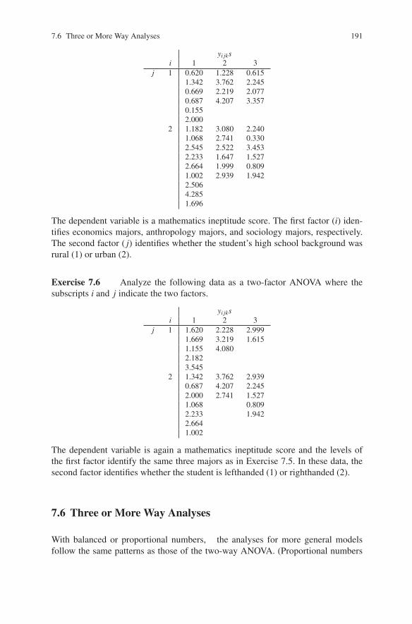
7.6 Three or More Way Analyses 191
yi jksi 1 2 3
j 1 0.620 1.228 0.6151.342 3.762 2.2450.669 2.219 2.0770.687 4.207 3.3570.1552.000
2 1.182 3.080 2.2401.068 2.741 0.3302.545 2.522 3.4532.233 1.647 1.5272.664 1.999 0.8091.002 2.939 1.9422.5064.2851.696
The dependent variable is a mathematics ineptitude score. The first factor (i) iden-tifies economics majors, anthropology majors, and sociology majors, respectively.The second factor ( j) identifies whether the student’s high school background wasrural (1) or urban (2).
Exercise 7.6 Analyze the following data as a two-factor ANOVA where thesubscripts i and j indicate the two factors.
yi jksi 1 2 3
j 1 1.620 2.228 2.9991.669 3.219 1.6151.155 4.0802.1823.545
2 1.342 3.762 2.9390.687 4.207 2.2452.000 2.741 1.5271.068 0.8092.233 1.9422.6641.002
The dependent variable is again a mathematics ineptitude score and the levels ofthe first factor identify the same three majors as in Exercise 7.5. In these data, thesecond factor identifies whether the student is lefthanded (1) or righthanded (2).
7.6 Three or More Way Analyses
With balanced or proportional numbers, the analyses for more general modelsfollow the same patterns as those of the two-way ANOVA. (Proportional numbers

192 7 Multifactor Analysis of Variance
can be defined in terms of complete independence in higher dimensional tables, seeFienberg (1980) or Christensen (1997).) Consider, for example, the model
yi jkm = μ +αi +η j + γk +(αη)i j +(αγ)ik +(ηγ) jk +(αηγ)i jk + ei jkm,
i = 1, . . . ,a, j = 1, . . . ,b, k = 1, . . . ,c, m = 1, . . . ,N. The sums of squares for the maineffects of α , η , and γ are based on the one-way ANOVA ignoring all other effects,e.g.,
SS(η) = acNb
∑j=1
(y· j·· − y····)2. (1)
The sums of squares for the two-way interactions, αη , αγ , and ηγ , are obtained asin the two-way ANOVA by ignoring the third effect, e.g.,
SS(αγ) = bNa
∑i=1
c
∑k=1
(yi·k· − yi··· − y··k· + y····)2. (2)
The sum of squares for the three-way interaction αηγ is found by subtracting allof the other sums of squares (including the grand mean’s) from the sum of squaresfor the full model. Note that the full model is equivalent to the one-way ANOVAmodel
yi jkm = μi jk + ei jkm.
Sums of squares and their associated projection operators are defined from reducedmodels. For example, Mη is the perpendicular projection operator for fitting the ηsafter μ in the model
yi jkm = μ +η j + ei jkm.
The subscripts i, k, and m are used to indicate the replications in this one-wayANOVA. SS(η) is defined by
SS(η) = Y ′MηY.
The algebraic formula for SS(η) was given in (1). Similarly, Mαγ is the projectionoperator for fitting the (αγ)s after μ , the αs, and the γs in the model
yi jkm = μ +αi + γk +(αγ)ik + ei jkm.
In this model, the subscripts j and m are used to indicate replication. The sum ofsquares SS(αγ) is
SS(αγ) = Y ′MαγY.
The algebraic formula for SS(αγ) was given in (2). Because all of the projectionoperators (except for the three-factor interaction) are defined on the basis of reducedmodels that have previously been discussed, the sums of squares take on the familiarforms indicated above.
The one new aspect of the model that we are considering is the inclusion of thethree-factor interaction. As mentioned above, the sum of squares for the three-factor

7.6 Three or More Way Analyses 193
interaction is just the sum of squares that is left after fitting everything else, i.e.,
SS(αηγ) = R((αηγ)|μ,α,η,γ,(αη),(αγ),(ηγ)).
The space for the three-factor interaction is the orthogonal complement (with re-spect to the space for the full model) of the design space for the model that includesall factors except the three-factor interaction. Thus, the space for the three-factorinteraction is orthogonal to everything else. (This is true even when the numbers arenot balanced.)
In order to ensure a nice analysis, we need to show that the spaces associatedwith all of the projection operators are orthogonal and that the projection operatorsadd up to the perpendicular projection operator onto the space for the full model.First, we show that C(Mμ ,Mα ,Mη ,Mγ ,Mαη ,Mαγ ,Mηγ) is the column space for themodel
yi jkm = μ +αi +η j + γk +(αη)i j +(αγ)ik +(ηγ) jk + ei jkm,
and that all the projection operators are orthogonal. That the column spaces are thesame follows from the fact that the column space of the model without the three-factor interaction is precisely the column space obtained by combining the columnspaces of all of the two-factor with interaction models. Combining the spaces ofthe projection operators is precisely combining the column spaces of all the two-factor with interaction models. That the spaces associated with all of the projectionoperators are orthogonal follows easily from the fact that all of the spaces comefrom reduced models. For the reduced models, characterizations have been givenfor the various spaces. For example,
C(Mη) = {v|v = [vi jkm], where vi jkm = d j for some d1, . . . ,db with d· = 0}.
Similarly,
C(Mαγ) = {w|w = [wi jkm], where wi jkm = rik for some rik
with ri· = r·k = 0 for i = 1, . . . ,a,k = 1, . . . ,c}.
With these characterizations, it is a simple matter to show that the projection opera-tors define orthogonal spaces.
Let M denote the perpendicular projection operator for the full model. The pro-jection operator onto the interaction space, Mαηγ , has been defined as
Mαηγ = M− [Mμ +Mα +Mη +Mγ +Mαη +Mαγ +Mηγ ];
thus,M = Mμ +Mα +Mη +Mγ +Mαη +Mαγ +Mηγ +Mαηγ ,
where the spaces of all the projection operators on the right side of the equation areorthogonal to each other.
Exercise 7.7 Show that C(Mη) ⊥C(Mαγ) and that C(Mηγ) ⊥C(Mαγ). Give an

194 7 Multifactor Analysis of Variance
explicit characterization of a typical vector in C(Mαηγ) and show that your charac-terization is correct.
If the α , η , and γ effects correspond to quantitative levels of some factor, thethree-way ANOVA corresponds to a polynomial in three variables. The main effectsand the two-way interactions can be dealt with as before. The three-way interactioncan be broken down into contrasts such as the linear-by-linear-by-quadratic.
For unequal numbers, the analysis can be performed by comparing models.
EXAMPLE 7.6.1. Table 7.8 below is derived from Scheffe (1959) and gives themoisture content (in grams) for samples of a food product made with three kinds ofsalt (A), three amounts of salt (B), and two additives (C). The amounts of salt, asmeasured in moles, are equally spaced. The two numbers listed for some treatmentcombinations are replications. We wish to analyze these data.
Table 7.8 Moisture Content of a Food Product.
A (salt) 1 2 3B (amount salt) 1 2 3 1 2 3 1 2 3
1 8 17 22 7 26 34 10 24 3913 20 10 24 9 36
C (additive)2 5 11 16 3 17 32 5 16 33
4 10 15 5 19 29 4 34
We will consider these data as a three-factor ANOVA. From the structure of thereplications, the ANOVA has unequal numbers. The general model for a three-factorANOVA with replications is
yi jkm = G+Ai +B j +Ck +[AB]i j +[AC]ik +[BC] jk +[ABC]i jk + ei jkm.
Our first priority is to find out which interactions are important. Table 7.9 con-tains the sum of squares for error and the degrees of freedom for error for all modelsthat include all of the main effects. Each model is identified in the table by thehighest order terms in the model (cf. Table 7.5, Section 5). Readers familiar withmethods for fitting log-linear models (cf. Fienberg, 1980 or Christensen, 1997) willnotice a correspondence between Table 7.9 and similar displays used in fitting three-dimensional contingency tables. The analogies between selecting log-linear modelsand selecting models for unbalanced ANOVA are pervasive.
All of the models have been compared to the full model using F statistics in Ta-ble 7.9. It takes neither a genius nor an F table to see that the only models that fitthe data are the models that include the [AB] interaction. A number of other compar-isons can be made among models that include [AB]. These are [AB][AC][BC] versus[AB][AC], [AB][AC][BC] versus [AB][BC], [AB][AC][BC] versus [AB][C], [AB][AC] ver-sus [AB][C], and [AB][BC] versus [AB][C]. None of the comparisons show any lackof fit. The last two comparisons are illustrated below.

7.6 Three or More Way Analyses 195
Table 7.9 Statistics for Fitting Models to the Data of Table 7.8.
Model SSE df F*[ABC] 32.50 14 —[AB][AC][BC] 39.40 18 0.743[AB][AC] 45.18 20 0.910[AB][BC] 40.46 20 0.572[AC][BC] 333.2 22 16.19[AB][C] 45.75 22 0.713[AC][B] 346.8 24 13.54[BC][A] 339.8 24 13.24[A][B][C] 351.1 26 11.44*The F statistics are for testing each model againstthe model with a three-factor interaction, i.e., [ABC].The denominator of each F statistic isMSE([ABC]) = 32.50/14 = 2.3214.
[AB][AC] versus [AB][C] :
R(AC|AB,C) = 45.75−45.18 = 0.57,
F = (0.57/2)/2.3214 = 0.123.
[AB][BC] versus [AB][C] :
R(BC|AB,C) = 45.75−40.46 = 5.29,
F = (5.29/2)/2.3214 = 1.139.
Note that, by analogy to the commonly accepted practice for balanced ANOVAs,all tests have been performed using MSE([ABC]), that is, the estimate of pure errorfrom the full model.
The smallest model that seems to fit the data adequately is [AB][C]. The F statis-tics for comparing [AB][C] to the larger models are all extremely small. Writing outthe model [AB][C], it is
yi jkm = G+Ai +B j +Ck +[AB]i j + ei jkm.
We need to examine the [AB] interaction. Since the levels of B are quantitative, amodel that is equivalent to [AB][C] is a model that includes the main effects for Cbut, instead of fitting an interaction in A and B, fits a separate regression equation inthe levels of B for each level of A. Let x j, j = 1,2,3, denote the levels of B. Thereare three levels of B, so the most general polynomial we can fit is a second-degreepolynomial in x j. Since the levels of salt were equally spaced, it does not mattermuch what we use for the x js. The computations were performed using x1 = 1,x2 = 2, x3 = 3. In particular, the model [AB][C] was reparameterized as
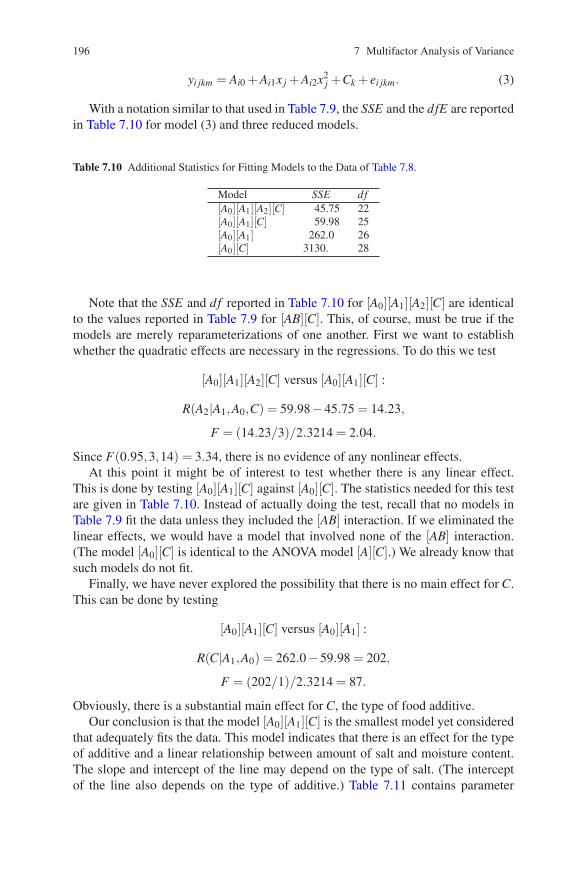
196 7 Multifactor Analysis of Variance
yi jkm = Ai0 +Ai1x j +Ai2x2j +Ck + ei jkm. (3)
With a notation similar to that used in Table 7.9, the SSE and the dfE are reportedin Table 7.10 for model (3) and three reduced models.
Table 7.10 Additional Statistics for Fitting Models to the Data of Table 7.8.
Model SSE df[A0][A1][A2][C] 45.75 22[A0][A1][C] 59.98 25[A0][A1] 262.0 26[A0][C] 3130. 28
Note that the SSE and df reported in Table 7.10 for [A0][A1][A2][C] are identicalto the values reported in Table 7.9 for [AB][C]. This, of course, must be true if themodels are merely reparameterizations of one another. First we want to establishwhether the quadratic effects are necessary in the regressions. To do this we test
[A0][A1][A2][C] versus [A0][A1][C] :
R(A2|A1,A0,C) = 59.98−45.75 = 14.23,
F = (14.23/3)/2.3214 = 2.04.
Since F(0.95,3,14) = 3.34, there is no evidence of any nonlinear effects.At this point it might be of interest to test whether there is any linear effect.
This is done by testing [A0][A1][C] against [A0][C]. The statistics needed for this testare given in Table 7.10. Instead of actually doing the test, recall that no models inTable 7.9 fit the data unless they included the [AB] interaction. If we eliminated thelinear effects, we would have a model that involved none of the [AB] interaction.(The model [A0][C] is identical to the ANOVA model [A][C].) We already know thatsuch models do not fit.
Finally, we have never explored the possibility that there is no main effect for C.This can be done by testing
[A0][A1][C] versus [A0][A1] :
R(C|A1,A0) = 262.0−59.98 = 202,
F = (202/1)/2.3214 = 87.
Obviously, there is a substantial main effect for C, the type of food additive.Our conclusion is that the model [A0][A1][C] is the smallest model yet considered
that adequately fits the data. This model indicates that there is an effect for the typeof additive and a linear relationship between amount of salt and moisture content.The slope and intercept of the line may depend on the type of salt. (The interceptof the line also depends on the type of additive.) Table 7.11 contains parameter

7.6 Three or More Way Analyses 197
estimates and standard errors for the model. All estimates in the example use theside condition C1 = 0.
Table 7.11 Parameter Estimates and Standard Errors for the Model yi jkm = Ai0 +Ai1x j +Ck +ei jkm.
Parameter Estimate S.E.A10 3.350 1.375A11 5.85 0.5909A20 −3.789 1.237A21 13.24 0.5909A30 −4.967 1.231A31 14.25 0.5476C1 0. noneC2 −5.067 0.5522
Note that, in lieu of the F test, the test for the main effect C could be performedby looking at t =−5.067/0.5522 =−9.176. Moreover, we should have t2 = F . Thet statistic squared is 84, while the F statistic reported earlier is 87. The difference isdue to the fact that the S.E. reported uses the MSE for the model being fitted, whilein performing the F test we used the MSE([ABC]).
Are we done yet? No! The parameter estimates suggest some additional ques-tions. Are the slopes for salts 2 and 3 the same, i.e., is A21 = A31? In fact, are theentire lines for salts 2 and 3 the same, i.e., are A21 = A31, A20 = A30? We can fitmodels that incorporate these assumptions.
Model SSE df[A0][A1][C] 59.98 25[A0][A1][C], A21 = A31 63.73 26[A0][A1][C], A21 = A31, A20 = A30 66.97 27
It is a small matter to check that there is no lack of fit displayed by any of thesemodels. The smallest model that fits the data is now [A0][A1][C], A21 = A31, A20 =A30. Thus there seems to be no difference between salts 2 and 3, but salt 1 has adifferent regression than the other two salts. (We did not actually test whether salt 1is different, but if salt 1 had the same slope as the other two, then there would be nointeraction, and we know that interaction exists.) There is also an effect for the foodadditives. The parameter estimates and standard errors for the final model are givenin Table 7.12.
Figure 7.1 shows the fitted values for the final model. The two lines for a givenadditive are shockingly close at B = 1, which makes me wonder if B = 1 is thecondition of no salt being used. Scheffe does not say.
Are we done yet? Probably not. We have not even considered the validity ofthe assumptions. Are the errors normally distributed? Are the variances the samefor every treatment combination? Some methods for addressing these questions arediscussed in Chapter 13. Technically, we need to ask whether C1 = C2 in this new

198 7 Multifactor Analysis of Variance
Table 7.12 Parameter Estimates and Standard Errors for the Model [A0][A1][C], A21 = A31, A20 =A30.
Parameter Estimate S.E.A10 3.395 1.398A11 5.845 0.6008A20 −4.466 0.9030A21 13.81 0.4078C1 0. noneC2 −5.130 0.5602
1.0 1.5 2.0 2.5 3.0
010
2030
40
B
Fitted
(A,C)(1,1)(1,2)(2,1)(2,2)
Fig. 7.1 Fitted values for Scheffe’s (1959) moisture content data.
model. A quick look at the estimate and standard error for C2 answers the questionin the negative. We also have not asked whether A10 = A20. Personally, I find thislast question so uninteresting that I would be loath to examine it. However, a look atthe estimates and standard errors suggests that the answer is no. A more interestingquestion is whether A10 +A11 = A20 +A21, but it is pretty clear from Figure 7.1 thatthere will be no evidence against this hypothesis that was suggested by the data, cf.Exercise 7.7.6.
As mentioned in Example 7.6.1, the correspondences between log-linear modelsand unbalanced ANOVAs are legion. Often these correspondences have been over-looked. We have just considered a three-factor unbalanced ANOVA. What wouldwe do with a four-factor or five-factor ANOVA? There is a considerable amount ofliterature in log-linear model theory about how to select models when there are a

7.7 Additional Exercises 199
large number of factors. In particular, Benedetti and Brown (1978) and Christensen(1997) have surveyed strategies for selecting log-linear models. Those strategies canbe applied to unbalanced ANOVAs with equal success.
I might also venture a personal opinion that statisticians tend not to spend enoughtime worrying about what high-dimensional ANOVA models actually mean. Log-linear model theorists do worry about interpreting their models. Wermuth (1976)has developed a method of searching among log-linear models that have nice inter-pretations, cf. also Christensen (1997). I believe that her method could be appliedequally well to ANOVA models.
Exercise 7.8 Analyze the following three-way ANOVA: The treatments (amountof flour, brand of flour, and brand of shortening) are indicated by the subscripts i,j, and k, respectively. The dependent variable is a “chewiness” score for chocolatechip cookies. The amounts of flour correspond to quantitative factors,
i 1 2 3xi 3.2 4.4 6.8
The data are:yi jks yi jks
j k i 1 2 3 j k i 1 2 31 1 1.620 3.228 6.615 2 1 2.282 5.080 8.240
1.342 5.762 8.245 2.068 4.741 6.3308.077 3.545 4.522 9.453
7.727
1 2 2.669 6.219 11.357 2 2 4.233 4.647 7.8092.687 8.207 4.664 4.999 8.9422.155 3.002 5.9394.000 4.506
6.3853.696
7.7 Additional Exercises
Exercise 7.7.1 In the mid-1970s, a study on the prices of various motor oilswas conducted in (what passes for) a large town in Montana. The study consisted ofpricing 4 brands of oil at each of 9 stores. The data follow.

200 7 Multifactor Analysis of Variance
BrandStore P H V Q
1 87 95 95 822 96 104 106 973 75 87 81 704 81 94 91 775 70 85 87 656 85 98 97 837 110 123 128 1128 83 98 95 789 105 120 119 98
Analyze these data.
Exercise 7.7.2 An experiment was conducted to examine thrust forces whendrilling under different conditions. Data were collected for four drilling speeds andthree feeds. The data are given below.
SpeedFeed 100 250 400 550
121 98 83 58124 108 81 59
0.005 104 87 88 60124 94 90 66110 91 86 56
329 291 281 265331 265 278 265
0.010 324 295 275 269338 288 276 260332 297 287 251
640 569 551 487600 575 552 481
0.015 612 565 570 487620 573 546 500623 588 569 497
Analyze these data.
Exercise 7.7.3 Consider the model
yi jk = μ +αi +η j + γi j + ei jk,
i = 1,2,3,4, j = 1,2,3, k = 1, . . . ,Ni j, where for i �= 1 �= j, Ni j = N, and N11 = 2N.This model could arise from an experimental design having α treatments of NoTreatment (NT), a1, a2, a3 and η treatments of NT, b1, b2. This gives a total of 12treatments: NT, a1, a2, a3, b1, a1b1, a2b1, a3b1 b2, a1b2, a2b2, and a3b2. Since NTis a control, it might be of interest to compare all of the treatments to NT. If NT is toplay such an important role in the analysis, it is reasonable to take more observationson NT than on the other treatments. Find sums of squares for testing

7.7 Additional Exercises 201
(a) no differences between a1, a2, a3,(b) no differences between b1, b2,(c) no {a1,a2,a3}×{b1,b2} interaction,(d) no differences between NT and the averages of a1, a2, and a3 when there
is interaction,(e) no differences between NT and the average of a1, a2, and a3 when there is
no interaction present,(f) no differences between NT and the average of b1 and b2 when there is
interaction,(g) no differences between NT and the average of b1 and b2 when there is no
interaction present.Discuss the orthogonality relationships among the sums of squares. For parts (e) and(g), use the assumption of no interaction. Do not just repeat parts (d) and (f)!
Exercise 7.7.4 Consider the linear model yi j = μ +αi +η j +ei j, i = 1, . . . ,a, j =1, . . . ,b. As in Section 1, write X = [X0,X1, . . . ,Xa,Xa+1, . . . ,Xa+b]. If we write theobservations in the usual order, we can use Kronecker products to write the modelmatrix. Write X = [J,X∗,X∗∗], where X∗ = [X1, . . . ,Xa], and X∗∗ = [Xa+1, . . . ,Xa+b].Using Kronecker products, X∗ = [Ia ⊗ Jb], and X∗∗ = [Ja ⊗ Ib]. In fact, with n = ab,J = Jn = [Ja ⊗ Jb]. Use Kronecker products to show that X ′∗(I − [1/n]Jn
n )X∗∗ = 0. In1 a a+1, . . . ,Za+b).
Also show that [(1/a)Jaa ⊗ Ib] is the perpendicular projection operator onto C(X∗∗)
and that Mη = [(1/a)Jaa ⊗ (Ib − (1/b)Jb
b )].
Exercise 7.7.5 Consider the balanced two-way ANOVA with interaction modelyi jk = μ + αi + η j + γi j + ei jk, i = 1, . . . ,a, j = 1, . . . ,b, k = 1, . . . ,N, with ei jksindependent N(0,σ 2). Find E[Y ′( 1
n Jnn + Mα)Y ] in terms of μ , the αis, the η js, and
the γi js.
Exercise 7.7.6 For Example 7.6.1, develop a test for H0 : A10 +A11 = A20 +A21.
C(Z , . . . ,Z )⊥C(Zterms of Section 1, this is the same as showing that


Chapter 8
Experimental Design Models
The design of an experiment is extremely important. It identifies the class of linearmodels that can be used to analyze the results of the experiment. Perhaps moreaccurately, the design identifies large classes of models that are inappropriate forthe analysis of the experiment. Finding appropriate models can be difficult even inwell-designed experiments.
In this chapter we examine three models used to analyze results obtained fromthree specific experimental designs. The designs are the completely randomizeddesign, the randomized complete block design, and the Latin square design. Wealso examine a particularly effective method of defining treatments for situations inwhich several factors are of interest.
Randomization, that is, the random application of treatments to experimentalunits, provides a philosophical justification for inferring that the treatments actu-ally cause the experimental results. In addition to the models considered here, Ap-pendix G examines estimation for completely randomized designs and randomizedcomplete block designs under an alternative error structure that is derived from theact of randomization.
Blocking is one of the most important concepts in experimental design. Blockingis used to reduce variability for the comparison of treatments. Blocking consists ofgrouping experimental units that will act similarly into blocks and then (randomly)applying the treatments to the units in each block. A randomized complete blockdesign is one in which each block has exactly the same number of units as there aretreatments. Each treatment is applied once in each block. If there are more units thantreatments, we can have a complete block with replications. If there are fewer unitsthan treatments, we have an incomplete block design. A major issue in the subject ofexperimental design is how one should assign treatments to blocks in an incompleteblock design. Latin square designs are complete block designs that incorporate twoseparate forms of blocking.
The analysis of balanced incomplete block designs is derived in Section 9.4.Alternative methods for blocking designs are examined in the exercises for Sec-tion 11.1 and in Section 12.11. For an excellent discussion of the concepts underly-ing the design of experiments, see Fisher (1935) or Cox (1958). For more detailed
© Springer Science+Business Media, LLC 2011
203Springer Texts in Statistics, DOI 10.1007/978-1-4419-9816-3_8, R. Christensen, Plane Answers to Complex Questions: The Theory of Linear Models,

204 8 Experimental Design Models
discussion of the design and analysis of experiments, there are many good booksincluding Hinkelmann and Kempthorne (1994), Cochran and Cox (1957), Casella(2008), or [blush, blush] Christensen (1996a).
8.1 Completely Randomized Designs
The simplest experimental design is the completely randomized design (CRD). Itinvolves no blocking. The experimental technique is simply to decide how manyobservations are to be taken on each treatment, obtain an adequate number of exper-imental units, and apply the treatments to the units (randomly). The standard modelfor this design is
yi j = μ +αi + ei j,
i = 1, . . . ,a, j = 1, . . . ,Ni, E(ei j) = 0, Var(ei j) = σ 2, Cov(ei j,ei′ j′) = 0 if (i, j) �=(i′, j′). This is a one-way ANOVA model and is analyzed as such.
8.2 Randomized Complete Block Designs: Usual Theory
The model usually assumed for a randomized complete block design (RCB) is
yi j = μ +αi +β j + ei j,
i = 1, . . . ,a, j = 1, . . . ,b, E(ei j) = 0, Var(ei j) = σ2, Cov(ei j,ei′ j′) = 0 if (i, j) �=(i′, j′). The β js stand for an additive effect for each block; the αis are an additiveeffect for each treatment. It is assumed that any block-treatment interaction is errorso that an estimate of σ 2 is available. This randomized complete block model is justa two-way ANOVA without interaction.
In this chapter, we are presenting models that are generally used for analyzingexperiments conducted with certain standard experimental designs. Many peoplebelieve that these models are useful only because they are good approximations tolinear models derived from the random application of the treatments to experimentalunits. This randomization theory leads to the conclusion that there is no valid testfor block effects. On the other hand, there is nothing in the two-way ANOVA modelgiven above to keep one from testing block effects. It is my opinion that this contra-diction arises simply because the two-way ANOVA model is not very appropriatefor a randomized complete block design. For example, a basic idea of blocking isthat results within a block should be more alike than results in different blocks. Thetwo-way ANOVA, with only an additive effect for blocks, is a very simplistic model.Another key idea of blocking is that it reduces the variability of treatment compar-isons. It is not clear how the existence of additive block effects reduces variabilityin a two-way ANOVA. The question of how blocking achieves variance reduction

8.3 Latin Square Designs 205
is addressed in Exercise 8.1. Exercises 11.4 through 11.6 discuss alternative modelsfor complete block designs.
Appendix G defines linear models for completely randomized designs and ran-domized complete block designs that are based on randomization theory. It is shown,using Theorem 10.4.5 (or Proposition 2.7.5), that least squares estimates are BLUEsfor the randomization theory models.
Exercise 8.1 Using a randomized complete block design is supposed to reducethe variability of treatment comparisons. If the randomized complete block modelis taken as
yi j = μ +αi +β j + ei j, ei js i.i.d. N(0,σ 2),
i = 1, . . . ,a, j = 1, . . . ,b, argue that the corresponding variance for a completelyrandomized design should be σ 2 +∑b
j=1(μ j − μ·)2/b, where μi = μ +β j.Hint: Figure out what population a completely randomized design would have to
be sampled from.
8.3 Latin Square Designs
A Latin square is a design that allows for treatment effects and two different kindsof block effects. The number of treatments must equal the number of blocks of eachkind. On occasion, the design is used with two kinds of treatments (each with thesame number of levels) and one block effect.
EXAMPLE 8.3.1. A 4× 4 Latin square has four treatments, say, T1, T2, T3, T4.Consider the block effects as row effects, R1, R2, R3, and R4 and column effects C1,C2, C3, and C4. We can diagram one example of a 4×4 Latin square as
C1 C2 C3 C4R1 T1 T2 T3 T4R2 T2 T3 T4 T1R3 T3 T4 T1 T2R4 T4 T1 T2 T3
The key idea is that each treatment occurs once in each row and once in each column.
The model for an a×a Latin square design is
yi jk = μ +αi +β j + γk + ei jk,
E(ei jk) = 0, Var(ei jk) = σ 2, Cov(ei jk,ei′ j′k′) = 0 if (i, j,k) �= (i′, j′,k′). The corre-spondence between the rows, columns, and treatments and the effects in the modelis: αi is the effect for row Ri, β j is the effect for column Cj, and γk is the effect fortreatment Tk. The subscripting in this model is unusual. The key point is that in a
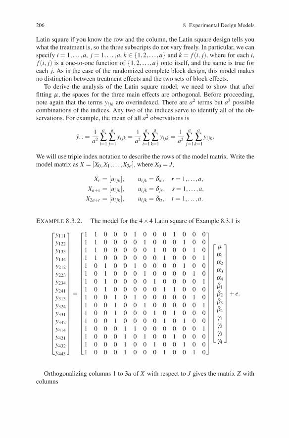
206 8 Experimental Design Models
Latin square if you know the row and the column, the Latin square design tells youwhat the treatment is, so the three subscripts do not vary freely. In particular, we canspecify i = 1, . . . ,a, j = 1, . . . ,a, k ∈ {1,2, . . . ,a} and k = f (i, j), where for each i,f (i, j) is a one-to-one function of {1,2, . . . ,a} onto itself, and the same is true foreach j. As in the case of the randomized complete block design, this model makesno distinction between treatment effects and the two sets of block effects.
To derive the analysis of the Latin square model, we need to show that afterfitting μ , the spaces for the three main effects are orthogonal. Before proceeding,note again that the terms yi jk are overindexed. There are a2 terms but a3 possiblecombinations of the indices. Any two of the indices serve to identify all of the ob-servations. For example, the mean of all a2 observations is
y··· =1a2
a
∑i=1
a
∑j=1
yi jk =1a2
a
∑i=1
a
∑k=1
yi jk =1a2
a
∑j=1
a
∑k=1
yi jk.
We will use triple index notation to describe the rows of the model matrix. Write themodel matrix as X = [X0,X1, . . . ,X3a], where X0 = J,
Xr = [ui jk], ui jk = δir, r = 1, . . . ,a,
Xa+s = [ui jk], ui jk = δ js, s = 1, . . . ,a,
X2a+t = [ui jk], ui jk = δkt , t = 1, . . . ,a.
EXAMPLE 8.3.2. The model for the 4×4 Latin square of Example 8.3.1 is⎡⎢⎢⎢⎢⎢⎢⎢⎢⎢⎢⎢⎢⎢⎢⎢⎢⎢⎢⎢⎢⎢⎢⎢⎢⎢⎣
y111y122y133y144y212y223y234y241y313y324y331y342y414y421y432y443
⎤⎥⎥⎥⎥⎥⎥⎥⎥⎥⎥⎥⎥⎥⎥⎥⎥⎥⎥⎥⎥⎥⎥⎥⎥⎥⎦
=
⎡⎢⎢⎢⎢⎢⎢⎢⎢⎢⎢⎢⎢⎢⎢⎢⎢⎢⎢⎢⎢⎢⎢⎢⎢⎢⎣
1 1 0 0 0 1 0 0 0 1 0 0 01 1 0 0 0 0 1 0 0 0 1 0 01 1 0 0 0 0 0 1 0 0 0 1 01 1 0 0 0 0 0 0 1 0 0 0 11 0 1 0 0 1 0 0 0 0 1 0 01 0 1 0 0 0 1 0 0 0 0 1 01 0 1 0 0 0 0 1 0 0 0 0 11 0 1 0 0 0 0 0 1 1 0 0 01 0 0 1 0 1 0 0 0 0 0 1 01 0 0 1 0 0 1 0 0 0 0 0 11 0 0 1 0 0 0 1 0 1 0 0 01 0 0 1 0 0 0 0 1 0 1 0 01 0 0 0 1 1 0 0 0 0 0 0 11 0 0 0 1 0 1 0 0 1 0 0 01 0 0 0 1 0 0 1 0 0 1 0 01 0 0 0 1 0 0 0 1 0 0 1 0
⎤⎥⎥⎥⎥⎥⎥⎥⎥⎥⎥⎥⎥⎥⎥⎥⎥⎥⎥⎥⎥⎥⎥⎥⎥⎥⎦
⎡⎢⎢⎢⎢⎢⎢⎢⎢⎢⎢⎢⎢⎢⎢⎢⎢⎢⎢⎢⎣
μα1α2α3α4β1β2β3β4γ1γ2γ3γ4
⎤⎥⎥⎥⎥⎥⎥⎥⎥⎥⎥⎥⎥⎥⎥⎥⎥⎥⎥⎥⎦
+ e.
Orthogonalizing columns 1 to 3a of X with respect to J gives the matrix Z withcolumns

8.3 Latin Square Designs 207
Z0 = X0
Zi = Xi − X ′i J
J′JJ = Xi − a
a2 J, i = 1, . . . ,3a.
The three spaces C(Z1, . . . ,Za), C(Za+1, . . . ,Z2a), and C(Z2a+1, . . . ,Z3a) are orthog-onal. For example, with r = 1, . . . ,a and t = 1, . . . ,a,
Z′rZ2a+t =
a
∑i=1
a
∑k=1
(δir − 1
a
)(δkt − 1
a
)=
a
∑i=1
a
∑k=1
δirδkt −a
∑i=1
a
∑k=1
δir/a−a
∑i=1
a
∑k=1
δkt/a+a
∑i=1
a
∑k=1
1/a2
= 1−1−1+1= 0.
Similar computations establish the other orthogonality relationships.Because of the orthogonality, the sum of squares for dropping, say, the αis from
the model is just the sum of squares for dropping the αis from a one-way ANOVAmodel that ignores the β j and γk effects. The ANOVA table is
ANOVASource d f SS E(MS)
μ 1 a2y2··· σ2 +a2(μ + α· + β· + γ·)2
α a−1 a∑ai=1(yi·· − y···)2 σ2 + a
a−1 ∑ai=1(αi − α·)2
β a−1 a∑aj=1(y· j· − y···)2 σ2 + a
a−1 ∑aj=1(β j − β·)2
γ a−1 a∑ak=1(y··k − y···)2 σ2 + a
a−1 ∑ak=1(γk − γ·)2
Error (a−2)(a−1) by subtraction σ2
Total a2 ∑ai=1 ∑a
j=1 y2i jk
Estimation and testing in one of the treatment (block) spaces depends only on theappropriate projection operator. Since we have the usual one-way ANOVA projec-tion operators, estimation and testing are performed in the usual way.
The Latin square model assumes that the (αβ ), (αγ), (βγ), and (αβγ) interac-tions are nonexistent. This assumption is necessary in order to obtain an estimate oferror. If an outside estimate of σ 2 is available, it might be hoped that the interactionscould be examined. Unfortunately, it is impossible to tell from which interaction thedegrees of freedom called “error” come from. For example, in the 4×4 Latin squareof the example, the (αβ ) interaction can be broken up into 3 degrees of freedom forγ and 6 degrees of freedom for error. Since a similar result holds for each of theinteractions, the 6 degrees of freedom for error involve all of the interactions.
Exercise 8.2 In the 4×4 Latin square of the examples, show that the 9 degreesof freedom for (αβ ) interaction are being divided into 3 degrees of freedom for γand 6 degrees of freedom for error.
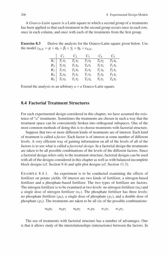
208 8 Experimental Design Models
A Graeco-Latin square is a Latin square in which a second group of a treatmentshas been applied so that each treatment in the second group occurs once in each row,once in each column, and once with each of the treatments from the first group.
Exercise 8.3 Derive the analysis for the Graeco-Latin square given below. Usethe model yhi jk = μ +αh +βi + γ j +ηk + ehi jk.
C1 C2 C3 C4 C5R1 T1τ1 T2τ3 T3τ5 T4τ2 T5τ4R2 T2τ2 T3τ4 T4τ1 T5τ3 T1τ5R3 T3τ3 T4τ5 T5τ2 T1τ4 T2τ1R4 T4τ4 T5τ1 T1τ3 T2τ5 T3τ2R5 T5τ5 T1τ2 T2τ4 T3τ1 T4τ3
Extend the analysis to an arbitrary a×a Graeco-Latin square.
8.4 Factorial Treatment Structures
For each experimental design considered in this chapter, we have assumed the exis-tence of “a” treatments. Sometimes the treatments are chosen in such a way that thetreatment space can be conveniently broken into orthogonal subspaces. One of themost common methods of doing this is to choose treatments with factorial structure.
Suppose that two or more different kinds of treatments are of interest. Each kindof treatment is called a factor. Each factor is of interest at some number of differentlevels. A very efficient way of gaining information on all of the levels of all of thefactors is to use what is called a factorial design. In a factorial design the treatmentsare taken to be all possible combinations of the levels of the different factors. Sincea factorial design refers only to the treatment structure, factorial designs can be usedwith all of the designs considered in this chapter as well as with balanced incompleteblock designs (cf. Section 9.4) and split plot designs (cf. Section 11.3).
EXAMPLE 8.4.1. An experiment is to be conducted examining the effects offertilizer on potato yields. Of interest are two kinds of fertilizer, a nitrogen-basedfertilizer and a phosphate-based fertilizer. The two types of fertilizer are factors.The nitrogen fertilizer is to be examined at two levels: no nitrogen fertilizer (n0) anda single dose of nitrogen fertilizer (n1). The phosphate fertilizer has three levels:no phosphate fertilizer (p0), a single dose of phosphate (p1), and a double dose ofphosphate (p2). The treatments are taken to be all six of the possible combinations:
n0 p0 n0 p1 n0 p2 n1 p0 n1 p1 n1 p2.
The use of treatments with factorial structure has a number of advantages. Oneis that it allows study of the interrelationships (interactions) between the factors. In

8.4 Factorial Treatment Structures 209
Example 8.4.1, it is possible to examine whether the levels of phosphate have dif-ferent effects depending on whether or not nitrogen was applied. Another advantageis that if there are no interactions, the experimental material is used very efficiently.Suppose that there is no interaction between nitrogen and phosphate. The effect ofnitrogen is the difference in yields between experimental units that have the samelevel of phosphate but different levels of nitrogen, that is,
n0 p0 −n1 p0,
n0 p1 −n1 p1,
andn0 p2 −n1 p2.
In each case, the only difference in the pair of treatments is the difference in ni-trogen. At the same time, the difference in, say, the effects of p1 and p2 can beexamined by looking at the differences
n0 p1 −n0 p2
andn1 p1 −n1 p2.
The same treatments are used to obtain estimates of both the nitrogen effect and thephosphate effect.
We now examine the analysis of designs having factorial treatment structure.Consider a randomized complete block design with c blocks, where the treatmentsare all combinations of two factors, say A and B. Suppose factor A has a levels andfactor B has b levels. The total number of treatments is ab. Rewriting the model ofSection 2 with τh denoting treatment effects and ξk denoting block effects, we get
yhk = μ + τh +ξk + ehk, (1)
h = 1, . . . ,ab, k = 1, . . . ,c. In this model, each treatment is indicated by an index h.Since the treatments consist of all combinations of two factors, it makes sense touse two indices to identify treatments: one index for each factor. With this idea wecan rewrite model (1) as
yi jk = μ + τi j +ξk + ei jk, (2)
i = 1, . . . ,a, j = 1, . . . ,b, k = 1, . . . ,c.
Exercise 8.4 For model (1), C(Mτ ) is given by Proposition 4.2.3. What is C(Mτ)in the notation of model (2)?
The orthogonal breakdown of the treatment space follows from a reparameteri-zation of model (2). Model (2) can be rewritten as

210 8 Experimental Design Models
yi jk = μ +αi +β j +(αβ )i j +ξk + ei jk. (3)
The new parameterization is simply τi j = αi +β j +(αβ )i j. Using the ideas of Sec-tions 7.1 and 7.2, the treatment space C(Mτ ) can be broken up into three orthogonalsubspaces: one for factor A, C(Mα), one for factor B, C(Mβ ), and one for interac-tion, C(Mαβ ). The analysis of model (3) follows along the lines of Chapter 7. Model(3) is just a balanced three-way ANOVA in which some of the interactions (namely,any interactions that involve blocks) have been thrown into the error.
In practice, it is particularly important to be able to relate contrasts in the treat-ments (τi js) to contrasts in the main effects (αis and β js) and contrasts in the inter-actions ((αβ )i js). The relationship is demonstrated in Exercise 8.5. The relationshipis illustrated in the following example.
EXAMPLE 8.4.2. Consider the treatments of Example 8.4.1. There is one contrastin nitrogen,
n0 n1N 1 −1
The two orthogonal polynomial contrasts in phosphate are:
p0 p1 p2P linear −1 0 1P quadratic 1 −2 1
The main effect contrasts define two orthogonal interaction contrasts: N −P linear
p0 p1 p2n0 −1 0 1n1 1 0 −1
and N −P quadratic
p0 p1 p2n0 1 −2 1n1 −1 2 −1
The corresponding contrasts in the six treatments are:
n0 p0 n0 p1 n0 p2 n1 p0 n1 p1 n1 p2N 1 1 1 −1 −1 −1P linear −1 0 1 −1 0 1P quadradic 1 −2 1 1 −2 1N −P linear −1 0 1 1 0 −1N −P quadradic 1 −2 1 −1 2 −1
It is easily verified that these five contrasts are orthogonal.
Exercise 8.5 Show that the contrasts in the τi js corresponding to the contrasts∑λiαi and ∑∑λiη j(αβ )i j are ∑∑λiτi j and ∑∑λiη jτi j, respectively.

8.5 More on Factorial Treatment Structures 211
Hint: Any contrast in the τi js corresponds to a vector in C(Mτ ), just as any con-trast in the αis corresponds to a vector in C(Mα) ⊂C(Mτ ). Recall that contrasts areonly defined up to constant multiples; and that contrasts in the αis also involve theinteractions when interaction exists.
8.5 More on Factorial Treatment Structures
We now present a more theoretical discussion of factorial treatment structures andsome interesting new models.
For two factors, say α at s levels and η at t levels, there are a total of p ≡ sttreatment groups. Start by considering a linear model for the data yi jk = (αη)i j +ei jk. In matrix form, the linear model Y = Xβ +e has X as the indicator matrix usedfor a one-way ANOVA model and β = [(αη)11, . . . ,(αη)st ]′ containing a separateeffect for every combination of the two factors.
More generally, if we have r factors αi with si levels respectively, the factorialstructure defines p = ∏r
i=1 si groups. We again take X to be the one-way ANOVAindicator matrix and define β = [αi1,...,ir ] as a vector providing a separate effect foreach combination of the factors.
The idea is that factorial models are defined by specifying a linear structure forthe group parameters. This consists of putting a linear constraint on β , say β =Up×qγ for some known matrix U , cf. Section 3.3. For example, in the two-factormodel, one such linear constraint is to force an additive main effects model forthe data, yi jk = μ + αi + η j + ei jk. In matrix terms using Kronecker products, thisamounts to specifying that
β =([Js ⊗ Jt ], [Is ⊗ Jt ], [Js ⊗ It ]
)⎡⎣μαη
⎤⎦≡Uγ, (1)
where α = (α1, . . . ,αs)′ and η = (η1, . . . ,ηt)′. As in Section 3.3, the linear modelfor the data has been transformed to Y = XUγ + e, where the model matrix is nowXU , which is a reduced model relative to the original, i.e., C(XU)⊂C(X). Note thatif we define a linear structure for the parameters, β = Uγ and a reduced structure,i.e., β = U0γ0, where C(U0) ⊂C(U), then this also defines a reduced linear modelfor the data in that C(XU0) ⊂C(XU).
I have no difficulty considering all such models to be factorial models, butMcCullagh (2000) proposes a more stringent definition involving “selection in-variance.” The idea is that if you drop various indices from various factors, themodel should somehow remain invariant. This idea can be executed in the follow-ing way: Begin with a linear structure β = Uγ but partition U into sets of columnsU = [U0,U1, . . . ,Um] and then specify that
Ui = [Vi1 ⊗Vi2 ⊗·· ·⊗Vir]. (2)

212 8 Experimental Design Models
Such structures should be sufficient to satisfy the basic idea of selection invariance.However, as will be seen later, other interesting selection invariant factorial modelsrequire us to consider matrices Ui that are linear combinations of matrices with thestructure (2).
An interesting aspect of factorial structures is dealing with factors that have thesame levels. Such factors are called homologous. Example 7.5.1 involves genotypesof mothers and genotypes of litters, but the genotypes are identical for the mothersand the litters, so it provides an example of homologous factors. In the additive two-factor model yi jk = μ +αi +η j + ei jk with s = t and homologous factors, we mightconsider situations such as symmetric additive effects where yi jk = μ +αi +α j +ei jkor alternating (skew symmetric) additive effects where yi jk = μ +αi −α j + ei jk. Asillustrated in (1), we can write the additive model for the parameters in matrix formas
β = Uγ = [Jst ,U1,U2]
⎡⎣μαη
⎤⎦ .
We can now specify symmetric additive effects by specifying α = η to get
β = [Jst ,U1,U2]
⎡⎣μαα
⎤⎦= [Jst ,(U1 +U2)][
μα
],
thus defining the linear model Y = X [Jst ,(U1 +U2)][
μα
]+ e. Similarly, specifying
alternating additive effects α = −η leads to Y = X [Jst ,(U1 −U2)][
μα
]+ e. In a
3 × 3 example with β = [(αη)11,(αη)12, . . . ,(αη)33]′, the additive main effectsmodel has
U = [Jst ,U1,U2] =
⎡⎢⎢⎢⎢⎢⎢⎢⎢⎢⎢⎢⎣
1 1 0 0 1 0 01 1 0 0 0 1 01 1 0 0 0 0 11 0 1 0 1 0 01 0 1 0 0 1 01 0 1 0 0 0 11 0 0 1 1 0 01 0 0 1 0 1 01 0 0 1 0 0 1
⎤⎥⎥⎥⎥⎥⎥⎥⎥⎥⎥⎥⎦.
The symmetric additive effects and alternating additive effects models have

8.5 More on Factorial Treatment Structures 213
[Jst ,U1 +U2] =
⎡⎢⎢⎢⎢⎢⎢⎢⎢⎢⎢⎢⎣
1 2 0 01 1 1 01 1 0 11 1 1 01 0 2 01 0 1 11 1 0 11 0 1 11 0 0 2
⎤⎥⎥⎥⎥⎥⎥⎥⎥⎥⎥⎥⎦, [Jst ,(U1 −U2)] =
⎡⎢⎢⎢⎢⎢⎢⎢⎢⎢⎢⎢⎣
1 0 0 01 1 −1 01 1 0 −11 −1 1 01 0 0 01 0 1 −11 −1 0 11 0 −1 11 0 0 0
⎤⎥⎥⎥⎥⎥⎥⎥⎥⎥⎥⎥⎦,
respectively. Given the simple structure of the original one-way ANOVA matrix X ,the reduced model matrices X [Jst ,(U1 +U2)] and X [Jst ,(U1 −U2)] have structuresvery similar to [Jst ,(U1 +U2)] and [Jst ,(U1 −U2)]. However, these linear structuresfor the parameters are not of the form (2), hence the need to consider linear combi-nations of terms like those in (2).
Models specifying such things as simple symmetry (αη)i j = (αη) ji can also bespecified quite easily by defining an appropriate U matrix, e.g.,⎡⎢⎢⎢⎢⎢⎢⎢⎢⎢⎢⎢⎣
(αη)11(αη)12(αη)13(αη)21(αη)22(αη)23(αη)31(αη)32(αη)33
⎤⎥⎥⎥⎥⎥⎥⎥⎥⎥⎥⎥⎦= β = Uφ =
⎡⎢⎢⎢⎢⎢⎢⎢⎢⎢⎢⎢⎣
1 0 0 0 0 00 1 0 0 0 00 0 1 0 0 00 1 0 0 0 00 0 0 1 0 00 0 0 0 1 00 0 1 0 0 00 0 0 0 1 00 0 0 0 0 1
⎤⎥⎥⎥⎥⎥⎥⎥⎥⎥⎥⎥⎦
⎡⎢⎢⎢⎢⎢⎣φ11φ12φ13φ22φ23φ33
⎤⎥⎥⎥⎥⎥⎦ .
These also fit into the class of linear combinations of matrices with the pattern (2),e.g., the column of U associated with φ23 can be written as⎛⎝⎡⎣0
10
⎤⎦⊗⎡⎣0
01
⎤⎦⎞⎠+
⎛⎝⎡⎣001
⎤⎦⊗⎡⎣0
10
⎤⎦⎞⎠ .
These ideas also apply to generalized linear models. For example, in log-linearmodels, symmetry is sometimes an interesting model, cf. Christensen (1997, Ex-ercise 2.7.10), and the symmetric additive effects model is the model of marginalhomogeneity, cf. Christensen (1997, Exercise 10.8.6). See McCullagh (2000) for amore extensive and theoretical treatment of these ideas.

214 8 Experimental Design Models
8.6 Additional Exercises
Exercise 8.6.1 A study was performed to examine the effect of two factorson increasing muscle mass in weight lifters. The first factor was dietary proteinlevel. The levels were use of a relatively low protein diet (L) and use of a highprotein diet (H). The second factor was the use of anabolic steroids. The first levelconsisted of no steroid use (N) and the second level involved the use of steroids (S).Subjects were chosen so that one subject was in each combination of four heightgroups (i) and four weight groups ( j). Treatments are identified as LN, LS, HN,and HS. The dependent variable is a measure of increase in muscle mass during thetreatment period. The study was replicated in two different years. The height groupsand weight groups changed from the first year to the second year. The design anddata are listed below. Heights are the columns of the squares and weights are therows. Analyze the data.
Year 1Weight
Trt(yi jk) 1 2 3 41 LN(2.7) LS( 4.6) HS(9.3) HN(0.0)
Height 2 LS(2.0) LN( 5.0) HN(9.1) HS(4.5)3 HN(6.4) HS(10.2) LS(6.1) LN(2.9)4 HS(8.3) HN( 6.3) LN(6.3) LS(0.9)
Year 2Weight
Trt(yi jk) 1 2 3 41 LN( 8.6) LS(3.3) HN( 7.6) HS(9.0)
Height 2 LS( 8.9) HN(4.7) HS(12.2) LN(5.2)3 HN(10.0) HS(7.6) LN(12.3) LS(5.4)4 HS(10.0) LN(0.5) LS( 5.0) HN(3.7)
Exercise 8.6.2 Show that the set of indices i = 1, . . . ,a, j = 1, . . . ,a, and k =(i+ j +a−1)mod(a) determines a Latin square design.
Hint: Recall that t mod(a) means t modulo a and is defined as the remainderwhen t is divided by a.

Chapter 9
Analysis of Covariance
Traditionally, analysis of covariance (ACOVA) has been used as a tool in the anal-ysis of designed experiments. Suppose one or more measurements are made ona group of experimental units. In an agricultural experiment, such a measurementmight be the amount of nitrogen in each plot of ground prior to the application ofany treatments. In animal husbandry, the measurements might be the height andweight of animals before treatments are applied. One way to use such informationis to create blocks of experimental units that have similar values of the measure-ments. Analysis of covariance uses a different approach. In analysis of covariance,an experimental design is chosen that does not depend on these supplemental obser-vations. The concomitant observations come into play as regression variables thatare added to the basic experimental design model.
The goal of analysis of covariance is the same as the goal of blocking. The re-gression variables are used to reduce the variability of treatment comparisons. Inthis traditional context, comparisons among treatments remain the primary goal ofthe analysis. Exercises 9.1 and 9.5 are important practical illustrations of how thisis accomplished. Snedecor and Cochran (1980, Chapter 18) discuss the practicaluses of analysis of covariance. Cox (1958, Chapter 4) discusses the proper role ofconcomitant observations in experimental design. Biometrics has devoted two en-tire issues to analysis of covariance: Volume 13, Number 3, 1957 and Volume 38,Number 3, 1982.
From a theoretical point of view, analysis of covariance involves the analysis ofa model with a partitioned model matrix, say
Y = [X ,Z][
βγ
]+ e, (1)
where X is an n× p matrix, Z is an n × s matrix, E(e) = 0, and Cov(e) = σ 2I.Analysis of covariance is a technique for analyzing model (1) based on the analysisof the reduced model
Y = Xδ + e. (2)
© Springer Science+Business Media, LLC 2011
215Springer Texts in Statistics, DOI 10.1007/978-1-4419-9816-3_9, R. Christensen, Plane Answers to Complex Questions: The Theory of Linear Models,

216 9 Analysis of Covariance
The point is that model (2) should be a model whose analysis is relatively easy.In traditional applications, X is taken as the model matrix for a balanced analysisof variance. The Z matrix can be anything, but traditionally consists of columns ofregression variables.
The practical application of general linear model theory is prohibitively difficultwithout a computer program to perform the worst of the calculations. There are,however, special cases: notably, simple linear regression, one-way ANOVA, andbalanced multifactor ANOVA, in which the calculations are not prohibitive. Analy-sis of covariance allows computations of the BLUEs and the SSE for model (1) byperforming several analyses on tractable special cases plus finding the generalizedinverse of an s× s matrix. Since finding the generalized inverse of anything biggerthan, say, a 3× 3 matrix is difficult for hand calculations, one would typically notwant more than three columns in the Z matrix for such purposes.
As mentioned earlier, in the traditional application of performing an ANOVAwhile adjusting for the effect of some regression variables, the primary interest isin the ANOVA. The regression variables are there only to sharpen the analysis. Theinference on the ANOVA part of the model is performed after fitting the regressionvariables. To test whether the regression variables really help to sharpen the analy-sis, they should be tested after fitting the ANOVA portion of the model. The basiccomputation for performing these tests is finding the SSE for model (1). This implic-itly provides a method for finding the SSE for submodels of model (1). Appropriatetests are performed by comparing the SSE for model (1) to the SSEs of the varioussubmodels.
Sections 1 and 2 present the theory of estimation and testing for general parti-tioned models. Sections 3 and 4 present nontraditional applications of the theory.Section 3 applies the analysis of covariance results to the problem of fixing up bal-anced ANOVA problems that have lost their balance due to the existence of somemissing data. Although applying analysis of covariance to missing data problems isnot a traditional experimental design application, it is an application that was usedfor quite some time until computational improvements made it largely unnecessary.Section 4 uses the analysis of covariance results to derive the analysis for balancedincomplete block designs. Section 5 presents Milliken and Graybill’s (1970) test ofa linear model versus a nonlinear alternative.
I might also add that I personally find the techniques of Sections 1 and 2 to besome of the most valuable tools available for deriving results in linear model theory.
9.1 Estimation of Fixed Effects
To obtain least squares estimates, we break the estimation space of model (9.0.1)into two orthogonal parts. As usual, let M be the perpendicular projection operatoronto C(X). Note that C(X ,Z) = C[X ,(I −M)Z]. One way to see this is that frommodel (9.0.1)

9.1 Estimation of Fixed Effects 217
E(Y ) = Xβ +Zγ = Xβ +MZγ +(I −M)Zγ = [X ,MZ][
βγ
]+(I −M)Zγ.
Since C(X)=C([X ,MZ]), clearly model (9.0.1) holds if and only if E(Y )∈C[X ,(I−M)Z].
Let P denote the perpendicular projection matrix onto C([X ,Z]) = C([X ,(I −M)Z]). Since the two sets of column vectors in [X ,(I −M)Z] are orthogonal, theperpendicular projection matrix for the entire space is the sum of the perpendicularprojection matrices for the subspaces C(X) and C[(I −M)Z], cf. Theorem B.45.Thus,
P = M +(I −M)Z[Z′(I −M)Z
]− Z′(I −M)
and writeM(I−M)Z ≡ (I −M)Z
[Z′(I −M)Z
]− Z′(I −M).
Least squares estimates satisfy X β +Zγ = PY = MY +M(I−M)ZY .We now consider estimation of estimable functions of γ and β . The formulae are
simpler if we incorporate the estimate
γ =[Z′(I −M)Z
]− Z′(I −M)Y, (1)
which we will later show to be a least squares estimate.First consider an estimable function of γ , say, ξ ′γ . For this to be estimable, there
exists a vector ρ such that ξ ′γ = ρ ′[Xβ +Zγ ]. For this equality to hold for all β andγ , we must have ρ ′X = 0 and ρ ′Z = ξ ′. The least squares estimate of ξ ′γ is
ρ ′PY = ρ ′{M +M(I−M)Z}
Y
= ρ ′MY +ρ ′(I −M)Z[Z′(I −M)Z
]− Z′(I −M)Y= 0+ρ ′Zγ= ξ ′γ.
The penultimate equality stems from the fact that ρ ′X = 0 implies ρ ′M = 0.An arbitrary estimable function of β , say, λ ′β , has λ ′β = ρ ′[Xβ +Zγ] for some
ρ . For this equality to hold for all β and γ , we must have ρ ′X = λ ′ and ρ ′Z = 0. Asa result, the least squares estimate is
ρ ′PY = ρ ′{M +M(I−M)Z}
Y
= ρ ′MY +ρ ′(I −M)Z[Z′(I −M)Z
]− Z′(I −M)Y= ρ ′MY +ρ ′(I −M)Zγ= ρ ′MY −ρ ′MZγ= ρ ′M(Y −Zγ)
≡ λ ′β .
Define

218 9 Analysis of Covariance
X β = M(Y −Zγ). (2)
We now establish thatX β +Zγ = PY
so that γ is a least squares estimate of γ and and X β is a least squares estimate ofXβ . Write
X β +Zγ = M(Y −Zγ)+Zγ= MY +(I −M)Zγ= MY +M(I−M)ZY = PY.
Often in ACOVA, the X matrix comes from a model that is simple to analyze,like one-way ANOVA or a balanced multifactor ANOVA. If the model Y = Xβ +e has simple formula for computing an estimate of some function λ ′β = ρ ′Xβ ,say a contrast, then that simple formula must be incorporated into ρ ′MY . Underconditions that we will explore, λ ′β is also an estimable function under the ACOVAmodel Y = Xβ +Zγ +e and, with the same vector ρ , the estimate is λ ′β = ρ ′M(Y −Zγ). That means that the same (simple) computational procedure that was appliedto the data Y in order to estimate λ ′β in Y = Xβ +e can also be applied to Y −Zγ toestimate λ ′β in Y = Xβ +Zγ + e, see Exercise 9.1. We now explore the conditionsnecessary to make this happen, along with other issues related to estimability inACOVA models.
Often Z consists of columns of regression variables, in which case Z′(I −M)Z istypically nonsingular. In that case, both γ and Xβ are estimable. In particular,
γ =[Z′(I −M)Z
]−1 Z′(I −M)[Xβ +Zγ]
with estimate
γ =[Z′(I −M)Z
]−1 Z′(I −M)PY
=[Z′(I −M)Z
]−1 Z′(I −M)[M +M(I−M)Z ]Y
=[Z′(I −M)Z
]−1 Z′(I −M)M(I−M)ZY
=[Z′(I −M)Z
]−1 Z′(I −M)Y.
X is traditionally the model matrix for an ANOVA model, so β is usually not es-timable. However, when Z′(I −M)Z is nonsingular, Xβ is estimable in the ACOVAmodel. Observe that{
I −Z[Z′(I −M)Z
]−1 Z′(I −M)}
[Xβ +Zγ]
= Xβ +Zγ −Z[Z′(I −M)Z
]−1 Z′(I −M)Zγ= Xβ +Zγ −Zγ= Xβ .

9.1 Estimation of Fixed Effects 219
Thus, in the nonsingular case, anything that is estimable in Y = Xβ + e is alsoestimable in the ACOVA model. In particular, if λ ′ = ρ ′X , the estimate of λ ′β inY = Xβ + e is ρ ′MY . Clearly, for the ACOVA model,
ρ ′{
I −Z[Z′(I −M)Z
]−1 Z′(I −M)}
[Xβ +Zγ] = ρ ′Xβ = λ ′β
and the estimate is
λ ′β = ρ ′{
I −Z[Z′(I −M)Z
]−1 Z′(I −M)}
PY.
We now show that λ ′β = ρ ′M(Y − Zγ). As mentioned earlier, the beauty of thisresult is that if we know how to estimate λ ′β in Y = Xβ + e using Y , exactly thesame method applied to Y −Zγ will give the estimate in the ACOVA model.
As discussed earlier, an estimable function λ ′β , has λ ′β = ρ ′[Xβ +Zγ] for someρ with ρ ′X = λ ′ and ρ ′Z = 0. Also as before, the least squares estimate is
ρ ′PY = ρ ′M(Y −Zγ).
In the nonsingular case, if ρ is any vector that has ρ ′X = λ ′, we can turn it into avector ρ that has both ρ ′X = λ ′ and ρ ′Z = 0, simply by defining
ρ ′ = ρ ′{
I −Z[Z′(I −M)Z
]−1 Z′(I −M)}
.
Moreover,ρ ′M(Y −Zγ) = ρ ′M(Y −Zγ),
so the same estimation procedure applied to Y in Y = Xβ +e gets applied to Y −Zγin Y = Xβ +Zγ + e when estimating the estimable function λ ′β .
In general, if [Z′(I −M)Z] is singular, neither γ nor Xβ are estimable. The es-timable functions of γ will be those that are linear functions of (I −M)Zγ . This isshown below.
Proposition 9.1.1. ξ ′γ is estimable if and only if ξ ′ = ρ ′(I −M)Z for somevector ρ .
PROOF. If ξ ′γ is estimable, there exists ρ such that ξ ′γ = ρ ′[X ,Z][
βγ
], so
ρ ′[X ,Z] = (0,ξ ′) and ρ ′X = 0. Therefore, ξ ′ = ρ ′Z = ρ ′(I −M)Z. Conversely, if
ξ ′ = ρ ′(I −M)Z then ρ ′(I −M)[X ,Z][
βγ
]= ξ ′γ . �
Proposition 9.1.1 is phrased in terms of estimating a function of γ , but it also applieswith appropriate changes to estimation of β .
Finally, if Xβ and γ are estimable, that is, if (I−M)Z is of full rank, it is easy tosee that

220 9 Analysis of Covariance
Cov[
X βγ
]= σ 2
[M +MZ [Z′(I −M)Z]−1 Z′M −MZ [Z′(I −M)Z]−1
− [Z′(I −M)Z]−1 Z′M [Z′(I −M)Z]−1
].
9.2 Estimation of Error and Tests of Hypotheses
The estimate of the variance σ 2 is the MSE. We will find SSE =Y ′(I−P)Y in termsof M and Z. The error sum of squares is
Y ′(I −P)Y = Y ′[(I −M)− (I −M)Z
[Z′(I −M)Z
]− Z′(I −M)]Y (1)
= Y ′(I −M)Y −Y ′(I −M)Z[Z′(I −M)Z
]− Z′(I −M)Y.
Using the notation EAB = A′(I −M)B, we have
Y ′(I −P)Y = EYY −EY ZE−ZZEZY .
EXAMPLE 9.2.1. Consider a balanced two-way analysis of variance with noreplication and one covariate (regression variable, concomitant variable, supplemen-tal observation). The analysis of covariance model can be written
yi j = μ +αi +η j + γzi j + ei j,
i = 1, . . . ,a, j = 1, . . . ,b. Thus X is the model matrix for the balanced two-wayANOVA without replication,
yi j = μ +αi +η j + ei j,
i = 1, . . . ,a, j = 1, . . . ,b, and Z is an ab× 1 matrix that contains the values of zi j.The sum of squares for error in the covariate analysis is EYY −E2
Y Z/EZZ , where
EYY =a
∑i=1
b
∑j=1
(yi j − yi· − y· j + y··)2 ,
EY Z = EZY =a
∑i=1
b
∑j=1
(yi j − yi· − y· j + y··)(zi j − zi· − z· j + z··) ,
EZZ =a
∑i=1
b
∑j=1
(zi j − zi· − z· j + z··)2 .
Tests for analysis of covariance models are found by considering the reductionsin sums of squares for error due to the models. For instance, if C(X0) ⊂ C(X) andwe want to test the reduced model

9.2 Estimation of Error and Tests of Hypotheses 221
Y = X0β0 +Zγ + e
against the full model (9.0.1), the test statistic is
[Y ′(I −P0)Y −Y ′(I −P)Y ]/ [r(X ,Z)− r(X0,Z)][Y ′(I −P)Y ]/ [n− r(X ,Z)]
,
where P0 is the perpendicular projection operator onto C(X0,Z). We have alreadyfound Y ′(I −P)Y . If M0 is the perpendicular projection operator onto C(X0),
Y ′(I −P0)Y = Y ′(I −M0)Y −Y ′(I −M0)Z[Z′(I −M0)Z
]− Z′(I −M0)Y.
Often these computations can be facilitated by writing an analysis of covariancetable.
EXAMPLE 9.2.1 CONTINUED. The analysis of covariance table is given below inmatrix notation. Recall that, for example,
Y ′MαY = ba
∑i=1
(yi· − y··)2 ,
Y ′MαZ = ba
∑i=1
(yi· − y··)(zi· − z··) ,
Z′MαZ = ba
∑i=1
(zi· − z··)2 .
ACOVA TableSource df SSYY SSY Z SSZZ
Grand Mean 1 Y ′ 1n Jn
nY Y ′ 1n Jn
n Z Z′ 1n Jn
n Z
Treatments (α) a−1 Y ′MαY Y ′Mα Z Z′MαZ
Treatments (η) b−1 Y ′MηY Y ′Mη Z Z′MηZ
Error n−a−b+1 Y ′(I −M)Y Y ′(I −M)Z Z′(I −M)Z
If we want to test H0 : η1 = η2 = · · ·= ηb, the error sum of squares under the reducedmodel is[
Y ′(I −M)Y +Y ′MηY]− [Y ′(I −M)Z +Y ′Mη Z
]× [Z′(I −M)Z +Z′Mη Z
]− [Z′(I −M)Y +Z′MηY].
All of these terms are available from the ACOVA table. With more than one covari-ate, the terms in the SSY Z and SSZZ columns would be matrices and it would be moreinvolved to compute [Z′(I −M)Z +Z′Mη Z]−.
Exercise 9.1 Consider a one-way ANOVA with one covariate. The model is

222 9 Analysis of Covariance
yi j = μ +αi +ξ xi j + ei j,
i = 1, . . . , t, j = 1, . . . ,Ni. Find the BLUE of the contrast ∑ti=1 λiαi. Find the variance
of the contrast.
Exercise 9.2 Consider the problem of estimating βp in the regression model
yi = β0 +β1xi1 + · · ·+βpxip + ei. (2)
Let ri be the ordinary residual from fitting
yi = α0 +α1xi1 + · · ·+αp−1xip−1 + ei
and si be the residual from fitting
xip = γ0 + γ1xi1 + · · ·+ γp−1xip−1 + ei.
Show that the least squares estimate of βp is ξ from fitting the model
ri = ξ si + ei, i = 1, . . . ,n, (3)
that the SSE from models (2) and (3) are the same, and that (β0, . . . , βp−1)′ = α −βpγ with α = (α0, . . . , αp−1)′ and γ = (γ0, . . . , γp−1)′. Discuss the usefulness of theseresults for computing regression estimates. (These are the key results behind thesweep operator that is often used in regression computations.) What happens to theresults if ri is replaced by yi in model (3)?
Exercise 9.3 Suppose λ ′1β and λ ′
2γ are estimable in model (9.0.1). Use thenormal equations to find find least squares estimates of λ ′
1β and λ ′2γ .
Hint: Reparameterize the model as Xβ +Zγ = Xδ +(I −M)Zγ and use the nor-mal equations on the reparameterized model. Note that Xδ = Xβ +MZγ .
Exercise 9.4 Derive the test for model (9.0.1) versus the reduced model Y =Xβ + Z0γ0 + e, where C(Z0) ⊂ C(Z). Describe how the procedure would work fortesting H0 : γ2 = 0 in the model yi j = μ +αi +η j + γ1zi j1 + γ2zi j2 +ei j, i = 1, . . . ,a,j = 1, . . . ,b.
Exercise 9.5 An experiment was conducted with two treatments. There werefour levels of the first treatment and five levels of the second treatment. Besides thedata y, two covariates were measured, x1 and x2. The data are given below. Analyzethe data with the assumption that there is no interaction between the treatments.

9.3 Application: Missing Data 223
i j yi j x1i j x2i j i j yi j x1i j x2i j1 1 27.8 5.3 9 3 1 22.4 3.0 13
2 27.8 5.2 11 2 21.0 4.5 123 26.2 3.6 13 3 30.6 5.4 184 24.8 5.2 17 4 25.4 6.6 215 17.8 3.6 10 5 15.9 4.1 9
2 1 19.6 4.7 12 4 1 14.1 5.4 102 28.4 5.8 17 2 29.5 6.8 183 26.3 3.3 22 3 29.2 5.3 224 18.3 4.1 8 4 21.5 6.2 95 20.8 5.7 11 5 25.5 6.4 22
9.3 Application: Missing Data
When a few observations are missing from, say, a balanced multifactor design, thebalance is lost and the analysis would seem to be quite complicated. One use of theanalysis of covariance is to allow the analysis with missing data to be performedusing results for the original balanced design.
Consider an original design
Y = Xβ + e,
with Y = (y1, . . . ,yn)′. For each missing observation yi, include a covariate zi =(0, . . . ,0,1,0, . . . ,0)′ with the 1 in the ith place. Set each yi that is missing equal tozero.
We wish to show that the SSE in this ACOVA model equals the SSE in the modelwith the missing observations deleted. The MSE in the covariance model will alsoequal the MSE in the model with deletions. In the covariance model, although weare artificially adding observations by setting missing observations to zero, we arealso removing those degrees of freedom from the error by adding covariates.
Suppose r observations are missing. Without loss of generality, we can assumethat the last r observations are missing. The n×r matrix of covariates can be written
Z =[
0Ir
],
where Ir is an r× r identity matrix and 0 is an (n− r)× r matrix of zeros. Let X bethe n× p model matrix for the model with no missing observations and let X∗ bethe (n− r)× p model matrix for the model with the missing observations deleted.Again we can assume that
X =[
X∗Xr
],

224 9 Analysis of Covariance
where Xr is the r × p matrix whose rows are the rows of X corresponding to themissing observations. The analysis of covariance model
Y = Xβ +Zγ + e
can now be written as
Y =[
X∗ 0Xr Ir
][βγ
]+ e.
Notice that
C([
X∗ 0Xr Ir
])= C([
X∗ 00 Ir
]).
Let M∗ be the perpendicular projection operator onto C(X∗) and let P be the perpen-dicular projection operator onto
C([
X∗ 0Xr Ir
]).
It is easy to see that
P =[
M∗ 00 Ir
].
Writing Y as Y ′ = [Y ′∗,0], we find that
Y ′(I −P)Y = [Y ′∗ 0 ][
I −M∗ 00 0
][Y∗0
]= Y ′
∗(I −M∗)Y∗.
Since Y ′(I −P)Y is the SSE from the covariate model and Y ′∗(I −M∗)Y∗ is the SSEfor the model with the missing observations dropped, we are done. Note that thevalues we put in for the missing observations do not matter for computing the SSE .Tests of hypotheses can be conducted by comparing SSEs for different models.
With Y ′ = [Y ′∗,0], estimation will be the same in both models. The least squaresestimate of [
X∗βXrβ + γ
]is
PY =[
M∗Y∗0
].
Any estimable function in the model Y∗ = X∗β + e∗ is estimable in the covariatemodel, and the estimates are the same. The function ρ ′∗X∗β equals ρ ′(Xβ + Zγ),where ρ ′ = [ρ ′∗,0] and 0 is a 1× r matrix of zeros. Thus, ρ ′PY = ρ ′∗M∗Y∗.
Exercise 9.6 Show that
P =[
M∗ 00 Ir
].

9.4 Application: Balanced Incomplete Block Designs 225
An alternative approach to the missing value problem is based on finding substi-tutes for the missing values. The substitutes are chosen so that if one acts like thesubstitutes are real data, the correct SSE is computed. (The degrees of freedom forerror must be corrected.)
Setting the problem up as before, we have
Y = Xβ +Zγ + e,
and the estimate γ can be found. It is proposed to treat Y −Zγ = [Y ′∗,−γ ′]′ as the datafrom an experiment with model matrix X . Recalling that γ = [Z′(I −M)Z]−1Z′(I −M)Y , we see that the SSE from this analysis is
(Y −Zγ)′(I −M)(Y −Zγ)= Y ′(I −M)Y −2γ ′Z′(I −M)Y + γ ′Z′(I −M)Zγ= Y ′(I −M)Y −2Y ′(I −M)Z[Z′(I −M)Z]−1Z′(I −M)Y
+Y ′(I −M)Z[Z′(I −M)Z]−1[Z′(I −M)Z][Z′(I −M)Z]−1Z′(I −M)Y= Y ′(I −M)Y −Y ′(I −M)Z[Z′(I −M)Z]−1Z′(I −M)Y,
which is the SSE from the covariate analysis. Therefore, if we replace missing valuesby −γ and do the regular analysis, we get the correct SSE .
This procedure also gives the same estimates as the ACOVA procedure. Usingthis method, the estimate of Xβ is M(Y − Zγ) just as in (9.1.2) of the ACOVAprocedure. The variance of an estimate, say ρ ′X β , needs to be calculated as in ananalysis of covariance. It is σ 2(ρ ′Mρ + ρ ′MZ[Z′(I −M)Z]−1Z′Mρ), not the naivevalue of σ 2ρ ′Mρ .
For r = 1 missing observation and a variety of balanced designs, formulae havebeen obtained for −γ and are available in many statistical methods books.
Exercise 9.7 Derive −γ for a randomized complete block design when r = 1.
9.4 Application: Balanced Incomplete Block Designs
The analysis of covariance technique can be used to develop the analysis of a bal-anced incomplete block design. Suppose that a design is to be set up with b blocksand t treatments, but the number of treatments that can be observed in any block isk, where k < t. One natural way to proceed would be to find a design where eachpair of treatments occurs together in the same block a fixed number of times, say λ .Such a design is called a balanced incomplete block (BIB) design.
Let r be the common number of replications for each treatment. There are twowell-known facts about the parameters introduced so far. First, the total number ofexperimental units in the design must be the number of blocks times the number ofunits in each block, i.e., bk, but the total number of units must also be the number

226 9 Analysis of Covariance
of treatments times the number of times we observe each treatment, i.e., tr; thus
tr = bk. (1)
Second, the number of within block comparisons between any given treatment andthe other treatments is fixed. One way to count this is to multiply the number ofother treatments (t−1) by the number of times each occurs in a block with the giventreatment (λ ). Another way to count it is to multiply the number of other treatmentsin a block (k− 1) times the number of blocks that contain the given treatment (r).Therefore,
(t −1)λ = r(k−1). (2)
EXAMPLE 9.4.1. An experiment was conducted to examine the effects of fertil-izers on potato yields. Six treatments (A, B, C, D, E, and F) were used but blockswere chosen that contained only five experimental units. The experiment was per-formed using a balanced incomplete block design with six blocks. The potato yields(in pounds) along with the mean yield for each block are reported in Table 9.1.
Table 9.1 Potato Yields in Pounds for Six Fertilizer Treatments.
BlockBlock Data Means
1 E 583 B 512 F 661 A 399 C 525 536.02 B 439 C 460 D 424 E 497 F 592 482.43 A 334 E 466 C 492 B 431 D 355 415.64 F 570 D 433 E 514 C 448 A 344 461.85 D 402 A 417 B 420 F 626 E 615 496.06 C 450 F 490 A 268 D 375 B 347 386.0
The six treatments consist of all of the possible combinations of two factors.One factor was that a nitrogen-based fertilizer was either applied (n1) or not applied(n0). The other factor was that a phosphate-based fertilizer was either not applied(p0), applied in a single dose (p1), or applied in a double dose (p2). In terms of thefactorial structure, the six treatments are A = n0 p0, B = n0 p1, C = n0 p2, D = n1 p0,E = n1 p1, and F = n1 p2. From the information in Table 9.1, it is a simple matterto check that t = 6, b = 6, k = 5, r = 5, and λ = 4. After deriving the theory forbalanced incomplete block designs, we will return to these data and analyze them.
The balanced incomplete block model can be written as
yi j = μ +βi + τ j + ei j, ei js i.i.d. N(0,σ 2), (3)
where i = 1, . . . ,b and j ∈ Di or j = 1, . . . , t and i ∈ A j. Di is the set of indices forthe treatments in block i. A j is the set of indices for the blocks in which treatment joccurs. Note that there are k elements in each set Di and r elements in each set A j .
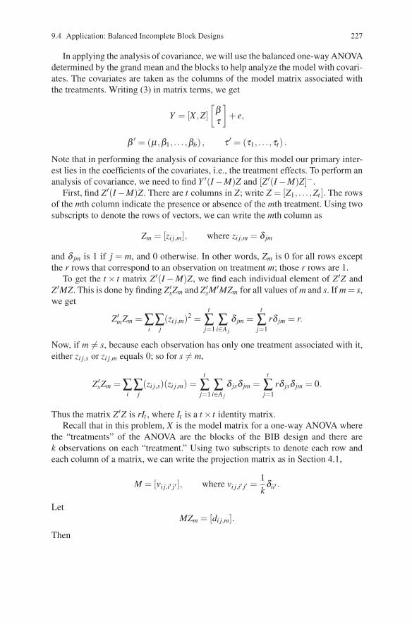
9.4 Application: Balanced Incomplete Block Designs 227
In applying the analysis of covariance, we will use the balanced one-way ANOVAdetermined by the grand mean and the blocks to help analyze the model with covari-ates. The covariates are taken as the columns of the model matrix associated withthe treatments. Writing (3) in matrix terms, we get
Y = [X ,Z][
βτ
]+ e,
β ′ = (μ,β1, . . . ,βb) , τ ′ = (τ1, . . . ,τt) .
Note that in performing the analysis of covariance for this model our primary inter-est lies in the coefficients of the covariates, i.e., the treatment effects. To perform ananalysis of covariance, we need to find Y ′(I −M)Z and [Z′(I −M)Z]−.
First, find Z′(I−M)Z. There are t columns in Z; write Z = [Z1, . . . ,Zt ]. The rowsof the mth column indicate the presence or absence of the mth treatment. Using twosubscripts to denote the rows of vectors, we can write the mth column as
Zm = [zi j,m], where zi j,m = δ jm
and δ jm is 1 if j = m, and 0 otherwise. In other words, Zm is 0 for all rows exceptthe r rows that correspond to an observation on treatment m; those r rows are 1.
To get the t × t matrix Z′(I −M)Z, we find each individual element of Z′Z andZ′MZ. This is done by finding Z′
sZm and Z′sM
′MZm for all values of m and s. If m = s,we get
Z′mZm = ∑
i∑
j(zi j,m)2 =
t
∑j=1
∑i∈A j
δ jm =t
∑j=1
rδ jm = r.
Now, if m �= s, because each observation has only one treatment associated with it,either zi j,s or zi j,m equals 0; so for s �= m,
Z′sZm = ∑
i∑
j(zi j,s)(zi j,m) =
t
∑j=1
∑i∈A j
δ jsδ jm =t
∑j=1
rδ jsδ jm = 0.
Thus the matrix Z′Z is rIt , where It is a t × t identity matrix.Recall that in this problem, X is the model matrix for a one-way ANOVA where
the “treatments” of the ANOVA are the blocks of the BIB design and there arek observations on each “treatment.” Using two subscripts to denote each row andeach column of a matrix, we can write the projection matrix as in Section 4.1,
M = [vi j,i′ j′ ], where vi j,i′ j′ =1k
δii′ .
LetMZm = [di j,m].
Then
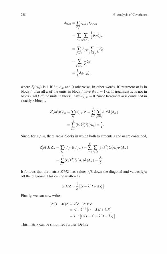
228 9 Analysis of Covariance
di j,m = ∑i′ j′
vi j,i′ j′zi′ j′,m
=t
∑j′=1
∑i′∈A j′
1k
δii′δ j′m
=t
∑j′=1
δ j′m ∑i′∈A j′
1k
δii′
= ∑i′∈Am
1k
δii′
=1k
δi(Am),
where δi(Am) is 1 if i ∈ Am and 0 otherwise. In other words, if treatment m is inblock i, then all k of the units in block i have di j,m = 1/k. If treatment m is not inblock i, all k of the units in block i have di j,m = 0. Since treatment m is contained inexactly r blocks,
Z′mM′MZm = ∑
i j(di j,m)2 =
b
∑i=1
∑j∈Di
k−2δi(Am)
=b
∑i=1
(k/k2)δi(Am) =rk.
Since, for s �= m, there are λ blocks in which both treatments s and m are contained,
Z′sM
′MZm = ∑i j
(di j,s)(di j,m) =b
∑i=1
∑j∈Di
(1/k2)δi(As)δi(Am)
=b
∑i=1
(k/k2)δi(As)δi(Am) =λk
.
It follows that the matrix Z′MZ has values r/k down the diagonal and values λ/koff the diagonal. This can be written as
Z′MZ =1k
[(r−λ )I +λJt
t].
Finally, we can now write
Z′(I −M)Z = Z′Z −Z′MZ
= rI − k−1 [(r−λ)I +λJtt]
= k−1 [(r(k−1)+λ )I −λJtt].
This matrix can be simplified further. Define

9.4 Application: Balanced Incomplete Block Designs 229
W = I − (1/t)Jtt . (4)
Note that W is a perpendicular projection operator and that equation (2) gives
r(k−1)+λ = λ t.
With these substitutions, we obtain
Z′(I −M)Z = (λ/k)[tI− Jt
t]= (λ t/k)
[I − (1/t)Jt
t]= (λ t/k)W.
We need to find a generalized inverse of Z′(I −M)Z. Because W is a projectionoperator, it is easily seen that[
Z′(I −M)Z]− = (k/λ t)W. (5)
We also need to be able to find the 1× t vector Y ′(I−M)Z. The vector (I−M)Yhas elements (yi j − yi·), so
Y ′(I −M)Zm = ∑i j
(yi j − yi·)zi j,m =t
∑j=1
δ jm ∑i∈A j
(yi j − yi·) = ∑i∈Am
(yim − yi·).
DefineQm = ∑
i∈Am
(yim − yi·).
ThenY ′(I −M)Z = (Q1, . . . ,Qt).
Since the β effects are for blocks, our primary interests are in estimable functionsξ ′τ and in estimating σ 2. From (9.1.1) and Proposition 9.1.1, write
ξ ′ = ρ ′(I −M)Z
to getξ ′τ = ρ ′(I −M)Z
[Z′(I −M)Z
]− Z′(I −M)Y
and, from (9.2.1),
SSE = Y ′(I −M)Y −Y ′(I −M)Z[Z′(I −M)Z
]− Z′(I −M)Y.
Both of these formulae involve the term (I −M)Z [Z′(I −M)Z]−. This term can besimplified considerably. Note that since the columns of Z are 0s and 1s, indicatingthe presence or absence of a treatment effect,
ZJ1t = J1
n .
Because M is defined from a one-way ANOVA,
0 = (I −M)J1n = (I −M)ZJ1
t . (6)

230 9 Analysis of Covariance
From (5), (4), and (6), it is easily seen that
(I −M)Z[Z′(I −M)Z
]− = (k/λ t)(I −M)Z.
Using this fact, we get that the BLUE of ξ ′τ is
ξ ′τ = ρ ′(I −M)Z[Z′(I −M)Z
]− Z′(I −M)Y= ρ ′(k/λ t)(I −M)ZZ′(I −M)Y= (k/λ t)ξ ′(Q1, . . . ,Qt)′
= (k/λ t)t
∑j=1
ξ jQ j.
jy·· that can be used to estimate contrasts, because ∑ j ξ j y·· = 0. The variance of theestimate of the contrast is
Var(ξ ′τ)
= σ 2ρ ′(I −M)Z[Z′(I −M)Z
]− Z′(I −M)ρ
= σ 2(k/λ t)ξ ′ξ .
From the estimate and the variance, it is a simple matter to see that
SS(ξ ′τ)
= (k/λ t)
[t
∑j=1
ξ jQ j
]2/ξ ′ξ .
The error sum of squares is
SSE = Y ′(I −M)Y −Y ′(I −M)Z[Z′(I −M)Z
]− Z′(I −M)Y= Y ′(I −M)Y − (k/λ t)Y ′(I −M)ZZ′(I −M)Y
= ∑i j
(yi j − yi·)2 − kλ t
t
∑j=1
Q2j .
Exercise 9.8 Show that ξ ′τ is estimable if and only if ξ ′τ is a contrast.Hint: One direction is easy. For the other direction, show that for ξ ′ = (ξ1, . . . ,ξt),
ξ ′ = (k/λ t)ξ ′Z′(I −M)Z.
Exercise 9.9 Show that if ξ ′τ and η ′τ are contrasts and that if ξ ′η = 0, thenξ ′τ = 0 and η ′τ = 0 put orthogonal constraints on C(X ,Z), i.e., the treatment sumof squares can be broken down with orthogonal contrasts in the usual way.
Hint: Let ξ ′ = ρ ′1[X ,Z] and η ′ = ρ ′
2[X ,Z]. Show that
Many computer programs, e.g., Minitab, present adjusted treatment means (k/λt)Q +

9.4 Application: Balanced Incomplete Block Designs 231
ρ ′1(I −M)Z
[Z′(I −M)Z
]− Z′(I −M)ρ2 = 0.
Suppose that the treatments have quantitative levels, say x1, . . . ,xt , that areequally spaced. Model (3) can be reparameterized as
yi j = μ +βi + γ1x j + γ2x2j + · · ·+ γt−1xt−1
j + ei j.
We would like to show that the orthogonal polynomial contrasts for the balancedincomplete block design are the same as for a balanced one-way ANOVA. In otherwords, tabled polynomial contrasts, which are useful in balanced ANOVAs, canalso be used to analyze balanced incomplete block designs. More generally, thetreatments in a BIB may have a factorial structure with quantitative levels in somefactor (e.g., Example 9.4.1). We would like to establish that the polynomial contrastsin the factor can be used in the usual way to analyze the data.
Because this is a balanced incomplete block design, Z is the model matrix fora balanced one-way ANOVA (without a grand mean). As in Section 7.3, defineorthogonal polynomials T = ZB by ignoring blocks. (Here we are not interestedin J as an orthogonal polynomial, so we take B as a t × t − 1 matrix.) Write B =[b1, . . . ,bt−1]. If treatments are levels of a single quantitative factor, then the b js aretabled orthogonal polynomial contrasts. If the treatments have factorial structure,the b js are obtained from tabled contrasts as in the continuation of Example 9.4.1below. The important fact is that the bjs are readily obtained. Note that J′t b j = 0 forall j, and b′ib j = 0 for i �= j.
A model with treatments replaced by regression variables can be written Y =Xβ +T η +e, where η = (η1, . . . ,ηt−1)′. For a simple treatment structure, η j wouldbe the coefficient for a jth degree polynomial. For a factorial treatment structure,η j could be the coefficient for some cross-product term. The key points are thatthe hypothesis η j = 0 corresponds to some hypothesis that can be interpreted as inSection 6.7 or Section 7.3, and that the columns of T are orthogonal.
As we have seen, the model Y = Xβ + T η + e is equivalent to the model Y =Xδ +(I −M)T η + e, where η is identical in the two models. Thus the test of η j =0 can be performed in the second model. In the second model, η is independentof δ because of the orthogonality. If the columns of (I −M)T are orthogonal, theestimates of the η js are independent. Finally, and most importantly, we can showthat the contrast in the τs that corresponds to testing η j = 0 is simply b′jτ , whereτ = (τ1, . . . ,τt)′.
To show that the columns of (I −M)T are orthogonal, it suffices to show thatT ′(I −M)T is diagonal.
T ′(I −M)T = B′Z′(I −M)ZB
= (λ t/k)B′WB
= (λ t/k)B′B.
The last equality follows from the definition of W and the fact that J′t b j = 0 for allj. Note that B′B is diagonal because b′ib j = 0 for i �= j.
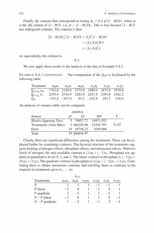
232 9 Analysis of Covariance
Finally, the contrast that corresponds to testing η j = 0 is ρ ′(I −M)Zτ , where ρis the jth column of (I −M)T , i.e., ρ = (I −M)Zb j. This is true because (I −M)Thas orthogonal columns. The contrast is then
[(I −M)Zbj]′(I −M)Zτ = b′jZ′(I −M)Zτ
= (λ t/k)b′jWτ= (λ t/k)b′jτ
or, equivalently, the contrast isb′jτ.
We now apply these results to the analysis of the data in Example 9.4.1.
EXAMPLE 9.4.1 CONTINUED. The computation of the Qms is facilitated by thefollowing table.
Treatment n0 p0 n0 p1 n0 p2 n1 p0 n1 p1 n1 p2
∑i∈Am yim 1762.0 2149.0 2375.0 1989.0 2675.0 2939.0∑i∈Am yi· 2295.4 2316.0 2281.8 2241.8 2391.8 2362.2Qm −533.4 −167.0 93.2 −252.8 283.2 576.8
An analysis of variance table can be computed.
ANOVASource df SS MS FBlocks (Ignoring Trts) 5 74857.77 14971.553Treatments (After Blks) 5 166228.98 33245.797 31.97Error 19 19758.22 1039.906Total 29 260844.97
Clearly, there are significant differences among the treatments. These can be ex-plored further by examining contrasts. The factorial structure of the treatments sug-gests looking at nitrogen effects, phosphate effects, and interaction effects. With twolevels of nitrogen, the only available contrast is (1)n0 +(−1)n1. Phosphate was ap-plied at quantitative levels 0, 1, and 2. The linear contrast in phosphate is (−1)p0 +(0)p1 +(1)p2. The quadratic contrast in phosphate is (1)p0 +(−2)p1 +(1)p2. Com-bining these to obtain interaction contrasts and rewriting them as contrasts in theoriginal six treatments gives b1, . . . ,b5.
b jsTreatments n0 p0 n0 p1 n0 p2 n1 p0 n1 p1 n1 p2N 1 1 1 −1 −1 −1P linear −1 0 1 −1 0 1P quadratic 1 −2 1 1 −2 1N −P linear −1 0 1 1 0 −1N −P quadratic 1 −2 1 −1 2 −1

9.5 Application: Testing a Nonlinear Full Model 233
Source df SS FN 1 51207.20 49.24P linear 1 110443.67 106.21P quadratic 1 2109.76 2.03N −P linear 1 2146.30 2.06N −P quadratic 1 322.06 0.31
The conclusions to be drawn are clear. There is a substantial increase in yieldsdue to adding the nitrogen-based fertilizer. For the dosages of phosphate used, thereis a definite increasing linear relationship between amount of phosphate and yieldof potatoes. There is no evidence of any interaction.
Note that the linear relationship between phosphate and yield is an approximationthat holds in some neighborhood of the dosages used in the experiment. It is wellknown that too much fertilizer will actually kill most plants. In particular, no potatoplant will survive having an entire truckload of phosphate dumped on it.
Exercise 9.10 Derive the analysis for a Latin square with one row missing.Hint: This problem is at the end of Section 9.4, not Section 9.3.
Exercise 9.11 Eighty wheat plants were grown in each of 5 different fields.Each of 6 individuals (A, B, C, D, E, and F) were asked to pick 8 “representative”plants in each field and measure the plants’s heights. Measurements were taken on 6different days. The data consist of the differences between the mean height of the 8“representative” plants and the mean of all the heights in the field on that day. Thusthe data measure the bias in selecting “representative” plants. The exact design andthe data are given below. Analyze the data. (Although they are barely recognizableas such, these data are from Cochran and Cox, 1957.)
FieldDay 1 2 3 4 5
1 E 3.50 A 0.75 C 2.28 F 1.77 D 2.282 D 3.78 B 1.46 A−1.06 E 1.46 F 2.763 F 2.32 C 2.99 B−0.28 D 1.18 E 3.394 C 4.13 D 4.02 E 1.81 B 1.46 A 1.505 A 1.38 E 1.65 F 2.64 C 2.60 B 1.506 B 1.22 F 2.83 D 1.57 A−1.30 C 1.97
9.5 Application: Testing a Nonlinear Full Model
Consider testing the model
Y = Xβ + e, e ∼ N(0,σ 2I), (1)
against a nonlinear model that involves a matrix function of Xβ , say
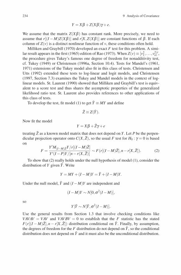
234 9 Analysis of Covariance
Y = Xβ +Z(Xβ )γ + e.
We assume that the matrix Z(Xβ ) has constant rank. More precisely, we need toassume that r[(I −M)Z(Xβ )] and r[X ,Z(Xβ )] are constant functions of β . If eachcolumn of Z(v) is a distinct nonlinear function of v, these conditions often hold.
Milliken and Graybill (1970) developed an exact F test for this problem. A simi-lar result appears in the first (1965) edition of Rao (1973). When Z(v)≡ [v2
1, . . . ,v2n]′,
the procedure gives Tukey’s famous one degree of freedom for nonadditivity test,cf. Tukey (1949) or Christensen (1996a, Section 10.4). Tests for Mandel’s (1961,1971) extensions of the Tukey model also fit in this class of tests. Christensen andUtts (1992) extended these tests to log-linear and logit models, and Christensen(1997, Section 7.3) examines the Tukey and Mandel models in the context of log-linear models. St. Laurent (1990) showed that Milliken and Graybill’s test is equiv-alent to a score test and thus shares the asymptotic properties of the generalizedlikelihood ratio test. St. Laurent also provides references to other applications ofthis class of tests.
To develop the test, fit model (1) to get Y ≡ MY and define
Z ≡ Z(Y ).
Now fit the modelY = Xβ + Zγ + e
treating Z as a known model matrix that does not depend on Y . Let P be the perpen-dicular projection operator onto C(X , Z), so the usual F test for H0 : γ = 0 is basedon
F =Y ′M(I−M)ZY/r[(I −M)Z]
Y ′(I −P)Y/[n− r(X , Z)]∼ F(r[(I −M)Z],n− r[X , Z]). (2)
To show that (2) really holds under the null hypothesis of model (1), consider thedistribution of Y given Y . Write
Y = MY +(I −M)Y = Y +(I −M)Y.
Under the null model, Y and (I −M)Y are independent and
(I −M)Y ∼ N[0,σ 2(I −M)],
soY |Y ∼ N[Y ,σ 2(I −M)].
Use the general results from Section 1.3 that involve checking conditions likeVAVAV = VAV and VAV BV = 0 to establish that the F statistic has the statedF(r[(I −M)Z],n− r[X , Z]) distribution conditional on Y . Finally, by assumption,the degrees of freedom for the F distribution do not depend on Y , so the conditionaldistribution does not depend on Y and it must also be the unconditional distribution.
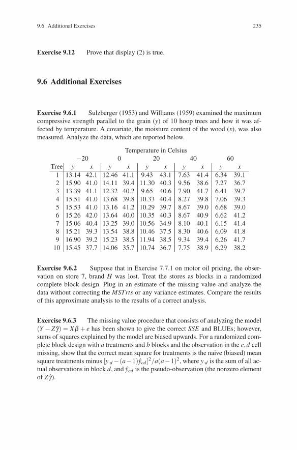
9.6 Additional Exercises 235
Exercise 9.12 Prove that display (2) is true.
9.6 Additional Exercises
Exercise 9.6.1 Sulzberger (1953) and Williams (1959) examined the maximumcompressive strength parallel to the grain (y) of 10 hoop trees and how it was af-fected by temperature. A covariate, the moisture content of the wood (x), was alsomeasured. Analyze the data, which are reported below.
Temperature in Celsius−20 0 20 40 60
Tree y x y x y x y x y x1 13.14 42.1 12.46 41.1 9.43 43.1 7.63 41.4 6.34 39.12 15.90 41.0 14.11 39.4 11.30 40.3 9.56 38.6 7.27 36.73 13.39 41.1 12.32 40.2 9.65 40.6 7.90 41.7 6.41 39.74 15.51 41.0 13.68 39.8 10.33 40.4 8.27 39.8 7.06 39.35 15.53 41.0 13.16 41.2 10.29 39.7 8.67 39.0 6.68 39.06 15.26 42.0 13.64 40.0 10.35 40.3 8.67 40.9 6.62 41.27 15.06 40.4 13.25 39.0 10.56 34.9 8.10 40.1 6.15 41.48 15.21 39.3 13.54 38.8 10.46 37.5 8.30 40.6 6.09 41.89 16.90 39.2 15.23 38.5 11.94 38.5 9.34 39.4 6.26 41.7
10 15.45 37.7 14.06 35.7 10.74 36.7 7.75 38.9 6.29 38.2
Exercise 9.6.2 Suppose that in Exercise 7.7.1 on motor oil pricing, the obser-vation on store 7, brand H was lost. Treat the stores as blocks in a randomizedcomplete block design. Plug in an estimate of the missing value and analyze thedata without correcting the MSTrts or any variance estimates. Compare the resultsof this approximate analysis to the results of a correct analysis.
Exercise 9.6.3 The missing value procedure that consists of analyzing the model(Y −Zγ) = Xβ + e has been shown to give the correct SSE and BLUEs; however,sums of squares explained by the model are biased upwards. For a randomized com-plete block design with a treatments and b blocks and the observation in the c,d cellmissing, show that the correct mean square for treatments is the naive (biased) meansquare treatments minus [y·d −(a−1)ycd ]2/a(a−1)2, where y·d is the sum of all ac-tual observations in block d, and ycd is the pseudo-observation (the nonzero elementof Zγ).

236 9 Analysis of Covariance
Exercise 9.6.4 State whether each design given below is a balanced incompleteblock design, and if so, give the values of b, t, k, r, and λ .
(a) The experiment involves 5 treatments: A, B, C, D, and E . The experimentis laid out as follows.
Block Treatments Block Treatments1 A,B,C 6 A,B,D2 A,B,E 7 A,C,D3 A,D,E 8 A,C,E4 B,C,D 9 B,C,E5 C,D,E 10 B,D,E
(b) The following design has 9 treatments: A, B, C, D, E, F , G, H, and I.
Block Treatments Block Treatments1 B,C,D,G 6 C,D,E, I2 A,C,E,H 7 A,D,H, I3 A,B,F, I 8 B,E,G, I4 A,E,F,G 9 C,F,G,H5 B,D,F,H
(c) The following design has 7 treatments: A, B, C, D, E, F , G.
Block Treatments Block Treatments1 C,E,F,G 5 B,C,D,G2 A,D,F,G 6 A,C,D,E3 A,B,E,G 7 B,D,E,F4 A,B,C,F

Chapter 10
General Gauss–Markov Models
A general Gauss–Markov model is a model
Y = Xβ + e, E(e) = 0, Cov(e) = σ 2V,
where V is a known matrix. Linear models can be divided into four categories de-pending on the assumptions made about V :
(a) V is an identity matrix,(b) V is nonsingular,(c) V is possibly singular but C(X) ⊂C(V ),(d) V is possibly singular.
The categories are increasingly general. Any results for category (d) apply to allother categories. Any results for category (c) apply to categories (a) and (b). Anyresults for (b) apply to (a).
The majority of Chapters 1 through 9 have dealt with category (a). In Sections 2.7and 3.8, models in category (b) were discussed. In this chapter, categories (c) and(d) are discussed. Section 1 is devoted to finding BLUEs for models in categories(c) and (d). Theorem 10.1.2 and the discussion following it give the main results forcategory (c). The approach is similar in spirit to Section 2.7. The model is trans-formed into an equivalent model that fits into category (a), and BLUEs are foundfor the equivalent model. Although similar in spirit to Section 2.7, the details areconsiderably more complicated because of the possibility that V is singular. Havingfound BLUEs for category (c), the extension to category (d) is very simple. Theextension follows from Theorem 10.1.3. Finally, Section 1 contains some results onthe uniqueness of BLUEs for category (d).
Section 2 contains a discussion of the geometry of estimation for category (d).In particular, it points out the need for a consistency criterion and the crucial role ofprojection operators in linear unbiased estimation. Section 3 examines the problemof testing a model against a reduced model for category (d). Section 4 discussesthe extension of least squares estimation to category (d) in light of the consistency
© Springer Science+Business Media, LLC 2011
237Springer Texts in Statistics, DOI 10.1007/978-1-4419-9816-3_10, R. Christensen, Plane Answers to Complex Questions: The Theory of Linear Models,

238 10 General Gauss–Markov Models
requirement of Section 2. Section 4 also contains the very important result that leastsquares estimates are BLUEs if and only if C(V X) ⊂C(X).
Section 5 considers estimable parameters that can be known with certainty whenC(X) �⊂ C(V ) and a relatively simple way to estimate estimable parameters thatare not known with certainty. Some of the nastier parts in Sections 1 through 4 arethose that provide sufficient generality to allow C(X) �⊂C(V ). The simpler approachof Section 5 seems to obviate the need for much of that. Groß (2004) surveyedimportant results in linear models with possibly singular covariance matrices.
10.1 BLUEs with an Arbitrary Covariance Matrix
Consider the model
Y = Xβ + e, E(e) = 0, Cov(e) = σ 2V, (1)
where V is a known matrix. We want to find the best linear unbiased estimate ofE(Y ).
Definition 10.1.1. Let Λ ′ be an r × p matrix with Λ ′ = P′X for some P. Anestimate B0Y is called a best linear unbiased estimate (BLUE) of Λ ′β if
(a) E(B0Y ) = Λ ′β for any β , and(b) if BY is any other linear unbiased estimate of Λ ′β , then for any r×1 vector ξ
Var(ξ ′B0Y ) ≤ Var(ξ ′BY ).
Exercise 10.1 Show that A0Y is a BLUE of Xβ if and only if, for every estimablefunction λ ′β such that ρ ′X = λ ′, ρ ′A0Y is a BLUE of λ ′β .
Exercise 10.2 Show that if Λ ′ = P′X and if A0Y is a BLUE of Xβ , then P′A0Yis a BLUE of Λ ′β .
In the case of a general covariance matrix V , it is a good idea to reconsiderwhat the linear model (1) is really saying. The obvious thing it is saying is thatE(Y ) ∈ C(X). From Lemma 1.3.5, the model also says that e ∈ C(V ) or, in othernotation, Y ∈ C(X ,V ). If V is a nonsingular matrix, C(V ) = Rn; so the conditionson e and Y are really meaningless. When V is a singular matrix, the conditions on eand Y are extremely important.
For any matrix A, let MA denote the perpendicular projection matrix onto C(A).M without a subscript is MX . Any property that holds with probability 1 will be saidto hold almost surely (a.s.). For example, Lemma 1.3.5 indicates that e ∈C(V ) a.s.and, adding Xβ to Y −Xβ , the lemma gives Y ∈C(X ,V ) a.s.

10.1 BLUEs with an Arbitrary Covariance Matrix 239
If R and S are any two random vectors with R = S a.s., then E(R) = E(S) andCov(R) = Cov(S). In particular, if R = S a.s. and R is a BLUE, then S is also aBLUE.
Results on estimation will be established by comparing the estimation problemin model (1) to the estimation problem in two other, more easily analyzed, models.
Before proceeding to the first theorem on estimation, recall the eigenvector de-composition of the symmetric, nonnegative definite matrix V . One can pick ma-trices E and D so that V E = ED. Here D = Diag(di), where the dis are the, saym, positive eigenvalues of V (with the correct multiplicities). E is a matrix of or-thonormal columns with the ith column an eigenvector corresponding to di. DefineD1/2 ≡ Diag
(√di). Write
Q ≡ ED1/2 and Q− ≡ D−1/2E ′.
Useful facts are
1. C(V ) = C(E) = C(Q)2. MV = EE ′ = QQ−3. Im = Q−Q4. V = QQ′5. QQ−Q = Q6. Q−V Q−′ = Im7. Q−′Q− = V−.
Consider the linear model
Q−Y = Q−Xβ +Q−e, E(Q−e) = 0, Cov(Q−e) = σ2Im. (2)
Models (1) and (2) are equivalent when C(X) ⊂C(V ). Clearly, (2) can be obtainedfrom (1) by multiplying on the left by Q−. Moreover, with C(X) ⊂ C(V ), each ofY , C(X), and e are contained in C(V ) a.s.; so multiplying (2) on the left by Q givesMVY = MV Xβ + MV e, which is model (1) a.s. Note that Q−Y ∈ Rm and that theGauss–Markov theorem can be used to get estimates in model (2). Moreover, ifC(X) ⊂C(V ), then X = MV X = QQ−X ; so Xβ is estimable in model (2).
Theorem 10.1.2. If C(X) ⊂ C(V ), then A0Y is a BLUE of Xβ in model (1) ifand only if (A0Q)Q−Y is a BLUE of Xβ in model (2).
PROOF. If this theorem is to make any sense at all, we need to first show thatE(A0Y ) = Xβ iff E(A0QQ−Y ) = Xβ . Recall that Y ∈C(X ,V ) a.s., so in this specialcase where C(X) ⊂C(V ), we have Y ∈C(V ) a.s. Thus, for the purposes of findingexpected values and covariances, we can assume that Y = MVY . Let B be an arbi-trary n× n matrix. Then E(BY ) = E(BMVY ) = E(BQQ−Y ), so E(A0Y ) = Xβ iffE(A0QQ−Y ) = Xβ . It is also handy to know the following fact:
Var(ρ ′BY ) = Var(ρ ′BMVY ) = Var(ρ ′BQQ−Y ).

240 10 General Gauss–Markov Models
Now suppose that A0Y is a BLUE for Xβ in model (1). We show that A0QQ−Y isa BLUE of Xβ in model (2). Let BQ−Y be another unbiased estimate of Xβ in model(2). Then Xβ = E(BQ−Y ), so BQ−Y is an unbiased estimate of Xβ in model (1) and,since A0Y is a BLUE in model (1), Var(ρ ′A0QQ−Y ) = Var(ρ ′A0Y )≤Var(ρ ′BQ−Y ).Thus A0QQ−Y is a BLUE of Xβ in model (2).
Conversely, suppose that A0QQ−Y is a BLUE of Xβ in model (2). Let BY be anunbiased estimate for Xβ in model (1). Then BQQ−Y is unbiased for Xβ in model(2) and Var(ρ ′A0Y ) = Var(ρ ′A0QQ−Y ) ≤ Var(ρ ′BQQ−Y ) = Var(ρ ′BY ); so ρ ′A0Yis a BLUE of Xβ in model (1). �
Note that with C(X)⊂C(V ), A0Y = A0MVY = A0QQ−Y a.s., so Theorem 10.1.2is really saying that A0Y is a BLUE in model (1) if and only if A0Y is a BLUE inmodel (2). The virtue of Theorem 10.1.2 is that we can actually find a BLUE for Xβin model (2). From Exercises 10.1 and 10.2, a BLUE of Xβ = QQ−Xβ from model(2) is
X β = QMQ−X Q−Y
= Q[Q−X(X ′Q−′Q−X)−X ′Q−′]Q−Y
= MV X(X ′V−X)−X ′V−Y
= X(X ′V−X)−X ′V−Y. (3)
It is useful to observe that we can get a BLUE from any choice of V− and(X ′V−X)−. First, notice that X ′V−X does not depend on V−. Since C(X) ⊂C(V ),we can write X = VC for some matrix C. Then X ′V−X = C′VV−VC = C′VC. Sec-ond, Q−X(X ′Q−′Q−X)−X ′Q−′ does not depend on the choice of (X ′Q−′Q−X)−.Therefore, X(X ′V−X)−X ′V− does not depend on the choice of (X ′V−X)−. More-over, for any Y ∈C(V ), X(X ′V−X)−X ′V− does not depend on the choice of V−. Tosee this, write Y = V b. Then X ′V−Y = (C′V )V−(V b) = C′V b. Since Y ∈C(V ) a.s.,X(X ′V−X)−X ′V−Y is a BLUE of Xβ for any choices of V− and (X ′V−X)−.
To obtain the general estimation result for arbitrary singular V , consider the linearmodel
Y1 = Xβ + e1, E(e1) = 0, Cov(e1) = σ 2 (V +XUX ′) , (4)
where U is any symmetric nonnegative definite matrix.
Theorem 10.1.3. A0Y is a BLUE for Xβ in model (1) if and only if A0Y1 is aBLUE for Xβ in model (4).
PROOF. Clearly, for any matrix B, BY is unbiased if and only if BY1 is unbiasedand both are equivalent to the condition BX = X . In the remainder of the proof,B will be an arbitrary matrix with BX = X so that BY and BY1 are arbitrary linearunbiased estimates of Xβ in models (1) and (4), respectively. The key fact in theproof is that
Var(ρ ′BY1) = σ2ρ ′B(V +XUX ′)B′ρ

10.1 BLUEs with an Arbitrary Covariance Matrix 241
= σ2ρ ′BV B′ρ +ρ ′BXUX ′B′ρ= Var(ρ ′BY )+σ2ρ ′XUX ′ρ.
Now suppose that A0Y is a BLUE for Xβ in model (1). Then
Var(ρ ′A0Y ) ≤ Var(ρ ′BY).
Adding σ 2ρ ′XUX ′ρ to both sides we get
Var(ρ ′A0Y1) ≤ Var(ρ ′BY1),
and since BY1 is an arbitrary linear unbiased estimate, A0Y1 is a BLUE.Conversely, suppose A0Y1 is a BLUE for Xβ in model (4). Then
Var(ρ ′A0Y1) ≤ Var(ρ ′BY1),
orVar(ρ ′A0Y )+σ 2ρ ′XUX ′ρ ≤ Var(ρ ′BY)+σ 2ρ ′XUX ′ρ.
Subtracting σ 2ρ ′XUX ′ρ from both sides we get
Var(ρ ′A0Y ) ≤ Var(ρ ′BY ),
so A0Y is a BLUE. �
As with Theorem 10.1.2, this result is useful because a BLUE for Xβ can ac-tually be found in one of the models. Let T = V + XUX ′. If U is chosen so thatC(X) ⊂ C(T ), then Theorem 10.1.2 applies to model (4) and a BLUE for Xβ isX(X ′T−X)−X ′T−Y . Exercise 10.3 establishes that such matrices U exist. Sincethis is an application of Theorem 10.1.2, X(X ′T−X)−X ′T−Y does not depend onthe choice of (X ′T−X)− and, for Y ∈ C(T ), it does not depend on the choice ofT−. Proposition 10.1.4 below shows that C(X) ⊂C(T ) implies C(T ) = C(X ,V ); soY ∈C(T ) a.s., and any choice of T− gives a BLUE.
Exercise 10.3 The BLUE of Xβ can be obtained by taking T = V +XX ′. Provethis by showing that
(a) C(X) ⊂C(T ) if and only if T T−X = X , and(b) if T = V +XX ′, then T T−X = X .
Hint: Searle and Pukelsheim (1987) base a proof of (b) on
0 = (I −T T−)T (I −T T−)′
= (I −T T−)V (I −T T−)′ +(I −T T−)XX ′(I −T T−)′
and the fact that the last term is the sum of two nonnegative definite matrices.

242 10 General Gauss–Markov Models
Proposition 10.1.4. If C(X) ⊂C(T ), then C(V ) ⊂C(T ) and C(X ,V ) = C(T ).
PROOF. We know that C(X) ⊂C(T ), so X = T G for some matrix G. If v ∈C(V ),then v =V b1, and v =V b1 +XUX ′b1 −XUX ′b1 = T b1−T G(UX ′b1); so v ∈C(T ).Thus, C(X ,V ) ⊂C(T ). But clearly, by the definition of T , C(T ) ⊂C(X ,V ); so wehave C(X ,V ) = C(T ). �
To complete our characterization of best linear unbiased estimates, we will showthat for practical purposes BLUEs of Xβ are unique.
Theorem 10.1.5. Let AY and BY be BLUEs of Xβ in model (1), then Pr(AY =BY ) = 1.
PROOF. It is enough to show that Pr[(A−B)Y = 0] = 1. We need only observethat E[(A−B)Y ] = 0 and show that for any ρ , Var[ρ ′(A−B)Y ] = 0.
Remembering that Var(ρ ′AY ) = Var(ρ ′BY ), we first consider the unbiased esti-mate of Xβ , 1
2(A+B)Y :
Var(ρ ′AY ) ≤ Var(
ρ ′ 12(A+B)Y
)but
Var(
ρ ′ 12(A+B)Y
)=
14[Var(ρ ′AY )+Var(ρ ′BY )+2Cov(ρ ′AY,ρ ′BY )
],
soVar(ρ ′AY ) ≤ 1
2Var(ρ ′AY )+
12
Cov(ρ ′AY,ρ ′BY ).
Simplifying, we find that
Var(ρ ′AY ) ≤ Cov(ρ ′AY,ρ ′BY ).
Now look at Var(ρ ′(A−B)Y ),
0 ≤ Var(ρ ′(A−B)Y
)= Var(ρ ′AY )+Var(ρ ′BY )−2Cov(ρ ′AY,ρ ′BY ) ≤ 0. �
Finally, the most exact characterization of a BLUE is the following:
Theorem 10.1.6. If AY and BY are BLUEs for Xβ in model (1), then AY = BYfor any Y ∈C(X ,V ).
PROOF. It is enough to show that AY = BY , first when Y ∈ C(X) and then whenY ∈C(V ). When Y ∈C(X), by unbiasedness AY = BY .

10.2 Geometric Aspects of Estimation 243
We want to show that AY = BY for all Y ∈C(V ). Let M = {Y ∈C(V )|AY = BY}.It is easily seen that M is a vector space, and clearly M ⊂ C(V ). If C(V ) ⊂ M ,then M = C(V ), and we are done.
From unbiasedness, AY = Xβ +Ae and BY = Xβ +Be, so AY = BY if and onlyif Ae = Be. From Theorem 10.1.5, Pr(Ae = Be) = 1. We also know that Pr(e ∈C(V )) = 1. Therefore, Pr(e ∈ M ) = 1.
Computing the covariance of e we find that
σ 2V =∫
ee′dP =∫
e∈Mee′dP;
so, by Exercise 10.4, C(V ) ⊂ M . �
Exercise 10.4 Ferguson (1967, Section 2.7, page 74) proves the following:
Lemma (3) If S is a convex subset of Rn, and Z is an n-dimensional randomvector for which Pr(Z ∈ S) = 1 and for which E(Z) exists and is finite, then E(Z)∈ S.
Use this lemma to show that
C(V ) = C[∫
e∈Mee′dP
]⊂ M .
After establishing Theorem 10.1.5, we only need to find any one BLUE, becausefor any observations that have a chance of happening, all BLUEs give the sameestimates. Fortunately, we have already shown how to obtain a BLUE, so this sectionis finished. There is only one problem. Best linear unbiased estimates might be puregarbage. We pursue this issue in the next section.
10.2 Geometric Aspects of Estimation
The linear model
Y = Xβ + e, E(e) = 0, Cov(e) = σ 2V, (1)
says two important things:
(a) E(Y ) = Xβ ∈C(X), and(b) Pr(e ∈C(V )) = 1.
Note that (b) also says something about E(Y ):
(b′) Xβ = Y − e ∈Y +C(V ) a.s.

244 10 General Gauss–Markov Models
Intuitively, any reasonable estimate of E(Y ), say X β , should satisfy the followingdefinition for consistency.
Definition 10.2.1. An estimate Xβ of Xβ is called a consistent estimate if
(i) Xβ ∈C(X) for any Y , and(ii) Xβ ∈Y +C(V ) for any Y ∈C(X ,V ).
Xβ is called almost surely consistent if conditions (i) and (ii) hold almost surely.
Note that this concept of consistency is distinct from the usual large sample ideaof consistency. The idea is that a consistent estimate, in our sense, is consistent withrespect to conditions (a) and (b′).
EXAMPLE 10.2.2. Consider the linear model determined by
X =
⎡⎣1 00 10 0
⎤⎦ and V =
⎡⎣ 12 0 1
20 1 012 0 1
2
⎤⎦ .
If this model is graphed with coordinates (x,y,z), then C(X) is the x,y plane andC(V ) is the plane determined by the y-axis and the line [x = z,y = 0]. (See Fig-ure 10.1.)
Fig. 10.1 Estimation space and singular covariance space for Example 10.2.2.

10.2 Geometric Aspects of Estimation 245
Suppose that Y = (7,6,2)′. Then (see Figure 10.2) E(Y ) is in C(X) (the x,y plane)and also in Y +C(V ) (which is the plane C(V ) in Figure 10.1, translated over untilit contains Y ). The intersection of C(X) and Y +C(V ) is the line [x = 5,z = 0], soany consistent estimate of Xβ will be in the line [x = 5,z = 0]. To see this, note thatC(X) consists of vectors with the form (a,b,0)′, and Y +C(V ) consists of vectorslike (7,6,2)′ +(c,d,c)′. The intersection is those vectors with c = −2, so they areof the form (5,6+d,0)′ or (5,b,0)′.
The problem with BLUEs of Xβ is that there is no apparent reason why a BLUEshould be consistent. The class of linear unbiased estimates (LUEs) is very broad. Itconsists of all estimates AY with AX = X . There are many linear unbiased estimatesthat are not consistent. For example, Y itself is a LUE and it satisfies condition (ii)of consistency; however, one would certainly not want to use it as an estimate.
EXAMPLE 10.2.2 CONTINUED. MY is a LUE and satisfies condition (i) ofconsistency; however, with Y = (7,6,2)′, MY = (7,6,0)′, but (7,6,0)′ is not inC(X)∩ [Y +C(V )] = [x = 5,z = 0]. (See Figure 10.2.)
Fig. 10.2 Consistent estimation for Example 10.2.2.
Before showing that BLUEs of Xβ are almost surely consistent, several observa-tions will be made. The object is to explicate the case C(X)⊂C(V ), give alternativeconditions that can be used in place of conditions (i) and (ii) of consistency, anddisplay the importance of projections in linear estimation.

246 10 General Gauss–Markov Models
(a) In practice, when a covariance matrix other than σ 2I is appropriate, most ofthe time the condition C(X) ⊂C(V ) will be satisfied. When C(X) ⊂C(V ), thenY ∈C(X ,V ) = C(V ) a.s., so the condition Xβ ∈ Y +C(V ) a.s. merely indicatesthat Xβ ∈C(V ) a.s. In fact, any estimate of Xβ satisfying condition (i) of consis-tency also satisfies condition (ii). (Note: The last claim is not restricted to linearestimates or even unbiased estimates.)
(b) An estimate AY satisfies condition (i) of consistency if and only if A = XB forsome matrix B.
(c) An estimate AY satisfies condition (ii) of consistency if and only if (I −A)Y ∈C(V ) for any Y ∈C(X ,V ).
(d) If AY is a LUE of Xβ , then AY satisfies condition (ii) of consistency if andonly if AY ∈C(V ) for any Y ∈C(V ), i.e., iff C(AV ) ⊂C(V ).PROOF. Y ∈ C(X ,V ) iff Y = x + v for x ∈ C(X) and v ∈ C(V ). (I −A)Y =(x− x)+(v−Av). v−Av ∈C(V ) iff Av ∈C(V ). �
(e) AY is a LUE satisfying condition (i) if and only if A is a projection matrix (notnecessarily perpendicular) onto C(X).PROOF. From unbiasedness, AX = X , and from (b), A = XB. Hence AA =AXB = XB = A, and so A is idempotent and a projection onto C(A). Since AX =X , we have C(X) ⊂C(A); and since A = XB, we have C(A) ⊂C(X). Therefore,C(A) = C(X). �
Exercise 10.5 Prove observations (a), (b), and (c).
Notice that in general all consistent linear unbiased estimates (CLUEs) are pro-jections onto C(X) and that if C(X) ⊂C(V ), all projections onto C(X) are CLUEs.This goes far to show the importance of projection matrices in estimation. In partic-ular, the BLUEs that we actually found in the previous section satisfy condition (i)by observation (b). Thus, by observation (e) they are projections onto C(X).
Before proving the main result, we need the following proposition:
Proposition 10.2.3. For T = V + XUX ′ with U nonnegative definite and A =X(X ′T−X)−X ′T− with C(X) ⊂C(T ), AV = VA′.
PROOF. Consider the symmetric matrix X(X ′T−X)−X ′, where the generalizedinverses are taken as in Corollary B.41. By the choice of T , write X = T G.
X ′ = G′T = G′T T−T = X ′T−T,
X(X ′T−X)−X ′ = X(X ′T−X)−X ′T−T = A(V +XUX ′).
Since A is a projection operator onto C(X), AXUX ′ = XUX ′; thus,
X(X ′T−X)−X ′ −XUX ′ = AV.
The lefthand side is symmetric. �

10.3 Hypothesis Testing 247
Proposition 10.2.4. There exists a BLUE of Xβ in model (1) that is a CLUE.
PROOF. AY = X(X ′T−X)−X ′T−Y is a BLUE satisfying condition (i). In Propo-sition 10.2.3, we proved that AV = VA′. By observation (d), the proposition holds.
�
Theorem 10.2.5. If AY is a BLUE of Xβ in model (1), then AY is almost surelyconsistent.
PROOF. By Proposition 10.2.4, a consistent BLUE exists. By Theorem 10.1.5,any BLUE must almost surely satisfy consistency. �
10.3 Hypothesis Testing
We consider the problem of testing the model
Y = Xβ + e, e ∼ N(0,σ2V
)(1)
against the reduced model
Y = X0γ + e, e ∼ N(0,σ 2V
), (2)
where C(X0) ⊂C(X). In particular, we use the approach of looking at reductions inthe sum of squares for error. First we need to define what we mean by the sum ofsquares for error.
In the remainder of this section, let A = X(X ′T−X)−X ′T−, where T− and(X ′T−X)− are chosen (for convenience) as in Corollary B.41 and as usual T =V + XUX ′ for some nonnegative definite matrix U such that C(X) ⊂ C(T ). AY isa BLUE of Xβ in model (1). We will define the sum of squares for error (SSE) inmodel (1) as
SSE = Y ′(I −A)′T−(I −A)Y. (3)
The idea of using a quadratic form in the residuals to estimate the error is reason-able, and any quadratic form in the residuals, when normalized, gives an unbiasedestimate of σ 2. The terminology SSE literally comes from the use of the quadraticform Y ′(I −A)′(I −A)Y . In particular, if V = I, then
Y ′(I −A)′(I −A)Y/σ 2 = Y ′(I −A)′[σ2I]−1(I −A)Y
has a χ2 distribution and is independent of AY . For an arbitrary covariance matrix,an analogous procedure would be to use Y ′(I−A)′V−(I −A)Y to get an estimate ofσ 2 and develop tests. To simplify computations, we have chosen to define SSE as in

248 10 General Gauss–Markov Models
(3). However, we will show that for Y ∈C(X ,V ), SSE = Y ′(I −A)′V−(I −A)Y forany choice of V−.
The sum of squares error in model (2) (SSE0) is defined similarly. Let T0 = V +X0U0X ′
0 for a nonnegative definite matrix U0 for which C(X0) ⊂ C(T0). Let A0 =X0(X ′
0T−0 X0)−X ′
0T−0 , where again for convenience take T−
0 and (X ′0T−
0 X0)− as inCorollary B.41.
SSE0 = Y ′(I −A0)′T−0 (I −A0)Y.
The test will be, for some constant K, based on
K (SSE0 −SSE)/
SSE,
which will be shown to have an F distribution. We will use Theorem 1.3.6 andTheorem 1.3.9 to obtain distribution results.
Theorem 10.3.1. If Y ∈C(T ), then
(a) Y ′(I −A)′T−(I −A)Y = Y ′(I −A)′V−(I −A)Y for any V−,(b) Y ′(I −A)′T−(I −A)Y = 0 if and only if (I −A)Y = 0.
PROOF. The proof is given after Proposition 10.3.6. �
These results also hold when A is replaced by A0. Denote C ≡ (I −A)′T−(I −A)and C0 ≡ (I −A0)′T−
0 (I −A0). Thus SSE = Y ′CY and SSE0 = Y ′C0Y . The distribu-tion theory is:
Theorem 10.3.2.
(a) Y ′CY/σ 2 ∼ χ2(tr(CV ),0).If Xβ ∈C(X0,V ), then
(b) Y ′(C0 −C)Y/σ 2 ∼ χ2(tr(C0V −CV ),β ′X ′C0Xβ )and
(c) Y ′CY and Y ′(C0 −C)Y are independent.
PROOF. The proof consists of checking the conditions in Theorems 1.3.6 and1.3.9. There are many conditions to be checked. This is done in Lemmas 10.3.7through 10.3.9 at the end of the section. �
The last result before stating the test establishes behavior of the distributionsunder the two models. Model (2) is true if and only if Xβ ∈C(X0).
Theorem 10.3.3.
(a) If Xβ ∈C(X0), then Pr(Y ∈C(X0,V )) = 1 and β ′X ′C0Xβ = 0.

10.3 Hypothesis Testing 249
(b) If Xβ �∈ C(X0), then either Xβ ∈ C(X0,V ) and β ′X ′C0Xβ > 0 or Xβ �∈C(X0,V ) and Pr(Y �∈C(X0,V )) = 1
PROOF.
(a) The first part is clear, the second is because C0X0 = 0.(b) If Xβ �∈C(X0), then either Xβ ∈C(X0,V ) or Xβ �∈C(X0,V ). If Xβ ∈C(X0,V ),
then by Theorem 10.3.1b, β ′X ′C0Xβ = 0 if and only if (I − A0)Xβ = 0 orXβ = A0Xβ . Since Xβ �∈ C(X0), β ′X ′C0Xβ > 0. If Xβ �∈ C(X0,V ), supposee ∈C(V ) and Y ∈C(X0,V ), then Xβ = Y −e ∈C(X0,V ), a contradiction. There-fore either e �∈ C(V ) or Y �∈ C(X0,V ). Since Pr(e ∈ C(V )) = 1, we must havePr(Y �∈C(X0,V )) = 1. �
The test at the α level is to reject H0 that model (2) is adequate if Y �∈C(X0,V )or if
(SSE0 −SSE)/tr[(C0 −C)V ]SSE/tr(CV )
> F(1−α, tr[(C0 −C)V ], tr(CV )).
This is an α level test because, under H0, Pr(Y �∈ C(X0,V )) = 0. The power of thetest is at least as great as that of a noncentral F test and is always greater than αbecause if β ′X ′C0Xβ = 0 under the alternative, Theorem 10.3.3 ensures that the testwill reject with probability 1.
In the next section we consider extensions of least squares and conditions underwhich such extended least squares estimates are best estimates.
Proofs of Theorems 10.3.1 and 10.3.2.
Before proceeding with the proofs of the theorems, we need some background re-sults.
Proposition 10.3.4. A′T−A = A′T− = T−A.
PROOF.
A′T− = T−X(X ′T−X)−X ′T− = T−A,
A′T−A = T−X(X ′T−X)−X ′T−X(X ′T−X)−X ′T−;
but, as discussed earlier, A does not depend on the choice of (X ′T−X)− and(X ′T−X)−X ′T−X(X ′T−X)− is a generalized inverse of X ′T−X , so A′T−A = T−A.
�
Corollary 10.3.5. (I −A)′T−(I −A) = (I −A)′T− = T−(I −A).

250 10 General Gauss–Markov Models
In the remainder of this discussion we will let X = T G and V = T BT . (The lattercomes from Proposition 10.1.4 and symmetry.)
Proposition 10.3.6.
(a) V T−(I −A) = T T−(I −A),(b) V T−(I −A)V = (I −A)V .
PROOF. From Corollary 10.3.5 and unbiasedness, i.e., AX=X,
T T−(I −A) = T (I −A)′T− = V (I −A)′T− = V T−(I −A).
With V = T BT and, from Proposition 10.2.3, AV symmetric, we have
V T−(I −A)V = T T−(I −A)V = T T−V (I −A)′
= T T−T BT (I −A)′ = T BT (I −A)′ = V (I −A)′ = (I −A)V. �
PROOF OF THEOREM 10.3.1. Recalling Proposition 10.1.4, if Y ∈ C(T ), writeY = Xb1 +V b2.
(a) Using Proposition 10.2.3,
Y ′(I −A)′T−(I −A)Y = (Xb1 +V b2)′(I −A)′T−(I −A)(Xb1 +V b2)= b′2V (I −A)′T−(I −A)V b2
= b′2(I −A)V T−(I −A)V b2
= b′2(I −A)(I −A)V b2
= b′2(I −A)V (I −A)′b2
= b′2(I −A)VV−V (I −A)′b2
= b′2V (I −A)′V−(I −A)V b2
= Y ′(I −A)′V−(I −A)Y.
(b) From the proof of (a),
Y ′(I −A)′T−(I −A)Y = b′2(I −A)V (I −A)′b2.
Recall that we can write V = EDE ′ with E ′E = I, D = Diag(di), and di > 0 forall i.
Y ′(I −A)′T−(I −A)Y = 0 iff b′2(I −A)V (I −A)′b2 = 0iff E ′(I −A)′b2 = 0iff (I −A)′b2 ⊥C(E)iff (I −A)′b2 ⊥C(V )

10.3 Hypothesis Testing 251
iff V (I −A)′b2 = 0iff (I −A)V b2 = 0iff (I −A)Y = 0. �
The following lemmas constitute the proof of Theorem 10.3.2.
Lemma 10.3.7.
(a) CVC = C and C0VC0 = C0,(b) CVC0V = CV ,(c) VCVCV = VCV , β ′X ′CVCXβ = β ′X ′CXβ = 0, VCVCXβ = VCXβ = 0.
PROOF.
(a) Using Corollary 10.3.5 and Proposition 10.3.6, CVC = CV T−(I − A) =CT T−(I −A) = (I −A)′T−T T−(I −A) = (I −A)′T−(I −A) = C.
(b) A similar argument gives the second equality: CVC0V = CV T−0 (I −A0)V =
C(I −A0)V = T−(I −A)(I −A0)V = T−(I −A)V = CV .(c) The equalities in (c) follow from (a) and the fact that CX = T−(I −A)X = 0.
�
Note that Lemma 10.3.7c leads directly to Theorem 10.3.2a. We now establishthe conditions necessary for Theorem 10.3.2b.
Lemma 10.3.8.
(a) V (C0 −C)V (C0 −C)V = V (C0 −C)V ,(b) β ′X ′(C0 −C)V (C0 −C)Xβ = β ′X ′(C0 −C)Xβ = β ′X ′C0Xβ ,(c) if Xβ ∈C(X0,V ), then V (C0 −C)V (C0 −C)Xβ = V (C0 −C)Xβ .
PROOF. From parts (a) and (b) of Lemma 10.3.7,
V (C0 −C)V (C0 −C)V = VC0VC0V −VC0VCV −VCVC0V +VCVCV
= VC0V −VCV −VCV +VCV
= VC0V −VCV
= V (C0 −C)V.
To show (b), we need only show that
X ′(C0 −C)V (C0 −C)X = X ′(C0 −C)X .
Since CX = 0, this is equivalent to showing X ′C0VC0X = X ′C0X . The result is im-mediate from part (a) of Lemma 10.3.7.
To show (c), we need to show that
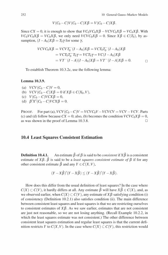
252 10 General Gauss–Markov Models
V (C0 −C)V (C0 −C)Xβ = V (C0 −C)Xβ .
Since CX = 0, it is enough to show that VC0VC0Xβ −VCVC0Xβ = VC0Xβ . WithVC0VC0Xβ = VC0Xβ , we only need VCVC0Xβ = 0. Since Xβ ∈ C(T0), by as-sumption, (I −A0)Xβ = T0γ for some γ ,
VCVC0Xβ = VCV T−0 (I −A0)Xβ = VCT0T−
0 (I −A0)Xβ= VCT0T−
0 T0γ = VCT0γ = VC(I −A0)Xβ= V T−(I −A)(I −A0)Xβ = V T−(I −A)Xβ = 0. �
To establish Theorem 10.3.2c, use the following lemma:
Lemma 10.3.9.
(a) VCV (C0 −C)V = 0,(b) VCV (C0 −C)Xβ = 0 if Xβ ∈C(X0,V ),(c) V (C0 −C)VCXβ = 0,(d) β ′X ′(C0 −C)VCXβ = 0.
PROOF. For part (a), VCV (C0−C)V =VCVC0V −VCVCV =VCV −VCV . Parts(c) and (d) follow because CX = 0; also, (b) becomes the condition VCVC0Xβ = 0,as was shown in the proof of Lemma 10.3.8. �
10.4 Least Squares Consistent Estimation
Definition 10.4.1. An estimate β of β is said to be consistent if X β is a consistentestimate of Xβ . β is said to be a least squares consistent estimate of β if for anyother consistent estimate β and any Y ∈C(X ,V ),
(Y −X β )′(Y −X β ) ≤ (Y −X β)′(Y −X β ).
How does this differ from the usual definition of least squares? In the case whereC(X) ⊂C(V ), it hardly differs at all. Any estimate β will have X β ∈C(X), and, aswe observed earlier, when C(X)⊂C(V ), any estimate of Xβ satisfying condition (i)of consistency (Definition 10.2.1) also satisfies condition (ii). The main differencebetween consistent least squares and least squares is that we are restricting ourselvesto consistent estimates of Xβ . As we saw earlier, estimates that are not consistentare just not reasonable, so we are not losing anything. (Recall Example 10.2.2, inwhich the least squares estimate was not consistent.) The other difference betweenconsistent least squares estimation and regular least squares is that the current defi-nition restricts Y to C(X ,V ). In the case where C(X) ⊂C(V ), this restriction would

10.4 Least Squares Consistent Estimation 253
not be necessary because a least squares estimate will have to be a least squaresconsistent estimate. In the general case, we need to actually use condition (ii) ofconsistency. Condition (ii) was based on the fact that e ∈ C(V ) a.s. Since e cannotbe observed, we used the related fact that Y ∈C(X ,V ) a.s., and made condition (ii)apply only when Y ∈C(X ,V ).
Theorem 10.4.2a. If AY is a CLUE and (I −A)r ⊥ C(X)∩ C(V ) for any r ∈C(X ,V ), then any β satisfying AY = X β is a least squares consistent estimate.
PROOF. Let β be any consistent estimate,
(Y −X β)′(Y −X β ) = (Y −AY +AY −X β )′(Y −AY +AY −X β )= Y ′(I −A)′(I −A)Y +(AY −X β )′(AY −X β )
+2Y ′(I −A)′(AY −X β ).
It is enough to show that
Y ′(I −A)′(AY −X β ) = 0 for Y ∈C(X ,V ).
Note that AY −X β ∈C(X). Also observe that since AY and X β are consistent, AY −X β = (Y −X β )−(I−A)Y ∈C(V ) for Y ∈C(X ,V ). Thus AY −X β ∈C(X)∩C(V ).For any Y ∈C(X ,V ), we have
(I −A)Y ⊥C(X)∩ C(V );
so Y ′(I −A)′(AY −X β ) = 0. �
We now give a formula for a least squares consistent estimate. Choose V0 with or-thonormal columns such that C(V0) = C(X)∩ C(V ). Also choose V1 with orthonor-mal columns such that C(V1) ⊥ C(V0) and C(V0,V1) = C(V ). It is easily seen thatMY −MV1γ is a CLUE, where γ = [V ′
1(I −M)V1]−1V ′1(I −M)Y . Observe that
C(X ,V ) = C(X ,V0,V1) = C(X ,(I −M)V1).
To put the computations into a somewhat familiar form, consider the analysis ofcovariance model
Y = [X ,(I −M)V1][
βγ
]+ e, E(e) = 0. (1)
We are interested in the least squares estimate of E(Y ), so the error vector e is of nointerest except that E(e) = 0. The least squares estimate of E(Y ) is MY +(I−M)V1γ ,where γ = [V ′
1(I −M)V1]−1V ′1(I −M)Y . It turns out that MY −MV1γ is a CLUE for
Xβ in model (10.1.1).First, MY −MV1γ is unbiased, because E(MY ) = Xβ and E(γ) = 0. E(γ) is found
by replacing Y with Xβ in the formula for γ , but the product of (I −M)Xβ = 0.
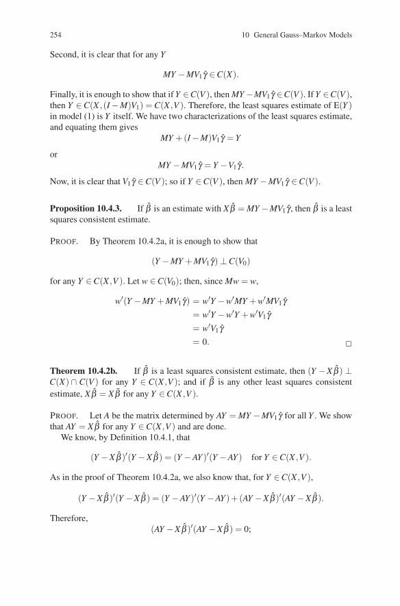
254 10 General Gauss–Markov Models
Second, it is clear that for any Y
MY −MV1γ ∈C(X).
Finally, it is enough to show that if Y ∈C(V ), then MY −MV1γ ∈C(V ). If Y ∈C(V ),then Y ∈C(X ,(I −M)V1) = C(X ,V ). Therefore, the least squares estimate of E(Y )in model (1) is Y itself. We have two characterizations of the least squares estimate,and equating them gives
MY +(I −M)V1γ = Y
orMY −MV1γ = Y −V1γ .
Now, it is clear that V1γ ∈C(V ); so if Y ∈C(V ), then MY −MV1γ ∈C(V ).
Proposition 10.4.3. If β is an estimate with X β = MY −MV1γ , then β is a leastsquares consistent estimate.
PROOF. By Theorem 10.4.2a, it is enough to show that
(Y −MY +MV1γ) ⊥C(V0)
for any Y ∈C(X ,V ). Let w ∈C(V0); then, since Mw = w,
w′(Y −MY +MV1γ) = w′Y −w′MY +w′MV1γ= w′Y −w′Y +w′V1γ= w′V1γ= 0. �
Theorem 10.4.2b. If β is a least squares consistent estimate, then (Y −X β ) ⊥C(X)∩ C(V ) for any Y ∈ C(X ,V ); and if β is any other least squares consistentestimate, X β = X β for any Y ∈C(X ,V ).
PROOF. Let A be the matrix determined by AY = MY −MV1γ for all Y . We showthat AY = X β for any Y ∈C(X ,V ) and are done.
We know, by Definition 10.4.1, that
(Y −X β )′(Y −X β) = (Y −AY )′(Y −AY ) for Y ∈C(X ,V ).
As in the proof of Theorem 10.4.2a, we also know that, for Y ∈C(X ,V ),
(Y −X β )′(Y −X β ) = (Y −AY )′(Y −AY )+(AY −X β )′(AY −X β ).
Therefore,(AY −X β )′(AY −X β ) = 0;

10.4 Least Squares Consistent Estimation 255
henceAY −X β = 0
orAY = X β for Y ∈C(X ,V ). �
Together, Theorems 10.4.2a and 10.4.2b give an “if and only if” condition for βto be a least squares CLUE.
In the future, any CLUE of Xβ , say AY , that satisfies (I −A)r ⊥ C(X)∩ C(V )for any r ∈ C(X ,V ) will be referred to as a least squares CLUE of Xβ . The mostimportant result on least squares CLUEs is:
Theorem 10.4.4. If in model (10.1.1), C(VV0) ⊂ C(V0), then a least squaresCLUE of Xβ is a best CLUE of Xβ (and hence a BLUE of Xβ ).
PROOF. Let AY be a least squares CLUE and BY any other CLUE. We need toshow that, for any vector ρ ,
Var(ρ ′AY ) ≤ Var(ρ ′BY ).
We can decompose Var(ρ ′BY ),
Var(ρ ′BY ) = Var(ρ ′(B−A)Y +ρ ′AY )= Var(ρ ′(B−A)Y )+Var(ρ ′AY )+2Cov(ρ ′(B−A)Y,ρ ′AY ).
Since variances are nonnegative, it suffices to show that
0 = Cov(ρ ′(B−A)Y,ρ ′AY ) = σ2ρ ′(B−A)VA′ρ.
First, we will establish that it is enough to show that the covariance is zero whenρ ∈C(X)∩C(V ). Let M0 be the perpendicular projection matrix onto C(X)∩C(V ).Then ρ = M0ρ +(I −M0)ρ and
ρ ′(B−A)VA′ρ = ρ ′(B−A)VA′M0ρ +ρ ′(B−A)VA′(I −M0)ρ= ρ ′M0(B−A)VA′M0ρ +ρ ′(I −M0)(B−A)VA′M0ρ
+ρ ′M0(B−A)VA′(I −M0)ρ+ρ ′(I −M0)(B−A)VA′(I −M0)ρ.
It turns out that all of these terms except the first is zero. Since AY and BY areCLUEs, unbiasedness and observation (d) in Section 2 give C(AV ) ⊂C(X)∩ C(V )and C(BV ) ⊂C(X)∩ C(V ). By orthogonality,
VA′(I −M0)ρ = 0 and ρ ′(I −M0)(B−A)V = 0;
so

256 10 General Gauss–Markov Models
ρ ′(B−A)VA′ρ = ρ ′M0(B−A)VA′M0ρ.
Henceforth, assume ρ ∈C(X)∩ C(V ).To obtain the final result, observe that since AY is a least squares CLUE, any
column of (I −A)V is orthogonal to ρ; so
V (I −A)′ρ = 0 and Vρ = VA′ρ.
Since, by assumption, C(VV0) ⊂C(V0), we also have V ρ ∈ C(X)∩ C(V ). The co-variance term is ρ ′(B−A)VA′ρ = ρ ′(B−A)V ρ. Since AY and BY are unbiased andV ρ ∈C(X), (B−A)Vρ = 0; hence
ρ ′(B−A)VA′ρ = 0. �
As mentioned in the statement of the theorem, a best CLUE is a BLUE. Thatoccurs because all BLUEs have the same variance and there is a BLUE that is aCLUE.
As would be expected, when C(X) ⊂ C(V ), a least squares CLUE will equalMY for all Y ∈ C(V ). When C(X) ⊂ C(V ), then C(X) = C(V0); so MV1 = 0 andMY −MV1γ = MY .
The following theorem characterizes when ordinary least squares estimates areBLUEs.
Theorem 10.4.5. The following conditions are equivalent:
(a) C(V X) ⊂C(X),(b) C(VV0) ⊂C(V0) and X ′V1 = 0,(c) MY is a BLUE for Xβ .
PROOF. Let X1 be a matrix with orthonormal columns such that C(X) =C(V0,X1)and V ′
0X1 = 0. Also let
V = [V0,V1][
B11 B12B21 B22
][V ′
0V ′
1
];
so V = V0B11V ′0 +V1B22V ′
1 +V0B12V ′1 +V1B21V ′
0. By symmetry, B12 = B′21. Recall
that V0 and V1 also have orthonormal columns.a ⇒ b
Clearly C(V X) ⊂ C(V ); so if C(V X) ⊂ C(X), we have C(V X) ⊂ C(V0). It iseasily seen that
C(V X) ⊂C(V0) if and only if C(VV0) ⊂C(V0) and C(V X1) ⊂C(V0).
We show that C(V X1) ⊂ C(V0) implies that X ′1V = 0; hence X ′
1V1 = 0 andX ′V1 = 0. First V X1 = V1B22V ′
1X1 +V0B12V ′1X1; we show that both terms are zero.

10.4 Least Squares Consistent Estimation 257
Consider VV0 =V0B11 +V1B21; since C(VV0)⊂C(V0), we must have V1B21 = 0. Bysymmetry, B12V ′
1 = 0 and V0B12V ′1X1 = 0. To see that V X1 =V1B22V ′
1X1 = 0, observethat since C(V X1) ⊂ C(V0), it must be true that C(V1B22V ′
1X1) ⊂ C(V0). However,C(V1B22V ′
1X1) ⊂C(V1) but C(V0) and C(V1) are orthogonal, so V1B22V ′1X1 = 0.
b ⇒ aIf X ′V1 = 0, then X ′
1V1 = 0 and X ′1V = 0. Write X = V0B0 + X1B1 so V X =
VV0B0 +V X1B1 = VV0B0. Thus,
C(V X) = C(VV0B0) ⊂C(VV0) ⊂C(V0) ⊂C(X).
b ⇒ cIf C(VV0) ⊂ C(V0), then MY −MV1γ is a BLUE. Since X ′V1 = 0, MV1 = 0 and
MY is a BLUE.c ⇒ b
If AY and BY are BLUEs, then AY = BY for Y ∈ C(X ,V ). As in Proposi-tion 10.2.3, there exists a BLUE, say AY , such that AV = VA′. Since MY is a BLUEand C(V ) ⊂C(X ,V ), AV = MV and MV = V M. Finally, VV0 = V MV0 = MVV0, soC(VV0) = C(MVV0) ⊂C(X). Since C(VV0) ⊂C(V ), we have C(VV0) ⊂C(V0).
From Theorem 10.4.4 we know that a least squares CLUE is a BLUE; henceMY = MY −MV1γ for Y ∈C(X ,V ) = C(X ,V1). Since
γ =[V ′
1(I −M)V1]−1 V ′
1(I −M)Y,
we must have 0 = MV1 [V ′1(I −M)V1]
−1 V ′1(I −M)V1 = MV1. Thus 0 = X ′V1. �
In the proof of a ⇒ b, it was noted that V1B21 = 0. That means we can write V =V0B11V ′
0 +V1B22V ′1. For ordinary least squares estimates to be BLUEs, C(V ) must
admit an orthogonal decomposition into a subspace contained in C(X) and a sub-space orthogonal to C(X). Moreover, the error term e in model (10.1.1) must havee = e0 + e1, where Cov(e0,e1) = 0, Cov(e0) = V0B11V ′
0, and Cov(e1) = V1B22V ′1.
Thus, with probability 1, the error can be written as the sum of two orthogonalvectors, both in C(V ), and one in C(X). The two vectors must also be uncorrelated.
Exercise 10.6 Show that V ′1(I −M)V1 is invertible.
Answer: The columns of V1 form a basis, so 0 =V1b iff b = 0. Also (I−M)V1b =0 iff V1b ∈C(X), but V1b ∈C(X) iff b = 0 by choice of V1. Thus, (I−M)V1b = 0 iffb = 0; hence (I −M)V1 has full column rank and V ′
1(I −M)V1 is invertible.
Exercise 10.7 Show that if MY −MV1γ is a BLUE of Xβ , then C(VV0)⊂C(V0).Hint: Multiply on the right by V0 after showing that[M−MV1
[V ′
1(I −M)V1]−1 V ′
1(I −M)]
V
= V[M− (I −M)V1
[V ′
1(I −M)V1]−1 V ′
1M].

258 10 General Gauss–Markov Models
We include a result that allows one to find the matrix V1, and thus find leastsquares CLUEs.
Proposition 10.4.6. r ⊥C(X)∩ C(V ) if and only if r ∈C(I −M, I −MV ).
PROOF. If r ∈C(I −M, I −MV ), then write r = (I −M)r1 +(I −MV )r2.Let w ∈ C(X)∩ C(V ) so that w = MV w = Mw. We need to show that w′r = 0.
Observe that
w′r = w′(I −M)r1 +w′(I −MV )r2
= w′M(I −M)r1 +w′MV (I −MV )r2
= 0.
The vector space here is, say, Rn. Let r[C(X)∩C(V )] = m. From the above result,C(I −M, I −MV ) is orthogonal to C(X)∩ C(V ). It is enough to show that the rankof C(I −M, I−MV ) is n−m. If this is not the case, there exists a vector w �= 0 suchthat w ⊥C(I −M, I −MV ) and w ⊥C(X)∩ C(V ).
Since w⊥C(I−M, I−MV ), we have (I−M)w = 0 or w = Mw∈C(X). Similarly,w = MV w ∈C(V ); so w ∈C(X)∩ C(V ), a contradiction. �
To find V1, one could use Gram–Schmidt to first get an orthonormal basis forC(I−M, I−MV ), then extend this to Rn. The extension is a basis for C(V0). Finally,extend the basis for C(V0) to an orthonormal basis for C(V ). The extension is a basisfor C(V1). A basis for C(X1) can be found by extending the basis for C(V0) to a basisfor C(X).
Exercise 10.8 Give the general form for a BLUE of Xβ in model (10.1.1).Hint: Add something to a particular BLUE.
Exercise 10.9 From inspecting Figure 10.2, give the least squares CLUE forExample 10.2.2. Do not do any matrix manipulations.
Remark. Suppose that we are analyzing the model Y = Xβ +e, E(e) = 0, Cov(e) =Σ(θ), where Σ(θ ) is some nonnegative definite matrix depending on a vector of un-known parameters θ . The special case where Σ(θ) = σ 2V is what we have beenconsidering so far. It is clear that if θ is known, our current theory gives BLUEs. Ifit happens to be the case that for any value of θ the BLUEs are identical, then theBLUEs are known even though θ may not be. This is precisely what we have beendoing with Σ(θ ) = σ 2V . We have found BLUEs for any value of σ 2, and they do notdepend on σ2. Another important example of this occurs when C(Σ(θ )X) ⊂C(X)for any θ . In this case, least squares estimates are BLUEs for any θ , and leastsquares estimates do not depend on θ , so it does not matter that θ is unknown. The

10.5 Perfect Estimation and More 259
split plot design model is one in which the covariance matrix depends on two pa-rameters, but for any value of those parameters, least squares estimates are BLUEs.Such models are examined in the next chapter.
Exercise 10.10 Show that ordinary least squares estimates are best linear unbi-ased estimates in the model Y = Xβ + e, E(e) = 0, Cov(e) = V if the columns of Xare eigenvectors of V .
Exercise 10.11 Use Definition B.31 and Proposition 10.4.6 to show thatMC(X)∩C(V ) = M−MW where C(W ) = C[M(I −MV )].
10.5 Perfect Estimation and More
One of the interesting things about the linear model
Y = Xβ + e, E(e) = 0, Cov(e) = σ 2V, (1)
is that when C(X) �⊂C(V ) you can learn things about the parameters with probability1. We identify these estimable functions of the parameters and consider the processof estimating those parameters that are not perfectly known.
Earlier, to treat C(X) �⊂ C(V ), we obtained estimates and tests by replacing Vin model (1) with T where C(X) ⊂ C(T ). Although we showed that the procedureworks, it is probably not the first thing one would think to do. In this section, afterisolating the estimable functions of Xβ that can be known perfectly, we replacemodel (1) with a new model Y =V0γ +e, E(e) = 0, Cov(e) = σ2V in which C(V0)⊂C(V ) and Y is just Y minus a perfectly known component of Xβ . I find it far moreintuitive to make adjustments to the model matrix X , something we do regularlyin defining reduced and restricted models, than to adjust the covariance matrix V .Additional details are given in Christensen and Lin (2010).
EXAMPLE 10.5.1. Consider a one-sample model yi = μ +εi, i = 1,2,3, with un-correlated observations but in which the second and third observations have variance0. If this model is correct, you obviously should have μ = y2 = y3 with probability1. The matrices for model (1) are
Y =
⎡⎣y1y2y3
⎤⎦ , X =
⎡⎣111
⎤⎦ , V =
⎡⎣1 0 00 0 00 0 0
⎤⎦ .
All of our examples in this section use this same Y vector.
The first thing to do with models having C(X) �⊂C(V ) is to see whether they areeven plausible for the data. In particular, Lemma 1.3.5 implies that Pr[(Y −Xβ ) ∈

260 10 General Gauss–Markov Models
C(V )] = 1 so that Y ∈C(X ,V ) a.s. This should be used as a model-checking device.If Y �∈C(X ,V ), you clearly have the wrong model.
EXAMPLE 10.5.1 CONTINUED. In this example, if y2 �= y3 we obviously havethe wrong model. It is easily seen that
C(X ,V ) = C
⎛⎝⎡⎣011
⎤⎦ ,
⎡⎣100
⎤⎦⎞⎠and if y2 �= y3, Y �∈C(X ,V ).
To identify the estimable parameters that can be known perfectly, let Q be a fullrank matrix with
C(Q) = C(V )⊥.
Note that if C(X) �⊂C(V ), then Q′X �= 0. Actually, the contrapositive is more obvi-ous, if Q′X = 0 then
C(X) ⊂C(Q)⊥ =[C(V )⊥
]⊥= C(V ).
The fact that Q′X �= 0 means that the estimable function Q′Xβ is nontrivial. Notealso that C(X) �⊂C(V ) implies that V must be singular. If V were nonsingular, thenC(V ) = Rn and C(X) has to be contained in it.
We can now identify the estimable functions that are known perfectly. BecausePr[(Y −Xβ ) ∈ C(V )] = 1, clearly Pr[Q′(Y −Xβ) = 0] = 1 and Q′Y = Q′Xβ a.s.Therefore, whenever C(X) �⊂ C(V ), there are nontrivial estimable functions of βthat we can learn without error. Moreover, Cov(Q′Y ) = σ2Q′V Q = 0 and only linearfunctions of Q′Y will have 0 covariance matrices, so only linear functions of Q′Xβwill be estimated perfectly.
Exercise 10.13 Show that Cov(B′Y ) = 0 iff B′ = B′∗Q′ for some matrix B∗.Hint: First, decompose B into the sum of two matrices B0 and B1 with C(B0) ⊂
C(V ) and C(B1)⊥C(V ). Then use a singular value decomposition of V to show thatB′
0V B0 = 0 iff B0 = 0.
If Q′X has full column rank, we can actually learn all of Xβ without error. In thatcase, with probability 1 we can write
Xβ = X(X ′QQ′X
)−1 [X ′QQ′X]
β = X(X ′QQ′X)−1X ′QQ′Y.
For convenience, define A so that AY ≡ X(X ′QQ′X)−1X ′QQ′Y , in which case Xβ =AY a.s. In particular, it is easy to see that E[AY ] = Xβ and Cov[AY ] = 0. We nowillustrate these matrix formulations in some simple examples to show that the matrixresults give obviously correct answers.

10.5 Perfect Estimation and More 261
EXAMPLE 10.5.1 CONTINUED. Using the earlier forms for X and V ,
Q =
⎡⎣0 01 00 1
⎤⎦ .
It follows that
Q′X =[
11
]and Q′Y = Q′Xβ reduces to [
y2y3
]= μJ2 a.s.
Obviously, for this to be true, y2 = y3 a.s. Moreover, since Q′X is full rank, uponobserving that X ′QQ′X = 2 we can compute
μJ3 = Xβ = AY = [(y2 + y3)/2]J3 a.s.
EXAMPLE 10.5.2. This is a two-sample problem, with the first two observationsfrom sample one and the third from sample two. Again, observations two and threehave 0 variance. Clearly, with probability 1, μ1 = y2 and μ2 = y3. The key matricesare
X =
⎡⎣1 01 00 1
⎤⎦ , V =
⎡⎣1 0 00 0 00 0 0
⎤⎦ , Q =
⎡⎣0 01 00 1
⎤⎦ .
Since β = [μ1,μ2]′ in the two-sample problem and
Q′X =[
1 00 1
],
we have [μ1μ2
]= Q′Xβ = Q′Y =
[y2y3
]a.s.
In particular, with probability 1,⎡⎣μ1μ1μ2
⎤⎦= Xβ = AY =
⎡⎣y2y2y3
⎤⎦ .
EXAMPLE 10.5.3. This is a one-sample problem similar to Example 10.5.1 ex-cept that now the first two observations have variance 1 but the third has variance 0.The key matrices are

262 10 General Gauss–Markov Models
X =
⎡⎣111
⎤⎦ , V =
⎡⎣1 0 00 1 00 0 0
⎤⎦ , Q =
⎡⎣001
⎤⎦ .
With Q′X = 1 we get Q′Xβ = μ equaling Q′Y = y3 with probability 1. Moreover,since X ′QQ′X = 1 we can easily compute
μJ3 = Xβ = AY = y3J3.
The next two examples do not have Q′X with full rank, so they actually havesomething to estimate.
EXAMPLE 10.5.4. Consider a two-sample problem similar to Example 10.5.2except that now the first two observations have variance 1 but the third has variance0. The key matrices are
X =
⎡⎣1 01 00 1
⎤⎦ , V =
⎡⎣1 0 00 1 00 0 0
⎤⎦ , Q =
⎡⎣001
⎤⎦ .
With β = [μ1,μ2]′ andQ′X = [0 1 ] ,
we get
μ2 = [0 1 ][
μ1μ2
]= Q′Xβ = Q′Y = y3 a.s.
Clearly, y3 = μ2 a.s. but μ1 would be estimated with the average (y1 + y2)/2. Moreon this later.
EXAMPLE 10.5.5 Finally, in the two-sample problem we move the second ob-servation from the first group to the second group. This time
X =
⎡⎣1 00 10 1
⎤⎦ , V =
⎡⎣1 0 00 1 00 0 0
⎤⎦ , Q =
⎡⎣001
⎤⎦ ,
withQ′X = [0 1 ] .
Again, with probability 1,
μ2 = [0 1 ][
μ1μ2
]= Q′Xβ = Q′Y = y3,
so y3 = μ2 a.s. But this time, only y1 would be used to estimate μ1, and y2 is of novalue for estimating the means. However, y2 could be used to estimate an unknown

10.5 Perfect Estimation and More 263
variance via (y2−μ2)2 = (y2−y3)2. Similar results on estimating the variance applyin all the examples except Example 10.5.4.
To get perfect estimation of anything, we need C(X) �⊂ C(V ). To get perfectestimation of everything we need C(X)∩C(V ) = {0}. In other words, to get perfectestimation of Xβ we need Q′X with full column rank and to get Q′X with fullcolumn rank, we need C(X)∩ C(V ) = {0}.
Proposition 10.5.6. For X of full column rank, Q′X is of full column rank if andonly if C(X)∩ C(V ) = {0}.
PROOF. This is a special case of Lemma 10.5.7. �
Although C(X)∩C(V ) = {0} is actually a necessary and sufficient condition forperfect estimation of Xβ , with the methods we have illustrated it is not obviouslysufficient. For our current method, we need Q′X to have full column rank, whichobviously will not happen if X is not full rank. Fortunately, we can always sim-ply choose X to have full column rank. In addition, we close this section with themathematics needed to deal with arbitrary X .
Now consider models in which some aspect of Xβ is known but some aspect isnot. In particular, we know that Q′Xβ is known, but how do we estimate the rest ofXβ? As discussed above, we must now consider the case where C(X)∩C(V ) �= {0}.Write β = β0 +β1 with β0 ∈C(X ′Q) and β1 ⊥C(X ′Q). We show that Xβ0 is known,so that we need only estimate Xβ1 to learn all that can be learned about Xβ . Thesemethods make no assumption about r(X).
In fact, β0 is known, not just Xβ0. Let PX ′Q be the ppo onto C(X ′Q). By thedefinition of β0 as part of an (unique) orthogonal decomposition, with probability 1,
β0 = PX ′Qβ = X ′Q[Q′XX ′Q]−Q′Xβ = X ′Q[Q′XX ′Q]−Q′Y.
Since the perpendicular projection operator does not depend on the choice of gen-eralized inverse, neither does β0.
Now we show how to estimate Xβ1. Let V0 be such that C(V0) = C(X)∩ C(V ).Proposition 10.4.6 can be used to find V0. Note that β1 ⊥C(X ′Q) iff Q′Xβ1 = 0 iffXβ1 ⊥C(Q) iff Xβ1 ∈C(V ) iff Xβ1 ∈C(V0) iff Xβ1 = V0γ for some γ . Since Xβ0is fixed and known, it follows that E(Y −Xβ0) = Xβ1 ∈C(V0) and Cov(Y −Xβ0) =σ 2V , so we can estimate Xβ1 by fitting
Y −Xβ0 = V0γ + e, E(e) = 0, Cov(e) = σ 2V, (2)
and takingX β1 ≡V0γ = V0(V ′
0V−V0)−V0V−(Y −Xβ0),
cf. Section 2. Under normality, tests are also relatively easy to construct.
EXAMPLE 10.5.4 CONTINUED. Using the earlier versions of X , V , Q, and Q′X ,observe that
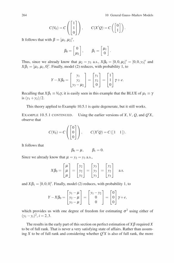
264 10 General Gauss–Markov Models
C(V0) = C
⎛⎝⎡⎣110
⎤⎦⎞⎠ , C(X ′Q) = C([
01
]).
It follows that with β = [μ1,μ2]′,
β0 =[
0μ2
], β1 =
[μ10
].
Thus, since we already know that μ2 = y3 a.s., Xβ0 = [0,0,μ2]′ = [0,0,y3]′ andXβ1 = [μ1,μ1,0]′. Finally, model (2) reduces, with probability 1, to
Y −Xβ0 =
⎡⎣ y1y2
y3 −μ2
⎤⎦=
⎡⎣y1y20
⎤⎦=
⎡⎣110
⎤⎦γ + e.
Recalling that Xβ1 ≡V0γ , it is easily seen in this example that the BLUE of μ1 ≡ γis (y1 + y2)/2.
This theory applied to Example 10.5.1 is quite degenerate, but it still works.
EXAMPLE 10.5.1 CONTINUED. Using the earlier versions of X , V , Q, and Q′X ,observe that
C(V0) = C
⎛⎝⎡⎣000
⎤⎦⎞⎠ , C(X ′Q) = C ([1 1 ]) .
It follows thatβ0 = μ , β1 = 0.
Since we already know that μ = y2 = y3 a.s.,
Xβ0 =
⎡⎣μμμ
⎤⎦=
⎡⎣y2y2y2
⎤⎦=
⎡⎣y3y3y3
⎤⎦=
⎡⎣y2y2y3
⎤⎦ a.s.
and Xβ1 = [0,0,0]′. Finally, model (2) reduces, with probability 1, to
Y −Xβ0 =
⎡⎣y1 −μy2 −μy3 −μ
⎤⎦=
⎡⎣y1 − y200
⎤⎦=
⎡⎣000
⎤⎦γ + e,
which provides us with one degree of freedom for estimating σ 2 using either of(y1 − yi)2, i = 2,3.
The results in the early part of this section on perfect estimation of Xβ required Xto be of full rank. That is never a very satisfying state of affairs. Rather than assum-ing X to be of full rank and considering whether Q′X is also of full rank, the more

10.5 Perfect Estimation and More 265
general condition for estimating Xβ perfectly is that r(X) = r(Q′X). Moreover, withA ≡ X(X ′QQ′X)−X ′QQ′, we always have perfect estimation of AXβ because AXβis a linear function of Q′Xβ = Q′Y a.s. but for perfect estimation of Xβ we need
Xβ = AXβ = AY a.s.
for any β which requires A to be a projection operator onto C(X). This added gen-erality requires some added work.
Lemma 10.5.7
(a) r(X) = r(Q′X) iff for any b, Q′Xb = 0 implies Xb = 0.(b) r(X) = r(Q′X) iff C(X)∩ C(V ) = {0}.
PROOF.Proof of (a): Recall that r(Q′X) = r(X) iff r[N (Q′X)] = r[N (X)]. Since the
null spaces have N (X)⊂N (Q′X), it is enough to show that N (Q′X) = N (X) isequivalent to the condition that for any b, Q′Xb = 0 implies Xb = 0 and, in particular,it is enough to show that N (Q′X)⊂N (X) is equivalent to the condition. But by thevery definition of the null spaces, N (Q′X) ⊂ N (X) is equivalent to the conditionthat for any b we have Q′Xb = 0 implies that Xb = 0.
Proof of (b): Note that for any b,
Q′Xb = 0 iff Xb ⊥C(Q) iff Xb ∈C(Q)⊥ =[C(V )⊥
]⊥= C(V ),
soQ′Xb = 0 iff Xb ∈C(V ) iff Xb ∈C(X)∩ C(V ).
If follows immediately that if C(X)∩ C(V ) = {0}, then Q′Xb = 0 implies Xb = 0and r(X) = r(Q′X). It also follows immediately that since Q′Xb = 0 is equivalent tohaving Xb ∈C(X)∩ C(V ), the condition that Q′Xb = 0 implies Xb = 0 means thatthe only vector in C(X)∩ C(V ) is the 0 vector. �
Proposition 10.5.8 If r(X) = r(Q′X), the matrix A ≡ X(X ′QQ′X)−X ′QQ′ is aprojection operator onto C(X).
PROOF. By its definition we clearly have C(A) ⊂C(X), so it is enough to show thatAX = X .
Let MQ′X be the ppo onto C(Q′X). Note that for any b, Xb−AXb ∈C(X). More-over, from the definitions of A and MQ′X ,
Q′Xb−Q′AXb = Q′Xb−MQ′X Q′Xb = 0.
Writing
0 = Q′Xb−MQ′X Q′Xb = Q′X[I − (X ′QQ′X)−X ′QQ′X
]b,

266 10 General Gauss–Markov Models
by the condition r(X) = r(Q′X) and Lemma 10.5.8a, we have
0 = X[I − (X ′QQ′X)−X ′QQ′X
]b = Xb−AXb,
hence X = AX . �
Exercise 10.13 Show that the results in this section do not depend on the partic-ular choice of Q.
Exercise 10.14 Let C(V0) = C(X)∩ C(V ), C(X) = C(V0,X1), C(V ) = C(V0,V1)with the columns of V0, V1, and X1 being orthonormal. Show that the columns of[V0,V1,X1] are linearly dependent.
Hint: Write V0b0 +V1b1 +X1b2 = 0 and show that bi = 0, i = 0,1,2. In particular,write
0.5V0b0 +V1b1 = −(0.5V0b0 +X1b2),
0.5V0b0 +V1b1 ∈C(V ) and −(0.5V0b0 +X1b2) ∈C(X) so the vector is in C(V0) =C(X)∩ C(V ).

Chapter 11
Split Plot Models
In an experiment with at least two factors, it is sometimes convenient to apply someof the factors to large experimental units (called whole plots) and then to split thelarge units into smaller parts to which the remaining factors are applied. The subdi-visions of the whole plots are called subplots or split plots.
Split plot designs are often used when either (1) the factors applied to wholeplots are not of direct interest or (2) some factors require larger experimental unitsthan the other factors. The first case is illustrated with an experiment to evaluatecrop yields when using varying levels of a standard herbicide and a new pesticide.If the standard herbicide is not of direct interest, but rather primary interest is inthe effects of the pesticide and any possible interaction between the herbicide andthe pesticide, then it is appropriate to apply herbicides as whole plot treatments.(It will be seen later that interaction contrasts and comparisons between pesticidesare subject to less error than comparisons among herbicides.) The second case thatsplit plot designs are often used for can also be illustrated with this experiment. Ifthe standard herbicide is applied using a tractor, but the new pesticide is applied bycrop dusting, then the experimental procedure makes it necessary to use pesticidesas whole plot treatments. (Clearly, an airplane requires a larger plot of ground forspraying than does a tractor.)
It is of interest to note that a split plot design can be thought of as an (unbal-anced) incomplete block design. In this approach, each whole plot is thought of asa block. Each block contains the treatments that are all combinations of the subplotfactor levels with the one combination of whole plot factor levels that was applied.As with other incomplete block designs, a split plot design is necessary when thereare not enough blocks available that can accommodate all of the treatment combina-tions. In split plot designs, this means that there are not enough subplots per wholeplot so that all treatment combinations could be applied at the subplot level. If, inaddition, there are not enough whole plots so that each treatment combination couldbe applied to a whole plot, then a split plot design is an attractive option.
Mathematically, the key characteristic of a split plot model is the covariancestructure. Typically, observations taken on the subplots of any particular whole plot
© Springer Science+Business Media, LLC 2011
267Springer Texts in Statistics, DOI 10.1007/978-1-4419-9816-3_11, R. Christensen, Plane Answers to Complex Questions: The Theory of Linear Models,

268 11 Split Plot Models
are assumed to have a constant nonzero correlation. Observations taken on differentwhole plots are assumed to be uncorrelated.
The main purpose of this chapter is to derive the analysis for split plot models. InSection 1, we consider a special cluster sampling model. The cluster sampling modelhas the same covariance structure as a split plot model. In Section 2, we considerways of generalizing the cluster sampling model that allow for an easy analysisof the data. The discussion in Section 2 is really an examination of generalizedsplit plot models. Section 3 derives the analysis for the traditional split plot modelby using the results of Section 2. Section 4 discusses the issues of identifying anappropriate error term and of subsampling.
Sections 1 and 2 are closely related to Christensen (1984) and (1987b), respec-tively. In fact, Christensen (1987b) is probably easier to read than Section 2 be-cause it includes more introductory material and fewer of the mathematical details.Closely related work is contained in Monlezun and Blouin (1988) and Mathew andSinha (1992). A general review of methods for analyzing cluster sampling modelsis given in Skinner, Holt, and Smith (1989).
11.1 A Cluster Sampling Model
A commonly used technique in survey sampling is cluster sampling (also calledtwo-stage sampling). This technique is applied when the population to be sampledconsists of some kind of clusters. The sample is obtained by taking a random sampleof clusters and then taking a random sample of the individuals within each of thesampled clusters. For example, suppose it was desired to sample the populationof grade school students in Montana. One could take a random sample of gradeschools in the state, and then for each school that was chosen take a random sampleof the students in the school. One complication of this method is that students fromthe same school will tend to be more alike than students from different schools. Ingeneral, there will be a nonnegative correlation among the individual units within acluster.
General Cluster Sampling Models
Suppose n observations are available from a two-stage sample with c clusters. Fromeach cluster, mi units are sampled and variables Y,X1, . . . ,Xp are obtained. Sinceobservations in a cluster are typically not independent, we will consider the linearmodel
Y = Xβ + e, e ∼ N(0,σ 2V
),
where X is n× p of rank r and (assuming the elements of Y are listed by clusters) Vis the block diagonal matrix

11.1 A Cluster Sampling Model 269
V = Blk diag(Vi),
where Vi is an mi ×mi intraclass correlation matrix
Vi =
⎡⎢⎢⎣1 ρ · · · ρρ 1 · · · ρ...
.... . .
...ρ ρ · · · 1
⎤⎥⎥⎦ .
If we let Jm(i) be an mi ×1 vector of ones, then
V = (1−ρ)I +ρBlk diag(Jm(i)J′m(i)).
Now let X1 be an n× c matrix of indicator variables for the clusters. In otherwords, a row of the ith column of X1 is 1 if the row corresponds to an observationfrom the ith cluster and 0 otherwise. It follows that X1X ′
1 = Blk diag(Jm(i)J′m(i)), so
V = (1−ρ)I +ρX1X ′1. (1)
In fact, equation (1) holds even if the elements of Y are not listed by cluster.We can now provide an interesting condition for when ordinary least squares
(OLS) estimates are best linear unbiased estimates (BLUEs) in cluster samplingmodels. Recall from Theorem 10.4.5 that OLS estimates are BLUEs if and only ifC(V X) ⊂ C(X). This condition holds if and only if C(X1X ′
1X) ⊂ C(X). Since thecolumns of X1 are indicator variables for the clusters, X1X ′
1X takes each column ofX , computes the cluster totals, and replaces each component with the correspondingcluster total. Thus, OLS estimates are BLUEs if and only if for any variable in themodel, the variable formed by replacing each component with the correspondingcluster total is also, either implicitly or explicitly, contained in the model.
A Special Cluster Sampling Model
We now consider a particular cluster sampling model for which OLS estimatesare BLUEs, and for which tests and confidence intervals are readily available forthe most interesting parameters. Consider a model in which X can be written asX = [X1,X2], where X1 is again the matrix of indicator variables for the clusters.Rewriting the linear model as
Y = [X1,X2][
αγ
]+ e (2)
leads to the interpretation that the αis are separate cluster effects. Typically, onewould not be very interested in these cluster effects. One’s primary interest wouldbe in the vector γ .

270 11 Split Plot Models
It is easily seen that C(V X)⊂C(X), so OLS estimates are BLUEs. The notewor-thy thing about this model is that inference on the parameter vector γ can proceedjust as when Cov(Y ) = σ 2I. Treating (2) as an analysis of covariance model, weobtain for any estimable function λ ′γ
λ ′γ = λ ′ [X ′2(I −M1)X2
]− X ′2(I −M1)Y,
where M1 is the perpendicular projection matrix onto C(X1).The variance of λ ′γ is
Var(λ ′γ) = σ 2λ ′ [X ′2(I −M1)X2
]−X ′2(I−M1)V (I−M1)X2
[X ′
2(I −M1)X2]−λ . (3)
From (1) observe that
V (I −M1) = (1−ρ)(I −M1).
Substitution into (3) gives
Var(λ ′γ) = σ 2(1−ρ)λ ′ [X ′2(I −M1)X2
]− λ , (4)
which, except for the term (1−ρ), is the variance from assuming Cov(Y ) = σ 2I.
Exercise 11.1 Prove that equation (4) is true.
The mean square error (MSE) from ordinary least squares provides an indepen-dent estimate of σ 2(1−ρ). Let M = X(X ′X)−X ′, so MSE = Y ′(I −M)Y/(n− r).
E(MSE) = (n− r)−1σ 2tr[(I −M)V ].
Since C(X1) ⊂C(X), from (1) we have
(I −M)V = (I −M)(1−ρ)I = (1−ρ)(I −M).
But, tr[(1−ρ)(I −M)] = (1−ρ)(n− r), so
E(MSE) = σ2(1−ρ).
Theorem 11.1.1.
(i) Y ′(I −M)Y/σ 2(1−ρ) ∼ χ2(n− r,0).(ii) MSE and X β are independent. In particular, MSE and λ ′γ are independent.
Exercise 11.2 Prove Theorem 11.1.1.Hint: For (i), use Theorem 1.3.6. For (ii), show that Cov[(I −M)Y,MY ] = 0.

11.1 A Cluster Sampling Model 271
These results provide a basis for finding tests and confidence intervals for anestimable function λ ′γ . We might also want to consider doing F tests. Suppose wewant to test some vector of estimable restrictions on γ , say Λ ′γ = 0. The test can bederived from Λ ′γ , Cov(Λ ′γ), and MSE, using Theorem 11.1.1 and Corollary 3.8.3.In particular,
Theorem 11.1.2.
(i)(Λ ′γ)′
(Λ ′ [X ′
2(I −M1)X2]−Λ)−
(Λ ′γ)/r(Λ )MSE
∼ F(r(Λ),n− r,π),
where π = (Λ ′γ)′(Λ ′ [X ′
2(I −M1)X2]−Λ)−
(Λ ′γ)/2σ 2(1−ρ).
(ii) (Λ ′γ)′(Λ ′ [X ′
2(I −M1)X2]−Λ)−
(Λ ′γ) = 0 if and only if Λ ′γ = 0.
An alternative to testing linear parametric functions is testing models. To testmodel (2) against a reduced model, say
Y = X0β0 + e, C(X1) ⊂C(X0) ⊂C(X),
the test is the usual Cov(Y ) = σ 2I test. With M0 = X0(X ′0X0)−X ′
0, we have:
Theorem 11.1.3.
(i)Y ′(M−M0)Y/[r(X)− r(X0)]
MSE∼ F(r(X)− r(X0),n− r,π),
where π = β ′0X ′(M−M0)Xβ0/2σ 2(1−ρ).
(ii) β ′0X ′(M−M0)Xβ0 = 0 if and only if E(Y ) ∈C(X0).
PROOF. For part (i), see Exercise 11.3. Part (ii) follows exactly as in Theo-rem 3.2.1. �
Exercise 11.3 Prove Theorem 11.1.3(i).
In summary, for a model that includes separate fixed effects for each cluster, theordinary least squares fit gives optimal estimates of all effects and valid estimates ofstandard errors for all effects not involving the cluster effects. If normal distributionsare assumed, the usual Cov(Y ) = σ 2I tests and confidence intervals are valid unlessthe cluster effects are involved. If the cluster effects are not of interest, the entireanalysis can be performed with ordinary least squares. This substantially reducesthe effort required to analyze the data.
The assumption that the αis are fixed effects is necessary for the result to hold.However, if additional random cluster effects are added to the model so that there

272 11 Split Plot Models
are both fixed and random cluster effects, then the basic structure of the covariancematrix remains unchanged and the optimality of ordinary least squares is retained.
Exercise 11.4 The usual model for a randomized complete block design wasgiven in Section 8.2 as
yi j = μ +αi +β j + ei j,
i = 1, . . . ,a, j = 1, . . . ,b, Var(ei j) = σ 2, and Cov(ei j,ei′ j′) = 0 for (i, j) �= (i′, j′).The β js are considered as fixed block effects. Consider now a model
yi j = μ +αi +β j +η j + ei j.
The η js are independent N(0,σ 22 ) and the ei js are independent N(0,σ 2
1 ). The η jsand ei js are also independent. The block effects are now (β j +η j). There is a fixedcomponent and a random component with mean zero in each block effect. Use theresults of this section to derive an analysis for this model. Give an ANOVA tableand discuss interval estimates for contrasts in the αis.
Exercise 11.5 An alternative model for a block design is
yi j = μ +αi +β j + ei j, (5)
where the β js are independent N(0,σ 22 ) and the β js and ei js are independent. If this
model is used for a balanced incomplete block design, the BLUEs are different thanthey are when the β js are assumed to be fixed. Discuss the appropriateness of theanalysis based on this model in light of the results of Exercise 11.4.
Exercise 11.6 Show that when using model (5) for a randomized complete blockdesign, the BLUE of a contrast in the αis is the same regardless of whether the β jsare assumed random or fixed. Show that the estimates of a contrast’s variance arethe same.
11.2 Generalized Split Plot Models
By placing additional conditions on model (11.1.2), we can get a simple analysis ofthe cluster effects while retaining a simple analysis for the noncluster effects. Theanalysis of the cluster effects corresponds to the analysis of whole plot treatmentsin a split plot model. The noncluster effects relate to effects on the subplot level.
Generalized split plot models are models obtained by imposing additional struc-ture on the cluster sampling model (11.1.2). This additional structure involves sim-plifying the covariance matrix and modeling the whole plot (cluster) effects. First,a condition on the whole plots is discussed. The condition is that the number ofobservations in each whole plot is the same. This condition simplifies the covari-

11.2 Generalized Split Plot Models 273
ance matrix considerably. Next, the whole plot effects are modeled by assuming areduced model that does not allow separate effects for each whole plot. As part ofthe modeling process, a condition is imposed on the model matrix of the reducedmodel that ensures that least squares estimates are BLUEs. The problem of drawinginferences about generalized split plot models is discussed in two parts, (1) estima-tion and testing of estimable functions and (2) testing reduced models. A conditionthat allows for a simple analysis of the whole plot effects is mentioned, a discussionof how to identify generalized split plot models is given, and finally some computa-tional methods are presented.
The Covariance Matrix
Writing Y so that observations in each whole plot are listed contiguously, we canrewrite the covariance matrix of model (11.1.2) as
σ 2V = σ2 [(1−ρ)I +ρM1{Blk diag(miIm(i))}],
where Im(i) is an mi ×mi identity matrix and M1 is the perpendicular projection ma-trix onto C(X1). This follows from Section 1 because M1 = Blk diag(m−1
i Jm(i)J′m(i)).This characterization of V is not convenient in itself because of the Blk diag(miIm(i))term. For example, the expected value of a quadratic form, say Y ′AY , is E(Y ′AY ) =σ 2tr(AV )+ β ′X ′AXβ . The trace of AV is not easy to compute. To simplify the sub-sequent analysis, we impose
Condition 11.2.1. All whole plots (clusters) are of the same size, say mi = m forall i.
It follows thatV = (1−ρ)I +mρM1. (1)
This form for V will be assumed in the remainder of Section 2.
Modeling the Whole Plots
Model (11.1.2) assumes separate effects for each whole plot (cluster). Modeling thecluster effects consists of imposing structure on those effects. This is done by puttinga constraint on C(X1). The simplest way to do this is by postulating a reduced model,say
Y = Zβ∗ + e, Z = [X∗,X2] , C(X∗) ⊂C(X1). (2)
Partitioning β∗ in conformance with Z, write

274 11 Split Plot Models
β ′∗ =[δ ′,γ ′
].
Remember, this is not the same γ as in (11.1.2), but it is the coefficient for X2, justas in (11.1.2). Define the perpendicular projection operators onto C(Z) and C(X∗)as MZ and M∗, respectively.
In Section 1, it was shown that least squares estimates were BLUEs for model(11.1.2). We are now dealing with a different model, model (2), so another proofis required. To check if least squares estimates are BLUEs, we need to see whetherC(V Z) ⊂ C(Z). Since by equation (1), V = (1−ρ)I + mρM1, we have V Z = (1−ρ)Z +mρM1Z. Clearly, it is enough to check whether C(M1Z) ⊂C(Z). This is truefor a special case.
Proposition 11.2.2. Let M and N be subspaces of C(Z). If C(Z) = M +N ,where M ⊂C(X1) and N ⊥C(X1), then C(M1Z) ⊂C(Z).
PROOF. For any v ∈C(Z), write v = v1 + v2, where v1 ∈ M and v2 ∈ N . M1v =M1v1 +M1v2 = v1, but v1 ∈ M ⊂C(Z). �
A condition that is easy to check is
Condition 11.2.3. C(Z) = C(X∗,(I −M1)X2) and C(X∗) ⊂C(X1).
If Condition 11.2.3 holds, then Proposition 11.2.2 applies with M = C(X∗) andN = C[(I −M1)X2]. If Proposition 11.2.2 applies, then least squares estimates areBLUEs.
EXAMPLE 11.2.4. Let whole plots be denoted by the subscripts i and j, and letsubplots have the subscript k. Let the dependent variable be yi jk and let xi jk1, xi jk2,and xi jk3 be three covariates. The model given below is a generalized split plot model(see Exercise 11.7.):
yi jk = μ +ωi + γ1xi j·1 + γ21xi j·2 +ηi j
+ τk +(ωτ)ik + γ22(xi jk2 − xi j·2)+ γ3(xi jk3 − xi j·3) (3)+ ei jk,
i = 1, . . . ,a, j = 1, . . . ,Ni, k = 1, . . . ,m. The ηi js and ei jks are all independent withηi j ∼ N(0,σ 2
w) and ei jk ∼ N(0,σ 2s ). With these assumptions
σ 2 = σ2w +σ 2
s
andρ = σ 2
w/(σ 2w +σ 2
s ).
The ωis are treatment effects for a one-way ANOVA with unequal numbers inthe whole plots. The whole plot treatments can obviously be generalized to include

11.2 Generalized Split Plot Models 275
multifactor ANOVAs with unequal numbers. The ωis, γ1, γ21, and μ make up theδ vector. The τks, (ωτ)iks, γ22, and γ3 make up the vector γ from model (2). Notethat the covariate used with γ22 could be changed to xi jk2 without changing C(Z) orinvalidating Condition 11.2.3.
Exercise 11.7 Verify that Condition 11.2.3 holds for model (3).
Estimation and Testing of Estimable Functions
We now discuss estimation and testing for model (2). Under Condition 11.2.1 andCondition 11.2.3, least squares estimates are BLUEs. Define
M2 = (I −M1)X2[X ′
2(I −M1)X2]− X ′
2(I −M1).
From Condition 11.2.3, the perpendicular projection operator onto C(Z) is
MZ = M∗ +M2. (4)
Given the perpendicular projection operator, the least squares estimates can be foundin the usual way.
First, consider drawing inferences about γ . For estimable functions of γ , the esti-mates are exactly as in Section 1. In both cases, the estimates depend only on M2Y .(See Proposition 9.1.1.) Since model (11.1.2) is a larger model than model (2) [i.e.,C(Z) ⊂C(X)], model (11.1.2) remains valid. It follows that all of the distributionalresults in Section 1 remain valid. In particular,
Y ′(I −M)Y/σ 2(1−ρ) ∼ χ2(n− r(X),0), (5)
and Y ′(I−M)Y/[n−r(X)] is an unbiased estimate of σ 2(1−ρ). In split plot models,σ 2(1 − ρ) is called the subplot error variance. Y ′(I − M)Y is called the sum ofsquares for subplot error [SSE(s)] and Y ′(I −M)Y/[n− r(X)] is the mean squarefor subplot error [MSE(s)].
The results in Section 1 are for functions of γ that are estimable in model (11.1.2).We now show that λ ′γ is estimable in (11.1.2) if and only if λ ′γ is estimable in (2).The argument is given for real-valued estimable functions, but it clearly applies tovector-valued estimable functions. First, suppose that λ ′γ is estimable in (11.1.2).Then there exists a vector ξ such that λ ′ = ξ ′X2 and ξ ′X1 = 0. It follows immedi-ately that λ ′ = ξ ′X2 and ξ ′X∗ = 0, so λ ′γ is estimable in model (2).
Now suppose that λ ′γ is estimable in model (2). There exists a vector ξ such thatξ ′X∗ = 0 and ξ ′X2 = λ ′. Using equation (4) and ξ ′M∗ = 0, it is easily seen that
λ ′ = ξ ′X2 = ξ ′MZX2 = ξ ′M2X2
and, since M2X1 = 0,
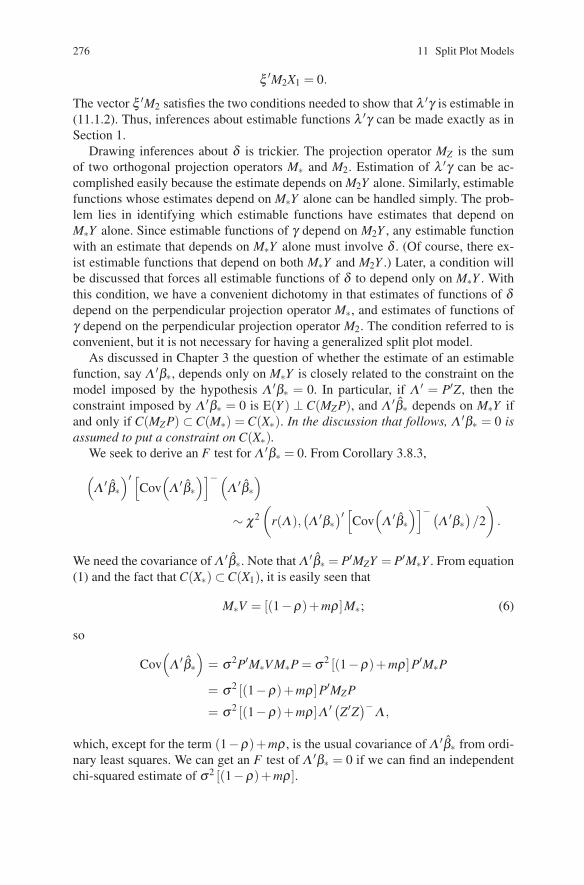
276 11 Split Plot Models
ξ ′M2X1 = 0.
The vector ξ ′M2 satisfies the two conditions needed to show that λ ′γ is estimable in(11.1.2). Thus, inferences about estimable functions λ ′γ can be made exactly as inSection 1.
Drawing inferences about δ is trickier. The projection operator MZ is the sumof two orthogonal projection operators M∗ and M2. Estimation of λ ′γ can be ac-complished easily because the estimate depends on M2Y alone. Similarly, estimablefunctions whose estimates depend on M∗Y alone can be handled simply. The prob-lem lies in identifying which estimable functions have estimates that depend onM∗Y alone. Since estimable functions of γ depend on M2Y , any estimable functionwith an estimate that depends on M∗Y alone must involve δ . (Of course, there ex-ist estimable functions that depend on both M∗Y and M2Y .) Later, a condition willbe discussed that forces all estimable functions of δ to depend only on M∗Y . Withthis condition, we have a convenient dichotomy in that estimates of functions of δdepend on the perpendicular projection operator M∗, and estimates of functions ofγ depend on the perpendicular projection operator M2. The condition referred to isconvenient, but it is not necessary for having a generalized split plot model.
As discussed in Chapter 3 the question of whether the estimate of an estimablefunction, say Λ ′β∗, depends only on M∗Y is closely related to the constraint on themodel imposed by the hypothesis Λ ′β∗ = 0. In particular, if Λ ′ = P′Z, then theconstraint imposed by Λ ′β∗ = 0 is E(Y ) ⊥ C(MZP), and Λ ′β∗ depends on M∗Y ifand only if C(MZP) ⊂ C(M∗) = C(X∗). In the discussion that follows, Λ ′β∗ = 0 isassumed to put a constraint on C(X∗).
We seek to derive an F test for Λ ′β∗ = 0. From Corollary 3.8.3,(Λ ′β∗
)′ [Cov(
Λ ′β∗)]−(
Λ ′β∗)
∼ χ2(
r(Λ),(Λ ′β∗
)′ [Cov(
Λ ′β∗)]− (
Λ ′β∗)/2)
.
We need the covariance of Λ ′β∗. Note that Λ ′β∗ = P′MZY = P′M∗Y . From equation(1) and the fact that C(X∗) ⊂C(X1), it is easily seen that
M∗V = [(1−ρ)+mρ]M∗; (6)
so
Cov(
Λ ′β∗)
= σ 2P′M∗V M∗P = σ 2 [(1−ρ)+mρ]P′M∗P
= σ 2 [(1−ρ)+mρ]P′MZP
= σ 2 [(1−ρ)+mρ]Λ ′ (Z′Z)−Λ ,
which, except for the term (1−ρ)+mρ , is the usual covariance of Λ ′β∗ from ordi-nary least squares. We can get an F test of Λ ′β∗ = 0 if we can find an independentchi-squared estimate of σ2 [(1−ρ)+mρ].

11.2 Generalized Split Plot Models 277
Theorem 11.2.5. Under model (2),
Y ′(M1 −M∗)Y/σ 2 [(1−ρ)+mρ] ∼ χ2(r(X1)− r(X∗),0) .
PROOF. Observe that
M1V = [(1−ρ)+mρ]M1. (7)
Using equations (6) and (7), it is easy to check the conditions of Theorem 1.3.6. Itremains to show that β ′∗Z′ (M1 −M∗)Zβ∗ = 0. Recall that MZ = M∗ +M2, and notethat M = M1 +M2. It follows that M1 −M∗ = M−MZ . Clearly, (M−MZ)Zβ∗ = 0.
�
The quadratic form Y ′(M1 −M∗)Y is called the sum of squares for whole plot(cluster) error. This is denoted SSE(w). An unbiased estimate of σ2 [(1−ρ)+mρ]is available from
MSE(w) = Y ′(M1 −M∗)Y/
[r(X1)− r(X∗)] .
To complete the derivation for the F test of Λ ′β∗ = 0, we need to show that Λ ′β∗and Y ′(M1 −M∗)Y are independent. It suffices to note that
Cov(M∗Y,(M1 −M∗)Y ) = σ 2M∗V (M1 −M∗)= σ 2 [(1−ρ)+mρ]M∗(M1 −M∗)= 0.
The F test is based on the distributional result(Λ ′β∗
)′[Λ ′(Z′Z)−Λ ]−
(Λ ′β∗
)/r(Λ )
MSE(w)∼ F(r(Λ ),r(X1)− r(X∗),π) ,
whereπ =(Λ ′β∗
)′ [Λ ′(Z′Z)−Λ]− (Λ ′β∗
)/2σ 2 [(1−ρ)+mρ]
and (Λ ′β∗)′ [Λ ′(Z′Z)−Λ ]− (Λ ′β∗) = 0 if and only if Λ ′β∗ = 0.The argument establishing the independence of Λ ′β∗ and MSE(w) can be ex-
tended to establish the independence of all the distinct statistics being used.
Theorem 11.2.6. M∗Y , M2Y , SSE(w), and SSE(s) are mutually independent.
PROOF. Since the joint distribution of Y is multivariate normal, it suffices to useequations (6) and (7) to establish that the covariance between any pair of M∗Y , M2Y ,(M1 −M∗)Y , and (I −M)Y is 0. �

278 11 Split Plot Models
To summarize the results so far, if the linear model satisfies Conditions 11.2.1 and11.2.3, then (a) least squares estimates are BLUEs, (b) inferences about estimablefunctions λ ′γ can be made in the usual way (i.e., just as if V = I) with the exceptionthat the estimate of error is taken to be MSE(s), and (c) inferences about estimablefunctions of Λ ′β∗ that put a constraint on C(X∗) can be drawn in the usual way,except that MSE(w) is used as the estimate of error.
As mentioned, it is not clear what kind of estimable functions put a constraint onC(X∗). Two ways of getting around this problem will be discussed. As mentionedabove, one way is to place another condition on the model matrix Z of model (2),a condition that forces the estimable functions of δ to put constraints on C(X∗). Asecond approach, that requires no additional conditions, is to abandon the idea oftesting estimable functions and to look at testing models.
Inferences About δ
One of the problems with generalized split plot models is in identifying the hypothe-ses that put constraints on C(X∗). In general, such hypotheses can involve both theδ and the γ parameters. For example, suppose that C(X∗)∩C(X2) contains a nonzerovector ξ . Then, since MZξ = ξ ∈ C(X∗), the hypothesis ξ ′X∗δ + ξ ′X2γ = 0 puts aconstraint on C(X∗). However, ξ ′X∗δ +ξ ′X2γ involves both the δ and γ parametersbecause, with ξ ∈ C(X∗)∩C(X2), neither ξ ′X∗ nor ξ ′X2 is 0. The most commonexample of this phenomenon occurs when X∗ and X2 are chosen so that C(X∗) andC(X2) both contain a column of 1s (i.e., Jn). It follows that inferences about thegrand mean, n−1JnZβ∗, are made using MSE(w).
The condition stated below ensures that any estimable function of the δ s puts aconstraint on C(X∗). This condition is typically satisfied when Z is the model matrixfor a balanced multifactor ANOVA (with some of the interactions possibly deleted).
Condition 11.2.7. For v ∈C(X), if v ⊥C(X2), then v ∈C(X1).
Suppose that λ ′δ is an estimable function. Then λ ′ = ξ ′X∗ and ξ ′X2 = 0 for someξ ∈C(Z). Since ξ ′X2 = 0, Condition 11.2.7 implies that ξ ∈C(X1); thus M2ξ = 0.Finally, by (4),
MZξ = M∗ξ ∈C(X∗).
Thus, estimable functions of δ put a constraint on C(X∗) and inferences about suchfunctions are made using M∗Y and MSE(w).
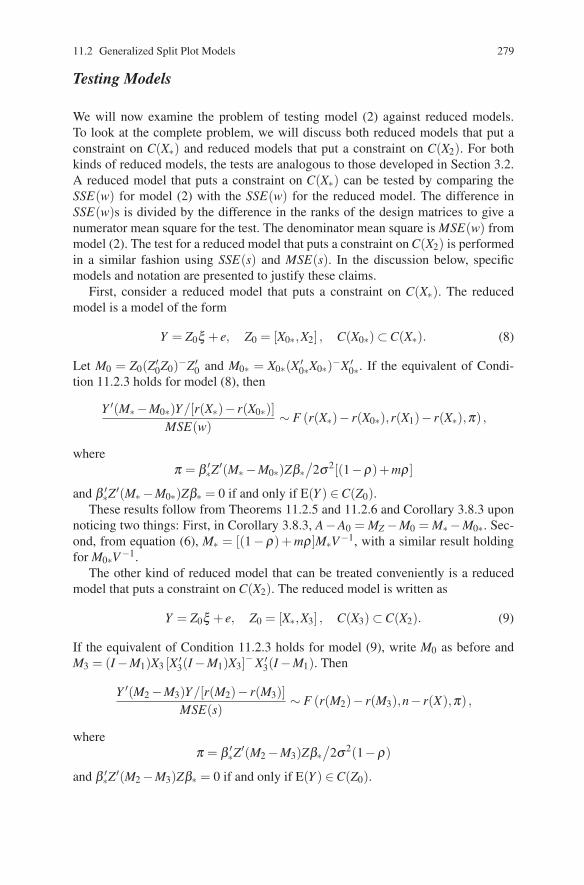
11.2 Generalized Split Plot Models 279
Testing Models
We will now examine the problem of testing model (2) against reduced models.To look at the complete problem, we will discuss both reduced models that put aconstraint on C(X∗) and reduced models that put a constraint on C(X2). For bothkinds of reduced models, the tests are analogous to those developed in Section 3.2.A reduced model that puts a constraint on C(X∗) can be tested by comparing theSSE(w) for model (2) with the SSE(w) for the reduced model. The difference inSSE(w)s is divided by the difference in the ranks of the design matrices to give anumerator mean square for the test. The denominator mean square is MSE(w) frommodel (2). The test for a reduced model that puts a constraint on C(X2) is performedin a similar fashion using SSE(s) and MSE(s). In the discussion below, specificmodels and notation are presented to justify these claims.
First, consider a reduced model that puts a constraint on C(X∗). The reducedmodel is a model of the form
Y = Z0ξ + e, Z0 = [X0∗,X2] , C(X0∗) ⊂C(X∗). (8)
Let M0 = Z0(Z′0Z0)−Z′
0 and M0∗ = X0∗(X ′0∗X0∗)−X ′
0∗. If the equivalent of Condi-tion 11.2.3 holds for model (8), then
Y ′(M∗ −M0∗)Y/[r(X∗)− r(X0∗)]MSE(w)
∼ F (r(X∗)− r(X0∗),r(X1)− r(X∗),π) ,
whereπ = β ′
∗Z′(M∗ −M0∗)Zβ∗/
2σ 2[(1−ρ)+mρ]
and β ′∗Z′(M∗ −M0∗)Zβ∗ = 0 if and only if E(Y ) ∈C(Z0).These results follow from Theorems 11.2.5 and 11.2.6 and Corollary 3.8.3 upon
noticing two things: First, in Corollary 3.8.3, A−A0 = MZ −M0 = M∗ −M0∗. Sec-ond, from equation (6), M∗ = [(1−ρ)+ mρ]M∗V−1, with a similar result holdingfor M0∗V−1.
The other kind of reduced model that can be treated conveniently is a reducedmodel that puts a constraint on C(X2). The reduced model is written as
Y = Z0ξ + e, Z0 = [X∗,X3] , C(X3) ⊂C(X2). (9)
If the equivalent of Condition 11.2.3 holds for model (9), write M0 as before andM3 = (I −M1)X3 [X ′
3(I −M1)X3]− X ′
3(I −M1). Then
Y ′(M2 −M3)Y/[r(M2)− r(M3)]MSE(s)
∼ F (r(M2)− r(M3),n− r(X),π) ,
whereπ = β ′
∗Z′(M2 −M3)Zβ∗/
2σ 2(1−ρ)
and β ′∗Z′(M2 −M3)Zβ∗ = 0 if and only if E(Y ) ∈C(Z0).

280 11 Split Plot Models
These results follow from Theorem 11.2.6, Corollary 3.8.3, and relation (5) uponnoticing that A−A0 = MZ −M0 = M2 −M3; and, since M2V = (1−ρ)M2, we have(1−ρ)−1M2 = M2V−1, and a similar result for M3.
Identifying Generalized Split Plot Models
There are only two conditions necessary for having a generalized split plot model,Condition 11.2.1 and Condition 11.2.3. The form of generalized split plot modelscan be read from these conditions. Condition 11.2.1 requires that an equal number ofobservations be obtained within each whole plot. Condition 11.2.3 requires C(Z) =C(X∗,(I − M1)X2), where C(X∗) ⊂ C(X1). Since C(X1) is the column space thatallows a separate effect for each cluster, X∗δ can be anything that treats all of theobservations in a given whole plot the same. The matrix X2 can contain the columnsfor any ANOVA effects that are balanced within whole plots. X2 can also containany columns that are orthogonal to C(X1). Model (3) in Example 11.2.4 displaysthese characteristics.
Computations
The simplest way to actually fit generalized split plot models would seem to be tofit both models (2) and (11.1.2) using an ordinary least squares computer program.Fitting model (2) provides least squares estimates of δ and γ . Fitting model (2) alsoprovides Y ′(I −MZ)Y as the reported SSE . This reported SSE is not appropriate forany inferences, but, as seen below, it can be used to obtain the whole plot sum ofsquares error. Fitting model (11.1.2) provides least squares estimates of α and γand the reported SSE is Y ′(I −M)Y . If the model is a generalized split plot model,the two estimates of γ should be identical. Since Y (I −M)Y is the SSE(s) (sum ofsquares for subplot error), any conclusions about γ obtained from fitting (11.1.2)will be appropriate. To obtain SSE(w) (sum of squares for whole plot error), notethat
Y ′(I −MZ)Y −Y ′(I −M)Y = Y ′(M−MZ)Y= Y ′(M1 +M2 −M∗ −M2)Y= Y ′(M1 −M∗)Y.
Thus, all of the computationally intensive work can be performed on standard com-puter programs.
Exercise 11.8 Give detailed proofs of the test statistic’s distribution for(a) testing model (8) against model (2),(b) testing model (9) against model (2).

11.3 The Split Plot Design 281
11.3 The Split Plot Design
The traditional model for a split plot design is a special case of the model pre-sented in Section 2. We will present the split plot model and a model equivalent tomodel (11.1.2). We will use the balance of the split plot design to argue that Con-ditions 11.2.1, 11.2.3, and 11.2.7 hold. The arguments based on the balance of thesplit plot model are similar to those presented in Section 7.6. Statistical inferencesare based on least squares estimates and quadratic forms in corresponding perpen-dicular projection matrices. The balance of the split plot model dictates results thatare very similar to those described in Sections 7.1, 7.2, and 7.6.
The traditional split plot model involves a randomized complete block designin the whole plots. In fact, a completely randomized design or a Latin square inthe whole plots leads to an analogous analysis. Suppose that there are r blocks oft whole plots available. Within each block, a different (whole plot) treatment is ap-plied to each whole plot. Let μ denote a grand mean, ξ s denote block effects, and ωsdenote whole plot treatment effects. Let each whole plot be divided into m subplotswith a different (subplot) treatment applied to each subplot. The τs denote subplottreatment effects, and the (ωτ)s denote interaction effects between the whole plottreatments and the subplot treatments. The split plot model has two sources of error,whole plot to whole plot variation denoted by η , and subplot to subplot variationdenoted by e. The split plot model is
yi jk = μ +ξi +ω j +ηi j + τk +(ωτ) jk + ei jk, (1)
i = 1, . . . ,r, j = 1, . . . , t, k = 1, . . . ,m, ηi js independent N(0,σ2w), ei jks independent
N(0,σ 2s ). The ηi js and ei jks are assumed to be independent. We can combine the er-
ror terms as εi jk = ηi j +ei jk. Writing the vector of errors as ε = [ε111,ε112, . . . ,εrtm]′,we get
Cov(ε) = Blk diag[σ 2s Im +σ 2
wJmm ]
= σ 2[(1−ρ)I +mρM1],
where σ 2 = σ2w +σ 2
s and ρ = σ 2w/(σ2
w +σ 2s ). In a split plot model, the whole plots
are considered as the different combinations of i and j. There are m observations foreach whole plot, so Condition 11.2.1 holds.
The model that includes separate effects αi j for each whole plot can be writtenas
yi jk = αi j +ηi j + τk +(ωτ) jk + ei jk .
Combining the error terms gives
yi jk = αi j + τk +(ωτ) jk + εi jk ,
or, using a parameterization with interactions,
yi jk = μ +ξi +ω j +(ξ ω)i j + τk +(ωτ) jk + εi jk . (2)

282 11 Split Plot Models
From Section 2, C(X1) is the space spanned by the columns associated with theαi js and C(X2) is the space spanned by the columns associated with the τks and(ωτ) jks. C(X) is the column space for model (2). Using the parameterization ofmodel (2) and the notation and results of Section 7.6 gives
C(X1) = C(Mμ +Mξ +Mω +Mξ ω),C(X2) = C(Mμ +Mω +Mτ +Mωτ),C(X) = C(Mμ +Mξ +Mω +Mξ ω +Mτ +Mωτ).
Recall that all of the M matrices on the right-hand sides are perpendicular projectionmatrices, and that all are mutually orthogonal. In particular, M = Mμ +Mξ +Mω +Mξ ω +Mτ +Mωτ and M1 = Mμ +Mξ +Mω +Mξ ω .
The split plot model (1) is a reduced model relative to model (2). The ξ ω inter-actions are dropped to create the split plot model. C(X∗) is the space spanned by thecolumns associated with μ , the ξis, and the ω js. Again using results from 7.6,
C(X∗) = C(Mμ +Mξ +Mω),C[(I −M1)X2] = C(Mτ +Mωτ ),
C(Z) = C(Mμ +Mξ +Mω +Mτ +Mωτ).
Clearly, Condition 11.2.3 applies.In fact, even Condition 11.2.7 holds, so that estimable functions of the ξ s and
ωs are tested using MSE(w). To check Condition 11.2.7, it suffices to show that ifv ∈ C(X) and v ⊥ C(X2), then v ∈ C(X1). If v ∈ C(X), then Mv = v. If v ⊥ C(X2),then (Mμ +Mω +Mτ +Mωτ)v = 0. Thus
v = Mv = (Mμ +Mξ +Mω +Mξ ω +Mτ +Mωτ)v= (Mξ +Mξ ω)v.
But, v = (Mξ +Mξ ω )v ∈C(X1). It should be noted that with (ωτ) interaction in themodel, contrasts in the ωs are not estimable. The usual procedure gives estimates ofcontrasts in the ω j +(ωτ) j·s. Without (ωτ) interaction, contrasts in the ωs becomeestimable. In either case, the estimates are obtained using M∗.
We can now write out an ANOVA table.Source df SS E(MS)
μ r(Mμ ) Y ′MμY (σ2s +mσ2
w)+β ′X ′Mμ Xβ/r(Mμ )ξ r(Mξ ) Y ′MξY (σ2
s +mσ2w)+β ′X ′Mξ Xβ/r(Mξ )
ω r(Mω ) Y ′MωY (σ2s +mσ2
w)+β ′X ′Mω Xβ/r(Mω )error 1 r(Mξ ω ) Y ′Mξ ωY σ2
s +mσ2w
τ r(Mτ ) Y ′MτY σ2s +β ′X ′Mτ Xβ/r(Mτ )
ωτ r(Mωτ ) Y ′MωτY σ2s +β ′X ′Mωτ Xβ/r(Mωτ )
error 2 r(I −M) Y ′(I−M)Y σ2s
Total n Y ′Y

11.3 The Split Plot Design 283
Note that σ 2[(1−ρ)+mρ] = σ2s +mσ2
w and σ 2(1−ρ) = σ2s . Algebraically, we can
write the table as
Source df SS E(MS)
μ 1 rtmy2···ξ r−1 tm∑i(yi·· − y···)2 (σ 2
s +mσ2w)+A
ω t −1 rm∑ j(y· j· − y···)2 (σ 2s +mσ 2
w)+Berror 1 (r−1)(t −1) m∑i j(yi j· − yi·· − y· j· + y···)2 σ 2
s +mσ 2w
τ m−1 rt ∑k(y··k − y···)2 σ 2s +C
ωτ (t −1)(m−1) r ∑ jk(y· jk − y· j· − y··k + y···)2 σ 2s +D
error 2 by by σ 2s
subtraction subtraction
Total n ∑i jk y2i jk
A = tm∑i(ξi − ξ·)2/(r−1),
B = rm∑j(ω j +(ωτ) j· − ω· − (ωτ)··)
2/(t −1),
C = rt ∑k
(τk +(ωτ)·k − τ· − (ωτ)··)2/(m−1),
D = r∑jk
((ωτ) jk − (ωτ) j· − (ωτ)·k +(ωτ)··)2/(t −1)(m−1).
Tests and confidence intervals for contrasts in the τks and (ωτ) jks are based onthe usual least squares estimates and use the mean square from the “error 2” linefor an estimate of variance. Tests and confidence intervals in the ξis and ω js alsouse least squares estimates, but use the mean square from the “error 1” line foran estimate of variance. Note that contrasts in the ω js are really contrasts in the(ω j +(ωτ) j·)s when interaction is present.
Finally, a word about missing data. If one or more whole plots are missing, thedata can still be analyzed as in Section 2. If one or more subplots are missing, thedata can still be analyzed as in Section 1; however, with missing subplots, some sortof ad hoc analysis for the whole plot effects must be used.
Exercise 11.9 Consider the table of means
τ1 2 · · · m
1 y·11 y·12 · · · y·1mω 2 y·21 y·22 · · · y·2m
......
.... . .
...t y·t1 y·t2 · · · y·tm
Let ∑mk=1 dk = 0. For any fixed j, find a confidence interval for ∑m
k=1 dkμ jk, whereμ jk = μ + ξ·+ω j +τk +(ωτ) jk. (Hint: The estimate of the variance comes from the

284 11 Split Plot Models
“error 2” line.) Let ∑tj=1 c j = 0. Why is it not possible to find a confidence interval
for ∑tj=1 c jμ jk?
11.4 Identifying the Appropriate Error
Statistics is all about drawing conclusions from data that are subject to error. One ofthe crucial problems in statistics is identifying and estimating the appropriate errorso that valid conclusions can be made. The importance of this issue has long beenrecognized by the statistical community. The necessity of having a valid estimateof error is one of the main points in The Design of Experiments, Fisher’s (1935)seminal work.
The key feature of split plot models is that they involve two separate sources ofvariation. The analysis involves two separate estimates of error, and a correct analy-sis requires that the estimates be used appropriately. If the existence of two separatesources of variability is not noticed, the estimate of error will probably be obtainedby pooling the sums of squares for the two separate errors. The pooled estimate oferror will generally be too small for comparing treatments applied to whole plotsand too large for comparing treatments applied to subplots. The whole plot treat-ments will appear more significant than they really are. The subplot treatments willappear less significant than they really are. The interactions between whole plot andsubplot treatments will also appear less significant than they really are.
The problem of identifying the appropriate error is a difficult one. In this section,some additional examples of the problem are discussed. First, the problem of sub-sampling is considered. The section ends with a discussion of the appropriate errorfor testing main effects in the presence of interactions.
Subsampling
One of the most commonly used, misused, and abused of models is the subsamplingmodel.
EXAMPLE 11.4.1. In an agricultural experiment, one treatment is applied to eachof 6 pastures. The experiment involves 4 different treatments, so there are a total of24 pastures in the experiment. On each pasture 10 observations are taken. The 10observations taken on each pasture are referred to as subsamples. Each observationis subject to two kinds of variability: (1) pasture to pasture variability and (2) withinpasture variability. Note, however, that in comparing the 10 observations taken on agiven pasture, there is no pasture to pasture variability. The correct model for thisexperiment involves error terms for both kinds of variability. Typically the model istaken as
yi jk = μ +ωi +ηi j + ei jk, (1)

11.4 Identifying the Appropriate Error 285
i = 1,2,3,4, j = 1, . . . ,6, k = 1, . . . ,10, ηi js i.i.d. N(0,σ 2w), ei jks i.i.d. N(0,σ 2
s ), andthe ηi js and ei jks are independent. In this model, σ 2
w is the pasture to pasture varianceand σ 2
s is the within pasture or subsampling variance.As will be seen below, the statistical analysis of model (1) acts like there is only
1 observation on each pasture. That 1 observation is the mean of the 10 actual obser-vations that were taken. If the analysis acts like only 1 observation was taken on apasture, why should an experimenter trouble to take 10 observations? Why not takejust 1 observation on each pasture?
With 1 real observation on each pasture, the statistical analysis is subject to thewhole weight of the within pasture variability. By taking 10 observations on a pas-ture and averaging them to perform the analysis, the mean of the 10 observations stillhas the full pasture to pasture variability, but the within pasture variability (variance)is cut by a factor of 10. The experiment is being improved by reducing the variabil-ity of the treatment estimates, but that improvement comes only in the reduction ofthe within pasture variability. The effects of pasture to pasture variability are notreduced by subsampling.
Rather than subsampling, it would be preferable to use more pastures. Usingmore pastures reduces the effects of both kinds of variability. Unfortunately, doingthat is often not feasible. In the current example, the same reduction in within pas-ture variation without subsampling would require the use of 240 pastures insteadof the 24 pastures that are used in the experiment with subsampling. In practice,obtaining 24 pastures for an experiment can be difficult. Obtaining 240 pastures canbe well nigh impossible.
In general, a subsampling model is
yi jk = μ +ωi +ηi j + ei jk, Var(ηi j) = σ 2w, Var(ei jk) = σ 2
s , (2)
i = 1, . . . , t, j = 1, . . . ,r, k = 1, . . . ,m. By checking Conditions 11.2.1, 11.2.3, and11.2.7, it is easily seen that this is a generalized split plot model with X2 vacuous.An ANOVA table can be written:
Source df SS E(MS)
ω t −1 rm∑i(yi·· − y···)2 σ2s +mσ2
w +A
error 1 t(r−1) m∑i j(yi j· − yi··)2 σ2s +mσ2
w
error 2 rt(m−1) ∑i jk(yi jk − yi j·)2 σ2s
where A = rm∑i(ωi − ω·)2/(t − 1). The entire analysis is performed as a standardone-way ANOVA. The variance of yi·· is (σ 2
s + mσ2w)/rm, so the “error 1” line is
used for all tests and confidence intervals.As mentioned above, an equivalent analysis can be made with the averages of the
observations in each subsample. The model based on the averages is
yi j· = μ +ωi +ξi j, Var(ξi j) = [σ2w +(σ2
s /m)],

286 11 Split Plot Models
i = 1, . . . , t, j = 1, . . . ,r. It is easily seen that this gives exactly the same tests andconfidence intervals as those obtained from model (2).
One of the most common mistakes in statistical practice is to mistake subsam-pling for independent replication in an experiment. Example 11.4.1 involves 6 in-dependent replications, i.e., the 6 pastures to which each treatment is applied. The10 observations on a given pasture are not independent because the random effectfor pastures is the same for all of them. The incorrect model that is often analyzedinstead of model (2) is
yi j = μ +ωi + ei j, (3)
i = 1, . . . , t, j = 1, . . . ,rm. The effect of analyzing model (3) is that the “error 1” and“error 2” lines of the ANOVA are pooled together. Since the expected mean squarefor “error 2” is only σ 2
s , the pooled mean square error is inappropriately small andall effects will appear to be more significant than they really are.
Subsampling can be an important tool, especially when the variability betweensubsamples is large. However, it is important to remember that subsampling is tobe used in addition to independent replication. It does not eliminate the need for anadequate number of independent replicates. In terms of Example 11.4.1, an experi-menter should first decide on a reasonable number of pastures and then address thequestion of how many observations to take within a pasture. If the pasture to pasturevariability is large compared to the within pasture variability, subsampling will beof very limited value. If the within pasture variability is large, subsampling can beextremely worthwhile.
The existence of subsampling can usually be determined by carefully identifyingthe treatments and the experimental units to which the treatments are applied. In theagricultural example, identifying the subsampling structure was easy. Treatmentswere applied to pastures. If differences between treatments are to be examined, thendifferences between pastures with the same treatment must be error.
Lest the reader think that identifying subsampling is easy, let us try to confuse theissue. The analysis that has been discussed is based on the assumption that pastureto pasture variability is error, but now suppose that the experimenter has an interestin the pastures. For example, different pastures have different fertilities, so somepastures are better than others. If differences in pastures are of interest, it may bereasonable to think of the ηi js as fixed effects, in which case there is no subsamplingand the ANOVA table gives only one error line. The expected mean squares are:
Source df E(MS)
ω 3 σ 2 +20∑i(ωi + ηi· − ω· − η··)2
η 20 σ 2 + .5∑i j(ηi j − ηi·)2
error 216 σ 2
The mean square for η can be used to test whether there are any differences betweenpastures that have the same treatment. The MSE(ω) provides a test of whether thetreatment effects added to their average pasture effects are different. The test from

11.4 Identifying the Appropriate Error 287
MSE(ω) may not be very interesting if there are different pasture effects. In sum-mary, the analysis depends crucially on whether the ηi js are assumed to be randomor fixed. When the ω treatments are of primary importance it makes sense to treatthe η effects as random.
Two-Way ANOVA with Interaction
The two-way ANOVA with interaction model from Section 7.2 is
yi jk = μ +αi +η j + γi j + ei jk, (4)
i = 1, . . . ,a, j = 1, . . . ,b, k = 1, . . . ,N. First, the question of subsampling in a two-way ANOVA will be addressed. The discussion of subsampling leads to an exam-ination of independent replication, and to the question of whether the interactionsshould be considered fixed or random. The discussion of identifying the appropriateerror begins with an example:
EXAMPLE 11.4.2. We want to investigate the effects of 4 fertilizers and 6 her-bicides on pastures used for raising cane (as in sugar cane). There are a total of4× 6 = 24 treatment combinations. If each treatment combination is applied to 5pastures, then model (4) is appropriate with a = 4, b = 6, and N = 5.
Now consider an alternative experimental design that is easily confused with this.Suppose each treatment combination is applied to 1 pasture and 5 observations aretaken on each pasture. There is no independent replication. The 5 observations oneach pasture are subsamples. Comparisons within pastures do not include pastureto pasture variability. If model (4) is used to analyze such data, the MSE is actuallythe estimated subsampling variance. It is based on comparisons within pastures. Ananalysis based on model (4) will inflate the significance of all effects.
The appropriate model for this subsampling design is
yi jk = μ +αi +η j + γi j +ξi j + ei jk,
where ξi j ∼ N(0,σ 2w) and ei jk ∼ N(0,σ2
s ). Note that the indices on γ and ξ areexactly the same. It is impossible to tell interactions apart from pasture to pasturevariability. As a result, unless the interactions can be assumed nonexistent, there isno appropriate estimate of error available in this experiment.
In the example, two extreme cases were considered, one case with no subsam-pling and one case with no independent replication. Of course, any combination ofsubsampling and independent replication can be used. In the example, the designswere clearly stated so that the subsampling structures were clear. In practice, thisrarely occurs. When presented with data that have been collected, it can be verydifficult to identify how the experiment was designed.

288 11 Split Plot Models
Designs without independent replications are actually quite common. When con-fronted with a two-factor ANOVA without any independent replication, the fixedinteraction effects are generally assumed to be zero so that an analysis can be per-formed. This is precisely the assumption made in Chapter 8 in analyzing the Ran-domized Complete Block model. An alternate way of phrasing this idea is that anyinteraction effects that exist must be due to error. This idea that interaction effectscan themselves be errors is important. If the interactions are errors, then model (4)needs to be changed. The standard assumption would be that the γi js are independentN(0,σ 2
w) random variables.Note that the assumption of random γi js does not imply the existence of sub-
sampling. Subsampling is a property of the experimental design. What is being dis-cussed is simply a choice about how to model interactions. Should they be modeledas fixed effects, or should they be modeled as random errors? One guideline is basedon the repeatability of the results. If the pattern of interactions should be the samein other similar studies, then the interactions are fixed. If there is little reason tobelieve that the pattern of interactions would be the same in other studies, then theinteractions would seem to be random.
The analysis of model (4) with random interactions is straightforward. The modelis a generalized split plot model with X2 vacuous. The mean square for interactionsbecomes the mean square for “error 1.” The mean square error from assuming fixedinteractions becomes the mean square for “error 2.” The analysis for main effectsuses the mean square “error 1” exclusively as the estimate of error.
Although this is not a subsampling model, it does involve two sources of varia-tion: 1) variation due to interactions, and 2) variation due to independent replication(i.e., variation from experimental unit to experimental unit). It seems to be diffi-cult to reduce the effects on comparisons among treatments of the variability dueto interactions. The effect of variation due to experimental units can be reduced bytaking additional independent replications.
11.5 Exercise: An Unusual Split Plot Analysis
Cornell (1988) considered data on the production of vinyl for automobile seat cov-ers. Different blends involve various plasticizers, stabilizers, lubricants, pigments,fillers, drying agents, and resins. The current data involve 5 blends of vinyl.
The 5 blends represent various percentages of 3 plasticizers that together makeup 40.7% of the product. The first plasticizer is restricted to be between 19.1% and34.6% of the product. The second plasticizer is restricted to be between 0% and10.2% of the product. The third plasticizer is restricted to be between 6.1% and11.4% of the product. Changing these restrictions to fractions of the 40.7% of thetotal, we get
0.47 ≤ x1 ≤ 0.85, 0 ≤ x2 ≤ 0.25, 0.15 ≤ x1 ≤ 0.28.

11.5 Exercise: An Unusual Split Plot Analysis 289
The 5 blends are
Blend (x1,x2,x3)1 (0.85, 0.000, 0.150)2 (0.72, 0.000, 0.280)3 (0.60, 0.250, 0.150)4 (0.47, 0.250, 0.280)5 (0.66, 0.125, 0.215)
Note that the first four blends have all combinations of x2 and x3 at their extremeswith x1 values decreasing at about 0.13 per blend. Blend 5 is in the center of theother blends. In particular, for i = 1,2,3, the xi value of blend 5 is the mean of theother four xi values. Eight groups of the five different blends were prepared.
The first group of 5 blends was run with the production process set for a highrate of extrusion (z1 = 1) and a low drying temperature (z2 = −1). The process wasthen reset for low extrusion rate and high drying temperature (z1 = −1,z2 = 1), andanother group of 5 blends was run. For subsequent runs of 5 blends, the process wasset for z1 = −1,z2 = −1, and z1 = 1,z2 = 1 to finish the first replication. Later, thesecond replication was run in the order z1 = −1,z2 = 1; z1 = 1,z2 = 1; z1 = 1,z2 =−1; z1 = −1,z2 = −1. The data are presented in Table 11.1
Table 11.1 Cornell’s Scaled Vinyl Thickness Values.
Blend x1 x2 x3 z1 z2 Rep. 1 Rep. 21 0.85 0.000 0.150 1 −1 8 72 0.72 0.000 0.280 1 −1 6 53 0.60 0.250 0.150 1 −1 10 114 0.47 0.250 0.280 1 −1 4 55 0.66 0.125 0.215 1 −1 11 101 0.85 0.000 0.150 −1 1 12 102 0.72 0.000 0.280 −1 1 9 83 0.60 0.250 0.150 −1 1 13 124 0.47 0.250 0.280 −1 1 6 35 0.66 0.125 0.215 −1 1 15 111 0.85 0.000 0.150 −1 −1 7 82 0.72 0.000 0.280 −1 −1 7 63 0.60 0.250 0.150 −1 −1 9 104 0.47 0.250 0.280 −1 −1 5 45 0.66 0.125 0.215 −1 −1 9 71 0.85 0.000 0.150 1 1 12 112 0.72 0.000 0.280 1 1 10 93 0.60 0.250 0.150 1 1 14 124 0.47 0.250 0.280 1 1 6 55 0.66 0.125 0.215 1 1 13 9
Compare the RCB model for the five blend treatments

290 11 Split Plot Models
yhi jk = γh + τi jk + εhi jk,
where the triples (i, j,k) only take on five distinct values, with the reduced regressionmodel
yhi jk = γh +β1x1i +β2x2 j +β3x3k + εhi jk.
Test lack of fit. Average over blends to do a whole plot analysis. Finally, do a splitplot analysis.

Chapter 12
Mixed Models and Variance Components
Traditionally, linear models have been divided into three categories: fixed effectsmodels, random effects models, and mixed models. The categorization depends onwhether the β vector in Y = Xβ + e is fixed, random, or has both fixed and randomelements. Random effects models always assume that there is a fixed overall meanfor observations, so random effects models are actually mixed.
Variance components are the variances of the random elements of β . Sections 1through 3 discuss mixed models in general and prediction for mixed models. Sec-tions 4 through 9 present methods of estimation for variance components. Section 10examines exact tests for variance components. Section 11 uses the ideas of the chap-ter to develop the interblock analysis for balanced incomplete block designs. Searle,Casella, and McCulloch (1992) give an extensive discussion of variance componentestimation. Khuri, Mathew, and Sinha (1998) give an extensive discussion of testingin mixed models.
The methods considered in this chapter are presented in terms of fitting generallinear models. In many special cases, considerable simplification results. For exam-ple, the RCB models of (11.1.5) and Exercise 11.4, the split plot model (11.3.1), andthe subsampling model (11.4.2) are all mixed models with very special structures.
12.1 Mixed Models
The mixed model is a linear model in which some of the parameters, instead of beingfixed effects, are random. The model can be written
Y = Xβ +Zγ + e, (1)
where X and Z are known matrices, β is an unobservable vector of fixed effects,and γ is an unobservable vector of random effects with E(γ) = 0, Cov(γ) = D, andCov(γ ,e) = 0. Let Cov(e) = R.
© Springer Science+Business Media, LLC 2011
291Springer Texts in Statistics, DOI 10.1007/978-1-4419-9816-3_12, R. Christensen, Plane Answers to Complex Questions: The Theory of Linear Models,

292 12 Mixed Models and Variance Components
For estimation of the fixed effects β , the mixed model can be written as a generalGauss–Markov model. Write
V = Cov(Y ) = Cov(Zγ + e) = ZDZ′ +R.
V is assumed to be nonsingular. Model (1) is equivalent to
Y = Xβ +ξ , E(ξ ) = 0, Cov(ξ ) = V.
The BLUE of Xβ can be found using the theory for general Gauss–Markov mod-els. Unfortunately, finding the BLUE requires knowledge (at least up to a constantmultiple) of V . This is rarely available. Currently, the best procedure available forestimating Xβ is to estimate V and then act as if the estimate is the real value of V .In other words, if V is estimated with V , then Xβ is estimated with
X β = X[X ′V−1X
]−X ′V−1Y. (2)
If V is close to V , then the estimate of Xβ should be close to the BLUE of Xβ .Corresponding standard errors will tend to be underestimated, cf. Eaton (1985),Harville (1985), or Christensen (2001, Section 6.5).
Estimation of V is obviously crucial for the estimation of the fixed effects. It isalso frequently of interest in its own right. Estimation of V is indirectly referred toas variance component estimation. We discuss several approaches to the problem ofestimating V .
If γ were a fixed effect, we would be interested in estimating estimable functionslike λ ′γ . Since γ is random, we cannot estimate λ ′γ , but we can predict λ ′γ from theobservable vector Y . The theory of Subsection 6.3.4 provides a best linear predictor,but requires knowledge of E(λ ′γ), Cov(λ ′γ ,Y ), E(Y ), and Cov(Y ). We know thatE(λ ′γ) = 0. As will be seen in Section 2, if we assume that D and R are known,our only problem in predicting λ ′γ is not knowing E(Y ) = Xβ . We will not be ableto find a best linear predictor, but we will find the best linear unbiased predictor(BLUP) of λ ′γ . Of course, D and R are not known, but we will have a theory forprediction of λ ′γ that is the equivalent of BLUE estimation. With good estimates ofD and R provided by variance component techniques, we can get predictions of λ ′γthat are close to the BLUP.
Sometimes we would like to obtain an estimate of Xβ without going to the trou-ble and expense of finding V−1, which is needed to apply equation (2). One simpleestimate is the least squares estimate, MY . This gives an unbiased estimate of Xβ ,but ignores the existence of the random effects. An alternative method is to fit themodel
Y = Xβ +Zδ +Zγ + e, R = σ2I, (3)
where δ is a vector of fixed effects corresponding to the vector of random effects γ .In model (3), there is no hope of estimating variance components because the fixedeffects δ and the random effects γ are completely confounded. However, it is easilyseen that C(V [X ,Z]) ⊂ C(X ,Z), so by Theorem 10.4.5, least squares estimates are

12.2 Best Linear Unbiased Prediction 293
BLUEs in model (3). To see that C(V [X ,Z]) ⊂C(X ,Z), observe that
C(V [X ,Z]) = C({σ 2I +ZDZ′}[X ,Z])= C(σ 2X +ZDZ′X ,σ 2Z +ZDZ′Z)⊂ C(X ,Z).
From Chapter 9, a least squares estimate of β is
β =[X ′(I −MZ)X
]− X ′(I −MZ)Y, (4)
where MZ = Z(Z′Z)−Z′. Although estimates obtained using (4) are not typicallyBLUEs for model (1), since model (3) is a larger model than model (1), the estimatesshould be reasonable. The only serious problem with using equation (4) is that it isnot clear which functions of β are estimable in model (3).
12.2 Best Linear Unbiased Prediction
In this section we consider the general theory of best linear unbiased prediction. In aseries of examples, this theory will be used to examine prediction in standard linearmodel theory, Kriging of spatial data, and prediction of random effects in mixedmodels. The placement of this section in Chapter 12 is obviously based on the lastof these applications.
Consider a set of random variables yi, i = 0,1, . . . ,n. We want to use y1, . . . ,yn topredict y0. Let Y = (y1, . . . ,yn)′. In Section 6.3 it was shown that the best predictor(BP) of y0 is E(y0|Y ). Typically, the joint distribution of y0 and Y is not available,so E(y0|Y ) cannot be found. However, if the means and covariances of the yis areavailable, then we can find the best linear predictor (BLP) of y0. Let Cov(Y ) =V , Cov(Y,y0) = Vy0, E(yi) = μi, i = 0,1, . . . ,n, and μ = (μ1, . . . ,μn)′. Again fromSubsection 6.3.4, the BLP of y0 is
E(y0|Y ) ≡ μ0 +δ ′∗(Y −μ), (1)
where δ∗ satisfies Vδ∗ = Vy0.We now want to weaken the assumption that μ and μ0 are known. Since the
prediction is based on Y and there are as many unknown parameters in μ as thereare observations in Y , we need to impose some structure on the mean vector μ beforewe can generalize the theory. This will be done by specifying a linear model for Y .Since y0 is being predicted and has not been observed, it is necessary either to knowμ0 or to know that μ0 is related to μ in a specified manner. In the theory below, itwill be assumed that μ0 is related to the linear model for Y .
Suppose that a vector of known concomitant variables x′i = (xi1, . . . ,xip) is as-sociated with each random observation yi, i = 0, . . . ,n. We impose structure on the

294 12 Mixed Models and Variance Components
μis by assuming that μi = x′iβ for some vector of unknown parameters β and alli = 0,1, . . . ,n.
We can now reset our notation in terms of linear model theory. Let
X =
⎡⎢⎣x′1...
x′n
⎤⎥⎦ .
The observed vector Y satisfies the linear model
Y = Xβ + e, E(e) = 0, Cov(e) = V. (2)
With this additional structure, the BLP of y0 given in (1) becomes
E(y0|Y ) = x′0β +δ ′∗(Y −Xβ ), (3)
where again Vδ∗ = Vy0.The standard assumption that μ and μ0 are known now amounts to the assump-
tion that β is known. It is this assumption that we renounce. By weakening theassumptions, we consequently weaken the predictor. If β is known, we can find thebest linear predictor. When β is unknown, we find the best linear unbiased predictor.
Before proceeding, a technical detail must be mentioned. To satisfy estimabilityconditions, we need to assume that x′0 = ρ ′X for some vector ρ . Frequently, model(2) will be a regression model, so choosing ρ ′ = x′0(X
′X)−1X ′ will suffice. In appli-cations to mixed models, x′0 = 0, so ρ = 0 will suffice.
Definition 12.2.1. A predictor f (Y ) of y0 is said to be unbiased if
E[ f (Y )] = E(y0).
Definition 12.2.2. a0 +a′Y is a best linear unbiased predictor of y0 if a0 +a′Yis unbiased and if, for any other unbiased predictor b0 +b′Y ,
E[y0 −a0 −a′Y
]2 ≤ E[y0 −b0 −b′Y
]2.
Theorem 12.2.3. The best linear unbiased predictor of y0 is x′0β +δ ′∗(Y −X β ),where Vδ∗ = Vy0 and X β is a BLUE of Xβ .
PROOF. The technique of the proof is to change the prediction problem into anestimation problem and then to use the theory of best linear unbiased estimation.Consider an arbitrary linear unbiased predictor of y0, say b0 + b′Y . By Proposi-tion 6.3.3,
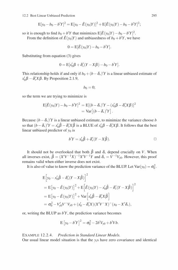
12.2 Best Linear Unbiased Prediction 295
E[y0 −b0 −b′Y ]2 = E[y0 − E(y0|Y )]2 +E[E(y0|Y )−b0 −b′Y ]2;
so it is enough to find b0 +b′Y that minimizes E[E(y0|Y )−b0 −b′Y ]2.From the definition of E(y0|Y ) and unbiasedness of b0 +b′Y , we have
0 = E[E(y0|Y )−b0 −b′Y ].
Substituting from equation (3) gives
0 = E[x′0β +δ ′∗(Y −Xβ )−b0 −b′Y ].
This relationship holds if and only if b0 +(b−δ∗)′Y is a linear unbiased estimate ofx′0β −δ ′∗Xβ . By Proposition 2.1.9,
b0 = 0;
so the term we are trying to minimize is
E[E(y0|Y )−b0 −b′Y ]2 = E[(b−δ∗)′Y − (x′0β −δ ′∗Xβ )]2
= Var[(b−δ∗)′Y
].
Because (b−δ∗)′Y is a linear unbiased estimate, to minimize the variance choose bso that (b−δ∗)′Y = x′0β −δ ′∗X β is a BLUE of x′0β −δ ′∗Xβ . It follows that the bestlinear unbiased predictor of y0 is
b′Y = x′0β +δ ′∗(Y −X β ). �
It should not be overlooked that both β and δ∗ depend crucially on V . Whenall inverses exist, β = (X ′V−1X)−1X ′V−1Y and δ∗ = V−1Vy0. However, this proofremains valid when either inverse does not exist.
It is also of value to know the prediction variance of the BLUP. Let Var(y0) = σ 20 .
E[y0 − x′0β −δ ′
∗(Y −X β )]2
= E[y0 − E(y0|Y )
]2 +E[E(y0|Y )− x′0β −δ ′
∗(Y −X β )]2
= E[y0 − E(y0|Y )
]2 +Var[x′0β −δ ′
∗X β]
= σ 20 −V ′
y0V−Vy0 +(x′0 −δ ′∗X)(X ′V−X)−(x0 −X ′δ∗),
or, writing the BLUP as b′Y , the prediction variance becomes
E[y0 −b′Y
]2 = σ 20 −2b′Vy0 +b′V b.
EXAMPLE 12.2.4. Prediction in Standard Linear Models.Our usual linear model situation is that the yis have zero covariance and identical

296 12 Mixed Models and Variance Components
variances. Thus, model (2) is satisfied with V = σ 2I. A new observation y0 wouldtypically have zero covariance with the previous data, so Vy0 = 0. It follows thatδ∗ = 0 and the BLUP of y0 is x′0β . This is just the BLUE of E(y0) = x′0β .
EXAMPLE 12.2.5. Spatial Data and Kriging.If yi is an observation taken at some point in space, then x′i typically contains thecoordinates of the point. In dealing with spatial data, finding the BLUP is oftencalled Kriging. The real challenge with spatial data is getting some idea of the co-variance matrices V and Vy0. See Christensen (2001) for a more detailed discussionwith additional references.
Exercise 12.1 Prove three facts about Kriging.(a) If b′Y is the BLUP of y0 and if xi1 = 1, i = 0,1, . . . ,n, then b′J = 1.(b) If (y0,x′0) = (yi,x′i) for some i ≥ 1, then the BLUP of y0 is just yi.(c) If V is nonsingular and b′Y is the BLUP of y0, then there exists a vector γ
such that the following equation is satisfied:[V XX ′ 0
][bγ
]=[
Vy0x0
].
Typically, this equation will have a unique solution.Hint: Recall that x′0 = ρ ′X and that X(X ′V−1X)−X ′V−1 is a projection operator
onto C(X).
EXAMPLE 12.2.6. Mixed Model Prediction.In the mixed model (12.1.1), we wish to find the BLUP of λ ′γ based on the data Y .The vector λ can be any known vector. Note that E(λ ′γ) = 0; so we can let y0 = λ ′γand x′0 = 0. From Section 1, V = ZDZ′ +R and
Vy0 = Cov(Y,λ ′γ)= Cov(Zγ + e,λ ′γ)= Cov(Zγ ,λ ′γ)= ZDλ .
The BLUP of λ ′γ isδ ′∗(Y −X β ),
where X β is the BLUE of Xβ and δ∗ satisfies (ZDZ′+R)δ∗ = ZDλ . The matrices X ,Z, and λ are all known. As in Kriging, the practical challenge is to get some idea ofthe covariance matrices. In this case, we need D and R. Estimates of D and R are onebyproduct of variance component estimation. Estimation of variance components isdiscussed later in this chapter.
Exercise 12.2 If λ ′1β is estimable, find the best linear unbiased predictor of

12.3 Mixed Model Equations 297
λ ′1β + λ ′
2γ . For this problem, b0 + b′Y is unbiased if E(b0 + b′Y ) = E(λ ′1β +λ ′
2γ).The best predictor minimizes E[b0 +b′Y −λ ′
1β −λ ′2γ]2.
Exercise 12.3 Assuming the results of Exercise 6.3, show that the BLUP of therandom vector Λ ′γ is Q′(Y −X β ), where V Q = ZDΛ .
12.3 Mixed Model Equations
We now develop the well-known mixed model equations. These equations are sim-ilar in spirit to normal equations; however, the mixed model equations simultane-ously provide BLUEs and BLUPs.
Suppose that R is nonsingular. If γ were not random, the normal equations formodel (12.1.1) would be[
X ′Z′
]R−1[X ,Z]
[βγ
]=[
X ′Z′
]R−1Y
or [X ′R−1X X ′R−1ZZ′R−1X Z′R−1Z
][βγ
]=[
X ′R−1YZ′R−1Y
].
For D nonsingular, the mixed model equations are defined as[X ′R−1X X ′R−1ZZ′R−1X D−1 +Z′R−1Z
][βγ
]=[
X ′R−1YZ′R−1Y
]. (1)
Theorem 12.3.1. If [β ′, γ ′] is a solution to the mixed model equations, then X βis a BLUE of Xβ and γ is a BLUP of γ .
PROOF. From Section 2.8, X β will be a BLUE of Xβ if β is a solution toX ′V−1Xβ = X ′V−1Y . To use this equation we need a form for V−1 in terms ofZ, D, and R:
V−1 = R−1 −R−1Z[D−1 +Z′R−1Z
]−1Z′R−1.
This follows from Theorem B.56.If β and γ are solutions, then the second row of the mixed model equations gives
Z′R−1X β +[D−1 +Z′R−1Z
]γ = Z′R−1Y
orγ =[D−1 +Z′R−1Z
]−1Z′R−1(Y −X β ). (2)
The first row of the equations is
X ′R−1X β +X ′R−1Zγ = X ′R−1Y.
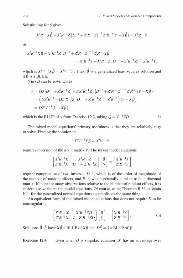
298 12 Mixed Models and Variance Components
Substituting for γ gives
X ′R−1X β +X ′R−1Z[D−1 +Z′R−1Z
]−1Z′R−1(Y −X β ) = X ′R−1Y
or
X ′R−1X β −X ′R−1Z[D−1 +Z′R−1Z
]−1Z′R−1X β
= X ′R−1Y −X ′R−1Z[D−1 +Z′R−1Z
]−1Z′R−1Y,
which is X ′V−1X β = X ′V−1Y . Thus, β is a generalized least squares solution andX β is a BLUE.
γ in (2) can be rewritten as
γ =(D[D−1 +Z′R−1Z
]−DZ′R−1Z)[
D−1 +Z′R−1Z]−1
Z′R−1(Y −X β)
=(
DZ′R−1 −DZ′R−1Z[D−1 +Z′R−1Z
]−1Z′R−1
)(Y −X β )
= DZ′V−1(Y −X β ),
which is the BLUP of γ from Exercise 12.3, taking Q = V−1ZD. �
The mixed model equations’ primary usefulness is that they are relatively easyto solve. Finding the solution to
X ′V−1Xβ = X ′V−1Y
requires inversion of the n×n matrix V . The mixed model equations[X ′R−1X X ′R−1ZZ′R−1X D−1 +Z′R−1Z
][βγ
]=[
X ′R−1YZ′R−1Y
]require computation of two inverses, D−1, which is of the order of magnitude ofthe number of random effects, and R−1, which generally is taken to be a diagonalmatrix. If there are many observations relative to the number of random effects, it iseasier to solve the mixed model equations. Of course, using Theorem B.56 to obtainV−1 for the generalized normal equations accomplishes the same thing.
An equivalent form of the mixed model equations that does not require D to benonsingular is [
X ′R−1X X ′R−1ZDZ′R−1X I +Z′R−1ZD
][βξ
]=[
X ′R−1YZ′R−1Y
]. (3)
Solutions β , ξ have X β a BLUE of Xβ and Dξ = γ a BLUP of γ .
Exercise 12.4 Even when D is singular, equation (3) has an advantage over

12.4 Variance Component Estimation: Maximum Likelihood 299
equation (1) in that equation (3) does not require D−1. Show that equations (1) and(3) are equivalent when D is nonsingular.
The mixed model equations can also be arrived at from a Bayesian argument.Consider the model
Y = Xβ +Zγ + e, e ∼ N(0,R),
and, as discussed in Section 2.9, incorporate partial prior information in the form
γ ∼ N(0,D),
where D is again assumed to be nonsingular. A minor generalization of equation(2.9.3) allows the data Y to have an arbitrary nonsingular covariance matrix, so theBayesian analysis can be obtained from fitting the generalized least squares model[
Y0
]=[
X Z0 I
][βγ
]+[
ee
],
[ee
]∼ N([
0n×10r×1
],
[R 00 D
]).
The generalized least squares estimates from this model will be the posterior meansof β and γ , respectively. However, the generalized least squares estimates can beobtained from the corresponding normal equations, and the normal equations arethe mixed model equations (1).
12.4 Variance Component Estimation: Maximum Likelihood
Assume that Y ∼ N(Xβ ,V ) and that V is nonsingular, so that the density of Y exists.In this chapter we write determinants as |V | ≡ det(V ). The density of Y is
(2π)−n/2|V |−1/2 exp[−(Y −Xβ )′V−1(Y −Xβ )/2
],
where |V | denotes the determinant of V . (The earlier notation det(V ) becomes awk-ward.) The log-likelihood is
L(Xβ ,V ) = −n2
log(2π)− 12
log(|V |)− 12(Y −Xβ )′V−1(Y −Xβ ).
For fixed V , this is maximized by minimizing (Y −Xβ )′V−1(Y −Xβ ). It followsfrom Section 2.8 that, given the maximum likelihood estimate of V , the maximumlikelihood estimate of Xβ is obtained by treating the MLE of V as the true value ofV and taking the usual generalized least squares estimator of Xβ .
Finding the MLE of V is rather more involved. In general, R could involven(n + 1)/2 distinct parameters, and D could involve another q(q + 1)/2, where qis the number of columns in Z. There is little hope of estimating that many pa-rameters from n observations. We need to assume some additional structure for themixed model. Traditionally, variance component problems are analysis of variance

300 12 Mixed Models and Variance Components
problems with random rather than fixed effects. The levels of any particular effectare assumed to be independent with the same variance. Different effects are al-lowed different variances and are assumed independent. A natural generalization ofmodel (12.1.1) is to partition Z into, say, r submatrices. Write Z = [Z1,Z2, . . . ,Zr]and γ ′ = [γ ′1,γ ′2, . . . ,γ ′r] with Cov(γi) = σ 2
i Iq(i) and, for i �= j, Cov(γi,γ j) = 0. Thenotation q(i) is used to indicate the number of columns in Zi. Iq(i) is a q(i)× q(i)identity matrix. The covariance matrix of γ is
D = Blk diag[σ 2i Iq(i)].
As usual, assume R = σ20 In. With these conventions we can write
V = σ 20 In +
r
∑i=1
σ 2i ZiZ′
i =r
∑i=0
σ2i ZiZ′
i ,
where we take Z0 ≡ I. This model is used for all the variance component estimationmethods that we will discuss.
To find the maximum likelihood estimates, take the partial derivatives of the log-likelihood and set them equal to zero. To find these equations, several results onmatrix differentiation are needed.
Proposition 12.4.1.
(1) ∂ Ax/
∂x = A.(2) ∂ x′Ax
/∂x = 2x′A.
(3) If A is a function of a scalar s,
∂A−1
∂ s= −A−1 ∂A
∂ sA−1.
(4) For V as above,
∂∂σ 2
ilog |V | = tr
[V−1 ∂V
∂σ2i
]= tr(V−1ZiZ′
i).
PROOF. (1), (2), and (3) are standard results. (4) can be found in Searle et al.(1992, p. 457). �
The partial derivatives of the log-likelihood are
∂L∂β
= −β ′X ′V−1X +Y ′V−1X
∂ L∂σ2
i= −1
2tr(V−1ZiZ′
i)+
12(Y −Xβ )′V−1 ∂V
∂σ 2i
V−1(Y −Xβ ),
i = 0, . . . ,r. Setting the partial derivatives equal to zero gives

12.4 Variance Component Estimation: Maximum Likelihood 301
X ′V−1Xβ = X ′V−1Y
tr(V−1ZiZ′
i)
= (Y −Xβ )′V−1ZiZ′iV
−1(Y −Xβ ),
i = 0, . . . ,r. Generally, some sort of iterative computation procedure is required tosolve these equations. In particular, methods based on solving a system of linearequations similar to those discussed in Section 6 can be used.
It is interesting to note that solving the likelihood equations also gives methodof moments (or estimating equation) estimates. The likelihood equations can beviewed as setting
X ′V−1Y = E[X ′V−1Y ]
and for i = 0, . . . , r.
(Y −Xβ )′V−1ZiZ′iV
−1(Y −Xβ ) = E[(Y −Xβ )′V−1ZiZ′iV
−1(Y −Xβ )].
There are many questions about this technique. The MLEs may be solutions tothe equations with σ 2
i > 0 for all i, or they may not be solutions, but rather be on aboundary of the parameter space. There may be solutions other than the maximum.What are good computing techniques? These questions are beyond the scope of thisbook.
EXAMPLE 12.4.2. Balanced One-Way ANOVA.Let yi j = μ +αi + ei j, i = 1, . . . , t, j = 1, . . . ,N, with the αis independent N(0,σ 2
1 ),the ei js independent N(0,σ 2
0 ), and the αis and ei js independent.The matrix [X ,Z] for the general mixed model is just the model matrix from
Chapter 4, where X = J1n , r = 1, and Z1 = Z = [X1, . . . ,Xt ]. As in Chapter 11,
V = σ 20 I +σ 2
1 ZZ′ = σ 20 I +Nσ 2
1 MZ ,
where MZ is the perpendicular projection matrix onto C(Z). The inverse of V iseasily seen to be
V−1 =1
σ 20
[I − Nσ 2
1σ 2
0 +Nσ 21
MZ
],
cf. Proposition 12.11.1.We can now find the estimates. It is easily seen that C(V X) ⊂ C(X), so least
squares estimates provide solutions to X ′V−1Xβ = X ′V−1Y . Simply put, μ = y··.For i = 0, the likelihood equation is
tr(V−1) = (Y − μJ)′V−2(Y − μJ).
Observe that
V−1(Y − μJ) =1
σ 20
[I − Nσ 2
1
σ 20 +Nσ 2
1MZ
](I − 1
nJn
n
)Y
=1
σ 20
[(I − 1
nJn
n
)Y − Nσ 2
1
σ 20 +Nσ 2
1
(MZ − 1
nJn
n
)Y]
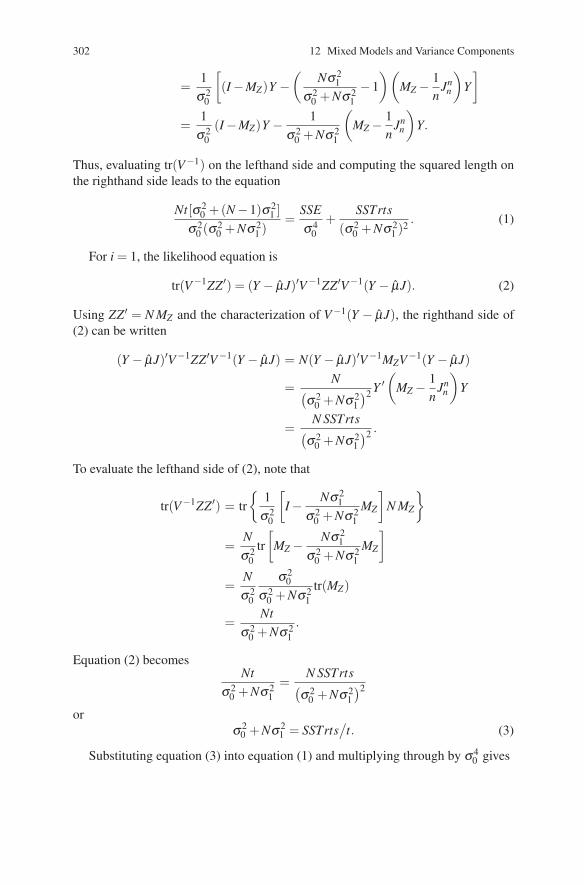
302 12 Mixed Models and Variance Components
=1
σ 20
[(I −MZ)Y −
(Nσ 2
1σ2
0 +Nσ 21−1)(
MZ − 1n
Jnn
)Y]
=1
σ 20
(I −MZ)Y − 1σ 2
0 +Nσ 21
(MZ − 1
nJn
n
)Y.
Thus, evaluating tr(V−1) on the lefthand side and computing the squared length onthe righthand side leads to the equation
Nt[σ 20 +(N −1)σ 2
1 ]σ 2
0 (σ20 +Nσ 2
1 )=
SSEσ 4
0+
SSTrts(σ2
0 +Nσ 21 )2 . (1)
For i = 1, the likelihood equation is
tr(V−1ZZ′) = (Y − μJ)′V−1ZZ′V−1(Y − μJ). (2)
Using ZZ′ = N MZ and the characterization of V−1(Y − μJ), the righthand side of(2) can be written
(Y − μJ)′V−1ZZ′V−1(Y − μJ) = N(Y − μJ)′V−1MZV−1(Y − μJ)
=N(
σ 20 +Nσ 2
1
)2 Y ′(
MZ − 1n
Jnn
)Y
=N SSTrts(
σ 20 +Nσ 2
1)2 .
To evaluate the lefthand side of (2), note that
tr(V−1ZZ′) = tr{
1σ 2
0
[I − Nσ 2
1σ 2
0 +Nσ 21
MZ
]N MZ
}=
Nσ 2
0tr[
MZ − Nσ 21
σ 20 +Nσ 2
1MZ
]=
Nσ 2
0
σ20
σ 20 +Nσ2
1tr(MZ)
=Nt
σ 20 +Nσ 2
1.
Equation (2) becomesNt
σ 20 +Nσ 2
1=
N SSTrts(σ 2
0 +Nσ 21
)2or
σ 20 +Nσ 2
1 = SSTrts/
t. (3)
Substituting equation (3) into equation (1) and multiplying through by σ40 gives

12.5 Maximum Likelihood Estimation for Singular Normal Distributions 303
Ntσ 20 [σ 2
0 +(N −1)σ 21 ]
(σ 20 +Nσ 2
1 )= SSE +
tσ 40
(σ 20 +Nσ 2
1 )
ort(N −1)σ 2
0 = SSE.
The maximum likelihood estimates appear to be σ 20 = MSE and σ2
1 = [(σ 20 +
Nσ21 )− σ 2
0 ]/N = [SSTrts/t −MSE]/N. However, this is true only if SSTrts/t −MSE > 0. Otherwise, the maximum is on a boundary, so σ 2
1 = 0 and σ20 = SSE/tN.
The maximum likelihood procedure tends to ignore the fact that mean parametersare being fitted. In the one-way ANOVA example, the estimate of σ 2
0 + Nσ 21 was
SSTrts/t instead of the unbiased estimate MSTrts. No correction was included forfitting the parameter μ . To avoid this, one can perform maximum likelihood on theresiduals, the subject of Section 6.
12.5 Maximum Likelihood Estimation for Singular Normal
Distributions
Maximum likelihood estimation involves maximizing the joint density of the obser-vations over the possible values of the parameters. This assumes the existence of adensity. A density cannot exist if the covariance matrix of the observations is sin-gular, as is the case with residuals. We consider an approach that allows maximumlikelihood estimation and show some uniqueness properties of the approach.
Suppose Y is a random vector in Rn, E(Y ) = μ , Cov(Y ) = V . If r(V ) = r < n,then, as seen in Lemma 1.3.5, Pr[(Y − μ) ∈ C(V )] = 1 and Y − μ is restricted toan r-dimensional subspace of Rn. It is this restriction of Y − μ to a subspace of Rn
(with Lesbesgue measure zero) that causes the nonexistence of the density. We seeka linear transformation from Rn to Rr that will admit a density for the transformedrandom vector. The linear transformation should not lose any information and theMLEs should, in some sense, be the unique MLEs.
Suppose we pick an n× r matrix B with C(B) = C(V ). B′Y together with a non-random function of Y can reconstruct Y with probability 1. Let MV be the per-pendicular projection operator onto C(V ), then Y = MVY + (I − MV )Y . MVY =B(B′B)−1B′Y is a function of B′Y while (I−MV )Y = (I−MV )μ with probability 1,because Cov[(I −MV )Y ] = (I −MV )V (I −MV ) = 0.
We would also like to see that Cov(B′Y ) = B′V B is nonsingular, so that a densitycan exist. Since C(B) = C(V ) and V is symmetric, V = BT B′ for some symmetricmatrix T . If T is nonsingular, then B′V B = (B′B)T (B′B) is nonsingular, becauseboth T and B′B are nonsingular. We now show that T is nonsingular. Suppose T issingular. Then there exists d ∈Rr, d �= 0, so that T d = 0. Since r(B) = r, there existsb �= 0 such that d = B′b. Because B′b = B′MV b, we can assume that b ∈C(V ). Now,V b = BT B′b = BT d = 0. However, for b ∈C(V ), V b = 0 can only happen if b = 0,which is a contradiction.

304 12 Mixed Models and Variance Components
As mentioned earlier, there is little hope of estimating the entire matrix V . Amore manageable problem is to assume that V is a function of a parameter vector θ .It should also be clear that in order to transform to a nonsingular random variable,we will need to know C(V ). This forces us to assume that C(V (θ )) does not dependon θ .
Suppose now that Y ∼ N(μ ,V (θ)); then B′Y ∼ N(B′μ ,B′V (θ )B). The density ofB′Y is
f (B′Y |μ ,θ )
=1
(2π)r2
1
|B′V (θ)B| 12
exp[−(B′Y −B′μ)′[B′V (θ )B]−1(B′Y −B′μ)/2]
= (2π)−r/2|B|−1|V (θ )|−1/2 exp[−(Y −μ)′B[B′V (θ)B]−1B′(Y −μ)/2].
The MLEs are obtained by maximizing this with respect to μ and θ . A direct conse-quence of Proposition 12.5.1 below is that maximization of f (B′Y ) does not dependon the choice of B.
Proposition 12.5.1. If B and B0 are two n× r matrices of rank r and C(B) =C(B0), then
(1) for some scalar k, k|B′V B| = |B′0V B0|;
(2) B[B′V B]−1B′ = B0[B′0V B0]−1B′
0 when the inverses exist.
PROOF. Since C(B) = C(B0) and both are full rank, B0 = BK for some nonsingu-lar K.
(1) |B′0V B0| = |K′B′V BK| = |K|2|B′V B|. Take k = |K|2.
(2) B0[B′0V B0]−1B′
0 = BK[K′B′V BK]−1K′B′
= BKK−1[B′V B]−1(K′)−1K′B′
= B[B′V B]−1B′. �
Corollary 12.5.2. f (B′Y |μ,θ) = k−1/2 f (B′0Y |μ ,θ).
12.6 Variance Component Estimation: REML
Restricted (or residual) maximum likelihood (REML) estimation involves findingmaximum likelihood estimates of variance components from the distribution of theresiduals. This allows for estimation of the variance components without the com-plication of the fixed effects. An apparent problem is that of defining the residuals,since V is unknown. We show that any reasonable definition gives the same answers.

12.6 Variance Component Estimation: REML 305
Consider the model of Section 4,
Y = Xβ +ξ , ξ ∼ N(0,V (θ)),
θ = (σ 20 , . . . ,σ 2
r )′, V (θ) = ∑ri=0 σ2
i ZiZ′i . As discussed in Section 10.2, the only rea-
sonable linear unbiased estimates of Xβ are of the form AY , where A is some projec-tion operator onto C(X). The residuals can be defined as (I −A)Y . The distributionof the residuals is
(I −A)Y ∼ N(0,(I −A)V (θ )(I −A)′).
V (θ ) is assumed nonsingular in the mixed model, so C((I − A)V (θ )(I − A)′) =C(I −A). Let r(X) ≡ s; so r(I −A) = n− s. For an n× s matrix B with C(B) =C(I −A), the MLE of θ maximizes
f (B′(I −A)Y |θ) = (2π)−(n−s)/2|B′(I −A)V (θ)(I −A)′B|−1/2
×exp[−Y ′(I −A)′B[B′(I −A)V (θ )(I −A)′B]−1B′(I −A)Y/2].
We will show that this depends on neither A nor B by showing that C[(I −A)′B] =C(X)⊥ and appealing to Section 5.
Proposition 12.6.1. C((I −A)′B) = C(X)⊥.
PROOF. Clearly, B′(I −A)X = 0, so C((I −A)′B) ⊂ C(X)⊥. The rank of C(X)⊥is n− s, so it is enough to show that the rank of (I −A)′B is n− s. Since (I −A)′Bis an n× (n− s) matrix it is enough to show that for any d ∈ Rn−s, (I −A)′Bd = 0implies d = 0. Since C(I−A) = C(B), Bd = (I −A)c for some c. If (I −A)′Bd = 0,then c(I −A)′Bd = d′B′Bd = 0; so Bd = 0. Since B is an n× (n− s) matrix of fullcolumn rank, d = 0. �
Frequently, REML is defined as maximum likelihood estimation from B′Y , wherer(B) = n− s and B′X = 0. This definition is equivalent to the one used here. ChooseA = M. Then I −M is the perpendicular projection operator onto C(X)⊥. Since forany choice of B in this alternative definition, r(B) = n− s and B′X = 0, we haveC(B) = C(X)⊥, and the B from this alternative definition also works in the origi-nal definition. The procedure presented here dictates doing maximum likelihood onB′(I −M)Y = B′Y . We will assume henceforth that r(B) = n− s and B′X = 0.
As in Section 4, setting the partial derivatives to zero determines the likelihoodequations
tr[(B′V B)−1B′ZiZ′iB] = Y ′B(B′V B)−1B′ZiZ′
iB(B′V B)−1B′Y, (1)
i = 0,1, . . . ,r. These can be written in a particularly nice form. To do this, we needsome results on projection operators. Recall that if A is idempotent, then A is theprojection operator onto C(A) along C(A′)⊥. The rank of A is s, so r(C(A′)⊥) isn− s. Moreover, for any w, w ∈C(A′)⊥ if and only if Aw = 0. To show that A is the

306 12 Mixed Models and Variance Components
projection operator onto M along N for two spaces M and N , it is enough toshow that 1) for v ∈ M , Av = v; 2) for w ∈ N , Aw = 0, and 3) r(M )+ r(N ) = n.
Lemma 12.6.2. Let A0 = X(X ′V−1X)−X ′V−1. Then I − A0 is the projectionoperator onto C(V B) along C(X).
PROOF. Since C(B) = C(X)⊥ and V is nonsingular, r(V B) = n− s = r(I −A0).Also, (I −A0)V B = V B−X(X ′V−1X)−X ′B = V B, so I −A0 is a projection ontoC(V B). It is along C(X) because r(X) = s and (I −A0)X = X −X = 0. �
Lemma 12.6.3. V B(B′V B)−1B′ is the projection operator onto C(V B) alongC(X).
PROOF. V B(B′V B)−1B′ = V B[(B′V )V−1(V B)]−1(B′V )V−1 is a projection ontoC(V B). Since C(B) = C(X)⊥, V B(B′V B)−1B′X = 0. Moreover, r(V B) = n− s andr(X) = s. �
It follows from the lemmas that (I − A0) = V B(B′V B)−1B′ and that V−1(I −A0) = B(B′V B)−1B′. Observing that tr[(B′V B)−1B′ZiZ′
iB] = tr[B(B′V B)−1B′ZiZ′i ],
(1) can be rewritten as
tr[V−1(I −A0)ZiZ′i ] = Y ′(I −A0)′V−1ZiZ′
iV−1(I −A0)Y,
i = 0,1, . . . ,r, where (I −A0)Y are the residuals from the BLUE of Xβ , i.e., (I −A0)Y = Y −X β .
As in Section 4, the REML equations can also be viewed as method of moments(estimating equation) methods because they involve setting a series of quadraticforms equal to their expectations. In particular, the REML equations involve setting
Y ′(I −A0)′V−1ZiZ′iV
−1(I −A0)Y = E[Y ′(I −A0)′V−1ZiZ′iV
−1(I −A0)Y ]
for i = 0,1, . . . ,r. To see this observe that
E[Y ′(I −A0)′V−1ZiZ′iV
−1(I −A0)Y ] = tr[(I −A0)′V−1ZiZ′iV
−1(I −A0)V ]= tr[V−1(I −A0)V (I −A0)′V−1ZiZ′
i ]= tr[V−1(I −A0)VV−1(I −A0)ZiZ′
i ]= tr[V−1(I −A0)(I −A0)ZiZ′
i ]= tr[V−1(I −A0)ZiZ′
i ].
To solve the REML equations, it is useful to write
tr[V−1(I −A0)ZiZ′i ] = tr[(I −A0)′V−1ZiZ′
iV−1(I −A0)V ]
= tr[V (I −A0)′V−1ZiZ′iV
−1(I −A0)]

12.7 Variance Component Estimation: MINQUE 307
= tr
[(r
∑j=0
σ 2j Z jZ′
j
)(I −A0)′V−1ZiZ′
iV−1(I −A0)
]
=r
∑j=0
σ 2j tr[ZjZ′
j(I −A0)′V−1ZiZ′iV
−1(I −A0)].
The equations for finding the REML estimates can now be written
r
∑j=0
σ 2j tr[ZjZ′
jV−1(I −A0)ZiZ′
iV−1(I −A0)
]= Y ′(I −A0)′V−1ZiZ′
iV−1(I −A0)Y,
i = 0, . . . ,r. Since V is unknown, typically an initial guess for V will be made andestimates of the σ 2
i will be computed as the solution to the system of linear equa-tions. These estimates of the variance components determine a new estimate of Vthat can be used to get updated values of the σ 2
i s. This iterative procedure is repeateduntil the σ 2
i s converge. Since the equations are linear, solutions are easy to find. Asmentioned in Section 4, similar methods can be used to find unrestricted MLEs. Infact, this only involves removing the terms (I −A0) from the traces.
Exercise 12.5 Consider the model Y = Xβ + e, e ∼ N(0,σ2I). Show that theMSE is the REML estimate of σ 2.
12.7 Variance Component Estimation: MINQUE
MINQUE is short for minimum norm quadratic unbiased (translation invariant)estimation. Attention is restricted to estimates that are translation invariant unbiasedquadratic forms in the observations.
Translation invariant means that a quadratic form, say Y ′BY , has the propertythat (Y + Xδ )′B(Y + Xδ ) = Y ′BY for all Y and δ . This simplifies to −2Y ′BXδ =δ ′X ′BXδ for all Y and δ . In particular, δ ′X ′BXδ =−2E(Y )′BXδ =−2β ′X ′BXδ forall β and δ . It follows that X ′BX = 0. Combining this with δ ′X ′BXδ = −2Y ′BXδimplies that Y ′BXδ = 0 for all Y and δ . This can occur only if BX = 0. Conversely,if BX = 0, then Y ′BY is translation invariant.
As seen in Appendix B, Y ′BY = Vec(B)′[Y ⊗Y ], which is a linear function of[Y ⊗Y ]. An alternative approach to variance component estimation involves fittinglinear models to the vector [Y ⊗Y ], cf. Searle et al. (1992, Chapter 12) or Christensen(1993). In this section we use a somewhat less appealing but more elementary ap-proach.
Minimum norm estimation considers unobservable “natural estimates” of the pa-rameters σ 2
0 , . . . ,σ 2r , and seeks real estimates of σ 2
0 , . . . ,σ 2r that are closest to the
“natural” estimates. “Closest” could be defined by minimizing the distance between
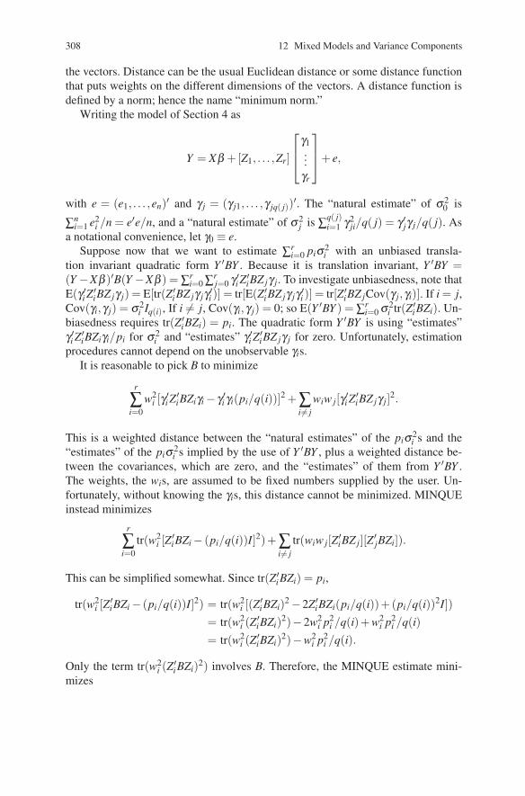
308 12 Mixed Models and Variance Components
the vectors. Distance can be the usual Euclidean distance or some distance functionthat puts weights on the different dimensions of the vectors. A distance function isdefined by a norm; hence the name “minimum norm.”
Writing the model of Section 4 as
Y = Xβ +[Z1, . . . ,Zr]
⎡⎢⎣γ1...
γr
⎤⎥⎦+ e,
with e = (e1, . . . ,en)′ and γ j = (γ j1, . . . ,γ jq( j))′. The “natural estimate” of σ 20 is
∑ni=1 e2
i /n = e′e/n, and a “natural estimate” of σ 2j is ∑q( j)
i=1 γ2ji/q( j) = γ ′jγ j/q( j). As
a notational convenience, let γ0 ≡ e.Suppose now that we want to estimate ∑r
i=0 piσ2i with an unbiased transla-
tion invariant quadratic form Y ′BY . Because it is translation invariant, Y ′BY =(Y −Xβ )′B(Y −Xβ ) = ∑r
i=0 ∑rj=0 γ ′i Z′
iBZ jγ j. To investigate unbiasedness, note thatE(γ ′i Z′
iBZ jγ j) = E[tr(Z′iBZ jγ jγ ′i )] = tr[E(Z′
iBZ jγ jγ ′i )] = tr[Z′iBZ jCov(γ j,γi)]. If i = j,
Cov(γi,γ j) = σ 2i Iq(i), If i �= j, Cov(γi,γ j) = 0; so E(Y ′BY ) = ∑r
i=0 σ 2i tr(Z′
iBZi). Un-biasedness requires tr(Z′
iBZi) = pi. The quadratic form Y ′BY is using “estimates”γ ′i Z′
iBZiγi/pi for σ 2i and “estimates” γ ′i Z′
iBZ jγ j for zero. Unfortunately, estimationprocedures cannot depend on the unobservable γis.
It is reasonable to pick B to minimize
r
∑i=0
w2i [γ
′i Z
′iBZiγi − γ ′i γi(pi/q(i))]2 + ∑
i �= jwiw j[γ ′i Z
′iBZ jγ j]2.
This is a weighted distance between the “natural estimates” of the piσ2i s and the
“estimates” of the piσ 2i s implied by the use of Y ′BY , plus a weighted distance be-
tween the covariances, which are zero, and the “estimates” of them from Y ′BY .The weights, the wis, are assumed to be fixed numbers supplied by the user. Un-fortunately, without knowing the γis, this distance cannot be minimized. MINQUEinstead minimizes
r
∑i=0
tr(w2i [Z
′iBZi − (pi/q(i))I]2)+ ∑
i�= jtr(wiw j[Z′
iBZ j][Z′jBZi]).
This can be simplified somewhat. Since tr(Z′iBZi) = pi,
tr(w2i [Z
′iBZi − (pi/q(i))I]2) = tr(w2
i [(Z′iBZi)2 −2Z′
iBZi(pi/q(i))+(pi/q(i))2I])= tr(w2
i (Z′iBZi)2)−2w2
i p2i /q(i)+w2
i p2i /q(i)
= tr(w2i (Z
′iBZi)2)−w2
i p2i /q(i).
Only the term tr(w2i (Z
′iBZi)2) involves B. Therefore, the MINQUE estimate mini-
mizes

12.7 Variance Component Estimation: MINQUE 309
r
∑i=0
r
∑j=0
tr(wiwj[Z′iBZ j][Z′
jBZi])
with respect to B, subject to the conditions that tr(Z′iBZi) = pi and BX = 0. (B is
assumed to be symmetric.)Define Vw = ∑r
i=0 wiZiZ′i and Aw = X(X ′V−1
w X)−X ′V−1w . With this notation the
MINQUE is minimizing tr[(BVw)2] subject to tr(Z′iBZi) = pi and BX = 0. Rao
(1971) has shown that the MINQUE estimate is Y ′B0Y , where
B0 =r
∑i=0
λi(I −Aw)′V−1w ZiZ′
iV−1w (I −Aw), (1)
and where λ0, . . . ,λr are defined as solutions to the set of equations
r
∑j=0
λ jtr[Z jZ′jV
−1w (I −Aw)ZiZ′
iV−1w (I −Aw)] = pi, (2)
i = 0, . . . ,r. Setting Y ′B0Y equal to ∑rj=0 p jσ 2
j and substituting for B0 and pi with(1) and (2), we can obtain estimates of the σ 2
i s.
r
∑i=0
λiY ′(I −Aw)′V−1w ZiZ′
iV−1w (I −Aw)Y = Y ′B0Y =
r
∑i=0
piσ 2i
=r
∑i=0
σ 2i
r
∑j=0
λ jtr[Z jZ′jV
−1w (I −Aw)ZiZ′
iV−1w (I −Aw)].
Changing the order of summation on the last term, one sees that for any set of pis,estimates can be obtained by solving
r
∑j=0
σ 2j tr[ZjZ′
jV−1w (I −Aw)ZiZ′
iV−1w (I −Aw)]
= Y ′(I −Aw)′V−1w ZiZ′
iV−1w (I −Aw)Y
for i = 0, . . . ,r.These equations are precisely the REML equations with Vw and Aw substituted
for V and A. MINQUE estimates with Vw = V are REML estimates. The key differ-ence in the methods is that Vw is a known matrix, whereas V is unknown.
If one finds the MINQUE estimates and then uses those estimates as weightsin another round of MINQUE estimation, one has an iterative procedure that willeventually give REML estimates.
As mentioned, the choice of weights for MINQUE estimation is up to the user.A frequently used choice of weights is wi = 1 for all i. This is the Euclidean norm.A very convenient set of weights is w0 = 1, wi = 0 for all i �= 0. These are con-venient in that with these weights, Vw = I and Aw = M, the perpendicular projec-tion matrix onto C(X). The estimates obtained from these weights are often called
310 12 Mixed Models and Variance Components
MINQUE(0) estimates and are sometimes called MIVQUE(0) estimates (see Sec-tion 8). Another possibility is to use an inexpensive estimation technique such asHenderson’s Method 3 to obtain estimates σ 2
i , i = 0, . . . ,r. The weights can be takenas wi = σ 2
i . The point of this adaptive method seems to be that the MINQUE esti-mates should then be very close to the REML estimates. In other words, with goodinitial weights, repeated iteration to the REML estimates should be unnecessary.One iteration may well do the job.
12.8 Variance Component Estimation: MIVQUE
MIVQUE is minimum variance quadratic unbiased (translation invariant) estima-tion. MIVQUE, like the maximum likelihood and REML procedures, and unlikeMINQUE, assumes that Y has a normal distribution. We need to know the varianceof a quadratic form.
Theorem 12.8.1. Suppose Y ∼N(μ,V ) and V is nonsingular. Then Var(Y ′BY ) =2tr[(BV )2
]+4μ ′BV Bμ .
PROOF. See Searle (1971, Section 2.5). �
Since we are considering translation invariant quadratic forms Y ′BY , we haveVar(Y ′BY ) = 2tr
[(BV )2
].
If Y ′B0Y is to be the minimum variance quadratic unbiased translation invariantestimate of ∑r
i=0 piσ 2i , then Y ′B0Y must minimize tr
[(BV )2
]subject to BX = 0 and
tr(Z′iBZi) = pi. This is precisely the condition for getting a MINQUE estimate when
Vw = V .Unfortunately, it is virtually impossible to find MIVQUE estimates. In order to
find B, one must minimize tr[(BV )2]. To do the minimization, one needs to know
V . It is difficult for me to imagine a situation in which V would be known, yet notprovide information about the variance components.
In practice, one can guess at V , find an appropriate MIVQUE matrix B basedon the guess, obtain a new estimate of V , and repeat the procedure using the newV as the guess of V . This procedure should give something close to a MIVQUE,but it will not be exact. Because of the iterations involved, the estimates will nottypically be quadratic unbiased translation invariant estimates. On the other hand,these iterated MIVQUE estimates can be viewed as iterated MINQUE estimates.Thus, they are precisely the REML estimates.

12.9 Variance Component Estimation: Henderson’s Method 3 311
12.9 Variance Component Estimation: Henderson’s Method 3
Long before the development of the other methods described, Henderson (1953)presented a way of obtaining unbiased method of moment estimates of variancecomponents. Suppose we want to estimate σ 2
r . (The choice of σ 2r is for convenience
only. The technique applies to estimating any of σ 21 to σ 2
r .) Let P be the perpendic-ular projection operator onto C(X ,Z1, . . . ,Zr) and P0 the perpendicular projectionoperator onto C(X ,Z1, . . . ,Zr−1). The expected value of Y ′(P−P0)Y is
E[Y ′(P−P0)Y ] = tr[(P−P0)V ]+β ′X ′(P−P0)Xβ .
Since C(X) ⊂ C(P0) ⊂ C(P), (P−P0)X = 0 and β ′X ′(P−P0)Xβ = 0. Rewriting(P−P0)V gives
(P−P0)V = (P−P0)σ 20 +
r
∑i=1
σ 2i (P−P0)ZiZ′
i
= (P−P0)σ 20 +(P−P0)ZrZ′
rσ2r ,
because (P−P0)Zi = 0 for i = 1, . . . ,r−1. It follows that
E[Y ′(P−P0)Y ] = tr[(P−P0)σ 2
0 +(P−P0)ZrZ′rσ
2r]
(1)
= σ 20 tr(P−P0)+σ2
r tr[(P−P0)ZrZ′
r].
A similar argument shows that
E[Y ′(I −P)Y ] = σ 20 tr(I −P).
An unbiased estimate of σ 20 is
σ 20 = [Y ′(I −P)Y ]
/tr(I −P). (2)
From (1) and (2), an unbiased estimate of σ2r is
σ2r = [Y ′(P−P0)Y − σ 2
0 tr(P−P0)]/
tr[(P−P0)ZrZ′
r], (3)
provided that P �= P0.Henderson’s Method 3 has no known (to me) optimality properties. Henderson
himself recommended the use of other techniques. Method 3’s greatest advantage isthat it is easy to compute. It uses standard techniques from fitting linear models byleast squares, except that it requires the computation of tr[(P−P0)ZrZ′
r]. Even thiscan be computed using standard techniques. Note that
tr[(P−P0)ZrZ′
r]= tr[Z′
r(P−P0)Zr]= tr[Z′
r(I −P0)Zr].
Write Zr =[Z1
r ,Z2r , . . . ,Zq(r)
r
], where each Z j
r is a vector. By fitting the model

312 12 Mixed Models and Variance Components
Z jr = Xβ +
r−1
∑i=1
Ziγi + e
as if the γis are all fixed, we can obtain (Z jr )′(I−P0)(Z
jr ) as the sum of squares error,
and thus
tr[Z′
r(I −P0)Zr]=
q(r)
∑j=1
(Z jr )
′(I −P0)(Z jr ).
In other words, all of the numbers required for estimating σ2r can be obtained from
a standard least squares computer program.
EXAMPLE 12.9.1. Balanced One-Way ANOVA, continued from Example 12.4.2.We relate the notation of this section to that of the earlier example:
P = MZ ,
P0 =1n
Jnn ,
tr(P−P0) = t −1,
tr(I −P) = t(N −1),
Y ′(P−P0)Y/
tr(P−P0) = MSTrts,
Y ′(I −P)Y/
tr(I −P) = MSE = σ 20 .
Recall that ZZ′ = N MZ , so
tr[(P−P0)ZZ′] = tr[(P−P0)N P]
= Ntr[(P−P0)]= N(t −1).
From (3) it is found that
σ 21 =
SSTrts−MSE(t −1)N(t −1)
=MSTrts−MSE
N.
Exercise 12.6 Consider the Method 3 estimates of σ 20 and σ 2
1 in Example 12.9.1.(a) Show that these are also the REML estimates.(b) Show that the vector (Y ′Y,Y ′MZY,J′Y )′ is a complete sufficient statistic for
the balanced one-way random effects model.(c) Show that the Method 3 estimates are minimum variance unbiased.(d) Find the distributions of SSTrts and SSE.(e) Find a generalized likelihood ratio test of level α for H0 : σ 2
1 = 0.Hint: Use the concepts of Section 2.5 and the methods of Example 12.4.2.

12.9 Variance Component Estimation: Henderson’s Method 3 313
For estimating more than one variance component, Method 3 is not, in general,well defined. Suppose that we desire to estimate both σ 2
r and σ2r−1. To estimate σ 2
r ,we proceed as before. To estimate σ 2
r−1, fit the model
Y = Xβ +r−2
∑i=1
Ziγi + e.
Let P∗ be the perpendicular projection matrix onto C(X ,Z1, . . . ,Zr−2).
E[Y ′(P0 −P∗)Y ] = tr[(P0 −P∗)V ]+β ′X ′(P0 −P∗)Xβ= tr[(P0 −P∗)σ 2
0 +(P0 −P∗)Zr−1Z′r−1σ 2
r−1 +(P0 −P∗)ZrZ′rσ 2
r]
= σ 20 t0 +σ 2
r−1tr−1 +σ 2r tr,
where t0 = tr(P0 −P∗), tr−1 = tr[(P0 −P∗)Zr−1Z′r−1], and tr = tr[(P0 −P∗)ZrZ′
r]. Anunbiased estimate of σ 2
r−1 is
σ2r−1 = [Y ′(P0 −P∗)Y − σ 2
0 t0 − σ2r tr]/
tr−1.
Note that t0, tr−1, and tr can also be obtained from a least squares program.The problem with this procedure is that the estimates depend on the order of
estimation. One could equally well estimate σ 2r−1 first with the technique as origi-
nally described, and use this second stage to estimate σ 2r . Generally, the estimates
of, say σ 2r , will be different for the two methods of estimation. For nested mod-
els, however, only one order of estimation is possible. If C(Zr−1) ⊂ C(Zr), we saythat γr is nested within γr−1. We can estimate σ 2
r first and then use it to estimateσ 2
r−1. The alternative order is not possible. If we desire to estimate σ 2r−1 first, we
require the perpendicular projection operator onto the orthogonal complement ofC(X ,Z1, . . . ,Zr−2,Zr) with respect to C(X ,Z1, . . . ,Zr). Because C(Zr−1) ⊂ C(Zr),we have C(X ,Z1, . . . ,Zr−2,Zr) = C(X ,Z1, . . . ,Zr). The orthogonal complement isthe zero space, and the projection matrix is the zero matrix.
For balanced ANOVA models, Henderson’s Method 3 gives unique answers, be-cause all of the effects are either orthogonal (e.g., main effects) or nested (e.g., atwo-factor interaction is nested within both of the main effects). The definition ofnested effects used here is somewhat nonstandard. To many people, interaction ef-fects are not nested. As used here, interaction effects are nested in more than oneother term.
Exercise 12.7 Data were generated according to the model
yi jk = μ +αi +η j + γi j + ei jk,
i = 1,2, j = 1,2,3, k = 1, . . . ,Ni j, where E(η j) = E(γi j) = E(ei jk) = 0, Var(ei jk) =σ 2
0 = 64, Var(η j) = σ 21 = 784, and Var(γi j) = σ 2
2 = 25. All of the random effects

314 12 Mixed Models and Variance Components
were taken independently and normally distributed. The fixed effects were taken asμ +α1 = 200 and μ +α2 = 150. The data are
j ji 1 2 3 i 1 2 31 250 211 199 2 195 153 131
262 198 184 187 150 133251 199 200 203 135 135
198 187 192184 184 209
184
Estimate the variance components using MINQUE(0), MINQUE with all weightsequal to 1, and Henderson’s Method 3. Estimate the variance components usingeach of these three sets of estimates as starting values for REML and as startingvalues for maximum likelihood. For each method of estimation, find estimates ofthe fixed effects. Compare all the estimates with each other and with the true values.What tentative conclusions can you draw about the relative merits of the estimationprocedures?
12.10 Exact F Tests for Variance Components
In this section we examine two procedures for testing whether a variance componentis zero. The first test method is closely related to Henderson’s estimation method.
12.10.1 Wald’s Test
Seely and El-Bassiouni (1983) considered extensions of Wald’s variance componenttest. They examined the mixed linear model
Y = Xβ +Z1γ1 +Z2γ2 + e. (1)
Here, Z1 and Z2 are, respectively, n×q and n× s matrices of known quantities. γ1,γ2, and e are independent random vectors with
γ1 ∼ N(0,R), γ2 ∼ N(0,σ 22 Is), e ∼ N(0,σ 2
0 In).
The null hypothesis H0 : σ 22 = 0 can be tested by using ordinary least squares calcu-
lations treating the γis as fixed effects. Let SSE(1) be the sum of squares error fromfitting model (1). The degrees of freedom error are dfE(1). Also let SSE(2) be thesum of squares error from the least squares fit of
Y = Xβ +Z1γ1 + e (2)

12.10 Exact F Tests for Variance Components 315
with degrees of freedom error dfE(2). The Wald test is simply based on the fact thatunder H0
[SSE(2)−SSE(1)]/[dfE(2)−dfE(1)]
SSE(1)/dfE(1)∼ F(dfE(2)−dfE(1),dfE(1)).
Of course, if the two model matrix column spaces are the same, i.e., if C(X ,Z1,Z2) =C(X ,Z1), then there is no test because both the numerator sum of squares and de-grees of freedom are zero.
We now verify the distribution given above. Note that under the mixed model,
Cov(Y ) ≡V = σ 20 I +σ 2
2 Z2Z′2 +Z1RZ′
1.
Let P0 be the perpendicular projection operator onto the column space C(X ,Z1),and let P be the perpendicular projection operator onto C(X ,Z1,Z2). It followsthat SSE(2)− SSE(1) = Y ′(P − P0)Y , dfE(2) − dfE(1) = r(P − P0), SSE(1) =Y ′(I −P)Y , and dfE(1) = r(I − P). Note that PZ1 = Z1 and PP0 = P0. We needto show that Y ′(I −P)Y/σ2
0 ∼ χ2(r(I −P)), that Y ′(I −P)Y and Y ′(P−P0)Y areindependent, and that, under H0, Y ′(P−P0)Y/σ 2
0 ∼ χ2(r(P−P0)). Using resultsfrom Section 1.3, we need only show that σ−4
0 (I −P)V (I −P) = σ−20 (I −P), that
(I−P)V (P−P0) = 0, and that, when σ 22 = 0, σ−4
0 (P−P0)V (P−P0) = σ−20 (P−P0).
Verifying these results involves only straightforward linear algebra along with prop-erties of projection operators. In general, the distribution of Y ′(P−P0)Y seems tobe intractable without the assumption that σ2
2 = 0, but see Subsection 3.To facilitate extensions of this test in the next subsection, we use a simple gener-
alization of the Seely and El-Bassiouni results. The mixed model considered in (1)can also be written as
Y ∼ N(Xβ ,σ 2
0 I +σ 22 Z2Z′
2 +Z1RZ′1),
so the test applies for any data with a distribution of this form. If we let Σ be anyknown nonnegative definite matrix, the method also applies to
Y ∼ N(Xβ ,σ 2
0 Σ +σ 22 Z2Z′
2 +Z1RZ′1). (3)
Simply write Σ = QQ′. Then there exists a matrix T such that T Q = I; so
TY ∼ N(T Xβ ,σ 2
0 I +σ 22 (T Z2)(T Z2)′ +(T Z1)R(T Z1)′
),
and the method applies to TY . Obviously, for Σ positive definite, T = Q−1. The testbased on (3) is simply the standard generalized least squares test of model (2) versus(1) when Cov(Y ) = σ2
0 Σ , see Section 3.8.

316 12 Mixed Models and Variance Components
12.10.2 Ofversten’s Second Method
Consider the special case of the model discussed in Subsection 1 with R = σ21 Iq.
Then Cov(Y ) ≡ V = σ 20 I + σ 2
2 Z2Z′2 + σ 2
1 Z1Z′1. The object of the second method
is to obtain an exact F test for H0 : σ 21 = 0. This is of primary interest when
C(X ,Z1) ⊂ C(X ,Z2). If C(X ,Z1) �⊂ C(X ,Z2), a Wald test of H0 : σ 21 = 0 is avail-
able by simply interchanging the roles of Z1γ1 and Z2γ2 in the previous sec-tion. If C(X ,Z1) ⊂ C(X ,Z2), this interchange does not provide a test because thenC(X ,Z2) = C(X ,Z1,Z2). As developed here, if Ofversten’s second method providesa test, that test is valid regardless of the relationship of C(X ,Z1) and C(X ,Z2). Atthe end of the subsection, the test is presented for more general models.
Ofversten’s (1993) second method as presented in Christensen (1996b) involvesusing an orthonormal basis. For example, use Gram–Schmidt on the columns of[X ,Z2,Z1, In] to obtain an orthonormal basis for Rn, say c1, . . . ,cn. Write these ascolumns of a matrix C = [c1, . . . ,cn]. Partition C as C = [C1,C2,C3,C4], where thecolumns of C1 are an orthonormal basis for C(X), the columns of C2 are an orthonor-mal basis for the orthogonal complement of C(X) with respect to C(X ,Z2), thecolumns of C3 are an orthonormal basis for the orthogonal complement of C(X ,Z2)with respect to C(X ,Z2,Z1), and the columns of C4 are an orthonormal basis for theorthogonal complement of C(X ,Z2,Z1). Note that if C(X ,Z1) ⊂ C(X ,Z2), then C3is vacuous.
The basic idea of this method is to choose a matrix K so that the extended Wald’stest for model (3) can be applied to C′
2Y +KC′4Y . In executing the test of H0 : σ 2
1 = 0,σ 2
1 plays the role assigned to σ22 in (3), a function of σ 2
0 and σ 22 plays the role
assigned to σ 20 in (3), and the role of R in (3) is vacuous. In particular, for some
number λ and some matrix K, we want to have
C′2Y +KC′
4Y ∼ N(0,(σ 2
2 +σ 20 /λ )C′
2Z2Z′2C2 +σ 2
1 C′2Z1Z′
1C2). (4)
This is of the form (3). As shown in Exercise 12.8, C′2Z2Z′
2C2 is a positive definitematrix, so the test follows immediately from generalized least squares. The testcannot be performed if C′
2Z1 = 0, which occurs, for example, if C(Z1)⊂C(X). Notethat C4C′
4Y is the vector of residuals from treating the random γ effects as fixed.Thus, in using KC′
4Y = KC′4C4C′
4Y we are using some of the residual variability toconstruct the test.
To get the degrees of freedom for the test, we identify correspondences between(3) and (4). There are r(C2) “observations” available in (4). In (3), the numeratordegrees of freedom for the test are r(X ,Z1,Z2)− r(X ,Z1). With mean zero in (4)there is no linear mean structure, i.e, nothing corresponding to X in (3), Z1 from (3)is also vacuous in (4), and C′
2Z1 is playing the role of Z2 in (3). Thus the numeratordegrees of freedom for the test are r(C′
2Z1) and the denominator degrees of freedomare r(C2)− r(C′
2Z1). In model (4), r(C2) = r(X ,Z2)− r(X). If C(Z1) ⊂C(X ,Z2), itis shown in Exercise 12.8 that r(C′
2Z1) = r(X ,Z1)−r(X) and the degrees of freedomfor the test are r(X ,Z1)− r(X) and r(X ,Z1,Z2)− r(X ,Z1), respectively.
Observe that

12.10 Exact F Tests for Variance Components 317
C′2Y ∼ N
(0,σ 2
0 I +σ 22 C′
2Z2Z′2C2 +σ 2
1 C′2Z1Z′
1C2).
In many interesting cases, C′2Z2Z′
2C2 = λ I; so an ordinary least squares Wald testcan be applied immediately without any use of C′
4Y as long as C′2Z1 �= 0.
It is not difficult to see that in balanced ANOVA problems either C′2Z2Z′
2C2 = λ Iwhen a standard balanced ANOVA test is available, or C′
2Z1 = 0 when such a test isnot available. For example, consider (1) as modeling a balanced two-way ANOVAyi jk = μ + γ1i + γ2 j + ei jk, i = 1, . . . ,q, j = 1, . . . ,s, k = 1, . . . ,N, with Xβ beingthe vector Jμ . The γ1 and γ2 treatments are often said to be orthogonal. LettingM be the perpendicular projection operator onto C(X), this orthogonality meansprecisely that C[(I −M)Z1] and C[(I −M)Z2] are orthogonal, i.e., Z′
2(I−M)Z1 = 0,cf. Section 7.1. Now, by the definition of C2, C(C2) = C[(I −M)Z2], so C′
2Z1 = 0iff Z′
2(I −M)Z1 = 0, which we know is true from orthogonality. Hence, no test ofH0 : σ 2
1 = 0 is available from this method.Now consider a balanced nested model yi jk = μ + γ1i + γ2i j + ei jk with i, j, and
k as above. In this model, C(X ,Z1) ⊂ C(Z2) and 1N Z2Z′
2 ≡ P is the perpendicularprojection operator onto C(Z2). Observing that C(C2) ⊂ C(Z2) and using the or-thonormality of the columns of C2,
C′2Z2Z′
2C2 = NC′2PC2 = NC′
2C2 = N I.
Thus an ordinary least squares Wald test is available. Given that a Wald test simplycompares models in the usual way, for H0 : σ 2
1 = 0 this test is simply the standardbalanced ANOVA test for no fixed γ1i effects when γ2 is random. Similar orthog-onality and containment results hold in more general balanced ANOVAs. For thespecial case of C(Z1) ⊂ C(X ,Z2) with C′
2Z2Z′2C2 = λ I, a general explicit form for
the test statistic is given in (7).In general, C′
2Z2Z′2C2 �= λ I, so the test requires C′
4Y . If r(X ,Z2,Z1) = t,
C′4Y ∼ N
(0,σ 2
0 In−t).
It is easy to see that C′2VC4 = 0, so C′
2Y and C′4Y are independent. To obtain (4),
simply pick K so that
KC′4Y ∼ N
(0,σ 2
0[λ−1C′
2Z2Z′2C2 − I
]).
Obviously one can do this provided that λ−1C′2Z2Z′
2C2 − I is a nonnegative definitematrix. λ is chosen to ensure that the matrix is nonnegative definite. By the choice ofC2, C′
2Z2Z′2C2 is a positive definite matrix and λ is taken as its smallest eigenvalue.
Then if we use the eigenvalue, eigenvector decomposition C′2Z2Z′
2C2 = WD(λi)W ′with W orthogonal,
λ−1C′2Z2Z′
2C2 − I = WD(
λi
λ−1)
W ′,
which is clearly nonnegative definite.

318 12 Mixed Models and Variance Components
Note that this development makes it obvious why λ needs to be the smallesteigenvalue. Actually, the test would still work if λ were chosen to be any positivenumber less than the smallest eigenvalue, but we want KC′
4Y to increase the vari-ability of C′
2Y as little as possible, and this is accomplished by taking λ as large aspossible. In particular, choosing λ as the smallest eigenvalue gives KC′
4Y a singu-lar covariance matrix and thus no variability in at least one direction. Other validchoices of λ can only increase variability.
Also note that KC′4Y = 0 a.s. if the eigenvalues of C′
2Z2Z′2C2 all happen to be the
same. In this case, λ−1C′2Z2Z′
2C2 − I = 0 and C′2Z2Z′
2C2 = λ I, so we get the simplerWald test alluded to earlier.
The difficulty with the second method is that K is not unique, and typically theresults of the test depend on the choice of K. In particular, K is a w× (n− t) matrix,where typically w ≡ r(X ,Z2)− r(X) < (n− t), while λ−1C′
2Z2Z′2C2 − I is a w×w
matrix. Thus, we can take K =[WD(√
λiλ −1
),0]
or K =[
0,WD(√
λiλ −1
)]or
any number of other matrices. Modifying Ofversten, a reasonable procedure mightbe just to pick one of these convenient K matrices, but first randomly permute therows of C′
4Y .This method applies quite generally. A proof consists of observing that the test
of H0 : σ 21 = 0 remains valid when X = [X1,X2], β = (β ′
1,β ′2)
′ with β2 ∼ N(0,R2),and β2 independent of γ1 and γ2. This model allows for interaction between tworandom factors and arbitrary numbers of factors. The method will be most usefulwhen C(X ,Z1) ⊂C(X ,Z2); if this is not the case, the simpler Wald test is available.Whenever C′
2Z1 = 0, no test is available. For example, this will occur wheneverC(Z1) ⊂C(X), which is precisely what happens when one tries to test the variancecomponent of a random main effect in a three-way analysis of variance with allinteractions.
12.10.3 Comparison of Tests
When C(Z1) �⊂ C(X ,Z2), we have two tests of H0 : σ 21 = 0 available. (See Lin and
Harville (1991) and Christensen and Bedrick (1999) for some alternatives to Wald’stest other than that just developed.) Let M, P2, P, and P0 be perpendicular projectionmatrices onto C(X), C(X ,Z2), C(X ,Z2,Z1), and C(X ,Z1), respectively. The simpleWald test has the F statistic
F =Y ′(P−P2)Y/r(P−P2)
Y ′(I −P)Y/r(I −P).
It can be of interest to examine the power (probability of rejecting the test) un-der some alternative to the null model, e.g., the model when the null hypothesis isfalse. The power of this test is quite complicated, but for given values of the param-

12.10 Exact F Tests for Variance Components 319
eters the power can be computed as in Davies (1980). Software is available throughSTATLIB. See also Christensen and Bedrick (1997).
Intuitively, the power depends in part (and only in part) on the degrees of free-dom, r(X ,Z2,Z1)− r(X ,Z2), n − r(X ,Z2,Z1) and the ratio of the expected meansquares,
1+σ 2
1σ 2
0
tr [Z′1(P−P2)Z1]
r(X ,Z2,Z1)− r(X ,Z2). (5)
The basic idea behind F tests is that under the null hypothesis the test statistic isthe ratio of two estimates of a common variance. Obviously, since the two are es-timating the same thing under H0, the ratio should be about 1. The F distributionquantifies the null variability about 1 for this ratio of estimates. If the numerator anddenominator are actually estimates of very different things, the ratio should deviatesubstantially from the target value of 1. In fixed effects models, the power of an Ftest under the full model is simply a function of the ratio of expected values of thetwo estimates and the degrees of freedom of the estimates. In mixed models, thepower is generally much more complicated, but the ratio of expected values can stillprovide some insight into the behavior of the tests. The ratio in (5) is strictly greaterthan 1 whenever the test exists and σ 2
1 > 0, thus indicating that larger values of thetest statistic can be expected under the alternative. The power of the test should tendto increase as this ratio increases but in fact the power is quite complicated. Notethat Y ′(P−P2)Y = Y ′C3C′
3Y and Y ′(I −P)Y = Y ′C4C′4Y ; so this test uses only C′
3Yand C′
4Y .The second test is based on C′
2Y +KC′4Y . Again, exact powers can be computed
as in Davies (1980). As shown in Exercise 12.8, the ratio of the expected meansquares for the second test is
1+σ 2
1
σ 22 +σ2
0 /λtr[(C′
2Z2Z′2C2)−1C′
2Z1Z′1C2]
r(C′2Z1)
. (6)
Again, this is strictly greater than 1 whenever the test exists and σ 21 > 0.
The degrees of freedom for the second test were given earlier. To compare thedegrees of freedom for the two tests, observe that
C(X) ⊂C(X ,{P2 −M}Z1) = C(X ,P2Z1) ⊂C(X ,Z2) ⊂C(X ,Z2,Z1).
The degrees of freedom for the second test are, respectively, the ranks of the or-thogonal complement of C(X) with respect to C(X ,{P2 −M}Z1) and the orthogo-nal complement of C(X ,{P2 −M}Z1) with respect to C(X ,Z2). (The first orthog-onal complement is C(C2C′
2Z1) with the same rank as C′2Z1, and the second or-
thogonal complement has rank r(X ,Z2)− [r(X) + r(C′2Z1)].) The degrees of free-
dom for the simple Wald test are, respectively, the ranks of the orthogonal comple-ment of C(X ,Z2) with respect to C(X ,Z2,Z1) and the orthogonal complement ofC(X ,Z2,Z1). In practice, the simple Wald test would typically have an advantagein having larger denominator degrees of freedom, but that could be outweighed byother factors in a given situation. We also see that, in some sense, the second test is

320 12 Mixed Models and Variance Components
being constructed inside C(X ,Z2); it focuses on the overlap of C(X ,Z2) and C(Z1).On the other hand, the simple Wald test is constructed from the overlap of C(Z1)with the orthogonal complement of C(X ,Z2).
In the special case of C(Z1) ⊂C(X ,Z2) with C′2Z2Z′
2C2 = λ I, the second methodgives the test statistic
F =Y ′(P0 −M)Y/r(P0 −M)Y ′(P2 −P0)Y/r(P2 −P0)
. (7)
See Exercise 12.8 for a proof. For example, in a two-way ANOVA, X can indicatethe grand mean and a fixed main effect, Z1 can indicate the random main effectto be tested, and Z2 can indicate the interaction. When the two-way is balanced,C′
2Z2Z′2C2 = λ I and we have the traditional test, i.e., the mean square for the random
main effect divided by the mean square for interaction.It should be noted that under H0 : σ 2
1 = 0, C′3Y also has a N(0,σ 2
0 I) distributionso it could also be used, along with C′
4Y , to adjust the distribution of C′2Y and still
maintain a valid F test. However, this would be likely to have a deleterious effecton the power since then both the expected numerator mean square and the expecteddenominator mean square would involve positive multiples of σ 2
1 under the alterna-tive.
The material in this section is closely related to Christensen (1996b). The nearreplicate lack of fit tests discussed in Subsection 6.6.2 can also be used to constructexact F tests for variance components. In fact, when used as a variance compo-nent test, Christensen’s (1989) test is identical to Wald’s test. See Christensen andBedrick (1999) for an examination of these procedures.
Exercise 12.8
(a) Prove that r(C′2Z1) = r(X ,Z1)− r(X) when C(Z1) ⊂C(X ,Z2).
(b) Prove that C′2Z2Z′
2C2 is positive definite.(c) Prove (6).(d) Prove (7).
Exercise 12.9 Use the data and model of Exercise 12.7 to test H0 : σ 21 = 0 and
H0 : σ 22 = 0.
12.11 Recovery of Interblock Information in BIB Designs
Consider the analysis of a balanced incomplete block (BIB) design in which blocksare random effects. This analysis is known as the recovery of interblock information.The mixed model for BIBs was mentioned previously in Exercise 11.5. The analysisinvolves ideas from Chapters 9 through 11. BIB designs are discussed in Section 9.4,from which most of the current notation is taken. In estimating treatment effects,Theorem 10.4.5 is used. The model is a mixed model, so variance components areestimated using methods from this chapter. Finally, the variance structure breaks up

12.11 Recovery of Interblock Information in BIB Designs 321
into within cluster and between cluster components as in Chapter 11. In our analysisof the model, blocks are clusters, within cluster error is called intrablock error, andbetween cluster error is interblock error.
We begin by fixing notation and relating it back to Section 9.4. The model for aBIB is
yi j = μ +βi + τ j + ei j,
i = 1, . . . ,b, with j ∈ Di or, equivalently, j = 1, . . . ,t, with i ∈ Ai. Here β and τindicate block and treatment effects, respectively, Di is the set of treatment indicesfor block i, and A j is the set of indices for blocks that contain treatment j. The modelis written using matrices as
Y = Jμ +Xβ +Zτ + e,
where μ , β , and τ are the grand mean, block effects vector, and treatment effectsvector, respectively. The matrix notation is a slight change from Section 9.4 in thatJ is no longer included in the X matrix. The matrix X is the matrix of indicators forthe blocks and can be written
X = [xi j,m], xi j,m = δim,
where the columns of X are m = 1, . . . ,b and the pair i j identifies a row of the matrix.Z is a matrix of indicators for the treatments and is defined as in Section 9.4, i.e.,Z = [zi j,r] with zi j,r = δ jr, r = 1, . . . , t, and the pair i j denoting a row of the matrix.Recall two fundamental relations necessary for a BIB,
rt = bk
and(t −1)λ = r(k−1),
where r is the number of replications for each treatment, k is the number of unitsin each block, and λ is the number of times any two treatments occur in the sameblock.
In the mixed model, β is a random vector with E(β ) = 0, Cov(β ) = σ 2BIb, and
Cov(β ,e) = 0. In a slight change of notation write Cov(e) = σ 2e In, where n = rt =
bk. Combining the random effects, write η = Xβ + e and the model as
Y = Zτ +η, E(η) = 0, Cov(η) = σ 2e In +σ 2
BXX ′. (1)
Note that we have dropped the grand mean, thus removing the overparameterizationassociated with the treatment effects. In other words, we are using the model yi j =τ j +ηi j, where ηi j ≡ β j + ei j is the random error term.
As in Chapter 11, write σ 2 = σ 2e + σ 2
B and ρ = σ 2B/(σ 2
e +σ2B). It follows that
σ 2e = σ 2(1−ρ) and σ2
B = σ 2ρ . A term that frequently appears in the analysis is theinterblock (between cluster) error term,

322 12 Mixed Models and Variance Components
σ2 [(1−ρ)+ kρ] = σ 2e + kσ 2
B.
With the notation given earlier, write
Cov(η) = σ 2V,
where, again as in Chapter 11,
V =[(1−ρ)I +ρXX ′]
= [(1−ρ)I + kρM]
and M is the perpendicular projection operator onto C(X).
12.11.1 Estimation
In this subsection we derive the BLUE of τ . From Section 2.7,
Zτ = AY
= Z(Z′V−1Z
)−1Z′V−1Y.
Note that finding τ is essentially equivalent to finding the oblique projection opera-tor A. Given τ we can easily find Zτ; thus we know AY . With AY known for any vec-tor Y , the matrix A is completely characterized. Finding τ =
(Z′V−1Z
)−1 Z′V−1Y
requires computation of both V−1 and(Z′V−1Z
)−1. These computations are facili-tated by the following result.
Proposition 12.11.1. Let P be a projection operator (idempotent), and let a andb be real numbers. Then
[aI +bP]−1 =1a
[I − b
a+bP].
PROOF.
1a
[I − b
a+bP][aI +bP] =
1a
[aI +bP− ab
a+bP− b2
a+bP]
= I. �
Using this result, we obtain two forms for V−1:
V−1 =1
1−ρ
[I − kρ
[(1−ρ)+kρ]M]
=1
1−ρ
[(I −M)+
1−ρ[(1−ρ)+ kρ]
M]. (2)
Both forms will be used frequently.

12.11 Recovery of Interblock Information in BIB Designs 323
We now compute Z′V−1Z and(Z′V−1Z
)−1. First note that the fundamental rela-tion (t −1)λ = r(k−1) implies
λ t = rk− (r−λ ).
Using this equality, the characterizations of Z′Z and Z′MZ given in Section 9.4, thefirst form for V−1 in equation (2), and writing Pt = 1
t Jtt , we get
(Z′V−1Z) =1
1−ρ
[Z′Z− kρ
[(1−ρ)+ kρ]Z′MZ
]=
11−ρ
[rI − ρ
[(1−ρ)+ kρ]{(r−λ )I +λ tPt}
]=
11−ρ
[r(1−ρ)
[(1−ρ)+kρ]I +
λ tρ[(1−ρ)+ kρ]
(I −Pt)]
=1
(1−ρ) [(1−ρ)+kρ][r(1−ρ)I +λ tρ(I −Pt)] .
From Proposition 12.11.1,
(Z′V−1Z)−1 =[(1−ρ)+ kρ]
r
[I − λ tρ
r(1−ρ)+λ tρ(I −Pt)
](3)
=[(1−ρ)+ kρ]
r
[r(1−ρ)
r(1−ρ)+λ tρI +
λ tρr(1−ρ)+λ tρ
Pt
].
Rather than computing τ = (Z′V−1Z)−1Z′V−1Y directly, it is convenient to de-compose Z′V−1Y into intrablock and interblock components. The intrablock com-ponent is related to the fixed block effect analysis. The interblock component iswhat is left. The fixed block effect analysis is based on
Q = (Q1, . . . ,Qt)′,
where Q ≡ Z′(I −M)Y , cf. Section 9.4. Similarly, define
W = (W1, . . . ,Wt)′,
where W ≡ Z′MY . M is the perpendicular projection operator for the one-wayANOVA in blocks (ignoring treatments) so
MY = [ti j], ti j = yi· ,
withyi· ≡ 1
k ∑j∈Di
yi j .
Z is a matrix of treatment indicators, so Z′MY yields

324 12 Mixed Models and Variance Components
Wj = ∑i∈A j
yi· .
In Section 9.4, the Wjs were computed in the process of computing the Q js. Inparticular,
Q j = ∑i∈A j
(yi j − yi·) = ∑i∈A j
yi j −Wj,
as in the first table in the continuation of Example 9.4.1. In computing τ , we willalso have occasion to use
W · ≡ 1t
t
∑j=1
Wj
and the fact that
Q· ≡1t
t
∑j=1
Q j =1t
J′t Z′(I −M)Y =
1t
J′n(I −M)Y = 0.
Using the second form of V−1 given in (2),
Z′V−1Y =1
1−ρZ′(I −M)Y +
1(1−ρ)+ kρ
Z′MY (4)
=1
1−ρQ+
1(1−ρ)+ kρ
W.
Finally, using (3) and (4),
τ = (Z′V−1Z)−1Z′V−1Y
=[(1−ρ)+ kρ]
r
[r(1−ρ)
r(1−ρ)+λ tρI +
λ tρr(1−ρ)+λ tρ
Pt
]Z′V−1Y
=[(1−ρ)+ kρ] (1−ρ)
r(1−ρ)+λ tρZ′V−1Y +
[(1−ρ)+ kρ]λ tρr [r(1−ρ)+λ tρ]
PtZ′V−1Y
=[(1−ρ)+ kρ]r(1−ρ)+λ tρ
Q+(1−ρ)
r(1−ρ)+λ tρW +
λ tρW ·r [r(1−ρ)+λ tρ]
Jt .
The last equality comes from PtQ = Q·Jt = 0 and PtW = W ·Jt . In particular, anindividual component of τ is
τ j =[(1−ρ)+kρ]r(1−ρ)+λ tρ
Q j +(1−ρ)
r(1−ρ)+λ tρWj +
λ tρW ·r [r(1−ρ)+λ tρ]
.
For purposes of comparing treatments, the term involving W ·, which is constant, canbe dropped. Finally, the projection operator is characterized by
AY = Zτ = [ti j], ti j = τ j .

12.11 Recovery of Interblock Information in BIB Designs 325
There are three additional aspects of the analysis to consider. First, we need toconsider testing the hypothesis τ1 = · · ·= τt . Second, we need to examine contrasts.Third, we need to deal with the fact that our estimate of τ is useless. The estimate de-pends on ρ = σ 2
B/(σ 2e +σ2
B). This is an unknown parameter. Writing τ = (σ 2/σ 2)τ ,and using σ 2(1−ρ) = σ 2
e and σ2ρ = σ 2B , gives
τ =σ2
e + kσ 2B
rσ2e +λ tσ 2
BQ+
σ 2e
rσ 2e +λ tσ 2
BW +
λ tσ 2BW ·
rσ2e +λ tσ 2
BJt . (5)
Model (1) is a mixed model, so the methods of this chapter can be used to estimateσ 2
e and σ 2B . The variance estimates can be substituted into (5) to give a usable es-
timate of τ . Traditionally, Henderson’s Method 3 has been used to obtain varianceestimates. The use of Henderson’s Method 3 will be discussed in detail later. Testsof models and examination of contrasts will be discussed as if σ2
e and σ 2B (hence σ 2
and ρ) were known. A discussion in which only ρ is assumed known is also given.Throughout we assume that η ≡ Xβ + e ∼ N(0,σ 2V ).
12.11.2 Model Testing
We desire to test model (1) against the reduced model
Y = Jμ +η. (6)
In particular, we will show that an α level test rejects H0 if
rσ 2e +λ tσ 2
B
σ 2e[σ 2
e + kσ 2B
] t
∑i=1
(τ j − τ·) > χ2(1−α,t −1), (7)
where τ· = ∑tj=1 τ j/t is the mean of the τ js. The remainder of this subsection is
devoted to showing that this is the appropriate test.We begin by finding the BLUE of Jμ from model (6). The BLUE is Jμ = A0Y =
J(J′V−1J
)−1 J′V−1Y . However, we can apply Theorem 10.4.5 to see that the simpleleast squares estimate Jμ with μ = ∑i j yi j/rt is the BLUE. To use Theorem 10.4.5,we need to show that C(V J)⊂C(J). Because J ∈C(X), V J = [(1−ρ)I + kρM]J =(1−ρ)J + kρJ = [(1−ρ)+ kρ]J ∈C(J).
From Corollary 3.8.3,
Y ′(A−A0)′V−1(A−A0)Y/
σ 2 ∼ χ2(t −1,0)
if and only if model (6) is true. We wish to show that the test statistic is identical tothat used in (7). Our argument involves five algebraic identities. First,
t
∑j=1
(τ j − τ·)2 = τ ′(I −Pt)τ .

326 12 Mixed Models and Variance Components
Second, we show that μ = τ·. Using the second form for V−1 in (2) gives V−1J =[(1−ρ)+ kρ]−1J; also recall that J ∈C(Z) so AJ = J. These equalities lead to theresult.
τ· =1t
J′t τ =1rt
J′Zτ =1rt
J′AY
=(1−ρ)+ kρ
rtJ′V−1AY
=(1−ρ)+ kρ
rtJ′A′V−1Y
=(1−ρ)+ kρ
rtJ′V−1Y
=1rt
J′Y = μ.
Third,
τ ′(I −Pt)τ = τ ′τ − t(
1t
τ ′J′t
)2
= τ ′τ − t μ2
= [τ − Jt μ ]′[τ − Jt μ ].
Fourth, recall from Section 9.4 that
Z′(I −M)Z =λ tk
(I −Pt) ,
and, finally, from Section 9.4, and because r−λ = rk−λ t,
Z′MZ =1k
[(r−λ )I +λ tPt ]
=1k
[rkI −λ t (I −Pt)] .
Using the second form of V−1 in (2),
Y ′ (A−A0)′V−1 (A−A0)Y
= [Zτ − Jμ ]′V−1 [Zτ − Jμ ]
=1
1−ρ[Zτ − Jμ ]′ (I −M) [Zτ − Jμ ]+
1(1−ρ)+kρ
[Zτ − Jμ]′ M [Zτ − Jμ ]
=1
1−ρτ ′Z′(I −M)Zτ +
1(1−ρ)+ kρ
[Zτ −ZJt μ ]′M[Zτ −ZJt μ ]
=1
1−ρλ tk
τ ′(I −Pt)τ +1
(1−ρ)+ kρ[τ − Jt μ ]′Z′MZ[τ − Jt μ ]
12.11 Recovery of Interblock Information in BIB Designs 327
=1
1−ρλ tk
τ ′(I −Pt)τ +1
(1−ρ)+ kρ[τ − Jt μ ]′
{1k
[rkI −λ t (I −Pt)]}
[τ − Jt μ ]
=λ tk
τ ′(I −Pt)τ{
11−ρ
− 1(1−ρ)+ kρ
}+
r(1−ρ)+kρ
[τ − Jt μ]′[τ − Jt μ ]
=kρ
[(1−ρ)+ kρ] (1−ρ)λ tk
τ ′(I −Pt)τ +r
(1−ρ)+ kρτ ′(I −Pt)τ
=r(1−ρ)+λ tρ
(1−ρ) [(1−ρ)+ kρ]τ ′(I −Pt)τ
=rσ 2(1−ρ)+λ tσ 2ρ
σ 2(1−ρ) [(1−ρ)+ kρ ]τ ′(I −Pt)τ
=rσ 2
e +λ tσ 2B
σ 2e [(1−ρ)+kρ]
τ ′(I −Pt)τ.
Dividing by σ 2 gives
Y ′ (A−A0)′V−1 (A−A0)Yσ 2 =
rσ2e +λ tσ 2
B
σ 2e[σ 2
e + kσ 2B] τ ′(I −Pt)τ,
which is the test statistic in (7). In practice, estimates of σ2e and σ2
B are used tocompute both the multiplier and τ . The substitution is then ignored and the χ2 testis conducted as if σ2
e and σ 2B were known.
12.11.3 Contrasts
Model (1) is a one-way ANOVA model with an unusual covariance structure. How-ever, estimable functions do not depend on the covariance matrix, so contrasts areestimable. This is true regardless of whether μ is included as a parameter in themodel. A contrast is a linear parametric function ξ ′τ with ξ ′Jt = 0. The estimate isξ ′τ = ∑t
j=1 ξ ′jτ j, where τ has already been characterized.
We need to compute the variance of the estimate. Recall that with ξ ′Jt = 0 wehave ξ ′Pt = 0. Using the second form in (3),
Var(ξ ′τ)
= ξ ′Cov(τ)ξ
= σ 2ξ ′ (Z′V−1Z)−1 ξ
= σ 2 [(1−ρ)+ kρ] (1−ρ)r(1−ρ)+λ tρ
ξ ′ξ +σ 2 [(1−ρ)+ kρ]λ tρr [r(1−ρ)+λ tρ]
ξ ′Ptξ
=
[σ 2(1−ρ)+ kσ2ρ
]σ 2(1−ρ)
rσ 2(1−ρ)+λ tσ 2ρξ ′ξ
=
[σ 2
e + kσ 2B]
σ 2e
rσ 2e +λ tσ 2
Bξ ′ξ .
328 12 Mixed Models and Variance Components
Note that the variance can also be written as
Var(ξ ′τ) = σ 2e
[(1−ρ)+kρ]r(1−ρ)+λ tρ
ξ ′ξ ;
this second form will be used in the next subsection. Under normality,
ξ ′τ ∼ N
(ξ ′τ,
[σ2
e + kσ 2B]
σ 2e
rσ2e +λ tσ 2
Bξ ′ξ
). (8)
In practice, estimates of σ2e and σ 2
B are substituted to find τ and the estimated vari-ance. Tests and confidence intervals are conducted using the distribution (8), ignor-ing the fact that estimates have been substituted for σ2
e and σ 2B .
12.11.4 Alternative Inferential Procedures
Traditionally, statistical inferences have been conducted using the distributions in(7) and (8). These are based on the incorrect assumption that both σ 2
e and σ 2B are
known. Some improvement is made by assuming that only ρ = σ 2B/(σ 2
e +σ 2B)
isknown while σ 2 is unknown. In particular, it follows from Section 11.1 that themodel with both fixed block effects δ and random block effects β , i.e.,
Y = Jμ +Xδ +Zτ +η,
provides an estimate of σ2(1−ρ) = σ 2e . This estimate is σ 2
e , the mean squared errorfor the fixed block effect model of Section 9.4.
The key results are that, under model (1),
σ 2e /σ 2
e (1−ρ) ∼ χ2(rt −b− t +1)
and σ 2e is independent of τ . We show the independence and leave the distributional
result to the reader:Let P be the perpendicular projection operator onto C(X ,Z) so
σ2e =
Y ′(I −P)Yrt −b− t +1
.
Independence follows from Theorem 1.2.3 upon observing that
Cov((I −P)Y,(A−A0)Y
)= σ 2(I −P) [(1−ρ)I + kρM] (A−A0)
= σ 2(1−ρ)(I −P)(A−A0)+σ 2kρ(I −P)M(A−A0)= 0 .

12.11 Recovery of Interblock Information in BIB Designs 329
The last equality holds because C(A−A0) ⊂ C(X ,Z) = C(P) so that (I −P)(A−A0) = 0 and (I −P)M = 0.
A test of model (6) versus model (1) can be based on
r(1−ρ)+λ tρσ 2
e [(1−ρ)+kρ]τ ′(I −Pt)τ
t −1∼ F(t −1,rt − t −b−1). (9)
This is true because the lefthand side equals
Y ′ (A−A0)′V−1 (A−A0)Y/σ 2(t −1)σ 2
e /σ 2(1−ρ),
which has the appropriate F distribution under H0. To see the equality of the twostatistics, examine the third to the last equality given earlier in the simplification ofY ′ (A−A0)
′V−1 (A−A0)Y . Similarly, tests and confidence intervals can be basedon
ξ ′τ −ξ ′τ√σ 2
e [(1−ρ)+ kρ]/[r(1−ρ)+λ tρ]∼ t(rt − t −b+1). (10)
This uses the second form for Var(ξ ′τ) given earlier. To actually use (9) and (10), weneed to estimate ρ = σ 2
B/(σ2
e +σ 2B). If we estimate σ2
B and take ρ = σ2B/(σ 2
e + σ2B),
the inferential procedures will be identical to those based on (7) and (8), except thatthey will be based on the more realistic F and t distributions rather than the χ2 andnormal. Thus we have replaced the traditional analysis, which does not account forthe estimation of either of the two unknown parameters σ 2
e and σ 2B , with an analysis
that does not account for the estimation of only one parameter, ρ .
12.11.5 Estimation of Variance Components
The traditional analysis of a BIB with recovery of interblock information uses thevariance component estimates of Henderson’s Method 3, cf. Section 9. The estimateof σ 2
e is just that described in the previous subsection. To estimate σ 2B , let Pτ be the
perpendicular projection operator onto C(Z) and recall that P is the perpendicularprojection operator onto C(X ,Z). Using Henderson’s Method 3,
σ 2B =
[Y ′ (P−Pτ )Y − σ 2
e tr(P−Pτ)]
tr [X ′ (P−Pτ)X ].
All of these terms are easily computed. Y ′ (P−Pτ)Y =Y ′PY −Y PτY . Y ′PY is avail-able from the fixed block effect analysis. In particular,
Y ′PY = SS(Grand Mean)+SS(Blocks)+SS(Treatments After Blocks)
andY ′PτY = SS(Grand Mean)+SS(Treatments),

330 12 Mixed Models and Variance Components
where SS(Treatments) is just the sum of squares from a standard one-way ANOVAthat ignores the blocks and the covariance structure. The term tr(P−Pτ) is simplyb−1. It is shown later that tr[X ′ (P−Pτ)X ] = t(r−1); thus
σ 2B =
SS(Blocks after Treatments)− σ 2e (b−1)
t(r−1).
To see that tr [X ′ (P−Pτ)X ] = t(r−1), note that tr [X ′ (P−Pτ )X ] = tr(X ′PX)−tr(X ′PτX) = tr(X ′X)− tr(X ′Pτ X). However, X ′X = kIb, so tr(X ′X) = bk = rt. Thetrace of X ′Pτ X is more complicated. From the one-way ANOVA, for any vector Y ,
PτY = [ti j], where ti j =1r ∑
i∈A j
yi j.
The matrix X = [X1, . . . ,Xb] has
Xm = [vi j], where vi j = δim,
for m = 1, . . . ,b; so applying Pτ to Xm gives
Pτ Xm = [ti j], where ti j =1r ∑
i∈A j
δim =1r
δm(A j).
Recall that A j is the set of indices for blocks that include treatment j so that δm(A j)is 1 if block m contains treatment j, and 0 otherwise. This occurs if and only iftreatment j is in block m, so δm(A j) = δ j(Dm). Again, Dm is the set of indices forthe treatments contained in block m. It follows that
X ′mPτXm = [PτXm]′ [PτXm]
=t
∑j=1
∑i∈A j
1r2 δm(A j)
=1r2
t
∑j=1
δm(A j) ∑i∈A j
1
=1r
t
∑j=1
δm(A j)
=1r
t
∑j=1
δ j(Dm)
=kr,
and therefore
tr(X ′Pτ X
)=
b
∑m=1
X ′mPτXm =
bkr
=rtr
= t.

12.11 Recovery of Interblock Information in BIB Designs 331
Combining results gives
tr[X ′ (P−Pτ )X
]= rt − t = t(r−1).
Exercise 12.10 Do an interblock analysis of the BIB data of Example 9.4.1.
Exercise 12.11 Find the REML estimates of σ 2e and σ 2
B .


Chapter 13
Model Diagnostics
This book deals with linear model theory, and as such we have assumed that thedata are good and that the models are true. Unfortunately, good data are rare andtrue models are even rarer. Chapters 13 through 15 discuss some additional toolsused by statisticians to deal with the problems presented by real data.
All models are based on assumptions. We typically assume that E(Y ) has a lin-ear structure, that the observations are independent, that the variance is the samefor each observation, and that the observations are normally distributed. In truth,these assumptions will probably never be correct. It is our hope that if we check theassumptions and if the assumptions look plausible, then the mathematical methodspresented here will work quite well.
If the assumptions are checked and found to be implausible, we need to havealternate ways of analyzing the data. In Section 2.7, Section 3.8, Chapter 10, andChapter 12, we discussed the analysis of linear models with general covariance ma-trices. If an approximate covariance matrix can be found, the methods presentedearlier can be used. (See also the discussion of the deleterious effects of estimatingcovariance matrices in Christensen (2001, Section 6.5).) Another approach is to finda transformation of the data so that the assumptions seem plausible for a standardlinear model in the transformed data.
The primary purpose of this chapter is to present methods of identifying whenthere may be trouble with the assumptions. Analysis of the residuals is the methodmost often used for detecting invalidity of the assumptions. Residuals are used tocheck for nonnormality of errors, nonindependence, lack of fit, heteroscedasticity(inequality) of variances, and outliers (unusual data). They also help identify influ-ential observations.
The vector of residuals is, essentially, an estimate of e in the model
Y = Xβ + e, E(e) = 0, Cov(e) = σ 2I.
The residual vector ise = Y −X β = (I −M)Y,
with
© Springer Science+Business Media, LLC 2011
333Springer Texts in Statistics, DOI 10.1007/978-1-4419-9816-3_13, R. Christensen, Plane Answers to Complex Questions: The Theory of Linear Models,

334 13 Model Diagnostics
E(e) = (I −M)Xβ = 0
andCov(e) = (I −M)σ2I(I −M)′ = σ 2(I −M).
For many of the techniques that we will discuss, the residuals are standardizedso that their variances are about 1. The standardized residuals are
ri = ei/√
MSE(1−mii),
where mii is the ith diagonal element of M and e = [e1, . . . , en]′.When checking for nonnormality or heteroscedastic variances, it is important to
use the standardized residuals rather than unstandardized residuals. As just seen, theordinary residuals have heteroscedastic variances. Before they are useful in check-ing for equality of the variances of the observations, they need to be standardized.Moreover, methods for detecting nonnormality are often sensitive to inequality ofvariances, so the use of ordinary residuals can make it appear that the errors are notnormal even when they are.
Some computer programs used to use e/√
MSE as standardized residuals, but Ihope that is a thing of the past. This method is inferior to the standardization givenabove because it ignores the fact that the variances of the residuals are not all equal.The standardized residuals are also sometimes called the Studentized residuals, butthat term is also sometimes used for another quantity discussed in Section 6.
Influential observations have been mentioned. What are they? One idea is thatan observation is influential if it greatly affects the fitted regression equation. Influ-ential observations are not intrinsically good or bad, but they are always important.Typically, influential observations are outliers: data points that are, in some sense,far from the other data points being analyzed. This happens in two ways. First, they value associated with a particular row of the X matrix can be unlike what wouldbe expected from examining the rest of the data. Second, a particular row of the Xmatrix can be unlike any of the other rows of the X matrix.
A frequently used method for analyzing residuals is to plot the (standardized)residuals against various other variables. We now consider an example that will beused throughout this chapter to illustrate the use of residual plots. In the example,we consider a model that will later be perturbed in various ways. This model andits perturbations will provide residuals that can be plotted to show characteristics ofresidual plots and the effects of unsatisfied assumptions.
EXAMPLE 13.0.1. Draper and Smith (1998) presented an example with 25 ob-servations on a dependent variable, pounds of steam used by a company per month,and two predictor variables: x1, the average atmospheric temperature for the month(in ◦F); and x2, the number of operating days in the month. The values of x1 and x2are listed in Table 13.1.
Draper and Smith’s fitted equation is
y = 9.1266−0.0724x1 +0.2029x2.

13.1 Leverage 335
Table 13.1 Steam Data
Obs. Obs.no. x1 x2 no. x1 x21 35.3 20 14 39.1 192 29.7 20 15 46.8 233 30.8 23 16 48.5 204 58.8 20 17 59.3 225 61.4 21 18 70.0 226 71.3 22 19 70.0 117 74.4 11 20 74.5 238 76.7 23 21 72.1 209 70.7 21 22 58.1 2110 57.5 20 23 44.6 2011 46.4 20 24 33.4 2012 28.9 21 25 28.6 2213 28.1 21
Our examples will frequently be set up so that the true model is
yi = 9.1266−0.0724xi1 +0.2029xi2 + ei . (1)
The vector Y = (y1, . . . ,y25)′ can be obtained by generating the eis and adding theterms on the right-hand side of the equation. Once Y is obtained, the equation yi =β0 +β1xi1 +β2xi2 +ei can be fitted by least squares and the residuals computed. Bygenerating errors that have independent identical normal distributions, nonnormaldistributions, serial correlations, or unequal variances, we can examine how residualplots should look when these conditions exist. By fitting models with incorrect meanstructure, we can examine how residual plots for detecting lack of fit should look.
The material in this chapter is presented with applications to regression modelsin mind, but can be applied to ANOVA models with little modification. Excellentdiscussions of residuals and influential observations are found in Cook and Weis-berg (1982), Atkinson (1985), and elsewhere. Cook and Weisberg (1994) give anextensive discussion of regression graphics.
Exercise 13.1 Show that e is the BLUP of e.
13.1 Leverage
A data point (case) that corresponds to a row of the X matrix that is “unlike” theother rows is said to have high leverage. In this section we will define the Maha-lanobis distance and use it as a basis for identifying rows of X that are unusual. Itwill be shown that for regression models that include an intercept (a column of 1s),

336 13 Model Diagnostics
the diagonal elements of the ppo M and the Mahalanobis distances are equivalentmeasures. In particular, a diagonal element of the ppo is an increasing function ofthe corresponding Mahalanobis distance. (There are some minor technical difficul-ties with this claim when X is not a full rank matrix.) This equivalence justifiesthe use of the diagonal elements to measure the abnormality of a row of the modelmatrix. The diagonal elements of the ppo are the standard tool used for measuringleverage.
In addition to their interpretation as a measure of abnormality, it will be shownthat the diagonal elements of the projection matrix can have direct implicationson the fit of a regression model. A diagonal element of the projection matrix thathappens to be near 1 (the maximum possible) will force the estimated regressionequation to go very near the corresponding y value. Thus, cases with extremely largediagonal elements have considerable influence on the estimated regression equation.It will be shown through examples that diagonal elements that are large, but not near1, can also have substantial influence.
High leverage points are not necessarily bad. If a case with high leverage is con-sistent with the remainder of the data, then the case with high leverage causes noproblems. In fact, the case with high leverage can greatly reduce the variability ofthe least squares fit. In other words, with an essentially correct model and good data,high leverage points actually help the analysis.
On the other hand, high leverage points are dangerous. The regression modelthat one chooses is rarely the true model. Usually it is only an approximation ofthe truth. High leverage points can change a good approximate model into a badapproximate model. An approximate model is likely to work well only on data thatare limited to some particular range of values. It is unreasonable to expect to find amodel that works well in places where very little data were collected. By definition,high leverage points exist where very little data were collected, so one would notexpect them to be modeled well. Ironically, just the opposite result usually occurs.The high leverage points are often fit very well, while the fit of the other data isoften harmed. The model for the bulk of the data is easily distorted to accommodatethe high leverage points. When high leverage points are identified, the researcher isoften left to decide between a bad model for the entire data and a good model for amore limited problem.
The purpose of this discussion of cases with high leverage is to make one point.If some data were collected in unusual places, then the appropriate goal may beto find a good approximate model for the area in which the bulk of the data werecollected. This is not to say that high leverage points should always be thrown out ofa data set. High leverage points need to be handled with care, and the implicationsof excluding high leverage points from a particular data set need to be thoroughlyexamined. High leverage points can be the most important cases in the entire data.
We begin by defining the Mahalanobis distance and establishing its equivalenceto the diagonal elements of the projection operator. This will be followed by anexamination of diagonal elements that are near 1. The section closes with a series ofexamples.

13.1 Leverage 337
13.1.1 Mahalanobis Distances
The Mahalanobis distance measures how far a random vector is from the middleof its distribution. For this purpose, we will think of the rows of the matrix X as asample of vectors from some population. Although this contradicts our assumptionthat the matrix X is fixed and known, our only purpose is to arrive at a reasonablesummary measure of the distance of each row from the other rows. The Mahalanobisdistance provides such a measure. The notation and ideas involved in estimatingMahalanobis distances are similar to those used in estimating best linear predictors.Estimation of best linear predictors was discussed in Subsection 6.3.4. In particular,we write the ith row of X as (1,x′i) so that the corresponding linear model containsan intercept.
Let x be a random vector.
Definition 13.1.1. Let E(x) = μ and Cov(x) = V . The squared Mahalanobisdistance is
D2 = (x−μ)′V−1(x−μ).
For a sample x1, . . . ,xn, the relative distances of the observations from the center ofthe distribution can be measured by the squared distances
D2i = (xi −μ)′V−1(xi −μ), i = 1, . . . ,n.
Usually, μ and V are not available, so they must be estimated. Write
Z =
⎡⎢⎣x′1...
x′n
⎤⎥⎦ .
Then μ can be estimated with x′· = (1/n)Jn1 Z, and V can be estimated with
S =1
n−1
[n
∑i=1
(xi − x·)(xi − x·)′]
=1
n−1Z′(
I − 1n
Jnn
)Z.
Definition 13.1.2. The estimated squared Mahalanobis distance for the ith casein a sample of vectors x1, . . . ,xn is
D2i = (xi − x·)′S−1(xi − x·).
Note that the values of D2 are precisely the diagonal elements of
(n−1)(
I − 1n
Jnn
)Z[
Z′(
I − 1n
Jnn
)Z]−1
Z′(
I − 1n
Jnn
).

338 13 Model Diagnostics
Our interest in these definitions is that for a regression model Y = Xβ + e, thedistance of the ith row of X from the other rows can be measured by the estimatedsquared Mahalanobis distance D2
i . In this context the rows of X are treated as a sam-ple from some population. As mentioned earlier, when the model has an intercept,the diagonal elements of M and the estimated squared Mahalanobis distances areequivalent measures. When an intercept is included in the model, X can be writtenas X = [J,Z]. Since the rows of J are identical, the matrix S, defined for the entirematrix X , is singular. Thus, S−1 does not exist and the estimated Mahalanobis dis-tances are not defined. Instead, we can measure the relative distances of the rows ofZ from their center.
Theorem 13.1.3. Consider the linear model Y = Xβ + e, where X is a full rankmatrix and X = [J,Z]. Then,
mii =1n
+D2
n−1.
PROOF. The theorem follows immediately from the fact that
M =1n
Jnn +(
I − 1n
Jnn
)Z[
Z′(
I − 1n
Jnn
)Z]−1
Z′(
I − 1n
Jnn
)(cf. Sections 6.2, 9.1, and 9.2). The inverse in the second term of the right-hand sideexists because X , and therefore
(I − 1
n Jnn)
Z, are full rank matrices. �
From this theorem, it is clear that the rows with the largest squared Mahalanobisdistances are precisely the rows with the largest diagonal elements of the perpen-dicular projection matrix. For identifying high leverage cases in a regression modelwith an intercept, using the diagonal elements of M is equivalent to using the squaredMahalanobis distances.
Of course, for regression models that do not include an intercept, using thesquared Mahalanobis distances is not equivalent to using the diagonal elements ofthe projection matrix. For such models it would probably be wise to examine bothmeasures of leverage. The diagonal elements of the projection matrix are eithergiven by or easily obtained from many computer programs. The information in thesquared Mahalanobis distances can be obtained by the artifice of adding an inter-cept to the model and obtaining the diagonal elements of the projection matrix forthe augmented model.
For linear models in which X is not of full rank, similar definitions could bemade using a generalized inverse of the (estimated) covariance matrix rather thanthe inverse.
Exercise 13.2 Show that for a regression model that does not contain an inter-cept, the diagonal elements of the perpendicular projection operator are equivalent

13.1 Leverage 339
to the estimated squared Mahalanobis distances computed with the assumption thatμ = 0.
13.1.2 Diagonal Elements of the Projection Operator
Having established that the diagonal elements of M are a reasonable measure of howunusual a row of X is, we are left with the problem of calibrating the measure. Howbig does mii have to be before we need to worry about it? The following propositionindirectly establishes several facts that allow us to provide some guidelines.
Proposition 13.1.4. For any i
mii(1−mii) = ∑j �=i
m2i j.
PROOF. Because M is a symmetric idempotent matrix,
mii =n
∑j=1
mi jm ji =n
∑j=1
m2i j = m2
ii + ∑j �=i
m2i j.
Subtracting givesmii(1−mii) = mii −m2
ii = ∑j �=i
m2i j. �
The term on the right-hand side of Proposition 13.1.4 is a sum of squared terms.This must be nonnegative, so mii(1−mii) ≥ 0. It follows immediately that the miismust lie between 0 and 1.
Since the largest value that an mii can take is 1, any value near 1 indicates a pointwith extremely high leverage. Other values, considerably less than 1, can also indi-cate high leverage. Because tr(M) = r(M), the average value of the miis is p/n. Anymii value that is substantially larger than p/n indicates a point with high leverage.Some useful but imprecise terminology is set in the following definition.
Definition 13.1.5. Any case that corresponds to a row of the model matrix thatis unlike the other rows is called an outlier in the design space (or estimation space).Any case corresponding to an mii substantially larger than p/n is called a case withhigh leverage. Any case corresponding to an mii near 1 is called a case with ex-tremely high leverage.
Points with extremely high leverage have dramatic effects. If mii happens tobe near 1, then mii(1−mii) must be near zero and the right-hand side of Propo-sition 13.1.4 must be near zero. Since the right-hand side is a sum of squared terms,
340 13 Model Diagnostics
for all j �= i the terms mi j must be near zero. As will be shown, this causes a pointwith extremely high leverage to dominate the fitting process.
Let ρi be a vector of zeros with a 1 in the ith row, and let x′i = ρ ′i X . The mean for
the ith case is ρ ′i Xβ = x′iβ , which is estimated by x′iβ = ρ ′
i MY = ∑nj=1 mi jy j. If mii is
close to 1, mi j is close to zero for all j �= i; thus, the rough approximation ρ ′i MY .= yi
applies. This approximation is by no means unusual. It simply says that the modelfits well; however, the fact that the estimate largely ignores observations other thanyi indicates that something strange is occurring. Since mii is near 1, x′i is far from theother rows of X . Thus, there is little information available about behavior at x′i otherthan the observation yi.
The fact that yi is fit reasonably well has important implications for the estimatedregression equation f (x) = x′β . This function, when evaluated at xi, must be near yi.Regardless of whether yi is an aberrant observation or whether a different approxi-mate model is needed for observations taken near xi, the estimated regression equa-tion will adjust itself to fit yi reasonably well. If necessary, the estimated regressionequation will ignore the structure of the other data points in order to get a reason-able fit to the point with extremely high leverage. Thus, points with extremely highleverage have the potential to influence the estimated regression equation a greatdeal.
13.1.3 Examples
EXAMPLE 13.1.6. Simple Linear Regression.Consider the model yi = β0 +β1xi + ei, i = 1, . . . ,6, x1 = 1, x2 = 2, x3 = 3, x4 = 4,x5 = 5, x6 = 15. x6 is far from the other x values, so it should be a case with highleverage. In particular, m66 = .936, so case six is an extremely high leverage point.(Section 6.1 gives a formula for M.)
For i = 1, . . . ,5, data were generated using the model
yi = 2+3xi + ei,
with the eis independent N(0,1) random variates. The y values actually obtainedwere y1 = 7.455, y2 = 7.469, y3 = 10.366, y4 = 14.279, y5 = 17.046. The modelwas fit under three conditions: (1) with the sixth case deleted, (2) with y6 = 47 =2 +3(x6), and (3) with y6 = 11 = 2 +3(x3). The results of fitting the simple linearregression model are summarized in the table below.
Condition y6 y6 β0 β1√
MSE dfE1 deleted 43.91 3.425 2.699 1.423 32 47 46.80 2.753 2.937 1.293 43 11 13.11 10.599 0.1674 4.345 4
Figure 13.1 contains a scatterplot of the data under condition (3) and the fittedlines for conditions (1) and (3). Under conditions (1) and (2), reasonably consistent

13.1 Leverage 341
fits are obtained. In particular, the extremely high leverage case has little effect onpoint estimation in these situations where the data are good and the model is true.(The high leverage case could have a large effect in decreasing the size of intervalestimates.)
0 5 10 15 20
010
2030
4050
x
y
Fig. 13.1 Scatterplot and fitted lines for Example 13.1.6. (Note the optical illusions.)
Under condition (3), when the model is no longer valid for case six, the fit isgrossly different from those obtained under conditions (1) and (2). When the ex-tremely high leverage case is inconsistent with the rest of the data, the fit of theregression equation is dominated by that case. Note that the first five cases lead usto expect a value for y6 in the mid-40s, but with y6 = 11, the fitted value is 13.11,close to 11 and far from the mid-40s. Finally, the fit of the model, as measured bythe MSE, is good under conditions (1) and (2), but much poorer under condition (3).
Other things being equal, under condition (2) it would be wise to include casesix in the analysis. Under condition (3), it might be wiser not to try to model all thedata, but rather to model only the first five cases and admit that little is known aboutbehavior at x values substantially larger than 5. Unfortunately, in order to distinguishbetween conditions (2) and (3), the true model must be known, which in practice isnot the case.
Finally, a word about residuals for case six. Under condition (2), the regressionequation is right on the data point, e6 = 0.2, and r6 = 0.611. On the other hand,for condition (3) there is a reasonable amount of error. The residual is e6 = −2.11.Compared to the other residuals (cf. Figure 13.1), e6 is not large, but neither is it

342 13 Model Diagnostics
extremely small. The standardized residuals have a standard deviation of about 1, sothe standardized residual for case six, r6 = −1.918, is quite substantial.
Another useful tool is to look at the predicted residuals. For case six, this in-volves looking at the predicted value with case six deleted, 43.91, and comparingthat to the observed value. For condition (2), the predicted residual is 3.09. For con-dition (3), the predicted residual is −32.91, which seems immense. To get a betterhandle on what these numbers mean, we need to standardize the predicted residu-als. Predicted residuals are discussed in more detail in Sections 5 and 6. Proposi-tion 13.6.1 gives a simple formula for computing standardized predicted residuals.Using this formula, the standardized predicted residual for case six under condi-tion (2) is t6 = 0.556, which is very reasonable. For condition (3), it is t6 = −5.86,which is large enough to cause concern. (Section 6 explains why t6 is not huge undercondition (3).)
EXAMPLE 13.1.7. We now modify Example 13.1.6 by adding a second point faraway from the bulk of the data. This is done in two ways. First, the extremely highleverage point is replicated with a second observation taken at x = 15. Second, ahigh leverage point is added that is smaller than the bulk of the data. In both cases,the y values for the first five cases remain unchanged.
With two observations at x = 15, m66 = m77 = 0.48. This is well above the valuep/n = 2/7 = 0.29. In particular, the diagonal values for the other five cases are allless than 0.29.
To illustrate the effect of the high leverage points on the regression equation,conditions (2) and (3) of the previous example were combined. In other words, thetwo y values for x = 15 were taken as 11 and 47. The estimated regression equationbecomes y = 6.783 + 1.5140x. The slope of the line is about halfway between theslopes under conditions (2) and (3). More importantly, the predicted value for x = 15is 29.49. The regression equation is being forced near the mean of y6 and y7. (Themean is 29.)
One of the salient points in this example is the effect on the root mean squared er-ror. Under condition (2), where the high leverage point was consistent with the otherdata, the root mean squared error was 1.293. Under condition (3), where the highleverage point was grossly inconsistent with the other data, the root mean squarederror was 4.293. In this case, with two high leverage points, one consistent with thebulk of the data and one not, the root mean squared error is 11.567. This drasticchange is because, with two y values so far apart, one point almost has to be anoutlier. Having an outlier in the ys at a high leverage point has a devastating effecton all estimates, especially the estimated error.
In the second illustration, x7 was taken as −9. This was based on adding a secondobservation as far to the left of the bulk of the data as x6 = 15 is to the right. Theleverages are m66 = m77 = 0.63. Again, this value is well above 2/7 and is far abovethe other diagonal values, which are around 0.15.
To illustrate the effect of high leverage on estimation, the y values were taken asy6 = y7 = 11. The estimated regression equation was 11.0906 + 0.0906x. The root

13.1 Leverage 343
mean squared error was 3.921. The t statistic for testing that the slope equaled zerowas 0.40.
In essence, the data in the second illustration have been reduced to three points:a point x = −9 with a y value of 11, a point x = 15 with a y value of 11, and apoint x = 3 (the mean of x1 to x5) with a y value of 11.523 (the mean of y1 toy5). Compared to the high leverage points at −9 and 15, the five points near 3 areessentially replicates.
Both of these scenarios illustrate situations where the leverages contain gaps. Thefirst illustration has no points with leverages between 0.28 and 0.48. The second hasno leverages between 0.16 and 0.63. Such gaps in the leverages indicate the thepredictor variables contain clusters of observations that are separated from eachother.
The final example of this section illustrates that high leverage points are modeldependent. Since our measure of leverage is based on the perpendicular projectionoperator onto C(X), it is not surprising that changing the model can affect the lever-age of a case. The example below is a polynomial regression where a particular casedoes not have high leverage for fitting a line, but does have high leverage for fittinga parabola.
EXAMPLE 13.1.8. Quadratic Regression.Consider fitting the models
yi = β0 +β1xi + ei,
yi = γ0 + γ1xi + γ2x2i + ei,
i = 1, . . . ,7. The values of the xis used were x1 = −10, x2 = −9, x3 = −8, x4 = 0,x5 = 8, x6 = 9, x7 = 10. Note that the value of x4 appears to be in the center ofthe data. For fitting a straight line, that appearance is correct. For fitting a line, theleverage of the fourth case is 0.14.
The model matrix for the quadratic model is
X =
⎡⎢⎢⎢⎢⎢⎢⎢⎣
1 −10 1001 −9 811 −8 641 0 01 8 641 9 811 10 100
⎤⎥⎥⎥⎥⎥⎥⎥⎦.
Note that the choice of the xis makes the second column of x orthogonal to theother two columns. An orthonormal basis for C(X) is easily obtained, and thus thediagonal elements of M are also easily obtained. The value of m44 is 0.84, which isquite large. From inspecting the third column of the model matrix, it is clear that thefourth case is unlike the rest of the data.
To make the example more specific, for i �= 4 data were generated from the model

344 13 Model Diagnostics
yi = 19.6+0.4xi −0.1x2i + ei
= −0.1(xi −2)2 +20+ ei,
with the eis independent N(0,1) random variables. The values 0, 11.5, and 19.6were used for y4. These values were chosen to illustrate a variety of conditions. Thevalue 19.6 is consistent with the model given above. In particular, 19.6 = E(y4).The value 11.5 = E(y2 + y6)/2 should give a fit that is nearly linear. The value 0 issimply a convenient choice that is likely to be smaller than any other observation.The Y vector obtained was
Y = (6.230,8.275,8.580,y4,16.249,14.791,14.024)′.
Figure 13.2 contains a scatterplot of the data that includes all three values for y4 aswell as a plot of the true regression curve.
−10 −5 0 5 10
05
1015
20
x
y
Fig. 13.2 Scatterplot for Example 13.1.8.
The linear and quadratic models were fitted with all three of the y4 values andwith the fourth case deleted from the model. For all models fitted, the coefficientof the linear term was 0.4040. As mentioned above, the second column (the linearcolumn) of the matrix X is orthogonal to the other columns. Thus, for any valueof y4 the linear coefficient will be the same for the quadratic model and the linearmodel. The linear coefficient does not depend on the value of y4 because x4 = 0.Also, because x4 = 0, the predicted value for y4 is just the intercept of the line.Fitting simple linear regressions resulted in the following:

13.1 Leverage 345
Linear Fitsy4 y4 = β0
√MSE dfE
deleted 11.36 1.263 40.0 9.74 4.836 5
11.5 11.38 1.131 519.6 12.54 3.594 5
As designed, the fits for y4 deleted and y4 = 11.5 are almost identical. The othervalues of y4 serve merely to move the intercept up or down a bit. They do not movethe line enough so that the predicted value y4 is close to the observed value y4. They4 values of 0 and 19.6 do not fit the line well, which is reflected in the increasedvalues for the root mean squared error. In summary, the values of y4 do not have agreat effect on the fitted lines.
The results of the quadratic fits, including the t statistic for testing γ2 = 0, are
Quadratic Fitsy4 y4 = γ0 γ2 t(γ2)
√MSE dfE
deleted 16.564 −0.064 −3.78 0.607 30.0 2.626 0.102 2.55 3.339 4
11.5 12.303 −0.013 −0.97 1.137 419.6 19.119 −0.094 −9.83 0.802 4
As expected, the y4 deleted and y4 = 19.6 situations are similar, and approximatethe true model. The y4 = 11.5 situation gives essentially a straight line; the t statisticfor testing H0 : γ2 = 0 is very small. The true quadratic structure of all but one caseis ignored in favor of the linear fit. (Note that the root mean squared error is almostidentical in the linear and quadratic fits when y4 = 11.5.) Finally, with y4 = 0, theentire structure of the problem is turned upside down. The true model for all casesexcept case four is a parabola opening down. With y4 = 0, the fitted parabola opensup. Although the fourth case does not have high leverage for the linear fits, the fourthcase greatly affects the quadratic fits.
It is important to note that the problems caused by high leverage points are notunique to fitting models by least squares. When fitting by least squares, high lever-age points are fit well, because it is assumed that the model is correct for all of thedata points. Least squares accommodates all the data points, including the pointswith high leverage. If a model, say model A, fits the bulk of the data, but a differ-ent model, say model B, is necessary to explain the data when including the caseswith high leverage, then the error of fitting model A to the high leverage cases islikely to be large. Any method of fitting models (e.g., robust regression) that seeksto minimize errors will modify the fit so that those large errors do not occur. Thus,any fitting mechanism forces the fitted model to do a reasonable job of fitting allof the data. Since the high leverage cases must be fit reasonably well and since, bydefinition, data are sparse near the high leverage points, the high leverage points areoften fit extremely well.

346 13 Model Diagnostics
13.2 Checking Normality
We give a general discussion of the problem of checking normality for a randomsample and then relate it to the analysis of residuals. Suppose v1, . . . ,vn are i.i.d.N(μ,σ 2) and z1, . . . ,zn are i.i.d. N(0,1). Ordering these from smallest to largestgives the order statistics v(1) ≤ ·· · ≤ v(n) and z(1) ≤ ·· · ≤ z(n). The expected values ofthe standard normal order statistics are E[z(1)], . . . ,E[z(n)]. Since the vis are normal,[v(i) − μ ]/σ ∼ z(i) and we should have the approximate equality, [v(i) − μ]/σ .=E[z(i)] or v(i)
.= σE[z(i)]+ μ .Suppose now that v1, . . . ,vn are observed and we want to see if they are a random
sample from a normal distribution. If the vis are from a normal distribution, a graphof the pairs (E[z(i)],v(i)) should be an approximate straight line. If the graph is notan approximate straight line, nonnormality is indicated. These graphs are variouslycalled rankit plots, normal plots, or q-q plots.
To make the graph, one needs the values E[z(i)]. These values, often calledrankits, normal scores, or theoretical (normal) quantiles, are frequently approxi-mated as follows. Let
Φ(x) =∫ x
−∞(2π)−1/2 exp[−t2/2]dt.
Φ(x) is the cumulative distribution function for a standard normal random variable.Let u have a uniform distribution on the interval (0,1). Write u ∼U(0,1). It can beshown that
Φ−1(u) ∼ N(0,1).
If z1, . . . ,zn are i.i.d. N(0,1) and u1, . . . ,un are i.i.d. U(0,1), then
z(i) ∼ Φ−1(u(i)),
andE[z(i)] = E[Φ−1(u(i))].
One reasonable approximation for E[z(i)] is
E[z(i)].= Φ−1(E[u(i)]) = Φ−1
(i
n+1
).
In practice, better approximations are available. Take
E[z(i)].= Φ−1
(i−a
n+(1−2a)
). (1)
For n ≥ 5, an excellent approximation is a = 3/8, see Blom (1958). The R program-ming language defaults to a = 3/8 when n ≤ 10 with a = 0.5 otherwise. MINITABalways uses a = 3/8.

13.2 Checking Normality 347
−1.5 −0.5 0.5 1.5
−2.0
−0.5
0.5
(a)
Rankits
Ord
er S
tats
−1.5 −0.5 0.5 1.5
−1.0
0.0
1.0
(b)
Rankits
Ord
er S
tats
−1.5 −0.5 0.5 1.5
−1.5
−0.5
0.5
1.5
(c)
Rankits
Ord
er S
tats
−1.5 −0.5 0.5 1.5
−1.5
0.0
1.0
2.0
(d)
Rankits
Ord
er S
tats
−1.5 −0.5 0.5 1.5
−1.5
−0.5
0.5
(e)
Rankits
Ord
er S
tats
−1.5 −0.5 0.5 1.5
−1.5
−0.5
0.5
(f)
Rankits
Ord
er S
tats
−1.5 −0.5 0.5 1.5
−2.0
−1.0
0.0
1.0
(g)
Rankits
Ord
er S
tats
−1.5 −0.5 0.5 1.5
−1.0
0.0
1.0
(h)
Rankits
Ord
er S
tats
−1.5 −0.5 0.5 1.5
−2−1
01
(i)
Rankits
Ord
er S
tats
Fig. 13.3 Normal plots for normal data, n = 10.
To check whether e ∼ N(0,σ2I) in a linear model, the standardized residuals areplotted against the rankits. If the plot is not linear, nonnormality is suspected.
EXAMPLE 13.2.1. For n = 10,25,50, nine random vectors, say Ei, i = 1, . . . ,9,were generated so that the Eis were independent and
Ei ∼ N(0, I).
The corresponding Ei — rankit plots in Figures 13.3 through 13.5 give an idea ofhow straight one can reasonably expect rankit plots to be for normal data. All plotsuse rankits from equation (1) with a = 3/8.
Figure 13.3 gives rankit plots for random samples of size n = 10. Notice the sub-stantial deviations from linearity in these plots even though the data are iid normal.Figure 13.4 gives rankit plots for samples of size n = 25 and Figure 13.5 gives plotsfor samples of size n = 50. As the sample sizes increase, the plots become morelinear.

348 13 Model Diagnostics
−2 −1 0 1 2
−2−1
01
(a)
Rankits
Orde
r Stat
s
−2 −1 0 1 2
−1.5
0.01.0
2.0
(b)
Rankits
Orde
r Stat
s
−2 −1 0 1 2
−2.0
−0.5
0.51.5
(c)
Rankits
Orde
r Stat
s
−2 −1 0 1 2
−1.5
−0.5
0.51.5
(d)
Rankits
Orde
r Stat
s
−2 −1 0 1 2
−10
12
(e)
Rankits
Orde
r Stat
s
−2 −1 0 1 2
−1.5
0.01.0
(f)
Rankits
Orde
r Stat
s−2 −1 0 1 2
−10
12
(g)
Rankits
Orde
r Stat
s
−2 −1 0 1 2
−2−1
01
(h)
Rankits
Orde
r Stat
s
−2 −1 0 1 2
−3−1
01
2
(i)
Rankits
Orde
r Stat
s
Fig. 13.4 Normal plots for normal data, n = 25.
−2 −1 0 1 2
−1.5
−0.5
0.51.5
(a)
Rankits
Orde
r Stat
s
−2 −1 0 1 2
−3−1
12
3
(b)
Rankits
Orde
r Stat
s
−2 −1 0 1 2
−2−1
01
2
(c)
Rankits
Orde
r Stat
s
−2 −1 0 1 2
−10
12
(d)
Rankits
Orde
r Stat
s
−2 −1 0 1 2
−20
12
3
(e)
Rankits
Orde
r Stat
s
−2 −1 0 1 2
−10
12
(f)
Rankits
Orde
r Stat
s
−2 −1 0 1 2
−20
12
34
(g)
Rankits
Orde
r Stat
s
−2 −1 0 1 2
−2−1
01
(h)
Rankits
Orde
r Stat
s
−2 −1 0 1 2
−10
12
(i)
Rankits
Orde
r Stat
s
Fig. 13.5 Normal plots for normal data, n = 50.

13.2 Checking Normality 349
In addition, for n = 25 the Eis were used with (13.0.1) to generate nine Y vectorsand the standardized residuals from fitting
yi = β0 +β1xi1 +β2xi2 + ei (2)
were computed. The Eis and the corresponding standardized residual vectors (Ris)were plotted against the approximate rankits. Two Ri — rankit plots are provided togive some idea of how the correlations among the residuals can affect the plots. Ofthe nine pairs of plots generated, only the two that look least normal (based on Ei asdetermined by the author) are displayed in Figures 13.6. The standardized residualsin plot (b) seem more normal than the original normal observations in plot (a).
−2 −1 0 1 2
−10
12
(a)
Theoretical Quantiles
E7
−2 −1 0 1 2
−10
12
(b)
Theoretical Quantiles
R7
−2 −1 0 1 2
−3−2
−10
12
(c)
Theoretical Quantiles
E9
−2 −1 0 1 2
−2−1
01
(d)
Theoretical Quantiles
R9
Fig. 13.6 Normal plots for normal data and corresponding standardized residual plots.

350 13 Model Diagnostics
Duan (1981) established that the residuals provide an asymptotically consistentestimate of the underlying error distribution. Thus for large samples, the residual —rankit plot should provide an accurate evaluation of normality. In practice, however,the real question is not whether the data are nonnormal, but whether they are suf-ficiently nonnormal to invalidate a normal approximation. This is a more difficultquestion to address. See Arnold (1981, Chapter 10) for a discussion of asymptoticconsistency of least squares estimates.
Shapiro and Wilk (1965) developed a formal test for normality related to normalplots. Unfortunately, the test involves knowing the inverse of the covariance matrixof z(1), . . . ,z(n). An excellent approximation to their test was suggested by Shapiroand Francia (1972). The approximate test statistic is the square of the sample corre-lation coefficient computed from the pairs (E[z(i)],v(i)), i = 1, . . . ,n. Let
W ′ =
(n
∑i=1
E[z(i)]v(i)
)2/ n
∑i=1
(E[z(i)])2
n
∑i=1
(v(i) − v)2.
(Note: ∑ni=1 E[z(i)] = 0 by symmetry.) If W ′ is large, there is no evidence of nonnor-
mality. Small values of W ′ are inconsistent with the hypothesis that the data are arandom sample from a normal distribution. Approximate percentage points for thedistribution of W ′ are given by Christensen (1996a).
To test for normality in linear models, the vis are generally replaced by the ris,i.e., the standardized residuals.
EXAMPLE 13.2.2. The W ′ statistics were computed for the Eis and Ris fromExample 13.2.1 with n = 25. The values are listed below.
i W ′(E) W ′(R)1 0.966 0.9512 0.975 0.9823 0.980 0.9804 0.973 0.9685 0.978 0.9736 0.981 0.9757 0.945 0.9648 0.955 0.9479 0.946 0.948
Note that, in this example (as in previous editions of the book), the W ′ values donot seem to be either systematically higher or lower when computed on the residualsrather than the true errors. Denoting the lower α percentile of W ′ from a sample ofsize n as W ′(α,n), a simulation similar to that used in Christensen (1996a) givesW ′(0.01,25) = 0.874 and W ′(0.05,25) = 0.918. None of the tests are rejected.
To give some indication of the power of the W ′ test, the example was repeatedusing ten samples of data generated using nonnormal errors. In one case, the errors

13.2 Checking Normality 351
were generated from a Cauchy distribution (a t distribution with 1 degree of free-dom), and in a second case the errors were generated from a t distribution with threedegrees of freedom. The results follow.
Cauchy t(3)i W ′(E) W ′(R) i W ′(E) W ′(R)1 0.491 0.553 1 0.861 0.8712 0.539 0.561 2 0.878 0.9663 0.903 0.909 3 0.891 0.8564 0.822 0.783 4 0.654 0.6375 0.575 0.644 5 0.953 0.9516 0.354 0.442 6 0.912 0.9057 0.502 0.748 7 0.978 0.9798 0.753 0.792 8 0.958 0.9599 0.921 0.952 9 0.896 0.881
10 0.276 0.293 10 0.972 0.967
With the Cauchy distribution, all but two of the tests are rejected at the 0.01 level,and one of these is rejected at the 0.05 level. With the t(3) distribution, only twotests are rejected at the 0.01 level, with six of the tests based on E and five of thetests based on R rejected at 0.05.
The techniques for checking normality are applied directly to the standardizedresiduals. The theory assumed that the vis were independent, but Cov(e) = σ 2(I −M), so both the residuals and the standardized residuals are correlated. One way toavoid this problem is to consider the (n− p)×1 vector O′e, where the columns ofO are an orthonormal basis for C(I −M).
Cov(O′e) = σ 2O′(I −M)O = σ 2O′O = σ 2I,
so the procedures for checking normality can be validly applied to O′e. The prob-lem with this is that there are an infinite number of ways to pick O and the resultsdepend on the choice of O. In fact, one can pick O so that W ′ = 1. Note that forany choice of O′, O1O′ is another valid choice, where O1 is any n− p orthogonalmatrix. Because O1 is an arbitrary orthogonal matrix, O1O′e can be any rotationof O′e. In particular, it can be one that is in exactly the same direction as the vec-tor an−p = (an−p,1, . . . ,an−p,n−p)′, where an,i = E[z(i)] from a sample of size n. Thesample correlation between these two vectors will be 1; thus W ′ = 1.
Exercise 13.3 Show that the sample correlation between two (mean adjusted)vectors in the same direction is 1.
Exercise 13.4 Using the model of Example 13.2.2, estimate the power of detect-ing a t(3) with α = 0.05 by simulation.

352 13 Model Diagnostics
13.2.1 Other Applications for Normal Plots
We close this section with two variations on the use of normal rankit plots.
EXAMPLE 13.2.3. Consider an ANOVA, say
yi jk = μi j + ei jk,
i = 1, . . . ,a, j = 1, . . . ,b, k = 1, . . . ,Ni j. Rather than using residuals to check whetherthe ei jks are i.i.d. N(0,σ 2), for each pair i, j we can check whether yi j1, . . . ,yi jNi j arei.i.d. N(μi j,σ2). The model assumes that for each treatment i j, the Ni j observationsare a random sample from a normal population. Each treatment can be checked fornormality individually. This leads to forming ab normal plots, one for each treat-ment. Of course, these plots will only work well if the Ni js are reasonably large.
EXAMPLE 13.2.4. We now present a graphical method for evaluating the inter-action in a two-way ANOVA with only one observation in each cell. The modelis
yi j = μ +αi +η j +(αη)i j + ei j,
i = 1, . . . ,a, j = 1, . . . ,b. Here the ei js are assumed to be i.i.d. N(0,σ2). With oneobservation per cell, the (αη)i js are confounded with the ei js; the effects of inter-action cannot be separated from those of error.
As was mentioned in Section 7.2, the interactions in this model are often assumedto be nonexistent so that an analysis of the main effects can be performed. As analternative to assuming no interaction, one can evaluate graphically an orthogonalset of (a− 1)(b− 1) interaction contrasts, say λ ′
rsβ . If there are no interactions,the values λ ′
rsβ/√
λ ′rs(X ′X)−λrs are i.i.d. N(0,σ 2). Recall that for an interaction
contrast, λ ′β = ∑i j qi j(αη)i j,
λ ′β = ∑i j
qi j yi j
andλ ′(X ′X)−λ = ∑
i jq2
i j.
The graphical procedure is to order the λ ′rsβ/√
λ ′rs(X ′X)−λrs values and form a nor-
mal rankit plot. If there are no interactions, the plot should be linear. Often there willbe some estimated interactions that are near zero and some that are clearly nonzero.The near zero interactions should fall on a line, but clearly nonzero interactions willshow up as deviations from the line. Contrasts that do not fit the line are identifiedas nonzero interaction contrasts (without having executed a formal test).
The interactions that fit on a line are used to estimate σ 2. This can be done ineither of two ways. First, an estimate of the slope of the linear part of the graph can

13.2 Checking Normality 353
be used as an estimate of the standard deviation σ . Second, sums of squares for thecontrasts that fit the line can be averaged to obtain a mean squared error.
Both methods of estimating σ 2 are open to criticism. Consider the slope estimateand, in particular, assume that (a−1)(b−1) = 12 and that there are three nonzerocontrasts all yielding large positive values of λ ′
rsβ/√
λ ′rs(X ′X)−λrs. In this case, the
ninth largest value is plotted against the ninth largest rankit. Unfortunately, we donot know that the ninth largest value is the ninth largest observation in a randomsample of size 12. If we could correct for the nonzero means of the three largestcontrasts, what we observed as the ninth largest value could become anything fromthe ninth to the twelfth largest value. To estimate σ , we need to plot the mean ad-justed statistics
(λ ′
rsβ −λ ′rsβ)/√
λ ′rs(X ′X)−λrs. We know that 9 of the 12 values
λ ′rsβ are zero. The ninth largest value of λ ′
rsβ/√
λ ′rs(X ′X)−λrs can be any of the or-
der statistics of the mean adjusted values(
λ ′rsβ −λ ′
rsβ)/√
λ ′rs(X ′X)−λrs between 9
and 12. The graphical method assumes that extreme values of λ ′rsβ/√
λ ′rs(X ′X)−λrs
are also extreme values of the mean adjusted statistics. There is no justification forthis assumption. If the ninth largest value were really the largest of the 12 meanadjusted statistics, then plotting the ninth largest value rather than the ninth largestmean adjusted value against the ninth largest rankit typically indicates a slope thatis larger than σ . Thus the graphical procedure tends to overestimate the variance.Alternatively, the ninth largest value may not seem to fit the line and so, inappro-priately, be declared nonzero. These problems should be ameliorated by droppingthe three clearly nonzero contrasts and replotting the remaining contrasts as if theywere a sample of size 9. In fact, the replotting method will tend to have a downwardbias, as discussed in the next paragraph.
The criticism of the graphical procedure was based on what happens when thereare nonzero interaction contrasts. The criticism of the mean squared error procedureis based on what happens when there are no nonzero interaction contrasts. In thiscase, if one erroneously identifies contrasts as being nonzero, the remaining con-trasts have been selected for having small absolute values of λ ′
rsβ/√
λ ′rs(X ′X)−λrs
or, equivalently, for having small sums of squares. Averaging a group of sums ofsquares that were chosen to be small clearly underestimates σ 2. The author’s incli-nation is to use the mean squared error criterion and try very hard to avoid erro-neously identifying zero interactions as nonzero. This avoids the problem of esti-mating the slope of the normal plot. Simulation envelopes such as those discussedby Atkinson (1985, Chapter 4) can be very helpful in deciding which contrasts toidentify as nonzero.
Some authors contend that, for visual reasons, normal plots should be replacedwith plots that do not involve the sign of the contrasts, see Atkinson (1981, 1982).Rather than having a graphical procedure based on the values λ ′
rsβ/√
λ ′rs(X ′X)−λrs,
the squared values, i.e., the sums of squares for the λ ′rsβ contrasts, can be used.
When there are no interactions,
SS(λ ′rsβ )
σ 2 ∼ χ2(1).

354 13 Model Diagnostics
The contrasts are orthogonal so, with no interactions, the values SS(λ ′rsβ ) form a
random sample from a σ 2χ2(1) distribution. Let w1, . . . ,wr be i.i.d χ2(1), wherer = (a− 1)(b−1). Compute the expected order statistics E[w(i)] and plot the pairs(E[w(i)],SS(λ ′
(i)β )), where SS(λ ′
(i)β ) is the ith smallest of the sums of squares. Withno interactions, this should be an approximate straight line through zero with slopeσ 2. For nonzero contrasts, SS(λ ′
rsβ ) has a distribution that is σ 2 times a noncentralχ2(1). Values of SS(λ ′
rsβ ) that are substantially above the linear portion of the graphindicate nonzero contrasts. A graphical estimate of σ 2 is available from the sums ofsquares that fit on a line; this has bias problems similar to that of a normal plot. Thetheoretical quantiles E[w(i)] can be approximated by evaluating the inverse of theχ2(1) cdf at i/(n+1).
A corresponding method for estimating σ , based on the square roots of the sumsof squares, is called a half-normal plot. The expected order statistics are often ap-proximated as Φ−1((n+ i)/(2n+1)).
These methods can be easily extended to handle other situations in which thereis no estimate of error available. In fact, this graphical method was first proposedby Daniel (1959) for analyzing 2n factorial designs. Daniel (1976) also contains auseful discussion.
13.3 Checking Independence
Lack of independence occurs when Cov(e) is not diagonal. One reason that goodmethods for evaluating independence are difficult to develop is that, unlike the otherassumptions involved in e ∼ N(0,σ2I), independence is not a property of the pop-ulation in question. Independence is a property of the way that the population issampled. As a result, there is no way to check independence without thinking hardabout the method of sampling. Identifying lack of independence is closely relatedto identifying lack of fit. For example, consider data from a randomized completeblock (RCB) experiment being analyzed with a one-way analysis of variance modelthat ignores blocks. If the blocks have fixed effects, the one-way model suffers fromlack of fit. If the blocks have random effects with a common mean, the one-waymodel suffers from lack of independence. We begin with a general discussion ofideas for testing the independence assumption based upon Christensen and Bedrick(1997). This is followed by a subsection on detecting serial correlation.
A key idea in checking independence is the formation of rational subgroups. Toevaluate whether a group of numbers form a random sample from a population,Shewhart (1931) proposed using control charts for means. The means being chartedwere to be formed from rational subgroups of the observations that were obtainedunder essentially identical conditions. Shewhart (1939, p. 42) suggests that a controlchart is less a test for whether data form a random sample and more an operationaldefinition of what it means to have a random sample. It is easily seen that a meanschart based on rational subgroups is sensitive to lack of independence, lack of fit(nonconstant mean), inequality of variances, and nonnormality. In analyzing linear

13.3 Checking Independence 355
models, statisticians seek assurance that any lack of independence or other viola-tions of the assumptions are not so bad as to invalidate their conclusions. Essentially,statisticians need an operational definition of when traditional linear model theorycan be applied.
As used with linear models, rational subgroups are simply clusters of observa-tions. They can be clustered in time, or in space, by having similar predictor vari-ables, by being responses on the same individual, or by almost anything that thesampling scheme suggests could make observations within a cluster more alike thanobservations outside a cluster. To test for lack of independence, the near replicatelack of fit tests presented in Subsection 6.6.2 can be used. Simply replace the clus-ters of near replicates with clusters of rational subgroups determined by the sam-pling scheme. Christensen and Bedrick (1997) found that the analysis of covariancetest, i.e., the Christensen (1989) test, worked well in a wide variety of situations,though the Shillington test often worked better when the clusters were very small.Of course, specialized tests for specific patterns of nonindependence can work muchbetter than these general tests when the specific patterns are appropriate.
13.3.1 Serial Correlation
An interesting case of nonindependence is serial correlation. This occurs frequentlywhen observations y1,y2, . . . ,yn are taken serially at equally spaced time periods. Amodel often used when the observations form such a time series is
Cov(e) = σ 2
⎡⎢⎢⎢⎢⎣1 ρ1 ρ2 · · · ρn−1ρ1 1 ρ1 · · · ρn−2ρ2 ρ1 1 · · · ρn−3...
......
. . ....
ρn−1 ρn−2 ρn−3 · · · 1
⎤⎥⎥⎥⎥⎦ ,
where ρ1,ρ2, . . . ,ρn−1 are such that Cov(e) is positive definite. Typically, only thefirst few of ρ1,ρ2, . . . ,ρn−1 will be substantially different from zero. One way ofdetecting serial correlation is to plot ri versus i. If, say, ρ1 and ρ2 are positive andρ3, . . . ,ρn are near zero, a plot of ri versus i may have oscillations, but residuals thatare adjacent should be close. If ρ1 is negative, then ρ2 must be positive. The plotof ri versus i in this case may or may not show overall oscillations, but adjacentresiduals should be oscillating rapidly. An effective way to detect a nonzero ρs is toplot (ri,ri+s) for i = 1, . . . ,n−s or to compute the corresponding sample correlationcoefficient from these pairs.
A special case of serial correlation is ρs = ρs for some parameter ρ between −1and 1. This AR(1), i.e., autoregressive order 1, covariance structure can be obtainedby assuming 1) e1 ∼ N(0,σ 2), and 2) for i > 1, ei+1 = ρei + vi+1, where v2, . . . ,vnare i.i.d. N(0,(1−ρ2)σ 2) and vi+1 is independent of ei for all i. Other models for

356 13 Model Diagnostics
5 10 15 20 25
−4−2
02
4
Run
rρ = − 0.9
5 10 15 20 25
−4−2
02
4
Run
r
ρ = − 0.5
5 10 15 20 25
−4−2
02
4
Run
r
ρ = 0.5
5 10 15 20 25
−4−2
02
4
Run
r
ρ = 0.9
Fig. 13.7 Serial correlation standardized residual plots.
serial correlation are discussed in Christensen et al. (2010, Section 10.3). Most arebased on ARMA time series models, cf. Christensen (2001, Chapter 5).
EXAMPLE 13.3.1. For ρ equal to −0.9, 0.5, 0.5, and 0.9, serially correlatederror vectors were generated as just described. Dependent variable values y wereobtained using (13.0.1) and the model (13.2.2) was fitted, giving a standardizedresidual vector r. For all values of ρ , the standardized residuals are plotted againsttheir observation numbers. Within each figure, z1,z2, . . . ,zn are i.i.d. N(0,1) withe1 = z1 and vi =
√1−ρ2zi, so only ρ changes. Figures 13.7 through 13.9 give
three independent sets of plots. Note that when ρ is positive, adjacent observationsremain near one another. The overall pattern tends to oscillate slowly. When ρ isnegative, the observations oscillate very rapidly; adjacent observations tend to befar apart, but observations that are one apart (e.g., ei and ei+2) are fairly close.
Figures 13.10 through 13.14 contain plots with ρ = 0. Figure 13.10 is in the sameform as Figures 13.7 through 13.9. The other figures use a different style. ComparingFigure 13.10 with Figures 13.7–13.9, it does not seem easy to distinguish betweenρ = 0 and moderate correlations like ρ = ±0.5.
Figures 13.10 through 13.14 are of interest not only for illustrating a lack ofserial correlation, but also as examples of what the plots in Section 4 should looklike, i.e., these are standardized residual plots when all the model assumptions arevalid. Note that the horizontal axis is not specified, because the residual plots shouldshow no correlation, regardless of what they are plotted against. It is interesting to

13.3 Checking Independence 357
5 10 15 20 25
−4−2
02
4
Run
rρ = − 0.9
5 10 15 20 25
−4−2
02
4
Run
r
ρ = − 0.5
5 10 15 20 25
−4−2
02
4
Run
r
ρ = 0.5
5 10 15 20 25
−4−2
02
4
Run
r
ρ = 0.9
Fig. 13.8 Serial correlation standardized residual plots.
5 10 15 20 25
−4−2
02
4
Run
r
ρ = − 0.9
5 10 15 20 25
−4−2
02
4
Run
r
ρ = − 0.5
5 10 15 20 25
−4−2
02
4
Run
r
ρ = 0.5
5 10 15 20 25
−4−2
02
4
Run
r
ρ = 0.9
Fig. 13.9 Serial correlation standardized residual plots.

358 13 Model Diagnostics
5 10 15 20 25
−4−2
02
4
Run
rρ = 0
5 10 15 20 25
−4−2
02
4
Run
r
ρ = 0
5 10 15 20 25
−4−2
02
4
Run
r
ρ = 0
5 10 15 20 25
−4−2
02
4
Run
r
ρ = 0
Fig. 13.10 Serial correlation standardized residual plots with uncorrelated data.
5 10 15 20 25
−2−1
01
r
ρ = 0
5 10 15 20 25
−2−1
01
2
r
ρ = 0
5 10 15 20 25
−2−1
01
2
r
ρ = 0
5 10 15 20 25
−2−1
01
r
ρ = 0
Fig. 13.11 Standardized residual plots when model assumptions are valid.
try to detect patterns in Figures 13.10 though 13.14 because the human eye is goodat detecting/creating patterns, even though none exist in these plots.

13.3 Checking Independence 359
5 10 15 20 25
−10
12
rρ = 0
5 10 15 20 25
−2−1
01
23
r
ρ = 0
5 10 15 20 25
−2−1
01
2
r
ρ = 0
5 10 15 20 25
−2−1
01
r
ρ = 0
Fig. 13.12 Standardized residual plots when model assumptions are valid.
5 10 15 20 25
−1.5
−0.5
0.51.5
r
ρ = 0
5 10 15 20 25
−2−1
01
2
r
ρ = 0
5 10 15 20 25
−2−1
01
2
r
ρ = 0
5 10 15 20 25
−2−1
01
2
r
ρ = 0
Fig. 13.13 Standardized residual plots when model assumptions are valid.

360 13 Model Diagnostics
5 10 15 20 25
−2−1
01
rρ = 0
5 10 15 20 25
−2−1
01
2
r
ρ = 0
5 10 15 20 25
−1.5
−0.5
0.51.5
r
ρ = 0
5 10 15 20 25
−10
12
3
r
ρ = 0
Fig. 13.14 Standardized residual plots when model assumptions are valid.
Durbin and Watson (1951) provided an approximate test for the hypothesis ρ = 0.The Durbin–Watson test statistic is
d =n−1
∑i=1
(ei+1 − ei)2/ n
∑i=1
e2i .
Here d is an estimate of ∑n−1i=1 (ei+1 − ei)2/∑n
i=1 e2i . For an AR(1) structure,
ei+1 − ei = ρei + vi+1 − ei = (1−ρ)ei + vi+1,
so we have
E[ei+1 − ei]2 = E[(1−ρ)ei + vi+1]2 = (1−ρ)2σ2 +(1−ρ2)σ 2 = 2(1−ρ)σ2,
andE[e2
i ] = σ 2.
It follows that ∑n−1i=1 (ei+1− ei)2 should, for some constant K1, estimate K1(1−ρ)σ 2,
and ∑ni=1 e2
i estimates K2σ2. d is a rough estimate of (K1/K2)(1−ρ) or K[1−ρ]. Ifρ = 0, d should be near K. If ρ > 0, d will tend to be small. If ρ < 0, d will tend tobe large.
The exact distribution of d varies with X . For example, ∑n−1i=1 (ei+1 − ei)2 is just a
quadratic form in e, say eAe = Y ′(I −M)A(I −M)Y . It takes little effort to see thatA is a very simple matrix. By Theorem 1.3.2,

13.4 Heteroscedasticity and Lack of Fit 361
E(eAe) = tr[(I −M)A(I −M)Cov(Y )].
Thus, even the expected value of the numerator of d depends on the model matrix.Since the distribution depends on X , it is not surprising that the exact distribution ofd varies with X .
Exercise 13.5 Show that d is approximately equal to 2(1− ra), where ra is thesample (auto)correlation between the pairs (ei+1, ei) i = 1, . . . ,n−1.
13.4 Heteroscedasticity and Lack of Fit
Heteroscedasticity refers to having unequal variances. In particular, an independentheteroscedastic model has
Cov(e) = Diag(σ 2i ).
Lack of fit refers to having an incorrect model for E(Y ). In Section 6.6 on testinglack of fit, we viewed this as having an insufficiently general model matrix. Whenlack of fit occurs, E(e) ≡ E(Y −Xβ ) �= 0. Both heteroscedasticity and lack of fitare diagnosed by plotting the standardized residuals against any variable of choice.The chosen variable may be case numbers, time sequence, any predictor variableincluded in the model, any predictor variable not included in the model, or the pre-dicted values Y = MY . If there is no lack of fit or heteroscedasticity, the residualplots should form a horizontal band. The plots in Section 3 with ρ = 0.0 are exam-ples of such plots when the horizontal axis has equally spaced entries.
13.4.1 Heteroscedasticity
A horn-shaped pattern in a residual plot indicates that the variance of the observa-tions is increasing or decreasing with the other variable.
EXAMPLE 13.4.1. Twenty-five i.i.d. N(0,1) random variates, z1, . . . ,z25 weregenerated and y values were computed using (13.0.1) with ei = xi1zi/60. The vari-ance of the eis increase as the xi1s increase.
Figure 13.15 plots the standardized residuals R1 against Y and X2. The plot ofR1 versus Y shows something of a horn shape, but it opens to the left and is largelydependent on one large residual with a y of about 8.3. The plot against X2 showsvery little. It is difficult to detect any pattern in either plot. In (b) the two relativelysmall values of x2 don’t help. The top left component of Figure 13.16 plots R1against X1 where you can detect a pattern but, again, by no means an obvious one.The impression of a horn shape opening to the right is due almost entirely to onelarge residual near x1 = 70. The remaining plots in Figure 13.16 as well as the plots

362 13 Model Diagnostics
in Figures 13.17 and 13.18 are independent replications. Often you can detect thehorn shape but sometimes you cannot.
8 9 10 11
−10
12
(a)
R1
y
12 14 16 18 20 22
−10
12
(b)
R1
x2
Fig. 13.15 Variance increasing with x1.
EXAMPLE 13.4.2. To illustrate horn shapes that open to the left, Example 13.4.1was repeated using ei = 60zi/xi1. With these eis, the variance decreases as x1 in-creases. The plots are contained in Figures 13.19 through 13.21. In Figure 13.19(a)of R1 versus Y , we see a horn opening to the right. Note that from (13.0.1), if x2 isheld constant, y increases as x1 decreases. In the plot, x2 is not being held constant,but the relationship still appears. There is little to see in Figure 13.19(b) R1 versusX2. The plot of R1 versus X1 in the top left of Figure 13.20 shows a horn opening to

13.4 Heteroscedasticity and Lack of Fit 363
30 40 50 60 70
−10
12
R1
x1
30 40 50 60 70
−2−1
01
R2
x1
30 40 50 60 70
−2−1
01
R3
x1
30 40 50 60 70
−10
12
3
R4
x1
Fig. 13.16 Variance increasing with x1.
30 40 50 60 70
−10
12
R1
x1
30 40 50 60 70
−2−1
01
2
R2
x1
30 40 50 60 70
−2−1
01
2
R3
x1
30 40 50 60 70
−3−2
−10
12
R4
x1
Fig. 13.17 Variance increasing with x1.

364 13 Model Diagnostics
30 40 50 60 70
−1.5
−0.5
0.51.5
R1
x1
30 40 50 60 70
−10
12
R2
x1
30 40 50 60 70
−2−1
01
2
R3
x1
30 40 50 60 70
−3−2
−10
12
R4
x1
Fig. 13.18 Variance increasing with x1.
the left. The remaining plots in Figure 13.20 as well as the plots in Figure 13.21 areindependent replications.
Although plotting the residuals seems to be the standard method for examiningheteroscedasticity of variances, Examples 13.4.1 and 13.4.2 indicate that residualplots are far from foolproof.
For one-way ANOVA models (and equivalent models such as two-way ANOVAwith interaction), there are formal tests of heteroscedasticity available. The bestknown of these are Hartley’s, Bartlett’s, and Cochran’s tests. The tests are basedon the sample variances for the individual groups, say s2
1, . . . ,s2t . Hartley’s and
Cochran’s tests require equal sample sizes for each treatment group; Bartlett’stest does not. Hartley’s test statistic is maxi s2
i /mini s2i . Cochran’s test statistic is
maxi s2i/
∑ti=1 s2
i . Bartlett’s test statistic is (n− t) log s2· −∑i(Ni −1) log s2i . Descrip-
tions of these and other tests can be found in Mandansky (1988).All of these tests are based on the assumption that the data are normally dis-
tributed, and the tests are quite notoriously sensitive to the invalidity of that assump-tion. For nonnormal data, the tests frequently reject the hypothesis of all variancesbeing equal, even when all variances are, in fact, equal. This is important becauset and F tests tend not to be horribly sensitive to nonnormality. In other words, ifthe data are not normally distributed (and they never are), the data may be closeenough to being normally distributed so that the t and F tests are approximatelycorrect. However, the nonnormality may be enough to make Hartley’s, Bartlett’s,

13.4 Heteroscedasticity and Lack of Fit 365
6 7 8 9 10 11
−20
12
3(a)
R1
y
12 14 16 18 20 22
−20
12
3
(b)
R1
x2
Fig. 13.19 Variance decreasing with x1.
and Cochran’s tests reject, so that the data analyst worries about a nonexistent prob-lem of heteroscedasticity.
13.4.2 Lack of Fit
An additional use of residual plots is to identify lack of fit. The assumption is thatE(e) = 0, so any systematic pattern in the residuals (other than a horn shape) canindicate lack of fit. Most commonly, one looks for a linear or quadratic trend in the

366 13 Model Diagnostics
30 40 50 60 70
−2−1
01
23
R1
x1
30 40 50 60 70
−2−1
01
2
R2
x1
30 40 50 60 70
−2−1
01
R3
x1
30 40 50 60 70
−2−1
01
2
R4
x1
Fig. 13.20 Variance decreasing with x1.
30 40 50 60 70
−3−2
−10
12
R1
x1
30 40 50 60 70
−1.5
−0.5
0.51.5
R2
x1
30 40 50 60 70
−2−1
01
23
R3
x1
30 40 50 60 70
−3−2
−10
12
R4
x1
Fig. 13.21 Variance decreasing with x1.

13.4 Heteroscedasticity and Lack of Fit 367
residuals. Such trends indicate the existence of effects that have not been removedfrom the residuals, i.e., effects that have not been accounted for in the model.
Theorems 6.3.3 and 6.3.6 indicate that the residuals should be uncorrelated withany function of the predictor variables when we have the best possible model. Soa nonzero correlation between the residuals and any other variable, say z, indicatesthat something is wrong with the model. If z were not originally in the model, thenit needs to be. A quadratic relationship between the residuals and z is indicative ofa nonzero correlation between the residuals and z2, although the linear relationshipmight be much clearer when plotting the residuals against a standardized version ofz, say z− z.
For examining heteroscedasticity, the standardized residuals need to be used be-cause the ordinary residuals are themselves heteroscedastic. For examining lack offit, the ordinary residuals are preferred but we often use the standardized residualsfor convenience.
EXAMPLE 13.4.3. Data were generated using (13.0.1) and the incorrect model
yi = β0 +β2xi2 + ei
was fitted. In the independently generated Figures 13.22 and 13.23, the ordinaryresiduals e and the standardized residuals R are plotted against x1 in (a) and (b) toexamine whether X1 needs to be added to the model. The decreasing trends in theresidual plots indicate that x1 may be worth adding to the model.
30 40 50 60 70
−3−2
−10
12
3
(a)
e
x1
30 40 50 60 70
−2−1
01
2
(b)
R
x1
−20 −10 0 10 20
−3−2
−10
12
3
(c)
e(x1)
e
Fig. 13.22 Linear lack of fit plots.

368 13 Model Diagnostics
Part (c) contains an added variable plot. To obtain it, find the ordinary residuals,say e(x1), from fitting
xi1 = γ0 + γ2xi2 + ei.
By Exercise 9.2, a plot of e versus e(x1) gives an exact graphical display of the effectof adding x1 to the model.
30 40 50 60 70
−3−2
−10
12
3
(a)
e
x1
30 40 50 60 70
−10
12
(b)
R
x1
−20 −10 0 10 20
−3−2
−10
12
3
(c)
e(x1)
e
Fig. 13.23 Linear lack of fit plots.
The disadvantage of added variable plots is that it is time consuming to adjust thepredictor variables under consideration for the variables already in the model. It ismore convenient to plot residuals against predictor variables that have not been ad-justed. As in Example 13.4.3, such plots are often informative but could, potentially,be misleading.
The final example in this section displays a quadratic lack of fit:
EXAMPLE 13.4.4. Data were generated by adding 0.005x21 to (13.0.1). The model
yi = β0 +β1xi1 +β2xi2 + ei
was fitted and standardized residuals R were obtained. Figures 13.24 and 13.25 areindependent replications in which the standardized residuals are plotted against pre-dicted values y, against x2, and against x1. The quadratic trend appears clearly in theplots of residuals versus y and x1, and even seems to be hinted at in the plot versusx2.
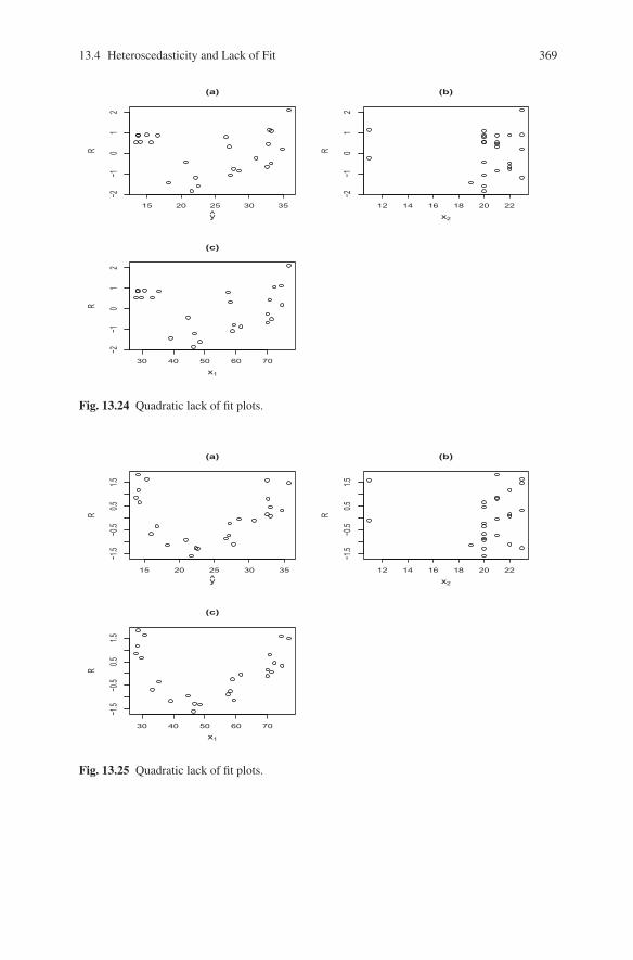
13.4 Heteroscedasticity and Lack of Fit 369
15 20 25 30 35
−2−1
01
2
(a)R
y12 14 16 18 20 22
−2−1
01
2
(b)
R
x2
30 40 50 60 70
−2−1
01
2
(c)
R
x1
Fig. 13.24 Quadratic lack of fit plots.
15 20 25 30 35
−1.5
−0.5
0.51.5
(a)
R
y12 14 16 18 20 22
−1.5
−0.5
0.51.5
(b)
R
x2
30 40 50 60 70
−1.5
−0.5
0.51.5
(c)
R
x1
Fig. 13.25 Quadratic lack of fit plots.

370 13 Model Diagnostics
In Figures 13.24 and 13.25, it would not be possible to have a linear effect. Theresiduals are being plotted against variables x1 and x2 that are already included in thefitted model as well as y which is a linear combination of x1 and x2. Any linear effectof these variables would be eliminated by the fitting procedure. However, plottingthe residuals against a variable not included in the model does allow the possibilityof seeing a linear effect, e.g., plotting against (xi1 − x·1)2.
EXAMPLE 13.4.5. As mentioned earlier, lack of independence and lack of fit areclosely related. In Figures 13.7 through 13.9, we plotted residuals against case num-bers. When observations are taken sequentially, the case numbers can be thought ofas a measure of time. There was no lack of fit present in the fitted models for theseplots. Nonetheless, the serial correlation can cause the plots to look like the modelsare lacking linear or quadratic effects in time, respectively, especially when ρ = 0.9.
Tests for lack of fit were discussed in Section 6.6. Although no examples of ithave been presented, it should be noted that it is possible to have both lack of fit andheteroscedasticity in the same plot.
13.5 Updating Formulae and Predicted Residuals
Frequently, it is of interest to see how well the data could predict yi if the ith casewere left out when the model was fitted. The difference between yi and the estimatey[i] with the ith case deleted is called either the predicted residual or the deletedresidual. The computations for fitting the model with the ith case left out can beperformed by using simple updating formulae on the complete model. We give sev-eral of these formulae.
Let X[i] and Y[i] be X and Y with the ith row deleted. Write x′i for the ith row of Xand
β[i] = (X ′[i]X[i])
−1X ′[i]Y[i]
for the estimate of β without the ith case. The predicted residual is defined as
e[i] = yi − x′iβ[i].
The predicted residuals are useful in checking for outliers. They are also used formodel selection. The Predicted REsidual Sum of Squares (PRESS) is defined as
PRESS =n
∑i=1
e2[i].
Models with relatively low values of the PRESS statistic should be better than mod-els with high PRESS statistics. It is tempting to think that PRESS is a more validmeasure of how well a model fits than SSE, because PRESS predicts values notused in fitting the model. This reasoning may seem less compelling after the updat-ing formula for the predicted residuals has been established.

13.5 Updating Formulae and Predicted Residuals 371
The predicted residuals can also be used to check normality, heteroscedasticity,and lack of fit in the same way that the usual residuals are used. For these purposesthey should be standardized. Their variances are
Var(e[i]) = σ 2 +σ2x′i(X′[i]X[i])
−1xi
= σ 2[1+ x′i(X
′[i]X[i])
−1xi
].
A reasonable estimate of σ 2 is MSE[i], the mean squared error for the model with theith case deleted. Alternatively, σ 2 could be estimated with the regular MSE. If MSEis used, then the standardized predicted residuals are identical to the standardizedresiduals (see Exercise 13.6). Standardized predicted residuals will be discussedagain in Section 6. A more useful formula for Var(e[i]) is given in Proposition 13.5.4.
We now present a series of results that establish the updating formulae for modelswith one deleted case.
Proposition 13.5.1. Let A be a p× p nonsingular matrix, and let a and b be q× prank q matrices. Then, if all inverses exist,
(A+a′b)−1 = A−1 −A−1a′(I +bA−1a′)−1bA−1.
PROOF. This is a special case of Theorem B.56. �
The application of Proposition 13.5.1 is
Corollary 13.5.2.
(X ′[i]X[i])
−1 = (X ′X)−1 +[(X ′X)−1xix′i(X′X)−1]
/[1− x′i(X
′X)−1xi].
PROOF. The corollary follows from noticing that X ′[i]X[i] = (X ′X − xix′i). �
Proposition 13.5.3. β[i] = β − [(X ′X)−1xiei]/(1−mii).
PROOF. First, note that x′i(X′X)−1xi = mii and X ′
[i]Y[i] = X ′Y − xiyi. Now, fromCorollary 13.5.2,
β[i] = (X ′[i]X[i])
−1X ′[i]Y[i]
= (X ′[i]X[i])
−1(X ′Y − xiyi)
= β − (X ′X)−1xiyi +[(X ′X)−1xix′iβ − (X ′X)−1xix′i(X
′X)−1xiyi
]/(1−mii).
Writing (X ′X)−1xiyi as (X ′X)−1xiyi/(1−mii)−mii(X ′X)−1xiyi/(1−mii), it is eas-ily seen that

372 13 Model Diagnostics
β[i] = β − [(X ′X)−1xi(yi − x′iβ )]/(1−mii)
+[mii(X ′X)−1xiyi − (X ′X)−1ximiiyi
]/(1−mii)
= β − [(X ′X)−1xiei]/(1−mii). �
The predicted residuals can now be written in a simple way.
Proposition 13.5.4.
(a) e[i] = ei/(1−mii).(b) Var(e[i]) = σ 2/(1−mii).
PROOF.
(a) e[i] = yi − x′iβ[i]
= yi − x′i
[β − (X ′X)−1xiei
1−mii
]= ei +miiei/(1−mii)= ei/(1−mii).
(b) This follows from having e[i] = ei/(1−mii) and Var(ei) = σ 2(1−mii). �
The PRESS statistic can now be written as
PRESS =n
∑i=1
e2i/(1−mii)2.
The value of e2i/(1−mii)2 will usually be large when mii is near 1. Model selec-
tion with PRESS puts a premium on having models in which observations withextremely high leverage are fitted very well. As will be discussed in Chapter 14,when fitting a model after going through a procedure to select a good model, the fit-ted model tends to be very optimistic in the sense of indicating much less variabilitythan is appropriate. Model selection using the PRESS statistic tends to continue thatphenomenon, cf. Picard and Cook (1984) and Picard and Berk (1990).
Later, we will also need the sum of squares for error with the ith case deleted,say SSE[i].
Proposition 13.5.5. SSE[i] = SSE − e2i/(1−mii).
PROOF. By definition,
SSE[i] = Y ′[i]Y[i]−Y ′
[i]X[i](X′[i]X[i])
−1X ′[i]Y[i]
= (Y ′Y − y2i )−Y ′
[i]X[i]β[i].

13.6 Outliers and Influential Observations 373
The second term can be written
Y ′[i]X[i]β[i] = (Y ′X − yix′i)
{β − [(X ′X)−1xiei]
/(1−mii)
}= Y ′X β − yix′iβ − x′iβ ei
/(1−mii)+ yimiiei
/(1−mii)
= Y ′MY − yix′iβ + yiei/(1−mii)− x′iβ ei
/(1−mii)
− yiei/(1−mii)+ yimiiei
/(1−mii)
= Y ′MY − yix′iβ + e2i/(1−mii)− yiei
= Y ′MY + e2i/(1−mii)− y2
i .
Therefore,
SSE[i] = Y ′Y − y2i − [Y ′MY + e2
i/(1−mii)− y2
i ]
= Y ′(I −M)Y − e2i/(1−mii)
= SSE − e2i/(1−mii). �
Exercise 13.6 Show that the standardized predicted residuals with σ 2 estimatedby MSE are the same as the standardized residuals.
13.6 Outliers and Influential Observations
Realistically, the purpose of fitting a linear model is to get a (relatively) succinctsummary of the important features of the data. Rarely is the chosen linear modelreally correct. Usually, the linear model is no more than a rough approximation toreality.
Outliers are cases that do not seem to fit the chosen linear model. There are twokinds of outliers. Outliers may occur because the predictor variables for the case areunlike the predictor variables for the other cases. These are cases with high leverage.If we think of the linear model as being an approximation to reality, the approxima-tion may be quite good within a certain range of the predictor variables, but pooroutside that range. A few cases that fall outside the range of good approximationcan greatly distort the fitted model and lead to a bad fit, even on the range of goodapproximation. Outliers of this kind are referred to as outliers in the design space(estimation space).
The other kind of outliers are those due to bizarre values of the dependent vari-able. These may occur because of gross measurement error, or from recording thedata incorrectly. Not infrequently, data are generated from a mixture process. Inother words, the data fit one pattern most of the time, but occasionally data with adifferent pattern are generated. Often it is appropriate to identify the different kindsof data and model them separately. If the vast majority of data fit a common pattern,there may not be enough of the rare observations for a complete analysis; but it is

374 13 Model Diagnostics
still important to identify such observations. In fact, these rare observations can bemore important than all of the other data.
Not only is it important to be able to identify outliers, but it must also be decidedwhether such observations should be included when fitting the model. If they areleft out, one gets an approximation to what usually happens, and one must be awarethat something unusual will happen every so often.
Outliers in the design space are identified by their leverages, the miis. Bizarre val-ues of yi can often be identified by their standardized residuals. Large standardizedresiduals indicate outliers. Typically, these are easily spotted in residual plots. How-ever, if a case with an unusual yi also has high leverage, the standardized residualmay not be large. If there is only one bizarre value of yi, it should be easy to identifyby examining all the cases with either a large standardized residual or high leverage.With more than one bizarre value, they may mask each other. (I believe that carefulexamination of the leverages will almost always identify possible masking, cf. thecomments in Section 1 on gaps in the leverage values.)
An alternative to examining the standardized residuals is to examine the stan-dardized predicted residuals, also known as the standardized deleted residuals, thet residuals, and sometimes (as in the R programming language) the Studentizedresiduals. The standardized predicted residuals are
ti =e[i]√
MSE[i]/(1−mii)=
yi − x′iβ[i]√MSE[i]/(1−mii)
.
Since yi, β[i], and MSE[i] are independent,
ti ∼ t(n− p−1),
where p = r(X). This allows a formal t test for whether the value yi is consistentwith the rest of the data. Actually, this procedure is equivalent to examining thestandardized residuals, but using the t(n− p− 1) distribution is more convenientthan using the appropriate distribution for the ris, cf. Cook and Weisberg (1982).
When all the values ti, i = 1, . . . ,n, are computed, the large values will naturallybe singled out for testing. The appropriate test statistic is actually maxi |ti|. Thenull distribution of this statistic is quite different from a t(n− p− 1). Fortunately,Bonferroni’s inequality provides an appropriate, actually a conservative, P value bymultiplying the P value from a t(n− p− 1) distribution by n. Alternatively, for anα level test, use a critical value of t(1−α/2n,n− p−1).
If yi corresponds to a case with extremely high leverage, the standard error forthe predicted residual,
√MSE[i]/(1−mii), will be large, and it will be difficult to
reject the t test. Recall from Example 13.1.6 that under condition (3) the y valuefor case six is clearly discordant. Although the absolute t value is quite large,t6 = −5.86 with m66 = 0.936, it is smaller than one might expect, considering theobvious discordance of case six. In particular, the absolute t value is smaller thanthe critical point for the Bonferroni method with α = 0.05. (The critical point is

13.6 Outliers and Influential Observations 375
t(1− 0.025/6,3) = 6.23.) Of course, with three degrees of freedom, the power ofthis test is very small. A larger α level would probably be more appropriate. Usingthe Bonferroni method with α = 0.10 leads to rejection.
The updating formula for ti is
Proposition 13.6.1.
ti = ri
√n− p−1n− p− r2
i.
PROOF. Using the updating formulae of Section 5,
ti = e[i]/√
MSE[i]/(1−mii)
= e[i]√
(1−mii)/√
MSE[i]
= ri√
MSE/√
MSE[i]
= ri√
(n− p−1)/(n− p)√
SSE/
SSE[i]
= ri√
(n− p−1)/(n− p)√
SSE/[SSE − e2
i /(1−mii)]
= ri√
(n− p−1)/(n− p)√
1/[1− r2
i /(n− p)]
= ri
√(n− p−1)
/(n− p− r2
i ). �
As indicated earlier, ti really contains the same information as ri.A test that a given set of y values does not fit the model is easily available from
general linear model theory. Suppose that the r observations i = n− r +1, . . . ,n aresuspected of being outliers. The model Y = Xβ + e can be written with
Y =[
Y0Y1
], X =
[X0X1
], e =
[e0e1
],
where Y1, X1, and e1 each have r rows. If Z =[
0Ir
], then the model with the possible
outliers deletedY0 = X0β + e0 (1)
and the modelY = Xβ +Zγ + e (2)
are equivalent for estimating β and σ 2. A test of the reduced model Y = Xβ + eagainst the full model Y = Xβ +Zγ + e is rejected if
(SSE −SSE0)/rMSE0
> F(1−α ,r,n− p− r).

376 13 Model Diagnostics
If the test is rejected, the r observations appear to contain outliers. Note that thisprocedure is essentially the same as Utts’s Rainbow Test for lack of fit discussed inSection 6.6. The difference is in how one identifies the cases to be eliminated.
In my opinion, the two most valuable tools for identifying outliers are the miisand the tis. It would be unusual to have outliers in the design space without largevalues of the miis. Such outliers would have to be “far” from the other data withoutthe Mahalanobis distance being large. For bizarre values of the yis, it is useful todetermine whether the value is so bizarre that it could not reasonably come from themodel under consideration. The tis provide a test of exactly what is needed.
Cook (1977) presented a distance measure that combines the standardized resid-ual with the leverage to get a single measure of the influence a case has on the fit ofthe regression model. Cook’s distance (Ci) measures the statistical distance betweenβ and β[i]. It is defined as
Ci =(β[i] − β )′(X ′X)(β[i]− β )
pMSE.
Written as a function of the standardized residual and the leverage, Cook’s distanceis:
Proposition 13.6.2. Ci = r2i [mii/p(1−mii)].
Exercise 13.7 Prove Proposition 13.6.2.
From Proposition 13.6.2 it can be seen that Cook’s distance takes the size ofthe standardized residual and rescales it based on the leverage of the case. For anextremely high leverage case, the squared standardized residual gets multiplied bya very large number. For low leverage cases the multiplier is very small. Anotherinterpretation of Cook’s distance is that it is a standardized version of how far thepredicted values X β move when the ith case is deleted.
In Section 1, after establishing that the miis were a reasonable measure of lever-age, it was necessary to find guidelines for what particular values of mii meant. Thiscan also be done for Cook’s distance. Cook’s distance can be calibrated in terms ofconfidence regions. Recall that a (1−α)100% confidence region for β is{
β∣∣∣ (β − β )′(X ′X)(β − β )
pMSE< F(1−α , p,n− p)
}.
If Ci.= F(0.75, p,n− p), then deleting the ith case moves the estimate of β to the
edge of a 75% confidence region for β based on β . This is a very substantial move.Since F(0.5, p,n− p) .= 1, any case with Ci > 1 probably has above average in-fluence. Note that Ci does not actually have an F distribution. While many peopleconsider such calibrations a necessity, other people, including the author, prefer sim-

13.7 Transformations 377
ply to examine those cases with distances that are substantially larger than the otherdistances.
Cook’s distance can be modified in an obvious way to measure the influence ofany set of observations. Cook and Weisberg (1982) give a more detailed discussionof all of the topics in this section.
Updating formulae and case deletion diagnostics for linear models with gen-eral covariance matrices are discussed by Christensen, Johnson, and Pearson (1992,1993), Christensen, Pearson, and Johnson (1992), and by Haslett and Hayes (1998)and Martin (1992). A nice review of these procedures is given by Shi and Chen(2009).
Haslett (1999) establishes two results that can greatly simplify case deletion di-agnostics for correlated data. First, he shows that an analysis based on Y[i], X[i], andV[ii] (the covariance matrix with the ith row and column removed) is the same as ananalysis based on Y (i), X , and V where
Y (i) =[
yi(Y[i])Y[i]
]and yi(Y[i]) is the BLUP of yi based on Y[i]. Second, he shows that there is a relativelysimple way to find a matrix Pi such that Y (i) = PiY .
13.7 Transformations
If the residuals suggest nonnormality, heteroscedasticity of variances, or lack of fit, atransformation of the yis may eliminate the problem. Cook and Weisberg (1982) andAtkinson (1985) give extensive discussions of transformations. Only a brief reviewis presented here.
Picking a transformation is often a matter of trial and error. Different transfor-mations are tried until one is found for which the residuals seem reasonable. Threemore systematic methods of choosing transformations will be discussed: Box–Coxpower transformations, variance stabilizing transformations, and the generalizedleast squares approach of Grizzle, Starmer, and Koch (1969).
Box and Cox (1964) suggested a systematic method of picking transformations.They suggested using the family of transformations
y(λ ) ={
(yλ −1)/λ , λ �= 0logy, λ = 0
and choosing λ by maximum likelihood. Convenient methods of executing this pro-cedure are discussed in Cook and Weisberg (1982), Weisberg (1985), and Chris-tensen (1996a).

378 13 Model Diagnostics
If the distribution of the yis is known, the commonly used variance stabilizingtransformations can be tried (cf. Rao, 1973, Section 6g, or Christensen, 1996a). Forexample,
if yi ∼ Binomial(Ni, pi), use arcsin(√
yi/Ni),if yi ∼ Poisson(λi), use
√yi,
if yi has σi/E(yi) constant, use log(yi).
More generally, arcsin(√
yi/Ni) can be tried for any problem where yi is a countbetween 0 and Ni or a proportion,
√yi can be used for any problem where yi is a
count, and log(yi) can be used if yi is a count or amount.The transformation log(yi) is also frequently used because, for a linear model
in log(yi), the additive effects of the predictor variables transform to multiplicativeeffects on the original scale. If multiplicative effects seem reasonable, the log trans-formation may be appropriate.
As an alternative to the variance stabilizing transformations, there exist general-ized linear models specifically designed for treating binomial and Poisson data. ForPoisson data there exists a well developed theory for fitting log-linear models. Onebranch of the theory of log-linear models is the theory of logistic regression, whichis used to analyze binomial data. As shown by Grizzle, Starmer, and Koch (1969),generalized least squares methods can be used to fit log-linear models to Poissondata and logistic regression models to binomial data. The method involves both atransformation of the dependent variable and weights. The appropriate transforma-tion and weights are:
Distribution of yi Transformation WeightsPoisson(λi) logyi yiBinomial(Ni, pi) log(yi/[Ni − yi]) yi(Ni − yi)/Ni
With these weights, the asymptotic variance of the transformed data is 1.0. Standarderrors for regression coefficients are computed as usual except that no estimate ofσ 2 is required (σ 2 is known to be 1). Since σ 2 is known, t tests and F tests arereplaced with normal tests and chi-squared tests. In particular, if the linear modelfits the data and the observations yi are large, the SSE has an asymptotic chi-squareddistribution with the usual degrees of freedom. If the SSE is too large, a lack of fit isindicated. Tests of various models can be performed by comparing the difference inthe SSEs for the model. The difference in the SSEs has an asymptotic chi-squareddistribution with the usual degrees of freedom. If the difference is too large, thenthe smaller model is deemed inadequate. Unlike the lack of fit test, these modelcomparison tests are typically valid if n is large even when the individual yis arenot. Fitting log-linear and logistic models both by generalized least squares and bymaximum likelihood is discussed in detail by Christensen (1997).
Exercise 13.8 The data given below were first presented by Brownlee (1965)and have subsequently appeared in Daniel and Wood (1980), Draper and Smith(1998), and Andrews (1974), among other places. The data consist of measurements

13.7 Transformations 379
taken on 21 successive days at a plant that oxidizes ammonia into nitric acid. Thedependent variable y is stack loss. It is 10 times the percentage of ammonia that islost (in the form of unabsorbed nitric oxides) during the oxidation process. Thereare three predictor variables: x1, x2, and x3. The first predictor variable is air flowinto the plant. The second predictor variable is the cooling water temperature as itenters the countercurrent nitric oxide absorption tower. The third predictor variableis a coded version of the nitric acid concentration in the absorbing liquid. Analyzethese data giving special emphasis to residual analysis and influential observations.
Obs. x1 x2 x3 y Obs. x1 x2 x3 y1 80 27 89 42 12 58 17 88 132 80 27 88 37 13 58 18 82 113 75 25 90 37 14 58 19 93 124 62 24 87 28 15 50 18 89 85 62 22 87 18 16 50 18 86 76 62 23 87 18 17 50 19 72 87 62 24 93 19 18 50 19 79 88 62 24 93 20 19 50 20 80 99 58 23 87 15 20 56 20 82 15
10 58 18 80 14 21 70 20 91 1511 58 18 89 14
Exercise 13.9 For testing whether one observation yi is an outlier, show that theF statistic is equal to the squared standardized predicted residual.


Chapter 14
Variable Selection
Suppose we have a set of variables y,x1, . . . ,xs and observations on these variablesy1,xi1, . . . ,xis, i = 1, . . . ,n. We want to identify which of the independent variablesx j are important for a regression on y. There are several methods available for doingthis.
Obviously, the most complete method is to look at all possible regression equa-tions involving x1, . . . ,xs. There are 2s of these. Even if one has the time and moneyto compute all of them, it may be very difficult to assimilate that much informa-tion. Tests for the adequacy of various models can be based on general linear modeltheory, assuming of course that the model
yi = β0 +β1xi1 + · · ·+βsxis + ei (1)
is an adequate model for the data.A more efficient procedure than computing all possible regressions is to choose a
criterion for ranking how well different models fit and compute only the best fittingmodels. Typically, one would want to identify several of the best fitting modelsand investigate them further. The computing effort for this “best subset regression”method is still considerable.
An older group of methods is stepwise regression. These methods consider theefficacy of adding or deleting individual variables to a model that is currently underconsideration. These methods have the flaw of considering variables only one at atime. For example, there is no reason to believe that the best two variables to add to amodel are the one variable that adds most to the model followed by the one variablethat adds the most to this augmented model. The flaw of stepwise procedures is alsotheir virtue. Because computations go one variable at a time, they are relatively easy.
In this book, the term “mean squared error” (MSE) has generally denoted thequantity Y ′(I −M)Y/r(I −M). This is a sample quantity, a function of the data. InChapters 6 and 12, when discussing prediction, we needed a theoretical concept ofthe mean squared error. Fortunately, up until this point we have not needed to discussboth the sample quantity and the theoretical one at the same time. To discuss variableselection methods and techniques of dealing with collinearity, we will need both
© Springer Science+Business Media, LLC 2011
381Springer Texts in Statistics, DOI 10.1007/978-1-4419-9816-3_14, R. Christensen, Plane Answers to Complex Questions: The Theory of Linear Models,
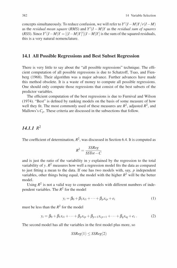
382 14 Variable Selection
concepts simultaneously. To reduce confusion, we will refer to Y ′(I−M)Y/r(I−M)as the residual mean square (RMS) and Y ′(I −M)Y as the residual sum of squares(RSS). Since Y ′(I−M)Y = [(I−M)Y ]′[(I−M)Y ] is the sum of the squared residuals,this is a very natural nomenclature.
14.1 All Possible Regressions and Best Subset Regression
There is very little to say about the “all possible regressions” technique. The effi-cient computation of all possible regressions is due to Schatzoff, Tsao, and Fien-berg (1968). Their algorithm was a major advance. Further advances have madethis method obsolete. It is a waste of money to compute all possible regressions.One should only compute those regressions that consist of the best subsets of thepredictor variables.
The efficient computation of the best regressions is due to Furnival and Wilson(1974). “Best” is defined by ranking models on the basis of some measure of howwell they fit. The most commonly used of these measures are R2, adjusted R2, andMallows’s Cp. These criteria are discussed in the subsections that follow.
14.1.1 R2
The coefficient of determination, R2, was discussed in Section 6.4. It is computed as
R2 =SSReg
SSTot−C
and is just the ratio of the variability in y explained by the regression to the totalvariability of y. R2 measures how well a regression model fits the data as comparedto just fitting a mean to the data. If one has two models with, say, p independentvariables, other things being equal, the model with the higher R2 will be the bettermodel.
Using R2 is not a valid way to compare models with different numbers of inde-pendent variables. The R2 for the model
yi = β0 +β1xi1 + · · ·+βpxip + ei (1)
must be less than the R2 for the model
yi = β0 +β1xi1 + · · ·+βpxip +βp+1xi p+1 + · · ·+βqxiq + ei . (2)
The second model has all the variables in the first model plus more, so
SSReg(1) ≤ SSReg(2)

14.1 All Possible Regressions and Best Subset Regression 383
andR2(1) ≤ R2(2).
Typically, if the R2 criterion is chosen, a program for doing best subset regressionwill print out the models with the highest R2 for each possible value of the numberof predictor variables. It is the use of the R2 criterion in best subset regression thatmakes computing all possible regressions obsolete. The R2 criterion fits all the goodmodels one could ever want. In fact, it probably fits too many models.
14.1.2 Adjusted R2
The adjusted R2 is a modification of R2 so that it can be used to compare models withdifferent numbers of predictor variables. For a model with p−1 predictor variablesplus an intercept, the adjusted R2 is defined as
Adj R2 = 1− n−1n− p
(1−R2) .
(With the intercept there are a total of p variables in the model.)Define s2
y = (SSTot−C)/(n−1). Then s2y is the sample variance of the yis ignor-
ing any regression structure. It is easily seen (Exercise 14.1) that
Adj R2 = 1− RMSs2
y.
The best models based on the Adj R2 criterion are those models with the smallestresidual mean squares.
As a method of identifying sets of good models, this is very attractive. The mod-els with the smallest residual mean squares should be among the best models. How-ever, the model with the smallest residual mean square may very well not be the bestmodel.
Consider the question of deleting one variable from a model. If the F for testingthat variable is greater than 1, then deleting the variable will increase the residualmean square. By the adjusted R2 criterion, the variable should not be deleted. How-ever, unless the F value is substantially greater than 1, the variable probably shouldbe deleted. The Adj R2 criterion tends to include too many variables in the model.(See Exercise 14.2.)
Exercise 14.1 Show that Adj R2 = 1− (RMS/s2y).
Exercise 14.2 Consider testing the regression model (1) against (2). Show thatF > 1 if and only if the Adj R2 for model (1) is less than the Adj R2 for model (2).

384 14 Variable Selection
14.1.3 Mallows’s Cp
Suppose we have a model that is assumed to be correct, say Y = Xβ + e. In theregression setup, this is the model with all the predictor variables yi = β0 +β1xi1 +· · ·+βsxis +ei. Our problem is that some of the β js may be zero. Rather than merelytrying to identify which β js are zero, Mallows suggested that the appropriate crite-rion for evaluating a reduced model Y = X0γ + e is by its mean squared error forestimating Xβ , i.e.,
E[(X0γ −Xβ )′(X0γ −Xβ )
].
As mentioned earlier, to distinguish between this use of the term “mean squarederror” and the estimate of the variance in a linear model with E(Y ) = Xβ , we referto Y ′(I−M)Y as the residual sum of squares, i.e., RSS(β ), and Y ′(I−M)Y/r(I−M)as the residual mean square, i.e., RMS(β ). The statistics RSS(γ) and RMS(γ) are thecorresponding quantities for the model Y = X0γ + e.
The quantity(X0γ −Xβ )′(X0γ −Xβ)
is a quadratic form in the vector (X0γ −Xβ ). Writing
M0 = X0(X ′0X0)−X ′
0
gives(X0γ −Xβ ) = M0Y −Xβ ,
E(X0γ −Xβ ) = M0Xβ −Xβ = −(I −M0)Xβ ,
Cov(X0γ −Xβ ) = σ 2M0.
From Theorem 1.3.2
E[(X0γ −Xβ )′(X0γ −Xβ )
]= σ 2tr(M0)+β ′X ′(I −M0)Xβ .
We do not know σ2 or β , but we can estimate the mean squared error. First notethat
E[Y ′(I −M0)Y
]= σ 2tr(I −M0)+β ′X ′(I −M0)Xβ ;
so
E[(X0γ −Xβ )′(X0γ −Xβ )
]= σ 2 [tr(M0)− tr(I −M0)]+E
[Y ′(I −M0)Y
].
With p = tr(M0), an unbiased estimate of the mean squared error is
RMS(β )[2p−n]+RSS(γ).
Mallows’s Cp statistic simply rescales the estimated mean squared error,
Cp =RSS(γ)
RMS(β )− (n−2p).

14.2 Stepwise Regression 385
The models with the smallest values of Cp have the smallest estimated mean squarederror and should be among the best models for the data.
Exercise 14.3 Give an informal argument to show that if Y = X0γ +e is a correctmodel, then the value of Cp should be around p. Provide a formal argument for thisfact. Show that if (n− s) > 2, then E(Cp) = p + 2(s− p)/(n− s− 2). To do thisyou need to know that if W ∼ F(u,v,0), then E(W ) = v/(v−2) for v > 2. For largevalues of n (relative to s and p), what is the approximate value of E(Cp)?
Exercise 14.4 Consider the F statistic for testing model (1) against model(14.0.1): (a) Show that Cp = (s− p)(F − 2) + s; (b) show that, for a given valueof p, the R2, Adj R2, and Cp criteria all induce the same rankings of models.
14.2 Stepwise Regression
Stepwise regression methods involve adding or deleting variables one at a time.
14.2.1 Forward Selection
Forward selection sequentially adds variables to the model. Since this is a sequen-tial procedure, the model in question is constantly changing. At any stage in theselection process, forward selection adds the variable that:
1. has the highest partial correlation,2. increases R2 the most,3. gives the largest absolute t or F statistic.
These criteria are equivalent.
EXAMPLE 14.2.1. Suppose we have variables y, x1, x2, and x3 and the currentmodel is
yi = β0 +β1xi1 + ei.
We must choose between adding variables x2 and x3. Fit the models
yi = β0 +β1xi1 +β2xi2 + ei,
yi = β0 +β1xi1 +β3xi3 + ei.
Choose the model with the higher R2. Equivalently, one could look at the t (or F)statistics for testing H0 : β2 = 0 and H0 : β3 = 0 and choose the model that gives thelarger absolute value of the statistic. Finally, one could look at ry2·1 and ry3·1 andpick the variable that gives the larger absolute value for the partial correlation.

386 14 Variable Selection
Exercise 14.5 Show that these three criteria for selecting a variable are equiva-lent.
Forward selection stops adding variables when one of three things happens:
1. p∗ variables have been added,2. all absolute t statistics for adding variables not in the model are less than t∗,3. the tolerance is too small for all variables not in the model.
The user picks the values of p∗ and t∗. Tolerance is discussed in the next subsection.No variable is ever added if its tolerance is too small, regardless of its absolute tstatistic.
The forward selection process is often started with the initial model
yi = β0 + ei.
14.2.2 Tolerance
Regression assumes that the model matrix in Y = Xβ + e has full rank. Mathemat-ically, either the columns of X are linearly independent or they are not. In practice,computational difficulties arise if the columns of X are “nearly linearly dependent.”By nearly linearly dependent, we mean that one column of X can be nearly repro-duced by the other columns.
Suppose we have the model
yi = β0 +β1xi1 + · · ·+βp−1xi p−1 + ei,
and we are considering adding variable xp to the model. To check the tolerance, fit
xip = α0 +α1xi1 + · · ·+αp−1xi p−1 + ei. (1)
If the R2 from this model is high, the column vectors, say J,X1, . . . ,Xp, are nearlylinearly dependent. The tolerance of xp (relative to x1, . . . ,xp−1) is defined as thevalue of 1− R2 for fitting model (1). If the tolerance is too small, variable xp isnot used. Often, in a computer program, the user can define which values of thetolerance should be considered too small.
14.2.3 Backward Elimination
Backward elimination sequentially deletes variables from the model. At any stagein the selection process, it deletes the variable with the smallest absolute t or Fstatistic. Backward elimination stops deleting variables when:

14.3 Discussion of Variable Selection Techniques 387
1. p∗ variables have been eliminated,2. the smallest absolute t statistic for eliminating a variable is greater than t∗.
The user can usually specify p∗ and t∗ in a computer program.The initial model in the backward elimination procedure is the model with all of
the predictor variables included,
yi = β0 +β1xi1 + · · ·+βsxis + ei.
Backward elimination should give an adequate model. We assume that the pro-cess is started with an adequate model, and so only variables that add nothing areeliminated. The model arrived at may, however, be far from the most succinct. Onthe other hand, there is no reason to believe that forward selection gives even anadequate model.
14.2.4 Other Methods
Forward selection is such an obviously faulty method that several improvementshave been recommended. These consist of introducing rules for eliminating and ex-changing variables. Four rules for adding, deleting, and exchanging variables follow.
1. Add the variable with the largest absolute t statistic if that value is greater thant∗.
2. Delete the variable with the smallest absolute t statistic if that value is less thant∗.
3. A variable not in the model is exchanged for a variable in the model if the ex-change increases R2.
4. The largest R2 for each size model considered so far is saved. Delete a variable ifthe deletion gives a model with R2 larger than any other model of the same size.
These rules can be used in combination. For example, 1 then 2, 1 then 2 then 3,1 then 4, or 1 then 4 then 3. Again, no variable is ever added if its tolerance is toosmall.
14.3 Discussion of Variable Selection Techniques
Stepwise regression methods are fast, easy, cheap, and readily available. When thenumber of observations, n, is less than the number of variables, s + 1, forward se-lection or a modification of it is the only available method for variable selection.Backward elimination and best subset regression assume that one can fit the modelthat includes all the predictor variables. This is not possible when n < s+1.
There are serious problems with stepwise methods. They do not give the bestmodel (based on any of the criteria we have discussed). In fact, stepwise methods

388 14 Variable Selection
can give models that contain none of the variables that are in the best regressions.That is because, as mentioned earlier, they handle variables one at a time. Anotherproblem is nontechnical. The user of a stepwise regression program will end upwith one model. The user may be inclined to think that this is the model. It probablyis not. In fact, the model probably does not exist. Even though the Adjusted R2
and Mallows’s Cp methods define a unique best model and could be subject to thesame problem, best subset regression programs generally present several of the bestmodels.
A problem with best subset selection methods is that they tend to give modelsthat appear to be better than they really are. For example, the Adjusted R2 criterionchooses the model with the smallest RMS. Because one has selected the smallestRMS, the RMS for that model is biased toward being too small. Almost any measureof the fit of a model is related to the RMS, so the fit of the model will appear to bebetter than it is. If one could sample the data over again and fit the same model, theRMS would almost certainly be larger, perhaps substantially so.
When using Mallows’s Cp statistic, one often picks models with the smallestvalue of Cp. This can be justified by the fact that the model with the smallest Cp isthe model with the smallest estimated expected mean squared error. However, if thetarget value of Cp is p (as suggested by Exercise 14.3), it seems to make little senseto pick the model with the smallest Cp. It seems that one should pick models forwhich Cp is close to p.
The result of Exercise 14.4, that for a fixed number of predictor variables thethree best regression criteria are equivalent, is very interesting. The Adj R2 andCp criteria can be viewed as simply different methods of penalizing models thatinclude more variables. The penalty is needed because models with more variablesnecessarily explain more variation (have higher R2s).
Influential observations are a problem in any regression analysis. Variable se-lection techniques involve fitting lots of models, so the problem of influential ob-servations is multiplied. Recall that an influential observation in one model is notnecessarily influential in a different model.
Some statisticians think that the magnitude of the problem of influential obser-vations is so great as to reject all variable selection techniques. They argue that themodels arrived at from variable selection techniques depend almost exclusively onthe influential observations and have little to do with any real world effects. Moststatisticians, however, approve of the judicious use of variable selection techniques.(But then, by definition, everyone will approve of the judicious use of anything.)
John W. Tukey, among others, has emphasized the difference between exploratoryand confirmatory data analysis. Briefly, exploratory data analysis (EDA) deals withsituations in which you are trying to find out what is going on in a set of data.Confirmatory data analysis is for proving what you already think is going on. EDAfrequently involves looking at lots of graphs. Confirmatory data analysis looks atthings like tests and confidence intervals. Strictly speaking, you cannot do both ex-ploratory data analysis and confirmatory data analysis on the same set of data.
Variable selection is an exploratory technique. If you know what variables areimportant, you do not need it and should not use it. When you do use variable

14.3 Discussion of Variable Selection Techniques 389
selection, if the model is fitted with the same set of data that determined the variableselection, then the model you eventually decide on will give biased estimates andinvalid tests and confidence intervals. This sounds a lot worse than it is. The biasedestimates may very well be better estimates than you could get by refitting withanother data set. (This is related to James–Stein estimation. See also Section 15.4.)The test and confidence intervals, although not strictly valid, are often reasonable.
One solution to this problem of selecting variables and fitting parameters withthe same data is to divide the data into two parts. Do an exploratory analysis onone part and then a confirmatory analysis on the other. To do this well requires alot of data. It also demonstrates the problem of influential observations. Dependingon where the influential observations are, you can get pretty strange results. ThePRESS statistic was designed to be used in procedures similar to this. However, aswe have seen, the PRESS statistic is highly sensitive to influential observations.
Finally, a word about R2. R2 is a good statistic for measuring the predictive abilityof a model. R2 is also a good statistic for comparing models. That is what we usedit for here. But the actual value of R2 should not be overemphasized when it isbeing used to identify correct models (rather than models that are merely useful forprediction). If you have data with a lot of variability, it is possible to have a verygood fit to the underlying regression model without having a high R2. For example,if the SSE admits a decomposition into pure error and lack of fit, it is possible tohave very little lack of fit while having a substantial pure error so that R2 is smallwhile the fit is good.
If transformations of the dependent variable y are considered, it is inappropriateto compare R2 for models based on different transformations. For example, it ispossible for a transformation to increase R2 without really increasing the predictiveability of the model. One way to check whether this is happening is to comparethe width of confidence intervals for predicted values after transforming them to acommon scale.
To compare models based on different transformations of y, say y1 = f1(y) andy2 = f2(y), fit models to the transformed data to obtained predicted values y1 andy2. Return these to the original scale with y1 = f−1
1 (y1) and y2 = f−12 (y2). Finally,
define R21 as the squared sample correlation between the ys and the y1s and define
R22 as the squared sample correlation between the ys and the y2s. These R2 values
are comparable.
Exercise 14.6 Mosteller and Tukey (1977) reported data on verbal test scoresfor sixth graders. They used a sample of 20 Mid-Atlantic and New England schoolstaken from The Coleman Report. The dependent variable y was the mean verbal testscore for each school. The predictor variables were: x1 = staff salaries per pupil,x2 = percent of sixth grader’s fathers employed in white collar jobs, x3 = a com-posite score measuring socioeconomic status, x4 = the mean score on a verbal testadministered to teachers, and x5 = one-half of the sixth grader’s mothers’ meannumber of years of schooling. Compare the results of using the various model se-lection techniques on the data.

390 14 Variable Selection
Obs. x1 x2 x3 x4 x5 y
1 3.83 28.87 7.20 26.60 6.19 37.012 2.89 20.10 −11.71 24.40 5.17 26.513 2.86 69.05 12.32 25.70 7.04 36.514 2.92 65.40 14.28 25.70 7.10 40.705 3.06 29.59 6.31 25.40 6.15 37.106 2.07 44.82 6.16 21.60 6.41 33.907 2.52 77.37 12.70 24.90 6.86 41.808 2.45 24.67 −0.17 25.01 5.78 33.409 3.13 65.01 9.85 26.60 6.51 41.01
10 2.44 9.99 −0.05 28.01 5.57 37.2011 2.09 12.20 −12.86 23.51 5.62 23.3012 2.52 22.55 0.92 23.60 5.34 35.2013 2.22 14.30 4.77 24.51 5.80 34.9014 2.67 31.79 −0.96 25.80 6.19 33.1015 2.71 11.60 −16.04 25.20 5.62 22.7016 3.14 68.47 10.62 25.01 6.94 39.7017 3.54 42.64 2.66 25.01 6.33 31.8018 2.52 16.70 −10.99 24.80 6.01 31.7019 2.68 86.27 15.03 25.51 7.51 43.1020 2.37 76.73 12.77 24.51 6.96 41.01

Chapter 15
Collinearity and Alternative Estimates
Collinearity or multicollinearity refers to the problem in regression analysis of thecolumns of the model matrix being nearly linear dependent. Ideally, this is no prob-lem at all. There are numerical difficulties associated with the actual computations,but there are no theoretical difficulties. If, however, one has any doubts about theaccuracy of the model matrix, the analysis could be in deep trouble.
Section 1 discusses what collinearity is and what problems it can cause. Fourtechniques for dealing with collinearity are examined. These are regression incanonical form, principal component regression, generalized inverse regression, andclassical ridge regression. The methods, other than classical ridge regression, are es-sentially the same. Section 4 presents additional comments on the potential benefitsof biased estimation. Section 5 discusses penalized estimation. Finally, Section 6presents an alternative to least squares estimation. Least squares minimizes the ver-tical distances between the dependent variable and the regression surface. Section 6considers minimizing the perpendicular distance between the dependent variableand the regression surface.
15.1 Defining Collinearity
In this section we define the problem of collinearity. The approach taken is to quan-tify the idea of having columns of the model matrix that are “nearly linearly depen-dent.” The effects of near linear dependencies are examined. The section concludesby establishing the relationship between the definition given here and other com-monly used concepts of collinearity.
Suppose we have a regression model
Y = Xβ + e, E(e) = 0, Cov(e) = σ 2I, (1)
where Y is n × 1, X is n × p, β is p × 1, and r(X) = p. The essence of model(1) is that E(Y ) ∈ C(X). Suppose that the model matrix consists of some predictor
© Springer Science+Business Media, LLC 2011
391Springer Texts in Statistics, DOI 10.1007/978-1-4419-9816-3_15, R. Christensen, Plane Answers to Complex Questions: The Theory of Linear Models,
392 15 Collinearity and Alternative Estimates
variables, say x1,x2, . . . ,xp, that are measured with some small error. A near lineardependence in the observed model matrix X could mean a real linear dependencein the underlying model matrix of variables measured without error. Let X∗ be theunderlying model matrix. If the columns of X∗ are linearly dependent, there existsan infinite number of least squares estimates for the true regression coefficients.If X is nearly linearly dependent, the estimated regression coefficients may not bemeaningful and may be highly variable.
The real essence of this particular problem is that C(X) is too large. Generally, wehope that in some sense, C(X) is close to C(X∗). Regression should work well pre-cisely when this is the case. However, when X∗ has linearly dependent columns, Xtypically will not. Thus r(X) > r(X∗). C(X∗) may be close to some proper subspaceof C(X), but C(X) has extra dimensions. By pure chance, these extra dimensionscould be very good at explaining the Y vector that happened to be observed. In thiscase, we get an apparently good fit that has no real world significance.
The extra dimensions of C(X) are due to the existence of vectors b such thatX∗b = 0 but Xb �= 0. If the errors in X are small, then Xb should be approximatelyzero. We would like to say that a vector w in C(X) is ill-defined if there exists b suchthat w = Xb is approximately zero, where w is approximately the zero vector if itslength is near zero. Unfortunately, multiplying w by a scalar can increase or decreasethe length of the vector arbitrarily, while not changing the direction determinedwithin C(X). To rectify this, we can restrict attention to vectors b with b′b = 1(i.e., the length of b is 1), or, equivalently, we make the following:
Definition 15.1.1. A vector w = Xb is said to be ε ill-defined if w′w/b′b =b′X ′Xb/b′b < ε . The matrix X is ε ill-defined if any vector in C(X) is ε ill-defined.We use the terms “ill-defined” and “ill-conditioned” interchangeably.
The assumption of a real linear dependence in the X∗ matrix is a strong one. Wenow indicate how that assumption can be weakened. Let X = X∗ + Δ , where theelements of Δ are uniformly small errors. Consider the vector Xb. (For simplicity,assume b′b = 1.) The corresponding direction in the underlying model matrix isX∗b.
Note that b′X ′Xb = b′X ′∗X∗b+2b′Δ ′X∗b+b′Δ ′Δb. The vector Δ ′b is short; so ifXb and X∗b are of reasonable size, they have about the same length. Also
b′X ′∗Xb = b′X ′
∗X∗b+b′X ′∗Δb, (2)
where b′X ′∗Δb is small; so the angle between Xb and X∗b should be near zero.(For any two vectors x and y, let θ be the angle between x and y. Then x′y =√
x′x√
y′y cosθ .) On the other hand, if Xb is ill-defined, X∗b will also be small,and the term b′X ′∗Δb could be a substantial part of b′X ′∗Xb. Thus, the angle betweenXb and X∗b could be substantial. In that case, the use of the direction Xb is calledinto question because it may be substantially different from the underlying directionX∗b. In practice, we generally cannot know if the angle between Xb and X∗b is large.Considerable care must be taken when using a direction in C(X) that is ill-defined.

15.1 Defining Collinearity 393
So far we have not discussed whether the columns of X should be adjusted fortheir mean values or rescaled. I think that one should not be dogmatic about thisissue; however, it should be noted that if the squared length of a column of X is lessthan ε , that direction will be ε ill-defined, regardless of what other vectors are inC(X). The question of standardizing the columns of X arises frequently.
The intercept term is frequently handled separately from all other variables intechniques for dealing with collinearity. The model
yi = β0 +β1xi1 + · · ·+βp−1xi p−1 + ei (3)
Y = [J,Z][
β0β∗
]+ e
is often rewritten as
yi = α +β1(xi1 − x·1)+ . . .+βp−1(xi p−1 − x·p−1)+ei, (4)
or
Y =[
J,(
I − 1n
Jnn
)Z][
αβ∗
]+ e,
where x· j = n−1 ∑ni=1 xi j. It is easily seen that β∗ is the same in both models, but
β0 �= α . We dispense with the concept of the underlying model matrix and write
X∗ =(
I − 1n
Jnn
)Z.
Because of orthogonality, α = y·, and β∗ can be estimated from the model
Y∗ = X∗β∗ + e, (5)
where Y ′∗ = [y1 − y·,y2 − y·, . . . ,yn − y·].Frequently, the scales of the x variables are also standardized. Let q2
j = ∑ni=1(xi j−
x· j)2. Model (5) is equivalent to
Y∗ = X∗Diag(q−1j )γ∗ + e, (6)
where γ∗ = Diag(q j)β∗. In model (6), the model matrix is X∗Diag(q−1j ).
Model (3) is rarely used in techniques for dealing with collinearity. Usuallymodel (6) is assumed, and sometimes model (5). To retain full generality, our dis-cussion uses model (3), but all the results apply to models (5) and (6). Note thatthe matrix X ′∗X∗ is proportional to the sample covariance matrix of the Xs when(xi1, . . . ,xi p−1), i = 1, . . . ,n, is thought of as a sample of size n from a p−1 dimen-sional random vector. Diag(q−1
j )X ′∗X∗Diag(q−1j ) is the sample correlation matrix.
We now present the relationship between ε ill-defined matrices and three othercommonly used methods of identifying ill-conditioned matrices.

394 15 Collinearity and Alternative Estimates
One of the main tools in the examination of collinearity is the examination of theeigenvalues of X ′X . We discuss the relationship between Definition 15.1.1 and aneigen-analysis of X ′X .
Recall that X has linearly dependent columns if and only if X ′X is singular, whichhappens if and only if X ′X has a zero eigenvalue. One often-used (but I think unintu-itive) definition is that the columns of X are nearly linearly dependent if X ′X has atleast one small eigenvalue. Suppose that v1, . . . ,vp is an orthogonal set of eigenvec-tors for X ′X corresponding to the eigenvalues δ1,δ2, . . . ,δp. Then v1, . . . ,vp form abasis for Rp. If δi < ε , then δi = v′iX
′Xvi/v′ivi; so Xvi is a direction in C(X) that is εill-defined. Conversely, if an ε ill-defined vector exists, we show that at least one ofthe δis must be less than ε . Let w = Xd be ε ill-defined. Write d = ∑p
i=1 αivi. Thenw′w = d′X ′Xd = ∑p
i=1 α2i δi and d′d = ∑p
i=1 α2i . Since ∑p
i=1 α2i δi/∑p
i=1 α2i < ε , and
since the δis are all nonnegative, at least one of the δis must be less than ε . We haveproved:
Theorem 15.1.2. The matrix X is ε ill-defined if and only if X ′X has an eigen-value less than ε .
The orthogonal eigenvectors of X ′X lead to a useful breakdown of C(X) intoorthogonal components. Let δ1, . . . ,δr be eigenvalues of at least ε and δr+1, . . . ,δpeigenvalues less than ε . It is easily seen that Xvr+1, . . . ,Xvp form an orthogonal basisfor a subspace of C(X) in which all vectors are ε ill-defined. The space spanned byXv1, . . . ,Xvr is a subspace in which none of the vectors are ε ill-defined. These twospaces are orthogonal complements with respect to C(X). (Note that by taking alinear combination of a vector in each of the orthogonal subspaces one can get avector that is ε ill-defined, but is in neither subspace.)
A second commonly used method of identifying ill-conditioned matrices waspresented by Belsley, Kuh, and Welsch (1980). See also Belsley (1991). They usethe condition number (CN) as the basis of their definition of collinearity. If thecolumns of X are rescaled to have length 1, the condition number is
CN ≡√
maxi
δi
/min
iδi.
Large values of the condition number indicate that X is ill-conditioned.
Theorem 15.1.3.
(a) If CN >√
p/ε , then X is ε ill-defined.(b) If X is ε ill-defined, then CN >
√1/ε .
PROOF. See Exercise 15.2. �
If the columns of X have not been rescaled to have length 1, the CN is inappropri-ate. If X has two orthogonal columns, with one of length 103 and one of length 10−3,
15.1 Defining Collinearity 395
the condition number is 106. Rescaling would make the columns of X orthonormal,which is the ideal of noncollinearity. (Note that such an X matrix is also ill-definedfor any ε > 10−6.)
Finally, in Section 14.2 the tolerance was used to measure collinearity. In Sec-tion 14.2 the motivation was to exclude from consideration any variables that weretoo similar to other variables already in the model. The relationship between theconcept of tolerance and ill-defined vectors is complex. The tolerance is defined asT = 1−R2. R2, as a measure of predictive ability, examines the predictive abilityafter correcting all variables for their means. While this is usually appropriate, inthe current discussion it would be more appropriate to define tolerance as
T = sum of squares error/sum of squares total(uncorrected).
If it is decided to adjust all variables for their means, this becomes the usual defini-tion. We will use this alternative definition of T .
In a more subtle way, T also adjusts for the scale of Xp = [x1p, . . . ,xnp]′. The scaleadjustment comes because T is the ratio of two squared lengths. This issue arisesagain in our later analysis.
Rewrite model (14.2.1) asXp = Xβ + e. (7)
The new dimension added to C(X) by including the variable xp in the regression isthe vector of residuals from fitting model (7), i.e., Xp−X β . Our question is whetherXp −X β is ill-defined within C(X ,Xp).
Let M be the perpendicular projection operator onto C(X). By definition,
T = X ′p(I −M)Xp
/X ′
pXp
= X ′p(I −M)Xp
/[X ′
p(I −M)Xp +X ′pMXp].
T is small when X ′p(I −M)Xp is small relative to X ′
pMXp.The residual vector, Xp −X β , is ε ill-defined in C(X ,Xp) if
ε >(Xp −X β )′(Xp −X β )
1+ β ′β=
X ′p(I −M)Xp
1+ β ′β.
By examining the regression in canonical form (see Section 5 and Exercise 15.3), itis easy to see that
δ1X ′
p(I −M)Xp
δ1 +X ′pMXp
≤ X ′p(I −M)Xp
1+ β ′β≤ δp
X ′p(I −M)Xp
δp +X ′pMXp
,
where δ1 and δp are the smallest and largest eigenvalues of X ′X . Note that for pos-itive a and b, a/(a + b) < ε implies a/(δp + b) < a/b < ε/(1− ε); so it followsimmediately that if T < ε , Xp −X β is δpε/(1−ε) ill-defined. On the other hand, ifXp −X β is ε ill-defined, some algebra shows that

396 15 Collinearity and Alternative Estimates
T <δ1ε
(δ1 + ε)X ′pXp
+ε
δ1 + ε.
By picking ε small, the tolerance can be made small. This bound depends on thesquared length of Xp. In practice, however, if Xp is short, Xp may not have smalltolerance, but the vector of residuals may be ill-defined. If Xp is standardized so thatX ′
pXp = 1, this problem is eliminated. Standardizing the columns of X also ensuresthat there are some reasonable limits on the values of δ1 and δp. (One would assumein this context that X is not ill-defined.)
Exercise 15.1 Show that any linear combination of ill-defined orthonormaleigenvectors is ill-defined. In particular, if w = X(avi +bv j), then
w′w(avi +bv j)′(avi +bv j)
≤ max(δi,δ j).
Exercise 15.2 Prove Theorem 15.1.3.Hint: For a model matrix with columns of length 1, tr(X ′X) = p. It follows that
1 ≤ maxi δi ≤ p.
15.2 Regression in Canonical Form and on Principal
Components
Regression in canonical form involves transforming the Y and β vectors so that themodel matrix is particularly nice. Regression in canonical form is closely related totwo procedures that have been proposed for dealing with collinearity. To transformthe regression problem we need
Theorem 15.2.1. The Singular Value Decomposition.Let X be an n× p matrix with rank p. Then X can be written as
X = ULV ′,
where U is n× p, L is p× p, V is p× p, and
L = Diag(λ j).
The λ js are the square roots of the eigenvalues (singular values) of X ′X (i.e., λ 2j =
δ j). The columns of V are orthonormal eigenvectors of X ′X with
X ′XV = V L2,

15.2 Regression in Canonical Form and on Principal Components 397
and the columns of U are p orthonormal eigenvectors of XX ′ with
XX ′U = UL2.
PROOF. We can pick L and V as indicated in the theorem. Note that since X ′X isnonsingular, λ j > 0 for all j. We need to show that we can find U so that the theoremholds. If we take U = XV L−1, then
XX ′U = XX ′XV L−1 = XV L2L−1 = XV L = XV L−1L2 = UL2;
so the columns of U are eigenvectors of XX ′ corresponding to the λ 2i s. The columns
of U are orthonormal because the columns of V are orthonormal and
U ′U = L−1V ′X ′XV L−1 = L−1V ′V L2L−1 = L−1IL = I.
Having found U we need to show that X = ULV ′. Note that
U ′XV = U ′XV L−1L = U ′UL = L,
thusUU ′XVV ′ = ULV ′.
Note that VV ′ = I and, by Proposition B.54, C(U) = C(X); so by Theorem B.35,UU ′ is the perpendicular projection operator onto C(X). Hence, X = ULV ′. �
We can now derive the canonical form of a regression problem. Consider thelinear model
Y = Xβ + e, E(e) = 0, Cov(e) = σ 2I. (1)
Write X = ULV ′ as in Theorem 15.2.1 and write U∗ = [U,U1], where the columnsof U∗ are an orthonormal basis for Rn. Transform model (1) to
U ′∗Y = U ′
∗Xβ +U ′∗e. (2)
Let Y∗ = U ′∗Y and e∗ = U ′∗e. Then
E(e∗) = 0, Cov(e∗) = σ2U ′∗U∗ = σ2I.
Using Theorem 15.2.1 again,
U ′∗Xβ = U ′
∗ULV ′β =[
U ′U ′
1
]ULV ′β =
[L0
]V ′β .
Reparameterizing by letting γ = V ′β gives the canonical regression model
Y∗ =[
L0
]γ + e∗, E(e∗) = 0, Cov(e∗) = σ 2I. (3)

398 15 Collinearity and Alternative Estimates
Since this was obtained by a nonsingular transformation of model (1), it contains allof the information in model (1).
Estimation of parameters becomes trivial in this model:
γ = (L−1,0)Y∗ = L−1U ′Y,
Cov(γ) = σ 2L−2,
RSS = Y ′∗
[0 00 In−p
]Y∗,
RMS =n
∑i=p+1
y2∗i
/(n− p).
In particular, the estimate of γ j is γ j = y∗ j/λ j, and the variance of γ j is σ 2/λ 2j . The
estimates γ j and γk have zero covariance if j �= k.Models (1) and (3) are also equivalent to
Y = ULγ + e, (4)
so, writing U = [u1, . . . ,up] and V = [v1, . . . ,vp], γ j is the coefficient in the directionλ ju j. If λ j is small, λ ju j = Xv j is ill-defined, and the variance of γ j , σ 2/λ 2
j , is large.Since the variance is large, it will be difficult to reject H0 : γ j = 0. If the data areconsistent with γ j = 0, life is great. We conclude that there is no evidence of aneffect in the ill-defined direction λ ju j. If H0 : γ j = 0 is rejected, we have to weighthe evidence that the direction u j is important in explaining Y against the evidencethat the ill-defined direction u j should not be included in C(X).
Regression in canonical form can, of course, be applied to models (15.1.5) and(15.1.6), where the predictor variables have been standardized.
Exercise 15.3 Show the following.(a) Y ′MY = ∑p
i=1 y2∗i .
(b) Y ′(I −M)Y = ∑ni=p+1 y2
∗i .(c) β ′β = ∑p
i=1 y2∗i/
λ 2i .
(d) If λ 21 ≤ ·· · ≤ λ 2
p , then
λ 21
Y ′(I −M)Yλ 2
1 +Y ′MY≤ Y ′(I −M)Y
1+ β ′β≤ λ 2
pY ′(I −M)Yλ 2
p +Y ′MY.
15.2.1 Principal Component Regression
If the direction u j is ill-defined, we may decide that the direction should not be usedfor estimation. Not using the direction u j amounts to setting γ j = 0 in model (4). Ifill-defined directions are not to be used, and if ill-defined is taken to mean that λ j < ε
15.3 Classical Ridge Regression 399
for some small value of ε , then we can take as our estimate of γ , γ = (γ1, . . . , γp)′,where
γ j ={
γ j, if λ j ≥ ε0, if λ j < ε .
As an estimate of β in the original model (1) we can use β = V γ . This is reasonablebecause V ′β = γ; so V γ = VV ′β = β .
If we take as our original model a standardized version such as (15.1.5) or(15.1.6), the model matrix UL of model (4) has columns that are the principal com-ponents of the multivariate data set (xi1, . . . ,xi p−1)′, i = 1, . . . ,n. See Johnson andWichern (1988) or Christensen (2001) for a discussion of principal components.The procedure outlined here for obtaining an estimate of β is referred to as princi-pal component regression. See Christensen (1996a, Section 15.6) for an example.
15.2.2 Generalized Inverse Regression
To deal with collinearity, Marquardt (1970) suggested using the estimate
β = (X ′X)−r X ′Y,
where
(X ′X)−r =p
∑j=p−r+1
v jv′j/λ 2j ,
and the λ js are written so that λ1 ≤ λ2 ≤ ·· · ≤ λp. (X ′X)−r would be the (Moore–Penrose) generalized inverse of (X ′X) if r(X ′X) = r, i.e., if 0 = λ1 = · · · = λp−r.Since X = ULV ′,
β = (X ′X)−r X ′Y =p
∑j=p−r+1
v jv′jV LU ′Y/λ 2j =
p
∑j=p−r+1
v j γ j.
This is the same procedure as principal component regression. Marquardt originallysuggested this as an alternative to classical ridge regression, which is the subject ofthe next section.
15.3 Classical Ridge Regression
Ridge regression was originally proposed by Hoerl and Kennard (1970) as a methodto deal with collinearity. Now it is more commonly viewed as a form of penalizedlikelihood estimation, which makes it a form of Bayesian estimation. In this section,we consider the traditional view of ridge regression. In the penultimate section werelate ridge regression to penalty functions.

400 15 Collinearity and Alternative Estimates
Hoerl and Kennard (1970) looked at the mean squared error, E[(β −β )′(β −β )],for estimating β with least squares. This is the expected value of a quadratic formin (β −β ). E(β −β ) = 0 and Cov(β −β ) = σ2(X ′X)−1; so by Theorem 1.3.2
E[(β −β )′(β −β )] = tr[σ 2(X ′X)−1].
If λ 21 , . . . ,λ 2
p are the eigenvalues of (X ′X), we see that tr[(X ′X)−1] = ∑pj=1 λ−2
j ; so
E[(β −β )′(β −β )] = σ 2p
∑j=1
λ−2j .
If some of the values λ 2j are small, the mean squared error will be large.
Hoerl and Kennard suggested using the estimate
β = (X ′X + kI)−1X ′Y, (1)
where k is some fixed scalar. The choice of k will be discussed briefly later. Theconsequences of using this estimate are easily studied in the canonical regressionmodel. The canonical regression model (15.2.3) is
Y∗ =[
L0
]γ + e∗.
The ridge regression estimate is
γ = (L′L+ kI)−1[L′,0]Y∗ = (L2 + kI)−1L2γ. (2)
In particular,
γ j =λ 2
j
λ 2j + k
γ j.
If λ j is small, γ j will be shrunk toward zero. If λ j is large, γ j will change relativelylittle from γ j .
Exercise 15.4 illustrates the relationship between ridge regression performed onthe canonical model and ridge regression performed on the usual model. The trans-formation matrix V is defined as in Section 2.
Exercise 15.4 Use equations (1) and (2) to show that(a) β = V γ ,(b) E[(β −β)′(β −β )] = E[(γ − γ)′(γ − γ)].
The estimate β has expected mean square
E[(β −β )′(β −β )] = σ 2tr[(X ′X + kI)−1X ′X(X ′X + kI)−1]
+β ′{(X ′X + kI)−1X ′X − I}′{
(X ′X + kI)−1X ′X − I}
β .

15.3 Classical Ridge Regression 401
Writing X ′X =V L2V ′, I =VV ′, and in the second term I = (X ′X +kI)−1(X ′X +kI),so that (X ′X + kI)−1X ′X − I = −(X ′X + kI)−1kI, this can be simplified to
E[(β −β )′(β −β )] = σ 2p
∑j=1
λ 2j/(λ 2
j + k)2 + k2β ′(X ′X + kI)−2β .
The derivative of this with respect to k at k = 0 can be shown to be negative. Sincek = 0 is least squares estimation, in terms of mean squared error there exists k >0 that gives better estimates of β than least squares. Unfortunately, the particularvalues of such k are not known.
Frequently, a ridge trace is used to determine k. A ridge trace is a simultaneousplot of the estimated regression coefficients (which are functions of k) against k. Thevalue of k is chosen so that the regression coefficients change little for any largervalues of k.
Because the mean squared error, E[(β −β )′(β −β )], puts equal weight on eachregression coefficient, it is often suggested that ridge regression be used only onmodel (15.1.6).
The ridge regression technique admits obvious generalizations. One is to use β =(X ′X +K)−1X ′Y , where K = Diag(k j). The ridge estimates for canonical regressionbecome
γ j =λ 2
j
λ 2j + k j
γ j.
The ridge regression estimate (1) can also be arrived at from a Bayesian argu-ment. With Y = Xβ + e and e ∼ N(0,σ 2I), incorporating prior information of theform β |σ 2 ∼ N[0,(σ 2/k)I] leads to fitting a version of (2.9.3) that has[
Y0
]=[
XI
]β +[
ee
],
[ee
]∼ N([
0n×10p×1
],σ 2[
In 00 (1/k)Ip)
]).
It is easily seen that the generalized least squares estimate of β associated with thismodel is (1). When k is near 0, the prior variance is large, so the prior informationis very weak and the posterior mean is very close to the least squares estimate.
Exercise 15.5 Evaluate the data of Exercise 14.6 for collinearity problems andif necessary apply an appropriate procedure.
Exercise 15.6 It could be argued the the canonical model should be standardizedbefore applying ridge regression. Define an appropriate standardization and showthat under this standardization
γ j =1
1+ k jγ j.

402 15 Collinearity and Alternative Estimates
15.4 More on Mean Squared Error
For the canonical regression model, Goldstein and Smith (1974) have shown thatfor 0 ≤ h j ≤ 1, if γ j is defined by
γ j = h j γ j
and ifγ2
j
Var(γ j)<
1+h j
1−h j, (1)
then γ j is a better estimate than γ j in that
E(γ j − γ j)2 ≤ E(γ j − γ j)2.
In particular, ifγ2
j < Var(γ j) = σ 2/λ 2j , (2)
then γ j = 0 is a better estimate than γ j . Estimating σ 2 with RMS and γ j with γ j leadsto taking γ j = 0 if the absolute t statistic for testing H0 : γ j = 0 is less than 1. Thisis only an approximation to condition (2), so taking γ j = 0 only for larger values ofthe t statistic may well be justified.
For ridge regression, h j = λ 2j/(λ 2
j + k j), and condition (1) becomes
γ2j <
σ 2
λ 2j
2λ 2j + k j
k j= σ2
[2k j
+1
λ 2j
].
If λ 2j is small, almost any value of k will give an improvement over least squares. If
λ 2j is large, only very small values of k will give an improvement.
Note that, since the γ js are unbiased, the γ js will, in general, be biased estimates.
15.5 Penalized Estimation
In applications of linear model theory to nonparametric regression (cf. Subsec-tion 6.2.1 and Christensen, 2001, Chapter 7) and in applications where p is largerelative to n, it is not uncommon to replace least squares estimates with estimatesthat incorporate a penalty on the regression coefficients. These estimates are deter-mined by adding a nonnegative penalty function p(β ) to the least squares criterionfunction, i.e., they minimize
(Y −Xβ )′(Y −Xβ )+ k p(β ), (1)
where k ≥ 0 is a tuning parameter. Obviously, if k = 0, the estimates are leastsquares estimates. Typical penalty functions are minimized at the vector β = 0, so

15.5 Penalized Estimation 403
as k gets large, the penalty function dominates the minimization and the procedure,in some fashion, shrinks the least squares estimates towards 0.
Because of the nature of commonly used penalty functions, it is often suggestedthat the model matrix X should be standardized as in (15.1.6). If the height of mydoghouse is a predictor variable, the appropriate regression coefficient depends agreat deal on whether the height is measured in kilometers or microns. For a penaltyfunction to be meaningful, it needs to be defined on an appropriate scale in eachdimension.
As in Subsection 6.2.1, when using a basis function approach for nonparametricregression of y on a scalar predictor x, the linear model is
yi = β0 +β1φ1(xi)+ · · ·+βp−1φp−1(xi)+εi
for known functions φ j. The basis functions φ j(x) are frequently subjected to someform of standardization when being defined, thus obviating a strong need for furtherstandardization. For example, if 0 ≤ xi ≤ 1 and φ j(x) = cos(π jx), there is little needto standardize X further. When using simple polynomials φ j(x) = x j, the model ma-trix should be standardized. When using the corresponding Legendre polynomials,it need not be.
Penalty functions are often used to avoid overfitting a model. For example, withφ j(x) = cos(π jx), when j is large the cosine functions oscillate very rapidly, lead-ing to nonsmooth or noisy behavior. Typically, with basis function approaches tononparametric regression, large j is indicative of more noisy behavior. We want toallow noisy behavior if the data require it, but we prefer smooth functions if theyseem reasonable. It therefore makes sense to place larger penalties on the regres-sion coefficients for large j. In other words, for large values of j we shrink the leastsquares estimate β j towards 0 more than when j is small. Such penalty functionsmake it possible to use numbers of parameters that are similar to the number of ob-servations without overfitting the model. See Christensen (1996, Section 7.11) forsome plots of overfitted polynomials.
to using the penalty function
pR(β ) =p−1
∑j=0
β 2j = β ′β .
Note that this application does not penalize coefficients differently based on j. It iseasy to see that the function (Y −Xβ )′(Y −Xβ )+kβ ′β is the least squares criterionfunction for the model [
Y0
]=[
X√kI
]β +[
ee
].
Fitting this augmented model by least squares yields the ridge regression estimateβR = (X ′X + kI)−1X ′Y.
Generalized ridge regression takes the form of a penalty
Classical ridge regression provides one application of penalty functions. It amounts

404 15 Collinearity and Alternative Estimates
pGR(β ) = β ′Qβ ,
where Q is a nonnegative definite matrix. Most often Q is diagonal so that pGR(β ) =∑p−1
j=0 q j jβ 2j . We can minimize
(Y −Xβ )′(Y −Xβ )+ kβ ′Qβ (2)
using the least squares fit to [Y0
]=[
X√kQ
]β +[
ee
],
where Q = Q′Q. Alternatively, when Q is nonsingular, finding the generalized leastsquares estimate for the model[
Y0
]=[
XI
]β +[
ee
], E[
ee
]=[
0n×10p×1
], Cov
[ee
]= σ 2
[In 00 (1/k)Q−1
]also leads to minimizing the criterion function (2) and gives the generalized ridgeestimate βGR = (X ′X + kQ)−1X ′Y .
Green and Silverman (1994, Section 3.6) discuss different choices for Q. Thosechoices generally follow the pattern of more shrinkage for β js that incorporate nois-ier behavior into the model. In particular, they often determine Q = D(q j j) with q j jincreasing in j. In Section 3, our generalized ridge estimates used k j ≡ kq j j.
Currently, a very popular penalty function is Tibshirani’s (1996) lasso (least ab-solute shrinkage and selection operator),
pL(β ) =p−1
∑j=0
|β j|. (3)
Because this penalty function is not a quadratic form in β , unlike ridge regressionthe estimate cannot be obtained by fitting an augmented linear model using leastsquares. Lasso estimates can be computed efficiently for a variety of values k usinga modification of the LARS algorithm of Efron et al. (2004).
As the actual name (not the acronym) suggests, one of the benefits of the lassopenalty is that it automates variable selection. Rather than gradually shrinking allregression coefficients towards 0 like ridge regression, lasso can make some of theregression coefficients collapse to 0.
Just as, in Section 3, we used canonical regression to explore ridge estimation,we can also use canonical regression to explicate the behavior of lasso regression.Applying the lasso criterion to canonical regression we need to minimize
p
∑j=1
[(y∗ j −λ jγ j)2 + k|γ j|
].

15.5 Penalized Estimation 405
Because of the simple structure of canonical regression, the lasso criterion acts in-dependently on each coefficient. Without loss of generality, assume y∗ j > 0. Clearly,γ j < 0 will not minimize the criterion, because γ j = 0 will be better. We thereforewant to minimize (y∗ j −λ jγ j)2 + kγ j for γ j ≥ 0.
With γ j = y∗ j/λ j being the least squares estimate, a little bit of work shows thatthe derivative of the criterion function with respect to γ j is zero at γ j = γ j − k/2λ 2
j .However, if γ j < k/2λ 2
j , the critical point is outside the domain of the function, sothe minimum must occur at the boundary. Therefore, the lasso estimate is
γL j =
⎧⎪⎨⎪⎩γ j − k/2λ 2
j , if γ j ≥ k/2λ 2j
0, if |γ j| < k/2λ 2j
γ j + k/2λ 2j , if γ j ≤−k/2λ 2
j
.
Clearly, if the least squares estimate is too small, the lasso estimate is zero and thevariable is effectively removed from the model.
The lasso penalty (3) treats every coefficient the same. An obvious modificationof lasso to penalize coefficients at different rates has
pGL(β ) =p−1
∑j=0
q j j|β j|
with q j j often increasing in j.
Exercise 15.7 Using the standardization for the canonical model of Exer-cise 15.6, find the lasso estimates.
15.5.1 Bayesian Connections
Another way to address the issue of penalizing regression coefficients is through theBayesian methods illustrated in Section 2.9. The likelihood function for normal datais
L(β ,σ 2) = (2π)−n/2[det(σ2I)]−1/2 exp[−(Y −Xβ )′(Y −Xβ )/2σ 2] .
We take a prior density of the form π(β ,σ 2) ≡ π1(β |σ2)π2(σ 2) where the condi-tional density of β given σ 2 is written as
π1(β |σ 2) = h(σ 2)exp[−k p(β )/2σ2] ,
with p(β ) once again being the penalty function. The posterior is proportional tothe likelihood times the prior, so it has the form
π(β ,σ 2|Y ) ∝(σ 2)−n/2 π2(σ 2)h(σ 2)×

406 15 Collinearity and Alternative Estimates
exp{− 1
2σ 2
[(Y −Xβ )′(Y −Xβ )+ k p(β )
]}.
The value β that minimizes (1) is also the posterior mode, regardless of the value ofσ 2. A further prior can be placed on k.
Ridge regression amounts to placing a normal prior on β and using the one num-ber that is the posterior mean, median, and mode as an estimate of β . In particular,the generalized ridge estimate devolves from the prior distribution
β |σ 2 ∼ N(
0,σ 2
kQ−1)
.
When Q is diagonal, large penalties clearly correspond to small prior variances, i.e.,strong prior beliefs that β j is near the prior mean of 0.
Lasso regression can be constructed as the posterior mode of β by putting aLaplace (double exponential) prior on β . Given the discontinuous nature of the lassominimization problem, it is not surprising that technical difficulties can arise. Parkand Casella (2008) provide a good discussion, but use a slightly different prior.
Another interesting Bayesian method for avoiding overfitting is thresholding, seeSmith and Kohn (1996), Clyde and George (2004), or Christensen et al. (2010, Sec-tion 15.2). The idea is to put positive prior probability on each regression coefficientbeing 0, so there will be positive, although perhaps very small, posterior probabil-ity of it being 0. For example, with a basis function model a form of generalizedridge regression corresponds to independent normal priors on β j with mean 0 and avariance σ 2/kq j j decreasing in j. Instead, we might write
β j = δ jβ ∗j
with β ∗j ∼ N(0,σ 2/k) independent of δ j ∼ Bern(2− j), i.e., Pr[δ j = 1] = 2− j . This
obviously makes it harder, but not impossible, for β j to be nonzero as j increases.
15.6 Orthogonal Regression
Suppose we have bivariate data (xi,yi) and want to fit a line y = β0 + β1x. Ratherthan using least squares (that minimizes vertical distances to the line) we will doorthogonal regression that minimizes perpendicular distances to the line. We willrun this line through the point (x·, y·) so we need only worry about the slope of theline.
Transform (xi,yi)′ into vi ≡ (xi − x·,yi − y·)′. We want to find a vector a, or moreproperly a one-dimensional column space C(a), that minimizes the squared per-pendicular distances between the data vi and the regression line that consists of allmultiples of the vector a. We need to take vi and project it onto the line, that is,project it into C(a). The projection is Mavi. The squared perpendicular distance be-tween the data and the line is ‖vi −Mavi‖2 = ‖(I −Ma)vi‖2 = v′i(I −Ma)vi. It will
15.6 Orthogonal Regression 407
become important later to recognize this as the squared length of the perpendicularprojection of vi onto the orthogonal complement of the regression surface vectorspace. In any case, we need to pick the line so as to minimize the sum of all thesesquared distances, i.e., so that ∑n
i=1 v′i(I −Ma)vi is minimized. However, if a mini-mizes ∑n
i=1 v′i(I −Ma)vi, it maximizes ∑ni=1 v′iMavi. Note also that
maxa
n
∑i=1
v′iMavi = maxa
n
∑i=1
v′ia(a′a)−1a′vi
= maxa
1a′a
n
∑i=1
a′viv′ia
= maxa
1a′a
a′(
n
∑i=1
viv′i
)a
= maxa
n−1a′a
a′Sa,
where S is the sample covariance matrix of the data.It is enough to find a such that
a′Saa′a
= maxa
a′Saa′a
.
It is well-known (see Christensen, 2001, Proposition 2.3.4) that this max is achievedby eigenvectors associated with the largest eigenvalue of S. In particular, if we picka maximizing eigenvector a to be a′ = (1, β ), then β is the orthogonal regressionslope estimate. The estimated line becomes
y = y· + β (x− x·).
Technically, this occurs because for the fitted values to fall on the regression line,they must determine a multiple of the eigenvector, i.e., y is defined so that[
x− x·y− y·
]≡ (x− x·)
[1β
].
Normally, we would find the eigenvector corresponding to the largest eigenvaluecomputationally, but our problem can be solved analytically. To find the maximizingeigenvector we need to solve the matrix equation[
s2x −λ sxysxy s2
y −λ
][1β
]=[
00
].
This simplifies to the set of equations
λ = s2x + sxyβ (1)
and

408 15 Collinearity and Alternative Estimates
sxy +(s2y −λ )β = 0. (2)
Substituting λ from (1) into (2),
sxy +(s2y − s2
x)β − sxyβ 2 = 0. (3)
Applying the quadratic formula gives
β =−(s2
y − s2x)±√
(s2y − s2
x)2 +4s2xy
−2sxy=
(s2y − s2
x)±√
(s2y − s2
x)2 +4s2xy
2sxy.
Substituting β back into (1), the larger of the two values of λ corresponds to
β =(s2
y − s2x)+√
(s2y − s2
x)2 +4s2xy
2sxy,
which is our slope estimate.If you find the eigenvalues and eigenvectors computationally, remember that
eigenvectors for a given eigenvalue (essentially) form a vector space. (Eigenvec-tors are not allowed to be 0.) Thus, a reported eigenvector (a1,a2)′ for the largesteigenvalue also determines the eigenvector we want, (1,a2/a1)′.
It turns out that we can also get least squares estimates by modifying these matrixequations. Consider[
s2x +[s2
y − s2xy/s2
x ]−λ sxy
sxy s2y −λ
][1β
]=[
00
]or equivalently, [
s2x +[s2
y − s2xy/s2
x ] sxy
sxy s2y
][1β
]= λ[
1β
].
Rather than solving this for β , simply observe that one solution is λ = s2x + s2
y and(1, β )′ = (1,sxy/s2
x)′. Note that [s2
y − s2xy/s2
x ] = [(n−2)/(n−1)]MSE where MSE isthe mean squared error from the least squares fit of yi = β0 +β1xi + εi.
To generalize the orthogonal regression procedure to multiple regression we needa more oblique approach. With data (x′i,yi) consisting of p-dimensional vectors, alinear regression surface corresponds to a (p− 1)-dimensional hyperplane so thatif we specify a (p− 1) vector of predictor variables x, we know the fitted value ybecause it is the point corresponding to x on the hyperplane. By considering datav′i ≡ (x′i − x′·,yi − y·), the regression surface goes through the origin and becomesa (p − 1)-dimensional vector space. Rather than specify the (p− 1)-dimensionalspace, it is easier to find the orthogonal complement which is one-dimensional.Writing the one-dimensional space as C(a) for a p vector a, the regression sur-face will be C(a)⊥. The squared distances from the vis to the (p− 1)-dimensionalregression space are now v′iMavi, so we want to minimize ∑n
i=1 v′iMavi. Similar toour earlier argument,

15.6 Orthogonal Regression 409
mina
n
∑i=1
v′iMavi = mina
n−1a′a
a′Sa,
with S being the sample covariance matrix of the complete data. However, nowwe obtain our fitted values differently. The minimum is achieved by choosing theeigenvector a = (β ′,−1)′ corresponding to the smallest eigenvalue. Our fitted valuesy now must determine vectors that are orthogonal to this eigenvector, so they satisfy
[β ′ −1
][x− x·y− y·
]= 0
ory = y· + β ′(x− x·).
As illustrated earlier for p = 2, any eigenvector (for the smallest eigenvalue) re-ported by a computer program is easily rescaled to (β ′,−1)′
Finally, this approach better give the same answers for simple linear regressionthat we got from our first procedure. It is not difficult to see that[
s2x −λ sxysxy s2
y −λ
][β−1
]=[
00
]once again leads to equation (3) but now
β =(s2
y − s2x)+√
(s2y − s2
x)2 +4s2xy
2sxy
corresponds to the smallest eigenvalue. If you think about it, with distinct eigenval-ues, the eigenvector (1, β)′ corresponding to the largest eigenvalue must be orthog-onal to any eigenvector for the smallest eigenvalue, and (β ,−1)′ is orthogonal to(1, β )′.
Like least squares, this procedure is a geometric justification for an estimate, nota statistical justification. In Chapter 2 we showed that least squares estimates havestatistical optimality properties like being BLUEs, MVUEs, and MLEs. The ideasused here are similar to those needed for looking at the separating hyperplanes usedin support vector machines, see Moguerza and Munoz (2006) or Zhu (2008).


Appendix A
Vector Spaces
This appendix reviews some of the basic definitions and properties of vector spaces.It is presumed that, with the possible exception of Theorem A.14, all of the materialpresented here is familiar to the reader.
Definition A.1. A set M is a vector space if, for any x,y,z ∈ M and scalarsα,β , operations of vector addition and scalar multiplication are defined such that:
(1) (x+ y)+ z = x+(y+ z).(2) x + y = y+ x.(3) There exists a vector 0 ∈ M such that x +0 = x = 0+ x for any x ∈ M .(4) For any x ∈ M , there exists y ≡−x such that x + y = 0 = y+ x.(5) α(x+ y) = αx +αy.(6) (α +β )x = αx+βx.(7) (αβ )x = α(βx).(8) There exists a scalar ξ such that ξ x = x. (Typically, ξ = 1.)
In nearly all of our applications, we assume M ⊂ Rn.
Definition A.2. Let M be a vector space, and let N be a set with N ⊂M . Nis a subspace of M if and only if N is a vector space.
Vectors in Rn will be considered as n× 1 matrices. The 0 vector referred to inDefinition A.1 is just an n×1 matrix of zeros. Think of vectors in three dimensionsas (x,y,z)′, where w′ denotes the transpose of a matrix w. The subspace consistingof the z axis is
⎧⎨⎩⎛⎝0
0z
⎞⎠∣∣∣∣ z ∈ R
⎫⎬⎭ .
© Springer Science+Business Media, LLC 2011
411Springer Texts in Statistics, DOI 10.1007/978-1-4419-9816-3, R. Christensen, Plane Answers to Complex Questions: The Theory of Linear Models,

412 A Vector Spaces
The subspace consisting of the x,y plane is⎧⎨⎩⎛⎝ x
y0
⎞⎠∣∣∣∣ x,y ∈ R
⎫⎬⎭ .
The subspace consisting of the plane that is perpendicular to the line x = y in the x,yplane is ⎧⎨⎩
⎛⎝ x−x
z
⎞⎠∣∣∣∣ x,z ∈ R
⎫⎬⎭ .
Theorem A.3. Let M be a vector space, and let N be a nonempty subset ofM . If N is closed under vector addition and scalar multiplication, then N is asubspace of M .
Theorem A.4. Let M be a vector space, and let x1, . . . ,xr be in M . The setof all linear combinations of x1, . . . ,xr, i.e., {v |v = α1x1 + · · ·+αrxr,αi ∈ R}, is asubspace of M .
Definition A.5. The set of all linear combinations of x1, . . . ,xr is called the spacespanned by x1, . . . ,xr. If N is a subspace of M , and N equals the space spannedby x1, . . . ,xr, then {x1, . . . ,xr} is called a spanning set for N .
For example, the space spanned by the vectors
x1 =
⎛⎝111
⎞⎠ , x2 =
⎛⎝100
⎞⎠consists of all vectors of the form (a,b,b)′, where a and b are any real numbers.
Let A be an n× p matrix. Each column of A is a vector in Rn. The space spannedby the columns of A is called the column space of A and written C(A). (Some peoplerefer to C(A) as the range space of A and write it R(A).) If B is an n× r matrix, thenC(A,B) is the space spanned by the p+ r columns of A and B.
Definition A.6. Let x1, . . . ,xr be vectors in M . If there exist scalars α1, . . . ,αrnot all zero so that ∑αixi = 0, then x1, . . . ,xr are linearly dependent. If such αis donot exist, x1, . . . ,xr are linearly independent.
Definition A.7. If N is a subspace of M and if {x1, . . . ,xr} is a linearly inde-pendent spanning set for N , then {x1, . . . ,xr} is called a basis for N .
A Vector Spaces 413
Theorem A.8. If N is a subspace of M , all bases for N have the same numberof vectors.
Theorem A.9. If v1, . . . ,vr is a basis for N , and x∈N , then the characterizationx = ∑r
i=1 αivi is unique.
PROOF. Suppose x = ∑ri=1 αivi and x = ∑r
i=1 βivi. Then 0 = ∑ri=1(αi−βi)vi. Since
the vectors vi are linearly independent, αi −βi = 0 for all i. �
Definition A.10. The rank of a subspace N is the number of elements in a basisfor N . The rank is written r(N ). If A is a matrix, the rank of C(A) is called therank of A and is written r(A).
The vectors
x1 =
⎛⎝111
⎞⎠ , x2 =
⎛⎝100
⎞⎠ , x3 =
⎛⎝233
⎞⎠are linearly dependent because 0 = 3x1 − x2 − x3. Any two of x1,x2,x3 form a basisfor the space of vectors with the form (a,b,b)′. This space has rank 2.
Definition A.11. The (Euclidean) inner product between two vectors x and yin Rn is x′y. Two vectors x and y are orthogonal (written x ⊥ y) if x′y = 0. Twosubspaces N1 and N2 are orthogonal if x ∈ N1 and y ∈ N2 imply that x′y = 0.{x1, . . . ,xr} is an orthogonal basis for a space N if {x1, . . . ,xr} is a basis for Nand for i �= j, x′ix j = 0. {x1, . . . ,xr} is an orthonormal basis for N if {x1, . . . ,xr}is an orthogonal basis and x′ixi = 1 for i = 1, . . . ,r. The terms orthogonal and per-pendicular are used interchangeably. The length of a vector x is ‖x‖ ≡ √
x′x. Thedistance between two vectors x and y is the length of their difference, i.e., ‖x− y‖.
The lengths of the vectors given earlier are
‖x1‖ =√
12 +12 +12 =√
3, ‖x2‖ = 1, ‖x3‖ =√
22 .= 4.7.
Also, if x = (2,1)′, its length is ‖x‖ =√
22 +12 =√
5. If y = (3,2)′, the distancebetween x and y is the length of x− y = (2,1)′ − (3,2)′ = (−1,−1)′, which is ‖x−y‖ =
√(−1)2 +(−1)2 =
√2.
Just prior to Section B.4 and in Sections 2.7 and 6.3 we discuss more generalversions of the concepts of inner product and length. In particular, a more generalversion of Definition A.11 is given in Subsection 6.3.5. The remaining results anddefinitions in this appendix are easily extended to general inner products.
Our emphasis on orthogonality and our need to find orthogonal projection ma-trices make both the following theorem and its proof fundamental tools in linearmodel theory:

414 A Vector Spaces
Theorem A.12. The Gram–Schmidt Theorem.Let N be a space with basis {x1, . . . ,xr}. There exists an orthonormal basis for N ,say {y1, . . . ,yr}, with ys in the space spanned by x1, . . . ,xs, s = 1, . . . ,r.
PROOF. Define the yis inductively:
y1 = x1/√
x′1x1 ,
ws = xs −s−1
∑i=1
(x′syi)yi ,
ys = ws/√
w′sws .
See Exercise A.1. �
The vectors
x1 =
⎛⎝111
⎞⎠ , x2 =
⎛⎝100
⎞⎠are a basis for the space of vectors with the form (a,b,b)′. To orthonormalize thisbasis, take y1 = x1/
√3. Then take
w2 =
⎛⎝100
⎞⎠− 1√3
⎛⎝1/√
31/
√3
1/√
3
⎞⎠=
⎛⎝ 2/3−1/3−1/3
⎞⎠ .
Finally, normalize w2 to give
y2 = w2
/√6/9 = (2/
√6,−1/
√6,−1/
√6)′.
Note that another orthonormal basis for this space consists of the vectors
z1 =
⎛⎝ 01/
√2
1/√
2
⎞⎠ , z2 =
⎛⎝100
⎞⎠ .
Definition A.13. For N a subspace of M , let N ⊥M ≡ {y ∈ M |y ⊥ N }. N ⊥
Mis called the orthogonal complement of N with respect to M . If M is taken as Rn,then N ⊥ ≡ N ⊥
M is simply referred to as the orthogonal complement of N .
Theorem A.14. Let M be a vector space, and let N be a subspace of M . Theorthogonal complement of N with respect to M is a subspace of M ; and if x ∈M ,x can be written uniquely as x = x0 + x1 with x0 ∈ N and x1 ∈ N ⊥
M . The ranks ofthese spaces satisfy the relation r(M ) = r(N )+ r(N ⊥
M ).

A Vector Spaces 415
For example, let M = R3 and let N be the space of vectors with the form(a,b,b)′. It is not difficult to see that the orthogonal complement of N consists ofvectors of the form (0,c,−c)′. Any vector (x,y,z)′ can be written uniquely as⎛⎝x
yz
⎞⎠=
⎛⎝ x(y+ z)/2(y+ z)/2
⎞⎠+
⎛⎝ 0(y− z)/2−(y− z)/2
⎞⎠ .
The space of vectors with form (a,b,b)′ has rank 2, and the space (0,c,−c)′ hasrank 1.
For additional examples, let
X0 =
⎡⎣111
⎤⎦ and X =
⎡⎣1 11 21 3
⎤⎦ .
In this case,
C(X0)⊥ = C
⎛⎝⎡⎣−1 10 −21 1
⎤⎦⎞⎠ , C(X0)⊥C(X) = C
⎛⎝⎡⎣−101
⎤⎦⎞⎠ ,
and
C(X)⊥ = C
⎛⎝⎡⎣ 1−2
1
⎤⎦⎞⎠ .
PROOF OF THEOREM A.14. It is easily seen that N ⊥M is a subspace by checking
Theorem A.3. Let r(M ) = n and r(N ) = r. Let v1, . . . ,vr be a basis for N and ex-tend this with w1, . . . ,wn−r to a basis for M . Apply Gram–Schmidt to get v∗1, . . . ,v
∗r ,
w∗1, . . . ,w
∗n−r an orthonormal basis for M with v∗1, . . . ,v
∗r an orthonormal basis for
N .If x ∈ M , then
x =r
∑i=1
αiv∗i +n−r
∑j=1
β jw∗j .
Let x0 = ∑ri=1 αiv∗i and x1 = ∑n−r
j=1 β jw∗j . Then x0 ∈ N , x1 ∈ N ⊥
M , and x = x0 + x1.To establish the uniqueness of the representation and the rank relationship, we
need to establish that {w∗1, . . . ,w
∗n−r} is a basis for N ⊥
M . Since, by construction, thew∗
js are linearly independent and w∗j ∈N ⊥
M , j = 1, . . . ,n− r, it suffices to show that{w∗
1, . . . ,w∗n−r} is a spanning set for N ⊥
M . If x ∈ N ⊥M , write
x =r
∑i=1
αiv∗i +n−r
∑j=1
β jw∗j .
However, since x ∈ N ⊥M and v∗k ∈ N for k = 1, . . . ,r,

416 A Vector Spaces
0 = x′v∗k =
(r
∑i=1
αiv∗i +n−r
∑j=1
β jw∗j
)′v∗k
=r
∑i=1
αiv∗′i v∗k +n−r
∑j=1
β jw∗′j v∗k
= αkv∗′k v∗k = αk
for k = 1, . . . ,r. Thus x = ∑n−rj=1 β jw∗
j , implying that {w∗1, . . . ,w
∗n−r} is a spanning set
and a basis for N ⊥M .
To establish uniqueness, let x = y0 + y1 with y0 ∈ N and y1 ∈ N ⊥M . Then y0 =
∑ri=1 γiv∗i and y1 = ∑n−r
j=1 δ jw∗j ; so x = ∑r
i=1 γiv∗i + ∑n−rj=1 δ jw∗
j . By the uniqueness ofthe representation of x under any basis, γi = αi and β j = δ j for all i and j; thusx0 = y0 and x1 = y1.
Since a basis has been found for each of M , N , and N ⊥M , we have r(M ) = n,
r(N ) = r, and r(N ⊥M ) = n− r. Thus, r(M ) = r(N )+ r(N ⊥
M ). �
Definition A.15. Let N1 and N2 be vector subspaces. Then the sum of N1 andN2 is N1 +N2 = {x|x = x1 + x2,x1 ∈ N1,x2 ∈ N2}.
Theorem A.16. N1 +N2 is a vector space and C(A,B) = C(A)+C(B).
Exercises
Exercise A.1 Give a detailed proof of the Gram–Schmidt theorem.
Questions A.2 through A.13 involve the following matrices:
A =
⎡⎢⎣1 1 0 01 1 0 00 0 1 00 0 1 1
⎤⎥⎦, B =
⎡⎢⎣1 0 01 0 00 1 00 0 1
⎤⎥⎦, D =
⎡⎢⎣1 01 02 50 0
⎤⎥⎦, E =
⎡⎢⎣1 21 22 70 0
⎤⎥⎦,
F =
⎡⎢⎣1 5 61 5 60 7 20 0 9
⎤⎥⎦, G =
⎡⎢⎣1 0 5 21 0 5 22 5 7 90 0 0 3
⎤⎥⎦, H =
⎡⎢⎣1 0 2 2 61 0 2 2 67 9 3 9 −10 0 0 3 −7
⎤⎥⎦,

A Vector Spaces 417
K =
⎡⎢⎣1 0 01 0 01 1 01 0 1
⎤⎥⎦, L =
⎡⎢⎣2 0 02 0 01 1 01 0 1
⎤⎥⎦, N =
⎡⎢⎣1234
⎤⎥⎦.Exercise A.2 Is the space spanned by the columns of A the same as the spacespanned by the columns of B? How about the spaces spanned by the columns ofK,L,F,D, and G?
Exercise A.3 Give a matrix whose column space contains C(A).
Exercise A.4 Give two matrices whose column spaces contain C(B).
Exercise A.5 Which of the following equalities are valid: C(A) = C(A,D),C(D) = C(A,B), C(A,N) = C(A), C(N) = C(A), C(A) = C(F), C(A) = C(G),C(A) = C(H), C(A) = C(D)?
Exercise A.6 Which of the following matrices have linearly independentcolumns: A, B, D, N, F , H, G?
Exercise A.7 Give a basis for the space spanned by the columns of each of thefollowing matrices: A, B, D, N, F , H, G.
Exercise A.8 Give the ranks of A, B, D, E, F , G, H, K, L, N.
Exercise A.9 Which of the following matrices have columns that are mutuallyorthogonal: B, A, D?
Exercise A.10 Give an orthogonal basis for the space spanned by the columnsof each of the following matrices: A, D, N, K, H, G.
Exercise A.11 Find C(A)⊥ and C(B)⊥ (with respect to R4).
Exercise A.12 Find two linearly independent vectors in the orthogonal comple-ment of C(D) (with respect to R4).
Exercise A.13 Find a vector in the orthogonal complement of C(D) with respectto C(A).

418 A Vector Spaces
Exercise A.14 Find an orthogonal basis for the space spanned by the columnsof
X =
⎡⎢⎢⎢⎢⎢⎣1 1 41 2 11 3 01 4 01 5 11 6 4
⎤⎥⎥⎥⎥⎥⎦ .
Exercise A.15 For X as above, find two linearly independent vectors in theorthogonal complement of C(X) (with respect to R6).
Exercise A.16 Let X be an n× p matrix. Prove or disprove the following state-ment: Every vector in Rn is in either C(X) or C(X)⊥ or both.
Exercise A.17 For any matrix A, prove that C(A) and the null space of A′ areorthogonal complements. Note: The null space is defined in Definition B.11.

Appendix B
Matrix Results
This appendix reviews standard ideas in matrix theory with emphasis given to im-portant results that are less commonly taught in a junior/senior level linear algebracourse. The appendix begins with basic definitions and results. A section devotedto eigenvalues and their applications follows. This section contains a number ofstandard definitions, but it also contains a number of very specific results that areunlikely to be familiar to people with only an undergraduate background in linearalgebra. The third section is devoted to an intense (brief but detailed) examinationof projections and their properties. The appendix closes with some miscellaneousresults, some results on Kronecker products and Vec operators, and an introductionto tensors.
B.1 Basic Ideas
Definition B.1. Any matrix with the same number of rows and columns is calleda square matrix.
Definition B.2. Let A = [ai j] be a matrix. The transpose of A, written A′, is thematrix A′ = [bi j], where bi j = a ji.
Definition B.3. If A = A′, then A is called symmetric. Note that only squarematrices can be symmetric.
Definition B.4. If A = [ai j] is a square matrix and ai j = 0 for i �= j, then A is a di-agonal matrix. If λ1, . . . ,λn are scalars, then D(λ j) and Diag(λ j) are used to indicatean n×n matrix D = [di j] with di j = 0, i �= j, and dii = λi. If λ ≡ (λ1, . . . ,λn)′, then
419
420 B Matrix Results
D(λ ) ≡ D(λ j). A diagonal matrix with all 1s on the diagonal is called an identitymatrix and is denoted I. Occasionally, In is used to denote an n×n identity matrix.
If A = [ai j] is n× p and B = [bi j] is n× q, we can write an n× (p + q) matrixC = [A,B], where ci j = ai j, i = 1, . . . ,n, j = 1, . . . , p, and ci j = bi, j−p, i = 1, . . . ,n,
j = p+1, . . . , p+q. This notation can be extended in obvious ways, e.g., C′ =[
A′B′
].
Definition B.5. Let A = [ai j] be an r×c matrix and B = [bi j] be an s×d matrix.The Kronecker product of A and B, written A⊗B, is an r×c matrix of s×d matrices.The matrix in the ith row and jth column is ai jB. In total, A⊗B is an rs×cd matrix.
Definition B.6. Let A be an r× c matrix. Write A = [A1,A2, . . . ,Ac], where Ai isthe ith column of A. Then the Vec operator stacks the columns of A into an rc× 1vector; thus,
[Vec(A)]′ = [A′1,A
′2, . . . ,A
′c].
EXAMPLE B.7.
A =[
1 42 5
], B =
[1 30 4
],
A⊗B =
⎡⎢⎢⎣1(
1 30 4
)4(
1 30 4
)2(
1 30 4
)5(
1 30 4
)⎤⎥⎥⎦=
⎡⎢⎣1 3 4 120 4 0 162 6 5 150 8 0 20
⎤⎥⎦ ,
Vec(A) = [1,2,4,5]′.
Definition B.8. Let A be an n×n matrix. A is nonsingular if there exists a matrixA−1 such that A−1A = I = AA−1. If no such matrix exists, then A is singular. If A−1
exists, it is called the inverse of A.
Theorem B.9. An n×n matrix A is nonsingular if and only if r(A) = n, i.e., thecolumns of A form a basis for Rn.
Corollary B.10. An×n is singular if and only if there exists x �= 0 such thatAx = 0.
For any matrix A, the set of all x such that Ax = 0 is easily seen to be a vectorspace.
Definition B.11. The set of all x such that Ax = 0 is called the null space of A.

B.2 Eigenvalues and Related Results 421
Theorem B.12. If A is n× n and r(A) = r, then the null space of A has rankn− r.
B.2 Eigenvalues and Related Results
The material in this section deals with eigenvalues and eigenvectors either in thestatements of the results or in their proofs. Again, this is meant to be a brief reviewof important concepts; but, in addition, there are a number of specific results thatmay be unfamiliar.
Definition B.13. The scalar λ is an eigenvalue of An×n if A−λ I is singular. λ isan eigenvalue of multiplicity s if the rank of the null space of A−λ I is s. A nonzerovector x is an eigenvector of A corresponding to the eigenvalue λ if x is in the nullspace of A− λ I, i.e., if Ax = λx. Eigenvalues are also called singular values andcharacteristic roots.
For example, [2 11 2
](11
)= 3(
11
)and [
2 11 2
](−11
)= 1(−1
1
).
Combining the two equations gives[2 11 2
][1 −11 1
]=[
1 −11 1
][3 00 1
].
Note that if λ �= 0 is an eigenvalue of A, the eigenvectors corresponding to λ(along with the vector 0) form a subspace of C(A). For example, if Ax1 = λx1 andAx2 = λx2, then A(x1 + x2) = λ (x1 + x2), so the set of eigenvectors is closed un-der vector addition. Similarly, it is closed under scalar multiplication, so it forms asubspace (except that eigenvectors cannot be 0 and every subspace contains 0). Ifλ = 0, the subspace is the null space of A.
If A is a symmetric matrix, and γ and λ are distinct eigenvalues, then the eigen-vectors corresponding to λ and γ are orthogonal. To see this, let x be an eigenvectorfor λ and y an eigenvector for γ . Then λx′y = x′Ay = γx′y, which can happen onlyif λ = γ or if x′y = 0. Since λ and γ are distinct, we have x′y = 0.
Let λ1, . . . ,λr be the distinct nonzero eigenvalues of a symmetric matrix A withrespective multiplicities s(1), . . . ,s(r). Let vi1, . . . ,vis(i) be a basis for the space ofeigenvectors of λi. We want to show that v11,v12, . . . ,vrs(r) is a basis for C(A). Sup-pose v11,v12, . . . ,vrs(r) is not a basis. Since vi j ∈C(A) and the vi js are linearly inde-

422 B Matrix Results
pendent, we can pick x∈C(A) with x⊥ vi j for all i and j. Note that since Avi j = λivi j,we have (A)pvi j = (λi)pvi j. In particular, x′(A)pvi j = x′(λi)pvi j = (λi)px′vi j = 0, soApx ⊥ vi j for any i, j, and p. The vectors x, Ax, A2x, . . . cannot all be linearly inde-pendent, so there exists a smallest value k ≤ n such that
Akx+bk−1Ak−1x + · · ·+b0x = 0.
Since there is a solution to this, for some real number μ we can write the equationas
(A−μI)(
Ak−1x+ γk−2Ak−2x+ · · ·+ γ0x)
= 0,
and μ is an eigenvalue. (See Exercise B.1.) An eigenvector for μ is y = Ak−1x +γk−2Ak−2x + · · ·+ γ0x. Clearly, y ⊥ vi j for any i and j. Since k was chosen as thesmallest value to get linear dependence, we have y �= 0. If μ �= 0, y is an eigenvectorthat does not correspond to any of λ1, . . . ,λr, a contradiction. If μ = 0, we haveAy = 0; and since A is symmetric, y is a vector in C(A) that is orthogonal to everyother vector in C(A), i.e., y′y = 0 but y �= 0, a contradiction. We have proven
Theorem B.14. If A is a symmetric matrix, then there exists a basis for C(A)consisting of eigenvectors of nonzero eigenvalues. If λ is a nonzero eigenvalue ofmultiplicity s, then the basis will contain s eigenvectors for λ .
If λ is an eigenvalue of A with multiplicity s, then we can think of λ as beingan eigenvalue s times. With this convention, the rank of A is the number of nonzeroeigenvalues. The total number of eigenvalues is n if A is an n×n matrix.
For a symmetric matrix A, if we use eigenvectors corresponding to the zero eigen-value, we can get a basis for Rn consisting of eigenvectors. We already have a basisfor C(A), and the eigenvectors of 0 are the null space of A. For A symmetric, C(A)and the null space of A are orthogonal complements. Let λ1, . . . ,λn be the eigenval-ues of a symmetric matrix A. Let v1, . . . ,vn denote a basis of eigenvectors for Rn,with vi being an eigenvector for λi for any i.
Theorem B.15. If A is symmetric, there exists an orthonormal basis for Rn
consisting of eigenvectors of A.
PROOF. Assume λi1 = · · ·= λik are all the λis equal to any particular value λ , andlet vi1, . . . ,vik be a basis for the space of eigenvectors for λ . By Gram–Schmidt thereexists an orthonormal basis wi1, . . . ,wik for the space of eigenvectors correspondingto λ . If we do this for each distinct eigenvalue, we get a collection of orthonormalsets that form a basis for Rn. Since, as we have seen, for λi �= λ j, any eigenvectorfor λi is orthogonal to any eigenvector for λ j, the basis is orthonormal. �
Definition B.16. A square matrix P is orthogonal if P′ = P−1. Note that if P isorthogonal, so is P′.

B.2 Eigenvalues and Related Results 423
Some examples of orthogonal matrices are
P1 =1√6
⎡⎣√2 −√3 1√
2 0 −2√2
√3 1
⎤⎦ , P2 =1√2
[1 11 −1
],
P3 =
⎡⎣1 0 00 −1 00 0 1
⎤⎦ .
Theorem B.17. Pn×n is orthogonal if and only if the columns of P form anorthonormal basis for Rn.
PROOF. ⇐ It is clear that if the columns of P form an orthonormal basis for Rn,then P′P = I.
⇒ Since P is nonsingular, the columns of P form a basis for Rn. Since P′P = I,the basis is orthonormal. �
Corollary B.18. Pn×n is orthogonal if and only if the rows of P form an or-thonormal basis for Rn.
PROOF. P is orthogonal if and only if P′ is orthogonal if and only if the columnsof P′ are an orthonormal basis if and only if the rows of P are an orthonormal basis.
�
Theorem B.19. If A is an n×n symmetric matrix, then there exists an orthogonalmatrix P such that P′AP = Diag(λi), where λ1,λ2, . . . ,λn are the eigenvalues of A.
PROOF. Let v1,v2, . . . ,vn be an orthonormal set of eigenvectors of A correspond-ing, respectively, to λ1,λ2, . . . ,λn. Let P = [v1, . . . ,vn]. Then
P′AP =
⎡⎢⎣v′1...
v′n
⎤⎥⎦ [Av1, . . . ,Avn]
=
⎡⎢⎣v′1...
v′n
⎤⎥⎦ [λ1v1, . . . ,λnvn]
=
⎡⎢⎣λ1v′1v1 . . . λnv′1vn...
. . ....
λ1v′nv1 . . . λnv′nvn
⎤⎥⎦= Diag(λi). �

424 B Matrix Results
The singular value decomposition for a symmetric matrix is given by the follow-ing corollary.
Corollary B.20. A = PD(λi)P′.
For example, using results illustrated earlier,[2 11 2
]=[
1/√
2 −1/√
21/
√2 1/
√2
][3 00 1
][1/√
2 1/√
2−1/
√2 1/
√2
].
Definition B.21. A symmetric matrix A is positive (nonnegative) definite if, forany nonzero vector v ∈ Rn, v′Av is positive (nonnegative).
Theorem B.22. A is nonnegative definite if and only if there exists a squarematrix Q such that A = QQ′.
PROOF. ⇒ We know that there exists P orthogonal with P′AP = Diag(λi). Theλis must all be nonnegative, because if e′j = (0, . . . ,0,1,0, . . . ,0) with the 1 in the jthplace and we let v = Pej, then 0 ≤ v′Av = e′jDiag(λi)e j = λ j. Let Q = PDiag
(√λi).
Then, since PDiag(λi)P′ = A, we have
QQ′ = PDiag(λi)P′ = A.
⇐ If A = QQ′, then v′Av = (Q′v)′(Q′v) ≥ 0. �
Corollary B.23. A is positive definite if and only if Q is nonsingular for anychoice of Q.
PROOF. There exists v �= 0 such that v′Av = 0 if and only if there exists v �= 0 suchthat Q′v = 0, which occurs if and only if Q′ is singular. The contrapositive of this isthat v′Av > 0 for all v �= 0 if and only if Q′ is nonsingular. �
Theorem B.24. If A is an n×n nonnegative definite matrix with nonzero eigen-values λ1, . . . ,λr, then there exists an n× r matrix Q = Q1Q−1
2 such that Q1 has or-thonormal columns, C(Q1) = C(A), Q2 is diagonal and nonsingular, and Q′AQ = I.
PROOF. Let v1, . . . ,vn be an orthonormal basis of eigenvectors with v1, . . . ,vr cor-responding to λ1, . . . ,λr. Let Q1 = [v1, . . . ,vr]. By an argument similar to that in theproof of Theorem B.19, Q′
1AQ1 = Diag(λi), i = 1, . . . ,r. Now take Q2 = Diag(√
λi)and Q = Q1Q−1
2 . �
Corollary B.25. Let W = Q1Q2. Then WW ′ = A.

B.3 Projections 425
PROOF. Since Q′AQ = Q−12 Q′
1AQ1Q−12 = I and Q2 is symmetric, Q′
1AQ1 = Q2Q′2.
Multiplying gives
Q1Q′1AQ1Q′
1 = (Q1Q2)(Q′2Q′
1) = WW ′.
But Q1Q′1 is a perpendicular projection matrix onto C(A), so Q1Q′
1AQ1Q′1 = A (cf.
Definition B.31 and Theorem B.35). �
Corollary B.26. AQQ′A = A and QQ′AQQ′ = QQ′.
PROOF. AQQ′A = WW ′QQ′WW ′ = WQ2Q′1Q1Q−1
2 Q−12 Q′
1Q1Q2W ′ = A. More-over, QQ′AQQ′ = QQ′WW ′QQ′ = QQ−1
2 Q′1Q1Q2Q2Q′
1Q1Q−12 Q′ = QQ′. �
Definition B.27. Let A = [ai j] be an n× n matrix. The trace of A is tr(A) =∑n
i=1 aii.
Theorem B.28. For matrices Ar×s and Bs×r, tr(AB) = tr(BA).
PROOF. See Exercise B.8. �
Theorem B.29. If A is a symmetric matrix, tr(A) = ∑ni=1 λi, where λ1, . . . ,λn are
the eigenvalues of A.
PROOF. A = PD(λi)P′ with P orthogonal
tr(A) = tr(PD(λi)P′) = tr(D(λi)P′P)
= tr(D(λi)) =n
∑i=1
λi. �
To illustrate, we saw earlier that the matrix[
2 11 2
]had eigenvalues of 3 and 1.
In fact, a stronger result than Theorem B.29 is true. We give it without proof.
Theorem B.30. tr(A) = ∑ni=1 λi, where λ1, . . . ,λn are the eigenvalues of A. More-
over, the determinant of A is det(V ) = ∏ni=1 λi.
B.3 Projections
This section is devoted primarily to a discussion of perpendicular projection opera-tors. It begins with their definition, some basic properties, and two important char-acterizations: Theorems B.33 and B.35. A third important characterization, Theo-rem B.44, involves generalized inverses. Generalized inverses are defined, briefly

426 B Matrix Results
studied, and applied to projection operators. The section continues with the ex-amination of the relationships between two perpendicular projection operators andcloses with discussions of the Gram–Schmidt theorem, eigenvalues of projectionoperators, and oblique (nonperpendicular) projection operators.
We begin by defining a perpendicular projection operator (ppo) onto an arbitraryspace. To be consistent with later usage, we denote the arbitrary space C(X) forsome matrix X .
Definition B.31. M is a perpendicular projection operator (matrix) onto C(X) ifand only if
(i) v ∈C(X) implies Mv = v (projection),(ii) w ⊥C(X) implies Mw = 0 (perpendicularity).
For example, consider the subspace of R2 determined by vectors of the form(2a,a)′. It is not difficult to see that the orthogonal complement of this subspaceconsists of vectors of the form (b,−2b)′. The perpendicular projection operator ontothe (2a,a)′ subspace is
M =[
0.8 0.40.4 0.2
].
To verify this note that
M(
2aa
)=[
0.8 0.40.4 0.2
](2aa
)=(
(0.8)2a+0.4a(0.4)2a+0.2a
)=(
2aa
)and
M(
b−2b
)=[
0.8 0.40.4 0.2
](b
−2b
)=(
0.8b+0.4(−2b)0.4b+0.2(−2b)
)=(
00
).
Notationally, M is used to indicate the ppo onto C(X). If A is another matrix, MAdenotes the ppo onto C(A). Thus, M ≡ MX . When using X with a subscript, say 0,write the ppo onto C(X0) as M0 ≡ MX0 .
Proposition B.32. If M is a perpendicular projection operator onto C(X), thenC(M) = C(X).
PROOF. See Exercise B.2. �
Note that both columns of
M =[
0.8 0.40.4 0.2
]have the form (2a,a)′.

B.3 Projections 427
Theorem B.33. M is a perpendicular projection operator on C(M) if and only ifMM = M and M′ = M.
PROOF. ⇒ Write v = v1 + v2, where v1 ∈ C(M) and v2 ⊥ C(M), and let w =w1 + w2 with w1 ∈ C(M) and w2 ⊥ C(M). Since (I −M)v = (I −M)v2 = v2 andMw = Mw1 = w1, we get
w′M′(I −M)v = w′1M′(I −M)v2 = w′
1v2 = 0.
This is true for any v and w, so we have M′(I−M) = 0 or M′ = M′M. Since M′M issymmetric, M′ must also be symmetric, and this implies that M = MM.
⇐ If M2 = M and v ∈C(M), then since v = Mb we have Mv = MMb = Mb = v.If M′ = M and w ⊥ C(M), then Mw = M′w = 0 because the columns of M are inC(M). �
In our example,
MM =[
0.8 0.40.4 0.2
][0.8 0.40.4 0.2
]=[
0.8 0.40.4 0.2
]= M
and
M =[
0.8 0.40.4 0.2
]= M′.
Proposition B.34. Perpendicular projection operators are unique.
PROOF. Let M and P be perpendicular projection operators onto some space M .Let v ∈ Rn and write v = v1 + v2, v1 ∈ M , v2 ⊥ M . Since v is arbitrary and Mv =v1 = Pv, we have M = P. �
For any matrix X , we will now find two ways to characterize the perpendicu-lar projection operator onto C(X). The first method depends on the Gram–Schmidttheorem; the second depends on the concept of a generalized inverse.
Theorem B.35. Let o1, . . . ,or be an orthonormal basis for C(X), and letO = [o1, . . . ,or]. Then OO′ = ∑r
i=1 oio′i is the perpendicular projection operator ontoC(X).
PROOF. OO′ is symmetric and OO′OO′ = OIrO′ = OO′; so, by Theorem B.33, itonly remains to show that C(OO′) =C(X). Clearly C(OO′)⊂C(O) =C(X). On theother hand, if v ∈C(O), then v = Ob for some vector b ∈ Rr and v = Ob = OIrb =OO′Ob; so clearly v ∈C(OO′). �

428 B Matrix Results
For example, to find the perpendicular projection operator for vectors of the form(2a,a)′, we can find an orthonormal basis. The space has rank 1 and to normalize(2a,a)′, we must have
1 = (2a,a)′(
2aa
)= 4a2 +a2 = 5a2;
so a2 = 1/5 and a = ±1/√
5. If we take (2/√
5,1/√
5)′ as our orthonormal basis,then
M =(
2/√
51/√
5
)(2/
√5,1/
√5) =
[0.8 0.40.4 0.2
],
as was demonstrated earlier.One use of Theorem B.35 is that, given a matrix X , one can use the Gram–
Schmidt theorem to get an orthonormal basis for C(X) and thus obtain the perpen-dicular projection operator.
We now examine properties of generalized inverses. Generalized inverses are ageneralization on the concept of the inverse of a matrix. Although the most commonuse of generalized inverses is in solving systems of linear equations, our interest liesprimarily in their relationship to projection operators. The discussion below is givenfor an arbitrary matrix A.
Definition B.36. A generalized inverse of a matrix A is any matrix G such thatAGA = A. The notation A− is used to indicate a generalized inverse of A.
Theorem B.37. If A is nonsingular, the unique generalized inverse of A is A−1.
PROOF. AA−1A = IA = A, so A−1 is a generalized inverse. If AA−A = A, thenAA− = AA−AA−1 = AA−1 = I; so A− is the inverse of A. �
Theorem B.38. For any symmetric matrix A, there exists a generalized inverseof A.
PROOF. There exists P orthogonal so that P′AP = D(λi) and A = PD(λi)P′. Let
γi ={
1/λi, if λi �= 00, if λi = 0 ,
and G = PD(γi)P′. We now show that G is a generalized inverse of A. P is orthogo-nal, so P′P = I and
AGA = PD(λi)P′PD(γi)P′PD(λi)P′
= PD(λi)D(γi)D(λi)P′
= PD(λi)P′
= A. �

B.3 Projections 429
Although this is the only existence result we really need, later we will show thatgeneralized inverses exist for arbitrary matrices.
Theorem B.39. If G1 and G2 are generalized inverses of A, then so is G1AG2.
PROOF. A(G1AG2)A = (AG1A)G2A = AG2A = A. �
For A symmetric, A− need not be symmetric.
EXAMPLE B.40. Consider the matrix[a bb b2/a
].
It has a generalized inverse [1/a −1
1 0
],
and in fact, by considering the equation[a bb b2/a
][r st u
][a bb b2/a
]=[
a bb b2/a
],
it can be shown that if r = 1/a, then any solution of at +as+bu = 0 gives a gener-alized inverse.
Corollary B.41. For a symmetric matrix A, there exists A− such that A−AA− =A− and (A−)′ = A−.
PROOF. Take A− as the generalized inverse in the proof of Theorem B.38. Clearly,A− = PD(γi)P′ is symmetric and
A−AA− = PD(γi)P′PD(λi)P′PD(γi)P′ = PD(γi)D(λi)D(γi)P′ = PD(γi)P′ = A−.�
Definition B.42. A generalized inverse A− for a matrix A that has the propertyA−AA− = A− is said to be reflexive.
Corollary B.41 establishes the existence of a reflexive generalized inverse for anysymmetric matrix. Note that Corollary B.26 previously established the existence ofa reflexive generalized inverse for any nonnegative definite matrix.
Generalized inverses are of interest in that they provide an alternative to the char-acterization of perpendicular projection matrices given in Theorem B.35. The tworesults immediately below characterize the perpendicular projection matrix ontoC(X).

430 B Matrix Results
Lemma B.43. If G and H are generalized inverses of (X ′X), then
(i) XGX ′X = XHX ′X = X ,(ii) XGX ′ = XHX ′.
PROOF. For v ∈ Rn, let v = v1 + v2 with v1 ∈ C(X) and v2 ⊥ C(X). Also letv1 = Xb for some vector b. Then
v′XGX ′X = v′1XGX ′X = b′(X ′X)G(X ′X) = b′(X ′X) = v′X .
Since v and G are arbitrary, we have shown (i).To see (ii), observe that for the arbitrary vector v above,
XGX ′v = XGX ′Xb = XHX ′Xb = XHX ′v. �
Since X ′X is symmetric, there exists a generalized inverse (X ′X)− that is symmetric.For this generalized inverse, X(X ′X)−X ′ is symmetric; so, by the above lemma,X(X ′X)−X ′ must be symmetric for any choice of (X ′X)−.
Theorem B.44. X(X ′X)−X ′ is the perpendicular projection operator onto C(X).
PROOF. We need to establish conditions (i) and (ii) of Definition B.31. (i) For v ∈C(X), write v = Xb, so by Lemma B.43, X(X ′X)−X ′v = X(X ′X)−X ′Xb = Xb = v.(ii) If w ⊥C(X), X(X ′X)−X ′w = 0. �
For example, one spanning set for the subspace of vectors with the form (2a,a)′is (2,1)′. It follows that
M =(
21
)[(2,1)
(21
)]−1
(2,1) =[
0.8 0.40.4 0.2
],
as was shown earlier.The next five results examine the relationships between two perpendicular pro-
jection matrices.
Theorem B.45. Let M1 and M2 be perpendicular projection matrices on Rn.(M1 + M2) is the perpendicular projection matrix onto C(M1,M2) if and only ifC(M1) ⊥C(M2).
PROOF. ⇐ If C(M1) ⊥C(M2), then M1M2 = M2M1 = 0. Because
(M1 +M2)2 = M21 +M2
2 +M1M2 +M2M1 = M21 +M2
2 = M1 +M2

B.3 Projections 431
and(M1 +M2)′ = M′
1 +M′2 = M1 +M2,
M1 +M2 is the perpendicular projection matrix onto C(M1 + M2). Clearly C(M1 +M2) ⊂ C(M1,M2). To see that C(M1,M2) ⊂ C(M1 + M2), write v = M1b1 + M2b2.Then, because M1M2 = M2M1 = 0, (M1 + M2)v = v. Thus, C(M1,M2) = C(M1 +M2).
⇒ If M1 +M2 is a perpendicular projection matrix, then
(M1 +M2) = (M1 +M2)2 = M21 +M2
2 +M1M2 +M2M1
= M1 +M2 +M1M2 +M2M1.
Thus, M1M2 +M2M1 = 0.Multiplying by M1 gives 0 = M2
1 M2 + M1M2M1 = M1M2 + M1M2M1 and thus−M1M2M1 = M1M2. Since −M1M2M1 is symmetric, so is M1M2. This gives M1M2 =(M1M2)′ = M2M1, so the condition M1M2 + M2M1 = 0 becomes 2(M1M2) = 0 orM1M2 = 0. By symmetry, this says that the columns of M1 are orthogonal to thecolumns of M2. �
Theorem B.46. If M1 and M2 are symmetric, C(M1) ⊥ C(M2), and (M1 + M2)is a perpendicular projection matrix, then M1 and M2 are perpendicular projectionmatrices.
PROOF.(M1 +M2) = (M1 +M2)2 = M2
1 +M22 +M1M2 +M2M1.
Since M1 and M2 are symmetric with C(M1) ⊥C(M2), we have M1M2 +M2M1 = 0and M1 +M2 = M2
1 +M22 . Rearranging gives M2−M2
2 = M21 −M1, so C(M2−M2
2) =C(M2
1 −M1). Now C(M2 −M22) ⊂ C(M2) and C(M2
1 −M1) ⊂ C(M1), so C(M2 −M2
2) ⊥C(M21 −M1). The only way a vector space can be orthogonal to itself is if it
consists only of the zero vector. Thus, M2 −M22 = M2
1 −M1 = 0, and M2 = M22 and
M1 = M21 . �
Theorem B.47. Let M and M0 be perpendicular projection matrices withC(M0) ⊂C(M). Then M−M0 is a perpendicular projection matrix.
PROOF. Since C(M0)⊂C(M), MM0 = M0 and, by symmetry, M0M = M0. Check-ing the conditions of Theorem B.33, we see that (M−M0)2 = M2 −MM0 −M0M +M2
0 = M−M0 −M0 +M0 = M−M0, and (M−M0)′ = M−M0. �
Theorem B.48. Let M and M0 be perpendicular projection matrices withC(M0) ⊂ C(M). Then C(M −M0) is the orthogonal complement of C(M0) withrespect to C(M), i.e., C(M−M0) = C(M0)⊥C(M).

432 B Matrix Results
PROOF. C(M−M0)⊥C(M0) because (M−M0)M0 = MM0−M20 = M0−M0 = 0.
Thus, C(M−M0) is contained in the orthogonal complement of C(M0) with respectto C(M). If x∈C(M) and x⊥C(M0), then x = Mx = (M−M0)x+M0x = (M−M0)x.Thus, x ∈C(M−M0), so the orthogonal complement of C(M0) with respect to C(M)is contained in C(M−M0). �
Corollary B.49. r(M) = r(M0)+ r(M−M0).
One particular application of these results involves I, the perpendicular projectionoperator onto Rn. For any other perpendicular projection operator M, I −M is theperpendicular projection operator onto the orthogonal complement of C(M) withrespect to Rn.
For example, the subspace of vectors with the form (2a,a)′ has an orthogonalcomplement consisting of vectors with the form (b,−2b)′. With M as given earlier,
I −M =[
1 00 1
]−[
0.8 0.40.4 0.2
]=[
0.2 −0.4−0.4 0.8
].
Note that
(I −M)(
b−2b
)=(
b−2b
)and (I −M)
(2aa
)= 0;
so by definition I −M is the perpendicular projection operator onto the space ofvectors with the form (b,−2b)′.
At this point, we examine the relationship between perpendicular projection op-erations and the Gram–Schmidt theorem (Theorem A.12). Recall that in the Gram–Schmidt theorem, x1, . . . ,xr denotes the original basis and y1, . . . ,yr denotes the or-thonormal basis. Let
Ms =s
∑i=1
yiy′i.
Applying Theorem B.35, Ms is the ppo onto C(x1, . . . ,xs). Now define
ws+1 = (I −Ms)xs+1.
Thus, ws+1 is the projection of xs+1 onto the orthogonal complement of C(x1, . . . ,xs).Finally, ys+1 is just ws+1 normalized.
Consider the eigenvalues of a perpendicular projection operator M. Let v1, . . . ,vrbe a basis for C(M). Then Mvi = vi, so vi is an eigenvector of M with eigenvalue 1.In fact, 1 is an eigenvalue of M with multiplicity r. Now, let w1, . . . ,wn−r be a basisfor C(M)⊥. Mwj = 0, so 0 is an eigenvalue of M with multiplicity n− r. We havecompletely characterized the n eigenvalues of M. Since tr(M) equals the sum of theeigenvalues, we have tr(M) = r(M).
In fact, if A is an n× n matrix with A2 = A, any basis for C(A) is a basis forthe space of eigenvectors for the eigenvalue 1. The null space of A is the space ofeigenvectors for the eigenvalue 0. The rank of A and the rank of the null space of A

B.3 Projections 433
add to n, and A has n eigenvalues, so all the eigenvalues are accounted for. Again,tr(A) = r(A).
Definition B.50.
(a) If A is a square matrix with A2 = A, then A is called idempotent.(b) Let N and M be two spaces with N ∩M = {0} and r(N )+ r(M ) = n.
The square matrix A is a projection operator onto N along M if 1) Av = v forany v ∈ N , and 2) Aw = 0 for any w ∈ M .
If the square matrix A has the property that Av = v for any v ∈C(A), then A is theprojection operator (matrix) onto C(A) along C(A′)⊥. (Note that C(A′)⊥ is the nullspace of A.) It follows immediately that if A is idempotent, then A is a projectionoperator onto C(A) along N (A) = C(A′)⊥.
The uniqueness of projection operators can be established like it was for perpen-dicular projection operators. Note that x ∈ Rn can be written uniquely as x = v+wfor v ∈N and w∈M . To see this, take basis matrices for the two spaces, say N andM, respectively. The result follows from observing that [N,M] is a basis matrix forRn. Because of the rank conditions, [N,M] is an n×n matrix. It is enough to showthat the columns of [N,M] must be linearly independent.
0 = [N,M][
bc
]= Nb+Mc
implies Nb = M(−c) which, since N ∩M = {0}, can only happen when Nb =0 = M(−c), which, because they are basis matrices, can only happen when b = 0 =
(−c), which implies that[
bc
]= 0, and we are done.
Any projection operator that is not a perpendicular projection is referred to as anoblique projection operator.
To show that a matrix A is a projection operator onto an arbitrary space, sayC(X), it is necessary to show that C(A) = C(X) and that for x ∈ C(X), Ax = x. Atypical proof runs in the following pattern. First, show that Ax = x for any x ∈C(X).This also establishes that C(X) ⊂C(A). To finish the proof, it suffices to show thatAv ∈C(X) for any v ∈ Rn because this implies that C(A) ⊂C(X).
In this book, our use of the word “perpendicular” is based on the standard innerproduct, that defines Euclidean distance. In other words, for two vectors x and y,their inner product is x′y. By definition, the vectors x and y are orthogonal if theirinner product is 0. In fact, for any two vectors x and y, let θ be the angle between xand y. Then x′y =
√x′x
√y′y cosθ . The length of a vector x is defined as the square
root of the inner product of x with itself, i.e., ‖x‖ ≡√x′x. The distance between two
vectors x and y is the length of their difference, i.e., ‖x− y‖.These concepts can be generalized. For a positive definite matrix B, we can define
an inner product between x and y as x′By. As before, x and y are orthogonal if theirinner product is 0 and the length of x is the square root of its inner product with

434 B Matrix Results
itself (now ‖x‖B ≡ √x′Bx). As argued above, any idempotent matrix is always a
projection operator, but which one is the perpendicular projection operator dependson the inner product. As can be seen from Proposition 2.7.2 and Exercise 2.5, thematrix X(X ′BX)−X ′B is an oblique projection onto C(X) for the standard innerproduct; but it is the perpendicular projection operator onto C(X) with the innerproduct defined using the matrix B.
B.4 Miscellaneous Results
Proposition B.51. For any matrix X , C(XX ′) = C(X).
PROOF. Clearly C(XX ′)⊂C(X), so we need to show that C(X)⊂C(XX ′). Let x∈C(X). Then x = Xb for some b. Write b = b0 +b1, where b0 ∈C(X ′) and b1 ⊥C(X ′).Clearly, Xb1 = 0, so we have x = Xb0. But b0 = X ′d for some d; so x = Xb0 = XX ′dand x ∈C(XX ′). �
Corollary B.52. For any matrix X , r(XX ′) = r(X).
PROOF. See Exercise B.4. �
Corollary B.53. If Xn×p has r(X) = p, then the p× p matrix X ′X is nonsingular.
PROOF. See Exercise B.5. �
Proposition B.54. If B is nonsingular, C(XB) = C(X).
PROOF. Clearly, C(XB) ⊂ C(X). To see that C(X) ⊂ C(XB), take x ∈ C(X). Itfollows that for some vector b, x = Xb; so x = XB(B−1b) ∈C(XB). �
It follows immediately from Proposition B.54 that the perpendicular projection op-erators onto C(XB) and C(X) are identical.
We now show that generalized inverses always exist.
Theorem B.55. For any matrix X , there exists a generalized inverse X−.
PROOF. We know that (X ′X)− exists. Set X− = (X ′X)−X ′. Then XX−X =X(X ′X)−X ′X = X because X(X ′X)−X ′ is a projection matrix onto C(X). �

B.5 Properties of Kronecker Products and Vec Operators 435
Note that for any X−, the matrix XX−is idempotent and hence a projection oper-ator.
Proposition B.56. When all inverses exist,
[A+BCD]−1 = A−1 −A−1B[C−1 +DA−1B
]−1DA−1.
PROOF.
[A+BCD][A−1 −A−1B
[C−1 +DA−1B
]−1DA−1
]= I −B
[C−1 +DA−1B
]−1DA−1 +BCDA−1
−BCDA−1B[C−1 +DA−1B
]−1DA−1
= I −B[I +CDA−1B
][C−1 +DA−1B
]−1DA−1 +BCDA−1
= I −BC[C−1 +DA−1B
][C−1 +DA−1B
]−1DA−1 +BCDA−1
= I −BCDA−1 +BCDA−1 = I. �
When we study linear models, we frequently need to refer to matrices and vectorsthat consist entirely of 1s. Such matrices are denoted by the letter J with varioussubscripts and superscripts to specify their dimensions. Jc
r is an r× c matrix of 1s.The subscript indicates the number of rows and the superscript indicates the numberof columns. If there is only one column, the superscript may be suppressed, e.g.,Jr = J1
r . In a context where we are dealing with vectors in Rn, the subscript mayalso be suppressed, e.g., J = Jn = J1
n .A matrix of 0s is always denoted by 0.
B.5 Properties of Kronecker Products and Vec Operators
Kronecker products and Vec operators are extremely useful in multivariate analysisand some approaches to variance component estimation. They are also often used inwriting balanced ANOVA models. We now present their basic algebraic properties.
1. If the matrices are of conformable sizes, [A⊗ (B+C)] = [A⊗B]+ [A⊗C].2. If the matrices are of conformable sizes, [(A+B)⊗C] = [A⊗C]+ [B⊗C].3. If a and b are scalars, ab[A⊗B] = [aA⊗bB].4. If the matrices are of conformable sizes, [A⊗B][C⊗D] = [AC⊗BD].5. The transpose of a Kronecker product matrix is [A⊗B]′ = [A′ ⊗B′].6. The generalized inverse of a Kronecker product matrix is [A⊗B]− = [A−⊗B−].7. For two vectors v and w, Vec(vw′) = w⊗ v.8. For a matrix W and conformable matrices A and B, Vec(AWB′) = [B⊗A]Vec(W ).

436 B Matrix Results
Most of these are well-known facts and easy to establish. Two of them are some-what more unusual, and we present proofs.
ITEM 8. We show that for a matrix W and conformable matrices A and B,Vec(AWB′) = [B ⊗ A]Vec(W ). First note that if Vec(AW ) = [I ⊗ A]Vec(W ) andVec(WB′) = [B ⊗ I]Vec(W ), then Vec(AWB′) = [I ⊗ A]Vec(WB′) = [I ⊗ A][B ⊗I]Vec(W ) = [B⊗A]Vec(W ).
To see that Vec(AW) = [I ⊗A]Vec(W ), let W be r× s and write W in terms ofits columns W = [w1, . . . ,ws]. Then AW = [Aw1, . . . ,Aws] and Vec(AW ) stacks thecolumns Aw1, . . . ,Aws. On the other hand,
[I ⊗A]Vec(W ) =
⎡⎣A 0. . .
0 A
⎤⎦⎡⎣w1...
ws
⎤⎦=
⎡⎣Aw1...
Aws
⎤⎦ .
To see that Vec(WB′) = [B⊗ I]Vec(W ), take W as above and write Bm×s = [bi j]with rows b′1, . . . ,b
′m. First note that WB′ = [Wb1, . . . ,Wbm], so Vec(WB′) stacks the
columns Wb1, . . . ,Wbm. Now observe that
[B⊗ Ir]Vec(W ) =
⎡⎣ b11Ir · · · b1sIr...
. . ....
bm1Ir · · · bmsIr
⎤⎦⎡⎣w1...
ws
⎤⎦=
⎡⎣Wb1...
Wbm
⎤⎦ .
ITEM 11. To see that if Ar×r and Bs×s are positive definite, then A ⊗ B ispositive definite, consider the eigenvalues and eigenvectors of A and B. Recall that asymmetric matrix is positive definite if and only if all of its eigenvalues are positive.Suppose that Av = φv and Bw = θw. We now show that all of the eigenvalues ofA⊗B are positive. Observe that
[A⊗B][v⊗w] = [Av⊗Bw]= [φv⊗θw]= φθ [v⊗w].
This shows that [v⊗w] is an eigenvector of [A⊗B] corresponding to the eigenvalueφθ . As there are r choices for φ and s choices for θ , this accounts for all rs of theeigenvalues in the rs× rs matrix [A⊗B]. Moreover, φ and θ are both positive, so allof the eigenvalues of [A⊗B] are positive.
9. For conformable matrices A and B, Vec(A)′Vec(B) = tr(A′B).
Vec(A)+Vec(B) and Vec(φA) = φVec(A).11. If A and B are positive definite, then A⊗B is positive definite.
10. The Vec operator commutes with any matrix operation that is performed ele-mentwise. For example, E{Vec(W )} = Vec{E(W)} when W is a random ma-trix. Similarly, for conformable matrices A and B and scalar φ ,Vec(A + B) =

B.6 Tensors 437
B.6 Tensors
Tensors are simply an alternative notation for writing vectors. This notation hassubstantial advantages when dealing with quadratic forms and when dealing withmore general concepts than quadratic forms. Our main purpose in discussing themhere is simply to illustrate how flexibly subscripts can be used in writing vectors.
Consider a vector Y = (y1, . . . ,yn)′. The tensor notation for this is simply yi.We can write another vector a = (a1, . . . ,an)′ as ai. When written individually, thesubscript is not important. In other words, ai is the same vector as a j. Note that thelength of these vectors needs to be understood from the context. Just as when wewrite Y and a in conventional vector notation, there is nothing in the notation yi orai to tell us how many elements are in the vector.
If we want the inner product a′Y , in tensor notation we write aiyi. Here we areusing something called the summation convention. Because the subscripts on ai andyi are the same, aiyi is taken to mean ∑n
i=1 aiyi. If, on the other hand, we wrote aiy j,this means something completely different. aiy j is an alternative notation for theKronecker product [a⊗Y ] = (a1y1, . . . ,a1yn,a2y1, . . . ,anyn)′. In [a⊗Y ] ≡ aiy j, wehave two subscripts identifying the rows of the vector.
Now, suppose we want to look at a quadratic form Y ′AY , where Y is an n vectorand A is n×n. One way to rewrite this is
Y ′AY =n
∑i=1
n
∑j=1
yiai jy j =n
∑i=1
n
∑j=1
ai jyiy j = Vec(A)′[Y ⊗Y ].
Here we have rewritten the quadratic form as a linear combination of the elementsin the vector [Y ⊗Y ]. The linear combination is determined by the elements of thevector Vec(A). In tensor notation, this becomes quite simple. Using the summationconvention in which objects with the same subscript are summed over,
Y ′AY = yiai jy j = ai jyiy j.
The second term just has the summation signs removed, but the third term, whichobviously gives the same sum as the second, is actually the tensor notation forVec(A)′[Y ⊗Y ]. Again, Vec(A) = (a11,a21,a31, . . . ,ann)′ uses two subscripts to iden-tify rows of the vector. Obviously, if you had a need to consider things like
n
∑i=1
n
∑j=1
n
∑k=1
ai jkyiy jyk ≡ ai jkyiy jyk,
the tensor version ai jkyiy jyk saves some work.There is one slight complication in how we have been writing things. Suppose A
is not symmetric and we have another n vector W . Then we might want to consider
W ′AY =n
∑i=1
n
∑j=1
wiai jy j.

438 B Matrix Results
From item 8 in the previous subsection,
W ′AY = Vec(W ′AY ) = [Y ′ ⊗W ′]Vec(A).
Alternatively,
W ′AY =n
∑i=1
n
∑j=1
wiai jy j =n
∑i=1
n
∑j=1
ai jy jwi = Vec(A)′[Y ⊗W ]
or W ′AY = Y ′A′W = Vec(A′)′[W ⊗Y ]. However, with A nonsymmetric, W ′A′Y =Vec(A′)′[Y ⊗W ] is typically different from W ′AY . The Kronecker notation requiresthat care be taken in specifying the order of the vectors in the Kronecker product, andwhether or not to transpose A before using the Vec operator. In tensor notation, W ′AYis simply wiai jy j. In fact, the orders of the vectors can be permuted in any way; so,for example, ai jy jwi means the same thing. W ′A′Y is simply wia jiy j . The tensornotation and the matrix notation require less effort than the Kronecker notation.
For our purposes, the real moral here is simply that the subscripting of an indi-vidual vector does not matter. We can write a vector Y = (y1, . . . ,yn)′ as Y = [yk](in tensor notation as simply yk), or we can write the same n vector as Y = [yi j] (intensor notation, simply yi j), where, as long as we know the possible values that iand j can take on, the actual order in which we list the elements is not of muchimportance. Thus, if i = 1, . . . , t and j = 1, . . . ,Ni, with n = ∑t
i=1 Ni, it really doesnot matter if we write a vector Y as (y1, . . . ,yn), or (y11, . . . ,y1N1 ,y21, . . . ,ytNt )
′ or(yt1, . . . ,ytNt ,yt−1,1, . . . ,y1N1)
′ or in any other fashion we may choose, as long aswe keep straight which row of the vector is which. Thus, a linear combination a′Ycan be written ∑n
k=1 akyk or ∑ti=1 ∑Ni
j=1 ai jyi j. In tensor notation, the first of theseis simply akyk and the second is ai jyi j. These ideas become very handy in exam-ining analysis of variance models, where the standard approach is to use multiplesubscripts to identify the various observations. The subscripting has no intrinsic im-portance; the only thing that matters is knowing which row is which in the vectors.The subscripts are an aid in this identification, but they do not create any problems.We can still put all of the observations into a vector and use standard operations onthem.
B.7 Exercises
Exercise B.1
(a) Show that
Akx+bk−1Ak−1x + · · ·+b0x = (A−μI)(
Ak−1x+ τk−2Ak−2x + · · ·+ τ0x)
= 0,

B.7 Exercises 439
where μ is any nonzero solution of b0 + b1w + · · ·+ bkwk = 0 with bk = 1 andτ j = −(b0 +b1μ + · · ·+bjμ j)/μ j+1, j = 0, . . . ,k.
(b) Show that if the only root of b0 +b1w+ · · ·+bkwk is zero, then the factor-ization in (a) still holds.
(c) The solution μ used in (a) need not be a real number, in which case μ is acomplex eigenvalue and the τis are complex; so the eigenvector is complex. Showthat with A symmetric, μ must be real because the eigenvalues of A must be real. Inparticular, assume that
A(y+ iz) = (λ + iγ)(y+ iz),
for y, z, λ , and γ real vectors and scalars, respectively, set Ay = λy − γz, Az =γy+λ z, and examine z′Ay = y′Az.
Exercise B.2 Prove Proposition B.32.
Exercise B.3 Show that any nonzero symmetric matrix A can be written asA = PDP′, where C(A) = C(P), P′P = I, and D is nonsingular.
Exercise B.4 Prove Corollary B.52.
Exercise B.5 Prove Corollary B.53.
Exercise B.6 Show tr(cIn) = nc.
Exercise B.7 Let a,b,c, and d be real numbers. If ad −bc �= 0, find the inverseof [
a bc d
].
Exercise B.8 Prove Theorem B.28, i.e., let A be an r×s matrix, let B be an s× rmatrix, and show that tr(AB) = tr(BA).
Exercise B.9 Determine whether the matrices given below are positive definite,nonnegative definite, or neither.
⎡⎣ 3 2 −22 2 −2
−2 −2 10
⎤⎦ ,
⎡⎣ 26 −2 −7−2 4 −6−7 −6 13
⎤⎦ ,
⎡⎣26 2 132 4 6
13 6 13
⎤⎦ ,
⎡⎣ 3 2 −22 −2 −2
−2 −2 10
⎤⎦ .
Exercise B.10 Show that the matrix B given below is positive definite, and find

440 B Matrix Results
a matrix Q such that B = QQ′. (Hint: The first row of Q can be taken as (1,−1,0).)
B =
⎡⎣ 2 −1 1−1 1 0
1 0 2
⎤⎦ .
Exercise B.11 Let
A =
⎡⎣2 0 41 5 71 −5 −3
⎤⎦ , B =
⎡⎣1 0 00 0 10 1 0
⎤⎦ , C =
⎡⎣ 1 4 12 5 1
−3 0 1
⎤⎦ .
Use Theorem B.35 to find the perpendicular projection operator onto the columnspace of each matrix.
Exercise B.12 Show that for a perpendicular projection matrix M,
∑i
∑j
m2i j = r(M).
Exercise B.13 Prove that if M = M′M, then M = M′ and M = M2.
Exercise B.14 Let M1 and M2 be perpendicular projection matrices, and let M0be a perpendicular projection operator onto C(M1)∩C(M2). Show that the followingare equivalent:
(a) M1M2 = M2M1.(b) M1M2 = M0.(c)
{C(M1)∩ [C(M1)∩C(M2)]
⊥}⊥{
C(M2)∩ [C(M1)∩C(M2)]⊥}
.Hints: (i) Show that M1M2 is a projection operator. (ii) Show that M1M2 is sym-
metric. (iii) Note that C(M1)∩ [C(M1)∩C(M2)]⊥ = C(M1 −M0).
Exercise B.15 Let M1 and M2 be perpendicular projection matrices. Show that(a) the eigenvalues of M1M2 have length no greater than 1 in absolute value
(they may be complex);(b) tr(M1M2) ≤ r(M1M2).Hints: For part (a) show that with x′Mx ≡ ‖Mx‖2, ‖Mx‖ ≤ ‖x‖ for any per-
pendicular projection operator M. Use this to show that if M1M2x = λx, then‖M1M2x‖ ≥ |λ |‖M1M2x‖.
Exercise B.16 For vectors x and y, let Mx = x(x′x)−1x′ and My = y(y′y)−1y′.Show that MxMy = MyMx if and only if C(x) = C(y) or x ⊥ y.

B.7 Exercises 441
Exercise B.17 Consider the matrix
A =[
0 10 1
].
(a) Show that A is a projection matrix.(b) Is A a perpendicular projection matrix? Why or why not?(c) Describe the space that A projects onto and the space that A projects along.
Sketch these spaces.(d) Find another projection operator onto the space that A projects onto.
Exercise B.18 Let A be an arbitrary projection matrix. Show that C(I −A) =C(A′)⊥.
Hints: Recall that C(A′)⊥ is the null space of A. Show that (I−A) is a projectionmatrix.
Exercise B.19 Show that if A− is a generalized inverse of A, then so is
G = A−AA− +(I −A−A)B1 +B2(I −AA−)
for any choices of B1 and B2 with conformable dimensions.
Exercise B.20 Let A be positive definite with eigenvalues λ1, . . . ,λn. Show thatA−1 has eigenvalues 1/λ1, . . . ,1/λn and the same eigenvectors as A.
Exercise B.21 For A nonsingular, let
A =[
A11 A12A21 A22
],
and let A1·2 = A11 −A12A−122 A21. Show that if all inverses exist,
A−1 =
⎡⎣ A−11·2 −A−1
1·2A12A−122
−A−122 A21A−1
1·2 A−122 +A−1
22 A21A−11·2A12A−1
22
⎤⎦and that
A−122 +A−1
22 A21A−11·2A12A−1
22 =[A22 −A21A−1
11 A12]−1
.


Appendix C
Some Univariate Distributions
The tests and confidence intervals presented in this book rely almost exclusively onthe χ2, t, and F distributions. This appendix defines each of the distributions.
Definition C.1. Let Z1, . . . ,Zn be independent with Zi ∼ N(μi,1). Then
W =n
∑i=1
Z2i
has a noncentral chi-squared distribution with n degrees of freedom and noncen-trality parameter γ = ∑n
i=1 μ2i /2. Write W ∼ χ2(n,γ).
See Rao (1973, Section 3b.2) for a proof that the distribution of W depends only onn and γ .
It is evident from the definition that if X ∼ χ2(r,γ) and Y ∼ χ2(s,δ ) with Xand Y independent, then (X +Y ) ∼ χ2(r + s,γ + δ ). A central χ2 distribution is adistribution with a noncentrality parameter of zero, i.e., χ2(r,0). We will use χ2(r)to denote a χ2(r,0) distribution. The 100αth percentile of a χ2(r) distribution is thepoint χ2(α,r) that satisfies the equation
Pr[χ2(r) ≤ χ2(α,r)
]= α.
Note that if 0 ≤ a < 1, the 100a percentile of a central χ2(b) is denoted χ2(a,b).However, if a is a positive integer, χ2(a,b) denotes a noncentral chi-squared distri-bution.
Definition C.2. Let X ∼N(μ,1) and Y ∼ χ2(n) with X and Y independent. Then
W =X√Y/n
443

444 C Some Univariate Distributions
has a noncentral t distribution with n degrees of freedom and noncentrality pa-rameter μ . Write W ∼ t(n,μ). If μ = 0, we say that the distribution is a centralt distribution and write W ∼ t(n). The 100αth percentile of a t(n) distribution isdenoted t(α,n).
Definition C.3. Let X ∼ χ2(r,γ) and Y ∼ χ2(s,0) with X and Y independent.Then
W =X/rY/s
has a noncentral F distribution with r numerator and s denominator degrees of free-dom and noncentrality parameter γ . Write W ∼ F(r,s,γ). If γ = 0, write W ∼ F(r,s)for the central F distribution. The 100αth percentile F(r,s) is denoted F(α,r,s).
As indicated, if the noncentrality parameter of any of these distributions is zero,the distribution is referred to as a central distribution (e.g., central F distribution).The central distributions are those commonly used in statistical methods courses. Ifany of these distributions is not specifically identified as a noncentral distribution, itshould be assumed to be a central distribution.
It is easily seen from Definition C.1 that any noncentral chi-squared distributiontends to be larger than the central chi-squared distribution with the same numberof degrees of freedom. Similarly, from Definition C.3, a noncentral F tends to belarger than the corresponding central F distribution. (These ideas are made rigorousin Exercise C.1.) The fact that the noncentral F distribution tends to be larger thanthe corresponding central F distribution is the basis for many of the tests used inlinear models. Typically, test statistics are used that have a central F distribution ifthe reduced (null) model is true and a noncentral F distribution if the full model istrue but the null model is not. Since the noncentral F distribution tends to be larger,large values of the test statistic are more consistent with the full model than with thenull. Thus, the form of an appropriate rejection region when the full model is true isto reject the null hypothesis for large values of the test statistic.
The power of these F tests is simply a function of the noncentrality parameter.Given a value for the noncentrality parameter, there is no theoretical difficulty infinding the power of an F test. The power simply involves computing the probabilityof the rejection region when the probability distribution is a noncentral F . Davies(1980) gives an algorithm for making these and more general computations.
We now prove a theorem about central F distributions that will be useful in Chap-ter 5.
Theorem C.4. If s > t, then sF(1−α,s,v) ≥ tF(1−α,t,v).
PROOF. Let X ∼ χ2(s), Y ∼ χ2(t), and Z ∼ χ2(v). Let Z be independent of Xand Y . Note that (X/s)
/(Z/v) has an F(s,v) distribution; so sF(1−α,s,v) is the
100(1−α) percentile of the distribution of X/(Z/v). Similarly, tF(1−α,t,v) is the
100(1−α) percentile of the distribution of Y/(Z/v).

C Some Univariate Distributions 445
We will first argue that to prove the theorem it is enough to show that
Pr [X ≤ d] ≤ Pr [Y ≤ d] (1)
for all real numbers d. We will then show that (1) is true.If (1) is true, if c is any real number, and if Z = z, by independence we have
Pr [X ≤ cz/v] = Pr [X ≤ cz/v|Z = z] ≤ Pr [Y ≤ cz/v|Z = z] = Pr [Y ≤ cz/v] .
Taking expectations with respect to Z,
Pr[X/(Z/v) ≤ c
]= E(Pr [X ≤ cz/v|Z = z])≤ E(Pr [Y ≤ cz/v|Z = z])= Pr
[Y/(Z/v) ≤ c
].
Since the cumulative distribution function (cdf) for X/(Z/v) is always no greater
than the cdf for Y/(Z/v), the point at which a probability of 1−α is attained for
X/(Z/v) must be no less than the similar point for Y
/(Z/v). Therefore,
sF(1−α ,s,v) ≥ tF(1−α,t,v).
To see that (1) holds, let Q be independent of Y and Q ∼ χ2(s− t). Then, becauseQ is nonnegative,
Pr [X ≤ d] = Pr [Y +Q ≤ d] ≤ Pr [Y ≤ d] . �
Exercise
Definition C.5. Consider two random variables W1 and W2. W2 is said to bestochastically larger than W1 if for every real number w
Pr [W1 > w] ≤ Pr [W2 > w] .
If for some random variables W1 and W2, W2 is stochastically larger than W1, thenwe also say that the distribution of W2 is stochastically larger than the distributionof W1.
Exercise C.1 Show that a noncentral chi-squared distribution is stochasticallylarger than the central chi-squared distribution with the same degrees of freedom.Show that a noncentral F distribution is stochastically larger than the correspondingcentral F distribution.


Appendix D
Multivariate Distributions
Let (x1, . . . ,xn)′ be a random vector. The joint cumulative distribution function (cdf)of (x1, . . . ,xn)′ is
F(u1, . . . ,un) ≡ Pr [x1 ≤ u1, . . . ,xn ≤ un] .
If F(u1, . . . ,un) is the cdf of a discrete random variable, we can define a (joint)probability mass function
f (u1, . . . ,un) ≡ Pr [x1 = u1, . . . ,xn = un] .
If F(u1, . . . ,un) admits the nth order mixed partial derivative, then we can define a(joint) density function
f (u1, . . . ,un) ≡ ∂ n
∂u1 · · ·∂ unF(u1, . . . ,un).
The cdf can be recovered from the density as
F(u1, . . . ,un) =∫ u1
−∞· · ·∫ un
−∞f (w1, . . . ,wn)dw1 · · ·dwn.
For a function g(·) of (x1, . . . ,xn)′ into R, the expected value is defined as
E [g(x1, . . . ,xn)] =∫ ∞
−∞· · ·∫ ∞
−∞g(u1, . . . ,un) f (u1, . . . ,un)du1 · · ·dun.
We now consider relationships between two random vectors, say x = (x1, . . . ,xn)′and y = (y1, . . . ,ym)′. Assume that the joint vector (x′,y′)′ = (x1, . . . ,xn,y1, . . . ,ym)′has a density function
fx,y(u,v) ≡ fx,y(u1, . . . ,un,v1, . . . ,vm).
Similar definitions and results hold if (x′,y′)′ has a probability mass function.
447

448 D Multivariate Distributions
The distribution of one random vector, say x, ignoring the other vector, y, is calledthe marginal distribution of x. The marginal cdf of x can be obtained by substitutingthe value +∞ into the joint cdf for all of the y variables:
Fx(u) = Fx,y(u1, . . . ,un,+∞, . . . ,+∞).
The marginal density can be obtained either by partial differentiation of Fx(u) or byintegrating the joint density over the y variables:
fx(u) =∫ ∞
−∞· · ·∫ ∞
−∞fx,y(u1, . . . ,un,v1, . . . ,vm)dv1 · · ·dvm.
The conditional density of a vector, say x, given the value of the other vector, sayy = v, is obtained by dividing the density of (x′,y′)′ by the density of y evaluated atv, i.e.,
fx|y(u|v) ≡ fx,y(u,v)/
fy(v).
The conditional density is a well-defined density, so expectations with respect to itare well defined. Let g be a function from Rn into R,
E[g(x)|y = v] =∫ ∞
−∞· · ·∫ ∞
−∞g(u) fx|y(u|v)du,
where du = du1du2 · · ·dun. The standard properties of expectations hold for condi-tional expectations. For example, with a and b real,
E[ag1(x)+bg2(x)|y = v] = aE[g1(x)|y = v]+bE[g2(x)|y = v] .
The conditional expectation of E[g(x)|y = v] is a function of the value v. Since yis random, we can consider E[g(x)|y = v] as a random variable. In this context wewrite E[g(x)|y]. An important property of conditional expectations is
E[g(x)] = E[E[g(x)|y] ] .
To see this, note that fx|y(u|v) fy(v) = fx,y(u,v) and
E[E[g(x)|y] ] =∫ ∞
−∞· · ·∫ ∞
−∞E[g(x)|y = v] fy(v)dv
=∫ ∞
−∞· · ·∫ ∞
−∞
[∫ ∞
−∞· · ·∫ ∞
−∞g(u) fx|y(u|v)du
]fy(v)dv
=∫ ∞
−∞· · ·∫ ∞
−∞g(u) fx|y(u|v) fy(v)dudv
=∫ ∞
−∞· · ·∫ ∞
−∞g(u) fx,y(u,v)dudv
= E[g(x)] .

D Multivariate Distributions 449
In fact, both the notion of conditional expectation and this result can be gen-eralized. Consider a function g(x,y) from Rn+m into R. If y = v, we can de-fine E[g(x,y)|y = v] in a natural manner. If we consider y as random, we writeE[g(x,y)|y]. It can be easily shown that
E[g(x,y)] = E[E[g(x,y)|y]] .
A function of x or y alone can also be considered as a function from Rn+m into R.A second important property of conditional expectations is that if h(y) is a func-
tion from Rm into R, we have
E[h(y)g(x,y)|y] = h(y)E[g(x,y)|y] . (1)
This follows because if y = v,
E[h(y)g(x,y)|y = v] =∫ ∞
−∞· · ·∫ ∞
−∞h(v)g(u,v) fx|y(u|v)du
= h(v)∫ ∞
−∞· · ·∫ ∞
−∞g(u,v) fx|y(u|v)du
= h(v)E[g(x,y)|y = v] .
This is true for all v, so (1) holds. In particular, if g(x,y) ≡ 1, we get
E[h(y)|y] = h(y).
Finally, we can extend the idea of conditional expectation to a function g(x,y)from Rn+m into Rs. Write g(x,y) = [g1(x,y), . . . ,gs(x,y)]
′. Then define
E[g(x,y)|y] = (E[g1(x,y)|y] , . . . ,E[gs(x,y)|y])′ .
If their densities exist, two random vectors are independent if and only if theirjoint density is equal to the product of their marginal densities, i.e., x and y areindependent if and only if
fx,y(u,v) = fx(u) fy(v).
Note that if x and y are independent,
fx|y(u|v) = fx(u).
If the random vectors x and y are independent, then any vector-valued functionsof them, say g(x) and h(y), are also independent. This follows easily from a moregeneral definition of the independence of two random vectors: The random vectorsx and y are independent if for any two (reasonable) sets A and B,
Pr[x ∈ A,y ∈ B] = Pr[y ∈ A]Pr[y ∈ B].
450 D Multivariate Distributions
To prove that functions of random variables are independent, recall that the set in-verse of a function g(u) on a set A0 is g−1(A0) = {u|g(u) ∈ A0}. That g(x) and h(y)are independent follows from the fact that for any (reasonable) sets A0 and B0,
Pr[g(x) ∈ A0,h(y) ∈ B0] = Pr[x ∈ g−1(A0),y ∈ h−1(B0)]= Pr[x ∈ g−1(A0)]Pr[y ∈ h−1(B0)]= Pr[g(x) ∈ A0]Pr[h(y) ∈ B0].
The characteristic function of a random vector x = (x1, . . . ,xn)′ is a function fromRn to C, the complex numbers. It is defined by
ϕx(t1, . . . , tn) =∫ ∞
−∞· · ·∫ ∞
−∞exp
[i
n
∑j=1
t ju j
]fx(u1, . . . ,un)du1 · · ·dun.
We are interested in characteristic functions because if x = (x1, . . . ,xn)′ and y =(y1, . . . ,yn)′ are random vectors and if
ϕx(t1, . . . , tn) = ϕy(t1, . . . , tn)
for all (t1, . . . , tn), then x and y have the same distribution.For convenience, we have assumed the existence of densities. With minor modi-
fications, the definitions and results of this appendix hold for any probability definedon Rn.
Exercise
Exercise D.1 Let x and y be independent. Show that(a) E[g(x)|y] = E[g(x)];(b) E[g(x)h(y)] = E[g(x)]E[h(y)].

Appendix E
Inference for One Parameter
Since the third edition of this book, I have thought hard about the philosophy of test-ing as a basis for non-Bayesian statistical inference, cf. Christensen (2005, 2008).This appendix has been modified accordingly. The approach taken is one I call Fish-erian, as opposed to the Neyman–Pearson approach. The theory presented here hasno formal role for alternative hypotheses.
A statistical testing problem is essentially a form of proof by contradiction. Wehave a null model for the data and we determine whether the observed data seemto contradict that null model or whether they are consistent with it. If the data con-tradict the null model, something must be wrong with the null model. Having dataconsistent with the null model certainly does not suggest that the null model is cor-rect but may suggest that the model is tentatively adequate. The catch is that werarely get an absolute contradiction to the null model, so we use probability to de-termine the extent to which the data seem inconsistent with the null model.
In the current discussion, it is convenient to break the null model into two parts:a general model for the data and a particular statement about a single parameterof interest, called the null hypothesis (H0).
Many statistical tests and confidence intervals for a single parameter are appli-cations of the same theory. (Tests and confidence intervals for variances are an ex-ception.) To use this theory we need to know four things: [1] The unobservableparameter of interest (Par). [2] The estimate of the parameter (Est). [3] The stan-dard error of the estimate (SE(Est)), wherein SE(Est) is typically an estimate ofthe standard deviation of Est, but if we happened to know the actual standard devi-ation, we would be happy to use it. And [4] an appropriate reference distribution.Specifically, we need the distribution of
Est−ParSE(Est)
.
If the SE(Est) is estimated, the reference distribution is usually the t distributionwith some known number of degrees of freedom df , say, t(df ). If the SE(Est) isknown, then the distribution is usually the standard normal distribution, i.e., a t(∞).
451
452 E Inference for One Parameter
In some problems (e.g., problems involving the binomial distribution) large sampleresults are used to get an approximate distribution and then the technique proceedsas if the approximate distribution were correct. When appealing to large sampleresults, the known distribution of part [4] is the standard normal (although I suspectthat a t(df ) distribution with a reasonable, finite number of degrees of freedomwould give more realistic results).
These four required items are derived from the model for the data (althoughsometimes the standard error incorporates the null hypothesis). For convenience,we may refer to these four items as “the model.”
The 1−α percentile of a distribution is the point that cuts off the top α of thedistribution. For a t distribution, denote this t(1−α,df ) as seen in Figure E.1. For-mally, we can write
Pr[
Est−ParSE(Est)
≥ t(1−α,df )]
= α.
By symmetry about zero, we also have
Pr[
Est−ParSE(Est)
≤−t(1−α ,df )]
= α.
To keep the discussion as simple as possible, numerical examples have been re-stricted to one-sample normal theory. However, the results also apply to inferenceson each individual mean and the difference between the means in two-sample prob-lems, contrasts in analysis of variance, coefficients in regression, and, in general, toone-dimension estimable parametric functions in arbitrary linear models.
E.1 Testing
We want to test the null hypothesis
H0 : Par = m,
where m is some known number. In significance (Fisherian) testing, we cannot dothat. What we can do is test the null model, which is the combination of the modeland the null hypothesis. The test is based on the assumption that both the modeland H0 are true. As mentioned earlier, it is rare that data contradict the null modelabsolutely, so we check to see if the data seem inconsistent with the null model.
What kind of data are inconsistent with the null model? Consider the test statistic
Est−mSE(Est)
.
With m known, the test statistic is an observable random variable. If the null model istrue, the test statistic has a known t(df ) distribution as illustrated in Figure E.1. The

E.1 Testing 453
t(1 − α, df)0
0
1 − α α
Fig. E.1 Percentiles of t(df ) distributions.
t(df ) distribution is likely to give values near 0 and is increasingly less likely to givevalues far from 0. Therefore, weird data, i.e., those that are most inconsistent withthe null model, are large positive and large negative values of [Est−m]/SE(Est).The density (shape) of the t(df ) distribution allows us to order the possible valuesof the test statistic in terms of how weird they are relative to the null model.
To decide on a formal test, we need to decide which values of the test statistic willcause us to reject the null model and which will not. In other words, “How weirdmust data be before we question the null model?” We solve this problem by pickinga small probability α that determines a rejection region, sometimes called a criticalregion. The rejection region consists of the weirdest test statistic values under thenull model, but is restricted to have a probability of only α under the null model.Since a t(df ) distribution is symmetric about 0 and the density decreases as we goaway from 0, the α critical region consists of points less than −t(1−α/2,df ) andpoints larger than t(1−α/2,df ). In other words, the α level test for the model withH0 : Par = m is to reject the null model if
Est−mSE(Est)
≥ t(
1− α2
,df)

454 E Inference for One Parameter
or ifEst−mSE(Est)
≤−t(
1− α2
,df)
.
This is equivalent to rejecting the null model if
|Est−m|SE(Est)
≥ t(
1− α2
,df)
.
What causes us to reject the null model? Either having a true model that is so dif-ferent from the null that the data look “weird,” or having the null model true andgetting unlucky with the data.
Observing weird data, i.e., data that are inconsistent with the null model, gives uscause to question the validity of the null model. Specifying a small α level merelyensures that everything in the rejection region really constitutes weird data. Moreproperly, specifying a small α level is our means of determining what constitutesweird data. Although α can be viewed as a probability, it is better viewed as ameasure of how weird the data must be relative to the null model before we willreject. We want α small so that we only reject the null model for data that are trulyweird, but we do not want α so small that we fail to reject the null model even whenvery strange data occur.
Rejecting the null model means that either the null hypothesis or the model isdeemed incorrect. Only if we are confident that the model is correct can we concludethat the null hypothesis is wrong. If we want to make conclusions about the nullhypothesis, it is important to do everything possible to assure ourselves that themodel is reasonable.
If we do not reject the null model, we merely have data that are consistent withthe null model. That in no way implies that the null model is true. Many othermodels will also be consistent with the data. Typically, Par = m + 0.00001 fits thedata about as well as the null model. Not rejecting the test does not imply that thenull model is true any more than rejecting the null model implies that the underlyingmodel is true.
EXAMPLE E.1. Suppose that 16 independent observations are taken from a normalpopulation. Test H0 : μ = 20 with α level 0.01. The observed values of y· and s2
were 19.78 and 0.25, respectively.
[1] Par = μ ,[2] Est = y·,[3] SE(Est) =
√s2/16. In this case, the SE(Est) is estimated.
[4] [Est−Par]/SE(Est) = [y· −μ ]/√
s2/16 has a t(15) distribution.
With m = 20, the α = 0.01 test is to reject the H0 model if
|y· −20|/[s/4] ≥ 2.947 = t(0.995,15).
Having y· = 19.78 and s2 = 0.25, we reject if

E.2 P values 455
|19.78−20|√.25/16
≥ 2.947.
Since |19.78−20|/√.25/16 = |−1.76| is less than 2.947, we do not reject the nullmodel at the α = 0.01 level.
Nobody actually does this! Or at least, nobody should do it. Although this proce-dure provides a philosophical basis for our statistical inferences, there are two otherprocedures, both based on this, that give uniformly more information. This proce-dure requires us to specify the model, the null hypothesis parameter value m, andthe α level. For a fixed model and a fixed null parameter m, P values are more infor-mative because they allow us to report test results for all α levels. Alternatively, fora fixed model and a fixed α level, confidence intervals report the values of all pa-rameters that are consistent with the model and the data. (Parameter values that areinconsistent with the model and the data are those that would be rejected, assumingthe model is true.) We now discuss these other procedures.
E.2 P values
The P value of a test is the probability under the null model of seeing data as weirdor weirder than we actually saw. Weirdness is determined by the distribution of thetest statistic. If the observed value of the test statistic from Section 1 is tobs, then theP value is the probability of seeing data as far or farther from 0 than tobs. In general,we do not know if tobs will be positive or negative, but its distance from 0 is |tobs|.The P value is the probability that a t(df ) distribution is less than or equal to −|tobs|or greater than or equal to |tobs|.
In Example E.1, the value of the test statistic is −1.76. Since t(0.95,15) = 1.75,the P value of the test is approximately (just smaller than) 0.10. An α = 0.10 testwould use the t(0.95,15) value.
It is not difficult to see that the P value is the α level at which the test would justbarely be rejected. So if P ≤ α , the null model is rejected, and if P > α , the dataare deemed consistent with the null model. Knowing the P value lets us do all αlevel tests of the null model. In fact, historically and philosophically, P values comebefore α level tests. Rather than noticing that the α level test has this relationshipwith P values, it is more general to define the α level test as rejecting precisely whenP ≤ α . We can then observe that, for our setup, the α level test has the form givenin Section 1.
While an α level constitutes a particular choice about how weird the data mustbe before we decide to reject the null model, the P value measures the evidenceagainst the null hypothesis. The smaller the P value, the more evidence against thenull model.

456 E Inference for One Parameter
E.3 Confidence Intervals
A (1−α)100% confidence interval (CI) for Par is defined to be the set of all pa-rameter values m that would not be rejected by an α level test. In Section 1 we gavethe rule for when an α level test of H0 : Par = m rejects. Conversely, the null modelwill not be rejected if
−t(
1− α2
,df)
<Est−mSE(Est)
< t(
1− α2
,df)
. (1)
Some algebra, given later, establishes that we do not reject the null model if andonly if
Est− t(
1− α2
,df)
SE(Est) < m < Est+ t(
1− α2
,df)
SE(Est). (2)
This interval consists of all the parameter values m that are consistent with the dataand the model as determined by an α level test. The endpoints of the CI can bewritten
Est± t(
1− α2
,df)
SE(Est).
On occasion (as with binomial data), when doing an α level test or a P value,we may let the standard error depend on the null hypothesis. To obtain a confidenceinterval using this approach, we need a standard error that does not depend on m.
EXAMPLE E.2. We have 10 independent observations from a normal populationwith variance 6. y· is observed to be 17. We find a 95% CI for μ , the mean of thepopulation.
[1] Par = μ ,[2] Est = y·,[3] SE(Est) =
√6/10. In this case, SE(Est) is known and not estimated.
[4] [Est−Par]/SE(Est) = [y· −μ ]/√
6/10 ∼ N(0,1) = t(∞).
The confidence coefficient is 95% = (1−α)100%, so 1−α = 0.95 and α = 0.05.The percentage point from the normal distribution that we require is t
(1− α
2 ,∞)
=t(0.975,∞) = 1.96. The limits of the 95% CI are, in general,
y· ±1.96√
6/10
or, since y· = 17,17±1.96
√6/10.
The μ values in the interval (15.48,18.52) are consistent with the data and the nor-mal random sampling model as determined by an α = 0.05 test.
To see that statements (1) and (2) are algebraically equivalent, the argument runsas follows:

E.4 Final Comments on Significance Testing 457
−t(
1− α2
,df)
<Est−mSE(Est)
< t(
1− α2
,df)
if and only if −t(1− α
2 ,df)
SE(Est) < Est−m < t(1− α
2 ,df)
SE(Est);if and only if t
(1− α
2 ,df)
SE(Est) > −Est+m > −t(1− α
2 ,df)
SE(Est);if and only if Est+ t
(1− α
2 ,df)
SE(Est) > m > Est− t(1− α
2 ,df)
SE(Est);if and only if Est− t
(1− α
2 ,df)
SE(Est) < m < Est+ t(1− α
2 ,df)
SE(Est).
E.4 Final Comments on Significance Testing
The most arbitrary element in Fisherian testing is the choice of a test statistic. Al-though alternative hypotheses do not play a formal role in significance testing, in-teresting possible alternative hypotheses do inform the choice of test statistic.
For example, in linear models we often test a full model Y = Xβ + e against areduced model Y = X0γ + e, with e ∼ N(0,σ 2I) and C(X0) ⊂ C(X). Although wechoose a test statistic based on comparing these models, the significance test is onlya test of whether the data are consistent with the reduced model. Rejecting the Ftest does not suggest that the full model is correct, it only suggests that the reducedmodel is wrong. Nonetheless, it is of interest to see how the test behaves if thefull model is correct. But models other than the full model can also cause the testto reject, see Appendix F, especially Section F.2. For example, it is of interest toexamine the power of a test. The power of an α level test at some alternative modelis the probability of rejecting the null model when the alternative model is true. Butin significance testing, there is no thought of accepting any alternative model. Anynumber of things can cause the rejection of the null model. Similar comments holdfor testing generalized linear models.
When testing a null model based on a single parameter hypothesis H0 : Par = m,interesting possible alternatives include Par �= m. Our test statistic is designed to besensitive to these alternatives, but problems with the null model other than Par �= mcan cause us to reject the null model.
In general, a test statistic can be any function of the data for which the distribu-tion under the null model is known (or can be approximated). But finding a usabletest statistic can be difficult. Having to choose between alternative test statistics forthe same null model is something of a luxury. For example, to test the null modelof equal means in a balanced one-way ANOVA, we can use either the F test ofChapter 4 or the Studentized range test of Section 5.4


Appendix F
Significantly Insignificant Tests
Philosophically, the test of a null model occurs almost in a vacuum. Either the datacontradict the null model or they are consistent with it. The discussion of modeltesting in Section 3.2 largely assumes that the full model is true. While it is inter-esting to explore the behavior of the F test statistic when the full model is true, andindeed it is reasonable and appropriate to choose a test statistic that will work wellwhen the full model is true, the act of rejecting the null model in no way impliesthat the full model is true. It is perfectly reasonable that the null (reduced) modelcan be rejected when the full model is false.
Throughout this book we have examined standard approaches to testing in whichF tests are rejected only for large values. The rationale for this is based on the fullmodel being true. We now examine the significance of small F statistics. Small Fstatistics can be caused by an unsuspected lack of fit or, when the mean structure ofthe reduced model is correct, they can be caused by not accounting for negativelycorrelated data or not accounting for heteroscedasticity. We also demonstrate thatlarge F statistics can be generated by not accounting for positively correlated dataor heteroscedasticity, even when the mean structure of the reduced model is correct.
Christensen (1995, 2005, 2008) argues that (non-Bayesian) testing should beviewed as an exercise in examining whether or not the data are consistent with aparticular (predictive) model. While possible alternative hypotheses may drive thechoice of a test statistic, any unusual values of the test statistic should be consideredimportant. By this standard, perhaps the only general way to decide which valuesof the test statistic are unusual is to identify as unusual those values that have smallprobabilities or small densities under the model being tested.
The F test statistic is driven by the idea of testing the reduced model againstthe full model. However, given the test statistic, any unusual values of that statisticshould be recognized as indicating data that are inconsistent with the model beingtested. If the full model is true, values of F much larger than 1 are inconsistent withthe reduced model. Values of F much larger than 1 are consistent with the full modelbut, as we shall see, they are consistent with other models as well. Similarly, valuesof F much smaller than 1 are also inconsistent with the reduced model and we willexamine models that can generate small F statistics.
459

460 F Significantly Insignificant Tests
I have been hesitant to discuss what I think of as a Fisherian F test, since no-body actually performs them. (That includes me, because it is so much easier to usethe reported P values provided by standard computer programs.) Although the teststatistic comes from considering both the reduced (null) model and the full model,once the test statistic is chosen, the full model no longer plays a role. From Theo-rem 3.2.1(ii), if the reduced model is true,
F ≡ Y ′(M−M0)Y/r(M−M0)Y ′(I −M)Y/r(I −M)
∼ F(r(M−M0),r(I −M),0) .
We use the density to define “weird” values of the F distribution. The smaller thedensity, the weirder the observation. Write r1 ≡ r(M−M0) and r2 ≡ r(I−M), denotethe density g( f |r1,r2), and let Fobs denote the observed value of the F statistic. Sincethe P value of a test is the probability under the null model of seeing data as weirdor weirder than we actually saw, and weirdness is defined by the density, the P valueof the test is
P = Pr[g(F |r1,r2) ≤ g(Fobs|r1,r2)],
wherein Fobs is treated as fixed and known. This is computed under the only distri-bution we have, the F(r1,r2) distribution. An α level test is defined as rejecting thenull model precisely when P ≤ α .
If r1 > 2, the F(r1,r2) density has the familiar shape that starts at 0, rises to amaximum in the vicinity of 1, and drops back down to zero for large values. UnlessFobs happens to be the mode, there are two values f1 < f2 that have
g(Fobs|r1,r2) = g( f1|r1,r2) = g( f2|r1,r2).
(One of f1 and f2 will be Fobs.) In this case, the P value reduces to
P = Pr[F ≤ f1]+Pr[F ≥ f2].
In other words, the Fisherian F test is a two-sided F test, rejecting both for verysmall and very large values of Fobs. For r1 = 1,2, the Fisherian test agrees withthe usual test because then the F(r1,r2) density starts high and decreases as f getslarger.
I should also admit that there remain open questions about the appropriatenessof using densities, rather than actual probabilities, to define the weirdness of obser-vations. The remainder of this appendix is closely related to Christensen (2003).
F.1 Lack of Fit and Small F Statistics
The standard assumption in testing models is that there is a full model Y = Xβ + e,E(e) = 0, Cov(e) = σ 2I that fits the data. We then test the adequacy of a reducedmodel Y = X0γ +e, E(e) = 0, Cov(e) = σ 2I in which C(X0)⊂C(X), cf. Section 3.2.Based on second moment arguments, the test statistic is a ratio of variance estimates.

F.1 Lack of Fit and Small F Statistics 461
We construct an unbiased estimate of σ 2, Y ′(I−M)Y/r(I−M), and another statisticY ′(M −M0)Y/r(M −M0) that has E[Y ′(M −M0)Y/r(M −M0)] = σ 2 + β ′X ′(M −M0)Xβ/r(M −M0). Under the assumed covariance structure, this second statisticis an unbiased estimate of σ 2 if and only if the reduced model is correct. The teststatistic
F =Y ′(M−M0)Y/r(M−M0)
Y ′(I −M)Y/r(I −M)
is a (biased) estimate of
σ 2 +β ′X ′(M−M0)Xβ/r(M−M0)σ 2 = 1+
β ′X ′(M−M0)Xβσ 2 r(M−M0)
.
Under the null model, F is an estimate of the number 1. When the full model is true,values of F much larger than 1 suggest that F is estimating something larger than 1,which suggests that β ′X ′(M−M0)Xβ/σ2 r(M−M0) > 0, something that occurs ifand only if the reduced model is false. The standard normality assumption leads toan exact central F distribution for the test statistic under the null model, so we areable to quantify how unusual it is to observe any F statistic greater than 1. Althoughthe test is based on second moment considerations, under the normality assumptionit is also the generalized likelihood ratio test, see Exercise 3.1, and a uniformly mostpowerful invariant test, see Lehmann (1986, Section 7.1).
In testing lack of fit, the same basic ideas apply except that we start with the(reduced) model Y = Xβ + e. The ideal situation would be to know that if Y =Xβ + e has the wrong mean structure, then a model of the form
Y = Xβ +Wδ + e, C(W ) ⊥C(X) (1)
fits the data where assuming C(W ) ⊥ C(X) creates no loss of generality. Unfortu-nately, there is rarely anyone to tell us the true matrix W . Lack of fit testing is largelyabout constructing a full model, say, Y = X∗β∗ + e with C(X) ⊂ C(X∗) based onreasonable assumptions about the nature of any lack of fit. The test for lack of fit issimply the test of Y = Xβ +e against the constructed model Y = X∗β∗+e. Typically,the constructed full model involves somehow generalizing the structure already ob-served in Y = Xβ + e. Section 6.6 discusses the rationale for several choices ofconstructed full models. For example, the traditional lack of fit test for simple lin-ear regression begins with the replication model yi j = β0 + β1xi + ei j, i = 1, . . . ,a,j = 1, . . . ,Ni. It then assumes E(yi j) = f (xi) for some function f (·), in other words,it assumes that the several observations associated with xi have the same expectedvalue. Making no additional assumptions leads to fitting the full model yi j = μi +ei jand the traditional lack of fit test. Another way to think of this traditional test viewsthe reduced model relative to the one-way ANOVA as having only the linear contrastimportant. The traditional lack of fit test statistic becomes
F =SSTrts−SS(lin)
a−2
/MSE, (2)

462 F Significantly Insignificant Tests
where SS(lin) is the sum of squares for the linear contrast. If there is no lack of fit inthe reduced model, F should be near 1. If lack of fit exists because the more generalmean structure of the one-way ANOVA fits the data better than the simple linearregression model, the F statistic tends to be larger than 1.
Unfortunately, if the lack of fit exists because of features that are not part of theoriginal model, generalizing the structure observed in Y = Xβ + e is often inappro-priate. Suppose that the simple linear regression model is balanced, i.e., all Ni = N,that for each i the data are taken in time order t1 < t2 < · · · < tN , and that the lack offit is due to the true model being
yi j = β0 +β1xi +δ t j + ei j, δ �= 0. (3)
Thus, depending on the sign of δ , the observations within each group are subject toan increasing or decreasing trend. Note that in this model, for fixed i, the E(yi j)s arenot the same for all j, thus invalidating the assumption of the traditional test. In fact,this causes the traditional lack of fit test to have a small F statistic. One way to seethis is to view the problem in terms of a balanced two-way ANOVA. The true model(3) is a special case of the two-way ANOVA model yi j = μ +αi +η j + ei j in whichthe only nonzero terms are the linear contrast in the αis and the linear contrast in theη js. Under model (3), the numerator of the statistic (2) gives an unbiased estimateof σ 2 because SSTrts in (2) is SS(α) for the two-way model and the only nonzeroα effect is being eliminated from the treatments. However, the mean squared errorin the denominator of (2) is a weighted average of the error mean square from thetwo-way model and the mean square for the η js in the two-way model. The sumof squares for the significant linear contrast in the η js from model (3) is includedin the error term of the lack of fit test (2), thus biasing the error term to estimatesomething larger than σ 2. In particular, the denominator has an expected value ofσ 2 +δ 2a∑N
j=1(t j − t·)2/a(N −1). Thus, if the appropriate model is (3), the statisticin (2) estimates σ 2/[σ 2 + δ 2a∑N
j=1(t j − t·)2/a(N − 1)] which is a number that isless than 1. Values of F much smaller than 1, i.e., very near 0, are consistent witha lack of fit that exists within the groups of the one-way ANOVA. Note that in thisbalanced case, true models involving interaction terms, e.g., models like
yi j = β0 +β1xi +δ t j + γxit j + ei j,
also tend to make the F statistic small if either δ �= 0 or γ �= 0. Finally, if there existslack of fit both between the groups of observations and within the groups, if can bevery difficult to identify. For example, if β2 �= 0 and either δ �= 0 or γ �= 0 in the truemodel
yi j = β0 +β1xi +β2x2i +δ t j + γxit j + ei j,
there is both a traditional lack of fit between the groups (the significant β2x2i term)
and lack of fit within the groups (δ t j + γxit j). In this case, neither the numerator northe denominator in (2) is an estimate of σ 2.
More generally, start with a model Y = Xβ + e. This is tested against a largermodel Y = X∗β∗+e with C(X)⊂C(X∗), regardless of where the larger model comes

F.2 The Effect of Correlation and Heteroscedasticity on F Statistics 463
from. The F statistic is
F =Y ′(M∗ −M)Y/r(M∗ −M)Y ′(I −M∗)Y/r(I −M∗)
.
We assume that the true model is (1). The F statistic estimates 1 if the originalmodel Y = Xβ + e is correct. It estimates something greater than 1 if the largermodel Y = X∗β∗ + e is correct, i.e., if Wδ ∈C(X)⊥C(X∗). F estimates something less
than 1 if Wδ ∈C(X∗)⊥, i.e., if Wδ is actually in the error space of the larger model,because then the numerator estimates σ2 but the denominator estimates
σ 2 +δ ′W ′(I −M∗)Wδ/r(I −M∗) = σ 2 +δ ′W ′Wδ/r(I −M∗).
If Wδ is in neither of C(X)⊥C(X∗) nor C(X∗)⊥, it is not clear how the test will behavebecause neither the numerator nor the denominator estimates σ2. Christensen (1989,1991) contains related discussion of these concepts.
The main point is that, when testing a full model Y = Xβ +e, E(e) = 0, Cov(e) =σ 2I against a reduced model Y = X0γ + e, C(X0) ⊂C(X), if the F statistic is small,it suggests that Y = X0γ +e may suffer from lack of fit in which the lack of fit existsin the error space of Y = Xβ + e. We will see in the next section that other possibleexplanations for a small F statistic are the existence of “negative correlation” in thedata or heteroscedasticity.
F.2 The Effect of Correlation and Heteroscedasticity on FStatistics
The test of a reduced model assumes that the full model Y = Xβ + e, E(e) = 0,Cov(e) = σ 2I holds and tests the adequacy of a reduced model Y = X0γ +e, E(e) =0, Cov(e) = σ 2I, C(X0) ⊂ C(X). Rejecting the reduced model does not imply thatthe full model is correct. The mean structure of the reduced model may be perfectlyvalid, but the F statistic can become large or small because the assumed covariancestructure is incorrect.
We begin with a concrete example, one-way ANOVA. Let i = 1, . . . ,a, j =1, . . . ,N, and n ≡ aN. Consider a reduced model yi j = μ +ei j which in matrix termswe write Y = Jμ +e, and a full model yi j = μi + ei j, which we write Y = Zγ +e. Inmatrix terms the usual one-way ANOVA F statistic is
F =Y ′[MZ − (1/n)Jn
n ]Y/(a−1)Y ′(I −MZ)Y/a(N −1)
. (1)
We now assume that the true model is Y = Jμ + e, E(e) = 0, Cov(e) = σ 2V andexamine the behavior of the F statistic (1).
For a homoscedastic balanced one-way ANOVA we want to characterize the con-cepts of overall positive correlation, positive correlation within groups, and positive

464 F Significantly Insignificant Tests
correlation for evaluating differences between groups. Consider first a simple exam-ple with a = 2, N = 2. The first two observations are a group and the last two are agroup. Consider a covariance structure
V1 =
⎡⎢⎣1 0.9 0.1 0.09
0.9 1 0.09 0.10.1 0.09 1 0.9
0.09 0.1 .9 1
⎤⎥⎦ .
There is an overall positive correlation, high positive correlation between the twoobservations in each group, and weak positive correlation between the groups. Asecond example,
V2 =
⎡⎢⎣1 0.1 0.9 0.09
0.1 1 0.09 0.90.9 0.09 1 0.1
0.09 0.9 0.1 1
⎤⎥⎦ ,
has an overall positive correlation but weak positive correlation between the two ob-servations in each group, with high positive correlation between some observationsin different groups.
We now make a series of definitions for homoscedastic balanced one-way ANOVAbased on the projection operators in (1) and V . Overall positive correlation is char-acterized by Var(y··) > σ 2/n, which in matrix terms is written
nVar(y··)
σ 2 = tr[(1/n)JJ′V ] >1n
tr(V )tr[(1/n)JJ′] =1n
tr(V ). (2)
Overall negative correlation is characterized by the reverse inequality. For ho-moscedastic models the term tr(V )/n is 1. For heteroscedastic models the term onthe right is the average variance of the observations divided by σ 2.
Positive correlation within groups is characterized by ∑ai=1 Var(yi·)/a > σ 2/N,
which in matrix terms is written
a
∑i=1
NVar(yi·)
σ 2 = tr[MZV ] >1n
tr(V )tr[MZ] =an
tr(V ). (3)
Negative correlation within groups is characterized by the reverse inequality.Positive correlation for evaluating differences between groups is characterized
by∑a
i=1 Var(yi· − y··)a
>a−1
aσ 2
N.
Note that equality obtains if V = I. In matrix terms, this is written
Nσ 2
a
∑i=1
Var(yi· − y··) = tr([MZ − (1/n)JJ′]V )
>1n
tr(V )tr[MZ − (1/n)JJ′] =a−1
ntr(V ) (4)

F.2 The Effect of Correlation and Heteroscedasticity on F Statistics 465
and negative correlation for evaluating differences between groups is characterizedby the reverse inequality. If all the observations in different groups are uncorrelated,there will be positive correlation for evaluating differences between groups if andonly if there is positive correlation within groups. This follows because having ablock diagonal covariance matrix σ 2V implies that tr(MZV ) = tr[(1/N)Z′V Z] =atr[(1/n)J′V J] = atr[(1/n)JJ′V ].
For our example V1,
2.09 = (1/4)[4(2.09)] = tr[(1/n)JnnV1] >
1n
tr(V1) = 4/4 = 1,
so there is an overall positive correlation,
3.8 = 2(1/2)[3.8] = tr[MZV1] >an
tr(V1) = (2/4)4 = 2,
so there is positive correlation within groups, and
1.71 = 3.8−2.09 = tr([MZ − (1/n)Jnn ]V1) >
a−1n
tr(V1) = (1/4)4 = 1,
so there is positive correlation for evaluating differences between groups.For the second example V2,
2.09 = (1/4)[4(2.09)] = tr[(1/n)JnnV2] >
1n
tr(V2) = 4/4 = 1,
so there is an overall positive correlation,
2.2 = 2(1/2)[2.2] = tr[MZV2] >an
tr(V2) = (2/4)4 = 2,
so there is positive correlation within groups, but
0.11 = 2.2−2.09 = tr([MZ − (1/n)Jnn ]V2) <
a−1n
tr(V2) = (1/4)4 = 1,
so positive correlation for evaluating differences between groups does not exist.The existence of positive correlation within groups and positive correlation for
evaluating differences between groups causes the one-way ANOVA F statistic in (1)to get large even when there are no differences in the group means. Assuming thatthe correct model is Y = Jμ + e, E(e) = 0, Cov(e) = σ 2V , by Theorem 1.3.1, thenumerator of the F statistic estimates
E{Y ′[MZ − (1/n)Jnn ]Y/(a−1)} = tr{[MZ − (1/n)Jn
n ]V}/(a−1)
>a−1
ntr(V )/(a−1) = tr(V )/n
and the denominator of the F statistic estimates

466 F Significantly Insignificant Tests
E{Y ′(I −MZ)Y/a(N −1)} = tr{[I −MZ ]V}/a(N −1)= (tr{V}− tr{[MZ ]V})/a(N −1)
<(
tr{V}− an
tr(V ))
/a(N −1)
=n−a
ntr(V )/a(N −1) = tr(V )/n.
In (1), F is an estimate of
E{Y ′[MZ − (1/n)Jnn ]Y/(a−1)}
E{Y ′(I −MZ)Y/a(N −1)} =tr{[MZ − (1/n)Jn
n ]V}/(a−1)tr{[I −MZ]V}/a(N −1)
>tr(V )/ntr(V )/n
= 1,
so having both positive correlation within groups and positive correlation for evalu-ating differences between groups tends to make F statistics large. Exactly analogouscomputations show that both negative correlation within groups and negative corre-lation for evaluating differences between groups tends to make F statistics less than1.
Another example elucidates some additional points. Suppose the observationshave the AR(1) correlation structure discussed in Subsection 13.3.1:
V3 =
⎡⎢⎣1 ρ ρ2 ρ3
ρ 1 ρ ρ2
ρ2 ρ 1 ρρ3 ρ2 ρ 1
⎤⎥⎦ .
Using the same grouping structure as before, when 0 < ρ < 1, we have overallpositive correlation because
1+ρ2
(3+2ρ +ρ2) = tr[(1/n)JJ′V3] > 1,
and we have positive correlation within groups because
2(1+ρ) = tr[MZV3] > 2.
If −1 < ρ < 0, the inequalities are reversed. Similarly, for −1 < ρ < 0 we havenegative correlation for evaluating differences between groups because
1+ρ2
(1−2ρ −ρ2)2 = tr([MZ − (1/n)JJ′]V3) < 1.
However, we only get positive correlation for evaluating differences between groupswhen 0 < ρ <
√2− 1. Thus, for negative ρ we tend to get small F statistics, for
0 < ρ <√
2−1 we tend to get large F statistics, and for√
2−1 < ρ < 1 the resultis not clear.
F.2 The Effect of Correlation and Heteroscedasticity on F Statistics 467
To illustrate, suppose ρ = 1 and the observations all have the same mean, thenwith probability 1, all the observations are equal and, in particular, yi· = y·· withprobability 1. It follows that
0 = ∑ai=1 Var(yi· − y··)
a<
a−1a
σ 2
N
and no positive correlation exists for evaluating differences between groups. Moregenerally, for very strong positive correlations, both the numerator and the denom-inator of the F statistic estimate numbers close to 0 and both are smaller than theywould be under V = I. On the other hand, it is not difficult to see that, for ρ = −1,the F statistic is 0.
In the balanced heteroscedastic one-way ANOVA, V is diagonal. This gener-ates equality between the left sides and right sides of (2), (3), and (4), so underheteroscedasticity F still estimates the number 1. We now generalize the ideas ofwithin group correlation and correlation for evaluating differences between groups,and see that heteroscedasticity can affect unbalanced one-way ANOVA.
In general, we test a full model Y = Xβ + e, E(e) = 0, Cov(e) = σ 2I against areduced model Y = X0γ + e, in which C(X0) ⊂ C(X). We examine the F statisticwhen the true model is Y = X0γ + e, E(e) = 0, Cov(e) = σ 2V . Using argumentssimilar to those for balanced one-way ANOVA, having
tr[MV ] >1n
tr(V )tr[M] =r(X)
ntr(V )
and
tr([M−M0]V ) >1n
tr(V )tr[M−M0] =r(X)− r(X0)
ntr(V )
causes large F statistics even when the mean structure of the reduced model is true,and reversing the inequalities causes small F statistics. These are merely sufficientconditions so that the tests intuitively behave certain ways. The actual behavior ofthe tests under normal distributions can be determined numerically, cf. Christensenand Bedrick (1997).
These covariance conditions can be caused by patterns of positive and negativecorrelations as discussed earlier, but they can also be caused by heteroscedasticity.For example, consider the behavior of the unbalanced one-way ANOVA F test whenthe observations are uncorrelated but heteroscedastic. For concreteness, assume thatVar(yi j) = σ 2
i . Because the observations are uncorrelated, we need only check thecondition
tr[MV ] ≡ tr[MZV ] >1n
tr(V )tr[MZ ] =an
tr(V ),
which amounts toa
∑i=1
σ 2i/
a >a
∑i=1
Ni
nσ2
i .
Thus, when the groups’ means are equal, F statistics will get large if many obser-vations are taken in groups with small variances and few observations are taken on

468 F Significantly Insignificant Tests
groups with large variances. F statistics will get small if the reverse relationshipholds.
The general condition
tr[MV ] >1n
tr(V )tr[M] =r(X)
ntr(V )
is equivalent to∑n
i=1 Var(x′iβ )r(X)
>∑n
i=1 Var(yi)n
.
So, under homoscedasticity, positive correlation in the full model amounts to havingan average variance for the predicted values (averaging over the rank of the covari-ance matrix of the predicted values) that is larger than the common variance of theobservations. Negative correlation in the full model involves reversing the inequal-ity. Similarly, having positive correlation for distinguishing the full model from thereduced model means
∑ni=1 Var(x′iβ − x′0iγ)
r(X)− r(X0)=
tr[(M−M0)V ]r(M−M0)
>tr(V )
n=
∑ni=1 Var(yi)
n.

Appendix G
Randomization Theory Models
The division of labor in statistics has traditionally designated randomization the-ory as an area of nonparametric statistics. Randomization theory is also of specialinterest in the theory of experimental design because randomization has been usedto justify the analysis of designed experiments.
It can be argued that the linear models given in Chapter 8 are merely good ap-proximations to more appropriate models based on randomization theory. One as-pect of this argument is that the F tests based on the theory of normal errors are agood approximation to randomization (permutation) tests. Investigating this is be-yond the scope of a linear models book, cf. Hinkelmann and Kempthorne (1994)and Puri and Sen (1971). Another aspect of the approximation argument is thatthe BLUEs under randomization theory are precisely the least squares estimates. ByTheorem 10.4.5, to establish this we need to show that C(V X)⊂C(X) for the model
Y = Xβ + e, E(e) = 0, Cov(e) = V,
where V is the covariance matrix under randomization theory. This argument willbe examined here for two experimental design models: the model for a completelyrandomized design and the model for a randomized complete block design. First,we introduce the subject with a discussion of simple random sampling.
G.1 Simple Random Sampling
Randomization theory for a simple random sample assumes that observations yi arepicked at random (without replacement) from a larger finite population. Suppose
469

470 G Randomization Theory Models
the elements of the population are s1,s2, . . . , sN . We can define elementary samplingrandom variables for i = 1, . . . ,n and j = 1, . . . ,N,
δ ij ={
1, if yi = s j0, otherwise.
Under simple random sampling without replacement
E[δ ij] = Pr[δ i
j = 1] =1N
.
E[δ ijδ
i′j′ ] = Pr[δ i
jδi′j′ = 1] =
⎧⎨⎩1/N, if (i, j) = (i′, j′)1/N(N −1), if i �= i′ and j �= j′0, otherwise.
If we write μ = ∑Nj=1 s j/N and σ 2 = ∑N
j=1(s j −μ)2/N, then
yi =N
∑j=1
δ ijs j = μ +
N
∑j=1
δ ij(s j −μ).
Letting ei = ∑Nj=1 δ i
j(s j −μ) gives the linear model
yi = μ + ei.
The population mean μ is a fixed unknown constant. The eis have the properties
E[ei] = E
[N
∑j=1
δ ij(s j −μ)
]=
N
∑j=1
E[δ i
j](s j −μ) =
N
∑j=1
(s j −μ)/
N = 0,
Var(ei) = E[e2i ] =
N
∑j=1
N
∑j′=1
(s j −μ)(s j′ −μ)E[δ ijδ
ij′ ] =
N
∑j=1
(s j −μ)2/N = σ 2.
For i �= i′,
Cov(ei,ei′) = E[eiei′ ] =N
∑j=1
N
∑j′=1
(s j −μ)(s j′ −μ)E[δ ijδ
i′j′ ]
= [N(N −1)]−1 ∑j �= j′
(s j −μ)(s j′ −μ)
= [N(N −1)]−1
⎛⎝[ N
∑j=1
(s j −μ)
]2
−N
∑j=1
(s j −μ)2
⎞⎠= −σ 2/(N −1).
In matrix terms, the linear model can be written

G.2 Completely Randomized Designs 471
Y = Jμ + e, E(e) = 0, Cov(e) = σ2V,
where
V =
⎡⎢⎢⎢⎢⎣1 −(N −1)−1 −(N −1)−1 · · · −(N −1)−1
−(N −1)−1 1 −(N −1)−1 · · · −(N −1)−1
−(N −1)−1 −(N −1)−1 1 · · · −(N −1)−1
......
.... . .
...−(N −1)−1 −(N −1)−1 −(N −1)−1 · · · 1
⎤⎥⎥⎥⎥⎦ .
Clearly V J = [(N −n)/(N −1)]J, so the BLUE of μ is y· .
G.2 Completely Randomized Designs
Suppose that there are t treatments, each to be randomly assigned to N units out of acollection of n = tN experimental units. A one-way ANOVA model for this designis
yi j = μi + ei j, (1)
i = 1, . . . , t, j = 1, . . . ,N. Suppose further that the ith treatment has an effect τi andthat the experimental units without treatment effects would have readings s1, . . . ,sn.The elementary sampling random variables are
δ i jk ={
1, if replication j of treatment i is assigned to unit k0, otherwise.
With this restricted random sampling,
E[δ i jk ] = Pr[δ i j
k = 1] =1n
E[δ i jk δ i′ j′
k′ ] = Pr[δ i jk δ i′ j′
k′ = 1] =
⎧⎨⎩1/n, if (i, j,k) = (i′, j′,k′)1/n(n−1), if k �= k′ and (i, j) �= (i′, j)′0, otherwise.
We can write
yi j = τi +n
∑k=1
δ i jk sk.
Taking μ = ∑nk=1 sk/n and μi = μ + τi gives
yi j = μi +n
∑k=1
δ i jk (sk −μ).
To obtain the linear model (1), let ei j = ∑nk=1 δ i j
k (sk − μ). Write σ2 = ∑nk=1(sk −
μ)2/n. Then

472 G Randomization Theory Models
E[ei j] = E
[n
∑k=1
δ i jk (sk −μ)
]=
n
∑k=1
E[δ i j
k
](sk −μ) =
n
∑k=1
(sk −μ)/
n = 0,
Var(ei j) = E[e2i j] =
n
∑k=1
n
∑k′=1
(sk −μ)(sk′ −μ)E[δ i jk δ i j
k′ ] =n
∑k=1
(sk −μ)2/n = σ 2.
For (i, j) �= (i′, j′),
Cov(ei j,ei′ j′) = E[ei jei′ j′ ] =n
∑k=1
n
∑k′=1
(sk −μ)(sk′ −μ)E[δ i jk δ i′ j′
k′ ]
= [n(n−1)]−1 ∑k �=k′
(sk −μ)(sk′ −μ)
= [n(n−1)]−1
⎛⎝[ n
∑k=1
(sk −μ)
]2
−n
∑k=1
(sk −μ)2
⎞⎠= −σ 2/(n−1).
In matrix terms, writing Y = (y11,y12, . . . ,ytN)′, we get
Y = X
⎡⎢⎣μ1...
μt
⎤⎥⎦+ e, E(e) = 0, Cov(e) = σ 2V,
where
V =
⎡⎢⎢⎢⎢⎣1 −1/(n−1) −1/(n−1) · · · −1/(n−1)
−1/(n−1) 1 −1/(n−1) · · · −1/(n−1)−1/(n−1) −1/(n−1) 1 · · · −1/(n−1)
......
.... . .
...−1/(n−1) −1/(n−1) −1/(n−1) · · · 1
⎤⎥⎥⎥⎥⎦=
nn−1
I − 1n−1
Jnn .
It follows thatV X =
nn−1
X − 1n−1
Jnn X .
Since J ∈ C(X), C(V X) ⊂C(X), and least squares estimates are BLUEs. Standarderrors for estimable functions can be found as in Section 11.1 using the fact that thismodel involves only one cluster.
Exercise G.1 Establish whether least squares estimates are BLUEs in a com-pletely randomized design with unequal numbers of observations on the treatments.

G.3 Randomized Complete Block Designs 473
G.3 Randomized Complete Block Designs
Suppose there are a treatments and b blocks. The experimental units must begrouped into b blocks, each of a units. Let the experimental unit effects be sk j,k = 1, . . . ,a, j = 1, . . . ,b. Treatments are assigned at random to the a units in eachblock. The elementary sampling random variables are
δ ik j ={
1, if treatment i is assigned to unit k in block j0, otherwise.
E[δ ik j] = Pr[δ i
k j = 1] =1a.
E[δ ik jδ
i′k′ j′ ] = Pr[δ i
k jδi′k′ j′ = 1] =
⎧⎪⎨⎪⎩1/a, if (i, j,k) = (i′, j′,k′)1/a2, if j �= j′1/a(a−1), if j = j′, k �= k′, i �= i′0, otherwise.
If αi is the additive effect of the ith treatment and β j ≡ s· j, then
yi j = αi +β j +a
∑k=1
δ ik j(sk j −β j).
Letting ei j = ∑ak=1 δ i
k j(sk j −β j) gives the linear model
yi j = αi +β j + ei j. (1)
The column space of the design matrix for this model is precisely that of the modelconsidered in Section 8.3. Let σ 2
j = ∑ak=1(sk j −β j)2/a. Then
E[ei j] =a
∑k=1
(sk j −β j)/
a = 0,
Var(ei j) =a
∑k=1
a
∑k′=1
(sk j −β j)(sk′ j −β j)E[δ ik jδ
ik′ j]
=a
∑k=1
(sk j −β j)2/a = σ 2j .
For j �= j′,
Cov(ei j,ei′ j′) =a
∑k=1
a
∑k′=1
(sk j −β j)(sk′ j′ −β j′)E[δ ik jδ
i′k′ j′ ]
= a−2a
∑k=1
(sk j −β j)a
∑k′=1
(sk′ j′ −β j′)

474 G Randomization Theory Models
= 0.
For j = j′, i �= i′,
Cov(ei j,ei′ j′) =a
∑k=1
a
∑k′=1
(sk j −β j)(sk′ j −β j)E[δ ik jδ
i′k′ j]
= ∑k �=k′
(sk j −β j)(sk′ j −β j)/
a(a−1)
= [a(a−1)]−1
⎛⎝[ a
∑k=1
(sk j −β j)
]2
−a
∑k=1
(sk j −β j)2
⎞⎠= −σ 2
j/(a−1).
Before proceeding, we show that although the terms β j are not known, the differ-ences among these are known constants under randomization theory. For any unit kin block j, some treatment is assigned, so ∑a
i=1 δ ik j = 1.
y· j =1a
[a
∑i=1
(αi +β j +
a
∑k=1
δ ik j(sk j −β j)
)]
=1a
[a
∑i=1
αi +aβ j +a
∑k=1
(sk j −β j)a
∑i=1
δ ik j
]
= α· +β j +a
∑k=1
(sk j −β j)
= α· +β j .
Therefore, y· j − y· j′ = β j − β j′ = s· j − s· j′ . Since these differences are fixed andknown, there is no basis for a test of H0 : β1 = · · · = βb. In fact, the linear model isnot just model (1) but model (1) subject to these estimable constraints on the β s.
To get best linear unbiased estimates we need to assume that σ21 = σ 2
2 = · · · =σ 2
b = σ 2. We can now write the linear model in matrix form and establish thatleast squares estimates of treatment means and contrasts in the αis are BLUEs. Inthe discussion that follows, we use notation from Section 7.1. Model (1) can berewritten
Y = Xη + e, E(e) = 0, Cov(e) = V, (2)
where η = [μ,α1, . . . ,αa,β1, . . . ,βb]′. If we let X2 be the columns of X correspond-ing to β1, . . . ,βb, then (cf. Section 11.1)
V = σ 2 [a/(a−1)][I − (1/a)X2X ′
2]= σ 2 [a/(a−1)]
[I −Mμ −Mβ
].
If model (2) were the appropriate model, checking that C(V X) ⊂ C(X) wouldbe trivial based on the fact that C(X2) ⊂ C(X). However, we must account for theestimable constraints on the model discussed above. In particular, consider

G.3 Randomized Complete Block Designs 475
Mβ Xη = [ti j],
whereti j = β j − β· = y· j − y·· = s· j − s·· .
This is a fixed known quantity. Proceeding as in Section 3.3, the model is subject tothe estimable constraint
Mβ Xη = MβY.
Normally a constraint has the form Λ ′β = d, where d is known. Here d = MβY ,which appears to be random but, as discussed, MβY is not random; it is fixed andupon observing Y it is known.
The equivalent reduced model involves X0 = (I −MMP)X = (I −Mβ )X and aknown vector Xb = MβY . Thus, the constrained model is equivalent to
(Y −MβY ) = (I −Mβ )Xγ + e. (3)
We want to show that least squares estimates of contrasts in the αs based on Yare BLUEs with respect to this model. First we show that least squares estimatesfrom model (3) based on (Y −MβY ) = (I−Mβ )Y are BLUEs. We need to show that
C(V (I −Mβ )X) = C[(I −Mμ −Mβ )(I −Mβ )X ] ⊂C[(I −Mβ )X ].
Because (I −Mμ −Mβ )(I −Mβ ) = (I −Mμ −Mβ ), we have
C(V (I −Mβ )X) = C[(I −Mμ −Mβ )X ],
and because C(I −Mμ −Mβ ) ⊂C(I −Mβ ) we have
C[(I −Mμ −Mβ )X ] ⊂C[(I −Mβ )X ].
To finish the proof that least squares estimates based on Y are BLUEs, note thatthe estimation space for model (3) is C[(I −Mβ )X ] = C(Mμ + Mα). BLUEs arebased on
(Mμ +Mα)(I −Mβ )Y = (Mμ +Mα)Y.
Thus, any linear parametric function in model (2) that generates a constraint onC(Mμ +Mα) has a BLUE based on (Mμ +Mα)Y (cf. Exercise 3.9.5). In particular,this is true for contrasts in the αs. Standard errors for estimable functions are foundin a manner analogous to Section 11.1. This is true even though model (3) is notthe form considered in Section 11.1 and is a result of the orthogonality relationshipsthat are present.
The assumption that σ 21 = σ 2
2 = · · · = σ2b is a substantial one. Least squares es-
timates without this assumption are unbiased, but may be far from optimal. It isimportant to choose blocks so that their variances are approximately equal.
Exercise G.2 Find the standard error for a contrast in the αis of model (1).


References
Aitchison, J. and Dunsmore, I. R. (1975). Statistical Prediction Analysis. Cambridge UniversityPress, Cambridge.
Anderson, T. W. (1984). An Introduction to Multivariate Statistical Analysis, Second Edition. JohnWiley and Sons, New York.
Andrews, D. F. (1974). A robust method for multiple regression. Technometrics, 16, 523-531.Arnold, S. F. (1981). The Theory of Linear Models and Multivariate Analysis. John Wiley and
Sons, New York.Atkinson, A. C. (1981). Two graphical displays for outlying and influential observations in regres-
sion. Biometrika, 68, 13-20.Atkinson, A. C. (1982). Regression diagnostics, transformations and constructed variables (with
discussion). Journal of the Royal Statistical Society, Series B, 44, 1-36.Atkinson, A. C. (1985). Plots, Transformations, and Regression: An Introduction to Graphical
Methods of Diagnostic Regression Analysis. Oxford University Press, Oxford.Atwood, C. L. and Ryan, T. A., Jr. (1977). A class of tests for lack of fit to a regression model.
Unpublished manuscript.Bailey, D. W. (1953). The Inheritance of Maternal Influences on the Growth of the Rat. Ph.D.
Thesis, University of California.Bedrick, E. J., Christensen, R., and Johnson, W. (1996). A new perspective on priors for generalized
linear models. Journal of the American Statistical Association, 91, 1450-1460.Belsley, D. A. (1991). Collinearity Diagnostics: Collinearity and Weak Data in Regression. John
Wiley and Sons, New York.Belsley, D. A., Kuh, E., and Welsch, R. E. (1980). Regression Diagnostics: Identifying Influential
Data and Sources of Collinearity. John Wiley and Sons, New York.Benedetti, J. K. and Brown, M. B. (1978). Strategies for the selection of log-linear models. Bio-
metrics, 34, 680-686.Berger, J. O. (1993). Statistical Decision Theory and Bayesian Analysis. Revised Second Edition.
Springer-Verlag, New York.Berry, D. A. (1996). Statistics: A Bayesian Perspective. Duxbery, Belmont, CA.Blom, G. (1958). Statistical Estimates and Transformed Beta Variates. John Wiley and Sons, New
York.Box, G. E. P. and Cox, D. R. (1964). An analysis of transformations. Journal of the Royal Statistical
Society, Series B, 26, 211-246.Box, G. E. P. and Draper, N. R. (1987). Empirical Model-Building and Response Surfaces. John
Wiley and Sons, New York.Box, G. E. P., Hunter, W. G., and Hunter, J. S. (1978). Statistics for Experimenters. John Wiley and
Sons, New York.
477

478
Box, G. E. P. and Tiao, G. C. (1973). Bayesian Inference in Statistical Analysis. John Wiley andSons, New York.
Brockwell, P. J. and Davis, R. A. (1991). Time Series: Theory and Methods, Second Edition.Springer-Verlag, New York.
Brownlee, K. A. (1965). Statistical Theory and Methodology in Science and Engineering, SecondEdition. John Wiley and Sons, New York.
Casella, G. (2008). Statistical Design. Springer-Verlag, New York.Casella, G. and Berger, R. L. (2002). Statistical Inference, Second Edition. Duxbury Press, Pacific
Grove, CA.Christensen, R. (1984). A note on ordinary least squares methods for two-stage sampling. Journal
of the American Statistical Association, 79, 720-721.Christensen, R. (1987a). Plane Answers to Complex Questions: The Theory of Linear Models.
Springer-Verlag, New York.Christensen, R. (1987b). The analysis of two-stage sampling data by ordinary least squares. Journal
of the American Statistical Association, 82, 492-498.Christensen, R. (1989). Lack of fit tests based on near or exact replicates. The Annals of Statistics,
17, 673-683.Christensen, R. (1991). Small sample characterizations of near replicate lack of fit tests. Journal of
the American Statistical Association, 86, 752-756.Christensen, R. (1993). Quadratic covariance estimation and equivalence of predictions. Mathe-
matical Geology, 25, 541-558.Christensen, R. (1995). Comment on Inman (1994). The American Statistician, 49, 400.Christensen, R. (1996a). Analysis of Variance, Design, and Regression: Applied Statistical Meth-
ods. Chapman and Hall, London.Christensen, R. (1996b). Exact tests for variance components. Biometrics, 52, 309-315.Christensen, R. (1997). Log-Linear Models and Logistic Regression, Second Edition. Springer-
Verlag, New York.Christensen, R. (2001). Advanced Linear Modeling: Multivariate, Time Series, and Spatial Data;
Nonparametric Regression, and Response Surface Maximization, Second Edition. Springer-Verlag, New York.
Christensen, R. (2003). Significantly insignificant F tests. The American Statistician, 57, 27-32.Christensen, R. (2005). Testing Fisher, Neyman, Pearson, and Bayes. The American Statistician,
59, 121-126.Christensen, R. (2008). Review of Principals of Statistical Inference by D. R. Cox. Journal of the
American Statistical Association, 103, 1719-1723.Christensen, R. and Bedrick, E. J. (1997). Testing the independence assumption in linear models.
Journal of the American Statistical Association, 92, 1006-1016.Christensen, R. and Bedrick, E. J. (1999). A survey of some new alternatives to Wald’s variance
component test. Tatra Mountains Mathematical Publications, 17, 91-102.Christensen, R., Johnson, W., Branscum, A. and Hanson, T. E. (2010). Bayesian Ideas and Data
Analysis: An Introduction for Scientists and Statisticians. Chapman and Hall/CRC Press, BocaRaton, FL.
Christensen, R., Johnson, W., and Pearson, L. M. (1992). Prediction diagnostics for spatial linearmodels. Biometrika, 79, 583-591.
Christensen, R., Johnson, W., and Pearson, L. M. (1993). Covariance function diagnostics for spa-tial linear models. Mathematical Geology, 25, 145-160.
Christensen, R. and Lin, Y. (2010). Perfect Estimation in Linear Models with Singular CovarianceMatrices. Unpublished manuscript.
Christensen, R., Pearson, L. M., and Johnson, W. (1992). Case deletion diagnostics for mixedmodels. Technometrics, 34, 38-45.
Christensen, R. and Utts, J. (1992). Testing for nonadditivity in log-linear and logit models. Journalof Statistical Planning and Inference, 33, 333-343.
Clyde, M. and George, E. I. (2004). Model uncertainty. Statistical Science, 19, 81-94.
References

479
Cochran, W. G. and Cox, G. M. (1957). Experimental Designs, Second Edition. John Wiley andSons, New York.
Cook, R. D. (1977). Detection of influential observations in linear regression. Technometrics, 19,15-18.
Cook, R. D. and Weisberg, S. (1982). Residuals and Influence in Regression. Chapman and Hall,New York.
Cook, R. D. and Weisberg, S. (1994). An Introduction to Regression Graphics. John Wiley andSons, New York.
Cook, R. D. and Weisberg, S. (1999). Applied Regression Including Computing and Graphics. JohnWiley and Sons, New York.
Cornell, J. A. (1988). Analyzing mixture experiments containing process variables. A split plotapproach. Journal of Quality Technology, 20, 2-23.
Cox, D. R. (1958). Planning of Experiments. John Wiley and Sons, New York.Cox, D. R. and Hinkley, D. V. (1974). Theoretical Statistics. Chapman and Hall, London.Cressie, N. (1993). Statistics for Spatial Data, Revised Edition. John Wiley and Sons, New York.Daniel, C. (1959). Use of half-normal plots in interpreting factorial two-level experiments. Tech-
nometrics, 1, 311-341.Daniel, C. (1976). Applications of Statistics to Industrial Experimentation. John Wiley and Sons,
New York.Daniel, C. and Wood, F. S. (1980). Fitting Equations to Data, Second Edition. John Wiley and
Sons, New York.Davies, R. B. (1980). The distribution of linear combinations of χ2 random variables. Applied
Statistics, 29, 323-333.de Finetti, B. (1974, 1975). Theory of Probability, Vols. 1 and 2. John Wiley and Sons, New York.DeGroot, M. H. (1970). Optimal Statistical Decisions. McGraw-Hill, New York.deLaubenfels, R. (2006). The victory of least squares and orthogonality in statistics. The American
Statistician, 60, 315-321.Doob, J. L. (1953). Stochastic Processes. John Wiley and Sons, New York.Draper, N. and Smith, H. (1998). Applied Regression Analysis, Third Edition. John Wiley and Sons,
New York.Duan, N. (1981). Consistency of residual distribution functions. Working Draft No. 801-1-HHS
(106B-80010), Rand Corporation, Santa Monica, CA.Durbin, J. and Watson, G. S. (1951). Testing for serial correlation in least squares regression II.
Biometrika, 38, 159-179.Eaton, M. L. (1983). Multivariate Statistics: A Vector Space Approach. John Wiley and Sons, New
York. Reprinted in 2007 by IMS Lecture Notes – Monograph Series.Eaton, M. L. (1985). The Gauss-Markov theorem in multivariate analysis. In Multivariate Analysis
– VI, edited by P. R. Krishnaiah. Elsevier Science Publishers B. V.Efron, B., Hastie, T., Johnstone, I., and Tibshirani, R. (2004). Least angle regression, with discus-
sion. The Annals of Statistics, 32, 407499.Ferguson, T. S. (1967). Mathematical Statistics: A Decision Theoretic Approach. Academic Press,
New York.Fienberg, S. E. (1980). The Analysis of Cross-Classified Categorical Data, Second Edition. MIT
Press, Cambridge, MA.Fisher, R. A. (1922). The goodness of fit of regression formulae, and the distribution of regression
coefficients. Journal of the Royal Statistical Society, 85, 597-612.Fisher, R. A. (1935). The Design of Experiments, Ninth Edition, 1971. Hafner Press, New York.Furnival, G. M. and Wilson, R. W. (1974). Regression by leaps and bounds. Technometrics, 16,
499-511.Geisser, S. (1971). The inferential use of predictive distributions. In Foundations of Statistical
Inference, edited by V.P. Godambe and D.A. Sprott. Holt, Reinhart, and Winston, Toronto.Geisser, S. (1993). Predictive Inference. An Introduction. Chapman and Hall, New York.Gnanadesikan, R. (1977). Methods for Statistical Analysis of Multivariate Observations. John Wi-
ley and Sons, New York.
References

480
Goldstein, M. and Smith, A. F. M. (1974). Ridge-type estimators for regression analysis. Journalof the Royal Statistical Society, Series B, 26, 284-291.
Graybill, F. A. (1976). Theory and Application of the Linear Model. Duxbury Press, North Scituate,MA.
Green, P. J. and Silverman, B. W. (1994). Nonparametric Regression and Generalized Linear Mod-els: A Roughness Penalty Approach, Chapman and Hall, London.
Grizzle, J. E., Starmer, C. F., and Koch, G. G. (1969). Analysis of categorical data by linear models.Biometrics, 25, 489-504.
Groß, J. (2004). The general Gauss–Markov model with possibly singular dispersion matrix. Sta-tistical Papers, 25(3), 311-336.
Guttman, I. (1970). Statistical Tolerance Regions. Hafner Press, New York.Haberman, S. J. (1974). The Analysis of Frequency Data. University of Chicago Press, Chicago.Hartigan, J. (1969). Linear Bayesian methods. Journal of the Royal Statistical Society, Series B,
31, 446-454.Harville, D. A. (1985). Decomposition of prediction error. Journal of the American Statistical
Association, 80, 132-138.Haslett, J. (1999). A simple derivation of deletion diagnostic results for the general linear model
with correlated errors. Journal of the Royal Statistical Society, Series B, 61, 603-609.Haslett, J. and Hayes, K. (1998). Residuals for the linear model with general covariance structure.
Journal of the Royal Statistical Society, Series B, 60, 201-215.Henderson, C. R. (1953). Estimation of variance and covariance components. Biometrics, 9, 226-
252.Hinkelmann, K. and Kempthorne, O. (1994). Design and Analysis of Experiments. John Wiley and
Sons, New York.Hinkley, D. V. (1969). Inference about the intersection in two-phase regression. Biometrika, 56,
495-504.Hochberg, Y. and Tamhane, A. (1987). Multiple Comparison Procedures. John Wiley and Sons,
New York.Hoerl, A. E. and Kennard, R. (1970). Ridge regression: Biased estimation for non-orthogonal prob-
lems. Technometrics, 12, 55-67.Hsu, J. C. (1996). Multiple Comparisons: Theory and Methods. Chapman and Hall, London.Huynh, H. and Feldt, L. S. (1970). Conditions under which mean square ratios in repeated mea-
surements designs have exact F-distributions. Journal of the American Statistical Association,65, 1582-1589.
Jeffreys, H. (1961). Theory of Probability, Third Edition. Oxford University Press, London.Johnson, R. A. and Wichern, D. W. (1988). Applied Multivariate Statistical Analysis. Prentice-Hall,
Englewood Cliffs, NJ.Khuri, A. I., Mathew, T., and Sinha, B. K. (1998). Statistical Tests for Mixed Linear Models. John
Wiley and Sons, New York.Kutner, M. H., Nachtsheim, C. J., Neter, J., and Li, W. (2005). Applied Linear Statistical Models,
Fifth Edition. McGraw-Hill Irwin, New York.Lehmann, E. L. (1983). Theory of Point Estimation. John Wiley and Sons, New York.Lehmann, E. L. (1986). Testing Statistical Hypotheses, Second Edition. John Wiley and Sons, New
York.Lin, T-H. and Harville, D. A. (1991). Some alternatives to Wald’s confidence interval and test.
Journal of the American Statistical Association, 86, 179-187.Lindley, D. V. (1971). Bayesian Statistics: A Review. SIAM, Philadelphia.McCullagh, P. (2000). Invariance and factorial models, with discussion. Journal of the Royal Sta-
tistical Society, Series B, 62, 209-238.McCullagh, P. and Nelder, J. A. (1989). Generalized Linear Models, Second Edition. Chapman
and Hall, London.Mandansky, A. (1988). Prescriptions for Working Statisticians. Springer-Verlag, New York.Mandel, J. (1961). Nonadditivity in two-way analysis of variance. Journal of the American Statis-
tical Association, 56, 878-888.
References
481
Mandel, J. (1971). A new analysis of variance model for nonadditive data. Technometrics, 13, 1-18.Marquardt, D. W. (1970). Generalized inverses, ridge regression, biased linear estimation, and
nonlinear estimation. Technometrics, 12, 591-612.Martin, R. J. (1992). Leverage, influence and residuals in regression models when observations are
correlated. Communications in Statistics – Theory and Methods, 21, 1183-1212.Mathew, T. and Sinha, B. K. (1992). Exact and optimum tests in unbalanced split-plot designs
under mixed and random models. Journal of the American Statistical Association, 87, 192-200
Miller, F. R., Neill, J. W., and Sherfey, B. W. (1998). Maximin clusters for near replicate regressionlack of fit tests. The Annals of Statistics, 26, 1411-1433.
Miller, F. R., Neill, J. W., and Sherfey, B. W. (1999). Implementation of maximin power cluster-ing criterion to select near replicates for regression lack-of-fit tests. Journal of the AmericanStatistical Association, 94, 610-620.
Miller, R. G., Jr. (1981). Simultaneous Statistical Inference, Second Edition. Springer-Verlag, NewYork.
Milliken, G. A. and Graybill, F. A. (1970). Extensions of the general linear hypothesis model.Journal of the American Statistical Association, 65, 797-807.
Moguerza, J. M. and Munoz, A. (2006). Support vector machines with applications. StatisticalScience, 21, 322-336.
Monlezun, C. J. and Blouin, D. C. (1988). A general nested split-plot analysis of covariance. Jour-nal of the American Statistical Association, 83, 818-823.
Morrison, D. F. (1976). Multivariate Statistical Methods. McGraw-Hill, New York.Mosteller, F. and Tukey, J. W. (1977). Data Analysis and Regression. Addison-Wesley, Reading,
MA.Neill, J. W. and Johnson, D. E. (1984). Testing for lack of fit in regression – a review. Communi-
cations in Statistics, Part A – Theory and Methods, 13, 485-511.Ofversten, J. (1993). Exact tests for variance components in unbalanced linear models. Biometrics,
49, 45-57.Park, T. and Casella, G. (2008). The Bayesian lasso. Journal of the American Statistical Associa-
tion, 103, 681-686.Peixoto, J. L. (1993). Four equivalent definitions of reparameterizations and restrictions in linear
models. Communications in Statistics, A, 22, 283-299.Picard, R. R. and Berk, K. N. (1990). Data splitting. The American Statistician, 44, 140-147.Picard, R. R. and Cook, R. D. (1984). Cross-validation of regression models. Journal of the Amer-
ican Statistical Association, 79, 575-583.Puri, M. L. and Sen, P. K. (1971). Nonparametric Methods in Multivariate Analysis. John Wiley
and Sons, New York.Raiffa, H. and Schlaifer, R. (1961). Applied Statistical Decision Theory. Division of Research,
Graduate School of Business Administration, Harvard University, Boston.Rao, C. R. (1971). Estimation of variance and covariance components—MINQUE theory. Journal
of Multivariate Analysis, 1, 257-275.Rao, C. R. (1973). Linear Statistical Inference and Its Applications, Second Edition. John Wiley
and Sons, New York.Ravishanker, N. and Dey, D. (2002). A First Course in Linear Model Theory. Chapman and
Hall/CRC Press, Boca Raton, FL.Rencher, A. C. (2008). Linear Models in Statistics, Second Edition. John Wiley and Sons, New
York.Ripley, B. D. (1981). Spatial Statistics. John Wiley and Sons, New York.St. Laurent, R. T. (1990). The equivalence of the Milliken-Graybill procedure and the score test.
The American Statistician, 44, 36-37.Savage, L. J. (1954). The Foundations of Statistics. John Wiley and Sons, New York.Schafer, D. W. (1987). Measurement error diagnostics and the sex discrimination problem. Journal
of Business and Economic Statistics, 5, 529-537.
References

482
Schatzoff, M., Tsao, R., and Fienberg, S. (1968). Efficient calculations of all possible regressions.Technometrics, 10, 768-779.
Scheffe, H. (1959). The Analysis of Variance. John Wiley and Sons, New York.Searle, S. R. (1971). Linear Models. John Wiley and Sons, New York.Searle, S. R., Casella, G., and McCulloch, C. (1992). Variance Components. John Wiley and Sons,
New York.Searle, S. R. and Pukelsheim, F. (1987). Estimation of the mean vector in linear models, Technical
Report BU-912-M, Biometrics Unit, Cornell University, Ithaca, NY.Seber, G. A. F. (1966). The Linear Hypothesis: A General Theory. Griffin, London.Seber, G. A. F. (1977). Linear Regression Analysis. John Wiley and Sons, New York.Seely, J. F. and El-Bassiouni, Y. (1983). Applying Wald’s variance component test. The Annals of
Statistics, 11, 197-201.Shapiro, S. S. and Francia, R. S. (1972). An approximate analysis of variance test for normality.
Journal of the American Statistical Association, 67, 215-216.Shapiro, S. S. and Wilk, M. B. (1965). An analysis of variance test for normality (complete sam-
ples). Biometrika, 52, 591-611.Shewhart, W. A. (1931). Economic Control of Quality. Van Nostrand, New York.Shewhart, W. A. (1939). Statistical Method from the Viewpoint of Quality Control. Graduate School
of the Department of Agriculture, Washington. Reprint (1986), Dover, New York.Shi, L. and Chen, G. (2009). Influence measures for general linear models with correlated errors.
The American Statistician, 63, 40-42.Shillington, E. R. (1979). Testing lack of fit in regression without replication. Canadian Journal of
Statistics, 7, 137-146.Shumway, R. H. and Stoffer, D. S. (2000). Times Series Analysis and Its Applications. Springer-
Verlag, New York.Skinner, C. J., Holt, D., and Smith, T. M. F. (1989). Analysis of Complex Surveys. John Wiley and
Sons, New York.Smith, A. F. M. (1986). Comment on an article by B. Efron. The American Statistician, 40, 10.Smith, M. and Kohn, R. (1996). Nonparametric regression using Bayesian variable selection. Jour-
nal of Econometrics, 75, 317-343.Snedecor, G. W. and Cochran, W. G. (1980). Statistical Methods, Seventh Edition. Iowa State
University Press, Ames.Sulzberger, P. H. (1953). The effects of temperature on the strength of wood, plywood and glued
joints. Department of Supply, Report ACA-46, Aeronautical Research Consultative Commit-tee, Australia.
Tibshirani, R. J. (1996). Regression shrinkage and selection via the LASSO. Journal of the RoyalStatistical Society, Series B, 58, 267-288.
Tukey, J. W. (1949). One degree of freedom for nonadditivity. Biometrics, 5, 232–242.Utts, J. (1982). The rainbow test for lack of fit in regression. Communications in Statistics—Theory
and Methods, 11, 2801-2815.Weisberg, S. (1985). Applied Linear Regression, Second Edition. John Wiley and Sons, New YorkWermuth, N. (1976). Model search among multiplicative models. Biometrics, 32, 253-264.Wichura, M. J. (2006). The Coordinate-free Approach to Linear Models. Cambridge University
Press, New York.Williams, E. J. (1959). Regression Analysis. John Wiley and Sons, New York.Zellner, A. (1971). An Introduction to Bayesian Inference in Econometrics. John Wiley and Sons,
New York.Zhu, M. (2008). Kernels and ensembles: Perspectives on statistical learning. The American Statis-
tician, 62, 97-109.
References

Author Index
Aitchison, J., 47, 159Anderson, T. W., 134Andrews, D. F., 378Arnold, S. F., 17, 350Atkinson, A. C., 335, 353, 377Atwood, C. L., 153
Bailey, D. W., 188Bedrick, E. J., 39, 318-320, 354, 355, 467Belsley, D. A., 394Benedetti, J. K., 199Berger, J. O., 38Berger, R. L., 61Berk, K. N., 372Berry, D. A., 38Blom, G., 346Blouin, D. C., 268Box, G. E. P., 38, 160, 377Branscum, A., 18, 38, 39, 356, 406Brockwell, P. J., 134Brown, M. B., 199Brownlee, K. A., 378
Casella, G., 61, 204, 291, 300, 307, 406Chen, G., 377Christensen, R., xi, 12, 18, 38, 39, 74, 105, 113,
128-131, 134, 149-151, 154, 157, 160,192, 194, 199, 204, 213, 234, 259, 268,292, 296, 307, 316, 318-320, 333, 350,354-356, 377, 378, 399, 402, 403, 406,407, 451, 459, 460, 463, 467
Clyde, M., 406Cochran, W. G., 113, 157, 204, 215, 233Cook, R. D., xiv, 122, 335, 372, 374, 376, 377Cornell, J. A., 288Cox, D. R., 30, 203, 215, 377
Cox, G. M., 204, 233Cressie, N., 134
Daniel, C., 122, 354, 378Davies, R. B., 319, 444Davis, R. A., 134de Finetti, B., 38DeGroot, M. H., 38, 43deLaubenfels, R., vii, 133Dey, D., 17Doob, J. L., 134Draper, N., 122, 125, 160, 334, 378Duan, N., 350Dunsmore, I. R., 47, 159Durbin, J., 360
Eaton, M. L., xiii, 17, 292Efron, B., 404El-Bassiouni, Y., 314
Feldt, L. S., 87, 88Ferguson, T. S., 243Fienberg, S. E., 192, 194, 382Fisher, R. A., 118, 147, 203, 284Francia, R. S., 350Furnival, G. M., 382
Geisser, S., 38, 47, 131George, E. I., 406Gnanadesikan, R., 149Goldstein, M., 402Graybill, F. A., 17, 216, 234Green, P. J., 404Grizzle, J. E., 377, 339Groß, J., 238
483

484 Author Index
Guttman, I., 47
Haberman, S. J., xivHanson, T. E., 18, 38, 39, 356, 406Hartigan, J., 134Harville, D. A., 292, 318Haslett, J., 377Hastie, T., 404Hayes, K., 377Henderson, C. R., 311Hinkelmann, K., 204, 469Hinkley, D. V., 30, 160Hochberg, Y., 105Hoerl, A. E., 399, 400Holt, D., 268Hsu, J. C., 103Hunter, J. S., 160Hunter, W. G., 160Huynh, H., 87, 88
Jeffreys, H., 38Johnson, D. E., 149Johnson, R. A., 399Johnson, W., 18, 38, 39, 356, 377, 406Johnstone, I., 404
Kempthorne, O., 204, 469Kennard, R., 399, 400Khuri, A. I., 291Koch, G. G., 377, 378Kohn, R., 406Kuh, E., 394Kutner, M. H., 113
Lehmann, E. L., 30, 58, 459Li, W., 113Lin, T-H., 318Lin, Y., 259Lindley, D. V., 38
McCullagh, P., 12, 211, 213McCulloch, C., 291, 300, 307Mandansky, A., 364Mandel, J., 234Marquardt, D. W., 399Martin, R. J., 377Mathew, T., 268, 291Miller, F. R., 149Miller, R. G., Jr., 105Milliken, G. A., 216, 234Monlezun, C. J., 268Moguerza, J. M., 409Morrison, D. F., 135
Mosteller, F., 389Munoz, A., 409
Nachtsheim, C. J., 113Neill, J. W., 149Nelder, J. A., 12Neter, J., 113
Ofversten, J., 318
Park, T., 406Pearson, L. M., 377Peixoto, J. L., 51Picard, R. R., 372Pukelsheim, F., 241Puri, M. L., 469
Raiffa, H., 38Rao, C. R., 17, 142, 234, 309, 378, 443Ravishanker, N., 17Rencher, A. C., 17Ripley, B. D., 134Ryan, T. A., Jr., 153
St. Laurent, R. T., 234Savage, L. J., 38Schafer, D. W., 41Schatzoff, M., 382Scheffe, H., 17, 188, 194, 198Schlaifer, R., 38Searle, S. R., 17, 241, 291, 300, 307, 310Seber, G. A. F., 17Seely, J. F., 314Sen, P. K., 469Shapiro, S. S., 350Sherfey, B. W, 149Shewhart, W. A., 354Shi, L., 377Shillington, E. R., 149Shumway, R. H., 134Silverman, B. W. , 404Sinha, B. K., 268, 291Skinner, C. J., 268Smith, A. F. M., 130, 402Smith, H., 122, 125, 334, 378Smith, M., 406Smith, T. M. F., 268Snedecor, G. W., 113, 157, 215Starmer, C. F., 377, 378Stoffer, D. S., 134Sulzberger, P. H., 235
Tamhane, A., 105

Author Index 485
Tiao, G. C., 38Tibshirani, R.. 404Tsao, R., 382Tukey, J. W., 234, 389
Utts, J., 153, 234, 376
Watson, G. S., 360Weisberg, S., xiv, 123, 335, 374, 377Welsch, R. E., 394
Wermuth, N., 201Wichern, D. W., 401Wichura, M. J., 17Wilk, M. B., 352Williams, E. J., 237Wilson, R. W., 384Wood, F. S., 124, 380
Zellner, A., 38Zhu, M., 411


Index
C(A), 412CN, 394Cp, 384F distribution, 56, 84, 444
doubly noncentral, 151MSE, 27MSTrts, 98P value, 455, 460R(·), 81RMS, 382RSS, 382R2, 139, 382SSE, 27SSLF , 146SSPE , 146SSR(·), 77SSReg, 125SSTot, 97SSTot −C, 97SSTrts, 97α level test, 57, 453, 460χ2, 443ε ill-defined, 392d f E, 27r(A), 413t distribution, 36, 444t residual, 374Ofversten’s tests, 316
ACOVA, 215ACOVA table, 221added variable plot, 222, 368adjusted R2, 383adjusted treatment means, 230almost surely consistent, 244alternating additive effects, 212analysis of covariance, 215
estimation, 216for BIBs, 225missing observations, 223nonlinear model, 234testing, 220
analysis of covariance table, 221analysis of means, 106analysis of variance, 1
BIBs, 225, 320multifactor, 163one-way, 91three-factor
balanced, 192unbalanced, 194
two-factorbalanced with interaction, 169balanced with quantitative factors, 179balanced without interaction, 163proportional numbers, 182unbalanced, 184
ANOVA, 1ANOVA table, 98, 125, 168, 178assumptions, 333, 452, 460asymptotic consistency, 350
backwards elimination, 386balanced ANOVA, 163balanced incomplete block design, 225, 320balanced three-way ANOVA, 192balanced two-way ANOVA, 163, 169, 179basis, 412Bayesian estimation, 299, 399, 401, 405Bayesian statistics, 38, 130, 451best linear predictor, 131, 134, 292, 293best linear unbiased estimate, 28, 33, 36, 238,
256, 269, 273, 294
487

488 Index
best linear unbiased predictor, 137, 292–294,335
best predictor, 131, 132, 134, 293best subset selection, 382BIB, 225, 320binomial distribution, 12, 378blocking, 203BLP, 293BLUE, 28, 33, 36, 238, 256, 269, 273, 294BLUP, 137, 292–294, 335Bonferroni, 105, 111, 374Box–Cox transformations, 377BSD, 111
calibration, 159canonical form, regression in, 396, 400, 404Cauchy–Schwartz inequality, 140cell means model, 170, 187centering data, 122, 127, 393central
F distribution, 444t distribution, 444chi-squared distribution, 443
change of scale, 393characteristic function, 5, 450characteristic root, 421chi-squared distribution, 8, 32, 57, 86, 247,
248, 270, 275, 276, 443classification models, 1cluster error, 277cluster sampling, 268coefficient of
determination, 139, 382partial determination, 145variation, 378
collinearity, 391column space, 412comparisons, 99complete statistic, 30, 31completely randomized design, 204compound symmetry, 88concomitant variable, 220condition number, 394confidence
bands, 123ellipsoid, 83interval, 32, 456
simultaneous, 109region, 83
confirmatory data analysis, 388consistent, 244, 350constrained estimation, 69, 90constraint on, 68constraints
estimable, 64, 71, 219estimation under, 69, 89linear, 61nonestimable, 20nonidentifiable, 62, 63, 70, 71, 96, 102, 172
contrastsBIBs, 229, 327one-way, 99orthogonal, 80, 101polynomial, 156, 180two-way with interaction, 173, 179two-way without interaction, 167
Cook’s distance, 376correlation coefficient, 140, 161
multiple, 140partial, 143, 161, 385serial, 355
counts, 378covariance, 3, 134
analysis of, 215covariance matrix, 3covariate, 220CRD, 204critical region, 453
degrees of freedom, 443for error, 27
deleted residual, 370design matrix, 1design space, 49determinant, 6, 299, 425diagnostics, 333diagonal matrix, 419dispersion matrix, 3distance measures, 139, 337, 413, 433distributions
F , 444doubly noncentral, 151
t, 444chi-squared, 8, 443gamma, 39, 42multivariate normal, 5
Duncan’s multiple range test, 105, 115Dunnett’s method, 106Durbin–Watson test, 360
EDA, 388eigenvalue, 421eigenvector, 421error degrees of freedom, 27error mean square, 27error rate, 105error space, 50estimable, 18, 19, 33

Index 489
estimable constraints, 64, 71, 219estimable part, 69estimating equations, 301, 306estimation
Bayesian, 38, 299, 399, 401, 405best linear unbiased (BLUE), 28, 33, 294consistent linear unbiased (CLUE), 246general Gauss–Markov models, 237generalized least squares (GLS), 33, 237generalized split plot, 275, 278Henderson’s method, 311least squares, 23, 36, 256, 269, 273maximum likelihood, 29, 33, 299minimum norm quadratic unbiased
(MINQUE), 307minimum variance quadratic unbiased
(MIVQUE), 310minimum variance unbiased, 30, 33, 312ordinary least squares (OLS), 23, 36, 256,
269, 273residual maximum likelihood (REML), 304restricted maximum likelihood (REML),
304simple least squares, 23, 36, 256, 269, 273unbiased, 22
for variance, 26, 311uniformly minimum variance unbiased
(UMVU), 30, 33, 312variance, unbiased, 26, 311weighted least squares (WLS), 36with constraints, 69, 89
estimation space, 49expected mean squares, 97, 99, 167, 171expected squared error, 131, 381expected values, 447
quadratic forms, 8random vectors and matrices, 3
experimental unit, 203experimentwise error rate, 105, 118exploratory data analysis, 388exponential regression, 12
factor, 208factorial design, 208, 211factorial experiment, 208factorial treatment structure, 208, 211Fieller’s method, 159Fisher significant difference, 110Fisherian testing, 58, 118, 451, 452, 459, 460fitted values, 26, 361fixed effects, 292fixed effects model, 291forward selection, 385FSD, 110
full model, 52, 56, 460fundamental theorem of least squares
estimation, 23
gamma distribution, 39, 42gamma regression, 12Gauss–Markov Theorem, 28Gaussian distribution, 5general Gauss–Markov
estimation, 237testing, 247
general linear model, 12generalized additive models, 129generalized inverse, 428generalized inverse regression, 399generalized least squares
estimation, 33testing, 84
generalized likelihood ratio test, 58, 61, 89,312
generalized linear model, 12, 18, 22, 128, 132generalized split plot models, 272Graeco-Latin squares, 208Gram–Schmidt orthogonalization, 78, 155,
165, 414, 422, 427, 428, 432grand mean, 97
Henderson’s method, 311heterogeneous variances, 334heteroscedastic, 334, 467high leverage, 339homologous factors, 212homoscedastic, 463Honest Significant Difference, 105, 112HSD, 105, 112Huynh-Feldt condition, 88
i.i.d., 5idempotent matrix, 433identifiable, 18identity matrix, 420ill-conditioned, 394ill-conditioned model matrix, 392ill-defined, 392incomplete blocks, 203, 225, 320independence, 6, 10, 192
linear, 412random vectors, 449
independent identically distributed, 5influential observation, 334inner product, 37, 138, 413, 433interaction
BIB designs, 232contrasts, 173

490 Index
factorial treatment structure, 208plot, 179split plot designs, 281test, 171three-way ANOVA, 191, 194two-way ANOVA, 173, 180, 187
interblock error, 321interblock information, 320interval estimation, 32, 456intrablock error, 321intraclass correlation, 88, 269invariance, 58, 307inverse matrix, 420
joint distribution, 447
Kriging, 296Kronecker product, 201, 211, 420, 435, 437
lack of fit, 146, 169, 361, 459near replicate tests, 149partitioning tests, 151residual analysis, 132, 365traditional test, 147
lasso, 404Latin square design, 205least absolute shrinkage and selection operator,
404least significant difference, 105, 110least squares
consistent estimate, 252estimate, 23, 273generalized, 33, 84, 237ordinary, 33, 36, 256, 269, 281simple, 33, 36, 256, 269, 281weighted, 36
Legendre polynomials, 158, 403length, 139, 413, 433, 434leverage, 335likelihood function, 29, 34, 299, 304likelihood ratio test, 58, 61, 89, 312linear combination, 50, 412linear constraint, 61linear dependence, 412linear estimable function, 19linear estimate, 22linear independence, 412locally weighted scatterplot smoother, 129log-linear model, 12, 74, 378logistic regression, 12, 74, 378logit model, 12, 74, 378lowess, 129LSD, 105, 110LSE, 23
Mahalanobis distance, 337Mallows’s Cp, 384marginal distribution, 448matrix
design, 1diagonal, 419generalized inverse, 428idempotent, 433identity, 420inverse, 420model, 1nonnegative definite, 424orthogonal, 422partitioned, 420, 441positive definite, 424projection, 433
oblique, 433perpendicular, 426
square, 419symmetric, 419zero, 435
maximum likelihood estimatesgeneralized least squares models, 33mixed models, 299residual, 304restricted, 304singular normal distributions, 303standard models, 29
mean squared error, 27population, 131, 381
mean squared treatments, 98method of moments, 301Milliken and Graybill test, 234minimum norm quadratic unbiased (translation
invariant) estimation, 307minimum variance quadratic unbiased
(translation invariant) estimation, 310minimum variance unbiased estimate, 30, 312MINQUE, 307missing data, 223MIVQUE, 310mixed model, 291mixed model equations, 297MLE, 29model matrix, 1model selection, 381models, 1
analysis of covariance, 215analysis of variance
BIB, 225, 320multifactor, 191one-way, 91three-way, 191two-way, 163, 169, 179, 182, 184

Index 491
balanced incomplete block (BIB) design,225, 320
cell means, 170, 187cluster sampling, 268completely randomized design (CRD), 204estimable constraints, 89experimental design, 203fixed effects, 291full, 52, 56general Gauss–Markov, 237generalized least squares, 33, 84generalized split plot, 272Graeco-Latin square, 208Latin square, 205mixed, 291random effects, 291randomization theory, 469randomized complete block (RCB) design,
204, 272reduced, 52, 56split plot design, 281subsampling, 284
multicollinearity, 391multifactor structures, 191multiple comparisons, 105multiple correlation coefficient, 140multiple range method, 114, 115multiple regression, 123multivariate distribution, 447multivariate normal, 5
nested models, 313Newman–Keuls multiple range test, 105, 114Neyman–Pearson testing, 58, 118, 451, 459noisy, 403noncentral
F distribution, 444t distribution, 444chi-squared distribution, 443
noncentrality parameter, 56, 84, 443nonestimable, 20nonestimable constraints, 25nonidentifiable, 19, 20nonidentifiable constraints, 62, 63, 70, 71, 96,
102, 172nonnegative definite matrix, 424nonnormality, 334nonparametric methods, 469nonparametric regression, 128nonsingular covariance matrix, 33, 84, 237nonsingular distribution, 3nonsingular matrix, 420normal distribution, 5normal equations, 37
normal plot, 346normal score, 346normality, test for, 350null hypothesis, 451null model, 58, 451, 460null space, 420
oblique projection operator, 433offset, 47, 59, 71Ofversten’s tests, 316OLS, 33one sample, 32, 61one-way analysis of variance (ANOVA), 91optimal allocation of x values, 160ordinary least squares, 33, 36, 256, 281ordinary residual, 12, 222, 334orthogonal, 139, 413, 434
basis, 413complement, 414constraints, 76, 77contrasts, 80, 81, 101distance regression, 406matrix, 422polynomials, 155, 180, 403projection, 139, 414, 426, 434
orthonormal basis, 413–415, 422, 423, 427outliers
in dependent variable, 370, 373in the design space, 339, 373in the estimation space, 339, 373
overfitting, 403
parameter, 1, 18, 451parameterization, 18partial correlation coefficient, 143, 161, 385partial determination, coefficient of, 145partially identifiable, 18partitioned matrices, 420, 441partitioned model, 215penalized least squares, 402penalized likelihood, 406penalty function, 402percentile, 443perfect estimation, 259perpendicular, 139, 413, 434
projection, 132, 137projection operator (ppo), 139, 336, 426,
434Poisson distribution, 12, 378polynomial contrasts, 156, 180, 181polynomial regression, 123, 155, 179positive definite matrix, 424power, 58, 457power transformations, 377

492 Index
ppo, 336, 426, 434predicted residual, 342, 370predicted residual sum of squares, 370predicted values, 26, 361prediction, 130, 293
best linear predictor (BLP), 134, 293best linear unbiased predictor (BLUP), 137,
292–294, 335best predictor (BP), 132, 293
prediction interval, 46predictor, 294PRESS, 370principal component regression, 399probability distribution, 447projection
oblique, 433perpendicular, 132, 137, 139, 426
projection operator, 433proportional numbers, 182, 192proportions, 378pure error, 146, 169
q-q plot, 346quadratic forms, 8, 437
distribution, 9expectation, 8independence, 10, 11variance, 310
quantile, 346quantitative factors, 156, 179
random effects, 291random effects model, 291random matrix, 3random vector, 3randomization, 203randomization theory, 469randomized complete block design, 204, 272range, 112range space, 412rank, 413rankit plot, 346RCB, 204, 272reduced model, 52, 56, 460reduction in sums of squares, 81reference distribution, 451reflexive generalized inverse, 429regression analysis, 1, 121
in canonical form, 396multiple regression, 123nonparametric, 128polynomial, 155, 179simple linear regression, 122
rejection region, 58, 444, 453
REML, 304reparameterization, 31, 50, 51, 60–62, 70, 122,
127, 222residual maximum likelihood, 304residual mean square, 382residual plots, 334
heteroscedasticity, 361lack of fit, 365normality, 346serial correlation, 355, 370
residual sum of squares, 382residuals, 12, 26
deleted, 342, 370predicted, 342, 370standardized, 334standardized deleted, 374standardized predicted residuals, 374Studentized, 334
response surface, 160restricted maximum likelihood, 304ridge regression, 399, 402, 403ridge trace, 401robust regression, 345row structure, 147
sample partial correlation coefficient, 144scaling the model matrix, 393Scheffe’s method, 105, 106, 123sequential fitting, 77, 81, 124sequential sums of squares, 77, 81, 124serial correlation, 355
test, 360side conditions, 25, 62, 63, 70, 71, 96, 102, 172
estimation under, 69, 89significance testing, 58, 118, 451, 452, 459,
460simple least squares, 33simple linear regression, 122simultaneous confidence intervals, 109simultaneous inference, 105, 123singular covariance matrix, 237singular distribution, 3singular normal distribution, 303singular value, 421singular value decomposition, 396, 424skew symmetric additive effects, 212spanning set, 412spanning space, 412spatial data, 296split plot designs, 267, 281
generalized, 272split plot model, 88square matrix, 419squared predictive correlation, 142

Index 493
standard error, 451standardized deleted residual, 374standardized predicted residual, 374standardized residuals, 334stepwise regression, 385stochastically larger, 445Student’s t, 32, 40, 46, 444, 451Studentized range, 112Studentized residuals, 334, 374subplot analysis, 267, 281subplot error, 275subsampling, 284subspace, 411sum of squares
contrast, 101error, 27for regressing, 77reduction in, 81regression, 125total, 97treatments, 97
summation convention, 437supplemental observations, 220sweep operator, 222symmetric additive effects, 212symmetric matrix, 419
tensor, 437test space, 78test statistic, 55, 58, 60, 65, 68, 71, 76, 77, 84,
86, 452, 459, 460tests, 49, 452
α level, 57, 453, 460Durbin–Watson, 360generalized likelihood ratio, 58, 61, 89, 312independence, 354lack of fit, 146Milliken and Graybill, 234models
cluster sampling, 271general Gauss-Markov, 247generalized least squares, 84generalized split plot, 279standard, 52
multiple comparisons, 105normality, 350Ofversten’s, 316one-parameter, 451parametric functions
cluster sampling models, 271generalized least squares models, 85generalized split plot models, 275, 278standard models, 61
serial correlation, 360
single degree of freedom, 32, 76Tukey’s one degree of freedom, 234variance components, 314variances, 89Wald, 314Wilk–Shapiro, 350
three-way ANOVA, 191thresholding, 406tolerance, 386trace, 425transformations, 377
Box–Cox, 377Grizzle, Starmer, Koch, 378power, 377variance stabilizing, 378
translation invariance, 307transpose, 411, 419Tukey’s HSD, 105, 112Tukey’s one degree of freedom, 234tuning parameter, 402two independent samples, 32, 61two-phase linear regression, 160two-stage sampling, 268two-way ANOVA, 163, 169, 179, 182, 184
UMPI test, 58UMVU, 30, 33, 312unbalanced ANOVA, 184, 194unbiased estimate, 22, 26, 28, 30, 238, 248,
311unbiased predictor, 294unequal numbers, 184, 194uniformly minimum variance unbiased
estimate, 30, 312uniformly most powerful invariant test, 58unreplicated experiments, 352updating formulae, 370usual constraints, 96
variable selection, 381, 382, 385, 387variance component, 291, 292, 300variance component models, 299, 304, 307,
310variance estimation
Bayesian, 40, 45general Gauss–Markov models, 247, 248generalized least squares models, 35standard models, 26, 29, 31variance component models, 299, 304, 307,
310, 311variance stabilizing transformations, 377, 378variance-covariance matrix, 3Vec operator, 420, 435vector, 411

494 Index
vector space, 411
weak experimentwise error rate, 105weighted least squares, 36whole plot, 267whole plot analysis, 272, 273, 278, 279, 281whole plot error, 277
Wilk–Shapiro test, 350WLS, 36Working–Hotelling confidence bands, 123
Youden squares, 233
zero matrix, 411, 435