Center for Turbulence ResearchAnnual Research Briefs 199_

Plane mixing layer vortical structure kinematics

By R. L. LeBoeuf

The objective of the current project was to experimentally investigate the struc-ture and dynamics of the streamwise vgrticity in a plane mixing layer. The first

part of this research program was intended to clarify whether the observed decreasein mean streamwise vorticity in the far-field of mixing layers (Bell & Mehta 1992)

is due primarily to the "smearing" caused by vortex meander or to diffusion. Two-

point velocity correlation measurements have been used to show that there is little

spanwise meander of the large-scale streamwise vortical structure. The correlationmeasurements also indicate a large degree of transverse meander of the streamwise

vorticity which is not surprising since the streamwise vorticity exists in the inclined

braid region between the spanwise vortex core regions. The streamwise convectionof the braid region thereby introduces an apparent transverse meander into mea-

surements using stationary probes. These results were corroborated with estimated

secondary velocity profiles in which the streamwise vorticity produces a signaturewhich was tracked in time. _

1. Motivation and objectives

An extensive data set consisting of single-point mean and turbulence statisticshas been obtained for a two-stream mixing layer (Bell &: Mehta 1989b, 1992). The

plane unforced mixing layer originating from laminar boundary layers was examined

in order to quantify the development of streamwise vorticity which previously wasidentified only through flow visualization studies (e.g. Bernal & Roshko, 1986). The

mean streamwise vorticity derived from the mean velocity field shows a continuous

decrease in magnitude with streamwise distance from its nearfield occurrence. It isunclear whether the decrease in mean vorticity is a result of diffusion of the stream-

wise vorticity or due to meander of concentrated vorticity. Based on comparisonswith forced streamwise vortex meander in a boundary layer, Bell & Mehta (1992)

argued that the observed decrease of the mean vorticity in the far-field mixing layerwas more likely a result of diffusion.

Townsend (1976) showed that the governing equations for a free-shear flow admitto self-preserving solutions for sufficiently high Reynolds numbers. The resulting

"self-similar" mean and Reynolds stress profiles become functions of single length

and velocity scales. Previous measurements (Bell _5 Mehta 1992) have indicatedthat the streamwise vorticity persists even in what would normally be considered

the "self-similar" region (where a linear mixing layer growth rate and asymptotic

peak Reynolds stresses were achieved). The peak streamwise vorticity and the

secondary shear stress (_-_), which was strongly correlated with the streamwisevorticity, were found to exhibit significant levels in this region (although they de-creased with streamwise distance to levels comparable with the noise threshold). It

358 R. L. LeBoeu[

is important for the establishment of the criteria for "self-similarity" to investigate

whether the measured decay is due to true diffusion of the streamwise vorticity or

an artifact of meander. In addition, this assessment will have important implica-

tions regarding the ability of the layer to enhance mixing and reaction rates in thefar-field.

To resolve the questions regarding the persistence of streamwise vorticity in the

far-field, it was proposed to perform two-point cross-wire measurements of the ve-

locity field (Bell 1990). The dependence of the velocity cross-correlation on the

fixed probe location is considered a good indicator of the stationarity of the stream-

wise vortex location. Additional information regarding meander can be obtained

from instantaneous velocity profiles. These were estimated using a newly developed

technique and the current apparatus (LeBoeuf & Mehta 1992). The facility and

flow conditions that were used for the current study are similar to those of Bell &:

Mehta (1992).

2. Accomplishments

2.1 Experiment and apparatus

The experiments were conducted in a Mixing Layer Wind Tunnel specifically

designed for free-shear flow experiments (Bell &: Mehta 1989b). The wind tunnel

consists of two separate legs which are driven independently by centrifugal blowers

connected to variable speed motors. The two streams merge at the sharp trailing

edge of a slowly tapering splitter plate; the included angle at the splitter plate edge,

which extends 15 cm into the test section, is about 1°. The test section is 36 cm in

the cross-stream direction, 91 cm in the spanwise direction, and 366 cm in length.

One side-wall is adjustable for streamwise pressure gradient control and slotted for

probe access.

In the present experiments, the two sides of the mixing layer were set to 15 m/s

and 9 m/s for a velocity ratio, r = U2/U_ = 0.6 [A = (U_ - U2)/(U_ +U2) =

0.25]. For these operating conditions, the measured streamwisc turbulence level

(u'/Ue) was approximately 0.15% and the transverse levels (v'/Ue and w'/U,) wereapproximately 0.05%. The mean core-flow was found to be uniform to within 0.5%

and cross-flow angles were less than 0.25 ° (Bell & Mehta 1989a). The boundary

layers on the splitter plate were laminar at these operating conditions.

Measurements were made using two independently traversed cross-wire probes.

The probes could be rotated in order to measure flow in two-coordinate planes.

The geometry of the instrumentation resulted in a minimum probe spacing of 7

mm. One probc was mounted on a 2-D traverse which was designed and con-

structcd for the current work. The new traverse was manually controlled using

an indexing stepper motor controller. The second probe was mounted on a pre-

existing computer-controlled 3-D traverse. Both cross-wires were linked to a fully

automated data acquisition and reduction system controlled by a DEC Micro Vax H

computer. The software required for multiple-probe measurements was dcvcloped

for the current study. The Dantec cross-wire probes (Model 55P51) consisted of

5 pm platinum-plated tungsten sensing elements approximately 1 mm long with

o

3.75

1.25

-1.25

-3.75-10.0

Plane mixing layer vortical structure 359

:, / \,, ,.'l---k\ -..__.1 ! ." " .... ...

',\, ///,,_ll:,: I ,_1//_ \ N,':_II " { iI_l_l ,, I" h. ,. \ I/\ I

II/.,_)_;'_/ ::i_:/_ _; ))_.._._,'x<"-" "'";:

::f" i;'//:',i:,i: ii" "

._ : \.I," : i I _ "_....":" ." _ : e ! ."" ...'" _:.'...• I "" I " " " I I I

-75 -5.0 -2.5 0.0 2.5 5.0

Z (cm)

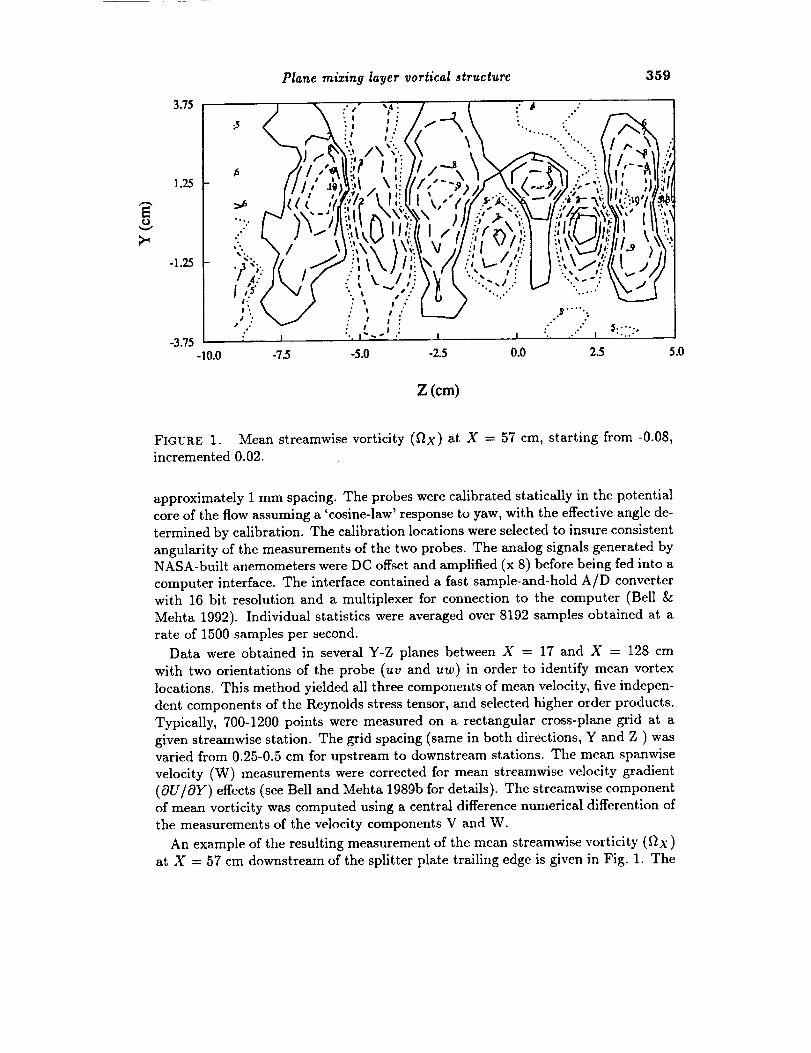
FIGURE 1. Mean streamwise vorticity (fix) at X = 57 cm, starting from -0.08,

incremented 0.02.

approximately 1 mm spacing. The probes were calibrated statically in the potential

core of the flow assuming a 'cosine-law' response to yaw, with the effective angle de-

termined by calibration. The calibration locations were selected to insure consistent

angularity of the measurements of the two probes. The analog signals generated byNASA-built anemometers were DC offset and amplified (x 8) before being fed into a

computer interface. The interface contained a fast sample-and-hold A/D converter

with 16 bit resolution and a multiplexer for connection to the computer (Bell &

Mehta 1992). Individual statistics were averaged over 8192 samples obtained at a

rate of 1500 samples per second.

Data were obtained in several Y-Z planes between X = 17 and X = 128 cm

with two orientations of the probe (uv and uw) in order to identify mean vortex

locations. This method yielded all three components of mean velocity, five indepen-

dent components of the Reynolds stress tensor, and selected higher order products.

Typically, 700-1200 points were measured on a rectangular cross-plane grid at a

given streamwise station. The grid spacing (same in both directions, Y and Z ) was

varied from 0.25-0.5 cm for upstream to downstream stations. The mean spanwise

velocity (W) measurements were corrected for mean streamwise velocity gradient

(OU/OY) effects (see Bell and Mehta 1989b for details). The streamwise component

of mean vorticity was computed using a central difference numerical differention of

the measurements of the velocity components V and W.

An example of the resulting measurement of the mean streamwise vorticity (fix)

at X = 57 cm downstream of the splitter plate trailing edge is given in Fig. 1. The

360 R. L. LeBoeu/

selection of the traverse grid for the correlation measurements is also noted on the

figure. Except for the decreasing peak magnitude and increasing size (for increasing

streamwise distance), the nominally linear array of counter-rotating vortices was

typical of all measurement locations except the first. At the first measurement

location, X = 17, the streamwise vorticity had not yet organized into a single

spanwise row. The correlation locations were nominally selected to cross the location

of maximum mean streamwise vorticity.

The two-polnt cross-correlation measurements required for the estimation of ve-

locity profiles were acquired on grids of equally spaced probe positions. The spacing

of measurement locations in the grids was 0.4 cm. The minimum distance between

estimation and reference locations was limited by probe geometry to two grid spac-

ings (i.e. 0.8 cm). Therefore, the estimated velocity profile is twice as dense as it

could be using probes of the same geometry to measure at all grid locations simulta-

neously. The grids were positioned 78 cm downstream of the splitter plate trailing

edge for the measurements discussed in this paper. It is estimated that this station

is located after the third pairing of the spanwise vortex structures.

_.2 Results and discussion

The transverse (v) and spanwise (w) velocity correlations in the spanwise (Z)

and transverse (Y) directions, respectively, are shown in Figs. 2a and b for the

streamwise location X = 57 cm from the splitter plate trailing edge. One noteworthy

feature of the sets of curves for each station is the relative phase of each curve.

There is generally a shift of the curves from right to left with increasing stationary

probe location. There would be a one-to-one correspondence between the change

in the probe spacing at the correlation extremes and the change in position of

the stationary probe if no meander of the large scale structure is occurring. The

transverse velocity correlations on a spanwise measurement grid approximate this

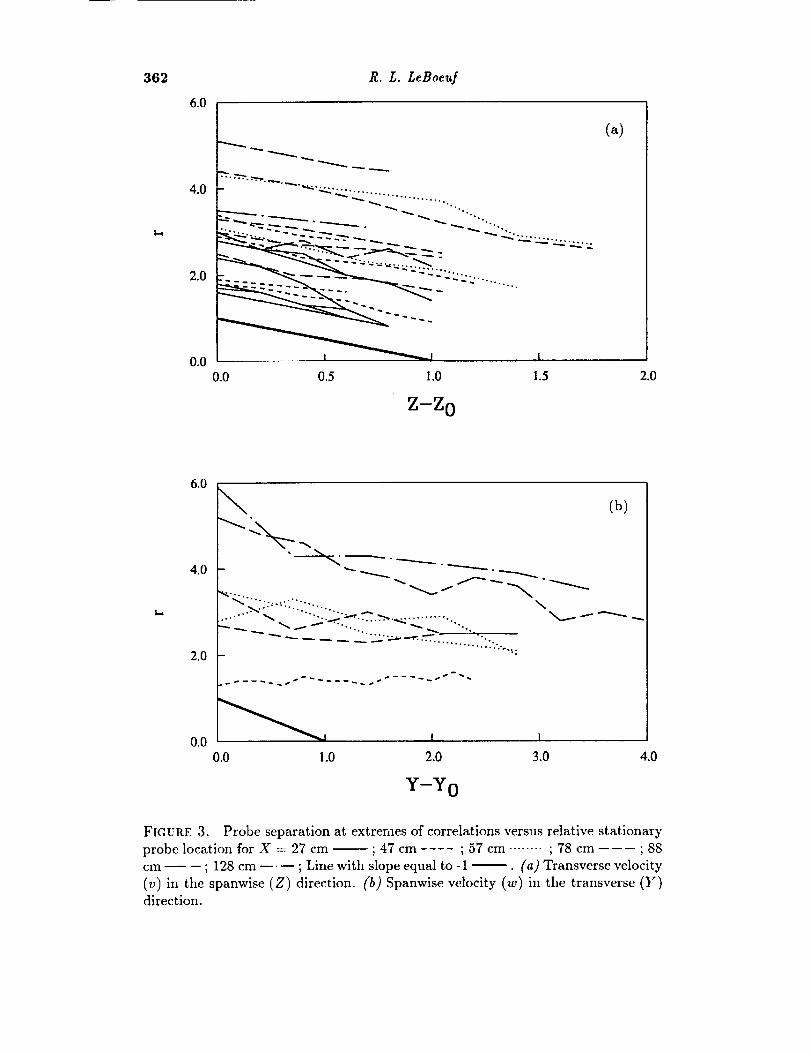
no-meander relative phase shift. For example, Figs. 3a and 3b show the probe

separation at the first minimum and first maximum (excluding zero spacing) of all

of the correlation measurements versus stationary probe location. The slope of the

resulting curves for the transverse velocity measurements (Fig. 3a) is very close

to -1, indicating that meander in the spanwise (z) direction is negligible at thisstreamwise location.

The spanwise velocity correlations across the mixing layer have a less consistent

phase shift for changing stationary probe location. Typically, the shift of the first

minimum is a fraction of the shift of the stationary probe for two sets of correlations

(see Fig. 2b). This is reflected in Fig. 3b where the slope of the curve of first

minimum versus stationary probe location for the spanwise velocity measurements

has a much more gradual slope, which would indicate a large degree of apparent

transverse meander. The slope of the curves may be linked to the aspect ratio ofthe mean streamwise vortices.

A simple, more direct way to identify meander of the large-scale structure is to

track them in temporal multi-point velocity records. The presence of streamwise

structure should appear clearly in profiles of the secondary velocity. In particu-

lar, spanwisc meander should produce a jittered signature in spanwise profiles of

1.0

0.5

0.0

Plane mi=ing layer vortical structure 361

(a)

.......0.0 2.0 4.0 6.0 8.0 10.0 12.0

r

0.50

I 0.25

0.00

..... _ _(b)

-0.25 I l i0.0 2.0 4.0 6.0 8.0

r

FIGURE 2. Two-point cross-correlation at X = 57 cm. (a) Transverse velocity (v)

in the spanwise (Z) direction at Y = 0 and Z = -8.5 cm -- ; -8.15 cm .... ;-7.8 cm ........ ; -7.45 cm --- (b) Spanwise velocity (w) in the transverse (Y)

direction at Z = -5 cm and Y = -2.1 cm -- ; -1.4 cm .... ; -0.7 cm ........ ,0.0

CII1 _ --

362 R. L. LeBoeuf

6.0

4.0

2.0

(_)

0.0 I I

0.0 0.5 1.0 1.5

Z-Z 0

2.0

6.0

4.0

2.0

0.0

\ (b)

Y-Yo

FIGURE 3. Probe separation at extremes of correlations versus relative stationary

probe location for X = 27 cm -- ; 47 cm .... ; 57 cm ........ ; 78 cm ----- ; 88

cm -- - ; 128 cm --,-- ; Line with slope equal to -1 --. (a) Transverse velocity

(v) in the spanwise (Z) direction. (b) Spanwise velocity (w) in the transverse (Y)

direction.

Plane mixing layer vortical structure 363

transverse velocity and transverse meander should produce a jittered signature in

transverse profiles of spanwise velocity. Profiles of simultaneous velocity recordswith sufficient spatial resolution would be very difficult using cross-wire probes and

would entail a significant increase in hardware costs. Use of optical techniques

such as digital particle image velocimetry would probably be the best suited to this

problem, but would also be costly. An alternative approach whereby the velocity

profiles were estimated using one or two reference velocities was used to producesimultaneous velocity profiles. This approach required no further investment in

hardware.The linear estimate of the velocity component fii(x') based on m reference (mea-

sured) velocity components ui(x(k) ) at n locations at the same time can be expressed

as:n 171

fii(x') = _ _ Aijkuj(x(k)). (1)k=l j=l

Minimizing the mean-square error, [ai(x') - ui(x')] 2, of the estimate yields an equa-tion for the linear estimation coefficients (Aijk):

11 m

__, __, Aii_,ui(x(k))ut(x(p)) = ut(x(P))u,(x'). (2)k=l j=l

Thus, given the cross-correlation tensors, the linear mean-square (MS) estimationcoefficients can be determined. It can be shown [using Eq. (1)] that the left hand

side of Eq. (2) is equal to ut(x(P))_i(z'). Hence, the estimation-reference cross-

correlation tensor is equal to the measurements used to produce the coefficients.

The mean-squared estimation error__increases with the distance away from the

measurement location (approaching u_), as the velocity loses correlation with thereference (Adrian & Moin 1988). The estimated signal can be amplified in a ratio-

nal manner by including the velocity covariance at the estimation locations in thescheme to calculate the estimation coefficients. This optimization which includes the

estimation covariance in addition to the two-point cross-correlation tensors forms

the basis for the proposed technique.

Consider the error vector,

F = (uj(x')ui(x(k)) - fiJ(x')ui(z(k))'_ Vi,j,k.\ uj(z')u,(x') /

(3)

Then the estimation coefficients (Aijk) can be optimally determined with respect to

both the estimation-reference cross-correlation, fij(x')u_(x(_)), and the estimation

covariance, _j(x')fii(x'), by minimizing (FTF), where the superscript T indicatestranspose. The statistics of the estimates can be calculated for any value of thecoefficients using known reference signals and estimation signals generated using

Eq. (1). This optimization can be accelerated, however, by calculating the statistics

of the estimates in terms of the reference cross-correlation tensor, uj(x(k))ul(x(P)),

364 R. L. LeBoeuf

and the estimation-reference cross-correlation tensor, ut(x(P))ui(x'). By operating

on Eq. (1), it can easily be shown that the estimation-reference correlation can be

expressed as:n m

fiJ(x')ui(z(k)) = E Z AJqP%(xCP))u'(x(k)) (4)p=l q----1

and the estimated Reynolds stresses can be expressed as:

n m n m

p----I q=l k=l /=1

(5)

Thus, the new technique requires the same cross-correlation tensor data as the

traditional mean-square estimate along with the estimation covariance data. The

optimization described above is a non-linear, least-squares optimization which can

be solved using standard techniques such as, for example, the modified Levenberg-

Marquardt algorithm implemented in the IMSL subroutine DUNLSF.

Another alternative to minimizing the mean-squared error is to maximize the

correlation coefficient of the estimated signal and the true signal at the estimationlocation. When this criterion is used to determine the linear estimation coefficients

for a two-component one-point estimate, the maximum correlation coefficient is

independent of the energy of the estimate:

where

and

1/_

-a_(x,)a )pii = 2 (6)

(b/2) 2- _i(x (k)) [_]'al ['_(x')u,(x (k']

l-i(X')Ue(X(k)) U_(x(k)) 20"(X')Ue(X(k))Ul(X(k))Ue(X(k)) (7)a = + _(x(k)) -

[_(_,)u,(x(k))]_ _(x,),,,(x(k))

-piibA2- 2a (9)

and

Ai = piia=(x') - Aefi(x')ue(x(k))fi(x')u,(x(k)) , (10)

5= 2_(z,) (8)_(=,)u,(=(k))

Hence, once the maximum correlation coefficient has been calculated, the estimationcoefficients can then be determined from

Plane mizing layer vortical structure 365

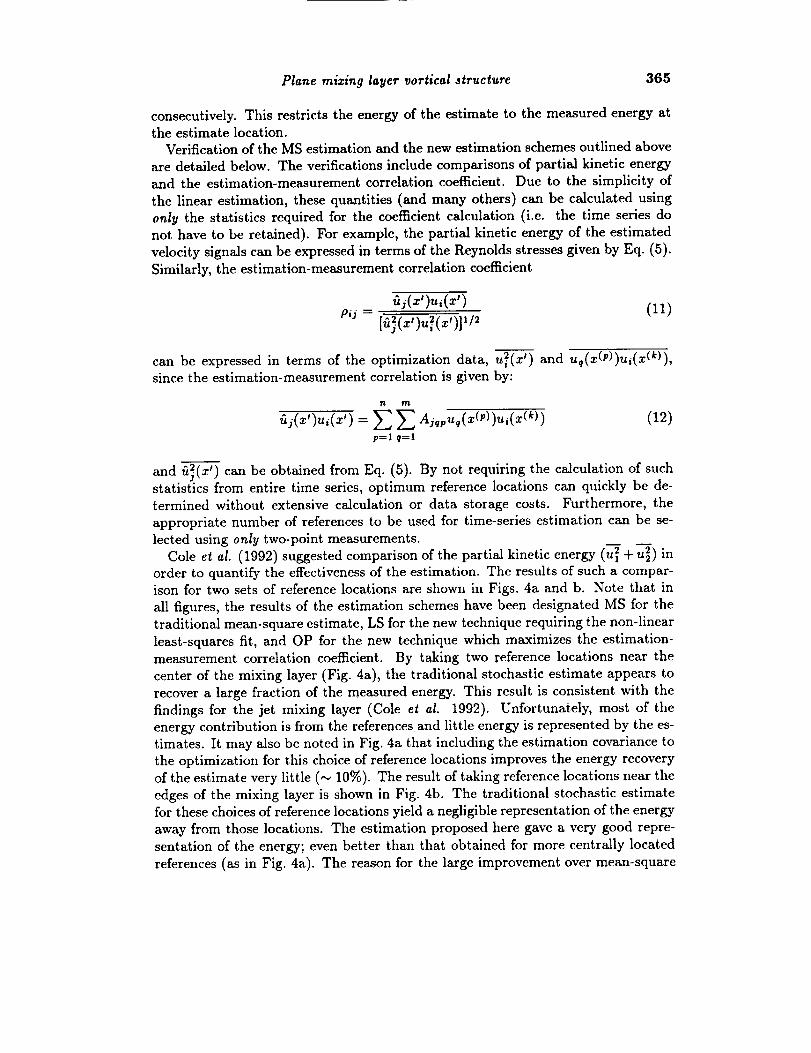
consecutively. This restricts the energy of the estimate to the measured energy atthe estimate location.

Verification of the MS estimation and the new estimation schemes outlined above

are detailed below. The verifications include comparisons of partial kinetic energy

and the estimation-measurement correlation coefficient. Due to the simplicity of

the linear estimation, these quantities (and many others) can be calculated using

only the statistics required for the coefficient calculation (i.e. the time series do

not have to be retained). For example, the partial kinetic energy of the estimated

velocity signals can be expressed in terms of the Reynolds stresses given by Eq. (5).

Similarly, the estimation-measurement correlation coefficient

fij(x')ui(x') (11)p,i=

can be expressed in terms of the optimization data, u_(x') and Uq(X(P))ui(x(k)),since the estimation-measurement correlation is given by:

p=lq=l

(12)

and fi_(x') can be obtained from Eq. (5). By not requiring the calculation of suchstatistics from entire time series, optimum reference locations can quickly be de-

termined without extensive calculation or data storage costs. Furthermore, the

appropriate number of references to be used for time-series estimation can be se-

lected using only two-point measurements.

Cole et al. (1992) suggested comparison of the partial kinetic energy (u_ + u22) inorder to quantify the effectiveness of the estimation. The results of such a compar-ison for two sets of reference locations are shown in Figs. 4a and b. Note that in

all figures, the results of the estimation schemes have been designated MS for the

traditional mean-square estimate, LS for the new technique requiring the non-linear

least-squares fit, and OP for the new technique which maximizes the estimation-measurement correlation coefficient. By taking two reference locations near the

center of the mixing layer (Fig. 4a), the traditional stochastic estimate appears to

recover a large fraction of the measured energy. This result is consistent with thefindings for the jet mixing layer (Cole et al. 1992). Unfortunately, most of the

energy contribution is from the references and little energy is represented by the es-

timates. It may also be noted in Fig. 4a that including the estimation covariance to

the optimization for this choice of reference locations improves the energy recoveryof the estimate very little (,-, 10%). The result of taking reference locations near the

edges of the mixing layer is shown in Fig. 4b. The traditional stochastic estimate

for these choices of reference locations yield a negligible representation of the energy

away from those locations. The estimation proposed here gave a very good repre-

sentation of the energy; even better than that obtained for more centrally located

references (as in Fig. 4a). The reason for the large improvement over mean-square

366 R. £. LeBoeuf

3.0

+

2.0

1.O

0.0

(a)

3.0

+

2.0

1.0

0.0

(b).°.

t

-5.0 -2.5 0.0 2.5 5.0

Y

FIGURE 4. Transverse partial kinetic energy comparisons. (a) Two-point estimates

with references at Y = -0.6 cm and Y = 0.2 cm and one-point estimates with

reference at Y = -0.6 cm. (b) Two-point estimates with references at Y = -5.0 cm

and Y = 3.4 cm and one-point estimates with reference at Y = 3.4 cm, Measured

o ; Measured reference • ; Two-point MS .... ; Two point LS __.w ; One-pointMS ------ ; One-point LS ........ ; One-point OP

estimation for this choice of reference locations is that the estimate-reference cross-

correlation is much less than the estimation covariance. Therefore, minimizing the

error in both quantities results in a better fit to the estimation covariance (which

includes u_ and u_). This trade-off does not occur for reference locations near the

center of the mixing layer. Consequently, the energy recovery for spanwise profiles

Q.

1.0

0.5

0.0

Plane raizing layer vortical structure 367

dL

\ ......... (a)

I I I

Q.

0.0I I I

(b)

-5.0 -2.5 0.0 2.5

Y

5.0

FIGURE 5. Transverse estimation-measurement correlation coefficients. Two-point

estimates with references at Y = -5.0 cm and Y = 3.4 cm and one-point estimates

with reference at Y = 3.4 cm. (a) Streamwise component (u). (b) Transverse

component (v), Reference t ; Two-po_t MS .... ; Two-point LS --'-- ; One-

point MS ---- ; One-point L$ ........ ; One-point OP ---

near the center of the mixing layer was very poor for both estimation techniques.

By taking spanwise grids near the mixing layer edge, a very good representation of

the energy by the new estimation was obtained.Another measure of the success of an estimation is the correlation coefficient

for corresponding estimated and measured velocities at the same location. If an

estimated velocity matches the measurement exactly, then the correlation coefficient

368 R. L. LeBoeuf

v

"_ O.O

1>

-2.0

I I

"VI I

I ..... I ........... L, I

I I I I

ill A :,, _ (b)

A I I I I

//,.! _. /I (c)

& 9,a,,at;t\,

-0.8 i i i i

0.0 20.0 40.0 60.0 80.0 100.0

Time step

FIGURE 6. Transverse velocity (v) measurement vs. estimate time series compar-

isons forareferenceat Y = 3.4cm. (a) Y = 2.6cm. (b) Y =-0.6cm. (c) Y =

-5.0 cm, Measured _ ; MS ........ ; LS .... ; OP ----

-20.0 -15.0 -10.0 -5.0

X (cm)

0.0 5.0 10.0

o • _=...2 :" i ,,-..J / ( _2.;..,7

-lO.O I I I l I

-20.0 -15.0 -10.0 -5.0 0.0 5.0

X (cm)

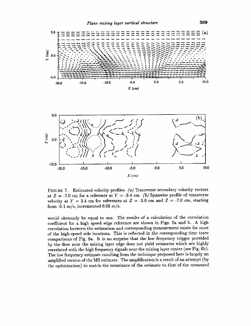
lO.O

FIGURE 7. Estimated velocity profiles. (a) Transverse secondary velocity vectorsat Z = -7.0 cm for a reference at Y = -3.4 cm. (b) Spanwise profile of transverse

velocity at Y = 3.4 cm for references at Z = -5.0 cm and Z = -7.0 cm, starting

from -0.1 m/s, incremented 0.08 m/s.

would obviously be equal to one. The results of a calculation of the correlation

coefficient for a high speed edge reference are shown in Figs. 5a and b. A highcorrelation between the estimation and corresponding measurement exists for most

of the high-speed side locations. This is reflected in the corresponding time trace

comparisons of Fig. 6a. It is no surprise that the low frequency trigger provided

by the flow near the mixing layer edge does not yield estimates which are highlycorrelated with the high frequency signals near the mixing layer center (see Fig. 6b).

The low frequency estimate resulting from the technique proposed here is largely an

amplified version of the MS estimate. The amplification is a result of an attempt (by

the optimization) to match the covariance of the estimate to that of the measured

370 R. L. LeBoeuf

signal. The estimation of flow on the opposite side of the layer is remarkably good

as suggested by the high correlation coefficient for those locations (Figs 5a and b).

Presumably, the large-scale structure providing the trigger at the high-speed edge

produces similar signatures at the low speed edge, resulting in a good estimation of

the flow there (Fig. 6c). The streamwise component time series comparisons were

left out for brevity since they were qualitatively similar to the transverse component

comparisons of Figs. 6a through 6c.

The results of estimating the one-component simultaneous multi-point velocity

profile using the OP method is presented as Fig. 7a. This profile was generated for

a transverse grid at Z = -7 cm using a reference at Y = -5 cm. Taylor's hypoth-

esis was used to approximate the spatial development from the temporal signals.

This entailed calculating the relative spatial locations of velocity vectors as Uc/fs,

where f_ is the sampling frequency and Uc is the mean convection velocity. The

secondary velocity vector plot clearly shows the spanwise rollers passing through

the measurement station. In spite of the poor representation of the broad-band

signals near the center of the mixing layer, the large-scale structure is adequately

represented when edge references are selected. In particular, the relationship be-

tween the kinematics of the large-scale streamwise and spanwise flow structures can

be inferred from simultaneous estimates of velocity profiles on spanwise and trans-

verse grids. For example, using two cross-wire probes makes it possible to estimate

three velocity components in one profile (in one direction) and two velocity compo-

nents in another profile (in another direction) provided the grids have a common

reference location. This can be achieved by measuring reference signals ui and u2

(or u3) at the common grid location and simultaneously measuring ul u3 (or u2)

in the grid for which three velocity components are desired. With the use of such

a combination of grid locations, it was possible to estimate the transverse velocity

(v) as shown in Fig. 7b. The signature of the streamwise vortices which ride the

braid between spanwise vortices appear each time the spanwise vortices carry them

through the measurement grid. This gives rise to the juxtaposed spanwise sets of

islands in Fig. 7b between time steps -17 and -12. The lack of significant structure

to structure spanwise relative motion of this signature observed in longer simulta-

neous time series profiles is indicative of the low degree of spanwise meander whichwas also inferred from the correlation measurements.

3. Future plans

During the remainder of the program, phase locked velocity measurements will

be obtained by acoustically forcing the mixing layer. The hardware required for

this phase of the program has already been preparcd. By establishing a periodic

sequence of spanwise vortices, it should be possible to examine the detailed structure

of the streamwise vortices. By measuring the scale and spacing of the streamwise

vorticity in the braid region of the mixing layer vortices, more direct comparisons of

the wind tunnel measurements can be made with the direct numerical simulations

of the same flow (Rogers, M. M. & Moser, R. D. private communication). In

particular, initial conditions (streamwise vortex strength and distribution) will be

measured in detail so that thcy may be used as input to numerical simulations.

Plane mizing layer vortical structure 371

During the latter part of the program, some scalar mixing studies using heat to tagone of the streams will also be conducted. An extension of the estimation to include

space-time correlations will also be attempted if time permits.

AcknowledgementsThis work is being performed in the Fluid Mechanics Laboratory, NASA Ames

Research Center in collaboration with Dr. R. D. Mehta.

REFERENCES

ADRIAN R. J. &: MOIN, P. 1988 Stochastic estimation of organized turbulent

structure: homogeneous shear flow. J. Fluid Mech. 190, 531.

BELL, J. H. 1990 An Experimental Study of Secondary Vortex Structure in Mix-

ing Layers. Annual Research Briefs. Center for Turbulence Research, Stanford

Univ./NASA Ames, 59-79.

BELL, J. H. &: MEHTA, R. D. 1989a Design and Calibration of the Mixing LayerWind Tunnel. JIAA TR-8_. Dept. of Aeronautics and Astronautics, Stanford

University.

BELL, J. H. & MEHTA, R. D. 1989b Three-Dimensional Structure of Plane Mixing

Layers. JIAA Repor_ TR-90.

BELL, J. H. & MEItTA, R. D. 1990 Development of a Two-Stream Mixing Layerfrom Tripped and Untripped Boundary Layers. AIAA Journal. 28, 2034-2042.

BELL, J.H. AND MEItTA, R.D. 1992 Measurements of the Streamwise Vortical

Structures in a Plane Mixing Layer. J. Fluid Mech. 239, 213.

BERNAL, L. P. &: RosltI<O, A. 1986 Streamwise Vortex Structure in Plane Mixing

Layers. J. Fluid Mech. 170, 499-525.

COLE, D. R., GLAUSEa, M. N. & GUEZENNEC, V. G. 1992 An application ofthe stochastic estimation to the jet mixing layer. Phys. Fluids A. 4, 192.

LEBOEUF, R. L. &: MEItTA, R. D. 1992 An Improved Linear Estimation Scheme.

Bulletin of American Physical Society, Division of Fluid Dynamics, 45th Meet-

ing. also submitted to Phys. Fluids A.

TOWNSEND, A. A. 1976 Structure of Turbulent Shear Flow (2nd Edition) Cam-

bridge University Press.