Assignment 3: Vehicle Forces and Kinematics

CEE 3604: Introduction to Transportation Engineering Fall 2011

Assignment 3: Vehicle Forces and KinematicsDate Due: September 16, 2011 Instructor: Trani

Problem 1

a) A commuter train with a mass of 305,000 kg. travels downhill at a grade of -2% and 50 mph when the brakes fail. Estimate the maximum speed the train will achieve downhill if the following parameters apply:

S = 14 m2, froll = 0.0018,Cd = 0.75 (dim) and Cl = 0.03 (dim)

Here we do not have any tractive effort since the train is un runaway mode. Balance of the forces as the train travels downhill is the gravity force accelerating the train and the friction and drag forces opposing the motion. At equilibrium:

Gf = Ff + Dmgsin(θ) = (mgcos(θ) − L) froll + D

mgsin(θ) = (mgcos(θ) − 12ρV 2SCl ) froll +

12ρV 2SCd

where:

Gf = gravity force pushing the trainFf = friction forceD = drag force

all in Newtons

Solve for V in the equation to obtain the balancing speed of the train at equilibrium. A numerical solution can be obtained using a simple Matlab script to estimate the sum all three forces as a function of speed and then watch for the value of speed that makes zero the sum of all forces acting on the train. The diagram is shown in the figure below.

CEE 3604 A3 Trani of 11

Figure 1. Diagram of Forces for a Runaway Train (No Tractive Force).The “balancing” speed is estimated at 91.35 m/s (204 mph). b) During normal operations, the train described in part (a) has a tractive force as shown in Table 1. The tractive force was obtained from actual testing of the vehicle.Table 1. Tractive Force for Train in Problem 1.

Speed (m/s) Tractive Force (N)

0 180000

20 155000

40 95000

60 65000

80 50000

100 35000

c) Plot the speed vs tractive force data shown in Table 1 using Matlab.


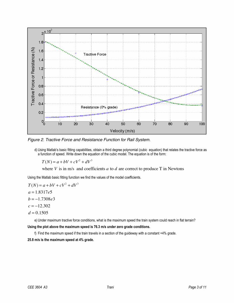
Figure 2. Tractive Force and Resistance Function for Rail System.

d) Using Matlab’s basic fitting capabilities, obtain a third degree polynomial (cubic equation) that relates the tractive force as a function of speed. Write down the equation of the cubic model. The equation is of the form:

T (N ) = a + bV + cV 2 + dV 3

where V is in m/s and coefficients a to d are correct to produce T in Newtons

Using the Matlab basic fitting function we find the values of the model coefficients.

T (N ) = a + bV + cV 2 + dV 3

a = 1.8317e5b = −1.7308e3c = −12.302d = 0.1505

e) Under maximum tractive force conditions, what is the maximum speed the train system could reach in flat terrain?Using the plot above the maximum speed is 76.3 m/s under zero grade conditions.

f) Find the maximum speed if the train travels in a section of the guideway with a constant +4% grade.25.8 m/s is the maximum speed at 4% grade.


Problem 2

Use the bus parameters defined in the section below to answer the following questions:

Ca = 0.027; % CoefficientC1 = 6.9; % NondimensionalC2 = 0.055; % NondimensionalW = 140; % Bus weight in kNA = 8.1; % Frontal area (square meters)i = +0; % Grade in percent (%) % Define bus engine parameters to estimate tractive force D = 0.90; % Wheel diameter (m)u(1) = 4.2; u(2) = 2.3; u(3) = 1.5; u(4) = 1.3; % gear ratios in explicit vector formJ = 2.2; % Differential reduction ratiocon1 = .06; % conversion factor (to convert km/hr to m/s) %con2 = 2650; % conversion factor (to convert hp to N) %nu = 0.85; % efficiency of engine P = [90 145 195 245 253 286 340]; % power output vector (HP)RPM = [800 1400 1800 2400 2800 3400 4200]; % RPM vector

a) Find the maximum acceleration the bus can generate while traveling at 25 km/hr in flat terrain.

Figure 3. Tractive Force and resistance Diagram for the Bus. Zero Grade.


Fx∑ = max

ax =Fx∑m

=(13100 −1283N )

14272kg= 0.83m / s2

This is the acceleration at 25 km/hr.b) Find the total travel time between two adjacent bus stations located 400 meters apart. Assume the bus driver uses full

“throttle” to accelerate the bus to the speed limit of the road. Assume the driver decelerates at −1 m/s2from cruise

speed to zero speed at the final station. The road has a speed limit of 88 km/hr and for this example, assume has the road has zero gradient. Show me all your work. In solving this problem, you can use the tractive force approximation demonstrated on page 53 of the class notes.

Figure 4. Bus Tractive Force and Resistance Diagram.

The acceleration of the bus is bounded by the curves above. For any point in the force/resistance diagram, the acceleration of the bus is the quotient of the sum of the forces (T-R) and the mass. Using the tractive force and resistance shown above, we can derive an acceleration function of the vehicle. The table below contains the pertinent information. For example, for a speed of 40 km/hr, the tractive force (T) is approximately 11,000 N and the basic resistance (R) is 1594 N. This means an acceleration,

Fx∑ = (T − R) = max

ax =T − Rm

=(11000 −1594N )

14272kg= 0.659m / s2

The process is repeated for multiple values of speed. The acceleration function is the used in the calculation of the acceleration profile and travel time between stations. Using the values shown the table below, we can establish a simple relationship between


acceleration and speed. For example, using the data points presented in the table below, we can produce a regression model to predict acceleration as a function of speed. This is illustrated in Figure 5 below. Two models are presented in the figure: a) a linear model and 2) a quadratic model. Both models seem reasonable approximations. Certainly, the use of the linear model is simpler in the context of our analysis because the equations to predict velocity and distance are already known in close form solution (see handout titled “Fundamentals of Ground Vehicles” pages 59-60). Figure 6 is the same as Figure 5 but with the x-axis units converted to m/s.

Table 2. Derivation of the Acceleration Function for the Bus. Bus Mass is 140kN.Speed (km/hr) Tractive Force (N) Basic Resistance (N) Acceleration (m/s2)

0 14,000 966 0.9133

20 13,200 1,200 0.8409

40 11,000 1,594 0.6591

60 7,200 2,147 0.3541

80 5,800 2,861 0.2059

100 4,500 3,734 0.0537

Figure 5. Acceleration Functions for Bus. Velocity Axis in Km/hr.


Figure 6. Acceleration Functions for Bus. Velocity Axis in meters/second.

Method 1: Use linear equation of acceleration vs. velocity Here we assume the bus acceleration model is linear with speed:

a = 0.9693− 0.03347Va in m/s2

V in m/s

Integrating once and twice the equation above we get equations of speed and distance as a function of time (see pages 59-60 of handout “Fundamentals of Ground Vehicles”):

Vt = V0ek2 t +

k1k2(1− e−k2 t )

St =k1k2t − k1

k22 (1− e

−k2 t ) +V0 (1− e−k2 t )

These equations are programmed in the Matlab script Vehicle_kinematics_general.m available in the syllabus (week 3). You can run this script substituting the correct values of k1 and k2 in the script.


Figure 7. Matlab Script to Study the Acceleration of the Vehicle with Time.

Executing the Matlab code produces the results shown below. I ran the script for 40 seconds of the motion of the vehicle. It is evident that the distance traveled by the bus grows rapidly beyond the 400 meters between stations after only 35 seconds. At that point the bus will be traveling at 20 m/s (72 km/hr). This provides a clue that the bus is unlikely to reach the 88 km/hr speed limit in the motion between the two stations.

Figure 8. Speed and Distance Traveled Profiles for Bus.

For the deceleration phase, we know the deceleration rate is constant at -1.0 m/s-s. For the constant deceleration motion phase, the velocity and distance traveled by the bus are given by equations:


Vt = V0 + a2t

St = S0 +Vot +12a2t

2

where the deceleration of the bus is shown as variable a2 in m/s2.

The solution of the deceleration distance and acceleration distance equations simultaneously provides a solution to the problem. The bus reaches 16.98 m/s while traveling 256 meters. The bus decelerates from 16.98 m/s and takes the remaining 144 meters. Another useful relationship for a constant deceleration to estimate the deceleration distance is:

Sd =−V

2

2a2Adding the deceleration and the acceleration distances we can obtain the total distance traveled. This is shown in Figure 9. The maximum speed of the bus is 16.98 m/s to travel 400 meters.

Figure 9. Total Distance vs. Speed.

Method 2: Use the quadratic equation of acceleration vs. velocity Here we assume the bus acceleration model is quadratic with speed:

a = 0.9536 − 0.02922V + 0.000153V 2

a in m/s2

V in m/s

To solve this problem we use the procedure of numerical integration explained in the course notes (ground vehicle performance).


Vt = Vt−Δt +dVdt

Δt

Vt = is the velocity of the vehicle at time tVt−Δt = is the velocity of the vehicle at a previous time stepΔt = is the step size

We can solve the equation above using numerical integration as shown in the table below. Note that the bus reaches 16.98 m/s in about 22.5 seconds. This is very close to the time obtained using the close form solution shown in Figure 8.

Figure 10. Excel Simulation for Acceleration Phase of the Bus Motion. Includes Velocity Profile in Second Column.Using the numerical integration procedure stated in the course notes we can also solve for the distance traveled.

St = St−Δt +dSdt

Δt = St−Δt +VtΔt

Vt = is the velocity of the vehicle at time tVt−Δt = is the velocity of the vehicle at a previous time stepSt = is the distance traveled by the vehicle at time tSt−Δt = is the distance traveled by the vehicle at a previous time stepΔt = is the step size


Figure 11. Excel Simulation for Acceleration Phase of the Bus Motion. Includes Distance Profile in Sixth Column.

c) Calculate the fraction of the time the bus is accelerating, cruising and decelerating. Comment on the observed trends.The bus takes 26.4 seconds to accelerate to 16.98 m/s. The bus takes 16.98 seconds to decelerate from 16.98 m/s. The time spent on the acceleration mode is ~ 61%.


Assignment 3: Vehicle Forces and Kinematics

Documents

Transcript of Assignment 3: Vehicle Forces and Kinematics