KINEMATICS ASSIGNMENT - UTeM OPEN JOURNAL SYSTEM

ISSN: 2180-1053 Vol. 9 No.2 July – December 2017 1

FORWARD AND INVERSE KINEMATICS ANALYSIS AND

VALIDATION OF THE ABB IRB 140 INDUSTRIAL ROBOT

Mohammed Almaged1*

, Omar Ismael2

1,2 Nineveh University, College of Electronics Engineering,

Department of Systems & Control Engineering, Nineveh, Iraq

ABSTRACT

The main goal of this paper is to derive the forward and inverse kinematics

model of the ABB IRB 140 industrial manipulator. This work provides essential

kinematics information that could be a useful reference for future research on the

robot. It can also serve as teaching material for students in the area of robotics,

especially forward and inverse kinematics, to aid students' understanding of

these subjects. Denavit-Hartenberg analysis (DH) is presented to write the

forward kinematic equations. Initially, a coordinate system is attached to each of

the six links of the manipulator. Then, the corresponding four link parameters

are determined for each link to construct the six transformation matrices ( 𝑇𝑖𝑖−1 )

that define each frame relative to the previous one. While, to develop the

kinematics that calculates the required joint angles (𝜃1 − 𝜃6), both geometrical

and analytical approaches are used to solve the inverse kinematic problem. After

introducing the forward and inverse kinematic models, a MATLAB code is

written to obtain the solutions of these models. Then, the forward kinematics is

validated by examining a set of known positions of the robot arm, while the

inverse kinematics is checked by comparing the results obtained in MATLAB

with a simulation in Robot Studio.

KEYWORDS: Robotics; Forward Kinematics; Inverse Kinematics; IRB 140 Manipulator

1.0 INTRODUCTION

'Kinematics is the science of geometry in motion' (Jazar, 2010). This means it deals only

with geometrical issues of motion such as the position and orientation regardless the

force that causes them. There are two types of kinematics, the forward and inverse

kinematics. Forward kinematic analysis is concerned with the relationship between the

joint angle of the robot manipulator and the position and orientation of the end-effector

(Spong, Hutchinson, & Vidyasagar, 2006) (Paul, 1981) . In other words, it deals with

finding the homogeneous transformation matrix that describes the position and

orientation of the tool frame with respect to the global reference frame. On the other

hand, inverse kinematics is used to calculate the joint angles required to achieve the

desired position and orientation. The same transformation matrix which resulted from

the forward kinematics in order to describe the position and the orientation of the tool

frame relative to the robot base frame is used here in the inverse kinematics to solve for

the joint angles. Several academic studies investigating the kinematics of the robot

manipulators have been carried out to increase their intelligence and usability. Various

*Corresponding author e-mail: [email protected]

Journal of Mechanical Engineering and Technology


approaches have been introduced for the analysis. In his book, Selig (Selig, 2013) has

discussed several ways of analyzing robots using geometrical approach. Jazar (Jazar,

2010) also reviewed a number of analytical methods for the analysis of serial robots.

The concept of the homogeneous transformation matrix is very old in the area of

kinematic analysis. However, it is still very popular and valuable.

Several authors (Craig, 2005; Jazar, 2010; Shahinpoor, 1987; Uicker, Pennock, &

Shigley, 2011) have discussed the formulation of the homogeneous transformation

matrix. In 2012, K. Mitra introduced a different procedure for the formulation of the

homogeneous matrix. His method was based on motion transfer at the joints from the

base to the end effector. This technique was validated through a numerical study on a 5

DOF robot (Mitra, 2012). Also, A. Khatamian produced a new analytical method for

solving the forward kinematics of a six DOF manipulator (Khatamian, 2015).

Several approaches have been used to solve the inverse kinematic problem. Some

researchers have investigated the inverse kinematics of robot manipulators using

standard techniques such as geometric, algebraic, etc. In 2012, Deshpande and George

presented an analytical solution for the inverse kinematics derived from the D-H

homogeneous transformation matrix (Deshpande & George, 2012). In the same vein,

Neppalli et al developed a closed-form analytical approach to solve the inverse

kinematics for multi-section robots. In this novel approach, the problem is decomposed

into several easier sub-problems. Then, an algorithm is employed to produce a complete

solution to the inverse kinematic problem (Neppalli, Csencsits, Jones, & Walker, 2009).

S. Yahya et al proposed a new geometrical method to find the inverse kinematics of the

planar manipulators (Samer Y, 2009).

Other researchers have solved the inverse kinematic problem using advanced techniques

such as artificial neural network and biomimetic approach. In 2014, Feng et al produced

a novel learning algorithm, called extreme learning machine, based on a neural network

to generate the inverse kinematic solution of robot manipulator (Feng, Yao-nan, & Yi-

min, 2014). The findings of this advanced method revealed that the extreme learning

machine has not only significantly reduced the computation time but also enhanced the

precision.

2.0 ROBOT SPECIFICATIONS

Figure 1 shows the compact six degree of freedom industrial ABB IRB 140

manipulator. The robot has six revolute joints controlled by Ac-motors. It is designed

specifically for manufacturing industries to perform a wide range of applications such as

welding, packing, assembly, etc. The specifications, axes and dimensions of the robot

manipulator are shown below in Table 1.

Forward and Inverse Kinematics Analysis and Validation of the ABB IRB 140 Industrial Robot


Table 1. The ABB IRB 140 specifications (ABB, 2000)

Manipulator Weight 98 kg

Tool Centre Point TCP Max. Speed 250 mm/s

Endurance Load in XY Direction ± 1300 N

Endurance Load in Z Direction ± 1000 N

Endurance Torque in XY Direction ± 1300 N.m

Endurance Torque in Z Direction ± 300 N.m

Figure 1. The ABB IRB 140 manipulator (ABB, 2000)

3.0 FORWARD KINEMATICS

To mathematically model a robot and hence determine the position and orientation of

the end effector with respect to the base or any other point, it is necessary to assign a

global coordinate frame to the base of the robot and a local reference frame at each

joint. Then, the Denavit-Hartenberg analysis (DH) is presented to build the

homogeneous transformation matrices between the robot joint axes (Craig, 2005)

(Siciliano, Sciavicco, Villani, & Oriolo, 2010). These matrices are a function of four

parameters resulted from a series of translations and rotations around different axes. The

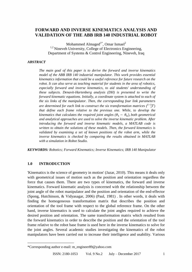
illustration of how frame {i} is related to the previous frame {i −1} and the description

of the frame parameters are shown in figure 2 below.



Figure 2. The description of frame {i} with respect to frame {i −1}(Craig, 2005)

These modified D-H parameters can be described as:

αi-1: Twist angle between the joint axes Zi and Zi-1 measured about Xi-1.

ai-1: Distance between the two joint axes Zi and Zi-1 measured along the common

normal.

θi: Joint angle between the joint axes Xi and Xi-1 measured about Zi.

di: Link offset between the axes Xi and Xi-1 measured along Zi.

Thus, the four Transformations between the two axes can be defined as:

After finishing the multiplication of these four transformations, the homogeneous

transform can be obtained as:

Tii−1 =

(

cθi −sθi 0 ai−1

sθicαi−1 cθicαi−1 −sαi−1 −disαi−1sθisαi−1 cθisαi−1 cαi−1 dicαi−10 0 0 1 )

(1.1)

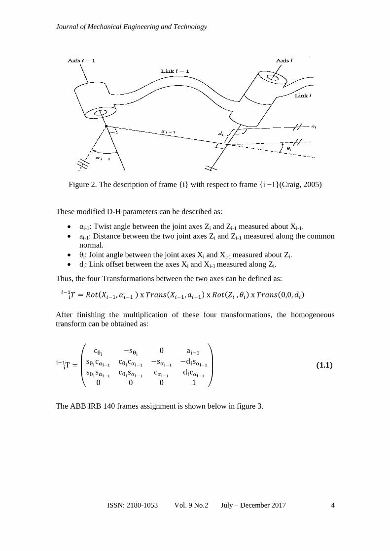
The ABB IRB 140 frames assignment is shown below in figure 3.

𝑇𝑖𝑖−1 = 𝑅𝑜𝑡(𝑋𝑖−1, 𝛼𝑖−1 ) x 𝑇𝑟𝑎𝑛𝑠(𝑋𝑖−1, 𝑎𝑖−1) x 𝑅𝑜𝑡(𝑍𝑖 , 𝜃𝑖) x 𝑇𝑟𝑎𝑛𝑠(0,0, 𝑑𝑖)



Figure 3. ABB IRB140 frames assignment

According to this particular frame assignment, the modified D-H parameters are defined

in Table 2 below.

Table 2. The ABB IRB 140 D-H parameters

For the simplicity of calculations and matrix product, it can be assumed that S2 = sin

(θ2-90), C2 = cos (θ2-90). After achieving the D-H table, the individual transformation

matrix for each link is achieved by substituting the link parameters into the general

homogeneous transform derived in matrix (1.1) above.

Axis (i) αi-1 ai-1 di θi

1 0 0 d1 = 352 θ1

2 -90 a1 = 70 0 θ2-90

3 0 a2 = 360 0 θ3

4 -90 0 d4 = 380 θ4

5 90 0 0 θ5

6 -90 0 0 θ6



𝑇10 =

(

𝑐𝜃1 −𝑠𝜃1 0 𝑎0

𝑠𝜃1𝑐𝛼0 𝑐𝜃𝑖𝑐𝛼01 −𝑠𝛼0 −𝑑1𝑠𝛼0𝑠𝜃1𝑠𝛼0 𝑐𝜃1𝑠𝛼0 𝑐𝛼0 𝑑1𝑐𝛼00 0 0 1 )

𝑇1

0 = (

𝑐1 −𝑠1 0 0 𝑠1 𝑐1 0 00 0 1 𝑑10 0 0 1

)

𝑇21 =

(

𝑐𝜃2 −𝑠𝜃2 0 𝑎1

𝑠𝜃2𝑐𝛼1 𝑐𝜃2𝑐𝛼1 −𝑠𝛼1 −𝑑2𝑠𝛼1𝑠𝜃2𝑠𝛼1 𝑐𝜃2𝑠𝛼1 𝑐𝛼1 𝑑2𝑐𝛼10 0 0 1 )

𝑇2

01 = (

𝑐2 −𝑠2 0 𝑎10 0 1 0−𝑠2 −𝑐2 0 00 0 0 1

)

𝑇32 =

(

𝑐𝜃3 −𝑠𝜃3 0 𝑎2


𝑇3

2 = (

𝑐3 −𝑠3 0 𝑎2 𝑠3 𝑐3 0 00 0 1 00 0 0 1

)

𝑇43 =

(

𝑐𝜃4 −𝑠𝜃4 0 𝑎3


𝑇4

3 = (

𝑐4 −𝑠4 0 0 0 0 1 𝑑4−𝑠4 −𝑐4 0 00 0 0 1

)

𝑇54 =

(

𝑐𝜃5 −𝑠𝜃5 0 𝑎4


𝑇5

4 = (

𝑐5 −𝑠5 0 0 0 0 −1 0𝑠5 𝑐5 0 00 0 0 1

)

𝑇65 =

(

𝑐𝜃6 −𝑠𝜃6 0 𝑎5


𝑇6

5 = (

𝑐6 −𝑠6 0 0 0 0 1 0−𝑠6 −𝑐6 0 00 0 0 1

)

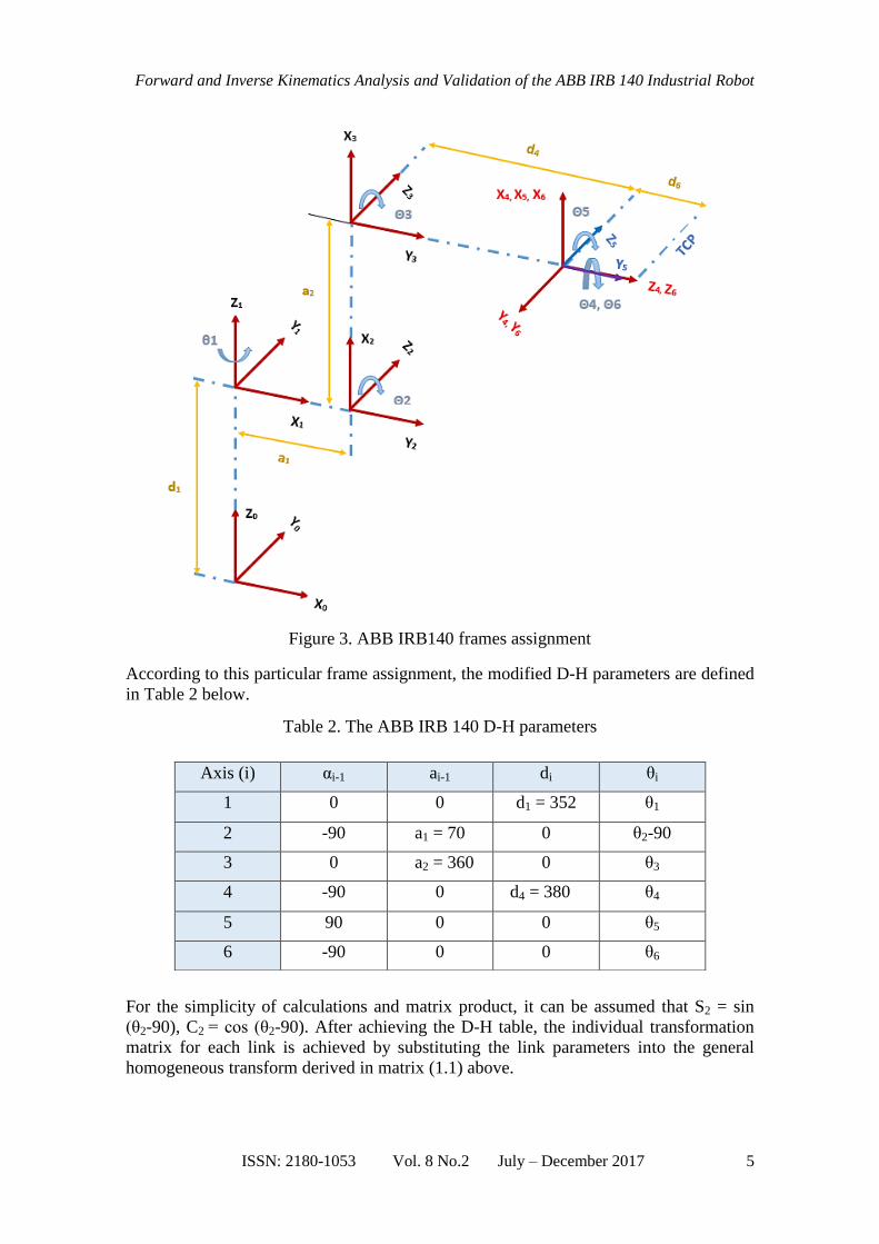
Once the homogeneous transformation matrix of each link is obtained, forward

kinematic chain can be applied to achieve the position and orientation of the robot end-

effector with respect to the global reference frame (robot base).

𝑇20 = 𝑇1

0 X 𝑇21

𝑇2 0 = (

𝑐1 −𝑠1 0 0 𝑠1 𝑐1 0 00 0 1 𝑑10 0 0 1

) X (

𝑐2 −𝑠2 0 𝑎10 0 1 0−𝑠2 −𝑐2 0 00 0 0 1

) = (

𝑐1𝑐2 −𝑐1𝑠2 −𝑠1 𝑐1𝑎1𝑠1𝑐2 −𝑠1𝑠2 𝑐1 𝑠1𝑎1−𝑠2 −𝑐2 0 𝑑10 0 0 1

)

𝑇30 = 𝑇2

0 X 𝑇32



𝑇3 0 = (

𝑐1𝑐2 −𝑐1𝑠2 −𝑠1 𝑐1𝑎1𝑠1𝑐2 −𝑠1𝑠2 𝑐1 𝑠1𝑎1−𝑠2 −𝑐2 0 𝑑10 0 0 1

)𝑋(

𝑐3 −𝑠3 0 𝑎2 𝑠3 𝑐3 0 00 0 1 00 0 0 1

)

𝑇30 = (

𝑐1𝑐2𝑐3 − 𝑐1𝑠2𝑠3 −(𝑐1𝑐2𝑠3 + 𝑐1𝑠2𝑐3) −𝑠1 𝑐1𝑐2𝑎2 + 𝑐1𝑎1 )𝑠1𝑐2𝑐3 − 𝑠1𝑠2𝑠3 −(𝑠1𝑐2𝑠3 + 𝑠1𝑠2𝑐3) 𝑐1 𝑠1𝑐2𝑎2 + 𝑠1𝑎1 )−(𝑠2𝑐3 + 𝑐2𝑠3) 𝑠2𝑠3 − 𝑐2𝑐3 0 −𝑠2𝑎2 + 𝑑1

0 0 0 1

)

𝑇 30 = (

𝑐1𝑐23 −𝑐1𝑠23 −𝑠1 𝑐1(𝑐2𝑎2 + 𝑎1 )𝑠1𝑐23 −𝑠1𝑠23 𝑐1 𝑠1(𝑐2𝑎2 + 𝑎1 )−𝑠23 −𝑐23 0 −𝑠2𝑎2 + 𝑑10 0 0 1

)

𝑇64 = 𝑇 5

4 X 𝑇65

𝑇 =6 4 (

𝑐5 −𝑠5 0 0 0 0 −1 0𝑠5 𝑐5 0 00 0 0 1

)𝑋(

𝑐6 −𝑠6 0 0 0 0 1 0−𝑠6 −𝑐6 0 00 0 0 1

) = (

𝑐5𝑐6 −𝑐5𝑠6 −𝑠5 0 𝑠6 𝑐6 0 0𝑠5 𝑐6 −𝑠5 𝑠6 𝑐5 00 0 0 1

)

𝑇63 = 𝑇 4

3 X 𝑇64

𝑇63 = (

𝑐4 −𝑠4 0 0 0 0 1 𝑑4−𝑠4 −𝑐4 0 00 0 0 1

)𝑋(

𝑐5𝑐6 −𝑐5𝑠6 −𝑠5 0 𝑠6 𝑐6 0 0𝑠5 𝑐6 −𝑠5 𝑠6 𝑐5 00 0 0 1

)

𝑇63 = (

𝑐4𝑐5𝑐6−𝑠4𝑠6 −𝑐4𝑐5𝑠6−𝑠4𝑐6 −𝑐4𝑠5 0 𝑠5 𝑐6 −𝑠5 𝑠6 𝑐5 𝑑4

−𝑠4𝑐5𝑐6−𝑐4𝑠6 𝑠4𝑐5𝑠6−c4𝑐6 𝑠4𝑠5 00 0 0 1

)

𝑇60 = 𝑇 X3

0 𝑇6 3

𝑇 =60 (

𝑐1𝑐23 −𝑐1𝑠23 −𝑠1 𝑐1(𝑐2𝑎2 + 𝑎1 )𝑠1𝑐23 −𝑠1𝑠23 𝑐1 𝑠1(𝑐2𝑎2 + 𝑎1 )−𝑠23 −𝑐23 0 −𝑠2𝑎2 + 𝑑10 0 0 1

)𝑋(

𝑐4𝑐5𝑐6−𝑠4𝑠6 −𝑐4𝑐5𝑠6−𝑠4𝑐6 −𝑐4𝑠5 0 𝑠5 𝑐6 −𝑠5 𝑠6 𝑐5 𝑑4

−𝑠4𝑐5𝑐6−𝑐4𝑠6 𝑠4𝑐5𝑠6−c4𝑐6 𝑠4𝑠5 00 0 0 1

)

𝑇 60 = (

𝑟11 r12 r13 x r21 r22 r23 yr31 r32 r33 𝑧0 0 0 1

)

r11 = 𝑐1𝑐23 (𝑐4𝑐5𝑐6−𝑠4𝑠6) − 𝑐1𝑠23𝑠5 𝑐6 + 𝑠1(𝑠4𝑐5𝑐6+𝑐4𝑠6) r12 = 𝑐1𝑐23(−𝑐4𝑐5𝑠6−𝑠4𝑐6) + 𝑐1𝑠23𝑠5 𝑠6 − 𝑠1(𝑠4𝑐5𝑠6−c4𝑐6) r13 = −𝑐1𝑐23𝑐4𝑠5 − 𝑐1𝑠23𝑐5 − 𝑠1𝑠4𝑠5



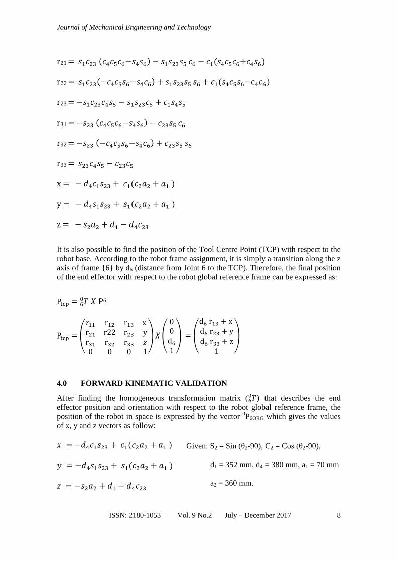
r21 = 𝑠1𝑐23 (𝑐4𝑐5𝑐6−𝑠4𝑠6) − 𝑠1𝑠23𝑠5 𝑐6 − 𝑐1(𝑠4𝑐5𝑐6+𝑐4𝑠6) r22 = 𝑠1𝑐23(−𝑐4𝑐5𝑠6−𝑠4𝑐6) + 𝑠1𝑠23𝑠5 𝑠6 + 𝑐1(𝑠4𝑐5𝑠6−c4𝑐6) r23 = −𝑠1𝑐23𝑐4𝑠5 − 𝑠1𝑠23𝑐5 + 𝑐1𝑠4𝑠5 r31 = −𝑠23 (𝑐4𝑐5𝑐6−𝑠4𝑠6) − 𝑐23𝑠5 𝑐6 r32 = −𝑠23 (−𝑐4𝑐5𝑠6−𝑠4𝑐6) + 𝑐23𝑠5 𝑠6 r33 = 𝑠23𝑐4𝑠5 − 𝑐23𝑐5 x = − 𝑑4𝑐1𝑠23 + 𝑐1(𝑐2𝑎2 + 𝑎1 ) y = − 𝑑4𝑠1𝑠23 + 𝑠1(𝑐2𝑎2 + 𝑎1 ) z = − 𝑠2𝑎2 + 𝑑1 − 𝑑4𝑐23

It is also possible to find the position of the Tool Centre Point (TCP) with respect to the

robot base. According to the robot frame assignment, it is simply a transition along the z

axis of frame {6} by d6 (distance from Joint 6 to the TCP). Therefore, the final position

of the end effector with respect to the robot global reference frame can be expressed as:

Ptcp = 𝑇60 𝑋 P6

Ptcp = (

𝑟11 r12 r13 x r21 r22 r23 yr31 r32 r33 𝑧0 0 0 1

)𝑋(

00d61

) = (

d6 r13 + x d6 r23 + yd6 r33 + z

1

)

4.0 FORWARD KINEMATIC VALIDATION

After finding the homogeneous transformation matrix ( 𝑇)60 that describes the end

effector position and orientation with respect to the robot global reference frame, the

position of the robot in space is expressed by the vector 0P6ORG which gives the values

of x, y and z vectors as follow:

𝑥 = −𝑑4𝑐1𝑠23 + 𝑐1(𝑐2𝑎2 + 𝑎1 ) 𝑦 = −𝑑4𝑠1𝑠23 + 𝑠1(𝑐2𝑎2 + 𝑎1 ) 𝑧 = −𝑠2𝑎2 + 𝑑1 − 𝑑4𝑐23

Given: S2 = Sin (θ2-90), C2 = Cos (θ2-90),

d1 = 352 mm, d4 = 380 mm, a1 = 70 mm

a2 = 360 mm.



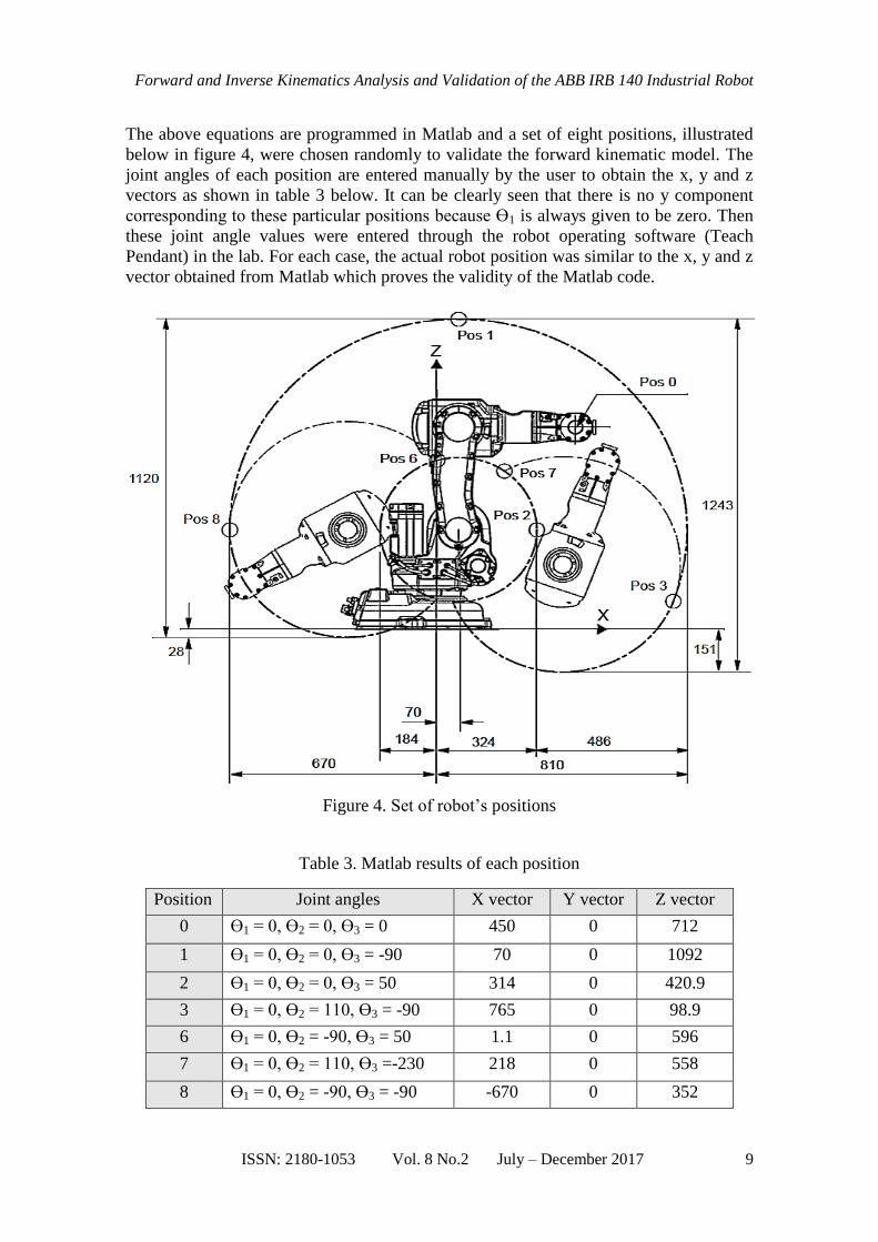
The above equations are programmed in Matlab and a set of eight positions, illustrated

below in figure 4, were chosen randomly to validate the forward kinematic model. The

joint angles of each position are entered manually by the user to obtain the x, y and z

vectors as shown in table 3 below. It can be clearly seen that there is no y component

corresponding to these particular positions because Ɵ1 is always given to be zero. Then

these joint angle values were entered through the robot operating software (Teach

Pendant) in the lab. For each case, the actual robot position was similar to the x, y and z

vector obtained from Matlab which proves the validity of the Matlab code.

Figure 4. Set of robot’s positions

Table 3. Matlab results of each position

Position Joint angles X vector Y vector Z vector

0 Ɵ1 = 0, Ɵ2 = 0, Ɵ3 = 0 450 0 712

1 Ɵ1 = 0, Ɵ2 = 0, Ɵ3 = -90 70 0 1092

2 Ɵ1 = 0, Ɵ2 = 0, Ɵ3 = 50 314 0 420.9

3 Ɵ1 = 0, Ɵ2 = 110, Ɵ3 = -90 765 0 98.9

6 Ɵ1 = 0, Ɵ2 = -90, Ɵ3 = 50 1.1 0 596

7 Ɵ1 = 0, Ɵ2 = 110, Ɵ3 =-230 218 0 558

8 Ɵ1 = 0, Ɵ2 = -90, Ɵ3 = -90 -670 0 352



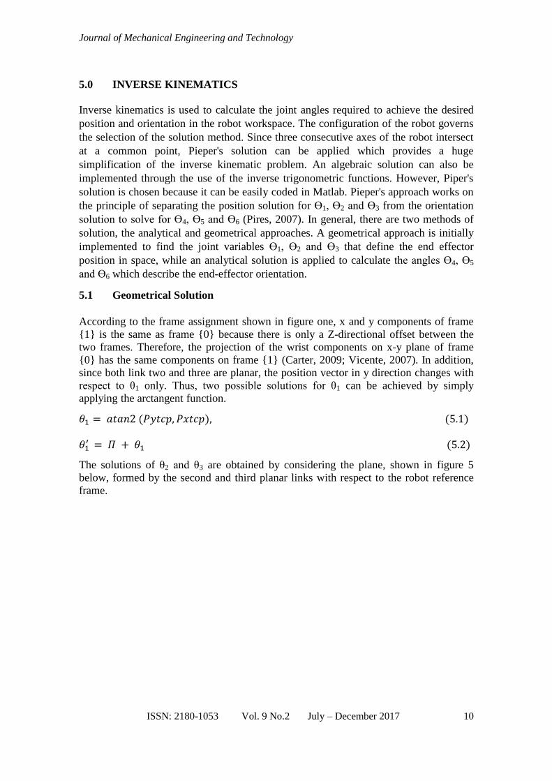
5.0 INVERSE KINEMATICS

Inverse kinematics is used to calculate the joint angles required to achieve the desired

position and orientation in the robot workspace. The configuration of the robot governs

the selection of the solution method. Since three consecutive axes of the robot intersect

at a common point, Pieper's solution can be applied which provides a huge

simplification of the inverse kinematic problem. An algebraic solution can also be

implemented through the use of the inverse trigonometric functions. However, Piper's

solution is chosen because it can be easily coded in Matlab. Pieper's approach works on

the principle of separating the position solution for Ɵ1, Ɵ2 and Ɵ3 from the orientation

solution to solve for Ɵ4, Ɵ5 and Ɵ6 (Pires, 2007). In general, there are two methods of

solution, the analytical and geometrical approaches. A geometrical approach is initially

implemented to find the joint variables Ɵ1, Ɵ2 and Ɵ3 that define the end effector

position in space, while an analytical solution is applied to calculate the angles Ɵ4, Ɵ5

and Ɵ6 which describe the end-effector orientation.

5.1 Geometrical Solution

According to the frame assignment shown in figure one, x and y components of frame

{1} is the same as frame {0} because there is only a Z-directional offset between the

two frames. Therefore, the projection of the wrist components on x-y plane of frame

{0} has the same components on frame {1} (Carter, 2009; Vicente, 2007). In addition,

since both link two and three are planar, the position vector in y direction changes with

respect to θ1 only. Thus, two possible solutions for θ1 can be achieved by simply

applying the arctangent function.

𝜃1 = 𝑎𝑡𝑎𝑛2 (𝑃𝑦𝑡𝑐𝑝, 𝑃𝑥𝑡𝑐𝑝), (5.1)

𝜃1′ = 𝛱 + 𝜃1 (5.2)

The solutions of θ2 and θ3 are obtained by considering the plane, shown in figure 5

below, formed by the second and third planar links with respect to the robot reference

frame.



Figure 5. Projection of links two and three onto the x y plane

The cosine low is used to solve for θ3 as follow:

ℎ2 = 𝐿22 + 𝐿3

2 − 2 𝑥 𝐿2 𝑥 𝐿3 𝑥 𝑐𝑜𝑠 (180 − 𝜁)

Since the position is given with respect to robot’s Tool Center Point (TCP), L3 should

be equal to d4+d6, where d6 is the distance from Joint 6 to the TCP. While,

𝐿2 = 𝑎2 , ℎ2 = 𝑠2 + 𝑟2 , 𝑐𝑜𝑠 (180 − 𝜁) = − 𝑐𝑜𝑠 (𝜁)

𝑠2 + 𝑟2 = 𝑎22 + (𝑑4 + 𝑑6)

2 + 2 𝑥 𝑎2 𝑥 (𝑑4 + 𝑑6 ) 𝑐𝑜𝑠 (𝜁)

𝐶𝑜𝑠 (𝜁) = 𝑠2 + 𝑟2 — 𝑎2

2 — (𝑑4 + 𝑑6)2

2 𝑥 𝑎2 𝑥 (𝑑4 + 𝑑6 ) (5.3)

Now, we should have the value of (s) and (r) in term of Pxtcp, Pytcp, Pztcp and θ1.

𝑆 = (𝑃𝑧𝑡𝑐𝑝 — 𝑑1)

𝑟 = ± √ (𝑃𝑥𝑡𝑐𝑝 — 𝑎1 𝑐𝑜𝑠 (𝜃1))2 + (𝑃𝑦𝑡𝑐𝑝 — 𝑎1 𝑠𝑖𝑛 (𝜃1))2

Sub. (s) and (r) in (5.3) yield:

𝐶𝑜𝑠 (𝜁) =(𝑃𝑧𝑡𝑐𝑝 − 𝑑1)

2+ (𝑃𝑥𝑡𝑐𝑝 − 𝑎1 𝐶𝑜𝑠 𝜃1)

2 + (𝑃𝑦𝑡𝑐𝑝 − 𝑎1 𝑆𝑖𝑛 𝜃1)2 − 𝑎2

2 − (𝑑4 + 𝑑6)2

2 𝑥 𝑎2 𝑥 (𝑑4 + 𝑑6 )



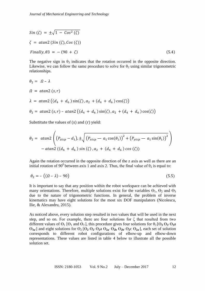
𝑆𝑖𝑛 (𝜁) = ±√1 − 𝐶𝑜𝑠2 (𝜁)

𝜁 = 𝑎𝑡𝑎𝑛2 (𝑆𝑖𝑛 (𝜁), 𝐶𝑜𝑠 (𝜁))

𝐹𝑖𝑛𝑎𝑙𝑙𝑦, 𝜃3 = − (90 + 𝜁) (5.4)

The negative sign in θ3 indicates that the rotation occurred in the opposite direction.

Likewise, we can follow the same procedure to solve for θ2 using similar trigonometric

relationships.

𝜃2 = 𝛺 – 𝜆

𝛺 = 𝑎𝑡𝑎𝑛2 (𝑠, 𝑟)

𝜆 = 𝑎𝑡𝑎𝑛2 ((𝑑4 + 𝑑6 ) sin(𝜁) , 𝑎2 + (𝑑4 + 𝑑6 ) cos(𝜁))

𝜃2 = 𝑎𝑡𝑎𝑛2 (𝑠, 𝑟) – 𝑎𝑡𝑎𝑛2 ((𝑑4 + 𝑑6 ) sin(𝜁) , 𝑎2 + (𝑑4 + 𝑑6 ) cos(𝜁))

Substitute the values of (s) and (r) yield:

𝜃2 = 𝑎𝑡𝑎𝑛2 ((𝑃𝑧𝑡𝑐𝑝 − 𝑑1), ±√ (𝑃𝑥𝑡𝑐𝑝 — 𝑎1 cos(𝜃1))2+ (𝑃𝑦𝑡𝑐𝑝 — 𝑎1 sin(𝜃1))

2 )

− 𝑎𝑡𝑎𝑛2 ((𝑑4 + 𝑑6 ) 𝑠𝑖𝑛 (𝜁) , 𝑎2 + (𝑑4 + 𝑑6 ) 𝑐𝑜𝑠 (𝜁))

Again the rotation occurred in the opposite direction of the z axis as well as there are an

initial rotation of 900

between axis 1 and axis 2. Thus, the final value of θ2 is equal to:

𝜃2 = – ((𝛺 – 𝜆) – 90) (5.5)

It is important to say that any position within the robot workspace can be achieved with

many orientations. Therefore, multiple solutions exist for the variables Ɵ1, Ɵ2 and Ɵ3

due to the nature of trigonometric functions. In general, the problem of inverse

kinematics may have eight solutions for the most six DOF manipulators (Nicolescu,

Ilie, & Alexandru, 2015).

As noticed above, every solution step resulted in two values that will be used in the next

step, and so on. For example, there are four solutions for ζ that resulted from two

different values of Ɵ1 [Ɵ1 and Ɵ1'], this procedure gives four solutions for θ3 [Ɵ3 Ɵ3' Ɵ3a

Ɵ3a'] and eight solutions for Ɵ2 [Ɵ2 Ɵ2' Ɵ2a Ɵ2a' Ɵ2b Ɵ2b' Ɵ2c Ɵ2a'], each set of solution

corresponds to different robot configurations of elbow-up and elbow-down

representations. These values are listed in table 4 below to illustrate all the possible

solution set.



Table 4. Possible solution set

Solution THETA1 THETA3 THETA2 Set

1

Ɵ1

Ɵ3

Ɵ2 SET 1

2 Ɵ2'

3 Ɵ3'

Ɵ2a SET 2

4 Ɵ2a'

5

Ɵ1'

Ɵ3a

Ɵ2b SET 3

6 Ɵ2b'

7 Ɵ3a'

Ɵ2c SET 4

8 Ɵ2c'

5.2 Analytical Solution

After solving the first inverse kinematic sub-problem which gives the required position

of the end effector, the next step of the inverse kinematic solution will deal with the

procedure of solving the orientation sub-problem to find the joint angles Ɵ4, Ɵ5 and Ɵ6.

This can be done using Z-Y-X Euler's formula. As the orientation of the tool frame with

respect to the robot base frame is described in term of Z-Y-X Euler's rotation, this

means that each rotation will take place about an axis whose location depends on the

previous rotation (Craig, 2005). The Z-Y-X Euler's rotation is shown below in figure 6.

Figure 6. Z—Y—X Euler rotation

The final orientation matrix that results from these three consecutive rotations will be as

follow:

𝑅60 = Rz'y'x' = Rz (α) Ry (β) Rx (γ)

𝑅60 = (

𝑐α −𝑠α 0𝑠α 𝑐α 00 0 1

) 𝑋 (𝑐β 0 𝑠β

0 1 0−𝑠β 0 𝑐β

) 𝑋 (

1 0 0 0 𝑐γ −𝑠γ0 𝑠γ 𝑐γ

)

𝑅60 = (

𝑐α𝑐β 𝑐α𝑠β𝑠γ − 𝑠α𝑐γ 𝑐α𝑠β𝑐γ + 𝑠α𝑠γ

𝑠α𝑐β 𝑠α𝑠β𝑠γ + 𝑐α𝑐γ 𝑠α𝑠β𝑐γ − 𝑐α𝑠γ−𝑠β 𝑐β𝑠γ 𝑐β𝑐γ

)



Recall the forward kinematic equation,

𝑅30 = (

𝑐1𝑐23 −𝑐1𝑠23 −𝑠1𝑠1𝑐23 −𝑠1𝑠23 𝑐1−𝑠23 −𝑐23 0

)

𝑅63 = ( 𝑅) 𝑅6

𝑇 030

𝑅63 = (

𝑐1𝑐23 𝑠1𝑐23 −𝑠23−𝑐1𝑠23 −𝑠1𝑠23 −𝑐23−𝑠1 𝑐1 0

)𝑥 (

𝑐α𝑐β 𝑐α𝑠β𝑠γ − 𝑠α𝑐γ 𝑐α𝑠β𝑐γ + 𝑠α𝑠γ

𝑠α𝑐β 𝑠α𝑠β𝑠γ + 𝑐α𝑐γ 𝑠α𝑠β𝑐γ − 𝑐α𝑠γ−𝑠β 𝑐β𝑠γ 𝑐β𝑐γ

)

𝑅63 = (

𝑔11 𝑔12 𝑔13𝑔21 𝑔22 𝑔23𝑔31 𝑔32 𝑔33

)

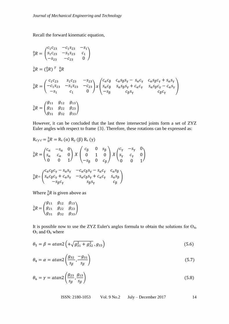
However, it can be concluded that the last three intersected joints form a set of ZYZ

Euler angles with respect to frame {3}. Therefore, these rotations can be expressed as:

Rz'y'z' = 𝑅63 = Rz (α) Ry (β) Rz (γ)

𝑅63 = (

𝑐α −𝑠α 0𝑠α 𝑐α 00 0 1

) 𝑋 (𝑐β 0 𝑠β

0 1 0−𝑠β 0 𝑐β

) 𝑋 (

𝑐γ −𝑠γ 0

𝑠γ 𝑐γ 0

0 0 1

)

𝑅63 = (

𝑐α𝑐β𝑐γ − 𝑠α𝑠γ −𝑐α𝑐β𝑠γ − 𝑠α𝑐γ 𝑐α𝑠β

𝑠α𝑐β𝑐γ + 𝑐α𝑠γ −𝑠α𝑐β𝑠γ + 𝑐α𝑐γ 𝑠α𝑠β−𝑠β𝑐γ 𝑠β𝑠γ 𝑐β

)

Where 𝑅63 is given above as

𝑅63

= (

𝑔11 𝑔12 𝑔13𝑔21 𝑔22 𝑔23𝑔31 𝑔32 𝑔33

)

It is possible now to use the ZYZ Euler's angles formula to obtain the solutions for Ɵ4,

Ɵ5 and Ɵ6 where

𝜃5 = 𝛽 = 𝑎𝑡𝑎𝑛2 (+√𝑔312 + 𝑔32

2 , 𝑔33) (5.6)

𝜃4 = 𝛼 = 𝑎𝑡𝑎𝑛2(𝑔32 𝑠𝛽,−𝑔31𝑠𝛽

) (5.7)

𝜃6 = 𝛾 = 𝑎𝑡𝑎𝑛2(𝑔23𝑠𝛽,𝑔13𝑠𝛽) (5.8)



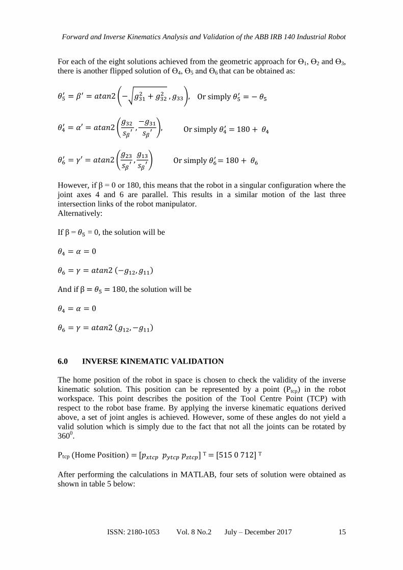
For each of the eight solutions achieved from the geometric approach for Ɵ1, Ɵ2 and Ɵ3,

there is another flipped solution of Ɵ4, Ɵ5 and Ɵ6 that can be obtained as:

𝜃5′ = 𝛽′ = 𝑎𝑡𝑎𝑛2 (−√𝑔31

2 + 𝑔322 , 𝑔33),

𝜃4′ = 𝛼′ = 𝑎𝑡𝑎𝑛2(

𝑔32 𝑠𝛽′

,−𝑔31𝑠𝛽′

),

𝜃6′ = 𝛾′ = 𝑎𝑡𝑎𝑛2(

𝑔23𝑠𝛽′,𝑔13𝑠𝛽′)

However, if β = 0 or 180, this means that the robot in a singular configuration where the

joint axes 4 and 6 are parallel. This results in a similar motion of the last three

intersection links of the robot manipulator.

Alternatively:

If β = 𝜃5 = 0, the solution will be

𝜃4 = 𝛼 = 0 𝜃6 = 𝛾 = 𝑎𝑡𝑎𝑛2 (−𝑔12, 𝑔11) And if β = 𝜃5 = 180, the solution will be

𝜃4 = 𝛼 = 0 𝜃6 = 𝛾 = 𝑎𝑡𝑎𝑛2 (𝑔12, −𝑔11)

6.0 INVERSE KINEMATIC VALIDATION

The home position of the robot in space is chosen to check the validity of the inverse

kinematic solution. This position can be represented by a point (Ptcp) in the robot

workspace. This point describes the position of the Tool Centre Point (TCP) with

respect to the robot base frame. By applying the inverse kinematic equations derived

above, a set of joint angles is achieved. However, some of these angles do not yield a

valid solution which is simply due to the fact that not all the joints can be rotated by

3600.

Ptcp (Home Position) = [𝑝𝑥𝑡𝑐𝑝 𝑝𝑦𝑡𝑐𝑝 𝑝𝑧𝑡𝑐𝑝] T = [515 0 712] T

After performing the calculations in MATLAB, four sets of solution were obtained as

shown in table 5 below:

Or simply 𝜃4′ = 180 + 𝜃4

Or simply 𝜃5′ = − 𝜃5

Or simply 𝜃6′ = 180 + 𝜃6



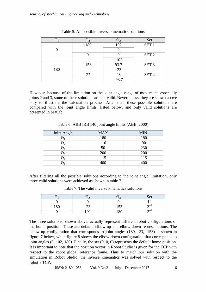
Table 5. All possible Inverse kinematics solutions

Ɵ1 Ɵ3 Ɵ2 Set

0

-180

102 SET 1

0

0

0 SET 2

-102

180

-153

93.7 SET 3

-23

-27

23 SET 4

-93.7

However, because of the limitation on the joint angle range of movement, especially

joints 2 and 3, some of these solutions are not valid. Nevertheless, they are shown above

only to illustrate the calculation process. After that, these possible solutions are

compared with the joint angle limits, listed below, and only valid solutions are

presented in Matlab.

Table 6. ABB IRB 140 joint angle limits (ABB, 2000)

Joint Angle MAX MIN

Ɵ1 180 -180

Ɵ2 110 -90

Ɵ3 50 -230

Ɵ4 200 -200

Ɵ5 115 -115

Ɵ6 400 -400

After filtering all the possible solutions according to the joint angle limitation, only

three valid solutions were achieved as shown in table 7.

Table 7. The valid inverse kinematics solutions

Ɵ1 Ɵ2 Ɵ3 Set

0 0 0 1st

180 -23 -153 2nd

0 102 -180 3rd

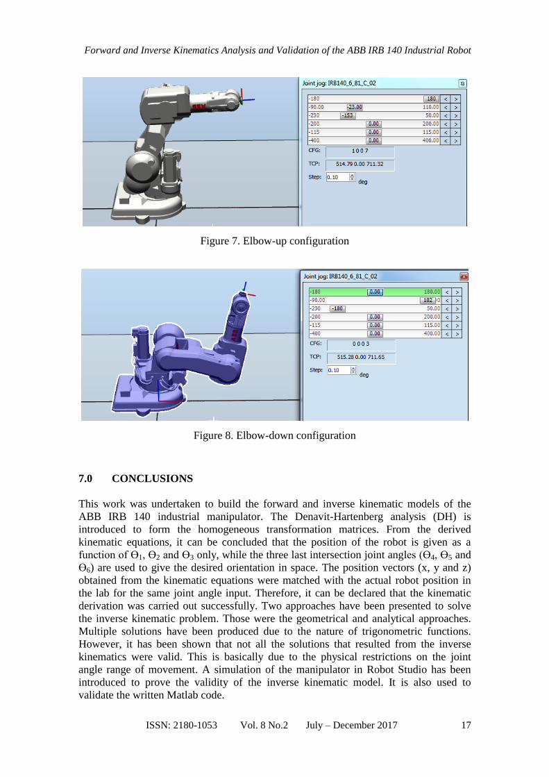
The three solutions, shown above, actually represent different robot configurations of

the home position. These are default, elbow-up and elbow-down representations. The

elbow-up configuration that corresponds to joint angles (180, -23, -153) is shown in

figure 7 below, while figure 8 shows the elbow-down configuration that corresponds to

joint angles (0, 102, 180). Finally, the set (0, 0, 0) represents the default home position.

It is important to note that the position vector in Robot Studio is given for the TCP with

respect to the robot global reference frame. Thus to match our solution with the

simulation in Robot Studio, the inverse kinematics was solved with respect to the

robot’s TCP.



Figure 7. Elbow-up configuration

Figure 8. Elbow-down configuration

7.0 CONCLUSIONS

This work was undertaken to build the forward and inverse kinematic models of the

ABB IRB 140 industrial manipulator. The Denavit-Hartenberg analysis (DH) is

introduced to form the homogeneous transformation matrices. From the derived

kinematic equations, it can be concluded that the position of the robot is given as a

function of Ɵ1, Ɵ2 and Ɵ3 only, while the three last intersection joint angles (Ɵ4, Ɵ5 and

Ɵ6) are used to give the desired orientation in space. The position vectors (x, y and z)

obtained from the kinematic equations were matched with the actual robot position in

the lab for the same joint angle input. Therefore, it can be declared that the kinematic

derivation was carried out successfully. Two approaches have been presented to solve

the inverse kinematic problem. Those were the geometrical and analytical approaches.

Multiple solutions have been produced due to the nature of trigonometric functions.

However, it has been shown that not all the solutions that resulted from the inverse

kinematics were valid. This is basically due to the physical restrictions on the joint

angle range of movement. A simulation of the manipulator in Robot Studio has been

introduced to prove the validity of the inverse kinematic model. It is also used to

validate the written Matlab code.



8.0 REFERENCES

ABB. (2000). IRB 140 M2000 Product Specification. Retrieved December 01, 2015

http://www.abb.com

Carter, T. J. (2009). The Modeling of a Six Degree-of-freedom Industrial Robot for the

Purpose of Efficient Path Planning. The Pennsylvania State University.

Craig, J. J. (2005). Introduction to robotics: mechanics and control: Pearson/Prentice

Hall Upper Saddle River, NJ, USA:.

Deshpande, V. A., & George, P. (2012). Analytical Solution for Inverse Kinematics of

SCORBOT-ER-Vplus Robot. International Journal of Emerging Technology

and Advanced Engineering, 2(3).

Feng, Y., Yao-nan, W., & Yi-min, Y. (2014). Inverse kinematics solution for robot

manipulator based on neural network under joint subspace. International

Journal of Computers Communications & Control, 7(3), 459-472.

Jazar, R. N. (2010). Theory of applied robotics (Vol. 1): Springer.

Khatamian, A. (2015). Solving Kinematics Problems of a 6-DOF Robot Manipulator.

Paper presented at the Proceedings of the International Conference on Scientific

Computing (CSC).

Mitra, A. K. (2012). Joint Motion-based Homogeneous Matrix Method for Forward

Kinematic Analysis of Serial Mechanisms. Int. J. Emerg. Technol. Adv. Eng, 2,

111-122.

Neppalli, S., Csencsits, M. A., Jones, B. A., & Walker, I. D. (2009). Closed-form

inverse kinematics for continuum manipulators. Advanced Robotics, 23(15),

2077-2091.

Nicolescu, A.-F., Ilie, F.-M., & Alexandru, T.-G. (2015). Forward and Inverse

Kinematics Study of Industrial Robots Taking into Account Constructive and

Functional Parameter's Moduling. Proceedings in Manufacturing Systems,

10(4), 157.

Paul, R. P. (1981). Robot manipulators: mathematics, programming, and control: the

computer control of robot manipulators: Richard Paul.

Pires, J. N. (2007). Industrial robots programming: building applications for the

factories of the future: Springer.

Samer Y, H. A., Moghavvemi M. (2009). A New Geometrical Approach for the Inverse

Kinematics of the Hyper Redundant Equal Length Links Planar Manipulators.

http://www.abb.com/



Selig, J. (2013). Geometrical methods in robotics: Springer Science & Business Media.

Shahinpoor, M. (1987). A robot engineering textbook: Harper & Row Publishers, Inc.

Siciliano, B., Sciavicco, L., Villani, L., & Oriolo, G. (2010). Robotics: modelling,

planning and control: Springer Science & Business Media.

Spong, M. W., Hutchinson, S., & Vidyasagar, M. (2006). Robot modeling and control

(Vol. 3): Wiley New York.

Uicker, J. J., Pennock, G. R., & Shigley, J. E. (2011). Theory of machines and

mechanisms (Vol. 1): Oxford University Press New York.

Vicente, D. B. (2007). Modeling and Balancing of Spherical Pendulum Using a

Parallel Kinematic Manipulator.

KINEMATICS ASSIGNMENT - UTeM OPEN JOURNAL SYSTEM

Documents

Transcript of KINEMATICS ASSIGNMENT - UTeM OPEN JOURNAL SYSTEM