Rectangular grid drawings of plane graphs

ELSEVIER Computational Geometry 10 (1998) 203-220

Computational Geomet ry

Theory and Applications

Rectangular grid drawings of plane graphs Md. Saidur Rahman 1, Shin-ichi Nakano *, Takao Nishizeki 2 Graduate School of lnformation Sciences, Tohoku University, Sendai 980-77, Japan

Communicated by R. Tamassia; submitted 31 March 1997; accepted 7 January 1998

Abstract

The rectangular grid drawing of a plane graph G is a drawing of G such that each vertex is located on a grid point, each edge is drawn as a horizontal or vertical line segment, and the contour of each face is drawn as a rectangle. In this paper we give a simple linear-time algorithm to find a rectangular grid drawing of G if it exists. We also give an upper bound W + H <~ n /2 on the sum of required width W and height H and a bound W H <. n2/16 on the area of a rectangular grid drawing of G, where n is the number of vertices in G. These bounds are best possible, and hold for any compact rectangular grid drawing. © 1998 Elsevier Science B.V.

Keywords: Algorithm; Rectangular drawing; Grid drawing; Grid area; Floorplanning

1. Introduction

Recently automatic drawing of graphs has created intense interest due to its broad applications to represent various concepts and objects in software, computer architecture, networks, VLSI circuits, etc. [6]. One important criteria of a graph drawing is that it should be easily understandable and good looking [4,14,19]. In this paper we thus consider the rectangular drawing of a plane graph, where each edge of the graph is drawn as a horizontal or vertical line segment with no bend and the contour of each face is drawn as a rectangle as illustrated in Fig. l(a). Our input graph G has four vertices of degree 2 on its outer face and all other vertices have degree 3. It is not always possible to draw such a graph in this way. For example, the graph in Fig. 2 has no rectangular drawing. Thomassen obtained a necessary and sufficient condition for such a plane graph to have a rectangular drawing [22]. His proof does not look to lead to an efficient algorithm for rectangular drawing; a straightforward implementation of his method requires at least O(n 3) time, where n is the number of vertices in G.

On the other hand, Kozminski and Kinnen [12] established a necessary and sufficient condition for the existence of a "rectangular dual" of a plane graph, that is a rectangular drawing of the dual

* Corresponding author. E-maih [email protected]. E-mail: saidur @ nishizeki.ecei.tohoku.ac.j p.

2 E-maih nishi @ ecei.tohoku.ac.jp.

0925-7721/98/$19.00 © 1998 Elsevier Science B.V. All rights reserved. PII S0925-7721 (98)00003-0

204 Md.S. Rahman et al. / Computational Geometry 10 (1998) 203-220

P W

U 4

V l V 2 V:

4

! :,:

u 3

PS

(a)

u 2 ul Uo

G ~.C w

(b)

Pc

pZ C

(c) c~ (d) G 2

Fig. I. A rectangular grid drawing of a plane graph and patching.

, / w

Fig. 2. A graph with no rectangular drawing.

Md.S. Rahman et al. / Computational Geometry 10 (1998) 203-220 205

graph of a given plane graph, and gave an O(n 2) algorithm to obtain it. Since a rectangular dual has practical applications on VLSI floorplan [13,21], much attention has been paid to [12]. Based on the characterization of [12], Bhasker and Sahni [1] and He [8], respectively, developed linear-time algorithms to find a rectangular dual of a plane graph. Recently Kant and He [11] presented two more linear-time algorithms. The algorithm in [1] is fairly complicated and consists of two steps: (1) finding a "regular edge labeling" of G, and (2) constructing the rectangular dual using that labeling. He [8] simplified step (2), but used the complicated algorithm in [1] for step (1). Two methods for simplifying step (1) are given in [11]. The first one finds a regular edge labeling using "edge contraction and edge expansion techniques" and is indeed not a simple method. The second one finds a "canonical ordering" of the given graph in linear time and then obtains a regular edge labeling from the canonical ordering in linear time.

The two works [12,22] were completely independent. Since there exists a linear-time algorithm to find the dual graph of a plane graph, algorithms in [1,8,1 l] can be used to find a rectangular drawing of a given plane graph and also Thomassen's characterization can be applied to VLSI floorplan problems.

A drawing in which each vertex is located at a grid point is called a grid drawing. It is a very challenging problem to draw a plane graph on a grid of the minimum size. In recent years, several works are devoted to this field [2,3,5,7,10,16,18,20]; for example, any plane graph with n vertices has a straight line drawing on a grid of area W H ~< (n - 1)2, where W is the width and H is the height of the grid. In the straight line drawing, edges are drawn by straight line segments, not necessarily by horizontal or vertical line segments.

In this paper we first give a new constructive proof of Thomassen's characterization, and then derive from the proof a simple algorithm to find a rectangular grid drawing of a plane graph in linear time. Our algorithm is completely different from those of [1,8,11], and is simple: we do not need to find any regular edge labeling or a canonical ordering, and our algorithm directly finds a rectangular grid drawing using a depth-first search. We also give upper bounds W H <~ n2/16 on the the area and W + H ~< n / 2 on the sum of width and height of rectangular grid drawings. These bounds are interesting in a sense that they are best possible and hold for any "compact" rectangular grid drawing of a plane graph.

The rest of the paper is organized as follows. Section 2 introduces some definitions and presents a characterization of plane graphs having rectangular drawings. Section 3 gives a rectangular drawing algorithm and shows that the algorithm takes linear time. Section 4 deals with rectangular grid drawings and upper bounds on the area and on the sum of width and height of the grid. Finally, Section 5 concludes with discussions and some open problems. An early version of the paper has been presented at [15].

2. Characterization of rectangular drawings

In this section we introduce some definitions and then prove a necessary and sufficient condition for a plane graph to have a rectangular drawing.

Let G = (V, E) be a 2-connected graph with vertex set V and edge set E. We denote the set of vertices of G by V(G), and the set of edges of G by E(G). An edge joining vertices u and v is denoted by uv. The union G = G t U G" of two graphs G I and G" is a graph G = (V(G I) U


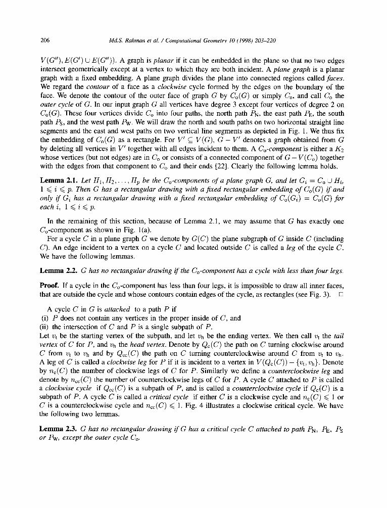
V(G"), E(G') U E(G")). A graph is planar if it can be embedded in the plane so that no two edges intersect geometrically except at a vertex to which they are both incident. A plane graph is a planar graph with a fixed embedding. A plane graph divides the plane into connected regions called faces. We regard the contour of a face as a clockwise cycle formed by the edges on the boundary of the face. We denote the contour of the outer face of graph G by Co(G) or simply Co, and call Co the outer cycle of G. In our input graph G all vertices have degree 3 except four vertices of degree 2 on Co(G). These four vertices divide Co into four paths, the north path PN, the east path RE, the south path Ps, and the west path Pw. We will draw the north and south paths on two horizontal straight line segments and the east and west paths on two vertical line segments as depicted in Fig. 1. We thus fix the embedding of Co(G) as a rectangle. For V t c_ V(G), G - W denotes a graph obtained from G by deleting all vertices in V ~ together with all edges incident to them. A Co-component is either a K2 whose vertices (but not edges) are in Co or consists of a connected component of G - V(Co) together with the edges from that component to Co and their ends [22]. Clearly the following lemma holds.

Lemma 2.1. Let H1, H 2 , . . . , Hp be the Co-components of a plane graph G, and let Gi = Co U Hi, 1 <<, i <~ p. Then G has a rectangular drawing with a fixed rectangular embedding of Co(G) if and only if Gi has a rectangular drawing with a fixed rectangular embedding of Co(Gi) = Co(G) for each i, 1 <<, i <<, p.

In the remaining of this section, because of Lemma 2.1, we may assume that G has exactly one Co-component as shown in Fig. 1 (a).

For a cycle C in a plane graph G we denote by G(C) the plane subgraph of G inside C (including C). An edge incident to a vertex on a cycle C and located outside C is called a leg of the cycle C. We have the following lemmas.

Lemma 2.2. G has no rectangular drawing if the Co-component has a cycle with less than four legs.

Proof. If a cycle in the Co-component has less than four legs, it is impossible to draw all inner faces, that are outside the cycle and whose contours contain edges of the cycle, as rectangles (see Fig. 3). []

A cycle C in G is attached to a path P if (i) P does not contain any vertices in the proper inside of C, and

(ii) the intersection of C and P is a single subpath of P. Let vt be the starting vertex of the subpath, and let Vh be the ending vertex. We then call vt the tail vertex of C for P, and vh the head vertex. Denote by Qc (C) the path on C turning clockwise around C from vt to vh and by Qcc(C) the path on C turning counterclockwise around C from vt to vh. A leg of C is called a clockwise leg for P if it is incident to a vertex in V(Qc(C)) - {vt, Vh}. Denote by n~(C) the number of clockwise legs of C for P. Similarly we define a counterclockwise leg and denote by ncc (C) the number of counterclockwise legs of C for P. A cycle C attached to P is called a clockwise cycle if Qcc(C) is a subpath of P, and is called a counterclockwise cycle if Qc(C) is a subpath of P. A cycle C is called a critical cycle if either C is a clockwise cycle and nc(C) ~< 1 or C is a counterclockwise cycle and ncc (C) ~< 1. Fig. 4 illustrates a clockwise critical cycle. We have the following two lemmas.

Lemma 2.3. G has no rectangular drawing if G has a critical cycle C attached to path PN, PE, Ps or Pw, except the outer cycle Co.


face leg

face face ] leg

Fig. 3. Illustration for Lemma 2.2.

v, gO4C)

vt P

counterclockwise legs

. . . . . . . . . . . . . . . . . . . . . . . . . . . .

Q (c) C C

.......... c!°ck.wise

Qc (C)

leg

Fig. 4. Clockwise critical cycle C attached to path P.

P vt u Qd C ) vh

P~ face

(c) C c P~ e~

face 1

? (c) ¢ c

I

' face 2

P~

P~ P~

(a) (b)

Fig. 5. Illustration for Lemma 2.3. (a) Case when nee(C) = 0. (b) Case when nc~(C) = 1.

Proof. If G has a critical cycle C attached to path PN, PE, Ps or Pw, then it is impossible to draw all inner faces, that are outside C and whose contours contain edges of Qcc(C), as rectangles (see Fig. 5). []

L e m m a 2.4. G has no rectangular drawing if G has a cycle C with ncc(C) -- 0 attached to path P -- PN + PE, PE + Ps, Ps + Pw, or Pw + PN, except the outer cycle Co.

Proof. It is impossible to draw the inner face, which is outside C and whose contour contains Qcc(C), as a rectangle (see Fig. 6). []

A Co-component is called a bad component if it satisfies either Lemma 2.2 or Lemma 2.3 or Lemma 2.4. In particular, we call the Co-component mentioned in Lemma 2.4 a bad corner. We now have the following theorem on the necessary and sufficient condition for a graph to have a rectangular drawing.


P~ Q (c)

c c

P~

P~

Fig. 6. Illustration for Lemma 2.4.

Theorem 2.5. Let G be a plane graph such that all vertices have degree 3 except for the four corner vertices of degree 2 dividing the outer cycle Co into four paths PN, PE, Ps and Pw. Then G has a rectangular drawing if and only if G has no bad component.

Theorem 2.5 is essentially equivalent to Thomassen's characterization [22, Theorem 7.1], although the presentations are different. The proof of the necessity of Theorem 2.5 immediately follows from Lemmas 2.2-2.4. In the remaining of this section we give a constructive proof of the sufficiency, which will yield a linear time algorithm to find a rectangular grid drawing of G. We thus assume that G has no bad component.

Let PN = V0Vl, V l v2 , . . . , Vp_ 1Vp and Ps = u0ul, u l u2, • • • , Uq_ 1 Uq. An NS-path is defined to be a path starting at a vertex vi on PN and ending at a vertex uj on Ps without passing through any other vertex on Co. An NS-path P divides graph G into two subgraphs GPw and GP; G P is the west part of G including P , and G P is the east part of G including P. Drawing P as a straight line segment, we fix the embedding of Co(G P) as a rectangle with the north path P~ = roY1, vlv2,..., vi-lvi, the east path r P~ = P , the south path P~ = u~Uj+l,Uj+lUj+2,... ~Uq--lU q, and the west path P~v = Pw. Similarly we fix the embedding of Co(G~) as a rectangle. We say that P is an NS-partitioning path if neither G P nor G P has a bad component. Similarly we define SN-, WE- and EW-partitioning paths. If G has a partitioning path, say an NS-partitioning path P, then one can obtain a rectangular drawing of G by recursively finding rectangular drawings of GPw and G P and patching them together along P.

An inner face of G is called a boundary face if its contour contains at least one edge of Co. A boundary path is a maximal (directed) path on the contour of a boundary face connecting two vertices on Co without passing through any edge on Co. Note that the direction of a boundary path is the same as the contour of the face, and hence is clockwise. For X, Y E {N, E, S, W}, a boundary XY-path is a boundary path starting at a vertex on Px and ending at a vertex on PY. We have the following lemma.

Lemma 2.6. Any boundary NS-, SN-, EW- or WE-path P of G is a partitioning path.

Proofi One may assume that P is a boundary NS-path. Then P divides G into two subgraphs G P and G~. We shall show that neither G P nor GE P has a bad component. Since P is a boundary NS-path, G(v is a cycle and hence GPw has no bad component. If G P is also a cycle, then obviously GE P has no bad component. Thus one may assume that GE P is not a cycle. If GE P has a bad component mentioned


in Lemma 2.2, then it is also a bad component in G, a contradiction. If GE P has a bad component mentioned in Lemma 2.3, then GE P contains a critical cycle attached to P, and hence G contains a bad component as in Lemma 2.2, a contradiction. If GE P has a bad corner as in Lemma 2.4, then either G has a bad corner or G contains a bad component as in Lemma 2.3, a contradiction. Thus P is a partitioning path. []

Thus we may assume that G has none of boundary NS-, SN-, EW- and WE-paths. Then the Co- component has at least one vertex on each of the paths PN, PE, Ps and Pw. In this case we find a pair of partitioning paths Pc and Pcc instead of a single partitioning path, and divide G into two or more subgraphs having no bad components by splitting G along Pc and Pcc. Both Pc and Pcc are NS-paths which have the same ends and do not cross each other in the plane although they share several edges. Thus, if Pc ~ Pcc, then E(Pc) • E(Pcc) = E(Pc) O E(Pcc) - E(Pc) (q E(Pcc) induces vertex-disjoint cycles C1, C2 , . . . , Ck, k >~ 1, as illustrated in Fig. 7. Thus Pc and Pcc share k + 1 maximal subpaths P1, P2, . . . , Pk+l. We assume that Pc turns around cycles C1, C2 , . . . , Ck clockwise, and Pcc tums around them counterclockwise. We choose Pc and Pcc so that each cycle Ci has exactly four legs; assuming clockwise order, the first one is contained in Pi, the second one is a clockwise leg, the third one is contained in Pi+l and the fourth one is a counterclockwise leg. Thus G is divided into ~Pcc

" ~ ' W '

GI~, G(C1 ), G(C2), G(Ck). In Fig. l(a) Pc and Pcc are indicated by dotted lines. Fig. l(b) depicts E ' " ' " ~

four subgraphs, "~w~PCc, GEPC, G(C1) and G(C2), obtained by splitting G in Fig. l(a) along Pc and Pcc. We now have the following lemma.

Lemma 2.7. Assume that G has no bad component and that a cycle C in the Co-component has exactly four legs dividing C into four paths P~, P~, P~ and P~v" Then the subgraph G(C) of G inside C has no bad component for any rectangular embedding of C fixed by P~, P~, P~ and P~v.

i , N

Fig. 7. Partition-pair Pc and Pcc indicated by dotted lines.


Proof. If G(C) has a bad component for a rectangular embedding of C fixed by P~, /3,~, P~ and P~v, then it is also a bad component in G as mentioned in Lemma 2.2, a contradiction to the assumption that G has no bad component. []

By Lemma 2.7 we can assume that none of G(CI), G(C2),..., G(Ck) has a bad component for any fixed rectangular embeddings of C1, C2, . . . , Ck. For each cycle Ci, 1 ~< i ~< k, there are two alternative rectangular embeddings of Ci as illustrated in Fig. 8. Therefore there are 2 t¢ different embeddings of cycles C1, C2 , . . . , Ck where Pc and Pcc are embedded as alternating sequences of horizontal and vertical line segments (see Fig. 9). We can arbitrarily choose one of them, since none of G(CI) ,G(C2) , . . . ,G(Ck) has a bad component for any fixed rectangular embeddings of Cj, C2, • • •, Ck. Let G1 be the graph obtained from Gv~ c by contracting all edges of Pcc that are on the horizontal sides of rectangular embeddings of C1, C2 , . . . , Ck. (Contracting an edge e = vw means removing it and identifying its ends v and w so that the resulting vertex is incident with those edges

Pu Pu

Pw

P

iiiii!i!!i~!~iii~!!i:i!F~:i!ii!~ii~ii~i~i!iiiii!ii!iiiiiiiiiiiiiiiiiiiiiii!iiiiii iiii:i!ii!i iiiiiiiiiii iiiiliiiiiiiiiiiiiiii!iiiii:ii!iiiiiiili!il p-

Ps" P

P Pw E

P

p,, E P

E

Ps Ps

Fig. 8. Two alternative rectangular embeddings of cycle C~.

PN

P~ Pcc

G w Pc G e

f !

1 es

&

Fig. 9. An example of the embedding of a partition-pair.


(other than e) that were originally incident with v or w.) We denote by Pc~c the resulting path obtained from Pcc by the contraction above (see Fig. l(c)). Then one can observe that if G1 has a rectangular drawing with fixing the path Pc~c as a vertical straight line segment, then the rectangular drawing of G1 can be easily modified to a drawing of Gv~ c fitted in the area for Gv~ c where Poe is drawn as an alternating sequence of horizontal and vertical line segments. Let G2 be the graph obtained from G ( ~ by contracting all edges of Pc that are on the horizontal sides of rectangular embeddings of C1, C 2 , . . . , Ck and let Pc ~ be the resulting path obtained from Pc by the contraction (see Fig. l(d)). Then, if G2 has a rectangular drawing, it can be easily modified to a drawing of G~ ~ fitted in the area

for G~ ~ where Pc is drawn as an alternating sequence of horizontal and vertical line segments. Thus

~P~ ~P~ G(C1) G(C2), . . G(Ck), then we can immediately patch if we have drawings of graphs "-'w , "-'E , , •, them to get a rectangular drawing of G. One can observe that G1 and G2 have no bad components if and only if Gv~ c and G~ ~ have no bad components when Pcc and Pc are fixed as straight line segments, respectively. Note that Pc~c and P~ are obtained from Pcc and Pc, respectively, by contracting those edges which are on the horizontal sides of the rectangular embeddings of C1, C2 , . . . , Ck, and that all the vertices on these horizontal sides except the ends have degree 2 in G ~ ~ or G~ ~. We thus call

Pc and Pcc a pair of partitioning paths or simply a partition-pair if neither G~ c nor G ~ ~ has a bad component. Especially when Pc = Pcc, it is a single partitioning path.

In Fig. l(a), for the pair of partitioning paths Pc and Pcc indicated by dotted lines, there are two cycles Ci and C2, i.e., k = 2. Figs. l(c) and (d) depict rectangular drawings of G1 and G2, and Fig. l(b) depicts their modifications Gv~ ~ and G~ ° fitted in the areas with alternating sequences of horizontal and vertical line segments. Rectangular drawings of G(C1) and G(C2) are also depicted in Fig. l(b). These can be patched into a rectangular drawing of G shown in Fig. l(a).

Thus the problem is how to find a partition-pair efficiently. Our idea is to find a partition-pair from the "westmost NS-path" defined as follows. An NS-path P is westmost if (1) P starts at Vl, (2) P ends at Uq-1, and (3) the number of edges in Gv~ is minimum. The westmost NS-path is drawn in thick lines in Fig. l(a). One can find the westmost NS-path by the "counterclockwise depth-first search" starting from Vl, that is, a depth-first search where the edge counterclockwise next to the currently visited edge is searched in each step.

The Co-component may have cycles attached to the westmost NS-path P. Clearly all these cycles are clockwise attached to P. Either the proper insides of any two of the cycles are disjoint or one is contained in the other. A cycle among them is said to be maximal if its inside is not contained in the inside of any other cycle. Fig. 10 illustrates the hierarchical structure of the cycles, where the westmost path P is drawn on a vertical line and the insides of seven maximal critical cycles Cml, Cruz,-.-, Cm7 are shaded.

Lenuna 2.8. If G has no bad component and has none of boundary NS-, SN-, EW- and WE-paths, then G has a partition-pair Pc and Pcc-

Proof. Assume that G has no bad component and has none of boundary NS-, SN-, EW- and WE- paths. Then we can find a partition-pair Pc and Pcc from the westmost NS-path P -- el, e2 , . . . , ej as follows.


w l

......

P

ebi ~¢r ( " . . . .

,i!i:iiiiiiii ' . . ~ . r _ I

?s Fig. lO. Clockwise critical cycles attached to the westmost NS-path P .

Firstly, we find two paths Pst and Pen; /)st is the starting subpath shared by Pc and Pcc, and Pen is the ending subpath shared by Pc and Pcc. Let a be the largest index among 1 ,2 , . . . , j such that ea E E ( P ) is contained in a boundary NN- or EN-path, say Q . . . . , e a , w l w 2 , . . . ,wz- lwt , where wl E V(PN) (see Fig. 10). Choose Pst = w l w l - 1 , . . . , w2wl, ea. Similarly, let b be the smallest index such that eb E E ( P ) is contained in a boundary SS- or SE-path, say R = z l x 2 , . . . , Xr-lXr, e b , . . . , where Xl E V(Ps). Choose Pen -- eb, x r x r - 1 , . . . ,x2xl . Then a < b; otherwise, there would exist a

pt boundary SN-path. Furthermore, neither GE P' nor G w has a bad comer for any NS-path p / whose


starting subpath is Pst and ending subpath is Pen; otherwise, a contradiction either to the selection of Pst and Pen or to the assumption that G has no bad component would occur.

Secondly, if an edge among ca, Ca+l, • • •, eb on P is not contained in any maximal critical cycle C attached to P, then we let both Pc and Pcc pass through it, that is, we include it in a common subpath Pl, P 2 , . . . , or Pk+l. (We will give the detail how to find maximal critical cycles later in Section 3.)

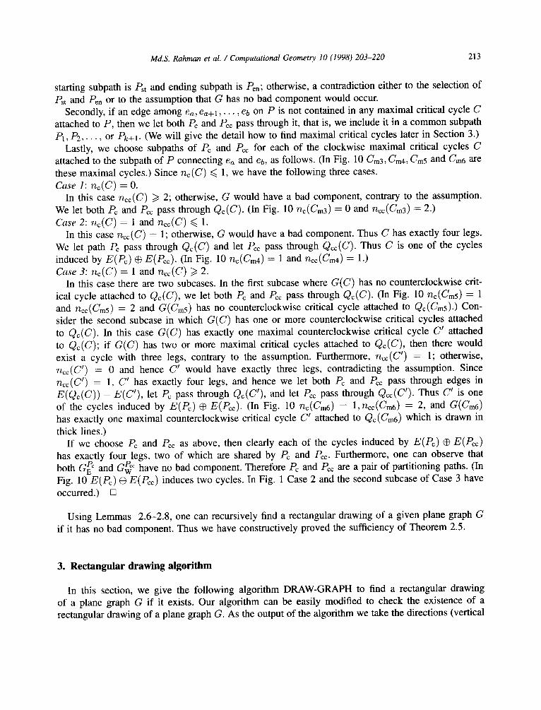
Lastly, we choose subpaths of Pc and Pcc for each of the clockwise maximal critical cycles C attached to the subpath of P connecting ea and eb, as follows. (In Fig. 10 Cm3, Cm4, Cm5 and Cm6 are these maximal cycles.) Since nc(C) ~< 1, we have the following three cases. Case 1: nc(C) = 0.

In this case nee(C) >~ 2; otherwise, G would have a bad component, contrary to the assumption. We let both Pc and Pcc pass through Qc(C). (In Fig. 10 nc(Cm3) = 0 and ncc(Cm3) = 2.) Case 2: nc(C) = 1 and rice(C) 4 1.

In this case ncc(C) = 1; otherwise, G would have a bad component. Thus C has exactly four legs. We let path Pc pass through Qc(C) and let Pcc pass through Qcc(C). Thus C is one of the cycles induced by E(Pc) ® E(Pcc). (In Fig. 10 nc(Cm4) = 1 and ncc(Cm4) = 1.) Case 3: nc(C) = 1 and ncc(C) >~ 2.

In this case there are two subcases. In the first subcase where G(C) has no counterclockwise critical cycle attached to Qc(C), we let both Pc and Pcc pass through Qc(C). (In Fig. 10 nc(Cms) = 1 and ncc(Cms) = 2 and G(Cms) has no counterclockwise critical cycle attached to Qc(Cms)-) Con- sider the second subcase in which G(C) has one or more counterclockwise critical cycles attached to Qc(C). In this case G(C) has exactly one maximal counterclockwise critical cycle C' attached to Qc(C); if G(C) has two or more maximal critical cycles attached to Qc(C), then there would exist a cycle with three legs, contrary to the assumption. Furthermore, ncc(C') = 1; otherwise, ncc(C') = 0 and hence C' would have exactly three legs, contradicting the assumption. Since ncc(C') = 1, C' has exactly four legs, and hence we let both Pc and Pcc pass through edges in E(Qc(C)) - E(C'), let Pc pass through Qc(C'), and let Pcc pass through Qcc(C'). Thus C' is one of the cycles induced by E(Pc) ® E(Pcc). (In Fig. 10 nc(Cm6) = 1, ncc(Cm6) = 2, and G(Cm6) has exactly one maximal counterclockwise critical cycle C' attached to Qc(Cm6) which is drawn in thick lines.)

If we choose Pc and Pcc as above, then clearly each of the cycles induced by E(Pc) ® E(Pcc) has exactly four legs, two of which are shared by Pc and Pcc. Furthermore, one can observe that both GE Pc and Gv~ c have no bad component. Therefore Pc and Pcc are a pair of partitioning paths. (In Fig. 10 E(Pc) ® E(Pcc) induces two cycles. In Fig. 1 Case 2 and the second subcase of Case 3 have occurred.) []

Using Lemmas 2.6-2.8, one can recursively find a rectangular drawing of a given plane graph G if it has no bad component. Thus we have constructively proved the sufficiency of Theorem 2.5.

3. Rectangular drawing algorithm

In this section, we give the following algorithm DRAW-GRAPH to find a rectangular drawing of a plane graph G if it exists. Our algorithm can be easily modified to check the existence of a rectangular drawing of a plane graph G. As the output of the algorithm we take the directions (vertical


or horizontal) of edges of G, although we can take as the output either the directions or the real- valued coordinates of vertices in a rectangular drawing. From the directions one can decide the integer coordinates of vertices as we show later in the succeeding section.

We treat each Co-component independently as in Lemma 2.1. If there exists a boundary NS-, SN-, WE- or EW-path, we choose it as a partitioning path. Otherwise, we find a partition-pair Pc and Pcc from the westmost NS-path, and then recurse to the subgraphs divided by Pc and Pcc.

Algorithm DRAW-GRAPH(G) begin 1. draw the contour Co(G) of the outer face of G as a rectangle by two horizontal line segments PN

and Ps and two vertical line segments PE and Pw; {the directions of edges on Co are decided}

2. find all Co-components H 1 , / / 2 , . . . , Hp; 3. for each Co-component Hi do

begin 4. Gi : Co U Hi; {Gi is the union of graphs Co and Hi} 5. DRAW(H/, Gi)

end end. Procedure DRAW(H, G) {H is the Co-component of graph G} begin 1. if G has a boundary NS-, SN-, EW- or WE-path P

{P is a partitioning path} then

begin assume without loss of generality that P is a boundary NS-path;

2. draw all edges of P on a vertical line; {the directions of edges of P are decided to be vertical}

3. if IE(e)l ~> 2 then begin

let F1, F 2 , . . . , Fq be the Co-components of G~ for the fixed rectangular embedding of cycle Co(G~); {Gv~ is a cycle}

4. for each Fi do DRAW(F/, Co(G~) U Fi) end

end 5. else {G has none of boundary NS-, SN-, EW- and WE-paths}

begin 6. find the westmost NS-path P; 7. find a partition-pair Pc and Pcc from P as in the proof of Lemma 2.8; 8. if Pc = Pcc then

begin 9. draw all edges of Pc on a vertical line segment;

let G1 = G~ and G2 = G~ ¢ be two resulting subgraphs with fixed rectangular em-


10.

11.

12.

13.

14.

15.

end end

beddings of cycles Co(G~) and Co(GPE c); for each Gi do

begin let F1, F 2 , . . . , Fq be the Co-components of Gi; for each Fj do DRAW(Fj, Co(Gi) U Fj)

end end

else begin

draw all edges of Pc and Pcc on alternating sequences of horizontal and vertical line segments as in Fig. 9;

{the directions of all edges of Pc and Pcc are decided} let G1 be the graph obtained from Gv~ c by contracting all edges of Pcc that are on the horizontal sides of rectangular embeddings of C1, C2,. •., Ce; let G2 be the graph obtained from GE Pc by contracting all edges of Pc that are on the horizontal sides of rectangular embeddings of C1, C2,. • •, Ck; let G3 = G(C1) , . . . , Gk+2 = G(Ck) be the subgraphs with fixed rectangular embeddings of cycles C1,. . •, Ck; for each G~ do

begin let F1, F 2 , . . . , Fq be the Co-components of Gi; for each Fj do DRAW(Fj, Co(Gi) U Fj)

end end

We now show that the algorithm DRAW-GRAPH(G) takes linear time. We find all Co-components of G, and for each Co-component we find boundary NS-, SN-, EW- and

WE-paths if they exist. We do this by traversing all boundary paths of G using the counterclockwise depth-first search. During the traversal every edge on a boundary path is marked according to the boundary path, and each boundary path gets a label, NN, N E , . . . , WW, according to the location of their starting and ending vertices on PN, PE, Ps and Pw. Therefore boundary NS-, SN-, EW- and WE-paths, if they exist, can be readily found from the labels of the boundary paths in constant time.

We then need to find the westmost NS-path P if no boundary NS-, SN-, EW- or WE-paths exists. We find P by traversing the boundary paths with ends on Pw using the counterclockwise depth- first search. During the traversal, we can find all edges that are on P and on a boundary NN-, EN-, SS- or SE-path by checking the labels of boundary paths on which edges of P lie. Thus we can find Pst and Pen as mentioned in the proof of Lemma 2.8. Traversing the contours of all faces clockwise attached to the subpath of P connecting ea and eb, we detect the clockwise critical cycles attached to the subpath if they exist. An edge, which is not incident to a vertex on P and is traversed twice during this traversal, is detected as the leg of a clockwise critical cycle. One can observe that the head vertices and the tail vertices of all the critical cycles attached to P obey the so-called parenthesis rule. Therefore, considering the parenthesis structures of the found critical cy-


cles attached to P , we can find the maximal critical cycles attached to P. From the found maximal critical cycles we find a partition-pair Pc and Pcc as mentioned in the proof of Lemma 2.8. One can do this by traversing the following edges a constant number of times: (i) the edges on Pc and Pcc, (ii) the edges on the contour of the faces clockwise attached to the subpath of P connecting ea and eb, and (iii) the edges on boundary paths newly created in the graphs divided by Pc

and Pcc. After finding a partitioning path or a partition-pair, we give labels to the newly created boundary

paths by traversing them. The labels of some old boundary paths are updated for the newly found partitioning path or partition-pair. Clearly this can be done by traversing the respective boundary paths only once.

A problem arises if a subpath of the westmost NS-path P , which is neither on Pc nor on Pcc, is chosen as the westmost NS-path Pt in a later recursive stage. If we again traversed the contour of the faces attached to P~ as mentioned before, then the time complexity of the algorithm would not be bounded by linear time. To overcome this difficulty, we keep the following information for later use when P is first constructed:

(i) a list of all edges ei E E(P) contained in boundary NN- and EN-paths; (ii) a list of all edges e~ E E,(P) contained in boundary SS- and SE-paths;

(iii) an array of length IV I containing marks indicating whether the vertex corresponding to each element is a head or a tail vertex of a clockwise critical cycle C attached to P and whether ncc(C) : 1 or ncc(C) > 1.

We use lists of (i) and (ii) to find Pst and Pen directly in later recursive stages. Marks of vertices in (iii) indicate the existence of critical cycles attached to P~. Since we select the westmost NS-path P~ in a later recursive stage, we need not to find these critical cycles again.

Throughout the execution of the algorithm, every face of G become a boundary face and then will never become non-boundary face. Hence each face is traversed by a constant number of times. Therefore the algorithm runs in linear time.

Theorem 3.1. The algorithm DRAW-GRAPH finds a rectangular drawing of a given plane graph in linear time if it exists.

4. Rectangular grid drawings

In this section we first show how to find a rectangular grid drawing from a rectangular drawing of a given plane graph G in linear time, and then give upper bounds on the area and the sum of width and height of the grid.

The algorithm DRAW-GRAPH(G) in the preceding section only finds the directions of all edges in G. From the directions the integer coordinates of vertices in G can be determined in linear time [18,20]. To make this paper self-contained we give an alternative simple strategy as follows.

We now give a method of determining y-coordinates of the vertices in G; x-coordinates can be determined similarly. For each vertex v in G we will assign an integer temp(v) as a temporary value of the y-coordinate of v. The rectangular drawing of G is composed of some maximal horizontal and vertical line segments. For each maximal horizontal line segment L, we will assign an integer y(L) as the y-coordinate for every vertex v on L. There are two cases: either v has a neighbor u located


Fig. 11. Illustration of three types of edges.

PN

i . . . .

= : = =

eE

Fig. 12. Illustration of T v by thick lines.

below v or v has no neighbor u located below v. For the former case, we set temp(v) = y(L ' ) + 1 where L t is the maximal horizontal line segment containing vertex u. For the latter case, we set temp(v) = 0. We then set y(L) = maxv{temp(v)} where the maximum is taken over all vertices v on L. Clearly Y(Ps) = 0 since temp(v) = 0 for all vertices v on Ps. Consider a graph T u obtained from G by deleting all upward vertical edges of three types indicated by dotted lines in Fig. 11. T u is a spanning tree of G, because the contour of each face of G contains at least one vertical edge of the three types and the upward vertical edge starting from the west end of each maximal horizontal line segment is not deleted. (T u for the graph G in Fig. l(a) is drawn in thick lines in Fig. 12.) One can easily compute y(L) for all maximal horizontal line segments L from bottom to top using the counterclockwise depth-first search on T u starting from the downward edge incident to the north-west comer vertex of degree two.

Thus we have shown that a rectangular grid drawing can be obtained in linear time. Let the coordinate of the south-west comer be (0, 0), and let that of the north-east comer be (W, H).

Then our grid drawing is "compact" in a sense that there is at least one vertical line segment of x-coordinate i for each i, 0 ~< i <~ W, and there is at least one horizontal line segment of y-coordinate j for each j, 0 <~ j ~< H. We have the following theorem on the sizes of a compact rectangular grid drawing.

Theorem 4.1. The sizes of any compact rectangular grid drawing D of G satisfy W + H <~ n / 2 and W H <~ n2/16.


Proof. Let l be the number of maximal horizontal and vertical line segments in D. Each of the segments has exactly two ends. Each of the vertices except the four comer ones is an end of exactly one of the l - 4 maximal line segments other than PN, PE, Ps and Pw. Therefore we have

n - 4 = 2 ( / - 4 )

and hence n

/ - 2 = - . (1) 2

Let lh be the number of maximal horizontal line segments and Iv the number of maximal vertical line segments in D. Since D is compact, we have

and

H ~< lh -- 1 (2)

W <<, l v - 1 .

By using (1)-(3), we obtain

n W + H <~ lv + lh - 2 = 1 - 2 = - .

2

This relation immediately implies the bound on area: W H <<. n2/16. []

(3)

The bounds above are tight, because there are an infinite number of examples attaining the bounds, as one in Fig. 13.

Several results have been published on the bounds on width and height of orthogonal grid drawings of graphs with the maximum degree ~< 4 where edges are drawn as alternating sequences of horizontal and vertical line segments with bends and faces are not necessarily drawn as rectangles [2,17]. After publishing the preliminary version of our paper [15], Biedl [3] obtained a bound

W + H <<, b + 2 n - m - 2

for any orthogonal grid drawing of a plane graph with n vertices, m edges, and b bends. This result also implies the same bound W + H <~ n / 2 for rectangular grid drawings of our input graphs.

Fig. 13. An example of a rectangular grid drawing attaining the upper bounds.


5. Conclusion

In this paper we presented a simple linear-time algorithm to find a rectangular grid drawing of a plane graph and also gave upper bounds on the area and the sum of width and height of the grid. The bounds are tight and best possible.

Our algorithm always finds a partition-pair from the westmost NS-path. However, any of the four sides of the rectangular embedding of Co can be considered as PN. Therefore we may generate different rectangular drawings if we apply our algorithm after rotating G by 90 °, 180 ° or 270 °. Furthermore, there are 2 k different rectangular embeddings of C1, C2, • . . , Ck when E(Pc) ® E(Pcc) induces cycles C1, C 2 , . . . , Ck for a partition-pair Pc and Pcc. Therefore we can generate many rectangular drawings of G by rotating G and by choosing different combinations of embeddings of induced cycles for partition-pairs. Such an algorithm is useful for finding a suitable rectangular drawing for an efficient VLSI-floorplanning [21].

Although we consider that our input graph has exactly four vertices of degree 2 on Co, our technique can handle the case where there are more than four vertices of degree 2 on Co. In this case, we select four suitable vertices of degree 2 as the four comer vertices of a rectangular embedding of Co, and then apply our algorithm.

Our work raises several interesting open problems: (1) What is the necessary and sufficient condition to have a rectangular drawing of a plane graph with

vertices of degree less than or equal to 4? (2) What is the complexity of an optimal parallel algorithm for rectangular grid drawings [9] ?

Acknowledgements

We wish to thank the three anonymous referees for their valuable comments and suggestions for improving the presentation of the paper.

References

[ 1 ] J. Bhasker, S. Sahni, A linear algorithm to find a rectangular dual of a planar triangulated graph, Algorithmica 3 (1988) 247-278.

[2] T.C. Biedl, New lower bounds for orthogonal graph drawings, in: Proc. Graph Drawing '95, Lecture Notes in Computer Science 1027, 1996, pp. 28-39.

[3] T.C. Biedl, Optimal orthogonal drawings of triconnected plane graphs, in: Proc. Scandinavian Workshop on Algorithm Theory, SWAT'96, Lecture Notes in Computer Science 1097, 1996, pp. 333-344.

[4] N. Chiba, K. Onoguchi, T. Nishizeki, Drawing planar graphs nicely, Acta Informatica 22 (1985) 187-201. [5] M. Chrobak, S. Nakano, Minimum-width grid drawings of plane graphs, Technical Report, UCR-CS-94-5,

Department of Computer Science, University of California at Riverside, 1994. Also in: Proc. Graph Drawing '94, Lecture Notes in Computer Science 894, pp. 104-110.

[6] G. Di Battista, E Eades, R. Tamassia, I.G. Tollis, Algorithms for drawing graphs: an annotated bibliography, Computational Geometry: Theory and Applications 4 (5) (1994) 235-282.

[7] H. de Fraysseix, J. Pach, R. Pollack, How to draw a planar graph on a grid, Combinatorica 10 (1990) 41-51.


[8] X. He, On finding the rectangular duals of planar triangulated graphs, SIAM J. Comput. 22 (6) (1993) 1218-1226.

[9] X. He, An efficient parallel algorithm for finding rectangular duals of plane triangulated graphs, Algorithmica 13 (1995) 553-572.

[10] X. He, Grid embedding of 4-connected plane graphs, Discrete Comput. Geom. 17 (1997) 339-358. [11] G. Kant, X. He, Regular edge labeling of 4-connected plane graphs and its applications in graph drawing

problems, Theor. Comput. Sci. 172 (1997) 175-193. [12] K. Kozminski, E. Kinnen, An algorithm for finding a rectangular dual of a planar graph for use in area

planning for VLSI integrated circuits, in: Proc. 21st DAC, Albuquerque, June 1984, pp. 655-656. [13] T. Lengauer, Combinatorial Algorithms for Integrated Circuit Layout, Wiley, Chichester, 1990. [14] T. Nishizeki, N. Chiba, Planar Graphs: Theory and Algorithms, North-Holland, Amsterdam, 1988. [15] M.S. Rahman, S. Nakano, T. Nishizeki, Rectangular grid drawings of plane graphs, in: Computing and

Combinatorics, Proc. 2nd Annual International Conference, COCOON'96, Lecture Notes in Computer Science 1090, 1996, pp. 92-105.

[16] W. Schnyder, Embedding planar graphs in the grid, in: Proc. 1st ACM-SIAM Symposium on Discrete Algorithms, San Francisco, 1990, pp. 138-147.

[17] J.A. Storer, On minimal node-cost planar embeddings, Networks 14 (1984) 181-212. [18] R. Tamassia, On embedding a graph in the grid with the minimum number of bends, SIAM J. Comput. 16

(3) (1987) 421-444. [19] R. Tamassia, G. Di Battista, C. Batini, Automatic graph drawing and readability of diagrams, IEEE Trans.

Systems Man Cybernet. 18 (1988) 61-79. [20] R. Tamassia, I.G. Tollis, Planar grid embedding in linear time, IEEE Trans. Circuits Systems 36 (9) (1989)

1230-1234. [21] K. Tani, S. Tsukiyama, S. Shinoda, I. Shirakawa, On area-efficient drawings of rectangular duals for VLSI

floor-plan, Math. Programming 52 (1991) 29-43. [22] C. Thomassen, Plane representations of graphs, in: J.A. Bondy, U.S.R. Murty (Eds.), Progress in Graph

Theory, Academic Press, Canada, 1984, pp. 43-69.

Rectangular grid drawings of plane graphs

Documents

Transcript of Rectangular grid drawings of plane graphs