A Robust and Flexible model of Hierarchical

Self Organizing Maps for Nonstationary

Environments

R. Salas a,b,∗, S. Moreno b, H. Allende b, C. Moraga c,d,

aUniversidad de Valparaıso; Departamento de Computacion; Valparaıso, Chile.bUniversidad Tecnica Federico Santa Marıa; Dept. de Informatica; Casilla 110-V;

Valparaıso, Chile.cEuropean Centre for Soft Computing; E-33600 Mieres, Spain.

dUniversity of Dortmund; Department of Computer Science; D-44221 Dortmund,Germany.

Abstract

In this paper we extend the Hierarchical Self Organizing Maps model (HSOM )to address the problem of learning topological drift under non stationary and noisyenvironments. The new model combines the capabilities of robustness against noiseand, at the same time, the flexibility to adapt to the changing environment. We callthis model RoFlex-HSOM.

The RoFlex-HSOM model consists in a hierarchical tree structure of growing selforganizing maps that adapts its architecture based on the data. The model preservesthe topology mapping from the high-dimensional time dependent input space ontoa neuron position in a low-dimensional hierarchical output space grid. Furthermorethe RoFlex-HSOM algorithm has the plasticity to track and adapt to the topologicaldrift, it gradually forgets (but no catastrophically) previous learned patterns andit is resistant to the presence of noise. We empirically show the capabilities of ourmodel with experimental results using synthetic sequential data sets and the “ElNino” real world data.

Key words: Time-dependent non-stationary environments, Topological Drift,Robust and Flexible Architectures, Hierarchical Self Organizing Maps

∗ Corresponding author. Departamento de Computacion, Universidad de Val-paraıso, Av. Gran Bretana 1091, Playa Ancha, Valparaıso, Chile.

Email addresses: rodrigo.salas@uv.cl (R. Salas), smoreno@inf.utfsm.cl (S.Moreno), hallende@inf.utfsm.cl (H. Allende), moraga@uni-dortmund.de (C.Moraga).

Preprint submitted to Elsevier 22 November 2007

1 Introduction

In most real world applications the environments are non-stationary and theproblem may change over time. Consider, for example, the weather predictionproblem, where the environment may vary radically with the change of season.Another example is the detection and filtering of spam e-mails, where the de-scriptions of the classes evolve with time. In this work we deal with the El NinoSouthern Oscillation (ENSO) cycles consisting of oceanographic and surfacemeteorological readings taken from a several buoys positioned throughout theequatorial Pacific.

L. Kuncheva [15] mentions that a model, if intended for real world applica-tions, should be equipped with a mechanism to adapt to the changes in theenvironment. Furthermore, L. Kuncheva [15], based on the works of [1], [12]and [23], recognizes that the type of changes could be roughly summarized asrandom noise, random trends (gradual changes), random substitutions (abruptchanges) and systematic trends (“recurring contexts”). These changes may af-fect both the underlying probability distributions and the classification task.In the machine learning literature the change in the probabilities is knownas population drift, otherwise, if the task is changing the problem is termedconcept drift.

Unfortunately, several simulations results show that when static models havesequential learning in non-stationary environments, they catastrophically for-get the previously learned patterns as was shown in [9], [7] and [12].

G. Widmer [24] remarks that one of the difficult problems in incrementallearning is distinguishing between “real” concept drift and slight irregularitiesthat are due to noise in the training data. If the model has the flexibilityto react and adapt rapidly to every concept drift will over react to noise byincorrectly interpreting it as concept drift. On the other hand if the model ishighly robust to noise will react very slowly and late to the concept drift.

An ideal learner should combine the seemingly incompatible capabilities ofrobustness against noise and the flexibility of effectively tracking the concept.There exists a clear compromise between flexibility and robustness in theincremental learning systems, as was noted by Grossberg [9] and Widmer [24].

In this paper we extend the Hierarchical Self Organizing Maps model ofRauber et al. [18] to non stationary time-dependent environments by incorpo-rating Robustness and Flexibility to the incremental learning algorithm. Wecall this extended algorithm RoFlex-HSOM, where Ro stands for Robustness,Flex for Flexibility and HSOM for Hierarchical Self Organizing Maps. Thisextended model preserves the topology to represent the hierarchical relationof the data in non stationary environments. Furthermore the RoFlex-HSOM

2

model combines both, the architectural flexibility of adapting to the changingenvironment and the resistance to irrelevant noise. In addition we have intro-duced a forgetting operator to the model that will gradually forget (but nocatastrophically) previous learned patterns.

The remainder or this paper is organized as follows. In the next section webriefly discuss the difficulty of modeling time-dependent and non stationaryenvironments where we state the concept drift problem and the artificial neuralnetworks Catastrophic Interference problem. In the section 3 we briefly intro-duce the Self Organizing Maps model. Then, in section 4, we introduce theM-estimators as a robust method for parameter estimation. Our proposal ofthe RoFlex-HSOM model is stated in section 5. In section 6 we provide somesimulation results on synthetic and real data sets. Conclusions and furtherwork are given in the last section.

2 The difficulty of modeling environments which are time-dependentand non stationary

2.1 The concept drift problem

A difficult problem with learning in many real world domains is the non sta-tionary of the environment to be modeled. The task may change over timeand an effective learner should be able to track such changes and to quicklyadapt to them. In the literature when the change occurs in the concept thenit is known as Concept Drift, on the other hand, when the change occurs inthe underlying data distribution then it is known as population drift.

A. Tsymbal [22] recognizes three approaches to handling concept drift in theavailable systems: (1) Instance Selection, (2) Instance weighting, and (3) mul-tiple concept descriptions. In [22] several algorithms that belong to some ofthese classes are mentioned, we just make a brief description in what follows.

In instance selection, the goal is to select instances relevant to the currentconcept. The most common technique is to use a sliding window that keeps themost recent data. Examples of this category are the Flora family of algorithms[23].

The instance weighting uses the ability of some learning algorithms to pro-cess weighted instances. In [13] a Support Vector Machine is used to processweighted instances but the author shows in his experiments that this approachhas not been successful.

3

In multiple concept descriptions several models are used to learn the concepts.Ensemble and modular algorithms are used as incremental learning that usessome criteria to dynamically create, reactive or eliminate a member of themodel. An example is the STAGGER algorithm [20].

Most of the existing models that handle concept drift are for classificationtasks and we did not find any work that tracks change in the topology ofthe environment. In this work we extend the Hierarchical Self OrganizingMaps (HSOM) model to handle the population and topological drift of theenvironment, we use a modular learning (multiple concept description) witha discrete sliding window (instance weighting) approach.

2.2 The catastrophic interference problem

Artificial neural networks with highly distributed memory forget catastroph-ically when faced with sequential learning tasks in non stationary environ-ments, i.e., the new learned information most often erases the one previouslylearned. This major weakness is not only cognitively implausible, as humangradually forget, but disastrous for most practical applications. (See [7] and[16] for a review)

Catastrophic interference is a radical manifestation of a more general problemfor connectionist models of memory, the so-called stability-plasticity problem(see [9] and [6]). The problem is how to design a system that is simultane-ously sensitive to, but not radically disrupted by, a new input. A number ofways have been proposed to avoid the problem of catastrophic interference inconnectionist networks (see [5], [7]).

An adequate system must be capable of plasticity in order to learn aboutsignificant new events, yet it must also remain stable in response to irrelevantor often repeated events. Thus a primary goal of the present article is tocharacterize a model capable of self-stabilizing the self-organization of theirrecognition codes in response to an arbitrary complex environment of inputpatterns in a way that parsimoniously reconciles the requirements of plasticity,stability and low complexity.

3 Self Organizing Maps

Self Organizing Maps (SOM) model was introduced by T. Kohonen [14] andit is a special kind of artificial neural network with unsupervised learning. Themodel preserves the topology mapping from the high-dimensional input space

4

onto a low-dimensional display. This model and its variants have been verysuccessful in several real applications areas (see [21] for examples).

In this section we briefly introduce the SOM model, for further details pleaserefer to [14]. The Map M consists of an ordered set of prototypes mr ∈ Rd

with a neighborhood relation between these units forming a grid, where rindexes the location of the prototype in the grid. The most common usedlattices are the linear, the rectangular and the hexagonal array of cells. In thispaper we will consider a rectangular grid where r(mr) = (i, j) ∈ N2 is thevectorial location of the unit mr in the grid, where i and j stand for the rowand column of the prototype in the rectangular array.

When the data vector x ∈ Rd is presented to the model M, it is projected toa neuron position of the low dimensional grid by searching the best matchingunit (bmu), i.e., the prototype that is closest to the input, and it is obtainedas follows

c(x) = arg minmr∈M

{‖x−mr‖} (1)

where ‖·‖ is some norm, for example the classical Euclidean norm.

The learning process of this model consists in moving the reference vectorstowards the current input by adjusting the location of the prototype in theinput space. The winning unit and its neighbors adapt to represent the inputby applying iteratively the following learning rule:

mr(t + 1) = mr(t) + hc(xi)(r, t)[xi −mr(t)] for all mr ∈M and i = 1..n(2)

The amount the units learn is governed by a neighborhood kernel hc(x)(r, t),which is a decreasing function of the distance between the unit mr and thebmu mc(x) on the map lattice at time t. The kernel is usually given by aGaussian function,

hc(x)(r, t) = α(t) exp

−

∥∥∥r(mr)− r(mc(x))∥∥∥2

2σ(t)2

(3)

where 0 < α(t) < 1 is the learning rate parameter and σ(t) is the neighborhoodrange. The vector r(mr) and r(mc(x)) are the vectorial location of the unit mr

and the bmu mc(x) in the grid respectively. In practice the neighborhood kernelis chosen to be wide at the beginning of the learning process to guarantee global

5

ordering of the map, and both its width and height decrease slowly duringlearning. The learning parameter function α(t) is a monotonically decreasingfunction with respect to time, for example this function could be linear α(t) =α0 +(αf −α0)t/tα or exponential α(t) = α0(αf/α0)

t/tα , where α0 is the initiallearning rate (< 1.0), αf is the final rate (≈ 0.01) and tα is the maximumnumber of iteration steps to arrive αf .

The disadvantage of these models is that the neural designer has to decide inadvance the architecture of the SOM that will be used. Unfortunately this isa difficult task due to the high dimensionality of the data. To overcome thearchitectural design problem several algorithms with an adaptive structureduring the training process have been proposed, as for example, we refer tothe growing cell structures [8], the Dynamic SOM [2], the GHSOM [18], andthe HDGSOM [4].

4 Robust M-Estimators for the Learning Process

The learning process of Artificial Neural Networks models can be seen asa parameter estimation process, and their inference relies on the data [3].When observations substantially different from the bulk of data exist, theycan influence badly the model structure bringing degradation in the estimates.In this work we seek for a robust estimator for the parameters of the RoFlex-HSOM by applying M-estimators introduced by Huber [11].

Let the data set {x1, ...,xn} consist of an independent and identically dis-tributed (i.i.d.) sample of size n obtained from the input space X ⊆ Rd ofdimension d, i.e, xi ∈ X . An M-estimator θM

n is defined as

θMn = arg min{RLn(θ) : θ ∈ Θ} with RLn(θ) =

1

n

n∑

i=1

ρ (xi, θ) (4)

where Θ ⊆ RD is the parametric space, RLn(θ) is a robust functional cost andρ : X ×Θ → R is the robust function that introduces a bound to the influenceof outliers data during the training process. By assuming that the function ρ isdifferentiable with respect the parameter θ = (θ1, ..., θD), we obtain the scorefunction ψ(x, θ) = (ψ1, ..., ψD)′ whose components are the partial derivatives

ψj(x, θ) = ∂ρ(xi,θ)∂θj

, j = 1..D. Then the M-estimator can be defined implicitly

as the solution of the system equation,

1

n

n∑

i=1

ψj (xi, θ) = 0, j = 1..D (5)

6

If the vector parameter θ is the estimator of location, with d = D, then wecan define the robust function as a function of the difference between the datasample and the parameter x − θ. Unfortunately, location M-estimators areusually not invariant with respect to scale, which is often a nuisance parameter.To overcome this problem we can define the standardized residual zi for eachdata xi = (x1, ..., xd)

′ as zi = (z1, ..., zd)′ = S−1/2(x−θ), where S is the robust

estimation of the covariance matrix of the difference x−θ and S−1/2 =√

S−1 isthe square root of the inverse of the covariance matrix 1 . Now we can redefinethe robust functional cost of equation (4) as a function of the standardizedresidual zi as follows

RLn(θ) =1

n

n∑

i=1

ρ(S−1/2(x− θ)

)=

1

n

n∑

i=1

ρ (zi) (6)

One could compute θ and S simultaneously as M-estimator of location andscale respectively. However, simulations have shown the superiority of M-estimators with initial scale estimation given by the scaled version of themedian of the absolute deviations from the median (sMAD):

sMAD(x1, ..xn) =1

Φ−1(34)median

l=1..n

{∣∣∣∣xl −mediank=1..n

(xk))∣∣∣∣}

(7)

where Φ−1(p) is the inverse of the standard Gaussian accumulative distribu-tion function at the probability p. The constant 1

Φ−1( 34)≈ 1.483 is needed to

make the sMAD scale estimator S Fisher consistent when the data behave asGaussian distribution. The estimator of the covariance matrix is obtained as:

S = [s2ij]i=1..d,j=1..d where s2

ij =

{sMAD(x1(j), ...,xn(j))}2 if i = j

0 otherwise

(8)

where xl(j), j = 1..d is the j-th component of the vector xl, l = 1..n. We haveassumed independence between the components of the vector xl.

2

Some famous examples of M-estimators are the least square method ρLS(z) =z′z with the sample mean Z = 1

nzi as the estimator, and, for a given probability

1 The covariance matrix S is a symmetric matrix and positive definite2 Note that me matrix built as equation (8) is a positive definite diagonal matrixand its inverse is given by inverting its diagonal. Furthermore the square root isgiven by the square root of its elements.

7

density function fθ(z) , the choice ρML(z) = − log fθ(z) yields the maximumlikelihood estimator (MLE). Unfortunately these estimators are non-robust.Example of robust estimators are the least absolute values (LAV) methodρLAV (z) = |z| with the sample median mediani=1..n(zi) as the estimator, andthe Huber estimator proposed by P. Huber [11] whose robust function ρH(z)and score function ψH(z) are given by

ρH(z) = (ρH1 (z1), ...., ρ

Hd (zd))

′ ψH(z) = (ψH1 (z1), ...., ψ

Hd (zd))

′

ρHj (zj) =

−κzj − κ2

2if zj < −κ

12z2

j if − κ ≥ zj ≥ κ

κzj − κ2

2if zj > κ

ψHj (zj) =

−κ if zj < −κ

zj if − κ ≥ zj ≥ κ

κ if zj > κ

(9)

where κ > 0. Please refer to [10] for other examples of robust functions.

5 The Robust and Flexible Hierarchical Self Organizing Maps model(RoFlex-HSOM )

The RoFlex-HSOM model consists of a hierarchical tree structure of growingself organizing maps that automatically adapts its structure based on the data.The construction of the model was based in previous works of A. Rauber et al.[18], S. Moreno et al. [17] and R. Salas et al. [19]. Figure 1 schematically showsthe RoFlex-HSOM model. The model preserves the topology mapping fromthe high-dimensional input space onto a neuron position in a low-dimensionaloutput space grid. It has the capability of detecting novel data or clusters andcreates new maps to learn these patterns avoiding that other maps catastroph-ically forget. Furthermore the maps with low volume of data can graduallyforget by reducing their size and contracting their grid lattice. In additionwe incorporate several robust strategies, such as outlier resistant scheme andnovel data identification.

The construction and learning process of the RoFlex-HSOM model has twoparts. The first part consists in constructing a base structure created to learnthe data for the first time. After we have the base structure and more streamingdata are arriving, the second part the model learns and adapt to the newenvironment without starting again from scratches. The description of thealgorithm is given in the next subsections.

In what follows we introduce the notation that is explained below. Let m0 bethe root neuron of the hierarchical structure. For each layer of the hierarchi-

8

Fig. 1. The hierarchical tree structure of the RoFlex-HSOM model. The root neuronm0 is located at level 0. The growing maps are showed in the successive levels. Theinput data are projected into this hierarchical structure.

cal structure of the RoFlex-HSOM model we will consider a particular SelfOrganizing Map denoted as M. Let mr ∈ M be the r-th prototype of themap, and M = |M| is the number of units that belongs to the map M. Theoperator |A| counts the elements of the set A. In this paper we will consider asquare grid; however the results can be extended to other lattices. Let C(mr)be the set of input vectors that belong to the Voronoi polygon of the unitmr, i.e., is the input space region where the neuron is the best matching unit.Furthermore, we define m as the centroid of the grid computed as the meanvalue of the prototypes, i.e.,

m =1

M

∑

mr∈Mmr mr ∈M (10)

Define C(M) =⋃

mr∈MC(mr) as the set of all input vectors that belongs to the

Voronoi polygon of the map M.

For the training process, we consider a time window of fixed size that movesdiscretely over the stream of examples. We denote as IT the set of trainingdata at stage T , T = 1, 2, 3, ..., that belongs to the window between the times(T−1)∆

kand ∆+(T−1)∆

k, where ∆ is the size of the window. ∆

k, k ≥ 1, is the

time step of each stage. Note that if k = 1 we are considering non-overlappingwindows, while for k > 1 the window begins to overlap previous windows.

Finally, we define HT the hypothesis RoFlex-HSOM model obtained afterlearning of the dataset IT at the stage T . Let us consider the set NL of allunits that are leaf prototypes and the setNI of all units that are internal nodesof the current hierarchical structure HT . In what follows, we will consider the

9

Euclidean norm ‖x‖ =√

x′x unless otherwise is stated.

5.1 First Part: Constructing the Base Model

In this section we explain how to construct the base RoFlex-HSOM model H1

at stage 1 when the dataset I1 is presented. To construct the hierarchical modelof self organizing maps, we need to explain how to locate the first neuron, howto expand the model hierarchically, how to train and grow the Self OrganizingMaps. At the end of this subsection we summarize with algorithms the processof constructing the base model structure.

5.1.1 Locating the root neuron

The construction of the model begins with the location of the root neuronm0 as the centroid of the whole data set I1. To accomplish this we robustlyestimate the centroid m0 by minimizing the robust functional RLn(m0) =

1|I1|

∑xi∈I1

ρ(S−1/20 (xi −m0)

), where S0 is the robust scale estimator of the

covariance matrix. S0 was estimated with equation (8) and considering thewhole data set I1.

After the location of the first neuron, a new square grid with initial size of2 × 2 units is created beneath it. The map could be created randomly ordeterministically around the root neuron m0. We will consider the prototypem0 as the parent of the recently created map.

5.1.2 Robust Learning Algorithm of the Self Organizing Map (RSOM)

In [3] we introduced a robust learning algorithm for the Kohonen’ SOM [14].The influence of outliers was diminished by introducing a robust score functionψ(·) in the update rule (2) as follows:

mr(t+1) = mr(t)+hc(xi)(r, t)ψ(S−1/2

r [xi −mr(t)]), mr ∈M and xi ∈ C(M)

(11)

where the neighborhood kernel hc(x)(r, t) is given by equation (3) and the bmu

mc(x) is determined with equation (1). Sr is the robust scale estimator forthe neuron mr, the estimation of Sr is accomplished with equation (8) but the

vector set of data {hc(r,t)α(t)

(xi −mr),xi ∈ C(M)} is considered instead.

10

5.1.3 Quality Measure.

In order to decide if certain map needs to grow or we need to introduce morelevels of description to the model, we quantify the quality of adaptation of theprototypes. The quality of adaptation of the prototype mr ∈ HT is measuredwith the robust quantization error rqer of the unit. The computation of therqer value will depend on whether the unit is a leaf (mr ∈ NL) or an internalnode (mr ∈ NI) as:

rqer =

∑xi∈C(mr) ρ

(S−1/2

r (xi −mr))

if mr ∈ NL

1|Mu|

∑mi∈Mu

rqei if mr ∈ NI

(12)

where, for the case of an internal node (mr ∈ NI), Mu is its child map. Therobust quantization error of the root neuron rqe0 is computed over the wholedata set IT .

5.1.4 Hierarchical Growth

To decide if a neuron mr needs to grow hierarchically we need a criterion ofhow good the prototype represents the data of its respective Voronoi polygonC(mr). The robust quantization error rqer of all leaf units mr ∈ NL are com-pared with the rqe0 of the root neuron. If the leaf unit satisfies the followinghierarchical growth criterion:

rqer ≥ τ · rqe0 and |C(mr)| ≥ Nmin 0 < τ << 1 (13)

then, a new map with initial size of 2 × 2 units is created randomly or de-terministically around the unit mr. We will consider the prototype mr as theparent of the recently created map. The constant Nmin is the minimal quantityof data required to create a new map. The equation (13) means that the rqer

of the mr prototype must be at most τ · 100% of the rqe0 of the root unit.

5.1.5 Growth Process

During the growth process the map can extend its grid by adding rows orcolumns of prototypes inside or outside the lattice. To decide if the map Mneeds to grow in order to reach a desired description of the data, the rqer arecomputed for all the units mr that belong to this map. Then, we determine themaximum error unit me as the prototype with the highest robust quantizationerror, i.e, me = arg max{rqer|mr ∈M}.

11

Fig. 2. The internal growth process. A column of prototypes is inserted in betweenthe units me and md.

To decide if the map will introduce new prototypes inside the grid then wecompute the map’s robust quantization error as:

MRQE =∑

xi∈C(M)

ρ(S−1/2(xi −m)

)(14)

where m is the center of the map computed with equation (10), and S is thescale estimator obtained with equation (8) considering the set C(M). If themap accomplish this growth criterion

1

M

∑

mr∈Mrqer ≥ γMRQE, where 0 < γ << 1 (15)

then the map grows its grid by adding prototypes inside the grid. In the insidegrowing process, the most dissimilar neighbor md to the unit me is detectedas the farthest neighbor unit, md = arg max {‖mr −me‖ |mr ∈ Ne}, whereNe is the set of neighboring units of the error unit me. A row or column ofunits is inserted between me and md and their model vectors are initializedas the means of their respective neighbors. Figure 2 shows schematically howa column of prototypes are inserted.

To decide if the map will grow by adding prototypes to the outside part of thegrid, we compare the robust quantization error of the error unit with respectto all other units of the maps. The map will grow externally if the rqee isgreater than a factor of the maximum value of the robust quantization errorsof the other units, i.e.,

rqee ≥ β maxmr∈M,mr 6=me

rqer, with β >> 1 (16)

To accomplish the outside growing process, the neighbor md unit to the pro-totype me with the greatest rqed is detected. A row (or column) of units isadded in the side where the units me and md are located in the grid, andtheir model vectors are initialized at half the distance of the neighbor row (or

12

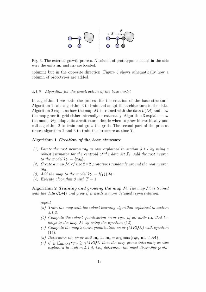
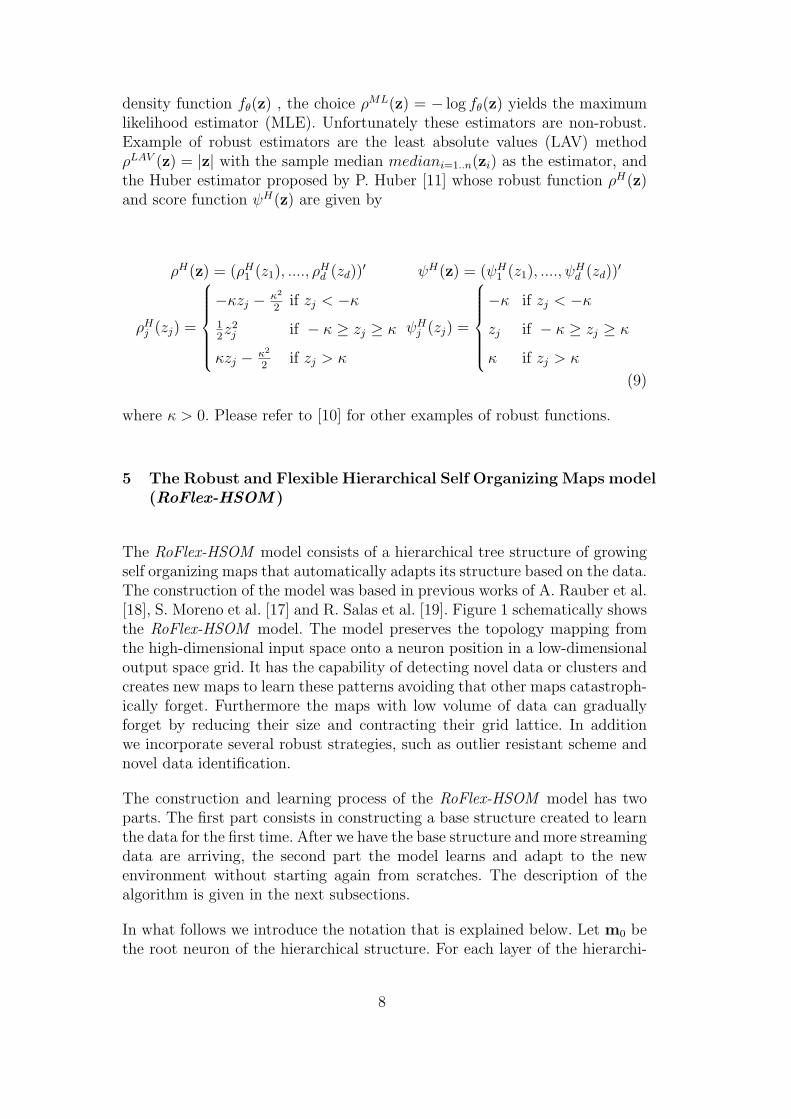
Fig. 3. The external growth process. A column of prototypes is added in the sidewere the units me and md are located.

column) but in the opposite direction. Figure 3 shows schematically how acolumn of prototypes are added.

5.1.6 Algorithm for the construction of the base model

In algorithm 1 we state the process for the creation of the base structure.Algorithm 1 calls algorithm 3 to train and adapt the architecture to the data.Algorithm 2 explains how the map M is trained with the data C(M) and howthe map grow its grid either internally or externally. Algorithm 3 explains howthe model HT adapts its architecture, decide when to grow hierarchically andcall algorithm 2 to train and grow the grids. The second part of the processreuses algorithm 2 and 3 to train the structure at time T .

Algorithm 1 Creation of the base structure

(1) Locate the root neuron m0 as was explained in section 5.1.1 by using arobust estimator for the centroid of the data set I1. Add the root neuronto the model H1 = {m0}.

(2) Create a map M of size 2×2 prototypes randomly around the root neuronm0.

(3) Add the map to the model H1 = H1⋃M.

(4) Execute algorithm 3 with T = 1

Algorithm 2 Training and growing the map M The map M is trainedwith the data C(M) and grow if it needs a more detailed representation.

repeat(a) Train the map with the robust learning algorithm explained in section

5.1.2.(b) Compute the robust quantization error rqer of all units mr that be-

longs to the map M by using the equation (12).(c) Compute the map’s mean quantization error (MRQE) with equation

(14).(d) Determine the error unit me as me = arg max{rqer|mr ∈M}.(e) if 1

M

∑mr∈M rqer ≥ γMRQE then the map grows internally as was

explained in section 5.1.5, i.e., determine the most dissimilar proto-

13

type md; insert a row or column between me and md and initializetheir model vectors as the mean of their respective neighbors.

(f) if rqee ≥ β maxmr∈M,mr 6=me rqer then the map grows externally aswas explained in section 5.1.5, i.e., determine the neighbor unit md

with the highest robust quantization error. A row (or column) of unitsis added in the side where the units me and md are located and theirmodel vectors are located at half the distance of the neighbor row (orcolumn) but in the opposite direction

until no more changes are done in the architecture.

Algorithm 3 Learning and adapting the model HT to the data set IT at stageT

(1) Compute the robust quantization error of the root neuron rqe0 using equa-tion (12) with the data set IT

(2) For each map M that belongs to the model HT do(a) Consider the data set C(M).(b) Train the map M by executing algorithm 2 with the data set C(M).(c) repeat

(i) For each leaf unit mr of the map M do(A) Compute the robust quantization error rqer with equation

(12).(B) if rqer ≥ τrqe0 and |C(mr)| ≥ Nmin then create a map M

of size 2 × 2 prototypes randomly around the neuron mr;train the map M by executing algorithm 2 with the dataset C(mr). Add the map to the model HT = HT

⋃M.until the model HT is stabilized, i.e., no more units were added.

(d) Update the internal node mu who is the parent of the map M by com-puting the mean value of the prototypes of the map by using equation(10), mu = m.

5.2 Second Part: Adapting to changing environments

In this part of the process we need to incorporate additional capabilities tothe model to be able to adapt to the topological drift of the environment.The learner will be able to track and adapt to the topological drift, detectnovel concepts, recognize and treat recurring contexts and forget outdatedknowledge. In what follows, we explain how we introduce these capabilitiesand at the end of this section we summarize the process of adapting to thechanging environment.

14

5.2.1 Projecting the data to the model

We define the best matching unit mη(x) of the model HT (bmm) to the datax as the leaf unit:

mη(x) = arg min{‖x−mr‖ |mr ∈ NL} (17)

The sample x is projected from the high-dimensional input space X onto thebest matching unit mη(x) of the model. All the samples that do not havea good topological representation with the current model HT are identifiedand are considered as novel data and we construct the set I [new]

T = {xi ∈IT |

∥∥∥x−mη(x)

∥∥∥ > ε} consisting of all the data whose distance to the modelare bigger than some threshold ε.

5.2.2 Freezing and Updating the Internal Units.

The prototypes mr that belong to the set NI of internal nodes of the modelHT will not adapt when the map learning algorithm explained in section 5.1.2is executed, i.e., these units are frozen. The prototypes will be updated asthe mean values of the neurons belonging to their respective child maps as inequation (10).

5.2.3 Gradually forgetting outdated knowledge.

To achieve better generalization and to keep the model stable, a forgettingstrategy is needed. The strategy consists in gradually forgetting by shrinkingthe lattices towards their respective centroids and, if the grids are sufficientlysmall, they are contracted by deleting rows or columns of prototypes.

Compute the centroid neurons m with equation (10). The map M will forgetthe old data by applying once the forgetting rule:

mr(T ) = mr(T − 1) + λ[mr(T − 1)−m] mr ∈M (18)

where λ is the forgetting rate. mr(T −1) and mr(T ) are the values of the pro-totypes at the end of the stage T−1 and the beginning of stage T respectively.If the units of the map are too close then the map is contracted. Consider therectangular grid; the prototype is indexed by r(mr) = (i, j), where i and j arethe row and column of the unit in the rectangular array (see section 3). Wesearch for two rows or columns whose neurons are very close. To accomplishthis the value ν is computed as

15

Fig. 4. The contraction process. (left) The map before it is contracted. (middle)A column of prototypes is inserted in between the columns e and d. (right) Thecolumns e and d of prototypes are eliminated from the grid.

Contraction Process:

ν = arg mine=1..Nr−1;d=1..Nc−1

1

Nc

Nc∑

j=1

∥∥∥m(e,j) −m(e+1,j)

∥∥∥ ,1

Nr

Nr∑

i=1

∥∥∥m(i,d) −m(i,d+1)

∥∥∥

where Nr and Nc are the number of rows and columns of the map latticerespectively. If the criterion ν < ε for the row (or column) is met and if theprototypes of one of the row (column) ν or ν + 1 are all leafs then the map iscontracted. In the contraction process we insert a row (or a column) of unitsbetween ν and ν + 1 and their model vectors are initialized as the mean oftheir respective neighbors, and then the rows (or columns) ν and ν + 1 ofprototypes are both eliminated. In figure 4 the column contraction process isshown. The map is contracted iteratively until no other row or column satisfiesthe criterion. If the map reaches its minimum size of 2 × 2 and none of itsprototypes have a child map and the distance of the prototypes of both, therow and column, are less than ε, then the map is eliminated from the model.

5.3 Model capabilities to deal with concept and topological drift

The model with the capability of adapting its architecture based on the dataas was explained in section 5.1, gives to the system abilities to deal with novelconcepts, topological drift and recurrent context as we will explain below.

When a novel concept appears in the data stream during the stage T the modelHT−1 will detect the concept during its training at some of its level dependingthe degree of novelty. The novel concept will increase the robust quantizationerror of some prototypes of the map M at certain level u of its structure. Ifthe novel concept location is detected in between previous learned concepts,the map will grow internally its grid by introducing prototypes towards thisnovel concept. If the novel concept is located outside the previous learnedconcepts, the map will grow externally its grid by introducing prototypestowards this novel concept. Finally, if the concept is strengthening a previous

16

learned concept, then the prototype, that it is modeling the concept, will growhierarchically to obtain a more detailed description.

The recurring context occurs when concepts are present in certain stages, andvanish and reappear in future stages. To deal with this phenomenon, notethat the model only adapts its leaf prototypes while the internal nodes remainfrozen. The internal node will not move from its current location until itschild map are contracted and eliminated. For this reason, if the concepts werestrong enough to create at least a two level structure, then the model willslowly forget and contract when the concept no longer exists. If the conceptvanishes forever or for a very long period of time, the structure will begin todisappear until only one prototype will remain and will move away towardother concept and forgetting the previous learned concept.

Note that if the internal prototypes are not fixed in their location, when theconcept disappears, the model will catastrophically forget the concept.

5.4 Algorithm for Adapting to the changing environment

Algorithm 4 Adapting to the changing environment

(1) Freeze all internal nodes during the maps training process.(2) Forget the outdated data by shrinking and contracting the grids as was

explained in section 5.2.3. Update the model HT by extracting all theprototypes that were removed.

(3) Execute algorithm 3 with T > 1

5.5 Evaluation of the adaptation Quality

To evaluate the quality of adaptation to the data a common measure to com-pare the algorithms is needed. The following metric based on the mean squarequantization error is proposed:

MSQE =1

|I|∑

xi∈I

∥∥∥xi −mη(x)

∥∥∥2

(19)

where |I| is the number of data that belongs to the input set I, and mη(x)

is the best matching unit of the model HT to the data x defined in equation(17)

17

6 Simulation Results

In this section we empirically show the capabilities of our RoFlex-HSOMmodel proposal compared to the HSOM model and some of its extensions,as they will be described bellow. In subsection 6.1 and 6.2 we show the per-formance results for computer generated data and El Nino real data set re-spectively.

For the experiments we evaluated four models. The first model is the basicHierarchical Self Organizing Maps (HSOM ), and the other three models wereobtained by extending this model. The second model is the Robust HSOM(Ro HSOM ) where we added robustness to the basic model. The third modelis the Flexible HSOM (Flex HSOM ) where we added flexibility to the basicmodel. And finally we have the Robust and Flexible HSOM (RoFlex HSOM )where we added both, robustness and flexibility.

The models have the following characteristics. Non flexible models, i.e., theHSOM and Ro HSOM, have static structures meaning that, at each stage,the previous model is eliminated and constructed again. In this work thestatic models were trained, for each stage, with the first part of the trainingalgorithm explained in section 5.1. While flexible models, i.e., the Flex HSOMand RoFlex HSOM, have adaptive structure meaning that during the firststage the models were trained with the first part of the training algorithmexplained in section 5.1 and, for the following stages, with the second part ofthe training algorithm explained in section 5.2.

For the non robust models, i.e., the HSOM and Flex HSOM, the sample meanestimator Z = 1

n

∑ni=1 zi was used to locate the root neuron; the classical

standard deviation s2 = 1n

∑ni=1(xi −X)2 was used to estimate scales instead

of equation (7); and the Least Square score function ψLS(z) = z was used totrain the maps in equation (11). To compute the robust quantization error ofequation (12) and the map’s robust quantization error of equation (14) theLeast Square function ρLS(z) = z′z was used.

While for the robust models, i.e., the Ro HSOM and RoFlex HSOM, the sam-ple median estimator mediani=1..n(zi) was used to locate the root neuron; thesMAD scale estimator given by equation (7) was used to estimate scales; andthe Huber score function ψH(z) of equation (9) was used to train the mapsin equation (11). To compute the robust quantization error of equation (12)and the map’s robust quantization error of equation (14) the Huber robustfunction ρH(z) given by equation (9) was used.

The data of both, synthetics and real data sets, were separated in trainingand test sets for each stage. All the models obtained after training at stage Twere evaluated with the mean square quantization error (MSQE) (see equa-

18

tion (19)) with the current test set ITestT , the previous test set ITest

T−1 and thefollowing test set ITest

T+1 corresponding to the stages T , T − 1 and T + 1 re-spectively. The performance of the models with the current test set ITest

T willgive us information of how well the model did adapt to the current stage.The performance of the models with the previous test set ITest

T−1 will give usinformation of how the model forgot previous concepts. The performance ofthe models with the following test set ITest

T+1 will give us information of howthe model will behave with future concepts.

All the results reported were obtained for each model as the mean value ofthe metrics computed for 20 runs evaluated at each stage and considering thesame sets of data.

6.1 Experiment #1: Computer generated data

The synthetic experiment consists in six two dimensional clusters created alongthe four stages. Let I2 be the identity matrix of size 2× 2. The characteristicsfor each cluster are:

• Cluster 1: Consists in three little Gaussian clusters created equidistant tothe centroid location [0.9 0.01]′, each with the covariance matrix of Σ =0.0082I2. The cluster is composed of 500 samples for each stage. Startingfrom the second stage this cluster is vanished and reappears at stage 4 with50 samples.

• Cluster 2: Consists in three little Gaussian clusters created equidistant to thecentroid location [0.8 0.5]′, each with the covariance matrix of Σ = 0.0082I2.The cluster is composed of 500 samples in the first and second stage, 333samples in the third stage and 166 in the fourth stage.

• Cluster 3: Consists in three little Gaussian clusters created equidistant to thecentroid location [0.6 0.8]′, each with the covariance matrix of Σ = 0.0082I2.The cluster begins with no sample at stage 1 and appears at stage 2 with500 samples. Starting from stage 3 the three little Gaussian clusters areconverted in two little Gaussian clusters equidistant to the same centroid,but each with the covariance matrix of Σ = 0.01252I2.

• Cluster 4: Consists in three little Gaussian clusters created equidistant to thecentroid location [0.1 0.8]′, each with the covariance matrix of Σ = 0.0082I2.The cluster moves, and the centroid is located in [0.125 0.775]′ at stage 2,in [0.15 0.75]′ at stage 3 and in [0.1750 0.7250]′ at stage 4. The clusteris composed of 500 samples for each stage. Starting from stage 2 the threelittle Gaussian clusters are converted in one big Gaussian clusters with meanequal to the centroid and the covariance matrix is Σ = 0.052I2.

• Cluster 5: Consists in one big Gaussian clusters with mean [0.2 0.1]′, andcovariance matrix of Σ = 0.052I2. The cluster is composed of 500 samples

19

for each stage. The covariance was increased in the following stages, thecovariance matrix is Σ = 0.0542I2 at stage 2, Σ = 0.05832I2 at stage 3 andΣ = 0.0632I2 at stage 4. Furthermore, starting from stage 3 the one bigGaussian clusters are converted in three little Gaussian clusters equidistantto the previous mean, but each with the covariance matrix of Σ = 0.0082I2.

• Cluster 6: Consists in three little Gaussian clusters created equidistant to thecentroid location [0.5 0.5]′, each with the covariance matrix of Σ = 0.0082I2.The cluster begins with no sample at stage 1 and appears at stage 3 with1500 samples.

The observational process was obtained by including additive outliers: Zk =Xk + Vk Uk, where Xk are the clusters generated as was previously explained,Vk is zero-one process with P (Vk 6= 0) = α, 0 < α ¿ 1, and Uk has distributionN (0, ΣUk

) with covariance matrix |ΣUk| À |Σk|. The generating process was

affected with α = 0%, 1% and 10% of outliers and ΣUk= 102 ∗ Σk, k = 1..6.

The generated data sets were divided, for each stage, in training and test setsboth of equal size.

For the experiments the growing parameters must be adjusted, i.e., the τ andNmin of equation (13) that control the hierarchical growing process; the γ ofequation (15) that controls the internal growing process; and the β of equation(16) that controls the external growing process. For the robust models weconsidered the following configuration τ = 0.01 , Nmin = 15, γ = 0.06 andβ = 10; while for the non robust models we used the following configurationτ = 0.2, Nmin = 15, γ = 0.2 and β = 100. The latter configuration makesthe model simpler than the former, but, unfortunately, with lower values thenon robust models become instable in some simulations by growing their mapsbigger as we really wanted and consuming a plenty of time.

The forgetting parameters for the flexible models were set at λ = 0.5 forthe forgetting rule of equation (18) and ε = 0.01 for the contraction. At thebeginning of each stage the maps will shrink to the half of their current size.

Figure 5 shows the adaptation of the models to the data sets for each stageand considering 1% of outliers. Each column of graphs of figure 5, from leftto right, correspond to the stages T = 1, 2, 3 and 4. Each row of graphs offigure 5, from top to bottom, correspond to the models HSOM, Ro HSOM,Flex HSOM and RoFlex HSOM respectively. Note that the HSOM modelcreated a very simple structure and, in most of the cases, did not create aparticular map for the clusters that it was modeling; in the second stage, itcan be appreciated how the model forgot the cluster 1; and in the last stagethe model was not able to model the recurrent cluster 1. The Ro HSOM modelof the second row was able to create maps for each of the cluster; it also forgotthe cluster 1 at the second stage; and in the last stage create a map at thethird level of its structure to model the recurrent cluster 1; note that when

20

0

0.5

1

00.2

0.40.6

0.810

0.5

1

XY 0

0.5

1

00.2

0.40.6

0.810

0.5

1

XY 0

0.5

1

00.2

0.40.6

0.810

0.5

1

XY 0

0.5

1

00.2

0.40.6

0.810

0.5

1

XY

0

0.5

1

00.2

0.40.6

0.810

0.5

1

XY 0

0.5

1

00.2

0.40.6

0.810

0.5

1

XY 0

0.5

1

00.2

0.40.6

0.810

0.5

1

XY 0

0.5

1

00.2

0.40.6

0.810

0.5

1

XY

0

0.5

1

00.2

0.40.6

0.810

0.5

1

XY 0

0.5

1

00.2

0.40.6

0.810

0.5

1

XY 0

0.5

1

00.2

0.40.6

0.810

0.5

1

XY 0

0.5

1

00.2

0.40.6

0.810

0.5

1

XY

0

0.5

1

00.2

0.40.6

0.810

0.5

1

XY 0

0.5

1

00.2

0.40.6

0.810

0.5

1

XY 0

0.5

1

00.2

0.40.6

0.810

0.5

1

XY 0

0.5

1

00.2

0.40.6

0.810

0.5

1

XY

Fig. 5. Configuration of the hierarchical tree structures modeling the synthetic dataset with 1% of outliers. Each column, from left to right, correspond to the stages 1,23 and 4. (First row) the HSOM model. (Second row) the Ro HSOM model. (Thirdrow) the Flex HSOM model. (Fourth row) the RoFlex HSOM model.

the clusters changed their topologies, the maps were also changed (see, e.g,the map modeling the cluster 5). The Flex HSOM model of the third rowwas able to create maps for each of the cluster; it did not forget the cluster1 at the second stage; and in the last stage it still remembered the recurrentcluster 1; note that the maps were badly affected by the presence of outliers bylocating it far from the clusters of data (see, e.g, the map modeling the cluster5 at stages 3 and 4) or by overextending the maps of the clusters 3, 4 and 5.Finally, the RoFlex HSOM model of the fourth row was able to combine thebest capabilities of both the Ro HSOM and Flex HSOM models; It createdmaps for each of the cluster; it did not forget the cluster 1 at the second stagealthough it slowly forgot the cluster; it created a second level map to modelthe recurrent cluster 1 at stage 4; note that the maps were barely affected bythe presence of outliers by over extending the map of the clusters 4. As canbe seen in figure 5, the robust models obtained a more detailed description ofthe data sets and were not badly affected by the outliers. The flexible modelsdid not catastrophically forget previously learned patterns.

21

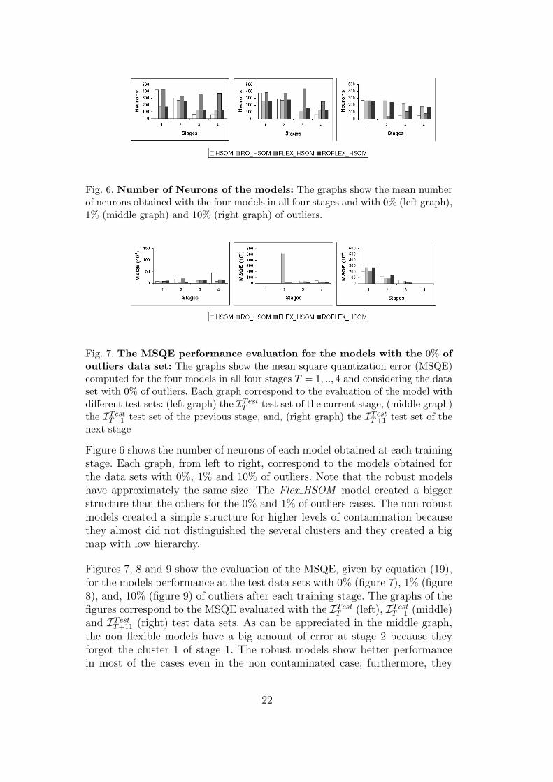
Fig. 6. Number of Neurons of the models: The graphs show the mean numberof neurons obtained with the four models in all four stages and with 0% (left graph),1% (middle graph) and 10% (right graph) of outliers.

Fig. 7. The MSQE performance evaluation for the models with the 0% ofoutliers data set: The graphs show the mean square quantization error (MSQE)computed for the four models in all four stages T = 1, .., 4 and considering the dataset with 0% of outliers. Each graph correspond to the evaluation of the model withdifferent test sets: (left graph) the ITest

T test set of the current stage, (middle graph)the ITest

T−1 test set of the previous stage, and, (right graph) the ITestT+1 test set of the

next stage

Figure 6 shows the number of neurons of each model obtained at each trainingstage. Each graph, from left to right, correspond to the models obtained forthe data sets with 0%, 1% and 10% of outliers. Note that the robust modelshave approximately the same size. The Flex HSOM model created a biggerstructure than the others for the 0% and 1% of outliers cases. The non robustmodels created a simple structure for higher levels of contamination becausethey almost did not distinguished the several clusters and they created a bigmap with low hierarchy.

Figures 7, 8 and 9 show the evaluation of the MSQE, given by equation (19),for the models performance at the test data sets with 0% (figure 7), 1% (figure8), and, 10% (figure 9) of outliers after each training stage. The graphs of thefigures correspond to the MSQE evaluated with the ITest

T (left), ITestT−1 (middle)

and ITestT+11 (right) test data sets. As can be appreciated in the middle graph,

the non flexible models have a big amount of error at stage 2 because theyforgot the cluster 1 of stage 1. The robust models show better performancein most of the cases even in the non contaminated case; furthermore, they

22

Fig. 8. The MSQE performance evaluation for the models with the 1% ofoutliers data set: The graphs show the mean square quantization error (MSQE)computed for the four models in all four stages T = 1, .., 4 and considering the dataset with 1% of outliers. Each graph correspond to the evaluation of the model withdifferent test sets: (left graph) the ITest

T test set of the current stage, (middle graph)the ITest

T−1 test set of the previous stage, and, (right graph) the ITestT+1 test set of the

next stage

Fig. 9. The MSQE performance evaluation for the models with the 10% ofoutliers data set: The graphs show the mean square quantization error (MSQE)computed for the four models in all four stages T = 1, .., 4 and considering the dataset with 10% of outliers. Each graph correspond to the evaluation of the model withdifferent test sets: (left graph) the ITest

T test set of the current stage, (middle graph)the ITest

T−1 test set of the previous stage, and, (right graph) the ITestT+1 test set of the

next stage

show better behavior in predicting future data. Note that the RoFlex HSOMmodel combined both, the good performance of the robust models and the notcatastrophically forgetting capability of the flexible models.

If figure 10 the time performances for the training process of the models areshown. The evaluations were made for the data sets with 0% (left), 1% (mid-dle) and 10% (right) of outliers. As can be noted, the Flex HSOM modelshows the worst training time for the 0% and 1% of outliers data sets. Therobust models needed almost the same time for all the stages and data sets,i.e, they were not much affected by the contamination. The training times ofthe HSOM show better performance than the robust methods in some cases,probably due to the simpler structure, and worse performance in other cases.Note that the combination of robustness and flexibility in the RoFlex HSOM

23

Fig. 10. The time evaluation of the training process: The graphs show themean time evaluation of the training process computed for the four models in allfour stages. (Left) data set with 0% of outliers. (Middle) data set with 1% of outliers.(Right) data set with 10% of outliers.

model reduces the training time cost, and the training algorithm is more stablethan the HSOM model.

6.2 Experiment #2: “El Nino” real data

In the real data set experiment we tested the algorithm with the El NinoData. The data can be obtained from the following site

http://kdd.ics.uci.edu/databases/el nino/el nino.html.

The El Nino Data are expected to aid in the understanding and predictionof El Nino Southern Oscillation (ENSO) cycles and was collected by the Pa-cific Marine Environmental Laboratory National Oceanic and AtmosphericAdministration. The data set contains oceanographic and surface meteorolog-ical readings taken from a several buoys positioned throughout the equatorialPacific.

The data consist of the following variables: date, latitude, longitude, zonalwinds (west < 0, east > 0), meridional winds (south < 0, north > 0),relative humidity, air temperature, sea surface temperature and subsurfacetemperatures down to a depth of 500 meters. Data taken from the buoys areas early as 1980 for some locations.

The data set was modified by discarding those data with missing values. Wekept eight stages corresponding to the first eight years of data collection, from1980 until 1988. We used 6311 instances of 4 dimensions (meridional winds,relative humidity, sea surface temperature and subsurface temperatures) fromwhom 4415 were used for training and 1896 for testing. To execute the simu-lations and to compute the metrics, all the dimensions of the training data setof the first stage were scaled to the unit interval, and with the same scale, therest of training and test data sets were scaled (Notice that with this scaling

24

Fig. 11. “El Nino” real data experiment: The graphs show the mean squarequantization error (MSQE) computed for the four models obtained at all eightstages. Each graph correspond to the evaluation of the model with different testsets: (left graph) the ITest

T test set of the current stage, (middle graph) the ITestT−1

test set of the previous stage, and, (right graph) the ITestT+1 test set of the next stage

the training and test data will not necessarily fall in the unit interval). Wedivided the data set according to the years into 8 training data sets composedof 110, 226, 293, 160, 411, 337, 837 and 2041 samples respectively for eachyear stage; and into 8 test data sets composed of 48, 97 , 126, 69, 177, 145,359 and 875 samples respectively for each year stage.

Figure 11 shows the evaluation of the MSQE, given by equation (19), for themodels performance at the test data sets after each training stage. The graphsof the figure correspond to the MSQE evaluated with the ITest

T (left), ITestT−1

(middle) and ITestT+1 (right) test data sets. As can be easily appreciated the

robust models outperforms the non robust models in all stages except for thefirst one, and the former obtained approximately half of the MSQE of thenon robust models. Furthermore the robust models have better performancein predicting the past and the future. We can conclude that the behavior ofthis data set is non Gaussian or is highly contaminated, for this reason isaffecting very badly the non robust models. Furthermore, by observing thefourth stage of the middle graph of figure 11 we can conclude that the nonrobust models obtained at stage 4 were not able to remember and predict thedata set of the third stage; and by observing the first, second and fourth stagesof the right graph of figure 11 we can conclude that the non robust modelswere not able to predict the data sets of the second, third and fifth stageswith the models obtained at stages 1,2 and 4 respectively. This last resultcould signify that the “El Nino” data set either has a topological drift or thecontamination is affecting badly the non robust models. We cannot concludewhether the Ro HSOM or RoFlex HSOM had a better performance. Furtherstudies will be needed to understand why the non robust models outperformsthe robust models at the first stage while for the other stages the oppositeoccurs, probably this phenomenon is due to some unknown change in thebehavior of the “El Nino” data set.

25

7 Concluding Remarks

In this paper we have postulated a method of how to incorporate Robustnessand Flexibility to the Hierarchical Self Organizing Maps model. The extendedmodel was called (RoFlex-HSOM ). We had empirically shown that the RoFlex-HSOM had the plasticity to find the structure that suits the best to the data,gradually forgets (but no catastrophically) previous learned patterns, it isrobust to the presence of outliers and preserves the topology to represent thehierarchical relation of the data under environments that are time dependentand non stationary. The theory and the method presented in this work can behelpful to incorporate robustness and/or flexibility to other classical modelsand with this we can extend their capabilities to more complex environments.

In the experimental study we made a comparative analysis of four modelswith synthetic and real data sets. The data of the synthetic experiment wereaffected with different degrees of noise. The models used were the HSOMmodel and three extensions of itself by adding the capabilities of robustness(Ro HSOM ), the flexibility (Flex HSOM ) and both, robustness and flexibil-ity (RoFlex HSOM ). With the synthetic data sets we were able to show thatthe robust models (Ro HSOM and RoFlex HSOM ) obtained better perfor-mance under contaminated environments and their behavior were more stableduring the training process. In addition we showed that the flexible models(flex HSOM and RoFlex HSOM ) were able to slowly (and not catastrophi-cally) forget outdated knowledge. Only the RoFlex HSOM model was suc-cessfully in combining the capabilities of robustness against noise and theflexibility of effectively tracking the topological drift.

For the real case, we investigated the El Nino data. The performance of therobust models (Ro HSOM and RoFlex HSOM ) outperforms the non robustmodels (HSOM and Flex HSOM ). We suspect that the data either is highlycontaminated or has a behavior radically different to the Gaussian distribu-tion, furthermore the data set presented unknown drifts that needs furtheranalysis.

In further studies, the training algorithm should be fine tuned to improve thespeed of learning and the quality of adaptation. The RoFlex HSOM modelcould be further applied in several other real applications as e.g. self organi-zation of a massive document collection, weather prediction and spam e-mailtopology modeling to name a few complex real problems.

26

Acknowledgments

This work was supported by the following research grants: Fondecyt 1061201,1040365 and 7050205, DGIP-UTFSM, and, BMBF-CHL 03-Z13 from the Ger-man Ministry of Education and Research. The authors like to thank the or-ganizers of IWANN 2005 for inviting us to submit this extended version ofour paper [17] to Neurocomputing. We would also thankfully acknowledge thedetailed observations and suggestions of the anonymous reviewers.

References

[1] D. Aha, D. Kibler, and M.K. Albert, Instance-based learning algorithms,Machine Learning 6 (1991), 37–66.

[2] D. Alahakoon, S. Halgamuge, and B. Srinivasan, Dynamic self-organizing mapswith controlled growth for knowledge discovery, IEEE Trans. on Neural Networks11 (2000), no. 3, 601–614.

[3] H. Allende, S. Moreno, C. Rogel, and R. Salas, Robust self organizing maps,CIARP. LNCS 3287 (2004), 179–186.

[4] R. Amarasiri, D. Alahakoon, and K. Smith, HDGSOM: a modified growingself-organizing map for high data clustering, Proc. of the Fourth InternationalConference on Hybrid Intelligent Systems. HIS’04. IEEE Press., 2004.

[5] B. Ans, Sequential learning in distributed neural networks without catastrophicforgetting: A single and realistic self-refreshing memory can do it, NeuralInformation Processing - Letters and Reviews 4 (2004), no. 2, 27–37.

[6] G. Carpenter and S. Grossberg, A massively parallel architecture for a self-organizing neural pattern recognition machine, Computer Vision, Graphics andImage Processing 37 (1987), 54–225.

[7] R. French, Catastrophic forgetting in connectionist networks, Trends inCognitive Sciences 3 (1999), 128–135.

[8] B. Fritzke, Growing cell structures - a self-organizing network for unsupervisedand supervised learning, Neural Networks 7 (1994), no. 9, 1441–1460.

[9] S. Grossberg, Studies of mind and brain: Neural principles of learning,perception, development, cognition, and motor control, Reidel Press., 1982.

[10] F.R. Hampel, E.M. Ronchetti, P.J. Rousseeuw, and W.A. Stahel, Robuststatistics, Wiley Series in Probability and Mathematical Statistics, 1986.

[11] Peter J. Huber, Robust statistics, Wiley Series in Probability and MathematicalStatistics, 1981.

27

[12] M.G. Kelly, D.J. Hand, and N.M. Adams, The impact of changing populationson classifier performance, In Proc. 5th ACM SIGDD International Conferenceon Knowledge Discovery and Data Mining, ACM Press., 1999, pp. 367–371.

[13] R. Klinkenberg, Learning drift concepts: example selection vs. exampleweighting., Intelligent Data Analysis, Special issue on incremental LearningSystems Capable of Dealing with Concept Drift 8 (2004), no. 3, To appear.

[14] T. Kohonen, Self-Organizing Maps, Springer Series in Information Sciences,vol. 30, Springer Verlag, Berlin, Heidelberg, 2001, Third Extended Edition 2001.

[15] L. Kuncheva, Classifier ensembles for changing environments, MCS2004, LNCS3077 (2004), 1–15.

[16] M. McCloskey and N. Cohen, Catastrophic interference in connectionistnetworks: The sequential learning problem, The psychology of Learning andMotivation 24 (1989), 109–164.

[17] S. Moreno, H. Allende, C. Rogel, and R. Salas, Robust growing hierarchical selforganizing map, IWANN 2005. LNCS 3512 (2005), 341–348.

[18] A. Rauber, D. Merkl, and M. Dittenbach, The growing hierarchical self-organizing map: Exploratory analysis of high-dimensional data, IEEE Trans.on Neural Networks 13 (2002), no. 6, 1331–1341.

[19] R. Salas, H. Allende, S. Moreno, and C. Saavedra, Flexible architecture of selforganizing maps for changing environments, CIARP 2005. LNCS 3773 (2005),642–653.

[20] J.C. Schlimmer and R.H. Granger, Incremental learning from noisy data.,Machine Learning 1 (1986), no. 3, 317–354.

[21] U. Seiffert and L. Jain (eds.), Self-organizing neural networks: Recent advancesand applications, Studies in Fuzziness and Soft Computing, vol. 78, SpringerVerlag, 2002.

[22] A. Tsymbal, The problem of concept drift: definitions and related work, Tech.Report TCD-CS-2004-15, Trinity College Dublin, 2004.

[23] G. Widmer and M. Kubat, Learning in the presence of concept drift and hiddencontext, Machine Learning 23 (1996), 69–101.

[24] Gerhard Widmer, Combining robustness and flexibility in learning driftingconcepts, European Conference on Artificial Intelligence, 1994, pp. 468–472.

28