HAL Id: hal-01270701https://hal.archives-ouvertes.fr/hal-01270701

Submitted on 8 Feb 2016

HAL is a multi-disciplinary open accessarchive for the deposit and dissemination of sci-entific research documents, whether they are pub-lished or not. The documents may come fromteaching and research institutions in France orabroad, or from public or private research centers.

L’archive ouverte pluridisciplinaire HAL, estdestinée au dépôt et à la diffusion de documentsscientifiques de niveau recherche, publiés ou non,émanant des établissements d’enseignement et derecherche français ou étrangers, des laboratoirespublics ou privés.

Theoretical and applied aspects of the self-organizingmaps

Marie Cottrell, Madalina Olteanu, Fabrice Rossi, Nathalie Vialaneix

To cite this version:Marie Cottrell, Madalina Olteanu, Fabrice Rossi, Nathalie Vialaneix. Theoretical and applied as-pects of the self-organizing maps. WSOM 2016, Jan 2016, Houston, TX, United States. pp.3-26,�10.1007/978-3-319-28518-4_1�. �hal-01270701�

Theoretical and Applied Aspects of the

Self-Organizing Maps

Marie Cottrell1, Madalina Olteanu1, Fabrice Rossi1, and NathalieVilla-Vialaneix2

1 SAMM - Université Paris 1 Panthéon-Sorbonne90, rue de Tolbiac, 75013 Paris, France

marie.cottrell,madalina.olteanu,fabrice.rossi@univ-paris1.fr2 INRA, UR 0875 MIAT

BP 52627, F-31326 Castanet Tolosan, Francenathalie.villa@toulouse.inra.fr

Abstract. The Self-Organizing Map (SOM) is widely used, easy to im-plement, has nice properties for data mining by providing both clusteringand visual representation. It acts as an extension of the k-means algo-rithm that preserves as much as possible the topological structure of thedata. However, since its conception, the mathematical study of the SOMremains difficult and has be done only in very special cases. In WSOM2005, Jean-Claude Fort presented the state of the art, the main remain-ing difficulties and the mathematical tools that can be used to obtaintheoretical results on the SOM outcomes. These tools are mainly Markovchains, the theory of Ordinary Differential Equations, the theory of sta-bility, etc. This article presents theoretical advances made since then. Inaddition, it reviews some of the many SOM algorithm variants whichwere defined to overcome the theoretical difficulties and/or adapt thealgorithm to the processing of complex data such as time series, missingvalues in the data, nominal data, textual data, etc.

Keywords: SOM, batch SOM, Relational SOM, Stability of SOM

1 Brief history of the SOM

Since its introduction by T. Kohonen in his seminal 1982 articles (Kohonen[1982a,b]), the self-organizing map (SOM) algorithm has encountered a verylarge success. This is due to its very simple definition, to the easiness of itspractical development, to its clustering properties as well as its visualizationability. SOM appears to be a generalization of basic clustering algorithms andat the same time, provides nice visualization of multidimensional data.

The basic version of SOM is an on-line stochastic process which has beeninspired by neuro-biological learning paradigms. Such paradigms had previouslybeen used to model some sensory or cognitive processes where the learning is di-rected by the experience and the external inputs without supervision. For exam-ple, Ritter and Schulten [1986] illustrate the somatosensory mapping property of

2 Cottrell et al.

SOM. However, quickly in the eighties, SOM was not restricted to neuro-biologymodeling and has been used in a huge number of applications (see e.g. Kaskiet al. [1998b], Oja et al. [2003] for surveys), in very diverse fields as economy,sociology, text mining, process monitoring, etc.

Since then, several extensions of the algorithms have been proposed. For in-stance, for users who are not familiar with stochastic processes or for industrialapplications, the variability of the equilibrium state was seen as a drawbackbecause the learnt map is not always the same from one run to another. To ad-dress this issue, T. Kohonen introduces the batch SOM, (Kohonen [1995, 1999])which is deterministic and thus leads 3 to reproducible results (for a given ini-tialization). Also, the initial SOM (on-line or batch versions) was designed forreal-valued multidimensional data, and it has been necessary to adapt its defi-nition in order to deal with complex non vectorial data such as categorical data,abstract data, documents, similarity or dissimilarity indexes, as introduced inKohonen [1985], Kaski et al. [1998a], Kohohen and Somervuo [1998]. One canfind in Kohonen [1989, 1995, 2001, 2013, 2014] extensive lists of references re-lated to SOM. At this moment more than 10 000 papers have been published onSOM or using SOM.

In this paper, we review a large selection of the numerous variants of theSOM. One of the main focus of this survey is the question of convergence of theSOM algorithms, viewed as stochastic processes. This departs significantly fromthe classical learning theory setting. In this setting, exemplified by the pioneer-ing results of Pollard et al. [1981], one generally assumes given an optimizationproblem whose solution is interesting: for instance, an optimal solution of thequantization problem associated to the k-means quality criterion. The optimiza-tion problem is studied with two points of view: the true problem which involvesa mathematical expectation with respect to the (unknown) data distribution andits empirical counterpart where the expectation is approximated by an averageon a finite sample. Then the question of convergence (or consistency) is whetherthe solution obtained on the finite sample converges to the true solution thatwould be obtained by solving the true problem.

We focus on a quite different problem. A specific stochastic algorithm such asthe SOM one defines a series of intermediate configurations (or solutions). Doesthe series converge to something interesting? More precisely, as the algorithmmaps the inputs (the data) to an output (the prototypes and their array), one cantake this output as the result of the learning process and may ask the followingquestions, among others:

– How to be sure that the learning is over?– Do the prototypes extract a pertinent information from the data set?– Are the results stables?– Are the prototypes well organized?

In fact, many of these questions are without a complete answer, but in the fol-lowing, we review parts of the questions for which theoretical results are knownand summarize the main remaining difficulties. Section 2 is devoted to the defi-nition of SOM for numerical data and to the presentation of the general methods

Theoretical and Applied Aspects 3

used for studying the algorithm. Some theoretical results are described in thenext sections: Section 3 explains the one dimensional case while in Section 4, theresults available for the multidimensional case are presented. The batch SOM isstudied in Section 5. In Section 6, we present the variants proposed by Heskes toget an energy function associated to the algorithm. Section 7 is dedicated to nonnumerical data. Finally, in Section 8, we focus on the use of the stochasticity ofSOM to improve the interpretation of the maps. The article ends with a veryshort and provisional conclusion.

2 SOM for numerical data

Originally, (in Kohonen [1982a] and Kohonen [1982b]), the SOM algorithm wasdefined for vector numerical data which belong to a subset X of an Euclideanspace (typically R

p). Many results in this paper additionally require that the sub-set is bounded and convex. There are two different settings from the theoreticalpoint of view:

– continuous setting: the input space X can be modeled by a probability dis-tribution defined by a density function f ;

– discrete setting: the data space X comprises N data points x1, . . . , xN inR

p (In this paper, by discrete setting, we mean a finite subset of the inputspace).

The theoretical properties are not exactly the same in both cases, so we shalllater have to separate these two settings.

2.1 Classical on-line SOM, continuous or discrete setting

In this section, let us consider that X ⊂ Rp (continuous or discrete setting).

First we specify a regular lattice of K units (generally in a one- or two-dimensional array). Then on the set K = {1, . . . ,K}, a neighborhood structureis induced by a neighborhood function h defined on K × K. This function canbe time dependent and, in this case, it will be denoted by h(t). Usually, h issymmetrical and depends only on the distance between units k and l on thelattice (denoted by dist(k, l) in the following)). It is common to set hkk = 1 andto have kkl decrease with increasing distance between k and l. A very commonchoice is the step function, with value 1 if the distance between k and l is lessthan a specific radius (this radius can decrease with time), and 0 otherwise.Another very classical choice is

hkl(t) = exp

(

−dist2(k, l)

2σ2(t)

)

,

where σ2(t) can decrease over time to reduce the intensity and the scope of theneighborhood relations.

A prototype mk ∈ Rp is attached to each unit k of the lattice. Prototypes

are also called models, weight vectors, code-vectors, codebook vectors, centroids,

4 Cottrell et al.

etc. The goal of the SOM algorithm is to update these prototypes according tothe presentation of the inputs in such a way that they represent the input spaceas accurately as possible (in a quantization point of view) while preserving thetopology of the data by matching the regular lattice with the data structure.For each prototype mk, the set of inputs closer to mk than to any other onedefines a cluster (also called a Voronoï cell) in the input space, denoted by Ck,and the neighborhood structure on the lattice induces a neighborhood structureon the clusters. In other words, after running the SOM process, close inputsshould belong to the same cluster (as in any clustering algorithm) or to neighborclusters.

From any initial values of the prototypes, (m1(0), . . . ,mK(0)), the SOM al-gorithm iterates the following steps:

1. At time t, if m(t) = (m1(t), . . . ,mK(t)) denotes the current state of the pro-totypes, a data point x is drawn according to the density f in X (continuoussetting) or at random in the finite set X (discrete setting).

2. Then ct(x) ∈ {1, . . . ,K} is determined as the index of the best matchingunit, that is

ct(x) = arg mink∈{1,...,K}

‖x−mk(t)‖2, (1)

3. Finally, all prototypes are updated via

mk(t+ 1) = mk(t) + ǫ(t)hkct(x)(t)(x−mk(t)), (2)

where ǫ(t) is a learning rate (positive, less than 1, constant or decreasing).

Although this algorithm is very easy to define and to use, its main theoret-ical properties remain without complete proofs. Only some partial results areavailable, despite a large amount of works and empirical evidences. More pre-cisely, (mk(t))k=1,...,K are K stochastic processes in R

p and when the number tof iterations of the algorithm grows,mk(t) could have different behaviors: oscilla-tion, explosion to infinity, convergence in distribution to an equilibrium process,convergence in distribution or almost sure to a finite set of points in R

p, etc.

This is the type of convergence that we will discuss in the sequel. In particular,the following questions will be addressed:

– Is the algorithm convergent in distribution or almost surely, when t tends to+∞?

– What happens when ǫ is constant? when it decreases?

– If a limit state exists, is it stable?

– How to characterize the organization?

One can find in Cottrell et al. [1998] and Fort [2006] a summary of the main rig-orous results with most references as well as the open problems without solutionsuntil now.

Theoretical and Applied Aspects 5

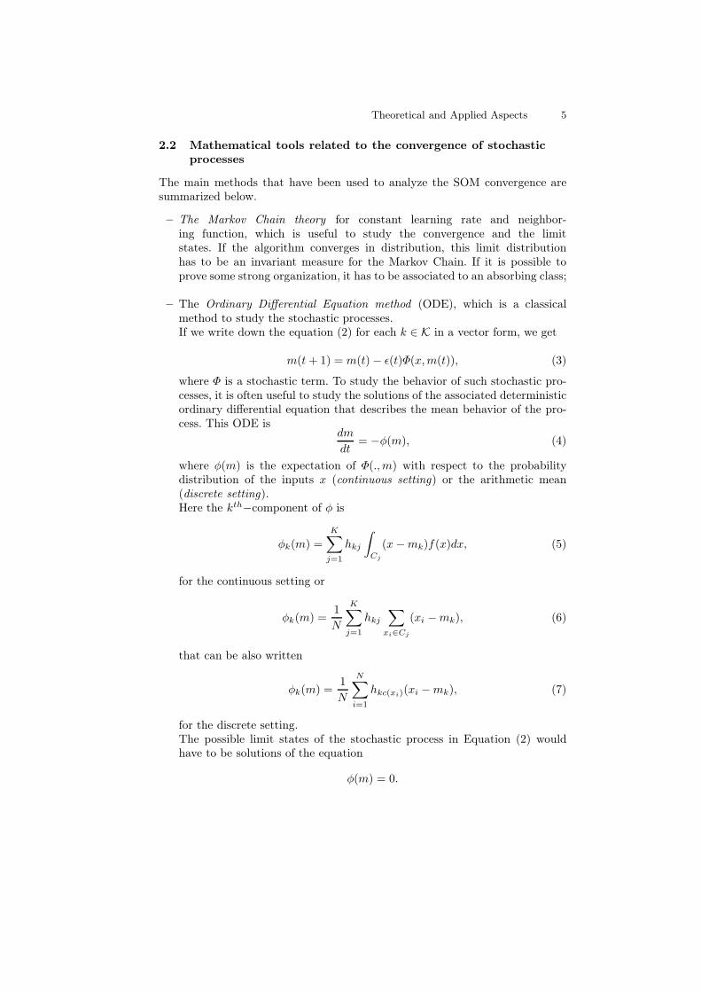
2.2 Mathematical tools related to the convergence of stochasticprocesses

The main methods that have been used to analyze the SOM convergence aresummarized below.

– The Markov Chain theory for constant learning rate and neighbor-ing function, which is useful to study the convergence and the limitstates. If the algorithm converges in distribution, this limit distributionhas to be an invariant measure for the Markov Chain. If it is possible toprove some strong organization, it has to be associated to an absorbing class;

– The Ordinary Differential Equation method (ODE), which is a classicalmethod to study the stochastic processes.If we write down the equation (2) for each k ∈ K in a vector form, we get

m(t+ 1) = m(t)− ǫ(t)Φ(x,m(t)), (3)

where Φ is a stochastic term. To study the behavior of such stochastic pro-cesses, it is often useful to study the solutions of the associated deterministicordinary differential equation that describes the mean behavior of the pro-cess. This ODE is

dm

dt= −φ(m), (4)

where φ(m) is the expectation of Φ(.,m) with respect to the probabilitydistribution of the inputs x (continuous setting) or the arithmetic mean(discrete setting).Here the kth−component of φ is

φk(m) =

K∑

j=1

hkj

∫

Cj

(x−mk)f(x)dx, (5)

for the continuous setting or

φk(m) =1

N

K∑

j=1

hkj∑

xi∈Cj

(xi −mk), (6)

that can be also written

φk(m) =1

N

N∑

i=1

hkc(xi)(xi −mk), (7)

for the discrete setting.The possible limit states of the stochastic process in Equation (2) wouldhave to be solutions of the equation

φ(m) = 0.

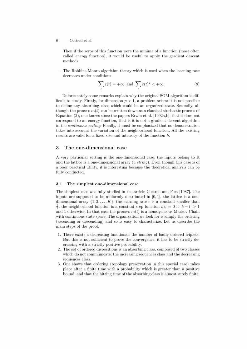
6 Cottrell et al.

Then if the zeros of this function were the minima of a function (most oftencalled energy function), it would be useful to apply the gradient descentmethods.

– The Robbins-Monro algorithm theory which is used when the learning ratedecreases under conditions

∑

t

ε(t) = +∞ and∑

t

ε(t)2 < +∞. (8)

Unfortunately some remarks explain why the original SOM algorithm is dif-ficult to study. Firstly, for dimension p > 1, a problem arises: it is not possibleto define any absorbing class which could be an organized state. Secondly, al-though the process m(t) can be written down as a classical stochastic process ofEquation (3), one knows since the papers Erwin et al. [1992a,b], that it does notcorrespond to an energy function, that is it is not a gradient descent algorithmin the continuous setting. Finally, it must be emphasized that no demonstrationtakes into account the variation of the neighborhood function. All the existingresults are valid for a fixed size and intensity of the function h.

3 The one-dimensional case

A very particular setting is the one-dimensional case: the inputs belong to R

and the lattice is a one-dimensional array (a string). Even though this case is ofa poor practical utility, it is interesting because the theoretical analysis can befully conducted.

3.1 The simplest one-dimensional case

The simplest case was fully studied in the article Cottrell and Fort [1987]. Theinputs are supposed to be uniformly distributed in [0, 1], the lattice is a one-dimensional array {1, 2, . . . ,K}, the learning rate ǫ is a constant smaller than12 , the neighborhood function is a constant step function hkl = 0 if |k − l| > 1and 1 otherwise. In that case the process m(t) is a homogeneous Markov Chainwith continuous state space. The organization we look for is simply the ordering(ascending or descending) and so is easy to characterize. Let us describe themain steps of the proof.

1. There exists a decreasing functional: the number of badly ordered triplets.But this is not sufficient to prove the convergence, it has to be strictly de-creasing with a strictly positive probability.

2. The set of ordered dispositions is an absorbing class, composed of two classeswhich do not communicate: the increasing sequences class and the decreasingsequences class.

3. One shows that ordering (topology preservation in this special case) takesplace after a finite time with a probability which is greater than a positivebound, and that the hitting time of the absorbing class is almost surely finite.

Theoretical and Applied Aspects 7

0

1

j − 1 j j + 1 j − 1 j j + 1 j − 1 j j + 1 j − 1 j j + 1

Fig. 1. Four examples of triplets of prototypes (mj−1,mj ,mj+1). For each j, j−1 andj + 1 are its neighbors. The y-axis coordinates are the values of the prototypes thattake values in [0, 1]. The first two triplets on the left are badly ordered. In the caseunder study, SOM will order them with a strictly positive probability. The last twotriplets (on the right) are well ordered and SOM will never disorder them.

4. Then one shows that the Markov Chain has the Doeblin property: thereexists an integer T , and a constant c > 0, such that, given that the processstarts from any ordered state, and for all set E in [0, 1]n, with positivemeasure, the probability to enter in E with less than T steps is smaller thanc vol(E).

5. This implies that the chain converges in distribution to a monotonous sta-tionary distribution which depends on ǫ (which is a constant in that part).

6. If ǫ(t) tends towards 0 and satisfies the Robbins-Monro conditions (8), oncethe state is ordered, the Markov Chain almost surely converges towards aconstant (monotonous) solution of an explicit linear system.

So in this very simple case, we could prove the convergence to a uniqueordered solution such that

m1(+∞) < m2(+∞) < . . . < mK(+∞),

orm1(+∞) > m2(+∞) > . . . > mK(+∞).

Unfortunately, it is not possible to find absorbing classes when the dimensionis larger than 1. For example, in dimension 2, with 8 neighbors, if the x- andy-coordinates are ordered, it is possible (with positive probability) to disorderthe prototypes as illustrated in Figure 2.

3.2 What we know about the general one-dimensional case

We summarize in this section the essential results that apply to the generalone dimension case (with constant neighborhood function and in the continuoussetting). References and precise statements can be found in Fort [2006] andCottrell et al. [1998]. Compared to the previous section, hypothesis on the datadistribution and/or the neighborhood function are relaxed.

8 Cottrell et al.

B

A

C

Fig. 2. This figure represents 2-dimensional prototypes (x- and y-axes are not shownbut are the standard horizontal and vertical axes) which are linked as their correspond-ing units on the SOM grid. At this step of the algorithm, the x- and y- coordinatesof the prototypes are well ordered. But contrarily to the one-dimensional case, thisdisposition can be disordered with a positive probability; in an 8-neighbors case, A isC’s neighbor, but B is not a neighbor of C. If C is repeatedly the best matching unit,B is never updated, while A becomes closer and closer to C. Finally, the y coordinateof A becomes smaller than that of B and the disposition is disordered.

– The process m(t) is almost surely convergent to a unique stable equilibriumpoint in a very general case: ǫ(t) is supposed to satisfy the conditions (8),there are hypotheses on the density f and on the neighborhood functionh. Even though these hypotheses are not very restrictive, some importantdistributions, such as the χ2 or the power distribution, do not fulfill them.

– For a constant ǫ, the ordering time is almost surely finite (and has a finiteexponential moment).

– With the same hypotheses as before to ensure the existence and uniquenessof a stable equilibrium x∗, from any ordered state, for each constant ǫ, thereexists an invariant probability measure πǫ. When ǫ tends to 0, this measureconcentrates on the Dirac measure on x∗.

– With the same hypotheses as before to ensure the existence and uniquenessof a stable equilibrium x∗, from any ordered state, the algorithm convergesto this equilibrium provided that ǫ(t) satisfies the conditions (8).

As the hypotheses are sufficiently general to be satisfied in most cases, onecan say that the one-dimensional case is more or less well-known. However noth-ing is proved neither about the choice of a decreasing function for ǫ(t) to ensuresimultaneously ordering and convergence, nor for the case of decreasing neigh-borhood function.

4 Multidimensional case

When the data are p-dimensional, one has to distinguish two cases, the contin-uous setting and the discrete one.

4.1 Continuous setting

In the p−dimensional case, we have only partial results proved by Sadeghi in(Sadeghi [2001]). In this paper, the neighborhood function is supposed to have

Theoretical and Applied Aspects 9

a finite range, the learning rate ǫ is a constant, the probability density functionis positive on an interval (this excludes the discrete case). Then the algorithmweakly converges to a unique probability distribution which depends on ǫ.

Nothing is known about the possible topology preservation properties of thisstationary distribution. This is a consequence of the difficulty of defining anabsorbing organized state in a multidimensional setting. For example, two resultsof Flanagan and Fort-Pagès illustrate the complexity of the problem. These twoapparently contradictory results hold. For p = 2, let us consider the set F++ ofsimultaneously ordered coordinates (respectively x and y coordinates). We thenhave:

– for a constant ǫ and very general hypotheses on the density f , the hittingtime of F++ is finite with a positive probability (Flanagan [1996]),

– but in the 8-neighbor setting, the exit time is also finite with positive prob-ability (Fort and Pagès [1995]).

4.2 Discrete setting

In this setting, the stochastic process m(t) of Equations (2) and (4) derives froma potential function, which means that it is a gradient descent process associatedto the energy. When the neighborhood function does not depend on time, Ritteret al. [1992] have proven that the stochastic process m(t) of Equations (2) and(3) derives from a potential, that is it can be written

mk(t+ 1) = mk(t) + ǫ(t)hkc(x)(t)(x −mk(t)),

= mk(t)− ǫ(t)Φk(x,m(t)),

= mk(t)− ǫ(t)∂

∂mk

E(x,m(t)),

where E(x,m) is a sample function of E(m) with

E(m) =1

2N

K∑

k=1

K∑

j=1

hkj∑

xi∈Cj

‖mk − xi‖2, (9)

or in a shorter expression

E(m) =1

2N

N∑

i=1

K∑

k=1

hkc(xi)‖mk − xi‖2. (10)

In other words the stochastic process m(t) is a stochastic gradient descentprocess associated to function E(m). Three interesting remarks can be made:

1. The energy function is a generalization of the distortion function (or intraclasses variance function) associated to the Simple Competitive Learningprocess (SCL, also known as the Vector Quantization Process/Algorithm),

10 Cottrell et al.

which is the stochastic version of the deterministic Forgy algorithm. TheSCL process is nothing else than the SOM process where the neighborhoodfunction is degenerated, ie when hkl = 1 only for k = l and hkl = 0 elsewhere.In that case, E reduces to

E(m) =1

2N

N∑

i=1

‖mc(xi) − xi‖2.

For that reason, E is called extended intra-classes variance.2. The above result does not ensure the convergence of the process: in fact the

gradient of the energy function is not continuous and the general hypothesesused to prove the convergence of the stochastic gradient descent processesare not valid. This comes from the fact that there are discontinuities whencrossing the boundaries of the clusters associated to the prototypes, becausethe neighbors involved in the computation change from a side to another.However this energy gives an interesting insight on the process behavior.

3. In the 0-neighbor setting, the Vector Quantization algorithm converges, sincethere is no problem with the neighbors and the gradient is continuous. How-ever there are a lot of local minima and the algorithm converges to one ofthese minima.

5 Deterministic batch SOM

As the possible limit states of the stochastic process (2) would have to be solu-tions of the ODE equation

φ(m) = 0,

it is natural to search how to directly get these solutions. The definition of thebatch SOM algorithm can be found in Kohonen [1995, 1999].

From Equation (5), in the continuous setting, the equilibriumm∗ must satisfy

∀k ∈ K,

K∑

j=1

hkj

∫

Cj

(x−m∗k)f(x)dx.

Hence, for the continuous setting, the solution complies with

m∗k =

∑Kj=1 hkj

∫

Cjxf(x)dx

∑K

j=1 hkj∫

Cjf(x)dx

.

In the discrete setting, the analogous is

m∗k =

∑Kj=1 hkj

∑

xi∈Cjxi

∑K

j=1 hkj |Cj |=

∑N

i=1 hkc(xi)xi∑N

i=1 hkc(xi)

Thus, the limit prototypesm∗k have to be the weighted means of all the inputs

which belong to the cluster Ck or to its neighboring clusters. The weights aregiven by the neighborhood function h.

Theoretical and Applied Aspects 11

Using this remark, it is possible to derive the definition of the batch algo-rithm.

mk(t+ 1) =

∑K

j=1 hkj(t)∫

Cj(mk(t))xf(x)dx

∑K

j=1 hkj(t)∫

Cj(mk(t))f(x)dx

. (11)

for the continuous setting, and

mk(t+ 1) =

∑Ni=1 hkct(xi)(t)xi

∑Ni=1 hkct(xi)(t)

(12)

for the discrete case.

This algorithm is deterministic, and one of its advantages is that the limitstates of the prototypes depend only on the initial choices. When the neighbor-hood is reduced to the unit itself, this batch algorithm for the SOM is nothingelse than the classical Forgy algorithm (Forgy [1965]) for clustering. Its theoret-ical basis is solid and a study of the convergence can be found in Cheng [1997].One can prove (Fort et al. [2001, 2002]) that it is exactly a quasi-Newtonianalgorithm associated to the extended distortion (energy) E (see Equation (10)),when the probability to observe a x in the sample which is exactly positionedon the median hyperplanes (e.g., the boundaries of Ck) is equal to zero. Thisassumption is always true in the continuous setting but it is not relevant in thediscrete setting since there is no guarantee that data points never belong to theboundaries which vary along the iterations.

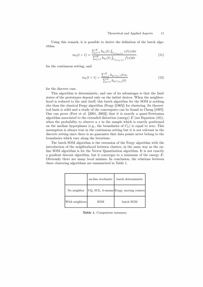
The batch SOM algorithm is the extension of the Forgy algorithm with theintroduction of the neighborhood between clusters, in the same way as the on-line SOM algorithm is for the Vector Quantization algorithm. It is not exactlya gradient descent algorithm, but it converges to a minimum of the energy E.Obviously there are many local minima. In conclusion, the relations betweenthese clustering algorithms are summarized in Table 1.

on-line stochastic batch deterministic

No neighbor VQ, SCL, k-means Forgy, moving centers

With neighbors SOM batch SOM

Table 1. Comparison summary.

12 Cottrell et al.

6 Other algorithms related to SOM

As explained before, the on-line SOM is not a gradient algorithm in the continu-ous setting (Erwin et al. [1992a,b]). In the discrete setting, there exists an energyfunction, which is an extended intra-classes variance as in Equation (10), but thisfunction is not continuously differentiable. To overcome these problems, Heskes[1999] proposes to slightly modify the on-line version of the SOM algorithm so itcan be seen as a stochastic gradient descent on the same energy function. To doso, he introduces a new hard assignment of the winning unit and a soft versionof this assignment.

6.1 Hard assignment in the Heskes’s rule

In order to obtain an energy function for the on-line SOM algorithm, Heskes[1999] modifies the rule for computing the best matching unit (BMU). In hissetting, Equation (1) becomes

ct(x) = arg mink∈{1,...,K}

K∑

j=1

hkj(t)‖x−mk(t)‖2 (13)

The energy function considered here is

E(m) =1

2

K∑

j=1

K∑

k=1

hkj(t)

∫

x∈Cj(m)

‖x−mk(t)‖2f(x)dx, (14)

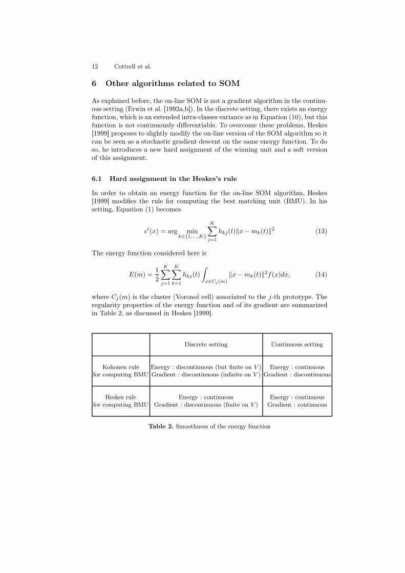
where Cj(m) is the cluster (Voronoï cell) associated to the j-th prototype. Theregularity properties of the energy function and of its gradient are summarizedin Table 2, as discussed in Heskes [1999].

Discrete setting Continuous setting

Kohonen rule Energy : discontinuous (but finite on V ) Energy : continuousfor computing BMU Gradient : discontinuous (infinite on V ) Gradient : discontinuous

Heskes rule Energy : continuous Energy : continuousfor computing BMU Gradient : discontinuous (finite on V ) Gradient : continuous

Table 2. Smoothness of the energy function

Theoretical and Applied Aspects 13

6.2 Soft Topographic Mapping (STM)

The original SOM algorithm is based on a hard winner assignment. Generaliza-tions based on soft assignments were derived in Heskes [1999] and Graepel et al.[1998]. First, let us remark that the energy function in the discrete case can alsobe written as

E(m, c) =1

2

K∑

k=1

N∑

i=1

cik

K∑

j=1

hkj(t)‖mj(t)− xi‖2

where cik is equal to 1 if xi belongs to cluster k and zero otherwise. This crispassignment may be smoothed by considering cik ≥ 0 such that

∑K

k=1 cik = 1.The soft assignments may be viewed as the probabilities of input xi to belongto class k.

Since the optimization of the energy function with gradient descent-like al-gorithms would get stuck into local minima, the problem is transformed into adeterministic annealing scheme. The energy function is smoothed by adding anentropy term and transforming it into a “free energy” cost function, parameter-ized by a parameter β :

F (m, c, β) = E(m, c)−1

βS(c) ,

where S(c) is the entropy term associated to the full energy. For low values ofβ, only one global minimum remains and may be easily determined by gradientdescent or EM schemes. For β → +∞, the free energy has exactly the sameexpression as the original energy function.When using deterministic annealing, one begins by computing the minimum ofthe free energy at low values of β and then attempts to compute the minimumfor higher values of β (β may be chosen to grow exponentially), until the globalminimum of the free energy for β → +∞ is equal to the global minimum of theoriginal energy function.For a fixed value of β, the minimization of the free energy leads to iteratingover two steps given by Equations (15) and (16), in batch version, and verysimilar to the original SOM (the neighborhood function h is not varied duringthe optimization process) :

P(xi ∈ Ck) =exp(−βeik)

∑Kj=1 exp(−βeij)

, (15)

where eik = 12

∑Kj=1 hjk(t)‖xi −mj(t)‖

2 and

mk(t) =

∑N

i=1 xi∑K

j=1 hjk(t)P(xi ∈ Cj)∑N

i=1

∑K

j=1 hjk(t)P(xi ∈ Cj)(16)

The updated prototypes are written as weighted averages over the data vec-tors. For β → +∞, the classical batch SOM is retrieved.

14 Cottrell et al.

6.3 Probabilistic views on the SOM

Several attempts have been made in order to recast the SOM algorithm (andits variants) into a probabilistic framework, namely the general idea of mixturemodels (see e.g. McLachlan and Peel [2004]). The central idea of those approachesis to constrain a mixture of Gaussian distributions in a way that mimic the SOMgrid. Due to the heuristic nature of the SOM, the resulting models depart quitesignificantly from the SOM algorithms and/or from standard mixture models.We describe below three important variants. Other variants are listed in e.g.Verbeek et al. [2005].

SOM and regularized EM One of the first attempt in this direction can befound in Heskes [2001]. Based on his work on energy functions for the SOM, Hes-kes shows in this paper that the batch SOM can be seen as a form of regularizedExpectation Maximization (EM) algorithm1.

As mentioned above, the starting point of the this analysis consists in in-troducing an isotropic Gaussian mixture with K components. The multivariateGaussian distributions share a single precision parameter β, with the covariancematrix 1

βI, and are centered on the prototypes.

However, up to some constant terms, the opposite of the log likelihood of sucha mixture corresponds to the k-means quantization error. And therefore, maxi-mizing the likelihood does not provide any topology preservation. Thus Heskesintroduces a regularization term which penalizes prototypes that do not respectthe prior structure (the term does not depend directly on the data points), seeHeskes [2001] for details. Then Heskes shows that applying the EM principle tothe obtained regularized (log)likelihood leads to an algorithm that resembles thebatch SOM one.

This interpretation has very interesting consequences, explored in the paper.It is easy for instance to leverage the probabilistic framework to handle missingvalues in a principled (non heuristic) way. It is also easy to use other mixtures e.g.for non numerical data (such as count data). However, the regularization itselfis rather ad hoc (it cannot be easily interpreted as a prior distribution on theparameters, for instance). In addition, the final algorithm is significantly differentfrom the batch SOM. Indeed, as in the case of the STM, crisp assignments arereplaced by probabilistic ones (the crispness of the assignments is controlled bythe precision parameter β). In addition, as in STM, the neighborhood functionis fixed (as it is the core of the regularization term). To our knowledge, thepractical consequences of those differences have not been studied in detail onreal world data. While one can argue that β can be increased progressively andat the same time, one can modify the neighborhood function during the EMalgorithm, this might also have consequences that remain untested.

SOM and variational EM Another take at this probabilistic interpretationcan be found in Verbeek et al. [2005]. As in Heskes [2001] the first step consists

1 EM is the standard algorithm for mixture models.

Theoretical and Applied Aspects 15

in assuming a standard mixture model (e.g. a K components Gaussian isotropicmixture for multivariate data). Then the paper leverages the variational principle(see e.g. Jordan et al. [1999]).

In summary, the variational principle is based on introducing an arbitrarydistribution q on the latent (hidden) variables Z of the problem under study.In a standard mixture model, the hidden variables are the assignment ones,which map each data point to a component of the mixture (a cluster in thestandard clustering language). One can show that the integrated log likelihoodof a mixture model with Θ as parameters, log p(X |Θ), is equal to the sum ofthree components: the complete likelihood (knowing both the data points X andthe hidden variables Z) integrated over the hidden variables with respect to q,Eq log p(X,Z|Θ), the entropy of q, H(q), and the Kullback-Leibler divergence,KL(q|p(Z|X,Θ)), between q and the posterior distribution of the hidden vari-ables knowing the data points p(Z|X,Θ). This equality allows one to derive theEM algorithm when the posterior distribution of the hidden variables knowingthe data points can be calculated exactly. The variational approach consists inreplacing this distribution by a simpler one when it cannot be calculated.

In standard mixture models (such as the multivariate Gaussian mixture),the variational approach is not useful as the posterior distribution of the hiddenvariables can be calculated. However Verbeek et al. [2005] propose nevertheless touse the variational approach as a way to enforce regularity in the mixture model.Rather than allowing p(Z|X,Θ) to take an arbitrary form, they constrain it to asubset of probability distributions on the hidden variables that fulfill topologicalconstraint corresponding to the prior structure of the SOM. See Verbeek et al.[2005] for details.

This solution shares most of the advantages of the older proposal in Heskes[2001], with the added value of being based on a more general principle that canbe applied to any mixture model (in practice, Heskes [2001] makes sense onlyfor the exponential family). In addition, Verbeek et al. [2005] study the effectsof shrinking the neighborhood function during training and conclude that itimproves the quality of the solutions. Notice that, in Verbeek et al. [2005], theshared precision of the Gaussian distributions (β) is not a meta-parameter as inHeskes [2001] but a regular parameter that is learned from the data.

The Generative Topographic Mapping The Generative Topographic Map-ping (GTM, Bishop et al. [1998]) is frequently presented as a probabilistic versionof the SOM. It is rather a mixture model inspired by the SOM rather than anadaptation. Indeed the aim of the GTM designers was not to recover a learningalgorithm close to a SOM variant, but rather to introduce a mixture model thatenforce topology preservation.

The GTM is based on uniform prior distribution on a fixed grid which ismapped via an explicit smooth nonlinear mapping to the data space (with someadded isotropic Gaussian noise). It can be seen as a constrained Gaussian mix-ture, but with yet another point of view compared to Heskes [2001] and Verbeeket al. [2005]. In Heskes [2001], the constraint is enforced by a regularization term

16 Cottrell et al.

on the data space distribution while in Verbeek et al. [2005] the constraint isinduced at the latent variable level (via approximating p(Z|X,Θ) by a smoothdistribution). In the GTM the constraint is induced on the data space distribu-tion because it is computed via a smooth mapping. In other words, the centers ofthe Gaussian distributions are not freely chosen but rather obtained by mappinga fixed grid to the data space via the nonlinear mapping.

The nonlinear mapping is in principle arbitrary and can therefore implementvarious type of regularity (i.e. topology constraints). The use of Gaussian ker-nels lead to constraints that are quite similar to the SOM constraints. Noticethat those Gaussian kernels are not to be confused with the isotropic Gaussiandistributions used in the data space (the same confusion could arise in Verbeeket al. [2005] where Gaussian kernels can be used to specify the constraints onp(Z|X,Θ)).

Once the model has been specify (by choosing the nonlinear mapping), itsparameters are estimated via an EM algorithm. The obtained algorithm is quitedifferent from the SOM (see Heskes [2001] for details), at least in its naturalformulation. However the detailed analysis contained in Heskes [2001] showsthat the GTM can be reformulated in a way that is close to the batch SOM withprobabilistic assignments (as in e.g. the STM). Once again, however, this is notexactly the same algorithm. In practice, the results on real world data can bequite different. Also, as all the probabilistic variants discussed in this section,the GTM benefits from the probabilistic setting that enables principled missingdata analysis as well as easy extensions to the exponential family of distributionsin order to deal with non numerical data.

7 Non numerical data

When the data are not numerical, the SOM algorithm has to be adapted. Seefor example Kohonen [1985], Kohonen [1996], Kaski et al. [1998a], Kohohenand Somervuo [1998], Kohonen [2001], Kohonen and Somervuo [2002], Kohonen[2013], Kohonen [2014], Cottrell et al. [2012], where some of these adaptationsare presented. Here we deal with categorical data collected in surveys and withabstract data which are known only by a dissimilarity matrix or a kernel matrix.

7.1 Contingency table or complete disjunctive table

Surveys collect answers of the surveyed individuals who have to choose an answerto several questions among a finite set of possible answers. The data can consistin

– a simple contingency table, where there are only two questions, and where theentries are the numbers of individuals who choose a given pair of categories,

– a Burt table, that is a full contingency table between all the pairs of cate-gories of all the questions,

Theoretical and Applied Aspects 17

– a complete disjunctive table that contains the answers of all the individuals,coded in 0/1 against dummy variables which represent all the categories ofall the questions.

In all these settings, the data consist in a positive integer-valued matrix,which can be seen as a large “contingency table”. In classical data analysis, oneuses Multiple Correspondence Analysis (MCA) that are designed to deal withthese tables. MCA is nothing else than two simultaneous weighted PrincipalComponent Analysis (PCA) of the table and of its transposed, using the χ2

distance instead of the Euclidean distance. To use a SOM algorithm with suchtables, it is therefore sufficient to apply a transformation to the data, in order totake into account the χ2 distance and the weighting, in the same way that it isdefined to use Multiple Correspondence Analysis. After transforming the data,two coupled SOM using the rows and the columns of the transformed table canthus be trained. In the final map, related categories belong to the same clusteror to neighboring clusters. The reader interested by a detailed explanation ofthe algorithm can refer to Bourgeois et al. [2015a] . More details and real-worldexamples can also be found in Cottrell et al. [2004], Cottrell and Letrémy [2005].Notice that the transformed tables are numerical data tables, and so there is noparticular theoretical results to comment on. All the results that we presentedfor numerical data still hold.

7.2 Dissimilarity Data

In some cases, complex data such as graphs (social networks) or sequences (DNAsequences) are described through relational measures of resemblance or dissem-blance, such as kernels or dissimilarity matrices. For these general situations,several extensions of the original algorithm, both in on-line and batch versions,were proposed during the last two decades. A detailed review of these algorithmsis available in Rossi [2014].

More precisely, these extensions consider the case where the data are valuedin an arbitrary space X , which is not necessarily Euclidean. The observationsare described either by a pairwise dissimilarity D = (δ(xi, xj))i,j=1,...,N , or by akernel matrix K = (K(xi, xj))i,j=1,...,N

2. The kernel matrix K naturally inducesan Euclidean distance matrix, but the dissimilarity matrix D may not necessarilybe transformed into a kernel matrix.

The first class of algorithms designed for handling relational data is basedon the median principle (median SOM ): prototypes are forced to be equal toan observation, or to a fixed number of observations. Hence, optimal prototypes

2 A kernel is a particular case of symmetric similarity such that K is a symmetricmatrix, semi-definite positive with K(xi, xi) = 0 and satisfies the following positiveconstraint

∀M > 0, ∀ (xi)i=1,...,M ∈ X , ∀ (αi)i=1,...,M ,∑

i,j

αiαjK(xi, xj) ≥ 0.

18 Cottrell et al.

are computed by searching through (xi)i=1,...,N , instead of X , as in Kohohenand Somervuo [1998], Kohonen and Somervuo [2002], El Golli et al. [2004a] andEl Golli et al. [2004b]. The original steps of the algorithm are thus transformedin a discrete optimization scheme, which is performed in batch mode:

1. Equation (1) is replaced by the affectation of all data to their best matchingunits: c(xi) = arg mink=1,...,K δ(xi,mk(t));

2. Equation (2) is replaced by the update of all prototypes within the dataset

(xi)i=1,...,N : mk(t) = minxi : i=1,...,N

∑N

j=1 hc(xi)j(t)δ(xi, xj).

Since the algorithm explores a finite set when updating the prototypes, itis necessarily convergent to a local minimum of the energy function. However,this class of algorithms exhibits strong limitations, mainly due to the restric-tion of the prototypes to the dataset, in particular, a large computational cost(despite efficient implementations such as in Conan-Guez et al. [2006]) and nointerpolation effect which yields to a deterioration of the quality of the maporganization.

The second class of algorithms, kernel SOM and relational/dissimilaritySOM, rely on expressing prototypes as convex combinations of the input data.Although these convex combinations do not usually have sense in X (consider,for instance, that input data are various texts), a convenient embedding in anEuclidean or a pseudo-Euclidean space gives a sound theoretical framework andgives sense to linear combinations of inputs.

For kernel SOM, it is enough to use the kernel trick as given by Aron-szajn [1950] which prove that there exists a Hilbert space H, also called fea-ture space, and a mapping ψ : X → H, called feature map, such thatK(x, x′) = 〈ψ(x), ψ(x′)〉H. In the case where data are described by a symmet-ric dissimilarity measure, they may be embedded in a pseudo-Euclidean spaceψ : x ∈ X → ψ(x) = (ψ+(x), ψ−(x)) ∈ E , as suggested in Goldfarb [1984]. Emay be written as the direct decomposition of two Euclidean spaces, E+ and E−,with a non-degenerate and indefinite inner product defined as

〈ψ(x), ψ(y)〉E = 〈ψ+(x), ψ+(u)〉E+ − 〈ψ−(x), ψ−(u)〉E−

The distance naturally induced by the pseudo-Euclidean inner product is notnecessarily positive.

For both kernel and relational/dissimilarity SOM, the input data are em-bedded in H or E and prototypes are expressed as convex combinations of theimages of the data by the feature maps. For example, in the kernel case,

mk(t) =

N∑

i=1

γtkiψ(xi) , with γtki ≥ 0 and∑

i

γtki = 1.

The above writing of the prototypes allows the computation of the distancefrom an input xi to a prototype mk(t) in terms of the coefficients γtki and thekernel/dissimilarity matrix only. For kernel SOM, one has

‖ψ(xi)−mk(t)‖2 =

(

γtk)T

Kγtk − 2Kiγtk +Kii ,

Theoretical and Applied Aspects 19

where Ki is the ith row of K and (γtk)T

=(

γtk,1, ..., γtk,N

)

. For rela-

tional/dissimilarity SOM, one obtains a similar expression

‖ψ(xi)−mk(t)‖2 = Diγ

tk −

1

2

(

γtk)T

Dγtk .

The first step of the algorithm, finding the best matching unit of an observation,as introduced in Equation (1), can thus be directly generalized to kernels anddissimilarities, both for on-line and batch settings.

In the batch framework, the updates of the prototypes are identical to theoriginal algorithm (see Equation (12)), by simply noting that only the coefficientsof the xi’s (or of their images by the feature maps) are updated :

mk(t+ 1) =

N∑

i=1

hkct(xi)(t)∑N

j=1 hkct(xj)(t)ψ(xi) ⇔ γt+1

ki =hkct(xi)(t)

∑N

j=1 hkct(xj)(t)(17)

This step is the same, both for batch kernel SOM, Villa and Rossi [2007],and for batch relational SOM, Hammer et al. [2007].

In the on-line framework, updating the prototypes is similar to the originalalgorithm, as in Equation (2). Here also, the update rule concerns the coefficientsγtki only, and the linear combination of them remains convex :

γt+1k = γtk + ε(t)hkct(xi)(t)

(

1i − γtk)

, (18)

where xi is the current observation and 1i is a vector in RN , with a single

non-null coefficient, equal to 1, on the i-th position. As previously, this step isidentical for on-line kernel SOM, Mac Donald and Fyfe [2000], and for on-linerelational SOM, Olteanu and Villa-Vialaneix [2015].

In the case where the dissimilarity is the squared distance induced by thekernel, kernel SOM and relational SOM are strictly equivalent. Moreover, in thiscase, they are also fully equivalent to the original SOM algorithm for numericaldata in the feature (implicit) Euclidean space induced by the dissimilarity or thekernel, as long as the prototypes are initialized in the convex hull of the inputdata. The latter assertion induces that the theoretical limitations of the originalalgorithm also exist for the general kernel/relational versions. Furthermore,these may worsen for the relational version since the non-positivity of thedissimilarity measure adds numerical instability when using a gradient-descentlike scheme for updating the prototypes.

The third class of algorithms uses the soft topographic maps setting intro-duced in section 6.2. Indeed, in the algorithm described in equations (15) and(16), the soft assignments depend on the distances between input data and pro-totypes only, while prototypes update consists in making an update if the co-efficients of the input data. Using a mean-field approach and similarly to theprevious framework for kernel and dissimilarity/relational SOM, Graepel et al.[1998] obtain the extensions of soft topographic mapping (STM) algorithm for

20 Cottrell et al.

kernels and dissimilarities. The updates for the prototype coefficients are thenexpressed as

γki(t+ 1) =

∑K

j=1 hjk(t)P(xi ∈ Aj)∑N

l=1

∑K

j=1 hjk(t)P(xl ∈ Aj), (19)

where mk(t) =∑N

i=1 γtkiψ(xi) and ψ is the feature map.

8 Stochasticity of the Kohonen maps for the on-line

algorithm

Starting from a given initialization and a given size of the map, different runs ofthe on-line stochastic SOM algorithm provide different resulting maps. On thecontrary, the batch version of the algorithm is a deterministic algorithm withalways provides the same results for a given initialization. For this reason, thebatch SOM algorithm is often preferred over the stochastic one because its resultsare reproducible. However, this hides the fact that all the pairs of observationswhich are associated in a given cluster do not have the same significance. Moreprecisely, interpreting a SOM result, we can use the fact that close input databelong to close clusters, i.e. their best matching units are identical or adjacent.But if two given observations are classified in the same or in neighboring unitsof the map, then they may not be close in the input space. This drawback comesfrom the fact that there is not perfect matching between a a multidimensionalspace and a one- or two-dimensional map.

More precisely, given a pair of observations (data), {xi, xj}, three cases canbe distinguished, depending on the way their respective mapping on the mapcan be described:

– significant association: the pair is classified in the same cluster or in neighbor-ing clusters because xi and xj are close in the input space. The observationsare said to attract each other;

– significant non-association: the pair is never classified in neighboring clustersand xi and xj are remote in the input space. The observations are said torepulse each other;

– fickle pair : the pair is sometimes classified in the same cluster or in neighbor-ing clusters but xi and xj are not close in the input space: their proximityon the map is due to randomness.

The stochasticity of the on-line SOM results can be used to precisely qualifyevery pairs of observations by performing several runs of the algorithm. Thequestion is addressed in a bootstrap framework in de Bodt et al. [2002] and usedfor text mining applications in Bourgeois et al. [2015a,b]. The idea is simple:since the on-line SOM algorithm is stochastic, its repetitive use may allow toidentify the pairs of data in each case.

More precisely, if L is the number of different and independent runs of theon-line SOM algorithm and if Yi,j denotes the number of times xi and xj are

Theoretical and Applied Aspects 21

neighbors on the resulting map in the L runs, a stability index can be defined:for the pair (xi, xj), this index is equal to:

Mi,j =Yi,j

L.

Using an approximation of the binomial distribution that would hold if the datawere neighbors by chance in a pure random way, and a test level of 5%, for aK-units map, the following quantities are introduced

A =9

Kand B = 1.96

√

9

KL(1 −

9

K). (20)

These values give the following decision rule to qualify every pair {xi, xj}:

– if Mi,j > A+B, the association between the two observations is significantlyfrequent;

– if A − B ≤ Mi,j ≤ A + B, the association between the two observations isdue to randomness. {xi, xj} is called a fickle pair;

– if Mi,j < A−B, the non-association between the two observations is signif-icantly frequent.

In de Bodt et al. [2002], the method is used in order to qualify the stabilityand the reliability of the global Kohonen map, while both other papers (Bour-geois et al. [2015a] and Bourgeois et al. [2015b]) study the fickle data pairs forthemselves. In these last work, the authors also introduce the notion of fickleword which is defined as an observation which belongs to a huge number offickle pairs by choosing a threshold.

These fickle pairs and fickle words can be useful in various way: first, ficklepairs can be used to obtain more robust maps, by distinguishing stable neigh-boring and non neighboring pairs from fickle pairs. Also, once identified, ficklewords can be removed from further studies and representations: for instance,Factorial Analysis visualization is improved. In a text mining setting, Bourgeoiset al. [2015b] have shown that a graph of co-occurrences between words can besimplified by removing fickle words and Bourgeois et al. [2015a] have used thefickle words for interpretation: they have shown that the fickle words form alexicon shared between the studied texts.

9 Conclusion

We have reviewed some of the variants of the SOM, for numerical and nonnumerical data, in their stochastic (on-line) and batch versions. Even if a lot oftheoretical properties are not rigorously proven, the SOM algorithms are veryuseful tools for data analysis in different contexts. Since the Heskes’s variantsof SOM have a more solid theoretical background, SOM can appear as an easy-to-develop approximation of these well-founded algorithms. This remark shouldease the concern that one might have about it.

22 Cottrell et al.

On a practical point of view, SOM is used as a statistical tool which hasto be combined with other techniques, for the purpose of visualization, of vec-tor quantization acceleration, graph construction, etc. Moreover, in a big datacontext, SOM-derived algorithms seem to have a great future ahead since thecomputational complexity of SOM is low (proportional to the number of data).In addition, it is always possible to train the model with a sample randomlyextracted from the database and then to continue the training in order to adaptthe prototypes and the map to the whole database. As most of the stochasticalgorithm, SOM is particularly well suited for stream data (see Hammer andHasenfuss [2010] which proposed a “patch SOM” to handle this kind of data).Finally, it would also be interesting to have a look at the robust associationsrevealed by SOM, to improve the representation and the interpretation of tooverbose and complex information.

References

N. Aronszajn. Theory of reproducing kernels. Transactions of the American Mathe-matical Society, 68(3):337–404, 1950.

Christopher M. Bishop, Markus Svensén, and Christopher K. I. Williams. GTM: Thegenerative topographic mapping. Neural Computation, 10(1):215–234, 1998.

N. Bourgeois, M. Cottrell, B. Deruelle, S. Lamassé, and P. Letrémy. How to improverobustness in kohonen maps and display additional information in factorial analysis:Application to text minin. Neurocomputing, 147:120–135, 2015a.

N. Bourgeois, M. Cottrell, S. Lamassé, and M. Olteanu. Search for meaning throughthe study of co-occurrences in texts. In I. Rojas, G. Joya, and A. Catala, editors, Ad-vances in Computational Intelligence, Proceedings of IWANN 2015, Part II, volume9095 of LNCS, pages 578–591. Springer, 2015b.

Y. Cheng. Convergence and ordering of kohonen’s batch map. Neural Computation, 9:1667–1676, 1997.

B. Conan-Guez, F. Rossi, and A. El Golli. Fast algorithm and implementation ofdissimilarity self-organizing maps. Neural Networks, 19(6-7):855–863, 2006.

M. Cottrell and J.C. Fort. Étude d’un processus d’auto-organisation. Annales de l’IHP,section B, 23(1):1–20, 1987.

M. Cottrell and P. Letrémy. How to use the Kohonen algorithm to simultaneouslyanalyse individuals in a survey. Neurocomputing, 63:193–207, 2005.

M. Cottrell, J.C. Fort, and G. Pagès. Theoretical aspects of the SOM algorithm.Neurocomputing, 21:119–138, 1998.

M. Cottrell, S. Ibbou, and P. Letrémy. Som-based algorithms for qualitative variables.Neural Networks, 17:1149–1167, 2004.

M. Cottrell, M. Olteanu, F. Rossi, J. Rynkiewicz, and N. Villa-Vialaneix. Neuralnetworks for complex data. Künstliche Intelligenz, 26(2):1–8, 2012. doi: 10.1007/s13218-012-0207-2.

E. de Bodt, M. Cottrell, and M. Verleisen. Statistical tools to assess the reliabilityof self-organizing maps. Neural Networks, 15(8-9):967–978, 2002. doi: 10.1016/S0893-6080(02)00071-0.

Aïcha El Golli, Brieuc Conan-Guez, and Fabrice Rossi. Self organizing map and sym-bolic data. Journal of Symbolic Data Analysis, 2(1), 11 2004a.

Theoretical and Applied Aspects 23

Aïcha El Golli, Brieuc Conan-Guez, and Fabrice Rossi. A self organizing map fordissimilarity data. In D. Banks, L. House, F. R. McMorris, P. Arabie, and W. Gaul,editors, Classification, Clustering, and Data Mining Applications (Proceedings ofIFCS 2004), pages 61–68, Chicago, Illinois (USA), 7 2004b. IFCS, Springer.

E. Erwin, K. Obermayer, and K. Schulten. Self-organizing maps: ordering, convergenceproperties and energy functions. Biological Cybernetics, 67(1):47–55, 1992a.

E. Erwin, K. Obermayer, and K. Schulten. Self-organizing maps: stationnary states,metastability and convergence rate. Biological Cybernetics, 67(1):35–45, 1992b.

J.A. Flanagan. Self-organisation in kohonen’s som. Neural Networks, 6(7):1185–1197,1996.

E.W. Forgy. Cluster analysis of multivariate data: efficiency versus interpretability ofclassifications. Biometrics, (21):768–769, 1965.

J.-C. Fort, M. Cottrell, and P. Letrémy. Stochastic on-line algorithm versus batchalgorithm for quantization and self organizing maps. In Neural Networks for Sig-nal Processing XI, 2001, Proceedings of the 2001 IEEE Signal Processing SociétyWorkshop, pages 43–52, North Falmouth, MA, USA, 2001. IEEE.

J.-C. Fort, P. Letrémy, and M. Cottrell. Advantages and drawbacks of the batch ko-honen algorithm. In M. Verleysen, editor, European Symposium on Artificial NeuralNetworks, Computational Intelligence and Machine Learning (ESANN 2002), pages223–230, Bruges, Belgium, 2002. d-side publications.

J.C. Fort. SOM’s mathematics. Neural Networks, 19(6-7):812–816, 2006.J.C. Fort and G. Pagès. About the kohonen algorithm: strong or weak self-organisation.

Neural Networks, 9(5):773–785, 1995.L. Goldfarb. A unified approach to pattern recognition. Pattern Recognition, 17(5):

575–582, 1984. doi: 10.1016/0031-3203(84)90056-6.T. Graepel, M. Burger, and K. Obermayer. Self-organizing maps: generalizations and

new optimization techniques. Neurocomputing, 21:173–190, 1998.B. Hammer and A. Hasenfuss. Topographic mapping of large dissimilarity data sets.

Neural Computation, 22(9):2229–2284, September 2010.B. Hammer, A. Hasenfuss, F. Rossi, and M. Strickert. Topographic processing of

relational data. In Bielefeld University Neuroinformatics Group, editor, Proceed-ings of the 6th Workshop on Self-Organizing Maps (WSOM 07), Bielefeld, Germany,September 2007.

T. Heskes. Energy functions for self-organizing maps. In E. Oja and S. Kaski, editors,Kohonen Maps, pages 303–315. Elsevier, Amsterdam, 1999. URL http://www.snn.

ru.nl/reports/Heskes.wsom.ps.gz.Tom Heskes. Self-organizing maps, vector quantization, and mixture modeling. IEEE

Transactions on Neural Networks, 12(6):1299–1305, November 2001.Michael I Jordan, Zoubin Ghahramani, Tommi S Jaakkola, and Lawrence K Saul. An

introduction to variational methods for graphical models. Machine learning, 37(2):183–233, 1999.

S. Kaski, T. Honkela, K. Lagus, and T. Kohonen. Websom - self-organizing maps ofdocument collections. Neurocomputing, 21(1):101–117, 1998a.

Samuel Kaski, Kangasb Jari, and Teuvo Kohonen. Bibliography of self-organizing map(SOM) papers: 1981–1997. Neural Computing Surveys, 1(3&4):1–176, 1998b.

T. Kohohen and P.J. Somervuo. Self-organizing maps of symbol strings. Neurocom-puting, 21:19–30, 1998.

T. Kohonen. Self-organized formation of topologically correct feature maps. Biol.Cybern., 43:59–69, 1982a.

T. Kohonen. Analysis of a simple self-organizing process. Biol. Cybern., 44:135–140,1982b.

24 Cottrell et al.

T. Kohonen. Median strings. Pattern Recognition Letters, 3:309–313, 1985.T. Kohonen. Self-organization and associative memory. Springer, 1989.T. Kohonen. Self-Organizing Maps, volume 30 of Springer Series in Information Sci-

ence. Springer, 1995.T. Kohonen. Self-organizing maps of symbol strings. Technical report a42, Laboratory

of computer and information science, Helsinki University of technoligy, Finland,1996.

T. Kohonen. Comparison of som point densities based on different criteria. NeuralComputation, 11:2081–2095, 1999.

T. Kohonen. Self-Organizing Maps, 3rd Edition, volume 30. Springer, Berlin, Heidel-berg, New York, 2001.

T. Kohonen. Essentials of self-organizing map. Neural Networks, 37:52–65, 2013.T. Kohonen. MATLAB Implementations and Applications of the Self-Organizing Map.

Unigrafia Oy, Helsinki, Finland, 2014.T. Kohonen and P.J. Somervuo. How to make large self-organizing maps for nonvec-

torial data. Neural Networks, 15(8):945–952, 2002.D. Mac Donald and C. Fyfe. The kernel self organising map. In Proceedings of 4th

International Conference on knowledge-based Intelligence Engineering Systems andApplied Technologies, pages 317–320, 2000.

Geoffrey McLachlan and David Peel. Finite mixture models. John Wiley & Sons, 2004.Merja Oja, Samuel Kaski, and Teuvo Kohonen. Bibliography of self-organizing map

(SOM) papers: 1998–2001 addendum. Neural Computing Surveys, 3:1–156, 2003.M. Olteanu and N. Villa-Vialaneix. On-line relational and multiple relational SOM.

Neurocomputing, 147:15–30, 2015. doi: 10.1016/j.neucom.2013.11.047.David Pollard et al. Strong consistency of k-means clustering. The Annals of Statistics,

9(1):135–140, 1981.H. Ritter and K. Schulten. On the stationary state of kohonen’s self-organizing sensory

mapping. Biol. Cybern., 54:99–106, 1986.H. Ritter, T. Martinetz, and K. Schulten. Neural computation and self-Organizing

Maps, an Introduction. Addison-Wesley, 1992.F. Rossi. How many dissimilarity/kernel self organizing map variants do we need?

In T. Villmann, F.M. Schleif, M. Kaden, and M. Lange, editors, Advances inSelf-Organizing Maps and Learning Vector Quantization (Proceedings of WSOM2014), volume 295 of Advances in Intelligent Systems and Computing, pages 3–23, Mittweida, Germany, 2014. Springer Verlag, Berlin, Heidelberg. doi: 10.1007/978-3-319-07695-9_1.

A. Sadeghi. Convergence in distribution of the multi-dimensional kohonen algorithm.J. of Appl. Probab., 38(1):136–151, 2001.

Jakob J. Verbeek, Nikos Vlassis, and Ben J. A. Kröse. Self-organizing mixture models.Neurocomputing, 63:99–123, January 2005.

N. Villa and F. Rossi. A comparison between dissimilarity SOM and kernel SOM forclustering the vertices of a graph. In 6th International Workshop on Self-OrganizingMaps (WSOM 2007), Bielefield, Germany, 2007. Neuroinformatics Group, BielefieldUniversity. ISBN 978-3-00-022473-7. doi: 10.2390/biecoll-wsom2007-139.