STOCHASTIC ON-LINE ALGORITHM

VERSUS BATCH ALGORITHM FOR

QUANTIZATION AND SELF ORGANIZING

MAPS

Jean-Claude Fort

Institut Elie Cartan et SAMOS-MATISSE

Université Nancy 1, F-54506 Vandoeuvre-Lès-Nancy, France

E-mail: fortjc@iecn.u-nancy.fr

and

Marie Cottrell, Patrick Letremy

SAMOS-MATISSE UMR CNRS 8595

Université Paris 1, F-75634 Paris Cedex 13, France

E-mail : cottrell,pley@univ-paris1.fr

Abstract. The Kohonen algorithm (SOM) was originally designed

as a stochastic algorithm which works in an on-line way and which

was designed to model some adaptative features of the human

brain. In fact it is nowadays extensively used for data mining,

data visualization, and exploratory data analysis. Some users are

tempted to use the batch version of the Kohonen algorithm since it

is a deterministic algorithm which can be convenient if one needs

to get reproducible results and which can go faster in some cases.

In this paper, we try to elucidate the mathematical nature of this

batch variant and give some elements of comparison of both algo-

rithms. Then we compare both versions on a real data set.

INTRODUCTION

Since about twenty years, the Self-Organizing Maps (SOM) of Teuvo Kohonen

have spread through numerous domains where it found e�ective applications

by itself or coupled with other data analysis devices (source separation al-

gorithm or classical �ltering for signal processing, multilayer perceptrons for

speech recognition, etc.). See for example [15], [16], [14], [8], [18], [4] etc. for

de�nitions and numerous applications.

Nevertheless, SOM appears to be a very powerful extension (see [7], or

[6]) of the classical Simple Competitive Learning algorithm (SCL) used to

realize the quantization of probability measures, (see for example in [13]

the de�nition of SCL). So we will treat simultaneously the two algorithms,

mentioning when it will be necessary some special features.

The Kohonen algorithm and the SCL algorithm are both on-line algo-

rithms, which means they compute the current values of the code vectors (or

weight vectors) at each arrival of a data. They mimic the adaptation of a bi-

ological system to a variable environment, susceptible to su�er some changes.

These potential modi�cations are instantaneously taken into account through

the variations of the distribution and of the statistics along the observed data

series.

Another point of view to design an algorithm in order to quantify or build

organized maps is to use all the available information. If we have already

observed N data, then we use at one go these N values. Of course we cannot

�nd all at once the good code vectors (or weight vectors). So by iterating this

process, we hope to increase the quality of the result at each new iteration.

This is the case for the algorithms known as Kohonen Batch algorithm ([17])

or Forgy algorithm ([10]) when there is no neighborhood relations.

ON-LINE ALGORITHMS

The ingredients necessary to the de�nition of these algorithms are:

� An initial value of the d-dimensional code vectors X0(i); i 2 I, where I

is the set of units;

� A sequence (!t)t�1 of observed data which are also d-dimensional vec-

tors;

� A symmetric neighborhood function �(i; j) which measures the link

between units i and j;

� A gain (or adaptation parameter) ("t)t�1, constant or decreasing.

Then the algorithm works in 2 steps:

1. Choose a winner (in the winner-take-all version) or compute an acti-

vation function (we mention this case, but we will concentrate only on

the previous winner-take-all version)

� winner : i0(t + 1) = argmini dist(!t+1; Xt(i)), where dist is gen-erally the Euclidean distance, but could be any other one;

� activation function, for instance :

�(i;Xt) =exp( 1

T)dist(!t+1; Xt(i))P

j2I exp(1T)dist(!t+1; Xt(j))

:

In this expression, if we let the positive parameter T going to

in�nity, we retrieve the winner-take-all case.

2. Modify the code vectors (or weight vectors) according to a reinforce-

ment rule: the closer to the winner, the stronger is the change.

� Xt+1(i) = Xt(i)+"t+1�(i0(t+1); i)(!t+1(i)�Xt(i)) in the winner-take-all case or

� Xt+1(i) = Xt(i) + "t+1P

j�(j; i)�(j;Xt)(!t+1(i) � Xt(i)) in the

activation function case.

The case of the SCL algorithm ( i.e. only quantization) is obtained by

taking �(i; i) = 1 and �(i; j) = 0; i 6= j. It can be viewed as a 0-neighbor

Kohonen algorithm.

Actually few results are known about the mathematical properties of these

algorithms (see [2], [3], [11], [1], [20], [21]) except in the one dimensional

case. The good framework of study, as for almost all the neural networks

learning algorithms, is the theory of stochastic approximation ([12]). In this

framework, the �rst and most informative quantity is the associated Ordinary

Di�erential Equation (ODE). Before writing it down, let us introduce some

notations.

From now and for simplicity, we choose the Euclidean distance to compute

the winner unit. For any set of code vectors x = (x(i)); i 2 I, we put

Ci(x) = f!=kx(i)� !k = minjkx(j) � !kg;

that is the set of data for which the unit i is the winner. The set of the

(Ci(x)); i 2 I is called the Voronoï tessellation de�ned by x.

When it is convenient, we write x(i; t) instead of xt(i) and x(:; t) for

xt = (xt(i); i 2 I).Then the ODE (in the winner-take-all case) reads :

8i 2 I;dx(i; u)

du= �

Xj2I

�(i; j)

ZCj(x(:;u))

(x(i; u)� !)�(d!);

where � stands for the probability distribution of the data set and where the

second member is the expectation of �(i0(t); i)(!t+1(i)�Xt(i)) with respect

to the distribution �.

In practice, distribution � looks like a discrete one, because we only use

a �nite number of "examples" or at least a denumerable set. But generally

the good way to model the actual set of possible data is to consider a con-

tinuous probability distribution (for a frequency, some Fourier coe�cients or

coordinate in an Hilbertian base, a level of gray, ...).

When � is discrete (in fact has a �nite support), one can see that the ODE

locally derives from an energy function (it means that the second member

can be seen as the opposite gradient of this energy function, which is then de-

creasing along the trajectories of the ODE), that we call extended distortion,

in reference to the classical distortion in the SCL case. See [19] for elements

of proof.

In the SCL case, the (classical) distortion is

D(x) =Xi2I

ZCi(x)

kx(i)� !k2�(d!) (1)

=

Zminikx(i)� !k2�(d!): (2)

In the general case of SOM, the extended distortion is

D(x) =Xi2I

Xj

�(i; j)

ZCj(x)

kx(i)� !k2�(d!):

When � is di�use (or has a di�use part), then D is no more an energy

function for the ODE, because there are spurious (or parasite) terms due to

the neighborhood function (see [9] for proof). Then when � is di�use, the

only case where D is still an energy function for the ODE is the SCL case.

Nevertheless, it has to be noticed that

� when D is an actual energy function, then it is not everywhere di�eren-

tiable and we only get local information which is not what is expected

from such a function. In particular, the existence of this energy function

is not su�cient to rigorously prove the convergence !

� when D is everywhere di�erentiable, then it is no more an actual energy

function even if it gives a very good information about the convergence

of the algorithm.

In any case, if they would be convergent, both algorithms (SOM and SCL)

would converge toward an equilibrium of the ODE (even if this fact is not

mathematically proved). These equilibria are de�ned by

8i 2 I;Xj

�(i; j)

ZCj(x�)

(x�(i) � !)�(d!) = 0:

This also reads

x�(i) =

Pj�(i; j)

RCj(x�)

! �(d!)Pj �(i; j)�(Cj(x�))

(3)

In the SCL case, it means that all the x�(i) are the centers of gravity

of their Voronoï tiles. In the statistical literature, it is called self-consistent

point. More generally, in the SOM case, x�(i) is the center of gravity (for

the weights which are given by the neighborhood function) of all the centers

of the tiles.

From this remark, the de�nitions of the batch algorithms can be derived.

THE BATCH ALGORITHMS

Using (3), we immediately derive the de�nitions of the batch algorithms. Our

aim is to �nd a solution of (3) through a deterministic iterative procedure.

In a �rst approach, let us de�ne a sequence of code vectors by:

� x0 is an initial value

� and

xk+1(i) =

Pj�(i; j)

RCj (xk)

! �(d!)Pj �(i; j)�(Cj(xk))

:

Now if the sequence converges (or at least for any sub-sequence that con-

verges, which always exists if (xk)k�1 is bounded), it converges toward a

solution of (3).

This de�nes exactly the Kohonen Batch algorithm when � weights only

a �nite number N of data. It reads :

xk+1N (i) =

Pj �(i; j)

PN

l=1 !l 1Cj(xk)(!l)Pj �(i; j)

PN

l=1 1Cj(xk)(!l):

Recall that 1Cj(xk)(!l) is 1 if !l belongs to Cj(xk) and 0 elsewhere.

Moreover, if we assume that when N goes to in�nity, �N = 1N

PN

l=1 �!l

(�! stands for the Dirac measure at !) weakly converges toward �, we then

have (under mild conditions)

limN!1

limk!1

xk+1N (i) = x�(i);

where x� is a solution of (3).

The extended distortion is piecewise convex since the changes of convexity

take place on the median hyperplanes which are the frontiers of the Voronoï

tessellation. And at this stage, we may notice that the Kohonen Batch al-

gorithm is nothing else but a "quasi-Newtonian" algorithm which minimizes

the extended distortion D associated with �N .

In fact, when there is no data on the borders of the Voronoï tessellation,

it is possible to verify that

xk+1N = xkN ��diagr2D(xkN )

��1rD(xkN )

where diagM is the diagonal matrix made with the diagonal of M , rD is

the gradient of D and r2D is the Hessian of D, which exists. It is a "quasi-

Newtonian" algorithm because it uses only the diagonal part of the Hessian

matrix and not the full matrix.

This proves that in every convex set where D is di�erentiable, (xkN ) con-verges toward a x� minimizingD. Unfortunately, there are many such disjoint

sets and in each of them there is a local minimumof D, even if we do not take

into account the possible symmetries or geometric transformations letting �

invariant.

A COMPARISON ON SIMULATED DATA

Actually, it very often happens that the batch algorithm �nds not fully satis-

factory solution of (3). It strongly depends on the choice of the initial value

x0. On the contrary, the on-line algorithm, especially with constant ", can

escape from reasonably deep traps and �nd a better solution of equation (3)

even starting from the attraction basin of a poor quality solution.

In Fig.1 and Fig.2, are depicted two solutions respectively found by a

Kohonen Batch and an on-line SOM algorithms in the following conditions :

The units are organized on a (7�7) grid endowed with a 8 nearest neigh-

bors topology. The data set is made of a 500-sample of independent, uni-

formly distributed on [0; 1], random variables. The initial code vectors are

random too.

The Batch algorithm is processed for 100 times, which leads to the limit

(numerically at least).

The stochastic on-line algorithm is iterated 50 000 times by drawing at

random one data at each step.

The gain "t is decreasing and given by "t = 0:125=(1 + 6:10�4t):The two solutions that we found are very stable for each algorithm, but

due to the random property, the on-line algorithm discovers the best one.

0 0.1 0.2 0.3 0.4 0.5 0.6 0.7 0.8 0.9 10

0.1

0.2

0.3

0.4

0.5

0.6

0.7

0.8

0.9

1

Figure 1: Kohonen Batch for a 7 by 7 grid

We can observe that the Kohonen Batch get trapped in a local minimum

and do not correctly realize neither the self-organization nor the quantization.

We did a lot of similar simulations and always got the same kind of results.

0 0.1 0.2 0.3 0.4 0.5 0.6 0.7 0.8 0.9 10

0.1

0.2

0.3

0.4

0.5

0.6

0.7

0.8

0.9

1

Figure 2: On-line SOM for a 7 by 7 grid

APPLICATION TO DATA ANALYSIS

If the data consist in a set of N observations, each of one being described

by a d-dimensional vector, the Kohonen algorithms (both on-line and batch

versions) provide a very powerful tool to classify, represent and visualize the

data in a Kohonen map (most of time a two- or one-dimensional map, one

speaks of grid or string). See [4], [14], [18] for numerous examples.

After learning, that is after convergence of the algorithm (whatever it is),

each unit i is represented in the Rd space by its code vector X(i). Each code

vector resembles more to its neighbors than to the other code vectors, due

to the topology conservation property. This feature provides an organized

map of the code vectors, which gives prominence to the progressive varia-

tions across the map for each variable which describes the data.

Classi�cation and Representation

After convergence, each observation is classi�ed by the nearest neighbor

method (in Rd) : observation l belongs to class Ci if and only if the code vec-

tor X(i) is closer to observation i than to any other. Similar observations are

classi�ed into the same class or into neighbor classes, that is not true when

using any other classi�cation method. Then the observations can be listed

or drawn inside their classes and this fact provides a two- or one-dimensional

representation on the grid (or along the string). In this kind of map, one can

appreciate how the observations di�er from one class to the next ones, and

can study the homogeneity of the classes.

Two-level classi�cation

The classi�cation that we get in the �rst step is generally based on a large

number of classes, and this fact makes the interpretation and the establish-

ment of a typology di�cult. So it is very convenient to reduce the number

of classes by using a hierarchical clustering of the code vectors. So the most

similar classes are grouped into a reduced number of larger ones. These

macro-classes create connected areas in the initial maps, and the neighbor-

hood relations are kept. This grouping together facilitates the interpretation

of the contents and the description of a typology of the observations.

Quality of the organization

We can control the quality of the organization by considering the results of

the two-level classi�cation. The fact that the hierarchical clustering of the

code vectors only groups connected areas means that the map is well orga-

nized, since it means that to be close in the data space coincides with to be

close on the map.

Quality of the quantization

It is given by the distortion (2).

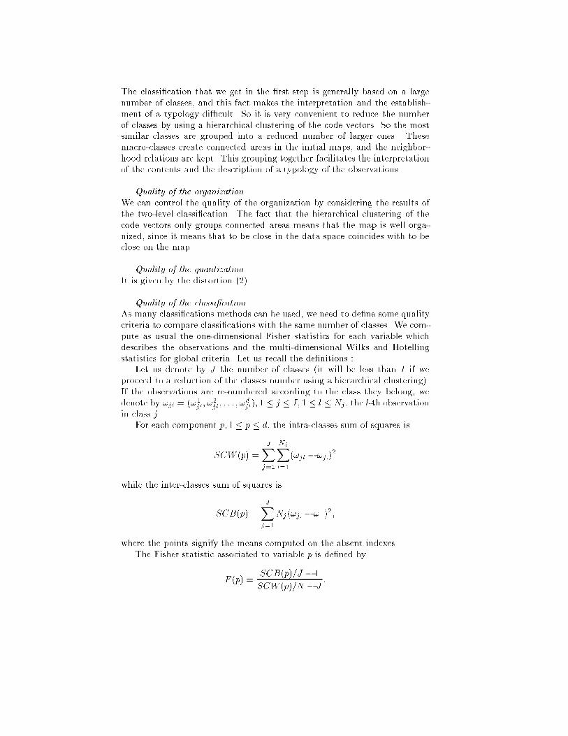
Quality of the classi�cation

As many classi�cations methods can be used, we need to de�ne some quality

criteria to compare classi�cations with the same number of classes. We com-

pute as usual the one-dimensional Fisher statistics for each variable which

describes the observations and the multi-dimensional Wilks and Hotelling

statistics for global criteria. Let us recall the de�nitions :

Let us denote by J the number of classes (it will be less than I if we

proceed to a reduction of the classes number using a hierarchical clustering).

If the observations are re-numbered according to the class they belong, we

denote by !jl = (!1jl; !2jl; : : : ; !

djl); 1 � j � I; 1 � l � Nj , the l-th observation

in class j.

For each component p; 1 � p � d, the intra-classes sum of squares is

SCW (p) =JX

j=1

NjXl=1

(!jl � !j:)2

while the inter-classes sum of squares is

SCB(p) =JX

j=1

Nj(!j: � !::)2;

where the points signify the means computed on the absent indexes.

The Fisher statistic associated to variable p is de�ned by

F (p) =SCB(p)=J � 1

SCW (p)=N � J:

This statistics has a Fisher(J � 1; N � J) distribution when the classes have

no sense, that is when the J classes can be confounded. So the larger the

value of F (p) is, the better the variable p is discriminating.

These statistics are very useful, but give indications only for each variable

separately. In order to globally evaluate the quality of the classi�cation,

one has to de�ne in the same way the intra-classes variance matrix W , and

the inter-classes variance matrix B, and to compute for example the Wilks

statistics

Wilks =det(W )

det(W +B)

or the Hotelling statistics

Hot = trace(W�1B):

These statistics are tabulated, but very often one uses an approximation

by a chi-squared distribution. The smaller (resp. larger) the Wilks (resp.

Hotelling) statistic is, the better is the classi�cation. Note that it is not

possible to �nd a criterion which would be better than any other, since there

does not exist an uniformly most powerful test of the hypothesis �the classes

can be confounded� against �the classes are di�erent�, except for a two-classes

problem.

Let us remark that a �good� classi�cation is that one which has a strong

homogeneity inside the classes and a strong separation between the classes.

So we will use these indicators of quality to compare several classi�cations.

The data

We use in this part a real database. It contains seven ratios measured

in 1996 on the macroeconomic situation of 96 countries: annual population

growth, mortality rate, analphabetism rate, population proportion in high

school, GDP per head, GDP growth rate and in�ation rate. This kind of

dataset (but not always for the same year) has been already used in [14], [18]

or [8] and is available through http://panoramix.univ-paris1.fr/SAMOS.

So in order to compare both Kohonen algorithms (on-line and Batch), we

classify the 96 countries using a 6 � 6 grid, and a simpli�ed neighborhood

function where �(i; j) = 1 if i and j are neighbors and = 0 if not. The size ofthe neighborhood decreases with time. The initial values of the code vectors

are randomly chosen.

First we use the classical SOM algorithm, with 500 iterations, a decreasing

function ". For lack of space, we do not represent the resulting map. It

provides a nice representation of all the countries displayed over the 36 classes.

Rich countries are at the right and at the top, the very poor countries are at

the left, there is continuity from the rich countries to the poor ones. There

are two countries in the corner at the top and at the left and they are those

which have a very large in�ation rate, etc. Figure (3) shows the macro-

classes and the code vectors which can be considered as typical countries

which summarize the countries of their classes. We choose to keep 7 macro-

classes, and it would be easy to describe them and derive a simple typology

Figure 3: SOM on-line algorithm, 36 code-vectors, 7 macro-classes, the 7-

dimensional code vectors are drawn as curves which join the 7 points

of the countries. We observe that the code vectors are very well organized,

vary with continuity from one class to the next ones and that the clustering

groups together only connected classes. That is a visual proof of the quality

of the organization.

Secondly, we use the Batch Kohonen algorithm, with 5 iterations (which is

equivalent to 500 for the on-line algorithm), and a decreasing neighborhood

function. First we start from the same initialization as in the �rst case.

The resulting map is not organized. All the 96 countries are grouped into

4 classes (among the 36). One class contains the rich countries (Germany,

France, USA, etc...). In the second we �nd some intermediate countries

(Greece, Argentina, Czechoslovakia, etc...). The poor countries are divided

into two classes, the poor (Cameroon, Bolivia, Lebanon, etc...) and the very

poor ones (Yemen, Haiti, Angola, etc...). The classi�cation is meaningful,

but there is no organization on the map, close code vectors are not similar,

the macro classes gather not connected classes, etc. See �gure (4). In this

case, it is not necessary to compute the macro-classes, since there are only 4

non- empty classes.

At last, we use the Batch Kohonen algorithm, with the same parameters,

but starting from another initial values for the code vectors. In that case,

we get a reasonably organized map, the countries are displayed over all the

map, but the two countries characterized by the high in�ation rate are in

opposite classes (at the right top and at the left bottom). When we use a

hierarchical clustering with 7 macro-classes, these opposite classes belong to

the same macro-class and that means that the organization is not complete.

See �gure (5).

In the next table, we compare the classi�cation criteria and the distor-

tion for 4 classi�cations: On-line SOM with 4 macro classes (SOM4), Batch

algorithm I with 4 non-empty classes (Batch4), On-line SOM with 7 macro-

Figure 4: Batch algorithm I, 36 code-vectors, 7 macro-classes, only 4 non-empty

classes

classes (SOM7), Batch algorithm II with 7 macro-classes (Batch7).

SOM4 Batch4 SOM 7 Batch7

F (1) 51.80 52.84 29.16 47.32

F (2) 126.92 146.24 63.14 80.70

F (3) 135.98 164.91 76.66 67.52

F (4) 71.79 60.96 37.40 57.22

F (5) 102.58 160.56 76.02 78.24

F (6) 18.80 21.28 22.65 18.13

F (7) 4.37 2.24 81.74 91.55

Wilks 0.023 0.017 0.001 0.0007

Hotelling 12.23 13.79 21.49 24.98

Distortion 0.99 2.71 0.99 0.4

So the Batch algorithm II gives the best results from both points of view of

classi�cation and quantization. But we saw that it is not perfectly organized.

We note also that the Batch algorithm is extremely sensitive to the initial

values while the SOM algorithm is very robust. We did a lot of di�erent runs

and always got similar results. See for example [5].

CONCLUSION

We have tried to clearly de�ne and compare the two most spread methods to

compute SOM maps: one (on-line SOM) belongs to the family of stochastic

algorithms while the second one is linked to quasi-Newtonian methods. De-

Figure 5: Batch algorithm II, 36 code-vectors, 7 macro-classes

spite its simplicity, we put some insight into the fact that randomness could

lead to better performances. This is not truly surprising, but we aimed at

giving precise de�nitions and clear numerical results. In fact, these remarks

lead to conclude that the initialization choice is much more crucial for the

Kohonen Batch algorithm. The Kohonen Batch algorithm could seem to be

easier to use because there is no gain function "t to adjust and because it can

converge quicker than the on-line one. But this can be misleading because

for the batch algorithm, it is much more necessary to carefully choose the

initial values and eventually repeat a lot of computations in order to �nd

better solutions.

REFERENCES

[1] M. Benaïm, J. Fort and G. Pagès, �Convergence of the one-dimensional Ko-

honen algorithm,� Advances in Applied Probability, vol. 30, 1998.

[2] M. Cottrell, J. Fort and G. Pagès, �Two or three things that we know about

the Kohonen algorithm,� in Proc. of ESANN'94, Bruges: D Facto, 1994,

pp. 235�244.

[3] M. Cottrell, J. Fort and G. Pagès, �Theoretical aspects of the SOM algorithm,�

Neurocomputing, vol. 21, pp. 119�138, 1998.

[4] M. Cottrell and P. Rousset, �The Kohonen Algorithm: A Powerful Tool for

Analysing and Representing Multidimensional Quantitative and Qualitative

Data,� in Proc. IWANN'97, Biological and Arti�cial Computation:

From Neuroscience to Technology, Springer, 1997, pp. 861�871.

[5] E. de Bodt and M. Cottrell, �Bootstrapping Self-Organizing Maps to Assess

the Statistical Signi�cance of Local Proximity,� in Proc. of ESANN'2000,

Bruges: D Facto, 2000, pp. 245�254.

[6] E. de Bodt, M. Cottrell and M. Verleysen, �Using the Kohonen Algorithm for

Quick Initialization of Simple Competitive Learning Algorithm,� in Proc. of

ESANN'99, Bruges: D Facto, 1999, pp. 19�26.

[7] E. de Bodt, M. Verleysen and M. Cottrell, �Kohonen Maps versus Vector

Quantization for Data Analysis,� in Proc. of ESANN'97, Bruges: D Facto,

1997, pp. 211�218.

[8] G. Deboeck and T. Kohonen, Visual explorations in Finance with Self-

Organizing Maps, Springer, 1998.

[9] E. Erwin, K. Obermayer and K. Shulten, �Self-organizing maps : ordering, con-

vergence properties and energy functions,� Biological Cybernetics, vol. 67,

pp. 47�55, 1992.

[10] E. Forgy, �Cluster analysis of multivariate data: e�ciency versus interpretabil-

ity of classi�cations,� Biometrics, vol. 21, no. 3, pp. 768, 1965.

[11] J. Fort and G. Pagès, �On the a.s. convergence of the Kohonen algorithm with

a general neighborhood function,� Annals of Applied Probability, vol. 5,

no. 4, pp. 1177�1216, 1995.

[12] J. Fort and G. Pagès, �Convergence of Stochastic Algorithms: from the Kush-

ner & Clark theorem to the Lyapunov functional,� Advances in Applied

Probability, vol. 28, no. 4, pp. 1072�1094, 1996.

[13] J. Hertz, A. Krogh and R. Palmer, Introduction to the Theory of Neural

Computation, Santa Fe Institut, 1991.

[14] S. Kaski, �Data Exploration Using Self-Organizing Maps,� Acta Polytech-

nica Scandinavia, vol. 82, 1997.

[15] T. Kohonen, Self-Organization and Associative Memory, Berlin:

Springer, 1984-1989.

[16] T. Kohonen, Self-Organizing Maps, Berlin: Springer, 1995.

[17] T. Kohonen, �Comparison of SOM Point Densities Based on Di�erent Crite-

ria,� Neural Computation, vol. 11, pp. 2081�2095, 1999.

[18] E. Oja and S. Kaski, Kohonen Maps, Elsevier, 1999.

[19] H. Ritter, T. Martinetz and K. Shulten, Neural Computation and Self-

Organizing Maps, an Introduction, Reading: Addison-Wesley, 1992.

[20] A. Sadeghi, �Asymptotic Behavior of Self-Organizing Maps with Non-Uniform

Stimuli Distribution,� Annals of Applied Probability, vol. 8, no. 1,

pp. 281�289, 1997.

[21] A. Sadeghi, �Self-organization property of Kohonen'smap with general type of

stimuli distribution,� Neural Networks, vol. 11, pp. 1637�1643, 1998.