J Sched (2006) 9: 97–114

DOI 10.1007/s10951-006-6774-z

Self-organizing feature maps for the vehicle routingproblem with backhauls

Hassan Ghaziri · Ibrahim H. Osman

C© Springer Science + Business Media, LLC 2006

Abstract In the Vehicle Routing Problem with Backhauls (VRPB), a central depot, a fleet of

homogeneous vehicles, and a set of customers are given. The set of customers is divided into

two subsets. The first (second) set of linehauls (backhauls) consists of customers with known

quantity of goods to be delivered from (collected to) the depot. The VRPB objective is to design

a set of minimum cost routes; originating and terminating at the central depot to service the

set of customers. In this paper, we develop a self-organizing feature maps algorithm, which

uses unsupervised competitive neural network concepts. The definition of the architecture of the

neural network and its learning rule are the main contribution. The architecture consists of two

types of chains: linehaul and backhaul chains. Linehaul chains interact exclusively with linehaul

customers. Similarly, backhaul chains interact exclusively with backhaul customers. Additonal

types of interactions are introduced in order to form feasible VRPB solution when the algorithm

converges. The generated routes are then improved using the well-known 2-opt procedure. The

implemented algorithm is compared with other approaches in the literature. The computational

results are reported for standard benchmark test problems. They show that the proposed approach

is competitive with the most efficient metaheuristics.

Keywords Vehicle routing problem with backhauls . Self-organizing feature maps . Neural

networks . Metaheuristics

Introduction

The Vehicle Routing Problem with Backhauls (VRPB) can be defined as follows. Let G = (N , A)

be an undirected network where N = {d0, . . . , dn} is the set of nodes and A = {(di , d j ) : di �=d j/di and d j ∈ V} is the set of arcs. It is assumed that the arc (di, dj) is associated with a cost

Ci j representing the travel cost/time or distance between customers i and j located at nodes di

and d j , respectively. Node d0 represents the central depot at which a fleet of vehicles is located,

H. Ghaziri and I. H. OsmanSchool of Business, American University of Beirut, Bliss Street, Beirut, Lebanone-mail: {ghaziri, ibrahim.osman}@aub.edu.lb

98 J Sched (2006) 9: 97–114

while the remaining nodes correspond to two different sets of customers. The set of Linehaulcustomers, L, requires a known quantity of goods to be delivered from the central depot to each

linehaul customer, where the set of Backhaul customers, B, requires a known quantity of goods to

be collected from each backhaul customer to the central depot. The VRPB requires all backhaul

customers to be visited contiguously after all linehaul customers on each vehicle route. The

quantity of goods to be delivered or collected must not exceed, separately, the given capacity of

the vehicle. The objective of the VRPB is to design a set of feasible routes for a given fleet of

homogenous vehicles and minimizes the total delivery and collection cost without violating the

customers and vehicles constraints.

The VRPB is NP-hard combinatorial optimization problem in the strong sense, since it gen-

eralizes both the vehicle routing problem and the traveling salesman problem with backhauls

(Ghaziri and Osman, 2003). Hence, it can be solved exactly for small-sized instances, but only

approximately for large-sized instances. The VRPB variant considered in this paper has re-

cently attracted the attention of a number of researchers to develop for it exact and approximate

procedures. Their works are briefly classified into exact and approximate methods. Exact meth-ods are proposed using branch- and bound-tree search approaches by Toth and Vigo (1997)

based on Lagrangian relaxation and cutting plane methods, Mingozzi et al. (1996) based on

linear-programming relaxations, and Yano et al. (1987) based on a set covering exact algorithm.

Approximate methods (heuristics) are classified into: constructive heuristics, the savings method

by Deif and Bodin (1984), the insertion method by Golden et al. (1985), and the saving-insertion

and assignment approaches by Wassan and Osman (2002); Two-phase heuristics, the space-filling

curves by Goetschalckx and Jacobs-Blecha (1989), the cluster-first route-second algorithm by

Goetschalckx and Jacobs-Blecha (1993), a K -tree Lagrangian relaxation approach and the well-

known 2-opt and 3-opt improvement procedures by Toth and Vigo (1996) with an improved

version of the above heuristic by Toth and Vigo (1999); Metaheuristics, the reactive tabu-search

approach by Wassan and Osman (2002).To our knowledge, no work has been published using the neural networks (NN) approach for

the VRPB. In this paper, the aim is to fill in this gap in the literature by designing a self-organizing

feature map (SOFM) for the problem. The remaining part of the paper is organized as follows.

In Section 2, we present a brief review of neural networks on routing problems. In Section 3,

we describe our implementation of the SOFM algorithm to the VRPB. Computational results

are reported in Section 4 with a comparison to other approaches in the literature on a set of

benchmarks instances followed by a conclusion in Section 5.

2. Neural networks for routing problems

In this section, we provide a brief survey of the most important applications of NN for routing

problems. The first attempt to use NN for optimization problems was developed by Hopfield

and Tank (HT) and applied to the travelling salesman problem (TSP), Hopfield and Tank (1985).

Although innovative, the new HT approach was not competitive with the most powerful meta-

heuristics such as Tabu Search or Simulated Annealing. This work was followed by several

studies to improve the performance of this approach. Recently, an investigation into the im-

provement of the local optima of the HT network to the TSP was conduced by Peng et al. (1996).

They obtained good results for improving the local minima on small-sized TSP of less than 14

cities. This approach was also extended to other routing problems such as the generalized TSP

(GTSP) by Andresol et al. (1999). The main drawbacks were remaining the same: an expen-

sive computational time and a failure to deal with large-size problems. Thorough surveys of the

J Sched (2006) 9: 97–114 99

applications NN to routing problems are provided by Burke (1994), Looi (1992), Potvin (1993),

and Smith (1999).

The other more promising NN approach for routing problems is based on the Kohonen’s

Self-Organizing Feature Map (SOFM), Kohonen (1995). The SOFM is an unsupervised neural

network, which does not depend on any energy function. It simply inspects the input data for

regularities and patterns and organizes itself in such a way to form an ordered description of the

input data. Kohonen’s SOFM converts input patterns of arbitrary dimensions into the responses

of a one- or two-dimensional array of neurons. Learning is achieved through adaptation of the

weights connecting the input (layer) to the array on neurons. The learning process comprises

a competitive stage of identifying a winning neuron, which is closest to the input data, and an

adaptive stage where the weights of the winning neuron and its neighboring neurons are adjusted

in order to approach the presented input data.

Applications of the SOFM to the TSP started with the work of Fort (1988). In this approach,

one-dimensional circular array of neurons is generated, and mapped onto the TSP cities in such

a way that two neighboring points on the array are also neighbors in distance. Durbin and

Willshaw (1987) already introduced a similar idea for the TSP and called it an elastic network.

The elastic network starts with k nodes (k is greater than n) lying on an artificial “elastic band.”

The nodes are then moved in the Euclidean space, thus stretching the elastic band, in such a way

to minimize an energy function. The main difference between the two approaches is that Fort’s

approach incorporates stochasticities into the weight adaptations, whereas the elastic network is

completely deterministic. Also there is no energy function in Fort’s approach.

Encouraged by the improved NN results, researchers began combining features of both elastic

network and SOFM to derive better algorithms for solving TSPs including Angeniol, De-La-

Croix and Le-Texier (1988), Burke (1994), and Vakhutinsky and Golden (1995). It should be

noted that the best NN results for TSP instances taken from the TSPLIB literature were obtained

by Aras et al. (1999) using a modified SOFM algorithm. Lately, Ghaziri and Osman extended the

SOFM application to TSP with backhauls Ghaziri and Osman (2003). Finally, there are also few

SOFM applications extended to the vehicle routing problems by Modares et al.(1999), Potvin

and Robillard (1995), and Ghaziri (1996, 1991).

3. SOFM for the VRP with backhauls

The purpose of this section is to describe the new algorithm based on the SOFM approach for the

vehicle routing problem with backhauls. The VRPB problem we are considering in this paper

consists of designing delivery routes to serve two types of customers, linehaul and backahul

customers. The algorithm we are considering here is an extension of the algorithm introduced

by Ghaziri and Osman (2003) for the travelling saleman problem with backhauls (TSPB). The

following information is given:� The Customers. The position of the customers is provided through their coordinates in the

Euclidean space. Along with their position, the weight or quantity of goods, of each customer

and its type are also provided. There are two types of customers, the backhaul and linehaul

customers. A certain quantity of goods is delivered from the depot to the linehaul customers and

a certain quantity of goods must be picked up from each backhaul customer and brought to the

depot.� The Vehicles. A fleet of homogeneous vehicles is given. It means that the number of vehicles

is known and the capacity of all vehicles is the same. No vehicle can ship a quantity of goods

that exceeds its capacity.

100 J Sched (2006) 9: 97–114

Depot

Fig. 1 A set of linehaul customers and backhaul customers served by two vehicles

� The Depot. The location of the depot is known and its coordinates in the Euclidean space are

given.

Each vehicle must start its route by delivering first the required quantity of goods to the linehaul

customers assigned to it and then collect the corresponding goods from each backhaul customer

and bring them back to the depot.

Figure 1 shows an example of VRPB with a fleet consisting of two vehicles.

3.1. The SOFM for routing problems

The classical SOFM approach consists of a neural network with a defined architecture that is

interacting with its environment to represent it according to the following principle: Two neigh-

boring inputs should be represented by two neighboring neurons. From a routing perspective, it is

clear that two neighboring customers should be assigned close positions in the routing schedule

in order to minimize the total distance traveled by the vehicle.

Using the SOFM approach to solve any problem consists of three main procedures:

1. Definition of the network architecture. Each network consists of a certain number of nodes.

The way the nodes are connected together corresponds to the network architecture.

2. Selection procedure. The SOFM approach is based on a winner-take-all principle. This means

that when a customer is presented to the algorithm the nearest neuron in terms of a certain

distance (here the Euclidean distance) will be selected.

3. Adaptation procedure. It consists of identifying the way neurons are adapting their states or

positions.

SOFM for the TSP

The architecture that is usually used for routing problems and that was introduced by Fort (1988)

is the ring architecture. It consists of a set of neurons placed on a deformable ring. The concept

of tour is embedded in the ring architecture, since the location of a neuron on the ring can

J Sched (2006) 9: 97–114 101

Initial State Intermediate State

Final State

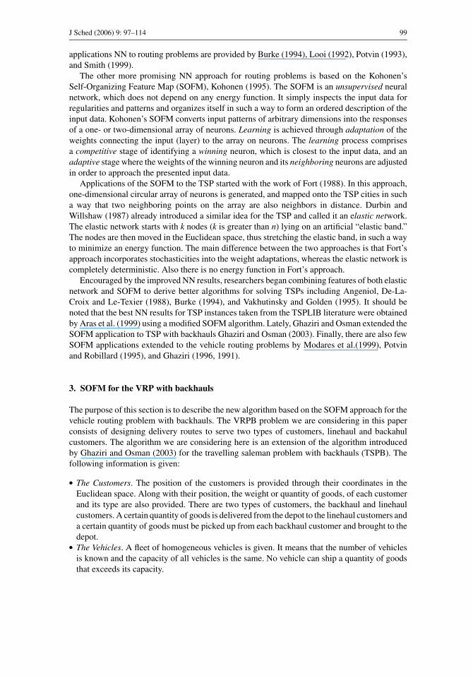
Fig. 2 An illustration of the tour concept represented by a ring of neurons. The deformation of the ring due to theinteraction with the customers leads to tour according to which the customers will be visited

be identified with the position in the visit as shown in Figure 2. This is the most important

advantage of this approach. The ring can be considered as a route for an ideal problem. The

interaction of the network with its environment, here the customers and the adaptation of its

neurons will force iteratively the ring to represent the real tour that will visit sequentially the

customers.

From a practical point of view, the SOFM algorithm starts by specifying the architecture

of the network, which consists of a one ring upon which the artificial neurons are spatially

distributed. The ring is embedded in the Euclidean space. Each neuron is identified by its

position in the Euclidean space and its position on the ring. The Euclidean distance will be used

to compare the positions of neurons with the positions of cities. The lateral distance will be

used to define the distance on the ring between two neurons. The lateral distance between any

two neurons is defined to be the smallest number of neurons separating them plus one. In the

first step, a customer is randomly picked up, his position is compared to all positions of neurons

on the ring. The nearest neuron to the customer is then selected and moved towards him. The

neighbors of the selected neuron move also towards the customer with a decreasing intensity

controlled by the lateral function (Kohonen, 1982). Figure 2 illustrates the evolution of the

algorithm starting from the initial state of the ring (a), reaching an intermediate stage after some

iterations (b) and stopping at the final state (c). An extensive analysis of this algorithm could be

found in the works published by Fort (1988), Angeniol et al. (1988), and Smith (1999).

3.2. The SOFM for the VRPB

In this section, we will explain how to extend the SOFM–VRPP algorithm (Ghaziri, 1996–1991)

to the VRPB. This extension is based on the design of a new architecture in which the TSP ring

is replaced by a certain number of rings. Each ring represents a vehicle. In order to represent the

concept of linehaul customers and backhaul customers, each ring will consist of two parts. The

first part is a sequence of neurons that will interact exclusively with linehaul customers. They are

102 J Sched (2006) 9: 97–114

called linehaul neurons. The second part of the ring consists of backhaul neurons, which means

that these neurons will interact exclusively with backhaul customers. Experiments show that this

architecture lacks flexibility, preventing the network from evolving adequately. Therefore, the

concept of ring has been replaced by the concept of chain. There will be two types of chains.

Linehaul chains, which are chains formed of linehaul neurons and backhaul chains formed of

backhaul neurons. The Linehaul customers will interact exclusively with the linehaul chains,

the backhaul customers will interact exclusively with the backhaul chains. It is clear that those

chains will not form tours. Therefore, a procedure has to be implemented in order to respect the

following requirements:� Rings should be formed to represent the sequence according to which the customers are visited.� Each ring must be formed of a linehaul sequence followed by a backhaul sequence. The linehaul

sequence represents the schedule of visiting the linehaul customers served by the corresponding

vehicle and the backhaul sequence represents the schedule of visiting the backhaul customers

served by the same vehicle.� Each ring must pass by the depot.

Accordingly, the procedure consists of connecting the chain such that the requirements are

respected. Consequently, four types of interactions are introduced to generate a feasible VRPB

tour. Let us introduce the following notations:

L = {li = (x1i , x2i , x3i ), for i = 1, . . . , N1} be the set of N1 Linehaul customers where (x1i, x2i )

are the coordinates of the Linehaul customer li and x3i its weight.

B = {bj = (y1 j , y2 j , y3 j ), for j = 1, . . . , N2} be the set of N2 backhaul customers where (y1 j,

y2 j ) are the coordinates of the backhaul customer b j and y3 j its weight.

D = (xd, yd) be the coordinates of the depot.

V = {vk, for k = 1, . . . , Nv} be the set of vehicles, where Nv is the number of vehicles

Q is the vehicle capacity. Q is fixed because we have a homogenous fleet.

wm is the current amount of goods delivered to Linehaul customers by the vehicle vm , where

m = 1, . . . , Nv

gn is the current amount of goods picked up by backhaul customers from the vehicle vn , where

n = 1, . . . , Nv

Nk = {Nkl , Nkb} is the set of customers served by vehicle vk , where Nkl is the set of linehaul

customers and Nkb is the set of backhaul customers, where k = 1, . . . , Nv

Cm = {Lmj = (Xm

1 j , Xm2 j ), for j = 1, . . . , Nm} be the set of Nm connected neurons forming the

Linehaul chain of neurons, where m = 1, . . . , Ny and (Xm1 j , Xm

2 j ) are the coordinates in the

Euclidean space of the neuron Lmj .

C̃n = {Bnj = (Y n

1 j , Y n2 j ) , for j = 1, . . . , Nn} be the set of Nn connected neurons forming the

Backhaul chain of neurons, where n = 1, . . . , Ny and (Y n1 j , Y n

2 j ) are the coordinates in the

Euclidean space of the neuron Bnj .

(i) Interaction between the chains Cm and the Linehaul customers in L. In this interaction,

the Linehaul customers in L will be presented to the chains Cm one by one in a random

order. In order to choose the chain that will interact with the presented customer, we have to

consider two factors: (1) The distance of the nearest neuron from each chain to the customer.

(2) The current weight of each chain. Each time a customer is assigned to a certain chain its

current weight wm will be increased by the corresponding weight. The winning chain will

be selected randomly according to a probability distribution, taking into consideration these

J Sched (2006) 9: 97–114 103

two factors. Once a chain is selected, the position of its neurons will be adjusted according

to the adaptation rule.

(ii) Interaction between the chains C̃n and the backhaul customers in B. In this interaction the

backhaul customers in B will interact with C̃n in a similar way to the interaction of type (i)

and use the same adaptation rule.

(iii) Interaction between the chains Cm and C̃n . Using the previous types of interactions, the

chains will evolve independently. Nothing is forcing them to be connected in order to form a

feasible route. For this reason, an interaction between the two chains Cm and C̃n is introduced.

We assume that each chain has a head and a tail. The tail and the head are represented by the

last and the first neurons, respectively. After presenting all backhaul and Linehaul customers,

the chain Cm will interact with the chain C̃n having the nearest neuron tail to the Cm neuron

head. The objective of this interaction is to make the tail of the linehaul chain and the head of

the corresponding backhaul chain converge. This convergence will allow the formation of a

single ring representing a tour visiting the Linehaul and backhaul customers consecutively.

The first neuron of the backhaul chain is assigned as the winner neuron in this interaction.

This means that the algorithm at this level is not anymore a competitive algorithm but a

supervised one in the sense that the last neuron of the linehaul chain has to be attracted

by the first neuron of the backhaul chain. After this assignment, the adaptation rule has

to be applied on the neurons of C̃n .We apply the same procedure to the backahul chain,

by presenting the first neuron of C̃n to the first chain, assigning the last neuron of Cm as

the winner neuron and updating the positions of the neurons of Cm according to the same

adaptation rule.

(iv) Interaction between the two types of chains and the depot. This type of interaction is similar

to the last one, where the depot is presented to the linehaul chains. The first neuron of each Cm

is assigned to the depot and considered as the winner neuron. Once this neuron is assigned,

we update this neuron and its neighboring neurons according to the usual adaptation rule.

The same procedure is applied to the last neuron of each chain C̃n . When we apply all these

interactions, the different chains will evolve towards a m ring, passing through the depot,

the Linehaul customers, the backhaul customers, and returning back to the depot. At the

end, we will obtain a feasible routes defined by the m rings. The position of each customer

will coincide with the position of one neuron. The position of the neuron in the chains will

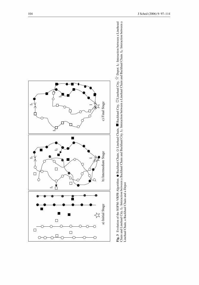
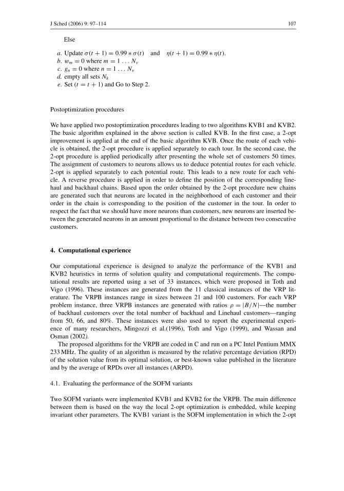
give the position of the customers in the route. Figure 3 illustrates the evolution stages of

the SOFM algorithm into a feasible VRPB schedule.

The interactions are repeated iteratively at the end of presentations of all cities to the chains

and the depot.

The SOFM–VRPB Algorithm

In this section the SOFM–VRPB algorithm is sketched in pseudocode. Let us introduce the fol-

lowing additional notations: dL: is the lateral distance; δ, β: parameters to control the probability

function; η, α: parameters to control adaptation rule t : iteration number.

Step 1: Initialization

i Read the input data for the Linehaul and Backhaul customers

ii Generate the positions of N L neurons for each chain Cm

iii Generate the positions of N B neurons for each chain Cn

iv Set Wm = 0 ∀m = 1, . . . , Nv.

v Set gn = 0 ∀n = 1, . . . , Nv.

vi Set t = 0

104 J Sched (2006) 9: 97–114

I 1

a) I

nit

ial

Sta

ge

I 3

I 2

I 4

b)

Inte

rmed

iate

Sta

ge

I 3

I 2

I 1

I

c) F

inal

Sta

ge

Fig

.3E

volu

tio

no

fth

eS

OF

M–

VR

PB

Alg

ori

thm

.•B

ack

hau

lC

hai

n,◦L

ineh

aul

Ch

ain

,B

ack

hau

lC

ity,

Lin

ehau

lC

ity,

Dep

ot.

I 1:

Inte

ract

ion

bet

wee

na

Lin

ehea

ul

Ch

ain

and

Lin

ehau

lC

ity.

I 2:

Inte

ract

ion

bet

wee

na

Bac

kh

aul

Ch

ain

and

Bac

kh

aul

Cit

y.I 3

:In

tera

ctio

nb

etw

een

aL

ineh

aul

Ch

ain

and

Bac

kh

aul

Ch

ain

.I 4

:In

tera

ctio

nb

etw

een

aL

ineh

aul

Ch

ain

,a

Bac

kh

aul

Ch

ain

and

aD

epo

t

J Sched (2006) 9: 97–114 105

0.00

0.50

1.00

1.50

2.00

50 66 80

Percentage Backhauls

AR

PD

Valu

es

KVB1 KVB2Fig. 4 Average percentagedeviations of KVB1 and KVB2 withrespect to changes in percentage ofbackhauls

Step 2: Select a city randomly. Select randomly a customer C from L U B, every customer will

be selected once during an iteration.

Step 3: Select a Winner neuron

If (C belongs to L) Then

I. Selection of the nearest neuron for each Cm , L∗m . Let L∗m be the winning neuron belonging

to Cm , i.e. L∗m= (X1∗m, X∗m

2

)such that (x1c − X∗m

1 )2 + (x2c − X∗m2 )2 ≤ (x1c − X1i)

2 + (x2c − X2i)2,

∀ i = 1, . . . , N1

∀ m = 1, . . . , Nv.

d(C , L∗m ) is the Euclidean distance between C and L∗m

II. Select the assigned chain according to the probability

P(C, Cm)=exp

(−d(C,L∗m )2

δ(t)

)/1 + exp(−m + wm + x3k )

β(t)∑m exp

(−d(C,L∗m )2

δ(t)

)/1 + exp(−m+wm+x3k )

β(t)

∀ m = 1, . . . , Nv.

Assume C̃s to be the assigned chain

ws = ws + x3k

Add C to Nsl

0

1

2

3

4

5

6

21 22 29 32 50 75 100

Instance sizes

AR

PD

Val

ues

KVB1 KVB2 HTV RTSFig. 5 Average relative percentagedeviations for all comparedalgorithms

106 J Sched (2006) 9: 97–114

III. Update the coordinates of each neuron in set Cs , for example the x-coordinate is updated

by the following rule:

Xs1 j (t + 1) = Xs

1 j (t) + η(t) × �(C, L∗s)(x1C − Xs

1 j (t)) ∀ j = 1, . . . , Ns .

where

�(C, L∗s) = 1√2

exp

(−d2L (Ls

j , L∗s)

2σ (t)2

)If (C belongs to B ) ThenI. Selection of the nearest neuron for each C̃n, B∗n

Let B∗n be the winning neuron belonging to Cn , i.e. B∗n = (Y∗n1 , Y∗n

2 ) such that (y1c − y∗n1 )2 +

(y2c − y∗n2 )2 ≤ (y1c − y1i)

2 + (y2c − y2i)2, ∀ i = 1, . . . , N2 ∀ n = 1, . . . , Nv.

II. Select the assigned chain according to the probability

P(C, C̃n)=exp

(−d(C,B∗n )2

δ(t)

)/1 + exp(−m+gn+y3i )

β(t)∑n exp

(−d(C,B∗n )2

δ(t)

)/1 + exp(−m+gn+y3i )

β(t)

∀ n = 1, . . . , Nv.

Assume C̃s to be the assigned chain

gs = gs + y3k

Add C to Nsb

III. Update the coordinates of each neuron in set C̃s , for example the x-coordinate is updated

by the following rule:

Y s1 j (t + 1) = Y s

1 j (t) + η(t) × �(C, B∗s)(y1C − Y s

1 j

)(t)), ∀ j = 1, . . . , Ns.

where

�(C, B∗s) = 1√2

exp

(−d2L

(Bs

j , B∗s)

2σ (t)2

)Step 4. Extremities interactions:

Apply the different types of Interactions

I. Interaction with the Depot.

II. Interaction of the two chains.

Step 5. End-Iteration Test:

If Not {all customers are selected at the current

iteration} Then go to Step 2.

Step 6. Stopping Criterion:

If {all customers are within 10−4 of their nearest

neurons in the Euclidean space}Then Stop

J Sched (2006) 9: 97–114 107

Else

a. Update σ (t + 1) = 0.99 ∗ σ (t) and η(t + 1) = 0.99 ∗ η(t).b. wm = 0 where m = 1 . . . Nv

c. gn = 0 where n = 1 . . . Nv

d. empty all sets Nk

e. Set (t = t + 1) and Go to Step 2.

Postoptimization procedures

We have applied two postoptimization procedures leading to two algorithms KVB1 and KVB2.

The basic algorithm explained in the above section is called KVB. In the first case, a 2-opt

improvement is applied at the end of the basic algorithm KVB. Once the route of each vehi-

cle is obtained, the 2-opt procedure is applied separately to each tour. In the second case, the

2-opt procedure is applied periodically after presenting the whole set of customers 50 times.

The assignment of customers to neurons allows us to deduce potential routes for each vehicle.

2-opt is applied separately to each potential route. This leads to a new route for each vehi-

cle. A reverse procedure is applied in order to define the position of the corresponding line-

haul and backhaul chains. Based upon the order obtained by the 2-opt procedure new chains

are generated such that neurons are located in the neighborhood of each customer and their

order in the chain is corresponding to the position of the customer in the tour. In order to

respect the fact that we should have more neurons than customers, new neurons are inserted be-

tween the generated neurons in an amount proportional to the distance between two consecutive

customers.

4. Computational experience

Our computational experience is designed to analyze the performance of the KVB1 and

KVB2 heuristics in terms of solution quality and computational requirements. The compu-

tational results are reported using a set of 33 instances, which were proposed in Toth and

Vigo (1996). These instances are generated from the 11 classical instances of the VRP lit-

erature. The VRPB instances range in sizes between 21 and 100 customers. For each VRP

problem instance, three VRPB instances are generated with ratios ρ = |B/N |—the number

of backhaul customers over the total number of backhaul and Linehaul customers—ranging

from 50, 66, and 80%. These instances were also used to report the experimental experi-

ence of many researchers, Mingozzi et al.(1996), Toth and Vigo (1999), and Wassan and

Osman (2002).The proposed algorithms for the VRPB are coded in C and run on a PC Intel Pentium MMX

233 MHz. The quality of an algorithm is measured by the relative percentage deviation (RPD)

of the solution value from its optimal solution, or best-known value published in the literature

and by the average of RPDs over all instances (ARPD).

4.1. Evaluating the performance of the SOFM variants

Two SOFM variants were implemented KVB1 and KVB2 for the VRPB. The main difference

between them is based on the way the local 2-opt optimization is embedded, while keeping

invariant other parameters. The KVB1 variant is the SOFM implementation in which the 2-opt

108 J Sched (2006) 9: 97–114

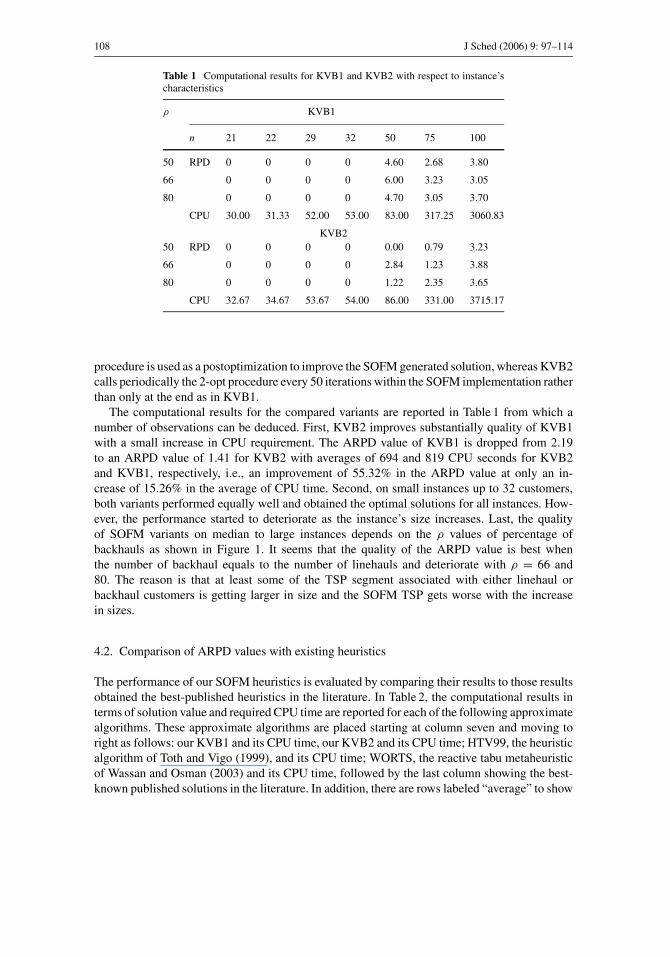
Table 1 Computational results for KVB1 and KVB2 with respect to instance’scharacteristics

ρ KVB1

n 21 22 29 32 50 75 100

50 RPD 0 0 0 0 4.60 2.68 3.80

66 0 0 0 0 6.00 3.23 3.05

80 0 0 0 0 4.70 3.05 3.70

CPU 30.00 31.33 52.00 53.00 83.00 317.25 3060.83

KVB2

50 RPD 0 0 0 0 0.00 0.79 3.23

66 0 0 0 0 2.84 1.23 3.88

80 0 0 0 0 1.22 2.35 3.65

CPU 32.67 34.67 53.67 54.00 86.00 331.00 3715.17

procedure is used as a postoptimization to improve the SOFM generated solution, whereas KVB2

calls periodically the 2-opt procedure every 50 iterations within the SOFM implementation rather

than only at the end as in KVB1.

The computational results for the compared variants are reported in Table 1 from which a

number of observations can be deduced. First, KVB2 improves substantially quality of KVB1

with a small increase in CPU requirement. The ARPD value of KVB1 is dropped from 2.19

to an ARPD value of 1.41 for KVB2 with averages of 694 and 819 CPU seconds for KVB2

and KVB1, respectively, i.e., an improvement of 55.32% in the ARPD value at only an in-

crease of 15.26% in the average of CPU time. Second, on small instances up to 32 customers,

both variants performed equally well and obtained the optimal solutions for all instances. How-

ever, the performance started to deteriorate as the instance’s size increases. Last, the quality

of SOFM variants on median to large instances depends on the ρ values of percentage of

backhauls as shown in Figure 1. It seems that the quality of the ARPD value is best when

the number of backhaul equals to the number of linehauls and deteriorate with ρ = 66 and

80. The reason is that at least some of the TSP segment associated with either linehaul or

backhaul customers is getting larger in size and the SOFM TSP gets worse with the increase

in sizes.

4.2. Comparison of ARPD values with existing heuristics

The performance of our SOFM heuristics is evaluated by comparing their results to those results

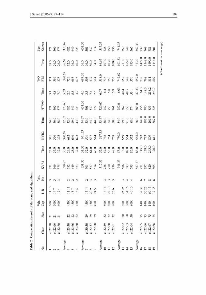
obtained the best-published heuristics in the literature. In Table 2, the computational results in

terms of solution value and required CPU time are reported for each of the following approximate

algorithms. These approximate algorithms are placed starting at column seven and moving to

right as follows: our KVB1 and its CPU time, our KVB2 and its CPU time; HTV99, the heuristic

algorithm of Toth and Vigo (1999), and its CPU time; WORTS, the reactive tabu metaheuristic

of Wassan and Osman (2003) and its CPU time, followed by the last column showing the best-

known published solutions in the literature. In addition, there are rows labeled “average” to show

J Sched (2006) 9: 97–114 109

Tabl

e2

Co

mp

uta

tio

nal

resu

lts

of

the

com

par

edal

go

rith

ms

Veh

.V

eh.

WO

Bes

t

No

Cla

ssS

ize

Cap

LB

No

KV

B1

Tim

eK

VB

2T

ime

HT

V9

9T

ime

RT

ST

ime

Kn

own

1ei

l22

.50

21

60

00

11

10

33

71

23

.03

71

24

.03

71

5.1

37

12

8.0

37

1

2ei

l22

.66

21

60

00

14

73

36

63

5.0

36

63

6.0

36

64

.83

66

26

.03

66

3ei

l22

.80

21

60

00

17

43

37

53

2.0

37

53

8.0

37

57

.03

75

26

.03

75

Aver

age

37

0.6

73

0.0

37

0.6

73

2.6

73

70

.67

5.6

33

70

.67

26

.67

37

0.6

7

4ei

l23

.50

22

45

00

11

11

26

82

29

.06

82

32

.06

82

2.6

72

93

2.0

68

2

5ei

l23

.66

22

45

00

15

72

64

92

8.0

64

92

9.0

64

95

.56

58

36

.06

49

6ei

l23

.80

22

45

00

18

42

62

33

7.0

62

34

3.0

62

33

.96

75

40

.06

23

Aver

age

65

1.3

33

1.3

36

51

.33

34

.67

65

1.3

34

.06

87

.33

36

.06

51

.33

7ei

l30

.50

29

45

00

15

14

25

01

52

.05

01

53

.05

01

3.3

50

39

6.0

50

1

8ei

l22

.57

29

45

00

20

93

53

76

1.0

53

76

4.0

53

97

.45

37

80

.05

37

9ei

l22

.58

29

45

00

24

53

51

44

3.0

51

44

4.0

52

27

.55

14

84

.05

14

Aver

age

51

7.3

35

2.0

51

7.3

35

3.6

75

20

.67

6.0

75

18

.08

6.6

75

17

.33

10

eil2

2.5

93

28

00

01

61

63

73

85

7.0

73

85

8.0

74

21

6.4

73

81

07

.07

38

11

eil2

2.6

03

28

00

02

21

03

75

05

3.0

75

45

4.0

75

31

5.8

75

01

03

.07

50

12

eil2

2.6

13

28

00

02

66

37

36

49

.07

58

50

.07

61

15

.97

55

10

0.0

73

6

Aver

age

74

1.3

35

3.0

75

0.0

54

.07

52

.01

6.0

37

47

.67

10

3.3

37

41

.33

13

eil2

2.6

25

08

00

02

52

53

58

67

6.0

55

97

9.0

56

24

0.4

55

92

71

.05

59

14

eil2

2.6

35

08

00

03

41

64

58

38

7.0

56

49

1.0

55

34

8.5

54

84

55

.05

48

15

eil2

2.6

45

08

00

04

01

04

59

38

6.0

57

28

8.0

57

45

3.1

57

03

93

.05

65

Aver

age

58

7.2

78

3.0

56

5.0

86

.05

63

.04

7.3

35

59

.03

73

.05

57

.33

16

eil2

2.6

57

51

40

37

38

67

71

14

5.0

74

31

49

.07

56

16

4.3

73

91

42

2.0

73

9

17

eil2

2.6

67

51

40

50

25

77

97

17

8.0

77

31

83

.07

80

14

8.3

76

81

14

8.0

76

8

18

eil2

2.6

77

51

40

60

15

88

20

24

3.0

80

92

69

.08

33

23

8.2

81

11

49

0.0

78

1

19

eil2

2.6

87

51

00

37

38

88

05

37

6.0

81

13

87

.08

25

24

0.7

80

91

14

4.0

80

1

(Con

tinu

edon

next

page

)

110 J Sched (2006) 9: 97–114

Tabl

e2

(Con

tinu

ed)

Veh

.V

eh.

WO

Bes

t

No

Cla

ssS

ize

Cap

LB

No

KV

B1

Tim

eK

VB

2T

ime

HT

V9

9T

ime

RT

ST

ime

Kn

own

20

eil2

2.6

97

51

00

50

25

10

89

24

51

.08

85

46

5.0

89

12

41

.08

73

99

7.0

87

3

21

eil2

2.7

07

51

00

60

15

12

93

65

69

.09

32

58

7.0

94

82

40

.79

31

91

5.0

91

9

22

eil2

2.7

17

51

80

37

38

57

30

32

1.0

72

33

46

.07

15

11

0.5

71

51

62

0.0

71

3

23

eil2

2.7

27

51

80

50

25

67

54

24

3.0

75

62

50

.07

45

14

8.7

73

41

35

2.0

73

4

24

eil2

2.7

37

51

80

60

15

77

59

32

4.0

74

23

43

.07

59

21

9.4

73

68

41

.07

33

25

eil2

2.7

47

52

20

37

38

47

17

19

8.0

69

02

13

.06

91

93

.76

90

13

77

.06

90

26

eil2

2.7

57

52

20

50

25

57

49

34

2.0

71

53

52

.07

17

89

.77

15

22

96

.07

15

27

eil2

2.7

67

52

20

60

15

67

10

41

7.0

71

84

28

.07

10

19

0.6

69

43

05

6.0

69

4

Aver

age

78

6.5

53

17

.25

77

4.7

53

31

.00

78

0.8

31

77

.15

76

7.9

21

47

1.5

76

3.3

3

28

eil2

2.7

71

00

20

05

05

04

86

68

34

.08

64

10

23

.08

52

21

3.5

84

25

50

8.0

84

2

29

eil2

2.7

81

00

20

06

73

36

87

91

98

1.0

86

82

03

8.0

86

82

40

.68

52

32

27

.08

46

30

eil2

2.7

91

00

20

08

02

06

91

42

36

1.0

90

22

78

9.0

90

02

41

.08

75

46

10

.08

75

31

eil2

2.8

01

00

11

25

05

07

98

02

76

3.0

97

13

45

0.0

96

22

41

.69

36

92

80

.09

33

32

eil2

2.8

11

00

11

26

73

39

10

23

45

92

.01

05

36

53

4.0

10

40

24

1.3

99

87

78

9.0

99

8

33

eil2

2.8

21

00

11

28

02

01

11

05

45

83

4.0

10

67

64

39

.01

06

02

41

.61

02

12

58

0.0

10

21

Aver

age

95

2.5

53

06

0.8

39

54

.17

37

12

.17

94

7.0

23

6.6

92

0.6

75

49

9.0

91

9.1

7

Over

all

71

9.9

36

94

.55

71

4.7

08

19

.03

71

5.9

11

14

.62

70

8.7

01

59

1.7

97

02

.70

J Sched (2006) 9: 97–114 111

the averages of computational results for each set of test instances. The computational results

for KVB1 and KVB2 are obtained from a single run on each data instance using the standard

setting explained in the text.

A summary of the quality of the APRD values for all compared algorithm are depicted in

Figure 2. On small-sized instances up to 32 customers, it can be seen that the ranking of the

algorithms from best to worst is as follows: KVB1, KVB2, HTV99, and WORTS. However, as

the instance sizes increase, the performance of the best algorithms deteriorate, leading to a new

ranking based on the overall average from best to worst as follows: WORTS, KVB2, HTV99,

and KVB1. It should be noted that KVB1 and KVB2 uses a very simple 2-opt improvement

procedure and their performances can be further improved if a more sophisticated improvement

procedure is used.

4.3. Comparison of CPU times with existing heuristics

The compared algorithms are coded in different programming languages and run on different

computers. The KVB1 and KVB2 heuristics are coded in C, and run on an Intel Pentium PC

MMX 233 MHz, WORTS was coded in Fortran and run on a SUN Sparc 1000 server, and HTV99

on an IBM PC 486/33. Hence, it becomes very difficult to compare algorithms, as it is not only

the speed of the CPU that indicates the performance, but also the memory, compilers play a role.

However, the benchmark results in Dongarra (2002) can be used to give a rough guideline on

the performance of different computers in terms of millions floating-point operations completed

per second, Mflop/s. The SUN Sparc performance is 23 Mflop/s, whereas the Intel Pentium PC

MMX performance is 32 Mflop/s and the IBM PC is 0.94 Mflop/s. A summary of the average

CPU requirements with other performance measures for all algorithms is presented in Table 3.

From the table, it can be seen that the SOFM algorithms require more CPU time than other

algorithms when the vehicle capacity is tight and when the number of linehaul and backhaul

customers are not balanced. This can be seen especially for the instances 28–33, corresponding

to 100 customers.

Table 3 Average performance of the different algorithms

KVB1 KVB2 WORTS HTV99

Average of Solutions 719.93 714.7 708.69 715.91

ARPD 2.19 1.41 0.86 1.63

NB 12 14 21 7

NW 21 19 12 26

CPU Time 694.00a 819.00 a 1591.78b 114.62 c

Mflop 32 32 10 0.94

Equivalent MMX CPU time 694.00 819.00 497.43 3.37

NB: Number of best known solutions attained.NW: Number of solutions worse than the best solutions attained.Mflop/s: Millions floating-point operations completed per second.aCPU time on PC Intel Pentium MMX 233 MHz.bCPU rime on a Sun Sparc 1000 server.cCPU rime on an IBM PC 486/33.

112 J Sched (2006) 9: 97–114

5. Conclusion

The self-organizing feature map (SOFM) heuristic variants KVB1 and KVB2 are designed and

implemented for the VRPB. Their comparisons with the best existing heuristics show that they are

competitive with respect to solution quality, but they require more computational effort, similar

to other neural networks in the literature. In particular, KVB1 heuristic is the best performing

algorithms for small-sized instances up to 32 customers. Therefore, it must be recommended

for such instances. For the medium to large instances, the performance of KVB1 was enhanced

by embedding a periodic-improvement strategy within its implementation leading to KVB2.

In general, our SOFM-based neural approach is by far more powerful, flexible, and simple to

implement than the Hopfield–Tank neural network method. Further research should be conducted

to deal with capacity issue more efficienly in terms of CPU time. In addition, the effect of

replacing the 2-opt postoptimization procedure by a more sophisticated procedure should be

investigated.

Acknowledgements We thank Professor Daniel Vigo for sending us the test instances and Mr. Iyad Wehbe fromRCAM (Research and Computer Aided Management company, Lebanon) for helping us in coding and running thevarious experiments.

References

Aiyer, S. V. B., M. Niranjan, and F. Fallside, “A theoretical investigation into the performance of the HopfieldModel,” IEEE Transactions On Neural Networks, 1, 204–215 (1990).

Andresol, R., M. Gendreau, and J.-Y. Potvin, “A Hopfield-tank neural network model for the generalized travelingsalesman problem,” in S. Voss, S. Martello, I. H. Osman, and C. Roucairol, (eds.), Meta-Heuristics Advancesand Trends in Local Search Paradigms for Optimization, pp. 393–402, Kluwer Academic Publishers, Boston,1999.

Angeniol, B., G. De-La-Croix, and J.-Y. Le-Texier, “Self-organizing feature maps and the traveling salesmanproblem,” Neural Networks, 1, 289—293 (1988).

Anily, S., “The vehicle routing problem with delivery and backhaul options,” Naval Research Logistics, 43, 415–434(1996).

Aras, N., B. J. Oommen, and I. K. Altinel, “The Kohonen network incorporating explicit statistics and its applicationto the traveling salesman problem,” Neural Networks, 12, 1273–1284 (1999).

Burke, L. I. “Adaptive neural networks for the traveling salesman problem: Insights from operations research,”Neural Networks, 7, 681–690 (1994).

Casco, D., B. L. Golden, and E. Wasil, “Vehicle routing with backhauls: Models algorithms and cases studies,” inB. L. Golden and A. A. Assad (eds.), Vehicle Routing: Methods and Studies, Studies in Management Scienceand Systems, Vol. 16, pp. 127–148 Amsterdam: North Holland, 1988.

Chisman, J. A., “The clustered traveling salesman problem,” Computers and Operations Research, 2, 115–119 (1975).

Deif, I. and L. Bodin, “Extension of the Clarke and Wright algorithm for solving the vehicle routing problemwith backhauling,” in Proceedings of the Babson Conference on Software Uses in Transportation and LogisticManagement, Babson Park, pp. 75–96, (1984).

Dongarra, J. J., “Performance of Various Computers using standard linear equation software,” Technical Re-port, Computer Science department, University of Tennessee, USA (2002). http://www.netlib.org/ bench-mark/performance.ps.

Durbin, R. and D. Willshaw, “An analogue approach to the traveling salesman problem using elastic net method,”Nature, 326, 689–691 (1987).

Fischetti, M., and P. Toth, “An additive bounding procedure for the asymmetric traveling salesman problem,”Mathematical Programming, 53, 173–197 (1992).

Fort, J. C., “Solving a combinatorial problem via self-organizing process: An application to the traveling salesmanproblem,” Biological Cybernetics, 59, 33–40 (1988).

Gendreau, G., A. Hertz, and G. Laporte, “New insertion and post-optimization procedures for the traveling salesmanproblem,” Operations Research, 40, 1086–1094 (1992).

J Sched (2006) 9: 97–114 113

Gendreau, G., A. Hertz, and G. Laporte, “The traveling salesman problem with backhauls,” Computers andOperations Research, 23, 501–508 (1996).

Ghaziri, H., “Solving routing problem by self-organizing maps,” in T. Kohonen, K. Makisara, O. Simula, and J.Kangas (eds.), Artificial Neural Networks. Amsterdam: North Holand, 1991, pp. 829–834.

Ghaziri, H. “Supervision in the self-organizing feature map: Application to the vehicle routing problem,” in I. H.Osman and J. P. Kelly (eds.), Meta-Heuristics: Theory and Applications. Boston: Kluwer Academic publishers,1996, pp. 651–660.

Ghaziri H., and I. Osman, “A neural network algorithm for traveling sales man problem With backhauls,” Computersand Industrial Engineering, 44, 267–281 (2003).

Goetschalckx, M., and C. Jacobs-Blecha, “The vehicle routing problem with backhauls,” European Journal ofOperational Research, 42, 39–51 (1989).

Goetschalckx, M., and C. Jacobs-Blecha, The vehicle routing problem with backhauls: Properties and solutionalgorithms. Techinical Report MHRC-TR-88-13, Georgia Institute of Technology, 1993.

Golden, B., E. Baker, J. Alfaro, and J. Schaffer, “The vehicle routing problem with backhauling: two approaches,”in Proceedings of the XXI Annual Meeting of S. E. Tims, Martle Beach, 1985, pp. 90–92.

Hopfield, J. J. and D. W. Tank, “Neural computation of decisions in optimization problem,” Biological Cybernetics,52, 141–152 (1985).

Jongens, K. and T. Volgenant, “The symmetric clustered traveling salesman problem,” European Journal of Op-erational Research, 19, 68–75 (1985).

Kalantari, B., A. V. Hill, and S. R. Arora, “An algorithm for the traveling salesman with pickup and deliverycustomers,” European Journal of Operational Research, 22, 377–386 (1985).

Kennedy, P., RISC Benchmark Scores, 1998. http://kennedyp. iccom.com/riscscore.htmKohonen, T., “Self-Organized formation of topologically correct feature maps,” Biological Cybernetics, 43, 59–69

(1982).Kohonen, T., Self-Organizing Maps. Berlin: Springer-Verlag, 1995.Laporte, G. and I. H. Osman, “Routing problems: A bibliography,” Annals of Operations Research, 61, 227–

262 (1995).Looi, C.-K., “Neural network methods in combinatorial optimization,” Computers and Operations Research, 19,

191–208 (1992).Lotkin, F. C. J., “Procedures for traveling salesman problems with additional constraints,” European Journal of

Operational Research, 3, 135–141 (1978).Mladnovic, N. and P. Hansen, “Variable neighborhood search,” Computers and Operations Research, 24, 1097–

1100 (1997).Mladenovic, N., Personal communication, 2001.Modares, A., S. Somhom, and T. Enkawa, “A self-organizing neural network approach for multiple traveling

salesman and vehicle routing problems,” International Transactions in Operational Research, 6, 591–606(1999).

Mosheiov, G., “The traveling salesman problem with pickup and delivery,” European Journal of OperationalResearch, 72, 299–310 (1994).

Osman I. H., “An introduction to Meta-heuristics,” in M. Lawrence and C. Wilsdon (eds.), Operational ResearchTutorial, pp. 92–122. 1995, Operational Research Society: Birmingham, UK, 1995.

Osman, I. H., and G. Laporte, “Meta-heuristics: A bibliography,” Annals of Operations Research, 63, 513–623 (1996).

Osman, I. H., and N. A. Wassan, “A reactive tabu search for the vehicle routing problem with Backhauls,” Journalof Scheduling, Forthcoming (2002).

Peng, E., K. N. K. Gupta, and A. F. Armitage, “An investigation into the improvement of local minima of theHopfield network,” Neural Networks, 9, 1241–1253 (1996).

Potvin, J.-Y. “The traveling salesman problem: A neural network perspective,” ORSA Journal on Computing, 5,328–348 (1993).

Potvin, J. Y. and F. Guertin, “The clustered traveling salesman problem: A genetic approach,” in I. H. Osman and J. PKelly (eds.), Meta-heuristics Theory and Applications. Boston: Kluwers Academic Publishers, 1996, pp. 619–631.

Potvin, J.-Y. and C. Robillard, “Clustering for vehicle routing with a competitive neural network,” Neurocomputing,8, 125–139 (1995).

Renaud, J., F. F. Boctor, and J. Quenniche, “A heuristic for the pickup and delivery traveling problem,” Computersand Operations Research, 27, 905–916 (2000).

Smith, K. A. “Neural network for combinatorial optimization: A review of more than a decade of research,”INFORMS Journal on Computing, 11, 15–34 (1999).

Thangiah, S. R., J. Y. Potvin, and T. Sung, “Heuristic approaches to the vehicle routing with backhauls and timewindows,” Computers and Operations Research, 1043–1057 (1996).

114 J Sched (2006) 9: 97–114

Toth, P. and D. Vigo, “A heuristic algorithm for the vehicle routing problem with backhauls,” in Advanced Methodsin Transportation Analysis, Bianco L, 1996, pp. 585–608.

Toth, P. and D. Vigo, “An exact algorithm for the vehicle routing problem with backhauls,” Transportation Science,31(4), 372–385 (1997).

Toth, P. and D. Vigo, “A heuristic algorithm for the symmetric and asymmetric vehicle routing problems withbackhauls,” European Journal of Operational Research, 113, 528–543 (1999).

Vakhutinsky, A. I. and B. L. Golden, “A hierarchical strategy for solving traveling salesman problems using elasticnets,” Journal of Heuristics, 1, 67–76 (1995).

Yano, C., T. Chan, L. Richter, L. Culter, K. Murty, and D. McGettigan, “Vehicle routing at Quality Stores,”Interfaces, 17, 52–63 (1987).