Self-Organizing Map Quality Control Index

Self-Organizing Map Quality Control Index

Sila Kittiwachana,† Diana L. S. Ferreira,† Louise A. Fido,‡ Duncan R. Thompson,‡

Richard E. A. Escott,§ and Richard G. Brereton*,†

Centre for Chemometrics, School of Chemistry, University of Bristol, Cantocks Close, Bristol BS8 1TS, U.K.,GlaxoSmithKline, Gunnels Wood Road, Stevenage, Hertfordshire SG1 2NY, U.K., and GlaxoSmithKline, Old PowderMills, Tonbridge, Kent TN11 9AN, U.K.

A new approach for process monitoring is described, theself-organizing map quality control (SOMQC) index. Thebasis of the method is that SOM maps are formed fromnormal operating condition (NOC) samples, using a leave-one-out approach. The distances (or dissimilarities) of theleft out sample can be determined to all the units in themap, and the nth percentile measured distance of the leftout sample is used to provide a null distribution of NOCdistances which is generated using the Hodges-Lehmannmethod. The nth percentile distance of a test sample to amap generated from all NOC samples can be measuredand compared to the null distribution at a given confi-dence level to determine whether the sample can bejudged as out of control. The approach described in thispaper is applied to online high-performance liquid chro-matography (HPLC) measurements of a continuous phar-maceutical process and is compared to other establishedmethods including Q and D statistics and support vectordomain description. The SOMQC has advantages in thatthere is no requirement for multinormality in the NOCsamples, or for linear models, or to perform principalcomponents analysis (PCA) prior to the analysis withconcomitant issues about choosing the number of PCs.It also provides information about which variables areimportant using component planes. The influence ofextreme values in the background data set can also betuned by choosing the distance percentile.

There has been significant interest in the application ofmultivariate methods to process monitoring, often called multi-variate statistical process control (MSPC), over the past 2decades.1-3 Most classical approaches have been applied formonitoring using spectroscopy, especially near-infrared (NIR).Spectra are recorded regularly, and any changes in the expectedspectrum suggest that there could be a problem with a process,such as impurities or unacceptable quality products. Multivariatemethods have been slow to gain acceptance in industry but aregradually being incorporated, especially with the process analytical

technology (PAT) initiative.4 Most approaches currently availableare based on statistical principles first proposed in the 1970s and1980s. Concepts such as the D or T2 statistic,1-3,5-7 Q statistic,or squared prediction error (SPE)1-3,5-7 were first reported atthat era and have been gradually refined. Many methods rely ondetermining a normal operating conditions (NOC) region andassessing whether future test samples deviate from this. There issome debate as to how to determine which samples are part ofthe NOC region with no universally agreed criterion; however,this could be defined, for example, by the operator, or in aregulated industry, by legal requirements. The samples to beincluded in the NOC could even be established using consumertests.

A weakness of most existing approaches is that they are basedon linear least-squares multivariate statistics and assume that thedata are multinormal. However, it is not always the case that thesethree assumptions of normality, linearity, and minimizing least-squares residuals (often in the presence of outliers, asymmetry,or heteroscedastic noise) are requirements for defining an NOCregion. In order to consider a wider range of methods, processmonitoring can be formulated as a one-class classificationproblem8-11 in which the NOC samples are modeled as a group,and the aim is to determine how well a test sample, that is, asample obtained in the future, fits into the NOC class model at agiven confidence level. The D statistic can be considered as aone-class classifier using a model based on quadratic discriminantanalysis (QDA) and disjoint principal component (PC) projections(that is, principal components analysis (PCA) is performed onlyon the NOC region). However, there are many other recentmethods for pattern recognition, such as support vector domaindescription (SVDD)7-10,12 and self-organizing maps (SOMs),13-16

* To whom correspondence should be addressed.† University of Bristol.‡ GlaxoSmithKline, Gunnels Wood Road.§ GlaxoSmithKline, Old Powder Mills.

(1) Nomikos, P.; MacGregor, J. F. Technometrics 1995, 37, 41–59.(2) Kourti, T.; MacGregor, J. F. Chemom. Intell. Lab. Syst. 1995, 28, 3–21.(3) Westerhuis, J. A.; Gurden, S. P.; Smilde, A. K. Anal. Chem. 2000, 72, 5322–

5330.

(4) Workman, J.; Koch, M.; Veltkamp, D. Anal. Chem. 2007, 79, 4345–4364.(5) Qin, S. J. J. Chemom. 2003, 17, 480–502.(6) Jackson, J. E.; Mudholkar, G. S. Technometrics 1979, 21, 341–349.(7) Brereton, R. G. Chemometrics for Pattern Recognition; Wiley: Chichester,

U.K., 2009.(8) Tax, D. M. J. One-Class Classification; Concept-Learning in the Absence

of Counter-Examples. Ph.D. Thesis, Delft University of Technology (NL),2001, http://ict.ewi.tudelft.nl/∼davidt/papers/thesis.pdf.

(9) Tax, D. M. J.; Duin, R. P. W. Pattern Recognit. Lett. 1999, 20, 1119–1199.(10) Tax, D. M. J.; Duin, R. P. W. Mach. Learn. 2004, 54, 45–66.(11) Kittiwachana, S.; Ferreira, D. L. S.; Lloyd, G. R.; Fido, L. A.; Thompson,

D. R.; Escott, R. E. A.; Brereton, R. G. J. Chemom. 2010, 24, 96–110.(12) Brereton, R. G.; Lloyd, G. R. Analyst 2010, 135, 230–267.(13) Kohonen, T. Construction of Similarity Diagrams for Phenomes by a Self-

Organising Algorithm; Helsinki University of Technology: Espoo, Finland,1981.

(14) Kohonen, T. Biol. Cybernetics 1982, 43, 59–69.(15) Kohonen, T. Self-Organizing Maps; Springer: New York, 2001.

Anal. Chem. 2010, 82, 5972–5982

10.1021/ac100383g 2010 American Chemical Society5972 Analytical Chemistry, Vol. 82, No. 14, July 15, 2010Published on Web 06/17/2010

that are increasingly common in machine learning. These ap-proaches are much more computationally intensive compared tothe traditional statistical methods and would have been inconceiv-able online in the past. But, at the time of writing with rapidincrease in computing power, these calculations can be performedonline using contemporary scientific desktop computers. Further-more, methods reported in papers might find themselves usefulin practical situations several years down the line when computerswill be even more powerful. Hence it is opportune to investigatethe potential of such approaches for process monitoring as aprecursor for a new generation of methods for MSPC.

Previously, the potential of SVDD for process monitoring hasbeen reported,11 and it is shown that it overcomes many of thelimitations of traditional approaches, including no longer requiringthe NOC region to be multinormal. In chemistry, SOMs, whichalso are a form of machine learning, recently have been appliedfor pattern recognition,16-20 structure-activity relationshipstudies,21-23 calibration,24,25 and process monitoring.26-28 Theyhave many of the advantages of SVDD and also allow insight intowhich variables are important by having the additional potentialof determining which chemicals or regions of a spectrum areinfluential in the model. PCA-based methods also have thisadvantage but are linear least-squares approaches, so SOMscombine the advantages of PCA with those of SVDD. For processmonitoring, most applications are to determine where a samplelies on a map; so, for example, the provenance of a test samplecould be assessed.26-28 However, an alternative is to determinehow well a sample fits into a mapsthis can be done by measuringthe distance from a map. If, for example, there are 100 units (orcells) in a map, the distance or dissimilarity from each unit in themap can be determined. The greater these distances, the lesslikely the sample is to fit into the groups of samples that are usedto form the map. In this way, SOMs can be used as one-classclassifiers, the map consisting of samples just from one class (theNOC samples) with a cutoff distance (or confidence) being definedto indicate whether a sample is a member of the NOC group at adefined probability.

In this paper, a new approach of using SOMs as a one-classclassifier is reported. It can be used to determine how well a testsample fits the NOC region, and the method is exemplified byapplication to online high-performance liquid chromatography(HPLC) of a continuous process. For brevity, a single NOC region

is chosen, using an already reported criterion11,29 although, ofcourse, any method could be used to define such a region. Theresults are compared with some more established methods suchas D and Q statistics and SVDD.

EXPERIMENTAL DATAThis work is illustrated by the monitoring of a continuous

process using online HPLC. The data set used in this paper hasbeen published previously;11 therefore, only a summary isprovided in this section for brevity. More details of the processand the HPLC conditions have been described elsewhere.29-31

The reaction was monitored over 105.11 h. The first sample wastaken from the process 1.13 h after the reaction started. Subse-quent samples were taken from the process with 5-21 minintervals between each sample resulting in 309 samples overall.Each sample was analyzed chromatographically using a single-wavelength ultraviolet spectrometer detector at 245 nm, over anelution time of 2.5 min at a sampling rate of 13.72 scan/s resultingin 2058 data points per chromatogram. Chromatographic datawere exported to Matlab version R2008b (Mathworks, Natick,MA) for further analysis. All software was written in-house inMatlab. A data matrix of 309 rows corresponding to the processtimes and 2058 columns corresponding to the scans was obtained.

METHODSIt is important that any method developed can be applied

dynamically to analyze online data rather than restricted to aretrospective assessment. Therefore, to emulate real-time dataacquisition, the chromatograms were sequentially input from thefirst to the last with only historic information available to thealgorithms. Hence when analyzing, for example, chromatogramsrecorded over 50 h, it is assumed that no information about futuresamples is available so that the methods reported in this papercan be implemented in real time online.

Data Preparation. Although it is possible to analyze the datausing baseline-corrected and peak-aligned chromatograms (totalchromatographic intensity),29,30 in this paper, the data is analyzedin the form of a peak table whose rows consist of samples andwhose columns consist of chromatographic peaks. The steps indata preparation including the parameters used have beendescribed in greater detail elsewhere and are not repeated in thispaper for brevity.29 The cumulative relative standard deviation(CRSD)11,29 was used to determine which group of samples (or“window”) exhibits low variation and so could be defined as theNOC region. Once this NOC region containing Nc samples isfound, chromatographic peaks are aligned according to areference chromatogram found in this region, as discussedpreviously.29 Afterward, peak picking (to determine how manydetectable peaks and what their elution times are) and peakmatching (to determine which peaks in each chromatogramor sample correspond to the same compound) are performedto obtain a peak table. Prior to data analysis, the elements ofthe peak table are square-root-transformed to reduce het-

(16) Lloyd, G. R.; Brereton, R. G.; Duncan, J. C. Analyst 2008, 133, 1046–1059.(17) Marini, F.; Zupan, J.; Magri, A. L. Anal. Chim. Acta 2005, 544, 306–314.(18) Melssen, W.; Wehrens, R.; Buydens, L. Chemom. Intell. Lab. Syst. 2006,

83, 99–113.(19) Latino, D. A. R. S.; Aires-de Sousa, J. Anal. Chem. 2007, 79, 854–862.(20) Wongravee, K.; Lloyd, G. R.; Silwood, C. J.; Grootveld, M.; Brereton, R. G.

Anal. Chem. 2010, 92, 628–638.(21) Kawakami, J.; Hoshi, K.; Ishiyama, A.; Miyagishima, S.; Sato, K. Chem.

Pharm. Bull. 2004, 52, 751–755.(22) Zhang, Q.-Y.; Aires-de-Sousa, J. J. Chem. Inf. Model. 2005, 45, 1775–1783.(23) Guha, R.; Serra, J. R.; Jurs, P. C. J. Mol. Graphics Modell. 2004, 23, 1–14.(24) Marini, F.; Magri, A. L.; Bucci, R.; Magri, A. D. Anal. Chim. Acta 2007,

599, 232–240.(25) Melssen, W.; Ustun, B.; Buydens, L. Chemom. Intell. Lab. Syst. 2007, 86,

102–120.(26) Jamsa-Jounela, S. L.; Vermasvuori, M.; Enden, P.; Haavisto, S. Control Eng.

Pract. 2003, 11, 83–92.(27) Diaz, I.; Dominguez, M.; Cuadrado, A. A.; Fuertes, J. J. Expert Syst. Appl.

2008, 34, 2953–2965.(28) Kampjarvi, P.; Sourander, M.; Komulainen, T.; Vatanski, N.; Nikus, M.;

Jamsa-Jounela, S. L. Control Eng. Pract. 2008, 16, 1–13.

(29) Kittiwachana, S.; Ferreira, D. L. S.; Fido, L. A.; Thompson, D. R.; Escott,R. E. A.; Brereton, R. G. J. Chromatogr., A 2008, 1213, 130–144.

(30) Zhu, L.; Brereton, R. G.; Thompson, D. R.; Hopkins, P. L.; Escott, R. E. A.Anal. Chim. Acta 2007, 584, 370–378.

(31) Ferreira, D. L. S.; Kittiwachana, S.; Fido, L. A.; Thompson, D. R.; Escott,R. E. A.; Brereton, R. G. Analyst 2009, 134, 1571–1585.

5973Analytical Chemistry, Vol. 82, No. 14, July 15, 2010

eroscedastic noise.32 This transformation can be shown to beequivalent to a Box-Cox transformation with λ ) 0.5 onstandardized data. Additionally, this square-root transformationhelps to ease the effect from large peaks unduly influencingthe signal. Then, each row of the peak table is scaled to aconstant value of 1. After that, the peak table is standardizedto ensure that each peak has a similar influence on the model.

Process Monitoring Methods. Although each of the methodsdescribed in this paper uses different criteria for determiningwhether a sample is in control, they will be compared using thesame reference (or NOC) samples for modeling. The same datapreprocessing is used for all the methods, and the heteroscedasticnoise which is quite injurious to PCA but SOM stands is removed,so there is no bias from the data preprocessing employed.

The methods used in this paper can be categorized into twogroups: parametric methods such as D and Q statistics thatassume the data arise from a multinormal distribution andnonparametric methods such as SVDD and SOMs that make noassumptions about the distribution of the data. In this paper, Dand Q statistics and SVDD are applied to disjoint PC models33 ofthe preprocessed peak table of the NOC region, whereas SOMsare applied to the preprocessed peak table of the NOC regionwithout prior PCA. The test samples are preprocessed using themean and the standard deviation of the NOC samples.

D and Q Statistics. D and Q statistics are commonly usedmethods for process monitoring.1-3,5-7 The distinction betweenthese two methods is that they assess different aspects of thevariation from the NOC region, which can be modeled using PCAby

X ) TP + E

where T represents the scores and P the loadings. The variationin the NOC samples X can be divided into two parts: a systematicvariation part TP and a residual part E which is not described bythe model.7 The D statistic assesses the systematic variation inthe NOC region. In contrast, the Q statistic looks at the residualsfrom the PC model of the NOC region and sees how large thenonsystematic variation is. One of the most important consider-ations is to ensure that the NOC model has an appropriate numberof PCs. In this study, cross-validation7,34 was used to determinethe optimal number of PCs used to describe the NOC region. Analternative technique, the bootstrap,35 can also be employed;however, it is not the prime aim of this paper to compare differentapproaches for determining the number of PCs. In fact, for thedata used in this paper, the results from both methods giveidentical results for the number of PCs to be used in the modeland this is another advantage of the proposed SOM method asthere is no need to optimize the number of PCs.

A sample is classified as in control if its D or Q value fallswithin a predefined control limit at a given confidence level. Thedescription of how to calculate the D and Q values and theirconfidence limit is presented elsewhere.1,2,5-7 In this study, the

value of the relevant statistic is calculated for each sample andvisualized together with the critical values in a bar chart. The 90%control limits for the D and Q statistics are used in this paper,and the bar graphs are plotted on a logarithmic scale, althoughthe work in this paper could be generalized to any control limit.

Support Vector Domain Description. Support vector domaindescription7-10,12 is a modified version of support vector machines(SVMs)12,36-38 and can be described as a one-class classifier,8-11

requiring only one group to define the model. SVDD defines aboundary around the NOC samples in the form of a hyperspherein kernel space, and this boundary can be used as a confidencelimit for the model. The model does not require that the datafollows a multivariate normal distribution, and when projected intodata space, it can be represented as nonellipsoidal, although it isnecessary to use a kernel for this purpose.

The mathematical basis of SVDD is well-described else-where.7-10,12 In this paper, a radial basis function (RBF) was usedfor the kernel, since it requires only one parameter to define it.12,36

Two parameters control the SVDD model, the sample rejectionrate D7,8 and the kernel width σ for the RBF. In this paper, the Dparameter used for the modeling is fixed at 0.1 corresponding toa 90% confidence limit for D and Q statistics for comparison. Howto optimize σ is described elsewhere;11,12 it involves finding acompromise solution that attempts to minimize the proportion oftest set samples (generated using the bootstrap) rejected asbelonging to the NOC (or in-control samples) while also minimiz-ing the radius of the hypersphere that surrounds the bootstraptraining set in kernel space, since the smaller the radius of thehypersphere the closer it fits to the training set samples.

The distance of a sample in kernel space from the center ofthe model can be calculated and compared to the distance that isgiven by a boundary characterized by D ) 0.1. If it is below, thissample is classified as in control with 90% confidence. Althoughthe model is bounded by a hypersphere in kernel space so thedistance from the center in this space is directly related to theprobability that a sample is a member of the group, the data areno longer bounded by a hypersphere when projected back intodata space and are consequently enclosed within irregularlyshaped regions. Hence, when projected back into data space,boundaries for different values of D (or confidence limits) are notnecessarily concentric12 or of the same shape. An analogy to theD statistics can be obtained using SVDD, but because theconfidence boundaries in data space are not necessarily concentricor of the same shape for different values of D, the SVDD chartsdiffer in appearance according to the value of D, unlike for theother measures described in this paper, where the only differenceis the position of the cutoff limit.

Self-Organizing Maps. Self-organizing maps were first describedby Kohonen in the 1980s as a method of visualizing the relation-ship between different speech patterns.13,14 SOMs can be con-sidered as an unsupervised method, which is an alternative toPCA, since they can be used to present the characteristic structureof data in a low-dimensional display. However, they also can be

(32) Kvalheim, O. M.; Brakstad, F.; Liang, Y.-Z. Anal. Chem. 1994, 66, 43–51.(33) Li, D.; Lloyd, G. R.; Duncan, J. C.; Brereton, R. G. J. Chemom. 2010, 24,

273-287.(34) Wold, S. Technometrics. 1978, 20, 397–405.(35) Efron, B.; Tibshirani, R. J. An Introduction to the Bootstrap; Chapman &

Hall/CRC: Florida, 1993.

(36) Xu, Y.; Zomer, S.; Brereton, R. G. Crit. Rev. Anal. Chem. 2006, 36, 177–188.

(37) Vapnik, V. N. The Nature of Statistical Learning Theory; Springer: New York,2000.

(38) Cortes, C.; Vapnik, V. Mach. Learn. 1995, 20, 273–295.

5974 Analytical Chemistry, Vol. 82, No. 14, July 15, 2010

modified for using in a supervised mode.20,39 SOMs are neuralnetworks that employ adaptive learning algorithms, so they canbe well-suited for many real systems.40 A SOM involves a map,which is often represented by a two-dimensional grid consistingof a certain number of units, and the aim is to locate the sampleson the map such that the relative distances between them in theoriginal data space are preserved as far as possible within thislower dimensional map. Other geometries such as circles orspheres can also be envisaged,15 but this paper uses the mostwidespread, rectangular representation. In process monitoring,it is difficult to generate a sufficiently representative class ofabnormal samples so that only one group (in control) samplesare available for modeling. Therefore, in this paper, SOMs aretrained based on only one class of samples, the NOC samples,analogous to one-class classifiers. After that, a confidence limit isestimated using the jackknife.41

Training. The full SOM algorithm is described elsewhere,12-16

and only essential steps are described in this section. In this paper,a trained map consists of a total of K () Q × R) map units (usuallysquares or hexagons), where Q and R are the number of rowsand columns of the map, respectively. Each map unit k ischaracterized by a weight for each variable, resulting in a 1 × Jweight vector wk (Figure 1), where J corresponds to the numberof variables. Therefore, each variable j has K × 1 weight unitswhich, for this work, were generated from randomly selectedvalues from a uniform distribution within the measured range ofvariable j. In the training process, a sample vector (randomlyselected from the training samples) is compared to each of themap unit weight vector. The dissimilarity between a randomlyselected sample xz and a weight vector for map unit k is givenby

s(xz,wk)) �∑

j)1

J

(xzj - wkj)2

The map unit with the most similar weight vector is declared asthe “winner” or the best matching unit (BMU) defined as follows:

s(xz,wb)) min

k{s(xz,wk)

}

where b is the value of k with the most similar weight vector wk

to the randomly selected sample xz:

b ) arg mink

{s(xz,wk)}

This BMU and its neighboring map units are then updated tobecome more like the selected sample. The amount that the unitscan “learn” to represent the input sample is controlled by thelearning rate ω and the neighborhood weight �. As the learningproceeds, the samples gradually move toward a region of the mapthat they are most similar to, and so samples that are closetogether in the high-dimensional input space are mapped to SOMunits that are close together in the map space. If the map spaceis two-dimensional, there are a number of ways of visualizing therelationship between samples, such as the U-matrix,42 hit histo-grams,43 and supervised color shading.16

For this work, SOM maps of different sizes (10 × 5, 10 × 15,and 20 × 30 units) were trained using 10 000 learning iterations,an initial learning rate of 0.1, and an initial neighborhood widthof half of the smallest dimension of the map, as describedpreviously.16 In each map, the quantization error (QE) for eachsample i can be defined as the dissimilarity of its correspondingvector xi and its BMU. The mean quantization error (MQE)15,16

is defined as the mean QEs for all samples in the training set fora given map. Since the initial weight vector was generatedrandomly, the map will appear to be different each time it isgenerated. In this paper, five maps of each size were generated,and the maps with the lowest MQE are used for the analysis andpresented in this paper. Naturally, there are many possible variantsbut this approach is used for simplicity and provides a demon-strable and simple protocol.

SOM Quality Control Index. A summary of the steps used toobtain an SOM quality control (SOMQC) index is presented inFigure 2 and described in detail below.

The first step is to determine the dissimilarity and SOMdistance map for each sample. Once an SOM has been trained,the dissimilarity between a sample xi and the weight vector foreach map unit k defined by s(xi,wk) can be calculated andorganized into a distance map Si of size Q × R correspondingto the K grid units in the trained map (Figure 3). This map canbe used to review how different a test sample is compared to theNOC samples and also which NOC samples are the most similaror dissimilar to the test sample. Fault detection can be based onthe distance between an unknown sample to the trained map.When a test sample is too far (too different) from the trained map,this might be due to a new feature which could be the conse-quence from a faulty process. In order to identify an out of controlsample, the nth percentile of the ranked distances of sample i toall units in the trained map is calculated, defined by vin (hence,if n ) 0 then the smallest distance from the map is used,whereas if n ) 50, the median is used) which will be definedas an SOMQC index. If this value exceeds a predefinedconfidence limit as described below, the process is consideredto be out of control. The SOMQC index is different from the

(39) Lloyd, G. R.; Wongravee, K.; Silwood, C. J. L.; Grootveld, M.; Brereton,R. G. Chemom. Intell. Lab. Syst. 2009, 98, 149–161.

(40) Mao, J. C.; Jain, A. K. IEEE Trans. Neural Networks 1995, 6, 296–317.(41) Wolter, K. M. Introduction to Variance Estimation; Springer: New York,

2007.

(42) Ultsch, A.; Siemon, H. P. Proceedings of the INNC’90 International NeuralNetwork Conference; Kluwer Academic Publishers: Dordrecht, The Neth-erlands, 1990.

(43) Vesanto, J. Intell. Data Anal. 1999, 3, 111–126.

Figure 1. Q × R map with J weights containing a total of K mapunits and the corresponding weight matrix W.


quantization error since the index depends on choosing thenth percentile used but the quantization error is the minimumdistance of a sample vector to the map equivalent to theSOMQC index when n ) 0.

The next step is to calculate the confidence limit. In thispaper, jackknife method41 is used to calculate the confidence limitfor the SOMQC index. The jackknife method as applied in thispaper is similar to leave-one-out cross-validation, but it is employedto define a confidence limit rather than to validate or optimize amethod. Each sample is removed in turn, and the remainingsamples are used to train the SOM model. This model is usedfor prediction of the distances of the left out sample to all of themap units based on the remaining samples. The percentiledistance, calculated using the same nth percentile as definedabove, is then retained for this sample. The procedure is repeatedforeachoftheNOCsamplesleftout.Afterthat, theHodges-Lehmann(HL) method44,45 is used to obtain a null distribution from thedistances obtained above, and the confidence limit can beestimated from the null distribution using the steps below. The

(44) Alloway, J. A.; Raghavachari, M. J. Qual. Technol. 1991, 23, 336–347.(45) Das, N. Int. J. Adv. Manuf. Technol. 2009, 41, 799–807.

Figure 2. Overview of the SOMQC for process monitoring as illustrated by an SOM trained using four NOC samples (in practice there will bemany more samples) and n ) 50th percentile.

Figure 3. Q × R trained map and Q × R distance map Si calculatedfrom a sample vector xi.


reason for the HL method is to obtain a finer distribution ofdistances; for example, if there are 10 NOC samples, the HLmethod will result in (10 × 11)/2 ) 55 measures rather than 10.

The method is as follows.1. Define a distribution characterized by M ) Nc(Nc + 1)/2numbers. Each of the numbers equals the average pairwisesimilarity of samples i and l, namely:

HLm ) (vin + vln)/2

where m ) 1, ..., M and i e l; i ) 1, ..., Nc and l ) i, ..., Nc.Here, Nc is the number of NOC samples. vin and vln are theSOMQC indices using the nth percentile of sample i and l,respectively, based on their trained maps.2. Calculate the confidence limit of the null distribution whereR% confidence limit is the Rth percentile of the null distributionof the M pairwise average distances. This paper uses a one-tailed 90% confidence limit. The SOMQC index can be calculatedfor any sample whether it is part of the NOC region or not andvisualized together with the confidence limit values obtained fromthe null distribution using the HL method, as described above,in the form of a bar chart.

Component Planes. It is possible to display component planes15,16

of the trained map for each variable separately which aresomewhat analogous to loadings in PCA. Component planes canbe used to see how each variable influences the map and whichsamples a variable is most associated with. In this paper, the

component planes were scaled in the range from 0 to 1 so thateach variable can be compared on a similar scale whatever itsoriginal range.

RESULTS AND DISCUSSIONNOC Region. The data used in this paper were from online

HPLC of a continuous process monitored over 105.11 h. Theoverlaid plots of the chromatograms of all 309 samples after thebaseline correction and peak alignment are shown in SupportingInformation Figure S-1. An overview of the peak table obtainedfrom these data after the final sample was obtained is presentedin Supporting Information Figure S-2. In this work, only the CRSDwas used as a criterion for the NOC region.11,29 From the logbook, samples early in the process that were recorded with knowndetector faults were excluded. As a result, using a windowcontaining 30 samples and 7% CRSD as a threshold, samples 28(8.98 h) to 59 (21.02 h) were defined as the NOC region, excludingsamples 38 and 50 which had known detector faults. It is not theprime aim of this paper to compare approaches for determiningthe NOC samples. Although the choice made in this paper istypical of real-time process decisions, the NOC samples are earlyin the process, consisting of a sufficiently large number of samples,and exclude samples with known detector faults. The distributionof samples in this region is not described by a multinormaldistribution as it fails the Doornik-Hansen Omnibus multinor-

Figure 4. (a) D statistic 90% confidence limit, (b) SVDD D ) 0.1 (equivalent to 90% confidence limit), and (c) Q statistic 90% confidence limit,represented by a plane. For panel c only NOC samples are shown for clarity, and all the models use projections onto two PCs of the NOCsamples (disjoint PC models).


mality test46 at 95% confidence level using two PC models. Mostmethods for MSPC assume multinormality in the NOC region,but it may require long process runs before such conditions arefound, if at all, and so methods for MSPC should be able to provideprocess information even if the samples in the NOC region arenot normally distributed. In this paper, a locked peak table11,29 isused which means that the number of peaks considered duringanalysis was fixed according to the number of peaks detected inthe NOC region, and new peaks detected after the NOC regionwere not considered as part of the model. Since the peaks fromthe mobile phase did not provide any information about theprocess, they were also removed from the model. A total of 12peaks were used for monitoring the reaction. All samples afterthe NOC region whether they corresponded to known detectoror suspected process faults were assessed by the modeling. Afterthe data preprocessing was performed as discussed in the DataPreparation section, and the last sample was obtained from theprocess, a data matrix of dimensions 309 × 12 was used foranalysis, where each row corresponds to samples obtained as theprocess evolves and each column corresponds to the intensity ofthe detected chromatographic peak.

Optimization of PC and SVDD Models. The optimumnumber of PCs selected for the defined NOC region was

determined using the cross-validation7,34 It is found that two PCscan be used to describe the NOC samples. The optimum σ valuefor SVDD using the bootstrap with 100 repetitions in the NOCregion was found to be 2.52; here, the data have been standardizedprior to PCA.

NOC on the First Two PCs Space. Parts a-c of Figure 4show the score plots of PC2 against PC1 for D and Q statisticswith 90% confidence limits and SVDD with D ) 0.1. In this paper,all the models use disjoint projections onto two PCs of the NOCspace. From the PC space, it can be seen that there are two groupsof NOC samples, a larger one containing the majority, on the leftof the plot, and a smaller one containing samples 34, 39, 40, and51 on the right of the plot. Using the D statistic, the samples inthe smaller group are excluded from the model and classified tobe out of control at 90% confidence, whereas using SVDD, theboundary is more flexible, and therefore, it extends to cover thesmaller group. Since 90% control limits are used, it is anticipatedthat around three samples will be misclassified. In contrast, theQ statistic provides different results from the D statistic, becauseit considers the data from a different point of view; the Q statisticmodels the Euclidean distances from the PC space, but the Dstatistic models the Mahalanobis distances in the PC space.

SOM for Process Monitoring. Trained Maps. SOMs of sizes10 × 5, 10 × 15, and 20 × 30 units were trained using thepreprocessed peak intensities of the NOC region. In this paper,

(46) Doornik, J. A.; Hansen, H. Bull. Oxford Univ. Inst. Econ. Stat. 2008, 70,927–939.

Figure 5. U-matrix visualizations for the trained map consisting of the 30 NOC samples where the numbers represent the BMU of eachsample.


the trained maps are visualized using a U-matrix: the similaritybetween a unit and its neighbors is represented. A low value inthe U-matrix implies similar neighbors (e.g., in the middle of acluster of map units), whereas a high value represents parts ofthe map where there are dissimilar neighbors (e.g., on the

boundaries between different clusters or between an outlier andthe main sample cluster). These visualizations are shown in Figure5. The use of higher resolution describes the data in more detailas there are more interpolation units (units that are not the BMUof any training sample and represent the transition between

Figure 6. The 10 × 15 map unit component planes for each variable (chromatographic peak) where the BMU for each of the NOC samplesis labeled, corresponding to the 10 × 15 map of Figure 5.


adjacent units), but it takes longer for training. From theU-matrices, four samples (nos. 34, 39, 40, and 51) are clusteredseparately from the rest (in the top right of the 10 × 15 map) asthe boundary between these samples and the others is high. Thiscorresponds to the out of control samples in Figure 4, suggestingthat SOMs are also able to pick up outliers. Since these SOMmaps are formed from the NOC region, it is unlikely that therewill be very strong outliers, although there will be a few samplesthat are on the extremes of the distribution.

Component Planes. Component planes can be used to visualizewhere variables have been mapped onto the SOM, and labelingallows us to see which samples are best associated with thesevariables. Component planes for each variable using the 10 × 15trained map are presented in Figure 6. Similar results can beachieved from the maps with different sizes. The 10 × 15 trainedmap is chosen as a compromise between training time and mapresolution. From the component planes, peaks 3, 4, and 5 appearto be correlated (although peak 3 is inversely correlated to peaks4 and 5). Peak 3 is the only peak not detected in all samples andis missing in samples 34, 39, 40, and 51, so the component planeis heavily weighted toward the remaining samples. It is notanticipated that there will be too many strong trends for peaks inthe NOC regions, although component planes do illustratewhether there is a relationship between peak intensities andsamples. If there is not much variation, the component planes willbe quite flat.

SOM Chart. In order to investigate how different a sample isfrom the trained map, the SOMQC index is calculated. SOMmodels can be constructed using different value of n. As anillustration of the influence of n, a graph of the number of samplesfrom the process found to be out of control using a 90% controllimit and the nth percentile ranging from 0 to 100, separated intosamples where peak 3 both is and is not detected, is presented inFigure 7. To interpret this result, it is important to remember that,in the NOC, there is a group of four extreme samples where peak

3 is not detected, but this is not considered particularly abnormal.Employing higher percentiles uses similarities to more extremeNOC samples as part of the assessment criterion, and as a result,the number of samples judged to be out of control without peak3 detected decreases with a reverse trend for samples containingpeak 3. Therefore, the sensitivity of the SOM model can be tuned.A high value of n makes the method for process control lesssensitive to dissimilarities from the extreme NOC samples.However, it is not recommended to use values of n that are toolarge or too small. When low values of n are used, samples mustbe particularly similar to the average NOC samples to be classifiedas in control, whereas, when large values of n are used, extremefeatures in the NOC region might influence the model too much,which can be especially tricky if the NOC distribution is asym-metric. Variation in n is less influential when multinormal data isused. Below, results with n ) 50 are reported, as a compromise.

A SOM chart for the overall process is shown in Figure 8. Thechart was compared with the results using D and Q statistics andSVDD using a 90% confidence limit. It can be seen that the Dstatistic and SVDD show similar trends. This could be becauseboth methods analyze the variation on the PC space. Thedifference in results could be due to boundary shapessSVDD ismore flexible and is fitted to the overall data, whereas the Dstatistic boundary is primarily based on the density of the biggergroup. In contrast, the Q statistic and SOMQC are expected toshare similar patterns because both focus on the Euclideandistance of a sample onto the model space (the Q statistic looks

Figure 7. Plots of the numbers of out-of-control samples from theSOM model using a 90% confidence limit against the percentiles usedto calculate the SOMQC index ranging from 0 to the 100th percentile.

Figure 8. D, Q, SVDD, and SOMQC charts.


at the Euclidean distance between a sample and the PC space,whereas SOM looks at the Euclidean distance between a sampleand the trained map). The Q statistic shows most samples to beout of control, probably because of overfitting. It would normallybe desirable to use a higher confidence level or to adjust the NOCregion as the process progresses. This is typical of the behaviorof the Q statistic. In contrast, the D statistic is often underfitaccepting too many samples that are out of control. The SOMQCtest appears to be a compromise between Q and D statistics: manyfailed samples are close to the 90% control limit. For this paper,a 90% control limit is chosen because this clearly shows thedifference in performance of the methods. In practice, a higherlimit might be employed, and this can be adjusted based on theprocess engineer’s experience. In addition, the performance ofSOMQC can be changed by the tunable parameters employed.

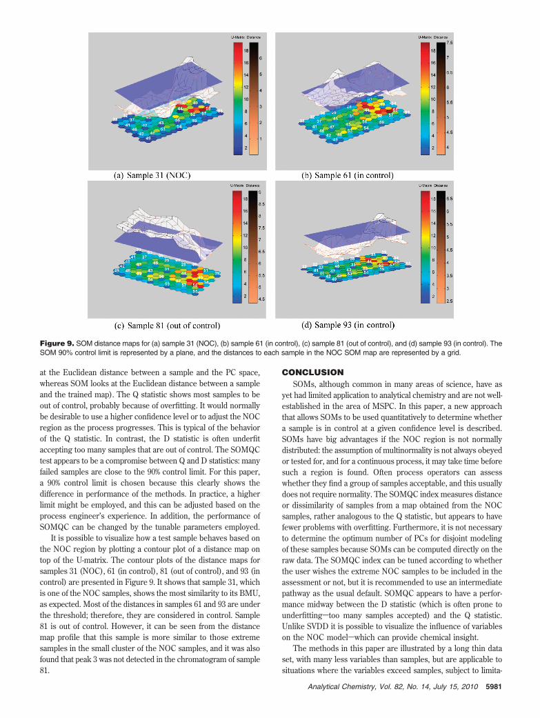
It is possible to visualize how a test sample behaves based onthe NOC region by plotting a contour plot of a distance map ontop of the U-matrix. The contour plots of the distance maps forsamples 31 (NOC), 61 (in control), 81 (out of control), and 93 (incontrol) are presented in Figure 9. It shows that sample 31, whichis one of the NOC samples, shows the most similarity to its BMU,as expected. Most of the distances in samples 61 and 93 are underthe threshold; therefore, they are considered in control. Sample81 is out of control. However, it can be seen from the distancemap profile that this sample is more similar to those extremesamples in the small cluster of the NOC samples, and it was alsofound that peak 3 was not detected in the chromatogram of sample81.

CONCLUSIONSOMs, although common in many areas of science, have as

yet had limited application to analytical chemistry and are not well-established in the area of MSPC. In this paper, a new approachthat allows SOMs to be used quantitatively to determine whethera sample is in control at a given confidence level is described.SOMs have big advantages if the NOC region is not normallydistributed: the assumption of multinormality is not always obeyedor tested for, and for a continuous process, it may take time beforesuch a region is found. Often process operators can assesswhether they find a group of samples acceptable, and this usuallydoes not require normality. The SOMQC index measures distanceor dissimilarity of samples from a map obtained from the NOCsamples, rather analogous to the Q statistic, but appears to havefewer problems with overfitting. Furthermore, it is not necessaryto determine the optimum number of PCs for disjoint modelingof these samples because SOMs can be computed directly on theraw data. The SOMQC index can be tuned according to whetherthe user wishes the extreme NOC samples to be included in theassessment or not, but it is recommended to use an intermediatepathway as the usual default. SOMQC appears to have a perfor-mance midway between the D statistic (which is often prone tounderfittingstoo many samples accepted) and the Q statistic.Unlike SVDD it is possible to visualize the influence of variableson the NOC modelswhich can provide chemical insight.

The methods in this paper are illustrated by a long thin dataset, with many less variables than samples, but are applicable tosituations where the variables exceed samples, subject to limita-

Figure 9. SOM distance maps for (a) sample 31 (NOC), (b) sample 61 (in control), (c) sample 81 (out of control), and (d) sample 93 (in control). TheSOM 90% control limit is represented by a plane, and the distances to each sample in the NOC SOM map are represented by a grid.


tions in computing power. It is anticipated that over the next fewyears, with the rapid increase in computing power, there will beflexibility to re-evaluate the traditional statistical approaches forprocess monitoring and to employ new methods, side by side,that are more computationally intensive but originate primarilyfrom pattern recognition.

ACKNOWLEDGMENTThis work was supported by GlaxoSmithKline (D.L.S.F.) and

the Strategic Scholarships Fellowships Frontier Research Net-

works from the Commission on Higher Education, Governmentof Thailand (S.K.).

SUPPORTING INFORMATION AVAILABLEAdditional information as noted in text. This material is available

free of charge via the Internet at http://pubs.acs.org.

Received for review February 10, 2010. Accepted May 28,2010.

AC100383G


Self-Organizing Map Quality Control Index

Documents

Transcript of Self-Organizing Map Quality Control Index