
Light Robust Goal Programming - Semantic Scholar
16
Mathematical and Computational Applications Article Light Robust Goal Programming Emmanuel Kwasi Mensah * and Matteo Rocca Department of Economics, Università degli Studi dell’Insubria, Via Monte Generoso 71, 21100 Varese, Italy; [email protected] * Correspondence: [email protected] Received: 10 September 2019; Accepted: 25 September 2019; Published: 28 September 2019 Abstract: Robust goal programming (RGP) is an emerging field of research in decision-making problems with multiple conflicting objectives and uncertain parameters. RGP combines robust optimization (RO) with variants of goal programming techniques to achieve stable and reliable goals for previously unspecified aspiration levels of the decision-maker. The RGP model proposed in Kuchta (2004) and recently advanced in Hanks, Weir, and Lunday (2017) uses classical robust methods. The drawback of these methods is that they can produce optimal values far from the optimal value of the “nominal” problem. As a proposal for overcoming the aforementioned drawback, we propose light RGP models generalized for the budget of uncertainty and ellipsoidal uncertainty sets in the framework discussed in Schöbel (2014) and compare them with the previous RGP models. Conclusions regarding the use of different uncertainty sets for the light RGP are made. Most importantly, we discuss that the total goal deviations of the decision-maker are very much dependent on the threshold set rather than the type of uncertainty set used. Keywords: goal programming (GP); robust optimization; robust goal programming (RGP); light robust goal programming (LRGP); multi-criteria decision making (MCDM) 1. Introduction A decision-making process implies the need to face conflicts, whether it is a management strategy, government policy, firm resource allocation, or individual budget planning; a certain course of action usually involving multiple conflicting objectives or criteria has to be taken [1]. Multicriteria decision analysis has been a widespread decision tool for problems involving multiple and usually conflicting objectives or criteria. For instance, the multicriteria optimization is deemed as the ideal setting to analyze portfolio optimization problems in the sense of Markowitz, in which a pair objective—the risk function and the expected return function—are minimized and maximized, respectively, to achieve a portfolio goal [2]. In multicriteria decision making (MCDM) problems, there is usually an infinite number of efficient solutions due to the conflicts among objectives. The goal programming (GP) technique, along with its variants—lexicographic GP, weighted GP, and fuzzy GP—is a well-known method that is commonly used to optimize multiple goals and derive efficient solutions for the decision-maker (DM). The GP provides a special compromise multi-criteria framework by which the DM can optimize multiple, conflicting objectives and concurrently achieve satisfiable solutions by minimizing the deviations of objectives from aspiration levels or goals set [3]. GP has obtained huge success in engineering, management, and social science problems [4]. However, the standard GP approaches deal with deterministic goals that are precisely defined while practical scenarios involving uncertainties in decision problems are ignored. One of the basic assumptions in mathematical programming including the GP is that the exact value of the input data is fixed and known in advance. This assumption can, however, be violated in many situations arising when real-world problems are considered. This can be due to the fact that the parameters used in the model are just Math. Comput. Appl. 2019, 24, 85; doi:10.3390/mca24040085 www.mdpi.com/journal/mca
-
Upload
khangminh22 -
Category
Documents
-
view
0 -
download
0
Transcript of Light Robust Goal Programming - Semantic Scholar
Mathematical
and Computational
Applications
Article
Light Robust Goal Programming
Emmanuel Kwasi Mensah * and Matteo Rocca
Department of Economics, Università degli Studi dell’Insubria, Via Monte Generoso 71, 21100 Varese, Italy;[email protected]* Correspondence: [email protected]
Received: 10 September 2019; Accepted: 25 September 2019; Published: 28 September 2019 �����������������
Abstract: Robust goal programming (RGP) is an emerging field of research in decision-makingproblems with multiple conflicting objectives and uncertain parameters. RGP combines robustoptimization (RO) with variants of goal programming techniques to achieve stable and reliable goalsfor previously unspecified aspiration levels of the decision-maker. The RGP model proposed inKuchta (2004) and recently advanced in Hanks, Weir, and Lunday (2017) uses classical robust methods.The drawback of these methods is that they can produce optimal values far from the optimal value ofthe “nominal” problem. As a proposal for overcoming the aforementioned drawback, we proposelight RGP models generalized for the budget of uncertainty and ellipsoidal uncertainty sets in theframework discussed in Schöbel (2014) and compare them with the previous RGP models. Conclusionsregarding the use of different uncertainty sets for the light RGP are made. Most importantly, wediscuss that the total goal deviations of the decision-maker are very much dependent on the thresholdset rather than the type of uncertainty set used.
Keywords: goal programming (GP); robust optimization; robust goal programming (RGP); lightrobust goal programming (LRGP); multi-criteria decision making (MCDM)
1. Introduction
A decision-making process implies the need to face conflicts, whether it is a management strategy,government policy, firm resource allocation, or individual budget planning; a certain course of actionusually involving multiple conflicting objectives or criteria has to be taken [1]. Multicriteria decisionanalysis has been a widespread decision tool for problems involving multiple and usually conflictingobjectives or criteria. For instance, the multicriteria optimization is deemed as the ideal setting toanalyze portfolio optimization problems in the sense of Markowitz, in which a pair objective—the riskfunction and the expected return function—are minimized and maximized, respectively, to achievea portfolio goal [2]. In multicriteria decision making (MCDM) problems, there is usually an infinitenumber of efficient solutions due to the conflicts among objectives.
The goal programming (GP) technique, along with its variants—lexicographic GP, weighted GP,and fuzzy GP—is a well-known method that is commonly used to optimize multiple goals and deriveefficient solutions for the decision-maker (DM). The GP provides a special compromise multi-criteriaframework by which the DM can optimize multiple, conflicting objectives and concurrently achievesatisfiable solutions by minimizing the deviations of objectives from aspiration levels or goals set [3].GP has obtained huge success in engineering, management, and social science problems [4]. However,the standard GP approaches deal with deterministic goals that are precisely defined while practicalscenarios involving uncertainties in decision problems are ignored. One of the basic assumptions inmathematical programming including the GP is that the exact value of the input data is fixed and knownin advance. This assumption can, however, be violated in many situations arising when real-worldproblems are considered. This can be due to the fact that the parameters used in the model are just
Math. Comput. Appl. 2019, 24, 85; doi:10.3390/mca24040085 www.mdpi.com/journal/mca
Math. Comput. Appl. 2019, 24, 85 2 of 16
estimates of real parameters or more generally to the effect of uncertainty affecting some parameters.When uncertainty is taken into account, an optimal solution with respect to the nominal values of theparameters can be suboptimal (or even infeasible) according to the actual parameters. Hence, smalluncertainty in the input data can make the nominal optimal solution completely meaningless from apractical viewpoint.
The robust optimization (RO) is an approach that is widely used to deal with optimizationproblems in which the parameters have uncertain values. The RO has gained a great interest amongacademics and practitioners as an important concept in uncertain linear programming since the seminalpaper of [5]. Other approaches in the literature include the stochastic approach and the fuzzy method(e.g., [6,7]). One of the drawbacks of this RO approach is that the solutions provided can be suboptimalif compared with the solution of the so-called nominal problem, i.e., a problem without uncertaintyin which the parameter values are fixed (for instance, to some point estimation). We clarify formallythe concept of nominal problems in Section 2. Although classical RO approaches are still relevant inpractice, in recent time, Fischetti and Monaci [8] proposed a light RO approach intended to focus onthe robust but quality solution of the optimization problem. A “quality solution” or a “good solution”(e.g., [9–11]) of an RO problem is intended as a solution for which the optimal value of the robustobjective function is close to the optimal value of the objective function in the nominal problem. In theliterature (see [5,12–14]), the term “conservative solution” is used with reference to the differencebetween the optimal values of the robust problem and the nominal problem. When the differencebetween the two values is high (i.e., the solution of the robust problem is highly suboptimal), it issaid that such a solution is very conservative. Hence, to say that a solution is a “quality solution” isequivalent to say that it is slightly conservative.
Although the RO was born as an approach to optimization problems with a single objective [15],it has been extended in the literature to address MCDM problems, for example, the multiobjectiveportfolio optimization [2,16] and the data envelopment analysis [14,17,18]. One growing area ofresearch in this field is the robust goal programming (RGP), which combines the RO with theGP technique. The RGP was first introduced by [19], and its potential use in multi-criteria linearprogramming problems is discussed in [20]. RGP has been applied, for example, to the multi-objectiveportfolio selection problem in [16], the capital budgeting problem in [21], and a transportation problem,specifically, the United States Transportation Command’s (USTRANSCOM) liner rate-setting problemin [22]. Despite this, the RGP methodology remains underdeveloped and less applied, specificallywhen considering different robust concepts and variants of GP techniques. In fact, since the modelproposal of [19], only recently in [13] was the conceptual foundation of the RGP touched upon heavily,deepening the application to MCDM problems. Hanks et al. [13] proposed norm-based uncertaintysets using cardinality-constrained robustness and strict robustness via ellipsoidal uncertainty andcompared their approach with the interval-based approach in [19]. However, their robust modelshave the aforementioned drawback—they can be highly suboptimal if compared to the solution of thenominal problem, e.g., their quality is low or, equivalently, they are very conservative. See [23] fordiscussion on reducing the conservatism of the RO.
The aim of this paper is to overcome this drawback in the RGP models. To this extent, weintroduce a model that we call light robust goal programming which gathers the features of lightrobustness introduced in [8,12] and and “Γ-robustness” proposed in [13,19]. The light robustnessapproach addresses the conservatism of the RGP by setting a limit to the deterioration of the objectivevalue compared to the nominal solution. We focus our proposed model on two arbitrary sets, i.e., thebudget of uncertainty of [12] and the ellipsoidal uncertainty sets of [24,25]. As a main result, we showthat the new model’s solution is “not too far” from optimality from the nominal GP model or—inthe aforementioned terminology—is a quality solution or, equivalently, a less conservative solutionif compared with the solutions obtained with the approaches in [13,19]. Furthermore, the proposedmodels are generalized to include modeling uncertainties in the hard constraint of the GP model thatwere left unconsidered in previous studies.

Math. Comput. Appl. 2019, 24, 85 3 of 16
The outline of the paper is the following. In Section 2, we provide a thorough review of the GPmethod, the RO concepts, and the RGP approaches. This section also includes a review of the RGPmodels in [13,19]. Section 3 introduces the proposed light RGP models. We perform a numericalcomparison in Section 4 and conclude the paper in Section 5.
2. Preliminaries
In this section, we provide a brief introduction to the GP technique, the RO approach, and the RGP.The section also reviews the RGP methodology in the literature and sets the pace for a new approachin the next section.
2.1. The Goal Programming Method
GP arose from the study of the executive compensation plan in [26], where the authors soughtto minimize the total deviations between realized goals and expected goals. Since then, the GP hasbecome by far the most popular technique used in dealing with decision problems with a multiplicity ofobjectives due to its versatility and the underlying concept of satisfying solution to decision situations.The literature evidence to the bulk of applications of the GP technique to MCDM can be found, e.g.,in [4,27].
The basic idea of the GP technique is to set up specific goals gt for each objective functionft(x), t = 1, . . . , T. Then, the total deviation
∑Tt=1|dt| where dt is the deviation from the goal gt
for the t-th objective function is minimized. For simplicity of computation, mostly, the absolutedeviation is split into positive and negative deviations (respectively d+t and d−t ) such that
∣∣∣dt∣∣∣= d+t − d−t .
The deviations can be defined as d+t = max( ft(x)− gt, 0) and d−t = max(gt − ft(x), 0). The positive andthe negative deviations underscore the over- and the underachievement of goals for each t-th goal ofthe objective function. Overachievement of the DM goals subject to constraints is attained if d+t > 0,while underachievement means d−t > 0. When the deviations are driven to zero, the goals of the modelare achieved [7,19]. A typical GP model for a min-type cost function is formulated as follows:
z∗ = Min∑T
t=1 wt(d+t + d−t )s.t.
(1)
ft(x) + d−t − d+t = gt ∀t ∈ T (2)
Ax ≤ b (3)
x ≥ 0, d−t , d+t ≥ 0 ∀t ∈ T (4)
where x ∈ Rn is a vector of decision variables, and wt is the penalty weight for missing the goal. In thesequel, we assume implicitly that the penalty weight is equal for all deviations, hence we set wt = 1for all t. The objective function then minimizes the sum of the positive and the negative deviationsfor each goal. Constraint (2) computes the respective positive and negative deviation from each goal.Constraint (3) relates to additional constraints in the decision space that is not related to the DM goals.It is important to note that the achievement function is a key element to variants’ consideration of goalsand the priorities attached to them by the decision-maker. As indicated in [28], the GP method resultsare sensitive to the type of function used. Different variants of the achievement function, namely, thetraditional weighted GP, the pre-emptive lexicographic GP, and the Chebyshev MINMAX GP, whichreflect different preferences structures have been introduced.
2.2. RO and Concepts
Uncertainty in the parameters of MCDM problems including the GP can lead to inaccurate andunreliable decisions that are sometimes meaningless from a practical point of view [12,25,29]. The ROenables us to overcome this problem since it focuses on finding the worst-case performance for all
Math. Comput. Appl. 2019, 24, 85 4 of 16
feasible realization of the uncertain parameters. The robust solution is obtained through an altenativereformulation of the uncertain problem called the robust counterpart. A general form of the robustcounterpart to the uncertain linear program is given as:
Minx[Max(A, b, c)∈U ctx
]s.t.
(5)
Ax ≤ b ∀(A, b, c) ∈ U (6)
where (A, b, c) are uncertain technological coefficients, a right-hand side vector, and a cost coefficientvector that take values in the uncertainty set U ⊆ Rn. The robust problem re-casted in this formproduces a solution that is the best possible in the worst-case scenario. If we consider an element(A0, b0, c0) ∈ U we can consider the so-called nominal problem:
Minx[ct
0x]
s.t.(7)
A0x ≤ b0 (8)
The vector (A0, b0, c0) can be interpreted as a point estimation of the parameters’ value. Clearly, thetrue value of the parameters is unknown, and such uncertainty is taken into account by assumingthat they can take values in the uncertainty setU. As indicated in [30], the robust counterpart is themain precursor of several RO concepts, e.g., strict robustness, interval-based/cardinality constrainedrobustness, norm-based robustness, adjustable robustness, and recoverable robustness. Here, weprovide but a few of these concepts.
2.2.1. Strict Robustness
Strict robustness follows the pessimistic view of maximizing the worst-case over all scenarios inthe uncertainty set. It was introduced in [31] and significantly extended in [9]. It is the highest formof robustness with guaranteed feasibility for all (A, b, c) ∈ U in that the probability of violating thei-th constraint is zero. Mathematically, a solution x to the optimization problem max
{ctx : A(ξ)x ≤ b
}where ξ denotes an uncertain parameter is called strictly robust if it is feasible for all scenarios inU,i.e., if A(ξ)x ≤ b ∀ξ ∈ U. The notion of strict robustness is plausible in some applications, suchas constructing a very stable bridge or nuclear power plants; however, the idea to hedge againstall scenarios in most other applications could be counterproductive. For example, in the robustformulation for the timetabling for public transport, being strictly robust provides a less practicallyapplicable timetable, since it is difficult to meet all announced arrival and departure times even withhigh buffer times considered in the uncertainty set [32]. In fact, applying strict robustness can lead to avery conservative solution. An approach that provides less conservative solutions is due to [24], whointroduced the ellipsoidal uncertainty set in which the “most likely“ values of the uncertain parametersare scaled down by the DM via the size of the ellipsoid. Further in [25], the authors combined theinterval uncertainty set of [31] with the ellipsoid to provide a robust model that is less conservativeand practically reliable.
2.2.2. “Γ-robustness” or Budget of Uncertainty
Bertsimas and Sim [12] introduced the concept of “Γ-robustness” predicated on the fact that notall uncertain parameters will simultaneously take their worst-case values; instead, up to Γ of thecoefficients that are allowed to change are protected against. The Bertsimas and Sim approach thusrelaxes the assumption of feasibility for all (A, b, c) ∈ U to feasibility for some (A, b, c) ∈ U in model (5)and (6), restricting the number of coefficients allowed to change from the nominal values. The approachleads to the concept of cardinality constrained robustness [30]. Thus, for the uncertain matrix A =
(ai j
)
Math. Comput. Appl. 2019, 24, 85 5 of 16
where each ai j, j ∈ Ji and Ji ={j∣∣∣ai j > 0
}is the set of coefficients in row i that are subject to uncertainty,
and each ai j lies in the interval[ai j − ai j, ai j + ai j
], denote by n = |N| and m = |M| the number of
variables and constraints in the linear programming (LP) model, respectively. The robust counterpartis obtained by replacing each row i ∈M of Constraint (6) by the new constraint:∑n
j=1 ai jx j + max{Si |Si⊆Ji, |S|=Γi }
{∑
j∈S ai j|xi|} ≤ bi ∀i ∈M . (9)
where, at most, Γi of the parameters in the i-th constraint are “budgeted” for the uncertainty toguarantee robustness for the solution. The parameter Γi ∈ [0, |Ji|] determines the quality of the solutionsof the model. Γi = 0 implies no robust solution is sought for the model. A solution is very conservative(i.e., not a quality solution) when all the parameters take their worst-case values and lead to a solutionmuch worse than the nominal solution or even infeasibility, i.e., if Γi = |Ji|. In this case, the robustsolution is equivalent to the strict robustness proposed in [31]. Values of Γi ∈ (0, |Ji|) lead to lessconservative solutions. Nothwithstanding, the robust solution is always feasible, i.e., given that notall the parameters will assume their worst-case values, and up to Γi of the parameters are allowed tochange. On the other hand, if more than Γi of the uncertain parameters change, the robust solution willstill be feasible with a probability bounded by an exponential term. Note here that the robust conceptin [12] is built on the principles similar to those in [25], where the model has an analogous probabilityof constraint violation. It can be shown that the cardinality constrained approach used in [12] is similarto strict robustness using the convex hull of the cardinality-constrained uncertainty set wherefore theapproach can lead to conservative solutions [32].
2.2.3. Light Robustness
A more relaxed condition for robustness that allows the user to control the quality of the solutionswas given in [8]. The robust concept introduced, known as light robustness, relies on a solution in whichthe objective function value is not much different from the objective function value of the nominalproblem. The light robustness approach is structured in two stages to ensure a less conservative robustsolution. The first stage considers a solution for the nominal problems (7) and (8). Subsequently, theconstraints are relaxed for local violations that are absorbed by slack variables γi, acting as measures ofinfeasibility for each constraint i ∈M of the nominal problem. Hence, Constraint (9) becomes:∑n
j=1 ai jx j + max{Si |Si⊆Ji, |S|=Γi }
{∑
j∈S ai j|xi|}+ γi ≤ bi ∀i ∈M . (10)
The second stage minimizes all the possible infeasibilities γi in the objective function:
Min∑i∈M
wiγi (11)
where wi are the weights for the possibly different scales of constraints. Since the goal of the lightrobustness is to guarantee a balance between the quality (optimality) and the feasibility (robustness) ofthe solution, an additional constraint: ∑n
j=1c jx j ≤ (1 + ρ)z∗ (12)
imposing a maximum worsening of the optimal solution of the nominal problem is added. Theparameter ρ is fundamental in the trade-off between the quality (optimality) and the feasibility of thesolution; ρ = 0 corresponds to the nominal problem where robustness is only considered to break tiesamong equivalent optimal solutions, whereas ρ = ∞ implies that the nominal objective function is notconsidered at all.
It should be clear now that the light robust models (10)–(12) rely on the robust approach of [12].On the other hand, the model can be formulated without it. Fischetti and Monaci [8] justified this
Math. Comput. Appl. 2019, 24, 85 6 of 16
with some heuristic methods. In an earlier application, Fischetti et al. [8] showed that light robustness,among others, is most suitable for railway timetabling problems where delays are encountered and acertain “quality and most reliable” solution is required for constraint violation. This has also beenthe case for some applications in similar contexts, for example, the timetabling information for publictransport in [10], the robust airport runway scheduling problem in [33], and the potential line planningof public transport in [34]. Light robustness has also found usefulness in RO applications such as themaster surgery scheduling problem in [35] and the multi-period multi-product aggregate productionplanning in [36]. Schöbel [11] in recent times extended the idea of [8] to the notion of generalized lightrobustness wherein optimization problems with arbitrary uncertainty sets can be applied.
2.3. The RGP Approach
The RGP methodology combines RO and GP techniques to solve decision problems with amultiplicity of objectives in an uncertain environment. Here, any of the RO concepts mentionedabove can be used with any variants of the GP. In the RGP, the goals of the DM that are marked byuncertain aspiration levels are confined to an uncertainty set and optimized with respect to theirfeasible realization in an uncertainty set to obtain a robust solution. Before proposing a new robustconcept for the RGP modeling, in the subsections that follow, we provide a review of the modelsin [1,2], highlighting their limitations.
2.3.1. Kuchta’s RGP Approach
Kuchta [19] introduced the robust approach to the GP technique in a single objective LP, where sheassumed that uncertain variations pertain only to the cost coefficients in the original objective functionof the LP. This approach translates uncertainty analysis to the goal constraints in which the nominalcost values, ct j, are assumed to vary within the interval
[ct j − δt j, ct j + δt j
], where δt j is a possible
deviation from the nominal cost value that accounts for the negative influence in the attainment ofgoals. Kuchta [19] adopted a robust methodology based on the interval-based uncertainty sets withcardinality-constraints developed in [12]. She supposed that each cost coefficient is subject to deviationand hence introduced the concept of K robust solution; K = (kt)
Tt=1 where kt, t = 1, . . . , T is any integer
such that the level of robustness of the RGP model or the optimal value of the total deviation isdetermined by the DM using the parameter kt.
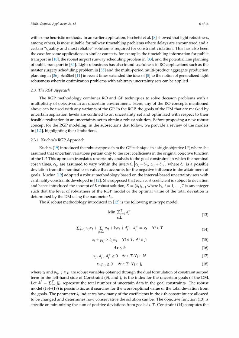
The K robust methodology introduced in [12] is the following min-type model:
Min∑T
t=1 d+ts.t.
(13)
∑nj=1 ct jx j +
∑j∈Gt
pt j + ktzt + d−t − d+t = gt ∀t ∈ T (14)
zt + pt j ≥ δt jx j ∀t ∈ T, ∀ j ∈ Jt (15)
Ax ≤ b (16)
x j, d−t , d+t ≥ 0 ∀t ∈ T,∀ j ∈ N (17)
zt, pt j ≥ 0 ∀t ∈ T, ∀ j ∈ Jt (18)
where zt and pt j, j ∈ Jt are robust variables obtained through the dual formulation of constraint secondterm in the left-hand side of Constraint (9), and Jt is the index for the uncertain goals of the DM.Let
Math. Comput. Appl. 2019, 24, x FOR PEER 7 of 17
2.3.2. Hanks et al‘s RGP Approach
Recently, Hanks et al. [13] broadened the scope of the RGP construct by proposing models that
extend the robust methodology of [19] to different uncertainty sets. They proposed three RGP
models. The first two models relate to cardinality-constrained robustness via norm-based uncertainty
sets using the �� -norm and the �� -norm, see [38]. Particularly, considering that the robust
counterpart of the �� -norm, ∑ ����������� , ∀� ∈ � accounts for data uncertainty given some
deviational value ���, in [13], the authors proposed the following ��-norm-based RGP model:
Min � ���
�
���
s.t. (19)
� �����
�
���+ �� + ��
� − ��� = �� ∀� ∈ � (20)
�� ≥ ��������
�∈��
+ ���������� ∀ �� ∈ ��, |��| = ��, � ∈ ��\��, � ∈ � (21)
�� ≤ � (22)
��, ���, ��
� ≥ 0 ∀� ∈ �, ∀� ∈ � (23)
where �� is the set of indices of all coefficients subject to deviation in goal � = 1, … , � where �� ⊂
� and �� = �� − ⌊��⌋, is the remainder value when �� is non-integer. Hanks [13] showed that model
(19)–(23) is equivalent to model (13)–(18). This is apparent since the robustness of both models is
obtained through cardinality-constraints via interval uncertainty. On the contrary, while model (19)–
(23) imposes a total penalty of ∑ ����∈��+ ���� for the variability in each goal, model (19)–(23)
identifies a total goal-specific penalty �� through every combination of ����� in some given ��, as
indicated in Constraint (21). Observe that Constraint (21) applies ��-norm uncertainty sets to the
possible set of coefficient subject to parametric uncertainty (i.e., �� ∈ ��, |��| = ��, � ∈ ��\��, � ∈ �). The
penalty difference is observed in Constraints (14) and (20) of the two models through a combination
of ∑ ��������∈��+ ���������� of the latter. Moreover, it is important to note that model (19)–(23) has
higher complexity compared to model (13)–(18), given that the former uses � + �� ∑ (�� − ��) ���
����
���
constraints to obtain the same optimal solution as the latter. The second model of [13] relates to the
RGP using the ��-norm. The model is obtained by replacing Constraint (21) with the following
constraint:
�� ≥ ����������
�∈��
+ �����������
∀ �� ∈ ��, |��| = ��, � ∈ ��\��, � ∈ � (24)
through which the model becomes a second-order cone programming. Unlike Constraint (21), the
penalty ��, � ∈ � is induced via the greatest lower bound over every combination of possible subsets
of variables taking on uncertainty for each goal.
The third model proposed in [13] considers strict robustness using an ellipsoidal uncertainty set
of [24]. The RGP model is presented as follows:
Min � ���
�
���
s.t. (25)
� �����
�
���+ �� ��� ���
� ���
�
���� + ��
� − ��� = �� ∀� ∈ � (26)
�� ≤ � (27)
t =∑T
t=1|Jt| represent the total number of uncertain data in the goal constraints. The robustmodel (13)–(18) is pessimistic, as it searches for the worst-optimal value of the total deviation fromthe goals. The parameter kt indicates how many of the coefficients in the t-th constraint are allowedto be changed and determines how conservative the solution can be. The objective function (13) isspecific on minimizing the sum of positive deviations from goals t ∈ T. Constraint (14) computes the
Math. Comput. Appl. 2019, 24, 85 7 of 16
respective positive and negative deviations from each goal t ∈ T for a given solution x j. It also containsthe protection function
∑j∈Gt pt j + ktzt with robustness parameter kt to the uncertain cost, which is
bounded for each combination of decision variables and goals via Constraint (15). Constraints (17)and (18) impose nonnegativity on all decision variables. The model involves t + t
Math. Comput. Appl. 2019, 24, x FOR PEER 7 of 17
2.3.2. Hanks et al‘s RGP Approach
Recently, Hanks et al. [13] broadened the scope of the RGP construct by proposing models that
extend the robust methodology of [19] to different uncertainty sets. They proposed three RGP
models. The first two models relate to cardinality-constrained robustness via norm-based uncertainty
sets using the �� -norm and the �� -norm, see [38]. Particularly, considering that the robust
counterpart of the �� -norm, ∑ ����������� , ∀� ∈ � accounts for data uncertainty given some
deviational value ���, in [13], the authors proposed the following ��-norm-based RGP model:
Min � ���
�
���
s.t. (19)
� �����
�
���+ �� + ��
� − ��� = �� ∀� ∈ � (20)
�� ≥ ��������
�∈��
+ ���������� ∀ �� ∈ ��, |��| = ��, � ∈ ��\��, � ∈ � (21)
�� ≤ � (22)
��, ���, ��
� ≥ 0 ∀� ∈ �, ∀� ∈ � (23)
where �� is the set of indices of all coefficients subject to deviation in goal � = 1, … , � where �� ⊂
� and �� = �� − ⌊��⌋, is the remainder value when �� is non-integer. Hanks [13] showed that model
(19)–(23) is equivalent to model (13)–(18). This is apparent since the robustness of both models is
obtained through cardinality-constraints via interval uncertainty. On the contrary, while model (19)–
(23) imposes a total penalty of ∑ ����∈��+ ���� for the variability in each goal, model (19)–(23)
identifies a total goal-specific penalty �� through every combination of ����� in some given ��, as
indicated in Constraint (21). Observe that Constraint (21) applies ��-norm uncertainty sets to the
possible set of coefficient subject to parametric uncertainty (i.e., �� ∈ ��, |��| = ��, � ∈ ��\��, � ∈ �). The
penalty difference is observed in Constraints (14) and (20) of the two models through a combination
of ∑ ��������∈��+ ���������� of the latter. Moreover, it is important to note that model (19)–(23) has
higher complexity compared to model (13)–(18), given that the former uses � + �� ∑ (�� − ��) ���
����
���
constraints to obtain the same optimal solution as the latter. The second model of [13] relates to the
RGP using the ��-norm. The model is obtained by replacing Constraint (21) with the following
constraint:
�� ≥ ����������
�∈��
+ �����������
∀ �� ∈ ��, |��| = ��, � ∈ ��\��, � ∈ � (24)
through which the model becomes a second-order cone programming. Unlike Constraint (21), the
penalty ��, � ∈ � is induced via the greatest lower bound over every combination of possible subsets
of variables taking on uncertainty for each goal.
The third model proposed in [13] considers strict robustness using an ellipsoidal uncertainty set
of [24]. The RGP model is presented as follows:
Min � ���
�
���
s.t. (25)
� �����
�
���+ �� ��� ���
� ���
�
���� + ��
� − ��� = �� ∀� ∈ � (26)
�� ≤ � (27)
t constraints and iscomputationally tractable irrespective of the number of coefficients subject to deviation.
2.3.2. Hanks et al.’s RGP Approach
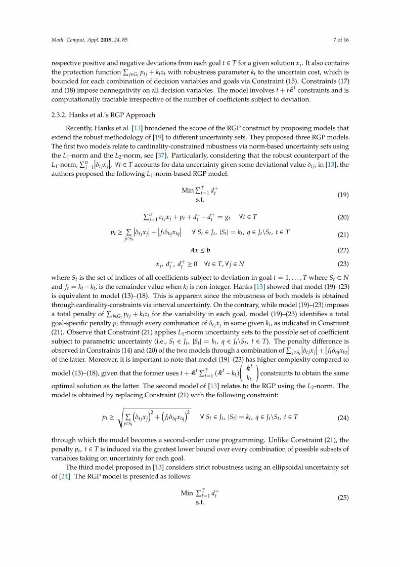
Recently, Hanks et al. [13] broadened the scope of the RGP construct by proposing models thatextend the robust methodology of [19] to different uncertainty sets. They proposed three RGP models.The first two models relate to cardinality-constrained robustness via norm-based uncertainty sets usingthe L1-norm and the L2-norm, see [37]. Particularly, considering that the robust counterpart of theL1-norm,
∑nj=1
∣∣∣δt jx j∣∣∣, ∀t ∈ T accounts for data uncertainty given some deviational value δt j, in [13], the
authors proposed the following L1-norm-based RGP model:
Min∑T
t=1 d+ts.t.
(19)
∑nj=1 ct jx j + pt + d−t − d+t = gt ∀t ∈ T (20)
pt ≥∑
j∈St
∣∣∣δt jx j∣∣∣+ ∣∣∣ ftδtqxtq
∣∣∣ ∀ St ∈ Jt, |St| = kt, q ∈ Jt\St, t ∈ T (21)
Ax ≤ b (22)
x j, d−t , d+t ≥ 0 ∀t ∈ T,∀ j ∈ N (23)
where St is the set of indices of all coefficients subject to deviation in goal t = 1, . . . , T where St ⊂ Nand ft = kt − kt, is the remainder value when ki is non-integer. Hanks [13] showed that model (19)–(23)is equivalent to model (13)–(18). This is apparent since the robustness of both models is obtainedthrough cardinality-constraints via interval uncertainty. On the contrary, while model (19)–(23) imposesa total penalty of
∑j∈Gt pt j + ktzt for the variability in each goal, model (19)–(23) identifies a total
goal-specific penalty pt through every combination of δt jx j in some given kt, as indicated in Constraint(21). Observe that Constraint (21) applies L1-norm uncertainty sets to the possible set of coefficientsubject to parametric uncertainty (i.e., St ∈ Jt, |St| = kt, q ∈ Jt\St, t ∈ T). The penalty difference isobserved in Constraints (14) and (20) of the two models through a combination of
∑j∈St
∣∣∣δt jx j∣∣∣+ ∣∣∣ ftδtqxtq
∣∣∣of the latter. Moreover, it is important to note that model (19)–(23) has higher complexity compared to
model (13)–(18), given that the former uses t +
Math. Comput. Appl. 2019, 24, x FOR PEER 7 of 17
2.3.2. Hanks et al‘s RGP Approach
Recently, Hanks et al. [13] broadened the scope of the RGP construct by proposing models that
extend the robust methodology of [19] to different uncertainty sets. They proposed three RGP
models. The first two models relate to cardinality-constrained robustness via norm-based uncertainty
sets using the �� -norm and the �� -norm, see [38]. Particularly, considering that the robust
counterpart of the �� -norm, ∑ ����������� , ∀� ∈ � accounts for data uncertainty given some
deviational value ���, in [13], the authors proposed the following ��-norm-based RGP model:
Min � ���
�
���
s.t. (19)
� �����
�
���+ �� + ��
� − ��� = �� ∀� ∈ � (20)
�� ≥ ��������
�∈��
+ ���������� ∀ �� ∈ ��, |��| = ��, � ∈ ��\��, � ∈ � (21)
�� ≤ � (22)
��, ���, ��
� ≥ 0 ∀� ∈ �, ∀� ∈ � (23)
where �� is the set of indices of all coefficients subject to deviation in goal � = 1, … , � where �� ⊂
� and �� = �� − ⌊��⌋, is the remainder value when �� is non-integer. Hanks [13] showed that model
(19)–(23) is equivalent to model (13)–(18). This is apparent since the robustness of both models is
obtained through cardinality-constraints via interval uncertainty. On the contrary, while model (19)–
(23) imposes a total penalty of ∑ ����∈��+ ���� for the variability in each goal, model (19)–(23)
identifies a total goal-specific penalty �� through every combination of ����� in some given ��, as
indicated in Constraint (21). Observe that Constraint (21) applies ��-norm uncertainty sets to the
possible set of coefficient subject to parametric uncertainty (i.e., �� ∈ ��, |��| = ��, � ∈ ��\��, � ∈ �). The
penalty difference is observed in Constraints (14) and (20) of the two models through a combination
of ∑ ��������∈��+ ���������� of the latter. Moreover, it is important to note that model (19)–(23) has
higher complexity compared to model (13)–(18), given that the former uses � + �� ∑ (�� − ��) ���
����
���
constraints to obtain the same optimal solution as the latter. The second model of [13] relates to the
RGP using the ��-norm. The model is obtained by replacing Constraint (21) with the following
constraint:
�� ≥ ����������
�∈��
+ �����������
∀ �� ∈ ��, |��| = ��, � ∈ ��\��, � ∈ � (24)
through which the model becomes a second-order cone programming. Unlike Constraint (21), the
penalty ��, � ∈ � is induced via the greatest lower bound over every combination of possible subsets
of variables taking on uncertainty for each goal.
The third model proposed in [13] considers strict robustness using an ellipsoidal uncertainty set
of [24]. The RGP model is presented as follows:
Min � ���
�
���
s.t. (25)
� �����
�
���+ �� ��� ���
� ���
�
���� + ��
� − ��� = �� ∀� ∈ � (26)
�� ≤ � (27)
t ∑Tt=1 (
Math. Comput. Appl. 2019, 24, x FOR PEER 7 of 17
2.3.2. Hanks et al‘s RGP Approach
Recently, Hanks et al. [13] broadened the scope of the RGP construct by proposing models that
extend the robust methodology of [19] to different uncertainty sets. They proposed three RGP
models. The first two models relate to cardinality-constrained robustness via norm-based uncertainty
sets using the �� -norm and the �� -norm, see [38]. Particularly, considering that the robust
counterpart of the �� -norm, ∑ ����������� , ∀� ∈ � accounts for data uncertainty given some
deviational value ���, in [13], the authors proposed the following ��-norm-based RGP model:
Min � ���
�
���
s.t. (19)
� �����
�
���+ �� + ��
� − ��� = �� ∀� ∈ � (20)
�� ≥ ��������
�∈��
+ ���������� ∀ �� ∈ ��, |��| = ��, � ∈ ��\��, � ∈ � (21)
�� ≤ � (22)
��, ���, ��
� ≥ 0 ∀� ∈ �, ∀� ∈ � (23)
where �� is the set of indices of all coefficients subject to deviation in goal � = 1, … , � where �� ⊂
� and �� = �� − ⌊��⌋, is the remainder value when �� is non-integer. Hanks [13] showed that model
(19)–(23) is equivalent to model (13)–(18). This is apparent since the robustness of both models is
obtained through cardinality-constraints via interval uncertainty. On the contrary, while model (19)–
(23) imposes a total penalty of ∑ ����∈��+ ���� for the variability in each goal, model (19)–(23)
identifies a total goal-specific penalty �� through every combination of ����� in some given ��, as
indicated in Constraint (21). Observe that Constraint (21) applies ��-norm uncertainty sets to the
possible set of coefficient subject to parametric uncertainty (i.e., �� ∈ ��, |��| = ��, � ∈ ��\��, � ∈ �). The
penalty difference is observed in Constraints (14) and (20) of the two models through a combination
of ∑ ��������∈��+ ���������� of the latter. Moreover, it is important to note that model (19)–(23) has
higher complexity compared to model (13)–(18), given that the former uses � + �� ∑ (�� − ��) ���
����
���
constraints to obtain the same optimal solution as the latter. The second model of [13] relates to the
RGP using the ��-norm. The model is obtained by replacing Constraint (21) with the following
constraint:
�� ≥ ����������
�∈��
+ �����������
∀ �� ∈ ��, |��| = ��, � ∈ ��\��, � ∈ � (24)
through which the model becomes a second-order cone programming. Unlike Constraint (21), the
penalty ��, � ∈ � is induced via the greatest lower bound over every combination of possible subsets
of variables taking on uncertainty for each goal.
The third model proposed in [13] considers strict robustness using an ellipsoidal uncertainty set
of [24]. The RGP model is presented as follows:
Min � ���
�
���
s.t. (25)
� �����
�
���+ �� ��� ���
� ���
�
���� + ��
� − ��� = �� ∀� ∈ � (26)
�� ≤ � (27)
t− kt)
(
Math. Comput. Appl. 2019, 24, x FOR PEER 7 of 17
2.3.2. Hanks et al‘s RGP Approach
Recently, Hanks et al. [13] broadened the scope of the RGP construct by proposing models that
extend the robust methodology of [19] to different uncertainty sets. They proposed three RGP
models. The first two models relate to cardinality-constrained robustness via norm-based uncertainty
sets using the �� -norm and the �� -norm, see [38]. Particularly, considering that the robust
counterpart of the �� -norm, ∑ ����������� , ∀� ∈ � accounts for data uncertainty given some
deviational value ���, in [13], the authors proposed the following ��-norm-based RGP model:
Min � ���
�
���
s.t. (19)
� �����
�
���+ �� + ��
� − ��� = �� ∀� ∈ � (20)
�� ≥ ��������
�∈��
+ ���������� ∀ �� ∈ ��, |��| = ��, � ∈ ��\��, � ∈ � (21)
�� ≤ � (22)
��, ���, ��
� ≥ 0 ∀� ∈ �, ∀� ∈ � (23)
where �� is the set of indices of all coefficients subject to deviation in goal � = 1, … , � where �� ⊂
� and �� = �� − ⌊��⌋, is the remainder value when �� is non-integer. Hanks [13] showed that model
(19)–(23) is equivalent to model (13)–(18). This is apparent since the robustness of both models is
obtained through cardinality-constraints via interval uncertainty. On the contrary, while model (19)–
(23) imposes a total penalty of ∑ ����∈��+ ���� for the variability in each goal, model (19)–(23)
identifies a total goal-specific penalty �� through every combination of ����� in some given ��, as
indicated in Constraint (21). Observe that Constraint (21) applies ��-norm uncertainty sets to the
possible set of coefficient subject to parametric uncertainty (i.e., �� ∈ ��, |��| = ��, � ∈ ��\��, � ∈ �). The
penalty difference is observed in Constraints (14) and (20) of the two models through a combination
of ∑ ��������∈��+ ���������� of the latter. Moreover, it is important to note that model (19)–(23) has
higher complexity compared to model (13)–(18), given that the former uses � + �� ∑ (�� − ��) ���
����
���
constraints to obtain the same optimal solution as the latter. The second model of [13] relates to the
RGP using the ��-norm. The model is obtained by replacing Constraint (21) with the following
constraint:
�� ≥ ����������
�∈��
+ �����������
∀ �� ∈ ��, |��| = ��, � ∈ ��\��, � ∈ � (24)
through which the model becomes a second-order cone programming. Unlike Constraint (21), the
penalty ��, � ∈ � is induced via the greatest lower bound over every combination of possible subsets
of variables taking on uncertainty for each goal.
The third model proposed in [13] considers strict robustness using an ellipsoidal uncertainty set
of [24]. The RGP model is presented as follows:
Min � ���
�
���
s.t. (25)
� �����
�
���+ �� ��� ���
� ���
�
���� + ��
� − ��� = �� ∀� ∈ � (26)
�� ≤ � (27)
t
kt
)constraints to obtain the same
optimal solution as the latter. The second model of [13] relates to the RGP using the L2-norm. Themodel is obtained by replacing Constraint (21) with the following constraint:
pt ≥
√ ∑j∈St
(δt jx j
)2+
(ftδtqxtq
)2∀ St ∈ Jt, |St| = kt, q ∈ Jt\St, t ∈ T (24)
through which the model becomes a second-order cone programming. Unlike Constraint (21), thepenalty pt, t ∈ T is induced via the greatest lower bound over every combination of possible subsets ofvariables taking on uncertainty for each goal.
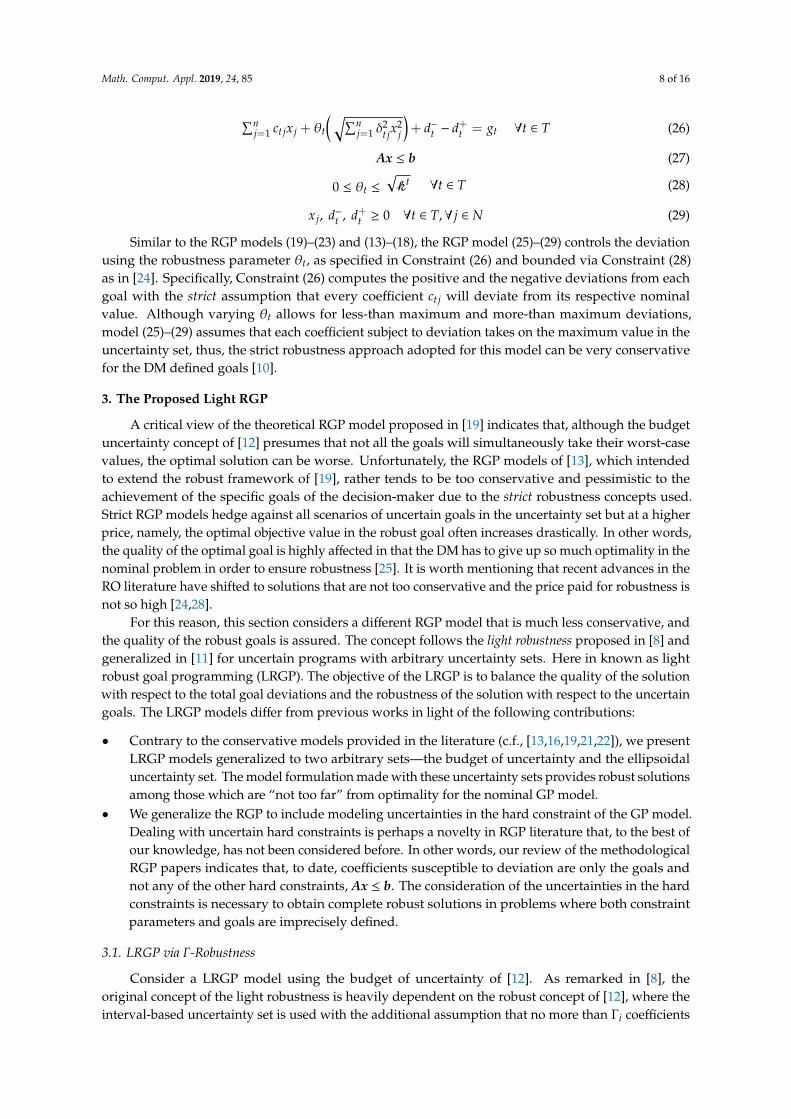
The third model proposed in [13] considers strict robustness using an ellipsoidal uncertainty setof [24]. The RGP model is presented as follows:
Min∑T
t=1 d+ts.t.
(25)
Math. Comput. Appl. 2019, 24, 85 8 of 16
∑nj=1 ct jx j + θt
(√∑nj=1 δ
2t jx
2j
)+ d−t − d+t = gt ∀t ∈ T (26)
Ax ≤ b (27)
0 ≤ θt ≤√
Math. Comput. Appl. 2019, 24, x FOR PEER 7 of 17
2.3.2. Hanks et al‘s RGP Approach
Recently, Hanks et al. [13] broadened the scope of the RGP construct by proposing models that
extend the robust methodology of [19] to different uncertainty sets. They proposed three RGP
models. The first two models relate to cardinality-constrained robustness via norm-based uncertainty
sets using the �� -norm and the �� -norm, see [38]. Particularly, considering that the robust
counterpart of the �� -norm, ∑ ����������� , ∀� ∈ � accounts for data uncertainty given some
deviational value ���, in [13], the authors proposed the following ��-norm-based RGP model:
Min � ���
�
���
s.t. (19)
� �����
�
���+ �� + ��
� − ��� = �� ∀� ∈ � (20)
�� ≥ ��������
�∈��
+ ���������� ∀ �� ∈ ��, |��| = ��, � ∈ ��\��, � ∈ � (21)
�� ≤ � (22)
��, ���, ��
� ≥ 0 ∀� ∈ �, ∀� ∈ � (23)
where �� is the set of indices of all coefficients subject to deviation in goal � = 1, … , � where �� ⊂
� and �� = �� − ⌊��⌋, is the remainder value when �� is non-integer. Hanks [13] showed that model
(19)–(23) is equivalent to model (13)–(18). This is apparent since the robustness of both models is
obtained through cardinality-constraints via interval uncertainty. On the contrary, while model (19)–
(23) imposes a total penalty of ∑ ����∈��+ ���� for the variability in each goal, model (19)–(23)
identifies a total goal-specific penalty �� through every combination of ����� in some given ��, as
indicated in Constraint (21). Observe that Constraint (21) applies ��-norm uncertainty sets to the
possible set of coefficient subject to parametric uncertainty (i.e., �� ∈ ��, |��| = ��, � ∈ ��\��, � ∈ �). The
penalty difference is observed in Constraints (14) and (20) of the two models through a combination
of ∑ ��������∈��+ ���������� of the latter. Moreover, it is important to note that model (19)–(23) has
higher complexity compared to model (13)–(18), given that the former uses � + �� ∑ (�� − ��) ���
����
���
constraints to obtain the same optimal solution as the latter. The second model of [13] relates to the
RGP using the ��-norm. The model is obtained by replacing Constraint (21) with the following
constraint:
�� ≥ ����������
�∈��
+ �����������
∀ �� ∈ ��, |��| = ��, � ∈ ��\��, � ∈ � (24)
through which the model becomes a second-order cone programming. Unlike Constraint (21), the
penalty ��, � ∈ � is induced via the greatest lower bound over every combination of possible subsets
of variables taking on uncertainty for each goal.
The third model proposed in [13] considers strict robustness using an ellipsoidal uncertainty set
of [24]. The RGP model is presented as follows:
Min � ���
�
���
s.t. (25)
� �����
�
���+ �� ��� ���
� ���
�
���� + ��
� − ��� = �� ∀� ∈ � (26)
�� ≤ � (27)
t ∀t ∈ T (28)
x j, d−t , d+t ≥ 0 ∀t ∈ T,∀ j ∈ N (29)
Similar to the RGP models (19)–(23) and (13)–(18), the RGP model (25)–(29) controls the deviationusing the robustness parameter θt, as specified in Constraint (26) and bounded via Constraint (28)as in [24]. Specifically, Constraint (26) computes the positive and the negative deviations from eachgoal with the strict assumption that every coefficient ct j will deviate from its respective nominalvalue. Although varying θt allows for less-than maximum and more-than maximum deviations,model (25)–(29) assumes that each coefficient subject to deviation takes on the maximum value in theuncertainty set, thus, the strict robustness approach adopted for this model can be very conservativefor the DM defined goals [10].
3. The Proposed Light RGP
A critical view of the theoretical RGP model proposed in [19] indicates that, although the budgetuncertainty concept of [12] presumes that not all the goals will simultaneously take their worst-casevalues, the optimal solution can be worse. Unfortunately, the RGP models of [13], which intendedto extend the robust framework of [19], rather tends to be too conservative and pessimistic to theachievement of the specific goals of the decision-maker due to the strict robustness concepts used.Strict RGP models hedge against all scenarios of uncertain goals in the uncertainty set but at a higherprice, namely, the optimal objective value in the robust goal often increases drastically. In other words,the quality of the optimal goal is highly affected in that the DM has to give up so much optimality in thenominal problem in order to ensure robustness [25]. It is worth mentioning that recent advances in theRO literature have shifted to solutions that are not too conservative and the price paid for robustness isnot so high [24,28].
For this reason, this section considers a different RGP model that is much less conservative, andthe quality of the robust goals is assured. The concept follows the light robustness proposed in [8] andgeneralized in [11] for uncertain programs with arbitrary uncertainty sets. Here in known as lightrobust goal programming (LRGP). The objective of the LRGP is to balance the quality of the solutionwith respect to the total goal deviations and the robustness of the solution with respect to the uncertaingoals. The LRGP models differ from previous works in light of the following contributions:
• Contrary to the conservative models provided in the literature (c.f., [13,16,19,21,22]), we presentLRGP models generalized to two arbitrary sets—the budget of uncertainty and the ellipsoidaluncertainty set. The model formulation made with these uncertainty sets provides robust solutionsamong those which are “not too far” from optimality for the nominal GP model.
• We generalize the RGP to include modeling uncertainties in the hard constraint of the GP model.Dealing with uncertain hard constraints is perhaps a novelty in RGP literature that, to the best ofour knowledge, has not been considered before. In other words, our review of the methodologicalRGP papers indicates that, to date, coefficients susceptible to deviation are only the goals andnot any of the other hard constraints, Ax ≤ b. The consideration of the uncertainties in the hardconstraints is necessary to obtain complete robust solutions in problems where both constraintparameters and goals are imprecisely defined.
3.1. LRGP via Γ-Robustness
Consider a LRGP model using the budget of uncertainty of [12]. As remarked in [8], theoriginal concept of the light robustness is heavily dependent on the robust concept of [12], where theinterval-based uncertainty set is used with the additional assumption that no more than Γi coefficients

Math. Comput. Appl. 2019, 24, 85 9 of 16
are expected to change to their worst-case values in constraint i. Assume further from Section 2.3.1 thatthe uncertain constraint parameter ai j takes value in the interval
[ai j − ai j, ai j + ai j
]. Analogous to [19],
K robust solution, the maximum values for the budget of uncertainty are Γt ∈ [0, |Jt|] and Γ′i ∈ [0, |Ji|]
where
Math. Comput. Appl. 2019, 24, x FOR PEER 7 of 17
2.3.2. Hanks et al‘s RGP Approach
Recently, Hanks et al. [13] broadened the scope of the RGP construct by proposing models that
extend the robust methodology of [19] to different uncertainty sets. They proposed three RGP
models. The first two models relate to cardinality-constrained robustness via norm-based uncertainty
sets using the �� -norm and the �� -norm, see [38]. Particularly, considering that the robust
counterpart of the �� -norm, ∑ ����������� , ∀� ∈ � accounts for data uncertainty given some
deviational value ���, in [13], the authors proposed the following ��-norm-based RGP model:
Min � ���
�
���
s.t. (19)
� �����
�
���+ �� + ��
� − ��� = �� ∀� ∈ � (20)
�� ≥ ��������
�∈��
+ ���������� ∀ �� ∈ ��, |��| = ��, � ∈ ��\��, � ∈ � (21)
�� ≤ � (22)
��, ���, ��
� ≥ 0 ∀� ∈ �, ∀� ∈ � (23)
where �� is the set of indices of all coefficients subject to deviation in goal � = 1, … , � where �� ⊂
� and �� = �� − ⌊��⌋, is the remainder value when �� is non-integer. Hanks [13] showed that model
(19)–(23) is equivalent to model (13)–(18). This is apparent since the robustness of both models is
obtained through cardinality-constraints via interval uncertainty. On the contrary, while model (19)–
(23) imposes a total penalty of ∑ ����∈��+ ���� for the variability in each goal, model (19)–(23)
identifies a total goal-specific penalty �� through every combination of ����� in some given ��, as
indicated in Constraint (21). Observe that Constraint (21) applies ��-norm uncertainty sets to the
possible set of coefficient subject to parametric uncertainty (i.e., �� ∈ ��, |��| = ��, � ∈ ��\��, � ∈ �). The
penalty difference is observed in Constraints (14) and (20) of the two models through a combination
of ∑ ��������∈��+ ���������� of the latter. Moreover, it is important to note that model (19)–(23) has
higher complexity compared to model (13)–(18), given that the former uses � + �� ∑ (�� − ��) ���
����
���
constraints to obtain the same optimal solution as the latter. The second model of [13] relates to the
RGP using the ��-norm. The model is obtained by replacing Constraint (21) with the following
constraint:
�� ≥ ����������
�∈��
+ �����������
∀ �� ∈ ��, |��| = ��, � ∈ ��\��, � ∈ � (24)
through which the model becomes a second-order cone programming. Unlike Constraint (21), the
penalty ��, � ∈ � is induced via the greatest lower bound over every combination of possible subsets
of variables taking on uncertainty for each goal.
The third model proposed in [13] considers strict robustness using an ellipsoidal uncertainty set
of [24]. The RGP model is presented as follows:
Min � ���
�
���
s.t. (25)
� �����
�
���+ �� ��� ���
� ���
�
���� + ��
� − ��� = �� ∀� ∈ � (26)
�� ≤ � (27)
i =m∑
i=1|Ji| represents the total number of uncertain data in the hard constraints. Note that Γt
and Γ′i allow the DM to control robustness via the goal and the hard constraints, as is considered in themodels of [8,12]. We introduce slack variables γt for t = 1, . . . , T and γ′i for i = 1, . . . , M where T and Mare set indices for the goals and the decision variables pertaining to the hard constraint. These variablesdefine the robustness level with respect to parameter uncertainties and control the model infeasibility.Therefore, the objective of the LRGPΓ is to minimize the sum of γt and γ′i in the following model:
LRGPΓ = Min∑t∈T
∑i∈M
(γt + γ′i
)s.t.
(30)
∑T
t=1d+t ≤ (1 + ρ)z∗ (31)∑n
j=1 ct jx j +∑
j∈Gt
pt j + Γtzt − γt + d−t − d+t = gt ∀t ∈ T (32)∑nj=1 ai jx j +
∑j∈Ji
qi j + Γ′i wi − γ′
i ≤ bi ∀i ∈M (33)
zt + pt j ≥ δt jx j ∀t ∈ T, ∀ j ∈ Jt (34)
wi + qi j ≥ σi jx j ∀i ∈M, ∀ j ∈ Ji (35)
γt, γ′i ≥ 0 ∀t ∈ T, ∀i ∈M (36)
x j, d−t , d+t ≥ 0 ∀i ∈M,∀ j ∈ N (37)
zt, pt j ≥ 0 ∀t ∈ T, ∀ j ∈ Jt (38)
wi, qi j ≥ 0 ∀i ∈M, ∀ j ∈ Ji (39)
The main differences between model (30)–(39) and the previous models given in (13)–(18), (19)–(23),and (25)–(29) occur in the objective function (30) and Constraints (31)–(33). A degree of relaxation forstrict robustness is made by allowing for local violation of the t-th constraint (32) and the i-th constraint(33), where γt and γ′i are then used to recover and deal with any possible infeasibility issues. Hence,the objective function is designed to control robustness and minimize possible infeasibility of themodel to changes in the aspiration levels of the DM and other parameter uncertainties. Moreover, toensure the quality of the generated solution, the generalized RGP model (30)–(39) requires first anoptimal solution z∗ to the nominal GP problem in (1)–(4) as the reference scenario. Constraint (31)therefore ensures that an acceptable deviation of the generated solution from the nominal solutionis made through the parameter ρ. Constraint (32) identifies a total goal penalty
∑j∈Gt pt j + Γtzt − γt
which, in contrast to the model of [19], includes the additional penalty term γt, specifically for theviolation of the cost parameter ct j from its nominal value. Constraints (34) and (35) are a combinationof bounded terms for the robust variables. Finally, Constraints (36)–(39) impose nonnegativity on alldecision variables.
3.2. LRGP via Ellipsoidal Uncertainty Set
This section considers a special case of the generalized LRGP to the ellipsoidal uncertainty set.Let Ut
1 ={C = P0 +
∑Nl=1 ulPl : ‖ut
‖2 ≤ 1, ut∈ RT
}where Pl =
(pl), l = 0, . . . , T are t × n matrices,
and ‖·‖2 denotes the Euclidean norm (analogously to [11], this norm is independent of the particularnorm chosen for generalized light robustness). The setUt
1 is defined for perturbation of the DM goals.
Math. Comput. Appl. 2019, 24, 85 10 of 16
A finite mathematical program for the defined uncertainty set is obtained if the RGP problem is solvedwith parameter u instead of the cost matrix ct j [24]. To this end, we let Rt contain all the t-th rows of allmatrices P1, . . . , PN. Then, for ct j ∈ U
t1, following [11], the goal constraint
∑nj=1 ct jx j −γt + d−t − d+t = gt
translates to Pot x + ‖Rtx‖2 − γt + d−t − d+t = gt for all u ∈ RN with ‖ut
‖2 ≤ 1. Similarly, let the m × nmatrix Sl, l = 0, . . . , k inUi
2 ={A = Q0 +
∑Nl=1 µlQ
l : ‖µi‖2 ≤ 1, µi
∈ RN}
be defined for the uncertain
parameters in the hard constraint, where Si is the i-th rows of the matrices Q1, . . . , QN. We obtainthe constraint Qo
i x + ‖Six‖2 − γ′i ≤ bi for all µi∈ RN with ‖µi
‖2 ≤ 1. The generalized LRGP using theellipsoidal set is thus equivalent to the following program:
LRGPe = Min(‖γt‖+ ‖γ′i‖
)s.t.
(40)
∑T
t=1d+t ≤ (1 + ρ)z∗ (41)
Pot x + ‖Rtx‖2 − γt + d−t − d+t = gt ∀t ∈ T (42)
Qoi x + ‖Six‖2 − γ′i ≤ bi ∀i ∈M (43)
γt, γ′i ≥ 0 ∀t ∈ T, ∀i ∈M (44)
x j, d−t , d+t ≥ 0 ∀i ∈M,∀ j ∈ N (45)
Similar to model (30)–(39), Equation (40) minimizes the sum of the arbitrary norm of theinfeasibilities of the goal and the hard constraints. Constraint (41) controls the nominal quality by theparameter ρ. Constraints (42) and (43) apply ellipsoidal uncertainty to allow a deviation of the goals inthe t-th constraint and uncertain parameters in the i-th constraint, respectively, wherein the infeasibilityinduced in the constraints by such deviations is controlled by γt and γ′i . Similarly, Constraints (44)–(45)impose nonnegativity on all decision variables.
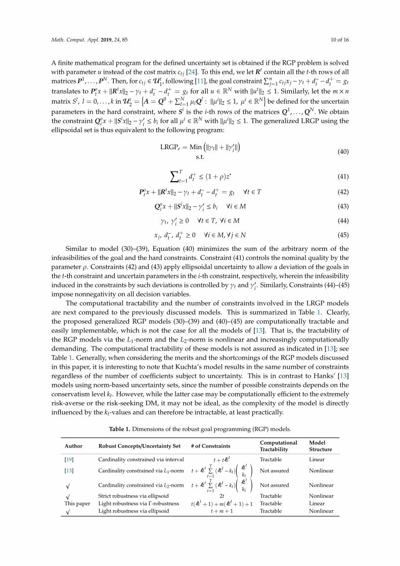
The computational tractability and the number of constraints involved in the LRGP modelsare next compared to the previously discussed models. This is summarized in Table 1. Clearly,the proposed generalized RGP models (30)–(39) and (40)–(45) are computationally tractable andeasily implementable, which is not the case for all the models of [13]. That is, the tractability ofthe RGP models via the L1-norm and the L2-norm is nonlinear and increasingly computationallydemanding. The computational tractability of these models is not assured as indicated in [13]; seeTable 1. Generally, when considering the merits and the shortcomings of the RGP models discussedin this paper, it is interesting to note that Kuchta’s model results in the same number of constraintsregardless of the number of coefficients subject to uncertainty. This is in contrast to Hanks’ [13]models using norm-based uncertainty sets, since the number of possible constraints depends on theconservatism level kt. However, while the latter case may be computationally efficient to the extremelyrisk-averse or the risk-seeking DM, it may not be ideal, as the complexity of the model is directlyinfluenced by the kt-values and can therefore be intractable, at least practically.
Table 1. Dimensions of the robust goal programming (RGP) models.
Author Robust Concepts/Uncertainty Set # of Constraints ComputationalTractability
ModelStructure
[19] Cardinality constrained via interval t + t
Math. Comput. Appl. 2019, 24, x FOR PEER 7 of 17
2.3.2. Hanks et al‘s RGP Approach
Recently, Hanks et al. [13] broadened the scope of the RGP construct by proposing models that
extend the robust methodology of [19] to different uncertainty sets. They proposed three RGP
models. The first two models relate to cardinality-constrained robustness via norm-based uncertainty
sets using the �� -norm and the �� -norm, see [38]. Particularly, considering that the robust
counterpart of the �� -norm, ∑ ����������� , ∀� ∈ � accounts for data uncertainty given some
deviational value ���, in [13], the authors proposed the following ��-norm-based RGP model:
Min � ���
�
���
s.t. (19)
� �����
�
���+ �� + ��
� − ��� = �� ∀� ∈ � (20)
�� ≥ ��������
�∈��
+ ���������� ∀ �� ∈ ��, |��| = ��, � ∈ ��\��, � ∈ � (21)
�� ≤ � (22)
��, ���, ��
� ≥ 0 ∀� ∈ �, ∀� ∈ � (23)
where �� is the set of indices of all coefficients subject to deviation in goal � = 1, … , � where �� ⊂
� and �� = �� − ⌊��⌋, is the remainder value when �� is non-integer. Hanks [13] showed that model
(19)–(23) is equivalent to model (13)–(18). This is apparent since the robustness of both models is
obtained through cardinality-constraints via interval uncertainty. On the contrary, while model (19)–
(23) imposes a total penalty of ∑ ����∈��+ ���� for the variability in each goal, model (19)–(23)
identifies a total goal-specific penalty �� through every combination of ����� in some given ��, as
indicated in Constraint (21). Observe that Constraint (21) applies ��-norm uncertainty sets to the
possible set of coefficient subject to parametric uncertainty (i.e., �� ∈ ��, |��| = ��, � ∈ ��\��, � ∈ �). The
penalty difference is observed in Constraints (14) and (20) of the two models through a combination
of ∑ ��������∈��+ ���������� of the latter. Moreover, it is important to note that model (19)–(23) has
higher complexity compared to model (13)–(18), given that the former uses � + �� ∑ (�� − ��) ���
����
���
constraints to obtain the same optimal solution as the latter. The second model of [13] relates to the
RGP using the ��-norm. The model is obtained by replacing Constraint (21) with the following
constraint:
�� ≥ ����������
�∈��
+ �����������
∀ �� ∈ ��, |��| = ��, � ∈ ��\��, � ∈ � (24)
through which the model becomes a second-order cone programming. Unlike Constraint (21), the
penalty ��, � ∈ � is induced via the greatest lower bound over every combination of possible subsets
of variables taking on uncertainty for each goal.
The third model proposed in [13] considers strict robustness using an ellipsoidal uncertainty set
of [24]. The RGP model is presented as follows:
Min � ���
�
���
s.t. (25)
� �����
�
���+ �� ��� ���
� ���
�
���� + ��
� − ��� = �� ∀� ∈ � (26)
�� ≤ � (27)
t Tractable Linear
[13] Cardinality constrained via L1-norm t +
Math. Comput. Appl. 2019, 24, x FOR PEER 7 of 17
2.3.2. Hanks et al‘s RGP Approach
Recently, Hanks et al. [13] broadened the scope of the RGP construct by proposing models that
extend the robust methodology of [19] to different uncertainty sets. They proposed three RGP
models. The first two models relate to cardinality-constrained robustness via norm-based uncertainty
sets using the �� -norm and the �� -norm, see [38]. Particularly, considering that the robust
counterpart of the �� -norm, ∑ ����������� , ∀� ∈ � accounts for data uncertainty given some
deviational value ���, in [13], the authors proposed the following ��-norm-based RGP model:
Min � ���
�
���
s.t. (19)
� �����
�
���+ �� + ��
� − ��� = �� ∀� ∈ � (20)
�� ≥ ��������
�∈��
+ ���������� ∀ �� ∈ ��, |��| = ��, � ∈ ��\��, � ∈ � (21)
�� ≤ � (22)
��, ���, ��
� ≥ 0 ∀� ∈ �, ∀� ∈ � (23)
where �� is the set of indices of all coefficients subject to deviation in goal � = 1, … , � where �� ⊂
� and �� = �� − ⌊��⌋, is the remainder value when �� is non-integer. Hanks [13] showed that model
(19)–(23) is equivalent to model (13)–(18). This is apparent since the robustness of both models is
obtained through cardinality-constraints via interval uncertainty. On the contrary, while model (19)–
(23) imposes a total penalty of ∑ ����∈��+ ���� for the variability in each goal, model (19)–(23)
identifies a total goal-specific penalty �� through every combination of ����� in some given ��, as
indicated in Constraint (21). Observe that Constraint (21) applies ��-norm uncertainty sets to the
possible set of coefficient subject to parametric uncertainty (i.e., �� ∈ ��, |��| = ��, � ∈ ��\��, � ∈ �). The
penalty difference is observed in Constraints (14) and (20) of the two models through a combination
of ∑ ��������∈��+ ���������� of the latter. Moreover, it is important to note that model (19)–(23) has
higher complexity compared to model (13)–(18), given that the former uses � + �� ∑ (�� − ��) ���
����
���
constraints to obtain the same optimal solution as the latter. The second model of [13] relates to the
RGP using the ��-norm. The model is obtained by replacing Constraint (21) with the following
constraint:
�� ≥ ����������
�∈��
+ �����������
∀ �� ∈ ��, |��| = ��, � ∈ ��\��, � ∈ � (24)
through which the model becomes a second-order cone programming. Unlike Constraint (21), the
penalty ��, � ∈ � is induced via the greatest lower bound over every combination of possible subsets
of variables taking on uncertainty for each goal.
The third model proposed in [13] considers strict robustness using an ellipsoidal uncertainty set
of [24]. The RGP model is presented as follows:
Min � ���
�
���
s.t. (25)
� �����
�
���+ �� ��� ���
� ���
�
���� + ��
� − ��� = �� ∀� ∈ � (26)
�� ≤ � (27)
t T∑t=1
(
Math. Comput. Appl. 2019, 24, x FOR PEER 7 of 17
2.3.2. Hanks et al‘s RGP Approach
Recently, Hanks et al. [13] broadened the scope of the RGP construct by proposing models that
extend the robust methodology of [19] to different uncertainty sets. They proposed three RGP
models. The first two models relate to cardinality-constrained robustness via norm-based uncertainty
sets using the �� -norm and the �� -norm, see [38]. Particularly, considering that the robust
counterpart of the �� -norm, ∑ ����������� , ∀� ∈ � accounts for data uncertainty given some
deviational value ���, in [13], the authors proposed the following ��-norm-based RGP model:
Min � ���
�
���
s.t. (19)
� �����
�
���+ �� + ��
� − ��� = �� ∀� ∈ � (20)
�� ≥ ��������
�∈��
+ ���������� ∀ �� ∈ ��, |��| = ��, � ∈ ��\��, � ∈ � (21)
�� ≤ � (22)
��, ���, ��
� ≥ 0 ∀� ∈ �, ∀� ∈ � (23)
where �� is the set of indices of all coefficients subject to deviation in goal � = 1, … , � where �� ⊂
� and �� = �� − ⌊��⌋, is the remainder value when �� is non-integer. Hanks [13] showed that model
(19)–(23) is equivalent to model (13)–(18). This is apparent since the robustness of both models is
obtained through cardinality-constraints via interval uncertainty. On the contrary, while model (19)–
(23) imposes a total penalty of ∑ ����∈��+ ���� for the variability in each goal, model (19)–(23)
identifies a total goal-specific penalty �� through every combination of ����� in some given ��, as
indicated in Constraint (21). Observe that Constraint (21) applies ��-norm uncertainty sets to the
possible set of coefficient subject to parametric uncertainty (i.e., �� ∈ ��, |��| = ��, � ∈ ��\��, � ∈ �). The
penalty difference is observed in Constraints (14) and (20) of the two models through a combination
of ∑ ��������∈��+ ���������� of the latter. Moreover, it is important to note that model (19)–(23) has
higher complexity compared to model (13)–(18), given that the former uses � + �� ∑ (�� − ��) ���
����
���
constraints to obtain the same optimal solution as the latter. The second model of [13] relates to the
RGP using the ��-norm. The model is obtained by replacing Constraint (21) with the following
constraint:
�� ≥ ����������
�∈��
+ �����������
∀ �� ∈ ��, |��| = ��, � ∈ ��\��, � ∈ � (24)
through which the model becomes a second-order cone programming. Unlike Constraint (21), the
penalty ��, � ∈ � is induced via the greatest lower bound over every combination of possible subsets
of variables taking on uncertainty for each goal.
The third model proposed in [13] considers strict robustness using an ellipsoidal uncertainty set
of [24]. The RGP model is presented as follows:
Min � ���
�
���
s.t. (25)
� �����
�
���+ �� ��� ���
� ���
�
���� + ��
� − ��� = �� ∀� ∈ � (26)
�� ≤ � (27)
t− kt)
(
Math. Comput. Appl. 2019, 24, x FOR PEER 7 of 17
2.3.2. Hanks et al‘s RGP Approach
Recently, Hanks et al. [13] broadened the scope of the RGP construct by proposing models that
extend the robust methodology of [19] to different uncertainty sets. They proposed three RGP
models. The first two models relate to cardinality-constrained robustness via norm-based uncertainty
sets using the �� -norm and the �� -norm, see [38]. Particularly, considering that the robust
counterpart of the �� -norm, ∑ ����������� , ∀� ∈ � accounts for data uncertainty given some
deviational value ���, in [13], the authors proposed the following ��-norm-based RGP model:
Min � ���
�
���
s.t. (19)
� �����
�
���+ �� + ��
� − ��� = �� ∀� ∈ � (20)
�� ≥ ��������
�∈��
+ ���������� ∀ �� ∈ ��, |��| = ��, � ∈ ��\��, � ∈ � (21)
�� ≤ � (22)
��, ���, ��
� ≥ 0 ∀� ∈ �, ∀� ∈ � (23)
where �� is the set of indices of all coefficients subject to deviation in goal � = 1, … , � where �� ⊂
� and �� = �� − ⌊��⌋, is the remainder value when �� is non-integer. Hanks [13] showed that model
(19)–(23) is equivalent to model (13)–(18). This is apparent since the robustness of both models is
obtained through cardinality-constraints via interval uncertainty. On the contrary, while model (19)–
(23) imposes a total penalty of ∑ ����∈��+ ���� for the variability in each goal, model (19)–(23)
identifies a total goal-specific penalty �� through every combination of ����� in some given ��, as
indicated in Constraint (21). Observe that Constraint (21) applies ��-norm uncertainty sets to the
possible set of coefficient subject to parametric uncertainty (i.e., �� ∈ ��, |��| = ��, � ∈ ��\��, � ∈ �). The
penalty difference is observed in Constraints (14) and (20) of the two models through a combination
of ∑ ��������∈��+ ���������� of the latter. Moreover, it is important to note that model (19)–(23) has
higher complexity compared to model (13)–(18), given that the former uses � + �� ∑ (�� − ��) ���
����
���
constraints to obtain the same optimal solution as the latter. The second model of [13] relates to the
RGP using the ��-norm. The model is obtained by replacing Constraint (21) with the following
constraint:
�� ≥ ����������
�∈��
+ �����������
∀ �� ∈ ��, |��| = ��, � ∈ ��\��, � ∈ � (24)
through which the model becomes a second-order cone programming. Unlike Constraint (21), the
penalty ��, � ∈ � is induced via the greatest lower bound over every combination of possible subsets
of variables taking on uncertainty for each goal.
The third model proposed in [13] considers strict robustness using an ellipsoidal uncertainty set
of [24]. The RGP model is presented as follows:
Min � ���
�
���
s.t. (25)
� �����
�
���+ �� ��� ���
� ���
�
���� + ��
� − ��� = �� ∀� ∈ � (26)
�� ≤ � (27)
t
kt
)Not assured Nonlinear
√ Cardinality constrained via L2-norm t +
Math. Comput. Appl. 2019, 24, x FOR PEER 7 of 17
2.3.2. Hanks et al‘s RGP Approach
Recently, Hanks et al. [13] broadened the scope of the RGP construct by proposing models that
extend the robust methodology of [19] to different uncertainty sets. They proposed three RGP
models. The first two models relate to cardinality-constrained robustness via norm-based uncertainty
sets using the �� -norm and the �� -norm, see [38]. Particularly, considering that the robust
counterpart of the �� -norm, ∑ ����������� , ∀� ∈ � accounts for data uncertainty given some
deviational value ���, in [13], the authors proposed the following ��-norm-based RGP model:
Min � ���
�
���
s.t. (19)
� �����
�
���+ �� + ��
� − ��� = �� ∀� ∈ � (20)
�� ≥ ��������
�∈��
+ ���������� ∀ �� ∈ ��, |��| = ��, � ∈ ��\��, � ∈ � (21)
�� ≤ � (22)
��, ���, ��
� ≥ 0 ∀� ∈ �, ∀� ∈ � (23)
where �� is the set of indices of all coefficients subject to deviation in goal � = 1, … , � where �� ⊂
� and �� = �� − ⌊��⌋, is the remainder value when �� is non-integer. Hanks [13] showed that model
(19)–(23) is equivalent to model (13)–(18). This is apparent since the robustness of both models is
obtained through cardinality-constraints via interval uncertainty. On the contrary, while model (19)–
(23) imposes a total penalty of ∑ ����∈��+ ���� for the variability in each goal, model (19)–(23)
identifies a total goal-specific penalty �� through every combination of ����� in some given ��, as
indicated in Constraint (21). Observe that Constraint (21) applies ��-norm uncertainty sets to the
possible set of coefficient subject to parametric uncertainty (i.e., �� ∈ ��, |��| = ��, � ∈ ��\��, � ∈ �). The
penalty difference is observed in Constraints (14) and (20) of the two models through a combination
of ∑ ��������∈��+ ���������� of the latter. Moreover, it is important to note that model (19)–(23) has
higher complexity compared to model (13)–(18), given that the former uses � + �� ∑ (�� − ��) ���
����
���
constraints to obtain the same optimal solution as the latter. The second model of [13] relates to the
RGP using the ��-norm. The model is obtained by replacing Constraint (21) with the following
constraint:
�� ≥ ����������
�∈��
+ �����������
∀ �� ∈ ��, |��| = ��, � ∈ ��\��, � ∈ � (24)
through which the model becomes a second-order cone programming. Unlike Constraint (21), the
penalty ��, � ∈ � is induced via the greatest lower bound over every combination of possible subsets
of variables taking on uncertainty for each goal.
The third model proposed in [13] considers strict robustness using an ellipsoidal uncertainty set
of [24]. The RGP model is presented as follows:
Min � ���
�
���
s.t. (25)
� �����
�
���+ �� ��� ���
� ���
�
���� + ��
� − ��� = �� ∀� ∈ � (26)
�� ≤ � (27)
t T∑t=1
(
Math. Comput. Appl. 2019, 24, x FOR PEER 7 of 17
2.3.2. Hanks et al‘s RGP Approach
Recently, Hanks et al. [13] broadened the scope of the RGP construct by proposing models that
extend the robust methodology of [19] to different uncertainty sets. They proposed three RGP
models. The first two models relate to cardinality-constrained robustness via norm-based uncertainty
sets using the �� -norm and the �� -norm, see [38]. Particularly, considering that the robust
counterpart of the �� -norm, ∑ ����������� , ∀� ∈ � accounts for data uncertainty given some
deviational value ���, in [13], the authors proposed the following ��-norm-based RGP model:
Min � ���
�
���
s.t. (19)
� �����
�
���+ �� + ��
� − ��� = �� ∀� ∈ � (20)
�� ≥ ��������
�∈��
+ ���������� ∀ �� ∈ ��, |��| = ��, � ∈ ��\��, � ∈ � (21)
�� ≤ � (22)
��, ���, ��
� ≥ 0 ∀� ∈ �, ∀� ∈ � (23)
where �� is the set of indices of all coefficients subject to deviation in goal � = 1, … , � where �� ⊂
� and �� = �� − ⌊��⌋, is the remainder value when �� is non-integer. Hanks [13] showed that model
(19)–(23) is equivalent to model (13)–(18). This is apparent since the robustness of both models is
obtained through cardinality-constraints via interval uncertainty. On the contrary, while model (19)–
(23) imposes a total penalty of ∑ ����∈��+ ���� for the variability in each goal, model (19)–(23)
identifies a total goal-specific penalty �� through every combination of ����� in some given ��, as
indicated in Constraint (21). Observe that Constraint (21) applies ��-norm uncertainty sets to the
possible set of coefficient subject to parametric uncertainty (i.e., �� ∈ ��, |��| = ��, � ∈ ��\��, � ∈ �). The
penalty difference is observed in Constraints (14) and (20) of the two models through a combination
of ∑ ��������∈��+ ���������� of the latter. Moreover, it is important to note that model (19)–(23) has
higher complexity compared to model (13)–(18), given that the former uses � + �� ∑ (�� − ��) ���
����
���
constraints to obtain the same optimal solution as the latter. The second model of [13] relates to the
RGP using the ��-norm. The model is obtained by replacing Constraint (21) with the following
constraint:
�� ≥ ����������
�∈��
+ �����������
∀ �� ∈ ��, |��| = ��, � ∈ ��\��, � ∈ � (24)
through which the model becomes a second-order cone programming. Unlike Constraint (21), the
penalty ��, � ∈ � is induced via the greatest lower bound over every combination of possible subsets
of variables taking on uncertainty for each goal.
The third model proposed in [13] considers strict robustness using an ellipsoidal uncertainty set
of [24]. The RGP model is presented as follows:
Min � ���
�
���
s.t. (25)
� �����
�
���+ �� ��� ���
� ���
�
���� + ��
� − ��� = �� ∀� ∈ � (26)
�� ≤ � (27)
t− kt)
(
Math. Comput. Appl. 2019, 24, x FOR PEER 7 of 17
2.3.2. Hanks et al‘s RGP Approach
Recently, Hanks et al. [13] broadened the scope of the RGP construct by proposing models that
extend the robust methodology of [19] to different uncertainty sets. They proposed three RGP
models. The first two models relate to cardinality-constrained robustness via norm-based uncertainty
sets using the �� -norm and the �� -norm, see [38]. Particularly, considering that the robust
counterpart of the �� -norm, ∑ ����������� , ∀� ∈ � accounts for data uncertainty given some
deviational value ���, in [13], the authors proposed the following ��-norm-based RGP model:
Min � ���
�
���
s.t. (19)
� �����
�
���+ �� + ��
� − ��� = �� ∀� ∈ � (20)
�� ≥ ��������
�∈��
+ ���������� ∀ �� ∈ ��, |��| = ��, � ∈ ��\��, � ∈ � (21)
�� ≤ � (22)
��, ���, ��
� ≥ 0 ∀� ∈ �, ∀� ∈ � (23)
where �� is the set of indices of all coefficients subject to deviation in goal � = 1, … , � where �� ⊂
� and �� = �� − ⌊��⌋, is the remainder value when �� is non-integer. Hanks [13] showed that model
(19)–(23) is equivalent to model (13)–(18). This is apparent since the robustness of both models is
obtained through cardinality-constraints via interval uncertainty. On the contrary, while model (19)–
(23) imposes a total penalty of ∑ ����∈��+ ���� for the variability in each goal, model (19)–(23)
identifies a total goal-specific penalty �� through every combination of ����� in some given ��, as
indicated in Constraint (21). Observe that Constraint (21) applies ��-norm uncertainty sets to the
possible set of coefficient subject to parametric uncertainty (i.e., �� ∈ ��, |��| = ��, � ∈ ��\��, � ∈ �). The
penalty difference is observed in Constraints (14) and (20) of the two models through a combination
of ∑ ��������∈��+ ���������� of the latter. Moreover, it is important to note that model (19)–(23) has
higher complexity compared to model (13)–(18), given that the former uses � + �� ∑ (�� − ��) ���
����
���
constraints to obtain the same optimal solution as the latter. The second model of [13] relates to the
RGP using the ��-norm. The model is obtained by replacing Constraint (21) with the following
constraint:
�� ≥ ����������
�∈��
+ �����������
∀ �� ∈ ��, |��| = ��, � ∈ ��\��, � ∈ � (24)
through which the model becomes a second-order cone programming. Unlike Constraint (21), the
penalty ��, � ∈ � is induced via the greatest lower bound over every combination of possible subsets
of variables taking on uncertainty for each goal.
The third model proposed in [13] considers strict robustness using an ellipsoidal uncertainty set
of [24]. The RGP model is presented as follows:
Min � ���
�
���
s.t. (25)
� �����
�
���+ �� ��� ���
� ���
�
���� + ��
� − ��� = �� ∀� ∈ � (26)
�� ≤ � (27)
t
kt
)Not assured Nonlinear
√ Strict robustness via ellipsoid 2t Tractable NonlinearThis paper Light robustness via Γ-robustness t(
Math. Comput. Appl. 2019, 24, x FOR PEER 7 of 17
2.3.2. Hanks et al‘s RGP Approach
Recently, Hanks et al. [13] broadened the scope of the RGP construct by proposing models that
extend the robust methodology of [19] to different uncertainty sets. They proposed three RGP
models. The first two models relate to cardinality-constrained robustness via norm-based uncertainty
sets using the �� -norm and the �� -norm, see [38]. Particularly, considering that the robust
counterpart of the �� -norm, ∑ ����������� , ∀� ∈ � accounts for data uncertainty given some
deviational value ���, in [13], the authors proposed the following ��-norm-based RGP model:
Min � ���
�
���
s.t. (19)
� �����
�
���+ �� + ��
� − ��� = �� ∀� ∈ � (20)
�� ≥ ��������
�∈��
+ ���������� ∀ �� ∈ ��, |��| = ��, � ∈ ��\��, � ∈ � (21)
�� ≤ � (22)
��, ���, ��
� ≥ 0 ∀� ∈ �, ∀� ∈ � (23)
where �� is the set of indices of all coefficients subject to deviation in goal � = 1, … , � where �� ⊂
� and �� = �� − ⌊��⌋, is the remainder value when �� is non-integer. Hanks [13] showed that model
(19)–(23) is equivalent to model (13)–(18). This is apparent since the robustness of both models is
obtained through cardinality-constraints via interval uncertainty. On the contrary, while model (19)–
(23) imposes a total penalty of ∑ ����∈��+ ���� for the variability in each goal, model (19)–(23)
identifies a total goal-specific penalty �� through every combination of ����� in some given ��, as
indicated in Constraint (21). Observe that Constraint (21) applies ��-norm uncertainty sets to the
possible set of coefficient subject to parametric uncertainty (i.e., �� ∈ ��, |��| = ��, � ∈ ��\��, � ∈ �). The
penalty difference is observed in Constraints (14) and (20) of the two models through a combination
of ∑ ��������∈��+ ���������� of the latter. Moreover, it is important to note that model (19)–(23) has
higher complexity compared to model (13)–(18), given that the former uses � + �� ∑ (�� − ��) ���
����
���
constraints to obtain the same optimal solution as the latter. The second model of [13] relates to the
RGP using the ��-norm. The model is obtained by replacing Constraint (21) with the following
constraint:
�� ≥ ����������
�∈��
+ �����������
∀ �� ∈ ��, |��| = ��, � ∈ ��\��, � ∈ � (24)
through which the model becomes a second-order cone programming. Unlike Constraint (21), the
penalty ��, � ∈ � is induced via the greatest lower bound over every combination of possible subsets
of variables taking on uncertainty for each goal.
The third model proposed in [13] considers strict robustness using an ellipsoidal uncertainty set
of [24]. The RGP model is presented as follows:
Min � ���
�
���
s.t. (25)
� �����
�
���+ �� ��� ���
� ���
�
���� + ��
� − ��� = �� ∀� ∈ � (26)
�� ≤ � (27)
t+ 1)+m(
Math. Comput. Appl. 2019, 24, x FOR PEER 7 of 17
2.3.2. Hanks et al‘s RGP Approach
Recently, Hanks et al. [13] broadened the scope of the RGP construct by proposing models that
extend the robust methodology of [19] to different uncertainty sets. They proposed three RGP
models. The first two models relate to cardinality-constrained robustness via norm-based uncertainty
sets using the �� -norm and the �� -norm, see [38]. Particularly, considering that the robust
counterpart of the �� -norm, ∑ ����������� , ∀� ∈ � accounts for data uncertainty given some
deviational value ���, in [13], the authors proposed the following ��-norm-based RGP model:
Min � ���
�
���
s.t. (19)
� �����
�
���+ �� + ��
� − ��� = �� ∀� ∈ � (20)
�� ≥ ��������
�∈��
+ ���������� ∀ �� ∈ ��, |��| = ��, � ∈ ��\��, � ∈ � (21)
�� ≤ � (22)
��, ���, ��
� ≥ 0 ∀� ∈ �, ∀� ∈ � (23)
where �� is the set of indices of all coefficients subject to deviation in goal � = 1, … , � where �� ⊂
� and �� = �� − ⌊��⌋, is the remainder value when �� is non-integer. Hanks [13] showed that model
(19)–(23) is equivalent to model (13)–(18). This is apparent since the robustness of both models is
obtained through cardinality-constraints via interval uncertainty. On the contrary, while model (19)–
(23) imposes a total penalty of ∑ ����∈��+ ���� for the variability in each goal, model (19)–(23)
identifies a total goal-specific penalty �� through every combination of ����� in some given ��, as
indicated in Constraint (21). Observe that Constraint (21) applies ��-norm uncertainty sets to the
possible set of coefficient subject to parametric uncertainty (i.e., �� ∈ ��, |��| = ��, � ∈ ��\��, � ∈ �). The
penalty difference is observed in Constraints (14) and (20) of the two models through a combination
of ∑ ��������∈��+ ���������� of the latter. Moreover, it is important to note that model (19)–(23) has
higher complexity compared to model (13)–(18), given that the former uses � + �� ∑ (�� − ��) ���
����
���
constraints to obtain the same optimal solution as the latter. The second model of [13] relates to the
RGP using the ��-norm. The model is obtained by replacing Constraint (21) with the following
constraint:
�� ≥ ����������
�∈��
+ �����������
∀ �� ∈ ��, |��| = ��, � ∈ ��\��, � ∈ � (24)
through which the model becomes a second-order cone programming. Unlike Constraint (21), the
penalty ��, � ∈ � is induced via the greatest lower bound over every combination of possible subsets
of variables taking on uncertainty for each goal.
The third model proposed in [13] considers strict robustness using an ellipsoidal uncertainty set
of [24]. The RGP model is presented as follows:
Min � ���
�
���
s.t. (25)
� �����
�
���+ �� ��� ���
� ���
�
���� + ��
� − ��� = �� ∀� ∈ � (26)
�� ≤ � (27)
t+ 1)+ 1 Tractable Linear
√ Light robustness via ellipsoid t + m + 1 Tractable Nonlinear

Math. Comput. Appl. 2019, 24, 85 11 of 16
Specifically, the RGP formulation presented in (30)–(39) is linear and deterministically feasibleunder the assumptions of [12] and the minimization of γt and γ′i if the parameters ct j and ai j respectivelydeviate from their nominal values or whenever an optimal solution z∗ to the nominal scenario exists.Note that the model (30)–(39) involves constraints and variables that are polynomial in the size ofthe input. Moreover, the RGP model (40)–(45) can be solved as a second-order cone programming,given that ‖·‖ in (40) is a Euclidean norm or any norm with ellipsoid as a unit block [3,14]. Contrastingthe RGP model (25)–(29) to the proposed model (40)–(45), although the presence of θt in the formermodel controls the risk preference of the DM that could be introduced in the latter model, such risk isinitially allowed for by constraint violation in (42) and (43), which is then minimized in the objectivefunction. In summary, the proposed models in this paper (i) generalize robustness to the DM goalproblem under polyhedral and ellipsoidal based uncertainty set, (ii) derive quality robust solutions tothe DM goals, (iii) are less computationally expensive and fully tractable, and (iv) are applicable togeneral multi-criteria decision problems.
4. Computational Study
To verify the proposed model, we consider a hypothetical example used in [13,19]. The goal withthis example is to demonstrate the performance of our new model in terms of DM’s conservatismcompared to the models of the aforementioned authors. The problem statement of the example isgiven as follows:
A company manufactures three divisible products. Let x j, j = 1, 2, 3 denote the amount of the respectiveproducts to be manufactured in the coming period. Here is the matrix ci j, i = 1, 2, 3, 4 and j = 1, 2, 3, where:
a) c1 j ( j = 1, 2, 3) represents the most possible (normal) amount of material needed to manufacture thejth product.
b) c2 j ( j = 1, 2, 3) represents the most possible (normal) amount of human work needed to manufacture thejth product.
c) c3 j ( j = 1, 2, 3) represents the most possible (normal) amount of machine time needed to manufacture thejth product.
d) c4 j ( j = 1, 2, 3) represents the most possible (normal) selling price of the jth product (multiplied by −1due to minimization problem).
Table 2 shows the nominal and the possible deviations as well as the target values for each productin the example. It should be noted that when uncertainty in the data is not present (implying thenominal value ci j), the term “the most possible (normal) amount” is considered to be the coefficientassociated with each decision variable x j, ∀ j ∈ N for each goal i ∈ M. To account for uncertainty,Kuchta [19] assumed that the possible variations of the coefficient are 10% of the nominal values. Thus,mathematically, δi j = ϕci j where ϕ = 0.1 is the uncertainty level. Note that, in regards to the aboveexample, the uncertainties considered for models (30)–(39) and (40)–(45) are those of deviations onlyand not the hard constraints. The exclusion of the hard constraints (33), (35), and (43) thus makes thenumerical comparison with the previous RGP models more plausible.
Table 2. Nominal values and possible deviations for each product.
j=1 j=2 j=3Target Values
ci1 δi1 ci2 δi2 ci3 δi3
i = 1 3 0.3 7 0.7 5 0.5 200i = 2 6 0.6 5 0.5 7 0.7 200i = 3 3 0.3 6 0.6 5 0.5 200i = 4 −28 2.8 −40 4 −32 3.2 −1500
In this example, the different kt-values (also the same as Γt-values) of varying scenarios summarizedin [13] (see pp 642, Table 3) are used to understand the DM’s view on the conservatism of the robust
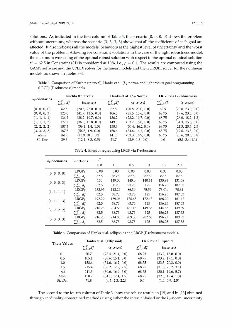
Math. Comput. Appl. 2019, 24, 85 12 of 16
solutions. As indicated in the first column of Table 3, the scenario (0, 0, 0, 0) shows the problemwithout uncertainty, whereas the scenario (3, 3, 3, 3) shows that all the coefficients of each goal areaffected. It also indicates all the models’ behaviors at the highest level of uncertainty and the worstvalue of the problem. Allowing for constraint violations in the case of the light robustness model,the maximum worsening of the optimal robust solution with respect to the optimal nominal solutionz∗ = 62.5 in Constraint (31) is considered at 10%, i.e., ρ = 0.1. The results are computed using theGAMS software and the CPLEX solver for the linear models and the GUROBI solver for the nonlinearmodels, as shown in Tables 3–5.
Table 3. Comparison of Kuchta (interval), Hanks et al. (L2-norm), and light robust goal programming(LRGP) (Γ-robustness) models.
kt-ScenariosKuchta (Interval) Hanks et al. (L2-Norm) LRGP via Γ-Robustness∑T
t=1 d+t (x1,x2,x3)∑T
t=1d+t (x1,x2,x3)∑T
t=1d+t (x1,x2,x3)
(0, 0, 0, 0) 62.5 (20.8, 23.0, 0.0) 62.5 (20.8, 23.0, 0.0) 62.5 (20.8, 23.0, 0.0)(0, 0, 0, 3) 125.0 (41.7, 12.5, 0.0) 106.5 (35.5, 15.6, 0.0) 68.75 (19.6, 23.5, 0.0)(1, 1, 1, 1) 136.2 (28.2, 19.7, 0.0) 136.2 (28.2, 19.7, 0.0) 68.75 (26.0, 18.2, 1.3)(1, 1, 1, 3) 172.2 (36.9, 15.8, 0.0) 149.0 (33.7, 16.8, 0.0) 68.75 (31.3, 15.6, 0.0)(2, 2, 2, 2) 187.3 (56.1, 1.4, 1.0) 158.6 (34.6, 16.2, 0.0) 68.75 (21.3, 20.6, 2.5)(3, 3, 3, 3) 187.5 (56.8, 1.9, 0.0) 158.6 (34.6, 16.2, 0.0) 68.75 (19.6, 23.5, 0.0)
Mean 161.6 (43.9, 10.3, 0.2) 141.8 (33.3, 16.9, 0.0) 68.75 (23.6, 20.3, 0.8)St. Dev 29.3 (12.4, 8.3, 0.5) 21.7 (2.9, 1.6, 0.0) 0.0 (5,1, 3.4, 1.1)
Table 4. Effect of regret using LRGP via Γ-robustness.
kt-Scenarios Functionsρ
0.0 0.1 0.5 1.0 1.5 2.0
(0, 0, 0, 0) LRGPΓ 0.00 0.00 0.00 0.00 0.00 0.00∑Tt=1 d+t 62.5 68.75 87.5 87.5 87.5 87.5
(0, 0, 0, 3) LRGPΓ 150 149.00 145.0 140.14 135.86 131.58∑Tt=1 d+t 62.5 68.75 93.75 125 156.25 187.53
(1, 1, 1, 1) LRGPΓ 133.95 112.24 86.30 75.54 73.01. 70.61∑Tt=1 d+t 62.5 68.75 93.75 125 156.25 187.53
(1, 1, 1, 3) LRGPΓ 192.29 189.06 178.65 172.47 166.90 161.42∑Tt=1 d+t 62.5 68.75 93.75 125 156.25 187.53
(2, 2, 2, 2) LRGPΓ 216.25 204.63 161.15 149.65 144.63 139.89∑Tt=1 d+t 62.5 68.75 93.75 125 156.25 187.53
(3, 3, 3, 3) LRGPΓ 216.25 214.88 209.38 202.60 196.27 189.93∑Tt=1 d+t 62.5 68.75 93.75 125 156.25 187.53
Table 5. Comparison of Hanks et al. (ellipsoid) and LRGP (Γ-robustness) models.
Theta ValuesHanks et al. (Ellipsoid) LRGP via Ellipsoid∑Tt=1d+t (x1,x2,x3)
∑Tt=1d+t (x1,x2,x3)
0.1 70.7 (23.4, 21.4, 0.0) 68.75 (33.2, 18.0, 0.0)0.5 105.1 (33.6, 15.4, 0.0) 68.75 (33.2, 19.1, 0.0)1.0 158.6 (34.6, 16.2, 0.0) 68.75 (33.5, 20.3, 0.0)1.5 215.4 (33.2, 17.2, 2.5) 68.75 (31.6, 20.2, 3.1)√
3 241.3 (30.6, 16.9, 5.0) 68.75 (30.1, 19.6, 5.7)Mean 158.2 (31.1, 17.4, 1.5) 68.75 (32.3, 19.4, 1.8)
St. Dev 71.8 (4.5, 2.3, 2.2) 0.0 (1.4, 0.9, 2.5)
The second to the fourth column of Table 3 show the robust results in [19] and in [13] obtainedthrough cardinality-constrained methods using either the interval-based or the L2-norm uncertainty
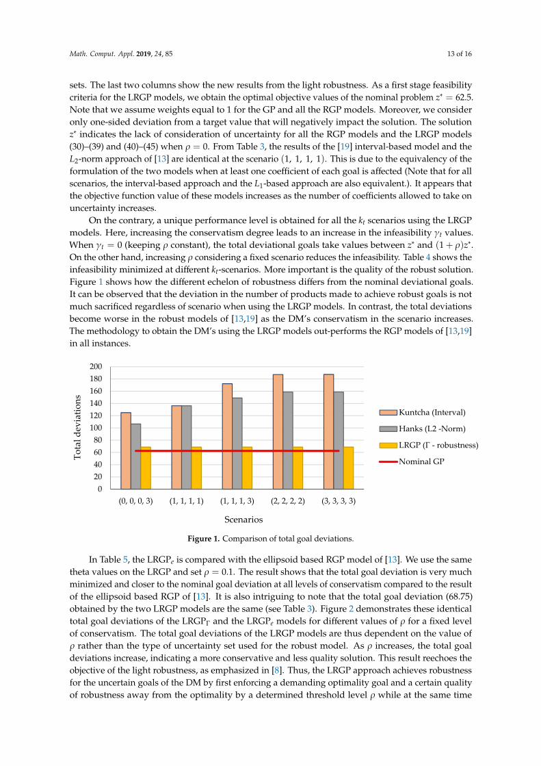
Math. Comput. Appl. 2019, 24, 85 13 of 16
sets. The last two columns show the new results from the light robustness. As a first stage feasibilitycriteria for the LRGP models, we obtain the optimal objective values of the nominal problem z∗ = 62.5.Note that we assume weights equal to 1 for the GP and all the RGP models. Moreover, we consideronly one-sided deviation from a target value that will negatively impact the solution. The solutionz∗ indicates the lack of consideration of uncertainty for all the RGP models and the LRGP models(30)–(39) and (40)–(45) when ρ = 0. From Table 3, the results of the [19] interval-based model and theL2-norm approach of [13] are identical at the scenario (1, 1, 1, 1). This is due to the equivalency of theformulation of the two models when at least one coefficient of each goal is affected (Note that for allscenarios, the interval-based approach and the L1-based approach are also equivalent.). It appears thatthe objective function value of these models increases as the number of coefficients allowed to take onuncertainty increases.
On the contrary, a unique performance level is obtained for all the kt scenarios using the LRGPmodels. Here, increasing the conservatism degree leads to an increase in the infeasibility γt values.When γt = 0 (keeping ρ constant), the total deviational goals take values between z∗ and (1 + ρ)z∗.On the other hand, increasing ρ considering a fixed scenario reduces the infeasibility. Table 4 shows theinfeasibility minimized at different kt-scenarios. More important is the quality of the robust solution.Figure 1 shows how the different echelon of robustness differs from the nominal deviational goals.It can be observed that the deviation in the number of products made to achieve robust goals is notmuch sacrificed regardless of scenario when using the LRGP models. In contrast, the total deviationsbecome worse in the robust models of [13,19] as the DM’s conservatism in the scenario increases.The methodology to obtain the DM’s using the LRGP models out-performs the RGP models of [13,19]in all instances.
Math. Comput. Appl. 2019, 24, x FOR PEER 13 of 17
Table 5. Comparison of Hanks et al. (ellipsoid) and LRGP (Γ-robustness) models.
Theta values Hanks et al. (ellipsoid) LRGP via ellipsoid
𝑑 (𝑥 , 𝑥 , 𝑥 ) 𝑑 (𝑥 , 𝑥 , 𝑥 )
0.1 70.7 (23.4, 21.4, 0.0) 68.75 (33.2, 18.0, 0.0) 0.5 105.1 (33.6, 15.4, 0.0) 68.75 (33.2, 19.1, 0.0) 1.0 158.6 (34.6, 16.2, 0.0) 68.75 (33.5, 20.3, 0.0) 1.5 215.4 (33.2, 17.2, 2.5) 68.75 (31.6, 20.2, 3.1) √3 241.3 (30.6, 16.9, 5.0) 68.75 (30.1, 19.6, 5.7)
Mean 158.2 (31.1, 17.4, 1.5) 68.75 (32.3, 19.4, 1.8) St. Dev 71.8 (4.5, 2.3, 2.2) 0.0 (1.4, 0.9, 2.5)
The second to the fourth column of Table 3 show the robust results in [19] and in [13] obtained through cardinality-constrained methods using either the interval-based or the 𝐿 -norm uncertainty sets. The last two columns show the new results from the light robustness. As a first stage feasibility criteria for the LRGP models, we obtain the optimal objective values of the nominal problem 𝑧∗ =62.5. Note that we assume weights equal to 1 for the GP and all the RGP models. Moreover, we consider only one-sided deviation from a target value that will negatively impact the solution. The solution 𝑧∗ indicates the lack of consideration of uncertainty for all the RGP models and the LRGP models (30)–(39) and (40)–(45) when 𝜌 = 0. From Table 3, the results of the [19] interval-based model and the 𝐿 -norm approach of [13] are identical at the scenario (1, 1, 1, 1) . This is due to the equivalency of the formulation of the two models when at least one coefficient of each goal is affected (Note that for all scenarios, the interval-based approach and the 𝐿 -based approach are also equivalent.). It appears that the objective function value of these models increases as the number of coefficients allowed to take on uncertainty increases.
Figure 1. Comparison of total goal deviations.
On the contrary, a unique performance level is obtained for all the 𝑘 scenarios using the LRGP models. Here, increasing the conservatism degree leads to an increase in the infeasibility 𝛾 values. When 𝛾 = 0 (keeping 𝜌 constant), the total deviational goals take values between 𝑧∗ and (1 + 𝜌)𝑧∗. On the other hand, increasing 𝜌 considering a fixed scenario reduces the infeasibility. Table 4 shows the infeasibility minimized at different 𝑘 -scenarios. More important is the quality of the robust solution. Figure 1 shows how the different echelon of robustness differs from the nominal deviational goals. It can be observed that the deviation in the number of products made to achieve robust goals is not much sacrificed regardless of scenario when using the LRGP models. In contrast, the total deviations become worse in the robust models of [13] and [19] as the DM‘s conservatism in
020406080
100120140160180200
(0, 0, 0, 3) (1, 1, 1, 1) (1, 1, 1, 3) (2, 2, 2, 2) (3, 3, 3, 3)
Tota
l dev
iatio
ns
Scenarios
Kuntcha (Interval)
Hanks (L2 -Norm)
LRGP (Γ - robustness)
Nominal GP
Figure 1. Comparison of total goal deviations.
In Table 5, the LRGPe is compared with the ellipsoid based RGP model of [13]. We use the sametheta values on the LRGP and set ρ = 0.1. The result shows that the total goal deviation is very muchminimized and closer to the nominal goal deviation at all levels of conservatism compared to the resultof the ellipsoid based RGP of [13]. It is also intriguing to note that the total goal deviation (68.75)obtained by the two LRGP models are the same (see Table 3). Figure 2 demonstrates these identicaltotal goal deviations of the LRGPΓ and the LRGPe models for different values of ρ for a fixed levelof conservatism. The total goal deviations of the LRGP models are thus dependent on the value ofρ rather than the type of uncertainty set used for the robust model. As ρ increases, the total goaldeviations increase, indicating a more conservative and less quality solution. This result reechoes theobjective of the light robustness, as emphasized in [8]. Thus, the LRGP approach achieves robustnessfor the uncertain goals of the DM by first enforcing a demanding optimality goal and a certain qualityof robustness away from the optimality by a determined threshold level ρ while at the same time
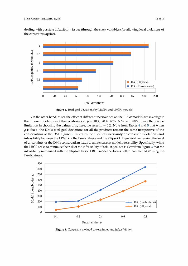
Math. Comput. Appl. 2019, 24, 85 14 of 16
dealing with possible infeasibility issues (through the slack variables) for allowing local violations ofthe constraints apriori.
Math. Comput. Appl. 2019, 24, x FOR PEER 14 of 17
the scenario increases. The methodology to obtain the DM‘s using the LRGP models out-performs the RGP models of [13] and [19] in all instances.
In Table 5, the LRGP is compared with the ellipsoid based RGP model of [13]. We use the same theta values on the LRGP and set 𝜌 = 0.1. The result shows that the total goal deviation is very much minimized and closer to the nominal goal deviation at all levels of conservatism compared to the result of the ellipsoid based RGP of [13]. It is also intriguing to note that the total goal deviation (68.75) obtained by the two LRGP models are the same (see Table 3). Figure 2 demonstrates these identical total goal deviations of the LRGP and the LRGP models for different values of 𝜌 for a fixed level of conservatism. The total goal deviations of the LRGP models are thus dependent on the value of 𝜌 rather than the type of uncertainty set used for the robust model. As 𝜌 increases, the total goal deviations increase, indicating a more conservative and less quality solution. This result reechoes the objective of the light robustness, as emphasized in [8]. Thus, the LRGP approach achieves robustness for the uncertain goals of the DM by first enforcing a demanding optimality goal and a certain quality of robustness away from the optimality by a determined threshold level 𝜌 while at the same time dealing with possible infeasibility issues (through the slack variables) for allowing local violations of the constraints apriori.
Figure 2. Total goal deviations by LRGP and LRGP models.
On the other hand, to see the effect of different uncertainties on the LRGP models, we investigate the different violations of the constraints at 𝜑 = 10%, 20%, 40%, 60%, and 80%. Since there is no limitation in choosing the values of 𝜌, here, we select 𝜌 = 0.2. Note from Table 4 and Table 5 that when 𝜌 is fixed, the DM‘s total goal deviations for all the products remain the same irrespective of the conservatism of the DM. Figure 3 illustrates the effect of uncertainty on constraint violations and infeasibility between the LRGP via the Γ-robustness and the ellipsoid. In general, increasing the level of uncertainty or the DM‘s conservatism leads to an increase in model infeasibility. Specifically, while the LRGP seeks to minimize the risk of the infeasibility of robust goals, it is clear from Figure 3 that the infeasibility minimized with the ellipsoid based LRGP model performs better than the LRGP using the Γ-robustness.
0 20 40 60 80 100 120 140 160 180 200
0
0.1
0.5
1
1.5
2
Total deviations
Robu
st q
ualit
y th
resh
old,
𝜌
LRGP (Ellipsoid)LRGP (Γ- robustness)
Figure 2. Total goal deviations by LRGPΓ and LRGPe models.
On the other hand, to see the effect of different uncertainties on the LRGP models, we investigatethe different violations of the constraints at ϕ = 10%, 20%, 40%, 60%, and 80%. Since there is nolimitation in choosing the values of ρ, here, we select ρ = 0.2. Note from Tables 4 and 5 that whenρ is fixed, the DM’s total goal deviations for all the products remain the same irrespective of theconservatism of the DM. Figure 3 illustrates the effect of uncertainty on constraint violations andinfeasibility between the LRGP via the Γ-robustness and the ellipsoid. In general, increasing the levelof uncertainty or the DM’s conservatism leads to an increase in model infeasibility. Specifically, whilethe LRGP seeks to minimize the risk of the infeasibility of robust goals, it is clear from Figure 3 that theinfeasibility minimized with the ellipsoid based LRGP model performs better than the LRGP using theΓ-robustness.
Math. Comput. Appl. 2019, 24, x FOR PEER 15 of 17
Figure 3. Constraint violated uncertainties and infeasibilities.
4. Conclusion
In this paper, we addressed GP models in an uncertain environment in which the validity and the reliability of the GP technique are determined by—and therefore greatly influenced by—the accuracy of the DM goals. Although the RGP, a recent approach based on RO and GP, has been introduced to deal with such a situation, its methodology is not widely researched. The main methodology offered in the literature—interval-based, norm-based, ellipsoidal uncertainty sets RGP—produces solutions that are too often conservative. In this paper, we propose new RGP models—light RGP generalized on two arbitrary sets, i.e., the budget of uncertainty in [12] and the ellipsoidal uncertainty sets in [24]. Some observations regarding the use of different uncertainty sets for the LRGP are proposed. We also compare our new model with the RGP models developed in the literature and show that our model’s solution is much less conservative and is “quality” in terms of the DM goals in that the robust solution is "not too far" from optimality from the nominal GP model. Furthermore, we show that, rather than the specific uncertainty set used, the total goal deviations of the decision-maker are very much dependent on the robust quality threshold set as the trade-off between the quality (optimality) and the feasibility of the robust solution.
Further research can focus on the applicability of the proposed models to a real-world situation such as the portfolio selection and the capital budgeting problem, as described respectively in [10,11] or the multi-criteria data envelopment analysis. Until now, the RGP has concentrated on the weighted GP. Therefore, an interesting future study that would be of merit would be to extend and compare the RGP with different GP techniques such as the pre-emptive lexicographic GP and the Chebyshev MINMAX GP.
Author Contributions: Conceptualization: E.K.M. and M.R.; Methodology: E.K.M. and M.R.; Writing original draft: E.K.M.; writing-review and editing: E.K.M. and M.R.; The submission was approved by both authors.
Conflicts of Interest: The authors declare no conflict of interest.
References
1. Crespi, G.P.; Kuroiwa, D.; Rocca, M. Robust optimization: Sensitivity to uncertainty in scalar and vector cases, with applications. Oper. Res. Perspect. 2018, 5, 113–119.
2. Fliege, J.; Werner, R. Robust multiobjective optimization & applications in portfolio optimization. Eur. J. Oper. Res. 2014, 234, 422–433.
3. Larbani, M.; Aouni, B. A new approach for generating efficient solutions within the goal programming model. J. Oper. Res. Soc. 2011, 62, 175–182.
0
100
200
300
400
500
600
700
800
900
0.1 0.2 0.4 0.6 0.8
Mod
el in
feas
ibili
ties,
𝛾 t
Uncertainties, 𝜑
LRGP (Γ-robustness)LRGP (Ellipsoid)
Figure 3. Constraint violated uncertainties and infeasibilities.
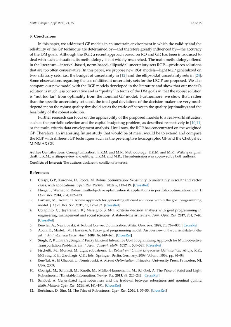
Math. Comput. Appl. 2019, 24, 85 15 of 16
5. Conclusions
In this paper, we addressed GP models in an uncertain environment in which the validity and thereliability of the GP technique are determined by—and therefore greatly influenced by—the accuracyof the DM goals. Although the RGP, a recent approach based on RO and GP, has been introduced todeal with such a situation, its methodology is not widely researched. The main methodology offeredin the literature—interval-based, norm-based, ellipsoidal uncertainty sets RGP—produces solutionsthat are too often conservative. In this paper, we propose new RGP models—light RGP generalized ontwo arbitrary sets, i.e., the budget of uncertainty in [12] and the ellipsoidal uncertainty sets in [24].Some observations regarding the use of different uncertainty sets for the LRGP are proposed. We alsocompare our new model with the RGP models developed in the literature and show that our model’ssolution is much less conservative and is “quality” in terms of the DM goals in that the robust solutionis “not too far” from optimality from the nominal GP model. Furthermore, we show that, ratherthan the specific uncertainty set used, the total goal deviations of the decision-maker are very muchdependent on the robust quality threshold set as the trade-off between the quality (optimality) and thefeasibility of the robust solution.
Further research can focus on the applicability of the proposed models to a real-world situationsuch as the portfolio selection and the capital budgeting problem, as described respectively in [10,11]or the multi-criteria data envelopment analysis. Until now, the RGP has concentrated on the weightedGP. Therefore, an interesting future study that would be of merit would be to extend and comparethe RGP with different GP techniques such as the pre-emptive lexicographic GP and the ChebyshevMINMAX GP.
Author Contributions: Conceptualization: E.K.M. and M.R.; Methodology: E.K.M. and M.R.; Writing originaldraft: E.K.M.; writing-review and editing: E.K.M. and M.R.; The submission was approved by both authors.
Conflicts of Interest: The authors declare no conflict of interest.
References
1. Crespi, G.P.; Kuroiwa, D.; Rocca, M. Robust optimization: Sensitivity to uncertainty in scalar and vectorcases, with applications. Oper. Res. Perspect. 2018, 5, 113–119. [CrossRef]
2. Fliege, J.; Werner, R. Robust multiobjective optimization & applications in portfolio optimization. Eur. J.Oper. Res. 2014, 234, 422–433.
3. Larbani, M.; Aouni, B. A new approach for generating efficient solutions within the goal programmingmodel. J. Oper. Res. Soc. 2011, 62, 175–182. [CrossRef]
4. Colapinto, C.; Jayaraman, R.; Marsiglio, S. Multi-criteria decision analysis with goal programming inengineering, management and social sciences: A state-of-the art review. Ann. Oper. Res. 2017, 251, 7–40.[CrossRef]
5. Ben-Tal, A.; Nemirovski, A. Robust Convex Optimization. Math. Oper. Res. 1998, 23, 769–805. [CrossRef]6. Aouni, B.; Martel, J.M.; Hassaine, A. Fuzzy goal programming model: An overview of the current state-of-the
art. J. Multi-Criteria Decis. Anal. 2009, 16, 149–161. [CrossRef]7. Singh, P.; Kumari, S.; Singh, P. Fuzzy Efficient Interactive Goal Programming Approach for Multi-objective
Transportation Problems. Int. J. Appl. Comput. Math. 2017, 3, 505–525. [CrossRef]8. Fischetti, M.; Monaci, M. Light robustness. In Robust and Online Large-Scale Optimization; Ahuja, R.K.,
Möhring, R.H., Zaroliagis, C.D., Eds.; Springer: Berlin, Germany, 2009; Volumn 5868, pp. 61–84.9. Ben-Tal, A.; El Ghaoui, L.; Nemirovski, A. Robust Optimization; Princeton University Press: Princeton, NJ,
USA, 2009.10. Goerigk, M.; Schmidt, M.; Knoth, M.; Müller-Hannemann, M.; Schöbel, A. The Price of Strict and Light
Robustness in Timetable Information. Transp. Sci. 2013, 48, 225–242. [CrossRef]11. Schöbel, A. Generalized light robustness and the trade-off between robustness and nominal quality.
Math. Methods Oper. Res. 2014, 80, 161–191. [CrossRef]12. Bertsimas, D.; Sim, M. The Price of Robustness. Oper. Res. 2004, 1, 35–53. [CrossRef]
Math. Comput. Appl. 2019, 24, 85 16 of 16
13. Hanks, R.W.; Weir, J.D.; Lunday, B.J. Robust goal programming using different robustness echelons vianorm-based and ellipsoidal uncertainty sets. Eur. J. Oper. Res. 2017, 262, 636–646. [CrossRef]
14. Mensah, E.K. Robust Optimization in Data Envelopment Analysis: Extended Theory and Applications. Ph.D.Thesis, University of Insubria, Varese, Italy, 2019.
15. Gabrel, V.; Murat, C.; Thiele, A. Recent advances in robust optimization: An overview. Eur. J. Oper. Res.2014, 235, 471–483. [CrossRef]
16. Ghahtarani, A.; Najafi, A.A. Robust goal programming for multi-objective portfolio selection problem.Econ. Model. 2013, 33, 588–592. [CrossRef]
17. Arabmaldar, A.; Jablonsky, J.; Saljooghi, F.H. A new robust DEA model and super-efficiency measure.Optimization 2017, 66, 723–736. [CrossRef]
18. Toloo, M.; Mensah, E.K. Robust optimization for nonnegative decision variables: A DEA approach. Comput.Chem. Eng. 2019, 127, 313–325. [CrossRef]
19. Kuchta, D. Robust goal programming. Control Cybern. 2004, 33, 501–510.20. Kuchta, D. A concept of a robust solution of a multicriterial linear programming problem. Cent. Eur. J. Oper.
Res. 2011, 19, 605–613. [CrossRef]21. Ghasemi Bojd, F.; Koosha, H. A robust goal programming model for the capital budgeting problem. J. Oper.
Res. Soc. 2018, 69, 1105–1113. [CrossRef]22. Hanks, R.W.; Lunday, B.J.; Weir, J.D. Robust goal programming for multi-objective optimization of data-driven
problems: A use case for the United States transportation command’s liner rate setting problem. Omega 2018,in press. [CrossRef]
23. Liu, P.; Yang, W.; Guo, T. A discussion on the conservatism of robust linear optimization problems.Optimization 2016, 65, 1641–1650. [CrossRef]
24. Ben-Tal, A.; Nemirovski, A. Robust solutions of uncertain linear programs. Oper. Res. Lett. 1999, 1, 1–13.[CrossRef]
25. Ben-Tal, A.; Nemirovski, A. Robust optimization of linear programming problems contamined with uncertaindata. Math. Program. 2000, 88, 411–424. [CrossRef]
26. Charnes, A.; Cooper, W.W.; Ferguson, R.O. Optimal Estimation of Executive Compensation by LinearProgramming. Manag. Sci. 1955, 1, 138–151. [CrossRef]
27. Tamiz, M.; Jones, D.; Romero, C. Goal programming for decision making: An overview of the currentstate-of-the-art. Eur. J. Oper. Res. 1998, 111, 569–581. [CrossRef]
28. Romero, C. A general structure of achievement function for a goal programming model. Eur. J. Oper. Res.2003, 153, 675–686. [CrossRef]
29. Birge, J.; Louveaux, F. Introduction to Stochastic Programming, 2nd ed.; Springer: New York, NY, USA, 2001.30. Bertsimas, D.; Brown, D.B.; Caramanis, C. Theory and Applications of Robust Optimization. SIAM Rev. 2011,
53, 464–501. [CrossRef]31. Soyster, A.L. Convex programming with set-inclusive constraints and applications to inexact linear
programming. Oper. Res. 1973, 21, 1154–1157. [CrossRef]32. Goerigk, M.; Schöbel, A. Algorithm engineering in robust optimization. In Algorithm Engineering; Kliemann, L.,
Sanders, P., Eds.; Springer: Berlin, Germany, 2016; pp. 245–279.33. Heidt, A.; Helmke, H.; Kapolke, M.; Liers, F.; Martin, A. Robust runway scheduling under uncertain
conditions. J. Air Transp. Manag. 2016, 56, 28–37. [CrossRef]34. Schöbel, A. Line planning in public transportation: Models and methods. OR Spectr. 2012, 34, 491–510.
[CrossRef]35. Mannino, C.; Nilssen, E.J.; Nordlander, T.E. A pattern based, robust approach to cyclic master surgery
scheduling. J. Sched. 2012, 15, 553–563. [CrossRef]36. Rahmani, D.; Zandi, A.; Behdad, S.; Entezaminia, A. A light robust model for aggregate production planning
with consideration of environmental impacts of machines. Oper. Res. 2019, 1–25. [CrossRef]37. Bertsimas, D.; Pachamanova, D.; Sim, M. Robust linear optimization under general norms. Oper. Res. Lett.
2004, 32, 510–516. [CrossRef]
c© 2019 by the authors. Licensee MDPI, Basel, Switzerland. This article is an open accessarticle distributed under the terms and conditions of the Creative Commons Attribution(CC BY) license (http://creativecommons.org/licenses/by/4.0/).