1

DIRECTED HYPERGRAPHS AND APPLICATIONS (* )

Giorgio Gallo1 Giustino Longo1

Sang Nguyen2 Stefano Pallottino1

Abstract

We deal with directed hypergraphs as a tool to model and solve some classes of problems arising in

Operations Research and in Computer Science. Concepts such as connectivity, paths and cuts are defined. An

extension of the main duality results to a special class of hypergraphs is presented. Algorithms to perform

visits of hypergraphs and to find optimal paths are studied in detail. Some applications arising in

propositional logic, And-Or graphs, relational data bases and transportation analysis are presented.

January 1990

Revised, October 1992

(*)This research has been supported in part by the “Comitato Nazionale Scienza e Tecnologia

dell'Informazione”, National Research Council of Italy, under Grant n.89.00208.12, and in part

by research grants from the National Research Council of Canada.

1 Dipartimento di Informatica, Università di Pisa, Italy2 Département d'Informatique et de Recherche Opérationnelle, Université de Montréal, Canada

2

INTRODUCTION

Hypergraphs, a generalization of graphs, have been widely and deeply studied in Berge (1973,1984, 1989), and quite often have proved to be a successful tool to represent and model conceptsand structures in various areas of Computer Science and Discrete Mathematics.

Here we deal with directed hypergraphs. Sometimes with different names such as “labelledgraphs” and “And-Or graphs”, directed hypergraphs have been introduced in the literature as a wayto deal with particular problems arising in Computer Science and in Combinatorial Optimization(see, for example, Nilsson (1971), Martelli and Montanari (1973), Levi and Sirovich (1976), Boley(1977), Furtado (1978), Maier (1980), Nilsson (1980), Gnesi, Montanari and Martelli (1981),Ullman (1982), Nguyen and Pallottino (1989)).

Directed hypergraphs have also been explicitly introduced in Torres and Aráoz (1988), Longo(1989), Gallo, Longo, Nguyen and Pallottino (1989). In addition, particular instances of directedhypergraphs can be found in Dowling and Gallier (1984), Ausiello, D'Atri and Saccà (1985, 1986),Nguyen and Pallottino (1988), Gallo and Urbani (1989), Ausiello, Italiano and Nanni (1990),Italiano and Nanni (1989).

The remaining of the paper is organised as follows. After a general presentation of directedhypergraphs, section 3 introduces the concept of connection in hypergraphs and defines paths andhyperpaths. Section 4 introduces cuts and cutsets in relation to connectivity. Sections 5 and 6develop algorithms to visit hypergraphs and to solve some classes of minimum path problemsdefined on hypergraphs. Several applications are studied in section 7. In particular, it is shown thathypergraph concepts and algorithms are elegant and powerful tools to model and to solve problemswhich arise in areas such as propositional logic (Dowling and Gallier (1984), Gallo and Urbani(1989)), And-Or graphs (Martelli and Montanari (1973), Levi and Sirovich (1976), Nilsson (1980),Gnesi, Montanari and Martelli (1981)), data bases (Maier (1980), Ullman (1982), Ausiello, D'Atriand Saccà (1983, 1985, 1986)), and urban transportation (Nguyen and Pallottino (1986, 1988,1989)).

2. DIRECTED HYPERGRAPHS

A hypergraph is a pair H=(V ,E), where V={v1, v2,..., vn} is the set of vertices (or nodes) andE={ E1, E2,..., Em}, with Ei ⊆

V for i=1,…, m, is the set of hyperedges. Clearly, when |

E

i|

=

2

,

i=1,…, m, the hypergraph is a standard graph.While the size of a standard graph is uniquely defined by n and m, the size of a hypergraph

depends also on the cardinality of its hyperedges; we define the size of H as the sum of thecardinalities of its hyperedges:

size(H) = ΣEi∈E|Ei|.

It is worth noting that there is a one-to-one correspondence between hypergraphs and Booleanmatrices. Indeed, any nxm matrix A=[aij ] such that aij∈{0,1} may be considered as the incidencematrix of a hypergraph H where each row i is associated with a vertex vi and each column j with ahyperedge Ej.

3

A directed hyperedge or hyperarc is an ordered pair, E = (X,Y), of (possibly empty) disjointsubsets of vertices; X is the tail of E while Y is its head. In the following, the tail and the head ofhyperarc E will be denoted by T(E) and H(E), respectively.

A directed hypergraph is a hypergraph with directed hyperedges. In the following, directedhypergraphs will simply be called hypergraphs. An example of hypergraph is illustrated in Fig. 1.Note that hyperarc E5 has an empty head.

1

2

3

4

5

6

7

8

9

10

11

12

1 -1 0 0 0 0

2 -1 0 0 0 0

3 0 -1 0 0 0

4 1 -1 0 0 0

5 1 0 0 0 0

6 1 0 -1 0 0

7 0 1 0 0 0

8 0 1 0 0 -1

9 0 0 1 0 -1

10 0 0 1 -1 0

11 0 0 0 -1 0

12 0 0 0 1 0

E1

E2

E 3

E 4

E5

E 4E 3E2E1 E5

Fig. 1 - A hypergraph and its incidence matrix.

As for directed graphs, the incidence matrix of a hypergraph H is a nxm matrix [aij ] defined asfollows (see Fig. 1):

aij =

{

-110

if vi ∈ T(E j) ‚ if vi ∈ H(E j) ‚ otherwise.

Clearly, there is a one-to-one correspondence between hypergraphs and (-1, 0, 1) matrices.A Backward hyperarc, or simply B-arc, is a hyperarc E =

(T

(

E)

,

H(

E)

)

w

i

t

h

|

H(

E)|=1 (Fig.2a). A Forward hyperarc, or simply F-arc, is a hyperarc E =

(T

(

E)

,

H(

E)

)

w

i

t

h

|

T(

E)|=1 (Fig.2b).

(a) (b)

Fig. 2 - A B-arc (a) and a F-arc (b).

A B-graph (or B-hypergraph) is a hypergraph whose hyperarcs are B-arcs. A F-graph (or F-hypergraph) is a hypergraph whose hyperarcs are F-arcs. A BF-graph (or BF-hypergraph) is ahypergraph whose hyperarcs are either B-arcs or F-arcs.

Given a hypergraph H=(V,E), we define its symmetric image the hypergraph ~H =(V ,

~E ) where~

E ={(X,Y): (Y,X) ∈E}. Note that the symmetric image of a B-graph is a F-graph, and viceversa.

4

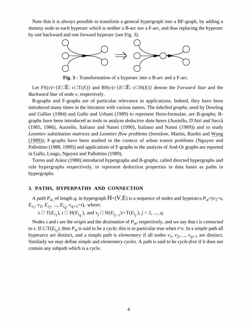
Note that it is always possible to transform a general hypergraph into a BF-graph, by adding adummy node to each hyperarc which is neither a B-arc nor a F-arc, and thus replacing the hyperarcby one backward and one forward hyperarc (see Fig. 3).

Fig. 3 - Transformation of a hyperarc into a B-arc and a F-arc.

Let FS(v)={ E∈E: v∈T(E)} and BS(v)={ E∈E: v∈H(E)} denote the Forward Star and theBackward Star of node v, respectively.

B-graphs and F-graphs are of particular relevance in applications. Indeed, they have beenintroduced many times in the literature with various names. The labelled graphs, used by Dowlingand Gallier (1984) and Gallo and Urbani (1989) to represent Horn-formulae, are B-graphs; B-graphs have been introduced as tools to analyze deductive data bases (Ausiello, D'Atri and Saccà(1985, 1986), Ausiello, Italiano and Nanni (1990), Italiano and Nanni (1989)) and to studyLeontiev substitution matrices and Leontiev flow problems (Jeroslow, Martin, Rardin and Wang(1989)); F-graphs have been studied in the context of urban transit problems (Nguyen andPallottino (1988, 1989)) and applications of F-graphs to the analysis of And-Or graphs are reportedin Gallo, Longo, Nguyen and Pallottino (1989).

Torres and Aráoz (1988) introduced hypergraphs and B-graphs, called directed hypergraphs andrule hypergraphs respectively, to represent deduction properties in data bases as paths inhypergraphs.

3. PATHS, HYPERPATHS AND CONNECTION

A path Pst, of length q, in hypergraph H=(V,E) is a sequence of nodes and hyperarcs Pst=(v1=s,Ei1, v2, Ei2, ..., Eiq, vq+1=t), where:

s ∈ T(Ei1), t ∈ H(Eiq ), and vj ∈ H(Ei j -1)∩T(Ei j ), j = 2, ..., q.

Nodes s and t are the origin and the destination of Pst, respectively, and we say that t is connectedto s. If t∈T(Ei1), then Pst is said to be a cycle; this is in particular true when t=s. In a simple path allhyperarcs are distinct, and a simple path is elementary if all nodes v1, v2,…, vq+1 are distinct.Similarly we may define simple and elementary cycles. A path is said to be cycle-free if it does notcontain any subpath which is a cycle.

5

2

79

8

3

6

4

5

1

Fig. 4 - A path P1,8.

In Fig. 4, node 8 is connected to node 1, while node 9 is not. The elementary path connecting 8 to1 is drawn in thick line.

Consider a hypergraph H=(V ,E). A B-path (or B-hyperpath) Πst is a minimal hypergraphHΠ=(VΠ,EΠ) such that:

i) EΠ⊆

E ;

ii) s, t ∈

VΠ = ∪Ei∈EΠ

Ei ⊆

V ;

iii) x∈VΠ ⇒ x is connected to s in HΠ by means of a cycle-free simple path.

We say that HΠ=(VΠ,EΠ) is a F-path (or F-hyperpath) from s to t if its symmetric image is a B-

path from t to s.

A BF-path (or BF-hyperpath) from s to t is a hypergraph which is at the same time a B-path and aF-path from s to t.

Node y is B-connected (F-connected, BF-connected) to node x if a B-path (F-path, BF-path) Πxyexists in H.

1

1E

2E

3E4E 5E

2

3

4 5

6

1

1E

2E

3E4E 5

E

2

3

4 5

6

(a)

(b)

7

7

Fig. 5 - A B-path (a) and a B-graph which is not a B-path (b).

The hypergraph in Fig. 5a is a B-path; note that the cycle (4, E4, 5, E5, 4) is not contained in anysimple path from node 1 to node 7. On the contrary, the hypergraph in Fig. 5b is not a B-pathbecause the only path connecting node 3 to the origin contains the cycle (2, E3, 4, E2, 3).

6

The following proposition trivially holds:

Proposition 1 - Given a B-path Πst and a hyperarc E∈EΠ, one has that each node x∈T(E) is B-connected to s.

Given a hyperarc E = (T(E),H(E)), a B-reduction of E is a B-arc E* = (T(E*),{v}) such thatT(E) = T(E*) and v ∈H(E).

A B-reduction of a hypergraph H is the B-graph HB obtained from H by replacing each hyperarcby one of its B-reductions. Clearly, a hypergraph may have many B-reductions; we shall denote byB(H) the set of all the B-reductions of H.

In an analogous way it is possible to define F-reductions and BF-reductions of hypergraphs. Notethat a BF-reduction of a hypergraph is a standard digraph.

We say that node y is super-connected to node x in hypergraph H if y is B-connected to x in anyB-reduction HB of H. Then to say that y is not super-connected to x we need at least one B-reduction in which y is not B-connected to x.

Note that in B-graphs the concepts of B-connection and super-connection coincide.The definitions of connection introduced above can be generalized as follows: given a set S of

nodes, we say that node y is B-connected (F-connected, BF-connected, super-connected) to S inthe hypergraph H if y is B-connected (F-connected, BF-connected, super-connected) to s in thehypergraph H' obtained from H by addition of the new origin node s and an arc (s,x) for eachx∈S. Similarly, we can define the connection of a set of nodes T to a single origin node x.

4. CUTS AND CUTSETS

Let H=(V ,E) be a hypergraph and s and t be two distinguished nodes, the source and the sinkrespectively.

A cut Tst=(Vs,V t) is a partition of V into two subsets Vs and V t such that s∈Vs and t∈V t.Given the cut Tst, its cutset Est is the set of all hyperarcs E such that T(E)⊆

V s and H(E)⊆

V t.Such a cutset may be empty; see for instance the cut ({1,2},{3,4,5,6,7}) in the B-graph of Fig. 5b.

The cardinality of a cut is the cardinality of its cutset. In Fig. 6 three cuts are indicated; thecardinality of T 1

st is 2, while T 2

st and T 3

st have cardinality 1. Note that t is not necessarily

disconnected from s by removing the hyperarcs of a cutset. For example, in Fig. 6 by removing thecutset of T 1

st we disconnect t from s, by removing the cutset of T 2

st only the B-connection of t to

s is lost, while t remains both connected and B-connected to s when we remove the cutset of T 3st

.

1 3

42

5

6

s t

T 3st

T 2st

T 1st

Fig. 6 - Only cut T 1st

disconnects source s and sink t.

7

The following two theorems relate cuts to connection in hypergraphs.

Theorem 1 - In a B-graph H=(V ,E), a cut Tst of cardinality 0 exists if and only if t is not B-connected to s.Proof: (⇒) Assume that a cut Tst with an empty cutset Est exists and there is a node v ∈ V t B-connected to s. Then a B-arc E=(T(E),{v}) must exist with the property that every node x∈T(E) beB-connected to s (see Proposition 1). Clearly, as Est is empty, at least one node u∈T(E) mustbelong to V t. By repeating the same argument on u, we may eventually conclude that s alsobelongs to V t, which is a contradiction.(⇐) Now assume that t is not B-connected to s. Define Vs as the set of all the nodes B-connectedto s and V t = V \ V s. Tst is necessarily a cut of cardinality 0, for the existence of a B-arcE=(T(E),{v}) in the cut, being T(E) ⊆

Vs and v ∈ V t, imply the B-connection of v to s.♦Theorem 2 - In a hypergraph H=(V ,E) a cut Tst of cardinality 0 exists if and only if t is notsuper-connected to s.Proof: (⇒) Let Tst=(Vs,Vt) be a cut of cardinality 0. Consider the B-reduction HB of H obtainedby replacing each hyperarc E with a B-arc (T(E),{v}) with the condition that if T(E)⊆

Vs then alsov ∈ Vs. This reduction is always possible since for any hyperarc E with T(E)⊆

V s at least onenode in its head must belong to Vs, otherwise E belongs to the cutset which, by hypothesis, isempty. By Theorem 1, t is not B-connected to s in HB and therefore t is not super-connected to s inH.(⇐) If t is not super-connected to s, then a B-reduction exists such that t is not B-connected to s init, and, by Theorem 1, the proof is completed.♦

Theorems 1 and 2 generalize to hypergraphs the property holding for standard digraphs that theremoval of all the arcs of a cutset disconnects the sink from the source. Unfortunately, other niceproperties do not hold for hypergraphs, even if we restrict our attention to B-graphs. In particular, itis well known that the two following equivalent facts hold for standard digraphs:

P1: the minimum cardinality of an s-t path in a digraph is equal to the maximum numberof disjoint s-t cutsets.

P2: the minimum cardinality of an s-t cut in a digraph is equal to the maximum numberof disjoint s-t paths.

Such properties do not hold for hypergraphs, although the following theorems show that they holdin a weaker form for B-graphs.

Theorem 3 - In a B-graph H=(V,E) the following inequalities hold:

min{|Πst|: Πst is a s-t B-path} ≥ maximum number of disjoint s-t cutsets ≥ min{|Pst|: Pst is a s-t

path}.

Proof: The first inequality follows directly from the fact that, due to Theorem 1, a cutset mustcontain at least a B-arc of every B-path, then the number of disjoint s-t cutsets cannot exceed thecardinality of any B-path.

The second inequality can be proved as follows. Let Vk denote the set of nodes {i} for whichthere exists a path Psi with cardinality ≤ k. Clearly, if h is the minimum cardinality of the s-t paths,then we have {s}= V0 ⊂ V1 ⊂…⊂ Vh ⊆ V ; then (V0,V \V0), (V1,V \V1)… (Vh-1,V \Vh-1) are

8

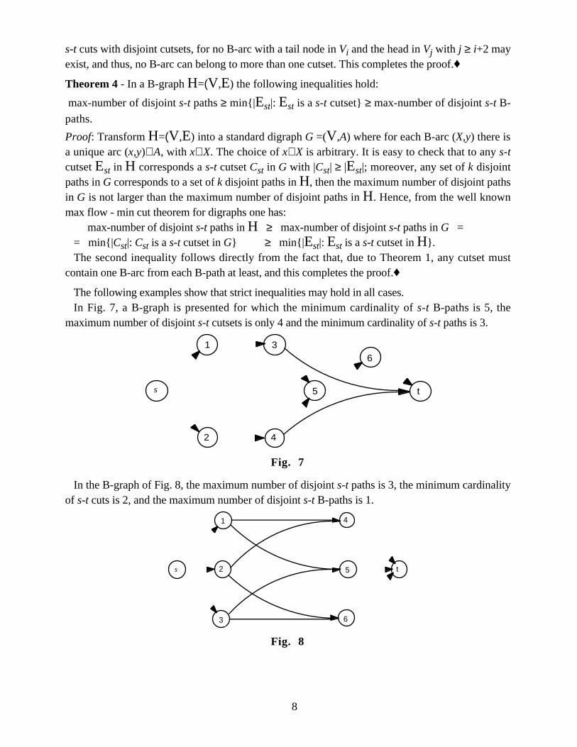
s-t cuts with disjoint cutsets, for no B-arc with a tail node in Vi and the head in Vj with j ≥ i+2 mayexist, and thus, no B-arc can belong to more than one cutset. This completes the proof.♦Theorem 4 - In a B-graph H=(V,E) the following inequalities hold:

max-number of disjoint s-t paths ≥ min{|Est|: Est is a s-t cutset} ≥ max-number of disjoint s-t B-

paths.

Proof: Transform H=(V,E) into a standard digraph G =(V,A) where for each B-arc (X,y) there isa unique arc (x,y)∈A, with x∈X. The choice of x∈X is arbitrary. It is easy to check that to any s-tcutset Est in H corresponds a s-t cutset Cst in G with |Cst| ≥ |Est|; moreover, any set of k disjointpaths in G corresponds to a set of k disjoint paths in H, then the maximum number of disjoint pathsin G is not larger than the maximum number of disjoint paths in H. Hence, from the well knownmax flow - min cut theorem for digraphs one has:

max-number of disjoint s-t paths in H ≥ max-number of disjoint s-t paths in G == min{|Cst|: Cst is a s-t cutset in G} ≥ min{|Est|: Est is a s-t cutset in H}.The second inequality follows directly from the fact that, due to Theorem 1, any cutset must

contain one B-arc from each B-path at least, and this completes the proof.♦The following examples show that strict inequalities may hold in all cases.In Fig. 7, a B-graph is presented for which the minimum cardinality of s-t B-paths is 5, the

maximum number of disjoint s-t cutsets is only 4 and the minimum cardinality of s-t paths is 3.

1

2

3

4

5

6

ts

Fig. 7

In the B-graph of Fig. 8, the maximum number of disjoint s-t paths is 3, the minimum cardinalityof s-t cuts is 2, and the maximum number of disjoint s-t B-paths is 1.

1

2

3

4

5

6

ts

Fig. 8

9

In section 7.1 we will show that the problem of finding the minimum cardinality s-t cut is NP-hard also in the case of B-graphs.

5. VISIT OF A HYPERGRAPH

Here we consider the problem of visiting a hypergraph starting from an origin node r, i.e. offinding all the nodes which are connected (B-connected, super-connected) to r.

The simplest case is to find in a hypergraph all the nodes which are connected to r. ProcedureVisit described below finds all such nodes and returns a set of paths connecting them to r. Suchpaths, which define a tree rooted at r, are described by two predecessor functions: Pe(E) points tothe node i∈T(E) which precedes hyperarc E in the path, Pv(i) points to the arc E∈BS(

i

)

whichprecedes node i in the path.

Procedure Visit

(r,H ):begin

for each i ∈ V do Pv[i]:= 0;for each Ej ∈ E do Pe[Ej

]:= 0;Pv[r]:= nil ; Q:= {r};repeat

select and remove i∈Q;for each Ej∈FS(

i

)

such that Pe[Ej

]=0 dobegin

Pe[Ej

] := i ;for each h∈H(Ej) such that Pv[h]=0 do begin Pv[h] := Ej

; Q := Q ∪ {h} end-forend-for

until Q = Øend-procedure.

It is easy to check that Visit runs in O(size(H)) time. In fact, the initialization phase runs inO(n+m) time and, since each node is inserted and removed from the candidate set Q at most once,each hyperarc is examined only once, i.e. the first time the hyperarc is selected.

Now, consider the case of B-connection. Procedure B-Visit returns a set of B-paths containingall the nodes B-connected to r. Such B-paths define a B-tree rooted at r.

Notice that in this case only one predecessor function, Pv, is necessary. In fact, by the definitionof B-path, if hyperarc E belongs to a B-path, then all the nodes of its tail must belong to the sameB-path. Nevertheless, we shall maintain the use of the second predecessor function, Pe. Suchfunction defines a particular tree among the trees contained in the B-tree returned by the procedure.In connection with the function Pe, a node function, ν, is introduced which, for each node h, givesthe cardinality of the path from r to h in the tree defined by Pe and Pv. The motivation ofintroducing such a function will be made clear in the next section.

A counter kj is used to provide for each hyperarc Ej

the number of nodes of its tail alreadyremoved from Q. To stress the fact that functions Pe and ν are not essential to the computation ofthe B-tree, the statements involving them have been written in italics.

10

Procedure B-Visit

(r,H ):begin

for each i ∈ V do begin Pv[i] := 0; ν[i] := ∞ end-for;for each Ej ∈ E do Pe[Ej

] := kj

:= 0;Pv[r] := nil ; Q := {r}; ν[r] := 0;repeat

select and remove i∈Q;for each Ej∈FS(

i

)

dobegin

kj

:= kj

+ 1;if kj

= |T(Ej)| thenbegin

Pe[Ej

] := i;for each h∈H(Ej) such that Pv[h]=0 do

begin Pv[h] := Ej

; Q := Q ∪ {h} ; ν[h]:= ν[Pe[Ej

]]+1 end-forend-if

end-foruntil Q = Ø

end-procedure.

Procedure B-Visit runs in O(size(H)) time. In fact, each hyperarc E is selected at most |T(E)|times and only the last time its head is examined. Moreover, each node is inserted and removedfrom Q at most once.

In a similar way it is possible to define a procedure F-Visit which finds a set of F-paths whichhave r as terminal node and all the nodes to which r is F-connected. Note that while the B-Visitstarts from the origin of the B-paths, the F-Visit must start from the destination of the F-paths toretain a linear time complexity.

One can also define a BF-Visit . Unfortunately, the problem of performing such a visit is not aneasy one unless the hypergraph is either a B-graph or a F-graph; in the former case a BF-path issimply a B-path, while in the latter it is a F-path.

The following procedure SuperVisit checks whether a node t is super-connected to a node s ona general hypergraph.

Procedure SuperVisit

(s,t,H ) :begin

superconnected := true;while superconnected and B(H) ≠ Ø do

beginselect and remove HB from B(H); B-Visit(s, HB);if Pv[t]=0 then superconnected := false

end-whileend-procedure.

SuperVisit

runs in O(size(H).|B(H)|) time, where |B(H)| = ΠEj∈E|H(Ej)| is the number of allpossible B-reductions of H.

A quite efficient Branch&Bound scheme to solve this problem can be easily derived from thesecond algorithm for the satisfiability problem presented in Gallo and Urbani (1989).

11

6. WEIGHTED HYPERGRAPHS

6.1. Weighting functionsA weighted hypergraph is one in which each hyperarc E is assigned a real weight vector w(E).

Depending on the particular application, the components of w(E) may represent costs, lengths,capacities etc. For the sake of simplicity, in the following we shall consider only scalar weights.

Given a B-path Π=(VΠ,EΠ) from s to t, by weighting function we mean a node function WΠwhich assigns weights to all its nodes depending on the weights of its hyperarcs. WΠ(t) is theweight of the B-path Π under the chosen weighting function.

We shall restrict ourselves to weighting functions for which WΠ(s)=0 and WΠ(y), for each y≠s,depends only on the hyperarcs which precede y in the B-path Π, i.e. the hyperarcs belonging to allB-paths from s to y contained in Π.

A typical example of this kind of weighting function is the cost, CΠ, defined as the sum of theweights of all the hyperarcs preceding node y in Π:

CΠ(s) = 0;

CΠ(y) = ΣE∈{EΠsy: Πsy⊆Π}

w(E), y ∈ VΠ\{ s},

Clearly, CΠ(t)=ΣE∈EΠw(E) is the cost of Π. This function is the usual cost in the graph setting,and the problem of finding a minimum cost B-path is a natural generalization of the minimum costpath problem. Note that when the weights are all equal to 1, the cost of Π is its cardinality.

A relevant class of weighting functions is the one in which the weight of node y can be written asa function of both the weights of the hyperarcs entering into y and that of the nodes in their tails:

WΠ(y) = min{w(E) + FΠ(T(E)): E∈EΠ∩BS(y)}, y ∈ VΠ\{ s}, (1)

where FΠ(T(E)) is a function of the weights of the nodes in T(E):

FΠ(T(E)) = F({WΠ(x): x∈T(E)}), E∈EΠ, (2)

where F is a non-decreasing function of WΠ(x) for each x∈T(E). Such weighting functions will becalled additive weighting functions.

In the particular case of B-graphs, the B-paths have the property that there is only one B-arc Eentering into every node y≠s; in this case (1) becomes:

WΠ(y) = w(E) + FΠ(T(E)), y ∈ VΠ\{ s}. (1')

Two particular additive weighting functions which have been presented in the literature in thecontext of some relevant applications of hypergraphs are the distance and the value.

Given a s-t B-path Π=(VΠ,EΠ), the distance in Π from s to all the nodes y∈VΠ\{ s} which areB-connected to s, DΠ(y), is defined by the following recursive equations:

DΠ(s) = 0;

DΠ(y) = min{l(E) + max{DΠ(x): x∈T(E)}: E∈EΠ∩BS(y)}, y ∈ VΠ\{ s};(3)

where l(E) is the length of hyperarc E.For B-graphs, equation (3) becomes:

DΠ(y) = l(E) + max{DΠ(x): x∈T(E)}, y ∈ VΠ\{ s}. (3')

12

In the case of unit hyperarc lengths, i. e. l(E)=1 ∀ E∈E, the distance will be called depth. Galloand Urbani (1989) have introduced the depth function on B-graphs in the context of the satisfiabilityanalysis of propositional Horn formulae. Note that, in this case, procedure B-Visit , with the useof function ν and a breadth-first search strategy, finds the minimum depth B-tree in O(size(H))time.

The value, VΠ, defined by Jeroslow, Martin, Rardin and Wang (1989) in the context of theLeontiev flow problem for the case of B-graphs, is the solution of the following recursiveequations:

VΠ(s) = 0;

VΠ(y) = c(E) + Σx∈T(E)

a(x,E)VΠ(x), E∈EΠ∩BS(y), y ∈ VΠ\{ s};(4)

where c(E) is the cost of B-arc E and, for each E and each x∈T(E), a(x,E) is a non-negative realcoefficient.

6.2. Minimum weight B-pathsThis section addresses the problem of finding a minimum weight B-path in a weighted

hypergraph. Such problem can be viewed as a natural generalization of the shortest path problemfor standard digraphs.

Unfortunately, at least in general, the minimum weight B-path problem on hypergraphs is NP-hard. In fact, Italiano and Nanni (1989) have proved that the particular problem of finding minimumcardinality B-paths in a B-graph is NP-hard. Nevertheless, many particular cases exist for whichthe problem is easy to solve. One example is when the weighting functions are additive, and this isexactly the case of the standard shortest path problem in digraphs.

From now on, we shall restrict ourselves to the case of additive weighting functions.Furthermore, we shall assume throughout that arc weights are non-negative and that all cycles arenon-decreasing. A non-decreasing cycle is a cycle C={v1, E1, v2, E2, …, vr, Er, v1} such that , forany real z:

W(Er) + F(vr)( )W(Er-1) + F(vr-1)( )…+ F(v2)( )W(E1) + F(v1)(z) … ≥ z, (5)

where, for each Ei, F(vi)(w) is the restriction of FC(T(Ei)) to the case in which all the nodes of T(Ei)have weight zero except node vi which has weight w.

Condition (5) ensures that no node weight can be decreased through a cycle, and plays the samerole as the non-negative cycles condition in digraphs.

To provide a deeper understanding of condition (5) we will apply it to both the distance functionand to the value function below. In the first case, since FC(T(Ei)) is the maximum among theweights of the nodes belonging to T(Ei), F(vi)(w) = w, and condition (5) becomes:

∑i=1

r W(Ei) + z ≥ z,

from which we get

∑i=1

r W(Ei) ≥ 0.

13

We have thus derived the non-negativity condition for cycle weights, which is a standardassumption when dealing with shortest paths in digraphs.

Quite different is the case of the value function. Here we get:

W(Er)+a(vr,Er)( )W(Er-1) + a(vr-1,Er-1)( )W(Er-2) + … + a(v2,E2)( )W(E1) + a(v1,E1)z …

≥ z,and

W(Er) + ∑h=1

r-1 (W(Er-h) ∏

l=0

h-1a(vr-l ,Er-l)) + z ∏

i=1

ra(vi,Ei) ≥ z,

which is true for any real z if:

∏i=1

ra(vi,Ei) ≥ 1.

We have thus obtained the “gain-free condition” stated in Jeroslow, Martin, Rardin and Wang(1989).

Now, consider the problem of finding a set of minimum weight B-paths from origin r to all thenodes y which are B-connected to r. This is the generalization of the well known shortest path treeproblem. Such problem is strictly related to that of finding a solution to the following GeneralizedBellman's Equations:

W(r) = 0;

W(y) = min{w(E) + F({W(x): x∈T(E)}): E∈BS(y)}, y∈V \{ r}.(6)

The following procedure SBT finds a solution of (6) together with a minimum weight B-treerooted at r, i.e. a cycle-free set of minimum weight B-paths connecting r to all the nodes y whichare B-connected to it. If y is not B-connected to r, SBT returns W(y) =+∞. As in B-Visit , the B-tree computed by SBT is described by the predecessor function Pv.

14

Procedure SBT(r,H ):begin

for each i∈V do W(i) := +∞;for each Ej∈E do kj

:= 0;Q := {r}; W(r)=0;repeat

select and remove u∈Q;for each Ej∈FS(

u

)

dobegin

kj

:= kj

+ 1;if kj

=|T(Ej)| thenbegin

f := F(T(Ej));for each y∈H(Ej) such that W(y)>w(Ej)+f do

beginif y∉Q then

beginQ := Q ∪ {y};if W(y)<+∞ then for each Eh∈FS(y) do kh

:=kh

-1end-if;

W(y) := w(Ej)+f; Pv[y] := Ejend-for

end-ifend-for

until Q = Øend-procedure.

The counter kj, for each hyperarc Ej

, represents the number of nodes belonging to T(Ej

) whichhave been removed from Q at a previous iteration and are currently out of Q. The use of the counterpermits to reduce substantially the number of updating operations (for each y∈H(Ej)…); in fact,for each Ej, instead of checking the values W(y) of the nodes belonging to H(Ej) every time a nodeu∈T(Ej) is selected from Q, this is done only when the last node u∈T(Ej) is removed from Q, i.e.when kj=|T(Ej)|.

The correctness of SBT directly follows from the fact that, at termination, equations (6) aresatisfied; moreover, the number of iterations is finite since:

i) each time a weight is updated, a new B-tree is found, and no B-tree can be found twice;ii) the number of consecutive iterations which do not lead to a change in the node weights is

bounded by n.Clearly, the complexity of SBT depends on the implementation of the candidate set Q and on thecost needed to evaluate the function F.

For the sake of simplicity, we shall assume that F(T(E)) can be computed in O(|T(E)|) time, whichis the case in most applications. As for Q, we shall consider three different implementations: thequeue, with a FIFO selection policy, the unordered list, and the heap, both with the selection of theminimum weight element. According to the notation introduced in Gallo and Pallottino (1986) weshall call the corresponding versions of SBT: SBT-queue, SBT-Dijkstra and SBT-heap,respectively.

Consider first SBT-queue. The cost of the initialization is O(n+m) time. Each operation ofselection and removal from Q and insertion into Q has unit cost. As in the classical shortest path

15

algorithms, one can easily prove that if Q is implemented as a queue then each node is selected andprocessed at most n times. Also each hyperarc E is examined at most n times; this is due to the factthat the nodes of H(E) are only examined when all the nodes in T(E) no longer belong to Q. Thescanning of H(E) costs O(|T(E)|) time for the evaluation of F(T(E)) and O(|H(E)|) time for thetesting of condition W(y)>w(E)+F(T(E)), for each y∈H(E). Thus, algorithm SBT-queue runs inO(n.size(H)) time.

It is worth noting that condition (5) on non-decreasing cycles is tighter than what is actuallyneeded; in fact, for the correctness of SBT-queue, it is enough that during its operations nonegative cycle is detected, where by negative cycle we mean a decreasing cycle which actually leadsto cyclic improvements of its node weights. Note that, SBT-queue can be easily modified in orderto detect such negative cycles, by simply bounding the number of improvements on the weight of asingle node.

Now, consider the case in which at each iteration a node u such that W(u)=min{W(x):x∈Q} isselected. In this case, the well-known assumption of non-negative arc weights for standarddigraphs in Dijkstra Theorem can be generalized to:

w(E) + F({W(x): x∈T(E)}) ≥ W(x), x∈T(E), E∈E.

Under this additional assumption Dijkstra Theorem can be easily extended to hypergraphs:

Theorem 5 - If W(u)=min{W(x): x∈Q}, then W(u) is the minimum among the weights of the B-paths from r to u.Corollary - Each node u∈V is removed from Q only once.

A consequence of the above Corollary is that statement “if W(y)<+∞ then for each Eh∈FS(y)do kh

:= kh

- 1” can be dropped since it is no longer necessary to decrease the counters.The complexity for SBT-Dijkstra and for SBT-heap directly follow from the Corollary:

- Algorithm SBT-Dijkstra runs in O(max{n2, size(H)}) time, as the total cost of node selectionsand removals from Q is O(n2) and the total cost of processing all hyperarcs E (evaluation of F(T(E))and scanning of H(E)) is O(size(H)).

- Algorithm SBT-heap runs in O(size(H).logn) time, as each time the value W(y) of a node y isupdated the heap must be updated at cost O(logn).

- In the case of B-graphs, algorithm SBT-heap runs in O(max{mlogn, size(H)}) time, as each B-arcproduces at most one weight improvement, thus the overall cost of updating the heap is O(mlogn).

Jeroslow, Martin, Rardin and Wang (1989) presented an algorithm to find the optimal values ofV(y) for each node y in a B-graph. This algorithm generalizes the Bellman-Ford-Moore algorithmand runs in O(n.size(H)).It is as fast as SBT-queue and slower than SBT-Dijkstra and SBT-heap.

7. APPLICATION OF HYPERGRAPHS

7.1. SatisfiabilityLet P be a set of n atomic propositions, which can be either true or false, and denote by t a

proposition which is always true, and by f a proposition which is always false. Let C be a set of mclauses, each of the form:

16

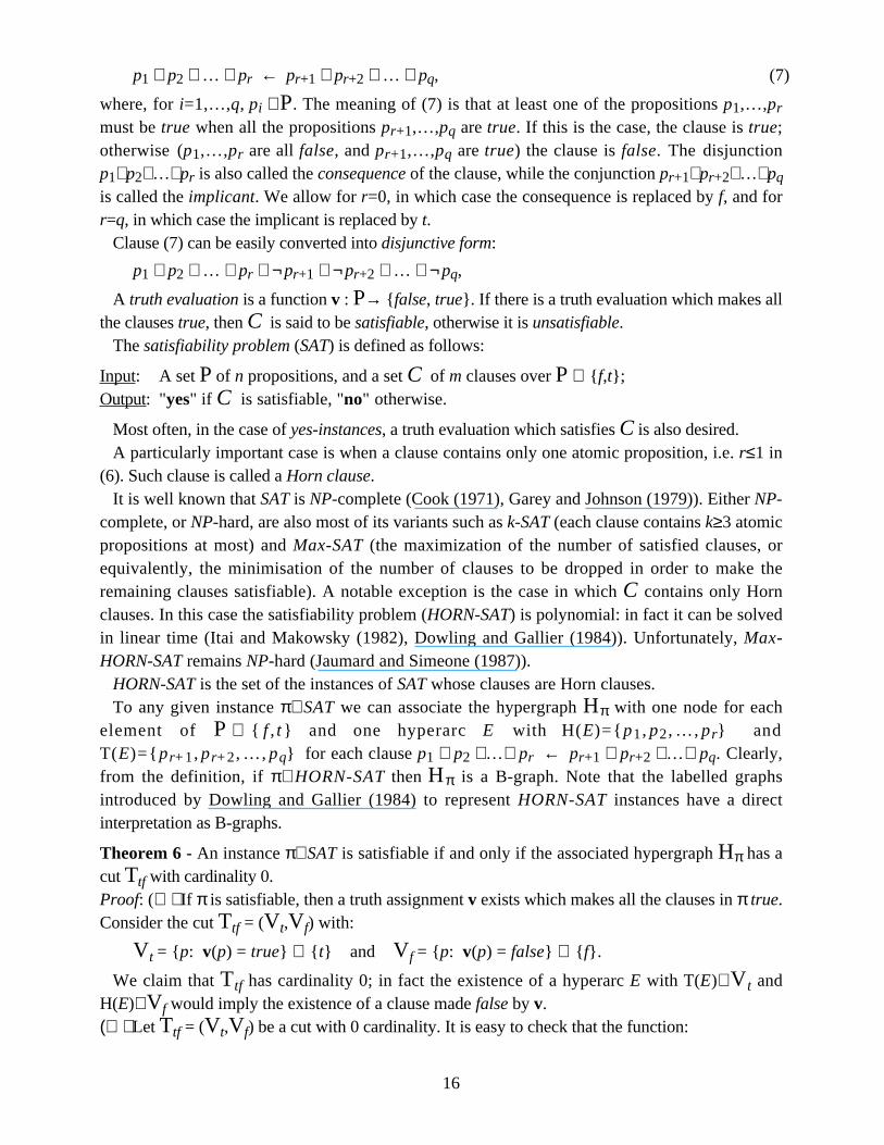
p1 ∨ p2 ∨ … ∨ pr ← pr+1 ∧ pr+2 ∧ … ∧ pq, (7)

where, for i=1,…,q, pi ∈P. The meaning of (7) is that at least one of the propositions p1,…,pr

must be true when all the propositions pr+1,…,pq are true. If this is the case, the clause is true;otherwise (p1,…,pr are all false, and pr+1,…,pq are true) the clause is false. The disjunctionp1∨p2∨…∨pr is also called the consequence of the clause, while the conjunction pr+1∧pr+2∧…∧pq

is called the implicant. We allow for r=0, in which case the consequence is replaced by f, and forr=q, in which case the implicant is replaced by t.

Clause (7) can be easily converted into disjunctive form:

p1 ∨ p2 ∨ … ∨ pr ∨ ¬pr+1 ∨ ¬pr+2 ∨ … ∨ ¬pq,

A truth evaluation is a function v : P→ { false, true}. If there is a truth evaluation which makes allthe clauses true, then C is said to be satisfiable, otherwise it is unsatisfiable.

The satisfiability problem (SAT) is defined as follows:

Input: A set P of n propositions, and a set C of m clauses over P ∪ { f,t};Output: "yes" if C is satisfiable, "no" otherwise.

Most often, in the case of yes-instances, a truth evaluation which satisfies C is also desired.A particularly important case is when a clause contains only one atomic proposition, i.e. r≤1 in

(6). Such clause is called a Horn clause.It is well known that SAT is NP-complete (Cook (1971), Garey and Johnson (1979)). Either NP-

complete, or NP-hard, are also most of its variants such as k-SAT (each clause contains k≥3 atomicpropositions at most) and Max-SAT (the maximization of the number of satisfied clauses, orequivalently, the minimisation of the number of clauses to be dropped in order to make theremaining clauses satisfiable). A notable exception is the case in which C contains only Hornclauses. In this case the satisfiability problem (HORN-SAT) is polynomial: in fact it can be solvedin linear time (Itai and Makowsky (1982), Dowling and Gallier (1984)). Unfortunately, Max-HORN-SAT remains NP-hard (Jaumard and Simeone (1987)).

HORN-SAT is the set of the instances of SAT whose clauses are Horn clauses.To any given instance π∈SAT we can associate the hypergraph Hπ with one node for each

element of P ∪ { f , t } and one hyperarc E with H

(

E

)

=

{

p

1

,

p

2

,

…

,

p

r

}

a

n

d

T

(

E

)

=

{

p

r

+

1

,

p

r

+

2

,

…

,

p

q

}

for each clause p1 ∨ p2 ∨…∨ pr ← pr+1 ∧ pr+2 ∧…∧ pq. Clearly,from the definition, if π∈HORN-SAT then Hπ is a B-graph. Note that the labelled graphsintroduced by Dowling and Gallier (1984) to represent HORN-SAT instances have a directinterpretation as B-graphs.

Theorem 6 - An instance π∈SAT is satisfiable if and only if the associated hypergraph Hπ has acut Ttf with cardinality 0.Proof: (⇒) If π is satisfiable, then a truth assignment v exists which makes all the clauses in π true.Consider the cut Ttf = (V t,V f) with:

V t = {p: v(p) = true} ∪ { t} and V f = {p: v(p) = false} ∪ { f}.

We claim that Ttf has cardinality 0; in fact the existence of a hyperarc E with T(E)⊆V t andH(E)⊆Vf would imply the existence of a clause made false by v.(⇐) Let Ttf = (Vt,Vf) be a cut with 0 cardinality. It is easy to check that the function:

17

v(p) = {

true

false

if p∈V t‚

if p∈V f

is a truth assignment which makes all the clauses of π true.♦A direct consequence of Theorem 6 and of the results of sections 4 and 5 is that HORN-SAT is

equivalent to the problem of finding a B-path in a B-graph. Then, B-Visit can solve any instanceof HORN-SAT in linear time. Actually, B-Visit bears a strong resemblance with the linearalgorithm for HORN-SAT proposed by Dowling and Gallier (1984).

Similarly, as one can easily check, SuperVisit can be used to solve the instances of SAT.Another interesting consequence of Theorem 6 is that:

Theorem 7 - Max-SAT can be solved by finding a minimum cardinality t-f cut on thecorresponding hypergraph.Proof: The proof follows directly from Theorem 6 and from the fact that a minimum cardinalitycutset provides the minimum number of hyperarcs to be removed to make f not superconnected tot.♦

Since Max-SAT is NP-hard, Theorem 7 implies the NP-hardness of the minimum cardinality(capacity) cut in hypergraphs.

7.2. And-Or graphsAn And-Or graph is a digraph G = (N, A) where each arc a∈A is assigned a label l(a) with the

property that if l(a)=l(b) for two arcs a,b ∈ A, then a and b have a common tail, i.e. T(a)=T(b).An arc a is an And arc if it shares its label with some other arc, while an arc a is an Or arc if

l(a)≠l(b) for all b ≠a.In the literature, different notations have been used by different authors. Particularly relevant are

the work of Nilsson (1971), in which the nodes are defined as being And nodes or Or nodesaccording to the type of the ingoing arcs, and that of Martelli and Montanari (1973), in which thenodes are defined as being And nodes or Or nodes according to the type of the outgoing arcs. Thedefinition adopted here is more general and include the others as particular cases.

A connection from a node x to a node y in an And-Or graph is a minimal set of arcs A* such that:i) a ∈ A* and l(a')=l(a) ⇒ a' ∈ A*; ii) G*=(N,A*) is the union of paths from x to y.

An And-Or graph can be viewed as an F-graph, with the same set of nodes and one F-arc for eachset of arcs with the same label. It is easy to see that a connection on an And-Or graph is a F-path inthe corresponding F-graph.

Nilsson (1971), Martelli and Montanari (1973), Levi and Sirovich (1976) and Gnesi, Martelli andMontanari (1981) have studied the problem of finding a minimum cost connection between twonodes in an And-Or graph where each arc is assigned a real cost. With respect to the presentframework, this is the problem of finding a minimum length F-path on a F-graph considered insection 6.2.

It is interesting to note that most often the problems considered in the literature lead to acyclicAnd-Or graphs. In this case the algorithms presented in section 6.2 can be further simplified if the(acyclic) F-graph H=(V ,E) corresponding to the And-Or graph is pre-processed in order to re-number its nodes in inverse topological order such that:

18

E ∈ E: (T(E)={ i}) ∧ (j∈H(E)) ⇒ (j<i). (8)

Such node pre-ordering can be accomplished by the following procedure F-Acyclic, ageneralization of the classical procedure described in Knuth (1968), proposed by Longo (1989).

Procedure F-Acyclic(H ):begin

for each i ∈ V do ri

:= 0 ;for each E=({i},H(E)) ∈ E do ri

:= ri

+ |T(E)|;k:= 0; Q:= Ø;for each i ∈ V do if ri

= 0 then Q:= Q ∪ {i};while Q ≠ Ø do

beginselect and remove u∈Q;k:= k+1; eu:= k;for each E=({i},H(E)) ∈BS(u) do

begin ri

:= ri

- 1; if ri

= 0 then Q:= Q ∪ {i} end-forend-while;

if k = n then return “H is acyclic” else return “H is not acyclic”end-procedure.

The number of nodes (with repetitions) which follow node i and are not yet scanned is maintainedin counter r i. Initially r i is equal to the sum of the cardinalities of the heads of the F-arcs havingnode i as tail. When r i = 0, then node i can be inserted into the set of candidate nodes Q,implemented as a queue. Procedure F-Acyclic checks whether the F-graph is acyclic or not. In thecase it is acyclic, a label eu satisfying conditions (8) is assigned to each node u.

Since each F-arc is examined only once, the procedure runs in O(size(H)).Let H=(V,E) be an acyclic F-graph whose nodes satisfy conditions (8). The following procedure

SFT-Acyclic (Shortest F-Tree for Acyclic F-graphs) is the adaptation to F-graphs of procedureSBT described in section 6.2 in which conditions (8) are exploited; it finds a shortest F-pathstarting from root node r=|V|, which is the last-one in the ordering.

Procedure SFT-Acyclic(r,H ):begin

for each i ∈V dobegin

Pv[i] := 0;if FS(i)=ø then W(i):=0 else W(i):=∞

end-forfor each Ej ∈ E do kj

:= 0;for i = 1 to |V |-1 do for each Ej=({y},H(E j))∈BS(

i

)

dobegin

kj

:= kj

+ 1;if kj

= |H(Ej)| thenbegin

f := F(H(Ej));if W(y)>w(Ej)+f then

begin W(y) := w(Ej)+f; Pv[y] := Ej end-ifend-if

end-forend-procedure.

19

Procedure SFT-Acyclic selects all the nodes following the inverse topological order. A F-arcE=({y},H(E)) is considered for the improvement of the F-path originating from node y only when ashortest F-path is known for each node belonging to H(E). Thus, each node and each F-arc areselected at most once leading to an overall complexity of O(size(H)).

7.3. Relational data basesIn the last years a substantial amount of research has been devoted to the analysis of relational data

bases using graph related techniques (Martin (1977), Maier (1980), Ullman (1982), Ausiello,D'Atri and Saccà (1983, 1985), Smith (1985), Yang (1989)).

A Relational Data Base (RDB) is often represented by a set of relations over a certain domain ofattribute values, together with a set of Functional Dependencies.

Functional Dependencies have been studied by means of several types of generalized graphs, suchas FD-graphs, Implication Graphs, Deduction Graphs, etc.

Let N be the set of attributes of a RDB. A Functional Dependency F(X,Y), with both X and Ysubsets of N, defines uniquely the value of the attributes in Y once the value of the attributes in X isgiven.

A set of Functional Dependencies together with some inference rules allows us to derive new factsfrom that explicitly stored in the data base. Typical inference rules are (see Yang (1986, 1989)):i) reflexivity: F(X,Y) if Y⊆X;ii) transitivity: F(X,Z) if F(X,Y) and F(Y,Z);iii) conjunction: F(X,Y∪Z) if F(X,Y), F(X,Z).

Given a set of Functional Dependencies, F, we might need to solve problems such as:a) find whether a given Functional Dependency F(X,Y)∉F can be derived from F based on inference

rules;b) given a set of attributes X∈F, find its closure with respect to F, i.e. find the largest set X* such

that F(X,X*) either belongs to or can be derived from F.

Here we show briefly that hypergraphs provide a natural and unifying formalism to deal withmost problems arising in the analysis of Functional Dependencies in RDB.

A set F of Functional Dependencies on the attribute set N can be represented by a hypergraphH=(V ,E), with V =N and E = {(X,Y\X): F(X,Y)∈F, Y⊆ /X}. It is easy to see that a B-path on Hcorresponds to a sequence of implications based on rules (i), (ii) and (iii). For example, the B-pathof Fig.9 corresponds to the derivation of F({1,2,3,4},{9,10}) starting from the implicationrelationships F({2},{5}), F({3,4},{6,7,8}), F({5,7},{9}) and F({4,8},{10}), where attributesare denoted by natural numbers.

20

1

2

4

3

5

6

8

7

9

1 0

Fig. 9 - A B-path representation of a sequence of implications.

Procedure B-Visit solves problems (a) and (b) in O(size(H)) = O(size(F)) time. In both cases,the set Q used in B-Visit is initialized to X. Let X' be the set of nodes visited by the procedure,i.e. the set of nodes B-connected to X. In problem (a), the answer is that F(X,Y) is derivable fromF if and only if Y⊆X', while in problem (b) the answer is X*=X'.

When the set Y is a singleton, i.e. the Functional Dependency is of the type F(X,y) where y∈N.The directed hypergraphs representing sets of Functional Dependencies of this type are B-graphs.This interesting case has been studied in Ausiello, D'Atri and Saccà (1985, 1986), Ausiello, Italianoand Nanni (1990) and Italiano and Nanni (1989), where several problems on sets of FunctionalDependencies are defined, and graph algorithms for their solution presented. All these algorithmshave a natural interpretation in terms of hypergraph algorithms.

7.4. Urban transit applicationThe analysis of passenger distribution in a transit system is an interesting application of F-graphs

(Nguyen and Pallottino (1986, 1988, 1989)).A transit system can be modelled as a special network in which transit lines are superimposed on a

ground network. Each transit line is a circuit, i.e. a close alternating sequence of nodes representingthe line-stops and arcs representing the in-vehicle line segments.

The ground network is formed by nodes representing geographical points (either stops or zone-centroids) in the urban area, and arcs representing walking paths between centroids and/or stops.

For each stop node i on the ground network, let Li be the set of lines which stop at i. Each node iwill be connected to the corresponding nodes on the lines belonging to Li by a leaving arc and aboarding arc. An example is given in Fig. 10.

stop node

leaving arcs boarding arcs

line 1

line 3

line 2

Fig. 10 - A stop served by three lines.

21

From a local standpoint, consider a passenger waiting at a stop i, who wishes to reach his/herdestination s with the least expected travel time. The problem consists in determining the optimalsubset L*i ⊆Li, the so called attractive set, such that by always boarding the first carrier of theselines arriving at the stop, the expected travel time will be minimized.

Consider the following notation:- φj the frequency of line lj∈Li;- Φ(L'i ) the “combined” frequency of the lines-set L'i ;- π j(L 'i ) the probability that a carrier serving line l j will arrive at stop i before carriers serving

other lines of L'i ;- tj the expected travel time between stop i and the destination, if line lj is used, not including the

waiting time at i;- w(L 'i ) the average waiting time at stop i.

In general, the travel times tj are composed of walking times, in-vehicle travel times and waitingtimes associated with transfers from one line to another which can occur in the sequel of the trip.These times are the lengths of the associated arcs of the network; the lengths of in-vehicle arcs arethe corresponding carrier travel times, the lengths of walking arcs are walking times, and thelengths of leaving arcs are set to 0. The waiting times are associated with boarding arcs; the value ofa boarding arc (i,j) from a stop i to the corresponding line-stop of line l j depends on the subset oflines L'i considered. Moreover, all the boarding arcs of lines belonging to L'i have the same length,which is the average waiting time w(L'i ).

Under reasonable hypotheses on the distribution of passenger and carrier arrivals at the stops, thefollowing results are obtained:

Φ(L'i ) = Σl j∈L'i φ j, w(L 'i ) = 1

2Φ(L'i ) , π j(L 'i ) =

φj

Φ(L'i ) ,

and the expected travel time between stop i and the destination, when the set L'i is selected, is:

T(L 'i ) = w(L'i ) + Σl j∈L'i tjπ j(L 'i ) = 1

2Φ(L'i ) + Σl j∈L'i

tj φ j

Φ(L'i ) =

12 + Σ l j∈L 'i t j φ j

Φ(L'i ) .

The optimal set L*i is the subset of Li which minimizes the expected travel time:

T(L*i ) = min{T(L'i ): L'i ⊆Li}.

When travel times tj for every l j∈Li are known, the optimal set L*i is easily found with a localgreedy algorithm. This algorithm works as follows: first, sort the lines in non-decreasing order oftravel times, and then iteratively insert the lines one by one into L*i until a line l j for which tj > T(L*i

) is found (Nguyen and Pallottino (1986, 1988)).The global problem is that of determining the least expected travel times tr for every origin r and a

given destination s. To solve this, the least expected travel times tj for every l j∈Li and the optimalsets L*i for all stops i must be computed simultaneously.

For this purpose, F-graphs have been introduced to represent transit networks; boarding arcscorresponding to L'i may be modelled by a boarding F-arc E(L'i ) with length w(L'i ). The resultingF-graph is said full because if there is a F-arc E=({ i},H(E)), then each E'=({ i},H(E')) with E'⊆Ealso exists. E' is called a contained F-arc. The contained F-arcs are treated implicitly to keep the sizeof the F-graph at a reasonable level.

22

Let H=(V,E) be the F-graph in which contained F-arcs are omitted. The problem of finding theleast expected travel times for destination s is equivalent to that of finding shortest F-pathsterminating at s in F-graph H. In section 5 we mentioned that F-visits are easy when they areorganized from the destination node towards origin nodes; this is also true for shortest F-paths. Forthe above transportation problem, the following generalized Bellman's equations can be written, inwhich the weighted average distances are defined separately for stops and other nodes. Let VS bethe set of stops, then:

ds(s) = 0;

ds(x) = min{txy + ds(y): (x,y)∈FS(x)} x∈V \VS;

ds(x) = min{w(L'x )+Σyj∈H(E(L 'x )) ds(yj )πj(L'x ): E(L'x )∈FS(x)}

= min

12 + Σyj∈H(E(L 'x)) ds(yj)φj

Φ(L'x): E(L 'x)∈FS(x) x∈V S.

Similar to procedures SBT, Shortest F-Tree procedures (SFT) have been developed to solve theabove equations. Both type of SFT-queue and SFT-Dijkstra procedures are described inNguyen and Pallottino (1988, 1989).

REFERENCES

Ausiello, G., A. D’Atri and D. Saccà: Graph algorithms for functional dependency manipulation, J. ACM, 30(1983), 752-766.

Ausiello, G., A. D’Atri and D. Saccà: Strongly equivalent directed hypergraphs, in: Analysis and Design ofAlgorithms for Combinatorial Problems (G. Ausiello e M. Lucertini, eds.), Annals of DiscreteMathematics, 25 (1985), 1-25.

Ausiello, G., A. D’Atri and D. Saccà: Minimal representation of directed hypergraphs, SIAM J. Comput., 15(1986), 418-431.

Ausiello, G., G.F. Italiano and U. Nanni: Dynamic maintenance of directed hypergraphs, Theor. Comp. Sci. 72(1990), 97-117.

Berge, C.: Graphs and Hypergraphs, North-Holland, Amsterdam (1973).

Berge, C.: Minimax theorems for normal hypergraphs and balanced hypergraphs - a survey, Annals of DiscreteMathematics, 21 (1984), 3-19.

Berge, C.: Hypergraphs: Combinatorics of Finite Sets, North-Holland, Amsterdam (1989).

Boley, H.: Directed recursive labelnode hypergraphs: a new representation language, Artificial Intelligence, 9(1977), 49-85.

Cook, S.: The complexity of theorem-proving procedures, Proc. 3-th ACM Symp. on Theory ofComputing (1971), 151-158.

Dowling, W. and J. Gallier: Linear-time algorithms for testing the satisfiability of propositional Horn formulae, J. ofLogic Programming, 3 (1984), 267-284.

Furtado, A.L.: Formal aspects of the relational model, Inform. Systems, 3 (1978), 131-140.

Gallo, G., G. Longo, S. Nguyen and S. Pallottino: Gli ipergrafi orientati: un nuovo approccio per la formulazione e

risoluzione di problemi combinatori, Atti AIRO 89, (1989), 217-236.

Gallo, G. and S. Pallottino: Shortest path methods: a unifying approach, Math. Progr. Study, 26 (1986), 38-64.

Gallo, G. and G. Urbani: Algorithms for testing the satisfiability of propositional formulae, J. of LogicProgramming, 7 (1989), 45-61.

23

Garey, M.R. and D.S. Johnson: Computers and Intractability: A Guide to the Theory of NP-completeness, W. H. Freeman, San Francisco, CA (1979).

Gnesi, S., U. Montanari and A. Martelli: Dynamic programming as graph searching: an algebraic approach, J.Assoc. Comp. Mach., 28 (1981), 737-751.

Itai, A. and J. Makowsky: On the complexity of Herbrand's theorem, Tech. Rept. 243, Dept. Comp. Sci., Israel

Inst. of Technology (1982).

Italiano, G.F. and U. Nanni: On line maintenance of minimal directed hypergraphs, Proc. 3º Convegno Italianodi Informatica Teorica , Mantova, World Science Press (1989), 335-349.

Jaumard, B. and B. Simeone: On the complexity of the maximum satisfiability problem for Horn formulas, Inf.Proc. Letters, 26 (1987), 1-4.

Jeroslow, R.G., R.K. Martin, R.R. Rardin and J. Wang: Gainfree Leontiev flows problems, Tech. Rept., School of

Business, University of Chicago (1989).

Knuth, D.E.: The Art of Computer Programming, Addison-Wesley, Reading, MA (1968).

Levi, G. and F. Sirovich: Generalized And/Or graphs, Artificial Intelligence, 7 (1976), 243-259.

Longo, G.: Per una nuova teoria degli ipergrafi orientati, tesi di laurea, Dip. Informatica, Univ. Pisa (1989).

Maier, D.: Minimum covers in the relational data base model, J. Assoc. Comp. Mach., 27 (1980), 664-674.

Martelli, A. and U. Montanari: Additive AND

/

O

R graphs, Proc. IJCAI, 3 (1973), 1-11.

Martin, J.: Computer Data-Base Organization, Prentice-Hall, Englewood Cliffs, NJ (1977).

Nguyen, S. and S. Pallottino: Assegnamento dei passeggeri ad un sistema di linee urbane: determinazione degli

ipercammini minimi, Ricerca Operativa, 38 (1986), 28-47.

Nguyen, S. and S. Pallottino: Equilibrium traffic assignment for large scale transit network, Eur. J. of Oper.Res., 37 (1988), 176-186.

Nguyen, S. and S. Pallottino: Hyperpaths and shortest hyperpaths, in: Combinatorial Optimization (B.

Simeone, ed.), Lecture Notes in Mathematics, 1403, Springer-Verlag, Berlin (1989), 258-271.

Nilsson, N.J.: Problem Solving Methods in Artificial Intelligence, McGraw-Hill, New York, NY (1971).

Nilsson, N.J.: Principles of Artificial Intelligence , Morgan Kaufmann, Los Altos, CA (1980).

Smith, H.C.: Database design: composing fully normalized tables from a rigourous dependency diagram,Commun.ACM, 28 (1985), 826-838.

Torres, A.F. and J.D. Aráoz: Combinatorial models for searching in knowledge bases, Mathematicas, ActaCientifica Venezolana, 39 (1988) 387-394.

Ullman, J.D.: Principles of Database Systems, Computer Science Press, Rockville, MD (1982).

Yang, C.C.: Relational Databases, Prentice-Hall, Englewood Cliffs, NJ (1986).

Yang, C.C.: Deduction graphs: an algorithm and applications, IEEE Tans. on Software Engng., 15 (1989) 60-

67.