Compressed-Sensing MRI With Random Encoding

IEEE TRANSACTIONS ON MEDICAL IMAGING, VOL. 30, NO. 4, APRIL 2011 893

Compressed-Sensing MRI With Random EncodingJustin P. Haldar*, Student Member, IEEE, Diego Hernando, Student Member, IEEE, and Zhi-Pei Liang, Fellow, IEEE

Abstract—Compressed sensing (CS) has the potential to reducemagnetic resonance (MR) data acquisition time. In order forCS-based imaging schemes to be effective, the signal of interestshould be sparse or compressible in a known representation, andthe measurement scheme should have good mathematical proper-ties with respect to this representation. While MR images are oftencompressible, the second requirement is often only weakly satisfiedwith respect to commonly used Fourier encoding schemes. Thispaper investigates the use of random encoding for CS-MRI, in aneffort to emulate the “universal” encoding schemes suggested bythe theoretical CS literature. This random encoding is achievedexperimentally with tailored spatially-selective radio-frequency(RF) pulses. Both simulation and experimental studies were con-ducted to investigate the imaging properties of this new schemewith respect to Fourier schemes. Results indicate that randomencoding has the potential to outperform conventional encoding incertain scenarios. However, our study also indicates that randomencoding fails to satisfy theoretical sufficient conditions for stableand accurate CS reconstruction in many scenarios of interest.Therefore, there is still no general theoretical performanceguarantee for CS-MRI, with or without random encoding, andCS-based methods should be developed and validated carefully inthe context of specific applications.

Index Terms—Compressed sensing, magnetic resonance imaging(MRI), radio-frequency encoding.

I. INTRODUCTION

C OMPRESSED sensing/compressive sampling (CS)theory [1]–[7] has generated significant interest in the

signal processing community because of its potential to enablesignal reconstruction from much fewer data samples thansuggested by conventional sampling theory. Since magneticresonance (MR) images are often highly compressible, severalmagnetic resonance imaging (MRI) reconstruction schemesinspired by CS theory have been reported in the literature (see,e.g., [8]–[20]). The data acquisition model for CS is given by

ρ η (1)

where ρ is a length- signal vector of interest, is a length-data vector, is an encoding matrix with ,

Manuscript received August 10, 2010; revised September 16, 2010; acceptedSeptember 30, 2010. Date of publication October 11, 2010; date of currentversion April 01, 2011. This work was supported in part by the National In-stitutes of Health (NIH) under Grant NIH-P41-EB001977-21 and Grant NIH-P41-RR023953-01, and in part by the National Science Foundation (NSF) NSF-CBET-07-30623. Asterisk indicates corresponding author.

*J. Haldar is with the Department of Electrical and Computer Engineeringand the Beckman Institute for Advanced Science and Technology, University ofIllinois at Urbana-Champaign, Urbana, IL 61801 USA.

D. Hernando and Z.-P. Liang are with the Department of Electrical and Com-puter Engineering and the Beckman Institute for Advanced Science and Tech-nology, University of Illinois at Urbana-Champaign, Urbana, IL, 61801 USA.

Color versions of one or more of the figures in this paper are available onlineat http://ieeexplore.ieee.org.

Digital Object Identifier 10.1109/TMI.2010.2085084

and η is a length- noise vector. There are two key assump-tions underlying the CS reconstruction procedure: (1) the signalvector ρ is sparse or compressible in a given linear transformdomain, and (2) the observation matrix satisfies certain mathe-matical conditions with respect to this transformation.

Let be a sparsifying transform matrix such that

ρ (2)

is sparse (i.e., the vector has few nonzero entries) or com-pressible (i.e., has few significant entries). The basic CS re-construction ρ is obtained by solving

ρ ρ (3)

where the -norm and -norm are defined asand , respectively. The parameter con-trols the allowed level of data discrepancy, and is usually chosenbased on an estimate of the noise variance.

The accuracy of CS reconstruction using (3) can be guaran-teed if and satisfy certain mathematical conditions. For ex-ample, consider the case where is a square, invertible ma-trix, and define . In this case, the performance ofCS reconstruction can be guaranteed if satisfies appropriaterestricted isometry properties (RIPs) [4], [5], [21], [22], inco-herence properties [23]–[25], or null-space properties (NSPs)[26]–[28]. While NSPs provide necessary and sufficient con-ditions for accurate CS in the absence of noise, this paper willfocus on RIPs, which can provide some of the strongest existingperformance guarantees for stable and accurate reconstructionin the presence of noise [5], [29], [30]. To define the RIP, first let

and denote the largest and smallest coefficients, respec-tively, such that

(4)

is true for all vectors with at most nonzero entries. A simplegeneralization of the results in [21] yields that the best possible1

restricted isometry constant of order is given by

(5)

The performance guarantees for CS reconstruction with (3) im-prove as gets smaller. For example, Candès [21] shows thatif and in the absence of noise, the solu-tion to (3) with perfectly recovers any sparse vector withfewer than nonzeros. In the more general setting with noise

1The restricted isometry constant as defined in [21] is the smallest number� such that (4) holds with � � � � � and � � � � � for all vectors �with at most � nonzero entries. This definition of � is not invariant with respectto rescaling of ��, despite the fact that the solution to (3) would remain exactlythe same (other than scaling) under this problem transformation. Equation (5)represents the minimal value of � over the set of all possible rescalings of��.

0278-0062/$26.00 © 2010 IEEE

894 IEEE TRANSACTIONS ON MEDICAL IMAGING, VOL. 30, NO. 4, APRIL 2011

and a compressible , a trivial modification of the results in [21]shows that if and if the noise obeys η ,then the CS reconstruction satisfies

(6)

where is the optimal -term approximation of [21],, and and are dependent on . Recent

improvements on this result have been made that provide similarguarantees for stable and accurate reconstruction, but are validunder the weaker conditions that [30] or

[29].For an arbitrary pair of matrices and , it is often computa-

tionally infeasible to calculate practically-useful guarantees onthe quality and robustness of the CS reconstruction with (3).As a result, joint optimization of and for optimal perfor-mance in the context of specific reconstruction scenarios is aneven more challenging problem. Therefore, a common practicehas been to construct CS matrices based on randomization, sincecertain randomized data acquisition schemes have a high prob-ability of possessing good CS properties [4], [5], [31], [32]. No-tably for Fourier-encoded MRI, if is an identity matrix and

and are large, then CS reconstruction is guaranteed to berobust with high probability if is a randomly undersampleddiscrete Fourier transform operator [5], [31]. However, Fourierencoding is not necessarily well suited to CS reconstruction witharbitrary . For example, Lustig et al. [8] have demonstratedthat using slice-selective excitation as an additional encodingmechanism can improve CS reconstruction in 3D imaging withcompressibility in a wavelet basis. As a result, the use of othernon-Fourier encoding schemes for CS-MRI could also poten-tially yield benefits.

In this work, we investigate the use of random encoding forCS-MRI. This choice is motivated by the insight from the CSliterature that if the entries of are chosen independently froma Gaussian distribution and and are large, then there isa high probability that the RIP will be satisfied for any uni-tary matrix [4]. In addition, random Gaussian matriceshave been shown to be nearly optimal with respect to other en-coding schemes for CS, and can be obtained without signifi-cant computational effort. This leads Candès and Tao to describeGaussian measurements as a “universal encoding strategy” [3].Many useful transforms for compressing medical images areunitary, including the identity transform, various wavelet trans-forms, the discrete cosine transform, and the discrete Fouriertransform. Recent results also suggest that Gaussian measure-ments can often lead to good CS reconstructions even whenis not unitary [33]. An objective of this paper is to evaluate theutility of random encoding for practical MR imaging problems.

A preliminary account of this work was first presented in[34], and related work on CS-MRI with random and other non-Fourier encoding has subsequently been performed by other au-thors [35]–[39]. While this paper focuses on the MRI modality,the results could provide insight into the utility of similar ran-domized encoding schemes with CS reconstruction in the con-text of other imaging modalities, including coded-aperture com-puted tomography [40], radio interferometry [37], and coded-aperture optical imaging [41], [42].

II. CS-MRI WITH RANDOM ENCODING

The proposed random encoding scheme is achieved usingtailored spatially-selective radio-frequency (RF) excitationpulses. Non-Fourier encoding schemes using selective exci-tation have been investigated previously (see [43]–[46] andtheir references), though outside of the context of CS-MRI. Incontrast to these previous works, we use selective excitationto implement an encoding scheme similar to the “universal”encoding suggested by the CS literature [3].

Consider the general MR data acquisition model

(7)

where is the desired image function, and repre-sent the acquired data and noise, respectively, at the th -spacelocation , and represents the effects of RF excitationfor the th sample.2 In conventional Fourier encoding, the RFexcitation profile is designed in such a way that is a con-stant. In this work, we allow to vary with and toachieve the desired random encoding effect.

To connect with the CS formulation in (1), we first approxi-mate (7) using a discrete image model. In particular, we repre-sent as the sum of voxels

(8)

In this equation, is the voxel basis function (typical choicesinclude Dirac delta and box functions, and we use Dirac deltafunctions for the remainder of this paper), and arevoxel coefficients that comprise the vector ρ. Under this param-eterization, (7) can be written as (1), with defined as

(9)

In the following two subsections, we describe two schemesfor designing to achieve random encoding.

A. Ideal Random Encoding

Ideally, we would like to have excitation profiles such that thematrix entries in (9) are drawn independently from a Gaussiandistribution. One way to achieve this would be to havebe approximately constant within each voxel to minimize in-travoxel signal dephasing, and choose the value of at thecenter of each voxel randomly from a complex Gaussian distri-bution. Mathematically, this excitation profile can be described,in the 2D imaging case, as

(10)

2In principle,� �� could also be used to absorb the effects of using a receivecoil with spatially nonuniform sensitivity, and this would be important to dowhen doing parallel imaging with an array of receiver coils (e.g., as in [47]).To simplify the notation and discussion, we assume for this paper that only asingle receiver coil is used for data acquisition and that any nonuniformity inthe receive � field is treated as a part of the image function ��.

HALDAR et al.: COMPRESSED-SENSING MRI WITH RANDOM ENCODING 895

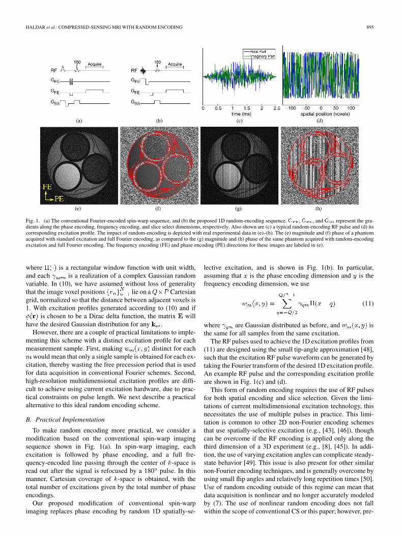
Fig. 1. (a) The conventional Fourier-encoded spin-warp sequence, and (b) the proposed 1D random-encoding sequence. � , � , and � represent the gra-dients along the phase encoding, frequency encoding, and slice select dimensions, respectively. Also shown are (c) a typical random-encoding RF pulse and (d) itscorresponding excitation profile. The impact of random-encoding is depicted with real experimental data in (e)–(h). The (e) magnitude and (f) phase of a phantomacquired with standard excitation and full Fourier encoding, as compared to the (g) magnitude and (h) phase of the same phantom acquired with random-encodingexcitation and full Fourier encoding. The frequency encoding (FE) and phase encoding (PE) directions for these images are labeled in (e).

where is a rectangular window function with unit width,and each is a realization of a complex Gaussian randomvariable. In (10), we have assumed without loss of generalitythat the image voxel positions lie on a Cartesiangrid, normalized so that the distance between adjacent voxels is1. With excitation profiles generated according to (10) and if

is chosen to be a Dirac delta function, the matrix willhave the desired Gaussian distribution for any .

However, there are a couple of practical limitations to imple-menting this scheme with a distinct excitation profile for eachmeasurement sample. First, making distinct for each

would mean that only a single sample is obtained for each ex-citation, thereby wasting the free precession period that is usedfor data acquisition in conventional Fourier schemes. Second,high-resolution multidimensional excitation profiles are diffi-cult to achieve using current excitation hardware, due to prac-tical constraints on pulse length. We next describe a practicalalternative to this ideal random encoding scheme.

B. Practical Implementation

To make random encoding more practical, we consider amodification based on the conventional spin-warp imagingsequence shown in Fig. 1(a). In spin-warp imaging, eachexcitation is followed by phase encoding, and a full fre-quency-encoded line passing through the center of -space isread out after the signal is refocused by a 180 pulse. In thismanner, Cartesian coverage of -space is obtained, with thetotal number of excitations given by the total number of phaseencodings.

Our proposed modification of conventional spin-warpimaging replaces phase encoding by random 1D spatially-se-

lective excitation, and is shown in Fig. 1(b). In particular,assuming that is the phase encoding dimension and is thefrequency encoding dimension, we use

(11)

where are Gaussian distributed as before, and isthe same for all samples from the same excitation.

The RF pulses used to achieve the 1D excitation profiles from(11) are designed using the small tip-angle approximation [48],such that the excitation RF pulse waveform can be generated bytaking the Fourier transform of the desired 1D excitation profile.An example RF pulse and the corresponding excitation profileare shown in Fig. 1(c) and (d).

This form of random encoding requires the use of RF pulsesfor both spatial encoding and slice selection. Given the limi-tations of current multidimensional excitation technology, thisnecessitates the use of multiple pulses in practice. This limi-tation is common to other 2D non-Fourier encoding schemesthat use spatially-selective excitation (e.g., [43], [46]), thoughcan be overcome if the RF encoding is applied only along thethird dimension of a 3D experiment (e.g., [8], [45]). In addi-tion, the use of varying excitation angles can complicate steady-state behavior [49]. This issue is also present for other similarnon-Fourier encoding techniques, and is generally overcome byusing small flip angles and relatively long repetition times [50].Use of random encoding outside of this regime can mean thatdata acquisition is nonlinear and no longer accurately modeledby (7). The use of nonlinear random encoding does not fallwithin the scope of conventional CS or this paper; however, pre-


liminary empirical investigations of nonlinear random encodingcan be found in [39], in which regularization is used in thecontext of a parametric nonlinear signal model.

III. EVALUATION AND DISCUSSION

Experiments and simulations were performed to investigatethe properties of random encoding for CS-MRI. In all cases, wecompared three different data acquisition schemes with a fixednumber of data samples.

• Random Encoding. The proposed practical random en-coding scheme with 1D spatially-selective RF excitations,as described in Section II-B.

• Fourier Encoding 1 (FE1). This scheme uses the standardspin-warp sequence from Fig. 1(a). The phase encodinglocations are evenly-spaced at the Nyquist rate, and coverthe low-frequency portion of -space.

• Fourier Encoding 2 (FE2). Similar to FE1, FE2 makes useof the standard spin-warp sequence. However, the phase-encoding locations are chosen randomly from the Nyquistgrid according to a discretized Gaussian distribution cen-tered at low-frequency -space. This type of variable-den-sity random sampling scheme performs empirically betterthan sampling -space uniformly at random, and is consis-tent with both the prior knowledge that the typical imagesseen in MRI have energy concentrated at low-frequenciesand the existing CS-MRI literature [8], [51].

A. Experiments

The three different encoding schemes were implemented ona 14.1 T magnet system (Oxford Instruments, Abingdon, U.K.)interfaced with a Unity console (Varian, Palo Alto, CA). The flipangle for FE1 and FE2 encoding and the root mean square flipangle for random encoding was 5 , with an RF pulse duration of2.5 ms. The field of view was 3 cm 3 cm, the slice thicknesswas 4 mm, the sequence timing parameters were

, and the bandwidth of the random encoding pulseswas approximately 200 kHz. Data was collected for reconstruc-tion on a 256 256 voxel grid using two different test objects:a compartmental phantom and a section of kiwi fruit. The esti-mated SNR3 for full 256 256 Fourier encoded data was ap-proximately 4 for the compartmental phantom image [shown inFig. 1(e)], and approximately 6 for the kiwi fruit image [shownin Fig. 2(a)].

Due to nonideal experimental conditions (e.g., and in-homogeneity at this field strength), the experimentally achievedexcitation profiles used for random encoding did not match ex-actly with the designed profiles. As such, the excitation pro-file of each pulse was calibrated using prescans. Specifically,a fully-Fourier encoded image was acquired for eachof the spatially-selective excitation pulses [one such image is

3Noise variances were empirically estimated from background regions offully-sampled Fourier-encoded reference images that were free of visibleartifacts, while signal levels were computed using the average value of thereference images in signal-containing regions of interest. The estimated SNRwas calculated as the ratio between the signal level and the noise standarddeviation.

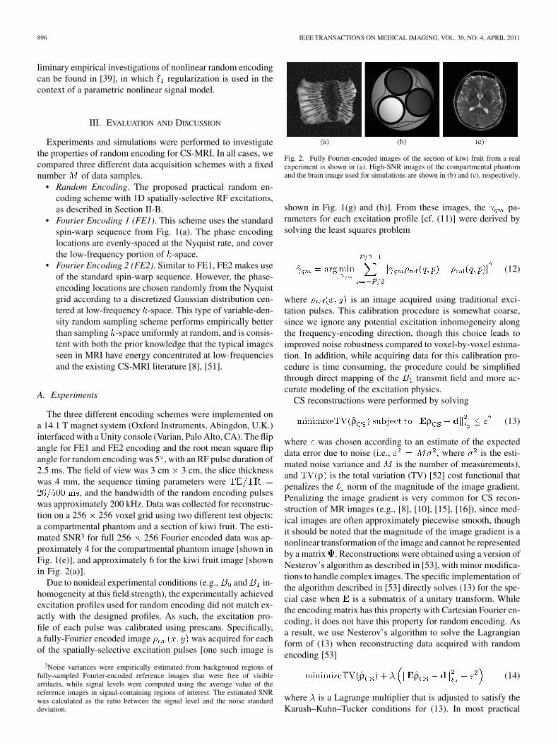
Fig. 2. Fully Fourier-encoded images of the section of kiwi fruit from a realexperiment is shown in (a). High-SNR images of the compartmental phantomand the brain image used for simulations are shown in (b) and (c), respectively.

shown in Fig. 1(g) and (h)]. From these images, the pa-rameters for each excitation profile [cf. (11)] were derived bysolving the least squares problem

(12)

where is an image acquired using traditional exci-tation pulses. This calibration procedure is somewhat coarse,since we ignore any potential excitation inhomogeneity alongthe frequency-encoding direction, though this choice leads toimproved noise robustness compared to voxel-by-voxel estima-tion. In addition, while acquiring data for this calibration pro-cedure is time consuming, the procedure could be simplifiedthrough direct mapping of the transmit field and more ac-curate modeling of the excitation physics.

CS reconstructions were performed by solving

ρ ρ (13)

where was chosen according to an estimate of the expecteddata error due to noise (i.e., , where is the esti-mated noise variance and is the number of measurements),and ρ is the total variation (TV) [52] cost functional thatpenalizes the norm of the magnitude of the image gradient.Penalizing the image gradient is very common for CS recon-struction of MR images (e.g., [8], [10], [15], [16]), since med-ical images are often approximately piecewise smooth, thoughit should be noted that the magnitude of the image gradient is anonlinear transformation of the image and cannot be representedby a matrix . Reconstructions were obtained using a version ofNesterov’s algorithm as described in [53], with minor modifica-tions to handle complex images. The specific implementation ofthe algorithm described in [53] directly solves (13) for the spe-cial case when is a submatrix of a unitary transform. Whilethe encoding matrix has this property with Cartesian Fourier en-coding, it does not have this property for random encoding. Asa result, we use Nesterov’s algorithm to solve the Lagrangianform of (13) when reconstructing data acquired with randomencoding [53]

ρ ρ (14)

where is a Lagrange multiplier that is adjusted to satisfy theKarush–Kuhn–Tucker conditions for (13). In most practical


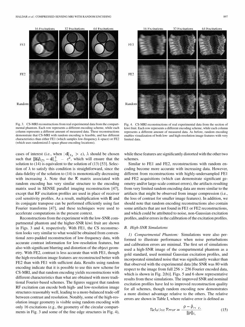
Fig. 3. CS-MRI reconstructions from real experimental data from the compart-mental phantom. Each row represents a different encoding scheme, while eachcolumn represents a different amount of measured data. These reconstructionsdemonstrate that CS-MRI with random encoding is feasible, and has differentcharacteristics than either FE1 (which samples low-frequency �-space) or FE2(which uses randomized �-space phase-encoding locations).

cases of interest (i.e., when ), should be chosensuch that ρ , which will ensure that thesolution to (14) is equivalent to the solution of (13) [53]. Selec-tion of to satisfy this condition is straightforward, since thedata-fidelity of the solution to (14) is monotonically decreasingwith increasing . Note that the matrix associated withrandom encoding has very similar structure to the encodingmatrix used in SENSE parallel imaging reconstruction [47],except that RF excitation profiles are used in place of receivercoil sensitivity profiles. As a result, multiplication with andits conjugate transpose can be performed efficiently using fastFourier transforms [47], and these techniques were used toaccelerate computations in the present context.

Reconstructions from the experiment with the low-SNR com-partmental phantom and the higher-SNR kiwi fruit are shownin Figs. 3 and 4, respectively. With FE1, the CS reconstruc-tion looks very similar to what would be obtained from conven-tional zero-padded reconstruction of low-frequency data, withaccurate contrast information for low-resolution features, butalso with significant blurring and distortion of the object geom-etry. With FE2, contrast is less accurate than with FE1, thoughthe high-resolution image features are reconstructed better withFE2 than with FE1 with sufficient data. Results using randomencoding indicate that it is possible to use this new scheme forCS-MRI, and that random encoding yields reconstructions withdifferent characteristics than what are obtained with more tradi-tional Fourier-based schemes. The figures suggest that randomRF excitation can encode both high- and low-resolution imagestructures reasonably well, leading to a more-balanced trade-offbetween contrast and resolution. Notably, some of the high-res-olution image geometry is visible using random encoding withonly 16 excitations (e.g., the geometry of the circular compart-ments in Fig. 3 and some of the fine edge structures in Fig. 4),

Fig. 4. CS-MRI reconstructions of real experimental data from the section ofkiwi fruit. Each row represents a different encoding scheme, while each columnrepresents a different amount of measured data. As before, random encodingenables visualization of both low- and high-resolution image features with verylimited data.

while these features are significantly distorted with the other twoschemes.

Similar to FE1 and FE2, reconstructions with random en-coding become more accurate with increasing data. However,different from reconstructions with highly-undersampled FE1and FE2 acquisitions (which can demonstrate significant ge-ometry and/or large-scale contrast errors), the artifacts resultingfrom very limited random encoding data are more similar to theartifacts that might be observed from image compression (i.e.,the loss of contrast for smaller image features). In addition, weshould note that random encoding reconstructions also containsome artifacts that are not found in FE1 or FE2 reconstructions,and which could be attributed to noise, non-Gaussian excitationprofiles, and/or errors in the calibration of the excitation profiles.

B. High-SNR Simulations

1) Compartmental Phantom: Simulations were also per-formed to illustrate performance when noise perturbationsand calibration errors are minimal. The first set of simulationsused a high-SNR image of the compartmental phantom as agold standard, used nominal Gaussian excitation profiles, andincorporated simulated noise that was significantly weaker thanthat observed with the experimental data [the SNR was 80 withrespect to the image from full 256 256 Fourier encoded data,which is shown in Fig. 2(b)]. Figs. 5 and 6 show representativeresults from these simulations. The improved SNR and nominalexcitation profiles have led to improved reconstruction qualityfor all schemes, though random encoding now demonstratesa more distinct advantage relative to the others. The relativeerrors are shown in Table I, where relative error is defined as

ρ ρρ

(15)


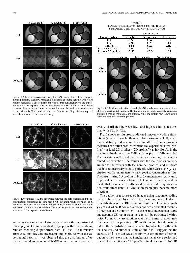
Fig. 5. CS-MRI reconstructions from high-SNR simulations of the compart-mental phantom. Each row represents a different encoding scheme, while eachcolumn represents a different amount of measured data. Relative to the experi-mental data, the improved SNR leads to better reconstructions for all encodingschemes. Reasonably accurate reconstruction was obtained using random en-coding with only 32 excitations, while the Fourier encoding schemes requiredmore data to achieve the same accuracy.

Fig. 6. Error images (i.e., the difference between the gold standard and the re-construction) corresponding to the high-SNR simulation results shown in Fig. 5.Each row represents a different encoding scheme, while each column representsa different amount of measured data. The error images have been scaled up bya factor of 3 for improved visualization.

and serves as a measure of similarity between the reconstructedimage ρ and the gold-standard image ρ. For these simulations,random encoding outperformed both FE1 and FE2 in relativeerror at all investigated undersampling levels. As with the ex-perimental results, it was observed that the distribution of er-rors with random encoding CS-MRI reconstructions was more

TABLE IRELATIVE RECONSTRUCTION ERRORS FOR THE HIGH-SNR

SIMULATIONS USING THE COMPARTMENTAL PHANTOM

Fig. 7. CS-MRI reconstructions from high-SNR random encoding simulationsof the compartmental phantom. The top row shows results using the calibratedexcitation profiles from a real experiment, while the bottom row shows resultsusing random 2D excitation profiles.

evenly distributed between low- and high-resolution featuresthan with FE1 or FE2.

Fig. 7 shows results from additional random encoding simu-lations (relative errors for these are also shown in Table I), wherethe excitation profiles were chosen to either be the empiricallymeasured excitation profiles from the real experiment (“real pro-files”) or ideal 2D profiles (“2D profiles”) as in (10). As in theprevious simulations, the SNR with respect to fully-encodedFourier data was 80, and one frequency encoding line was ac-quired per excitation. The results with the real profiles are verysimilar to the results with the nominal profiles, and illustratethat it is not necessary to have perfectly white Gaussian ex-citation profile parameters to have good reconstruction results.The results using 2D profiles in Fig. 7 demonstrate significantlyimproved performance relative to 1D random encoding, and in-dicate that even better results could be achieved if high-resolu-tion multidimensional RF excitation techniques become morepractical.

The quality of reconstructed images using random encodingcan also be affected by errors in the encoding matrix due tomiscalibration of the RF excitation profiles. Theoretical anal-ysis of (3) when contains errors has been presented recentlyby Herman and Strohmer [54]. These results indicate that stableand accurate CS reconstructions can still be guaranteed with anoisy , under the assumptions that the true measurement ma-trix satisfies an appropriate RIP condition and that the magni-tude of the perturbation is not too large. In particular, the theoret-ical analysis and numerical simulations in [54] suggest that thestability of ρ should scale linearly with the amount of pertur-bation to the system matrix. Simulation studies were performedto examine the effects of RF profile miscalibration. High-SNR


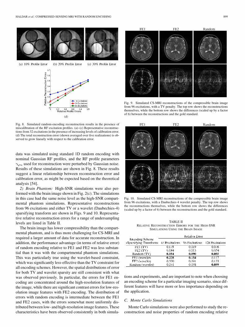
Fig. 8. Simulated random-encoding reconstruction results in the presence ofmiscalibration of the RF excitation profiles. (a)–(c) Representative reconstruc-tions from 32 excitations in the presence of increasing levels of calibration error.(d) The total reconstruction error (shown averaged over five realizations) is ob-served to grow linearly with respect to the calibration error.

data was simulated using standard 1D random encoding withnominal Gaussian RF profiles, and the RF profile parameters

used for reconstruction were perturbed by Gaussian noise.Results of these simulations are shown in Fig. 8. These resultssuggest a linear relationship between reconstruction error andcalibration error, as might be expected based on the theoreticalanalysis [54].

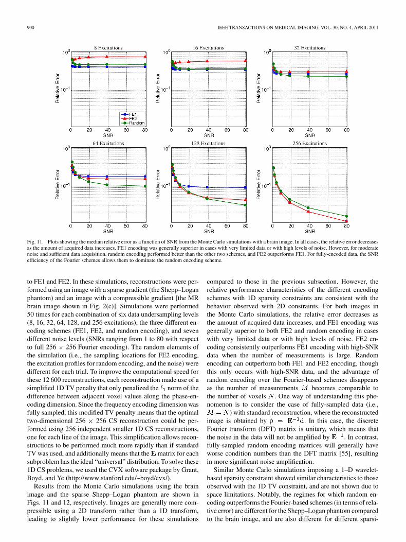
2) Brain Phantom: High-SNR simulations were also per-formed with the brain image shown in Fig. 2(c). The simulationsin this case had the same noise level as the high-SNR compart-mental phantom simulations. Representative reconstructionsfrom 96 excitations and either TV or a wavelet (Daubechies-4)sparsifying transform are shown in Figs. 9 and 10. Representa-tive relative reconstruction errors for a range of undersamplinglevels are listed in Table II.

The brain image has lower compressibility than the compart-mental phantom, and is thus more challenging for CS-MRI andrequired a larger amount of data for accurate reconstruction. Inaddition, the performance advantage (in terms of relative error)of random encoding relative to FE1 and FE2 was less substan-tial than it was with the compartmental phantom simulations.This was particularly true using the wavelet-based constraint,which was significantly less-effective than the TV constraint forall encoding schemes. However, the spatial distributions of errorfor both TV and wavelet sparsity are still consistent with whatwas observed previously. In particular, the errors for FE1 en-coding are concentrated around the high-resolution features ofthe image, while there are significant contrast errors for low-res-olution image features with FE2 encoding. The distribution oferrors with random encoding is intermediate between the FE1and FE2 cases, with the errors somewhat more uniformly dis-tributed between low- and high-resolution image features. Thesecharacteristics have been observed consistently in both simula-

Fig. 9. Simulated CS-MRI reconstructions of the compressible brain imagefrom 96 excitations, with a TV penalty. The top row shows the reconstructionsthemselves, while the bottom row shows the differences (scaled up by a factorof 6) between the reconstructions and the gold standard.

Fig. 10. Simulated CS-MRI reconstructions of the compressible brain imagefrom 96 excitations, with a Daubechies-4 wavelet penalty. The top row showsthe reconstructions themselves, while the bottom row shows the differences(scaled up by a factor of 6) between the reconstructions and the gold standard.

TABLE IIRELATIVE RECONSTRUCTION ERRORS FOR THE HIGH-SNR

SIMULATIONS USING THE BRAIN IMAGE

tions and experiments, and are important to note when choosingan encoding scheme for a particular imaging scenario, since dif-ferent features will have more or less importance depending onthe application.

C. Monte Carlo Simulations

Monte Carlo simulations were also performed to study the re-construction and noise properties of random encoding relative


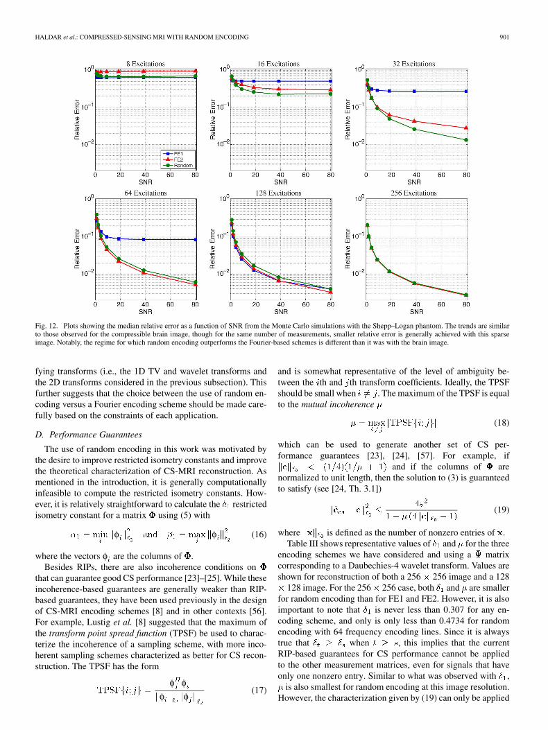
Fig. 11. Plots showing the median relative error as a function of SNR from the Monte Carlo simulations with a brain image. In all cases, the relative error decreasesas the amount of acquired data increases. FE1 encoding was generally superior in cases with very limited data or with high levels of noise. However, for moderatenoise and sufficient data acquisition, random encoding performed better than the other two schemes, and FE2 outperforms FE1. For fully-encoded data, the SNRefficiency of the Fourier schemes allows them to dominate the random encoding scheme.

to FE1 and FE2. In these simulations, reconstructions were per-formed using an image with a sparse gradient (the Shepp–Loganphantom) and an image with a compressible gradient [the MRbrain image shown in Fig. 2(c)]. Simulations were performed50 times for each combination of six data undersampling levels(8, 16, 32, 64, 128, and 256 excitations), the three different en-coding schemes (FE1, FE2, and random encoding), and sevendifferent noise levels (SNRs ranging from 1 to 80 with respectto full 256 256 Fourier encoding). The random elements ofthe simulation (i.e., the sampling locations for FE2 encoding,the excitation profiles for random encoding, and the noise) weredifferent for each trial. To improve the computational speed forthese 12 600 reconstructions, each reconstruction made use of asimplified 1D TV penalty that only penalized the norm of thedifference between adjacent voxel values along the phase-en-coding dimension. Since the frequency encoding dimension wasfully sampled, this modified TV penalty means that the optimaltwo-dimensional 256 256 CS reconstruction could be per-formed using 256 independent smaller 1D CS reconstructions,one for each line of the image. This simplification allows recon-structions to be performed much more rapidly than if standardTV was used, and additionally means that the matrix for eachsubproblem has the ideal “universal” distribution. To solve these1D CS problems, we used the CVX software package by Grant,Boyd, and Ye (http://www.stanford.edu/~boyd/cvx/).

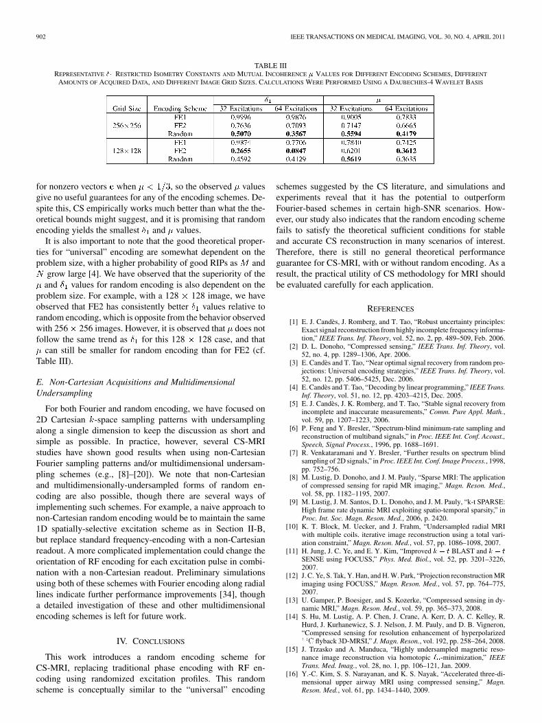
Results from the Monte Carlo simulations using the brainimage and the sparse Shepp–Logan phantom are shown inFigs. 11 and 12, respectively. Images are generally more com-pressible using a 2D transform rather than a 1D transform,leading to slightly lower performance for these simulations

compared to those in the previous subsection. However, therelative performance characteristics of the different encodingschemes with 1D sparsity constraints are consistent with thebehavior observed with 2D constraints. For both images inthe Monte Carlo simulations, the relative error decreases asthe amount of acquired data increases, and FE1 encoding wasgenerally superior to both FE2 and random encoding in caseswith very limited data or with high levels of noise. FE2 en-coding consistently outperforms FE1 encoding with high-SNRdata when the number of measurements is large. Randomencoding can outperform both FE1 and FE2 encoding, thoughthis only occurs with high-SNR data, and the advantage ofrandom encoding over the Fourier-based schemes disappearsas the number of measurements becomes comparable tothe number of voxels . One way of understanding this phe-nomenon is to consider the case of fully-sampled data (i.e.,

) with standard reconstruction, where the reconstructedimage is obtained by ρ . In this case, the discreteFourier transform (DFT) matrix is unitary, which means thatthe noise in the data will not be amplified by . In contrast,fully-sampled random encoding matrices will generally haveworse condition numbers than the DFT matrix [55], resultingin more significant noise amplification.

Similar Monte Carlo simulations imposing a 1–D wavelet-based sparsity constraint showed similar characteristics to thoseobserved with the 1D TV constraint, and are not shown due tospace limitations. Notably, the regimes for which random en-coding outperforms the Fourier-based schemes (in terms of rela-tive error) are different for the Shepp–Logan phantom comparedto the brain image, and are also different for different sparsi-


Fig. 12. Plots showing the median relative error as a function of SNR from the Monte Carlo simulations with the Shepp–Logan phantom. The trends are similarto those observed for the compressible brain image, though for the same number of measurements, smaller relative error is generally achieved with this sparseimage. Notably, the regime for which random encoding outperforms the Fourier-based schemes is different than it was with the brain image.

fying transforms (i.e., the 1D TV and wavelet transforms andthe 2D transforms considered in the previous subsection). Thisfurther suggests that the choice between the use of random en-coding versus a Fourier encoding scheme should be made care-fully based on the constraints of each application.

D. Performance Guarantees

The use of random encoding in this work was motivated bythe desire to improve restricted isometry constants and improvethe theoretical characterization of CS-MRI reconstruction. Asmentioned in the introduction, it is generally computationallyinfeasible to compute the restricted isometry constants. How-ever, it is relatively straightforward to calculate the restrictedisometry constant for a matrix using (5) with

φ φ (16)

where the vectors φ are the columns of .Besides RIPs, there are also incoherence conditions on

that can guarantee good CS performance [23]–[25]. While theseincoherence-based guarantees are generally weaker than RIP-based guarantees, they have been used previously in the designof CS-MRI encoding schemes [8] and in other contexts [56].For example, Lustig et al. [8] suggested that the maximum ofthe transform point spread function (TPSF) be used to charac-terize the incoherence of a sampling scheme, with more inco-herent sampling schemes characterized as better for CS recon-struction. The TPSF has the form

φ φφ φ

(17)

and is somewhat representative of the level of ambiguity be-tween the th and th transform coefficients. Ideally, the TPSFshould be small when . The maximum of the TPSF is equalto the mutual incoherence

(18)

which can be used to generate another set of CS per-formance guarantees [23], [24], [57]. For example, if

and if the columns of arenormalized to unit length, then the solution to (3) is guaranteedto satisfy (see [24, Th. 3.1])

(19)

where is defined as the number of nonzero entries of .Table III shows representative values of and for the three

encoding schemes we have considered and using a matrixcorresponding to a Daubechies-4 wavelet transform. Values areshown for reconstruction of both a 256 256 image and a 128

128 image. For the 256 256 case, both and are smallerfor random encoding than for FE1 and FE2. However, it is alsoimportant to note that is never less than 0.307 for any en-coding scheme, and only is only less than 0.4734 for randomencoding with 64 frequency encoding lines. Since it is alwaystrue that when , this implies that the currentRIP-based guarantees for CS performance cannot be appliedto the other measurement matrices, even for signals that haveonly one nonzero entry. Similar to what was observed with ,

is also smallest for random encoding at this image resolution.However, the characterization given by (19) can only be applied


TABLE IIIREPRESENTATIVE � RESTRICTED ISOMETRY CONSTANTS AND MUTUAL INCOHERENCE � VALUES FOR DIFFERENT ENCODING SCHEMES, DIFFERENT

AMOUNTS OF ACQUIRED DATA, AND DIFFERENT IMAGE GRID SIZES. CALCULATIONS WERE PERFORMED USING A DAUBECHIES-4 WAVELET BASIS

for nonzero vectors when , so the observed valuesgive no useful guarantees for any of the encoding schemes. De-spite this, CS empirically works much better than what the the-oretical bounds might suggest, and it is promising that randomencoding yields the smallest and values.

It is also important to note that the good theoretical proper-ties for “universal” encoding are somewhat dependent on theproblem size, with a higher probability of good RIPs as and

grow large [4]. We have observed that the superiority of theand values for random encoding is also dependent on the

problem size. For example, with a 128 128 image, we haveobserved that FE2 has consistently better values relative torandom encoding, which is opposite from the behavior observedwith 256 256 images. However, it is observed that does notfollow the same trend as for this 128 128 case, and that

can still be smaller for random encoding than for FE2 (cf.Table III).

E. Non-Cartesian Acquisitions and MultidimensionalUndersampling

For both Fourier and random encoding, we have focused on2D Cartesian -space sampling patterns with undersamplingalong a single dimension to keep the discussion as short andsimple as possible. In practice, however, several CS-MRIstudies have shown good results when using non-CartesianFourier sampling patterns and/or multidimensional undersam-pling schemes (e.g., [8]–[20]). We note that non-Cartesianand multidimensionally-undersampled forms of random en-coding are also possible, though there are several ways ofimplementing such schemes. For example, a naive approach tonon-Cartesian random encoding would be to maintain the same1D spatially-selective excitation scheme as in Section II-B,but replace standard frequency-encoding with a non-Cartesianreadout. A more complicated implementation could change theorientation of RF encoding for each excitation pulse in combi-nation with a non-Cartesian readout. Preliminary simulationsusing both of these schemes with Fourier encoding along radiallines indicate further performance improvements [34], thougha detailed investigation of these and other multidimensionalencoding schemes is left for future work.

IV. CONCLUSIONS

This work introduces a random encoding scheme forCS-MRI, replacing traditional phase encoding with RF en-coding using randomized excitation profiles. This randomscheme is conceptually similar to the “universal” encoding

schemes suggested by the CS literature, and simulations andexperiments reveal that it has the potential to outperformFourier-based schemes in certain high-SNR scenarios. How-ever, our study also indicates that the random encoding schemefails to satisfy the theoretical sufficient conditions for stableand accurate CS reconstruction in many scenarios of interest.Therefore, there is still no general theoretical performanceguarantee for CS-MRI, with or without random encoding. As aresult, the practical utility of CS methodology for MRI shouldbe evaluated carefully for each application.

REFERENCES

[1] E. J. Candès, J. Romberg, and T. Tao, “Robust uncertainty principles:Exact signal reconstruction from highly incomplete frequency informa-tion,” IEEE Trans. Inf. Theory, vol. 52, no. 2, pp. 489–509, Feb. 2006.

[2] D. L. Donoho, “Compressed sensing,” IEEE Trans. Inf. Theory, vol.52, no. 4, pp. 1289–1306, Apr. 2006.

[3] E. Candès and T. Tao, “Near optimal signal recovery from random pro-jections: Universal encoding strategies,” IEEE Trans. Inf. Theory, vol.52, no. 12, pp. 5406–5425, Dec. 2006.

[4] E. Candès and T. Tao, “Decoding by linear programming,” IEEE Trans.Inf. Theory, vol. 51, no. 12, pp. 4203–4215, Dec. 2005.

[5] E. J. Candès, J. K. Romberg, and T. Tao, “Stable signal recovery fromincomplete and inaccurate measurements,” Comm. Pure Appl. Math.,vol. 59, pp. 1207–1223, 2006.

[6] P. Feng and Y. Bresler, “Spectrum-blind minimum-rate sampling andreconstruction of multiband signals,” in Proc. IEEE Int. Conf. Acoust.,Speech, Signal Process., 1996, pp. 1688–1691.

[7] R. Venkataramani and Y. Bresler, “Further results on spectrum blindsampling of 2D signals,” in Proc. IEEE Int. Conf. Image Process., 1998,pp. 752–756.

[8] M. Lustig, D. Donoho, and J. M. Pauly, “Sparse MRI: The applicationof compressed sensing for rapid MR imaging,” Magn. Reson. Med.,vol. 58, pp. 1182–1195, 2007.

[9] M. Lustig, J. M. Santos, D. L. Donoho, and J. M. Pauly, “k-t SPARSE:High frame rate dynamic MRI exploiting spatio-temporal sparsity,” inProc. Int. Soc. Magn. Reson. Med., 2006, p. 2420.

[10] K. T. Block, M. Uecker, and J. Frahm, “Undersampled radial MRIwith multiple coils. iterative image reconstruction using a total vari-ation constraint,” Magn. Reson. Med., vol. 57, pp. 1086–1098, 2007.

[11] H. Jung, J. C. Ye, and E. Y. Kim, “Improved � � � BLAST and � � �SENSE using FOCUSS,” Phys. Med. Biol., vol. 52, pp. 3201–3226,2007.

[12] J. C. Ye, S. Tak, Y. Han, and H. W. Park, “Projection reconstruction MRimaging using FOCUSS,” Magn. Reson. Med., vol. 57, pp. 764–775,2007.

[13] U. Gamper, P. Boesiger, and S. Kozerke, “Compressed sensing in dy-namic MRI,” Magn. Reson. Med., vol. 59, pp. 365–373, 2008.

[14] S. Hu, M. Lustig, A. P. Chen, J. Crane, A. Kerr, D. A. C. Kelley, R.Hurd, J. Kurhanewicz, S. J. Nelson, J. M. Pauly, and D. B. Vigneron,“Compressed sensing for resolution enhancement of hyperpolarized� flyback 3D-MRSI,” J. Magn. Reson., vol. 192, pp. 258–264, 2008.

[15] J. Trzasko and A. Manduca, “Highly undersampled magnetic reso-nance image reconstruction via homotopic � -minimization,” IEEETrans. Med. Imag., vol. 28, no. 1, pp. 106–121, Jan. 2009.

[16] Y.-C. Kim, S. S. Narayanan, and K. S. Nayak, “Accelerated three-di-mensional upper airway MRI using compressed sensing,” Magn.Reson. Med., vol. 61, pp. 1434–1440, 2009.


[17] C. O. Schirra, S. Weiss, S. Krueger, S. F. Pedersen, R. Razavi, T. Scha-effter, and S. Kozerke, “Toward true 3D visualization of active cathetersusing compressed sensing,” Magn. Reson. Med., vol. 62, pp. 341–347,2009.

[18] D. Liang, B. Liu, J. J. Wang, and L. Ying, “Accelerating SENSE usingcompressed sensing,” Magn. Reson. Med., vol. 62, pp. 1574–1584,2009.

[19] M. Seeger, H. Nickisch, R. Pohmann, and B. Schölkopf, “Optimiza-tion of �-space trajectories for compressed sensing by Bayesian exper-imental design,” Magn. Reson. Med., vol. 63, pp. 116–126, 2010.

[20] S. Ajraoui, K. J. Lee, M. H. Deppe, S. R. Parnell, J. Parra-Robles, andJ. M. Wild, “Compressed sensing in hyperpolarized �� lung MRI,”Magn. Reson. Med., vol. 63, pp. 1059–1069, 2010.

[21] E. J. Candès, “The restricted isometry property and its implicationsfor compressed sensing,” C. R. Acad. Sci. Paris, Ser. I, vol. 346, pp.589–592, 2008.

[22] M. E. Davies and R. Gribonval, “Restricted isometry constants where� sparse recovery can fail for � � � � �,” IEEE Trans. Inf. Theory,vol. 55, pp. 2203–2214, 2009.

[23] D. L. Donoho and M. Elad, “Optimally sparse representation in general(nonorthogonal) dictionaries via � minimization,” Proc. Natl. Acad.Sci. USA, vol. 100, pp. 2197–2202, 2003.

[24] D. L. Donoho, M. Elad, and V. N. Temlyakov, “Stable recovery ofsparse overcomplete representations in the presence of noise,” IEEETrans. Inf. Theory, vol. 52, no. 1, pp. 6–18, Jan. 2006.

[25] E. Candès and J. Romberg, “Sparsity and incoherence in compressivesampling,” Inverse Probl., vol. 23, pp. 969–985, 2007.

[26] A. Cohen, W. Dahmen, and R. DeVore, “Compressed sensing and best�-term approximation,” J. Am. Math. Soc., vol. 22, pp. 211–231, 2009.

[27] D. L. Donoho and X. Huo, “Uncertainty principles and ideal atomic de-composition,” IEEE Trans. Inf. Theory, vol. 47, no. 7, pp. 2845–2862,Nov. 2001.

[28] R. Gribonval and M. Nielsen, “Sparse representations in unions ofbases,” IEEE Trans. Inf. Theory, vol. 49, no. 12, pp. 3320–3325, Dec.2003.

[29] S. Foucart, “A note on guaranteed sparse recovery via � -minimiza-tion,” Appl. Comput. Harmon. Anal., vol. 29, pp. 97–103, 2009.

[30] T. T. Cai, L. Wang, and G. Xu, “New bounds for restricted isometryconstants,” IEEE Trans. Inf. Theory, vol. 56, no. 9, pp. 4388–4394, Sep.2010.

[31] M. Rudelson and R. Vershynin, “On sparse reconstruction from Fourierand Gaussian measurements,” Comm. Pure Appl. Math., vol. 61, pp.1025–1045, 2008.

[32] D. L. Donoho and J. Tanner, “Exponential bounds implying construc-tion of compressed sensing matrices, error-correcting codes, and neigh-borly polytopes by random sampling,” IEEE Trans. Inf. Theory, vol. 56,pp. 2002–2016, 2010.

[33] E. J. Candès, Y. C. Eldar, and D. Needell, Compressed sensing withcoherent and redundant dictionaries 2010 [Online]. Available: http://arxiv.org/abs/1005.2613

[34] J. P. Haldar, D. Hernando, B. P. Sutton, and Z.-P. Liang, “Data acquisi-tion considerations for compressed sensing in MRI,” in Proc. Int. Soc.Magn. Reson. Med., 2007, p. 829.

[35] F. M. Sebert, Y. Zou, B. Liu, and L. Ying, “Compressed sensing MRIwith random B1 field,” in Proc. Int. Soc. Magn. Reson. Med., 2008, p.1318.

[36] D. Liang, G. Xu, H. Wang, K. F. King, D. Xu, and L. Ying, “Toeplitzrandom encoding MR imaging using compressed sensing,” in Proc.IEEE Int. Symp. Biomed. Imag., 2009, pp. 270–273.

[37] G. Puy, Y. Wiaux, R. Gruetter, J.-P. Thiran, D. V. de Ville, and P.Vandergheynst, “Spread spectrum for interferometric and magneticresonance imaging,” in Proc. IEEE Int. Conf. Acoust., Speech, SignalProcess., 2010, pp. 2802–2805.

[38] Y. Wiaux, G. Puy, R. Gruetter, J.-P. Thiran, D. V. de Ville, and P. Van-dergheynst, “Spread spectrum for compressed sensing techniques inmagnetic resonance imaging,” in Proc. IEEE Int. Symp. Biomed. Imag.,2010, pp. 756–759.

[39] E. C. Wong, “Efficient randomly encoded data acquisition for com-pressed sensing,” in Proc. Int. Soc. Magn. Reson. Med., 2010, p. 4893.

[40] X. Pan, E. Y. Sidky, and M. Vannier, “Why do commercial CT scannersstill employ traditional, filtered back-projection for image reconstruc-tion?,” Inverse Probl., vol. 25, p. 123009, 2009.

[41] M. F. Duarte, M. A. Davenport, D. Takhar, J. N. Laska, T. Sun, K.F. Kelly, and R. G. Baraniuk, “Single-pixel imaging via compressivesensing,” IEEE Signal Process. Mag., vol. 25, pp. 83–91, 2008.

[42] R. F. Marcia, Z. T. Harmany, and R. M. Willett, “Compressive codedaperture imaging,” in Proc. SPIE, 2009, vol. 7246, p. 72460G.

[43] L. P. Panych, G. P. Zientara, and F. A. Jolesz, “MR image encodingby spatially selective RF excitation: An analysis using linear responsemodels,” Int. J. Imag. Syst. Tech., vol. 10, pp. 143–150, 1999.

[44] G. Johnson, E. X. Wu, and S. K. Hilal, “Optimized phase scramblingfor RF phase encoding,” J. Magn. Reson. B, vol. 103, pp. 59–63, 1994.

[45] C. H. Cunningham, G. A. Wright, and M. L. Wood, “High-order multi-band encoding in the heart,” Magn. Reson. Med., vol. 48, pp. 689–698,2002.

[46] D. Mitsouras, G. P. Zientara, A. Edelman, and F. J. Rybicki, “En-hancing the acquisition efficiency of fast magnetic resonance imagingvia broadband encoding of signal content,” Magn. Reson. Imag., vol.24, pp. 1209–1227, 2006.

[47] K. P. Pruessmann, M. Weiger, P. Börnert, and P. Boesiger, “Advancesin sensitivity encoding with arbitrary k-space trajectories,” Magn.Reson. Med., vol. 46, pp. 638–651, 2001.

[48] J. Pauly, D. Nishimura, and A. Macovski, “A k-space analysis of small-tip-angle excitation,” J. Magn. Reson., vol. 81, pp. 43–56, 1989.

[49] S. T. S. Wong, M. S. Roos, R. D. Newmark, and T. F. Budinger, “Dis-crete analysis of stochastic NMR. I,” J. Magn. Reson., vol. 87, pp.242–264, 1990.

[50] R. D. Peters and M. L. Wood, “Multilevel wavlet-transform encodingin MRI,” J. Magn. Reson. Imag., vol. 6, pp. 529–540, 1996.

[51] Z. Wang and G. R. Arce, “Variable density compressed image sam-pling,” IEEE Trans. Image Process., vol. 19, no. 1, pp. 264–270, Jan.2010.

[52] L. I. Rudin, S. Osher, and E. Fatemi, “Nonlinear total variation basednoise removal algorithms,” Physica D, vol. 60, pp. 259–268, 1992.

[53] S. Becker, J. Bobin, and E. J. Candès, NESTA: A fast and accuratefirst-order method for sparse recovery California Inst. Technol., Tech.Rep., 2009 [Online]. Available: http://www.acm.caltech.edu/nesta/

[54] M. A. Herman and T. Strohmer, “General deviants: An analysis of per-turbations in compressed sensing,” IEEE J. Sel. Topics Signal Process.,vol. 4, pp. 342–349, 2010.

[55] A. Edelman, “Eigenvalues and condition numbers of random matrices,”SIAM J. Matrix Anal. Appl., vol. 9, pp. 543–560, 1988.

[56] M. Elad, “Optimized projections for compressed sensing,” IEEE Trans.Signal Process., vol. 55, no. 12, pp. 5695–5702, Dec. 2007.

[57] T. T. Cai, L. Wang, and G. Xu, “Stable recovery of sparse signalsand an oracle inequality,” IEEE Trans. Inf. Theory, vol. 56, no. 7, pp.3516–3522, Jul. 2010.

Compressed-Sensing MRI With Random Encoding

Documents

Transcript of Compressed-Sensing MRI With Random Encoding