Theory and Applications of Compressed Sensing

Gitta Kutyniok

August 29, 2012

Abstract

Compressed sensing is a novel research area, which was introduced in 2006, and sincethen has already become a key concept in various areas of applied mathematics, com-puter science, and electrical engineering. It surprisingly predicts that high-dimensionalsignals, which allow a sparse representation by a suitable basis or, more generally, aframe, can be recovered from what was previously considered highly incomplete linearmeasurements by using efficient algorithms. This article shall serve as an introductionto and a survey about compressed sensing.

Key Words. Dimension reduction. Frames. Greedy algorithms. Ill-posed inverseproblems. `1 minimization. Random matrices. Sparse approximation. Sparse recovery.

Acknowledgements. The author is grateful to the reviewers for many helpful sugges-tions which improved the presentation of the paper. She would also like to thank EmmanuelCandes, David Donoho, Michael Elad, and Yonina Eldar for various discussions on relatedtopics, and Sadegh Jokar for producing Figure 3. The author acknowledges support by theEinstein Foundation Berlin, by Deutsche Forschungsgemeinschaft (DFG) Grants SPP-1324KU 1446/13 and KU 1446/14, and by the DFG Research Center Matheon “Mathematicsfor key technologies” in Berlin.

1 Introduction

The area of compressed sensing was initiated in 2006 by two groundbreaking papers, namely[18] by Donoho and [11] by Candes, Romberg, and Tao. Nowadays, after only 6 years, anabundance of theoretical aspects of compressed sensing are explored in more than 1000articles. Moreover, this methodology is to date extensively utilized by applied mathemati-cians, computer scientists, and engineers for a variety of applications in astronomy, biology,medicine, radar, and seismology, to name a few.

The key idea of compressed sensing is to recover a sparse signal from very few non-adaptive, linear measurements by convex optimization. Taking a different viewpoint, itconcerns the exact recovery of a high-dimensional sparse vector after a dimension reductionstep. From a yet another standpoint, we can regard the problem as computing a sparsecoefficient vector for a signal with respect to an overcomplete system. The theoretical foun-dation of compressed sensing has links with and also explores methodologies from various

1

arX

iv:1

203.

3815

v2 [

cs.I

T]

28

Aug

201

2

other fields such as, for example, applied harmonic analysis, frame theory, geometric func-tional analysis, numerical linear algebra, optimization theory, and random matrix theory.

It is interesting to notice that this development – the problem of sparse recovery – can infact be traced back to earlier papers from the 90s such as [24] and later the prominent papersby Donoho and Huo [21] and Donoho and Elad [19]. When the previously mentioned twofundamental papers introducing compressed sensing were published, the term ‘compressedsensing’ was initially utilized for random sensing matrices, since those allow for a minimalnumber of non-adaptive, linear measurements. Nowadays, the terminology ‘compressedsensing’ is more and more often used interchangeably with ‘sparse recovery’ in general,which is a viewpoint we will also take in this survey paper.

1.1 The Compressed Sensing Problem

To state the problem mathematically precisely, let now x = (xi)ni=1 ∈ Rn be our signal of

interest. As prior information, we either assume that x itself is sparse, i.e., it has very fewnon-zero coefficients in the sense that

‖x‖0 := #{i : xi 6= 0}

is small, or that there exists an orthonormal basis or a frame1 Φ such that x = Φc with cbeing sparse. For this, we let Φ be the matrix with the elements of the orthonormal basisor the frame as column vectors. In fact, a frame typically provides more flexibility than anorthonormal basis due to its redundancy and hence leads to improved sparsifying properties,hence in this setting customarily frames are more often employed than orthonormal bases.Sometimes the notion of sparsity is weakened, which we for now – before we will make thisprecise in Section 2 – will refer to as approximately sparse. Further, let A be an m × nmatrix, which is typically called sensing matrix or measurement matrix. Throughout wewill always assume that m < n and that A does not possess any zero columns, even if notexplicitly mentioned.

Then the Compressed Sensing Problem can be formulated as follows: Recover x fromknowledge of

y = Ax,

or recover c from knowledge ofy = AΦc.

In both cases, we face an underdetermined linear system of equations with sparsity as priorinformation about the vector to be recovered – we do not however know the support, sincethen the solution could be trivially obtained.

This leads us to the following questions:

• What are suitable signal and sparsity models?

• How, when, and with how much accuracy can the signal be algorithmically recovered?

• What are suitable sensing matrices?

1Recall that a frame for a Hilbert space H is a system (ϕi)i∈I in H, for which there exist frame bounds0 < A ≤ B <∞ such that A‖x‖22 ≤

∑i∈I |〈x, ϕi〉|2 ≤ B‖x‖22 for all x ∈ H. A tight frame allows A = B. If

A = B = 1 can be chosen, (ϕi)i∈I forms a Parseval frame. For further information, we refer to [12].

2

In this section, we will discuss these questions briefly to build up intuition for the subsequentsections.

1.2 Sparsity: A Reasonable Assumption?

As a first consideration, one might question whether sparsity is indeed a reasonable assump-tion. Due to the complexity of real data certainly only a heuristic answer is possible.

If a natural image is taken, it is well known that wavelets typically provide sparseapproximations. This is illustrated in Figure 1, which shows a wavelet decomposition [50]of an exemplary image. It can clearly be seen that most coefficients are small in absolutevalue, indicated by a darker color.

(a) (b)

Figure 1: (a) Mathematics building of TU Berlin (Photo by TU-Pressestelle); (b) Waveletdecomposition

Depending on the signal, a variety of representation systems which can be used toprovide sparse approximations is available and is constantly expanded. In fact, it wasrecently shown that wavelet systems do not provide optimally sparse approximations ina regularity setting which appears to be suitable for most natural images, but the novelsystem of shearlets does [47, 46]. Hence, assuming some prior knowledge of the signal to besensed or compressed, typically suitable, well-analyzed representation systems are alreadyat hand. If this is not the case, more data sensitive methods such as dictionary learningalgorithms (see, for instance, [2]), in which a suitable representation system is computedfor a given set of test signals, are available.

Depending on the application at hand, often x is already sparse itself. Think, forinstance, of digital communication, when a cell phone network with n antennas and musers needs to be modelled. Or consider genomics, when in a test study m genes shall beanalyzed with n patients taking part in the study. In the first scenario, very few of theusers have an ongoing call at a specific time; in the second scenario, very few of the genesare actually active. Thus, x being sparse itself is also a very natural assumption.

In the compressed sensing literature, most results indeed assume that x itself is sparse,and the problem y = Ax is considered. Very few articles study the problem of incorporatinga sparsifying orthonormal basis or frame; we mention specifically [61, 9]. In this paper, wewill also assume throughout that x is already a sparse vector. It should be emphasized that‘exact’ sparsity is often too restricting or unnatural, and weakened sparsity notions need

3

to be taken into account. On the other hand, sometimes – such as with the tree structureof wavelet coefficients – some structural information on the non-zero coefficients is known,which leads to diverse structured sparsity models. Section 2 provides an overview of suchmodels.

1.3 Recovery Algorithms: Optimization Theory and More

Let x now be a sparse vector. It is quite intuitive to recover x from knowledge of y bysolving

(P0) minx‖x‖0 subject to y = Ax.

Due to the unavoidable combinatorial search, this algorithm is however NP-hard [53]. Themain idea of Chen, Donoho, and Saunders in the fundamental paper [14] was to substitutethe `0 ‘norm’ by the closest convex norm, which is the `1 norm. This leads to the followingminimization problem, which they coined Basis Pursuit:

(P1) minx‖x‖1 subject to y = Ax.

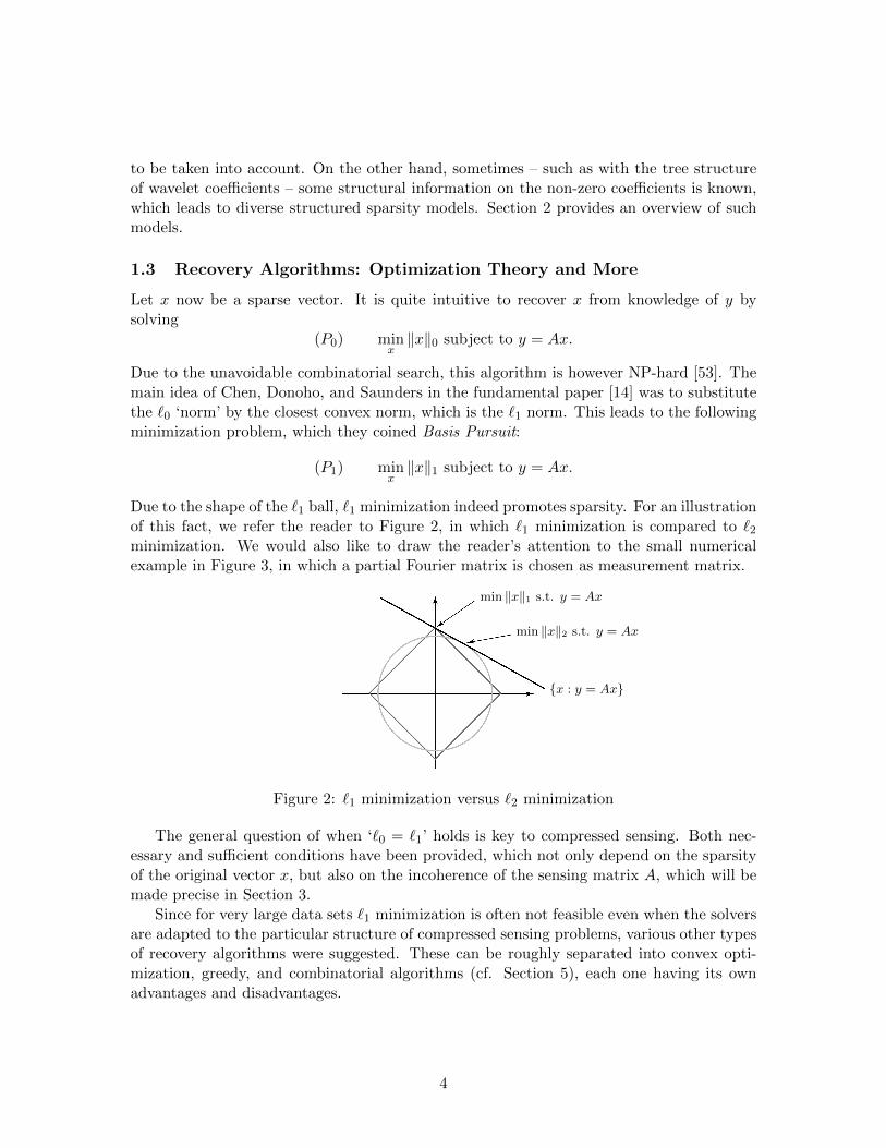
Due to the shape of the `1 ball, `1 minimization indeed promotes sparsity. For an illustrationof this fact, we refer the reader to Figure 2, in which `1 minimization is compared to `2minimization. We would also like to draw the reader’s attention to the small numericalexample in Figure 3, in which a partial Fourier matrix is chosen as measurement matrix.

{x : y = Ax}

min ‖x‖2 s.t. y = Ax

min ‖x‖1 s.t. y = Ax

Figure 2: `1 minimization versus `2 minimization

The general question of when ‘`0 = `1’ holds is key to compressed sensing. Both nec-essary and sufficient conditions have been provided, which not only depend on the sparsityof the original vector x, but also on the incoherence of the sensing matrix A, which will bemade precise in Section 3.

Since for very large data sets `1 minimization is often not feasible even when the solversare adapted to the particular structure of compressed sensing problems, various other typesof recovery algorithms were suggested. These can be roughly separated into convex opti-mization, greedy, and combinatorial algorithms (cf. Section 5), each one having its ownadvantages and disadvantages.

4

(a) (b)

(c) (d)

Figure 3: (a) Original signal f with random sample points (indicated by circles); (b) TheFourier transform f ; (c) Perfect recovery of f by `1 minimization; (d) Recovery of f by `2minimization

1.4 Sensing Matrices: How Much Freedom is Allowed?

As already mentioned, sensing matrices are required to satisfy certain incoherence conditionssuch as, for instance, a small so-called mutual coherence. If we are allowed to choose thesensing matrix freely, the best choice are random matrices such as Gaussian iid matrices,uniform random ortho-projectors, or Bernoulli matrices, see for instance [11].

It is still an open question (cf. Section 4 for more details) whether deterministic matricescan be carefully constructed to have similar properties with respect to compressed sensingproblems. At the moment, different approaches towards this problem are being taken suchas structured random matrices by, for instance, Rauhut et al. in [58] or [60]. Moreover, mostapplications do not allow for a free choice of the sensing matrix and enforce a particularlystructured matrix. Exemplary situations are the application of data separation, in whichthe sensing matrix has to consist of two or more orthonormal bases or frames [32, Chapter11], or high resolution radar, for which the sensing matrix has to bear a particular time-frequency structure [38].

1.5 Compressed Sensing: Quo Vadis?

At present, a comprehensive core theory seems established except for some few deep ques-tions such as the construction of deterministic sensing matrices exhibiting properties similarto random matrices.

One current main direction of research which can be identified with already variousexisting results is the incorporation of additional sparsity properties typically coined struc-tured sparsity, see Section 2 for references. Another main direction is the extension or

5

transfer of the Compressed Sensing Problem to other settings such as matrix completion,see for instance [10]. Moreover, we are currently witnessing the diffusion of compressed sens-ing ideas to various application areas such as radar analysis, medical imaging, distributedsignal processing, and data quantization, to name a few; see [32] for an overview. Theseapplications pose intriguing challenges to the area due to the constraints they require, whichin turn initiates novel theoretical problems. Finally, we observe that due to the need of, inparticular, fast sparse recovery algorithms, there is a trend to more closely cooperate withmathematicians from other research areas, for example from optimization theory, numericallinear algebra, or random matrix theory.

As three examples of recently initiated research directions, we would like to mentionthe following. First, while the theory of compressed sensing focusses on digital data, it isdesirable to develop a similar theory for the continuum setting. Two promising approacheswere so far suggested by Eldar et al. (cf. [52]) and Adcock et al. (cf. [1]). Second, incontrast to Basis Pursuit, which minimizes the `1 norm of the synthesis coefficients, severalapproaches such as recovery of missing data minimize the `1 norm of the analysis coefficients– as opposed to minimizing the `1 norm of the synthesis coefficients –, see Subsections 6.1.2and 6.2.2. The relation between these two minimization problems is far from being clear,and the recently introduced notion of co-sparsity [54] is an interesting approach to shed lightonto this problem. Third, the utilization of frames as a sparsifying system in the contextof compressed sensing has become a topic of increased interest, and we refer to the initialpaper [9].

The reader might also want to consult the extensive webpage dsp.rice.edu/cs con-taining most published papers in the area of compressed sensing subdivided into differenttopics. We would also like to draw the reader’s attention to the recent books [29] and [32]as well as the survey article [7].

1.6 Outline

In Section 2, we start by discussing different sparsity models including structured sparsityand sparsifying dictionaries. The next section, Section 3, is concerned with presenting bothnecessary and sufficient conditions for exact recovery using `1 minimization as a recoverystrategy. The delicateness of designing sensing matrices is the focus of Section 4. In Section5, other algorithmic approaches to sparse recovery are presented. Finally, applications suchas data separation are discussed in Section 6.

2 Signal Models

Sparsity is the prior information assumed of the vector we intend to efficiently sense orwhose dimension we intend to reduce, depending on which viewpoint we take. We will startby recalling some classical notions of sparsity. Since applications typically impose a certainstructure on the significant coefficients, various structured sparsity models were introducedwhich we will subsequently present. Finally, we will discuss how to ensure sparsity throughan appropriate orthonormal basis or frame.

6

2.1 Sparsity

The most basic notion of sparsity states that a vector has at most k non-zero coefficients.This is measured by the `0 ‘norm’, which for simplicity we will throughout refer to as anorm although it is well-known that ‖ · ‖0 does not constitute a mathematical norm.

Definition 2.1 A vector x = (xi)ni=1 ∈ Rn is called k-sparse, if

‖x‖0 = #{i : xi 6= 0} ≤ k.

The set of all k-sparse vectors is denoted by Σk.

We wish to emphasize that Σk is a highly non-linear set. Letting x ∈ Rn be a k-sparsesignal, it belongs to the linear subspace consisting of all vectors with the same support set.Hence the set Σk is the union of all subspaces of vectors with support Λ satisfying |Λ| ≤ k.

From an application point of view, the situation of k-sparse vectors is however unrealis-tic, wherefore various weaker versions were suggested. In the following definition we presentone possibility but do by no means claim this to be the most appropriate one. It mightthough be very natural, since it analyzes the decay rate of the `p error of the best k-termapproximation of a vector.

Definition 2.2 Let 1 ≤ p < ∞ and r > 0. A vector x = (xi)ni=1 ∈ Rn is called p-

compressible with constant C and rate r, if

σk(x)p := minx∈Σk

‖x− x‖p ≤ C · k−r for any k ∈ {1, . . . , n}.

2.2 Structured Sparsity

Typically, the non-zero or significant coefficients do not arise in arbitrary patterns but arerather highly structured. Think of the coefficients of a wavelet decomposition which exhibita tree structure, see also Figure 1. To take these considerations into account, structuredsparsity models were introduced. A first idea might be to identify the clustered set ofsignificant coefficients [22]. An application of this notion will be discussed in Section 6.

In the following definition as well as in the sequel, for some vector x = (xi)ni=1 ∈ Rn and

some subset Λ ⊂ {1, . . . , n}, the expression 1Λx will denote the vector in Rn defined by

(1Λx)i =

{xi : i ∈ Λ,0 : i 6∈ Λ,

i = 1, . . . , n.

Moreover, Λc will denote the complement of the set Λ in {1, . . . , n}.

Definition 2.3 Let Λ ⊂ {1, . . . , n} and δ > 0. A vector x = (xi)ni=1 ∈ Rn is then called

δ-relatively sparse with respect to Λ, if

‖1Λcx‖1 ≤ δ.

7

The notion of k-sparsity can also be regarded from a more general viewpoint, whichsimultaneously imposes additional structure. Let x ∈ Rn be a k-sparse signal. Then itbelongs to the union of linear one-dimensional subspaces consisting of all vectors withexactly one non-zero entry; this entry belonging to the support set of x. The number ofsuch subspaces equals k. Thus, a natural extension of this concept is the following definition,initially introduced in [49].

Definition 2.4 Let (Wj)Nj=1 be a family of subspaces in Rn. Then a vector x ∈ Rn is

k-sparse in the union of subspaces⋃Nj=1Wj, if there exists Λ ⊂ {1, . . . , N}, |Λ| ≤ k, such

thatx ∈

⋃j∈Λ

Wj .

At about the same time, the notion of fusion frame sparsity was introduced in [6].Fusion frames are a set of subspaces having frame-like properties, thereby allowing forstability considerations. A family of subspaces (Wj)

Nj=1 in Rn is a fusion frame with bounds

A and B, if

A‖x‖22 ≤N∑j=1

‖PWj (x)‖22 ≤ B‖x‖22 for all x ∈ Rn,

where PWj denotes the orthogonal projection onto the subspace Wj , see also [13] and [12,Chapter 13]. Fusion frame theory extends classical frame theory by allowing the anal-ysis of signals through projections onto arbitrary dimensional subspaces as opposed toone-dimensional subspaces in frame theory, hence serving also as a model for distributedprocessing, cf. [62]. Fusion frame sparsity can then be defined in a similar way as for aunion of subspaces.

Applications such as manifold learning assume that the signal under consideration liveson a general manifold, thereby forcing us to leave the world of linear subspaces. In suchcases, the signal class is often modeled as a non-linear k-dimensional manifold M in Rn,i.e.,

x ∈M = {f(θ) : θ ∈ Θ}

with Θ being a k-dimensional parameter space. Such signals are then considered k-sparsein the manifold model, see [65]. For a survey chapter about this topic, the interested readeris referred to [32, Chapter 7].

We wish to finally mention that applications such as matrix completion require gener-alizations of vector sparsity by considering, for instance, low-rank matrix models. This ishowever beyond the scope of this survey paper, and we refer to [32] for more details.

2.3 Sparsifying Dictionaries and Dictionary Learning

If the vector itself does not exhibit sparsity, we are required to sparsify it by choosing anappropriate representation system – in this field typically coined dictionary. This problemcan be attacked in two ways, either non-adaptively or adaptively.

If certain characteristics of the signal are known, a dictionary can be chosen from thevast class of already very well explored representation systems such as the Fourier basis,

8

wavelets, or shearlets, to name a few. The achieved sparsity might not be optimal, butvarious mathematical properties of these systems are known and fast associated transformsare available.

Improved sparsity can be achieved by choosing the dictionary adaptive to the signalsat hand. For this, a test set of signals is required, based on which a dictionary is learnt.This process is customarily termed dictionary learning. The most well-known and widelyused algorithm is the K-SVD algorithm introduced by Aharon, Elad, and Bruckstein in[2]. However, from a mathematician’s point of view, this approach bears two problemswhich will hopefully be both solved in the near future. First, almost no convergence resultsfor such algorithms are known. And, second, the learnt dictionaries do not exhibit anymathematically exploitable structure, which makes not only an analysis very hard but alsoprevents the design of fast associated transforms.

3 Conditions for Sparse Recovery

After having introduced various sparsity notions, in this sense signal models, we next con-sider which conditions we need to impose on the sparsity of the original vector and on thesensing matrix for exact recovery. For the sparse recovery method, we will focus on `1 min-imization similar to most published results and refer to Section 5 for further algorithmicapproaches. In the sequel of the present section, several incoherence conditions for sensingmatrices will be introduced. Section 4 then discusses examples of matrices fulfilling those.Finally, we mention that most results can be slightly modified to incorporate measurementsaffected by additive noise, i.e., if y = Ax+ ν with ‖ν‖2 ≤ ε.

3.1 Uniqueness Conditions for Minimization Problems

We start by presenting conditions for uniqueness of the solutions to the minimization prob-lems (P0) and (P1) which we introduced in Subsection 1.3.

3.1.1 Uniqueness of (P0)

The correct condition on the sensing matrix is phrased in terms of the so-called spark, whosedefinition we first recall. This notion was introduced in [19] and verbally fuses the notionsof ‘sparse’ and ‘rank’.

Definition 3.1 Let A be an m × n matrix. Then the spark of A denoted by spark(A) isthe minimal number of linearly dependent columns of A.

It is useful to reformulate this notion in terms of the null space of A, which we willthroughout denote by N (A), and state its range. The proof is obvious. For the definitionof Σk, we refer to Definition 2.1.

Lemma 3.1 Let A be an m× n matrix. Then

spark(A) = min{k : N (A) ∩ Σk 6= {0}}

and spark(A) ∈ [2,m+ 1].

9

This notion enables us to derive an equivalent condition on unique solvability of (P0).Since the proof is short, we state it for clarity purposes.

Theorem 3.1 ([19]) Let A be an m× n matrix, and let k ∈ N. Then the following condi-tions are equivalent.

(i) If a solution x of (P0) satisfies ‖x‖0 ≤ k, then this is the unique solution.

(ii) k < spark(A)/2.

Proof. (i) ⇒ (ii). We argue by contradiction. If (ii) does not hold, by Lemma 3.1, thereexists some h ∈ N (A), h 6= 0 such that ‖h‖0 ≤ 2k. Thus, there exist x and x satisfyingh = x− x and ‖x‖0, ‖x‖0 ≤ k, but Ax = Ax, a contradiction to (i).

(ii) ⇒ (i). Let x and x satisfy y = Ax = Ax and ‖x‖0, ‖x‖0 ≤ k. Thus x − x ∈ N (A)and ‖x− x‖0 ≤ 2k < spark(A). By Lemma 3.1, it follows that x− x = 0, which implies (i).2

3.1.2 Uniqueness of (P1)

Due to the underdeterminedness of A and hence the ill-posedness of the recovery problem,in the analysis of uniqueness of the minimization problem (P1), the null space of A alsoplays a particular role. The related so-called null space property, first introduced in [15], isdefined as follows.

Definition 3.2 Let A be an m × n matrix. Then A has the null space property (NSP) oforder k, if, for all h ∈ N (A) \ {0} and for all index sets |Λ| ≤ k,

‖1Λh‖1 < 12‖h‖1.

An equivalent condition for the existence of a unique sparse solution of (P1) can now bestated in terms of the null space property. For the proof, we refer to [15].

Theorem 3.2 ([15]) Let A be an m× n matrix, and let k ∈ N. Then the following condi-tions are equivalent.

(i) If a solution x of (P1) satisfies ‖x‖0 ≤ k, then this is the unique solution.

(ii) A satisfies the null space property of order k.

It should be emphasized that [15] studies the Compressed Sensing Problem in a muchmore general way by analyzing quite general encoding-decoding strategies.

3.2 Sufficient Conditions

The core of compressed sensing is to determine when ‘`0 = `1’, i.e., when the solutions of(P0) and (P1) coincide. The most well-known sufficient conditions for this to hold true arephrased in terms of mutual coherence and of the restricted isometry property.

10

3.2.1 Mutual Coherence

The mutual coherence of a matrix, initially introduced in [21], measures the smallest anglebetween each pair of its columns.

Definition 3.3 Let A = (ai)ni=1 be an m × n matrix. Then its mutual coherence µ(A) is

defined as

µ(A) = maxi 6=j

|〈ai, aj〉|‖ai‖2‖aj‖2

.

The maximal mutual coherence of a matrix certainly equals 1 in the case when twocolumns are linearly dependent. The lower bound presented in the next result, also knownas the Welch bound, is more interesting. It can be shown that it is attained by so-calledoptimal Grassmannian frames [63], see also Section 4.

Lemma 3.2 Let A be an m× n matrix. Then we have

µ(A) ∈[√ n−m

m(n− 1), 1].

Let us mention that different variants of mutual coherence exist, in particular, the Babelfunction [19], the cumulative coherence function [64], the structured p-Babel function [4],the fusion coherence [6], and cluster coherence [22]. The notion of cluster coherence will infact be later discussed in Section 6 for a particular application.

Imposing a bound on the sparsity of the original vector by the mutual coherence of thesensing matrix, the following result can be shown; its proof can be found in [19].

Theorem 3.3 ([30, 19]) Let A be an m× n matrix, and let x ∈ Rn \ {0} be a solution of(P0) satisfying

‖x‖0 < 12(1 + µ(A)−1).

Then x is the unique solution of (P0) and (P1).

3.2.2 Restricted Isometry Property

We next discuss the restricted isometry property, initially introduced in [11]. It measuresthe degree to which each submatrix consisting of k column vectors of A is close to being anisometry. Notice that this notion automatically ensures stability, as will become evident inthe next theorem.

Definition 3.4 Let A be an m× n matrix. Then A has the Restricted Isometry Property(RIP) of order k, if there exists a δk ∈ (0, 1) such that

(1− δk)‖x‖22 ≤ ‖Ax‖22 ≤ (1 + δk)‖x‖22 for all x ∈ Σk.

Several variations of this notion were introduced during the last years, of which examplesare the fusion RIP [6] and the D-RIP [9].

Although also for mutual coherence, error estimates for recovery from noisy data areknown, in the setting of the RIP those are very natural. In fact, the error can be phrasedin terms of the best k-term approximation (cf. Definition 2.2) as follows.

11

Theorem 3.4 ([8, 15]) Let A be an m×n matrix which satisfies the RIP of order 2k withδ2k <

√2− 1. Let x ∈ Rn, and let x be a solution of the associated (P1) problem. Then

‖x− x‖2 ≤ C ·(σk(x)1√

k

)for some constant C dependent on δ2k.

The best known RIP condition for sparse recovery by (P1) states that (P1) recovers allk-sparse vectors provided the measurement matrix A satisfies δ2k < 0.473, see [34].

3.3 Necessary Conditions

Meaningful necessary conditions for ‘`0 = `1’ in the sense of (P0) = (P1) are significantlyharder to achieve. An interesting string of research was initiated by Donoho and Tannerwith the two papers [25, 26]. The main idea is to derive equivalent conditions utilizing thetheory of convex polytopes. For this, let Cn be defined by

Cn = {x ∈ Rn : ‖x‖1 ≤ 1}. (1)

A condition equivalent to ‘`0 = `1’ can then be formulated in terms of properties of aparticular related polytope. For the relevant notions from polytope theory, we refer to [37].

Theorem 3.5 ([25, 26]) Let Cn be defined as in (1), let A be an m × n matrix, and letthe polytope P be defined by P = ACn ⊆ Rm. Then the following conditions are equivalent.

(i) The number of k-faces of P equals the number of k-faces of Cn.

(ii) (P0) = (P1).

The geometric intuition behind this result is the fact that the number of k-faces of Pequals the number of indexing sets Λ ⊆ {1, . . . , n} with |Λ| = k such that vectors x satisfyingsuppx = Λ can be recovered via (P1).

Extending these techniques, Donoho and Tanner were also able to provide highly ac-curate analytical descriptions of the occurring phase transition when considering the areaof exact recovery dependent on the ratio of the number of equations to the number of un-knowns n/m versus the ratio of the number of nonzeros to the number of equations k/n.The interested reader is referred to [27] for further details.

4 Sensing Matrices

Ideally, we aim for a matrix which has high spark, low mutual coherence, and a smallRIP constant. As our discussion in this section will show, these properties are often quitedifficult to achieve, and even computing, for instance, the RIP constant is computationallyintractable in general (see [59]).

In the sequel, after presenting some general relations between the introduced notions ofspark, NSP, mutual coherence, and RIP, we will discuss some explicit constructions for, inparticular, mutual coherence and RIP.

12

4.1 Relations between Spark, NSP, Mutual Coherence, and RIP

Before discussing different approaches to construct a sensing matrix, we first present severalknown relations between the introduced notions spark, NSP, mutual coherence, and RIP.This allows to easily compute or at least estimate other measures, if a sensing matrix isdesigned for a particular measure. For the proofs of the different statements, we refer to[32, Chapter 1].

Lemma 4.1 Let A be an m× n matrix with normalized columns.

(i) We have

spark(A) ≥ 1 +1

µ(A).

(ii) A satisfies the RIP of order k with δk = kµ(A) for all k < µ(A)−1.

(iii) Suppose A satisfies the RIP of order 2k with δ2k <√

2− 1. If

√2δ2k

1− (1 +√

2)δ2k

<

√k

n,

then A satisfies the NSP of order 2k.

4.2 Spark and Mutual Coherence

Let us now provide some exemplary classes of sensing matrices with advantageous sparkand mutual coherence properties.

The first observation one can make (see also [15]) is that an m×n Vandermonde matrixA satisfies

spark(A) = m+ 1.

One serious drawback though is the fact that these matrices become badly conditioned asn→∞.

Turning to the weaker notion of mutual coherence, of particular interest – compareSubsection 6.1 – are sensing matrices composed of two orthonormal bases or frames for Rm.If the two orthonormal bases Φ1 and Φ2, say, are chosen to be mutually unbiased such asthe Fourier and the Dirac basis (the standard basis), then

µ([Φ1|Φ2]) =1√m,

which is the optimal bound on mutual coherence for such types of m× 2m sensing matrix.Other constructions are known for m×m2 matrices A generated from the Alltop sequence[38] or by using Grassmannian frames [63], in which cases the optimal lower bound isattained:

µ(A) =1√m.

The number of measurements required for recovery of a k-sparse signal can then be deter-mined to be m = O(k2 log n).

13

4.3 RIP

We begin by discussing some deterministic constructions of matrices satisfying the RIP.The first noteworthy construction was presented by DeVore and requires m & k2, see [17].A very recent, highly sophisticated approach [5] by Bourgain et al. still requires m & k2−α

with some small constant α. Hence up to now deterministic constructions require a largem, which is typically not feasible for applications, since it scales quadratically in k.

The construction of random sensing matrices satisfying RIP is a possibility to circumventthis problem. Such constructions are closely linked to the famous Johnson-LindenstraussLemma, which is extensively utilized in numerical linear algebra, machine learning, andother areas requiring dimension reduction.

Theorem 4.1 (Johnson-Lindenstrauss Lemma [41]) Let ε ∈ (0, 1), let x1, . . . , xp ∈Rn, and let m = O(ε−2 log p) be a positive integer. Then there exists a Lipschitz mapf : Rn → Rm such that

(1− ε)‖xi − xj‖22 ≤ ‖f(xi)− f(xj)‖22 ≤ (1 + ε)‖xi − xj‖22 for all i, j ∈ {1, . . . , p}.

The key requirement for a matrix to satisfy the Johnson-Lindenstrauss Lemma withhigh probability is the following concentration inequality for an arbitrarily fixed x ∈ Rn:

P(

(1− ε)‖x‖22 ≤ ‖Ax‖22 ≤ (1 + ε)‖x‖22)≤ 1− 2e−c0ε

2m, (2)

with the entries of A being generated by a certain probability distribution. The relation ofRIP to the Johnson-Lindenstrauss Lemma is established in the following result. We alsomention that recently even a converse of the following theorem was proved in [43].

Theorem 4.2 ([3]) Let δ ∈ (0, 1). If the probability distribution generating the m × nmatrices A satisfies the concentration inequality (2) with ε = δ, then there exist constantsc1, c2 such that, with probability ≤ 1 − 2e−c2δ

2m, A satisfies the RIP of order k with δ forall k ≤ c1δ

2m/ log(n/k).

This observation was then used in [3] to prove that Gaussian and Bernoulli randommatrices satisfy the RIP of order k with δ provided that m & δ−2k log(n/k). Up to aconstant, lower bounds for Gelfand widths of `1-balls [35] show that this dependence on kand n is indeed optimal.

5 Recovery Algorithms

In this section, we will provide a brief overview of the different types of algorithms typicallyused for sparse recovery. Convex optimization algorithms require very few measurementsbut are computationally more complex. On the other extreme are combinatorial algorithms,which are very fast – often sublinear – but require many measurements that are sometimesdifficult to obtain. Greedy algorithms are in some sense a good compromise between thoseextremes concerning computational complexity and the required number of measurements.

14

5.1 Convex Optimization

In Subsection 1.3, we already stated the convex optimization problem

minx‖x‖1 subject to y = Ax

most commonly used. If the measurements are affected by noise, a conic constraint isrequired; i.e., the minimization problem needs to be changed to

minx‖x‖1 subject to ‖Ax− y‖22 ≤ ε,

for a carefully chosen ε > 0. For a particular regularization parameter λ > 0, this problemis equivalent to the unconstrained version given by

minx

12‖Ax− y‖

22 + λ‖x‖1.

Developed convex optimization algorithms specifically adapted to the compressed sens-ing setting include interior-point methods [11], projected gradient methods [33], and it-erative thresholding [16]. The reader might also be interested to check the webpageswww-stat.stanford.edu/~candes/l1magic and sparselab.stanford.edu for availablecode. It is worth pointing out that the intense research performed in this area has slightlydiminished the computational disadvantage of convex optimization algorithms for com-pressed sensing as compared to greedy type algorithms.

5.2 Greedy Algorithms

Greedy algorithms iteratively approximate the coefficients and the support of the originalsignal. They have the advantage of being very fast and easy to implement. Often thetheoretical performance guarantees are very similar to, for instance, `1 minimization results.

The most well-known greedy approach is Orthogonal Matching Pursuit, which is de-scribed in Figure 4. OMP was introduced in [57] as an improved successor of MatchingPursuit [51].

Interestingly, a theorem similar to Theorem 3.3 can be proven for OMP.

Theorem 5.1 ([64, 20]) Let A be an m× n matrix, and let x ∈ Rn \ {0} be a solution of(P0) satisfying

‖x‖0 < 12(1 + µ(A)−1).

Then OMP with error threshold ε = 0 recovers x.

Other prominent examples of greedy algorithms are Stagewise OMP (StOMP) [28],Regularized OMP (ROMP) [56], and Compressive Sampling MP (CoSaMP) [55]. For asurvey of these methods, we wish to refer to [32, Chapter 8].

An intriguing, very recently developed class of algorithms is Orthogonal MatchingPursuit with Replacement (OMPR) [40], which not only includes most iterative (hard)-thresholding algorithms as special cases, but this approach also permits the tightest knownanalysis in terms of RIP conditions. By extending OMPR using locality sensitive hashing(OMPR-Hash), this also leads to the first provably sub-linear algorithm for sparse recovery,see [40]. Another recent development is message passing algorithms for compressed sensingpioneered in [23]; a survey on those can be found in [32, Chapter 9].

15

Input:

• Matrix A = (ai)ni=1 ∈ Rm×n and vector x ∈ Rn.

• Error threshold ε.

Algorithm:

1) Set k = 0.

2) Set the initial solution x0 = 0.

3) Set the initial residual r0 = y −Ax0 = y.

4) Set the initial support S0 = suppx0 = ∅.5) Repeat

6) Set k = k + 1.

7) Choose i0 such that minc ‖cai0 − rk−1‖2 ≤ minc ‖cai − rk−1‖2for all i.

8) Set Sk = Sk−1 ∪ {i0}.9) Compute xk = argminx‖Ax− y‖2 subject to suppx = Sk.

10) Compute rk = y −Axk.11) until ‖rk‖2 < ε.

Output:

• Approximate solution xk.

Figure 4: Orthogonal Matching Pursuit (OMP): Approximation of the solution of (P0)

5.3 Combinatorial Algorithms

These methods apply group testing to highly structured samples of the original signal,but are far less used in compressed sensing as opposed to convex optimization and greedyalgorithms. From the various types of algorithms, we mention the HHS pursuit [36] and asub-linear Fourier transform [39].

6 Applications

We now turn to some applications of compressed sensing. Two of those we will discuss inmore detail, namely data separation and recovery of missing data.

6.1 Data Separation

The data separation problem can be stated in the following way. Let x = x1 + x2 ∈ Rn.Assuming we are just given x, how can we extract x1 and x2 from it? At first glance, thisseems to be impossible, since there are two unknowns for one datum.

16

6.1.1 An Orthonormal Basis Approach

The first approach to apply compressed sensing techniques consists in choosing appropriateorthonormal bases Φ1 and Φ2 for Rn such that the coefficient vectors ΦT

i xi (i = 1, 2) aresparse. This leads to the following underdetermined linear system of equations:

x = [ Φ1 | Φ2 ]

[c1

c2

].

Compressed sensing now suggests to solve

minc1,c2

∥∥∥∥[ c1

c2

]∥∥∥∥1

subject to x = [ Φ1 | Φ2 ]

[c1

c2

]. (3)

If the sparse vector [ΦT1 x1,Φ

T2 x2]T can be recovered, the data separation problem can be

solved by computingx1 = Φ1(ΦT

1 x1) and x2 = Φ2(ΦT2 x2).

Obviously, separation can only be achieved provided that the components x1 and x2 arein some sense morphologically distinct. Notice that this property is indeed encoded in theproblem if one requires incoherence of the matrix [ Φ1 | Φ2 ].

In fact, this type of problem can be regarded as the birth of compressed sensing, since thefundamental paper [21] by Donoho and Huo analyzed a particular data separation problem,namely the separation of sinusoids and spikes. In this setting, x1 consists of n samples of acontinuum domain signal which is a superposition of sinusoids:

x1 =

(1√n

n−1∑ω=0

c1,ωe2πiωt/n

)0≤t≤n−1

Letting Φ1 be the Fourier basis, the coefficient vector

ΦT1 x1 = c1, where Φ1 = [ ϕ1,0 | . . . | ϕ1,n−1 ] with ϕ1,ω =

(1√ne2πiωt/n

)0≤t≤n−1

,

is sparse. The vector x2 consists of n samples of a continuum domain signal which is asuperposition of spikes, i.e., has few non-zero coefficients. Thus, letting Φ2 denote theDirac basis (standard basis), the coefficient vector

ΦT2 x2 = x2 = c2

is also sparse. Since the mutual coherence of the matrix [ Φ1 | Φ2 ] can be computed to be1√n

, Theorem 3.3 implies the following result.

Theorem 6.1 ([21, 30]) Let x1, x2 and Φ1,Φ2 be defined as in the previous paragraph,and assume that ‖ΦT

1 x1‖0 + ‖ΦT2 x2‖0 < 1

2(1 +√n). Then[

ΦT1 x1

ΦT2 x2

]= argminc1,c2

∥∥∥∥[ c1

c2

]∥∥∥∥1

subject to x = [ Φ1 | Φ2 ]

[c1

c2

].

17

6.1.2 A Frame Approach

Now assume that we cannot find sparsifying orthonormal bases but Parseval frames2 Φ1

and Φ2 – notice that this situation is much more likely due to the advantageous redundancyof a frame. In this case, the minimization problem we stated in (3) faces the followingproblem: We are merely interested in the separation x = x1 + x2. However, for each suchseparation, due to the redundancy of the frames the minimization problem searches throughinfinitely many coefficients [c1, c2]T satisfying xi = Φici, i = 1, 2. Thus it computes not onlymuch more than necessary – in fact, it even computes the sparsest coefficient sequence of xwith respect to the dictionary [ Φ1 |Φ2 ] – but this also causes numerical instabilities if theredundancy of the frames is too high.

To avoid this problem, we place the `1 norm on the analysis, rather than the synthesisside as already mentioned in Subsection 1.5. Utilizing the fact that Φ1 and Φ2 are Parsevalframes, i.e., that ΦiΦ

Ti = I (i = 1, 2), we can write

x = x1 + x2 = Φ1(ΦT1 x1) + Φ2(ΦT

2 x2).

This particular choice of coefficients – which are in frame theory language termed analysiscoefficients – leads to the minimization problem

minx1,x2

‖ΦT1 x1‖1 + ‖ΦT

2 x2‖1 subject to x = x1 + x2. (4)

Interestingly, the associated recovery results employ structured sparsity, wherefore we willalso briefly present those. First, the notion of relative sparsity (cf. Definition 2.3) is adaptedto this situation.

Definition 6.1 Let Φ1 and Φ2 be Parseval frames for Rn with indexing sets {1, . . . , N1}and {1, . . . , N2}, respectively, let Λi ⊂ {1, . . . , Ni}, i = 1, 2, and let δ > 0. Then the vectorsx1 and x2 are called δ-relatively sparse in Φ1 and Φ2 with respect to Λ1 and Λ2, if

‖1Λc1ΦT

1 x1‖1 + ‖1Λc2ΦT

2 x2‖1 ≤ δ.

Second, the notion of mutual coherence is adapted to structured sparsity as alreadydiscussed in Subsection 3.2.1. This leads to the following definition of cluster coherence.

Definition 6.2 Let Φ1 = (ϕ1i)N1i=1 and Φ2 = (ϕ2j)

N2j=1 be Parseval frames for Rn, respec-

tively, and let Λ1 ⊂ {1, . . . , N1}. Then the cluster coherence µc(Λ1,Φ1; Φ2) of Φ1 and Φ2

with respect to Λ1 is defined by

µc(Λ1,Φ1; Φ2) = maxj=1,...,N2

∑i∈Λ1

|〈ϕ1i, ϕ2j〉|.

The performance of the minimization problem (4) can then be analyzed as follows. Itshould be emphasized that the clusters of significant coefficients Λ1 and Λ2 are a mereanalysis tool; the algorithm does not take those into account. Further, notice that thechoice of those sets is highly delicate in its impact on the separation estimate. For the proofof the result, we refer to [22].

2Recall that Φ is a Parseval frame, if ΦΦT = I.

18

Theorem 6.2 ([22]) Let x = x1 + x2 ∈ Rn, let Φ1 and Φ2 be Parseval frames for Rn withindexing sets {1, . . . , N1} and {1, . . . , N2}, respectively, and let Λi ⊂ {1, . . . , Ni}, i = 1, 2.Further, suppose that x1 and x2 are δ-relatively sparse in Φ1 and Φ2 with respect to Λ1 andΛ2, and let [x?1, x

?2]T be a solution of the minimization problem (4). Then

‖x?1 − x1‖2 + ‖x?2 − x2‖2 ≤2δ

1− 2µc,

where µc = max{µc(Λ1,Φ1; Φ2), µc(Λ2,Φ2; Φ1)}.

Let us finally mention that data separation via compressed sensing has been applied, forinstance, in imaging sciences for the separation of point- and curvelike objects, a problemappearing in several areas such as in astronomical imaging when separating stars fromfilaments and in neurobiological imaging when separating spines from dendrites. Figure 5illustrates a numerical result from [48] using wavelets (see [50]) and shearlets (see [47, 46]) assparsifying frames. A theoretical foundation for separation of point- and curvelike objects by`1 minimization is developed in [22]. When considering thresholding as separation methodfor such features, even stronger theoretical results could be proven in [45]. Moreover, a firstanalysis of separation of cartoon and texture – very commonly present in natural images –was performed in [44].

+

Figure 5: Separation of a neurobiological image using wavelets and shearlets [48]

For more details on data separation using compressed sensing techniques, we refer to[32, Chapter 11].

6.2 Recovery of Missing Data

The problem of recovery of missing data can be formulated as follows. Let x = xK + xM ∈W ⊕W⊥, where W is a subspace of Rn. We assume only xK is known to us, and we aimto recover x. Again, this seems unfeasible unless we have additional information.

19

6.2.1 An Orthonormal Basis Approach

We now assume that – although x is not known to us – we at least know that it is sparsifiedby an orthonormal basis Φ, say. Letting PW and PW⊥ denote the orthogonal projectionsonto W and W⊥, respectively, we are led to solve the underdetermined problem

PWΦc = PWx

for the sparse solution c. As in the case of data separation, from a compressed sensingviewpoint it is suggestive to solve

minc‖c‖1 subject to PWΦc = PWx. (5)

The original vector x can then be recovered via x = Φc. The solution of the inpaintingproblem – a terminology used for recovery of missing data in imaging science – was firstconsidered in [31].

Application of Theorem 3.3 provides a sufficient condition for missing data recovery tosucceed.

Theorem 6.3 ([19]) Let x ∈ Rn, let W be a subspace of Rn, and let Φ be an orthonormalbasis for Rn. If ‖ΦTx‖0 < 1

2(1 + µ(PWΦ)−1), then

ΦTx = argminc‖c‖1 subject to PWΦc = PWx.

6.2.2 A Frame Approach

As before, we now assume that the sparsifying system Φ is a redundant Parseval frame.The adapted version to (5), which places the `1 norm on the analysis side, reads

minx‖ΦT x‖1 subject to PW x = PWx. (6)

Employing relative sparsity and cluster coherence, an error analysis can be derived in asimilar way as before. For the proof, the reader might want to consult [42].

Theorem 6.4 ([42]) Let x ∈ Rn, let Φ be a Parseval frame for Rn with indexing set{1, . . . , N}, and let Λ ⊂ {1, . . . , N}. Further, suppose that x is δ-relatively sparse in Φ withrespect to Λ, and let x? be a solution of the minimization problem (6). Then

‖x? − x‖2 ≤2δ

1− 2µc,

where µc = µc(Λ, PW⊥Φ; Φ).

6.3 Further Applications

Other applications of compressed sensing include coding and information theory, machinelearning, hyperspectral imaging, geophysical data analysis, computational biology, remotesensing, radar analysis, robotics and control, A/D conversion, and many more. Since anelaborate discussion of all those topics would go beyond the scope of this survey paper, werefer the interested reader to dsp.rice.edu/cs.

20

References

[1] B. Adcock and A. C. Hansen. Generalized sampling and infinite dimensional com-pressed sensing. Preprint, 2012.

[2] M. Aharon, M. Elad, and A. M. Bruckstein. The K-SVD: An algorithm for designing ofovercomplete dictionaries for sparse representation. IEEE Trans. Signal Proc., 54:4311–4322, 2006.

[3] R. G. Baraniuk, M. Davenport, R. A. DeVore, and M. Wakin. A simple proof of theRestricted Isometry Property for random matrices. Constr. Approx., 28:253-263, 2008.

[4] L. Borup, R. Gribonval, and M. Nielsen. Beyond coherence: Recovering structuredtime-frequency representations. Appl. Comput. Harmon. Anal., 14:120–128, 2008.

[5] J. Bourgain, S. Dilworth, K. Ford, S. Konyagin, and D. Kutzarova. Explicit construc-tions of rip matrices and related problems. Duke Math. J., to appear.

[6] B. Boufounos, G. Kutyniok, and H. Rauhut. Sparse recovery from combined fusionframe measurements. IEEE Trans. Inform. Theory, 57:3864–387, 2011.

[7] A. M. Bruckstein, D. L. Donoho, and A. Elad. From sparse solutions of systems ofequations to sparse modeling of signals and images. SIAM Rev., 51:34–81, 2009.

[8] E. J. Candes. The restricted isometry property and its implications for compressedsensing. C. R. Acad. Sci. I, 346:589–592, 2008.

[9] E. J. Candes, Y. C. Eldar, D. Needell, and P. Randall. Compressed Sensing with Co-herent and Redundant Dictionaries. Appl. Comput. Harmon. Anal., 31:59–73, 2011.

[10] E. J. Candes and B. Recht. Exact matrix completion via convex optimization. Found.of Comput. Math., 9:717–772, 2008.

[11] E. Candes, J. Romberg, and T. Tao. Robust uncertainty principles: Exact signal recon-struction from highly incomplete Fourier information. IEEE Trans. Inform. Theory,52:489-509, 2006.

[12] P. G. Casazza and G. Kutyniok. Finite Frames: Theory and Applications, Birkhauser,Boston, 2012.

[13] P. G. Casazza, G. Kutyniok, and S. Li. Fusion Frames and Distributed Processing.Appl. Comput. Harmon. Anal. 25:114–132, 2008.

[14] S. S. Chen, D. L. Donoho, and M. A. Saunders. Atomic decomposition by basis pursuit.SIAM J. Sci. Comput., 20:33–61, 1998.

[15] A. Cohen, W. Dahmen, and R. DeVore. Compressed sensing and best k-term approx-imation. J. Am. Math. Soc., 22:211–231, 2009.

21

[16] I. Daubechies, M. Defrise, and C. De Mol. An iterative thresholding algorithm for linearinverse problems with a sparsity constraint. Comm. Pure Appl. Math., 57:1413-1457,2004.

[17] R. DeVore. Deterministic constructions of compressed sensing matrices. J. Complexity,23:918–925, 2007.

[18] D. L. Donoho. Compressed sensing. IEEE Trans. Inform. Theory, 52:1289–1306, 2006.

[19] D. L. Donoho and M. Elad. Optimally sparse representation in general (nonorthogonal)dictionaries via l1 minimization, Proc. Natl. Acad. Sci. USA, 100:2197–2202, 2003.

[20] D. L. Donoho, M. Elad, and V. Temlyakov. Stable recovery of sparse overcompleterepresentations in the presence of noise. IEEE Trans. Inform. Theory, 52:6–18, 2006.

[21] D. L. Donoho and X. Huo. Uncertainty principles and ideal atomic decomposition.IEEE Trans. Inform. Theory, 47:2845–2862, 2001.

[22] D. L. Donoho and G. Kutyniok. Microlocal analysis of the geometric separation prob-lem. Comm. Pure Appl. Math., to appear.

[23] D. L. Donoho, A. Maleki, and A. Montanari. Message passing algorithms for com-pressed sensing. Proc. Natl. Acad. Sci. USA, 106:18914–18919, 2009.

[24] D. L. Donoho and P. B. Starck. Uncertainty principles and signal recovery. SIAM J.Appl. Math., 49:906–931, 1989.

[25] D. L. Donoho and J. Tanner. Neighborliness of Randomly-Projected Simplices in HighDimensions. Proc. Natl. Acad. Sci. USA, 102:9452–9457, 2005.

[26] D. L. Donoho and J. Tanner. Sparse Nonnegative Solutions of Underdetermined LinearEquations by Linear Programming. Proc. Natl. Acad. Sci. USA, 102:9446–9451, 2005.

[27] D. L. Donoho and J. Tanner. Observed universality of phase transitions in high-dimensional geometry, with implications for modern data analysis and signal process-ing. Philos. Trans. Roy. Soc. S.-A, 367:4273–4293, 2009.

[28] D. L. Donoho, Y. Tsaig, I. Drori, and J.-L. Starck. Sparse Solution of UnderdeterminedLinear Equations by Stagewise Orthogonal Matching Pursuit. Preprint, 2007.

[29] M. Elad. Sparse and Redundant Representations. Springer, New York, 2010.

[30] M. Elad and A. M. Bruckstein. A generalized uncertainty principle and sparse repre-sentation in pairs of bases. IEEE Trans. Inform. Theory, 48:2558–2567, 2002.

[31] M. Elad, J.-L. Starck, P. Querre, and D. L. Donoho. Simultaneous cartoon and tex-ture image inpainting using morphological component analysis (MCA). Appl. Comput.Harmon. Anal., 19:340–358, 2005.

[32] Y. C. Eldar and G. Kutyniok. Compressed Sensing: Theory and Applications. Cam-bridge University Press, 2012.

22

[33] M. A. T. Figueiredo, R. D. Nowak, and S. J. Wright. Gradient projection for sparsereconstruction: Application to compressed sensing and other inverse problems. IEEEJ. Sel. Top. Signa., 1:586–597, 2007.

[34] S. Foucart. A note on guaranteed sparse recovery via .1-minimization. Appl. Comput.Harmon. Anal., 29:97–103, 2010.

[35] S. Foucart, A. Pajor, H. Rauhut, and T. Ullrich. The Gelfand widths of `p-balls for0 < p ≤ 1. J. Complexity, 26:629–640, 2010.

[36] A. C. Gilbert, M. J. Strauss, and R. Vershynin. One sketch for all: Fast algorithms forCompressed Sensing. In Proc. 39th ACM Symp. Theory of Computing (STOC), SanDiego, CA, 2007.

[37] B. Grunbaum. Convex polytopes. Graduate Texts in Mathematics 221, Springer-Verlag,New York, 2003.

[38] M. Herman and T. Strohmer. High Resolution Radar via Compressed Sensing. IEEETrans. Signal Proc., 57:2275–2284, 2009.

[39] M. A. Iwen. Combinatorial Sublinear-Time Fourier Algorithms. Found. of Comput.Math., 10:303–338, 2010.

[40] P. Jain, A. Tewari, and I. S. Dhillon. Orthogonal Matching Pursuit with Replacement.Preprint, 2012.

[41] W. B. Johnson and J. Lindenstrauss. Extensions of Lipschitz mappings into a Hilbertspace. Contemp. Math, 26:189-206, 1984.

[42] E. King, G. Kutyniok, and X. Zhuang. Analysis of Inpainting via Clustered Sparsityand Microlocal Analysis. Preprint, 2012.

[43] F. Krahmer and R. Ward. New and improved Johnson-Lindenstrauss embeddings viathe Restricted Isometry Property. SIAM J. Math. Anal., 43:1269–1281, 2011.

[44] G. Kutyniok. Clustered Sparsity and Separation of Cartoon and Texture. Preprint,2012.

[45] G. Kutyniok. Geometric Separation by Single-Pass Alternating Thresholding. Preprint,2012.

[46] G. Kutyniok and D. Labate. Shearlets: Multiscale Analysis for Multivariate Data.Birkhauser, Boston, 2012.

[47] G. Kutyniok and W.-Q Lim. Compactly supported shearlets are optimally sparse. J.Approx. Theory, 163:1564–1589, 2011.

[48] G. Kutyniok and W.-Q Lim. Image separation using shearlets. In Curves and Surfaces(Avignon, France, 2010), Lecture Notes in Computer Science 6920, Springer, 2012.

23

[49] Y. Lu and M. Do. Sampling signals from a union of subspaces. IEEE Signal Proc.Mag., 25:41–47, 2008.

[50] S. G. Mallat. A wavelet tour of signal processing: The sparse way. Academic Press,Inc., San Diego, CA, 1998.

[51] S. G. Mallat and Z. Zhang. Matching pursuits with time-frequency dictionaries. IEEETrans. Signal Proc., 41:3397–3415, 1993.

[52] M. Mishali, Y. C. Eldar, and A. Elron. Xampling: Signal Acquisition and Processingin Union of Subspaces. IEEE Trans. Signal Proc., 59:4719-4734, 2011.

[53] S. Muthukrishnan. Data Streams: Algorithms and Applications. Now Publishers,Boston, MA, 2005.

[54] S. Nam, M. E. Davies, M. Elad, and R. Gribonval. The Cosparse Analysis Model andAlgorithms. Appl. Comput. Harmon. Anal., to appear.

[55] D. Needell and J. A. Tropp. CoSaMP: Iterative signal recovery from incomplete andinaccurate samples. Appl. Comput. Harmonic Anal., 26:301–321, 2008.

[56] D. Needell and R. Vershynin. Uniform Uncertainty Principle and signal recovery viaRegularized Orthogonal Matching Pursuit. Found. of Comput. Math., 9:317–334, 2009.

[57] Y. C. Pati, R. Rezaiifar, and P. S. Krishnaprasad. Orthogonal matching pursuit: Re-cursive function approximation with applications to wavelet decomposition. In Proc.of the 27th Asilomar Conference on Signals, Systems and Computers, 1:40-44, 1993.

[58] G. Pfander, H. Rauhut, and J. Tropp. The restricted isometry property for time-frequency structured random matrices. Prob. Theory Rel. Fields, to appear.

[59] M. Pfetsch and A. Tillmann. The Computational Complexity of the Restricted Isom-etry Property, the Nullspace Property, and Related Concepts in Compressed Sensing.Preprint, 2012.

[60] H. Rauhut, J. Romberg, and J. Tropp. Restricted isometries for partial random circu-lant matrices. Appl. Comput. Harmonic Anal., 32:242–254, 2012.

[61] H. Rauhut, K. Schnass, and P. Vandergheynst. Compressed sensing and redundantdictionaries. IEEE Trans. Inform. Theory, 54:2210–2219, 2008.

[62] C. J. Rozell and D. H. Johnson. Analysis of noise reduction in redundant expansionsunder distributed processing requirements. In Proceedings of the International Confer-ence on Acoustics, Speech, and Signal Processing (ICASSP), 185–188, Philadelphia,PA, 2005.

[63] T. Strohmer and R. W. Heath. Grassmannian frames with applications to coding andcommunication. Appl. Comput. Harmon. Anal., 14:257-275, 2004.

[64] J. A. Tropp. Greed is good: Algorithmic results for sparse approximation. IEEE Trans.Inform. Theory, 50:2231–2242, 2004.

24

[65] X. Weiyu and B. Hassibi. Compressive Sensing over the Grassmann Manifold: a UnifiedGeometric Framework. IEEE Trans. Inform. Theory, to appear.

25