Signal Recovery in Perturbed Fourier Compressed Sensing

IEEE TRANSACTIONS ON SIGNAL PROCESSING 1

Signal Recovery in PerturbedFourier Compressed Sensing

Eeshan Malhotra, Student Member, IEEE, Himanshu Pandotra, Ajit Rajwade, Member, IEEE and Karthik S.Gurumoorthy

Abstract—In many applications in compressed sensing, themeasurement matrix is a Fourier matrix, i.e., it measures theFourier transform of the underlying signal at some specified‘base’ frequencies {ui}Mi=1, where M is the number of mea-surements. However due to system calibration errors, the systemmay measure the Fourier transform at frequencies {ui + δi}Mi=1

that are different from the base frequencies and where {δi}Mi=1

are unknown. Ignoring perturbations of this nature can lead tomajor errors in signal recovery. In this paper, we present a simplebut effective alternating minimization algorithm to recover theperturbations in the frequencies in situ with the signal, which weassume is sparse or compressible in some known basis. In manycases, the perturbations {δi}Mi=1 can be expressed in terms of asmall number of unique parameters P � M . We demonstratethat in such cases, the method leads to excellent quality resultsthat are several times better than baseline algorithms (whichare based on existing off-grid methods in the recent literatureon direction of arrival (DOA) estimation, modified to suit thecomputational problem in this paper). Our results are also robustto noise in the measurement values. We also provide theoreticalresults for (1) the convergence of our algorithm, and (2) theuniqueness of its solution under some restrictions.

Index Terms—Compressed sensing, Fourier measurements,Frequency Perturbation

I. INTRODUCTION

COMPRESSED sensing (CS) is today a very widelyresearched branch of signal and image processing. Con-

sider a vector of compressive measurements y ∈ CM ,y = Φxfor signal x ∈ CN , acquired through a sensing matrixΦ ∈ CM×N ,M < N . CS theory offers guarantees on the errorof reconstruction of x that is sparse or compressible in a givenorthonormal basis Ψ ∈ CN×N , assuming that the sensingmatrix (also called measurement matrix) Φ ∈ CM×N (andhence the product matrix ΦΨ) obeys some properties suchas the restricted isometry (RIP) [1]. Moreover, the guaranteesapply to efficient algorithms such as basis pursuit. However theunderlying assumption is that the sensing matrix Φ is knownaccurately. If Φ is known inaccurately, then signal-dependentnoise will be introduced in the system causing substantial lossin reconstruction accuracy.

Eeshan Malhotra and Himanshu Pandotra are both first authors with equalcontribution. Eeshan Malhotra and Ajit Rajwade are with the Department ofComputer Science and Engineering at IIT Bombay. Himanshu Pandotra is withthe Department of Electrical Engineering at IIT Bombay. Karthik Gurumoor-thy is with the International Center for Theoretical Sciences, Bengaluru. Theemail addresses of the authors are [email protected], [email protected],[email protected] and [email protected] respectively. Cor-responding author is Ajit Rajwade. Ajit Rajwade acknowledges generoussupport from IITB seed grant #14IRCCSG012. Karthik Gurumoorthy thanksthe AIRBUS Group Corporate Foundation Chair in Mathematics of ComplexSystems established in ICTS-TIFR.

Of particular interest in many imaging applications such asmagnetic resonance imaging (MRI), tomography or Fourieroptics [2], [3], [4], [5], is the case where the measurementmatrix is a row-subsampled version of the Fourier matrix,where the frequencies may or may not lie on a Cartesiangrid of frequencies used in defining the Discrete FourierTransform (DFT). However, it is well-known that such Fouriermeasurements are prone to inaccuracies in the acquisitionfrequencies. This may be due to an imperfectly calibratedsensor. In case of specific applications such as MRI, thisis due to perturbations introduced by gradient delays in theMRI machine [6], [7], [8]. In case of computed tomography(CT), it may be due to errors in specification of the angles oftomographic acquisition due to geometric calibration errors ina CT machine [5], or in the problem of tomographic underunknown angles [9].

A. Relation to Previous Work

The problem we deal with in this paper is a specialcase of the problem of ‘blind calibration’ (also termed ‘self-calibration’) where perturbations in the sensing matrix areestimated in situ along with the signal. Here, we expresslydeal with the case of Fourier sensing matrices with imperfectlyknown frequencies. There exists a decent-sized body of earlierliterature on the general blind calibration problem (not appliedto Fourier matrices) beginning with theoretical bounds derivedin [10]. Further on, [11] analyze a structured perturbationmodel of the form y = (A + B∆)x where x,∆ are theunknown signal and diagonal matrix of perturbation valuesrespectively, and A,B are the fully known original sensingmatrix and perturbation matrix respectively. The theory is thenapplied to direction of arrival (DOA) estimation in signalprocessing. Further work in [12] uses the notion of group-sparsity to infer the signal x and the perturbations ∆ using aconvex program based on a first order Taylor expansion of theparametric DOA matrix. A total least squares framework thatalso accounts for sparsity of the signal is explored in [13] fora perturbation model of the form y + e = (A +E)x wheree,E are the additive errors in the measurement vector y andmeasurement matrix A respectively. In [14], [15], [16],[17],the following framework is considered: y = ∆Ax, where∆ is a diagonal matrix containing the unknown sensor gainswhich may be complex, x is the unknown sparse signal,and A is the known sensing matrix. Both x and ∆ arerecovered together via linear least squares in [14], via thelifting technique on a biconvex problem in [15], using a variety

arX

iv:1

708.

0139

8v2

[cs

.IT

] 8

Feb

201

8

[email protected]

[email protected]

[email protected]

[email protected]


of convex optimization tools in [16], and in [17] using a non-convex method. The problem we deal with in this paper cannotbe framed as a single (per measurement) unknown phase oramplitude shift/gain unlike these techniques, and hence isconsiderably different.

Related to (but still very different from) the aforementionedproblem of a perturbed sensing matrix, is the problem of aperturbed or mismatched signal representation matrix Ψ whichcan also cause significant errors in compressive recovery[18]. This has been explored via alternating minimization in[19], via a perturbed form of orthogonal matching pursuit(OMP) in [20], and via group-sparsity in [12]. The problemof estimating a small number of complex sinusoids with off-the-grid frequencies from a subset of regularly spaced sampleshas been explored in [21]. Note that in [18], [21], [12], [19],the emphasis is on mismatch in the representation matrixΨ and not in the sensing matrix Φ - see Section III-Afor more details. The problem of additive perturbations inboth the sensing matrix as well as the representation matrixhas been analyzed in [22], using several assumptions onboth perturbations. Note that the perturbations in the Fouriersensing matrix do not possess such an additive nature.

To the best of our knowledge, there is no previous workon the analysis of perturbations in a Fourier measurementmatrix in a compressive sensing framework. Some attemptshave been made to account for frequency specification er-rors in MRI, however, most of these require a separate off-line calibration step where the perturbations are measured.However in practice, the perturbations in frequencies maybe common to only subsets of measurements (or even varywith each measurement), and need not be static. In caseswhere the correction is made alongside the recovery step,a large number of measurements may be required [23], asthe signal reconstruction does not deal with a compressedsensing framework involving `q (q < 1) minimization. Theproblem of perturbations in the Fourier matrix also occurs incomputed tomography (CT). This happens in an indirect wayvia the Fourier slice theorem, since the 1D Fourier transformof a parallel beam tomographic projection in some acquisitionangle α is known to be equal to a slice of the Fourier transformof the underlying 2D image at angle α. In CT, the anglesfor tomographic projection may be incorrectly known due togeometric errors [5] or subject motion, and uncertainty in theangle will manifest as inaccuracy of the Fourier measurements.Especially in case of subject motion, the measurement matrixwill contain inaccuracies that cannot be pre-determined, andmust be estimated in situ along with the signal. While thereexist approaches to determine even the completely unknownangles of projection, they require a large number of angles, andalso the knowledge of the distribution of the angles [24], [25].Our group has presented a method [9] which does not requirethis knowledge, but in [9], the angles are estimated only alongwith the image moments. The image itself is estimated afterdetermining the angles. In contrast, in this paper, the errors infrequency are determined along with the underlying signal.

A large body of existing work is also lacking in theoret-ical backing. For instance [22] makes assumptions on theproperties of the perturbed measurement matrix, such as the

magnitudes of the perturbations. Some existing approachesto handle perturbations in Ψ simplify the problem using aTaylor approximation [12], [11], [26]. However, when suchan approach is tailored to the problem of perturbation in Φ,it proves to be adequate only at extremely small perturbationlevels in our case, rendering the adjustment for the perturbationto be much less effective (See Section IV).

Contributions: A method for simultaneous recovery of theperturbations and the signal in a perturbed Fourier compressedsensing structure is proposed in this paper. The algorithmis verified empirically over a large range of simulated dataunder noise-free and noisy cases. Further, we analyze theconvergence of the algorithm, as well as the uniqueness of thesolution to our specific computational problem under specificbut realistic assumptions about the measurement perturbations.We also provide guarantees on the recovered signal given a lin-earized approximation of the original objective function, andalso analyze the reconstruction error for an average sensingmatrix if the perturbations in the Fourier measurements wereignored.

B. Organization of the Paper

This paper is organized as follows. Section II defines theproblem statement. The recovery algorithm is presented inSection III, followed by extensive numerical results in SectionIV. The theoretical treatment is covered in Section V, followedby a conclusion in Section VI

II. PROBLEM DEFINITION

Formally, let F ∈ CM×N be a Fourier matrix using aknown (possibly, but not necessarily on-grid) frequency setu , {ui}Mi=1 ∈ RM , x ∈ RN be a signal that is sparse (with atthe most s non-zero values) or compressible, measured usinga perturbed Fourier matrix Ft ∈ CM×N . That is,

y = Ftx+ η, (1)

where, η is a signal-independent noise vector, Ft is a Fouriermeasurement matrix at the set of unknown frequencies u+δ ,{ui + δi}Mi=1, with ∀i, δi ∈ R, |δi| ≤ r, r ≥ 0, δ , {δi}Mi=1.Note that we assume full knowledge of {ui}Mi=1, i.e., the basefrequencies. The problem is to recover both, the sparse signalx, and the unknown perturbations in the frequencies, δ. Thisis formalized as the following:

minx,δ∈[−r,r]M

J(x, δ) , ‖x‖1 + λ‖y − F (δ)x‖2 (2)

where F (δ) is the Fourier measurement matrix at frequenciesu+ δ, and δ denotes the estimate of δ. Note that the aboveproblem is a perturbed version of the so-called square-rootLASSO (SQ-LASSO), since the second term involves an `2norm and not its square. We used the SQ-LASSO due to itsadvantages over the LASSO in terms of parameter tuning, asmentioned in [27].

Eqn. 2 presents the most general formulation of the problem.The signal may be sparse in a non-canonical basis, saythe Discrete Wavelet transform (DWT), in which case the


objective function in Eqn. 2 can be changed, leading to thefollowing problem:

minθ,δ∈[−r,r]M

J(θ, δ) , ‖θ‖1 + λ‖y − F (δ)Ψθ‖2, (3)

where θ = ΨTx are the wavelet coefficients of x. We alsodiscuss an important modification. In Eqn. 2, we have assumedthat all perturbations, i.e. entries in δ are independent. How-ever, this may not necessarily be the case in many applications.For example, consider the following three cases (though theapplicability of our technique and analysis is not restricted tojust these):

1) Consider parallel beam tomographic reconstruction of a2D signal f(x, y) with incorrectly specified angles. The1D Fourier transform of the tomographic projection off acquired at some angle α is equal to a slice throughthe 2D Fourier transform of f at angle α and passingthrough the origin of the Fourier plane. The frequenciesalong this slice can be expressed in the form u(1) =ρ cosα, u(2) = ρ sinα where ρ =

√(u(1))2 + (u(2))2 is

the distance between (u(1), u(2)) and (0, 0) in frequency-space. If the specified angle has an error α, the effec-tive Fourier measurements are at frequencies u(1) =ρ cos(α + α), u(2) = ρ sin(α + α). In such a case, theperturbations in all the frequencies along a single sliceare governed by a single parameter α which is unknown.(The parameter ρ is known since the base frequencies(u(1), u(2)) are known.) This basic principle also extendsto other projection methods such as cone-beam and tohigher dimensions. (See Fig. 9 for sample reconstructionsfor this application).

2) The problem of tomography under unknown angles isof interest in cryo-electron microscopy to determine thestructure of virus particles [28]. Here the angles oftomographic projection as well as the underlying im-age are both unknown. In some techniques, the anglesof projection are estimated first using techniques fromdimensionality reduction [25] or geometric relationships[9], [24]. Any error in the angle estimates affects theestimate of the underlying image in a manner similar tothat described in the previous point.

3) In MRI, gradient delays can cause errors in the specifiedset of frequencies at which the Fourier transform ismeasured [8]. The gradient delays are essentially thedifference between the programmed or specified starttime and the start time which the machine uses for themeasurement. For a single axis, the gradient G(t) wouldproduce a trajectory of measurements of the form k(t) =K∫ tτ=0

G(τ)dτ at time t where K is a hardware-relatedproportionality constant and u(t) , (u(1)(t), u(2)(t) for2D measurements. Given a gradient delay of t, the actualtrajectory would be k′(t) = K

∫ tτ=0

G(τ − t)dτ . Forsmall-valued t, this leads to a trajectory error proportionalto G(t)t [28]. Thus frequency perturbations in MRImeasurements for a single axis are governed by a singleparameter t. In some specific MRI sampling schemessuch as radial, a single global trajectory error is assumedfor all frequencies in one or all radial spokes (see Eqn.

3 of [29], and ‘Methods section’ in [30]). This globalerror arises due to gradient delays, which again presentsa case of perturbations in multiple measurements beingexpressed in terms of a single parameter.

Handling cases such as these in fact makes the recoveryproblem more tractable, since the number of unknowns isessentially reduced. We now present our recovery algorithmand its modified version for handling cases where many mea-surements share a common set of ‘perturbation parameters’,in the following section. The convergence of the algorithm isanalyzed in Section V-A.

III. RECOVERY ALGORITHM

We present an algorithm to determine x and δ by using analternation between two sub-problems. Starting with a guessδ for the perturbations δ, we recover x, an estimate for x,using the SQ-LASSO mentioned before, which is essentiallyan unconstrained l1 norm minimization approach common incompressive sensing. Next, using this first estimate x, weupdate δ to be the best estimate, assuming x to be the truth,using a linear brute force search in the range −r to r. Alinear search is possible because each measurement yi isthe dot product of a single row of Ft with x, and hence asingle (ui, δi) value is involved. Consequently, the different δivalues can be recovered through independent parallel searches(see Section III-A for a comparison to related computationalproblems). From here on, we alternate between the two steps -recovery of x and recovery of δ, till convergence is achieved.

Since the search space is highly non-convex, we also employa multi-start strategy, where, we perform multiple runs of thealternating algorithm to recover δ and x, each time, initializingthe first guess for δ randomly. We ultimately select the solutionthat minimizes the objective function J(x, δ). In practice, wehave observed that the number of starts required for a goodquality solution is rather small (around 10).

The full algorithm, including the optimization for multi-startis presented in Algorithm 1. Note that Fk(δk) denotes the kth

row of F (δ). We now consider the important and realisticcases where values in δ can be expressed in terms of a smallnumber of unique parameters β , {βi}Pi=1 where P � M .We henceforth term these ‘perturbation parameters’. In otherwords, there are subsets of measurements whose frequencyperturbation values are expressed fully in terms of a singleperturbation parameter from β (besides the base frequencyitself). We assume that ∀k, 1 ≤ k ≤ P, |βk| ≤ r, where r > 0is known. Let the kth unique value in β correspond to theperturbation parameter for measurements in a set Lk, indexinginto the measurement vector y. Thus ∀i ∈ Lk, δi = h(βk, ui)where h is a known function of the perturbation parameter βkand base frequency ui. The exact formula for h is dictated bythe specific application.

For example, in the CT application cited at the end ofthe previous section, let us define set Lk to contain indicesof all frequencies along the kth radial spoke at some angleαk. The perturbation values δi for all base frequencies uiin Lk can be expressed in terms of a single parameter -the error βk in specifying the angle. Here, for frequency


Algorithm 1 Alternating Minimization Algorithm1: procedure ALTERNATIVERECOVERY2: converged← False, χ← 0.00013: δ ← sample from Uniform[−r,+r]4: while converged == False do5: F ← Fourier matrix at (u+ δ)6: Estimate x as:7: min

x‖x‖1 + λ‖y − F (δ)x‖2

8:9: for k in 1→M do

10: Test each discretized value of δk in range−r to r and select the value to achieve

11: minδk

‖yk − Fk(δk)x‖2

12: if ‖δ − δprev‖2 < χ and‖x− xprev‖2 < χ then

13: converged← True

14: return x, δ

15: procedure MULTISTART16: minobjective←∞17: xbest ← null18: δbest ← null19: for start in 1→ numstarts do20: x, δ ← AlternatingRecovery()21: F ← Fourier matrix at (u+ δ)22: objective← ‖x‖1 + λ‖y − F x(δ)‖223: if objective < minobjective then24: xbest ← x25: δbest ← δ26: minobjective← objective27: return xbest, δbest

ui = (u(1)i , u

(2)i ), we would have δi = h(βk, ui) ,

(ρi(cos(αk +βk)− cosβk), ρi(sin(αk +βk)− sinαk)) where

ρi =

√(u

(1)i )2 + (u

(2)i )2, u

(1)i = ρi cosαk, u

(2)i = ρi sinαk.

In the MRI example, the perturbation values for all basefrequencies ui along the kth axis can be expressed in termsof a single perturbation parameter βk, which stands for thegradient delay for the kth axis. In this case, δi = h(βk, ui) ,(K ′βkGx(t),K ′βkGy(t)) for hardware-related proportionalityconstant K ′ and where Gx(t), Gy(t) are the x, y componentsof the gradient at time t (at which the Fourier transform atfrequency ui + δi was measured). In the case of radial MRI,the parallel and perpendicular components of the error at everyfrequency in the trajectory along the radial spoke at angleα are expressed as δpar = K(tx cos2 α + ty sin2 α), δperp =K(−tx cosα sinα+ty sinα cosα) where tx, ty represent gra-dient delays [30] and K is a hardware-related constant. Here,the perturbation parameters are β1 = tx, β2 = ty , and they arecommon to all radial spokes.

To suit these cases of perturbation parameters common tomany measurements, we modify Algorithm 1, for which Step

9 can then be replaced by:

for k in 1→ P doTest each discretized value of dk in range − r to r

βk = argmindk

‖yLk − FLk(dk)x‖2

for each i in Lk doCompute δi from βk using δi = h(βk, ui)

In the above steps, yLk is a subvector of y, containingmeasurements for frequencies at indices only in Lk, andFLk(dk) denotes a sub-matrix of F containing only thoserows with indices in Lk and assuming perturbation parameterdk. Note that the modification to the main algorithm essentiallycomputes only each unique value in β separately. Convergenceresults for Algorithm 1 (or its modification) are analyzed inSection V-A.

A. Comparison with Algorithms for Basis Mismatch or DOAestimation

We emphasize that our computational problem is verydifferent from the basis mismatch problem [19], [18], [20].There, the signal is to be represented as a linear combinationof (possibly sinsuoidal) bases whose frequencies are assumedto lie on a discrete grid, i.e. x = ΦΨθ = Φ

∑K−1k=0 Ψkθk,

where Ψk ∈ CN is the basis vector at discrete frequency k,and θ ∈ CN . However in many applications, the signals maybe sparse linear combinations of bases whose frequencies lieoff the grid. Hence the representation problem involves solvingfor the frequency perturbations δk along with θ given x, wherex = Ψδθ =

∑K−1k=0 Ψδkθk. Here Ψδ is a perturbed form

of Ψ, and δk denotes the difference between the kth off-gridfrequency and its nearest grid-point. The problem can be ex-tended to a compressive setting, where we have measurementsof the form y = Φ

∑K−1k=0 Ψδkθk. In this (compressive) basis

mismatch problem, the perturbations are in Ψ and not in Φ,unlike in our paper where the perturbations are in Φ. Thisleads to the following major points of difference:

1) In the basis mismatch problem, the number of δ valuesis equal to the signal dimension N (or in some variants,equal to ‖θ‖0), unlike the problem in this paper where itis equal to M (or P if we count perturbation parametersin β).

2) Moreover, unless ΦΨ is orthonormal (which is not possi-ble in a compressive setting), the different δ values cannotbe solved through independent searches in the basismismatch problem and require block coordinate descentfor optimization. This is in contrast to the problem in thispaper (See Algorithm 1 and its modification).

3) In the basis mismatch problem, the performance is af-fected by the minimal separation between the componentsof θ [21] (and increased frequency resolution can makethe problem more under-determined and increase thecoherence of the matrix ΦΨ), unlike in our problem.

4) A Taylor approximation approach in the basis mismatchproblem would yield a system of equations of the form

y = (F + F ′∆)x+ ηTaylor, (4)


where x and ∆x are vectors with the same support,F represents the Fourier measurement matrix at knownfrequency set {ui}Mi=1, F ′ is the first derivative of theFourier matrix w.r.t. δ, ∆ , diag(δ) and ηTaylor rep-resents error due to truncation of the Taylor series. Thisallows for simultaneous estimation of x and ∆x usingjoint sparsity. For our problem, the Taylor expansion leadsto equations of the form:

y = Ftx ≈ (F + ∆F ′)x+ ηTaylor. (5)

Here, we notice that even if x is sparse, the vector F ′x(and hence ∆F ′x) is not sparse. Hence a joint-sparsitymodel cannot be directly used for our problem.

The DOA estimation techniques in [11], [12] and thesynthetic aperture radar (SAR) target location estimation tech-nique in [26] (see Eqns. (3) and (13) of [26]) are also related tothe basis mismatch problem, and use the aforementioned jointsparsity. The DOA estimation technique follows the modely = A(d+δ)θ where d is a vector that contains parametersthat represent the N different grid-aligned directions. The jth

column of A(d+δ) is given as al(dj , δj) = 1√n

exp(ιπ(dj +

δj)(l−(M+1)/2)) where l = 0, ...,M−1 and j = 0, ..., N−1and ι ,

√−1 (see for example, Section III-F of [11]). Here

again, the number of δ values is equal to N similar to thebasis mismatch problem.

IV. EMPIRICAL RESULTS

A. Recovery of 1-D signals

We present recovery results on signals in a multitude ofcases below, using the modified version of Algorithm 1 (i.e.with a replacement of step 9 as described in the previoussection). In each chart (see Figures 1,2,3,4), 1D signals of N =101 elements were used, the sparsity s , ‖x‖0 of the signalwas varied along the x-axis, and the number of measurementsM was varied along the y-axis. The cell at the intersection de-picts the relative recovery error (RRMSE), ‖x−x‖2‖x‖2 , averagedacross 5 different signals. For any sparsity level, the signalswere generated using randomly chosen supports with randomvalues at each index in the support. Thus, different signalshad different supports. The base frequencies u for the MFourier compressive measurements for each signal were cho-sen uniformly randomly from {−N/2,−N/2 + 1, ..., N/2}.Each base frequency was subjected to perturbations chosenfrom Uniform[−r,+r], for two separate cases with r = 1and r = 0.5 respectively. (See Section II for the meaningof r.) Note that the same M base frequencies u for theFourier sensing matrix were chosen for each signal, but theperturbations δ were chosen differently for each signal. InFigures 1,2,3,4, black (RGB (0,0,0)) indicates perfect recovery,and white (RGB (1,1,1)) indicates recovery error of 100% orhigher. Note that all the figures show error values plottedon the same scale, and hence the shades are comparablewithin and across figures. In all experiments, a multi-startstrategy with 10 starts was adopted. In principle, we can avoidambiguity in the estimation of the δ values only if r is lessthan half the smallest difference between the selected basefrequencies. However even relaxation of this condition did not

have any major adverse effect on the signal reconstruction.Note that the regularization parameter λ in Eqn. 2 was chosenby cross-validation on a small ‘training set’ of signals. Thesame λ was used in all experiments. For our implementation,we used the CVX package1.

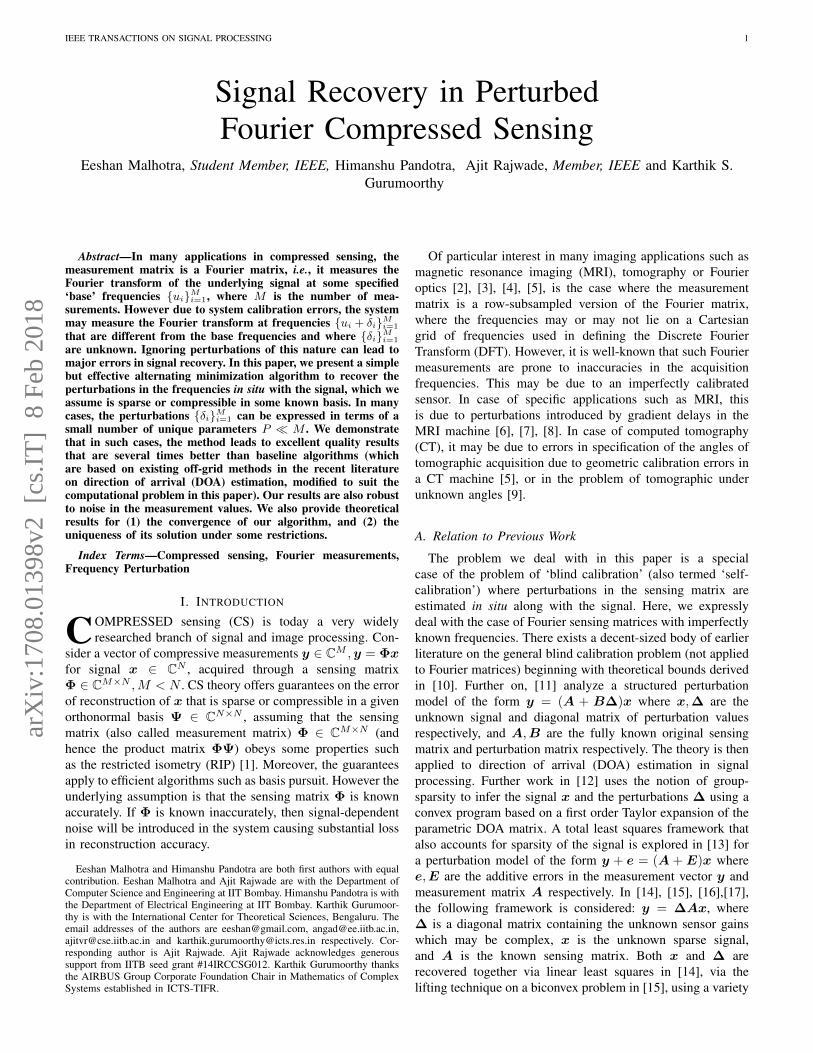
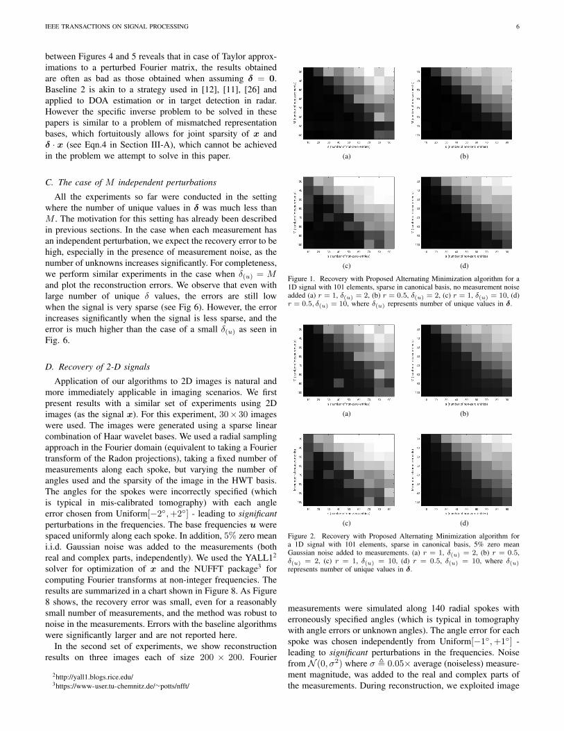
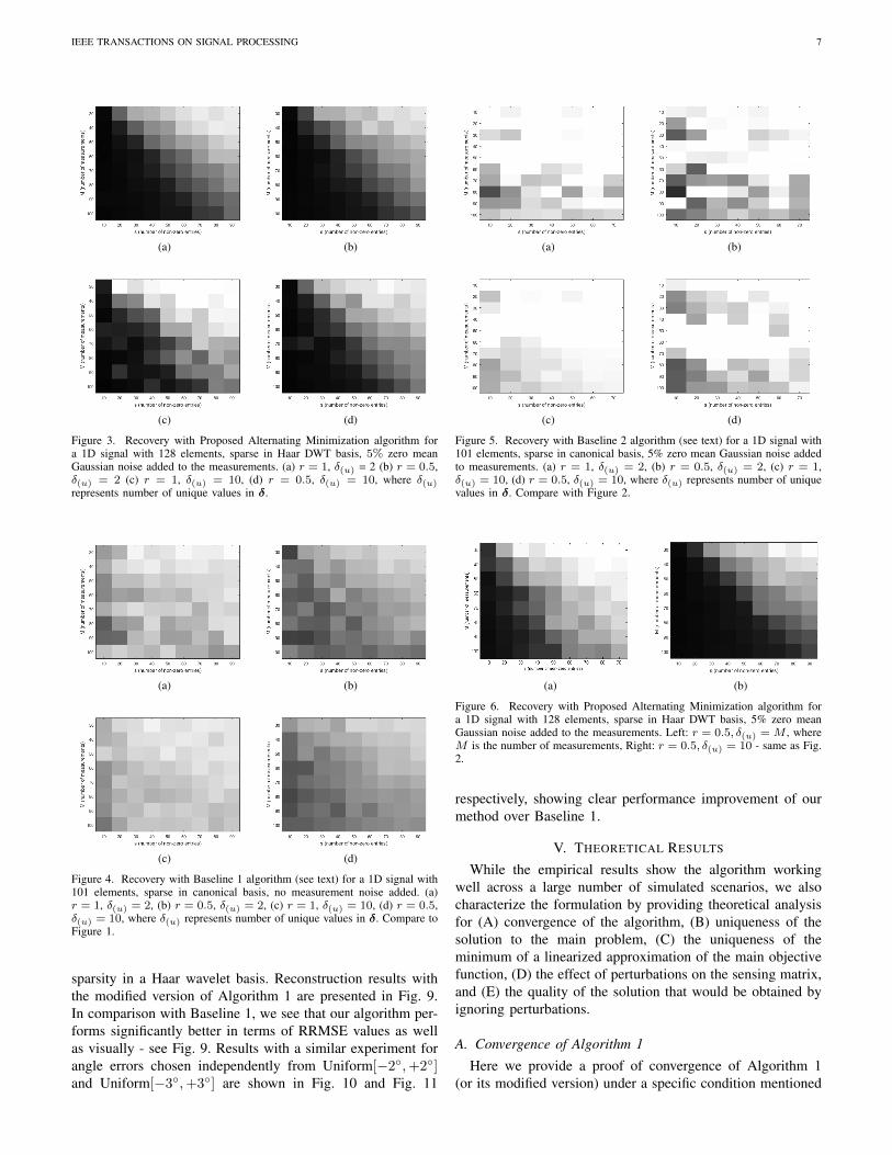
Figure 1 shows results for two different cases (top andbottom figures, for both r = 1 and r = 0.5): where thenumber of unique values in δ are 2 and 10 respectively(this is henceforth denoted as δ(u)), although there are Mmeasurements. (In this experiment, the perturbation parametersin β are the same as the perturbation values in δ.) In bothcases, no external noise was added to the measurements. Onecan see that the average recovery error decreases with thenumber of measurements and increases with s, although therelationship is not strictly monotonic. Figure 2 shows the sametwo cases as in Figure 1, but with an addition of zero meani.i.d. Gaussian noise with σ = 5% of the average magnitudeof the individual (noiseless) measurements. The same trend ofdecrease in error with increased number of measurements andincrease in error with increased s is observed here as well.For reference, we also include a typical sample reconstructionin 1D canonical basis for a signal of length 101, which is 10-sparse, in Figure 7. Figure 3 shows similar results as in Figure2 but using signals that are sparse in the Haar wavelet basisinstead of the canonical basis.

B. Baselines for Recovery of 1-D signals

For comparison, we also establish two baselines:1) A naive reconstruction algorithm (termed ‘Baseline 1’),

which ignores the perturbations and recovers the signalusing a straightforward basis pursuit approach, with theunperturbed, on-grid Fourier matrix as the measurementmatrix, i.e. assuming δ = 0. Results in similar settingsas in Figure 1 are shown in Figure 4. The parameterλ for this approach was set using cross-validation on atraining set of signals.

2) A Taylor approximation approach (termed ‘Baseline 2’):Here, the signal as well as the perturbations are recoveredusing an alternating minimization algorithm based on afirst order Taylor approximated formulation, from Eqn.5. Results in similar settings as in Figure 1 are shownin Figure 5 for two cases: one where the number ofunique values in δ, , i.e. δ(u), is two; and another whereδ(u) = 10. This baseline is similar in spirit to thetruncated Taylor series approach presented in [12], [11],[26] but modified for our (very different) computationalproblem. The parameter λ for this approach was againset using cross-validation on a training set of signals.

As is clear from the figures, Baseline 1 performs consid-erably worse, since inaccurate frequencies are trusted to beaccurate. Baseline 2 also performs badly because the first orderTaylor error, ηTaylor, can be overwhelmingly large since it isdirectly proportional to the unknown ‖x‖2, and consequently,the signal recovered is also inferior. In fact, a comparison

1http://cvxr.com/cvx/

http://cvxr.com/cvx/


between Figures 4 and 5 reveals that in case of Taylor approx-imations to a perturbed Fourier matrix, the results obtainedare often as bad as those obtained when assuming δ = 0.Baseline 2 is akin to a strategy used in [12], [11], [26] andapplied to DOA estimation or in target detection in radar.However the specific inverse problem to be solved in thesepapers is similar to a problem of mismatched representationbases, which fortuitously allows for joint sparsity of x andδ · x (see Eqn.4 in Section III-A), which cannot be achievedin the problem we attempt to solve in this paper.

C. The case of M independent perturbations

All the experiments so far were conducted in the settingwhere the number of unique values in δ was much less thanM . The motivation for this setting has already been describedin previous sections. In the case when each measurement hasan independent perturbation, we expect the recovery error to behigh, especially in the presence of measurement noise, as thenumber of unknowns increases significantly. For completeness,we perform similar experiments in the case when δ(u) = Mand plot the reconstruction errors. We observe that even withlarge number of unique δ values, the errors are still lowwhen the signal is very sparse (see Fig 6). However, the errorincreases significantly when the signal is less sparse, and theerror is much higher than the case of a small δ(u) as seen inFig. 6.

D. Recovery of 2-D signals

Application of our algorithms to 2D images is natural andmore immediately applicable in imaging scenarios. We firstpresent results with a similar set of experiments using 2Dimages (as the signal x). For this experiment, 30× 30 imageswere used. The images were generated using a sparse linearcombination of Haar wavelet bases. We used a radial samplingapproach in the Fourier domain (equivalent to taking a Fouriertransform of the Radon projections), taking a fixed number ofmeasurements along each spoke, but varying the number ofangles used and the sparsity of the image in the HWT basis.The angles for the spokes were incorrectly specified (whichis typical in mis-calibrated tomography) with each angleerror chosen from Uniform[−2◦,+2◦] - leading to significantperturbations in the frequencies. The base frequencies u werespaced uniformly along each spoke. In addition, 5% zero meani.i.d. Gaussian noise was added to the measurements (bothreal and complex parts, independently). We used the YALL12

solver for optimization of x and the NUFFT package3 forcomputing Fourier transforms at non-integer frequencies. Theresults are summarized in a chart shown in Figure 8. As Figure8 shows, the recovery error was small, even for a reasonablysmall number of measurements, and the method was robust tonoise in the measurements. Errors with the baseline algorithmswere significantly larger and are not reported here.

In the second set of experiments, we show reconstructionresults on three images each of size 200 × 200. Fourier

2http://yall1.blogs.rice.edu/3https://www-user.tu-chemnitz.de/∼potts/nfft/

(a) (b)

(c) (d)

Figure 1. Recovery with Proposed Alternating Minimization algorithm for a1D signal with 101 elements, sparse in canonical basis, no measurement noiseadded (a) r = 1, δ(u) = 2, (b) r = 0.5, δ(u) = 2, (c) r = 1, δ(u) = 10, (d)r = 0.5, δ(u) = 10, where δ(u) represents number of unique values in δ.

(a) (b)

(c) (d)

Figure 2. Recovery with Proposed Alternating Minimization algorithm fora 1D signal with 101 elements, sparse in canonical basis, 5% zero meanGaussian noise added to measurements. (a) r = 1, δ(u) = 2, (b) r = 0.5,δ(u) = 2, (c) r = 1, δ(u) = 10, (d) r = 0.5, δ(u) = 10, where δ(u)represents number of unique values in δ.

measurements were simulated along 140 radial spokes witherroneously specified angles (which is typical in tomographywith angle errors or unknown angles). The angle error for eachspoke was chosen independently from Uniform[−1◦,+1◦] -leading to significant perturbations in the frequencies. Noisefrom N (0, σ2) where σ , 0.05× average (noiseless) measure-ment magnitude, was added to the real and complex parts ofthe measurements. During reconstruction, we exploited image

https://www-user.tu-chemnitz.de/~potts/nfft/


(a) (b)

(c) (d)

Figure 3. Recovery with Proposed Alternating Minimization algorithm fora 1D signal with 128 elements, sparse in Haar DWT basis, 5% zero meanGaussian noise added to the measurements. (a) r = 1, δ(u) = 2 (b) r = 0.5,δ(u) = 2 (c) r = 1, δ(u) = 10, (d) r = 0.5, δ(u) = 10, where δ(u)represents number of unique values in δ.

(a) (b)

(c) (d)

Figure 4. Recovery with Baseline 1 algorithm (see text) for a 1D signal with101 elements, sparse in canonical basis, no measurement noise added. (a)r = 1, δ(u) = 2, (b) r = 0.5, δ(u) = 2, (c) r = 1, δ(u) = 10, (d) r = 0.5,δ(u) = 10, where δ(u) represents number of unique values in δ. Compare toFigure 1.

sparsity in a Haar wavelet basis. Reconstruction results withthe modified version of Algorithm 1 are presented in Fig. 9.In comparison with Baseline 1, we see that our algorithm per-forms significantly better in terms of RRMSE values as wellas visually - see Fig. 9. Results with a similar experiment forangle errors chosen independently from Uniform[−2◦,+2◦]and Uniform[−3◦,+3◦] are shown in Fig. 10 and Fig. 11

(a) (b)

(c) (d)

Figure 5. Recovery with Baseline 2 algorithm (see text) for a 1D signal with101 elements, sparse in canonical basis, 5% zero mean Gaussian noise addedto measurements. (a) r = 1, δ(u) = 2, (b) r = 0.5, δ(u) = 2, (c) r = 1,δ(u) = 10, (d) r = 0.5, δ(u) = 10, where δ(u) represents number of uniquevalues in δ. Compare with Figure 2.

(a) (b)

Figure 6. Recovery with Proposed Alternating Minimization algorithm fora 1D signal with 128 elements, sparse in Haar DWT basis, 5% zero meanGaussian noise added to the measurements. Left: r = 0.5, δ(u) =M , whereM is the number of measurements, Right: r = 0.5, δ(u) = 10 - same as Fig.2.

respectively, showing clear performance improvement of ourmethod over Baseline 1.

V. THEORETICAL RESULTS

While the empirical results show the algorithm workingwell across a large number of simulated scenarios, we alsocharacterize the formulation by providing theoretical analysisfor (A) convergence of the algorithm, (B) uniqueness of thesolution to the main problem, (C) the uniqueness of theminimum of a linearized approximation of the main objectivefunction, (D) the effect of perturbations on the sensing matrix,and (E) the quality of the solution that would be obtained byignoring perturbations.

A. Convergence of Algorithm 1Here we provide a proof of convergence of Algorithm 1

(or its modified version) under a specific condition mentioned


Figure 7. Sample recovery for 1D signal sparse canonical basis, N = 100,M = 60, s = 20, zero mean 5% Gaussian noise added to measurements. Relativereconstruction error by proposed algorithm: 5.5%. Relative reconstruction error by Baseline 2 (Taylor approximation): 88.7%.

Figure 8. Recovery error for 30× 30 2D image, sparse in 2D Haar Waveletbasis, with 5% zero mean Gaussian measurement noise and angle errors fromUniform[−2◦,+2◦]

further. Let Fδ denote the Fourier transform computed at thefrequencies values u + δ where δ = h(β,u). Assign z ={x,β}. Recall that our objective is to determine the solutionz∗ that minimizes the objective function J(z) , ‖x‖1+λ‖y−F (δ)x‖2, namely z∗ = argminzJ(z).

Let zt = {xt,βt} be the present solution of our alternatingsearch algorithm at iteration t. Our alternating search algo-rithm ensures that the sequence of function values {J(zt)}t∈Nis monotonically decreasing. As J is bounded below by 0, thesequence {J(zt)}t∈N converges to a limit value E ∈ R+ bythe monotone convergence theorem.

However, this does not yet prove the convergence of thesolution sequence {zt}. To this end, let x(β) denote theminimizer for the convex objective function on x with β heldfixed, namely x(β) = argminxJβ(x), where Jβ(x) = J(z)with β held constant. In the context of our alternating searchalgorithm, we have xt+1 = x(βt). Letting zt+ 1

2= {xt+1,βt}

Figure 9. Reconstruction for 200 × 200 images with 5% zero mean Gaus-sian measurement noise, 70% compressive measurements, angle error fromUniform[−1◦,+1◦]. In each row, left: original image, middle: reconstructionusing Baseline 1 (RRMSE 25%, 23.36%, 8.82%), right: reconstruction usingmodified version of Algorithm 1 (RRMSE 6.76%, 5.27%, 4.5%).

we find

‖xt+1‖2 ≤ ‖xt+1‖1 ≤ J(zt+ 1

2

)= Jβt

(xt+1) ≤ Jβt(0) = λ‖y‖2

giving an upper bound on the norm of xt. The last but oneinequality follows from that fact that xt+1 minimizes Jβt

(x).


Figure 10. Reconstruction for 200× 200 images with 5% zero mean Gaus-sian measurement noise, 70% compressive measurements, angle error fromUniform[−2◦,+2◦]. In each row, left: original image, middle: reconstructionusing Baseline 1 (RRMSE 38.7%, 30.98%, 12.63%), right: reconstructionusing modified version of Algorithm 1 (RRMSE 10.65%, 5.22%, 4.87%).

Figure 11. Reconstruction for 200× 200 images with 5% zero mean Gaus-sian measurement noise, 70% compressive measurements, angle error fromUniform[−3◦,+3◦]. In each row, left: original image, middle: reconstructionusing Baseline 1 (RRMSE 38.75%, 35.48%, 14.59%), right: reconstructionusing modified version of Algorithm 1 (RRMSE 13.15%, 5.29%, 5.85%).

Further, as −r ≤ βi ≤ r for each i, we see that the sequence{zt}t∈N lie within a compact space. Hence as per Theorem4.9 in [31], this sequence has atleast one accumulation point.Another statement in the same theorem states that if a certaincondition is satisfied, then limt→∞‖zt+1 − zt‖ = 0, whichestablishes convergence of the solution. The condition is thatfor each such accumulation point, the minimization of J(z)

Figure 12. Uniqueness of the solution for δ keeping x fixed, where x is theestimated signal at empirically observed convergence of Algorithm 1.

gives (i) a unique solution for x if β is fixed, and (ii) a uniquesolution for β if x is fixed. Condition (i) is easy to satisfy asthe problem is convex in x if β is fixed. We do not have aproof for Condition (ii), but we have observed uniqueness inpractice, especially since the values in β are bounded between−r to +r. As an example, in Fig. 12, we show a plot ofthe function ‖y − Fδx‖2 keeping x and all but one valuein δ fixed. Note that here x denotes the estimated signalvalue upon (empirically observed) convergence of Algorithm1. We would like to emphasize that Theorem 4.9 in [31] onlyrequires continuity of the function J and no other conditionslike biconvexity. Thus, we have established the followingLemma for conditional convergence of Algorithm 1 (andits modification) to a local minimum of J . Given the non-convexity of J , global guarantees are very difficult to establish.

Lemma 1: Algorithm 1 is locally convergent if for everyaccumulation point of the sequence zt, Condition (ii) issatisfied.

B. Uniqueness of Solution

It is quite natural to question whether the recovery of x fromcompressive measurements of the form y = Ftx is unique,where Ft is as defined in Eqn. 1. We answer this questionin the affirmative (in the noiseless case, of course) under thecondition that the perturbation parameters β be independentof the base frequencies u, i.e. ∀i, 1 ≤ i ≤ P, δi = h(βi) whereh is a known function of only βi. We comment on the effectof relaxing this condition, at the end of the section.First consider real-valued x, which is typical in tomographyand certain protocols in MR (if the magnetization is propor-tional to the contrast-weighted proton density [32]). Considerthe case where there is only a single unknown perturbationparameter value β in all measurements and where x is a 1Dsignal. Then, we have:

y = Ftx = F (x · vβ), (6)

where vβ is a vector in CN whose lth entry is equal toexp(−ι2πh(β)l/N) where l is a spatial/time index and ι =


√−1. To see this, consider the ith measurement as follows:

yi =1√M

∑l

exp(−ι2π(u+ δ)l/N)x(l) (7)

=1√M

∑l

exp(−ι2πul/N)(x(l) exp(−ι2πh(β)l/N)).

Let xβ , x · vβ . Using standard compressive sensing resultsfrom [1], we can prove unique recovery of xβ using basispursuit, for sufficiently large M (M ≥ s logN for s-sparsex) and an RIP-obeying F (which is true if the base frequencieswere chosen uniformly at random [33]). Since x is real-valued,both x and β are uniquely recovered. Moreover this recoveryis robust to measurement noise and compressibility (instead ofstrict sparsity) of xβ and the bounds from [1] would follow.This result extends to x in higher dimensions as well. Ifx ∈ CN , although xβ can be recovered uniquely, there isan inevitable phase ambiguity in estimating x. By the Fouriershift theorem, this implies that x can be estimated only up toa global shift, which depends upon β. However, the magnitudeof each element of x, i.e. |x|, can be recovered uniquely underthe afore-stated conditions.

Consider the case of P �M unique perturbation parametervalues in β, x ∈ RN , and x is s-sparse. Let FLk be the sub-matrix of measurements corresponding to a particular valueβk. Using the earlier arguments, unique recovery of x, δ canbe guaranteed if for at least one k ∈ {1, 2, ..., P}, the matrixFLk obeys the RIP of order s. If x ∈ CN , then one canguarantee unique recovery of only |x|.

These uniqueness results can be further strengthened (i.e. interms of weaker conditions on the number of measurements),by observing that in the case of P > 1 unique values in β, weneed to recover different (complex) signals xβ1 ,xβ2 , ...,xβP

where ∀i, 1 ≤ i ≤ P,xβi, x · vβi

and the lth entry of vβi

equals exp(−ι2πh(βi)l/N). All these signals are s-sparse ifx is s-sparse, and they have the same support. This recoveryproblem is therefore an example of multiple measurementvectors (MMV), for which stronger recovery results exist - seeTheorem 18 of [34]. However, our computational problem hasfurther refinements to MMV: the sensing sub-matrices corre-sponding to the different values in β are necessarily different,which is termed the generalized MMV (GMMV) problem[35],[36], for which stronger results exist. For example, wemodify Theorem 1 of [35] which guarantees unique recoveryof the sparsity pattern of the signals, to state the followingLemma:

Lemma 2: Consider measurements ∀k, 1 ≤ k ≤P,yLk = FLkxβk

where xβk= x · vβk

and vβk(l) =

exp(−ι2πh(βk)l/N). Assume that x is s-sparse with supportset denoted S and has sub-Gaussian entries. Assume that thefollowing conditions hold:

∀j /∈ S,( 1

P

P∑k=1

‖F †Lk,SFLk,j‖2)0.5

≤ α1 < 1 (8)

∀j /∈ S,maxk∈{1,...,P}‖F †Lk,SFLk,j‖2 ≤ α2 > 0, (9)

where † denotes the pseudo-inverse, FLk,j is the jth columnof FLk and FLk,S is a sub-matrix of FLk with columns

corresponding to entries in S. Then the solution to the fol-lowing optimization problem (Q1) is able to recover the exactsolution for the signals xβ1 ,xβ2 , ...,xβP

with high probabilitydecreasing in α1, α2. The problem (Q1) is defined as follows:min‖x‖1 s. t. ∀k ∈ {1, ..., P} yLk = FLkxβk

. ♣Clearly, GMMV results require weaker conditions than MMV(see eqn. 12 of [35]). However, our computational problemin fact has further structure over and above GMMV. First,∀i, 1 ≤ i ≤ N, |xβ1

(i)| = |xβ2(i)| = ... = |xβP

(i)|.Second, the phase factors of all elements of xβ1

,xβ2, ...,xβP

are completely determined by just the P values in β. Themodified version of Algorithm 1 imposes this structure bydesign. At this point, we conjecture that the lower bound onthe required number of measurements is actually much lower,if we use Algorithm 1 for estimation of x,β, as compared tothe predictions from the aforementioned CS, MMV, GMMVapproaches. Moreover, we conjecture that Algorithm 1 is alsomore robust to measurement noise by design, as compared tothese approaches.

Lastly, we consider the case when the values in δ are func-tions of the base frequencies in addition to the values in β (i.e.∀i ∈ {1, 2, ...,M},∃!k ∈ {1, 2, ..., P} s. t. δi = h(βk, ui)where ∃! is the unique existential quantifier), which is morechallenging. This is because it requires estimation of M (asopposed to P ) signals, albeit all with common support andwith the aforementioned structure. Empirically however, wehave observed success of Algorithm 1 even in such a scenario(see Fig. 9).

C. Theoretical Analysis for a Linearized Approximation

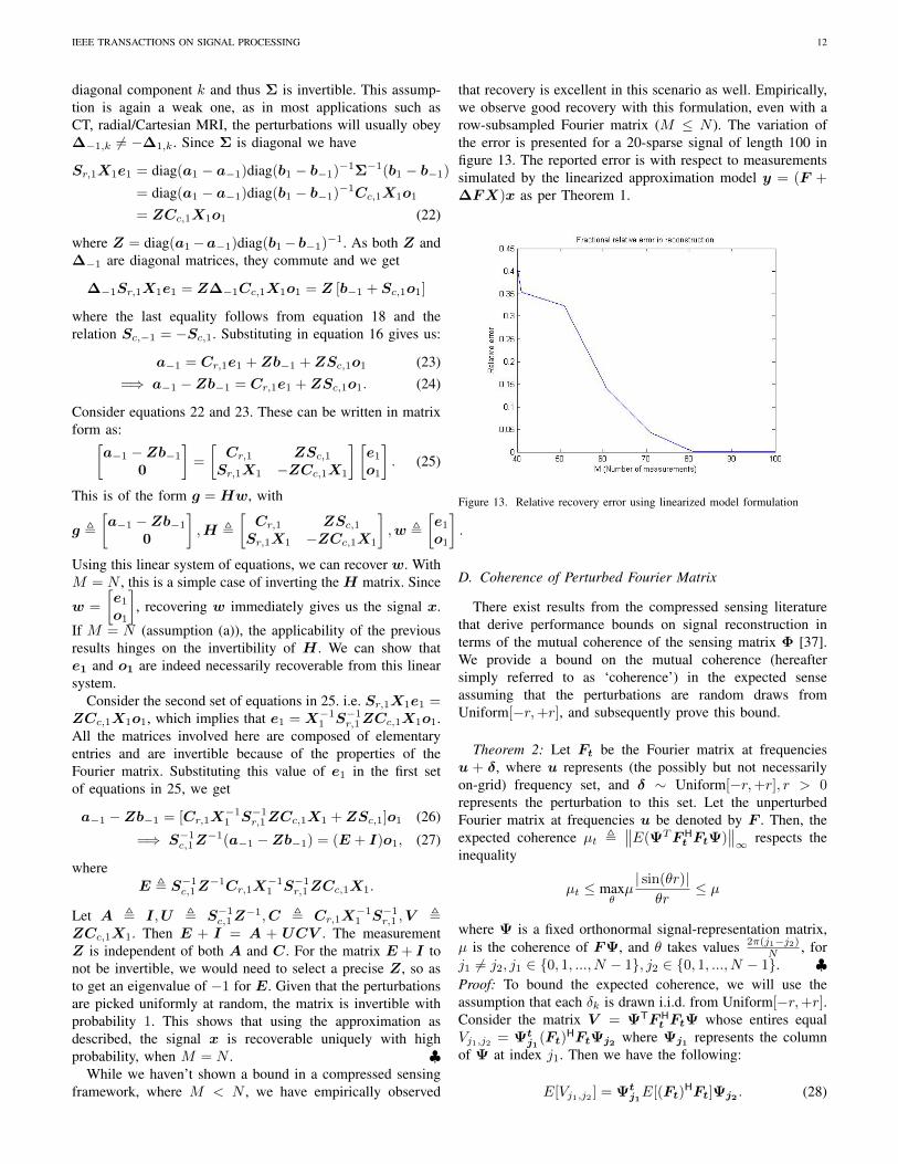
The analysis in the previous section requires that at leastone measurement sub-matrix FLk (corresponding to a givenperturbation parameter βk) obeys the RIP. The analysis doesnot hold in the case where P = M . As such, theoretical errorbounds for the global optimum of Algorithm 1 are difficultdue to the fact that the perturbations δ feature non-linearlyinside the Fourier matrix F . Therefore, we set out to analyzea linearized measurement model given in the statement ofTheorem 1 below, which is applicable in the P = M case.Even for such an approximation and with M = N , the analysisis far from simple and the uniqueness of a solution is notobvious. The sole purpose of Theorem 1 is to establish thatthere exists a unique solution in the linearized noiseless setting.We hope that Theorem 1 will pave the way for future researchfor obtaining uniqueness results in the general non-linear case.

In the following, we consider ∆ , diag(δ). Let F denotethe Fourier matrix at frequencies u. We can treat Ft asapproximated by F +∆F ′, where F ′ = FX is the derivativeof the Fourier matrix with respect to the elements in ∆ and Xis a diagonal matrix, withXll = 2πl

N where l is the index to thespatial location ranging from −(N + 1)/2 ≤ l ≤ (N + 1)/2.In other words, Ft ≈ F + ∆F ′. Without loss of generalitywe assume N is odd. We now state and prove the followingtheorem:

Theorem 1: For measurements y ∈ CM of the form

y = (F + ∆FX)x,


the signal x ∈ RN and the perturbations ∆ (diagonal N ×Nmatrix) can both be uniquely recovered with probability 1,independent of the sparsity of the signal x and the magnitudeof the values in ∆, if (a) M = N , (b) x is neither purely evennor purely odd, (c) y does not contain any pair of elements thatare conjugate symmetric, and (d) the frequencies in u forman anti-symmetric set such that u(M+1)/2−k = −u(M+1)/2+k

for 1 ≤ k ≤ M−12 . ♣

Proof: To prove this, we perform a series of non-trivialalgebraic manipulations to arrive at a linear system of the formg = Hw where w is related purely to x, and g,H dependonly upon y,F . The uniqueness of the solution then followsby showing the invertibility ofH (with high probability) in theM = N case. We comment upon the M < N case thereafter.During the proof for the M = N case, we also precisely pointout why the four assumptions (a)-(d) in the Theorem statementare required, and argue that they are weak assumptions.

We utilize the following defined relations:

F , C + ιS,x , e+ o,y , yr + ιyc (10)

where,C is the cosine component and S is the sine componentof F , e is the even component of x (having N elements), ando is the odd component of x (having N elements), yr is thereal component of y, and ιyc is the complex component ofy. Given x, we note that e and o are uniquely defined.

Therefore, y = (F + ∆FX)x can be rewritten as:

yr + ιyc = Cx+ ιSx+ ι∆(C + ιS)Xx, (11)

which implies that

yr = Cx−∆SXx, and (12)yc = Sx+ ∆CXx. (13)

Note that Co = SXo = Se = CXe = 0.We now divide C into smaller submatrices: The centralcolumn, C0, and the left & right components, C−1 and C1

respectively. That is,

let C =[C−1 C0 C1

]=

C−1,−1 C0,−1 C1,−1

C−1,0 C0,0 C1,0

C−1,1 C0,1 C1,1

.

where the second division is done in a similar fashion, alongthe row axis. To summarise, C0,0 is a single centre element,C−1,0 and C1,0 are row vectors, C0,−1 and C0,1 are columnvectors, and finally C−1,−1, C1,−1, C−1,1 and C1,1 arematrices of size (M − 1)/2× (N − 1)/2.Similarly, let

S =[S−1 S0 S1

]=

S−1,−1 S0,−1 S1,−1

S−1,0 S0,0 S1,0

S−1,1 S0,1 S1,1,

where

S−1,S1,S0 are similarly defined.Consider the case that the frequencies in u form an anti-

symmetric set about 0, which is stated in assumption (d). Notethat this is true for on-grid frequencies from −(N + 1)/2 to(N + 1)/2 used in a typical DFT matrix, or in applicationssuch as radial/Cartesian MRI or CT. Then, we further have

C−1 = C1, S−1 = −S1,C−1,−1 = C−1,1, S−1,−1 = −S−1,1,C1,−1 = C1,1, S1,−1 = −S1,1,

C0 =

11...1

, and S0 =

00...0

.Separating out e and o and X also in a similar fashion, let

e =

e−1

e0

e1

, o =

o−1

o0

o1

and X =

X−1 0 00 0 00 0 X1

where

e−1 = e1, o−1 = −o1 and X−1 = −X1. Using these,equations 12 and 13 can be rewritten as:

yr = 2C1e1 +C0e0 −∆(2S1X1e1) (14)yc = 2S1o1 + ∆(2C1X1o1). (15)

When x is purely even (o1 = 0) or purely odd (e1 = 0), thenyc or yr is respectively zero and we have N+dN/2e unknownquantities to solve using N known values of either yr or yc.Clearly, we do not have uniqueness. Consequently, we requireassumption (b) in the theorem. (Note also that this assumptionis a weak one, as most signals encountered in practice areneither purely even nor purely odd.) Using 14, the middlecomponent yr0 is given by:

yr0 = 2C1,0e1 +C0,0e0 −∆0(2S1,0X1e1).

As S1,0 = 0 we get C0,0e0 = yr0 − 2C1,0e1. Substitutingthis in equation 14, we get

yr − 1yr0 = 2(C1 −∆C1,0)e1 − 2∆S1X1e1

where 1 is a column vector of 1s. Define the quantities

Cr , 2(C1 −∆C1,0), Sr , Sc = 2S1,

Cc , 2C1, a , yr − 1yr0, b , yc.

Further, write a ,

a−1

0a1

, b ,

b−1

b0

−b1

and

∆ ,

∆−1 0 00 ∆0 00 0 ∆1

. We then obtain the reduced set of

equations:

a−1 = Cr,−1e1 −∆−1Sr,−1X1e1 (16)a1 = Cr,1e1 −∆1Sr,1X1e1 (17)b−1 = Sc,−1o1 + ∆−1Cc,−1X1o1 (18)−b1 = Sc,1o1 + ∆1Cc,1X1o1 (19)

where Cr,−1 = Cr,1, Sr,−1 = −Sr,1, Cc,−1 = Cc,1 andSc,−1 = −Sc,1. Ergo,

a1 − a−1 = −(∆1 + ∆−1)Sr,1X1e1

b1 − b−1 = −(∆1 + ∆−1)Cc,1X1o1.

Let Σ , −(∆1 + ∆−1)

=⇒ Sr,1X1e1 = Σ−1(a1 − a−1) (20)

Cc,1X1o1 = Σ−1(b1 − b−1). (21)

It can be verified that the assumption (c) in the theoremis equivalent to presuming that ∆−1,k 6= −∆1,k for any


diagonal component k and thus Σ is invertible. This assump-tion is again a weak one, as in most applications such asCT, radial/Cartesian MRI, the perturbations will usually obey∆−1,k 6= −∆1,k. Since Σ is diagonal we have

Sr,1X1e1 = diag(a1 − a−1)diag(b1 − b−1)−1Σ−1(b1 − b−1)

= diag(a1 − a−1)diag(b1 − b−1)−1Cc,1X1o1

= ZCc,1X1o1 (22)

where Z = diag(a1−a−1)diag(b1−b−1)−1. As both Z and∆−1 are diagonal matrices, they commute and we get

∆−1Sr,1X1e1 = Z∆−1Cc,1X1o1 = Z [b−1 + Sc,1o1]

where the last equality follows from equation 18 and therelation Sc,−1 = −Sc,1. Substituting in equation 16 gives us:

a−1 = Cr,1e1 +Zb−1 +ZSc,1o1 (23)=⇒ a−1 −Zb−1 = Cr,1e1 +ZSc,1o1. (24)

Consider equations 22 and 23. These can be written in matrixform as:[

a−1 −Zb−1

0

]=

[Cr,1 ZSc,1Sr,1X1 −ZCc,1X1

] [e1

o1

]. (25)

This is of the form g = Hw, with

g ,

[a−1 −Zb−1

0

],H ,

[Cr,1 ZSc,1Sr,1X1 −ZCc,1X1

],w ,

[e1

o1

].

Using this linear system of equations, we can recover w. WithM = N , this is a simple case of inverting the H matrix. Since

w =

[e1

o1

], recovering w immediately gives us the signal x.

If M = N (assumption (a)), the applicability of the previousresults hinges on the invertibility of H . We can show thate1 and o1 are indeed necessarily recoverable from this linearsystem.

Consider the second set of equations in 25. i.e. Sr,1X1e1 =ZCc,1X1o1, which implies that e1 = X−1

1 S−1r,1ZCc,1X1o1.

All the matrices involved here are composed of elementaryentries and are invertible because of the properties of theFourier matrix. Substituting this value of e1 in the first setof equations in 25, we get

a−1 −Zb−1 = [Cr,1X−11 S−1

r,1ZCc,1X1 +ZSc,1]o1 (26)

=⇒ S−1c,1Z

−1(a−1 −Zb−1) = (E + I)o1, (27)

whereE , S−1

c,1Z−1Cr,1X

−11 S−1

r,1ZCc,1X1.

Let A , I,U , S−1c,1Z

−1,C , Cr,1X−11 S−1

r,1 ,V ,ZCc,1X1. Then E + I = A + UCV . The measurementZ is independent of both A and C. For the matrix E + I tonot be invertible, we would need to select a precise Z, so asto get an eigenvalue of −1 for E. Given that the perturbationsare picked uniformly at random, the matrix is invertible withprobability 1. This shows that using the approximation asdescribed, the signal x is recoverable uniquely with highprobability, when M = N . ♣

While we haven’t shown a bound in a compressed sensingframework, where M < N , we have empirically observed

that recovery is excellent in this scenario as well. Empirically,we observe good recovery with this formulation, even with arow-subsampled Fourier matrix (M ≤ N ). The variation ofthe error is presented for a 20-sparse signal of length 100 infigure 13. The reported error is with respect to measurementssimulated by the linearized approximation model y = (F +∆FX)x as per Theorem 1.

Figure 13. Relative recovery error using linearized model formulation

D. Coherence of Perturbed Fourier Matrix

There exist results from the compressed sensing literaturethat derive performance bounds on signal reconstruction interms of the mutual coherence of the sensing matrix Φ [37].We provide a bound on the mutual coherence (hereaftersimply referred to as ‘coherence’) in the expected senseassuming that the perturbations are random draws fromUniform[−r,+r], and subsequently prove this bound.

Theorem 2: Let Ft be the Fourier matrix at frequenciesu + δ, where u represents (the possibly but not necessarilyon-grid) frequency set, and δ ∼ Uniform[−r,+r], r > 0represents the perturbation to this set. Let the unperturbedFourier matrix at frequencies u be denoted by F . Then, theexpected coherence µt ,

∥∥E(ΨTF Ht FtΨ)

∥∥∞ respects the

inequality

µt ≤ maxθµ| sin(θr)|

θr≤ µ

where Ψ is a fixed orthonormal signal-representation matrix,µ is the coherence of FΨ, and θ takes values 2π(j1−j2)

N , forj1 6= j2, j1 ∈ {0, 1, ..., N − 1}, j2 ∈ {0, 1, ..., N − 1}. ♣Proof: To bound the expected coherence, we will use theassumption that each δk is drawn i.i.d. from Uniform[−r,+r].Consider the matrix V = ΨTF H

t FtΨ whose entires equalVj1,j2 = Ψt

j1(Ft)

HFtΨj2 where Ψj1 represents the columnof Ψ at index j1. Then we have the following:

E[Vj1,j2 ] = Ψtj1E[(Ft)

HFt]Ψj2 . (28)


We define B , E[(Ft)HFt] and let θj1,j2 , 2π(j1 − j2)/N .

Using the uniform distribution of each δk we find

Bj1,j2 =

∫ r

−r

1

M

∑k

exp (ιθj1,j2(uk + δk))1

2rdδk

=1

M

∑k

exp (ιθj1,j2uk)

2r

∫ r

−rexp (ιθj1,j2δk) dδk.

Furthermore, since we know that∫ r

−rsin(θj1,j2δk)dδk = 0,

and ∫ r

−rcos(θj1,j2δk)dδk =

2

θj1,j2sin(θj1,j2r),

we get

Bj1,j2 =1

N

∑k

exp (ιθj1,j2uk)

2r

2

θj1,j2sin(θj1,j2r) (29)

=sin(θj1,j2r)

θj1,j2r

(1

N

∑k

exp(ιθj1,j2uk)

). (30)

Let C be a matrix such that Cj1,j2 , 1N

∑k exp(ιθj1,j2uk).

Then

Bj1,j2 =sin(θj1,j2r)

θj1,j2r(Cj1,j2) . (31)

Substituting back in equation 28,

E[Vj1,j2 ] = |Ψtj1BΨj2 | (32)

= |Ψtj1

sin(θj1,j2r)

θj1,j2rCΨj2 | (33)

= |(

sin(θj1,j2r)

θj1,j2r

)Ψtj1CΨj2 |. (34)

By the definition of C, we see thatmaxj1,j2,j1 6=j2 |Ψt

j1CΨj2 | ≤ µ. This yields us the following:

E[Vj1,j2 ] = |Ψtj1BΨj2 | ≤

∣∣∣ sin(θj1,j2r)

rθj1,j2

∣∣∣∣∣∣Ψtj1CΨj2

∣∣∣. (35)

Since the last quantity on the RHS is nothing but the coherenceµ, this further yields,

E(Vj1,j2) ≤ µ∣∣∣ sin(θj1,j2r)

rθj1,j2

∣∣∣. (36)

Since∣∣∣ sin(θj1,j2

r)

θj1,j2r

∣∣∣ is the absolute value of a sinc function,it takes a maximum value of 1. Therefore, the expectedcoherence is less than or equal to the coherence of FΨ. Inpractice, the coherence values of the two matrices were foundto be extremely close. ♣If Ψ = I , then FΨ has low coherence with high probability ifthe frequencies are chosen uniformly at random [38]. Hence,in this case, we can call upon well-established compressivesensing results [37], [38] to show that our problem is well-founded in theory.

E. Bound on Recovery in Expectation

Assuming the frequency perturbations are obtained i.i.d.from Uniform[−r,+r], consider the expected measurementvector from the system Ftx + η where η represents a mea-surement noise vector. That is,

y = E∆[y] + η = E∆[Ftx] + η. (37)

We now show a bound on the error in reconstructing x fromy if the unperturbed Fourier matrix F were to be used duringreconstruction, i.e. if one simply assumed the perturbationsto be all equal to zero. For this, we invoke results and proofmethodology from [10].

Since each perturbation ∆k is assumed to be independent,we can calculate the value of E∆k

[(Ftx)k].

E∆k[(Ftx)k]

= E∆k

1√M

∑j

exp(−2πιj(uk + ∆k)

N)xj

= E∆k

1√M

∑j

exp(−2πιjuk

N)xj exp(

−2πιj∆k

N)

=

1√M

∑j

exp(−2πιjuk

N)xj

sin 2πjrN

2πjrN

.The last equality follows the steps from Section V-D. Defining

G to be a diagonal matrix such that Gjj ,sin 2πjr

N2πjrN

, we can

see thatE∆[Ftx] = FGx. (38)

Using this result, we can concretely state the recovery boundin the following theorem:

Theorem 3: Let y , FGx + η and x∗ be the solution tothe recovery problem

min ‖x‖1s.t. ‖y − Fx‖2 ≤ ε′

where F is the Fourier matrix at unperturbed frequencies.Under mild conditions of F and x as assumed in Theorem 2of [10], there exists a suitable value of ε′ and constants C0,C1, for which the recovery error is bounded as:

‖x∗ − x‖2 ≤C0√s‖x− x(s)‖2 + C1ε

′

where x(s) is the best s−term approximation of x containingthe largest s coefficients of x with the rest set to zero. ♣

We now prove this result drawing upon the proof of Theo-rem 2 of [10], to which our formulation is analogous. To seethe analogy more clearly, we define the following quantities:

E , F (G− I), εF , ‖G− I‖2.

We know that ‖F ‖2 equals the largest singular value of matrixF . Let ‖F ‖(s)2 denote the largest singular value taken over alls-column sub-matrices of F . We have

‖E‖2‖F ‖2

≤ ‖F ‖2‖G− I‖2‖F ‖2

= ‖G− I‖2 = εF . (39)


Further, since G and I are both diagonal matrices, multi-plication by (G − I) conserves the sparsity of any s-sparsesignal xs. Therefore, ‖E‖(s)2 ≤ ‖F ‖(s)2 ‖G − I‖2 and hence‖E‖(s)2

‖F ‖(s)2

≤ εF . From here, we follow exactly along the lines

of the proof of Theorem 2 in [10], and arrive at a value ofε′ (see Eqn. 14 of [10]) satisfying ‖y − Fx‖2 ≤ ε′ giventhat ‖y − FGx‖2 = ‖η‖2 ≤ ε. We also arrive at appropriatevalues of the constants C0 and C1 to derive the bound statedin our Theorem 3. ♣Note that this minimization problem does not account for theactual matrix Ft being known or even estimated during therecovery process. In practice, using the algorithm we haveproposed in section III, the matrix ∆ (and hence Ft) isestimated at each step, and the recovery is realistically, muchbetter than the bound arrived at using the approach above. Infuture work, we hope to be able to also provide a bound forthis scenario where Ft is estimated.

VI. CONCLUSIONS AND DISCUSSION

We have presented a method to correct for perturbationsin a compressive Fourier sensing matrix in situ during signalreconstruction. Our method is simple to implement, robust tonoise and well grounded in theory. We have discussed severalapplications of our framework. Moreover, we have provedconditional convergence of our algorithm to a local optimum,and shown that the basic computational problem has a uniquesolution under reasonable conditions. We conjecture that dueto the special structure of our problem, the requirements onthe number of measurements is much below what is predictedby the theoretical development so far. In the case whenP = M = N , we prove the uniqueness of the solutionto a problem that minimizes a linear approximation to theoriginal objective function. For the main algorithm and itsanalysis, however, we have consciously avoided using a Taylorapproximation (Baseline 2) for the algorithm presented unlike[11], [12], even though it may initially appear to simplify theproblem considerably. The primary reason for this is to avoidintroduction of modeling error due to the Lagrange remainderterm which can be quite significant except at small values ofr. Our experimental results justify this choice.

Future work will involve proving analytical bounds for theglobal optimum of Algorithm 1, which we believe will bestronger than those provided by results from standard CS[1], MMV [34] or GMMV [35]. We also aim to explore ouralgorithm in the context of different sampling strategies inpractical MRI acquisition or various modes of tomographicacquisition. Furthermore, the problem of mismatch of both, theFourier sensing matrix and the signal representation matrix, isan interesting avenue for research.

REFERENCES

[1] E. Candes and M. Wakin, “An introduction to compressive sampling,”IEEE signal processing magazine, vol. 25, no. 2, pp. 21–30, 2008.

[2] O. Katz, J. M. Levitt, and Y. Silberberg, “Compressive fourier transformspectroscopy.” Optical Society of America, 2010.

[3] P. Schniter and S. Rangan, “Compressive phase retrieval viageneralized approximate message passing,” IEEE Trans. SignalProcessing, vol. 63, no. 4, pp. 1043–1055, 2015. [Online]. Available:https://doi.org/10.1109/TSP.2014.2386294

[4] M. Lustig, “Compressed sensing MRI,” IEEE Signal Processing Maga-zine, 2008.

[5] M. Ferrucci, R. Leach, C. Giusca, S. Carmignato, and W. Dewulf, “To-wards geometrical calibration of X-ray computed tomography systems: areview,” Measurement Science and Technology, vol. 26, no. 9, p. 092003,2015.

[6] H. Jang and A. B. McMillan, “A rapid and robust gradient measurementtechnique using dynamic single-point imaging,” Magnetic Resonance inMedicine, 2016.

[7] R. K. Robison, A. Devaraj, and J. G. Pipe, “Fast, simple gradient delayestimation for spiral MRI,” Magnetic resonance in medicine, vol. 63,no. 6, pp. 1683–1690, 2010.

[8] E. Brodsky, A. Samsonov, and W. Block, “Characterizing and correctinggradient errors in non-cartesian imaging: Are gradient errors linear-time-invariant?” Magnetic Resonance Imaging, vol. 62, pp. 1466–1476, 2009.

[9] E. Malhotra and A. Rajwade, “Tomographic reconstruction from projec-tions with unknown view angles exploiting moment-based relationships,”in ICIP, 2016, pp. 1759–1763.

[10] M. A. Herman and T. Strohmer, “General deviants: An analysis ofperturbations in compressed sensing,” J. Sel. Topics Signal Processing,vol. 4, no. 2, pp. 342–349, 2010.

[11] Z. Yang, C. Zhang, and L. Xie, “Robustly stable signal recovery in com-pressed sensing with structured matrix perturbation,” IEEE Transactionson Signal Processing, vol. 60, no. 9, pp. 4658–4671, 2012.

[12] T. Zhao, Y. Peng, and A. Nehorai, “Joint sparse recovery methodfor compressed sensing with structured dictionary mismatches,” IEEETransactions on Signal Processing, vol. 62, no. 19, pp. 4997–5008, 2014.

[13] H. Zhu, G. Leus, and G. Giannakis, “Sparsity-cognizant total least-squares for perturbed compressive sampling,” IEEE Transactions onSignal Processing, vol. 59, 2011.

[14] S. Ling and T. Strohmer, “Self-calibration via linear least squares,”CoRR, vol. abs/1611.04196, 2016. [Online]. Available: http://arxiv.org/abs/1611.04196

[15] ——, “Self-calibration and biconvex compressive sensing,” InverseProblems, vol. 31, 2015.

[16] C. Bilen, G. Puy, R. Gribonval, and L. Daudet, “Convex optimization ap-proaches for blind sensor calibration using sparsity,” IEEE Transactionson Signal Processing, vol. 62, no. 8, pp. 4847–4856, 2014.

[17] V. Cambareri and L. Jacques, “A non-convex blind calibration methodfor randomised sensing strategies,” in 4th International Workshop onCompressed Sensing Theory and its Applications to Radar, Sonar andRemote Sensing (CoSeRa), 2016, p. 16–20.

[18] Y. Chi, L. L. Scharf, A. Pezeshki, and A. R. Calderbank, “Sensitivity tobasis mismatch in compressed sensing,” IEEE Trans. Signal Processing,vol. 59, no. 5, pp. 2182–2195, 2011.

[19] J. M. Nichols, A. K. Oh, and R. M. Willett, “Reducing basis mismatchin harmonic signal recovery via alternating convex search,” IEEE SignalProcess. Lett., vol. 21, no. 8, pp. 1007–1011, 2014.

[20] O. Teke, A. C. Gurbuz, and O. Arikan, “Perturbed orthogonal matchingpursuit,” IEEE Transactions on Signal Processing, vol. 61, no. 24, pp.6220–6231, 2013.

[21] G. Tang, B. N. Bhaskar, P. Shah, and B. Recht, “Compressed sensing offthe grid,” IEEE Trans. Information Theory, vol. 59, no. 11, pp. 7465–7490, 2013.

[22] A. Aldroubi, X. Chen, and A. M. Powell, “Perturbations of measurementmatrices and dictionaries in compressed sensing,” Applied and Compu-tational Harmonic Analysis, vol. 33, no. 2, pp. 282–291, 2012.

[23] J. D. Ianni and W. A. Grissom, “Trajectory auto-corrected imagereconstruction,” Magnetic resonance in medicine, vol. 76, no. 3, pp.757–768, 2016.

[24] S. Basu and Y. Bresler, “Uniqueness of tomography with unknown viewangles,” IEEE Transactions on Image Processing, vol. 9, no. 6, pp. 1094–1106, 2000.

[25] Y. Fang, M. Sun, S. Vishwanathan, and K. Ramani, “sLLE: Sphericallocally linear embedding with applications to tomography,” in ComputerVision and Pattern Recognition (CVPR), 2011 IEEE Conference on.IEEE, 2011, pp. 1129–1136.

[26] A. Fannjiang and H.-C. Tseng, “Compressive radar with off-grid targets:a perturbation approach,” Inverse Problems, vol. 29, no. 5, 2013.

[27] A. Belloni, V. Chernozhukov, and L. Wang, “Square-root LASSO:pivotal recovery of sparse signals via conic programming,” Biometrika,vol. 98, no. 4, p. 791, 2011.

https://doi.org/10.1109/TSP.2014.2386294

http://arxiv.org/abs/1611.04196

http://arxiv.org/abs/1611.04196


[28] V. Lucic, A. Rigort, and W. Baumeister, “Cryo-electron tomography:The challenge of doing structural biology in situ,” The Journal of CellBiology, vol. 202, no. 3, pp. 407–419, 2013.

[29] A. Moussavi, M. Untenberger, M. Uecker, and J. Frahm, “Correction ofgradient-induced phase errors in radial MRI,” Magnetic Resonance inMedicine, vol. 71, no. 1, 2014.

[30] A. Deshmane, M. Blaimer, F. Breuer, P. Jakob, J. Duerk, N. Seiber-lich, and M. Griswold, “Self-calibrated trajectory estimation and signalcorrection method for robust radial imaging using GRAPPA operatorgridding,” Magnetic Resonance in Medicine, vol. 75, no. 2, pp. 883–896, 2016.

[31] J. Gorski, F. Pfeuffer, and K. Klamroth, “Biconvex sets and optimiza-tion with biconvex functions: a survey and extensions,” MathematicalMethods of Operations Research, vol. 66, no. 3, pp. 373–407, Dec 2007.

[32] “Wikipedia article on k-space in magnetic resonance imaging,”https://tinyurl.com/yd4u7eap, online; accessed Jan 2018.

[33] M. Rudelson and R. Vershynin, “On sparse reconstruction from fourierand gaussian measurements,” Communications on Pure and AppliedMathematics, vol. 61, no. 8, pp. 1025–1045, 2008.

[34] M. F. Duarte and Y. C. Eldar, “Structured compressed sensing: Fromtheory to applications,” Trans. Sig. Proc., vol. 59, no. 9, pp. 4053–4085,2011.

[35] R. Heckel and H. Bolcskei, “Joint sparsity with different measurementmatrices,” in Allerton Conference on Communication, Control, andComputing, 2012, pp. 698–702.

[36] N. Rajamohan, A. Joshi, and A. P. Kannu, “Joint block sparse signal re-covery problem and applications in LTE cell search,” IEEE Transactionson Vehicular Technology, vol. 66, no. 2, pp. 1130–1143, Feb 2017.

[37] C. Studer and R. Baraniuk, “Stable restoration and separation of approx-imately sparse signals,” Applied and Computational Harmonic Analysis,vol. 37, no. 1, pp. 12–35, 2014.

[38] E. Candes, J. Romberg, and T. Tao, “Robust uncertainty principles: exactsignal reconstruction from highly incomplete frequency information,”IEEE Transactions on Information Theory, vol. 52, no. 2, pp. 489–509,2006.

Signal Recovery in Perturbed Fourier Compressed Sensing

Documents

Transcript of Signal Recovery in Perturbed Fourier Compressed Sensing